Organoid Engineering Techniques
1. Foundations of Organoid Engineering and Experimental Design
1.1 Organoid definitions, model types, and what each is used for
An organoid is a 3D cellular system grown from cells that self-organize into structures resembling aspects of an organ. “Resembling” matters: organoids are not miniature organs with every feature intact, and that’s a good thing for experimental clarity. You choose an organoid type based on which biological question you’re asking and which features you need to measure.
What “organoid” means in practice
A useful working definition is: a reproducible 3D culture that shows tissue-like organization and function relative to a specific biological context. That organization can be spatial (layering, lumens), cellular (multiple cell types), or functional (barrier properties, secretion, contractility). Different labs may use the word “organoid” for slightly different starting materials and levels of complexity, so it helps to specify three things in your notes:
- Origin: embryonic stem cells, induced pluripotent stem cells (iPSCs), adult stem cells, or primary tissue.
- Architecture: whether the culture forms a lumen, a layered epithelium, a branching structure, or a compact aggregate.
- Function: what phenotype you expect to observe (for example, polarized transport or lineage-specific markers).
Model types: a practical taxonomy
Below is a model map that groups organoid-like systems by how they’re built and what they’re best at.
Mind map: organoid model types and typical use cases
1) Adult stem cell–derived organoids
Definition: Organoids initiated from adult tissue stem cells or enriched progenitors. They often form structures that resemble the tissue’s normal architecture, including crypt-like or gland-like organization depending on the tissue.
What they’re used for:
- Tissue-specific biology: signaling pathways that govern differentiation and maintenance.
- Drug response in a relevant context: because the cells are already “tissue-trained.”
- Genotype–phenotype links: especially when combined with perturbations.
Concrete example: If you’re studying intestinal epithelial differentiation, you can start from intestinal crypt-derived cells. With the right matrix and growth factors, you typically see organized domains and lineage marker patterns that correspond to the tissue’s normal maturation program. The key experimental advantage is that the model’s baseline organization is often closer to the in vivo state than many pluripotent-derived systems.
Common limitation: Adult-derived organoids can be sensitive to handling and may show donor-to-donor variability. That’s not a flaw; it’s a reminder to define acceptance criteria (for example, growth rate range, marker expression thresholds, and morphology consistency).
2) iPSC-derived organoids
Definition: Organoids generated from iPSCs through directed differentiation. They can be engineered to carry specific genetic variants, which is a major reason people choose them.
What they’re used for:
- Genetic control: comparing isogenic lines reduces background noise.
- Developmental questions: mapping how cell states transition.
- Patient modeling: using iPSCs from individuals to capture disease-relevant phenotypes.
Concrete example: For modeling a lung epithelial program, you can differentiate iPSCs into airway-like epithelial cells and then culture them in 3D to encourage lumen formation and polarization. The readouts might include epithelial markers, barrier-related measurements, and response to stimuli.
Common limitation: Differentiation protocols can produce heterogeneity in maturity. Two batches can look similar under a microscope yet differ in functional readiness, so you need functional checkpoints, not just morphology.
3) Embryonic stem cell–derived organoids
Definition: Organoids derived from embryonic stem cells using differentiation cues that guide lineage formation.
What they’re used for:
- Lineage specification and developmental transitions.
- Mechanistic studies where you want to observe early state changes.
Concrete example: In a developmental context, you might culture cells through a sequence of signaling conditions and then form a 3D structure that reflects a particular developmental stage. The experimental focus is often on time-resolved marker changes and spatial organization.
Common limitation: Because these models are tied to developmental programs, the timing of differentiation steps becomes a core variable. If you compare conditions, you must align developmental stage, not just calendar time.
4) Organoid-on-chip and microfluidic organoids
Definition: A 3D organoid culture integrated into a microfluidic device that provides controlled flow, oxygenation, and mechanical cues.
What they’re used for:
- Transport and barrier function under defined flow.
- Drug exposure profiles that mimic physiological delivery.
- Longer-term culture with better control of nutrient and waste exchange.
Concrete example: For a gut barrier assay, you can place an epithelial organoid-derived monolayer or organoid structure in a microfluidic setup where you perfuse media across a defined compartment. You can then measure permeability changes after adding a test compound, with reduced confounding from stagnant diffusion.
Common limitation: Device setup adds complexity. You’ll spend time standardizing chip loading, flow rates, and sampling methods so that comparisons remain fair.
5) Tissue explants and slices (not always called organoids, but often used similarly)
Definition: Small pieces of tissue maintained ex vivo. They preserve native architecture and cell composition.
What they’re used for:
- Short-term responses to stimuli.
- Validation of relevance: checking whether a mechanism seen in organoids also appears in more intact tissue.
Concrete example: If you’re testing an inflammatory stimulus, a tissue slice can show immediate changes in signaling and cell recruitment. The advantage is structural preservation; the tradeoff is limited culture duration and less control over cell composition.
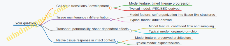
Choosing the right model: a quick decision logic
A practical way to decide is to match your question to the model’s strengths:
- If you need tissue-like organization and stable maintenance: adult-derived organoids are often a strong starting point.
- If you need genetic control or developmental staging: iPSC-derived or embryonic-derived systems fit better.
- If you need flow-dependent transport or barrier readouts: microfluidic formats help.
- If you need native architecture for short experiments: explants/slices can be appropriate.
Mind map: question → model features
A note on naming: “organoid” vs “organoid-like”
In protocols and papers, the label matters less than the described behavior. Two cultures can both be called organoids while differing in origin, maturation level, and functional readouts. When you write your methods, include the three anchors—origin, architecture, and function—so readers can interpret what “organoid” means in your specific context.
That’s the foundation for the rest of the book: once you know what kind of 3D model you’re building, the next steps—matrix choice, initiation, differentiation, and scaling—become targeted rather than generic.
1.2 Selecting the right biological source and starting material
Choosing the biological source is less about “what’s possible” and more about “what will behave consistently enough to answer your question.” In organoid work, the starting material sets the ceiling for viability, growth kinetics, and lineage stability. A good selection also reduces the number of times you have to troubleshoot the same problem under different names.
Start with the question, then match the source
Write your primary readout in plain terms: what tissue function or cell state do you need to model, and what level of fidelity matters (cell identity, architecture, barrier function, immune interactions, etc.). Then map that to a source type.
- Patient-derived tissue (biopsy, resection): best when you need patient-specific genetics, disease state, or drug response.
- Primary stem/progenitor cells: useful when you want controlled differentiation from a known compartment.
- Established cell lines: convenient for throughput and genetic manipulation, but they may not reproduce the original tissue’s differentiation constraints.
- Donor-derived organoids (from existing lines): helpful for standardization, but you still need to verify that the line matches your intended lineage and maturity.
A practical rule: if your readout depends on a specific cell lineage, prioritize sources enriched for that lineage rather than sources that merely come from the same organ.
Decide what “starting material” means for your workflow
“Starting material” can be cells, tissue fragments, or pre-formed organoids. Each option changes the variability profile.
- Tissue fragments preserve native cell-cell contacts and extracellular cues, which can improve initiation for some tissues. The tradeoff is heterogeneity in fragment size and composition.
- Single cells enable uniform seeding and easier genetic perturbations. The tradeoff is that dissociation can stress cells and reduce the fraction that re-enters the growth program.
- Pre-formed organoids reduce initiation time and can be used for expansion and assays. The tradeoff is that you may be studying a “selected” subpopulation that already adapted to culture.
When you’re comparing conditions, keep the starting material format constant across groups. Otherwise, differences in growth may reflect handling effects rather than biology.
Use a simple decision checklist before you commit
Before collecting or thawing anything, score the candidate source against five criteria.
- Lineage relevance: Does the source contain the cell population that can generate your target organoid type?
- Viability at initiation: Can you reasonably expect high survival after dissociation or thaw?
- Genetic and phenotypic stability: Will the source maintain the traits you need during the time window of your experiment?
- Reproducibility across donors/batches: Are there known variability drivers (age, treatment history, ischemia time, passage number)?
- Compatibility with your downstream steps: Does the source support imaging, drug dosing, co-culture, or genome editing without excessive re-optimization?
A quick example: if you need consistent lumen formation for quantification, a source with high initiation variability will force you to normalize away biology. Better to choose a starting material that yields a predictable fraction of structured organoids.
Tissue procurement variables that matter (and how to control them)
For patient-derived material, the biggest hidden variable is often time and handling between excision and culture.
Key factors to standardize:
- Cold ischemia time: Longer delays generally reduce viability and can bias toward more stress-tolerant subpopulations.
- Transport conditions: Temperature and medium composition affect survival and stress signaling.
- Tissue region: Even within the same organ, different anatomical sites can contain different progenitor fractions.
- Tissue handling: Excess mechanical force during processing can increase cell death and alter surface markers.
Concrete practice: record the time from excision to processing, the transport temperature, and the tissue region. Then, when you see poor initiation, you can separate “culture protocol issue” from “starting material issue” without guessing.
Cell source quality: what to check before organoid initiation
Even if the source is “the right tissue,” quality determines whether it can enter the organoid growth program.
For primary cells or single-cell suspensions, check:
- Viability (e.g., dye exclusion) after dissociation.
- Clumping: aggregates can cause uneven seeding and misleading density effects.
- Identity markers: confirm enrichment for the expected compartment.
For tissue fragments, check:
- Fragment size distribution (too small can reduce the number of initiating units; too large can create diffusion limits).
- Gross contamination (blood, necrotic tissue) that can increase background debris.
For cell lines or established organoids, check:
- Passage number and growth history.
- Morphology consistency across thaw/expansion cycles.
- Functional baseline relevant to your readout (for example, barrier-like behavior if that’s central to your assay).
A small but effective habit: run a short “starter QC” on the day of initiation—viability, clumping/fragment size notes, and a quick marker check if feasible. It’s faster than diagnosing failure after a week of culture.
Donor variability: plan for it instead of pretending it won’t happen
Donor-to-donor differences are real, especially for primary tissue. The goal is not to eliminate variability, but to structure it so you can interpret results.
Best practices:
- Use multiple donors when the biological question involves patient heterogeneity.
- Balance donor representation across experimental conditions (e.g., don’t put all “good growers” into one treatment group).
- Track donor metadata that plausibly affects outcomes (age, sex, prior treatment, tissue site).
Example: if you’re testing a drug response, assign organoid batches from each donor to all treatment arms. Then analyze treatment effects within donor rather than across donors only.
Mind maps
Mind map: Selecting biological source and starting material
Mind map: Common failure points tied to starting material
Worked examples (practical choices)
Example A: Modeling patient-specific drug response
- Choose patient-derived tissue.
- Use tissue fragments if dissociation viability is low and initiation is historically better with preserved contacts.
- Standardize cold ischemia time and tissue region.
- Assign each donor’s organoid batches to all treatment arms to control donor effects.
Example B: Building a reproducible lineage model for imaging quantification
- Choose a primary compartment enriched for the target lineage or an established organoid line with known morphology.
- Prefer single-cell seeding if you need uniform starting conditions and consistent imaging fields.
- Record passage number and confirm baseline morphology before starting the experiment.
Example C: Testing a genetic perturbation
- Choose a source that supports efficient editing and recovery.
- If editing efficiency drops after dissociation, start from pre-formed organoids and apply perturbation at a stage that balances editing access with viability.
- Verify on-target outcomes with a quick identity check before committing to long differentiation timelines.
What “good selection” looks like in practice
Good selection shows up as predictable initiation, stable morphology within your experimental window, and manageable variability that you can explain with recorded factors. If you can’t describe the starting material’s origin, handling timeline, and quality checks in a few sentences, you’re likely to spend your time troubleshooting the wrong layer of the system.
1.3 Defining measurable endpoints and building a testable experimental plan
A good organoid experiment starts with endpoints that can be measured without arguing about what you meant. “Better growth” is not an endpoint; “organoid area increases by at least 20% by day 7 under defined imaging settings” is.
Step 1: Translate your biological question into a measurable claim
Write a single-sentence claim that includes (1) the process you care about, (2) the direction of change, and (3) the time window.
- Example claim (matrix choice): “Organoids embedded in Matrix A show higher lumen formation by day 10 than Matrix B, measured as the fraction of organoids with a continuous lumen-like region in confocal z-stacks.”
- Example claim (media adaptation): “After stepwise media adaptation, viability remains above 80% at 24 hours post-transition, measured by live/dead staining and automated segmentation.”
If you can’t specify the time window, you’ll end up measuring whatever looks interesting that day.
Step 2: Choose endpoint types that match what you’re testing
Use a mix of endpoints so you can tell whether you improved the right thing.
- Primary endpoint (decision-maker): The one you use to accept/reject the main hypothesis.
- Secondary endpoints (explainers): Additional measures that help interpret why the primary endpoint changed.
- Quality endpoints (gatekeepers): Checks that confirm the culture is “in bounds” before you trust the biology.
A practical example for initiation optimization:
- Primary: percentage of organoids exceeding a minimum size threshold by day 7.
- Secondary: median viability score at day 3.
- Quality gate: contamination-free status and consistent starting cell viability.
Step 3: Define measurement methods with enough detail to reproduce
For each endpoint, specify:
- What is measured (e.g., lumen presence, area, marker intensity)
- How it is measured (assay type and analysis approach)
- When it is measured (day/time after initiation or treatment)
- How results are summarized (mean, median, fraction, distribution)
- Acceptance criteria (what counts as success)
Example: lumen endpoint
- Measure: fraction of organoids with a lumen-like region.
- Method: confocal z-stack, segmentation of lumen channel, require lumen continuity across at least N consecutive slices.
- Time: day 10.
- Summary: fraction per well.
- Acceptance: ≥ 0.30 lumen-positive fraction.
This avoids the classic problem where one person counts “almost a lumen” and another counts only “obvious lumen.”
Step 4: Build a testable experimental plan (variables, controls, and structure)
A testable plan answers: what changes, what stays fixed, what you compare, and how you’ll know the result isn’t just noise.
Core components
- Independent variable(s): the factor(s) you intentionally change (e.g., matrix stiffness, growth factor concentration, seeding density).
- Dependent variables: your endpoints.
- Controls: conditions that anchor interpretation.
- Replication: enough wells/organoids to estimate variability.
- Randomization and blinding (when feasible): reduce systematic bias.
A simple template
Use this structure for each experiment:
| Component | What to write | Example |
|---|---|---|
| Hypothesis | One sentence | “Matrix A improves lumen formation vs Matrix B.” |
| Independent variable | What changes | Matrix type (A vs B). |
| Fixed conditions | What must match | Same cell source, same seeding density, same incubation time. |
| Primary endpoint | Decision metric | Lumen-positive fraction at day 10. |
| Secondary endpoints | Interpretation metrics | Viability at day 3; organoid area at day 10. |
| Quality gates | Trust conditions | Viability at start ≥ 90%; no contamination. |
| Controls | Baseline and reference | Include a “standard matrix” condition. |
| Replication | How many units | ≥ 3 wells per condition; analyze ≥ 20 organoids per well. |
| Analysis plan | How you compare | Two-sided test or predefined rule based on effect size. |
Step 5: Decide on sample size logic without pretending it’s exact
You don’t need a perfect power calculation to be disciplined. You do need a consistent rule.
- If you expect a large effect (e.g., a clear shift in lumen fraction), fewer replicates may be acceptable.
- If you expect subtle differences (e.g., small changes in marker intensity), you need more replication and better measurement stability.
A practical approach:
- Run a small pilot to estimate variability (e.g., standard deviation of lumen fraction across wells).
- Use that variability to set replication for the main run.
Even without formal statistics, you should predefine what “enough” means, such as “at least 3 independent wells per condition and at least 20 organoids per well.”
Step 6: Use a mind map to keep endpoints aligned to decisions
Mind map: From question to endpoints to decisions
Step 7: Work through an integrated example
Goal: Compare two initiation strategies: single-cell seeding vs aggregate seeding.
Independent variable: seeding format (single cells vs aggregates).
Fixed conditions: same donor batch, same matrix lot, same media recipe, same incubation schedule.
Primary endpoint: organoid formation efficiency at day 5.
- Definition: fraction of seeded units that produce organoids exceeding a minimum area threshold.
- Measurement: automated image analysis; threshold set using a small calibration set.
Secondary endpoints:
- Viability at day 2 (live/dead fraction).
- Median organoid area at day 5 and day 10.
- Lumen-positive fraction at day 10 (if relevant to the model).
Quality gates:
- Starting viability ≥ 90%.
- No contamination by microscopy.
- Imaging QC: consistent focus and exposure settings across wells.
Controls:
- Include a “standard” condition (whichever format you currently use) so you can interpret whether the new method is an improvement or a detour.
Replication:
- 3 wells per condition per run.
- Analyze ≥ 20 organoids per well.
Decision rule (predefined):
- Accept the new strategy if the primary endpoint improves by at least 15 percentage points and the quality gates are met.
This plan is testable because every endpoint has a definition, every comparison has a control, and the decision rule is stated before you see the results.
Step 8: Predefine how you handle “messy reality”
Organoids do not always behave nicely. You can still be systematic.
- Outlier wells: define criteria such as “imaging artifacts in >30% of fields” or “starting viability below gate.”
- Segmentation failures: define a rule for reprocessing vs excluding, and keep it consistent.
- Missing data: specify whether a well is excluded or re-imaged, and document the reason.
A plan that includes these rules is easier to trust because it reduces post-hoc storytelling.
Quick checklist (use before starting)
- Primary endpoint is a single, measurable decision metric.
- Time window is specified for each endpoint.
- Measurement method includes enough detail to reproduce.
- Quality gates exist and are not optional.
- Controls are included to anchor interpretation.
- Replication units and counts are defined.
- A decision rule is written before data collection.
1.4 Establishing baseline controls and benchmarking across runs
Baseline controls are the boring part that keeps your organoids from becoming a choose-your-own-adventure. The goal is simple: separate “the system worked” from “the system changed.” This section lays out a practical approach to controls, benchmarking metrics, and run-to-run comparability.
Define what “baseline” means for your question
Start by deciding which biological and technical variables you want to hold steady.
- Biological baseline: the expected organoid state before any treatment or perturbation (e.g., size distribution, viability, marker expression).
- Technical baseline: the expected performance of your workflow (e.g., matrix handling, media preparation, incubation conditions).
A useful rule: if you cannot measure it within the first week, you probably cannot use it as a baseline endpoint.
Concrete example: You are testing a signaling inhibitor. Your baseline should include (1) organoid formation efficiency, (2) early morphology score, and (3) a marker panel at the start of treatment. Without these, a “no effect” result might actually be a “different starting state” result.
Build a control set that matches your sources of variation
Use controls that map directly to likely failure modes.
-
Negative controls (should not show the target phenotype):
- Vehicle-only treatment.
- Matrix-only or scaffold-only condition if relevant.
- Untreated organoids handled identically through the same media-change schedule.
-
Positive controls (should show the target phenotype):
- A known inducer or inhibitor at a concentration that reliably produces the phenotype in your hands.
- A reference organoid line or batch with established behavior.
-
Process controls (should reflect workflow consistency):
- A “matrix quality” check (e.g., gelation time or mechanical consistency proxy).
- A “media readiness” check (e.g., pH/osmolality or temperature equilibration timing).
- A handling control: the same steps performed without the variable you are testing.
-
Assay controls (should validate your measurement):
- Staining controls for background and non-specific signal.
- Imaging controls for exposure and segmentation stability.
Concrete example: If your readout is immunostaining intensity, include a no-primary control and a standardized imaging setting control. Otherwise, run-to-run differences can masquerade as biology.
Choose benchmarking metrics that are hard to “accidentally” match
Benchmarking is not just “did it grow.” Pick metrics that reflect both formation and function.
A practical metric set for most organoid workflows:
- Formation efficiency: fraction of wells/organoids that reach a predefined morphology threshold by a fixed day.
- Growth kinetics: size or volume distribution at set timepoints (not just a single endpoint).
- Viability proxy: live/dead ratio or metabolic readout at a consistent stage.
- Morphology score: a simple rubric (e.g., lumen presence, necrotic core fraction, boundary sharpness).
- Marker expression: at least one early marker (state) and one later marker (function).
To keep benchmarking honest, predefine acceptance ranges using historical data or pilot runs.
Concrete example: For lumen-forming organoids, define “lumen-positive” as a visible internal cavity with a minimum area threshold. Then track the lumen-positive fraction across runs. If a run’s fraction drops, you know the issue is earlier than your treatment.
Standardize run structure: what changes, what stays fixed
Run-to-run comparability improves when the experimental unit and timing are consistent.
- Fix the experimental unit: same well format, same organoid number per well, same matrix volume per unit.
- Fix the schedule: media change days and timing windows (e.g., “within 30 minutes of the usual time”).
- Fix the handling order: matrix preparation order, pipetting technique, and incubation start time.
- Fix the sampling plan: which wells are used for imaging, which for flow/histology, and when.
If you must vary something (e.g., donor batch), treat it as a planned factor and include it in the benchmarking record.
Create a benchmarking dashboard (and actually use it)
A dashboard is a compact summary of whether the run behaved like your baseline.
Minimum dashboard fields:
- Run ID, date, operator, incubator ID.
- Matrix lot(s) and media lot(s).
- Formation efficiency (day X).
- Morphology score distribution (day X).
- Viability proxy (day X).
- Marker expression summary (day Y).
- Notes on deviations (e.g., delayed media change, temperature excursion).
Concrete example: Suppose your day-3 morphology score is usually centered around 2.0 (on a 0–3 scale). If a new run averages 1.2 with a wider spread, you flag the run before running expensive downstream assays.
Use statistical thinking without turning it into a math class
Benchmarking across runs benefits from simple, consistent comparisons.
- Track distributions, not only means: size and marker expression often skew.
- Use consistent denominators: formation efficiency should be computed from the same starting count.
- Define outlier rules: for example, “flag if formation efficiency is below the 10th percentile of prior runs.”
A straightforward approach is to compute a z-score relative to your baseline history for each metric: \[ z = \frac{x - \mu}{\sigma} \] where \(x\) is the run’s metric, and \(\mu\), \(\sigma\) come from prior baseline runs.
Concrete example: If viability proxy z-score is -2.1 for a run, you can stop early or quarantine the run’s data. You are not claiming a cause; you are enforcing comparability.
Mind maps: how controls and benchmarking connect
Mind map: Baseline controls and benchmarking
Worked example: comparing two runs before treatment
Imagine you run the same organoid initiation protocol twice: Run A and Run B.
Pre-treatment day-3 checks:
- Formation efficiency: Run A 0.82, Run B 0.61.
- Morphology score (0–3): Run A median 2.3, Run B median 1.6.
- Viability proxy: Run A 0.88 live fraction, Run B 0.79.
Decision:
- If your acceptance range for formation efficiency is ≥ 0.70 and viability ≥ 0.85, Run B fails baseline.
- You quarantine Run B’s downstream treatment results. You can still analyze it, but you do not compare it directly to Run A as if both started from the same baseline.
Concrete follow-up: You review deviations and find that Run B’s media change was delayed by 2 hours. That detail becomes part of the run record, and it explains the baseline shift without guessing.
Common pitfalls (and the fix)
- Pitfall: using only one endpoint (e.g., final size).
Fix: include formation and early morphology so you can detect baseline drift. - Pitfall: treating positive controls as optional.
Fix: positive controls validate that the system can still produce the expected response. - Pitfall: changing imaging settings between runs.
Fix: lock exposure/thresholding rules and include imaging controls. - Pitfall: averaging everything and ignoring spread.
Fix: track distributions and flag runs with unusually wide variance.
Baseline controls and benchmarking are not about perfection; they are about knowing when your starting point changed. When you can state that clearly, your later comparisons become much easier to interpret.
1.5 Documenting protocols with reproducible metadata and versioning
Reproducibility starts before the first pipette: if someone can’t reconstruct your exact conditions, they can’t tell whether differences come from biology or from paperwork. This section shows how to document organoid protocols so that another lab (or your future self) can repeat the work without guessing.
A. What “reproducible metadata” means in organoid work
Reproducible metadata is the set of fields that explain what you did and under what constraints, even when the protocol text is unchanged. In organoid engineering, the most common sources of irreproducibility are not the headline steps, but the details:
- reagent identity and preparation (matrix lot, media components, supplement concentrations)
- timing and handling (incubation windows, temperature exposure, mixing duration)
- physical parameters (plate type, well geometry, orbital speed, oxygen conditions)
- culture history (passage number, prior treatments, thaw-to-start interval)
- acceptance criteria (what “good” looked like before proceeding)
A practical rule: if a field could plausibly change outcomes, record it. If it can’t change outcomes, you can omit it.
B. A metadata schema you can actually use
Use a structured record that can be copied into a lab notebook, ELN, or spreadsheet. Keep it consistent across experiments so you can filter and compare later.
Core metadata fields (minimum viable set):
- Protocol identity: protocol name, version, and effective date.
- Biological inputs: cell source, donor ID (or line ID), passage number, and QC status.
- Reagents: matrix type and lot, media base, supplement list with concentrations, and any antibiotics/antifungals.
- Equipment and settings: incubator model (if relevant), centrifuge speed, shaker speed, imaging system.
- Process timeline: start/end timestamps for each major step, including any deviations.
- Environment: oxygen tension (if controlled), temperature during handling, and any CO\(_2\) settings.
- Batch identifiers: matrix batch ID, media batch ID, and reagent preparation dates.
- Acceptance criteria: what you measured (e.g., viability threshold, morphology score) and the result.
- Deviations: what changed, why it changed, and whether you considered it acceptable.
Example metadata record (condensed):
- Protocol: “Organoid initiation—Matrigel dome, 24-well” v1.3 (effective 2026-01-10)
- Cell input: intestinal organoid line, passage 18, QC: mycoplasma negative, viability 85% pre-seeding
- Matrix: growth-factor reduced matrix, lot MFR-2407B, prepared on 2026-02-02, stored at −80°C
- Media: base Advanced DMEM/F12 + GlutaMAX; supplements A/B/C at 1×; no antibiotics
- Handling: all matrix steps on ice; dome formation within 8 minutes of thaw
- Incubation: 37°C, 5% CO\(_2\), humidified; no hypoxia
- Timeline: seeding 09:40, first media change 24 h ± 2 h
- Acceptance: at 72 h, morphology score ≥ 3/5 and debris < 10% of field
- Deviations: centrifugation reduced from 300×g to 200×g due to rotor calibration check; documented and accepted
C. Versioning: treat protocols like software (minus the drama)
Protocol versioning should answer two questions: what changed and what effect it might have. A simple semantic approach works well:
- Major version: changes that alter critical parameters (e.g., matrix type, seeding density, incubation conditions).
- Minor version: changes that refine steps without changing intent (e.g., clarifying mixing time, adding a QC checkpoint).
- Patch version: corrections that don’t affect execution (e.g., typo fixes, unit corrections).
Example version log entry:
- v1.3.0 (2026-01-10): added explicit dome formation window (≤ 10 min after thaw) and acceptance criterion at 72 h.
- v1.2.1 (2025-12-18): corrected supplement concentration from 10 ng/mL to 1 0 ng/mL (unit clarification); no procedural change.
Keep a short “change summary” at the top of each protocol document. When you update a protocol, record:
- what changed
- why it changed (briefly)
- which experiments used the old version
- whether old data remains comparable
D. Mind maps for protocol documentation
Mind map 1: Metadata fields and why they matter
Mind map: Reproducible metadata for organoid protocols
Mind map 2: Versioning workflow
Mind map: Protocol versioning workflow
E. Concrete examples of “good documentation” decisions
Example 1: Matrix lot tracking
Two batches of the same matrix type can behave differently. Record the lot and preparation date, and note whether the matrix was thawed once or multiple times. A short line like “thawed once, aliquoted, used within 4 h” prevents a common hidden variable.
Example 2: Timing windows as acceptance criteria
Instead of writing “incubate overnight,” specify a window and what you do if you miss it. For instance: “incubate 16–18 h; if outside window, record deviation and do not proceed to downstream step unless viability remains above threshold.” This turns timing from a suggestion into a controlled condition.
Example 3: Documenting deviations without rewriting history
If you change centrifuge speed due to calibration, record the exact value used and the reason. Avoid retroactively editing the protocol text to match what happened. The protocol describes intent; the experiment record describes reality.
F. A practical template for the top of every protocol
Use a consistent header so readers can find the essentials quickly.
Protocol header template (copy/paste):
- Protocol name:
- Version:
- Effective date:
- Scope (what organoid type / format):
- Critical parameters (list 5–10):
- Required metadata fields:
- Acceptance criteria checkpoints:
- Deviation policy (what triggers a stop/redo):
- Change summary (last update only):
G. How to keep documentation consistent across a team
Consistency is mostly about reducing interpretation. Define terms like “dome formation window,” “viability threshold,” and “morphology score” in one place. When multiple people run the same protocol, require that they:
- use the same protocol version
- record batch IDs for matrix and media
- log deviations immediately
- confirm acceptance criteria before proceeding
When documentation is structured this way, reproducibility becomes less about memory and more about checklists—exactly where it should be.
2. Cell Sourcing, Culture Readiness, and Quality Control
2.1 Preparing primary cells and cell lines for 3D culture
3D culture is less forgiving than 2D: cells must survive handling, adapt to a new physical context, and still produce the behaviors you measure. Preparation is therefore mostly about reducing stress and standardizing starting conditions.
What “ready for 3D” means
Before you seed, confirm four things: (1) the cells are healthy enough to recover from dissociation, (2) the cell state matches the biology you want (cycle stage, differentiation status, receptor expression), (3) the suspension is compatible with your 3D format (single cells vs aggregates), and (4) your workflow keeps exposure to non-ideal conditions short and consistent.
Primary cells: extra care, fewer shortcuts
Primary cells often arrive as a mixed population with donor-specific variability. Your job is to convert that variability into controlled inputs.
1) Intake and acclimation
- If cells arrive cryopreserved, thaw quickly and dilute immediately into pre-warmed medium to reduce osmotic shock.
- After thaw, allow a short recovery period in 2D (commonly 24–48 hours, depending on the cell type) before moving to 3D. This helps cells repair membranes and re-establish normal metabolism.
- Use the same passage window for each donor batch so that “day of 3D” corresponds to comparable cell history.
2) Dissociation strategy matters
- For 3D formats that tolerate aggregates (e.g., organoid initiation from fragments), avoid harsh single-cell dissociation when possible.
- For single-cell seeding, choose a dissociation method that preserves surface proteins relevant to your model. Over-digestion often shows up later as poor attachment, low viability, or altered morphology.
3) Cell cycle and functional state
- If your readout depends on a specific functional state (for example, epithelial polarity or immune activation), synchronize your preparation as much as practical.
- A practical approach is to seed 3D at a consistent time after the last medium change, so that signaling conditions are comparable across runs.
Cell lines: standardization with a reality check
Cell lines are easier to handle, but they still drift. 3D culture amplifies differences in growth rate, receptor expression, and stress tolerance.
1) Passage number and growth behavior
- Keep passage number within a defined range for experiments.
- Avoid seeding 3D when cultures are either over-confluent or too sparse. Both conditions change how cells respond to dissociation and matrix contact.
2) Mycoplasma and baseline health
- Run routine contamination checks. Mycoplasma can change growth and metabolism without obvious visual cues.
- Use a quick viability check before dissociation and again after final resuspension. If viability drops sharply during handling, fix the process rather than compensating with more cells.
A practical preparation workflow (works for both)
Use this as a checklist to reduce variability.
- Plan the format first: Decide whether you need single cells, small aggregates, or tissue fragments. This determines dissociation intensity and seeding density.
- Prepare media and matrix components in advance: Warm media to the correct temperature and keep matrix components on ice (or as specified) to prevent premature gelation.
- Dissociate with timing discipline: Start dissociation, stop at the target endpoint, and proceed quickly to neutralization and washing.
- Control mechanical stress: Mix gently during washes and resuspension. Repeated pipetting can damage cells and increase debris.
- Remove clumps (only if you truly need single cells): Filter through an appropriate mesh size, but don’t over-filter if it increases cell loss.
- Count accurately: Use a consistent counting method. If you use viability dyes, apply them consistently and record the same gating logic.
- Seed promptly: Delays after final resuspension can reduce viability and alter attachment behavior.
Choosing dissociation intensity: a decision guide
Different 3D formats tolerate different levels of dissociation. Use this guide to avoid “single-cell when you meant aggregates.”
- If your model forms lumen-like structures or requires cell-cell contacts: consider aggregate-based initiation or gentler dissociation.
- If you need uniform seeding density across wells: single-cell seeding may be necessary, but optimize dissociation to preserve viability.
- If you’re embedding fragments: minimize dissociation; focus on fragment size consistency.
Example: preparing cells for a single-cell seeded 3D culture
Suppose you’re seeding a cell line into a hydrogel where uniform distribution matters.
- Start with a healthy, actively growing culture at a consistent confluence.
- Dissociate to single cells using a protocol tuned to your cell type, then neutralize promptly.
- Wash once to remove residual enzymes.
- Resuspend in the 3D-compatible medium at a defined concentration.
- Count viable cells and adjust to your target seeding density.
- Seed immediately and mix gently to avoid bubbles and uneven distribution.
Common failure pattern: viability is acceptable right after dissociation, but drops after seeding. That often points to enzyme carryover, temperature mismatch, or excessive mechanical stress during mixing.
Example: preparing primary cells for aggregate-based organoid initiation
Suppose you have primary epithelial cells and you want to preserve cell-cell contacts.
- Use a mild dissociation approach that yields small aggregates rather than fully dissociated single cells.
- After dissociation, avoid aggressive trituration; aim for a controlled aggregate size distribution.
- If you must reduce clumps, do it gently and consistently.
- Seed aggregates into the matrix or onto a scaffold using a standardized volume and mixing method.
- Track aggregate size indirectly by recording the time to settle or by using a quick microscopy check on a representative sample.
Common failure pattern: organoids start but show irregular sizes. That often comes from inconsistent aggregate size or uneven mixing during seeding.
Mind map: preparation variables and where they show up
Mind map: Preparing cells for 3D culture
Mind map: dissociation choices mapped to 3D format
Mind map: Dissociation choice → expected 3D behavior
Quick acceptance criteria for the day of seeding
Define these before you start so decisions are objective.
- Viability threshold: set a minimum acceptable viability after final resuspension.
- Clump threshold: for single-cell formats, set a maximum acceptable clumpiness based on microscopy.
- Consistency checks: confirm cell concentration and seeding volume match the plan.
- Matrix readiness: verify matrix components are prepared to the correct temperature and timing so gelation occurs when you expect.
Common “fix the process” troubleshooting notes
- If viability is low after dissociation: adjust dissociation endpoint and reduce mechanical stress.
- If viability is fine but growth is poor: check enzyme carryover, medium compatibility, and seeding timing.
- If morphology is inconsistent across wells: standardize mixing technique, aggregate size (if applicable), and seeding density.
Preparing cells for 3D is mostly about controlling inputs: how cells are stressed, how they are suspended, and how quickly they enter the 3D environment. When those inputs are consistent, the biology has a fair chance to show up in the data.
2.2 Handling donor variability with standardized intake criteria
Donor variability is not a nuisance you eliminate; it’s a parameter you manage. In organoid work, the same protocol can yield different growth rates, different morphologies, and different lineage outcomes depending on donor age, tissue handling time, baseline health, and even how the sample was transported. Standardized intake criteria turn that variability into something you can compare, document, and control.
Why intake criteria matter (and what they should cover)
A good intake form answers three questions for every donor batch:
- What is the starting material and how was it treated before it reached the lab? (collection method, time-to-processing, transport conditions)
- What is the biological baseline and how healthy is it? (viability, tissue quality, marker status when applicable)
- What constraints will you enforce so the downstream protocol stays interpretable? (minimum viability thresholds, exclusion rules, acceptance windows)
If you only record “donor ID” and “date,” you’ll later discover that two runs that look comparable on paper were not comparable in reality.
Build a donor intake workflow that is consistent
Use a two-stage approach: pre-screening (fast, before you spend reagents) and final acceptance (after you measure key quality indicators).
Stage A: Pre-screening (fast gates)
Pre-screening should be doable within the first day of receipt. Typical gates include:
- Time-to-processing window: record the interval from collection to lab processing. If you see a wide spread, set an upper limit for inclusion.
- Transport conditions: temperature range, transport medium type, and whether the sample was kept cold or shipped at controlled conditions.
- Tissue integrity: gross appearance score (e.g., intact vs. fragmented), and whether the sample arrived clotted or degraded.
Example: If you receive intestinal tissue, you might set a criterion like “process within X hours” and “no visible extensive necrosis.” A batch that arrives outside the time window can still be processed for exploratory work, but it should not be mixed into your main experimental cohort.
Stage B: Final acceptance (measured gates)
Final acceptance should rely on measurements that correlate with downstream success. Common categories:
- Viability: use a consistent viability assay and reporting format.
- Cell yield and concentration: record total cells or tissue-derived cell counts per unit input.
- Identity checks (when relevant): for certain sources, a quick marker panel can confirm the expected cell population.
- Functional baseline (optional but powerful): if you can measure a simple functional readout early, do it. For example, barrier-forming capacity in epithelial models can be approximated by early polarization markers.
Example: Suppose you’re starting with primary epithelial cells. You set acceptance criteria such as minimum viability and minimum yield per gram of tissue. If a donor batch meets viability but yields are low, you can still proceed, but you label it as “low-yield cohort” and adjust seeding numbers accordingly.
Standardize how you record donor metadata
Donor metadata should be structured so it can be compared across runs. Use consistent units and controlled vocabularies.
A practical intake record includes:
- Donor demographics (age range, sex if relevant)
- Source details (organ, region, collection method)
- Collection-to-processing time (with units)
- Transport temperature and medium
- Tissue handling notes (washing steps, mechanical disruption method)
- Viability assay type and result
- Yield metrics (cells per gram, total cells, or equivalent)
- Any exclusions and why
Example: Two batches both show “viability 70%,” but one used a different assay or gating strategy. If you record the assay type and gating method, you can interpret the numbers correctly instead of treating them as interchangeable.
Create acceptance tiers instead of a single pass/fail
A single threshold can be too rigid. Use tiers so you can keep data while preserving interpretability.
A simple tier system:
- Tier 1 (ideal): meets all gates.
- Tier 2 (acceptable): meets most gates but has one deviation (e.g., slightly longer time-to-processing).
- Tier 3 (exploratory): fails one key gate but is still processed for learning.
Example: If time-to-processing is slightly above your target but viability is still high, you can classify as Tier 2. You then analyze Tier 2 separately or include it with a donor-quality covariate.
Use intake criteria to set seeding and normalization rules
Standardized intake criteria should directly inform how you start the organoid culture.
Common normalization strategies:
- Seed by viable cell number, not by tissue mass alone. If viability differs, equal tissue input can yield unequal viable starting cells.
- Adjust aggregate size or seeding density based on yield. Low-yield batches may require different handling to avoid under-seeding.
- Normalize media volumes and matrix ratios to batch size. If you scale down without adjusting, you can change diffusion conditions.
Example: You receive two donors with the same tissue region. Donor A yields 1.0×10^6 viable cells; Donor B yields 0.4×10^6 viable cells. If you seed both at the same “number of organoids per well” without accounting for viable cell input, Donor B will look like it has poor growth even if the culture conditions are fine.
Mind map: Donor intake criteria and how they connect to culture decisions
Mind map: Standardized donor intake for organoid variability
Concrete example: epithelial organoid intake with tiering
Imagine you’re building a cohort of epithelial organoids from donor tissue.
Pre-screening gates (example):
- Process within 6 hours of collection.
- Transport at 2–8°C.
- Tissue must show no extensive necrosis.
Final acceptance gates (example):
- Viability ≥ 60% by your chosen assay.
- Minimum viable cell yield ≥ 5×10^5 per sample.
Tiering logic (example):
- Tier 1: meets all gates.
- Tier 2: meets viability and yield, but time-to-processing is 6–8 hours.
- Tier 3: viability < 60% or yield below threshold; process only if you need exploratory data.
Normalization rule (example):
- Seed organoids based on viable cell number so each well receives the same viable input.
- If a Tier 2 batch has lower viability, you compensate by using more tissue input to reach the target viable cell count, while still labeling the batch as Tier 2.
This approach prevents a common failure mode: treating “donor B grew less” as a biological effect when it may simply reflect fewer viable starting cells.
Practical checklist for the intake form
- Time-to-processing recorded with units
- Transport temperature and medium recorded
- Tissue integrity score recorded
- Viability assay type recorded
- Viability result recorded
- Yield metric recorded (with units)
- Tier assigned with explicit reason(s)
- Normalization rule applied (e.g., viable cell number)
- Deviations documented per run
Standardized intake criteria make your organoid results easier to interpret because they separate “culture performance” from “starting material quality.” When you can explain why a batch is Tier 2 and how you normalized it, your downstream comparisons stop being guesswork.
2.3 Mycoplasma, contamination checks, and sterility assurance
Sterility in organoid work is less about “never having problems” and more about catching problems early, isolating them quickly, and keeping records tight enough to trace what happened. Mycoplasma deserves special attention because it often grows silently and can subtly change cell behavior without obvious turbidity.
What you’re trying to prevent (and why it matters)
Contamination usually falls into three buckets:
- Bacteria and fungi: often visible as turbidity, clumps, or pH drift. They can also consume nutrients fast.
- Mycoplasma: no visible cloudiness, but it can alter metabolism, growth rate, and differentiation outcomes.
- Cross-contamination: not “microbes,” but the wrong cells or wrong organoid line ending up in the wrong well.
A practical sterility plan treats all three as separate failure modes with different detection methods.
Baseline sterility workflow (the routine you can actually keep)
Use a consistent cadence so you’re not relying on memory.
-
Before starting a new culture batch
- Confirm incubator cleanliness (no standing spills, no old plates left to dry).
- Verify that all media and matrix components are prepared under the same aseptic habits you’ll use during culture.
- Label every tube and plate with date, batch ID, and operator initials.
-
During culture
- Inspect cultures at the same time each day. Look for changes in pH indicator color, cell morphology, and surface debris.
- Keep a “dirty-to-clean” movement pattern: reagents and sterile consumables handled before open culture plates.
-
After culture changes
- Record what you did: split ratio, media volume, matrix lot, and any deviations (for example, “matrix warmed 10 minutes longer than usual”).
Mycoplasma testing: what to test and when
Mycoplasma testing should be tied to decision points, not just calendar dates.
Test at least these moments:
- Upon receiving a new cell source (primary cells, established lines, or co-culture partners).
- After thawing a frozen stock.
- After any event that increases risk, such as a shared centrifuge run, a long interruption, or a change in handling personnel.
- At regular intervals for ongoing lines, using a schedule your lab can maintain.
What to sample:
- Test the cell suspension or organoid-containing fraction that represents the line you’ll use for experiments.
- If you maintain multiple lines, test them separately rather than pooling.
How to interpret results (practical handling):
- If a test is positive, treat that line as contaminated even if morphology looks normal.
- Quarantine the line immediately and stop using it for experiments.
- Do not “try one more passage” as a workaround; it increases the chance of spreading contamination.
Contamination checks beyond mycoplasma
Mycoplasma is only one part of the story. A good contamination program includes quick checks that catch common issues.
1) Visual and pH-based screening
- Turbidity in media, unusual granularity, or floating particles can indicate bacterial or fungal growth.
- pH indicator drift (for example, consistent color shift across wells) can signal microbial metabolism.
Example: If only one well shows a color shift while neighboring wells remain stable, suspect a localized handling issue (for example, a pipette tip touched the wrong surface) rather than a whole-batch media problem.
2) Microscopic inspection
Use a consistent microscope setting and time window.
- Look for unexpected refractile particles or cell debris that appears suddenly.
- Compare to a known-good control well from the same line.
Example: If organoids become smaller and more fragmented while the media remains clear, consider whether the issue is mechanical stress, matrix concentration drift, or contamination that doesn’t cause turbidity. Mycoplasma testing helps separate these.
3) Media and reagent sterility
- If you suspect a reagent problem, test the specific lot of media, supplements, or matrix components.
- Keep aliquots so you can trace which batch was used.
Example: If multiple lines cultured with the same supplement show similar issues within a short window, the supplement is a prime suspect. Trace the lot ID and preparation date.
Sterility assurance: habits that reduce risk
Sterility is built from small choices that limit opportunities for contamination.
Aseptic technique, but with concrete rules
- Use fresh sterile tips for every aspiration and dispense.
- Avoid touching the rim of culture vessels with pipette tips.
- Keep caps closed as much as possible; open time matters.
A simple rule that helps: if you pause mid-transfer, close the vessel before you resume.
Workflow organization
- Prepare sterile reagents first, then handle cultures.
- Separate areas for “clean” reagent preparation and “open” culture handling.
- If you share equipment (centrifuges, water baths), clean it on a schedule and after spills.
Example: If you routinely thaw supplements in the same spot where you later open culture plates, you’ve created a contamination bridge. Reorganize so thawing happens in a dedicated area.
Incubator management
- Remove dead cultures promptly.
- Wipe condensation and spills quickly.
- Avoid overloading incubators so airflow and temperature stability remain consistent.
Quarantine and response plan (what to do when something looks off)
When you detect a potential contamination event, act in a way that prevents spread.
- Isolate immediately: move the suspect line to a designated area.
- Stop sharing consumables: use dedicated pipettes/tips for that line.
- Document: record when the issue started, which reagents were used, and which other lines were handled in the same session.
- Test appropriately: run mycoplasma testing on the suspect line and consider testing shared reagents if multiple lines are affected.
Example: If a single line shows unexpected debris after a media change, quarantine that line and review the handling steps for that session. If several lines show issues after using the same media lot, test that lot.
Mind maps
Mind map: Mycoplasma and contamination control
Mind map: Decision points during routine culture
A concrete example: building a “sterility-ready” batch record
Create a batch record that makes it easy to answer three questions: What did we use? When did we use it? Who handled it?
Include fields such as:
- Cell line/source ID and passage or thaw date
- Matrix lot and preparation date
- Media base and supplement lot IDs
- Mycoplasma test status (date and result)
- Incubator ID and location
- Daily inspection notes (pH color, morphology observations)
- Any deviations (for example, “matrix warmed longer”)
Example: If an organoid line underperforms, you can quickly check whether the matrix lot changed, whether the supplement lot changed, and whether mycoplasma testing was current for that line.
Summary checklist (quick reference)
- Test mycoplasma at key decision points: new sources, thaw events, and high-risk handling.
- Use daily visual and pH screening plus consistent microscopy.
- Trace contamination by lot IDs and session timelines.
- Quarantine immediately and use dedicated consumables.
- Record everything that affects culture conditions.
2.4 Viability, identity, and functional QC before organoid initiation
Before you seed anything into a 3D system, you want three answers: (1) the cells are alive and healthy enough to start, (2) they are the right cells, and (3) they can do at least one relevant job. This section focuses on practical QC checks that catch common “looks fine in 2D, fails in 3D” problems.
Viability QC: confirm you’re starting with living material
What to check
- Immediate viability after thaw or isolation (before any 3D-specific steps).
- Stress sensitivity: whether cells tolerate the handling you’ll do during seeding.
- Clumping and debris: dead cells and debris can seed necrotic cores and confuse downstream readouts.
Easy-to-implement approach
- Count and viability using a dye-exclusion method (e.g., trypan blue) or a viability dye compatible with your workflow.
- Record viability by fraction: if you have multiple fractions (e.g., epithelial-enriched vs. stromal-enriched), measure each separately.
- Assess clumps: if you see large aggregates from the start, plan a gentle dissociation step or adjust seeding format.
Acceptance logic (example)
- If viability is below your lab’s baseline (often set from historical success runs), either repeat the preparation (thaw handling, wash steps) or do not proceed with organoid initiation for that batch.
- If viability is acceptable but clumping is high, you can still proceed, but you should expect more variability in aggregate size and lumen formation.
Concrete example A donor-derived epithelial prep shows 85% viability by dye exclusion, but microscopy reveals many cell fragments. You proceed with seeding but add a brief, controlled wash and filter step (if compatible with your cell type). You also lower the initial seeding density to reduce necrotic core formation from debris.
Identity QC: confirm the cells are what you think they are
Identity QC prevents a classic failure mode: the culture “works,” but it’s the wrong lineage or mixed populations that won’t behave consistently in 3D.
What to check
- Lineage markers appropriate to your organoid type.
- Contaminating populations (e.g., fibroblast overgrowth in epithelial organoids).
- Stability across handling: identity should remain consistent after the steps you’ll do before seeding.
Practical options
- Flow cytometry or immunostaining for a small panel of markers.
- qPCR for a few lineage-defining genes when flow is not available.
- Morphology + marker confirmation: morphology alone is not sufficient, but it can guide which marker panel to run.
Mind map: identity QC decision flow
Concrete example For intestinal organoids, you might expect high expression of epithelial lineage markers and low expression of mesenchymal markers. If your QC shows epithelial markers are present but mesenchymal markers are elevated, you can either improve enrichment before seeding or plan a co-culture strategy explicitly. Proceeding without addressing it often leads to altered morphology and slower growth.
Functional QC: confirm the cells can perform a relevant task
Viability and identity tell you the cells are “alive and correct.” Functional QC tells you they can respond in a way that predicts organoid establishment.
What to check (choose one or two, not ten)
- Clonogenic potential in a simplified format (e.g., 2D colony formation or semi-3D spheroid formation).
- Response to a defined stimulus (e.g., a short signaling activation window that should induce a measurable change).
- Baseline functional phenotype relevant to your organoid type (e.g., barrier-related activity, secretion markers, or contractility readouts).
A simple functional test that maps to 3D success
- Run a small pilot seeding in the same matrix and media you plan to use.
- Use a short time window (often 24–72 hours) to assess early events: attachment/aggregate integrity, survival, and early marker induction.
Concrete example You plan to initiate liver organoids. Before committing the full batch, you seed a small number of organoids in the intended matrix and media. After 48 hours, you check for early expression of a hepatocyte-associated marker and confirm that organoids maintain structural integrity without excessive necrotic regions. If early marker induction is absent and organoids fragment, you stop and troubleshoot media adaptation or matrix preparation.
QC panel design: keep it lean and decision-oriented
A QC panel should answer “go/no-go” questions with minimal extra work.
Recommended structure
- Viability: one quantitative measure.
- Identity: one quantitative method (flow/qPCR) or a validated immunostaining panel.
- Functional: one short pilot assay using the real matrix/media conditions.
Mind map: QC panel selection
Interpreting results and deciding what to do next
Pass
- Viability meets threshold.
- Identity matches baseline pattern.
- Functional pilot shows early establishment signals.
Borderline
- One category is slightly off (e.g., viability acceptable but identity markers show mild contamination).
- You can proceed if you adjust the plan and document the deviation (for example, refine enrichment or change seeding density).
Fail
- Viability is low, identity is clearly wrong, or functional pilot shows no early establishment.
- Stop organoid initiation for that batch and correct the upstream issue.
Concrete example A batch passes viability but fails identity: epithelial markers are low and mesenchymal markers are high. Even if the pilot aggregates survive, the organoids often develop abnormal morphology. The correct move is to improve the enrichment step before repeating the functional pilot.
Documentation: make QC results usable later
Record QC results in a way that supports troubleshooting.
- Batch identifiers: donor/isolation batch, reagent lots, matrix lot.
- Quantitative outputs: viability %, marker positivity %, pilot readout metrics.
- Method details: gating thresholds, antibody clone IDs, assay timing.
- Disposition: pass/borderline/fail and the reason.
A QC record is not paperwork for its own sake; it’s how you later connect “this batch grew slowly” to a specific upstream change, like a different matrix lot or a handling step that reduced viability.
2.5 Example QC workflow for a new donor batch
A “donor batch” is the set of primary cells (or tissue-derived cells) collected from one donor and processed through the same intake steps. The goal of QC is not to prove perfection; it’s to confirm the batch is consistent enough to start organoid work and to catch issues early—before they turn into confusing morphology.
Step-by-step workflow (with acceptance logic)
1) Intake and labeling (same day)
- Assign a batch ID that links donor, collection date, processing date, operator, and intended organoid type.
- Record key metadata: age/sex (if applicable), tissue source, ischemia time (if known), transport conditions, and any pre-processing notes.
- Split the batch into QC aliquots before any culture expansion. A common pattern is: one aliquot for sterility testing, one for viability/identity, and one for functional readiness checks.
Why this matters: if later results don’t match expectations, you want to know whether the issue is biological (donor variability) or procedural (handling differences).
2) Sterility and contamination checks (same day to 3–7 days)
- Mycoplasma test: run immediately on a QC aliquot.
- Bacterial/fungal sterility: inoculate appropriate media using the QC aliquot.
- Microscopy screen: inspect cultures daily for unexpected granularity, rapid pH shifts, or abnormal motile particles.
Acceptance logic:
- If sterility tests are negative but microscopy shows suspicious changes, treat the batch as contaminated and do not proceed.
- If sterility tests are pending, you can proceed with non-critical steps (e.g., preparing matrices and media) but hold organoid initiation until mycoplasma is cleared.
3) Viability and recovery after handling (Day 0–1)
- Viability by dye exclusion (or equivalent): measure right after plating and again after a short recovery window (often 4–24 hours depending on cell type).
- Recovery curve check: compare viability to your internal baseline for that cell type.
Example thresholds (illustrative):
- Day 0 viability should be above your lab’s minimum acceptable value.
- A large drop between Day 0 and Day 1 suggests stress from dissociation, transport, or matrix incompatibility.
4) Identity and purity (Day 1–2)
- Identity markers: use flow cytometry, immunostaining, or qPCR panels appropriate to the expected cell population.
- Purity check: confirm the absence of common unwanted contaminants (e.g., fibroblast overgrowth in epithelial preparations, or immune-cell carryover when not expected).
Practical example:
- If your organoid protocol expects epithelial progenitors, you might require a minimum fraction of epithelial marker-positive cells and a maximum fraction of a mesenchymal marker-positive population.
Acceptance logic:
- If identity is low, you can sometimes salvage by adjusting enrichment or culture conditions, but you should document the deviation and re-run QC on the adjusted culture.
5) Functional readiness (Day 2–4)
Functional readiness is the “can these cells do the job?” check.
- Short-term 3D competence assay: initiate a small pilot organoid-like culture using the standard matrix and a reduced scale.
- Readouts (choose 2–3 to keep it manageable):
- Aggregate formation or survival after 48–72 hours
- Early marker expression relevant to your organoid lineage
- Morphology consistency (e.g., lumen-like structures if expected)
Example decision point:
- If pilot cultures show poor survival or no lineage marker signal by the chosen time window, pause the main batch initiation and investigate matrix preparation, media freshness, or cell dissociation conditions.
6) Batch record and release criteria (before main initiation)
Create a one-page “release sheet” that includes:
- QC results with dates and operator
- Any deviations from standard intake or culture steps
- Pilot assay outcomes and whether they meet predefined criteria
- Final decision: Release / Conditional release / Hold
Conditional release is useful when sterility tests are pending but mycoplasma is negative and functional readiness looks acceptable.
Mind maps
QC workflow mind map
Acceptance logic mind map
- Release criteria
- Must pass
- Mycoplasma negative
- Viability above minimum
- Identity within acceptable range
- Should pass
- Purity acceptable
- Pilot competence shows expected early morphology/markers
- Can be conditional
- Sterility tests pending (if no microscopy red flags)
- Hold triggers
- Suspicious microscopy
- Large viability drop after recovery
- Identity markers far from expected
- Pilot shows no competence
- Must pass
### Concrete examples (what “good” and “not good” looks like)

#### Example A: Batch passes cleanly
- Mycoplasma: negative
- Sterility: pending but microscopy normal
- Viability: 85% Day 0, 80% Day 1
- Identity: epithelial marker-positive fraction meets your minimum; mesenchymal marker fraction below your maximum
- Pilot 3D competence: aggregates form by 24–48 hours; lineage marker signal appears by Day 3

**Release decision:** Release. Start main organoid initiation with the standard seeding density and matrix lot.

#### Example B: Identity is borderline
- Mycoplasma: negative
- Viability: acceptable
- Identity: epithelial marker-positive fraction is slightly below the lab’s usual range; purity is still workable
- Pilot: survival is fine, but early lineage marker signal is delayed

**Release decision:** Conditional release with a documented adjustment.
- Example adjustment: use a slightly enriched starting population or modify early signaling exposure per your standard protocol.
- Re-check identity on the adjusted culture if your workflow supports it.

#### Example C: Functional readiness fails
- Mycoplasma: negative
- Viability: acceptable
- Identity: matches expectation
- Pilot 3D competence: poor survival and no expected morphology by the chosen time window

**Release decision:** Hold.
- Investigate matrix preparation (concentration, neutralization, temperature handling)
- Check media freshness and supplement handling
- Review dissociation conditions and cell clumping state

### QC checklist (copy-ready)
- [ ] Batch ID and metadata recorded
- [ ] QC aliquots plated for sterility and assays
- [ ] Mycoplasma result reviewed
- [ ] Viability measured Day 0 and recovery checked Day 1
- [ ] Identity and purity markers measured
- [ ] Small-scale 3D competence pilot completed
- [ ] Release sheet completed with Release / Conditional / Hold
- [ ] Main initiation proceeds only if criteria are met
3. Matrices, Scaffolds, and Microenvironment Engineering
3.1 Choosing Hydrogels and Extracellular Matrix Components
Hydrogels and extracellular matrix (ECM) components are the “rules of the road” for 3D organoid behavior. They shape how cells attach, spread, migrate, and differentiate by controlling mechanics (stiffness), transport (diffusion and permeability), and chemistry (adhesion ligands and degradability). A good choice is rarely about picking the most complex material; it’s about matching material properties to the biology you want to measure.
Start with the question, not the material
Before selecting a hydrogel, write down three constraints:
- What should cells do? Examples: form a lumen, invade, remain compact, or differentiate into a specific lineage.
- What should the environment allow? Examples: cell migration through pores, diffusion of growth factors, or remodeling of the matrix.
- What can you measure? Examples: viability gradients, size distributions, marker expression, or barrier integrity.
If your readout depends on gradients (common in organoids), you need a matrix that supports stable diffusion over the timescale of the experiment.
Core hydrogel categories and what they tend to do
Hydrogels differ in how they present adhesion sites, how they degrade, and how they respond to cell forces.
- Natural ECM-derived gels (e.g., collagen, Matrigel-like mixtures, laminin-rich extracts): Often support strong cell attachment and remodeling. They can be forgiving for initiation but may vary between lots.
- Defined ECM proteins (e.g., collagen I/IV, laminin, fibronectin): Provide clearer chemistry and more consistent behavior, but you may need to tune concentration and crosslinking to achieve the right mechanics.
- Synthetic or semi-synthetic hydrogels (e.g., PEG-based systems, hyaluronic acid derivatives, synthetic crosslinked networks): Offer control over stiffness, mesh size, and functionalization. They typically require explicit incorporation of adhesion ligands and degradable motifs.
- Hybrid systems: Combine the reproducibility of defined components with the biological friendliness of natural ECM.
A practical rule: if you need comparability across experiments, favor defined composition and document lot information; if you need robust establishment, natural ECM-derived gels can reduce early failures.
Mechanics: stiffness and viscoelasticity
Cells sense stiffness through focal adhesions and cytoskeletal tension. In 3D, stiffness also affects how easily cells can compact the matrix and how quickly they can form organized structures.
- Too soft: organoids may spread excessively, lose shape, or show weak lumen formation.
- Too stiff: cells can become mechanically constrained, leading to reduced growth or altered differentiation.
Easy example: If you’re building a compact epithelial organoid, start with a matrix that supports epithelial polarization and controlled compaction. Run a small stiffness panel (e.g., three concentrations or crosslink densities) and compare lumen frequency and viability at the same timepoint.
Transport: diffusion, permeability, and gradients
Hydrogels act like diffusion media with added barriers. Mesh size and crosslink density influence how quickly nutrients and signaling molecules reach the interior.
- Dense networks can create viability cores (cells survive near the surface but not in the center).
- More permissive networks can support larger organoids but may reduce the formation of stable gradients.
Easy example: If your organoids consistently show necrotic centers, test whether the matrix is too dense or whether the organoid size is too large for the diffusion limits of your system. Adjusting matrix concentration or using a more permeable formulation often improves outcomes.
Chemistry: adhesion ligands and presentation
Cells need binding sites to attach and generate traction. ECM-derived gels naturally contain many ligands, while defined hydrogels require you to add them.
Common adhesion strategies:
- Use ECM-derived gels when you want broad ligand availability.
- Functionalize defined hydrogels with specific peptides or full-length proteins to bias cell attachment.
Easy example: For epithelial organoids, adding an adhesion ligand that supports epithelial attachment can rescue initiation when using a defined hydrogel that otherwise lacks cell-binding cues.
Degradability and remodeling
Many organoids rely on matrix remodeling to invade, expand, or form lumens. If the matrix is non-degradable, cells may remain trapped in place.
- Degradable matrices (e.g., those containing protease-sensitive linkages) allow remodeling.
- Non-degradable matrices can be useful when you want structural stability and minimal invasion.
Easy example: If you’re modeling a tissue that should invade, choose a formulation that supports protease-mediated remodeling. If you’re modeling a barrier-like structure that should stay compact, a less degradable matrix may improve reproducibility.
Practical selection workflow (a checklist)
Use this sequence to avoid random trial-and-error:
- Choose the matrix type based on whether you need natural remodeling and broad ligands (natural/ECM-derived) or tight control (defined/synthetic).
- Set mechanics with a small panel of stiffness or concentration.
- Confirm transport suitability by monitoring viability distribution and growth rate.
- Verify adhesion competence by checking early attachment and morphology within the first days.
- Decide on degradability based on whether invasion or compaction is required.
- Lock in a recipe with documented lot numbers, preparation steps, and acceptance criteria.
Mind map: hydrogel decision logic
Mind map: Choosing hydrogels and ECM components
Examples you can map directly to experiments
Example 1: Compact epithelial organoid with lumen formation
- Selection logic: You want controlled compaction and polarization, not extensive invasion.
- Typical choice: A matrix that supports epithelial adhesion and allows moderate remodeling, with stiffness tuned to prevent excessive spreading.
- What to watch: Early morphology (days 1–3) and lumen frequency (later timepoints). If lumen formation is low, adjust stiffness and adhesion presentation before changing growth factors.
Example 2: Invasive tumor organoid model
- Selection logic: Cells should remodel and move through the matrix.
- Typical choice: A degradable hydrogel with protease-sensitive features and sufficient permeability.
- What to watch: Invasion depth and viability at the invasion front. If invasion stalls, check degradability and matrix density before changing signaling conditions.
Example 3: Organoid scaling where diffusion becomes limiting
- Selection logic: Larger organoids require transport that can sustain interior viability.
- Typical choice: A more permeable network or reduced crosslink density, paired with careful monitoring of size distributions.
- What to watch: Viability gradients and necrotic core frequency. If you see a consistent interior failure, reduce matrix density or adjust organoid size rather than repeatedly changing media.
Common pitfalls (and how to avoid them)
- Lot-to-lot variability: Natural ECM-derived gels can shift outcomes. Record lot numbers and include a baseline benchmark run when a new lot arrives.
- Over-tuning mechanics without checking transport: A stiffer matrix can also reduce diffusion. Always pair stiffness changes with viability distribution checks.
- Assuming “more ECM” always helps: Higher ECM concentration can increase diffusion barriers and reduce growth. Use concentration panels rather than escalating blindly.
Choosing hydrogels and ECM components is mostly about matching matrix properties to the behaviors your organoids must perform. Once you connect mechanics, transport, chemistry, and remodeling to your specific readouts, the material selection becomes a controlled experiment rather than a guessing game.
3.2 Matrix preparation, storage, and lot-to-lot consistency
Matrix is the “where” for organoid cells. If the “where” changes between batches, the cells will report it through growth rate, morphology, and marker expression. This section focuses on practical steps that reduce variability: consistent preparation, controlled storage, and a simple acceptance framework for each lot.
Start with a preparation plan (before you touch the matrix)
Before mixing anything, define three things in your lab notebook:
- Target final concentration and working volume (e.g., 8 mg/mL final hydrogel, 1.0 mL per well).
- Temperature window for handling (e.g., keep on ice until mixing; avoid warming above the gelation threshold).
- Timing window from mixing to dispensing (e.g., dispense within 10 minutes of final mixing).
A short plan prevents the most common failure mode: matrix that partially gels during preparation, then behaves differently across wells.
Concrete example: If your protocol says “keep on ice,” treat it as a measurable constraint. Use a thermometer in the ice bath and record the matrix temperature at the moment you start mixing. Two batches prepared at 2–4°C versus 8–10°C can gel at different times even if the recipe is identical.
Matrix preparation: consistency beats cleverness
Most matrix variability comes from handling rather than the nominal recipe.
A. Thawing and mixing
- Thaw slowly and uniformly (especially for protein-based matrices). Avoid repeated freeze–thaw cycles.
- Mix gently but thoroughly to remove gradients. Vortexing can introduce bubbles that later look like “morphology defects.”
- Use the same order of operations every time. For example: buffer + matrix component first, then add supplements, then final dilution.
Concrete example: When adding a supplement that changes viscosity, add it at the same step in every preparation. If you add it before dilution in one batch and after dilution in another, you can change effective concentration and mixing behavior.
B. pH, ionic strength, and buffer matching
Matrix proteins and polysaccharides respond to their environment. If your matrix is prepared in a buffer that differs from the one used during culture, you may see delayed growth or altered lumen formation.
- Match buffer composition as closely as possible to the culture conditions.
- If you must change buffers, do it consistently and record the reason.
Concrete example: Suppose you prepare matrix in PBS but culture in a bicarbonate-buffered medium. The initial gelation and early diffusion can differ. If you switch to a matched buffer, you should see fewer “mystery” differences in early viability.
C. Avoiding bubbles and uneven dispensing
- Pre-warm or pre-equilibrate dispensing tips if your matrix is temperature-sensitive.
- Dispense with consistent technique and volume.
- If bubbles appear, remove them promptly using a consistent method (e.g., brief, gentle aspiration with a sterile tip).
Concrete example: In a 24-well plate, a bubble trapped near the center can create a persistent void that cells interpret as a boundary. If you only notice it after staining, you lose both time and interpretability.
Storage: protect the matrix from time and temperature surprises
Storage affects both mechanical behavior (gelation and stiffness) and biochemical behavior (available binding sites).
A. Aliquoting strategy
- Aliquot into single-use or minimal-use volumes.
- Label each aliquot with lot number, date, and intended concentration.
Concrete example: If you have 10 mL of matrix and you aliquot into 0.5 mL tubes, you reduce freeze–thaw events from 20 cycles (if you repeatedly thaw a large tube) to 20 cycles total only if you thaw each aliquot once. The key is that each aliquot is thawed once.
B. Freeze–thaw control
- Record the number of freeze–thaw cycles per aliquot.
- If your workflow requires thawing, keep the thawed aliquot cold and use it within a defined time window.
Concrete example: Two technicians might both “use it the same day,” but one might thaw at 9:00 and use at 15:00, while another thaw at 13:00 and use at 14:00. The longer thawed time can change viscosity and gelation kinetics.
C. Storage temperature and container effects
- Use consistent storage temperatures and containers.
- Avoid repeated opening of large storage vessels that cause temperature fluctuations.
Concrete example: A matrix stored in a frequently accessed rack at the edge of a freezer can experience warmer excursions. If you notice a lot of “slightly off” gels, check whether the storage location differs between lots.
Lot-to-lot consistency: measure it, don’t just hope
Even with the same product name, lots can differ in concentration, composition, and functional properties.
A. Build a minimal acceptance panel
For each new lot, run a small set of checks before using it in full experiments:
- Preparation timing: record gelation time under your standard conditions.
- Dispensing behavior: note viscosity and bubble formation frequency.
- Structural readout: use a simple imaging check (e.g., morphology of a standard organoid line or a surrogate assay).
- Cell response: compare early viability and a single morphological metric.
Concrete example: If your organoid line typically forms a lumen by day 7, compare lumen frequency at day 7 between the old lot and the new lot using the same seeding density and media schedule. If lumen formation drops sharply, you have a matrix problem rather than a cell problem.
B. Record “matrix history” like you record cell history
Create a matrix batch record that includes:
- Lot number and supplier
- Storage location and temperature
- Number of freeze–thaw cycles
- Preparation date and operator
- Final concentration and buffer used
- Gelation time (or equivalent timing metric)
This turns troubleshooting from guesswork into a traceable chain.
C. Normalize experiments using a reference lot
If you run many experiments, include a reference matrix lot in each batch day. This lets you separate “today’s matrix” from “today’s cells.”
Concrete example: On a day you test a drug, include wells prepared with the reference lot alongside wells prepared with the current lot. If the reference lot behaves normally but the new lot underperforms, you can attribute the issue to matrix.
Practical mind maps
Mind map: Matrix preparation workflow
Mind map: Storage and lot-to-lot control
Example: a simple acceptance checklist for a new matrix lot
Use this as a one-page template for each new lot.
- Gelation time test
- Condition: same temperature, same volume, same dispensing method
- Record: time to visible gel formation (mean of 3 replicates)
- Dispensing quality
- Record: bubble count per well (or “none / occasional / frequent”)
- Record: any clumping during mixing
- Cell response check
- Run: standard organoid line at fixed seeding density
- Readout: viability at early timepoint and one morphology metric at a defined day
- Decision rule
- If gelation time deviates beyond your lab’s tolerance, or if the morphology metric drops beyond your threshold, do not use the lot for critical experiments.
Concrete example: If your lab tolerance for gelation time is ±10% and the new lot gels 25% faster, you can still use it for exploratory work, but you should adjust timing and document the change before using it for comparative studies.
Common pitfalls and how to prevent them
- Pitfall: “Same recipe” but different handling time. Fix: record preparation start and end times.
- Pitfall: buffer mismatch. Fix: standardize buffer for matrix preparation and document deviations.
- Pitfall: repeated freeze–thaw. Fix: aliquot and track cycles per aliquot.
- Pitfall: no baseline for new lots. Fix: run a minimal acceptance panel and include a reference lot.
When matrix preparation and storage are treated as controlled variables rather than background details, downstream organoid engineering becomes easier to interpret. Cells still do surprising things, but at least you know which surprises belong to biology and which belong to the gel.
3.3 Controlling stiffness, porosity, and diffusion with practical adjustments
Organoids behave like tiny tissues with opinions. If the matrix is too soft, cells may spread and lose structure; if it’s too stiff, they can struggle to remodel it. Porosity and diffusion determine whether nutrients and signals reach the interior before cells exhaust local resources. The practical goal is not to chase a single “correct” matrix, but to tune three coupled properties—stiffness, mesh/porosity, and effective diffusion—while keeping everything else stable.
A. Stiffness: measure the target, then adjust the matrix
What stiffness controls. In 3D, stiffness influences cell traction, spreading, and the balance between proliferation and differentiation. It also affects how quickly cells can create their own microenvironments by remodeling the matrix.
Practical adjustment levers.
- Polymer concentration (primary lever): Increasing hydrogel concentration typically raises stiffness and reduces free water fraction.
- Crosslinking density (secondary lever): For chemically crosslinked systems, stronger crosslinking increases stiffness without necessarily changing polymer mass fraction.
- Crosslinking time and temperature (process lever): Even with the same formulation, curing conditions can shift stiffness.
Easy-to-understand example. You observe that organoids form smaller lumens and show patchy necrotic cores after day 7.
- First check whether the matrix is unusually stiff compared with your baseline batch.
- If you used a higher polymer concentration “because it held shape better,” return to the baseline and re-run a small batch.
- If stiffness is correct but necrosis persists, move to diffusion/porosity adjustments (Section B).
Best-practice workflow.
- Pick a baseline stiffness you know supports healthy morphology.
- Run a short stiffness series (e.g., three concentrations or two crosslinking conditions) with identical seeding density and media schedule.
- Score outcomes at early and late timepoints: early for compaction/attachment, late for interior viability and structure.
B. Porosity and diffusion: think “mesh size” and “transport time”
What porosity controls. Porosity affects how easily solutes move through the matrix. In practice, this changes how fast oxygen, glucose, growth factors, and waste products reach cells.
Two practical realities.
- Diffusion is not just a property of the hydrogel; it depends on molecule size and binding to matrix components.
- Even if diffusion is adequate, consumption by cells can create gradients. Stiffness changes can indirectly alter consumption by changing cell density and proliferation.
Practical adjustment levers.
- Polymer type and molecular weight: Different polymers form different network structures.
- Polymer concentration: Higher concentration usually reduces mesh size.
- Crosslinking density: More crosslinks can reduce effective pore size.
- Incorporated degradability: If the matrix is degradable, cells can locally open pathways, improving transport over time.
Easy-to-understand example. You keep stiffness constant but see that organoids develop a “ring of life” (viable outer layer, dead interior).
- If the ring appears early, diffusion may be limiting from the start.
- If the ring appears later, cells may be consuming faster than transport can keep up.
- Adjust matrix concentration downward slightly to increase effective diffusion, then confirm that morphology still compacts appropriately.
C. Coupling stiffness, porosity, and diffusion: use small, targeted experiments
Because these properties are linked, changing one often changes the others. The trick is to design experiments that isolate the dominant effect.
**Mind map: matrix property tuning logic **
D. Practical “knobs” you can turn without changing the whole protocol
1) Matrix concentration micro-series. Run three concentrations around your baseline (e.g., 0.9×, 1.0×, 1.1×). Keep everything else identical: same batch handling, same curing time, same seeding density.
- If stiffness is the main issue, you’ll see systematic changes in compaction and structure.
- If diffusion is the main issue, you’ll see changes in interior viability and gradient severity.
2) Crosslinking time adjustment. If your system allows it, shorten or lengthen curing within a narrow window while keeping chemistry constant.
- Shorter curing often yields lower stiffness and larger effective mesh.
- Longer curing can improve shape retention but may worsen transport.
3) Degradability tuning. For matrices that cells can remodel, increasing degradability can improve transport over time by creating local channels.
- If you see late-stage interior failure, degradability can help without making the entire matrix softer.
4) Culture format and media exchange. Even with the same matrix, diffusion depends on boundary conditions.
- In static cultures, nutrients must cross the matrix from the surrounding medium.
- Increasing media exchange frequency reduces boundary-layer depletion.
Easy-to-understand example. You’re using a static format and see interior necrosis. Before changing the matrix, try a short media-exchange tweak (e.g., one additional exchange at a critical window) while keeping matrix identical.
- If necrosis improves, diffusion at the boundary was limiting.
- If necrosis doesn’t change, the matrix network is likely the bottleneck.
E. How to interpret outcomes without guessing
Morphology vs viability separation.
- Poor compaction, irregular shape, or weak attachment often points to stiffness mismatch.
- Viability gradients with relatively normal outer morphology often point to diffusion/porosity limits.
Timepoint logic.
- Early issues (first few days) usually reflect initiation conditions, stiffness, or immediate transport limits.
- Later issues (after organoids grow larger) often reflect consumption outpacing diffusion.
A simple scoring approach. Score each organoid for:
- Compaction (none/partial/robust)
- Interior viability (uniform/outer-only/mostly necrotic)
- Structure (single lumen, multiple lumens, no lumen)
Then relate these scores to your matrix variable. If stiffness changes shift compaction and lumen formation together, mechanics are likely dominant. If viability shifts without major structural changes, transport is likely dominant.
F. Worked example: fixing “small lumens + interior death”
- Baseline check: Confirm polymer concentration, curing time, and batch-to-batch consistency.
- Stiffness test: Reduce stiffness slightly (e.g., 0.95× baseline concentration) while keeping seeding density constant.
- If lumens enlarge and interior viability improves, mechanics were limiting.
- Diffusion test: If stiffness reduction helps only partially, keep stiffness closer to baseline and reduce network density (e.g., lower concentration by a smaller step or adjust crosslinking conditions).
- If interior death decreases more than lumen size changes, diffusion/porosity was the main issue.
- Boundary condition check: If interior death persists, increase media exchange frequency during the growth phase.
- If improvement occurs, diffusion from the medium boundary was limiting.
G. Diagram: decision flow for matrix tuning
    flowchart TD
  A[Observe outcome] --> B{Is compaction/structure off?}
  B -->|Yes| C[Adjust stiffness]
  B -->|No| D{Is interior viability gradient present?}
  D -->|Yes| E[Adjust porosity/diffusion]
  D -->|No| F{Does failure correlate with size/time?}
  F -->|Yes| G[Improve transport boundary conditions]
  F -->|No| H[Re-check seeding density and media schedule]
  C --> I[Run small matrix series and score early+late]
  E --> I
  G --> I
  H --> I
H. Practical constraints to keep experiments interpretable
- Keep seeding density constant when tuning matrix properties; otherwise you’ll confuse transport limits with cell-number effects.
- Use consistent curing and handling; small differences in gelation time can change stiffness and network structure.
- Avoid changing multiple variables at once (e.g., matrix concentration and media composition) unless you’re doing a deliberate factorial design.
When you tune stiffness, porosity, and diffusion with these constraints, the matrix stops being a mysterious blob and becomes a set of controllable parameters. The organoids will still be particular, but at least you’ll know which knob you turned.
3.4 Patterning and compartmentalization using simple scaffold strategies
Organoid patterning is the art of giving cells a map. Compartmentalization is the trick of making that map matter by controlling where cells can interact. You do not need elaborate fabrication to get useful structure; you need repeatable boundaries, predictable diffusion, and a plan for how cells will behave when they meet those boundaries.
Core idea: boundaries that cells can respect
A practical boundary has three properties:
- Physical separation (cells are physically discouraged from crossing),
- Biochemical separation (signals and nutrients are slowed or redirected), and
- Mechanical compatibility (the boundary does not collapse or tear during handling).
Simple scaffold strategies usually combine at least two of these properties.
Mind map: scaffold strategies and what they control
Strategy A: Molded hydrogel compartments (pre-patterned geometry)
If you can reliably cast the same shape, you can reliably place cells in the same neighborhood. The simplest approach is to use a mold that creates separated wells or channels inside a hydrogel.
How it works (conceptually):
- Cast a hydrogel with pre-defined cavities or raised ridges.
- Seed cells into each cavity.
- Let the hydrogel hold the geometry while cells self-organize.
Easy-to-understand example: two-compartment intestinal-like model
- Use a mold that creates two adjacent cavities separated by a thin hydrogel wall (e.g., 200–500 µm thick).
- Seed epithelial organoid cells into cavity A and stromal-supporting cells into cavity B.
- Keep the wall thin enough for slow diffusion of soluble factors but thick enough to prevent immediate mixing.
Best-practice details that matter:
- Wall thickness is your dial. Thinner walls increase cross-talk; thicker walls reduce it.
- Matrix composition should be uniform across compartments unless you intentionally want biochemical differences.
- Degassing and consistent polymerization timing reduce voids that can create unintended shortcuts for diffusion.
What to check:
- After 24–72 hours, confirm that cells remain in their intended cavities using a quick live stain or fixed imaging.
- If you see mixing, the boundary likely has microchannels from casting defects or the wall is too thin.
Strategy B: Removable inserts (temporary barriers that become permanent structure)
Removable inserts are a good way to create compartment boundaries without permanent fabrication. You place an insert during early culture, then remove it to leave a defined gap or to create a controlled interface.
Two common variants:
- Insert-then-remove gap: cells are seeded around the insert; after removal, a gap remains.
- Insert as a spacer: the insert defines separation distance while cells establish contacts; later, the insert is removed or replaced.
Example: epithelial barrier with a controlled “apical–basal” interface
- Cast a hydrogel layer in a well.
- Insert a thin spacer strip to create two regions separated by a narrow gap.
- Seed epithelial cells on both sides or seed one side and add a supporting cell type on the other.
- Remove the spacer after cells attach (often within 1–3 days, depending on cell type).
Best-practice details:
- Removal timing is critical. Remove too early and cells detach; remove too late and the interface becomes messy.
- Choose insert materials that do not leach. Even “inert” plastics can affect adhesion if they shed residues.
- Plan for surface wetting. If the insert changes local hydrophobicity, cells may avoid the boundary.
What to check:
- Measure barrier-like behavior using a permeability readout (e.g., fluorescent tracer diffusion) rather than relying only on morphology.
Strategy C: Patterned microchannels (guiding diffusion and organization)
Microchannels can be simple: you can create them with spacers, ridges, or channel-forming inserts. The goal is to guide nutrient and signal movement so that cells form structures in predictable locations.
Example: co-culture with controlled proximity using a single channel
- Create a hydrogel with a straight microchannel running between two cell populations.
- Seed population 1 on one side of the channel and population 2 on the other.
- The channel acts as a controlled conduit for soluble factors.
Best-practice details:
- Channel geometry affects diffusion time. A wider channel increases exchange; a narrower one slows it.
- Avoid sharp corners that trap bubbles or create local shear during medium changes.
- Standardize medium exchange technique so you do not wash cells across the channel boundary.
What to check:
- Use a reporter cell line or a localized marker to confirm that signaling is strongest near the channel and weaker farther away.
Mind map: choosing the right compartment strategy
Practical workflow: from design to validation
- Define the boundary purpose. Is it to prevent mixing, to slow diffusion, or to create a specific interface?
- Pick a boundary type. Start with physical separation if you need strict localization; add biochemical control only if necessary.
- Set a measurable acceptance criterion. For example: “Less than 5% of cells cross the boundary by 48 hours,” or “Tracer diffusion across the wall is reduced by at least 50%.”
- Run a boundary-only pilot. Use a simple cell type or even inert fluorescent beads to test diffusion and leakage before committing to full differentiation.
- Iterate one parameter at a time. Change wall thickness, then matrix composition, then removal timing—never all at once.
Common failure modes (and what they usually mean)
- Cells migrate across boundaries: boundary is too thin, insert removal damaged the interface, or casting created microchannels.
- Compartment boundaries blur over time: matrix remodeling or degradation is dissolving the barrier; adjust matrix stability or reduce enzymatic activity.
- Unexpected marker patterns: diffusion gradients are different from what you assumed; confirm with a tracer experiment.
Quick design checklist
- Boundary thickness and expected diffusion distance are specified.
- Insert materials and removal timing are planned.
- Medium exchange is standardized to avoid mechanical disruption.
- Validation includes both morphology and at least one functional or quantitative localization readout.
When you treat compartmentalization as a controlled boundary problem—geometry, diffusion, and mechanics—you get patterns that are not just pretty, but interpretable.
3.5 Example matrix recipes and how to troubleshoot poor growth
Organoid growth is often limited by the matrix before it is limited by the cells. The matrix provides physical support, controls diffusion, and presents biochemical cues. When growth is poor, the fastest path to improvement is to change one matrix variable at a time and measure the effect.
Mind map: matrix variables and failure modes
Three practical matrix “recipes” (with reasoning)
These recipes are templates. Use them as starting points, then adjust based on your organoid type, size, and desired architecture.
Recipe A: Basement-membrane extract (BME) domes for epithelial organoids
Goal: Support attachment and lumen formation with minimal tuning.
- Base: BME-like extract
- Typical dilution: 1:1 to 1:3 with cold basal medium (keep everything cold)
- Polymerization: 10–20 minutes at 37°C (until the dome holds shape)
- Use when: You want consistent 3D architecture and you are still stabilizing a new line.
Why it works: BME provides a mix of ECM proteins and growth-factor-binding components. Dilution tunes stiffness and diffusion. Too concentrated can trap nutrients; too dilute can fail to hold shape.
Easy example: If your organoids form tiny, irregular clumps, try reducing BME concentration (e.g., from 1:1 to 1:2 dilution). If they collapse or spread, increase concentration (e.g., from 1:2 to 1:1).
Recipe B: Collagen I gel for mesenchymal or stromal-like models
Goal: Provide a degradable, fibrous scaffold that supports migration and remodeling.
- Base: Collagen I (neutralized to physiological pH)
- Typical concentration: 1.0–2.0 mg/mL
- Optional supplement: Laminin or a small amount of BME (low percentage) to improve adhesion
- Polymerization: 30–60 minutes at 37°C
- Use when: Cells need traction and the model benefits from remodeling.
Why it works: Collagen I forms a fibrillar network. Higher concentration increases stiffness and can slow diffusion. Cells that degrade collagen can create space for expansion; cells that cannot may stall.
Easy example: If organoids remain compact and show limited outward growth, increase collagen concentration slightly (e.g., 1.0 → 1.5 mg/mL) only if necrosis is low. If necrosis is high, lower collagen concentration (e.g., 1.5 → 1.0 mg/mL) to improve diffusion.
Recipe C: Defined hydrogel with tunable stiffness (for controlled comparisons)
Goal: Separate “biochemistry” from “mechanics” by changing stiffness without changing cell-binding motifs.
- Base: A synthetic or semi-defined hydrogel system with adjustable crosslinking
- Cell-binding: Include an adhesion ligand (e.g., RGD-containing component) at a fixed level
- Stiffness range: Choose two or three stiffness points spanning your expected working window
- Use when: You need to compare treatments and want fewer matrix confounders.
Why it works: When stiffness changes, diffusion and cell behavior change. Keeping adhesion constant helps you interpret whether poor growth is mechanical rather than biochemical.
Easy example: If treatment A reduces growth in BME but not in a defined gel, the effect may be matrix-dependent. If it reduces growth in both, the effect is more likely cell-intrinsic.
Troubleshooting poor growth: a practical decision path
Start by categorizing the failure. The matrix can cause distinct symptoms, and each symptom points to a different adjustment.
1) No attachment or immediate collapse (first 24 hours)
Likely causes
- Matrix polymerized too little (gel is soft and cells float)
- Matrix is too dilute or contains insufficient adhesion cues
- Cells were stressed before embedding (low viability, harsh handling)
What to try (one change at a time)
- Increase matrix concentration by one step (e.g., BME dilution 1:2 → 1:1)
- Confirm polymerization time and temperature consistency
- Reduce time cells spend outside the incubator during setup
Quick check: If the gel surface looks “watery” or domes lose shape within minutes, polymerization conditions are the first suspect.
2) Slow expansion with normal early survival (days 2–5)
Likely causes
- Stiffness too high (cells cannot expand)
- Diffusion too limited (nutrients/waste exchange is constrained)
- Matrix degradation is too slow for the cell type
What to try
- For BME: reduce concentration slightly to improve diffusion
- For collagen: lower collagen concentration or add a small adhesion-supporting component if attachment is weak
- If using a defined gel: test a softer stiffness point while keeping adhesion constant
Easy example: If spheroids grow but remain small and dense, try reducing stiffness rather than adding more growth factors. Matrix mechanics can be the bottleneck.
3) Irregular morphology (bumpy edges, fragmented structures)
Likely causes
- Uneven mixing or bubbles in the matrix
- Inconsistent polymerization timing across wells
- Embedding technique creates shear stress
What to try
- Mix gently but thoroughly; remove bubbles before plating
- Prepare one batch and plate quickly with consistent timing
- Standardize the volume per dome or well
Quick check: If only some wells show fragmentation, the issue is often handling variability rather than biology.
4) Excess necrosis or a large dead core (often after day 3–7)
Likely causes
- Organoids are too large for the diffusion limits of the matrix
- Matrix is too concentrated or too stiff
- Medium exchange is too infrequent or too slow to replenish nutrients
What to try
- Reduce initial aggregate size or seeding density so diffusion can keep up
- Lower matrix concentration (BME) or collagen concentration
- Increase medium exchange frequency within your experimental constraints
Concrete example: If necrosis appears in every condition at the same time, reduce starting aggregate size first. If necrosis timing shifts with matrix concentration, diffusion limitation is likely.
5) Detachment after medium change (days 1–4)
Likely causes
- Weak adhesion to the matrix
- Matrix surface not fully polymerized before adding medium
- Mechanical disturbance during pipetting
What to try
- Ensure full polymerization before adding medium
- Add medium gently along the side of the well
- Consider increasing adhesion cues (slightly higher BME concentration or adding a fixed adhesion component in defined gels)
Mini experiment: a two-factor matrix screen that stays interpretable
When growth is poor, avoid changing five things at once. Use a small matrix screen with clear variables.
- Factor 1: Matrix concentration (low vs medium)
- Factor 2: Aggregate size (small vs large)
Readout: attachment at 24–48 h, expansion at day 5, necrosis score at day 7.
Decision logic:
- If small aggregates rescue growth at both concentrations, diffusion/size is the main issue.
- If medium concentration rescues growth for both sizes, stiffness/structure is the main issue.
- If only one aggregate size works, you likely need to optimize seeding format rather than matrix chemistry.
Common “gotchas” that look like biology
- Lot variability: BME-like extracts vary. Track lot numbers and keep a reference lot for comparisons.
- Temperature drift: Matrix handling at room temperature can change polymerization behavior. Keep timing and temperature consistent.
- Overmixing bubbles: Bubbles can create local voids that disrupt nutrient flow.
- Inconsistent volumes: Small differences in dome volume can change diffusion distance and stiffness.
A compact troubleshooting checklist
- Confirm polymerization: gel holds shape before medium addition
- Verify handling: consistent mixing, no bubbles, gentle pipetting
- Adjust one variable: concentration OR stiffness OR aggregate size
- Match matrix to phenotype: degradable scaffolds for remodeling; diffusion-friendly matrices for larger structures
- Score early and late: attachment (day 1–2) and necrosis (day 3–7)
When you treat the matrix like an experimental variable rather than a background ingredient, poor growth becomes diagnosable. The goal is not to find a “perfect” recipe on day one, but to converge on the limiting constraint with minimal, measurable changes.
4. Organoid Initiation Protocols and Seeding Strategies
4.1 Seeding formats: single cells, aggregates, and tissue fragments
Choosing a seeding format is less about preference and more about controlling what the organoid “starts with.” The format determines how cells meet each other, how quickly they establish local gradients, and how much selection pressure you apply from the first day.
Quick comparison: what each format tends to optimize
- Single cells are best when you need uniform starting conditions, defined genetic backgrounds, or controlled mixing with other cell types. The tradeoff is that many cells lose viability or lineage competence when forced into isolation.
- Aggregates (cell clumps) preserve cell–cell contacts and often establish 3D structure more reliably than single cells. The tradeoff is that aggregate size and composition can vary, which affects diffusion limits and growth kinetics.
- Tissue fragments provide a ready-made microenvironment and resident cell states. The tradeoff is that fragment size, necrotic cores, and donor-to-donor variability can dominate outcomes.
Mind map: seeding format decision logic
Single-cell seeding
When it works well
Single-cell seeding is most successful when dissociation is gentle enough to keep cells functional and when the early environment supports survival while cells re-establish contacts.
A common scenario: you want to mix two populations at a defined ratio, such as epithelial cells plus a supporting stromal type. With single cells, you can pipette a calculated number of each cell type into the same suspension, then seed into matrix. With aggregates, you often end up with uneven mixing because each aggregate carries its own composition.
What to control
- Dissociation severity: Over-digestion increases membrane damage and stress signaling, which can reduce establishment even if viability looks acceptable.
- Cell concentration: Too low increases the chance that cells never find partners; too high can create early hypoxia pockets.
- Time between dissociation and embedding: Cells that sit in suspension too long may change their behavior before they ever see the matrix.
- Clumping prevention: If cells re-aggregate unintentionally, you lose the “single-cell” premise and introduce hidden variability.
Easy-to-understand example
Suppose you have a cell line that forms organoids at low efficiency after dissociation. You can test whether the limiting factor is survival or contact formation by running three conditions:
- Single cells at low density
- Single cells at higher density
- A matched aggregate condition (same total cell number, but formed as clumps)
If higher density rescues growth, the main issue is likely insufficient cell–cell encounters. If neither density improves outcomes, dissociation damage or loss of competence is probably the bottleneck.
Practical best practices
- Use a viability gate based on live-cell counts rather than total counts. A “high total count” with low live fraction often predicts poor establishment.
- Consider a two-step workflow: dissociate, briefly recover in a supportive medium, then seed. The goal is to stabilize cells before they face 3D constraints.
Aggregate seeding
Why aggregates often behave better
Aggregates start with cell–cell contacts, which can reduce the immediate stress of isolation. They also create micro-scale gradients sooner, which can help drive morphogenesis in models where structure depends on local signaling.
What to control
- Aggregate size distribution: Growth and lumen formation depend on how far nutrients and oxygen can diffuse. Two batches with the same average size can still differ if one has a wider distribution.
- Aggregate formation method: Gentle mechanical mixing, controlled centrifugation, or standardized settling can produce more consistent clumps than uncontrolled pipetting.
- Total seeding density: Even with aggregates, you still need enough “starting units” to reach the desired number of organoids per well.
- Matrix timing: If aggregates settle before gelation, you can create uneven spatial distribution.
Easy-to-understand example
Imagine you want 50–100 organoids per well for imaging. You can standardize by targeting a specific number of aggregates rather than a total cell number.
A practical approach:
- Prepare aggregates and measure their count per volume under a microscope.
- Seed a fixed number of aggregates per well.
- Keep total matrix volume constant.
If you later change the aggregate size, the organoid count may stay similar while growth rate changes. That separation helps you identify whether the main variable is “how many starting units” or “how much internal structure each unit can support.”
Practical best practices
- Use size screening: a simple filtration or settling step can narrow the distribution. Even a coarse narrowing can improve reproducibility.
- Track aggregate count and size as routine metadata. Many “mystery failures” are actually aggregate drift.
Tissue fragment seeding
When fragments are the right choice
Tissue fragments are useful when the organoid depends on resident niche signals or when you want to preserve architecture-like cues. They can also be the most straightforward option when you start from biopsy material where dissociation would be too harsh.
What to control
- Fragment size: Small fragments diffuse better but may lose niche structure; large fragments may develop necrotic cores before they can reorganize.
- Handling time: Delays after collection can change cell state and increase cell death.
- Washing and debris removal: Excess blood, mucus, or dead tissue can interfere with matrix embedding and imaging.
- Orientation and embedding: Fragments can float or rotate; consistent embedding helps reduce variability.
Easy-to-understand example
If you have fragments that range from 0.2 mm to 1.0 mm, you can run a controlled comparison by sorting into three size bins (small, medium, large) and seeding equal numbers of fragments per well.
You’ll typically see:
- Small fragments: more uniform establishment but sometimes weaker morphogenesis if niche cues are diluted.
- Large fragments: stronger initial niche retention but higher risk of central cell death.
- Medium fragments: often a compromise where both survival and signaling are adequate.
This kind of size-binning experiment is simple, and it turns a vague “fragment size matters” into a measurable relationship.
Practical best practices
- Aim for consistent fragment thickness rather than only surface area. Thickness strongly affects diffusion distance.
- Use gentle embedding: avoid forcing fragments deep into the matrix where they may be difficult to access for imaging or media exchange.
Choosing between formats: a practical checklist
Use this checklist during protocol planning:
- Do you need defined mixing ratios? If yes, start with single cells.
- Do you expect low survival after dissociation? If yes, consider aggregates or fragments.
- Is the niche signal essential? If yes, fragments often preserve it best.
- Do you need high throughput and consistent starting units? Aggregates are frequently easier to standardize than fragments.
- Can you measure and control size? If you can’t reliably track aggregate or fragment size, single-cell seeding may be more controllable.
Common failure modes tied to format
- Single-cell failure: low establishment despite good viability often indicates loss of competence or insufficient early contact formation.
- Aggregate failure: wide variability in organoid size or delayed lumen formation often tracks back to aggregate size drift.
- Fragment failure: inconsistent growth across wells often correlates with fragment size and necrotic core formation.
Summary
Single cells, aggregates, and tissue fragments each impose a different “starting structure” on the culture. The most reliable protocols treat seeding format as a controlled variable: they measure what matters (live-cell counts, aggregate size/count, fragment size/thickness), keep matrix timing consistent, and interpret outcomes in terms of survival, contact formation, and diffusion limits.
4.2 Optimizing seeding density and aggregate size for reproducibility
Reproducibility in organoid initiation often comes down to two knobs: how many cells you start with (seeding density) and how they’re packaged at time zero (aggregate size). If either knob drifts, you can still get organoids—but the distribution of sizes, necrotic cores, and differentiation timing will shift too.
Why density and aggregate size matter
Seeding density affects how quickly cells establish cell–cell contacts and how fast they consume nutrients. Too low, and aggregates fail to compact or differentiate consistently. Too high, and you get early hypoxia in the center, leading to variable lumen formation or patchy viability.
Aggregate size determines diffusion distances. In a simple mental model, oxygen and nutrients must travel from the surface to the center. As aggregate radius increases, diffusion time grows roughly with the square of distance, so larger aggregates reach stressful gradients sooner.
A practical way to think about it: density controls the probability of contact; aggregate size controls the distance over which gradients must be managed.
Define your target window before you optimize
Start by choosing measurable outcomes that reflect both viability and structure. For example:
- Day 2–3 compaction: percentage of wells showing compact aggregates (not loose clumps).
- Day 5–7 viability: live/dead staining or metabolic readout.
- Day 7–10 morphology: fraction of aggregates reaching a defined size range or showing lumen-like features (if relevant).
Then decide what “good” looks like. A common approach is to set acceptance criteria such as: “At least 70% of wells show compact aggregates, and the median aggregate diameter falls within a pre-specified band.”
Mind map: the optimization logic
Mind map: seeding density × aggregate size
Step 1: choose an aggregate generation method and standardize it
Aggregate size is not only a function of density; it’s also a function of how aggregates form. Three common patterns:
- Passive aggregation in U-bottom wells: aggregate size depends on cell concentration, well geometry, and settling time.
- Micro-well arrays: aggregate size is constrained by well dimensions, so density mainly changes the number of occupied wells.
- Controlled aggregation (e.g., centrifugation-assisted): aggregate size can be tuned by spin force/time and starting cell number per aggregate.
Pick one method for the optimization phase and keep it constant. If you change method midstream, you’ll be optimizing two variables at once and learning less.
Step 2: run a small factorial screen (not a giant one)
A compact design is a 2×3 or 3×3 grid.
- Density levels: low, medium, high (e.g., 1×, 1.5×, 2× your current practice)
- Aggregate size targets: small, medium, large (achieved by adjusting starting cell number per aggregate or by using different micro-well sizes)
Example screen layout (conceptual):
- Density: 3 levels
- Aggregate size: 3 levels
- Replicates: 3–4 wells per condition
For each condition, record:
- Mean and coefficient of variation (CV) of aggregate diameter at a fixed timepoint (e.g., Day 1 or Day 2).
- Fraction of aggregates that are “in range” (e.g., within ±15% of your target diameter).
- Viability and morphology metrics at later timepoints.
The key is to optimize for low variance. A condition that yields a high average but a wide spread often produces inconsistent downstream behavior.
Step 3: measure aggregate size distribution the same way every time
Aggregate size should be measured at a consistent timepoint and with a consistent imaging approach. Two common pitfalls:
- Measuring at different times after seeding (aggregates compact over time).
- Measuring different features (diameter vs. projected area vs. volume proxy).
A simple standardization:
- Fix the timepoint (e.g., 18–24 hours after seeding).
- Use one measurement definition (e.g., projected diameter from brightfield images).
- Measure at least 30 aggregates per condition if feasible.
Practical example: tuning for a “medium” aggregate window
Suppose your current method produces aggregates that range from 150 to 350 µm in diameter, with frequent small clumps that don’t compact well.
Observation pattern:
- Low density: many tiny clumps, low compaction rate.
- High density: more aggregates, but a larger fraction shows poor viability in the center.
Optimization move:
- Reduce density slightly to improve compaction consistency.
- Constrain aggregate size by using a micro-well format that limits maximum diameter.
Expected outcome:
- Aggregate diameter distribution narrows.
- Compaction rate increases because cell–cell contacts occur reliably.
- Viability improves because diffusion distances are less variable.
Even if the mean diameter stays similar, narrowing the distribution often improves downstream consistency.
Step 4: account for pipetting and handling losses
Seeding density is only as accurate as your effective delivered cell number. Handling losses can be surprisingly systematic:
- Cells stuck to tips or tube walls
- Incomplete resuspension after centrifugation
- Temperature-related changes in cell clumping
A practical mitigation:
- Prepare a single master suspension for the density condition.
- Mix gently but consistently before each aliquot.
- Use the same pipetting technique and tip type across conditions.
If you can, count cells in the master suspension and record the actual concentration used. That turns “we think we seeded X” into “we seeded X.”
Step 5: choose density based on aggregate size, not in isolation
If aggregation is passive, density and aggregate size are coupled: higher density tends to increase aggregate size. That means you can’t interpret density effects cleanly unless aggregate size is controlled.
A clean strategy:
- First, lock aggregate size using a method that constrains it.
- Then optimize density within that size window.
This separates “diffusion stress from size” from “contact probability from density.”
Step 6: use a simple decision rule
After the screen, pick the condition that best satisfies all three:
- Compaction: highest fraction of compact aggregates.
- Viability: acceptable viability median.
- Morphology distribution: narrowest spread in the key morphology metric.
If two conditions tie, choose the one with lower CV in aggregate diameter. That’s usually the most reliable predictor of downstream consistency.
Mind map: what to record during optimization
Mind map: optimization record-keeping
Quick checklist for reproducible seeding
- Use one aggregation method during optimization.
- Measure aggregate size at a fixed timepoint with one definition.
- Optimize for low variance, not only high averages.
- Standardize pipetting and resuspension to reduce effective density drift.
- If density and size are coupled, constrain one before optimizing the other.
When these steps are followed, “same protocol” starts to mean the same starting geometry and contact history—two things organoids care about immediately, even before they start caring about differentiation cues.
4.3 Media composition fundamentals and stepwise adaptation
Organoid media is less about finding a “perfect” recipe and more about controlling transitions. Early cultures are sensitive to sudden changes in signaling, osmolarity, and nutrient availability. Stepwise adaptation reduces shock and helps you separate “the cells didn’t like the new conditions” from “the cells were already unhealthy.”
Core components and what they do
A typical organoid medium is a mix of:
- Basal medium (e.g., DMEM/F12 or similar): provides salts, buffering capacity, and baseline nutrients.
- Supplements (often small molecules and proteins): support survival, metabolism, and general growth.
- Growth factors / signaling modulators: drive lineage programs and maintenance states.
- Lipids and antioxidants (commonly present via supplements): support membrane synthesis and reduce oxidative stress.
- Buffering and pH control: usually handled by the basal medium plus CO₂ incubation; you still need to avoid large temperature and CO₂ mismatches during media changes.
A practical rule: treat each additive as a “lever.” If you change multiple levers at once, you won’t know which one caused the outcome.
Start with a composition map (before you touch the cells)
Before any adaptation, write a composition map that lists what is present now and what will be present later. This prevents accidental omissions (like forgetting a supplement) and helps you plan which changes can be combined.
Mind map: Media composition and adaptation planning
Why stepwise adaptation works
Organoid cells adjust to new media through multiple processes: receptor signaling changes, metabolism shifts, and extracellular matrix interactions stabilize. When you switch abruptly, cells may temporarily reduce proliferation or increase cell death, which can look like “the protocol failed.” Stepwise adaptation spreads the transition across several media changes so the culture can re-equilibrate.
The adaptation ladder: a simple, reliable pattern
Use a ladder that gradually replaces the current medium with the target medium. The exact timing depends on your system, but the logic stays the same.
Example ladder (4-step, commonly usable):
- Step 0 (baseline): current medium (100%).
- Step 1: 75% current + 25% target.
- Step 2: 50% current + 50% target.
- Step 3: 25% current + 75% target.
- Step 4: target medium (100%).
Perform each step with the same handling routine: pre-warm media, minimize time out of the incubator, and use consistent mixing. If you are changing matrix conditions too, do it on a separate schedule so you can interpret results.
What to keep constant during adaptation
To interpret outcomes, keep these variables stable:
- Temperature: pre-warm both media to the same temperature.
- Osmolarity: avoid large changes in solute concentration; mixing current and target media helps.
- Volume and exchange frequency: keep the fraction exchanged consistent across steps.
- Matrix exposure time: if you must remove organoids from matrix, do it consistently.
If you must change one of these (for example, moving to a different vessel format), do it at a time when you can still observe recovery.
A concrete example: maintenance → differentiation transition
Suppose your organoids are maintained in a medium with Maintenance Factors A/B and you want to switch to a differentiation medium that includes Differentiation Factor C and reduced Maintenance Factor A.
Instead of switching the whole recipe at once, adapt in two dimensions:
- First, introduce the differentiation factor gradually while keeping maintenance factors mostly intact.
- Then, reduce maintenance factor levels once the culture shows stable morphology.
Example schedule (illustrative):
- Day 0: baseline maintenance.
- Day 1: 75% maintenance + 25% differentiation (aim to introduce Factor C at low dose).
- Day 2: 50/50.
- Day 3: 25% maintenance + 75% differentiation.
- Day 4: full differentiation.
If differentiation medium also removes a key survival component, watch viability closely at Day 2 and Day 3. If viability drops, slow the ladder (more intermediate steps) rather than skipping ahead.
A concrete example: media adaptation for poor early growth
If early organoids stall, it’s tempting to add more growth factors. Often the issue is a mismatch between the culture’s current state and the new medium.
A practical approach:
- Confirm you are not changing matrix and media simultaneously.
- Use a slower ladder (e.g., 90/10 → 80/20 → 70/30) over more days.
- Keep the basal medium constant and only adjust the signaling inputs.
Mind map: Troubleshooting media adaptation
How to decide “enough adaptation”
Define acceptance criteria before you start. For example:
- Morphology: aggregates remain intact; no widespread fragmentation.
- Viability: no obvious increase in dead-cell debris compared with baseline.
- Growth trend: organoid size or number of budding structures increases over the next 1–2 media changes.
If the culture meets criteria at a given ladder step, proceed. If not, repeat that step or reduce the rate of change.
Practical mixing and labeling habits
- Label tubes with step number, date/time, and final intended composition.
- Mix gently to avoid foaming and to keep components evenly distributed.
- Use consistent exchange volumes (e.g., same fraction of medium removed each time).
These habits sound mundane, but they prevent the most common “mystery failures”: a wrong supplement, a missed aliquot, or an inconsistent exchange volume.
Summary: the adaptation mindset
Stepwise adaptation is a controlled transition. You plan which levers change, you keep physical conditions stable, and you move through the ladder only when the culture shows recovery. When you treat media changes like experiments rather than guesses, the protocol becomes easier to debug—and easier to reproduce.
4.4 Managing oxygen, nutrients, and waste in early establishment
Early establishment is when organoids are most sensitive to “small” culture differences. Oxygen and nutrients set the pace for cell survival and early organization, while waste products quietly accumulate and can stall growth even when cells look fine under a microscope. The goal is not to chase perfect conditions; it’s to keep the microenvironment within a workable range long enough for the organoid to establish its own internal gradients.
Why early oxygen and nutrient management matters
In 3D, diffusion is the bottleneck. Cells near the outside get oxygen and nutrients first, while the center depends on what can diffuse through the matrix and through the organoid itself. Waste follows the same path in reverse: metabolites and byproducts build up where diffusion is slowest. Early on, organoids are small enough that diffusion can keep up, but only if you avoid conditions that slow transport (too much matrix density, too large starting aggregates, or media that is not refreshed appropriately).
A practical way to think about it: early establishment is a race between (1) diffusion delivering essentials and (2) metabolism consuming them. Your protocol controls both sides of that race.
Mind map: oxygen, nutrients, and waste levers
Oxygen: what you can control (and what you can’t)
Most labs use a standard incubator with controlled temperature, CO2, and humidity. Oxygen is often set to atmospheric levels unless you use hypoxia chambers. Even without special equipment, you can influence oxygen delivery by managing how quickly fresh media contacts the organoid surface.
1) Keep aggregate size small enough for diffusion. If you start with aggregates that are too large, the center becomes oxygen-limited before the organoid can organize. A simple check is to compare aggregate diameter distributions across runs. If one run has a heavier tail of large aggregates, it often shows up later as slower growth or central cell death.
2) Use consistent media volume and well geometry. In multiwell plates, oxygen transfer depends on surface area and how often the media surface is disturbed. Keep media volume per well consistent, and avoid “creative” deviations like using half the volume to save media.
3) Avoid long out-of-incubator times during early handling. Oxygen and CO2 exchange with the environment can shift pH quickly. Even if temperature is controlled, prolonged time outside the incubator can cause pH drift that affects early survival.
Example: If your protocol requires a media change at day 2, plan the workflow so plates spend minimal time at room temperature. If you routinely do one plate at a time, the first plate may experience longer exposure and show slightly worse viability.
Nutrients: make availability predictable
Nutrients are not just about “having the right media.” In 3D, the effective nutrient supply depends on diffusion through matrix and the organoid’s own consumption rate.
1) Match media changes to consumption. Early establishment often benefits from more frequent media exchange than later maintenance, because waste accumulation and nutrient depletion both happen quickly when cells are actively reorganizing.
2) Ensure matrix and media compatibility. Some matrices bind growth factors or alter diffusion. If you change matrix lot or concentration, nutrient delivery can change even when the media recipe stays the same.
3) Use consistent supplementation handling. Growth factors and supplements can degrade with repeated freeze-thaw or prolonged time at room temperature. Prepare aliquots and keep timing consistent across batches.
Example: Suppose you add a supplement at day 0 and again at day 1. If one operator prepares the supplement earlier and leaves it at room temperature for 45 minutes, while another prepares it right before addition, the difference can show up as altered growth kinetics. Consistency matters as much as composition.
Waste: watch pH and metabolite accumulation
Waste management is mostly about preventing harmful accumulation in the culture environment and inside the organoid.
1) pH is your early warning system. Many protocols rely on phenol red as a visual cue. A shift toward more yellow indicates lower pH, often associated with increased lactate production and CO2 imbalance. Use it as a trigger for action, not as a diagnosis by itself.
2) Media change timing prevents “silent” failure. If you wait too long between changes, the organoid center can become stressed even when the outer layer still looks healthy.
3) Avoid over-handling that increases stress. Excessive pipetting can damage aggregates or disturb matrix integrity, which can increase cell death and waste release. Gentle, repeatable handling is part of waste control.
Example: Two cultures start identically. Culture A gets a media change at day 2 and day 4; Culture B gets only at day 2. If Culture B shows normal size at day 3 but reduced viability at day 5, waste accumulation is a likely contributor.
A practical monitoring plan for early establishment
Use a short, structured schedule so you can distinguish oxygen/nutrient limitations from handling or matrix issues.
Suggested checkpoints (adapt to your timeline):
- Day 0 (post-seeding): Record aggregate size distribution and note any immediate disaggregation.
- Day 1–2: Check pH color, look for compaction, and confirm that organoids remain intact.
- Day 3–4: Assess viability indirectly (morphology consistency) and directly if you use viability stains.
- At each media change: Note media volume, appearance, and any deviations in timing.
Acceptance criteria examples:
- pH indicator remains within the expected range for your media.
- Organoids maintain compact structure without widespread debris.
- Growth rate is consistent with prior runs (even if absolute size varies).
Decision logic: what to do when things go wrong
When early cultures stall, the cause is often coupled: diffusion limits and waste accumulation reinforce each other.
If pH drops early (more yellow):
- Shorten the interval between media changes.
- Confirm incubator CO2 calibration and ensure plates are returned promptly.
- Re-check seeding density and aggregate size distribution.
If organoids show central darkening or fragmentation:
- Reduce starting aggregate size or adjust seeding method to narrow size distribution.
- Consider increasing media volume per well to improve surface renewal.
- Review matrix concentration for diffusion resistance.
If outer cells look okay but overall growth is slow:
- Increase nutrient availability by adjusting media change frequency.
- Confirm supplement handling consistency.
Example: comparing two early establishment schedules
Setup: Same cell source, same matrix lot, same seeding method, same starting aggregate size target.
- Schedule A: Media change at day 1 and day 3.
- Schedule B: Media change at day 2 only.
What you might observe:
- Schedule B may show a stronger pH shift by day 2–3 and reduced viability by day 4, even if morphology at day 2 looks acceptable.
- Schedule A often maintains more stable morphology and supports continued compaction and early organization.
Why this happens: Waste products accumulate faster than diffusion can clear them, and nutrient levels drop enough to slow early metabolic activity.
Example: controlling aggregate size to manage oxygen and waste together
If your protocol uses aggregates formed by centrifugation or gentle mixing, you can reduce variability by standardizing the aggregation step.
- Keep centrifugation time and speed consistent.
- Use the same resuspension volume and mixing pattern.
- Sample aggregates from each batch and record a simple size proxy (e.g., count of aggregates above a threshold diameter).
Outcome: Narrower size distributions reduce the fraction of organoids with diffusion-limited centers, which improves both oxygen delivery and waste clearance.
Summary checklist for early establishment
- Keep aggregate size and seeding geometry consistent.
- Maintain consistent media volume and minimize time outside the incubator.
- Use pH indicator as an action cue and align media change frequency with consumption.
- Ensure matrix and supplement handling are consistent across runs.
- Use a short monitoring schedule with clear acceptance criteria.
When oxygen, nutrients, and waste are managed together, early establishment becomes less about luck and more about controlled diffusion. The organoid still has to do the hard work, but you stop the culture from sabotaging it.
4.5 Example initiation protocol for a consistent starting batch
This example is written as a practical template for initiating a 3D organoid batch from a single starting material type (e.g., dissociated cells or small aggregates). The goal is not to force one “perfect” recipe, but to make the first 48–72 hours consistent so later differences reflect biology rather than setup.
Assumptions and scope
- Starting material: single cells or small aggregates prepared from a matched source batch.
- Matrix: a cold, liquid hydrogel or ECM-like matrix that gels at physiological temperature.
- Readouts: early viability, size distribution, and morphology at day 1 and day 3.
Mind map: initiation workflow
Materials (example list)
- Cells/aggregates: prepared and QC-cleared (viability and identity checks completed before initiation).
- Matrix: thawed on ice, mixed gently to avoid bubbles.
- Initiation medium: a defined base medium plus any required supplements for early survival and establishment.
- Pre-warmed incubator: set to the target temperature and gas conditions.
- Low-attachment plates or standard plates with a surface treatment appropriate for 3D culture.
- Sterile pipettes and tips sized for the matrix viscosity.
Experimental design: make variability visible
A consistent starting batch depends on how you plan replicates.
- Use at least 3 biological replicates per condition.
- Within a condition, distribute wells across the plate (e.g., avoid placing all replicates in one corner).
- Randomize the order of seeding if you are doing multiple batches in one session.
Plate layout example
- 24-well plate.
- For each condition: 3 wells.
- Include 1–2 “process control” wells per plate (e.g., a known-good initiation condition from a previous run).
Step-by-step protocol (example)
Step 1: Prepare a seeding plan (10–15 minutes)
- Decide the target seeding density or aggregate count per well.
- Choose a target final matrix volume per well (commonly 30–80% of the well volume, depending on your matrix and imaging needs).
- Pre-label tubes for each condition and replicate.
Reasoning: If you decide density and final volume before touching the matrix, you reduce the time matrix spends warming or sitting, which helps consistency.
Step 2: Cell/aggregate readiness check (5–10 minutes)
- Confirm viability is within your acceptable range.
- Confirm the suspension is uniform (no obvious clumps if you are seeding single cells).
- If using aggregates, confirm size distribution is within your established window.
Easy example: If your aggregates are too large, you will see a wider size distribution by day 3 and more necrotic cores in the largest ones. Fixing aggregate size at the start saves you from “mystery morphology” later.
Step 3: Matrix and medium temperature control (critical, 5 minutes)
- Keep matrix cold until mixing.
- Pre-warm initiation medium to the incubation temperature.
- Pre-warm plates only if your workflow requires it; otherwise keep plates at room temperature to avoid premature gelation.
Reasoning: Matrix gelation kinetics are temperature-sensitive. Small temperature differences can change effective stiffness and diffusion, which changes early survival.
Step 4: Mix cells with matrix (timed, 10–20 minutes total)
- Prepare a cell suspension at the working concentration.
- Combine matrix and cell suspension using gentle mixing.
- Avoid bubbles by pipetting slowly and using consistent technique.
- Dispense into wells promptly.
Best practice: Use the same pipetting pattern for every replicate (e.g., same number of aspirate/dispense cycles). Consistency beats “careful” in this step.
Step 5: Gelation and initial incubation (15–30 minutes)
- After dispensing, allow gelation to complete at the required temperature.
- Add pre-warmed initiation medium carefully along the side of the well to avoid dislodging the gel.
Easy example: If you pour medium directly onto the gel surface, you may create surface erosion or floating fragments. Side addition reduces that risk.
Step 6: Day 0–1 feeding schedule (24 hours)
- Use a defined feeding volume that covers the gel without excessive dilution.
- Keep the schedule consistent across plates.
Example schedule:
- Day 0: medium added immediately after gelation.
- Day 1: perform a gentle medium change if your matrix and medium system requires it (some systems tolerate no change until day 2).
Reasoning: Early medium changes can help remove dead-cell debris, but too frequent changes can stress fragile early structures. Your schedule should match your system’s behavior.
QC gates: acceptance criteria that prevent wasted runs
Day 1 QC gate (quick check)
Record:
- Presence of intact gels (no widespread detachment).
- Early viability indicators (e.g., live staining if you use it, or morphology-based proxies).
- Size distribution trend (do not chase perfection; look for obvious outliers).
Acceptance example:
- At least 80% of wells show intact gel structures.
- No condition shows a dramatic shift toward very small fragments compared to the process control.
Day 3 QC gate (decision point)
Record:
- Organoid size distribution (median and spread).
- Morphology consistency (e.g., lumen presence if relevant, or uniformity of tissue-like compaction).
- Evidence of necrosis in larger structures.
Acceptance example:
- Median size within your historical window.
- No more than one replicate per condition shows severe fragmentation.
Troubleshooting guide (targeted, not vague)
If viability is low on day 1
- Check temperature timing during matrix mixing.
- Confirm cell viability before initiation.
- Reduce mechanical stress during mixing (slower pipetting, fewer mixing cycles).
If organoids are too small or too fragmented
- Increase seeding density slightly or adjust aggregate size.
- Verify matrix concentration and gelation timing.
- Ensure side-wall medium addition to avoid shear.
If organoids are too large too fast
- Reduce seeding density.
- Confirm feeding volume and schedule are not inadvertently increasing nutrient availability.
- Check for clumping in the starting suspension.
Mind map: QC and decisions
Example batch record (what to write down)
Use a short, consistent record so you can compare runs.
- Date and operator.
- Starting material batch ID and pre-QC results.
- Matrix lot and preparation time (from thaw to dispense).
- Seeding density and final matrix volume per well.
- Incubator conditions.
- Feeding schedule and any deviations.
- Day 1 and day 3 QC notes with acceptance outcomes.
Practical “consistency checklist” (before you start)
- Cells/aggregates are uniform enough for your intended seeding format.
- Matrix is cold and handled with the same timing each run.
- Seeding density and final volume are pre-calculated.
- Replicates are distributed across the plate.
- Medium is pre-warmed and feeding schedule is fixed.
- Day 1 and day 3 QC gates are defined before culture begins.
When these pieces are consistent, the initiation phase becomes a controlled starting point. Later changes—growth rate, differentiation outcomes, and functional readouts—are then more likely to reflect what you actually tested, not what happened during the first hour.
5. Differentiation, Patterning, and Lineage Control
5.1 Induction versus maintenance media and how to transition safely
Organoid cultures often need two “modes” of chemical instruction: maintenance keeps cells comfortable and cycling, while induction gives a specific signal pattern that pushes cells toward a lineage or structural program. The transition between these modes is where many cultures quietly drift off course—usually because the cells experience a sudden change in multiple conditions at once.
What maintenance media is doing (and what it is not)
Maintenance media is designed to support survival, growth, and baseline organization without forcing a strong fate decision. In practice, it typically provides:
- A stable nutrient and salt environment (so cells don’t spend the day reacting to starvation or osmotic stress).
- Growth-supporting factors at levels that sustain proliferation or homeostasis.
- A matrix-compatible formulation so the hydrogel or scaffold remains hydrated and behaves consistently.
A useful mental model: maintenance media is the “keep the lights on” recipe. It should not be expected to generate new lineage features by itself.
What induction media is doing (and why it needs discipline)
Induction media is a controlled perturbation. It changes the signaling landscape so cells interpret time and context as “different now.” Induction media commonly includes:
- Lineage-driving signaling cues (for example, pathway agonists/antagonists).
- A defined timing window so cells receive the signal long enough to commit but not so long that they overshoot into abnormal states.
- A media environment aligned to the induction goal, such as altered growth factor balance or reduced proliferation pressure.
Induction is not just “more factors.” It’s a different instruction set, and cells respond to the rate and sequence of changes.
The safe transition principle: change one thing at a time (when possible)
A safe transition aims to minimize shock. Even if the final induction recipe is very different from maintenance, you can reduce stress by controlling:
- Temperature and handling time (cells dislike long waits outside the incubator).
- Matrix exposure (avoid letting organoids dry or sit in low-volume conditions).
- Gradual factor adjustment (when the protocol allows, step down or step up key components rather than switching everything at once).
- Osmolality and pH stability (use pre-warmed media and consistent buffering).
Transition workflow: a practical, repeatable sequence
Below is a general workflow that fits many organoid systems. Adjust the specific factors and timing to your lineage protocol.
-
Plan the switch day
- Choose a day when you can complete the change quickly and consistently.
- Confirm you have induction media prepared, warmed, and labeled with batch and time.
-
Assess the culture state before switching
- Look for signs that the culture is ready: appropriate size distribution, minimal necrotic cores (if applicable), and consistent morphology.
- If organoids are already stressed (fragmentation, widespread debris), induction may amplify the problem.
-
Perform a gentle media exchange
- Use the smallest practical volume change to avoid dislodging organoids.
- If you must remove spent media, do it carefully and avoid direct aspiration onto the organoid mass.
-
Choose a transition style
- Direct switch: maintenance → induction in one step.
- Stepwise transition: partial induction for a short period, then full induction.
- Conditioned transition: mix induction and maintenance media in a defined ratio for a short period.
-
Standardize the first induction day
- Keep the first 24 hours consistent across batches.
- Record the exact time of switch and the volume used per well or per vessel.
-
Monitor early readouts
- Check morphology at the next media change.
- Track viability indicators (for example, debris level, organoid compaction, or lumen-like structures if your system forms them).
Transition styles with concrete examples
Example A: Direct switch for robust systems
Use when your induction recipe is known to tolerate immediate exposure.
- Maintenance day: organoids in maintenance media.
- Switch: remove maintenance media and add induction media at the next scheduled change.
- Expectation: cells may show minor morphological adjustments within 24 hours, but should not collapse or fragment.
Best practice: keep the time between removing maintenance and adding induction as short as possible, ideally within a tight handling window.
Example B: Stepwise transition to reduce stress
Use when induction factors are strong or when cultures are sensitive to abrupt signaling changes.
- Hour 0: exchange maintenance → 50% induction + 50% maintenance.
- After 6–12 hours: exchange to 100% induction.
- After 24 hours: proceed with the induction schedule.
Why this works: cells experience a gradual change in signaling intensity and media composition, which often reduces early cell death and preserves structure.
Example C: Conditioned transition using spent maintenance
Use when you want to preserve some “background” cues present in the culture.
- Collect a small amount of spent maintenance media from the same culture batch.
- Mix induction media with a defined fraction of that spent media for the first transition period.
Caution: only do this if your workflow already controls for contamination risk and you can keep the fraction consistent. The goal is consistency, not improvisation.
Mind map: induction vs maintenance and the transition checklist
Mind map: Media modes and safe switching
What to record so transitions stay reproducible
A transition is only “safe” if it’s repeatable. Record:
- Switch timestamp (start and end of media exchange).
- Media batch IDs for both maintenance and induction.
- Mixing ratio if using stepwise or conditioned transitions.
- Volume per organoid unit (well volume, droplet volume, or vessel volume).
- Matrix handling notes (any deviations in washing or exposure time).
- Immediate observations (compaction, fragmentation, debris level).
Common failure patterns and what they imply
- Immediate fragmentation after induction: often indicates handling shock, matrix disturbance, or overly abrupt factor changes.
- High debris within 24 hours: may reflect osmotic/pH mismatch, temperature differences, or induction stress exceeding the culture’s readiness.
- No visible progression despite correct timing: can happen if induction cues were diluted unintentionally, if media was not at the intended temperature, or if the culture was not at the correct developmental state.
A simple decision guide for choosing a transition style
Closing the loop: aligning transition with your induction goal
Maintenance and induction are not interchangeable; they are different tools for different tasks. Safe transitions treat the switch as a controlled event: consistent timing, consistent handling, and a deliberate strategy for how quickly the cells experience the new instruction set. When those pieces are stable, the induction schedule becomes interpretable—meaning you can tell whether the biology is working, rather than whether the media change was the variable.
5.2 Growth factor and signaling modulation with titration examples
Organoid differentiation often hinges on how strongly and how long a signaling pathway is pushed. Growth factors are rarely “on” or “off”; instead, they behave like knobs with a range of useful settings. Titration is the practical way to find those settings without guessing.
Why titration matters (and what it really controls)
A growth factor dose affects at least four things:
- Receptor occupancy: higher ligand can increase signaling, but only up to the point where receptors saturate.
- Timing of pathway activation: the same total exposure delivered quickly vs. slowly can yield different outcomes.
- Cell-state sensitivity: early progenitors may respond differently than later, more committed cells.
- Cross-talk: one pathway can change the responsiveness of another, so “too much” can indirectly suppress the desired lineage.
A good titration plan therefore specifies dose, schedule, and acceptance criteria before you start.
Mind map: titration logic for organoid signaling
Mind map: Growth factor titration in organoid differentiation
Choosing a titration range without overcomplicating it
Start with a three- to five-point dose series that spans likely effective and ineffective regions.
- Low: below the expected threshold for pathway activation.
- Mid: around the commonly used “standard” dose.
- High: high enough to reveal saturation or toxicity.
If you have no prior information, a practical starting range is often 1:3 to 1:10 serial dilutions across points. The key is spacing that can reveal a trend, not just a single “best” number.
Example 1: Titrating a single pathway during early induction
Scenario: You want to induce a lineage that depends on a signaling pathway activated by a growth factor (call it GF-X). You suspect that too much GF-X pushes cells into an off-target state.
Design:
- Conditions: GF-X at 0 (vehicle), 1×, 2×, 4× relative to a lab’s typical starting dose.
- Schedule: add GF-X for 3 days, then switch all conditions to the same maintenance medium.
- Replicates: at least 3 organoids per condition per timepoint.
Readouts:
- Day 1–2: pathway activity marker (e.g., a phospho-protein by immunostaining).
- Day 5–7: lineage marker panel.
- Day 10–14: morphology score and viability.
How to interpret results:
- If pathway activity increases with dose but lineage markers peak at 2× and drop at 4×, you likely found a dose where the desired program is strongest before cross-talk or stress dominates.
- If lineage markers are flat across doses, the issue may be timing (wrong window) or baseline competence (cells not ready), not the dose.
Best-practice detail: When you switch to maintenance medium, do it at the same time for all conditions. A one-day drift can look like a dose effect because signaling activation decays and cells continue to respond.
Example 2: Pulse vs. continuous exposure (same total dose, different outcome)
Scenario: You want a strong early signal but worry that continuous exposure keeps cells in a proliferative, uncommitted state.
Design:
- Dose: choose a mid dose, 2×.
- Schedule variants:
- Pulse: GF-X for 24 hours, then maintenance.
- Short continuous: GF-X for 48 hours, then maintenance.
- Continuous: GF-X for 3 days.
- Control: vehicle only.
Readouts:
- Early: pathway activity marker at 6–12 hours after addition.
- Mid: lineage marker at day 5.
- Late: functional morphology at day 12.
Reasoning: Pulse conditions often separate “activation” from “commitment.” If pulse yields lineage markers comparable to continuous but with better morphology, you’ve reduced unnecessary exposure. If pulse fails while continuous works, the cells likely require sustained signaling for commitment.
Best-practice detail: Use the same handling steps across schedules. The only difference should be how long GF-X is present, not how often you disturb organoids during medium changes.
Example 3: Two-factor titration with a simple matrix (avoid full factorial explosion)
Scenario: Lineage depends on GF-A and GF-B, and you suspect they interact. Full factorial testing (all combinations) can get expensive quickly.
Design:
- Choose three doses for each factor: low, mid, high.
- Instead of testing all 9 combinations, test a diagonal plus controls approach:
- (A low, B low)
- (A mid, B mid)
- (A high, B high)
- (A mid, B low)
- (A mid, B high)
- (A low, B mid)
- (A high, B mid)
- plus vehicle-only.
Readouts:
- Early pathway activity for each factor (two markers).
- Mid lineage markers.
How to interpret:
- If increasing GF-A improves lineage only when GF-B is mid/high, GF-A likely needs GF-B-mediated competence.
- If high GF-A suppresses lineage regardless of GF-B, GF-A may be causing stress or pushing an alternative program.
Best-practice detail: Keep total medium volume and matrix exposure identical across conditions. Small differences in dilution can change effective concentrations, especially when organoids are small.
Practical titration workflow you can run repeatedly
- Define one variable per experiment (dose or schedule or factor combination).
- Pre-assign acceptance criteria (e.g., viability ≥ a threshold, lineage marker above baseline).
- Use consistent timing for additions and medium changes.
- Record actual concentrations from dilution calculations and lot numbers.
- Pick the lowest effective dose that meets criteria, then confirm in a second batch.
Common pitfalls (and what to do instead)
- Pitfall: Using “standard” dose without checking viability.
- Fix: Include a high dose that can reveal toxicity, and track viability alongside markers.
- Pitfall: Measuring only late outcomes.
- Fix: Add an early pathway activity readout so you can tell whether failure is due to weak signaling vs. wrong differentiation.
- Pitfall: Changing multiple variables at once (dose and matrix and timing).
- Fix: Titrate one axis at a time, then combine once you have a workable window.
Quick reference: choosing a titration plan
| What you suspect | Best titration approach | Example outcome pattern |
|---|---|---|
| Dose sensitivity | 3–5 point dose series | Marker rises then plateaus or drops at high dose |
| Wrong exposure window | Pulse vs continuous at one dose | Pulse works for commitment; continuous causes off-target |
| Factor interaction | Diagonal + controls across two factors | One factor only works when the other is mid/high |
A well-run titration doesn’t just produce a number; it produces a range and a schedule that you can reuse. That’s what makes signaling modulation feel less like guessing and more like engineering.
5.3 Timing schedules for differentiation and maturation steps
Timing is the quiet driver of organoid outcomes. Two cultures can use the same media and matrix, yet diverge simply because one spends too long in an induction window or transitions too abruptly into maturation. A good schedule does three things: (1) defines when cells should be exposed to each signaling state, (2) specifies what to measure to confirm the transition is working, and (3) includes a decision rule for when to adjust.
Core idea: schedule by state, not by calendar
Instead of treating differentiation as a fixed sequence of days, treat it as a sequence of cellular states. Your “day 3” is only meaningful if the culture has reached the expected state by then.
A practical way to implement this is to pair each transition with a checkpoint assay. For example:
- Checkpoint A (induction success): morphology and early marker readout.
- Checkpoint B (commitment): lineage marker or functional precursor signal.
- Checkpoint C (maturation readiness): structural features (e.g., lumen formation) and viability.
If the checkpoint fails, you adjust the timing (extend, shorten, or re-balance factors) rather than continuing blindly.
A baseline schedule template (with built-in checkpoints)
Below is a generic schedule you can adapt. It assumes a typical workflow: initiation → induction → maturation.
Example schedule: 14-day differentiation + maturation
- Day 0–2: Induction phase (state-setting)
- Use induction media at the planned factor concentrations.
- Daily observation: aggregate compaction, surface smoothness, and absence of widespread necrosis.
- Checkpoint A (Day 2): early lineage marker by immunostaining or flow on dissociated samples.
- Day 2–5: Transition phase (reduce induction pressure)
- Switch to a transition/maintenance blend that supports survival while allowing lineage programs to proceed.
- Checkpoint B (Day 4): commitment marker and viability (e.g., live/dead or ATP-based readout).
- Day 5–14: Maturation phase (structure + function)
- Maintain maturation media with periodic medium changes.
- Checkpoint C (Day 7 and Day 10): structural scoring (e.g., lumen presence, layer organization) and functional proxy (e.g., transport assay in a small pilot).
A schedule like this works because it separates “tell cells what to become” from “let them build and refine.” The transition phase prevents the common failure mode where cells remain under induction conditions long enough to stall or mis-specify.
Mind map: how to design a timing schedule
Mind map: Timing schedules for differentiation and maturation
Concrete examples of timing decisions
Example 1: Extending induction by 24 hours
Situation: On Day 2, early lineage marker is weak and aggregates show slow compaction.
Reasoning: Cells may not have reached the induction state by the planned transition time. Extending induction gives additional exposure without changing the rest of the protocol.
Action:
- Keep induction media for one extra day.
- Perform Checkpoint A again at the end of the extension.
- If the marker improves and viability remains acceptable, proceed to transition on the next day.
What to avoid: Extending induction repeatedly without a checkpoint. If the marker does not improve after one extension, the issue is likely not “not enough time,” but something else (factor activity, matrix diffusion, or starting cell readiness).
Example 2: Shortening induction to protect viability
Situation: By Day 2–3, you see increased debris and reduced live fraction.
Reasoning: Induction conditions can be stressful, especially when diffusion is limited in larger aggregates. If cells are dying before commitment, maturation cannot recover.
Action:
- Reduce induction exposure by 24 hours (transition earlier).
- Use the transition/maintenance blend immediately to reduce stress.
- Re-check commitment marker at the next checkpoint.
What to avoid: Increasing medium volume or changing matrix composition midstream without recording the change. If you do adjust, do it deliberately and document it so you can interpret outcomes.
Example 3: Maturation timing split based on structure
Situation: Some organoids form lumens by Day 7, others do not.
Reasoning: Maturation is not one-size-fits-all; structural development can lag due to aggregate size distribution or local diffusion differences. A single global “Day 10 is maturation day” can mix populations.
Action:
- Use Day 7 structural scoring to categorize cultures.
- For lumen-positive organoids: proceed with the standard maturation schedule.
- For lumen-negative organoids: keep them in the earlier maturation-supporting conditions for an additional 2 days, then re-score.
What to avoid: Sorting too aggressively. If you separate groups, do it consistently and with the same criteria across batches.
Medium change frequency as part of timing
Timing is not only “when you switch media.” It also includes how often you refresh.
A simple rule: if factors are short-lived or if waste accumulation is a concern, more frequent changes can stabilize the effective exposure window.
Example: During maturation (Day 5–14), you might compare:
- Option A: medium change every 2 days
- Option B: medium change daily for the first 3 days of maturation, then every 2 days
You would keep factor concentrations identical and only vary refresh frequency. If Option B improves viability at Day 7 without altering final structure at Day 14, it suggests that the early maturation window is sensitive to waste or nutrient gradients.
A practical “decision table” for schedule adjustments
| Observation at checkpoint | Likely interpretation | Timing adjustment | Next checkpoint to confirm |
|---|---|---|---|
| Early marker low at Day 2 | Induction state not reached | Extend induction by 24–48 h | Early marker at end of extension |
| Viability drops during induction | Induction stress too high | Shorten induction by ~24 h | Commitment marker + viability |
| Structure delayed at Day 7 | Maturation support insufficient or diffusion limited | Add 2 days in earlier maturation-supporting conditions | Structural score at Day 9 |
| Morphology unstable after transition | Transition too abrupt | Use an intermediate blend for 24 h | Viability + early marker |
How to write your schedule so others can reproduce it
A schedule should specify:
- Exact transition days (or hours) and what media is used at each step.
- Medium change frequency for each phase.
- Checkpoint assays and the acceptance criteria (even if simple).
- Adjustment rules tied to those criteria.
For example, instead of “induce for a few days,” write “induce for 48 h, then transition if early marker is above threshold and viability remains above a set level; otherwise extend induction by 24 h and re-check.” That turns timing from a guess into a controlled variable.
Summary
Good timing schedules treat differentiation as a sequence of cellular states, not a fixed calendar. By pairing transitions with checkpoints and using explicit adjustment rules, you reduce batch-to-batch drift and make maturation outcomes easier to interpret. The schedule becomes a tool for controlling exposure, not just a list of days.
5.4 Verifying lineage outcomes with practical assays
Lineage verification is where “it looks right” becomes “it is right.” In organoids, the same morphology can arise from different underlying states, so you want assays that collectively answer: (1) which cell types are present, (2) whether they are in the expected spatial arrangement, and (3) whether they function as those cell types.
A practical assay stack (use multiple, not one)
A good verification set usually includes:
- Identity assays: markers at the RNA/protein level.
- Spatial assays: where those markers appear inside the organoid.
- State assays: whether cells are mature/activated rather than merely present.
- Functional assays: whether the organoid performs a task associated with the lineage.
A simple rule: if you can’t connect an assay to a specific lineage claim, it’s probably decorative.
1) Marker panels: RNA and protein with a decision mindset
Start by defining a marker panel for each expected lineage outcome. Keep the panel small enough to interpret, but broad enough to avoid false confidence.
Example: intestinal organoid lineage outcomes Suppose you expect absorptive enterocytes and secretory goblet cells.
- Enterocyte identity: an enterocyte-associated transcript/protein (e.g., ALPI or FABP1).
- Goblet identity: a goblet-associated marker (e.g., MUC2).
- General epithelial identity: an epithelial marker (e.g., EPCAM) to confirm you’re not measuring stray cells.
- Proliferation/state: a proliferation marker (e.g., MKI67) to distinguish “formed” from “actively cycling.”
Practical approach
- Use qPCR or targeted RNA profiling on pooled organoids for a quick yes/no.
- Use immunostaining on sections for spatial confirmation.
- If RNA and protein disagree, treat it as a clue: transcription may be present without stable protein, or the protein may be masked by fixation/epitope issues.
Easy-to-understand example workflow
- Run a small pilot with three differentiation timepoints.
- Measure marker expression by qPCR.
- Pick the timepoint where both lineage markers rise while epithelial identity stays stable.
- Confirm that timepoint with immunostaining.
2) Spatial verification: immunostaining and segmentation-friendly readouts
Lineage outcomes in organoids are often position-dependent. A marker that appears only on the outside might indicate differentiation of a surface layer rather than the intended internal compartment.
What to measure
- Localization: apical vs basal, lumen-associated vs peripheral.
- Proportion: fraction of organoid area (or cell count) positive for each marker.
- Co-localization: whether two markers appear in the same cells or distinct populations.
Practical example: lumen-associated differentiation If your protocol aims for a lumen-facing cell type, you should see marker signal enriched near the lumen boundary.
- Stain for the lineage marker plus a lumen/epithelial polarity marker.
- Quantify distance of marker-positive pixels to the lumen boundary.
- Compare treated vs control organoids using the same imaging settings.
3) State and maturation assays: proving it’s not just “marker-positive”
Cells can express lineage markers without reaching the functional maturation stage you care about. State assays help you separate “committed” from “operational.”
Common state readouts
- Differentiation-associated enzymes (e.g., activity-based assays when available).
- Cytokine or secretion profiles for lineages that produce soluble factors.
- Electrophysiology or barrier properties when relevant.
Example: secretory maturation For a secretory lineage, you can test whether cells actually secrete the expected product.
- Collect conditioned media at a defined interval.
- Measure the secreted factor by ELISA or a comparable assay.
- Normalize to organoid number or total protein to avoid “more organoids = more signal” confusion.
4) Functional assays: connect outcome to behavior
Functional assays should match the biological claim. If the claim is “these cells behave like X,” then the assay should test an X-associated behavior.
Example: barrier and transport (epithelial lineages) To verify a barrier-forming lineage:
- Use a permeability assay with a tracer that can cross compromised barriers.
- Include a positive control (known compromised condition) and a negative control (baseline).
- Interpret results alongside viability and marker expression.
Example: drug response as a functional sanity check If your lineage is expected to respond to a pathway-specific perturbation:
- Treat organoids with a pathway modulator at a small dose range.
- Measure lineage markers and a functional readout (e.g., secretion, transport, or reporter activity).
- A consistent shift in both identity and function supports the lineage claim.
5) Quantification that doesn’t lie to you
Quantification is where many lineage checks quietly fail.
Best practices
- Predefine acceptance criteria (e.g., minimum fraction of marker-positive area).
- Use consistent organoid size windows or normalize by size metrics.
- Blind the analysis when possible, especially for morphological scoring.
- Report variability across organoid batches and donors.
Concrete example: avoiding size bias If you quantify marker-positive area, larger organoids naturally yield more signal. Normalize by total epithelial area or total organoid area within a defined mask.
6) A compact mind map for assay planning
7) Worked example: verifying a two-lineage differentiation
Assume your protocol aims for Lineage A and Lineage B.
Step 1: Identity panel
- Lineage A marker: A1 (RNA + protein)
- Lineage B marker: B1 (RNA + protein)
- Epithelial marker: EPI (protein)
Step 2: Spatial check
- Stain A1 and B1 on sections.
- Confirm whether A1 and B1 occupy expected regions (e.g., A1 near lumen, B1 in peripheral zones).
Step 3: State check
- Measure a maturation-associated readout for each lineage.
- If A1 is high but maturation readout is low, you likely have commitment without full differentiation.
Step 4: Functional check
- Run one functional assay aligned to the dominant behavior of each lineage.
- If function matches identity and spatial distribution, you can be confident.
Step 5: Acceptance criteria
- Define thresholds for A1 and B1 positivity.
- Require that EPI remains stable to rule out general culture deterioration.
8) Controls you should not skip
Controls prevent you from mistaking technical artifacts for biology.
- Undifferentiated or baseline control: shows what “background” marker expression looks like.
- Positive control: a condition known to drive the lineage.
- Isotype/secondary-only controls for immunostaining.
- Viability assessment: dead cells can still stain for some markers, and dead tissue can distort spatial interpretation.
9) Interpreting common outcomes (what each pattern suggests)
- Markers present, function absent: likely immature state, wrong timing, or assay mismatch.
- Function present, markers weak: possible marker choice issue or epitope/antibody performance problem.
- Markers present but spatial pattern wrong: differentiation may be occurring in the wrong compartment.
- Strong spatial signal but poor reproducibility: batch variability in matrix, seeding, or media transitions.
A lineage claim becomes credible when identity, spatial distribution, and function agree within your predefined criteria. That’s the whole game: fewer surprises, more evidence, and a protocol you can actually trust.
5.5 Example differentiation workflow with decision points
This example walks through a common, practical pattern: start with a defined induction step, move into a maturation phase, and use clear checkpoints to decide whether to continue, adjust, or pause. The goal is not to “optimize everything,” but to make the next action obvious from what you observe.
Overview: phases and checkpoints
- Phase A: Induction (Day 0–3) — drive cells toward the target lineage.
- Phase B: Early differentiation (Day 3–7) — stabilize lineage commitment and reduce stress.
- Phase C: Maturation (Day 7–14 or longer) — promote functional structure and refine phenotype.
- Checkpoint cadence — quick readouts every 1–2 days; deeper readouts at Day 3, Day 7, and Day 14.
Mind map: decision logic at a glance
Starting assumptions (so decisions mean something)
Before induction, confirm three basics in a way that supports later interpretation:
- Uniform starting material: organoids should be similar in size and compaction. If you see a wide size spread, your “marker differences” may just be diffusion differences.
- Matrix consistency: use the same matrix lot or record lot number and concentration. A small change in stiffness can shift differentiation.
- Baseline viability: if viability is already low at Day 0, treat the first days as recovery rather than induction.
Phase A: Induction (Day 0–3)
Day 0 (setup)
- Replace maintenance medium with induction medium.
- Use the same volume-to-organoid ratio across wells (for example, keep total volume constant and seed equal numbers of organoids).
- Keep handling gentle: avoid vigorous pipetting that breaks aggregates.
Day 1 (first decision point) Measure two things: morphology and viability. If you can, add a quick marker trend (even a single immunostain or flow sample from a subset).
- If morphology looks intact and viability is acceptable (e.g., no widespread fragmentation): continue induction as planned.
- If organoids fragment or show widespread dark regions: reduce stress by either
- lowering induction factor concentration by a small step (for example, 2× lower), or
- extending a short recovery window with a less aggressive medium for 24 hours before resuming induction.
- If viability is fine but morphology is unchanged: you may be under-inducing. Consider increasing factor concentration modestly or adjusting exposure time (e.g., keep induction medium for an extra 12–24 hours).
Concrete example You start with 1,000 organoids per condition. On Day 1, Condition A shows intact spheroids with bright edges; Condition B shows partial disintegration. You keep A on schedule. For B, you switch to a “recovery induction” medium: same base medium, but induction factors reduced by half for one day, then return to full induction.
Phase B: Early differentiation (Day 3–7)
Day 3 checkpoint At Day 3, you want evidence of lineage direction without excessive cell death.
Readouts:
- Lineage markers: pick one early marker and one “not-yet” marker (to confirm you’re not just getting generic stress response).
- Apoptosis or stress: a simple viability stain or a cleaved marker can help.
Decision rules:
- Proceed if lineage marker signal is increasing and apoptosis is not elevated.
- Adjust timing if lineage marker signal is weak but apoptosis is low: extend early differentiation by 1–2 days before moving to maturation.
- Reduce stressors if apoptosis is high: consider lowering induction factor exposure, improving matrix hydration, or switching to a stepwise transition (instead of abrupt medium changes).
Medium transition best practice If you observe frequent stress after medium changes, switch from abrupt to stepwise transitions:
- Day 2: 75% induction medium + 25% maintenance
- Day 3: 50/50
- Day 4: 25% induction + 75% maintenance This reduces osmotic and signaling shocks that can masquerade as “failed differentiation.”
Concrete example At Day 3, you compare two induction schedules:
- Schedule 1: induction medium for 3 days, then maturation medium.
- Schedule 2: induction medium for 2 days, then stepwise transition over 2 days. Schedule 2 shows stronger early marker staining and fewer necrotic cores. You choose Schedule 2 for the rest of the experiment.
Phase C: Maturation (Day 7–14)
Maturation is where structure and function start to separate. A culture can look “differentiated” by marker staining but still fail to organize.
Day 7 checkpoint Readouts:
- Organization: presence of consistent epithelial-like layers, lumen formation (if relevant), or tissue-like layering.
- Spatial marker distribution: confirm markers localize where they should, not just appear somewhere.
Decision rules:
- If organization is improving: continue maturation on schedule.
- If markers are present but organization is poor: adjust microenvironment constraints.
- Reduce organoid size (smaller aggregates improve diffusion).
- Ensure matrix concentration and gelation timing are consistent.
- Consider gentler mixing or improved oxygenation if using stirred/perfused systems.
- If organization is deteriorating: pause and diagnose. Common causes include matrix degradation, overgrowth, or repeated mechanical stress.
Day 14 checkpoint (or end point) Choose a functional readout aligned to your model. Examples of practical readouts:
- Barrier-like function: permeability assay using a tracer.
- Secretion: collect supernatant and quantify a target protein.
- Contractility-like behavior: record spontaneous contractions and quantify frequency or amplitude.
Decision rules:
- Harvest if functional readout meets your acceptance threshold and morphology is stable.
- Extend maturation if function is trending upward but not yet stable.
- Freeze aliquots if you need a stable reference batch for later experiments.
Concrete example At Day 14, Condition C shows strong marker staining but low tracer retention. Imaging shows disrupted organization near the center. You reduce aggregate size in the next run and keep maturation medium composition the same. In the current run, you harvest for analysis but do not use it as a “functional benchmark.”
Acceptance criteria and documentation (so you can repeat decisions)
Define acceptance criteria before you start, then record what you observed:
- Morphology score (e.g., intact / partially fragmented / fragmented)
- Viability threshold (relative or absolute)
- Marker trend (increasing / flat / decreasing)
- Organization score (consistent structure / mixed / disorganized)
- Functional threshold (pass/fail or numeric range)
Keep a simple batch record:
- matrix lot and concentration
- induction and maturation factor concentrations
- exact medium change schedule
- imaging settings (magnification, exposure, time point)
Troubleshooting mini-flow (common fork in the road)
- Low viability early (Day 1–2) → treat as stress: reduce induction intensity or use stepwise transition.
- Weak lineage markers (Day 3) but low apoptosis → extend induction or slightly increase factor exposure.
- Markers present but poor organization (Day 7) → adjust diffusion/geometry and matrix consistency.
- Function low at end → verify spatial localization and consider earlier structural issues rather than only changing end-point media.
This workflow works because each decision ties an observation to a specific class of cause: stress, signaling strength, or microenvironment constraints. When you keep those categories separate, you spend less time guessing and more time making controlled changes.
6. Passaging, Expansion, and Cryopreservation at Scale
6.1 Passaging methods: mechanical, enzymatic, and hybrid approaches
Passaging is the controlled act of moving organoids from one culture condition to another while preserving the traits you care about. The “right” method depends on how tightly your cells stick together, how fragile your structure is, and how much you need to standardize size.
What you’re trying to control
- Aggregate size distribution: Smaller pieces tend to establish faster but can lose architecture.
- Cell state preservation: Some lineages tolerate stress better than others.
- Viability and recovery time: Enzymes can improve consistency, but overexposure reduces function.
- Reproducibility across operators: A method that depends on “feel” is harder to standardize.
Mind map: choosing a passaging approach
Mechanical passaging
Mechanical passaging uses physical disruption (pipetting, cutting, or gentle trituration) with minimal enzymatic exposure.
Core idea: You’re trading biochemical uniformity for structural gentleness.
Typical workflow (aggregate-based organoids):
- Pre-plan the target size. Decide whether you want “small clusters” (faster establishment) or “larger fragments” (better architecture).
- Use consistent disruption geometry. For pipetting, the same pipette type, tip diameter, and number of strokes matter more than speed.
- Keep exposure time short. Mechanical stress accumulates quickly; aim for a brief disruption window.
- Re-embed immediately if using a matrix. Delayed re-embedding can change local concentration gradients.
Easy-to-understand example:
- If your organoids form tight spheroids, try a gentle trituration approach: break each organoid into ~3–10 cell-thick fragments. You’ll often see faster re-growth than with intact organoids, while keeping lumen-like features more intact than with full dissociation.
Best-practice details:
- Standardize the “stroke count.” For example, define 8 slow aspirate/dispense cycles per sample and keep it fixed.
- Avoid foaming and bubbles. They create shear hotspots and can damage membranes.
- Mix gently after disruption. Overmixing can turn “fragments” into near-single cells, changing behavior.
Common failure mode:
- Too much fragmentation. Symptoms include reduced size after re-embedding, slower recovery, and loss of expected morphology.
Enzymatic passaging
Enzymatic passaging uses proteases or other enzymes to dissociate organoids into smaller units. The goal is controlled dissociation, not a full single-cell suspension unless that’s what your protocol requires.
Core idea: Enzymes provide size control, but they also alter cell surfaces and signaling.
Typical workflow (fragmentation rather than full dissociation):
- Pre-warm everything that contacts cells. Temperature affects reaction rate.
- Start with a short exposure. Begin with a conservative incubation time and adjust based on observed fragment size.
- Quench promptly. Use the appropriate inhibitor or serum-containing medium to stop the reaction.
- Wash to remove residual enzyme. Residual activity continues dissociation after you think you’re done.
- Assess under the microscope. You should see fragments, not a uniform cloud of single cells (unless intended).
Easy-to-understand example:
- For organoids that resist mechanical breakup, a brief enzymatic incubation can convert intact structures into reproducible clusters. If you previously got a wide size distribution, you’ll often see tighter clustering after switching from purely mechanical to short enzymatic fragmentation.
Best-practice details:
- Time is the main variable. If you change enzyme concentration, you must re-validate outcomes; if you change time, you can often tune more directly.
- Gentle trituration after quench. A small amount of pipetting can help separate fragments without extending enzymatic damage.
- Track recovery. Record how long until organoids re-attach and show early growth.
Common failure mode:
- Over-dissociation. Symptoms include poor re-attachment, altered marker expression, and increased cell death.
Hybrid passaging
Hybrid passaging combines a brief enzymatic step with mechanical disruption. It’s often the most practical compromise when you need reproducible fragment size but want to avoid the consequences of full dissociation.
Core idea: Use enzymes to “loosen the grip,” then use mechanics to set the final fragment size.
Typical workflow:
- Short enzyme exposure to partially separate cells.
- Immediate quench and wash to stop the reaction.
- Controlled mechanical fragmentation to reach your target cluster size.
- Re-embed and monitor early attachment.
Easy-to-understand example:
- Suppose mechanical passaging yields fragments that are too variable. A hybrid approach can standardize the starting material: the enzyme step reduces adhesion strength, and the pipetting step sets the final size.
Best-practice details:
- Define a “fragment size target” and stick to it. For instance, aim for clusters that are visibly smaller than the original organoid but still clearly multicellular.
- Keep the mechanical step consistent. Hybrid methods fail when the enzyme step is controlled but the pipetting step varies.
- Use a two-stage acceptance check. First check fragment size right after passaging; then check viability and morphology after re-embedding.
Standardization: split ratio, timing, and acceptance criteria
Regardless of method, passaging becomes reliable when you define what “good” looks like.
Split ratio:
- Use a ratio that maintains growth without pushing organoids into stress. If you don’t know the right starting point, begin with a moderate split and adjust based on recovery and morphology.
Timing:
- Record the time from removal from the matrix to re-embedding. Longer handling can reduce viability and change attachment behavior.
Acceptance criteria (practical):
- Fragment size distribution: Most fragments fall within your target range.
- Viability: Minimal debris and few floating dead cells.
- Early morphology: Within the expected window, organoids show attachment and early structure formation.
Mind map: troubleshooting by symptom
Practical comparison summary
- Mechanical: Best when preserving structure matters and you can tolerate some size variability.
- Enzymatic: Best when you need tighter size control and can manage enzyme exposure carefully.
- Hybrid: Best when you want reproducible fragments without the extremes of full dissociation.
A good passaging method is the one that produces consistent fragment size, acceptable viability, and the morphology you expect—using steps that you can repeat without relying on guesswork.
6.2 Standardizing Split Ratios and Recovery Conditions
Standardizing split ratios and recovery conditions is how you turn “it worked last time” into “it works every time.” The goal is not to make organoids identical down to the last cell; it’s to make the process consistent enough that differences you observe are mostly biological.
Why split ratio and recovery matter
A split changes three things at once: (1) cell number, (2) aggregate size distribution, and (3) the time cells spend in stress (enzymes, centrifugation, temperature shifts). If you standardize only one of these, the other two will still drift and show up as variable growth rate, necrotic cores, or altered morphology.
Define your “split unit” before you touch the cells
Pick a unit that you can measure quickly and repeatably.
- Aggregate-based unit: split by number of organoids/aggregates (best when aggregates are fairly uniform).
- Mass-based unit: split by wet weight or cell count (best when you can dissociate reliably).
- Volume-based unit: split by starting volume of suspension (useful for early optimization, less reliable long-term).
A practical compromise is to use aggregate count for routine passaging and size gating (see below) to keep aggregate distributions comparable.
Standardizing the split ratio
A split ratio is usually expressed as X:Y (e.g., 1:3 means one part culture into three parts new matrix/media). The key is to define what “one part” means.
Step 1: Measure baseline growth to choose a starting ratio
Run a short baseline window (e.g., 2–3 passages) where you record:
- average organoid/aggregate count per well (or per mL)
- average size distribution (simple microscopy scoring is enough)
- time to reach your chosen endpoint (e.g., “ready to passage”)
Then choose a split ratio that keeps cultures in your preferred growth window. If organoids become too large before the next passage, you’ll see necrosis and uneven differentiation. If they stay too small, you’ll see slow recovery and inconsistent lineage.
Step 2: Use size gating to reduce hidden variability
Even with the same split ratio, different aggregate size distributions behave differently. Standardize by selecting aggregates within a target range.
A simple approach:
- After dissociation/collection, let aggregates settle briefly.
- Remove the smallest fraction (often debris or incomplete aggregates).
- Use a consistent pipetting technique to collect the middle fraction.
If you can measure diameters, set a target band (example: “collect aggregates with diameter roughly 100–250 µm”). If you can’t, use a consistent visual scoring rubric (e.g., “small/medium/large” with reference images).
Step 3: Convert your ratio into a pipetting plan
Once you know your split ratio and your seeding format, translate it into a routine plan.
Example (aggregate-based):
- Target: 1:4 split into a 24-well plate.
- Baseline: you typically have ~80 usable aggregates per well at passage time.
- Plan: seed ~80 aggregates into 4 wells (or seed ~20 aggregates per well if you prefer to count per well).
The important part is that the plan is written in terms of what you will actually do at the bench: how many aggregates you transfer, and how you distribute them.
Standardizing recovery conditions
Recovery is the period after passaging when cells reattach, re-aggregate, and resume growth. Variability here often comes from timing, temperature, matrix handling, and media changes.
Recovery checklist (what to standardize)
- Time out of incubator: track the total time from removing cultures to returning them.
- Temperature control: keep matrix and media at consistent temperatures (room temperature vs cold) and use the same handling time each passage.
- Enzyme exposure (if dissociating): standardize incubation time and neutralization steps.
- Mechanical stress: standardize pipetting number and force (e.g., “10 gentle passes with a wide-bore tip”).
- Matrix composition and polymerization time: use the same lot acceptance criteria and the same gelation window.
- Media volume and first feed timing: keep the first media change consistent.
A useful rule: if you can’t measure it, you can’t standardize it. Start by measuring time and volumes; those are easy wins.
A concrete example workflow
Below is a routine passaging plan that standardizes both split ratio and recovery.
Assumptions: organoids are passaged every ~7 days; you use a matrix droplet format; you dissociate to aggregates rather than single cells.
- At passage day: record starting aggregate count and size category.
- Dissociation: incubate with enzyme for a fixed time (example: 5 minutes), then neutralize immediately with pre-warmed medium.
- Aggregate selection: collect the “medium” fraction using a consistent pipetting and settling method.
- Split ratio: seed at 1:4 so that each new well receives the same number of medium aggregates.
- Matrix handling: mix matrix and cells using the same pipetting technique and keep the mixture at the same temperature for the same duration before plating.
- Polymerization: place plate at the same location in the incubator to ensure consistent gelation time.
- Recovery feed: add a fixed volume of complete medium and do not change media for the first 24 hours.
- First assessment: at 24 hours, record attachment/aggregate integrity score (simple 0–3 scale).
This plan reduces the most common sources of drift: inconsistent aggregate selection, variable enzyme exposure, and different “first 24 hours” handling.
Mind map: split ratio and recovery standardization
Mind map: Standardizing split ratios and recovery conditions
Acceptance criteria that actually help
Standardization without a pass/fail signal turns into paperwork. Use simple, measurable criteria.
Example acceptance criteria for the first 48 hours:
- Attachment/aggregate integrity score: median score ≥ 2 on a 0–3 scale.
- No widespread debris layer: visually comparable to baseline.
- No obvious size collapse: aggregate size distribution remains within your target band.
For later growth (e.g., day 3–5 after passage):
- Growth rate within a set range compared to your baseline passage (for example, “within ±20% of typical organoid count increase”).
Common failure modes (and what to standardize next)
- Recovery is slow even with the same ratio: enzyme exposure time or temperature handling likely varies.
- High variability between wells: aggregate selection or pipetting distribution is inconsistent.
- Frequent necrotic cores: split ratio is too low (overgrowth before next passage) or matrix diffusion is insufficient.
- Morphology drifts: matrix polymerization timing or media change schedule differs.
When you see a pattern, adjust the process variable first, not the biological interpretation.
Summary
To standardize split ratios and recovery conditions, define your split unit, choose a ratio based on baseline growth, control aggregate size distribution, and lock down recovery variables like time, temperature, enzyme exposure, and first-feed timing. Record the few metrics that predict success early, and use them to keep the process stable across passages.
6.3 Preventing overgrowth, necrosis, and loss of function
Overgrowth, necrosis, and functional decline usually share the same root cause: the organoid’s inner cells are working harder than the culture system can support. The practical goal is to keep the organoid in a “supported growth window” where nutrients, oxygen, and waste removal keep pace with cell proliferation and differentiation.
1) Build a supported-growth window (what to monitor and why)
Overgrowth often shows up first as a change in shape and surface texture: organoids become larger, darker, and less defined at the edges. Necrosis tends to appear later as internal pallor, grainy texture, or a hollowing pattern. Loss of function can occur even before obvious necrosis, especially when cells shift toward stress responses or stop maintaining specialized structures.
Use a small set of routine indicators that you can score quickly:
- Size distribution: track median diameter and the fraction of “oversized” organoids.
- Morphology score: define 3–5 categories (e.g., compact, expanding, irregular, fragmented).
- Viability proxy: use a consistent live/dead or metabolic readout at fixed timepoints.
- Functional proxy: pick one assay that reflects the organoid’s job (e.g., barrier tightness, lumen integrity, secretion level, beating frequency).
A simple rule of thumb: if morphology and size drift upward together, you are likely approaching a diffusion limit. If viability drops without a size jump, you may have a media or matrix issue.
2) Control growth rate before it becomes a problem
Overgrowth is easier to prevent than to reverse. Start by reducing the number of variables that can accelerate growth.
A. Standardize starting conditions
- Keep aggregate size consistent at initiation and passaging. Larger starting aggregates reach diffusion limits sooner.
- Use tight seeding density targets. If you seed too densely, you get faster compaction and earlier central stress.
B. Use media transitions deliberately Many protocols include a “growth” phase and a “maintenance” phase. If you keep organoids in growth-promoting conditions for too long, they expand faster than the system can support.
- Define the maximum duration in each media type.
- When you see consistent size drift across batches, shorten the growth phase rather than compensating later.
C. Adjust feeding frequency with a purpose More frequent media changes can help, but only if they also improve waste removal and nutrient replenishment.
- If necrosis appears in the center while the surface looks fine, increase feeding frequency or switch to a format with better mass transport.
- If necrosis appears across the whole organoid, check matrix integrity, osmolarity, and handling stress.
3) Passaging strategy that avoids “too big, too soon”
Passaging is where many cultures quietly drift into failure.
A. Choose split ratios based on function, not just survival A split ratio that yields good viability can still produce loss of function if the organoids are repeatedly pushed into stress.
- Track functional proxy after passaging, not only live/dead.
- If function drops while viability remains acceptable, reduce the split ratio (less expansion per cycle) or shorten the time between passages.
B. Passage on a schedule tied to morphology Instead of relying only on days in culture, use a morphology trigger.
Example decision logic:
- If median diameter increases by a fixed amount (e.g., +20% from baseline) and morphology shifts from compact to expanding, passage.
- If morphology stays compact but function declines, investigate media composition or matrix lot effects.
C. Avoid “late passaging” Late passaging often means the organoids have already crossed the diffusion threshold. Splitting them then can increase fragmentation and reduce the chance of restoring organized structures.
A practical benchmark: if you routinely see internal pallor before passaging, you are passing too late.
4) Reduce necrosis by improving mass transport
Necrosis is frequently a diffusion problem: oxygen and nutrients can’t reach the center, and waste accumulates.
A. Keep organoid size within a diffusion-friendly range
- Smaller aggregates generally resist central necrosis longer.
- If your protocol allows variable aggregate sizes, add a selection step (e.g., remove extremes by gentle size grading).
B. Optimize matrix properties Matrix can help cells organize, but it can also slow diffusion.
- Ensure matrix concentration and gelation conditions are consistent.
- If necrosis increases after a matrix lot change, verify gel stiffness and porosity indirectly by observing growth speed and morphology.
C. Improve mixing and media contact (format matters) Even in static systems, media contact affects transport.
- Avoid trapping organoids in regions with poor media exchange.
- When using larger volumes, ensure organoids are not settling into low-exchange zones.
5) Prevent functional loss by maintaining structure and cell state
Functional decline can be caused by stress, dedifferentiation, or structural disruption.
A. Protect specialized structures during handling Mechanical stress during passaging can break delicate architectures.
- Use the gentlest dissociation method that still achieves consistent passaging.
- Keep exposure times short and standardized.
B. Watch for “looks fine, works worse” Some organoids maintain overall size and viability while losing the specific feature you care about.
- Run the functional proxy at the same relative timepoint after passaging.
- If function drops before necrosis is visible, treat it as a process issue (media composition, timing, handling), not a diffusion issue.
C. Use acceptance criteria that include function Define what “good” means before you start scaling.
Example acceptance criteria for a batch:
- Morphology: ≥80% in compact/expanding categories.
- Viability proxy: above your established threshold.
- Functional proxy: within a defined range of baseline.
If function fails but viability passes, you still discard or troubleshoot.
6) Troubleshooting: a fast, non-mystical workflow
Use a short sequence that narrows the cause.
- Confirm timing: when did the first signs appear (after initiation, after a media change, after passaging)?
- Compare size vs viability:
- Size high + viability low → diffusion/overgrowth.
- Size normal + viability low → handling, matrix, or media quality.
- Compare viability vs function:
- Viability low + function low → general stress.
- Viability acceptable + function low → structural disruption or wrong signaling balance.
- Check recent changes: matrix lot, media prep, feeding schedule, passaging method, operator handling.
Mind map: preventing overgrowth, necrosis, and functional loss
Mind Map: 6.3 Preventing overgrowth, necrosis, and loss of function
Concrete example: two failure patterns and targeted fixes
Example A: Overgrowth leading to necrosis
- Observation: median diameter increases steadily; morphology shifts to irregular; internal pallor appears by day 10.
- Likely cause: growth phase too long and/or aggregates too large.
- Fixes:
- Shorten growth-phase duration by one media cycle.
- Passage earlier using a morphology trigger (compact → expanding).
- Reduce split ratio so organoids don’t expand as aggressively per cycle.
Example B: Function loss without necrosis
- Observation: live/dead remains acceptable; organoid size is stable; functional proxy drops after passaging.
- Likely cause: handling stress or signaling transition timing.
- Fixes:
- Reduce dissociation intensity and exposure time.
- Standardize the exact timing of media transitions.
- Re-check matrix lot and gelation conditions, since subtle changes can alter organization.
Practical checklist for the next passage
- Starting aggregate size within your defined range
- Growth-phase duration capped and consistent
- Passage triggered by morphology (not only calendar days)
- Matrix lot and preparation verified
- Feeding schedule matches the culture format
- Viability proxy and functional proxy measured at fixed relative timepoints
- Batch acceptance includes function, not just survival
When these elements are aligned, organoids tend to stay organized long enough to produce reliable readouts—without needing heroic interventions mid-crisis.
6.4 Cryopreservation workflows and thaw-to-growth benchmarks
Cryopreservation is a controlled interruption: you want cells to pause, not suffer. The workflow below focuses on three practical goals—consistent freezing, predictable thaw recovery, and measurable “thaw-to-growth” benchmarks that tell you whether the batch is usable.
Mind map: Cryopreservation workflow (end-to-end)
Pre-freeze readiness: standardize the “starting line”
- Freeze from a defined culture state. For organoids, pick a consistent stage (for example, after a set number of days in maintenance medium). Freezing early often yields faster outgrowth but can increase variability in differentiation markers later.
- Run a quick health check. Use a viability estimate (dye exclusion or equivalent), and record morphology notes (size distribution, necrotic cores, lumen presence if relevant). If the culture already shows stress, cryopreservation will mostly preserve the problem.
- Match the cryopreservation format to the downstream use. If you need reproducible initiation, freezing as small fragments can outperform freezing as large intact structures, because thawed fragments re-establish contact and nutrient access more uniformly.
Example (fragment-based): If your routine passaging yields fragments around a target size range, freeze those fragments directly rather than re-aggregating later. That reduces “thaw variability” caused by inconsistent fragment size.
Freeze formulation: choose protection that fits your cells
Cryoprotectants reduce ice damage and osmotic shock. The key is not just the ingredient, but the concentration, exposure time, and mixing.
- Single-cell suspensions: Cryoprotectant exposure during freezing and thaw dilution is critical. Cells are more sensitive to osmotic changes, so thaw dilution should be prompt and gentle.
- Organoid fragments: Fragments tolerate handling better than single cells, but large fragments can develop gradients during freezing. If you see inconsistent recovery, reduce fragment size or increase mixing uniformity before freezing.
Practical best practice: Pre-chill components that must be cold (depending on your formulation), and mix thoroughly but avoid extended time at temperatures that increase toxicity. Record the time from mixing to loading into freezing containers.
Controlled-rate freezing: make the cooling predictable
A controlled-rate freezer (or an equivalent controlled method) helps avoid random thermal histories.
- Target cooling rate: Use your lab’s validated rate (commonly around 1°C/min down to a subzero hold point). The goal is consistent ice formation behavior across vials.
- Container choice: Use cryovials designed for low-temperature storage and ensure consistent fill volume. Overfilling can change heat transfer and cooling behavior.
- Storage verification: Confirm that storage temperatures are stable. A freezer that fluctuates can turn “controlled freezing” into “controlled chaos.”
Example: If you run two batches with the same formulation but different vial fill volumes, you may observe one batch recovering faster. Treat fill volume as a controlled variable, not a convenience.
Thaw procedure: minimize cryoprotectant exposure and maximize recovery
Thawing is where many losses happen. The aim is to warm quickly enough to reduce cryoprotectant toxicity, then dilute it out.
- Rapid warming step: Thaw vials quickly using your validated method (commonly a controlled water bath). Keep the thaw time consistent.
- Dilution to reduce cryoprotectant: Immediately dilute into pre-warmed recovery medium. Use a stepwise dilution if your cells are sensitive to osmotic shock.
- Post-thaw recovery conditions: Provide a recovery medium that supports attachment/outgrowth without forcing differentiation immediately. If your usual maintenance medium is harsh for freshly thawed material, use a short recovery window.
Example (stepwise dilution for sensitive cells): If you notice post-thaw swelling or poor attachment, add a first dilution step to reduce osmolarity gradually, then complete dilution after a short interval.
Thaw-to-growth benchmarks: measure recovery, then release or discard
Benchmarks should be specific enough to guide decisions and consistent enough to compare across batches.
Recommended timepoints and metrics
- T0 (immediately after thaw): Record viability estimate and note any gross morphology issues.
- T6–T12 hours: Check for cell settling/fragment attachment and early viability trends. This is often where you see whether the thaw was gentle.
- T24 hours: Quantify outgrowth initiation (for fragments) or attachment and early proliferation (for single cells).
- Day 3 (or your standard early growth window): Assess growth rate proxy and morphology score.
- Day 7 (optional depending on your workflow): Confirm that the culture reaches the expected structural or functional baseline.
Example benchmark table (adapt to your system)
| Metric | Timepoint | How to measure | Typical acceptance target |
|---|---|---|---|
| Viability | T0 | Dye exclusion or equivalent | ≥70% (or your historical mean minus a set margin) |
| Attachment/outgrowth initiation | T24 | Imaging-based area or count of outgrowths | ≥60% of expected wells show outgrowth |
| Growth proxy | Day 3 | Outgrowth area, organoid count, or confluence-like metric | ≥80% of reference batch median |
| Morphology score | Day 3 | Simple rubric (e.g., compactness, necrotic fraction) | Score within defined range |
| Consistency across vials | Day 3 | CV of outgrowth metric | CV ≤ set threshold |
Morphology scoring rubric (simple and useful)
Use a 1–4 scale with clear anchors:
- 1: Mostly debris, minimal outgrowth
- 2: Sparse outgrowth, irregular structure, frequent necrosis
- 3: Robust outgrowth with minor irregularities
- 4: Uniform outgrowth, expected structure and minimal necrosis
Example: If a batch shows viability above target at T0 but morphology scores cluster around 2 at Day 3, the issue is likely thaw dilution timing, recovery medium mismatch, or fragment size.
Batch release logic: decide with evidence, not hope
A practical release rule combines early viability with later growth.
- Release: Viability meets threshold AND Day 3 growth proxy meets ≥80% of reference median AND morphology score is within range.
- Conditional: One metric is slightly low (e.g., viability marginal) but growth proxy is strong; repeat thaw or run a small pilot expansion.
- Reject: Growth proxy is low and morphology score is poor, even if T0 viability looks acceptable.
Example decision: If outgrowth initiation at T24 is low, you can stop early without waiting for Day 7. That saves time and reduces reagent waste.
Documentation: make the thaw-to-growth story traceable
Record the fields that explain variability:
- Cryoprotectant lot and concentration
- Cooling method and cooling rate setting
- Vial fill volume and container type
- Thaw method, thaw time, and dilution schedule
- Recovery medium composition and timing
- Fragment size distribution (if applicable)
- Benchmarks results per vial and per replicate
Mind map: Thaw-to-growth benchmarks
Worked example: interpreting a “mixed” thaw batch
Suppose you thaw 10 vials. Viability at T0 is 75% on average (acceptable), but Day 3 growth proxy is only 55% of the reference median, and morphology scores average 2.5.
A likely pattern is that cells survived the thaw but did not re-establish structure. Check, in order:
- Thaw dilution timing: Was cryoprotectant removed promptly?
- Recovery medium: Did you use the correct recovery medium for freshly thawed material?
- Fragment size: Were fragments larger than usual, causing diffusion limits?
- Mixing during thaw: Were vials handled consistently to avoid clumping?
Then rerun a small pilot with corrected handling and compare Day 3 metrics to confirm improvement.
Summary of the workflow in one line
Freeze from a standardized culture state, thaw quickly and dilute promptly, then judge success using early initiation plus Day 3 growth and morphology benchmarks with clear acceptance criteria.
6.5 Example expansion plan with batch tracking and acceptance criteria
This example shows a practical way to expand organoids while keeping batches traceable and outcomes comparable. The plan assumes you already have an established organoid line that can be passaged reliably.
Goal and scope
- Goal: Expand organoids to produce enough material for downstream assays while maintaining morphology and function.
- Scope: One expansion cycle from a starting thawed or passaged batch through two expansion passages, ending with a “ready-to-use” batch.
- Primary constraints: Consistent starting material, controlled split ratios, and acceptance criteria that catch drift early.
Batch tracking: what to record every time
Use a batch ID that encodes lineage and passage, plus a unique run number. Example: ORG-HT-07-P1-R3.
Record these fields in a batch sheet (paper or electronic):
- Lineage: organoid line ID, source (donor/clone), and matrix lot.
- Passage details: passage number, split ratio, dissociation method, and aggregate size target.
- Culture conditions: incubator ID, temperature/CO₂/O₂ settings, media lot numbers, and supplement lot numbers.
- Timing: day-by-day schedule (initiation day = Day 0), media change times, and harvest time.
- Quality checks: viability estimate, morphology score, and any deviations (e.g., delayed media change).
- Outputs: number of wells/vessels seeded, expected yield, actual yield, and storage/cryovial IDs.
A simple rule keeps tracking useful: if a variable could change the outcome, it gets a value or a “not changed” note.
Mind map: expansion workflow and decision points
Example schedule (two passages)
Assume organoids are typically expanded over ~7–10 days per passage.
Day 0 (Passage 1 setup)
- Start from ORG-HT-07-P0-R2.
- Target aggregate size: ~150–250 µm (achieved by controlled mechanical trituration and gentle filtering if used).
- Seed format: 24-well plates or equivalent, with consistent matrix volume per well.
Day 2 (QC gate A)
- Quick check: morphology score and viability estimate.
- If aggregates are collapsing or showing widespread debris, stop and diagnose before continuing.
Day 5/6 (QC gate B)
- Growth rate check: compare confluence/size distribution to the line’s baseline.
- Decide whether to proceed to Passage 2 without changes.
Day 7/8 (Passage 2 setup)
- Passage using the same dissociation approach.
- Maintain split ratio unless QC gate B fails.
Day 9/10 (Final QC and harvest)
- Confirm acceptance criteria.
- Harvest for downstream use and prepare cryovials.
Split ratio and yield math (kept intentionally simple)
Define a baseline “expected yield” from your historical data. For example:
- Historical mean: 1.0× relative yield at split ratio 1:5.
- Define acceptable yield window: 0.8× to 1.2×.
If you seed 24 wells and expect 1.0×, then:
- Minimum acceptable output: 0.8× of baseline.
- Maximum acceptable output: 1.2× of baseline.
This prevents two common failure modes:
- Too low yield means the culture is unhealthy or inconsistent.
- Too high yield can indicate over-dissociation or altered differentiation state.
Acceptance criteria: what “pass” means
Use gates so you don’t wait until the end to discover drift.
Gate A (Day 2) — early morphology and viability
- Morphology score: ≥ 3.5/5 on your established rubric.
- Viability estimate: ≥ 80% by your routine method (e.g., live/dead staining on a small sample).
- Aggregate integrity: ≥ 70% of aggregates remain intact (no widespread fragmentation).
Example rubric (5-point scale):
- 1: mostly debris, no clear structure
- 2: sparse structures, irregular edges
- 3: partial structures, inconsistent lumen/organization
- 4: clear structures in most aggregates
- 5: uniform structures with expected organization
Gate B (Day 5/6) — growth rate and consistency
- Growth rate: relative yield between 0.8× and 1.2× vs baseline.
- Size distribution: median aggregate size within ±20% of baseline.
- Contamination check: negative for routine sterility indicators.
Final acceptance (Day 9/10) — readiness and minimal function
- Morphology score: ≥ 4.0/5.
- Viability: ≥ 85%.
- Functional checkpoint (minimal): one assay aligned to your line’s expected behavior.
- Example: if your line forms a lumen-like structure, quantify lumen-positive fraction ≥ 60%.
- Batch traceability: all required fields completed with no “unknown” values for matrix/media lots.
What to do when a gate fails (decision rules)
Keep responses proportional.
-
If Gate A fails (Day 2):
- Do not proceed to Passage 2.
- Record deviations (media change delay, matrix lot mismatch, incubator issue).
- Repeat Passage 1 from a fresh starting batch if available; otherwise, pause expansion and investigate.
-
If Gate B fails (Day 5/6):
- Proceed only if the failure is explainable (e.g., delayed media change) and morphology is still acceptable.
- If unexplained, repeat Passage 1 with the same split ratio but verify aggregate size control.
-
If final acceptance fails:
- The batch is not used for downstream assays.
- Cryopreservation is allowed only if viability is above a lower threshold you define (e.g., ≥75%) and morphology is not severely degraded.
Worked example: one run with batch IDs
Run R3:
- Starting batch: ORG-HT-07-P0-R2.
- Matrix lot: M-24A, media lot: MED-11C.
- Passage 1 split ratio: 1:5.
- Passage 1 output: 24 wells seeded → expected baseline yield = 24 “units.”
Gate A results (Day 2):
- Morphology score: 3.8/5
- Viability: 82%
- Aggregate integrity: 74%
- Decision: Pass Gate A.
Gate B results (Day 6):
- Relative yield: 1.05×
- Median size: +10% vs baseline
- Decision: Pass Gate B.
Passage 2:
- Same split ratio: 1:5.
- Same matrix/media lots.
Final QC (Day 10):
- Morphology score: 4.2/5
- Viability: 88%
- Lumen-positive fraction: 63%
- Traceability: all fields complete
- Decision: Batch accepted as ORG-HT-07-P2-R3 (Ready).
Cryopreservation tied to acceptance
Prepare cryovials only from accepted material.
- Assign cryovial IDs that link back to the ready batch: ORG-HT-07-P2-R3-C01.
- Store a small aliquot for post-thaw QC so you can confirm that expansion quality translates into recovery.
Minimal deviation log template
Use a short log so you can interpret results later without hunting.
- Date/time:
- Batch ID:
- Deviation type (media delay / matrix lot / incubator / operator):
- Duration or magnitude:
- Observed impact (if any):
- Corrective action:
- Gate outcome (A/B/Final):
This expansion plan works because it treats batch tracking as part of the protocol, not paperwork. The acceptance criteria are specific enough to guide decisions, and the decision rules prevent “almost fine” cultures from silently entering downstream experiments.
7. Bioreactors and Scalable 3D Culture Formats
7.1 When to use static versus stirred versus perfused systems
Choosing a culture format is mostly a question of how mass moves inside the organoid environment. Static systems rely on diffusion and occasional convection; stirred systems add controlled mixing; perfused systems actively replace medium and remove waste through flow. The “right” choice depends on whether your organoids are small enough to be diffusion-friendly, whether you need uniform exposure to soluble factors, and how sensitive your model is to shear or oxygen gradients.
Quick decision logic (use this before you buy anything)
- Use static when organoids are relatively small, your medium changes are frequent enough, and you can tolerate gradients.
- Use stirred when you need better mixing (e.g., more uniform drug exposure) but want to avoid the complexity of continuous flow.
- Use perfused when you need sustained nutrient delivery and waste removal over longer culture windows, especially for larger or more metabolically active tissues.
A useful mental model: diffusion is a short-range messenger; stirring is a “local courier”; perfusion is a “delivery route.” If your organoids are larger than the effective diffusion length for your medium and matrix, static culture will often show it first as a necrotic core or inconsistent marker expression.
Mind map: system choice and what it changes
Static systems: what they do well (and where they struggle)
Static formats include well plates, static inserts, and many hanging-drop or droplet-like approaches where the culture volume is not actively mixed. They are attractive because they minimize mechanical stress and are easy to standardize.
Strengths
- Low mechanical disturbance. Organoids experience minimal shear, which helps when delicate structures (lumen formation, epithelial polarity) are easily disrupted.
- Good for short to medium time windows. If you can change medium frequently, you can keep average nutrient levels acceptable even if gradients exist.
- Simpler sampling. You can image and assay without worrying about flow-induced artifacts.
Common failure modes
- Core hypoxia and necrosis. As organoids grow, oxygen and glucose must diffuse through the matrix and tissue. The center becomes the last stop.
- Uneven exposure to soluble factors. If a treatment relies on consistent concentration across the organoid, static conditions can produce “edge responders” and “core non-responders.”
- Batch-to-batch variability from evaporation and edge effects. Small differences in volume and temperature can change evaporation rates, which shifts osmolarity and growth.
Concrete example
- You are testing a differentiation factor that should act throughout a spheroid. In static culture, you may see strong marker expression near the periphery but weak expression in the center. Switching to stirred or perfused conditions often improves uniformity because the medium composition is more consistent around the organoid surface.
Stirred systems: better mixing without full flow complexity
Stirred systems include orbital shaking, magnetic stirring in bioreactors, and gentle mixing designs that keep the culture in motion. The goal is to reduce concentration gradients and improve mass transfer.
Strengths
- More uniform medium composition. Mixing reduces the time organoids spend in locally depleted zones.
- Improved oxygen transfer (often). Depending on gas exchange and mixing intensity, oxygen availability can become more consistent.
- Compatibility with moderate scale-up. Stirred vessels can handle larger volumes than many static formats.
Tradeoffs and constraints
- Shear sensitivity. Too much mixing can deform organoids, disrupt fragile lumens, or increase cell death. The “sweet spot” is typically gentle enough to mix without turning the culture into a washing machine.
- Foaming and bubble formation. Gas exchange combined with agitation can create bubbles that adhere to organoids or interfere with imaging.
- Mixing artifacts. If organoids collide with impellers or walls, you may introduce mechanical heterogeneity.
Concrete example
- You want reproducible drug response across organoids in a batch. In static culture, you observe a wide spread in viability outcomes. In a stirred system with gentle agitation, the spread often narrows because each organoid experiences a more similar drug concentration over time.
Perfused systems: controlled delivery and removal
Perfused systems continuously or intermittently exchange medium through a chamber, scaffold, or microfluidic network. They are used when diffusion alone cannot keep up with demand.
Strengths
- Sustained nutrient supply and waste removal. Perfusion reduces accumulation of lactate and other metabolites that can suppress growth.
- Defined exposure history. You can control residence time and medium composition, which helps when timing matters.
- Better support for larger tissues. When organoids exceed diffusion limits, perfusion can maintain viability in deeper regions.
Tradeoffs and constraints
- Shear and pressure. Flow can stress tissues, especially if the organoid is directly exposed to high velocities. Many designs aim to keep shear low while still enabling exchange.
- System complexity and maintenance. Tubing, pumps, and sterilization steps add operational overhead.
- Sampling and imaging challenges. Continuous flow can complicate microscopy unless the setup is designed for optical access.
Concrete example
- You culture larger organoids for longer differentiation periods. In static conditions, you see a decline in viability after several days and inconsistent maturation markers. Perfusion helps by maintaining more stable nutrient and oxygen levels, which can preserve function deeper in the tissue.
A practical “fit check” before choosing
Use these questions to match the system to your model.
-
How big are your organoids during the key readout window?
- Small: static often works.
- Larger or thick: stirred may help; perfused is often needed.
-
Do you need uniform exposure to soluble factors?
- If yes, mixing or perfusion reduces concentration gradients.
-
How sensitive is the biology to mechanical stress?
- If highly sensitive, start with static or very gentle stirring, then move to perfusion with low-shear designs.
-
How often can you change medium without disrupting the experiment?
- If frequent changes are feasible, static can be competitive.
- If you need long stable windows, perfusion becomes more attractive.
Mind map: constraints that decide the format
Example scenarios mapped to formats
| Scenario | Likely starting choice | Why | What to watch |
|---|---|---|---|
| Early establishment of fragile organoids | Static | Minimal mechanical stress | Edge effects, evaporation |
| Drug testing where uniform exposure matters | Stirred | Reduces concentration gradients | Shear-induced variability |
| Long differentiation with thick tissues | Perfused | Maintains nutrients/waste removal | Flow shear, sampling logistics |
| Comparing two media formulations over short time | Static | Simple and fast to benchmark | Batch-to-batch QC |
| Maintaining viability during expansion | Stirred or perfused | Better mass transfer over time | Foaming, oxygen transfer changes |
A simple rule of thumb for choosing the first system
If you are unsure, start with the format that matches your biology’s tolerance and your readout’s sensitivity:
- If your readout is mostly surface morphology and you can change medium frequently, static is a sensible baseline.
- If your readout depends on consistent soluble factor exposure, stirred is a strong next step.
- If your readout depends on deep tissue viability or function over longer periods, perfused is the most direct way to address diffusion limits.
In practice, many teams use a staged approach: static for early optimization, stirred for uniformity and reproducibility, and perfused when diffusion becomes the limiting factor. That progression keeps experiments interpretable and avoids paying for complexity before you know you need it.
7.2 Designing scale-up experiments with controlled variables
Scale-up is where “it worked in small” meets “why is it different now?” The fix is not magic—it’s a design that keeps variables controlled enough that you can tell what changed and why. The goal of this section is to help you plan scale-up experiments so that each run answers a specific question.
Start with a scale-up question (not a scale-up wish)
Pick one primary question and one secondary question. Examples:
- Primary: “Does organoid size distribution stay within acceptance limits when moving from 24-well plates to 6-well plates?”
- Secondary: “If size shifts, is it due to mixing, oxygen transfer, or matrix handling?”
Write these as measurable statements. For instance:
- Primary endpoint: fraction of organoids with diameter 200–350 µm at day 7.
- Secondary endpoint: viability (live/dead) and lumen formation rate at day 14.
Define what “controlled variables” means in practice
In organoid scale-up, “controlled” usually means “held constant across conditions” or “systematically varied one at a time.” Common variables include:
- Geometry and surface area (well diameter, vessel shape, working volume)
- Mixing regime (static vs gentle rocking vs stirring; rpm or rocking angle)
- Oxygen and gas exchange (incubator settings; headspace; membrane oxygenation if used)
- Matrix handling (temperature, polymerization time, pipetting method)
- Seeding format (single cells vs aggregates; aggregate size distribution)
- Media composition and refresh schedule (same concentrations; same timing)
- Sampling strategy (when and how many organoids are removed)
A scale-up experiment should specify which of these are fixed, which are varied, and which are measured as covariates.
Use a two-stage design: feasibility first, then optimization
A practical approach is:
- Feasibility run: move to the larger format while holding everything else constant. You’re checking whether the process is stable enough to proceed.
- Optimization run: vary one or two factors that are most likely to explain differences.
Example workflow:
- Feasibility: 24-well → 6-well using the same matrix recipe, same media, same refresh schedule, and the same seeding method.
- Optimization: if organoids become larger and more necrotic, test mixing intensity (gentle rocking amplitude) and refresh frequency (every 48 h vs every 24 h) while keeping seeding and matrix constant.
Choose scale metrics that match your biology
“Scale” can mean different things. Decide which metric you care about:
- Per-organoid exposure: nutrient/oxygen availability per unit volume
- Total culture throughput: number of organoids per batch
- Process time: hands-on time and time between steps
- Reproducibility: variance in size, marker expression, or functional readouts
If your main concern is consistent organoid morphology, prioritize endpoints like size distribution, necrotic fraction, and marker localization. If your main concern is throughput, prioritize batch-level acceptance rates and time-to-readout.
Control the seeding distribution before you blame the bioreactor
Many scale-up failures are actually seeding failures. When moving to larger formats, the same nominal seeding density can produce different aggregate size distributions due to pipetting shear, settling, or mixing differences.
Best practice: measure aggregate size distribution (or organoid size at an early timepoint) and treat it as a covariate.
- If aggregate size shifts, you can correct seeding handling before changing media or mixing.
- If aggregate size stays stable but growth diverges, then microenvironment differences are more likely.
Plan a variable matrix with minimal confounding
A simple and effective structure is a factorial design with one “scale factor” and one “process factor.”
Example: static scale-up with controlled mixing
- Scale factor: working volume (1 mL in 24-well vs 3 mL in 6-well)
- Process factor: mixing method (static vs gentle rocking)
- Fixed: matrix recipe, seeding format, media composition, refresh schedule
This yields four conditions:
- 24-well static
- 24-well rocking
- 6-well static
- 6-well rocking
Interpretation logic:
- If 6-well static differs from 24-well static, volume/geometry is implicated.
- If rocking reduces the difference, mixing is a likely contributor.
- If both differ similarly, the issue may be oxygen transfer or matrix handling.
Include acceptance criteria and a sampling plan
Before running, define what counts as “success.” Examples:
- Size distribution: at least 70% of organoids between 200–350 µm at day 7.
- Viability: live fraction > 80% at day 14.
- Morphology: lumen formation in > 60% of organoids.
Sampling plan should be consistent:
- Decide how many organoids per condition you will measure.
- Keep the sampling timepoints identical across conditions.
- Avoid removing different fractions of culture volume unless that’s part of the design.
Mind map: controlled-variable scale-up logic
Concrete example: plate-to-plate scale-up with a controlled test
Suppose you scale from 24-well plates (1 mL working volume) to 6-well plates (3 mL working volume) for the same organoid line.
Fixed across all conditions
- Same matrix batch (same lot) and same polymerization timing
- Same media formulation and same refresh schedule
- Same seeding format: aggregates of target size range
- Same incubation conditions
Varied
- Working volume/geometry (24-well vs 6-well)
- Mixing method (static vs gentle rocking at a defined angle and duration)
Measured
- Aggregate size distribution at early timepoint (e.g., day 1)
- Organoid size distribution at day 7
- Live/dead viability at day 14
- Lumen formation rate at day 14
Interpretation
- If day-1 aggregate distributions match but day-7 organoid sizes diverge, the difference is likely transport-related (nutrient/oxygen gradients) or matrix diffusion constraints.
- If day-1 aggregate distributions differ, you first correct seeding handling (pipetting speed, mixing duration, settling time) because the downstream biology is being driven by a different starting population.
Concrete example: separating matrix-handling effects from transport effects
Matrix handling can change effective gelation and diffusion properties. To isolate this, run a controlled comparison:
- Condition A: same scale and same mixing, but matrix polymerization time is matched precisely to the small-scale protocol.
- Condition B: same scale and mixing, but polymerization time is shortened or lengthened by a small, predefined amount.
If the shortened polymerization changes outcomes without changing early aggregate distribution, you have evidence that matrix microstructure is a key driver. If outcomes change only when mixing changes, transport is more likely.
Keep the experiment readable for future-you
A scale-up plan should fit on one page:
- Conditions table (what varies, what is fixed)
- Endpoints and acceptance criteria
- Sampling timepoints and organoid counts
- Execution notes that affect reproducibility (matrix temperature, polymerization timing, mixing duration)
When you can summarize the design in plain language, you can also troubleshoot it. And when troubleshooting is possible, scale-up stops being a guessing game and becomes a controlled engineering problem.
7.3 Mixing, shear considerations, and protecting organoid integrity
Scaling organoid culture is mostly about keeping the organoid’s “inside life” stable while you change the outside conditions. Mixing and shear are the two knobs that most often disturb that balance. The goal is simple: move nutrients and remove waste without turning the organoid into a stress test.
Why mixing matters in 3D
In static cultures, diffusion does a lot of the work, and the organoid’s interior can become nutrient-limited. In stirred or perfused systems, mixing improves mass transport, but it also introduces gradients in local velocity and pressure. Those gradients translate into shear forces at the organoid surface and, depending on geometry, can also create transient compression.
A practical way to think about it: diffusion is slow but gentle; mixing is faster but can be rough. Your protocol should choose the gentlest mixing that still meets your transport needs.
Shear: what it is and where it shows up
Shear stress is the force per area associated with velocity differences in a fluid. In stirred systems, shear is highest near impellers, baffles, and any constriction where flow accelerates. In perfused systems, shear can spike at tubing bends, filters, and connectors.
For organoids, the risk is not just “breaking.” Shear can also:
- Strip or deform delicate surface structures (especially lumen-forming models).
- Promote uneven exposure to signaling factors, which can shift differentiation trajectories.
- Increase cell death in the outer layer, which then changes the organoid’s internal architecture.
Mixing strategies that protect integrity
Start by matching the mixing method to the organoid’s fragility.
- Gentle bulk mixing (stirred tanks, low agitation)
- Use the lowest agitation speed that prevents visible settling or stratification.
- Prefer impellers and geometries that create circulation rather than strong jets.
- If you see organoids repeatedly contacting the vessel wall, reduce speed or change vessel geometry.
- Localized mixing (perfusion, controlled flow paths)
- Keep flow paths smooth and avoid abrupt contractions.
- Use tubing and connectors with consistent internal diameters.
- Place sampling ports so they don’t become high-velocity zones that repeatedly hit organoids.
- Intermittent mixing
- If continuous mixing is too harsh, brief mixing pulses can maintain transport while limiting cumulative shear exposure.
- This is especially useful when organoids are sensitive during early establishment.
A simple, practical shear check
You can’t measure shear stress directly in most routine setups, but you can do a functional check.
Shear exposure test (small scale):
- Run a short mixing exposure at the intended agitation/flow conditions.
- Compare organoid morphology and viability to a static control after a fixed time window.
- Use the same matrix and media batch to isolate the effect of mixing.
A good acceptance criterion is not “no change at all,” but “no systematic loss of structure or viability beyond your baseline variability.”
Controlling mixing intensity with measurable proxies
Instead of relying on speed alone, track proxies that reflect mixing quality.
- Suspension stability: Do organoids settle into a layer? If yes, mixing is insufficient.
- Aggregate size distribution: If aggregates fragment, mixing is too aggressive.
- Oxygen and pH stability: Large gradients suggest mixing is insufficient or gas transfer is limiting.
- Sampling consistency: If samples taken from different locations differ, mixing is uneven.
These proxies help you tune mixing without guessing.
Practical design choices in stirred systems
- Vessel geometry and headspace
- A deeper liquid volume can reduce the fraction of time organoids spend near surfaces.
- Excess headspace can increase surface turbulence during agitation.
- Baffles and impeller placement
- Baffles can improve mixing but can also increase local shear.
- Keep organoids away from impeller tips by using appropriate impeller height.
- Gas transfer and foam
- Foaming can change effective mixing and can physically trap organoids.
- If you use sparging, keep bubble size small and avoid direct bubble impingement on organoids.
Practical design choices in perfused systems
- Flow rate ramping
- Start with a lower flow rate and ramp to the target after organoids have stabilized.
- This reduces sudden pressure-driven deformation.
- Avoiding high-velocity bottlenecks
- Filters, valves, and narrow tubing sections can create shear hotspots.
- If you must filter, choose pore sizes and configurations that minimize clogging and pressure spikes.
- Residence time and mixing in the chamber
- A chamber that is well mixed reduces the need for high flow.
- If the chamber is poorly mixed, you may be tempted to increase flow, which increases shear.
Protecting organoid integrity during handling transitions
Mixing often becomes harsh during transitions: moving from plates to bioreactors, changing media, or sampling.
Handling best practices:
- Use gentle transfer methods that minimize sudden acceleration (for example, avoid pouring directly into the vessel).
- Pre-equilibrate media temperature and gas conditions to reduce stress from rapid environmental shifts.
- When sampling, avoid repeatedly drawing from the same location; that can create a local depletion zone and a local shear zone.
Mind map: mixing and shear protection
Example 1: Tuning agitation for a fragile lumen-forming model
A lumen-forming organoid often has a delicate internal structure. In a stirred vessel, you start with a low agitation setting that keeps organoids suspended but avoids visible swirling jets.
Workflow:
- Run a 30–60 minute mixing exposure at the candidate agitation speed.
- Compare to a static control for: (a) lumen presence, (b) surface smoothness, (c) outer-layer viability.
- If lumen collapse or fragmentation appears, reduce agitation and repeat.
Reasoning: lumen collapse is frequently a sign of repeated surface deformation or uneven exposure to factors during the mixing window.
Example 2: Perfusion ramping to reduce deformation
In perfusion, the first minutes after starting flow can be the most stressful because pressure and shear rise quickly.
Workflow:
- Begin perfusion at a reduced flow rate.
- After organoids show stable morphology in the chamber (no sudden swelling or deformation), ramp to the target flow.
- Keep tubing routes smooth and minimize sharp bends.
Reasoning: ramping limits the initial mechanical shock while still establishing transport.
Example 3: Intermittent mixing to balance transport and stress
If continuous mixing causes fragmentation, intermittent mixing can maintain transport without constant shear.
Workflow:
- Mix for short intervals (for example, a few minutes), then pause.
- During pauses, diffusion continues and organoids experience lower mechanical stress.
- Confirm that oxygen/pH proxies remain within acceptable ranges.
Reasoning: cumulative shear exposure often matters more than instantaneous shear for sensitive models.
A quick checklist before you scale
- Hotspot avoidance: Are organoids likely to contact impeller tips, baffles, or constrictions?
- Transition gentleness: Are media changes and sampling done without sudden acceleration?
- Verification plan: Do you have a short mixing exposure test with clear morphology/viability endpoints?
- Proxy monitoring: Can you detect settling, fragmentation, or spatial gradients?
When these are in place, mixing becomes a controlled variable rather than a source of mystery. The organoid stays the main character; the bioreactor just provides the stage lighting.
7.4 Sampling, monitoring, and maintaining consistent culture conditions
Consistent organoid culture is less about “keeping everything perfect” and more about keeping the inputs consistent enough that the biology can speak. Sampling and monitoring are the tools that let you distinguish a real biological shift from a preventable process wobble.
Sampling strategy: what to sample, when, and why
Start by mapping each sampling point to a decision you might need to make.
- Early establishment (days 0–3): sample for viability and attachment/aggregate integrity. If you see widespread debris or sudden loss of structure, you adjust seeding density, matrix handling, or media transition timing.
- Growth phase (days 3–7 or line-specific): sample for growth rate and morphology stability. If growth stalls while viability remains acceptable, the issue is often matrix properties, nutrient delivery, or signaling balance.
- Differentiation/maturation (after induction): sample for lineage-relevant structure and functional readiness. Here, you’re not just checking “alive vs dead”; you’re checking whether the model is progressing in the expected direction.
A practical rule: sample the minimum number of wells needed to answer the next question. Over-sampling increases handling variability and can itself change outcomes.
Sampling types
-
Non-destructive sampling
- Imaging: take the same fields of view (or the same plate coordinates) at consistent timepoints.
- Supernatant volume checks: measure how much medium remains to infer evaporation or consumption.
-
Low-destructive sampling
- Small supernatant aliquots for metabolite/secreted factor assays.
- Targeted dissociation from a subset of organoids if you need flow cytometry or viability staining.
-
Terminal sampling
- Fixation for histology/immunostaining.
- Complete dissociation for RNA/protein readouts.
Monitoring: build a “culture dashboard”
Monitoring works best when it’s structured like a dashboard with a few high-signal indicators. Use the same indicators across runs so you can compare batches without reinterpreting everything.
Core indicators (choose a small set)
- Morphology score (e.g., compactness, lumen presence if relevant, necrotic core size).
- Viability estimate (live/dead staining on a subset, or an assay aligned to your system).
- Medium condition
- pH (if your workflow allows consistent measurement).
- Osmolality (especially if evaporation is a known issue).
- Glucose/lactate (or other metabolite proxies) when you need to understand nutrient stress.
- Matrix integrity
- Evidence of gel contraction, detachment, or unexpected softening.
Consistency checks that prevent “mystery drift”
- Temperature and CO₂ stability: confirm incubator calibration and avoid frequent door openings during critical windows.
- Timing discipline: media changes and sampling should occur at the same relative time after prior steps.
- Mixing discipline: when preparing media, mix to the same standard (e.g., same inversion count or gentle stir time) so components distribute evenly.
- Aliquoting discipline: avoid repeated freeze-thaw cycles and reduce variability from thawing behavior.
Maintaining consistent culture conditions: the operational details
Small operational differences can create large biological differences in 3D systems. The goal is to standardize the “boring” parts.
Media changes without disturbing the model
- Plan the aspiration path: aspirate from the edge of the well first, then from the opposite side, leaving a small residual volume to reduce shear.
- Add media gently: dispense against the wall of the well rather than directly onto organoids.
- Use consistent volumes: both the total medium volume and the fraction replaced should be fixed for a given protocol.
Example: If you replace 50% of the medium daily, keep the replaced volume identical across plates. If one operator replaces 40% and another replaces 60%, you’ll see differences in metabolite accumulation and signaling exposure.
Evaporation control
Evaporation changes osmolality and can concentrate matrix components.
- Use plate lids and consistent sealing: if you use breathable membranes, keep the same type and handling.
- Balance edge effects: either avoid using outer wells for critical samples or fill them with sterile buffer/media to stabilize humidity.
Example: In a 96-well plate, if outer wells show systematically higher necrotic cores, treat it as an evaporation signature rather than a biology failure.
Oxygen and diffusion management
Even without fancy equipment, you can reduce diffusion variability.
- Keep organoid size within a target range: large organoids develop gradients faster.
- Standardize aggregate formation: if aggregates vary widely in size, diffusion conditions vary too.
- Maintain consistent matrix thickness: uneven gel thickness changes diffusion distances.
Example: If you notice that lumen formation appears earlier in one batch, check whether the organoids in that batch are smaller or more uniform—both can shift diffusion dynamics.
Decision rules: what to do when monitoring flags a problem
Monitoring should lead to actions with clear boundaries.
A simple decision framework
- Confirm the signal: repeat the observation in a second well or plate position.
- Localize the cause: determine whether the issue correlates with operator, reagent lot, matrix batch, or plate position.
- Adjust one variable at a time: change only one process parameter in the next run so you can interpret outcomes.
Example: If viability drops only in wells that received media changes later than scheduled, the likely cause is timing/temperature exposure rather than a reagent problem.
Mind map: Sampling, monitoring, and consistency
Mind map: 7.4 Sampling, monitoring, and maintaining consistent culture conditions
Worked example: a day-by-day monitoring plan
Scenario: You’re running a 10-day protocol with media changes every day and a differentiation induction on day 3.
- Day 0: record seeding format, aggregate size distribution (quick imaging), and matrix lot.
- Day 1: non-destructive imaging in the same plate coordinates; note compactness and debris level.
- Day 2: measure medium volume remaining to detect evaporation drift; take a small supernatant aliquot if metabolite tracking is part of your acceptance criteria.
- Day 3 (induction): confirm media transition timing; sample a subset for baseline viability so later changes can be interpreted.
- Days 4–7: daily morphology scoring; on day 5, run a low-destructive viability check on a subset.
- Days 8–10: terminal sampling for structure/function readouts; compare morphology scores to the earlier dashboard indicators to see whether any batch deviated early.
If you see late-stage differences, the dashboard helps you answer whether the model diverged because of early establishment issues (e.g., aggregate variability) or because of later differentiation conditions (e.g., media composition or matrix diffusion constraints).
Practical acceptance criteria (keep them measurable)
Define acceptance criteria before you start. Examples of measurable criteria include:
- Morphology score within a defined range for a specified fraction of organoids.
- Viability above a threshold in the subset sampled.
- Medium volume loss within a defined band across plates.
- Matrix integrity indicators (no widespread detachment or unexpected contraction).
When criteria are met, you proceed. When they are not, you document the deviation and adjust the next run using the decision framework above.
7.5 Example scale-up from small plates to larger vessels
Scaling organoid culture is mostly about keeping the culture experience consistent: same effective nutrient delivery, similar mixing and oxygen exposure, and comparable matrix contact. The trick is that “bigger” changes transport and shear, so you scale by measuring what matters rather than copying volumes.
A practical example: from 24-well plates to a 1–2 L stirred tank
Goal. Expand a lumen-forming epithelial organoid line while preserving morphology and functional readouts (e.g., lumen area fraction and viability).
Starting point (plate benchmark). Run a 24-well plate batch in parallel with the scale-up plan.
- Matrix: Use the same matrix formulation and final working concentration.
- Organoid format: Use uniform aggregates (e.g., 200–300 µm diameter) to reduce size-driven diffusion differences.
- Media: Keep the same base medium and supplement set.
- Feeding: Replace a fixed fraction daily (e.g., 50% volume exchange) to establish a baseline nutrient refresh rate.
Define the “experience metrics.” Before scaling, decide what you will match.
- Effective exchange rate (how quickly fresh medium reaches the organoids).
- Oxygen availability (indirectly via dissolved oxygen trends or directly via oxygen probes if available).
- Shear exposure (kept low enough to avoid aggregate disruption).
- Matrix contact time (how long organoids remain embedded without drying or detaching).
You can’t match all of these perfectly without instrumentation, but you can match them well enough to keep outcomes stable.
Step 1: Convert plate conditions into vessel targets
Volume and geometry. A 24-well plate has shallow depth and minimal mixing, while a stirred vessel has deeper liquid and active circulation.
- In plates, diffusion dominates and mixing is mostly from gentle handling.
- In vessels, mixing reduces concentration gradients but introduces shear.
Set initial vessel parameters using conservative defaults.
- Agitation: Start with low impeller speed and increase only if oxygen or gradients look limiting.
- Impeller type: Use designs that minimize vortexing and direct flow through aggregates.
- Working volume: Use a volume that keeps the liquid depth comparable to the plate’s effective diffusion path length.
Example starting point. If plate organoids experience a typical diffusion path of ~1–2 mm (set by matrix thickness and aggregate size), choose a vessel working depth that does not force much larger gradients. Then rely on gentle mixing to prevent stratification rather than to “push” nutrients.
Step 2: Pilot with a “scale-down” vessel run
Before committing to the full batch, run a pilot that uses the vessel but keeps the organoid load low.
- Reasoning: This isolates transport and mixing effects from high-density crowding.
- Readouts: Compare aggregate integrity, viability, and morphology at the same timepoints as the plate benchmark.
Acceptance criteria (example).
- Aggregate size distribution remains within a defined range (e.g., ±20% of baseline median).
- Lumen area fraction changes less than a set threshold (e.g., ±15% vs plate).
- Viability stays above a minimum (e.g., >80% by a live/dead assay).
If these fail, adjust agitation, aggregate size, or matrix handling before increasing load.
Step 3: Match feeding and sampling schedules
Feeding strategy. Plates often use partial daily exchange. In vessels, you can do:
- Batch: No exchange during the run (simpler, but gradients can build).
- Semi-continuous: Controlled medium replacement at a fixed rate.
- Perfusion-like: Continuous or near-continuous exchange (more complex).
For a first scale-up, semi-continuous or scheduled partial exchange is usually the closest analog to plates.
Sampling plan. Sample frequently enough to see trends, not just endpoints.
- Measure pH and dissolved oxygen at least daily.
- Track glucose and lactate (or other key metabolites) to confirm that the vessel is not “running out” faster than plates.
Example schedule.
- Day 0: Initiation and baseline sampling.
- Day 1–3: Daily pH/DO and metabolite checks.
- Day 3–5: Morphology imaging and viability.
Step 4: Handle matrix and aggregates without turning them into confetti
Matrix behavior changes with scale because mixing and temperature gradients are different.
Matrix placement options.
- Pre-embedded aggregates: Combine aggregates with matrix in a controlled way, then distribute into the vessel.
- Matrix-coated surfaces: Less common for lumen-forming organoids, but useful when aggregates need stable attachment.
- Matrix in a controlled compartment: If available, use a basket or chamber to reduce direct shear on embedded structures.
Best-practice example. If your aggregates are sensitive, pre-embed them and keep the vessel agitation low enough that aggregates do not collide violently. Increase mixing only after you confirm that oxygen and metabolite profiles resemble plate behavior.
Step 5: Scale the organoid load in controlled steps
Scaling is not a single jump. Increase load gradually so you can see where transport becomes limiting.
Example load ladder.
- Run 1: 25% of target organoid number.
- Run 2: 50%.
- Run 3: 75%.
- Run 4: 100%.
At each step, compare the experience metrics and acceptance criteria. If viability drops sharply at a certain load, the limiting factor is likely oxygen diffusion or metabolite accumulation rather than matrix composition.
Step 6: Use a decision framework to adjust parameters
When outcomes drift, adjust one variable at a time.
- If aggregates fragment: reduce agitation speed, change impeller configuration, or reduce aggregate collision frequency.
- If viability drops but morphology looks intact: check oxygen availability and metabolite accumulation; consider increasing exchange rate or lowering organoid density.
- If lumen formation is delayed: verify matrix concentration and gelation timing; confirm that the differentiation cues are delivered at similar effective concentrations.
Mind map: scale-up workflow and control points
Mind map: Scale-up from plates to larger vessels
Example data sheet (what to record each run)
| Category | Plate benchmark | Vessel pilot | Vessel full run |
|---|---|---|---|
| Working volume (mL) | 500 (per well) | 1000–2000 | 1000–2000 |
| Agitation setting | N/A | low RPM | adjusted RPM |
| Aggregate size (median µm) | 240 | 235 | 245 |
| Matrix concentration (final %) | 100% | 100% | 100% |
| Feeding mode | 50% exchange daily | semi-continuous or scheduled exchange | same as pilot |
| DO trend | stable | stable/checked | stable/checked |
| Viability at day 5 | 85% | 82% | 83% |
| Lumen area fraction | baseline | within ±15% | within ±15% |
A concrete “first successful” outcome
A typical successful scale-up looks like this: the vessel pilot at low load produces organoids with intact aggregates and comparable lumen area fraction to plates. Metabolite trends show that glucose consumption and lactate accumulation are in the same general range as the benchmark. Only after that do you increase load, keeping agitation and feeding mode unchanged. If you must change agitation, do it gradually and re-check morphology and viability at the same timepoints.
This approach keeps scale-up grounded in measurable culture behavior, not just larger numbers on a tank label.
8. Imaging, Quantification, and Morphological Scoring
8.1 Selecting imaging modalities for 3D organoids
Choosing an imaging modality for 3D organoids is mostly about matching three constraints: (1) what you need to measure, (2) how much the organoid can tolerate, and (3) how the sample will be prepared. If you pick the modality first, you often end up forcing the biology to fit the instrument. If you start from the measurement goal, the instrument choice becomes much more straightforward.
Start with the measurement goal
Write down the primary readout before you touch the microscope. Common goals include:
- Size and growth: overall area, volume, and morphology changes over time.
- Viability and gradients: live/dead distribution, oxygen/nutrient gradients, necrotic cores.
- Lineage and spatial organization: marker localization, lumen formation, tissue polarity.
- Function: transport, secretion, beating, contraction, barrier integrity.
- Mechanics and microstructure: stiffness proxies, ECM organization, fiber alignment.
Each goal maps to a modality with different strengths. For example, growth and morphology are often easiest with brightfield or low-magnification fluorescence, while lineage mapping usually requires higher resolution and specific labeling.
Match modality to sample depth and resolution
3D organoids are thick enough that “seeing” depends on optical sectioning and light scattering. A practical way to decide is to estimate the organoid’s typical thickness (or the depth of the structure you care about):
- Shallow structures (near the surface): widefield fluorescence or brightfield can work well.
- Deeper structures (tissue interior): confocal or light-sheet approaches reduce out-of-focus blur.
- Very thick or highly scattering samples: consider clearing-compatible workflows or sectioning-based imaging.
Resolution is not just about magnification; it’s also about how much blur you get from the rest of the organoid. If you need crisp subcellular localization, you generally need optical sectioning and careful labeling.
Decide whether you need live imaging
Live imaging changes everything: labeling strategy, phototoxicity, and time resolution.
- Live imaging (time-lapse): choose modalities that minimize light dose and allow repeated imaging. Use low laser power, longer intervals, and fluorophores that stay stable under imaging.
- Endpoint imaging (fixed samples): you can use stronger labeling and more aggressive preparation because the sample is not expected to survive.
A simple rule of thumb: if you need to compare many conditions, live imaging is convenient for kinetics; if you need detailed spatial mapping, fixed imaging is often more reliable.
Consider labeling compatibility
Imaging modalities differ in how they handle fluorophores and stains.
- Widefield fluorescence: efficient for screening and for samples where out-of-focus signal is manageable.
- Confocal: better optical sectioning, but can be slower and more phototoxic.
- Light-sheet: often faster for volumetric imaging with lower phototoxicity, but requires specific instrument setup and sample mounting.
- Histology (sectioning): excellent for high-contrast marker localization after fixation, but it’s destructive and loses the original 3D continuity.
If your labeling plan includes multiple markers, check spectral separation and whether the modality supports sequential acquisition without excessive bleed-through.
Modalities in practice: what to use and why
Brightfield and phase contrast
Best for: morphology, size, lumen presence, gross defects, and quick screening.
Why it works: organoids often have visible refractive differences, and you can image without adding dyes.
Example: Track organoid growth over 7 days by imaging each well daily with a consistent field of view. Use the same illumination settings and analyze area or projected diameter. If you see sudden shrinkage, follow up with viability staining at the endpoint.
Common pitfall: brightfield can’t reliably distinguish cell death from changes in extracellular matrix density.
Widefield fluorescence
Best for: surface marker localization, reporter expression, and moderate-depth imaging.
Why it works: it’s fast, accessible, and good for comparing many samples.
Example: Use a membrane reporter to score lumen formation. Image at a fixed exposure time across conditions, then quantify the fraction of organoids with a continuous lumen-like signal.
Common pitfall: out-of-focus fluorescence can make interior structures look falsely “present.”
Confocal laser scanning microscopy
Best for: optical sectioning, 3D reconstruction, and marker co-localization.
Why it works: confocal pinholes reject out-of-focus light, improving contrast inside the organoid.
Example: After fixation, stain for two lineage markers and acquire z-stacks with a step size that matches your expected feature size. Reconstruct a volume and quantify co-localization in defined regions (e.g., near the lumen vs. outer layer).
Common pitfall: high laser power during thick imaging can bleach fluorophores and increase photodamage in live samples.
Light-sheet fluorescence microscopy
Best for: fast volumetric imaging with reduced phototoxicity.
Why it works: it illuminates only a thin plane at a time, which helps when you need whole-organoid 3D volumes.
Example: For a reporter line, image organoids in a time-lapse format where you need volumetric context. Acquire volumes at intervals that preserve signal quality, then quantify changes in 3D marker distribution.
Common pitfall: sample mounting and refractive index matching can dominate the workflow. If mounting varies between samples, quantification becomes messy.
Two-photon microscopy
Best for: deeper imaging in thick samples with reduced scattering compared to single-photon approaches.
Why it works: longer excitation wavelengths can penetrate deeper and reduce photobleaching outside the focal region.
Example: Image a fluorescent reporter in thicker organoids without sectioning. Use z-stacks to map reporter intensity across depth, then compute depth-dependent profiles.
Common pitfall: excitation conditions and detector settings must be standardized; otherwise, depth comparisons become unreliable.
Clearing and sectioning-based imaging
Best for: high-contrast 3D mapping after fixation, and detailed marker localization throughout thick samples.
Why it works: clearing reduces scattering, and sectioning provides crisp cellular detail.
Example: Fix organoids, clear them, and image whole volumes to map multiple markers. Alternatively, embed and section to quantify marker distribution in defined anatomical planes.
Common pitfall: clearing can distort dimensions or alter fluorescence intensity. If you quantify size or intensity, include a calibration strategy and keep processing consistent.
Practical decision checklist
Use this checklist before you commit to an imaging plan:
- What is the primary measurement? (growth, viability, spatial markers, function)
- Is the sample live or fixed?
- How deep is the structure of interest?
- Do you need volumetric data or is 2D sufficient?
- What labels are available, and do they match the modality’s excitation/detection?
- How many samples and timepoints are required?
- What is the acceptable level of phototoxicity and photobleaching?
Mind maps
Mind map: modality selection
graph TD
A[Imaging goal] --> B[What to measure]
A --> C[Sample state]
A --> D[Depth of interest]
A --> E[Throughput needs]
B --> B1[Growth/morphology]
B --> B2[Viability/gradients]
B --> B3[Lineage/spatial]
B --> B4[Function]
C --> C1[Live]
C --> C2[Fixed]
D --> D1[Near surface]
D --> D2[Moderate depth]
D --> D3[Deep/thick]
E --> E1[Many samples]
E --> E2[Few samples, high detail]
B1 --> M1[Brightfield/phase]
B2 --> M2[Fluorescence viability]
B3 --> M3[Confocal or light-sheet]
B4 --> M4[Reporter imaging or specialized assays]
C1 --> L1[Minimize light dose]
C2 --> L2[More labeling options]
D1 --> O1[Widefield]
D2 --> O2[Confocal]
D3 --> O3[Light-sheet / two-photon / clearing]
E1 --> T1[Fast acquisition]
E2 --> T2[High-resolution stacks]
Mind map: labeling and preparation
graph TD
A[Labeling plan] --> B[Fluorophores]
A --> C[Stains]
A --> D[Antibodies]
B --> B1[Single reporter]
B --> B2[Multiple markers]
C --> C1[Live/dead dyes]
C --> C2[Metabolic indicators]
D --> D1[Immunostaining]
D --> D2[Genetic reporters]
B2 --> S1[Check spectral bleed-through]
C1 --> S2[Imaging speed matters]
D1 --> S3[Fixation and permeabilization]
D2 --> S4[Live imaging compatibility]
S3 --> P1[Consistent z-stacks or section planes]
S4 --> P2[Low phototoxicity settings]
Integrated examples: choosing the modality end-to-end
Example 1: comparing growth across conditions
- Goal: quantify growth rate and morphology.
- Choice: brightfield or phase contrast for daily imaging.
- Follow-up: endpoint confocal for marker localization if morphology suggests lineage shifts.
This two-step approach keeps the time-lapse lightweight while still giving you mechanistic detail when needed.
Example 2: mapping lineage organization around a lumen
- Goal: spatial arrangement of two markers relative to lumen.
- Choice: fixed immunostaining plus confocal z-stacks.
- Reasoning: you need optical sectioning to separate lumen-adjacent signal from surrounding tissue.
Quantify marker intensity in a shell around the lumen rather than using whole-organoid averages, which can hide spatial patterns.
Example 3: tracking viability gradients in thick organoids
- Goal: live/dead distribution over time.
- Choice: live fluorescence with minimal illumination, ideally with a modality that supports optical sectioning if depth matters.
- Reasoning: viability dyes can be sensitive to imaging conditions, so you standardize exposure and acquisition intervals.
Summary
Selecting an imaging modality for 3D organoids is a measurement-driven decision. Start from what you need to quantify, then choose the modality that can resolve that structure at the required depth while staying compatible with your sample state and labeling plan. When in doubt, use a fast modality for screening and reserve higher-resolution 3D imaging for the comparisons that actually need it.
8.2 Building a segmentation and measurement workflow
Segmentation is the step where you turn images into numbers you can trust. In organoids, the “numbers” usually mean volumes, surface areas, lumen size, marker-positive fractions, and distances between structures. A good workflow makes two things easy: (1) repeat the same measurement across batches, and (2) explain why a number changed.
1) Start with a measurement plan (before touching pixels)
Write down what you will measure, where it will be measured, and how you will handle ambiguous cases.
- Define the object: whole organoid, epithelium layer, lumen, necrotic core, or a marker-positive region.
- Define the measurement: volume (\(\mu m^3\)), area (\(\mu m^2\)), diameter (\(\mu m\)), intensity-based fraction, or distance-to-boundary.
- Define the inclusion rule: e.g., “include only objects larger than 200 \(\mu m^3\)” or “exclude fragments touching the image edge.”
- Define the failure rule: e.g., “if segmentation confidence is below threshold, mark as ‘manual review’ rather than forcing a mask.”
A practical example: if you care about lumen formation, you need a segmentation strategy that can separate lumen from surrounding tissue even when the lumen is faint. That requirement should influence your imaging settings and your segmentation approach.
2) Choose an imaging representation that supports segmentation
Segmentation is easier when the image has consistent contrast.
- Use channels intentionally: one channel for structure (e.g., membrane or nuclear), one for phenotype (e.g., marker), and optionally one for lumen (e.g., polarity marker).
- Prefer isotropic or near-isotropic voxels for 3D measurements. If z-step is much larger than x-y resolution, volume estimates become biased unless you correct for it.
- Normalize acquisition across runs: keep exposure and gain consistent when possible. If you must vary, store metadata and apply the same normalization method during analysis.
Concrete example: for 3D organoids with a lumen, a membrane-like channel often yields cleaner boundaries than a nuclear-only channel. If you only have nuclei, you can still measure lumen indirectly (e.g., by thresholding low-intensity cavities), but you should expect more manual review.
3) Build a segmentation pipeline in stages
A reliable pipeline separates “find the organoid” from “measure the feature.”
Stage A: Preprocessing
Goal: reduce noise and correct uneven illumination.
- Denoise: use a mild filter that preserves edges. Over-smoothing shrinks small structures like early lumens.
- Background correction: subtract a rolling-estimate background or apply flat-field correction if your microscope supports it.
- Rescale: convert pixel units to \(\mu m\) using voxel size so measurements are comparable.
Example: if your images show a bright center and dim edges, background correction prevents the segmentation threshold from “following” illumination rather than biology.
Stage B: Coarse organoid mask
Goal: get a mask that covers the organoid region.
Common approaches:
- Global thresholding on a structure channel when contrast is consistent.
- Adaptive thresholding when illumination varies.
- Watershed when objects touch or when there are holes.
Best practice: start with a coarse mask even if it’s imperfect. Many downstream measurements (like lumen fraction) can be computed within the organoid mask, reducing false positives.
Stage C: Feature segmentation (lumen, epithelium, marker-positive regions)
Goal: isolate the specific structure you measure.
- Lumen: often segmented as a low-intensity region inside an epithelium boundary, or as a positive signal if you have a lumen marker.
- Marker-positive fraction: typically thresholded intensity within the organoid or epithelium mask.
- Necrotic core: can be segmented by a viability dye channel or by texture/intensity patterns.
Example: for lumen as a cavity, you can compute a “tissue mask” first, then define lumen as the complement inside the organoid. This avoids lumen detection leaking into the background.
Stage D: Postprocessing and cleanup
Goal: remove artifacts and enforce biological plausibility.
- Morphological operations: fill small holes, remove tiny islands.
- Connected component filtering: keep the largest component(s) based on size.
- Edge handling: if the organoid touches the image boundary, decide whether to exclude or to measure only the interior.
A simple rule that saves time: if a mask produces a lumen larger than the organoid volume, something is wrong—flag it for review.
4) Use a segmentation quality checklist (so you know when to stop)
Create a small set of checks that can be applied automatically.
- Mask coverage: organoid mask volume should fall within a reasonable range for your model.
- Boundary sanity: overlay mask edges on the original image for a subset of samples.
- Lumen plausibility: lumen count and size should not jump wildly between replicates unless treatment predicts it.
- Marker threshold sanity: marker-positive fraction should not exceed 100% or collapse to near-zero for all samples.
If you cannot explain a failure with these checks, you likely need to revisit preprocessing or imaging contrast.
5) Measurement definitions that match biology
Measurements should be tied to the segmentation objects.
- Volume: count voxels in the mask \(V = N_{vox} \cdot v_{voxel}\).
- Surface area: compute from the 3D mask boundary; ensure you use the correct voxel spacing.
- Diameter: use equivalent sphere diameter \(d = 2\left(\frac{3V}{4\pi}\right)^{1/3}\) for comparable single-number summaries.
- Distances: distance-to-boundary is useful for gradients, but only if the boundary is stable.
- Intensity-based fraction: define marker-positive as \(I > T\) within a region mask, then compute \(f = \frac{N_{pos}}{N_{region}}\).
Concrete example: if you measure lumen diameter, use the lumen mask and compute equivalent diameter. If you instead measure the maximum Feret diameter, you’ll get sensitivity to orientation and partial segmentation.
6) Thresholding strategy: choose it once, then justify it
Thresholds are where reproducibility lives or dies.
- Use controls: negative controls (no primary antibody, no reporter) help set baseline.
- Use a fixed threshold per experiment: if you change thresholds per image, you can accidentally “correct away” real biology.
- Prefer percentile-based thresholds when intensity distributions vary, but keep the rule consistent.
Example workflow for marker-positive fraction:
- Compute intensity histogram within the organoid mask.
- Set threshold \(T\) using the negative control distribution (e.g., a percentile that captures background).
- Apply \(T\) to all samples in that experiment.
- Report both fraction and a representative overlay for spot-checking.
7) Mind maps for the workflow
Mind map: segmentation pipeline
Mind map: decision points
8) Worked example: lumen size and marker-positive fraction
Assume you have 3D images with a membrane-like channel (structure) and a lumen marker channel.
- Preprocess both channels: mild denoise, background correction, then rescale to \(\mu m\).
- Coarse organoid mask from the membrane-like channel using an adaptive threshold, then keep the largest connected component.
- Lumen mask from the lumen marker channel within the organoid mask: threshold using the negative control distribution, then fill small holes and remove tiny components.
- Compute lumen volume and equivalent diameter from the lumen mask.
- Compute marker-positive fraction for a phenotype channel within the epithelium region.
- If epithelium is not directly segmented, approximate it as a shell around the lumen boundary (e.g., take voxels within a fixed distance band from the lumen surface).
- Quality checks:
- lumen volume must be less than organoid volume,
- lumen count should be consistent with expected biology,
- overlay masks on 5–10 representative samples.
This example shows why segmentation and measurement are inseparable: the way you define the epithelium region determines the meaning of the marker-positive fraction.
9) Practical tips that prevent common mistakes
- Don’t measure outside the organoid mask unless the measurement explicitly targets background.
- Avoid “one-size-fits-all” thresholds across experiments; keep thresholds tied to controls and document the rule.
- Track segmentation versions: if you change preprocessing or thresholds, you should be able to reproduce the old numbers.
- Report both the metric and the mask for at least a subset of samples so reviewers can see what the number came from.
A segmentation workflow is successful when a colleague can take the same images, apply the same rules, and get the same measurements—within expected variation. The workflow above is designed to make that outcome realistic.
8.3 Quantifying growth, viability, and lumen formation
Quantification in 3D organoids is mostly about choosing measurements that (1) track the biology you care about, (2) can be repeated across days and operators, and (3) survive the reality that organoids are not perfect spheres. This section focuses on three linked outcomes—growth, viability, and lumen formation—and shows how to measure each without turning your workflow into a full-time image-processing job.
What to measure (and why these three)
- Growth: tells you whether the culture is progressing or stalling.
- Viability: distinguishes “bigger” from “healthier,” especially when necrotic cores form.
- Lumen formation: captures a key structural feature that often correlates with functional maturation.
A practical approach is to measure growth and viability from the same imaging dataset, then quantify lumen properties from either the same dataset (if resolution is sufficient) or a matched staining/imaging run.
Experimental design for quantification
Choose a consistent sampling unit
Use one of these units and stick to it:
- Per organoid (best for morphology and lumen metrics).
- Per field of view (best for high-throughput, but requires careful normalization).
- Per well (best for batch-level comparisons, but organoid counts must be controlled).
A simple rule: if your readout depends on organoid size or number, normalize to the number of organoids per well or the number of segmented organoids per image.
Define acceptance criteria early
Before you start scoring, decide what “good enough” looks like for each metric. For example:
- Growth: median organoid area increases by a set fraction over a defined time window.
- Viability: necrotic fraction stays below a threshold.
- Lumen: lumen-positive organoids exceed a minimum fraction.
These criteria prevent the common failure mode where you collect data for weeks and only then realize the metrics were never operationally defined.
Growth quantification
Common growth metrics
- Projected area (2D): easiest and fast, but sensitive to orientation.
- Volume (3D): more accurate, but requires z-stacks and segmentation.
- Organoid count: useful when growth is accompanied by fragmentation.
If you can acquire z-stacks, volume is usually more informative than area. If you cannot, projected area still works well when imaging conditions are consistent.
A concrete workflow (image-based)
- Acquire images with fixed magnification, exposure, and z-step.
- Segment organoids using a thresholding method that you validate on a few representative images.
- Compute per-organoid metrics: area, volume (if 3D), and optionally sphericity.
- Summarize per well: median and interquartile range (IQR) across organoids.
Why median and IQR? Organoid cultures often produce a skewed distribution: a few organoids grow well while others lag. Median reduces the influence of outliers without hiding variability.
Normalization that actually helps
When comparing across time points, use either:
- Fold-change: \(\text{FC} = \frac{M_{t}}{M_{t_0}}\)
- Delta: (\Delta M = M_{t} - M_{t_0}\)
Fold-change is intuitive, but delta can be more stable when baseline sizes vary widely. Pick one and keep it consistent.
Viability quantification
Viability is tricky because “dead” can mean different things: early apoptosis, late necrosis, or loss of membrane integrity. Choose a staining strategy that matches your question.
Viability readouts
- Live/dead membrane dyes: membrane integrity-based; good for quick screening.
- Metabolic dyes: activity-based; can be influenced by media composition.
- Nuclear morphology: segmentation-based; requires careful thresholds.
For lumen-forming organoids, membrane integrity dyes are often practical because they highlight necrotic cores that can coexist with a formed lumen.
Quantifying viability from images
- Segment the organoid boundary.
- Within the organoid mask, classify pixels or regions as live vs dead using intensity thresholds.
- Compute viable fraction:
\[ \text{Viable fraction} = \frac{A_{\text{live}}}{A_{\text{organoid}}} \]
- Optionally compute necrotic core fraction by restricting analysis to the central region (e.g., inner 30–50% of radius) to reduce sensitivity to surface staining.
Example: interpreting a common pattern
- Organoids show increased area over time, but viable fraction decreases.
- This often indicates growth accompanied by central stress (diffusion limits, matrix density, or oxygen gradients).
In that case, you should report both growth and viability together rather than letting growth alone drive conclusions.
Lumen formation quantification
Lumen formation is not just “present or absent.” Two cultures can both be lumen-positive but differ in lumen size, number, and location.
Define lumen positivity
A lumen-positive organoid should meet an operational criterion, such as:
- A contiguous low-intensity region enclosed by epithelial markers.
- A hollow cavity detected after segmentation and hole-filling.
Operational definitions matter because “hole-like” artifacts can appear in brightfield or uneven illumination.
Metrics for lumen formation
- Lumen incidence: fraction of organoids with at least one lumen.
- Lumen number: count of distinct lumens per organoid.
- Lumen area or volume: size of the lumen cavity.
- Lumen position: distance from organoid centroid or relative to the outer boundary.
A practical segmentation strategy
For many lumen assays, a robust approach is:
- Segment the organoid (outer boundary).
- Segment the epithelial layer (marker channel) if available.
- Detect the lumen cavity as the enclosed region inside the epithelial mask.
If you only have a single channel, you can still detect cavities by thresholding for low-intensity regions and then applying morphological constraints (e.g., minimum size and enclosure).
Example: reporting lumen outcomes clearly
Suppose you test two conditions:
- Condition A: 70% lumen-positive, median lumen area 1200 px².
- Condition B: 70% lumen-positive, median lumen area 500 px².
Even with identical incidence, Condition A likely supports more robust cavity expansion. Reporting both incidence and size prevents misleading conclusions.
Mind maps (decision logic)
Mind map: choosing metrics
Mind map: image-to-metric pipeline
Example reporting template (what to include)
When you write results for this section, include:
- Imaging modality and channel(s) used.
- Segmentation method at a high level (e.g., threshold + size filter).
- Thresholding approach for live/dead and lumen positivity.
- Summary statistics: median and IQR per well, plus number of organoids analyzed.
- A short interpretation that links metrics (e.g., “growth without viability” or “lumen incidence unchanged but lumen size reduced”).
Example dataset summary (illustrative)
- Growth: median volume increased by 1.8× from day 3 to day 7.
- Viability: viable fraction decreased from 0.78 to 0.62.
- Lumen: lumen incidence remained at 60%, but median lumen area increased from 400 to 900 px².
This combination suggests that cavities expand even as central stress increases, which is exactly the kind of nuance you want quantification to reveal.
Common pitfalls (and how to avoid them)
- Changing imaging settings mid-study: thresholds drift, and “real” differences become measurement artifacts.
- Using only one metric: growth alone can hide necrosis; lumen incidence alone can hide weak cavity expansion.
- Over-segmentation: debris or staining artifacts get counted as organoids or lumens, inflating incidence.
- Ignoring organoid count: if one condition produces fewer organoids, per-well comparisons can be misleading.
A good quantification workflow is less about finding the perfect algorithm and more about making your measurement rules explicit, consistent, and tied to biological meaning.
8.4 Histology and immunostaining workflows that preserve structure
Organoids are 3D objects, so “fix, slice, stain” is really “fix, stabilize, section, and interpret.” The biggest structural threats are shrinkage, loss of lumen or crypt-like architecture, and antibody penetration that favors the outside. A good workflow makes those failure modes visible and manageable.
A. Plan the workflow around the structure you care about
Start by choosing what must remain intact:
- Lumen shape and polarity (e.g., cysts, ducts): prioritize gentle fixation and sectioning that preserves the cavity.
- Epithelial layering and thickness: prioritize minimal compression during embedding.
- Spatial gradients (e.g., hypoxia near cores): prioritize consistent fixation time and section thickness.
A practical way to decide is to map your readout to the handling step that can break it.
Mind map: Structure-first histology decisions
B. Fixation that stabilizes without flattening
Fixation is the first structural decision. Over-fixation can mask epitopes and increase background; under-fixation can leave tissue soft and prone to deformation.
Best-practice approach:
- Use consistent organoid size at fixation. If one batch is mostly tiny aggregates and another is large, diffusion and fixation uniformity will differ.
- Fix for a defined time window and record it in batch notes. Even small timing differences can change antigen accessibility.
- Minimize mechanical stress during transfers. Pipetting organoids like they’re liquid is a great way to turn “3D” into “sad 2D.”
Concrete example: if you’re comparing two treatments, fix both at the same post-treatment time and use the same organoid selection criteria (e.g., diameter range or growth stage).
C. Processing and embedding: orientation is structure
During dehydration and clearing, organoids can drift or rotate. That matters when you want to interpret apical vs basolateral markers.
Workflow principles:
- Orient organoids consistently before embedding. For cyst-like structures, place them so the lumen faces the same direction relative to the mold.
- Avoid trapping bubbles and ensure the embedding medium fully contacts the sample.
- Control embedding temperature and handling time to reduce ice crystal artifacts (for cryosections) or uneven polymerization (for paraffin).
Choice note (without making it mystical):
- Paraffin often supports robust morphology and thin sections.
- Cryosectioning can preserve some epitopes better but may be more sensitive to freezing artifacts.
D. Sectioning: thickness and cutting quality drive interpretability
Two sectioning problems are common: compression (tissue looks squashed) and chatter (wavy sections that complicate quantification).
Practical best practices:
- Pick a thickness that matches your imaging plan. Thicker sections can show more signal but blur depth; thinner sections improve spatial clarity.
- Collect multiple sections from the same block to reduce sampling bias.
- Keep section handling consistent: same slide type, same drying time, same storage conditions.
Concrete example: if you’re quantifying a marker that localizes to the outer layer, use a section thickness that doesn’t average signal across multiple layers. Then quantify on sections that show the same structural plane.
E. Antigen retrieval and permeabilization: match to the target
Immunostaining has two competing needs: epitope exposure and tissue access.
A useful decision map:
Mind map: Antibody access vs epitope exposure
Permeabilization guidance:
- Start with the lowest permeabilization that gives acceptable signal.
- If staining is strong at the edges but weak in the center, consider that penetration is the limiting step rather than antibody concentration.
F. Blocking, antibody incubation, and washing: reduce variability
Background often comes from inconsistent blocking and washing rather than from “bad antibodies.”
Best practices:
- Use blocking conditions that match your tissue type and record them.
- Incubate with consistent volumes so each slide receives the same effective reagent concentration.
- Wash with consistent timing and agitation. Gentle rocking is usually enough; aggressive washing can detach sections.
Concrete example: if you run multiple slides per batch, randomize slide positions on the rack to avoid edge effects from temperature gradients.
G. Controls that actually help interpret structure
Controls should answer specific questions:
- No-primary control: checks non-specific secondary binding.
- Isotype or irrelevant primary control: helps detect antibody-specific background patterns.
- Known-positive control tissue: confirms the staining chemistry worked.
- Structure-aware negative control: choose a marker expected to be absent in the organoid region you’re analyzing.
A structure-aware control example: if you’re staining for a marker that should localize to a specific compartment, include an organoid stage where that compartment is known to be underdeveloped. That way, “no signal” is meaningful.
H. Imaging: capture the plane you sectioned
To preserve structure in interpretation, imaging must be consistent:
- Use the same microscope settings across groups when comparing intensity.
- Acquire z-stacks when needed to avoid misreading out-of-plane signal as structural localization.
- Record exposure and gain so you can reproduce comparisons.
Concrete example: if you quantify lumen boundary staining, image at a consistent focal plane relative to the lumen. If you use z-stacks, define a rule for which slice(s) count for quantification.
I. Quantification that respects 3D structure
Even with 2D sections, you can quantify in a way that reflects 3D organization:
- Measure distances (e.g., marker-positive region thickness) rather than only area.
- Segment compartments (lumen vs epithelium) before calculating marker intensity.
- Report sampling strategy: number of organoids per condition and number of sections per organoid.
A simple, structure-respecting workflow:
- Select sections where the organoid shows the target architecture clearly.
- Define the compartment mask (e.g., epithelium ring around lumen).
- Quantify marker intensity within that mask.
- Exclude sections where the architecture is cut obliquely, but document the exclusion rule.
J. Troubleshooting without guesswork
Common structural staining issues and what to check first:
- Tissue looks shrunken or distorted: fixation time inconsistency or harsh processing.
- Sections detach: slide coating, drying time, or overly aggressive washes.
- Strong edge staining, weak center: penetration limits; consider permeabilization and section thickness.
- High background throughout: blocking/washing conditions or antibody dilution.
Mind map: Troubleshooting map
K. A cohesive example workflow (end-to-end)
- Select organoids by size range and developmental stage.
- Fix both control and treated samples for the same time window.
- Embed with consistent orientation so the lumen-facing plane is comparable.
- Section at a defined thickness, collect multiple sections per block.
- Perform antigen retrieval appropriate to the target, then optimize permeabilization to balance access and structure.
- Run controls on the same day with the same reagent lots.
- Image using consistent settings, using z-stacks if localization depends on depth.
- Quantify within compartment masks and document the section selection rule.
When these steps are consistent, histology and immunostaining stop being a “pretty picture generator” and become a structured measurement tool that preserves the organoid’s geometry—exactly what you need for interpreting 3D biology.
8.5 Example analysis pipeline for comparing treatment groups
This pipeline assumes you have multiple treatment groups (e.g., control, drug A, drug B) and you want to compare organoid growth, viability, and a morphology-based outcome. The goal is to turn raw measurements into a decision-ready summary without accidentally comparing apples to oranges.
Step 0: Define the comparison question before touching the data
Write down three items:
- Primary endpoint (what you care about most): e.g., “lumen area at day 10”.
- Secondary endpoints (supporting evidence): e.g., “viability score” and “organoid circularity”.
- Unit of analysis: usually organoid (not image), but sometimes well if you can’t confidently segment individual organoids.
A common mistake is treating multiple images from the same well as independent replicates. If you image 10 fields per well, you still have one biological replicate per well.
Step 1: Organize data with a tidy structure
Use a “long” format table where each row is one measured unit.
Example columns
experiment_id(unique run)batch_id(cell/matrix batch)well_idgroup(control, drugA, drugB)day(e.g., 7, 10, 14)organoid_id(if available)lumen_area_um2viability_score(0–1 or 0–100)circularity(0–1)imaging_channel(if relevant)
If segmentation fails for some organoids, keep the row but mark measurements as missing rather than silently dropping them.
Step 2: Pre-processing and sanity checks
Perform checks that catch issues early:
- Out-of-range values: lumen area cannot be negative; circularity should be between 0 and 1.
- Day alignment: confirm that “day 10” measurements truly come from the same incubation schedule across groups.
- Segmentation consistency: verify that the same thresholding/segmentation settings were used across groups within an experiment.
Quick example If drug A shows a dramatic lumen area increase but also shows a sharp rise in “segmentation confidence” failures, you may be measuring artifacts. In that case, revisit segmentation quality metrics before running statistics.
Step 3: Decide on transformations and robust summaries
Biological measurements often have skewed distributions.
- For area-like variables (lumen area), consider log-transforming: \[ y = \log(\text{lumen_area} + 1) \] The “+1” avoids log(0).
- For scores already bounded (0–1), avoid unnecessary transformations; instead use medians and robust tests.
Summaries that work well:
- Median and interquartile range (IQR) per group.
- Mean only if distributions look roughly symmetric after checks.
Step 4: Handle batch and repeated measures correctly
If you ran multiple experiments (different days, different cell batches), include them.
- Treat
experiment_idas a random effect or blocking factor. - If you measure multiple days, use a model that accounts for repeated measures per well.
Practical approach (often sufficient)
- For a single day (e.g., day 10 only): compare groups using a model that includes
experiment_idas a blocking factor. - For multiple days: analyze each day separately for clarity, or use a repeated-measures model if you need one unified test.
Step 5: Statistical testing with a clear hierarchy
Use a hierarchy to prevent “test everything, celebrate nothing”:
- Test the primary endpoint first.
- If primary is significant, interpret secondary endpoints as supportive.
Example primary test
- Outcome:
log(lumen_area_um2 + 1)at day 10. - Model: linear mixed model with fixed effect
groupand random effectexperiment_id.
Example secondary tests
- Viability: compare group medians using a robust approach (e.g., rank-based test) within each experiment or with a mixed model variant.
- Circularity: same approach as viability.
Step 6: Effect sizes and confidence intervals (not just p-values)
Report effect sizes that match the question.
- For log-transformed lumen area, convert back to a multiplicative effect.
If the model estimates a difference \(\Delta\) on the log scale, then the ratio of medians/means is approximately: \[ \text{fold change} = e^{\Delta} \]
Example interpretation If drug A vs control yields \(\Delta = \log(1.6)\), then drug A increases lumen area by about 1.6×.
Step 7: Multiple comparisons control
If you compare multiple treatments to control (control vs drug A, control vs drug B), adjust for multiple testing.
- Use a standard correction such as Benjamini–Hochberg for controlling false discovery rate.
Keep the adjustment tied to the set of tests you actually planned.
Step 8: Visualizations that reveal problems and patterns
Create plots that answer “what changed, and is it consistent?”
Recommended plots
- Per-experiment dot plots: each point is one well or organoid; overlay group median.
- Distribution plots: violin or box plots for lumen area (or log lumen area).
- Scatter with correlation: viability vs lumen area to see whether growth is accompanied by survival.
Example If drug B increases lumen area but reduces viability, that might indicate larger but less healthy structures. The scatter plot makes this obvious.
Step 9: Quality gating before final conclusions
Define acceptance rules that prevent over-interpreting noisy data.
Example gating rules
- Minimum number of organoids per well (e.g., at least 10 segmented organoids).
- Minimum segmentation success rate (e.g., >80% of expected organoids).
- Exclude wells only with documented technical failures (e.g., imaging crash), not based on “looks weird.”
Keep a log of excluded wells with reasons.
Step 10: Produce a treatment-group comparison summary
Your final output should include:
- Primary endpoint result (effect size, CI, adjusted p-value).
- Secondary endpoints (brief, consistent with primary).
- A short “consistency check” statement referencing per-experiment plots.
Example summary text (template)
- “At day 10, drug A increased lumen area relative to control by 1.6× (95% CI: 1.2–2.1), adjusted p = 0.01. The increase was observed across all experiments, with no major segmentation-quality differences. Viability remained comparable to control (adjusted p = 0.35).”
Mind maps
Mind map: Analysis pipeline for treatment-group comparisons
Mind map: What to look for in the plots

Concrete mini-example (end-to-end)
Assume you have 3 groups (control, drug A, drug B), 3 experiments, and you measure lumen area at day 10.
- You compute
log(lumen_area_um2 + 1)per organoid. - You verify circularity is within [0,1] and lumen area has no negatives.
- You fit a mixed model:
log_lumen ~ group + (1|experiment_id). - You extract drug A vs control and drug B vs control contrasts, convert log differences to fold changes using \(e^{\Delta}\).
- You adjust p-values across the two comparisons.
- You plot per-experiment dot plots to confirm the direction matches across all experiments.
- You report the primary endpoint result and briefly comment on viability and circularity.
The pipeline stays disciplined: it uses the right unit of analysis, blocks by experiment, and pairs statistics with visuals so you can spot when the numbers are telling a story that the images don’t support.
9. Functional Assays and Readouts for Model Validation
9.1 Choosing Functional Readouts Aligned to the Biological Question
A functional readout is what your organoid does, not just what it looks like. The trick is to match the readout to the biological question so tightly that a reviewer could predict the assay from the hypothesis. Start by writing the question as an “if–then” statement, then choose measurements that can confirm or refute it.
Step 1: Translate the question into a measurable function
Write the biological question in one sentence, then add the missing pieces: the relevant cell type, the expected behavior, and the direction of change.
-
Question: “Does this organoid model intestinal absorption?”
- Function: transport of nutrients across a barrier
- Expected change: increased uptake after adding a substrate
-
Question: “Does the treatment reduce inflammatory signaling?”
- Function: cytokine production and pathway activation
- Expected change: lower secreted cytokines and reduced reporter activity
This translation prevents a common mismatch: using a morphology score to answer a transport question. Organoids can look healthy while failing the function you care about.
Step 2: Pick readouts that map to mechanism
Functional readouts come in layers. Use at least two layers when possible: one close to the mechanism and one that reflects the outcome.
-
Mechanism-near readouts (what the pathway or process is doing)
- Example: barrier permeability (tracer flux), transporter activity (substrate uptake), contractility (force or beating frequency)
-
Outcome readouts (what the tissue-level behavior looks like)
- Example: epithelial polarization markers paired with functional transport, or coordinated beating paired with calcium dynamics
-
Specificity checks (to show it’s not a generic “cells are dying” effect)
- Example: viability-normalized readouts, or pathway inhibition controls
Step 3: Choose assay types that fit the organoid format
Your culture format affects what you can measure reliably.
- Lumen-forming or polarized organoids are ideal for barrier and transport assays.
- Contractile or excitable organoids fit well with imaging-based activity readouts.
- Secretory organoids are well-suited to sampling media and quantifying secreted factors.
- Mixed organoids require careful gating: measure both the relevant cell population and the functional output.
If your organoid is not polarized, a “flux across a barrier” assay may produce noisy results because there is no consistent directionality.
Mind map: mapping questions to functional readouts
Mind map: Functional readouts for organoid experiments
Common functional readouts, with concrete examples
1) Barrier integrity and transport
Best aligned questions: “Does the organoid form a functional barrier?” or “Can it transport molecules directionally?”
- Tracer flux example: Add a fluorescent tracer to one side of a polarized organoid setup and measure fluorescence appearance on the opposite side over time. A useful practice is to run a time course and compute a slope (rate), not just a single endpoint.
- Normalization example: Report flux per unit viable area or per organoid count to avoid confusing “bigger organoids” with “better barriers.”
Controls that prevent false conclusions:
- A vehicle-treated group to establish baseline permeability.
- A known barrier disruptor as a positive control for increased flux.
2) Transporter or enzymatic activity
Best aligned questions: “Does the organoid express functional transporters/enzymes?”
- Substrate uptake example: Provide a labeled substrate specific to the transporter of interest, then quantify intracellular signal after a fixed incubation. Keep incubation time short enough that uptake is in a measurable range rather than saturating.
- Enzyme conversion example: Incubate with a substrate that changes signal upon conversion, then quantify product in lysates or supernatant.
Practical detail: If the readout depends on cell number, include a parallel viability or total protein measurement so you can express activity as “per viable unit.”
3) Secreted factors
Best aligned questions: “Does the organoid produce cytokines/growth factors in response to a stimulus?”
- Media sampling example: Stimulate organoids, collect supernatant at defined time points, and quantify secreted factors by ELISA or multiplex assays.
- Time-course example: Use at least two time points (early and later). Early changes can indicate pathway activation, while later changes can reflect sustained production.
Specificity practice: Include a pathway inhibitor control that should reduce the targeted secreted factor. If the factor drops but viability also collapses, interpret cautiously and report viability alongside secretion.
4) Excitability and contractility
Best aligned questions: “Does the organoid generate coordinated activity?”
- Calcium transient example: Record calcium imaging and quantify transient frequency, amplitude, and synchrony across regions. Synchrony is often more informative than average intensity.
- Beating/contractile example: For rhythmic tissues, quantify beating frequency and contraction amplitude from time-lapse imaging.
Normalization practice: Measure activity alongside a viability metric because reduced activity can come from stress rather than altered signaling.
Step 4: Build a readout plan that includes controls and normalization
A functional readout without controls is like a map without a legend. At minimum, include:
- Vehicle/untreated control for baseline.
- Positive control that should produce the expected functional change.
- Specificity control (e.g., pathway blocker or inactive analog) to show the effect is on-target.
- Viability or integrity control so you can normalize or interpret changes.
Step 5: Decide on endpoints and timing
Functional assays often fail because timing is wrong.
- Early endpoints capture activation (minutes to a few hours for signaling-linked readouts).
- Mid endpoints capture functional output (hours to a day for secretion and transport).
- Late endpoints capture maturation or adaptation (multiple days for differentiation-linked function).
Pick timing based on the biology you’re testing, then keep it consistent across experiments.
A quick example workflow (transport question)
Hypothesis: “Treatment improves nutrient transport across polarized organoids.”
- Confirm polarization with a marker readout.
- Perform tracer flux with a time course and compute rate.
- Normalize flux to viable area or total protein.
- Include vehicle, a known barrier disruptor, and a transporter-specific inhibitor.
- Interpret: increased flux with preserved viability and transporter inhibition sensitivity supports a transport-specific effect.
Functional readouts work best when they are specific, timed correctly, and paired with controls that separate “the organoid is alive” from “the organoid is doing the thing you asked about.”
9.2 Barrier, transport, secretion, and contractility style assays
Organoids often behave like miniature tissues with boundaries, gradients, and coordinated mechanics. The trick is to measure those behaviors with assays that match the biology you’re asking about. This section groups common “style” assays into four categories—barrier, transport, secretion, and contractility—then shows how to design each one so the readout actually reflects function.
Mind map: choosing assays by function
Assay selection mind map
Barrier assays: measuring “staying power”
Barrier assays answer whether the organoid boundary restricts passage. The most convincing results come from a clear donor-to-receiver geometry, even if it’s simple.
A. Tracer permeability across a boundary
Concept: Add a fluorescent or radiolabeled tracer to one side of the organoid-containing compartment and measure appearance on the other side.
Practical setup (easy example):
- Use a transwell-like format or a chamber where organoids sit near a membrane or within a defined lumen.
- Add a small fluorescent tracer (choose a size that matches your biological question).
- Sample receiver medium at fixed time points (e.g., 30, 60, 120 minutes).
- Measure fluorescence and convert to concentration using a standard curve.
Key reasoning: If you only measure tracer loss from the donor, you can’t tell whether it crossed the barrier or just stuck to matrix. Receiver-side quantification distinguishes those outcomes.
Controls that prevent false confidence:
- Positive barrier disruption control: a condition known to weaken junctions (e.g., a calcium chelation approach or a junction-disrupting treatment used in your system).
- Negative control: vehicle-treated organoids.
- Matrix-only control: tracer in the same matrix without organoids, to estimate non-specific adsorption.
Normalization: Report permeability as receiver concentration per unit time and normalize by organoid count or total protein, depending on your workflow.
B. Tight junction marker localization (supporting evidence)
Barrier function isn’t only permeability. Imaging tight junction proteins helps interpret permeability changes.
Easy example:
- Fix organoids after the permeability assay window.
- Stain for a junction marker (e.g., ZO-1 or occludin) and quantify continuity along the boundary.
Key reasoning: A permeability increase with intact junction staining suggests a different mechanism (e.g., altered endocytosis or matrix porosity) than a permeability increase with disrupted junction localization.
Transport assays: measuring flux, not just uptake
Transport assays focus on movement across a boundary or through a structured compartment. The goal is to measure kinetics and directionality.
A. Directional flux using two-compartment sampling
Concept: Track tracer movement from compartment A to B, then compute flux.
Practical example:
- Place organoids in a setup where compartment A contacts the “apical” side and compartment B contacts the “basolateral” side.
- Add tracer to compartment A.
- Sample compartment B over time.
- Optionally sample compartment A to confirm tracer depletion kinetics.
Simple flux calculation: If (C_B(t)) is tracer concentration in compartment B at time (t), and (V_B) is receiver volume, then the amount transferred is (M(t)=C_B(t)V_B). A practical flux metric is the slope of (M(t)) over a linear window: \[ \text{Flux} \approx \frac{\Delta M}{\Delta t} \]
Key reasoning: Flux depends on geometry and sampling volume. Using a slope over a consistent time window reduces sensitivity to early mixing artifacts.
B. Uptake kinetics with competitive inhibition
Concept: Measure how quickly cells take up a substrate and whether transporters mediate it.
Easy example:
- Add a fluorescent substrate to the compartment that contacts the organoid surface.
- Measure intracellular fluorescence at multiple time points.
- Include a competitive inhibitor at the same time as the substrate.
Key reasoning: Uptake that is blocked by a transporter inhibitor supports transporter-mediated transport rather than passive diffusion.
Normalization: Normalize uptake to total organoid area or cell count proxies, because larger organoids naturally accumulate more.
Secretion assays: measuring release with clean timing
Secretion assays quantify molecules released into the surrounding medium. The main pitfalls are inconsistent sampling timing and failure to normalize.
A. Basal vs stimulated secretion with time-resolved sampling
Concept: Measure baseline release, then apply a defined stimulus and sample over a short window.
Practical example:
- Pre-equilibrate organoids in fresh medium for a short period to reduce carryover.
- Collect a baseline sample.
- Add stimulus (chosen to activate the pathway relevant to your organoid).
- Collect samples at fixed intervals (e.g., 15, 30, 60 minutes).
Readout options:
- ELISA for a specific secreted protein.
- Multiplex immunoassay if you need multiple analytes.
- Reporter assays if your system supports them.
Key reasoning: Secretion is often fast and transient. Sampling only once can miss the peak and make treatments look ineffective.
B. Normalization strategies that actually work
- Per organoid: count organoids at the start of the assay.
- Per viable tissue: pair secretion with a viability readout from a matched well.
- Per protein content: lyse a parallel set and normalize secretion to total protein.
Key reasoning: Without normalization, a treatment that changes organoid size can masquerade as a secretion effect.
C. Distinguish secretion from leakage
Easy example:
- Include a viability marker or a membrane integrity readout.
- If secretion increases while viability drops, interpret results as possible leakage rather than regulated secretion.
Contractility assays: quantifying motion and force proxies
Contractility is measurable even when you can’t measure force directly. The goal is to quantify motion in a way that’s consistent across organoids.
A. Imaging-based contraction metrics
Concept: Record time-lapse videos and quantify contraction frequency, amplitude, and relaxation.
Practical example:
- Place organoids in a consistent imaging chamber.
- Acquire short videos at a fixed frame rate.
- Use image analysis to track boundary position or lumen diameter over time.
Metrics to report:
- Contraction frequency: number of contraction cycles per minute.
- Amplitude: change in diameter or area between peak and trough.
- Duty cycle: fraction of time in a contracted state.
Key reasoning: A treatment might reduce amplitude but increase frequency. Reporting only one number hides that distinction.
B. Induced contraction with a controlled stimulus
Concept: Apply a stimulus that triggers contraction and compare response profiles.
Easy example:
- Record baseline spontaneous activity.
- Add a contractile agonist.
- Continue imaging for a fixed duration.
- Wash out if your system supports reversibility.
Controls:
- Vehicle control.
- A condition that reduces contractile responsiveness (e.g., pathway inhibition) to confirm the assay is measuring contractility rather than random motion.
Integrated example workflow: one organoid batch, four readouts
Use the same culture batch to connect structure to function.
- Barrier: run tracer permeability with receiver sampling at 60 and 120 minutes.
- Transport: in a matched well, run directional flux with the same tracer class and compute flux slope over a linear window.
- Secretion: collect baseline and stimulated medium samples in parallel wells for a secreted marker.
- Contractility: image time-lapse contraction in a separate well at the same time point as the secretion stimulus.
Key reasoning: Running assays at matched time points reduces the chance that differences are due to culture drift rather than treatment effects.
Common pitfalls and how to avoid them
- Confusing permeability with adsorption: always include a matrix-only control.
- Mixing artifacts in flux: use a linear slope window and consistent sampling volumes.
- Single time-point secretion: use time-resolved sampling around the expected response window.
- Motion quantification bias: define the tracked feature (lumen diameter, boundary position) before analysis and keep it consistent across wells.
Minimal checklist for a publishable functional assay
- Boundary is defined (apical/basolateral or donor/receiver).
- Controls include vehicle, barrier/transport disruption, and non-specific adsorption where relevant.
- Sampling windows are fixed and justified by kinetics.
- Readouts are normalized to organoid number, size, or viability.
- Imaging and analysis parameters are consistent and documented.
This approach turns “barrier, transport, secretion, and contractility” from a list of assays into a coherent set of measurements that agree with each other about what the organoid is doing.
9.3 Drug response testing with reproducible dosing and controls
Drug response testing in organoids is mostly about boring consistency: the same exposure history, the same measurement window, and controls that tell you whether the system is behaving. The goal is not just to see “more dead cells,” but to quantify how a treatment changes growth, viability, and function in a way you can compare across days, batches, and organoid lines.
Core experimental logic (what you’re actually testing)
- Exposure: organoids receive a defined drug concentration for a defined time.
- Response: you measure outcomes that reflect viability and/or function.
- Attribution: controls show whether effects come from the drug and whether the assay itself is stable.
A practical rule: if you cannot explain the exposure schedule in one sentence, you will struggle to interpret the results.
Reproducible dosing: concentration, timing, and handling
1) Choose a dosing window that matches the biology.
- For many cytotoxic or cytostatic effects, a common starting point is 24–72 hours.
- For pathway modulation (e.g., signaling changes), shorter windows can be informative, but you still need a viability readout to avoid confusing “no signal change” with “assay failure.”
2) Prepare a dosing series with a clear dilution plan.
- Use a log-spaced concentration series (e.g., 8–10 points) so you can estimate a curve rather than a single threshold.
- Make a master stock dilution plan so every plate uses the same dilution scheme.
3) Control solvent effects.
- If the drug is dissolved in DMSO or another solvent, keep the final solvent concentration constant across all wells, including vehicle controls.
- Example: if the highest drug concentration uses 0.1% DMSO, then every well (including controls) should be 0.1% DMSO.
4) Standardize drug addition and mixing.
- Add drug to the medium gently and consistently (same pipetting technique, same order of operations).
- Avoid bubbles and minimize time organoids sit outside the incubator.
5) Decide whether you refresh dosing.
- Some drugs lose activity over time or bind to plastics; others remain stable.
- If you refresh medium, do it for all groups on the same schedule.
Controls: what each one should prove
Controls are not decoration; each one answers a specific question.
Vehicle control (negative control)
- Proves that the solvent and handling do not cause the observed effect.
- If vehicle causes a large viability drop, your baseline is unstable.
Positive control (assay sensitivity control)
- A compound with a known effect in your system.
- The point is to confirm that the organoids can respond measurably under your current conditions.
Matrix-only or medium-only control (context control)
- Useful when organoids are embedded in a matrix or when matrix components can interfere with readouts.
- Helps separate “drug effect” from “matrix interference.”
Time-zero baseline (optional but powerful)
- Measure a baseline viability or morphology before dosing (or at the earliest timepoint).
- Helps interpret whether differences arise from initial variability.
Readouts: align measurement with the question
Pick readouts that match your intended interpretation.
Viability and growth
- Common options include metabolic assays, live/dead staining, or imaging-based viability.
- For growth inhibition, quantify size, organoid count, or lumen metrics over time.
Functional readouts
- If the drug targets a pathway tied to function (e.g., barrier integrity, secretion, contractility), include at least one functional metric.
- Functional readouts often require careful normalization to organoid size or cell number.
Morphology and structure
- Morphology changes can be early indicators of stress, but they should be quantified rather than described.
Mind map: drug response testing workflow
Example: a practical dosing and control setup
Scenario: You want to test a kinase inhibitor dissolved in DMSO on organoids embedded in a hydrogel.
Design choices
- Concentration series: 10 points, log-spaced from low to high.
- Exposure: 48 hours.
- Solvent: keep DMSO at 0.1% in every well.
- Readouts: viability imaging at 48 hours plus a functional marker if feasible.
Plate layout concept
- Include vehicle wells at every plate (not just once per experiment).
- Include a positive control at least in duplicate.
- Randomize organoids across treatments to reduce positional bias.
What “reproducible dosing” looks like in practice
- You prepare one dilution series per experiment day.
- You aliquot drug dilutions so each well receives the same volume and the same exposure time.
- You document the exact time of drug addition and the time of measurement.
Example: interpreting outcomes without overreaching
- Vehicle shows no effect: you can attribute changes to the drug.
- Positive control works: the assay is sensitive.
- Drug shows a graded response: you can fit a dose–response curve.
- Drug causes uniform loss of signal at all doses: consider solvent mismatch, dosing error, or assay interference.
- Drug affects function but not viability: the compound may be cytostatic or pathway-specific; interpret potency using the functional readout.
Dose–response analysis essentials (minimal but correct)
You typically want a curve rather than a single comparison.
A common four-parameter logistic form is: \[ Y = Bottom + \frac{Top - Bottom}{1 + (\frac{X}{IC_{50}})^H} \] Where:
- \(Y\) is the measured response (e.g., viability fraction)
- \(X\) is drug concentration
- \(IC_{50}\) is the concentration producing half-maximal effect
- \(H\) is the Hill slope
Best practice: report both the potency (e.g., \(IC_{50}\)) and the effect range (Top/Bottom), because a compound can be potent but produce a small maximal effect, or vice versa.
Mind map: controls checklist for interpretation
Practical acceptance criteria (define them before you start)
Set simple thresholds so you don’t argue with your own data later. For example:
- Vehicle wells must remain within a predefined viability range.
- Positive control must show a minimum effect size.
- Replicates should agree within a set coefficient of variation or absolute difference.
If these criteria fail, treat the run as a technical failure rather than a biological surprise.
Documentation that actually helps
Record the details that affect exposure and interpretation:
- organoid stage and approximate size distribution
- matrix lot and preparation conditions
- drug stock concentration, dilution scheme, and solvent %
- exact drug addition and measurement times
- plate map and randomization method
When these are consistent, drug response curves become comparable across experiments instead of becoming a collection of isolated snapshots.
9.4 Co-culture and microenvironment functional testing
Co-culture turns a “pretty 3D structure” into a system with interactions: one cell type changes the conditions for another, and the microenvironment mediates that conversation. Functional testing is how you prove those interactions are real and measurable, not just coexisting.
Choose a co-culture question before choosing partners
Start by writing one sentence that states the interaction you want to test.
- Example question (paracrine): “Do epithelial organoids increase macrophage phagocytosis via secreted factors?”
- Example question (contact-dependent): “Does direct contact between tumor cells and fibroblasts alter invasion-like behavior?”
- Example question (microenvironment-mediated): “Does hypoxia change how immune cells respond to the organoid?”
Then map the expected mechanism to a measurable readout:
| Interaction type | What changes | Typical functional readouts |
|---|---|---|
| Paracrine | Secreted signals | Reporter assays, cytokine panels, uptake assays |
| Contact-dependent | Membrane interactions | Cell clustering, junction markers, migration/invasion proxies |
| Microenvironment-mediated | Oxygen/nutrients/ECM | Viability gradients, barrier integrity, transport assays |
A practical rule: if you cannot name the mechanism, you will end up measuring “everything,” which makes interpretation harder.
Pick a co-culture architecture that matches the mechanism
Co-culture formats control whether cells share soluble factors, contact each other, or both.
- Mixed co-culture (same compartment): Best for paracrine plus contact effects. Example: organoid + immune cells embedded in the same matrix.
- Layered co-culture (separate but adjacent): Best for contact-dependent effects with controlled proximity. Example: epithelial organoid in a matrix with fibroblasts seeded on a nearby surface.
- Compartmentalized co-culture (separated by a barrier): Best for paracrine-only testing. Example: immune cells in a porous insert above a matrix-embedded organoid.
When you select an architecture, also decide what you will keep constant. For instance, if you change the ratio of cell types, keep matrix batch, matrix concentration, and media schedule identical across conditions.
Mind map: designing functional co-culture tests
Co-culture functional testing mind map
Build the experiment with controls that prevent false conclusions
Functional assays are sensitive to confounders. Co-culture adds more of them.
Minimum control set (recommended):
- Organoid monoculture (same matrix and media schedule).
- Co-culture partner monoculture (same handling, same exposure to matrix and media).
- Co-culture condition at the chosen ratio.
- Vehicle or baseline stimulation control if you include an activating agent.
Normalization matters. If organoids differ in size, a cytokine increase might simply reflect more cells. Normalize readouts to organoid area/volume, total cell number, or a stable marker count.
Viability guardrail. If a treatment reduces viability, functional changes may be secondary. Include a viability readout at the same time point as the functional assay, and interpret functional differences only when viability is comparable.
Example 1: Immune co-culture to test phagocytosis-like function
Scenario: You want to know whether immune cells become more active when exposed to organoid-derived signals.
Architecture: Mixed co-culture in the same matrix compartment.
Design choices:
- Use a ratio series (e.g., 1:1, 1:5, 1:10 immune:organoid cells) to see whether the response scales.
- Add immune cells at a defined organoid stage (e.g., after a stable morphology is reached) so “stage” does not masquerade as “interaction.”
Functional readout: A fluorescent uptake assay using a standardized particle or target. Measure:
- Uptake per immune cell (not just total fluorescence).
- Viability of immune cells in parallel.
Interpretation logic:
- If uptake increases while viability is stable, the effect is likely functional activation.
- If uptake increases only at conditions where organoids are larger or more numerous, normalize to organoid size to confirm it is not a scaling artifact.
Example 2: Fibroblast-epithelial co-culture to test barrier integrity
Scenario: You want to test whether fibroblasts improve or disrupt epithelial barrier-like behavior.
Architecture: Layered adjacency or mixed co-culture, depending on whether contact is expected.
Functional readouts:
- Barrier integrity proxy: quantify tight junction marker localization and continuity.
- Transport assay: measure movement of a labeled tracer across the organoid system.
Practical details that prevent confusion:
- Ensure the tracer assay is performed at a time point when fibroblast effects are expected but before major necrosis occurs.
- Include a fibroblast monoculture control to confirm that any tracer signal is not coming from fibroblasts alone.
Interpretation logic:
- Improved junction continuity plus reduced tracer leakage supports a barrier-enhancing role.
- Junction markers without transport changes suggests structural changes that do not translate into functional barrier behavior.
Example 3: Microenvironment-mediated testing with oxygen and ECM constraints
Scenario: You want to know whether microenvironment conditions change how co-cultured cells respond.
Architecture: Use compartmentalized co-culture to isolate soluble signaling from direct contact.
Microenvironment variables:
- Compare two oxygen conditions (e.g., normoxia vs hypoxia) while keeping matrix composition constant.
- Keep matrix concentration fixed so stiffness does not become an unintended variable.
Functional readouts:
- Immune activation markers or uptake under each oxygen condition.
- Epithelial survival and barrier proxy under the same conditions.
Interpretation logic:
- If the immune functional response changes with oxygen but the epithelial viability remains similar, oxygen likely modulates immune function directly or via soluble factors.
- If both immune function and epithelial viability drop together, the oxygen effect may be primarily cytotoxic rather than regulatory.
Data handling: make comparisons that match the biology
When you compare co-culture conditions, use a consistent unit of comparison.
- Per organoid metrics: uptake per organoid, tracer leakage per organoid area.
- Per partner cell metrics: uptake per immune cell, activation marker intensity per immune cell.
- Ratio-aware reporting: present results across cell ratios rather than a single point, because many interactions are dose-like.
A simple reporting template:
- Condition
- Architecture
- Cell ratio
- Time of sampling
- Viability metric
- Functional metric (normalized)
- Notes on morphology changes
Common failure modes and how to avoid them
- Partner cells dominate the readout: fix by normalizing to organoid size or partner cell count.
- Matrix effects masquerade as biology: keep matrix batch and concentration constant; verify matrix integrity before starting.
- Timing mismatch: sample at the same relative stage (e.g., 24 hours after co-culture initiation) rather than the same absolute day.
- Activation state drift: confirm baseline activation markers in monoculture and co-culture partners.
Co-culture functional testing works best when the architecture, controls, and normalization all point to the same biological question. If they don’t, the data will still look interesting—just not interpretable.
9.5 Example validation package for a newly established organoid line
A “validation package” is a set of checks that answers three practical questions: Is the line what you think it is? Does it behave consistently? Does it do the job you care about? Below is a concrete example you can adapt to most organoid systems.
A. Line identity and provenance (what it is)
A1. Source traceability (paper trail that matches the bench)
- Record donor/cell source, passage number, and initiation date.
- Store a “line card” with: morphology notes, matrix type, media recipe IDs, and any deviations.
Example: If you initiate from a donor biopsy, log the biopsy ID, the time from collection to processing, and the matrix lot used. When morphology later shifts, you can tell whether it tracks with matrix lot or with passage.
A2. Genetic/marker confirmation (identity that survives handling)
- Use at least one genetic check (e.g., targeted locus panel or karyotype-style summary) and one cell-state check (e.g., lineage markers by immunostaining or flow).
- Confirm markers at two timepoints: early establishment and a later maintenance stage.
Example: For an epithelial organoid line, verify a baseline epithelial marker and a key lineage marker. If the lineage marker is weak at initiation but strong after stabilization, that pattern is still informative—just don’t treat it as “mysterious drift.”
A3. Mycoplasma and contamination status (because false positives are expensive)
- Run routine mycoplasma testing.
- Inspect cultures for bacterial/fungal contamination signs and document negative results.
Example: If you see slow growth plus unusual granularity, don’t jump straight to biology. Confirm contamination status first.
B. Consistency and stability (how it behaves)
B1. Morphology scoring with a predefined rubric
- Define 3–5 observable features (e.g., size distribution, lumen presence, edge smoothness, necrotic core frequency).
- Score blinded if possible, using the same imaging setup.
Example rubric (simple and usable):
- Lumen: 0 (none), 1 (partial), 2 (clear)
- Necrotic core: 0 (none), 1 (rare), 2 (frequent)
- Compactness: 0 (loose), 1 (moderate), 2 (compact)
B2. Growth kinetics across passages (not just “it grew”)
- Measure at least two timepoints per passage interval.
- Track: number of organoids per well (or per field), average size, and viability proxy.
Example: Compare passage 3 vs passage 6 using the same seeding density and matrix volume. If growth slows only in later passages, you likely have a handling or overgrowth issue rather than a one-off initiation problem.
B3. Differentiation competence (can it produce the expected states)
- Include a short differentiation/maturation challenge.
- Use marker readouts that correspond to the intended lineage or functional phenotype.
Example: If your line is meant to model a specific tissue state, run the same induction schedule used during establishment and confirm marker shifts match the expected direction.
C. Function and relevance (does it do the job)
C1. Choose one “primary function” assay and one “supporting” assay
- Primary function: directly tied to the biological question (e.g., barrier integrity, transport, secretion, contractility).
- Supporting assay: confirms a mechanism or structural feature that underpins the primary function.
Example: For a barrier-like organoid model:
- Primary: permeability/transport readout using a tracer.
- Supporting: tight junction marker localization by immunostaining.
C2. Treatment response sanity check (does it react in the expected direction)
- Test a small panel of perturbations with known effect directions.
- Include vehicle/control and at least one positive-control condition.
Example: If a pathway inhibitor is expected to reduce a target readout, verify that the target decreases relative to vehicle. The goal is not perfect magnitude; it’s consistent direction and reproducible response.
C3. Batch-to-batch reproducibility (the “same line, different day” test)
- Run the same validation assays on at least two independent culture days.
- Use the same acceptance criteria each time.
Example: Validate on two separate weeks using different matrix lots if available. If performance collapses only with one lot, you’ve learned something actionable.
D. Acceptance criteria and documentation (what counts as “validated”)
Define thresholds before you run everything. A practical approach is to set pass/fail for identity and contamination, and range-based criteria for morphology, growth, and function.
Example acceptance criteria (illustrative):
- Identity markers: present above a minimum signal threshold in ≥80% of organoids/fields.
- Mycoplasma: negative.
- Morphology: lumen score median ≥1 with necrotic core score median ≤1.
- Growth: organoid count and size within a predefined range relative to the establishment baseline.
- Primary function: response to positive control shows the expected direction with a minimum effect size.
Documentation checklist:
- Matrix lot, media recipe ID, incubation conditions, seeding density, and passage number.
- Imaging settings (magnification, exposure/laser power if applicable).
- Assay timing (e.g., hours post-treatment).
- Raw data storage location and analysis version.
Mind map: validation package workflow
Validation package mind map (new organoid line)
Example validation run sheet (one line, one week)
Day 0 (initiation already done): confirm line card exists and record passage number.
Day 1–2:
- Imaging for morphology scoring using the rubric.
- Viability proxy measurement.
Day 3:
- Marker panel for identity and differentiation competence (early maintenance stage).
Day 4–5:
- Primary function assay with vehicle + positive control.
- Supporting assay (e.g., localization or structural marker).
Day 6:
- Repeat a subset (morphology + one marker) to confirm day-to-day stability.
Example “what to do if it fails” logic
Use a short decision tree so you don’t interpret every discrepancy as a new discovery.
    flowchart TD
  A[Validation run complete] --> B{Identity markers OK?}
  B -- No --> C[Check sample mix-up, re-test contamination, confirm source records]
  C --> A
  B -- Yes --> D{Primary function direction OK?}
  D -- No --> E[Verify assay timing, reagent prep, and positive control performance]
  E --> A
  D -- Yes --> F{Morphology/growth within range?}
  F -- No --> G[Check matrix lot, seeding density, and passage handling]
  G --> A
  F -- Yes --> H[Document pass and lock acceptance criteria]
Output format: the validation summary you keep
At the end, produce a single-page summary with:
- Line ID, passage range validated, and matrix/media IDs.
- Identity results (markers + contamination status).
- Morphology and growth metrics with the rubric/thresholds.
- Primary function outcome (vehicle vs positive control) and supporting assay result.
- Acceptance status (pass/fail) and any deviations with their likely cause.
This package turns “we think it’s working” into a structured statement you can reuse for future experiments on the same line.
10. Genetic Engineering and Perturbation in Organoids
10.1 Planning edits and selecting appropriate targeting strategies
Before you pick a genome-editing method, write down what you want to change and what you need to measure afterward. In organoids, the “what” and “how” are tightly linked: the same edit can behave differently depending on whether you’re working with cycling progenitors, differentiated cells, or mixed populations.
Step 1: Define the edit precisely (not just the gene)
Start with a one-sentence spec that includes the exact genomic outcome.
- Knockout (KO): “Disrupt gene X so no functional protein is produced.”
- Knock-in (KI): “Insert a reporter or tag at locus Y without altering regulatory context.”
- Point mutation: “Change codon Z to produce variant A.”
- Regulatory edit: “Modify a promoter/enhancer element to change expression level.”
Then add two practical constraints:
- Which cell state matters? If the organoid contains multiple lineages, decide whether the edit must occur in all lineages or only in a specific compartment.
- What readout will confirm success? For example, protein loss by immunostaining, reporter signal by microscopy, or functional change by a transport assay.
Example decision
You’re studying a transporter gene in intestinal organoids. A KO might remove function but also affect differentiation. A KI reporter could let you track expression dynamics while keeping the transporter intact. If your main goal is spatial expression mapping, the KI often answers the question with fewer confounds.
Step 2: Choose the targeting strategy based on edit type
Think of strategies as matching the edit to the most reliable molecular outcome.
A. CRISPR nuclease + repair pathway
Most CRISPR workflows rely on a nuclease creating a cut, after which the cell repairs it.
- KO via frameshift: Use a cut near an early coding exon so small insertions/deletions likely disrupt the reading frame.
- KI via homology-directed repair (HDR): Provide a donor template so the cell can copy in a precise sequence.
- Point mutation via HDR: Similar to KI, but the donor encodes the exact base changes.
Practical tradeoff: HDR-based edits are more sensitive to cell cycle state and delivery efficiency. If your organoid model is hard to edit after differentiation, consider editing earlier in a more permissive stage.
B. Base editing and prime editing (when you need precision)
These approaches are designed to change bases with fewer double-strand breaks.
- Base editing: Useful for single-nucleotide substitutions within a constrained window.
- Prime editing: Can support small insertions/deletions and broader substitutions, but still depends on guide placement and editing efficiency.
Practical tradeoff: You must confirm that the desired change is compatible with the editing window and that the local sequence context supports efficient editing.
C. CRISPRi/CRISPRa for reversible modulation
If you want to reduce or increase expression without changing the DNA sequence permanently, use transcriptional control.
- CRISPRi: Typically uses a repressor fused to a guide-targeting system to reduce transcription.
- CRISPRa: Uses an activator to increase transcription.
Practical tradeoff: These strategies are often easier to tune and less likely to cause permanent loss-of-function phenotypes, but they require stable expression of the control machinery.
Step 3: Select the guide target with “editability” in mind
A good guide is not only “near the right place.” It is also compatible with the repair outcome you want.
For KO
- Target an exon where frameshifts are likely to produce a nonfunctional protein.
- Prefer regions where small indels disrupt essential domains.
- Avoid guides that cut in alternative exons that could rescue function through splicing.
Example: If gene X has two major isoforms, a cut in a shared early exon may KO both. A cut in a late exon might KO only one isoform, leaving the other to partially compensate.
For KI/point mutation
- Place the cut so the donor can be integrated with minimal unintended changes.
- Ensure the donor design includes the exact sequence and appropriate homology arms.
- Consider whether the edit will create or remove restriction sites or guide-binding sites, which affects genotyping.
Example: If you insert a reporter, you may also want to prevent re-cutting after integration by altering the guide target sequence in the donor.
For CRISPRi/CRISPRa
- Choose guide positions relative to the transcription start site and the regulatory architecture.
- Validate that the guide affects the intended promoter or enhancer region.
Step 4: Plan delivery and timing around organoid biology
Organoids are not uniform cell cultures. Delivery strategy should match the stage when cells are most likely to accept the edit.
- Edit before organoid formation: Often improves editing efficiency because cells are more accessible and more uniformly cycling.
- Edit after organoid establishment: Can preserve the native microenvironment, but editing may be patchy and lineage-biased.
Example workflow
If you need a clean KO across the organoid, edit the precursor cells first, then seed into 3D. If you only need to perturb a subset, editing established organoids can be acceptable, but you’ll need a plan for identifying edited cells.
Step 5: Build a genotyping and validation plan before you start
A targeting strategy without a validation strategy is like a map without a destination.
Minimum validation set
- Genotype confirmation: PCR across the edited locus and sequencing of the amplicon.
- Allele interpretation: Determine whether you have mono-allelic or bi-allelic edits.
- Protein/phenotype readout: Confirm the biological effect that matches your edit type.
Example: KO validation logic
If you target an early exon, you expect loss of protein. If protein remains, check for:
- in-frame indels,
- alternative splicing that bypasses the cut,
- mosaicism where only part of the organoid carries the edit.
Mind maps
Mind map: Choosing a targeting strategy
Mind map: Validation checkpoints
Worked example: picking between KO and KI
You want to study gene X’s role in organoid differentiation.
- KO spec: “Eliminate gene X function.”
- KI spec: “Insert a fluorescent tag while preserving gene X function.”
- Readout: Differentiation markers plus spatial localization.
If you KO, differentiation may fail because gene X is required early, making it hard to interpret later-stage effects. If you KI a tag, you can track where gene X is expressed and still test differentiation markers. The KI strategy is often the better match when you need both localization and function.
Practical checklist for 10.1
- Write an exact edit outcome spec.
- Match strategy to edit type and required precision.
- Choose guide targets that support the intended repair outcome.
- Decide whether to edit before or after organoid formation based on accessibility and mosaic risk.
- Predefine genotyping (PCR + sequencing) and protein/functional validation.
- Include allele interpretation so “edited” means the right thing, not just “some editing happened.”
10.2 Delivery methods for genome editing components in 3D
Genome editing in 3D organoids is mostly a logistics problem: getting the editing components to the right cells, in the right form, at the right time, without wrecking the organoid’s structure. Delivery choices determine which cells get edited (surface vs. deep), how long components persist, and how much stress the culture can tolerate.
Decide what you’re delivering (and why it matters)
Most workflows deliver one of these:
- Ribonucleoprotein (RNP): Cas nuclease pre-complexed with guide RNA. It tends to act quickly and then disappear, which can reduce prolonged cutting stress.
- Plasmid DNA: A DNA construct that expresses nuclease and guide. It can work, but expression timing is slower and can increase variability across cells.
- mRNA + guide RNA: The nuclease is translated after entry, typically faster than plasmid expression but still not as immediate as RNP.
- Donor templates: Single-stranded DNA (ssDNA) or double-stranded DNA (dsDNA) for homology-directed repair (HDR), delivered alongside the nuclease/guide.
Practical reasoning: In 3D, penetration is limited. If you need edits in deeper regions, you often trade off between “gets in” and “stays long enough to edit.” RNP generally edits quickly once it reaches cells; plasmids may require more time for expression, which can be harder when diffusion is slow.
Delivery routes in organoids: what they can and can’t do
A) Direct exposure (diffusion-based)
You add editing components to the culture medium and rely on diffusion through the matrix and organoid interior.
- Best for: small organoids, thin matrices, short-lived components (like RNP), and edits that don’t require deep penetration.
- Common failure mode: surface cells edit well, inner cells remain mostly unmodified.
Easy example: If you’re editing a gene where a small fraction of edited cells is enough to see a phenotype, start with direct exposure using RNP and a short incubation window. If you see only a surface-biased edit, increase penetration by reducing matrix thickness or using a delivery method that physically brings components closer to cells.
B) Microinjection into organoid lumens or tissue cores
A fine needle delivers components directly into a defined space.
- Best for: organoids with accessible lumens, localized edits, and experiments where you want spatial control.
- Common failure mode: mechanical stress and low throughput.
Easy example: For lumen-facing targets (e.g., genes expressed in a cavity), microinject RNP plus donor into the lumen. This can produce a strong signal even if overall organoid penetration is limited.
C) Electroporation (bulk or localized)
Electric pulses transiently permeabilize membranes so nucleic acids or RNP can enter cells.
- Best for: dissociated organoid cells (then re-aggregate), or for formats where you can control cell state.
- Common failure mode: high cell death in 3D; variable uptake if cells are not uniformly permeabilized.
Easy example: Dissociate organoids into small aggregates, electroporate RNP with guide, then re-embed. This often yields better editing than trying to electroporate intact 3D structures.
D) Viral delivery (lentivirus/AAV)
Viruses can deliver nucleic acids efficiently, but they introduce additional variables: tropism, integration (for some vectors), and immune-like responses.
- Best for: hard-to-transfect cell types, stable expression needs, or when you require a high fraction of edited cells.
- Common failure mode: altered organoid behavior due to vector effects.
Easy example: If you need a donor template delivered broadly, AAV-like approaches can be used to deliver donor DNA while supplying nuclease/guide separately as RNP. This separates “editing timing” from “donor availability.”
Choosing between RNP, plasmid, and donor templates for 3D
A useful decision rule is to match component persistence to the organoid’s tolerance.
- RNP + ssDNA donor: Often a good starting point for 3D because RNP acts fast and ssDNA donors can be less bulky.
- Plasmid + donor: Consider when you need sustained expression, but expect more variability in timing across cells.
- Donor-only delivery: Rarely sufficient; donor must coincide with nuclease activity for HDR.
Easy example: If your target is a locus where HDR is low, you can still get useful results by optimizing the timing: deliver RNP first (to create breaks), then provide donor during the window when repair machinery is active. In practice, this can be done by mixing donor with RNP for co-delivery or by adding donor shortly after RNP exposure.
Practical delivery workflows (with concrete checkpoints)
Workflow 1: Direct exposure with RNP (minimal disruption)
- Prepare organoids at a consistent size (e.g., avoid mixing very small and very large structures).
- Replace medium with fresh medium containing RNP (and donor if using HDR).
- Incubate for a short, defined period.
- Wash thoroughly to remove residual components.
- Return to standard organoid maintenance conditions.
Checkpoints:
- Confirm organoid morphology is stable after wash.
- Measure editing at an early timepoint (for indels) and later timepoint (for HDR outcomes).
Easy example: If you’re editing a surface marker gene, you can sample organoids after the incubation window and quantify editing by sequencing. If editing is low, the issue is often penetration rather than nuclease activity.
Workflow 2: Dissociation → electroporation → re-aggregation
- Dissociate organoids into small aggregates or single cells, using conditions that preserve viability.
- Electroporate with RNP (and donor if applicable).
- Re-aggregate and re-embed in matrix.
- Allow recovery before applying any additional differentiation cues.
Checkpoints:
- Track viability immediately after electroporation.
- Compare re-aggregated organoid formation rates to untreated controls.
Easy example: If intact 3D delivery yields mostly surface edits, electroporation after dissociation often increases uniformity because every cell gets a chance to take up the RNP.
Workflow 3: Microinjection for spatially targeted edits
- Select organoids with accessible lumens or defined internal spaces.
- Load RNP (and donor) into injection needles.
- Inject a controlled volume into the target space.
- Culture under conditions that support recovery.
Checkpoints:
- Confirm injected organoids maintain lumen integrity.
- Use spatial sampling (e.g., separate outer vs. inner regions) to verify where edits occurred.
Easy example: For a gene whose phenotype is visible only in lumen-facing cells, microinjection can produce a clearer readout than bulk exposure.
Mind maps: delivery strategy and troubleshooting
Mind map: Delivery method selection for 3D organoids
Mind map: Troubleshooting low editing in 3D
A compact example decision flow
If you need indels and want minimal disruption, start with RNP direct exposure and a short incubation, then wash and assess editing. If edits are surface-biased, switch to dissociation + electroporation for more uniform uptake. If you need region-specific edits, use microinjection. If you need broad delivery in a difficult cell type, consider viral delivery, but validate that organoid behavior remains comparable to controls.
Reporting details that make delivery interpretable
When documenting a delivery method, include:
- Organoid size distribution and matrix conditions at the time of delivery.
- Exact component form (RNP vs plasmid vs mRNA) and whether donor was co-delivered.
- Exposure duration, wash steps, and recovery conditions.
- Delivery route parameters (e.g., electroporation settings or injection volume) and viability outcomes.
- Editing readout timing (early vs late) and how you sampled cells (whole organoid vs spatial regions).
These details prevent the common “it worked in one run” problem, because delivery in 3D is sensitive to geometry, diffusion, and recovery time.
10.3 Selection, enrichment, and confirming on-target outcomes
After you deliver genome-editing components into organoids, the next job is boring in the best way: separate edited from unedited cells, then prove the edit is where you intended and behaves like you expect. In 3D cultures, this is trickier than in 2D because cells are embedded in matrix and exist in gradients of oxygen and nutrients. The workflow below is designed to be practical for organoid systems while keeping the logic tight.
Plan the selection strategy before you start
Selection is not just “pick the edited ones.” It’s a set of assumptions about what the edit changes.
- If your edit creates a selectable marker (e.g., antibiotic resistance or a fluorescent reporter), selection can enrich edited cells directly.
- If your edit does not create a selectable marker, enrichment relies on sorting (fluorescence/marker expression) or screening (genotyping many clones/aggregates).
- If your edit is intended to disrupt a gene without a marker, you typically enrich by functional readouts or by genotyping bulk organoids after editing.
A simple decision check:
- Does the edit produce a detectable phenotype or marker?
- Is the phenotype detectable early enough to enrich before the culture drifts?
- Can you measure it reliably in 3D (imaging, dissociation, or reporter expression)?
Selection and enrichment options that work in organoids
A) Marker-based selection (antibiotic or reporter)
How it works: Only cells that express the marker survive (or remain fluorescent), so the population becomes enriched for edited cells.
Practical example: You introduce a donor template that includes a fluorescent reporter linked to the edit. After a short recovery period, you dissociate organoids into single cells, then sort for reporter-positive cells.
Best-practice details:
- Use a recovery window long enough for marker expression, but not so long that unedited cells overtake the culture.
- When sorting, keep dissociation gentle and short to avoid stress-induced transcriptional changes that can confuse downstream phenotyping.
- If the marker is expressed from the edited locus, confirm that fluorescence correlates with the genotype in a small pilot.
B) Fluorescence-activated cell sorting (FACS) enrichment
How it works: You enrich based on reporter expression or a surface marker that appears after editing.
Practical example: You edit a gene that controls a surface protein. After editing, you stain for the surface protein and sort positive cells.
Best-practice details:
- Include viability gating and a no-stain control to prevent false positives.
- Use single-cell or small-aggregate sorting depending on how your organoid system re-forms.
- Expect that sorting can bias toward cells that tolerate dissociation; plan to validate on-target outcomes in the sorted population.
C) Bulk enrichment by genotyping (screening many organoids)
How it works: Instead of selecting, you genotype bulk organoids and keep those with the desired edit.
Practical example: You perform editing on organoid cultures that are hard to dissociate without losing structure. You then extract DNA from multiple organoids, PCR-amplify the target locus, and quantify the fraction of edited alleles.
Best-practice details:
- Use replicate organoids per condition so you can separate “editing efficiency” from “random sampling.”
- If you need a specific genotype (e.g., homozygous knock-in), bulk screening alone may be slow; you can still use it to identify the best-performing batches.
A mind map for selection and enrichment logic
Mind map: Selection, enrichment, and confirming on-target outcomes
Confirming on-target outcomes: what to measure and how
Confirmation has three layers: site correctness, edit composition, and biological consequence.
Layer 1: Site correctness (did the edit happen at the intended locus?)
- Amplicon-based genotyping targets the edited region using PCR primers flanking the cut or insertion site.
- Sanger sequencing of the PCR product can show mixed peaks, but it’s not ideal for precise quantification.
- Targeted deep sequencing provides allele-level frequencies, which matters when you need to know whether you achieved the intended edit fraction.
Concrete example: You designed an insertion that adds 30 bp. After editing, you PCR across the insertion junction. A gel band shift indicates insertion presence, and sequencing of the amplicon quantifies the proportion of alleles with the correct junction.
Layer 2: Edit composition (what kinds of edits are present?)
Genome editing often produces a mix of outcomes: perfect edits, small insertions/deletions, and occasional partial integrations.
- For knock-in designs, confirm both left and right junctions.
- For knock-out designs, quantify the distribution of indel sizes and frameshifts.
Concrete example: You aim for a frameshift knock-out. Deep sequencing reveals that most edited alleles are frameshifting, but a minority are in-frame. If your phenotype depends on complete loss, you may need additional enrichment or a different guide design.
Layer 3: Zygosity and allele phasing (how many alleles are edited?)
If you need a specific genotype (e.g., homozygous knock-in), allele frequency alone can be misleading.
- Heterozygous vs homozygous can be inferred from allele fractions in some cases, but confirm with a method suited to your locus complexity.
- If the locus is repetitive or the edit creates similar-sized alleles, interpret sequencing carefully and consider orthogonal confirmation.
Concrete example: In a diploid organoid line, you observe ~50% edited alleles by bulk sequencing. That suggests heterozygosity, but it could also reflect mosaicism across organoids. Genotyping multiple organoids helps distinguish “mixed genotype within a culture” from “true heterozygous genotype.”
Controls that prevent false confidence
On-target confirmation fails most often due to missing controls.
- No-edit control: establishes baseline PCR and sequencing artifacts.
- Non-targeting guide control: captures effects of delivery and stress.
- Positive control for assay performance: a sample known to contain the edit (or a synthetic template) verifies that your PCR/sequencing pipeline can detect the expected product.
- Mock dissociation control (if sorting): ensures that dissociation itself doesn’t change your readout.
A practical confirmation workflow for organoids
- Recover after delivery long enough for edited alleles to be detectable (marker expression or repair outcomes).
- Enrich using the chosen method (sort, antibiotic selection, or keep best-genotyped organoids).
- Genotype a small panel of enriched material before scaling.
- Quantify edit fraction at the target locus using targeted sequencing.
- Verify junctions for knock-ins, or frameshift distribution for knock-outs.
- Run a functional check that matches the edit’s expected consequence (e.g., loss of protein staining, altered reporter signal, or pathway readout).
- Set acceptance criteria (e.g., minimum edited allele fraction and minimum proportion of correct junctions) and only then proceed to expansion.
Example: knock-in with reporter, then confirm junctions
- You edit an organoid line with a donor that inserts a reporter.
- After recovery, you dissociate and sort reporter-positive cells.
- You PCR across the insertion region and run targeted deep sequencing.
What you expect to see:
- A strong enrichment of the correct insertion junctions.
- A low fraction of alleles with partial integration.
- A functional reporter signal that matches the genotype in the enriched population.
What you do if it doesn’t match:
- If fluorescence is high but correct junctions are low, the reporter may be expressed from an unintended integration or from transient expression.
- If junctions are correct but fluorescence is weak, the reporter may be silenced or improperly expressed, so you rely on genotype and functional assays rather than fluorescence alone.
A mind map for confirmation measurements
Mind map: Confirming on-target outcomes
Acceptance criteria: decide what “good enough” means
Before you move to large-scale expansion, define thresholds that reflect your experimental goal.
- For mechanistic studies: you may accept a moderate edited allele fraction if the phenotype is robust.
- For genotype-dependent assays: you typically require higher correct-edit fractions and clearer zygosity.
- For downstream differentiation: confirm that the edit does not break organoid formation or lineage patterning.
A simple rule: if the phenotype depends on the edit being present in most cells, then your acceptance criteria should be based on the measured edited allele fraction and correct-junction proportion, not on sorting purity or fluorescence intensity alone.
10.4 Off-target and phenotype verification with practical checks
Genome editing in organoids is a two-part job: prove the intended change happened, and prove the organoid still behaves like the biology you think you edited. Off-target effects can be subtle, and phenotype changes can be caused by anything from stress to selection artifacts. The goal of this section is to keep both risks measurable.
A. Off-target verification: what to check and how to interpret it
1) Start with a realistic expectation
Even with careful guide design, off-target sites are not “all or nothing.” You’re looking for whether off-target editing is present at meaningful levels and whether it correlates with phenotype.
Practical checks
- On-target first: quantify on-target editing in the same DNA prep used for off-target checks. If on-target editing is low, off-target results are harder to interpret.
- Use matched controls: include unedited organoids and mock-edited organoids (same handling, no nuclease or no guide) so you can separate editing effects from culture stress.
- Report editing as fractions: present editing outcomes as percentages (or allele fractions) rather than only “positive/negative.”
2) Choose off-target sites that are actually testable
Off-target prediction tools can generate long lists. Testing everything is usually impossible, so pick a small set that covers the most plausible risk.
Practical checks
- Rank by predicted similarity: prioritize sites with the highest predicted likelihood.
- Include genomic context: sites in accessible chromatin in your organoid type are more relevant than distant, inaccessible regions.
- Add a “near-miss”: include one or two guides’ closest mismatches to catch cases where prediction misses.
3) Use targeted assays that match the edit type
Different edits require different readouts.
Practical checks by edit type
- Small indels (CRISPR nuclease): use amplicon sequencing at candidate sites. Report indel spectra, not just total indel frequency.
- Base editing / prime editing: verify the exact base-change window and check for bystander edits within the editing footprint.
- Large insertions: confirm junctions at the intended locus and check for partial integrations at candidate off-targets if your delivery method can integrate.
4) Interpret off-target results with a correlation mindset
A detected off-target edit is not automatically a problem. The key question is whether it explains the phenotype.
Practical checks
- Compare phenotype vs editing fraction: if phenotype strength tracks on-target editing but not off-target editing, off-target is less likely to be causal.
- Look for consistency across clones: if multiple independently edited organoid lines show the same phenotype with similar on-target edits but different off-target profiles, that supports causality.
- Check for “shared” off-targets: if the same off-target site is edited across lines that show the phenotype, that site becomes a candidate mechanism.
B. Phenotype verification: proving the change is real and specific
1) Define phenotype readouts before you edit
A phenotype readout should be measurable, not just visually plausible. Predefine what “success” means.
Practical checks
- Primary readout: the one assay that directly tests your biological hypothesis.
- Secondary readouts: assays that confirm the phenotype is not an artifact (e.g., viability, proliferation, differentiation markers).
- Negative and positive controls: negative controls should not show the phenotype; positive controls should.
2) Use a “minimum viable panel” of assays
A common failure mode is running one assay and calling it a day. A small panel reduces false conclusions.
Minimum viable panel example (generic)
- Genotype: on-target editing quantification.
- Morphology: size distribution, lumen presence (if relevant), and necrotic core fraction.
- Marker panel: 2–4 markers that represent the expected lineage or functional state.
- Functional assay: one assay that measures the biology you care about.
- Stress/health: viability and proliferation markers to detect editing-induced culture problems.
3) Separate “editing effect” from “selection effect”
If you enrich edited cells, you can accidentally select for cells that grow better under selection conditions.
Practical checks
- Compare edited vs mock without selection when feasible.
- Track growth kinetics: measure growth rate and viability across the same time window.
- Check marker expression early: if markers shift immediately after editing but before selection pressure, the effect is more likely direct.
4) Confirm phenotype specificity with rescue logic
When possible, use a specificity strategy that ties phenotype to the edited locus.
Practical checks
- Independent guides: edit the same gene with two different guides and compare phenotypes.
- Allele series: compare clones with different on-target allele fractions (e.g., low vs high editing) if your system supports it.
- Complementation: if you can reintroduce the wild-type allele, phenotype should revert.
C. Practical clone strategy: make verification efficient
1) Clone vs bulk: choose based on your question
- Bulk is faster for screening and for edits where clonal isolation is difficult.
- Clones are better for causality because each clone has a simpler genotype-to-phenotype mapping.
Practical checks
- If you see a phenotype in bulk, isolate multiple independent clones and re-test.
- If you see no phenotype in bulk, don’t assume it’s absent; confirm on-target editing levels and assay sensitivity.
2) A simple decision workflow
Use a structured path so you don’t chase noise.
    flowchart TD
A[Start: edit organoids] --> B[Quantify on-target editing]
B --> C{On-target editing sufficient?}
C -- No --> C1[Optimize delivery/conditions; repeat]
C -- Yes --> D[Run off-target candidate assays]
D --> E[Measure phenotype panel]
E --> F{Phenotype matches on-target?}
F -- No --> F1[Check viability/stress; review assay timing]
F -- Yes --> G{Off-target correlates with phenotype?}
G -- Yes --> G1[Prioritize candidate off-targets; re-edit with new guide]
G -- No --> H[Confirm with independent clones or guides]
H --> I[Finalize genotype-phenotype link]
D. Mind maps: verification logic you can reuse
1) Off-target verification mind map
2) Phenotype verification mind map
E. Concrete examples of “practical checks”
Example 1: CRISPR indel at a differentiation regulator
- Setup: Edit organoids with one guide targeting the regulator.
- On-target check: amplicon sequencing shows ~40% indel fraction.
- Off-target check: test 6 predicted candidate sites; all show <0.1% indels.
- Phenotype panel: differentiation marker shifts as expected; viability remains stable.
- Decision: because phenotype tracks on-target editing and off-target signals are negligible, proceed to independent clones for confirmation.
Example 2: Phenotype appears but viability drops
- Setup: Edited organoids show reduced organoid size and altered marker expression.
- On-target check: editing is present.
- Phenotype panel: marker changes correlate with reduced viability and increased stress markers.
- Off-target check: candidate sites show low editing.
- Decision: treat the marker shift as a possible stress artifact until you normalize for viability (e.g., compare marker expression at matched viability windows) and re-test with improved culture conditions.
Example 3: Off-target correlation suggests a follow-up
- Setup: Two independent clones show the same phenotype.
- On-target check: both clones have similar on-target editing.
- Off-target check: one candidate off-target site shows higher editing in the phenotype-positive clone.
- Decision: re-edit using a different guide for the same gene; if phenotype persists with reduced editing at that candidate site, the off-target is less likely causal.
F. Reporting checklist for this subsection
- On-target editing method and allele fraction reporting
- Candidate off-target site selection rationale
- Off-target assay type and reporting format
- Phenotype panel: primary, secondary, and health/stress readouts
- Controls: unedited and mock-edited
- Clone strategy: bulk screen followed by independent clones or guides
- Interpretation rules: correlation with on-target, and correlation (or lack of it) with off-target editing
10.5 Example CRISPR workflow from design to validated organoid phenotype
This example walks through a practical CRISPR experiment in organoids, using a single gene knockout as the baseline case. The same logic applies to knock-in edits, but the checkpoints differ.
Goal and scope
- Goal: Create organoids with a targeted loss-of-function allele in gene X and confirm the phenotype matches the expected biology.
- Scope: Design guide(s), deliver editing reagents, enrich edited cells if needed, validate genotype and expression, then confirm phenotype with at least one functional readout.
Mind map: end-to-end workflow
Step 1: Define the edit and acceptance criteria
Start by writing down what “success” means before touching a guide.
- Choose the edit type. For an example knockout, target an early coding exon so frameshift mutations likely disrupt the protein.
- Set genotype acceptance. Example: in bulk sequencing, require that the dominant allele class includes indels with a high probability of frameshift (e.g., >70% of reads are indels, and >80% of indels are predicted frameshifts).
- Set phenotype acceptance. Example: in treated organoids, the functional readout (e.g., barrier integrity score) must shift by at least a pre-defined effect size relative to non-targeting controls, with statistical separation.
Controls you will need:
- Mock (delivery reagent without guide)
- Non-targeting guide (same delivery conditions)
- Positive control (optional but useful): a guide known to cut efficiently in your system
Step 2: Guide design with redundancy
Even good guides can underperform in 3D contexts, so plan for redundancy.
- Pick 2–4 candidate guides within the same early exon. Keep them close enough that a single PCR assay can cover all cut sites.
- Avoid problematic sequence features when possible (extreme GC, repetitive regions) because they complicate PCR and sequencing.
- Screen off-target candidates using your standard in-house criteria. Record the top predicted off-target sites and whether they fall in coding regions.
Concrete example: guide selection logic
- Guide A: cut site near the start of exon 2
- Guide B: cut site near the middle of exon 2
- Guide C: cut site in exon 1 (if present)
- You will test all three, but only one will be used for the final phenotype batch.
Step 3: Delivery planning and timing
Organoids are not a flat monolayer, so delivery timing matters.
- Choose delivery format. A common approach is Cas9 RNP (protein + guide RNA) because it reduces prolonged nuclease exposure.
- Decide the organoid stage for editing. Example: use organoids at an early growth stage where cells are more accessible and recovery is reliable.
- Plan recovery. After delivery, allow a recovery window before applying any enrichment or downstream assays.
Practical checkpoint
Before running the full experiment, do a small pilot with one guide and a short time course to confirm that editing is detectable.
Step 4: Execute editing with a pilot-to-main workflow
Pilot (small scale)
- Deliver reagents to a small number of organoids.
- Collect samples at two time points (e.g., early and later recovery).
- Extract DNA and run a PCR spanning the cut site.
- Use sequencing (preferred) or a quick indel assay to estimate editing efficiency.
Main experiment (scaled)
- Select the best guide from the pilot.
- Deliver to replicate organoid batches.
- Maintain identical culture conditions across all groups.
Step 5: Enrichment strategy (optional, but decide explicitly)
If you have a selectable marker (for knock-in) or a robust enrichment method, use it. For a simple knockout without selection, bulk screening is often the most straightforward.
Example decision
- If editing efficiency is high (e.g., bulk indel fraction already strong): proceed without enrichment and validate genotype in bulk.
- If editing efficiency is low: consider enrichment or single-organoid cloning (more work, but cleaner genotype-phenotype links).
Step 6: Genotype validation
Genotype validation should answer two questions: Did cutting happen? and What allele outcomes dominate?
- PCR across the cut site. Use primers that amplify a short region (good for sequencing quality).
- Sequence the amplicon. Bulk amplicon sequencing provides allele distribution.
- Quantify indel spectrum. Confirm that the majority of edits are consistent with loss-of-function.
Concrete example: interpreting sequencing
- Bulk sequencing shows indels at the expected cut site.
- Predicted frameshift indels account for most edited reads.
- Non-targeting controls show negligible indel rates.
Step 7: Expression and protein validation
A knockout should reduce transcript and/or protein, but the exact pattern depends on nonsense-mediated decay and protein stability.
- RT-qPCR for gene X transcript.
- Expect a reduction if frameshifts trigger decay.
- Protein-level check using Western blot or immunostaining.
- In organoids, immunostaining can be more informative because it shows spatial distribution.
Checkpoint logic
- If transcript drops but protein does not: consider protein stability or incomplete knockout.
- If neither drops: revisit guide performance, target choice, or delivery effectiveness.
Step 8: Phenotype validation with aligned readouts
Pick phenotype assays that connect directly to the biology of gene X.
Example phenotype package
- Morphology metrics
- Organoid size distribution
- Lumen formation frequency (if relevant)
- Functional assay
- Barrier/transport assay, secretion readout, or cell-state marker quantification
- Specificity check
- Compare to non-targeting controls under identical conditions
Concrete example: linking genotype fraction to phenotype strength
If bulk sequencing indicates ~60% edited alleles, you may see partial phenotype. If the phenotype is absent, consider whether:
- the edited allele class is not loss-of-function,
- the phenotype requires complete knockout,
- or the assay window is mis-timed.
Step 9: Data integration and pass/fail decision
Create a simple table per batch:
- Editing efficiency (bulk indel fraction)
- Frameshift fraction (predicted)
- Transcript reduction (relative)
- Protein loss (yes/no and intensity)
- Functional readout shift (effect size)
Example pass/fail rule
- Pass: frameshift-dominant edits + reduced transcript/protein + functional shift consistent with gene X loss.
- Fail: editing detected but no loss-of-function signature, or functional shift inconsistent with controls.
Mind map: validation checkpoints

Example workflow summary (one run)
- Design 3 guides targeting early exon 2.
- Pilot with guide A; confirm indels by amplicon sequencing.
- Choose guide A for the main run.
- Deliver RNP to early-stage organoids; recover.
- Validate genotype in bulk at the planned assay time.
- Confirm transcript and protein loss.
- Measure morphology and a functional assay.
- Decide pass/fail using the pre-written acceptance criteria.
11. Contamination Control, Troubleshooting, and Process Robustness
11.1 Common failure modes and how to diagnose them systematically
Organoid cultures fail in recognizable patterns. The trick is to diagnose by symptoms first, then map them to likely causes, then confirm with one or two targeted checks. Below is a practical, repeatable approach you can run the same way every time.
A. A systematic diagnosis workflow (use every time)
- Record the timeline: when the first deviation appears (day 0–2, day 3–7, or later). Many causes show up at characteristic times.
- Classify the failure mode: growth arrest, poor viability, abnormal morphology, loss of lumen/structure, lineage drift, or contamination.
- Check the “inputs” in order of impact: cell quality → matrix → media → handling conditions (temperature, mixing, oxygenation) → protocol steps (timing, transitions, passaging).
- Run one confirmatory test: e.g., viability stain, matrix concentration check, media pH/osmolality check, or a quick marker panel.
- Decide corrective action: adjust one variable at a time so you can learn what fixed it.
B. Mind map: failure modes and diagnostic branches
C. Common failure modes with concrete diagnosis steps
1) No growth or very slow expansion
Typical symptom: organoids remain small and rounded with minimal increase in size by the expected window.
Most common causes
- Starting cells are unhealthy or stressed.
- Seeding density or aggregate size is off.
- Matrix concentration is incorrect (too dilute or too stiff).
- Media components were prepared incorrectly or degraded.
Diagnosis steps
- Day 0 viability check: sample a small aliquot right after initiation and assess viability. If viability is low, you’re diagnosing the input, not the culture conditions.
- Aggregate size distribution: if you use aggregates, verify that the size range matches your target. A narrow distribution often correlates with consistent growth.
- Matrix concentration audit: compare your current matrix preparation to the last known-good batch. Pay attention to dilution steps, incubation time, and whether the matrix was kept at the correct temperature before dispensing.
- Media prep log review: confirm correct concentrations, correct order of addition, and correct storage/thawing behavior. Even a correct recipe can fail if components were left at room temperature too long.
Example: A batch shows minimal growth across all wells. Day 0 viability is 55% (previously ~85%). The matrix and media match the protocol, but the donor-derived cells were held longer during transport. The fix is to tighten the intake window and re-run; don’t change matrix concentration first.
2) Rapid cell death after initiation
Typical symptom: widespread loss of viability within 24–72 hours, often with debris.
Most common causes
- Contamination introduced early.
- Osmotic or pH shock from incorrect dilutions.
- Mechanical stress from harsh mixing.
Diagnosis steps
- Microscopy scan: look for particulate matter, unusual motility, or fungal-like structures.
- pH/osmolality check: if you suspect dilution errors, measure pH and osmolality on the current media batch.
- Handling review: check pipetting technique and mixing intensity. If you changed pipette tips, aspiration speed, or vortexing steps, revert to the previous method.
Example: Cultures collapse overnight. Sterility tests are pending, but microscopy shows motile particles. The likely cause is contamination introduced during media changes. The immediate action is to quarantine the batch and trace the workflow step where sterile handling was interrupted.
3) Abnormal morphology (swelling, fragmentation, irregular shapes)
Typical symptom: organoids look “wrong” even if they grow, such as excessive swelling, frequent fragmentation, or uneven compaction.
Most common causes
- Matrix properties not matching the intended microenvironment.
- Gelation timing/temperature mismatch.
- Overgrowth causing necrotic regions.
- Differentiation schedule errors.
Diagnosis steps
- Matrix gelation observation: confirm that the matrix reached gel state within the expected time window and at the expected temperature.
- Size vs viability mapping: image a subset and look for necrotic cores. If necrosis appears early, reduce organoid size or adjust passaging frequency.
- Schedule comparison: compare your transition day and factor additions to the protocol. A one-day shift can change morphology.
Example: Organoids fragment during medium changes. The matrix is correct, but the fragmentation correlates with a new pipetting approach that aspirates too close to the organoid. Switching to gentler aspiration and adding media along the well wall restores intact structures.
4) Loss of lumen/structure (or no polarization)
Typical symptom: organoids grow but fail to form expected internal structures.
Most common causes
- Missing or mistimed signaling cues.
- Organoid size too large for diffusion.
- Passaging stress disrupting polarity.
Diagnosis steps
- Marker panel at the relevant timepoint: confirm polarity/lineage markers rather than relying only on morphology.
- Diffusion check via size: if organoids are larger than usual, reduce aggregate size or adjust seeding density.
- Passaging method review: if you changed from mechanical to enzymatic dissociation (or altered exposure time), revert and compare.
Example: Lumen formation stops after a protocol update. The only change was moving a factor addition by one day. Marker staining shows reduced polarity marker expression at the expected window, confirming the schedule shift as the cause.
5) Lineage drift (markers change, function changes)
Typical symptom: morphology may look acceptable, but marker expression shifts away from the intended lineage.
Most common causes
- Media transition errors.
- Reagent lot variability.
- Prolonged maintenance beyond the planned window.
- Passage number effects.
Diagnosis steps
- Timepoint marker tracking: sample at the same days each run and compare to a baseline.
- Lot comparison: if drift appears after a reagent change, test the previous lot in parallel.
- Passage number audit: confirm that you didn’t exceed your usual passage range.
Example: Two runs show different marker profiles despite similar morphology. The difference is that one run used an older matrix lot and extended maintenance by two extra days. Returning to the planned transition day and matching matrix lot restores the baseline marker pattern.
D. A compact decision checklist
- First question: Is the failure visible by day 1–2, day 3–7, or later?
- Second question: Is it primarily viability, growth, morphology, or marker identity?
- Third question: Which input changed most recently—cells, matrix lot, media prep, or handling?
- Fourth question: What single measurement can confirm the suspected cause today (viability, pH/osmolality, sterility microscopy, or marker panel)?
This approach keeps troubleshooting grounded: you don’t guess endlessly, and you don’t change five variables at once. You diagnose, confirm, and correct—then document what you learned so the next batch starts with fewer surprises.
11.2 Matrix and media issues that lead to poor growth or morphology changes
Organoid cultures are sensitive to the “boring” details: how the matrix is made, how media is mixed, and how often conditions drift. When growth slows or morphology changes, treat it like a systems problem. Start with the matrix, then the media, then the interface between them.
Quick triage: what changed first?
- Growth rate drop (smaller size, fewer structures, slower expansion).
- Morphology shift (loss of lumen, altered polarity, irregular edges, excessive compaction).
- Viability decline (more debris, darker cores, increased cell death).
- Heterogeneity increase (some organoids look fine, others fail).
A useful habit is to record the exact day of the change and compare it to the last batch of matrix lot, media lot, supplement preparation, and incubation handling. Many “mystery” failures are actually a single upstream variable.
Mind map: matrix and media failure modes
Matrix issues
1) Concentration and mechanical properties
If the matrix is too dilute, cells may fail to organize and instead form loose aggregates with poor survival. If it’s too dense, diffusion of oxygen and nutrients drops, leading to necrotic cores and “hollowing” that looks like lumen loss.
Easy example: Two batches of the same matrix are prepared. Batch A uses the target concentration. Batch B is made by “eyeballing” a slightly lower concentration. Organoids in Batch B often show slower expansion and more irregular shapes because cells lack stable cues. Batch B’s organoids may also show more debris after media changes, since weak support makes cells more vulnerable to mechanical stress.
Best practice: Treat matrix concentration like a reagent, not a vibe. Use calibrated pipettes, mix thoroughly, and document the final concentration with the same units every time (e.g., mg/mL or % w/v). If you adjust concentration, change only one variable per experiment.
2) Temperature and gelation timing
Many matrices gel in a temperature-dependent way. Mixing at the wrong temperature can cause premature gelation or uneven gel formation.
Easy example: A lab warms matrix components “just until liquid,” but the actual temperature varies by room conditions. In one run, gelation begins during pipetting, creating micro-gaps. Organoids then show patchy morphology: some regions look compact while others look collapsed.
Best practice: Standardize the workflow: pre-equilibrate components to a defined temperature, mix within a fixed time window, and record the time from mixing to dispensing. If you see morphology variability within the same plate, suspect uneven gelation.
3) Incomplete thawing and uneven mixing
Viscous components that are not fully thawed can create local concentration gradients. Those gradients translate into inconsistent stiffness and factor availability.
Easy example: A matrix aliquot is partially thawed and then mixed quickly. The resulting gel has pockets of higher concentration. Organoids in those pockets may form smaller, more compact structures with altered lumen formation.
Best practice: Thaw completely, mix until uniform, and avoid foaming. If you must handle viscous materials, use a consistent mixing method and time.
4) Storage and degradation
Matrix components can degrade with repeated temperature cycling or long storage. Even when the matrix “looks fine,” its functional properties can change.
Easy example: A matrix lot is stored longer than usual. Organoids still initiate, but they fail to mature: lumen formation is delayed or absent, and the outer layer becomes irregular.
Best practice: Track matrix lot age and storage history. When a new lot is introduced, run a small side-by-side comparison using the same seeding and media schedule.
5) Geometry and thickness
Diffusion limits are real. Too thick a matrix layer can starve inner regions, while too thin a layer may not provide enough support.
Easy example: Two otherwise identical cultures differ only in gel thickness. The thicker condition shows more central cell death and a “shrinking” appearance over time. The thinner condition shows poor structural integrity and more disorganized growth.
Best practice: Keep gel thickness consistent using a physical reference (plate type, spacer, or dispensing volume). If you change thickness, measure it indirectly by volume and dispensing method, not by guesswork.
Media issues
1) Supplement concentration errors
A small concentration error can shift signaling balance and change morphology. The most common mistakes are incorrect dilution factors, mixing order, and using the wrong stock concentration.
Easy example: A supplement stock is labeled in one unit system, but the dilution is calculated as if it were another. Organoids may still grow, but lineage markers shift and lumen formation changes. The phenotype can look like a “biology change,” but it’s often just a math change.
Best practice: Use a dilution worksheet and a second-person check for new media formulations. Record the final concentrations in the batch record, not just the starting stocks.
2) Freeze-thaw damage and aliquot handling
Repeated freeze-thaw can reduce activity of sensitive supplements.
Easy example: A growth factor aliquot is thawed, used, refrozen, and thawed again. Early growth looks normal, but later maturation fails and morphology becomes flatter or more irregular.
Best practice: Aliquot supplements to single-use volumes when possible. If you must reuse, track the number of freeze-thaw cycles in the batch record.
3) Media change routine and temperature shock
Switching media at room temperature can transiently stress cells, especially in 3D where diffusion is slower.
Easy example: One team warms media to incubation temperature; another uses media straight from the refrigerator. The “cold media” condition often shows a temporary growth pause and increased debris after changes.
Best practice: Pre-warm media to a consistent temperature and standardize the time between removal and replacement.
4) pH and CO2 mismatch
pH drift can alter cell behavior and matrix interactions.
Easy example: A CO2 incubator is miscalibrated. Organoids show slower growth and altered morphology across all conditions in that incubator, even when matrix and media are correct.
Best practice: Verify incubator settings and monitor media color/pH indicator behavior consistently. If only one incubator shows issues, don’t blame the biology first.
Matrix–media interface problems
1) Factor binding or sequestration
Some matrices bind growth factors or alter their effective availability. A media that works with one matrix may behave differently with another.
Easy example: Switching from one matrix lot to another changes the effective availability of a key factor. Organoids initiate but fail to mature, showing delayed or absent lumen formation.
Best practice: When changing matrix type or lot, run a short pilot that measures both initiation and early maturation endpoints. Don’t assume the same media schedule will work.
2) Residual reagents from prior steps
Carryover from dissociation enzymes, washing buffers, or prior media can affect matrix gelation and cell survival.
Easy example: Incomplete removal of a dissociation reagent leads to reduced viability and abnormal morphology. The matrix looks correct, but the cells behave as if the environment is hostile.
Best practice: Standardize wash steps and volumes. If you see sudden viability drops after a protocol change, check carryover first.
Practical examples: diagnosing common patterns
| Observation | Likely matrix issue | Likely media issue | What to check first |
|---|---|---|---|
| Slower growth, irregular edges | Too dilute or uneven gelation | Supplement concentration drift | Matrix concentration + mixing time |
| Necrotic cores, hollowing | Too thick / too dense | pH drift or poor oxygenation | Gel thickness + incubator settings |
| Loss of lumen/polarity | Wrong matrix composition or stiffness | Wrong signaling balance | Matrix lot + media formulation record |
| High variability within a plate | Uneven dispensing or gelation | Inconsistent media mixing | Pipetting technique + timing |
| Viability drops after media change | Mechanical disruption | Temperature shock | Media pre-warm + handling time |
A simple corrective workflow
- Confirm the matrix batch record: concentration, lot, storage duration, preparation temperature, and timing.
- Confirm the media batch record: final concentrations, supplement aliquot history, and media change schedule.
- Run a minimal side-by-side: same cells, same seeding, two conditions that isolate the suspected variable (e.g., matrix lot A vs B while keeping media constant).
- Use one endpoint per decision: initiation success (early day), morphology (midpoint), and viability (end). Stop changing variables once you identify the culprit.
When growth or morphology changes, the goal isn’t to guess the biology—it’s to identify which “environment knob” moved. Matrix and media problems often leave fingerprints: timing patterns, within-plate variability, and consistent phenotypes across conditions that share the same reagent batch.
11.3 Handling batch effects with standardized acceptance criteria
Batch effects are the quiet saboteurs of organoid experiments: the organoids look “fine,” but the results shift because something upstream changed—matrix lot, donor age, incubator temperature drift, or even how long a sample sat between steps. Standardized acceptance criteria turn that uncertainty into a measurable gate. The goal is not to eliminate every difference; it’s to prevent untracked variation from masquerading as biology.
What counts as a batch effect (and what doesn’t)
A “batch” can be defined at multiple levels, so pick one that matches your workflow. Common batch units include:
- Reagent batch: a specific matrix lot, growth factor lot, or basal media lot.
- Cell batch: a donor batch, passage number range, or thaw date.
- Process batch: a run performed on the same day with the same operator and incubator.
Not every difference is a batch effect. If you intentionally vary a factor (e.g., matrix stiffness) as part of the experiment, that variation is the point, not a confound.
Build acceptance criteria around three layers
Use a layered approach so you catch problems early and avoid overreacting to harmless noise.
- Pre-run criteria (inputs) These checks happen before organoids are initiated.
- Matrix lot acceptance: verify key properties (e.g., gelation time window, storage conditions, and a basic functional check such as a small pilot gel test for handling consistency).
- Media and supplements: confirm preparation date, thaw/handling time, and that supplements were added within a defined window.
- Cell readiness: confirm viability and identity markers appropriate for your system.
- In-process criteria (process stability) These checks detect drift while cultures are forming.
- Timing adherence: record time from cell harvest to seeding, and from media change to return to incubator.
- Environmental stability: track incubator temperature and CO\(_2\) (or equivalent) logs; flag runs with out-of-range intervals.
- Seeding consistency: verify aggregate size distribution or single-cell seeding density targets.
- Post-run criteria (outputs) These checks ensure the batch produces organoids that meet baseline performance.
- Morphology and growth: use a consistent scoring rubric and growth metrics at defined timepoints.
- Viability: apply a viability readout that matches your model (and use the same staining/handling each time).
- Functional baseline: include at least one assay that reflects the expected biology for your model.
Standardize thresholds using historical distributions
Acceptance criteria should be anchored to your own data, not generic rules. A practical method:
- Collect baseline results from multiple prior runs (e.g., 6–12 runs).
- For each metric, compute a center and spread (mean and standard deviation, or median and interquartile range if distributions are skewed).
- Define acceptance thresholds that reflect both biological relevance and operational variability.
A simple example for a growth metric measured at day 7:
- Let \(G\) be the growth score.
- Compute \(\mu\) and \(\sigma\) from historical runs.
- Set acceptance as \(G \in [\mu - 2\sigma,\ \mu + 2\sigma]\).
If you have a metric where “higher is worse” (e.g., necrotic area), flip the inequality. The key is that thresholds are explicit and consistent.
Create a decision rule that tells you what to do
Acceptance criteria are only useful if they lead to actions. Use a small set of outcomes:
- Accept: proceed with full experimental use.
- Accept with caution: proceed, but require extra normalization or additional replicates.
- Reject: do not use the batch for primary conclusions.
Example decision rule for a batch:
- Reject if viability is below the 10th percentile of historical values.
- Accept with caution if morphology score is within range but growth is in the bottom quartile.
- Accept if all metrics are within the central 80%.
This avoids the “everything is fine” trap while preventing unnecessary waste.
Acceptance criteria template (metrics, timing, and actions)
Use the same structure every time so comparisons are straightforward.
| Layer | Metric | Timepoint | Threshold type | Action |
|---|---|---|---|---|
| Inputs | Matrix handling check | Pre-run | Pass/Fail | Reject if fail |
| Inputs | Cell viability | Pre-run | Percentile | Reject if <10th |
| Process | Seeding density/size | Day 0 | Target ± range | Accept with caution if off |
| Process | Incubator log | Run window | Pass/Fail | Reject if out-of-range |
| Outputs | Morphology score | Day 3/5 | Central range | Reject if below rubric |
| Outputs | Growth metric | Day 7 | \(\mu \pm 2\sigma\) | Accept with caution if low |
| Outputs | Functional baseline | Day 7/10 | Predefined pass | Reject if fail |
Mind map: batch effects and acceptance criteria
Concrete example: matrix lot variation
Suppose you notice that one matrix lot tends to produce smaller organoids. Instead of treating it as a mystery, you quantify it.
- Pre-run: run a small pilot gel test and confirm handling properties match the expected window.
- Post-run: measure growth score at day 7 for organoids seeded with that lot.
- Threshold: if historical data show that growth scores for acceptable lots cluster around \(\mu\), set a lower bound such that the lot is still within the range that supports your functional baseline.
If the matrix lot passes the functional baseline but fails the growth metric, you might choose “accept with caution” and increase replicate count for the primary experiment. If it fails functional baseline, reject the lot for that model.
Concrete example: imaging batch effects
Sometimes the biology is fine, but the measurement changes. A common culprit is imaging settings or segmentation drift.
- Define an imaging acceptance check: include a reference sample (e.g., a fixed organoid type or a standardized phantom) imaged with the same settings.
- Track segmentation outputs: if the segmentation area distribution shifts abruptly between runs, flag the batch.
- Tie actions to measurement failures: if segmentation fails, reprocess with the same pipeline parameters or reject the batch’s quantitative comparisons.
This prevents “batch effect in the data” from being mistaken for “batch effect in the culture.”
Practical checklist for running acceptance criteria
- Use the same timepoints for every metric.
- Record the batch unit definition (reagent batch vs process batch) at the top of the run sheet.
- Apply thresholds consistently and document the action taken.
- When a batch is “accepted with caution,” record the reason so downstream analysis can account for it.
Standardized acceptance criteria make batch effects visible and manageable. You stop arguing about whether a run “seems different” and start making decisions based on agreed, measurable gates.
11.4 Sterility and cross-contamination prevention in routine workflows
Sterility in organoid work is less about one heroic clean step and more about controlling how materials, people, and time move through the workflow. Cross-contamination usually happens through predictable routes: shared surfaces, reused tools, aerosols from handling, and “temporary” transfers that become permanent habits.
Core principles that actually prevent contamination
-
Separate “clean” and “dirty” zones
- Keep organoid culture handling (media changes, passaging, imaging prep) in a clean area.
- Keep waste, used tips, and dirty tubes in a separate area.
- If you cannot physically separate zones, separate them by workflow order: clean tasks first, dirty tasks last.
-
Minimize contact and reduce time at the bench
- Every open tube is an invitation for dust and droplets.
- Plan your sequence so that once a container is opened, you finish the intended action without pausing.
-
Use single-use where it matters
- Sterile, single-use tips and tubes prevent “mystery carryover.”
- If a tool must be reused (e.g., forceps), it needs a validated sterilization step and a clear storage method.
-
Control airflow and movement
- Work with the laminar flow hood (or equivalent) according to its intended airflow direction.
- Avoid leaning over open cultures; reposition yourself instead.
- Keep door openings and rapid movements to a minimum during open-tube work.
-
Treat gloves as a contamination tool, not a magic shield
- Gloves become contaminated when you touch non-sterile surfaces.
- Change gloves when switching from “dirty” tasks (waste, labeling outside the hood) to “clean” tasks (opening culture vessels).
Routine workflow: a practical sterility sequence
A good routine is one you can repeat without thinking. Here’s a common pattern for daily media changes or passaging.
-
Before you start
- Confirm incubator temperature and CO\(_2\) settings.
- Label tubes and plates first, so you don’t handle open cultures while searching for labels.
- Pre-warm media to the required temperature to avoid repeated door openings and prolonged bench time.
-
Set up inside the hood
- Arrange sterile consumables so you don’t reach over open vessels.
- Keep only what you need within reach; extra items increase the chance of accidental contact.
-
Handle cultures in a consistent order
- Work from the healthiest-looking cultures to the most questionable ones.
- If you suspect contamination in one line, handle it last and with dedicated consumables.
-
Close containers immediately
- After aspiration, close the vessel before moving to the next step.
- When transferring between vessels, keep the time open as short as possible.
-
End-of-session cleanup
- Dispose of tips and waste promptly.
- Wipe down the hood surfaces using the lab’s approved disinfectant and contact time.
- Remove non-sterile items from the clean area.
Mind map: sterility and cross-contamination prevention
Examples: how contamination actually spreads (and how to stop it)
Example 1: The “same tip for two cultures” shortcut
- What happens: A tip touches one culture, then is reused for a second culture after a quick rinse or a “just a little.” Even if the rinse looks clean, microorganisms can remain in droplets or on the tip surface.
- Prevention: Use a new sterile tip for each culture vessel. If you’re worried about cost, the cheaper option is still a new tip.
Example 2: Labeling after opening cultures
- What happens: You open a culture tube, then step away to label another tube. During that pause, dust and droplets can settle into the open container.
- Prevention: Label everything before opening cultures. If a label must be added mid-work, close the culture first.
Example 3: Gloves touched the outside of a reagent bottle
- What happens: Gloves contact the outside of a bottle or rack, then those gloves touch the inside of a hood workspace or the rim of a culture vessel.
- Prevention: Treat the outside of reagent bottles as non-sterile. Either handle bottles with clean technique (e.g., using a designated clean-handling method) or change gloves after touching non-sterile surfaces.
Example 4: Cross-contamination during passaging
- What happens: During mechanical or enzymatic passaging, aerosols can form when pipetting vigorously. If you then use the same pipette or pipetting motion across multiple lines without changing tips, you can spread contaminants.
- Prevention: Use gentle, consistent pipetting; change tips between lines; keep the number of open vessels low.
Sterility checks: what to do routinely
A sterility program should include both visual inspection and scheduled testing, with clear actions when something looks off.
-
Visual inspection (daily or per session)
- Look for unexpected turbidity, abnormal granularity, or sudden changes in morphology.
- Check media clarity and look for floating particulates that weren’t present before.
-
Scheduled testing (per lab policy)
- Run contamination tests on representative samples or at defined milestones (e.g., after thaw, after expansion, after major manipulations).
-
Acceptance criteria
- Define what “contaminated” means in your lab: e.g., any confirmed microbial growth triggers removal.
- Define what “suspect” means: e.g., ambiguous visual changes triggers isolation and additional checks.
Response plan: what to do when contamination is suspected
-
Stop and isolate immediately
- Keep the suspect culture separate from others.
- Use dedicated consumables for any further handling of that line.
-
Do not “rescue” by mixing
- Combining a suspect culture with a clean one spreads the problem.
- If the line is contaminated, discard according to your lab’s biosafety rules.
-
Check the likely routes
- Review what was handled immediately before the issue: shared tips, shared media reservoirs, or a common piece of equipment.
- Inspect whether gloves or tools were reused across lines.
-
Document the incident
- Record date, affected lines, what steps were performed, and any deviations from the routine.
- Documentation helps prevent repeating the same failure mode.
Quick checklist for routine sterility
- Zones: clean tasks first; waste stays separate
- Labels and setup done before opening cultures
- New sterile tips/tubes for each culture vessel
- Gloves changed when switching between dirty and clean tasks
- Hood workflow minimizes reaching over open vessels
- Incubator door opened only when necessary
- Visual inspection completed each session
- Suspect cultures isolated and handled last with dedicated consumables
Sterility is a system: if you make the correct behavior the easiest behavior, cross-contamination becomes a rare event instead of a recurring surprise.
11.5 Example troubleshooting decision tree for stalled organoid cultures
When organoids stall, the goal is to identify which “layer” is failing: starting material, matrix, media, handling, or readout. The decision tree below assumes you already confirmed basic sterility and that the culture is not simply slow for that specific line.
Quick triage checklist (do this before branching)
- Timepoint sanity: Compare to your lab’s expected timeline for initiation and first visible expansion.
- Morphology snapshot: Note whether you see (a) no aggregates, (b) aggregates but no growth, (c) growth then necrotic cores, or (d) growth but altered structure.
- Viability signal: Use a live/dead stain or a viability proxy you already trust (e.g., metabolic readout) on a representative well.
- Culture history: Confirm matrix lot, media lot, incubation conditions, and any deviations (temperature, centrifugation, mixing).
Mind map: stalled culture causes and where to look
Decision tree (use in order)
    flowchart TD
A[Stalled organoid culture] --> B{Any growth at all?}
B -- No visible aggregates --> C[Check seeding format]
B -- Aggregates present, no expansion --> D[Check matrix + media support]
B -- Expansion then necrosis --> E[Check diffusion + oxygenation]
B -- Expansion but wrong morphology --> F[Check lineage cues + handling]

C --> C1[Verify cell viability at seeding]
C1 --> C2[Confirm seeding density and aggregate size]
C2 --> C3[Check matrix polymerization timing]

D --> D1[Matrix concentration and thickness]
D1 --> D2[Media composition + factor stability]
D2 --> D3[Incubation conditions and media change schedule]

E --> E1[Reduce effective diffusion distance]
E1 --> E2[Adjust matrix density or organoid size]
E2 --> E3[Consider oxygenation/perfusion if applicable]

F --> F1[Confirm signaling transition timing]
F1 --> F2[Review passaging method and shear]
F2 --> F3[Check imaging/quantification criteria]
Branch details with concrete examples
Branch C: No visible aggregates
Most common causes: seeding density too low, cells too dead, or matrix polymerized too early/too late.
- Check seeding viability
- Example: You seed 5,000 cells per droplet, but viability is 40% after a long spin or extended time outside the incubator.
- Fix: Reduce time between harvest and seeding, and target a viability threshold you’ve validated (e.g., >70% for your line). If viability is borderline, increase seeding density modestly and keep aggregate size consistent.
- Confirm aggregate size control
- Example: In a protocol that expects ~200–300 µm aggregates, you accidentally pipette too aggressively and create many tiny clumps.
- Fix: Standardize mixing steps (same pipetting pattern, same number of inversions, same centrifugation settings). Record the aggregate size distribution from a quick microscope check.
- Matrix polymerization timing
- Example: Matrix is added, but droplets sit at room temperature for 20 minutes before incubation, causing partial gelation and uneven cell embedding.
- Fix: Keep matrix handling on a defined schedule (prepare, mix, dispense, then incubate promptly). If you use pre-warmed matrix, document the temperature and timing.
Branch D: Aggregates present, no expansion
Most common causes: matrix concentration/thickness too restrictive, missing media components, or factor degradation.
- Matrix concentration and thickness
- Example: A batch of matrix is prepared at 2.0 mg/mL instead of 1.5 mg/mL, or the droplet is thicker because the well volume was increased.
- Fix: Verify matrix concentration by weight/volume and confirm droplet volume with a pipette calibration. If you see no expansion across multiple wells, test a small matrix concentration gradient (e.g., ±20%) while keeping everything else constant.
- Media composition and factor stability
- Example: A growth factor stock was thawed, left at room temperature during setup, and then used later in the day.
- Fix: Use aliquots to avoid repeated freeze-thaw. Prepare media fresh for the initiation window and keep components on ice until mixing. If you suspect degradation, compare to a known-good control well prepared from the same master media.
- Media change schedule mismatch
- Example: You changed media every 3 days, but your protocol requires daily changes during the first 72 hours to prevent nutrient depletion.
- Fix: Align the schedule to the protocol’s initiation phase. If you must reduce frequency, compensate by adjusting starting media volume or using a format that improves exchange.
Branch E: Expansion then necrosis
Most common causes: diffusion limits, organoid size too large, or insufficient oxygenation.
- Reduce effective diffusion distance
- Example: Aggregates are larger than intended, so the core becomes hypoxic and necrotic after expansion begins.
- Fix: Reduce initial aggregate size or seeding density to limit growth before maturation. If you passaged too aggressively, you may have created larger clumps—standardize passaging to preserve the intended size distribution.
- Adjust matrix density
- Example: A denser matrix slows diffusion, leading to necrotic centers even when media is correct.
- Fix: Decrease matrix concentration slightly or reduce droplet thickness. Validate by comparing necrosis onset time across a small matrix gradient.
- Oxygenation/perfusion considerations
- Example: Static cultures show necrosis at day 7, while a perfused format in your lab supports longer survival.
- Fix: If you are using a bioreactor or perfusion system, confirm flow rate, bubble-free connections, and sampling volumes. If you are not, keep organoids smaller and consider reducing matrix thickness rather than changing the entire platform.
Branch F: Expansion but wrong morphology
Most common causes: incorrect signaling transition timing, passaging shear, or scoring/measurement mismatch.
- Signaling transition timing
- Example: You transitioned from induction to maintenance one day early, and the organoids expand but do not form the expected structures.
- Fix: Use a time-stamped transition schedule. If you need flexibility, test a narrow window (e.g., transition at day 3 vs day 4) rather than changing multiple variables at once.
- Passaging method and shear
- Example: Enzymatic dissociation is too harsh, producing cells that reaggregate but with altered organization.
- Fix: Shorten exposure time, reduce mechanical trituration, and standardize the number of pipetting strokes. Confirm that the reaggregation size matches your target.
- Imaging plane and quantification criteria
- Example: Organoids are growing, but your imaging captures only the top region where structure is incomplete.
- Fix: Acquire z-stacks or use consistent imaging depth. Update scoring criteria to reflect the phenotype you expect at that stage, not the final mature morphology.
Example “decision log” template (what to write during troubleshooting)
- Observation: e.g., aggregates present at day 2, no expansion by day 5.
- Branch chosen: D (aggregates present, no expansion).
- Hypothesis: matrix too restrictive or factor degradation.
- Test performed: matrix concentration check + fresh media preparation for a subset.
- Outcome: expansion restored in fresh-media wells but not in high-matrix wells.
- Conclusion: factor stability was the primary issue; matrix concentration needs correction.
A practical mind map for action
This structure keeps troubleshooting grounded: you start with what you can see, map it to the most likely failure layer, then run one or two targeted checks that can actually change the outcome.
12. Data Management, Reporting, and Reproducible Protocol Execution
12.1 Recording experimental parameters and culture history
Organoid work is sensitive to small changes: a slightly different matrix lot, a longer time between thaw and seeding, or a media change done at a different hour. Recording culture history turns “it worked once” into “it works when these conditions are met.” The goal is not to write a novel; it’s to capture the minimum set of facts that explain outcomes.
What to record (and why)
A. Experimental identity
- Project/experiment ID: A unique label that ties together all plates, vessels, and assays.
- Organoid source ID: Donor/tissue ID or cell line ID, plus any derivation steps.
- Batch IDs: Matrix lot, media component lots, growth factor lot numbers, and any supplements.
B. Culture timeline (the “when” matters)
- Start time and end time for each phase (initiation, differentiation, maturation).
- Time between key events, such as thaw → recovery → seeding, or matrix mixing → gelation.
- Media change schedule with exact times, not just “every other day.”
C. Physical and handling parameters
- Seeding format: single cells vs aggregates vs tissue fragments.
- Seeding density: cells per organoid-equivalent unit, or aggregate size distribution.
- Matrix handling: temperature at mixing, gelation time, and whether matrix was diluted.
- Incubation conditions: incubator ID, (\mathrm{CO_2}\), temperature setpoint, and whether the incubator is humidified.
D. Observations and deviations
- Morphology notes: e.g., lumen formation timing, necrotic core appearance, detachment.
- Deviations: “Media warmed for 15 minutes longer than usual” is useful; “something happened” is not.
E. Sampling and assay linkage
- Which wells/vessels were sampled and when.
- Fixation/processing details: fixative type, fixation time, and whether samples were washed.
A practical mind map: culture history as a chain of evidence
Culture History Mind Map
Minimum viable record (MVR)
If you’re trying to standardize across a team, define an MVR that every run must include. A good MVR is short enough to complete under time pressure.
MVR checklist (per experiment):
- Experiment ID, date, operator initials.
- Organoid source ID and passage/derivation stage.
- Matrix lot(s) and preparation notes (including dilution and gelation time).
- Media recipe version and component lots.
- Seeding format and density (with how it was measured).
- Incubator ID and setpoints.
- Media change schedule with exact times.
- Sampling/imaging/fixation times and processing parameters.
- Deviations and morphology milestones.
Example: a filled-in culture history entry
Below is an example of what “good enough to explain results” looks like. It’s written as a log entry, but it can also be copied into a lab notebook template.
Experiment ID: ORG-2403-17A
Organoid source: Donor 12-08 (intestinal), passage 3, initiation date 2026-03-10
Matrix: Basement membrane extract, lot BM-8841; diluted 1:1 with cold DMEM; mixed at 4°C; gelation 12 minutes at 37°C
Media: Differentiation medium v2.1
- Component lots: B27 lot BR-331, N2 lot N2-120, growth factor GF-77
Incubator: Incubator #2, (37.0,^{\circ}\mathrm{C}\), (5%\) (\mathrm{CO_2}\), humidified
Timeline:
- 2026-03-10 09:20 thaw/recovery start (cells thawed into recovery medium)
- 2026-03-11 14:05 seeding start (single-cell suspension; target 8,000 cells per organoid-equivalent)
- 2026-03-11 15:00 first media change (after gelation)
- 2026-03-13 15:10 media change (±10 min)
- 2026-03-15 09:30 differentiation induction start (media switched to differentiation v2.1)
- 2026-03-18 10:00 sampling for imaging (fixation started 10:05)
Handling notes:
- Matrix kept on ice for 6 minutes before mixing; pipetting performed with wide-bore tips.
- One well (B3) had partial detachment at 24 hours; excluded from quantification.
Morphology milestones:
- 48 hours: compact aggregates; minimal debris.
- 96 hours: early lumen-like structures in ~60% of organoids.
Assay linkage:
- Imaging: confocal, z-stack step size 2.5 \(\mu\mathrm{m}\), exposure kept constant across groups.
- Fixation: 4% PFA, 20 minutes at room temperature; washed 3× with PBS.
A simple parameter table for consistency
Use a table to reduce ambiguity. The trick is to record values that can be checked later.
| Category | Field | Example value |
|---|---|---|
| Identity | Experiment ID | ORG-2403-17A |
| Source | Passage stage | Passage 3 |
| Matrix | Lot / dilution | BM-8841, 1:1 |
| Matrix | Gelation time | 12 min |
| Seeding | Format | Single cells |
| Seeding | Density | 8,000 cells per organoid-equivalent |
| Incubation | Incubator ID | #2 |
| Timeline | Induction start | 2026-03-15 09:30 |
| Sampling | Imaging timepoint | 2026-03-18 10:00 |
| Deviations | Exclusions | Well B3 excluded |
Culture history as a “diff” between runs
When results differ, you want to compare runs like software versions. Record fields in consistent units and naming so you can spot differences quickly.
Common comparison targets:
- Matrix lot and dilution.
- Exact timing of media changes relative to induction.
- Seeding density and aggregate size distribution.
- Incubator ID (especially if multiple incubators exist).
- Any deviations that affect temperature or timing.
Minimal templates that teams can actually use
Final sanity check
Before you close the notebook entry, verify that someone else could reconstruct the run without guessing. If a field is missing, ask: “Would this omission change how we interpret the outcome?” If yes, record it; if no, keep the log lean.
12.2 Managing batch records for media, matrix, and reagents
Batch records are the paper trail that lets you answer three questions quickly: What did we make?, How consistent was it?, and What changed between runs? In organoid work, small shifts in media composition, matrix handling, or reagent prep can show up as altered growth rate, morphology, or differentiation timing. A good batch record makes those shifts visible before they become a mystery.
What to record (and why)
A batch record should be structured so a different person can reproduce the batch without guessing. Think in layers: identity, composition, process, and verification.
-
Identity
- Batch ID (unique), date/time, operator, location.
- Reagent lot numbers and expiration dates.
- Storage conditions used before preparation (e.g., “kept at 4°C for 2 weeks”).
-
Composition
- Exact recipe with concentrations and final volumes.
- Any supplements added (growth factors, antibiotics, ROCK inhibitor, etc.).
- Buffer or matrix components with their source and lot.
-
Process
- Order of addition and mixing steps.
- Temperature and timing for steps that matter (e.g., matrix kept cold, media warmed, dwell times).
- Filtration method (pore size, filter type) and whether it was used.
- Aliquoting scheme (how many aliquots, volumes per aliquot).
-
Verification
- Simple checks: pH, osmolality (if used), appearance, turbidity.
- For matrix: gelation behavior or viscosity check method (even if qualitative).
- For media: sterility check plan (and results when available).
A practical rule: if a variable could plausibly affect organoid behavior, it belongs in the record. If it cannot affect anything, it probably does not need to be written down.
Batch record structure (copy-and-fill)
Use a consistent template across media, matrix, and key reagents. Below is a compact structure that works well for routine operations.
- Header: Batch ID, type (media/matrix/reagent), preparation date, operator, storage location.
- Inputs: Table of reagent name, supplier, catalog number, lot, expiration, storage state.
- Recipe: Final concentrations and volumes; include dilution factors.
- Process log: Temperatures, times, mixing steps, filtration, aliquoting.
- Deviations: Anything that differed from the planned procedure.
- Acceptance: Checks performed and pass/fail.
- Release: Who approved it and when.
- Usage: Which organoid batches it fed, with dates.
This last “usage” line is often skipped, but it is the fastest way to connect a culture outcome to the materials it received.
Managing media batches
Media batches are usually the most frequent source of “silent drift.” Common recordable details include:
- Warm/cold handling: Note whether supplements were added to cold or warmed base media.
- Order of addition: Some supplements are sensitive to temperature or time at room temperature.
- Mixing time: Record a target mixing duration and whether it was followed.
- Aliquot count: Fewer, larger aliquots increase freeze-thaw cycles.
Example: Media batch record snippet (text form)
- Batch ID: MED-2026-03-15-A
- Base: DMEM/F12, lot DFMF12-8841, exp 2026-09-01
- Supplements: B27 minus vitamin A, lot B27M-2210; N2, lot N2-0193; GlutaMAX, lot GM-7712
- Antibiotic: none
- Process: Base media prepared at 4°C; supplements added sequentially; mixed 10 minutes on gentle stir; filtered through 0.22 µm; aliquoted 10 mL each
- Verification: pH 7.30 at 22°C; clear appearance; sterility check pending
- Release: approved by J.S. at 16:40
- Usage mapping: Organoid batch ORG-12 received 2026-03-16
The record doesn’t need to be long; it needs to be specific.
Managing matrix batches
Matrix handling is where process details matter most. Two matrix batches can have the same nominal composition but behave differently if handled at different temperatures or with different dwell times.
Record:
- Matrix source and lot: Supplier, catalog number, lot, expiration.
- Storage state before use: “Thawed on ice for 20 minutes” is more useful than “thawed.”
- Temperature control: Note the target temperature range during mixing.
- Mixing method: Gentle inversion vs pipette mixing; avoid foaming.
- Timing: Time from mixing to dispensing; time from dispensing to gelation start.
- Dispensing volume and pattern: Volume per well, droplet size, and whether droplets were pre-chilled.
Example: Matrix batch record snippet
- Batch ID: MAT-2026-03-15-B
- Component: Growth-factor reduced Matrigel, lot MGR-3307, exp 2026-10-10
- Diluent: DMEM/F12, lot DFMF12-8841
- Final concentration: 8 mg/mL (1:1 dilution with DMEM/F12)
- Process: Matrigel kept on ice; diluted at 4°C; mixed by slow pipetting (no bubbles) for 60 seconds; dispensed within 12 minutes of dilution
- Gelation: incubated at 37°C for 20 minutes before adding cells
- Verification: gel formed uniformly; no visible phase separation
- Usage mapping: ORG-12 and ORG-13 (2026-03-16)
If a culture fails, the matrix record often explains why.
Managing reagents (the “small stuff” that matters)
Reagents include buffers, enzymes, antibiotics, and any supplement that changes cell state. For each reagent, record:
- Lot and expiration
- Preparation method (especially for enzymes and any solutions made in-house)
- Storage and handling (freeze-thaw count, temperature, light exposure)
- Working concentration and how it was made
Example: Enzyme working solution record snippet
- Reagent: Trypsin/EDTA working solution
- Stock: lot TE-1042, exp 2026-06-30
- Working: 0.05% trypsin in HBSS, prepared 2026-03-10
- Process: diluted at room temperature; aliquoted 1 mL; stored at -20°C
- Freeze-thaw policy: max 2 cycles; batch MAT-2026-03-15-B used thawed aliquot #3
That “aliquot #3” line can save hours.
Mind maps
Mind map: Batch record essentials
Mind map: Traceability workflow
Deviation handling without turning records into novels
When something goes off-script, record it immediately and keep it factual:
- What happened (one sentence).
- When it happened (timestamp or step number).
- What was different (temperature, time, volume, order).
- Whether the batch was still used (yes/no).
Example deviation entry
- Step 3: Supplements added 25 minutes after thaw instead of 10 minutes; batch still released after pH check and appearance were acceptable.
This is enough to interpret later results.
A simple example: connecting three batches to one culture
Suppose organoid batch ORG-12 shows slower growth and patchy morphology.
- MED-2026-03-15-A: pH 7.30, supplements added at 4°C, filtered.
- MAT-2026-03-15-B: diluted at 4°C, dispensed within 12 minutes.
- REAG-2026-03-12-C: enzyme working solution thawed for 45 minutes at room temperature (deviation recorded).
Even without additional assays, the record points to the enzyme handling as a likely contributor to stress during passaging. The point is not to blame; it is to narrow the search.
Practical best practices that keep records usable
- Use consistent naming: MED-YYYY-MM-DD-X, MAT-YYYY-MM-DD-X, REAG-YYYY-MM-DD-X.
- Record once, not twice: If a value is in the template, do not retype it elsewhere.
- Prefer timestamps for time-sensitive steps: “Mixed for 10 minutes” is good; “mixed from 10:20 to 10:30” is better.
- Keep the record close to the work: If the record is updated later, it will be incomplete.
Batch records are not bureaucracy for its own sake. They are the fastest way to make your next run less dependent on memory and more dependent on evidence.
12.3 Statistical planning for growth and assay endpoints
Statistical planning starts before the first organoid is seeded. The goal is simple: choose endpoints that answer the question, then design sampling and analysis so the results are interpretable rather than merely “significant.” A good plan also prevents the common situation where the experiment is finished but the analysis choices are still being debated.
Define the endpoint hierarchy (primary, secondary, exploratory)
Primary endpoint: the single outcome that determines whether the experiment “worked.” For growth studies, this might be organoid size at a fixed day, fraction of viable organoids, or a normalized reporter intensity.
Secondary endpoints: outcomes that support the primary conclusion, such as morphology scores, lumen formation rate, or viability by a second method.
Exploratory endpoints: everything else. These can be useful, but they should not drive the main claim.
Practical example: Testing a matrix stiffness condition.
- Primary: day-7 median organoid diameter (or volume proxy) per well.
- Secondary: fraction of organoids with lumen-like structures.
- Exploratory: marker intensity for a differentiation marker.
This hierarchy matters because it determines how you handle multiple comparisons and how you interpret borderline results.
Choose the unit of analysis (well, organoid, or field)
Organoids are not independent if they share a well. Treating each organoid as an independent replicate inflates sample size and makes p-values too optimistic.
- If you randomize treatments at the well level, the well is usually the unit of analysis.
- If you randomize at the organoid level (rare in standard 3D workflows), then organoids can be the unit.
Practical example: You seed 30 organoids per well and image 10 per well.
- Compute a per-well summary (e.g., median diameter of the imaged organoids).
- Analyze those per-well summaries across wells.
This approach keeps the analysis aligned with how experimental conditions were assigned.
Plan sampling: how many wells, how many organoids per well, and when
A useful rule is to separate biological replication (independent wells) from measurement density (how many organoids you measure inside each well).
- Increase wells to improve power to detect treatment effects.
- Increase measurement density to reduce noise in the per-well summary.
Concrete starting point (adjustable):
- 3–6 wells per condition per experiment for pilot estimates.
- 6–10 wells per condition for confirmatory comparisons, depending on effect size and variability.
Timing: pick timepoints that match the biology and the endpoint.
- For growth: choose a baseline day (e.g., day 0 or day 1) and one or two later days.
- For differentiation: choose timepoints that correspond to expected induction and maturation.
If you measure many timepoints, consider whether you will analyze them as repeated measures or as separate comparisons with correction.
Decide on the statistical model before seeing the data
Growth and assay endpoints often have different distributions.
- Continuous outcomes (diameter, volume proxy, reporter intensity): often modeled with linear models or nonparametric alternatives.
- Proportions (lumen fraction, viability fraction): modeled with binomial or beta-binomial approaches, or analyzed with transformations if appropriate.
- Counts (number of positive organoids): often modeled with Poisson or negative binomial models.
Common model pattern: treatment as a fixed effect, with batch or donor as a random effect when relevant.
Practical example: Two treatments (A vs B) tested across three donor batches.
- Model: per-well endpoint ~ treatment + (1|batch)
- This avoids treating donor-to-donor differences as noise.
Handle multiple comparisons and multiple timepoints
If you test several endpoints, several doses, or multiple timepoints, you need a rule for controlling false positives.
- If you have one primary endpoint, you can focus correction on comparisons involving that endpoint.
- If you compare many conditions to a control, consider controlling the family-wise error rate.
Simple, defensible approach:
- Predefine the set of comparisons that count toward the primary endpoint.
- Apply a correction method consistently (e.g., controlling false discovery rate across secondary endpoints).
The key is not the specific method; it’s that the method is chosen before data collection ends.
Power and effect size: plan using pilot data
Power calculations require an estimate of variability and an expected effect size. In organoid work, variability can be large, so pilot runs are often necessary.
Practical workflow:
- Run a small pilot with the planned endpoint.
- Compute per-well summary statistics (mean/SD or median/IQR depending on distribution).
- Estimate effect size as the difference between conditions divided by variability (or use a proportion difference for binary outcomes).
- Use those estimates to choose the number of wells.
Example: Diameter at day 7.
- Pilot: mean diameter A = 420 µm (SD 80), B = 480 µm (SD 80).
- Effect size (Cohen’s d): \[ d = \frac{480-420}{80} = 0.75 \]
- With an effect size around 0.75, fewer wells may be sufficient than if the effect size were 0.2.
If the pilot suggests a small effect, you may need more wells or a refined endpoint (e.g., volume proxy rather than diameter).
Predefine exclusion and missing-data rules
Exclusions should be rare and rule-based.
Examples of rule-based exclusions:
- Wells with obvious contamination.
- Wells where imaging failed due to technical reasons.
- Wells where the organoids did not reach a minimum size threshold required for the assay.
Predefine whether excluded wells are removed entirely or replaced by another measurement strategy. For missing data, document the reason and keep the rule consistent.
Plan how you summarize and report results
For each endpoint, decide:
- Summary statistic: mean ± SD, median (IQR), or geometric mean.
- Confidence intervals: report them alongside p-values.
- Visualization: box/violin plots for distributions, and per-well scatter for transparency.
Example reporting template (conceptual):
- Primary endpoint: per-well median diameter at day 7, reported as median (IQR) across wells, with 95% confidence intervals for the treatment difference.
- Secondary endpoint: lumen fraction per well, reported as mean proportion with confidence intervals.
This makes it clear whether the effect is consistent across wells or driven by a few.
Mind maps for statistical planning
Mind map: Statistical planning for organoid endpoints
Mind map: Choosing the unit of analysis
Worked example: growth + viability with two treatments
Scenario: Treatment A vs B. You seed organoids into 8 wells per condition. You image 10 organoids per well at day 3 and day 7. You also measure viability fraction from a live/dead assay.
Plan:
- Primary endpoint: day-7 median diameter per well.
- Secondary endpoint: day-7 viability fraction per well.
- Unit of analysis: well.
- Model: for diameter, compare treatments using a linear model on per-well medians; for viability fraction, use a binomial-based model or analyze per-well proportions with an appropriate variance structure.
- Multiple comparisons: only the primary endpoint drives the main inference; secondary is interpreted with caution and consistent correction if you test multiple secondary outcomes.
- Exclusions: remove wells only if contamination is confirmed or imaging is technically invalid; document counts.
Reasoning check: If you compute p-values using organoid-level measurements as if they were independent, you effectively pretend you had 80 replicates when you only had 8. The plan above avoids that by analyzing per-well summaries.
A statistical plan is successful when it is boring in execution: the endpoint is defined, the unit of analysis is consistent, the model matches the data type, and the reporting makes the assumptions visible.
12.4 Writing methods that enable replication across labs
Replication starts long before anyone touches a pipette. A good methods section tells a reader what to do, what to expect, and what to record so results can be compared without guesswork. The goal is not to write a novel; it’s to remove ambiguity.
What “replicable” means in practice
A methods section supports replication when another lab can:
- Reproduce the same biological starting point (cell source, passage history, donor criteria).
- Reproduce the same physical environment (matrix composition, incubation conditions, mixing approach).
- Reproduce the same decision logic (acceptance criteria, branching troubleshooting steps).
- Produce comparable outputs (assay definitions, imaging settings, quantification rules).
A useful trick: write the methods as if a new technician will follow them on day one, and a second scientist will audit the records on day ten.
Core components of a replicable methods section
1) Scope and boundaries
State what the protocol covers and what it does not. Include the organoid type, culture format, and the intended use of the protocol (e.g., initiation, maintenance, differentiation, passaging). If a step differs by lineage, list the branch conditions explicitly.
Example sentence:
- “This protocol describes initiation and maintenance for 3D organoids in 24-well plates; it does not cover differentiation beyond day 7.”
2) Materials with operational definitions
List reagents, but also define how they are prepared and validated.
- Matrix: specify components, concentrations, crosslinking method, and storage limits.
- Media: specify base medium, supplements, and how often media is changed.
- Supplements: specify lot acceptance criteria when relevant (e.g., growth factor activity window).
Operational definitions matter more than brand names. If two labs use different vendors but the same functional spec, replication is still possible.
3) Starting material traceability
Include:
- Cell source (primary, iPSC-derived, cell line), identity checks, and mycoplasma status.
- Passage number range and how it was determined.
- Donor inclusion/exclusion criteria (age window, tissue processing time, viability threshold).
- Thaw-to-use timing for cryopreserved materials.
Example sentence:
- “Organoids were initiated from cell suspensions with viability ≥80% by trypan blue and used within 2 hours of dissociation.”
4) Step-by-step procedure with measurable parameters
Write steps in the order performed, and attach numbers to anything that affects outcomes.
- Volumes per well or per unit area.
- Seeding density or aggregate size distribution.
- Incubation conditions (temperature, CO₂, O₂ if controlled).
- Mixing and handling (centrifugation speed/time, gentle vs vigorous, pipetting technique).
Avoid vague verbs like “mix well.” Replace them with a time and a method.
Example sentence:
- “Mix matrix by gentle inversion for 10 seconds, then immediately dispense to prevent premature gelation.”
5) Decision points and acceptance criteria
Replication fails most often at the “if this happens, do that” moments. Include explicit criteria.
- When to discard a batch.
- When to adjust media or matrix.
- How to handle outliers (e.g., one well looks different).
Example decision logic:
- “If average organoid diameter on day 3 is <200 µm in ≥2/3 wells, repeat initiation with a 20% higher seeding density.”
6) Assay definitions and quantification rules
Methods must define what is being measured.
- Imaging: microscope type, objective, exposure settings (or range), z-stack parameters.
- Segmentation: thresholding approach, manual correction rules, exclusion criteria.
- Metrics: define growth rate calculation, viability scoring method, and how lumen formation is classified.
Example sentence:
- “Organoid diameter was measured as the maximum Feret diameter from the brightest plane in the z-stack; objects touching the image border were excluded.”
7) Controls and comparability
List controls and explain why they are appropriate.
- Negative controls (no treatment, vehicle).
- Positive controls (known responsive condition).
- Batch controls (matrix lot, media lot, instrument settings).
Also specify how many replicates and how they are distributed across plates or days.
Mind maps for writing replicable methods
Mind map: Replication-ready methods
Concrete examples of “good” vs “not enough” writing
Example 1: Matrix preparation
Not enough:
- “Prepare matrix on ice and keep it cold.”
More replicable:
- “Thaw matrix components at 4°C overnight. Combine at 4°C to final concentrations of X and Y. Mix by gentle inversion for 10 seconds, then dispense within 5 minutes of mixing to each well.”
Why it works: it specifies temperature, timing, and mixing behavior.
Example 2: Seeding aggregates
Not enough:
- “Seed aggregates at an appropriate density.”
More replicable:
- “Use aggregates with 150–250 µm diameter (measured from brightfield images). Seed 25 aggregates per well in 24-well plates, aiming for 1–2 aggregates per field of view at 10×.”
Why it works: it defines the size gate and the unit of replication.
Example 3: Imaging and quantification
Not enough:
- “Measure organoid size and viability.”
More replicable:
- “Acquire a z-stack spanning the full organoid height with 5 µm step size. Measure diameter using maximum Feret diameter on the brightest plane. Viability is scored by live/dead staining intensity threshold; objects with ambiguous staining are excluded and logged.”
Why it works: it defines measurement geometry and exclusion rules.
A methods checklist you can use while writing
- Did you specify every parameter that changes the physical or chemical environment?
- Did you define how you decide whether a batch passes?
- Did you state how you handle outliers and deviations?
- Did you define exactly how measurements are computed?
- Did you include enough metadata to reconstruct the culture history?
Records and deviations: the quiet part that makes replication possible
Even with perfect writing, real experiments deviate. Include a deviations log template in the methods narrative so teams record what changed and why.

Final writing principle: make the implicit explicit
If a step depends on tacit knowledge—how long to wait before dispensing, what “gentle” means, when to exclude an image—write it down. Replication is mostly the removal of hidden assumptions.
A good methods section reads like a set of constraints. When two labs follow the same constraints, they should land in the same neighborhood of outcomes, and any differences can be traced to a specific, recorded variable.
12.5 Example protocol template and checklist for routine execution
This template is designed for repeatable organoid runs where the goal is not just to “make organoids,” but to make the same kind of organoid, on purpose, every time. Use it as a fill-in document for each batch.
Mind map: Routine execution workflow
Mind map: What to record (and why)
Protocol template (copy, then fill)
A. Batch header
- Project/Study ID:
- Organoid type / lineage target:
- Cell source (donor or line):
- Cell batch ID:
- Passage number (if applicable):
- Day 0 definition: (e.g., “seeding completed”)
- Operator(s):
- Start date/time:
- Intended format: (plate type, well volume, vessel size)
B. Acceptance prerequisites (do not start without these)
- Sterility status: mycoplasma result and date:
- Viability threshold: target and measured value:
- Identity check status: (e.g., marker panel or prior verification):
- Matrix readiness: matrix lot, preparation date, and storage condition:
- Media readiness: supplement lot numbers and preparation dates:
C. Reagent preparation record
- Matrix preparation
- Protocol version:
- Lot number(s):
- Dilution scheme (with final working concentration):
- Handling notes (kept on ice? thaw time?):
- Media preparation
- Base medium:
- Supplements list with final concentrations:
- Media change schedule (Day X → Day Y):
- Temperature equilibration plan:
D. Seeding plan
- Seeding format: single cells / aggregates / tissue fragments
- Target seeding density: (cells per well or per mL)
- Aggregate size target: (e.g., diameter range or mass proxy)
- Mixing method: (pipetting scheme or gentle centrifugation)
- Volume per well/vessel:
- Replicates: biological vs technical definition:
E. Execution timeline (example)
- Day 0 (Seeding completed):
- Time window for seeding:
- Seeding density verification method:
- Immediate post-seeding handling: (e.g., gentle rocking, no disturbance)
- Day 1:
- Media change: volume and method:
- Notes on attachment/aggregate settling:
- Day 2–N:
- Media change frequency:
- Any induction steps: (what, when, duration)
- Sampling days:
- Timepoint list with sample type (fix/lysis/supernatant):
F. Monitoring and scoring rubric
- Morphology checklist (quick):
- Size uniformity: pass/fail
- Edge clarity / necrotic core presence: pass/fail
- Lumen formation (if relevant): pass/fail
- Viability indicator: (live/dead imaging, metabolic readout, or proxy)
- Contamination screening: frequency and method:
G. Deviation log (required if anything changes)
- Deviation ID:
- What changed: reagent lot, timing, temperature exposure, mixing intensity, seeding density, etc.
- When it changed:
- Magnitude: (e.g., ±% density, minutes of delay)
- Immediate mitigation: (e.g., repeat seeding, discard criteria)
- Expected impact: (choose from predefined categories: minimal/moderate/unknown)
H. Acceptance criteria and batch disposition
- Primary acceptance criteria:
- Morphology score threshold:
- Viability threshold:
- Functional readout threshold (if applicable):
- Secondary criteria: contamination-free, consistent growth rate, reproducible imaging metrics
- Disposition: proceed / repeat / discard
Routine checklist (printable)
Before you start
- Confirm incubator settings match protocol (temperature, CO₂, O₂ if used)
- Verify mycoplasma status for the cell batch
- Confirm matrix lot and preparation date are within allowed window
- Prepare media with correct supplement concentrations and record lot numbers
- Label plates/vessels with batch ID, replicate IDs, and timepoint plan
- Calibrate pipettes or confirm volumes (especially for small volumes)
During execution
- Use the same mixing approach across replicates (record any changes)
- Seed within the defined time window after cell preparation
- Avoid bubbles and minimize shear during transfers
- Perform media changes gently along the wall to reduce organoid disruption
- Record any delays (even “minor” ones) with timestamps
Monitoring and sampling
- Capture morphology images at the same magnification and lighting settings
- Apply the same scoring rubric to every batch (no improvising mid-run)
- Collect samples at defined timepoints; note any missed points
- Store samples with clear labels and freezer location
After the run
- Compile imaging and assay outputs linked to batch ID and timepoint
- Decide acceptance using the predefined criteria
- File deviation log entries and mark batch disposition
- Confirm that all raw data files are present and correctly named
Concrete example: a filled-in mini section
Batch header: Organoid type: intestinal epithelial; Cell batch ID: IE-24-07-A; Day 0: seeding completed at 10:30. Format: 24-well plate, 500 µL per well.
Seeding plan: target density 8,000 cells/well; aggregate size target 150–250 µm (estimated by brief microscopy check on a representative well). Replicates: 3 biological replicates, each seeded from a separate resuspension.
Monitoring: Day 2 morphology pass if organoids show compact growth with minimal necrotic core; viability pass if live/dead shows >70% live cells in representative fields.
Deviation log example: At Day 1 media change, one operator delayed by 20 minutes due to centrifuge availability; mitigation was immediate gentle media replacement and no further delays. Impact category: moderate.
Acceptance: If two of three biological replicates meet morphology and viability thresholds, the batch proceeds; otherwise repeat initiation.
Mindful habit: “one source of truth” for the batch
Keep a single batch record document where every decision is traceable: if an organoid looks different, you should be able to point to the exact row in the record that explains why. This reduces the most common failure mode in routine work: the run “feels” consistent until you try to compare it later.