Synthetic Biology Programming
1. From Genetic Parts to Programs
1.1 What It Means to Program Biology
Programming biology means designing a system whose behavior follows a set of rules you can state, test, and revise. In genetic circuits, those rules are implemented by DNA sequences and the cellular machinery that reads them: promoters control when transcription starts, ribosome binding sites affect translation rate, and terminators stop read-through. The “program” is not a script that runs on a CPU; it’s a causal chain that turns molecular events into measurable outputs.
A useful way to think about it is: you write specifications for behavior, then you choose biological parts and arrangements that realize those behaviors under real conditions. That’s why programming here is closer to engineering logic than to writing software code. Still, the mindset is similar: define inputs and outputs, establish rules for how state changes, and verify the result.
The core mapping: behavior → mechanism → sequence
Most confusion comes from mixing levels. Programming forces you to keep them separate.
- Behavior level (what you want): e.g., “When input increases, output turns on and stays on.”
- Mechanism level (how cells do it): e.g., “A repressor binds a promoter; binding probability changes with repressor concentration.”
- Sequence level (what you build): e.g., “Place a promoter upstream of a gene, include a repressor gene, and ensure binding sites are oriented correctly.”
If you skip a level, you end up with designs that work once and fail silently later. If you keep all three, you can reason about why a change helps or hurts.
What counts as “programming” in genetic circuits
A genetic circuit behaves like a program when it has:
- State: something persists long enough to matter (protein concentration, mRNA abundance, or DNA-bound complexes).
- Update rules: how state changes in response to other states and conditions (transcription, translation, degradation, binding/unbinding).
- Inputs and outputs: a controllable signal and a measurable response (inducer concentration, growth conditions, fluorescence).
- Composition: you can combine modules without losing the meaning of the parts.
A single gene under a constitutive promoter doesn’t really meet all of these. It’s more like a fixed device than a program. Add regulation, feedback, or conditional expression, and the system starts to resemble something you can “run” by changing inputs.
A concrete example: from “if input then output” to a circuit
Suppose you want a simple rule: if input is present, output turns on.
- Behavior rule: output should be low without input and high with input.
- Mechanism choice: use an inducible promoter that activates transcription when a regulator binds the promoter.
- Sequence construction: include the regulator gene and the inducible promoter upstream of the output gene.
Even in this simple case, programming means you don’t stop at “it should work.” You specify what “low” and “high” mean, how sharp the transition should be, and what happens during time delays.
Here’s a practical acceptance checklist you can treat like unit tests:
- Threshold: At what input level does output rise above background?
- Leakiness: How much output appears without input?
- Timing: How quickly does output reach a usable level?
- Stability: Does output stay high after input is removed (if that matters)?
Each item connects to a measurable quantity, which keeps the design loop honest.
Mind map: levels and responsibilities
Mind map: Programming biology (levels and responsibilities)
Mind map: what you “write” when you program
Mind map: What you write (even if you don’t write code)
Why “code-driven” thinking matters even before code
In code-driven approaches, you treat designs as structured objects rather than one-off constructs. That means you can:
- Compare designs systematically: if you change one promoter, you can attribute differences.
- Reuse logic: the same regulatory pattern can be instantiated with different parts.
- Automate checks: you can verify that the architecture matches the intended graph (e.g., the regulator actually controls the right promoter).
Even if you’re not writing software yet, the discipline is the same: represent intent explicitly, keep it consistent across stages, and test it.
A small “programming” example with explicit rules
Consider a toggle-like behavior at a conceptual level: output A should dominate when input favors A, and output B should dominate when input favors B.
A programming approach starts by stating rules you can test:
- If input favors A strongly, then A output should exceed B output by a margin.
- If input favors B strongly, then B output should exceed A output by a margin.
- Under intermediate input, the system may choose either state; you decide whether that’s acceptable.
Then you choose mechanisms that can support those rules, such as mutual repression. Finally, you build sequences that implement the chosen interactions.
The key point is not that the toggle is “cool.” The key point is that programming forces you to decide what behavior is acceptable and what is not, before you spend time assembling DNA.
The simplest definition to keep you grounded
Programming biology is the practice of turning biological cause-and-effect into a set of explicit, testable rules, and then implementing those rules with DNA architecture and regulatory interactions.
If you can state the rules, measure whether they hold, and explain why a change affects the outcome, you’re programming. If you can’t, you’re just hoping.
1.2 Mapping Circuit Behavior to Computational Abstractions
Synthetic biology circuits behave like physical systems, but you still need a computational story that helps you design, test, and debug. Mapping circuit behavior to computational abstractions means choosing the right “computing model” for the job: what you treat as inputs, what you treat as outputs, what rules you assume between them, and what you ignore.
A good mapping is not about forcing biology into software. It’s about making the smallest set of abstractions that still predicts the behavior you care about.
The core mapping: from wet-lab knobs to computational signals
Start by writing a signal-level interface.
- Inputs: what you can control (e.g., inducer concentration, temperature, growth phase, plasmid copy conditions).
- Outputs: what you can measure (e.g., fluorescence, reporter mRNA, protein concentration).
- State variables: what the system “remembers” (e.g., protein levels, promoter occupancy, resource availability).
- Dynamics: how outputs change over time after an input change.
In computational terms, you’re deciding whether the circuit is best treated as:
- A static function (steady-state input-output mapping).
- A dynamic system (time-dependent state evolution).
- A logic-like device (discrete regimes with thresholds).
You can use more than one abstraction in the same circuit, as long as you’re explicit about when each one applies.
Abstraction choice: static, dynamic, or logic-like
Static function: when time doesn’t matter much
Use a static abstraction when measurements are taken after the circuit reaches a stable regime.
Example: a repressible promoter driving GFP.
- Input: inducer concentration (I).
- Output: steady-state fluorescence (F_\mathrm{ss}).
A common abstraction is a transfer function: \[ F_\mathrm{ss}(I) \approx F_\mathrm{max}, \frac{1}{1 + \left(\frac{I}{K}\right)^n} \] Here, (K) is a half-effect scale and (n) controls steepness. This is not a guarantee of truth; it’s a compact model that often fits steady-state curves well enough to guide part selection.
Best practice: record the time-to-steady-state and only apply the static mapping when your measurement window is consistent.
Dynamic system: when timing and transients matter
Use a dynamic abstraction when you care about rise time, overshoot, or behavior after step changes.
Example: a toggle switch or feedback loop where the output depends on history.
A minimal dynamic model might track a protein concentration (P(t)): \[ \frac{dP}{dt} = \alpha, f(\text{regulators}) - \beta P \]
- (\alpha) sets production scale.
- (\beta) sets degradation/dilution.
- (f(\cdot)) is a regulatory function (often Hill-like).
Best practice: decide what “state” you track. If you only track protein but the circuit is strongly transcription-limited, your model will systematically mis-predict timing.
Logic-like device: when you only need regimes
Use a logic-like abstraction when you can tolerate coarse behavior and focus on correct switching.
Example: a promoter that is effectively “ON” above a threshold and “OFF” below it.
You can map continuous signals to discrete states: \[ \text{ON} \iff X \ge \theta,\quad \text{OFF} \iff X < \theta \] Then you can represent a gate as a truth table or a Boolean expression.
Best practice: define thresholds using measured distributions, not just mean values. If noise causes frequent threshold crossings, the logic abstraction needs probabilistic interpretation or a different design.
Mind map: mapping decisions that shape the model
Mind map: Mapping circuit behavior to computational abstractions
Concrete example 1: promoter repression as a computational function
Suppose you have a repressor protein (R) that binds a promoter and reduces transcription. You can control (R) indirectly by varying an inducer that changes (R) production.
A computational mapping might look like this:
- Input: inducer (I\) (what you titrate).
- Intermediate: repressor level (R\) (not directly measured).
- Output: fluorescence (F\).
You have two modeling options.
-
Direct mapping: treat (F\) as a function of (I\) only.
- Pros: simple, fits data directly.
- Cons: hides mechanism; parameter meaning is weaker.
-
Mechanism-aware mapping: model (R\) dynamics or steady-state, then map (R\) to transcription.
- Pros: better extrapolation across protocols.
- Cons: more parameters and more opportunities to mismatch.
Best practice: choose the simplest mapping that can explain the protocol you will actually run. If you only ever do inducer titrations at steady state, a direct mapping is often enough.
Concrete example 2: step response as a dynamic abstraction
Now consider the same promoter, but you apply a step change in inducer and measure fluorescence over time.
A useful computational abstraction is a first-order response model: \[ \frac{dF}{dt} = k,\big(F_\mathrm{target}(I) - F\big) \]
- (F_\mathrm{target}(I)) is the steady-state level predicted by the static mapping.
- (k\) controls how quickly the system approaches the target.
This is a “glue model” that connects steady-state behavior to dynamics without pretending you know every molecular detail.
Best practice: fit (F_\mathrm{target}(I)) from steady-state data first, then fit (k\) from step experiments. If the model fails, the failure tells you whether the issue is in the steady-state mapping, the time constant, or both.
Concrete example 3: mapping to logic with thresholds (and admitting noise)
Imagine a two-input circuit where input A activates a promoter and input B represses it. You want to treat the output as a logic gate.
A practical mapping:
- Compute a regulatory score (S(A,B)) from a continuous model (or from measured surfaces).
- Convert score to output state using a threshold (\theta\).
If you measure output distributions, you can define:
- \(P(\text{ON} \mid A,B)\): probability output is above threshold.
Even if you ultimately want a Boolean gate, this probability view prevents you from pretending the system is noiseless.
Best practice: report gate correctness as a function of input conditions, not just a single representative plot.
Common pitfalls in abstraction mapping
- Mixing regimes: using a static transfer curve to predict transient behavior.
- Unclear state: forgetting that some circuits retain memory (e.g., due to slow degradation or sequestration).
- Input mismatch: treating “input” as inducer concentration when the real effective input is intracellular inducer or regulator level.
- Overconfident thresholds: defining ON/OFF cutoffs from means while ignoring variance.
A practical checklist for your next circuit
- Write the interface: inputs, outputs, and what you assume is state.
- Pick an abstraction type (static, dynamic, logic-like) for each question you’re asking.
- Define the mapping explicitly (function form, state update rule, or threshold rule).
- Validate using the same protocol class you used to define the mapping (steady-state vs step vs switching).
- Record failure modes as model-interface mismatches, not just “the model is wrong.”
When you do this consistently, the computational abstraction becomes a tool for reasoning rather than a decorative diagram. It tells you what to measure next, what to fit, and what kind of mismatch to expect when biology refuses to be perfectly tidy.
1.3 Determinism, Stochasticity, and Model Boundaries
When you “program” a genetic circuit, you’re really choosing a modeling stance. Some parts of the system behave predictably enough to treat as deterministic; other parts are dominated by randomness. The art is not picking one forever, but matching the model to the question you’re asking.
Determinism: when the system behaves like a clock
A deterministic model assumes that if you start from the same state with the same parameters, you get the same trajectory every time. In practice, this is a good approximation when molecule counts are high enough that fluctuations average out.
A common deterministic starting point is a set of ordinary differential equations (ODEs) for concentrations. For a simple gene with transcription and translation, you might write:
\[ \frac{d m}{dt} = \alpha ; f(\text{regulators}) - \gamma_m m \] \[ \frac{d p}{dt} = \beta m - \gamma_p p \]
Here, \(m\) is mRNA concentration and \(p\) is protein concentration. The function \(f(\cdot)\) captures regulation (often a Hill-type nonlinearity). Determinism shows up as smooth curves: if you simulate twice, the traces overlap.
Easy example (deterministic intuition):
- Suppose a promoter is strongly induced and produces many mRNA molecules per cell.
- If you measure protein over time, the average trajectory is often smooth and reproducible.
- A deterministic model can capture the mean behavior and the timing of rise and fall.
Best-practice implication: Use deterministic models to design for mean performance: thresholds, steady-state levels, and approximate timing.
Stochasticity: when randomness is the signal
Stochastic models treat reactions as events that occur probabilistically. Even with identical parameters and initial conditions, different simulation runs produce different trajectories because reaction timing and event counts vary.
A useful mental model is: deterministic equations describe the “expected flow,” while stochastic models describe the “actual event stream.” The difference matters most when copy numbers are low.
Two places stochasticity bites
-
Low molecule numbers
- If a gene has only a few active copies of regulator or a few mRNA molecules at a time, random bursts can dominate.
-
Switching and threshold crossings
- In bistable circuits, noise can trigger transitions between stable states.
- In oscillators, noise can shift phase and change cycle-to-cycle timing.
Easy example (stochastic intuition):
- Consider a toggle switch with two mutually repressing genes.
- Even if the deterministic model predicts a stable “Gene A high, Gene B low” state, individual cells may occasionally flip due to random reaction events.
- If you only compare deterministic steady states, you’ll miss the observed fraction of cells in each state.
Modeling options without getting lost
You can represent stochasticity at different levels:
- Discrete-event / chemical master equation (CME): most faithful but expensive.
- Stochastic simulation (e.g., Gillespie-type methods): event-based and practical for small systems.
- Stochastic differential equations (SDEs): approximate noise as continuous fluctuations.
The boundary is not “stochastic vs deterministic,” but “how you represent randomness.”
Model boundaries: what your model assumes away
A model boundary is the set of assumptions you’re making about what matters and what can be ignored. Boundaries are not weaknesses; they are the reason the model is usable.
Common boundaries in genetic circuit models
-
Well-mixed assumption
- Deterministic and many stochastic models assume molecules mix instantly within the cell.
- If spatial effects matter (e.g., localization), a well-mixed model can mispredict dynamics.
-
Constant parameters
- Models often assume fixed degradation rates and constant transcription/translation efficiencies.
- In reality, growth state, burden, and resource competition can change effective rates.
-
Regulation form
- Hill functions are convenient, but they compress mechanistic detail into a single curve.
- If the biology uses a different regulatory mechanism (cooperativity, multi-step binding), the curve shape may be wrong.
-
Measurement mapping
- Fluorescence reporters, Western blots, and RNA-seq do not measure the same variable the model uses.
- If you compare model \(p(t)\) directly to fluorescence without a mapping, you create a boundary mismatch.
A boundary checklist for design work
Before fitting or optimizing, ask:
- What variable am I predicting (mRNA, protein, reporter signal)?
- What timescale am I modeling (minutes, hours, cell cycle)?
- What molecule counts are typical in the regime I’m designing for?
- Which assumptions are likely violated by my construct (burden, localization, copy number changes)?
If you can’t answer these, your model may still be useful, but you should treat it as a hypothesis generator for mean trends rather than a precise predictor.
Mind maps
Mind map: choosing determinism vs stochasticity
Mind map: model boundaries that break predictions
Worked mini-example: same circuit, different modeling choices
Imagine a repression-controlled gene producing a reporter.
Deterministic setup
- You model protein concentration \(p\) with: \[ \frac{dp}{dt} = \beta ; f(\text{repressor}) - \gamma p \]
- You simulate induction and compare the mean reporter curve.
- If the reporter rises smoothly and matches the average, your boundary assumptions are likely adequate for this question.
Stochastic setup
- You simulate the same system with event-based reactions.
- You compare not only the mean but also the distribution of reporter levels across cells.
- If the deterministic model matches the mean but underestimates the spread, stochasticity is doing real work in the biology.
Key reasoning: the model can be “right for the wrong metric.” Determinism might predict the average correctly while failing to predict variability, and that failure is exactly the information you need when designing for reliable behavior.
Practical guidance for circuit programming
-
Start with deterministic models for structure and mean targets.
- Use them to sanity-check qualitative behavior: monotonicity, steady-state ordering, and approximate timing.
-
Add stochasticity when the design requirement includes distributions or switching.
- If your acceptance criteria mention fractions of cells, noise tolerance, or state stability, deterministic-only modeling is usually insufficient.
-
Treat model boundaries as part of the specification.
- Write down what the model assumes (well-mixed, constant rates, reporter mapping). This prevents silent mismatches during iteration.
-
Choose validation metrics that match the model type.
- Deterministic: compare trajectories and means.
- Stochastic: compare distributions, state occupancy, and variability measures.
Summary
Determinism and stochasticity are not competing religions; they are tools for different questions. Deterministic models are efficient for mean behavior when fluctuations are small. Stochastic models are necessary when randomness drives variability, switching, or phase noise. Model boundaries define what you assume away, and those assumptions determine whether your predictions are meaningful for the metric you care about.
1.4 A Practical Workflow Overview From Spec to Construct
A good workflow turns “what we want” into “what we can build” without losing track of assumptions. In synthetic biology programming, the trick is to keep the same intent visible at every step: the specification, the model, the design, and the assembled DNA should all agree on what success means.
The workflow at a glance
Think of the process as a loop with checkpoints:
- Write a specification that is testable and measurable.
- Choose a modeling level that matches the decisions you need to make.
- Design the circuit structure (topology and regulatory logic).
- Select parts and parameterize them using characterization data.
- Generate candidate constructs and run automated sanity checks.
- Plan assembly and produce sequences.
- Build and measure using a protocol aligned with the spec.
- Update the model (or the design assumptions) and iterate.
If you do these steps in order, you reduce the chance that you optimize the wrong thing. If you iterate, you avoid treating the first model as scripture.
Mind map: the end-to-end loop
Step 1: Write a specification that can survive contact with the bench
A specification is not a wish list. It is a set of statements you can test.
Include:
- Inputs: e.g., inducer concentration range, timing of induction, growth conditions.
- Outputs: e.g., fluorescence normalized to cell density, reporter maturation time handling.
- Operating regimes: e.g., “steady-state within 2 hours” or “response within 30 minutes.”
- Constraints: e.g., maximum number of parts, allowed promoters, plasmid copy constraints.
- Acceptance criteria: e.g., “output changes by at least 10× between low and high input” and “leakage below 5% of high state.”
Concrete example (mini spec):
- Goal: a transcriptional switch that turns on when inducer exceeds a threshold.
- Inputs: inducer in \({0, 10, 50, 100}\) nM.
- Output: normalized reporter fluorescence at 90 minutes.
- Criteria:
- At 0 nM: \(F_{0} \le 0.05,F_{100}\)
- At 100 nM: \(F_{100} \ge 10,F_{0}\)
- At 50 nM: \(F_{50} \ge 0.5,F_{100}\)
- Constraints: max 6 coding parts, single plasmid.
Notice what’s missing: no mention of a particular promoter or a particular cloning method. Those belong later.
Step 2: Choose a modeling level that matches the decisions you must make
Modeling is not about being fancy; it’s about being useful.
- Use a reduced deterministic model when you mainly need steady-state relationships and threshold behavior.
- Use a dynamic model when timing matters (rise time, settling time, oscillation period).
- Use a stochastic model when noise and low-copy effects dominate, such as bistability near switching boundaries.
Concrete example: threshold switch
- If your spec only checks fluorescence at one timepoint, a reduced model can be enough.
- If your spec includes “response within 30 minutes,” you need dynamics (even if simplified).
A practical rule: if the model cannot produce the quantities in your acceptance criteria, it’s not the right model yet.
Step 3: Design the circuit structure before you obsess over parameters
Separate structure from parameterization.
- Structure answers: what interacts with what (and in what direction)?
- Parameterization answers: how strong are those interactions in your host and conditions?
Concrete example: toggle vs single-threshold
- If you need memory (state persists after removing inducer), a toggle-like feedback architecture is appropriate.
- If you only need a one-way response, a simpler feed-forward regulatory design may suffice.
This separation prevents a common failure mode: tuning parameters for the wrong topology.
Step 4: Map parts to model parameters using characterization data
Parts characterization is where “programming” becomes grounded. You want a consistent mapping from measured part behavior to model parameters.
For each part type, decide what you will treat as a parameter:
- Promoter: effective transcription rate or maximal expression.
- RBS: translation efficiency.
- Terminator: transcriptional termination efficiency (often folded into effective transcription).
Concrete example: using a transfer function
- Suppose you have promoter characterization that relates inducer \(I\) to transcription rate \(k_{tx}(I)\).
- Your model uses \(k_{tx}(I)\) directly, rather than inventing a new relationship.
If you lack direct characterization for a part in your exact context, you can still proceed, but you must label those parameters as uncertain and reflect that uncertainty in later checks.
Step 5: Generate candidates and run sanity checks
Candidate generation should be systematic, not manual.
Sanity checks catch issues that waste lab time:
- Architecture rules: correct orientation, no missing terminators, no duplicate incompatible parts.
- Sequence validity: no forbidden motifs for your assembly method.
- Model consistency: candidates that violate hard constraints (e.g., predicted leakage above the spec ceiling) can be filtered early.
Concrete example: leakage filter
- If your spec requires \(F_{0} \le 0.05,F_{100}\), you can compute predicted leakage for each candidate and discard those that cannot meet it, even before assembly.
Step 6: Plan assembly aligned with the construct representation
Your construct representation should mirror what you will physically build:
- Ordered list of parts
- Orientation (forward/reverse)
- Linkers or spacer sequences if applicable
- Assembly junction identifiers
Concrete example: assembly planning checklist
- Confirm each junction is compatible with your cloning scheme.
- Ensure the final plasmid includes required backbone elements.
- Record the mapping from “candidate ID” to “sequence file” to “tube label.”
This is where traceability becomes practical: when something fails, you want to know which assumption failed.
Step 7: Measure in a way that matches the spec
Measurement protocols should be chosen to make the acceptance criteria meaningful.
Concrete example: timepoint alignment
- If the spec evaluates fluorescence at 90 minutes, your protocol should sample at (or interpolate to) that time.
- If reporter maturation delays matter, you either correct for it or incorporate it into the model-to-data comparison.
Step 8: Iterate with a clear decision rule
After measurement, decide what to change:
- If the structure is correct but predictions are off, update parameters.
- If the behavior qualitatively disagrees (e.g., monotonic response when you expected bistability), revise structure or the spec assumptions.
Concrete example: mismatch diagnosis
- Predicted threshold exists, but measured response is shifted to higher inducer.
- Likely causes: promoter context differences, parameter mismatch, or induction protocol differences.
- Action: update promoter parameters using the measured dose-response, then re-run candidate generation.
Mind map: checkpoints and what to verify
A compact example run (one iteration)
- Write a spec for a threshold switch with explicit timepoint and leakage criteria.
- Choose a reduced dynamic model because rise time is part of the criteria.
- Select a topology that can produce a sharp transition.
- Parameterize promoter and RBS using characterization curves from similar contexts.
- Generate 200 candidates, filter by predicted leakage and response speed.
- Plan assembly for the top 20 candidates, ensuring junction compatibility.
- Measure dose-response and compute fluorescence at the spec time.
- Update promoter parameters from the measured dose-response and re-run candidate generation.
This loop is not glamorous, but it is reliable: each step produces artifacts that the next step can consume without guessing.
1.5 Choosing the Right Level of Abstraction for Each Task
Synthetic biology programming is mostly about choosing the right “view” of the system. The trick is not to find the single best model, but to match the abstraction level to the task: specification, design, prediction, assembly, or troubleshooting. A good rule of thumb is: if the next step needs decisions, the abstraction should be detailed enough to support those decisions; if the next step needs understanding, the abstraction should be simple enough to explain what’s going on.
A practical abstraction ladder
Think of abstraction levels as a ladder you climb and descend as needed:
- Requirements view (what you want): inputs, outputs, operating regimes, acceptance criteria.
- Regulatory logic view (how control is wired): promoters/RBS/TFs as operators; gates and motifs as compositions.
- Rate-equation view (how concentrations change): ODEs for transcription/translation and degradation.
- Stochastic view (how randomness matters): noise sources and distributions for low-copy behavior.
- Sequence/assembly view (how DNA is built): parts, orientations, linkers, cloning constraints.
- Experimental view (what you measured): readouts, normalization, batch effects, instrument noise.
You rarely use only one rung. Most workflows bounce between them.
Mind map: mapping tasks to abstraction levels
How to decide: a checklist that actually helps
Use this checklist before you commit to a model or representation.
-
What decision comes next?
- If you must decide which topology to build, start with regulatory logic.
- If you must decide which parameters to tune, move to rate equations.
- If you must decide whether variability will break the function, include stochastic effects.
- If you must decide how to assemble, switch to sequence/assembly constraints.
-
What is the dominant source of error?
- If the main uncertainty is “which parts work in this context,” you need a part characterization model and an experimental view.
- If the main uncertainty is “the dynamics are too slow/fast,” rate-equation timing matters.
- If the main uncertainty is “sometimes it fails even when the mean looks fine,” noise modeling is relevant.
-
What data do you already have?
- If you only have dose–response curves, you can often fit transfer functions without full dynamic modeling.
- If you have time series, ODEs become more justified.
- If you have single-cell distributions or low-copy regimes, stochastic modeling becomes more than a luxury.
-
How expensive is iteration?
- Early iterations should use abstractions that are fast to compute and easy to update.
- Later iterations can afford more detail because you’re narrowing down candidates.
Concrete examples: choosing the right view
Example 1: Designing a simple inducible gate
You want an output that turns on when an inducer crosses a threshold.
- Start with requirements view: define the input range (e.g., inducer concentrations), the desired output window (e.g., ON must exceed a fraction of max), and the acceptable OFF leakage.
- Use regulatory logic view: represent the gate as a single transfer function block. You don’t need full ODEs to compare candidate promoters if the goal is threshold placement.
- Use rate-equation view only if timing matters: if you need the output to reach ON within a specific time, then include transcription/translation and degradation rates.
- Use experimental view to interpret readouts: if your fluorescence is normalized to a reference strain or corrected for growth rate, encode that in the comparison so the model matches the measurement.
A common mistake is jumping straight to ODEs for threshold design. If you don’t have time-series data and the decision is mostly about steady-state behavior, the extra detail just adds parameters you can’t identify.
Example 2: Tuning a toggle switch
A toggle switch needs bistability and stable state retention.
- Regulatory logic view for topology: model the system as mutual repression with two components. This helps you reason about whether the architecture can support two stable states.
- Rate-equation view for parameter tuning: bistability depends on degradation, repression strength, and basal expression. ODEs let you explore whether the system has two attractors and how large the hysteresis region is.
- Stochastic view for reliability: if the toggle is intended to work in low-copy regimes, noise can cause spontaneous switching. Here, a deterministic model may predict stability that doesn’t survive cell-to-cell variability.
- Sequence/assembly view for practical constraints: if the two repressors are on different plasmids with different copy numbers, the “same parameter” in your model may not be the same in reality. Encoding assembly context (copy number, promoter strength context) prevents silent mismatch.
The key abstraction shift is that bistability is not just about mean behavior; it’s about the shape of the dynamics and the barriers between states.
Example 3: Planning assembly for a multi-part circuit
You have a circuit graph and need to produce DNA constructs.
- Use sequence/assembly view for constraints: part boundaries, orientations, and cloning method rules (e.g., which junctions are allowed) determine feasibility.
- Keep regulatory logic view attached as metadata: even when you’re working at the DNA level, store which regulatory element each sequence corresponds to. This prevents “we built it but don’t know what it is” failures.
- Use experimental view for verification: your assembly plan should include how you’ll confirm correctness (e.g., colony PCR strategy, sequencing coverage targets) and how those confirmations map to the model’s assumptions.
Here, the abstraction is not about predicting biology; it’s about ensuring the constructed system matches the modeled system.
A simple rule for switching levels
When you switch abstraction levels, do it intentionally and record the interface.
- Interface = what stays the same across views.
- From requirements to logic: the input/output definitions and operating regimes.
- From logic to rate equations: the mapping from regulatory interactions to kinetic terms.
- From rate equations to experiments: the readout model and normalization.
- From experiments to assembly: the part identity and context.
If you can’t state the interface, you’re probably mixing models in a way that will be hard to debug.
Mind map: the “interface-first” workflow
Quick self-check before you model
Ask three questions:
- What is the decision I’m trying to make right now?
- What level of detail does that decision require, and no more?
- What interface will I use to connect this model to the next step?
Answering these keeps your code and your biology aligned. It also makes debugging less mysterious: when results disagree, you can usually point to the exact abstraction boundary where the mismatch entered.
2. Circuit Specifications as Executable Requirements
2.1 Translating Biological Goals Into Formal Requirements
Turning a biological goal into formal requirements is mostly about removing ambiguity. “Make it respond to input” is not a requirement; it’s a wish. A requirement states what must happen, under which conditions, and how you will decide whether it happened.
Start with a goal statement that can be tested
Write one or two sentences that describe the biological intent in plain language, then immediately attach measurable expectations.
Example goal (plain): “Produce a strong signal only when the inducer is present.”
What’s missing: signal strength, baseline behavior, inducer range, time window, and the decision rule.
A good translation step asks: What would you measure, and what would count as success?
Convert intent into a requirement checklist
Use a consistent structure for every requirement so later design and testing can be automated.
Each requirement should include:
- Stimulus (input): what you add (e.g., inducer concentration, nutrient state).
- Response (output): what you measure (e.g., fluorescence, growth rate, reporter mRNA).
- Regime: where the behavior should hold (e.g., low vs high inducer, exponential vs stationary phase).
- Timing: when you measure (e.g., 2–4 hours after induction).
- Acceptance criteria: thresholds and tolerances.
- Constraints: what must not happen (e.g., no growth arrest, no leaky expression above a limit).
Define inputs and outputs with units and measurement details
Formal requirements fail when inputs and outputs are vague. Units and measurement context prevent that.
Example (input): “Inducer concentration $[I]\( in the range 0–1,\mu\text{M} \), measured at time of addition.”
Example (output): “Reporter fluorescence normalized by OD600, reported as mean over 30 minutes, background-subtracted using no-reporter controls.”
If you cannot specify the measurement, you cannot specify the requirement.
Use explicit acceptance criteria with decision rules
Acceptance criteria should be written so a person can decide pass/fail without interpreting the intent.
A common pattern is to specify:
- Baseline limit (leakiness)
- Induced level (dynamic range)
- Separation (signal-to-background)
- Response shape (monotonicity or thresholding)
Example requirement set for an inducible reporter
- R1 (baseline): For $[I]=0$, normalized fluorescence \( F_{norm} \) must be $\le 0.05$ within the 2–4 hour window.
- R2 (induced): For \( [I]=0.5,\mu\text{M} \), \( F_{norm} \) must be $\ge 0.8$.
- R3 (dynamic range): \( F_{norm}(0.5,\mu\text{M}) / F_{norm}(0) \ge 16 \).
- R4 (timing): The induced level must reach $\ge 0.8$ by 4 hours.
- R5 (monotonicity): For $[I]\( values in 0–0.5,\mu\text{M} \), the mean response must not decrease by more than 10% between adjacent concentrations.
Notice how each line implies a specific measurement plan.
Specify regimes and experimental conditions
Biological behavior depends on context. Requirements should state the context where they apply.
Example regime specification:
- “Cells in mid-log phase (OD600 0.3–0.6), at 37°C, with inducer added at $t=0$.”
If you omit this, the same construct might pass in one lab and fail in another, even if the design is consistent.
Include constraints that protect the biology
Constraints are requirements about what must not happen or what must remain within bounds.
Example constraints for a reporter circuit
- C1 (burden): Growth rate during the 0–6 hour window must be within 90% of the no-circuit control.
- C2 (toxicity): No visible growth arrest; OD600 must remain above 0.2.
- C3 (resource usage): Total plasmid copy number must match the chosen backbone class (e.g., medium-copy), to keep expression burden comparable.
Constraints prevent you from optimizing only the output while accidentally breaking the host.
Translate qualitative behaviors into formal properties
Many biological goals describe behavior patterns. You can formalize them using properties.
Toggle-like behavior: “Switches between states” becomes:
- Two stable output levels separated by a gap.
- Hysteresis under changing input.
- Stability over a specified time.
Oscillation: “Produces periodic pulses” becomes:
- A dominant frequency band.
- Minimum peak-to-trough amplitude.
- Period stability within tolerance.
Logic gate behavior: “Acts like AND” becomes:
- Output high only when both inputs are present.
- Output low when either input is absent.
- Defined thresholds for each input level.
Mind map: from goal to requirements
Mind map: Translating biological goals into formal requirements
Example: turning a design story into requirements
Biological goal (plain): “When glucose is low, the circuit should turn on a reporter quickly, but it should stay mostly off when glucose is high.”
Step 1: choose measurable input and output
- Input: glucose concentration $[G]$ with two regimes: high and low.
- Output: reporter fluorescence normalized by OD600.
Step 2: define regimes and timing
- High glucose: $[G]=2,%$.
- Low glucose: $[G]=0.1,%$.
- Timing: measure at 1 hour and 3 hours after the glucose shift.
Step 3: write acceptance criteria
- R1 (off at high glucose): At 3 hours, \( F_{norm}([G]=2,%) \le 0.1 \).
- R2 (on at low glucose): At 3 hours, \( F_{norm}([G]=0.1,%) \ge 0.7 \).
- R3 (speed): At 1 hour, \( F_{norm}([G]=0.1,% ) \ge 0.4 \).
- R4 (switch separation): \( F_{norm}(0.1,\%) / F_{norm}(2,\%) \ge 7 \).
Step 4: add constraints
- C1 (burden): OD600 at 6 hours must be at least 80% of the no-circuit control.
- C2 (no runaway): Fluorescence must not exceed \( F_{norm} \ge 1.2 \) at any time point in the 0–6 hour window.
This set is now actionable: it tells you what to measure, when to measure it, and how to judge success.
A compact template you can reuse
Common failure modes (and how requirements prevent them)
- Missing units: “low inducer” becomes a range with explicit thresholds.
- No timing: “turns on quickly” becomes a response-time criterion.
- No decision rule: “high signal” becomes a numeric pass/fail threshold.
- No context: “in bacteria” becomes growth phase and media conditions.
- Optimizing only output: constraints add host viability and burden limits.
When requirements are written this way, later steps—modeling, design search, and experimental iteration—can operate on the same definitions instead of renegotiating meaning every time you run a test.
2.2 Defining Inputs, Outputs, and Operating Regimes
A genetic circuit behaves differently depending on what you feed it, what you measure, and the conditions under which you run it. Defining inputs, outputs, and operating regimes turns a vague goal (“make it respond to X”) into something you can test, model, and iterate.
Inputs: what the circuit can “see”
In code-driven design, treat inputs as variables you can control or characterize. In synthetic biology, inputs usually come from:
- External inducers: small molecules added to the culture (e.g., arabinose, IPTG, aTc).
- Environmental signals: temperature, pH, oxygen level, growth medium composition.
- Host state: growth phase, plasmid copy number regime, resource availability.
- Upstream genetic activity: expression from another module (e.g., a transcription factor produced by a previous circuit).
A practical input definition includes three details:
- Identity: what it is (chemical, gene product, or condition).
- Control knob: how you vary it (concentration, time schedule, promoter strength, induction protocol).
- Observable mapping: how you know what “input level” actually occurred (measured inducer concentration, proxy reporter, or inferred TF activity).
Easy example (inducer input):
- Input: IPTG.
- Control knob: IPTG concentration series (0, 10, 50, 200 µM).
- Observable mapping: assume IPTG uptake is fast and use the nominal concentration; if you see hysteresis, add a proxy measurement (e.g., a fast reporter under the same promoter).
Easy example (genetic input):
- Input: transcription factor A produced by module 1.
- Control knob: vary module 1 promoter strength or induction of module 1.
- Observable mapping: measure A indirectly via a reporter that uses A-responsive promoter.
Outputs: what you measure and how you score success
Outputs are not just “readouts.” They are the variables your design objective optimizes. Common outputs include:
- Fluorescence (GFP, mCherry): often reported as mean intensity over time.
- Reporter mRNA: measured by RT-qPCR.
- Protein activity: functional readout such as enzyme activity or growth phenotype.
- Population-level metrics: fraction of cells above a threshold, oscillation period, or switching fraction.
Define outputs with:
- Measurement: assay type and units (e.g., fluorescence arbitrary units, normalized to OD).
- Aggregation: how you summarize data (mean, median, fraction above threshold, area under curve).
- Timing: when you measure (steady-state after induction, first peak, time-to-threshold).
Easy example (fluorescence output):
- Output: GFP fluorescence normalized by OD.
- Aggregation: mean over the last 30 minutes of a 2-hour induction.
- Timing: after induction reaches a stable regime.
Easy example (binary output):
- Output: “ON” if fluorescence exceeds 5000 AU.
- Aggregation: fraction of cells above threshold at 3 hours.
- Timing: fixed timepoint to avoid comparing different growth rates.
Operating regimes: the conditions that change the rules
Operating regimes specify the context in which input-output relationships are valid. Two circuits can share the same input and output definitions but behave differently under different regimes.
A regime definition should include:
- Growth conditions: medium, temperature, aeration.
- Induction protocol: constant vs pulsed induction; induction start time; ramp schedules.
- Time window: transient vs steady-state; sampling interval.
- Host and construct context: plasmid copy regime, copy-number control, strain background.
A helpful way to think about regimes is: they determine which parameters in your model are stable enough to reuse.
Easy example (steady-state regime):
- Growth: 37°C, rich medium.
- Induction: constant IPTG at 50 µM.
- Time window: measure at 4–5 hours post-induction.
- Context: same plasmid backbone across builds.
Easy example (transient regime):
- Growth: 30°C to slow expression.
- Induction: 10-minute IPTG pulse.
- Time window: measure first 60 minutes after pulse.
- Context: same promoter and RBS, but allow different terminators to test mRNA stability effects.
A compact specification template
Use a structured template so every design decision has a place to land.
| Category | Field | Example | Notes |
|---|---|---|---|
| Input | Identity | IPTG | Chemical inducer |
| Input | Control knob | 0–200 µM series | Include step size |
| Input | Mapping | nominal concentration | Add proxy if needed |
| Output | Measurement | GFP/OD | Choose normalization |
| Output | Aggregation | mean last 30 min | Avoid mixing timepoints |
| Output | Timing | 4–5 hours | Match model regime |
| Regime | Growth | 37°C, LB | Fix medium and temperature |
| Regime | Protocol | constant induction | Or pulse schedule |
| Regime | Context | same backbone | Control copy-number |
Mind maps
Mind map: Inputs, Outputs, Regimes
Mind map: Turning definitions into testable behavior
Concrete mini-case: a dose-response circuit
Suppose your goal is: “GFP should increase with inducer concentration.” That’s not yet a testable requirement.
- Input: inducer concentration (x\) (IPTG), controlled as a series (x \in {0, 10, 50, 200},\mu\text{M}).
- Output: normalized GFP \(y = \text{GFP}/\text{OD}\).
- Regime: 37°C, constant induction, measure at 4–5 hours.
Now you can state acceptance criteria in a way that matches the regime:
- (y(x=0)\) is near baseline (within a chosen tolerance).
- (y(x=200)\) is at least (k\) times baseline.
- The curve is monotonic over the tested range.
If you later change the regime (e.g., a short IPTG pulse), you must re-define the output timing and possibly the acceptance criteria, because the circuit may not reach steady-state.
Common pitfalls to avoid
- Mixing regimes: measuring output at different times across inducer levels without accounting for growth differences.
- Unclear output aggregation: using peak fluorescence in one experiment and mean fluorescence in another.
- Assuming input equals what the cell experiences: nominal inducer concentration may not match effective intracellular activity.
- Leaving host context implicit: plasmid copy-number changes can shift the input-output relationship even when the genetic parts are identical.
When inputs, outputs, and regimes are explicitly defined, the rest of the design loop becomes much easier: your models know what they’re allowed to assume, and your experiments know what they’re supposed to measure.
2.3 Encoding Constraints on Timing, Thresholds, and Dynamic Range
When you design a genetic circuit, you’re rarely free to choose any behavior you want. You’re constrained by biology (resource limits, delays, noise), measurement (sampling rate, detection limits), and the intended use (how fast the system must respond, where it should switch, and how much it should change). Encoding those constraints in your specification makes the difference between “a model that looks good” and “a construct that behaves as required.”
Timing constraints: response time and settling time
Timing constraints describe when outputs should change after an input change, and how long they need to stabilize.
What to encode
- Latency: time from input step to first meaningful output movement.
- Rise time: time to reach a target fraction (e.g., 90%) of the final value.
- Settling time: time until the output stays within a tolerance band.
- Update cadence: if inputs change repeatedly, how quickly the circuit can track them without lagging into the next step.
A concrete example: inducible switch
Suppose you want a transcriptional switch that turns on after adding inducer.
- Input: inducer concentration steps from 0 to (I_{\text{on}}).
- Output: fluorescence from a reporter.
You might encode:
- Latency (\le 60\) minutes (first detectable increase).
- Rise time (\le 120\) minutes to reach 90% of (F_{\text{on}}).
- Settling time (\le 30\) minutes after reaching 90%.
In a model, you implement this by simulating the time course and checking whether the output trajectory satisfies inequalities at specific times.
Practical encoding pattern
Define a time grid that matches your measurement schedule, then evaluate constraints on that grid.
- If you measure every 15 minutes, you can check “by 120 minutes” as “by index 8.”
- This avoids the common mistake of validating against a continuous-time curve when your data are discrete.
Threshold constraints: where switching happens
Threshold constraints specify the input level at which the circuit changes state or crosses a decision boundary.
What to encode
- Switch point: input value where output reaches a defined fraction.
- Hysteresis window (if applicable): separate thresholds for turning on vs turning off.
- Slope requirement: how sharp the transition must be (related to noise tolerance).
A concrete example: logic gate threshold
Consider a gate that should behave like an AND gate using a promoter activated by two inputs (A) and (B). Let the output be normalized fluorescence (y\in[0,1]).
You can encode constraints like:
- For “false” region (e.g., (A=0\), (B=1\) or (A=1\), (B=0\)), require (y \le 0.1\).
- For “true” region (e.g., (A=1\), (B=1\)), require (y \ge 0.9\).
If your inputs are continuous inducer concentrations rather than binary, threshold constraints become:
- (y(I) \le 0.1\) for (I \le I_{\text{low}}
- (y(I) \ge 0.9\) for (I \ge I_{\text{high}}
- with (I_{\text{low}} < I_{\text{high}}) leaving a gap that absorbs noise and model mismatch.
Why the gap matters
If you set (I_{\text{low}} = I_{\text{high}}), you’re asking for a perfect step function. Real circuits smear transitions because of finite cooperativity, resource limits, and measurement noise. A gap turns an impossible demand into a testable requirement.
Dynamic range constraints: how much the output moves
Dynamic range constraints ensure the output changes enough to be distinguishable and useful.
What to encode
- Minimum separation between “off” and “on” outputs.
- Fold change or absolute difference depending on your readout.
- Background tolerance: maximum allowed off-state output.
- Saturation limit: maximum allowed on-state output if you need headroom.
A concrete example: reporter dynamic range
Let off-state fluorescence be (F_{\text{off}}) and on-state fluorescence be (F_{\text{on}}).
You might encode:
- (F_{\text{off}} \le 200\) arbitrary units.
- (F_{\text{on}} \ge 1000\) units.
- Fold change (\frac{F_{\text{on}}}{F_{\text{off}}} \ge 5\).
If you normalize to \(y = \frac{F - F_{\text{off}}}{F_{\text{on}} - F_{\text{off}}}\), you can express the same constraints as bounds on (y\) for each regime. Either way, the key is to tie constraints to the measurement scale you actually use.
Encoding constraints in a model: from inequalities to checks
A clean way to encode constraints is to treat them as pass/fail predicates over simulated trajectories and input sweeps.
Timing predicate (example)
Let (y(t)) be simulated output after an input step at (t=0). Define:
- (t_{90}\): first time where (y(t) \ge 0.9\).
- (t_{\text{settle}}\): first time after which (y(t)\) stays within \(\pm 0.05\) of its final value.
Then encode:
- (t_{90} \le 120\) min
- (t_{\text{settle}} \le 150\) min
Threshold predicate (example)
For a sweep over input (I), encode:
- (\max_{I \le I_{\text{low}}} y(I) \le 0.1\)
- (\min_{I \ge I_{\text{high}}} y(I) \ge 0.9\)
Dynamic range predicate (example)
From simulated steady states (y_{\text{off}}) and (y_{\text{on}}):
- (y_{\text{off}} \le 0.1\)
- (y_{\text{on}} \ge 0.9\)
- (y_{\text{on}} - y_{\text{off}} \ge 0.7\)
These predicates are easy to evaluate and easy to debug: when a design fails, you can see which inequality broke.
Mind maps
Mind map: constraint categories
Mind map: how to turn biology into inequalities
A small integrated example: specifying a timed thresholded response
Imagine you want a circuit that responds to inducer (I\) and produces output (y\) with three requirements:
- Timing: after a step to (I_{\text{high}}), output should reach (y\ge 0.9\) within 120 minutes.
- Threshold: for (I\le I_{\text{low}}), output should never exceed (y=0.1\).
- Dynamic range: when switching from (I_{\text{low}}) to (I_{\text{high}}), the steady-state difference should be at least 0.7.
You encode:
- Timing: (t_{90}(I_{\text{high}}) \le 120\).
- Threshold: (\max_{I \le I_{\text{low}}} y_{\text{steady}}(I) \le 0.1\).
- Dynamic range: (y_{\text{steady}}(I_{\text{high}}) - y_{\text{steady}}(I_{\text{low}}) \ge 0.7\).
This specification is coherent because each constraint targets a different failure mode:
- too slow (timing predicate fails),
- too leaky (threshold predicate fails),
- not enough separation (dynamic range predicate fails).
When you run design iterations, you don’t just get “good” or “bad.” You get a map from observed behavior to the exact requirement that was violated, which makes the next adjustment more direct.
2.4 Writing Testable Acceptance Criteria for Genetic Behavior
Acceptance criteria are the bridge between “we want the biology to do X” and “we can verify it did X.” In genetic circuit work, the tricky part is that behavior depends on context: strain, media, copy number, induction protocol, measurement timing, and even how you normalize fluorescence. Good acceptance criteria specify what to measure, how to measure it, and what counts as pass or fail.
What “testable” means in this context
A criterion is testable when a lab team can run an experiment and decide pass/fail without guessing. That requires four ingredients:
- Observable: the measurable output (e.g., GFP fluorescence, OD-normalized reporter, time-to-threshold).
- Stimulus/inputs: the conditions you apply (e.g., inducer concentration series, initial cell density, temperature).
- Expected behavior: the shape and magnitude of the response (e.g., monotonic increase, switching threshold, oscillation period range).
- Decision rule: the exact thresholding logic (e.g., “at least 80% of replicates meet criterion,” “slope must exceed X,” “no more than Y% of cells remain OFF”).
A mind map for acceptance criteria
Acceptance Criteria Mind Map
Start from a behavior statement, then constrain it
Write a one-sentence behavior statement first, then convert it into measurable constraints.
Example behavior statement (toggle-like):
- “The circuit should switch from OFF to ON when inducer crosses a threshold and remain ON after the inducer is removed.”
Now constrain it:
- Define OFF and ON using measurable reporter levels.
- Define the threshold using inducer concentration.
- Define persistence using a post-removal time window.
Concrete templates you can reuse
Template A: Dose–response acceptance (single-input)
Use this when you expect a monotonic response with a threshold.
- Inputs: inducer concentrations \({c_1,\dots,c_n}\), fixed growth and sampling time \(t\).
- Observable: normalized reporter \(R(c)\).
- Expected behavior:
- OFF region: for \(c \le c_{\text{off}}\), \(R(c)\le R_{\text{off,max}}\).
- ON region: for \(c \ge c_{\text{on}}\), \(R(c)\ge R_{\text{on,min}}\).
- Threshold: at \(c_{\text{th}}\), \(R(c_{\text{th}})\) crosses a specified fraction of the ON level.
- Decision rule: pass if all dose points meet bounds in at least \(k\) of \(m\) biological replicates, and the median response is monotonic (no more than one local decrease across the series).
Easy-to-understand example:
- OFF: \(c\le 10,\text{nM}\) gives \(R\le 0.1\).
- ON: \(c\ge 100,\text{nM}\) gives \(R\ge 0.8\).
- Threshold: at \(c_{\text{th}}=30,\text{nM}\), \(R\ge 0.5\).
- Decision: pass if these hold for at least 4/5 replicates and the median curve increases with dose.
Template B: Timing acceptance (time-to-event)
Use this when the circuit must respond quickly or with a specific delay.
- Inputs: a single step change in inducer at \(t=0\).
- Observable: time series \(R(t)\).
- Expected behavior:
- Time-to-threshold \(t_{\text{on}}\): first time \(R(t)\ge R_{\text{th}}\).
- Rise shape: slope near threshold exceeds a minimum.
- No premature activation: \(R(t)\) stays below \(R_{\text{prem}}\) for \(t < t_{\text{guard}}\).
- Decision rule: pass if median \(t_{\text{on}}\) is within a window and at least \(p\)% of replicates meet the guard condition.
Example:
- After induction, \(R(t)\) must reach \(R_{\text{th}}=0.5\) within 6–10 hours.
- For the first 2 hours, \(R(t)\le 0.2\).
- Pass if median \(t_{\text{on}}\) is in range and 5/5 replicates satisfy the guard.
Template C: Logic gate acceptance (truth table)
Use this for AND/OR/NOT-like behavior.
- Inputs: combinations of inducers \(A\) and \(B\) (and optionally a third input).
- Observable: \(R\) under each input combination.
- Expected behavior: specify bounds for each truth-table row.
- Decision rule: pass if each row meets its bounds and the “forbidden” rows do not accidentally activate.
Example for an AND gate:
- Define inputs as presence/absence: \(A\in{0,1}\), \(B\in{0,1}\).
- Expected:
- \(A=0,B=0\): \(R\le 0.1\)
- \(A=1,B=0\): \(R\le 0.1\)
- \(A=0,B=1\): \(R\le 0.1\)
- \(A=1,B=1\): \(R\ge 0.8\)
- Decision: pass if all four conditions hold for at least 3/4 replicates, and the ON row has \(R\) at least 5× the OFF median.
Include controls without turning the criteria into a lab manual
Acceptance criteria should mention controls because they define what “good” looks like.
Minimum control set for many reporter circuits:
- Negative control: chassis without the regulatory element (or with a nonfunctional reporter).
- Positive control: a construct known to express the reporter under the same measurement pipeline.
- Input control: verify inducer activity using a simple reporter if the circuit depends on induction.
Instead of describing every pipetting step, specify what the controls must demonstrate:
- “Negative control must remain below \(R\le 0.1\) under all tested inputs.”
- “Positive control must reach \(R\ge 0.8\) at the chosen time point.”
Make failure modes explicit
If you only state what you want, you often get ambiguous “almost works” outcomes. Add explicit forbidden behaviors.
Common genetic circuit failure modes to encode:
- Leakiness: OFF state too high.
- Insufficient gain: ON minus OFF not large enough.
- Timing drift: response too slow or too variable.
- Non-monotonicity: unexpected dips or peaks in dose–response.
- Population heterogeneity: bimodal behavior when you expected a smooth response.
Example forbidden behavior for a threshold device:
- “For doses \(c\le c_{\text{off}}\), no more than 5% of cells may exceed \(R=0.3\) at the evaluation time.”
Tie criteria to how you will analyze data
A criterion that ignores analysis details becomes untestable in practice. Specify:
- Normalization: e.g., reporter divided by negative control median at each time point.
- Aggregation: median across cells or mean across wells.
- Evaluation time: a single time point vs an interval.
- Outlier rule: what happens if one replicate fails quality checks.
Example analysis-linked criterion:
- “Compute \(R\) as (GFP median)/(negative control median) at \(t=8,\text{h}\). Pass if \(R\) bounds hold using well medians, not raw cell counts.”
A compact example: acceptance criteria for a simple inducible switch
Behavior goal: “Induction produces a strong ON state with low OFF leak, and the ON state persists for at least 12 hours after inducer removal.”
Test setup:
- Induction step: inducer at \(c=100,\text{nM}\) for 8 hours, then wash/remove and continue culture.
- Evaluation times: \(t=8,\text{h}\) (during induction) and \(t=20,\text{h}\) (after removal).
- Replicates: 5 biological replicates.
Expected behavior:
- OFF leak: with \(c=0\), \(R(8,\text{h})\le 0.1\).
- ON activation: with \(c=100,\text{nM}\), \(R(8,\text{h})\ge 0.8\).
- Persistence: with \(c=100,\text{nM}\) then removal, \(R(20,\text{h})\ge 0.6\).
Decision rule:
- Pass if at least 4/5 replicates meet all three bounds, and the negative control remains below \(R\le 0.1\) in every replicate.
This style of criteria is specific enough to guide both modeling and experiments: the model can predict \(R\) at the same evaluation times, and the lab can measure the same normalized reporter.
2.5 Building a Specification Template for Reproducible Designs
A specification template is the “contract” between what you intend and what you build. In code-driven circuit design, it also becomes the input to modeling, assembly planning, and experiment execution. The goal is simple: if someone else (or future you) reads the template, they should be able to reproduce the design intent and repeat the same evaluation.
What the template must capture
A good template separates intent from implementation. Intent answers “what behavior do we want and under what conditions?” Implementation answers “which parts and sequences realize that behavior?” Reproducibility comes from recording both, plus the assumptions that connect them.
Use four layers:
- Behavior layer (requirements): measurable outputs, operating regimes, and acceptance criteria.
- Model layer (assumptions): equations, parameter sources, and how predictions are computed.
- Design layer (construct): circuit topology, part choices, and assembly architecture.
- Execution layer (experiment): induction protocol, measurement settings, data processing, and QC checks.
Mind map: specification template structure
A concrete template: fields and example values
Below is a practical template you can copy into a lab notebook system, a repository, or a spreadsheet. The key is that each field has a clear expected content type.
1) Header and identity
- spec_id:
GCC-2.5-TOGGLE-001 - template_version:
1.0 - design_goal: “Bistable toggle with stable ON/OFF states.”
- host_context:
E. coli K-12, plasmid copy ~medium, 37°C - intended_readout:
GFP and RFP fluorescence over time
Why this matters: the same circuit can behave differently across hosts, copy number regimes, and measurement pipelines. Recording the context prevents “mystery drift.”
2) Behavior layer (requirements)
Record requirements as testable statements.
- inputs:
IPTG(0 to 1 mM)aTc(0 to 50 ng/mL)
- outputs:
GFP_meanatt = 120 minRFP_meanatt = 120 min
- operating_regimes:
Regime A: IPTG high, aTc lowRegime B: IPTG low, aTc highRegime C: both low (should remain in whichever state it was initialized)
- acceptance_criteria:
ON state: target reporter / off reporter >= 20in both regimes A and Bswitching: when initialized in ON, it stays ON for >= 180 minunder regime Cmonotonicity: within each regime, increasing inducer should not reduce the target reporter by more than 10%
- failure_modes:
cross-talk: ON target < 5x off targetinstability: spontaneous flips more than 1 event per 20 wells
Easy example reasoning: “target/off >= 20” is a ratio, so it tolerates absolute fluorescence scaling differences across days. “>= 180 min” turns a vague stability claim into a time window.
3) Model layer (assumptions)
- model_form:
deterministic ODE with Hill repression/activation - state_variables:
GFP mRNA, GFP protein, RFP mRNA, RFP protein - regulatory_functions:
repression: f(x)=1/(1+(x/K)^n)activation: f(x)=(x/K)^n/(1+(x/K)^n)
- parameter_sources:
K and n from characterization dataset T-CHIP-014translation and degradation rates from dataset T-EXP-009
- parameter_uncertainty:
use ±20% on K, ±10% on n for robustness checks - prediction_method:
simulate 0–240 min; compute predicted GFP_mean at 120 min
Easy example: if you record the exact Hill form and where parameters came from, you can reproduce the same curves even if you later change plotting code.
4) Design layer (construct)
- topology_summary:
toggle: IPTG controls repressor A; aTc controls repressor B; mutual repression at promoters - part_list (by role):
Promoter_A: P_tetO_1 (repressed by TetR)RBS_A: RBS_0.8 (tuned for medium expression)CDS_A: tetR (codon-optimized)Terminator_A: T1Promoter_B: P_lacO (repressed by LacI)RBS_B: RBS_0.8CDS_B: lacIReporter_CDS: GFP under promoter responsive to repressor A; RFP under promoter responsive to repressor B
- assembly_architecture:
single plasmid; two transcriptional units; shared backbone - sequence_constraints:
no internal BsaI sites within assembly fragmentsjunctions follow Golden Gate standard with 4 bp overhangs
- in_silico_qc:
check for frame disruptionsverify promoter orientation and terminator placement
Easy example: “no internal BsaI sites” is a concrete constraint that prevents assembly failure. Recording it in the spec avoids re-discovering it during cloning.
5) Execution layer (experiment)
- strain_and_culture:
transform into strain X; grow in LB + antibiotic; induce at OD600=0.4 - induction_protocol:
Regime A: IPTG 1 mM, aTc 0 ng/mLRegime B: IPTG 0 mM, aTc 25 ng/mLRegime C: IPTG 0 mM, aTc 0 ng/mL after initializationsampling: every 30 min; final at 240 min
- measurement_settings:
GFP excitation/emission: standard filter set; RFP: standard filter set; background subtraction using blank wells - data_processing:
baseline: subtract time-0 fluorescence per wellnormalize: report target/off ratio at t=120 minreplicates: n=3 biological, 3 technical
- qc_checks:
exclude wells with OD600 < 0.1 at inductionflag if control wells show >2x expected background
Easy example: specifying “exclude wells with OD600 < 0.1” makes the analysis rule explicit. Without it, two people can reach different conclusions from the same raw files.
Mind map: traceability links
Minimal “spec-to-build” checklist
Before you call a design reproducible, verify these links:
- The timepoint used in acceptance criteria matches the timepoint used in model predictions and analysis.
- The inputs in requirements match the inducer concentrations in the execution protocol.
- The output metric (e.g., target/off ratio) is computed the same way in both prediction and data processing.
- The part list in the design layer matches the actual sequences used in assembly.
- The QC rules are written down so the same wells are included or excluded.
A specification template is not a formality; it’s how you prevent silent mismatches between “what you asked for” and “what you measured.”
3. Modeling Gene Expression for Code Driven Design
3.1 Deterministic Models and When They Work
Deterministic models treat the behavior of a genetic circuit as if randomness averages out. Instead of tracking individual molecules and stochastic events, they track concentrations or molecule counts through ordinary differential equations (ODEs) or discrete-time updates. The payoff is speed and clarity: you can see how parameters shape trajectories without waiting for many simulation runs.
What “deterministic” means in circuit modeling
A typical deterministic gene expression model uses state variables such as mRNA concentration \(m(t)\) and protein concentration \(p(t)\). Regulatory effects enter through functions like Hill terms. A minimal two-stage model often looks like:
\[ \frac{dm}{dt} = \alpha, f(p) - \delta_m m \] \[ \frac{dp}{dt} = \beta m - \delta_p p \]
Here, \(f(p)\) might represent activation or repression, for example:
\[ \text{Repression: } f(p)=\frac{1}{1+(p/K)^n} \]
In a deterministic setting, if you start from the same initial conditions and use the same parameters, you get the same trajectory every time. That property is useful when you’re debugging model structure or comparing design variants.
The core assumptions (and what breaks them)
Deterministic models work best when the system has enough molecules that fluctuations are relatively small compared to the mean behavior. They also assume that the model structure captures the dominant dynamics.
Common assumptions:
- Large effective copy numbers: When mRNA and protein counts are high, relative noise scales down.
- Smooth regulatory response: Hill-like functions approximate averaged promoter occupancy.
- Well-mixed conditions: Spatial gradients and compartmentalization are not dominant.
- Time-scale separation is either captured or not needed: If fast binding/unbinding dominates, you may need a reduced model.
What breaks them:
- Low-copy regimes: A few mRNA molecules can cause noticeable burstiness.
- Switching and bistability near boundaries: Small perturbations can push the system between stable states.
- Strong delays and transport: Deterministic ODEs can miss discrete event timing.
- Model mismatch: If the regulatory logic is wrong, deterministic simulations will still be wrong—just consistently wrong.
A concrete example: repression with a deterministic ODE
Consider a repressor protein \(p\) that suppresses transcription of mRNA \(m\). Let transcription be:
\[ \alpha f(p)=\alpha\frac{1}{1+(p/K)^n} \]
Assume degradation rates \(\delta_m\) and \(\delta_p\), and translation rate \(\beta\). With initial conditions \(m(0)=0\), \(p(0)=0\), the model predicts a rise in mRNA and protein until repression balances production.
Easy-to-interpret outputs
Deterministic models give you:
- Time to reach steady state (how quickly the circuit settles)
- Steady-state protein level (how strong repression is)
- Sensitivity to parameters (which knob actually matters)
For example, increasing \(K\) shifts repression to require higher protein levels. Increasing \(n\) makes the repression curve steeper, which can sharpen the transition between “high” and “low” expression regimes.
Best-practice check: compare predicted steady states
Before worrying about transient dynamics, compute steady states by setting \(\frac{dm}{dt}=0\) and \(\frac{dp}{dt}=0\). This often yields a simple relationship between \(p\) and parameters. If the predicted steady-state protein is wildly inconsistent with measured averages, you likely have a parameter scaling issue (units, promoter strength, or measurement normalization) or a missing regulatory layer.
When deterministic models are especially useful
Deterministic models shine when you need to reason about design changes systematically.
1) Parameter fitting to mean trajectories
If your experimental readout is averaged over many cells or time windows, deterministic ODEs often match the mean well. You can fit parameters like \(\alpha, \beta, \delta_m, \delta_p, K, n\) by minimizing error between predicted and observed means.
2) Exploring design space quickly
Deterministic simulations are fast enough to run many candidate designs. That makes them ideal for:
- comparing two promoter strengths
- testing whether a feedback loop changes the settling time
- checking whether a proposed topology can produce the required monotonic behavior
3) Debugging model structure
If you suspect the regulatory logic is wrong (e.g., activation treated as repression), deterministic behavior can reveal it quickly. The model may still converge to a stable state, but the direction of change will be incorrect.
A mind map of deterministic modeling decisions
A quick “should I trust deterministic?” checklist
Use this checklist before committing to ODE-based design.
- Are your measurements population averages? If yes, deterministic models are more likely to match.
- Do you expect bursty expression? If yes, deterministic fits may match means but miss variability.
- Is the circuit near a threshold or bistable boundary? If yes, deterministic predictions can be stable while real cells hop between states.
- Are molecule counts likely low? If yes, deterministic dynamics may understate fluctuations.
- Does the model reproduce the correct qualitative trend? If repression increases protein in the model, the structure is wrong regardless of noise.
Example: deterministic vs. “what you’d see” in low-copy regimes
Imagine a toggle-like motif where two proteins repress each other. A deterministic model may predict two stable steady states separated by an unstable saddle. If you start near one basin, the deterministic trajectory stays there.
In a low-copy regime, individual cells can cross the barrier due to fluctuations, producing a mixed population even when deterministic dynamics would predict a single state. The deterministic model can still be useful for locating stable equilibria, but it will not reproduce the fraction of cells in each state unless you explicitly model noise.
Practical takeaway
Deterministic models are a strong default for mean behavior, parameter reasoning, and fast design iteration. They become unreliable when noise-driven effects dominate, when discrete events matter, or when the model structure misses key biology. The best practice is not to treat determinism as “truth,” but to use it as a structured hypothesis: if deterministic predictions fail qualitatively, fix the model; if they fail quantitatively in variability, consider whether stochasticity is the missing ingredient.
3.2 Stochastic Modeling of Transcription and Translation
Deterministic models treat molecule counts as if they were smooth numbers. In many genetic circuits, that assumption breaks: transcription initiation is sporadic, translation bursts are uneven, and copy numbers can be low enough that random events matter. Stochastic modeling keeps the randomness, so you can predict not only the average behavior but also the variability you will actually measure.
Why randomness shows up in gene expression
Gene expression is a chain of discrete events:
- RNA polymerase binds and initiates transcription at random times.
- Transcripts degrade stochastically.
- Ribosomes bind and initiate translation at random times.
- Proteins degrade (and sometimes dilute) stochastically.
When molecule counts are small, the timing of these events creates noticeable fluctuations. Even when counts are moderate, feedback loops can amplify noise, so variability becomes part of the circuit’s function rather than a nuisance.
Modeling choices: state variables and event rates
A stochastic model starts by choosing what you track. Common choices:
- mRNA count \(m\)
- protein count \(p\)
- Optional intermediate states (e.g., promoter bound/unbound, ribosome-bound mRNA)
Then you define propensities: rates at which events occur given the current state. Typical events:
- Transcription initiation: \(\emptyset \to m\) with rate \(a_m(m,p)=k_{\text{tx}}\) (or a function of regulatory state)
- mRNA degradation: \(m \to \emptyset\) with rate \(a_{\text{deg},m}=\gamma_m m\)
- Translation initiation: \(m \to m + p\) with rate \(a_{\text{tl}}=k_{\text{tl}} m\)
- Protein degradation/dilution: \(p \to \emptyset\) with rate \(a_{\text{deg},p}=\gamma_p p\)
A key best practice: keep the event list aligned with the biology you can justify. If you do not model promoter binding explicitly, do not expect promoter-state noise to appear in the right way.
The two-stage birth–death model (mRNA → protein)
A minimal stochastic model uses mRNA as an intermediate. The reactions are: \[ \emptyset \xrightarrow{k_{\text{tx}}} m, \quad m \xrightarrow{\gamma_m} \emptyset, \quad m \xrightarrow{k_{\text{tl}}} m+p, \quad p \xrightarrow{\gamma_p} \emptyset. \]
This model produces translation bursts automatically: each mRNA molecule can generate multiple proteins before it degrades. The burst size depends on the ratio \(k_{\text{tl}}/\gamma_m\), and the burst frequency depends on \(k_{\text{tx}}\) and \(\gamma_m\).
What you can compute from the model
Even without simulating every trajectory, you can derive useful statistics. For the two-stage model with constant transcription rate, the stationary mean and variance satisfy: \[ \mathbb{E}[p]=\frac{k_{\text{tx}}k_{\text{tl}}}{\gamma_m\gamma_p}, \] \[ \mathrm{Var}(p)=\mathbb{E}[p] + \frac{k_{\text{tx}}k_{\text{tl}}^2}{\gamma_m\gamma_p(\gamma_m+\gamma_p)}. \] The first term \(\mathbb{E}[p]\) is the baseline Poisson-like contribution; the second term captures extra variability from the two-stage process.
A practical interpretation: if your measured protein noise is higher than the mean would suggest, the mRNA stage (and its burstiness) is often the culprit.
Promoter-state noise: adding a hidden switch
Transcription initiation is often better represented by promoter switching between OFF and ON states. A common model: \[ \text{OFF} \xrightarrow{k_{\text{on}}} \text{ON}, \quad \text{ON} \xrightarrow{k_{\text{off}}} \text{OFF}, \] with transcription occurring only in the ON state: \[ \text{ON} \xrightarrow{k_{\text{tx}}} \text{ON} + m. \]
Now the state includes promoter occupancy \(s\in{0,1}\) plus counts \(m,p\). This introduces telegraph noise: long OFF periods create gaps in transcription, and ON periods create bursts.
When to use promoter switching
Use this when:
- You observe bimodal or bursty mRNA/protein traces.
- You expect regulation to act by changing promoter occupancy rather than continuously scaling transcription.
If your circuit uses a transcription factor that effectively changes initiation probability, promoter switching is a natural fit.
Stochastic simulation: Gillespie’s algorithm (SSA)
To generate trajectories, you can use the stochastic simulation algorithm (SSA). The idea:
- Compute all event propensities from the current state.
- Sample the next reaction time \(\tau\) from an exponential distribution with rate equal to the sum of propensities.
- Choose which reaction occurs by sampling proportional to each propensity.
- Update the state and repeat.
For the two-stage model, the propensities are:
- \(a_1=k_{\text{tx}}\) (transcription)
- \(a_2=\gamma_m m\) (mRNA degradation)
- \(a_3=k_{\text{tl}} m\) (translation)
- \(a_4=\gamma_p p\) (protein degradation)
SSA is exact for the chosen model, but it can be slow for large molecule counts. A common workflow is to start with SSA for insight, then move to approximate methods if needed.
A concrete example: predicting noise from a bursty gene
Suppose you have a gene with:
- \(k_{\text{tx}}=0.5,\text{min}^{-1}\)
- \(\gamma_m=0.2,\text{min}^{-1}\)
- \(k_{\text{tl}}=10,\text{min}^{-1}\)
- \(\gamma_p=0.01,\text{min}^{-1}\)
The mean protein level is: \[ \mathbb{E}[p]=\frac{0.5\cdot 10}{0.2\cdot 0.01}=250. \] The burst size scale is \(k_{\text{tl}}/\gamma_m=50\), meaning each mRNA can produce many proteins before it disappears. That typically yields protein noise substantially above a simple Poisson model.
Best practice: when you fit parameters, fit both the mean and the variance (or Fano factor \(\mathrm{Var}(p)/\mathbb{E}[p]\)). If you only match the mean, you can get the right average but the wrong noise structure.
Mind map: stochastic transcription and translation
Practical modeling workflow (integrated best practices)
- Start with the simplest stochastic model that matches your measurement granularity. If you only measure protein, the two-stage model is often a reasonable first pass.
- Check whether promoter switching is needed by comparing observed burstiness or by seeing whether variance is too large for a model with constant transcription.
- Use SSA to generate trajectories for qualitative checks: do you see bursts, long quiet periods, or smooth fluctuations?
- Fit parameters using both mean and variability. For protein, match \(\mathbb{E}[p]\) and \(\mathrm{Var}(p)\) (or Fano factor). For mRNA, match \(\mathbb{E}[m]\) and \(\mathrm{Var}(m)\) if you have it.
- Validate with time structure, not just steady-state statistics. Two models can share the same mean and variance but produce different autocorrelation times.
A small code-driven intuition (no implementation required)
When you write a simulator, you are essentially encoding the event list and propensities. A good sanity check is to verify limiting behavior:
- If \(\gamma_m\) increases (mRNA degrades faster), burst size decreases and protein noise typically drops.
- If \(\gamma_p\) increases (protein degrades faster), protein responds faster and noise often changes because the system forgets history sooner.
These checks are quick and catch many sign errors in rate expressions.
Stochastic modeling is not just “more realistic.” It changes what you can predict: variability becomes a first-class output. Once you treat transcription and translation as random event streams, you can design circuits with an intentional noise profile rather than hoping the averages will carry the day.
3.3 Parameterization Strategies Using Measured Data
Parameterization is the step where you turn measured behavior into numbers your model can use. In gene expression models, those numbers usually live in three places: (1) transcription/translation rates, (2) regulatory strengths (often Hill-function parameters), and (3) degradation and dilution terms. The goal is not to “fit everything,” but to fit what your model can actually identify from the data you have.
Start with a parameter map (what you can estimate)
Before fitting, write down which parameters affect which observables. For example, if your observable is fluorescence over time after induction, then parameters controlling mRNA dynamics and protein dynamics both matter, but parameters that only scale absolute fluorescence may be confounded with measurement gain.
A practical mind map for parameterization looks like this:
Use a measurement-to-parameter pipeline
A clean pipeline reduces confusion:
- Normalize the data to remove measurement artifacts. If fluorescence is proportional to protein, subtract background and optionally scale by a reference strain. Keep the scaling factor explicit in the model if you can.
- Pick a fitting window that matches the model assumptions. If your model assumes constant growth rate, avoid early phases where growth changes rapidly.
- Estimate “fast” parameters from “fast” experiments. Degradation rates and time constants often show up clearly in short perturbations.
- Estimate regulatory parameters from dose-response or step-response experiments. Hill parameters need variation in input; otherwise the fit can trade off threshold and gain.
A simple example: suppose you model protein concentration (P(t)) with \[ \frac{dP}{dt} = k_{\text{tl}},m(t) - (\delta_P + \mu)P \] where (m(t)) is mRNA. If you cannot measure (m(t)), you can still estimate an effective protein time constant from fluorescence decay after shutting off transcription, but you must treat (k_{\text{tl}}\) and (m(t)) as partially confounded.
Sequential fitting: estimate what you can first
Sequential fitting works well when your model has parameters with different time scales.
Step A: estimate degradation/dilution from shutoff experiments. If you can induce a transcriptional shutoff (e.g., by removing inducer or using a repressible promoter), protein decay often follows an exponential form: \[ P(t) \approx P_0,e^{-(\delta_P+\mu)t} \] Fit the slope of \( \ln P(t) \) versus time to get (\delta_P+\mu). Do the same for mRNA if you have mRNA measurements.
Step B: estimate production/translation from steady-state levels. Once degradation is known, steady-state protein under constant induction satisfies \[ P_{\text{ss}} \approx \frac{k_{\text{tl}},m_{\text{ss}}}{\delta_P+\mu} \] If you measure only protein, you can still estimate an effective production term (k_{\text{eff}} = k_{\text{tl}},m_{\text{ss}} \) for each inducer level.
Step C: estimate regulatory parameters from how production changes with input. For a promoter controlled by a regulator (R), a common form is \[ P_{\text{ss}}(R) \propto \frac{1}{1 + \left(\frac{R}{K}\right)^n} \] Fit (K) (threshold) and (n) (steepness) using dose-response data.
Why this helps: sequential fitting prevents the optimizer from using degradation parameters to compensate for regulatory mismatch. It also makes residuals easier to interpret.
Joint fitting: when parameters are entangled
Joint fitting is necessary when you cannot separate time scales or when the data are limited. The key is to include constraints that reflect what you already know.
A good joint-fitting practice is to:
- Share parameters across conditions. For example, keep (\delta_P) constant across inducer levels.
- Allow only the production term to vary with input. This keeps the model honest about what changes.
- Include measurement gain explicitly. If fluorescence is (F(t) = aP(t) + b), fit (a) and (b) along with biological parameters.
A minimal model-fitting checklist:
- Decide which parameters are shared across all experiments
- Decide which parameters are condition-specific
- Include measurement scaling (gain/offset) if needed
- Fit using time series when possible; use steady-state only when time series is unavailable
- Use replicates to estimate uncertainty and avoid over-weighting a single run
Constrained fitting with priors from measurements
Even without formal Bayesian machinery, you can use constraints to stabilize fits.
Example: if you measured (\delta_P+\mu = 0.12,\text{h}^{-1}) from a shutoff experiment, you can fix it or penalize deviations. Fixing is simplest when the measurement is reliable; penalizing is safer when growth rate varies slightly across days.
A practical constraint approach uses a weighted loss: \[ \mathcal{L} = \sum_i w_i,|F_i^{\text{obs}} - F_i^{\text{pred}}|^2 + \lambda,(\delta_P-\delta_0)^2 \] where (\delta_0) is the measured degradation estimate. This keeps the fit from “inventing” degradation changes to explain regulatory errors.
Identifiability checks that don’t require magic
A parameter is identifiable if the data can determine it uniquely. You can test this with simple perturbation logic.
Local sensitivity check: vary one parameter by a small amount and see whether predictions change in a way your data could detect. If changing (n) barely changes the predicted curve over your measured input range, then (n) is not identifiable from that dataset.
Residual pattern check: if residuals systematically curve upward at high inducer levels, the model may be missing saturation or cooperative effects, and the fit might be compensating by distorting parameters.
Cross-condition validation: fit parameters on one set of conditions and test on another. If the model matches only the training conditions, the fitted parameters likely reflect dataset quirks rather than biology.
Concrete example: estimating a Hill repression curve
Suppose you have a repressor (R) and measure steady-state fluorescence (F_{\text{ss}}) at several (R) levels. Your model predicts \[ F_{\text{ss}}(R) = a,\frac{F_{\max}}{1 + \left(\frac{R}{K}\right)^n} + b \] where (a) and (b) capture measurement scaling and baseline.
A straightforward workflow:
- Background-correct: compute (F’ = F_{\text{ss}} - F_{\text{baseline}}). If baseline is stable, you can set (b\approx 0).
- Estimate (F_{\max}): use the highest (R) values if repression is weak there, or use the lowest (R) values if repression is strongest at high (R) (choose based on your biology).
- Fit (K) and (n): use the mid-range points where the curve bends; points near saturation contribute less information about (n).
- Check plausibility: if (K) lands outside the measured (R) range by orders of magnitude, the data likely do not constrain the threshold.
This example shows why parameterization is not just curve fitting: you’re deciding which parts of the curve carry information about which parameters.
Practical mind map: common parameterization pitfalls
Summary of best practices
Parameterization using measured data is most reliable when you (1) normalize and align measurements to model observables, (2) estimate degradation and time constants from perturbations, (3) estimate regulatory parameters from input variation, and (4) use constraints and identifiability checks to prevent the fit from using one parameter to compensate for another. When these steps are followed, the fitted parameters become reusable building blocks rather than one-off numbers that only work for a single dataset.
3.4 Model Reduction for Fast Iteration
A full gene-expression model can be accurate and slow. Model reduction keeps the parts that matter for the design loop and trims the rest so you can iterate quickly without losing the ability to predict the behavior you care about.
Why reduction helps (and what it must preserve)
In code-driven circuit design, you typically run many evaluations: parameter sweeps, topology comparisons, and repeated “build → measure → update” cycles. If each evaluation takes minutes because the model solves stiff differential equations with many states, the design loop becomes the bottleneck.
Reduction should preserve:
- Input–output behavior over the operating regime (e.g., induction range, time window, steady-state vs transient).
- Sensitivity to the parameters you will tune (e.g., promoter strength, degradation rates, binding affinities).
- Constraints you enforce in code (e.g., monotonicity, threshold location, response time).
It should remove:
- States that relax quickly compared to the timescale you measure.
- Parameters that are unidentifiable from your planned readouts.
- Nonlinearities that don’t change the shape of the response in your regime.
Step 1: Identify timescale separation
A common starting point is a model with mRNA and protein dynamics: \[ \frac{dm}{dt}=\alpha,f(\text{reg})-\delta_m m,\qquad \frac{dp}{dt}=\beta m-\delta_p p. \] If \(\delta_m\gg \delta_p\), mRNA reaches a quasi-steady state quickly. You can approximate \(dm/dt\approx 0\), giving: \[ m\approx \frac{\alpha}{\delta_m}f(\text{reg}). \] Substitute into the protein equation: \[ \frac{dp}{dt}=\beta\left(\frac{\alpha}{\delta_m}f(\text{reg})\right)-\delta_p p. \] Now the model has one dynamic state instead of two. That’s not just faster; it also reduces the number of parameters you must estimate from time-series data.
Concrete example: Suppose you measure protein fluorescence every 10 minutes, but mRNA half-life is about 2 minutes. The two-state model will spend effort resolving mRNA transients you never observe. The reduced one-state model matches the protein trajectory shape you actually record.
Step 2: Replace fast subsystems with effective functions
Not all reductions come from timescale separation. Sometimes a subsystem is fast because it is algebraic.
Consider a transcription factor binding step: \[ \text{TF}+\text{DNA}\rightleftharpoons \text{DNA:TF}. \] If binding equilibrates quickly relative to transcription, you can use a fractional occupancy model. With total DNA concentration fixed and assuming equilibrium, the active fraction becomes: \[ \theta = \frac{[\text{TF}]}{K_d+[\text{TF}]} \] or, for cooperative binding with Hill coefficient \(n\): \[ \theta = \frac{[\text{TF}]^n}{K_d^n+[\text{TF}]^n}. \] You then write transcription as \(\alpha\theta\) rather than simulating binding kinetics.
Best-practice detail: Use the reduced function only in the regime where equilibrium is plausible. If you apply the reduced model to a rapid pulse experiment where binding cannot equilibrate, you’ll get the right steady-state but the wrong transient.
Step 3: Collapse linear chains into effective delays or first-order filters
Many circuits include cascades: protein A activates protein B, which activates protein C. If each step is approximately first-order and the timescale is dominated by the slowest step, you can reduce a chain.
For a chain of two first-order filters: \[ \dot{x}=k_1(u-x),\qquad \dot{y}=k_2(x-y), \] if \(k_1\gg k_2\), then \(x\approx u\) and \(\dot{y}\approx k_2(u-y)\). You keep one state and preserve the dominant lag.
Concrete example: In a two-stage reporter system, you might see that the first stage equilibrates within your sampling interval. The reduced model predicts the second stage dynamics well while cutting simulation time roughly in half.
Step 4: Reduce parameter dimensionality with identifiability checks
Reduction is not only about fewer states; it’s also about fewer parameters.
A practical identifiability check uses the idea of lumped parameters. In the two-state model above, the steady-state protein level depends on combinations like \(\beta\alpha/\delta_m\) rather than each factor separately.
For constant regulation \(f\), steady state gives: \[ 0=\beta m-\delta_p p,\quad m=\frac{\alpha}{\delta_m}f \] so \[ p_{ss}=\frac{\beta}{\delta_p}\frac{\alpha}{\delta_m}f. \] If your data only measures protein fluorescence at steady state, you can fit \(\gamma=\frac{\beta\alpha}{\delta_m\delta_p}\) directly and treat the individual rates as nuisance parameters.
Best-practice detail: In code, represent both “full” and “reduced” parameter sets. The reduced set should be what your optimizer touches; the full set can be reconstructed later if needed.
Step 5: Validate reduction with targeted tests
Reduction should be tested, not assumed. Use three checks that are cheap compared to full optimization.
- Static curve check: Compare reduced vs full model outputs for a grid of input levels at steady state.
- Transient shape check: Compare time courses after a step input using the same initial conditions.
- Sensitivity check: Perturb each tunable parameter by a small amount and verify that the reduced model preserves the direction and relative magnitude of change.
If any check fails, either the reduction assumptions are violated (e.g., timescale separation not true) or the reduced model needs a different effective form.
Mind maps
Reduction workflow
Common reduction patterns
Example: reducing a practical design loop
Suppose you’re designing a promoter with an activator \(A\) and you measure protein fluorescence after induction. Your full model includes mRNA \(m\), protein \(p\), and an activator binding state \(c\):
- \(\dot{m}=\alpha,c-\delta_m m\)
- \(\dot{p}=\beta m-\delta_p p\)
- \(\dot{c}=k_{on}A(1-c)-k_{off}c\)
If binding equilibrates quickly, set \(\dot{c}\approx 0\) and use \(c\approx \frac{A}{K_d+A}\). If mRNA is also fast, set \(\dot{m}\approx 0\) and obtain: \[ \dot{p}=\beta\left(\frac{\alpha}{\delta_m}\frac{A}{K_d+A}\right)-\delta_p p. \] Now your optimizer evaluates a single ODE with one effective gain \(\frac{\beta\alpha}{\delta_m}\) and one binding parameter \(K_d\). You can sweep promoter strengths and predict the protein response curve shape without simulating binding and mRNA transients.
In code terms, the reduced model becomes a faster “surrogate” evaluator inside the search, while the full model remains available for final verification on the top candidates.
A small implementation tip for code-driven workflows
Keep reduction explicit in your data structures. For each circuit component, store:
- the assumptions used (e.g., \(\delta_m\gg\delta_p\), equilibrium binding)
- the mapping from full parameters to reduced parameters (e.g., lumped gain)
- the validation metrics (static curve error, transient error, sensitivity mismatch)
That way, when a design fails, you can tell whether the failure is biological (wrong circuit) or mathematical (reduction assumptions didn’t hold).
3.5 Validating Models Against Experimental Readouts
A model is only useful if it predicts what you can measure. Validation is the step where you compare model outputs to experimental readouts using a protocol that is specific enough to be repeatable and strict enough to catch mismatches.
Decide what “agreement” means
Start by defining the readout mapping and the acceptance criteria before you look at the data.
- Readout mapping: Specify how model state becomes an observable. For example, if the model predicts protein concentration \(P(t)\), and the assay reports fluorescence \(F(t)\), you need a mapping such as \(F(t)=a,P(t)+b\) (often with \(a\) and \(b\) fitted).
- Agreement metric: Choose a metric that matches the failure mode you care about.
- If timing matters, compare time-to-threshold (e.g., time when \(F\) crosses 50% of steady state).
- If steady-state matters, compare final level and dynamic range.
- If shape matters, compare trajectory error across time points.
- Acceptance criteria: Use thresholds that reflect experimental noise and measurement resolution. For instance, require that predicted and measured steady-state differ by less than a fixed fraction (e.g., 10–20%) and that the predicted time-to-threshold is within a tolerance window.
A practical rule: if your acceptance criteria can’t be checked automatically from saved model outputs and raw readouts, they’re not yet criteria.
Build a validation dataset that is not the training dataset
Validation fails when the same data is used to fit parameters and to judge performance.
- Hold-out strategy: Split experiments by condition (e.g., different inducer concentrations or different growth media batches). Fit parameters on one set and validate on the other.
- Replicate strategy: If you have replicates, fit using the mean (or a hierarchical model), but validate against replicate distributions using error bars or likelihood-based comparisons.
- Protocol consistency: Keep measurement settings aligned (exposure time, plate reader gain, sampling interval). If you must change them, include the mapping parameters \(a,b\) per protocol.
Align model time, units, and measurement delays
Most mismatches come from “boring” details.
- Time alignment: If the model starts at transcription initiation but the assay starts after induction mixing, include a dead time \(\tau\) so that \(t_{model}=t_{meas}+\tau\).
- Unit alignment: Many models use concentrations, while assays report arbitrary fluorescence units. Use a linear mapping \(F(t)=aP(t)+b\) or a saturating mapping if the reporter saturates.
- Delay in reporter maturation: Fluorescent proteins often have maturation time. If your model predicts mature protein but the assay measures immature reporter, add a maturation delay term or a simple convolution.
A quick sanity check: plot model-predicted and measured readouts on the same axes after applying the time shift and mapping. If the curves are “phase shifted” but otherwise similar, you likely need timing or delay parameters rather than new biology.
Compare predictions to data with a structured workflow
Use a repeatable pipeline so that validation is not a manual eyeballing exercise.
- Run the model under each experimental condition using the parameter set obtained from training.
- Transform model outputs into predicted readouts using the readout mapping.
- Compute metrics (trajectory error, steady-state error, time-to-threshold error).
- Summarize results per condition and overall.
- Inspect residuals to identify systematic failure modes.
Residual inspection is where you learn what the model is missing.
- If residuals are consistently positive early and negative later, the model may overestimate early activation or underestimate degradation.
- If residuals scale with signal magnitude, the mapping may be wrong (e.g., linear mapping where saturation exists).
- If residuals vary strongly between replicates, the model may be too deterministic for the regime.
Mind maps for validation decisions
Mind map: Model validation against experimental readouts
Concrete example: validating a simple inducible promoter model
Assume a model predicts protein concentration \(P(t)\) for an inducible promoter with degradation rate \(\delta\) and effective production rate \(\beta(I)\), where \(I\) is inducer concentration.
Experimental readout: fluorescence \(F(t)\) measured every 10 minutes.
Readout mapping: \(F(t)=aP(t)+b\).
Validation protocol:
- Train parameters \(\beta(I)\) and \(\delta\) using data at \(I=0.1\) and \(I=1\).
- Validate at \(I=0.3\) and \(I=3\).
- Fit \(a,b\) per experiment using a least-squares fit over the full time series, but do not refit \(\beta(I)\) or \(\delta\).
Metrics:
- Trajectory RMSE: \(\text{RMSE}=\sqrt{\frac{1}{N}\sum_{k=1}^{N}(F_{meas}(t_k)-F_{pred}(t_k))^2}\).
- Time-to-50%: define \(t_{50}\) as the first time \(F(t)\) exceeds \(0.5,F_{ss}\).
Interpretation:
- If RMSE is small but \(t_{50}\) is consistently late, the model likely needs a time shift \(\tau\) or maturation delay.
- If \(t_{50}\) matches but steady-state is off, production or degradation terms are likely mis-specified.
- If both are off and residuals are curved (not random), the functional form \(\beta(I)\) may be wrong (e.g., missing cooperativity).
This example shows a key discipline: you can often fix validation failures by adjusting the measurement model (mapping and delays) before changing the biological model.
Concrete example: validating stochastic predictions with replicate distributions
For circuits operating in low-copy regimes, deterministic trajectories can match the mean but fail to match variability.
Experimental readout: fluorescence distributions across single cells at a fixed time \(t^*\).
Model output: a distribution of protein counts or concentrations at \(t^*\).
Validation approach:
- Compare predicted and measured distributions using a metric that respects distribution shape.
- Example: compare quantiles (median, 25th/75th percentiles).
- Example: compare a histogram using a distance measure like \(\chi^2\) or Earth Mover’s Distance (computed from binned data).
- Check whether the model captures skew and tail behavior, not just the average.
Interpretation:
- If the median matches but the tail is too narrow, the noise model may underestimate burstiness or extrinsic variability.
- If the mean matches but quantiles shift, the model’s effective degradation or maturation timing may be wrong.
Common validation pitfalls (and how to avoid them)
- Refitting while validating: If you adjust parameters after seeing validation errors, you’re no longer validating.
- Ignoring measurement mapping: A model can be biologically correct and still fail validation if \(F\) is not mapped correctly from \(P\).
- Over-weighting dense time points: If you compute RMSE across many early samples, you may overweight early dynamics. Consider weighting or using feature-based metrics.
- Mixing protocols silently: Changing plate reader settings without updating mapping parameters can create apparent model failures.
What to do after validation
Validation is not just a pass/fail gate. It produces a diagnosis.
- If errors are mostly explained by time shift or mapping, update the measurement model and re-run validation.
- If errors are systematic across conditions, revisit the biological assumptions (functional forms, regulatory logic, degradation/production structure).
- If variability is mismatched, revisit whether the model should be stochastic and what noise sources are included.
A good validation outcome leaves you with a short list of specific, testable reasons for mismatch—each tied to a measurable feature of the readout.
4. Regulatory Logic and Circuit Semantics
4.1 Promoters, RBS, and Terminators as Logic Primitives
Treat promoters, RBSs, and terminators as the three “wires” of gene expression: they decide when transcription starts, how efficiently translation proceeds, and where transcripts stop. Once you view them this way, you can build logic-like behavior without pretending biology is a perfect digital circuit.
The three primitives in one sentence each
- Promoter: controls the rate of transcription initiation as a function of regulatory inputs.
- RBS: controls translation initiation efficiency as a function of mRNA context and available ribosomes.
- Terminator: controls transcript termination and therefore the effective availability of mRNA for translation.
Mind map: expression control as a logic pipeline
Promoters as logic-like input gates
A promoter is the part that most directly maps to “if input then output.” In practice, promoters implement a transfer function: as the concentration of a regulator changes, transcription rate changes. Many promoter-regulator relationships are well approximated by a Hill-type curve, which gives you threshold-ish behavior.
Concrete example: inducible promoter as an ON gate
- Setup: a promoter activated by an inducer-bound regulator.
- Behavior: low inducer → low transcription; high inducer → higher transcription.
- Logic interpretation: the promoter acts like an input-controlled gate where the “switch point” is set by regulator binding and promoter architecture.
Best-practice reasoning:
- If you want a clean ON/OFF, you care about the dynamic range (ratio of high to low transcription) and the leakiness (basal transcription when the input is absent).
- If you want graded control, you care more about the shape of the response curve than about perfect saturation.
RBS as a translation gain stage
If the promoter sets how much mRNA you make, the RBS sets how much protein you get per mRNA. That makes the RBS a natural “gain knob” in your design.
Concrete example: tuning output level without changing input response
- Suppose you already have a promoter that responds to an input with the right qualitative shape.
- You then swap the RBS to adjust translation initiation efficiency.
- Result: the input-dependent transcription pattern stays similar, while the protein output level shifts.
Why this matters for logic primitives:
- Promoters often determine the threshold (where the response turns on).
- RBSs often determine the slope and amplitude (how strongly the output changes once transcription is present).
Best-practice reasoning:
- RBS effects are sensitive to the 5’ UTR sequence and spacing to the start codon.
- Two RBSs with the same nominal “strength” can behave differently in a new context because ribosome access depends on local mRNA structure and sequence.
Terminators as output isolation and “stop” semantics
Terminators control how reliably transcription ends. In code terms, they define the boundary between “this message continues” and “this message ends.”
Concrete example: preventing readthrough in multi-gene constructs
- You place Gene A upstream and Gene B downstream.
- If the terminator after Gene A is weak, RNA polymerase may read through, producing unintended transcripts that include Gene B.
- That creates cross-talk: Gene B appears “on” even when its promoter is off.
Logic interpretation:
- A strong terminator improves separation between modules, so each promoter’s logic affects only its intended gene.
Best-practice reasoning:
- Terminator choice influences not only termination efficiency but also the effective mRNA pool available for translation.
- If you see unexpected protein expression in a “should be off” condition, terminator readthrough is a prime suspect.
How the three primitives compose into logic behavior
A protein output rate is shaped by the product of transcription initiation, transcript availability, and translation initiation. Even if each primitive is not a perfect digital gate, their combination can yield logic-like behavior through nonlinearities.
A simple conceptual model: \[ \text{Protein rate} \propto \underbrace{T_{\text{tx}}(\text{inputs})}_{\text{promoter}} \times \underbrace{T_{\text{tl}}}_{\text{RBS}} \times \underbrace{F_{\text{term}}}_{\text{terminator}} \] Here, \(T_{\text{tx}}\) changes with regulatory inputs, while \(T_{\text{tl}}\) and \(F_{\text{term}}\) are largely context-dependent constants you choose.
Concrete example: building an AND-like behavior using two promoters
- Design: Gene expression requires both regulators to be present.
- Implementation: use a promoter that is only strongly active when both regulators are bound (for example, via cooperative activation or requiring two inputs for activation).
- Then use a fixed RBS and terminator.
- Result: the input logic is primarily encoded in the promoter, while RBS/terminator set the gain and isolation.
Practical “primitive selection” checklist
Use this when you translate a logic requirement into parts.
| Requirement | Primary primitive | What to check | Quick example |
|---|---|---|---|
| Low basal expression | Promoter + terminator | leakiness, readthrough | OFF state should show minimal protein even with neighboring genes |
| Correct ON threshold | Promoter | response curve shape, regulator dependence | small inducer changes should not flip output too early |
| High output amplitude | RBS | translation efficiency in context | increase RBS strength to raise protein without changing promoter logic |
| Module isolation | Terminator | termination efficiency, downstream interference | multi-gene plasmid where Gene B stays off when Gene A is induced |
| Consistent behavior across constructs | All three | context sensitivity | same promoter logic but different 5’ UTR/terminator should still behave predictably |
Mind map: debugging logic failures by primitive
A small worked example: specifying a “clean switch” module
Suppose you want a module that behaves like a switch: OFF should be near baseline, ON should be clearly higher, and it should not affect neighboring genes.
- Promoter choice: pick a promoter with low basal activity and a strong induced state.
- RBS choice: choose an RBS that yields the desired protein amplitude given the expected mRNA levels.
- Terminator choice: use a terminator that minimizes readthrough into the next gene.
What you learn from this decomposition:
- If OFF is too high, the promoter and terminator are the first places to look.
- If ON is too weak, the RBS is often the fastest lever.
- If neighboring genes respond when they shouldn’t, terminators (and transcriptional layout) are the likely cause.
By treating these parts as logic primitives—input sensing (promoter), gain (RBS), and boundary/stop semantics (terminator)—you can design circuits with clearer cause-and-effect, and you can debug them with fewer guesses.
4.2 Transcriptional and Translational Control as Operators
Treat gene regulation as a small set of operators that transform an input state into an output state. In a code-driven design workflow, operators are useful because they compose: you can build a circuit by chaining simple transformations rather than inventing a new model every time.
Operator view: two stages, two knobs
A common modeling split is:
- Transcriptional control: how regulatory proteins affect mRNA production.
- Translational control: how regulatory proteins affect protein production from existing mRNA.
In practice, many designs mix both. The operator view helps you decide what each part of the circuit is responsible for, and it makes debugging easier when behavior doesn’t match the model.
Transcriptional operator: from regulator state to mRNA rate
Let (x) be the concentration of a regulator (often a transcription factor). A typical transcriptional operator maps (x\) to an mRNA synthesis rate (k_{\text{tx}}(x)):
\[ \frac{dm}{dt} = k_{\text{tx}}(x) - \gamma_m m \]
A standard choice for (k_{\text{tx}}(x)) is a Hill-type function:
\[ k_{\text{tx}}(x) = k_{\max} \cdot \frac{x^n}{K^n + x^n} + k_{\min} \]
- (K): the effective threshold.
- (n): cooperativity.
- (k_{\min}): basal transcription.
For repression, you can flip the fraction:
\[ k_{\text{tx}}(x) = k_{\max} \cdot \frac{K^n}{K^n + x^n} + k_{\min} \]
Operator interpretation: transcriptional control is a nonlinear gain applied to the regulator state before mRNA dynamics even start.
Easy example: one repressor, one promoter
Suppose a repressor (R) binds a promoter and reduces transcription. Model the mRNA rate as
\[ k_{\text{tx}}(R) = k_{\max} \cdot \frac{K^n}{K^n + R^n} + k_{\min}. \]
If you simulate two conditions—low (R\) and high (R\)—you’ll see mRNA production drop while mRNA decay stays the same. That separation is exactly what you want when you later fit parameters: changes in (K\) and (n\) shift the curve; changes in (\gamma_m\) change the time constant.
Translational operator: from mRNA to protein rate
Now treat translation as an operator that maps mRNA concentration (m\) to protein synthesis rate (k_{\text{tl}}(m, x)\). A minimal protein dynamics model is:
\[ \frac{dp}{dt} = k_{\text{tl}}(m, x) - \gamma_p p \]
A simple baseline is linear translation:
\[ k_{\text{tl}}(m, x) = k_{\text{tl}}^{0} \cdot m \]
To represent translational repression or activation, you can modulate the effective translation rate by a regulator state (x\):
\[ k_{\text{tl}}(m, x) = k_{\text{tl}}^{0} \cdot m \cdot f(x) \]
where (f(x)\) is often Hill-like and bounded between 0 and 1 (or between (f_{\min}\) and (f_{\max}\)).
Operator interpretation: translational control changes how efficiently existing mRNA becomes protein, without necessarily changing mRNA abundance.
Easy example: translational repression without mRNA change
Imagine a design where a regulator binds the RBS or blocks translation initiation. In a model, you can keep (k_{\text{tx}}\) constant and only apply repression in (k_{\text{tl}}\):
\[ \frac{dm}{dt} = k_{\text{tx}} - \gamma_m m \] \[ \frac{dp}{dt} = k_{\text{tl}}^{0} \cdot m \cdot \frac{K^n}{K^n + R^n} - \gamma_p p \]
If experiments show mRNA levels stay roughly constant while protein levels drop, this operator split is consistent. If both mRNA and protein change together, you likely need transcriptional control too.
Composing operators: the “chain rule” for biology
In operator form, the circuit is a pipeline:
- Regulators (x\) affect transcription: (x \rightarrow k_{\text{tx}}(x) \rightarrow m(t)
- mRNA affects translation: \(m \rightarrow k_{\text{tl}}(m, x) \rightarrow p(t\)
A useful mental model is that transcriptional and translational operators multiply or add at different points in the chain.
- Transcriptional operator changes the input to mRNA dynamics.
- Translational operator changes the gain from mRNA to protein.
This matters when you design for timing. If you want a fast response in protein without waiting for mRNA to accumulate, translational control can reduce the delay. If you want sustained changes in protein level that track regulator binding more directly at the RNA level, transcriptional control often provides a cleaner lever.
Mind map: operators and what they change
Mind map: Transcription vs Translation as Operators
Practical modeling choices that keep you sane
- Use bounded functions for translational modulation. If (f(x)\) can go negative or exceed 1 without a reason, your model will fit noise instead of biology.
- Keep basal terms explicit. Basal transcription (k_{\min}\) and basal translation efficiency (k_{\text{tl}}^{0}\) prevent the model from forcing unrealistic “perfect off” behavior.
- Separate time constants from gains. (\gamma_m\) and (\gamma_p\) control how quickly levels relax. Hill parameters control how quickly the system responds to regulator concentration.
Concrete operator example: two-layer regulation
Consider a promoter regulated transcriptionally by (R\), and translation regulated by (S\) through an RBS mechanism. A composed model is:
\[ \frac{dm}{dt} = k_{\max} \cdot \frac{R^n}{K^n + R^n} + k_{\min} - \gamma_m m \]
\[ \frac{dp}{dt} = k_{\text{tl}}^{0} \cdot m \cdot \frac{L^m}{L^m + S^m} - \gamma_p p \]
Here the transcriptional operator shapes the mRNA trajectory, while the translational operator scales protein production from that trajectory.
If you simulate increasing (R\) while holding (S\) fixed, protein rises because mRNA rises. If you increase (S\) while holding (R\) fixed, mRNA stays similar but protein drops because translation efficiency falls. That separation is exactly what you want when you later interpret experimental readouts.
Operator-to-design mapping: how to choose what to model
When you read a circuit diagram, ask two questions:
- Where does the regulator act? Promoter-level effects suggest a transcriptional operator; RBS/translation initiation effects suggest a translational operator.
- What do the measurements show? If mRNA and protein move together, transcriptional control is likely involved. If protein changes without mRNA shifts, translational control is likely involved.
This isn’t about being perfectly right on the first attempt. It’s about choosing operator structure that matches the observable you have, so parameter fitting has a fighting chance.
Summary
Viewing transcriptional and translational control as operators turns regulation into composable transformations. Transcriptional operators map regulator state to mRNA synthesis rate; translational operators map mRNA (and sometimes regulator state) to protein synthesis rate. When you compose them, you get a model whose structure mirrors the biology, which makes both simulation and troubleshooting more direct.
4.3 Modeling Hill Functions and Regulatory Nonlinearity
Gene regulation rarely behaves like a smooth linear dial. Promoters switch from “mostly off” to “mostly on” over a narrow range of regulator concentrations, and the transition can be steep. A Hill function is a compact way to capture that nonlinearity in models that are still simple enough to fit parameters and run design loops.
Hill-function basics (what the nonlinearity is doing)
A common form for activation by a transcription factor $A\( is:
\[ \text{Activation:}\quad f(A)=\frac{A^n}{K^n+A^n} \]
For repression by a factor \)R\( :
\[ \text{Repression:}\quad g(R)=\frac{K^n}{K^n+R^n}=1-\frac{R^n}{K^n+R^n} \]
Here, \)K$ is the concentration where the output is at half-maximal level (for activation) or half-maximal repression (for repression). The exponent $n$ is the Hill coefficient and controls how sharp the transition is.
A practical interpretation that helps when you fit models: $n$ is not “number of binding sites” in a literal sense unless your system supports that mechanism. In many circuit models, $n$ is a phenomenological steepness parameter that absorbs multiple effects (cooperativity, multiple binding steps, chromatin context, and measurement scaling).
Why the exponent matters (and how to reason about it)
Consider activation \( f(A)=\frac{A^n}{K^n+A^n} \). When $A=K\( , then \( f(K)=\frac{1}{2} \) regardless of \)n$. The difference shows up away from $K$:
- If $n=1$, the curve is relatively gentle; doubling $A$ above $K$ increases output, but not dramatically.
- If $n>1$, the curve becomes steeper; output stays near low values until $A$ approaches $K$, then rises quickly.
In circuit terms, higher $n$ makes the system behave more like a switch. That can help build logic-like behavior, but it can also make parameter fitting more sensitive because small changes in $K$ or $n\( shift the transition region.
Adding basal expression and maximal limits
Real promoters rarely go to exactly zero or exactly one. A more realistic activation model includes basal and maximal transcription:
\[ \text{Activation with baselines:}\quad \nu(A)=\nu_{\min}+\left(\nu_{\max}-\nu_{\min}\right)\frac{A^n}{K^n+A^n} \]
Similarly for repression:
\[ \nu(R)=\nu_{\min}+\left(\nu_{\max}-\nu_{\min}\right)\frac{K^n}{K^n+R^n} \]
This matters because your measured output might be fluorescence, mRNA abundance, or protein level. Each readout has its own baseline offsets and scaling, so including \)\nu_{\min}$ and \( \nu_{\max} \) often prevents the model from forcing $K$ and $n$ to compensate for missing offsets.
Mapping Hill functions to mechanistic intuition
Hill functions are often used as “regulatory transfer functions.” A useful modeling habit is to decide what each variable represents:
- Is $A$ the regulator concentration in the nucleus, cytoplasm, or total protein?
- Is the model output proportional to transcription rate, mRNA abundance, or protein production?
If your model uses protein concentration $P$ directly, then $A$ is effectively a proxy for the regulator’s effective activity. That’s fine as long as you’re consistent and you fit $K$ and $n$ to the same definition of $A$.
Mind map: choosing and using Hill functions
Mind map: Hill functions and regulatory nonlinearity
Example 1: Fitting an activation curve with baselines
Suppose you measure promoter output $\nu$ as a function of inducer-driven activator concentration $A$. You observe that output saturates near \( \nu_{\max} \) but never drops below a nonzero level \( \nu_{\min} \). A baseline-free Hill model would try to explain that offset by shifting $K$ and distorting $n\( .
A better model is:
\[ \nu(A)=\nu_{\min}+\left(\nu_{\max}-\nu_{\min}\right)\frac{A^n}{K^n+A^n} \]
A concrete fitting strategy:
- Estimate \)\nu_{\min}$ from the lowest $A$ condition.
- Estimate \( \nu_{\max} \) from the highest $A$ condition.
- Fit $K$ and $n\( to the normalized response \[ \tilde{\nu}(A)=\frac{\nu(A)-\nu_{\min}}{\nu_{\max}-\nu_{\min}}=\frac{A^n}{K^n+A^n} \]
This normalization reduces parameter coupling and makes \)K$ interpretable as the concentration where \( \tilde{\nu}=0.5 \).
Example 2: Repression and the “direction” check
For repression, it’s easy to accidentally use the activation form and invert the behavior. A quick sanity check is to evaluate the function at extremes:
- If $R\to 0$, repression should yield near-maximal output.
- If $R\to \infty\( , repression should yield near-minimal output.
Using \[ \nu(R)=\nu_{\min}+\left(\nu_{\max}-\nu_{\min}\right)\frac{K^n}{K^n+R^n} \]
you get \)\nu(0)=\nu_{\max}$ and \( \nu(\infty)=\nu_{\min} \). If your plotted curve does the opposite, the model form is wrong or the input variable is inverted.
Example 3: Combining nonlinearity with dynamics (why Hill functions alone aren’t enough)
Hill functions often appear inside differential equations. For instance, if protein $P$ is produced at a rate controlled by a regulator $A$ and degraded with rate $\gamma\( :
\[ \frac{dP}{dt}=\nu(A)-\gamma P \]
Even if \)\nu(A)$ is a sharp switch, the time response depends on $\gamma$ and on how $A$ itself changes over time. A steep Hill curve can create fast transitions in steady state, but the transient behavior still follows the system’s kinetics.
This is a useful modeling nuance: when you see delayed switching experimentally, you shouldn’t immediately blame the Hill exponent. First check whether the regulator dynamics or degradation rates explain the delay.
Example 4: Interpreting $n$ without overcommitting
Imagine you fit $n=3.5$ for an activation promoter. You might be tempted to conclude “there are 3.5 binding sites.” A safer interpretation is: the effective regulatory response is steep, consistent with cooperative binding or multiple steps, but the model is phenomenological.
In practice, you can still use $n$ productively:
- If $n$ is large, expect threshold-like behavior and potentially bistability in feedback systems.
- If $n$ is near 1, expect graded responses and smoother input-output relationships.
The key is to treat $n$ as a parameter that shapes the input-output curve, not as a literal mechanistic count.
Common pitfalls (and how to avoid them)
- Forgetting baselines. If your data show nonzero minima or incomplete saturation, include \( \nu_{\min} \) and \( \nu_{\max} \).
- Mixing units or definitions. Ensure $A$ and $R$ are the same “effective activity” variable across experiments and across the circuit.
- Overfitting $n$ with limited data. If you only sample far below and far above $K$, $n$ may be weakly identifiable. Add intermediate points near the transition.
- Using the wrong direction. Repression should decrease output with increasing regulator; activation should increase.
Quick reference: choosing the right Hill form
| Regulatory effect | Typical transfer function | Output trend |
|---|---|---|
| Activation | \( \frac{A^n}{K^n+A^n} \) | increases with $A$ |
| Repression | \( \frac{K^n}{K^n+R^n} \) | decreases with $R$ |
| With baselines | \( \nu_{\min}+(\nu_{\max}-\nu_{\min})\times(\cdot) \) | matches nonzero leak and saturation |
Hill functions are small, but they carry the core idea of regulatory nonlinearity: a system can behave like a smooth curve in one regime and like a switch in another. When you model them with correct baselines, consistent variable definitions, and careful parameter interpretation, they become a reliable foundation for building more complex circuit behavior.
4.4 Composing Logic With Real Biological Constraints
A genetic “logic gate” is only as good as the assumptions behind its model. In practice, promoters compete for transcriptional machinery, ribosomes get shared across transcripts, and delays sneak in through transcription, translation, and degradation. Composing logic with real biological constraints means you treat these effects as first-class design inputs, not afterthoughts.
Start with a constraint-aware logic target
Instead of specifying only truth-table behavior (ON/OFF), specify what the gate must tolerate.
- Input range: the inducer or regulator levels that define OFF and ON.
- Time window: how quickly the output must settle after an input change.
- Load tolerance: how much the output can be perturbed by other genes sharing the same host.
- Resource budget: whether the design should avoid saturating transcription or translation.
A simple example: you want an AND gate where output is high only when both inputs are present. A constraint-aware target might say: “Output must exceed 80% of max within 2 hours, remain below 10% when either input is absent, and maintain these bounds when a second reporter is co-expressed.”
Mind map: constraints that shape logic
Mind map: Biological constraints for logic composition
Constraint 1: promoter leak and finite dynamic range
Many logic failures are not “wrong logic,” but imperfect separation between OFF and ON.
Consider a NOT gate implemented by repression: output is high when a repressor is absent. If the promoter has basal transcription, the output never truly goes to zero. When you later compose this NOT with other logic, that residual output can act like a phantom input.
Practical composition rule: treat leak as an effective input.
- If your NOT gate output in OFF is (L) (fraction of max), then downstream logic should be designed so that (L) still maps to OFF.
- In transfer-function terms, if downstream activation uses a Hill curve, ensure the downstream OFF threshold exceeds the leak-induced activation.
Concrete example: Suppose downstream activation uses \[ \text{Output} = \frac{u^n}{K^n + u^n} \] where (u) is the activator level. If your upstream leak produces (u=L\), you need \[ \frac{L^n}{K^n + L^n} \le 0.1 \] for an OFF requirement of 10%.
This turns “leak” into a numeric constraint you can check while composing gates.
Constraint 2: resource sharing couples “independent” logic
A common modeling shortcut is assuming each gene’s expression depends only on its own regulatory inputs. In reality, multiple transcripts compete for shared resources.
Two common coupling mechanisms:
- Transcriptional burden: strong promoters can reduce effective transcription for other genes.
- Translational burden: strong RBS sequences can reduce ribosome availability for other mRNAs.
Design implication: when you compose gates, you must test them under the expected load.
Easy example: You build a two-input AND gate by placing two repressors that each control a shared output promoter. Individually, each repressor behaves nicely. When both are present, the output drops more than predicted because both upstream modules increase total transcription and translation demand, shifting the host’s effective resource allocation.
Constraint-aware fix:
- Use weaker promoters or RBSs in upstream modules so the combined load stays within the host’s comfortable operating regime.
- Alternatively, reduce the number of simultaneously expressed proteins by using shared components (when it doesn’t break logic).
Constraint 3: delays turn combinational logic into sequential behavior
Logic composition often assumes instantaneous response. Biological systems have delays:
- transcription delay (regulator binding and polymerase initiation)
- translation delay (ribosome loading and elongation)
- degradation delay (protein half-life)
Why this matters: a gate that is correct in steady state can be wrong during transitions. If you cascade gates, the output of the first gate becomes the input of the second while it’s still moving.
Concrete example: Build a cascade where Gate 1 is a repressor-based NOT and Gate 2 is an activator-based AND. When you switch inputs, Gate 1 output changes with a delay. Gate 2 sees a moving activator level, so it may briefly cross its activation threshold, producing a transient spike that violates a time-window requirement.
Composition rule: specify and design for the transition behavior.
- If you need monotonic transitions, choose protein degradation rates and expression strengths that prevent overshoot.
- If you can tolerate transient behavior, define acceptance criteria that ignore short-lived excursions.
Constraint 4: genetic context changes the transfer functions
Even “standard” parts behave differently depending on surrounding sequence, orientation, and genetic neighborhood.
Examples of context effects:
- Promoter–RBS coupling: changing the 5’ UTR or spacing can alter translation efficiency.
- Insulation gaps: without insulation, regulatory elements can interfere with each other.
- Copy number and plasmid architecture: multi-plasmid setups can create inconsistent stoichiometry.
Easy example: You characterize a promoter driving a reporter in one plasmid. Later you place it in a multi-gene construct with a different backbone and copy number. The promoter’s effective strength shifts, so the same Hill parameters no longer match.
Composition rule: when composing logic, treat characterization parameters as conditional.
- Keep the genetic architecture consistent between characterization and assembly.
- If you must change architecture, re-estimate the transfer functions for the composed context.
Constraint 5: measurement artifacts can masquerade as logic errors
Reporters and assays introduce their own delays and noise.
- Fluorescent proteins have maturation times.
- Flow cytometry and plate readers have baseline drift.
- Sampling time can miss the true peak or steady state.
Concrete example: Your model predicts that output reaches steady state in 30 minutes. Your fluorescence readout shows a slow rise because the reporter matures over 45 minutes. The logic is correct, but the measured behavior looks delayed.
Composition rule: align the model’s output variable with the measurement.
- If the reporter maturation is significant, incorporate it as an additional delay or use a readout with faster dynamics.
- Define acceptance criteria based on the measured signal’s time course.
A constraint-aware composition workflow (with a worked mini-case)
- Choose topology that naturally matches the constraint direction.
- If you need strong OFF, prefer repression-based OFF rather than activation-based OFF.
- Quantify leak and thresholds using measured transfer functions.
- Budget resources by checking combined expression load in the composed construct.
- Account for delays by simulating time-dependent behavior and defining a settling-time acceptance window.
- Validate under load by co-expressing the expected “neighbors” (other modules, reporters, selection markers).
Mini-case: You want an OR gate using two activators that drive the same output promoter.
- Constraint check A (dynamic range): ensure each activator alone produces output below 10% when absent, but above 80% when present.
- Constraint check B (resource sharing): if both activators are present, total transcription may saturate the output promoter’s effective capacity, flattening the OR’s top end.
- Constraint check C (delays): if one activator turns on slower, the OR output may show a stepwise rise; if your requirement is “no more than 20% deviation during the first hour,” you must tune strengths and degradation.
The result is not just a correct truth table, but a gate that behaves correctly under the conditions you actually run.
Practical checklist for composing logic with constraints
- OFF is a number, not a vibe: verify downstream sensitivity to upstream leak.
- Load matters: test composed gates with the expected co-expression context.
- Time matters: define acceptance windows and simulate transient behavior.
- Context matters: keep architecture consistent or re-estimate parameters.
- Measurement matters: match model outputs to what you actually read.
When you compose logic this way, the “program” becomes less fragile. You still use code-like structure—inputs, outputs, composition rules—but the rules are grounded in how cells actually allocate resources and time.
4.5 Ensuring Consistent Semantics Across Design Stages
When you move from a circuit idea to a DNA construct, the biggest source of confusion is not the biology—it’s the meaning of the same symbol at different stages. In programming terms, you want “one name, one behavior.” In circuit terms, you want the promoter you modeled to be the promoter you built, and the transfer function you fit to be the one you later optimize against.
The semantic contract: define what each artifact means
A design stage produces artifacts: requirements, models, graphs, sequences, and lab readouts. Each artifact should carry a semantic contract: what it represents, what assumptions it uses, and what it expects as input.
A practical way to enforce this is to write a short “contract” for each artifact type:
- Specification: what signals exist, how they are measured, and what counts as success.
- Model: which equations map inputs to outputs, which parameters are free, and which units/time scales are assumed.
- Circuit graph: which regulatory edges exist and how they map to model terms.
- Construct plan: which parts realize each node/edge, including orientation and context.
- Experiment protocol: how induction, sampling, and normalization are done.
If any contract is missing, the pipeline still runs, but the semantics drift. That drift often shows up as “the model was right in spirit, wrong in detail.”
A mind map of semantic alignment
Naming: one symbol, one meaning
A common failure mode is reusing names like A, a, geneA, and pA for different things. For example, A might mean “activator protein concentration” in the model, but in the graph it might label “the gene encoding activator,” and in the construct it might label “the promoter driving activator.” Those are related, but not identical.
Best practice: adopt a naming convention that encodes the semantic layer.
- Model layer:
A_protfor protein concentration,mA_mRNAfor mRNA. - Graph layer:
geneAfor the coding sequence node,pAfor the promoter node. - Construct layer:
part_pA_v3for the specific promoter sequence,part_rbsA_v2for the RBS.
Then enforce a mapping table that states exactly how each graph element maps to model variables. This mapping table is small, but it prevents hours of “why does the optimizer think A is fast?”
Units and time scales: the silent semantic killer
Even when the biology is correct, the model can be semantically inconsistent if time units differ between stages. Suppose your model uses minutes, but your experimental sampling is in hours and you normalize by a baseline measured at a different time. The equations still run, but the fitted parameters no longer correspond to the same dynamics.
Concrete example:
- Model assumes transcription rate
k_txin \(\text{mRNA}/(\text{min}\cdot\text{cell})\). - Experiment uses sampling every 60 minutes and reports fluorescence per hour.
- If you fit without converting time scales, you effectively scale rates by a factor of 60.
Best practice: include explicit unit metadata in every parameter set and in every readout conversion. A simple check catches many issues:
- If the model output is “mRNA count,” but the experiment output is “fluorescence,” you need a defined readout mapping (e.g., proportionality constant and maturation delay).
- If the mapping includes a delay, the delay must be expressed in the same time units as the model.
Mapping tables: make the links explicit
A mapping table is the semantic glue between layers. It answers questions like:
- Which promoter in the construct corresponds to which regulatory edge in the graph?
- Which model output corresponds to which measured channel?
- Which parameters are tied to which parts?
Example mapping table (conceptual):
| Layer | Artifact | Meaning | Maps to |
|---|---|---|---|
| Graph | edge pA -> geneB | A activates transcription of B | Model term: activation function \(f(A_{prot})\) |
| Construct | part_pA_v3 | promoter sequence driving geneB | Graph node pA |
| Model | \(A_{prot}\) | activator protein concentration | Construct: geneA expression + translation model |
| Experiment | channel GFP | fluorescence from reporter | Model output: \(Y\) with maturation delay |
Notice what this table does: it forces you to decide whether “A” is a promoter, a gene, or a protein. Once you decide, the rest of the pipeline can be consistent.
Context and composition: semantics depend on neighbors
Parts are not isolated. A promoter’s effective behavior can change with upstream sequence, RBS context, and the backbone. If your model assumes a transfer function measured in one context, you must either:
- restrict designs to that context, or
- explicitly model context changes, or
- treat context mismatch as a known uncertainty and reflect it in acceptance criteria.
A simple, non-heroic approach is to tag context.
- Context tag:
backbone_pUC19,UTR_set_1,RBS_family_2. - Model tag: the same tags used during parameter fitting.
- Design rule: only combine parts when tags match, unless you have a defined correction.
Concrete example: RBS swapping.
- Your model uses a translation efficiency parameter \(k_{tl}\) fitted for
RBS_family_2. - You later substitute
RBS_family_5but keep the same \(k_{tl}\) prior. - The semantics are now inconsistent: the model is describing a different biological mechanism than the construct contains.
Tagging makes this visible before you build.
Sanity checks that enforce semantics
Semantic consistency is easiest to maintain when you automate the boring checks.
-
Graph-to-construct completeness
- Every node in the graph must correspond to a part in the construct plan.
- Every regulatory edge must correspond to a promoter/operator region in the sequence plan.
-
Parameter-to-part traceability
- If the model uses \(k_{tx}\) for promoter
pB, the fitted parameter must reference the exact promoter version.
- If the model uses \(k_{tx}\) for promoter
-
Readout mapping validation
- If the model output is “reporter protein,” the experiment must measure a reporter channel that corresponds to that protein.
- If there is maturation delay, the experiment sampling schedule must cover it.
-
Unit consistency checks
- Time units, concentration units, and normalization baselines must be declared and converted.
Here’s a compact checklist you can embed in your pipeline documentation:
- Each model variable has a defined biological species and unit.
- Each graph node/edge maps to a model term.
- Each model parameter references a specific part version and context tag.
- Each construct element maps back to the graph element.
- Each experiment channel maps to a model output with an explicit conversion.
A worked mini-example: from requirement to construct without semantic drift
Suppose the requirement is: “Reporter output should reach 80% of steady state within 2 hours after induction, and remain within 10% for 4 hours.”
- Specification semantics: define induction time \(t=0\), define “steady state” as the mean over \([t_4, t_5]\), and define reporter output as normalized fluorescence.
- Model semantics: choose a model where reporter protein \(R_{prot}(t)\) is computed with a maturation delay \(\tau\) and output is \(Y(t)=\alpha R_{prot}(t)\). Units: time in hours.
- Graph semantics: represent the circuit as a transcriptional activation edge from regulator protein to reporter promoter.
- Construct semantics: select
part_pReporter_v3andpart_RBSReporter_v1that match the context tags used to fit \(\alpha\) and \(\tau\). - Experiment semantics: sample fluorescence at times that align with the model’s definition of 80% and steady state windows.
If any of these definitions are inconsistent—say the experiment uses minutes but the model uses hours, or the reporter promoter version differs—the pipeline may still produce a “good” design by its own internal logic, while the real behavior won’t match the requirement.
Summary
Consistent semantics across design stages comes down to three habits: (1) define meaning at each layer, (2) make mappings explicit with traceable tables and tags, and (3) enforce unit and readout conversions with sanity checks. Once those are in place, the rest of the workflow becomes less about guessing and more about engineering the same story from spec to sequence to measurement.
5. Building Blocks and Part Characterization Pipelines
5.1 Selecting Parts With Known Context and Performance
Selecting genetic parts is less like buying components and more like choosing ingredients for a recipe where the oven, pan, and altitude all matter. In code-driven circuit design, you want parts whose behavior you can predict under the conditions you will actually use. That means you select not only a promoter or RBS, but also the context that shapes its output.
What “known context” means
A part’s performance is conditional. “Known context” means you can point to the experimental conditions under which the part’s transfer function (or other behavioral metric) was measured, and you can map those conditions onto your design environment.
Key context variables include:
- Host strain and genotype: growth rate, protease activity, and basal transcription machinery can shift expression.
- Genetic background: copy number, chromosomal vs plasmid location, and nearby regulatory elements.
- Induction and media: inducer identity/concentration, carbon source, temperature, and oxygen availability.
- Measurement definition: what is measured (fluorescence, mRNA, protein), normalization method, and time window.
- Construct architecture: promoter-to-RBS spacing, 5’ UTR sequence, coding sequence choice, and terminator strength.
A practical rule: if you cannot describe the measurement conditions in a way that matches your build plan, treat the part as “unknown context,” even if the part name is familiar.
A mind map for part selection
Part selection mind map
Evidence you should look for
For code-driven design, you typically need one of these evidence types:
- A transfer function: e.g., promoter activity vs inducer concentration, or regulator-controlled expression vs regulator level.
- A characterization table: discrete points (inducer levels, timepoints) with uncertainty.
- A parameterized model: Hill-like parameters or other fitted forms, ideally with stated fitting method.
If you only have a single “on/off” measurement, you can still use the part, but you must restrict your design to regimes where that coarse behavior is sufficient. For example, a binary gate design can tolerate limited resolution, while analog control (tracking a setpoint) needs a fuller curve.
Context mapping: from characterization to your construct
A good selection process explicitly maps characterization context to build context. Here’s a concrete checklist you can apply to each part.
1) Match the expression layer
Promoters and RBS/5’ UTRs act at different stages. If a promoter was characterized driving a specific coding sequence and reporter, swapping the coding sequence can change translation efficiency and mRNA stability.
Example: Suppose a promoter was characterized using a fluorescent protein with a particular codon usage and maturation time. If you replace it with a fast-folding enzyme or a different reporter, the measured “protein output” curve may shift even if transcription is unchanged.
Best practice: when possible, keep the coding sequence and reporter consistent with the characterization. If you must change it, treat the part’s measured curve as an approximation and plan to re-estimate parameters.
2) Match the regulatory wiring
If the part is regulated (e.g., by a transcription factor), confirm that the regulator is present, expressed at comparable levels, and uses the same binding site architecture.
Example: A promoter with a repressor operator characterized under one operator copy number might behave differently when you change operator spacing or number of sites. In code terms, the effective gain and threshold shift.
3) Match the genetic context that affects copy number
Plasmid copy number and chromosomal integration can change absolute expression levels and noise.
Example: A promoter characterized on a high-copy plasmid may saturate quickly on a low-copy backbone. In a design loop, that can cause your optimizer to “work” in silico but fail in the lab because the real dynamic range is compressed.
Best practice: select parts characterized on the same backbone class (or at least with comparable copy number) and document the mapping.
4) Match the measurement definition
Fluorescence often depends on maturation time, instrument settings, and normalization strategy.
Example: If characterization used flow cytometry with gating and your lab uses plate reader bulk fluorescence, the same construct can show different apparent noise and timing. For analog control, timing differences can matter.
Best practice: record the measurement method and time window, then decide whether your design objective is compatible with that measurement.
A concrete selection workflow
- Write the required behavior in terms of measurable quantities: e.g., “expression should reach 80% of max at inducer level X and stay within ±10% between Y and Z.”
- Filter parts by evidence type: prefer transfer functions with uncertainty over single-point measurements.
- Map context variables: host, backbone class, induction protocol, and architecture.
- Check compatibility with neighboring parts: terminators, 5’ UTR boundaries, and spacing.
- Select a small candidate set: typically 3–6 variants per role (promoter, RBS/5’ UTR, terminator) so you can iterate without exploding the search space.
Easy-to-understand examples
Example A: Choosing a promoter for an inducible analog output
You need an inducible promoter to produce a smooth response from low to high expression.
- You require a curve, not just “on/off.”
- You select a promoter characterized with inducer titration and a fitted model (or at least multiple points across the range).
- You confirm the characterization used the same host strain and similar growth conditions.
If the characterization curve shows a steep transition, you can still use it, but you must design your controller to avoid operating in the region where small inducer changes cause large output jumps.
Example B: Choosing an RBS/5’ UTR for translation tuning
You want to tune protein output while keeping transcription constant.
- You select RBS/5’ UTR variants characterized as translation modulators under a fixed promoter.
- You keep the coding sequence and 5’ boundary consistent with the characterization.
If you swap the coding sequence, you may unintentionally change translation kinetics and mRNA stability, which breaks the assumption that only translation changed.
Example C: Avoiding a “looks right” mismatch
A part library includes a promoter variant that was characterized on a high-copy plasmid. Your design uses a low-copy backbone.
- In simulation, the promoter seems to match your target dynamic range.
- In the lab, you observe reduced maximum expression and altered sensitivity.
The fix is not “tune harder,” but “select parts with matching context” or re-characterize the promoter on your backbone class so the model parameters reflect reality.
Decision criteria you can encode
To make selection systematic, translate your reasoning into criteria:
- Context match score: host match, backbone class match, induction protocol match, architecture match.
- Evidence completeness: number of points across the operating range, presence of uncertainty.
- Model usability: whether a transfer function can be used directly or needs re-fitting.
- Compatibility constraints: terminator compatibility, boundary sequence constraints, and regulatory wiring assumptions.
When these criteria are explicit, the part selection step becomes a reliable input to the rest of the code-driven pipeline.
5.2 Standardizing Measurement Conditions and Metadata
If you want code-driven design to be more than a guess, your measurements need to be comparable. Standardization is not about making every experiment identical; it’s about making the differences explicit, so models can learn from what changed and ignore what didn’t.
What to standardize (and why)
Standardize the “stimulus path.” For gene circuits, the stimulus is usually an inducer, a nutrient shift, a temperature change, or a time-varying input. If the inducer concentration differs by 20% between runs, your transfer function will quietly inherit that error.
Standardize the “measurement path.” Fluorescence depends on instrument settings, plate geometry, gain/exposure, and even how long the plate sits before reading. If you don’t record these, you can’t tell whether a shift is biological or optical.
Standardize the “cell state.” Growth phase, media composition, strain genotype, and pre-culture conditions affect expression capacity. You don’t need to freeze biology, but you do need to describe it precisely.
A practical metadata schema
Use a consistent set of fields for every dataset. The goal is that someone else (or your future self) can reconstruct the conditions without guessing.
Core metadata fields
- Construct identifiers: plasmid name, part IDs, version hash, and assembly method.
- Host details: strain, genotype notes, antibiotic markers, and any chromosomal background.
- Culture conditions: media type, batch/lot, temperature, shaking speed, vessel type, and starting OD (or starting cell count).
- Induction protocol: inducer identity, stock concentration, dilution scheme, final concentration, timing (t=0 definition), and mixing method.
- Sampling schedule: exact timepoints, sampling volume, and whether sampling perturbs the culture.
- Measurement settings: instrument model, plate type, well format, excitation/emission filters, gain/exposure, integration time, and whether readings are endpoint or kinetic.
- Normalization references: blank wells, autofluorescence controls, and reference strain or constitutive reporter.
- Data processing notes: background subtraction method, smoothing (if any), gating rules for flow cytometry, and exclusion criteria.
A simple rule: if a field could change the measured signal, it belongs in metadata.
Standardizing conditions: a checklist you can actually use
Below is a checklist for a typical plate-based fluorescence time course.
- Define t=0 clearly. Example: t=0 is the moment inducer is added and the plate is mixed for 30 seconds.
- Fix the mixing step. Example: same pipetting pattern and same mixing time for every well.
- Use the same plate type and lid condition. Lid on/off and plate brand can change evaporation and optics.
- Record instrument settings per run. Gain/exposure should be stored with the dataset, not assumed.
- Include blanks and controls every plate. At minimum: media-only blank and an uninduced control for each host.
- Track growth phase. Record starting OD and the OD at each timepoint if possible; at least record starting OD and incubation duration.
- Document any deviations. If one row was read later due to a scheduling issue, note the delay.
Example: inducer standardization with explicit timing
Suppose you test a promoter with inducer I across concentrations. A common failure mode is that “induction time” is treated loosely.
Bad practice: “Induced at 2 hours, measured at 4 hours.”
- You don’t know whether the 2-hour mark is when the culture reached a target OD or when the inducer was actually added.
- You don’t know whether the plate was read immediately after mixing.
Better practice:
- Define t=0 as “inducer addition completed.”
- Record inducer addition start time and addition end time.
- Record mixing method (e.g., pipette mix 10x, then brief spin if used).
- Record read start time for each plate.
This makes it possible to align your model’s time axis with the biological reality.
Example: measurement standardization with gain/exposure and blanks
Fluorescence often shifts when instrument settings change. Even if the biological signal is stable, the measured value can move.
Bad practice: store only the processed fluorescence values.
- You lose the link between raw intensity and instrument configuration.
Better practice: store both raw and processed, plus the settings.
- Record excitation/emission filters, gain, and exposure.
- Include media-only blanks and subtract them consistently.
- If you normalize to a reference reporter, record the reference’s measurement settings too.
Concrete normalization example (conceptual):
- Raw fluorescence: (F_{raw})
- Blank-subtracted: (F = F_{raw} - F_{blank})
- Optional normalization to a constitutive reporter: \(F_{norm} = \frac{F}{F_{ref}}\)
The key is that the same formula and inputs are used across all runs.
Metadata mind maps
Mind map: measurement conditions
Mind map: metadata fields for traceability
Example: plate layout metadata that prevents confusion
A plate layout is part of metadata, not an afterthought. Two datasets can share the same conditions but differ in which wells correspond to which constructs.
Good practice: store a layout table with columns like:
- well (e.g., A1)
- construct_id
- inducer_concentration
- replicate_index
- control_type (blank/uninduced/reference)
Then your analysis can join fluorescence time series to the correct construct without manual mapping.
Example: documenting deviations without breaking comparability
Sometimes you must deviate: a plate read is delayed, or one row is incubated longer.
Bad practice: “Read later.”
- No quantification.
Better practice:
- Record read start delay in minutes relative to the planned schedule.
- If the delay is systematic (e.g., every plate read starts 10 minutes late), record it once per run.
- If it’s per well/row, record it per well/row.
This keeps the dataset usable instead of forcing you to discard it.
A minimal template for dataset metadata
Use a consistent structure so every dataset has the same “shape.”
Summary
Standardizing measurement conditions means controlling the stimulus path, the measurement path, and the cell state—or recording them so differences are accounted for. Metadata is the bridge between wet-lab reality and code-driven models: it turns “we measured fluorescence” into “we measured fluorescence under known, reproducible conditions.”
5.3 Characterization Experiments for Transfer Functions
A transfer function is a mapping from an input signal (often an inducer concentration or regulator activity) to an output (often fluorescence, luminescence, or mRNA/protein abundance). Characterization experiments are how you turn “the circuit should behave like X” into “the circuit behaves like X under these conditions.” The goal is not to measure everything; it’s to measure enough to fit a usable model and to know where that model is trustworthy.
What you are fitting (and what you are not)
Most transfer functions in genetic circuit design are expressed as a relationship between an input variable \(u\) and an output \(y\):
\[ y(u) \approx y_{\min} + (y_{\max}-y_{\min}), f(u;,\theta) \]
Here \(f\) is a chosen functional form (commonly Hill-like for regulatory effects), and \(\theta\) are parameters you estimate. A practical best practice is to explicitly decide which parameters represent biology (e.g., threshold and slope) and which represent measurement scaling (e.g., baseline offsets). If you don’t separate those roles, you’ll end up “fitting” your plate reader instead of your circuit.
Mind map: characterization experiment design
Step 1: pick the input variable that matches the model
For a promoter regulated by an inducer, \(u\) might be inducer concentration. For a transcription factor-controlled promoter, \(u\) might be the regulator concentration, but you may not measure it directly. In that case, you can use an experimentally controllable proxy (e.g., inducer concentration that drives regulator expression) and fit the transfer function in terms of that proxy. The key is consistency: whatever you call \(u\), it must be the same quantity used later in design-time predictions.
Easy example:
- You have a promoter \(P\) activated by a transcription factor \(A\).
- You can’t measure \([A]\) quickly, but you can vary inducer \(I\) that controls \(A\) production.
- You fit \(y(I)\) directly. Later, when you simulate the circuit, you should simulate \(I\) as the input to \(P\), not \([A]\), unless you also model the \(I\to [A]\) relationship.
Step 2: choose the output and make it comparable across conditions
Common outputs include:
- Fluorescence/protein reporter: fast, convenient, but affected by maturation time and growth.
- mRNA reporter: closer to transcription, but noisier and requires careful normalization.
- Flow cytometry: gives distributions, but adds complexity.
A practical approach is to measure a reporter at a fixed time after induction and normalize using either:
- Cell count or OD (to reduce growth differences), or
- Reference reporter (to reduce well-to-well variability).
Easy example:
- You measure GFP fluorescence \(F\) and OD \(\mathrm{OD}_{600}\).
- Use \(y = F/\mathrm{OD}_{600}\) as the output. This reduces the chance that a slower-growing culture looks “less expressed” simply because it has fewer cells.
Step 3: design the input sweep so the fit is identifiable
A transfer function fit needs data that cover:
- Baseline (low \(u\))
- Transition region (where slope and threshold matter)
- Saturation (high \(u\))
If you only sample near baseline, the model can’t tell whether the promoter is weak or just not induced yet. If you only sample near saturation, it can’t estimate the threshold.
Spacing rule of thumb:
- Use more points near the expected transition.
- Log-spaced inducer concentrations often work well because biological responses frequently change over orders of magnitude.
Easy example:
- Inducer range: \(I\in{0, 0.01, 0.03, 0.1, 0.3, 1, 3, 10}\) (arbitrary units).
- If you expect a threshold around \(0.1\), you include extra points around \(0.03\) to \(0.3\).
Step 4: control the experimental context
Transfer functions are context-dependent. At minimum, keep these consistent:
- Genetic context: same backbone, same integration site (or same plasmid copy number strategy), same reporter.
- Growth conditions: media composition, temperature, shaking speed.
- Induction protocol: induction time, inducer mixing method, and whether induction is continuous or pulse.
If you change any of these later, you should expect the transfer function parameters to change.
Easy example:
- You characterize a promoter on a plasmid with a particular origin.
- Later you move it to a different backbone with a different copy number.
- The fitted \(y_{\max}\) and effective slope may shift, even if the promoter sequence is identical.
Step 5: collect time-resolved data when timing matters
Many transfer functions are measured at a single time point, but timing can distort the apparent shape.
Two common issues:
- Reporter maturation delay: fluorescence lags behind expression.
- Dynamics: the system may not reach steady state at the chosen sampling time.
A simple mitigation is to run a short time course for a subset of inducer levels (e.g., low, mid, high) to pick a sampling window where the response is stable.
Easy example:
- Measure \(y\) at 2, 3, 4, and 5 hours after induction for \(I=0.03\), \(0.3\), and \(3\).
- Choose the time where curves are most separated but not drifting rapidly.
Step 6: background subtraction and normalization
Raw fluorescence includes background from media autofluorescence and instrument offsets. A standard practice is:
- Subtract a no-reporter or no-inducer baseline as appropriate.
- Normalize by OD or reference reporter.
Easy example:
- You have a strain with the same backbone but no GFP.
- Compute \(F_{\text{corr}} = F_{\text{measured}} - F_{\text{noGFP}}\).
- Then compute \(y = F_{\text{corr}}/\mathrm{OD}_{600}\).
Step 7: fit the transfer function and check residuals
A common regulatory form is a Hill function:
\[ y(u) = y_{\min} + (y_{\max}-y_{\min})\frac{u^n}{K^n + u^n} \]
where \(K\) is the half-max input and \(n\) is the Hill coefficient (slope/steepness). You can fit \(y_{\min}, y_{\max}, K, n\) using nonlinear least squares.
After fitting, do two checks:
- Residuals vs \(u\): systematic residual patterns suggest the functional form is wrong or the data include a confound.
- Holdout points: fit on a subset of inducer levels and test predictions on the rest.
Easy example:
- Fit using \(I\in{0, 0.01, 0.03, 0.1, 1, 10}\).
- Predict \(I=0.3\) and \(I=3\) and compare to measured \(y\).
- If predictions fail consistently near threshold, you may need a different model (or more points).
Step 8: quantify uncertainty and define the domain of validity
Even with good data, parameters have uncertainty. Report:
- Estimated parameter values \(\hat{\theta}\)
- Confidence intervals (or bootstrap intervals)
- The input range where the fit was supported
A domain-of-validity statement prevents misuse. For example: “This transfer function is fit for \(u\in[0.03, 3]\) under the specified growth and induction protocol.”
Easy example:
- Your fit looks good from \(0.03\) to \(3\).
- At \(10\), the response plateaus early due to toxicity or resource limitation.
- You mark \(u\le 3\) as the valid domain.
Step 9: produce characterization outputs that plug into design
At the end of characterization, you want artifacts that are easy to reuse:
- A parameter set \(\hat{\theta}\) for the chosen \(f(u;\theta)\)
- The exact definition of \(u\) and \(y\)
- Metadata: strain, backbone, reporter, induction timing, sampling time, normalization method
Easy example (transfer function record):
- \(u\): inducer concentration in the well (units)
- \(y\): GFP fluorescence corrected by no-GFP background and divided by OD
- Sampling time: 4 hours post-induction
- Fit: Hill model with parameters \(y_{\min}, y_{\max}, K, n\)
Common pitfalls (and how to avoid them)
- Mixing induction protocols: if induction differs between characterization and later use, the transfer function won’t match.
- Ignoring growth effects: if expression correlates with growth rate, normalize by OD or use a reference reporter.
- Too few points near threshold: the model may fit baseline and saturation but miss the transition.
- Overfitting with unnecessary parameters: if a simpler model fits well, prefer it; extra flexibility can hide measurement artifacts.
A compact example workflow
- Run a short time course at three inducer levels to choose a stable sampling time.
- Perform a full inducer sweep with log-spaced points and biological replicates.
- Compute \(y\) using background subtraction and OD normalization.
- Fit a Hill function and validate with holdout inducer levels.
- Store parameters plus metadata and the valid input range.
That’s the characterization loop in practice: define the mapping, measure it under controlled context, fit with checks, and package the result so it can be used without guessing what the experiment actually did.
5.4 Handling Batch Effects and Experimental Noise
Even when your circuit design is correct, your data can disagree because the experiment changed in ways your model didn’t know about. Batch effects are systematic shifts between runs (different days, operators, media lots, plate readers, induction stocks). Experimental noise is the random variation you’d see even if everything stayed the same. Good code-driven design treats both as first-class citizens: you measure them, model them, and design experiments that make them separable from circuit behavior.
What counts as “batch” in genetic circuit experiments
A batch is any grouping where multiple conditions share the same hidden variables. Common examples:
- Time batch: measurements taken on different days.
- Reagent batch: different inducer stocks, antibiotic lots, or media preparations.
- Instrument batch: different plate reader settings, calibration drift, or different gain/exposure.
- Protocol batch: slight differences in induction timing, mixing, or sampling.
A practical rule: if two samples are likely to share an unrecorded cause, treat them as belonging to the same batch.
A mind map for diagnosing noise vs batch
Design-time best practices (so the problem is smaller)
-
Randomize within each batch. If you always measure high inducer concentrations first, you may capture drift as “biology.” Randomizing the order of wells reduces confounding between time drift and induction.
-
Balance conditions across batches. If circuit A is only tested in batch 1 and circuit B only in batch 2, you can’t tell whether differences are biological or batch-driven. Spread each circuit across multiple batches whenever feasible.
-
Include per-batch controls. At minimum, include:
- A negative control (no inducer or empty vector) to anchor baseline.
- A reference circuit or reference promoter with known behavior to track gain/scale shifts.
- If you measure fluorescence, include a blank and a single-color control if relevant.
-
Replicate at two levels.
- Technical replicates: multiple wells from the same culture.
- Biological replicates: independent cultures prepared separately.
Technical replicates estimate reading and pipetting noise; biological replicates capture real variability in expression and growth.
A concrete example: batch-shifted dose-response
Suppose you measure GFP fluorescence versus inducer concentration for a repressor circuit. You fit a Hill function per batch:
\[ F(c) = F_{\min} + (F_{\max}-F_{\min})\frac{c^n}{K^n + c^n}. \]
You notice that batch 1 has a baseline \(F_{\min}\) around 200 a.u., while batch 2 has \(F_{\min}\) around 320 a.u. The fitted \(K\) and \(n\) are similar, but the whole curve is shifted upward.
A naive approach fits one curve to all data and gets a compromise baseline and a worse residual pattern. A better approach is to include batch-specific baseline and scale terms:
\[ F_{b}(c) = a_b + b_b\left[F_{\min} + (F_{\max}-F_{\min})\frac{c^n}{K^n + c^n}\right]. \]
Here, \(a_b\) and \(b_b\) capture additive and multiplicative shifts for batch \(b\). This keeps the biological parameters \((K,n,F_{\min},F_{\max})\) from being forced to explain instrument or media differences.
Modeling batch effects without overfitting
Batch models can become too flexible. The goal is to capture the dominant systematic differences with minimal parameters.
Common modeling choices:
- Additive batch offset: good when baseline shifts but dynamic range stays similar.
- Multiplicative batch gain: good when fluorescence scaling changes.
- Both additive and multiplicative: when both baseline and dynamic range shift.
- Batch-specific variance: when one batch is noisier.
A simple hierarchical noise model:
\[ y_{b,i} = \mu(c_{b,i};\theta) + \delta_b + \epsilon_{b,i},\quad \epsilon_{b,i} \sim \mathcal{N}(0,\sigma_b^2). \]
- \(\delta_b\) is the batch offset.
- \(\sigma_b\) lets each batch have its own noise level.
If you have enough data, you can also let \(\sigma_b\) depend on inducer level, because noise often grows when signals are near the detection limit.
Estimating noise: separate “scatter” from “signal”
A useful diagnostic is to compute residuals after fitting a baseline model (with or without batch terms) and then examine:
- Residuals vs inducer concentration: systematic curvature suggests the model is missing biology or normalization.
- Residuals vs batch ID: non-random patterns indicate batch terms are incomplete.
- Residual variance vs predicted mean: heteroscedasticity means constant-variance assumptions are wrong.
If variance increases with mean, consider a variance-stabilizing transform (for example, modeling log-fluorescence) or using a heteroscedastic likelihood.
Normalization strategies that don’t hide problems
Normalization can reduce batch effects, but it can also erase meaningful differences.
-
Blank subtraction per plate/reader run.
- If blanks differ by batch, subtracting them is usually safe.
-
Reference scaling using a control circuit.
- If a reference promoter shows a consistent gain shift, scaling your circuit’s fluorescence by the reference can correct systematic differences.
- Keep the reference’s uncertainty in mind; don’t treat it as perfect.
-
OD or growth-rate normalization when expression depends on cell density.
- If you normalize by OD, ensure OD measurement noise is accounted for.
A good practice is to compare results with and without normalization. If the fitted biological parameters change drastically, your normalization is probably compensating for a missing model component.
A mind map for practical handling steps
Example workflow: from raw reads to batch-aware fit
-
Record metadata. For each well, store: batch ID, plate ID, inducer concentration, measured fluorescence, and OD (if available).
-
Preprocess consistently. Subtract blanks using the same rule for every batch. If you apply any thresholding (e.g., removing outliers), apply it with the same criteria across batches.
-
Fit a batch-aware model. Start with a shared Hill curve and batch-specific baseline and gain:
\[ F_{b}(c) = a_b + b_b\left[F_{\min} + (F_{\max}-F_{\min})\frac{c^n}{K^n + c^n}\right]. \]
-
Inspect residuals by batch. If batch 2 still shows structured residuals, you likely need either a different noise model (heteroscedasticity) or a missing biological effect (e.g., growth-rate differences changing effective inducer response).
-
Quantify parameter stability. Refit while excluding one batch at a time. If \(K\) and \(n\) swing wildly, your batch model is incomplete or your design lacks balance.
Common pitfalls (and what to do instead)
-
Pitfall: treating all replicates as identical. Technical and biological replicates have different variance sources. If you ignore this, you’ll underestimate uncertainty and overfit.
-
Pitfall: normalizing by a quantity measured with noise. If OD is noisy, OD normalization can inject additional variance. Model it or propagate uncertainty.
-
Pitfall: adding too many batch parameters. If you give every batch its own full set of Hill parameters, you’ll fit noise. Prefer shared biological parameters with a small number of batch correction terms.
-
Pitfall: mixing preprocessing rules across batches. Changing thresholds or blank subtraction rules between days creates artificial batch effects. Keep preprocessing deterministic and logged.
Summary: how batch-aware noise handling supports code-driven design
When you treat batch effects as measurable structure rather than annoying nuisance, your code-driven loop becomes more reliable. You can compare circuits using parameters that reflect biology, not day-to-day measurement shifts. And when noise is modeled explicitly, your optimization doesn’t chase artifacts; it chases consistent behavior that survives across batches.
5.5 Creating a Usable Part Library for Automated Design
A part library is only “usable” when a design program can (1) find the right parts, (2) trust the numbers it uses, and (3) assemble constructs without constant human babysitting. That means you need more than sequences: you need standardized metadata, consistent measurement context, and clear rules for what can be combined.
What to store for each part
Think of each part record as having four layers: identity, function, performance, and assembly compatibility.
- Identity
- Stable part ID (never reuse IDs for different sequences).
- Sequence (with explicit orientation rules).
- Versioning fields: when a sequence or annotation changes, create a new record.
- Function
- Part type: promoter, RBS, coding sequence, terminator, degron, scaffold element, etc.
- Intended role in the circuit (e.g., “transcriptional control element for gene X”).
- Context assumptions: host strain, growth medium, induction method, and whether the part is measured as a standalone module or embedded in a larger construct.
- Performance
- Model-ready parameters (or raw data plus a defined fitting procedure).
- Measurement conditions and units.
- Uncertainty estimates or at least replicate counts.
- Assembly compatibility
- Allowed neighbors: which parts can be placed upstream/downstream.
- Linker or spacer requirements (if any).
- Cloning method constraints (e.g., restriction sites present/absent, overlap compatibility for Golden Gate, or junction rules for Gibson).
A common failure mode is storing performance numbers without the measurement context. Your code will happily optimize against the wrong regime, and the wet lab will pay the price.
Standardize measurement context so code can compare parts
Automated design needs comparable data. If promoter A was measured with a different induction scheme than promoter B, their parameters may not be commensurate.
A practical approach is to define measurement profiles and attach them to every performance record. For example:
- Profile P1: same host strain, same medium, same temperature.
- Profile P2: same host strain and medium, but different inducer or induction timing.
Then your design code can either:
- restrict itself to one profile when building a model, or
- explicitly model profile differences as separate parameter sets.
Easy example: promoter transfer functions
Suppose you want promoter parts that behave like a saturating activation curve. For each promoter, store either:
- fitted parameters for a Hill function, or
- raw fluorescence vs inducer concentration data plus a specified fitting script.
A minimal model-ready record might include:
- (\text{baseline}\) (leak)
- (\text{max}\) (saturation)
- (K\) (half-max)
- (n\) (Hill coefficient)
- fit method and replicate count
If you later measure the same promoter under a different profile, you create a new performance record tied to that profile, not overwrite the old one.
Define part interfaces and composition rules
To assemble circuits automatically, you need interfaces. Interfaces describe what a part expects on its left and right.
For genetic constructs, interfaces often include:
- upstream junction type (e.g., promoter-to-RBS boundary)
- downstream junction type (e.g., coding sequence-to-terminator boundary)
- reading frame constraints for coding sequences
- whether a part includes its own start/stop elements
Easy example: RBS interface
If your RBS parts are measured with a specific 5’ coding context, you should record that context. Your library can then enforce:
- only combine RBS with coding sequences that match the expected 5’ region, or
- treat the mismatch as a known penalty (e.g., “RBS performance valid only for coding context C1”).
This prevents the classic “it worked in the characterization plasmid” problem.
Store performance in a form your optimizer can use
Your library should support at least two views of performance:
- Model parameters for fast design loops.
- Raw data for auditing and re-fitting.
If you only store parameters, you lose the ability to check whether the fitting assumptions were reasonable. If you only store raw data, your optimization loop becomes slow and inconsistent.
Easy example: noise-aware design
If your design objective includes output variance, store replicate-level statistics (mean and variance) or a noise model parameter. Even a simple summary helps:
- mean expression at each inducer level
- standard deviation across replicates
Then your code can compute an objective like: \[ \text{score} = \sum_i \left(\mu_i - \mu_i^{\text{target}}\right)^2 + \lambda \sum_i \sigma_i^2 \]
The key is that (\mu_i\) and (\sigma_i\) come from the same measurement profile and replicate scheme.
Mind maps
Mind map: Part library schema
Part Library Schema (Mind Map)
Mind map: Automated design usage
Automated Design Usage (Mind Map)
Practical examples of library entries
Example 1: promoter record (conceptual)
- Part ID: Pm-001
- Type: promoter
- Sequence: (stored as annotated DNA)
- Interfaces: upstream = “none” (or “any”), downstream = RBS interface RBS-std
- Performance profile: P1
- Parameters: leak, max, (K\), (n\)
- Uncertainty: replicate count and confidence intervals from the fitting method
- Assembly rules: promoter ends with a defined transcription start region boundary used by your RBS junction generator
A design program can now:
- pick Pm-001 when it needs a promoter with the right downstream interface,
- use the P1 parameters when building a model trained on P1 data,
- generate a junction sequence that matches your assembly constraints.
Example 2: coding sequence record with frame constraints
- Part ID: CDS-101
- Type: coding sequence
- Interfaces: upstream = RBS interface RBS-std; downstream = terminator interface Term-std
- Frame: fixed reading frame relative to the RBS junction
- Start/stop: includes start codon, excludes stop codon (or includes both—just be explicit)
- Performance context: measured with a specific promoter strength range
Your assembler can enforce that CDS-101 only appears in constructs where the RBS junction produces the correct frame.
Data quality flags that prevent silent mistakes
Even with careful protocols, some measurements are unreliable. Add simple flags that your code can respect.
Examples:
fit_converged: true/falseoutlier_replicates: countdynamic_range: low/highsequence_integrity_checked: true/false
Then your optimizer can either:
- exclude low-quality records, or
- down-weight them in objectives.
Keep the library coherent over time
A library becomes unusable when records drift: old parts get re-annotated, performance numbers get overwritten, and interface rules change without a migration plan.
Use these practices:
- Never overwrite performance for a given sequence and profile; create new records.
- Treat interface definitions as versioned schemas.
- Require that every new part comes with at least one performance record and explicit interface mapping.
Easy example: schema versioning
If you change your RBS junction definition from J1 to J2, you should:
- keep J1-compatible parts tagged as such,
- mark J2-compatible parts separately,
- have the assembler refuse to mix incompatible junctions.
That one rule saves hours of debugging.
Summary checklist
A part library supports automated design when each part record includes:
- stable identity and versioning
- explicit interfaces for assembly
- performance tied to a measurement profile
- model-ready parameters (and raw data for audit)
- uncertainty or replicate information
- data quality flags and provenance
When these pieces are consistent, your code can search, predict, and assemble without guessing. The wet lab still tests reality, but it stops paying for avoidable bookkeeping errors.
6. Code Driven Circuit Synthesis and Assembly Planning
6.1 Representing Constructs as Structured Data
When you “program” genetic circuits, the first practical question is not logic or optimization—it’s representation. A construct is more than a list of parts; it’s an object with structure, constraints, and traceable decisions. Structured data makes those properties explicit, so downstream steps (design generation, assembly planning, simulation, and documentation) can share the same source of truth.
What a “construct” must remember
A useful construct representation typically separates what you want from how you will build it.
- Biological intent: regulatory relationships (who controls whom), expected behavior (e.g., toggle bistability), and measurement expectations (e.g., fluorescence under induction).
- Genetic architecture: ordered sequence elements (promoter → RBS → CDS → terminator), orientation, and boundaries between parts.
- Assembly plan: cloning method constraints (overhangs, junction rules, allowed part reuse), and intermediate steps if needed.
- Provenance: which part library entries were used, which parameters were assumed, and which checks were run.
If any of these are implicit, you’ll eventually re-derive them by reading notes, which is slow and error-prone.
A mind map of construct structure
Minimal schema: enough structure to be useful
You don’t need a massive data model on day one. Start with a minimal schema that can represent common constructs and support assembly planning.
A practical approach is to represent a construct as:
- A list of expression units (each unit is ordered and oriented).
- A list of junctions derived from that ordering.
- A mapping to parts (each unit references library entries).
This keeps the representation consistent: junctions are not hand-written; they’re computed from the architecture.
Example: representing a simple inducible reporter
Suppose you want a single expression unit: an inducible promoter driving a fluorescent reporter.
- Promoter:
pInd - RBS:
rbsStrong - CDS:
gfp - Terminator:
tTerm - Orientation: all forward
A structured representation might look like this (conceptually):
construct.id:c_reporter_001construct.units[0]: expression unitu1u1.promoter = pIndu1.rbs = rbsStrongu1.cds = gfpu1.terminator = tTermu1.orientation = +
construct.junctions:pInd→rbsStrongrbsStrong→gfpgfp→tTerm
Why this helps: if you later swap rbsStrong for rbsMedium, you update one reference. Junctions and any assembly compatibility checks can be recomputed automatically.
Example: representing a two-gene circuit with shared constraints
Now consider a construct with two expression units arranged back-to-back:
- Unit A:
pA → rbsA → cdsA → tA - Unit B:
pB → rbsB → cdsB → tB
Even if each unit is internally consistent, the overall construct has cross-unit constraints:
- There must be a terminator between units.
- Junctions at the boundary must be compatible with the assembly method.
- If you model resource sharing (e.g., limited transcription machinery), you need to know both units exist in the same molecule.
Structured data captures this by keeping units separate but still belonging to one construct object.
Encoding orientation and junction semantics
Orientation is a common source of silent mistakes. If you store only sequences, you can’t easily reason about architecture. If you store only parts, you can’t generate sequences. The sweet spot is to store part references plus orientation, and derive sequence later.
Junction semantics matter too. A junction is not just “adjacent.” For assembly planning, it has a type:
- promoter–RBS junction
- RBS–CDS junction
- CDS–terminator junction
- unit boundary junction (terminator–next promoter)
These junction types can carry rules such as allowed overhangs or forbidden motifs.
A concrete data model (JSON-like, conceptual)
Below is a compact example showing how architecture, parts, and derived junctions can be represented together.
{
  "construct": {
    "id": "c_toggle_001",
    "units": [
      {
        "id": "u1",
        "orientation": "+",
        "elements": {
          "promoter": "pTet",
          "rbs": "rbs1",
          "cds": "cdsA",
          "terminator": "tTerm1"
        }
      },
      {
        "id": "u2",
        "orientation": "+",
        "elements": {
          "promoter": "pLac",
          "rbs": "rbs2",
          "cds": "cdsB",
          "terminator": "tTerm2"
        }
      }
    ],
    "junctions": [
      {"type": "promoter-rbs", "left": "pTet", "right": "rbs1"},
      {"type": "rbs-cds", "left": "rbs1", "right": "cdsA"},
      {"type": "cds-terminator", "left": "cdsA", "right": "tTerm1"},
      {"type": "terminator-promoter", "left": "tTerm1", "right": "pLac"},
      {"type": "promoter-rbs", "left": "pLac", "right": "rbs2"},
      {"type": "rbs-cds", "left": "rbs2", "right": "cdsB"},
      {"type": "cds-terminator", "left": "cdsB", "right": "tTerm2"}
    ]
  }
}
This example intentionally omits sequences. That’s the point: structured data should be architecture-first, sequence-second.
Deriving sequence without losing traceability
Once you have units and junctions, you can generate sequences by:
- Looking up each part’s canonical sequence.
- Applying orientation (reverse-complement when needed).
- Concatenating with junction rules (e.g., removing/adding boundary bases).
Traceability stays intact because each generated segment can be attributed back to a part reference and a junction type.
Validation checks that become straightforward
With structured data, validation becomes a set of deterministic rules.
- Architecture completeness: every unit must have promoter, RBS, CDS, terminator.
- Orientation consistency: if a unit is reverse-oriented, all its elements must be reverse-complemented consistently.
- Junction compatibility: junction types must match the assembly method’s allowed overhangs.
- Model mapping readiness: each CDS should map to a modeled species (e.g., protein A, protein B).
A small but useful habit: store the results of these checks (pass/fail plus reason) alongside the construct object. That way, later steps can skip re-checking or can report errors with context.
Common pitfalls (and how structured data prevents them)
- Storing only sequences: you lose architecture semantics, so you can’t reliably regenerate junction types or model mappings.
- Storing only parts: you can’t verify sequence-level constraints (motifs, repeats, length limits) without generating sequences.
- Hand-editing junctions: you create inconsistencies when units are reordered; deriving junctions from unit ordering avoids that.
- Mixing intent and build details: keep the specification (what behavior you want) separate from assembly metadata (how you will build it), even if they’re linked.
Summary
Representing constructs as structured data means treating a DNA molecule as an object with explicit architecture, derived junction semantics, and traceable part references. This foundation makes later steps—design generation, assembly planning, simulation mapping, and documentation—operate on the same consistent structure rather than on scattered notes or ad hoc parsing.
6.2 Generating DNA Designs From Circuit Graphs
A circuit graph is a convenient way to represent intent: nodes are functional elements (promoters, coding sequences, regulators), and edges represent regulatory or physical connections (transcriptional control, translation coupling, or wiring between modules). Generating a DNA design from that graph means producing an ordered, oriented sequence architecture that a cloning workflow can assemble and that a cell can interpret the way your model assumes.
Define the graph-to-DNA contract
Before writing any generator, specify what the graph means in DNA terms. A common failure mode is treating “an edge exists” as if it automatically implies a specific DNA adjacency, even when the biology requires a particular mechanism.
Use a contract with three layers:
- Semantic layer (graph meaning): what each node type does (e.g., promoter drives transcription of a downstream CDS).
- Assembly layer (DNA constraints): what your assembly method can place next to each other (e.g., parts must be flanked by compatible overlaps).
- Sequence layer (actual strings): the exact sequences, including orientation, linkers, and terminators.
A practical way to keep these layers consistent is to attach metadata to every node and edge. For example:
- Promoter node: includes promoter sequence, expected transcription start region, and a “drives” capability.
- CDS node: includes coding sequence and optional tags.
- Edge type:
transcriptionalvstranslationalvsphysical.
Normalize the circuit graph into an assembly-ready form
Most circuit graphs are not yet “linearizable.” You may have fan-out (one promoter controlling multiple CDSs) or fan-in (multiple regulators converging on one promoter). DNA assembly prefers explicit ordering, so you normalize the graph into constructs.
A useful normalization step is to convert the graph into modules that can be rendered as DNA segments:
- Transcriptional module: promoter → (optional 5’ UTR) → CDS → terminator.
- Regulatory module: regulator CDS → promoter it controls (often represented as a separate segment).
- Combinational module: multiple regulators controlling a single promoter, represented as a single promoter node with a parameterized regulatory logic model.
When fan-out exists, you typically create multiple transcriptional modules that share the same promoter sequence, rather than trying to place one promoter once and magically split its transcript. The generator should make that choice explicitly.
Choose a rendering strategy: linear segments vs. hierarchical constructs
Two rendering strategies work well.
Strategy A: Linear segments You render each module into a linear DNA segment and then concatenate segments according to a top-level plan.
- Pros: simple and easy to debug.
- Cons: can duplicate shared parts if not careful.
Strategy B: Hierarchical constructs You render a construct as a tree: submodules become children, and the parent defines their order and boundaries.
- Pros: avoids duplication and keeps shared interfaces consistent.
- Cons: requires more bookkeeping.
Either way, the generator needs a deterministic rule for boundaries: where one module ends and the next begins. In practice, boundaries are defined by terminators and insulation sequences (even if those insulation sequences are just “nothing but a defined junction”).
Mind map: graph-to-DNA generation pipeline
Graph → DNA Design Mind Map
Concrete example: a simple transcriptional unit
Suppose the circuit graph contains:
- Node
P(promoter) - Node
X(CDS for protein X) - Node
T(terminator) - Edge
P -> Xof typetranscriptional - Edge
X -> Tof typephysical(meaning: terminator is placed after CDS)
A generator should render a transcriptional module as:
- promoter sequence (in forward orientation)
- optional 5’ UTR (if specified by the CDS node)
- CDS sequence (forward orientation)
- terminator sequence (forward orientation)
If the graph also includes a tag node that must be fused to the CDS, the generator inserts the tag sequence at the correct boundary inside the CDS rendering step, not as a separate module. That keeps the promoter→CDS relationship intact.
Common best practice: treat terminators as required boundary elements. If the graph lacks a terminator edge, the generator should either error or insert a default terminator only if the specification explicitly allows it.
Concrete example: fan-out promoter driving two CDSs
Graph:
- Node
P(promoter) - Node
A(CDS A) - Node
B(CDS B) - Edges:
P -> Atranscriptional,P -> Btranscriptional
DNA cannot “split” a single transcript into two independent expression units without defining how transcripts terminate and where they continue. The generator should normalize this into two transcriptional modules:
- Module 1:
P -> A -> T_A - Module 2:
P -> B -> T_B
Now you must decide whether to reuse the same promoter sequence twice or to use a single promoter followed by two CDSs in one long transcript. The latter changes the biology: both CDSs share one transcript and may be co-regulated by transcript stability and readthrough. If your model assumes independent transcription units, the generator should duplicate the promoter and include separate terminators.
A robust generator encodes this decision as a rule tied to the edge semantics. If edges are transcriptional and the model assumes independent units, duplication is the correct rendering.
Concrete example: combinational logic into a promoter node
Graph:
- Node
R1(repressor 1 CDS) - Node
R2(repressor 2 CDS) - Node
P_logic(a promoter controlled by both repressors) - Edges:
R1 -> P_logicregulatory,R2 -> P_logicregulatory
In DNA, P_logic is a specific promoter variant with operator sites arranged to implement the intended logic (e.g., AND-like behavior via cooperative binding, or OR-like behavior via independent sites). The generator should not attempt to represent the logic as two separate promoter sequences. Instead, it should render a single promoter sequence chosen by the logic parameters.
That means the graph-to-DNA step includes a mapping from regulatory logic parameters to a concrete promoter sequence. The mapping can be as simple as selecting from a library of characterized promoter variants, or as detailed as constructing operator-site arrangements. Either way, the output must be a single promoter segment with a defined sequence.
Sanity checks that catch real mistakes
After rendering, run checks that are cheap and high-signal:
- Orientation consistency: if a node is required to be forward (e.g., promoter driving transcription), ensure the rendered segment respects it.
- No orphan CDS: every CDS must be downstream of a promoter in the same transcriptional module.
- Terminator presence: every transcriptional module must end with a terminator.
- Junction compatibility: ensure assembly junctions match the chosen assembly method’s rules.
- Edge semantics match layout: if an edge is
transcriptional, confirm the DNA layout places the target CDS in the transcriptional scope of the promoter.
These checks prevent the most common “it assembled but it doesn’t behave” outcomes.
Output artifacts: what your generator should produce
A good generator returns more than a final sequence. It should output:
- Construct map: ordered list of parts with IDs and orientations.
- Rendered sequences: final DNA strings for each construct.
- Assembly plan: part order, junction definitions, and any reuse decisions.
- Traceability: a mapping from each graph node/edge to the rendered DNA regions.
That traceability is what makes debugging possible when the wet lab reports “correct size” but the expression pattern is off.
6.3 Managing Orientation, Linkers, and Genetic Context
When you generate DNA from a circuit graph, the “same” gene can behave differently depending on which way it faces, what sits next to it, and how much sequence you place between functional elements. This section treats orientation, linkers, and genetic context as first-class design variables, not afterthoughts.
Orientation: direction is part of the circuit
Orientation determines which strand is transcribed and translated, and it also affects how regulatory elements interact with nearby sequences.
Best practices:
- Represent orientation explicitly in your construct model. Store promoter→RBS→CDS→terminator as an ordered list with a direction (e.g., 5’→3’ on the plasmid map).
- Use consistent conventions across tools. If your assembly planner assumes “forward” means promoter points toward increasing coordinates, enforce that everywhere.
- Check for accidental reverse complements. A common failure mode is correct logic but wrong orientation for one module, especially when you reuse parts.
Easy example: a two-input AND gate
- You want: Input A activates promoter (P_A), which drives expression of a repressor (R); Input B activates promoter (P_B), which drives expression of an activator (A). The output reporter (G) is under a promoter controlled by (R) and (A).
- In your design data, each module has a direction. If the reporter cassette is reversed, the promoter may still be present, but the reporter CDS will not be transcribed correctly.
- A simple sanity check: for each cassette, verify that the promoter’s transcription direction points toward the start codon of the CDS.
Linkers: sequence between parts controls translation and insulation
In genetic circuits, “linkers” are not only for proteins. DNA linkers include short spacer sequences between regulatory elements and coding regions, and they also include the practical reality that assembly junctions introduce new sequence.
Best practices:
- Separate “functional adjacency” from “assembly adjacency.” If two elements must be adjacent for function (e.g., RBS to CDS), keep the junction minimal. If adjacency is not required, add a spacer to reduce unintended interactions.
- Use standardized junctions. Define a small set of allowed junction sequences for each assembly method. This makes behavior more consistent and makes debugging faster.
- Avoid creating new regulatory motifs at junctions. Even short sequences can introduce cryptic promoters, terminator-like structures, or altered mRNA stability.
Easy example: RBS–CDS spacing
- Suppose your library characterizes an RBS with a known distance to the CDS start codon. If you assemble with a linker that changes that spacing by even a few bases, the effective translation initiation rate can shift.
- Practical rule: treat the RBS–start-codon distance as a measured parameter. When you define a linker, include it in the distance calculation and enforce the expected range.
Genetic context: what’s next matters
Genetic context includes everything surrounding a part: neighboring promoters, terminators, coding sequences, copy-number effects, and local DNA features that influence transcription and translation.
Key context effects:
- Read-through transcription. If a terminator is weak or missing, transcription can continue into the next cassette, producing unintended mRNA.
- Promoter interference. Nearby promoters can compete for transcriptional machinery or affect each other’s effective activity.
- Ribosome competition. Multiple translation units can compete for ribosomes, changing expression ratios.
- Copy-number and plasmid architecture. The same cassette can behave differently depending on plasmid backbone and overall layout.
Best practices:
- Model cassettes as blocks with boundaries. Define each block’s “influence region” (what it can affect upstream or downstream). In code, store boundaries and required flanking elements.
- Require terminators where you expect isolation. If a module is intended to be independent, include a terminator with known performance for that host.
- Keep module interfaces consistent. If your output module expects a specific upstream terminator type, enforce it in the assembly plan.
Easy example: two reporters in one plasmid
- You place Reporter 1 under promoter (P_1) and Reporter 2 under promoter (P_2). If Reporter 1’s terminator is weak, mRNA may read through into Reporter 2’s CDS, creating signal where you expected none.
- The fix is not “add more DNA” randomly; it’s to ensure the boundary after Reporter 1 includes a terminator that stops transcription reliably in your host and context.
Mind maps
Mind map: Orientation
Mind map: Linkers
Mind map: Genetic context

Practical workflow: from graph to sequence with checks
A robust pipeline treats orientation, linkers, and context as constraints.
-
Define module interfaces
- For each module, specify required upstream and downstream boundary elements (e.g., “requires strong terminator on the left”).
- Specify the expected RBS–start distance if the module includes translation.
-
Assemble with junction rules
- When connecting modules, select junction sequences from an allowed set.
- Enforce that the junction does not alter measured distances.
-
Run structural validation
- Confirm promoter→RBS→CDS ordering in the correct direction.
- Confirm terminator presence at boundaries where isolation is required.
- Confirm that any spacer length falls within the characterized range.
-
Run behavioral sanity checks using simple predictions
- If you have transfer functions for parts, ensure the assembled distances match the conditions used to fit those functions.
- If not, flag the design for “context-sensitive” review rather than pretending it’s identical.
Concrete mini-example: assembling a modular expression cassette
Goal: build a cassette with promoter (P), RBS (R), CDS (C), and terminator (T), then place it next to another cassette.
Design data (conceptual):
- Orientation: (P) and (R) face toward (C).
- Linker policy: junction between (R) and (C) must preserve the characterized RBS–start distance.
- Context policy: the downstream boundary must include (T) with known read-through suppression.
Failure mode and fix:
- Failure: you reuse an RBS–CDS junction from a different assembly scheme, changing the spacer by 3 bases.
- Symptom: expression is lower than expected even though the promoter and CDS are correct.
- Fix: switch to the junction sequence that preserves the measured RBS–start distance, or redesign the RBS–CDS interface to match the characterization.
Summary constraints to enforce in code
- Orientation constraint: promoter transcription direction must align with CDS start codon.
- Linker constraint: junctions must preserve characterized distances and allowed spacer lengths.
- Context constraint: module boundaries must include required terminators/insulators for the intended isolation.
Treat these as compile-time checks for your construct descriptions. When they fail, you want the error to be about “direction mismatch” or “boundary missing,” not about “the circuit didn’t work,” which is the least actionable message you can get.
6.4 Assembly Constraints for Common Cloning Workflows
Code-driven design only helps if the wet-lab assembly plan is realistic. This section turns “can we build it?” into concrete constraints you can encode, validate, and explain. We focus on the constraints that show up most often in everyday workflows: fragment boundaries, overlap rules, scar management, orientation, and the practical limits of part counts.
Start with a workflow contract
A cloning workflow is a set of rules that determine what sequences can be adjacent and how they are joined. Treat it like an interface between your design graph and your assembly planner.
Workflow contract checklist
- Join method: Gibson-style homology, Golden Gate type restriction-ligation, or ligation with compatible ends.
- Fragment granularity: whether you assemble at the gene level, operon level, or smaller.
- Boundary rules: what must be at each fragment edge (e.g., fixed primer sites, fixed overlaps, or restriction sites).
- Scar policy: whether junctions introduce extra bases and whether those bases are acceptable in coding regions.
- Orientation policy: how you represent reverse-complement fragments in the assembly plan.
- Selection/verification: what markers or readouts are used to confirm correct assembly.
Easy example (why boundaries matter): Suppose your design graph says promoter → RBS → CDS. If your workflow requires fixed 20 bp overlaps at every junction, then the RBS edge must be chosen so that the overlap lands in a region that tolerates sequence variation. If you instead place the overlap inside a highly constrained motif (like a ribosome binding site with tight spacing), you may get correct assembly but wrong expression.
Fragment boundaries and junction semantics
Your design model should distinguish between biological adjacency and assembly adjacency.
- Biological adjacency: promoter drives transcription into RBS/CDS.
- Assembly adjacency: fragment A ends with a sequence that must match fragment B’s start (overlaps) or must be compatible with restriction sites.
A common failure mode is assuming that “adjacent in biology” implies “adjacent in assembly without constraints.” In practice, junctions are where constraints accumulate.
Best practice: Define a junction object in your code that stores:
- left feature (e.g., promoter)
- right feature (e.g., RBS)
- allowed junction locations (e.g., overlap may start at the last 5 bases of the promoter terminator region)
- scar/overlap length and sequence rules
- orientation requirement
Easy example (scar policy): If your workflow inserts a 6 bp scar at every junction inside a coding sequence, then a multi-junction protein-coding construct will likely break the reading frame. Your planner should forbid junctions that would shift frame unless the workflow explicitly supports frame-preserving scars.
Overlap design constraints (Gibson-like workflows)
For homology-based assembly, overlaps are the “glue.” Your planner should enforce overlap length, uniqueness, and placement.
Overlap constraints to encode
- Length: choose a fixed overlap length (e.g., 20–40 bp) to simplify validation.
- Uniqueness: overlaps should not appear elsewhere in the assembly set in a way that creates unintended matches.
- GC balance: avoid extreme GC content that can reduce effective annealing.
- Boundary placement: overlaps should not split critical motifs unless you explicitly allow it.
- No internal repeats: repeated overlaps can cause mis-assembly even when the final junction is correct.
Easy example (uniqueness check): You design two different fragments that both end with the same 25 bp sequence because that region is part of a shared terminator. If your overlaps are identical, the assembly can swap fragments. A uniqueness check prevents this by either redesigning overlaps or splitting the shared region into a single “adapter” fragment.
Restriction site constraints (Golden Gate-like workflows)
Restriction-ligation workflows add a different set of constraints: sites must be present, unique, and positioned correctly.
Restriction constraints to encode
- Site availability: the required enzyme recognition sites must exist at fragment boundaries.
- Site uniqueness: each recognition site should appear only where intended.
- No forbidden internal sites: if an enzyme site appears inside a CDS or regulatory element, it can cut the wrong place.
- Reading frame safety: if a junction introduces bases from a recognition site or overhang, ensure frame preservation.
- Methylation/compatibility assumptions: if your workflow depends on enzyme behavior, represent it as a constraint rather than a hope.
Easy example (silent mutation tradeoff): A CDS contains an internal recognition site for the chosen enzyme. The planner can propose a synonymous mutation to remove the site, but only if the mutation does not break other constraints (e.g., overlap boundaries, codon usage constraints, or motif integrity). Your code should treat “remove internal site” as a constrained optimization, not a free edit.
Ligation with compatible ends (end-join workflows)
Traditional ligation is flexible but constraint-heavy in practice.
End-join constraints to encode
- Compatible ends: ensure ends are compatible and not self-ligating in ways that create empty vectors.
- Vector background: represent whether the vector backbone is pre-digested and dephosphorylated.
- Insert count limits: as the number of fragments increases, the probability of correct multi-fragment assembly drops.
- Verification strategy: plan colony screening logic that matches the assembly complexity.
Easy example (vector background): If your workflow does not remove the vector’s original insert, you can get many colonies that are “correctly assembled” only in the sense that they are the old plasmid. Your assembly plan should include a constraint that the vector backbone must be treated to reduce background, and your verification plan should match that.
Part count, complexity, and combinatorics
Even when each junction is valid, the overall assembly can still be impractical. Complexity constraints should be explicit.
Complexity constraints
- Maximum fragments per reaction: set a cap based on your workflow’s typical success rate.
- Maximum number of variable junctions: if many junctions depend on variable overlaps or site edits, the chance of a subtle mismatch rises.
- Re-use strategy: shared adapters can reduce variability.
- Staging: multi-step assembly can be modeled as intermediate constructs.
Easy example (staging logic): If a 6-fragment assembly is unreliable in one step, split into two 3-fragment intermediates. Your code should represent intermediates as first-class nodes so that verification and sequence constraints apply at each stage.
Orientation, reverse complements, and representation
Orientation errors are common because sequence-level operations are easy to get wrong.
Representation best practices
- Store each fragment with an explicit strand/orientation field.
- When generating overlaps or restriction boundaries, compute them from the oriented sequence.
- Validate that the assembled construct’s features appear in the intended order.
Easy example (orientation sanity check): If your design graph says “promoter drives CDS,” but the planner accidentally reverse-complements the CDS fragment, the assembly may still succeed at the DNA level while producing no functional expression. Add a post-assembly feature-order check that compares expected feature order to assembled feature order.
Verification constraints: making “correct” measurable
Assembly constraints should include how you confirm correctness.
Verification types
- Junction PCR: checks that boundaries are correct.
- Colony screening logic: chooses which colonies to sequence based on expected assembly outcomes.
- Sequence verification targets: decide which junctions must be confirmed for each construct.
Easy example (targeted sequencing): If your workflow guarantees that internal fragment sequences are unchanged, you can focus sequencing on junction regions. Your planner can generate a list of “must-sequence” junctions based on which constraints are most error-prone.
Mind maps
Mind map 1: Assembly constraints overview
Mind map 2: What to validate in code
Concrete examples
Example A: Gibson-like overlaps with motif safety
Goal: promoter → RBS → CDS.
- You choose 30 bp overlaps.
- You define that the overlap into the RBS must start after the last 5 bases of the promoter terminator region.
- Your planner checks that the overlap does not split the RBS spacing window.
Outcome: If a candidate overlap would split the RBS motif, the planner rejects it and tries alternative boundary positions within the allowed promoter terminator region.
Example B: Golden Gate with internal restriction site removal
Goal: assemble a CDS using enzyme X.
- The CDS contains an internal X site.
- The planner proposes synonymous codon changes to remove the site.
- It then re-checks that the modified CDS still matches the intended protein sequence and does not introduce new X sites.
Outcome: Only edits that satisfy both “protein unchanged” and “no internal X sites” are accepted.
Example C: Staged assembly for a 6-fragment circuit
Goal: build a circuit with 6 fragments.
- Workflow cap is 4 fragments per reaction.
- The planner creates two intermediates: (1–3) and (4–6).
- It then assembles intermediate A + intermediate B.
Outcome: Verification targets are assigned per stage: junctions inside intermediates are confirmed before the final assembly, reducing the number of ambiguous failures.
6.5 Automated Sanity Checks for Sequence and Architecture
Automated sanity checks catch the boring failures that waste wet-lab time: wrong orientation, missing parts, inconsistent naming, accidental frame shifts, and sequences that violate basic constraints. The goal is not to predict performance; it’s to ensure the construct you plan to build is the construct you intended to build.
What to check (and what not to check)
Sanity checks fall into two buckets:
- Architecture checks: verify the structure of the construct (part order, orientation, junctions, copy number, and regulatory wiring).
- Sequence checks: verify the sequence-level properties (length constraints, forbidden motifs, reading frames, and compatibility with assembly rules).
A good sanity-check pipeline is fast enough to run on every design iteration and strict enough to fail early with actionable messages.
Mind map: sanity-check pipeline
Architecture sanity checks (with concrete examples)
1) Required-part completeness
Rule: Every expression cassette must include promoter → RBS → ORF → terminator in the correct transcriptional direction.
Example failure: A design generator accidentally omits the terminator when a module is optional. Your check should detect that the cassette ends with an ORF and then immediately transitions into the next module without a terminator.
Implementation idea: Represent each cassette as a typed list of parts. Then validate that the list matches a schema.
2) Orientation consistency
Rule: Promoters and terminators must face the transcriptional direction of the ORF.
Example failure: A reverse-complement operation is applied to an entire cassette, flipping promoter and terminator. The construct still “looks” complete, but transcription will not terminate where expected.
Check: For each junction, confirm that the upstream part’s output direction matches the downstream part’s input direction.
3) Junction integrity and overlap mapping
Rule: Adjacent parts must connect through the intended junction sequences (e.g., assembly overlaps or linker regions).
Example failure: The architecture says “RBS connects to ORF,” but the sequence builder uses the wrong overlap index, producing an RBS that ends with the last three bases of a previous part.
Check: Compute the expected junction sequence from the design spec and compare it to the actual junction extracted from the assembled sequence.
4) Topology and copy-number assumptions
Rule: If the design assumes a single-copy plasmid backbone, the architecture must not include duplicated backbones or unintended repeats.
Example failure: A multi-part circuit is assembled by concatenating modules, but the backbone module is included twice due to a loop in the graph traversal.
Check: Count backbone occurrences by type and fail if the count differs from the design requirement.
Sequence sanity checks (with concrete examples)
1) Alphabet and character validity
Rule: Sequences must use only allowed symbols (typically A/C/G/T, sometimes N if you explicitly permit it).
Example failure: A part imported from a spreadsheet includes “U” instead of “T.” The sequence builder might silently convert it or fail later during synthesis.
Check: Validate the alphabet before any downstream processing.
2) Reading frame preservation at junctions
Rule: For coding sequences, the ORF must start with a valid start codon and maintain a consistent reading frame through every junction.
Example failure: A linker is inserted with a length not divisible by 3, shifting the frame. The protein becomes nonsense even though the DNA assembles cleanly.
Check:
- Confirm ORF start and stop codons.
- Translate the ORF and ensure no internal stop codons appear unexpectedly.
- Verify that each coding junction preserves frame: \[ (\text{junction_offset} \bmod 3) = 0 \]
3) Stop codon and terminator placement
Rule: The ORF should end with a stop codon before the terminator region begins.
Example failure: The terminator is placed immediately after the RBS due to a mis-ordered module list. The ORF never gets translated.
Check: Locate the first in-frame stop codon and ensure it occurs before the terminator’s expected start.
4) Forbidden motifs and assembly-unfriendly patterns
Rule: Flag or reject sequences containing motifs that break your assembly plan.
Example failure: A restriction site appears inside an overlap region, causing a cloning step to cut the fragment unexpectedly.
Check: Maintain a list of forbidden motifs (e.g., specific restriction sites) and scan each fragment and overlap.
Also flag extreme homopolymers (e.g., long runs of A or T) that often cause synthesis or sequencing issues.
5) Overlap compatibility
Rule: Overlaps used for assembly must match exactly between adjacent fragments.
Example failure: Two overlaps are similar but not identical; the architecture uses one overlap set, while the sequence builder uses another due to a naming mismatch.
Check: For each adjacent pair, compare:
- the suffix of the upstream fragment
- to the prefix of the downstream fragment
They must match the overlap specification exactly.
A practical gating strategy: fail fast, warn smart
Not every issue deserves the same response. A simple policy works well:
- Fail: missing required parts, orientation contradictions, reading-frame breaks, overlap mismatches, illegal characters.
- Warn: GC% outside a preferred range, mild motif presence that you can tolerate, borderline homopolymer lengths.
This keeps the pipeline strict where it matters and flexible where it doesn’t.
Example: sanity-check report format
A useful report tells you what to fix and where.
Build Manifest Sanity Report

Status: FAIL

Errors:
1) Orientation mismatch in cassette[1]
   - Promoter faces wrong direction relative to ORF
   - Part IDs: prom_12 -> orf_7
2) Reading frame break at junction[orf_7|linker_3]
   - Coding insertion length = 10 nt (10 mod 3 = 1)
3) Overlap mismatch between frag[3] and frag[4]
   - Expected overlap: AGCTTACG
   - Observed overlap:  AGCTTACt  (case/character mismatch)

Warnings:
- GC% of frag[2] = 72% (above preferred range)

Suggested actions:
- Reverse-complement promoter module or fix cassette direction flag
- Adjust linker length to be divisible by 3
- Recompute overlaps using the overlap set referenced by frag[3]
Minimal example mind map: checks to run in order
Example: architecture-to-sequence mismatch scenario
Suppose your architecture graph says: promoter → RBS → ORF → terminator. Your sequence builder concatenates fragments by part ID, but one part ID is reused across two different ORFs in the library.
A robust sanity check catches this in three places:
- Architecture: the ORF type matches the expected cassette schema.
- Sequence: the ORF start codon and length match the ORF definition for that part ID.
- Junction: the RBS-to-ORF junction overlap matches the expected RBS tail.
If any one of these fails, you stop the build and correct the mapping rather than discovering the problem after sequencing.
Summary
Automated sanity checks should be deterministic, fast, and specific. They verify that your construct’s structure matches your design intent and that the assembled DNA obeys basic constraints needed for correct translation and reliable assembly. When they fail, they should point to the exact part, junction, or sequence region that needs attention.
7. Computational Design, Optimization, and Search
7.1 Choosing an Optimization Objective That Matches Biology
Optimization is only as useful as the objective you give it. In genetic circuit design, the objective should reflect what you can measure, what you can control, and what “good” means under biological constraints. A mismatch here is a common reason code-driven designs look great in silico and behave like strangers in the lab.
Start with the biology you can actually observe
Before writing an objective function, list the measurable readouts and the experimental knobs. Typical readouts include fluorescence over time, reporter output at steady state, switching probability, oscillation period, and phase relationships between channels. Knobs include inducer concentration, timing of induction, growth conditions, and initial plasmid copy number (or proxies for it).
A practical rule: if a term in your objective cannot be measured with a reasonable protocol, it will either be ignored by the optimizer or forced through a model that may not match reality.
Match objective shape to the behavior you want
Different circuit behaviors correspond to different objective “shapes.” For example:
- Monotonic transfer (input → output): You want the output to track input with a specific slope and threshold.
- Switching (bistability): You care about hysteresis and the ability to remain in a state after removing input.
- Oscillation: You care about period, amplitude, and stability of oscillations across time.
- Timing/phase: You care about delays and alignment between signals.
If you use a single generic loss like “minimize squared error to a curve,” you may accidentally reward the wrong behavior. A circuit that matches the curve at one time point but fails elsewhere can still score well.
Use objectives that separate “performance” from “plausibility”
A good objective often has two layers:
- Performance terms: enforce the desired behavior (e.g., correct steady-state output, correct switching threshold).
- Plausibility terms: penalize biologically unreasonable solutions (e.g., extreme parameter values that imply impossible kinetics).
This separation helps you debug. If performance improves but plausibility worsens, you know the model is being exploited. If plausibility improves but performance doesn’t, you likely need a different model structure or a different set of parts.
Mind map: objective design workflow
Concrete examples of objective choices
Example A: Transfer function with correct threshold and dynamic range
Suppose you want a promoter-RBS-reporter module that turns on around an inducer level and reaches a target dynamic range. You measure output (y(x)) at inducer concentrations (x_1,\dots,x_n).
A naive objective might be: \[ \min \sum_{i=1}^n \left(y_{\text{model}}(x_i)-y_{\text{target}}(x_i)\right)^2. \] This can fail if the model matches the high-output region but has the wrong threshold. A better objective weights regions differently:
- Weight the transition region more heavily (where threshold lives).
- Weight the low region to prevent leakage.
- Weight the high region to enforce saturation.
One simple approach is piecewise weighting: \[ \min \sum_{i=1}^n w_i\left(y_{\text{model}}(x_i)-y_{\text{target}}(x_i)\right)^2, \] where (w_i) is larger for (x_i) near the desired threshold and smaller where you only need rough agreement.
Biology-aligned nuance: if measurement noise is larger at low fluorescence, you should use inverse-variance weighting so the optimizer doesn’t chase noise.
Example B: Bistable toggle with hysteresis and state retention
For a toggle switch, you might test by ramping inducer up and down and recording which state the system occupies. The objective should reward hysteresis, not just matching a single steady-state curve.
A useful objective includes:
- Up-ramp agreement: fraction of trajectories that end in the “ON” state at high inducer.
- Down-ramp agreement: fraction that remain “ON” (or switch “OFF”) at lower inducer, depending on your desired hysteresis width.
- Retention penalty: discourage solutions that flip states too easily.
If your model is stochastic, evaluate the objective using simulated ensembles and compare summary statistics (e.g., switching probability) rather than single trajectories. This avoids the optimizer learning a fragile parameter set that only works for one random seed.
Example C: Oscillator with period and amplitude, not just a pretty trace
For oscillations, a squared error on the full time trace can overemphasize amplitude mismatches at peaks while letting the period drift. A better objective extracts metrics:
- Period error: difference between detected periods.
- Amplitude error: difference in peak-to-trough or RMS amplitude.
- Stability: penalize growth/decay of oscillations over time.
A compact objective might look like: \[ \min \alpha,\text{MSE}(T_{\text{model}},T_{\text{target}}) + \beta,\text{MSE}(A_{\text{model}},A_{\text{target}}) + \gamma,\text{Penalty}(\text{amplitude drift}). \] The key biological nuance is that oscillations are dynamic objects. If you only match one segment, you can get a circuit that oscillates briefly and then collapses.
Weighting: the quiet source of success or failure
Weights determine what the optimizer “cares about.” Common pitfalls include:
- Overweighting early time points: the model may fit transient behavior that doesn’t matter for the intended use.
- Underweighting rare events: switching might occur only in a subset of conditions; if those conditions are lightly weighted, the optimizer ignores them.
- Ignoring measurement uncertainty: equal weighting assumes equal noise, which is rarely true for fluorescence.
A practical approach is to compute weights from experimental variance estimates: if low-output measurements have higher relative noise, reduce their influence accordingly.
Align objective evaluation with the intended use case
If your circuit will be used across a range of inducer concentrations, don’t optimize only at one concentration. Use multiple conditions in the objective so the design learns the correct behavior across regimes.
A simple protocol:
- Optimize using a set of conditions that cover the transition region and at least one saturation region.
- Validate on held-out conditions (e.g., intermediate inducer levels not used in fitting).
This prevents the optimizer from learning a curve that only works where you happened to look.
Mind map: objective components and common failure modes
A checklist you can apply before coding
- What is the primary behavior (transfer, switching, oscillation, timing)?
- What are the measurable summaries that represent that behavior?
- Does the objective include region-aware or metric-aware terms rather than only pointwise error?
- Are there plausibility constraints to prevent the optimizer from exploiting model weaknesses?
- Are weights noise-aware and regime-aware?
- Does the objective evaluation match the intended experimental protocol?
Choosing the objective is not a formality; it’s how you translate biology into math in a way the optimizer can’t misunderstand. When the objective mirrors what the experiment cares about, the rest of the pipeline—modeling, search, and iteration—has a fighting chance.
7.2 Parameter Search for Model Based Tuning
Parameter search is the step where you stop guessing and start fitting. In model-based tuning, you pick a model structure (for example, a transcriptional Hill function or a reduced ODE model), then choose which parameters to adjust (thresholds, gains, degradation rates, time constants, etc.), and finally run a search that minimizes a mismatch between model predictions and measured data.
A good parameter search is less about fancy algorithms and more about disciplined choices: what you fit, how you measure error, how you constrain parameters, and how you verify that the fitted parameters actually generalize to new conditions.
What you are fitting (and what you are not)
Start by separating parameters into three buckets:
- Directly observable parameters: e.g., steady-state output levels under saturating induction, or apparent half-max thresholds.
- Dynamics parameters: e.g., effective degradation rates or time constants that shape transient responses.
- Context-sensitive parameters: e.g., effective promoter strength in a specific strain, plasmid copy context, or temperature.
If your dataset only contains steady-state measurements, fitting dynamics parameters is like tuning a car’s suspension using only a speedometer. You can still do it, but the fit will be underdetermined and unstable.
Mind map: parameter search workflow
Step 1: Choose a parameterization that behaves
Parameter search works best when parameters have sensible ranges and monotonic effects. For example, if your model uses a Hill function
\[ \text{Output}(x) = B + \frac{A,x^n}{K^n + x^n} \]
then a practical parameter vector might be \(\theta = (A, B, \log K, n)\). Using \(\log K\) instead of \(K\) makes the search less sensitive to scale and avoids negative values.
Also, enforce positivity where it matters. If \(A\) is an amplitude and must be nonnegative, constrain \(A \ge 0\). If \(n\) must be positive, constrain \(n \ge 0.5\) or similar. Constraints reduce wasted evaluations and prevent the optimizer from exploring nonsense.
Step 2: Define an error metric that matches the measurement
For steady-state dose-response data, a common choice is weighted least squares on log-transformed output when the dynamic range is large.
Let measured outputs be \(y_i\) at inducer levels \(x_i\). A robust residual can be:
\[ r_i(\theta) = \log(y_i + \epsilon) - \log(\hat{y}_i(\theta) + \epsilon) \]
and the objective:
\[ J(\theta) = \sum_i w_i, r_i(\theta)^2 \]
where \(w_i\) can be inverse-variance weights from replicate measurements, and \(\epsilon\) prevents issues near zero.
For time-course data, you often want to weight early and late times differently. If early time points are noisy due to mixing delays, you can down-weight them. The key is to reflect measurement reality, not to force the model to match every point equally.
Step 3: Use a staged search strategy
A staged strategy is usually more reliable than a single monolithic run.
Stage A: coarse search to locate a promising region.
- Use a small grid for two parameters and random sampling for the rest.
- Or do random search with broad bounds to find at least one low-error basin.
Stage B: local refinement.
- Start a local optimizer from multiple top candidates.
- Keep the best result.
Stage C: sanity checks.
- Plot residuals versus inducer level or time.
- Confirm that the fitted curve matches the overall shape, not just a few points.
Concrete example: fitting a Hill dose-response
Suppose you measure steady-state fluorescence for a promoter-driven reporter across inducer concentrations \(x\). You fit the Hill model:
\[ \hat{y}(x;\theta) = B + \frac{A,x^n}{K^n + x^n} \]
You decide to fit \(A\), \(B\), \(\log K\), and \(n\). You set bounds:
- \(A \in [0, 10^5]\)
- \(B \in [0, 10^4]\)
- \(\log K \in [-6, 2]\) (so \(K\) spans \(10^{-6}\) to \(10^2\))
- \(n \in [0.5, 4]\)
You compute \(J(\theta)\) using weighted log residuals. After coarse random search, you find a candidate near \(\hat{\theta}=(A=32000, B=900, \log K=-2.1, n=1.7)\). You then run local optimization from the top 10 candidates.
A practical check: if multiple parameter sets yield similar \(J\), you may have identifiability issues. For Hill models, \(A\) and \(B\) can trade off when the data do not include both low and high saturation regions. The fix is not to “try harder,” but to adjust the experimental design or restrict the model (for example, fix \(B\) from a no-inducer measurement).
Concrete example: fitting a reduced time-course model
Consider a simple first-order model for reporter dynamics under constant inducer:
\[ \frac{dy}{dt} = k_{\text{syn}}(x;\theta) - k_{\text{deg}},y \]
where \(k_{\text{syn}}(x;\theta)\) is a Hill function in \(x\). Here you might fit \(k_{\text{deg}}\) and the Hill parameters for \(k_{\text{syn}}\), but only if you have time-course data that spans a meaningful fraction of the rise and decay.
A common staged approach:
- Fit \(k_{\text{deg}}\) using a decay experiment (turn off inducer and measure decay).
- Fix \(k_{\text{deg}}\) and fit the synthesis parameters using the rise curves.
This reduces the search dimension and prevents the optimizer from compensating for a wrong \(k_{\text{deg}}\) by distorting synthesis parameters.
Mind map: identifiability and constraints
Practical implementation pattern (pseudo-code)
Given: model y_hat(t, x; theta), data D = {(t_i, x_i, y_i, sigma_i)}
Choose: parameter subset theta_fit and bounds
Define: objective J(theta) = sum_i w_i * (y_i - y_hat_i(theta))^2

1) Coarse search:
   - sample N candidates theta_k within bounds
   - compute J(theta_k)
   - keep top M candidates

2) Local refinement:
   - for each theta in top M:
       run local optimizer with constraints
       store refined theta and J

3) Select best theta:
   - choose theta with minimal J

4) Validate:
   - evaluate on held-out conditions
   - inspect residual plots
Validation: don’t trust the fit until it survives a split
Even when the objective is minimized, you should validate on conditions not used in fitting. For example:
- Fit Hill parameters using half the inducer concentrations, then test on the remaining concentrations.
- Fit time-course parameters using one inducer level, then test on a different level.
If performance collapses on held-out data, the model may be missing a mechanism (e.g., induction-dependent degradation, resource limits, or context effects). In that case, the parameter search is doing its job; the model structure is the problem.
Common failure modes and how to respond
- Overfitting to one regime: the curve matches the fitted region but misses the rest. Fix by fitting across multiple regimes or reducing parameter flexibility.
- Parameter swapping: different parameter combinations produce nearly identical predictions. Fix by constraining parameters using measurements (baseline, decay rates) or by simplifying the model.
- Systematic residual patterns: residuals are not random; they curve up or down. Fix by revisiting model form (e.g., Hill exponent handling, baseline offset, or time delay).
Parameter search is most effective when it is paired with measurement design. The best objective function is the one that corresponds to what you can actually measure reliably, and the best parameter set is the one that remains stable when you change the conditions.
7.3 Structure Search for Selecting Topologies and Parts
Structure search answers a practical question: which circuit architecture and which parts should we wire together to meet the spec? In code-driven design, you treat “architecture” as a structured object (a graph, a template, or a grammar), then search over that space using models and constraints.
1) Define the search space so it’s not infinite
A common failure mode is letting the search space explode: every topology, every part, every parameter choice. Instead, separate the problem into layers.
- Topology layer (structure): what regulates what (edges) and how signals flow (graph shape).
- Part layer (components): which promoter/RBS/terminator/regulator instances fill each role.
- Parameter layer (tuning): numeric values like effective thresholds, degradation rates, and expression strengths.
For structure search, you typically fix the parameterization method (e.g., map each regulatory edge to a transfer function form) and let the search choose topology + parts. Parameters can be optimized later.
Example spec fragment:
- Input: inducer $I$ in a defined range.
- Output: reporter $R$.
- Requirement: low $R$ at $I=0$, high $R$ at \( I=I_{max} \), and a monotonic response.
This spec suggests a topology family (single-input transcriptional activation or repression) and rules out architectures that introduce oscillations or strong memory.
2) Represent topologies as graphs with typed nodes and edges
Use a representation that matches biology and supports constraints.
- Nodes: functional roles like
Sensor,Regulator,Output,OrthogonalReporter. - Edges: regulatory relationships like activation/repression, with direction.
- Types: restrict which part classes can occupy each node role.
A typed graph prevents nonsense like connecting an output protein as if it were a promoter.
Mind map: structure search inputs and outputs

3) Use a topology grammar or template set
Instead of searching over arbitrary graphs, define a template set that encodes plausible circuit families.
Common template families for structure search:
- Feed-forward activation/repression: one input controls output directly, optionally through an intermediate regulator.
- Toggle switch: two mutually repressing nodes with positive feedback.
- Single-loop feedback: output regulates an upstream regulator.
- Two-input logic: AND/OR-like behavior using shared regulators.
Templates reduce the search space while still allowing meaningful variation.
Example template: single-input monotonic activation
- Template A:
Sensor(I) -> Output(R) - Template B:
Sensor(I) -> Regulator(X) -> Output(R)
Both can produce monotonic behavior, but Template B adds a degree of freedom that may improve dynamic range.
4) Score candidates with a spec-aligned objective
Structure search needs a scoring function that reflects the spec without requiring perfect parameter tuning.
A practical approach is to compute predicted outputs under a small set of conditions and score them.
Let the model predict \( \hat{R}(I_k) \) for $k=1\dots K\( .
Example objective for monotonic activation: \[ \text{score} = w_{low},\hat{R}(I_{0}) + w_{high},\frac{1}{\hat{R}(I_{max})} + w_{mono},\sum_{k=1}^{K-1} \max\big(0, \hat{R}(I_{k})-\hat{R}(I_{k+1})\big) \]
- The first term penalizes high output at zero input.
- The second term rewards high output at max input.
- The third term penalizes non-monotonic steps.
You can add penalties for predicted burden proxies (e.g., too many strong promoters) if your part library includes expression strength metadata.
Mind map: scoring pipeline
5) Search strategy: start broad, then narrow
You can search structure and parts together, but doing it naively is expensive. A staged strategy works well.
Stage 1: topology-only ranking
- For each topology template, assign placeholder parts using typical choices (e.g., median-strength promoter, standard RBS).
- Score topologies quickly.
Stage 2: part assignment refinement
- For the top few topologies, enumerate or optimize part assignments.
- Use constraints like “only promoters compatible with the sensor context” or “avoid parts with known strong leak.”
Stage 3: local parameter tuning
- After topology + parts are chosen, tune parameters (or effective parameters) to improve fit.
This staged approach keeps computation proportional to how many candidates survive each filter.
6) Concrete example: choosing between direct activation and a two-step cascade
Assume a part library where each promoter has a characterized transfer curve for activation by a regulator \)X$:
- promoter $P_i$ maps $X$ to transcription rate $T_i(X)$.
We want a monotonic reporter response to inducer $I$.
Topology candidates:
- Topology 1 (direct):
I -> X -> Rwhere $X$ is the sensor output that directly activates the reporter promoter. - Topology 2 (cascade):
I -> X -> Y -> Rwhere $Y$ is an intermediate regulator.
Step A: topology-only placeholders
- Choose a representative promoter for $R$ (say \( P_{rep} \)).
- Choose representative expression strengths for $X$ and $Y$.
- Predict \( \hat{R}(I) \) for both topologies.
Suppose results show:
- Topology 1 has insufficient dynamic range: \( \hat{R}(I_{max})/\hat{R}(I_0) \approx 5 \).
- Topology 2 achieves $\approx 30$ because the cascade reduces effective leak at low $I$.
Step B: part assignment refinement Now enumerate parts for the intermediate promoter controlling $Y$ and the reporter promoter controlling $R$.
- Constraint: pick promoters with low basal activity for the $Y$ promoter to prevent leak amplification.
- Constraint: pick a reporter promoter with a steep activation region to sharpen the transition.
You might end up with:
- Topology 2 + (low-leak promoter for $Y$) + (steep promoter for $R$).
Step C: parameter tuning Tune effective thresholds and expression strengths so the predicted curve aligns with measured transfer curves.
The key point: structure search doesn’t need perfect tuning to choose the right architecture; it needs enough discrimination to avoid wasting time on clearly wrong families.
7) Constraints that should be enforced during structure search
Structure search is more reliable when constraints are “hard” (filter) rather than “soft” (penalize).
Examples of hard constraints:
- Assembly constraints: maximum number of parts, forbidden overlaps, required orientation.
- Context constraints: promoter/regulator compatibility (e.g., regulator binding site present only in certain contexts).
- Orthogonality constraints: avoid reusing regulators that share binding sites.
Examples of soft constraints:
- Prefer lower predicted burden if your model includes an expression load proxy.
- Prefer fewer parts if two candidates score similarly.
Mind map: constraints
8) Practical output: keep candidates traceable
For each candidate, store:
- topology template ID and graph edges
- part assignment per node/edge
- predicted outputs at test inputs
- score breakdown (so you know why it won)
A score breakdown prevents “black box selection,” where you only know the winner but not the reason.
Example trace record (conceptual):
- Candidate:
Cascade-Template-B - Parts:
P_Y = low-leak,P_R = steep,RBS_X = medium,RBS_Y = low - Predicted: \( \hat{R}(I_0)=0.02 \), \( \hat{R}(I_{max})=0.95 \)
- Score terms: low penalty small, high penalty small, monotonic penalty near zero
When you later build and test, you can map failures back to specific structure or part roles rather than treating the whole design as a single blob.
9) Summary of the method
Structure search works best when you:
- Restrict topology space using templates or grammars.
- Represent circuits as typed graphs.
- Score candidates using spec-aligned objectives on a small test set.
- Use staged search: topology-first, then part assignment, then parameter tuning.
- Enforce feasibility constraints early and keep traceable records.
That combination keeps the search efficient and the results interpretable, which is the real win when you’re trying to build something that behaves the way the spec says it should.
7.4 Multi Objective Optimization for Robust Performance
Single-objective optimization often finds a design that looks great on paper and then behaves like a different circuit in the lab. Multi objective optimization (MOO) is the practical fix: you optimize several goals at once and keep the trade-offs explicit. In genetic circuit design, the goals are usually not “maximize everything,” but “maximize the right behavior while limiting failure modes.”
What you optimize: a concrete objective set
A typical robust performance objective set for a regulatory circuit might include:
- Mean tracking error across an input range (how close the output is to the target).
- Worst-case error (how bad it gets at the hardest input).
- Robustness to parameter drift (how sensitive performance is to uncertain parts or context).
- Constraint penalties (e.g., avoid excessive expression burden, keep outputs within a measurable window, or enforce monotonicity).
A clean way to express this is to define a vector of objectives \(\mathbf{f}(\theta)\) for parameters \(\theta\):
\[ \mathbf{f}(\theta)=\big[f_1(\theta), f_2(\theta), f_3(\theta), f_4(\theta)\big] \]
where each \(f_i\) is something you can compute from a model and a set of evaluation conditions.
Mind map: turning biology into objectives
Example 1: Robust dose-response with mean and worst-case objectives
Suppose you’re designing a transcriptional regulator to approximate a target dose-response curve \(y_{\text{target}}(x)\) over input \(x\) (e.g., inducer concentration). Your model predicts \(y(x;\theta)\).
Choose an input grid \({x_i}_{i=1}^N\). Define:
-
Mean squared error \[ f_1(\theta)=\frac{1}{N}\sum_{i=1}^N \big(y(x_i;\theta)-y_{\text{target}}(x_i)\big)^2 \]
-
Worst-case absolute error \[ f_2(\theta)=\max_{1\le i\le N}\left|y(x_i;\theta)-y_{\text{target}}(x_i)\right| \]
These two objectives often disagree. A design that fits the middle of the curve can still fail at the low end where measurements are harder and background dominates.
Now add robustness to drift. Let uncertain parameters be \(\phi\subset\theta\) with a distribution representing part-to-part variation. Sample \(M\) perturbations \(\theta^{(m)}\) around \(\theta\) and compute:
- Drift-robust error \[ f_3(\theta)=\frac{1}{M}\sum_{m=1}^M f_1(\theta^{(m)}) \]
Finally, enforce a feasibility constraint: keep predicted output within a measurable window \([y_{\min}, y_{\max}]\) for all \(x_i\). A simple penalty is:
- Constraint penalty \[ f_4(\theta)=\sum_{i=1}^N \Big(\max(0, y_{\min}-y(x_i;\theta))^2 + \max(0, y(x_i;\theta)-y_{\max})^2\Big) \]
You now have four objectives. Instead of collapsing them into one number too early, you keep candidates that are non-dominated: no other candidate is better in all objectives simultaneously.
How MOO actually behaves: Pareto intuition with a small table
Imagine you evaluate three candidate parameter sets A, B, C and get objective values (lower is better):
| Candidate | Mean error \(f_1\) | Worst-case \(f_2\) | Drift error \(f_3\) | Penalty \(f_4\) |
|---|---|---|---|---|
| A | 0.010 | 0.050 | 0.012 | 0.00 |
| B | 0.012 | 0.030 | 0.015 | 0.00 |
| C | 0.009 | 0.060 | 0.020 | 0.00 |
None dominates the others: A has the best drift and decent worst-case, B has the best worst-case, C has the best mean but poor drift and worst-case. The Pareto front contains all three. This is useful because it prevents you from accidentally discarding a design that is “worse on average” but safer in the worst region.
Example 2: Multi objective for a logic gate truth table
For a logic gate, you often care about multiple operating points. Let inputs be \(u\in{0,1}\) (or low/high inducer levels). For each truth-table row \(r\), define a target output \(y_{\text{target}}^{(r)}\) and a model prediction \(y^{(r)}(\theta)\).
Define two objectives:
-
Truth accuracy across rows \[ f_1(\theta)=\frac{1}{R}\sum_{r=1}^R \big(y^{(r)}(\theta)-y_{\text{target}}^{(r)}\big)^2 \]
-
Separation margin between “ON” and “OFF” rows If ON rows are \(\mathcal{O}\) and OFF rows are \(\mathcal{F}\), define \[ f_2(\theta)=\max\Big(0,; (\max_{r\in\mathcal{F}} y^{(r)}(\theta)) - (\min_{r\in\mathcal{O}} y^{(r)}(\theta)) + \Delta\Big) \]
Here \(\Delta\) is the minimum separation you want for reliable thresholding. This objective directly encodes a practical measurement issue: even if the mean is right, overlapping ON/OFF distributions cause misclassification.
Add robustness by evaluating under stochastic noise or parameter perturbations and averaging \(f_1\) and \(f_2\) across replicates.
Choosing an MOO method: weighted sums vs Pareto ranking
Weighted sums combine objectives into one score \(S(\theta)=\sum_i w_i f_i(\theta)\). They’re easy, but they can hide trade-offs: if weights are slightly off, you may never see designs that are better where it matters (like worst-case behavior).
Pareto ranking keeps non-dominated candidates and uses selection pressure based on dominance and diversity. It’s more work, but it matches the engineering reality: you want to see the trade-off curve, not just a single number.
A practical compromise is:
- Use Pareto ranking to generate a set of candidates.
- Use a decision rule to pick one design for assembly.
Selecting a final design from the Pareto set
A decision rule should be explicit and tied to your experimental constraints. Common choices:
- Minimize worst-case among Pareto candidates: pick the design with the smallest \(f_2\) (or smallest quantile error).
- Minimize penalty first: discard any candidate with \(f_4\) above a threshold, then optimize the remaining objectives.
- Choose a balanced point: select the candidate with the smallest distance to an “ideal” vector \(\mathbf{f}^*\) (often \(\mathbf{f}^*\) is the component-wise minima observed in the Pareto set).
For example, define: \[ \text{score}(\theta)=\sqrt{\sum_{i=1}^k \left(\frac{f_i(\theta)-f_i^*}{s_i}\right)^2} \] where \(s_i\) are scaling factors so one objective doesn’t dominate purely due to units.
Mind map: evaluation protocol for MOO
Example 3: Robust optimization loop with a small “held-out” check
Even with MOO, you can overfit to the evaluation conditions. A simple guardrail is to split conditions into:
- Optimization set: used to compute objectives and rank candidates.
- Validation set: used only after selection.
For the dose-response example, you might optimize on a dense grid in the middle of the curve and validate on extra points near the extremes. If the chosen design performs well on validation, you’ve reduced the chance that you optimized a quirk of the grid.
Summary of best practices embedded in the workflow
- Use multiple objectives that reflect different failure modes (average error vs worst-case error vs drift sensitivity).
- Keep constraints as explicit penalties or hard filters so “good behavior” doesn’t come from violating feasibility.
- Prefer Pareto ranking when trade-offs matter; use a decision rule to pick one candidate.
- Validate the selected design on held-out conditions so the objectives don’t become a memorization exercise.
Multi objective optimization is not magic; it’s a disciplined way to stop pretending that one number can represent all the ways a circuit can be wrong.
7.5 Practical Strategies to Avoid Overfitting to Models
Overfitting in genetic circuit design happens when your model matches the data you trained on, but fails when conditions shift: different media, different strain background, different plasmid copy, or simply a new batch of parts. In code-driven workflows, the risk is extra sneaky because the optimizer can “win” by exploiting quirks in the model rather than capturing biology.
1) Split data by experiment, not just by samples
A common mistake is random train/test splitting of measurements that came from the same plate, induction batch, or day. If the model learns plate-specific offsets, it will look brilliant on the test set and then stumble in the next run.
Practice: group by experimental unit (e.g., plate ID, day, strain prep). Train on some groups and test on unseen groups.
Example: You measure a promoter’s transfer function at 6 inducer concentrations across 3 days. If you randomly split the 18 points, the model can infer “Day 2 is shifted up by 0.2.” If you split by day, the model must generalize across that shift.
2) Use a validation objective that penalizes behavior you care about
If your objective only matches a curve shape at a single condition, the optimizer will happily distort other regimes.
Practice: define an objective that includes multiple operating points and summary metrics.
Example objective: For an inducible gate, you might require:
- correct low-state baseline (e.g., mean output below a threshold)
- correct high-state saturation (e.g., output above a threshold)
- correct dynamic range (e.g., high minus low)
- acceptable slope around the switching region (e.g., derivative magnitude within bounds)
Even if your model is imperfect, this objective forces the search to respect the full behavior profile.
3) Constrain the optimizer with “physics-like” priors
Overfitting often comes from letting parameters wander into unrealistic regions. A model can fit data using parameter values that biology would never support.
Practice: impose bounds and regularization on parameters with known meaning.
Example: If your model uses a Hill function with parameters \(K\) (effective dissociation) and \(n\) (cooperativity), you can restrict \(n\) to a plausible range and bound \(K\) to the inducer concentration range you actually tested. This prevents the optimizer from creating a razor-thin switching region that matches a few points but collapses elsewhere.
4) Perform “leave-one-regime-out” tests
A model can fit the middle of a curve while failing at extremes. Random splits won’t catch that.
Practice: hold out entire regimes: low inducer, mid inducer, or high inducer.
Example: Train on mid and high concentrations only, then predict low-state behavior. If the model was trained mostly on the region where noise is smaller, it may overestimate repression strength. You’ll see it immediately.
5) Track residual patterns, not just error magnitude
Two models can have the same mean squared error but very different failure modes. Residual plots reveal whether the model is systematically wrong.
Practice: inspect residuals versus input, time, and construct context.
Example: Suppose your model predicts fluorescence over time after induction. If residuals are consistently positive early and negative later, the model may be missing a delay term (e.g., maturation time). The optimizer will then “compensate” by tuning parameters that mask the missing biology.
6) Use model ensembles or multiple plausible models
When you have uncertainty about model structure, a single model invites overconfidence. Ensembles reduce the chance that one lucky structure dominates.
Practice: fit multiple models with different assumptions (e.g., include or exclude a delay, use different noise models). Optimize using the average prediction and penalize disagreement.
Example: For a transcriptional model, you can compare a simple deterministic ODE to a stochastic approximation. If both predict similar outputs across regimes, you can trust the design more. If they disagree, you should treat the predicted optimum as uncertain and test it more carefully.
7) Separate “design selection” from “parameter fitting”
If you repeatedly refit parameters after every design candidate, you can accidentally tune the model to the candidate set.
Practice: freeze model parameters during selection, then refit only after you’ve chosen a batch of candidates.
Example: You have 200 candidate circuits. Fit parameters once using a training dataset. Select the top 20 based on frozen parameters. Only then run experiments and refit using the new data. This keeps the selection process honest.
8) Add explicit robustness terms to the objective
Overfitting often manifests as fragile designs: tiny parameter changes cause large output changes. Robustness terms discourage that.
Practice: optimize for performance under perturbations.
Example: If your model has parameters \(\theta\), define a robustness penalty using local sensitivity: \[ \text{Penalty} = \sum_i \left(\frac{\partial y}{\partial \theta_i}\right)^2 \] Then minimize \(\text{Loss} = \text{BehaviorLoss} + \lambda,\text{Penalty}\).
Even if your sensitivity estimate is imperfect, it nudges the search away from brittle corners.
9) Validate with “out-of-distribution” constructs
A model can generalize poorly to new contexts even when it fits the original constructs.
Practice: test on constructs that differ in a controlled way from training data: different promoter families, different RBS strengths, different copy-number backbones.
Example: Train on circuits using promoter A and RBS set 1. Then test a design using promoter B and RBS set 2. If performance collapses, the model likely learned context-specific artifacts.
10) Mind-map: a checklist for avoiding overfitting
11) A concrete mini-workflow that resists overfitting
- Collect training data across multiple experimental units.
- Fit a model and freeze parameters.
- Define an objective covering multiple operating points.
- Run optimization with parameter bounds and a robustness penalty.
- Select candidates based on frozen predictions.
- Test candidates on held-out regimes and at least one construct context not used in training.
Example: You design an inducible gate. The optimizer finds a candidate that matches the mid-range curve perfectly. Your leave-one-regime-out test reveals it fails at low inducer because the model underestimated basal leak. You discard it before spending time assembling the full set.
The goal is not to make the model “more correct” in every detail. It’s to make the design process harder to fool—so the circuit you build is the one that performs, not the one that merely matches the training story.
8. Designing for Robustness and Uncertainty
8.1 Sensitivity Analysis for Critical Parameters
Sensitivity analysis answers a practical question: if a parameter wiggles within a realistic range, how much does the circuit’s behavior move? In code-driven circuit design, this is the difference between “the model says it works” and “the design is likely to survive messy biology.”
What to analyze (and what to ignore)
Start by listing parameters that directly control the shape, timing, or stability of your output. In gene regulatory models, these often include:
- Threshold/affinity terms (e.g., (K) in Hill functions) that set where activation turns on.
- Maximal expression rates (e.g., (\alpha\)) that set output scale.
- Degradation/dilution rates (e.g., (\delta\)) that set time constants.
- Hill coefficients (e.g., (n)) that control steepness.
- Basal leak terms that shift the baseline and can break “off” states.
Then decide what not to analyze yet. If a parameter is poorly identifiable from your measurements, sensitivity results can be misleadingly confident. A good rule: analyze parameters that you either (1) can measure, (2) can bound from literature/parts specs, or (3) are known to vary strongly with context.
Two complementary sensitivity views
Use both because they answer different questions.
1) Local (derivative-based) sensitivity
Local sensitivity measures how the output changes for a small parameter perturbation around a nominal value.
Let (y(t;\theta)) be an output trajectory and (\theta_i\) a parameter. A common choice is the normalized sensitivity:
\[ S_i(t) = \frac{\partial y(t;\theta)/\partial \theta_i}{y(t;\theta)},\theta_i \]
Interpretation:
- (S_i(t)=0.2) means a 1% change in (\theta_i) produces about a 0.2% change in (y(t)) at time (t).
- If (y(t)) crosses zero or becomes very small, normalized sensitivity can blow up; in that case, use absolute sensitivity or sensitivity of a derived metric.
Example (logic gate transfer curve): Suppose your model predicts output (y\) as a function of input (u\): \[ y(u)=y_{\min}+\frac{y_{\max}-y_{\min}}{1+(K/u)^n} \] If your “critical behavior” is the output at a specific input (u^\) (say the induction level you will actually use), compute sensitivity at (u^\): \[ S_K = \frac{\partial y/\partial K}{y},K \] If (S_K\) is large, then small uncertainty in affinity will shift the effective threshold, potentially causing gate misclassification.
2) Global (range-based) sensitivity
Global sensitivity asks: over plausible parameter ranges, how variable is the output? This is more aligned with wet-lab reality.
A simple approach is one-at-a-time (OAT) range scanning:
- Choose a baseline parameter set (\theta\).
- For each critical parameter (\theta_i\), sample values (\theta_i\in[\theta_i(1-\epsilon),\theta_i(1+\epsilon)]\) while holding others fixed.
- Compute an output metric (M\) (e.g., steady-state output, rise time, fold-change).
- Compare the spread of (M\) across the scan.
Example (oscillator period): If you care about period (T\), define (M(\theta)=T\). Scan (\delta\) (degradation/dilution) over \([\delta(0.8),\delta(1.2)]\). If (T\) changes by 5% while other parameters change it by 1%, then (\delta\) is a critical parameter for timing.
Choose output metrics that match your acceptance criteria
Sensitivity is only meaningful relative to what you will accept.
Common metrics for genetic circuits:
- Steady-state level: (y_{ss}\) after a fixed settling time.
- Fold-change: (\text{FC}=y_{on}/y_{off}\).
- Threshold position: input value where (y\) reaches a fraction (e.g., 50%).
- Switching time: time to cross a fraction of final value.
- Overshoot: max deviation from steady state.
- Stability margin: e.g., whether trajectories converge to the intended attractor.
Example (toggle switch): If your acceptance criteria are “two stable states with minimal cross-talk,” then analyze sensitivity of:
- the equilibrium outputs for each state,
- the basin boundary (how easily the system flips),
- and the leak level that can erode state separation.
Mind map: sensitivity analysis workflow
A concrete worked example: Hill-threshold sensitivity
Consider a simple activation module used as a gate: \[ y(u)=y_{\min}+\frac{y_{\max}-y_{\min}}{1+(K/u)^n} \] Assume you will classify output as “high” if (y\ge y_{thr}\). Let (y_{thr}\) be fixed by your assay.
Step 1: compute the threshold input
Solve for the input (u_{50}\) where (y(u_{50})=\frac{y_{min}+y_{max}}{2}\). For this form, (u_{50}=K\) when (n\) is the Hill coefficient and the midpoint corresponds to the half-max level.
So if your design relies on the midpoint being near a specific induction level, then (K\) is immediately suspicious.
Step 2: quantify how uncertainty shifts the decision
Let (K\) vary by \(\pm 10\%\). Then (u_{50}\) shifts by the same relative amount because (u_{50}=K\).
Now connect that to classification. If your induction protocol uses (u=u_{prot}\), then the output depends on the ratio (u_{prot}/K\). A 10% increase in (K\) reduces (u_{prot}/K\) by about 9.1%, which can move you across the decision boundary if the curve is steep.
Step 3: include steepness via (n\)
If (n\) is larger, the transition region narrows. That means small shifts in (K\) can cause larger changes in (y\) near the boundary.
Practical takeaway:
- If (n\) is high and (K\) is uncertain, your gate’s classification is fragile.
- If (n\) is low, you get smoother behavior but potentially weaker separation between “off” and “on.”
Sensitivity analysis makes this trade-off explicit by ranking which parameter dominates the metric you care about (classification error, fold-change, or threshold position).
Handling interactions: when one-at-a-time is not enough
OAT scanning can miss cases where two parameters compensate each other. For example, increasing (y_{\max}\) while also increasing leak (y_{\min}\) might keep fold-change nearly constant, even though both parameters individually look sensitive.
To catch this, use a small two-parameter grid for the top candidates:
- Pick the two most sensitive parameters from OAT.
- Sample each across a modest range (e.g., 5 values each).
- Evaluate the metric (M\) on the grid.
If the metric varies strongly across the grid, you have interaction sensitivity. If it stays stable along a diagonal pattern, you can treat the combination as a “functional parameter” and focus measurement effort accordingly.
Turning sensitivity results into design decisions
Sensitivity analysis should end with actions that reduce risk:
- Tighten bounds: If \(S_i\) is large for threshold position, prioritize characterizing the parameter that sets that threshold.
- Constrain optimization: In your search loop, restrict critical parameters to ranges that keep the acceptance metric within tolerance.
- Redesign topology: If robustness is poor because a single parameter dominates, consider circuit architectures that reduce dependence on that parameter (e.g., adding buffering stages or using feedback to stabilize outputs).
Example (robust fold-change): If sensitivity shows fold-change is dominated by leak (y_{\min}\), then optimizing only (y_{\max}\) is wasted effort. Instead, you constrain leak-related parameters during design and assembly planning.
Quick checklist for good sensitivity runs
- Metrics match acceptance criteria.
- Parameter ranges reflect realistic uncertainty.
- Local sensitivity is used for ranking near a nominal point; global scanning is used for robustness.
- Normalization is handled carefully when outputs approach zero.
- Interactions are checked for the top candidates.
When done this way, sensitivity analysis becomes a practical filter: it tells you which parameters deserve attention, which can be left alone, and which design choices are likely to hold up once the wet lab starts doing its own thing.
8.2 Robustness to Parameter Drift and Context Variation
Robustness means your circuit keeps doing the intended job even when biology refuses to hold still. Two common reasons are parameter drift (the same parts behave slightly differently over time or across cultures) and context variation (the same design behaves differently because the surrounding genetic and cellular environment changes). In code-driven design, you can treat both as “the model is right on average, but not always right on the day.”
What changes: drift vs. context
Parameter drift usually shows up as gradual or batch-dependent shifts in parameters like effective promoter strength, degradation rates, or translation efficiency. A practical example: you tune a toggle switch using measured transfer curves from one day, then later the same promoter produces a slightly lower expression level because media, temperature, or strain physiology shifted.
Context variation is more structural. The same regulatory element can behave differently when moved to a new genomic location, placed behind a different upstream sequence, or expressed in a different host strain. Even within plasmids, context can change due to copy number differences, read-through transcription, or changes in mRNA secondary structure near the RBS.
A useful mental model is to separate “parameters that drift” from “parameters that depend on context.” In practice, both can be present at once.
Mind map: robustness targets and levers
Step 1: Identify which parameters are likely to drift
Start from your model and list parameters that map to measurable biological knobs. Then ask: “Which of these are known to vary in our workflow?” For a simple inducible expression model,
\[ \frac{d m}{dt} = \alpha,u - \delta_m m, \quad \frac{d p}{dt} = \beta m - \delta_p p \]
- \(\alpha\) captures effective transcription strength.
- \(\beta\) captures translation efficiency.
- \(\delta_m\), \(\delta_p\) capture degradation.
If your induction protocol is consistent but your cultures are grown on different days, you might expect \(\alpha\) and degradation rates to drift. If your plasmid copy number changes between constructs, you might see drift that looks like a change in \(\alpha\) or an overall scaling.
Best practice: don’t guess blindly. Use your existing characterization data to estimate plausible ranges for each parameter. If you have only one dataset, use conservative ranges based on observed replicate variability.
Step 2: Model drift as distributions, not single values
A fragile design is one that works only at the “nominal” parameter set. Robust design tests performance across plausible parameter variations.
A simple approach is to sample parameters from ranges:
- \(\alpha \sim \mathcal{N}(\alpha_0, \sigma_\alpha^2)\) truncated to positive values
- \(\delta_p \sim \mathcal{N}(\delta_{p0}, \sigma_{\delta_p}^2)\)
Then evaluate your circuit behavior for each sample and compute a robustness score such as:
\[ \text{score} = \min_{k \in {1..K}} \text{fitness}(\theta_k) \]
Using the minimum is strict: it forces the design to survive the worst sampled drift case. If that is too harsh, use a percentile (e.g., 10th percentile) to avoid overreacting to rare samples.
Easy example: Suppose your objective is that output protein \(p\) should exceed a threshold \(p_{\text{min}}\) at inducer \(u=1\) and stay below \(p_{\text{max}}\) at \(u=0\). For each sampled parameter set, compute whether both inequalities hold. Your robust score is the fraction of samples that pass.
Step 3: Identify context-sensitive effects and isolate them
Context variation often comes from three sources:
- Sequence neighborhood effects: upstream transcription can cause read-through; local mRNA structure can alter RBS accessibility.
- Genetic architecture effects: orientation, spacing, and terminators change how transcriptional machinery behaves.
- Host physiological effects: growth rate and resource availability change effective expression.
Best practice: add “insulation” elements where the model is least trustworthy. For instance, if read-through is a concern, include strong terminators between transcriptional units and treat the remaining uncertainty as drift in effective transcription.
Concrete example: You design a two-gene circuit where gene A should not leak into gene B’s promoter region. If your model assumes perfect independence but your measurements show basal activation in gene B, you can update the design by adding a terminator and then re-characterize. In the code loop, you can represent the uncertainty as a parameter that scales the leak term \(\ell\) in gene B’s input:
\[ \text{effective input} = u + \ell \]
Then robustness testing includes plausible \(\ell\) values.
Step 4: Use margin where thresholds matter
Many circuit requirements are threshold-like: “turn on above X,” “stay off below Y.” Robustness improves when the design has margin between predicted behavior and acceptance boundaries.
Instead of optimizing for equality at the boundary, optimize for separation. For example, if you require:
- ON state: \(p_{\text{ON}} \ge 10\)
- OFF state: \(p_{\text{OFF}} \le 2\)
A robust design might target predicted means of \(p_{\text{ON}}\approx 15\) and \(p_{\text{OFF}}\approx 0.5\), then verify that drift samples still satisfy the inequalities.
Easy example: For a Hill-function input-output model,
\[ p(u)=p_{\max}\frac{u^n}{K^n+u^n} \]
If \(K\) drifts upward, the curve shifts right. Robustness improves when the ON condition uses a region where the slope is not too shallow and the OFF condition uses a region where the curve is already near baseline.
Step 5: Validate robustness with cross-condition testing
Robustness claims are only as good as the conditions you test. A practical workflow is to train or tune under one condition (e.g., one growth rate or one induction protocol) and then test under variations that mimic drift and context.
Concrete example workflow for a logic gate:
- Build and characterize under condition A.
- Fit parameters and design for acceptance criteria.
- Test the same constructs under condition B (different growth rate or different day’s culture handling).
- Compare pass/fail rates against the robustness score computed from your drift distributions.
If the pass rate drops sharply, it suggests your drift model is missing a parameter or underestimating variance.
Mind map: robustness test design
Debugging: when robustness fails, find the first broken constraint
A common mistake is to look at average error and call it “good enough.” Robustness debugging is more specific: determine which requirement fails first.
- If OFF state violates the upper bound, suspect leak terms, read-through, or incomplete repression.
- If ON state violates the lower bound, suspect reduced effective activation or degradation changes.
- If timing constraints fail, suspect degradation and resource-limited dynamics rather than steady-state parameters.
Easy example: In an inducible promoter system, if steady-state ON levels are fine but the time-to-threshold is too slow under drift, then your model likely underestimates \(\delta_p\) or overestimates \(\beta\). You can update the uncertainty model to include faster degradation or slower translation and re-run robustness sampling.
Summary
Robustness to parameter drift and context variation is achieved by (1) identifying which parameters and leak pathways are uncertain, (2) testing performance across plausible variations rather than a single nominal set, (3) designing with margin around threshold requirements, and (4) validating under cross-condition experiments that mirror real workflow variability. When you do this, “it worked once” becomes “it keeps working when the biology changes its mind.”
8.3 Noise Budgeting and Output Variance Control
Noise is not a nuisance you eliminate once; it’s a collection of effects you account for. In genetic circuits, variance comes from stochastic gene expression, measurement noise, and biological context shifts (cell state, growth rate, resource availability). Noise budgeting means you decide which sources matter for your output and how much variance each source is allowed to contribute.
What “noise budgeting” means in practice
Start with a target output metric, such as steady-state fluorescence at a fixed time, or the time-to-threshold for a reporter. Then define a variance budget for that metric. A simple way is to split total output variance into components:
\[ \mathrm{Var}(Y) \approx \mathrm{Var}_{\text{expr}}(Y) + \mathrm{Var}_{\text{meas}}(Y) + \mathrm{Var}_{\text{context}}(Y) \]
You don’t need perfect additivity; the point is to force decisions. If your measurement system already contributes 30% of the observed variance, spending effort to reduce intrinsic expression noise below that level is wasted.
Step 1: Identify the output and the variance you can measure
Pick an output definition that matches the biology and the assay. For example:
- Output as mean level: variance of fluorescence intensity at 6 hours post-induction.
- Output as event timing: variance of the time when fluorescence crosses a threshold.
- Output as logic correctness: variance of the probability of being “ON” vs “OFF” under input conditions.
Each choice changes what “variance control” means. Timing variance often comes from noise in the effective rate of reporter accumulation, while level variance is more directly tied to expression fluctuations and regulatory nonlinearity.
Easy example: A toggle switch output is often treated as a binary state. Instead of budgeting variance of fluorescence directly, budget the probability of state flips under repeated inductions. That probability is the variance-relevant quantity.
Step 2: Build a noise budget from measurable pieces
A practical workflow:
- Measure measurement noise using technical replicates of the same sample or repeated readings of the same culture.
- Measure biological baseline noise using a reference construct with known behavior (e.g., constitutive expression) under the same growth and handling conditions.
- Measure context sensitivity by repeating the circuit in slightly different but controlled conditions (e.g., different inducer batches, different growth phases).
Then allocate a budget. Suppose your observed variance in output fluorescence is \(\sigma_Y^2\). If technical noise contributes \(\sigma_{\text{meas}}^2\) and baseline biological noise contributes \(\sigma_{\text{expr}}^2\), the remaining variance is what your design must address:
\[ \sigma_{\text{context}}^2 \approx \sigma_Y^2 - \sigma_{\text{meas}}^2 - \sigma_{\text{expr}}^2 \]
If the subtraction yields a negative number, treat it as “within error bars” and re-check assumptions or measurement repeatability.
Step 3: Use a sensitivity view to connect noise to design knobs
Noise budgeting becomes actionable when you connect variance to parameters. A common approach is to use a local sensitivity approximation for the output mean \(\mu_Y\) and variance \(\sigma_Y^2\) with respect to parameters \(\theta\):
\[ \sigma_Y^2 \approx \sum_i \left(\frac{\partial \mu_Y}{\partial \theta_i}\right)^2 \sigma_{\theta_i}^2 \]
This is not a universal law; it’s a planning tool. It tells you which parameters are “variance multipliers.” If the output is highly sensitive to a threshold parameter, then noise that perturbs that threshold will dominate.
Easy example: Consider a repression-based gene with a Hill function for repression strength. If your operating point sits on the steep part of the curve, small fluctuations in effective repressor concentration cause large output swings. Budgeting variance then points you toward moving the operating point to a flatter region or increasing effective cooperativity only if it improves separation without amplifying sensitivity.
Step 4: Control variance with design patterns that target specific noise sources
Different noise sources respond to different interventions.
1) Intrinsic expression noise (stochastic transcription/translation)
- Increase effective copy number of key regulators or reporters (e.g., stronger expression, longer-lived mRNAs/proteins only if it doesn’t harm dynamics).
- Use regulatory architectures that average noise (negative feedback can reduce variance around a setpoint; feedforward can reduce output sensitivity to upstream fluctuations).
Concrete example: A single promoter driving a reporter will show cell-to-cell variability. If you add a simple negative feedback loop where the reporter (or its product) represses its own promoter, the system tends to pull trajectories back toward a target level. In practice, you still need to budget timing effects: feedback can slow responses, so you budget variance at the time window you care about.
2) Regulatory threshold noise (noise amplified by steep transfer functions)
- Avoid operating exactly at the steepest slope when you care about stable levels.
- Add buffering by using intermediate layers (e.g., a regulator that integrates upstream signal) so that the final output sees a smoothed input.
Concrete example: For a logic gate that should be mostly ON for input above a threshold, choose inducer levels and promoter strengths so the output is not perched on the edge. If you must operate near the edge, budget for higher variance and consider widening the acceptable input range.
3) Context noise (cell state, growth rate, resource availability)
- Insulate critical steps from global fluctuations by choosing promoters with similar behavior across conditions or by using architectures that reduce dependence on growth-coupled parameters.
- Normalize outputs when possible (e.g., ratio to a reference reporter) so that variance from growth changes is partially canceled.
Concrete example: If growth rate changes shift both your circuit reporter and a constitutive reference reporter, using a ratio \(R = I_{\text{circuit}}/I_{\text{ref}}\) can reduce apparent variance. Your noise budget should then be expressed in terms of \(\mathrm{Var}(R)\), not \(\mathrm{Var}(I_{\text{circuit}})\).
4) Measurement noise
- Reduce technical variance through consistent handling, calibration, and replicate strategy.
- Use summary statistics that match the noise model (e.g., median across cells if outliers dominate).
Concrete example: If flow cytometry shows occasional clogs that create extreme outliers, the mean variance inflates. A robust statistic can make the variance budget reflect biological noise rather than instrument artifacts.
Mind map: Noise budgeting and variance control
Worked example: budgeting variance for a thresholded reporter
Suppose you want a reporter to be ON when input \(u\) exceeds a threshold \(u_0\). You measure fluorescence \(Y\) at a fixed time and define ON as \(Y > Y_{\text{cut}}\). You observe:
- Total variance \(\sigma_Y^2 = 1.6\) (arbitrary units squared)
- Measurement variance from technical repeats \(\sigma_{\text{meas}}^2 = 0.4\)
- Baseline intrinsic variance from a constitutive reference \(\sigma_{\text{expr}}^2 = 0.6\)
So the remaining context variance budget is roughly \(1.6 - 0.4 - 0.6 = 0.6\). Your design changes should primarily target context sensitivity.
Next, you fit a simple model that predicts \(\mu_Y(u)\) and estimates a threshold parameter \(\theta\) that shifts with growth state. Sensitivity analysis shows \(\partial \mu_Y/\partial \theta\) is large near your chosen \(u\) values, meaning context-driven threshold shifts are amplified by the slope of the transfer function.
Design action:
- Move the operating point by choosing input levels that place the system on a flatter part of \(\mu_Y(u)\).
- Add normalization using a reference reporter driven by a promoter that tracks growth changes similarly.
After implementing, you re-measure \(\mathrm{Var}(Y)\) and also the ON probability \(P(\text{ON} | u)\). If \(\sigma_Y^2\) drops from 1.6 to 0.9 and ON probability becomes more stable across condition shifts, you’ve reduced variance in the metric that matters, not just in a convenient intermediate.
Practical checklist for variance control
- Budget variance in the exact output metric you will use for decisions.
- Measure technical noise first so you don’t optimize the wrong thing.
- Use sensitivity to find variance multipliers (steep slopes, threshold parameters, gain terms).
- Match mitigation to noise source (feedback/averaging for intrinsic; insulation/normalization for context; calibration/statistics for measurement).
- Re-validate variance after each change within the same time window and assay pipeline.
Noise budgeting turns “make it more stable” into a set of testable constraints. It also keeps your design loop honest: if variance doesn’t drop where you budgeted it to, the next iteration has a clear target rather than a vague hope.
8.4 Redundancy, Insulation, and Buffering Patterns
Genetic circuits rarely fail because the math is wrong. They fail because the biological context is different from the one you assumed: expression levels drift, parts behave differently in a new strain, and measurements include noise you didn’t model. Redundancy, insulation, and buffering are three design patterns that reduce sensitivity to those mismatches.
Redundancy: “More than one way to get the job done”
Redundancy means you provide multiple paths that can produce the same functional outcome. In genetic circuits, this usually shows up as duplicated regulatory elements, parallel expression routes, or multiple sensors feeding the same decision.
Best practice: Use redundancy when a single failure mode is likely to dominate. Examples include:
- A promoter whose activity varies strongly with growth phase.
- A repressor that is expressed at low levels, making it easy to miss the threshold.
- A circuit step that depends on a single fragile binding interaction.
Easy example: redundant activation for a thresholded output
Suppose you want output protein \(Y\) to turn on when input \(X\) is present. A simple design uses one activator \(A(X)\) that drives \(Y\). A redundant design uses two independent activators, each driven by \(X\) but using different regulatory parts:
- Path 1: \(X \rightarrow A_1 \rightarrow Y\)
- Path 2: \(X \rightarrow A_2 \rightarrow Y\)
In code-driven terms, you treat the “activation” as an OR-like behavior at the level of regulatory influence, even if the underlying biology is not a perfect logic gate. If either activator is strong enough, \(Y\) rises.
Concrete reasoning: If \(A_1\) is weak in a particular context, \(A_2\) may still reach the activation threshold. The circuit’s output becomes less sensitive to which path underperforms.
Implementation detail: Keep redundancy functionally aligned. Both paths should drive the same output promoter (or the same downstream module) rather than creating competing outputs that fight each other.
Insulation: “Protect the circuit from the environment”
Insulation reduces coupling between your circuit and the rest of the cell. The goal is to prevent external changes—resource availability, global transcriptional shifts, or changes in host physiology—from directly altering your circuit’s transfer function.
Best practice: Insulate the parts of the circuit that are most sensitive to context. In practice, that’s often the steps that consume shared resources (transcription/translation capacity) or the steps that set thresholds (repressor/activator levels).
Easy example: insulating a repressor with a dedicated expression cassette
Imagine a toggle switch where repressor \(R\) controls promoter \(P_R\). If \(R\) is expressed from a cassette that competes with other strong transcription units, its effective concentration can shift with unrelated constructs.
An insulation pattern is to:
- Use a dedicated promoter and RBS for \(R\) with characterized behavior.
- Keep the repressor cassette architecture consistent across constructs.
- Avoid placing \(R\) under promoters that are known to be growth-phase sensitive unless you explicitly model that dependence.
Concrete reasoning: You’re not removing all variability, but you reduce the number of external degrees of freedom that can move \(R\). That makes your design loop less noisy.
Code-driven angle: Treat insulation choices as first-class configuration. In a design spec, record which promoter/RBS pair defines the repressor’s “expression identity,” and ensure the synthesis step preserves it.
Buffering: “Soak up fluctuations before they reach the decision”
Buffering introduces intermediate dynamics that smooth noise or delay the propagation of disturbances. It’s often used when you care about stable behavior rather than instantaneous response.
Buffering can be implemented in multiple ways:
- Kinetic buffering: add delays or intermediate steps so short-lived fluctuations don’t immediately flip the output.
- Signal buffering: use a low-pass-like structure where the output depends on an averaged input.
- Population buffering: use sequestration or intermediate storage so transient changes in regulator concentration don’t immediately change free regulator levels.
Easy example: buffering a noisy input for a stable output
Let input \(X\) be noisy (common with induction systems and variable uptake). A direct design might use \(X\) to regulate \(Y\) immediately. Instead, insert an intermediate species \(M\) that integrates \(X\):
- \(X \rightarrow M\)
- \(M \rightarrow Y\)
Even if \(X\) spikes briefly, \(M\) changes more slowly, and \(Y\) responds to the sustained level of \(M\), not the momentary spike.
Concrete reasoning: In a simple dynamical view, buffering adds a time constant. If the input fluctuation timescale is shorter than the buffering timescale, the output sees a smoothed version of the input.
Practical constraint: Buffering can also slow down legitimate responses. The design decision is about matching timescales to your requirement: fast switching vs stable steady-state.
Mind maps
Mind map: Redundancy, insulation, buffering (how they differ)
Mind map: Where to apply each pattern in a circuit
Putting patterns together: a worked design sketch
Consider a circuit that must maintain \(Y\) ON when \(X\) is present, but avoid flicker when \(X\) briefly dips.
A combined pattern set could be:
- Buffering: Insert an intermediate integrator \(M\) so \(Y\) depends on sustained \(M\), not instantaneous \(X\).
- Insulation: Express the integrator \(M\) from a dedicated, characterized promoter/RBS pair so its integration behavior doesn’t shift with unrelated transcription.
- Redundancy: Use two independent activation paths to drive \(M\) (or directly drive \(Y\) if you prefer), so one weak path doesn’t collapse the ON state.
Concrete reasoning: Buffering handles transient dips, insulation stabilizes the integration dynamics, and redundancy reduces the chance that context-specific underperformance turns the circuit OFF.
Design checks you can encode in your workflow
To make these patterns actionable, define checks that correspond to failure modes.
- Redundancy check: If one path’s effective gain drops by a factor \(k\), does the other path still exceed the activation threshold?
- Insulation check: Compare predicted transfer functions across contexts that differ in global expression burden; the insulated module should show smaller shifts.
- Buffering check: Verify that the buffering timescale is longer than the expected fluctuation timescale of the input, while still short enough for the required response time.
Even without heavy math, these checks translate into measurable experiments: test the circuit under controlled perturbations (weaker induction, altered growth conditions, added competing expression) and confirm that the output behavior changes less than it would for a non-insulated, non-buffered, single-path design.
Summary
- Redundancy reduces sensitivity to component-level underperformance by providing parallel functional routes.
- Insulation reduces coupling to host context by stabilizing how key species are expressed.
- Buffering reduces sensitivity to transient disturbances by adding intermediate dynamics.
Used together, they turn a circuit from “works in one set of conditions” into “behaves consistently when the cell does what cells do: vary.”
8.5 Using Uncertainty Aware Models in the Design Loop
When you design genetic circuits, the model is never the whole story. Uncertainty comes from measurement noise, biological variability, imperfect parameter transfer across contexts, and simplifications in the equations. An uncertainty-aware model doesn’t just predict a mean response; it also predicts how wrong that mean might be. In a design loop, that extra information helps you choose designs that are not only good on paper, but also reliable under realistic variation.
What “uncertainty-aware” means in practice
For each predicted output (y) (e.g., fluorescence at 6 hours, steady-state fold-change, oscillation period), you maintain a distribution rather than a single number. A simple and useful representation is a mean and variance:
\[ y \sim \mathcal{N}(\mu, \sigma^2) \]
In more complex cases, you may use non-Gaussian distributions or ensembles, but the design-loop logic stays the same: propagate uncertainty from parameters to outputs, then use it to guide selection.
Mind map: uncertainty-aware design loop
Step 1: Put uncertainty on parameters, not just outputs
A common mistake is to add noise at the output stage and call it “uncertainty.” That can work for quick demos, but it doesn’t help much when you need to decide which part to change. Instead, represent uncertainty in the parameters you actually control or estimate.
Example: modeling a repression gate with a Hill function. Suppose the output is
\[ y(\theta) = \frac{y_{\max}}{1 + \left(\frac{X}{K}\right)^n} \]
Here (\theta = (y_{\max}, K, n)). If your characterization data suggests (K) varies across experiments, encode that as a distribution, e.g., (K \sim \mathcal{N}(\mu_K, \sigma_K^2)) truncated to positive values. Then propagate to (y). The result is a distribution over repression strength, not just a noisy point estimate.
Step 2: Propagate uncertainty through the circuit model
You have three practical options.
-
Local linearization (fast): approximate how output variance depends on parameter variance using a Jacobian. This is quick for small parameter uncertainty, but it can break when the model is highly nonlinear (Hill functions can be spicy).
-
Monte Carlo sampling (robust): sample parameters from their distributions, compute outputs, and summarize. This is often the best default for design loops because it handles nonlinearity naturally.
-
Ensembles (model-form uncertainty): train multiple models (or multiple parameterizations) and treat disagreement as uncertainty. This helps when the model structure is wrong, not just the parameters.
A minimal Monte Carlo approach looks like this conceptually:
- Draw (\theta^{(1)},\dots,\theta^{(N)}) from the parameter posterior.
- Compute (y^{(i)} = f(X, \theta^{(i)})).
- Use the empirical mean and quantiles of \({y^{(i)}}\) as your uncertainty-aware prediction.
Step 3: Use uncertainty-aware decision criteria
Once you have a predicted distribution for the output, you need a selection rule that matches your biological goal.
Probability of meeting a spec
If your spec is “output must exceed (y_{\text{min}}),” compute:
\[ P(y \ge y_{\text{min}}) \approx \frac{1}{N}\sum_{i=1}^N \mathbf{1}[y^{(i)} \ge y_{\text{min}}] \]
Pick designs with high probability, not just high mean.
Concrete example: You’re choosing between two promoter-RBS combinations. Design A has mean output 10 with standard deviation 1. Design B has mean output 9 with standard deviation 0.2. If the spec is (y_{\text{min}}=9.5), A might still pass often, but B will pass almost always. The uncertainty-aware criterion makes that explicit.
Quantile-based robustness
Instead of using variance alone, use a lower quantile (for “must not drop too low” specs). For instance, require the 10th percentile to exceed a threshold:
\[ Q_{0.10}(y) \ge y_{\text{min}} \]
This is intuitive: “Even in the pessimistic tail, we still meet the requirement.”
Robustness penalties in the objective
If you optimize a score like mean error, add a penalty for uncertainty. For example:
\[ \text{score} = \mathbb{E}[|y- y_{\text{target}}|] + \lambda,\text{Std}(y) \]
The weight (\lambda\) controls how much you prefer stable designs over high-average designs.
Step 4: Calibrate uncertainty so it’s not just decoration
Uncertainty that is systematically too small leads to overconfident choices. Too large leads to paralysis. Calibration means your predicted intervals match observed frequencies.
A practical check: hold out some characterization experiments, compute predicted intervals for outputs, and verify that (say) a nominal 90% interval contains the true measurement about 90% of the time. If it doesn’t, adjust your parameter uncertainty model or noise assumptions.
Step 5: Choose the next experiments to reduce the right uncertainty
Uncertainty-aware design loops are most useful when they guide what you measure next.
A simple strategy is uncertainty-targeted sampling:
- Identify designs that are currently close to the decision boundary (e.g., probability of meeting spec near 0.5).
- Identify which parameters dominate output uncertainty for those designs.
- Plan experiments that directly constrain those parameters.
Example: Suppose your model uncertainty is dominated by \(K) (effective repression threshold) rather than (n) (cooperativity). Then measuring dose-response points around the transition region (where (X \approx K)\) will reduce uncertainty efficiently. Measuring far above or far below the transition mostly refines parameters that barely affect the decision.
Step 6: Track uncertainty sources so you know what to trust
Not all uncertainty is equal.
- If uncertainty is mostly measurement noise, more replicates help.
- If uncertainty is mostly context mismatch, you need context-matched characterization.
- If uncertainty is mostly model mismatch, you need a better functional form or missing biology (like resource limitations or degradation terms).
A useful internal practice is to tag each uncertainty contribution and record which one shrinks after each iteration. That prevents you from repeatedly “improving” the wrong thing.
Mini example: selecting a two-input logic gate
You want an AND gate where output should be high only when both inputs are present. Your model predicts output distributions for the four input combinations.
- For (0,0), you want low output: use a lower quantile constraint.
- For (1,1), you want high output: use a probability-of-meeting constraint.
- For (1,0) and (0,1), you want low output: again use quantiles.
You evaluate candidate designs by computing these probabilities/quantiles from propagated uncertainty. A design with slightly lower mean for (1,1) but much tighter uncertainty can win because it avoids accidental leakage into the wrong input states.
Summary
Uncertainty-aware models turn “best guess” predictions into distributions that support decision-making. In the design loop, you (1) represent uncertainty in parameters, (2) propagate it to circuit outputs, (3) select designs using spec-aligned criteria like probability and quantiles, (4) calibrate uncertainty against held-out data, and (5) choose experiments that reduce the uncertainty that actually affects the decision. The result is a model that behaves less like a fortune teller and more like a careful teammate.
9. Implementing Common Circuit Motifs With Code
9.1 Toggle Switches and Bistability Design Patterns
A toggle switch is a genetic circuit with two stable expression states. In one state, gene A is “on” and gene B is “off”; in the other state, gene B is “on” and gene A is “off”. The key design goal is not just to create mutual repression, but to make the system stay put after an input is removed. That “staying put” is bistability.
What bistability means in practice
For a toggle, bistability usually shows up as hysteresis: if you sweep an inducer up and then sweep it down, the switching point differs. In code-driven design, you treat this as a measurable acceptance criterion.
A simple conceptual model is mutual repression with nonlinear regulation. A common reduced form uses Hill functions:
\[ \frac{dx_A}{dt} = \alpha_A, f(B) - \beta_A x_A,\quad \frac{dx_B}{dt} = \alpha_B, f(A) - \beta_B x_B \]
where \(x_A\) and \(x_B\) represent expression levels (or mRNA/protein proxies), and \(f\) is a decreasing function such as
\[ f(B)=\frac{1}{1+(B/K_B)^{n_B}}. \]
Bistability is favored when repression is strong (small \(K\)), cooperativity is high (large \(n\)), and degradation/production rates create a suitable balance. In real circuits, you rarely know every parameter perfectly, so you design patterns that are robust to mismatches.
Mind map: toggle switch design patterns
Toggle Switches and Bistability — Mind Map
Pattern 1: Symmetric mutual repression (the classic toggle)
Architecture
Gene A produces a repressor that inhibits gene B’s promoter. Gene B produces a repressor that inhibits gene A’s promoter. Each gene also has a basal production term so the system can move.
A practical way to implement this is with two transcriptional repressors and two promoters that each respond strongly to the opposite repressor. You then add a controllable inducer that temporarily increases one side’s effective production.
Easy-to-understand example
Suppose you have two repressors, R_A and R_B.
- Promoter P_A drives expression of R_A and a reporter.
- Promoter P_B drives expression of R_B and a reporter.
- P_A is repressed by R_B.
- P_B is repressed by R_A.
To switch from (A on, B off) to (B on, A off), you apply an inducer that reduces R_A repression of P_B. After the inducer is removed, the circuit should remain in the new state.
Best practices that matter here
- Model leak explicitly. If both promoters have significant basal activity, the circuit can settle into a mixed state rather than a clean toggle.
- Aim for strong repression with enough nonlinearity. If repression is too weak, the system becomes monostable.
- Use step tests before full sweeps. A step test (apply inducer, hold briefly, remove) tells you whether the system can commit to a state.
Pattern 2: Asymmetric toggle for reliable initialization
A symmetric toggle can be hard to initialize if both states are equally stable and the starting condition is ambiguous. An asymmetric toggle intentionally biases one state by adjusting promoter strengths or repression thresholds.
Easy-to-understand example
Keep the same mutual repression structure, but choose:
- Promoter P_A slightly stronger than P_B, or
- R_A slightly more effective at repressing P_B than R_B is at repressing P_A.
Now, when you start from a “blank” culture, the circuit tends to settle into the A-on state more often. You can still switch to B-on using an inducer pulse, but the baseline behavior is more predictable.
Best practices
- Bias only one direction. If you bias both sides too strongly, you lose bistability.
- Quantify the bias. In code, represent asymmetry as different \(\alpha\), \(K\), or \(n\) values and check that two stable fixed points remain.
Pattern 3: Toggle with RNA-level repression (faster commitment)
Transcriptional repression can be slow because it depends on protein accumulation and promoter response. RNA-level repression (for example, using RNA-binding repressors or CRISPRi-like mechanisms) can reduce effective delays.
Easy-to-understand example
Let A repress B at the RNA level. When A is present, B’s mRNA is degraded or blocked, so B protein production drops quickly. The reverse holds for B repressing A.
This can improve switching speed, but it also changes the model: you may need to treat mRNA dynamics explicitly because they can dominate the transient.
Best practices
- Include an mRNA state in your model. Even a two-stage model (mRNA then protein) often predicts switching behavior better than a single-state approximation.
- Watch for unintended coupling. RNA-level systems can have different off-target or context effects than protein repressors, so crosstalk checks are essential.
Pattern 4: Inducer-driven switching without breaking bistability
A toggle needs an external handle that moves the system between basins of attraction. The inducer should bias the dynamics temporarily, not permanently.
Easy-to-understand example
Use an inducer that reduces the effective repression from one side. For instance:
- Inducer I_A binds R_A and inactivates it.
- While I_A is present, P_B is less repressed, so B rises.
- After I_A is removed, B remains high enough to keep P_A repressed.
Best practices
- Use pulse duration as a design variable. Too short: you don’t cross the separatrix. Too long: you may drive the system into a different regime or increase burden.
- Measure both transient and final state. A toggle can start switching but fail to commit.
Failure modes and how to recognize them
- Monostability (both off or both on): Sweeps show a single transition or no hysteresis. In modeling terms, the system has only one stable fixed point.
- Mixed steady state: Both reporters settle at intermediate levels. This often indicates leak or insufficient nonlinearity.
- Slow switching: Step tests show long delays before commitment. Degradation rates or effective repression strength may be too low.
- Unexpected oscillations: If delays are large and feedback is effectively too strong, you can see repeated transitions. A reduced model may miss this, so include time constants.
A code-driven checklist for toggle design
- Define the acceptance criteria: two stable states, acceptable switching threshold, and hysteresis (if required).
- Choose a model form: start with mutual repression Hill functions; add mRNA states if you expect fast RNA-level dynamics.
- Parameterize from measurements: use characterized transfer functions for repression and basal expression.
- Search for parameter sets that keep two fixed points: verify stability, not just fit.
- Plan experiments that discriminate failure modes: step tests for commitment, sweeps for hysteresis.
Minimal “design-to-test” example workflow
- Start with symmetric mutual repression.
- Fit or assume Hill parameters for repression and include basal leak.
- Simulate a step of inducer that transiently weakens one repression.
- If the system returns to the original state, increase effective repression strength or cooperativity in the model.
- If the system settles into a mixed state, reduce leak (choose lower-basal promoters or adjust design to reduce unintended expression).
- If initialization is unreliable, introduce mild asymmetry and re-check bistability.
A toggle switch is, at heart, a controlled argument between two nonlinear feedback loops. Your job is to make that argument end with two stable conclusions, not a stalemate at intermediate expression levels.
9.2 Oscillators and Timing Control Motifs
Oscillators are circuits whose outputs repeat in time. Timing control motifs are the smaller patterns that make oscillators start, stop, synchronize, or match a desired period. In code-driven design, you treat these motifs as reusable “program blocks” with clear inputs, outputs, and parameters.
What counts as an oscillator (and what doesn’t)
A useful working definition for design is: an oscillator produces sustained periodic behavior under the intended operating conditions. In practice, you’ll see three common outcomes:
- Damped oscillation: it rings briefly and settles. This is often a parameter mismatch or insufficient feedback strength.
- Bistable switching: it flips between two states but doesn’t repeat. This can happen when the feedback is present but the loop lacks the right nonlinearity and delay.
- Sustained oscillation: the system returns to the same state after each cycle, within measurement noise.
A code-driven workflow starts by deciding which outcome you want, then choosing a motif that makes that outcome likely.
Timing motifs you’ll reuse
Before building a full oscillator, it helps to separate “timing” from “oscillation.” Common motifs include:
- Start/stop gating: a control input enables or disables the feedback loop.
- Phase control: an input shifts the timing without changing the waveform shape too much.
- Period setting: parameters tune the cycle length.
- Reset: a signal forces the system into a known phase or state.
You can implement these motifs by adding one or two regulatory layers around the oscillator core.
Core oscillator motif A: transcriptional negative feedback with delay
A classic way to get oscillations is negative feedback combined with an effective delay. In gene circuits, delay can come from transcription/translation time, multistep processing, or explicit sequestration steps.
Mind map: transcriptional negative feedback oscillator
Easy-to-understand example: delayed repression loop
Consider a simplified model where an activator (A) drives its own production indirectly through a repressor (R). The repressor inhibits (A)’s production.
Let (A(t)) be the activator level and (R(t)) the repressor level. Use Hill repression:
\[ \frac{dA}{dt} = \alpha_A \cdot \frac{1}{1 + \left(\frac{R}{K}\right)^n} - \delta_A A \] \[ \frac{dR}{dt} = \alpha_R A - \delta_R R \]
To represent delay without explicit time-delay differential equations, you can add an intermediate step (X) (a “processing” layer):
\[ \frac{dX}{dt} = \alpha_X A - \delta_X X, \quad R = X \]
Design reasoning:
- Increasing effective delay (larger (1/\delta_X) or slower processing) can shift the loop toward oscillation.
- Increasing feedback nonlinearity (larger (n)) can sharpen transitions, but if it’s too strong relative to delay, the system may prefer switching.
Best-practice checks
- Simulate before you assemble. Use the same model structure you’ll later fit to data.
- Measure periodicity, not just “looks oscillatory.” A practical metric is the variance of the signal after transients, or the peak-to-peak amplitude over a fixed time window.
- Keep the gating separate. If you add an enable input, model it as a multiplier on the production term so you can test the oscillator core independently.
Core oscillator motif B: repressilator-style ring
A ring oscillator uses multiple repressors in sequence. Each node represses the next, forming a loop. The ring provides both feedback and a natural phase progression.
Mind map: repressilator ring
Easy-to-understand example: three-node ring with one reporter
Let (A_1, A_2, A_3) be node activities. Each node is produced with repression by the previous node:
\[ \frac{dA_1}{dt} = \alpha \cdot \frac{1}{1 + \left(\frac{A_3}{K}\right)^n} - \delta A_1 \] \[ \frac{dA_2}{dt} = \alpha \cdot \frac{1}{1 + \left(\frac{A_1}{K}\right)^n} - \delta A_2 \] \[ \frac{dA_3}{dt} = \alpha \cdot \frac{1}{1 + \left(\frac{A_2}{K}\right)^n} - \delta A_3 \]
Design reasoning:
- If all links are symmetric, the oscillator tends to be regular.
- If one link is weaker, the phase relationships drift and the waveform becomes uneven.
Best-practice example:
- Start with a symmetric parameter set in the model.
- When you fit to data, update link parameters separately rather than forcing a single global (K) and (n). That keeps your code’s “motif” abstraction honest.
Timing control: gating, reset, and synchronization
Once you have an oscillator core, timing motifs let you control it.
Gating: enable the feedback loop
A simple gating strategy multiplies the production term by an enable signal (E\in{0,1}):
\[ \frac{dA}{dt} = E\cdot \alpha \cdot \frac{1}{1 + (R/K)^n} - \delta A \]
Example behavior:
- With (E=0), the oscillator state decays toward baseline.
- With (E=1), the loop re-enters the oscillatory regime.
Best practice: include a short “settling window” in your experimental protocol so you can compare cycles under the same initial conditions.
Reset: force a known phase or state
Reset is easiest when you can strongly bias one node. For instance, drive (A_1) production with a transient pulse that overrides repression.
Example:
- Apply a pulse that temporarily sets (A_1\) high.
- After the pulse ends, the ring resumes oscillation from a predictable phase.
Design reasoning: reset works best when the pulse duration is long enough to move the system across the nonlinear region where repression dominates.
Synchronization: align phase using a periodic input
Synchronization can be implemented by injecting a periodic modulation into one production term. In a model, represent it as:
\[ \alpha(t) = \alpha_0\cdot (1 + m\sin(\omega t)) \]
Example:
- Use a weak modulation (m\) so the oscillator doesn’t stop oscillating.
- Tune \(\omega\) to match the oscillator’s natural period from simulation.
Best practice: quantify synchronization by comparing cycle times across multiple runs, not by eyeballing a single trace.
Practical design workflow for oscillator motifs
- Pick the motif based on what you can measure. If you can only read one reporter, choose a motif where that reporter’s dynamics are representative.
- Define parameters you will actually tune. Degradation rates and repression strengths are common knobs; don’t pretend you can tune everything.
- Use a periodicity objective. For example, maximize amplitude and minimize period drift over a fixed window after transients.
- Add timing controls as wrappers. Keep the oscillator core unchanged while you test gating/reset/synchronization.
Minimal “motif-to-code” mapping
Treat each motif as a function that takes parameters and returns time-series outputs.
Mind map: motif interface
Example: period and amplitude summary
A simple summary you can compute from simulated or measured traces:
- Transient length: first time when the signal enters a stable oscillation band.
- Amplitude: mean peak-to-trough value over several consecutive cycles.
- Period: average time between peaks in the same window.
This keeps your design loop grounded in measurable quantities, which is exactly what you want when you’re iterating between model and experiment.
9.3 Logic Gates and Combinational Circuit Construction
Combinational genetic circuits produce outputs that depend only on current inputs. In practice, “only” means “no long-lived internal state dominates the output,” so we design for short memory: fast degradation, limited sequestration, and careful choice of promoters and repressors. The code-driven approach is to treat each gate as a small, testable component with a defined input/output contract, then compose gates into a larger directed acyclic graph.
What counts as a logic gate in cells
A gate maps inputs to an output level. For example, a two-input AND gate should satisfy two conditions:
- Truthfulness: output is high when both inputs are high, and low otherwise.
- Margin: the “high” and “low” output levels are separated enough to tolerate noise and parameter variation.
A useful mental model is to represent each regulatory interaction as a transfer function. For a repressor-controlled promoter, a common form is: \[ Y = \frac{1}{1 + (X/K)^n} \] where \(X\) is the repressor concentration, \(K\) is the half-inhibition constant, and \(n\) captures cooperativity. For an activator-controlled promoter, the same structure can be used with \(Y\) increasing with \(X\). In code, you can store these functions as “gate semantics” so the design loop can predict whether a composition will meet the required truth table.
Gate primitives: NAND, NOR, and their friends
In genetic circuits, NAND and NOR are often easier to build robustly because repression is frequently stronger and more modular than activation. Still, the best choice depends on your part library.
NAND from a double-repressor promoter
A simple NAND idea: output is high unless both inputs are high. One implementation uses a promoter repressed by either input, but with logic that makes “both high” produce maximal repression.
A concrete pattern is two repressors that both target the same promoter. If both repressors bind effectively, the promoter is strongly repressed when both inputs are present.
- Inputs: \(A\) and \(B\) expressed as repressors.
- Output: reporter under a promoter repressed by both.
If your model treats combined repression as multiplicative inhibition, you can approximate: \[ Y_{NAND} \approx 1 - \left(1 - Y_{A}\right)\left(1 - Y_{B}\right) \] where \(Y_A\) and \(Y_B\) are the fractional activities under each input alone. This is not exact for every biology, but it gives a starting point for parameter fitting and sanity checks.
NOR from a shared promoter repressed by either input
NOR outputs high only when neither input is high. If either input represses the output promoter, then any single high input drives the output low.
- Inputs: \(A\) and \(B\) repressors.
- Output: reporter under a promoter repressed by \(A\) or \(B\).
In modeling terms, you can treat the effective activity as: \[ Y_{NOR} \approx \frac{1}{1 + (A/K_A)^n + (B/K_B)^n} \] with a shared promoter activity baseline. Again, the exact form depends on binding competition and cooperativity, but the structure helps you reason about parameter sensitivity.
Inverters and fan-out
An inverter is the workhorse for building other gates. If you have a promoter that is repressed by a transcription factor, then expressing that factor under an input gives you a NOT gate.
Fan-out is where combinational designs often break: one input must drive multiple downstream gates without collapsing into a single shared resource. In code, represent fan-out explicitly and in wet lab, consider separate expression cassettes or buffering layers so that each gate sees a comparable input level.
Mind map: gate construction and composition
Mind map: Logic gates and combinational construction
Building a combinational circuit: a worked example (2-input XOR)
XOR is a classic example because it is not directly a single repression/activation pattern. A standard combinational construction uses four gates:
\[ A \oplus B = (A \text{ NAND } (A \text{ NAND } B)) \text{ NAND } (B \text{ NAND } (A \text{ NAND } B)) \] This uses NAND-only logic, which is convenient if your library has strong NAND implementations.
Step 1: Define the gate contracts
For each NAND gate instance, define:
- Input logic levels: \(A\in{0,1}\), \(B\in{0,1}\)
- Output logic levels: \(Y\in{0,1}\)
- Measured or modeled output ranges for each input combination
In code, you can store a small table per gate instance:
- \(Y_{00}\), \(Y_{01}\), \(Y_{10}\), \(Y_{11}\)
- plus a threshold \(\theta\) that maps output concentration to logic HIGH/LOW.
A practical best practice: choose \(\theta\) midway between the observed HIGH and LOW output means for that gate, not a universal constant.
Step 2: Simulate the composition
Treat the circuit as a directed acyclic graph of gate instances. For each input pair \((A,B)\), propagate predicted output levels through the network.
The key detail is that you should propagate continuous levels, not just 0/1. If you only propagate booleans, you miss the case where an intermediate node sits near threshold and later gates amplify the mistake.
Step 3: Check margins at every node
For XOR, the desired outputs are:
- \(A\oplus B = 1\) when \((A,B)\in{(0,1),(1,0)}\)
- \(A\oplus B = 0\) when \((A,B)\in{(0,0),(1,1)}\)
But the more important check is that intermediate nodes also have separation. If the intermediate NAND output that feeds two other NANDs has poor margin, the final XOR will be unreliable even if the final truth table looks correct in a coarse simulation.
Step 4: Wet lab mapping: avoid unintended coupling
In genetic implementations, coupling can happen through shared promoters, shared resources (like limited ribosomes), or shared regulators that diffuse across cassettes. For XOR, where you have multiple NAND instances, keep each gate’s output regulator distinct or carefully insulated.
A concrete tactic: use separate transcriptional units with consistent terminators and avoid reusing the same regulator species for multiple roles unless you explicitly model sequestration.
Common pitfalls and how to design around them
-
Cascaded threshold drift: If gate outputs are only barely above/below threshold, the next gate’s input becomes ambiguous. Fix by selecting parts with steeper transfer functions (larger effective cooperativity) or by adjusting expression strengths so intermediate nodes land farther from threshold.
-
Slow degradation = hidden memory: Even without feedback wiring, outputs can linger. Ensure that the output regulator (or reporter) has a degradation timescale compatible with your intended logic evaluation window.
-
Fan-out resource bottlenecks: One input driving multiple gates can reduce effective input level at downstream nodes. Use buffering (extra expression cassettes or intermediate regulators) and model fan-out explicitly.
-
Assuming independence where biology isn’t: Two-input repression might not combine multiplicatively if binding is competitive. Use characterization data for the specific promoter-regulator pair and update the gate semantics accordingly.
Code-driven composition checklist
- Represent each gate as a contract: input level ranges → output level ranges.
- Simulate continuous propagation through the DAG.
- Evaluate truth table and margin at every node.
- Plan constructs to minimize unintended coupling and shared-resource effects.
- Validate each gate in isolation before assembling the full combinational circuit.
When these steps are followed, combinational genetic circuits stop being a collection of parts and become a predictable system: a graph of small, testable transformations whose behavior you can reason about from the gate level upward.
9.4 Feedback Control for Stabilization and Tracking
Feedback control is what you add when “open-loop” behavior is close enough to start, but not close enough to trust. In genetic circuits, the reason is simple: expression levels drift with growth rate, inducer uptake, plasmid copy number, and cellular state. Feedback gives the circuit a way to correct itself using a measured signal.
What stabilization and tracking mean in circuit terms
- Stabilization: keep an output near a setpoint despite disturbances. Example: maintain a reporter level even when cells grow faster.
- Tracking: follow a changing reference. Example: make an output follow a time-varying inducer profile.
A practical way to think about both is: the circuit computes an error signal, then uses it to adjust gene expression.
A minimal architecture that works in practice
A common pattern is a measurement → controller → actuation loop.
- Measurement: a sensor converts the controlled variable into a measurable proxy (often a fluorescent reporter or a transcriptional readout).
- Controller: logic or a model-based rule turns the error into a control action.
- Actuation: the control action changes transcription, translation, degradation, or sequestration.
Even if you don’t implement a literal PID controller, you still need the same ingredients: an error, a way to compute it, and an actuator with enough authority.
Mind map: feedback control design choices
Feedback Control for Stabilization and Tracking (Mind Map)
Error signals: how to get “reference minus output” in biology
Biology rarely gives you subtraction for free, so you implement error in one of two ways.
-
Direct comparison via regulatory logic
- Use a reference-controlled regulator to set a target transcriptional activity.
- Use the output-controlled regulator to counteract it.
- The net transcriptional activity behaves like a difference.
-
Indirect error via integral action
- Instead of computing subtraction, you accumulate mismatch over time.
- If the output is too low, the controller keeps pushing until the mismatch is resolved.
A useful sanity check: if you can’t explain what happens when the output is high and when it is low, you don’t yet have an error signal.
Stabilization example: a proportional controller with a tunable gain
Objective: keep a reporter (y) near a setpoint (y_{sp}) when an external disturbance changes expression.
Conceptual control law: \[ u = k_p (y_{sp} - y) \] where (u) is the actuation command (for instance, effective promoter strength).
Biological implementation idea: use a repressor whose activity is driven by the measured output, and whose baseline is set by the reference.
- Let the reference (r) control the baseline of repression.
- Let the output (y) control additional repression.
- Net repression determines transcription of the reporter.
Easy-to-understand behavior:
- If (y) rises above (y_{sp}), output-driven repression increases, reducing reporter transcription.
- If (y) falls below (y_{sp}), output-driven repression weakens, allowing transcription to increase.
Gain tuning: (k_p) corresponds to how strongly the output changes repression. Too low: the circuit corrects slowly and leaves steady error. Too high: the loop can oscillate because the correction arrives after delays.
Test protocol:
- Apply a step disturbance (e.g., change inducer concentration that affects transcription).
- Measure (y(t)) and compute settling time and overshoot.
Tracking example: integral action to remove steady-state error
Proportional control often leaves a steady offset because disturbances shift the operating point. Integral action reduces that offset by accumulating error.
Conceptual integral control: \[ \frac{dI}{dt} = y_{sp} - y, \quad u = k_i I \] where (I) is an internal “memory” variable.
Biological implementation idea: use a controller species whose production depends on the mismatch and whose degradation is slow enough to integrate.
- When (y < y_{sp}), the controller species accumulates.
- When (y > y_{sp}), accumulation slows or reverses (depending on the design).
- The controller species then modulates transcription of the output.
Concrete design pattern:
- Output (y) drives a repressor.
- Reference (r) drives an activator.
- The controller output is produced when activator dominates and is suppressed when repressor dominates.
This doesn’t literally compute (y_{sp}-y), but it behaves like it when the regulatory transfer functions are monotonic and the controller species has an appropriate timescale.
Tracking test:
- Use a ramp reference (slowly increasing (y_{sp})).
- Check whether (y(t)) lags behind and whether the lag shrinks over time.
If the lag stays constant, you likely have mostly proportional behavior. If the lag shrinks, you have meaningful integral action.
Handling delay: why “it worked in the model” sometimes doesn’t
Genetic circuits have unavoidable delay: transcription, translation, maturation of reporters, and measurement integration. Delay can turn negative feedback into effective positive feedback at certain frequencies.
A practical modeling move is to include a lumped delay \(\tau\) so the controller reacts to an earlier output: \[ u(t) = f\big(y(t-\tau)\big) \]
Design implication: you must limit controller aggressiveness when delay is large.
Easy diagnostic:
- If you see oscillations after a step, reduce effective gain (weaker output-to-actuation coupling) or slow the controller dynamics (increase controller species degradation time or reduce actuator bandwidth).
Saturation and authority: the loop can’t correct what it can’t reach
Even a perfect controller fails if the actuator saturates.
- Promoters have maximum transcriptional rates.
- Ribosome availability and degradation capacity can limit translation and turnover.
- Sequestration systems have finite binding capacity.
Model check: include actuator saturation using a bounded transfer function, such as a Hill-type nonlinearity.
Design rule of thumb: verify that the required control action for the largest disturbance stays within the actuator’s effective range.
Noise: feedback can help, but it can also amplify
Gene expression noise is real, and feedback changes how it propagates.
- With proportional control, high gain can amplify measurement noise because the controller reacts strongly to fluctuations.
- With integral control, noise can accumulate into unwanted drift if the measurement is noisy and the controller integrates too aggressively.
Mitigation strategies that map to concrete circuit choices:
- Use a measurement proxy with sufficient averaging (e.g., slower reporter maturation or longer integration windows in the readout).
- Tune controller timescales so the controller responds to meaningful changes rather than single-cell bursts.
A compact implementation checklist
- Define the controlled variable: what exactly is (y)?
- Define the reference: how does (y_{sp}) enter the circuit?
- Choose controller type: proportional for quick correction, integral for steady-state accuracy.
- Estimate delay: include maturation and measurement lag in your mental model.
- Check actuator range: can the circuit produce enough control action?
- Plan tests: step disturbance for stabilization; ramp reference for tracking.
- Tune gains systematically: start conservative, then increase until performance improves without oscillation.
Worked mini-example: stabilizing a reporter against a transcriptional disturbance
Suppose a disturbance increases the effective transcription rate by a factor (d>1). Without feedback, (y) increases and stays high.
With feedback, the loop reduces transcription when (y) rises.
- If the controller is proportional, the steady-state error decreases as gain increases, but it may not reach zero.
- If you add integral action, the controller accumulates mismatch and drives the steady-state error closer to zero.
In both cases, the key is that the controller must “see” the output change quickly enough to counteract the disturbance before the system settles into the wrong operating point.
Summary
Feedback control for genetic circuits is about building a loop that computes an error, applies corrective action with enough authority, and does so while respecting delay and saturation. Stabilization focuses on step disturbances and settling behavior, while tracking focuses on how well the output follows a changing reference. When you design the loop with clear error semantics and test it with step and ramp protocols, the circuit stops being a guess and starts behaving like a system.
9.5 Layered Designs Using Modular Interfaces
Layered design means you build a genetic circuit in “slices,” where each slice has a clear job and a clear contract. The contract is the interface: what signals go in, what signals come out, and what assumptions the slice makes about timing, context, and measurement.
A practical way to think about this is to separate (1) signal representation, (2) regulatory behavior, and (3) physical implementation. When those layers are explicit, you can swap parts without rewriting everything, and you can debug by checking one layer at a time.
1) Define the interface contract (inputs, outputs, and guarantees)
For a modular interface, write down three things:
- Input channels: which molecular species or reporter readouts act as inputs (e.g., inducer concentration, transcription factor level, or a proxy reporter).
- Output channels: which species or reporter readouts the module produces (e.g., GFP fluorescence, mRNA level, or a repressor protein).
- Behavioral guarantees: what the module promises under stated conditions (e.g., monotonic response, approximate thresholding, bounded output range, or latency).
A simple example interface for a transcriptional module:
- Input: activator protein concentration \(A\)
- Output: mRNA \(m\) for a gene
- Guarantee: \(m\) follows a Hill-like response \(m(A) \approx m_{\min} + (m_{\max}-m_{\min})\frac{A^n}{K^n + A^n}\) within a specified induction window
Even if you don’t know parameters precisely, you can still state qualitative guarantees like “output increases with input” and “output saturates.” Those statements guide both modeling and experiment.
2) Choose a layering scheme that matches your circuit type
A good default layering for many gene circuits is:
- Layer L0: Signal normalization (turn raw inputs into a standardized internal signal)
- Layer L1: Regulatory computation (logic, gain, filtering, or feedback)
- Layer L2: Actuation and reporting (produce the final protein or reporter)
You can implement L0 using a sensor/translator module (e.g., an inducible promoter driving a transcription factor), L1 using regulatory motifs (e.g., toggle, gate, or controller), and L2 using the output gene.
The key is that L0 and L2 should be “boring.” Their job is to convert between measurement units and internal signals. L1 is where you do the interesting work.
3) Mind map: modular interfaces across layers
Layered modular interfaces (mind map)
4) Example: composing an AND gate from two modules
Suppose you want an AND gate that outputs GFP only when both inputs \(A\) and \(B\) are present. A layered approach makes the composition explicit.
Module M1 (L0 for A): converts inducer 1 into activator protein \(A\).
- Input: inducer 1
- Output: \(A\)
- Interface guarantee: \(A\) increases with inducer 1 and saturates
Module M2 (L0 for B): converts inducer 2 into activator protein \(B\).
- Input: inducer 2
- Output: \(B\)
- Interface guarantee: \(B\) increases with inducer 2 and saturates
Module M3 (L1 for AND): a promoter that requires both \(A\) and \(B\) to drive transcription.
- Input: \(A\) and \(B\)
- Output: mRNA \(m_{gfp}\)
- Interface guarantee: low output when either input is low; higher output when both are high
Module M4 (L2 for reporting): GFP expression and measurement mapping.
- Input: \(m_{gfp}\)
- Output: fluorescence
- Interface guarantee: fluorescence increases with \(m_{gfp}\) in the measurement window
Now the interface contracts let you test each layer separately:
- Verify M1 and M2 independently by measuring \(A\) and \(B\) proxies.
- Verify M3 by measuring mRNA or a temporary reporter under controlled \(A\) and \(B\) levels.
- Verify M4 by swapping in a known transcription source and checking that fluorescence tracks expected expression.
This avoids the common “everything is wrong” situation where you can’t tell whether the gate logic failed or the reporter scaling failed.
5) Example: modular feedback controller with a stable I/O boundary
For feedback, the interface matters even more because delays and gain can destabilize behavior.
Consider a controller module C that takes an output protein \(P\) and adjusts an internal transcriptional drive \(u\) to keep \(P\) near a target.
-
Plant layer (L2): \(u \rightarrow P\)
- Input: drive \(u\) (e.g., activator level)
- Output: \(P\)
- Interface guarantee: \(P\) increases with \(u\) with a known monotonic trend
-
Controller layer (L1): \(P \rightarrow u\)
- Input: \(P\) proxy (often a transcription factor regulated by \(P\), or a reporter-derived signal)
- Output: \(u\)
- Interface guarantee: controller response is approximately monotone decreasing in \(P\) (negative feedback)
-
Normalization layer (L0): \(\text{controller output} \rightarrow u\) with consistent scaling
- Interface guarantee: the controller’s output maps to the plant’s expected input range
A concrete best practice: define the controller output in the same “units” the plant expects. If the plant responds to activator protein concentration, then the controller should output an activator protein (or a direct transcriptional drive with a characterized mapping). If you instead output a reporter, you’ll need an extra conversion layer, and that conversion becomes part of the interface contract.
6) Interface testing: “contract tests” for biology
Borrow a software idea without the software theater: run small experiments that check whether a module meets its contract.
For each module, create a minimal test plan:
- Single-input sweep: vary one input across a range while holding others fixed.
- Boundary checks: confirm behavior at low and high extremes (e.g., near saturation and near baseline).
- Cross-talk check: introduce plausible perturbations to other channels and verify the module output doesn’t change beyond tolerance.
Example tolerance statements:
- “When \(A\) is below baseline, output is within 10% of \(m_{\min}\).”
- “When \(A\) is above saturation, output changes by less than 10% across a twofold input increase.”
These are easy to measure and they prevent silent interface drift.
7) Mind map: what to document for each module
Module documentation checklist (mind map)
8) Common pitfalls when layering
- Hidden coupling: if L0 and L1 share a resource (like a transcription factor pool) but you treat them as independent, the interface contract breaks. Make resource sharing explicit or isolate it.
- Unmatched scaling: if the controller outputs a signal that the plant interprets differently, the system may behave “wrong” even if each module individually works.
- Overfitting contracts: if you only characterize a module at one condition, the interface may not generalize. State the operating window.
9) A compact workflow for layered modular design
- Write interface contracts for L0, L1, and L2.
- Build and contract-test L0 modules first.
- Build and contract-test L1 modules using standardized internal signals.
- Attach L2 reporting/actuation and verify measurement mapping.
- Only then compose full circuits and re-check the interfaces under composition.
Layering doesn’t reduce the work; it reduces the confusion. When each module has a clear input-output contract and a small set of contract tests, debugging becomes a sequence of targeted checks rather than a guessing game.
10. From In Silico Predictions to Wet Lab Execution
10.1 Experimental Design for Model Discrimination
Model discrimination is the art of choosing experiments that tell two (or more) plausible models apart. In code-driven circuit design, you typically have a model class (e.g., deterministic ODEs, stochastic models, or reduced transfer-function models) and a parameter set that fits existing data. Discrimination asks a sharper question: if the biology behaves according to model A, what will we measure under a new protocol, and how would that differ from model B?
What you are discriminating
Start by listing the exact differences between candidate models. Common sources of mismatch include:
- Noise source: transcriptional bursting vs. measurement noise vs. translation variability.
- Regulatory nonlinearity: Hill coefficient fixed vs. free; cooperative binding vs. effective saturation.
- Time-scale assumptions: quasi-steady-state promoter binding vs. explicit binding dynamics.
- Model structure: single-step repression vs. multi-step sequestration or intermediate states.
A good discrimination plan targets one or two differences at a time. If you try to separate everything at once, you often end up with experiments that are informative but hard to interpret.
Mind map: the discrimination workflow
Step 1: Make candidate models comparable
Before designing new experiments, ensure the models produce the same type of outputs. For example, if one model predicts protein concentration and another predicts fluorescence after a linear calibration, decide whether you will compare in concentration space or fluorescence space.
A practical rule: compare in the space you actually measure, but keep a mapping to concentration for interpretation. If fluorescence is approximately linear in concentration over your working range, you can write
\[ F(t) = a,P(t) + b \]
and fit \(a\) and \(b\) jointly or calibrate them separately. This prevents “model discrimination” from being dominated by calibration mismatch.
Step 2: Choose observables that separate mechanisms
Different model differences show up in different observables.
-
Dynamics after a step input
- If one model includes an intermediate delay (e.g., sequestration or binding), the early-time slope and time-to-half-max will differ.
- Example: compare a repression model with direct Hill repression vs. a two-step model where repressor binds an intermediate. Under a step of inducer, the two-step model often shows a slower initial response and a different curvature.
-
Dose-response shape
- If Hill coefficient or effective cooperativity differs, steady-state curves will separate.
- Example: two models both match the midpoint but one predicts a sharper transition. A protocol that samples more concentrations near the midpoint increases discrimination power.
-
Noise statistics
- If one model attributes variability to transcriptional bursting, it predicts specific variance patterns across inducer levels.
- Example: measure single-cell fluorescence distributions at multiple inducer concentrations. A bursting model often yields variance that does not scale simply with mean, while a purely measurement-noise model may show near-constant relative variance.
A common mistake is to rely only on mean trajectories. Means can match even when the underlying mechanism differs; adding variance or early-time behavior often makes the difference visible.
Step 3: Design protocols that reduce confounding
Confounding happens when an experiment changes multiple biological processes at once in a way your models do not represent.
To reduce confounding:
- Keep growth conditions fixed: media, temperature, and growth phase strongly affect expression kinetics.
- Use consistent induction timing: record the exact time of inducer addition and mixing.
- Control for resource limits: if your models assume constant transcriptional capacity, avoid protocols that push cells into strong stress.
- Randomize plate layout: edge effects and handling order can create systematic biases.
A simple but effective design is a two-stage protocol:
- Stage A: a short pre-induction period to bring cells to a baseline.
- Stage B: a controlled input schedule (step or pulse) while sampling frequently.
This helps distinguish parameter effects from initial-condition effects.
Step 4: Use summary metrics that match the model differences
Instead of fitting everything at once, define metrics that directly reflect the discriminating assumptions.
For dynamic discrimination, useful metrics include:
- Time-to-threshold \(t_{50}\): time to reach 50% of the final value.
- Early-time slope \(s_{0}\): slope over the first few sampling intervals.
- Curvature: compare second differences or fit a low-order polynomial to early-time points.
For static discrimination:
- Hill slope near midpoint: estimate local log-derivative.
- Asymptotes: compare predicted maximum and minimum.
For noise discrimination:
- Fano factor \(\mathrm{Var}(F)/\mathbb{E}[F]\) across inducer levels.
- Coefficient of variation \(\sigma/\mu\) at fixed mean.
These metrics can be computed from each model’s simulation outputs and then compared across candidate models.
Step 5: Example discrimination experiment (step response)
Suppose you have two models for a repressor-controlled promoter:
- Model A (direct repression): protein production follows a Hill repression term.
- Model B (two-step sequestration): repressor first binds an intermediate, then represses transcription.
Both models can be tuned to match the steady-state dose-response. To discriminate, design a step-input experiment.
Protocol
- Grow cells to the same baseline.
- Apply inducer (or repressor) as a step at time \(t=0\).
- Measure fluorescence at times \(t = 0, 5, 10, 20, 40, 60\) minutes (or your system’s relevant timescale).
- Use at least 3 biological replicates and multiple technical replicates per timepoint.
Why this works
Model B includes an extra effective delay or intermediate dynamics, so you expect:
- A different early-time slope \(s_{0}\).
- A shifted \(t_{50}\) even if final steady-state matches.
Decision rule
Fit both models to the same time-series data and compare an error metric such as weighted least squares in fluorescence space. If Model B consistently reduces error in early-time points without harming the fit later, you have evidence that the intermediate dynamics are real.
A practical weighting trick: give early-time points higher weight if the discrimination is about early curvature.
Step 6: Example discrimination experiment (noise vs mean)
Now suppose Model A is deterministic (noise only from measurement), while Model B includes transcriptional bursting.
Protocol
- Choose 5–7 inducer concentrations spanning below, near, and above the expected midpoint.
- For each concentration, measure single-cell fluorescence distributions at a fixed time after induction (e.g., when mean is stable).
- Use enough cells per condition to estimate variance reliably.
What to compare
Compute mean \(\mu\) and variance \(\sigma^2\) of fluorescence per condition. Then compare the scaling of \(\sigma^2\) with \(\mu\).
- If variance grows faster than expected from measurement noise alone, Model B is favored.
- If variance scales roughly linearly with mean with constant relative noise, deterministic-with-measurement-noise may be sufficient.
This is a discrimination strategy that uses the “shape” of variability rather than just the average.
Step 7: Fit, compare, and avoid over-claiming
After running the protocol, compare models using a consistent procedure:
- Fit each model to the new data (not just the old data).
- Use the same parameter priors or bounds if applicable.
- Report which aspects improved (early-time, dose-response, or noise), not only a single global score.
If two models remain indistinguishable, that is information too: it suggests the experiment did not target the discriminating differences, or the models differ in ways your observables cannot see.
Step 8: A quick checklist for discrimination-ready experiments
- Protocol targets a specific difference (dynamics, nonlinearity, or noise).
- Observables match model outputs (calibration handled explicitly).
- Confounding minimized (growth phase, induction timing, plate randomization).
- Sampling is dense where it matters (early-time points for delay models).
- Replication supports variance estimates if noise is part of discrimination.
When you design experiments this way, model discrimination stops being a vague “try more data” request and becomes a controlled test of which biological assumptions your circuit model can justify.
10.2 Choosing Induction and Measurement Protocols
Induction and measurement protocols are where good models meet messy biology. The goal is simple: make the experimental conditions match the assumptions in your model, and collect data that can actually identify the parameters you care about. This section focuses on practical choices—what to vary, what to hold constant, and how to structure time and sampling so the resulting dataset is informative.
Start with a “protocol-to-model” checklist
Before touching a pipette, write down what your model expects.
- Input form: Does your model assume a step input (instant induction), a ramp, or a periodic input?
- Readout mapping: Is the measured signal proportional to mRNA, protein, or a reporter proxy?
- Time scale: Are you modeling fast transcriptional dynamics, slower protein accumulation, or both?
- Noise source: Are you expecting variability from induction timing, cell state, or measurement instrumentation?
A useful rule: if you can’t point to which model parameter your protocol will help estimate, you’re likely collecting data that looks nice but doesn’t constrain anything.
Induction protocol design: step, pulse, or dose series
Most induction strategies fall into three patterns.
1) Step induction (single concentration)
Use when you want a clean time course and your model assumes a constant inducer level after time (t_0\).
Best practice:
- Pre-equilibrate cells to a consistent growth phase.
- Add inducer quickly and record the effective start time (mixing delay matters).
- Sample frequently early, then less frequently later.
Example: For a transcriptional regulator with expected response within 30–90 minutes, take samples at 0, 10, 20, 30, 45, 60, 90, 120 minutes after induction.
2) Pulse induction (on/off)
Use when you need to separate activation from degradation or dilution.
Best practice:
- Keep the “on” window short enough to avoid saturating the system.
- Use an “off” window long enough to observe decay.
- Measure the same readout during both phases.
Example: Induce for 20 minutes, then remove inducer (or switch to a non-inducing condition) and sample at 0, 10, 20, 40, 80 minutes after switch-off.
3) Dose series (vary concentration)
Use when you need transfer-function parameters like thresholds and slopes.
Best practice:
- Choose concentrations that span the expected dynamic range.
- Include at least one “near-threshold” dose and one “high” dose.
- Randomize plate positions to reduce spatial effects.
Example: Test 0, 0.1×, 0.3×, 1×, 3× inducer relative to a known effective concentration, then fit a Hill-type response.
Mind map: induction choices and what they identify
Measurement protocol design: sampling strategy and readout integrity
A measurement protocol is more than “take fluorescence.” It defines what part of the biology you observe and how measurement noise enters your dataset.
Choose the readout that matches the model
If your model uses mRNA dynamics, a protein-only readout can still work, but you must account for translation delay and protein stability. A common compromise is to use a reporter that is closer to the modeled species (e.g., transcriptional reporter for mRNA-like dynamics) and keep protein readouts for slower validation.
Example: If you model transcriptional activation with a Hill function and a single time constant, use a transcriptional reporter (or mRNA proxy) for parameter fitting, then use protein reporter as a secondary check.
Sampling frequency: capture the fastest relevant change
Sampling should be dense enough to resolve the fastest time constant you intend to estimate. If you sample too slowly, the fitted parameters will compensate for missing dynamics.
A practical approach:
- Estimate the fastest expected change from prior runs or pilot data.
- Sample at intervals of about one-quarter to one-half of that time scale.
- After the system reaches a plateau, you can sample less frequently.
Example: If you expect a 20-minute rise, sample every 5–10 minutes during the first hour, then every 20–30 minutes afterward.
Replication: separate biological variability from measurement noise
Use both biological replicates (independent cultures) and technical replicates (multiple wells or repeated reads from the same culture). Technical replicates help quantify instrument noise; biological replicates constrain model parameters robustly.
Example: For each induction condition, run 3 independent cultures. Within each culture, measure 2 wells if you suspect well-to-well variation. Fit parameters using culture-level means, but use technical variance to weight measurement noise.
Control conditions that prevent parameter confounding
Include controls that let you interpret baseline and normalization.
Common controls:
- No inducer baseline to estimate leak and background.
- Positive control construct to confirm the system is responsive.
- Reference reporter (if available) to normalize for growth or global expression shifts.
Example: If your model includes a basal transcription rate and an induced rate, you need the no-inducer condition to anchor the basal term.
Align measurement timing with effective induction time
Induction “time” is rarely the same as “time inside the cell.” Mixing delay, inducer uptake, and reporter maturation can shift the apparent response.
Best practice:
- Record the exact time of inducer addition.
- If possible, estimate mixing delay by running a dye or using a rapid reporter.
- Treat the effective induction start time as a fixed offset if your protocol is consistent.
Example: If your lab consistently sees a 6-minute delay between addition and detectable reporter change, incorporate that offset into your model’s (t_0) rather than letting the optimizer invent it.
A concrete protocol template (what to write in your lab notebook)
Use a structured description so the dataset can be traced back to assumptions.
| Protocol element | What to specify | Why it matters for modeling |
|---|---|---|
| Inducer type and stock | Chemical identity, stock concentration, solvent | Determines effective input and potential toxicity |
| Induction schedule | Step/pulse/dose series, timing, mixing method | Defines input function (u(t)) |
| Sampling times | Exact time points, frequency early vs late | Resolves time constants |
| Readout method | Fluorescence/OD, exposure settings, gating | Defines measurement noise and scaling |
| Replication | # cultures, # wells per culture | Separates biological vs technical variance |
| Normalization | Background subtraction, reference reporter | Prevents confounded baseline terms |
Example: designing data for a simple activation model
Suppose your model is: \[ \frac{d m}{dt} = \alpha,\frac{u(t)^n}{K^n + u(t)^n} - \delta m \] where (m) is mRNA-like reporter activity, (u(t)) is inducer level, and you want (\alpha, K, n, \delta\).
A good protocol combines:
- Step induction at multiple doses to identify (K) and (n).
- Dense early sampling to identify (\delta\) from the rise/approach to steady state.
- No-inducer baseline to estimate any leak term (or confirm it’s negligible).
Example plan:
- Dose series: 0, 0.2×, 0.6×, 1×, 2×.
- For each dose: sample at 0, 10, 20, 30, 45, 60, 90, 120 minutes after induction.
- Use 3 biological replicates per dose.
If you later add a pulse experiment, you can estimate (\delta\) more directly from decay after switch-off, but the step series already gives you a workable starting point.
Mind map: measurement protocol decisions
Common failure modes (and how protocols avoid them)
- Plateaus too early: If sampling misses the rise, the model may fit an artificially small time constant.
- Dose range too narrow: If all doses are either fully on or fully off, (K) and (n) become weakly identifiable.
- Untracked baseline drift: If growth conditions change during the run, normalization can hide real biological effects.
- Inconsistent effective (t_0): If mixing differs across wells, the dataset smears dynamics and inflates noise.
A good protocol prevents these issues by making the dataset informative for the parameters you actually plan to estimate.
10.3 Data Collection for Parameter Estimation
Parameter estimation is where your model stops being a story and starts being a tool. The goal is not to collect “more data,” but to collect the right measurements under the right conditions so the parameters you care about can be identified from the data you have.
What you are estimating (and why it matters)
In gene-expression models, parameters typically fall into a few buckets:
- Kinetics: transcription/translation rates, degradation rates.
- Regulatory shape: thresholds and Hill coefficients for promoter response.
- Noise and variability: measurement noise, cell-to-cell variability, burstiness.
- Experimental scaling: effective reporter gain, normalization factors.
A practical rule: if a parameter barely changes the model output across your planned experiments, you will not estimate it reliably. Data collection should therefore be designed to create sensitivity—conditions where the model output meaningfully depends on the parameter.
Mind map: data collection plan
Mind map: Data Collection for Parameter Estimation
Step 1: Choose the measurement type that matches the parameters
If your model includes fast dynamics (e.g., transcriptional activation followed by reporter accumulation), you need time-resolved measurements. If your model is mostly steady-state (e.g., Hill-shaped dose response), you can use fewer time points but must cover the input range.
Easy example: estimating a Hill threshold. Suppose you model promoter activity as \[ A(I)=A_{\max}\frac{I^n}{K^n+I^n} \] If you only measure at high inducer concentrations, \(K\) and \(n\) become hard to separate because \(A(I)\approx A_{\max}\). A better plan is to include points below and around the expected threshold (e.g., a geometric series of inducer levels spanning several orders of magnitude).
Easy example: estimating degradation from decay. If you can perform a shutoff experiment (stop induction and measure reporter decay), you can estimate an effective degradation rate from the slope of the log-transformed signal. Without a shutoff, degradation may trade off with production rate in the fit.
Step 2: Design the input schedule to excite the model
Parameter estimation improves when the experiment “excites” different parts of the model.
Common input designs:
- Step inputs: useful for transient response and time constants.
- Ramp inputs: helpful when you expect hysteresis or delayed regulation.
- Pulses: useful for distinguishing fast activation from slower accumulation.
- Multi-dose series: useful for dose-response curves and regulatory nonlinearity.
Concrete example: step-and-hold for a first-order reporter model. Let the reporter state \(x(t)\) follow \[ \frac{dx}{dt}=k_{\text{prod}}(I)-k_{\text{deg}}x \] A step in \(I\) makes \(k_{\text{prod}}\) constant, so \(x(t)\) approaches a new steady state with time constant \(\tau\approx 1/k_{\text{deg}}\). Collecting early points (to capture the rise) and late points (to confirm the plateau) reduces parameter tradeoffs.
Step 3: Pick a sampling schedule that matches the fastest relevant timescale
A common failure mode is sampling too slowly. If the model predicts a change within minutes but you measure every hour, the data will look like noise around a constant.
Practical guidance:
- Use dense sampling early after an input change.
- Use fewer points once the signal is near steady state.
- Ensure at least a couple of points before the change to estimate baseline.
Easy example: choosing time points for a transient. If you expect a time constant around 30 minutes, measure at something like 0, 5, 10, 20, 30, 45, 60, 90 minutes after induction. If you instead measure at 0, 60, 120 minutes, you may only observe the tail.
Step 4: Replication strategy (technical vs biological)
Replication affects what you can infer.
- Technical replicates (same culture, repeated measurements) estimate instrument and measurement noise.
- Biological replicates (independent cultures) capture variability from growth, handling, and cell state.
If you fit a model that assumes independent Gaussian noise, you need a realistic estimate of that noise. Without technical replication, you may incorrectly attribute measurement noise to biological variability, or vice versa.
Concrete example: estimating observation noise. If you measure fluorescence repeatedly from the same sample, you can estimate the variance of the measurement error. Then, when fitting kinetic parameters, you avoid letting the optimizer “explain” noise by distorting kinetics.
Step 5: Controls and normalization that prevent parameter confusion
Controls are not decoration; they prevent the fit from using parameters to compensate for missing baselines.
Minimum useful controls:
- No-input / basal control: estimates baseline production and reporter offset.
- No-regulator control: isolates the effect of the regulatory element.
- Positive control (if available): confirms the system can respond.
Normalization choices:
- If you measure fluorescence per well, normalize by cell density or total protein when possible.
- If growth changes across conditions, include a growth metric so the model does not treat growth-driven signal changes as regulatory effects.
Easy example: baseline offset. If your reporter has a nonzero background, fitting without a baseline term can force \(K\) or \(A_{\max}\) to shift to compensate. Add a baseline parameter (or subtract a measured background) so the regulatory parameters represent biology, not instrument quirks.
Step 6: Metadata and traceability for the fit to be meaningful
Every data point should be traceable to:
- construct identity (sequence version, part IDs)
- culture conditions (media, temperature, growth phase)
- induction protocol (exact schedule)
- measurement settings (exposure time, gain, gating)
Even small inconsistencies can create systematic shifts that look like parameter changes. When you later fit a model, you want to know whether differences are biological or procedural.
Step 7: A simple estimation-ready data format
Collect data in a way that directly supports fitting.
A practical structure:
- time (or input level) per measurement
- input value \(I\)
- output \(y\)
- replicate ID
- normalization factor (if used)
- uncertainty estimate (if available)
Example table schema (conceptual):
replicate_idcondition_idtime_mininducer_uMfluorescence_a.u.cell_densityfluorescence_norm = fluorescence / cell_density
Step 8: Residual checks that tell you whether the data are sufficient
After fitting, inspect residuals and compare them to what the model assumes.
- If residuals show structure over time, the sampling schedule likely missed a dynamic feature.
- If residuals widen at high signal, you may need a different noise model (e.g., variance proportional to mean).
- If the fit is sensitive to initial guesses, parameters may be weakly identifiable.
Easy example: noise model mismatch. If fluorescence variance increases with mean, a constant-variance least squares fit can overweight low-signal points and underfit high-signal behavior. Collecting technical replicates helps you decide whether to model heteroscedasticity.
Summary checklist for parameter-estimation data
- Cover the input range where the model output changes shape.
- Sample fast enough to resolve the fastest predicted dynamics.
- Include baseline and no-regulator controls.
- Use both technical and biological replication appropriately.
- Normalize for growth or cell density when signal depends on it.
- Record metadata so systematic shifts can be explained.
- Fit, then check residuals to confirm the data actually support the model.
When these pieces are in place, parameter estimation becomes a controlled inference problem rather than a guessing game with a spreadsheet.
10.4 Iterative Build Test Learn Cycles With Code
Iterative build–test–learn (BTL) is the practical way to turn “the model says it should work” into “the construct does work under the conditions we care about.” In a code-driven workflow, the loop is not just a habit; it’s a set of artifacts you can rerun, compare, and audit.
The loop as a set of versioned artifacts
A good BTL cycle produces five things every time:
- A build plan: which parts, which architecture, and which assembly constraints.
- A run protocol: induction, growth conditions, measurement settings, and sampling schedule.
- A prediction: expected outputs with uncertainty (even if the uncertainty is crude).
- A dataset: raw measurements plus metadata that explains how they were produced.
- An update: parameter changes, model corrections, or specification edits.
If any of these are missing, the next iteration becomes guesswork dressed up as science.
Mind map: the BTL loop
Step 1: Build candidates from a specification, not from vibes
Start each iteration by generating a small set of candidates that are meaningfully different. “Small” matters because wet-lab time is not infinite.
A practical pattern is:
- Keep the architecture fixed for one iteration (e.g., same topology and regulatory wiring).
- Vary tunable parameters (promoter strength class, RBS choice, or induction scaling).
- Keep measurement compatibility constant (same reporter, same sampling times).
Easy example: Suppose you want a transcriptional switch that flips at an inducer concentration near a target (C^*). You generate three candidates with different promoter/RBS combinations that shift the effective threshold. You do not change the logic wiring yet; you want to learn how threshold moves.
Step 2: Choose test conditions that separate failure modes
Many mismatches come from testing the circuit in a way that makes multiple explanations equally plausible. Your job is to design the protocol so that the data can discriminate.
Common failure modes include:
- Wrong dynamic range (outputs saturate too early or too late).
- Wrong threshold (switching occurs at the wrong inducer level).
- Wrong timing (rise/fall is too slow or too fast).
- Wrong shape (sigmoid vs. non-sigmoid behavior).
Easy example: For a threshold problem, measure at a log-spaced inducer series and include a timepoint early enough to capture the onset. If you only measure at steady state, you can’t tell whether the circuit is slow or simply weak.
A simple acceptance criterion might be:
- Threshold within a factor of 2 of (C^*).
- Hill-like slope above a minimum.
- Output separation between “off” and “on” above a minimum.
Step 3: Collect data with quality flags that travel with the dataset
Code-driven iteration lives or dies on metadata. Every dataset should carry:
- Strain, plasmid map/version, and growth conditions.
- Induction schedule and sampling times.
- Instrument settings and normalization method.
- Replicate identifiers.
- Quality flags (e.g., “culture contaminated,” “OD out of range,” “plate edge effect suspected”).
Easy example: If one replicate has a growth curve that deviates strongly, you can exclude it from parameter fitting while still keeping it for troubleshooting. The dataset should make that decision explicit.
Step 4: Learn by fitting what you can, and diagnosing what you can’t
Learning has two jobs: update parameters and explain mismatch.
- Fit parameters using the model you already have.
- Check residual structure to see whether the model is missing a mechanism.
Residual structure means patterns in the error, not just the average error. For instance:
- Errors are largest at low inducer: likely threshold/offset issue.
- Errors are largest at high inducer: likely saturation or resource limitation.
- Errors are largest at early times: likely delays or transcription/translation timing mismatch.
Easy example: If your model predicts a smooth sigmoid but the data show a kink, you might be seeing a two-regime behavior (e.g., inducer uptake delay or regulator sequestration). You can still fit a reduced model for this iteration, but you should record the mismatch type.
Step 5: Update the loop inputs—model, parts, or specification
Not every iteration should change the model. Sometimes the right move is to revise the specification or the part choices.
Use a decision table:
| Observation | Likely cause | Update action |
|---|---|---|
| Threshold shifted | Parameter scaling or part strength mismatch | Refit scaling parameters; try different promoter/RBS classes |
| Dynamic range too small | Reporter saturation or insufficient regulation | Adjust reporter range or choose parts with higher contrast |
| Timing off | Missing delay terms or growth coupling | Add delay parameter; change sampling schedule next round |
| Shape wrong | Model form too simple | Use a more expressive transfer function; keep architecture fixed |
Easy example: If the circuit flips but the “off” state leaks too much, you might keep the same topology and swap only the repressor promoter/RBS pair. That targets the likely mechanism without changing everything at once.
A minimal code-driven workflow pattern
Below is a compact pattern for organizing one iteration. The key idea is that each step writes outputs that the next step consumes.
# iteration_04.py
spec = load_spec("spec_v12.json")
model = load_model("model_v07.json")

candidates = propose_candidates(spec, model, n=3)
build_plan = make_build_plan(candidates, constraints="assembly_rules.json")

run_protocol = make_protocol(spec, measurement="flow_or_plate", times=[0,2,4,8,16])

pred = predict_outputs(model, candidates, protocol=run_protocol)

dataset = run_and_collect(build_plan, run_protocol)  # wet-lab integration point

fit_results = fit_model(model, dataset, candidates)
update = decide_update(spec, model, fit_results, acceptance=spec.acceptance)

save_iteration_outputs(iter_id=4, pred=pred, dataset=dataset, fit=fit_results, update=update)
This structure forces discipline: the iteration produces a prediction, a dataset, and a learning outcome tied to a specific spec and model version.
Mind map: what to record each iteration
Example: one concrete BTL cycle for a toggle switch
Goal: Achieve bistability with a clear separation between high and low states.
- Build: Keep the toggle topology fixed. Choose three candidates that differ only in repressor expression strength.
- Test: Run inducer series and include a short “settling” window plus a longer timepoint. Include controls: reporter-only and single-repressor constructs.
- Learn: Fit a reduced toggle model to estimate effective repression strengths and cooperativity.
- Diagnose:
- If both states converge to the same output, repression strength is insufficient or timing is too slow.
- If switching occurs but separation is small, cooperativity or leak is wrong.
- Update:
- If repression is weak, swap to stronger repressor parts.
- If leak dominates, adjust promoter/RBS for the repressor or add insulation by changing genetic context.
The loop ends when the next iteration’s candidates are selected based on what the data actually say, not what the model hoped.
Practical guardrails that keep iterations efficient
- Limit candidate count per iteration to what you can measure with consistent protocol.
- Keep one major variable fixed whenever possible so you can interpret changes.
- Use acceptance criteria early to avoid spending time fitting models to data that already fails obvious requirements.
- Record mismatch types (threshold, range, timing, shape) so future iterations start with a diagnosis, not a blank page.
Iterative BTL with code is less about automation for its own sake and more about making each cycle legible: inputs are known, outputs are stored, and learning has a clear target.
10.5 Troubleshooting Mismatches Between Model and Reality
When a genetic circuit behaves differently from the model, the mismatch is usually not one big mystery. It’s a chain of smaller assumptions that stopped matching the biology. The goal of troubleshooting is to identify which assumption broke, then decide whether to fix the model, fix the design, or fix the experiment.
A quick mental model: where mismatches come from
Most mismatches fall into four buckets: (1) wrong structure, (2) wrong parameters, (3) wrong operating conditions, and (4) missing biology. A good first pass is to ask: “Is the model predicting the right shape of behavior, just at the wrong scale, or is the shape itself wrong?”
- Wrong scale often points to parameter issues (e.g., promoter strength, degradation rates, effective copy number).
- Wrong shape often points to missing mechanisms (e.g., resource limits, cooperativity changes, unintended repression/activation).
- Correct shape but wrong regime often points to experimental conditions not matching the model (e.g., inducer uptake, growth phase, media composition).
Mind map: mismatch diagnosis workflow
Step 1: Compare the right things
A common mistake is to compare only one summary statistic (like “max expression” or “half-max input”) between model and data. Instead, compare the entire response curve and the time course.
Example: Hill-function mismatch Suppose your model uses a Hill function for repression: \[ \text{Output}(x)=\frac{1}{1+\left(\frac{x}{K}\right)^n} \] Your data show the same sigmoidal shape but the curve is shifted right by about a factor of 10 in input. That pattern usually means (K) is off (parameter mismatch), not (n) (structure mismatch). A targeted parameter re-fit on the same dataset is often the fastest fix.
If instead the data show a flatter response at intermediate inputs, that suggests the effective cooperativity (n) is different or that additional processes are smoothing the response (e.g., dilution, burden, or reporter maturation).
Step 2: Audit the mapping from “input” to “internal state”
Models often treat an inducer concentration as if it directly equals the active regulator concentration. In practice, uptake, binding, and sequestration can break that assumption.
Example: Inducer uptake and effective input You model induction with input \(x\) as the inducer concentration. In the lab, the same nominal concentration produces different intracellular regulator levels across growth conditions. If your mismatch appears only when you change media or growth rate, the issue is likely the input mapping, not the circuit logic.
A practical check is to measure an orthogonal proxy for regulator activity (for instance, a simple transcriptional reporter that depends only on the regulator). If the proxy shifts with growth conditions while your circuit output shifts differently, you’ve learned that the model’s input mapping is incomplete.
Step 3: Check units and scaling factors
Unit errors are boring but common. They can masquerade as biology.
- Are you using molecules/cell, nM, or relative fluorescence?
- Are degradation rates in per hour while the model integrates in per minute?
- Does the model assume a single copy number, while the construct is integrated at variable copy or carried on a plasmid?
Example: Time-scale mismatch Your model reaches steady state in 2 hours, but experiments take 8 hours. If you used degradation rates that are too large by ~4×, the model will converge too quickly. A quick sanity check is to compare the model’s dominant time constants to the measured approach-to-steady-state time.
Step 4: Separate reporter behavior from circuit behavior
Many circuits are modeled as if the reporter output equals the regulated transcription rate. But reporters have their own dynamics.
Example: Reporter maturation delay If your model predicts immediate changes after induction but the data show a lag, the mismatch may be due to reporter maturation time (translation and folding) rather than circuit dynamics. A simple fix is to include a reporter maturation term or to fit the model to the time window where maturation effects are less dominant.
Step 5: Look for missing biology terms
When the curve shape is wrong, the model may be missing a mechanism. Common missing terms include:
- Resource limits: transcription/translation capacity constraints.
- Burden and growth coupling: expression changes growth rate, which changes dilution.
- Sequestration: regulators bind to unintended sites.
- Context effects: neighboring sequences alter expression.
Example: Resource limitation in multi-gene circuits A two-gene circuit is modeled as independent modules with separate transfer functions. In experiments, increasing input causes both outputs to drop after a point. That pattern can happen if the system hits a resource ceiling, so the effective transfer functions change with load. The fix is not to “tune parameters harder,” but to add a term that captures shared capacity or to redesign to reduce load.
Step 6: Use targeted experiments to discriminate causes
Troubleshooting is faster when each experiment answers a specific question.
- Single-variable sweeps: vary one input while holding everything else constant.
- Time-course sampling: distinguish fast transcription changes from slower reporter dynamics.
- Mutant or control constructs: remove one interaction to test whether the model’s structure is correct.
Example: Testing whether cooperativity is real If your model assumes cooperativity (n=2) for a repression interaction, build a control where the binding site architecture is altered to change cooperativity. If the measured curve changes in the way predicted by the altered architecture, the structure assumption is supported. If not, the cooperativity parameter is compensating for missing biology.
Step 7: Decide what to change (model, experiment, or design)
A clean decision rule helps prevent endless re-fitting.
- If multiple datasets under the same protocol disagree with the same parameter set, update parameters.
- If the model cannot reproduce the qualitative shape even after reasonable parameter ranges, add missing mechanisms or revise structure.
- If the mismatch appears only when protocol variables change, fix the experimental-to-model mapping (inputs, growth state, measurement pipeline).
- If the circuit fails in ways consistent with burden or unintended interactions, redesign (simplify topology, reduce load, add insulation).
A compact checklist you can run before blaming the model
- Are we comparing full curves and time courses?
- Does the mismatch look like wrong scale, wrong shape, or wrong regime?
- Are units consistent across model and data?
- Does the input mapping (nominal inducer → active regulator) match conditions?
- Does the reporter dynamics match what the model assumes?
- Are there shared-resource or sequestration effects in multi-part designs?
- Do targeted controls support the assumed regulatory interactions?
- Is the fix changing one thing at a time (so we learn something)?
Worked mini-scenario: three iterations, three different fixes
- Iteration A: Model predicts the right sigmoidal shape but the curve is shifted. You re-fit (K) and the fit improves without changing (n). Fix: parameter update.
- Iteration B: After adding a second gene, the response flattens at high input. Re-fitting parameters no longer helps. Fix: add a resource/load mechanism or redesign to reduce burden.
- Iteration C: The redesigned circuit works in one media but not another. The time-course lag changes with growth rate. Fix: update input mapping and dilution/reporting assumptions for that protocol.
The key is that each iteration should teach you which assumption failed. When you do that, mismatches stop being surprises and start being structured information.
11. Data, Traceability, and Reproducible Circuit Engineering
11.1 Capturing Design Intent and Versioned Specifications
A genetic circuit project usually fails in one of two places: the intent gets lost (what you meant to build), or the build drifts (what you actually built). Versioned specifications are the antidote. They turn “we want a switch-like response” into a concrete, testable contract that survives handoffs, iteration, and time.
What “design intent” means in practice
Design intent is the set of decisions that explain why a construct exists, not just what it is. In code-driven circuit engineering, intent should cover:
- Behavioral goal: the input–output relationship you expect (shape, thresholds, timing).
- Operating context: the conditions under which the goal is defined (promoter induction range, growth phase, temperature, host strain).
- Acceptance criteria: measurable pass/fail rules tied to readouts.
- Constraints: what must not change (part families, assembly method, sequence constraints, safety limits).
- Rationale for choices: why specific motifs or parameters were selected, so later edits don’t undo them accidentally.
A useful mental model: intent answers “What should happen, where, and how we judge it,” while the specification answers “How we will check it.”
A versioned specification is a contract, not a paragraph
A specification should be written so that someone can run the same checks without guessing. Treat it like an interface definition:
- Inputs: induction levels, time points, environmental variables.
- Outputs: fluorescence, reporter mRNA/protein proxies, growth-normalized signals.
- Model assumptions: which equations or transfer functions are used to interpret data.
- Test protocol: sampling schedule, replicates, normalization steps.
- Pass/fail rules: numeric thresholds with units.
When you change any of these, you bump the version.
Mind map: intent → specification → versioning
A concrete specification template (copyable structure)
Below is a compact template you can adapt. The key is that every field is either measurable or explicitly marked as a constraint.
Specification ID: SPEC-11.1-001
Version: 1.2.0
Circuit: ToggleSwitch_A (construct family)

1) Behavioral goal
- Input: inducer X (0, 10, 30, 60 ng/mL)
- Output: reporter Y fluorescence (a.u.), normalized by OD600
- Expected behavior: bistable response with hysteresis

2) Operating context
- Host: E. coli strain K-12 derivative
- Medium: LB + antibiotic
- Temperature: 37°C
- Induction protocol: pre-growth 3 h, then induction for 2 h

3) Acceptance criteria (pass/fail)
- For X=10 ng/mL: Y_low mean < 200 a.u.
- For X=60 ng/mL: Y_high mean > 800 a.u.
- Hysteresis: difference between up-sweep and down-sweep means > 300 a.u.
- Replicates: n=3 biological replicates

4) Measurement and processing
- Sampling: 0.5 h, 1 h, 2 h after induction
- Use 2 h time point for acceptance
- Background subtraction: subtract no-inducer control

5) Constraints
- Parts: promoter P1 and RBS R1 must be used
- Assembly: Gibson workflow only

6) Traceability
- Model: Hill-based two-state approximation (Model M-3.4)
- Parts list: PartSet PS-5.3-014

7) Change log
- 1.2.0: updated hysteresis threshold from 250 to 300 a.u. to match assay noise
- 1.1.0: added background subtraction step
This format forces clarity: if you can’t write a field in measurable terms, you either refine the intent or you admit the specification is incomplete.
Versioning policy that prevents silent drift
A common failure mode is “minor edits” that change the meaning of results. A simple versioning policy helps:
- Major: acceptance criteria change (pass/fail meaning changes).
- Minor: protocol changes that affect comparability (sampling schedule, normalization).
- Patch: documentation fixes or clarifications that do not change checks.
Even if you don’t follow semantic versioning strictly, you should keep the principle: the version number should correlate with whether old results remain valid for the same question.
Examples of intent vs. specification (and how they get mixed up)
Example 1: vague intent
- Intent: “We want a fast response.”
- Problem: “fast” has no units, no readout definition, and no acceptance rule.
- Fix: specify “response time” as the earliest time point where normalized fluorescence exceeds a threshold, e.g., “crosses 500 a.u. by 1 hour.”
Example 2: missing operating context
- Intent: “The gate should work in rich media.”
- Problem: rich media can mean different batches, antibiotics, and growth phases.
- Fix: record medium recipe, antibiotic identity and concentration, and the induction timing relative to growth.
Example 3: constraints that aren’t constraints
- Intent: “Use the standard promoter.”
- Problem: later builds swap promoter variants and still claim they followed the spec.
- Fix: list the exact promoter part IDs and allowed alternatives (if any).
Traceability: linking intent to artifacts
A versioned specification should point to the artifacts that embody it:
- Part set IDs: which promoters, RBSs, terminators, and reporters were allowed.
- Construct naming: how the build corresponds to the specification.
- Model ID: which equations were used to interpret or predict behavior.
- Protocol ID: the exact measurement and processing steps.
This prevents the “same spec, different reality” problem. If a construct is built under SPEC-11.1-001 v1.2.0, the trace should show which protocol and parts were used.
A small checklist for writing a good specification
Use this before you bump a version:
- Every acceptance criterion has units and a time point.
- Inputs list exact levels (or a defined range with sampling points).
- Outputs define normalization and background subtraction.
- Constraints specify exact part IDs or allowed sets.
- The change log states why the update matters for interpretation.
When these are satisfied, the specification becomes something you can run like a test suite. That’s the point: the circuit doesn’t just get built; it gets judged consistently.
11.2 Tracking Sequences, Parts, and Assembly Decisions
When a construct behaves unexpectedly, the fastest path to the cause is usually not “more modeling.” It’s knowing exactly what you built: which sequences, which parts, which assembly steps, and which decisions were made along the way. This section describes a practical tracking approach that treats every construct like a traceable artifact rather than a one-off experiment.
What to track (and why it matters)
Track at three levels: sequence, part, and assembly decision.
- Sequence: the exact DNA sequence (or a cryptographic hash of it) for every generated intermediate and final construct. This prevents “we ordered the same thing” confusion when small differences slip in.
- Part: the biological component identity (promoter, RBS, CDS, terminator, spacer, etc.), including its intended orientation, reading frame expectations, and characterization context.
- Assembly decision: the concrete choices that affect the final DNA: cloning method, junction design, linker sequences, restriction sites used (or avoided), and any manual edits.
A useful rule: if two constructs could differ in behavior, then at least one of these three levels must record the difference.
A minimal record schema that stays useful
You don’t need a database to start, but you do need consistent fields. A good record is compact enough to fill quickly and structured enough to search later.
Construct record (one per final plasmid):
construct_iddesign_spec_id(the requirements it was meant to satisfy)sequence_hash(e.g., SHA-256 of the final sequence)sequence_source(generated, ordered, received, edited)assembly_plan_idassembly_method(Gibson, Golden Gate, restriction-ligation, etc.)junctions(list of junction identifiers)part_instances(ordered list of part IDs with orientation and coordinates)verification(Sanger/NGS results summary)
Part instance record (one per component placement):
part_idpart_version(because “the same promoter” can mean different sequences)role(promoter, RBS, CDS, terminator, spacer)orientation(+ or -)frame(for CDS and any fused segments)context_notes(e.g., “characterized in strain X, medium Y”)
Assembly decision record (one per step):
decision_idstep_type(PCR, digestion, ligation, assembly, transformation)inputs(template IDs, primers IDs, fragment IDs)constraints(e.g., “avoid internal site,” “use overhang A/B”)outputs(intermediate IDs)operator_notes(only what changes the DNA or interpretation)
Mind map: traceability workflow
Mind map: Tracking sequences, parts, and assembly decisions
Example 1: tracking a simple transcriptional unit
Suppose you design a promoter–RBS–GFP–terminator cassette.
Planned part instances (in order):
P_promoter_v3(role: promoter, orientation: +)R_RBS_v1(role: RBS, orientation: +)C_gfp_v2(role: CDS, orientation: +, frame: 0)T_terminator_v4(role: terminator, orientation: +)
Assembly decisions might include:
- Golden Gate using Type IIS sites with overhangs
A(promoter→RBS) andB(RBS→CDS) - A junction spacer of 3 bp to preserve a known motif
Now imagine the received plasmid differs by one base in the promoter→RBS junction due to an ordering or assembly slip.
If you only recorded “promoter v3 + RBS v1 + GFP v2 + terminator v4,” you’d have no immediate explanation. With sequence hashing and junction identifiers, you can do this:
- Compare
sequence_hash_receivedtosequence_hash_planned. - If they differ, map the mismatch to the junction region
A. - Re-check the assembly decision that created junction
A(e.g., overhang design or spacer rule).
The key is that the record links the mismatch to the specific decision and the specific junction, not just to “the construct.”
Example 2: tracking a fused CDS with frame sensitivity
Consider a fusion protein: CDS_A fused to CDS_B with a linker.
Two constructs can share the same part IDs but differ in frame or linker sequence. Your tracking should therefore record:
framefor the first CDS and the fusion boundary- the exact linker sequence used
- whether a stop codon was removed or retained
A practical way to avoid mistakes is to treat the fusion as a composite part instance:
C_fusion_v1with internal subcomponentsCDS_A,linker_L_v2,CDS_B
Then your record can answer, quickly:
- “Did we use linker L_v2 or L_v3?”
- “Was the fusion boundary designed for frame 0?”
This prevents the common failure mode where the fusion “looks right” in a map, but the actual DNA differs in the boundary region.
Example 3: tracking intermediates to make troubleshooting faster
If you assemble a multi-part circuit in fragments, intermediates often matter more than the final plasmid.
Record each intermediate fragment with:
fragment_idsource(which part instances and which assembly decisions produced it)sequence_hashverificationstatus (if you Sanger a fragment, note it)
When the final construct fails, you can narrow the search:
- If fragment 2 is verified and fragment 1 is not, focus on fragment 1’s assembly decisions.
- If fragment 2’s hash matches planned but the final hash does not, the error likely occurred during the final assembly step.
This approach turns troubleshooting into a structured question: “Which link in the chain is inconsistent?”
Practical best practices that keep records honest
- Version everything that can change DNA. If a part sequence changes, increment
part_versioneven if the part name stays the same. - Store hashes alongside human-readable sequences. Humans make typos; hashes make mismatches obvious.
- Record junction identifiers, not just “junctions exist.” Junction IDs let you map mismatches to assembly decisions.
- Write operator notes only when they change meaning. “Incubated 30 min” doesn’t help trace DNA; “replaced primer due to synthesis failure” does.
- Link records by IDs, not by prose. “Used Gibson” is less searchable than
assembly_plan_id=AP_014.
A compact example record (single construct)
construct_id: C_042
design_spec_id: S_009
assembly_plan_id: AP_014
assembly_method: Golden Gate
sequence_hash_planned: 3f9a...c1
sequence_hash_received: 3f9a...c1

part_instances:
- P_promoter_v3 (+) [coord 1..250]
- R_RBS_v1 (+) [coord 251..320]
- C_gfp_v2 (+, frame 0) [coord 321..1150]
- T_terminator_v4 (+) [coord 1151..1320]

junctions:
- J_A: promoter->RBS (overhang A, spacer 3bp)
- J_B: RBS->CDS (overhang B)
- J_C: CDS->terminator (overhang C)

verification:
- Sanger: pass (J_A, J_B, J_C)
- notes: none
If sequence_hash_received didn’t match, you’d keep the rest of the record unchanged and add a verification note describing the mismatch location and its likely origin.
Summary
Good tracking is not paperwork for its own sake. It is a chain of evidence that connects the DNA you intended to the DNA you actually received, and then connects that DNA back to the specific parts and assembly decisions that produced it. When you do this consistently, “unexpected behavior” becomes a solvable question rather than a vague mystery.
11.3 Organizing Experimental Results for Automated Reuse
Automated reuse depends on one thing: experimental results must be stored in a way that makes them easy to interpret later without guessing. That means consistent identifiers, explicit context, and data products that match the models you intend to update.
What “automated reuse” needs from your lab data
Reuse usually fails for boring reasons: missing metadata, unclear units, or files that can’t be traced back to the design that produced them. To prevent that, treat each experiment as a small, self-contained record with three layers:
- Design layer: what you built (construct ID, parts, sequence version, promoter/RBS/terminator choices, copy number assumptions).
- Protocol layer: how you measured it (culture conditions, induction scheme, sampling times, instrument settings, gating/threshold choices).
- Data layer: what you observed (raw files, processed traces, extracted features, uncertainty estimates).
A good rule: if you can’t reconstruct the design and protocol from the record alone, you can’t safely reuse the results.
A mind map for experimental result organization
The minimum viable schema: make it hard to store ambiguous data
Start with a small set of required fields. If a field doesn’t apply, store an explicit null with a reason (for example, “no flow cytometry used”). This keeps downstream code from treating missing values as “unknown but maybe fine.”
Recommended required fields for each experiment run
experiment_id: unique, immutable.date_time_start: with timezone or a lab-standard convention.operator: optional, but helpful for resolving anomalies.construct_id: stable identifier for the plasmid/construct.construct_version: increments when sequence or architecture changes.sequence_hash: hash of the exact sequence used.strain_id: genotype and relevant markers.growth_conditions: media, temperature, shaking, and target growth phase.induction_protocol: inducer identity, concentrations, timing, and ramp vs step.measurement_type: plate reader, flow cytometry, microscopy, etc.instrument_settings: exposure time, laser settings, filter set, gain, etc.normalization: how you normalized (OD, cell count, background subtraction).analysis_version: version of the script/notebook that produced processed outputs.raw_data_paths: pointers to immutable raw files.processed_data_paths: pointers to derived files.feature_table_paths: extracted parameters used for model fitting.
A practical trick: store analysis_version and feature_table_version separately. If you change only how you compute features, you can reuse raw data without pretending everything is identical.
File naming and identifiers: stable keys beat clever names
Use stable keys that survive renaming. For example, avoid encoding experimental conditions into filenames because conditions often change mid-run.
A simple pattern:
construct_ididentifies the genetic design.experiment_ididentifies the run.sample_ididentifies a specific timepoint/replicate.
Example naming scheme:
construct_id:C0123experiment_id:E2026-03-14_01sample_id:E2026-03-14_01_S03_t120
Then store the mapping in metadata rather than in the filename.
Data products: store raw, processed, and model-ready outputs separately
Raw data should be treated as immutable. Processed data should be reproducible from raw data plus analysis settings. Feature tables should be the smallest set of numbers that your model consumes.
Example: promoter induction curve workflow
- Raw: fluorescence readings per well over time.
- Processed: background-subtracted fluorescence, normalized by OD.
- Features: for each inducer concentration, estimate steady-state mean and variance; optionally fit a Hill curve and store fitted parameters with confidence intervals.
If you only store the fitted parameters, you lose the ability to re-fit with a different model or to diagnose outliers. If you only store raw data, reuse becomes slow and error-prone. The middle ground—raw + processed + features—is the sweet spot.
Provenance for derived numbers: every extracted value needs a trail
When you extract features (like EC50, Hill_n, or basal_rate), store:
- the exact rows used (which samples/time windows)
- the fitting model name and version
- the objective function (least squares, weighted least squares, maximum likelihood)
- the parameter constraints (bounds)
- the resulting fit quality metric (e.g., residual summary)
This makes it possible to reuse features confidently and to detect when a later analysis change would alter them.
Handling replicates and uncertainty without making it complicated
Reuse works best when uncertainty is explicit and consistent.
A practical approach:
- Store replicate-level processed values (one row per replicate per condition).
- Store aggregated summaries (mean, SD/SEM) as derived outputs.
- Store the uncertainty model used for fitting (for example, “weights are inverse variance from replicate SD”).
Example feature table columns
condition: inducer concentrationreplicate_id:R1,R2,R3steady_state_value: normalized fluorescencesteady_state_time_window:t=90..120mean_value: computed from replicatessd_value: computed from replicatesn_reps: number of replicates
Then fitting code can choose whether to use replicate-level data or aggregated summaries.
A concrete example record (what you store for one experiment)
Experiment: E2026-03-14_01
Construct: C0123 v2
Sequence hash: 9f3a...c1
Strain: MG1655 ΔlacI, genotype recorded in strain_id

Protocol
- Media: M9 + 0.2% glucose
- Growth: 37°C, 250 rpm, OD600 0.2 at induction
- Induction: IPTG step at 0, 10, 50, 200 µM
- Sampling: every 10 min for 180 min
- Measurement: plate reader, excitation/emission 485/520 nm
- Normalization: fluorescence / OD600, background from no-inducer wells

Analysis
- analysis_version: featfit_v1.4.0
- steady-state window: t=120..180 min
- Fit model: Hill_4param, bounds: n in [0.5, 5]

Outputs
- raw: /raw/E2026-03-14_01/*.csv
- processed: /processed/E2026-03-14_01/normalized_traces.parquet
- features: /features/E2026-03-14_01/induction_features.csv
- provenance: stored in features file header (fit settings + sample mapping)
This record is reusable because it contains enough information to reproduce processed traces and to re-fit features if needed.
Validation checks: catch reuse-breaking issues early
Before saving results as “reusable,” run checks that prevent common failures:
- Unit check: concentrations stored with units; time stored with a defined origin.
- Completeness check: required fields present; raw paths exist.
- Consistency check: construct_id matches sequence_hash; sample_id belongs to the experiment.
- Analysis compatibility check: feature_table_version matches analysis_version.
A lightweight validation report can be stored alongside the experiment record so you know whether the dataset passed checks.
Linking results back to design intent
Finally, reuse is easier when you store the mapping from design intent to measured outputs. For example, if a construct includes a transcriptional regulator and a reporter, store which channel corresponds to which gene product, and whether the readout is expected to reflect transcription, translation, or protein accumulation.
A simple mapping table in the experiment record can prevent weeks of confusion later:
readout_channel: fluorescence channel namebiological_target: reporter proteinexpected_delay: qualitative (none/short/long) or numeric if you estimate it
When this mapping is explicit, automated pipelines can decide which features to feed into which model parameters without manual intervention.
Organized experimental results are not just “stored data.” They are structured evidence with provenance, units, and model-ready outputs. Once you treat each experiment as a reproducible record, automated reuse becomes a straightforward consequence rather than a heroic effort.
11.4 Reproducibility Practices for Computational Pipelines
Reproducibility in computational pipelines means that someone else can take the same inputs and get the same outputs, or at least understand exactly why results differ. In synthetic biology, that “someone else” might be you next month, staring at a plot with no idea which parameter file produced it.
What to make reproducible (and what not to)
Start by separating three categories:
- Deterministic outputs: given the same code, inputs, and random seeds, the pipeline should produce identical results.
- Controlled variability: results may vary due to measured biological noise, but the pipeline should still produce the same processing and analysis outputs.
- External nondeterminism: web downloads, changing reference genomes, or lab instrument firmware updates. These should be pinned or recorded, not silently allowed.
A practical rule: if a step affects outputs, it must record its inputs, versions, and configuration.
Mind map: reproducibility checklist
Pin the environment, not just the code
A pipeline can be “the same” in spirit while still producing different numbers due to dependency changes. Use a lock file for dependencies and record the exact code commit.
Example: recording provenance in a run folder
Create a run directory like runs/2026-03-26_001/ containing:
config.yaml(the full configuration)provenance.json(versions and checksums)inputs/(copies or immutable references to raw files)outputs/(plots, tables, model parameters)
A minimal provenance.json might include:
git_commit: the current commit hashdependencies: package versions from a lock fileruntime: Python version and OSchecksums: SHA-256 for each critical input file
This makes it possible to answer: “Did the model change because the data changed, or because the code changed?”
Make configuration explicit and validated
Reproducibility fails most often when configuration is scattered across scripts, notebooks, and ad-hoc command-line flags. Use one configuration file as the single source of truth, and validate it before running.
Example: configuration schema for a circuit model fit Suppose your pipeline fits a transfer function for a promoter using measured fluorescence. Your config should explicitly specify:
- which dataset file(s) to use
- preprocessing steps (baseline subtraction method, smoothing window)
- model form (e.g., Hill function)
- parameter bounds and initial guesses
- optimization settings (tolerance, max iterations)
- random seed
Validation catches mistakes early, like mixing time units (minutes vs hours) or using the wrong column name for fluorescence.
Control randomness the boring way
Even when you think “we don’t use randomness,” randomness often sneaks in through:
- randomized train/validation splits
- stochastic optimizers
- sampling-based inference
- parallel execution order
Set a global seed at the start of the pipeline and pass it into every module that uses randomness. Also record it in the run folder.
Example: seed strategy Use one seed for the whole run, then derive module-specific seeds deterministically:
seed_global = 12345seed_split = hash(seed_global, "split")seed_opt = hash(seed_global, "optimizer")
This keeps results stable while still allowing different parts of the pipeline to be reproducible independently.
Treat intermediate files as first-class artifacts
Intermediate outputs (preprocessed datasets, feature matrices, intermediate model states) are often deleted to save space, but that makes debugging painful. A good compromise:
- store intermediates needed to reproduce final outputs
- keep them versioned and checksummed
- document their meaning in filenames or a manifest
Example: intermediate naming Use consistent names like:
inputs/fluorescence_baseline_subtracted.parquetintermediate/design_matrix_v3.csvmodels/hill_fit_seed12345_epoch200.json
If you later regenerate intermediates, you can compare checksums to confirm they match.
Verify with regression tests and rerun checks
Reproducibility isn’t a claim; it’s a test. Use small fixtures—tiny datasets and simplified circuits—so tests run quickly.
Example: regression test for a preprocessing step
- Input: a fixed raw fluorescence file
- Expected: baseline-subtracted output matches a stored checksum
Example: rerun test for a model fit
- Run the fit twice with the same seed
- Assert that final parameters match within a strict tolerance
If floating-point differences occur due to hardware or threading, the test should record the tolerance and the execution settings that make it stable.
Keep a provenance manifest for every output
Each output file should be traceable to the exact inputs and configuration that produced it. A simple approach is to write a manifest like outputs/manifest.csv with columns:
output_pathoutput_type(plot, table, model)config_hashinput_checksumspipeline_steptimestamp
This turns “where did this come from?” into a quick lookup.
A small, concrete pipeline example
Consider a pipeline step: “fit a Hill function to induction-response data and generate a plot.” A reproducible run would:
- Copy or reference the raw dataset file into
inputs/. - Record its checksum.
- Load
config.yamlspecifying preprocessing and model bounds. - Set seeds and record them.
- Fit the model and save parameters to
models/. - Generate the plot and save it to
outputs/. - Write
provenance.jsonandmanifest.csv.
If you rerun the pipeline with the same run folder contents, you should get identical outputs (or, if not, the manifest should make the reason obvious: different code commit, different dependency versions, or different input checksums).
Practical habits that pay off
- Never rely on notebook state: notebooks can be useful for exploration, but pipeline runs should be driven by the same entry point every time.
- Avoid silent defaults: if a preprocessing step has a default, make it explicit in
config.yaml. - Record units at the boundary: convert units once at ingestion and store the converted values.
- Keep run directories immutable: treat past runs as read-only; create new runs for changes.
Reproducibility is mostly about making the “chain of custody” for computation visible. When that chain is explicit, debugging becomes a matter of checking links, not guessing which one broke.
11.5 Building an End to End Audit Trail for Every Construct
An audit trail is a record that lets a different person (or your future self) reconstruct what you built, why you built it, and what happened when you tested it. In synthetic biology, this matters because small differences—part versions, cloning strategy, induction timing, plate layout—can change results. The goal is not to write a novel; it’s to capture the minimum set of facts needed to reproduce the construct and interpret the data.
What the audit trail must answer
For each construct, the audit trail should answer these questions without searching across folders:
- Identity: What is the construct called, and what unique ID does it have?
- Intent: What behavior was targeted, and which requirements were used?
- Design inputs: Which part library entries, parameter values, and modeling assumptions were used?
- Assembly plan: What DNA architecture was ordered or assembled (order, orientation, junctions, backbone)?
- Execution details: What protocol steps were performed (cloning method, transformation, colony selection, verification)?
- Verification evidence: What sequence reads or gel/colony PCR results confirm the final construct?
- Experiment metadata: What strain, growth conditions, induction scheme, measurement settings, and analysis code version were used?
- Outputs: What raw data and processed results were produced, and how were they computed?
- Traceability: Which earlier artifacts (specs, models, intermediate assemblies) connect to this construct?
If any of these are missing, you can still run experiments, but you lose the ability to explain discrepancies later.
Mind map: the audit trail as a chain of custody
A practical structure: “one folder, one record, many files”
Use a consistent folder layout and a single human-readable record file (for example, construct_record.md) that summarizes the construct. Keep large files (raw reads, microscopy images, plate reader exports) in subfolders, but reference them from the record.
A simple pattern:
constructs/<ConstructID>/construct_record.md(the summary and pointers)design/(spec snapshot, model config, part list)assembly/(ordered sequences, assembly plan, maps)qc/(sequence QC, gel images, colony PCR results)experiments/<ExperimentID>/(metadata + raw + processed)analysis/(scripts, config, computed outputs)change_log.md(what changed across versions)
The record file should be short enough to read in one sitting, but complete enough to avoid guessing.
Concrete example: a construct record that actually helps
Below is an example of what construct_record.md might contain. The point is to include stable identifiers and explicit links between decisions and outcomes.
Notice what’s missing: no vague statements like “followed standard protocol.” Instead, it records the specific induction scheme, measurement settings, and the exact analysis config.
Change logs: versioning the decisions, not just the DNA
A common failure mode is treating “v2” as a new construct without explaining what changed. A change log should list modifications in a way that maps to likely causes of behavior changes.
Example entries:
v2 -> v3: replacedRBS_B003_v2withRBS_B003_v3(measured translation rate increased by ~1.4x in prior characterization)v2 -> v3: changed backbone from pSB1K3 to pUC19 (different copy number expectation)v2 -> v3: updated model parameter set fromtheta_2totheta_3(new fit using batch-corrected data)
Even if you don’t know the effect yet, you’ve preserved the causal chain.
Traceability rules: make links explicit
To keep the audit trail usable, enforce a few rules:
- Every design artifact gets an ID. Specs, model configs, part library snapshots, and analysis configs should each have stable identifiers.
- Every experiment references the construct version. If you test
C-0142 v3, record that exact version in the experiment metadata. - Every processed result points back to raw data and analysis config. A summary table without its computation recipe is just a guess.
- QC outcomes are binary plus evidence. Record PASS/FAIL and attach the evidence files (sequence coverage summary, gel images).
Mind map: the “minimum viable audit trail”
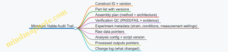
A quick checklist for end-to-end completeness
Before closing a construct’s record, verify:
- The construct record can be read top-to-bottom without opening other files.
- Each experiment has a unique ID and a link to the construct version.
- Each processed output has a link to the raw data and the exact analysis config.
- QC results include evidence files and a clear pass/fail.
- The change log explains differences between versions in terms of parts, architecture, or analysis assumptions.
When these are satisfied, the audit trail becomes a tool for interpretation, not paperwork. It turns “we built it and measured it” into “we can explain what we built, how we tested it, and why the results look the way they do.”
12. End to End Case Studies in Genetic Programming
12.1 Case Study Spec to Model to Construct for a Logic Module
This case study designs a small logic module: a two-input AND gate that outputs a reporter when both inputs are present. The goal is not just “it works once,” but “it works in a way you can predict, test, and reproduce.”
Step 1: Write the spec like it will be tested
Define inputs, outputs, and operating regime
- Inputs: two inducers, A and B, each added at defined concentrations.
- Output: fluorescence (or luminescence) from a reporter gene.
- Operating regime: choose a concentration range where the reporter signal is measurable and the cells are healthy.
A practical spec includes a table of what “present” and “absent” mean.
| Signal | Meaning in the experiment | Example concentration band |
|---|---|---|
| A = 0 | baseline induction | 0–low (e.g., 0–0.1× nominal) |
| A = 1 | active induction | mid/high (e.g., 0.5–1× nominal) |
| B = 0 | baseline induction | 0–low |
| B = 1 | active induction | mid/high |
Define truth table and quantitative acceptance criteria
For an AND gate, the truth table is:
- A=0, B=0 → output OFF
- A=1, B=0 → output OFF
- A=0, B=1 → output OFF
- A=1, B=1 → output ON
Quantitative acceptance criteria prevent vague “high vs low” arguments. For example:
- Leak: max output for any OFF condition ≤ 10% of ON output.
- Dynamic range: ON output ≥ 5× OFF output.
- Separation: OFF conditions should cluster tightly (e.g., coefficient of variation below a chosen threshold).
Add constraints that affect design choices
Include constraints early so the model and construct don’t chase impossible targets.
- Time: measure at a fixed time after induction (e.g., 6 hours) to match model assumptions.
- Host: specify strain and growth conditions because they shift expression capacity.
- Copy number / burden: keep total expression load moderate by limiting strong promoters and high-copy plasmids.
Step 2: Turn the spec into a model you can use
Choose a modeling level
For a logic module, you usually need a model that captures:
- how each input regulates transcription of an intermediate or directly regulates the reporter,
- how nonlinearity creates threshold-like behavior,
- how basal expression contributes to leak.
A common starting point is a steady-state transcription model with regulatory functions, then optionally add a simple time constant.
Represent each input as a regulatory transfer function
Assume each input controls a regulator that affects transcription of the reporter. A typical form is a Hill function.
For an activator-like input: \[ \text{Act}(x)=\frac{x^{n}}{K^{n}+x^{n}} \] For a repressor-like input: \[ \text{Rep}(x)=\frac{K^{n}}{K^{n}+x^{n}} \]
Here, (x\) is inducer concentration, (K\) is the half-max concentration, and (n\) is the Hill coefficient.
Model AND behavior as a composition of regulation
A clean AND gate can be implemented by requiring both regulators to be present at the transcription step. In the simplest model, combine the two regulatory terms multiplicatively: \[ \text{Reg}(A,B)=\text{Act}(A)\cdot \text{Act}(B) \] Then reporter expression is: \[ R(A,B)=R_{\min}+ (R_{\max}-R_{\min})\cdot \text{Reg}(A,B) \] This structure makes leak explicit via (R_{\min}\).
Parameterize using measured transfer functions
Before fitting the full AND model, measure each input’s effect in isolation.
- Build single-input constructs: A-only and B-only versions.
- Fit (K\) and (n\) for each input’s regulatory function.
- Estimate (R_{\min}\) from the double-zero condition.
Then fit any remaining parameters (like (R_{\max}\)) using the A=1,B=1 condition.
Mind map: spec → model → construct
Mind map: AND logic module (spec → model → construct)
Step 3: Choose a construct architecture that matches the model
Align biological mechanism with the math
The multiplicative AND model assumes that both inputs contribute to transcription in a way that scales together. A practical architecture is:
- Input A activates transcription of a regulator or directly contributes to promoter activation.
- Input B activates the same promoter (or a promoter that requires both activators).
If you use two separate activators that converge on the same promoter, the promoter’s activity often behaves like a product of activation terms, especially when each activator binding event is rate-limiting.
Concrete example architecture
A minimal, testable design uses a reporter under a promoter that is activated only when both regulators are present.
- Regulator A: expressed from a promoter induced by A.
- Regulator B: expressed from a promoter induced by B.
- AND promoter: reporter transcription requires both regulators.
To keep the design honest, include these constructs:
- Reporter under AND promoter with both regulators present.
- A-only: regulator B omitted (or its expression blocked).
- B-only: regulator A omitted.
- Double-zero: both regulators absent.
These controls let you verify that the leak is truly (R_{\min}\) and that OFF conditions are not caused by accidental activation.
Example parameter-to-design mapping
- If the model predicts insufficient separation (OFF too high), increase nonlinearity by choosing regulators/promoters with higher effective Hill coefficient or by reducing basal promoter strength.
- If ON is too low, adjust expression capacity: stronger RBS for the reporter, or a promoter variant that increases (R_{\max}\).
This is where code-driven design helps: you can change a parameter in the model and immediately see what design knob likely fixes it.
Step 4: Build and test in a loop that matches the model
Experimental matrix
Run a small grid that matches the spec bands.
- A ∈ {0, 1}
- B ∈ {0, 1}
- Replicates per condition (enough to estimate variance)
Measure reporter output at the time used in the model (or fit a simple time-to-steady-state correction if needed).
Sanity checks before full fitting
Before fitting the AND model, check:
- Monotonicity: A-only should increase with A; B-only should increase with B.
- Leak source: double-zero should be low; if not, the promoter or regulator system has unintended basal activity.
Fit and compare to acceptance criteria
Fit the model parameters using the measured single-input curves and then compute predicted (R(A,B)\) for the four truth-table points.
- If OFF conditions exceed the leak threshold, revisit promoter basal activity or regulator expression leakage.
- If ON is below requirement, revisit expression strength or timing.
Step 5: Mind map for the build/test artifacts
Mind map: artifacts you must produce
Step 6: What “done” looks like for this case study
A successful AND logic module satisfies the acceptance criteria using the same measurement protocol used for modeling. The final evidence is not a single plot; it’s the consistency between:
- single-input transfer behavior (supports the regulatory functions),
- double-zero leak (supports (R_{\min}\)),
- double-one output (supports (R_{\max}\)),
- and the OFF/ON separation in the full truth table (supports the AND composition).
When those align, the spec-to-model-to-construct pipeline is working as intended: the model isn’t just a story, and the construct isn’t just a lucky build.
12.2 Case Study Robust Parameter Tuning for a Feedback System
Problem setup: a feedback circuit with a measurable goal
We want a genetic feedback system that tracks a target output level despite day-to-day variation in growth rate, induction strength, and part performance. Concretely, imagine an output reporter (Y\) (e.g., fluorescence) controlled by an input inducer (I\). A controller gene produces a repressor (R\) that downregulates the output transcription. The wet-lab goal is simple to state and hard to satisfy: when (I\) changes, (Y\) should move toward a desired setpoint (Y_{\text{sp}}\) with limited overshoot and acceptable settling time.
A practical modeling choice is to treat the system as a reduced dynamical model with a small number of parameters:
- (k_{\text{prod}}\): output production rate scale
- (k_{\text{deg}}\): output degradation/dilution rate
- (k_{\text{rep}}\): repression strength
- (K\): repression half-effect parameter
- (n\): Hill coefficient (nonlinearity)
- (k_{\text{ctrl}}\): controller production scale
- (\tau\): effective delay (optional; can be approximated as a first-order lag)
The tuning task is to pick parameter values that satisfy the specification under uncertainty, not just for one “best” dataset.
Mind map: what “robust tuning” means here
Step 1: define metrics that match the biology
Instead of tuning to a single curve fit, define metrics that correspond to what you can observe.
Assume a step in inducer from (I_0\) to (I_1\) at (t=0\). Let (Y(t)\) be the simulated output.
-
Steady-state error \[ E_{\text{ss}} = \left|Y( T_{\text{end}}) - Y_{\text{sp}}\right| \] Pick (T_{\text{end}}\) after the response has largely settled (e.g., 6–10 time constants of the output).
-
Overshoot ratio \[ M_{\text{os}} = \max_{t\in[0,T_{\text{end}}]} \frac{Y(t)}{Y_{\text{sp}}} \] If (M_{\text{os}}\) is too high, the circuit likely oscillates or has excessive loop gain.
-
Settling time Define a tolerance band (\epsilon\) (e.g., 10% of setpoint): \[ T_{\text{set}} = \inf\left{t: \forall s\ge t,\ |Y(s)-Y_{\text{sp}}|\le \epsilon,Y_{\text{sp}}\right} \] This metric penalizes slow recovery even if the final value is correct.
-
Robustness score under uncertainty We will evaluate the metrics across sampled uncertain conditions and aggregate them, for example with a worst-case or percentile statistic: \[ J(\theta) = \text{Quantile}_{0.9}\left( w_1 E_{\text{ss}} + w_2 (M_{\text{os}}-1)_+ + w_3 T_{\text{set}} \right) \] where \((x)_+ = \max(x,0)\), \(\theta\) is the parameter vector, and \(w_i\) are weights.
A slightly playful but useful rule: choose weights so that “bad overshoot” is expensive even if steady-state is fine.
Step 2: build a reduced closed-loop model
A minimal structure for output repression by controller (R\):
\[ \frac{dY}{dt} = k_{\text{prod}}, f(I), g(R) - k_{\text{deg}} Y \] \[ \frac{dR}{dt} = k_{\text{ctrl}}, h(I) - \frac{1}{\tau}R \] Here:
- (f(I)\) maps inducer to output transcription drive (often a saturating Hill function)
- (g(R)\) is repression, e.g. \[ g(R)=\frac{1}{1+\left(\frac{R}{K}\right)^n} \]
- (\tau\) is an effective controller response time; if you omit it, set (R\) dynamics to a simple first-order decay with rate (k_{\text{deg,R}}\)
The point of the reduced model is not to be perfect; it’s to be consistent enough that tuning decisions are meaningful.
Step 3: encode uncertainty as parameter perturbations
You need uncertainty that reflects reality and is measurable.
A common approach is to define priors from characterization:
- (k_{\text{deg}}\): log-normal around a measured mean with variance from replicate experiments
- (k_{\text{prod}}\) and (k_{\text{rep}}\): normal or log-normal around measured transfer-function fits
- (K\) and (n\): either fixed from characterization or allowed to vary within confidence intervals
- Induction scaling: treat (f(I)\) as having an effective gain (\alpha\), so (I\) becomes (\alpha I\)
Example uncertainty model (conceptual):
- (\alpha \sim \mathcal{N}(1, 0.15^2)\) truncated to positive values
- (k_{\text{deg}} \sim \mathcal{N}(\mu_{\text{deg}}, (0.2\mu_{\text{deg}})^2)\)
- (k_{\text{rep}} \sim \mathcal{N}(\mu_{\text{rep}}, (0.25\mu_{\text{rep}})^2)\)
Then, for each candidate parameter set (\theta\), sample (N\) uncertain draws and compute the aggregated score (J(\theta)\).
Step 4: run a robust tuning loop with a concrete example
Suppose you start with a baseline tuned for nominal conditions. You then observe that in some experiments the output overshoots and oscillates slightly.
A robust tuning loop might proceed like this:
- Choose a search space for the controller gain (k_{\text{ctrl}}\) and repression strength (k_{\text{rep}}\). Keep (K\) and (n\) fixed if they are well-characterized.
- For each candidate (\theta\), sample uncertain conditions (e.g., 50 draws of (\alpha\) and (k_{\text{deg}}\)).
- Simulate the step response for each draw.
- Compute (E_{\text{ss}}, M_{\text{os}}, T_{\text{set}}\) and aggregate into (J(\theta)\).
- Select the candidate with the best robust score.
A key detail: if you only simulate one step size, you may tune for the wrong regime. Use multiple step targets (Y_{\text{sp}}\) or multiple inducer levels (I_1\) that you actually plan to test.
Step 5: interpret tuning outcomes like a scientist, not a spreadsheet
After optimization, you’ll likely see parameter tradeoffs:
- Increasing loop gain (via larger (k_{\text{ctrl}}\) or (k_{\text{rep}}\)) can reduce steady-state error but increase overshoot.
- Increasing effective delay (\tau\) (or having a slower controller) can worsen oscillations even if steady-state remains correct.
- Changing (k_{\text{deg}}\) affects both speed and damping; faster dilution can make the loop behave “more stable” or “more twitchy” depending on the controller dynamics.
A practical sanity check is to compute sensitivity of the score to each parameter around the optimum. If the robust optimum is extremely sensitive to one parameter you cannot control experimentally, you should either widen the uncertainty model or redesign the circuit so that parameter becomes less critical.
Step 6: validation experiment design that tests robustness
To validate robust tuning, you need tests that stress the uncertainty sources.
- Induction scaling stress: run the same setpoint target using different inducer preparation batches or different induction protocols that shift effective gain (\alpha\).
- Growth stress: test at different growth phases or media conditions that change dilution (k_{\text{deg}}\).
- Multiple setpoints: repeat tuning validation for at least two target output levels so you don’t accidentally optimize only the easiest operating point.
For each condition, measure (Y(t)\) at a time resolution fine enough to estimate overshoot and settling time.
Step 7: what to do when the model and data disagree
If the tuned circuit still overshoots, check whether the mismatch is systematic:
- If overshoot is consistently higher than predicted, the model likely underestimates effective delay (\tau\) or overestimates repression strength.
- If steady-state is correct but settling is slow, the controller response may be slower than modeled (again pointing to (\tau\) or controller degradation).
- If behavior changes shape across conditions, the uncertainty model may be missing a key variable (often induction scaling or a non-modeled saturation).
Then update the model parameters using the new data, but keep the robust objective. The goal is not to “fit the last experiment,” but to keep performance acceptable across the range you care about.
Mini worked example: choosing between two candidate tunings
Assume two candidate parameter sets (\theta_A\) and (\theta_B\) produce the following aggregated metrics across uncertainty samples:
- (\theta_A\): (E_{\text{ss}}=0.08\), (M_{\text{os}}=1.25\), (T_{\text{set}}=5.0\) hours
- (\theta_B\): (E_{\text{ss}}=0.12\), (M_{\text{os}}=1.10\), (T_{\text{set}}=6.0\) hours
If overshoot is the main failure mode in your lab workflow (e.g., it triggers stress responses or causes downstream burden), you choose (\theta_B\) even though steady-state error is slightly worse. This is exactly what the robust objective is for: it encodes which kinds of mistakes you can tolerate.
Mind map: the full case study workflow
12.3 Case Study Automated Assembly Planning for a Multi Part Circuit
This case study plans an assembly for a three-module genetic circuit: a sensor module, a logic module, and an output module. The goal is to show how a code-driven pipeline can turn a circuit graph into an ordered, constraint-satisfying assembly plan.
Circuit goal and constraints
Circuit behavior (high level):
- The sensor produces an input signal (transcription factor A) in response to a chemical inducer.
- The logic uses A to control expression of output protein B.
- The output includes a reporter and a terminator to stop transcription cleanly.
Assembly constraints (typical, but explicit):
- Use a Type IIS cloning workflow (e.g., Golden Gate style) with fixed overhangs.
- Each module must be assembled in a specific order to preserve transcriptional direction.
- Avoid forbidden combinations: no two adjacent parts may share the same overhang set.
- Maintain a consistent orientation: promoters face the downstream coding sequence.
- Include a selection marker once, not per module.
Design inputs (what code receives):
- A circuit graph: nodes are parts (promoters, RBS, CDS, terminators), edges are “transcribed into” relationships.
- A part library: each part has sequence, length, and overhang compatibility metadata.
- A cloning scheme: overhang mapping rules and assembly stages.
Mind map: assembly planning pipeline
Step 1: Define modules and interfaces
We treat the circuit as three modules with clear interfaces.
Module S (sensor):
- Promoter (P_{sens}) → RBS (R_{A}) → CDS (A) → terminator (T_{sens})
Module L (logic):
- Promoter (P_{logic}(A)) → RBS (R_{B}) → CDS (B) → terminator (T_{logic})
Module O (output packaging):
- A reporter CDS (RPT) and a final terminator (T_{out})
To keep assembly manageable, we decide that Module L already includes the transcriptional control and the coding region for B, while Module O only adds the reporter and final termination. That choice reduces the number of promoter/terminator junctions the planner must reason about.
Interface rule: every module exports a “left boundary” and “right boundary” overhang signature that the next module must accept.
Step 2: Represent parts as structured records
Each part record includes: part_id, sequence, default_orientation, left_overhang, right_overhang, and role (promoter, RBS, CDS, terminator, marker).
A practical best practice is to store overhangs as identifiers, not raw sequences, so compatibility rules stay readable.
Example part metadata (conceptual):
P_sens: role=promoter, left_overhang=H01, right_overhang=H02R_A: role=RBS, left_overhang=H02, right_overhang=H03CDS_A: role=CDS, left_overhang=H03, right_overhang=H04T_sens: role=terminator, left_overhang=H04, right_overhang=H05
The planner uses these signatures to connect parts without manually checking every junction.
Step 3: Stage partitioning (how many assemblies?)
Golden Gate style workflows often assemble multiple fragments in one pot, but practical limits exist: fragment count, pipetting burden, and error isolation.
We choose a two-stage plan:
- Stage 1: assemble Module S and Module L into intermediate constructs.
- Stage 2: assemble the intermediate(s) with Module O and the selection marker.
Reasoning: Module S and Module L each have internal structure that must be correct; isolating them reduces the search space when something fails. Stage 2 then focuses on the junctions between modules.
Step 4: Assign overhangs and order parts
The planner performs a topological traversal of the circuit graph, but with an important twist: it must output linear assembly order for each stage.
For Module S, the linear order is:
- (P_{sens})
- (R_{A})
- (CDS_{A})
- (T_{sens})
For Module L, the linear order is:
- (P_{logic}(A))
- (R_{B})
- (CDS_{B})
- (T_{logic})
For Module O, the linear order is:
- (RPT)
- (T_{out})
Selection marker (M) is placed once in the final backbone region, with known overhang compatibility.
Overhang compatibility check:
- The right overhang of one part must match the left overhang of the next.
- If a match is missing, the planner either rejects the design or requests an alternative part with compatible overhangs.
Step 5: Enforce orientation and forbidden adjacency
Even if overhangs match, orientation can break transcription.
Orientation rule: promoters and RBS must be oriented so transcription flows toward CDS, and terminators must face upstream transcription.
The planner checks each junction:
- If
role=promoterthen the downstream neighbor must berole in {RBS, CDS}depending on whether an RBS is explicit. - If
role=terminatorthen the downstream neighbor must be a boundary element (e.g., marker or next promoter) that is allowed by the cloning scheme.
Forbidden adjacency rule example:
- Overhang signature
H05cannot be followed byH05because it creates a junction that frequently misassembles. - The planner encodes this as a constraint:
forbidden_pair=(H05,H05).
Step 6: Produce the assembly plan output
Below is a compact example of what the planner might emit.
{
  "constructs": [
    {
      "name": "Intermediate_S",
      "stage": 1,
      "parts": ["P_sens","R_A","CDS_A","T_sens"],
      "overhangs": [["H01","H02"],["H02","H03"],["H03","H04"],["H04","H05"]]
    },
    {
      "name": "Intermediate_L",
      "stage": 1,
      "parts": ["P_logic","R_B","CDS_B","T_logic"],
      "overhangs": [["H05","H06"],["H06","H07"],["H07","H08"],["H08","H09"]]
    },
    {
      "name": "Final_Circuit",
      "stage": 2,
      "parts": ["Backbone_M","Intermediate_S","Intermediate_L","RPT","T_out"],
      "junctions": [["H10","H01"],["H05","H06"],["H09","H11"],["H11","H12"]]
    }
  ]
}
The key detail is that intermediate constructs are treated as named fragments with their own boundary overhangs. That lets the stage 2 planner avoid re-deriving internal junctions.
Step 7: Validation report (what the code checks before ordering)
A good assembly planner produces a validation summary that is easy to audit.
Checks performed:
- Every required role appears exactly once (e.g., selection marker appears once).
- All junctions have matching overhang signatures.
- No forbidden adjacency pairs occur.
- Orientation is consistent with promoter-to-CDS flow.
- No part is used in two different incompatible contexts (e.g., a terminator variant with different overhangs).
Example validation outcomes (illustrative):
OK: 3 stage fragments assembled with 100% overhang matches.OK: marker used once.OK: promoter orientation consistent in 6/6 junctions.
If a check fails, the planner should report the exact junction that broke, such as junction T_sens -> P_logic: expected left overhang H05, got H04.
Mind map: constraints and checks
Step 8: Concrete example of a junction failure and fix
Suppose the planner detects a mismatch at the boundary between Module S and Module L in stage 2:
- Expected:
T_sens.right_overhang = H05connects toP_logic.left_overhang = H05 - Actual library metadata:
P_logic.left_overhang = H04
Fix options the code can consider (without guessing blindly):
- Swap to an alternative promoter variant
P_logic_altwith left overhangH05. - Repartition stages so that Module S and Module L are assembled in stage 1 separately and only their internal boundaries are used in stage 2.
In this case, stage 2 uses module boundaries, so option (1) is simplest if the alternative promoter variant is functionally equivalent in the part library.
The planner updates the plan and reruns validation, producing a new traceable mapping: P_logic -> P_logic_alt.
Output artifacts for wet lab execution
The final assembly plan typically includes:
- A stage-by-stage fragment list.
- A junction map for each construct.
- A traceability table linking each fragment in the plan back to the original circuit graph nodes.
This keeps the wet lab workflow grounded: if a construct fails, you can identify whether the failure is likely internal (stage 1) or at a boundary (stage 2), based on where the plan isolates complexity.
12.4 Case Study Iterative Refinement Using Experimental Data
Scenario
You built a simple transcriptional logic module: an inducible promoter driving a reporter. The goal is not to “match a curve perfectly,” but to get behavior that is consistent enough to compose with other modules.
Initial design target (measured as reporter fluorescence vs. inducer concentration):
- Low inducer: fluorescence near baseline (leak suppression)
- Mid inducer: steep transition (usable dynamic range)
- High inducer: plateau (saturation)
You start with a model that assumes a standard regulatory form (Hill-type activation) and a single effective parameter set. The first build produces data that are close in shape but off in key places: baseline is higher than predicted, and the transition is shifted.
Mind map: the refinement loop
Step 1: Compare prediction and measurement
You run the same induction protocol as in the initial characterization: identical growth phase, induction time, and measurement settings. You then overlay the model prediction with the new data.
A useful habit is to compute residuals at each inducer concentration: \[ r_i = y_i - \hat{y}(x_i) \] where \(y_i\) is measured fluorescence and \(\hat{y}(x_i)\) is the model prediction.
What you see in the first iteration (example numbers):
- At the lowest inducer point, measured fluorescence is ~2.5× the predicted baseline.
- Around the midpoint, the measured curve reaches half-max at an inducer concentration about 3× higher than predicted.
- At high inducer, the plateau is slightly lower than predicted.
These aren’t random errors. The residuals have a consistent sign in regions, which is your cue to adjust the model in a targeted way.
Step 2: Diagnose likely causes from residual patterns
Instead of changing everything, you map each mismatch to a small set of plausible mechanisms.
Baseline too high suggests one of:
- Effective leak in the promoter (not captured by the initial model)
- Background fluorescence or autofluorescence subtraction mismatch
- Reporter expression not fully under promoter control (e.g., readthrough)
Transition shifted right suggests:
- Effective inducer concentration at the promoter is lower than assumed
- Cooperativity (Hill coefficient) differs from the initial assumption
- Induction kinetics during the measurement window differ from the steady-state assumption
Plateau too low suggests:
- Expression capacity limits (RBS strength, transcriptional machinery saturation)
- Reporter degradation or maturation affecting the readout
- Measurement saturation or normalization issues
Step 3: Update the model with constrained parameter fitting
Your initial model is: \[ \hat{y}(x) = y_{\min} + (y_{\max}-y_{\min})\frac{x^n}{K^n + x^n} \]
The first iteration used fixed \(n\) and a rough \(K\). Now you refit with constraints that match what you know from biology and measurement.
Refinement rule: only free parameters that correspond to observed mismatch.
- Because baseline is wrong, free \(y_{\min}\).
- Because the transition is shifted, free \(K\).
- Because plateau is slightly off, free \(y_{\max}\).
- Keep \(n\) fixed at first if the curve shape isn’t dramatically different; otherwise free it.
You fit parameters by minimizing a weighted loss. A simple choice is weighted least squares to avoid one region dominating: \[ \min_{y_{\min},y_{\max},K}\sum_i w_i\left(y_i-\hat{y}(x_i)\right)^2 \] where \(w_i\) can be larger near the transition if that region matters most for composition.
Example outcome of the refit:
- \(y_{\min}\) increases to match the observed leak.
- \(K\) increases ~3×, aligning the midpoint.
- \(y_{\max}\) decreases slightly, matching the plateau.
At this point, you check whether residuals are now small and sign-consistent.
Step 4: Decide whether the model needs structural changes
You might be tempted to add new terms immediately. Don’t. Structural changes should be justified by residual shape.
Residual check after refit:
- If residuals are now mostly within measurement noise across all points, stop.
- If residuals show a systematic curvature (e.g., consistently underpredicting mid-range while overpredicting high-range), then the Hill form may be missing something.
A common structural addition is an explicit induction offset or a two-state model. But in this case, the residuals after parameter refit look random around the curve, so you avoid adding complexity.
Step 5: Plan the next build to reduce uncertainty efficiently
Now you choose inducer concentrations that improve parameter identifiability.
Information-focused sampling:
- Add more points near the transition region to refine \(K\) and \(n\) (if \(n\) is free).
- Keep at least one low point to verify baseline.
- Keep one high point to verify plateau.
Example next experiment design:
- Use 6 inducer concentrations instead of 4.
- Place two points below the current half-max estimate, two around it, and two above.
- Keep everything else fixed.
This is where code-driven workflows help: you can generate the next induction schedule from the current posterior or from the sensitivity of \(\hat{y}(x)\) to parameters.
Mind map: what to change next
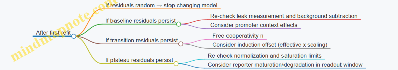
Step 6: Iterate and verify composition readiness
You build the same construct again (or a small set of variants if you’re also testing robustness). You collect the new dataset and refit.
Success criteria for this case study:
- Baseline is within an acceptable band relative to the module’s intended downstream threshold.
- Mid-range behavior aligns so that downstream logic gates see the expected input-output mapping.
- Plateau is stable enough that downstream modules don’t saturate unexpectedly.
Concrete check: you compute the predicted input concentration that yields a target output level (e.g., half-max). If that concentration is stable across replicates, the module is composition-ready.
Step 7: Capture the refinement in a reproducible record
Even in a small case study, you want traceability.
Record:
- The exact model form used
- Which parameters were free in each iteration
- The loss function and weighting
- The inducer schedule for each build
- The acceptance criteria and whether they were met
This turns “we adjusted until it looked right” into a repeatable process that another construct can follow.
Summary of the iteration
- Compare prediction vs. data and compute residuals.
- Diagnose mismatches by residual patterns (baseline, shift, plateau).
- Refit with constrained parameter changes tied to observed errors.
- Only add structural complexity if residuals demand it.
- Plan the next build to target the most uncertain region (usually the transition).
- Verify that the refined behavior is stable enough for downstream composition.
By the end of this loop, the model is not just a better fit; it is a better tool for deciding what to build next and how to interpret the next batch of measurements.
12.5 Case Study Packaging a Reusable Modular Circuit Library
This case study shows how to package a small set of genetic circuit modules into a reusable library that can be assembled, simulated, and tested with minimal rework. The goal is not to “store parts,” but to store design intent plus the information needed to reproduce behavior.
What “reusable” means in practice
A module is reusable when you can:
- Assemble it into a larger construct without re-deriving its architecture.
- Predict its behavior using the same modeling assumptions used during design.
- Swap parameters (e.g., promoter strength or degradation rate) without breaking interfaces.
- Trace every output back to the inputs that produced it.
To make that concrete, we’ll package three modules:
- Input module: an inducible promoter driving a transcription factor (TF).
- Logic module: a TF-regulated gate producing an output reporter.
- Output module: a reporter with a tunable degradation tag.
Each module will have a stable interface: what it consumes, what it produces, and what assumptions it relies on.
Mind map: library packaging workflow
Step 1: Define module interfaces as contracts
Interfaces prevent “it worked once” designs. For each module, define:
- Signal type: what variable the module expects (e.g., TF concentration proxy from fluorescence).
- Transfer behavior: how the input signal maps to an output production rate.
- Operating regime: where the model is valid (e.g., induction range where promoter response is monotonic).
- Measurement mapping: how simulation outputs correspond to experimental readouts.
Example interface contract (logic module):
- Input: TF concentration proxy \(x\) (arbitrary fluorescence units mapped to model units via calibration).
- Output: reporter production rate \(p_{out}(x)\).
- Model form: Hill repression with parameters \(K\) and \(n\).
- Validity: \(x\) within the calibrated range; outside it, predictions are not used for optimization.
A simple transfer function used in the library: \[ p_{out}(x) = p_{max} \cdot \frac{1}{1 + \left(\frac{x}{K}\right)^n} \]
Best practice: store the assumptions alongside the equation. If \(x\) is a fluorescence proxy, record the calibration method used to map fluorescence to model units.
Step 2: Package part metadata and model artifacts together
A reusable module needs both wet-lab facts and modeling facts.
For each module, store:
- Sequence-level identifiers: promoter ID, RBS ID, ORF ID, terminator ID, degradation tag ID.
- Context notes: whether the promoter was characterized with the same backbone, copy number, and measurement strain.
- Measurement conditions: media, temperature, induction protocol, and time window.
- Model artifacts: fitted parameters, confidence intervals (or at least residual summaries), and the validity domain.
Concrete example: input module metadata
- Promoter: “P_ind_01”
- Characterization: measured in the same backbone as the library’s assembly standard
- Output mapping: TF fluorescence measured after a fixed delay \(t_{delay}\)
- Stored model: promoter-to-TF production rate curve \(p_{TF}(I)\)
If you later assemble the module into a different backbone, the library should flag the context mismatch rather than silently reusing parameters.
Step 3: Use a construct schema that mirrors biological assembly
Instead of treating constructs as flat strings, represent them as a module graph with explicit ordering and orientation.
Mind map: construct schema
A minimal code-driven synthesis approach can be represented as structured data. The key is that the schema includes both what to assemble and how to check it.
Example pseudocode for generating an assembly plan (kept short and schematic):
plan = new AssemblyPlan()
plan.add(module("input", promoter="P_ind_01", rbs="RBS_02"))
plan.add(module("logic", gate="G_rep_01", tf="TF_A"))
plan.add(module("output", reporter="GFP", degron="dA"))

plan.connect("input.TF", "logic.TF_input")
plan.connect("logic.output", "output.reporter")

plan.check(orientation_rules=true, context_rules=true, frame_rules=true)
plan.export("assembly_manifest.json")
Between modules, the library enforces fixed boundaries: for example, the logic module always ends with a terminator that matches the output module’s promoter-free start. That reduces the number of “mystery failures” when swapping modules.
Step 4: Embed sanity checks that catch common mistakes
Reusable libraries fail when they accept invalid combinations. Add checks that are cheap and informative.
Common checks:
- Orientation: promoters must face the correct direction; coding sequences must be in-frame.
- Interface compatibility: the logic module expects TF_A; if the input module produces TF_B, the plan should stop.
- Context mismatch: if a promoter was characterized in a different backbone, the plan should require an explicit override.
- Regime mismatch: if the intended induction range is outside the stored validity domain, the library should warn and avoid using those parameters for optimization.
Example check logic (conceptual):
- If \(\text{module.logic.tf} \neq \text{module.input.tf}\), raise “TF interface mismatch.”
- If \(\text{module.input.backbone} \neq \text{library.standard_backbone}\), raise “context mismatch: promoter parameters not guaranteed.”
Step 5: Version the library like a software artifact
Versioning prevents silent drift. A module version should change when any of the following changes:
- Sequence content (even if functionally similar).
- Interface contract (e.g., output mapping units).
- Model form or parameterization.
- Validity domain.
A practical rule: treat each module as immutable once released. If you improve the promoter characterization, create a new module version rather than editing the old one.
Step 6: Package a small release with a reproducible test set
A library release should include a minimal set of constructs that exercise interfaces.
Release contents (example):
- Module versions: input v1.2, logic v1.0, output v0.9
- Three assembled constructs:
- Input + Logic + Output (full chain)
- Input + Logic with a nonbinding TF control (checks gate baseline)
- Logic + Output with a fixed TF expression (checks output mapping)
Each construct includes:
- Assembly manifest
- Simulation configuration (which parameters were used)
- Measurement protocol summary (time window, readout channel)
- Data schema for storing results
This makes reuse practical: when someone swaps a module version, they can compare against the release test set.
Step 7: Keep traceability tight from design to data
Traceability is what makes the library trustworthy.
For every build, store:
- Module versions used
- Assembly manifest ID
- Simulation run ID
- Parameter set ID
- Raw measurement file IDs
Then, when a mismatch occurs, you can answer quickly:
- Was the mismatch due to a sequence change, a context change, or a modeling assumption?
Mind map: release artifact structure
Concrete example: packaging the three-module chain
Suppose the full chain is:
- Input module: inducible promoter \(P_{ind_01}\) producing TF_A
- Logic module: TF_A repression gate producing reporter transcript
- Output module: GFP with degradation tag dA
The library stores:
- The promoter-to-TF model \(p_{TF}(I)\)
- The gate transfer \(p_{out}(x)\)
- The output degradation mapping (e.g., effective half-life parameter)
When assembling a new construct that uses the same logic and output but swaps the input promoter to \(P_{ind_03}\), the library can reuse the logic and output modules while requiring a new input model (or a context-validated parameter mapping). That’s the difference between “parts in a folder” and “modules that behave predictably.”
The result is a compact library where each module is a self-contained unit: it carries its interface, its assumptions, its sequences, and its model artifacts. That packaging turns circuit design into a repeatable engineering process rather than a series of one-off experiments.