Universal Profiling with eBPF
1. Foundations of eBPF for Universal Profiling
1.1 What Universal Profiling Means for Real Systems
Universal profiling is the practice of observing how applications behave while they run, using signals from the operating system and runtime environment rather than requiring changes to the application’s source code. In real systems, that matters because the “thing you want to understand” is often deployed as an artifact you cannot easily rebuild, or it’s shared across teams with different release cycles. Universal profiling aims to answer questions like: Which code paths are consuming CPU? Where does time go during a request? What is waiting on what? And which workload is responsible for the observed behavior?
A useful way to think about it is as a loop with three parts: observe, attribute, and summarize. Observe means collecting events from the system at the right points. Attribute means mapping those events back to the process, thread, and sometimes the function or request context. Summarize means turning raw events into metrics that are stable enough to compare across time windows.
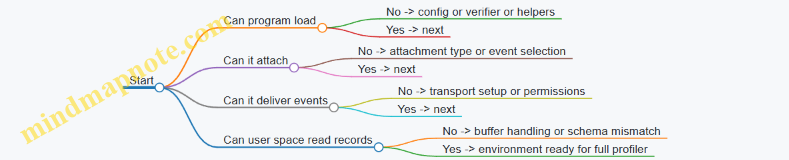
Mind Map: Universal Profiling in Practice
What “Without Modifying Source Code” Really Implies
Not modifying source code usually means you can’t add explicit instrumentation calls inside the application. So you rely on observation points that already exist: kernel events, runtime behaviors, and function boundaries that can be intercepted from the outside. For example, if you want to know why a web service is slow, you can measure request duration by correlating a start event with an end event, even if the application never logs those timestamps.
The key is choosing observation points that are both meaningful and stable. Meaningful means the signal changes when the behavior changes. Stable means the signal remains available across deployments and doesn’t depend on a specific build configuration.
A Concrete Example: CPU Hot Paths Without Instrumentation
Imagine a service that suddenly uses more CPU after a configuration change. Universal profiling can sample execution at the CPU level and attribute samples to the running process and thread. If the profiler also captures stack traces, you can often identify which functions are on the hot path.
A practical workflow looks like this:
- Start a short profiling window during the suspected regression.
- Collect CPU samples and stack traces.
- Aggregate by process and function.
- Compare against a baseline window from a known-good period.
Suppose the baseline window is 2026-03-20 to 2026-03-20 30 minutes, and the regression window is 2026-03-20 60 minutes later. If the aggregated results show that the same thread now spends more time in a specific parsing routine, you have a direct lead that doesn’t require rebuilding the service with custom logging.
Another Example: Latency Histograms from System Events
Latency profiling is often more actionable than raw traces because it answers “how long” and “how often.” Universal profiling can build histograms by measuring durations between two events. For a request, those events might be tied to socket activity or application-level boundaries inferred from runtime behavior.
The important detail is correlation. If you measure durations without a reliable way to pair start and end, you end up with misleading averages. Universal profiling therefore focuses on correlation keys such as thread identity, file descriptors, or other handles that persist across the request’s lifetime.
What Makes It “Universal” Across Systems
Universal doesn’t mean one technique fits every scenario. It means the approach is consistent: observe from the outside, attribute to the right execution context, and summarize into comparable metrics. In practice, that consistency lets you apply the same mental model whether you’re profiling a database, a JVM service, or a Go worker.
The constraints are real and shape design choices. Overhead limits how much data you can collect. Data loss can happen under heavy load, so you design for graceful degradation. Cardinality limits how many unique keys you track, because “every request gets its own bucket” quickly becomes a memory problem.
If you keep those constraints in mind, universal profiling becomes less of a magic trick and more of disciplined measurement: pick signals that map cleanly to behavior, correlate them carefully, and summarize them in ways that survive real-world noise.
1.2 eBPF Architecture and Execution Model
eBPF is a small program format that runs inside the kernel, but it is not “just code in the kernel.” It is a controlled execution environment with strict verification, well-defined data paths, and explicit ways to move data to user space. Universal profiling depends on this model because it lets you observe behavior across processes without changing their source code.
The Big Picture
Think of the system as three cooperating parts:
- A loader in user space that compiles or loads eBPF bytecode, sets up maps, and attaches programs to kernel hooks.
- The eBPF runtime in the kernel that verifies safety, schedules execution at hook points, and enforces limits.
- A consumer in user space that reads events from ring buffers or perf buffers, aggregates them, and produces reports.
This separation matters: the kernel runs the eBPF program, but the heavy lifting—parsing, symbolization, grouping, and reporting—belongs in user space.
Program Types and Hook Points
An eBPF “program” is not one universal thing; it is a specific program type tied to a hook. Common types include:
- Tracepoint programs that run when a named kernel event fires.
- Kprobe and tracepoint-like function hooks that run on entry or return of kernel functions.
- Uprobe programs that run on entry or return of user-space functions.
- Socket and networking programs that run on packet-related events.
For universal profiling, the key idea is that you choose observation points that already exist in the system. You then attach small programs that extract just enough context to identify what happened.
The Execution Path from Event to Report
When a hook fires, the kernel executes the attached eBPF program with a context object. The context contains fields relevant to that hook, such as pointers, IDs, or timestamps. Your program then:
- Reads context safely using helper functions and bounded reads.
- Optionally looks up state in maps, such as per-thread counters or in-flight request start times.
- Emits data via ring buffer or perf buffer, or updates maps for later aggregation.
- Returns quickly so the hook can continue with minimal disruption.
User space receives the emitted data, enriches it if needed, and aggregates it into profiling views.
Verification and Safety Rules
Before any eBPF program runs, the kernel verifier checks that it is safe. The verifier enforces rules like:
- No unbounded loops (or loops only in tightly controlled forms).
- No invalid memory access through pointers.
- Bounded access to packet or buffer data when applicable.
- Proper initialization of variables used in memory operations.
This is why eBPF programs often look “boring” compared to regular code: the constraints are there so the kernel stays stable even when you attach new probes.
Maps as the Memory Model
Maps are eBPF’s persistent state. They are the bridge between events and profiling logic. Typical map roles include:
- Counters and histograms keyed by process ID, thread ID, or function identifier.
- Correlation state keyed by a request ID or tuple, storing start timestamps until completion.
- Configuration that user space can update without reloading programs.
A practical best practice is to keep map keys stable and low-cardinality. If you key by something that explodes in uniqueness, you will pay for it in memory and lookup overhead.
Data Movement with Ring Buffers
Ring buffers are a common choice for universal profiling because they support high-throughput event streaming. The eBPF program writes a small record; user space reads it and aggregates.
A simple mental model: maps are for state you want to keep inside the kernel, while ring buffers are for “here is what happened” messages.
Mind Map: eBPF Architecture and Execution Model
Example: Correlating Request Duration
Suppose you want to measure how long a request takes from “start” to “finish” without modifying the application. You attach two probes: one at the start event and one at the completion event.
- On start, the eBPF program records a timestamp in a map keyed by a request identifier.
- On completion, it looks up the timestamp, computes duration, emits a record, and deletes or overwrites the entry.
This pattern works because the execution model guarantees that each probe runs with a consistent context and that map operations are safe and bounded.
Example: Keeping Kernel Work Small
A common mistake is to do expensive formatting in eBPF, like building long strings or doing heavy symbol logic. Instead, emit compact numeric identifiers (process ID, thread ID, function ID) and let user space translate them. The execution model supports this because ring buffer records are just data, and user space is where you can afford more CPU time.
Diagram: Event to User Space Pipeline
    flowchart TD
  A[Hook fires in kernel] --> B[eBPF program runs with context]
  B --> C[Safe reads and map lookups]
  C --> D[Emit event to ring buffer]
  D --> E[User space consumer reads record]
  E --> F[Aggregate and correlate]
  F --> G[Profiling report output]
Practical Takeaway
Universal profiling succeeds when you treat eBPF as a fast, safe observation tool: keep programs small, use maps for correlation, stream events for aggregation, and rely on the verifier to prevent kernel instability. The execution model is strict, but that strictness is exactly what makes it dependable.
1.3 Maps, Ring Buffers, and Data Flow Patterns
Universal profiling lives or dies by how you move data from the kernel to user space. eBPF programs run in tight constraints, so you typically separate “capture” from “aggregation.” Maps store state across events; ring buffers stream event payloads with minimal coordination; and user space turns raw events into profiles.
Maps as Persistent State
A map is a kernel-resident data structure keyed by something you choose, like a thread id, a stack id, or a request id. The key idea is that the eBPF program can update the map on every event, while user space reads it periodically.
Common map patterns for profiling:
- Counters by identity: key by
(pid, tid)to count events per thread. - Histograms by bucket: key by
(metric, bucket)to accumulate latency distributions. - Correlation state: key by
request_idto store a start timestamp until the end event arrives. - Stack trace aggregation: key by
stack_idto count samples per call path.
A practical rule: keep map keys small and stable. If you key by high-cardinality strings, you’ll spend memory and time just managing keys.
Ring Buffers as Event Streams
A ring buffer is a streaming channel from kernel to user space. Instead of storing every event forever in a map, you write each event into the ring buffer and let user space consume it. This is ideal for high-frequency events like sampling hits or short-lived markers.
Ring buffers shine when:
- You want near-real-time visibility.
- You don’t need to query individual events later.
- You can tolerate occasional loss when the consumer can’t keep up.
A simple mental model: maps are “remembering,” ring buffers are “reporting.”
Data Flow Patterns That Work
Most profiling pipelines follow one of three patterns.
Pattern 1: Stream Then Aggregate
- Kernel emits events to a ring buffer.
- User space aggregates into maps or in-memory structures.
- Output is produced from aggregates.
This pattern keeps kernel logic lightweight. It also makes it easier to change aggregation logic without reloading eBPF programs.
Pattern 2: Aggregate in Kernel Then Export
- Kernel updates maps on each event.
- User space periodically reads map contents.
- User space formats results.
This pattern is good when aggregation is simple and you want minimal event traffic.
Pattern 3: Correlate with Maps, Stream Summaries
- Kernel stores correlation state in maps (e.g., start timestamps).
- On completion, kernel emits a compact summary event to a ring buffer.
- User space aggregates summaries.
This avoids streaming large raw sequences while still producing per-request measurements.
Mind Map: Choosing Between Maps and Ring Buffers
Example: Correlating Request Duration
Suppose you want request latency without modifying the application. You capture a start event and an end event. The kernel needs a place to remember the start time until the end arrives.
- Use a map keyed by
request_idto storestart_ns. - On end, compute
duration_ns = now - start_ns. - Emit a small event to a ring buffer containing
(pid, tid, request_id, duration_ns).
User space reads duration events and builds a histogram by duration bucket. The kernel never stores the full request history, only the minimal correlation state.
Example: Stack Sampling with Minimal Kernel Work
For CPU profiling, you often sample at a fixed rate. Each sample needs to record “what stack did we see?”
- Use a map to count samples per
stack_id. - Optionally also emit a ring-buffer event for debugging or sampling verification.
If you only need the final profile, you can skip ring-buffer emission entirely and export the stack count map periodically. If you want to validate sampling behavior live, stream a small subset of samples.
Practical Best Practices for Data Flow
- Keep kernel event payloads small: ring buffers are faster when each record is compact.
- Use maps for state with clear lifecycle: correlation keys should be removed or overwritten when no longer needed.
- Design for consumer lag: ring buffer drops are better than blocking; user space should handle missing events gracefully.
- Separate capture from interpretation: kernel captures facts, user space decides how to present them.
When you get these choices right, your profiler behaves like a well-organized notebook: maps remember what must be remembered, ring buffers deliver what must be delivered, and user space turns it into something you can actually reason about.
1.4 Kernel Tracepoints, Kprobes, and Uprobes as Observation Points
Universal profiling works because you can observe behavior without changing application code. The trick is choosing the right “observation point” in the kernel or in user space, then shaping the data so it stays useful under real load.
Mind Map: Observation Points
Kernel Tracepoints: Structured Signals with Predictable Semantics
Kernel tracepoints are predefined hooks that emit events with a known schema. For profiling, that means you can treat them like “typed log lines” generated by the kernel itself.
A practical example is observing scheduler behavior. Tracepoints often include fields such as the process identifiers and state transitions. When you attach to a tracepoint, you typically receive a consistent set of arguments, so your user space program can aggregate without special casing every kernel build.
Best practice: use tracepoints for “what happened” questions. For example, “a task switched in” or “a packet was queued.” These are usually stable across versions because the event contract is maintained.
Kprobes and Retprobes: Function-Level Observation When Tracepoints Are Not Enough
Kprobes attach to kernel functions by symbol name. Retprobes attach to function returns, which is handy for duration measurement when you cannot find a tracepoint that already provides timing.
The key difference from tracepoints is that Kprobes are less about a stable event contract and more about “run this handler when execution reaches this instruction.” That flexibility is powerful, but it also means you must be careful about symbol availability and calling conventions.
Best practice: use Kprobes for “how it got there” questions. For example, if you need to see when a specific filesystem helper is called, tracepoints may be too coarse.
Example: measure time spent in a kernel function by storing a start timestamp keyed by thread id, then subtracting at return.
// Pseudocode sketch for timing with Kprobe and Retprobe
BPF_HASH(start, u64 /*tid*/, u64 /*nsec*/);

int kprobe__target_fn(struct pt_regs *ctx) {
  u64 tid = bpf_get_current_pid_tgid();
  u64 now = bpf_ktime_get_ns();
  start.update(&tid, &now);
  return 0;
}

int kretprobe__target_fn(struct pt_regs *ctx) {
  u64 tid = bpf_get_current_pid_tgid();
  u64 *t0 = start.lookup(&tid);
  if (!t0) return 0;
  u64 dt = bpf_ktime_get_ns() - *t0;
  start.delete(&tid);
  // emit dt to ring buffer or aggregate histogram
  return 0;
}
Best practice: always guard against missing start entries. In real systems, probes can miss events due to attachment timing, and recursion can overwrite keys if you don’t account for it.
Uprobes: User Space Observation Without Recompiling
Uprobes attach to user space functions in a running process. This is the closest you get to “profiling the application as written,” while still avoiding source modifications.
The main constraint is that you need a reliable way to resolve the target symbol. If the binary is stripped, uses dynamic linking, or the function is inlined, the symbol you want may not exist as a callable entry point.
Best practice: pick observation points that are likely to remain addressable. In practice, that often means exported functions, stable runtime hooks, or functions referenced by dynamic symbol tables.
Example: time a user space function by correlating entry and return with a per-thread key.
// Pseudocode sketch for timing with Uprobe and Uretprobe
BPF_HASH(start_u, u64 /*tid*/, u64 /*nsec*/);

int uprobe__app_fn(struct pt_regs *ctx) {
  u64 tid = bpf_get_current_pid_tgid();
  start_u.update(&tid, &(u64){bpf_ktime_get_ns()});
  return 0;
}

int uretprobe__app_fn(struct pt_regs *ctx) {
  u64 tid = bpf_get_current_pid_tgid();
  u64 *t0 = start_u.lookup(&tid);
  if (!t0) return 0;
  u64 dt = bpf_ktime_get_ns() - *t0;
  start_u.delete(&tid);
  // emit dt
  return 0;
}
Best practice: confirm the mapping between the process and the binary you targeted. If the process replaces libraries or uses multiple instances, your probe may attach to the wrong code region.
Choosing the Right Observation Point Without Guessing
A simple decision rule keeps projects sane:
- If you need stable, kernel-owned semantics with structured fields, start with tracepoints.
- If you need function-level timing or a specific internal call path, use Kprobes and Retprobes.
- If you need to observe application behavior without recompiling, use Uprobes, but verify symbol resolution and binary mapping.
Finally, design your correlation keys once and reuse them everywhere. Using pid and tid consistently lets you merge tracepoint events, kernel function timings, and user function timings into one coherent story, instead of three separate timelines that refuse to line up.
1.5 Constraints That Shape Practical Profiling Designs
Universal profiling with eBPF is powerful, but it’s not magic. The kernel is strict, the verifier is picky, and the data path is finite. Good designs treat these constraints as part of the specification: they determine what you can measure, how accurately you can measure it, and how safely you can run it in production.
The Kernel Verifier Shapes What You Can Write
The eBPF verifier checks safety properties before your program runs. That means loops are restricted, pointer use must be provably safe, and memory access must be bounded. Practically, this pushes you toward:
- Small, predictable programs that do one job per event.
- Bounded work per event, such as fixed-size reads and simple conditionals.
- Precomputed constants and careful map access patterns.
Example: If you want to record a string like a command name, you read a fixed-length buffer and explicitly terminate it. If you try to scan until a null byte, the verifier may reject the code because the loop bounds are not provable.
Event Volume Forces You to Choose What Matters
Even a “light” probe can fire a lot. If you attach to a high-frequency function, you’ll quickly hit CPU overhead, ring buffer pressure, or dropped events. The constraint isn’t just performance; it’s also interpretability. Too many events means your aggregation becomes expensive and your results become noisy.
Best practice: decide early what you need—counts, histograms, or samples—and then reduce the event stream accordingly.
Example: For CPU profiling, you might sample stack traces at a fixed rate rather than recording every function entry. For latency, you might record only durations above a threshold or bucket durations into a histogram rather than storing every raw timing.
Data Path Limits Determine Your Data Model
Your program emits data, but the pipeline has limits: map memory, ring buffer capacity, and user-space processing throughput. If user space can’t keep up, events are lost. If maps grow without bounds, you risk allocation failures or eviction patterns that silently bias results.
Design rule: keep kernel-side state small and bounded, and make user space responsible for expensive formatting.
Example: Store numeric identifiers and compact keys in maps, then resolve them to human-readable names in user space. This avoids large strings and reduces per-event work.
Correlation Requires Stable Keys and Careful Time Handling
Profiling often needs correlation: “this CPU sample belongs to that request,” or “this I/O completion matches that submission.” Correlation is constrained by time granularity, clock domains, and the possibility of reordering.
Best practice: use stable identifiers and monotonic timing where possible.
Example: When measuring request latency, record a start timestamp and a request identifier at the start event, then compute duration at the end event. If the request identifier can be reused, include enough context to avoid collisions, such as process ID plus a per-process sequence number.
Attachment Choice Trades Stability for Detail
Different probe types observe different layers. Tracepoints are stable and structured; kprobes are flexible but can be sensitive to kernel changes; uprobes depend on user-space symbol availability and calling conventions.
Constraint-driven approach:
- Prefer tracepoints for stable kernel signals.
- Use kprobes when you need function-level detail not exposed by tracepoints.
- Use uprobes when you can reliably identify the target functions and you accept the overhead of symbol resolution.
Example: If you want to observe network send behavior, a tracepoint may provide enough fields for throughput and latency histograms. If you need application-specific arguments, uprobes can capture them, but you must handle cases where symbols are stripped or inlined.
Mind Map: Practical Constraints
A Constraint-First Checklist
Before writing code, map your goal to constraints:
- What is the output type: raw events, aggregated counts, histograms, or samples?
- What is the maximum acceptable overhead per second?
- What is the bounded key space for maps and histograms?
- What correlation key will you use, and can it collide?
- Which probe type gives the needed fields with the least fragility?
Example: Suppose you need “slow requests” and “where time goes.” You might attach to request start and end events for duration histograms, then separately sample stacks during the request window using a correlation key. This avoids recording every function call while still producing actionable breakdowns.
Putting It Together in a Cohesive Design
A practical universal profiler is usually layered: stable observation points for correctness, bounded sampling for coverage, and compact aggregation for performance. The constraints are not obstacles to overcome; they are the guardrails that keep the profiler usable, safe, and interpretable. If you design around them, the resulting system behaves predictably—even when the workload is not.
2. Preparing the Environment for Safe and Repeatable Tracing
2.1 Kernel Requirements and Feature Checks
Universal profiling with eBPF only works when the kernel exposes the right building blocks. The goal of this section is to help you verify those building blocks before you write or load a single tracing program, so you fail fast with clear reasons instead of mysterious “permission denied” or “program load failed” errors.
What You Need from the Kernel
Start by separating requirements into three categories.
- eBPF execution support: the kernel must support loading eBPF programs and running them at the chosen hook points.
- Attachment support: the kernel must allow attaching to the specific event types you plan to use (tracepoints, kprobes, uprobes, perf events, etc.).
- Data path support: the kernel must support the data structures and transport you plan to use (maps, ring buffers, perf buffers, helpers, and required helper semantics).
A practical way to think about it: if execution is missing, nothing runs; if attachment is missing, the program loads but never fires; if data path is missing, events may fire but you cannot deliver them reliably.
Feature Checks That Prevent Common Failures
Run checks in this order.
-
Kernel version and config sanity
- Confirm the kernel is new enough for your intended eBPF features.
- Verify kernel configuration enables eBPF and required subsystems.
- On many systems, the config flags are the difference between “works on my machine” and “works nowhere.”
-
BPF filesystem and permissions
- Ensure the BPF filesystem is mounted and accessible.
- Confirm you have the privileges to load programs and create maps.
- If you’re using containers, remember that capabilities and cgroup restrictions can block loading even when the host kernel supports it.
-
Verifier and helper availability
- The eBPF verifier enforces safety rules. Some program patterns that compile fine will still be rejected.
- Helper availability matters: a helper used for ring buffer output or stack capture may not exist on older kernels.
-
Event delivery mechanisms
- Ring buffer support and perf event support are not guaranteed everywhere.
- If your plan relies on stack traces, confirm stack trace helpers and related kernel support.
Mind Map: Kernel Requirements and Checks
A Systematic Validation Workflow
Use a minimal “canary” approach. Instead of immediately building the full profiler, validate each layer.
- Validate environment: confirm eBPF is enabled and the BPF filesystem is mounted.
- Validate loading: load a tiny program that does nothing but returns a safe value.
- Validate attachment: attach it to one known event type.
- Validate delivery: emit a single event through your chosen transport and confirm user space receives it.
This workflow turns kernel feature checks into concrete outcomes: you know whether the problem is configuration, permissions, attachment, or event transport.
Example: Interpreting Feature Check Outcomes
If your minimal program loads but never triggers, the issue is usually attachment support or event selection. If it triggers but no events arrive in user space, the issue is usually transport support or buffer setup. If it fails to load, the verifier or missing helpers are the likely causes.
Here’s a compact checklist you can apply while reading error messages.
| Symptom | Likely Layer | What To Check First |
|---|---|---|
| Program load fails | Execution or verifier | Kernel config, helper availability, verifier constraints |
| Program loads but no events | Attachment | Event type support, correct attach point, symbol availability |
| Events arrive but are empty or dropped | Data path | Ring/perf buffer setup, map sizes, lost event counters |
| Permission errors | Permissions | Capabilities, BPF filesystem access, container restrictions |
Example: Minimal Canary Program Strategy
You don’t need a full profiler to test kernel readiness. A canary program should:
- attach to one stable hook,
- write a single fixed-size record,
- use the same transport mechanism your real profiler will use.
That way, you validate the exact data path you care about, not a convenient substitute.
Mind Map: Decision Points During Validation
Practical Notes for Real Systems
Kernel feature checks are not just about “version numbers.” Two kernels with the same version can differ due to configuration, security policies, or container capability sets. Treat each check as a gate with a clear pass/fail meaning, and keep your canary tests aligned with the transport and attachment types you will use in the real profiler.
2.2 Installing Tooling for eBPF Development and Loading
Universal profiling with eBPF is only as smooth as your tooling setup. The goal of this section is to get you from “I can build an eBPF program” to “I can load it, attach it, and confirm events are flowing,” with minimal surprises.
Tooling Checklist That Matches the Kernel
Start by aligning your user-space tooling with the kernel features you will use. Your kernel must support eBPF loading, verifier checks, and the specific attachment types you plan to use (tracepoints, kprobes, uprobes). In practice, you want a workflow where:
- You can compile eBPF bytecode without guessing include paths.
- You can load programs with clear error messages when the verifier rejects something.
- You can attach and detach probes deterministically.
A common pitfall is installing tools that compile fine but fail at load time due to missing kernel features or mismatched headers. Treat “build success” and “load success” as separate gates.
Mind Map: Tooling Setup Flow
Build Toolchain Essentials
For most modern eBPF workflows, you need:
- A compiler that can target eBPF bytecode.
- Kernel headers and BTF data so the loader can understand types.
- A user-space loader mechanism that can create maps, load programs, and attach them.
A practical way to validate the environment is to run a tiny “hello” program that does nothing but load and attach. If that works, you can trust the pipeline before adding profiling logic.
Verifier-Friendly Compilation Practices
The verifier is strict, so your build should produce code that is easy for it to analyze. Keep these practices in mind while setting up tooling:
- Prefer bounded loops and explicit limits.
- Avoid uninitialized data in structs sent to user space.
- Use fixed-size buffers for event payloads.
Tooling helps here because it can surface verifier logs. Ensure your loader prints verifier output on failure; otherwise, you’ll be stuck guessing why a program was rejected.
Example: Minimal Load-and-Attach Skeleton
The exact code varies by framework, but the workflow is consistent: compile, load, attach, then read events.
// Pseudocode-style example for the workflow
int main() {
  struct bpf_object *obj = bpf_object__open("prog.o");
  if (!obj) return 1;

  if (bpf_object__load(obj)) return 1; // verifier runs here

  struct bpf_program *p = bpf_object__find_program_by_name(obj, "on_event");
  int prog_fd = bpf_program__fd(p);

  int link_fd = attach_tracepoint(prog_fd, "syscalls", "sys_enter_execve");
  if (link_fd < 0) return 1;

  read_events_from_ringbuf();
  cleanup_link(link_fd);
  bpf_object__close(obj);
}
This example is intentionally abstract, but it highlights the two critical checkpoints: bpf_object__load for verifier acceptance, and the attach call for event delivery.
Permissions and Capabilities That Actually Matter
Loading and attaching eBPF programs often requires elevated privileges. Instead of running everything as full root, prefer the least privilege that works in your environment. Your tooling should support capability-based execution so you can:
- Load programs.
- Create and update maps.
- Attach probes.
If you see errors like “operation not permitted,” treat it as a permissions mismatch, not a code problem. Fix permissions first, then re-run the same minimal load test.
Confirming Event Flow Without Guessing
After attachment, confirm that events are arriving. A reliable confirmation loop:
- Starts the event reader before generating workload.
- Prints a small counter or sample event.
- Stops cleanly and detaches.
If you attach successfully but see no events, the issue is usually one of these:
- Wrong attachment target name.
- Event reader started too late.
- Map or ring buffer not wired correctly.
A Small, Concrete Setup Timeline
If you want a stable reference point for your environment, aim to lock your toolchain versions on a specific date such as 2026-03-20. Then, when something breaks later, you can compare changes in kernel, headers, or compiler behavior without mixing multiple variables.
Operational Hygiene for Repeatable Runs
Finally, make cleanup part of your tooling, not an afterthought. Your loader should:
- Detach links on exit.
- Close file descriptors.
- Remove pinned maps if you created them.
This prevents “it works on my machine” situations caused by leftover pinned state or lingering attachments.
2.3 Permissions, Capabilities, and Secure Deployment Practices
Universal profiling with eBPF usually needs more than “root or nothing.” The goal is to grant the smallest set of privileges that still lets the program attach to the right kernel hooks and safely move data to user space.
Core Permission Model
eBPF loading and attachment are privileged operations because they can observe sensitive system behavior and consume kernel resources. In practice, you’ll manage three layers: (1) who can load programs, (2) who can attach them to specific hook points, and (3) who can read the collected data.
A common baseline is running the loader with elevated privileges, then dropping privileges before starting long-lived event processing. This reduces the time window where a bug in user space could be used to escalate. For example, a profiling agent can start as root, load and attach the eBPF programs, then switch to an unprivileged UID for reading ring buffer events and writing aggregated output.
Linux Capabilities That Matter
Instead of giving full root, you can use capabilities to narrow permissions. The most relevant ones are typically:
CAP_BPF: allows loading eBPF programs.CAP_SYS_ADMIN: historically required for many eBPF operations; on newer systems, it may be reduced depending on kernel features and tooling.CAP_PERFMON: often needed for certain performance monitoring attachments.CAP_NET_ADMIN: only if you attach to networking-related hooks that require it.
Best practice is to test with a minimal capability set in a staging environment, then add only what’s required for your specific attachment types. If your profiler uses tracepoints and ring buffers, you may not need networking capabilities at all.
Secure Deployment Workflow
A systematic deployment flow keeps the “privileged part” short and auditable.
- Preflight checks: verify kernel features, BTF availability, and that the target hooks exist.
- Load and attach: perform all privileged operations in a dedicated initialization phase.
- Lock down: drop capabilities, set a restrictive seccomp profile, and run as a non-root user.
- Consume events safely: validate event sizes, handle lost events, and avoid unsafe parsing.
- Persist configuration carefully: treat config files as untrusted input; validate paths and numeric ranges.
Here’s a minimal pattern for the “privileged then drop” approach.
# Run Loader with Privileges Only for the Init Phase
sudo -E profiler-agent --mode init --config /etc/profiler/config.yaml

# Then Run the Event Consumer Unprivileged
sudo -u nobody profiler-agent --mode consume --config /etc/profiler/config.yaml
This split can be implemented as two processes or one process that drops privileges after attachment. Either way, the principle is the same: keep the kernel-facing operations in a small, controlled section.
Seccomp and Syscall Hygiene
Even after dropping capabilities, a bug in the consumer can still do damage if it can call arbitrary syscalls. A tight seccomp profile reduces the blast radius. For a consumer that only reads from ring buffers and writes aggregated output, you can typically restrict syscalls to a small set (file I/O, time, memory management, and event reading).
A practical approach is to start permissive in development, log denied syscalls, then tighten. The key is to ensure the consumer never needs to spawn shells, modify network settings, or access sensitive filesystem paths.
Data Access and Least Exposure
Permissions also apply to who can read the profiling output. If your agent writes to a file, set restrictive permissions (for example, owner-only). If it exposes data via an HTTP endpoint, enforce authentication and authorization, and ensure the endpoint runs in the same locked-down process model.
If you use shared memory or sockets, treat them like a public interface: validate message framing, cap payload sizes, and reject malformed events. Ring buffer consumers should assume the kernel might deliver unexpected data due to version mismatches or partial reads.
Mind Map: Permissions and Secure Deployment
Example: Minimal Capability Setup for Tracepoint Profiling
Suppose your profiler only attaches to stable tracepoints and uses a ring buffer for events. A secure setup is:
- Run the init phase with only
CAP_BPF(and any additional capability your kernel/tooling requires for attachments). - Drop all capabilities before starting the consumer.
- Use a seccomp profile that blocks process creation and network configuration.
- Write output with
0600permissions.
This keeps the system observation capability constrained to the moment it’s needed, and it makes the consumer’s behavior predictable. The result is less “it works on my machine” and more “it fails safely when something changes.”
2.4 Verifying Program Attachments and Event Delivery
A profiler is only as good as its evidence pipeline. In eBPF terms, that means two checks: (1) the program is actually attached to the intended kernel hook, and (2) events really reach user space with the expected shape and frequency. Treat these as separate gates so failures are easy to localize.
Attachment Verification Basics
Start by confirming the attachment point you think you used is the one the kernel is using. For tracepoints, the hook name must match exactly. For kprobes, symbol resolution must succeed for the running kernel. For uprobes, the target binary and symbol must match what the process actually loads.
A practical workflow is: load the program, attach it, then immediately query the attachment state before running any workload. If you wait until after a test run, you may end up debugging “missing events” when the real issue is “nothing was attached.”
Event Delivery Verification Basics
Next, verify that events flow end-to-end. Even with a correct attachment, events can be dropped due to ring buffer configuration, map capacity, or user space polling logic. The goal is to observe at least a small number of events during a controlled action.
Use a minimal stimulus: a single request, a single function call, or a short command that triggers the chosen hook. Then confirm three things: (1) at least one event arrives, (2) the event fields are populated consistently, and (3) timestamps and PIDs/TIDs match the process you triggered.
Mind Map: Attachment and Delivery Checks
Concrete Example: Tracepoint Attachment and First Event
Suppose you attach to a tracepoint that fires on a scheduler event. After attaching, run a command that creates a short-lived thread. In user space, start the consumer loop before the stimulus, not after. If you start the consumer late, the first events may fill the buffer or be missed due to scheduling.
Then validate the event payload. A common mistake is a struct mismatch: the kernel program writes one layout, while user space reads another. You can catch this quickly by printing the raw event size you expect and comparing it to what the consumer receives. If the consumer sees zeroed fields for PID/TID while the attachment is correct, you likely have a field offset or type mismatch.
Concrete Example: Kprobe Symbol Resolution and Return Probes
For kprobes, symbol names can differ across kernel versions or configuration options. A robust check is to log the resolved address or confirm the attach call succeeded and did not fall back to a no-op. Also verify you attached to the correct semantic: entry vs return. If you intended to measure duration, attaching only to entry will produce timestamps but no end marker, which looks like “missing events” even though events are arriving.
A simple test is to run a workload that calls the target function once, then confirm you receive both the entry and return events in the expected order. If you only see one side, the hook type is wrong or the function is inlined/optimized away in a way that changes observability.
Concrete Example: Uprobe Targets and Process Identity
Uprobes depend on the user binary and the symbol being present at runtime. Verify that the process you test is the one you think you are profiling. If you start a wrapper script or a launcher, the target binary may differ from the one you attached to.
A good sanity check is to filter events by PID in user space and print the first few PIDs you see. If your PID filter yields nothing, the attachment might be correct but aimed at a different binary instance. If you see events from other PIDs, your uprobe is attached, but your test stimulus is not.
Event Shape Validation and Loss Checks
Once you see events, confirm they are not just “some bytes.” Validate invariants: PID/TID should be non-zero for process-scoped hooks, durations should be non-negative, and histogram buckets should move when you trigger the corresponding action.
Also check for loss indicators. Ring buffers can drop events when the consumer can’t keep up. If you observe a steady stream of “lost” counts while your workload is small, your consumer loop likely has a bug or is not running concurrently with the stimulus.
Minimal Verification Script Pattern
Below is a compact pattern for a consumer that starts first, then triggers a small workload, and finally reports how many events arrived. Adjust the event parsing to your schema.
// Pseudocode sketch
start_consumer_thread();
attach_bpf_programs();

pid = run_controlled_stimulus();

wait_for_events(max_wait_ms);

stop_consumer_thread();

print("events_seen=", events_seen);
print("events_for_pid=", events_for_pid);
print("lost=", lost_events);
Common Failure Modes and Targeted Fixes
If attachment fails, you’ll usually get an error at attach time; fix the hook name or symbol resolution first. If attachment succeeds but no events arrive, check consumer startup timing and buffer configuration. If events arrive but fields are wrong, fix struct layout and alignment. If events arrive but don’t match your PID, fix the target binary or the stimulus process.
Verification is not glamorous, but it saves hours. Once you can reliably produce a handful of correct events from a controlled action, you can trust the rest of the profiling pipeline to behave like a measurement tool rather than a guessing game.
2.5 Capturing Baseline Data for Controlled Comparisons
Baseline data is your “known-good” snapshot of behavior before you change anything. In eBPF profiling, that means capturing event streams and derived aggregates under stable conditions, then comparing later runs using the same collection rules. The goal is not perfect sameness; it’s controlled differences you can explain.
What Baseline Means in Practice
A baseline run should answer three questions: what events appear, how often they occur, and what their typical shapes look like. For example, if you’re profiling request latency, the baseline includes the usual histogram shape and the normal distribution of durations across processes. If you’re profiling CPU time, it includes the typical hot functions and the expected sampling rate behavior.
To keep comparisons honest, treat baseline capture as a repeatable procedure:
- Use the same kernel and eBPF program versions.
- Use the same attachment points and filters.
- Use the same user-space consumer logic for aggregation.
- Run with the same workload type and similar concurrency.
Establishing Control Variables
Start with a short checklist before you even start tracing.
- Workload shape: same request mix, same payload sizes, same concurrency level.
- System state: avoid mixing interactive activity with the baseline run.
- Resource availability: keep CPU frequency scaling and container limits consistent.
- Time window: compare windows of equal duration, not “until it looks stable.”
A practical trick is to define a warm-up period and a measurement period. For instance, run 30 seconds of warm-up, then collect 60 seconds of measurement. The baseline should include the same warm-up and measurement boundaries each time.
Baseline Capture Workflow
Think of baseline capture as a pipeline with checkpoints.
- Confirm event coverage: verify that your probes attach and that events arrive.
- Capture raw events: store enough data to reproduce aggregates.
- Compute aggregates deterministically: histograms, top-N, and per-thread summaries.
- Record run metadata: kernel version, program hash, filters, and workload parameters.
- Validate sanity: check for missing fields, unexpected zero rates, or sudden spikes.
If you only store aggregates, you lose flexibility when you later discover that a field was mis-parsed. Storing raw events for the baseline window is usually worth the extra disk usage.
Mind Map: Baseline Data for Comparisons
Example: Baseline for Latency Histograms
Suppose you measure request duration using start and end correlation. Your baseline run produces:
- a histogram with percentiles (p50, p90, p99)
- a count of correlated pairs
- a count of unmatched starts or ends
During baseline validation, you check that unmatched counts are low and stable. If unmatched starts are 5% in baseline but 30% in a later run, the comparison is partly about instrumentation health, not application behavior.
When you compare later runs, compute deltas using the same binning and the same normalization. If your baseline uses 1 ms bins up to 200 ms, keep that exact configuration. Changing bin widths makes “shape” comparisons misleading.
Example: Baseline for CPU Hot Functions
For CPU sampling, baseline includes:
- sampling rate behavior (events per second)
- top functions by aggregated sample counts
- distribution across processes or threads
A controlled comparison starts by ensuring the sampling rate is comparable. If the later run has a much higher event rate, your top-N might shift simply because you sampled more. Normalize by total samples or compare relative shares within the same run window.
Also record whether symbol resolution and stack unwinding are identical. If one run resolves symbols and another falls back to raw addresses, the “hot function” list will change for the wrong reason.
Handling Lost Events Without Lying to Yourself
Lost events can happen due to buffer pressure. Baseline should capture the “normal” loss rate so you can interpret later loss.
A simple sanity rule: if lost events are near zero in baseline and large in later runs, treat comparisons as conditional. You can still compare, but you should focus on metrics less sensitive to missing samples, such as coarse rate trends or aggregated counts that tolerate small gaps.
Baseline Metadata That Actually Matters
Store metadata alongside the baseline aggregates:
- eBPF program identifier and build hash
- attachment list and filters
- consumer version and aggregation settings
- measurement window boundaries
- workload parameters (concurrency, request mix, payload sizes)
This metadata is what turns “we changed something” into “we changed exactly X and observed Y.”
A Minimal Baseline Template
Use the same structure every time:
- Warm-up duration: 30 seconds
- Measurement duration: 60 seconds
- Event set: tracepoints/probes used
- Correlation method: start/end keys
- Aggregates: histograms + top-N + unmatched counts
- Metadata: program hash + filters + workload parameters
With that template, baseline capture becomes a controlled experiment rather than a one-off recording session.
3. Building Blocks for Observability Data Collection
3.1 Designing Event Schemas for Profiling Use Cases
A profiling event schema is the contract between what the kernel program observes and what user space can reliably interpret. If you treat it like a database table—explicit fields, stable meanings, and predictable types—you avoid the classic failure mode: “it worked yesterday” because the consumer silently misread a field.
Start with the use case, not the data. For each profiling goal, write down: (1) the question you want answered, (2) the minimum set of facts needed to answer it, and (3) what you will aggregate or correlate. Then map those facts to event fields.
Step 1: Define the Event’s Job
Common profiling jobs include:
- Attribution: “Which function or code path caused this time?”
- Latency: “How long did a request take?”
- Throughput: “How many operations happened per unit time?”
- Causality: “Which request triggered which I/O?”
Each job implies different fields. Attribution needs identifiers for stack frames or call sites. Latency needs start/end correlation keys. Throughput needs counts and time buckets. Causality needs correlation IDs.
Step 2: Choose a Stable Event Identity
Every event should carry enough identity to route it through the pipeline. A practical pattern is:
- event_type: a small integer enum (e.g., 1=cpu_sample, 2=io_start, 3=io_done)
- version: schema version for safe evolution
- timestamp: monotonic time in nanoseconds
Even if you only have one event type today, the enum prevents painful rewrites when you add a second.
Step 3: Model the “Who” and “Where”
Profiling is usually about behavior of a specific execution context. Include:
- pid and tid (process and thread)
- cpu (useful for debugging scheduling artifacts)
- comm (short process name for human readability)
For kernel-side observations, you may also include cgroup_id or namespace identifiers if you need scoping. Keep these fields optional in the sense that your consumer can handle missing values, but don’t omit them if your use case depends on them.
Step 4: Model the “What” with Typed Fields
Use explicit types that match how you’ll compute later:
- duration_ns as u64 for latency
- bytes as u64 for I/O size
- ret_code as s32 for return values
- stack_id as u32 when you store stacks in a map
Avoid “string fields everywhere.” Strings are expensive to move and hard to aggregate. Prefer numeric identifiers and resolve to strings in user space.
Step 5: Add Correlation Keys Only When You Need Them
Correlation is powerful and easy to overuse. If you’re measuring latency, you need a way to pair start and end. A typical approach:
- corr_id: a u64 derived from a pointer, request id, or a combination of tid and a counter
- phase: start or end
If you’re doing throughput counts, you don’t need corr_id; it just increases event size.
Step 6: Plan for Aggregation Early
Decide what the consumer will do:
- For histograms, include bucket inputs (e.g., duration_ns) and let user space bucket.
- For top-N, include keys (e.g., stack_id or function_id).
- For filtering, include attributes (e.g., device id, operation type).
This prevents the “we collected everything, now we can’t compute anything” situation.
Mind Map: Event Schema Design Flow
Example: Latency Event Schema
Suppose the use case is “measure request latency for a specific operation.” A minimal schema might be:
- event_type=2 (latency)
- version=1
- timestamp
- pid, tid, cpu, comm
- corr_id
- phase (0=start, 1=end)
- duration_ns (only meaningful on end)
- op_id (numeric operation identifier)
- ret_code (optional but helpful)
Why this works: the consumer can pair start/end using corr_id, then bucket duration_ns. If duration_ns is only set on end, the consumer must treat missing values as “not applicable,” not “zero.” That rule should be documented in the schema.
Example: CPU Sampling Event Schema
For stack sampling, you often want small, frequent events:
- event_type=1 (cpu_sample)
- version=1
- timestamp
- pid, tid, cpu
- stack_id (points to a stack stored in a map)
- sample_weight (optional, e.g., 1)
This keeps the event payload compact. The consumer resolves stack_id to frames and aggregates by stack_id or by selected frame depth.
Practical Best Practice: Document Field Semantics
A schema isn’t just a list of fields; it’s also rules for meaning. For each field, specify:
- when it is present
- what units it uses
- whether it can be zero
- how the consumer should interpret “missing”
If you do that, schema changes become controlled rather than accidental. Your pipeline stays boring, which is exactly what you want when the data volume is not.
3.2 Correlating Events with Process and Thread Identity
When you collect profiling events, correlation is what turns “a stream of kernel notifications” into “a story about one request.” The core problem is simple: the same process can generate many events concurrently, and the same thread can move across CPUs. So you need a stable identity key for the process and a precise identity key for the thread, then you need a consistent way to attach them to every event.
Process Identity and Why It Must Be Stable
At minimum, every event should carry a process identifier that stays constant for the lifetime of the process. In Linux, that’s typically the PID. In practice, PID reuse can bite you when long-running collectors compare events across time windows. The safe approach is to include both:
- PID: identifies the process within the system.
- Start time: distinguishes a new process that reuses the same PID.
A common pattern is to use pid plus start_time_ns (from task info) as a composite process key. This makes correlation robust even when your trace spans multiple process lifetimes.
Thread Identity and Why PID Alone Is Not Enough
Threads share a process, but they have independent execution contexts. If you only correlate by PID, you’ll mix events from different threads and get misleading “hot paths.” For thread-level correlation, include:
- TID: the kernel thread ID.
- TGID: the thread group ID, which is the process ID for the group leader.
Many eBPF contexts provide both pid and tgid-like values, but the exact fields depend on the hook. The rule of thumb is: use TGID for process correlation and TID for thread correlation.
Capturing Identity in eBPF Events
Every event record should include identity fields plus a timestamp. The timestamp is not for identity, but it’s what lets you order events within a thread.
A practical event schema for correlation looks like this:
pid(TGID)tidstart_time_ns(process start)ts_ns(event timestamp)cpuevent_typepayload(function name, syscall number, bytes, etc.)
Below is a minimal example of how identity fields can be populated in an eBPF program.
struct event_t {
  u32 pid;              // TGID
  u32 tid;              // TID
  u64 start_time_ns;   // process start
  u64 ts_ns;
  u32 cpu;
  u32 event_type;
};

static __always_inline void fill_identity(struct event_t *e) {
  u64 id = bpf_get_current_pid_tgid();
  e->tid = (u32)id;
  e->pid = (u32)(id >> 32);
  e->ts_ns = bpf_ktime_get_ns();
  e->cpu = bpf_get_smp_processor_id();
  // start_time_ns typically comes from task_struct lookup
}
If you need start_time_ns, you usually fetch it via a helper that reads task_struct fields. Keep that lookup consistent across all probes so your composite keys match.
Correlation Keys and Their Use Cases
Use different keys depending on the question:
- Process key:
(pid, start_time_ns)for request-level aggregation. - Thread key:
(pid, start_time_ns, tid)for per-thread timelines. - Event correlation: add a per-request or per-operation identifier when available (for example, a pointer value or a correlation token), but only after identity is correct.
A frequent mistake is to correlate by thread pointer or stack address without identity. Those values can be reused, and you’ll end up attributing events to the wrong thread.
Mind Map: Correlating Events with Process and Thread Identity
Example: Building a Per-Thread Timeline
Suppose you trace two functions in a web server: handle_request and db_query. You attach one probe to each function entry and emit events with identity fields.
In user space, you group events by (pid, start_time_ns, tid). Then you sort by ts_ns. The result is a clean timeline for one thread handling one request, even if other threads are active at the same time.
If you instead group only by pid, you’ll see interleaving: handle_request from thread A followed by db_query from thread B. The timeline still looks “busy,” but it’s not meaningful.
Example: Handling PID Reuse in Long Traces
Imagine you run a collector for several minutes and a worker process restarts. The new process may reuse the same PID. If your event records include only PID, your aggregates will silently combine old and new lifetimes.
With start_time_ns included, the composite process key changes, so your user space reducer naturally splits the data into distinct process lifetimes. That’s the difference between “accurate averages” and “averages that lie politely.”
Practical Best Practices for Identity Correlation
- Always include both TGID and TID in every event.
- Use a composite process key with start time to avoid PID reuse issues.
- Keep identity field population consistent across probes so correlation doesn’t depend on which hook fired.
- Sort within thread keys using
ts_nsrather than assuming event order of arrival.
With these pieces in place, correlation becomes deterministic: every event can be assigned to exactly one process lifetime and one thread execution context.
3.3 Handling Timestamps, CPU Context, and Ordering
Universal profiling lives or dies by how you interpret time. A timestamp without context is just a number; a timestamp with CPU and ordering rules becomes a usable story about what happened and where.
Core Concepts for Time in EBPF
Start with three facts about eBPF event timing:
- Clock source matters. In kernel space you typically use a monotonic clock (time that only moves forward). That makes durations reliable even if the wall clock changes.
- CPU locality matters. Each CPU can run probes independently, so events from different CPUs can interleave.
- Ordering is not global by default. Even if you read timestamps, the arrival order in user space may differ from the execution order on the CPU.
A practical rule: treat timestamps as per-CPU ordering hints, then reconstruct cross-CPU order using additional metadata and conservative assumptions.
Capturing CPU Context Without Overfitting
When you emit an event, include at least:
- CPU ID: which CPU executed the probe.
- Thread ID and process ID: who triggered it.
- A monotonic timestamp: when the probe ran.
This lets you group events by execution stream. For example, if you see a burst of events from CPU 3 with the same thread ID, you can assume they are mostly in execution order for that stream.
A common mistake is to assume that “earlier timestamp means earlier event” across CPUs. That can fail when clocks are read at different moments and events are delivered with buffering.
Ordering Strategies That Actually Work
Use ordering in layers:
- Within a CPU stream: sort by timestamp, and break ties using a secondary field such as an incrementing per-CPU sequence number.
- Within a thread stream: if you correlate start and end events for the same thread, ordering becomes much more reliable.
- Across CPUs: avoid strict total ordering. Instead, compute durations and aggregates using windows or by correlating events that share identifiers.
For duration measurement, prefer correlation over global ordering. If you record a start event and later an end event for the same thread and request key, you can compute end - start even if other CPUs interleave unrelated events.
Example Event Schema for Reliable Reconstruction
Design your event payload so user space can do the minimum necessary reconstruction:
ts_ns: monotonic timestamp in nanosecondscpu: CPU IDpid,tid: process and thread identifiersseq: per-CPU sequence numberevent_type: start, end, or samplekey: correlation key for the profiled operation
This schema supports both sorting and correlation without forcing user space to guess.
Minimal Kernel-Side Example
Below is a compact sketch of how you might populate fields. The exact helper names vary by environment, but the structure is the point.
struct evt {
  u64 ts_ns;
  u32 cpu;
  u32 pid;
  u32 tid;
  u64 seq;
  u32 type;
  u64 key;
};

static __always_inline void fill_evt(struct evt *e, u32 type, u64 key) {
  e->cpu = bpf_get_smp_processor_id();
  e->pid = bpf_get_current_pid_tgid() >> 32;
  e->tid = (u32)bpf_get_current_pid_tgid();
  e->ts_ns = bpf_ktime_get_ns();
  e->seq = bpf_get_prandom_u32();
  e->type = type;
  e->key = key;
}
If you want stronger ordering than a random sequence, use a per-CPU counter map and increment it on each event. That gives you deterministic tie-breaking.
Mind Map: Time, CPU, and Ordering
Practical Ordering Example: Start and End Correlation
Suppose you profile a request lifecycle with key = request_id. You emit:
type=startwithts_ns_startfor threadtidtype=endwithts_ns_endfor the samekeyandtid
Even if CPU 1 emits unrelated events between those two probes, your computed duration remains correct because it uses the same thread and key. Ordering across CPUs becomes irrelevant for that specific measurement.
Practical Ordering Example: Sorting Samples Safely
For stack sampling, you often emit periodic type=sample events without start/end pairs. In that case:
- Sort samples by
(cpu, ts_ns, seq). - Aggregate per time window per CPU first.
- Only then merge across CPUs by summing counts per bucket.
This avoids pretending you can reconstruct a single global timeline from interleaved CPU streams.
Common Pitfalls and How to Avoid Them
- Pitfall: Using wall clock time. Wall clock changes can create negative durations.
- Pitfall: Assuming arrival order equals execution order. Ring buffer delivery can reorder across CPUs.
- Pitfall: Ignoring tie cases. Two events can share the same timestamp resolution; tie-break with
seq. - Pitfall: Correlating without keys. Correlation keys prevent mixing operations from different requests.
A good profiling pipeline treats timestamps as evidence, not truth. CPU context tells you which evidence stream you’re looking at, and ordering rules tell you how to interpret it without inventing a timeline that the system never promised.
3.4 Sampling Strategies for High Volume Workloads
High-volume profiling fails in two predictable ways: you collect too much data to process, or you collect too little to be useful. Sampling strategies aim to keep the signal while controlling overhead. In eBPF, the sampling decision is usually made inside the BPF program because that’s where you can prevent events from ever reaching user space.
Core Idea: Decide Early, Keep Context
A practical sampling plan starts with three choices:
- What to sample: CPU samples, latency events, I/O completions, or stack traces.
- How to sample: probabilistic, rate-limited, or conditional.
- What context to retain: enough identifiers to attribute samples later (PID/TID, command, cgroup, and optionally a stack id).
A common mistake is to sample only the “interesting” part while dropping the identifiers that make it interesting. If you sample stack traces but not the process identity, you can’t aggregate by workload.
Mind Map: Sampling Strategy Building Blocks
Probabilistic Sampling with a Fixed Rate
Probabilistic sampling picks events with probability p. If p is 1/100, you expect about 1% of events to pass. This is simple and works well when events are roughly stationary.
In eBPF, a typical approach uses a per-CPU counter or a pseudo-random value to avoid global contention. The key best practice is to keep the sampling decision cheap: a single arithmetic check is better than a map lookup per event.
Example: CPU profiling by sampling at function entry. Suppose you sample 1 out of every 100 hits. If a function executes 10 million times during a run, you’ll collect about 100k samples, which is usually enough to see hot paths after aggregation.
Rate Limiting for Bursty Workloads
Probabilistic sampling can underperform when events arrive in bursts. Rate limiting enforces a maximum number of events per time window. This prevents user space from being overwhelmed during spikes.
A straightforward pattern is a token bucket per CPU or per process group. Tokens refill at a steady rate; events consume a token. When tokens are empty, you skip the event.
Best practice: choose the limiter scope carefully. Per-CPU limits reduce contention and keep overhead predictable. Per-process limits improve fairness across workloads but require more state.
Example: You trace network send completions. During a burst, you cap events at 50k per second per CPU. You still get a representative view of the burst without turning the profiler into a firehose.
Conditional Sampling for Rare but Valuable Events
Conditional sampling triggers collection only when a predicate is true. This is useful when you care about specific patterns like long durations, error codes, or unusual sizes.
For latency, a common rule is: always sample events above a threshold, and probabilistically sample the rest. That keeps rare slow requests visible while keeping the overall rate bounded.
Example: For request duration histogramming, record every request longer than 50ms. For shorter requests, sample 1 out of 20. The histogram remains accurate in the tail, and the bulk stays manageable.
This approach also avoids bias toward “everything is normal.” You’re explicitly choosing what “normal” means by threshold.
Stack Sampling Without Exploding Cardinality
Stack traces are expensive because they require unwinding and symbolization later. A good strategy is to sample stacks less frequently than you sample lightweight events.
A practical two-tier plan:
- Collect cheap counters for every sampled event (PID/TID, event type).
- Collect stack traces only for a subset of those events.
Example: For CPU profiling, you might sample 1% of events for attribution, but only capture stacks for 10% of those samples. That yields 0.1% stack traces overall, which is often enough to identify hot call paths.
Avoiding Correlation Breaks in Start-End Measurements
When you measure durations using start and end events, sampling must preserve correlation. If you sample start events but not the matching end events, you create gaps.
Best practice: sample at the start and carry a correlation key (like a request id) so the end event can be recognized. If you can’t carry state, prefer histogramming from a single event source that already contains duration.
Example: If you trace a syscall that includes both start and completion timestamps, you can compute duration directly and sample that single event. If you trace separate entry and exit points, sample both consistently using the same rule.
Validating Sampling Quality
Sampling is only “good” if it stays useful. Validate by comparing:
- Event rate: confirm the output rate matches expectations.
- Per-process coverage: ensure no single process dominates due to biased sampling.
- Dropped event counters: if drops occur, your sampling isn’t preventing overload.
A simple validation workflow is to run the same workload twice: once with a low sampling rate and once with a higher rate, then check whether the top contributors remain stable.
Practical Selection Guide
- Use probabilistic sampling when event frequency is steady.
- Use rate limiting when bursts cause overload.
- Use conditional sampling when you care about thresholds or specific outcomes.
- Use two-tier sampling when stacks are involved.
The best strategy is the one that keeps overhead predictable while preserving the specific patterns you intend to measure. In other words: sample like you’re building a measurement instrument, not like you’re rolling dice for fun.
3.5 Error Handling and Backpressure in User Space Consumers
User space consumers read events from eBPF programs and turn them into aggregates, logs, or metrics. The tricky part is that the kernel can produce events faster than user space can process them, and the consumer must fail safely when something goes wrong. A good consumer treats “lost events” as an expected outcome under load, while still preserving correctness of what it does manage to process.
Core Failure Modes
Start by naming the ways things can break, because each one suggests a different mitigation.
- Event loss due to ring buffer overflow: the kernel drops events when the buffer is full.
- Consumer overload: parsing, symbolization, or aggregation becomes CPU-bound.
- Partial reads or malformed payloads: schema mismatches or version drift.
- Slow downstream sinks: writing to disk, exporting metrics, or sending over the network blocks the pipeline.
- Program lifecycle issues: the reader keeps running after the eBPF program is detached.
A practical rule: handle errors locally, keep the reader loop responsive, and surface health signals so operators can see when data quality degrades.
Backpressure Strategy That Doesn’t Stall the Reader
Backpressure in this context should not mean “block the ring buffer reader until everything is processed.” Blocking increases the chance of kernel-side drops. Instead, use a bounded queue between the reader and the processor.
- Reader thread: only decodes the minimal event fields and enqueues work.
- Processor workers: perform heavier tasks like aggregation, formatting, and optional symbolization.
- Bounded queue: when full, drop or coalesce events deterministically.
When the queue is full, choose a policy that matches the profiling goal. For CPU sampling, dropping some samples is acceptable; for latency histograms, you may prefer dropping only the least useful detail (for example, per-event payload) while still updating coarse aggregates.
Mind Map: Error Handling and Backpressure
Example: Bounded Queue with Drop and Coalesce
Below is a minimal pattern. It keeps the reader responsive and makes drop behavior explicit.
from queue import Queue, Full

queue = Queue(maxsize=50000)
drops = 0

def reader_loop(event_iter):
    global drops
    for ev in event_iter:
        if ev.version != EXPECTED_VERSION:
            continue
        try:
            queue.put_nowait(ev)
        except Full:
            drops += 1
            # Coalesce: Keep Only Aggregate Keys
            queue.put_nowait(make_aggregate_key(ev))
This approach assumes your processor can handle both full events and pre-coalesced keys. The key idea is that the reader never waits on heavy work.
Example: Handling Malformed Events Without Breaking Aggregation
Malformed payloads happen when schemas drift or when an event is truncated. The consumer should reject them early and keep counters.
def process_event(ev):
    try:
        pid = int(ev.pid)
        ts = int(ev.ts_ns)
        key = (pid, ev.comm)
    except (TypeError, ValueError, AttributeError):
        stats['malformed'] += 1
        return
    stats['processed'] += 1
    aggregates[key] = aggregates.get(key, 0) + 1
Notice what’s missing: no retries, no blocking, and no attempt to “guess” missing fields. Guessing turns data quality problems into silent correctness problems.
Health Signals That Make Problems Visible
Backpressure is easier to manage when you can measure it. Track at least these signals:
- Queue depth: rising depth indicates processing can’t keep up.
- Drop rate: count how many events were dropped or coalesced.
- Processing latency: time from enqueue to processed.
- Malformed rate: schema or decoding issues.
Emit these as periodic logs or metrics so you can correlate them with observed profiling gaps.
Advanced Detail: Choosing Drop Policies by Event Type
Not all events are equal. A good consumer assigns policies per event category:
- Sampling events: drop freely under load; keep aggregates.
- Histogram updates: drop per-event detail but keep bucket increments if possible.
- Start/End correlated events: if you can’t correlate due to drops, degrade gracefully by recording unpaired counts.
This keeps the consumer honest: it may lose fidelity, but it won’t pretend it has complete data.
Advanced Detail: Graceful Shutdown and Flush
When the eBPF program detaches or the process exits, stop the reader loop, then flush aggregates. If you have a queue, drain it with a time limit so shutdown doesn’t hang. The goal is to preserve what was already accepted, not to chase new events.
A consumer that handles errors locally, avoids blocking the reader, and reports health signals will produce stable profiling output even when the system is busy. It’s not glamorous, but it’s exactly what makes the data trustworthy.
4. Capturing Application Behavior with Tracepoints and Probes
4.1 Selecting Kernel Events for Application Level Signals
Kernel events are the raw “where did something happen” feed. The trick is choosing events that map cleanly to application-level questions like “what request was slow” or “which code path caused extra work,” without drowning in noise or losing correlation.
Start with the Application Question
Before picking any kernel hook, write the question in terms of observable signals:
- Latency: “How long did an operation take?”
- Throughput: “How many operations completed per unit time?”
- Resource usage: “How much CPU, memory, or I/O did each operation trigger?”
- Causality: “Which thread or process initiated the work?”
Each question implies a minimum event set. For example, latency needs a start and end (or a duration-like event), plus a way to group events by request identity.
Identify the Correlation Keys You Can Actually Get
Application-level profiling lives or dies by correlation. Decide which keys you can reliably attach to events:
- Process and thread identity:
pid,tgid,tid, command name. - File descriptor identity:
fdand sometimessockfd. - Socket identity:
saddr,daddr,sport,dport,skpointer. - Request identity: a userspace ID is best, but if you can’t access it, you’ll fall back to kernel-visible proxies.
A practical rule: if you can’t group events by a stable key, prefer aggregations (counts, histograms) over per-request timelines.
Choose Event Types Based on Stability and Semantics
Kernel events come in several flavors, each with different tradeoffs.
Tracepoints
Tracepoints are designed for stable instrumentation and consistent field layouts. They’re usually the first choice when available.
- Good for: system call entry/exit, scheduler events, networking, block layer.
- Example signal: “time spent in
readsyscalls” using syscall entry/exit tracepoints.
Kprobes and Retprobes
Kprobes attach to kernel functions and can expose internal behavior, but function signatures and call paths can vary across kernel versions.
- Good for: when tracepoints don’t expose the needed detail.
- Example signal: “lock contention path” by probing a kernel lock acquisition function.
Uprobes
Uprobes attach to user-space functions, which is powerful but requires symbol availability and careful handling of binaries.
- Good for: application-specific functions when you can map symbols.
- Example signal: “duration of a specific request handler function” without source changes.
Map Kernel Events to Application-Level Signals
Once you have candidate events, map them to the application concept they represent.
Latency Mapping
You need one of these patterns:
- Start/End correlation: syscall entry + syscall exit.
- Duration events: events that already include a duration.
- Proxy timing: scheduler-in/scheduler-out for CPU time, combined with I/O completion for blocking time.
For syscall-based latency, the grouping key is typically pid/tid plus a per-thread in-flight timestamp stored in a map.
Throughput Mapping
Throughput is usually counts of completion events. Prefer “done” events over “started” events to avoid partial work.
- Example: count completed
sendmsgexits rather than entries.
Resource Mapping
CPU time often comes from scheduler events or stack sampling. I/O time comes from block/network completion events. The key is to avoid mixing “attempt” with “completion” unless you explicitly want queueing behavior.
Mind Map: Event Selection Workflow
Practical Example: Profiling “Slow Reads”
Suppose the application complains about slow file reads. A solid event set is:
- Syscall entry for
readto capture timestamp and grouping keys. - Syscall exit for
readto capture return value and duration.
Grouping keys:
pidandtidto keep concurrent reads from different threads from mixing.- Optional
fdto separate reads from different files.
If you also want to explain why reads are slow, add:
- Block layer completion events to see whether the delay aligns with storage latency.
- Scheduler events to see whether the thread was descheduled during the read.
This layered approach prevents a common mistake: attributing all delay to the syscall itself when part of it is waiting for the thread to run.
Practical Example: Profiling “Slow Requests” over TCP
For a request that ends when the server finishes sending a response:
- Use network send completion events to mark response completion.
- Use socket identity or
pid/tidto connect sends to the handling thread. - If you need request start, use a receive completion event as the proxy start.
If you can’t reliably connect receive to send with a request ID, keep the output at the level of:
- per-thread histograms of “request duration proxy,” or
- per-socket timing distributions.
Validation Checklist Before You Commit
Before writing the eBPF program, confirm the event fields you need exist and are usable:
- Can you extract the grouping keys from the event?
- Are the fields stable across your target kernels?
- Will the grouping explode cardinality (for example, unique addresses per event)?
- Are you measuring completion rather than initiation when you care about end-to-end time?
A good selection is boring in the best way: it gives you the right correlation keys, the right semantics (start vs completion), and enough stability to produce consistent results.
4.2 Using Tracepoints for Stable Instrumentation
Tracepoints are one of the steadier ways to observe kernel behavior because they are designed for instrumentation: the kernel defines the event and its argument layout, and user space can subscribe without rewriting kernel code. For universal profiling, that stability matters—your tooling should keep working across rebuilds and minor kernel changes, as long as the tracepoint interface remains compatible.
Core Idea: Kernel-Defined Events
A tracepoint is a named event emitted by the kernel at specific code locations. When the event fires, it carries a fixed set of arguments such as process identifiers, timestamps, device IDs, or network addresses. Your eBPF program attaches to the tracepoint and receives those arguments in a predictable shape.
A practical way to think about tracepoints is as “structured breadcrumbs.” They are not tied to a particular function symbol name, so you avoid breakage when compiler optimizations inline or rename functions. That’s the main reason tracepoints are often the first choice for stable instrumentation.
Choosing Tracepoints That Match Application Behavior
Universal profiling aims to connect kernel activity to application-level outcomes. Tracepoints help when you pick events that naturally align with request lifecycles.
Start with three selection rules:
- Prefer events that already represent boundaries: request start, request completion, scheduler switches, page faults, network send/receive.
- Prefer events with low ambiguity: events that include PID/TID and a clear object identifier (socket, inode, block device).
- Prefer events that are not too chatty: if an event fires per packet or per instruction, you’ll need sampling or aggregation.
Example: if you want to understand latency spikes for a web service, tracepoints around TCP retransmits, socket state transitions, and block I/O completion are more actionable than raw scheduler ticks.
Mind Map: Tracepoint Workflow
Attaching to Tracepoints Without Guesswork
Before writing the eBPF program, confirm the tracepoint exists on the target system. Tracepoint names are typically grouped by subsystem, and the event name is the leaf. A common failure mode is assuming an event exists on one kernel but not another.
Once you have the correct event, your eBPF program should:
- Extract only the arguments you need.
- Copy them into a compact struct.
- Emit via a ring buffer or perf buffer.
Keep the event handler small. Tracepoint handlers run in the kernel context, so every extra branch and large stack use increases risk.
Example: Measuring Request-Adjacent Kernel Events
Suppose you want to correlate application threads with block I/O completion. A tracepoint-based approach looks like this conceptually:
- Attach to a block I/O completion tracepoint.
- Read PID/TID and device identifiers.
- Record a timestamp and an operation size.
- Aggregate per PID/TID and device in a map.
Below is a minimal sketch of the kernel-side handler. It focuses on argument extraction and compact emission.
struct event {
  u64 ts_ns;
  u32 pid;
  u32 tid;
  u32 dev_major;
  u32 dev_minor;
  u64 bytes;
};

SEC("tracepoint/block/block_rq_complete")
int on_block_complete(struct trace_event_raw_block_rq_complete *ctx) {
  struct event e = {};
  e.ts_ns = bpf_ktime_get_ns();
  e.pid = bpf_get_current_pid_tgid() >> 32;
  e.tid = (u32)bpf_get_current_pid_tgid();
  e.dev_major = ctx->dev >> 20;
  e.dev_minor = ctx->dev & ((1 << 20) - 1);
  e.bytes = ctx->nr_sector * 512ULL;
  bpf_ringbuf_output(&rb, &e, sizeof(e), 0);
  return 0;
}
This example stays stable because it relies on the tracepoint’s declared argument struct rather than on a function signature that might vary.
Reliability Practices That Prevent “It Works on My Machine”
- Validate tracepoint availability at startup: if the event is missing, fail gracefully or disable that probe.
- Treat argument layouts as part of the contract: don’t reinterpret fields with guesswork.
- Guard high-frequency events: if an event fires too often, add sampling (for example, only emit 1 out of N events per PID).
- Keep map keys intentional: use composite keys like (PID, TID, device) only when you need that granularity; otherwise aggregate more coarsely.
Advanced Detail: Correlation and Enrichment
Tracepoints give you kernel truth, but profiling needs context. A common pattern is:
- Use tracepoint data for timing and object identifiers.
- Enrich in user space by mapping PID/TID to metadata like command name.
- Optionally include cgroup ID to separate containers.
This split keeps the kernel handler lean while still producing reports that make sense to humans. Your tracepoint handler should not try to resolve paths or symbols; it should capture what the kernel already knows at the moment of the event.
Summary: When Tracepoints Are the Right Tool
Use tracepoints when you want stable, structured kernel events with predictable arguments and low maintenance burden. They are especially effective for universal profiling because they connect kernel activity to application threads through identifiers the kernel already provides—without requiring source code changes or fragile symbol hunting.
4.3 Using Kprobes and Retprobes for Function Level Visibility
Kprobes and retprobes let you observe function entry and exit inside the kernel. They’re a good fit when tracepoints are too coarse and you need function-level timing or parameter visibility. The trick is to be precise about what you attach to, and disciplined about what you record so you don’t drown in events.
Core Concepts and Mental Model
A kprobe fires when the CPU reaches a chosen kernel instruction address, typically associated with a function entry. A retprobe fires when that function returns. In practice, you use them together to compute durations: store a timestamp at entry, then subtract at return.
Because probes run in kernel context, your eBPF program must be short and predictable. You also need a way to correlate entry and return. The simplest correlation key is usually a thread identifier (PID/TID) plus a call context. For nested calls, you’ll want a stack-like structure rather than a single slot.
Choosing Targets Without Guesswork
Start by selecting the exact kernel function you care about. If you attach to a symbol that doesn’t exist on your running kernel, the attachment fails. If you attach to a very hot function, you’ll generate a lot of events and increase overhead.
A practical workflow is:
- Identify the function name from symbols (not from assumptions).
- Confirm it’s hit by your workload.
- Attach entry first, validate event volume, then add return correlation.
Mind Map: Kprobes and Retprobes
Entry and Exit Correlation with a Stack Map
If the probed function can be re-entered before it returns (directly or indirectly), a single timestamp per thread will break. A stack map stores multiple timestamps per thread so returns match the correct entry.
Below is a minimal pattern. It records start time on kprobe and computes duration on retprobe. The example uses a stack map so nested calls are handled correctly.
// Pseudocode-style eBPF sketch
BPF_MAP(start_times, BPF_MAP_TYPE_STACK_TRACE, ...);

SEC("kprobe/target_func")
int BPF_KPROBE(on_entry, void *arg0) {
  u64 ts = bpf_ktime_get_ns();
  u32 tid = bpf_get_current_pid_tgid();
  bpf_map_update_elem(&start_times, &tid, &ts, BPF_ANY);
  return 0;
}

SEC("kretprobe/target_func")
int BPF_KRETPROBE(on_return) {
  u32 tid = bpf_get_current_pid_tgid();
  u64 *tsp = bpf_map_lookup_elem(&start_times, &tid);
  if (!tsp) return 0;
  u64 dur = bpf_ktime_get_ns() - *tsp;
  // Aggregate dur or emit sampled event
  return 0;
}
If you implement a true stack, the update and pop operations differ by map type, but the conceptual flow stays the same: push at entry, pop at return, then compute.
Capturing Arguments and Return Values
Kprobes can expose function arguments, while retprobes expose the return value. The exact argument types depend on the kernel function signature, so you must align your eBPF program with the real prototype.
A common best practice is to record only what you can explain later. For example, if you’re profiling a filesystem function, capturing a pointer address might be less useful than capturing a small integer like a flags field or a length. If you need richer context, capture identifiers (like inode number) rather than raw pointers.
Practical Example: Measuring Function Duration
Suppose you want to measure how long a kernel helper takes during a workload. You attach:
- kprobe to capture entry time and a small context field (like a flags value).
- retprobe to compute duration and aggregate it.
Aggregation is usually better than emitting every event. A typical approach is a histogram map keyed by duration buckets. That way, you can answer questions like “what’s the typical duration” and “how often do we see slow calls” without flooding user space.
Practical Example: Diagnosing Unexpected Slow Calls
If you see a long tail in durations, don’t immediately assume the function is “slow.” First validate that your correlation is correct. A mismatch often happens when:
- The function is re-entered and you used a single timestamp slot.
- The probe target isn’t the function you think it is (symbol aliasing or wrapper functions).
- You’re recording time in the wrong unit or mixing monotonic and non-monotonic clocks.
Once correlation is solid, you can add a small context field to the histogram key. For instance, bucket durations separately by a mode or flags value. That turns a generic “slow” observation into a concrete “slow under these conditions” answer.
Operational Checklist for Kprobes and Retprobes
- Attach entry and confirm event rate before adding return logic.
- Use a correlation strategy that matches call nesting behavior.
- Keep probe code minimal: compute, store, and return.
- Prefer aggregation in maps; sample only when you need raw events.
- Validate duration sanity by checking for obvious outliers caused by correlation errors.
When you follow these steps, kprobes and retprobes become a reliable way to see function-level behavior without modifying kernel source code—just enough instrumentation to answer specific questions, not a full-time job for your CPU.
4.4 Using Uprobes for User Space Function Entry and Exit
Uprobes let you attach eBPF programs to user space function entry and exit points. The key idea is simple: the kernel can observe when a process hits an address in its own memory, and your eBPF code can emit structured events. The practical challenge is also simple: you must be precise about which binary, which symbol, and how you correlate entry with exit.
Core Concepts You Need Before Writing Anything
What Uprobes Actually Attach To
Uprobes attach to a user space instruction address. In practice you usually target a symbol (like malloc or net/http.(*Server).Serve) and let the tooling resolve it to an address at attach time. If the symbol is missing, stripped, or inlined away, you won’t get events.
Entry and Exit Correlation
Entry and exit are separate probe points. To measure duration, you need a correlation key that survives across the function call. A common choice is (pid, tid, call_id) where call_id can be a monotonic counter stored in a per-thread map. Another choice is a stack-based approach, but that’s more complex and not always necessary.
Event Shape Matters
At entry, record what you’ll need at exit: timestamp, thread identifiers, and any lightweight context like request ID if you can extract it. At exit, emit the duration and return value (if available). Keep the entry payload small because it runs frequently.
Mind Map: Uprobes Entry and Exit
Building a Reliable Correlation Pipeline
Step 1: Choose a Correlation Key
If you only use (pid, tid), nested calls will overwrite each other. If your target function can re-enter itself (directly or indirectly), you need a per-thread call depth or call counter.
A practical pattern:
- Maintain a per-thread
call_idcounter in a map. - On entry: increment
call_id, storestart_nsunder(pid, tid, call_id). - On exit: look up the same key, compute
duration_ns, emit, then delete the entry.
This keeps memory bounded because each call cleans up.
Step 2: Decide What to Capture at Entry
Capture only what you can’t reconstruct later. For duration, start_ns is mandatory. For attribution, you might also capture:
comm(process name)- a lightweight argument like a pointer-derived ID (only if you can safely interpret it)
- a request identifier if your application passes one as an argument
If you capture large strings or deep structures, you’ll either fail verifier constraints or burn CPU copying data.
Step 3: Handle Return Values Carefully
Return values are useful, but their type matters. If the function returns an integer error code, you can record it directly. If it returns a pointer, you can record it as an address, but don’t assume you can safely dereference it from eBPF.
Example: Measuring Function Duration with Entry and Exit
Assume you want to measure how long a user space function do_work() runs.
Example: Event Flow
- Entry probe fires: store
start_nsandcall_id. - Exit probe fires: compute
duration_ns, emit an event.
Example: Minimal Data Model
start_ns: u64call_id: u64duration_ns: u64ret_code: i64 (or u64)
Example: Pseudocode for Correlation Logic
// Entry probe
call_id = inc_call_counter(pid, tid);
key = {pid, tid, call_id};
store_start[key] = now_ns();

// Exit probe
call_id = get_call_counter(pid, tid);
key = {pid, tid, call_id};
start = load_start[key];
if (start) {
  duration = now_ns() - start;
  emit_event(pid, tid, duration, ret_code);
  delete_start[key];
}
Note the subtlety: the exit probe must know the exact call_id for the matching entry. If you increment on entry and decrement on exit, you can track depth instead. If you use a counter, you need to store the call_id in a way the exit probe can retrieve reliably.
Advanced Details That Prevent Common Bugs
Nested Calls and Re-entrancy
If do_work() can call itself, a single per-thread counter is not enough unless you store the call_id used for each call. The robust approach is to store start_ns under a key that includes call_id, and to ensure exit uses the same call_id value that entry created.
One reliable method is to store call_id in a per-thread “current” slot and also push it onto a small per-thread stack map. That adds complexity but handles nesting cleanly.
Symbol Resolution Failures
If you attach by symbol name and the binary is stripped, you may get no events. In that case, you must attach using an address or ensure the symbol is available. Also watch for functions that the compiler inlines; there may be no callable symbol boundary to probe.
Multi-Threaded Workloads
Always include tid in your key. Otherwise, concurrent calls from different threads will collide and produce nonsense durations. The verifier won’t catch this; your graphs will.
Example: Filtering to Reduce Noise
Instead of tracing every process, filter by PID set or cgroup membership. This keeps your maps small and your event stream manageable. A typical workflow is:
- attach uprobes globally
- in the eBPF program, early-return unless
pidmatches your target - aggregate durations in user space
Practical Checklist for Entry and Exit Uprobes
- Confirm the symbol exists and is not optimized away.
- Use a correlation key that handles nesting.
- Store only
start_nsand minimal context at entry. - Compute duration at exit and delete map entries.
- Filter by PID or cgroup to control overhead.
- Treat return values as typed data, not as “whatever looks useful.”
4.5 Practical Attachment Recipes for Common Runtime Patterns
Universal profiling works best when you attach to stable “behavior boundaries” instead of chasing every internal function name. The recipes below start with the simplest boundary, then add correlation and robustness until you can handle real runtimes with minimal source changes.
Mind Map: Attachment Strategy by Runtime Boundary
Recipe 1: Attach Around Syscalls for Language-Agnostic I/O
Start with syscalls because they exist regardless of whether the program is Go, Java, Node, Python, or “mysteriously assembled from parts.” Attach to syscall entry and exit to measure duration and capture parameters.
Core idea: entry probe records timestamp and identifiers; exit probe computes duration and emits an event.
Practical steps:
- Attach to a syscall tracepoint for entry and the matching tracepoint for exit.
- Store start time keyed by
(pid, tid, syscall_id)in a map. - On exit, look up the start time, compute
delta_ns, and delete the entry. - Emit a compact event with
pid,tid,fd,bytes, anddelta_ns.
Example: profiling read and write to see whether latency spikes come from slow storage or network backpressure. If you also capture fd and correlate with socket vs file later, you can separate “waiting for the world” from “busy computing.”
Recipe 2: Attach to Process Lifecycle for Clean Scoping
If you want profiles that don’t mix unrelated runs, attach to process lifecycle events and maintain an “active set.” This is especially useful when you run profiling continuously on a host.
Core idea: mark processes as eligible when they start, and stop collecting when they exit.
Practical steps:
- Attach to
sched_process_execto learn executable path and PID. - Attach to
sched_process_exitto remove state. - Use an allowlist filter in user space to decide which PIDs are “interesting.”
- In eBPF, check membership in a map before emitting events.
Example: when profiling a service that restarts frequently, you avoid polluting histograms with old PIDs that happen to reuse thread IDs.
Recipe 3: Attach to Thread Scheduling for Contention Signals
Scheduling events are a reliable boundary for understanding contention without needing runtime internals. You can infer run-queue pressure and waiting behavior by observing when threads stop running and later resume.
Core idea: use scheduler tracepoints to measure time between “not running” and “running again.”
Practical steps:
- Attach to tracepoints like
sched_switch. - Track the outgoing thread’s timestamp and CPU.
- When the thread comes back in, compute a “deschedule duration.”
- Aggregate by
(pid, tid)or by higher-level labels you derive in user space.
Example: a thread pool that looks fine in CPU usage but shows long deschedule durations often indicates lock contention or insufficient worker availability. You can then correlate those periods with syscall latency from Recipe 1.
Recipe 4: Attach to User Space Function Boundaries with Uprobes
Uprobes are the bridge when you need runtime-specific behavior without recompiling. They work best when you can identify stable symbols or use a known offset.
Core idea: attach to a function entry and return, then correlate with thread IDs.
Practical steps:
- Resolve the target binary and symbol addresses in user space.
- Attach an entry uprobe and a return uretprobe for the same function.
- Store start time keyed by
(pid, tid, call_id)wherecall_idcan be a per-thread counter. - On return, compute duration and emit.
Example: instrumenting a request handler function in a C/C++ service to measure “time spent in handler” even if the service uses a custom allocator or event loop. If you can’t find symbols, you can still attach by offset, but you must verify the mapping against the running binary.
Recipe 5: Attach to Managed Runtimes with USDT or Stable Hooks
Managed runtimes often expose stable probe points via USDT. When available, USDT is usually cleaner than guessing internal function names.
Core idea: attach to USDT probes that already represent meaningful events like “request start” or “GC pause.”
Practical steps:
- Identify the USDT provider and probe names for the runtime.
- Attach entry and exit probes if the runtime emits both.
- Capture identifiers such as thread IDs or request IDs provided by the runtime.
- Use those identifiers to correlate with kernel-level I/O from Recipe 1.
Example: if you capture “GC pause duration” and also capture syscall latency, you can tell whether a latency spike is caused by stop-the-world pauses or by external I/O.
Mind Map: Correlation Keys That Actually Work
Recipe 6: Validate Attachments Before Trusting Results
Before you interpret any histogram, confirm that your attachments produce plausible event counts.
Core idea: treat attachment validation as part of the profiling workflow, not an afterthought.
Practical steps:
- Emit a small “heartbeat” event on first attach success.
- In user space, check that event rates are non-zero and stable.
- Compare a small sample against expectations, like “read duration should be near-zero for cached reads.”
- If you see missing exits, add safeguards such as timeouts for map entries.
Example: if your syscall duration histogram is empty except for a few huge buckets, you likely have a mismatch between entry and exit probes or a keying bug in the map.
Recipe 7: Combine Recipes into One Coherent Profile
A useful universal profile usually mixes boundaries: scheduler for waiting, syscalls for external work, and user-space probes for application-level phases.
Core idea: build a single event stream with consistent identifiers, then aggregate by phase.
Practical steps:
- Use PID/TID everywhere.
- Add a
phasefield in user space based on which probe emitted the event. - Aggregate CPU time, syscall latency, and handler duration into separate views.
- Correlate by time windows and thread identity rather than trying to force everything into one metric.
Example: during a throughput drop, you can show that handler duration increased, scheduler deschedule time increased too, and syscall latency increased only for a subset of threads. That combination points to contention around a shared resource rather than a system-wide I/O failure.
5. Profiling CPU Time with eBPF Based Sampling and Attribution
5.1 Understanding CPU Profiling Goals and Metrics
CPU profiling answers a simple question: where does time go when the CPU is busy? In practice, “time” can mean different things, and choosing the right metric prevents you from building a report that looks precise but points at the wrong problem.
What You Are Trying to Learn
Start by naming the decision you want to make. Common goals map cleanly to metrics:
- Find hot code paths: identify functions or call stacks that consume the most CPU.
- Explain latency: connect CPU work to request duration, especially when requests stall elsewhere.
- Diagnose regressions: compare CPU behavior across versions or configurations.
- Validate tuning: confirm that changes reduce CPU spent in the intended places.
A useful rule: if you cannot state the decision, you will end up collecting “everything,” then arguing about what “everything” means.
CPU Time Versus CPU Utilization
CPU profiling is about CPU time attribution, not just system-wide utilization.
- CPU utilization answers “how busy is the machine.” It does not tell you which code caused the busy period.
- CPU time attribution answers “which threads and code paths consumed that busy time.”
For application profiling, you usually want attribution down to process, thread, and often stack frames.
The Core Metrics
Think of CPU profiling metrics as three layers: samples, aggregation, and derived summaries.
- Sampling events: each observation captures a momentary instruction pointer (or stack) for a thread.
- Raw counts: number of samples per entity (function, stack, PID/TID).
- Normalized measures: convert counts into time-like quantities.
The most common metrics you will see are:
- Sample count: straightforward and robust, but not directly time.
- Estimated CPU time: sample count scaled by sampling rate or by measured interval.
- Percent of CPU: estimated CPU time divided by total CPU time for the selected scope.
- Frequency of events: how often a function appears in samples, which can highlight churn even if each appearance is short.
A subtle but important nuance: if you change sampling rate, sample counts change even when behavior does not. Percent-of-CPU and estimated time are more comparable when computed consistently.
Choosing the Right Scope
Metrics depend on what you include.
- Per process: useful for multi-tenant hosts.
- Per thread: useful for thread pool issues and lock contention symptoms.
- Per CPU core: useful when you suspect imbalance or affinity effects.
If you mix scopes, you can create contradictions. Example: a function might look hot within one process but irrelevant when you consider the whole host.
Mind Map: CPU Profiling Goals and Metrics
Example: Interpreting “Hot” Correctly
Suppose you sample at 1000 Hz for 10 seconds. You observe 50,000 samples total.
- Function A appears in 10,000 samples.
- Function B appears in 2,000 samples.
If you compute percent-of-CPU within the same scope and window:
- A ≈ 20% of sampled CPU
- B ≈ 4% of sampled CPU
Now the practical part: if Function A is hot but mostly in short-lived helper code, you might see high frequency with modest estimated time per call. If Function B is fewer samples but deeper stacks, it may indicate a long-running loop or blocking-free computation. Both are “hot,” but they suggest different fixes.
Example: When Metrics Mislead
Imagine you compare two runs but one run includes more background load. If you report “percent of CPU” without normalizing to the same scope, the ranking can flip. A function that is unchanged can appear to improve or worsen purely because the denominator changed.
The fix is mechanical: keep the same selection criteria (same PIDs, same time window boundaries, same normalization method). Profiling is not magic; it is accounting.
From Goals to Metric Selection
To move from goal to metric choice, use this checklist:
- Need ranking of code paths: use sample counts and percent-of-CPU within a fixed window.
- Need time-like comparisons: compute estimated CPU time using consistent sampling rate or interval.
- Need attribution to threads: include PID/TID in aggregation keys.
- Need cross-run comparisons: keep filters and normalization identical.
Once these choices are explicit, later sections can focus on how to collect the data with eBPF rather than arguing about what the numbers mean.
5.2 Implementing Stack Aware Sampling with eBPF
Stack-aware sampling answers a simple question: “When the CPU is busy, which call paths are showing up?” Instead of recording every event, we sample at a controlled rate, and we attach a stack trace to each sampled hit. The result is a profile that can point to hot functions and the paths that lead there.
Core Idea from First Principles
A CPU sample needs three pieces of information:
- A sampling trigger: when to take a sample.
- A stack capture: which functions were active.
- A place to store and aggregate: how to count samples without blowing up memory.
Stack-aware sampling typically uses a periodic trigger (or a trigger tied to a specific event) and captures a stack at that moment. The stack capture is the part that makes the profile actionable: counts become tied to call paths, not just instruction pointers.
Mind Map: Stack Aware Sampling Pipeline
Choosing a Sampling Trigger
For CPU profiling, a common approach is a perf event style periodic trigger. The kernel fires at a configured frequency, and the eBPF program runs on each tick. This keeps the sampling logic uniform and avoids bias from application-specific events.
If you only sample on a narrow event (like a syscall entry), you get a profile of that event’s call paths, not general CPU usage. Periodic sampling gives a broader view of “where time goes,” which is usually what you want for a CPU profiler.
Capturing Stacks Without Turning the System into a Museum
Stack capture has two knobs: depth and type.
- Depth limits how many frames you record. Too deep wastes time and memory; too shallow hides the caller chain.
- Type determines whether you capture kernel stacks, user stacks, or both.
A practical default is to capture kernel stacks first, then add user stacks when you can reliably resolve them. User stacks require mapping instruction pointers to symbols, and that mapping is where overhead and complexity can creep in.
Designing the Aggregation Key
You need a stable key for counting. A typical key includes:
- stack trace identifier (from a stack map)
- PID and TID (or PID only, if you want process-level profiles)
- optionally CPU id if you want to spot imbalance
If you include too many dimensions, you increase cardinality and memory usage. If you include too few, you lose attribution.
A good compromise is PID + stack for most reports, with an option to switch to PID/TID + stack when diagnosing thread-level issues.
Example: Minimal Stack-Aware Aggregation Flow
Below is a conceptual eBPF program skeleton showing the control flow. The exact helper names vary by toolchain and kernel version, but the structure is the point.
// Pseudocode-like structure for stack sampling
struct key_t {
  u32 pid;
  u32 stack_id;
};

BPF_MAP(stack_traces, BPF_MAP_TYPE_STACK_TRACE);
BPF_MAP(counts, BPF_MAP_TYPE_HASH, key_t, u64);

int on_sample(struct pt_regs *ctx) {
  u32 pid = bpf_get_current_pid_tgid() >> 32;

  int stack_id = bpf_get_stackid(ctx, &stack_traces, 0);
  if (stack_id < 0) return 0;

  key_t key = {.pid = pid, .stack_id = (u32)stack_id};
  u64 *v = bpf_map_lookup_elem(&counts, &key);
  if (v) __sync_fetch_and_add(v, 1);
  else {
    u64 one = 1;
    bpf_map_update_elem(&counts, &key, &one, 0);
  }
  return 0;
}
This flow does two important things: it stores stacks in a dedicated stack map (so stacks are deduplicated), and it counts by referencing the stack’s identifier.
Mind Map: Practical Tuning Knobs
Advanced Details That Matter in Real Systems
1. Per-CPU vs global maps. Per-CPU aggregation reduces contention when many samples arrive at once. If you use a global hash map, you can create lock contention inside the profiling path.
2. Handling missing stacks. Stack capture can fail when unwinding is unavailable or when symbols can’t be resolved. Treat “missing stack” as a separate outcome so you don’t silently bias results.
3. Symbol resolution strategy. Keep raw stack identifiers in the kernel-side maps, and resolve symbols in user space. This keeps the eBPF program focused on sampling and counting, not on expensive string work.
4. Bias control. If you sample only when a specific thread is running, you’ll overrepresent that thread’s call paths. Periodic sampling across CPUs reduces this bias because it samples whatever is executing at the moment.
Example: Interpreting the Output
Suppose your aggregation produces counts for keys like:
- pid 1234, stack A: 12,400 samples
- pid 1234, stack B: 1,050 samples
- pid 5678, stack C: 9,800 samples
You interpret this as: for process 1234, stack A dominates CPU time. If stack A includes a user-space function above a kernel scheduler frame, you can often infer whether the process is CPU-bound in user code or frequently entering the kernel for blocking or scheduling.
Implementation Checklist That Prevents Common Bugs
- Confirm the sampling trigger actually fires at the intended frequency.
- Set a reasonable stack depth and measure overhead.
- Use stack trace deduplication via a stack map.
- Keep aggregation keys minimal to control memory growth.
- Validate that stack capture failures are counted and visible.
- Ensure the user-space consumer merges counts correctly and resolves symbols consistently.
Stack-aware sampling works when the sampling trigger is stable, the stack capture is reliable, and the aggregation is memory-safe. Get those three right, and the profile becomes a practical tool rather than a pile of numbers.
5.3 Attributing Samples to Processes and Threads
Attributing CPU samples to the right process and thread is what turns “something is hot” into “this workload is responsible.” The core idea is simple: every time your eBPF program records a sample, it also records identifiers that let user space group samples by process and thread. The tricky part is doing it consistently under concurrency, CPU migration, and short-lived threads.
Foundational Identifiers You Need
Start with three layers of identity:
- Process identity: typically the PID (and sometimes the TGID for thread groups). This answers “which program.”
- Thread identity: typically the TID. This answers “which execution context.”
- CPU context: the CPU number and a timestamp so you can reason about ordering and gaps.
In practice, you’ll often use pid/tgid and tid from the kernel context. For universal profiling, you should treat “process” as the thread group leader (TGID) and “thread” as the individual TID.
Mind Map: Attribution Data Flow
Designing the Aggregation Key
Choose keys that match your reporting goals.
- If you want a per-process hot list, aggregate by TGID.
- If you want a per-thread hot list, aggregate by (TGID, TID).
- If you want both, store two counters: one keyed by TGID and one keyed by (TGID, TID). This avoids recomputing later.
A good rule: keep the eBPF-side key small. Large keys increase map memory and slow updates. If you need extra labels like thread name, capture them sparingly and cache them in user space.
Capturing Identity in the Sampling Path
Your sampling hook should do these steps in order:
- Read identity fields (TGID, TID).
- Capture the stack (or whatever profiling payload you use).
- Emit or aggregate the sample with the identity included.
Keeping identity capture in the same path as stack capture prevents mismatches caused by time gaps.
Here’s a compact example of how the event payload might be structured conceptually. (The exact helpers vary by framework, but the shape is what matters.)
struct sample_event {
  u32 tgid;      // process group leader
  u32 tid;       // thread id
  u32 cpu;
  u64 ts_ns;
  u64 stack_id;  // or raw stack addresses
  u64 weight;    // 1 for each sample, or scaled
};
If you aggregate in-kernel instead of emitting every sample, the same fields become part of the map key or map value update logic.
Handling Thread Lifetimes and PID Reuse
Threads can exit quickly. If you aggregate by TID alone, you risk mixing samples from different threads that reused the same TID later. The safe approach is to include TGID in the key, and optionally include a generation-like signal.
A practical compromise is:
- Use (TGID, TID) as the primary key.
- In user space, resolve thread metadata at aggregation time by reading
/proc/<tgid>/task/<tid>/...when possible. - If metadata is missing, still keep the numeric key so counts remain correct.
PID reuse is rarer but still real. If you run long profiling sessions, consider scoping your aggregation to the profiling window by resetting maps at start and end, so reused identifiers from a later run don’t contaminate earlier results.
User Space Grouping Strategy
User space typically receives events and performs aggregation for reporting. A clean approach is to maintain two hash maps:
proc_counts[TGID] += weightthread_counts[(TGID,TID)] += weight
Then you attach human-readable labels:
- Process label: command name from TGID.
- Thread label: thread name or a short descriptor from TID.
If you also have stack IDs, you can attribute “where” (stack) and “who” (TGID/TID) separately, then join them for final output.
Example: Explaining a Hot Thread vs Hot Process
Suppose you observe high CPU samples with a stack that includes a JSON serialization function.
- Aggregation by TGID shows the whole service is busy.
- Aggregation by (TGID, TID) reveals that one worker thread accounts for most samples.
This distinction matters operationally: the service-level view tells you “the service is the problem,” while the thread-level view tells you “one worker is doing the heavy lifting,” which changes how you interpret configuration, load balancing, and thread pool sizing.
Mind Map: Common Pitfalls and Fixes
When you get attribution right, every sample becomes a precise vote: which process, which thread, and which code path. The rest of the profiler can then focus on turning those votes into useful summaries without guessing.
5.4 Aggregating Hot Paths with Maps and User Space Reduction
Universal profiling quickly runs into a simple problem: raw events are plentiful, but humans need summaries. The goal of this section is to aggregate “hot paths” (repeated execution patterns) inside eBPF with maps, then reduce them in user space into stable, readable reports.
Core Idea: Aggregate Early, Reduce Often
Start by deciding what “hot” means for your use case. For CPU sampling, “hot” usually means frequent stacks or frequent call sites. For latency profiling, it often means frequent request paths or frequent duration buckets. Aggregation happens in two stages:
- In-kernel aggregation: count or bucket events keyed by something compact (PID/TID, stack id, function id, or a small tuple).
- User space reduction: merge, filter, enrich with symbols, and format into final views.
This division matters because eBPF maps are fast but limited, while user space can afford heavier processing.
Choosing Map Keys That Stay Small
A map key should be stable, hashable, and bounded in size. Common key patterns include:
- Stack-based keys: use a stack trace id as the key. The stack itself lives in a separate structure (often a stack trace map), and the key stays small.
- Call-site keys: key by instruction pointer or function id for “where time goes” views.
- Context keys: include PID/TID or a thread group id when you need per-process separation.
A practical rule: if your key would require variable-length strings, don’t put the string in the key. Put ids in the key and resolve names later.
Map Types for Hot Path Aggregation
Use the simplest map type that matches your aggregation goal.
- Hash maps for counters: key → count. Great for “how many times did this path appear?”
- Array maps for fixed buckets: bucket index → count. Great for histogram-like views.
- Per-CPU maps for contention-free writes: reduce lock overhead by writing per CPU, then sum in user space.
When you sample at high frequency, per-CPU counters often reduce lost events caused by contention.
In-Kernel Aggregation Pattern
The typical flow in eBPF is:
- Capture an event trigger (for example, a sampling tick or a tracepoint).
- Build a compact key (stack id, function id, or tuple of ids).
- Increment a counter in a map.
- Optionally emit a lightweight event only when you need user space to react immediately.
Here is a minimal counter increment sketch. The exact map definitions depend on your loader and BPF framework.
// Pseudocode style sketch
struct key_t {
  u32 pid;
  u32 stack_id;
};

BPF_HASH(counts, struct key_t, u64, 10240);

int on_sample(struct pt_regs *ctx) {
  struct key_t k = {};
  k.pid = bpf_get_current_pid_tgid() >> 32;
  k.stack_id = get_stack_id(ctx); // from a stack trace map

  u64 *v = counts.lookup(&k);
  if (v) {
    __sync_fetch_and_add(v, 1);
  } else {
    u64 one = 1;
    counts.update(&k, &one);
  }
  return 0;
}
The important part is not the syntax; it’s the discipline: keep the key compact, increment quickly, and avoid expensive symbol work in kernel space.
Mind Map: Aggregation Pipeline
User Space Reduction: From Counts to Meaning
Once you have counters, user space turns them into a useful report. A systematic reduction approach:
- Merge per-CPU counters: if you used per-CPU maps, sum across CPUs before ranking.
- Resolve ids: translate stack ids and function ids into symbol names and file/line info when available.
- Normalize: compute percentages relative to total samples for the chosen scope (all processes, one process, or one thread group).
- Filter: drop keys below a threshold to keep the report readable. A common choice is “show top N plus everything above X%”.
- Group: optionally collapse stacks by module or by function prefix to reduce fragmentation.
Filtering is not just for aesthetics; it prevents the report from being dominated by one-off stacks that happen during warmup or background activity.
Example: Top Hot Stacks per Process
Suppose your sampling key is (pid, stack_id). In user space you:
- Read all entries from the map.
- Group by PID.
- For each PID, sort by count descending.
- Resolve each stack id into a list of frames.
- Print the top 10 stacks with counts and percentages.
A small but effective refinement is to show both the full stack and the “leaf frame” (the last function). Many investigations start with the leaf, then expand to the full path.
Example: Bucketing for Latency Hot Paths
If you’re aggregating latency, you might key by (pid, stack_id, bucket_index) or keep bucket counts in a separate array map keyed by (pid, stack_id) and update the bucket index. The user space view then becomes a histogram per hot path, which helps distinguish “frequent but short” from “rare but long”.
Practical Best Practices That Keep Results Stable
- Cap map sizes: set reasonable maximum entries so the profiler fails gracefully rather than consuming memory indefinitely.
- Use bounded keys: ids only, not strings.
- Prefer per-CPU counters: they reduce overhead and make counts more consistent under load.
- Resolve symbols after aggregation: symbol resolution is expensive and should not affect sampling.
- Keep scopes explicit: total samples should be computed per scope so percentages mean something.
With these pieces in place, your kernel maps become compact “evidence piles,” and user space becomes the careful clerk that turns evidence into a ranked set of hot paths.
5.5 Validating Profiling Results Against Known Workloads
Validation is the part where you stop trusting your instrumentation and start trusting your evidence. The goal is not to prove the profiler is perfect; it’s to confirm that it behaves consistently when the system behavior is predictable.
Establishing a Known Baseline
Start with workloads where you already know what should be “hot” and what should be “quiet.” For example, run a CPU-bound loop in one process and an I/O-bound workload in another. If your profiler reports CPU time concentrated in the loop’s functions and low activity in the I/O process, you’ve passed the first sanity check.
A practical baseline checklist:
- Deterministic inputs: fixed dataset sizes, fixed concurrency, fixed request patterns.
- Stable environment: same kernel version, same container settings, same CPU frequency policy.
- Clear expected behavior: define which functions, syscalls, or kernel events should dominate.
Cross-Checking Multiple Signals
Single-signal validation is fragile. Instead, compare at least two independent views of the same phenomenon.
Example: CPU profiling
- eBPF samples should show the hot user-space functions.
- Kernel scheduling events should show the same threads consuming CPU.
- Optional: compare with coarse counters like per-process CPU time from the OS.
Example: latency profiling
- Duration histograms should shift when you change request size or concurrency.
- Start/end correlation should produce consistent durations without a large fraction of missing pairs.
If the views disagree, treat it as a debugging clue, not a mystery.
Designing Validation Experiments
Use a small set of experiments that each changes one variable.
- Control run: baseline workload.
- Perturbation run: change one knob (e.g., thread count, payload size, cache warmup).
- Regression run: return to control conditions.
A good profiler should show:
- The control run matches your expectations.
- The perturbation run changes results in the expected direction.
- The regression run returns close to the control profile.
Mind Map: Validation Strategy
Concrete Example: CPU Hotspot Validation
Suppose you profile a service that calls compute() repeatedly. You want to confirm that samples attribute CPU time to compute().
Run three cases:
- Case A:
compute()dominates. - Case B: replace
compute()with a sleep loop. - Case C: return to
compute().
Acceptance criteria:
- In A,
compute()accounts for the majority of samples among the top functions. - In B,
compute()drops sharply, and you see more time in scheduling or wait-related paths. - In C, the top functions and relative proportions resemble A.
If A and C match but B still shows compute() as hot, you likely have stale symbol mapping, incorrect PID filtering, or a probe attached to the wrong binary.
Concrete Example: Latency Histogram Validation
For request latency, validate both shape and plumbing.
- Shape check: increase payload size or add artificial delay in the request handler. The histogram should shift right.
- Plumbing check: measure the fraction of events that successfully correlate start and end.
Acceptance criteria:
- The histogram shift is monotonic with the perturbation.
- Correlation success rate stays within a reasonable band; a sudden drop usually indicates lost events, timestamp issues, or mismatched keys.
Failure Modes and How to Respond
- Missing correlations: verify key selection (thread id vs request id), ensure both sides of the measurement are instrumented, and check event loss.
- Lost events: reduce event rate (sampling), enlarge buffers, or narrow filters.
- Symbol resolution mismatches: confirm you’re resolving the same binary and build ID, especially with containers and rolling deployments.
- Cardinality explosions: if histograms or maps use high-cardinality keys, results may look noisy even when the underlying behavior is correct.
Acceptance Criteria That Don’t Lie
Define thresholds before you run experiments:
- Directional correctness: results move the right way when you change one variable.
- Distribution stability: repeated runs produce similar top-N rankings and histogram shapes.
- Error bounds: quantify missing correlations and lost events, then ensure they’re not dominating conclusions.
A profiler that passes these checks is ready for real workloads. One that fails them is still useful, but only as a debugging tool for your instrumentation pipeline.
6. Profiling Latency with Event Timing and Histograms
6.1 Defining Latency Measurements for Real Requests
Latency measurements only make sense when you define what “a request” is and where time starts and ends. In universal profiling with eBPF, you’re often stitching together kernel events and user-space observations without changing the application. That means your definitions must be consistent enough to survive missing events, scheduling delays, and retries.
What Counts as a Request
A “real request” is the unit of work your system promises to users. In practice, it’s usually one of these:
- HTTP request: from accept/read of headers to response write completion.
- RPC call: from client stub invocation to server handler completion and response delivery.
- Job execution: from queue dequeue to final status update.
Best practice: pick one unit and keep it stable across the whole measurement pipeline. If you later change the unit (for example, from “handler execution” to “end-to-end including network”), you must treat it as a new metric.
Choosing Start and End Points
You need two timestamps per request: start and end. The tricky part is that “start” and “end” can mean different things depending on where you observe.
A practical approach is to define multiple latency views:
- Service latency: time spent in the server handler.
- Queue latency: time from enqueue to handler start.
- End-to-end latency: time from client initiation to response completion.
For eBPF, you typically implement these with event pairs:
- Start event: a kernel tracepoint or uprobe that fires when the request begins processing.
- End event: a corresponding event when processing finishes.
To keep definitions coherent, ensure the start and end events refer to the same request identity. If you can’t reliably correlate, you’ll measure “something that happened near a request,” which is not the same thing.
Correlation Keys That Actually Work
Correlation is the difference between useful latency and a pile of numbers. Common keys include:
- Thread ID (TID) for single-threaded request handling.
- Socket tuple plus PID for network flows.
- Application-level request ID if the runtime exposes it (sometimes via structured logs, sometimes via known memory layouts).
When you don’t have an application request ID, you can still correlate using a combination such as PID + TID + a monotonic sequence captured at start. The sequence can be stored in a map and incremented per thread.
Handling Retries, Timeouts, and Partial Failures
Real systems don’t behave politely. A request may be retried, timed out, or fail mid-flight.
Define how you treat these cases:
- Retry policy: either measure each attempt separately or collapse attempts into one end-to-end request. Pick one.
- Timeouts: if you only have an end event for successful completions, you’ll bias results downward. Instead, define a timeout end using a separate event source (for example, a timer-based cleanup when a request exceeds a threshold).
- Partial failures: if the response write fails, decide whether “end” is handler completion or response completion.
A good rule: the end timestamp should match the user-visible completion point for the metric you’re reporting.
Mind Map: Latency Measurement Definition
Example: Defining Service Latency for HTTP
Suppose you want service latency for an HTTP server. You define:
- Start: when the server handler begins executing.
- End: when the handler returns.
Correlation key: PID + TID.
In the eBPF pipeline:
- On handler entry, store
start_nsin a map keyed bypid_tid. - On handler exit, look up
start_ns, computeduration = end_ns - start_ns, then delete the map entry. - If the exit arrives without a start, drop the sample and count it as “unpaired end.”
- If a start remains too long without an exit, count it as “unpaired start” and optionally expire it.
This yields a latency distribution for handler execution time. It won’t include time spent waiting for the network or for the request to be scheduled, because those are outside your chosen boundaries.
Example: Defining End-to-End Latency for Client Requests
For end-to-end latency, you define:
- Start: when the client initiates the request.
- End: when the client finishes reading the response.
Correlation key: often socket tuple + PID, or PID + a per-thread sequence if you can’t rely on socket identity.
If you measure both service latency (server-side) and end-to-end latency (client-side), you can compare them directly because both are defined as durations between explicit boundaries. The difference then has a clear interpretation: time spent in transit, queuing, and any time the request spends outside the server handler.
Data Quality Rules That Keep Metrics Honest
Even with careful definitions, you’ll see missing or out-of-order events. Apply consistent rules:
- Unpaired events are counted separately and excluded from latency histograms.
- Negative durations (from clock or ordering issues) are discarded.
- Clock source consistency: use a single monotonic clock source for both start and end within a measurement pipeline.
With these rules, your latency metric becomes a well-defined measurement rather than a best-effort guess. That’s what makes it comparable across runs and across services.
6.2 Measuring Duration With Start and End Event Correlation
Duration profiling answers a simple question: “How long did this thing take?” The tricky part is that the kernel usually emits the start and end signals at different times, possibly on different CPUs, and sometimes with different levels of detail. Start/end correlation is the method that stitches those signals into one measured interval.
Core Idea: Correlate by Identity, Not by Time
A duration measurement needs three ingredients:
- A start event that marks the beginning of an operation.
- An end event that marks the completion.
- A correlation key that lets you match the end to the correct start.
If you only subtract timestamps, you’ll accidentally pair unrelated operations that happen to overlap. The correlation key is what prevents that. In practice, the key is often a combination of:
- Process ID (tgid) and thread ID (tid)
- A request identifier (when available)
- A pointer or handle that uniquely represents the in-flight operation
When you don’t have a request ID, thread identity plus a pointer-like value is usually the next best option.
Choosing Start and End Events
Start and end events should be chosen so they bracket the same logical operation. For example, if you’re measuring HTTP request latency, a good start is when the request is handed to the networking stack, and a good end is when the response bytes are fully written or the socket is closed.
For kernel-level operations, common patterns include:
- Syscall entry and exit: easy to correlate, but measures syscall time, not necessarily application-level time.
- Block I/O submit and completion: correlates well to storage latency, but you must map I/O back to the originating process.
- Scheduler events: useful for “time spent running” but not for “time spent waiting on a specific request.”
A practical rule: pick start/end pairs that are emitted in the same subsystem and share a stable identifier.
Correlation Mechanics with In-Flight State
The usual approach is to store start timestamps in a map keyed by the correlation key. When the end event arrives, you look up the start timestamp, compute the delta, emit the duration, and then delete the entry.
This avoids keeping a full history and keeps memory bounded. It also prevents double-counting when the same key is reused.
Mind Map: Start End Correlation
Timestamp Handling That Doesn’t Lie
Use a monotonic clock source for duration math. Monotonic time won’t jump backward if the system clock changes. In eBPF, you typically rely on kernel-provided monotonic timestamps.
Also remember that start and end might occur on different CPUs. That’s fine as long as the timestamps share the same time base. The correlation key handles identity; the timestamp handles elapsed time.
Handling Missing Events and Outliers
Real systems don’t always cooperate. You’ll see cases where:
- The end event arrives but the start wasn’t recorded (map miss).
- The start was recorded but the end never arrives (map entry leak).
- The key collides and pairs the wrong start with an end.
A robust implementation includes:
- Map miss policy: drop the measurement or record it as “unmatched end.”
- A cleanup policy: periodically evict old entries using a timestamp threshold.
- Sanity checks: ignore durations that are negative (shouldn’t happen with monotonic time) or wildly larger than expected for the operation type.
Sanity checks are not about hiding problems; they’re about preventing one bad pair from poisoning your histogram.
Example: Correlating a Syscall Duration
Suppose you want syscall duration for read. The start event is syscall entry, and the end event is syscall exit. The correlation key can be (tgid, tid, syscall_id).
- On entry: store
start_nsin a map. - On exit: look up
start_ns, computedelta_ns, emit it, and delete.
This measures how long the syscall took in the kernel, which is often a good proxy for “time spent waiting for the kernel to do the work.”
Example: Correlating Application Requests Without Source Changes
For application-level operations, you often correlate using a handle visible to both start and end events. A common pattern is:
- Start when a request is created or submitted to a subsystem.
- End when the response is fully written or when a completion event fires.
If the runtime exposes a stable pointer-like value in both events, you can use that as the correlation key. If it doesn’t, you fall back to thread identity and a short-lived window, then rely on cleanup to avoid stale matches.
Practical Validation Steps
After implementing correlation, validate with three checks:
- Match rate: how many end events find a start entry.
- Duration distribution shape: does it look plausible (e.g., not a single spike at zero unless you expect it)?
- Histogram stability: rerun the same workload and confirm the major peaks stay in roughly the same places.
If match rate is low, your key is wrong or your start/end pair doesn’t bracket the same logical operation. If durations are wildly broad, you may be pairing across different request lifecycles.
Mind Map: Failure Modes and Mitigations
Start/end correlation is the difference between “we saw events” and “we measured time.” Once the key is correct and the in-flight state is managed, duration histograms become trustworthy enough to guide debugging without turning your system into a science project.
6.3 Building Histograms and Percentiles from Kernel Events
Histograms and percentiles turn raw kernel events into distributions you can reason about. A histogram groups observed durations into buckets; percentiles summarize where the “typical” tail lives. The trick is to build both from the same event stream without losing correctness when events arrive out of order or get dropped.
Core Idea from Events to Distributions
Start with a kernel event that contains at least:
- A duration value (for example, nanoseconds spent in a request)
- A key that scopes the measurement (for example, operation type, PID, or service label)
- Enough context to correlate start and end if you measure duration across two events
If you already have duration per request, histogramming is straightforward. If you only have start and end, you must correlate them first, then emit a single “duration complete” record.
Mind Map: Histogram and Percentile Pipeline
Choosing Buckets That Behave
Buckets are where most profiling accuracy is won or lost. Use buckets that match the shape of your durations.
A practical default is log-spaced buckets for latency: small buckets near zero, wider buckets as durations grow. That keeps percentiles stable when the tail is long.
Define bucket boundaries in the same unit as your duration (usually nanoseconds). If your duration is in nanoseconds but you display milliseconds, convert only at the end.
Kernel Side Histogramming with Maps
In eBPF, you typically maintain a per-scope histogram in a map. A common pattern is per-CPU maps to reduce contention, then merge in user space.
Bucket selection is a pure function:
- Given duration d
- Find the smallest bucket upper bound b such that d <= b
- Increment count for that bucket
Here is a minimal pseudo-implementation of bucket selection logic (the exact map types vary by implementation):
static __always_inline int bucket_index(u64 d_ns) {
    // Example: 0-1ms, 1-2ms, 2-4ms, 4-8ms, ... style
    // Replace with your chosen boundaries.
    if (d_ns <= 1000000ULL) return 0;
    if (d_ns <= 2000000ULL) return 1;
    if (d_ns <= 4000000ULL) return 2;
    if (d_ns <= 8000000ULL) return 3;
    if (d_ns <= 16000000ULL) return 4;
    return 5; // overflow bucket
}
Then, on each completed duration event, update the bucket counter for the appropriate key.
Example: Histogram Buckets for Request Latency
Suppose you measure HTTP request duration and scope by operation name. You might produce buckets like:
- 0–1 ms
- 1–2 ms
- 2–4 ms
- 4–8 ms
- 8–16 ms
- >16 ms
If counts look like this for a 10-second window:
- 0–1 ms: 40,000
- 1–2 ms: 30,000
- 2–4 ms: 20,000
- 4–8 ms: 7,000
- 8–16 ms: 2,000
- >16 ms: 1,000
Total is 100,000. P50 is the point where cumulative count reaches 50,000. After 0–1 ms you have 40,000; after 1–2 ms you reach 70,000. So P50 lies in the 1–2 ms bucket. You can report the bucket upper bound (2 ms) or do a simple interpolation within the bucket if you also track additional info.
Percentiles from Histograms Without Overpromising
Percentiles from histograms are estimates because each bucket represents a range, not exact values. Still, they’re useful when bucket boundaries are chosen sensibly.
Algorithm for a percentile p:
- Compute target = p * total_count
- Walk buckets in ascending order, accumulating counts
- The first bucket where cumulative >= target contains the percentile
- Report a representative value for that bucket
Representative value options:
- Bucket upper bound (simple and conservative for “<=” style)
- Bucket midpoint (often better for “typical within bucket”)
- Lower bound for a pessimistic view
Pick one and keep it consistent across runs.
Handling Lost Events and Windowing
Kernel event loss can skew tails more than middles. Two practical mitigations:
- Track a “dropped” counter if your pipeline can expose it, and include it in the output so you know when percentiles are less trustworthy.
- Use short, fixed windows and compare like with like. A histogram computed over 10 seconds is not directly comparable to one computed over 2 seconds.
Mind Map: Percentile Computation from Buckets
Example: Computing P90 And P99 From the Same Histogram
Using the earlier counts (total 100,000):
- P90 target = 90,000
- cumulative after 0–1 ms: 40,000
- after 1–2 ms: 70,000
- after 2–4 ms: 90,000
- P90 lands exactly at the 2–4 ms bucket boundary, so report 4 ms if using upper bounds.
- P99 target = 99,000
- after 2–4 ms: 90,000
- after 4–8 ms: 97,000
- after 8–16 ms: 99,000
- P99 lands at the 8–16 ms bucket boundary, so report 16 ms.
This is why bucket design matters: P99 is only as precise as your bucket granularity in the tail.
Practical Best Practices That Keep Results Honest
- Use per-CPU maps for counts, then merge in user space to avoid kernel-side contention.
- Keep bucket boundaries stable across versions so dashboards don’t “move” due to re-bucketing.
- Always include the total sample count for each histogram scope; percentiles without sample size are just pretty numbers.
- Validate units end-to-end by emitting a few known durations in a test workload and confirming they land in the expected buckets.
With these pieces in place, histograms become a reliable foundation for percentiles, and percentiles become a compact summary of kernel-observed behavior that you can compare across time windows and scopes.
6.4 Managing Key Cardinality and Memory Footprint
Key cardinality is the number of distinct values you store per map key. In eBPF profiling, high cardinality usually means you accidentally turn a useful aggregation into a memory-hungry “store everything” system. The goal is to keep keys stable and bounded while still answering the question you care about.
Why Cardinality Explodes in Practice
Cardinality rises when you include fields that vary too much for aggregation. Common culprits include full paths, full command lines, request IDs, thread IDs, and socket tuples. Even if each value appears only a few times, the map keeps them all until eviction or restart.
A practical rule: if a field can take many values within minutes, it probably does not belong in a long-lived aggregation key. For example, using pid alone is usually fine for short-lived profiling windows, but using tid plus stack_id plus fd plus pathname can create a key space that grows faster than your map can hold.
Start with a Target Question
Before choosing a key, write the question in one sentence. Examples:
- “Which functions consume CPU time per service?”
- “What latency distribution do we see per endpoint?”
- “Which files generate the most read bytes?”
Then pick keys that match that question. If you need “per endpoint,” you want a normalized endpoint identifier, not the raw URL string. If you need “per service,” you want a stable service label, not the full process command line.
Choose Bounded Keys with Normalization
Normalization reduces distinct values without losing meaning.
- Paths: store a prefix or a hashed bucket, not the full pathname.
- Command lines: store a short program name or a curated label.
- Sockets: aggregate by protocol and local port range, not full 5-tuples.
- Requests: avoid request IDs in keys; use them only for correlation fields that you don’t store long-term.
A simple pattern is to convert raw values into a small set of categories:
- map
/api/v1/users/123and/api/v1/users/456toapi/v1/users/:id - map
/static/app.9f3a.jstostatic/app.*.js
Use Map Types That Match Your Retention Needs
Memory footprint depends on both key cardinality and map type.
- Aggregation maps (counts, sums, histograms) should have bounded keys.
- Scratch maps used for short-lived correlation should be small and cleared promptly.
- Ring buffers avoid long-lived storage for raw events; you aggregate in user space.
If you must store per-entity state, prefer time-bounded state. For example, if you correlate start and end events, store the start timestamp keyed by a correlation ID, then delete it when the end arrives.
Control Memory with Explicit Limits
Even with good keys, you need guardrails.
- Set a maximum map size appropriate for your expected key count.
- Use histogram bucket counts that fit your memory budget.
- Keep value structs compact: prefer integers over nested structs, and avoid large arrays inside map values.
When a map fills, behavior varies by map type and loader settings. The safe assumption is that you will lose some data, so design keys so that the remaining data is still useful.
Example Key Design for Latency Histograms
Suppose you want latency percentiles per endpoint. A naive key might include the full URL string, which can be extremely high cardinality.
A better approach is to normalize the endpoint and keep the key small:
- key fields:
{service_id, endpoint_id, status_class} - endpoint_id derived from a normalized template
- status_class derived from HTTP status family (2xx, 4xx, 5xx)
This keeps keys stable across requests and makes histogram aggregation meaningful.
Example: Cardinality Budgeting with Buckets
If you expect roughly 200 endpoints and 3 status classes, your key count is about 600. If you also include cpu or tid, you multiply that quickly.
A budgeting mindset helps:
- Decide which dimensions are “must-have” for the report.
- Treat everything else as either a value (aggregated) or a transient correlation field.
Mind Map: Cardinality and Memory Control
Quick Checklist Before You Ship
- Does every key field have a clear purpose in the final report?
- Could any key field take thousands of distinct values in a short window?
- Are you storing raw strings in keys when a normalized ID would do?
- Are you using long-lived maps for data that should be transient?
- Is your map size consistent with your expected key count?
If you answer “no” to the first question and “yes” to the second, you likely have a cardinality problem. Fixing it is usually simpler than trying to outsmart memory limits after the fact.
6.5 Producing Actionable Output for Operators and Developers
Actionable output means the data answers a question someone actually has, in the form they can act on. For operators, that usually means “what is broken and where is the cost?” For developers, it means “which code path is responsible and what changed?” The trick is to shape raw eBPF events into a small set of views with consistent keys, clear units, and predictable time windows.
Define the Operator and Developer Questions
Start by writing down the questions your dashboards and reports must answer. Keep them concrete and testable.
- Operator questions
- “Which endpoints or request types are slow right now?”
- “Is the latency caused by CPU, waiting, or I/O?”
- “Are we dropping events or sampling too aggressively?”
- Developer questions
- “Which functions are hottest for the slow requests?”
- “What is the distribution of durations for a specific code path?”
- “Do changes correlate with a new hot stack or a new error pattern?”
This step prevents the common failure mode: collecting everything and presenting nothing.
Choose a Stable Event Identity
Every downstream view depends on consistent grouping keys. Use a small set of identifiers that exist across event types.
A practical identity set for profiling latency and CPU attribution:
- time window bucket (for example, 10s)
- pid and tid
- cgroup or container id (if available)
- request correlation id (if you can derive it)
- function or stack key (for example, resolved symbol string or hashed stack)
If you cannot derive a request id, fall back to a “best-effort correlation” using pid/tid plus a short duration window. Document the limitation in the output so users don’t assume perfect pairing.
Convert Raw Events into Three Output Layers
Operators and developers need different levels of aggregation, but they should come from the same underlying facts.
-
Health and coverage layer
- event rate per probe
- lost events count
- sampling rate and effective sample count
- clock skew indicators if you compare start and end events
-
Symptom layer
- top latency buckets by endpoint or operation name
- CPU time share by process or cgroup
- I/O wait share by device or socket state
-
Root-cause layer
- top stacks or functions for the selected symptom bucket
- duration histograms for the same stack key
- error or slow-path markers correlated with that stack
This layering keeps the report navigable: first confirm data quality, then locate the problem, then explain it.
Make Units and Windows Explicit
Every metric needs units and a time basis.
- Durations: milliseconds with a consistent rounding rule
- CPU: either “on-CPU time” or “CPU samples” with a conversion note
- Histograms: define bucket boundaries and whether they are inclusive
- Time windows: show the start and end of the aggregation window
A small example output row for operators:
- Endpoint: POST /checkout
- Window: 10s ending 2026-03-25T14:10:00Z
- p95 latency: 182 ms
- CPU share: 35% of request time
- I/O wait share: 48% of request time
- Effective samples: 12,430
The row is actionable because it points to a likely cause category and provides confidence via sample count.
Provide “Click-Through” Drill Paths
Even in text form, you can mimic drill-down by using consistent keys.
Example drill path:
- Symptom: p95 latency high for operation X
- Filter: stack key within operation X
- View: histogram for that stack key
- Explain: top frames and their contribution
To support this, emit the same stack key in both the symptom and root-cause layers.
Mind Map: Actionable Output Design
Example: Operator Summary with Developer Drill-Down
Operator summary (single window):
- “Latency regression detected for operation X: p95 increased from 90 ms to 160 ms.”
- “Cause category: I/O wait dominates request time (48% vs CPU 35%).”
- “Data quality: lost events = 0.7%, effective samples = 12,430.”
Developer drill-down (same window and operation):
- “Top stack key S1 accounts for 31% of slow requests.”
- “S1 p95 duration: 210 ms; median: 95 ms.”
- “Top frames: net_recv, tls_decrypt, app_handler.”
Notice how the developer view does not restate the operator summary; it uses the same keys to explain the “why” behind the symptom.
Validate Output with Small, Repeatable Checks
Before shipping dashboards, run checks that catch common mistakes:
- Duration sanity: ensure end >= start for correlated pairs
- Key consistency: confirm stack keys match across layers
- Coverage: verify event rates align with expected traffic volume
- Cardinality control: confirm histograms don’t explode in size
These checks make the output trustworthy, which is the real feature operators and developers rely on.
7. Tracing I/O Behavior and Resource Usage
7.1 Capturing File and Block Device Activity
File and block activity is where “application behavior” meets the kernel’s reality. eBPF lets you observe what processes ask for, what the kernel actually does, and where time gets spent—without changing the application. The trick is to capture the right events, correlate them correctly, and keep the data model stable.
Core Concepts and Event Sources
Start with three layers of observation:
- File layer: operations on paths and file descriptors (open, read, write, close). This is where you can often attach a pathname or at least a file identity.
- Block layer: operations on devices and requests (submit, completion). This is where you see sizes, offsets, and latency at the storage boundary.
- Correlation layer: the glue that links file operations to block requests. Without correlation, you end up with two separate stories that never meet.
In practice, you’ll combine kernel tracepoints and kprobes/uprobes. Tracepoints are usually stable and low-friction; kprobes are more flexible when you need a specific function argument.
Data You Should Capture
For file activity, aim for:
- Process identity: PID, TID, command name.
- File identity: file descriptor (fd) and a stable file key when possible.
- Operation type: open/read/write/close.
- Timing: start timestamp and duration when you can measure it.
- I/O size: bytes requested and bytes completed.
For block activity, aim for:
- Device identity: major/minor or device name.
- Request identity: a request pointer or ID that can be correlated.
- Offset and size: where on disk and how much.
- Latency: submit-to-complete duration.
- Result: success or error code.
A useful best practice is to define a single “event envelope” in user space: every event carries process identity, a timestamp, and a type tag. Then you can route events into separate aggregations without rewriting the kernel-side schema.
Mind Map: File and Block Activity Capture
Example: Correlating Read Latency to Storage Requests
A common workflow is:
- Observe a file read start and end to get an application-visible duration.
- Observe block request submit and completion to get storage-visible duration.
- Correlate by request identity or by a mapping keyed on process + fd + time window.
When correlation is imperfect, you can still produce a useful report by treating it as a join with a tolerance window. For example, match block requests whose submit timestamp falls within ±5 ms of the file read start for the same PID/TID.
Example: Minimal Event Schema for User Space Aggregation
Use a compact schema that keeps correlation keys explicit.
EventEnvelope
- ts_ns
- pid
- tid
- comm
- kind  (FILE_OPEN, FILE_RW, FILE_CLOSE, BLK_SUBMIT, BLK_COMPLETE)
- corr_key (fd or request_id)
- corr_key2 (file_key or dev_id)

FilePayload
- op (open/read/write)
- fd
- bytes
- ret
- flags
- file_key or pathname_hash

BlockPayload
- dev_id
- offset
- bytes
- req_id
- result
This structure makes it straightforward to build histograms like “read duration by pathname_hash” and “block completion latency by dev_id” without mixing incompatible fields.
Advanced Details That Prevent Common Bugs
1. Concurrency and reuse: file descriptors can be reused quickly. If you store fd→file identity mappings, include a generation counter or timestamp so you don’t attribute a later operation to an earlier file.
2. Partial reads and short writes: the return value matters. A read request of 1 MiB might return 64 KiB; record both requested bytes and returned bytes.
3. Queueing vs service time: block completion duration includes queueing. If you want service time, you need additional events or kernel-specific timing points; otherwise, be explicit that your metric is end-to-end request latency.
4. Map pressure: correlation maps grow with in-flight operations. Use bounded maps and eviction policies that prefer keeping the newest entries, since those are most likely to complete soon.
Example: Turning Events into Practical Reports
Once events are correlated, you can produce three operator-friendly views:
- Per-process I/O rate: bytes/sec and ops/sec split by read vs write.
- Per-path latency: histogram of file-level durations, with counts of errors.
- Per-device bottleneck: histogram of block completion latency and top offsets by bytes.
These views answer the basic questions: who is doing I/O, what they asked for, and whether the storage layer is the slow part.
7.2 Correlating I/O Operations with Application Threads
Correlating I/O with application threads means answering a simple question: “Which thread caused this I/O, and what was it doing around that time?” In eBPF profiling, the trick is that the kernel sees I/O events in one place, while your application logic lives in another. Correlation bridges that gap using identifiers (PID/TID, file descriptors, request IDs) and time windows.
Core Idea and Data You Need
Start by deciding the correlation grain:
- Per thread: group I/O by thread ID (TID) and show what each thread reads/writes.
- Per request: group I/O by a request identifier you can propagate (often via application-level IDs, sometimes approximated).
- Per file or socket: group by inode or socket tuple, then map back to threads.
For thread correlation, you typically need these fields in every event:
pidandtidcomm(thread name)timestamp(monotonic time)fdorinode(depending on the event type)op(read/write/send/recv)
A practical best practice is to capture entry and completion events for the same operation type, so you can compute duration and still attribute it to the originating thread.
Choosing Observation Points
I/O shows up in two broad categories:
- Syscall-level events: the thread calls
read,write,sendmsg, etc. These events naturally carrypid/tid. - Kernel I/O completion events: the kernel finishes the work. These events may carry less direct thread context.
To correlate reliably, capture syscall entry and completion, then enrich completion events using the same identifiers.
Common syscall entry points include sys_enter_read, sys_enter_write, sys_enter_sendto, and sys_enter_recvfrom. For completion, use the matching sys_exit_* events. For file-backed I/O, you can also correlate with inode-level events, but syscall correlation is usually the first step because it anchors to tid.
Correlation Strategy with Time Windows
Not every kernel event pair shares a perfect key. When a stable request ID is unavailable, use a time window approach:
- Record syscall entry with
pid/tid,fd, andstart_ts. - Record completion with
pid/tidandend_ts. - Match completion to the most recent unmatched entry for that
pid/tidandfdwithin a small window.
Keep the window tight enough to avoid cross-thread mixing. A good starting point is a few milliseconds, then adjust based on observed syscall durations.
Mind Map: Correlating I/O with Threads
Example: Thread-Attributed File Reads
Suppose you want to see which threads are responsible for slow reads from a specific file descriptor.
- On syscall entry (
read): store{pid, tid, fd, start_ts}in a per-thread map. - On syscall exit: look up the entry by
{pid, tid, fd}and computeduration = end_ts - start_ts. - Emit an event containing
tid,fd,bytes_read, andduration.
If you also want to know which file the fd refers to, you can later map fd -> inode in user space by reading /proc/<pid>/fd/<fd> at the time of processing. This keeps the kernel program lean and avoids heavy filesystem work in eBPF.
Example: Socket I/O with Thread Attribution
For networking, the syscall entry already carries pid/tid and often enough socket context to correlate.
- On
sendto/recvfromentry, store{pid, tid, fd, start_ts, bytes_expected}. - On exit, compute duration and record
bytes_sent/received.
If you need more detail than fd, enrich with socket tuple (local/remote IP and port). Do this in user space when possible, because it reduces kernel-side complexity and keeps correlation focused on thread attribution.
Practical Best Practices That Prevent Confusing Results
- Use per-thread keys: prefer maps keyed by
pid/tidto avoid collisions across threads. - Limit in-flight entries: cap the number of stored syscalls per thread to prevent memory blowups under load.
- Record syscall return codes: a failed syscall still tells you the thread attempted I/O; include
retso you can separate errors from successful reads. - Validate with a simple sanity check: pick one process, run a workload, and confirm that the sum of bytes attributed to threads matches the workload’s expected I/O volume.
What You Should End Up With
A successful correlation produces a per-thread view like:
- thread
tid=1234spent 60% of its I/O time inread(fd=5) - slow reads cluster around a specific time range
- errors are concentrated in the same thread that shows the highest retry rate
That’s enough to connect application behavior to the I/O it triggers, without guessing or rewriting the application.
7.3 Measuring I/O Size, Queueing, and Completion Times
Measuring I/O behavior with eBPF is mostly about turning kernel events into three numbers you can reason about: how big the operation was, how long it waited, and how long it took to finish. The trick is to pick event points that let you compute those durations without guessing.
Core Concepts for I/O Timing
I/O size is usually the byte count associated with a request. For block devices, that’s typically derived from the request’s sector range and sector size. For file I/O, you may need to map higher-level operations to block requests, which is why block-layer events are the most direct.
Queueing time is the time between “the request becomes ready to be processed” and “the device starts working on it.” In practice, you approximate this using timestamps from queue insertion and dispatch/start events.
Completion time is the time from “ready” to “completed.” If you already computed queueing time and you also measure service time (start to completion), you can sanity-check your results: completion ≈ queueing + service.
Event Selection That Makes the Math Work
For block-layer profiling, a common approach is to use tracepoints that correspond to:
- Queue insertion: request enters the device queue.
- Dispatch or start: request is handed to the driver or begins service.
- Completion: request finishes.
You correlate events by a stable identifier. Depending on the kernel and tracepoint, you may use a request pointer, request ID, or a combination of device major/minor plus request-specific fields. Your goal is to store a timestamp at queue insertion and retrieve it at completion.
Data Model in User Space
A practical schema for each observed request looks like:
dev(device identifier)op(read/write)bytes(computed from sectors)t_queue(queue insertion timestamp)t_start(dispatch/start timestamp, optional)t_done(completion timestamp)queue_us=t_start - t_queue(ift_startexists)service_us=t_done - t_start(ift_startexists)total_us=t_done - t_queue
If you can’t reliably capture t_start, you still get total_us, which is often enough to spot slowdowns. When t_start is available, queueing becomes a first-class signal.
Mind Map: I/O Size, Queueing, and Completion
Example: Computing Queueing and Completion for a Single Device
Imagine you observe a read request on /dev/sdb with:
t_queue = 10,000,000 nst_start = 10,120,000 nst_done = 10,480,000 ns
Then:
queue_us = 120,000 ns = 120 usservice_us = 360,000 ns = 360 ustotal_us = 480,000 ns = 480 us
A quick check: 120 + 360 = 480, so the event mapping is consistent. If you repeatedly see large mismatches, it usually means your correlation key is wrong or one of the timestamps is missing.
Example: Size Buckets That Stay Interpretable
Raw bytes are too granular for dashboards, so bucket them. A simple scheme for block I/O:
- 0–4 KiB
- 4–16 KiB
- 16–64 KiB
- 64 KiB–256 KiB
- 256 KiB+
When you aggregate queue_us by these buckets, you can answer questions like: “Are small reads waiting longer than large reads?” If queueing dominates for small buckets, it often points to scheduling and contention effects rather than device service speed.
Example: Histograms That Separate Queueing from Service
Instead of one latency histogram, keep three:
H_totalfortotal_usH_queueforqueue_usH_serviceforservice_us
If H_queue shifts right while H_service stays similar, the device isn’t necessarily slower; it’s being fed more slowly or waiting longer in the queue. If both shift right, the device service path is likely slower too.
Practical Best Practices for Reliable Measurements
- Use the same correlation key across events. If you store
t_queueunder one key and look it up under another, you’ll get zeros or nonsense durations. - Handle missing
t_startgracefully. Recordtotal_usalways, and only compute queue/service when both timestamps exist. - Bucket sizes before aggregating. This reduces memory pressure and makes results stable across workloads.
- Validate with consistency checks. Even a small sample of
total_us ≈ queue_us + service_uscatches many instrumentation mistakes. - Aggregate per device and operation. Mixing reads and writes hides patterns because they often behave differently under load.
Minimal Pseudocode for the Timing Pipeline
on_queue_event(req_key, dev, op, bytes, t_queue):
  store[req_key] = {t_queue, dev, op, bytes}

on_start_event(req_key, t_start):
  if req_key in store:
    store[req_key].t_start = t_start

on_complete_event(req_key, t_done):
  if req_key in store:
    rec = store.pop(req_key)
    total_us = t_done - rec.t_queue
    emit_total(rec.dev, rec.op, bucket(rec.bytes), total_us)
    if rec.t_start exists:
      queue_us = rec.t_start - rec.t_queue
      service_us = t_done - rec.t_start
      emit_queue(rec.dev, rec.op, bucket(rec.bytes), queue_us)
      emit_service(rec.dev, rec.op, bucket(rec.bytes), service_us)
This pipeline keeps the logic simple: queue insertion starts the clock, completion ends it, and start time splits the total into waiting and service when available.
7.4 Tracking Network Activity with Socket Level Events
Socket-level events let you connect “what the application asked for” to “what the kernel actually did,” without changing application code. The core idea is to observe socket lifecycle and data-path milestones—creation, connect, accept, send, receive, and close—then correlate them by process, thread, and socket identity.
Foundational Model of Socket Events
Start with a simple mental model: a socket is created, transitions through states, carries bytes, and eventually closes. eBPF programs can attach to kernel hooks that fire at these transitions. Your user-space consumer turns raw events into per-socket timelines and aggregates.
A practical profiling workflow looks like this:
- Emit an event when a socket is created or first becomes visible.
- Emit state-change events for connect and accept paths.
- Emit data-path events for send and receive, including byte counts.
- Emit close events to finalize the socket record.
- Correlate events using a stable socket key and enrich with process metadata.
Choosing the Right Socket Identity
Socket identity is the glue. If you pick a key that changes across events, your timeline breaks. In practice, you want a key derived from the kernel socket object (often a pointer-like identifier) plus enough context to avoid collisions across processes.
Best practice: include process identifiers (PID/TID) and a socket key in every event. That way, even if the socket key is reused later, your aggregation can still separate lifetimes by process.
Capturing Lifecycle Events
Lifecycle events answer: “Which sockets exist, and how long do they live?”
- Creation: record local address/port when available.
- Connect: record remote address/port and connection result.
- Accept: record the listening socket identity and the new accepted socket identity.
- Close: record final counters and termination reason if exposed.
Easy-to-understand example: suppose a web service opens many short-lived connections. Lifecycle events let you compute connection duration distribution and correlate spikes in short lifetimes with latency increases.
Capturing Data-Path Events
Data-path events answer: “How much data moved, and when?”
For send and receive, include:
- Byte count
- Direction (send vs receive)
- Socket key
- Timestamp
- Optional flags (e.g., whether the send is non-blocking)
Then aggregate per socket and per process. A common pitfall is treating every send as a full application message. TCP splits and coalesces data, so you should interpret byte counts as transport-level movement, not message boundaries.
Correlation and Attribution
Once you have lifecycle and data-path events, attribution becomes straightforward:
- Attribute bytes to the process that owned the socket at the time of the event.
- Attribute connection outcomes to the connect/accept path.
- Attribute “time in socket” to close minus first-seen.
If you also track thread identity, you can see whether a single thread drives most network traffic or whether work migrates across a pool.
Mind Map: Socket Level Network Profiling
Example: Building a Per-Socket Timeline
Imagine you want to answer: “For each connection, how many bytes were sent before the first receive, and how long did it take?”
- On socket creation, create a record keyed by socket identity.
- On connect/accept, store remote and local endpoints.
- On send, append byte counts with timestamps.
- On receive, if it is the first receive, compute
first_receive_time - first_send_time. - On close, finalize totals and duration.
This produces a compact timeline summary that is easy to inspect and compare across processes.
Example: Detecting Connection Churn
Connection churn shows up as many sockets with short lifetimes and low total bytes. With socket-level events you can:
- Count sockets per process in a time window.
- Compute median and tail duration.
- Compute bytes per socket.
If a process suddenly increases socket count while bytes per socket stays low, you likely have retries, short timeouts, or aggressive connection management. The key is that you can see it at the transport layer without instrumenting application code.
Practical Best Practices for Correctness
- Emit consistent fields: every event should carry socket key, PID, TID, and timestamp.
- Handle missing events: if you miss creation, still create a record on first send/receive.
- Bound memory: keep per-socket state in maps with time-based eviction.
- Use sampling carefully: if you sample send/receive, document that byte totals are approximate.
Mind Map: Event Correlation Strategy
Socket-level events are most useful when you treat them as a transport timeline: connections have lifetimes, bytes move in directions, and processes own the activity. With consistent keys and careful aggregation, you get a clear picture of network behavior that stays grounded in what the kernel actually observed.
7.5 Summarizing Resource Hotspots With Practical Aggregations
Resource hotspots are the places where the system spends time waiting, moving data, or burning CPU on work that doesn’t help the request. In eBPF-based profiling, you rarely want raw per-event logs for everything. You want summaries that answer a few concrete questions: Which resources are busiest? Which processes and threads cause the load? What is the shape of the cost over time? And which operations are responsible for the worst tail latency?
Core Aggregation Strategy
Start by choosing a “unit of meaning” for each summary.
- Resource unit: CPU time, run-queue delay, bytes read/written, socket send/receive counts, block I/O duration, or lock wait time.
- Attribution unit: PID/TID, cgroup, container ID, executable name, or a request identifier if you have one.
- Grouping key: usually a tuple like
(resource, pid, operation)or(resource, pid, device). - Time window: fixed windows (e.g., 10s) for trend views, or histogram buckets for distribution views.
A practical rule: if you can’t explain what one aggregated row means in one sentence, the grouping key is too vague.
Mind Map: Resource Hotspots Aggregation
Practical Aggregations That Stay Useful
Top-N Total Cost by Resource
Use totals to answer “who is responsible?” For example, aggregate block I/O duration per (pid, device, op).
- Metric:
total_io_time_us - Key:
(pid, device, op) - Output: top 10 rows sorted by
total_io_time_us
Easy example: if nginx shows the highest total_io_time_us on sda for read, you likely have a cache miss pattern or upstream backpressure causing more reads.
Tail Cost by Percentiles
Totals hide pain. A small number of operations can dominate user-perceived latency. Build histograms for durations and compute percentiles per (pid, operation).
- Metric:
duration_histogram_us - Key:
(pid, syscall_or_op) - Output: p50, p95, p99 per key
Example: a database process might have moderate average I/O time, but p99 is huge for fsync. That points to durability behavior rather than general disk slowness.
Rate and Throughput Counters
Some hotspots are about volume, not duration. Count operations and bytes per window.
- Metric:
ops_per_sec,bytes_per_sec - Key:
(pid, resource, direction) - Output: time series by window
Example: a service shows rising bytes_per_sec on outbound sockets while CPU stays flat. That suggests network pressure or response size growth rather than compute saturation.
Queueing and Wait Time Summaries
When you observe scheduler or lock wait events, summarize waiting separately from running.
- Metric:
total_wait_time_us,wait_histogram_us - Key:
(pid, wait_type) - Output: top wait types by total and p95
Example: if thread_pool threads spend most time in lock wait for a single mutex, the system is likely serialized around a shared structure.
Correlation Without Overcomplication
A single aggregation rarely explains everything. Use lightweight correlation by joining summaries on the same time windows.
- Compute per-window totals for CPU and I/O for each PID.
- Compute per-window p95 I/O duration for the same PID.
- Look for windows where I/O p95 rises and CPU time rises or falls.
Example: if CPU drops while I/O p95 rises, threads may be blocked waiting for storage. If both rise, you might be doing more work per request while also suffering slower I/O.
Validation Checks That Prevent Misleading Reports
Before trusting “top” lists, verify three things.
- Units: durations must be consistent (ns vs us) and bytes must be consistent (KiB vs MB).
- Event loss: if ring buffers overflow, totals and tails can be biased toward shorter events.
- Sanity against system counters: aggregated bytes should roughly track device-level counters for the same window.
If these checks fail, fix collection first; aggregation can’t correct missing data.
Example Aggregation Output Shape
A good report is a small table per window or per time range.
- Columns:
window_start,pid,resource,operation,total_cost,p95_cost,count,bytes - Sorting: primarily by
p95_costfor tail-focused views, secondarily bytotal_costfor responsibility.
This layout makes it easy to answer: “Which process caused the worst tail on which resource, and how often did it happen?”
8. Understanding Synchronization and Contention Signals
8.1 Identifying Contention Symptoms in System Behavior
Contention shows up as “work that should be fast but isn’t,” and eBPF profiling helps you see where time goes when multiple threads compete for shared resources. The key is to start with symptoms you can observe at the system level, then map them to likely contention mechanisms, and finally confirm with targeted measurements.
Foundational Symptoms You Can Measure
Begin with four system-level patterns. Each one has a distinct shape in time and counters.
- CPU is busy but throughput is low. Threads burn cycles, yet requests complete slowly. This often points to lock contention, excessive context switching, or spin loops.
- Latency has a long tail. Average latency looks acceptable, but percentiles spike. Tail behavior frequently comes from queueing behind locks, throttling, or scheduler delays.
- Run queues grow while cores remain underutilized. You see runnable tasks piling up, but progress stalls. This can happen when tasks block on the same resource or when wakeups are inefficient.
- I/O waits cluster with thread stalls. Threads appear “stuck” near syscalls or completion paths. While I/O can be the root cause, contention can also amplify it by serializing access to shared buffers or file descriptors.
A practical rule: if you can’t explain the symptom using one bottleneck, check whether multiple bottlenecks are synchronized. Contention tends to create synchronized delays across threads.
Mind Map: Contention Mechanisms and Observable Signals
Contention Symptoms to Signals Mind Map
From Symptoms to Hypotheses
Once you pick a symptom, form a small set of hypotheses. For example, if CPU is high and throughput is low, the most common culprits are lock contention and busy waiting. If latency percentiles spike, queueing behind synchronization primitives and scheduler delays are the first suspects.
To avoid guessing, use correlation. Contention often produces a repeating pattern: when one thread enters a critical section, others wait; when it exits, many wake up, and then the cycle repeats. That “burstiness” is easier to spot than raw averages.
Concrete Example: Lock Contention Pattern
Imagine a web service with a shared in-memory cache protected by a mutex. During a load test, you observe:
- CPU usage rises.
- Request rate drops.
- p99 latency increases sharply.
A confirmation workflow looks like this:
- Check scheduling behavior. If context switches jump and tasks spend more time runnable-but-not-running, the scheduler is juggling many threads that can’t proceed.
- Look for synchronization waits. If you see many threads blocked on futex-like waits, and wakeups cluster around the same timestamps, that’s a strong contention signature.
- Measure wait duration distribution. If lock wait time has a heavy tail, it explains the latency tail. A small number of unlucky requests wait much longer than the rest.
Even without reading application code, you can validate the mechanism by comparing two periods: before contention and during contention. If lock wait time increases while critical-section execution time stays similar, the bottleneck is waiting, not computation.
Concrete Example: Scheduler Contention and Wakeup Storms
Suppose a thread pool uses a shared queue and signals workers when new work arrives. Under load, you notice:
- Run queue length grows.
- CPU usage is high.
- Many threads wake up but quickly go back to waiting.
This points to inefficient wakeup patterns. The confirmation step is to correlate wake events with short-lived runnable intervals. If many threads become runnable at nearly the same time and then block again, you’re seeing a wakeup storm rather than useful parallelism.
Practical eBPF Measurement Strategy for This Section
To identify contention symptoms reliably, collect three categories of data:
- Scheduling: runnable time, context switch rate, and run queue indicators.
- Synchronization waits: time spent waiting on common primitives (for example, futex waits) and the frequency of those waits.
- Correlation: align spikes in waits with spikes in latency or CPU saturation.
When these three agree, you can confidently label the symptom as contention and narrow it to the mechanism. When they disagree, the symptom may be caused by something else, or contention may be secondary.
Quick Diagnostic Checklist
- Does the latency tail grow when CPU rises? If yes, check wait distributions.
- Do many threads block on the same primitive during the bad period? If yes, contention is likely.
- Do wakeups cluster and runnable intervals become short? If yes, suspect wakeup inefficiency.
- Does the system show runnable buildup without progress? If yes, verify whether the runnable tasks are waiting on a shared resource.
Contention identification is mostly pattern matching with measurement. The goal is to turn “things feel slow” into a concrete story: who is waiting, for what, and how that waiting maps to the observed latency and throughput.
8.2 Observing Scheduling and Run Queue Dynamics
Scheduling and run queue behavior explain why an application can be “doing nothing” while still consuming time, and why latency can spike even when CPU utilization looks calm. In Linux, the run queue is where runnable tasks wait for CPU time; the scheduler moves tasks between states based on time slices, wakeups, priorities, and CPU availability. With eBPF, you can observe those transitions and correlate them with application threads to see whether delays come from contention, throttling, or simply waiting for a CPU.
Core Concepts That Make Run Queue Signals Useful
A task is runnable when it can execute immediately, but it may not be running because other tasks are already on the CPU or because the scheduler is choosing among multiple runnable tasks. Two practical ideas guide your instrumentation:
- Wakeup-to-run delay: how long after a task becomes runnable it actually starts running.
- Run queue pressure: how many runnable tasks are competing for a CPU at a given moment.
Run queue pressure alone can mislead. A system can have many runnable tasks yet still keep wakeup-to-run delay low if tasks are short and the scheduler is fair. Conversely, a small queue can still produce long delays if a few tasks dominate CPU time or if the target task wakes at an unfortunate moment.
What to Measure with eBPF
Start with events that describe state changes and CPU assignment.
- Task wakeups: when a thread becomes runnable.
- Task switches: when the CPU changes from one task to another.
- CPU idle transitions: when a CPU goes idle or resumes work.
From these, compute:
- Wakeup-to-switch latency: time from wakeup to the first time the task is scheduled on a CPU.
- Time on CPU: duration between task switch-in and switch-out.
- Run queue length proxy: approximate runnable pressure using counts updated on wakeup and switch events.
A simple rule: measure both when the task becomes runnable and when it actually runs. Without both, you can’t separate “waiting to be scheduled” from “running slowly.”
Mind Map: Scheduling and Run Queue Dynamics
Practical Example: Wakeup-to-Run Delay for a Single Thread
Suppose you’re investigating a request handler thread that occasionally stalls. You want to know whether it waits in the run queue after being woken.
- Track wakeup timestamps keyed by thread identity (PID/TID).
- On each context switch, if the switched-in task matches the key, compute the delay.
- Aggregate delays into buckets so you can see whether spikes are rare outliers or a consistent pattern.
This approach is systematic: it turns raw scheduling events into a directly interpretable metric. If the delay spikes align with request latency spikes, you’ve found a scheduling-driven cause.
Practical Example: Run Queue Pressure Proxy from Switches
A full run queue length requires deeper scheduler internals, but you can build a useful proxy.
- Increment a counter when a task becomes runnable.
- Decrement when the task is observed running on a CPU.
- Sample the counter periodically or record it alongside switch events.
Interpretation is straightforward: if wakeup-to-run delay grows when the proxy counter rises, the system is experiencing contention for CPU time. If delay grows while the proxy stays low, the issue is likely priority, affinity, or a small set of long-running tasks.
Handling Common Pitfalls
Pitfall 1: Mixing threads with the same name. Always key by PID/TID, not just comm. Names collide; IDs don’t.
Pitfall 2: Overcounting due to repeated wakeups. A thread can wake multiple times before it runs. Store only the latest wakeup timestamp, or keep a small ring of timestamps and use the earliest that hasn’t been matched yet.
Pitfall 3: Misreading idle time. If CPUs are idle but your target thread still waits, the scheduler might be constrained by affinity or cgroup limits. Use CPU idle transitions to check whether the system is truly short on CPUs.
Turning Observations into a Diagnosis Workflow
- Baseline: run a steady workload and record wakeup-to-run delay distribution.
- Spike window: capture the same metrics during the problematic period.
- Compare: check whether spikes correlate with higher delay, higher pressure proxy, or both.
- Attribute: inspect which tasks dominate CPU time during the spike by aggregating time-on-CPU per TID.
If the target thread’s delay increases while its CPU time stays similar, the bottleneck is waiting. If its CPU time increases, the bottleneck is execution cost or blocking behavior that changes how long it remains runnable.
Minimal Instrumentation Outline
Below is a conceptual flow for the wakeup-to-run delay metric.
On wakeup event for (pid, tid):
  store wake_ts[pid, tid] = now

On context switch event to next task (pid, tid):
  if wake_ts[pid, tid] exists:
    delay = now - wake_ts[pid, tid]
    emit delay sample
    delete wake_ts[pid, tid]

In user space:
  bucket delay samples and report percentiles
This design keeps the kernel-side logic small and makes the output directly actionable: a distribution of how long your threads wait after becoming runnable.
8.3 Measuring Lock Wait Time with Targeted Probes
Lock wait time is the time a thread spends blocked because it cannot acquire a lock. Measuring it well means separating three things: the moment the thread starts waiting, the moment it stops waiting, and which lock it was waiting on. With eBPF, you can do this without modifying application code by attaching to kernel synchronization events and correlating them in user space.
Core Idea and Event Correlation
Start by choosing a lock type and the kernel events that expose its lifecycle. For many systems, the most practical path is to measure wait time for futex-based locks, because user space mutexes often fall back to futex when contended. The workflow is:
- Observe “wait begins” for a specific thread and lock key.
- Observe “wait ends” for the same thread and lock key.
- Compute duration and aggregate by lock identity and call site.
The “lock identity” should be stable enough to group contention. A common approach is to use the futex address (the user-space word) as the lock key. For attribution, you can also capture a stack trace at wait begin.
Mind Map: Lock Wait Measurement Pipeline
Targeted Probes for Futex Waits
A targeted approach uses two probe points: one when the kernel is about to block the thread, and one when it returns from the wait. In practice, you attach to kernel functions involved in futex waiting and waking. The exact function names vary by kernel version, but the logic stays consistent.
At wait begin, record:
tid(thread id)lock_key(futex address or equivalent)ts(monotonic timestamp)- optional
stack_id
At wait end, look up the pending record using (tid, lock_key), compute delta = now - ts, emit an event, and delete the pending entry.
This “pending record” pattern is the backbone of lock wait measurement. It prevents you from accidentally pairing a thread’s current wait with an older one.
Example: Minimal Correlation Logic
Below is a conceptual eBPF sketch showing the correlation map and event emission. It omits kernel-specific details, but the structure is what matters.
// Pseudocode for correlation
struct Key { u32 tid; u64 lock_key; };
struct Start { u64 ts; u32 stack_id; };
BPF_HASH(start_map, struct Key, struct Start);
BPF_RINGBUF(events, 1<<24);

int on_wait_begin(u32 tid, u64 lock_key) {
  struct Key k = {tid, lock_key};
  struct Start s = {bpf_ktime_get_ns(), get_stack_id()};
  start_map.update(&k, &s);
  return 0;
}

int on_wait_end(u32 tid, u64 lock_key) {
  struct Key k = {tid, lock_key};
  struct Start *sp = start_map.lookup(&k);
  if (!sp) return 0; // missing begin
  u64 delta = bpf_ktime_get_ns() - sp->ts;
  emit_event(tid, lock_key, delta, sp->stack_id);
  start_map.delete(&k);
  return 0;
}
When you implement this for real, keep the map key tight and the value small. A lock wait profiler can generate a lot of events, so you want correlation to be cheap.
Handling Edge Cases Without Guesswork
- Missing wait begin: If
on_wait_endcan’t find a record, drop the sample. This avoids inventing durations. - Missing wait end: If the process exits or the map grows too large, you may need a cleanup strategy. A simple one is to cap the map size and accept that some waits won’t be paired.
- Nested or repeated waits: If the same thread waits on the same lock key again before the previous wait ends, decide on a policy. Overwrite is usually safer than keeping multiple entries, because the kernel typically serializes waits per lock key per thread.
- Cardinality control:
lock_keycan be numerous across allocations. Aggregate by lock key but cap reporting to the top N by total wait time.
Mind Map: Aggregation and Interpretation
Example: Turning Samples into Actionable Reports
In user space, consume emitted events and build a histogram of wait durations per lock key. Use a log-spaced bucket scheme (for example, microseconds to seconds) so both short and long waits are visible. Then compute:
- total wait time per lock key
- wait count per lock key
- p95 wait duration per lock key
Finally, join with stack traces by stack_id to identify where contention originates. If one call site accounts for most waits on a small set of lock keys, you’ve found a concrete target for reducing contention.
Practical Best Practices for Targeted Probes
- Measure monotonic time: use monotonic timestamps so durations are stable.
- Keep correlation maps bounded: cap map size and handle evictions by dropping unmatched ends.
- Emit only what you need: if you only need wait duration and stack id, don’t also ship extra fields.
- Validate with controlled scenarios: run a workload that intentionally contends on a known lock and confirm that wait histograms shift as expected.
Lock wait time becomes useful when it’s both accurate and attributable. The correlation map gives accuracy; stack capture and aggregation give attribution. Together, they turn “threads are blocked” into “threads are blocked here, on this lock, for this long.”
8.4 Detecting Thread Pool Starvation and Backlog Effects
Thread pool starvation happens when worker threads can’t keep up with incoming work, even though the system is still “doing something.” Backlog effects are the visible symptoms: queues grow, latency rises, and throughput plateaus. With eBPF, you can observe these patterns without changing application code by correlating scheduling, wakeups, and request lifecycle events.
Core Signals to Observe
Start with three foundational signals that map cleanly to starvation.
- Queue growth: pending tasks increase over time. If you can’t read the app’s queue directly, infer it from request start delays or from time spent waiting before work begins.
- Worker utilization: workers appear busy but make little progress, or they are frequently idle while the queue is non-empty.
- Wait-to-run gap: tasks spend a long time waiting to be scheduled after they become runnable.
A practical approach is to measure two timelines per request: enqueue-to-start and start-to-complete. Starvation usually inflates the first more than the second, while backlog can inflate both.
Mind Map: Starvation and Backlog Causality
Building a Measurement Strategy
First, decide what “work” means. In many services it’s a request handled by a worker thread. If you have tracepoints or uprobes around request entry and completion, you can compute durations directly. If not, you can still infer backlog by tracking when threads become runnable and when they actually run.
A systematic workflow:
- Identify worker threads: group threads by TID and by observed behavior. If your app emits a consistent pattern (for example, a known function at request start), use uprobes to tag those threads.
- Measure runnable wait time: use scheduler events to record when a worker becomes runnable and when it is scheduled on-CPU. Long runnable wait with growing queue implies backlog.
- Measure blocking time: observe futex waits, lock waits, or I/O waits. If runnable wait is short but completion is slow, workers are likely blocked.
- Compute enqueue-to-start: if you can’t read the enqueue timestamp from the app, approximate it by the time the request becomes visible (for example, network receive) and the time the worker begins processing.
Example: Classifying the Bottleneck
Consider a service with a fixed-size pool. You collect:
- Histogram A: enqueue-to-start (request arrival to worker start)
- Histogram B: start-to-complete (worker start to completion)
- Scheduler view: runnable wait for worker threads
Interpretation:
- Starvation pattern: Histogram A shifts right strongly; Histogram B changes modestly. Runnable wait for workers increases, suggesting tasks are waiting for CPU or scheduling opportunities.
- Blocking pattern: Histogram A may not grow much, but Histogram B shifts right. Scheduler runnable wait stays moderate while futex or I/O wait dominates.
- Mixed pattern: both histograms shift right, and you see both runnable wait and blocking waits.
This classification prevents a common mistake: blaming CPU when the real issue is lock or I/O blocking.
Example: Detecting Backlog Growth Without App Queue Visibility
If you can’t observe the app’s internal queue, use a proxy:
- Track request arrival events (e.g., socket receive, accept, or HTTP handler entry).
- Track worker start events (e.g., function entry in the worker).
- The difference between them is your proxy for queueing.
Then plot the proxy over time windows. A steady increase indicates backlog even if CPU usage looks normal.
Practical eBPF Correlation Rules
To keep the data coherent:
- Use consistent keys: correlate by PID/TID and, when possible, by a request identifier extracted from arguments.
- Separate worker roles: some pools have “acceptor” threads and “worker” threads; mixing them hides starvation.
- Watch for lost events: if ring buffer drops occur, queueing histograms can look artificially flat. Treat missing data as a measurement issue, not as “no backlog.”
Mind Map: From Raw Events to Actionable Views
Example: A Minimal Output That Answers the Question
A useful report for operators answers three questions with numbers:
- Is backlog growing? Show queue proxy enqueue-to-start p95 over time.
- Are workers waiting for CPU? Show runnable wait p95 for worker threads.
- Are workers blocked? Show the share of time in futex or I/O waits.
When these three move together, you can confidently label the behavior as starvation with backlog effects, rather than guessing based on CPU alone.
8.5 Building Contention Reports from Collected Events
Contention reports turn raw “something waited” signals into a concrete story: what was contended, where the time went, and which threads were involved. The key is to standardize event collection first, then aggregate with care so the report stays readable even when the system is busy.
Define the Report Questions
Start by writing the questions the report must answer. A practical set is:
- Which lock or synchronization primitive caused the most waiting?
- How long did threads wait, and what percentiles matter?
- Which threads or request paths were most affected?
- Did contention correlate with CPU starvation or I/O stalls?
- What changed between two runs or two time windows?
This prevents the common failure mode: collecting everything, then producing a list of numbers with no decision path.
Normalize Collected Events into a Contention Model
Collected events usually include “attempt to acquire,” “acquired,” and sometimes “owner changed” or “wakeup.” Build a minimal model:
- Wait event: thread id, timestamp, lock identifier, and optional call site.
- Acquire event: thread id, timestamp, same lock identifier.
- Owner context: if available, the thread id that held the lock.
When you correlate wait and acquire, use a deterministic key: (pid, tid, lock_id) plus a bounded time window. If you cannot reliably match pairs, fall back to histogramming wait durations from “attempt” to “next state change” events.
Aggregate with Cardinality Controls
Contention reports die when keys explode. Use these aggregation layers:
- Lock-level summary: lock identifier → count, wait histogram, and top waiters.
- Thread-level summary: thread id → total wait time, number of waits, and top locks.
- Call-site summary: call site id or symbol → wait histogram for that site.
To keep memory stable, cap “top N” lists per lock and per thread. For histograms, prefer fixed bucket counts and reuse the same bucket layout across report runs.
Compute Metrics That Explain Behavior
A useful contention report includes:
- Total wait time per lock and per thread.
- Wait count per lock to distinguish “rare but huge” from “frequent but small.”
- Percentiles (p50, p95, p99) from wait histograms.
- Owner effectiveness if owner context exists: how often the same owner causes long waits.
- Concurrency pressure: number of distinct waiters over time windows.
A small but important nuance: if the system is overloaded, long waits may reflect scheduling delays rather than lock hold time. If you also collect run-queue or scheduling events, annotate the report with a “CPU pressure” indicator per time window.
Generate a Readable Report Layout
Use a consistent order so operators can scan quickly:
- Top contended locks: sorted by total wait time.
- For each lock: wait percentiles, top waiters, and representative call sites.
- Cross-cutting view: threads with the highest total wait time.
- Timeline slices: contention spikes aligned to time windows.
- Interpretation hints: whether contention looks like long hold time (few waiters, long durations) or convoying (many waiters, moderate durations).
Mind Map: Contention Report Pipeline
Example: Lock-Level Summary with Top Waiters
Imagine you collected events for a mutex-like primitive and produced these aggregates for a 60-second window:
- Lock
L42: 12,480 waits, total wait time 3.8s, p95 wait 420µs, p99 wait 980µs. - Top waiters: thread 1187 waited 1.1s across 3,200 waits; thread 1202 waited 0.7s across 2,450 waits.
- Call-site hotspots: symbol
worker::dispatchaccounts for 38% of waits.
A coherent interpretation follows directly: the lock is frequently contended, and a small set of threads repeatedly hits the same call path. If CPU pressure is low in the same window, the long tail likely reflects lock hold time or critical section work rather than pure scheduling delay.
Example: Convoying vs Long Hold Time
Two locks show different shapes:
- Lock
L7: 200 waits, p99 5ms, few distinct waiters. - Lock
L19: 8,000 waits, p95 250µs, many distinct waiters.
The first pattern suggests long hold time with limited contention breadth. The second suggests convoying or frequent lock handoffs where many threads line up behind the same primitive. Both are actionable, but they point to different investigation angles.
Validate the Report Against Sanity Checks
Before trusting the output, run checks that catch common correlation mistakes:
- Wait durations should not be negative and should fit within expected bounds.
- Acquire counts should roughly match wait counts for the same lock, allowing for sampling loss.
- If a lock shows massive wait time but near-zero wait counts, the correlation key is likely wrong.
These checks keep the report honest, which is the whole point of profiling without modifying source code.
9. Building Universal Profilers for Multiple Languages and Runtimes
9.1 Handling Process Discovery and Runtime Identification
Universal profiling starts with a boring truth: you can’t attribute behavior to an application if you can’t reliably decide which process is “the one” and which runtime it’s using. This section builds a practical pipeline for process discovery, runtime identification, and safe correlation with eBPF events.
Core Concepts for Discovery and Attribution
Process discovery answers three questions: which PIDs exist, which threads belong to them, and when they start or exit. Runtime identification answers a different question: which user-space component is executing the code you care about, even if the kernel only sees syscalls and scheduling.
A good design separates concerns:
- Discovery loop finds processes and updates an in-kernel or user-space registry.
- Identification logic classifies each process into a runtime profile using observable signals.
- Event correlation uses stable identifiers (PID/TID plus start time) to attach events to the right registry entry.
The “start time” detail matters because PIDs can be reused. If you store only PID, you can accidentally merge two unrelated lifetimes.
Mind Map: Process Discovery and Runtime Identification
Discovery Loop That Doesn’t Lie
A typical approach is to combine two sources of truth:
- User-space enumeration reads
/procto find new processes. - Kernel-side events (like process exec and exit notifications) confirm lifecycle changes.
In user space, you can scan /proc/[pid]/ periodically. For each PID, record:
- PID
- TID set is optional at first; you can populate threads lazily when events arrive.
- Process start time from
/proc/[pid]/stat(field 22 in Linux). - Executable path and command line.
Then, when eBPF events arrive, you attach them using a composite key: (PID, start_time). If you can’t compute start_time inside the eBPF program, compute it in user space and pass a lookup key to the consumer.
Example: Registry Entry Shape
Use a registry entry that supports updates without breaking correlation:
ProcessKey: (pid, start_time_ns)
Entry:
  exe_path
  cmdline
  runtime_label
  runtime_version_hint
  confidence
  first_seen_ts
  last_seen_ts
When a process exits, mark the entry inactive. If a new process reuses the PID, the start_time changes, so events won’t be merged.
Runtime Identification with Observable Signals
Runtime identification should be conservative: label what you can justify, and leave unknowns as unknown.
Practical signals, ordered from stable to more heuristic:
- Executable path and name: helps for packaged runtimes (e.g.,
java,node,python). - Command line arguments: often contains framework markers (e.g.,
-jar,--inspect,-m). - Loaded shared libraries: you can infer runtime components by checking mappings or library names.
- Memory mappings: useful when the executable is a launcher and the runtime lives in shared objects.
- Syscall patterns: only as a last resort, because many runtimes share similar syscall behavior.
Example: Classifying a Java Process
If the executable is java or the command line includes -jar plus a JAR path, label it as JVM. If the command line includes -XX: options, you can store a version hint without trying to be perfect. If none of these signals appear, keep the runtime label as unknown rather than guessing.
Example: Classifying a Node.js Process
If the command line includes node and a script path, label as Node.js. If the executable is a wrapper but the command line contains --require or --eval, you still have enough to label the runtime because those flags are runtime-specific.
Correlating Events to the Right Process
eBPF events often include PID and TID. The consumer should:
- Look up the process entry by (pid, start_time).
- If missing, create a temporary “unclassified” entry with low confidence.
- When discovery later fills in runtime details, update the entry and keep the historical events consistent.
This avoids a common race: events can arrive immediately after exec, before your next /proc scan.
Failure Modes and How to Handle Them
- Permissions: if you can’t read
/procor attach probes, fall back to partial classification based on what events provide. - Short-lived processes: you may miss discovery; rely on exec-related events to create entries early.
- Incomplete classification: treat “unknown” as a valid outcome and still profile behavior at the process level.
Best Practices That Keep the System Honest
- Prefer stable identifiers and signals; don’t overfit on one field.
- Store confidence and update it when new evidence arrives.
- Version your runtime labels so changes in heuristics don’t silently break comparisons.
With a reliable registry and conservative runtime labeling, later chapters can focus on profiling logic rather than arguing about which process was which.
9.2 Instrumenting Common Runtime Behaviors Without Source Changes
Universal profiling gets interesting when you stop thinking in terms of “application code” and start thinking in terms of “runtime behavior.” Runtimes already expose stable, repeatable patterns: thread creation and blocking, garbage collection pauses, allocator activity, dynamic loading, and event loops. The trick is to observe those patterns from the outside using eBPF, without requiring source changes.
Core Idea: Observe Runtime Signals at Stable Boundaries
Start by listing runtime boundaries that are consistent across builds: system calls, scheduler events, memory management hooks, and language runtime entry points that are discoverable by symbol or binary layout. Then map each boundary to an eBPF attachment point.
A practical workflow looks like this:
- Identify the runtime family (JVM, Go, Node.js, Python, .NET) using process metadata and loaded modules.
- Choose observation points that exist regardless of application source.
- Define a minimal event schema that supports correlation.
- Attach probes with conservative filters to reduce overhead.
- Validate by running a small workload and checking that event counts and timings make sense.
Mind Map: Runtime Behaviors to eBPF Observation Points
Thread Lifecycle Instrumentation That Stays Useful
Most runtimes create threads and then spend time waiting. You can capture that without source by combining scheduler-related events with process identity.
Best practice: record both “what happened” and “where it happened.” For example, when a thread blocks, store PID, TID, current comm, and a coarse reason signal derived from the blocking syscall or wait channel. In user space, aggregate by thread identity and time window.
Example: correlate CPU time with blocking frequency.
- Kernel side: sample CPU execution for a PID set, and separately count blocking events per TID.
- User space: compute a ratio like
run_samples / (run_samples + block_events)per thread.
If a thread shows low run ratio and high block count, it’s often waiting on locks, I/O, or condition variables. That’s already actionable without knowing the runtime’s internal code.
Garbage Collection Pause Windows Without Source
GC is a runtime behavior with a clear symptom: a burst of memory activity followed by a pause where application threads stop making progress. You can observe this externally by combining:
- allocation pressure proxies (allocator or page fault patterns)
- scheduler gaps for application threads
- runtime-specific markers when available (symbols in loaded modules)
Best practice: treat GC detection as a classification problem, not a single event. Build a “pause candidate” when you see a sustained reduction in runnable time for the target PID while memory-related signals spike.
Example: pause candidate detection using runnable time.
- Kernel side: periodically sample runnable state for threads in the PID.
- Kernel side: count major page faults and memory-related events in the same windows.
- User space: mark a pause window when runnable samples drop below a threshold for N consecutive intervals and memory signals rise.
This approach avoids relying on private runtime APIs while still producing a timeline you can align with latency spikes.
Allocation and Memory Pressure Signals
Allocation rate is often more stable than exact object types. Without source, you can still estimate allocation pressure by tracking:
- malloc-like activity via uprobes when symbols exist
- allocator-related kernel events when symbols don’t
- page faults as a fallback proxy
Best practice: keep keys low-cardinality. Use PID and maybe comm, not stack traces for every allocation. If you want stacks, sample them at a controlled rate.
Example: “pressure score” per process.
- Kernel side: count allocation-related events per PID per second.
- User space: compute a rolling average and correlate it with request latency.
When pressure rises and latency follows, you’ve found a likely memory bottleneck even if you can’t name the exact allocation site.
Event Loop and Worker Pool Behavior
Runtimes often multiplex work using an event loop and a worker pool. Without source, you can infer behavior by observing:
- timer-related wakeups (as a proxy for callback cadence)
- thread pool saturation via runnable vs blocked counts
- queue depth proxies using syscall patterns (e.g., accept/read readiness frequency)
Best practice: focus on relative changes. Absolute queue depth is hard to measure externally, but “more time blocked, fewer runnable threads, more wakeups” is a consistent pattern.
Example: detect worker starvation.
- Kernel side: track runnable samples and blocking events per TID.
- User space: if runnable threads drop while wakeups increase, threads are being scheduled but not making progress, or they’re blocked on shared resources.
Correlation That Makes Runtime Signals Actionable
Runtime behaviors matter because they explain application outcomes. Correlate using:
- PID/TID identity for thread-level timelines
- time windows for start-end pairing when you have two signals
- aggregation keys that match the question (per process, per comm, per thread)
A simple rule: if you can’t explain how two signals align in time, you don’t yet have correlation.
Minimal Example Schema for Runtime Profiling
Use a schema that supports timeline and aggregation:
ts_ns: event timestamppid,tidcommsignal_type: e.g.,block,run_sample,pause_candidate,alloc_pressurevalue: numeric payload (counts or durations)window_id: user-space computed bucket
This keeps the kernel side small and lets user space decide how to interpret runtime behavior.
Practical Attachment Strategy Without Overfitting
When you attach probes, prefer stable entry points:
- scheduler and syscall-related events for general runtime behavior
- uprobes only when you can reliably locate symbols in the target binary or runtime module
- conservative PID filters to avoid profiling everything on the host
If you follow that order, you’ll get useful runtime insight quickly, and you’ll still have room to add more specific probes later when you confirm what the workload is doing.
9.3 Capturing Garbage Collection and Allocation Signals
Garbage collection (GC) and allocation behavior are often the fastest way to explain why an application slows down without changing its steady-state throughput. With eBPF, you can observe allocation pressure and GC pauses indirectly by watching what the runtime does at the system boundary: memory mappings, page faults, thread activity, and runtime-specific events when available. The key is to treat “GC” as a set of observable phases rather than a single event.
Core Concepts for GC and Allocation Signals
Start by separating three layers of evidence:
- Allocation intent: the runtime requests memory for objects.
- Memory system response: the kernel observes page faults, faults-to-zero, and mapping changes.
- Runtime phase transitions: GC starts, marks, sweeps, compacts, or pauses threads.
eBPF can reliably capture layers 2 and 3 when you have stable hooks. Layer 1 is usually inferred from layer 2 plus runtime metadata.
Mind Map: Signal Sources and What They Mean
Practical Collection Strategy
Use a two-track approach: kernel-level memory signals for universality, and runtime-level probes when you can identify the runtime symbols.
Kernel-Level Memory Signals
Track these events per process:
- Anonymous memory growth via
mmappatterns (size and flags). - Page faults (minor vs major) to estimate how often the runtime touches newly allocated pages.
- Fault-to-zero behavior as a proxy for fresh heap pages.
A simple rule of thumb: if allocation pressure rises, you typically see more faults and more anonymous mappings, even when the runtime later reclaims memory.
Runtime-Level Phase Signals
If you can attach to runtime functions (via uprobes or USDT), capture:
- GC start and GC end timestamps.
- Whether the runtime is in a stop-the-world phase.
- Optional phase breakdown if the runtime exposes it (mark, sweep, compact).
Even when phase breakdown is unavailable, start/end still lets you build pause histograms and correlate them with latency.
Example: Correlating GC Pauses with Allocation Pressure
The following pseudocode shows the logic for correlating memory faults with GC pauses. It assumes you already have two event streams: gc_event and fault_event.
For each PID:
  Maintain a sliding window of fault counts per 10ms bucket
  When gc_event.start arrives:
    Record start time
    Freeze a snapshot of fault buckets covering [start, start+pause_window]
  When gc_event.end arrives:
    Compute pause duration
    Attach fault snapshot to this pause
    Emit one record: {pause_ms, fault_minor, fault_major, fault_to_zero}
Aggregate records:
  Build histogram of pause_ms
  Compute average faults per pause bucket
  Compare against baseline period
This produces a concrete answer to a common question: “Are pauses expensive because the runtime is doing more work, or because it’s reacting to allocation pressure?” If pauses coincide with a surge in faults, allocation pressure is likely a driver.
Example: Thread Attribution During Stop-The-World Pauses
When a runtime pauses threads, scheduling signals often show a distinctive pattern: fewer runnable threads and more blocked time. You can attach to scheduler events and compute per-thread runnable time around GC start/end.
On gc_event.start:
  Mark window start
On scheduler_event:
  If thread belongs to PID and time in window:
    Accumulate runnable_time and blocked_time
On gc_event.end:
  For each thread in PID:
    Emit {thread_id, runnable_time, blocked_time, pause_ms}
Summarize:
  Identify threads that dominate blocked time
  Compare with threads that were active pre-pause
This helps you distinguish “GC paused everything” from “GC paused only some workers,” which matters for runtimes that use mixed concurrent and stop-the-world strategies.
Best Practices That Keep Results Honest
- Use consistent time windows: align kernel events and runtime events using the same clock source in your user-space aggregator.
- Control cardinality: aggregate by PID and optionally by TID, but avoid per-object keys.
- Treat proxies as proxies: faults and mappings indicate memory activity, not object counts.
- Validate with a baseline: compare against a quiet period to avoid mistaking normal heap growth for GC-driven trouble.
- Handle missing events gracefully: if runtime probes fail, fall back to kernel signals so the report still answers something.
Output Shape for Operators and Developers
Produce three compact views:
- GC Pause Histogram: pause duration buckets per PID.
- Allocation Pressure Proxy: faults per second and anonymous mapping rate.
- Pause Attribution: per-thread blocked vs runnable time during pauses.
Together, these views let you explain behavior in plain terms: “Pauses happened, and they lined up with memory activity,” or “Pauses happened without a matching memory surge,” which points to different root causes.
9.4 Observing JIT and Dynamic Code Execution Patterns
JIT and dynamic code execution change the shape of a running program: code is generated, compiled, and executed under the same process identity, often without stable symbol names. For universal profiling with eBPF, the goal is not to “see the source,” but to observe repeatable signals that correlate with compilation, code patching, and execution of newly created code.
Core Observation Strategy
Start with three layers of evidence that can be collected without modifying application code.
- Runtime lifecycle events: when the runtime enters compilation or code generation phases.
- Memory and mapping changes: when executable pages are created, updated, or protected.
- Execution entry points: when threads begin executing code regions that did not exist at process start.
A practical workflow uses these layers together: memory events tell you where code appears, while execution events tell you when it runs.
Mind Map: JIT Signals and Correlation
Kernel Signals That Usually Work
Many runtimes allocate executable memory for generated code. Even when you cannot interpret the runtime’s internal structures, you can still capture the kernel-level transitions.
- Executable mappings: watch for
mmap-like behavior that includes execute permissions. Record the address range, size, and protection flags. - Protection changes: watch for
mprotect-like behavior that adds execute permissions to an existing region. This is common when code is written first and made executable later. - Thread context: always capture PID/TID and a timestamp so you can relate compilation activity to the thread that triggered it.
Best practice: store address ranges in a map keyed by PID, then expire them after a short window. JIT regions can be numerous, and unbounded maps turn profiling into a memory leak with better branding.
Execution Correlation Without Perfect Symbols
Once you know where executable regions appear, you can attribute execution samples to those regions.
- Track new executable ranges: on mapping/protection events, insert
{start, end, kind}into a per-process structure. - On execution samples: when you capture a stack or instruction pointer, check whether the address falls inside any tracked range.
- Aggregate by region: count samples per region and per thread, then summarize by time buckets.
This approach avoids pretending you can name JIT functions reliably. Instead, you get stable, address-based “region IDs” that are consistent for the lifetime of the mapping.
Example: Region Tracking and Attribution
The snippet below sketches the logic for range tracking and lookup. It is intentionally minimal and omits error handling and exact helper signatures.
struct range { u64 start; u64 end; u32 kind; };
struct key { u32 pid; };
BPF_HASH(ranges, struct key, struct range, 1024);

static __always_inline int in_range(u64 ip, struct range *r) {
  return ip >= r->start && ip < r->end;
}
When a mapping event indicates executable permissions, you insert a range for that PID. Later, when you sample execution, you iterate or query ranges (implementation depends on map type and constraints) and tag the sample with the matching region.
Example: Measuring Install-to-Execution Latency
A useful metric is the time between “code becomes executable” and “threads start executing it.”
- On executable mapping or protection change, record
t_installper region. - On execution sample that hits the region, record
t_exec. - Compute
t_exec - t_installand aggregate into a histogram.
This often reveals whether compilation work is followed immediately by execution (typical for hot paths) or whether code is installed ahead of use.
Practical Pitfalls and How to Avoid Them
- Address reuse: executable regions can be unmapped and later reused. Expire ranges quickly and include a generation counter per PID.
- Permission timing: some runtimes write code before making it executable. If you only watch for executable mappings, you may miss the actual “install” moment; include protection-change events.
- Thread attribution confusion: compilation may run on one thread while execution happens on another. Keep both: record the thread that triggered the mapping/protection change and the thread that executes the region.
Case Study: A Single Process with Two JIT Bursts
Consider a service that shows periodic CPU spikes. You observe two clusters of executable-range events for the same PID, each followed by execution samples hitting those ranges.
- Burst 1: short install-to-execution latency and high per-thread sample counts, suggesting immediate use.
- Burst 2: longer latency and broader thread distribution, suggesting code installation that later becomes shared.
The integrated view is straightforward: mapping/protection events define “what code appeared,” and execution samples define “what code ran,” with timing tying them together.
Summary of What You Can Conclude
With eBPF, you can reliably characterize JIT behavior using kernel-level memory transitions and execution correlation. You get measurable patterns—compilation bursts, region lifetimes, and install-to-execution timing—without needing runtime internals or source changes.
9.5 Normalizing Output Across Heterogeneous Workloads
Universal profiling gets messy fast when workloads differ: a Go service, a JVM app, and a native binary may all emit different event shapes, different timing semantics, and different identifiers. Normalization is the discipline of turning those differences into a consistent output model so comparisons are meaningful.
Core Normalization Goals
First, normalize identity so “the same thing” is labeled the same way. Second, normalize time so durations and rates are computed consistently. Third, normalize semantics so fields mean the same thing across probes. Fourth, normalize aggregation so dashboards and reports use the same grouping rules.
A practical approach is to define a canonical event schema and a canonical key strategy, then adapt each probe source into that schema.
Canonical Event Schema
Use a small set of stable fields that every collected event can populate. For example:
ts_ns: event timestamp in kernel timebasepid,tid: process and thread identifierscomm: short command nameruntime: runtime family label such asnative,jvm,go,nodeservice: optional logical service name derived from process metadataevent_type: one ofcpu_sample,latency_start,latency_end,io_read,io_write,alloc,gc_pausemetric: a numeric value whose meaning depends onevent_typelabels: a map of low-cardinality tags likepath_group,socket_state,phasetrace_id: correlation identifier when available
The key is that probe-specific fields become either metric plus labels, or they are mapped into a consistent event_type-specific structure.
Identity Normalization Strategy
Different runtimes expose different identifiers. Normalize in layers:
- Process layer:
pidandcommare always present. - Thread layer:
tidis used when the event is thread-scoped; otherwise storetid=0and rely onpid. - Runtime layer: detect runtime family from process metadata and symbol patterns, then store
runtime. - Service layer: derive
servicefrom command-line patterns or cgroup metadata.
When a runtime changes thread IDs or uses green threads, thread-scoped events may not align perfectly. In that case, keep the raw tid but also add a labels tag like thread_model=kernel or thread_model=managed so downstream grouping can choose the right key.
Time Normalization Strategy
Kernel time is consistent, but event semantics are not. For latency, you must decide whether durations are computed from paired events or from a single timestamp delta.
- For paired events, store
latency_startandlatency_endwith the sametrace_idand compute duration in user space. - For single-event durations, store the duration directly in
metricand taglabels.duration_source=single_event.
Also normalize units: always use nanoseconds internally, then convert at export time.
Semantic Normalization Rules
A common failure mode is treating “function name” as a universal field. In practice, function identity differs:
- Kernel stack samples yield kernel symbols.
- Uprobes yield user symbols, but may include mangling or offsets.
- JVM and Go may require runtime-aware symbol mapping.
Rule: represent callable identity as labels.callsite and keep it stable. For example, callsite can be module:function for native, class.method for JVM, and pkg.Func for Go. If you cannot map precisely, fall back to a coarse representation like unknown_symbol@offset while keeping the offset so you can still compare relative hotspots.
Aggregation Normalization
Aggregation is where “same schema” becomes “same meaning.” Define grouping keys explicitly:
- CPU sampling: group by
runtime,service, andlabels.callsite. - Latency: group by
runtime,service,labels.phase, andlabels.endpoint_group. - I/O: group by
runtime,service, andlabels.path_grouporlabels.fd_group.
To prevent cardinality blowups, enforce label budgets. For example, bucket paths into path_group using a deterministic rule (strip IDs, keep route templates). This keeps comparisons stable across deployments.
Mind Map: Normalization Pipeline
Example: Unifying CPU and Latency Outputs
Suppose you collect:
- CPU samples from kernel stack sampling
- Latency from uprobes around a request handler
You adapt both into the same schema:
- CPU sample event becomes
event_type=cpu_sample,metric=1,labels.callsite=<symbol>, andlabels.stack_depth_bucket. - Latency start/end events become
event_type=latency_startandevent_type=latency_end, withtrace_id=<request id>andlabels.phase=request_handler.
In user space, you compute duration for each trace_id, then export a single normalized latency record with event_type=latency_duration and metric=<duration_ns>. Now a report can compare “hot callsites” and “slow phases” using the same labels.callsite and labels.phase conventions, even though the underlying probes were totally different.
Example: Handling Managed Thread Models
If a JVM app uses managed threads, tid may not correspond to the logical worker. You still store pid and tid for traceability, but you also add labels.worker_id derived from runtime metadata when available. Aggregation then groups by labels.worker_id when present, otherwise it falls back to tid. This keeps the output consistent without pretending the runtime gives you perfect identifiers every time.
10. From Raw Events to Usable Reports in User Space
10.1 Designing User Space Pipelines for Event Processing
A user space pipeline turns raw eBPF events into something you can reason about: counts, histograms, timelines, and per-request views. The key design choice is deciding where each responsibility lives: the kernel program should do fast, bounded work; user space should do parsing, enrichment, aggregation, and output.
Core Pipeline Stages
- Event ingestion: receive records from a ring buffer or perf buffer.
- Validation and decoding: verify event size, version, and required fields; decode into a typed structure.
- Correlation: attach context such as PID/TID, command name, container ID, and request identifiers.
- Aggregation: update maps for metrics (counters, histograms) or build per-key state for durations.
- Emission: periodically flush aggregates to logs, metrics endpoints, or files.
- Housekeeping: handle timeouts, cleanup stale correlation state, and track dropped events.
A good pipeline keeps the kernel “dumb but reliable”: it emits events with enough identifiers for user space to correlate later. That avoids expensive symbol lookups or string formatting in kernel space.
Event Contract and Versioning
Define an explicit event contract so user space can evolve without breaking. Include fields like event_type, timestamp_ns, pid, tid, and a schema_version. If you change the struct layout, bump the version and keep decoding logic tolerant.
A practical pattern is to treat unknown event types as “count and ignore” rather than failing the whole pipeline. That way, one new event doesn’t stop profiling.
Correlation Strategy That Doesn’t Fight Reality
Correlation is where most pipelines get messy. Prefer correlation keys that already exist in the event stream.
- Process identity: use
(pid, tid)for thread-level attribution. - Request identity: if you have start/end events, use a
req_idcarried in both. - Socket identity: use
(pid, fd)or a stable socket cookie if available.
If you only have entry events, you can still build useful views by aggregating “time spent in kernel” or “call frequency” without pretending you know exact end-to-end durations.
Backpressure and Loss Handling
Ring buffers can drop events when user space can’t keep up. Your pipeline should measure this and degrade gracefully.
- Track a “lost events” counter from the buffer mechanism.
- Use bounded queues between ingestion and processing.
- Keep per-event processing constant-time: avoid per-event allocations and heavy lookups.
A simple rule: if a step might block (disk writes, network export), do it in a separate worker that consumes already-aggregated data.
Aggregation Design
Aggregation should match the question you’re answering.
- Counters: increment by
(key)where key is a small tuple like(event_type, comm). - Histograms: bucket durations using integer math; store counts per bucket.
- Top-N: maintain a bounded heap per category to avoid unbounded memory.
When keys have high cardinality (like URLs or SQL strings), normalize early. For example, hash long strings and keep a small LRU mapping from hash to a truncated representation.
Mind Map: User Space Pipeline Responsibilities
Example: Building a Duration Histogram from Start and End Events
Assume the kernel emits two event types: REQ_START and REQ_END, each carrying req_id and timestamp_ns. User space stores start times in a bounded map keyed by req_id, then updates a histogram when the end arrives.
Key detail: use timeouts so missing end events don’t leak memory.
On REQ_START(req_id, ts):
  if state_map.size < limit:
    state_map[req_id] = ts
  else:
    drop or evict oldest

On REQ_END(req_id, ts_end):
  ts_start = state_map.remove(req_id)
  if ts_start exists:
    dur = ts_end - ts_start
    histogram.add(dur)
  else:
    count as unmatched end

Every flush interval:
  remove entries older than timeout_ns
  emit histogram snapshot
Example: Keeping Processing Fast with Caching
If you need comm (command name) for every event, don’t read it from /proc per event. Cache it by PID with a TTL. The cache update can happen lazily: on first sight of a PID, fetch once, then reuse.
This reduces per-event overhead and keeps the pipeline stable under load.
Example: Emitting Aggregates Without Blocking Ingestion
Use two threads or processes: one for ingestion/aggregation, one for emission. The ingestion side updates in-memory aggregates; the emission side periodically snapshots them and writes out. This prevents slow output from causing ring buffer overflow.
Practical Checklist
- Validate event schema version and handle unknown types safely.
- Correlate using keys already present in events.
- Bound memory for per-request state and high-cardinality fields.
- Track lost events and unmatched correlation cases.
- Cache expensive lookups by PID or other stable identifiers.
- Separate ingestion/aggregation from blocking output.
When these pieces fit together, the pipeline becomes predictable: it either keeps up, or it tells you exactly what it couldn’t process—without turning profiling into a guessing game.
10.2 Enriching Events With Metadata and Symbol Information
Raw eBPF events are useful, but they’re rarely self-explanatory. Enrichment turns “something happened” into “what happened, where, and in whose context,” without changing the traced application. The key idea is to add fields in user space where you can afford more logic, lookups, and caching.
Event Metadata That Makes Data Usable
Start by standardizing a small set of metadata fields across all event types.
- Identity:
pid,tid,tgid, andcommlet you group events by process and thread. If you only storepid, you’ll later discover that threads blur together. - Timing: store
ktimeortimestamp_nsfrom the kernel side, plus a user-spaceingest_time_nsfor debugging pipeline delays. - CPU and Namespace Context:
cpu_idhelps explain ordering artifacts;mnt_ns_idandpid_ns_idmatter when you run in containers. - Correlation Keys: include a
request_idorspan_idwhen your probes can extract it. If you can’t, use a best-effort correlation like thread-based windows.
A practical rule: keep kernel-side events small and deterministic, then enrich with lookups and formatting in user space.
Symbol Information Without Guesswork
Symbol enrichment answers: “Which function name corresponds to this address?” For kernel and user space, the approach differs.
- Kernel symbols: map instruction addresses to names using
/proc/kallsymsor BTF-derived info when available. Prefer stable symbol sources and record the symbol table version you used. - User space symbols: map addresses to symbols using the process’s loaded binaries and shared libraries. You need the base address (load address) and the offset within the object.
Compute offset = ip - base_address. Then resolve offset to a symbol name and optionally a line number using debug info when present. If debug info is missing, fall back to function-level names.
Mind Map: Enrichment Pipeline
A Concrete Example: Resolving User Space Function Names
Assume your uprobe event includes ip (instruction pointer) and pid. In user space, you maintain a cache of loaded objects per process.
- On first sight of
pid, read/proc/<pid>/mapsto collect(start, end, path)ranges. - For each event, find the mapping whose range contains
ip. - Compute
offsetand resolve it to a symbol. - Attach
object_path,symbol_name, andsymbol_offsetto the event.
Example:
Event from uprobe
- pid=1234 tid=56 ip=0x7f9a12b34010
- raw timestamp

User space enrichment
- find mapping: /lib/x86_64-linux-gnu/libssl.so
  base=0x7f9a12a00000
- offset=ip-base=0x134010
- resolve offset -> symbol_name="SSL_read"
- attach fields
  object_path, symbol_name, symbol_offset
Confidence and Fallbacks That Prevent Misleading Output
Symbol resolution can fail for legitimate reasons: stripped binaries, missing debug info, or stale mappings during fast exec/exit cycles. Instead of silently producing empty names, add a symbol_resolved boolean and a symbol_resolution_mode enum like function_only, debug_line, or unresolved. This makes downstream aggregation honest.
Also record the resolution source. For kernel symbols, note whether you used kallsyms or BTF. For user symbols, note whether you used debug info or only dynamic symbol tables.
Enriched Schema Pattern for Profiling Aggregations
A good enriched event schema supports both raw inspection and aggregation.
- Dimensions:
pid,tid,comm,object_path,symbol_name,cpu_id,namespace ids - Measures:
duration_ns(if you correlated start/end),timestamp_ns - Quality Flags:
symbol_resolved,resolution_mode,correlation_mode
With this, a histogram can group by symbol_name while a troubleshooting view can filter out events with unresolved symbols.
Practical Best Practice: Cache with Invalidation
Symbol resolution is expensive if done per event. Cache per process and per object base, but invalidate when mappings change. A simple approach is to track a maps_generation value derived from the last observed /proc/<pid>/maps content hash. When it changes, rebuild the mapping index and keep the cache consistent.
Finally, keep enrichment deterministic: given the same raw event and the same symbol sources, you should produce the same enriched fields. That property makes profiling results comparable across runs.
10.3 Aggregation, Filtering, and Querying for Profiling Views
A profiling pipeline usually has three jobs: reduce raw events into stable aggregates, filter out noise and irrelevant dimensions, and answer questions quickly without reprocessing everything. The trick is to design the event schema and the user-space processing so that aggregation keys are cheap, filtering is deterministic, and queries are predictable.
Aggregation: Turning Events into Stable Views
Start by deciding what “view” means. A view is a table-like result such as “top functions by CPU time” or “p95 request latency by endpoint.” Each view needs:
- A metric: count, duration sum, duration histogram, bytes sum, or stack sample count.
- A key: what you group by, such as pid/tid, command name, cgroup, request id, or function symbol.
- A time window: rolling window, fixed interval, or session-based grouping.
A practical pattern is two-stage aggregation.
- Kernel-side aggregation: keep per-key counters or histograms in BPF maps to avoid shipping every event.
- User-space reduction: merge map snapshots across CPUs, apply symbolization, and compute derived metrics like percentiles.
When you choose keys, prefer low-cardinality fields. Grouping by full stack traces is useful, but grouping by “every unique URL string” is a fast way to create a memory leak with good intentions.
Example: Aggregating CPU Samples
Suppose you sample stacks periodically and emit records like {pid, tid, comm, stack_id, ts}. You can aggregate in user space by (pid, stack_id) for raw ranking, then later map stack_id to function names.
- Metric:
samples - Key:
(pid, stack_id) - Derived:
estimated_cpu_share = samples / total_samples
This keeps the kernel payload small and postpones expensive symbol work.
Filtering: Keeping Signal Without Losing Context
Filtering should happen at two levels.
- Early filtering reduces event volume before it hits maps or queues.
- Late filtering refines results after aggregation, when you can afford more compute.
Early filtering examples:
- Drop events from system processes by checking
commor cgroup id. - Drop events outside a time window if you only care about a specific interval.
- Apply sampling filters consistently so that “top N” results remain comparable.
Late filtering examples:
- Filter aggregated rows by pid range, command name, or cgroup.
- Filter histogram buckets by duration thresholds to focus on the tail.
A good rule: filter on dimensions you can explain. If a filter is hard to justify, it will be hard to trust.
Example: Filtering by Request Type
If your events include request_type and you aggregate latency histograms by (request_type, endpoint_id), you can later filter to a single request_type without recomputing histograms. That means your query layer should support “select subset of keys” rather than “re-run collection.”
Querying: Designing Profiling Views That Answer Questions
Querying is where users stop thinking about events and start thinking about decisions. Your query layer should support three operations:
- Rank: top keys by a metric.
- Slice: restrict by dimensions.
- Compare: compute differences between two windows.
To keep queries fast, store aggregates in structures that match the view. For example, store histograms keyed by (endpoint_id, method_id) so that “p95 by endpoint” is a direct lookup.
Mind Map: Aggregation, Filtering, and Querying
Example Query Flow for a Latency View
Imagine you have a histogram map updated from start/end timing events. The user asks: “Which endpoints have the worst p95 latency during 10:00–10:05?”
- Load snapshot of histograms for that window.
- Merge across CPUs into a single histogram per
(endpoint_id). - Compute p95 from bucket counts.
- Rank endpoints by p95.
- Slice results by
method_idif requested.
If the user then asks for “only endpoints with error rate above X,” you should have error counters aggregated by the same keys so the filter can be applied without reprocessing raw timing events.
Practical Best Practices for Cohesive Views
- Keep key sets consistent across metrics so joins are cheap: latency, error counts, and request counts should share
(endpoint_id, method_id). - Use stable identifiers like
endpoint_idrather than raw strings in aggregation keys. - Define window semantics clearly: fixed intervals are easier to compare than sliding windows with partial overlap.
- Make missing data explicit: if a key has zero samples, show it as zero rather than omitting it, unless the view is explicitly “top N.”
When aggregation, filtering, and querying are designed together, the profiling views feel coherent: you can answer “what changed,” “where,” and “how much” using the same underlying aggregates, without rebuilding the pipeline every time someone asks a slightly different question.
10.4 Exporting Metrics and Traces to Standard Formats
Export is where “collected events” become something other systems can read without guessing. The goal is consistent schemas, predictable timestamps, and stable identifiers so metrics and traces line up when you compare runs.
Core Concepts for Interoperable Output
Start by separating three layers.
- Event model: what you measured (CPU sample, latency duration, I/O size, syscall counts). This is your internal truth.
- Normalization: how you map internal fields to a standard representation (names, units, labels, and time semantics).
- Transport and encoding: how the data leaves the machine (OTLP, Prometheus exposition, JSON logs, or trace exporters).
A practical best practice is to define a single “canonical event” in user space, then create format-specific views from it. That prevents format changes from rippling back into your eBPF logic.
Mind Map: Data Path and Format Mapping
Metrics Export: From Aggregates to Time Series
Metrics are usually exported as aggregates because raw events are too chatty. A common pattern is:
- Maintain counters and histograms in eBPF maps.
- Periodically flush to user space.
- Convert to a standard metric format with explicit units.
For example, suppose you track request latency durations in nanoseconds. Your canonical event might store duration_ns. When exporting, convert to milliseconds for readability, but keep the original unit in your internal schema so you never lose precision.
Example: latency histogram export
- Internal:
latency_ns_histogram{service="api", route="/v1/orders"} - Exported:
http_server_request_duration_ms_bucket{service="api", route="/v1/orders", le="50"}
The key is label discipline. If you include route and user_id, you’ll explode cardinality. Prefer stable dimensions like service, route template, status code class, and protocol.
Traces Export: Spans Built from Kernel Events
Traces require correlation. In universal profiling, you often don’t have explicit “start span” and “end span” calls from the application, so you reconstruct spans from kernel observations.
A reliable approach is to create spans around a known lifecycle pair:
- Start: a syscall entry or a runtime function entry.
- End: a syscall completion or function return.
Use a correlation key such as (pid, tid, correlation_id) where correlation_id can be a pointer-like value, a request id extracted from arguments, or a synthetic id derived from timing windows. If you can’t get a stable id, use a conservative timeout window and accept that some spans may be incomplete.
Example: building a span from I/O
- Start span when a
readsyscall is observed for a thread. - End span when the same thread’s
readcompletes. - Add attributes:
fd,bytes,file_pathif available, anddevice.
Mind Map: Mapping Rules for Metrics and Traces
Export Encoding and Transport
Even when you choose a standard format, you still need operational behavior.
- Batching: send in batches to reduce overhead.
- Retries: retry on transient failures, but cap total retry time so you don’t stall profiling.
- Backpressure: if the exporter can’t keep up, drop the least useful data first (often raw spans) while keeping aggregated metrics.
A simple rule: metrics should degrade gracefully; traces can be partial.
Validation Checklist Before You Ship
Before exporting, validate these points in user space:
- Schema consistency: every exported metric has the same unit and label set.
- Timestamp semantics: use a single time basis (e.g., monotonic converted to wall time once) so ordering is stable.
- Cardinality limits: enforce maximum distinct values per label to prevent memory blowups.
- Completeness signals: record counts of dropped events so dashboards can explain gaps.
Minimal Example: Canonical Event to Metric Export
{
  "canonical": {
    "event_type": "latency",
    "time_ns": 1710000000000000000,
    "pid": 1234,
    "tid": 56,
    "dimensions": {"service": "api", "route": "/v1/orders"},
    "duration_ns": 2500000
  },
  "metric": {
    "name": "http_server_request_duration_ms",
    "unit": "ms",
    "labels": {"service": "api", "route": "/v1/orders"},
    "value_ms": 2.5
  }
}
This structure keeps the canonical truth separate from the exported view, so you can change exporters without rewriting your measurement logic.
10.5 Building Reproducible Runs with Configuration Management
Reproducible profiling runs start with treating configuration as a first-class artifact. In practice, that means every decision that affects what eBPF observes—kernel event selection, probe attachment points, sampling rates, map sizes, filters, and user-space aggregation—must be captured in a single, versioned configuration that can be replayed.
A good configuration has three layers. First is the environment layer, which records kernel version, eBPF feature availability, and runtime details like container vs host execution. Second is the instrumentation layer, which records exactly which probes attach where and what fields are emitted. Third is the analysis layer, which records how user space reduces raw events into metrics and reports.
Mind Map: Reproducible Run Configuration
Configuration as an Artifact
Store a configuration file alongside the program build output, and include a small metadata block that records the program build hash and the event schema version. This prevents a common failure mode: you replay a run with the same “intent” but a slightly different binary or schema, and then wonder why the numbers drift.
A practical pattern is to name outputs using a deterministic run identifier derived from configuration content. For example, hash the configuration file plus the build hash, then use that identifier for output directories and report filenames. That way, you can compare runs without relying on human memory.
Determinism Controls That Actually Matter
Sampling is the biggest source of non-reproducibility. If you use probabilistic sampling, include a fixed seed in the configuration and ensure the user-space consumer does not introduce additional randomness. Also define the sampling window boundaries: if you start collecting at “now” and stop at “now + duration,” two runs can capture different phases of a workload. Prefer explicit start and stop triggers, such as “start after N seconds of warmup” recorded in the configuration.
Time correlation also needs discipline. If you correlate start and end events using timestamps, record the clock source assumptions and the maximum allowed skew. Even if the kernel provides monotonic timestamps, your correlation logic might treat late arrivals differently depending on thresholds.
Integrated Example Configuration
Below is a compact example of a configuration file structure. The key idea is that every knob that changes behavior is explicit.
{
  "configVersion": "1.2",
  "runId": "auto",
  "environment": {
    "kernel": "6.8.x",
    "executionMode": "host",
    "cpuFreqPolicy": "performance"
  },
  "instrumentation": {
    "eventSchemaVersion": "app-prof-v3",
    "sampling": {"rate": 1000, "seed": 424242},
    "filters": {"pidAllow": ["*"], "cgroupAllow": ["*"]},
    "maps": {"ringBufferBytes": 16777216, "maxEntries": 1048576},
    "attachments": [
      {"type": "tracepoint", "name": "sched:sched_switch"},
      {"type": "uprobes", "binary": "/usr/bin/myapp", "symbol": "do_work"}
    ]
  },
  "analysis": {
    "aggregationWindowMs": 1000,
    "correlation": {"maxDurationNs": 5000000000},
    "percentiles": [50, 90, 99],
    "lostEventPolicy": "report"
  }
}
Validation and Replay Workflow
Before trusting results, validate that the run actually matches the configuration. First, verify attachments succeeded for every declared probe. Second, record event loss counters from the ring buffer and treat unexpected loss as a configuration or capacity issue, not as “noise.” Third, run sanity checks: total event counts should be within a reasonable band for a fixed workload and window.
When you replay, load the exact configuration, verify attachments, and compare metrics by category. If CPU attribution changes but I/O histograms do not, you likely changed sampling or correlation logic rather than probe selection. If everything shifts, the environment layer is the first suspect.
Practical Naming and Metadata
Use a consistent directory layout: one folder per run identifier, containing the configuration file, build hash, attachment verification output, and the final report. Include a short “run notes” field for operator actions that are not captured by config knobs, such as “workload warmed for 30 seconds” or “container restarted once.” Keep those notes factual and tied to the run, because reproducibility is mostly about removing ambiguity.
A final detail: record the configuration creation date in the metadata using a fixed recent date such as 2026-03-25. It’s not used for logic, but it helps humans track which configuration set was intended for which experiment batch.
11. Performance, Safety, and Operational Practices for eBPF Profiling
11.1 Measuring Overhead and Minimizing Perturbation
Universal profiling with eBPF is powerful precisely because it observes without source changes. The tradeoff is that observation costs CPU time, memory, and sometimes extra contention. The goal of this section is to measure that cost honestly, then reduce it without breaking the story your profiler tells.
What “Overhead” Means in Practice
Overhead is not one number. It includes time spent executing eBPF programs, time spent moving events to user space, and time spent handling lost events or backpressure. It also includes perturbation: changes to scheduling, cache behavior, or lock timing caused by the act of measuring.
A useful mental model is a pipeline with four stages: trigger, eBPF execution, event transport, and user-space processing. If you only measure end-to-end CPU usage of the whole system, you’ll miss where the cost comes from.
A Measurement Plan That Doesn’t Lie
Start with controlled baselines.
- Baseline run: workload only, no eBPF loaded.
- Warm-up run: load eBPF, run workload long enough for caches and JIT-like effects to stabilize.
- Measurement run: repeat workload with eBPF enabled, collect both system metrics and profiler-specific counters.
- Stress run: increase workload intensity until you see event loss or queue pressure, then measure again.
Use the same workload inputs and the same CPU affinity settings across runs. If you change CPU pinning, your “overhead” might just be a different scheduling pattern.
Mind Map: Overhead Sources and Levers
Measuring Stage Costs Without Getting Lost
To attribute cost, collect counters at each stage.
- Trigger frequency: count how many times your probe fires per second. If you see 200k events/s, you already know you’ll need sampling or filtering.
- eBPF execution time: approximate by measuring CPU time consumed by the eBPF program indirectly via system profiling tools and by comparing CPU deltas between baseline and enabled runs while keeping user-space processing constant.
- Transport pressure: track ring buffer fill level and lost event counters. Lost events are not just “missing data”; they often correlate with higher overhead because the system is busy handling backpressure.
- User-space processing time: measure CPU time of the consumer process. If the consumer is the bottleneck, the kernel side may look fine while overall overhead is still high.
A practical rule: if you can’t explain where the time goes, you can’t reduce it safely.
Minimizing Perturbation with Concrete Techniques
Filter Early, Filter Cheap
Filter by PID/TID as early as possible in the eBPF program. For example, if you only care about one service, store its PID in a map and check it before doing any expensive work. The check is cheap; the avoided work is not.
Sample Intelligently
For CPU profiling, sampling is often the right default. Instead of emitting an event on every function entry, emit one sample per N occurrences or per time window. The key is to keep sampling deterministic enough that you can compare runs.
Keep Event Payloads Small
Large structs increase copy cost and ring buffer pressure. Prefer fixed-size fields, avoid strings, and store IDs that user space can resolve later. If you need stack traces, consider capturing them only for sampled events.
Avoid Expensive Lookups in Hot Paths
Map lookups, especially multi-level lookups, add up quickly at high trigger rates. If a value is constant for the profiling session, pass it via a config map once and read it directly. If you need per-thread state, store only what you truly use.
Example: A Simple Overhead Budget
Suppose your target is to keep overhead under 5% CPU on a 4-core system during a latency-sensitive workload.
- Baseline: workload uses ~2.0 cores average.
- Enabled: workload uses ~2.1 cores average.
- Consumer process CPU: ~0.05 cores.
- Kernel-side overhead: ~0.05 cores.
That suggests the overhead is split evenly and is manageable. Now run a stress test where trigger rate doubles. If lost events jump and CPU rises to ~2.4 cores, you likely need to reduce trigger frequency or payload size.
Validation Checks That Catch Subtle Problems
After each change, verify both performance and profiling integrity.
- Performance: compare throughput and latency percentiles between baseline and enabled runs.
- Integrity: confirm correlation fields still match (for example, start/end pairing for durations) and that event counts scale as expected with sampling.
- Stability: ensure the consumer doesn’t fall behind, because delayed consumption can distort timing-based metrics.
When overhead is controlled, your profiler becomes a measurement tool rather than a second workload. That’s the whole point: you want the system’s behavior, not the system’s reaction to being watched.
11.2 Controlling Map Sizes and Event Rates
Universal profiling is only useful if it stays stable under load. Two knobs dominate stability: how much state you keep in eBPF maps, and how many events you emit per unit time. If either grows without bounds, you get dropped events, higher CPU usage, and misleading aggregates.
Core Concepts That Control Memory and Throughput
Start with the data path: kernel program writes to a map and/or submits an event; user space reads, aggregates, and decides what to keep. Map size affects kernel memory pressure and lookup costs. Event rate affects CPU time spent formatting payloads, submitting to ring buffers, and copying into user space.
A practical rule: treat maps as bounded caches, and treat events as a stream you must throttle or summarize.
Map Size Control
Maps come in different shapes. A per-CPU map reduces contention but multiplies storage. A hash map grows with distinct keys, so key cardinality is the real enemy. A ring buffer is not a map, but it has an analogous capacity: if you emit too fast, it fills and drops.
Choose the Smallest Key That Still Identifies the Thing
If you want per-process CPU attribution, prefer keys like (pid, tid) or (tgid, comm) over full command lines. If you want per-request latency, use a stable request identifier only when it already exists in kernel context; otherwise, aggregate by (tgid, operation) and accept coarser grouping.
Use Bounded Containers and Explicit Eviction
For hash maps, set a maximum entry count and design for eviction. When eviction happens, your aggregates become approximate, but still useful if you keep the “hot” keys. A common pattern is to maintain a small “top keys” map updated by user space, while the kernel emits raw samples at a controlled rate.
Prefer Aggregation Maps over Per-Event Storage
Instead of storing every event in a map, store counters and histograms. For example, a latency histogram keyed by (tgid, op) uses fixed buckets, while storing each duration as a unique entry would explode cardinality.
Event Rate Control
Event rate is controlled at three layers: when you decide to emit, how you batch, and how you handle backpressure.
Emit Less Often with Sampling
For CPU profiling, sampling is natural: you can emit one sample per N occurrences or per time window. For latency, you can sample only slow requests by comparing duration against a threshold in the kernel and emitting only when it crosses the line.
Batch in User Space, Not in the Kernel
The kernel should keep event payloads small. In user space, batch reads from the ring buffer and aggregate in memory. This reduces syscalls and amortizes parsing costs.
Handle Backpressure Explicitly
Ring buffers can drop. Your program should count drops and expose that count to user space so you can interpret results. If drops rise, you either reduce sampling, reduce payload size, or reduce the number of active probes.
Integrated Strategy for Stability
Use a two-stage design: kernel emits a bounded stream of minimal events; user space maintains bounded aggregates.
- Kernel: small payload, bounded maps, sampling or thresholding.
- User space: bounded aggregation structures, drop-aware reporting.
- Feedback loop: if drops exceed a threshold, reduce event volume by changing sampling rate or disabling low-value probes.
Mind Map: Map Sizes and Event Rates
Example: Bounded Latency Histograms with Drop-Aware Sampling
Suppose you measure request latency for an operation name already available as a small enum. In the kernel, you update a histogram map with fixed buckets. You only emit an event when the request crosses a slow threshold; otherwise, you keep it as an in-map update.
// Kernel-side sketch
struct key { u32 tgid; u32 op; };
struct hist { u64 buckets[64]; };

// 1) Fixed-size histogram map
// 2) Emit only slow events
// 3) Keep payload small

if (duration_ns >= slow_ns) {
  struct event e = { .tgid = tgid, .op = op, .bucket = bucket_id };
  bpf_ringbuf_output(&rb, &e, sizeof(e), 0);
}

hist_map.increment(key, bucket_id);
In user space, you read events in batches, update a “slow requests” counter, and always report ring buffer drops. If drops are non-zero, you treat the slow-request stream as partial, but the histogram remains complete for in-map updates.
Example: Preventing Map Explosion in Per-Thread Attribution
If you track per-thread CPU time, (tgid, tid) can still be large on systems with many short-lived threads. A safer approach is to cap the map entries and accept eviction, while sampling threads rather than tracking all threads.
// Kernel-side sketch
// - Cap entries
// - Sample threads by pid hash

u32 h = hash32(tid);
if (h % sample_div != 0) return;

// Update bounded map entry
cpu_map.increment((tgid, tid), 1);
This keeps map growth bounded while preserving enough signal to identify hot threads. The key is that both the map and the event stream are bounded by design, not by hope.
11.3 Handling Lost Events and Incomplete Data
Lost events happen when the kernel produces more data than your eBPF program and user-space consumer can safely move, decode, and aggregate. Incomplete data also occurs when you correlate start and end signals that never both arrive, or when metadata needed for attribution is missing. The goal is not to eliminate loss at all costs; it is to make loss measurable, bounded, and explainable in the final report.
Core Concepts That Drive Loss
Start with three bottlenecks:
- Event production rate: how often your probes fire.
- Transport capacity: how quickly events can be written into your chosen mechanism (for example, ring buffer).
- Consumer throughput: how fast user space reads, parses, and aggregates.
A fourth issue is correlation integrity. Even if events arrive, you can still end up with incomplete records when you rely on pairing logic (start/end, request/response, enqueue/dequeue).
Mind Map: Where Lost Events Come From
Measuring Loss Instead of Guessing
You need counters that answer two questions: How many events were dropped? and How many records are incomplete after correlation? For transport loss, prefer mechanisms that expose drop or lost-event counters. For correlation gaps, track the number of “open” items that never receive their matching completion.
A practical pattern is to maintain:
- Dropped events counter: incremented when the transport reports loss.
- Open correlation map size: sampled periodically to detect runaway growth.
- Expired correlation counter: incremented when a timeout closes an incomplete record.
This turns “the graph looks wrong” into “we lost 3.2% of events and 0.8% of requests never completed.” That’s the difference between debugging and guessing.
Designing for Bounded Incompleteness
Correlation logic should be explicit about what “complete” means.
- If you measure duration, define a timeout for pairing. When the timeout triggers, emit a record marked as incomplete (or exclude it from duration histograms but still count it in a separate bucket).
- If you attribute by stack, treat missing stacks as a first-class outcome. Emit events with a sentinel value like
stack_id = 0and count how often it happens.
This avoids silent bias. Without explicit handling, missing ends usually shorten observed durations, because long requests are more likely to be incomplete.
Example: Timeout-Based Pairing for Latency
Below is a minimal user-space strategy: store start timestamps keyed by a request identifier, expire them, and count incompletes. The exact key depends on your instrumentation.
// Pseudocode for correlation with timeouts
struct OpenReq { u64 start_ns; u64 pid_tid; };
HashMap<u64, OpenReq> open;

on_start(req_id, pid_tid, now_ns) {
  open[req_id] = { now_ns, pid_tid };
}

on_end(req_id, now_ns) {
  if (!open.contains(req_id)) { inc("orphan_end"); return; }
  s = open[req_id].start_ns;
  dur = now_ns - s;
  emit_latency(dur);
  open.erase(req_id);
}

periodic(now_ns) {
  for (each (req_id, s) in open) {
    if (now_ns - s.start_ns > TIMEOUT_NS) {
      inc("expired_incomplete");
      open.erase(req_id);
    }
  }
}
A good TIMEOUT_NS is tied to your workload’s typical request duration plus a safety margin. If you set it too low, you convert valid long requests into “incomplete.” If you set it too high, you risk map growth and memory pressure.
Example: Keeping the Consumer Fast
Transport loss often comes from user space doing too much per event. A reliable approach is to keep the eBPF payload small and defer expensive work.
- In the kernel program, emit only what you need for aggregation: timestamps, identifiers, and lightweight fields.
- In user space, aggregate immediately into maps or counters.
- Perform symbolization or formatting only after aggregation, and only for the top N items.
If you must parse large structures, do it in a separate stage that can fall behind without blocking the read loop.
Advanced Mitigations That Still Stay Practical
- Reduce event size: fewer fields, smaller structs, and avoid variable-length payloads.
- Sample at the source: probabilistic sampling or conditional sampling based on PID, cgroup, or event type.
- Use per-CPU aggregation: reduce lock contention by aggregating per CPU and merging later.
- Detect backpressure: if the consumer falls behind, stop doing expensive work and switch to “count-only” mode.
- Validate assumptions: confirm that your correlation key is stable and that identifiers don’t get reused within your timeout window.
Reporting Incomplete Data Without Confusing Users
When you present results, include a compact “data quality” section:
- dropped transport percentage
- expired correlation percentage
- orphan ends and orphan starts counts
- missing attribution rate (for example, stack_id missing)
This makes the output self-explanatory. A histogram with a note like “12% of durations were incomplete and excluded” is far more useful than a histogram that silently assumes completeness.
Mind Map: Mitigation Decision Flow
When you treat loss and incompleteness as measurable states, your profiling becomes more trustworthy even when the system is busy. The trick is to keep the accounting honest and the aggregation fast.
11.4 Secure Handling of Untrusted Inputs and Program Parameters
Universal profiling with eBPF often runs in a privileged context, so “inputs” are not only network payloads or user strings. They include anything that can influence which probes are attached, what filters are applied, what keys are used in maps, and what gets copied into events. Secure handling means you treat every parameter as hostile until proven otherwise.
Core Threat Model for eBPF Profiling
Start with a simple rule: untrusted inputs must never control memory layout, verifier-sensitive behavior, or kernel-side loops. In practice, that means:
- User space parameters must be validated before loading programs.
- Kernel-side code must assume that map lookups can fail and that event fields may be truncated.
- Any string-like data must have strict length limits and safe copying.
A useful mental checklist:
- Attachment control: Can an input change which symbols or addresses you attach to?
- Filter control: Can an input change map keys, filter predicates, or sampling rates?
- Data control: Can an input change what you copy into events?
- Resource control: Can an input cause unbounded map growth or event storms?
Validating Program Parameters Before Loading
Treat the loader as the security boundary. Validate parameters in user space, then pass only sanitized values to the kernel.
Parameter categories to validate
- PIDs and TIDs: Require numeric ranges and reject negatives. If you accept “all processes,” represent it with an explicit sentinel value rather than a magic number.
- UID/GID filters: Validate type and range, and avoid mixing signed and unsigned conversions.
- Symbol names and offsets: If you allow symbol-based attachment, enforce a strict character set and maximum length. Reject anything that could cause ambiguous parsing.
- Sampling rates: Clamp to a safe range. If you implement probabilistic sampling, ensure the kernel receives a bounded integer and uses it in a constant-time way.
- Histogram bucket counts: Cap bucket counts and precompute bucket edges in user space.
Example: safe parameter parsing in user space
Input: pidFilterStr
1) Parse as integer
2) If parse fails, reject
3) If pid < 0 or pid > 4194303, reject
4) If pid == 0, set pidFilter = ALL_PROCESSES sentinel
5) Pass pidFilter as u32 to kernel
This approach prevents the kernel from ever seeing malformed values that could lead to verifier rejection or unexpected branching.
Designing Kernel-Side Code to Tolerate Hostility
Even with validation, kernel code must be defensive.
- Bounded copying: When copying command names or paths, copy at most N bytes and always null-terminate within the event buffer.
- Fail-closed filters: If a filter lookup fails, default to “do not emit” rather than “emit everything.”
- No unbounded loops: Use fixed iteration counts or bounded data structures. If you need variable behavior, move it to user space.
- Map key hygiene: Normalize keys before lookup. For example, hash a string in user space with a fixed algorithm and store only the hash in the kernel.
Preventing Resource Exhaustion
Untrusted parameters can indirectly cause resource exhaustion by increasing cardinality or event volume.
- Cap map sizes: Use fixed maximum entries for LRU maps. If the map is full, accept eviction rather than growing.
- Limit cardinality: Avoid using raw strings as map keys. Prefer stable identifiers like hashed values or numeric IDs.
- Rate limit event emission: Implement per-CPU throttling in the kernel. If you need global throttling, do it in user space using aggregated counters.
Example: cardinality-safe keying
Instead of keying by full command string:
key = hash(comm) with fixed-length comm
Store comm separately only for display, truncated.
This keeps kernel maps from ballooning when an attacker (or just a noisy workload) introduces many unique strings.
Safe Handling of User-Provided Filters
Filters are where “looks harmless” becomes “quietly dangerous.”
- Prefer allowlists: If you support selecting probes, use an allowlist of known probe IDs rather than letting users provide arbitrary addresses.
- Normalize filter semantics: Define whether filters are AND/OR and enforce it consistently. Ambiguity leads to accidental broad matches.
- Use explicit sentinels: Represent “no filter” with a dedicated sentinel so the kernel can branch predictably.
Mind Map: Secure Handling of Untrusted Inputs and Program Parameters
Example: Putting It Together in a Minimal Policy
Assume you accept a user-provided PID filter and a sampling rate.
- User space parses PID, enforces range, and maps “0” to ALL_PROCESSES.
- User space clamps sampling rate to [1, 1000] and converts it to a bounded integer.
- Kernel code uses constant-time sampling logic and checks the PID filter with a fail-closed default.
- Kernel emits events only when both checks pass, and event emission is throttled per CPU.
The result is boring in the best way: parameters can be wrong, but they can’t make the kernel do surprising things.
11.5 Operational Runbooks for Troubleshooting Tracing Issues
Operational troubleshooting is mostly about answering three questions quickly: what you expected to see, what you actually saw, and where the mismatch was introduced. The runbooks below follow that order, starting with the simplest checks and moving toward deeper kernel and user-space causes.
Mind Map: Troubleshooting Flow
Step 1: Classify the Symptom
Begin by writing down the exact symptom and the scope. “No events” can mean nothing arrives at the consumer, or events arrive but are filtered out later. “Lost events” can be ring-buffer overflow, perf buffer drops, or user-space processing lag. “Wrong attribution” often means correlation keys are missing or mismatched across start and end events.
A practical habit: capture one short run (for example, 10 seconds) and record the consumer’s counters: events received, events dropped, and any parse errors. If you cannot explain those numbers, you cannot fix the pipeline.
Step 2: Verify Attachments and Delivery
If you see zero events, confirm the program is actually loaded and attached. Many failures are silent at the symptom level but loud at the attachment level. Check that the tracepoint exists on the running kernel, that the probe address matches the intended symbol, and that the process you care about is actually running in the same PID namespace you’re observing.
For delivery, validate the transport end-to-end. If you use a ring buffer, ensure the consumer is polling frequently enough and that it is reading the correct event type. A common mistake is reading the wrong struct layout, which can make events look like garbage and then get discarded by validation logic.
Step 3: Confirm Schema Compatibility
Schema mismatches are the stealthiest cause of “no events” and “wrong attribution.” If the kernel side writes a struct with a different packing than the user-space reader expects, fields like PID, TID, or timestamps may be corrupted. That can break correlation and make aggregations empty.
Use a minimal sanity schema during troubleshooting: include only a timestamp, PID, TID, and a constant marker value. If that marker arrives correctly, expand the schema gradually until the failure point appears.
Step 4: Diagnose Lost Events and Backpressure
Lost events usually come from one of two places: the kernel producer can’t write fast enough, or the user-space consumer can’t drain fast enough. For ring buffers, check capacity and consumer polling behavior. If the consumer thread is blocked on output formatting, it can fall behind even when the kernel is fine.
A simple mitigation is to reduce event volume temporarily: lower sampling rate, tighten filters, or aggregate in-kernel. If lost events disappear after reducing volume, the issue is throughput rather than correctness.
Step 5: Validate Correlation Keys
Latency and duration profiling depend on start and end events matching. If you correlate by PID/TID only, you can still get mismatches when threads reuse IDs quickly or when you cross namespaces. If you correlate by a request ID, ensure that ID is propagated consistently and stored with the same lifetime rules on both sides.
When correlation fails, you’ll typically see histograms with unexpected empty bins or durations that are negative or wildly large. Those are not “interesting data”; they’re usually a key mismatch or a timestamp unit mismatch.
Step 6: Handle Verifier and Crash Scenarios
Verifier failures are deterministic: the program is rejected before it runs. Treat them as compile-time issues, not runtime mysteries. Crashes after loading usually indicate a bug in map access, pointer handling, or assumptions about kernel structures.
During troubleshooting, keep the program small. Remove optional features first, then reintroduce them. If you use BTF-based CO-RE, confirm the target kernel provides the expected BTF data and that your field accesses are guarded.
Example: Runbook for “No Events”
- Confirm attachment: tracepoint exists and program reports successful attach.
- Confirm consumer: ring buffer polling loop is running and not exiting early.
- Confirm schema: read a minimal marker event and verify PID/TID fields.
- Confirm filters: temporarily disable PID/TID filters and sampling.
- Confirm namespaces: verify the target process PID matches what you observe.
If step 3 fails, stop there and fix struct layout and endianness. If step 3 passes but step 5 fails, the issue is namespace or PID mapping.
Example: Runbook for “Lost Events”
- Record lost counters during a short run.
- Reduce event volume by lowering sampling or restricting to one PID.
- Increase ring buffer capacity if available.
- Ensure consumer does not block on slow output; aggregate in memory first.
- Re-run and compare lost counters.
If lost events persist even at low volume, the consumer may be stuck or the event path may be misconfigured.
Step 7: Resolution and Documentation
Once you fix an issue, write down the exact change and the observed before/after metrics. For example: “Reduced sampling from 1/1000 to 1/100 and lost events dropped from 12% to 0.4%.” That turns the next incident from a guessing game into a checklist.
Finally, keep one known-good configuration for each tracing mode. When something breaks, you want to compare against a baseline that you trust, not against your memory of what “probably worked.”
12. End-to-End Profiling Workflows with Practical Examples
12.1 Profiling a Latency Spike with Correlated CPU and I/O Signals
A latency spike usually has a “where” and a “why”: where time is spent (CPU, waiting, I/O) and why it happened (contention, slow storage, queueing, or a code path change). With eBPF, you can capture both sides without modifying application source code, then correlate them by process, thread, and request identifiers.
Mind Map: Signals to Correlate During a Latency Spike
Step 1: Define the Spike Window and the Correlation Key
Start by choosing a time window around the spike, for example 10:00:00–10:05:00 on 2026-03-25. Your correlation key can be a request ID if it exists in user space, but you can also use a practical fallback: correlate by thread plus a short-lived “in-flight” timer.
A robust approach is to emit two event types:
- CPU samples: periodic stack samples or function entry/exit durations.
- I/O events: start and completion timestamps for reads/writes or send/recv.
Then correlate by PID/TID and by time proximity. If your application uses a thread pool, you’ll often see the same TID repeatedly responsible for the spike.
Step 2: Capture CPU Evidence Without Overwhelming the System
CPU evidence should answer: “Is the spike caused by running more code, or by waiting while the CPU is mostly idle?” Use sampling so overhead stays predictable.
Best practice: store only what you need in kernel space. For example, record stack IDs and process identifiers in a map, and reduce in user space.
Example event fields for CPU samples:
ts(monotonic)pid,tidstack_idcpu(optional)
If you see increased CPU samples in the same functions during the spike window, that suggests compute-heavy work. If CPU samples remain stable while latency rises, waiting is more likely.
Step 3: Capture I/O Evidence with Duration, Not Just Counts
I/O evidence should answer: “Are operations slower, or are they queued longer?” Counts alone can mislead because a small number of slow operations can dominate latency.
Best practice: measure duration for each I/O operation and aggregate into histograms by PID/TID and by operation type.
Example I/O event fields:
ts_start,ts_end(orduration_ns)pid,tidop(read/write/send/recv)fdor socket tuple (as available)bytes
If you observe a histogram shift to longer durations during the spike window, you’ve found a likely time sink.
Step 4: Correlate CPU and I/O by Timeline and Thread Identity
Now combine the two evidence streams.
A simple correlation method:
- For each TID in the spike window, compute total CPU sample time and total I/O duration.
- Compare against a baseline window immediately before the spike.
- Identify TIDs where I/O duration increases sharply while CPU sample time does not.
If both CPU and I/O increase, you might be seeing a feedback loop: more work triggers more I/O, or CPU-heavy code drives higher I/O concurrency.
Example: Minimal Correlation Logic in User Space
For each event in spike window:
  if event.type == CPU:
    cpu_time[pid, tid] += sample_weight
    cpu_stacks[stack_id] += 1
  if event.type == IO:
    io_time[pid, tid] += event.duration_ns
    io_hist[op][bucket(event.duration_ns)] += 1

For each (pid, tid):
  delta_cpu = cpu_time_spike - cpu_time_base
  delta_io  = io_time_spike  - io_time_base
  rank by (delta_io - delta_cpu)

Report top TIDs and their top I/O ops plus top CPU stacks.
This ranking favors threads where waiting grows more than running. It’s not perfect, but it’s a strong first cut.
Step 5: Interpret Results Without Guessing
Use these decision rules:
- I/O duration increases, CPU stable: latency spike is likely caused by slower storage/network or increased I/O queueing.
- CPU increases, I/O stable: latency spike is likely compute-bound (serialization, compression, parsing, lock contention that burns CPU).
- Both increase: likely a workload shift that increases demand; check whether I/O duration increases more than CPU time to avoid blaming CPU for waiting.
Then connect to the “why” by looking at which operation types dominate (e.g., reads vs writes, small vs large transfers) and whether the spike concentrates on a subset of TIDs.
Step 6: Validate Data Quality and Avoid False Conclusions
Before trusting the correlation:
- Check for lost events in your ring buffer or perf buffer. Lost I/O completions can make durations look artificially long.
- Confirm that the spike window contains enough events to form stable histograms.
- Cross-check with application logs only for timestamps and request counts, not for causal claims.
If the data quality checks pass, the correlated CPU/I-O view usually narrows the culprit to a small set of threads and operations, which is exactly what you want before moving to deeper function-level or socket-level investigation.
12.2 Diagnosing Throughput Drops with Scheduling and Contention Views
Throughput drops usually mean work is piling up somewhere: in CPU time, in waiting for locks, in waiting for I/O, or in threads that never get scheduled when they should. The goal of this section is to build a tight loop from symptoms to evidence using eBPF scheduling and contention signals, then to translate that evidence into a concrete next action.
Mind Map: What to Measure When Throughput Falls
Foundational Model: Where Time Goes
Start by separating “not doing work” from “doing work slowly.” In practice, you can treat each thread as spending time in three buckets: running, runnable-but-not-running, and waiting. Scheduling views estimate the runnable-but-not-running bucket; contention views estimate the waiting bucket. If throughput falls while CPU is still available, the runnable-but-not-running bucket often grows. If CPU is saturated and threads still wait, contention or blocking is likely.
A useful mental shortcut: if the run queue rises at the same time lock wait time rises, you likely have contention that is preventing progress, not just insufficient CPU.
Scheduling Views That Explain Run Queue Growth
Scheduling views focus on two questions: “Are threads getting CPU?” and “Are they getting CPU in the right order?”
- Run queue and wakeup pressure: When many threads become runnable but few run, the run queue grows. In eBPF terms, you want to observe wakeups and scheduling events for the target PIDs, then compute runnable backlog over time.
- Context switch churn: High context switch rates can indicate threads are waking frequently but not making progress, often because they immediately hit a lock or futex.
- CPU time skew: Compare CPU time share across worker threads. If one thread gets most CPU while others wait, you may have a bottleneck thread holding a lock or performing a critical section.
Example: Suppose a service processes requests with a fixed worker pool. During a throughput drop, you see runnable backlog climb and CPU time concentrate on a small subset of threads. That pattern suggests other workers are runnable but blocked quickly after waking, which points to contention rather than pure CPU shortage.
Contention Views That Identify Waiting Mechanisms
Contention views answer “What are threads waiting on?” The most actionable signals are lock wait durations and futex waits, because they map directly to common synchronization primitives.
- Lock wait time histograms: Build a histogram of wait durations per lock type or per call site. A shift from short waits to long waits is a strong indicator of a critical section becoming slower or more frequently contended.
- Futex wait and wake counts: Futex-based waits often show up as many threads sleeping and then waking in bursts. If wake bursts correlate with context switch churn, you likely have a thundering herd effect.
- Top waiters and top blockers: Use attribution to identify which threads spend the most time waiting and which threads spend the most time holding the lock (or are the last known owner before waits begin).
Example: If lock wait histograms show a new tail of waits above 10 ms exactly when throughput drops, and the top waiters are all workers while the top blocker is a single thread, you can focus on reducing that blocker’s critical section time or changing the locking strategy.
Correlation Strategy That Prevents False Conclusions
Correlation is where many investigations go wrong. A scheduling view without contention context can mislead you into blaming CPU. A contention view without scheduling context can mislead you into blaming locks when the real issue is that the lock holder is not scheduled.
Use a strict workflow:
- Pick a time window around the throughput drop.
- Filter to the service’s PIDs and capture per-thread events.
- Compute two timelines: runnable backlog (scheduling) and wait time (contention).
- Align onset times: if wait time rises first, contention is likely the cause. If runnable backlog rises first and wait time rises later, the lock holder may be starved.
Practical Example Workflow
Assume throughput drops at 14:20:00 and recovers at 14:25:00. In that window:
- Scheduling timeline shows runnable backlog rising steadily.
- Context switch rate spikes when backlog is highest.
- Contention timeline shows futex wait time tail expanding, with many waits clustering around the same call site.
- Attribution shows one thread repeatedly becoming the last runnable before others block, and that thread’s CPU time is lower than expected.
This combination points to a classic pattern: the lock holder is not getting enough CPU when it needs it, so other threads wake, contend, and then sleep again. The fix is not just “optimize the lock,” but also to ensure the lock holder runs promptly—often by reducing work inside the critical section and avoiding long operations while holding synchronization.
Mind Map: Evidence to Action
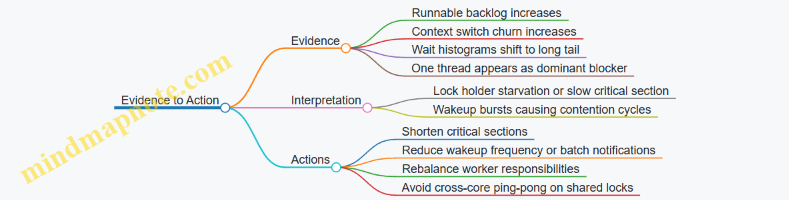
What a Good Output Looks Like
A useful end state is a report that lists: (1) the top contention sites with wait duration distributions, (2) the top waiting threads, (3) the top suspected blockers, and (4) the time alignment between scheduling pressure and contention onset. If those four pieces agree, you can make a targeted change without guessing. If they disagree, you have a clear reason to re-check filters, time windows, and thread attribution—because the system is telling you where your assumptions broke.
12.3 Finding Hot Functions with Stack Sampling and Attribution
Hot functions are the ones that show up often, spend meaningful CPU time, or both. With stack sampling, you collect occasional snapshots of where threads are executing, then attribute those snapshots to functions and aggregate them into a ranked view. The key is to make the sampling consistent, the stacks interpretable, and the attribution rules explicit.
Core Idea of Stack Sampling
Stack sampling works by sampling at a controlled rate and capturing a call stack at the sampling moment. For universal profiling, you typically combine:
- Kernel-side stacks for kernel execution paths.
- User-space stacks for application code, using uprobes or user stack capture where supported.
- A mapping layer that turns instruction addresses into function names using symbols.
A practical best practice is to treat “sample rate” as a contract. If you sample too aggressively, you distort behavior and increase lost events; if you sample too lightly, rare but important functions vanish. Start with a conservative rate, then increase only after you confirm stable event delivery.
Attribution Rules That Keep Results Honest
Attribution answers: “Which function gets the credit for this sample?” A simple approach credits the top frame (the currently executing function). A more informative approach credits multiple frames with weights, such as:
- Top frame weight 1.0
- Caller frame weight 0.5
- Grandcaller frame weight 0.25
This weighted scheme helps when the top frame is a small wrapper, while the real cost sits deeper. The best practice is to document the weighting in the output so that comparisons across runs remain meaningful.
Mind Map: Data Path from Sample to Hot List
Example: Minimal Stack Sampling Workflow
Assume you want to find hot functions in a service process. You run a sampler that periodically triggers on CPU time and captures stacks for threads belonging to the target PID.
- Filter early to reduce overhead.
- In user space, pass the target PID set to the loader.
- In the eBPF program, check current PID/TID before capturing stacks.
- Capture a bounded stack.
- Set a maximum depth so the stack capture cost stays predictable.
- Keep the same depth across runs for comparability.
- Emit samples to user space.
- Use a ring buffer to stream stack samples.
- Include metadata: PID, TID, CPU id, and a timestamp.
- Symbolize and attribute.
- Convert addresses to function names.
- Apply attribution weights.
- Aggregate counts per function.
Here is a compact pseudocode sketch of the attribution logic in user space.
for sample in samples:
  frames = sample.stack_frames
  for i, addr in enumerate(frames):
    weight = 1.0 / (2 ** i)
    func = symbolize(addr)
    if func is None: continue
    if is_noise(func): continue
    agg[func] += weight
Example: Excluding Noise Frames Without Hiding Real Work
Noise frames are those that dominate stacks but rarely represent meaningful application logic, such as generic runtime trampolines or tiny wrappers. Excluding them blindly can remove the very function you’re trying to measure. A safer rule is to exclude only when the function is both:
- Very shallow in the stack (for example, only the first frame), and
- Known to be a wrapper that immediately calls into a stable target.
In practice, start with top-frame-only attribution. If you see many wrapper functions at the top, switch to weighted attribution and exclude wrappers only after you confirm the deeper frames still show the expected hotspots.
Advanced Detail: Handling Incomplete Stacks and Lost Events
Stack capture can fail or truncate when depth limits are reached, memory pressure occurs, or events are dropped. Your output should treat these as first-class signals.
A robust approach is to track:
- Truncation rate per sample (how often the stack hit max depth).
- Lost event count from the ring buffer.
- Symbolization miss rate (addresses that cannot be mapped).
If truncation is high, increase max depth carefully and re-check overhead. If lost events rise, reduce sampling rate. If symbolization misses are common, ensure you load symbols for the binaries in question.
Mind Map: Attribution and Aggregation Choices
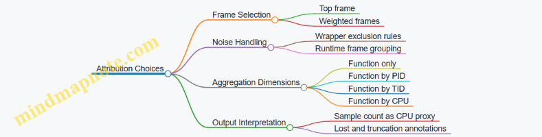
Example: Turning Aggregates into a Usable Hot List
After aggregation, produce a table with:
- Function name
- Weighted sample score
- Raw sample count
- PID/TID breakdown for the top entries
- Notes on truncation and lost events
A small but effective best practice is to show both weighted score and raw count. Weighted attribution can elevate deeper frames; raw counts keep you grounded in how often the function actually appears in sampled stacks.
Practical Checklist for Hot Function Discovery
- Use a stable sampling rate and confirm event delivery.
- Capture bounded stacks with consistent depth.
- Symbolize addresses deterministically.
- Choose attribution rules explicitly and keep them consistent across runs.
- Track truncation, lost events, and symbolization misses.
- Prefer top-frame-only first, then move to weighted attribution when wrappers obscure the real cost.
When these pieces line up, the “hot functions” list becomes more than a ranking. It becomes a reproducible summary of where CPU time is being spent, with enough guardrails to interpret the results without guessing.
12.4 Investigating Thread Pool Behavior with Timing and Queue Metrics
Thread pools fail in predictable ways: tasks wait too long, workers sit idle while the queue grows, or tasks run but complete too slowly. With eBPF-based universal profiling, you can measure both sides of the story: queueing time (how long tasks wait) and execution time (how long workers spend running). The trick is correlating events to the same logical task and to the same worker thread.
Core Concepts and What to Measure
Start by defining three timestamps per task: enqueue time, start time, and end time. From those you derive:
- Queueing time = start time − enqueue time
- Execution time = end time − start time
- Sojourn time = end time − enqueue time
Then measure worker behavior:
- Active workers over time (threads currently running tasks)
- Idle workers over time (threads waiting for work)
- Queue depth sampled periodically or inferred from enqueue/dequeue events
A practical best practice is to treat queueing time as the primary symptom. Execution time explains the “why,” but queueing time tells you “where the delay is happening.”
Mind Map: Thread Pool Timing and Queue Metrics
Instrumentation Strategy That Stays Practical
Use a two-layer approach: collect timing events from the runtime or framework, and collect worker state from the scheduler-adjacent behavior you can observe reliably.
- Task lifecycle events: attach to points where tasks are enqueued, begin execution, and complete. If you cannot get explicit lifecycle hooks, approximate enqueue/start with framework-specific functions and completion with return from the task wrapper.
- Worker state: observe when worker threads block waiting for work and when they wake up. Even if you cannot label “idle” directly, you can infer it from blocking and wake-up patterns.
- Queue depth: if the pool exposes a queue length, record it periodically. If not, infer depth by counting enqueues minus dequeues within a time window.
A key best practice is to keep correlation keys stable. Use process ID plus thread ID for worker state, and use a task identifier that is consistent across enqueue and start. If you only have pointers or IDs that may be reused, include a generation counter or a timestamp bucket to reduce accidental collisions.
Example: Queueing Time Histogram with Worker Utilization
Suppose you observe a latency regression. You collect:
- enqueue/start/end timestamps for tasks
- worker running vs waiting state
Then you compute a histogram for queueing time. A useful rule of thumb: if the median queueing time rises while execution time stays flat, the pool is under-provisioned or blocked on something external.
To make this concrete, imagine these outcomes:
- Queueing time: p50 jumps from 2 ms to 40 ms; p95 jumps from 10 ms to 200 ms
- Execution time: p50 stays around 5 ms; p95 stays around 30 ms
- Worker utilization: workers are mostly busy, but tasks still wait
This combination suggests contention outside the task body, such as upstream throttling, lock contention in shared resources, or a mismatch between task arrival rate and worker capacity.
Example: Worker Idle While Queue Grows
Another common failure mode is “idle workers with a growing queue.” You detect it when:
- queue depth increases steadily
- idle time for worker threads is non-trivial
- start events lag behind enqueue events
This can happen when workers are blocked on a condition unrelated to the queue, or when tasks are enqueued to a different pool than the one workers are consuming. The integrated approach helps: queue metrics alone can mislead, but queue plus worker state shows whether the system is failing to dispatch work or failing to execute it.
Advanced Details Without Guesswork
Handling Event Loss
If you sample aggressively or hit buffer limits, queueing time distributions can skew toward lower values. Mitigate this by tracking lost-event counters and by using conservative sampling for enqueue/start/end. When loss is detected, report metrics as “partial accounting” rather than silently treating them as complete.
Controlling Cardinality
Task identifiers can explode in number. Prefer aggregating by stable dimensions such as pool name, task type, and worker role. If you must include task IDs for correlation, keep them only long enough to match enqueue to start, then aggregate and discard.
Choosing Time Buckets
Use consistent time units and align histogram buckets across runs. If you compare two time windows, ensure the timestamp source is consistent and that you exclude warm-up periods where pools are still ramping.
Case Study: Diagnosing a Thread Pool Stall
In a controlled window, you see:
- queue depth rises from 0 to 500
- queueing time median rises from 1 ms to 60 ms
- execution time median stays around 8 ms
- worker state shows many threads in a blocked wait state
The integrated conclusion is straightforward: tasks are not being picked up promptly, even though the work itself is not slower. The next step is to inspect the specific blocking reason by correlating worker wake-up events with enqueue events. If wake-ups cluster but do not lead to task starts, the issue is likely in dispatch logic. If wake-ups are rare, the issue is likely in the signaling path that should notify workers.
Mind Map: Diagnostic Patterns and What They Imply
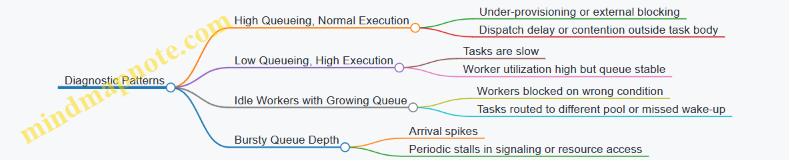
The overall workflow is consistent: measure queueing and execution separately, track worker state, correlate events with stable keys, and interpret patterns using both timing and queue depth together. That combination turns “the pool feels slow” into a specific, testable explanation.
12.5 Producing a Complete Profiling Report From Collected Data
A complete profiling report turns raw eBPF events into decisions. The trick is to keep a clean chain from “what happened” to “why it mattered,” while preserving enough detail to reproduce the result. The report below assumes you already collected events for CPU, latency, and I/O, and you have a user-space consumer that aggregates them.
Define the Report’s Questions
Start by writing three concrete questions the report must answer. For example:
- Which requests were slow, and where did time go?
- Which functions or code paths consumed the most CPU during the window?
- Did I/O or contention explain the slowdown?
This step prevents a common failure mode: collecting everything, then presenting averages that hide the actual bottleneck.
Normalize Events into a Single Timeline
Even when events come from different probes, the report should treat them as one timeline. Normalize each event into a shared schema with:
ts_ns: monotonic timestamppid,tid,commcpu: the CPU where the event occurredevent_type: e.g.,sched_in,req_start,req_end,io_submit,io_completekey: correlation key such as request id, socket tuple, or thread id
If you correlate start/end events, store both timestamps and compute duration in the aggregator, not in the presentation layer. That keeps the math consistent.
Aggregate with Purpose
Use separate aggregations for different questions:
- CPU attribution: counts or samples by stack/function and by
pid/tid - Latency: histogram buckets and percentiles by request type and correlation key
- I/O: bytes, operation counts, and completion latency by file/socket and thread
- Contention: lock wait time and scheduling delays by thread and lock identity
A practical rule: every aggregation must have a stated grouping key and a time window. If the window is “last 5 minutes,” include it in the report header and in every chart caption.
Build a Report Skeleton That Readers Can Scan
A good report reads like a checklist. Use this order:
- Summary of findings
- Method and scope
- Latency breakdown
- CPU hot paths
- I/O and resource behavior
- Contention and scheduling
- Evidence tables and raw excerpts
- Reproducibility details
The summary should be short and specific, such as “p95 latency increased from 42ms to 110ms; time shifted from user processing to lock wait and I/O completion.” If you cannot state a shift, you probably only have a symptom.
Mind Map: Producing a Complete Profiling Report
Evidence Tables That Don’t Lie
Charts are persuasive, but tables are accountable. Include at least two evidence tables:
- Top latency contributors: group by request type and show
count,p50,p95, and the dominant time component (e.g., user, lock wait, I/O wait). - Top CPU consumers: group by function/stack and show sample count or time estimate plus the top
pid/tid.
When you compute “dominant component,” define it explicitly. For example, if you have start/end around request handling and separate lock wait and I/O wait, then dominant means the largest measured sub-duration. If a component is missing due to correlation gaps, mark it as “unattributed,” not as zero.
Validation Checks Before You Publish
Perform three sanity checks:
- Event coverage: confirm the number of start/end pairs matches the number of requests you expect from logs.
- Time consistency: verify durations are non-negative and within a reasonable range for the workload.
- Attribution sanity: ensure CPU hot paths align with the threads that own the slow requests.
If lost events exist, report the loss rate and how it affects confidence. For instance, “I/O completion events were sampled at 1/10, so completion latency percentiles are approximate.”
Example Report Snippet
Summary
- Window: 2026-03-25 10:00–10:05
- Slowdown: p95 request latency increased by 2.6×.
- Attribution: lock wait time and I/O completion time grew together; CPU hot stacks shifted toward scheduler and synchronization code.
Latency Breakdown
- Request type A: p50 18ms, p95 92ms
- Dominant component: lock wait (largest measured sub-duration)
- Unattributed share: 6% (correlation gaps)
CPU Hot Paths
- Top stack:
worker_loop -> mutex_lock -> futex_wait - Concentration: 73% of samples from the same
pid/tidthat owns request type A.
I/O Behavior
- Socket group: increased completion latency; bytes per request remained stable.
- Interpretation: the system waited longer for the same amount of data.
Method and Scope
- Probes: tracepoints for scheduling and syscalls; uprobes for request boundaries
- Sampling: CPU stack sampling at 1/1000 events
- Filters: only processes matching
commpatternapp-*
Reproducibility Details That Matter
End with a compact “how to rerun” block:
- probe set and attachment points
- sampling rates
- filters for pid/comm and correlation keys
- aggregation window and histogram bucket settings
- output format and any normalization steps
A reader should be able to rerun the same configuration and get the same shapes, even if exact counts vary slightly. That’s the difference between a report and a story.