Weed Impact Mills and Herbicide Resistance in Crop Systems
1. Scope of Weed Impact Mills and Resistance Management in Broadacre Farming
1.1 Defining Weed Impact Mills in Crop System Weed Control
Weed impact mills are field tools designed to reduce weed seed production by mechanically damaging weeds at specific growth stages. In crop systems, the goal is not “perfect weed death everywhere,” but consistent interruption of the weed life cycle so fewer viable seeds enter the soil seed bank. Think of them as a targeted seed-suppression step that fits between crop establishment and harvest, rather than a replacement for herbicides or crop competition.
Core Purpose and What They Actually Control
Weed impact mills primarily affect weeds that are actively growing and producing biomass. They are most relevant when the management problem is seed rain: weeds that survive early control and later mature, dropping seed. By damaging stems, leaves, and growing points, these tools can reduce flowering success, delay maturation, and lower seed set. The practical definition is therefore stage-based: impact mills are defined by when they are used and what plant parts they disrupt.
Mechanism of Action in Plain Terms
An impact mill uses rotating or moving elements to strike or shear weed plants. The result is mechanical injury that can include:
- Loss of apical dominance when growing points are hit.
- Stem breakage that prevents normal transport of water and nutrients to developing reproductive structures.
- Leaf and canopy disruption that reduces photosynthesis and weakens the plant’s ability to finish seed development.
The key nuance is that mechanical injury must occur before seeds are fully formed and hardened. If weeds are already past the vulnerable stage, the tool may only reduce aboveground biomass without meaningfully reducing viable seed.
Where They Fit in a Weed Control Program
Weed impact mills are best defined as one component in an integrated sequence:
- Prevent early establishment through crop competitiveness and timely initial control.
- Suppress survivors before they contribute seed.
- Manage escapes with follow-up tactics so the seed bank does not rebuild.
This sequencing matters because impact mills work on plants that are present and accessible. If the crop canopy is too closed, weeds may be shielded; if the weeds are too small, the tool may not contact the right tissues.
Defining “Impact” by Timing and Target Weed Stage
A useful operational definition is: impact mills are tools that deliver mechanical damage to weeds during a window when seed viability is still sensitive to disruption. That window depends on weed species and local conditions, but the logic stays consistent. For example, a weed that flowers early may require earlier passes than a later-emerging species in the same field.
Practical Example in Broadacre Cropping
Consider a broadacre cereal field with scattered ryegrass and volunteer broadleaf weeds. Early-season herbicide reduces density, but some plants escape and reach the pre-flowering stage. A grower schedules an impact mill pass when most escapes are at the same developmental stage, aiming to hit the reproductive stems before seed formation. After the pass, scouting focuses on whether flowering is halted and whether seed heads remain empty or poorly developed. If seed heads still mature normally, the timing was likely late for that weed stage.
Mind Map: Defining Weed Impact Mills
Quick Checklist for a Clear Definition
A definition is complete when it answers three questions: What problem does it address? (seed rain), How does it work? (mechanical disruption of vulnerable tissues), and When does it work? (before viable seed formation). If any of these are missing, the term “weed impact mill” becomes a vague label instead of a usable management tool.
1.2 Understanding Herbicide Resistance Mechanisms in Field Conditions
Herbicide resistance is not a mysterious curse; it’s an evolutionary outcome. In a field, a herbicide creates a strong selection filter. Most susceptible weeds die, but any individuals with traits that reduce herbicide damage survive, reproduce, and gradually dominate the population. The key to understanding resistance is connecting three things: the herbicide’s target process, the weed’s biology, and the field conditions that shape selection.
Core Concepts That Explain What You See in Fields
Start with the herbicide’s job. Many herbicides block a specific plant function, such as an enzyme step in amino acid synthesis or pigment formation. When the target is blocked, the plant can’t grow normally and eventually dies. Resistance means the weed can still function despite the herbicide being present.
Next, consider how selection happens. A single treatment doesn’t “cause” resistance; it selects for it. If a few resistant plants already exist—through mutation or rare gene variants—they survive the treatment. Over repeated seasons, the proportion of survivors increases, and control failures become obvious.
Finally, field conditions determine how strong the selection filter is. Uneven spray coverage, poor timing, drought stress, and delayed crop canopy closure can all reduce herbicide effectiveness. When effectiveness drops, the selection filter becomes weaker and more variable, which can slow resistance development or change which resistance mechanisms become common.
Mechanisms of Resistance and How They Differ
Resistance mechanisms generally fall into two broad groups: target-site resistance and non-target-site resistance.
Target-site resistance happens when the herbicide can’t bind or can’t inhibit the target as effectively. A common example is a mutation in the target enzyme that reduces herbicide sensitivity. Another example is changes that alter the amount or form of the target protein. In field terms, target-site resistance often shows up as consistent survival of treated plants, with symptoms that look “wrong” for the herbicide’s usual pattern.
Non-target-site resistance involves the plant reducing herbicide concentration at the site of action or preventing the herbicide from reaching it effectively. This can occur through enhanced metabolism, where the plant breaks the herbicide down faster, or through reduced uptake and translocation, where the herbicide enters the plant poorly or doesn’t move to the target tissue.
A practical way to distinguish them is to look at pattern and consistency. Target-site resistance often produces plants that survive treatment similarly across the field where coverage is adequate. Non-target-site resistance can be more variable because uptake and metabolism are influenced by plant size, stress level, and environmental conditions.
Field Conditions That Shape Selection Pressure
Selection pressure is strongest when the herbicide performs well against susceptible plants. That sounds counterintuitive, but it’s simple: if susceptible weeds are reliably killed, survivors are more likely to be the resistant ones. Several field factors influence this.
- Timing relative to weed growth stage: Treating too late can mean weeds have already established enough biomass to tolerate partial herbicide effects. Those survivors may include both susceptible and resistant individuals, muddying selection.
- Coverage and spray quality: If droplets miss leaf surfaces or land unevenly, susceptible plants may escape without being truly resistant.
- Crop competition and canopy closure: A strong crop stand can reduce weed emergence and growth, limiting the number of individuals exposed to herbicide. A weak stand can increase the number of escapes.
- Environmental stress: Drought, heat, or cold can slow weed metabolism and growth. That can reduce herbicide uptake or alter metabolism, changing how strongly the herbicide filters the population.
Mind Map: Resistance Mechanisms in Field Conditions
Example Scenarios That Tie Mechanisms to Observations
Example 1: Consistent survivors after a single effective spray
A grower applies a foliar herbicide at the recommended stage. Most weeds collapse as expected, but a patch of plants survives with similar appearance across the patch. This pattern fits target-site resistance: the herbicide is reaching the plants, but the target is less inhibited in survivors.
Example 2: Variable control across the same paddock
Another paddock shows scattered escapes. Some surviving plants are small and stressed, others are larger. The control varies with soil moisture and canopy gaps. This pattern fits non-target-site resistance interacting with field conditions: uptake, metabolism, and translocation can change with plant size and stress, so the herbicide filter is inconsistent.
Example 3: Resistance risk increases when control is unreliable
If a herbicide is repeatedly applied when weeds are already beyond the best stage, or if spray coverage is uneven, many susceptible plants survive. That doesn’t create resistance by itself, but it reduces the selection pressure for resistant individuals and increases the chance that escapes—resistant or not—accumulate. Over time, resistant traits still gain ground because they survive treatments more reliably than susceptible traits.
Understanding resistance mechanisms in field conditions is about reading the system: the herbicide’s target, the weed’s survival strategy, and the practical realities of timing, coverage, and stress. When you connect those pieces, control failures stop being random and start being explainable.
1.3 Mapping Weed Life Cycles to Management Windows in Broadacre Crops
Weed control works best when you treat timing as a crop input. Mapping weed life cycles to management windows means you identify when a weed is most vulnerable, then align field operations so the weakest stage gets hit with the right tool. The goal is not “more spraying,” but fewer missed opportunities.
Core Idea: Vulnerability Changes with Growth Stage
Weeds shift from low-impact stages to high-impact stages as they move through germination, establishment, vegetative growth, flowering, seed set, and dormancy. Many control failures happen because an operation targets the wrong stage. For example, a pre-emergent herbicide window is about preventing establishment, while a post-emergent window is about reducing growth and preventing seed production.
A practical mapping starts with two questions:
- When does the weed typically emerge in your paddock?
- When does it reach the stage you can most effectively suppress or stop from producing viable seed?
Step 1: Build a Local Phenology Calendar
Broadacre fields rarely behave like textbook diagrams. Soil type, residue cover, and rainfall patterns shift emergence timing. Create a simple calendar for each target weed using your own observations.
- Record emergence events: note first emergence, peak emergence, and last emergence for each flush.
- Track key stages: seedling size, first true leaves, tillering/branching, flowering start, and seed maturity.
- Use consistent dates: if you need a reference point, pick a fixed seasonal marker such as “first week after the first major rain” rather than calendar day.
Example: In a winter cereal paddock, a ryegrass population may show early emergence after autumn rain, then a second flush after a later rain. If you only plan one “early” treatment, the second flush can still reach flowering.
Step 2: Convert Stages Into Management Windows
A management window is a time range where a specific tactic has the highest chance of success. Windows overlap because different tactics target different vulnerabilities.
Common Window Types
- Pre-emergent window: before seedlings break the soil surface; effectiveness depends on soil moisture and residual persistence.
- Early post-emergent window: when weeds are small; many herbicides perform better before weeds develop thicker stems or deeper root systems.
- Pre-flowering window: reduces biomass and delays flowering; useful for preventing seed set.
- Seed-targeting window: when seed is present but not yet fully mature; timing matters for any approach that aims to stop viable seed production.
- Late-season window: focuses on preventing late escapes from replenishing the seed bank.
Example: If a broadleaf weed flowers quickly after establishment, the early post-emergent window may be the only practical chance to prevent seed set. Waiting for a later “bigger weed” stage often turns into a seed-bank problem.
Step 3: Map Crop Operations Onto Weed Windows
Weed control is constrained by what you can physically do: seeding dates, spray access, harvest timing, and residue conditions. Your mapping should include crop operations as “hard edges” that limit when you can act.
- Seeding timing sets the crop’s competitive stage and determines whether you can use pre-emergent residuals.
- Canopy closure changes light and space, affecting weed growth rates and herbicide coverage.
- Harvest timing affects whether late-season escapes get a chance to mature seed.
Example: In a no-till system, residue can delay soil warming and shift emergence later. That means your pre-emergent residual might be applied correctly but still miss the main emergence flush if rainfall timing differs.
Step 4: Account for Multiple Flushes and Mixed Species
Broadacre paddocks often contain weeds with different life cycles and different emergence patterns. A single calendar rarely fits all.
- Multiple flushes: plan for at least the first two emergence peaks if the second flush can reach seed set.
- Mixed species: group weeds by similar vulnerability windows rather than treating everything the same day.
Example: If one grass species emerges early and another emerges later, a single early post-emergent spray may suppress the first but leave the second to flower.
Step 5: Use a Simple Decision Logic
When mapping is done well, decisions become straightforward: choose the window that prevents seed production for the weeds that matter most.
If a weed can still reach flowering and seed set after your planned actions, your window coverage is incomplete.
Mind Map: Weed Life Cycle to Management Windows
Worked Example: One Paddock, Two Flushes, One Goal
Goal: prevent viable seed return for a target grass and a fast-flowering broadleaf.
- Grass: first flush emerges soon after autumn rain; second flush follows a later rain.
- Window plan: pre-emergent residual for the first flush, early post-emergent for small seedlings, then a late-season check for escapes before seed maturity.
- Broadleaf: emerges later but reaches flowering quickly.
- Window plan: prioritize early post-emergent timing when weeds are small; avoid waiting for a larger stage.
The mapping outcome is a sequence of actions tied to weed vulnerability, not to a calendar habit. When you can point to the stage you’re targeting, you can also explain why the plan should work.
1.4 Establishing Baseline Weed Surveys and Resistance Risk Profiles
A baseline survey is the field’s way of telling you what you already know and what you’ve been guessing. The goal is to record weed species, their life stages, and how they respond to herbicides so you can estimate resistance risk before control options get narrow.
Define the Survey Scope and Decision Questions
Start with decisions, not data. Write two to four questions your plan must answer, such as: Which weeds are most likely to survive current herbicide programs? Which paddocks need tighter monitoring? Which herbicides are being relied on too heavily for the same weed group?
Then set the scope: crop types in the rotation, typical soil zones, and the herbicide modes of action used in the last two seasons. If you have a history of patchy control, include those paddocks even if they are small.
Choose Sampling Units and Map the Field Logic
Use sampling units that match how weeds actually vary. In broadacre systems, that often means management zones based on soil type, slope, yield maps, or past spray patterns. If you don’t have those layers, use practical proxies: headlands versus interior, low spots versus ridges, and areas with different establishment success.
Within each zone, sample multiple points rather than one “representative” spot. A simple rule: if you can see obvious differences in weed density, treat them as separate sub-units.
Record Weed Species and Life Stage with Consistent Rules
For each sampling point, record:
- Species identity using a consistent key or farm guide
- Growth stage (seedling, vegetative, flowering, seed set)
- Density or cover using a repeatable scale (for example, 0 none, 1 low, 2 moderate, 3 high)
- Patch size and whether weeds are clumped or evenly spread
Life stage matters because resistance selection pressure is tied to survival through the treatment window. A field full of seedlings is a different problem than a field with flowering survivors.
Capture Herbicide History and Control Outcomes
For each paddock, compile a concise herbicide timeline: product, active ingredient, mode of action, application date, and target weed stage. Then add outcomes you can verify: control score, density reduction, and whether escapes were scattered or concentrated.
A useful detail is “where failures show up.” If survivors consistently appear in the same zone, coverage or emergence timing may be involved. If failures appear across zones but with the same weed species, resistance becomes more plausible.
Build a Resistance Risk Profile Using Evidence Tiers
Create a risk profile per weed species and per paddock zone. Use evidence tiers so the profile is transparent and not based on vibes.
- Tier 1: High-confidence risk when you have repeated poor control of the same species after herbicides with the same mode of action, especially across seasons.
- Tier 2: Moderate risk when control is inconsistent, but the species is repeatedly present at the same growth stage during spraying.
- Tier 3: Low risk when the species is present but control has been consistently acceptable or the herbicide was not applied at the right stage.
Assign a risk score that reflects both frequency and pattern. A weed that survives once in a single patch is not the same as a weed that survives every time in multiple zones.
Mind Map: Baseline Survey Workflow
Example: Turning Field Notes Into a Risk Profile
Imagine a paddock with two zones: a sandy rise and a heavier low area. In both zones, ryegrass seedlings appear at spray time. In the rise, control is usually good, but in the low area, ryegrass survives after the same mode of action used in both seasons.
Your survey notes show:
- Ryegrass present in both zones, but density is higher in the low area.
- Survivors are mostly at the same growth stage at application.
- Control failures cluster in the low area across seasons.
Risk profile outcome:
- Ryegrass in low area: Tier 1 or Tier 2 depending on how many repeated failures you have.
- Ryegrass in sandy rise: Tier 2 or Tier 3 because outcomes are better and failures are not consistent.
This prevents the common mistake of treating the whole paddock as one problem and applying the same “fix” everywhere.
Example: When Poor Control Isn’t Resistance
In another paddock, broadleaf weeds are present, but the herbicide was applied late, when weeds had moved from vegetative to flowering. Survivors are scattered and match the timing mismatch rather than a consistent survival pattern.
Risk profile outcome:
- The weed species may be Tier 3 for resistance risk because the herbicide window was missed.
- Your monitoring priority shifts to improving timing and coverage quality rather than immediately changing every mode of action.
Output Format That Keeps Teams Aligned
End the baseline work with two practical outputs:
- A species-by-zone risk table with evidence tier and key notes.
- A short monitoring priority list that states what you will check next and where.
When the baseline is clear, later decisions become easier to justify. You’re not arguing about what you feel; you’re acting on what the field recorded.
1.5 Selecting Management Objectives for Seed Bank Reduction and Control Efficacy
Good weed control starts with clear objectives. In broadacre systems, the objective is rarely “kill weeds.” It’s usually “reduce future weed pressure while keeping current crop performance stable.” That means you set targets for both seed bank reduction and control efficacy, then choose tactics that can realistically hit them.
Step 1: Separate Current Control from Future Pressure
Control efficacy answers: “Did we stop weeds this season?” Seed bank reduction answers: “Did we prevent next season’s problem?” A field can look clean after a treatment yet still fail the next year if surviving plants produced seed.
Practical example: In a wheat paddock, a post-emergence herbicide may reduce visible ryegrass, but if escapes are allowed to head, the seed bank still gets replenished. Your objective should explicitly include preventing seed production from escapes.
Step 2: Define Measurable Targets
Use numbers you can measure without a lab every time.
- Seed bank reduction target: choose a percentage reduction for the main target weed(s) over a defined period (often 1–3 seasons).
- Efficacy target: set a threshold for acceptable weed density or biomass at key crop stages.
- Escape tolerance: define how many plants per square meter are allowed to survive to flowering.
Practical example: “Aim for <5 flowering plants per square meter by crop growth stage X” is more actionable than “good control.” It also forces you to time operations around the weed’s reproductive stage.
Step 3: Prioritize by Weed Impact, Not Just Abundance
Not all weeds contribute equally to yield loss or resistance risk. Prioritize weeds by:
- Seed output potential (how many seeds per plant)
- Persistence (seed longevity)
- Herbicide resistance history (how likely control failure is)
- Crop interference (competition and harvest issues)
Practical example: A low-density but highly fecund weed may deserve stronger seed destruction objectives than a more common weed with lower seed output.
Step 4: Set Objectives That Match Your Tactic Toolbox
Your objectives must fit what your operations can deliver.
- If you rely on seed destruction biological control, your objective should include timing relative to weed height and seed stage.
- If you rely on herbicide programs, your objective should include coverage quality and mode-of-action rotation constraints.
- If you use cultural controls, your objective should include establishment uniformity and canopy closure timing.
Practical example: If your equipment can only treat once before flowering, your seed bank objective should focus on preventing seed set during that window, not on “full-season suppression.”
Step 5: Build a Simple Objective Hierarchy
A hierarchy keeps decisions consistent when conditions change.
- Crop protection objective: maintain yield and quality by controlling weeds during critical competition periods.
- Seed bank objective: prevent seed production from the target weed(s).
- Resistance management objective: reduce selection pressure by limiting repeated reliance on the same mode of action and by reducing survivors that reproduce.
Practical example: If early control is imperfect, you can still meet the seed bank objective by ensuring late-season escapes are prevented from heading, which also reduces resistance selection pressure.
Step 6: Translate Objectives Into Field-Ready Success Criteria
Turn each objective into “what we check” and “what we do if we miss.”
- Before treatment: confirm weed stage matches the intended control window.
- After treatment: check density and presence of reproductive structures.
- At crop maturity: confirm whether any escapes reached seed set.
- Across seasons: compare weed density trends and resistance risk indicators.
Practical example: If scouting shows weeds are already at the reproductive stage when the plan calls for vegetative control, you adjust the next operation to protect against seed set rather than chasing perfect early suppression.
Mind Map: Management Objectives That Link Seed Bank Reduction and Efficacy
Example: Turning Objectives Into a One-Season Plan
Scenario: A broadacre wheat field has annual ryegrass with known herbicide resistance risk. Your objectives are:
- Efficacy: keep ryegrass density below a set threshold during early crop competition.
- Seed bank reduction: ensure no ryegrass plants reach heading.
- Resistance management: avoid repeated use of the same mode of action across the season.
How it plays out: You scout to confirm ryegrass stage before the main treatment. If a portion of the population is already close to heading, you adjust the sequence so the next intervention targets reproductive prevention rather than only reducing young plants. At maturity, you specifically check for seed heads; if you find them, you record where and why (stage mismatch, coverage gaps, or escapes) so the next season’s objectives and timing can be tightened.
Step 7: Keep Objectives Coherent with Evidence from the Field
Objectives aren’t set once and forgotten. They should be refined using what you actually observed, such as weed stage at treatment, patchiness, and whether escapes produced seed. When objectives are measurable and linked to scouting outcomes, the plan becomes easier to execute and easier to improve.
Practical example: If your seed bank objective repeatedly fails because escapes appear in the same low-coverage zones, the next season’s objective can stay the same while the operational success criteria become more specific about coverage uniformity in those zones.
2. Weed Biology Foundations for Seed Destruction and Control Timing
2.1 Seed Production Pathways and Seed Bank Dynamics
Weed control starts with a simple question: where do the seeds come from, and what happens to them after they land in the field? Seed production pathways explain how weeds add new seeds to the seed bank, while seed bank dynamics explain how many of those seeds remain available to germinate over time. Together, they tell you why a “good” season can still be followed by a “surprise” flush.
Seed Production Pathways
Most broadacre weeds follow one of a few seed production pathways. The key is not the weed’s name, but the timing and structure of seed set.
-
Single main flush with one seed set peak
- Example: Many winter annuals establish early, flower in a narrow window, and set most seed before crop canopy closure.
- Management implication: If you miss the flowering-to-seed-maturation window, you often miss the bulk of seed input.
-
Multiple flushes across the season
- Example: Some summer annuals emerge in waves after rainfall, producing staggered flowering.
- Management implication: A single treatment may reduce one flush but still allow later seed set.
-
Perennial or biennial pathways with repeated reproduction
- Example: Perennial weeds may produce seed each year while also regenerating from established structures.
- Management implication: Seed destruction helps, but you still need to manage the non-seed pathway that keeps the weed present.
-
Seed production supported by crop gaps
- Example: Weeds often concentrate where crop stands thin due to wheel tracks, poor emergence, salinity patches, or frost damage.
- Management implication: Field uniformity affects seed input. A patchy crop stand can turn a small weed problem into a seed bank problem.
A practical way to connect pathway to action is to track three stages in the field: flowering onset, seed maturation, and seed dispersal. Treatments aimed at seed destruction work best when they target the stage when seeds are present but not yet safely dispersed.
Seed Bank Dynamics
The seed bank is not a static pile. It behaves like a system with inputs, losses, and delayed germination.
- Input: seeds added by local plants during the season.
- Germination: a portion of seeds germinate when conditions match their requirements.
- Dormancy: many seeds remain viable but do not germinate immediately.
- Mortality: seeds die over time due to aging, predation, decay, and unfavorable conditions.
- Movement: seeds can shift depth through tillage, erosion, or soil cracking.
Two concepts matter for planning: viability and germination fraction.
- Viability answers: “How many seeds are still alive after time passes?”
- Germination fraction answers: “Of the viable seeds, how many will germinate under the conditions you create?”
Even if viability stays moderate, germination fraction can be low if the field conditions don’t match the weed’s cues. That’s why timing crop establishment and residue management can reduce germination without needing to eliminate every seed.
Linking Pathways to Dynamics
Seed production pathways determine the shape of seed bank inputs across time, while seed bank dynamics determine how those inputs translate into future emergence.
- If a weed has a single seed set peak, the seed bank input is concentrated. One well-timed seed destruction window can sharply reduce future emergence.
- If a weed has multiple flushes, seed bank input is spread out. You need repeated suppression of seed set or a strategy that targets multiple maturation windows.
- If a weed has perennial reproduction, seed bank input may be only part of the problem because new plants keep appearing.
Mind Map: Seed Production and Seed Bank
Example: Why One Missed Window Matters
Imagine a summer annual that produces most seed in two waves. In Wave 1, you apply a seed-destruction approach when plants are flowering and seeds are forming. In Wave 2, you treat after seeds have matured and started dispersal. Even if Wave 1 plants were reduced, the seed bank still receives a large input from Wave 2. The next season’s emergence then reflects that second input, not the first.
Example: How Crop Uniformity Changes Seed Bank Input
In a field with uneven emergence, weeds establish mainly in thin patches. Those patches become seed factories because weeds receive more light and space, and crop competition is weaker. Even if the average weed density across the whole field looks manageable, the seed bank can still build because seed production is concentrated where crop competition fails.
Practical Takeaway
Treat seed bank dynamics as the accounting system of weed control. Seed production pathways determine what gets added, and seed bank dynamics determine when it shows up again. When you connect those two, you can choose timing and tactics that reduce future emergence rather than just reducing weeds today.
2.2 Germination Requirements and Emergence Patterns by Weed Group
Weed control timing depends on two linked facts: seeds only germinate when their requirements are met, and seedlings only emerge when the seed is positioned and conditions stay suitable long enough. In broadacre fields, that means you can often predict where the “next flush” will come from by combining seed depth, soil moisture, temperature, and light cues.
Core Germination Requirements
Water is the first gate. Dry soil can keep seeds dormant even when temperature looks right. Once water is available, seeds begin the germination process, but uneven wetting creates uneven emergence.
Temperature sets the pace. Many weed seeds germinate over a range, but each species has a preferred window. When temperatures fluctuate around the threshold, germination may be slow and spread out across weeks.
Oxygen matters because seeds need respiration. Waterlogged patches can delay or reduce germination, while well-aerated topsoil supports faster, more synchronized emergence.
Light and burial depth create a second gate. Some species need light to germinate and therefore emerge mainly from the surface or very shallow layers. Others can germinate in darkness and often emerge from deeper burial.
Dormancy and after-ripening explain why the same field can produce different emergence patterns year to year. Many seeds require a period of dry storage, temperature cycling, or microbial and chemical cues before they respond to favorable conditions.
Emergence Patterns by Weed Group
Weed groups behave differently because their seeds differ in dormancy, depth response, and germination speed. The practical outcome is that some weeds show tight emergence windows, while others “keep showing up” because their seeds germinate over a long period.
Winter Annuals
Winter annuals typically germinate in autumn or early winter when temperatures are cool and moisture is reliable. Their emergence often clusters after the first sustained wetting events. If you delay crop establishment or leave bare soil, these seedlings can establish before the crop canopy closes.
Example: In a winter cereal paddock, a light rain followed by a week of cool, moist conditions can trigger a noticeable flush of winter annual seedlings from the top 1–2 cm.
Summer Annuals
Summer annuals usually germinate when soils warm and moisture is available. Their emergence often follows spring and early summer rainfall, with a strong temperature effect. If the first warm rains are followed by dry weather, emergence may stall and then resume when moisture returns.
Example: A warm spell in late spring with a single irrigation or rain event can produce an early flush, but a subsequent dry period may reduce stand density and spread later emergence.
Perennial Weeds
Perennials often rely on vegetative propagules or deep seed banks. For seed-based perennials, emergence can be sporadic because seeds may be buried deeper and face dormancy constraints. For vegetative perennials, emergence is less about seed germination and more about regrowth timing after disturbance.
Example: After cultivation, a perennial with deep reserves can regrow in patches even when surface seed germination is low.
Grasses Versus Broadleaves
Grasses frequently emerge from shallow to moderate depths and can respond quickly to favorable moisture and temperature. Many broadleaves show stronger light sensitivity, so surface disturbance and residue cover can shift emergence timing.
Example: Two weeds in the same paddock—one grass and one broadleaf—may both germinate after rain, but the broadleaf may emerge mainly where residue is sparse and soil is exposed.
Mind Map: Linking Requirements to Emergence
Practical Field Logic for Timing
Start with the question: “Where are the seeds right now?” If most viable seeds are near the surface, expect emergence to track wetting events and light exposure. If seeds are deeper, emergence may be slower and less synchronized, so a single treatment window may miss later seedlings.
Then ask: “How stable are conditions after the wetting event?” A short rain followed by drying often produces a smaller, uneven cohort. A longer period of cool or warm moisture supports more complete germination and a clearer emergence wave.
Finally, match the weed group to the likely season. Winter annuals tend to reward early-season attention in cool, moist periods, while summer annuals often require readiness for warm, wet triggers. Perennials require a different mindset because regrowth and deep propagules can keep producing new plants even when surface germination looks quiet.
2.3 Seedling Establishment Constraints in Crop Canopies
Seedling establishment is where many weed-control plans quietly succeed or fail. Before any herbicide or seed-destruction tactic matters, the crop has to form a canopy that limits weed emergence and survival. Constraints come from light, space, moisture, and mechanical effects of the crop itself. If you understand which constraint dominates in your field, you can time and combine tactics so weeds hit the hardest wall first.
Foundational Canopy Constraints
Light interception and shading. Many weeds germinate readily, but they struggle when seedlings are shaded during early growth. Crop canopies reduce the amount of light reaching the soil surface and change the light quality, which can slow weed development. A practical way to think about this is simple: if the crop closes rows quickly, weeds get fewer “good days” to grow before they are shaded.
Space and resource competition. Crop seedlings occupy water and nutrients in the top soil layer. Weeds that emerge later often start behind, with less access to moisture and nitrogen. This is especially important in broadacre systems where rainfall patterns can be patchy; a crop that captures resources early makes later weed cohorts less competitive.
Moisture availability and soil surface conditions. Weed emergence depends on a moist seedbed. Crop residues and canopy cover can reduce evaporation and stabilize soil moisture, but they can also change how quickly the soil warms. The result is that some weeds emerge in pulses tied to temperature and moisture windows, while others fail to establish when the crop keeps the surface cooler or drier.
Mechanical effects from crop growth. As the crop develops, stems and leaves can physically interfere with weed seedlings. In dense stands, weeds may be bent, suppressed, or prevented from reaching light. This mechanical suppression is strongest when weed emergence overlaps with the crop’s rapid leaf expansion.
Crop Stand Variables That Control Weed Establishment
Seeding rate and uniformity. Higher seeding rates can increase canopy closure, but uniform emergence matters more than raw numbers. If the crop stand has gaps, weeds exploit them like open doors. A field with good average density but uneven emergence often produces the most frustrating weed patches.
Row spacing and canopy architecture. Narrow rows generally close canopy faster, reducing the time weeds have access to light. Wide rows rely more on crop vigor and early leaf area to achieve suppression. If your crop canopy is slow to expand, wide rows can become a “weed runway.”
Crop vigor and establishment timing. Early crop emergence gives the crop a head start in capturing light and resources. Delayed crop emergence—whether from cool soils, crusting, or seedbed problems—extends the period when weeds can establish without being shaded.
Residue and soil cover. Residues can moderate soil temperature and moisture, influencing weed germination timing. They also affect how evenly the crop emerges by altering seed-to-soil contact. Good residue management supports a consistent crop stand, which indirectly constrains weed establishment.
Weed-Specific Constraints and Why They Matter
Weeds differ in how they respond to canopy constraints. Some species tolerate low light better, maintaining growth under shade longer than others. Others are more sensitive and collapse once shaded. Seed size and emergence depth also matter: weeds that emerge from deeper layers may appear after the crop canopy is already established, bypassing early shading effects.
A useful operational approach is to classify weeds by their likely emergence timing relative to crop canopy closure. If a weed tends to emerge early, it faces strong light competition. If it emerges later, it may escape the worst of canopy shading and rely more on gaps, moisture pockets, or reduced competition.
Integrated Examples from Broadacre Fields
Example: Winter cereals with uneven emergence. Suppose a winter cereal stand emerges unevenly due to variable soil moisture. In the denser zones, weed seedlings are shaded within weeks and often fail to reach a robust leaf area. In the gaps, weeds receive direct light and can grow fast enough to survive later herbicide applications. The lesson is that improving crop uniformity can reduce weed establishment even before chemistry enters the story.
Example: Wide-row crop with delayed canopy closure. In a wide-row system, the crop may take longer to cover the inter-row space. Early-emerging weeds then establish in the open rows, forming a first cohort that later treatments struggle to fully remove. If you adjust seeding depth, improve seedbed firmness, or correct emergence issues so the crop reaches leaf expansion sooner, you shorten the window for weed establishment.
Example: Residue-managed seedbed with moisture stability. In a residue-retained field, soil moisture may stay available longer near the surface. This can increase the number of weed emergence pulses. If the crop canopy closes quickly, those pulses still face shading and competition. If canopy closure is slow, the extra emergence pulses translate into more surviving plants.
Mind Map: Canopy Constraints on Weed Seedlings
Practical Takeaways for Integrated Programs
Treat canopy closure as a constraint you can manage, not a background condition. Prioritize crop uniformity and early leaf area so weeds face light and resource limits during the period when they are most vulnerable. Then align weed-targeting actions to the emergence timing that your canopy constraints actually allow.
2.4 Reproduction Timing and Seed Maturation Stages for Targeted Control
Targeted control works best when you treat weed reproduction like a calendar, not a mystery. Seed destruction and herbicide decisions both depend on where the plant is in its seed-making process, because different stages respond differently to management.
Core Idea: Stage Determines Vulnerability
Weeds typically move through flowering, seed fill, and maturity. During flowering, plants are building reproductive structures; during seed fill, seeds are accumulating resources; at maturity, seeds are hardened and ready to disperse. For broadacre fields, the practical goal is to intervene when the majority of the target population is in the most controllable stage.
Mapping Phenology to Field Timing
Start with a simple field observation routine: pick 10 to 20 plants per weed patch, then record the dominant stage you see. Use consistent cues such as first flowers, peak flowering, first seed visible, and seed color change. In many annual broadleaf weeds, the shift from flowering to seed fill happens quickly, so a one-week delay can move you from “seeds are still forming” to “seeds are already viable.”
A useful operational approach is to define a “control window” for each stage:
- Flowering window: good for preventing seed set and reducing the number of seeds formed.
- Seed fill window: good for seed destruction approaches that require soft, developing seeds.
- Maturity window: often too late for seed destruction methods that rely on immature seed stages, but still relevant for preventing dispersal.
Seed Maturation Stages and What They Mean
Seed maturation is not a single moment. It’s a sequence that affects both seed viability and how easily management measures can disrupt the process.
- Early seed development: seeds are small and soft; plants may still be producing new flowers.
- Mid seed fill: seeds enlarge and accumulate reserves; the plant is investing heavily in reproduction.
- Late seed fill: seeds approach full size; moisture content declines; seed coats begin to harden.
- Physiological maturity: seeds reach maximum viability potential; dispersal structures may be ready.
- Dispersal readiness: seeds are shed or easily detached; control must focus on preventing spread.
If you’re planning a treatment that aims to reduce the seed bank, the “best” stage is usually mid seed fill to early late seed fill, because seeds are present but still vulnerable. If your goal is to stop new seed production, flowering and early seed development are the priority.
Mind Map: Reproduction Timing to Control Decisions
Stage Spread Inside a Patch Matters
Weeds rarely mature uniformly. A patch can contain early-flowering plants and late-flowering plants at the same time, especially after uneven emergence. That means your “dominant stage” might be mid seed fill, while a minority of plants are still flowering. In practice, you manage the majority stage while designing follow-up actions for escapes.
A simple rule of thumb: if you see more than one stage clearly represented, plan for a two-step approach—first to hit the dominant stage, then to address the laggards when they move into the next window.
Example: Using Stage Cues for a Broadacre Decision
Imagine a paddock with a mixed stand of an annual broadleaf weed. On Monday, you find most plants at first seed visible with a few still flowering. By the next week, many plants show mid seed fill and seed color is shifting. If you apply a seed-targeted approach at Monday, you may destroy fewer seeds because many are not yet fully formed. If you wait until the next week, you increase the chance that the seeds are present and vulnerable.
Now consider the opposite scenario: if most plants are already at late seed fill and seeds detach easily, delaying further reduces the benefit of seed destruction because dispersal is already underway. In that case, the priority becomes preventing spread and reducing any remaining seed set rather than expecting large seed bank reductions.
Practical Checklist for Stage-Based Timing
- Choose 1 to 3 representative weed patches per field.
- Sample enough plants to see stage spread, not just the “average” plant.
- Record dominant stage and the proportion of plants in earlier and later stages.
- Match the treatment goal to the stage window: seed set prevention for flowering, seed vulnerability for seed fill, dispersal prevention for maturity.
- Use the same cues each time so your notes stay comparable.
A field log from early April can be as useful as a lab test if it consistently links stage observations to what you did and what you saw afterward. The goal is not perfection; it’s reducing the guesswork that lets seeds slip into the next cycle.
2.5 Linking Weed Phenology to Field Operations and Treatment Sequencing
Weed phenology is the calendar of plant development: emergence, vegetative growth, flowering, seed fill, and seed shed. Field operations happen on their own clock—weather windows, harvest schedules, sprayer availability, and crop growth stages. Linking the two means choosing actions that hit the weed when it is most vulnerable and when the crop and machinery can support the plan.
Start with Two Clocks: Weed Development and Crop Safety
First, list the target weeds and note their typical timing in your region. Then overlay crop stages that affect selectivity and equipment access. For example, a broadleaf weed that flowers early may require a different sequence than a late-emerging grass. If the crop canopy is thin, you can often target small weeds with better coverage; if the crop is tall and dense, you may need to shift toward earlier interventions or operations that rely on contact.
A practical way to keep this simple is to define three weed “windows”:
- Early window: newly emerged seedlings, before they establish a strong root system.
- Reproductive window: bud to early seed fill, when preventing seed production matters most.
- Seed window: late seed fill to shed, when seed destruction or preventing dispersal becomes the priority.
Translate Phenology Into Treatment Goals
Each weed stage suggests a different goal. Seedling stages focus on reducing survival and establishment. Reproductive stages focus on stopping seed production. Seed stages focus on reducing seed return to the soil.
Consider a mixed field with ryegrass and volunteer canola. Ryegrass may emerge in flushes and keep growing, while canola may flower in a more synchronized burst. Sequencing might look like this: use an early pass timed to the first ryegrass flush to reduce the base population, then schedule a later reproductive-stage action aimed at canola to prevent seed set. The key is that the “later” pass is not automatically better; it is better only if it matches the weed’s reproductive timing.
Build a Sequencing Logic That Respects Coverage and Contact
Many control failures are not about the active ingredient; they are about the match between weed stage and how the treatment reaches the plant.
- Small weeds: easier to cover uniformly, so contact and translocation both tend to perform more consistently.
- Larger weeds: coverage gaps increase, and some herbicides become less reliable because the plant’s structure shields parts of the canopy.
- Stressed weeds: drought or nutrient stress can change uptake and translocation, so the same treatment can behave differently across patches.
This is why sequencing should include an operational check: can you apply when the weeds are at the intended size and when the crop still allows good spray penetration or safe equipment movement?
Use Field Observations to Tighten the Plan
Phenology charts are useful, but fields rarely follow the textbook. Use scouting to confirm which stage is actually present.
A simple scouting routine works well:
- Walk the same transects at consistent intervals.
- Record the dominant stage for each target weed (for example, “10% seedlings, 60% rosette, 30% bolting”).
- Note patchiness drivers like soil type, compaction, and residue distribution.
If you see a reproductive-stage shift earlier than expected, you may need to move the reproductive-stage operation forward rather than waiting for the calendar. The goal is to keep the treatment aligned with the weed’s vulnerability window.
Mind Map of Phenology to Operations
Mind Map: Linking Weed Phenology to Treatment Sequencing
Example Sequencing for a Broadacre Rotation
Assume a winter cereal followed by a summer crop. Target weeds include annual ryegrass and a late-flowering broadleaf.
- Early season after crop emergence: scout for the first ryegrass flush. Apply an early-window action when most ryegrass plants are at the seedling stage. This reduces the base population before it can build multiple tillers.
- Mid season before broadleaf buds: watch the broadleaf transition from rosette to bud. Schedule the next operation so it lands in the bud to early seed fill window, aiming to prevent seed set rather than just “shrinking” plants.
- Late season around seed shed risk: if any broadleaf plants reach late seed fill, prioritize tactics that reduce seed return and dispersal. If the crop canopy prevents reliable herbicide coverage at this stage, use the operation that best matches the seed-focused goal.
The sequence works because each pass has a specific job tied to a specific weed stage, and each job is chosen based on what the field can support at that time.
Common Mistakes to Avoid
- Treating too late for the goal: applying a reproductive-stage objective when weeds are still mostly vegetative.
- Treating too early for the crop: choosing a timing that forces poor coverage or unsafe crop conditions.
- Ignoring patch variation: assuming the whole field is at one stage when scouting shows multiple cohorts.
When you keep the weed’s stage, the treatment goal, and the operational constraints in the same mental picture, sequencing becomes less guesswork and more controlled decision-making.
3. Herbicide Modes of Action and Resistance Selection Pressure
3.1 Herbicide Classification by Target Site and Biochemical Pathway
Herbicides are best understood as tools that interfere with a specific plant process. That process is usually tied to a target site inside the plant (for example, a particular enzyme or cellular structure) and a biochemical pathway (the chain of reactions the plant relies on). When you classify herbicides this way, resistance management becomes less guesswork and more engineering.
Target Site Versus Biochemical Pathway
A target site is the “where” and “what” the herbicide binds to or disrupts. A biochemical pathway is the “how” the plant builds or maintains something essential. Many herbicides share a pathway but differ in their exact binding site, and some herbicides share a target site but differ in how they move through the plant.
A practical way to remember this: if two herbicides stop the same critical reaction, resistance to one often increases the odds of reduced performance with the other.
Major Target Site Groups and What They Do
Below are common classification anchors used in crop protection. The exact labels vary by country, but the logic stays consistent.
-
Photosynthesis inhibitors
- What they hit: light-driven electron transport in chloroplasts.
- Why weeds fail: the plant can’t generate the energy and reducing power needed to grow.
- Field feel: symptoms often appear after a delay because the plant must exhaust existing energy reserves.
-
Amino acid synthesis inhibitors
- What they hit: enzymes that build essential amino acids.
- Why weeds fail: growth stops because proteins can’t be assembled.
- Field feel: susceptible plants often show chlorosis and stunting before death.
-
Lipid synthesis inhibitors
- What they hit: enzymes involved in building cell membranes.
- Why weeds fail: new tissue can’t form properly.
- Field feel: emerging shoots may be malformed or stop developing.
-
Cell division and growth regulators
- What they hit: processes controlling cell division, or hormone-like signaling.
- Why weeds fail: uncontrolled or disrupted growth leads to tissue collapse.
- Field feel: symptoms can look dramatic, but the key is that the plant’s growth program is being forced off-script.
-
Pigment and carotenoid pathway disruptors
- What they hit: protective pigment formation.
- Why weeds fail: the plant becomes vulnerable to oxidative damage.
- Field feel: bleaching can occur as protective capacity collapses.
How Classification Maps to Resistance Risk
Resistance is not random. It tends to emerge when the same target site is repeatedly pressured. If a weed population contains a rare plant with a target-site change, that plant survives and passes on the trait. Over seasons, the surviving fraction becomes the population.
This is why classification by target site matters: it tells you whether two herbicides are “different enough” to reduce selection pressure.
Movement and Timing as Part of the Classification Picture
Even within the same target site group, performance depends on whether the herbicide reaches the target.
- Uptake route: some herbicides rely more on root uptake, others on foliar absorption.
- Translocation: some move to growing points; others stay near where they land.
- Weed stage: many targets are most vulnerable when the plant is actively building new tissue.
So, classification is necessary but not sufficient. You still need to match the herbicide’s behavior to the weed’s biology.
Example: Two Herbicides, One Target Site
Imagine a broadacre field with ryegrass escapes. You used Herbicide A and then Herbicide B in the next season, both classified under the same photosynthesis-inhibitor target site. If the ryegrass population already has a target-site resistance mechanism, Herbicide B may show reduced control even if the product name is different. The classification tells you that the “difference” is mostly branding, not biology.
Mind Map: Herbicide Classification Logic
Quick Field Checklist for Using Classification
- Identify the herbicide’s target site group first.
- Confirm whether the next product shares the same target site or a different one.
- Match uptake and translocation to the weed stage you’re treating.
- Use classification to reduce repeated pressure on the same plant process.
That’s the core idea: classification turns herbicide choice from a product-by-product habit into a process-by-process plan.
3.2 How Selection Pressure Builds Across Seasons and Rotations
Selection pressure is what happens when a field repeatedly favors weeds that can survive the same control pattern. In broadacre systems, the pattern is rarely just one spray. It’s the combined effect of herbicide choice, timing, crop competition, and how consistently the same weed life stages are targeted.
Foundations: What “Selection” Means in Crop Fields
Selection pressure starts with variation. Within a weed population, some individuals naturally tolerate a herbicide more than others due to genetic differences. When a treatment is applied, susceptible plants die or fail to set seed, while tolerant survivors remain. Those survivors then contribute seed to the next generation, shifting the population toward tolerance.
A key detail is that selection is strongest when the treatment hits the same vulnerable stage repeatedly. If the control window consistently overlaps the weed’s most seed-producing period, fewer survivors get a chance to reproduce. If the window misses, survivors can set seed and selection accelerates.
Across Seasons: Why One Year Rarely Stays One Year
Herbicide resistance doesn’t appear overnight because seed banks and staggered emergence spread the “selection event” over time. Consider a typical broadacre weed with a seed bank: seeds germinate over multiple months and years. Each season adds another round of selection on whatever fraction of the population emerges and is exposed.
If the same herbicide mode of action is used year after year, the survivors from each season become the starting point for the next. Even if control looks “good” early, the field can be quietly accumulating tolerant individuals. The practical sign is often patchy escapes that persist despite repeated treatments, especially where coverage or timing is less consistent.
Across Rotations: How Crop Choice Shapes Herbicide Exposure
Rotations change the crop’s growth pattern, canopy closure, and the timing of field operations. Those differences affect when weeds emerge and how long they remain exposed to herbicides.
For example, a rotation that alternates between a fast-closing crop and a slow-closing crop can change weed survival even if the herbicide program stays the same. In the slow-closing phase, weeds may grow larger before control, which can reduce herbicide effectiveness and increase the chance that only the more tolerant individuals survive. In the fast-closing phase, fewer weeds may emerge, but the ones that do can still be selected if the same herbicide mode of action is used.
Rotation also affects which weeds dominate. If one weed species is suppressed in one crop but another species is favored, the resistance problem can shift from one target to another. That matters because the “same mode of action” can still be selecting, even if the visible weed species changes.
The Selection Loop: A Simple Mechanism with Real-World Inputs
Selection pressure is a loop:
- A portion of the weed population emerges.
- Herbicide exposure occurs during a specific growth stage.
- Survivors reproduce and refill the seed bank.
- The next season starts with a changed population.
The loop tightens when three conditions align: repeated mode of action use, consistent timing that targets the same stage, and reliable crop conditions that allow tolerant survivors to complete seed production.
Mind Map: Selection Pressure Across Seasons and Rotations
Example: Two-Season Pattern That Selects Without Obvious Failure
Imagine a field where a broadleaf weed emerges in waves. In Year 1, a single mode of action is applied at the same crop stage each season. The first emergence wave is controlled well, but a later wave escapes because it emerges after the spray window. Those escapes set seed. In Year 2, the same mode of action is used again at the same crop stage. The later wave still escapes, and now the field starts Year 2 with a seed bank already enriched by last year’s survivors. Even if the first wave still looks controlled, the later wave becomes more common, and patches expand.
Example: Rotation Change That Still Selects
Now switch crops in the rotation, but keep the herbicide mode of action the same and apply it at the same weed growth stage. If the new crop causes weeds to reach that stage more reliably, the herbicide exposure becomes more consistent. Consistency can increase selection because it reduces the chance that susceptible plants escape the treatment and reproduce. In other words, changing crops can change weed growth timing, but selection depends on whether the treatment repeatedly removes the susceptible fraction.
Practical Takeaway for Integrated Programs
Selection pressure is not just “how many sprays.” It’s how often the same vulnerable weed fraction is removed while the survivors are allowed to replenish the seed bank. Rotations can help or harm depending on whether they change the exposure pattern enough to break the loop.
3.3 Cross Resistance and Multiple Resistance in Common Weed Species
Herbicide resistance comes in two closely related flavors. Cross resistance means one resistance mechanism makes a weed less sensitive to more than one herbicide, even if those herbicides are not identical. Multiple resistance means a weed population carries more than one resistance mechanism at the same time, so it can shrug off several herbicide modes of action. In the field, these show up as “the same weeds keep coming back,” but the underlying reasons differ.
Cross Resistance: One Mechanism, Several Herbicides
Cross resistance is most common when herbicides share a similar target site or when the weed uses the same defense pathway against multiple chemistries. A classic example is target-site resistance where mutations change the herbicide’s binding site. If two herbicides bind to the same site, the mutation can reduce sensitivity to both. Another common route is enhanced metabolism, where the weed increases enzymes that break down herbicides; if those enzymes can process multiple herbicides, cross resistance follows.
A practical way to think about it: if you treat a field with Herbicide A and the weeds survive, you might assume only A is failing. With cross resistance, Herbicide B can fail too because the weed’s “defense gear” is shared.
Multiple Resistance: Stacked Defenses
Multiple resistance often arises when selection pressure is applied repeatedly with different herbicide modes of action, or when cross resistance already exists and then additional selection adds another mechanism. For instance, a population with cross resistance to one herbicide group may survive early treatments, reproduce, and later be exposed to another group. Over time, some individuals carry a second mechanism, and the population shifts from “some survivors” to “consistent survivors.”
In practice, multiple resistance is harder to manage because rotating modes of action may not restore control. You can rotate correctly and still lose, because the weeds are already carrying more than one “permission slip” to survive.
How Common Weed Species Tend to Show These Patterns
Different weed species vary in genetic diversity, reproduction rate, and how easily they accumulate resistance mechanisms. Broadacre systems often select for weeds that are well adapted to crop timing and can produce lots of seed.
- Lolium rigidum (annual ryegrass) often shows complex resistance patterns due to frequent herbicide exposure in many regions. Cross resistance can appear when herbicides share target-site sites or when metabolism defenses overlap. Multiple resistance can emerge when different modes of action are used across seasons.
- Alopecurus myosuroides (blackgrass) can develop resistance that behaves like cross resistance when target-site or metabolic pathways overlap across herbicides. Multiple resistance is possible when fields repeatedly rely on a limited set of herbicide groups.
- Amaranthus spp. (pigweeds) frequently exhibit rapid population turnover. Cross resistance can occur through metabolic defenses, and multiple resistance can develop when selection continues across different herbicide classes.
- Conyza spp. (fleabane) often survives because of timing mismatches and can accumulate resistance mechanisms under repeated selection. Cross resistance may occur when the same detoxification systems handle multiple herbicides.
These are not rules for every field, but they explain why resistance patterns can look similar across farms even when the exact weed mix differs.
Mind Map: Cross Resistance and Multiple Resistance
Example: Cross Resistance in a Two-Herbicide Rotation
A grower applies Herbicide A to control a mixed grass weed patch. Control is poor, and the same patch survives. Later, the grower uses Herbicide B because it has a different label name and a different application timing. If Herbicide A and B share the same target site, the survivors can already be “pre-adapted,” so Herbicide B also underperforms. The key clue is that failures cluster around herbicides that share a mechanism, not just around a specific product.
Example: Multiple Resistance After Repeated Mode Rotation
In a broadacre paddock, a rotation uses Mode 1 one year and Mode 2 the next. Early in the season, a few plants survive Mode 1, set seed, and increase the seedbank. When Mode 2 is applied, many of those survivors also resist it because they already carry a second mechanism or because cross resistance from the first mechanism reduces Mode 2 effectiveness. The result is a population that looks “immune” across the rotation, even though the grower followed the plan.
Practical Takeaway for Interpreting Field Results
When you see resistance, ask two mechanism questions. First: Are the failing herbicides linked by shared target sites or shared detoxification pathways? That points toward cross resistance. Second: Do failures persist across modes of action in a way that suggests more than one mechanism is present? That points toward multiple resistance. This distinction helps you choose responses that reduce selection pressure rather than just swapping products and hoping for a different outcome.
3.4 Practical Field Factors That Increase Resistance Risk
Resistance risk rises when the field repeatedly selects for weeds that survive the exact same control conditions. In practice, that selection pressure is shaped less by “what herbicide exists” and more by “how reliably the treatment hits the target across the whole weed population.” The factors below move from basics you can observe in minutes to details you can measure over a season.
Uneven Coverage That Misses Escapes
If some plants receive less active ingredient, they act like a training set for resistance. Uneven coverage can come from boom height errors, worn nozzles, speed changes, or wind drift. A simple field check is to compare weed control across the same patch: if control is patchy in a pattern that matches traffic lines or slope-driven drift, you likely have coverage variability.
Example: Two passes at different speeds on the same day can create a “striped” survival pattern. The survivors are not random; they are the plants that got sublethal exposure.
Application Timing That Targets the Wrong Life Stage
Herbicides work best when weeds are at a susceptible growth stage. If timing is off, you may kill the easy cohort but leave later-emerging plants, or you may treat too early when weeds are too small to absorb effectively.
Example: In a paddock with staggered emergence, a single early spray can reduce the first flush but allow a second flush to mature and set seed. Even if the first flush looks “successful,” the survivors from the second flush still contribute to selection.
Weed Escape Patches That Keep Selection Local
Resistance often starts in hotspots: fence lines, headlands, drainage edges, and areas with historical control failures. These patches receive different management intensity, so they accumulate survivors and seed.
Example: A headland treated with a different route or reduced overlap can become a seed source. Next season, the same headland shows higher weed density and more survivors after the same herbicide program.
Herbicide Dose and Mixing Variability
Resistance risk increases when the effective dose is lower than intended. Common causes include incorrect rate calibration, tank dilution errors, incomplete mixing, and product degradation under heat or long holding times.
Example: If the sprayer is calibrated for one water volume but later run with a different volume without adjusting the concentrate rate, the field may receive a lower dose than planned.
Repeated Use of Similar Modes of Action
Selection pressure is strongest when the same mode of action is used again and again, especially when combined with the uneven coverage and timing issues above. Even if the label rate is correct, repeated reliance on the same pathway narrows the survival options for weeds.
Example: A rotation that uses one herbicide family every year for the same weed species can produce resistance even when control looks acceptable early, because the survivors are quietly building.
Crop Competition Gaps That Reduce Weed Stress
Crop stand gaps reduce shading and resource competition, which can make weeds more tolerant to herbicide effects. Poor emergence, uneven seeding depth, and patchy crop vigor can all increase the number of weeds that survive.
Example: A paddock with wheel-track depressions can have thin crop zones. Weeds in those zones often survive treatments better, not because they are “stronger,” but because they are less stressed and can recover.
Soil and Weather Conditions That Change Herbicide Performance
Environmental conditions affect absorption, translocation, and persistence. Wind and temperature influence drift and evaporation; soil moisture influences uptake for some herbicides; heavy residue can intercept spray.
Example: Treating during hot, dry conditions can reduce uptake for contact-leaning products, while treating into heavy residue can reduce the fraction of spray that reaches the leaf surface.
Seed Bank Dynamics That Extend the Selection Window
Even when a spray reduces the current cohort, the seed bank can keep producing susceptible and less-susceptible plants across multiple emergence waves. The more emergence waves you allow to survive, the longer the field keeps selecting.
Example: If a program leaves multiple emergence flushes untreated or only partially controlled, the seed bank becomes a reservoir of survivors that repeatedly face the same selection conditions.
Mind Map: Field Factors That Increase Resistance Risk
Example: Turning Observations Into a Risk Check
Walk the paddock after treatment and record three things: where control is weakest, whether the pattern matches traffic or terrain, and whether weed size at spraying matched the target stage. If weak control clusters in the same locations or aligns with operational patterns, you have a practical path to reduce selection pressure by fixing coverage, timing, and hotspot management—before resistance has a chance to become the “new normal.”
3.5 Documenting Herbicide Use Histories for Resistance Management Decisions
Good resistance decisions start with boring paperwork done well. A herbicide use history is the farm’s evidence trail: what was applied, where, when, how, and what happened afterward. When you record it consistently, you can spot patterns that explain control failures and reduce guesswork.
What to Record and Why It Matters
Record the following fields for every application:
- Crop and field ID: so you can link outcomes to specific weed communities.
- Date and growth stage: timing matters because weeds vary in susceptibility by stage.
- Herbicide product, active ingredient, and rate: resistance risk is tied to active ingredient exposure, not just brand names.
- Mode of action group: use the official group label from the product label.
- Application method and equipment: boom sprayer, shielded sprayer, spot treatment, or other.
- Water volume, nozzle type, pressure, and speed: these affect coverage and dose delivery.
- Weather conditions: wind and temperature help interpret drift or poor deposition.
- Target weeds and estimated density: “weeds present” is not enough; note which species and approximate abundance.
- Outcome notes: control level at 2–4 weeks and any escapes or regrowth.
A practical rule: if you can’t explain a failure using your notes, your notes are missing something.
Build a Field-Level Timeline That Matches Weed Biology
Resistance management is easier when your timeline mirrors weed life cycles. For each field, create a season-by-season record that includes:
- Pre-emergence vs post-emergence applications
- Repeated exposures to the same mode of action group
- Gaps where no effective control occurred
Example: If a field received a Group 2 herbicide twice in the same season and control was only partial after the second application, your timeline should show both events clearly. Later, when you confirm resistance, you’ll know whether the pattern fits selection pressure from repeated exposure.
Standardize Mode of Action Grouping and Avoid Label Confusion
Different products can share the same active ingredient or share a mode of action group. To prevent accidental “same chemistry, different label” problems:
- Record active ingredient and mode of action group.
- If a tank mix includes multiple actives, record each one separately.
- Note when a product is used as a partner versus the main weed-killer.
Small inconsistency here causes big confusion later, especially in mixed weed stands.
Capture Coverage Quality Clues Alongside Herbicide Details
Resistance is not the only reason for failure. Your history should include coverage-quality indicators:
- Calibration date and last maintenance for the sprayer
- Nozzle spacing and condition
- Any known issues like clogged nozzles, uneven boom height, or rough terrain
Example: If a patch shows poor control and your notes show a nozzle issue on that pass, you can separate “dose delivery problem” from “resistance problem.” That saves time and prevents unnecessary mode of action changes.
Use a Simple Decision Workflow for Resistance Risk
When you review a field, ask three questions in order:
- Was the same mode of action group used repeatedly across seasons or within the same weed emergence window?
- Was control consistently partial or did it fail suddenly after a specific application?
- Do escapes match the expected biology of the target weed stage at application?
If answers point to selection pressure, prioritize resistance confirmation and adjust the program.
Mind Map: Herbicide Use History to Resistance Decisions
Example Field Log Entry and How It Gets Used
Example entry (for a wheat field):
- Field: W-14
- Date: 2026-03-20
- Crop stage: tillering
- Weeds: ryegrass (high), wild radish (low)
- Application: post-emergence
- Actives and groups: Group 1 herbicide at label rate + Group 14 partner at label rate
- Equipment: boom sprayer, 120 L/ha, flat-fan nozzles, calibrated two weeks prior
- Weather: light wind, stable temperature
- Outcome: ryegrass control 60–70%, wild radish controlled
How it informs decisions: ryegrass partial control with repeated exposure to the same group across prior seasons suggests selection pressure on ryegrass, while wild radish results indicate the program worked for that species. Your next step is to focus resistance confirmation on ryegrass rather than treating everything as resistant.
Keep It Usable, Not Perfect
A history system should be fast enough to maintain. Use consistent field IDs, keep mode of action groups standardized, and record outcomes at a similar post-application interval each time. When the notes are consistent, resistance management stops being a mystery and becomes a sequence of testable explanations.
4. Weed Impact Mills for Seed Destruction Biological Weed Control
4.1 Functional Principles of Weed Impact Mills in Seed Destruction
Weed impact mills are field tools designed to reduce the next generation of weeds by physically breaking weed seeds and seed-bearing structures. The core idea is simple: if you disrupt seed integrity before seeds disperse, you shrink the seed bank that fuels future infestations. The practical challenge is making that disruption consistent across variable weed height, density, and crop residue.
How Seed Destruction Works
Impact mills typically use rotating elements that strike or shear weed material as the machine passes. When the target is a seed head, the goal is not just to “cut something down,” but to fracture seeds so they cannot germinate or establish. In broadacre conditions, the machine must also handle uneven ground, lodged plants, and debris that can shield seeds from direct impact.
A useful way to think about performance is a chain of cause and effect:
- Weed material enters the impact zone.
- Seeds are exposed to sufficient mechanical force.
- Seeds are broken or damaged beyond viable thresholds.
- Damaged seeds fail to germinate or produce viable seedlings.
- The seed bank declines over time.
Each link matters. If seeds are mostly protected by stems, the machine may “look busy” while leaving viable seeds intact.
Targeting the Right Weed Stage
Seed destruction depends on seed maturity and structure. Many weeds have a window where seeds are formed but not yet fully dispersed. Hitting too early can mean seeds are still soft or not fully developed, while hitting too late can mean seeds have already fallen or been blown away. The best operational timing is when seed heads are present and still attached, and when the majority of seeds are within reach of the impact zone.
Example: In a cereal crop with a late flush of ryegrass, the first visible seed heads may appear while some seeds are still immature. A practical approach is to treat when a large portion of heads show developed seeds, then confirm by checking whether broken seed fragments are present after treatment.
Exposure, Contact, and Coverage
Impact mills work through contact quality. Coverage is not just how much area is covered; it is how much of the target plant material is actually struck. Three factors drive this:
- Height alignment: If weeds are taller than the effective impact height, the top portion may escape.
- Density and lodging: Dense stands can create a “shielding layer” where upper plants absorb impacts and lower seeds remain protected.
- Residue and debris: Crop stubble can deflect or cushion impacts, reducing force delivered to seed heads.
Example: In a stubble-heavy paddock, a grower may notice that seed heads near the ground are less damaged than those higher up. Adjusting forward speed and ensuring the machine maintains consistent engagement can improve contact.
Mechanical Force and Seed Integrity
Mechanical force must exceed what seeds can tolerate. Seeds vary in toughness, hull structure, and attachment strength to the seed head. Some species break readily when struck; others require more direct impact or multiple passes.
A practical field check is to compare treated and untreated seed heads by collecting fragments and observing whether intact seeds remain. While you cannot fully measure viability in every paddock, the presence of many intact seeds indicates the impact zone is not delivering enough effective force.
Operational Parameters That Matter
Even when the machine is capable, field settings determine outcomes.
- Forward speed: Faster travel reduces time in the impact zone, lowering the chance of repeated strikes.
- Rotor engagement and clearance: Too much clearance can let seed heads pass; too little can increase clogging or uneven engagement.
- Pass number: Some situations require a second pass to reach seeds that were initially shielded.
- Ground conditions: Wet, uneven ground can change machine height and contact consistency.
Example: If a paddock has patchy weed density, a single uniform pass may under-treat dense patches where plants block each other. A second pass targeted to those patches can be more efficient than slowing down everywhere.
Integration with Resistance Management
Seed destruction supports herbicide resistance management by reducing the number of survivors that can carry resistance traits into the next generation. This does not replace herbicide rotation, but it reduces reliance on any single chemical tactic.
A simple integrated logic works well:
- Use herbicides to control early growth and reduce seed head formation.
- Use impact milling at the seed stage to prevent seed bank replenishment.
- Rotate herbicide modes of action for any remaining escapes.
Example: If a field has a history of resistance in a grass weed, relying only on herbicide can select for survivors. Adding seed destruction at the right stage reduces the number of resistant seeds that would otherwise enter the soil.
Mind Map: Functional Principles
Quick Field Example Workflow
- Scout for seed heads and note maturity stage.
- Choose a treatment time when most seeds are still attached.
- Run a short test strip to check whether intact seeds remain.
- Adjust forward speed or engagement if seed heads near the ground appear less damaged.
- Plan herbicide rotations for any escapes so resistance selection pressure stays controlled.
4.2 Targeting Seed Stages and Weed Height Classes in Field Use
Seed destruction works best when you match the tool’s physical contact window to the weed’s actual reproductive stage and the plant’s height at the moment of operation. In practice, that means you’re not just “treating weeds”; you’re timing a contact event so the target structures—flowers, seed heads, or pods—are where the machine can reach them consistently.
Foundational Idea: Contact Timing Meets Plant Architecture
Weed impact mills rely on repeated contact and mechanical disruption. The same field can contain plants at different stages because emergence is staggered, and because weather and soil moisture vary across paddocks. Your job is to reduce that mismatch by (1) choosing the right stage target and (2) selecting the right height class window for the operation.
A simple way to think about it:
- Seed stage determines what you’re trying to break.
- Height class determines whether the target is in the contact zone.
- Uniformity determines how many plants you actually hit.
Step 1: Identify the Seed Stage You Can Reliably Target
Start with a field walk using a consistent method: pick 10–20 representative spots, then record the dominant stage for the target weed group. For broadacre use, you want stage categories that are easy to see.
Common stage categories for seed destruction decisions:
- Early reproductive: first flowers or early seed heads; targets are small and may be missed if contact is too high.
- Peak seed set: most plants have formed mature seed heads/pods; this is often the best balance of target size and seed viability.
- Late reproductive: seed heads are drying or already shedding; targets may be brittle but also more likely to have dropped seed before contact.
Easy example: In a ryegrass-like grass weed, early reproductive heads are thin and can pass through contact gaps. Peak seed set produces denser head material that is more consistently disrupted.
Step 2: Convert Stage Into Height Classes
Height is the practical bridge between biology and equipment. Two plants at the same stage can differ in height due to competition, soil fertility, or lodging. So you define height classes that map to your machine’s effective contact zone.
A practical height-class approach:
- Class A: below the main contact zone (targets often too low)
- Class B: within the main contact zone (targets align with contact)
- Class C: above the main contact zone (targets may be only partially contacted)
You don’t need fancy measurements. Use a quick field reference: mark a known height (for example, a staff or measuring tape) and note what fraction of plants fall into each class.
Easy example: If most seed heads are in Class C, you’ll see “partial disruption” patterns—some heads are damaged, but many remain intact and continue to seed.
Step 3: Choose the Operational Window That Balances Both
Once you know stage distribution and height-class distribution, you pick a treatment window that maximizes the overlap.
A systematic selection rule:
- Prefer the stage where the majority of plants are at peak seed set.
- Within that stage, choose the day when the largest share of plants are in Class B.
- If the field is split between Class B and Class C, consider whether a staged approach is better than forcing one pass.
Why this matters: treating too early can leave many plants in early reproductive form (small targets), while treating too late can allow seed shedding. Height mismatch adds a second failure mode: even perfect timing won’t help if the target structures are out of reach.
Step 4: Handle Patchiness with Simple Field Logic
Broadacre fields rarely behave like textbook diagrams. Patchiness comes from soil variability, wheel tracks, and uneven emergence.
Use a “patch-first” mindset:
- If patches show different height classes, treat patches separately when feasible.
- If patches show the same height class but different seed stages, adjust timing rather than equipment.
- If both differ, prioritize the patch that contributes most to the seed bank (often the densest or most mature patch).
Easy example: In a paddock with low spots, weeds may be taller and more advanced. If you treat the whole paddock at the same time, the low spots may be Class C while the high spots are Class A.
Mind Map: Matching Seed Stage and Height Class
Step 5: Quick Field Checklist for the Day of Use
Before you start, confirm three things:
- Dominant stage: most plants are at peak seed set (not early, not shedding).
- Dominant height class: most targets are in Class B.
- Coverage expectation: the field is dry enough for consistent operation and the contact zone won’t be blocked by residue or clods.
Easy example: If you see many seed heads already dropping when you walk, you’re likely in late reproductive. In that case, the “right” height class won’t compensate for seed already leaving the plant.
Step 6: Interpreting Results to Refine the Next Pass
After treatment, look for patterns rather than single-plant outcomes.
- If disruption is strong but only in certain patches, your height-class overlap likely varied.
- If disruption is weak across the whole paddock, your stage timing may be early or late, or the contact zone may be misaligned.
- If you see intact seed heads in the same height band, adjust timing to shift that band into peak seed set.
The goal is not perfection on one day. It’s consistent matching of biology to contact, so the next decision uses evidence instead of guesswork.
4.3 Operational Setup Including Speed Coverage and Residue Considerations
Operational setup is where good weed impact mills and seed-destruction plans either work as intended or quietly drift off course. The goal is simple: keep the target weed at the right height and stage, deliver the mechanical action consistently across the whole pass, and avoid residue and coverage issues that reduce contact.
Core Setup Logic from Field Reality to Machine Settings
Start with three field facts: weed height distribution, residue load, and the crop’s ability to tolerate contact. Then translate those facts into three operational choices: travel speed, overlap strategy, and residue handling.
- Weed height distribution determines how much of the weed body will enter the impact zone. If weeds vary from knee-high to waist-high, a single “average” setting will miss some plants.
- Residue load affects how evenly the mill head meets the ground and how much material blocks contact. Heavy residue can also change the effective working height.
- Crop tolerance matters because speed and contact intensity influence how much crop stubble and seedlings are disturbed.
Speed Coverage: How Travel Rate Changes Contact
Speed is not just about throughput. It controls the time the mill has to interact with the weed and the consistency of the working pattern.
- Choose a speed that maintains steady head engagement. If the machine bounces or rides up, the effective working height rises and contact drops. In practice, reduce speed when residue is thick or when the field surface is uneven.
- Match speed to weed stage and density. Dense stands require slower travel so the mill can repeatedly contact individual plants rather than skimming through gaps.
- Use a “coverage check” before committing to the whole paddock. Run a short pass, then inspect the treated strip for uniformity: look for missed patches, tall escapes, and areas where residue seems to shield weeds.
A practical example: in a winter cereals paddock with moderate residue, a grower might start at a conservative speed, then increase only if the treated strip shows consistent contact across the full width. If escapes cluster in wheel tracks or along stubble ridges, speed is usually too high for that surface.
Coverage Strategy: Overlap, Wheel Tracks, and Edge Effects
Even with correct speed, coverage gaps happen at edges and overlaps.
- Set overlap to eliminate striping. If the mill head width is W and the overlap is O, the effective coverage is W−O. Too little overlap creates narrow untreated lanes that become seed sources.
- Plan for wheel tracks. Wheel tracks often have slightly different residue compression and can change working height. Treat wheel-track zones as a coverage-critical area.
- Treat field edges deliberately. Turn-in and turn-out passes are where weeds often survive. Use consistent turn patterns and avoid lifting the mill head prematurely.
Example: if a field has a headland with thicker residue, keep the same operational height and speed on the headland as in the main body, then adjust only after you confirm contact.
Residue Considerations: Preventing Shielding and Maintaining Working Height
Residue affects both mechanical contact and the stability of the mill’s position.
- Residue shielding reduces contact. If residue forms a mat, weeds can fall onto it and avoid the impact zone. The fix is often operational: slow down, adjust working height, and ensure the mill head stays engaged.
- Residue changes the ground profile. Uneven stubble can cause bounce. Reduce speed and consider how the field was prepared so the surface is predictable.
- Manage crop residue without creating new problems. If residue is too heavy, the mill may spend more effort on material movement than on weed destruction. The aim is balance: enough residue to protect soil, not so much that it blocks contact.
A simple field test helps: after a short run, compare weed damage in areas with light versus heavy residue. If damage is consistently lower where residue is thick, treat residue as a primary driver of speed and height settings.
Integrated Setup Checklist for Consistent Performance
Use this sequence every time you change paddocks or conditions.
- Scout weed height and density across the paddock, not just one corner.
- Assess residue load by walking transects and noting thick patches.
- Set working height for contact and confirm it does not ride up on stubble ridges.
- Start at a conservative speed and run a short strip.
- Inspect for uniform contact across the strip, including overlap zones.
- Adjust speed and overlap based on where escapes occur.
- Record settings so the next pass uses the same logic.
Mind Map: Operational Setup Variables and Their Effects
Example: Turning Setup Into a Repeatable Field Routine
In a broadacre paddock with mixed weed heights and patchy residue, the operator runs a 30–50 m strip at the planned speed, then checks three zones: center, wheel track, and a thick-residue patch. If the thick-residue patch shows more intact seed heads, the operator slows slightly and confirms the mill stays engaged. If wheel tracks show taller escapes, overlap is increased and the turn pattern is adjusted so the headland receives the same treatment pattern as the main field.
4.4 Safety and Compliance Requirements for Equipment and Field Practices
Safety and compliance are not separate from weed control quality; they are the system that keeps people, crops, and the environment from getting “collateral damage.” In practice, this section turns broad rules into field-ready steps: who does what, what must be checked, and how to prove it was done.
Foundational Responsibilities and Site Rules
Start with the basics that prevent most incidents: clear roles, controlled access, and written site rules.
- Assign responsibility before work begins. One person is accountable for PPE compliance and another for equipment readiness. If you only have one person, they still need a checklist and a second set of eyes for critical steps.
- Control entry during operations. Mark the spray zone and keep bystanders and workers out until the risk period ends.
- Use the label as the controlling document. If a label requirement conflicts with a “common practice,” the label wins. This includes PPE, re-entry timing, buffer distances, and mixing limits.
Easy example: A contractor arrives to spray a paddock. The grower points to a nearby footpath and a waterway. The contractor checks the label buffer requirements, then sets a boundary marker and adjusts the route so the sprayer never crosses the restricted edge.
Personal Protective Equipment That Matches the Task
PPE is not a single outfit; it changes with exposure risk.
- Mixing and loading require the highest protection. Splashes happen here, not during steady application.
- Application PPE depends on exposure route. If drift risk is higher due to wind or nozzle issues, protection needs to reflect that.
- Gloves, eye protection, and respiratory protection must be compatible with the chemical and the task. A loose seal or incorrect cartridge defeats the purpose.
Easy example: During tank filling, a worker uses chemical-resistant gloves and eye protection. Later, during clean-up, they keep gloves on because residue on hoses can still contact skin.
Equipment Readiness and Maintenance Checks
A well-maintained machine reduces both safety hazards and compliance failures.
- Inspect hoses, fittings, and seals for leaks before mixing. A small seep becomes a big problem when the tank is full.
- Confirm nozzle condition and spray pattern. Worn nozzles increase drift and create uneven coverage, which can lead to repeat applications.
- Verify pressure and flow settings. Incorrect settings can cause off-target application and higher exposure.
- Ensure spill response materials are present. Absorbents, disposal bags, and a plan for contaminated waste should be ready before the first chemical is opened.
Easy example: A sprayer has one nozzle with a slightly different spray pattern. The operator notices streaking on the calibration sheet, replaces the nozzle, and avoids a whole paddock of uneven application.
Chemical Handling, Mixing, and Spill Prevention
Safe handling is mostly about preventing contact and preventing uncontrolled release.
- Use a designated mixing area. Keep it away from drains and traffic routes.
- Add chemicals in the order required by the label. This prevents foaming, clumping, and unexpected reactions.
- Avoid overfilling and splashing. Use correct measuring tools and controlled pour rates.
- Contain and manage spills immediately. Stop work, isolate the area, and follow the spill procedure.
Easy example: A worker measures concentrate carefully, adds it slowly, and keeps the container above the tank opening to reduce drips. When a small spill occurs on the mixing pad, they absorb it and bag it for disposal rather than washing it into the ground.
Field Practices That Reduce Risk and Ensure Compliance
Field practices determine whether the job stays within required buffers and re-entry rules.
- Plan the route and wind management. Avoid spraying when conditions increase drift risk beyond label allowances.
- Maintain buffer zones and setbacks. Use physical markers or GPS boundaries so the team can execute consistently.
- Manage re-entry timing. Post signs if required and keep a record of application time so re-entry aligns with label instructions.
- Use correct cleaning procedures. Triple-rinse where required, manage rinse water appropriately, and prevent contamination of other crops or equipment.
Easy example: The team applies in the morning. They record the start and finish times, then schedule re-entry for the exact label window rather than “later that day.”
Documentation and Proof of Compliance
Compliance is easiest when records are simple and consistent.
- Keep a treatment log. Include product, rate, batch/lot if required, water volume, nozzle setup, calibration notes, and application times.
- Record equipment checks. Calibration results and nozzle replacement dates reduce disputes and help diagnose performance issues.
- Document PPE and training. Keep attendance and competency records for operators and contractors.
- Maintain incident records. If something goes wrong, record what happened and what corrective action was taken.
Easy example: After a calibration, the operator signs off the nozzle type and pressure settings. Later, if a patch shows poor control, the team can confirm whether the issue was coverage or weed biology.
Mind Map: Safety and Compliance Workflow
Example: One Paddock Day from Start to Finish
- Before mixing: The operator checks hoses and fittings, confirms nozzle type and pattern, and verifies spill materials are on hand.
- PPE on: The team uses mixing/loading PPE, then transitions to application PPE appropriate to exposure.
- Mixing: Chemicals are measured and added in label order at the mixing pad, with controlled pour to avoid drips.
- Application: The route respects buffer zones, and wind conditions are monitored so drift risk stays within label limits.
- Re-entry: Application start and finish times are recorded, and re-entry is scheduled for the label-required window.
- Clean-up and records: Equipment is cleaned using the required procedure, contaminated waste is managed, and the treatment log is completed before leaving the site.
4.5 Field Implementation Examples for Broadacre Systems
Weed impact mills are easiest to use when you treat them like a timed crop operation: plan the target, set the machine to match the field, and verify results with a simple before-and-after check. The examples below move from foundational setup to more advanced decision-making.
Mind Map: Field Implementation Workflow
Example: Winter Cereals with Late-Season Seed Set
A common starting point is a winter cereal paddock where ryegrass is heading and a few plants are already flowering. The goal is not to “spray the weeds,” but to reduce the next season’s seed input.
- Pick the window by weed stage, not calendar. Walk the paddock and confirm that most target plants are in the same seed development stage. If the field has two distinct stages, split the paddock into zones and treat the more uniform zone first.
- Set the mill for contact without scalping the crop. Use a short calibration strip where you can adjust height and clearance. The practical target is to disrupt seed-bearing structures while keeping crop damage low.
- Run at a speed that keeps coverage consistent. If the machine is too fast, the contact becomes patchy. If it is too slow, you risk uneven residue and traffic issues. Choose a speed that gives stable results across the strip.
- Verify with a simple post-pass check. Within a day or two, compare treated and untreated patches by looking for reduced intact seed structures. Then, later, note emergence differences after the next rainfall or irrigation event.
This approach works especially well when herbicide resistance is already present, because the mill reduces seed production even if herbicide performance varies.
Example: Summer Broadacre with Mixed Weed Heights
In a summer crop, you may see a mix of short rosettes, taller bolters, and weeds emerging in flushes. A single pass rarely matches every plant.
- Segment by height and phenology. Mark zones where weeds are mostly short and zones where weeds are mostly tall. Treat zones separately so the mill height and speed match the dominant target.
- Use overlap discipline at headlands and turns. Many “mystery failures” come from skipped areas during turning. Plan your traffic so the mill path overlaps consistently at the edges.
- Pair with a herbicide plan that targets survivors. After the mill pass, apply a herbicide program that fits the resistance profile and the remaining weed stage. The mill handles seed destruction; the herbicide handles the plants that still have enough growth to contribute to seed.
A practical rule: if you can’t clearly explain what the mill is targeting in each zone, you probably can’t set it correctly.
Example: Patchy Escapes and Adaptive Re-Treatment
Sometimes you find escapes—usually where weed stage was advanced, where coverage was uneven, or where the field had a hidden flush.
- Map escapes immediately. Use simple grid notes or phone photos with location markers. Record weed stage at the time of treatment.
- Diagnose the cause before changing the plan. If escapes are clustered along a headland, it’s often a coverage or turning issue. If escapes are scattered, it may be mixed phenology or a missed flush.
- Adjust one variable at a time. For example, if height was correct in the calibration strip but escapes show intact seed structures, re-check clearance and contact consistency rather than changing speed, overlap, and herbicide all at once.
This keeps the next decision evidence-based, which is the whole point of integrated resistance management.
Example: Coordinating with Resistance Management Records
A mill pass is not a replacement for resistance planning; it is a complement. Keep a treatment log that includes:
- Target weed species and growth stage at the time of milling
- Machine settings used for each zone (height, speed, and any adjustments)
- Herbicide mode of action used afterward and the timing relative to weed stage
- Outcome notes from emergence checks and escape mapping
When you repeat the same crop rotation next season, these records help you choose the right window and avoid repeating the same “we treated it, but it still seeded” mistake.
Mind Map: What to Record for Each Zone

These examples share one consistent logic: match the mill to the weed stage and zone conditions, then use records and verification to tighten the next pass. That’s how seed destruction becomes a reliable part of broadacre weed control rather than a one-off event.
5. Integrating Seed Destruction with Crop Competition and Cultural Controls
5.1 Crop Establishment Strategies to Reduce Weed Establishment
Weed control starts before the first herbicide decision. Crop establishment determines how quickly the crop captures light, space, and soil moisture—things weeds need to get established. The goal is simple: make it harder for weeds to emerge, survive early competition, and set seed.
Foundational Principles for Competitive Stands
A competitive stand is built from three basics: uniform emergence, rapid canopy closure, and minimal bare soil. Uniform emergence matters because a patchy crop leaves “windows” where weeds can establish. Canopy closure matters because it reduces light at the soil surface, which many weed species require for germination and continued growth. Bare soil matters because it becomes a recruiting ground for new seedlings.
A practical way to think about this is timing plus coverage. If the crop is late or uneven, weeds arrive first and gain the height advantage. If the crop is dense and even, weeds struggle to catch up.
Seedbed Preparation That Favors the Crop
Start with a seedbed that supports even germination. Avoid creating a rough, cloddy surface that traps seeds at different depths. Many broadacre weeds can emerge from shallow depths, so burying crop seed too deep can backfire by delaying crop emergence while weeds still pop up.
Aim for a firm, fine seedbed where crop seed-to-soil contact is consistent. If you use residue, manage it so the planter can place seed reliably rather than leaving seed sitting on thick matting. Residue can be helpful for erosion control, but it should not turn planting into a guessing game.
Planting Depth and Seed Placement
Crop seed depth should match the crop’s requirements and the soil moisture profile. Too shallow can lead to drying and uneven emergence; too deep can delay emergence and reduce early vigor. Consistency is the key: if half the seed is planted at one depth and half at another, you get uneven emergence and a longer period of bare soil.
A simple field check is to inspect seed placement after planting. Look for depth uniformity and spacing accuracy. If you see wide variation, fix the planter settings before you blame weather.
Row Spacing and Seeding Rate for Early Suppression
Row spacing influences how quickly the crop shades the soil. Narrower rows generally close canopy sooner, reducing light for weed seedlings. Higher seeding rates increase the number of crop plants competing for resources, which helps suppress weeds even when some weeds escape.
Use these tools together rather than relying on one. For example, if you keep wide rows but increase seeding rate, you may still get gaps between rows where weeds can establish. If you narrow rows but plant too sparsely, you may close the canopy later than expected.
A practical example: in a cereal crop, a grower who reduced row spacing and maintained target seeding rate often saw fewer early weed flushes because the soil surface stayed shaded sooner. The herbicide program then had fewer “late arrivals” to manage.
Stand Uniformity and Planter Performance
Uniformity is not just a quality metric; it’s a weed control strategy. Uneven stands create patches where weeds can establish without being shaded or outcompeted.
Calibrate the planter for singulation and downforce. Check that seed meters are delivering consistent seed spacing and that closing wheels are firming the seedbed. If you run variable-rate seeding, ensure the prescription doesn’t create low-density zones that become weed recruitment hotspots.
A quick diagnostic: scout 2–3 weeks after emergence and map where crop plants are missing. If the same zones repeatedly show gaps, the issue is usually mechanical or operational, not “weed pressure.”
Managing Residue and Soil Disturbance
Residue can reduce weed emergence by limiting light and physically interfering with seedlings. However, excessive residue can also interfere with crop emergence if it prevents good seed-to-soil contact.
Soil disturbance should be targeted. If you disturb the soil broadly right before planting, you may stimulate weed germination at the same time as the crop. If you avoid unnecessary disturbance and plant into a stable seedbed, you reduce the number of weed seedlings that appear early.
A balanced approach is to manage residue so planting is consistent, while minimizing extra passes that bring new weed seeds to the surface.
Coordinating with Later Weed Control Steps
Crop establishment doesn’t replace herbicides or other tactics; it makes them more effective. When the crop emerges quickly and uniformly, post-emergence herbicide timing becomes more predictable because the crop stage is consistent across the field.
It also improves the performance of seed destruction and other integrated tactics by reducing the number of weeds that reach reproductive stages. Fewer early weeds means fewer plants that can recover after control measures.
Mind Map: Crop Establishment to Reduce Weed Establishment
Example: Turning a Patchy Stand Into a Competitive One
A grower notices weeds emerging in the same low-crop-density zones each season. Instead of increasing herbicide rates immediately, they first check planter depth and downforce, then confirm seed placement uniformity. After adjusting settings and ensuring residue doesn’t prevent seed contact, crop emergence becomes more even. In the next season, early weed flushes are reduced because the soil surface stays shaded sooner and weeds have fewer gaps to exploit.
5.2 Row Spacing Seeding Rate and Stand Uniformity Impacts
Row spacing, seeding rate, and stand uniformity are tightly linked because they all control the same thing: how many crop plants establish per unit area, and how evenly they occupy space. When those plants are evenly distributed, weeds have fewer “openings” to exploit, and crop competition becomes more predictable. When distribution is patchy, weeds benefit from the gaps—often right where you least want them.
Foundational Relationships
Row spacing sets the geometry of competition. Narrower rows usually create earlier canopy closure, which shades weed seedlings sooner. Wider rows delay closure, so weeds can grow in the light before the crop canopy fills in.
Seeding rate sets the total number of plants. But rate alone doesn’t guarantee uniformity. Two fields can have the same average plant count while one has a smooth stand and the other has streaks and skips. Uniformity matters because weed emergence is opportunistic: a small area with low crop density can become a weed hotspot.
Stand uniformity is the practical bridge between the two. It reflects how consistently seeds land, germinate, and produce plants across the field. Uniform stands reduce the number of “low-competition zones,” which helps both early weed suppression and later yield stability.
How Row Spacing Changes Weed Pressure
With wider rows, the crop’s ability to intercept light and occupy space is slower. That means weeds emerging early can establish before the crop canopy limits them. In practice, the same weed species can behave differently depending on row spacing because the crop’s shading and physical space capture arrive at different times.
A simple way to think about it: narrow rows reduce the maximum size of a weed-friendly gap. Wider rows increase the chance that a weed seedling lands in a region where crop plants are sparse for longer.
Seeding Rate and the “Average Plant” Trap
Seeding rate is often managed by targeting a target plant density, but the field outcome depends on how that density is distributed.
- If seed placement is consistent, increasing rate can improve uniformity and reduce weed establishment.
- If seed placement is inconsistent, increasing rate may raise the average density while leaving persistent skips. Those skips still act like weed recruitment sites.
A practical example: if a drill has worn openers on one side, it can create a repeating pattern of thinner rows. The field might still hit an average plant count, but weeds will show up in the thin zones because crop competition is locally weak.
Stand Uniformity Metrics That Actually Guide Decisions
Uniformity is best managed with measurements that reflect field reality:
- Within-row spacing uniformity: how evenly seeds are spaced along the row.
- Between-row establishment: whether rows establish similarly or one side consistently underperforms.
- Emergence uniformity: whether plants emerge at similar times, which affects early competition.
If emergence is uneven, later-emerging crop plants contribute less to early weed suppression, even if the final plant count looks acceptable.
Integrated Management Logic for Broadacre Crops
Row spacing and seeding rate should be treated as a system. For example, if you widen rows, you typically need to compensate with either higher seeding rate, improved placement accuracy, or both—because canopy closure arrives later.
However, compensation has limits. Pushing rate without fixing placement can increase intra-row crowding while still leaving inter-row gaps. The goal is not just more plants; it’s more plants where they can compete.
Mind Map: Row Spacing, Seeding Rate, and Uniformity
Example Scenarios with Clear Takeaways
Example 1: Wider rows with unchanged seeding rate
A grower switches from 25 cm to 40 cm rows but keeps the same seeding rate and drill settings. The crop canopy closes later, so early weed seedlings experience more light. Even if final plant density is similar, weeds often establish in the longer-lived open spaces between crop rows.
Example 2: Higher seeding rate but poor placement
Another field increases seeding rate to compensate for wider rows, but the drill has inconsistent depth due to uneven ground. Emergence becomes patchy. Weed patches appear where crop plants emerge late or thin, because early competition never fully arrives.
Example 3: Same row spacing, improved uniformity
A team recalibrates the drill, replaces worn components, and corrects downforce so depth is consistent. They keep the seeding rate the same, but within-row spacing improves and emergence becomes more synchronized. Weed emergence becomes more evenly suppressed, and the field shows fewer obvious weed hotspots.
Practical Checklist for Uniform Stands
Before focusing on rate changes, confirm the basics that control uniformity: drill calibration, opener condition, consistent seeding depth, and stable ground contact. Then verify establishment with simple field checks after emergence, looking for repeating patterns of skips or delayed emergence. If uniformity is poor, adjusting row spacing or rate without fixing placement usually just rearranges the problem.
5.3 Tillage and Residue Management to Support Seed Bank Reduction
Seed bank reduction is mostly a timing and contact problem: you want weed seeds to be exposed to conditions that prevent emergence, or to be destroyed before they can replenish the seed bank. Tillage and residue management influence those conditions by changing light, temperature, moisture, oxygen, and the physical ability of seedlings to establish. The goal is not “more disturbance,” it is the right disturbance at the right stage, matched to your crop rotation and the weed species you are targeting.
Core Principles for Seed Bank Reduction
Start with the seed’s job description. Many broadacre weeds rely on a period of dormancy followed by germination when conditions are favorable. Tillage can bring buried seeds closer to the surface where they experience light and temperature swings that often increase germination. That sounds counterintuitive until you pair it with a crop and residue plan that prevents successful establishment.
Residue adds another lever. A residue layer can suppress emergence by blocking light and physically slowing seedlings. It can also keep the soil surface cooler and moister, which may either reduce germination or shift it to a different window. The practical takeaway is to treat residue as a “timing tool” rather than a blanket rule.
Tillage Intensity and Depth Control
The most common failure mode is mixing tillage depth with weed biology in a way that helps seeds survive. If you repeatedly disturb deeper layers, you can keep replenishing the surface seed pool. A more reliable approach is to limit how often you move soil from deeper strata and to keep working depth consistent.
A simple way to think about it:
- Shallow disturbance encourages germination of surface seeds without constantly re-burying fresh ones.
- Deep disturbance increases the chance of bringing long-dormant seeds back into the active zone.
In practice, this means calibrating implements and tracking depth across passes. If you are using multiple operations, decide which one is responsible for seed exposure and which ones are responsible for residue placement and seedbed finishing.
Residue Placement and Seedbed Conditions
Residue management is about where residue ends up relative to the seedbed. If residue is spread evenly, it can create a consistent emergence barrier. If it clumps, you can get patchy suppression that later becomes patchy weed escapes.
Aim for a seedbed that supports crop emergence while maintaining enough residue cover to reduce weed establishment. For example, in a cereal stubble situation, leaving a uniform stubble cover can reduce early flushes of small-seeded weeds. But if the crop needs a warmer, drier seedbed for uniform emergence, you may need to adjust residue distribution or use a targeted seedbed preparation pass.
Sequencing Tillage with Crop and Weed Windows
Seed bank reduction works best when tillage and residue actions are sequenced around weed emergence windows. A typical logic chain is:
- Create a weed germination flush.
- Destroy that flush before it sets seed.
- Maintain suppression during the crop’s early competitive phase.
Tillage can be used to trigger the flush by exposing seeds, while residue management can be used to prevent the flush from becoming a successful crop of weeds. If you trigger germination and then leave the field undisturbed with low residue cover, you often get a clean-looking field that still produces seed later.
Operational Examples for Broadacre Systems
Example: Cereal Stubble With a Summer Broadleaf Target
After harvest, use a shallow operation to create a uniform surface layer and encourage a weed flush. Follow with a second pass or a targeted control step when the flush is small and before seed set. Then maintain residue during crop establishment so early weed seedlings face both reduced light and physical resistance.
Example: Rotational Tillage in a Mixed Weed Community
If your field has both shallow-germinating and deeper-dormant species, avoid repeated deep tillage. Use one controlled exposure pass to manage the active seed pool, then rely on residue and crop competition to prevent establishment. If you must use deeper tillage for agronomic reasons, keep it infrequent and pair it with a strong early-season suppression plan.
Mind Map: Tillage and Residue Levers
Practical Decision Checklist
Before choosing operations, confirm three things in your field notes: weed emergence timing, residue distribution after harvest, and the depth you actually achieve with your equipment. Then select one tillage action that creates exposure, one management step that destroys the flush, and a residue plan that maintains suppression during the crop’s early growth. When those pieces line up, seed bank reduction becomes less about “doing something” and more about controlling what the seeds experience.
5.4 Cover Crops and Competitive Cropping Tactics in Broadacre Rotations
Cover crops and competitive cropping tactics reduce weed pressure by changing the field’s “rules of engagement”: light, space, moisture use, and the timing of when weeds can establish. The goal is not to grow a perfect plant cover; it’s to make weed establishment harder while keeping the crop rotation practical.
Core Principles of Competition
Start with three basics. First, weeds need light to grow; dense crop or cover canopies limit light at the soil surface. Second, weeds need space and resources; uniform crop stands and well-timed cover growth reduce gaps. Third, weeds need time; if you occupy the field during the weed’s emergence window, fewer seedlings survive to seed.
A simple way to think about it: every tactic should either (1) reduce weed emergence, (2) reduce weed survival, or (3) reduce weed seed production. Cover crops often do (1) and (2), while competitive cropping mainly targets (2) and (3).
Choosing Cover Crops for Weed Suppression
Match cover crop traits to the weed problem and the rotation schedule.
- Fast early growth helps smother early-emerging weeds. For example, after a harvested cereal, a quick-establishing cover can cover the soil before the next flush.
- High biomass and canopy closure reduce light at the soil surface. If the cover produces a thick mat, small-seeded weeds have less chance to reach light.
- Rooting depth and water use can reduce moisture available to weeds. In dry seasons, a cover that uses water can still suppress weeds, but you must avoid stealing too much from the next cash crop.
- Residue persistence can extend suppression by shading and physical barriers. A cover that leaves durable residue can help during the early crop establishment phase.
A practical example: if your main weeds emerge in the first few weeks after harvest, prioritize a cover that establishes quickly and reaches canopy closure early. If weeds emerge later, focus on residue persistence and the timing of termination.
Timing and Termination That Actually Works
Cover crops only suppress weeds when they overlap the weed’s vulnerable stages.
- Establishment timing: Aim to have the cover present during the main weed emergence window. If you plant too late, weeds get a head start.
- Termination timing: Terminate when the cover has achieved the suppression you need but before it creates problems for the next crop.
- Termination method fit: Mechanical termination can be useful where herbicide use is constrained, but it must still leave enough residue for suppression. Chemical termination can be precise, but you still need the cover to have grown enough to shade and compete.
Example: In a broadacre rotation where you harvest in late summer, a cover established immediately after harvest can reduce early autumn weed establishment. Terminate it at a stage that leaves residue for early crop competition, rather than terminating so early that the soil is exposed.
Competitive Cropping Tactics in the Cash Crop
Competitive cropping is about making the cash crop “win the early contest.”
- Uniform emergence: Patchy stands create weed-friendly gaps. Use seedbed preparation and seeding depth practices that produce consistent emergence.
- Seeding rate and row spacing: Higher seeding rates and narrower row spacing can increase canopy closure sooner. For instance, if your crop usually struggles to close within the first month, adjusting spacing can reduce light reaching weed seedlings.
- Crop vigor and nutrition balance: Under-fertilized crops close canopy slowly. Over-fertilized crops can also cause issues, but the key is matching nutrition to support rapid early growth.
- Harvest and residue management: Residue distribution affects soil moisture and weed germination. Even residue helps avoid weed hotspots.
A concrete example: if you notice weed patches consistently in the same wheel-track or low-stand zones, treat the stand uniformity issue first. Better crop competition often reduces the number of weeds that ever reach the stage where herbicide resistance becomes a problem.
Integrating Cover Crops with Herbicide and Weed Impact Mills Logic
Even when you use seed destruction approaches, you still need to prevent weeds from producing new seed. Cover crops and competitive tactics reduce the number of escapes, which lowers the “workload” for later control.
Integration rule of thumb: use cover crops to reduce early establishment, then use targeted herbicide or mechanical/seed-focused tactics to handle the weeds that remain. This reduces repeated reliance on the same herbicide window and helps keep selection pressure lower.
Mind Map: Cover Crops and Competitive Cropping Tactics
Example Rotation Walkthrough
Consider a cereal–broadleaf rotation.
- After cereal harvest: Establish a fast-growing cover that reaches canopy closure quickly. This targets early autumn weed emergence.
- During cover growth: Manage for even establishment so there are no bare strips where weeds can establish.
- Termination before cash crop: Terminate at a stage that leaves residue for early shading and physical suppression.
- Cash crop establishment: Prioritize uniform emergence through consistent seeding depth and good seedbed conditions. If canopy closure is slow, adjust seeding rate or row spacing to reduce light at the soil surface.
- During the season: Use targeted control only where escapes appear, rather than treating the whole field as if weeds were uniformly established.
This sequence keeps weed pressure from building in the first place, which is the most reliable way to reduce the number of resistant survivors you have to deal with later.
5.5 Coordinating Cultural Controls With Weed Impact Mills Timing
Cultural controls and weed impact mills work best when they share the same calendar. The goal is simple: reduce the number of viable seeds entering the next crop cycle, while ensuring the weeds that do survive are the ones you can physically target at the right growth stage.
Foundational Timing Logic
Start by aligning three timelines: (1) weed emergence and growth stages, (2) crop canopy development, and (3) the operational window when the impact mill can contact the target plants without excessive crop damage.
A practical way to think about it is “stage matching.” If the impact mill is most effective when weeds are tall enough to be contacted but not yet setting seed, then cultural controls should aim to push the field toward that stage distribution. That means you don’t just ask, “When do I mill?” You also ask, “What did I do earlier so more weeds reach the target stage in the same window?”
Cultural Controls That Set Up the Mill
Cultural controls influence weed timing through light, soil disturbance, and crop competitiveness.
-
Crop establishment for uniform canopy: A uniform stand shades weeds more evenly. If emergence is patchy, weeds in gaps escape both shading and milling contact. For example, when seeding depth varies across the paddock, you often see early weed flushes in the shallow zones; those weeds may mature before the mill window.
-
Residue and seedbed management: Residue can reduce early weed emergence by limiting light at the soil surface. If you plan to mill later, you can use residue to delay the bulk of emergence so more weeds are present at the same growth stage. In a broadacre cereal, leaving heavier residue after harvest often shifts weed emergence later, which can improve the match between mill timing and weed reproductive stages.
-
Tillage as a “flush tool,” not a “forever solution”: A shallow, targeted disturbance can trigger a flush of weeds that you then manage with the mill. The key is to avoid repeated disturbances that keep bringing up new cohorts after you have already milled the first wave.
-
Cover crops and competitive rotations: When a cover crop suppresses early weeds, the remaining weeds tend to be fewer and more synchronized. That synchronization makes it easier to mill effectively because you’re not chasing scattered escapes across multiple weeks.
Stage Matching with a Simple Field Workflow
Use a short scouting-to-decision loop.
- Scout for stage distribution: Record the proportion of weeds in each growth stage class (e.g., vegetative, early reproductive, late reproductive). You’re looking for a “dominant stage,” not perfect uniformity.
- Choose the mill window: Pick the earliest date when most target weeds are tall enough for contact, but before seed set begins.
- Set cultural actions to support that window: If weeds are too small, delay or adjust the cultural action that would otherwise reduce emergence too strongly. If weeds are already late reproductive, focus on preventing seed set with the most compatible cultural measures and accept that the mill window may be missed for that cohort.
Mind Map: Coordinating Cultural Controls with Weed Impact Mills Timing
Example: Winter Cereals with Two Weed Cohorts
Imagine a winter cereal where ryegrass emerges in two waves. Early flushes appear in lighter, less-residue areas, while the main flush emerges after a late rain.
- Before the main flush: Maintain residue and avoid repeated shallow disturbance that would keep triggering new emergence.
- At the main flush stage: When most ryegrass is in early reproductive growth, run the impact mill during the crop stage that still supports canopy protection. The crop canopy should be developed enough to reduce weed regrowth, but not so dense that it prevents mill contact with the target plants.
- After milling: Use cultural measures that do not create fresh bare soil. If you must intervene, choose actions that maintain residue cover and canopy continuity so the second cohort doesn’t appear after you’ve already used the mill.
Example: Broadacre Summer Crops with Patchy Emergence
In a summer crop with uneven emergence, weeds often establish in the same patches where the crop is weak. If you mill based only on average weed height, you can end up contacting weeds in some zones while missing them in others.
- Fix the setup: Improve seeding uniformity so canopy shading becomes predictable.
- Scout by zone: Treat the paddock as management zones rather than one uniform block.
- Mill with stage matching: Run the mill when the dominant weed stage across zones is within the contact window, and use cultural controls to prevent new bare-soil emergence after milling.
Practical Coordination Checklist
- Confirm the dominant weed stage before choosing the mill date.
- Ensure crop establishment supports even shading and reduces escape gaps.
- Use residue and seedbed management to synchronize emergence waves.
- Avoid cultural actions that trigger new weed cohorts after milling.
- Scout again after milling to verify that escapes are limited to manageable patches.
6. Biological Weed Control Components and Practical Deployment
6.1 Biological Control Categories and Their Roles in Integrated Programs
Biological weed control fits into integrated programs because it targets weeds in ways that herbicides and cultivation cannot fully cover. The key is to treat biological control as a category of tools with different “jobs,” then place each job into the season at the right time.
Core Categories and What They Do
1. Bioherbicides are living organisms or natural products applied like a treatment. Their job is to reduce weed growth or kill specific weed stages after application. A practical way to think about them is “contact plus time”: the organism must reach the target and then do its work over days.
2. Inundative Biocontrol Agents are released in large numbers to achieve a direct effect. Their job is similar to bioherbicides, but the emphasis is on the quantity and timing of releases. In broadacre settings, this often means planning around application windows and ensuring the agent can survive the conditions long enough to act.
3. Classical Biocontrol Agents are introduced to establish long-term pressure on a weed. Their job is to reduce the weed’s ability to persist across years. This category is less about short-term field operations and more about matching the agent to the weed’s biology and the local environment.
4. Predators and Herbivores reduce weed performance by feeding on plants or plant parts. Their job is to lower vigor, seed production, or both. They tend to work best when the weed is present and accessible, so timing and habitat support matter.
5. Pathogens and Parasites attack weeds through infection or parasitism. Their job is to cause disease that suppresses growth or reproduction. Because pathogens are sensitive to moisture and temperature, integrated programs often pair them with tactics that create a more favorable microclimate.
How Categories Fit Into Integrated Resistance Management
Integrated resistance management aims to reduce selection pressure and keep weed control reliable. Biological control contributes by lowering weed biomass and seed output without relying on additional herbicide modes of action. That matters because resistance risk rises when the same herbicide chemistry is used repeatedly and when weeds escape due to poor coverage or late timing.
A useful rule of thumb: use biological control to reduce the “weed problem size,” not to replace every other tactic. For example, if a field has a patchy infestation, a biological agent that suppresses regrowth can help prevent those patches from becoming the next season’s seed source.
Mind Map: Categories and Roles
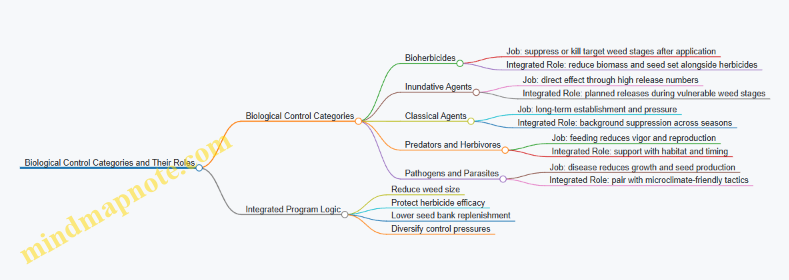
Examples That Show the Logic
Example: Seed bank reduction in a broadacre rotation. Suppose a winter cereal field has ryegrass escapes that head before harvest. A biological approach can be placed to target regrowth or late-season weed survival, reducing the number of plants that contribute seed. The integrated part is simple: you still manage emergence with crop competition and herbicides where needed, but you use biological control to shrink the “escape tail” that would otherwise refill the seed bank.
Example: Patch management instead of whole-field replacement. If only low-lying areas stay wet and weeds persist there, a pathogen-based category may perform better in those microclimates. You would map patches, treat them with the biological option when conditions favor infection, and use conventional herbicides elsewhere to keep overall control consistent.
Example: Herbivore support with crop and residue choices. Predators and herbivores often do better when the field has structural habitat. That can mean maintaining some residue cover or using crop rotation patterns that avoid removing all refuge at once. The integrated goal is to keep weed pressure low while avoiding a control plan that depends entirely on repeated herbicide applications.
Practical Integration Steps
- Match the category to the weed stage. Bioherbicides and inundative agents usually need a specific growth stage; predators and pathogens also have stage-dependent effects.
- Match the category to field conditions. Moisture, temperature, and canopy cover affect survival and performance, so your plan should reflect where the agent can actually work.
- Coordinate with herbicide timing and mode rotation. Use biological control to reduce escapes and regrowth, which helps you avoid “chasing” weeds with the same herbicide chemistry.
- Measure outcomes that matter. Track weed survival, regrowth, and seed production indicators so you can see whether the biological category is reducing the seed bank, not just changing appearance.
When these categories are used with clear roles—direct suppression, patch support, or long-term pressure—biological control becomes a dependable component of integrated resistance management rather than an add-on that only works when everything else goes perfectly.
6.2 Selecting Compatible Biological Control Options for Target Weeds
Choosing biological control for a specific weed is mostly about matching biology to field reality. Compatibility is not just “does it attack the weed,” but “does it survive long enough, find the weed reliably, and fit the rest of your integrated program.” A good selection process moves from weed traits to agent traits, then checks farm constraints.
Step 1: Identify Target Weed Traits That Matter
Start with the weed’s life stage you want to affect. Some agents work best on seedlings, others on flowering plants, and some target seeds or specific tissues. Note the weed’s growth habit (upright vs. creeping), typical height range, and how long it stays green under your local conditions. For broadacre systems, also record when the weed is most abundant relative to crop canopy development.
Example: If your target weed is most problematic as a late-emerging flush, prioritize agents that can establish quickly and persist through that window. If the weed’s main seed production happens over a short period, focus on agents that synchronize with flowering or seed set.
Step 2: Match Agent Biology to Weed Vulnerabilities
Next, translate weed traits into “vulnerabilities.” These are practical: leaf area available for feeding, presence of flowers for egg laying, or timing of susceptible plant stages. Then match the agent’s mode of action to that vulnerability.
A systematic compatibility check includes:
- Host specificity: The agent should reliably attack the target weed and not spend its effort on non-target plants.
- Life cycle timing: The agent’s development should overlap the weed’s susceptible stage.
- Dispersal and persistence: The agent must reach patches across the field and remain active long enough to matter.
- Environmental tolerance: Temperature and moisture ranges should fit your typical season.
Example: If your weed forms a dense basal rosette early, an agent that requires exposed stems may underperform. Conversely, an agent that attacks rosettes can reduce early establishment and make later herbicide timing less critical.
Step 3: Check Compatibility with Your Existing Weed Control Plan
Biological control rarely works alone. It must coexist with crop competition, herbicide programs, and any mechanical operations.
Compatibility questions to answer:
- Herbicide overlap: Are you applying herbicides during the agent’s active stage? If yes, select biological options that tolerate those products or adjust timing so the agent can establish before herbicide exposure.
- Canopy effects: Dense crop canopies can reduce agent movement and contact. If the agent needs direct contact with weed foliage, plan for timing when weeds are accessible.
- Residue and soil disturbance: Some agents rely on stable microhabitats. Frequent tillage or heavy residue removal can disrupt survival.
- Patchiness: If weeds are clumped, agents that spread slowly may only suppress hotspots. Plan scouting and targeted releases or treatments accordingly.
Example: Suppose you use a pre-emergence herbicide and later a post-emergence spray. If the biological agent targets seedlings, you may need to delay the post-emergence spray until after the agent has completed its most sensitive life stage.
Step 4: Evaluate Practical Deployment Constraints
Even a perfect biological match can fail if deployment is unrealistic.
Assess:
- Release method and placement: Will the agent be applied where the weed actually grows, including field edges and low spots?
- Coverage expectations: Some agents need repeated contact; others work with fewer interactions. Align your operational plan with that requirement.
- Monitoring capacity: You need to observe establishment and impact. If you cannot scout frequently during the agent’s key window, choose options with more forgiving timing.
Example: If your weed infestations are mostly along fence lines, a whole-field approach may waste effort. A targeted approach that prioritizes those zones can improve establishment and reduce unnecessary disturbance.
Step 5: Use a Simple Decision Filter Before Committing
A practical filter prevents “compatibility by hope.” Use a scoring mindset with clear pass/fail criteria.
Mind Map: Compatibility Selection Logic
Worked Example from Field Logic
You’re managing a broadleaf weed that emerges in two flushes. You want biological control to reduce the first flush so the second flush has fewer surviving plants.
- Choose an agent that attacks the weed at the early vegetative stage.
- Confirm the agent’s active period overlaps the first flush window.
- Review your herbicide schedule and avoid spraying during the agent’s most sensitive stage.
- Plan scouting to confirm establishment in the first flush areas, especially where weeds are clumped.
If the agent establishes poorly in the first flush hotspots, you don’t “keep going and hope.” You adjust placement, timing, or the biological option to match what the field is actually doing.
Step 6: Confirm Compatibility Through Field Observation
Finally, compatibility is verified by what you see: agent establishment, weed stage reduction, and changes in weed patch behavior. Record whether suppression is uniform or limited to accessible areas. That evidence feeds back into how you coordinate biological control with herbicide timing and cultural practices.
In short, selecting compatible biological control options is a matching exercise: weed stage to agent life cycle, then agent survival to your operational schedule. When those align, the biological component becomes a reliable partner rather than a hopeful side quest.
6.3 Habitat and Microclimate Requirements for Biological Agents
Biological weed control agents work best when the field environment supports their basic needs: survival, movement, feeding or infection, and reproduction. Habitat requirements are the “where,” while microclimate requirements are the “how it feels” at the agent’s scale—often just a few centimeters above the soil or on the leaf surface.
Habitat Foundations for Field Success
Start with habitat structure. Many agents need stable refuges from harsh sun and wind, plus a food source or host presence. In broadacre systems, that usually means managing the field so there are persistent weed patches or crop residues that buffer conditions.
A practical way to think about habitat is to separate three zones:
- Soil surface and residue layer: where many life stages persist.
- Weed canopy: where contact, feeding, or infection happens.
- Field edges and transitions: where microclimate is often less extreme and where recolonization can occur.
Example: If you release a seed-attacking agent but immediately remove all residue and repeatedly cultivate bare soil, you may reduce shelter and moisture retention. The agent might still establish, but the window for effective contact shrinks.
Microclimate Drivers at the Agent Scale
Microclimate is shaped by weather, canopy cover, residue, and timing of operations. The key drivers are temperature, humidity or leaf wetness, wind exposure, and light.
-
Temperature
Biological agents typically have a workable temperature range. Too cold slows activity; too hot reduces survival and can interrupt infection or feeding. Canopy cover moderates extremes. A dense crop canopy or residue can keep the weed surface closer to a stable range. -
Humidity and Leaf Wetness
Many foliar or surface-dependent agents require moisture for movement or infection. Leaf wetness can come from dew, light rain, or irrigation. If you apply during a dry period and then get a fast drying wind, performance often drops. -
Wind and Air Mixing
Wind increases evaporation and can physically remove agents from leaf surfaces. It also changes how quickly humidity falls after application. Shelterbelts, crop rows, and residue can reduce wind speed near the ground. -
Light and UV Exposure
Direct sun and UV can damage many biological agents. Shade from crop canopy or weed density can protect them, especially during the first hours after application.
Timing Biological Activity with Field Conditions
Microclimate is not constant across the day. A simple operational rule is to align application with periods when humidity is likely higher and evaporation is slower.
Example: In a winter cereal paddock, applying in late afternoon often increases the chance of dew formation overnight. That can extend the period when leaf surfaces remain moist enough for infection or establishment. If the forecast includes a strong drying wind, you can adjust by targeting a different window or focusing on agents that tolerate drier conditions.
If you need a concrete planning reference, use a recent historical pattern such as March 2026 weather records from your own farm logs to identify typical dew timing and heat spikes for your region.
Habitat Management Practices That Support Microclimate
These practices connect directly to microclimate drivers.
- Maintain residue cover to reduce soil heat and slow evaporation.
- Avoid unnecessary bare-soil periods between weed emergence and agent activity.
- Use crop canopy strategically so weeds are not fully shaded too early, but not exposed to full sun during the agent’s critical window.
- Minimize disruptive operations right after application. Cultivation or heavy spraying can strip residue, disturb refuges, and remove agents.
Example: If you plan to apply a foliar agent to target weeds in a barley crop, schedule it so you do not follow immediately with an operation that knocks down canopy cover or dries the field.
Mind Map: Habitat and Microclimate Requirements
Example Workflow for Setting Up a Successful Release
- Identify the target weed stage when the agent needs host contact (for example, early canopy stages for foliar agents).
- Check residue and canopy conditions so the weed surface is not fully exposed to midday sun.
- Choose an application window that favors leaf wetness or slower drying, such as late afternoon into night.
- Plan around field operations for the next 24–48 hours to avoid removing residue or disturbing the weed patch.
- Observe outcomes in the first week by checking whether treated weeds show signs consistent with the agent’s mode (for example, reduced vigor or visible infection structures).
This approach keeps habitat and microclimate connected to the agent’s actual job in the field: staying alive long enough to do the work, and doing it under conditions that don’t sabotage the biology.
6.4 Application Methods and Field Placement for Consistent Contact
Consistent contact is the difference between “we applied it” and “it actually met the target.” For biological weed control components, placement is about where the agent lands, how long it stays in the right microclimate, and whether it can reach the weed surface during the window when the weed is most vulnerable.
Start with Contact Requirements
Different agents need different contact routes. Some work best when they land directly on foliage; others must contact stems, seed heads, or the soil surface where germination occurs. Begin by writing a simple contact checklist: target surface type, target growth stage, and the acceptable contact duration. For example, a foliar-active agent should be applied when weeds have enough leaf area to intercept spray and before waxy cuticles or dense canopy shading reduce wetting.
Choose Application Method by Target Surface
Field placement starts with method selection.
- Foliar contact: Use spray delivery that produces droplets capable of sticking without excessive runoff. Aim for uniform coverage across the weed height band, not just the top leaves.
- Stem and collar contact: Direct the spray slightly upward or across the row so the agent reaches lower stems and the crown region.
- Soil or germination zone contact: Use banding or directed placement to concentrate agent where seeds or emerging seedlings will be. Broad broadcast can waste material and reduce contact probability.
A practical rule: if you can’t describe the target surface in one sentence, you can’t place the agent reliably.
Calibrate for Coverage, Not Just Rate
Rate tells you how much product you bought; coverage tells you how much the weeds actually received. Calibrate using water-sensitive cards placed at multiple heights (for example, 10 cm, mid-canopy, and upper canopy). If cards show dry patches or heavy pooling, adjust nozzle type, pressure, and travel speed.
Example: In a broadacre barley field with volunteer rye, a grower found strong results on the upper canopy but weak suppression lower down. After placing cards at two heights, they switched to a nozzle setup that improved lower-canopy interception and reduced runoff. The same total application rate produced more consistent contact.
Manage Droplet Behavior and Wetting
Droplets must balance two needs: they should reach the target and they should remain long enough to allow the agent to act. Too small and they drift; too large and they run off. Use weather conditions to help you: apply when wind is low and temperatures are moderate so droplets don’t evaporate before contact.
A simple field test: after spraying a small section, check whether droplets leave a light, even film on target leaves. If leaves are dry within minutes, you likely need to adjust droplet size distribution or timing.
Timing with Microclimate and Weed Stage
Placement is not only spatial; it’s temporal. Many agents perform best when the weed surface is receptive—often when leaves are not overly stressed and when humidity supports survival. Apply when weeds are actively growing and avoid periods that cause rapid drying.
Example: A team applied an agent to thistles after a hot, windy afternoon. Emergent leaves looked “treated,” but contact effectiveness was poor because the spray dried quickly and the agent lost viability on the leaf surface. Repeating the same method the next morning under calmer conditions improved contact without changing the product.
Field Placement Patterns That Reduce Waste
Uniformity matters, but so does targeting.
- Banding: Place the agent where weeds emerge or where row middles concentrate seedlings.
- Spot or patch treatment: When weed density is patchy, treat patches to maintain contact quality and reduce unnecessary exposure.
- Edge management: Many infestations start at field edges. Direct placement along borders can prevent early escapes that later become “everywhere.”
Handling and Mixing for Contact Consistency
Even perfect placement fails if the agent is damaged before it reaches the field. Mix gently, avoid long hold times, and keep agitation consistent so concentration doesn’t stratify. Rinse and clean equipment thoroughly to prevent residues that can harm biological components.
Mind Map: Application Methods and Field Placement
Example Workflow for a Broadacre Foliar Application
- Identify the target weed stage and the leaf height band.
- Place water-sensitive cards at two or three heights in a representative area.
- Calibrate travel speed and nozzle choice until cards show even coverage without heavy runoff.
- Schedule application for low wind and moderate temperature.
- Mix with gentle agitation and avoid long tank hold times.
- After spraying, inspect treated weeds for even wetting and minimal dry patches.
This workflow turns “we sprayed” into measurable contact quality, which is exactly what biological weed control needs to behave like a system rather than a hope.
6.5 Monitoring Establishment and Effectiveness in Treated Areas
Monitoring in biological weed control is less about “did it work?” and more about “what happened, where, and why?” You’re checking three things in sequence: whether the biological agent establishes, whether it reaches the target weed at the right life stage, and whether weed suppression translates into fewer viable seeds.
Establishment Monitoring Basics
Start with a simple baseline. Before treatment, record target weed density by patch (for example, low, medium, high) and note growth stage. Then, after application, monitor at consistent intervals so you can separate agent establishment from normal weed variation.
Use a small set of field indicators that match the agent’s expected behavior. For example, if the agent relies on contact with foliage, you should see signs on leaves or stems within a predictable window. If it relies on soil presence, you should see activity in the root zone or near the soil surface rather than only on aboveground parts.
A practical approach is to tag 3–5 representative spots per treated block. Each spot gets the same sampling method each time. If you change methods, you’ll end up comparing apples to “probably apples.”
Effectiveness Monitoring That Connects to Seed Outcomes
Effectiveness monitoring should include both short-term and seed-relevant measures.
Short-term measures:
- Weed survival rate at 2–4 weeks after treatment
- Reduction in new growth or flowering compared with untreated checks
- Patch expansion or contraction over time
Seed-relevant measures:
- Number of seed heads per square meter on surviving plants
- Seed set quality indicators such as aborted heads or reduced viable seed counts (when feasible)
- Seedling emergence in the following crop cycle, using the same emergence counts method each season
Even if you can’t measure viable seed directly, seed-head counts give you a grounded proxy. The key is consistency: count the same weed species, same plant size class, and same sampling area each time.
Designing Checks and Sampling Without Overcomplicating
Include untreated or differently managed checks. If you can’t leave a full untreated area, use edge strips or alternate passes, but document the layout clearly.
Sampling should reflect patchiness. Many biological effects are uneven because microclimate and weed density vary. If you only sample the “best-looking” area, you’ll overestimate performance.
A simple sampling rule: for each treated block, sample enough points to capture the range of weed density you observed at baseline. If baseline density ranged from 5 to 40 plants per square meter, your monitoring points should include both ends.
Mind Map: Monitoring Logic for Treated Areas
Example: Patchy Field with Mixed Weed Stages
Imagine a broadacre paddock where target weeds are in two stages: some are still vegetative, others are already forming seed heads. You apply a biological control timed for foliage contact.
Your monitoring plan includes:
- Spot A: mostly vegetative weeds
- Spot B: mostly seed-head weeds
- Spot C: mixed stage
Two weeks after treatment, you find stronger leaf signs and higher survival reduction in Spot A. Spot B shows limited visible agent activity on foliage because the plants have shifted to reproductive structures. Seed-head counts later confirm the difference: Spot A has fewer seed heads, while Spot B still produces many heads.
The lesson isn’t “the agent failed.” It’s that the treatment window matched one portion of the population better than the other. That information feeds directly into next season’s timing and into whether you need a complementary tactic for the already-reproductive patch.
Example: When Establishment Looks Good but Suppression Is Modest
In another block, you observe clear establishment indicators, yet weed survival drops only slightly. Monitoring shows the agent signs occur on non-target plants or on the target weed’s lower leaves, while the upper canopy remains active.
Your next monitoring visit focuses on contact coverage: you compare plant height classes and canopy position at the time of application. If the agent requires contact, you may need to adjust application timing to earlier growth stages or refine how you target the canopy height.
Interpreting Results Without Guesswork
When results are mixed, classify the outcome:
- Establishment failure: indicators absent where expected
- Targeting mismatch: indicators present but on the wrong weed stage or plant part
- Suppression gap: establishment and targeting occur, but seed-head reduction is limited
This classification keeps the discussion practical. It tells you what to change in the next monitoring cycle—sampling focus, timing, or integration with other weed control tactics—without turning the field into a mystery novel.
7. Designing Integrated Resistance Management Programs
7.1 Building a Resistance Management Plan From Weed and Herbicide Data
A resistance management plan is only as good as the data behind it. Start by turning field observations and spray records into a clear picture of (1) which weeds are present, (2) how they reproduce and spread, (3) which herbicides have been used, and (4) where selection pressure is likely to concentrate. Then you translate that picture into practical actions that reduce seed production and diversify control methods.
Step 1: Organize Weed Data Into Decision-Ready Form
Collect weed information at the scale you actually manage. For each weed species (or biotype if known), record: growth stage at survey time, density or cover, patch locations, and whether the weed is producing seed. Add notes on how the weed behaves in your system, such as whether it emerges in flushes or persists as a late-season escape.
Example: In a wheat paddock, you find ryegrass patches along fence lines and low-lying zones. The main crop canopy closes early in most areas, but the patches stay open longer. That detail matters because it changes which control window is realistic and where seed destruction efforts should be concentrated.
Step 2: Build a Herbicide History That Shows Selection Pressure
Create a season-by-season log for each herbicide active ingredient: product name, active ingredient, rate, application timing, target weeds, and the crop stage. Also record application quality indicators you can verify later, such as calibration date, nozzle type, and whether wind or temperature limited coverage.
Example: If a single mode of action was applied at the same growth stage for three consecutive years, selection pressure is likely to be high even if the weed was not obviously “failing” every time. Resistance often starts quietly, then shows up as patchy survivors.
Step 3: Link Weed Life Cycle to Control Windows
Resistance management is not only about rotating chemistry; it is about preventing resistant survivors from producing seed. Use weed phenology to identify the stages you must hit: emergence, early vegetative growth, flowering, and seed set. Then match those stages to what your operations can reliably do.
Example: If a weed produces seed after a late flush, a treatment timed only for early seedlings may reduce numbers but still allow seed production from late escapes. Your plan should then include a second tactic aimed at that later stage, or a cultural step that reduces the late flush.
Step 4: Identify Risk Drivers and Prioritize Actions
Not all weeds and not all paddocks deserve the same level of effort. Rank risk using simple criteria: repeated use of the same mode of action, high weed density, evidence of patchy survival, and proximity to likely seed sources (roadsides, waterways, headlands). Prioritize paddocks where you can most effectively reduce seed return.
Example: A paddock with repeated late-season escapes and heavy headland infestations should get tighter sequencing and more frequent monitoring of those zones, not just a generic spray schedule.
Step 5: Translate Data Into a Mode-of-Action Strategy
For each key weed, list the herbicide modes of action you have used and the ones you can use next season. Then set rules that prevent back-to-back reliance on the same mode of action. Where practical, combine herbicides with different modes of action in the same season, but only when the crop and weed stage make that combination sensible.
Example: If your ryegrass has a history of repeated Group 1 use, your plan should avoid repeating that group as the primary tool. Instead, you might use a different mode of action for the main flush and reserve the Group 1 for a different stage or a different tactic, depending on label and crop safety.
Step 6: Add Non-Herbicide Tactics That Reduce Seed Production
A resistance plan should include at least one non-herbicide lever that targets the same weed life cycle stage as the herbicide program. Options include crop competition improvements, residue management, targeted seed destruction, and timing changes that reduce establishment.
Example: If weed escapes are concentrated in thin crop areas, improving stand uniformity and adjusting establishment timing can reduce the number of plants that ever reach seed set. That lowers the “fuel” for resistance selection.
Step 7: Define Monitoring, Thresholds, and Response Rules
Monitoring should be planned, not improvised. Decide when you will scout, what you will measure (survivor counts, patch expansion, growth stage), and what triggers a response. Response rules should specify what you will change: timing, mode of action, mixture strategy, or non-herbicide tactics.
Example: If survivors appear in the same patch locations after a treatment, you do not just increase dose. You first verify application timing and coverage, then adjust the mode-of-action plan and add a tactic aimed at seed set.
Mind Map: Resistance Plan from Data to Actions
Example: Turning Records Into a One-Page Plan
Use a simple structure for each key weed in each paddock: (1) what you saw, (2) what you used, (3) which stage you targeted, (4) what you will do differently next time, and (5) how you will check whether it worked.
Example: For ryegrass in wheat, your one-page plan might state that you observed late flush seed set in headlands, your history shows repeated reliance on one mode of action at the same crop stage, and your next season will shift the main control window earlier while adding a second tactic aimed at preventing seed set in headlands. Your monitoring rule could require scouting headlands at two growth stages and documenting whether survivors reach flowering.
A good plan is specific enough to guide decisions in the field and structured enough to be updated when the data changes. When the weed data, herbicide history, and life cycle windows agree, the strategy becomes easier to execute and easier to evaluate.
7.2 Rotating Modes of Action Using Practical Field Constraints
Rotating herbicide modes of action (MoAs) is simple in theory and annoyingly real in the field. The trick is to rotate in a way that still fits your crop calendar, sprayer capacity, weed emergence patterns, and the herbicides you can actually access. Start by treating MoA rotation as a planning problem with constraints, not a wish list.
Foundational Rule for Rotation Planning
A rotation plan needs two layers: (1) the MoA used for each weed control event and (2) the timing of those events relative to weed growth stages. If you apply the same MoA repeatedly to the same weed cohort, you select for resistance faster. If you vary MoA across events that target the same cohort, you reduce repeated selection pressure.
A practical way to think about it: each “control window” is a chance to change the MoA. Your job is to ensure that consecutive windows do not accidentally reuse the same MoA on the same weed population.
Step 1: Build a Field Timeline That Matches Weed Reality
List your likely weed emergence flushes and your planned operations. For broadacre systems, emergence often clusters around rainfall and soil disturbance. Then map your crop stages and spray opportunities.
Example: In a winter cereal, you might have an early flush of ryegrass in autumn, then another flush after a late rain. If you plan one pre-emergence herbicide and one post-emergence herbicide, those are two separate windows. If both use the same MoA, you’ve effectively stacked selection pressure.
Step 2: Translate Constraints Into Rotation Choices
Constraints usually fall into four buckets:
- Crop safety windows: Some MoAs are only safe at specific crop stages.
- Weed size limits: Many post-emergence products work only on small weeds.
- Sprayer and labor capacity: You may not be able to spray every window.
- Product availability and tank-mix rules: Some MoAs are limited by label restrictions.
Instead of forcing a perfect rotation, choose a “rotation backbone” MoA sequence that respects crop safety and weed size, then fill gaps with compatible alternatives.
Step 3: Use a Constraint-First Rotation Backbone
Pick a backbone that alternates MoA groups across your main control windows. Then add “fallback” MoAs for windows you can’t treat.
Example: Suppose your backbone for a season is:
- Window A: MoA Group 1
- Window B: MoA Group 2
- Window C: MoA Group 3
If Window B is missed due to weather, you don’t automatically apply Group 1 again just because it’s on hand. You apply the best available MoA that still fits crop stage and weed size, even if it breaks the ideal sequence. The goal is to avoid repeating the same MoA on the same cohort.
Step 4: Prevent Accidental Reuse Through “Cohort Tracking”
Weed cohorts matter. A cohort is the group of weeds that emerged around the same time and will be targeted together. When you rotate MoAs, rotate across treatments that hit the same cohort.
Practical method: label your spray records by cohort window, not just by calendar date.
Example: If you spray after a rain that triggered a flush, call that cohort “Flush 1.” If you later spray again and the weeds are still from Flush 1, treat it as the same cohort even if the crop stage changed.
Step 5: Handle Mixed Weed Communities Without Losing the Plot
Mixed species can tempt you to use one MoA that “covers most weeds.” That’s where resistance risk creeps in.
A better approach is to prioritize the most resistance-prone species and rotate based on them. If one species requires a specific MoA to be effective, use that MoA for that species’ cohort window, and choose the remaining MoAs to support rotation rather than convenience.
Mind Map: Rotation Under Field Constraints
Example: A Constraint-Driven Rotation Plan
Assume three main windows in a broadacre crop:
- Window A: Early post-emergence when weeds are small and crop is tolerant.
- Window B: Mid-season post-emergence, but labor is tight.
- Window C: Late-season spot control, mainly for escapes.
A practical rotation plan might look like:
- Window A: MoA Group 1 (target small weeds)
- Window B: MoA Group 2 (only if weeds are still within size limits)
- Window C: MoA Group 3 for escapes, avoiding Group 1 reuse on the same cohort
If Window B is missed, you still choose Window C based on cohort tracking and label safety, not on what you used last time.
Quick Field Rules That Keep Rotation Honest
- Rotate by cohort, not just by season.
- If you miss a window, don’t “catch up” with the same MoA.
- Prioritize the species with the highest resistance risk when choosing fallback options.
- Record MoA by window and cohort so next season’s plan is based on evidence, not memory.
7.3 Combining Non Chemical Tactics With Herbicide Programs
Non-chemical tactics work best when they reduce the number of weeds that ever reach the “herbicide decision.” That means you use culture, timing, and physical disruption to lower weed pressure, then you use herbicides to finish the job on the weeds that still emerge. The trick is to coordinate the tactics so they don’t fight each other—especially around emergence timing, canopy closure, and seed set.
Start with a simple sequence for broadacre fields: (1) prevent or delay early weed establishment, (2) suppress survivors during crop canopy development, (3) target remaining weeds at the most effective growth stage, and (4) stop seed production so the next season starts with fewer problems. Herbicides still matter, but they become a tool for targeted control rather than a blanket response.
Building the Foundation with Crop Establishment
Uniform crop emergence is the non-chemical “multiplier.” If the crop stand is patchy, weeds fill gaps and you end up treating escapes repeatedly. Practical steps include matching seeding depth to soil moisture, calibrating seed meters for consistent spacing, and avoiding compaction that creates uneven emergence. A field with a uniform stand often needs fewer late-season interventions because the crop shades and outcompetes weeds earlier.
Row spacing and seeding rate influence canopy closure timing. Narrower rows and adequate seeding rate generally reduce light reaching the soil surface, which limits weed germination and slows growth of emerged weeds. If you can’t change row spacing, you can still improve canopy closure by ensuring the crop is not stressed early through balanced fertility and careful residue management.
Using Mechanical and Physical Tactics Without Creating New Weed Problems
Mechanical tactics include stale seedbed preparation, inter-row cultivation, and targeted hoeing where feasible. The key is to treat weeds when they are small and before they set seed. For a stale seedbed, you prepare the seedbed, allow a flush to emerge, then control that flush before crop sowing. This reduces the number of weeds competing with the crop at the start.
Physical tactics also include managing residue and soil surface conditions. Heavy residue can suppress some weed emergence, but it can also delay crop emergence if not managed correctly. The best approach is to align residue handling with your crop’s emergence requirements so you suppress weeds without slowing the crop into a vulnerable window.
Coordinating Timing with Herbicide Growth Stages
Herbicides are most reliable when weeds are at the correct growth stage and coverage is consistent. Non-chemical tactics can shift weed phenology by delaying emergence or thinning early cohorts. That’s useful, but it means you must re-check the field before spraying.
A practical coordination rule: use non-chemical tactics to reduce early cohorts, then schedule herbicide applications based on observed weed stage rather than calendar dates. For example, if a stale seedbed reduces early weeds, the next flush may be smaller and more synchronized, which can improve herbicide performance and reduce the need for multiple follow-up sprays.
Designing a Two-Track Plan for Mixed Weed Communities
Mixed weed communities often include species with different emergence patterns and herbicide sensitivities. Non-chemical tactics can be used to target the “easy wins” first: suppress the weeds that emerge early and compete strongly, then use herbicides to address the remaining species at their most controllable stages.
For instance, if broadleaf weeds emerge early and grasses emerge later, you can use crop canopy closure and early mechanical suppression to reduce broadleaf pressure, then apply a herbicide program timed to the later grass cohort. This reduces the total number of herbicide events and lowers selection pressure because fewer survivors remain to reproduce.
Mind Map: Combining Non Chemical Tactics with Herbicide Programs
Example: Stale Seedbed Plus Targeted Post Emergence
A grower prepares a seedbed and waits for a flush of small weeds to emerge. After the flush, they control it before sowing the crop. The crop then establishes with less early competition, leading to faster canopy closure. When weeds reappear, the grower scouts and applies a post-emergence herbicide when the remaining weeds are small and actively growing. The result is fewer escapes, fewer late-season treatments, and less seed rain into the next crop cycle.
Example: Inter-Row Cultivation Supporting a Reduced Spray Plan
In a crop where inter-row cultivation is feasible, the grower cultivates between rows when weeds are at a small stage and before they interfere with crop rows. This reduces the weed population in the inter-row spaces. Because the crop rows are already competing, the grower uses herbicides only where weeds persist in-row and where coverage can be achieved reliably. The spray plan becomes narrower in both area and timing, which helps maintain effectiveness and reduces unnecessary selection pressure.
The common thread across these examples is coordination: non-chemical tactics reduce early weed pressure and protect the crop’s ability to close the canopy, while herbicides handle the remaining weeds at the right stage with good coverage. When you treat the field as a sequence rather than a single event, the program becomes easier to execute and harder for resistance to exploit.
7.4 Managing Herbicide Application Timing and Coverage Quality
Timing and coverage quality are the two levers that decide whether an herbicide program actually hits the target. Timing controls the weed’s biology—whether the plant is actively growing and able to absorb and translocate the herbicide. Coverage quality controls the physics—whether the spray reaches the right plant surfaces at the right dose, with minimal gaps and minimal drift.
Timing Foundations for Reliable Control
Start with the weed’s growth stage, not the calendar. Many herbicide failures happen when the crop and weed are both “present,” but the weed is no longer in the window where the herbicide can work. For contact herbicides, the window is usually narrow: the weed must be small enough that the spray contacts most of the foliage. For systemic herbicides, the window often depends on active growth and translocation pathways.
A practical way to plan timing is to link three observations from the same scouting pass: weed size distribution, weed phenology (for example, early vegetative versus flowering), and crop stage. If you see a wide spread in weed sizes, you’re not just dealing with “more weeds”—you’re dealing with different herbicide susceptibility. In that situation, a single application can only be perfect for one slice of the population.
Coverage Quality Essentials
Coverage quality is about distribution, not just “sprayed or not.” Two fields can receive the same labeled rate and still differ in outcome because one has uneven droplet deposition. Uneven coverage creates survival pockets that later seed the next problem.
Key coverage drivers include nozzle type and spacing, boom height, travel speed, and wind. Boom height affects droplet overlap; too high increases gaps, too low increases runoff and uneven deposition. Travel speed changes the time droplets spend in the air and the distance they travel before impact. Wind can shift droplets off target, but it also changes droplet trajectory so that the pattern on leaves becomes patchy.
A Mind Map for Timing and Coverage Decisions
Mind Map: Timing and Coverage Quality
Systematic Workflow for Broadacre Fields
- Scout and stratify the field. Walk the field in a grid and record weed size classes. If you can’t describe the field in size classes, you can’t time the application precisely.
- Choose the timing window by weed stage. Decide whether you’re targeting early growth for contact activity or relying on systemic movement. If the majority of weeds are beyond the effective stage, coverage improvements won’t compensate.
- Match application setup to the target canopy. For low weeds, you want droplets to land on foliage rather than on residue. For taller weeds, you need enough penetration and overlap to reach upper leaves without excessive drift.
- Stabilize boom height and speed. Use the same travel speed you calibrated for. If the terrain forces speed changes, plan for it by adjusting setup and ensuring the boom stays at the intended height.
- Control drift and deposition gaps. Apply when wind is manageable and consistent. If wind direction shifts during the run, deposition becomes uneven even if the rate is correct.
- Verify early results and map survivors. After application, check within the period when symptoms should appear. Record where survivors occur; repeated survival in the same zones often points to coverage issues, while random survival can point to timing mismatch.
Example: Two Fields, Same Rate, Different Outcomes
Field A: Weeds are mostly at the 2–4 leaf stage. The sprayer is calibrated, boom height is stable, and wind is low enough to keep droplets landing on leaves. After treatment, you see uniform browning and reduced regrowth. The program works because timing aligns with susceptibility and coverage is consistent.
Field B: Weeds include many plants that have already formed thicker stems and some that are taller with more leaf area. The sprayer setup is adequate, but the application is late for the larger portion of the population. You get patchy control: small weeds collapse quickly, while larger weeds survive and later produce seed. The lesson is simple: coverage quality can’t fix a timing window miss.
Example: Coverage Gaps That Look Like “Resistance”
A grower notices survivors in narrow strips that match the sprayer’s turning and speed changes. The field history shows repeated “resistance” reports, but the pattern is consistent with deposition gaps. The fix is not a new herbicide mode of action; it’s correcting boom height stability, ensuring consistent overlap, and re-checking calibration and pattern uniformity.
Practical Checks Before You Start Spraying
- Calibration confirmation: Verify output matches the target rate at the planned travel speed.
- Pattern and overlap check: Ensure nozzle spacing and boom height produce the intended overlap on a flat surface.
- Operational plan: Decide how you’ll handle headlands and turns so you don’t create systematic skips.
- Weather gate: Set a go/no-go threshold for wind and stick to it; “almost acceptable” conditions can still produce uneven deposition.
Advanced Detail Without the Headache
When weed size distribution is wide, consider whether a single application can realistically cover the whole population. If not, you may need to adjust the plan so that the main portion of the weeds receives the herbicide at the correct stage, while escapes are managed with a subsequent tactic that targets the remaining cohort. Coverage quality and timing quality should be treated as a coupled system: good timing with poor coverage still leaves survivors, and good coverage with poor timing still leaves survivors. The goal is to reduce both failure modes at once—so the field doesn’t keep paying the “seed bank interest” bill.
7.5 Decision Framework for Adjusting Treatments During a Season
A good in-season decision is not a guess; it’s a short chain of evidence. The goal is to keep weed control effective while reducing the chance that resistance gets a free pass. This framework works for broadacre rotations where you may have multiple weed species, variable emergence, and limited time windows.
Step 1: Confirm the Problem Before Changing the Plan
Start with what you expected versus what you see.
- Expected outcome: target weeds should be suppressed or killed, and seed production should be prevented.
- Observed outcome: look for survivors, patchy control, or delayed emergence.
Quick field checks:
- Survivor pattern: scattered plants across the treated area often points to coverage or timing issues; clusters in low spots or along wheel tracks often point to application distribution.
- Stage mismatch: if weeds were taller than planned or past the most sensitive growth stage, reduced efficacy is expected even without resistance.
- Species mix: if a new species emerged after the treatment window, the “failure” may be a different weed, not a resistant one.
Step 2: Separate Resistance Signals from Non-Resistance Causes
Before you assume resistance, rule out the usual suspects.
Non-resistance causes to check first:
- Coverage gaps: missed strips, nozzle issues, boom height problems, or wind drift.
- Environmental mismatch: drought stress, heavy rain soon after application, or temperature extremes that reduce herbicide performance.
- Tank mix incompatibility: precipitation or poor mixing can reduce active ingredient delivery.
- Weed size and vigor: larger or stressed weeds can respond differently.
Resistance signals to consider when non-resistance causes are unlikely:
- Consistent survival across patches with good coverage quality.
- Survival across multiple herbicide applications that share similar selection pressure.
- Survival in the same species year after year despite rotation.
Step 3: Use a Decision Tree Based on Timing and Weed Stage
Once you’ve narrowed the cause, decide what you can still do within the season.
- If weeds are still small and before seed set: prioritize actions that prevent reproduction.
- If weeds are near seed set: focus on stopping seed production immediately, even if full kill is not realistic.
- If weeds already seeded: shift to seed bank reduction tactics for the next cycle; in-season rescue is limited.
Step 4: Choose the Adjustment Type
Adjustments usually fall into four categories. Pick one based on the evidence.
- Timing adjustment: treat the next flush at the correct growth stage.
- Coverage adjustment: fix equipment, boom height, speed, and drift conditions.
- Mode of Action adjustment: switch to a different mode of action when resistance is plausible.
- Non-chemical adjustment: use cultivation, crop competition tactics, or targeted biological seed destruction where feasible.
A practical rule: if the issue is likely coverage or timing, change those first. If the issue persists with good coverage and correct timing, then mode of action changes become the priority.
Step 5: Set a “Stop and Record” Threshold
Make the decision measurable so you don’t keep paying for the same mistake.
- Record the date of application, weed stage, weather window, product and rate, and field conditions.
- Define a threshold such as: “If control is below expectation in the same species after a second properly executed treatment, treat it as a resistance signal and change the mode of action or the non-chemical component.”
Example decision log entry (use your real field numbers):
- 2026-03-15: post-emergence herbicide applied at labeled rate; target weeds at 2–4 leaf; control patchiness observed along wheel tracks; next action scheduled for the next flush with corrected boom height.
Step 6: Implement the Adjustment and Monitor the Next Flush
Monitoring is part of the decision, not an afterthought.
- Re-scout within the expected response window.
- Compare treated versus untreated or edge areas.
- Note whether survivors are the same species and whether they are at the same stage.
If survivors are mostly the same species and stage, that supports a resistance or dose-delivery issue. If the species mix changes, it supports emergence timing and seed bank dynamics.
Mind Map: In-Season Treatment Adjustment Logic
Example: Two-Stage Response in a Mixed Broadacre Field
A grower applied a post-emergence herbicide when most target weeds were at early growth. Two weeks later, control was patchy: strong suppression in most of the paddock, but dense survivors along a low-lying section.
- Step 1: survivors are concentrated in one topographic zone, suggesting environmental or coverage delivery rather than uniform resistance.
- Step 2: the low area had a different soil moisture profile and the sprayer had slightly reduced output due to a partially clogged nozzle.
- Step 3: the surviving weeds were still before seed set.
- Step 4: the adjustment combined coverage correction (nozzle replacement and recalibration) with timing (treat the next flush at the same early stage).
- Step 5: the grower recorded the nozzle issue and set a threshold: if the same species survives again after a properly executed treatment, switch mode of action and add a non-chemical seed destruction component.
This approach keeps decisions grounded: first fix delivery and timing, then change chemistry or tactics only when the evidence supports it.
8. Herbicide Application Quality and Operational Practices
8.1 Calibration and Nozzle Selection for Broadacre Spraying
Broadacre spraying is a numbers game: the right nozzle, the right pressure, and the right travel speed must agree with each other. If they don’t, you don’t just get “less effective” results—you get a different dose pattern, which can change weed control and resistance risk.
Core Calibration Logic
Start with the target application rate (L/ha) and work backward to what the sprayer must deliver at your chosen speed and pressure. The key relationship is that flow per nozzle must match the required volume per hectare when the boom spacing and travel speed are fixed.
A practical workflow:
- Choose boom width and nozzle spacing based on the sprayer configuration and crop row/ground conditions.
- Select a nozzle type and size that can deliver the target rate at a reasonable pressure range.
- Calibrate travel speed using a measured distance and timed passes.
- Set pressure, then verify output by collecting discharge from nozzles into measuring containers.
- Re-check after any changes to pressure, speed, or nozzle replacements.
Nozzle Selection Principles
Nozzles mainly differ in spray pattern shape, droplet size class, and how flow changes with pressure. For broadacre weed control, droplet size matters because it affects both coverage and drift risk.
Pattern and coverage: A flat-fan nozzle is common for broadacre booms because it lays down a predictable fan across the boom width. Overlap between adjacent nozzle fans should be planned so you don’t create stripe gaps.
Droplet size and drift: Finer droplets increase coverage but drift more easily. Coarser droplets reduce drift but can leave coverage holes if overlap is insufficient or if weeds are tall and uneven.
Flow rate and pressure behavior: Two nozzles with the same nominal flow rating can behave differently across pressure ranges. Use the manufacturer’s flow chart to pick a nozzle that hits your target rate without forcing the sprayer to run at the extreme end of its pressure capability.
Step-by-Step Calibration Method
- Set up the sprayer dry run: Ensure boom height is consistent and nozzles are clean. Replace any worn tips; worn nozzles can shift flow and pattern.
- Confirm nozzle spacing and boom width: Measure nozzle-to-nozzle spacing and total boom width. Even small spacing errors can change the effective application rate.
- Choose a pressure setting: Set pressure based on the nozzle chart for the desired application rate at your planned speed.
- Measure travel speed accurately: Use a measured track and record time. If speed varies, the dose per hectare varies.
- Collect and measure nozzle output: Run the sprayer at the set pressure and speed, then collect discharge from a representative set of nozzles (for example, left, center, right). Calculate average flow per nozzle.
- Adjust and repeat: If output is high, reduce pressure or change nozzle size. If output is low, increase pressure within the recommended range or select a larger nozzle.
- Validate with a water-only run: Confirm that the boom delivers uniform output across the width, not just at a few points.
Uniformity Checks That Actually Matter
Uniformity failures often show up as “mystery patches” of poor control. Look for:
- Clogging or partial blockage: Especially after tank mixing or when water quality varies.
- Uneven boom height: Hills and uneven ground can change fan overlap and droplet deposition.
- Pressure instability: Worn regulators or leaks can cause nozzle-to-nozzle differences.
A simple field habit: after calibration, mark nozzle positions and visually inspect spray pattern symmetry from a safe distance during a short test run.
Mind Map: Calibration and Nozzle Selection
Example: Matching Nozzle Output to a Target Rate
Assume you want 120 L/ha on a broadacre boom with 0.5 m nozzle spacing and you plan to drive at 12 km/h. You pick a nozzle that, according to the flow chart, delivers the needed flow per nozzle at a practical pressure.
Then you calibrate:
- Set pressure to the chart-recommended value.
- Run at 12 km/h.
- Collect discharge from three nozzles (left, center, right) for a fixed time.
- If the average collected volume corresponds to, say, 130 L/ha, reduce pressure slightly or select a smaller nozzle size.
- If it corresponds to 105 L/ha, increase pressure within the nozzle’s recommended range or select a larger nozzle.
The point isn’t the exact numbers—it’s the loop: nozzle choice and pressure are only “correct” after you verify output at your speed.
Example: Droplet Size Choice for Canopy Height
If weeds are short and evenly distributed, a slightly finer droplet class can improve contact and coverage. If weeds are taller or windier conditions increase drift risk, shifting to a coarser droplet class helps keep spray where it lands. In both cases, you still maintain overlap and uniform boom height; droplet size can’t fix a coverage gap created by poor overlap.
Practical Calibration Habits
- Calibrate after any nozzle replacement, pressure regulator service, or major hose/boom change.
- Use the same water source and tank mix viscosity you’ll use in the field, because thick mixes can affect flow.
- Keep a simple log of speed, pressure, nozzle type, and measured output so the next calibration isn’t a guessing contest.
8.2 Water Volume Droplet Spectrum and Drift Management
Water volume and droplet spectrum determine how evenly herbicide lands, how long it stays on the target, and how much escapes to non-target areas. Drift management is not a separate topic; it is the practical consequence of droplet size, spray release height, wind, temperature, and how the boom is operated.
Water Volume as a Coverage Engine
Water volume is the carrier that transports active ingredient and creates the spray cloud. Higher water volume usually increases the number of droplets per square meter, which can improve coverage on waxy leaves or dense weed canopies. However, higher volume can also increase runoff if the target surface cannot absorb it. A useful way to think about it: water volume sets the “spray density,” while droplet spectrum sets the “spray behavior.”
Example: In a broadleaf weed patch with a thick leaf surface, a moderate water volume with a droplet spectrum that balances coverage and retention often performs better than a very low volume that relies on fewer, larger droplets.
Droplet Spectrum Fundamentals
Droplet spectrum describes the distribution of droplet sizes produced by nozzles at a given pressure. Two sprays can use the same total herbicide rate but behave differently if one produces many fine droplets and the other produces mostly coarse droplets.
- Fine droplets increase the chance of drifting because they remain airborne longer and can evaporate into smaller particles.
- Coarse droplets reduce drift risk but may miss small leaf targets or fail to cover uneven surfaces.
- Medium droplets often provide a practical compromise when the target is reachable and the weather is stable.
Droplet spectrum is influenced by nozzle type, nozzle orifice, operating pressure, and travel speed. Increasing pressure generally shifts the spectrum toward smaller droplets, which can improve coverage but raises drift risk.
Drift Path Control Through Droplet Choice
Drift occurs when droplets or their residues move off-target before deposition. The main drivers are:
- Droplet size distribution: more fine droplets means more drift potential.
- Air movement: wind speed and gustiness move the spray cloud.
- Evaporation and thermal effects: warm, dry air accelerates droplet shrinkage.
- Release height: higher booms increase the time droplets spend in the air.
- Spray cloud momentum: fan pattern and travel speed affect how the cloud forms.
Example: If you must spray during a breezy window, switching to a droplet spectrum that is less prone to airborne drift can be more effective than trying to “compensate” with higher pressure.
Drift Management Workflow for Field Operations
A systematic approach prevents last-minute guesswork.
-
Match nozzle and pressure to the target
- Choose a nozzle that produces the desired droplet spectrum for the weed canopy.
- Set pressure to achieve consistent output without pushing the spectrum too fine.
-
Set boom height to the crop and weed structure
- Keep the boom as low as practical while avoiding boom strikes and ensuring the spray pattern reaches the target.
-
Use weather conditions to protect deposition
- Prefer stable conditions with lower wind and lower evaporation pressure.
- Avoid spraying when gusts repeatedly change wind direction.
-
Control travel speed and pattern overlap
- Maintain consistent speed so the spray cloud does not thin out between passes.
- Ensure overlap is correct to avoid striping that looks like “mysterious herbicide failure.”
-
Verify output consistency
- Calibrate before the job and re-check if you change nozzles, pressure, or operating conditions.
Mind Map: Water Volume, Droplet Spectrum, and Drift
Example Scenarios with Clear Decisions
Scenario 1: Dense canopy, low drift priority
- Use a droplet spectrum that still reaches lower leaves, but avoid pushing into very fine droplets.
- If coverage is poor, adjust nozzle choice or water volume before increasing pressure.
Scenario 2: Near sensitive areas, wind present
- Reduce drift potential by selecting a coarser spectrum and lowering boom height.
- Keep travel speed steady to prevent uneven deposition.
Scenario 3: Uneven field strips after application
- Check overlap and speed consistency.
- Confirm nozzle output and pressure stability; striping often comes from operational variation, not “mystery weed behavior.”
Practical Checks That Prevent Drift Problems
Before leaving the yard, confirm nozzle condition, correct pressure, and boom height settings. During the job, watch for changes in spray pattern shape and uniformity across the boom. If the field conditions shift, it is better to pause and reset than to continue with a spectrum that no longer matches the drift risk.
8.3 Adjuvants and Tank Mixing Compatibility for Reliable Performance
Adjuvants and tank mixes decide whether an herbicide lands where it should, stays there long enough, and works the way the label expects. Think of the spray tank as a short-lived chemistry lab: if ingredients clash, the field gets the leftovers.
Foundations of Adjuvant Roles in Herbicide Performance
Adjuvants generally support one or more of these jobs: improving wetting so droplets spread on leaf surfaces, enhancing penetration so active ingredients move into target tissue, reducing water-related problems like hardness effects, and controlling droplet behavior so coverage is consistent. Not every herbicide needs every help, and adding the wrong adjuvant can reduce performance by changing droplet size, increasing runoff, or altering pH.
A practical way to choose is to start with the label’s requirements and restrictions, then match the adjuvant to the field problem. For example, if weeds have a waxy leaf surface and you see beading after spraying, a wetting-focused adjuvant may help. If the issue is water hardness, a conditioner may be more relevant than a sticker.
Water Chemistry and Why It Matters
Water hardness and pH influence how salts and acids behave in the tank and on the leaf. Hard water can tie up certain components, while extreme pH can destabilize formulations. Before you mix, check water source consistency and record it. If you routinely draw from a dam that changes with season, treat water variability as a real input, not a footnote.
A simple field habit: if you can, use the same water source for a given treatment window, or at least test the water each time you switch sources. Reliable performance is often just repeatable chemistry.
Compatibility Basics for Tank Mixing
Compatibility is about whether products stay mixed and whether they remain effective. In the tank, incompatibility can show up as clumps, persistent foam, separation, or unusual color changes. On the plant, incompatibility can show up as poor coverage, faster runoff, or reduced uptake.
The safest approach is sequential mixing and controlled agitation. Start with water, add products in the order that the label specifies, and keep agitation steady so heavier components don’t settle before you finish loading.
Stepwise Mixing Order and Agitation Control
A common workflow is: fill tank partially with water, add dry formulations first (if allowed), then liquids, then adjuvants last unless the label says otherwise. Always add products slowly to avoid localized concentration spikes. Maintain agitation during mixing and spraying so the tank contents remain uniform.
If you’re mixing multiple herbicides, treat the first tank as a test run. If the first tank behaves well, you can be confident the process is repeatable.
Jar Test for Early Detection of Problems
A jar test is a quick way to catch incompatibility before it becomes a full tank problem. Use clean jars, the same water you’ll use in the field, and the same mixing order you plan to follow.
Example: Jar Test for a Two-Herbicide Mix
- Water: 200 mL from the target source
- Herbicide A: scaled dose
- Herbicide B: scaled dose
- Adjuvant: added last if label allows
After mixing, observe for 10–15 minutes. Look for clumps that don’t break with gentle swirling, sediment that rapidly forms, or persistent separation. If you see these, don’t “hope it sprays fine.” Adjust the plan: change order, omit an adjuvant, or separate applications.
Adjuvant Selection by Target Problem
Choose adjuvants based on what you can observe.
- Wetting issues: If droplets bead and roll off, consider a wetting agent that reduces surface tension.
- Runoff in windy or dry conditions: If you see rapid drying before coverage is established, prioritize products that improve retention and spreading.
- Water hardness concerns: If your water is hard, use a conditioner designed for that purpose rather than adding more of a general adjuvant.
- Leaf surface differences: Grass weeds and broadleaf weeds can respond differently because leaf structure affects droplet behavior.
A useful rule: one adjuvant should solve one problem. If you stack multiple adjuvants, you increase the chance of interaction without guaranteeing added benefit.
Advanced Compatibility Checks for Real Tanks
Beyond jar tests, verify these practical points:
- Foam behavior: Excess foam can reduce effective concentration and interfere with agitation.
- Suspension stability: If the tank contents settle quickly, agitation settings may be inadequate.
- Tank residue risk: Some mixes leave residues that affect later products. Rinse and clean according to a consistent procedure.
- Order sensitivity: Even compatible products can behave differently if the order changes.
Mind Map: Adjuvants and Tank Mixing Compatibility
Example: A Clean, Repeatable Mixing Routine
- Confirm label permissions for each product and adjuvant.
- Measure water volume and record water source.
- Partially fill tank, start agitation.
- Add products in label order, allowing each to disperse before the next.
- Add adjuvant last if permitted.
- Maintain agitation during filling and spraying.
- Watch for foam, clumps, or separation; if seen, stop and correct.
Example: When to Separate Instead of Forcing a Mix
If a jar test shows persistent sediment, or if the first tank shows uneven spray behavior, separate the applications. Splitting can be cheaper than re-spraying, and it keeps the chemistry predictable. In broadacre systems, predictability is a performance feature, not a luxury.
8.4 Managing Environmental Conditions Including Wind and Temperature
Environmental conditions decide whether a herbicide program behaves like a plan or like a suggestion. Wind and temperature affect droplet movement, evaporation, and the plant’s ability to absorb and move the product. The goal is simple: match application conditions to the chemistry and the target weed stage, then verify you actually delivered what you intended.
Wind and Drift Control Foundations
Wind matters because it moves droplets off-target. Start by treating drift as a chain: wind speed and gustiness, droplet size, boom height, and the time it takes droplets to settle. If any link is weak, off-target deposition becomes likely.
- Use wind speed and gust awareness together. A steady breeze is easier to manage than gusts that repeatedly lift and redirect spray.
- Keep boom height consistent. Higher booms increase the time droplets are airborne, giving wind more opportunity to move them.
- Prefer droplet spectra that reduce drift. Coarser droplets generally drift less, but they may reduce coverage on small weeds. The practical compromise is to choose a droplet category that fits both drift risk and the weed size you’re targeting.
- Account for field edges and obstacles. Shelter belts, tree lines, and ditches can create turbulence. Turbulence can be worse than uniform wind because it causes lateral mixing.
Easy example: If you’re spraying a patch of small volunteer weeds near a fence line, and the wind is “acceptable” but gusty, you may see good control in the middle of the paddock and poor control near the edge. That pattern often points to drift loss and uneven deposition rather than resistance.
Temperature Effects on Evaporation and Plant Uptake
Temperature influences both the spray and the weed. Warm air speeds droplet evaporation, which can shorten the time droplets remain available for deposition and absorption. It also changes plant physiology, including stomatal behavior and growth rate.
- Avoid conditions that cause rapid evaporation. When droplets dry too quickly, you can end up with less effective herbicide contact and reduced uptake.
- Consider the weed’s growth stage under the day’s heat. A weed that is actively growing may absorb and translocate herbicide more effectively than one that is stressed.
- Watch for heat stress. If the weed is wilting from heat or drought, absorption can drop and symptoms may be delayed or patchy.
Easy example: Two adjacent fields receive the same product and rate. The one sprayed during a hotter part of the day shows slower, uneven symptoms. The cooler field shows more uniform response. The difference is often evaporation and plant stress, not application rate.
Timing the Application Window
A good environmental window is not just “low wind” and “moderate temperature.” It’s the overlap where droplets settle reliably and the weed is physiologically ready to respond.
- Spray when wind is stable and low. Early morning or late afternoon often provides calmer, less gusty conditions, but verify locally rather than assuming.
- Match the weed stage to the day’s conditions. If weeds are small and waxy, you may need conditions that support better deposition and uptake.
- Plan for travel and delays. If you start in good conditions and then the wind increases while you’re still spraying, the later passes may drift more.
Practical Field Checks Before and During Spraying
Environmental management becomes real through checks.
- Confirm wind at boom height. Wind at a weather station may not match what the boom “feels.” If you can’t measure at height, use a consistent proxy and be conservative.
- Use a consistent boom height and speed. Sudden changes alter droplet residence time and coverage.
- Monitor for visible drift indicators. If you see mist moving beyond the target area, stop and reassess. Don’t try to “push through” because the weeds are waiting.
- Record conditions per paddock. Keep notes on wind behavior and temperature range so you can interpret control results later.
Mind Map: Environmental Conditions and Their Effects
Example: Building a Simple Decision Rule
Create a short rule set for the day’s conditions. For instance:
- If wind is gusty, delay or reduce risk by adjusting droplet category and boom height.
- If temperature is high enough to cause rapid drying, shift to a cooler window and ensure weed stage is appropriate.
- If conditions change mid-paddock, finish only if drift risk remains controlled; otherwise pause and reassess.
This keeps decisions consistent across operators, which matters because environmental conditions are the one variable you can’t “fix” after the spray is on.
Example: Interpreting Uneven Results
If control is strong in the center but weak at edges, suspect drift and deposition loss. If symptoms are delayed and patchy across the whole paddock, suspect evaporation and plant stress. If weeds are controlled where coverage was likely better (e.g., where the canopy is more open) but not where they’re shaded or waxy, suspect the interaction between droplet behavior and weed physiology under the day’s temperature.
The practical takeaway is to treat environmental conditions as part of the application system, not background noise. When you manage wind and temperature deliberately, you reduce variability and make resistance management decisions more trustworthy.
8.5 Record Keeping for Traceability and Resistance Risk Reduction
Good record keeping turns “we think it failed” into “we can explain why it failed.” In resistance management, the goal is not paperwork for its own sake; it is traceability that links field actions to outcomes, so you can reduce selection pressure and fix the real problem.
What to Record and Why It Matters
Start with three layers of information that connect causality.
- Field identity: paddock, GPS boundary, soil type notes, and crop history. This prevents mixing results from different weed communities.
- Treatment identity: product name, active ingredient, concentration, rate, carrier volume, nozzle type, and application date. Resistance risk depends on the exact chemistry and exposure.
- Outcome identity: weed density, survival counts, and seed set indicators after treatment. Without outcomes, records become a museum exhibit.
A practical rule: if you cannot answer “what was applied, where, when, and what happened next?” from your records, the record set is incomplete.
Minimum Viable Logs for Broadacre Operations
Use a consistent structure across seasons.
- Spray log per tank load: operator, tractor/rig ID, field, product(s), rate(s), water volume, adjuvant details, nozzle model, pressure, travel speed, weather at start and end, and calibration date.
- Weed log per scouting event: date, growth stage, weed species, counts by quadrat or transect, and notes on patchiness.
- Resistance risk log per species: herbicide modes of action used in the last 2–3 years, plus any suspected failures and the likely reason (coverage gap, wrong stage, tank mix incompatibility, or resistance).
Example: If a paddock shows poor control of Lolium after a grass herbicide, your log should show whether the application matched the target growth stage and whether coverage was consistent across the field. If both were correct, the resistance risk score rises.
Linking Records to Decision Making
Records should feed decisions, not sit in a folder.
- After each treatment, record why that product was chosen using a short reason code: rotation plan, resistance management plan, or emergency patch control.
- When you scout, record what you expected. For instance, “expected 2–4 leaf control” is different from “expected suppression.”
- If you observe survivors, record their location (GPS points or grid) and their appearance (uniform survivors vs scattered escapes). Uniform survivors often point to resistance or consistent exposure failure.
A simple workflow keeps the logic tight: plan → apply → scout → interpret → update the resistance risk log.
Traceability for Weed Impact Mills and Biological Control
Seed destruction and biological control add extra traceability needs.
For weed impact mills, record:
- target weed height range and growth stage
- pass count, travel speed, and header/roller settings
- residue and soil surface conditions that could affect contact
- follow-up timing for any subsequent control
For biological weed control, record:
- agent type and batch/lot
- application method and placement details
- habitat notes that affect establishment (shade, moisture, residue cover)
- establishment checks and any non-target observations
Example: If seed destruction is inconsistent, your mill records can reveal whether contact was reduced by taller weeds, uneven ground, or insufficient pass coverage.
Mind Map of Record Keeping Flow
Mind Map: Record Keeping for Traceability and Resistance Risk Reduction
Example Record Set for One Season
Assume a paddock treated on 2026-03-20.
- Spray log: Field B12, product A (active ingredient X) at label rate, water volume 80 L/ha, nozzle TT11002, pressure 280 kPa, speed 12 km/h, calibration on 2026-02-10, wind light at start and moderate at end.
- Weed log: At 14 days, Avena density reduced but survivors clustered in the low-lying grid where spray drift and runoff risk notes were recorded.
- Interpretation: The records support a coverage inconsistency explanation rather than immediate resistance, so the next action focuses on improving distribution and timing rather than switching to the same mode of action again.
- Update: The resistance risk log notes “suspected coverage issue” and records the mode of action used so the rotation plan avoids repeating it in the next broadacre pass.
Common Failure Points in Records
Avoid these gaps:
- Missing product rate or active ingredient name.
- Scouting that records “weed present” without counts or growth stage.
- No link between application settings and field variability.
- Treating each paddock as identical when weed communities differ.
When records are complete, resistance management becomes a controlled process rather than a guessing game. The best part is that the same system also improves basic agronomy: calibration, timing, and scouting consistency.
9. Monitoring Weed Populations and Confirming Resistance Status
9.1 Survey Design Sampling Methods and Mapping for Field Diagnosis
Field diagnosis starts with a simple question: where are the weeds, and what pattern do they form? A good survey design answers that question with enough detail to guide decisions on seed destruction timing, herbicide rotation, and resistance confirmation. The goal is not to count every plant; it is to capture the spatial structure of the problem so you can act where it matters.
Core Principles for Sampling Design
Begin by defining the diagnosis target. For resistance risk, you want to locate patches with repeated herbicide exposure, poor control history, and unusual survival. For seed bank reduction planning, you want to map emergence hotspots and seed production sources. Then choose a sampling unit that matches field operations. In broadacre systems, management zones often align with soil type, slope, crop history, and machinery traffic lines.
Next, decide on sampling intensity. A practical rule is to use a two-tier approach: a field-wide reconnaissance grid to detect patterns, followed by denser sampling inside problem zones. This avoids spending time measuring weeds in areas that are likely uniform.
Reconnaissance Mapping with a Grid
Use a regular grid for the first pass. For example, in a 40-hectare paddock, a 100 m by 100 m grid yields about 4 points per hectare, which is usually enough to see whether escapes cluster. At each grid point, record weed presence, growth stage, and approximate density class. Density classes can be simple: 0 (absent), 1 (few plants), 2 (scattered), 3 (patchy), 4 (dominant). Keep the same class definitions across the whole paddock.
Add operational notes at each point. If a point sits near a headland, a wheel track, or a known sprayer overlap zone, record that. These details often explain why control failures appear in stripes rather than random patches.
Zone-Based Sampling for Problem Patches
After reconnaissance, define management zones. A zone is a contiguous area with similar weed density, similar crop performance, and similar treatment history. Within each zone, sample using fixed transects or multiple quadrats.
A clear example: suppose reconnaissance shows a band of surviving ryegrass along a low spot. You can place five transects perpendicular to the band, with quadrats at set intervals. In each quadrat, record weed stage and survival level after the most recent treatment window. If you also plan seed destruction biological control, note whether weeds are tall enough to be targeted by the mill concept or whether they are too short and likely to escape.
Quadrats, Transects, and What to Measure
Quadrats are best for estimating density and stage distribution. Use a consistent quadrat size, such as 1 m by 1 m, and keep placement systematic within each zone to reduce bias. Transects are best for mapping gradients, like changes across soil texture or compaction.
Minimum measurements that support diagnosis:
- Weed species and growth stage
- Density class and percent ground cover
- Survival after the last herbicide application window
- Patch boundaries and whether they follow traffic lines or topography
- Any visible signs of uneven emergence or regrowth
Turning Field Notes Into Maps
Mapping is where diagnosis becomes actionable. Start by plotting points and density classes. Then overlay layers that explain patterns: soil zones, crop type, and any known machinery traffic features. If you have treatment history by block or pass, include it as a categorical layer.
When you draw boundaries, use evidence, not vibes. A patch boundary should reflect a change in density class or stage distribution that repeats across multiple nearby points.
Mind Map: Survey Design Workflow
Example: Designing a Survey for Mixed Weed Patches
Imagine a paddock with two weed species: one dominates in wheel-track lanes, the other appears in scattered clumps across a sandy rise. The reconnaissance grid shows lane clustering for the first species and patchy clumps for the second.
You then create two zones:
- Wheel-track lanes: sample with transects that run along the lanes, using quadrats at fixed spacing. Record survival level and stage to see whether regrowth is uniform or staggered.
- Sandy rise clumps: sample with a denser grid inside the rise area, because emergence timing may differ from the rest of the paddock.
Finally, produce two maps. One map highlights lane-based clustering, which supports checking application coverage and overlap. The other map highlights clump-based emergence, which supports checking establishment conditions and whether seed destruction timing aligns with the dominant emergence window.
Quality Checks That Prevent Bad Conclusions
Before finalizing maps, verify consistency. Confirm that all observers used the same density class definitions and that quadrat placement rules were followed. If a patch appears only in one observer’s notes, treat it as a data quality issue until confirmed by a repeat visit. Maps should reflect field reality, not just field memory.
9.2 Visual Assessment Versus Quantitative Evaluation in the Field
Field scouting has two jobs: (1) tell you what’s happening now, and (2) help you decide what to do next without fooling yourself. Visual assessment and quantitative evaluation both contribute, but they answer different questions with different levels of certainty.
What Visual Assessment Can Do Well
Visual assessment is fast and practical for covering lots of ground. It works best when you need to sort weeds into categories such as “likely susceptible,” “suspect reduced control,” or “surviving after treatment.” The key is to standardize what you look for.
Start with clear, repeatable cues. For herbicide performance, use symptom timing and pattern. For example, after a post-emergence spray, susceptible weeds often show visible growth disruption within a predictable window, then die back. Reduced control may show delayed symptoms, partial chlorosis, or regrowth from the base. If you see survivors clustered in the same patch, that pattern can indicate a resistance hotspot or a coverage problem.
A simple field habit helps: take one photo per weed patch from the same angle and height each time. Even without measuring, consistent imagery makes comparisons across dates more reliable than memory.
Where Visual Assessment Breaks Down
Visual scoring can mislead when plants are stressed for reasons unrelated to herbicide. Drought, nutrient issues, waterlogging, and insect damage can mimic herbicide injury. Also, mixed weed species complicate interpretation because different species respond differently even with the same herbicide.
Another limitation is that visual assessment struggles with “how much” questions. If you need to decide whether to rotate modes of action, you usually need more than “looks worse.” You need evidence that control is consistently reduced beyond normal variability.
What Quantitative Evaluation Adds
Quantitative evaluation turns observations into numbers you can compare. It reduces arguments like “it looked better to me” by using counts, percentages, or biomass proxies.
Common quantitative approaches include:
- Control percentage: estimate the proportion of weeds killed relative to an untreated reference area.
- Survivor counts: count living plants per square meter after treatment.
- Density and cover: estimate weed cover using quadrats or grid overlays.
- Biomass proxies: use fresh or dry weights when feasible, or height/biovolume estimates when not.
Quantitative methods are especially useful when you’re distinguishing resistance from poor application. If survivors are present but density is low and symptoms match expected injury timing, the issue may be coverage or timing. If survivors are numerous and show consistent reduced injury across patches, resistance becomes more plausible.
Choosing the Right Method for the Right Question
Use a two-stage approach: visual assessment for triage, quantitative evaluation for confirmation.
- Stage 1: Triage after treatment. Walk the field and flag patches with suspicious survival or regrowth.
- Stage 2: Confirm in flagged areas using a simple measurement plan.
This keeps workload reasonable while still producing decisions you can defend.
Mind Map: Visual Assessment Versus Quantitative Evaluation
Example: Same Field, Two Scouting Outcomes
Scenario: A broadacre paddock is sprayed post-emergence. Two scouts report different impressions.
- Visual assessment outcome: Scout A notes “some weeds still green” and marks two patches. Scout B sees “mostly controlled” and doesn’t mark patches.
- Quantitative confirmation: In the marked patches, a 1 m² quadrat count shows 18 survivors per m² in treated areas versus 40 per m² in an untreated reference. In the rest of the field, survivors average 3 per m². Control percentage is therefore much lower in the patches than elsewhere.
Interpretation: The field isn’t uniformly failing. The patch-level reduction suggests either localized resistance or localized application issues. Because the rest of the field performs near expected control, the problem is likely not a total equipment failure.
Example: Stress Confusion Resolved by Measurement
Scenario: A dry spell coincides with herbicide application. Some weeds show yellowing even in untreated strips.
- Visual assessment outcome: Yellowing is interpreted as herbicide injury.
- Quantitative evaluation: Control percentage is calculated against the untreated strip, revealing that treated and untreated areas have similar weed survival and density. The “injury” was largely drought-related.
Interpretation: Quantification corrects the bias introduced by non-herbicide stress.
Practical Field Rules That Keep Both Methods Honest
- Always include an untreated reference when possible; it anchors interpretation.
- Sample patches and the background separately so you don’t average away the problem.
- Use the same timing for assessments each season so comparisons stay fair.
- Record weed species and growth stage because response varies by stage.
Visual assessment tells you where to look. Quantitative evaluation tells you how much is happening and whether it’s consistent. Together, they turn scouting from a gut-feel exercise into a decision tool.
9.3 Confirming Resistance Using Appropriate Testing Workflows
Confirming herbicide resistance is less about finding a “yes/no” answer and more about proving the cause of poor control. A good workflow starts with clean field evidence, then moves through controlled testing that separates resistance from look-alike problems such as poor application, drought stress, or wrong growth stage.
Step 1: Lock Down the Field Problem
Begin with a field pattern that suggests resistance: repeated failures in the same paddock, survival of the same weed species across multiple herbicide applications, and reduced efficacy even when conditions are favorable. Collect three kinds of notes for each failure patch: product and rate, application timing relative to weed growth stage, and weather or operational factors that could affect uptake. If the failure is patchy and tracks sprayer overlap or wind drift, treat it as an application issue until proven otherwise.
Example: In a wheat paddock, ryegrass survives after two post-emergence sprays. The survivors are clustered in low spots where the sprayer boom may have been slightly higher. Before testing resistance, verify boom height, nozzle condition, and overlap marks. If the survivors also appear in areas with correct overlap, resistance becomes more likely.
Step 2: Choose the Right Plant Material
Resistance testing depends on using the correct weed species and the correct life stage. Collect seeds or young plants from the suspected survivors and, if possible, from a nearby susceptible reference area. Keep samples separate by site and herbicide history. Labeling should include paddock ID, GPS or grid location, date collected, and the herbicide(s) that failed.
Practical rule: if you can’t confidently identify the species, don’t run a resistance test yet. Misidentification is the fastest way to get results that look scientific but don’t answer the question.
Step 3: Use a Controlled Susceptibility Baseline
A susceptibility baseline can come from a known susceptible population, a greenhouse reference, or a historical response pattern. The goal is to establish what “normal” looks like for that species under your testing conditions. Without a baseline, you can only measure survival, not resistance.
Example: If a population shows 60% survival at a labeled rate, that could be resistance, but it could also be that your test plants were stressed by cold nights. A baseline population tested in parallel under the same conditions tells you whether the survival is unusual.
Step 4: Run Dose-Response Experiments
Dose-response testing is the backbone of resistance confirmation. Instead of testing only the labeled rate, apply a range of doses that bracket the expected response. This allows you to estimate how the population responds across concentrations and to calculate a resistance ratio.
A typical workflow includes multiple doses plus a control with no herbicide. Replication matters because weed plants vary in size and vigor. Keep environmental conditions consistent across treatments.
Step 5: Interpret Results with Clear Criteria
Interpretation should focus on shifts in the dose-response curve. Resistance usually shows reduced sensitivity: higher doses are required to achieve the same level of control as the susceptible baseline. If the curve is similar to the baseline, the issue is likely not resistance.
Use two checks:
- Does the resistant population require a higher dose to reach the same effect level?
- Are the results consistent across replicates and across the tested doses?
Example: If the suspected population reaches 50% control only at a dose double the susceptible baseline, that supports resistance. If it reaches 50% control at the same dose but shows poor control only in one patch, application or timing is more likely.
Step 6: Confirm the Mechanism When Needed
Once resistance is confirmed, mechanism testing can be appropriate, especially when multiple herbicides have failed or when you need to choose alternatives. Mechanism work may include target-site assays or molecular tests, but those should be paired with the phenotypic dose-response results so you don’t confuse correlation with causation.
Step 7: Document the Workflow and Link Back to Management
Record every decision: why the field failure was selected, how samples were collected, the test design, the dose range, and the interpretation criteria. Then connect the outcome to management actions such as rotating modes of action, adjusting timing, and using non-chemical tactics to reduce selection pressure.
Mind Map: Testing Workflow for Resistance Confirmation
Example: A Practical Dose-Response Decision Path
A suspected ryegrass population survives two post-emergence sprays. You collect seeds from survivors and seeds from a nearby susceptible area. In the greenhouse, you test a dose series that spans below and above the labeled rate, plus an untreated control, with replicated pots. The susceptible population shows strong control at the labeled dose, while the suspected population requires a higher dose to reach the same control level. The dose-response curves separate clearly, supporting resistance rather than stress or timing. You then use the confirmed resistance result to avoid repeating the same mode of action in that paddock and to prioritize tactics that reduce seed production from survivors.
9.4 Interpreting Results for Multiple Resistance and Cross Resistance
When you test a weed population, the goal is not just to label it “resistant.” The goal is to understand which resistance mechanisms are likely involved and how that changes what will work next season. Multiple resistance means more than one resistance mechanism is present in the same population. Cross resistance means one mechanism makes the weed tolerant to more than one herbicide that shares the same vulnerability.
Step 1: Separate the Pattern from the Cause
Start by reading the results as patterns across herbicides, not as a single verdict. For each herbicide tested, note whether the response is clearly susceptible, clearly resistant, or mixed. Mixed responses often mean the population contains more than one genotype, or the test conditions created uneven exposure.
A practical way to structure your notes is to build a matrix: rows are weed populations or biotypes, columns are herbicides, and each cell is the response category. Then you look for repeated “resistant” columns that cluster by herbicide similarity.
Step 2: Use Mode of Action Grouping to Detect Cross Resistance
Cross resistance is most likely when resistance appears across herbicides that share the same mode of action target site or the same biochemical pathway. For example, if a population survives Herbicide A and Herbicide B, and both inhibit the same enzyme, the simplest interpretation is that the population carries a mechanism affecting that shared target.
Easy example: Suppose your test includes two herbicides from the same mode of action group. If both show high survival and poor control, you treat this as cross resistance. That means rotating to another herbicide from the same group will likely fail, even if the active ingredient name changes.
Step 3: Identify Multiple Resistance When Resistance Spans Unrelated Modes of Action
Multiple resistance becomes likely when the population shows resistance to herbicides from different mode of action groups that do not share the same target. In that case, one mechanism cannot explain all failures.
Easy example: A population survives a Group 1 herbicide (targeting an amino acid pathway) and also survives a Group 9 herbicide (affecting lipid synthesis). Because these groups do not share the same vulnerability, you interpret the results as multiple resistance. Operationally, that means you need a plan that includes at least one effective mode of action not compromised by either mechanism.
Step 4: Watch for “Partial Resistance” and Dose-Response Shape
Not all resistance looks like a clean switch from susceptible to resistant. Partial resistance can show as a right-shift in the dose-response curve, where higher doses are needed for control. If partial resistance occurs across multiple herbicides within the same mode of action group, it still supports cross resistance.
If partial resistance appears in one herbicide but full resistance appears in another, you consider two possibilities: different mechanisms with different strengths, or different test sensitivity due to application and plant growth stage. Either way, you avoid making a decision based on one column alone.
Step 5: Use Consistency Across Replicates to Reduce Guesswork
If replicate pots or plots show inconsistent outcomes, interpret cautiously. Consistency matters because resistance is genetic, while test variability is often environmental. A population that repeatedly shows survival across replicates for the same herbicide is a stronger signal than one-off escapes.
Step 6: Convert Interpretation Into a Management Meaning
Once you infer cross resistance and multiple resistance, translate it into constraints for future herbicide selection. The key rule is simple: do not rotate within a compromised mode of action group if cross resistance is supported. Instead, prioritize modes of action that are not implicated by the resistance pattern, and pair them with non-chemical tactics that reduce seed production.
Mind Map: Interpreting Multiple Resistance and Cross Resistance
Example: Two Herbicides, One Mechanism
You test Herbicide A and Herbicide B. Both are in the same mode of action group. The population shows poor control for both, with consistent replicate survival. You interpret this as cross resistance. Management meaning: you do not treat Herbicide B as a “new rotation” option if the group is already compromised.
Example: Three Herbicides, Two Mechanisms
You test Herbicide A (Group 1), Herbicide B (Group 9), and Herbicide C (Group 1). Results show resistance to A and C, and also resistance to B. Because A and C align by group, cross resistance explains that cluster. Because B is in a different group and still fails, multiple resistance is likely. Management meaning: you need a plan that includes at least one mode of action not represented by the resistant groups, plus seed destruction or other tactics that reduce the chance of resistant seed production.
Example: Mixed Responses That Still Teach You Something
A population shows partial resistance to Herbicide A and full resistance to Herbicide B, where A and B are in different mode of action groups. You interpret this as likely multiple resistance, but you also note that partial resistance can be influenced by plant stage and exposure. Management meaning: you still avoid relying on Herbicide A, and you treat Herbicide B as a confirmed failure, then select alternatives that are not in either implicated vulnerability set.
9.5 Updating Management Plans Based on Monitoring Outcomes
Monitoring is only useful if it changes decisions. Updating a management plan means translating field evidence into specific adjustments to timing, tactics, and herbicide choices—while keeping the plan consistent with the farm’s rotation and equipment reality.
Step 1: Summarize Monitoring Evidence Into Actionable Signals
Start by converting raw observations into a short set of signals. Use the same categories each season so comparisons stay fair.
- Weed pressure signal: Did density, patch size, or emergence timing change?
- Control performance signal: Did the treatment reduce survivors and prevent seed set?
- Resistance signal: Are survivors consistent with known resistance patterns or new shifts?
- Seed bank signal: Are you seeing fewer late escapes next generation, or do escapes keep returning?
Example: If a paddock shows normal early emergence but heavy late flush after a post-emergence spray, the signal is not “spray failed,” it is “timing missed the second cohort.” That points to sequencing changes rather than immediately switching herbicide groups.
Step 2: Assign Each Signal to a Likely Cause
For each signal, list the most likely causes and the evidence that supports or weakens them.
- Coverage or application issues: uneven control, streaks, or edge effects; check nozzle spacing, boom height, and wind records.
- Phenology mismatch: control drops when weeds are at a different growth stage than expected.
- Dose or product mismatch: inconsistent rates, wrong formulation, or tank mix incompatibility.
- Resistance or reduced sensitivity: survivors appear across multiple treatments or persist despite correct timing and coverage.
- Cultural control gaps: poor crop establishment, weak canopy closure, or residue conditions that favor emergence.
Example: If survivors are concentrated in low-lying areas with slower crop growth, the likely cause may be crop competition rather than resistance. You can confirm by comparing crop stand uniformity and weed size at application.
Step 3: Decide What Changes and What Stays
A good update is selective. Change only what the evidence supports.
- Change timing when cohorts escape due to emergence windows.
- Change tactics when crop competition or residue management is insufficient.
- Change herbicide strategy when resistance is confirmed or strongly indicated.
- Keep stable elements that are already working, such as a proven rotation or a reliable establishment method.
Example: If early cohorts are controlled well but late cohorts set seed, you may keep the same herbicide group for the first window and add a second non-chemical or targeted biological seed-destruction step for the late window.
Step 4: Update Herbicide Rotation Logic with Monitoring Constraints
Resistance management updates should be grounded in what you actually used and what the weeds did.
- Record which mode of action was used, when, and against what growth stage.
- Note where survivors occurred and whether they match field patterns.
- If resistance is suspected, avoid repeating the same mode of action in the same season window.
A practical rule: if survivors are present after a correctly timed and well-covered application, treat the next decision as a resistance-risk decision, not a “try again” decision.
Step 5: Translate Updates Into a Field-Ready Plan
Turn decisions into operational steps your team can execute.
- Scouting triggers: define when to start scouting and what thresholds require action.
- Treatment windows: specify growth stages and emergence cohorts.
- Equipment settings: include calibration checks and boom height targets.
- Integration points: define where seed destruction biological control and cultural tactics fit relative to herbicide steps.
Example: For a broadacre wheat system, the plan might specify scouting at first tiller and again after the second emergence flush, then scheduling seed-destruction actions to target seed set timing rather than just visible weed height.
Step 6: Document the Update and Close the Loop
Use a consistent template so the next season’s monitoring can test whether the update worked.
- What changed and why
- What stayed the same and why
- What evidence supported the decision
- What outcomes you will measure next
If you need a date for recordkeeping, use 2026-03-31.
Mind Map: Updating Management Plans from Monitoring Outcomes
Example: Patch with Late Escapes After Correct Early Control
- Monitoring outcome: Early flush controlled; late flush survives and produces seed.
- Cause check: Application records show uniform coverage; weeds at spray were within the intended growth stage for the early cohort.
- Likely cause: Emergence window shift or second cohort not targeted.
- Plan update: Keep the early-window herbicide step; add a second seed-destruction biological control action timed to prevent late seed set; adjust scouting triggers to detect the second cohort earlier.
- Next measurement: Compare late-season seedling emergence and seed bank indicators next cycle.
Example: Survivors Across Multiple Herbicide Modes
- Monitoring outcome: Survivors persist after different mode-of-action treatments with correct timing and coverage.
- Cause check: No consistent edge or equipment pattern; crop stand is uniform.
- Likely cause: Resistance or reduced sensitivity.
- Plan update: Stop repeating the same mode-of-action in the same emergence window; shift to an integrated sequence that relies more on cultural competition and seed destruction biological control for the vulnerable seed stage.
- Next measurement: Track whether escapes decline in subsequent cohorts and whether survivors cluster in the same micro-sites.
A management plan update is successful when it reduces uncertainty in the next monitoring cycle—by making the next season’s observations easier to interpret and the next decisions easier to justify.
10. Case Studies of Integrated Seed Destruction and Resistance Management
10.1 Case Study: Weed Impact Mills in a Winter Cereals Rotation
Rotation Setting and Starting Problems
A broadacre farm runs a winter cereals rotation: wheat followed by barley, with a short summer fallow or a cover crop depending on moisture. The recurring issue is seed rain from late-emerging weeds that escape early herbicide programs. In one paddock, ryegrass and wild oats were producing seed even when post-emergence herbicides were applied on schedule. The farm’s goal was not to “spray harder,” but to reduce seed return by targeting weeds at the moment they are most likely to contribute to the seed bank.
The farm introduced a weed impact mill as a seed-destruction tool during the period when weeds are tall enough to be contacted but before seed shatter. The key idea was simple: if you can physically disrupt seed heads consistently, you reduce the next season’s starting weed pressure.
Foundational Assumptions That Guided Decisions
The team treated the mill as one component in a system, not a standalone fix. They assumed:
- Weed emergence was staggered, so one treatment window would not catch everything.
- Seed heads differ in height, firmness, and timing, so the mill must be matched to weed stage.
- Crop canopy and residue affect contact, so field conditions must be checked before committing to a pass.
Field Workflow from Scouting to Treatment
Step 1: Baseline scouting. They mapped weed patches and noted growth stages using a simple scale: vegetative, booting, early head, full head, and seed set. They also recorded crop stage so the mill could be timed to avoid damaging the cereal.
Step 2: Choose the first target window. They targeted the earliest weed heads that were approaching seed set. This reduced the “first seed rain” that usually happens before the later flushes are controlled.
Step 3: Verify contact conditions. On the morning of treatment, they checked whether weeds stood above the crop and residue enough to be contacted. If weeds were too short, the pass would mainly hit leaves rather than seed heads.
Step 4: Run a controlled test strip. They milled a short strip, then inspected seed head disruption and crop injury. If seed heads remained intact, they adjusted speed and alignment rather than changing herbicide chemistry.
Step 5: Follow with the planned herbicide program. The mill did not replace herbicides entirely. It reduced seed return, while herbicides handled plants that were not contacted well due to patchiness or height variation.
Operational Details That Made the Difference
The farm used consistent travel speed and maintained overlap between passes to avoid untreated lanes. They also avoided treating when weeds were wet and pliable, because seed heads were less likely to be disrupted. Where residue was heavy, they prioritized fields with more open canopy structure, or they adjusted timing so weeds rose above residue rather than being buried under it.
A practical example: in one section, wild oats were tall but ryegrass heads were lower. The mill pass reduced wild oat seed heads strongly, while ryegrass seed reduction was partial. The team responded by adding a second mill pass later for ryegrass, timed to the next ryegrass seed set window, while keeping the cereal stage within safe limits.
Results Interpreted as System Outcomes
Instead of judging success by “weed looks,” they tracked outcomes that matter for the next season: seed head disruption quality, patch expansion, and early-season weed density the following year. Where the mill pass matched weed stage, seed head disruption was visible and early-season weed density dropped. Where timing was off by even a small window, the mill mainly affected vegetative tissue and the next season’s pressure stayed high.
Mind Map: Case Study Logic
Weed Impact Mill Case Study Mind Map
Example Decision Rules Used in the Field
- If most heads are still in booting, delay the mill and rely on herbicides for that stage.
- If heads are fully set and shattering, prioritize rapid seed capture with the mill only if contact is still reliable.
- If ryegrass heads are lower than crop residue, expect partial control and plan a second window rather than forcing a single pass.
Summary of What Was Learned
The case showed that weed impact mills work best when they are timed to seed head stage and integrated with herbicide and scouting. The mill reduced seed return where contact was consistent, and the farm avoided repeating the same mistake by using test strips and stage-based decisions instead of treating the paddock as uniform.
10.2 Case Study: Seed Bank Reduction in a Summer Cropping System
Setting the Scene
A broadacre farm runs a summer crop rotation with a typical problem: a mixed flush of summer annual weeds that mature quickly and replenish the seed bank. The goal for one season is not just to reduce visible weeds, but to cut the number of viable seeds entering the next year. The strategy combines tight crop establishment, targeted seed-stage control, and a weed impact approach that focuses on preventing seed return.
The farm uses a practical rule: every control action must link to a specific weed stage. If a treatment hits only early seedlings but the weeds still set seed, the seed bank barely budges. If a treatment targets seed production but the crop is too thin, weeds escape and still contribute seeds.
Foundational Assumptions
The team starts with three field facts gathered during scouting:
- The dominant weeds emerge in two main waves after the first summer rain.
- The weeds that survive early competition are the ones that reach seed maturity.
- Herbicide resistance is present in at least one common species, so reliance on a single mode of action is risky.
They also note the crop’s weak point: establishment variability across paddock zones. Low vigor patches create “weed-friendly” gaps where early control must be stronger.
Mind Map: Seed Bank Reduction Logic
Step 1: Map Emergence Waves to Operation Windows
Scouting begins before sowing and continues weekly. The team records emergence timing by weed group and notes which wave produces the majority of seed-bearing plants. In this case, the first wave is controlled well when the crop canopy closes early, but the second wave is the seed bank contributor.
So the plan assigns different roles to different actions:
- Early action: protect crop establishment and stop the first wave from building.
- Mid-season action: reduce seed production from the second wave.
- Late action: prevent seed return from any survivors that reach maturity.
Step 2: Strengthen Crop Competition Without Overcomplicating It
The farm improves sowing uniformity by calibrating seeding depth and checking row spacing consistency. They also adjust seeding rate slightly upward in zones known for thin stands, aiming for faster canopy closure.
A simple example: in one paddock corner, the crop emerges unevenly due to a compacted strip. Instead of treating the whole paddock harder, the team marks the strip and plans a stronger early weed control there. That keeps costs and selection pressure more focused.
Step 3: Early Post-Emergence Control with Resistance-Aware Rotation
The early post-emergence herbicide program is built around mode rotation and coverage quality. The team avoids repeating the same mode of action across the first wave and instead uses a different mode for the follow-up if needed.
They also treat only when weeds are small enough for reliable kill. If weeds are already tall, the treatment may suppress growth but still allow seed maturation later. In other words, “visible control” is not the same as “seed bank control.”
Step 4: Seed-Stage Targeting Using Weed Impact Approach
When the second wave reaches the seed production window, the farm applies a weed impact approach that focuses on preventing seed return. The key is timing: they do not run the operation when weeds are still too small to be affected, and they do not wait until seeds are already viable.
Operationally, they set travel speed and alignment to ensure consistent contact. They also check residue and canopy height so the equipment can reach the target weeds. A common failure mode is uneven coverage across the paddock; the team addresses this by walking the field after treatment and verifying that treated zones match planned passes.
Step 5: Patch Management and Spot Treatments
Even with good planning, escapes happen. The farm uses a patch strategy: if a weed patch is found after the main seed-stage action, they treat it promptly with the most appropriate option available for that weed stage and resistance profile.
Example: a low-lying area stays wetter longer, delaying crop closure and letting weeds persist. Spot treatment there prevents those plants from becoming the next season’s “seed bank hotspot.”
Step 6: Monitoring That Measures Seed Return, Not Just Weed Counts
Monitoring includes:
- Weed counts by wave at fixed points
- A quick seed set check on any survivors
- Notes on whether escapes were seed-bearing
If weed counts drop but seed set remains high, the seed bank reduction is likely limited. If weed counts are moderate but seed-bearing plants are rare, the seed bank impact is stronger.
Outcomes Observed in This Season
By the end of the season, the team sees fewer seed-producing survivors from the second wave, and the next season’s emergence is noticeably reduced in the previously treated zones. The biggest driver is not any single product or tactic; it is the alignment between weed stage, crop competition, and operational timing.
Practical Takeaways
- Tie every action to a weed stage that affects seed return.
- Use early control to protect crop uniformity, not just to reduce weeds temporarily.
- Target seed production windows with consistent coverage.
- Manage patches quickly so escapes do not become seed bank hotspots.
- Measure seed-bearing survivors, because that is what ultimately changes the seed bank.
10.3 Case Study: Managing Multiple Resistance in Mixed Weed Communities
A broadacre grower reports patchy control in a mixed community: ryegrass and wild oats in the cereal phase, plus a few broadleaf escapes that flower early. The key detail is that the failures are not uniform. Some patches show almost no response to one herbicide family, while other patches still respond but produce shorter, later-maturing survivors. That pattern usually means multiple resistance mechanisms are present, not just one.
Step 1: Confirm the Pattern Before Changing Everything
Start with field evidence that matches the symptom. In this case, the grower compares three zones: headlands, wheel tracks, and the interior. Headlands show the worst survival after the post-emergence spray, while wheel tracks show reduced efficacy but fewer survivors. That points to both selection pressure and coverage variability.
Practical actions:
- Record which products were used, at what timing, and at what label rate for each zone.
- Note weed stage at application. Survivors that were already tillering or near flowering often look like “resistance” even when the real issue is timing.
- Clip and bag representative survivors from each zone for later confirmation.
Step 2: Separate Coverage Problems from Resistance Problems
Before assuming resistance, check whether the spray actually reached the target. In this case, the nozzle wear on one boom section created a consistent under-application band. The interior zone had better coverage and showed more partial control.
Easy-to-understand example:
- If a banded under-application runs across the field, you can see a “stripe” of survivors even when the herbicide is still effective elsewhere.
- If survivors are scattered randomly across the zone, resistance becomes more likely.
The grower fixes the equipment and repeats the same herbicide only in a small test strip, using the corrected setup. The test strip still shows poor control where survivors were previously common, supporting resistance rather than only coverage failure.
Step 3: Build a Working Resistance Hypothesis
With mixed weeds, the hypothesis must be weed-specific. The grower creates a simple matrix: weed species by herbicide family used in the last two seasons, then marks whether control was poor, partial, or good.
Multiple Resistance Case Study Mind Map
Step 4: Use Seed Destruction Logic to Reduce Future Selection
Multiple resistance is expensive to manage if you only treat survivors. The grower shifts emphasis to preventing seed return from resistant patches.
In practice, they schedule operations to hit the “seed set window” for each weed group. For ryegrass and wild oats, that means focusing on the period when plants are producing viable seed but before seed shattering. For broadleaf escapes, the priority is earlier: remove flowering plants before they contribute seed.
Easy-to-understand example:
- If you kill a resistant ryegrass plant after it has already shed seed, you’ve reduced plants, not the next generation. If you stop seed production, you reduce the number of resistant individuals that selection can act on next season.
Step 5: Combine Mode Rotation with Coverage Discipline
The integrated plan uses three layers:
- Herbicide rotation by mode of action across seasons, not within the same spray.
- Residual support where label conditions allow, so late-emerging cohorts don’t escape.
- Coverage discipline through calibration checks and boom maintenance.
The grower also avoids repeating the same herbicide family just because it “worked once.” In mixed communities, a product can still look partly effective while selecting for additional resistance mechanisms in the background.
Step 6: Apply a Patch-Aware Treatment Sequencing
Instead of treating the whole paddock identically, the grower sequences treatments by zone. Headlands receive the most aggressive seed-prevention emphasis because they have the highest survivor density and often the highest historical selection pressure.
Example sequencing for the same season:
- Headlands: earlier intervention timed to prevent seed set, plus strict coverage checks.
- Wheel tracks: corrected application first, then a follow-up that targets the next emergence flush.
- Interior: standard program with monitoring to catch escapes early.
Step 7: Monitor Survivors and Update the Plan with Evidence
After treatment, the grower does not just record “pass or fail.” They map survivors and count them by species and stage. If ryegrass survivors are mostly in the same micro-zones, the plan focuses on seed prevention there. If wild oats survivors appear across the zone, the herbicide rotation and timing are adjusted for that species.
The final outcome is not a single miracle spray. It’s a consistent system: confirm the cause, reduce seed return from resistant patches, rotate modes of action, and treat coverage as part of resistance management rather than an afterthought.
10.4 Case Study: Coordinating Biological Control With Cultural Practices
This case study follows a broadacre rotation where herbicide resistance is already present in the weed community, so the goal is to reduce seed return while keeping the crop competitive. The farm uses a two-part approach: (1) cultural practices that limit establishment and (2) biological weed control that targets surviving weeds at the right life stage. The coordination matters because biological agents work best when weeds are present in predictable windows and when the field environment supports agent activity.
Starting Conditions and Constraints
The target weeds include a winter annual that sets seed before harvest and a summer annual that emerges in flushes after tillage or rain. The grower has three practical constraints: limited labor for repeated scouting, a fixed harvest date, and a sprayer schedule that cannot be changed every week. Herbicides are still used, but the plan aims to reduce reliance on any single mode of action by lowering the number of plants that reach reproduction.
Foundational Logic for Coordination
Biological control is treated as a “contact and timing” tool rather than a replacement for crop competition. Cultural practices create the conditions that make biological control more consistent:
- Crop canopy timing reduces light and space for weeds, so fewer plants survive to the stage where agents can act.
- Residue and soil moisture management affects weed emergence patterns and the microclimate around weed seedlings.
- Operation sequencing ensures that when weeds are most vulnerable, the field is not simultaneously disturbed in ways that break agent contact.
Step 1: Build a Weed Calendar from Field Observations
The farm begins with a simple calendar built from two seasons of scouting notes. They track emergence peaks, typical growth stages at key operations, and where escapes usually appear (headlands, wheel tracks, or low spots). For example, the winter annual emerges in a tight window after autumn rain, while the summer annual shows a broader emergence spread.
Easy-to-use practice: During scouting, record three numbers per weed group: first emergence date, peak emergence date, and the date when most plants reach the “seed set begins” stage. Even if exact dates vary, the relative timing stays useful for planning.
Step 2: Choose Cultural Levers That Shape Weed Stage Availability
The cultural plan is designed to “present” weeds to biological control at a manageable density.
- Stale seedbed before crop establishment: The grower prepares the seedbed, triggers a flush, and then controls that flush before sowing. This reduces the number of early weeds that would otherwise compete with the crop.
- Uniform crop establishment: Seeding depth and press-wheel consistency are checked so the crop emerges evenly. Uneven emergence creates gaps where weeds escape both cultural suppression and biological targeting.
- Residue management: Residue is kept at a level that supports soil moisture without burying crop seedlings. This balances weed emergence timing and the field’s surface conditions.
Step 3: Coordinate Biological Control with Cultural Timing
Biological control is applied when weeds are small enough for contact but large enough to be reliably identified.
Example sequence for the winter annual:
- After crop emergence, the farm monitors for the first flush reaching the target size.
- A biological agent is applied during a period when the crop canopy is present but not yet fully closed, so weeds are still accessible.
- Immediately after application, the farm avoids operations that would physically remove or bury the weeds (for instance, no cultivation passes).
Example sequence for the summer annual:
- After a post-emergence weed flush is stimulated, the farm uses a cultural suppression step to reduce density.
- Biological control is then applied to the remaining plants during the early reproductive transition, when seed production is about to start.
The coordination rule is simple: cultural practices reduce the number of weeds, while biological control reduces the seed contribution of the weeds that remain.
Step 4: Use a Feedback Loop Instead of Guesswork
The farm uses two field checks after biological control:
- Contact check: Are treated weeds visibly affected at the expected stage?
- Seed return check: Are there fewer seed heads in treated zones compared with untreated strips?
If contact is poor, the likely causes are operational (coverage gaps, weeds too tall, or weeds too small to be reliably targeted). If seed return is not reduced, the likely causes are timing (application too late) or density (too many plants competing for the same window).
Mind Map: Coordinating Biological Control with Cultural Practices
Practical Takeaway from the Case
The farm’s biggest improvement came from treating timing as a shared responsibility between cultural and biological steps. When the stale seedbed reduced early weeds, biological control became more effective because fewer plants competed and the target stage was easier to hit. When crop emergence was uneven, biological control underperformed because weeds escaped into gaps. The result was not a single “magic” intervention, but a coordinated sequence where each practice made the next one work better.
10.5 Case Study: Operational Lessons Learned from Field Implementation
A broadacre team ran an integrated program in a mixed weed community where herbicide resistance was already confirmed in at least one target species. The goal was practical: reduce seed return while keeping crop safety and operational reliability high. The program combined weed impact mills for seed destruction, targeted herbicide use for escapes, and cultural tactics to limit new establishment.
Operational Starting Point
The team began with a simple field map and a “who’s winning” weed inventory. They grouped weeds by height and likely seed stage at the planned operation window. This mattered because the mill’s effectiveness depended on contact with the right plant parts, not just “weed presence.” They also recorded which paddocks had the worst patchiness, since uneven weed density usually creates uneven treatment outcomes.
A key operational decision was to treat the field as zones rather than one uniform block. Zone boundaries were drawn using scouting notes from the same week, including crop stand gaps, wheel tracks, and known weed hotspots.
Mind Map: Field Implementation Logic
Equipment and Timing Lessons
The first season taught them that “running the mill” is not the same as “getting the mill to do the job.” They found that speed and overlap influenced contact consistency. When the operator increased travel speed to cover more area, the mill still looked active, but contact with the target plant parts dropped. The fix was boring but effective: set a conservative travel speed, then adjust only after confirming contact on the first pass in each zone.
Timing was the second lesson. In one zone, weeds were slightly more mature than expected. The mill reduced seed production, but not as much as in zones where plants were at the earlier seed stage. The team responded by tightening scouting-to-operation timing and using a short “stage check” in the morning of the operation day.
Herbicide Rescue Without Creating New Problems
Herbicide was used as a rescue tool, not as a blanket solution. The team avoided spraying everything “just in case,” because that increases selection pressure and can waste product on weeds that the mill already handled. Instead, they targeted late-emerging escapes and patches where weeds were too tall or too dense for reliable mill contact.
A practical example: in a wheel-track hotspot, weeds emerged later and were taller than the rest of the zone. The mill alone left a few plants intact there. The team applied a targeted herbicide treatment only to that hotspot, using the herbicide history to choose an option with the lowest resistance risk for the confirmed resistant population.
Verification That Actually Answers Questions
They used a verification plan with three checkpoints. First, they scouted within days to confirm whether the mill reduced viable seed heads and whether any plants were missed due to crop gaps. Second, they monitored seedling emergence later to see whether the seed bank contribution dropped. Third, they checked for patch expansion, because resistance and survival often show up as “new patches,” not just surviving individuals.
One concrete outcome: where the team matched seed stage closely, they saw fewer new seedlings in the following emergence window. Where timing was off, seedlings still appeared even though visible seed heads were reduced. That pattern helped them separate “looks controlled” from “seed return actually reduced.”
Documentation and Team Consistency
The most operationally valuable change was record discipline. Every treatment was logged by zone with mill settings, travel speed, and any deviations. They also noted weather conditions that could affect performance, such as wind that increased drift risk during rescue spraying.
A small but important practice was a pre-shift checklist. It included confirming overlap strategy, verifying nozzle condition for any herbicide application, and assigning one person to stage-check weeds before the main pass. This reduced the chance that two crews interpreted “ready” differently.
Mind Map: Common Failure Points and Fixes
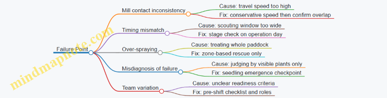
Summary of Operational Lessons
The program succeeded when it treated timing, contact, and zoning as linked decisions. The mill performed best when weeds were at the right seed stage and when travel speed supported consistent contact. Herbicide rescue worked when it was limited to escapes that the mill could not reliably handle. Verification focused on seedling emergence and patch behavior, which prevented false confidence based on short-term appearance. Finally, documentation turned individual good days into repeatable field practice.
11. Implementation Tools for Broadacre Growers and Advisors
11.1 Field Scouting Templates for Weed Impact and Resistance Indicators
Field scouting is where good intentions meet reality. The goal is simple: record what you see in a way that helps you decide what to do next, especially when seed destruction tactics and herbicide programs are both in play.
Foundational Setup for Consistent Scouting
Start with a repeatable layout so comparisons across weeks and seasons are meaningful.
- Choose a scouting unit: one paddock, or a consistent management zone (e.g., soil type or yield map band). If you split zones, keep the boundaries stable.
- Pick a sampling pattern: for broadacre fields, use a zigzag transect with fixed stops (e.g., every 1–2 hectares) or a grid of points. The key is consistency, not perfection.
- Define timing triggers: scout at crop emergence, mid-vegetative growth, pre-treatment (if applying), and after treatment when escapes are still small enough to count.
Weed Impact Indicators That Matter
Weed impact is not just “how many weeds.” It’s also whether weeds are reaching stages that contribute to seed return.
Record these for each stop:
- Weed stage: cotyledon/early seedling, tillering/rosette, flowering, seed set.
- Height or growth class: small (0–10 cm), medium (10–30 cm), tall (>30 cm). This matters for contact-based seed destruction timing.
- Density estimate: use a quick scale like 0 (none), 1 (few), 2 (patchy), 3 (heavy). Add a note if you can count within a small quadrat.
- Seed risk score: assign 0–3 based on stage (0 none, 1 low, 2 moderate, 3 high). This turns scouting into a seed-bank conversation.
Easy example: If you see ryegrass mostly at early seedling stage, seed risk is low even if density is moderate. If you see flowering plants in the same density class, seed risk jumps and your next action should prioritize preventing seed return.
Resistance Indicators You Can Spot Without Lab Work
Resistance confirmation requires testing, but scouting can flag patterns that justify targeted follow-up.
At each stop, record:
- Survivor pattern: scattered survivors across the whole paddock, or survivors clustered in the same zones.
- Dose response behavior: survivors look like “normal survivors” (same vigor as untreated) or “stressed survivors” (slower growth, partial control).
- Species identity: resistance is often species-specific, so accurate identification is non-negotiable.
- Herbicide exposure history: which active ingredients were used in the last 1–2 seasons, and whether the timing matched the weed stage.
Easy example: If one patch shows vigorous survivors after a post-emergence spray while other patches show good control, the issue may be coverage, timing, or resistance. Your template should capture the pattern so you can separate those causes.
Mind Map: Scouting Inputs for Weed Impact and Resistance
Practical Scouting Sheet Structure
Use a single page per paddock visit so field notes stay usable.
Template fields
- Date (use a consistent format)
- Paddock/zone ID
- Crop stage
- Weather at scouting (wind calm/variable, recent rain yes/no)
- Transect start and stop locations
- For each stop: weed species, growth stage, height class, density score, seed risk score, survivor notes
- For resistance flags: herbicide(s) applied recently, control level (good/partial/poor), and whether survivors are clustered
Easy example: At Stop 7 you record “Species: wild radish, flowering, medium height, density 2, seed risk 3, survivors vigorous after last spray.” That single line supports a seed-destruction priority and a resistance follow-up flag.
Evidence Quality Checks That Prevent Bad Decisions
Before leaving the paddock, do two quick checks:
- Photo coverage: at least one photo per stop cluster showing the dominant weeds and the crop background.
- Operational notes: record anything that could explain patchiness (missed passes, unusual soil moisture, obvious drift barriers, or uneven emergence).
Advanced Details Without Making It Complicated
When you see resistance-like patterns, add a short “why this matters” note:
- If survivors are clustered, note the cluster boundary and any likely cause (soil type, emergence timing, equipment turn areas).
- If survivors are scattered, note whether the same species shows consistent survival across the field.
Easy example: “Clustered survivors along a low-lying strip” suggests emergence timing or coverage differences. “Scattered vigorous survivors everywhere” suggests a stronger resistance signal.
Mind Map: From Notes to Actions
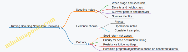
This template approach keeps scouting systematic: you record impact drivers, flag resistance signals by pattern and behavior, and translate both into clear next steps for seed destruction and integrated resistance management.
11.2 Herbicide Mode of Action Tracking Sheets and Rotation Logs
A good rotation log is not a diary of what you sprayed. It is a working document that links each herbicide product to the weed you were trying to stop, the timing you used, and the outcome you observed. When resistance shows up, the log helps you answer three practical questions: What did we use? When did we use it? Did it actually work on the target weeds?
Core Fields That Make Logs Useful
Start with a consistent set of fields so every paddock entry can be compared across seasons.
- Field and paddock ID: Use the same naming system every year.
- Crop and growth stage: Record crop stage at application, not just the crop type.
- Weed targets and growth stage: Note the dominant weeds and whether they were small seedlings, bolting, or flowering.
- Herbicide product and active ingredient: Write the product name and the active ingredient(s) exactly as on the label.
- Mode of Action group: Record the MoA group for each active ingredient.
- Rate and formulation: Include rate per hectare and whether it was EC, SC, WG, etc.
- Application details: Date, wind conditions, water volume, nozzle type, and speed.
- Tank mix and sequence: List all actives in the tank. If you used sequential applications, log each separately.
- Coverage notes: Mention visible skips, residue interference, or patchy emergence.
- Outcome: Use simple categories such as “excellent control,” “partial control,” “survived,” or “no effect,” plus a short reason.
- Follow-up actions: Record any rescue sprays, cultivation, or additional hand weeding.
A slightly playful rule: if someone else read your log next season, they should be able to recreate the decision path without guessing.
How to Track Mode of Action Without Getting Lost
Mode of action tracking works best when you treat each active ingredient as a separate “resistance pressure event.” For example, a tank mix with two actives applies two different selection pressures at the same time. Your log should therefore store MoA groups per active ingredient, not just per product.
When you rotate, rotate the MoA groups, not the product brands. Two products can share the same MoA group, so switching brands alone may not reduce selection pressure.
Rotation Logic That Matches Field Reality
Rotation logs should reflect how broadacre fields actually behave: weed emergence is patchy, weather shifts timing, and crop competition varies.
Use this systematic approach:
- Identify the main weed problem for that paddock and season.
- List the MoA groups used on that weed problem across the last 2–4 seasons.
- Check for repeats of the same MoA group in consecutive seasons or repeated timings.
- Confirm timing alignment: if the weed was at a stage where the herbicide should work, but control was poor, resistance becomes more likely.
- Record what changed: crop type, seeding date, tillage, residue, and spray conditions.
This prevents a common trap: blaming resistance when the real issue was poor coverage, wrong weed stage, or a missed patch.
Example: One Paddock Entry That Tells a Story
Paddock: N1-14, Crop: winter wheat, Crop stage: tillering.
Weed targets: annual ryegrass, small (2–3 leaves).
Application: 2026-03-20, water volume 120 L/ha, nozzle type consistent with prior calibrations.
Tank mix: Active A (MoA group 1), Active B (MoA group 2). Rate recorded for each active.
Outcome: annual ryegrass survived in low spots and along tramlines; overall control partial.
Notes: residue from previous crop reduced contact in the low spots; skips suspected due to wheel track pattern.
In the log, the MoA groups are stored separately, and the outcome is tied to where control failed. That makes later diagnosis more precise.
Mind Map: What Your Rotation Log Should Capture
Rotation Log Template Logic
A practical template groups entries by paddock and season, then summarizes MoA history for the dominant weed problem. The summary should show MoA groups used and whether control was excellent, partial, or failed.
Example summary format (one line per season):
- Season 1: MoA 1 + MoA 2, timing early seedling, outcome partial
- Season 2: MoA 1 only, timing later seedling, outcome poor
- Season 3: MoA 3 + MoA 2, timing early seedling, outcome excellent
This makes it easy to see whether the same MoA group keeps returning during the same weed stage window.
Advanced Detail That Prevents False Conclusions
When control is partial, record whether survivors are evenly distributed or patchy. Even distribution can suggest resistance, while patchy survival often points to coverage gaps, emergence timing differences, or residue interference.
Also record whether the weed population was mixed. If you treated a mixed stand but only one species survived, your log should reflect that species-level outcome. Otherwise, the next rotation decision may rotate the wrong MoA group for the wrong weed.
Finally, keep the log consistent about weed stage. “Small seedlings” is not the same as “late tiller” in herbicide performance, and your notes should reflect that difference clearly.
11.3 Treatment Sequencing Checklists for Integrated Programs
A good sequencing checklist answers one question: “What happens next, and why?” In integrated programs, the “next” step depends on weed stage, crop stage, equipment capability, and the resistance risk you’re carrying from earlier seasons. The checklist below is designed to be used in order, so you don’t accidentally treat a field like it’s a spreadsheet with no biology.
Treatment Sequencing Mind Map
Step 1: Confirm Weed Stage and Crop Stage
Before choosing any treatment, confirm the weed stage in the same zones you scouted. A common failure is treating “early” weeds as if they are all at the same height and leaf number.
Checklist
- Identify the dominant weed species in each zone.
- Record growth stage using simple field cues (e.g., cotyledons, 2–4 leaves, tillering, flowering).
- Note crop stage and whether the canopy will interfere with contact or coverage.
- Decide whether your priority is seed destruction, seedling control, or both.
Example:
If ryegrass is mostly at 2–4 leaves while wild radish is bolting, sequence the program so the first pass targets the most vulnerable stage without leaving the other species to mature and set seed.
Step 2: Review Herbicide History for Resistance Risk
Sequencing is where resistance management becomes practical. You’re not just rotating chemistry; you’re managing selection pressure.
Checklist
- List the last 2–3 seasons of herbicide active ingredients by paddock.
- Convert each product to its MoA group code.
- Identify repeated MoA groups and any known resistance patterns.
- Flag any “same MoA back-to-back” situations.
Example:
If a paddock received the same MoA group last year and the same weed species is now dominating, treat the next decision as higher risk: prioritize non-chemical suppression and choose a different MoA for any necessary herbicide step.
Step 3: Choose the Sequence Pattern
Integrated programs usually fit one of three patterns. Pick the pattern first, then fill in the details.
Pattern A Seed Bank First
- Goal: prevent seed production by targeting reproductive or near-reproductive weeds.
- Best when: weeds are clustered and timing is predictable.
Pattern B Seedling First
- Goal: stop establishment early to reduce later seed rain.
- Best when: emergence is synchronized and crop competition can close quickly.
Pattern C Split Targeting
- Goal: handle mixed phenology with staged actions.
- Best when: multiple weed species or staggered emergence exists.
Example:
In a broadacre rotation with mixed winter annuals, split targeting may mean an early pass for seedlings plus a later targeted action timed to prevent seed set in the survivors.
Step 4: Apply Decision Gates Before You Drive the Tractor
These gates prevent “we applied it, so it must have worked” thinking.
Gate Checklist
- Weed stage gate: does the target stage match the label window and your scouting notes?
- Compatibility gate: are tank mixes and adjuvants appropriate for the crop and weeds present?
- Coverage gate: can you achieve uniform distribution at the planned speed and boom height?
- Weather gate: wind and temperature conditions support performance and reduce drift.
Example:
If coverage is likely uneven due to wheel tracks or stubble height, adjust speed or boom settings before adding another treatment later. Uneven coverage creates patchy survivors, which is exactly what resistance management tries to avoid.
Step 5: Sequence the Actions and Define “Stop Rules”
A checklist should include what you will not do.
Execution Checklist
- Order actions from most selective to most corrective when possible.
- Avoid repeating the same MoA group within the same season unless the program explicitly accounts for resistance risk.
- Define stop rules: if weed density drops below a threshold after the first pass, you may skip a second herbicide step and rely on crop competition.
- Define escalation rules: if escapes exceed the threshold, schedule a targeted follow-up based on the next vulnerable stage.
Example:
After an early seedling-focused pass, if the field shows strong suppression and uniform crop emergence, you can hold off on a second herbicide step and instead plan a mechanical or cultural action that supports canopy closure.
Step 6: Record and Monitor to Feed the Next Decision
Monitoring is part of sequencing, not an afterthought.
Post-Treatment Checklist
- Record date, paddock, product, rate, MoA group, and conditions.
- Map escapes by zone and note their growth stage.
- Compare outcomes to your expected target stage window.
- Update next-pass timing using the actual weed phenology you observed.
Example:
If escapes are mostly at a later stage than expected, your next pass should shift earlier or use a different action timing window rather than simply increasing rate.
Step 7: Use a Simple Sequencing Template
Use this template each time you plan a treatment sequence.
1) Zones and dominant weeds:
2) Weed stage targets:
3) Crop stage constraints:
4) Herbicide history MoA groups:
5) Sequence pattern A/B/C:
6) Decision gates passed yes/no:
7) Action order and stop rules:
8) Monitoring plan and thresholds:
9) Records completed:
A checklist works best when it’s short enough to use in the field and strict enough to prevent “same plan, different paddock” mistakes. When you follow the gates in order, sequencing becomes a controlled process rather than a series of separate decisions.
11.4 Equipment Readiness and Maintenance Records for Consistent Performance
Consistent weed control is rarely a “one-off” success. It’s the result of equipment that behaves the same way every time: the same flow rate, the same spray pattern, the same contact time, and the same mechanical reliability. Equipment readiness and maintenance records are how you keep those variables from quietly drifting.
Start with a simple principle: record what affects performance. For broadacre spraying and seed-destruction-style operations, that usually means hydraulics, pumps, filtration, nozzles, booms, calibration settings, and any components that change output or coverage.
Foundational Readiness Checks Before Each Operating Day
Before the first pass, do a short readiness routine and log it. Include:
- Visual condition: boom straightness, hose wear, leaks, and loose fittings.
- Filter status: confirm filters are clean and correctly seated.
- Nozzle condition: check for blocked or dribbling nozzles; replace any that don’t match the rest.
- Control response: verify the rate controller responds smoothly when you change speed.
- Spray pattern sanity check: confirm all nozzles are producing a consistent fan pattern.
Example: If one nozzle is partially blocked, the field may still “look sprayed,” but the missed strip can become a seed source later. Your record should capture that you inspected and corrected the issue before work began.
Maintenance Records That Actually Help
A maintenance log should connect actions to outcomes. Use entries that answer four questions: what was done, where it was done, why it was done, and what performance should look like afterward.
Include these record types:
- Preventive maintenance: scheduled service intervals for pumps, seals, filters, and agitators.
- Corrective maintenance: repairs after faults, leaks, uneven output, or control errors.
- Calibration events: date, target rate, actual measured rate, and the settings used.
- Parts traceability: nozzle batch or part numbers when you replace critical components.
Example: After replacing a set of nozzles, record the measured flow uniformity and the pressure used. If later you see patchy control, you can distinguish “equipment drift” from “weed timing” without guessing.
Calibration and Verification Workflow
Calibration is not a single measurement; it’s a verification chain. A practical workflow:
- Set baseline pressure and speed to match the intended application.
- Measure output across representative nozzles or nozzle groups.
- Confirm uniformity meets your internal tolerance.
- Record the final settings so the next operator can repeat them.
Example: If you calibrate at one pressure but later operate at a different pressure due to a controller setting change, your record should show the mismatch. That’s often the difference between “it should work” and “it did work.”
Operational Consistency and Handover
Records should support handovers between operators and contractors. Use a standardized daily summary that includes:
- equipment ID and configuration
- last calibration date
- nozzle status notes
- any deviations during the day
- what was corrected before resuming
A short handover note prevents the classic scenario where the next operator assumes the system is unchanged and only discovers issues after the first pass.
Mind Map: Equipment Readiness and Maintenance Records
Example: A Record Entry That Guides the Next Decision
Use entries that are specific enough to be actionable. For example:
- Date: 2026-03-31
- Equipment: sprayer unit 2, boom 24 m
- Issue found: uneven output on left boom section
- Action: replaced 3 nozzles, cleaned filter, verified fan pattern
- Calibration check: measured output uniformity within tolerance at 280 kPa
- Outcome expectation: consistent coverage across the full boom
This kind of entry helps you avoid repeating the same checks blindly. It also makes it easier to compare performance between paddocks when weather and weed stage are similar.
Advanced Details Without the Mess
To keep records usable, avoid long narratives. Prefer structured notes and consistent units. If you track pressure, flow, and speed, record them in the same format every time. If you track nozzle replacements, record the nozzle type and the reason for replacement.
Finally, store records where the people doing the work can find them quickly. A maintenance log that no one can access is just paperwork with good intentions.
11.5 Training and Communication Plans for Farm Teams and Contractors
A good training plan turns “we should” into “we did,” and it does that with simple roles, clear messages, and records that survive a busy harvest. The goal is not to make everyone an agronomist; it’s to make sure the right person performs the right step at the right time, especially when seed destruction and resistance management depend on timing and coverage.
Foundational Roles and Responsibilities
Start with a one-page role map so no task is assumed. Assign ownership for scouting, treatment decisions, equipment setup, application execution, and post-treatment checks.
- Farm team lead: confirms objectives (seed bank reduction, resistance risk control) and approves the treatment window.
- Scouting person: documents weed species, growth stages, patch locations, and herbicide history indicators.
- Contractor supervisor: verifies equipment readiness, calibration, and coverage plan.
- Operator: follows the route, speed, boom height, and buffer rules.
- Recorder: logs product, rate, weather, and deviations, then files photos of key steps.
A practical rule: if a task affects seed destruction timing or herbicide selection pressure, it must have a named owner.
Training Sequence from Basics to Field Execution
Training should move from concepts to field actions without skipping the “why.” Use short modules that end with a checklist.
- Weed impact and timing basics: explain how seed production stages and weed height affect control outcomes. Example: if target weeds are already shedding, seed destruction efforts must focus on remaining seed sources and follow-up operations.
- Resistance risk basics: teach that repeated use of the same mode of action increases selection pressure. Example: if a field relied heavily on one herbicide group for three seasons, the next plan must reduce reliance and tighten non-chemical support.
- Seed destruction biological weed control fit: show how biological and mechanical tactics complement each other. Example: biological agents may work best where microclimate stays favorable, so operations should avoid unnecessary disturbance during the window.
- Application quality fundamentals: cover calibration, nozzle condition, boom height, and drift management. Example: a small speed increase can reduce coverage overlap and create untreated strips that later become resistance hotspots.
- Integrated decision workflow: practice how to adjust when weeds are at different stages across the paddock. Example: if one zone is ahead, the team uses zone-based notes to decide whether to treat all or prioritize the most seed-producing patches.
Communication Cadence and Message Templates
Use a predictable rhythm so information doesn’t get lost between days.
- Pre-season briefing: review target weeds, herbicide history indicators, and the intended sequence of tactics.
- Pre-treatment huddle: confirm weather constraints, route plan, and who checks what.
- During-application updates: record deviations immediately (speed, wind, skips, equipment issues).
- Post-treatment debrief: compare expected outcomes to observed weed stage and coverage.
Keep messages short and consistent. Example template for the operator: “Target weeds at growth stage X; treat zone A first; maintain speed Y; boom height Z; stop if wind exceeds threshold; report any skip immediately.”
Contractor Alignment and Quality Assurance
Contractors must be trained on your objectives, not just your paperwork.
- Calibration proof: require a documented calibration run before the first load.
- Coverage verification: use a simple method such as checking overlap marks or measuring effective swath width.
- Deviation reporting: define what counts as a deviation (missed area, nozzle failure, route change).
- Equipment care: specify cleaning steps when switching products to prevent cross-contamination.
A useful practice is a “walk the paddock” meeting where the contractor points out access constraints, turning areas, and likely skip zones.
Mind Map: Training and Communication Flow
Example: One-Week Training Plan
Use a compact schedule that fits real workloads.
- Day 1: role briefing and weed stage timing exercise using photos from your own fields.
- Day 2: resistance risk workshop using your herbicide history indicators and a simple rotation logic worksheet.
- Day 3: equipment calibration demonstration with hands-on nozzle checks.
- Day 4: route and coverage practice on a mock paddock layout, including turning and buffer areas.
- Day 5: integrated workflow drill where the team decides what to do when weeds differ by zone.
Example: Field Day Communication Checklist
Before leaving the yard, confirm these items in order: product and rate, target weed stage notes, weather constraints, route plan, calibration status, who records, and who checks coverage. During the run, deviations are logged immediately; after the run, photos and scouting notes are matched to the treated zones. This keeps the plan coherent even when the day goes sideways—because it usually does, just not in the same way twice.
12. Practical Troubleshooting for Seed Destruction and Control Failures
12.1 Diagnosing Poor Seed Destruction Performance in the Field
When seed destruction underperforms, the cause is usually one of three things: the target seed stage wasn’t reached, the treatment didn’t contact the right plants or seeds, or the field conditions prevented the mechanism from working. A good diagnosis starts with evidence from the field, not guesses from the shed.
Step 1: Confirm the Target Stage Was Actually Hit
Seed destruction methods depend on timing. If the weeds were already past the vulnerable stage, you can get “looks treated” plants that still drop viable seed.
- What to check: weed phenology at the moment of treatment and again 7–14 days later.
- Easy example: In a winter cereal paddock, if most ryegrass heads were already turning from green to straw, you may see fewer new heads but still find seed in the soil later.
- Field clue: treated patches show reduced flowering but not reduced seed viability.
Step 2: Verify Contact and Coverage Where Seeds Form
Even a perfect timing plan fails if the mechanism can’t reach the seed-bearing portion.
- What to check: uniformity of treatment across the paddock, especially at headlands, wheel tracks, and low spots.
- Easy example: If the operator slows on slopes or turns wider at headlands, seed-bearing plants at those edges may escape contact.
- Field clue: seed reduction is patchy, with “clean strips” where the pass was consistent and “seed islands” where it wasn’t.
Step 3: Rule Out Equipment and Operation Issues
Poor performance often comes from boring mechanics: speed, alignment, height, or maintenance.
- What to check: calibration records, wear on moving parts, and whether the working height matches the weed height class.
- Easy example: If the working height was set for 20–30 cm weeds but the field had 40–50 cm weeds, the treatment may miss the seed zone.
- Field clue: the effect is stronger on shorter plants and weaker on taller ones.
Step 4: Check Weed Community Composition and Mixed Stages
Mixed weed species can create mixed outcomes because each species has different seed timing and structure.
- What to check: which species are present, and whether they were at the same stage.
- Easy example: A paddock with both annual ryegrass and wild radish may show good suppression of one and poor seed destruction of the other because their vulnerable windows don’t overlap.
- Field clue: seed bank reduction occurs for some species but not others.
Step 5: Evaluate Field Conditions That Block the Mechanism
Many seed destruction approaches rely on physical or biological processes that are sensitive to moisture, residue, and weather.
- What to check: soil surface moisture, residue load, wind, and temperature at the time of treatment.
- Easy example: Heavy residue can shield seed-bearing plants from contact, especially when weeds are lodged under crop stubble.
- Field clue: performance is weaker where residue is thick or where weeds are shaded or lodged.
Step 6: Separate “Less Seed” from “No Viable Seed”
A reduction in seed heads is not the same as reduced seed viability. Your diagnosis should include both.
- What to check: seed head counts, seed set, and a simple viability assessment if available.
- Easy example: You may see fewer heads after treatment, but if the remaining heads still produce viable seed, the seed bank won’t drop as expected.
- Field clue: seed head suppression without viability loss.
Step 7: Use a Simple Decision Tree to Pinpoint the Likely Cause
graph TD
A[Poor seed destruction observed] --> B{Was the target stage reached?}
B -->|No| C[Adjust timing to vulnerable stage]
B -->|Yes| D{Was contact/coverage uniform?}
D -->|No| E[Improve pass consistency and working height]
D -->|Yes| F{Any equipment or operation faults?}
F -->|Yes| G[Calibrate, repair wear, standardize speed]
F -->|No| H{Are weeds mixed species or mixed stages?}
H -->|Yes| I[Split treatments or target dominant species]
H -->|No| J{Did field conditions block the mechanism?}
J -->|Yes| K[Adjust for residue, moisture, and weather]
J -->|No| L[Re-check viability vs seed head counts]
Mind Map: Diagnosing Poor Seed Destruction
Example: A Systematic Diagnosis in One Paddock
On 2026-03-31, a broadacre paddock shows fewer seed heads after treatment, but later scouting finds viable seed patches. The operator compares treated and untreated strips: seed reduction is strongest in the center where passes were consistent, and weakest at headlands. Weed phenology notes show some plants were already straw-colored at treatment. The combined evidence points to timing plus coverage uniformity, not equipment failure. The corrective action is to treat earlier at the vulnerable stage and tighten pass consistency at edges, while also confirming whether the dominant weed species had overlapping vulnerable windows.
Practical Checklist for Evidence Collection
- Record weed stage at treatment and 7–14 days later.
- Map treated vs untreated seed patches.
- Note headland and wheel-track performance.
- Verify working height and calibration against weed height class.
- Document residue load and moisture conditions.
- Measure both seed head suppression and seed viability where possible.
A diagnosis is complete when you can point to the specific link that broke: stage, contact, operation, community, conditions, or measurement.
12.2 Identifying Herbicide Failure Causes Other Than Resistance
Herbicide failure is not always resistance. In fact, many “resistance-looking” outcomes are caused by application and field conditions that prevent the herbicide from reaching the target weed in the right form, at the right dose, at the right time. A systematic check keeps you from blaming genetics when the real culprit is the sprayer, the weather, or the crop-weed setup.
Start with the Symptom Pattern
Begin by describing what you see, because patterns point to likely causes.
- Whole-field failure with uniform weed survival often suggests a calibration, mixing, or coverage problem.
- Patchy survival in bands or wheel tracks often suggests boom height, overlap gaps, or sprayer speed issues.
- Failure only on certain weed sizes or growth stages often suggests timing or weed emergence patterns.
- Failure only on certain species often suggests label mismatch, poor spray contact, or plant architecture.
Example: If ryegrass survives in every treated pass but broadleaf weeds are controlled, the issue may be species-specific label mismatch or poor leaf contact, not resistance.
Verify the Basics Before You Touch the Resistance Hypothesis
Use a short “evidence ladder” from most common and easiest to check to more complex causes.
-
Dose and delivery
- Confirm the rate used matches the label and the intended hectares per tank.
- Check calibration records, nozzle type, and whether nozzles were swapped or partially blocked.
- Look for speed changes during the run; a faster tractor increases underdosing.
-
Mixing and tank chemistry
- Confirm the product order and whether the tank was filled and agitated correctly.
- Check for tank contamination from previous chemicals that can reduce activity or cause precipitation.
- Verify whether water quality (hardness, pH) and adjuvant selection match label requirements.
-
Coverage and spray contact
- Measure boom height and confirm it stayed consistent.
- Inspect nozzle spacing, overlap, and pattern; uneven overlap creates survival “corridors.”
- Consider weed leaf angle and canopy density; some weeds need better contact than others.
-
Timing relative to weed stage
- Many herbicides require weeds to be at a specific growth stage for uptake.
- If weeds emerged after the spray, you will see “survival” that is actually untreated cohorts.
-
Weather and environmental conditions
- Wind and drift can reduce dose on target plants.
- Rain soon after application can wash off or reduce uptake depending on the herbicide.
- Temperature extremes can slow uptake or change plant physiology.
Example: A field sprayed on 2026-03-31 where a light rain fell within hours can show partial control that looks like resistance, especially if the herbicide relies on early uptake.
Use a Mind Map to Route Your Investigation
Apply the Checks in the Right Order
A practical workflow prevents wasted effort.
- Confirm the rate and calibration using the sprayer log and nozzle inspection.
- Confirm mixing and water/adjuvant choices against the label.
- Confirm coverage by reviewing boom height, overlap, and any visible drift patterns.
- Confirm timing by comparing weed growth stage at application to the label requirement.
- Confirm weather effects using the application window and rain/temperature notes.
Concrete Field Examples That Separate Causes
- Calibration error: Weeds survive evenly across the field, and the same tank mix controlled the previous paddock. The calibration was done months ago, and nozzle wear went unnoticed.
- Tank contamination: Control is poor across multiple species, and the tank previously held a different herbicide. Precipitation or clumping appears after mixing.
- Coverage gap: Survival forms a repeating pattern aligned with nozzle spacing or boom sections. The boom was raised slightly for a turn and never returned to the set height.
- Timing mismatch: Small weeds are controlled, but larger ones survive. The spray went on after the weeds passed the label stage.
- New emergence: A second flush appears after application, and the surviving weeds are mostly the same size and stage as the later cohort.
What to Document So the Next Step Is Clear
Record the following so you can distinguish “application failure” from “resistance suspicion” without guesswork:
- Product, rate, and nozzle configuration used
- Calibration evidence and any deviations during spraying
- Mixing order, water source, and adjuvant details
- Weed species, growth stage at application, and emergence timing
- Weather notes including wind and rain timing
- Field photos showing pattern and distribution
When these checks point to a controllable failure mode, you can correct the process and re-evaluate without jumping straight to resistance testing.
12.3 Addressing Coverage Gaps and Uneven Treatment Distribution
Coverage gaps are rarely caused by one dramatic mistake. More often, they come from small, repeatable issues: a sprayer that drifts off its line, a nozzle pattern that doesn’t match the boom height, a tank mix that changes viscosity, or a field pass that quietly overlaps too little. Uneven distribution matters because herbicide performance depends on receiving the right dose at the right time, and resistance risk rises when weeds escape sublethal exposure.
Foundational Checks Before You Chase Ghosts
Start with a simple dose math mindset. If your target rate is 200 g a.i./ha, then a 20% under-application is not “close enough”; it is a 40 g a.i./ha shortfall for the weeds in that zone. Coverage problems show up as patchy weed control, striping, or “bands” that align with pass direction.
A practical workflow:
- Confirm the intended boom height and nozzle type are consistent across the whole run.
- Verify calibration: speed, pressure, and flow rate should match the labeled application rate.
- Inspect nozzle condition: worn tips can widen patterns and reduce uniformity.
- Check boom stability: uneven suspension or worn hinges can create height variation.
- Review tank mixing: incomplete suspension can cause concentration gradients.
Diagnosing the Pattern of Unevenness
Different coverage failures leave different fingerprints.
- Striping parallel to travel direction often points to speed variation, pressure instability, or a boom section that intermittently shuts.
- Bands perpendicular to travel can indicate a turn/overlap strategy that changes during headland maneuvers.
- Patchy control in low spots suggests boom height changes with terrain or clogged strainers that intermittently restrict flow.
- Edge-only failures frequently come from wind drift, skipped swaths, or inconsistent end-row overlap.
Use field notes to connect symptoms to operations. For example, if the worst control is consistently on the downwind side, drift and crosswind exposure are more likely than resistance.
Systematic Fixes That Prevent Repeat Failures
1. Lock the boom height to the nozzle’s sweet spot. If the nozzle is designed for a 50 cm height, running at 65 cm changes droplet spread and overlap. Even if the total volume per hectare is correct, the spatial distribution can become uneven. A quick test is to measure height at multiple points along the boom during a representative pass.
2. Match nozzle spacing, pressure, and travel speed. Uniformity depends on overlap between nozzle patterns. If you change speed without recalibrating, the boom may deliver the right average rate but with local under-coverage where overlap thins.
3. Treat headlands as a separate operation. Many fields get “good enough” coverage in the middle and weaker coverage at ends. Define a consistent overlap rule for headlands and document it. Example: if you normally overlap 30 cm on the main runs, use the same overlap logic during turns rather than relying on habit.
4. Prevent flow interruptions. Partially clogged strainers or a failing pump can create momentary under-application. If you see patchy control that doesn’t align with travel direction, inspect filters and confirm the agitation system keeps the mix uniform.
5. Control overlap and shutoff behavior. Auto section control helps, but only if the guidance system is calibrated and the boom sections respond correctly. A common issue is delayed shutoff that creates double-applied strips alongside under-applied strips.
Mind Map: Coverage Gaps and Uneven Distribution
Example: Turning a “Mystery Patch” Into a Measurable Fix
A broadacre paddock shows weak control in two long bands that run across the field. The bands are not centered on wheel tracks, and they repeat on both headlands.
- Observation: bands align with the turn pattern, not with the main pass direction.
- Likely cause: headland overlap rule changed during turns, creating a consistent under-coverage strip.
- Fix: standardize the headland overlap distance and ensure the same section shutoff logic is used during turns. Then run a short calibration strip on the next application day and confirm that the boom height and pressure remain stable through the turn.
Example: When the Issue Is Droplet Placement, Not Dose Rate
A grower calibrates to the label rate, yet weed control is patchy. The worst areas are where the boom rides higher over a gentle rise.
- Observation: patchiness correlates with terrain elevation.
- Likely cause: boom height drift changes nozzle overlap and droplet placement.
- Fix: adjust boom suspension settings and re-check height at multiple points along the boom during a representative pass. Re-apply only after confirming that boom height stays within the nozzle’s intended operating range.
Verification After Changes
After any adjustment, verify with a controlled check rather than trusting memory. A short calibration strip or a limited-area run helps confirm that uniformity improves and that the symptom pattern disappears. The goal is not perfection; it is consistent coverage that reduces the chance of weeds receiving sublethal exposure in repeatable locations.
12.4 Managing Weed Escapes and Patch Expansion During the Season
Weed escapes happen when a few plants survive the planned control window and then spread enough to look like the field “changed its mind.” Patch expansion is usually not magic; it’s the predictable result of missed emergence cohorts, uneven coverage, late escapes that set seed, and patches that receive less competition than the surrounding crop.
Step 1: Identify Escape Patterns Early
Start with a fast field walk 7–14 days after the last key control action. Record where escapes cluster: along wheel tracks, near fence lines, in low-lying wet spots, or in areas with thin crop stands. Those locations point to the likely cause.
- Wheel-track clusters often indicate coverage gaps or sprayer overlap issues.
- Fence-line and headland clusters often indicate different weed pressure, different crop density, or missed spot treatments.
- Wet-spot clusters often indicate delayed crop establishment and staggered weed emergence.
A practical rule: if escapes are concentrated in one zone, treat the zone. If escapes are evenly distributed, treat the system (coverage, timing, or emergence control).
Step 2: Confirm Whether Escapes Are Seed-Bank Threats
Not every escaped plant is equally dangerous. Determine whether the escapes are:
- Pre-flowering and still growing: they can be stopped before seed set.
- Flowering or near maturity: they may already be on the clock.
- Perennial or regrowth-prone: they may require repeated suppression.
Example: In a broadacre cereal, a patch of ryegrass that is just heading should be treated immediately with the most selective option that still fits resistance management. A patch of seedlings at the 2–3 leaf stage may be handled with a different tactic that targets small plants and preserves herbicide diversity.
Step 3: Choose a Response That Matches Escape Stage
Use a stage-based decision so you don’t spend effort on the wrong target.
- Small seedlings: prioritize tactics that work on early growth and can be applied quickly to patches.
- Larger plants: focus on tactics that can still reduce survival and prevent seed set, even if they don’t fully “clean” the patch.
- Seed-set risk: prioritize actions that stop seed production, even if the patch remains visible.
A simple operational approach is to split the field into zones: Green (no escapes), Amber (few escapes), Red (dense escapes or near seed set). Treat Amber with the fastest corrective action that fits your resistance plan, and treat Red with the most urgent seed-prevention option.
Step 4: Prevent Patch Expansion with Targeted Coverage
Patch expansion is often driven by dispersal and local advantage. Reduce both.
- Treat the patch edge, not only the center. If you only hit the middle, the outer plants keep expanding.
- Use equipment settings that match the patch. For patch work, reduce speed and ensure overlap so you don’t create a new “escape corridor.”
- Avoid creating bare soil hotspots. If you use cultivation or disturbance, keep it localized and timed so you don’t invite a fresh flush.
Example: If a patch of volunteer canola is expanding from a headland, a targeted follow-up that covers the outer 1–2 mower-widths of the patch can reduce new seed rain more effectively than a second pass through the already-treated center.
Step 5: Keep Resistance Management Intact During Emergency Fixes
Emergency treatments are where resistance plans get bent. Keep them structured.
- Use a different mode of action than the last effective herbicide when the escape is likely due to resistance rather than timing.
- Don’t repeat the same product just because it worked once. If the escape is widespread, assume selection pressure has already been applied.
- Combine with non-chemical suppression when possible, such as crop competition improvements in the next window or localized tactics that reduce survival.
A useful mindset: the goal of a patch response is not perfection; it’s stopping seed production while preserving herbicide options for the next cohort.
Step 6: Document and Close the Loop
After treatment, re-check the same zones 10–21 days later. Note whether escapes were reduced, delayed, or only suppressed temporarily. This turns “we saw weeds” into a field record you can use to adjust timing and coverage next season.
Mind Map: Escape to Action Logic
Example: Zone-Based Patch Response in Broadacre Cereal
A grower scouts 10 days after a post-emergence program. Escapes are mostly in two headland strips and one low area. The headland escapes are at early flowering; the low-area escapes are at 2–3 leaf stage.
- Headland strips (Red): apply the most urgent seed-prevention option that fits the resistance plan, focusing on edge coverage.
- Low area (Amber): apply a tactic suited to small plants and ensure overlap by slowing down and verifying boom height.
- Green zones: no action, to avoid unnecessary selection pressure.
Two weeks later, the headland patches stop producing new flowering plants, and the low-area seedlings are largely suppressed with minimal regrowth.
Quick Checklist for the Next Field Walk
- Where are escapes clustered and what does that suggest?
- Are plants pre-flowering, flowering, or near maturity?
- Which zones are Green, Amber, or Red?
- Does the planned response match growth stage and resistance rules?
- Did you cover patch edges with consistent overlap?
- Did you re-check treated zones on schedule?
12.5 Corrective Action Plans for Next Season Based on Evidence
Corrective action starts with evidence, not vibes. Use what you measured this season—weed escapes, seed bank indicators, resistance test results, and treatment performance—to choose a small set of changes that are likely to move the needle next year.
Step 1: Summarize Evidence Into Decisions
Create a one-page “field truth” summary for each paddock or management zone. Include: (1) which weeds survived and at what growth stage, (2) which herbicide programs were used and when, (3) application quality notes like calibration checks and weather windows, and (4) any resistance confirmation. Then convert that into decisions using a simple rule: if the same failure pattern repeats across zones, treat it as a management design issue; if it’s isolated, treat it as an operational issue.
Example: In three paddocks, the same broadleaf escapes appeared after the same post-emergence timing. That points to either insufficient coverage at that stage, an incorrect target stage assumption, or resistance. If only one paddock shows patchy survival and the sprayer logs show a calibration drift, prioritize operational correction.
Step 2: Classify Failure Mode
Most “control failures” fit one of four buckets:
- Timing mismatch: weeds were treated too early or too late relative to the most sensitive stage.
- Coverage and contact gaps: weeds were missed, shielded by residue, or not reached by droplets.
- Program mismatch: the mode of action rotation didn’t actually change selection pressure enough.
- Resistance or cross-resistance: the same MOA repeatedly failed, and resistance tests or consistent patterns support it.
A practical check: compare survival stage to the label’s most responsive window. If escapes were already past that window, timing is the likely culprit even if the product was “correct.”
Step 3: Choose Corrective Actions That Fit the Failure Mode
Match actions to the bucket, then keep them specific.
- If timing mismatch: shift the operation to the next feasible window using your scouting thresholds. Example: if ryegrass escapes were mostly at tiller stage, tighten scouting so the treatment hits earlier emergence cohorts.
- If coverage gaps: adjust nozzle selection, boom height, travel speed, and residue management. Example: if weeds were under a mat of stubble, plan a residue-aware sequence such as earlier establishment control or a different crop canopy strategy.
- If program mismatch: redesign the rotation so each season uses different MOA groups and includes non-chemical suppression. Example: pair a pre-emergence residual with a different post-emergence MOA later, rather than repeating the same post-emergence chemistry.
- If resistance or cross-resistance: reduce reliance on the failing MOA and use integrated seed destruction and cultural suppression to lower seed return. Example: if a confirmed resistant population survives post-emergence, prioritize seed bank reduction tactics and avoid using that MOA as a “cleanup” option.
Step 4: Build a Paddock-Specific Plan with Guardrails
For each zone, set three guardrails:
- Seed return target: define what “better” means, such as fewer surviving plants per square meter or reduced seed set at maturity.
- Mode of action diversity: specify which MOA groups are used and which are excluded due to evidence.
- Operational quality checks: list the calibration and weather verification steps you will actually perform.
Example: A zone with confirmed resistance might exclude one MOA group entirely, require scouting at two emergence checkpoints, and mandate a calibration verification before the first spray pass.
Step 5: Translate Actions Into a Timeline
Turn the plan into a sequence of field tasks tied to weed stages, not calendar dates. Use a consistent template so teams can execute without guessing.
Example timeline anchor: “First scouting at first emergence cohort,” “treatment at 2–4 leaf stage,” “post-treatment follow-up at 14 days to confirm suppression,” and “seed bank reduction actions before seed maturation.” If you need a date for recordkeeping, use a fixed reference such as 2026-03-31 for the start of the planning cycle.
Step 6: Set Monitoring That Proves the Plan Worked
Monitoring should answer two questions: did you reduce survivors, and did you reduce seed return? Use the same sampling approach next season so comparisons are meaningful.
- Early season: count escapes and note growth stage.
- Mid to late season: estimate seed set risk by checking maturity timing and surviving plant density.
- After harvest: note residue and volunteer emergence patterns as indirect indicators.
Mind Map: Evidence to Next Season Actions
Example: Two Paddocks, Two Different Fixes
- Paddock A: Surviving weeds were mostly at the same stage each time, and the treatment was applied at the same crop growth stage. Fix: adjust scouting thresholds and shift timing to hit the sensitive weed stage.
- Paddock B: Survival was patchy, and sprayer logs show inconsistent calibration during the first pass. Fix: correct operational quality and repeat the same program only after calibration verification; then reassess if resistance evidence still supports a change.
A good corrective plan doesn’t try to fix everything at once. It targets the most likely failure mode with measurable guardrails, then uses next season’s monitoring to confirm the change actually reduced seed return and selection pressure.