Precision Soil Health Mapping and Soil Microbiome Engineering
1. Scope and Workflow for Precision Soil Health Mapping
1.1 Defining Soil Health Objectives for Drought Resilience
Soil health objectives should start with what you want to change on the ground, not with which measurements you plan to collect. Drought resilience is a practical target: plants must keep functioning when water supply drops. In soil terms, that usually means maintaining water availability in the root zone, supporting root growth, and keeping biological processes running so nutrients and water move in usable forms.
Step 1: Translate Drought Resilience Into Soil-Level Outcomes
Begin by writing 2–4 outcomes that are specific enough to guide decisions. Good outcomes are measurable and tied to drought stress.
- Outcome A: More plant-available water during dry spells. Example: In a field with sandy patches, aim to increase the fraction of water retained between “wilting” and “usable” ranges.
- Outcome B: Faster recovery after rewetting. Example: After irrigation or a rainfall event, aim for quicker soil infiltration and reduced crusting so roots can resume growth.
- Outcome C: Stable nutrient supply under low water. Example: Maintain nitrogen availability and reduce salt stress in zones that dry and concentrate solutes.
- Outcome D: Root systems that keep exploring. Example: Encourage deeper or more persistent rooting in dry areas by improving structure and biological activity.
A useful check is whether each outcome implies a management action. If it doesn’t, the objective is probably too vague.
Step 2: Identify the Limiting Factors That Control Water and Roots
Drought resilience is rarely one problem. Common soil constraints include poor aggregation, low organic matter, compaction, salinity, and weak biological activity. Map each constraint to a mechanism.
- Aggregation and pore continuity: Better structure creates connected pores that store and transmit water.
- Compaction and rooting depth: Compaction reduces root penetration and limits access to deeper moisture.
- Organic matter and microbial activity: Biological processes influence aggregation, nutrient cycling, and the stability of pore networks.
- Salinity and chemical stress: Drying can concentrate salts, reducing plant uptake even when some water remains.
Example: If a zone shows low infiltration and shallow roots, your objective might focus on improving structure and reducing compaction effects rather than only adding nutrients.
Step 3: Choose Metrics That Match Each Outcome
Metrics should connect directly to the mechanisms you identified. Use a small set of “core metrics” plus “supporting metrics.” Core metrics are the ones you will use to decide whether management is working.
- For plant-available water, core metrics can include water retention characteristics and infiltration behavior.
- For root resilience, core metrics can include rooting depth proxies and root-zone bulk density or penetration resistance.
- For biological function, core metrics can include enzyme activity or microbial biomass proxies tied to nutrient cycling.
- For nutrient stability, core metrics can include extractable nutrient pools and salinity indicators.
Example: If your objective is faster recovery after rewetting, you need metrics that respond to wetting events, such as infiltration rate and surface structure indicators, not only long-term averages.
Step 4: Set Zone-Specific Targets and Guardrails
Fields vary. Instead of one target for the whole farm, define targets per management zone so you don’t average away the problem.
- Targets: What you want to improve (e.g., higher water retention in the root-zone depth band).
- Guardrails: What you must not worsen (e.g., salinity rising, excessive compaction, or nutrient imbalances).
Example: In a low-salinity zone, you might prioritize structure and biological inputs. In a zone with elevated salts, your objective may include maintaining or reducing salinity while improving infiltration.
Step 5: Define the Time Window and Sampling Logic
Objectives must specify when you expect change and how you will verify it.
- Short window (weeks to a few months): infiltration, surface structure, early root response, and biological activity indicators.
- Medium window (one season): changes in water retention behavior proxies, rooting depth patterns, and nutrient availability stability.
- Verification logic: sample before interventions, then at key drought and rewetting moments, and again after the season.
A practical rule: if you can’t explain how a metric will change during your chosen window, the objective needs refinement.
Mind Map: Soil Health Objectives for Drought Resilience
Example: Turning Objectives Into a Field Plan
Suppose you have three zones: sandy ridge, loamy mid-slope, and compacted low spot.
- Sandy ridge objective: increase root-zone water retention and infiltration to reduce rapid drying.
- Compacted low spot objective: improve rooting depth access and reduce surface crusting so rewetting leads to usable infiltration.
- Loamy mid-slope objective: maintain nutrient cycling stability so drought does not cause sharp nutrient limitation.
Each objective implies different priorities, even if the overall theme is “drought resilience.” That’s the point: objectives should guide choices, not just describe hopes.
1.2 Selecting Management Zones Using Soil and Crop Constraints
Management zones are not “pretty map shapes.” They are decision units where the same set of constraints and actions make sense. The goal is to group locations that behave similarly for water availability, root growth, and crop performance, so you can apply inputs with fewer compromises.
Step 1: Start with Crop Constraints, Not Just Soil Numbers
Begin by listing constraints that directly limit yield or survival. For drought resilience, common constraints include shallow rooting due to hardpan, low plant-available water, salinity or sodicity, and nutrient limitations tied to soil chemistry. Then translate each constraint into a measurable proxy.
Example: If a field has patches of poor emergence, you might suspect crusting or salinity. Your proxies could be surface aggregate stability (or crusting risk), EC in the top 10–20 cm, and infiltration rate. If those proxies align with the emergence pattern, the constraint is real enough to drive zoning.
Step 2: Convert Soil Properties Into Actionable Limits
Soil properties become useful when they map to operational thresholds. For water retention work, the key is plant-available water (PAW) across the effective rooting depth. For root constraints, the key is whether roots can physically occupy the soil volume.
Practical approach:
- Define an effective rooting depth per crop and management (for many annuals, start with 60–90 cm unless you have evidence of shallower rooting).
- Identify zones where PAW is consistently low within that depth.
- Identify zones where physical barriers (compaction layers, cemented horizons) reduce usable depth.
Example: Two areas may have the same clay percentage, but one has stable aggregates and good infiltration while the other has a compacted layer at 35 cm. Only the second area should be treated as a “reduced rooting volume” zone.
Step 3: Use a Constraint Matrix to Decide Zone Boundaries
A constraint matrix helps you avoid mixing incompatible problems in one zone. Each location gets evaluated against constraints; zones form where the constraint pattern is consistent.
| Constraint | Proxy | Typical Zone Action | Example Outcome |
|---|---|---|---|
| Low PAW | Water retention curve or PAW estimate | Increase water-holding inputs and adjust irrigation timing | Less mid-season stress |
| Physical barrier | Penetrometer or bulk density layer | Deep loosening only where feasible; prioritize root-friendly biology | Better root penetration |
| Salinity/sodicity | EC, ESP, SAR | Salt-tolerant management and leaching strategy | Improved emergence |
| Nutrient availability | Extractable P/K, nitrate, pH | Zone-specific fertility rates | Reduced wasted fertilizer |
Step 4: Build Zones from Overlapping Layers, Then Simplify
Use overlapping layers rather than a single “best” map. A common stack is:
- water retention or PAW estimate,
- physical limitation indicator,
- crop performance proxy (yield, stand counts),
- management history if it explains persistent differences.
Then simplify. If you end up with 18 micro-zones, you will struggle to apply inputs consistently. Aim for a small set of zones where each has a distinct constraint profile and a distinct action plan.
Example: A field might split into three zones: (A) high PAW and good structure, (B) low PAW but no hardpan, (C) reduced rooting depth due to compaction. Even if salinity varies within C, you can still treat C as one operational unit if the action is the same.
Step 5: Check Zone Coherence with Field Evidence
Before finalizing, verify that each zone is coherent on the ground. Look for agreement between:
- soil proxies and observed plant response,
- depth-related constraints and where stress shows up in the season,
- map boundaries and practical field access for equipment.
Example: If a low-PAW zone is mapped but plants show stress only at the very end of the season, your PAW estimate may be too pessimistic or rooting depth may be deeper than assumed. Adjust the effective depth or revisit the physical barrier layer.
Mind Map: Management Zone Logic from Constraints to Actions
Example: Turning a Field Into Three Zones
Suppose you have sampling at 0–20 cm and 20–60 cm plus a penetrometer profile. You compute PAW for 0–60 cm and find two areas with consistently low PAW. You also detect a compacted layer at 30–40 cm in one of those low-PAW areas.
You create:
- Zone 1: adequate PAW, no barrier. Action: standard fertility and uniform irrigation scheduling.
- Zone 2: low PAW, no barrier. Action: water-retention focused biology and irrigation timing adjustments.
- Zone 3: low PAW plus reduced rooting depth. Action: prioritize root-friendly interventions and consider limiting operations that won’t reach the barrier.
This structure keeps the “why” consistent: each zone has a distinct constraint profile and therefore a distinct set of actions.
1.3 Building a Data Collection Plan for Field Sampling and Lab Testing
A good data collection plan answers three questions before anyone grabs a shovel: What are we trying to predict or explain, what measurements will represent that target, and how will we keep the measurements comparable across time, people, and locations. For precision soil health mapping tied to microbiome function and water retention, the plan must connect field observations, lab assays, and metadata so later modeling has fewer excuses.
Start with Decision Targets and Measurable Proxies
Define the decision target in plain terms, then list proxies that can be measured. For example, if the target is drought resilience in a management zone, proxies might include water retention parameters, aggregate stability, microbial enzyme activity, and root-zone indicators. A useful rule: every proxy should map to a later step—mapping, modeling, or treatment design—rather than being collected “because it’s interesting.”
Example: If you want to model plant-available water, you need soil water retention inputs (e.g., moisture release curve parameters or hydraulic proxies) plus texture and bulk density. If you also want to interpret biological differences, you need microbiome-compatible sampling handling and at least one functional readout (enzyme activity or respiration-based measures).
Define Sampling Units and Spatial Logic
Decide what a “sample” represents. Common units are management zones, grid cells, or landscape positions (e.g., backslope vs. footslope). Then set depth intervals that match the processes you care about. Microbial communities and root activity are often most informative in the top layers, while water retention modeling may require deeper horizons depending on rooting depth and irrigation depth.
Practical example: For a field with variable texture, take paired depths such as 0–10 cm and 10–30 cm. If the crop roots commonly reach 40 cm, include 30–60 cm in a subset of locations to avoid building a model that only “knows” the top.
Build a Sampling Matrix That Balances Coverage and Cost
A sampling matrix lists locations, depths, replicates, and sampling dates. Use it to prevent accidental gaps like “we sampled microbiome at 0–10 cm but not at 10–30 cm.”
A simple structure:
- Locations: stratified across zones or landscape positions
- Depths: fixed intervals per location
- Replicates: multiple cores per depth combined or kept separate depending on assay sensitivity
- Dates: baseline plus post-treatment or post-management sampling
Example: If you have 6 zones, sample 3 locations per zone (18 locations). At two depths, that becomes 36 depth samples. If microbiome assays require separate handling, keep cores separate until extraction; for bulk density and texture, you can composite after measuring mass and volume.
Specify Field Metadata So Lab Results Stay Interpretable
Metadata is not paperwork; it is the bridge between field reality and lab numbers. Record:
- GPS coordinates and elevation or landscape position
- Sampling date and time, recent rainfall or irrigation window, and soil moisture condition
- Crop stage, residue status, and any recent fertilizer or amendment application
- Soil temperature if feasible, and visible soil disturbance
- Sampling method details such as corer diameter, number of cores, and compositing rules
Example: Two samples with identical lab results can still mean different things if one was taken after irrigation and the other after a dry spell. That difference matters when you later compare zones or interpret enzyme activity.
Plan Sample Handling to Protect Microbial Integrity
Microbiome-related samples are sensitive to oxygen exposure, temperature changes, and delays. Your plan should include:
- A clear chain of custody from field to storage
- A time budget for transport and processing
- Storage conditions by assay type (e.g., immediate freezing for DNA work)
- Labeling conventions that prevent mix-ups
Concrete example: If transport to the lab takes 3 hours, pre-stage insulated coolers, pre-label tubes, and assign one person to manage timing. If you can’t guarantee consistent timing, reduce the number of locations rather than risking inconsistent handling.
Choose Lab Assays That Match the Modeling Needs
Lab testing should support the specific outputs you plan to map and model. For water retention modeling, you need measurements that feed hydraulic parameters or calibrations. For soil health mapping, you need physical and biological indicators that can be spatially interpolated.
Example mapping-to-lab alignment:
- Texture and bulk density support hydraulic calculations
- Aggregate stability supports structure-related interpretation
- Enzyme activity supports functional biological differences
- Microbiome profiling supports community composition differences, but only if handling and metadata are consistent
Quality Assurance and Quality Control Built Into the Plan
Quality control should be designed, not discovered. Include:
- Field blanks or equipment checks where appropriate
- Duplicate samples at a defined frequency
- Calibration standards for instruments
- Acceptance criteria for lab runs (e.g., minimum read depth, instrument performance thresholds)
Example: Take one duplicate depth sample per zone. If duplicates diverge beyond expected lab variability, you can flag handling issues early rather than after the modeling stage.
Create a Timeline with Roles and a “No Surprises” Checklist
Assign roles: sampler, metadata recorder, sample handler, and lab intake verifier. Use a timeline that includes pre-field preparation, field collection, transport, lab processing, and data entry.
Example timeline: On 2026-03-20, finalize tube counts, labeling, and cooler setup the day before. During sampling, record metadata immediately after each depth is collected, then verify tube labels before leaving the site.
Mind Map: Data Collection Plan Components
Example: A Complete Sampling Matrix for One Field
- Zones: 6
- Locations per zone: 3
- Depths: 0–10 cm and 10–30 cm
- Replicates: 3 cores per depth composited for physical assays; separate tubes for microbiome DNA
- Dates: baseline and one post-management date
- Metadata: GPS, soil moisture condition, crop stage, residue status, and recent irrigation/rain window
This matrix prevents the most common failure mode: collecting enough samples to run assays, but not enough consistent structure to interpret them.
1.4 Establishing Quality Assurance and Quality Control for Comparable Measurements
Comparable measurements are what let you trust patterns in soil health maps instead of trusting the day’s mood of the sampler, the lab, or the weather. Quality assurance (QA) sets the system so measurements are consistent; quality control (QC) checks that the system is working for each batch of samples.
QA Foundations for Consistency
QA starts before any soil is collected. Define what “comparable” means for your project: same sampling depth intervals, same extraction or assay method, same reporting units, and the same handling time windows from field to lab. Then lock those choices into a written protocol and a training checklist.
A practical example: if you sample 0–10 cm and 10–20 cm, specify whether the boundary is measured from the soil surface at each point or from a fixed reference. If you do not, two teams can produce “the same depth” that is actually shifted by a few centimeters, which matters for microbes and water retention.
QC Checks During Sampling
QC at the field stage focuses on contamination control and repeatability.
- Field blanks and tool blanks: After cleaning tools, collect a “blank” sample by exposing a sterile container to the air at the sampling site, then process it like a real sample. If blanks show up with strong signals, you know contamination is entering the workflow.
- Replicate cores: Take paired samples within a small radius in the same zone. Replicates reveal local variability and also whether your sampling technique adds noise.
- Chain of custody and timing: Record collection time, storage temperature, and time-to-freeze or time-to-extraction. Microbiome measurements are sensitive to delays, so timing is not paperwork; it is part of the measurement.
QC Checks in the Lab
Lab QC ensures that differences between zones reflect biology and soil properties, not instrument drift or batch effects.
- Calibration and standards: Run calibration checks for instruments and include assay standards that bracket expected concentrations. If a calibration check fails, you stop and troubleshoot before interpreting results.
- Duplicates and split samples: Split a homogenized sample into two aliquots and run the same assay twice. If duplicates disagree beyond your tolerance, you flag the batch.
- Extraction controls for microbiome work: Include extraction blanks and positive controls so you can separate contamination from true signal.
Acceptance Criteria and Tolerances
Quality control becomes actionable only when you define pass/fail thresholds. Use tolerances tied to your measurement type.
- For physical and chemical assays, tolerances often relate to instrument repeatability and method precision.
- For microbiome outputs, tolerances relate to sequencing depth consistency, control behavior, and contamination thresholds.
A simple rule for field teams: if replicate pairs differ more than the project’s pre-set tolerance, you do not average blindly; you investigate whether the issue is sampling location, mixing, or handling.
Documentation That Makes Comparisons Real
QA documentation should be searchable and consistent. Use a metadata schema that captures:
- sampling coordinates and zone ID
- depth interval definition
- date and time of collection
- storage condition and time-to-processing
- lab batch ID and assay method version
- operator ID and instrument ID
If you need a date example for labeling, use a fixed reference like 2026-03-15 for a pilot run batch tag. The point is not the date; it is that the label always maps to a known protocol and batch.
Mind Map: QA and QC for Comparable Measurements
Example: A One-Page QC Plan for a Sampling Day
| QC Item | What You Record | Pass Condition | What You Do If It Fails |
|---|---|---|---|
| Tool blank | blank sample ID and processing outcome | no meaningful signal | re-clean tools, repeat blank |
| Replicate cores | paired sample IDs and depth | within tolerance | flag zone samples for review |
| Time-to-freeze | collection time and storage start | within window | note delay and flag for interpretation |
| Lab batch ID | batch label and method version | matches protocol | rerun or exclude batch |
Example: Interpreting QC Without Guessing
If replicate cores show high disagreement but blanks are clean, the issue is likely spatial heterogeneity or inconsistent mixing, not contamination. If blanks show strong signals, you treat the batch as compromised and avoid drawing zone-level conclusions from it.
Quality assurance and quality control are not extra steps; they are the mechanism that turns “we sampled” into “we measured.”
1.5 Translating Soil Health Metrics Into Operational Management Targets
Soil health metrics only help if they turn into actions a field team can execute and verify. The goal of this section is to convert lab and map outputs into operational targets that specify what to do, where to do it, and how to check whether it worked.
Step 1: Translate Metrics Into Functions
Start by grouping each measured metric by the soil function it supports. For example, aggregate stability supports infiltration and resistance to crusting; available phosphorus supports early root growth; microbial biomass proxies support nutrient cycling and organic matter turnover.
A practical rule: every metric you use should have a “function statement” written in plain language. If you cannot write one sentence that links the metric to a crop-relevant process, the metric is not yet operational.
Step 2: Define Management Levers That Can Move the Function
Operational targets require levers. Common levers include residue management, tillage intensity, cover crop species and termination timing, compost or biochar additions, fertilizer placement and rate, irrigation scheduling, and traffic control.
For each function statement, list the levers that plausibly influence it and the constraints that limit your choices. Example: if infiltration is low due to poor structure, you may prioritize residue cover and reduced compaction rather than increasing nitrogen alone.
Step 3: Convert Lab Values Into Field-Usable Thresholds
Lab metrics often come as concentrations or indices that do not directly tell you what to do on a given day. Convert them into thresholds tied to management decisions.
Use a three-tier approach:
- Baseline band: values typical of your field or zone.
- Action band: values where you expect measurable performance differences.
- Ceiling band: values where additional inputs risk inefficiency or side effects.
Example: if a zone shows low aggregate stability and low infiltration, you might set an action target such as “increase surface cover duration to at least X days” and “reduce passes during wet conditions,” while treating any compost rate increase as secondary until structure improves.
Step 4: Build Zone-Specific Targets from Maps
Maps let you set different targets for different zones instead of averaging away the problem. For each zone, combine:
- soil health metrics,
- water retention behavior,
- root constraints,
- crop stage timing.
Then write targets in operational form. A target should include a measurable outcome and an implementation detail.
Example targets:
- Residue target: “Maintain at least 60% ground cover through early vegetative growth in Zone B.”
- Compaction target: “Restrict axle loads to designated lanes when soil moisture exceeds the field’s workable threshold.”
- Biological input target: “Apply compost at a rate that raises organic matter by the planned increment in Zone C, then hold fertilizer N rate constant for the first season to isolate response.”
Step 5: Specify Timing and Sequencing
Many soil processes respond to timing more than total input. Sequence targets so that biological inputs and structural improvements occur before the crop stage that needs them.
A simple sequencing logic:
- Pre-season: establish cover and reduce compaction risk.
- Early season: support root establishment with balanced nutrients and stable moisture.
- Mid-season: maintain residue and avoid disturbances that break structure.
- Post-season: plan residue and cover termination to set up the next cycle.
Step 6: Add Verification Metrics and Sampling Rules
Operational targets must include how you will verify them. Verification should match the function, not just the original metric.
Example verification set:
- Structure improvement: infiltration proxy or aggregate stability re-test.
- Biological activity: enzyme activity or microbial biomass proxy at consistent depth.
- Water behavior: retention-related field measurement or model-calibrated infiltration behavior.
Sampling rules should be consistent: same depth intervals, similar sampling windows relative to crop stage, and replicate counts sufficient to detect zone differences.
Mind Map: From Metrics to Targets
Example: Turning Three Metrics Into One Management Plan
Assume a zone has:
- low aggregate stability,
- low microbial biomass proxy,
- reduced plant-available water from retention modeling.
A coherent operational target set could be:
- Residue and traffic: keep ground cover high and limit compaction during wet windows to support infiltration and reduce breakdown of aggregates.
- Biological input: apply compost in a controlled rate and timing that supports microbial activity, while avoiding large fertilizer swings that would confound interpretation.
- Moisture management: adjust irrigation scheduling to maintain root-zone moisture during early establishment, using the retention model to set practical irrigation intervals.
Verification would then check whether structure improves (not just whether compost was applied), whether microbial proxies rise, and whether infiltration or water availability behavior matches the intended function.
2. Soil Sampling Design for Microbiome and Soil Property Fidelity
2.1 Stratified Sampling Across Depths and Landscape Positions
Stratified sampling means you don’t treat the field as one uniform blob. You split it into meaningful strata—here, soil depth and landscape position—then sample each stratum with a plan that keeps comparisons fair. The payoff is simple: when a lab result changes, you can tell whether it’s because the soil truly differs, or because you sampled unevenly.
Core Idea: Two Axes of Variation
Depth controls oxygen exposure, root access, organic matter turnover, and many microbial habitats. Landscape position controls water movement, erosion or deposition, and how long soils stay wet after rain. If you ignore either axis, you risk mixing processes and making the map harder to interpret.
A practical way to think about it: depth is the “vertical story,” landscape position is the “horizontal story.” Stratification lets you read both stories without smearing them together.
Step 1: Define Landscape Strata You Can Actually Walk
Start with landscape positions that match field behavior and are visible enough to reproduce. Common choices include:
- Upper slope: faster drainage, thinner topsoil, more exposure.
- Mid slope: transitional conditions.
- Lower slope or footslope: slower drainage, more accumulation.
- Depressions or swales: longest wetting periods.
Example: In a 20-hectare field, you might identify 3 positions (upper, mid, lower) using elevation contours and a quick look after a rain. You then assign sampling points within each position so each depth is represented.
Step 2: Choose Depth Strata That Match the Questions
Depths should align with root activity and water retention modeling needs. A common, workable set is:
- 0–10 cm: recent residue inputs, most biological activity.
- 10–30 cm: transition zone for structure and nutrient availability.
- 30–60 cm: root reach for many crops, key for drought buffering.
If your crop roots are shallow, you can reduce the deepest layer. If you’re modeling deeper water storage, keep 30–60 cm or extend further.
Example: For a drought-resilient plan, you might focus on 0–10, 10–30, and 30–60 cm because these layers often show distinct differences in infiltration, plant-available water, and microbial function.
Step 3: Decide Replication per Stratum
Replication is what turns “a difference” into “a reliable difference.” A simple rule of thumb is to sample multiple points per stratum rather than one heroic sample.
A workable field plan might be:
- 3 landscape strata × 3 depth strata = 9 strata.
- 3 cores per stratum = 27 cores total.
Example: If the lower slope shows higher moisture, you want enough cores to confirm it isn’t just one odd pocket of soil.
Step 4: Use a Sampling Geometry That Avoids Accidental Bias
Within each landscape stratum, choose point locations using one of these approaches:
- Grid within stratum: consistent spacing, good for mapping.
- Random points within boundaries: reduces pattern bias.
- Targeted points near features: only if you can justify the feature and keep counts balanced.
Avoid placing all points along wheel tracks or near fence lines unless those are part of the landscape strata.
Step 5: Collect Depth Samples Without Mixing Layers
Depth stratification fails if cores are mixed during extraction and handling. Use a consistent coring method and label each depth immediately.
Example workflow for one location:
- Take a core at the point.
- Separate soil into 0–10, 10–30, and 30–60 cm segments.
- Place each segment into a labeled container.
- Record depth boundaries, GPS, landscape position, and any visible constraints (stones, compaction).
Mind Map: Stratified Sampling Design
Example: Turning a Field Into a Sampling Matrix
Suppose you have 3 landscape positions (upper, mid, lower) and 3 depth layers (0–10, 10–30, 30–60). Your sampling matrix is:
- Upper: 3 depths × 3 cores
- Mid: 3 depths × 3 cores
- Lower: 3 depths × 3 cores
That yields 27 cores, each tied to a specific depth and position. When lab results come back, you can compare within depth across positions (horizontal differences) and within position across depths (vertical differences) without confusing the two.
Common Failure Modes to Prevent
- Unequal representation: sampling deeper layers only in one landscape position.
- Layer mixing: combining segments during collection or transfer.
- Unbalanced replication: one stratum gets many cores while another gets one.
- Boundary drift: landscape strata defined differently between days.
A good plan is boring in the best way: it makes the field differences measurable, not accidental.
2.2 Replication Strategy for Variability and Statistical Power
Replication is how you keep your conclusions from being held hostage by randomness. In soil microbiome and soil-property work, variability is expected: microbes shift with moisture, recent plant activity, sampling depth, and even how quickly samples reach cold storage. A good replication strategy separates “real differences between zones or treatments” from “differences caused by the field being a field.”
Foundational Concepts for Replication
Start with two ideas: units and sources of variation.
- Experimental unit: the smallest entity to which a treatment is applied or a comparison is made. In field work, this might be a plot, a management zone, or a row segment.
- Sampling unit: the physical sample you collect and analyze. One sampling unit can represent a portion of an experimental unit.
Then list likely variation sources:
- Within-plot spatial variability (soil texture, microtopography)
- Within-plot biological variability (microbial community heterogeneity)
- Depth variability (surface vs. subsoil processes)
- Processing variability (extraction batch, sequencing run, lab assay day)
- Time variability (before vs. after application, or sampling across weather windows)
Replication should target these sources directly, not just “more samples.”
Choosing Replication Levels
A practical hierarchy is replicate plots, replicate cores, and replicate lab runs.
- Plot replication answers: “Do treatments differ at the field scale?”
- Core replication answers: “Within a plot, how stable is the measurement?”
- Lab replication answers: “Is the assay pipeline consistent?”
A common mistake is to over-replicate cores while keeping plot replication at one. If the treatment effect is small and plot-to-plot variability is large, you cannot statistically separate them.
A Systematic Plan from Simple to Advanced
Step 1: Decide the Comparison and the Unit
If you compare two management zones, define whether the zone is the experimental unit. If you collect multiple cores per zone, those cores are sampling units nested within the experimental unit.
Example: You have Zone A and Zone B. You apply the same biological input across each zone. You collect 10 cores per zone and composite them into 2 composites per zone. Your experimental unit is the zone, while composites are a way to reduce within-zone noise.
Step 2: Use a Two-Stage Replication Logic
- Stage A: Spatial sampling replication within each experimental unit.
- Stage B: Experimental replication across multiple experimental units.
If you only do Stage A, you learn about within-zone variability but not treatment reliability.
Step 3: Match Replication to the Measurement Type
Soil properties like bulk density and aggregate stability often have smoother spatial patterns than microbiome relative abundances. For microbiome work, plan more core replication or avoid excessive compositing that can mask heterogeneity.
Rule of thumb: if you expect patchiness (common in rhizosphere-influenced layers), keep enough independent cores so that “one good core” does not dominate the zone summary.
Step 4: Control Processing Variability
Batch effects can mimic biological effects. Use replication to detect them:
- Distribute samples from each zone across extraction batches.
- Include a consistent internal control sample in every batch.
- Randomize sample order for sequencing or assay runs.
Lab replication is not a substitute for plot replication, but it prevents avoidable confusion.
Mind Map: Replication Strategy
Example: Replication That Actually Supports Power
Suppose you want to detect a difference in a soil water-retention proxy between two zones after a biological input.
- You select 4 plots per zone (8 plots total). This is plot replication.
- From each plot, you take 6 cores at the target depth and create 3 independent composites per plot (so you keep within-plot variability visible).
- You run each composite in the lab pipeline once, but you include an internal extraction control in every batch.
Why this works: plot replication estimates between-plot variability, composite replication estimates within-plot variability, and internal controls reduce the chance that batch artifacts drive the result.
Statistical Power Without Guessing in the Dark
Power depends on effect size, variance, and sample size. You rarely know effect size upfront, so start with a conservative design and use pilot data if available.
A useful workflow:
- Estimate variance from prior measurements or a small pilot.
- Decide the minimum effect worth detecting (for example, a change large enough to matter for irrigation decisions).
- Choose replication so that between-unit variance is adequately represented.
If you find that most variance is within plots, you increase core replication or adjust compositing. If most variance is between plots, you increase plot replication.
Practical Checklist for Replication
- Confirm the experimental unit for every comparison.
- Ensure at least two levels of replication: between experimental units and within them.
- Randomize and balance samples across lab batches.
- Keep depth replication aligned with the biological mechanism you are testing.
- Record metadata that explains variability (moisture conditions, time since last irrigation, and sampling order).
Replication is not a numbers game. It is a structure that makes variability measurable, so your conclusions can be about soil and biology rather than chance and handling.
2.3 Sample Handling Protocols for Microbial Community Integrity
Microbial community data is fragile because the community changes fast once soil is disturbed, warmed, or exposed to oxygen and moisture shifts. Sample handling is therefore less about “being careful” in general and more about controlling a few specific variables: time, temperature, moisture, oxygen exposure, and contamination from tools and hands.
Core Principles for Preserving Community Integrity
- Minimize time from collection to stabilization. Microbes start responding immediately to new conditions. A practical rule is to plan so that every sample reaches its stabilization step before the next sample is fully collected.
- Keep temperature stable and low. Cooling slows metabolic activity and reduces community drift. Use insulated coolers and pre-chilled packs; avoid letting samples sit in direct sun.
- Control moisture and oxygen exposure. If soil dries during transport, some taxa decline while others gain advantage. If soil is over-wetted or repeatedly opened, oxygen and water availability change.
- Prevent cross-contamination. Use single-use gloves, clean tools between samples, and keep sample labels visible without touching the label area.
- Record metadata immediately. Soil temperature, recent rainfall, crop residue presence, and sampling depth matter when interpreting differences. If you wait, you will forget.
Field Workflow from Collection to Stabilization
Step 1: Prepare a “clean path.” Lay out sterile containers, labels, and a checklist before entering the field. Assign one glove per sample batch; change gloves when switching depths or zones.
Step 2: Collect with consistent depth and tool handling. Remove surface litter consistently. For each depth, use the same technique and avoid scraping extra material. After each sample, clean tools using a method appropriate to your workflow (for example, wiping plus sterilization where feasible) and let them cool before the next use.
Step 3: Split samples immediately. If your lab needs both DNA-based microbiome profiling and soil chemistry, split on-site. For microbiome work, prioritize the portion that will be stabilized first.
Step 4: Stabilize using the lab’s specified method. Common approaches include chemical stabilization or immediate freezing. The key is to follow the lab’s protocol exactly, including container type and fill level.
Step 5: Transport with temperature control and minimal agitation. Keep tubes upright, avoid repeated opening, and prevent leaks. If using freezing, ensure samples reach the freezer quickly; if using chemical stabilization, ensure the soil is fully mixed with the reagent as required.
Step 6: Log chain-of-custody details. Record who collected, who stabilized, and when each step occurred. This is not bureaucracy; it’s how you explain unexpected results.
Practical Examples That Avoid Common Failure Modes
Example: Two samples collected 30 minutes apart. If Sample A is stabilized immediately and Sample B waits while the team finishes another task, you may observe differences that reflect handling rather than field conditions. The fix is scheduling: assign one person to stabilize while others continue sampling, or reduce the number of samples per batch.
Example: Tool reuse across depths. If a corer is used for 0–10 cm and then 10–20 cm without cleaning, DNA from the upper layer can carry downward. The fix is to clean between depths and to keep depth changes as a “glove and tool reset” moment.
Example: Overfilling containers. If tubes are filled too high, lids may not seal well and reagent contact can be inconsistent. The fix is to follow the lab’s fill guidance and to check seals before leaving the plot.
Mind Map: Sample Handling Controls
Advanced Details for Consistency Across Teams and Days
Replicate strategy for handling effects. Include handling-focused replicates: for instance, collect two subsamples from the same depth in a single plot and stabilize them in sequence. If they diverge more than expected, the issue is likely handling variability.
Container and labeling discipline. Use labels that survive cold and chemical exposure. Place labels on the container body, not on caps that may be swapped or re-seated.
Mixing and contact time. When chemical stabilization is used, ensure the soil is thoroughly mixed with the reagent and allow the contact time specified by the lab. Incomplete mixing can create partial stabilization, which looks like a biological signal but behaves like a technical artifact.
Temperature logging. If possible, log cooler temperature during transport. Even a simple record helps distinguish “field differences” from “transport differences.”
Metadata that actually matters. Record soil moisture condition at sampling, recent irrigation or rainfall, and whether the soil surface was disturbed by equipment. These details often explain why two nearby zones show different microbial patterns even when chemistry seems similar.
Quick Field Checklist for Microbial Integrity
- Labels prepared and verified before sampling
- Tools cleaned and cooled between samples and depths
- Samples stabilized immediately after collection
- Containers sealed, upright, and leak-checked
- Gloves changed at defined boundaries
- Cooler temperature controlled and logged when feasible
- Chain-of-custody and key metadata recorded on-site
2.4 Choosing Soil Property Assays That Support Water Retention Modeling
Water-retention modeling lives or dies by the quality of the soil property inputs. The trick is to choose assays that measure parameters your model actually uses, with sampling and lab handling that preserve the physical state of the soil. Think of it as matching “what you measure” to “what the math expects.”
From Model Inputs to Assay Targets
Most field-scale water retention models need a soil water retention curve: water content (or saturation) across a range of matric potentials (often expressed as pF or pressure head). Many also require hydraulic conductivity or at least a way to estimate it from the retention curve.
Start by listing the parameters your chosen model requires, then map each parameter to an assay that can produce it directly or with minimal transformation. For example, if your model uses bulk density and porosity, you need bulk density and particle density (or total porosity). If it uses pore-size distribution proxies, you need texture and structure-related measurements that can be translated into pore geometry.
A practical rule: prefer assays that measure the target property in the same units and physical basis the model expects. If you must convert, document the conversion path and test sensitivity later.
Core Assays for Water Retention Curves
Pressure Head and Water Content Measurements
The most direct route is to measure the retention curve using controlled suction methods (pressure plate or membrane apparatus) or centrifugation for higher suctions. These methods produce paired data: matric potential versus water content.
Easy-to-understand example: if your model needs water content at pF 2.0, 2.5, and 3.0, you should ensure your lab protocol covers those ranges with enough points to fit the curve. Sparse points force the model to “guess between dots,” which can distort drought-relevant behavior.
Bulk Density and Particle Density
Bulk density converts gravimetric water content to volumetric water content, which is what most retention equations use. Particle density supports porosity calculations.
Example: two samples can have the same gravimetric water content at a given suction, but different bulk densities. The one with lower bulk density will have higher volumetric water storage, which changes modeled plant-available water.
Texture and Mineralogy
Texture (sand silt clay) helps constrain pore-size distribution and supports pedotransfer relationships when direct curve fitting is limited. Mineralogy matters because clay type affects shrink-swell behavior and water adsorption.
Example: a clay-rich soil dominated by swelling clays can show hysteresis and structural changes after drying. If your assay ignores mineralogy, you may fit a curve that looks reasonable in the lab but behaves oddly in the field.
Supporting Assays for Hydraulic Conductivity and Structure
Saturated Hydraulic Conductivity Proxies
If your model includes conductivity, you can measure saturated hydraulic conductivity directly (e.g., constant head or falling head methods) or estimate it from retention parameters using established relationships.
Example: if two soils have similar retention curves but one has a more connected pore network, conductivity differs. Measuring conductivity (or a proxy) prevents the model from treating “water storage” as if it automatically implies “water movement.”
Aggregate Stability and Structure Indicators
Water retention at field scale is strongly influenced by aggregation, macropores, and preferential flow paths. Aggregate stability tests and structure-related metrics help interpret why two samples with similar texture behave differently.
Example: a soil with stable aggregates may retain more water at intermediate suctions because pores remain open. A soil with weak structure may collapse during drying, shifting the retention curve toward lower water contents.
Organic Matter and Carbonates
Organic matter affects pore space and wettability, while carbonates can influence aggregation and infiltration behavior. These assays help explain systematic deviations from texture-based expectations.
Example: adding compost can increase organic matter and change how water wets the soil. If you model retention without accounting for organic matter, you may misattribute the change to texture alone.
Assay Selection Logic That Prevents Common Failures
Match Sample Condition to Modeling Assumptions
Many retention models assume intact or at least representative pore structure. If you use disturbed samples for curve fitting, you may need to interpret results as “potentially conservative” for field macropores.
Example: if your field has visible biopores, but your lab uses sieved material, the measured curve may underrepresent fast-draining pore pathways. The model may then underestimate infiltration and overestimate drought stress.
Choose Replication That Covers Variability
Soil properties vary with depth, position, and management history. Replicate assays should reflect that variability, not just lab repeatability.
Example: in a management zone with both ridge and swale positions, at least one retention curve per position type prevents averaging from smoothing away the real contrast.
Plan for Hysteresis and Drying Versus Wetting
If your model or application depends on drying cycles, measure the appropriate branch of the retention curve. Otherwise, you risk fitting a curve that matches wetting but not drought.
Mind Map: Assay-to-Model Mapping
A Simple Example Workflow
- Pick a model that requires a retention curve and porosity.
- Run pressure plate or membrane measurements to cover the drought-relevant suction range.
- Measure bulk density and particle density on the same sampling campaign.
- Add texture and organic matter to support interpretation and any pedotransfer steps.
- If conductivity is needed, measure saturated conductivity or estimate it from retention parameters, then sanity-check against infiltration observations.
The result is a dataset where each assay earns its place: it either provides a required parameter, reduces uncertainty in conversions, or explains why the retention curve deviates from what texture alone would suggest.
2.5 Creating a Chain of Custody and Metadata Schema for Traceability
Traceability is what lets you answer one question quickly: “Which exact sample produced which exact result, and under what conditions?” A good chain of custody and metadata schema prevents mix-ups, supports audits, and makes later troubleshooting less painful.
Foundational Principles for Traceability
Start with three rules. First, every physical item gets a unique identifier before it leaves your control. Second, every transformation gets recorded: sampling, storage, transport, extraction, sequencing, and analysis. Third, metadata must be structured so it can be validated, not just stored.
A practical approach is to treat traceability as a pipeline with two parallel tracks: (1) physical custody events and (2) descriptive metadata. The custody track answers “who had it and when.” The metadata track answers “what it is and how it was handled.”
Chain of Custody Workflow
Use a custody log that records handoffs at each stage. Each custody event should include: timestamp, location, handler name or role, custody action (received, transferred, stored, opened), and a reference to the sample IDs involved.
Example custody sequence for a field day:
- 08:10 Receive cooler from farm manager; verify seal and temperature indicator; record cooler ID.
- 08:25 Collect Sample IDs S-1042 to S-1051; place into labeled bags; record depth and GPS in the sampling sheet.
- 10:05 Transfer bags to insulated cooler; record time, cooler placement, and target temperature.
- 12:40 Laboratory receives cooler; check seals; log temperature reading; sign receipt.
- 13:10 Subsample for DNA extraction; record which aliquot IDs were created.
If a sample is rejected due to contamination risk or labeling uncertainty, mark it as “quarantined” rather than silently discarding it. That single decision saves you from confusing gaps later.
Metadata Schema Design
Design metadata around entities: Field Site, Sampling Event, Sample, Aliquot, Assay, and Result. Keep the schema consistent across seasons and teams.
Core fields to include for each Sample:
- Sample ID and parent Sample ID if applicable
- Sampling event ID
- Depth interval and horizon description
- Soil condition notes (wet, crusted, root fragments present)
- Storage conditions and holding time before processing
- Extraction batch ID and operator
- Any deviations from protocol
Core fields to include for each Aliquot:
- Aliquot ID, parent Sample ID
- Aliquot mass or volume
- Tube type and labeling method
- Freeze-thaw count if known
Core fields to include for each Result:
- Assay ID and protocol version
- Instrument or kit identifiers
- Processing date and analysis batch ID
- Quality flags and thresholds used
To keep the schema usable, enforce controlled vocabularies for fields like soil condition, custody action, and assay type. Free-text is fine for notes, but controlled fields should be limited to prevent inconsistent spellings.
Mind Map: Traceability System
Example Metadata Record Set
Below is a compact example of how records can link across entities. Use your own field names, but keep the relationships.
{
  "field_site": {"site_id": "F-07", "name": "North Slope"},
  "sampling_event": {"event_id": "E-2026-03-18-A", "date": "2026-03-18"},
  "sample": {
    "sample_id": "S-1042",
    "event_id": "E-2026-03-18-A",
    "depth_cm": "0-10",
    "horizon": "A",
    "gps": {"lat": 35.1234, "lon": -97.5678},
    "storage": {"target_temp_c": 4, "actual_temp_c": 3.8},
    "holding_time_hours": 2.1,
    "deviation_notes": "None"
  },
  "aliquot": {"aliquot_id": "A-1042-1", "parent_sample_id": "S-1042", "mass_g": 0.25},
  "assay": {"assay_id": "AS-9001", "protocol_version": "DNA-EX-3"},
  "result": {"result_id": "R-9001-1", "assay_id": "AS-9001", "quality_flag": "PASS"}
}
Validation and Change Control
Add simple checks that catch common errors. For example: Sample IDs must be unique; Aliquot IDs must reference an existing parent Sample ID; Result records must reference an Assay ID; and required fields like depth and storage temperature cannot be empty.
When corrections are needed, avoid overwriting. Record a change event with: what field changed, old value, new value, who changed it, and why. This keeps the audit trail intact and prevents “mystery edits” that break reproducibility.
Operational Tips That Prevent Mix-Ups
- Use label formats that survive wet conditions and freezer handling.
- Record depth as an interval string (for example, “20-30”) rather than free text.
- Keep a single “cooler receipt” form that both field and lab teams sign.
- Quarantine uncertain samples immediately; do not wait until the end of the day.
A traceability system is only as strong as its weakest handoff. If you make the handoffs explicit and the metadata structured, the rest of the workflow becomes much easier to trust.
3. Laboratory Measurements That Support Soil Health Mapping
3.1 Physical Indicators Including Texture Structure and Aggregate Stability
Physical indicators tell you how soil behaves before biology and chemistry get a say. Texture sets the baseline “plumbing,” structure determines how that plumbing is arranged, and aggregate stability tells you whether the arrangement survives tillage, rainfall, and drying cycles.
Texture: The Baseline Plumbing
Texture describes the proportions of sand, silt, and clay. It controls pore size distribution: sand tends to create larger pores that drain quickly, while clay creates smaller pores that hold water more tightly. A simple field-relevant example: two soils can both be “loams,” yet one may have more clay and hold water longer during a dry spell, while the other drains faster and forces earlier irrigation.
To connect texture to management, focus on two practical consequences.
- Water movement: faster infiltration in sandier soils can reduce runoff but also increases leaching risk.
- Water availability: clay-rich soils often retain more water at higher tensions, but they can become hard when dry.
A quick way to sanity-check texture is the jar test, but treat it as a screening tool. For mapping and modeling, you’ll want lab texture analysis so your water-retention inputs aren’t built on guesswork.
Structure: How Particles Are Assembled
Structure refers to how sand, silt, and clay are grouped into aggregates and how those aggregates are connected. Good structure creates a mix of pore sizes: some pores store water, others allow oxygen diffusion, and larger pores drain excess water. Structure is also what makes a soil feel “crumbly” after rain or irrigation rather than “slimy” or “compacted.”
A concrete example: imagine a field with the same texture across zones. If one zone has better structure, it will typically show faster infiltration and less surface crusting. That difference can happen even without major texture changes, because structure responds to organic matter, root activity, and traffic patterns.
Aggregate Stability: Whether Structure Holds Up
Aggregate stability is the resistance of soil aggregates to breakdown under stress such as wetting, raindrop impact, and mechanical disturbance. When aggregates break down, you often see crusting, reduced infiltration, and higher erosion risk. Stability is not just a “nice-to-have”; it’s a direct physical pathway to drought resilience because it helps maintain pore continuity and reduces the formation of water-repellent or sealing layers.
A simple, field-friendly example: after a heavy rain, compare two spots. If one spot forms a thin crust and water ponds, aggregates likely broke down and clogged pores. The other spot may absorb water and maintain a crumbly surface, indicating better stability.
Measuring and Interpreting Aggregate Stability
Common approaches include wet-sieving and dispersion-based tests. Wet-sieving evaluates how much of a size fraction remains intact after controlled wetting and agitation. Dispersion tests help separate “weakly held” particles from those that resist separation.
Interpretation should be tied to texture and structure, not treated as a standalone score. Clay-rich soils can show high stability when aggregates are well formed, but they can also disperse if the soil chemistry and organic matter conditions don’t support binding. That’s why physical indicators work best as a set.
Mind Map: Physical Indicators Workflow
Example: Turning Physical Indicators Into Zone Logic
Suppose you map three management zones and find similar texture but different structure and stability.
- Zone A: moderate texture, high stability, crumbly surface after rain.
- Likely better infiltration and less crusting.
- Zone B: moderate texture, low stability, crusting after rainfall.
- Likely higher runoff and faster drying of the surface layer.
- Zone C: higher clay fraction, variable stability, hard when dry.
- Likely needs careful traffic control and practices that support aggregation.
In each case, the physical indicators explain what the soil is likely doing during wetting and drying cycles, which then guides how you interpret biological measurements and how you set water-retention model assumptions.
Practical Checklist for Consistent Physical Assessment
- Record soil moisture state at sampling because aggregates behave differently when dry versus wet.
- Note recent rainfall or irrigation timing so stability observations aren’t misleading.
- Sample across landscape positions to avoid mixing ridge and swale behavior.
- Keep sampling depth consistent, since structure often changes sharply with depth.
- Use texture as the baseline and treat structure and stability as the “response layer” you can improve.
Physical indicators are the soil’s operating manual for water movement. When you measure texture, structure, and aggregate stability together, you get a coherent picture of how the soil will accept water, store it, and keep the pathways open long enough for roots to use it.
3.2 Chemical Indicators Including Nutrient Availability and Salinity
Chemical indicators answer two practical questions: “Can the plant get what it needs?” and “Is the soil solution making uptake harder?” Nutrient availability and salinity are tightly linked because both depend on what’s dissolved in soil water, how strongly ions are held, and how easily roots can access them.
Nutrient Availability: What “Available” Means in Soil
Nutrients exist in multiple pools: solid minerals, organic matter, dissolved ions, and ions held on particle surfaces. “Available” usually refers to the dissolved and exchangeable fractions that can move toward roots between waterings. A simple way to think about it is a supply chain: dissolution and mineral weathering feed the soil solution, adsorption and desorption regulate ion release, and plant uptake removes ions from the solution.
Key indicators include:
- Soil test extractable nutrients such as nitrate-N, ammonium-N, phosphorus (often as an extractable proxy), potassium, calcium, magnesium, and sulfur.
- Soil organic matter and mineralogy context because the same extractable number can behave differently in sandy versus clayey soils.
- Cation exchange capacity and base saturation to interpret whether nutrients are held for later release or are easily leached.
Easy example: If two fields both show similar potassium extract levels, but one has low cation exchange capacity, that potassium is more likely to move downward with rainfall. The field with higher exchange capacity can buffer potassium availability longer, even if the initial test number looks the same.
Interpreting Nutrient Tests Without Getting Lost
Soil tests are not direct measurements of plant uptake; they are standardized extractions. That means interpretation must consider soil moisture, recent fertilization, and sampling depth.
A systematic interpretation flow:
- Check the sampling timing relative to fertilizer or manure application. Recent inputs can inflate nitrate or ammonium readings.
- Compare nutrients as a set, not individually. For instance, high potassium can suppress magnesium uptake, and high calcium can shift magnesium availability.
- Use depth logic. Surface layers reflect recent management and root activity; deeper layers reflect leaching and longer-term storage.
- Cross-check with soil texture and organic matter. Low organic matter often means less buffering for nutrients tied to biological mineralization.
Easy example: A field shows low nitrogen but adequate phosphorus and potassium. If the soil also has low organic matter, the likely limitation is not just fertilizer timing; mineralization may be weak, so nitrogen supply may need more frequent or split applications.
Salinity: What It Does to Roots
Salinity is primarily about the concentration of dissolved salts in soil water. High salt levels increase the osmotic pressure around roots, making it harder for plants to extract water even when the soil looks moist. Salinity also changes ion balance, which can lead to nutrient antagonisms.
Common salinity indicators include:
- Electrical conductivity (EC) of the soil extract or saturation paste, reported as ECe.
- Sodium-related measures such as exchangeable sodium percentage (ESP) or sodium adsorption ratio (SAR) when sodium is a concern.
- Chloride and sulfate when specific salt sources matter.
Easy example: Two soils may have similar EC, but one is dominated by sodium. Sodium can degrade soil structure by dispersing clays, reducing infiltration and root penetration. The plant then faces both chemical stress (osmotic effects) and physical stress (poorer water movement).
Linking Nutrient Availability and Salinity in One Picture
Salinity can reduce nutrient availability in two ways: it can suppress root water uptake, and it can shift the ionic environment so that certain nutrients become less available or less balanced. Meanwhile, nutrient management can influence salinity indirectly by adding salts through fertilizers, especially where drainage is limited.
A practical integrated interpretation approach:
- If EC is high, treat nutrient test results as potentially “compressed” by reduced uptake and altered ion competition.
- If sodium indicators are high, prioritize soil structure and infiltration alongside nutrient correction.
- If nitrate is low but EC is also low, the limitation is more likely supply or mineralization rather than salt stress.
Mind Map: Chemical Indicators and How They Guide Actions
Example: Turning Test Results Into a Zone-Level Decision
Imagine three management zones sampled at 0–15 cm:
- Zone A: Moderate nitrate, low EC, adequate potassium, low magnesium.
- Zone B: Low nitrate, low EC, low organic matter.
- Zone C: High EC, high sodium indicator, moderate potassium.
A coherent response is:
- Zone A: Correct magnesium while keeping potassium steady; watch for cation balance.
- Zone B: Increase nitrogen supply strategy (often split timing) and address organic matter inputs to support mineralization.
- Zone C: Treat salinity and sodium first because nutrient numbers may not translate into uptake; improve drainage and reduce salt inputs.
This is the core idea: nutrient availability and salinity are both chemical, but they act through different mechanisms. When you interpret them together, you avoid “fixing” a nutrient that the plant can’t access, or treating salt stress as if it were only a fertilizer problem.
3.3 Biological Indicators Including Enzyme Activity and Biomass Proxies
Soil biology is often treated like a black box, but enzyme activity and biomass proxies give you measurable handles. Enzymes act as functional tools that break down organic matter, while biomass proxies estimate how much living microbial material is present or how active it is. Used together, they help you connect “what microbes can do” with “how much microbial work is likely happening,” which is exactly what you need for soil health mapping.
Foundational Concepts for Enzyme Activity and Biomass Proxies
Enzymes are produced by microbes to access nutrients locked in complex compounds. When conditions are favorable—enough moisture, oxygen, and accessible carbon—enzyme activity typically increases because microbes invest in processing resources. Biomass proxies, in contrast, are indirect measures. They may reflect microbial mass, microbial respiration potential, or the amount of microbial material that can be extracted or detected.
A key practical point: enzyme activity is usually more sensitive to recent changes in management and moisture, while biomass proxies can be slower to shift. That difference is useful. If enzyme activity rises but biomass proxies lag, you may be seeing a short-term boost in activity rather than a sustained increase in microbial population.
Enzyme Activity Indicators and What They Mean
Common enzyme targets map to nutrient cycles:
- Carbon cycling enzymes (e.g., β-glucosidase) suggest the ability to process plant-derived carbohydrates.
- Nitrogen cycling enzymes (e.g., β-glucosidase is carbon; for nitrogen you often see urease and protease) indicate how microbes access nitrogen from organic sources.
- Phosphorus cycling enzymes (e.g., phosphatase) relate to the release of phosphate from organic compounds.
In practice, enzyme assays are usually performed on soil suspensions with a specific substrate. The assay measures how quickly a product forms, which becomes an activity rate. To compare samples across a field, you must standardize conditions such as incubation time, temperature, soil-to-buffer ratio, and substrate concentration.
Easy example: Suppose Zone A receives compost and Zone B does not. Two weeks later, Zone A shows higher phosphatase activity. That suggests microbes in Zone A are more actively releasing phosphate from organic matter, which can align with improved plant-available phosphorus—especially if soil tests show only moderate inorganic P.
Biomass Proxies and How to Interpret Them
Biomass proxies estimate microbial abundance or activity using measurements that correlate with living biomass. Examples include:
- Microbial biomass carbon (MBC) and microbial biomass nitrogen (MBN) using extraction-based methods.
- Respiration-based proxies such as basal respiration or substrate-induced respiration, which reflect how much microbial metabolism is occurring.
- Biomass-related staining or microscopy counts in some workflows, though these are less common for routine mapping.
Because these proxies are indirect, interpretation depends on what the proxy responds to. Respiration-based measures can spike after wetting events or fresh residue inputs. MBC/MBN can be influenced by extraction efficiency and soil texture.
Easy example: After a rainfall, Zone C shows higher basal respiration but enzyme activity is unchanged. That pattern can indicate that microbes are metabolizing existing substrates without necessarily increasing the production of specific enzymes measured in your assay panel.
Designing a Measurement Plan That Avoids Confusing Results
To make enzyme and biomass data comparable across management zones, plan sampling and lab handling with the same discipline you’d use for physical soil properties.
- Sample timing: If you want to capture management effects, sample at consistent crop stages and relative to irrigation or rainfall.
- Depth consistency: Keep depth the same across zones because enzyme activity and biomass vary strongly with depth.
- Replicates: Use enough replicates to separate real differences from within-zone variability.
- Storage and processing: Microbial activity can change during storage. Use consistent storage conditions and process samples on a predictable schedule.
Easy example: If one zone’s samples sit longer before extraction, biomass proxies may appear lower due to handling effects. Enzyme activity can also shift because microbial communities respond to storage conditions.
Integrating Enzyme Activity and Biomass Proxies Into Soil Health Mapping
Mapping works best when you treat these indicators as a pair. A simple integration logic is:
- High biomass proxy + high enzyme activity: likely strong microbial presence and active nutrient processing.
- High enzyme activity + moderate biomass proxy: likely a recent stimulation of function, possibly from fresh carbon or improved moisture.
- High biomass proxy + low enzyme activity: microbes present but constrained by substrate availability, oxygen limitation, or unfavorable pH/salinity.
- Low biomass proxy + low enzyme activity: likely limited microbial growth and low functional processing.
This logic can be turned into zone-level decisions. For instance, if a zone shows low phosphatase activity and low biomass proxy, a biological input strategy might focus on improving carbon availability and reducing constraints that limit microbial growth, rather than only targeting inorganic nutrient additions.
Mind Map: Biological Indicators for Enzyme Activity and Biomass Proxies
Practical Example Workflow for a Field Team
A field team divides a field into three management zones based on prior soil tests and yield variability. They sample each zone at the same depth and crop stage, then run a standardized enzyme panel (carbon, nitrogen, phosphorus related enzymes) and a biomass proxy (MBC/MBN or respiration-based measure). After results return, they classify each zone using the integration logic above. If Zone B has high enzyme activity but only moderate biomass, the team prioritizes practices that stabilize moisture and provide consistent carbon inputs. If Zone A has high biomass but low phosphatase, the team investigates constraints such as pH or salinity effects on phosphorus cycling and adjusts biological input timing to align with periods when microbes can process organic P.
This approach keeps the interpretation grounded: enzymes tell you what nutrient processing is happening, biomass proxies tell you whether the microbial community is present and metabolically capable, and together they guide zone-specific management without guessing.
3.4 Microbiome Profiling Workflows Including Extraction and Sequencing
Microbiome profiling is a chain of decisions where the weakest link sets the ceiling for interpretability. The workflow below moves from sample integrity to sequencing-ready data, with practical checkpoints so you can tell whether a result is biologically meaningful or just technically consistent.
From Field Sample to Extraction Ready Material
Start by treating every sample like it will be compared to others. That means consistent depth, consistent time-to-freeze, and consistent storage temperature. A simple rule: if two samples will be compared, they should experience the same handling steps.
Practical example: you collect two zones in the same morning. Zone A is frozen immediately; Zone B sits in a cooler for an extra hour. Even if the soil chemistry is similar, the microbial community can shift during that hour, and later differences may reflect handling rather than zone effects.
Before extraction, homogenize each sample using the same method and duration. Uneven mixing creates “micro-replicates” that are not real replicates. Record soil mass used, extraction batch ID, and any deviations.
Extraction Strategy and Controls
Extraction converts microbial cells and DNA into a purified template for sequencing. Different soils vary in inhibitors such as humic substances, so extraction buffers and cleanup steps matter.
Use controls to separate true signal from contamination and batch effects:
- Field blanks: exposed to the sampling environment without soil.
- Extraction blanks: run through extraction without soil.
- Positive controls: a known DNA standard to confirm the pipeline works.
Practical example: if extraction blanks show the same dominant taxa as real samples, you likely have reagent contamination. If positive controls fail, you may have a chemistry or instrument issue rather than a biological one.
DNA Quality and Quantity Checks
Measure DNA concentration and purity, then verify integrity. Concentration alone is not enough; inhibitors can reduce downstream performance even when DNA reads “high.”
A practical decision rule:
- If purity indicators suggest inhibition, apply cleanup or dilution before library prep.
- If DNA is highly degraded, expect lower yield and consider adjusting input amounts.
Keep extraction batches balanced across management zones. If all “dry-zone” samples are extracted on one day and all “wet-zone” samples on another, batch effects can masquerade as drought effects.
Library Preparation for Amplicon Sequencing
Amplicon sequencing targets a marker region, commonly the bacterial 16S rRNA gene or fungal ITS regions. Library prep typically includes PCR amplification, indexing, and cleanup.
Key practices:
- Use the same primer set across all samples.
- Minimize PCR cycle counts while maintaining sufficient yield.
- Include negative PCR controls to detect index hopping or contamination.
Practical example: if one sample has far fewer reads than others, it may still be biologically valid, but it will be harder to compare diversity and relative abundance. Planning for even coverage reduces this problem.
Sequencing Run Setup and Readout Expectations
Sequencing generates raw reads that must be demultiplexed by index. Confirm that index assignment looks clean and that run metrics (quality scores, cluster density, and read length) are within expected ranges.
Practical example: if one index shows unusually high cross-assignment, you may need stricter filtering or reprocessing rules for that run.
Bioinformatics Pipeline from Reads to Feature Table
The goal is a feature table that maps samples to microbial features (often amplicon sequence variants). The pipeline typically includes:
- Demultiplexing and adapter trimming
- Quality filtering and denoising
- Chimera removal
- Taxonomic assignment
- Construction of a sample-by-feature matrix
Integrated checkpoint: verify that the number of features and total reads per sample are not wildly inconsistent after filtering. Large inconsistencies often reflect extraction or PCR issues.
Normalization and Interpretation for Soil Health Mapping
Sequencing output is compositional, so “relative abundance” comparisons require care. For mapping and zone decisions, pair microbiome features with soil properties and water-retention metrics rather than treating taxa alone as the outcome.
Practical example: a zone may show higher relative abundance of a group linked to organic matter processing, but if that zone also has higher clay content and higher water retention, the taxon difference could be driven by moisture and structure. Interpreting microbiome patterns alongside physical and chemical layers prevents single-factor overreach.
Mind Map: Microbiome Profiling Workflow
Example: Batch-Aware Extraction and Sequencing Plan
You have 24 samples across 3 management zones and 2 depths. Split into two extraction batches of 12 samples, with each batch containing a balanced mix of zones and depths. Run one extraction blank per batch and one field blank per sampling day. During PCR, include one negative PCR control per primer batch. After sequencing, confirm that read counts are comparable across zones; if one zone has systematically lower reads, revisit extraction QC and PCR inhibition indicators before interpreting taxa differences.
Mind Map: Decision Points That Prevent Misleading Results
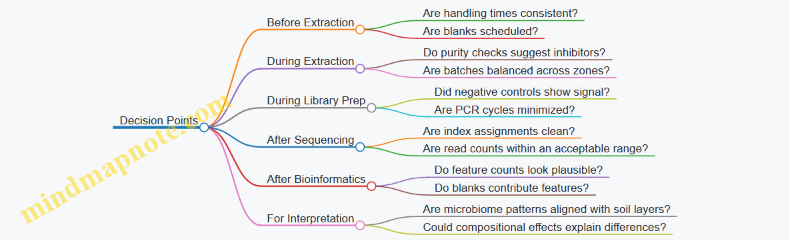
A well-run workflow produces more than a taxonomic list. It yields a feature table that you can trust enough to connect to root-system analytics and water-retention modeling, where the real value is in consistent, zone-specific biological signals.
3.5 Interpreting Results With Reference Ranges and Field Context
Reference ranges are useful guardrails, but they are not the whole story. A lab value can be “normal” and still fail in the field, and a value outside a range can still be part of a healthy trajectory. The goal is to interpret results by combining (1) how the measurement was made, (2) what the reference range actually represents, and (3) what the field was doing at the same time.
1) Start with What the Reference Range Means
Reference ranges usually come from a specific soil type, climate, crop, and sampling depth. Treat them like a map legend, not a universal rule. Before comparing numbers, confirm:
- Unit consistency: mg/kg vs g/kg, CFU vs gene copies, percent vs ratio.
- Depth and horizon: topsoil ranges rarely apply to subsoil.
- Extraction method: especially for nutrients and enzyme assays.
- Seasonality: microbial activity and mineralization can shift with temperature and moisture.
Example: A nitrate result of 18 mg/kg might be “low” in one dataset but “adequate” in a field that recently received irrigation and has active mineralization. The reference range may assume a different sampling window.
2) Check Measurement Quality Before Biological Meaning
Interpretation collapses if the measurement is noisy. Use QA/QC outputs to decide whether a value is trustworthy enough to act on.
- Replicate agreement: large spread suggests heterogeneity or handling issues.
- Controls and blanks: contamination or extraction failure can distort microbiome and enzyme signals.
- Detection limits: values near the limit should be treated as “present/absent” style evidence rather than precise abundance.
Example: If enzyme activity replicates vary by 60% while physical properties are consistent, prioritize repeating enzyme sampling rather than changing inputs.
3) Translate Lab Outputs Into Field-Relevant Questions
Instead of asking “Is it in range?”, ask “Does it match the field’s constraints and management?” Convert each metric into a decision question.
- Physical indicators: Do they explain infiltration and water retention behavior?
- Chemical indicators: Do they align with nutrient availability and salinity risk?
- Biological indicators: Do they align with root activity and residue status?
Example: A field with stable aggregates but low enzyme activity may be dominated by low root exudation (e.g., crop stage or root stress), not by poor soil structure.
4) Use Context Layers to Avoid False Conclusions
Field context includes crop stage, residue, irrigation history, compaction, and drainage. Even small differences can change microbial and nutrient readings.
- Crop stage: enzyme activity often tracks root growth phases.
- Moisture history: microbial communities respond quickly to wet-dry cycles.
- Recent amendments: compost, biochar, or fertilizers can temporarily shift chemistry and microbial composition.
Example: Two zones sampled on the same day show different microbial diversity. If one zone received a recent nitrogen application and the other did not, diversity differences may reflect substrate availability rather than drought resilience.
5) Interpret Patterns, Not Single Numbers
Look for coherent combinations across layers.
- Concordant improvement: structure + water retention + enzyme activity moving together suggests functional recovery.
- Mismatch: good structure but weak biological signals suggests limited biological drivers (root exudates, oxygen, or disturbance).
- Tradeoffs: high nutrient availability with low biological activity can indicate a system relying on inputs rather than cycling.
Example: If water retention is strong but microbiome indicators are weak, consider whether aeration and root contact are limiting rather than whether the soil “has enough water.”
6) Mind Map for a Practical Interpretation Workflow
7) A Worked Mini-Example for Zone Diagnosis
Suppose Zone A shows: moderate aggregate stability, nitrate near the lower reference boundary, and enzyme activity below range. Field notes show recent residue removal and a short period of dry-down before sampling.
A systematic interpretation is:
- Reference check: nitrate is low but not extreme; enzyme is the standout.
- Quality check: replicates are tight, controls pass.
- Context alignment: dry-down and reduced residue can reduce substrate for microbes and lower enzyme activity.
- Pattern logic: structure is fine, biology is lagging, so the likely limiter is biological substrate and root-driven activity rather than physical breakdown.
- Action confidence: prioritize biological driver adjustments and re-sample after a consistent moisture window.
This approach keeps the interpretation grounded: reference ranges guide expectations, QA/QC protects credibility, and field context explains why the numbers behave the way they do.
4. Geospatial Soil Health Mapping with Field Scale Resolution
4.1 Preparing Spatial Inputs Including Boundaries and Sampling Coordinates
Spatial inputs are the quiet foundation of soil health mapping. If boundaries are wrong or sampling coordinates drift, every later map looks confident while quietly being incorrect. This section turns field reality into clean spatial layers you can trust.
Define the Study Boundary with Operational Meaning
Start with a boundary that matches how you actually manage the land. A “field boundary” from a cadastral layer might include ditches, access lanes, or irregular edges you never treat. Instead, create an operational boundary by:
- Tracing the area where inputs and sampling will occur.
- Excluding permanent obstacles (ponds, buildings) and non-managed strips.
- Keeping the boundary consistent across seasons so comparisons stay fair.
Example: If you sample along a fence line but never apply amendments there, the operational boundary should stop short of the fence strip. Your later management zone maps should not “recommend” actions in a place you cannot operationally reach.
Choose a Coordinate System That Matches Your Workflow
Pick a projected coordinate system suitable for distance and area calculations. Geographic coordinates (latitude/longitude) can work for display, but they complicate buffering, spacing, and area-based summaries.
Practical rule: Use a projection where meters are meters. Then your sampling grid spacing and interpolation neighborhood sizes remain interpretable.
Example: If your sampling plan uses 30 m spacing, you want that spacing to be 30 m in the coordinate system you store and process.
Establish a Sampling Coordinate Standard
Every sample point needs a consistent definition of what the coordinate represents.
- Use the same point type: typically the center of the sampling location.
- Record depth separately from horizontal coordinates.
- Decide how you handle multi-core samples: either store one averaged point or store multiple points with a clear aggregation rule.
Example: For a composite sample made from five cores within a 1 m radius, store one coordinate at the composite center and record “composite radius = 1 m” in metadata. That keeps your map from implying false precision.
Clean Field Coordinates Before You Map Them
Raw GPS points often contain errors from signal multipath, canopy cover, or operator habits. Cleaning should be systematic, not guessy.
Steps:
- Remove obvious outliers that fall outside the operational boundary.
- Check for duplicates: same coordinate repeated with different sample IDs.
- Verify spacing: points that are far closer than your plan may be accidental re-logging.
- Confirm orientation: ensure northing/easting are not swapped.
Example: If a point intended for the northeast corner lands in the southwest corner, you’ll see it immediately when you overlay points on the boundary. Fixing this early prevents “mystery patterns” later.
Attach Metadata That Makes Coordinates Meaningful
Coordinates without context are just numbers. Store metadata that links each point to how it was collected and how it should be interpreted.
Minimum metadata fields:
- Sample ID and composite rule
- Date of collection (use the actual field date, e.g., 2026-03-15)
- Depth interval
- Sampling method (auger, core, composite radius)
- Operator or team ID
- Coordinate source (GPS device, post-processed correction)
Example: Two samples at the same horizontal coordinate but different depths should be treated as separate observations in mapping and modeling.
Build Sampling Layers for Modeling Inputs
Prepare separate layers for different modeling needs.
- Point layer: sample locations with attributes.
- Depth layer: either separate point layers per depth or a single point layer with depth as an attribute.
- Boundary layer: operational boundary polygon.
- Optional mask layer: exclude areas where interpolation should not occur (e.g., waterlogged zones you never sample).
Example: If you only sampled the top 0–20 cm, do not reuse the same point layer for deeper modeling. Create a depth-specific layer so your interpolation does not invent structure where you have no data.
Validate Spatial Inputs with Simple Visual Checks
Before interpolation, run quick checks that catch most problems.
- Overlay points on imagery or a field map to confirm they land where you expect.
- Plot point density to ensure it matches the sampling design.
- Confirm boundary containment: every point should fall inside the operational boundary or be explicitly flagged.
Example: If you see a cluster of points outside the boundary, it usually means the boundary polygon was drawn too tightly or the GPS was recorded with a different datum.
Mind Map: Spatial Inputs Preparation
Example: From Field Notes to Map-Ready Points
A team samples 0–20 cm at 25 locations using a 1 m composite radius. They record one coordinate per composite center, store depth as 0–20 cm, and tag the method as “5-core composite.” After cleaning, they confirm all 25 points fall within the operational boundary and that no duplicates exist. Only then do they generate the interpolation-ready point layer. This sequence prevents the most common failure mode: maps that look smooth because the data were quietly mislocated.
4.2 Selecting Interpolation Methods for Soil Property Surfaces
Soil property maps are only as useful as the interpolation choices behind them. The goal is not to “smooth everything,” but to create surfaces that respect how soil varies in space and how sampling was done. A good method matches three things: (1) the spatial pattern you expect, (2) the sampling geometry, and (3) the intended use of the map (planning inputs vs. estimating uncertainty).
Start with What You Know About Spatial Behavior
Begin by checking whether your property shows a trend with landscape position (e.g., slope-driven texture changes) or mostly local variation (e.g., patchy compaction). If you see a broad gradient, a method that can represent trend plus local structure will usually outperform a method that assumes stationarity everywhere.
A practical workflow is to compute a quick exploratory summary: plot points colored by value, inspect residuals after removing any obvious trend, and compare depth layers separately. If depth layers behave differently, interpolate each depth independently rather than forcing one surface to explain all layers.
Choose Based on Data Density and Sampling Pattern
Interpolation methods differ in how they use nearby points.
- Deterministic methods create a surface directly from measured values. They are straightforward and often stable with moderate data.
- Geostatistical methods treat spatial variation as a random process and explicitly model uncertainty through a variogram.
If you have dense sampling (many points per management zone), deterministic approaches can work well for operational maps. If you have sparse or uneven sampling, geostatistical methods are usually safer because they incorporate distance structure and help you quantify uncertainty.
Deterministic Methods and When They Fit
Inverse Distance Weighting (IDW) estimates each grid cell as a weighted average of nearby samples, where weights decrease with distance. It’s easy to explain to field teams: “closer samples matter more.” IDW works best when the property changes smoothly over space and when you don’t need formal uncertainty.
Example: Suppose bulk density is measured on a regular grid in a relatively uniform field. IDW with a sensible power parameter can produce a usable surface for zone delineation.
Spline interpolation creates a smooth surface that honors the data points. It can be helpful for properties that vary gradually, but it may overshoot in areas with sparse data. If your samples are clustered, splines can create unrealistic curvature between clusters.
Example: Soil organic carbon measured mostly near the center of a field might yield a surface that bends too strongly toward the edges. In that case, spline smoothing can mislead management decisions.
Geostatistical Methods and When They Fit
Kriging uses a variogram to describe how similarity decays with distance. It produces both an estimate and a prediction variance. That variance matters when you plan sampling follow-ups or decide where the map is trustworthy.
A common choice is ordinary kriging when you assume a constant mean over the local area. If there is a clear trend (like increasing clay content downslope), use universal kriging or remove the trend first and krige residuals.
Example: In a field with a slope-driven texture gradient, kriging raw values might blur the gradient. Modeling the trend and kriging residuals typically yields a surface that matches both the large-scale pattern and local variability.
Mind Map: Method Selection Logic
Validation Without Guesswork
After selecting candidate methods, validate them using the same grid resolution and the same preprocessing steps. Use cross validation by withholding points: predict at the withheld locations and compare predicted vs. observed values.
Track at least two metrics: one for accuracy (e.g., mean error or root mean square error) and one for bias (mean error near zero). Also check residual plots by landscape position. A method can have good overall error while still failing along a slope or near field edges.
Practical Example: Two Methods, One Field
Imagine a 40-hectare field where you sampled soil nitrate at 0–30 cm. Points are denser near the access road and sparser at the far corners.
- IDW will heavily weight the dense cluster, producing a surface that looks confident where data are plentiful and may underrepresent variability in the corners.
- Ordinary kriging will use the variogram to spread information more consistently across distances, and it will typically show higher prediction uncertainty in the corners.
If your goal is to target biological inputs, you might still use the kriging surface for decisions, but you would treat the corners as lower-confidence zones and avoid over-committing to fine-scale differences there.
Common Pitfalls to Avoid
- Mixing depth layers into one interpolation without checking whether variability patterns differ.
- Ignoring trends and forcing a constant-mean assumption when the landscape clearly drives change.
- Over-smoothing sparse areas so the map looks neat but stops reflecting measured variability.
- Comparing methods on different grids or after different preprocessing, which makes validation unfair.
A solid interpolation choice is the one that produces a surface consistent with both the measurements and the spatial logic of the field. If you can explain why the surface behaves the way it does—distance weighting, modeled spatial correlation, or trend removal—you’re already doing it right.
4.3 Managing Uncertainty With Variograms and Cross Validation
Uncertainty is not a flaw in mapping; it’s a measurement of how much you should trust each part of the surface. In soil health mapping, uncertainty comes from sampling gaps, lab noise, and the fact that soil properties change with depth and landscape position. Variograms help you quantify spatial structure, while cross validation tests whether your mapping method can predict unseen points.
From Spatial Structure to a Variogram
Start with the idea that nearby samples tend to be more similar than distant ones. A variogram summarizes that relationship by looking at how dissimilarity grows with separation distance.
- Compute semivariance for pairs of points at different lag distances.
- Plot semivariance against lag distance to see whether there is a clear trend.
- Fit a model curve that captures the pattern.
Key variogram terms matter operationally:
- Nugget reflects measurement error and micro-scale variability. If nugget is large, the map will be “rough” even with dense sampling.
- Sill is the plateau semivariance level. It indicates the overall variance once points are far enough apart.
- Range is the distance where the variogram reaches the sill. Beyond the range, additional distance adds little new information.
A practical example: suppose organic carbon shows a short range in a field. That means zone boundaries based on carbon may need to be tighter, because the property changes over short distances. If you ignore the short range and use a long one, the map will smooth away real differences.
Choosing a Variogram Model Without Guessing
Common model shapes include spherical, exponential, and Gaussian. The choice affects how quickly spatial correlation decays.
- Spherical often fits properties that level off relatively quickly.
- Exponential decays more gradually.
- Gaussian implies very smooth behavior near the origin.
A good workflow is to fit multiple models and compare them using cross validation rather than relying on visual fit alone. Also check whether the fitted model respects the data scale: if your sampling spacing is 20 m but the fitted range is 200 m, you are extrapolating correlation far beyond what the data can support.
Cross Validation as a Prediction Test
Cross validation evaluates the mapping method by repeatedly withholding data and predicting it. The simplest approach is leave-one-out, but for large datasets, k-fold is more practical.
For each validation run:
- Remove a subset of points.
- Fit the variogram on the remaining points.
- Predict the withheld points using kriging.
- Record prediction errors.
Useful error summaries include:
- Mean Error to detect bias (systematic over- or under-prediction).
- Root Mean Squared Error to measure typical error magnitude.
- Standardized Error to check whether uncertainty estimates are calibrated.
Calibration check example: if standardized errors are consistently larger than expected, your variogram model is too optimistic. The map may look precise, but the uncertainty intervals won’t cover the withheld points reliably.
Mind Map: Variograms and Cross Validation
Example: Comparing Two Variogram Choices in One Field
Imagine you map microbial biomass proxy across a 60 m by 60 m plot with samples every 10 m. You fit two variogram models:
- Model A: range 25 m, nugget moderate.
- Model B: range 60 m, nugget small.
Cross validation results show:
- Model A has lower RMSE and standardized errors near zero mean.
- Model B has higher RMSE and standardized errors that are too small in magnitude, meaning it underestimates uncertainty.
What to do with this information: use Model A for the final surface, and treat areas far from samples as higher uncertainty. If you must create management zones, avoid drawing sharp boundaries where uncertainty is consistently high.
Practical Rules for Interpreting Uncertainty Maps
- Uncertainty should increase with distance from samples. If it doesn’t, the variogram fit is likely inconsistent with the data.
- Depth layers need separate checks. A variogram that works at 0–10 cm may fail at 30–40 cm because processes and sampling noise differ.
- Outliers deserve context, not automatic removal. If a point is extreme due to a real feature like a wheel track or residue patch, removing it can distort the variogram and make predictions worse.
Diagram: End-to-End Uncertainty Workflow
    flowchart TD
  A[Start with sampled points and lab values] --> B[Compute experimental variogram]
  B --> C[Fit candidate variogram models]
  C --> D[Run cross validation]
  D --> E[Evaluate bias and error calibration]
  E --> F[Select best variogram model]
  F --> G[Kriging to generate surface and uncertainty]
  G --> H[Use uncertainty to guide zone boundaries]
When variograms and cross validation agree, you get more than a pretty surface. You get a map whose uncertainty matches what the data can actually support, which is exactly what drought-resilient decisions require.
4.4 Producing Management Zone Maps for Targeted Inputs
Management zone maps turn messy field measurements into practical decisions: where to apply more, where to apply less, and where to keep things steady. The goal is not to create pretty polygons; it’s to create zones that are stable enough for operations and meaningful enough for soil health and drought resilience.
Start with a Decision-First Zone Definition
Before mapping, define the decision the zone map will support. A zone map for targeted inputs usually answers one of these: (1) where to increase biological inputs, (2) where to adjust irrigation or water-retention strategies, or (3) where to prioritize sampling and verification. Each decision implies different zone behavior. For example, if the decision is biological inputs, zones should reflect differences in microbial function drivers and soil constraints. If the decision is water retention, zones should reflect hydraulic variability and water-holding capacity.
A practical way to keep this grounded is to set three rules:
- Action threshold rule: what minimum difference in the mapped variable justifies a different input rate.
- Operational stability rule: how much a zone boundary can shift between seasons without changing the action.
- Coverage rule: how many zones you can actually manage with your equipment and labor.
Example: If your sprayer can reliably handle two input rates plus a no-change buffer, you might use three zones total: low, medium, high. If your plan requires five zones, you’ll likely end up with “map-only” complexity.
Choose Zone Variables That Match the Input Mechanism
A zone map becomes more useful when it uses variables that connect to the input’s mechanism. For drought-resilient agriculture, common variable sets include:
- Soil structure and water retention proxies for water availability and infiltration behavior.
- Microbiome function indicators such as enzyme activity or biomass proxies, paired with constraints like salinity or nutrient imbalance.
- Root-system analytics such as root density or growth patterns, used to interpret whether biology and water are limiting.
Integrated practice: build a small “variable-to-decision” matrix. Each variable must justify its presence by linking to either (a) expected response to inputs or (b) the risk of applying inputs where they won’t work.
Standardize Layers So They Can Be Compared
Different layers often come in different units, scales, and noise levels. Standardization prevents one layer from dominating the clustering just because it has larger numeric values.
Use a consistent approach across the field:
- Resample all rasters to a common grid size.
- Apply the same masking for non-soil areas.
- Normalize variables using a method appropriate to the data distribution (for example, z-scores for roughly symmetric variables).
- Track uncertainty per pixel or per sampling neighborhood so later steps can avoid overconfident boundaries.
Example: If water retention is measured as a modeled parameter and microbiome function is measured from discrete samples, the microbiome layer may be smoother or noisier depending on interpolation. Standardization plus uncertainty tracking keeps the zone map from treating interpolation artifacts as real differences.
Build Zones Using a Two-Stage Approach
A two-stage approach keeps zones both interpretable and robust.
Stage 1: Create candidate surfaces. Combine standardized variables into a small set of composite surfaces that represent distinct constraints or opportunities. For instance:
- A Water Availability Surface from retention-related variables.
- A Biological Function Surface from microbial function indicators.
- A Constraint Surface from limiting factors like salinity or extreme pH.
Stage 2: Cluster into management zones. Use clustering or rule-based thresholds to group pixels into zones. Clustering works best when you limit the number of zones and require minimum area for each zone.
Operational guardrails:
- Enforce a minimum polygon size so you don’t create tiny slivers.
- Smooth boundaries using a consistent neighborhood rule.
- Keep a “no-decision buffer” around high-uncertainty areas.
Validate Zones with Ground Truth and Action Checks
Validation should be practical, not just statistical.
- Holdout validation: compare zone assignments against independent samples collected in the same season or a later season.
- Boundary plausibility check: verify that boundaries align with real landscape features or consistent soil behavior.
- Action check: confirm that each zone’s recommended input rate differs enough to matter.
Example: If a zone boundary falls entirely within a uniform soil texture area and the uncertainty is high, you may be better off merging it with a neighboring zone. That’s not a failure; it’s a decision-quality improvement.
Mind Map: From Variables to Zones
Example: Two Inputs, Three Zones
Assume you’re targeting both biological inputs and water-retention practices.
- Zone 1 (Low Water Availability + Low Biological Function): apply higher biological input rate and prioritize water-retention interventions.
- Zone 2 (Moderate Water Availability + Moderate Biological Function): apply baseline biological input and maintain current water strategy.
- Zone 3 (Higher Water Availability or Stronger Biological Function): apply reduced biological input and focus on monitoring rather than heavy intervention.
To keep this operational, you set action thresholds so that only meaningful differences trigger rate changes. If a pixel’s uncertainty is too high, it falls into the no-decision buffer and inherits the neighboring zone’s conservative rate.
Diagram: Zone Mapping Workflow
    flowchart TD
  A[Define decision and action rules] --> B[Select zone variables matching input mechanism]
  B --> C[Standardize layers and track uncertainty]
  C --> D[Build candidate surfaces]
  D --> E[Group pixels into management zones]
  E --> F[Apply operational guardrails]
  F --> G[Validate with holdout samples and boundary checks]
  G --> H[Export zone polygons and zone-specific input rates]
Output That Teams Can Use
A usable zone map includes more than boundaries. It should state:
- the variable logic behind each zone,
- the recommended input rate per zone,
- the uncertainty buffer behavior,
- and a short verification plan for the next sampling cycle.
When these elements are consistent, the map becomes a decision tool rather than a one-time visualization. That’s the difference between “mapped” and “managed.”
4.5 Validating Maps with Independent Samples and Ground Truth Checks
A soil health map is only as useful as its ability to predict what you would measure at new locations. Validation answers three practical questions: (1) does the map reproduce known patterns, (2) does it generalize to locations not used in building the surface, and (3) does it match field reality in a way that supports decisions.
Validation Goals and What “Good” Looks Like
Start by separating accuracy from usefulness. Accuracy is how close predicted values are to measured values. Usefulness is whether the error is small enough to keep management actions aligned with the intended zone behavior.
A simple way to define “good” is to set thresholds tied to decisions. For example, if your management zones differ by at least 0.3 units of a soil health index, then a validation error of 0.1 units is likely acceptable, while 0.3 units may cause frequent zone misclassification.
Independent Samples That Actually Test Generalization
Validation requires samples that were not used during interpolation or mapping. Independent samples can be created in two common ways.
-
Holdout points: Reserve a subset of original sampling locations before any modeling. Use them only after the map is built.
-
New locations: Collect additional samples in the same season and similar crop stage, but at coordinates not previously sampled.
A key detail is to keep the validation set representative. If you hold out only the easiest areas (flat, uniform soils), your validation will look better than it should. Aim for coverage across landscape positions, slope classes, and soil texture bands.
Ground Truth Checks That Go Beyond Numbers
Measured agreement is necessary, but not sufficient. Ground truth checks confirm that the spatial patterns make agronomic sense.
- Pattern plausibility: If the map shows higher water retention in depressions, verify that those depressions are indeed wetter and have different structure or texture.
- Process consistency: If microbiome indicators are higher where root density is higher, check whether root sampling or proxy indicators support that relationship.
- Boundary behavior: Pay attention to edges between management zones. Many mapping errors show up as “smearing” across boundaries.
A practical example: Suppose your map predicts a sharp transition in aggregate stability near a drainage line. During validation, you sample across that line with short spacing. If measurements change gradually instead of sharply, the map may be overconfident in the boundary.
A Systematic Validation Workflow
Use a repeatable sequence so results are interpretable.
- Freeze the model: Build the map using training data only.
- Extract predictions at validation coordinates: Record predicted values for each independent sample.
- Compute error metrics: Use at least one scale-dependent metric (like mean absolute error) and one rank-based metric (like correlation) to capture both magnitude and pattern.
- Check residual structure: Plot residuals against location, depth, and texture. If residuals cluster spatially, the map is missing a driver.
- Evaluate zone classification: Convert predicted values into zone labels and compute confusion counts. This tells you whether errors matter operationally.
- Document sampling conditions: Record sampling date, depth interval, and handling steps so differences can be traced to method rather than soil.
A small but important example: If validation samples were stored longer before analysis, microbiome-related metrics may shift. Your residual plot might show systematic bias rather than random noise.
Mind Map: Validation Logic and Evidence Types
Example: Validating a Water-Retention Surface
Imagine you mapped field-scale water retention using lab curves converted into a retention metric at a target matric potential. You then validate with 20 independent cores collected two weeks after the training sampling.
- Step 1: For each validation core, you compute the measured retention metric.
- Step 2: You compare it to the map prediction at the same coordinates.
- Step 3: You compute mean absolute error and correlation.
- Step 4: You plot residuals versus texture. If sandy areas show consistent underprediction, the interpolation may be missing a texture covariate.
- Step 5: You translate predictions into zone labels. If most misclassifications occur near the drainage line, you refine the boundary handling or sampling density there.
The point of this example is not the specific numbers; it’s the sequence. Validation becomes actionable when you can point to where the map is wrong and why.
Common Failure Modes to Watch For
- Validation leakage: Using validation points during model tuning inflates performance.
- Mismatch in sampling depth: Even a small shift in depth interval can change retention and microbiome signals.
- Inconsistent handling: Differences in storage time, moisture conditions, or extraction batch can create systematic bias.
- Over-smoothing: Interpolation that is too smooth can hide real transitions that matter for zone decisions.
When you see these issues, the fix is usually procedural: adjust the sampling plan, align methods, or revise how boundaries and covariates are represented. The goal is to make validation a check on the map, not a debate about measurement variability.
5. Root System Analytics for Linking Biology with Soil Function
5.1 Root Architecture Metrics Relevant to Drought Performance
Drought stress is partly a soil water problem and partly a plant geometry problem. Root architecture metrics translate that geometry into measurable traits that can be linked to water uptake, access to deeper moisture, and the plant’s ability to keep functioning when surface water disappears.
Core Concepts That Tie Roots to Water Under Stress
Root architecture affects drought performance through three mechanisms: (1) where roots grow, (2) how much root surface area is available for uptake, and (3) how effectively roots maintain growth and function as conditions worsen. A useful way to think about metrics is to group them into spatial reach, uptake capacity, and persistence.
Spatial reach answers: “Can the plant reach water that is still there?” Uptake capacity answers: “How much absorbing surface is available where water exists?” Persistence answers: “Does the root system keep working when the soil dries and oxygen drops?”
Spatial Reach Metrics
Spatial reach is measured by depth and distribution.
Rooting depth. Record the maximum depth with living roots or with root biomass above a detection threshold. A practical field proxy is the deepest soil layer where roots are consistently observed in excavated profiles. Example: if one management zone shows roots mostly in the top 30 cm while another reaches 60 cm, the deeper zone typically has access to later-season moisture.
Root length density by depth. Instead of only maximum depth, measure root length per soil volume at depth intervals (e.g., 0–20, 20–40, 40–60 cm). This prevents a misleading “deep but sparse” interpretation. Example: two fields both reach 60 cm, but the one with higher length density at 40–60 cm usually maintains uptake longer.
Lateral spread and zone coverage. Drought often creates patchy water availability. Measure lateral root spread relative to row spacing and the distance to likely dry boundaries. Example: if roots concentrate near the row but the inter-row dries faster, the plant may still face water limitation even with good depth.
Uptake Capacity Metrics
Uptake capacity is about surface area and fine-root contribution.
Fine root fraction. Fine roots (often defined by diameter classes) drive most absorption. Measure the proportion of total root length or biomass in fine diameter ranges. Example: after a dry spell, a system with a higher fine-root fraction tends to show better early recovery because absorbing surfaces remain available.
Specific root length. Specific root length is root length per unit dry mass. Higher values indicate thinner, longer roots that can increase absorbing surface per gram. Example: if two samples have similar biomass but one has higher specific root length, that sample likely supports greater uptake potential.
Root surface area proxies. When direct surface area measurement is impractical, use diameter and length distributions to estimate surface area. Example: a shift from thicker roots to more intermediate diameters can still raise effective surface area even if total biomass stays constant.
Persistence and Function Under Drying
Persistence metrics capture whether roots maintain growth and activity.
Root-to-shoot ratio. Under drought, plants often allocate more resources to roots. Measure root dry mass and shoot dry mass at comparable growth stages. Example: a higher ratio during early drought can indicate continued investment in water acquisition.
Root growth rate across time. Compare root length density or biomass at multiple time points (before stress, early stress, and late stress). Example: if one zone shows stable length density while another declines sharply, the stable zone is likely better at sustaining uptake.
Root viability indicators. Use viability staining or respiration-related proxies when available, and otherwise rely on consistent presence of living roots in profile observations. Example: roots that remain alive at depth during late-season dry conditions are more informative than roots that were present earlier but died back.
Measurement Strategy That Keeps Metrics Comparable
To compare zones, keep sampling consistent: same growth stage, similar soil moisture at sampling time, and identical depth intervals. Record soil texture and bulk density because they influence how roots can penetrate and how you interpret length density.
A simple decision rule: if you only measure rooting depth, you risk missing differences in fine-root uptake capacity. If you only measure fine roots, you risk missing differences in access to deeper water. The best drought-relevant picture uses at least one metric from each group: spatial reach, uptake capacity, and persistence.
Mind Map: Root Architecture Metrics for Drought Performance
Example Integration for a Field Zone Comparison
Suppose you compare two management zones at early drought. Zone A shows deeper rooting depth (to 55 cm) but low root length density at 40–60 cm. Zone B shows slightly shallower maximum depth (to 45 cm) but higher length density at 20–40 cm and a higher fine root fraction. If Zone B also maintains root-to-shoot ratio and shows less decline in length density by late drought, Zone B is likely better at sustaining uptake through the drying front. Zone A may access deeper water, but Zone B’s uptake capacity and persistence likely support more consistent water acquisition during the period when surface layers fail.
5.2 Measuring Root Growth Patterns Using Field and Controlled Methods
Root growth patterns are easiest to measure when you decide what “pattern” means before you start. In practice, you usually want three things: where roots are (spatial pattern), how much roots are present (magnitude), and how they change over time (dynamics). Field methods answer the “where” and “dynamics” questions under real constraints, while controlled methods answer the “how” questions with cleaner comparisons.
Foundational Concepts for Root Pattern Measurement
Start by separating root pattern into measurable components:
- Depth distribution: fraction of root mass or length in each depth interval.
- Lateral spread: how far roots extend from the plant row or stem.
- Root density gradients: changes in root abundance across distance and depth.
- Temporal shifts: movement of roots deeper or outward as water and nutrients change.
Then choose a measurement unit that matches your goal. Root length (often from imaging) supports architecture comparisons; root mass (often from washing and drying) supports biomass and allocation comparisons; root presence (often from cores and staining) supports mapping but can be less quantitative.
Field Methods for Real-World Patterns
Field measurements must handle soil heterogeneity, limited access, and sampling disturbance. A practical workflow is to define a sampling grid tied to management zones, then sample at consistent plant growth stages.
1) Core sampling with depth intervals
- Use a consistent core diameter and depth increments (for example, 0–10 cm, 10–20 cm, etc.).
- Take cores at fixed distances from the plant row (for example, 0–10 cm, 10–20 cm, 20–30 cm) to capture lateral gradients.
- Wash roots carefully and separate roots by depth interval.
Easy example: In a drought-prone sandy loam, sample three distances from the row and five depth intervals at two dates. If deeper intervals show a larger root fraction on the second date, the pattern suggests roots are tracking moisture downward.
2) Minirhizotron or transparent window observations
- Install transparent tubes or windows so you can observe root growth without repeated core destruction.
- Record images at fixed time intervals and at consistent magnification.
- Convert images to root length or root counts using the same thresholding approach each time.
Easy example: In a controlled irrigation strip inside a field, minirhizotron images can show whether roots increase in depth before yield differences appear.
3) Excavation for architecture snapshots
- Use targeted excavation around representative plants.
- Keep the excavation geometry consistent so comparisons across zones remain meaningful.
Easy example: If you suspect a biological input increases lateral rooting, excavation can show whether roots spread wider rather than just increasing total mass.
Controlled Methods for Cleaner Comparisons
Controlled systems reduce confounding from soil variability and allow you to impose specific water or nutrient conditions. The tradeoff is that container boundaries can alter root behavior, so you must design the setup to minimize artifacts.
1) Rhizoboxes and transparent growth chambers
- Use transparent panels to image roots directly.
- Control water delivery precisely (for example, fixed soil moisture targets).
- Image roots at consistent intervals and use the same segmentation settings.
Easy example: Compare two treatments under identical moisture profiles. If one treatment shows earlier root penetration into deeper layers, you can link that pattern to water access rather than to random field variation.
2) Soil columns with controlled hydraulic gradients
- Pack soil into columns with known bulk density and texture.
- Apply water at controlled rates or maintain a gradient.
- Harvest roots at defined times and quantify depth and lateral distribution.
Easy example: If roots in one column treatment concentrate near the wetting front, the pattern indicates strong responsiveness to water movement.
3) Hydroponic or aeroponic systems for architecture screening
- These systems are best for early-stage architecture traits rather than soil-structure interactions.
- Use them to compare root angles, branching frequency, and early growth rates.
Easy example: If a treatment increases branching under uniform nutrient supply, you can later test whether that branching translates into deeper rooting in soil.
Measurement Design That Prevents “Garbage in, Garbage Out”
A good design includes timing, replication, and consistent geometry.
- Timing: sample at comparable phenological stages and record soil moisture at sampling time.
- Replication: use enough plants or cores per zone to capture variability.
- Geometry: keep core diameter, depth intervals, and distances from the row consistent.
- Disturbance control: if using repeated observations, avoid mixing destructive and non-destructive methods without accounting for disturbance.
Mind Map: Root Growth Pattern Measurement
Example Workflow from Field to Controlled Validation
- In the field, map root depth distribution at two dates using cores in each management zone.
- Identify the zone with the strongest shift toward deeper layers.
- In a controlled soil column, impose the same irrigation pattern used in that zone and compare treatments.
- Quantify whether the deeper shift appears under the imposed water regime.
This approach keeps the field as the reality check and the controlled system as the explanation tool, without pretending one method can do everything.
5.3 Quantifying Root Exudation Proxies and Rhizosphere Activity
Root exudation is hard to measure directly in field soils, so we quantify it through practical proxies that track (1) carbon release patterns and (2) the biological response that follows. The goal is not to “prove” exudation in a single measurement; it’s to build a consistent chain of evidence that links root activity to rhizosphere processes relevant to drought resilience.
Foundational Concepts for Proxy Selection
Exudates are mostly water-soluble compounds released near roots, and they feed microbes and soil enzymes. In drought, exudation can shift because roots alter carbon allocation and because diffusion slows when soil dries. A useful proxy should therefore be measurable under your sampling conditions and should respond to root-driven carbon availability rather than only to bulk soil properties.
Start with two categories:
- Carbon availability proxies: indicators that reflect recent carbon inputs to the rhizosphere.
- Rhizosphere activity proxies: indicators that reflect microbial and enzymatic activity stimulated by those inputs.
Then add a practical constraint: proxies must be compatible with your sampling depth, moisture state, and lab turnaround time.
Sampling Logic That Keeps Proxies Meaningful
Rhizosphere activity is spatially tight, so sampling strategy matters more than the assay choice. Use a consistent approach across zones.
- Define the rhizosphere window: for field cores, a common operational definition is soil tightly adhering to roots after gentle shaking, or soil from a narrow distance around roots when roots are sampled.
- Separate rhizosphere from bulk soil: collect paired samples from the same plant row and depth—one rhizosphere operational fraction and one bulk fraction at the same depth.
- Control moisture at sampling: if soil is extremely dry, microbial activity assays can stall. Record gravimetric water content so you can interpret activity changes as “less carbon” versus “less mobility.”
A simple example: in a dry zone, you might see lower enzyme activity. If moisture is also lower, you should avoid concluding that exudation stopped; you may be seeing diffusion limits.
Carbon Availability Proxies You Can Measure
1. Soluble carbon pools
Measure dissolved organic carbon (DOC) or water-extractable organic carbon from rhizosphere-enriched fractions. Higher values often indicate more recent carbon release or reduced microbial consumption.
Example: If DOC is higher in rhizosphere than bulk soil but enzyme activity is unchanged, the carbon may be accumulating due to limited microbial processing, not necessarily due to higher exudation.
2. Respiration response to added substrate
Use short incubations with a standardized carbon addition and measure CO₂ evolution. This tests whether the microbial community is primed to process carbon.
Example: Two zones receive the same carbon addition in the lab. If the rhizosphere fraction from one zone produces more CO₂, the community there is more responsive to carbon availability.
3. Isotopic labeling in controlled plots
Where feasible, apply a labeled carbon source to plants or soil in a controlled manner and track incorporation into microbial biomass or CO₂. This is the most direct proxy, but it’s operationally heavier.
Example: In a small replicated plot, labeled carbon incorporation into microbial biomass can confirm that rhizosphere microbes are using plant-derived carbon.
Rhizosphere Activity Proxies That Reflect Function
1. Enzyme activity assays
Enzymes such as β-glucosidase and phosphatases respond to carbon and nutrient dynamics in the rhizosphere. Use rhizosphere and bulk comparisons to isolate root-driven stimulation.
Example: If β-glucosidase activity is elevated in rhizosphere but soluble carbon is not, the microbial community may be efficiently converting available carbon into enzyme production.
2. Microbial biomass and turnover
Measure microbial biomass carbon (fumigation-extraction) or microbial growth proxies. Biomass alone doesn’t show exudation, but it helps interpret whether activity changes are due to more microbes or more per-microbe activity.
Example: Higher enzyme activity with stable biomass suggests increased activity per unit biomass, which can be consistent with stronger root signaling or carbon pulses.
3. Microbial community activity via substrate-induced respiration
Substrate-induced respiration (SIR) measures CO₂ response after adding a small, standardized substrate. It’s a practical way to compare “activity potential” across zones.
Example: If SIR is higher in rhizosphere fractions, the microbial community there is likely better adapted to process available carbon.
Turning Proxy Measurements Into Interpretable Indices
Raw proxy values are noisy, so build a simple index that compares rhizosphere to bulk.
- Rhizosphere Enrichment Ratio = rhizosphere value / bulk value
- Activity-Carbon Consistency Check: compare whether carbon proxies and activity proxies move together.
Example workflow for one zone:
- DOC enrichment ratio is 1.8
- β-glucosidase enrichment ratio is 1.5
- SIR enrichment ratio is 1.6
This pattern supports the interpretation that root-driven carbon inputs are stimulating microbial processing.
If DOC enrichment is high but enzyme enrichment is low, you should check moisture, sampling tightness, and whether the microbial community is carbon-limited by something other than exudate supply.
Mind Map: Proxies and Interpretation Path
Example: A Zone Comparison with Clear Reasoning
Suppose you compare two management zones at 10–20 cm depth.
- Zone A: rhizosphere DOC enrichment ratio = 1.7; β-glucosidase enrichment ratio = 1.6
- Zone B: rhizosphere DOC enrichment ratio = 1.2; β-glucosidase enrichment ratio = 1.1
Because both carbon and enzyme activity show lower rhizosphere enrichment in Zone B, the most consistent interpretation is weaker root-driven carbon availability or reduced microbial processing of that carbon. If Zone B also has lower gravimetric moisture, you should treat the result as “root influence plus diffusion constraints,” not as a pure biological difference.
Practical Quality Checks That Prevent Misreads
- Replicate within plant row: rhizosphere signals vary at the scale of individual plants.
- Include bulk controls: bulk soil anchors the baseline so enrichment ratios mean something.
- Track moisture and handling time: activity assays are sensitive to both.
- Use consistent extraction and incubation conditions: small differences can shift CO₂ and enzyme readings more than the biological effect you’re trying to detect.
When these checks are in place, proxies become a coherent story: roots release carbon, microbes respond, enzymes reflect processing, and the rhizosphere-to-bulk contrast helps you map where drought resilience is being supported by active soil biology.
5.4 Connecting Root Traits With Soil Structure and Water Availability
Root traits matter because they determine how plants explore pores, resist drying, and keep functioning when water becomes patchy. Soil structure matters because it controls pore size distribution, connectivity, and how quickly water moves and drains. Water availability matters because roots respond to both the amount of water and the ease of getting it.
Foundational Links Between Traits, Structure, and Water
Start with a simple chain: soil structure shapes water behavior, water behavior sets root water status, and root water status drives root growth and function.
- Soil structure → water availability: Aggregates create pores of different sizes. Larger pores drain faster; smaller pores hold water longer but can be harder to extract.
- Water availability → root water status: When soil dries, matric potential drops and roots must spend more energy to pull water.
- Root traits → performance: Traits that improve access to small pores, maintain growth under low water, or reduce water loss help plants keep taking up water.
A practical way to connect these is to map traits to the pore types they target.
Root Traits That Match Soil Pore Types
1) Root diameter and surface area
Fine roots increase surface area per unit volume, which helps when water is held in smaller pores. In a compacted layer, fine roots may struggle to penetrate, so you often see reduced rooting depth.
Example: In a field with a traffic pan, plants may show shallow rooting and earlier wilting. If you compare root cores from the pan and adjacent areas, you typically find fewer fine roots inside the compacted zone.
2) Root length density and branching
High root length density increases the chance of contacting connected pores. Branching patterns matter because they determine how quickly roots can exploit new microhabitats after rainfall.
Example: After a rain, a well-structured zone with connected macropores can refill quickly. Roots with higher branching can capitalize on that refill by expanding into newly wetted patches.
3) Root growth angle and depth distribution
Roots that grow deeper access subsoil water that stays available longer. Depth distribution is strongly influenced by mechanical resistance and by how stable aggregates are with depth.
Example: If infiltration is slow and surface aggregates break down, the topsoil may stay wet briefly but dry quickly. Deeper rooting becomes more valuable, but only if the subsoil is not too hard or too poorly structured.
4) Root hydraulic conductance and water-use strategy
Hydraulic conductance reflects how easily water moves from soil to plant. When soils are dry, higher conductance can help maintain uptake, but it must be balanced with the plant’s ability to avoid excessive transpiration.
Example: Two zones can have the same measured soil water content, yet one supports better uptake because pores are more connected and roots can access water more effectively.
Soil Structure Measurements That Explain Trait Differences
To connect traits to structure, you need structure metrics that relate to water behavior.
- Aggregate stability: Stable aggregates resist breakdown, preserving pore networks and reducing crusting.
- Bulk density and penetration resistance: These indicate mechanical constraints that limit root penetration and branching.
- Porosity and pore-size distribution: Even without full lab pore-size curves, you can infer the balance between drainage pores and retention pores.
- Infiltration and drainage behavior: Simple field infiltration tests reveal whether water moves into the rooting zone or stalls at the surface.
Example: If penetration resistance spikes at 15–25 cm, you can expect reduced rooting depth there. That reduction changes the effective water reservoir the plant can use during dry spells.
Water Availability Metrics That Roots Actually Respond To
Roots respond to water availability in terms of how hard it is to extract water.
- Soil water content is a snapshot of quantity.
- Matric potential (or proxies) reflects extraction difficulty.
- Plant-available water combines both quantity and accessibility across a depth profile.
A useful operational approach is to compute available water by depth and then compare it to root depth distribution. If roots cannot reach the depths where water remains extractable, the plant’s effective available water shrinks.
Putting It Together with a Zone-Level Reasoning Loop
Use a loop that starts with structure, moves to water, and ends with trait expectations.
- Identify structural constraints: Where are compaction, low aggregate stability, or poor infiltration likely?
- Translate to water behavior: Which layers will drain quickly, and which will retain water?
- Predict root access: Which traits will be favored in each zone—more fine roots for small pores, deeper growth where subsoil is accessible, or higher branching where refill is patchy?
- Check with observations: Compare rooting depth, root density, and signs of water stress across zones.
Mind Map: Connecting Root Traits with Soil Structure and Water Availability
Integrated Example: Two Zones, One Crop
Assume two management zones.
- Zone A has stable aggregates and moderate bulk density. Infiltration is steady, and water refills pores after rainfall.
- Zone B has a compacted layer with lower aggregate stability. Infiltration slows, and water tends to drain or remain near the surface.
Trait expectations:
- In Zone A, roots can branch and maintain higher length density because pores are connected and penetration is less restricted.
- In Zone B, roots may concentrate near the surface where water appears first, and fine-root density in the compacted layer may be low.
Water availability outcome:
- Even if Zone B shows similar surface water content after rain, the plant’s effective plant-available water is smaller because deeper extractable water is out of reach.
Field check: Measure rooting depth and root density at the same growth stage across zones. If Zone B shows shallower rooting and earlier water stress, the trait–structure–water link is working as an explanation rather than a guess.
5.5 Building Root Based Indicators for Zone Level Decisions
Root based indicators translate root-system observations into practical, zone level actions. The key is to choose indicators that (1) respond to management, (2) relate to water capture and drought tolerance, and (3) can be measured with a consistent sampling plan.
Foundations for Zone Level Indicators
Start with a simple chain: management changes root traits → traits affect water access and soil contact → that changes yield stability under dry spells. Indicators should sit close to that chain, not far away in the “nice to know” category.
A useful indicator set usually includes three layers:
- Structure: how much root is present and where it is located.
- Function proxies: how actively roots are likely to be exploring soil.
- Constraints: what limits root growth, such as compaction or salinity.
Easy example: In a low-lying zone that stays wetter longer, you might see deeper rooting and higher fine root density. In a ridge zone with faster drying, you might see shallower rooting and thicker, slower-turnover roots. Both patterns can guide different amendment and irrigation coverage decisions.
Selecting Indicators That Match Decision Types
Different decisions need different indicators. Use this mapping to avoid collecting data that cannot change actions.
- Irrigation timing and coverage: prioritize indicators tied to water access depth and fine root activity.
- Biological input targeting: prioritize indicators tied to rhizosphere activity and root turnover.
- Soil physical remediation: prioritize indicators tied to root penetration resistance and rooting depth limits.
A practical approach is to define one “primary” indicator per decision type, plus two supporting indicators.
Core Indicator Definitions and How to Measure Them
Below are indicator candidates that work well at zone scale when you standardize sampling depth, timing, and plant stage.
-
Rooting Depth Index (RDI)
- Definition: fraction of sampled cores where roots are present below a chosen depth threshold.
- Why it helps: it directly reflects whether the crop can access deeper water.
- Example: If you sample 0–30 cm and 30–60 cm, RDI for 30–60 cm might be 0.8 in a valley zone and 0.3 on a ridge. The ridge zone then becomes a candidate for actions that improve infiltration and root penetration.
-
Fine Root Density (FRD)
- Definition: mass or length of fine roots per soil volume, using a consistent diameter cutoff.
- Why it helps: fine roots are the main interface for water and nutrient uptake.
- Example: After applying a compost-based biological input to one zone, FRD increases at 10–20 cm but not at 40–50 cm. That suggests the input improved near-surface exploration rather than deep access.
-
Root Length Density Gradient (RL-D Gradient)
- Definition: slope of root length density across depth bands.
- Why it helps: it captures whether roots shift deeper as soil dries.
- Example: A steep negative gradient indicates roots concentrate near the surface. A flatter gradient suggests better depth distribution.
-
Rhizosphere Activity Proxy (RAP)
- Definition: a standardized measure that tracks root-associated activity, such as root-associated enzyme activity or a consistent proxy tied to living root presence.
- Why it helps: it links root presence to functional soil processes.
- Example: If RAP is high in a zone but FRD is low, the limitation may be root quantity rather than activity. That changes the input rate or timing.
-
Penetration Constraint Score (PCS)
- Definition: a composite score from root penetration observations and a physical resistance measure (e.g., penetrometer readings) aligned to the same depth bands.
- Why it helps: it prevents misattributing poor rooting to biology when the real limiter is physical.
- Example: If PCS is high at 20–35 cm due to compaction, then biological inputs alone may not fix the depth problem.
Turning Indicators Into Zone Decisions
Indicators become decisions when you define thresholds and decision rules.
A simple rule set:
- If RDI deep is low and PCS is high, prioritize physical loosening or infiltration improvements before biological inputs.
- If RDI deep is moderate but FRD is low, prioritize biological inputs that support fine root formation and near-surface exploration.
- If RAP is low while FRD is adequate, adjust timing to match plant stage and soil moisture conditions so roots can express activity.
Easy example: Zone A shows low deep RDI and high PCS at 30–45 cm. Zone B shows adequate deep RDI but low FRD at 10–20 cm. Zone A gets a physical constraint fix; Zone B gets targeted biological input and possibly a coverage strategy that keeps the topsoil from drying too fast.
Mind Map: Root Based Indicators for Zone Level Decisions
Zone Scorecard Template
Use a compact scorecard so field teams can act without interpreting raw data every time.
- Zone: ________
- RDI deep: low / medium / high
- FRD: low / medium / high
- RL-D Gradient: steep / moderate / flat
- RAP: low / medium / high
- PCS: low / medium / high
- Primary action: physical / biological / timing / coverage
- Supporting action: ________
This structure keeps the logic consistent: indicators describe what the roots are doing and what is stopping them, and the decision rules translate that into zone-specific management.
6. Water Retention Modeling for Drought Resilient Planning
6.1 Selecting Water Retention Models for Field Use
Field use starts with a simple question: what decision will the model support? If the goal is irrigation scheduling, the model must translate soil water status into plant-available water and infiltration limits. If the goal is mapping drought risk across management zones, the model must be stable under spatial variability and compatible with the measurements you can realistically collect.
Foundational Concepts for Model Choice
Water retention models describe how volumetric water content changes as soil water potential changes. In practice, you rarely measure potential directly in the field, so you use lab or indirect estimates to fit a curve, then convert it into usable thresholds like “plant-available range.” The key selection criteria are:
- Parameter interpretability: Parameters should connect to measurable soil properties or at least be consistent across depths.
- Data requirements: Some models need more points across the wet-to-dry range than you can afford.
- Numerical behavior: A model that misbehaves near the dry end can produce irrigation recommendations that look precise but are wrong.
- Integration with hydraulics: If you later model infiltration or root water uptake, the retention model must work with those components.
A practical rule: choose the simplest model that fits your retention data well enough to preserve the thresholds you care about.
Common Model Families and When They Fit
Van Genuchten (VG) is widely used because it fits a smooth retention curve and provides parameters that are easy to compare across samples. It works well when you have multiple measurements spanning near-saturation to the dry range where plants start to struggle.
Brooks and Corey (BC) is often simpler and can be effective when you focus on the unsaturated range and have fewer data points. It can be less flexible near saturation, so it’s best when your measurements emphasize the mid-to-dry region.
Mualem–van Genuchten extensions matter when you also need hydraulic conductivity. If your workflow includes infiltration or drainage behavior, selecting a retention model that pairs naturally with conductivity equations reduces mismatch errors.
Empirical piecewise fits can be useful when lab data are noisy or when you only need a few operational thresholds. The tradeoff is that piecewise models can be harder to integrate with other physics-based steps.
Data-to-Model Workflow for Field Use
- Define operational targets. Example targets: field capacity proxy, permanent wilting proxy, and a “management trigger” like 50% depletion of plant-available water.
- Collect retention points that bracket targets. If your trigger sits around a specific water potential, ensure your lab measurements include points near that region.
- Fit candidate models and compare threshold accuracy. Don’t judge only by overall curve fit; compare predicted water content at your chosen potentials.
- Check physical plausibility. Parameters should yield monotonic behavior and reasonable residual water content.
- Validate with independent samples. Use a small holdout set from different landscape positions so the model doesn’t just memorize one soil type.
Example: Choosing Between Van Genuchten and Brooks and Corey
Suppose you sample a loam field and measure retention at five potentials: near saturation, two mid-range points, and two dry-range points. Your irrigation trigger corresponds to the mid-dry region.
- If VG predicts water content at the trigger within a small margin and produces a smooth curve, it’s a strong choice for zone-level mapping.
- If BC fits the mid-to-dry points well but shows a mismatch near saturation, that’s acceptable if your trigger never relies on the wet end.
A concrete check: compute plant-available water as
- PAW = θ(upper) − θ(lower)
where θ(upper) and θ(lower) come from your chosen proxies. If PAW changes materially between models, your irrigation schedule will too.
Mind Map: Model Selection Logic
Practical Selection Checklist
- Do you have enough retention points to support the model’s flexibility?
- Are your operational thresholds located in the region where the model fits best?
- Will the model be used alone, or will it feed into conductivity or infiltration steps?
- Do fitted parameters behave consistently across depths and landscape positions?
- Can you explain the resulting PAW and trigger water contents to a field team without hand-waving?
When these boxes are checked, the model becomes a tool rather than a mystery. It turns lab curves into repeatable decisions, which is the whole point of mapping water retention in the first place.
6.2 Measuring Soil Hydraulic Parameters with Practical Protocols
Soil hydraulic parameters describe how water moves and is stored in soil. In drought-resilient planning, you typically need two things: (1) a water-retention relationship (how much water remains at different suctions) and (2) a conductivity relationship (how easily water moves at those suctions). The practical challenge is measuring these properties without turning the field into a science fair.
Core Concepts You Must Measure
Start with the soil-water retention curve. It links volumetric water content (θ) to matric potential (often expressed as suction, e.g., kPa). Then pair it with hydraulic conductivity, K(θ) or K(h), which controls infiltration and drainage. Many workflows use a retention curve to estimate conductivity through a model, but you still need at least one conductivity check so the model does not quietly lie.
A useful mental model is: retention tells you what water is available; conductivity tells you how fast it can move to roots. If retention is high but conductivity is low, water may sit in pores roots cannot access quickly. If conductivity is high but retention is low, water drains before roots can use it.
Sampling Strategy That Keeps Measurements Comparable
Measure hydraulic parameters on intact cores whenever possible. Disturbed samples change pore continuity and can shift results more than the differences you are trying to map.
- Choose representative depths aligned with root activity and your mapping layers, such as 0–15 cm and 15–30 cm.
- Collect multiple cores per zone to capture variability. A practical minimum is 3–5 cores per zone per depth.
- Record core metadata: depth, bulk density, core diameter, and any visible structure changes.
- Keep cores intact from field to lab. Avoid drying before saturation; drying can create shrinkage cracks and alter pore geometry.
Laboratory Protocol for Water Retention Curves
A common approach is pressure plate or hanging water column methods, depending on suction range.
Step-by-step workflow
- Saturate the core: place it in water under vacuum or with a slow wetting protocol until no air bubbles remain.
- Apply suction increments: move the core to a plate or column at a target suction (e.g., 10, 33, 100, 300, 1000 kPa depending on equipment).
- Equilibrate: wait until mass change is negligible. Record time and temperature because evaporation and temperature drift affect equilibrium.
- Measure θ: weigh the core at each suction, dry at 105°C to get dry mass, then compute θ.
Practical example
If a core at 33 kPa has wet mass 210 g, dry mass 180 g, and core volume is 100 cm³, then dry mass corresponds to bulk density and water content is:
- Water mass = 30 g = 30 cm³ water
- θ = 30 / 100 = 0.30 m³/m³
Repeat for each suction step to build the retention curve.
Field-Compatible Conductivity Checks
Laboratory conductivity is ideal but not always feasible for every zone. A practical compromise is to measure infiltration or drainage behavior in the field and use it to validate lab-derived conductivity.
Option A: Double-ring infiltrometer
- Install rings to consistent depth.
- Apply water at a controlled rate.
- Record infiltration rate over time until it approaches a steady trend.
Option B: In-situ drainage test
- Apply a known water volume to a small plot.
- Monitor soil moisture decline with sensors at relevant depths.
- Convert decline to an effective conductivity using a water-balance approach.
Practical example
If moisture at 15 cm drops from 0.28 to 0.24 over a measured time window while rainfall and runoff are negligible, the effective conductivity is constrained by the observed drainage rate and the soil’s water capacity. You use this as a sanity check: if the lab model predicts much faster drainage than observed, you likely have a pore-structure mismatch from sampling or equilibration.
Fitting Parameters Without Overfitting
Once you have θ at multiple suctions, fit a retention model (commonly van Genuchten or similar forms). Use enough suction points to constrain the curve shape, especially around the range that matters for plant-available water.
Then handle conductivity carefully. If you estimate K from the retention fit, validate with at least one conductivity check. A model that matches θ perfectly but fails the conductivity check often indicates that pore connectivity differs from what the retention curve alone implies.
Mind Map: Hydraulic Measurement Chain
Quality Control That Prevents “Good Data, Wrong Story”
- Mass balance checks: confirm dry mass consistency across cores.
- Equilibration verification: if successive weighings change noticeably, the suction step is not at equilibrium.
- Core integrity inspection: cracks or slumping can invalidate retention and conductivity together.
- Replicate comparison: if one core is an outlier by a large margin, investigate handling rather than averaging it away.
Example Workflow from Zone to Model Inputs
- Define management zones from soil texture and landscape position.
- Collect intact cores at two depths per zone.
- Measure retention curves in the lab across a suction range that spans plant-available water.
- Fit retention parameters and compute θ at the suctions used in your water-retention model.
- Run one field infiltration or drainage check per zone to validate the conductivity behavior.
- Use the validated parameters to generate retention surfaces that later feed irrigation and coverage constraints.
This protocol keeps the measurement chain coherent: intact sampling supports retention accuracy, retention fitting supports water availability estimates, and conductivity checks prevent the model from becoming a well-behaved but incorrect storyteller.
6.3 Converting Laboratory Curves Into Usable Field Metrics
Laboratory water-retention curves describe how water content changes as soil suction (matric potential) changes. Field decisions rarely use suction directly, so the goal here is to convert lab curves into metrics you can plug into irrigation planning, zone comparisons, and water-balance calculations.
From Laboratory Inputs to Field Meaning
Start with what the curve actually gives you: a relationship between volumetric water content (θ) and matric potential (often reported as pF or kPa). In the lab, you typically measure θ at several suction points using pressure plates or similar methods. In the field, you need quantities like plant-available water, refill thresholds, and infiltration-relevant moisture states.
A practical workflow is to standardize the curve first, then derive field metrics from it.
Step 1: Standardize the Curve Into a Consistent Form
Different labs and instruments may report suction in different units or use different parameterizations. Convert everything to a consistent suction scale and ensure θ is volumetric. If your curve is sparse, fit a retention model (commonly van Genuchten or Brooks-Corey) so you can compute θ at any suction you need.
Easy example: Suppose your lab reports θ at 10, 33, and 100 kPa. You convert to a single unit system, then fit a smooth curve so you can estimate θ at 20 kPa without re-measuring.
Step 2: Define Field Suction Thresholds That Matter
Plants respond to water stress based on how hard it is for roots to pull water. A common approach is to define two suction thresholds:
- Lower threshold near the point where drainage slows and water is still readily available.
- Upper threshold near the point where uptake becomes limited and stress begins.
These thresholds are not universal constants; they depend on crop rooting depth, rooting density, and soil texture. For field use, you choose thresholds that match your crop and management zone assumptions.
Easy example: For a given zone, you might treat 10 kPa as “refill target” and 60 kPa as “stress onset” for a particular crop stage. The exact values come from your agronomic calibration, not from the lab curve alone.
Step 3: Compute Plant-Available Water as a Usable Metric
Once you have θ at the two suction thresholds, plant-available water (PAW) becomes:
- PAW = θ(upper) − θ(lower)
Because θ decreases as suction increases, PAW is the water that can be extracted between those states.
Easy example: If θ at 10 kPa is 0.28 m³/m³ and θ at 60 kPa is 0.20 m³/m³, then PAW is 0.08 m³/m³.
To convert PAW into an amount of water per soil depth, multiply by effective rooting depth (Zr):
- Water depth (mm) = PAW × Zr × 1000
If Zr is 0.35 m, then water depth is 0.08 × 0.35 × 1000 = 28 mm.
Step 4: Convert Moisture States Into Irrigation Triggers
Irrigation decisions usually need a “how much to add” and “when to stop.” Use the retention curve to translate between moisture states and suction.
A simple trigger logic is:
- Start irrigation when the soil moisture corresponds to a chosen suction (e.g., near the stress onset).
- Stop irrigation when moisture corresponds to the refill target.
The required water depth is the difference in θ between those two states times Zr.
Easy example: If θ at the trigger suction is 0.20 and at the refill target is 0.28, the refill depth is (0.28 − 0.20) × 0.35 × 1000 = 28 mm. You then adjust for application efficiency and runoff risk.
Step 5: Account for Bulk Density and Effective Porosity
Laboratory curves use volumetric water content, but field interpretation depends on how much of the soil volume is actually available for roots and water movement.
Check that your θ values are consistent with bulk density and porosity. If your fitted curve implies a saturated θ that doesn’t match field porosity, your derived PAW will be biased.
Easy example: If lab fitting yields θs = 0.46 but field porosity estimates suggest 0.42, PAW computed from the curve may be too large. Refit or constrain θs to a field-consistent value.
Step 6: Translate Zone Curves Into Zone Metrics
Your mapping step produces spatial layers of soil properties. For each management zone, you either:
- Use a representative curve per zone, or
- Compute zone-specific curves from property-based parameter estimates.
Then derive the same set of metrics per zone: PAW, refill water depth, and suction-to-moisture lookup tables.
Mind Map: Laboratory Curves to Field Metrics
Example: Turning a Curve Into an Irrigation Plan for One Zone
Assume a zone has effective rooting depth Zr = 0.40 m. Your standardized retention curve gives:
- θ at 12 kPa = 0.30 m³/m³
- θ at 55 kPa = 0.22 m³/m³
- PAW between 12 and 55 kPa is 0.30 − 0.22 = 0.08 m³/m³.
- Available water depth is 0.08 × 0.40 × 1000 = 32 mm.
- If you trigger irrigation at 55 kPa and refill to 12 kPa, the gross refill requirement is 32 mm.
- Apply an efficiency factor based on your system to estimate net application.
This is the core conversion: the lab curve becomes a small set of operational numbers tied to suction thresholds and rooting depth.
Step 7: Produce Field-Ready Outputs
For each zone, generate:
- A short table mapping suction (kPa) to θ for the suction range you use.
- PAW for your chosen thresholds.
- Water depth equivalents for refill actions.
Keep the outputs consistent across zones so comparisons are meaningful. If two zones use different threshold assumptions, record them explicitly so the numbers don’t quietly stop being comparable.
6.4 Integrating Retention Surfaces Into Management Zone Maps
Management zones work only if the water story is consistent across the map. A retention surface gives you that story by translating soil texture and structure into a spatially varying relationship between water content and matric potential. The goal in this section is to convert that relationship into zone boundaries and zone-level targets that match how you actually operate the field.
From Retention Curves to Usable Surfaces
Start with a retention model per sampling location, producing a curve such as θ(h) or θ(ψ). Convert each curve into a small set of field-relevant metrics, because zone decisions rarely need the full curve.
Common metrics include:
- Plant-available water between two pressure heads, such as between field capacity and a chosen depletion threshold.
- Water content at a fixed matric potential, for example at a drought-relevant ψ value.
- Effective hydraulic buffering, which reflects how quickly θ changes with ψ.
Example: If your depletion threshold is set where stomata begin to limit growth, compute θ at that ψ for every sample point. Interpolate θ(ψ*) as a surface, not the entire curve. This keeps the mapping stable and the interpretation direct.
Building Retention Surfaces with Spatial Consistency
Retention surfaces should be generated using the same spatial logic as your other soil layers. Use the same coordinate system, sampling density rules, and masking of non-soil areas. Then choose interpolation methods that respect smoothness where soils grade gradually and allow sharp transitions where you expect them, such as along drainage lines.
A practical workflow:
- Interpolate each derived metric surface separately.
- Check cross-validation errors for each metric.
- Apply a consistent uncertainty rule, such as masking areas where prediction error exceeds a threshold.
This avoids a common failure mode: a zone map that looks crisp but is built from surfaces with very different reliability.
Converting Surfaces Into Zone Boundaries
Zones are usually defined by thresholds, clustering, or a hybrid. Retention surfaces fit best when you define boundaries using water-relevant thresholds.
A threshold approach:
- Define Low, Medium, High plant-available water based on quantiles or agronomic cutoffs.
- Define Drought Sensitivity using θ at ψ* or buffering strength.
- Combine these into a two-axis rule, then simplify into a manageable number of zones.
Example: Suppose you compute plant-available water (PAW) and θ at ψ* (θ_dry). You can define:
- Zone A: High PAW and high θ_dry
- Zone B: High PAW and low θ_dry
- Zone C: Low PAW and high θ_dry
- Zone D: Low PAW and low θ_dry Then merge adjacent polygons with the same class to reduce operational complexity.
Mind Map: Integration Logic
Example: A Two-Metric Zone Map
Assume you have a retention surface for PAW and another for θ_dry at ψ*.
- Create PAW classes using field-relevant cutoffs, such as the lower third as Low.
- Create θ_dry classes using the same quantile logic.
- Build a combined classification grid.
- Convert the grid to polygons and smooth boundaries with a minimum mapping unit.
Operationally, you might set irrigation targets per zone as follows:
- Zone A: Standard irrigation depth
- Zone B: Same depth, but shorter cycles to avoid crossing the depletion threshold
- Zone C: Reduced depth early, with closer monitoring
- Zone D: Highest priority for water delivery and residue management alignment
Even if you do not change irrigation depth, you can change timing and monitoring frequency based on how quickly each zone approaches the depletion threshold.
Validation Inside the Zone Map
After zones are created, validate that the retention surfaces behave as expected within each zone. Compute zone summaries such as mean PAW and mean θ_dry, then compare them to independent measurements from a few withheld samples.
A simple check:
- If a zone labeled Low PAW contains many points with high PAW, the boundary rule is misaligned or the interpolation is unstable.
- If uncertainty is high along boundaries, keep those boundaries conservative by expanding the uncertainty mask.
This validation step is what turns a visually appealing map into a decision tool.
Deliverables for the Next Step
By the end of this integration, each management zone should have:
- A retention-based water metric summary
- A drought-relevant threshold interpretation
- A clear rule for how zone water targets will be set in later planning
When these are consistent, the rest of the water-retention modeling chapter becomes about execution rather than re-interpretation.
6.5 Using Model Outputs to Set Irrigation and Coverage Constraints
Model outputs become useful only when they translate into constraints that field operations can follow. The goal here is to turn water-retention predictions and uncertainty into practical limits for irrigation amount, irrigation timing, and where coverage actions apply.
Start with What the Model Actually Predicts
A water-retention model typically produces a relationship between soil water content and matric potential, plus derived quantities such as plant-available water (PAW) and infiltration-related behavior. Before setting constraints, identify the output variables you will act on:
- PAW by depth and zone: how much water the crop can access before stress.
- Drainage or refill dynamics: how quickly PAW declines after irrigation or rainfall.
- Uncertainty bounds: where the model is confident versus where it is guessing.
Easy example: if Zone B shows PAW of 35 mm in the top 30 cm but the uncertainty range is wide, you can still set a conservative irrigation cap for Zone B while allowing more flexibility in zones with tighter uncertainty.
Convert Outputs Into Decision Thresholds
Irrigation constraints require thresholds that represent “too dry” and “good enough.” Use two layers:
- Physiological threshold: a soil water content or matric potential level associated with reduced uptake.
- Operational threshold: a buffer that accounts for measurement lag, application variability, and uneven infiltration.
A practical approach is to define a target PAW fraction. For instance, aim to keep PAW above 60% of the zone’s modeled maximum for the next irrigation cycle. If the model predicts PAW will drop from 40 mm to 22 mm within the cycle, and your operational threshold corresponds to 24 mm, then irrigation must occur sooner or with a higher effective dose.
Set Irrigation Amount Constraints Using Mass Balance
For each zone, compute an irrigation amount that restores PAW without overshooting. A simple water balance works:
- Required refill = (PAW target − current PAW) + losses buffer
- Applied irrigation = required refill / application efficiency
Example: Zone A currently has 18 mm PAW, target is 26 mm, and you add a 10% losses buffer. With 75% efficiency, applied irrigation ≈ (8 mm × 1.10) / 0.75 = 11.7 mm. This becomes a hard constraint for scheduling software or crew instructions.
Set Irrigation Timing Constraints Using Predicted Decline Rates
Amount alone is not enough; timing determines whether the crop experiences stress. Use the model’s predicted decline to set a latest irrigation date per zone.
- Estimate the time until PAW reaches the operational threshold.
- Add a safety margin for weather forecast error and infiltration variability.
Example: if Zone C is predicted to reach threshold in 9 days, but your system needs 2 days for mobilization and setup, the latest irrigation start becomes 7 days.
Incorporate Uncertainty Into Conservative Limits
Uncertainty should change decisions, not just reports. A straightforward rule is to use the lower bound of PAW when setting irrigation constraints and the upper bound of loss rates when estimating decline.
Example: if Zone D’s PAW lower bound is 10 mm below the point estimate, you can reduce the irrigation interval or reduce the target PAW fraction so the plan remains feasible even under pessimistic soil behavior.
Translate Water Constraints Into Coverage Constraints
Coverage actions include where you apply biological inputs, where you run irrigation zones, and how you manage residue or ground cover. Water constraints determine whether coverage is likely to persist long enough to matter.
Use a coverage eligibility rule:
- Apply coverage only where modeled PAW and refill dynamics support the intended window of effect.
Example: if a biological input relies on sustained moisture for establishment over 14 days, then only zones whose predicted PAW stays above the operational threshold for at least 14 days qualify. Zones that drop below threshold at day 10 can still receive inputs, but only if irrigation is scheduled to extend the moisture window.
Mind Map: Irrigation and Coverage Constraints from Model Outputs
Worked Mini-Scenario with Integrated Rules
Assume three zones with modeled PAW targets and decline times:
- Zone A: PAW target 26 mm; predicted threshold reached in 8 days.
- Zone B: PAW target 24 mm; predicted threshold reached in 12 days.
- Zone C: PAW target 20 mm; predicted threshold reached in 9 days with high uncertainty.
Rules:
- Latest irrigation start = predicted threshold time − 2 days.
- Coverage requiring 14 days of moisture is allowed only where threshold is not reached within 14 days.
Results:
- Zone A latest start: 6 days; coverage allowed only if irrigation extends the window.
- Zone B latest start: 10 days; coverage allowed without extra irrigation.
- Zone C latest start: 7 days; coverage is conditional due to uncertainty and shorter moisture window.
This keeps the plan coherent: irrigation constraints protect the crop, and coverage constraints prevent spending effort where moisture conditions cannot support the intended outcome.
7. Designing Biological Inputs for Microbiome Function
7.1 Selecting Biological Inputs Including Compost Biochar and Inoculants
Biological inputs are only useful when they match the limiting factor in a specific soil zone. Start by separating “what the input provides” from “what the soil needs.” Compost, biochar, and inoculants can all support soil biology, but they do it through different mechanisms, so the selection should be mechanism-led rather than ingredient-led.
Step 1: Identify the Zone’s Limiting Constraint
Use your soil health map and water-retention model outputs to pick the most likely constraint.
- If water availability is low and structure is weak, prioritize inputs that improve aggregation and water-holding.
- If nutrients are present but cycling is slow, prioritize inputs that feed microbial activity and enzymes.
- If biological activity is low and the rhizosphere seems “stalled,” consider inoculants, but only after you address carbon and moisture constraints.
Easy example: In a sandy knoll zone with low clay and low aggregate stability, compost alone may break down quickly without improving structure. Biochar plus compost tends to hold onto nutrients and provide longer-lived habitat, while compost supplies readily available carbon.
Step 2: Choose Inputs by Function, Not by Name
Think in three functional buckets.
- Carbon and Habitat
- Compost supplies diverse organic substrates and microbial communities.
- Biochar supplies stable carbon and surfaces that can retain nutrients and water.
- Microbial Activity and Enzyme Support
- Compost typically boosts short-term microbial respiration and enzyme activity.
- Biochar can improve persistence of microbial habitats, especially when pre-conditioned.
- Targeted Community Shaping
- Inoculants aim to increase the abundance of specific functional groups (for example, mycorrhizal fungi or nitrogen-cycling bacteria).
- Inoculants work best when the soil environment supports them: moisture, pH, available carbon, and compatible crop roots.
Step 3: Match Input Type to Soil and Crop Reality
Compost
Select compost when you need:
- Improved aggregation and biological activity.
- A steady supply of organic matter that can be decomposed.
Practical checks:
- Use compost with consistent maturity (not overly fresh), because immature compost can temporarily tie up nitrogen.
- Prefer material with stable particle size and low weed seed risk.
Easy example: For a zone with moderate water retention but low enzyme activity, apply compost at a rate that increases organic carbon without oversupplying nitrogen. Pair with residue management that prevents rapid drying.
Biochar
Select biochar when you need:
- Better water retention and nutrient retention.
- Longer-lived habitat for microbes.
Practical checks:
- Choose biochar with known feedstock and production conditions.
- Consider pre-conditioning (for example, soaking in compost extract or nutrient solution) to reduce initial nutrient adsorption from the soil.
Easy example: In a low CEC zone, biochar can reduce nutrient losses, but if applied alone it may not feed microbes. A small compost-to-biochar pairing often performs better than either alone.
Inoculants
Select inoculants when you need:
- A specific functional group to be more abundant or active.
- Better root colonization under constraints.
Practical checks:
- Confirm the inoculant is compatible with your crop and application method.
- Plan application timing so inoculant meets active roots and adequate soil moisture.
Easy example: If your map shows low phosphorus availability and poor root performance, mycorrhizal inoculation can help, but only if phosphorus is not completely locked up and the soil isn’t too dry at establishment.
Step 4: Decide on Combination Logic
A simple rule: compost provides “fuel,” biochar provides “habitat,” inoculants provide “specialists.” If you skip the fuel, specialists often underperform; if you skip habitat, fuel may not translate into stable structure.
Mind Map: Biological Inputs Selection Logic
Example: Zone-Based Input Plan for a Drought-Prone Field
- Zone A: Sandy, low aggregation
- Compost to supply decomposable carbon.
- Biochar to improve water retention and reduce nutrient loss.
- Optional inoculant only if establishment moisture is adequate.
- Zone B: Moderate texture, low enzyme activity
- Compost-focused plan with residue management that avoids rapid drying.
- Biochar as a smaller supporting addition if nutrient retention is limiting.
- Zone C: Low phosphorus and weak root performance
- Inoculant timed to root establishment.
- Compost to support microbial activity.
- Biochar only if it won’t intensify phosphorus adsorption; pre-conditioning helps.
Step 5: Set Practical Application Constraints
Before finalizing rates and timing, ensure the input can be applied consistently across the mapped zone. Consistency matters more than theoretical perfection because soil biology responds to patterns of moisture and contact.
A good operational checklist:
- Can you apply uniformly across the zone boundaries?
- Will the input contact roots or soil surface where it matters?
- Are you aligning application with workable field moisture so microbes aren’t introduced into dry conditions?
- Do you have a plan to sample early and mid-season to confirm the input is doing what you selected it to do?
7.2 Matching Input Types to Soil Constraints and Crop Requirements
Matching biological inputs to what the soil can actually support is the difference between “applied” and “useful.” The goal is to choose an input type that fits three constraints at once: (1) soil physical and chemical conditions, (2) crop timing and nutrient demand, and (3) the biological job you want done (fast establishment, nutrient mobilization, or improved water retention).
Step 1: Translate Soil Constraints Into Actionable Limits
Start with a short constraint checklist based on your measurements and field observations.
- Water availability and infiltration: If infiltration is poor and surface crusting is common, inputs that rely on active microbial growth may underperform unless you also improve aeration and residue contact.
- pH and salinity: Many beneficial microbes struggle outside a moderate pH range or under high salt stress. If EC is elevated, prioritize salt-tolerant organic matter and avoid inputs that add readily soluble salts.
- N availability and C:N balance: High-carbon amendments can temporarily tie up nitrogen. If the crop is nitrogen-sensitive early, you need either a balanced amendment or a plan to supply nitrogen without disrupting microbial function.
- Texture and structure: Sandy soils often lose water quickly; heavy clays can restrict oxygen. Inputs should match the dominant limitation.
- Existing biological activity: Low enzyme activity or weak aggregate stability suggests you may need a “starter” approach—small, consistent inputs that build function rather than one large dose.
Example: A field with low infiltration and compacted wheel tracks shows runoff after irrigation. Compost alone may not fix the oxygen problem. You’d pair biological inputs with residue placement and traffic management so microbes have contact with moist, aerated microsites.
Step 2: Translate Crop Requirements Into Timing and Target Functions
Crop requirements change by growth stage, so input selection should follow the calendar.
- Early establishment: The crop needs rapid root establishment and early nutrient access. Inputs that support early colonization and root-zone activity are favored.
- Vegetative growth: The crop’s demand for nitrogen and potassium rises. Inputs should support nutrient cycling without causing nitrogen immobilization.
- Reproductive stage: Stability matters. Inputs that improve soil structure and water retention help reduce stress during flowering and grain fill.
Example: If you’re planting into cool, wet soil, you may prefer inputs that tolerate slower early microbial activity and focus on improving structure and root-zone conditions rather than expecting immediate high enzyme activity.
Step 3: Match Input Types to Soil Constraints
Use the table below as a practical decision guide. It’s not a universal rulebook, but it keeps choices grounded.
| Soil Constraint | Input Type That Often Fits | What You’re Counting On | Simple Field Example |
|---|---|---|---|
| Low organic matter | Compost or well-stabilized organic matter | Gradual build of microbial habitat | Apply compost in bands near the row to reduce waste between plants |
| High C:N residues | Balanced compost or compost + supplemental N | Prevent early N tie-up | Use a compost with moderate C:N and adjust N rate to match crop demand |
| Low pH or high acidity | Lime-compatible organic matter and pH buffering | Better microbial survival and enzyme function | Apply compost plus a pH correction plan before peak growth |
| Salinity stress | Organic matter with low soluble salt load | Reduce salt impact and support tolerant communities | Choose low-salt compost and avoid high-salt amendments |
| Compaction or poor aeration | Residue placement + structured organic inputs | Create oxygenated microsites | Keep residues on the surface and minimize tillage that smears soil |
| Drought-prone texture | Biochar or organic matter that improves retention | Increase water holding and habitat | Mix small biochar doses with compost to avoid overly dry pockets |
Step 4: Choose Application Method to Preserve the Intended Biology
Even the right input can fail if it’s delivered in the wrong way.
- Placement: Banding near roots can reduce dilution and improve contact. Broadcasting can work, but only if incorporation or residue contact is adequate.
- Incorporation depth: Too deep can reduce oxygen and slow microbial activity; too shallow can dry out. Match depth to your moisture regime.
- Timing: Apply when soil moisture supports microbial survival and when the crop can benefit (e.g., early root establishment for colonization-focused inputs).
Example: For a droughty sandy loam, surface-applied compost may dry before microbes establish. A shallow incorporation or residue-covered placement can keep moisture around the amendment long enough for colonization.
Step 5: Verify with a Small, Controlled Check
Before scaling, run a mini-check in the same management zone.
- Compare before-after soil tests for pH, EC, and a biological proxy like enzyme activity.
- Track crop response using simple measures: emergence uniformity, early vigor, and rooting depth.
- Keep controls consistent: same nitrogen rate, same irrigation schedule, and same residue management.
Example: If you apply an inoculant plus compost, but the crop shows no improvement, check whether nitrogen immobilization occurred or whether the soil was too dry at application. The fix is often operational, not biological.
Mind Map: Matching Inputs to Constraints and Crop Needs
Example: One Field, Two Constraints, One Coherent Plan
A field has low organic matter and compacted wheel lanes. You choose a plan that addresses both constraints: apply compost in bands near the crop row to build microbial habitat, and manage traffic to reduce ongoing compaction so oxygenated microsites persist. You also adjust nitrogen to avoid immobilization from any high-carbon fraction. The result is not just “more biology,” but biology delivered where roots can access it and where microbes can survive long enough to do work.
7.3 Formulation and Application Methods for Consistent Delivery
Consistent delivery starts before you mix anything. You’re trying to make three things line up: the biological input’s viability and activity, the physical placement in the soil-root zone, and the timing relative to crop growth and moisture. If any one of those drifts, the field ends up “averaging” your effort into something less predictable.
Foundational Principles for Consistent Delivery
1) Match formulation to the delivery job. A formulation is not just a container; it controls how the input survives handling and how it disperses in soil water. For example, a granular carrier is easier to meter with a spreader, while a liquid suspension may spread faster but is more sensitive to temperature and mixing time.
2) Protect biological activity during handling. Many inputs lose performance when left warm, exposed to direct sun, or mixed too early. A practical rule: keep the product in its labeled storage conditions until the moment it enters the application system, and mix only what you can apply within the working window.
3) Deliver where roots can actually use it. “Applied to the field” is not the same as “applied to the rhizosphere.” Placement depth, band width, and contact with soil moisture determine whether microbes meet root exudates.
4) Use application mechanics that reduce variability. Even a perfect formulation performs poorly if the spread pattern is inconsistent. Calibrate equipment, check flow rates, and verify uniformity with simple field checks.
Formulation Options and How to Choose
Granular carriers. These are typically easier for dry application and can be blended with other dry amendments. Example: If you’re applying a compost-based inoculant as a granule, you can use a calibrated spinner spreader to target a band over the row. Keep the carrier dry enough to flow, and avoid mixing with strongly hygroscopic materials that clump.
Liquid suspensions. Liquids can be applied through sprayers or injected into irrigation. Example: For a liquid inoculant, prepare a small batch, strain if the label allows, and maintain gentle agitation so solids don’t settle. If you’re using a tank mix, confirm compatibility with the other products to avoid killing the microbes.
Seed treatments. These are designed for early root contact. Example: A seed-applied inoculant works best when seeds are planted soon after treatment and when the coating is uniform. If you see uneven coating or dusting, you’ll likely see uneven establishment.
Solid amendments with biological activity. Some inputs are applied as composts or biochar blends. Example: If you’re using a compost-based amendment, consistency depends on particle size and moisture. Too wet makes it smear; too dry makes it segregate during spreading.
Application Methods That Control Placement and Contact
Band application. Place the input in a narrow zone near the seed or crop row. Example: Apply a granular inoculant in a band 5–10 cm wide at planting. This concentrates biological contact where roots begin, rather than diluting it across the entire inter-row.
Broadcast application. Useful when you want field-wide coverage, but it increases the chance that some material ends up far from roots. Example: Broadcast a dry amendment before planting, then incorporate lightly to improve contact without burying everything too deep.
Drip or fertigation. Delivers through irrigation water, which can improve contact with active root zones. Example: Inject a liquid inoculant through drip lines and run a short flush cycle afterward to clear the lines. Keep injection rates steady to avoid slugging.
Foliar application with soil follow-up. Some biological inputs are applied to leaves, but the soil outcome depends on how much reaches the ground and how quickly. Example: If you use foliar application, pair it with a soil placement method or ensure rainfall/irrigation moves material into the topsoil.
Mixing, Dilution, and Handling Without Surprises
Batch sizing. Mix only what you can apply promptly. If you must pause, keep agitation going and re-mix before restarting.
Water quality. Use clean water and avoid extremes in temperature. Example: If your water is very hard or chlorinated, it can reduce viability. Let the team check water source conditions before the day of application.
Order of operations. When tank mixing is allowed, add products in the order that prevents clumping and minimizes exposure time. Example: Start with water, add dispersible components first, then add biological inputs last, and keep the tank moving.
Temperature and time control. Plan application for periods that reduce heat stress on living organisms. Example: If the field is hot, schedule mixing in a shaded area and keep the tank covered.
Equipment Calibration and Uniformity Checks
Calibrate for the actual carrier. A spreader calibrated for fertilizer may not meter a biological granule the same way. Example: Run a short test, weigh output over a known area, and adjust gate settings until the mass per area matches the target.
Check distribution pattern. Use catch trays or a simple grid test. Example: After calibration, verify that the spread pattern is symmetric and that overlap between passes is consistent.
Minimize segregation. For blends, keep mixing time short and avoid long storage after blending. Example: If you blend a biological granule with another dry product, apply soon after mixing to prevent heavier particles from settling.
Mind Map: Formulation and Application Methods for Consistent Delivery
Example Workflow for a Practical Application Day
- Confirm the target rate and placement method for each management zone.
- Verify equipment calibration with a short test run using the same carrier type.
- Prepare a batch sized for the working window, using clean, appropriately conditioned water.
- Apply using the calibrated settings, maintaining agitation for liquids.
- Record batch ID, mixing time, application start/stop times, weather conditions, and any deviations.
This workflow turns “we applied the product” into “we delivered it consistently,” which is exactly what you need before you can interpret soil and root responses.
7.4 Establishing Baselines Before Input Application
A baseline is the “before” snapshot that makes later results interpretable. Without it, you can’t tell whether an input changed soil function, whether weather did, or whether the field was already trending in that direction. Baselines should cover soil chemistry, soil biology, and the physical water-holding context that controls drought stress.
Baseline Goals and What Counts as Evidence
Start by writing three measurable questions:
- Did the input change soil properties linked to water retention?
- Did it change microbiome-linked functions that support plant performance?
- Did it change root-zone conditions in the same places where you applied inputs?
Evidence should be tied to sampling units. If you plan to manage by management zones, collect baseline data per zone, not just per field.
Selecting Baseline Timing and Sampling Windows
Choose a baseline window that is close enough to application to reflect starting conditions, but far enough to avoid immediate disturbance effects.
- For pre-plant applications, sample after the last tillage or residue event has settled, typically 7–21 days before application.
- For in-season applications, sample at the same crop stage each year if possible, because root exudation and rhizosphere activity shift with growth.
Use the same day-of-week and similar time-of-day for field sampling when feasible, since moisture and temperature influence microbial measurements.
Designing Baseline Layout with Controls
A baseline is stronger when you include controls.
- Control type A: No-input strips within the same management zone.
- Control type B: A “standard practice” treatment that matches local farmer practice.
Keep replication simple but real. At minimum, use 3–5 sampling locations per zone per treatment, spaced to capture within-zone variability.
Example: In a field with three zones (ridge, mid-slope, low spot), you apply compost biochar only to the ridge zone. Baseline sampling still includes mid-slope and low spot controls, because those zones often differ in drainage and baseline organic matter.
Baseline Measurements That Map to Later Decisions
Pick a small set of indicators that connect to your later modeling and microbiome engineering steps.
Soil Water Context
- Texture and bulk density (or a proxy plan if bulk density is already known).
- Soil moisture at sampling time.
- Water retention curve inputs or field-relevant hydraulic indicators.
Easy example: If two zones have similar texture but different bulk density, the zone with higher compaction will likely show lower plant-available water even if nutrients look fine.
Soil Chemistry and Nutrient Constraints
- pH, EC or salinity proxy.
- Plant-available nutrients (at least N, P, K where relevant).
- Organic matter or carbon proxy.
These measurements help you avoid blaming microbiome changes for what is actually a nutrient limitation.
Soil Biology and Microbial Function
Use indicators that are stable enough to compare across time.
- Microbial biomass proxy.
- Enzyme activity relevant to nutrient cycling.
- Microbiome profiling plan (if sequencing is used, baseline should match the same extraction and storage workflow).
Easy example: If enzyme activity is already high in one zone, an inoculant may show little additional effect even if it changes community composition.
Standardizing Sampling Depths and Handling
Baseline comparisons fail when depth or handling differs.
- Use consistent depth intervals (for example, 0–10 cm and 10–30 cm) aligned with root activity and your water model layers.
- Composite samples within each location to reduce micro-heterogeneity.
- Keep microbial samples cool and process on the same schedule you will use later.
Create a chain-of-custody log that records: GPS, depth, moisture at sampling, storage time, and any deviations.
Turning Baseline Data Into a Usable Starting Point
After lab results return, convert them into baseline summaries per zone.
- Compute zone means and variability.
- Flag outliers that reflect sampling errors rather than true field conditions.
- Record “starting constraints,” such as low water retention potential or low enzyme activity.
Then define what “changed” will mean later. For example:
- A meaningful shift in enzyme activity should exceed normal baseline variability.
- A water retention-related metric should move in the direction expected from your input type.
Mind Map: Baseline Design Before Inputs
Example Baseline Plan for a Compost Biochar Trial
Field: three management zones, compost biochar applied only to the ridge zone.
- Baseline sampling: 5 locations per zone, two depths (0–10 cm, 10–30 cm), composite per location.
- Measurements: moisture at sampling, pH/EC, available N-P-K, bulk density proxy, enzyme activity, and a microbiome profiling subset using the same extraction workflow planned for post-sampling.
- Controls: no-input strips in ridge, plus standard practice strips in mid-slope and low spot.
- Baseline output: a table of zone means and variability for each indicator, plus a short “starting constraints” note per zone.
With this baseline in place, post-application results can be interpreted as changes relative to the actual starting conditions, not relative to hope.
7.5 Documenting Input Rates and Timing for Reproducible Results
Reproducibility starts with two things: the exact amount of input delivered and the exact moment it was delivered relative to plant growth and soil conditions. If either is vague, later comparisons become guesswork—even when the soil maps and microbiome measurements are excellent.
Foundations for Rate and Timing Records
Record inputs in the same units every time. For example, write compost as kg per hectare and inoculant as mL per hectare (or per kg of seed), not “a light application.” For foliar products, include carrier volume per hectare so dilution is unambiguous.
Timing needs two layers. First, capture the calendar date (use a consistent format). If you need a reference date, use something like 2026-03-20. Second, capture the biological timing: crop growth stage and whether the soil surface was wet, drying, or crusted.
A simple rule keeps records honest: every application entry must answer “what, how much, where, and under what conditions.”
A Practical Logging Template
Use one row per application event. Include the management zone ID from your mapping so you can later connect outcomes to spatial decisions.
- Input identity: product name, formulation, batch or lot number, and active ingredient if applicable.
- Rate: kg/ha, L/ha, or g/seed; include target rate and actual measured rate.
- Timing: date, time window, crop stage, and soil moisture descriptor (e.g., “field capacity,” “dry surface,” “after irrigation”).
- Placement: broadcast, banded, incorporated depth, seed coating method, or drench volume.
- Equipment settings: spreader calibration notes, nozzle type, travel speed, and overlap.
- Weather context: rainfall in the prior 24–48 hours and wind direction if spraying.
- Zone and area: zone ID, GPS boundary reference, and treated area in hectares.
Mind Map: What to Document
Easy Examples That Make Records Useful
Example 1: Compost broadcast in two zones
- Zone A: 4,000 kg/ha compost, broadcast on 2026-03-20, at early vegetative stage (leaf count target met). Soil surface described as “moist, not saturated.”
- Zone B: 2,500 kg/ha compost, same date, but soil surface described as “dry crust present.”
Why this matters: later differences in infiltration and microbial activity can be interpreted with the soil-surface condition, not blamed on “random variation.”
Example 2: Inoculant applied with irrigation
- Inoculant concentration: 2.0 L per 1000 L irrigation water.
- Delivery: injected during the first third of the irrigation run.
- Timing: applied when soil moisture was at “near field capacity” based on prior irrigation schedule.
Why this matters: injection timing changes contact time with roots and soil aggregates, so it must be recorded like a dosing schedule.
Example 3: Seed coating with a microbial product
- Record seed lot ID, coating rate in mL per kg seed, and mixing time.
- Note drying time before planting and whether seeds were planted immediately.
Why this matters: coating uniformity and viability depend on handling steps, not just the nominal dose.
Handling Deviations Without Losing Comparability
Deviations are normal. The key is to document them in a way that preserves interpretability.
- If the spreader under-delivers, record the measured delivered rate and the reason (clogging, calibration drift, operator change).
- If rain interrupts application, record whether the product was already incorporated or remained on the surface.
- If equipment settings change mid-run, split the log into separate application events.
A record that says “we applied as planned” is not a record; it’s a wish.
Verification Checks That Prevent Silent Errors
Before leaving the field, complete three quick checks:
- Mass balance check: compare total product used to expected usage from treated area and target rate.
- Zone coverage check: confirm the GPS boundary and treated area match the log.
- Mixing check: for tank mixes, record order of addition and final volume so dilution is reproducible.
When these checks are routine, your later microbiome and water-retention results can be trusted to reflect biology and soil physics—not documentation gaps.
8. Soil Microbiome Engineering with Targeted Management Practices
8.1 Defining Engineering Targets Using Measurable Microbial Functions
Engineering targets for soil microbiomes start with a simple rule: if you cannot measure it, you cannot engineer it. In practice, you define (1) a soil constraint tied to drought performance, (2) microbial functions that help relieve that constraint, and (3) measurable indicators that track whether the functions are actually changing in the field.
Step 1: Translate Drought Constraints Into Functional Needs
Drought stress usually shows up as limited water availability, reduced infiltration, and slower root water uptake. Those outcomes are influenced by microbial processes that affect soil structure, nutrient availability, and rhizosphere activity.
A useful way to begin is to pick one constraint per target. For example:
- Constraint: low aggregate stability leading to crusting and runoff.
- Functional need: microbial production of binding agents and enzymes that support aggregation.
This keeps the target narrow enough to test, while still being meaningful for plant performance.
Step 2: Choose Microbial Functions with Clear Mechanisms
Not all microbial traits matter equally for drought. Functions that often connect to water retention and root access include:
- Enzyme activity that supports organic matter breakdown and nutrient cycling.
- Exopolysaccharide and biofilm formation that can improve aggregation and pore continuity.
- Biological nitrogen transformations that reduce nutrient limitation when mineralization slows.
- Root-associated processes that influence rhizosphere chemistry and root growth.
To avoid vague targets like “more beneficial microbes,” define the function in terms of what it does to the soil system.
Step 3: Convert Functions Into Measurable Indicators
Each function needs at least one primary indicator and one supporting indicator. Primary indicators answer “did the function change?” Supporting indicators answer “does the change make sense mechanistically?”
Example mapping from function to indicators:
- Aggregation support
- Primary: aggregate stability index or wet-sieving stability.
- Supporting: microbial EPS proxy (for example, carbohydrate-based EPS extraction) and relevant enzyme activity.
- Nutrient cycling under stress
- Primary: potential mineralization rate or extractable nutrient response.
- Supporting: enzyme activity linked to N cycling and microbial biomass proxies.
- Rhizosphere activity
- Primary: rhizosphere respiration or enzyme activity in rhizosphere samples.
- Supporting: root exudate proxy measures and microbial community shifts at the genus or functional group level.
A practical note: pick indicators that match your sampling capacity. If you can only run a few assays, prioritize those that directly reflect the function rather than only describing community composition.
Step 4: Define Target Direction, Magnitude, and Time Window
A target is not just “higher.” It includes direction, magnitude, and timing.
Use a structure like:
- Direction: increase or decrease.
- Magnitude: a measurable threshold (for example, a percent change or an effect size relative to baseline).
- Time window: when you expect the change to appear.
Example target statement:
- “In zone A, wet aggregate stability should increase by at least 10% relative to baseline within one growing season after biological input application, with supporting evidence from EPS proxy and aggregate-related enzyme activity.”
This makes the target testable and prevents teams from arguing about whether “some improvement” counts.
Step 5: Build a Measurement Plan That Matches the Target
Targets fail when sampling does not align with the biology. If the function is rhizosphere-driven, bulk soil sampling may miss it. If the function is structural, you need physical measurements that reflect water movement.
A simple alignment checklist:
- Sample where the function acts (bulk vs rhizosphere vs depth).
- Sample when the function is likely active (early establishment vs mid-season).
- Include controls that separate input effects from weather and management.
Mind Map: Microbial Function Engineering Targets
Example: One Target, Two Indicators, One Decision
Suppose a field has low infiltration and poor stand establishment during dry spells.
- Target function: aggregation support via microbial EPS and aggregation-related enzymes.
- Primary indicator: wet aggregate stability increase of at least 10% in the top 10–15 cm.
- Supporting indicator: increase in an EPS proxy and aggregate-related enzyme activity in the same depth interval.
Decision rule: if primary increases but supporting does not, you investigate alternative explanations such as residue effects or compaction changes. If both increase, you treat the biological input as functionally effective for that zone.
Example: Avoiding a Common Targeting Mistake
A team measures only microbial community composition and labels the outcome as “engineering success.” Community shifts can happen without functional change, especially when conditions vary across micro-sites. A measurable function target prevents this by requiring at least one indicator that reflects what the microbes are doing, not only who is present.
Step 6: Document Targets So They Stay Consistent Across Zones
Finally, targets should be written in a way that survives field reality. For each management zone, record:
- baseline values for primary indicators,
- the target threshold and time window,
- the sampling depth and location,
- the primary and supporting assays,
- and the control treatment used for comparison.
When targets are consistent and measurable, biological inputs become a controlled variable rather than a hopeful guess.
8.2 Managing Crop Residues and Tillage to Shape Microbial Niches
Microbes don’t live in a single “soil environment.” They occupy niches created by residue type, residue placement, oxygen availability, moisture, and the stability of soil aggregates. Crop residues and tillage are powerful because they change those drivers quickly and repeatedly.
Foundational Idea: Residues Create Food and Microhabitats
Residues supply carbon and energy, but they also change physical conditions. A surface layer of straw tends to stay cooler and moister than bare soil, while incorporation can increase contact between residue and mineral soil. That contact can speed decomposition, but it can also expose microbes to oxygen pulses and temperature swings.
A practical way to think about residue management is to separate two questions:
- Where is the residue placed relative to soil pores and roots?
- How often is the soil disturbed enough to change oxygen and aggregate stability?
Tillage as an Oxygen and Structure Switch
Tillage breaks aggregates and increases oxygen diffusion, which often accelerates decomposition. That can be useful when you need faster nutrient release, but it can reduce long-term habitat stability if it repeatedly pulverizes soil.
A simple field check: after tillage, look for a finer, more uniform surface and faster drying compared with nearby undisturbed strips. If that happens consistently, you’re likely shifting the microbial community toward organisms that tolerate frequent oxygen exposure and rapid substrate turnover.
Residue Placement Strategies and What They Do
Surface retention (mulch or no-till with residue left on top) generally:
- Keeps residue in a cooler, often wetter zone.
- Favors microbes that work at the residue-soil interface and within aggregates.
- Reduces the frequency of oxygen spikes in the deeper layers.
Incorporation (disking or plowing) generally:
- Mixes residue with mineral soil, increasing contact area.
- Raises oxygen availability and can increase decomposition rate.
- Risks reducing aggregate stability if done frequently or too aggressively.
Strip placement (residue retained in bands or localized zones) can create a mosaic of niches. That mosaic matters because drought resilience often depends on having both fast-acting decomposers near residue and more stable, aggregate-protecting communities elsewhere.
Systematic Decision Framework for Residue and Tillage
Use this sequence to avoid “random acts of soil management”:
- Match residue handling to residue type: high C-to-N residues (like cereal straw) usually need careful timing so nitrogen isn’t immobilized during early growth.
- Choose placement: decide whether you want decomposition to occur mainly at the surface or within the tilled layer.
- Set disturbance frequency: fewer passes typically preserve aggregate structure and reduce repeated oxygen shocks.
- Align with crop stage: residue effects differ before planting, during early root establishment, and after canopy closure.
- Confirm with measurements: track residue cover, soil moisture patterns, and a small set of soil health indicators.
Example: Straw Management in a Drought-Prone Field
A grower has a wheat residue load and limited irrigation. They keep residue on the surface using no-till drills and avoid deep tillage.
- Why it helps: surface residue reduces evaporation and moderates temperature, which supports microbial activity without repeatedly exposing deeper soil to oxygen.
- Operational detail: they ensure good seed-to-soil contact by using residue management tools that prevent excessive matting in the seed row.
- Nitrogen nuance: they adjust nitrogen timing so early crop demand is met while residue decomposition ramps up more gradually.
If they instead incorporate the straw with a disk, they may see faster residue breakdown but also faster drying and a higher risk of nitrogen immobilization during early growth. The microbial niche shifts toward organisms that thrive under frequent disturbance.
Example: Partial Incorporation to Balance Speed and Stability
In a field with compaction and heavy residue, a grower uses a shallow incorporation pass only once, then switches to residue retention.
- Why it helps: the single disturbance improves residue contact and helps establish uniform planting conditions.
- After the pass: residue remains mostly on or near the surface, preserving aggregate stability and reducing repeated oxygen pulses.
- What to watch: if the soil surface dries quickly after each pass, reduce tillage depth or frequency.
Mind Map: Residues and Tillage Drivers of Microbial Niches
Practical Measurement Loop for This Section
To connect management to microbial niches without overcomplicating things, use a tight loop:
- Before changes: record residue cover, note soil moisture differences between disturbed and undisturbed spots, and document tillage depth and number of passes.
- After changes: compare residue persistence and early crop vigor patterns across zones.
- Adjust: if residue disappears quickly and the surface dries fast, reduce disturbance or keep more residue on the surface.
This section’s goal is simple: use residue placement and tillage disturbance as controllable levers so microbes get the food and habitat they need, while the soil keeps its structure long enough to matter during drought.
8.3 Using Cover Crops and Root Exudate Drivers for Rhizosphere Assembly
Rhizosphere assembly is the set of processes that shape which microbes get more access to carbon, nutrients, and physical niches near roots. Cover crops help because they grow a living root system before the cash crop and they continuously release compounds into the soil. Root exudate drivers are the specific plant traits and management choices that influence the quantity and timing of those releases.
Foundations: What Cover Crops Change in the Rhizosphere
Cover crops affect rhizosphere assembly through three linked pathways. First, roots create a zone of altered chemistry where microbes can use leaked carbon. Second, root growth changes soil structure locally, improving pore connectivity for water and oxygen. Third, plant residues and root turnover feed microbes after the plant dies, shifting the community from “root-feeding” to “decomposer and nutrient-cycling” roles.
A practical way to think about it: cover crops are not just biomass producers; they are scheduled carbon delivery systems.
Root Exudate Drivers: The Levers You Can Actually Manage
Root exudates are a mix of sugars, amino acids, organic acids, phenolics, and other small molecules. You can’t measure every compound on a farm, but you can manage the drivers that control exudation patterns.
- Rooting depth and density: Deeper, denser roots distribute carbon across more soil layers. Example: a mix with a deep taproot component can support microbial activity below the surface where drought stress often starts.
- Growth rate and phenology: Exudation tends to be higher during active growth. Example: if you terminate a cover crop too early, you may reduce the time window when root-feeding microbes build up.
- Species functional traits: Legumes often contribute different nitrogen-related compounds than grasses, which can change microbial competition. Example: pairing a grass with a legume can balance fast carbon inputs with nitrogen availability for microbes and subsequent crop uptake.
- Residue quality at termination: After termination, residue chemistry influences which decomposers dominate. Example: a high-residue, slower-decomposing cover can extend carbon supply, while a more rapidly decomposing cover can create a short, strong pulse.
Designing Cover Crop Choices for Rhizosphere Assembly
Start with the soil constraint you want to address, then match cover crop traits.
- Low aggregation or poor infiltration: Choose species with strong root architecture and good soil contact. Example: a grass-led cover with fibrous roots can help maintain pore continuity.
- Nutrient limitation or uneven nitrogen availability: Use functional diversity. Example: include a legume to support nitrogen inputs while keeping a grass component to capture and cycle carbon.
- Drought-prone zones: Prioritize rooting depth and persistence. Example: select a cover that establishes quickly and can survive until termination, so exudate delivery continues through the dry period.
Timing and Termination: When Exudates Matter
Rhizosphere assembly depends on timing because microbial responses lag behind plant growth.
- Establishment phase: Focus on uniform emergence. Uneven stands create uneven exudate delivery, which often shows up later as patchy soil function.
- Active growth phase: Maintain conditions that support root activity. Example: avoid severe nutrient deficiency during cover growth if your goal is to build a stable microbial community.
- Termination phase: Termination method changes residue contact and oxygen exposure. Example: mowing and rolling can leave residue on the surface, while incorporation increases contact with soil but may disrupt structure.
A simple operational rule: plan termination so the cash crop begins soon after the cover’s most active root period, not after a long idle gap.
Management Practices That Stabilize the Microbial Response
Cover crops work best when the rest of the system doesn’t undo the rhizosphere work.
- Minimize bare-soil time: Bare soil reduces carbon inputs and can reset microbial activity.
- Coordinate nutrient inputs: Excess readily available nitrogen can shift microbial behavior away from root-associated cycling. Example: if you apply nitrogen to the cash crop, consider whether it overlaps with cover growth or termination windows.
- Avoid repeated disturbance: Frequent tillage can break root channels and reduce the continuity of microbial niches.
Mind Map: Cover Crops and Root Exudate Drivers for Rhizosphere Assembly
Example: Building a Rhizosphere Plan for a Drought-Prone Field
A field has sandy loam patches that dry quickly and show inconsistent early vigor.
- Choose a functional mix: Use a deep-rooting grass component for rooting depth and a legume component for nitrogen-related microbial support.
- Plan establishment: Seed to achieve uniform emergence across the patchy areas; rework the seeding pattern where compaction reduces germination.
- Time termination: Terminate during active growth so root-feeding microbes have time to respond before the cash crop starts.
- Coordinate residue handling: Use a termination method that keeps residue in place to reduce evaporation and maintain surface carbon.
- Check early indicators: After termination, monitor emergence uniformity and early canopy development; patchiness often signals uneven rhizosphere assembly.
This approach treats exudates as a managed input: plant traits schedule carbon delivery, and management determines whether microbes get stable access to it.
8.4 Coordinating Nutrient Management with Microbial Activity Constraints
Nutrients steer both plant growth and microbial processes, but they do it with different time scales. Plants respond quickly to available nitrogen and phosphorus, while many microbial functions tied to soil structure, enzyme activity, and rhizosphere assembly respond to nutrient availability patterns over weeks. Coordinating nutrient management with microbial activity constraints means you treat nutrient inputs as part of a biological operating system, not just a fertilizer schedule.
Foundational Idea: Match Nutrient Forms to Microbial Jobs
Microbes perform multiple “jobs” in soil: breaking down residues, cycling nitrogen, mobilizing phosphorus, and producing sticky compounds that help aggregates form. Each job has constraints. For example, residue breakdown often needs a balanced carbon-to-nitrogen ratio, while phosphorus mobilization can be limited by pH and by the presence of competing ions. If you apply nitrogen in a way that creates a short, high spike of mineral N, you can shift microbial communities toward fast growers and away from residue decomposers, which may reduce aggregate-building processes.
A practical way to think about this is to separate nutrients into two roles:
- Growth support for the crop: enough N and P to avoid yield-limiting deficiencies.
- Support for microbial processes: nutrient levels that keep key microbial functions running without pushing the system into an imbalanced state.
Step 1: Identify the Microbial Constraints in Your Zones
Start from your soil health map and zone logic. In each management zone, list the likely constraints using measurable soil indicators you already have.
Common constraint patterns and what they imply:
- Low organic matter and weak aggregation: microbial residue processing and exudate-driven activity may be limited by low carbon availability and poor structure.
- High mineral N with low residue: microbial activity may be dominated by rapid nitrogen cycling rather than stable residue decomposition.
- Low available phosphorus with high pH: phosphorus may be chemically bound, and microbial P mobilization may be constrained.
- Salinity or high EC: osmotic stress can suppress microbial enzyme activity, so nutrient additions can worsen the stress if not managed carefully.
Easy example: In a sandy zone that dries quickly, you might see low aggregate stability and low organic matter. If you also observe that the crop shows early vigor but later stalls, you can suspect that nutrient timing supports the crop but does not sustain microbial residue processing that would help water retention.
Step 2: Set Nutrient Targets That Respect Microbial Thresholds
Instead of setting only crop targets, set microbial activity constraints as guardrails.
Guardrails you can operationalize:
- Avoid large mineral N spikes when residue-driven processes are a priority.
- Use nutrient ratios that support decomposition and cycling, especially when adding compost, manure, or cover crop biomass.
- Keep salinity and pH stress in mind so nutrient form and rate do not push microbial activity below functional levels.
A simple rule for planning: when you add carbon-rich inputs (cover crop biomass, compost), you can often reduce the risk of nitrogen imbalance by adjusting N rate and timing so microbes have enough N to process the carbon, without oversupplying mineral N right away.
Step 3: Coordinate Timing with Rhizosphere Windows
Microbial activity often peaks around root growth phases because roots provide carbon and signaling compounds. Nutrient timing should therefore align with root-driven windows.
Example schedule logic for a cereal crop:
- Early season: apply enough N to establish growth, but avoid the maximum rate all at once.
- Mid-season: when roots expand and residue inputs begin to matter, shift toward forms and rates that support microbial processing rather than only rapid plant uptake.
- Late season: reduce N intensity to avoid encouraging excessive vegetative growth that can crowd out residue processing and aggregate-building.
This is not about being “gentle.” It is about matching nutrient availability to when microbial functions are most likely to matter for soil structure and water retention.
Step 4: Choose Nutrient Forms That Reduce Biological Friction
Different nutrient forms change microbial access and stress.
- Ammonium vs nitrate: nitrate can move quickly and may encourage fast cycling; ammonium can interact differently with soil chemistry and microbial pathways.
- Phosphorus placement: banding can reduce total P loss and may support localized root and microbial uptake.
- Sulfur and micronutrients: deficiencies can limit enzyme systems and microbial metabolism, so correcting them can restore microbial function even when N and P are “correct.”
Easy example: If a zone shows strong crop response to P but weak soil structure improvement, you might be applying P correctly for plant uptake while missing a limiting micronutrient that supports microbial enzyme activity tied to residue breakdown.
Step 5: Integrate with Biological Inputs and Application Methods
Biological inputs like compost, biochar, or inoculants change nutrient dynamics. Compost can contribute mineral N and organic N, while biochar can adsorb nutrients and alter availability.
Coordination checklist:
- Estimate nutrient contribution from compost or manure so you do not double-count N.
- Plan application timing so nutrient availability does not outpace microbial processing capacity.
- Use placement strategies that keep nutrients near roots and residues rather than washing them away before microbes can use them.
Mind Map: Nutrient Management with Microbial Constraints
Example: Coordinated Plan for Two Zones
Zone A: Low Organic Matter, Fast Drying
- Apply N in splits to avoid a single early spike.
- If adding compost or cover crop biomass, adjust N rate so microbes can process carbon without leaving excess mineral N.
- Band P to reduce loss and keep it available during root expansion.
Zone B: Higher Organic Matter, Adequate Crop Vigor
- Reduce N intensity slightly to prevent pushing microbial processes toward fast cycling only.
- Focus on micronutrient sufficiency if enzyme proxies or residue breakdown indicators lag.
- Keep P timing aligned with root activity rather than applying only at planting.
Practical Summary
Coordinating nutrient management with microbial activity constraints means you set nutrient targets with biological guardrails, time inputs to rhizosphere windows, choose forms that minimize stress and friction, and adjust for nutrient contributions from biological amendments. When you do this by zone, the nutrient plan becomes a tool for sustaining the soil functions that drought resilience depends on.
8.5 Implementing Field Trials with Controls and Sampling Schedules
Field trials work when the design makes it hard for chance, management differences, or sampling mistakes to masquerade as treatment effects. The goal is simple: compare what you did against what you would have seen without it, using sampling that matches the biology and the water story you’re trying to measure.
Trial Design Foundations
Start by choosing the treatment unit and the randomization unit. If you apply an inoculant or compost to management zones, the treatment unit is the zone. If you apply irrigation differently, the treatment unit may be the irrigation block. Mixing these units is a common way to create “effects” that are really application artifacts.
Use controls that match the causal question. A no-input control answers whether the baseline system already performs. A carrier-only control answers whether the delivery material matters. A conventional practice control answers whether your biological input beats the current approach. In practice, many trials use three treatments: untreated, your biological input, and a conventional comparator.
Replicate each treatment across the field using a layout that respects spatial variability. If the field has a slope or known soil gradient, block the field along that gradient. Then randomize treatments within each block. This keeps the trial from confusing “low spot got more water” with “treatment worked.”
Plot Layout and Operational Consistency
Define plot boundaries in a way that field operations can follow. Mark buffer strips to prevent spray drift, wheel traffic mixing, or residue transfer. Keep plot sizes large enough to support normal equipment passes, but small enough to sample efficiently.
Standardize everything you can: seeding rate, row spacing, residue management, and herbicide timing. If you must vary one factor, record it and treat it as a covariate in analysis planning. For example, if one zone receives a different nitrogen rate due to prior fertility mapping, note it because microbial activity and root growth can respond quickly.
Sampling Schedule That Matches Soil Processes
A good schedule has three phases: baseline, response, and persistence. Baseline sampling should occur before any treatment application and before major disturbance. Response sampling should capture early biological shifts and mid-season water-availability changes. Persistence sampling checks whether effects remain after conditions change.
A practical schedule for a single growing season:
- Baseline: 2–4 weeks before application. Sample soil for physical properties, microbial indicators, and water retention proxies. Also record root observations if feasible.
- Early Response: 2–6 weeks after application. Focus on microbial function indicators and rhizosphere-linked measures. If you can only sample once early, choose a time when roots are actively growing.
- Mid-Season: around canopy peak or when irrigation decisions become critical. Sample for soil moisture dynamics, root architecture proxies, and any enzyme activity tied to nutrient cycling.
- Late Season: near maturity. Sample to see whether structure and microbial function persist through drying cycles.
Depth matters. If drought resilience is your target, include at least two depths: a surface layer where residue and amendments act, and a deeper layer where roots and stored water matter. Keep depth intervals consistent across all plots.
Controls in Sampling and Measurement
Controls aren’t only treatments; they’re also sampling controls. Use the same sampling tools, the same composite strategy, and the same handling time for all plots.
A simple composite strategy: within each plot, take multiple cores at fixed coordinates, then combine them for bulk analyses. For microbiome work, avoid over-mixing if you need within-plot variability; instead, keep subsamples separate but process them in parallel.
Include field blanks or extraction blanks for lab workflows where appropriate, and document storage conditions. Microbial community comparisons are sensitive to handling differences, so treat “time out of the fridge” as a real variable.
Example Trial Plan for Three Treatments
Assume a 30-hectare field with three treatments: untreated, biological input, and conventional comparator. Create 6 blocks along the soil gradient, with each block containing three plots randomized within it.
- Plot size: 0.5–1.0 ha each, with 5–10 m buffers.
- Sampling per plot: 8 cores per sampling date, composited for physical and chemical assays; separate subsamples for microbial function.
- Dates: baseline in early spring (about two months before the first major irrigation event), early response 1 month after application, mid-season at peak water stress management, and late season at maturity.
If irrigation is part of the drought strategy, keep irrigation scheduling identical across treatments unless the trial explicitly tests irrigation interaction. Otherwise, you’ll end up measuring irrigation effects instead of biological effects.
Mind Map: Trial Implementation Logic
Mind Map: What to Measure at Each Phase

Practical Checklist for Field Teams
Before application: confirm plot labels, buffer integrity, and sampling coordinates; verify that all sampling kits are staged and labeled. During application: log exact timing, weather conditions, and any deviations in delivery. On each sampling date: keep the same core count, depth intervals, and composite method; track time from field to storage. After the season: reconcile any operational differences plot-by-plot so the analysis can attribute effects to treatments rather than to logistics.
9. Integrating Mapping Root Analytics and Water Retention Into Decisions
9.1 Building a Unified Decision Framework Across Data Layers
A unified decision framework turns multiple measurements into one set of actions that make sense together. The core idea is simple: each data layer answers a different question, and the framework forces those answers to agree on what to do in each management zone.
Foundational Inputs and Their Roles
Start by listing the layers you will use and what decisions they support.
- Soil health mapping answers where soil function is strong or weak.
- Microbiome engineering inputs answer how you will change biological activity.
- Root system analytics answers how the crop can access water and nutrients under stress.
- Water-retention modeling answers how much plant-available water is likely to remain through dry periods.
A practical way to keep this from becoming a spreadsheet zoo is to define one decision object per management zone. For each zone, the object should include: (1) current constraints, (2) biological opportunities, (3) water availability limits, and (4) an action plan with measurable targets.
Step 1: Normalize Data Into Comparable Zone Statements
Different datasets use different units and scales, so you need a normalization step.
- Convert each soil property surface into zone-level summaries (mean, median, and variability).
- Convert microbiome outputs into functional indicators rather than only taxonomic labels. For example, enzyme activity proxies can be treated as “potential for nutrient cycling.”
- Convert root analytics into drought-relevant traits such as rooting depth distribution and root density in key layers.
- Convert water-retention curves into zone-level metrics like plant-available water in the top 30 cm and in the full modeled root zone.
Easy example: If Zone B shows lower aggregate stability and lower enzyme activity, you label it as “reduced structure and nutrient-cycling potential.” If Zone B also shows low plant-available water in the top 30 cm, you label the constraint as “early drought exposure.” Those labels become the shared language across layers.
Step 2: Define a Constraint-to-Action Logic
Now you connect zone statements to actions using a logic chain.
- If structure is weak, prioritize practices that improve aggregation and reduce physical stress.
- If nutrient cycling potential is low, prioritize biological inputs that support microbial activity and substrate availability.
- If root access is limited, prioritize practices that encourage deeper or more effective rooting.
- If plant-available water is low, prioritize water-retention improvements and irrigation scheduling that matches the modeled depletion curve.
This logic chain should be explicit, not implied. Write it as rules with thresholds.
Easy example:
- Rule: If plant-available water in top 30 cm is below your zone median by a chosen margin, then set an irrigation trigger earlier for that zone.
- Rule: If enzyme activity proxy is low and aggregate stability is low, then choose biological inputs that include both organic substrate and structure-supporting components, applied with timing that matches crop demand.
Step 3: Build a Decision Matrix That Prevents Contradictions
Contradictions happen when one layer suggests an action that another layer makes inefficient. A decision matrix helps you spot conflicts.
- Rows represent zone constraints.
- Columns represent candidate actions.
- Each cell states the expected effect on soil function, microbiome activity, root performance, and water retention.
Use a simple scoring approach: 0 (no clear benefit), 1 (moderate benefit), 2 (strong benefit). Then add a “feasibility” check for equipment and timing.
Easy example: A zone may benefit from increased residue retention for microbial activity, but if root analytics show shallow rooting due to compaction, you first address compaction-related constraints. The matrix makes that ordering visible.
Step 4: Add Uncertainty Handling Without Overcomplicating
Every layer has noise. Instead of pretending precision, propagate uncertainty into the decision.
- Use variability from zone summaries to widen thresholds when data are noisy.
- Require at least two independent indicators before committing to a high-impact action.
Easy example: If microbiome signals are inconsistent across sampling depths, you treat biological inputs as “supportive” rather than “primary,” while water-retention and structure actions remain the backbone.
Step 5: Specify Targets and Monitoring Triggers
A unified framework needs targets that can be checked.
- Soil targets: aggregate stability direction, infiltration proxy direction, or structure-related indicators.
- Microbiome targets: enzyme activity proxy direction and consistency across zones.
- Root targets: rooting depth shift or root density in modeled water-limited layers.
- Water targets: modeled plant-available water improvement direction and irrigation trigger alignment.
Monitoring triggers should be tied to the action plan. If a zone misses a target direction, you adjust the next cycle’s inputs or irrigation timing.
Mind Map: Unified Decision Framework Across Data Layers
Worked Example: One Zone, Four Layers, One Plan
Assume Zone C has: low aggregate stability, low enzyme activity proxy, shallow rooting distribution, and low plant-available water in the top 30 cm.
- Constraint statement: early drought exposure plus reduced structure and nutrient-cycling potential.
- Action plan: prioritize structure-supporting management first, pair it with a biological input that increases substrate availability for microbial activity, and adjust irrigation triggers to reduce the time the crop spends in the modeled low-available-water window.
- Targets: improved structure direction, increased enzyme activity proxy direction, deeper rooting shift, and irrigation timing that aligns with the depletion curve.
The framework works because each layer contributes a piece of the same story, and the decision object forces those pieces to produce one coherent action plan for the zone.
9.2 Selecting Zone Specific Actions for Biological Inputs
Zone-specific biological inputs work when you treat each zone like a small system with its own constraints. The goal is not to “add biology,” but to add the right biological drivers—carbon sources, microbial partners, and plant-root signals—at the right time and dose so the soil can hold water and keep functioning during dry spells.
Start with Zone Diagnosis That Actually Guides Actions
Begin by summarizing each management zone into three practical statements:
- Water constraint: Is the zone limited by low water retention, fast drainage, or shallow effective rooting depth?
- Biology constraint: Is the zone showing low organic matter quality, weak aggregation, low enzyme activity, or a microbiome pattern linked to poor nutrient cycling?
- Plant signal constraint: Does the crop have limited root access due to compaction, salinity, or poor stand establishment?
A simple example: a sandy knoll may have low water retention and low aggregate stability. Even if you apply compost, the zone may lose fine carbon quickly. Your action should therefore pair carbon inputs with structure-building practices and root-access improvements.
Translate Diagnosis Into Biological Input Categories
Use three categories so decisions stay consistent across zones.
- Carbon and structure drivers: compost, composted manure, biochar, crop-residue management, and humus-building amendments.
- Microbial partners and functional inoculants: targeted inoculants, mycorrhizal fungi, and microbial consortia when you can match them to the zone’s pH, salinity, and moisture reality.
- Rhizosphere signal boosters: cover crops, living mulches, root-exudate drivers through crop choice, and timing that aligns with active root growth.
Example: a zone with high salinity stress should not receive a “microbial inoculant first” approach. Start with practices that reduce stress and improve plant establishment, then add biological partners once roots can persist.
Match Inputs to Zone Constraints Using a Decision Logic
A reliable way to avoid mismatched inputs is to score each zone against a short checklist and then choose actions that address the highest-impact constraint.
Choose Rate and Placement with Soil Physics in Mind
Biological inputs behave differently depending on how water moves.
- In fast-draining zones, place carbon where it can contact moisture longer. Incorporate lightly or use banding strategies that keep material near the rooting zone.
- In water-holding but compacted zones, focus on structure and root access. Carbon without root access often becomes a surface layer that doesn’t translate into rooting benefits.
Easy example: if a zone shows shallow rooting and poor infiltration, apply compost with a practice that improves root penetration rather than relying on surface spreading alone.
Time Applications to Root Activity Windows
Microbes and plants cooperate best when roots are actively growing and can feed the rhizosphere.
- For pre-plant applications, use carbon and structure drivers to set up aggregation and water retention before the crop establishes.
- For in-season applications, prioritize rhizosphere signal boosters and any inoculants that require living plant roots.
A practical schedule example: apply compost before planting to improve structure, then use a cover crop or crop rotation choice that produces consistent root exudates during the period when soil moisture is most limiting.
Keep Tillage and Residue Decisions Consistent with the Biology Plan
Residue management is a biological input even when you never buy anything.
- If you want microbial activity that supports aggregation, avoid residue removal in zones where structure is weak.
- If residue is causing waterlogging in low spots, adjust residue placement or timing so the biological benefit doesn’t come with a moisture penalty.
Example: a low-lying zone with poor drainage may need residue reduction or altered timing so roots can access oxygen while still maintaining enough carbon for microbial function.
Use a Simple Zone Action Template
For each zone, record four items so field teams can execute without guesswork.
Example Template (fill per zone):
- Zone name: e.g., Sandy Knoll A
- Primary constraint: low water retention and weak aggregation
- Biological actions: composted carbon + light incorporation + residue retention
- Timing: pre-plant for structure; align cover crop or crop choice to root-active window
Verify with Zone-Specific Indicators, Not Just Yield
Verification should confirm that the biological action changed soil function.
- Moisture behavior: does the zone hold water longer after application?
- Aggregation and structure: do you see improved stability or reduced crusting?
- Biological function proxies: do enzyme activity or biomass indicators rise in the zone where you targeted carbon and rhizosphere signals?
If a zone shows no functional shift, the fix is usually not “more input.” It’s adjusting placement, timing, or stress alignment so the microbes and roots can actually do the work.
9.3 Aligning Root Trait Targets With Water Availability Limits
Root traits only matter if they can operate inside the water constraints of each management zone. This section turns water availability limits into concrete root trait targets, then shows how to check whether the targets are realistic for the soil and crop conditions you actually have.
Step 1: Define Water Availability Limits per Zone
Start with a simple, usable definition of “available water” for the crop growth stage you care about. For each zone, estimate:
- Plant available water (PAW): water held between a lower limit (often near crop wilting point) and an upper limit (often near field capacity).
- Effective rooting depth: the depth where roots can grow without hitting hard barriers or extreme salinity.
- Stage-specific stress window: how quickly PAW is depleted during the period when drought sensitivity is highest.
Easy example: if a zone has shallow effective rooting depth, PAW may be small even if the soil texture looks fine. In that case, the “limit” is not the soil’s maximum water holding; it’s the short time the crop can draw water before stress.
Step 2: Translate Water Limits Into Root Function Requirements
Water limits imply which root functions must be prioritized. Use three requirements:
- Access: roots must reach water-bearing layers before depletion.
- Extraction: roots must pull water efficiently at lower soil water potentials.
- Persistence: roots must maintain growth and activity under drying cycles.
A practical mapping looks like this:
- Low PAW and shallow rooting depth → prioritize faster early rooting and greater early root length density.
- Moderate PAW but strong drying cycles → prioritize root traits that support extraction under tension and rhizosphere activity that improves water uptake.
- Deep PAW but compacted subsoil → prioritize penetration traits and root growth into structured pores.
Step 3: Set Root Trait Targets That Fit the Soil Reality
Convert requirements into measurable targets. Choose traits you can observe or estimate with your root analytics workflow.
Common trait targets by water constraint:
- Rooting depth target: minimum depth reached by a growth stage (e.g., by mid-vegetative).
- Root length density target: relative increase in the topsoil and/or subsoil layers.
- Root diameter distribution target: a shift toward finer roots can increase surface area for extraction, especially when water is limited.
- Root growth rate target: early growth rate that matches the depletion timeline.
- Rhizosphere activity proxy target: indicators tied to water uptake efficiency, such as enzyme activity patterns that correlate with nutrient cycling and microbial support.
Easy example: In a zone where PAW depletes in two weeks during peak demand, a “reasonable” target is not maximum depth at harvest; it’s sufficient depth and root density by the second week to keep extraction going.
Step 4: Check Trait–Soil Compatibility with a Simple Constraint Test
Before finalizing targets, run a compatibility check using limiting factors:
- Physical barriers: compaction, high bulk density, or coarse layers that restrict penetration.
- Chemical constraints: salinity or extreme pH that slows root growth.
- Hydraulic constraints: low conductivity layers that make water hard to reach even if it exists.
If a trait target requires penetration through a barrier you know is present, the target must be paired with management that changes the barrier conditions (for example, residue placement, traffic control, or targeted biological inputs that improve structure). Otherwise, the target becomes a wish with a spreadsheet.
Step 5: Build an Alignment Matrix from Targets to Actions
Use an alignment matrix to connect water limits, trait targets, and the management levers you can actually apply.
| Zone Constraint | Root Trait Target | What You Can Control | What To Measure |
|---|---|---|---|
| Shallow PAW | Early rooting depth and topsoil root density | Timing of biological inputs, residue placement | Root depth at stage, root density by layer |
| Drying cycles | Extraction support traits and rhizosphere activity | Cover crop root drivers, nutrient timing | Soil water drawdown rate, rhizosphere proxies |
| Penetration barrier | Subsoil penetration and finer root fraction | Traffic management, structure-support inputs | Subsoil root presence, bulk density/structure indicators |
Mind Map: Water Limits to Root Trait Targets
Example: Two Zones, One Crop, Different Targets
Assume the same crop and similar surface texture, but different subsoil conditions.
- Zone A has shallow effective rooting depth and low PAW. Target earlier root depth and higher early root length density in the topsoil. Verification focuses on root distribution by mid-vegetative stage and soil water drawdown during the stress window.
- Zone B has deeper PAW but a compacted layer at mid-depth. Target subsoil penetration and a shift toward finer roots below the barrier. Verification includes subsoil root presence and structure indicators that explain whether penetration is possible.
The key is that both zones get root targets, but the targets differ because the limiting factor differs. Water availability limits tell you what the roots must do; soil compatibility tells you what the roots can do; the alignment matrix tells you what to manage and how to verify.
9.4 Creating Field Operation Plans From Model and Map Outputs
A field operation plan turns maps and models into a sequence of actions that people can execute with the equipment they have. The goal is simple: apply the right input at the right place and time, with enough measurement to confirm it worked. The plan should start with decisions, then translate those decisions into routes, rates, and verification steps.
Step 1: Convert Zone Maps Into Actionable Units
Begin by defining what a “zone” means operationally. A zone map might be based on soil properties, microbiome indicators, root traits, or water retention parameters. For operations, you also need practical boundaries: how the zone aligns with field edges, irrigation blocks, and equipment swaths.
Example: If a zone map shows three classes—dry-prone, moderate, and resilient—your operation plan should specify what each class receives. Dry-prone might get a biological input plus residue management, while resilient might receive only maintenance. If the map’s zone polygons are too small for equipment turns, merge them into “workable zones” using a minimum area rule.
Step 2: Translate Water-Retention Outputs Into Timing Rules
Water-retention modeling usually produces metrics like plant-available water, infiltration-related behavior, or water stress risk by depth. Convert those outputs into timing rules tied to observable triggers.
Example: If the model indicates low plant-available water in the top 30 cm for the dry-prone zone, schedule irrigation or coverage actions earlier in the season. If you cannot irrigate, use the model to prioritize residue retention and biological inputs that support aggregation and infiltration. The key is to express timing as a rule: “When soil moisture drops below X in the top 30 cm, apply Y to zones A and B.”
Step 3: Translate Root Analytics Into Placement and Coverage
Root-system analytics help you decide where roots will struggle and where they can exploit water. Use root trait outputs to refine placement depth, row spacing considerations, and the expected benefit of biological inputs.
Example: If root growth constraints are strongest in compacted micro-sites, plan a biological input that supports structure and infiltration, but also schedule a soil loosening pass only where compaction indicators are high. If root traits suggest better rhizosphere activity in certain zones, concentrate the biological application there rather than spreading uniformly.
Step 4: Build a Sequence of Operations with Dependencies
Operations are not independent. Tillage affects soil structure; residue management affects moisture; biological inputs depend on soil conditions and placement.
Use a dependency list:
- Soil condition prerequisite: “Apply biological input only when soil is workable and not waterlogged.”
- Coverage prerequisite: “Residue management must occur before planting so mulch distribution is stable.”
- Measurement prerequisite: “Collect baseline samples before the first input.”
Example sequence for a drought-resilient plan:
- Baseline sampling and quick field verification of zone boundaries.
- Residue management pass in dry-prone zones.
- Biological input application with zone-specific rates.
- Planting with consistent seeding depth across zones.
- Irrigation scheduling or moisture-conserving actions based on model timing rules.
Step 5: Create a Field Routing and Rate Sheet
A good plan includes a routing logic that reduces missed areas and overlaps. For each workable zone, specify:
- Target area and boundary reference
- Equipment type and swath width
- Application method and zone-specific rate
- Buffer rules near boundaries and waterways
Example: If your sprayer has a 24 m swath and your merged dry-prone zone is irregular, plan a “grid pass” with overlap margins. Record the overlap as a fixed percentage so the operator can repeat it.
Step 6: Add Verification and Feedback Loops
Verification is where the plan becomes more than a wish list. Include both field checks and post-operation sampling.
Minimum verification set:
- Field check: confirm residue distribution, soil moisture at a consistent depth, and whether equipment coverage matched the intended zone.
- Sampling check: collect soil samples from each zone class at baseline and after key operations.
- Data check: compare measured soil properties or microbial proxies against expected direction from the model.
Example: After biological input, verify that infiltration-related indicators improved in dry-prone zones and that the moderate zone did not degrade. If results are mixed, adjust only one variable next season: either timing or rate, not everything at once.
Mind Map: From Maps to Operations
Example: One-Page Operation Plan Template
-
Zone A: Dry-Prone
- Action: Residue retention + biological input
- Rate: Set by zone-specific target (record exact kg/ha or L/ha)
- Timing rule: Act when modeled plant-available water risk crosses threshold
- Verification: Moisture check at 0–30 cm and post-application soil sampling
-
Zone B: Moderate
- Action: Biological input only
- Rate: Lower than Zone A
- Timing rule: Apply at baseline moisture window
- Verification: Confirm no negative shift in infiltration indicators
-
Zone C: Resilient
- Action: Maintenance management
- Rate: Minimal or none depending on baseline
- Timing rule: Only if monitoring shows deviation
- Verification: Confirm stability of structure-related metrics
A plan like this stays usable because it ties each map and model output to a concrete action, then ties each action to a check that tells you whether the field agreed with the math.
9.5 Monitoring Implementation Using Checklists and Sampling Triggers
Monitoring is where the plan meets reality. The goal is simple: confirm that each zone receives what you intended, that the soil and plant respond in the expected direction, and that you can explain any mismatch without guessing. This section turns monitoring into a repeatable routine using checklists for field execution and sampling triggers for when to collect data.
Monitoring Foundations for Zone Based Actions
Start by defining three layers of “what to check.”
- Execution checks verify the physical actions happened: correct zone boundaries, correct product, correct rate, correct placement, correct timing.
- Response checks verify measurable outcomes: soil moisture behavior, infiltration indicators, root activity proxies, and microbiome related lab metrics.
- Interpretation checks prevent false conclusions: weather anomalies, equipment drift, and sampling contamination.
A practical rule: if you cannot tie a measurement to a decision you will make next, it probably belongs in execution notes rather than lab sampling.
Implementation Checklists That Prevent Silent Errors
Use one checklist per field operation and one combined checklist per sampling day.
Execution checklist example for biological inputs
- Zone map loaded on the tablet and matches the GPS track.
- Product lot number recorded; storage conditions noted.
- Calibration run completed; application rate verified with a catch test.
- Placement depth and band width confirmed against the implement settings.
- Weather constraints checked (wind for spreading, soil conditions for incorporation).
- Worker sign off and any deviations documented.
Sampling day checklist example
- Sampling plan printed with zone IDs and depth intervals.
- Sterile tools staged; gloves changed between zones.
- Field blanks and duplicate samples prepared according to the lab protocol.
- GPS coordinates captured for each sample location.
- Chain of custody form completed immediately after collection.
A slightly playful but useful habit: add a “last 60 seconds” line item. Before leaving a zone, confirm you have the right number of sample bags, labels match the map, and the cooler temperature is within the target range.
Sampling Triggers That Decide When to Collect
Sampling triggers are conditions that tell you “collect now” rather than “collect later.” They reduce the temptation to sample on a calendar alone.
Trigger categories
- Phenology triggers: sampling tied to crop stage (for example, early vegetative vs. flowering) because root exudation patterns shift.
- Soil state triggers: sampling tied to moisture and temperature windows that affect microbial activity and lab comparability.
- Event triggers: sampling after a major change such as irrigation, incorporation, or a residue management operation.
- Quality triggers: sampling repeated when field blanks indicate contamination or when duplicate variability exceeds a threshold.
Example trigger set for drought resilience monitoring
- Collect baseline samples before the first biological input application.
- Collect a “post application early response” sample 7–14 days after incorporation when soil temperature is stable and the field has not been heavily disturbed.
- Collect a “water stress response” sample after the first irrigation deficit period ends, using the same depth intervals as baseline.
- If duplicate samples differ beyond your pre-set lab tolerance, repeat sampling in that zone within the same soil state window.
Mind Map: Monitoring Logic from Actions to Decisions
Integrated Workflow for a Single Monitoring Cycle
- Before operations: load zone maps, confirm equipment settings, and complete the execution checklist.
- During operations: record deviations immediately, not at the end of the day.
- At trigger conditions: run the sampling day checklist, collect samples, and capture metadata.
- After lab results: compare execution notes with response metrics zone by zone, then decide whether to adjust only one variable at a time.
Example: Checklist and Trigger Pairing for One Zone
Suppose Zone B receives a compost plus biochar blend and a residue management change.
- Execution checklist confirms incorporation depth and application rate.
- Sampling triggers schedule baseline before application, early response 7–14 days after, and water stress response after the first deficit period.
- If the early response sample shows unusually high variability, a quality trigger prompts a repeat sample in Zone B during the next comparable soil state window.
This pairing matters because it separates “we did it wrong” from “the soil behaved differently.” Both are actionable, but only one is fixed by better field execution.
10. Field Implementation Case Studies for Drought Resilient Systems
10.1 Case Study: Mapping and Input Targeting in Sandy Loam Fields
A sandy loam field can look uniform from a distance, then behave like three different farms up close. In this case study, the goal was to target biological inputs and soil amendments to zones that were most likely to benefit for drought resilience, using a practical mapping workflow and a simple decision rule.
Field Setup and Baseline Logic
The field was divided into 1.5 ha management zones using a combination of elevation, apparent yield variability from the previous season, and soil texture observations from auger cores. The baseline sampling plan collected soil at 0–15 cm and 15–30 cm, with five cores per zone composited for routine chemistry and microbial indicators. A second set of single cores was kept for microbial handling to reduce cross-contamination between zones.
Example baseline results showed a consistent pattern: Zone A had lower aggregate stability and faster drying after irrigation, Zone B had moderate structure but lower nutrient availability, and Zone C had the highest infiltration but weaker biological activity indicators. The mapping step was not about finding “best” soil; it was about matching constraints to inputs.
Mapping Workflow from Samples to Zone Maps
First, each measured variable was quality-checked for outliers and batch effects. Then, spatial surfaces were built for key drivers:
- Bulk density and aggregate stability proxies for structure
- Soil organic carbon and total nitrogen for biological substrate
- Electrical conductivity and pH for salinity and nutrient availability constraints
- A microbial function indicator such as enzyme activity (measured consistently across samples)
Interpolation used a method that respected local variability rather than forcing overly smooth surfaces. Cross-validation was used to confirm that the map predicted held-out samples reasonably well. The output was a set of zone-level scores, not a single “soil health number.”
Zone Interpretation with Easy-to-Use Rules
To keep decisions operational, each zone was translated into a short constraint statement.
- Zone A constraint: structure and water retention are limiting. Example symptom: crusting after light rain.
- Zone B constraint: nutrient availability is limiting. Example symptom: patchy early vigor.
- Zone C constraint: biological activity is limiting. Example symptom: infiltration is good, but drought stress appears sooner during dry spells.
A simple scoring rule combined structure, nutrient availability, and microbial function into a priority order. Zone A received the first priority for structure-supporting inputs, Zone B for nutrient-matching inputs, and Zone C for biological activity support.
Input Targeting Plan with Concrete Application Details
The biological input strategy used two components applied at different rates by zone:
- A compost-based amendment aimed at adding stable organic matter and supporting microbial substrate.
- A microbial inoculant delivered with a carrier designed to improve survival during application.
Zone-specific targeting looked like this:
- Zone A: higher compost rate, lower inoculant rate. Reason: structure and retention were the bottleneck, so the compost had to do most of the work.
- Zone B: moderate compost rate, moderate inoculant rate. Reason: nutrient availability limited growth, so both substrate and microbial assistance were needed.
- Zone C: lower compost rate, higher inoculant rate. Reason: structure was not the main issue, so the inoculant focused on boosting biological function.
Application timing matched the soil moisture window. Compost was incorporated shallowly to reduce surface loss, while inoculant was applied closer to planting and followed by irrigation to move it into a workable moisture range.
Mind Map: Mapping to Targeting Logic
Verification and What “Success” Looked Like
After the application cycle, the field was resampled using the same depth intervals and handling steps. Success was defined as measurable shifts aligned with the constraint statements:
- Zone A: improved aggregate stability proxy and slower drying behavior after irrigation.
- Zone B: increased nutrient availability indicators without pH or salinity stress.
- Zone C: improved microbial function indicator with no loss of infiltration.
A practical check was also done during the season: if a zone received a structure-focused input but showed no change in crusting or infiltration behavior, the next cycle would adjust the rate or incorporation depth rather than changing everything at once.
Example Decision Summary for Field Teams
If a zone score shows high structure limitation and low microbial function, apply more compost and moderate inoculant. If nutrient limitation dominates with acceptable structure, increase compost and keep inoculant moderate. If structure is acceptable but microbial function is weak, prioritize inoculant while keeping compost moderate. This keeps the plan consistent and prevents “input roulette.”
10.2 Case Study: Microbiome Engineering Through Cover Crop Root Drivers
This case study shows how to engineer soil microbiomes using cover crops as root-driven “delivery systems” for microbial functions tied to drought resilience. The goal is not to change microbes for the sake of it; it is to shift measurable processes that help plants keep water longer and recover faster after dry spells.
Starting Conditions and Constraints
The field is divided into three management zones based on texture, organic matter, and water-holding capacity. Zone A is sandier with low aggregate stability, Zone B is loamier with moderate organic matter, and Zone C is heavier with occasional compaction. The cover crop must fit the existing planting window, tolerate local residue loads, and avoid creating a nitrogen deficit for the cash crop.
A practical baseline is collected two weeks before cover crop establishment: soil moisture at 10 and 30 cm, aggregate stability by wet sieving, and a microbial function proxy such as soil enzyme activity (for example, β-glucosidase for carbon cycling). Microbiome profiling is optional for the first season, but function measurements are not.
Root Drivers as the Mechanism
Cover crops influence microbiomes through three root-linked drivers:
- Root exudate composition changes with species and growth stage.
- Root architecture controls rhizosphere volume and oxygen gradients.
- Residue chemistry after termination feeds microbes that can persist through dry periods.
In this case, the cover crop mix is chosen to create complementary drivers: a grass for fibrous roots and residue persistence, and a legume for nitrogen inputs and altered exudate patterns. The mix is managed so that termination timing aligns with the cash crop’s nitrogen needs.
Design of the Cover Crop Treatment
The field receives two treatments and one control:
- Control: no cover crop, residue left as-is.
- Root Driver Mix: grass-legume cover crop.
- Root Driver Mix Plus Compost Tea: same cover crop, with a microbial-friendly liquid applied at early growth.
The compost tea is applied only to the top 10 cm and only once, because repeated applications can blur interpretation by adding both microbes and nutrients. The intent is to test whether root drivers alone are sufficient, and whether a small biological boost changes the outcome.
Implementation Timeline
- Week 0: seedbed preparation and sowing.
- Weeks 3–4: early growth sampling for soil moisture and enzyme activity; record root biomass estimates from a small destructive sampling strip.
- Weeks 8–10: pre-termination sampling; measure aggregate stability and collect rhizosphere-adjacent soil for microbial function proxies.
- Termination: mow and incorporate lightly in Zone A to reduce residue drying effects; in Zones B and C, terminate with minimal disturbance to protect structure.
- Cash Crop Planting: apply a standard fertility plan that avoids overcorrecting based on cover crop nitrogen.
Mind Map: Root Drivers to Drought Resilience
Root-Driven Microbiome Engineering Mind Map
What Changed and Why It Matters
In Zone A, the root driver mix increased aggregate stability compared with control. The mechanism is consistent: fibrous roots and rhizosphere carbon inputs support microbial production of binding agents, which helps soil resist slaking when the surface dries and re-wets. Enzyme activity for carbon cycling rose during cover crop growth and remained higher after termination, suggesting that the microbial community retained functional capacity rather than resetting completely.
In Zone B, the legume component improved nitrogen availability without causing a large spike in enzyme activity that would indicate an imbalance. The key nuance is that drought resilience depends on maintaining function under low moisture, not just boosting activity when conditions are favorable.
In Zone C, minimal disturbance at termination helped preserve structure. Where incorporation was heavier, aggregate stability gains were smaller, likely because compaction and pore disruption reduced rhizosphere recovery.
The compost tea treatment showed a smaller incremental effect than expected. It did not erase the zone differences, which supports the idea that root drivers and soil constraints set the main boundary conditions. In other words, the microbes followed the roots, not the other way around.
Example: Turning Measurements Into a Simple Decision
If pre-termination enzyme activity is high but aggregate stability is not improving in Zone A, the next season’s adjustment is not “more biology.” The more direct fix is to change termination and incorporation: terminate slightly earlier to avoid overly dry residue, and incorporate lightly to keep binding agents near the surface where re-wetting occurs.
If aggregate stability improves but early cash crop moisture drops faster than expected, the adjustment is to refine residue management and reduce surface drying rather than altering the cover crop species.
Summary of the Case Study Logic
Root-driven microbiome engineering works best when you treat cover crops as controlled inputs to rhizosphere processes, measure functions that connect to soil structure and water behavior, and manage termination in a way that respects zone-specific constraints. The result is a system where biological inputs and soil physics agree on the same problem: keeping water available long enough for plants to use it.
10.3 Case Study: Water Retention Modeling for Irrigation Scheduling
A 120-hectare farm grows maize on a field with strong within-field variability: a sandy ridge runs through the center, while the lower swales hold more clay and organic matter. The goal is not to “maximize water,” but to schedule irrigation so the crop experiences fewer days below a chosen soil-water threshold.
Step 1: Define the Scheduling Target
Start with a clear threshold tied to plant stress. For this case, the agronomist selects a target of maintaining soil water above 60% of plant-available water (PAW) in the 0–40 cm root zone during vegetative growth. A simple way to explain PAW to the team: it is the water the plant can actually use, not the water the soil merely contains.
Example: If a zone has PAW of 90 mm in the 0–40 cm layer, the irrigation target is 0.60 × 90 = 54 mm. The scheduling rule becomes: irrigate when cumulative depletion reaches 54 mm minus any allowance for rainfall uncertainty.
Step 2: Choose a Water Retention Model and Calibrate It
The farm uses a retention curve to translate water content into matric potential (and vice versa). The modeling workflow begins with lab-measured retention points at multiple tensions (for example, near field capacity and near a stress-relevant tension). Then the curve parameters are fit per management zone.
Foundational concept: retention curves are not interchangeable across soils. Two soils can share the same texture label yet differ in pore-size distribution, which changes how quickly water becomes unavailable.
Example: The sandy ridge shows a steep curve near the stress tension, meaning water drops rapidly once depletion begins. The swale curve is flatter, so the same depletion rate produces a slower decline in plant-available water.
Step 3: Build Zone-Specific Water Balance
For each management zone, compute daily soil water using a water balance:
- Inputs: rainfall and irrigation
- Losses: evapotranspiration (ET) and drainage or runoff
- State variable: root-zone water content or PAW remaining
Practical detail: ET is applied as a crop demand term, while drainage is handled with a simple runoff/drainage fraction based on texture and slope position. This keeps the model usable for field decisions.
Example: On the ridge, drainage fraction is set higher because infiltration capacity and pore connectivity favor deeper percolation. In the swales, drainage fraction is lower, so more water stays in the root zone.
Step 4: Convert Model Outputs Into Irrigation Actions
The model produces a time series of PAW remaining. Scheduling then uses a trigger and a dosing rule.
Trigger: irrigate when PAW remaining falls below the target (or when predicted depletion reaches the threshold by the next decision window).
Dosing rule: apply enough water to restore PAW to a chosen level, such as 80% of PAW, while respecting equipment limits and infiltration capacity.
Example: If the ridge zone PAW is 90 mm and the target is 60% (54 mm depleted), the model predicts depletion will reach 54 mm in two days. The irrigation dose is calculated to raise PAW back toward 80% (72 mm depleted). If the effective application efficiency is 0.75, the gross irrigation depth must be higher than the net water needed.
Step 5: Validate with Sensors and Field Observations
Validation is not a single metric. The farm installs a small sensor network: tensiometers or moisture probes in each zone at 20–30 cm depth, plus rain gauge data. The team compares modeled soil-water trajectories to measured trends.
Example: During one irrigation cycle, the ridge sensors show faster drying than modeled. The team adjusts the ridge ET factor slightly and increases the drainage fraction. After adjustment, the timing of the next irrigation trigger matches the observed depletion better.
Mind Map: Water Retention Modeling for Irrigation Scheduling
Example: One Irrigation Decision Walkthrough
On a Tuesday, the model predicts the swale zone PAW will drop below the 60% threshold by Thursday morning. Rainfall forecast is modest, so the team follows the schedule.
- Compute net water needed: restore from predicted PAW remaining to 80% of PAW.
- Convert net to gross using efficiency (for example, 0.80).
- Check equipment and infiltration: if the swale has slower infiltration, split the application into two shorter runs to reduce surface runoff.
- After irrigation, compare sensor readings to the model’s post-irrigation state. If the measured drop in PAW is slower than predicted, keep the curve parameters; if faster, revisit ET or drainage assumptions.
The result is a scheduling system that respects soil physics, uses zone-specific retention behavior, and turns model outputs into practical irrigation actions without requiring perfect predictions.
10.4 Case Study: Combined Root Analytics and Zone Based Amendments
Case Setting and Goals
A 120-hectare farm grows maize on a rolling field with two persistent patterns: a lighter, faster-drying ridge and a lower, slower-draining swale. The team’s goal was to improve drought resilience without blanket amendments. They used root analytics to identify where plants were investing in exploration versus where they were stuck, then paired those insights with zone-specific amendments designed to support water retention and microbial function.
Step 1: Zone Definition Using Soil and Root Signals
The field was divided into three management zones using soil texture, baseline water retention measurements, and early-season root observations.
- Zone A Ridge: sandier profile, lower aggregate stability, shallow root penetration.
- Zone B Transition: mixed texture, moderate root depth, uneven plant vigor.
- Zone C Swale: higher clay content, stronger structure, deeper roots but occasional oxygen stress after heavy rain.
Root analytics focused on two measurable outcomes: root depth distribution (how much biomass reached 20–40 cm) and root density gradients (how quickly roots thinned with depth). In Zone A, roots concentrated in the top 0–15 cm and declined sharply below 20 cm. In Zone C, roots reached deeper layers, but root density spiked near the surface after wet spells, suggesting periodic constraint.
Step 2: Root Analytics to Amendment Logic
The team translated root patterns into amendment logic using a simple rule: where roots fail to go deep, the limiting factor is usually water availability, structure, or both. For each zone, they matched amendments to the most likely constraint.
- Zone A Ridge needed water retention support and structure stabilization to keep moisture available long enough for roots to extend.
- Zone B Transition needed consistency so that roots could maintain depth rather than oscillate between shallow and deeper growth.
- Zone C Swale needed balanced aeration and microbial support without over-softening the profile or increasing waterlogging risk.
Step 3: Amendment Plan by Zone
They selected amendments that could be applied with existing equipment and verified delivery through pre-application sampling.
- Zone A Ridge: composted organic matter plus a small fraction of biochar, applied to the top 10–15 cm. The aim was to improve aggregation and increase plant-available water.
- Zone B Transition: compost plus a targeted microbial-friendly nutrient plan to avoid feeding only the fast growers. The aim was to reduce variability in rhizosphere activity.
- Zone C Swale: compost at a lower rate and a structure-supporting approach emphasizing minimal disturbance. The aim was to support deep rooting while preventing prolonged saturation around the root zone.
To keep the plan practical, they set application rates using zone area and verified coverage with a simple “load-to-row” check during spreading.
Step 4: Mind Map of the Decision Chain
Mind Map: Combined Root Analytics and Zone Amendments
Step 5: Field Execution and Sampling
They applied amendments at a consistent crop stage when roots were actively expanding but before peak drought risk. Sampling occurred at three points: pre-application, mid-season, and near maturity.
- Root checks: core sampling at 0–15 cm, 15–25 cm, and 25–40 cm to quantify depth distribution.
- Soil checks: simple retention-related indicators and structure observations to confirm the amendments were changing the physical environment.
A key detail was that they did not treat root depth as a standalone metric. They also tracked whether roots were spreading laterally, because a zone can show deeper roots while still suffering from poor overall access to resources.
Step 6: Results and Interpretation
By mid-season, Zone A showed a measurable shift: more root biomass reached 25–40 cm compared to the previous season’s baseline. The ridge plants were no longer “stuck” in the top layer during dry intervals, which matched the water-retention objective.
Zone B reduced the swing between shallow and deeper rooting. Plants maintained depth more consistently across the zone, aligning with the goal of smoothing variability.
Zone C maintained deep rooting without a surge in surface-only rooting after wet spells. That supported the decision to keep disturbance minimal and avoid over-amending the swale.
Example: How a Root Pattern Changed the Amendment Rate
In a sub-block within Zone A, early cores showed extreme shallow rooting and low aggregate stability. The team increased the organic matter fraction slightly while keeping biochar proportion constant. Later sampling confirmed improved structure indicators and a less steep root density gradient with depth, meaning roots were exploring deeper layers rather than compressing into the surface.
Step 7: What to Document for Repeatability
They recorded four items for each zone: amendment rate and timing, root depth distribution at mid-season, a structure indicator tied to water retention, and a stand uniformity measure. This made the case study usable for future decisions because it linked “what changed” to “what improved” without relying on guesswork.
10.5 Case Study: Validation With Yield Quality and Soil Health Outcomes
Validation answers a simple question: did the zone-specific plan actually improve what matters, without accidentally improving it for the wrong reasons? In this case study, the farm used drought-resilient management zones derived from soil health mapping, root-system analytics, and water-retention modeling. The validation focused on yield quality and measurable soil health outcomes, using a before-after design plus an untreated or baseline management comparison.
Validation Goals and Success Criteria
The team set three outcome categories, each with a clear measurement target:
- Yield quality: grain protein and test weight (or fruit firmness and soluble solids for horticulture). Example: a zone that received biological inputs plus residue management should show higher protein without a test-weight drop.
- Soil health function: aggregate stability and infiltration-related indicators. Example: improved structure should reduce surface crusting after a dry spell.
- Water retention behavior: modeled plant-available water translated into field-relevant proxies. Example: zones predicted to hold more plant-available water should show less yield loss during a mid-season dry period.
Success was defined as consistent improvements across replicates, not single-plot wins.
Experimental Layout and Controls
The field was split into management zones based on mapped soil properties and microbiome baseline patterns. Each zone had two treatments:
- Zone-specific plan: biological inputs matched to soil constraints, plus residue and cover-crop decisions aligned with root analytics.
- Baseline management: the farm’s standard practice for that crop and soil type.
To keep comparisons fair, sampling locations were fixed with GPS coordinates and sampled at the same depths each time. A practical rule: if a zone had fewer than three comparable sampling points, it was merged with the nearest zone that shared the same dominant constraint (for example, low aggregate stability or low plant-available water).
Measurement Plan with Timing
Validation sampling followed crop phenology rather than calendar dates. The key timepoints were:
- Pre-treatment baseline: before any inputs, including microbial sampling with strict chain-of-custody.
- Early growth: when root traits begin to express differences in rhizosphere activity.
- Pre-stress window: just before the period when drought typically reduces yield.
- Post-harvest: soil health outcomes and residue/structure indicators.
Example schedule: if the crop typically experiences stress around mid-season, the “pre-stress window” samples were collected about two weeks before that period, using the farm’s historical weather record.
Data Integration Logic
Validation used a “measure-to-decision” chain:
- Soil health mapping identified zones with low structure or low functional indicators.
- Root analytics identified zones where root growth patterns suggested limited access to water or nutrients.
- Water-retention modeling translated lab curves into plant-available water differences.
- Biological inputs and residue decisions were applied only where the constraints matched.
- Yield quality and soil outcomes were tested to confirm the chain worked.
If yield improved but structure did not, the team treated it as a partial success and investigated confounders like harvest timing or pest pressure.
Mind Map: Validation Path from Zones to Outcomes
Example Results and How They Were Interpreted
In one sandy loam zone, the model predicted higher plant-available water after inputs that improved structure and rhizosphere activity. The validation showed:
- Yield quality: grain protein increased while test weight remained stable.
- Soil health: aggregate stability improved, and infiltration-related indicators suggested less surface sealing.
- Water behavior: the zone experienced smaller yield loss during the dry window compared to baseline.
In a second zone with high baseline structure but low biological activity, the plan emphasized residue and root-exudate drivers rather than heavy amendments. The validation showed smaller yield quality gains but clear improvements in biological function indicators and modest structure changes. That pattern was treated as coherent rather than disappointing because the constraint was biological activity, not structure.
Validation Checklist for Field Teams
- Sampling points are fixed and repeated at the same depths.
- Yield quality is measured using the same grading method for all treatments.
- Soil health indicators include at least one physical and one functional measure.
- Water-retention outcomes are interpreted through field proxies, not only lab curves.
- Results are summarized per zone, then compared across zones.
Diagram: Validation Decision Flow
    flowchart TD
A[Define zones and treatments] --> B[Collect pre-treatment baseline]
B --> C[Sample early growth and pre-stress window]
C --> D[Apply zone-specific plan]
D --> E[Collect post-harvest soil health]
E --> F[Measure yield quality]
F --> G{Do outcomes align across layers?}
G -->|Yes| H[Full success: yield quality + soil function + water proxy]
G -->|Yield only| I[Partial success: investigate confounders]
G -->|No| J[No success: review zone matching and application consistency]
Final Outcome Statement
Validation concluded that the integrated approach worked when the biological inputs matched the dominant soil constraint and when sampling captured the crop’s stress timing. The strongest evidence came from zones where yield quality improvements coincided with measurable changes in structure and water-retention proxies, supporting the original mapping-to-management logic.
11. Measurement Plans for Verification and Performance Tracking
11.1 Selecting Verification Metrics for Soil Health and Microbial Function
Verification metrics answer one practical question: “Did the change we made actually improve the soil function we care about, in the zones we targeted?” Good metrics connect measurements to mechanisms, and they stay interpretable for both lab staff and field teams.
Start with Functional Outcomes
Pick a small set of verification outcomes that represent drought resilience. Typical soil health outcomes include water availability, infiltration, and nutrient cycling stability. Microbial function outcomes should map to those same soil processes.
Example outcomes and what they mean in practice
- Water availability: how much plant-available water the soil can store and release during dry spells.
- Infiltration and reduced crusting: how quickly water enters the soil rather than running off.
- Nutrient cycling stability: whether nitrogen and phosphorus become available in a usable pattern rather than spiking and collapsing.
- Biological activity consistency: whether microbial processes remain active under moisture stress.
Use a Metric Stack That Covers Structure, Function, and Biology
A verification stack prevents “false wins,” where a single lab number improves but the soil function does not.
Recommended stack
1. Soil physical structure: aggregate stability and bulk density.
2. Water retention and movement: water retention curve parameters and infiltration proxies.
3. Chemical constraints: salinity, pH, and nutrient availability that can limit biology.
4. Microbial function: enzyme activities tied to carbon, nitrogen, and phosphorus cycling.
5. Microbial community signals: community composition or diversity metrics used as supporting evidence.
Easy-to-understand example
If a biological input increases microbial enzyme activity but bulk density rises and aggregates break down, infiltration can still worsen. The stack catches that mismatch.
Choose Metrics with Clear Measurement Timing
Verification works best when sampling timing matches the biology’s response speed.
- Before treatment: establish baselines for each management zone.
- Early after treatment: capture short-term biological activity shifts (often weeks).
- Mid-season: link to plant uptake and soil water dynamics.
- Late season or post-harvest: confirm persistence and reduced variability.
Example schedule
- Week 0: baseline soil physical, water retention indicators, and microbial function.
- Week 4–6: enzyme activity and moisture-adjusted respiration.
- Mid-season: infiltration proxy and nutrient availability.
- Post-harvest: aggregate stability and community composition.
Define Acceptance Criteria and Variability Rules
A metric is only useful if you know what “good” looks like.
- Set directionality: e.g., aggregate stability should increase, bulk density should decrease.
- Set magnitude thresholds: use field-relevant effect sizes rather than tiny lab changes.
- Control variability: require consistent improvement across replicates within a zone.
Example acceptance rule
For a zone-level verification, require that enzyme activity increases by a minimum percentage in at least 2 of 3 replicates, and that bulk density does not increase beyond a set limit.
Match Microbial Metrics to the Mechanism You Target
Microbial function metrics should reflect the process you expect the treatment to influence.
- Carbon cycling: enzymes related to decomposition and organic matter turnover.
- Nitrogen cycling: enzymes and activity proxies tied to mineralization and transformation.
- Phosphorus cycling: phosphatase activity as a functional indicator.
- Stress tolerance: respiration under controlled moisture or temperature conditions.
Example mapping
If the plan emphasizes residue management and root-driven carbon inputs, prioritize carbon-cycling enzyme activity and moisture-adjusted respiration, then confirm with aggregate stability.
Use Community Metrics Carefully
Community composition and diversity can support interpretation, but they rarely serve as the primary proof of functional improvement.
- Treat community metrics as evidence, not the sole decision driver.
- Pair them with functional assays so you can explain why a change happened.
Example:
A shift toward taxa associated with faster organic matter turnover is useful only if enzyme activity and aggregate stability also improve.
Mind Map of Verification Metrics and How They Connect
Mind Map: Verification Metrics for Soil Health and Microbial Function
A Concrete Verification Example from Zone to Decision
Suppose you apply a biological input to improve drought resilience in a sandy loam zone.
- Physical check: aggregate stability increases and bulk density does not rise.
- Water check: water retention indicators show improved plant-available range.
- Functional check: carbon and nitrogen enzyme activities increase under the same moisture conditions used for baseline.
- Community support: composition shifts in the same direction as the functional changes.
If only the community shifts but enzyme activity and water behavior do not, the verification fails. If physical and water metrics improve but enzymes do not, the soil may be benefiting from non-biological factors, and you would adjust the next trial design.
Summary of What “Good” Looks Like
Select a compact set of metrics that (1) represent the soil functions you need, (2) cover physical structure, water behavior, and microbial function, (3) are sampled at biologically sensible times, and (4) include explicit acceptance criteria for zone-level decisions.
11.2 Designing Sampling Intervals for Before During and After Comparisons
Sampling intervals are the difference between “we measured something” and “we can explain why it changed.” The goal is to capture baseline conditions, observe response during management, and verify persistence after effects should have settled. A good interval plan also anticipates lag: soil biology and water behavior rarely move on the same clock.
Core Principles for Interval Design
Start by separating three timelines: (1) field operations, (2) biological response, and (3) hydrologic response. For example, a compost application changes available substrates quickly, but microbial community shifts may take weeks to stabilize. Soil water retention can respond more slowly because structure and pore connectivity depend on aggregation and root activity.
Next, define what “before” means. Baseline samples should represent the field state prior to the first meaningful input or disturbance. If you sample too close to application, you risk mixing baseline and early response.
Then, define what “during” means. During samples should bracket the period when the management action is actively influencing the system. For biological inputs, that often includes the window from incorporation through early root growth. For water-related changes, it includes the period when wetting and drying cycles reveal altered infiltration and retention.
Finally, define what “after” means. After samples should be far enough from the intervention to reduce short-term noise, but not so far that seasonal effects dominate. In practice, “after” often means multiple sampling points that track whether changes persist or revert.
Mind Map: Sampling Interval Logic
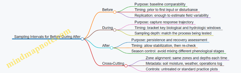
A Practical Interval Template
Use the same zone boundaries and sampling depths each time. Keep the number of samples manageable by prioritizing the most informative time points.
Template for a single growing season intervention
- Before: 2–4 weeks before the first application or tillage event.
- During: two points—one shortly after incorporation (about 1–2 weeks after) and one during peak root activity (often mid-season).
- After: two points—one after the main growth phase (late season) and one after harvest or dormancy onset (about 6–10 weeks after the late-season sample).
This structure captures early biological shifts, mid-season functional expression, and post-season persistence.
Example: Compost Biochar with Root-Driven Cover Crops
Assume compost biochar is applied and incorporated, followed by a cover crop that drives root exudation.
- Before: Sample at the same depths used for mapping (for instance 0–10 cm and 10–30 cm) two weeks before application. Record soil moisture at sampling time because it affects both microbial activity assays and water retention interpretation.
- During 1: Sample one week after incorporation. Expect changes in enzyme activity and labile carbon indicators to show up earlier than community composition.
- During 2: Sample at mid-season when roots are actively growing. This is when you’re most likely to see alignment between root analytics and rhizosphere microbial function.
- After 1: Sample near the end of the main growth phase. This checks whether the system is maintaining function rather than only reacting.
- After 2: Sample after harvest or when cover crop biomass is reduced. This tests whether the biological signal persists when root inputs decline.
If you only sampled “before” and “after 1,” you could miss the fact that early enzyme activity rose but later community function did not.
Example: Irrigation Scheduling Based on Water Retention Modeling
If the intervention is an irrigation schedule change derived from retention modeling, the interval plan should align with wetting events.
- Before: Sample after a comparable pre-irrigation period so baseline moisture and microbial conditions match across zones.
- During 1: Sample after the first two irrigation cycles under the new schedule. This is where infiltration and near-surface moisture dynamics begin to diverge.
- During 2: Sample after several cycles that include at least one drying phase. Water retention effects show up more clearly when the soil is allowed to drain and re-equilibrate.
- After: Sample at the end of the irrigation window, then again after a standardized rainfall or irrigation event that restores comparability.
Depth and Replication Choices That Affect Interval Value
Intervals are only as good as the sampling depth strategy. If you’re testing microbial inputs that act near the surface, include a shallow depth that responds quickly. If you’re testing structure and water retention, include a deeper depth that reflects pore connectivity and slower changes.
Replication should be consistent across time points. If you change the number of cores between “before” and “during,” you’ll confuse true change with measurement precision.
Minimum Viable Plan When Resources Are Tight
If you must reduce sampling frequency, keep the logic intact:
- Before: one baseline point.
- During: one point that coincides with peak root activity or after the first key wetting cycle.
- After: one persistence point late in the season.
This three-point plan can still support before/during/after comparisons, as long as you keep zones, depths, and handling consistent.
11.3 Statistical Approaches for Comparing Zones and Treatments
Comparing soil health zones and management treatments is mostly about answering one question: “Is the observed difference likely to be real, given the natural messiness of fields?” The messiness comes from spatial variability, sampling noise, and biological variation. A good analysis plan treats those sources explicitly instead of hoping the averages behave.
Start with the Comparison You Actually Need
Before choosing a test, write the comparison in plain language and decide what “success” means.
- Zone comparison: Are zone A and zone B different in soil moisture retention at 30–60 cm?
- Treatment comparison: Does compost plus inoculant outperform compost alone in enzyme activity?
- Interaction: Does the treatment work better in one zone than another?
A simple example: you apply a biological input to two zones. If treatment effects are similar in both zones, you care about treatment main effects. If the effect is strong in the low-retention zone but weak in the high-retention zone, you care about the zone-by-treatment interaction.
Choose a Model That Matches the Data Structure
Fields are not randomized lab benches. Samples taken near each other tend to be more similar than samples far apart, and repeated sampling across time creates correlation.
Common modeling choices
- Two-group or multi-group comparisons: Use ANOVA or linear models when assumptions are reasonable.
- Repeated measures: Use mixed-effects models when you sample the same plots over time.
- Spatial correlation: Use spatial terms or correlation structures when you have dense coordinates.
- Non-normal outcomes: Use transformations or generalized models when distributions are skewed or bounded.
A practical rule: if you have repeated sampling (before and after), avoid treating each time point as independent. Mixed models handle this without forcing you to throw away data.
Handle Replication Correctly
Replication can mean different things, and confusing them leads to false confidence.
- Experimental unit: The smallest unit that receives a treatment. If you apply inoculant to a whole management zone strip, individual cores within that strip are subsamples, not independent replicates.
- Biological replicate: Independent plots or strips receiving the same treatment.
- Technical replicate: Repeated lab measurements from the same sample.
Example: Suppose you have 4 strips per treatment and take 10 cores per strip. Your statistical replication is 4 per treatment, not 40. You can average cores within a strip for a primary analysis, or model within-strip variation if you have a clear structure.
Control Multiple Comparisons Without Killing Power
Soil datasets often include many variables: moisture at several depths, enzyme activity, microbial diversity indices, and retention parameters. Testing everything separately inflates the chance of false positives.
Use a correction strategy aligned with your goal:
- Family-wise error control: Conservative when you must limit any false positives across a set.
- False discovery rate control: More practical when you expect some true signals among many tests.
Example: You test 12 soil health indicators for treatment effects in one zone. If you use an unadjusted 0.05 threshold, you expect about 0.6 false positives by chance. With a false discovery rate approach, you reduce that inflation while still learning.
Use Effect Sizes Alongside P Values
A p-value answers “is it likely real?” but not “is it meaningful?” Effect sizes translate results into operational terms.
- For continuous outcomes: report difference in means or standardized differences.
- For retention parameters: report absolute change in water content at a target pressure head.
- For microbiome metrics: report change in diversity index or log-fold change in a functional proxy.
Example: If treatment increases plant-available water by 2% volumetric water content, that may be operationally relevant even if variability is high. If it increases by 0.2%, it probably isn’t.
Mind Map: Comparing Zones and Treatments
Worked Example with a Clear Decision
Imagine two zones (A and B) and two treatments (control and biological input). You sample enzyme activity and soil moisture at two times: before application and after application.
- Primary outcome: change from before to after for each plot.
- Model: a mixed-effects model with fixed effects for zone, treatment, and their interaction, plus random effects for plot.
- Interpretation:
- If treatment is significant and interaction is not, apply broadly.
- If interaction is significant, compare treatment effects within each zone.
- Reporting: provide the estimated change (with confidence intervals) for each zone-treatment combination.
This approach keeps the analysis aligned with the field reality: plots differ, time points correlate, and zones may change how treatments behave.
Diagnostics That Prevent Silent Failures
Even a correct model choice can fail if assumptions are badly violated.
- Check residual patterns versus fitted values.
- Inspect whether a few plots dominate the result.
- If outcomes are bounded (like proportions), verify the model respects that bound.
Example: If microbial diversity indices show strong skew, a transformation or a model that matches the distribution can stabilize inference. The goal is not mathematical perfection; it’s avoiding conclusions driven by a handful of extreme samples.
A Practical Summary for Field Teams
Use a model that matches your design (zones, treatments, time, and plot structure), treat the experimental unit correctly, control multiple comparisons by defining outcome families, and report effect sizes with units. If you do that, your comparisons become something you can act on, not just something you can argue about at the end of the season.
11.4 Interpreting Results With Confounding Controls and Covariates
Soil health and microbiome results rarely come from a single cause. Weather, soil texture, sampling depth, crop stage, residue management, and even how quickly samples reached the lab can all shift measurements. Interpreting results well means separating what you changed from what simply happened.
Foundational Idea: Distinguish Treatment Effects from Background Variation
Start by listing every factor that could influence your outcome variable, such as enzyme activity, microbial diversity, or water retention parameters. Then classify each factor:
- Confounders: linked to the treatment or management decision and also linked to the outcome.
- Covariates: measured variables that affect the outcome but are not necessarily caused by the treatment.
- Noise: unmeasured variation that still shows up in the data.
A practical example: if you apply a biological input only to zones that already look “better,” then zone quality becomes a confounder. Your microbiome shift might reflect starting conditions rather than the input.
Step 1: Build a Confounding Control Plan Before You Analyze
Use a simple checklist for each outcome.
- Timing: confirm sampling dates relative to irrigation, fertilization, and crop growth stage. If you sampled on 2026-03-20 and 2026-04-10, growth stage differences can matter even if the calendar dates look close.
- Depth and handling: ensure consistent depth intervals and consistent storage times.
- Spatial structure: recognize that nearby samples are more similar than distant ones.
- Management alignment: verify that treatments were applied according to the plan, not opportunistically.
When you cannot control a confounder, you can still measure it and include it as a covariate.
Step 2: Use Covariates That Actually Explain Variation
Good covariates are measurable, stable enough to quantify, and plausibly connected to the outcome.
- For microbiome outcomes, covariates often include soil moisture at sampling, soil organic carbon, pH, and sampling time since last irrigation.
- For water retention outcomes, covariates often include texture fractions, bulk density, and aggregate stability.
Example: Suppose enzyme activity increases after an input. If soil moisture at sampling also increased because of a different irrigation schedule, moisture is a covariate that can explain part of the enzyme change. Without accounting for it, you might attribute everything to the input.
Step 3: Choose an Analysis Strategy That Matches the Design
Match the method to how treatments and zones were assigned.
- Randomized or well-balanced designs: treatment comparisons are more direct.
- Zone-based or observational designs: you need stronger adjustment for baseline differences.
- Repeated sampling: include time or growth stage as a factor, and consider within-zone correlation.
A simple decision rule: if treatment assignment depends on baseline soil condition, treat baseline condition as a confounder and adjust for it.
Step 4: Interpret Adjusted Results with Effect Sizes, Not Just Significance
After adjustment, focus on:
- Direction: does the treatment increase the outcome where you expected?
- Magnitude: how large is the change relative to natural variability?
- Uncertainty: do confidence intervals overlap with zero or with a practically meaningful threshold?
Example: If diversity increases slightly but the interval is wide, the result may be real but not operationally useful. If enzyme activity increases consistently across zones with similar baseline moisture, that pattern is more convincing.
Step 5: Check Whether Adjustment Worked
Adjustment should reduce systematic bias, not just produce a new p-value.
- Compare baseline means between treated and control zones.
- Inspect residual patterns by depth, date, or location.
- Confirm that covariates are not acting as proxies for the treatment itself.
If treated zones were always sampled after a different irrigation event, then “time since irrigation” may be partially a treatment marker, not a neutral covariate.
Mind Map: Confounding Controls and Covariates
Example: A Zone-Based Biological Input Trial
Imagine two management zones: Zone A is applied with a compost-based input, Zone B is not. Zone A also has higher baseline organic carbon.
- Confounder: baseline organic carbon is linked to zone selection and influences microbiome outcomes.
- Covariates: include baseline organic carbon, pH, and soil moisture at sampling.
- Interpretation: if adjusted results show enzyme activity increases in Zone A beyond what baseline differences predict, you can attribute the change more confidently to the input.
Example: Handling Spatial and Depth Effects
If you sample multiple points within each zone and multiple depths, treat those as structured data.
- Nearby points share conditions, so independence is not guaranteed.
- Depth layers can have different microbial communities, so depth should be accounted for.
A good outcome interpretation states the level of inference: “within-zone comparisons after adjustment” is different from “across the whole farm without structure.”
Practical Takeaway
Confounding control is not a single step; it is a chain: define plausible bias sources, measure what you can, align analysis to the design, and interpret adjusted effects by magnitude and uncertainty. If the story still holds after those checks, your conclusion is likely to be the one your field data actually supports.
11.5 Reporting Templates for Farm Teams and Technical Stakeholders
A good report answers three questions fast: What changed, where it happened, and what to do next. The template should separate “field decisions” from “technical evidence” so each audience can scan without hunting.
Audience Split and Report Layers
Use a two-layer structure:
- Farm Team Layer: short, action-first, written for the people who will execute tasks.
- Technical Stakeholder Layer: methods, assumptions, uncertainty, and data lineage.
A simple rule keeps teams aligned: every action in the Farm Team Layer must point to a specific evidence item in the Technical Layer.
Farm Team Template
Report Header
- Farm name and field ID
- Reporting window (use a consistent date format)
- Responsible person and contact
- Sampling or measurement window (e.g., “Soil sampling: 2026-03-15 to 2026-03-18”)
1) Summary of What Changed
- Top 3 soil health or water-related findings by zone
- One sentence per finding describing the practical meaning
Example: “Zone B shows lower water retention at field-relevant depths, so it will dry faster after irrigation gaps.”
2) Zone Actions for This Cycle
Use a table so decisions are unambiguous.
| Zone | Evidence Snapshot | Action | Timing | Expected Outcome | Risk Check |
|---|---|---|---|---|---|
| A | Higher aggregate stability, moderate retention | Apply compost at standard rate | Pre-plant | Better infiltration and sustained moisture | Avoid over-application on already high OM |
| B | Lower retention, weaker structure | Split irrigation and add biological input | Early growth | Reduce stress during establishment | Confirm drainage after first irrigation |
3) Field Execution Checklist
- Equipment settings or application method
- Buffer zones and exclusion rules
- Who signs off after completion
Example: “Mark Zone B boundaries before application; verify spreader calibration on a short run; log actual application rate per pass.”
4) Monitoring Plan for This Cycle
- What will be checked weekly
- What triggers a corrective action
Example: “If soil probe readings drop below the zone threshold for two consecutive checks, adjust irrigation duration and re-check infiltration after the next event.”
Technical Stakeholder Template
1) Objective and Decision Link
- State the decision the report supports (e.g., “Zone-specific biological input rate selection”)
- List the evidence types used (soil properties, microbiome measures, root analytics, retention modeling)
2) Methods and Data Lineage
- Sampling design summary (depths, replication, handling)
- Lab assay list with units
- Microbiome workflow summary (what was sequenced, how reads were processed)
- Modeling approach for water retention (inputs, parameter sources)
3) Results by Zone With Uncertainty
For each zone, include:
- Key metrics and units
- Range or confidence interval where available
- A short interpretation tied to soil function
Example: “Zone B retention curve parameters indicate reduced plant-available water; uncertainty is higher where sampling density was lower.”
4) Evidence-to-Action Mapping
Create a trace table that links each action to the metric that justified it.
| Action | Metric | Threshold or Rule | Data Quality Note |
|---|---|---|---|
| Split irrigation | Modeled plant-available water | Below zone threshold | Higher variance in one depth layer |
| Biological input | Enzyme activity proxy and structure | Below target band | Confirmed with replicate agreement |
5) QA/QC and Deviations
- Any missing samples
- Any batch effects or instrument issues
- How deviations were handled
6) Appendix-Ready Outputs
- Map list (zone map, retention surface, sampling points)
- Raw summary tables
- Versioning notes for datasets and models
Mind Map: Reporting Components and Flow
Example: One-Page Report Layout
A practical one-page version can fit on a single sheet:
- Top: header and three findings
- Middle: zone action table
- Bottom: checklist and monitoring triggers
The technical layer can be a second page or a separate attachment, but the action table should remain identical in both versions so nobody wonders which numbers were used.
Example: Evidence-to-Action Rule Writing
Write rules in plain language:
- “If modeled plant-available water is below the zone threshold during establishment, split irrigation into two events separated by 48–72 hours.”
- “If aggregate stability is below the target band, prioritize structure-supporting inputs and avoid high-impact tillage during the same window.”
These rules reduce interpretation drift when multiple people contribute to execution and review.
12. Practical Protocols and Data Management for Reproducible Work
12.1 Standard Operating Procedures for Sampling and Storage
Purpose and Scope
A sampling and storage SOP exists to keep measurements comparable across time, people, and fields. If samples drift in temperature, moisture, or exposure to oxygen, the lab may measure the change instead of the soil. This SOP covers both routine soil properties and microbiome-ready samples, because the two often share collection steps but diverge at storage.
Core Principles
- Minimize time from collection to stabilization. Microbial communities shift quickly, especially at warm temperatures.
- Control temperature and oxygen exposure. Use coolers and sealed containers; avoid repeated warming.
- Separate sample types early. Soil for microbiome work should not be mixed with material intended for chemical or physical assays.
- Record metadata at the moment of collection. Notes made later are usually missing the details that matter.
Sampling Workflow from Field to Storage
Start with a checklist that matches your field plan: zone, depth, replicate, and target lab tests. Then follow a consistent sequence.
- Prepare materials before entering the field. Label tubes and bags with unique IDs, depth, date, and replicate. Pre-stage gloves, wipes, and sealable bags.
- Collect by depth using a clean tool strategy. Remove loose surface debris, then sample the target depth. Between samples, clean tools to reduce cross-contamination.
- Split samples immediately. For microbiome work, place a portion into sterile, airtight containers. For water retention or physical tests, keep the portion consistent with the lab’s requirements.
- Stabilize and cool promptly. Place microbiome containers into a cold chain device right away. Keep chemical/physical samples protected from heat and direct sun.
- Complete metadata capture. Record GPS or grid reference, crop stage, recent irrigation or rainfall, soil moisture feel, and any anomalies like stones or compaction.
Storage Rules That Prevent Common Failures
- Temperature control: Microbiome samples should remain cold from collection to the lab’s stabilization step. Chemical samples should avoid freezing unless the lab explicitly requests it.
- Moisture handling: Do not air-dry microbiome samples unless your lab protocol says so. For physical tests, follow the lab’s guidance on whether to preserve structure.
- Container integrity: Use containers that seal tightly. Replace lids or bags that show poor closure.
- Avoid freeze–thaw cycles: Repeated temperature swings can change microbial viability and DNA integrity.
Example: Two Sample Types from One Depth
Suppose you sample 0–10 cm in three management zones.
- Replicate A microbiome: 10–20 g into a sterile tube, sealed, placed in the cold chain immediately.
- Replicate A chemistry: a separate portion into a labeled bag, protected from heat, delivered according to lab timing.
- Replicate A physical: a portion reserved for structure-sensitive tests, kept consistent with the lab’s handling instructions. This split prevents one sample’s storage conditions from contaminating another sample’s intended measurement.
Mind Map: Sampling and Storage SOP
Chain of Custody and Verification
Before leaving the field, verify that every container ID matches the sampling sheet. At handover, confirm counts per depth and zone, and note any deviations like delayed cooling or damaged seals. If a deviation occurs, record it in the same place every time so the lab can interpret results consistently.
Example: Handling a Cooling Delay
If the cooler warms for a short period due to an unexpected schedule change, document the approximate duration and ambient conditions. Do not “fix” the sample by guessing; instead, flag it so the lab can decide whether to proceed, reprocess, or treat the sample as compromised.
Acceptance Criteria for Sample Readiness
A sample is ready for lab processing when: IDs are legible and unique, containers are sealed, storage conditions match the lab’s requirements, and metadata fields are complete for zone, depth, and collection timing. If any one of these fails, treat the sample as a data quality issue, not as a minor inconvenience.
Quick Field Checklist
- Labels match sampling sheet
- Tools cleaned between samples
- Microbiome portion sealed and cooled immediately
- Chemistry portion protected from heat
- Metadata recorded on site
- Counts verified before leaving
12.2 Bioinformatics and Data Processing Workflows for Microbiome Outputs
Microbiome outputs usually arrive as raw sequencing reads plus sample metadata. The goal of this section is to turn those reads into stable, comparable tables that can be mapped to soil health zones and linked to water-retention and root analytics. The workflow below is systematic: it starts with data integrity checks, then moves through quality filtering and feature inference, and ends with outputs that are ready for statistical modeling.
Foundational Inputs and Naming Rules
Start by standardizing what you already have. Each sample should have a unique ID that matches across sequencing files, lab metadata, and field maps. A simple convention prevents many downstream headaches: Farm_Block_Zone_Depth_SampleDate_Replicate. If you collected on 2026-03-20, keep that date format consistent across all files.
Also decide early what “feature” means for your analysis. Common choices are:
- Amplicon sequence variants (ASVs) for fine-grained resolution.
- Operational taxonomic units (OTUs) for coarser clustering.
- Functional profiles inferred from marker genes or metagenomic reads.
For soil microbiome engineering, ASVs are often easier to interpret when you want to compare zones and treatments without forcing an arbitrary similarity threshold.
Mind Map: End-to-End Microbiome Processing
Step 1: Read Integrity and Metadata Alignment
Before any trimming, confirm that every sample has both read files (for paired-end) and that file sizes are plausible. Then check that metadata fields used later—zone, depth, extraction batch, and replicate—are complete. If a sample lacks zone assignment, it should not silently enter the pipeline; it should be flagged so you can decide whether to exclude it or fix the metadata.
A practical example: suppose Block B has Zone 3 at 0–10 cm and 10–20 cm. If one depth is mislabeled in metadata, your downstream zone comparisons will look like “biology,” when it’s really a labeling error.
Step 2: Quality Filtering and Primer/Adapter Trimming
Quality filtering should be explicit and consistent across all samples. Typical actions include:
- Remove adapters and primers.
- Trim low-quality ends using a fixed quality threshold.
- Drop reads below a minimum length.
Paired-end reads should be merged only when overlap is sufficient; otherwise, you risk generating chimeric artifacts. If you use negative controls (extraction blanks), keep them through filtering so you can later identify features that appear only in controls.
Step 3: Feature Inference and Error Handling
For ASV workflows, the core idea is to model sequencing errors so that true biological variants are separated from artifacts. This step produces a feature table where rows are ASVs and columns are samples.
Example of why this matters: two samples may differ by a single nucleotide in a low-abundance feature. If you cluster too aggressively, that difference disappears; if you keep everything without error modeling, you may treat sequencing noise as real variation.
Step 4: Taxonomic Assignment with Confidence
Assign taxonomy using a reference database and record confidence. Keep unassigned features rather than forcing a guess, because unassigned reads can still be useful for relative comparisons across zones. When you later map features to soil health metrics, you can decide whether to analyze at the ASV level, genus level, or both.
Step 5: Build Tables That Survive Statistical Modeling
You typically need three linked outputs:
- Count table (ASV/OTU counts per sample).
- Relative abundance table (counts normalized by sample totals).
- Metadata-linked table (counts plus zone, depth, treatment, batch).
Filtering rare features is not just housekeeping. If a feature appears in only one sample with a handful of reads, it can inflate noise in distance calculations and differential tests. A common approach is to remove features below a minimum prevalence threshold (for example, present in at least a small number of samples) while documenting the rule.
Step 6: Normalization Choices and Diversity Calculations
Different analyses require different normalization strategies:
- Alpha diversity often uses metrics that depend on richness and evenness; ensure you handle varying sequencing depths consistently.
- Beta diversity uses distance measures; choose one that matches your interpretation needs and document it.
- Differential abundance methods should account for compositional effects and sampling depth.
Example: if one zone consistently has lower read counts due to extraction yield, diversity comparisons can be biased unless you control for sequencing depth or use an analysis method designed for count data.
Step 7: Outputs for Zone Mapping and Root-Water Integration
To connect microbiome outputs to drought-resilient decisions, convert sample-level results into zone-level summaries:
- Zone-level feature abundance summaries (mean or median across replicates).
- Diversity summaries per zone and depth.
- Feature lists that correlate with water-retention parameters or root traits.
Include an uncertainty flag for each zone summary based on replicate count and filtering thresholds. That way, when you later interpret patterns against water-retention modeling, you know which differences are supported by enough data to be taken seriously.
Minimal Processing Checklist
- Confirm sample IDs match metadata and map layers.
- Trim adapters and primers consistently.
- Use error modeling for ASVs or a documented clustering rule for OTUs.
- Keep controls through filtering and use them to identify contaminants.
- Produce count, relative abundance, and metadata-linked tables.
- Apply documented feature filtering and normalization.
- Summarize results at zone and depth for integration with soil and root analytics.
12.3 Geospatial Data Management Including Versioning and Metadata
Geospatial soil health mapping only works as well as the data trail behind it. Versioning and metadata are the boring parts that keep your maps from quietly drifting out of sync with the field reality they describe. This section gives a practical system you can run with a small team and a modest budget.
Foundational Concepts for Reliable Geospatial Records
Start by separating three ideas: the data, the meaning, and the history.
- Data is the geometry and measurements: points, polygons, rasters, attributes.
- Meaning is what those values represent: units, sampling depth, lab method, date, and quality flags.
- History is how the dataset changed: who edited it, when, why, and what was replaced.
A dataset without meaning becomes a pile of numbers. A dataset without history becomes a mystery. A dataset without both becomes a map that looks confident but can’t be trusted.
Metadata That Answers the Questions People Actually Ask
Use a metadata checklist that covers the full lifecycle: collection, processing, and delivery.
Minimum Metadata Fields
For each geospatial layer (e.g., sampling points, management zones, soil property rasters), capture:
- Coordinate reference system (CRS) and transformation steps.
- Spatial resolution for rasters and buffer rules for zone boundaries.
- Temporal scope for sampling and any resampling or aggregation windows.
- Depth convention (e.g., 0–10 cm, 10–30 cm) and whether values are averages or composites.
- Units for every numeric attribute.
- Provenance for measurements: lab ID, method, and any pre-processing.
- Quality flags: missingness rules, outlier handling, and replicate logic.
Example Metadata Snippet
A sampling point layer should clearly state whether “SOC” is measured on a dry-weight basis, and whether it represents a single core or a composite of multiple cores.
Versioning Strategy That Prevents Map Drift
Versioning is not just “saving copies.” It is making changes traceable and reversible.
Version Levels
Use three levels of versioning:
- Dataset version for the raw inputs (e.g., lab results table, field GPS points).
- Processing version for the derived products (e.g., interpolated rasters, zone maps).
- Publication version for the final deliverables used in decisions.
When you change any processing rule—like interpolation method, variogram model, or masking boundary—increment the processing version even if the dataset name stays the same.
Change Log Rules
Each version should include:
- Change summary in plain language.
- Affected layers (which rasters or tables).
- Reason (e.g., corrected CRS, updated lab batch, removed a bad replicate).
- Compatibility note (whether downstream layers must be regenerated).
A simple rule helps: if a person can’t reproduce the new output from the old inputs and the stated processing steps, treat it as a new processing version.
Data Packaging for Repeatable Workflows
Package geospatial outputs with a consistent folder structure so your future self doesn’t have to play detective.
- /raw: original GPS points, lab exports, field notes scans.
- /processed: cleaned tables, harmonized units, intermediate rasters.
- /products: final rasters, zone polygons, summaries.
- /metadata: machine-readable metadata files and human-readable readme.
- /logs: processing scripts run logs and error reports.
Include a “manifest” file listing every layer, its version, CRS, and the metadata file it points to.
Mind Map: Geospatial Data Management System
Example: Versioning a Zone Map After a CRS Fix
Suppose you discover that the sampling points were imported with the wrong CRS. The temptation is to “just reproject and move on.” Instead:
- Create a new dataset version for the corrected point layer.
- Re-run the processing pipeline and create a new processing version for interpolations and zone boundaries.
- Publish a new publication version for the management zone map.
In the change log, record the CRS correction and explicitly state that all downstream products were regenerated. This prevents someone from comparing an old zone map to a new raster and concluding the field changed when it didn’t.
Example: Metadata for a Depth Composite
If you combine 0–10 cm and 10–30 cm cores into a single “root-zone composite,” metadata must say:
- how the composite was computed (mean, weighted mean, or selected depth),
- whether replicates were averaged before or after compositing,
- and what the composite represents for modeling water retention.
That detail matters because water retention parameters are depth-sensitive, and root analytics often assume a specific depth window.
Practical Checklist for Each New Geospatial Product
Before you hand a map to a field team, verify:
- CRS is correct and stated.
- Units and depth conventions match the modeling assumptions.
- Metadata exists for every layer.
- Version numbers and change logs are updated.
- A manifest links products to the exact inputs used.
If you can answer these five points quickly, your geospatial outputs will stay consistent across sampling rounds, lab batches, and processing updates.
12.4 Modeling Data Pipelines for Water Retention and Uncertainty
Water-retention modeling only works as well as the pipeline that feeds it. A good pipeline turns raw measurements into consistent inputs, tracks assumptions, and produces uncertainty that you can interpret on the farm without needing a statistics degree.
Foundations of a Water-Retention Pipeline
Start with a single modeling goal: predict available water or infiltration-relevant moisture behavior for specific management zones. Then define the model form you will use (for example, a retention curve such as van Genuchten or Brooks-Corey) and the outputs you need (field moisture at target tensions, plant-available water, or water content at irrigation thresholds).
A practical pipeline has five stages:
- Ingest soil property data and metadata.
- Standardize units, depths, and sample identifiers.
- Fit retention parameters per sample or per zone.
- Propagate uncertainty from measurements to parameters to outputs.
- Validate with held-out samples and sanity checks.
Data Standardization That Prevents Silent Errors
Unit mismatches are the most common “it runs but it’s wrong” failure. Standardize early: moisture as volumetric water content (m³/m³), tension as kPa (or convert to consistent units), and depth as meters with a clear convention for top and bottom.
Depth handling deserves explicit rules. If you have lab cores at 0–10 cm and 10–20 cm, do not average them into 0–20 cm without recording the method. If you must aggregate, use a depth-weighted approach based on layer thickness and report the aggregation rule in metadata.
Parameter Fitting with Uncertainty, Not Just Best Fits
For each sample, fit retention parameters using the measured tension–water content pairs. Keep the raw pairs and the fitted curve together so you can later diagnose poor fits.
Uncertainty should include at least three sources:
- Measurement noise in water content and tension.
- Model mismatch when the chosen curve form cannot represent the data.
- Sampling variability when you later summarize to zones.
A simple approach is to use a bootstrap: resample the measured pairs within their plausible error bounds, refit parameters many times, and compute distributions for each parameter. This yields credible ranges for predicted water content at target tensions.
Propagating Uncertainty Through Outputs
Once you have parameter distributions, compute uncertainty for outputs such as plant-available water (PAW). For each bootstrap draw, calculate PAW, then summarize the resulting distribution (median and interval). This produces an uncertainty band you can map.
When you aggregate from samples to zones, propagate uncertainty again. If you average predicted PAW across multiple samples, combine both within-sample parameter uncertainty and between-sample variability. Otherwise, you’ll underestimate uncertainty and overtrust the map.
Mind Map: Pipeline Components and Flow
Example: From Lab Curves to Zone PAW with Uncertainty
Assume you measured tension–water content at 33, 100, 300, and 1500 kPa for multiple cores in a management zone. You fit parameters per core, then compute water content at 100 and 1500 kPa. PAW is the difference between these water contents.
To keep it concrete, do the following:
- For each core, generate 500 bootstrap fits by perturbing water content within lab repeatability and refitting.
- For each bootstrap draw, compute PAW at 100 and 1500 kPa.
- For the zone, summarize PAW across cores by taking the median of core medians and the interval from the combined distribution.
The result is not just “PAW = 85 mm,” but “PAW = 85 mm with an interval,” which helps you decide how conservative to be when irrigation timing is tight.
Example: Uncertainty Flags That Matter in Practice
Not all uncertainty is equal. Use QA flags to separate “uncertainty from measurement” from “uncertainty from bad data.” For instance:
- If a sample has missing tension points, mark it as incomplete and widen uncertainty.
- If residuals show systematic bias (curve consistently above observations at mid-tensions), flag model mismatch and consider a different curve form.
- If bulk density is inconsistent with texture expectations, treat derived saturation-related parameters as uncertain.
Diagram: End-to-End Pipeline with Checks
    flowchart TD
  A[Ingest lab tension–water data] --> B[Standardize units and depth]
  B --> C[QA filtering and metadata validation]
  C --> D[Fit retention parameters per sample]
  D --> E[Bootstrap uncertainty for parameters]
  E --> F[Compute outputs per draw]
  F --> G[Aggregate sample outputs to zones]
  G --> H[Propagate uncertainty to zone intervals]
  H --> I[Validate with held-out samples]
  I --> J[Export outputs and uncertainty maps]
Implementation Notes for Reproducibility
Treat the pipeline like a recipe with labeled ingredients. Every run should record:
- Which curve form was used.
- The exact unit conversions.
- The bootstrap settings and error assumptions.
- The QA rules for excluding or down-weighting points.
- The validation split used for held-out checks.
If you do this consistently, you can rerun the pipeline after adding one more lab batch and still know whether changes come from new data or from altered assumptions. That’s the difference between a model you can trust and a model you can only admire.
12.5 Building a Field Notebook and Digital Record System for Auditability
A good field notebook does two jobs at once: it captures what happened while it is happening, and it preserves enough context that someone else can reconstruct the logic later. Auditability is mostly about traceability—who did what, where, when, with which inputs, and how the data were handled.
Core Principles for Auditability
- One event, one record. Treat each sampling, application, measurement, or observation as a discrete event with a unique identifier.
- Metadata is not optional. Soil and microbiome work fails quietly when depth, timing, moisture conditions, or equipment settings are missing.
- Reproducibility beats perfection. You do not need fancy prose; you need consistent fields and clear links between paper notes, photos, lab IDs, and map layers.
- Version control for decisions. When you change a plan (for example, switching sampling depth after encountering roots), record the reason and the date.
Field Notebook Structure That Works in Real Life
Use a two-layer approach: a compact paper notebook for immediate capture, and a digital system for structured storage.
Paper Layer
- Event header: Event ID, date, field block or management zone, operator initials.
- Location: GPS point or boundary reference, plus a short description (e.g., “north edge of zone 3 near drainage swale”).
- Method: Sampling tool, depth range, number of subsamples, composite rule, and any deviations.
- Observations: Soil moisture feel, residue cover, visible roots, weather notes, and anything that could affect microbial activity.
- Outputs: Sample IDs written exactly as they appear on labels.
Digital Layer
- Structured form: Mirrors the paper header and method fields.
- Attachments: Photos, scan of handwritten pages, and instrument readouts.
- Data links: Maps to lab submission IDs, sequencing run IDs, and modeling dataset versions.
Mind Map: Field Notebook and Digital Record System
Event ID and Sample ID Conventions
A simple convention prevents most audit headaches. For example:
- Event ID:
FARM-YYYYMMDD-ZZ-### - Sample ID:
S-EventID-Depth-Rep
Example: On 2026-03-20, zone 04, third sampling event.
- Event ID:
FARM-20260320-04-003 - Depth 0–10 cm composite:
S-FARM-20260320-04-003-0-10C-COMP - Depth 10–30 cm replicate 1:
S-FARM-20260320-04-003-10-30C-R1
Keep IDs consistent across labels, photos, lab forms, and digital entries. If you must rename something, record the mapping from old ID to new ID.
Minimum Data Checklist for Each Event
Use the same checklist every time.
- Location: GPS coordinate or zone polygon reference.
- Depth: Exact depth interval and sampling depth method.
- Replicates and composites: Number of subsamples and composite rule.
- Handling: Storage temperature, container type, time from collection to storage.
- Contamination controls: Gloves changes, tool cleaning, and blank controls if used.
- Deviations: What changed and why.
- Evidence: Photo(s) showing sampling point and tool setup.
Integrated Example: Sampling and Chain of Custody
A field team collects microbiome samples in two depths.
- Paper notebook: writes Event ID, zone, depth intervals, and the exact Sample IDs.
- Digital form: repeats the same fields and adds storage details (cooler temperature, time stamps).
- Evidence: uploads one photo per sampling point and one photo of the labeled sample rack.
- Lab submission: records the lab submission ID and the list of Sample IDs shipped.
If a sample label smears and must be reprinted, the digital record notes the original unreadable ID, the corrected ID, and the reason. The lab receives only the corrected ID, but the audit trail still shows what happened.
Mind Map: Data Validation and Freeze Points
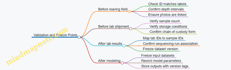
Practical Templates for Consistency
Create three short templates and reuse them.
- Sampling Event Template with required fields and a deviations section.
- Application Event Template with product, rate, placement method, weather, and incorporation details.
- Measurement Template for instruments with calibration notes and units.
A template is not bureaucracy; it is a way to stop important fields from being forgotten when the day gets busy.
Audit-Friendly Habits
- Write immediately, type later. Handwritten notes capture reality; digital entries standardize it.
- Use a single “source of truth” per field. If the digital form is the source for depth, do not let a spreadsheet silently override it.
- Freeze versions after review. Once a dataset is used for mapping or modeling, record the version and stop editing the underlying raw files.
When these pieces are in place, auditability becomes straightforward: every soil sample and every decision has a trail, and the trail is readable by someone who was not standing in the field with you.