Fertilizer Manufacturing Foundations
1. Fertilizer Systems, Product Forms, and Manufacturing Interfaces
1.1 Fertilizer Roles in Crop Nutrition and Soil Fertility Management
Fertilizers exist to fix a mismatch: crops need nutrients in specific forms and timing, while soils often supply them slowly, unevenly, or not at all. A good fertilizer plan treats nutrients as a system—what the plant can use, what the soil can hold, and what the weather can wash away.
Crop Nutrition: What the Plant Actually Uses
Plants require essential nutrients for structure, energy, and regulation. Nitrogen supports leaf growth and chlorophyll formation; phosphate supports root development and energy transfer; potash supports water regulation and enzyme activity. The key detail is “available to the plant.” A nutrient can be present in soil yet still be unavailable due to chemical form, soil pH, or physical conditions.
Availability depends on three practical factors:
- Chemical form: Phosphate, for example, can bind to soil minerals and become less soluble. Nitrogen can be lost as gas if conditions favor conversion.
- Timing: Roots take up nutrients when they are actively growing. If nutrients arrive too early or too late, the plant may not benefit.
- Placement and contact: Nutrients near the root zone are easier to access than nutrients scattered far away.
A simple example: if a field receives a heavy nitrogen dose right before heavy rain, much of it may move beyond the root zone before the crop can use it. The same total nitrogen applied in smaller, well-timed portions often performs better.
Soil Fertility: What the Soil Can Provide and Buffer
Soil fertility is not just nutrient content; it is the soil’s ability to store nutrients and release them gradually. Organic matter improves this buffering by holding nutrients and supporting microbial activity. Clay minerals can retain cations like potassium, while soil chemistry influences phosphate binding.
Soil fertility management focuses on maintaining a workable balance:
- Nutrient supply: Enough nitrogen, phosphate, and potash to meet crop demand.
- Soil chemical conditions: pH affects phosphate availability and nutrient interactions.
- Physical conditions: Compaction and poor drainage limit root growth, reducing nutrient uptake.
A practical example: two fields with the same measured phosphate level can behave differently. One soil may be more acidic, causing phosphate to bind tightly, while the other may release phosphate more readily.
The Nutrient Triangle: Nitrogen, Phosphate, and Potash Together
These nutrients interact in ways that matter for fertilizer decisions.
- Nitrogen and phosphate: Strong nitrogen growth increases demand for phosphate because roots and energy systems must keep up. If phosphate is limiting, nitrogen can’t translate into yield.
- Nitrogen and potash: Potash supports water regulation, helping plants tolerate stress. When potassium is low, nitrogen-driven growth can become fragile under heat or drought.
- Phosphate and soil chemistry: Phosphate availability is sensitive to pH and soil mineral composition, so “more phosphate” is not always “more uptake.”
Integrated best practice is to match nutrient rates to crop needs and soil test results, then choose product forms and application methods that fit the soil’s behavior.
Mind Map: Fertilizer Roles in Crop Nutrition and Soil Fertility
Example: Turning Soil and Crop Needs Into a Fertilizer Strategy
Suppose a crop requires 120 kg/ha nitrogen, 60 kg/ha P2O5, and 80 kg/ha K2O. Soil tests show moderate phosphate but low potassium, and the field has a history of heavy rainfall.
A systematic approach would:
- Use soil test values to estimate what the soil can supply so fertilizer targets the remaining need.
- Split nitrogen applications to reduce loss risk and align with crop uptake stages.
- Prioritize potassium where it is limiting, because potassium supports stress tolerance and consistent uptake.
- Apply phosphate in a way that improves contact with soil so it can become available in the rooting zone.
The result is not just “adding nutrients,” but managing the pathway from soil to root to plant performance.
Quick Check: Common Failure Points
Even well-chosen fertilizer products can underperform if the plan ignores basics:
- Nutrients applied at the wrong time relative to crop growth.
- Placement that leaves nutrients too far from roots.
- Soil pH that locks phosphate into less available forms.
- Physical constraints like compaction that prevent roots from accessing nutrients.
Fertilizer manufacturing may focus on nutrient content and product quality, but field success depends on how those nutrients behave once they meet soil and plants.
1.2 Common Fertilizer Product Forms: Granules, Prills, Solutions, and Blends
Fertilizer product form is not a cosmetic choice. It controls how nutrients dissolve, how evenly they spread, how safely they store, and how reliably they feed into application equipment. The same nutrient chemistry can behave very differently once it is packaged as a prill, a granule, a solution, or a blend.
Granules
Granules are solid particles engineered for strength and controlled size. They are typically produced by granulation routes such as drum or pan granulation, or by prilling followed by agglomeration. Granules matter because they resist crushing during handling, which reduces dust and helps maintain consistent nutrient delivery.
A practical way to think about granules is to separate three jobs: forming, drying, and conditioning. Forming sets the particle shape and initial composition. Drying removes water so the product does not cake in storage. Conditioning adjusts surface moisture and sometimes adds anti-caking treatment so particles flow through hoppers.
Example: A plant producing a urea-based granule targets a narrow size range so a spreader can meter it consistently. If the granules are too fine, they generate dust and can bridge in bins. If they are too large, they segregate during transport and create uneven field application.
Prills
Prills are solid particles formed by dropping molten material into a tower where it cools and solidifies into small spheres. The tower height and air flow determine cooling rate, which influences internal structure and hardness. Prills are common for products like urea and ammonium nitrate derivatives because the process can be continuous and scalable.
Prills tend to be more uniform in shape than many granules, but they can be more sensitive to moisture uptake depending on the chemistry and surface properties. That means storage design and anti-caking strategy are not optional.
Example: If prills of a hygroscopic product are stored in a humid warehouse, they can absorb moisture, form surface tackiness, and then stick together. The result is caking, which increases application variability because clumps do not break apart reliably.
Solutions
Solutions are nutrient dissolved in water, often used where rapid availability is desired or where application equipment can handle liquids efficiently. The key engineering variables are concentration, viscosity, and corrosion control. Unlike solids, solutions do not require drying, but they do require careful containment and materials selection.
A useful mental model is that solutions trade particle handling problems for system integrity problems. Instead of dust and caking, you manage corrosion, scaling, and freezing risk. Compatibility also matters: mixing different nutrient solutions can change pH and ionic strength, which can trigger precipitation.
Example: A fertilizer solution containing phosphate can form insoluble solids if mixed improperly with certain cations. In practice, operators control mixing order, temperature, and final composition to keep everything dissolved.
Blends
Blends combine nutrients in a single product, usually by physical mixing of finished solids or by granulating multiple nutrient sources together. Physical blends are simpler: you combine components like nitrogen and phosphate granules to meet an N-P-K target. Granulated blends create a more integrated particle where nutrients are co-located, which can improve uniformity during spreading.
The main challenge for blends is segregation. If components differ in particle size, density, or surface moisture, they can separate during transport and handling. That separation shows up on the field as inconsistent nutrient ratios.
Example: Suppose a blend contains a denser potassium chloride component and a lighter phosphate granule. During loading, the denser material can settle, so the first bags applied may be richer in potash than later bags. A good blending process uses controlled feed rates, adequate mixing time, and sometimes granulation to reduce segregation.
Mind Map: Product Forms and Their Practical Consequences
Example: Choosing a Form for a Specific Handling Reality
Imagine a distributor with bulk storage and bagging lines. A solid form with good flow properties reduces downtime from bridging and lowers dust cleanup. If the warehouse is humid, the choice shifts toward products with better moisture resistance and stronger conditioning. If the customer applies through liquid injection equipment, a solution can reduce solid handling and speed nutrient availability, provided corrosion and precipitation risks are controlled.
Summary: How Form Connects Chemistry to Field Performance
Granules and prills convert nutrient chemistry into particles that meter and spread predictably, with moisture behavior as the main storage constraint. Solutions convert chemistry into dissolved nutrients that act quickly, with corrosion and compatibility as the main system constraints. Blends combine nutrients into a single application target, with segregation control as the main quality constraint. When these constraints are managed, the product form becomes a reliable bridge between manufacturing and agricultural use.
1.3 Manufacturing Pathways by Nutrient: Nitrogen, Phosphate, and Potash
Fertilizer manufacturing is easier to understand when you group it by the nutrient you’re targeting. Nitrogen, phosphate, and potash each start from different feedstocks, use different reaction families, and end up with different product handling needs. The plant layout follows those choices: where you need high-pressure synthesis, where you need acid digestion and filtration, and where you need dissolution and crystallization.
Nitrogen Pathways
Most nitrogen fertilizer production centers on making ammonia first, because ammonia is the common “hub” for many downstream products. The core logic is: convert a carbon-containing feedstock into hydrogen, combine hydrogen with nitrogen from air, then condition and purify the gases so the synthesis loop runs steadily.
A typical pathway begins with hydrogen production (often from natural gas via reforming). The gas is cleaned to remove carbon oxides and other contaminants, then fed to an ammonia synthesis loop. Inside the loop, nitrogen and hydrogen react over a catalyst under elevated pressure and temperature. The product stream is condensed to separate ammonia from unreacted gases, and the unreacted portion is recycled.
Downstream, ammonia becomes urea, ammonium nitrate, or ammonium-based salts. Urea production uses a controlled conversion step followed by concentration and solidification. Ammonium nitrate production uses neutralization and concentration, then solidification or prilling/granulation depending on the grade. Each downstream route has a “quality bottleneck”: urea needs biuret control and moisture management; ammonium nitrate needs careful concentration control and safe solidification.
Example: If a plant targets a urea grade with tight biuret limits, the operator focuses on reaction conditions and residence time in the conversion step, then verifies concentration before prilling or granulation. A small drift in concentration can shift the solidification behavior and indirectly affect impurity distribution.
Phosphate Pathways
Phosphate manufacturing is built around turning phosphate rock into a usable form of phosphorus, usually by acidulation. The foundational choice is the acid route: sulfuric acid for the wet-process pathway. The logic is: grind and slurry the rock, react it with acid to dissolve phosphate, then separate the liquid product from the insoluble residue.
In the wet-process, phosphate rock is beneficiated and prepared as a slurry. Sulfuric acid reacts with the rock minerals, producing phosphoric acid in solution and generating a solid byproduct (often called phosphogypsum). Filtration removes the solids, and the clarified phosphoric acid is purified to reduce impurities that would otherwise cause poor crystal quality or corrosion issues.
Next comes concentration and product formation. Phosphoric acid is concentrated to the desired strength, then converted into MAP (monoammonium phosphate), DAP (diammonium phosphate), or other grades through neutralization with ammonia and controlled crystallization. Particle formation is not just a mechanical step; it determines how the fertilizer dissolves in soil and how it resists caking during storage.
Example: When producing MAP, the plant controls the neutralization ratio and the crystallization conditions so the product forms the intended crystal structure. If the slurry is too concentrated too early, you can get inconsistent crystal growth and wider particle size distribution, which then shows up as segregation in bulk storage.
Potash Pathways
Potash manufacturing typically starts with mined salts and ends with potassium chloride (KCl) or potassium sulfate products. The core logic is: dissolve the potassium-bearing salts, remove insolubles, then crystallize the potassium salt while managing mother liquor recycle.
In many operations, ore is mined and prepared, then dissolved in water to form a brine. Insoluble materials are removed by clarification and filtration. The brine is then processed through crystallization where KCl forms crystals and is separated from the remaining liquid. Mother liquor is recycled to improve overall recovery and to reduce waste streams.
Impurity management is central because chloride, sulfate, and other salts influence both product spec and downstream handling. Drying and finishing steps must also prevent caking and control moisture, since KCl is sensitive to storage conditions.
Example: If chloride spec is tight for a potassium sulfate product, the operator pays attention to brine composition and separation efficiency. A small reduction in filtration performance can carry more unwanted salts into the crystallizer feed, increasing the burden on washing and conditioning.
Integrated View of Plant Logic
Across all three nutrients, the “pathway” is really a chain of decisions: feedstock preparation, reaction family, separation strategy, and solid handling. Nitrogen emphasizes gas conditioning and synthesis loops; phosphate emphasizes acid digestion, filtration, and controlled crystallization; potash emphasizes dissolution, clarification, and crystallization with recycle.
How to Read a Plant Flowchart
When you look at a fertilizer plant diagram, identify the nutrient “hub” first: ammonia for nitrogen, phosphoric acid for phosphate, and potassium brine for potash. Then trace the separation step that follows the main reaction family. That separation step usually determines the quality bottleneck—biuret and moisture for urea, crystal quality and impurity levels for MAP/DAP, and washing efficiency and moisture control for KCl.
Example: If a flowchart shows a large filtration train after acidulation, that’s a phosphate signature. If it shows a synthesis loop with recycle and condensation, that’s nitrogen. If it shows dissolution, clarification, and crystallizers with mother liquor recycle, that’s potash. Once you spot the pattern, the rest of the equipment choices start making sense.
1.4 Process Integration Points: Feedstock Handling, Utilities, and Product Packaging
A fertilizer plant is a chain of “handoffs.” If the handoff is sloppy, the chemistry may still run, but the product spec won’t. This section connects three integration points—feedstock handling, utilities, and product packaging—so each upstream choice supports downstream quality, safety, and throughput.
Feedstock Handling Integration
Feedstock handling starts with the question: what form enters the plant, and what form must leave each unit? For nitrogen routes, ammonia or synthesis gas may arrive as pressurized streams; for phosphate, rock and acid components arrive as solids and liquids; for potash, brine or ore slurry arrives with dissolved and suspended impurities.
A practical integration approach uses three layers of control.
First, define acceptance criteria at receiving. For solids, this includes moisture, particle size, and insoluble content; for liquids, it includes density, acidity, and conductivity; for gases, it includes oxygen and sulfur contaminants that can poison catalysts or foul equipment. A simple example: if phosphate rock has higher-than-expected moisture, the slurry concentration target becomes harder to maintain, which can shift filtration performance and downstream crystal quality.
Second, design transfer lines and storage to prevent “spec drift.” Moisture pickup is a common culprit for hygroscopic materials. If you store a fertilizer intermediate in a humid warehouse without sealed silos, the next day’s batch may behave like a different product. The fix is not just better storage; it’s also consistent headspace conditions, venting strategy, and transfer procedures.
Third, integrate sampling and traceability. Sampling points should match where variability actually enters the process. If you sample only at the receiving dock but the material is blended in a reclaim hopper, you may miss the blend shift. A good rule is to sample after any major mixing or size adjustment step.
Utilities Integration
Utilities are the plant’s “shared nervous system.” Steam, cooling water, compressed air, electricity, and instrument air must be sized and managed so they don’t become hidden bottlenecks.
Begin with a utility map that links each unit operation to its utility demand and quality requirements. For example, steam quality matters: some steps need dry steam for evaporation, while others tolerate lower quality. Cooling water temperature affects crystallization and condensation; if cooling water warms during peak demand, you may see slower heat removal and altered crystal size distribution.
Then integrate utility control with process control. A common best practice is to use pressure and temperature control loops that protect equipment and stabilize product. Consider a urea or ammonium nitrate concentration step: if steam pressure fluctuates, the evaporator duty changes, and the solution may reach target concentration at a different time, changing impurity concentration and viscosity. The plant can compensate, but only if the control strategy accounts for utility variability.
Finally, plan for maintenance without breaking the chain. If a critical pump is down, you need a bypass or a controlled shutdown sequence that keeps upstream tanks from overflowing and downstream units from starving. Reliability integration is often more about valves, interlocks, and operating procedures than about adding more equipment.
Product Packaging Integration
Packaging is not an afterthought; it is the final process step that locks in moisture, particle integrity, and handling safety.
Start by aligning packaging format with product behavior. Granular products need drying and conditioning to reach a stable moisture level that resists caking during storage. If you package a product that is slightly too wet, it may still meet lab specs at packaging time but fail bulk handling later due to caking and reduced flowability.
Next, integrate dust and segregation control. Conveying from dryer to screen to bagging or bulk loading can create fines generation and segregation if particle size distribution shifts. A simple example: if screening removes too many fines before coating, the remaining particles may be larger and flow differently, causing inconsistent dosing in blend operations.
Then ensure packaging equipment matches the logistics plan. Bagging systems require consistent bulk density and particle size distribution to avoid underfilling. Bulk loading requires venting and dust capture to prevent pressure buildup and worker exposure. Storage integration matters too: pallet wrap and warehouse humidity control influence moisture uptake, especially for phosphate and nitrogen-containing products.
Mind Map: Integration Points
Example: One Change, Three Impacts
Suppose incoming phosphate rock moisture increases by 1–2 percentage points. In feedstock handling, slurry preparation may require more water correction to hit the target concentration. In utilities, the extra water increases evaporation duty, which can raise steam demand and cooling load. In packaging, the final product may exit conditioning with higher moisture, increasing caking risk during storage. The integration lesson is straightforward: treat receiving specs, utility capacity, and packaging moisture targets as one linked system rather than separate checklists.
1.5 Practical Example: Mapping a Farm Demand Profile to Product Specifications
A fertilizer plant can’t ship “nitrogen, phosphorus, and potash” in the abstract. It must ship a specific product grade with a specific nutrient analysis, physical form, moisture level, particle size, and—often—limits on impurities like chloride. This example shows how to translate a farm’s demand profile into production-ready specifications.
Step 1: Start with the Farm Demand Profile
Assume a cooperative has three fields and wants one delivery schedule. Their agronomist provides target rates and timing:
- Field A (corn, early season): 120 kg N/ha, 30 kg P2O5/ha, no K requirement yet.
- Field B (wheat, mid season): 90 kg N/ha, 40 kg P2O5/ha, 60 kg K2O/ha.
- Field C (vegetables, sensitive to salt): 70 kg N/ha, 20 kg P2O5/ha, 50 kg K2O/ha, with a strict chloride limit.
They also specify application method: Field A uses spreaders (needs free-flowing granules), Field C uses drip irrigation (prefers low solids and consistent dissolution).
Step 2: Convert Nutrient Targets Into Product Nutrient Ratios
Pick candidate product families:
- For Field A: a nitrogen-phosphate blend with minimal chloride.
- For Field B: an NPK granule with balanced N, P2O5, K2O.
- For Field C: a low-chloride potassium source and a formulation that dissolves predictably.
A practical way to map targets is to compute the required mass of product per hectare using the nutrient percentages.
Example candidate grades:
- Grade 1: 20-20-0 (20% N, 20% P2O5, 0% K2O)
- Grade 2: 18-46-0 (18% N, 46% P2O5, 0% K2O)
- Grade 3: 15-15-15 (15% N, 15% P2O5, 15% K2O)
- Grade 4: 12-24-12 (12% N, 24% P2O5, 12% K2O)
For Field A, you can meet 120 kg N/ha and 30 kg P2O5/ha with Grade 1 (20-20-0):
- Product mass = 120 / 0.20 = 600 kg/ha
- P2O5 delivered = 600 × 0.20 = 120 kg/ha (too high)
So Grade 1 overshoots phosphorus. Grade 2 (18-46-0) also overshoots P2O5 if used alone. The fix is to use a blend strategy: combine a nitrogen-rich, low-phosphate component with a phosphate-rich component, then verify the final analysis.
For Field B, Grade 3 (15-15-15) is a starting point:
- To deliver 90 kg N/ha: product mass = 90 / 0.15 = 600 kg/ha
- Delivered P2O5 = 600 × 0.15 = 90 kg/ha (high vs 40)
- Delivered K2O = 600 × 0.15 = 90 kg/ha (high vs 60)
So Field B needs a different balance, such as Grade 4 (12-24-12) plus an added nitrogen component, or a tailored blend using MAP/DAP and KCl-free or low-chloride potassium sources depending on the chloride requirement.
Step 3: Translate Nutrient Needs Into Product Specifications
Now convert the agronomic targets into manufacturing specs. A specification set typically includes:
- Nutrient analysis: N, P2O5, K2O percentages (and sometimes secondary nutrients)
- Form: granule/prill/solution
- Moisture: target range to prevent caking and ensure consistent bulk density
- Particle size distribution: to match spreader performance
- Chloride limit: especially for sensitive crops and irrigation
- Physical quality: hardness/attrition resistance, dust level
For Field A (spreader granules, minimal chloride):
- Target analysis: N and P2O5 matched exactly; K2O near zero
- Chloride: set a low maximum based on agronomist guidance
- Moisture: controlled to avoid bridging in storage
For Field C (drip irrigation, chloride-sensitive):
- Prefer a soluble or easily dissolvable formulation
- Chloride: strict maximum
- Consistency: avoid large agglomerates that clog emitters
Step 4: Use a Mind Map to Keep the Logic Straight
Mind Map: Mapping Farm Demand to Fertilizer Specifications
Step 5: Verification with a Simple “Delivered Nutrients” Check
Once you propose a blend, verify it with a delivered-nutrients calculation. The check is mechanical: delivered nutrient = product mass × nutrient fraction.
For each field, you should be able to show:
- The product mass that meets the N target.
- The resulting P2O5 and K2O delivered.
- Whether chloride and physical specs are compatible with the application method.
If any nutrient overshoots, you adjust the blend ratio or switch to a different base material. If chloride overshoots for Field C, you change the potassium source or move to a lower-chloride formulation.
This is the key integration: agronomy provides targets, manufacturing provides constraints, and the mapping step forces both to agree on numbers and physical behavior—before anything is produced.
2. Feedstocks, Impurities, and Quality Requirements
2.1 Nitrogen Feedstocks: Natural Gas, Naphtha, Ammonia, and Byproducts
Nitrogen fertilizer manufacturing starts with a simple requirement: you need a reliable source of nitrogen atoms and a practical way to turn them into ammonia (NH3). In most plants, the nitrogen comes from air, while the hydrogen comes from a hydrocarbon feedstock or from ammonia/byproducts already containing hydrogen. The feedstock choice mostly determines how the plant makes hydrogen, how much energy it uses, and what impurities must be managed.
Core Concept: Where Nitrogen and Hydrogen Come From
Air separation is not always part of the fertilizer line, but nitrogen is still “sourced” from air in the overall chemistry. The plant typically uses nitrogen in a synthesis loop, while hydrogen is supplied by reforming or by using ammonia as a hydrogen-containing intermediate. The practical goal is to produce ammonia with stable composition and manageable contaminants so downstream urea or ammonium nitrate units can run without surprises.
Natural Gas as a Hydrogen Source
Natural gas is usually methane-rich. In steam reforming, methane reacts with steam to form carbon monoxide and hydrogen, then shift reactions convert carbon monoxide into additional hydrogen. A typical flow logic is:
- Desulfurize and condition the gas to protect catalysts.
- Reform to generate synthesis gas.
- Shift and remove carbon dioxide.
- Compress and feed the synthesis loop.
A concrete example: if methane contains trace sulfur, the sulfur can poison reforming catalysts. A plant that measures sulfur at the inlet and adjusts guard-bed capacity prevents gradual activity loss that would otherwise show up as lower conversion and higher fuel use.
Natural gas also brings operational advantages. It is easy to meter, and its composition is often stable enough to support consistent reformer control. The tradeoff is that the plant must handle steam reforming heat duties and manage reformer outlet gas quality.
Naphtha as a Hydrogen Source
Naphtha contains heavier hydrocarbons than methane. Reforming routes for naphtha often require more extensive pretreatment and careful control to avoid coke formation. The plant typically uses desulfurization and then converts the feed into synthesis gas through reforming and/or partial oxidation concepts.
Example: if naphtha has higher aromatics content, the reformer may produce more soot precursors. Operators respond by tightening feed conditioning, adjusting reformer severity, and monitoring carbon deposition indicators. The payoff is that naphtha can be a flexible feedstock where natural gas supply is limited.
Because naphtha is more variable, plants rely more heavily on feed characterization. That includes boiling range, sulfur level, and nitrogen-containing compounds that can affect catalyst life.
Ammonia as a Feedstock and Intermediate
Ammonia is both a product and a feedstock. Some plants buy ammonia and convert it into urea, ammonium nitrate, or other nitrogen products. In that case, the “feedstock” is already in the right chemical form, so the main tasks shift from synthesis to purification, storage, and safe handling.
An easy example: if purchased ammonia contains water or dissolved impurities, it can affect downstream crystallization behavior in urea production. A plant can manage this by specifying ammonia grade, using appropriate filtration/conditioning steps, and controlling storage temperature to limit condensation and corrosion.
Ammonia handling also changes the utility profile. Instead of reforming and synthesis energy, the plant focuses on refrigeration, pumping, and maintaining tight safety controls for toxic, corrosive, and pressure-related hazards.
Byproducts as Nitrogen Feedstocks
Byproducts can include streams from other industrial operations that contain ammonia, nitrogen compounds, or hydrogen-rich gases. The key is that byproducts rarely arrive “clean.” They may contain oxygenates, sulfur species, or fine particulates.
Example: a refinery off-gas might contain small amounts of ammonia and hydrogen. If the stream is routed directly into a reforming section, trace contaminants can still cause catalyst damage. A practical best practice is to treat byproducts as a quality-managed input: sample frequently, define acceptance limits, and use pretreatment units sized for variability.
Byproduct integration also requires mass balance discipline. Even small nitrogen-bearing impurities can change overall nitrogen accounting, affecting synthesis loop stoichiometry and downstream product composition.
Mind Map: Nitrogen Feedstock Pathways
Practical Selection Logic
A plant’s feedstock decision is not just about availability. It is about controllability. Natural gas tends to be easier to meter and stabilize for reforming. Naphtha can be attractive where gas is constrained but demands stronger pretreatment and coke management. Ammonia feed shifts the challenge toward conditioning and safe storage. Byproducts can reduce waste handling costs, but only if quality control is treated as a core process, not an afterthought.
Quick Example: Matching Feedstock to a Product Plan
Suppose a site must supply urea and ammonium nitrate. If ammonia is purchased, the site can focus on consistent ammonia conditioning and storage reliability, then run urea and nitrate units with stable nitrogen input. If the site makes ammonia from natural gas, it must prioritize catalyst protection, CO₂ removal performance, and synthesis loop stability. If it uses naphtha, it must also manage coke risk and feed variability so reforming output stays within the synthesis gas quality envelope.
2.2 Phosphate Feedstocks: Phosphate Rock, Concentrates, and Additives
Phosphate fertilizer manufacturing starts with a simple question: what form of phosphorus is available, and what impurities come along for the ride? Phosphate rock is the raw source, concentrates are processed rock with less gangue, and additives are materials used to tune chemistry, handling, or product performance. Treat these as three layers of input quality, not three separate topics.
Phosphate Rock: What It Is and Why It Matters
Phosphate rock is a mined mixture of phosphate minerals plus non-phosphate minerals (often called gangue). The phosphate mineral is typically apatite, while gangue can include silica, carbonates, iron compounds, and clay minerals. Two rock properties drive process design: (1) the phosphorus content (often expressed as P2O5) and (2) the impurity profile, especially silica and iron.
A practical way to think about rock is as a “chemistry plus grit” package. In wet-process acidulation, the phosphate must react with sulfuric acid to form phosphoric acid and gypsum. If the rock contains lots of silica or clay, the slurry becomes harder to filter and the acid consumption rises because impurities also react or consume acid. If iron is high, it can increase filtration difficulty and affect downstream clarification.
Concentrates: Upgrading Rock Before Acidulation
Concentrates are produced by beneficiation, which aims to reduce gangue and raise the effective P2O5 content. Beneficiation can involve crushing, screening, washing, flotation, or gravity separation depending on ore type. The goal is not to “make it pure,” but to make it predictable.
Predictability shows up in three places. First, acid consumption becomes easier to estimate because the reactive fraction is more consistent. Second, filtration performance improves because less fine silica and clay carry over into the acidulation slurry. Third, gypsum handling can become more stable because the impurity-driven solids load is reduced.
A simple example: suppose two ores have the same nominal P2O5 on paper, but one has more clay. The clay ore may look acceptable in assay, yet it can still cause higher filtration resistance and more frequent filter cloth cleaning. A concentrate route often pays for itself by reducing operational friction.
Additives: Tuning Chemistry and Handling
Additives are not a substitute for good rock, but they can correct specific bottlenecks. In phosphate processing, common additive roles include:
- Acidulation aids and process modifiers: materials that help manage slurry behavior or reaction kinetics. The intent is to reduce viscosity and improve reaction uniformity.
- Impurity control aids: materials used to manage problematic components such as iron or silica-related behavior during clarification and filtration.
- Conditioning and anti-caking support: for downstream solid products, additives may help control moisture migration and surface properties.
The key best practice is to add only what the process needs. Every additive introduces its own impurities, cost, and QA requirements. A good rule of thumb is to treat additives as “targeted tools,” not general insurance.
Mind Map: Feedstock Roles and Process Impacts
Example: Converting Rock Analysis Into a Process Expectation
Imagine a plant receiving two phosphate rock lots. Lot A has higher P2O5 but also higher silica. Lot B has slightly lower P2O5 and lower silica. In a wet-process line, Lot A may still consume more sulfuric acid than expected because silica and clay can increase solids and reduce effective reaction efficiency. Lot B may filter faster and produce a gypsum cake with better dewatering behavior.
A systematic approach is to run a small set of lab or pilot tests that mirror plant conditions: acid concentration, slurry solids, temperature, and residence time. Then compare outcomes using operational metrics, not only chemical composition. For instance, measure filtration time or filterability index, and track acid consumption per unit of P2O5 in the product stream.
Best Practices for Receiving and Verifying Feedstocks
Start with sampling that represents the lot, because phosphate rock is heterogeneous by nature. Next, verify both chemistry and physical behavior: moisture, particle size distribution, and insoluble content can change how the slurry forms and how quickly it settles. Finally, document acceptance criteria that link feedstock properties to process targets such as filtration performance and product quality.
When rock, concentrates, and additives are treated as an integrated input system, the plant stops chasing symptoms. The feedstock becomes a controlled variable, and the process becomes easier to run with fewer surprises.
2.3 Potash Feedstocks: Sylvinite, Carnallite, and Brine Sources
Potash manufacturing starts with a simple question: where does the potassium come from, and what else comes along for the ride? Potash feedstocks differ mainly in mineral form, impurity profile, and how easily potassium can be separated from the rest of the salts. In practice, the feedstock choice shapes everything downstream: dissolution chemistry, filtration load, crystallization behavior, and the chloride and sulfate levels you can realistically hit.
Foundational Mineral Forms
Sylvinite is a mixed ore dominated by sylvite (KCl) with significant halite (NaCl) and often some clay or insoluble material. Because KCl and NaCl are both soluble, sylvinite is well suited to dissolution and crystallization routes where the goal is to crystallize KCl while managing the sodium-rich mother liquor.
Carnallite contains KCl mixed with MgCl2·KCl·6H2O (the carnallite structure) and typically more magnesium-related complexity. Magnesium salts are not just “extra”; they can increase viscosity, affect crystallization purity, and raise the burden on impurity removal steps. Carnallite is often processed with careful control of dissolution conditions and recycle streams to prevent magnesium from following potassium into the product.
Brine sources provide potassium already dissolved. This can come from underground brine extraction or from leaching operations that generate a potassium-bearing solution. Brine processing shifts the focus from ore handling to solution conditioning: removing insolubles, controlling dissolved impurities, and managing evaporation or crystallization without fouling.
Feedstock Characteristics That Matter
Three characteristics usually dominate plant performance.
- KCl content and distribution: Higher KCl generally improves yield, but distribution matters too. If potassium is locked in fine inclusions or associated with clays, dissolution efficiency drops and filtration becomes heavier.
- Chloride and sulfate balance: Chloride is expected because KCl is the target. Sulfate is the common “unwanted guest” because it can end up in mother liquor or precipitate depending on conditions. A feedstock with higher sulfate can force tighter control of recycle and washing.
- Insolubles and moisture: Clays and other insoluble solids increase filter area requirements and can carry over into crystals, hurting product appearance and bulk density.
A useful way to think about it: sylvinite challenges you with separation from sodium salts, carnallite challenges you with magnesium behavior, and brines challenge you with solution cleanliness.
Sylvinite Handling and Conditioning
Sylvinite is typically crushed and screened to reduce oversized material and to limit clay carryover. Before dissolution, plants often remove or manage very fine particles because they can pass into solution and later appear as “seed” for unwanted crystal growth or as filter cake that is hard to wash.
Example: If a batch of sylvinite shows higher clay content than usual, the dissolution step may still produce a potassium-rich solution, but filtration pressure can rise quickly. Operators respond by adjusting solid-liquid separation parameters and tightening the solids specification for the dissolution feed.
Carnallite Handling and Magnesium Control
Carnallite processing emphasizes magnesium. Magnesium chloride can increase the difficulty of producing clean KCl crystals because it changes solution composition and can influence crystallization kinetics. Plants manage this by controlling dissolution temperature, residence time, and the composition of recycle streams so that magnesium stays in the mother liquor rather than contaminating the product.
Example: Suppose two carnallite lots have similar KCl assays, but one has higher MgCl2 association. The higher-magnesium lot may require more aggressive conditioning or additional separation effort to maintain chloride and impurity specs in finished KCl.
Brine Sources and Solution Conditioning
Brine feedstocks reduce the mechanical steps of ore handling, but they introduce solution management challenges. Insolubles must be removed early to prevent filter plugging and to avoid crystal contamination later. Plants also monitor dissolved impurities that can precipitate during concentration or crystallization.
Example: A brine with elevated suspended solids can cause rapid filter fouling. Even if the potassium concentration is correct, the plant may struggle to maintain stable filtration and consistent crystal quality.
Mind Map: Potash Feedstocks
Practical Takeaway
When you compare these feedstocks, the “best” one is the one whose main challenge matches your plant strengths. If your separation system handles sodium well, sylvinite can be straightforward. If your impurity control is strong for magnesium, carnallite can be productive. If your filtration and solution conditioning are reliable, brine sources can reduce upstream complexity while keeping product quality consistent.
2.4 Impurity Control and Specifications: Sulfate, Chloride, Heavy Metals, and Moisture
Impurities decide whether a fertilizer product behaves in the bag, in the field, and in the customer’s storage shed. The control strategy starts with a simple idea: define the impurity’s role, set a measurable specification, then build process checks that prevent the impurity from entering—or from concentrating during—manufacturing.
Foundational Concepts for Impurity Control
Start by separating impurities into four practical categories.
- Sulfate: often tied to acid supply, neutralization balance, and byproduct formation. It can affect solubility, crystallization behavior, and sometimes corrosion.
- Chloride: commonly introduced through feed impurities or salt carryover. It can limit product acceptance because chloride can stress sensitive crops and can increase corrosion risk.
- Heavy Metals: typically enter via phosphate rock, process water, or contaminated reagents. They are controlled because they are toxic at low concentrations and because customers and regulators require strict limits.
- Moisture: not a “chemical impurity” in the same way, but it drives caking, flowability, and microbial or corrosion issues in storage.
A useful mental model is a “pathway map”: impurity source → unit operation exposure → concentration mechanism → finished product impact. Once you can name the pathway, you can target the right control point.
Specifications That Make Sense
Specifications should be written so operations can act on them. For each impurity, define:
- Limit (e.g., max chloride, max heavy metals, max moisture)
- Basis (as received, dry basis, or product basis)
- Test method (so results are comparable)
- Sampling plan (so the number reflects the lot)
Example: if moisture is specified “as packaged,” then drying performance must be judged against that basis, not against a lab sample dried to a different reference state.
Sulfate Control Through Balance and Separation
Sulfate often appears when sulfuric acid is used in phosphate processing or when sulfate-containing streams are recycled. Control begins with mass balance: track sulfur input and output so you can spot whether sulfate is increasing due to carryover.
Process checks that work in practice:
- Acid strength and composition verification: if acid concentration drifts, neutralization can shift and sulfate can end up in the mother liquor and then in the product.
- Clarification and filtration performance: suspended solids can trap sulfate-rich liquor, effectively dragging sulfate into the cake or crystals.
Easy example: imagine two batches with the same rock analysis. Batch A has better filtration, so less mother liquor remains with the crystals. Even if the chemistry is identical, sulfate in the final product can be lower because the “liquor carryover” is reduced.
Chloride Control by Feed Screening and Recycle Discipline
Chloride enters through feedstock impurities and sometimes through water. It can also build up in recycle loops if purge is insufficient.
Control actions:
- Incoming brine or water chloride checks: treat them like a reagent quality gate.
- Purge rate management: if a recycle stream concentrates chloride, the purge must keep pace with the concentration mechanism.
- Material compatibility checks: chloride can accelerate corrosion, so mechanical integrity is part of impurity control.
Easy example: if a plant increases recycle ratio to save water, chloride may rise even when production rate is unchanged. The “cost saving” can quietly become a specification risk.
Heavy Metals Control with Source Control and Clean Handling
Heavy metals are usually best controlled at the source because they are hard to remove once they are embedded in solids or trapped in crystal lattices.
Systematic approach:
- Rock and concentrate characterization: establish a baseline for cadmium, lead, arsenic, and other metals relevant to your product.
- Blending strategy: blend higher-impurity rock with lower-impurity material to hit a target metal profile.
- Process water and reagent cleanliness: avoid introducing metals through make-up water, pumps, or contaminated storage.
- Solid-liquid separation quality: if metals partition into mother liquor, improved washing can reduce metals in the product.
Easy example: if metals concentrate in mother liquor, then crystal washing becomes a “metals lever.” Better washing can reduce heavy metals without changing the core chemistry.
Moisture Control for Flowability and Stability
Moisture control is about preventing caking and ensuring consistent handling.
Key mechanisms:
- Drying endpoint: under-drying leaves residual moisture and promotes agglomeration.
- Re-absorption: even after drying, product can pick up moisture from humid air during cooling, transfer, or packaging.
- Particle size effects: smaller particles have higher surface area and can equilibrate faster with ambient humidity.
Operational examples:
- If the cooling air temperature is too low, product stays warm longer and can pick up moisture before it reaches a stable condition.
- If bagging is delayed, moisture uptake can occur even when the dryer performed correctly.
Mind Map: Impurity Control Pathway
Integrated Example: Turning Measurements Into Action
Suppose a finished lot fails chloride and moisture simultaneously. Chloride suggests a recycle or feed issue, while moisture suggests drying or post-drying exposure.
A practical response sequence:
- Check incoming chloride on the feed and make-up water for the lot window.
- Review purge and recycle ratios for the same period.
- Confirm dryer endpoint logs and cooling air conditions.
- Inspect transfer and packaging timing and humidity exposure.
If chloride is high but dryer logs look normal, focus on recycle discipline. If moisture is high but chloride is normal, focus on drying and handling. When both are high, it often points to a shared operational disturbance such as a change in cooling/packaging conditions that also affected recycle behavior.
The key is that specifications are not just numbers; they are operational targets tied to specific pathways. When the pathway is clear, control becomes systematic rather than reactive.
2.5 Practical Example: Building a Feedstock Acceptance Checklist for Plant Operations
A feedstock acceptance checklist is a simple idea: decide what “good enough to run” means, then prove it with measurements, paperwork, and a quick reality check on site. For a fertilizer plant, the checklist prevents slow-burn problems like off-spec impurities, inconsistent moisture, and mislabeled material that later show up as poor product quality, corrosion, or unstable reaction performance.
Step 1: Start with What the Process Can Tolerate
Begin by listing the feedstock streams that enter the plant and the process units they touch. For each stream, identify the failure modes that matter most. For example:
- Nitrogen routes: ammonia, natural gas/naphtha, and recycle gases. Key risks include sulfur compounds, oxygenates, and water that can foul catalysts or destabilize synthesis conditions.
- Phosphate routes: phosphate rock or concentrates and sulfuric acid. Key risks include silica and iron that increase filtration load and reduce acid efficiency.
- Potash routes: brine or ore concentrates. Key risks include insolubles and sulfate/chloride balance that affects crystallization and washing.
Then convert those risks into measurable acceptance criteria. If the process cares about “low impurities,” the checklist must say “impurity X ≤ Y mg/kg” or “moisture ≤ Z%.”
Step 2: Define the Checklist Structure
Use a consistent layout so operators can complete it under time pressure.
- Identity and traceability
- Supplier, lot/batch number, delivery date (e.g., 2026-04-15), and transport method.
- Material description matching the purchase specification.
- Physical condition
- Appearance (for solids), odor (for liquids where relevant), and visible contamination.
- Moisture content and particle size range for solids.
- Chemical composition
- Target nutrients (e.g., N, P2O5, K2O) and key impurities.
- Limits for corrosives and catalyst poisons where applicable.
- Safety and compatibility
- For liquids: density, flash point where required, and compatibility with storage materials.
- For all: temperature at receipt, segregation requirements, and labeling verification.
- Sampling and test method
- Sampling plan (how many increments, from where, and how mixed).
- Test methods or lab procedures referenced by number.
- Decision and disposition
- Accept, accept with restrictions, quarantine, or reject.
- Required actions for “accept with restrictions” (e.g., blend ratio, extended filtration, or adjusted operating setpoints).
Step 3: Build the Example Checklist for Three Feedstocks
Below is a practical example set. In a real plant, you would replace values with your site limits.
A. Phosphate Rock Acceptance (Solid)
- Traceability: lot number present and matches paperwork.
- Moisture: ≤ 8% (prevents handling issues and slurry variability).
- Insolubles: ≤ 12% (controls filtration load).
- Silica (SiO2): ≤ 6% (reduces acid consumption inefficiency).
- Iron (Fe2O3): ≤ 2% (limits scaling and downstream solids).
- Sampling: at least 10 increments per truck or rail car, combined into a composite.
- Decision: if moisture is high but impurities are within limits, allow “restricted use” with tighter slurry concentration control.
B. Sulfuric Acid Acceptance (Liquid)
- Traceability: concentration grade and lot number verified.
- Assay: target concentration within tolerance (e.g., 98–99% by weight).
- Impurities: chloride and heavy metals below limits (protects equipment and reduces contamination).
- Temperature: within storage operating range to avoid unexpected viscosity changes.
- Sampling: dip or inline sample with proper mixing; label sample container immediately.
- Decision: reject if assay is low enough to cause acid deficiency or if chloride exceeds limit.
C. Potash Brine Acceptance (Liquid)
- Traceability: source well/pit and brine composition report.
- Density and conductivity: within expected band for the season and source.
- Insolubles: ≤ 50 mg/L (prevents filter plugging).
- Sulfate and chloride balance: within limits that match crystallizer washing strategy.
- Sampling: collect from recirculation line or well outlet after stabilization.
- Decision: accept only if insolubles are controlled; otherwise require clarification step before feeding crystallizers.
Mind Map: Feedstock Acceptance Checklist Logic
Step 4: Add Decision Rules That Operators Can Use
A checklist is only useful if the decision is unambiguous. For example, “quarantine” should trigger a specific action: hold the lot in a labeled area, run confirmatory tests for the failing parameter, and do not blend until results match criteria. “Accept with restrictions” should specify what changes are allowed, such as tighter slurry concentration control for high-moisture rock or additional clarification for brine with elevated insolubles.
Step 5: Close the Loop with Feedback
After the batch is processed, compare actual performance to expectations. If a feedstock passed acceptance but still caused issues, update the criteria or sampling plan. The goal is not perfection; it’s fewer surprises with each iteration, and a checklist that reflects how the plant actually behaves.
3. Core Unit Operations and Plant Utilities for Fertilizer Production
3.1 Material Handling: Conveying, Storage, Drying, and Dust Control
Material handling is where fertilizer plants quietly decide whether the rest of the process will run smoothly. If solids arrive late, segregated, wet, or dusty, downstream units pay the bill through poor granulation, plugging, corrosion, and inconsistent product specs. The goal is simple: move material reliably, keep it in the right condition, and prevent dust from turning into an unwanted second product.
Conveying Foundations
Conveying starts with matching the transport method to particle size, abrasiveness, and flow behavior. For free-flowing granules, belt conveyors are common because they handle moderate capacities and allow straightforward routing. For fine powders or materials that bridge in chutes, screw conveyors can be more forgiving, but they need careful design to avoid dead zones and excessive wear.
A practical rule: design for the worst normal condition, not the average one. If a fertilizer stream sometimes arrives with higher moisture, it may clump and increase friction. That means belt tension, transfer points, and skirt seals must be sized for higher resistance, and screw flights must be selected for the expected abrasiveness.
Transfer points deserve special attention because that’s where most dust is created. A transfer from a screw to a belt, or from a belt to a hopper, should include controlled drop height, chute liners, and dust collection capture at the point of release. Keeping the drop short reduces particle impact, which reduces fines generation.
Storage That Preserves Product Specs
Storage is not just a warehouse; it is a process step that can change moisture, temperature, and composition. Covered storage reduces rain and condensation, while controlled venting helps prevent warm, humid air from condensing inside bins.
For solids that can segregate by size or density, storage and reclaim systems must avoid selective withdrawal. If a hopper draws from the bottom, the first material out may be the densest fraction. A common mitigation is using mass-flow hoppers and controlled draw rates so the bed moves as a whole.
Moisture management is the quiet hero. Wet material can cause caking in storage and can later form lumps in granulation or coating. That’s why storage design often includes moisture-protective covers, desiccant-free ventilation strategies that avoid humid air ingress, and clear housekeeping routines to remove settled dust.
Drying with Clear Targets
Drying should be treated as a controlled reduction of moisture, not a “heat it until it looks dry” activity. The drying system needs a defined target moisture range tied to the next unit’s requirements, such as granulator feed behavior or coating adhesion.
In practice, drying performance depends on residence time, airflow distribution, and temperature limits that prevent product degradation. Overheating can create hard-to-break agglomerates and can increase dustiness by generating fines.
A systematic approach is to measure inlet moisture, outlet moisture, and temperature profiles, then adjust airflow and residence time to hit the target. If outlet moisture drifts upward, the first checks are airflow rate, filter loading (which reduces effective airflow), and any changes in feed moisture variability.
Dust Control That Works Where Dust Is Generated
Dust control is most effective when it is engineered at the source. Conveying and transfer points are predictable dust generators, so capture systems should be placed where particles are released, not only where they settle.
Baghouses and cartridge collectors are common for particulate capture, but their performance depends on maintaining differential pressure and ensuring proper cleaning cycles. If a collector is underperforming, dust will escape through seals, doors, or poorly maintained ductwork.
Inside the plant, dust control also includes mechanical measures: sealed transfer chutes, skirted belts, and properly sized hooding. Cleaning methods matter too. Dry sweeping can re-aerosolize dust, so vacuum systems with proper filtration are typically preferred for routine cleanup.
Mind Map: Conveying, Storage, Drying, and Dust Control
Example: Preventing Caking from Wet Feed
A plant producing coated granules noticed intermittent lumps in the coating drum. The root cause was not the coating recipe; it was upstream handling. Inlet granules sometimes arrived with higher moisture after a rainy day, and the storage bin venting allowed humid air to condense during cool periods. The granules clumped, then produced uneven feed to the coating.
The fix was systematic: the team added covered storage to reduce rain ingress, adjusted venting to limit humid air entry, and tightened drying control by setting a specific outlet moisture target tied to coating performance. They also improved transfer chute liners and reduced drop height to limit fines generation. After these changes, the coating feed became consistent, and lump formation dropped because the material arrived in the same condition every shift.
Example: Reducing Dust Escape at a Screw-to-Belt Transfer
At a transfer from a screw conveyor to a belt, dust was visible near the belt head. The screw discharge had a high drop height into an open belt area, and the hood was positioned too far downstream to capture the release zone. The team reduced the drop height using a short chute, added a wear liner to reduce particle impact, and repositioned the hood to cover the release point. They then confirmed collector differential pressure stayed within the operating band. Dust escape decreased because capture matched where particles actually left the system.
3.2 Reaction Engineering Basics: Residence Time, Mixing, and Heat Transfer
Reaction engineering is where chemistry meets the real world: molecules meet other molecules, but only if the reactor gives them the right time, the right contact, and the right temperature. Three levers dominate most fertilizer reactions—residence time, mixing, and heat transfer. Treat them as a set, not as separate chores.
Residence Time: Getting the Right Time at the Right Place
Residence time is the average time material spends inside the reactor. For a steady-flow system, the basic idea is simple: longer residence time generally increases conversion for reactions that proceed forward without strong equilibrium limits.
Start with the two common ways to think about it:
- Mean residence time: how long the bulk material stays.
- Residence time distribution: how much that time varies between fluid elements.
A plug-flow-like behavior means most elements experience similar time, which is helpful when you want predictable conversion. A mixed-flow-like behavior spreads times out, which can reduce conversion for reactions that are sensitive to time or temperature.
Example: In a gas-phase reactor, if a portion of the gas bypasses the main reaction zone, the bypass stream effectively has a shorter residence time. The plant may still hit overall throughput, but the product quality can drift because the “fast” stream under-reacts.
To manage residence time, engineers use reactor volume, flow rate, and internal design. In practice, they also watch for dead zones where material sits without moving, because those zones can create unwanted side reactions or foul surfaces.
Mixing: Making Contact Efficient Without Creating Chaos
Mixing determines how quickly reactants become uniformly distributed. It also affects local temperature and concentration, which can change reaction rates dramatically.
There are two levels of mixing:
- Macromixing: bulk distribution across the reactor.
- Micromixing: how quickly reactants mix at the scale where reaction occurs.
In many fertilizer processes, mixing is limited by viscosity, gas–liquid mass transfer, or solid–liquid contact. Even if the average composition is correct, poor micromixing can create hot spots or concentration gradients.
Example: Consider a neutralization step where acid and base meet. If mixing is slow, the local pH can swing sharply near the injection point. That can change which salts form and how easily they crystallize later.
Mixing quality is often improved by:
- Choosing appropriate impeller or nozzle placement.
- Using staged addition so the reaction does not rely on one single injection point.
- Controlling viscosity and solids content so the mixing device operates in its intended regime.
A practical rule: if you can measure only one thing, measure the temperature profile and compare it to what you’d expect from uniform mixing. Temperature is a mixing proxy because many reactions are heat-producing or heat-consuming.
Heat Transfer: Controlling Temperature Gradients and Avoiding Surprises
Heat transfer governs the reactor temperature field. Temperature affects reaction rate, equilibrium position, and side reaction pathways.
You can think of heat transfer as three resistances in series:
- Heat transfer from the reaction mixture to the reactor wall or heat-transfer surface.
- Heat conduction through the wall.
- Heat transfer from the wall to the cooling/heating medium.
If the reaction mixture cannot transfer heat to the wall efficiently, the reactor develops temperature gradients. Those gradients can cause local rate spikes, which then change conversion and product distribution.
Example: In an exothermic step, a small region that heats up faster can produce more product locally, increasing viscosity or changing crystallization behavior. The rest of the reactor may lag behind, leading to uneven solids formation.
Engineers reduce temperature gradients by increasing heat-transfer area, improving agitation, selecting appropriate coolant flow rates, and managing fouling. Fouling matters because it quietly increases thermal resistance over time.
Coupling the Three Levers: Why “Average” Is Not Enough
Residence time, mixing, and heat transfer interact. A reactor with good mean residence time can still underperform if mixing is poor, because reactants may not meet where the reaction is fastest. Likewise, a well-mixed reactor can still drift if heat transfer cannot keep the temperature uniform.
A useful mental model is to imagine each fluid element experiencing its own time–temperature history. Mixing determines how similar those histories are; heat transfer determines how close they are to the target temperature.
Mind Map: Residence Time, Mixing, and Heat Transfer
Worked Example: From Target Conversion to Reactor Behavior
Suppose a reaction has a strong temperature dependence and you need a specific conversion. You start by setting the required mean residence time based on kinetics at the intended temperature. Next, you check mixing: if temperature measurements show a gradient, the reactor is not actually operating at the intended uniform temperature. Finally, you verify heat transfer capacity: if the coolant approach temperature is stable but the reactor temperature rises near injection points, the limitation is likely mixing and local heat removal, not bulk heat supply.
The result is a coherent diagnosis: you do not just “increase residence time” or “add more cooling.” You identify which lever is failing to deliver the correct time–temperature–contact conditions for the chemistry to behave as expected.
3.3 Separation and Purification: Filtration, Settling, Crystallization, and Washing
Separation and purification are where fertilizer chemistry turns into reliable product. The goal is simple: remove solids, remove dissolved impurities, and recover the desired phase with predictable quality. The steps often run in a loop: you separate, you check what remains, and you adjust conditions so the next separation step behaves better.
Foundational Concepts for Solid-Liquid Separation
Filtration is about forcing a slurry through a porous medium. Settling is about letting gravity do the work. Crystallization is about turning dissolved material into solid crystals, then separating those crystals from mother liquor. Washing is about removing adhering impurities from crystal surfaces without dissolving the product away.
A practical way to think about performance is by three measurable outcomes: clarity of the liquid, purity of the solid, and yield of the desired component. If clarity improves but yield drops, you likely over-filtered or washed too aggressively. If yield is high but purity is low, you likely under-separated or washed too lightly.
Filtration: Removing Suspended Solids
Filtration starts with slurry preparation. Particle size and shape determine how fast a filter clogs. If you can reduce agglomerates before filtration, you usually reduce pressure drop and improve throughput. A common best practice is to control slurry viscosity and temperature so the filter cake forms consistently.
Two operational realities matter. First, cake resistance grows as solids accumulate, so pressure and flow must be monitored rather than assumed stable. Second, filter media selection affects both capture and cleaning. For fertilizer streams, you often balance fine capture against the risk of rapid blinding.
Example: In a phosphate acidulation train, if the clarified acid is still cloudy, the issue may be too-coarse filtration or poor slurry conditioning. Increasing residence time in a clarifier can help, but if the slurry is already well-conditioned, switching to a tighter media or adjusting filter aid dosage can improve clarity.
Settling: Clarification by Gravity
Settling is slower but often gentler. It is useful when particles are large enough to settle and when you want to reduce solids loading before filtration. The key design idea is residence time versus overflow rate. If the liquid moves too quickly, fine particles escape with the overflow.
A good operating habit is to treat settling as a controllable separation stage, not a passive one. You watch turbidity trends and adjust feed rate or dilution to keep the clarifier within its effective range.
Example: If a potash brine clarification step shows rising suspended solids, the cause might be increased insolubles from ore variability. Rather than immediately changing downstream filtration, you can first correct the upstream solids load by adjusting brine preparation and clarifier operating conditions.
Crystallization: Turning Dissolved Impurities Into Manageable Solids
Crystallization separates by phase change. Supersaturation drives nucleation and crystal growth. Too little supersaturation yields small amounts of crystals and poor recovery. Too much creates excessive nucleation, producing fine crystals that are hard to filter and wash.
Control typically focuses on temperature profile, concentration, and agitation. A systematic approach is to set a target crystal size distribution that matches your filtration equipment. If the crystals are too small, filtration becomes slow and washing becomes inefficient.
Example: In KCl crystallization, if crystals are too fine, you may see higher mother liquor carryover and elevated chloride variability in the final product. Adjusting cooling rate and concentration control can shift the balance toward fewer, larger crystals.
Washing: Removing Mother Liquor Without Losing Product
Washing is the final purification step for crystals. The wash liquid displaces mother liquor trapped in the cake and on crystal surfaces. The wash must be compatible: it should dissolve impurities more readily than the product, or at least not dissolve the product significantly.
Two practical levers govern washing effectiveness. First, wash ratio and contact time determine how much mother liquor is displaced. Second, wash liquid temperature and composition affect solubility losses.
Example: For urea crystals, washing with a liquid that dissolves urea too much reduces yield. For salts like KCl, washing too aggressively can increase dissolution losses, especially if temperature is high. The best results come from matching wash conditions to the solubility behavior of the product and impurities.
Mind Map: Separation and Purification Flow
Integrated Decision Logic for Stable Operation
A reliable separation train follows a simple logic. If the liquid is not clear after filtration, check whether settling reduced solids load and whether slurry conditioning produced manageable particle sizes. If crystals form but filtration is slow, revisit supersaturation and crystal size targets. If crystals filter well but product purity is inconsistent, focus on washing compatibility and wash contact conditions.
Example: Suppose a phosphate product shows higher impurity levels while yield remains stable. That pattern often points to insufficient washing displacement rather than poor crystallization. Adjusting wash ratio and ensuring the wash liquid composition does not dissolve the product can improve purity without sacrificing recovery.
    flowchart TD
  A[Slurry or Solution Feed] --> B[Settling or Clarification]
  B --> C[Filtration]
  C --> D[Crystallization]
  D --> E[Crystal Solid-Liquid Separation]
  E --> F[Washing]
  F --> G[Final Product Crystals]
  F --> H[Wash Filtrate to Recycle or Treatment]
3.5 Practical Example: Designing a Utility Balance for Steam, Power, and Cooling Water
Start with the goal: a utility balance is a set of mass and energy accounting that tells you how much steam, electricity, and cooling water a fertilizer unit needs, and what the plant can supply internally. The trick is to keep the accounting consistent across boundaries: battery limits, utility headers, and heat exchangers.
Step 1: Define the Utility Boundary and Heat Sources
List every steam-using and heat-rejecting duty in the process area. For a nitrogen or phosphate line, typical steam duties include:
- Steam stripping and steam tracing
- Steam heating for solution concentration or slurry conditioning
- Steam for reboilers in distillation or ammonia recovery Cooling duties include:
- Condensers for overhead vapors
- Cooling for compressors and pumps
- Heat exchangers for product cooling and recycle conditioning
Example duty set (per hour):
- Reboiler duty: 12,000 MJ/h as heat input
- Steam stripping: 2,500 MJ/h
- Solution heater: 3,000 MJ/h
- Condenser heat rejection: 9,000 MJ/h
- Equipment cooling: 1,800 MJ/h
Step 2: Convert Heat Duties to Steam Requirements
Use steam properties at your headers. Assume saturated steam at 6 bar(g) with latent heat h_fg ≈ 2,100 kJ/kg and condensate return at 100°C with enthalpy h_cond ≈ 419 kJ/kg. If steam is used with a condensate return, the effective steam enthalpy credit matters.
For each steam-using duty, compute required steam mass:
- Total steam heat input = (12,000 + 2,500 + 3,000) MJ/h = 17,500 MJ/h
- Convert to kJ/h: 17,500 MJ/h = 17,500,000 kJ/h
- Effective enthalpy per kg steam = h_fg + (h_steam_sensible - h_cond). If you simplify with “latent-only” for a first pass, use h_fg.
First-pass steam flow:
- m_steam ≈ 17,500,000 / 2,100 ≈ 8,333 kg/h
Then refine: if your process uses subcooled steam or has significant sensible cooling, adjust the effective enthalpy. Also include steam losses from vents, sampling, and tracing.
Step 3: Account for Power Demand and Steam-to-Power Coupling
Electricity comes from motors (pumps, fans, compressors) and from any steam turbine-driven equipment. If you have a turbine, you can treat it as a conversion link: steam to mechanical power, then to electricity.
Example power loads (per hour):
- Feed pumps: 450 kW
- Compressor train: 1,200 kW
- Conveying and screening: 180 kW
- Cooling tower fans and pumps: 120 kW Total electric demand = 1,950 kW.
If the plant has a turbine generator, you can estimate required steam to cover net power. For a first pass, assume overall turbine efficiency η ≈ 0.35 (electric output per steam energy). If turbine steam provides 1,600 kW and the rest is purchased or from other generators, you can back-calculate steam allocation.
Step 4: Convert Cooling Duties to Cooling Water Flow
Cooling water sizing depends on allowable temperature rise ΔT and inlet/outlet conditions. A common design choice is ΔT = 10°C for many industrial services, but use your actual constraints.
Cooling water heat capacity: Q = m_w * c_p * ΔT.
Take c_p ≈ 4.18 kJ/kg·°C.
Total heat rejected to cooling water:
- Condenser: 9,000 MJ/h
- Equipment cooling: 1,800 MJ/h Total = 10,800 MJ/h = 10,800,000 kJ/h
Cooling water flow:
- m_w ≈ 10,800,000 / (4.18 * 10) ≈ 258,000 kg/h That is about 258 m³/h.
Now check whether any duties require chilled water or have tighter ΔT limits. If yes, split the cooling network into headers (e.g., CW vs. chilled water) and repeat the calculation per header.
Step 5: Build the Integrated Utility Balance
Use a single table to keep the accounting readable. Include steam supply, steam use, condensate return, and cooling water supply/return.
| Utility | Supply | Use | Losses | Notes |
|---|---|---|---|---|
| Steam (kg/h) | Boiler header | 8,333 | 300 | Include tracing and vent losses |
| Condensate (kg/h) | Return | 7,900 | 133 | Losses from flash and drains |
| Power (kW) | Turbine + grid | 1,950 | — | Include auxiliaries |
| Cooling water (m³/h) | CW system | 258 | 10 | Blowdown and drift |
Step 6: Mind Map for the Balance Logic
Mind Map: Utility Balance for Steam, Power, and Cooling Water
Step 7: Practical Cross-Checks That Prevent Costly Surprises
First, verify energy consistency: the sum of heat duties assigned to cooling should match the heat removed by condensers and coolers, within reasonable losses. Second, check that steam losses and condensate return are not double-counted; condensate return is a credit to boiler makeup. Third, confirm that cooling water flow does not exceed tower or pump capacity at the assumed ΔT; if it does, you must either reduce ΔT constraints by increasing flow or reassign duties to a different cooling level.
Finally, document assumptions clearly: steam enthalpy basis (latent-only vs. effective), ΔT choice, and whether equipment cooling is included in the same header as condensers. That documentation is what makes the next iteration faster and less painful—like tightening a bolt before it strips.
4.1 Evaporation and Concentration: Multiple-Effect and Forced-Circulation Concepts
Evaporation concentrates a fertilizer solution by removing water as vapor while keeping dissolved nutrients in the liquid phase. In fertilizer plants, this step shows up when producing phosphoric acid concentrates, urea solutions, ammonium nitrate solutions, and various recycle streams that must be brought back to spec. The core engineering problem is simple: you need enough heat transfer to boil the liquid, but you also need to avoid scaling, foaming, and excessive corrosion.
Foundational Heat Transfer Ideas
A typical evaporator provides heat on one side and boils liquid on the other. The driving force is the temperature difference between the heating medium and the boiling liquid, often expressed as an overall temperature difference. If the heating medium is steam, its condensing temperature stays nearly constant, which is why steam is popular.
As the liquid boils, the vapor leaves and the remaining liquid becomes more concentrated. Higher concentration usually increases viscosity and can increase boiling-point elevation, meaning the boiling temperature rises. That reduces the effective temperature difference and slows evaporation unless you compensate.
Multiple-Effect Logic
Multiple-effect evaporation uses a sequence of evaporator bodies. The vapor from the first effect becomes the heating steam for the second effect, and so on. This is not magic; it is a reuse of latent heat. Each effect operates at a lower pressure than the previous one, so the boiling temperature drops and the reused vapor can still condense.
A quick way to reason about performance is to compare the number of effects to the steam consumption. With more effects, you generally reduce steam usage because each kilogram of steam produces vapor that heats multiple bodies. The trade-off is that you must manage larger heat-transfer areas, vacuum systems, and tighter control of concentrations.
Forced-Circulation Logic
Forced-circulation evaporators keep liquid moving at high velocity through the heat-transfer tubes. This matters when the solution tends to foul or when boiling would otherwise create a thick, insulating layer on the tube surface.
In a forced-circulation design, the liquid velocity reduces the formation of a stagnant boundary layer. It also helps prevent localized overheating that can trigger scaling. The circulation loop typically includes a pump, an evaporator body, and a separator where vapor is removed and the remaining liquid returns to the tubes.
The key operational parameter is the circulation ratio, often defined as the mass flow rate in the loop divided by the mass flow rate of vapor produced. Higher circulation ratio increases turbulence and reduces fouling risk, but it also increases power consumption.
Mind Map: Multiple-Effect and Forced-Circulation
Systematic Walkthrough of an Integrated Operation
Start with a feed stream at a known concentration and temperature. You set the steam flow to the first effect so that the tube-side heat transfer stays within safe limits. As the first effect boils, vapor is separated and routed to the next effect as heating steam.
In the second effect, the pressure is lower, so the boiling temperature is lower too. This is why the vapor from the first effect can condense and boil the second-effect liquid. The same logic repeats across effects, with each body operating at a different pressure level.
Now consider forced circulation. If the solution is prone to scaling, you run the loop with sufficient circulation to keep the tube surface from reaching conditions that exceed solubility. You also monitor separator performance to minimize entrainment, because droplets carried with vapor can cause downstream contamination and apparent “concentration drift.”
Example: Choosing Effects and Circulation for a Concentration Target
Suppose you must concentrate a fertilizer solution from 20% to 35% by mass. If you use a single-effect evaporator, the steam demand is high because all latent heat comes from fresh steam. If you use a three-effect system, the same feed can be evaporated with less steam because the vapor from effect one heats effect two, and vapor from effect two heats effect three.
However, as concentration rises, boiling-point elevation increases and viscosity increases. That can reduce heat-transfer coefficients and increase the risk of scale. If the solution is known to foul, you select forced circulation in the most sensitive effects—often the later effects where concentration is highest. You then adjust circulation ratio so that tube-side conditions stay below the scaling threshold.
A practical check is to compare expected vapor generation to measured vapor flow and to verify that condensate removal is complete. If condensate backs up, the effective heat transfer drops and the system compensates by increasing temperatures, which can accelerate scaling.
Example: Diagnosing a Heat Transfer Drop
Imagine the evaporator is producing the correct vapor rate initially, but after some hours the vapor rate falls while steam flow remains steady. A common cause is increased fouling, which reduces overall heat transfer. Another cause is noncondensables building up in a condenser or effect, which reduces condensation effectiveness and increases the required temperature difference.
Forced circulation helps with fouling, but it cannot fix vacuum or condensate handling problems. That is why operators track both heat-transfer performance indicators and vacuum/condensation indicators together, rather than treating them as separate issues.
Key Takeaways
Multiple-effect evaporation reduces steam usage by reusing latent heat through staged pressure drops. Forced-circulation evaporation protects heat-transfer surfaces by maintaining high velocity and controlling tube-side conditions. In fertilizer service, the best results come from integrating both ideas with disciplined control of concentration, vacuum, and tube temperature limits.
4. Nitrogen Fertilizer Manufacturing: From Feedstock to Ammonia
4.1 Evaporation and Concentration: Multiple-Effect and Forced-Circulation Concepts
Evaporation concentrates a fertilizer solution by removing water as vapor while keeping dissolved nutrients in the liquid phase. In fertilizer plants, this step shows up when producing phosphoric acid concentrates, urea solutions, ammonium nitrate solutions, and various recycle streams that must be brought back to spec. The core engineering problem is simple: you need enough heat transfer to boil the liquid, but you also need to avoid scaling, foaming, and excessive corrosion.
Foundational Heat Transfer Ideas
A typical evaporator provides heat on one side and boils liquid on the other. The driving force is the temperature difference between the heating medium and the boiling liquid, often expressed as an overall temperature difference. If the heating medium is steam, its condensing temperature stays nearly constant, which is why steam is popular.
As the liquid boils, the vapor leaves and the remaining liquid becomes more concentrated. Higher concentration usually increases viscosity and can increase boiling-point elevation, meaning the boiling temperature rises. That reduces the effective temperature difference and slows evaporation unless you compensate.
Multiple-Effect Logic
Multiple-effect evaporation uses a sequence of evaporator bodies. The vapor from the first effect becomes the heating steam for the second effect, and so on. This is not magic; it is a reuse of latent heat. Each effect operates at a lower pressure than the previous one, so the boiling temperature drops and the reused vapor can still condense.
A quick way to reason about performance is to compare the number of effects to the steam consumption. With more effects, you generally reduce steam usage because each kilogram of steam produces vapor that heats multiple bodies. The trade-off is that you must manage larger heat-transfer areas, vacuum systems, and tighter control of concentrations.
Forced-Circulation Logic
Forced-circulation evaporators keep liquid moving at high velocity through the heat-transfer tubes. This matters when the solution tends to foul or when boiling would otherwise create a thick, insulating layer on the tube surface.
In a forced-circulation design, the liquid velocity reduces the formation of a stagnant boundary layer. It also helps prevent localized overheating that can trigger scaling. The circulation loop typically includes a pump, an evaporator body, and a separator where vapor is removed and the remaining liquid returns to the tubes.
The key operational parameter is the circulation ratio, often defined as the mass flow rate in the loop divided by the mass flow rate of vapor produced. Higher circulation ratio increases turbulence and reduces fouling risk, but it also increases power consumption.
Mind Map: Multiple-Effect and Forced-Circulation
Systematic Walkthrough of an Integrated Operation
Start with a feed stream at a known concentration and temperature. You set the steam flow to the first effect so that the tube-side heat transfer stays within safe limits. As the first effect boils, vapor is separated and routed to the next effect as heating steam.
In the second effect, the pressure is lower, so the boiling temperature is lower too. This is why the vapor from the first effect can condense and boil the second-effect liquid. The same logic repeats across effects, with each body operating at a different pressure level.
Now consider forced circulation. If the solution is prone to scaling, you run the loop with sufficient circulation to keep the tube surface from reaching conditions that exceed solubility. You also monitor separator performance to minimize entrainment, because droplets carried with vapor can cause downstream contamination and apparent “concentration drift.”
Example: Choosing Effects and Circulation for a Concentration Target
Suppose you must concentrate a fertilizer solution from 20% to 35% by mass. If you use a single-effect evaporator, the steam demand is high because all latent heat comes from fresh steam. If you use a three-effect system, the same feed can be evaporated with less steam because the vapor from effect one heats effect two, and vapor from effect two heats effect three.
However, as concentration rises, boiling-point elevation increases and viscosity increases. That can reduce heat-transfer coefficients and increase the risk of scale. If the solution is known to foul, you select forced circulation in the most sensitive effects—often the later effects where concentration is highest. You then adjust circulation ratio so that tube-side conditions stay below the scaling threshold.
A practical check is to compare expected vapor generation to measured vapor flow and to verify that condensate removal is complete. If condensate backs up, the effective heat transfer drops and the system compensates by increasing temperatures, which can accelerate scaling.
Example: Diagnosing a Heat Transfer Drop
Imagine the evaporator is producing the correct vapor rate initially, but after some hours the vapor rate falls while steam flow remains steady. A common cause is increased fouling, which reduces overall heat transfer. Another cause is noncondensables building up in a condenser or effect, which reduces condensation effectiveness and increases the required temperature difference.
Forced circulation helps with fouling, but it cannot fix vacuum or condensate handling problems. That is why operators track both heat-transfer performance indicators and vacuum/condensation indicators together, rather than treating them as separate issues.
Key Takeaways
Multiple-effect evaporation reduces steam usage by reusing latent heat through staged pressure drops. Forced-circulation evaporation protects heat-transfer surfaces by maintaining high velocity and controlling tube-side conditions. In fertilizer service, the best results come from integrating both ideas with disciplined control of concentration, vacuum, and tube temperature limits.
4.2 Ammonia Synthesis Fundamentals: Catalysts, Pressure, and Loop Operation
Ammonia synthesis is the step where hydrogen and nitrogen become a single product stream: NH3. The core reaction is:
N2 + 3H2 ⇌ 2NH3
Because it is an equilibrium reaction, the plant’s job is not just to “run the reaction,” but to keep the system conditions and the recycle loop working together so the net conversion stays high and the product stream stays clean.
Catalysts and Reaction Kinetics
The industrial catalyst is typically an iron-based formulation promoted with small amounts of other components. The catalyst’s practical role is to speed up the approach to equilibrium by lowering the activation barrier for forming NH3 from adsorbed reactants.
A useful way to think about catalyst performance is through three linked effects:
- Activity: how fast the reaction proceeds at a given temperature.
- Selectivity: whether side reactions consume reactants or form unwanted species.
- Stability: how well the catalyst resists deactivation.
Deactivation usually comes from impurities that either deposit on the catalyst surface or change its active sites. In ammonia plants, feed conditioning matters because trace oxygen, sulfur compounds, and other contaminants can reduce catalyst effectiveness. That is why upstream purification is not optional “extra work”; it is part of the synthesis fundamentals.
Example: If a feed contains a small amount of oxygen, it can react with hydrogen to form water. Water then competes with reactants at the surface and can accelerate catalyst aging. The result is lower conversion per pass, which forces the loop to recycle more gas and increases energy use.
Pressure and Equilibrium Control
The reaction favors ammonia formation at higher pressure because the gas-side mole count decreases when NH3 forms. Higher pressure shifts equilibrium toward products, but it also increases the cost and complexity of compression.
Plants balance these tradeoffs by choosing a pressure level that:
- improves equilibrium conversion,
- supports stable operation of compressors and valves,
- fits the mechanical design limits of the synthesis loop.
Temperature is the other major lever. Higher temperature increases reaction rate, but it shifts equilibrium back toward reactants. The result is a classic compromise: the loop uses a temperature profile that supports fast kinetics while still allowing meaningful equilibrium conversion.
Example: Suppose you increase temperature to raise rate. If equilibrium conversion drops more than the kinetic gain, the net ammonia produced per pass can fall. The loop then compensates by recycling more gas, which raises compressor duty and can worsen overall efficiency.
Loop Operation and Mass Balance Logic
The synthesis loop is built around a simple idea: most of the gas leaving the reactor is not ammonia yet. So the plant separates NH3 from the unreacted gases, then returns the remaining N2/H2 mixture to the reactor.
A typical loop includes:
- Feed conditioning: remove poisons and adjust gas composition.
- Compression: raise pressure to the synthesis level.
- Reactor train: convert reactants over catalyst beds.
- Heat management: control temperature across beds using heat exchange.
- Cooling and condensation: remove NH3 as a liquid or solid-free product stream.
- Recycle and purge: return unreacted gas while removing inerts.
The purge is essential because small amounts of inert gases accumulate over time. Even if inerts are tiny in the fresh feed, they build up because the loop recycles everything that is not condensed as NH3.
Mind Map: Ammonia Synthesis Loop Essentials
Bed-to-Bed Heat Management
Because the reaction releases heat, temperature rises as conversion proceeds. If the temperature climbs too high, equilibrium conversion can drop and catalyst life can suffer. Reactor trains therefore use multiple beds with heat removal between them.
A practical operating approach is to maintain a controlled temperature window across beds. Operators watch inlet temperature, differential pressure across beds, and conversion indicators derived from gas analysis. When conversion declines, the response is not always “raise temperature.” Sometimes the better move is to check catalyst condition and feed purity first.
Example: If differential pressure increases across a bed, it can indicate catalyst fouling or plugging. Raising temperature may temporarily improve kinetics, but it can accelerate deactivation and increase the purge requirement due to lower effective conversion.
Putting It Together: A Coherent Operating Picture
A stable synthesis loop is a coupled system: catalyst quality determines how much conversion you get at a given temperature, pressure determines the equilibrium ceiling, and the recycle/purge strategy determines whether inerts accumulate and dilute the reacting mixture.
When these pieces align, the plant produces ammonia with predictable conversion per pass and manageable compressor load. When one piece drifts—often catalyst activity or feed purity—the loop compensates through higher recycle and purge, which shows up as higher energy use and less consistent product rates.
Example: If feed conditioning fails and oxygen slips through, conversion per pass drops. The loop then needs more recycle to reach the same ammonia production rate, which increases compressor duty and changes the required purge rate to control inert buildup.
4.3 Purification and Gas Conditioning: CO₂ Removal and Recycle Management
Ammonia synthesis loops run on a simple idea: keep the useful gases circulating and remove what prevents good conversion. In practice, the loop is only as stable as its gas conditioning section. CO₂ is the main impurity to manage because it can form carbonate species with water and shift equilibrium behavior. The goal is not to “remove all CO₂ forever,” but to keep CO₂ low enough that downstream equipment stays clean and the loop keeps converting.
CO₂’s Role in the Loop
CO₂ enters the loop from upstream reforming or gas cleanup steps and can also appear through side reactions. Even when its concentration is small, CO₂ interacts with moisture and alkaline surfaces. If water is present, CO₂ can contribute to deposits and corrosion risk in cooler sections. If CO₂ accumulates, it can also increase the load on purge and recycle control because the loop must maintain a workable composition.
A good mental model is to treat CO₂ as a “tax” on circulation. Each pass through the loop costs energy and equipment wear, but CO₂ doesn’t contribute to ammonia formation. So the plant pays the tax by removing CO₂ and by using purge strategically.
Foundational Purification Concepts
Gas conditioning typically combines three actions: (1) remove CO₂ to protect equipment and maintain composition, (2) condition the gas for stable operation of compressors and reactors, and (3) manage recycle and purge so the loop composition stays within targets.
CO₂ removal is usually done by chemical absorption using an amine solvent. The gas contacts the solvent, CO₂ dissolves and reacts, and the solvent is regenerated later. The regenerated solvent returns to absorption, while CO₂ is released from the regenerator as a concentrated stream.
Key operating variables are solvent circulation rate, lean and rich solvent CO₂ loading, absorber temperature, and gas flow distribution. If the absorber is too warm, CO₂ solubility drops and removal efficiency falls. If the solvent is too cold, viscosity rises and mass transfer becomes harder. Plants tune these tradeoffs using measured CO₂ slip and solvent loading.
CO₂ Removal by Amine Absorption
In a typical arrangement, synthesis gas enters the absorber after cooling and particulate removal. Cooling matters because water and CO₂ together can cause unwanted chemistry. After absorption, the gas is reheated or conditioned to match compressor inlet requirements.
Solvent regeneration uses heat to drive CO₂ out of the rich solvent. The regenerator overhead composition and temperature indicate whether the solvent is fully regenerated. If regeneration is incomplete, the rich solvent returns with higher CO₂ loading, and the absorber must work harder to meet CO₂ slip limits.
A practical control approach is to track CO₂ slip across the absorber and solvent loading in the circulation. When slip rises, the first checks are absorber temperature profile, solvent flow rate, and packing condition. When slip is stable but solvent loading trends upward, regeneration performance is the likely culprit.
Gas Conditioning for Stable Recycle
After CO₂ removal, the gas must be conditioned for compression and reactor feed. Conditioning includes moisture management, removal of residual contaminants, and ensuring the gas temperature and pressure are compatible with the recycle compressor.
Moisture is handled by cooling and separation upstream, then by maintaining appropriate temperatures after absorption. Residual water can still appear due to solvent carryover or upstream variability. Plants reduce carryover by using demisters and by controlling solvent level and viscosity.
Residual oxygen, sulfur compounds, or heavy hydrocarbons are also relevant, but their control is usually handled earlier in the overall process. The conditioning section’s job is to prevent these species from causing deposits or catalyst poisoning in the loop.
Recycle Management and Purge Strategy
Recycle management balances two competing goals: maximize useful gas circulation and prevent impurity buildup. Purge is the safety valve. It removes a portion of loop gas so inert or accumulating components do not rise without bound.
The purge rate is tied to loop composition targets. If CO₂ is well controlled by absorption, purge can be reduced because CO₂ accumulation is slower. If CO₂ removal efficiency drops, purge must increase or loop composition will drift.
A systematic way to manage this is to use a composition-based purge control logic: measure key components in the loop (including CO₂ and inerts), compare them to targets, and adjust purge flow to maintain the desired inert level. In parallel, the recycle compressor suction and discharge conditions must remain stable to avoid surge or excessive power draw.
Example: Linking CO₂ Slip to Purge Adjustment
Suppose the absorber CO₂ slip increases from 0.2% to 0.5% due to a slight temperature rise. Over time, the loop CO₂ level trends upward. Operators can respond in two ways: increase purge immediately to arrest accumulation, or correct the absorber temperature and solvent performance first and then return purge to normal.
A disciplined approach is to do both, but in a controlled sequence. First, adjust purge to protect loop composition while the absorber issue is corrected. Second, restore absorber performance and then bring purge back down once loop CO₂ stabilizes. This prevents the loop from “chasing” composition changes with repeated large purge swings.
Mind Map: CO₂ Removal and Recycle Management
Practical Checks That Keep the System Coherent
When CO₂ slip changes, the fastest path to clarity is to compare absorber indicators (temperature profile, solvent flow, loading) with regenerator indicators (heat duty, overhead behavior). When purge changes, verify that loop pressure and compressor operating points remain within stable margins. The best systems don’t just remove CO₂; they keep the loop’s composition and hydraulics in sync so the plant can run without constant manual correction.
4.4 Heat Recovery and Energy Integration in Ammonia Plants
Heat recovery in an ammonia plant is less about collecting “extra heat” and more about matching heat sources to heat sinks with the right temperature, flow rate, and cleanliness. The synthesis loop, reforming section, steam system, and condensate network all produce useful energy—if you route it with discipline.
Start with the temperature ladder. High-temperature streams can drive steam generation or preheat combustion air, while medium-temperature duties often serve feed preheating and boiler feedwater. Low-temperature heat is still valuable, but it usually belongs in condensate polishing, cooling water systems, or final stack gas heat recovery where fouling risk is managed.
A practical way to think is to classify heat by “where it appears” and “what it can heat.” In the reforming and shift areas, hot process gas leaves reactors and furnaces. In the synthesis loop, heat is released in the converter and removed through heat exchange. In both cases, the recovered heat should reduce the external fuel or electricity demand, not just move energy around.
Heat Integration Targets and Constraints
The first target is reducing fired duty in reforming and steam generation. The second is stabilizing steam headers so downstream users—deaerators, condensate systems, and stripping—receive consistent pressure and temperature. The third is protecting equipment from fouling and corrosion. For example, recovering heat from gas streams containing ammonia, CO₂, or sulfur compounds requires careful material selection and heat exchanger design to avoid deposits and acid attack.
Constraints are real and measurable. Pinch analysis helps identify minimum temperature approaches where heat transfer becomes inefficient. If the pinch is tight, adding more heat exchange area may not improve overall energy use because the temperature driving force collapses. Similarly, pressure drops matter: a “perfect” heat exchanger that forces excessive compressor work can erase the benefit.
Common Heat Recovery Loops
Reforming and Shift Heat Recovery. Hot effluent from reforming and shift reactors can preheat feed streams such as desulfurized feed, boiler feedwater, or combustion air. A typical best practice is to recover heat in stages: first in high-temperature exchangers, then in medium-temperature exchangers, and finally in economizers or condensers. This staged approach keeps each exchanger in a range where fouling is less aggressive.
Synthesis Loop Heat Recovery. The converter is exothermic, so the loop naturally produces heat. Instead of rejecting it to cooling water, plants often use it to generate steam or to preheat feed and condensate. The key is temperature matching: the converter outlet temperature and heat transfer profile determine whether the duty fits steam drum conditions or only lower-grade heating.
Steam System Integration. Steam is the plant’s energy currency. Condensing steam in heat exchangers provides a stable driving force, but it also creates condensate return requirements. A good integration design includes a clear condensate hierarchy: high-quality condensate goes to deaeration and boiler feedwater, while lower-quality streams are treated or routed to appropriate recovery points.
Cooling Water and Condenser Network. Not all heat can be recovered to useful steam. Cooling water systems should be treated as a controlled sink with defined supply and return temperatures. If cooling water is used as a dumping ground, it can mask poor upstream recovery and raise overall energy consumption.
Example: Building a Heat Recovery Map
Imagine a plant with three major heat sources: reformer effluent at high temperature, synthesis loop heat at medium temperature, and purge/condensate streams at low temperature. The heat recovery map starts by listing each source temperature range and contaminant risk.
- High-temperature source: route to feed preheating and steam generation.
- Medium-temperature source: route to boiler feedwater and condensate heating.
- Low-temperature source: route to cooling water preheating or condensate polishing.
Then check pinch points between each source and its target sink. If the minimum approach temperature is violated, the exchanger either becomes oversized or ineffective. In that case, the fix is usually operational: adjust flow rates, change exchanger staging, or reassign duties.
Mind Map: Heat Recovery and Energy Integration
Example: Diagnosing a “Recovered Heat” That Isn’t
Suppose a plant adds an exchanger intended to recover synthesis heat into steam generation. Steam production rises slightly, but fired reformer duty does not fall. The likely cause is that the steam header pressure or temperature constraints prevent the recovered duty from displacing fuel use. Another common cause is that the exchanger is fouling, reducing heat transfer and increasing approach temperature. The systematic check is to compare exchanger duty (from measured inlet/outlet temperatures and flow) against the steam generation requirement, then verify steam header control logic.
Heat recovery works best when it is treated as a system: each exchanger is a component, but the plant’s energy balance is the product. When temperature matching, steam control, and fouling management are aligned, the recovered heat shows up where it matters—less purchased energy and steadier operation.
4.5 Practical Example: Troubleshooting a Synthesis Loop Based on Temperature and Conversion Data
A synthesis loop in ammonia production is a controlled cycle: fresh feed enters, gases pass through the catalyst bed, equilibrium and kinetics determine conversion, and the loop recycles unreacted components. When performance drifts, temperature and conversion data usually tell the story first—because they reflect both reaction progress and heat removal.
Step 1: Establish the Baseline from Data
Start with a simple reading of the trend: catalyst inlet temperature, bed temperature profile (or at least peak and outlet), pressure, and measured conversion (from analyzer data or inferred from composition). Conversion is often calculated from inlet and outlet nitrogen/hydrogen ratios, so confirm the calculation inputs are consistent.
Example baseline (steady operation):
- Pressure stable within ±1%.
- Catalyst inlet temperature stable.
- Bed shows a controlled temperature rise across the catalyst.
- Outlet composition indicates target conversion.
If conversion drops while pressure is stable, suspect catalyst activity, feed composition, or heat transfer. If conversion drops and temperatures shift, suspect heat removal, bypassing, or instrumentation.
Step 2: Use Temperature Shape to Classify the Fault
A catalyst bed is not just a thermometer collection; the temperature profile is a proxy for where reaction is happening.
- Lower peak temperature with lower conversion: reaction is not proceeding as expected. Causes include reduced catalytic activity, incorrect feed ratio, or poor gas distribution.
- Higher peak temperature with lower conversion: often indicates hot spots, maldistribution, or reduced heat removal leading to local equilibrium limits or catalyst damage.
- Normal peak temperature but lower conversion: points toward feed composition errors (e.g., nitrogen/hydrogen ratio), analyzer drift, or recycle flow imbalance.
Step 3: Check Feed Composition and Ratio Control
Ammonia synthesis depends on the availability of nitrogen and hydrogen in the correct ratio. Even small deviations can change conversion.
Practical checks:
- Compare measured inlet composition to the expected stoichiometric ratio.
- Verify purge and recycle flow logic are not causing an unintended dilution.
- Confirm CO/CO₂ removal upstream is still effective; residuals can affect catalyst behavior.
Easy example: If nitrogen is higher than expected while hydrogen is lower, the bed may show a temperature rise but conversion can stall because the limiting reactant is not in the right proportion.
Step 4: Verify Heat Transfer and Cooling Duty
The loop’s temperature control relies on heat exchange and the ability to remove reaction heat. If cooling duty is reduced, bed temperatures rise and conversion may not improve due to equilibrium constraints.
Concrete checks:
- Cooling water inlet/outlet temperatures and flow.
- Heat exchanger approach temperatures.
- Any fouling indicators from differential pressure trends.
Easy example: If cooling water flow drops by 20% due to a valve position issue, the bed peak temperature rises. Conversion might initially look “okay” but often declines as equilibrium limits are reached and catalyst conditions worsen.
Step 5: Confirm Pressure and Flow Distribution
Pressure affects equilibrium and kinetics. Flow distribution affects how uniformly gas contacts catalyst.
Checks:
- Loop pressure stability at the same measurement point.
- Differential pressure across the catalyst bed.
- Evidence of channeling or maldistribution from temperature spread.
Easy example: A partially blocked distributor can reduce effective contact area. You may see a narrower temperature rise region and lower overall conversion even if average inlet temperature is correct.
Step 6: Rule Out Instrumentation and Calculation Errors
Before blaming the process, verify the measurements.
- Cross-check analyzer calibration dates and span checks.
- Compare redundant temperature sensors if available.
- Validate conversion calculation using a mass balance sanity check.
Easy example: If one analyzer drifts high on nitrogen, the calculated conversion appears lower even though the bed temperature profile remains consistent.
Step 7: Apply a Decision Mind Map
Mind Map: Synthesis Loop Troubleshooting Using Temperature and Conversion
Step 8: Worked Example with Corrective Actions
Assume these observations during a shift:
- Conversion drops from 18% to 12%.
- Bed peak temperature drops by 25°C.
- Loop pressure is unchanged.
- Cooling water approach temperature is unchanged.
- Bed differential pressure is slightly higher than normal.
Interpretation: Lower peak temperature with lower conversion, stable pressure and cooling, suggests reduced effective reaction rate. The slightly higher differential pressure hints at distribution or catalyst bed resistance.
Most likely causes (ranked by fit):
- Gas distribution problem (distributor fouling or partial blockage).
- Catalyst activity reduction.
- Feed ratio deviation.
Corrective sequence:
- First, verify feed composition and ratio control signals against analyzer readings.
- Next, inspect distributor differential pressure trends and any recent maintenance that could affect internals.
- If feed and distribution look normal, review catalyst performance history and any signs of poisoning from upstream purification.
Confirmation criterion: after corrective action, the bed temperature profile should regain its prior shape (peak location and magnitude), and conversion should recover without requiring increased cooling duty.
This is the practical rhythm: temperature shape classifies the mechanism, conversion quantifies the impact, and the supporting measurements confirm whether the issue is chemistry, heat transfer, distribution, or measurement.
5. Nitrogen Fertilizer Manufacturing: Urea, Ammonium Nitrate, and Derivatives
5.1 Urea Synthesis and Crystallization: Concentration, Biuret Control, and Prilling/Granulation
Urea production starts with a synthesis solution that contains dissolved urea, water, and small amounts of byproducts. The job of concentration and crystallization is to convert that solution into a solid product with the right moisture, particle size, and biuret level—without turning the process into a slow-motion chemistry experiment.
Concentration as a Controlled Boil-Off
Urea is made by reacting ammonia with carbon dioxide to form ammonium carbamate, which then dehydrates to urea. In practice, the synthesis loop returns a hot solution containing urea and residual ammonium carbamate. Before crystallization, the solution must be concentrated so urea can reach its crystallization conditions.
Concentration is not just “evaporate more.” If you remove water too aggressively, you can drive local supersaturation, causing poor crystal formation and higher fines. If you remove water too slowly, you extend residence time at elevated temperature, which increases biuret formation.
A practical way to think about concentration is as a balance between two clocks: the water-removal clock and the biuret-formation clock. Both run during heating, but only one is the target.
Biuret Control Through Temperature and Residence Time
Biuret forms when urea reacts with itself under heat, producing a compound that reduces fertilizer quality. The key control levers are temperature, time, and how uniformly the solution is heated.
Uniform heating matters because biuret formation is faster where temperature is highest. That is why plants pay attention to heat-transfer surfaces, fouling, and mixing in evaporators and concentrators. If the heat transfer degrades, the same duty creates higher local temperatures, and biuret creeps upward.
A simple example: imagine two concentrators producing the same final urea concentration. One uses stable heat transfer and short residence time; the other suffers partial fouling and requires longer time to reach the same concentration. Even if the final concentration matches, the second one typically shows higher biuret because the solution spent more time at conditions that favor urea-to-biuret reactions.
Crystallization: Seeding, Supersaturation, and Crystal Growth
Crystallization converts concentrated melt or solution into solid urea crystals. The process typically uses a controlled supersaturation approach, often with seeding to start crystal growth at predictable sizes.
Seeding reduces the risk of uncontrolled nucleation. Without seeds, the system may generate many tiny crystals, which later become fines and dust. With seeds, crystals grow more evenly, improving downstream handling and product consistency.
Supersaturation is the driving force for crystallization. Too low, and you get incomplete conversion and more liquid that must be recycled. Too high, and you get excessive nucleation and smaller crystals. The goal is a stable operating window where crystal growth dominates over new crystal formation.
Prilling vs Granulation: Choosing the Solidification Route
After crystallization, the material must be solidified and finished. Two common routes are prilling and granulation.
Prilling forms droplets that solidify as they fall through a tower. The droplet size and cooling profile determine the final prill diameter and strength. If cooling is insufficient, prills can be soft and prone to caking. If droplets are too small, you increase fines and dust.
Granulation forms particles by agglomerating and shaping material in a controlled mixer or granulator. Granulation typically allows tighter control of particle size distribution and can incorporate conditioning steps more flexibly. It also tends to handle variations in feed properties better because the process builds particles rather than relying on free-fall droplet formation.
A concrete example of decision logic: if a plant needs a narrow particle size distribution for a specific spreading behavior, granulation often provides more direct control. If the plant prioritizes simpler equipment and can manage tower cooling and droplet formation reliably, prilling can be efficient.
Integrated Process Flow for Concentration to Finished Product
The steps connect tightly: concentration sets the crystallization conditions; crystallization sets the crystal size distribution; finishing sets moisture and mechanical strength; and biuret control depends on how long and how hot the material stays during concentration.
Mind Map: Urea Concentration, Biuret Control, and Solidification
Example: Linking Operating Choices to Quality Outcomes
Consider a plant targeting low biuret and a stable particle size distribution. If operators increase evaporator temperature to speed concentration, they may reach the same final concentration faster, but the higher temperature can raise biuret. If they instead keep temperature moderate and improve heat transfer (for example, by addressing fouling and ensuring good mixing), they can reduce biuret while maintaining crystallization performance.
For particle size, if crystallization produces too many small crystals, prilling will generate more fines because small droplets and crystals translate into dust-prone product. Granulation can mitigate this by building particles, but it still benefits from a good crystal size distribution upstream.
The integrated lesson is simple: concentration and crystallization are not separate tasks. They are one continuous quality pathway where heat exposure, mixing, and supersaturation jointly determine both biuret level and the physical behavior of the finished urea.
5.2 Ammonium Nitrate Production: Neutralization, Concentration, and Solidification Routes
Ammonium nitrate (AN) production starts with a simple goal: convert nitric acid and ammonia into a concentrated, pumpable solution, then solidify it into a stable product. The chemistry is straightforward; the engineering is where things get interesting, because water removal, heat management, and impurity control all fight each other.
Neutralization Fundamentals
Neutralization is the controlled reaction of nitric acid with ammonia (or ammonium-containing gas streams) to form ammonium nitrate in solution:
- Key reaction: HNO3 + NH3 → NH4NO3
- What to control: acid-to-ammonia ratio, mixing intensity, temperature, and residence time.
A practical way to think about neutralization is as a “composition and heat” problem. If ammonia is short, you carry excess acid into later steps, which can increase corrosion and shift crystallization behavior. If ammonia is excessive, you can end up with ammonium species that later affect filtration and product quality.
Easy example: Suppose you target a solution that will later crystallize cleanly. If you neutralize with a slight acid excess, the solution may stay more acidic, which can change the solubility path and lead to different crystal habits. The result is not just a lab number; it shows up as different filterability and different prill or crystal strength.
Concentration Routes and Their Logic
Once you have AN solution, you remove water to reach the concentration needed for solidification. Concentration is typically done by evaporation, and the route is chosen to balance energy use, scaling risk, and control of solution properties.
Common concentration approaches include:
- Single or multi-effect evaporation: Uses steam efficiently by reusing vapor heat across multiple effects.
- Forced-circulation evaporators: Helps manage high-viscosity or scaling-prone solutions by maintaining flow and reducing local hot spots.
The concentration step is where operators earn their coffee. AN solutions can form deposits when local conditions push the system toward supersaturation. That’s why temperature profiles and heat transfer surfaces matter.
Easy example: Imagine a heat exchanger surface that runs a few degrees hotter than the bulk liquid. Even if the bulk is “safe,” the surface can locally exceed solubility limits, causing scale. Scale then reduces heat transfer, which increases surface temperature further—a self-reinforcing loop. Forced circulation and careful control of inlet temperature reduce the chance of that loop.
Solidification Options
Solidification converts concentrated AN solution into a solid product. The two most common solidification styles are prilling and granulation/crystallization, each with different equipment and product characteristics.
Prilling Route
Prilling forms droplets that solidify as they fall through a tower. The tower design and droplet formation determine size distribution and surface properties.
- Core idea: controlled droplet size + controlled cooling.
- What to control: melt temperature, viscosity, droplet formation, and air cooling conditions.
Easy example: If melt temperature is too high, droplets can be larger and solidify more slowly, which can widen size distribution. If it’s too low, viscosity rises and droplet formation becomes unstable, increasing fines.
Crystallization and Granulation Route
Crystallization grows AN crystals from solution, often with controlled seeding and agitation. Granulation can be done by forming and growing particles in a controlled environment.
- Core idea: controlled supersaturation and crystal growth.
- What to control: concentration profile, temperature, seed quality, and mixing.
Easy example: If supersaturation is too aggressive, you get many small crystals and poor filterability. If it’s too mild, growth is slow and you may not reach the desired particle size distribution efficiently.
Impurity and Water Balance: The Hidden Steering Wheel
Impurities come from feedstock quality and from side reactions. They influence solubility, crystal habit, and corrosion. Water balance influences both concentration and solidification behavior.
A useful operational mindset is to treat the process as a chain of constraints:
- Neutralization sets composition.
- Evaporation sets concentration and thermal history.
- Solidification sets particle structure.
- Impurities and residual water set how forgiving the chain is.
If you keep the chain tight, the plant behaves. If you loosen one link, the others compensate—until they can’t.
Mind Map: Neutralization to Solidification
Integrated Example: From Target Product to Process Settings
Assume you want a solid AN product with consistent particle size and good downstream handling. You start by setting neutralization stoichiometry to minimize residual acid and residual ammonia. Next, you choose an evaporation strategy that limits scaling risk while achieving the required concentration. Finally, you select prilling or crystallization conditions that match the viscosity and supersaturation window of your concentrated solution.
If the neutralization step drifts, the evaporation step may still hit the concentration target, but solidification can produce a different size distribution because the solution’s impurity profile and thermal history changed. That’s why good practice treats the three stages as one system, not three separate checklists.
5.3 Ammonium Sulfate and Nitrate-Based Products: Formulation and Handling Considerations
Ammonium sulfate (AS) and ammonium nitrate (AN) products share a common theme: they are water-soluble, reactive in the presence of the wrong conditions, and sensitive to how you move them through the plant. Formulation choices determine not only nutrient content, but also how the product behaves during storage, bagging, and spreading.
Foundational Formulation Goals
Start with three targets: (1) meet nutrient grade, (2) control moisture and free-flow behavior, and (3) keep impurities within limits that affect corrosion, caking, and plant equipment wear. For AS, typical quality issues include high moisture leading to caking and increased corrosion risk. For nitrate-based products, the bigger operational concern is that contamination and improper handling can create unsafe conditions.
A practical way to think about formulation is to treat the product as a “salt system” with a few knobs: water content, particle size distribution, and surface condition. If you control those knobs, you control most downstream headaches.
Ammonium Sulfate Formulation Considerations
AS formulation is often straightforward because the chemistry is stable, but handling still matters. The key levers are:
- Moisture control: AS absorbs water from humid air. If you dry too aggressively, you may create dust and fines; if you dry too lightly, you invite caking. A good operational target is to keep moisture low enough for flow while avoiding excessive fines generation.
- Particle size distribution: Too many fines increase surface area, which increases moisture uptake and caking tendency. Too many oversized particles can segregate during blending and lead to uneven spreading.
- Anti-caking approach: Instead of relying only on drying, many plants condition the surface (for example, with controlled additives or conditioning steps) to reduce agglomeration.
Example: Suppose your AS bagging line shows rising bag-to-bag variability in bulk density. You check moisture and find it is within spec, but fines content is creeping upward after a screen change. The fix is not “dry more,” but “restore the particle size distribution” by adjusting screening and recycle handling.
Ammonium Nitrate Formulation Considerations
AN products require tighter discipline because nitrates are oxidizers and can be sensitive to contamination. Formulation typically focuses on:
- Nitrogen grade and nitrate form: Ensure the product meets the intended nitrogen specification and that the solid phase is consistent.
- Moisture and porosity: Moisture affects flow and can change how the product behaves in storage. Porosity influences how quickly water migrates through a pile.
- Impurity management: Chlorides, organics, and other contaminants can create corrosion or safety issues. Even small contamination can matter because it changes how the salt interacts with moisture.
Example: A plant notices increased corrosion on carbon steel near an AN storage hopper. Moisture is slightly high and chloride in incoming recycle is elevated. The root cause is a contamination pathway, not a “mystery corrosion.” Tightening segregation and improving recycle purity resolves both the corrosion and the flow complaints.
Blending and Compatibility Rules
When AS and nitrate-based products are blended (physically or in granulated systems), compatibility becomes a process constraint. The main risks are moisture transfer, segregation, and contamination.
- Moisture transfer: If one component is wetter, it can hydrate the other, increasing caking risk. Keep both components within a narrow moisture window before blending.
- Segregation: Differences in particle size and density cause uneven nutrient distribution. Use blending equipment and residence time that match the particle characteristics.
- Contamination control: Avoid cross-contact with materials that introduce organics, oils, or incompatible salts. Clean-out procedures should be treated as part of formulation, not as housekeeping.
Example: You blend AS with an AN-based product to hit a target N:S ratio. After a packaging change, you see more “hard lumps” in the first bags. The likely cause is that the new packaging line increases residence time in a humid zone, allowing moisture migration and localized agglomeration.
Handling and Storage Practices That Tie Back to Formulation
Good handling practices are really formulation practices in disguise.
- Humidity management: Store under conditions that limit moisture uptake. Ventilation and controlled air flow reduce surface hydration.
- Temperature discipline: Hot product plus humid air accelerates caking. Monitor temperature at transfer points, not just at the silo.
- Dust and fines management: Fines increase surface area and moisture uptake. Control dust collection systems so they do not become a contamination source.
- Segregated storage and clean transfer: Use dedicated lines or strict cleaning cycles to prevent cross-contamination.
Mind Map: Formulation and Handling Logic
Practical Control Checklist
Treat each batch like a small system audit: verify moisture, check fines fraction or particle size distribution, confirm impurity trends from feed and recycle, and confirm that transfer conditions match what the formulation assumed. If any one of those drifts, the product may still meet nutrient grade on paper, while failing as a physical material in the field.
5.4 Solution Fertilizers and Storage
Solution fertilizers are liquids where nutrients are dissolved as ions or coordinated species. Their manufacturing goal is not just “make it dissolve,” but also “keep it dissolved and safe from the moment it leaves the reactor until it lands in the customer’s tank.” In practice, that means controlling compatibility, corrosion, and safety as one connected system.
Compatibility Foundations
Compatibility starts with chemistry and ends with hardware. The first check is nutrient form: nitrogen solutions may be urea-based, ammonium-based, or nitrate-based; phosphate solutions may contain phosphoric acid species; potash solutions are typically potassium salts dissolved in water. Mixing two solutions is safe only if they do not create insoluble salts, excessive acidity/basicity shifts, or gas-forming reactions.
A simple way to reason about compatibility is to track three “failure modes”:
- Precipitation: ions combine into solids that plug lines and settle in tanks.
- Phase separation: components separate into layers or concentrate unevenly.
- Corrosive chemistry change: pH and ionic strength shift, changing corrosion rate.
Example: Suppose you blend a phosphate solution with a nitrogen solution that contains calcium contamination. Calcium and phosphate can form sparingly soluble solids. Even if the mixture looks clear at blending time, solids can form later as temperature changes or as water content varies.
Corrosion Mechanisms and Material Choices
Corrosion in fertilizer solutions is usually driven by three factors: electrochemistry, chemistry, and conditions. Electrochemistry depends on metal type and surface condition. Chemistry depends on acidity, dissolved oxygen, chloride content, and impurities. Conditions include temperature, flow velocity, and stagnant zones.
Key corrosion drivers in solution fertilizers:
- Acidic media: phosphoric acid solutions can attack carbon steel and some stainless grades, especially at higher temperatures.
- Chlorides: chloride ions accelerate pitting and crevice corrosion in stainless steels.
- Oxygen and temperature: dissolved oxygen increases general corrosion; warmer solutions often increase corrosion rate.
- Impurities: sulfate, iron, and trace metals can change scaling and corrosion behavior.
Material selection should be tied to measured composition, not just “it’s fertilizer.” A practical approach is to define a corrosion envelope using worst-case operating conditions: maximum chloride, minimum pH, highest temperature, and maximum oxygen exposure during transfers.
Example: A tank that is fine during normal operation might fail during cleaning if rinse water introduces oxygen and dilutes inhibitors. The cleaning chemistry becomes part of the corrosion story.
Storage System Design and Operational Controls
Storage is where small chemistry issues become big operational ones. The system must manage mixing, temperature, venting, and contamination.
- Tank mixing: prevents nutrient stratification and local precipitation.
- Temperature control: avoids solubility swings that trigger crystallization.
- Vent and pressure control: prevents pressure buildup from dissolved gases and temperature changes.
- Filtration and straining: catches solids before they enter pumps and valves.
- Clean-in-place discipline: ensures residues do not seed future precipitation.
Example: If a solution is stored without adequate circulation, the bottom region can become slightly more concentrated due to evaporation or heat gradients. That concentration shift can push the mixture past the solubility limit, forming crystals that later clog a transfer pump strainer.
Safety Controls That Match the Chemistry
Safety controls should be aligned with the hazards created by the solution itself and by the storage environment. Common hazards include corrosive exposure, toxic fumes from nitrogen species under upset conditions, and pressure hazards from thermal expansion or gas release.
A good safety plan covers normal operation and upset scenarios:
- Secondary containment to limit spill spread and simplify cleanup.
- Corrosion-resistant venting to prevent leaks and ensure safe discharge.
- Compatible seals and gaskets to avoid permeation and swelling.
- Emergency eyewash and shower placement near transfer points.
- Monitoring for pH, conductivity, and temperature to detect drift before it becomes a precipitation event.
Example: If conductivity rises while temperature stays constant, it may indicate water loss or contamination. Acting on that trend early prevents both quality loss and plugging during downstream use.
Mind Map: Solution Fertilizer Storage Controls
Integrated Example: From Blend to Transfer
Consider a plant preparing a nitrogen-phosphate solution for bulk storage. The process begins with a compatibility check using expected ion concentrations and impurity limits, then selects tank and piping materials based on the worst-case chloride and pH envelope. During filling, the system uses filtration to remove any solids from upstream lines. In storage, mixing prevents stratification, and temperature control keeps the solution within its solubility window. Monitoring tracks pH and conductivity so drift triggers investigation before transfer. Finally, venting and containment are designed for both routine thermal expansion and upset gas release.
This is the core idea: compatibility, corrosion, and safety are not separate checklists. They are one chain of cause and effect, and the best storage systems treat the chain as a single design problem.
5.5 Practical Example: Selecting a Production Route to Meet a Target Product Grade and Moisture Spec
A plant wants to produce a nitrogen fertilizer grade that will be sold as a solid prill or granule. The target is a specific nutrient grade (for example, 46% N as urea, or a defined N% for ammonium nitrate-based products) and a maximum moisture spec that protects flowability, storage stability, and bagging performance. The key decision is choosing the production route and the finishing steps that can reliably hit both the nutrient grade and the moisture limit.
Start with the grade target and translate it into measurable process outcomes. Nutrient grade is usually tied to composition and, for solids, to how much water remains in the product and how much is lost during concentration and solidification. Moisture spec is tied to the final drying duty, the residence time in dryer and cooler sections, and the product temperature history. If you can’t measure moisture consistently, you can’t control it; so the route selection begins with confirming the lab method and sampling plan for the moisture attribute.
Next, map the route options to the physical form you want. For urea, the common options are prilling or granulation after urea melt concentration. For ammonium nitrate and related products, routes differ by how the melt is neutralized or concentrated, then solidified and dried. The practical question becomes: which route gives you enough control authority over both water removal and final particle properties.
Then check the “water budget” for each route. Water leaves the system through evaporation in concentration steps and through drying in dedicated dryers. If a route produces a melt with high dissolved water or forms crystals that trap moisture, the drying duty rises and the final moisture becomes harder to hold. A simple way to compare routes is to list every step that adds water (make-up water, wash water, recycle streams) and every step that removes water (evaporation, flashing, dryer exhaust). The route with the lowest net water burden at the point of solidification usually wins.
Finally, verify that the route can meet the moisture spec without breaking other specs. Drying too aggressively can increase dusting, cause caking, or shift particle size distribution. Overheating can also increase biuret formation in urea systems if residence and temperature are not managed. So route selection is not just “can we dry it,” but “can we dry it while keeping the grade chemistry and physical specs inside limits.”
Mind Map: Route Selection Logic for Grade and Moisture
Example: Choosing Between Prilling and Granulation for Urea
Assume the sales spec requires 46.0% N (urea basis) and moisture ≤ 0.5% by mass. Both prilling and granulation can reach the nutrient grade, but moisture control differs.
Prilling typically relies on a prill tower where urea melt is dispersed and solidifies as droplets. Moisture is removed mainly by concentrating the melt before prilling and then drying the prills after solidification. If the melt concentration step is stable, prills can be dried efficiently. However, prills have a relatively narrow surface area-to-volume ratio, so if the melt contains extra water or if the prill temperature after tower is high, the dryer must work harder to reach ≤ 0.5%.
Granulation forms larger particles with added binders or recycle. This can increase surface area and improve drying efficiency, but it also introduces more opportunities for moisture to be reintroduced through recycle streams and surface wetting during granulation. The practical route choice becomes: which operation has better control of recycle moisture and dryer outlet conditions.
A systematic comparison uses two checks:
- At the point just before final drying, compare expected product temperature and water content for each route. The route with lower initial moisture and lower product temperature entering the dryer usually needs less drying time.
- Confirm that the dryer and cooler can hold stable conditions. If exhaust humidity swings or cooling air is inconsistent, granulation recycle can amplify moisture variation.
If the plant has a dryer with stable exhaust and good temperature measurement, prilling may be simpler. If the plant struggles with dryer stability but has strong granulation control and recycle management, granulation may be more forgiving.
Example: Route Selection for Ammonium Nitrate-Based Solids
For ammonium nitrate products, moisture spec is tightly linked to how the solidification step handles melt water and how the drying section prevents rehydration. If the route produces crystals that retain water, the dryer must remove it without causing excessive dusting or segregation. The route selection therefore emphasizes the solidification method and the conditioning step after drying.
A practical approach is to define a “moisture-critical checkpoint” right after drying and after cooling. If lab results show moisture rising during cooling, the issue is often not the dryer but the cooler air dew point and residence time. In that case, the route choice should favor a solidification and finishing sequence that yields a product temperature profile compatible with the available cooling conditions.
Execution Checklist for the Trial Run
- Confirm moisture lab method and sampling frequency.
- Establish a water budget for each route from feed to final product.
- Set initial dryer and cooler setpoints with constraints on product temperature.
- Track particle size distribution and dusting indicators alongside moisture.
- Use lab feedback to adjust concentration targets and recycle moisture limits.
The winning route is the one that gives you enough control authority to hit moisture ≤ spec while keeping the nutrient grade and physical behavior stable under normal feed variability.
6. Phosphate Fertilizer Manufacturing: Acidulation and Concentrate Processing
6.1 Phosphate Rock Processing: Beneficiation, Grinding, and Slurry Preparation
Phosphate rock rarely arrives at a plant as “ready to react.” It is a mix of phosphate minerals, gangue (mostly silica and carbonates), and a zoo of minor impurities. The job of beneficiation, grinding, and slurry preparation is to make that mix predictable: consistent particle size, controlled impurity levels, and a slurry that can be filtered, reacted, and handled without turning the plant into a clogging contest.
Foundations of Beneficiation
Beneficiation starts with the idea that you can separate materials by differences in physical behavior. In phosphate rock, the most common levers are density, surface properties, and particle size.
-
Size reduction before separation: Coarse rock is too heterogeneous. Primary crushing creates a workable feed size so that later separation steps see particles rather than boulders.
-
Density-based separation: Phosphate minerals are typically denser than much of the gangue. Gravity concentration (often with tables or spirals) can enrich phosphate-bearing fractions.
-
Surface-based separation: Flotation uses differences in how particles interact with reagents. Reagents modify surfaces so phosphate minerals attach to bubbles while some gangue stays in the water.
Easy example: Suppose a run-of-mine sample contains 28% P2O5 with visible silica-rich bands. After crushing to a manageable size and running gravity concentration, the concentrate might rise to 32–34% P2O5 while tailings drop to lower P2O5. That enrichment reduces downstream acid consumption and improves filtration performance.
Beneficiation Control That Actually Matters
Beneficiation is not just equipment; it is measurement discipline.
- Feed variability tracking: Keep a simple record of P2O5, SiO2, and carbonate indicators for each lot. If the rock source changes, the separation targets should adjust.
- Recovery versus grade trade-off: Higher recovery often lowers concentrate grade. Operators choose a balance that matches the plant’s acid and filtration constraints.
- Moisture and slimes awareness: Fine slimes can carry over into the concentrate and later cause filtration problems. If slimes increase, the plant may need tighter desliming or altered reagent dosing.
Grinding: Turning Rock into a Reaction-Friendly Feed
Grinding aims to reduce particle size so that acid can contact phosphate minerals efficiently. Too coarse means slow reaction and incomplete utilization. Too fine can increase slimes, raise viscosity, and worsen filtration.
A practical approach is to target a size distribution that supports both reaction kinetics and solid-liquid separation.
- Stage grinding: Many plants use staged crushing and milling to avoid over-grinding early.
- Mill selection: Ball mills and similar systems are common for producing the required fineness, but the choice depends on hardness and abrasion.
- Closed-loop control: A classifier returns oversized particles to the mill, stabilizing the product size.
Easy example: If the plant’s wet-process section expects a slurry that filters well, operators may target a grind where the majority of solids pass a defined sieve range. When grind becomes too fine, the filter cake can become thin and slow to drain because the fines behave like a stubborn crowd.
Slurry Preparation: Making Solids Behave in Water
Slurry preparation converts ground solids into a pumpable, stable suspension with controlled solids concentration and minimal settling problems.
Key elements include:
-
Slurry concentration: Higher solids can reduce reactor volume and improve throughput, but it increases viscosity and pumping load. Lower solids improves pumpability but can dilute reaction and increase downstream handling.
-
Mixing and residence time: Adequate mixing prevents local concentration spikes that lead to uneven reaction and inconsistent filtration.
-
Desliming and classification: If beneficiation and grinding generate too many ultra-fines, desliming can remove them before slurry formation.
-
Impurity management: Carbonates and certain silicates influence acid consumption and can affect filtration behavior. Keeping impurity levels within expected ranges helps the rest of the process stay on script.
Easy example: Consider two batches with the same P2O5 grade but different fines content. Batch A filters quickly and produces a manageable cake. Batch B, with higher slimes, forms a cake that traps water and slows filtration. The difference often traces back to slurry preparation choices, not the acid plant.
Mind Map: Beneficiation, Grinding, and Slurry Preparation
Integrated Workflow Example
Start with a crushed feed lot, run beneficiation to produce a concentrate with controlled gangue and reduced slimes, then grind using classification to hit a stable particle size distribution. Finally, prepare slurry at a solids concentration that matches pumping and filtration needs, with desliming if fines threaten filter performance. When each step is tuned to the next, the acidulation section receives a feed that reacts efficiently and separates cleanly—less guesswork, fewer surprises, and a plant that runs like it has read the same operating manual as everyone else.
6.2 Sulfuric Acid Route Wet-Process Fundamentals: Reaction, Filtration, and Acid Regeneration
Wet-process phosphate production turns phosphate rock into phosphoric acid using sulfuric acid. The core logic is simple: sulfuric acid reacts with calcium phosphate to form phosphoric acid and a calcium sulfate solid. The plant’s job is to run that reaction efficiently, separate the solids without creating a sludge mess, and regenerate sulfuric acid so the overall chemistry stays economical.
Reaction Fundamentals
Start with the rock slurry. Rock is ground and mixed with water to form a pumpable slurry, then sulfuric acid is added under controlled temperature and agitation. The reaction proceeds as calcium phosphate minerals react with sulfuric acid, producing phosphoric acid in the liquid phase and gypsum (calcium sulfate) in the solid phase.
Key operational variables are temperature, acid strength, and mixing intensity. Temperature affects reaction rate and also viscosity of the slurry; too cold slows kinetics, too hot can increase scaling and complicate filtration. Acid strength matters because it determines how much of the acid is available to react rather than dilute the slurry. Mixing matters because incomplete contact leaves unreacted acid and unreacted phosphate, which later shows up as lower acid yield and higher impurities in the filtrate.
A practical rule of thumb for thinking about the reaction is to track “how much acid is consumed” versus “how much acid remains.” If the filtrate shows high sulfate and low phosphate conversion, the reaction zone likely needs better mixing, more residence time, or a different acid-to-rock ratio.
Filtration and Solid-Liquid Separation
After reaction, the slurry contains phosphoric acid solution plus gypsum solids. Filtration is where good chemistry meets real-world physics. Gypsum crystals can form a filter cake that is either manageable or stubborn, depending on crystal size, slurry rheology, and washing strategy.
Filtration performance is commonly judged by cake moisture, filtrate clarity, and throughput. Cake moisture affects how much acid is trapped in the solids; trapped acid means lower overall recovery. Filtrate clarity affects downstream purification and concentration steps; if fines carry over, they can increase scaling risk later.
Washing is the quiet hero. Washing the gypsum cake with water or weak acid displaces entrained phosphoric acid solution from the cake. The goal is to recover acid without over-diluting the filtrate. Over-washing can increase volume and reduce concentration efficiency, while under-washing leaves too much acid in the cake.
A simple example: suppose a plant targets low cake moisture to maximize acid recovery. If the washing water flow is increased to reduce trapped liquid, the cake may become more permeable and recovery improves. But the filtrate volume rises, which can increase the load on evaporation. The best operating point balances both.
Acid Regeneration Concepts
The wet-process produces gypsum, which contains sulfate bound as calcium sulfate. Regeneration aims to convert sulfur contained in gypsum back into usable sulfuric acid. The most common approach is to treat gypsum with a reducing agent and heat to produce calcium sulfide, then oxidize it to sulfur dioxide and absorb it to form sulfuric acid.
Think of regeneration as two linked transformations: (1) sulfur is released from the solid as a reactive sulfur species, and (2) that species is converted into sulfuric acid with controlled gas handling. The plant must manage solids handling, gas cleaning, and corrosion-resistant equipment because the process moves between slurry-like solids and hot gas streams.
Operationally, regeneration performance depends on feed purity and moisture, reactor temperature control, and gas absorption efficiency. If the gas absorption step is inefficient, acid strength drops and more sulfur must be processed to achieve the same net acid production.
Mind Map: Reaction, Filtration, and Acid Regeneration
Integrated Example: Balancing Reaction and Filtration
Imagine a plant sees lower phosphoric acid yield than expected. Lab analysis shows higher sulfate in the filtrate and higher acid content in the gypsum cake. That pattern points to two issues: incomplete reaction and insufficient acid recovery during washing.
First, adjust the reaction zone by increasing effective mixing and verifying acid-to-rock ratio. Then, revisit filtration by checking cake moisture and wash efficiency. If cake moisture is high, trapped acid is likely driving the yield loss. Increasing wash water slightly may reduce trapped acid, but the plant should watch filtrate volume because evaporation load rises. The integrated fix is to tune both reaction conversion and wash strategy so the net acid recovery improves without creating a new bottleneck.
Practical Operating Checklist
- Confirm slurry preparation quality: particle size and pumpable viscosity.
- Verify reaction controls: temperature stability and acid addition distribution.
- Monitor conversion indicators: sulfate in filtrate and phosphate in solution.
- Optimize filtration: cake moisture, throughput, and solids carryover.
- Tune washing: enough to recover acid, not so much that dilution dominates.
- Track regeneration readiness: gypsum moisture and gas absorption performance.
This section’s takeaway is that the wet-process is one continuous system. Reaction determines what chemistry you create, filtration determines how much of it you keep, and regeneration determines whether you can afford to repeat the cycle.
6.3 Phosphoric Acid Purification: Clarification, Filtration, and Impurity Removal
Phosphoric acid purification starts with a simple goal: remove solids and dissolved impurities that would otherwise carry through to downstream concentration and product formation. In a wet-process line, the raw acid stream typically contains suspended solids from rock and silica, plus dissolved contaminants such as fluorides, iron, aluminum, and organics. Purification is therefore built as a sequence: clarify to separate bulk solids, filter to polish what remains, then manage dissolved impurities through targeted chemistry and controlled operating conditions.
Clarification Fundamentals
Clarification relies on gravity settling, aided by proper slurry chemistry and mixing discipline upstream. The raw acid is not just “acid with dirt”; its viscosity, temperature, and ionic strength affect settling speed and floc behavior. A practical approach is to control three variables consistently: temperature, residence time, and the degree of solids dispersion.
In many plants, clarification is performed in a clarifier or thickener where the feed is introduced in a way that avoids short-circuiting. If the feed enters too aggressively, it can keep fine particles suspended and reduce the clarifier’s effectiveness. A useful operational check is to compare the turbidity of the clarified overflow against the turbidity of the feed; if the reduction is small, the issue is usually mixing intensity, feed solids load, or flocculation conditions.
Filtration as Polishing
After clarification, filtration removes the remaining fine solids that settling cannot handle. Filter selection depends on particle size distribution, acid concentration, and scaling tendency. Common choices include pressure filters and vacuum filters, often with filter aids when the solids are difficult to compress or when cake permeability is poor.
Filter performance is best understood through cake behavior. If the cake builds too fast, differential pressure rises quickly and throughput drops. If the cake is too loose, solids breakthrough increases and downstream equipment sees higher scaling risk. Operators manage this by adjusting feed conditioning, filter cycle time, and wash steps. A straightforward example: if the filter cake is forming with high moisture retention, the wash may be insufficient, leaving entrained acid that increases impurity carryover.
Impurity Removal Targets
Purification must address both suspended and dissolved impurities, because dissolved species can later precipitate during concentration. Key targets include:
- Silica and suspended solids: cause scaling and filtration load.
- Fluorides: can contribute to corrosion and affect product quality.
- Iron and aluminum: can form colored species and interfere with downstream crystallization or granulation.
- Calcium and magnesium: can precipitate as phosphates or sulfates depending on conditions.
- Organics and colloids: can stabilize fine particles and reduce filtration efficiency.
The reasoning is mechanical and chemical: solids removal reduces scaling sites, while dissolved impurity control reduces the chance of forming new solids during evaporation and concentration.
Mind Map: Clarification and Filtration Logic
Integrated Example: From Raw Acid to Concentration-Ready Acid
Suppose a plant observes rising filter differential pressure and increasing turbidity in the filtrate. The clarification overflow turbidity is also higher than normal. The first corrective step is to verify clarifier feed conditions: check temperature and confirm that feed introduction is not creating excessive turbulence. Next, review solids load; if rock quality shifted toward higher fines, the clarifier may need longer residence time or improved upstream conditioning.
Once clarified overflow turbidity returns to target, filtration can be tuned. If differential pressure still climbs quickly, the issue is often cake permeability. A practical response is to adjust filter cycle timing and ensure wash steps remove entrained acid without over-wetting the cake. Finally, impurity removal is verified by sampling the purified acid for dissolved contaminants that are known to precipitate during concentration. If iron or aluminum remains high, the plant may need to revisit the chemistry used earlier in the process to prevent their carryover into the purified stream.
Operational Checks That Tie Everything Together
A purification system is only as good as its feedback loop. Track three measurements together: clarified overflow turbidity, filter differential pressure trend, and impurity levels in the purified acid. When these move in the same direction, the root cause is usually upstream solids or conditioning. When turbidity improves but impurity levels do not, the problem is more likely dissolved species management rather than filtration mechanics. This is the practical logic that keeps clarification, filtration, and impurity removal working as one system rather than three separate chores.
6.4 Concentration and Product Formation: Granulation, Drying, and Conditioning
Concentration and product formation turn a slurry or solution into a stable, flowable fertilizer granule or prill. The goal is simple to state and annoyingly specific to achieve: hit the target nutrient content, keep impurities within limits, and produce particles that survive handling without turning into dust or bricks.
Concentration as a Mass and Water Management Problem
Start with what you already have: a wet-process acidulation stream, a phosphoric acid concentrate, or a neutralized phosphate slurry. Concentration removes water so the product can crystallize or be formed into solids. The practical constraint is that water removal changes viscosity, heat transfer, and crystal behavior.
A useful way to think about it is to track two balances. First, the nutrient balance ensures the final product meets grade. Second, the water balance determines whether the system stays pumpable long enough to reach the next step. For example, if a MAP line targets a specific P2O5 and N ratio, the concentration step must land at a composition where neutralization products can crystallize rather than remain as a sticky, semi-solid paste.
Granulation Pathways and What They Control
Granulation is the step that creates particle size and structure. In phosphate production, granules often form by crystallization during prilling or granulation, then grow and harden through controlled drying.
Granulation choices mainly control three outcomes:
- Particle size distribution: determines segregation risk and spreading performance.
- Internal structure: affects strength and resistance to attrition.
- Surface condition: influences caking and how quickly the product rehydrates.
A concrete example: if you run a granulator too wet, particles can merge and form oversized lumps. If you run it too dry, you get weak granules with high fines. The “right” point is not a single moisture number; it is the moisture level that supports controlled nucleation and growth while keeping the bed or drum stable.
Drying as Controlled Solidification
Drying removes remaining free water and drives the product toward a stable solid state. Drying is not just “heat until dry.” Overheating can cause surface hardening that traps moisture inside, leading to later cracking and fines. Underheating leaves residual moisture that accelerates caking.
A systematic approach is to control drying in stages:
- Initial drying reduces surface wetness and prevents sticking.
- Main drying brings the bulk moisture down to the target.
- Final conditioning equalizes temperature and moisture gradients.
Consider a MAP product that must meet a moisture spec to avoid caking during storage. If the dryer outlet temperature is too high, you may reduce moisture quickly but increase the risk of surface crust formation. That crust can slow moisture migration, so the core remains wetter than expected, and the product later behaves like a slow leak—fine generation during handling becomes the symptom.
Conditioning for Flowability and Stability
Conditioning adjusts the particle surface and internal moisture state after drying. It often includes cooling and controlled residence time so the granules do not reabsorb moisture from the air.
Conditioning also helps manage the “surface chemistry” of phosphate fertilizers. Surfaces can contain soluble salts that attract water. If the surface is too wet or too reactive, the granule becomes tacky and clumps. If the surface is too dry, granules can be brittle and generate fines.
A practical example: suppose you observe rising fines after packaging. Before blaming the bagging line, check conditioning effectiveness. If granules leave the dryer hot and then cool rapidly in humid air, moisture can condense on surfaces, increasing stickiness and causing attrition during downstream transfer.
Integrated Process Logic from Slurry to Finished Granules
The steps connect like a chain: concentration sets the crystallization potential, granulation sets the particle architecture, drying sets the moisture and strength, and conditioning sets the final stability.
- If concentration is off, granules may form with the wrong internal composition.
- If granulation is off, you get the wrong size distribution even if moisture is correct.
- If drying is off, you either leave moisture that causes caking or overheat and create fines.
- If conditioning is off, you can undo dryer success through moisture uptake.
Mind Map: Concentration and Product Formation
Example: Diagnosing Caking vs. Fines
You can often distinguish the root cause by the failure mode.
- Caking during storage usually points to residual moisture, insufficient drying, or conditioning that allows moisture uptake. Check dryer outlet moisture and conditioning air conditions.
- High fines during handling often points to over-drying/overheating, weak granule structure from poor granulation moisture, or rapid cooling that creates thermal stress.
In both cases, the fix is not to “turn up the dryer.” The fix is to restore the correct sequence: concentration to the right composition, granulation at the right formation moisture, drying that avoids crust trapping, and conditioning that prevents surface rehydration.
6.5 Practical Example: Converting Rock Analysis into Expected Acid Consumption and P2O5 Yield
A wet-process phosphate plant starts with rock analysis and ends with two practical outcomes: how much sulfuric acid you will consume and how much P2O5 you will actually recover in phosphoric acid. The trick is turning lab numbers into stoichiometry, then correcting for real-world losses.
Step 1: Start with Rock Analysis
Assume a representative rock analysis on a dry basis:
- Total P2O5: 30.0% (as P2O5 equivalent)
- CaO: 38.0%
- SiO2: 10.0%
- Insolubles (mostly SiO2 and others): 10.0%
- F2 (fluorine, as F): 3.0%
- Moisture: 2.0% (so dry rock is 98% of as-received)
For a basis, take 1,000 kg of as-received rock. Dry mass = 1,000 × 0.98 = 980 kg.
P2O5 in that rock = 980 × 0.30 = 294 kg P2O5.
Step 2: Convert P2O5 to Phosphoric Acid Production
In the wet process, P2O5 is the nutrient you care about, but it appears in product as H3PO4. A common conversion is:
- 1 kg P2O5 ≈ 1.0–1.1 kg H3PO4 depending on basis and reporting convention.
For this example, we keep the accounting in P2O5 terms to avoid unit confusion. So the theoretical maximum P2O5 yield is 294 kg, before losses.
Step 3: Estimate Acid Demand from Neutralization Chemistry
The dominant acid-consuming reaction is the conversion of calcium phosphate to phosphoric acid. A practical way to estimate acid requirement is to use an acid requirement per unit P2O5, then adjust for impurities.
A widely used stoichiometric relationship for sulfuric acid demand is approximately:
- Theoretical H2SO4 (as pure) ≈ 1.0–1.1 kg H2SO4 per kg P2O5 (depending on how CaO and phosphate species are represented).
Because we have CaO explicitly, we can do a more grounded check: acid must neutralize CaO that is released/available during digestion and also react with phosphate minerals. A simple plant-style approach is:
- Compute acid needed to react with phosphate (P2O5 basis).
- Add extra acid for CaO neutralization beyond what is tied to phosphate.
For a worked estimate, use:
- Acid for phosphate digestion: 1.05 kg H2SO4 per kg P2O5
Phosphate digestion acid = 294 × 1.05 = 308.7 kg H2SO4 (pure).
Now account for extra CaO that does not end up as gypsum in the same proportion as the phosphate reaction would suggest. If CaO is 38% of dry rock, CaO mass = 980 × 0.38 = 372.4 kg CaO.
A practical correction is to assume a fraction of CaO contributes to additional acid consumption via side reactions and incomplete separation. Let’s use a conservative digestion efficiency factor for acid utilization, ηacid = 0.95 (meaning 5% of acid is lost to non-productive consumption and inefficiencies).
Corrected acid requirement = 308.7 / 0.95 = 325.0 kg H2SO4 (pure).
Step 4: Correct for Fluorine and Other Acid-Consuming Components
Fluorine can increase acid demand because it forms acid-soluble fluorides and affects reaction pathways and impurity handling. A simple correction method is to add an empirical acid penalty per kg F.
Assume an acid penalty of 0.10 kg H2SO4 per kg F (plant-specific, but this is a reasonable example value for calculation practice).
F mass = 980 × 0.03 = 29.4 kg F.
Fluorine acid penalty = 29.4 × 0.10 = 2.94 kg H2SO4.
Total pure acid = 325.0 + 2.94 = 327.9 kg H2SO4.
Step 5: Convert Pure Acid to Delivered Acid Concentration
If the plant uses 93% sulfuric acid:
- Delivered acid mass = pure acid / 0.93
Delivered acid = 327.9 / 0.93 = 352.6 kg of 93% H2SO4.
Step 6: Compute Expected P2O5 Yield After Losses
Not all P2O5 ends up in the clarified acid phase. Losses occur with insolubles, gypsum carryover, filtration inefficiency, and entrainment.
Use a yield factor ηP = 0.90 for P2O5 recovery to product (meaning 10% is lost to solids or remains with residues).
Expected P2O5 yield = 294 × 0.90 = 264.6 kg P2O5.
Step 7: Sanity Check Using Mass Balance Logic
- Acid consumed (pure basis) ≈ 327.9 kg H2SO4.
- P2O5 recovered ≈ 264.6 kg.
The effective acid per recovered kg P2O5 is 327.9 / 264.6 = 1.24 kg H2SO4 per kg recovered P2O5.
That number is higher than the theoretical 1.05 because losses force you to spend acid to digest rock that does not fully report to product. This is exactly what you want the calculation to reveal: yield losses show up as “extra acid per useful nutrient.”
Mind Map: Rock Analysis to Acid Consumption and P2O5 Yield
Example Summary with Numbers
- Basis: 1,000 kg as-received rock (2% moisture)
- Dry rock: 980 kg
- P2O5 in rock: 294 kg
- Pure acid for digestion: 308.7 kg
- Acid utilization correction: 308.7 / 0.95 = 325.0 kg
- Fluorine penalty: +2.94 kg
- Total pure acid: 327.9 kg
- Delivered 93% H2SO4: 352.6 kg
- P2O5 recovery: 294 × 0.90 = 264.6 kg
- Effective acid per recovered kg P2O5: 1.24 kg/kg
This workflow turns a lab report into operational targets you can actually compare against acid consumption meters and product P2O5 assays. When the effective acid per recovered kg drifts upward, the calculation points you toward the usual suspects: lower recovery, higher losses with insolubles, or poorer acid utilization in digestion and filtration.
7. Phosphate Fertilizer Manufacturing: MAP, DAP, and Blended Products
7.1 MAP and DAP Production Chemistry Neutralization and Crystallization Control
MAP (monoammonium phosphate) and DAP (diammonium phosphate) are made by reacting phosphoric acid with ammonia. The chemistry is simple to state and annoyingly sensitive to control in practice: the product you crystallize depends on how completely you neutralize the acid and how you manage supersaturation while solids form.
Core Reactions and What They Mean
Phosphoric acid is typically expressed as H3PO4. Neutralization with ammonia (NH3) proceeds in steps, but the plant goal is to drive the mixture toward the target ammonium phosphate composition.
- For MAP, the target is monoammonium phosphate, commonly written as NH4H2PO4.
- For DAP, the target is diammonium phosphate, commonly written as (NH4)2HPO4.
A useful way to think about it is as “how many ammonia equivalents per phosphorus” you add before crystallization. If you under-add ammonia, you leave more acidic species and risk MAP-like solids with higher acidity or poor crystal quality. If you over-add, you shift toward DAP and can increase the fraction of ammonium salts that don’t crystallize cleanly.
Neutralization Control: Stoichiometry Meets Mixing
Neutralization is not just a mass balance; it is a mixing and heat-transfer problem. The reaction releases heat, so local hot spots can form if ammonia is injected poorly. Those hot spots can cause uneven pH, which then creates uneven supersaturation later.
Best-practice control logic:
- Measure acid strength and composition before dosing. Acid concentration and impurities affect the effective stoichiometry.
- Dose ammonia based on ammonia equivalents, not just NH3 flow. Account for ammonia losses and any recycle streams.
- Control temperature during neutralization to keep reaction kinetics stable and to avoid premature precipitation.
- Ensure rapid mixing so the bulk slurry reaches the intended pH quickly and uniformly.
A practical example: if your phosphoric acid is slightly more concentrated than expected, the same ammonia flow will under-neutralize. You may still hit the right average pH, but the early region near the injection point can be too acidic, leading to crystals that form with the wrong composition.
From Neutralized Slurry to Crystallization
After neutralization, the solution contains ammonium phosphate species and water. Crystallization begins when the solution becomes supersaturated with respect to the desired solid phase.
Key control variables:
- Supersaturation level: too low gives slow growth and poor yield; too high gives many small crystals and higher fines.
- Temperature profile: cooling (or evaporation) changes solubility and drives supersaturation.
- Residence time: determines whether crystals have time to grow rather than just nucleate.
- Seed management: seeds reduce uncontrolled nucleation and help keep crystal size distribution stable.
MAP and DAP differ in how they respond to these variables because their solubilities and phase behavior are not identical. In both cases, the neutralization step sets the “chemical starting point,” and crystallization control decides the “physical outcome.”
Mind Map: Neutralization and Crystallization Control
Example: How Small Control Errors Show Up in Product
Imagine you are producing MAP and you notice higher-than-normal fines after centrifuging.
A systematic check often points to one of these causes:
- Neutralization overshot ammonia equivalents slightly, shifting the solution composition. The system may then nucleate more rapidly as it cools, producing smaller crystals.
- Temperature dropped too quickly during crystallization. Rapid cooling increases supersaturation abruptly, triggering nucleation before crystals can grow.
- Insufficient seeding allowed spontaneous nucleation. Even if the average chemistry is correct, the crystal population starts too many times.
The fix is usually not “change everything.” It is to adjust one lever at a time: confirm acid strength, verify ammonia equivalent calculation, then tune the cooling rate and seed addition to restore a stable crystal size distribution.
Practical Control Sequence for Consistent Crystals
A reliable operating sequence ties chemistry to physics:
- Confirm phosphoric acid concentration and composition.
- Dose ammonia to the target equivalents while controlling neutralization temperature.
- Maintain strong mixing to prevent local pH gradients.
- Transfer to crystallization with a known composition and controlled temperature ramp.
- Use seeds to stabilize nucleation and promote growth.
- Monitor crystal size distribution and filtration behavior as feedback to neutralization and cooling settings.
When these steps align, MAP and DAP crystallize with predictable composition and manageable solids handling—exactly what you want before granulation and downstream blending.
7.2 Crystal Growth and Prilling/Granulation: Controlling Particle Size and Strength
Crystal growth starts with a simple idea: particles get bigger when ions or molecules attach faster than they break away. In phosphate and nitrogen fertilizer systems, that attachment is shaped by supersaturation, temperature, mixing, and the presence of seed crystals or existing solids. If you control those levers, you control both particle size distribution and mechanical strength—because strength is largely a story about how crystals pack, how much liquid remains during solidification, and whether weak layers form.
Foundational Concepts That Actually Matter
Supersaturation is the driving force for crystallization. Too little supersaturation and growth stalls, leaving fine or incomplete solids. Too much and you get lots of new nuclei, which creates many small crystals and can weaken the final granules.
Nucleation vs. growth is the key separation. Nucleation creates new particles; growth enlarges existing ones. A practical goal is often “fewer, larger crystals,” which means managing supersaturation so nucleation is limited and growth dominates.
Residence time controls how long crystals have to grow. Short residence time yields smaller particles; long residence time can widen the distribution if conditions drift or if secondary nucleation occurs.
Impurities and additives can either help or hinder. Some impurities adsorb on crystal faces and slow growth unevenly, producing irregular shapes. Anti-caking or conditioning agents used later can’t fix weak internal structure, but they can reduce surface damage and moisture uptake.
Controlling Particle Size Through Process Levers
- Control supersaturation with concentration and temperature
In MAP/DAP-type systems, supersaturation is influenced by how concentrated the slurry becomes and by cooling or evaporation profiles. A common best practice is to stabilize temperature and concentration before the crystallization step so the system enters the crystallizer at a predictable supersaturation level.
Example: If a plant sees a shift toward fines, the first check is whether the crystallizer inlet temperature drifted upward (lower supersaturation) or whether evaporation spiked (higher supersaturation). Either direction can change the balance between nucleation and growth.
- Use seeding to steer the distribution
Seeding provides existing surfaces for growth, reducing the need for new nucleation. This typically narrows the particle size distribution and improves strength by promoting more uniform crystal development.
Example: When switching from a “no-seed” start-up to a seeded operation, operators often observe faster stabilization of particle size within the first batch hours because the system has a ready-made population of growth sites.
- Manage mixing intensity and flow patterns
Crystallizers are not stirred for decoration. Poor mixing creates local supersaturation spikes, which trigger unwanted nucleation and produce fines. Excessive mixing can also increase breakage of forming particles if mechanical agitation is too aggressive.
Example: If fines increase only during certain load changes, review mixing control during those transitions. A small mismatch between feed rate and agitator speed can create transient gradients.
- Set residence time with attention to “end effects”
Even if average residence time is correct, the last portion of the crystallization step can be where crystals either consolidate or fracture due to viscosity changes and slurry handling.
Example: If product strength drops while average size stays similar, it may indicate that the slurry is held too long at conditions that promote surface dissolution and reprecipitation, creating weak layers.
Turning Crystal Structure Into Strength
Particle strength depends on how crystals interlock and how much liquid remains during solidification. Weak granules often come from incomplete consolidation, trapped mother liquor, or microcracks formed during cooling.
Key mechanisms to control:
- Consolidation during solidification: As crystals grow and the slurry thickens, the system must reach a viscosity where particles can support their own structure.
- Mother liquor removal: Residual liquid can act like a lubricant during handling, then later crystallize in a way that creates stress points.
- Thermal history: Rapid cooling can trap stress; slow cooling can allow unwanted dissolution-reprecipitation cycles.
Example: Suppose granules crumble during screening but look fine under a microscope. That pattern often points to weak bonding at the crystal contact points, not just to particle size. Adjusting the crystallization-to-solidification transition—especially temperature ramp and hold time—can improve strength without changing target size.
Prilling and Granulation: Practical Control of Size and Strength
Prilling forms droplets that solidify as they fall. Droplet size largely sets final particle size, while cooling rate affects internal structure. Tight control of melt viscosity and atomization conditions is crucial.
Granulation grows particles by layering material onto existing seeds or nuclei. The process is sensitive to binder-like behavior of the melt or slurry, moisture content, and mixing regime.
Example: In drum granulation, if moisture is too high, particles can grow larger but remain soft, leading to poor screening performance. If moisture is too low, layering becomes inefficient and you get smaller, rougher particles with lower strength.
Mind Map: Particle Size and Strength Control
A Simple Integrated Example
A plant produces MAP granules and notices two issues after a shift change: more fines and slightly lower crushing strength. The first action is to compare crystallizer inlet temperature and concentration trends to the previous stable run, because supersaturation drift can simultaneously increase nucleation (fines) and weaken bonding (strength). Next, verify whether seeding rate or seed recycle changed during the transition. Finally, check the crystallization-to-solidification handoff: if the slurry spends longer at a viscosity range where consolidation is incomplete, the granules can look adequately sized but fail under mechanical stress.
When these controls are aligned, particle size distribution tightens and strength improves because the process stops creating “too many small crystals” and starts building a structure that can survive handling without turning into dust.
7.3 Anti-Caking and Conditioning: Moisture Management and Surface Treatment
Caking is what happens when fertilizer particles attract water, soften at the surface, and then stick to neighbors. For MAP and DAP, the culprit is usually not “too much water” in a vague sense, but a specific combination of moisture level, temperature, and salt chemistry that creates sticky bridges between granules. Conditioning is the set of actions that keeps particle surfaces dry enough and chemically stable enough that those bridges do not form.
Moisture Management Foundations
Start with the idea that moisture is both an input and a moving target. Incoming phosphate solids and recycled fines can carry water, and the product can also absorb moisture from air during cooling, handling, and bagging. The practical goal is to control moisture at three moments: after granulation, after drying, and after cooling.
A useful rule of thumb is to treat moisture like a budget. If drying removes water but cooling happens in humid air, the “spent” moisture budget gets refunded. That is why conditioning is not only about adding something to the surface; it also includes controlling the air environment around the product.
Key levers include:
- Drying endpoint control: Stop drying when the product reaches the target moisture, not when it “looks dry.” Surface dryness can be misleading if internal moisture remains.
- Cooling air control: Use air that is cool enough to avoid re-wetting and dry enough to prevent moisture uptake.
- Handling time minimization: Delays between cooling and packaging increase exposure to ambient humidity.
Surface Chemistry and Why Coatings Work
Even when bulk moisture is controlled, phosphate salts can be hygroscopic. Surface treatment helps by reducing the rate at which water migrates into the particle and by improving how fines behave during storage. The coating does not need to “seal” perfectly; it needs to slow moisture-driven adhesion below the threshold where caking becomes noticeable.
Common conditioning approaches include:
- Anti-caking additives that form a less sticky surface layer.
- Conditioning agents that adjust surface properties so fines do not act like glue.
- Granule conditioning that improves uniformity, so weak spots are fewer.
The best practice is to select additives based on compatibility with the fertilizer chemistry and the intended application method. A coating that reduces caking but increases dusting or affects solubility can trade one problem for another.
Process Integration for MAP and DAP
Conditioning begins before the coating step. If granulation produces wide particle size distribution, fines will have higher surface area and will dominate moisture uptake. That means anti-caking performance depends on granulation quality, not just additive choice.
A systematic workflow looks like this:
- Stabilize granule formation so the product has a predictable size distribution.
- Dry to the correct moisture using a controlled endpoint.
- Cool under controlled humidity so moisture does not rebound.
- Condition the surface with an additive at a controlled rate.
- Verify with storage-relevant tests rather than only immediate appearance.
Mind Map: Anti-Caking and Conditioning Logic
Example: Diagnosing a Caking Complaint
Suppose a batch of MAP shows hard lumps after two weeks in storage. Start with the simplest checks in order.
- Compare moisture at packaging to the target. If moisture is high, the coating cannot compensate.
- Review cooling conditions. If cooling air humidity spiked, the product may have reabsorbed water.
- Check additive rate and mixing. Under-dosing or poor distribution leaves unprotected surfaces.
- Inspect particle size distribution. Excess fines increase surface area and accelerate moisture-driven adhesion.
A concrete corrective action might be: tighten drying endpoint control, reduce cooling air humidity, and adjust additive dosing while also improving screening to remove excessive fines.
Example: Surface Treatment Without Overcorrecting
If moisture is already within spec, adding more anti-caking additive can still be counterproductive. Too much additive can increase dusting and may interfere with how granules break apart in the field. In that scenario, the better approach is to confirm coating uniformity and ensure cooling air conditions are stable, because the root cause is often moisture uptake rather than insufficient additive.
Practical Conditioning Targets and Verification
Use measurements that reflect the conditioning goal. Moisture content should be tracked at the same points every time, and caking behavior should be evaluated in a way that mimics storage exposure. When moisture, cooling conditions, and additive application are aligned, granules remain free-flowing and fines do not become gluey.
In short: moisture control prevents the chemistry from getting the water it needs, and surface treatment reduces the speed at which that water can cause particles to stick. When both are managed together, caking becomes a controllable process outcome rather than a surprise event.
7.4 Blending and Granulation of Phosphate Products: Compatibility and Segregation Prevention
Phosphate blending sounds simple until you notice that particles behave like tiny, opinionated objects. Compatibility and segregation prevention start with three facts: (1) phosphate products differ in moisture, acidity, and soluble salt content; (2) granulation changes surface properties and therefore flow; and (3) segregation is driven by particle size, density, and handling energy.
Foundational Compatibility Checks
Begin with a “chemistry first” screen. Compare product labels and internal specs for P2O5 form, free moisture, and any added acids or conditioners. A practical rule: if two streams have very different free moisture or acidity, the blend will likely redistribute water and form localized caking zones.
Next, check physical compatibility. Look at particle size distribution (PSD), bulk density, and expected angle of repose. If one component is much finer, it will tend to fill voids and increase the blend’s tendency to hold moisture at the surface. If one component is much coarser, it will roll and separate during conveying.
Finally, confirm that any anti-caking or conditioning agents are compatible with both streams. For example, a conditioner that works well on a dry MAP stream may not prevent sticky spots when mixed with a wetter DAP stream because the conditioner can be overwhelmed by available water.
Blending Strategy That Reduces Segregation
Segregation prevention is mostly about reducing opportunities for particles to separate. Use a controlled sequence: pre-blend each component to a stable feed condition, then blend in a way that minimizes drop height and residence time.
A common best practice is to blend using a weigh-batched approach rather than relying on belt-speed proportionality. Weigh batching corrects for density differences between streams, which otherwise cause ratio drift.
During blending, keep the mixing intensity high enough to distribute fines but not so high that you generate extra dust and heat. Dust is not just a cleanliness issue; it changes the effective PSD and can increase moisture uptake.
Granulation Choices for Phosphate Systems
Granulation is the bridge between “powdery” and “farm-friendly.” For phosphate products, granulation must manage two competing needs: strength and controlled dissolution.
If you granulate a blend, start by targeting a moisture window that supports agglomeration without creating persistent tackiness. Too little moisture yields weak granules that break during handling. Too much moisture yields sticky surfaces that trap fines and create hard lumps.
Conditioning after granulation matters. A short, controlled drying step reduces surface moisture, while screening removes oversized and undersized particles. Return streams should be handled carefully: recycle fines can shift the blend’s PSD and increase segregation risk if not controlled.
Mind Map: Compatibility and Segregation Prevention
Example: MAP and DAP Blend Without Caking
Suppose you blend MAP and DAP to hit a target nutrient ratio. The MAP stream is relatively dry with a stable PSD, while the DAP stream has higher free moisture and a higher fraction of fines.
- Precondition feeds: ensure both streams are at consistent temperature and free moisture before blending. If DAP arrives wetter, adjust with controlled drying or hold time so the blend doesn’t form wet pockets.
- Batch by weight: use weigh batching to maintain the nutrient ratio despite density differences.
- Mix with restraint: use mixing that distributes fines without excessive dust generation. If dust increases, you are effectively changing the PSD mid-process.
- Granulate with a tight moisture target: add conditioning liquid only to reach the agglomeration window. Monitor granule formation; if you see smeared surfaces, you overshot moisture.
- Screen and manage recycle: return only a controlled fraction of undersize material. If recycle increases fines too much, the blend will segregate during bagging.
A simple verification loop is to sample from multiple points during discharge and compare P2O5 and moisture. If samples show nutrient ratio drift or moisture clustering, the issue is segregation or uneven conditioning, not “random variation.”
Example: Preventing Segregation During Packaging
Even a well-blended product can segregate in the last meters. If you bag from a hopper with uneven flow, fines can concentrate at the outlet.
Use a discharge method that promotes uniform flow, such as a controlled feeder and consistent hopper level. Keep bag filling time short and avoid long pauses that allow fines to settle. After packaging, check bag-to-bag variability in nutrient content and moisture. If variability is high, the blending step may be fine, but the discharge and bagging sequence needs adjustment.
Compatibility and segregation prevention are not separate tasks. They are one system: chemistry determines how moisture and salts behave, and mechanics determines whether those behaviors stay uniform from blender to bag.
7.5 Practical Example: Formulating a MAP/DAP Blend to Meet Nitrogen and Phosphorus Targets
Suppose a customer wants a blended fertilizer with 18% total nitrogen (N) and 46% P2O5. You will meet those targets using MAP (monoammonium phosphate) and DAP (diammonium phosphate), then verify that the blend also behaves well in handling and granulation.
Step 1: Translate Targets Into Nutrient Math
Let the blend be made from two components:
- MAP grade: 12% N and 61% P2O5
- DAP grade: 18% N and 46% P2O5
Let x be the mass fraction of DAP in the final product. Then MAP fraction is 1 − x.
Nitrogen balance:
- N% = 12(1 − x) + 18x = 18 − 6x Set N% = 18:
- 18 − 6x = 18 → x = 0
That result says something important: if DAP is the only way to raise N up to 18% while MAP is lower, the blend would be all DAP. But the phosphorus target is 46% P2O5, which matches DAP exactly in this simplified grade set. So the “blend” becomes trivial.
To make the example useful, adjust the target slightly: 17% N and 46% P2O5. Now the blend is non-trivial.
Nitrogen balance:
- N% = 12(1 − x) + 18x = 12 + 6x Set N% = 17:
- 12 + 6x = 17 → x = 5/6 ≈ 0.8333
Phosphorus check:
- P2O5% = 61(1 − x) + 46x = 61(0.1667) + 46(0.8333) ≈ 10.1667 + 38.3333 ≈ 48.5%
So with these assumed grade analyses, you cannot hit both targets simultaneously using only MAP and DAP. In real formulation, you either:
- use a third component (for example, a different phosphate grade or a lower-P2O5 nitrogen source), or
- accept a small deviation within spec limits, or
- use a different MAP/DAP grade pair with different analyses.
Step 2: Choose a Workable Formulation Approach
Assume you can accept P2O5 between 46% and 49% while holding N at 17% ± 0.3%. Then the computed blend (x ≈ 0.8333 DAP) is acceptable for P2O5 at ~48.5%.
Mass recipe for 1,000 kg finished product:
- DAP = 0.8333 × 1000 ≈ 833 kg
- MAP = 0.1667 × 1000 ≈ 167 kg
Check nutrients:
- N = 0.8333×18% + 0.1667×12% = 15.0% + 2.0% = 17.0%
- P2O5 = 0.8333×46% + 0.1667×61% = 38.33% + 10.17% = 48.5%
Step 3: Practical Handling and Granulation Considerations
Even when nutrient targets are met, MAP/DAP blends can behave differently depending on moisture and particle properties.
- Moisture and caking risk: MAP is typically more hygroscopic than many users expect. If incoming MAP has higher moisture, the blend can form lumps during storage. A simple control is to set a blend moisture target and adjust with drying/conditioning upstream.
- Particle size distribution: If MAP is finer than DAP, the blend may show segregation during conveying. A practical mitigation is to ensure both components are within a similar screen range before blending.
- Surface conditioning: If your plant uses granulation or coating, the binder and anti-caking approach should be chosen to avoid dissolving too much surface during conditioning.
Step 4: Mind Map for the Formulation Workflow
Mind Map: MAP/DAP Blend Formulation to Meet N and P2O5 Targets
Step 5: Final verification checklist
Before releasing the batch, confirm:
- Nutrient calculations match the lab analyses used for the recipe.
- Moisture and particle size are within the plant’s blending and storage limits.
- The blend meets both nutrient specs and practical handling expectations.
In this example, the blend recipe is straightforward for nitrogen, and phosphorus lands within an assumed acceptable range. The key lesson is that nutrient math tells you whether the target pair is achievable with only two components; the plant constraints then decide whether you can accept the result or must reformulate.
8. Potash Fertilizer Manufacturing: Mining, Dissolution, and Crystallization
8.1 Potash Mining and Ore Preparation: Selective Mining and Handling of Mixed Salts
Potash ore is rarely a single clean mineral. In many deposits, sylvite (KCl) sits alongside sodium salts, magnesium salts, and insoluble material. Selective mining and careful ore preparation exist to keep that mix from turning into a quality problem later in dissolution and crystallization.
Foundations of Selective Mining
Selective mining starts with the idea that “ore” is a blend of zones, not a uniform substance. Geology maps the likely distribution of K-rich and Na- or Mg-rich layers. Sampling then checks the map with measurements that matter for processing: K2O (or KCl), NaCl, MgCl2/MgSO4 indicators, and insolubles.
A practical way to think about selectivity is to treat each mining face as a batch with a known composition range. If you can predict that range, you can route material to the right stockpile and later adjust dissolution conditions to match.
Ore Characterization That Drives Decisions
Before any truck moves, the plant needs a consistent basis for classification. Typical inputs include:
- Assay results for K and impurity salts.
- Moisture and particle size to anticipate handling and dissolution behavior.
- Insoluble content to estimate filtration load and yield loss.
A simple operational rule is to define “K-rich,” “K-middling,” and “K-lean” categories with clear boundaries. Those boundaries should align with downstream constraints, such as maximum allowable chloride in finished product and acceptable mother-liquor impurity levels.
Selective Extraction at the Face
Selective mining is implemented through planning and execution:
- Block modeling divides the deposit into blocks with predicted compositions.
- Cut design defines which blocks are mined together.
- Blast and loading discipline reduces mixing between adjacent zones.
Even with good planning, mixing happens through equipment behavior. For example, a loader that scoops from the edge of a K-rich zone can drag in fines from the floor where insolubles concentrate. The fix is not “more care” in general; it is defined operating practices such as loader positioning, travel paths, and segregation during loading.
Handling Mixed Salts Without Creating New Problems
Once mined, ore must be kept segregated long enough to be useful. The main risks are cross-contamination and moisture-driven changes.
Stockpile strategy is the first line of defense. Separate stockpiles by category and keep them physically distinct with clear reclaiming rules. Reclaiming should follow a predictable pattern so the plant receives a stable blend rather than a drifting average.
Moisture matters because wet ore can clump, change conveying performance, and alter dissolution kinetics. If moisture varies, the plant can compensate later, but only if it knows the variation. That means routine moisture checks and a consistent sampling method.
Ore Preparation Steps That Support Selectivity
Ore preparation usually includes crushing, screening, and sometimes washing or scrubbing. Each step should preserve the benefits of selectivity.
- Crushing should reduce size without generating excessive fines that increase filtration burden.
- Screening can remove oversized lumps that cause uneven dissolution.
- Scrubbing or washing helps when surface clays or adhering fines raise insolubles.
A key point: preparation equipment can mix streams if feed control is sloppy. If two categories are fed into the same crusher without strict metering, the plant loses the ability to correct for impurity differences later.
Integrated Decision Logic for Routing Ore
The routing decision is easiest when it is written as a rule set tied to measurable inputs.
Example: Routing a Mixed Load
Assume three mined categories are available:
- K-rich: high KCl, low NaCl, moderate insolubles
- K-middling: balanced K and Na, higher insolubles
- K-lean: lower KCl, higher Na and Mg indicators
A dissolution section typically has a target feed composition range. If the plant receives a day’s production that trends toward K-lean, it can still operate, but filtration and impurity buildup will rise. The selective strategy is to blend K-rich and K-middling to hold the dissolution feed near target, while routing K-lean to a separate path where it is either diluted with K-rich or used during periods when downstream constraints are less tight.
The operational “gotcha” is that blending at the crusher level can hide the problem until filtration. Keeping categories separate until after key preparation steps preserves the ability to correct routing based on actual assay and moisture.
Example: Sampling That Prevents False Confidence
If sampling is inconsistent, selectivity becomes an illusion. For instance, if samples are taken only from the top of a stockpile, they may underrepresent heavier insoluble material that settles near the bottom. The fix is a defined sampling plan that captures vertical variation and uses the same method each time.
When sampling is consistent, the plant can adjust routing with confidence. When it is not, the dissolution section ends up compensating for uncertainty with extra chemical and energy, which is the least efficient way to manage mixed salts.
8.2 Brine Preparation and Impurity Management: Insolubles, Sulfates, and Chlorides
Potash brines are basically water with dissolved salts, plus the occasional surprise particle that refuses to dissolve. Brine preparation aims to (1) get the right salt concentration, (2) keep solids low, and (3) control sulfate and chloride levels so downstream crystallization and product specs don’t turn into a guessing game.
Brine Preparation Foundations
Start with a clear target: the crystallization step needs a brine composition that favors KCl formation while keeping unwanted salts in the mother liquor. That target is expressed through measured concentrations and ratios, not just “how salty it looks.”
Brine preparation typically includes ore or salt dissolution, clarification, and conditioning. Dissolution is where insolubles begin as rock fragments and end as suspended solids. Clarification reduces those solids before the brine reaches filters and crystallizers. Conditioning adjusts concentration and sometimes chemistry so that precipitation and scaling are less likely.
A practical way to think about concentration is “how much salt per unit water,” measured by density, conductivity, or lab titration depending on plant practice. If concentration drifts, crystal size distribution and recovery can shift because the system reaches saturation at different points.
Insolubles Management
Insolubles are the particles that remain solid: clay, sand, and undissolved gangue. They cause three main problems: filter plugging, reduced heat and mass transfer, and crystal contamination.
The best control is upstream. During dissolution, agitation and residence time should be sufficient to dissolve the target salts without grinding the ore into extra fine solids. If the ore is wet and sticky, pre-screening and controlled feed can reduce the “mud load.”
Clarification is the next line of defense. Settling removes larger particles, while filtration captures the rest. A simple operational rule helps: if filter differential pressure rises faster than expected, treat it as a solids story first, not a “mysterious equipment” story.
Example: Suppose a plant sees filter ΔP increase from 0.6 to 1.2 bar over a shift. Lab samples show insolubles rising from 80 to 220 mg/L. The immediate response is to adjust clarification performance—often by increasing settling time, improving coagulant dosing if used, or tightening upstream screening—before changing pumps or filter media.
Sulfates Management
Sulfates in potash systems commonly show up as dissolved SO4 species that can form scale or co-crystallize depending on conditions. Sulfate control matters because it affects crystallizer fouling and can reduce KCl purity.
Sulfate management starts with feed characterization. If the ore source changes, sulfate levels can swing even when KCl content looks similar. That’s why brine sampling should be tied to ore batches and dissolution conditions.
Operationally, sulfate control is often achieved by managing water balance and separation efficiency. If clarification is poor, sulfate-bearing fine solids can carry through and later contribute to scale. If concentration is too high, sulfate salts may precipitate earlier than desired.
Example: A brine line runs at a target density, but operators notice more frequent cleaning cycles. Lab analysis shows sulfate increased by 25% while insolubles also increased. The combined evidence points to both carryover solids and altered saturation behavior, so the fix is to restore clarification performance and re-check concentration control.
Chlorides Management
Chlorides are central because KCl is the desired chloride salt. The challenge is that chloride accompanies both good and bad actors: sodium chloride and magnesium chloride can dilute the potassium fraction and influence crystallization pathways.
Chloride management is therefore about ratio control. A brine can have “high chloride” but still be low in potassium if NaCl and MgCl2 dominate. That’s why plants track chloride alongside potassium and magnesium, not chloride alone.
In crystallization, chloride-rich systems can also be sensitive to temperature and concentration gradients. Poor mixing or uneven heating can create local supersaturation, leading to unwanted crystal forms or entrained mother liquor.
Example: Two brine batches have similar chloride concentration, but Batch A yields higher KCl recovery. Batch A has lower MgCl2 and better potassium-to-sodium ratio. The lesson is that chloride concentration is not the same as potassium availability.
Integrated Control Logic
A robust brine system treats impurities as linked variables: insolubles affect filtration and scaling, sulfates affect precipitation and fouling, and chlorides affect crystallization selectivity.
Practical Operating Checks
Use a small set of measurements that connect directly to decisions. Insolubles should be tied to clarification and filtration performance. Sulfates should be tied to scaling risk and product purity outcomes. Chlorides should be tied to potassium recovery and mother liquor composition.
When results drift, the fastest path to a fix is to ask which impurity mechanism changed. If insolubles rose, look at ore handling and clarification. If sulfates rose without insolubles changes, look at feed chemistry and concentration control. If chloride ratios changed, look at dissolution conditions and any dilution or recycle streams.
A brine system that manages these three impurity families consistently will keep crystallizers cleaner, filters steadier, and product quality closer to spec—less firefighting, more predictable chemistry.
8.3 Dissolution and Clarification: Filtration, Settling, and Recycle Streams
Dissolution turns solid potash salts into a controlled brine that can be purified and crystallized. Clarification then removes insolubles and undissolved solids that would otherwise seed unwanted crystals, foul filters, and carry impurities into the crystallizer. The workflow is usually: prepare brine → dissolve ore → separate solids from liquor → recycle clarified streams to stabilize concentration and reduce fresh feed requirements.
Foundational Concepts for Dissolution Liquor Quality
A dissolution step is not just “mix and wait.” The key quality attributes are brine concentration, temperature, and impurity profile. Insolubles (clays, sand, and gangue) do not dissolve and must be separated. Undissolved salt particles can be trapped in filters or pass through and later form “nuisance” crystals.
A practical way to think about it: every solid you fail to remove becomes either (1) a filter loading problem, (2) a crystallizer scaling problem, or (3) a product quality problem. That’s why clarification and recycle are designed as one system, not as separate chores.
Dissolution Setup and Why It Affects Clarification
Dissolution vessels are typically agitated to improve mass transfer. Higher agitation can speed dissolution but may also keep fine solids suspended longer, making settling slower and filtration harder. Temperature also matters: warmer brine dissolves faster, but it can change viscosity and affect how solids behave in clarifiers.
A simple operational check is to compare the turbidity trend after dissolution changes. If turbidity rises after increasing temperature or agitation, the issue may be incomplete dissolution or increased entrainment of fines.
Settling as the First Line of Separation
Settling relies on gravity and particle settling velocity. In practice, clarifiers are sized for a target residence time and overflow clarity. The feed to the clarifier should be as uniform as possible; sudden changes in solids concentration create short-lived spikes that overflow with the clarified liquor.
Good settling practice includes:
- Maintain consistent feed rate to the clarifier.
- Control temperature so viscosity stays within a predictable range.
- Avoid excessive foaming or air entrainment, which can carry fine solids upward.
Example: If the clarifier overflow turbidity increases during a feed change, operators often find that the dissolution vessel produced more fines than usual. The fix is not only “filter harder,” but also to adjust dissolution conditions to reduce undissolved particles.
Filtration as the Polishing Step
Filtration removes remaining suspended solids that settling cannot capture. Filter choice depends on particle size distribution and expected solids loading. Common approaches include pressure filters or vacuum filters, often with a precoat or filter aid when solids are fine.
Filtration performance is governed by:
- Cake formation rate (how quickly solids build a layer)
- Differential pressure rise (a proxy for resistance growth)
- Filtrate clarity and solids breakthrough
A useful rule of thumb is to treat differential pressure trends as an early warning system. If pressure rises faster than expected at constant feed, the solids are likely finer or more compressible, which can happen when dissolution produces more slimes.
Example: Suppose the filter reaches its pressure limit sooner than normal. Instead of extending run time, check whether dissolution agitation increased and whether the clarifier overflow turbidity also rose. If both changed, the root cause is upstream solids generation, not filter media failure.
Recycle Streams as a Control Lever
Recycle streams route clarified brine back to earlier steps to manage concentration, reduce fresh water demand, and stabilize impurity levels. The goal is to recycle what is clean enough to avoid scaling and fouling, while preventing accumulation of non-dissolving impurities.
Recycle design typically includes two ideas:
- Mass balance control: Recycle affects brine concentration, so the dissolution target must be recalculated.
- Impurity management: Insolubles and dissolved impurities can accumulate if recycle is closed-loop without purge.
A purge is often required to keep chloride, sulfate, and other impurity levels within acceptable bounds. The purge rate is usually tied to measured impurity concentration and sometimes to solids carryover indicators.
Example: If sulfate in the crystallizer feed drifts upward over several batches, the recycle may be carrying more sulfate than expected. Increasing purge slightly can correct the trend without changing dissolution conditions.
Mind Map: Dissolution, Clarification, and Recycle Logic
Integrated Operating Sequence
A coherent operating sequence ties measurements to actions. Start by monitoring dissolution vessel conditions and the resulting solids generation indicators. Then track clarifier overflow turbidity to confirm settling performance. Use filter differential pressure and filtrate clarity to confirm polishing effectiveness. Finally, evaluate impurity trends in the crystallizer feed to set purge and recycle rates.
Example: During a normal run, clarifier overflow turbidity stays steady, filter pressure rise matches historical behavior, and crystallizer feed impurities remain within limits. That combination suggests the system is stable. If any one of these changes, the response should be targeted: turbidity points to settling or upstream solids; pressure points to filtration loading; impurity drift points to recycle/purge balance.
Practical Troubleshooting Map
When clarification underperforms, the fastest path is to identify which boundary failed: solids generation, separation, or recycle control. If solids generation increased, you’ll see higher turbidity and earlier filter loading. If separation failed, clarifier overflow clarity worsens without a matching change in dissolution conditions. If recycle control failed, solids may look acceptable while impurity levels drift, indicating accumulation rather than filtration failure.
8.4 Crystallization and Separation: Sylvite Formation and Mother Liquor Recycle
Potash plants often start with a brine that contains dissolved KCl along with other salts. Crystallization is the step where you turn that dissolved potassium into solid sylvite (KCl) while keeping impurities in the liquid phase as much as possible. The separation step then recovers the crystals and returns the remaining liquid—mother liquor—so the process does not waste dissolved values.
Sylvite Formation Fundamentals
Sylvite forms when the brine becomes supersaturated with respect to KCl. Supersaturation can be created by cooling, by evaporating water, or by both. Cooling is common because it is controllable and tends to preserve equipment life. As temperature drops, KCl solubility decreases, so KCl begins to crystallize. Other salts may also crystallize depending on their solubility behavior, which is why brine composition and cooling profile matter.
A practical way to think about the crystallizer is as a controlled “temperature-to-salt” converter. If you cool too aggressively, you can trigger excessive nucleation, producing many small crystals that are harder to separate and wash. If you cool too gently, you may not reach sufficient supersaturation, leaving too much KCl in the mother liquor.
Crystallizer Operation and Crystal Quality
Crystal size and purity are not accidents; they are outcomes of operating choices.
- Supersaturation level: Higher supersaturation increases nucleation rate, often reducing average crystal size. Moderate supersaturation supports growth on existing crystals.
- Residence time: Longer residence time allows crystals to grow, but it also increases the chance of unwanted salt deposition if the brine composition drifts.
- Agitation and heat transfer: Good mixing reduces local hot spots and concentration gradients. Poor mixing can create zones where supersaturation is locally higher, leading to uneven crystal populations.
- Seed management: Some operations use seed crystals to stabilize nucleation. Seeds help shift the process from “many new crystals” toward “growth of existing crystals.”
Crystal purity depends on how well the process keeps impurities in solution. Impurities such as NaCl and Mg/Ca salts can be incorporated into crystals or trapped in interstitial liquid. Washing later reduces this, but it cannot fix poor crystallizer selectivity.
Separation Methods After Crystallization
After crystallization, the slurry contains KCl crystals plus mother liquor. Separation removes liquid from solids so the crystals can be washed and dried.
Common separation approaches include:
- Centrifugation: Fast and effective for removing mother liquor from crystal surfaces. It is sensitive to slurry viscosity and crystal size distribution.
- Filtration: Useful when slurry properties support stable cake formation. It can be slower and more sensitive to fine particles.
- Washing: A controlled wash displaces mother liquor from crystal surfaces. The wash liquid is often chosen to minimize dissolution of KCl while still removing soluble impurities.
A key operational goal is to reduce “entrained liquor,” the thin film of mother liquor that clings to crystals. Centrifuge settings, wash ratio, and wash timing all influence entrained liquor and therefore final product chloride and moisture.
Mother Liquor Recycle Logic
Mother liquor is not waste; it is a working inventory of dissolved salts. Recycling it to the crystallizer increases overall KCl recovery and reduces fresh brine requirements.
However, recycle changes composition. As KCl crystallizes out, the mother liquor becomes relatively enriched in the salts that do not crystallize as readily. Over multiple cycles, impurities can build up, which can cause:
- higher risk of co-crystallization,
- more contamination in crystals,
- increased viscosity and poorer separation performance.
To manage this, plants use a purge-and-recycle balance. A portion of mother liquor is purged to control impurity buildup, while the remainder is recycled to recover KCl. The purge rate is tuned to maintain stable crystallization behavior and acceptable product quality.
Integrated Example: Cooling Profile and Purge Balance
Imagine a brine where KCl is the target and NaCl is a major impurity. If you cool from a higher temperature to a lower one, KCl begins to crystallize first. Early in the cycle, the mother liquor still has relatively low impurity concentration, so crystals form with fewer trapped impurities. As the cycle continues and KCl is removed, NaCl concentration rises in the mother liquor. If you keep recycling without purge, the next crystallization cycle starts with a more impurity-rich brine, increasing the chance of NaCl incorporation or trapped liquor.
A stable operating strategy is to:
- choose a cooling range that reaches sufficient supersaturation for KCl recovery,
- stop the cycle when crystal growth is adequate and before impurity-driven co-crystallization dominates,
- set purge based on impurity accumulation so the next cycle starts within the same composition window.
Mind Map: Sylvite Crystallization and Separation
Practical Checklist for Stable Operation
- Verify brine composition before crystallization so the cooling range matches expected KCl supersaturation.
- Monitor crystal size distribution; a shift toward fines usually signals excessive nucleation.
- Confirm separation performance using entrained liquor indicators such as wash efficiency and product moisture.
- Track mother liquor impurity levels to set purge that prevents co-crystallization and keeps product specs consistent.
8.5 Practical Example: Calculating Expected KCl Recovery from Brine Composition and Yield Targets
A potash plant brine rarely arrives as a single clean salt solution. It’s a mix of potassium chloride (KCl), sodium chloride (NaCl), magnesium salts, and other dissolved species. Recovery is therefore not just “how much KCl is in the brine,” but also “how much KCl survives dissolution, crystallization, separation, and recycle without ending up in the wrong stream.”
Step 1: Define the Brine Basis and Target Product
Assume you receive brine at a known flow rate and composition. Use a 1,000 kg brine basis to keep arithmetic friendly.
Example brine composition (mass fractions):
- KCl: 0.120 kg/kg
- NaCl: 0.240 kg/kg
- MgCl2: 0.080 kg/kg
- Other dissolved salts: 0.560 kg/kg
Yield target: 92% of the KCl present in the brine should report to the KCl product stream (crystals plus any acceptable entrainment).
Step 2: Convert Composition Into KCl Mass in the Brine
KCl mass in 1,000 kg brine:
- KCl = 1,000 kg × 0.120 = 120 kg KCl
This is your theoretical “available potassium chloride” before considering losses.
Step 3: Apply the Recovery Yield to Estimate Product KCl
Expected KCl in product:
- KCl in product = 120 kg × 0.92 = 110.4 kg
At this point, you have an expected KCl recovery in mass terms. Next you translate that into expected product mass and purity, because product specifications usually care about KCl content and chloride limits.
Step 4: Estimate Product Purity from Separation Behavior
Suppose the separated KCl product has 95% KCl by mass (the remaining 5% is mostly NaCl and minor impurities).
If 110.4 kg KCl is contained in the product, the total product mass is:
- Product mass = 110.4 kg / 0.95 = 116.21 kg
So, from 1,000 kg of brine, you expect about 116.2 kg of KCl product at 95% purity, assuming the stated recovery and purity assumptions hold.
Step 5: Compute what happens to the “missing” KCl
KCl not recovered:
- Missing KCl = 120 kg − 110.4 kg = 9.6 kg
Those losses typically split across mother liquor (uncrystallized KCl), wash liquor, and any purge/recycle losses. If you track streams, you can allocate the 9.6 kg using a simple split model.
Example allocation:
- 7.2 kg to mother liquor
- 2.0 kg to wash liquor
- 0.4 kg to purge
Check: 7.2 + 2.0 + 0.4 = 9.6 kg. This accounting is what makes the recovery number operational rather than just a single percentage.
Mind Map: KCl Recovery Calculation Flow
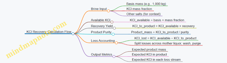
Step 6: Add a Quick Consistency Check
A useful check is to ensure the implied product mass is consistent with typical crystallization behavior: product mass should be larger than KCl mass (because purity is below 100%). Here, 116.21 kg product contains 110.4 kg KCl, which matches the 95% purity assumption.
You can also sanity-check the overall potassium balance: all potassium leaving the system as product plus losses must equal potassium entering with brine. In this example, 110.4 kg + 9.6 kg = 120 kg, so the potassium balance closes.
Example Summary Table
| Item | Value |
|---|---|
| Brine basis | 1,000 kg |
| KCl mass fraction in brine | 0.120 kg/kg |
| KCl available | 120.0 kg |
| Recovery yield | 92% |
| KCl in product | 110.4 kg |
| Product purity | 95% |
| Expected product mass | 116.21 kg |
| KCl lost | 9.6 kg |
Step 7: Turn the Method Into a Repeatable Calculation
When you change brine composition, you only update the KCl mass fraction and rerun the same sequence: available KCl → recovered KCl → product mass using purity → loss split if you track streams. The arithmetic stays simple; the discipline is in using consistent bases and definitions for “recovery” and “purity.”
If your plant defines recovery differently (for example, recovery based on KCl in crystals only, excluding entrained fines), adjust the purity and yield definitions accordingly. The method above is correct as long as the yield and purity refer to the same product boundary.
9. Potash Fertilizer Manufacturing: Product Finishing and Quality Assurance
9.1 Drying, Screening, and Sizing: Preventing Overheating and Caking
Drying and sizing decide whether finished KCl stays free-flowing or turns into a polite pile of lumps. The core idea is simple: remove surface moisture fast enough to prevent sticking, but avoid heat and residence time that damage crystal surfaces or drive moisture back into the product.
Foundational Concepts That Control Caking
Caking in KCl is usually a moisture-and-temperature story. Moisture can come from wet feed, humid air during handling, or condensation after cooling. Temperature matters because KCl can soften at the surface when moisture is present, and hot particles attract moisture from cooler surroundings. Screening and sizing then determine how much surface area is exposed and how easily air and moisture move through the bed.
A practical way to think about the system is three linked steps: drying removes moisture, cooling stabilizes temperature, and screening separates fines that would otherwise increase moisture uptake and promote bridging.
Drying Objectives and Operating Targets
Drying should achieve three outcomes: (1) reduce free moisture, (2) avoid overheating that can create hard-to-break agglomerates, and (3) keep the product temperature below the point where moisture migration and condensation become likely.
Start with a moisture target based on your product spec and packaging method. If you package in bags, you typically need lower moisture than for bulk storage because bags trap humidity. Then set an air temperature and residence time that reach the target without pushing particle temperature too high.
A useful rule of thumb for operators: if the dryer outlet air is hot but product temperature barely rises, you may be limited by airflow or mixing rather than by heat. If product temperature rises quickly while moisture removal stalls, you may be forming a surface crust that slows evaporation.
Drying Mechanisms and How to Prevent Overheating
Overheating shows up as increased dusting, darker or duller surfaces, and a tendency to form “hard” lumps that resist normal screening.
Common causes include:
- Excess residence time due to low throughput or poor solids distribution.
- Air temperature set too high for the actual moisture load.
- Inadequate airflow leading to localized hot spots.
- Poor heat recovery or insulation issues that raise dryer wall temperatures.
Mitigation is operational, not mystical. Use product temperature as the primary guardrail, not just inlet air temperature. When moisture load changes, adjust airflow and solids feed together so the dryer sees a consistent drying rate.
Cooling and Moisture Re-Entry Control
Cooling is where good drying can be undone. If hot KCl cools in humid air, water condenses on particle surfaces and creates the exact conditions for caking.
Control points:
- Cool the product to a stable temperature before it contacts humid air.
- Keep airflow through the cooler consistent so all particles cool similarly.
- Avoid long holding times between dryer and cooler.
A simple check: if you see moisture increasing after cooling, the issue is usually air humidity, airflow bypassing, or leaks that bring moist air into the cooling zone.
Screening Strategy for Free-Flowing Product
Screening is not just sorting; it is moisture management. Fines have higher surface area, absorb moisture faster, and can act as “glue” during storage.
Design the screening step around three goals:
- Remove undersize fines that drive caking.
- Break up soft agglomerates formed during drying or transfer.
- Maintain a stable size distribution so bulk density and flow behavior stay predictable.
Use the screen aperture size that matches your desired granule size distribution. If you remove too much, you increase recycle and energy use. If you remove too little, fines accumulate and caking risk rises.
Sizing and Product Consistency
Sizing determines how particles pack and how air moves through stored product. A narrow size distribution tends to flow more consistently, while a wide distribution can segregate during handling.
To keep sizing stable:
- Control feed rate to the screen so the bed depth stays within the intended range.
- Monitor screen differential pressure or motor load as an indicator of blinding.
- Keep transfer lines clean to prevent buildup that changes effective aperture.
Mind Map: Drying, Screening, and Sizing Controls
Example: Diagnosing a Caking Complaint
A plant receives complaints of hard lumps after bagging. Lab results show moisture is slightly above spec, and fines content is elevated.
A systematic response:
- Compare dryer outlet product temperature to the historical operating window. If it was higher, overheating likely reduced surface integrity and promoted agglomeration.
- Check cooler conditions. If cooler air humidity or airflow dropped, condensation could have increased surface moisture.
- Inspect screening performance. If screen motor load is higher than normal or differential pressure indicates blinding, fines removal is failing.
- Verify transfer time between dryer and cooler. If it increased due to a belt or valve issue, hot product may have spent longer in humid air.
Once the root cause is corrected, confirm by re-running the full chain: drying moisture, cooling temperature stability, and fines fraction after screening. When all three align with the operating window, caking typically stops being a recurring “mystery guest.”
9.2 Coating and Conditioning: Anti-Caking Agents and Surface Treatments
Anti-caking is the practical art of keeping fertilizer granules from sticking to each other during storage and handling. The goal is not to make the surface “perfectly dry”; it is to prevent moisture-driven bridges and reduce friction so particles flow through hoppers, spreaders, and bagging lines.
Foundational Mechanisms of Caking
Caking usually starts when water vapor condenses on particle surfaces. If the surface contains soluble salts or if the granule has a slightly sticky film, that thin moisture layer can dissolve a bit of material and then recrystallize as a hard bridge. Two levers matter most: (1) how much water the surface can attract, and (2) whether the surface chemistry encourages dissolution and re-solidification.
Conditioning therefore targets surface energy, hygroscopicity, and mechanical interlocking. A coating that is too thick can crack and create fines, which then become new nucleation points for caking. A coating that is too thin may not cover the “hot spots” created by impact during screening and conveying.
Anti-Caking Agents and Their Roles
Anti-caking agents are typically applied as a fine powder or as part of a coating system. Common categories include:
- Insoluble mineral dusts: They act like ball bearings between granules. They reduce contact area and slow moisture bridges.
- Hydrophobic or film-forming additives: They lower water uptake and reduce the chance of a continuous wet layer.
- Salt-compatible surface modifiers: They can reduce stickiness by changing how moisture interacts with the surface.
A good rule of thumb is to match the additive to the fertilizer’s chemistry. For example, chloride-sensitive products require careful selection because some additives can increase chloride mobility or create uneven dissolution behavior.
Surface Treatments: Coating Methods and Control
Surface treatments are applied after granulation and drying, when the granules are strong enough to survive handling but still have enough surface activity for the coating to adhere.
Coating approaches
- Drum or pan coating: Granules tumble while a controlled dose of coating is sprayed or dusted on. This is common for MAP/DAP and blended NPK grades.
- Fluidized-bed coating: Air suspension improves uniformity for smaller particles and more consistent film thickness.
- Post-drying conditioning: A light application of anti-caking powder can be used when the product is already within moisture spec.
Key control variables
- Coating rate: Too low leaves uncovered areas; too high increases dusting and can raise bulk density unexpectedly.
- Moisture at application: Applying coating when granules are too dry can reduce adhesion; applying when too wet can trap moisture and worsen caking.
- Particle temperature: Overheating can soften surfaces and promote internal migration of salts.
- Mixing intensity: Insufficient tumbling causes streaks; excessive tumbling generates fines.
Practical Example: Choosing a Coating for a Moisture-Sensitive Grade
Suppose a plant produces a MAP grade that tends to cake after two weeks in humid storage. Lab checks show the bulk moisture is within spec, but surface moisture behavior is worse than expected.
A systematic response looks like this:
- Confirm surface coverage: Compare coated vs. uncoated samples under controlled humidity and observe whether caking starts at the same granule-to-granule contact points.
- Select an additive that reduces water uptake: If the surface is hygroscopic, prioritize a film-forming or hydrophobic component rather than only an inert dust.
- Set a target application rate: Start with a small dose and increase in steps while monitoring dusting and flowability.
- Verify flow and bagging performance: Measure angle of repose and bag fill consistency, not just caking rating.
This approach avoids the common mistake of “adding more powder” when the real issue is moisture interaction at the surface.
Mind Map: Anti-Caking and Surface Treatment System
Advanced Details That Matter in Real Plants
Uniformity is often the difference between “works in the lab” and “works in the warehouse.” Coating systems can show gradients: granules near the inlet may receive more additive, while those near the outlet may be under-coated. Residence time distribution and spray pattern (for liquid coatings) should be treated as process variables, not fixed background conditions.
Also watch for fines. Coatings applied to granules that are already generating fines can increase dusting, which then changes how moisture is distributed across the bulk. If dusting rises after coating, the fix is usually to adjust application rate and mixing intensity before changing additive chemistry.
Finally, ensure compatibility with downstream packaging. Some coatings can increase static or change how bags breathe, which affects internal humidity. The best coating is the one that keeps the product within spec while behaving predictably in the full handling chain.
9.3 Packaging and Storage: Moisture Control and Corrosion Prevention
Moisture is the quiet saboteur of finished fertilizer. It can raise product temperature through hydration reactions, dissolve salts at the surface, and then drive caking as the dissolved layer recrystallizes. Corrosion follows moisture because many fertilizer components and residues create conductive films on steel and can accelerate rust under wet-dry cycling.
Moisture Control Fundamentals
Start with the product’s “water story.” Many fertilizers are hygroscopic to some degree, meaning they pull water from air. The practical question is not whether moisture exists, but how fast it accumulates under your site’s temperature and relative humidity.
A simple way to manage this is to treat storage as a controlled environment:
- Control air exposure: minimize time between cooling, bagging, and pallet wrapping.
- Match packaging to product behavior: choose liners and bag materials that limit vapor transmission.
- Keep product cool and dry at the moment of packaging: warm product condenses moisture when it meets cooler air.
Example: If a batch of granules is still warm when it reaches the bagging station, the surface temperature can drop below the dew point of the surrounding air. Condensation forms, and even if the bulk is not wet, the surface becomes tacky. That tackiness then traps dust and increases the chance of caking during storage.
Packaging Design for Vapor and Liquid Barriers
Packaging is a system: bag, liner, closure method, pallet arrangement, and warehouse airflow.
Key practices include:
- Use appropriate liners for hygroscopic grades. A liner reduces water vapor ingress and helps prevent surface dissolution.
- Seal closures consistently. Loose closures create “moisture highways” along the bag seam.
- Avoid pinholes and tears during filling and handling. Small defects matter because they concentrate moisture entry at the damaged spot.
- Manage headspace in bulk bags. Excess air increases the amount of humid air trapped near the product.
Example: Two pallets of the same fertilizer are wrapped the same way, but one has a torn stretch film edge. Over a few weeks, that pallet shows higher bag-to-bag moisture variation because the damaged edge allows humid air to circulate and repeatedly wet the outer layer.
Storage Conditions and Warehouse Management
Warehouse control is about keeping the product’s surface in a stable moisture regime.
Practical controls:
- Temperature stability reduces condensation cycles. Large day-night swings create repeated wetting and drying.
- Ventilation strategy should avoid pulling humid air directly into storage zones during high-humidity periods.
- Floor and wall moisture control prevents rising damp and condensation on the lower portions of pallets.
- First-in, first-out discipline limits how long bags sit exposed.
Example: A warehouse with a cold concrete floor can cause condensation on the bottom of pallets even when the air seems “dry.” The product near the floor absorbs moisture from that condensed film, leading to localized caking and higher chloride or sulfate migration into surface layers.
Corrosion Prevention Through Cleanliness and Dryness
Corrosion is driven by three things: a corrosive species, a conductive moisture film, and a susceptible metal surface. Fertilizer plants often have residues from spills, dust, and cleaning water that provide the conductive layer.
Integrated corrosion practices:
- Prevent residue accumulation on frames, hoppers, and conveyors. Dust plus moisture is a corrosion starter kit.
- Use drainage and proper slope so water does not pool on equipment or pallet areas.
- Select compatible materials for contact zones. Stainless steel or coated carbon steel can be appropriate depending on the fertilizer chemistry and cleaning method.
- Control cleaning water. If wash-down is used, ensure complete removal and drying of surfaces before normal operations resume.
Example: A transfer chute that is “mostly dry” still collects a thin dust layer. When humidity rises, that dust becomes a conductive film. Over time, pitting can start at crevices and weld seams where the film persists.
Monitoring and Acceptance Checks
Moisture and corrosion control should be measurable, not just hoped for.
Use a routine set of checks:
- Incoming and outgoing product moisture (or a proxy such as caking tendency) to confirm packaging effectiveness.
- Warehouse humidity and temperature logging to correlate storage conditions with observed caking.
- Visual inspection of bag integrity and pallet wrapping condition.
- Equipment surface condition checks for early corrosion spots, especially at joints and low points.
Practical Workflow from Packaging to Storage
A reliable workflow reduces variability. After cooling, keep product covered and minimize dwell time before bagging. During bagging, train operators to treat liner placement and closure as quality-critical steps, not “speed tasks.” In the warehouse, store pallets off wet floors, keep wrapping intact, and ensure the storage zone has stable temperature conditions.
Example: If your team records that bags stored near a particular wall show higher caking, the fix is usually not “more drying.” It is often a localized condensation pattern from airflow or wall temperature. Correcting that airflow and improving wall insulation or placement typically improves results faster than changing the product.
A final note on corrosion: if you can prevent moisture films from forming on equipment and packaging surfaces, you reduce corrosion without needing aggressive chemical interventions. Dryness and cleanliness are the most consistent tools you have.
9.4 Quality Testing: K₂O Content, Chloride Limits, Particle Size Distribution, and Bulk Density
Quality testing for finished KCl is about proving four things: the nutrient level is right (K₂O), the salt chemistry is safe for the crop and equipment (chloride), the physical form will behave predictably in handling and application (particle size distribution), and the product will meter and store consistently (bulk density). Each test has its own logic, but they connect through a single goal: stable performance from warehouse to field.
K₂O Content
K₂O content is the headline number because it translates directly into nutrient dosing. In practice, KCl contains potassium as K⁺, so K₂O is calculated from measured potassium (often by dissolution followed by analytical determination). The key is to control the sample preparation steps so the lab measures what the customer receives.
Best-practice example: If the plant ships two lots with the same KCl grade but different moisture, the lab sample can bias results if it is not dried or conditioned consistently before analysis. A simple approach is to define a moisture basis for reporting and apply it uniformly across all lots.
What to check in results:
- Repeatability across replicate samples from the same lot.
- Agreement between the calculated K₂O and the expected value from incoming brine/ore chemistry and process mass balance.
- Whether any outlier correlates with unusual moisture or segregation.
Chloride Limits
Chloride limits protect crops sensitive to Cl⁻ and reduce corrosion risk in storage and application equipment. Chloride testing is typically done by dissolving the sample and measuring chloride (commonly via titration or instrumental methods). The test must reflect the actual soluble chloride in the product, not just a surface residue.
Easy-to-understand example: Imagine two bags that look identical. One has chloride-rich fines that settled during handling; the other has more coarse crystals. Even if both are “KCl,” the fines can push chloride above the limit. That’s why sampling method matters as much as the chemistry.
Practical acceptance logic:
- Use a lot sampling plan that captures both coarse and fine fractions.
- Record the sampling location (top, middle, bottom) if product is stored in bulk.
- Treat chloride excursions as a system issue first: feed brine composition, crystallization conditions, and recycle purity.
Particle Size Distribution
Particle size distribution (PSD) affects flowability, dust generation, and how fertilizer dissolves in soil. PSD is measured by sieving (dry screening) or by laser-based methods, depending on plant capability and required resolution.
Foundational concept: PSD is not just “mean size.” Two products can share the same average but differ in the fraction of very fine particles, which often drives dust and caking behavior.
Concrete example: A product with a slightly lower average size but a higher <0.5 mm fraction can show worse flow in a spreader hopper. The hopper doesn’t care about the average; it cares about the fines that bridge or trickle inconsistently.
What to report:
- Percent retained or passing at defined sieve sizes.
- The fines fraction threshold tied to your handling and application performance.
- Consistency across lots, not only compliance.
Bulk Density
Bulk density influences storage stability, transport efficiency, and application metering. It is measured by filling a container of known volume under a defined procedure and weighing the contents. The procedure must be repeatable because bulk density changes with packing and how the sample is poured.
Example: If one operator “taps” the container to settle material and another does not, bulk density can shift even when the crystals are identical. That’s why bulk density testing should specify the fill height, pour method, and any settling time.
How bulk density connects to other tests:
- PSD shifts toward fines usually reduce bulk density.
- Moisture can increase apparent density by changing crystal surface behavior.
- Segregation can create a bulk density that looks fine while PSD and chloride reveal the underlying issue.
Mind Map: Quality Testing for Finished KCl
Integrated Example: Interpreting a Lot That Fails Chloride
Suppose a lot meets K₂O but exceeds the chloride limit. The PSD shows an elevated fines fraction, and bulk density is slightly lower than usual. That pattern suggests chloride-rich material concentrated in the fine fraction, likely from crystallization or recycle purity issues, and then amplified by handling segregation. The corrective action should therefore target the upstream purity and crystal formation conditions, while the sampling plan is reviewed to ensure future lots capture fines consistently.
Summary of What “Good” Looks Like
A compliant lot is not only within spec on each number; it also behaves coherently. K₂O confirms nutrient level, chloride confirms chemistry, PSD confirms physical form, and bulk density confirms handling behavior. When these agree, the product is likely to perform predictably. When they don’t, the mismatch is the clue that points to the real process cause.
9.5 Practical Example: Root-Cause Analysis of Off-Spec Chloride or Moisture in Finished KCl
You receive a finished KCl lot with chloride above spec or moisture above spec. The goal is to find the specific mechanism that moved chloride and/or water into the product, then confirm it with evidence from sampling, mass balance, and process logs. A useful mindset is: chloride and moisture usually travel with brine, fines, or inadequate drying, and they often show up first in certain particle size fractions.
Step 1: Confirm the Off-Spec Pattern
Start by checking whether the issue is uniform across the silo or concentrated in certain bins. If you have sieve data, compare chloride and moisture by size fraction. A common pattern is higher moisture and chloride in the smallest fraction because fines retain surface brine and dry more slowly. If the issue is localized, focus on the last handling steps (screening, transfer, packaging) rather than upstream crystallization.
Example: Lot A shows moisture of 0.8% in the 1–3 mm fraction, but 1.6% in <0.5 mm. Chloride follows the same trend. That points to brine carryover and/or insufficient drying of fines.
Step 2: Separate Chloride Sources from Moisture Sources
Chloride in KCl can come from:
- Mother liquor trapped in crystals (brine inclusion)
- Surface brine on crystal surfaces (wet cake)
- Recycled liquor carryover into washing or centrifuging
- Contamination from equipment or hoses used for brine-adjacent streams
Moisture in KCl can come from:
- Incomplete drying (insufficient residence time, low heat, poor airflow)
- Wet cake thickness causing uneven heat transfer
- Hygroscopic moisture uptake during storage or packaging
- Condensation from humid air leaks into dryers or enclosures
If chloride is high but moisture is normal, suspect brine inclusion or surface brine that was dried but not washed out. If moisture is high but chloride is normal, suspect drying or sealing issues. If both are high and correlated by particle size, suspect brine carryover plus drying shortfall.
Step 3: Build a Simple Evidence Map
Use a short list of measurements that can be collected quickly:
- Brine composition entering and leaving washing/centrifuging (Cl− or conductivity)
- Mother liquor recycle rate and any recent changes to recycle control
- Centrifuge/wash water flow and wash ratio
- Dryer inlet temperature, outlet temperature, and airflow rate
- Dryer residence time proxy (belt speed, screw speed, or feed rate)
- Moisture by sieve fraction after drying and after screening
Example: Logs show dryer outlet temperature dropped by 15°C for 6 hours due to a control valve sticking. During the same window, fines increased in the product stream. That aligns with both moisture and chloride being high in <0.5 mm.
Step 4: Use a Mini Mass Balance to Narrow the Mechanism
A practical approach is to estimate how much brine could be carried into the product based on wash efficiency.
- If the wash ratio decreased (less wash water), trapped mother liquor increases, raising chloride.
- If centrifuge separation efficiency dropped (worn scroll, imbalance, lower differential speed), more liquor remains on crystals.
- If dryer performance dropped, surface moisture remains, and chloride can appear higher because surface brine is not fully removed.
Example calculation logic (no fancy math required):
- Compare expected wash ratio from the operating sheet to the actual average during the off-spec window.
- If wash ratio fell by 20%, assume trapped liquor fraction rises roughly in proportion to reduced washing effectiveness.
- Check whether chloride increase magnitude is consistent with that trapped liquor change.
Step 5: Check the Most Common Failure Points in Order
- Washing and centrifuging
- Verify wash water flow meter calibration and strain/plugging in nozzles
- Inspect centrifuge basket condition and check differential speed history
- Confirm that mother liquor recycle was not inadvertently increased
- Dryer and hot-gas system
- Inspect temperature control loop tuning and valve position history
- Check airflow fans, dampers, and filter loading that can reduce gas flow
- Confirm feed rate did not exceed dryer capacity, especially for fines
- Handling and storage
- Verify enclosure seals and air humidity control
- Check whether product was exposed to humid air during transfer or packaging
Mind Map: Root Cause Logic for Chloride and Moisture
Step 6: Close the Loop with a Focused Verification
After corrective actions, confirm with targeted sampling:
- Sample after drying and after screening separately to isolate where moisture returns
- Sample by sieve fraction to ensure fines are within both chloride and moisture specs
- Compare brine composition trends during the same operating window
Example resolution: Restoring dryer outlet temperature, clearing the wash nozzle line, and rebalancing the centrifuge reduced <0.5 mm moisture from 1.6% to 0.9% and chloride from 1.2% to 0.7% (spec 0.8%). The improvement in fines confirmed the combined mechanism rather than a single-step issue.
Step 7: Document the Root Cause in One Sentence
A good root-cause statement is specific and testable, such as: “During the off-spec window, dryer outlet temperature control drifted low while wash water delivery was reduced, increasing mother liquor retention on fines and leaving surface brine that elevated both chloride and moisture in the <0.5 mm fraction.”
10. Integrated NPK Production: Blending, Granulation, and System Design
10.1 NPK Integration Concepts: Physical Blending vs. Chemical Granulation
NPK integration starts with a simple question: do you want nutrients to stay as separate particles that happen to sit together, or do you want them to form one engineered solid? That choice drives equipment layout, product consistency, and how you handle moisture and segregation.
Physical blending combines separately produced N, P, and K materials (for example, urea, MAP/DAP, and KCl) using weigh belts, screw feeders, or batch blenders. The goal is uniform distribution of each nutrient across the bulk. Because particles remain distinct, the blend’s performance depends heavily on particle size compatibility, density differences, and how the product behaves during handling.
Chemical granulation forms a single granule by reacting or chemically binding nutrients during granule growth. A common approach is to granulate phosphate with a nitrogen source, where the binder and nutrient chemistry create a more integrated particle. The result is typically better resistance to segregation and improved “nutrient co-location,” but it requires tighter control of reactions, moisture, and heat.
Mind Map: Physical Blending vs. Chemical Granulation
Physical Blending: What “Integrated” Means
In physical blending, integration is spatial, not chemical. Imagine a bag where each handful should contain roughly the same nutrient ratio. If KCl particles are larger and denser than urea, they tend to settle during vibration and transport. A practical best practice is to align particle size distributions so that settling rates are similar. Another is to use a mixing sequence that reduces stratification, such as pre-blending smaller fractions and then combining them in a controlled order.
Example: Suppose you target an N-P-K ratio of 20-10-10 using urea (46% N), MAP (12% N, 61% P2O5), and KCl (60% K2O). If urea is mostly 1–2 mm prills while KCl is 3–5 mm granules, the blend can drift toward higher K content in the bottom of a tote. A simple mitigation is to screen and rework to narrow the size range before blending, then verify uniformity with sampling from multiple locations.
Chemical Granulation: What “Integrated” Means
Chemical granulation integrates nutrients inside the granule. Instead of relying on mixing uniformity, you rely on granule formation to keep nutrients together. This shifts the critical path from blender performance to granulator and dryer control.
A typical chemical granulation logic is: create a controlled liquid phase (often from phosphate and nitrogen sources), grow granules by layering and nucleation, then dry and cool to lock in structure. If liquid addition is too high, granules can stick and form large agglomerates. If drying is too aggressive, you can create surface cracking and higher dust.
Example: For a MAP-like granule with added nitrogen, the binder liquid composition affects how quickly crystals form and how strong the granule becomes. If the liquid is too dilute, you may get weak granules that break during screening. If it is too concentrated, you can get sticky growth and poor yield. Operators manage this by controlling liquid-to-solid ratio, atomization quality, and residence time in the granulator.
Choosing Between the Two: A System View
The decision is rarely “either/or” in real plants. Many operations use physical blending for some grades and chemical granulation for others, sharing utilities and packaging lines.
Use physical blending when:
- You have stable, consistent upstream products.
- You need quick grade changes with minimal reaction control.
- You can manage segregation with screening, size matching, and robust mixing.
Use chemical granulation when:
- You need strong resistance to segregation and better nutrient co-location.
- You can support tighter control of moisture, drying, and granule strength.
- You want a single granule to carry the full nutrient ratio.
Practical Integration Checklist
- Define the grade requirement as a nutrient ratio and a physical spec (moisture, size, strength, dust).
- Match particle behavior: compare size distribution and density for physical blending; compare liquid chemistry and drying profile for chemical granulation.
- Plan sampling: physical blends require multi-point sampling across the batch; granulated products require checks on granule strength and friability after drying.
- Control moisture intentionally: both routes can fail from moisture, but in different ways—caking in blends versus sticking and poor drying in granulation.
In short, physical blending integrates nutrients by mixing discipline, while chemical granulation integrates nutrients by granule formation discipline. Both can produce reliable NPK, but each demands that you respect the physics of particles in one case and the chemistry and moisture balance in the other.
10.2 Granulation Technologies: Drum Granulation, Pan Granulation, and Fluidized Systems
Granulation turns powders or slurries into particles that handle well, meter consistently, and spread evenly in the field. The core idea is simple: you create controlled growth by repeatedly forming liquid bridges, then letting those bridges set into a solid structure. The details differ by technology, but the same levers show up everywhere—binder type, liquid addition rate, mixing intensity, bed moisture, residence time, and drying capacity.
Foundational Concepts for Particle Growth
A granulator needs a “wetting phase” and a “solidification phase.” In the wetting phase, binder solution or melt forms bridges between dry particles. In the solidification phase, those bridges harden through evaporation, chemical reaction, or cooling. If wetting is too aggressive, you get large, weak lumps; if it is too timid, you get dust and poor strength.
A practical way to think about control is to track three outcomes: granule size distribution, granule strength, and surface moisture. Size distribution depends on how often particles collide and how much binder they receive per collision. Strength depends on how completely the binder sets before the granules are broken by mixing. Surface moisture depends on the balance between liquid addition and drying removal.
Drum Granulation
Drum granulation uses a rotating cylinder with internal lifters. As the drum turns, material cascades and tumbles, giving frequent contact and steady growth. Drum systems are often chosen when you want robust operation with relatively forgiving feed variability.
Key operating variables include drum speed, lifter geometry, binder spray pattern, and inlet air conditions. Higher drum speed increases collision frequency, which can speed growth but also increases breakage if the bed is too wet. Binder spray should match the bed’s wetting capacity; if the spray hits too locally, you create wet spots that become oversized agglomerates.
A simple example: suppose you are producing a phosphate-based granule using a recycled return stream. If the return stream is wetter than expected, the bed reaches the “sticky” region sooner. You can respond by reducing binder flow slightly and increasing drying air, rather than only changing speed. That keeps collisions productive instead of destructive.
Pan Granulation
Pan granulation uses a shallow rotating pan with an agitator or rollers that lift and fold material. The motion is more controlled than a drum’s cascade, which helps when you need tighter control of granule shape and growth rate.
Pan systems commonly excel at producing more uniform granules because the bed experiences repeated, gentle folding. That reduces random over-wetting and helps maintain a stable nucleation zone where new granules form. The binder addition strategy matters: a well-distributed spray across the pan surface supports even bridge formation.
A simple example: when making a nitrogen-phosphate blend, you may see segregation if particle sizes drift apart. In a pan, you can maintain a steadier growth environment by keeping the pan load consistent and adjusting binder addition to hold bed moisture near the target. The result is fewer “fast growers” that steal binder and leave the rest undersized.
Fluidized Systems
Fluidized granulation uses an upward gas flow to suspend particles, creating a fluid-like bed. Binder is sprayed into the bed so that particles repeatedly collide and acquire liquid bridges. Because the bed is well mixed, fluidized systems can produce narrow size distributions and high throughput.
The main engineering constraint is gas-solid contact. Gas velocity must be high enough to fluidize but not so high that you blow out fines and lose material. Binder atomization also matters: droplets that are too large create wet cores; droplets that are too small can evaporate before they form stable bridges.
A simple example: if your feed has a higher fraction of very fine particles, the bed can become “faster” in terms of circulation and fines carryover. You can counter by adjusting gas flow downward slightly and increasing binder concentration modestly so bridges form quickly enough to keep granules from breaking into dust.
Comparative Decision Logic
Choose technology by matching your product needs to the dominant failure modes.
- Drum granulation tolerates variability and supports steady growth through tumbling.
- Pan granulation emphasizes uniformity and controlled folding.
- Fluidized systems emphasize tight size control and mixing, with stricter sensitivity to gas flow and atomization.
Mind Map: Granulation Technology Selection and Control
Integrated Example: Holding Quality Through Moisture Balance
Imagine a plant producing a granulated phosphate product using a recycle return stream. The recycle brings both seed particles and moisture. If recycle moisture rises, the bed reaches sticky conditions earlier. The integrated response is to reduce binder flow slightly and increase drying air capacity so that the wetting phase shortens and the solidification phase catches up.
In a drum, this prevents over-wetting during cascade. In a pan, it stabilizes the nucleation zone so new granules form without creating oversized lumps. In a fluidized system, it reduces the chance of fines agglomerating into weak, irregular particles that later break during circulation.
The common thread is that granulation is not just “adding liquid.” It is managing the timing between liquid addition and hardening, while keeping mixing productive rather than destructive.
10.3 Nutrient Compatibility and Reaction Management
NPK production often fails in predictable ways: one nutrient reacts with another, a trace impurity forms a stubborn solid, or a surface corrodes faster than expected. Compatibility management is the discipline of preventing those outcomes by controlling chemistry, moisture, and contact time—especially where streams mix.
Foundational Idea: What “Compatibility” Really Means
Compatibility is not just “no visible reaction.” It includes whether mixing creates:
- Unwanted solids that foul filters, plug lines, or settle in tanks.
- Unwanted corrosion from chloride, fluoride, sulfate, or acidic species.
- Unwanted phase changes such as crystallization during concentration, cooling, or storage.
A useful mental model is to treat each nutrient stream as a bundle of ions, acidity/basicity, and water activity. When two bundles meet, the outcome depends on equilibrium and kinetics, not just composition.
Step 1: Build a Compatibility Inventory for Each Stream
Start with a simple table for every incoming stream (acid, ammonia derivatives, phosphate slurry, potash brine, recycled liquor, and recycle condensate). Capture:
- Main nutrient ions (e.g., NH4+, NO3-, PO4 species, K+, Cl-, SO4 2-)
- Acidity or alkalinity (pH or acid equivalents)
- Conductivity and density (quick proxies for dissolved solids)
- Temperature at mixing
- Known “small” impurities (chloride, fluoride, iron, silica, organics)
Easy example: if a phosphate stream contains elevated silica and you later add a potassium source, silica can promote gel-like solids that trap fines. The nutrient ratio might still look correct, but the solids problem appears in filtration.
Step 2: Identify the Common Solid-Forming Pathways
Most unwanted solids in NPK lines come from a few families:
- Calcium phosphate or calcium sulfate formation when calcium is present and pH shifts.
- Magnesium ammonium phosphate (struvite) when Mg²⁺ and NH4+ meet under the right pH and concentration.
- Potassium salts precipitation when concentration rises or temperature drops.
- Iron and aluminum hydroxides from pH changes that cause metal ions to hydrolyze.
Practical rule: if you can name the ions, you can usually name the solid family. Then you can control the mixing conditions that drive precipitation.
Step 3: Manage PH and Acidity Like a Process Variable, Not a Measurement
pH affects both solubility and corrosion. In phosphate systems, small pH shifts can move species between soluble and less soluble forms. In nitrate/ammonium systems, pH also changes how impurities behave.
Easy example: adding a basic potassium source to an acidic phosphate solution can reduce solubility of certain phosphate species, increasing filter load. Instead of “mix and hope,” set a target pH window and control addition rate so the local pH at the injection point stays within bounds.
Step 4: Control Mixing Order and Contact Time
Many solids form at the moment of mixing due to local supersaturation. Two best practices prevent that:
- Sequence addition so the stream that controls pH and ionic strength is added first.
- Use staged mixing with short residence time in each stage, followed by bulk homogenization.
Example: in a MAP/DAP blend, adding phosphate solution to a concentrated potassium stream can create immediate supersaturation. Adding potassium to the phosphate solution under agitation, or using a dilution step before final concentration, reduces the “instant precipitation” zone.
Step 5: Prevent Corrosion by Matching Materials to the Chemistry
Corrosion risk rises when you combine:
- Chloride with acidic conditions
- Oxygen with wet surfaces
- High temperature with salt-rich films
Corrosion is often localized under deposits. Unwanted solids that stick to metal surfaces can create differential aeration cells, accelerating attack.
Concrete example: if a line sees chloride-bearing potash liquor and occasional acidic cleaning residues, pitting can start at crevices and weld seams. The fix is not only material selection; it also includes cleaning neutralization verification and minimizing chloride carryover into acidic zones.
Step 6: Use a “Compatibility Check” Before Full-Scale Mixing
A lightweight screening approach works well:
- Perform a jar test at the expected mixing temperature and final concentration.
- Observe haze, settling, and filterability using a consistent procedure.
- Compare results across mixing orders.
Example: a jar test that shows rapid haze when potassium is added first indicates local precipitation. Switching order or adding a dilution step often restores clarity without changing the final nutrient ratio.
Mind Map: Nutrient Compatibility and Reaction Management
Case Example: From “correct recipe” to “correct product”
A plant targets a consistent NPK grade using a phosphate solution and a potassium-bearing stream. After a grade change, filtration pressure rises and product moisture becomes inconsistent. The compatibility inventory shows a higher Mg²⁺ level in the potassium stream and a slightly lower pH in the phosphate solution due to upstream control drift. The mixing order created a brief local condition where NH4+ and Mg²⁺ met at high ionic strength, forming fine solids that later settled in tanks.
The corrective actions are straightforward and measurable:
- Restore phosphate pH to the target window.
- Switch mixing order so potassium is introduced into the phosphate under controlled agitation.
- Add a short dilution step before final concentration.
- Verify cleaning neutralization to reduce chloride-driven corrosion risk.
The result is not just fewer solids; it’s stable filtration, predictable moisture, and less deposit-driven corrosion.
10.4 Process Control for Consistent Product: Feed Ratio Control, Moisture Targets, and Recycle
Consistent NPK product quality comes from controlling three things at the same time: the nutrient feed ratio, the moisture level during granulation and drying, and the recycle streams that quietly carry “yesterday’s” variability into “today’s” batch. If you control only one of them, the others will still find a way to show up in the final spec.
Feed Ratio Control
Feed ratio control starts with a simple idea: the nutrient ratio in the product should match the recipe ratio, even when feedstock composition drifts. In practice, you measure two layers of reality.
First layer: flow rates. Use calibrated weigh feeders or mass flow meters for each nutrient component (for example, urea, MAP/DAP, and KCl). Second layer: composition. Urea can vary in biuret and moisture; phosphate concentrates can shift in P2O5 and impurities; potash brine or mined salts can shift in chloride and insolubles.
A practical control approach is ratio control with composition correction. The controller computes “effective nutrient flow” from measured mass flow and lab or online composition, then trims feeder setpoints to hold the target nutrient ratio.
Example: You target 15-15-15 by mass. Your phosphate feed analysis shows P2O5 is 1% lower than assumed. If you keep the same feeder rate, the product will come out phosphate-light. With composition-corrected ratio control, the controller increases phosphate feed slightly to restore the effective P2O5 contribution.
Moisture Targets
Moisture control is not just about meeting a final moisture spec; it governs granule formation, strength, and dusting. Too little moisture and you get weak granules and poor nucleation. Too much moisture and you get overwetting, sticking, and slow drying.
Set moisture targets at multiple points, not only at the end of drying. Typical control points include:
- Granulation zone moisture (drives nucleation and growth)
- Intermediate bed moisture (prevents sticking and uneven drying)
- Final product moisture (supports storage stability)
Use a cascade strategy: the drying heat or residence time is the manipulated variable, while moisture is the controlled variable. If you only adjust heat based on final moisture, you’ll often correct too late and create oscillations.
Example: Final moisture is high after drying. If you respond by increasing steam immediately, you may overshoot and create overdried product that generates more dust during handling. Better practice is to detect rising intermediate moisture earlier and adjust drying duty before the bed reaches the problematic region.
Recycle Management
Recycle streams—oversize return, undersize return, and sometimes wet fines—are useful because they reduce waste and stabilize bed inventory. They are also the main path for variability to re-enter the system.
Treat recycle as a controlled input with its own quality. Measure recycle moisture and nutrient content (or at least track it via process history). Then decide whether recycle is:
- Quality-matched: recycle is routed back only when it meets moisture and composition windows
- Dilution-controlled: recycle is allowed but the recipe is corrected to account for its nutrient contribution
- Inventory-controlled: recycle rate is adjusted to keep granulator bed level stable
A common failure mode is “silent nutrient drift,” where recycle contains more phosphate fines than fresh feed, shifting the effective nutrient ratio without any change in fresh feeder setpoints.
Example: Oversize recycle is wetter than fresh feed because it was generated during a brief over-wetting event. If recycle rate increases, the granulator receives extra water and the product ratio can shift due to altered granulation efficiency. The fix is to limit recycle during wet excursions and to correct feeder ratios using recycle nutrient accounting.
Integrated Control Logic
The three control loops should cooperate, not compete. Feed ratio control handles nutrient balance, moisture control handles granulation and drying behavior, and recycle management handles variability recirculation.
A Simple Control Checklist
- Confirm each feeder is mass-based and calibrated.
- Apply composition correction to nutrient ratio calculations.
- Set moisture targets at granulation and intermediate points, not only final.
- Use cascade control so drying responds to moisture trends early.
- Track recycle moisture and nutrient contribution, then either restrict or correct for it.
- Verify that recycle rate changes do not silently alter nutrient ratio by checking product lab results against predicted contributions.
When these elements work together, the plant stops treating “bad batches” as mysteries and starts treating them as measurable deviations with clear causes.
10.5 Practical Example: Designing an NPK Line to Produce Multiple Grades with Shared Equipment
A shared NPK line is basically a disciplined juggling act: the same core equipment handles different nutrient ratios, while the control system keeps the product within grade specs. The trick is to design around what must change (formulation targets) and what must stay stable (particle properties, moisture, and segregation risk).
Start with grade definitions. Suppose you need three grades using the same granulation train:
- Grade A: 15-15-15 (N-P2O5-K2O)
- Grade B: 20-10-10
- Grade C: 10-20-10
Assume you will use a common base of dry phosphate and potash materials plus a nitrogen source that can be added as a solution or melt. The shared equipment list typically includes: weigh hoppers, conveyors, a granulator (drum or pan), recycle handling, drying, screening, coating/conditioning, and packaging. Everything else is “just” process control and material compatibility.
Step 1: Build a Formulation Map from Nutrient Targets
Convert nutrient targets into component masses using lab-verified analyses. For example, if your phosphate concentrate is 46% P2O5 and your potash is 60% K2O (as KCl), then the required masses per metric ton of finished product are:
- Phosphate mass = (P2O5 target) / 0.46
- Potash mass = (K2O target) / 0.60
Then allocate the nitrogen source. If nitrogen is supplied as a solution, you also decide the water addition so the granulator sees a consistent wetting level. This is where shared equipment design pays off: you keep the granulator’s “wetness window” the same across grades, even when nutrient ratios change.
Step 2: Choose a Shared Granulation Strategy
For shared equipment, you want one dominant mechanism for forming granules. A practical approach is to use a controlled liquid binder addition (from a nitrogen solution) onto dry solids in a granulator, followed by drying and screening.
Key best practices that prevent grade-to-grade surprises:
- Keep liquid addition proportional to total solids, not just nitrogen. If you only chase N, granule strength and moisture drift.
- Use the same recycle ratio setpoint across grades unless you have evidence that crystal growth behavior changes significantly.
- Control mixing time and spray distribution so the binder contacts fines consistently.
Concrete example: if Grade A requires more nitrogen than Grade C, you increase binder flow. To keep granule formation consistent, you also adjust dry feed rate so the total liquid-to-solids ratio stays within the same operating band.
Step 3: Design the Control Logic Around “What Changes”
A shared line needs a control matrix that links grade selection to setpoints. The grade selector should update:
- Weigh hopper targets for each dry component
- Binder flow rate and spray pattern parameters
- Target granulator outlet moisture
- Dryer inlet temperature and residence time targets
- Coating/conditioning rate to manage dust and caking
A useful mental model is: nutrient ratio changes composition; moisture and particle size distribution determine whether the product behaves like the same product.
Step 4: Manage Segregation and Recycle Without Rewriting the Plant
Segregation is the enemy of “same equipment, different grade.” It happens when particle sizes or densities differ between components. Shared equipment helps if you standardize particle size distribution before final packaging.
Practical measures:
- Screen after drying to a consistent size band for all grades.
- Route off-size material to recycle with a controlled fraction, and ensure recycle is conditioned to the same moisture level.
- Use anti-segregation handling: avoid long belt runs without agitation and keep transfer points short.
Step 5: Validate with a Grade-by-Grade Mass Balance and a Single Runbook
Before running, do a mass balance for each grade to confirm that the binder water and dryer duty can remove the expected moisture. Then create one runbook with grade-specific parameter tables.
Example runbook logic for each grade:
- Set dry feed masses from nutrient analyses
- Set binder flow to hit the granulator moisture target
- Set dryer targets to achieve the same final moisture spec
- Set coating rate to reach the same dusting behavior
This is where “shared equipment” becomes real: the runbook stays one document, while the parameter values change.
Mind Map: Shared Equipment NPK Line Design
Example: Parameter Set for Three Grades
Assume the phosphate and potash masses are computed from analyses, and the nitrogen binder is adjusted to meet N. The shared setpoints then focus on particle behavior:
- Granulator outlet moisture target: same for A, B, and C
- Dryer final moisture spec: same for all grades
- Screen cut sizes: same for all grades
- Coating/conditioning rate: same target per ton
Only the weigh hopper targets and binder flow change between grades. If you keep those particle-property setpoints stable, the line produces different nutrient ratios without changing the “physics” of granule formation.
Finally, document the acceptance checks for each grade: nutrient assay, moisture, particle size distribution, and bulk density. If any grade fails, the first troubleshooting step is not “change the recipe,” but “check whether the granulator moisture and recycle behavior stayed inside the shared operating window.”
11. Process Control, Instrumentation, and Quality Management
11.1 Control Philosophy: Mass Balances, Control Loops, and Setpoint Strategy
A fertilizer plant is basically a system of promises: feed the right materials, convert them in the right way, and ship product that matches specs. Control philosophy is how you keep those promises when inputs vary, equipment ages, and disturbances show up uninvited.
Mass Balances as the Backbone
Start with steady-state mass balances, then add dynamic thinking. For any unit, you track how each component moves: nitrogen species in ammonia and urea sections, phosphate species in acidulation and concentration, and potassium chloride in potash crystallization. A practical way to write this is component-based balances around each control-relevant boundary.
Example: In a urea solution concentration step, the key components are urea and water. If the feed urea mass flow is 10,000 kg/h and the product urea mass flow is 9,800 kg/h, the missing 200 kg/h must be explained by purge, holdup changes, or measurement bias. If the balance doesn’t close, the control system will “fix” the wrong thing.
Mass balances also tell you what not to control. If a downstream spec depends on composition, controlling only temperature may not help if the real driver is feed ratio or evaporation rate.
Control Loops as the Delivery Mechanism
Control loops convert measurements into manipulated actions. A good loop has three parts that work together: a controlled variable (what you care about), a manipulated variable (what you can change), and a disturbance (what you can’t fully control).
Common loop patterns in fertilizer manufacturing:
- Flow ratio control: keep reactant stoichiometry stable (e.g., acid to rock slurry ratio).
- Level control: protect pumps and prevent flooding or starvation (e.g., surge drum levels).
- Temperature control: manage reaction rate and crystallization behavior (e.g., ammonia synthesis heat removal).
- Pressure control: stabilize phase behavior and prevent unwanted venting (e.g., gas recycle loop pressure).
- Composition control: use analyzers or infer composition from mass balance and density/conductivity.
A slightly playful but useful rule: if the controlled variable is hard to measure, you either estimate it (with a model or inferential logic) or you control a proxy that correlates tightly with it.
Setpoint Strategy as the Map of Intent
Setpoints are not just numbers; they encode priorities. A setpoint strategy answers: which variables get tight control, which get looser control, and how you handle constraints.
A systematic approach:
- Define product constraints: moisture, particle size, nutrient ratios, chloride limits, and impurity thresholds.
- Identify process constraints: maximum temperatures, corrosion limits, allowable pressure ranges, and equipment protection limits.
- Choose primary controlled variables: variables that directly influence product constraints.
- Set secondary variables: variables that stabilize the process so the primary loop can do its job.
- Apply constraint handling: when you hit limits, you change setpoints in a controlled way rather than letting loops fight each other.
Example: In MAP/DAP granulation, moisture affects caking and strength. If you tighten moisture control without respecting heat removal capacity, you may cause temperature swings that later change crystal growth. The setpoint strategy should coordinate moisture and temperature so both remain within safe operating windows.
Control Philosophy Mind Map
Mind Map: Control Philosophy in Practice
Example: Designing a Simple Cascade Without Chaos
Suppose you want to control reactor outlet temperature using cooling water. A single loop might work until feed rate changes. A better structure is cascade: use reactor temperature as the primary controlled variable, and drive cooling water flow as the manipulated variable through a secondary loop.
- Primary controlled variable: reactor outlet temperature.
- Secondary controlled variable: cooling water supply temperature or valve position proxy.
- Manipulated variable: cooling water valve.
- Disturbance: feed flow and inlet temperature.
This structure reduces overshoot because the secondary loop reacts faster to disturbances, while the primary loop focuses on meeting the temperature target.
Practical Checklist for Setpoints and Loops
- Every loop has a clear controlled variable tied to a mass balance or a spec driver.
- Setpoints are consistent with constraints, not just “comfortable” values.
- Loop tuning considers interaction: cascade relationships are explicit, not accidental.
- Balance closure is reviewed when control performance degrades.
- Operators can explain why a setpoint changed, using measured variables and constraints.
When these pieces align, control becomes less like guesswork and more like disciplined bookkeeping—just with valves.
11.2 Instrumentation for Fertilizer Plants
Instrumentation is the plant’s way of turning chemistry and physics into numbers operators can act on. For fertilizer manufacturing, the key variables—flow, pressure, temperature, pH, and conductivity—map directly to mass balance, reaction conditions, phase behavior, and product quality. The best systems measure the right thing, at the right location, with the right signal quality.
Foundational Measurement Logic
Start with a simple rule: every control action needs a measurement that responds quickly enough to matter. Flow signals support feed ratio control and residence time estimates. Pressure signals protect equipment and help infer phase changes. Temperature signals track reaction progress and heat transfer performance. pH and conductivity signals indicate solution chemistry, which is where phosphate and nitrogen solution operations live or die.
A practical way to organize instrumentation is by “what it controls.” Flow instruments typically drive ratio controllers. Pressure instruments drive level and safety interlocks. Temperature instruments drive reactor and evaporator control loops. pH and conductivity instruments drive neutralization control, acidulation control, and endpoint verification.
Flow Instrumentation
Flow measurement choices depend on fluid type and cleanliness. For clean liquids, magnetic or Coriolis meters can provide direct mass flow, which is handy when you need stable stoichiometry. For slurries, differential pressure meters can work if you manage plugging risk and calibrate against actual solids behavior.
Example: In a phosphate acidulation line, you may control acid feed by maintaining a target slurry pH. If the acid flow meter drifts, the pH loop will compensate by changing valve position, but the underlying mass balance will be off. That mismatch often shows up later as unexpected filtration load or off-spec product.
Best practice: place flow meters where the fluid is well mixed and avoid measuring immediately after strainers, elbows, or pumps that create pulsation.
Pressure Instrumentation
Pressure instruments serve two jobs: process control and mechanical protection. Control uses pressure to infer phase state and drive level control in vessels and evaporators. Protection uses pressure switches and transmitters tied to relief systems.
Example: During ammonia-related operations, pressure affects equilibrium and compressor performance. A slow or noisy pressure signal can cause oscillation in valve control, which then creates unstable temperatures and higher recycle variability.
Best practice: use impulse lines and heat tracing where needed, and verify that pressure taps match the physical phenomenon you intend to measure (static head versus dynamic pressure).
Temperature Instrumentation
Temperature is often the most “honest” variable in a plant because it reflects energy balance. Use thermowells for robustness, but remember they add thermal lag. For fast loops, choose sensor designs that minimize response time.
Example: In urea or ammonium nitrate solution concentration, temperature affects viscosity and crystallization tendency. If the temperature sensor sits in a dead zone, the loop may think the system is cooler than it is, leading to premature concentration and later caking.
Best practice: calibrate temperature sensors in situ when possible, and document sensor placement relative to heat transfer surfaces.
pH Instrumentation
pH probes measure hydrogen ion activity, not “acid concentration” directly. That distinction matters because fertilizers contain salts, buffering species, and suspended solids.
Example: In a phosphate neutralization step, two solutions can have the same pH but different phosphate species distribution. Conductivity may differ, and filtration behavior can change even though the pH reading looks stable.
Best practice: install pH probes in locations with representative mixing, provide cleaning or flushing where solids exist, and use temperature compensation correctly.
Conductivity Instrumentation
Conductivity measures ionic content and is strongly influenced by temperature. It’s excellent for tracking solution strength and detecting dilution or concentration changes.
Example: In a MAP/DAP blending preparation tank, conductivity can confirm that phosphate solution strength matches the intended recipe. If conductivity is stable but pH drifts, you likely have a probe issue or a change in buffering chemistry.
Best practice: use conductivity sensors with appropriate cell constants, keep them clean, and apply temperature compensation consistently.
System Integration and Signal Quality
A measurement is only useful if the signal is trustworthy. That means wiring integrity, calibration discipline, and alarm logic that reflects process reality.
Use a layered approach:
- Primary control signals: flow, pressure, temperature, pH, conductivity.
- Secondary checks: mass balance comparisons, trends across multiple variables.
- Interlocks: hard limits for safety and equipment protection.
Mind Map: Instrumentation Variables and Their Roles
Example: Neutralization Control Using pH and Conductivity
Suppose a phosphate neutralization step targets a pH endpoint while maintaining solution strength. A pH controller adjusts base or acid addition. Conductivity acts as a sanity check: if conductivity drops while pH remains steady, the system may be receiving unintended dilution or losing ions to side reactions. Operators then investigate feedstock quality and sampling accuracy before chasing the pH loop.
Example: Evaporator Stability Using Pressure and Temperature
In an evaporator, pressure relates to boiling temperature. A stable pressure signal helps the temperature controller maintain the intended vapor-liquid driving force. If pressure fluctuates due to valve chatter or blocked lines, temperature control may compensate incorrectly, increasing scaling risk and pushing the system toward off-spec concentration.
Practical Checklist for Instrumentation Deployment
- Place sensors where the fluid is representative and mixed.
- Match sensor response time to loop speed.
- Use temperature compensation for pH and conductivity.
- Calibrate with the same fluid matrix when feasible.
- Design alarms to guide action, not just report numbers.
- Verify signal health with cross-variable checks and trend review.
11.3 Laboratory and QA/QC Systems
A fertilizer plant lives and dies by measurements that are consistent across time, shifts, and labs. A good QA/QC system makes that consistency boring—in the best way—by defining what to test, how to sample, how to calibrate, and what results mean.
Sampling Plans
Sampling is where “the process” turns into “the number.” The goal is to make the sample represent the lot, not the moment.
Start with a clear sampling unit: a batch, a continuous production window, or a defined mass of product. Then choose a sampling method that matches the product form.
- Solids (urea, MAP, DAP, KCl): Use incremental sampling across the lot. For bags or bulk, take increments from different locations and depths. Mix increments to form a composite sample.
- Solutions (urea solutions, phosphoric acid blends): Sample from a well-mixed point. If stratification is possible, collect at multiple depths and combine.
- Crystalline or granulated products: Avoid sampling only from the top of a bin. Surface material often differs in moisture and fines content.
Define the frequency using risk and variability. High-variability steps (e.g., granulation moisture control, recycle streams) need tighter sampling. Stable steps can be sampled less often, but never “whenever someone remembers.”
A practical acceptance workflow is: collect → identify lot → test → compare to criteria → disposition. Disposition can be “release,” “hold,” “rework,” or “reject,” but the decision must be traceable to the criteria.
Mind Map: Sampling Plan Logic
Calibration and Measurement System Control
Calibration is not just adjusting instruments; it’s proving that measurements are trustworthy.
Use a calibration schedule tied to instrument type and usage intensity. Balance two realities: instruments drift, and calibrating too rarely creates surprises.
Key elements:
- Standards and reference materials: Use traceable standards where possible. For chemical assays, verify that reference solutions are prepared correctly and stored properly.
- Calibration method: Follow the method’s required range. For example, if you test moisture around 0.5–1.5%, calibrate or verify performance across that region, not just at one point.
- Acceptance of calibration: Define pass/fail limits and what happens if an instrument fails. A common rule is to quarantine results since the last known good calibration.
- Verification checks: Even after calibration, run a verification sample at a defined interval (e.g., per shift or per batch of analyses).
A measurement system also needs precision. Two analysts should get similar results on the same sample. If they don’t, the problem might be technique, sample prep, or the method itself.
Mind Map: Calibration and Verification
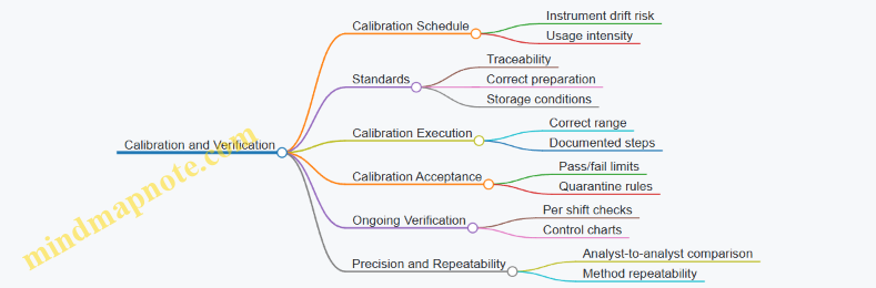
Acceptance Criteria and Test Methods
Acceptance criteria translate lab numbers into product decisions. They should be based on customer requirements and process capability, but expressed in testable terms.
Typical criteria include:
- Nutrient content: Total N, P2O5, K2O.
- Moisture and physical quality: Moisture %, particle size distribution, bulk density, fines.
- Impurities: Chloride limits for KCl products, sulfate levels where relevant, and heavy metal limits where applicable.
Test methods must be unambiguous about sample preparation, reagent grade, drying conditions, and calculation formulas. If two labs use “the same method” but dry at different temperatures or for different times, you get different numbers and a lot of frustration.
A useful practice is to maintain a method-to-criterion map: each acceptance criterion points to the method, instrument, sample handling steps, and calculation.
Example: Moisture Acceptance with Clear Decision Rules
Suppose a granulated product has a moisture limit of 1.0% max. The lab measures moisture using a defined drying method.
- If the result is 0.98%, release.
- If the result is 1.02%, hold and retest using the same composite sample or a defined resample plan.
- If the retest confirms >1.0%, disposition is rework or reject based on the plant’s product strategy.
This avoids arguing about “close enough” and keeps decisions consistent.
Putting It Together: A Cohesive QA/QC Loop
A strong system links sampling, calibration, and acceptance into one loop:
- Sampling creates representative material.
- Calibration ensures measurements are credible.
- Acceptance criteria convert measurements into actions.
When these pieces align, the lab becomes a stabilizer rather than a bottleneck. And yes, it should still be possible to explain a decision to an operator without turning it into a courtroom drama.
11.4 Managing Variability: Feedstock Fluctuations and Their Impact on Product Specs
Feedstock variability is the quiet saboteur of fertilizer quality. A plant can run “within spec” on paper while still producing off-grade product because the inputs drift in ways that matter to chemistry, solids formation, and downstream handling. The goal is not to eliminate variability, but to measure it early, translate it into expected product impacts, and control the process so the final specs stay stable.
Foundations: What Variability Actually Changes
Start by separating variability into three buckets:
- Composition changes: nutrient content, impurities, and reactive species shift. For example, phosphate rock with higher silica increases insoluble solids, which can raise filtration load and reduce usable P2O5 in the clarified acid.
- Physical property changes: particle size, moisture, density, and solubility affect mixing, dissolution rate, and heat transfer. A wetter feed can delay dissolution and change crystallizer supersaturation.
- Contaminant spikes: chloride, sulfate, heavy metals, or organics can appear intermittently. Even small spikes can push corrosion rates, alter crystallization behavior, or cause spec failures.
A useful mental model is: feed variability changes intermediate streams, and intermediate streams determine product quality. If you control only the final step, you’ll chase symptoms.
Translating Feed Changes Into Product Risks
For each nutrient system, map the most sensitive product attributes to the upstream variables.
- Nitrogen (urea, ammonium nitrate, solutions): moisture and biuret for urea; acidity and salt balance for solutions; impurities that affect corrosion and off-gas behavior.
- Phosphate (wet-process, MAP/DAP): insolubles and acid quality for wet-process; crystal size, moisture, and anti-caking performance for MAP/DAP.
- Potash (KCl): brine composition and insolubles for dissolution and clarification; chloride and moisture for finished KCl.
Concrete example: if phosphate rock has higher MgO and Al2O3, the acid clarification step may leave more dissolved impurities or increase filter cake formation. That can lead to poorer crystal quality in MAP/DAP, which then shows up as higher fines, worse flowability, and more caking risk.
Measurement Strategy: Catch Drift Before It Reaches the Reactor
Variability management works best when you measure in layers:
- Incoming checks: rapid assays for nutrient content and key impurities; moisture and particle size for physical properties.
- In-process indicators: pH, conductivity, density, and solids content in slurry or solution streams; temperature and pressure trends in reaction loops.
- Quality gates: sampling at points that represent “decision moments,” such as after clarification, after neutralization, and before granulation.
Example: for potash, brine chloride and insolubles should be tracked continuously or frequently enough to detect a shift in mother liquor recycle behavior. If you only test finished KCl, the plant has already spent energy and time crystallizing the wrong chemistry.
Control Logic: Use Feedforward, Not Just Feedback
Feedback control corrects after the process responds. Feedforward anticipates the response using measured feed properties.
A practical approach:
- Build a simple impact model: relate feed impurity levels to expected changes in an intermediate variable (like insoluble solids load, acid strength, or supersaturation).
- Adjust setpoints or ratios: change acid addition rate, recycle ratio, filtration duty, or granulation water based on the predicted intermediate shift.
- Lock the product spec: keep final moisture, particle size distribution, and impurity limits within target by adjusting upstream decisions.
Example: if incoming phosphate rock shows higher insolubles, increase clarification capacity and adjust filtration targets so the clarified acid quality stays consistent. Then granulation water can remain on its usual recipe, preserving flowability.
Mind Map: Variability Management Workflow
Advanced Details: Handling Uncertainty Without Overcorrecting
Variability rarely changes one variable at a time. When multiple inputs drift, overcorrection can create new problems, such as excessive recycle or unstable crystallization.
Use a staged response:
- Stage 1: Confirm the drift with at least one in-process indicator that correlates strongly with the suspected feed change.
- Stage 2: Constrain adjustments with operational limits (maximum filtration duty, maximum granulation water change, maximum recycle ratio).
- Stage 3: Validate by checking the intermediate stream quality gate before committing to full-rate production.
Example: if brine insolubles rise, don’t immediately change crystallizer conditions alone. First verify clarification performance and mother liquor clarity. If clarification is stable, then crystallizer adjustments may be appropriate; if not, the real fix is upstream.
Practical Example: A One-Shift Playbook
Suppose incoming phosphate rock shows a higher silica fraction. The playbook for the shift could be:
- Increase sampling frequency for clarified acid solids and filter performance.
- Adjust clarification targets to keep clarified acid quality consistent.
- Hold neutralization and crystallization recipes steady until the intermediate gate confirms stability.
- Only then fine-tune granulation water to maintain finished moisture and flow.
This sequence prevents “fixing” the wrong step. The plant spends less time reacting to symptoms and more time controlling the chain that leads to product specs.
11.5 Practical Example: Building a Control Matrix Linking Key Variables to Product Quality Attributes
A control matrix is a structured way to connect what you measure and manipulate in the plant to what you must deliver in the bag, bulk tank, or silo. The goal is simple: every critical product quality attribute (CQA) has at least one credible control path, and every control path has a clear reason to exist.
Start with a short list of CQAs for a typical NPK granulated product line. For example: total N, total P2O5, total K2O, moisture, particle size distribution, and chloride limits (if potassium source or raw materials introduce it). Then define the “key variables” that can move those CQAs. In practice, these are usually feed ratio signals, moisture/heat conditions, recycle rates, and any step that can change nutrient chemistry or segregation.
Step 1: Define the Quality Attributes and Their Measurement Rules
For each CQA, specify how it is measured and how fast you need the result. Moisture might be measured frequently on-site; nutrient analysis might be lab-based with a longer cycle time. This timing matters because the matrix must include both immediate controls (fast measurements) and slower verification (lab results).
Example rules:
- Total N: measured by lab; controlled indirectly via nitrogen feed rate and solution concentration.
- Moisture: measured frequently; controlled directly via dryer outlet temperature and granulator water addition.
- Particle Size Distribution: measured by sieve analysis; controlled via granulation energy, binder addition rate, and screen settings.
- Chloride Limit: measured by lab; controlled via raw material acceptance and blend ratio limits.
Step 2: Identify Manipulated Variables and Their Control Loops
Next, list manipulated variables (MV) that operators or controllers can change:
- N, P, K feed rates (or solution flow rates)
- Water addition rate
- Dryer heat input and residence time proxies
- Granulator speed and spray pattern (for granulation lines)
- Recycle stream fraction
- Coating/binder dosing (if used)
Then connect each MV to a likely mechanism that affects CQAs. For instance, water addition affects moisture and can indirectly affect particle size by changing granule growth conditions.
Step 3: Build the Matrix as a Cause-and-Effect Map
Use a matrix where rows are CQAs and columns are key variables and control actions. Each cell should state the mechanism and the control target.
A practical template:
- CQA
- Key Variable
- Control Action
- Setpoint/Target
- Measurement Method
- Control Interval
- Typical Failure Mode
- Detection and Response
Below is a compact example for an NPK granulation line.
| CQA | Key Variable | Control Action | Target | Detection | Response |
|---|---|---|---|---|---|
| Total N | Nitrogen feed rate or solution flow | Ratio control to master feed | Within grade tolerance | Lab check + feed audit | Adjust ratio; hold shipment if lab fails |
| Total P2O5 | Phosphate concentrate flow and slurry density | Density-compensated flow control | Stable density | Online density + periodic lab | Correct density; verify pump calibration |
| Total K2O | Potash feed rate and moisture correction | Ratio control with moisture compensation | Stable K2O basis | Online moisture + lab | Recalculate ratio; stop if chloride out of spec |
| Moisture | Water addition + dryer heat | Cascade control to dryer outlet moisture | Grade moisture window | Frequent moisture measurement | Reduce water or heat; check atomization |
| Particle Size | Granulator speed + binder/water rate | Maintain granulation energy and growth | Sieve targets | Sieve analysis | Adjust speed/spray; tune recycle fraction |
| Chloride | Raw material acceptance + blend ratio | Blend ratio limits and raw material hold | Below limit | Lab check | Quarantine lots; revise blend recipe |
Step 4: Add Guardrails So Controls Don’t “Win” the Wrong Game
A control matrix should include constraints that prevent controllers from chasing setpoints in ways that harm other CQAs. For example, pushing dryer heat to fix moisture can over-dry and increase dust, shifting particle size distribution. Guardrails can be simple: maximum dryer temperature, minimum granulator residence proxy, and recycle fraction limits.
Step 5: Validate the Matrix with a Simple Logic Test
For each CQA, ask: if the key variable drifts, what happens, how quickly do we detect it, and what action restores quality? If the answer is “we only find out after shipment,” the matrix needs a faster proxy measurement or an additional control layer.
Mind Map: Control Matrix from Variables to Quality
Worked Example: Moisture Drift and Particle Size Shift
Assume moisture starts trending high during a run. The matrix should show that moisture is controlled by water addition and dryer heat, with moisture measurement frequent enough to act before particle size changes become severe. If moisture rises while dryer outlet temperature is already at its normal range, the matrix points to water addition rate or atomization quality rather than blindly increasing heat. Once moisture is corrected, particle size should stabilize because granule growth conditions return to the target window.
The matrix becomes useful when it guides action quickly and consistently. It turns “we think the process is off” into “this variable is the most likely cause, here is the control target, and here is what we do next if it doesn’t respond.”
12. Safety, Environmental Compliance, and Operational Reliability
12.1 Hazard Identification in Fertilizer Manufacturing: Chemical, Mechanical, and Process Hazards
Hazard identification in fertilizer plants is easiest when you treat it like a map of “what can go wrong” tied to “where it happens” and “how it shows up.” The goal is not to list everything imaginable; it is to find credible hazards that could harm people, damage equipment, or disrupt production quality.
Foundational Approach
Start with three layers: chemical hazards, mechanical hazards, and process hazards. Chemical hazards come from the inherent properties of materials (toxicity, corrosivity, oxidizing behavior). Mechanical hazards come from energy and physical failure modes (pressure, rotating equipment, stored energy). Process hazards come from how the steps interact (reaction control, containment, utilities, and operating states).
A practical best practice is to identify hazards by scenario, not by ingredient. For example, “acid mist release during filtration” is more actionable than “sulfuric acid is corrosive.” Each scenario should include the initiating event, the barrier that fails or is missing, the release or energy path, and the consequence.
Mind Map: Hazard Identification Scope
Chemical Hazards: What to Look For
Chemical hazards often appear as “small leaks with big consequences.” Ammonia is a good example: it is irritating at low concentrations and can accumulate in low-lying areas if ventilation is poor. In phosphate processing, acid mist can travel farther than expected, especially when filtration or transfer steps generate aerosols.
A systematic way to capture chemical hazards is to walk through each unit operation and ask: What is the maximum credible release? Where would it go? What would people actually be exposed to, and how quickly? For instance, during transfer of concentrated solutions, the hazard is not only the liquid itself but also the splashing and atomization that can occur when hoses are disconnected or fittings are misaligned.
Mechanical Hazards: Energy and Failure Modes
Mechanical hazards are about energy sources and how equipment fails. Pressure systems deserve special attention because fertilizer plants routinely handle high-pressure synthesis loops, steam, and pressurized gas lines. A credible scenario is a blocked discharge line on a relief device: the relief event still happens, but the energy path becomes uncontrolled.
Rotating equipment hazards are often underestimated because they are “routine.” A pump seal failure can release corrosive or toxic material, while an unguarded coupling can cause severe injury. The best practice is to treat guarding, lockout/tagout, and seal inspection as part of the hazard barrier set, not as maintenance housekeeping.
Process Hazards: How Steps Interact
Process hazards come from deviations: wrong setpoints, unstable control loops, or missing interlocks. Consider a typical ammonia-related upset: if cooling fails, synthesis conditions can drift, increasing the likelihood of abnormal operation and stressing downstream separation equipment. In urea and nitrate-related sections, the hazard is often tied to temperature and concentration control, because solids formation, decomposition risk, or off-spec product can follow from poor control.
A useful technique is to identify “deviation types” for each unit: too high/too low, too fast/too slow, and wrong direction (flow reversal, wrong reagent). Then connect each deviation to likely causes such as instrument failure, valve mispositioning, fouling, or utility loss.
Integrated Examples by Scenario
Example: Acid Filtration Mist
- Initiating event: filter differential pressure rises due to plugging.
- Barrier gap: inadequate mist capture or worn seals.
- Release path: aerosol escapes at gasket interfaces.
- Consequence: inhalation exposure and equipment corrosion.
- Action focus: verify capture effectiveness, inspect gasket materials, and set differential pressure alarms with clear operator response.
Example: Wrong Valve Lineup During Solution Transfer
- Initiating event: similar valve tags and rushed changeover.
- Barrier gap: missing procedural verification step.
- Release path: backflow into an incompatible line.
- Consequence: corrosion acceleration and potential reaction with contaminants.
- Action focus: implement lineup verification, add physical indicators where feasible, and require a pre-transfer checklist signoff.
Example: Relief Device Discharge Obstruction
- Initiating event: discharge line partially blocked by ice, debris, or improper routing.
- Barrier gap: lack of periodic inspection.
- Release path: relief vents into an area not designed for it.
- Consequence: personnel exposure and equipment damage.
- Action focus: confirm discharge routing, define inspection intervals, and document acceptance criteria.
Turning Identification Into Usable Work
Hazard identification is complete only when it produces decisions. Each scenario should map to barriers (engineering, administrative, and PPE), a risk ranking method, and an action plan with owners and verification steps. If an action cannot be verified, it is not an action; it is a hope with paperwork.
Mind Map: Barrier Thinking
A good hazard identification effort ends with clarity: people know which scenarios matter, what prevents them, and what to do when barriers degrade. That clarity reduces both incidents and the “why didn’t we see this coming?” feeling that nobody enjoys.
12.2 Handling of Reactive and Oxidizing Materials: Storage, Segregation, and Ventilation Controls
Reactive and oxidizing materials in fertilizer plants tend to share three traits: they can accelerate reactions, they can react with common contaminants (like organics or metals), and they can create hazardous atmospheres if released. The goal of storage, segregation, and ventilation controls is to keep those three traits from meeting each other.
Foundational Concepts for Safe Handling
Start with the hazard “pairing” idea. Many incidents come from two things being co-located: an oxidizer and a fuel, or a reactive chemical and a material that can catalyze or absorb it. For example, oxidizing salts can intensify burning if they contact combustible dust or residues. Reactive acids can generate heat when mixed with incompatible bases, and some gases can form flammable mixtures if ventilation is poor.
Next, treat containment as layered. Primary containment prevents leaks, secondary containment limits spread, and ventilation manages any release that still escapes. Segregation reduces the chance that a leak becomes a reaction.
Storage Controls That Reduce Reaction Risk
Use storage layouts that match chemistry, not convenience. Keep oxidizers in dedicated areas with compatible construction materials and surfaces that won’t promote unwanted reactions. For oxidizing liquids and acids, choose tanks and piping materials based on corrosion behavior and avoid “mystery alloys.” For solids, control moisture and contamination because wet oxidizers can dissolve and migrate, carrying impurities to places they don’t belong.
Practical best practices:
- Use labeled, closed containers and keep them clean. A drum with residue from a previous chemical is like a mislabeled ingredient in a recipe.
- Control temperature where feasible. Some reactive materials become more aggressive as temperature rises, and cooling failures can turn a manageable upset into a runaway.
- Provide secondary containment sized for credible releases. If a spill reaches drains, it can spread to areas where it meets incompatible materials.
Segregation Rules That Prevent Hazard Pairing
Segregation is more than “keep them apart.” It includes physical separation, airflow separation, and procedural separation.
A simple segregation logic works well:
- Separate by hazard class: oxidizers away from fuels, acids away from bases, and reactive metals away from moisture sources.
- Separate by contamination pathway: avoid shared transfer lines, shared pumps, or shared tool sets unless decontamination is verified.
- Separate by spill consequence: even if two materials are individually stable, a spill can create a new mixture.
Concrete examples:
- Store oxidizing nitrates away from diesel, lubricants, and cleaning solvents. Even small residues can provide fuel.
- Keep acids segregated from carbonates and ammonia solutions. If a leak mixes them, you can generate heat and gases that complicate ventilation and emergency response.
Ventilation Controls That Manage Releases
Ventilation is the “last line” that limits exposure and reduces the chance that a released substance reaches an ignition source or reacts in the air.
Use a hierarchy:
- Local exhaust ventilation at likely release points (valves, flanges, sampling points, drum filling stations).
- General ventilation to dilute any residual vapors in the room.
- Pressure control where needed, so air flows from cleaner areas toward controlled exhaust areas.
Key design and operating practices:
- Maintain airflow direction. If doors open and airflow reverses, vapors can migrate to control rooms or maintenance bays.
- Verify capture effectiveness. A hood that looks correct on paper may fail if the worker’s position or process flow changes.
- Interlock critical fans with alarms and shutdown logic where appropriate. If exhaust fails, the process should not keep releasing material.
Mind Map: Storage, Segregation, Ventilation Controls
Integrated Example: Acid and Oxidizer Co-Location
Imagine a maintenance area where an acid transfer hose and an oxidizer drum are stored nearby. If the hose is left on a rack and the drum is moved for sampling, a small leak can wet the floor. Without segregation, the oxidizer can dissolve and spread, and the acid can react with residues on the floor or with incompatible cleaning agents. With proper controls, the acid hose is stored in a dedicated secondary containment tray, the oxidizer is in a separate cabinet or bay, and the sampling station has local exhaust. Even if a leak occurs, airflow directs vapors to exhaust and secondary containment limits spread.
Operational Discipline That Makes Controls Work
Controls fail most often due to routine drift: containers left open, shared carts used across areas, or ventilation systems treated as “set and forget.” Keep procedures simple and specific: define where each material goes, who can move it, what must be cleaned before reuse, and how exhaust performance is verified during shifts. When the plant treats storage, segregation, and ventilation as one system, reactive and oxidizing materials stay predictable.
12.3 Emissions and Effluent Management: Dust, NOx, SOx, Acid Mist, and Wastewater Treatment
Fertilizer plants generate emissions in predictable places: where solids move (dust), where combustion occurs (NOx and SOx), where acids are handled or concentrated (acid mist), and where process streams are clarified or neutralized (wastewater). The best management approach starts with mapping each emission source to a control mechanism, then verifying performance with measurements that match the emission’s chemistry and particle behavior.
Dust Control for Solids Handling and Drying
Dust usually comes from transfer points, storage bins, and drying/cooling equipment. The foundational idea is simple: capture at the source, then prevent re-entrainment.
- Capture: Use local exhaust ventilation at conveyors, screens, and bagging. For example, if a belt conveyor discharges into a hopper, a hood placed at the discharge lip captures the initial plume before it spreads.
- Contain: Maintain negative pressure in dusty enclosures and keep seals intact on rotating equipment.
- Clean: Install baghouses or cartridge filters sized for the expected gas flow and dust loading. A practical check is to compare differential pressure trends; a rising pressure drop at constant flow often signals filter blinding.
- Prevent: Control moisture and avoid over-drying. For instance, if a granulation line produces too-dry product, it will generate more dust during screening even if the filter is working.
NOx Control for Combustion and Hot Gas Streams
NOx forms mainly from nitrogen in air and fuel at high temperatures. Controls are most effective when they are paired: reduce formation and then manage remaining NOx.
- Reduce formation: Use staged combustion or low-NOx burners to lower peak flame temperature. Example: if a boiler operates with frequent excess air swings, tuning the air-fuel ratio to stable combustion can reduce NOx without changing hardware.
- Aftertreatment: Selective catalytic reduction (SCR) or selective non-catalytic reduction (SNCR) can convert NOx to nitrogen. Example: SCR performance depends on temperature window and ammonia dosing; operators often track NOx slip by correlating NOx at stack with ammonia feed rate.
- Operational discipline: Keep soot and deposits under control because they affect heat transfer and flue-gas temperature, which in turn affects NOx conversion.
SOx Control for Sulfur-Containing Fuels and Acid Regeneration
SOx is tied to sulfur in fuel or sulfur-bearing process inputs. The core strategy is to reduce sulfur entering the system and to capture sulfur in a scrubber or absorber.
- Fuel and feed management: If sulfur content varies, blend or schedule feeds to keep sulfur load stable. Example: a plant that switches between two fuel lots can see SOx spikes unless the boiler tune and scrubber setpoints are adjusted.
- Wet scrubbing: Use absorbers with alkaline reagent to convert SOx to sulfate in the scrubbing liquor. Example: maintaining correct pH prevents poor absorption and reduces scaling risk.
- Byproduct handling: Scrubber blowdown becomes part of the wastewater system. Treat it consistently rather than treating it as “just another drain.”
Acid Mist Control in Acid Handling and Concentration
Acid mist is a droplet problem, not just a vapor problem. Droplets form when gases contact hot acid surfaces or when atomization occurs during transfers.
- Source reduction: Improve containment during acid transfer and minimize splashing. Example: switching from open pouring to closed transfer with drip legs reduces mist generation at the start.
- Demisting equipment: Use mist eliminators such as vane packs or cyclones upstream of the stack. Example: if pressure drop increases across a demister, droplets may be bypassing or the unit may be fouling.
- Scrubbing: For remaining mist, use an acid mist scrubber with appropriate packing and recirculation. Example: monitor scrubber liquor conductivity and acidity to ensure it stays within operating range for efficient capture.
- Materials and corrosion control: Acid mist controls also protect ductwork and fans. If corrosion rates rise, it often indicates mist breakthrough or inadequate neutralization.
Wastewater Treatment for Clarification, Neutralization, and Scrubber Liquors
Wastewater management is about separating “what can be removed” from “what must be conditioned.” Most fertilizer wastewater contains dissolved salts, suspended solids, and sometimes residual acids or bases.
A systematic treatment train often looks like:
- Equalization: Buffer flow and strength so downstream units see stable conditions.
- Neutralization: Bring pH into the target range to control solubility and precipitation.
- Solid-liquid separation: Use clarification, filtration, or centrifugation to remove precipitated solids.
- Polishing and reuse: Depending on site goals, treat further for discharge limits or internal reuse.
Example: scrubber blowdown from SOx control may carry sulfate-rich liquor. Neutralization can precipitate some impurities, but sulfate often remains dissolved, so the plant may need conductivity-based polishing or controlled discharge.
Mind Map: Emissions and Effluent Management
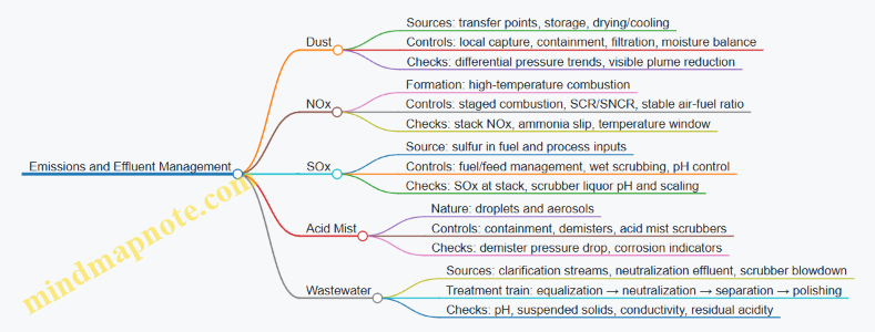
Integrated Example: One Plant, Five Streams
Imagine a plant that runs a wet-process phosphate unit plus a combustion boiler. Acid mist rises during a maintenance-related change in acid transfer routing, NOx increases after a burner tune shifts excess air, and SOx rises when a higher-sulfur fuel lot is used. Meanwhile, scrubber blowdown strength changes and increases suspended solids after a demister fouls. The integrated response is to treat each symptom as a linked system: verify source containment for mist, confirm combustion stability for NOx, check sulfur load and scrubber pH for SOx, and then adjust equalization and separation settings so wastewater sees consistent influent.
This is the practical point: emissions and effluent controls work best when they are managed as connected loops—capture, conversion, separation, and verification—rather than as isolated pieces of equipment.
12.4 Reliability Practices: Maintenance Planning, Turnarounds, and Critical Spares Strategy
Reliability in fertilizer plants is mostly about timing and discipline: doing the right work at the right moment, with the right parts, and with enough information to prevent repeat failures. Maintenance planning starts with understanding what can fail, how failure shows up in operations, and what the plant can tolerate before quality, safety, or throughput suffers.
Foundations of Maintenance Planning
Begin with a maintenance hierarchy. Reactive work handles failures that are already happening; preventive work reduces the chance of recurrence; predictive work targets specific degradation mechanisms using condition signals. In practice, most fertilizer assets need a blend. For example, a pump that sees abrasive slurry will benefit from inspection intervals and vibration trends, while a relief valve that must meet code requirements needs scheduled testing regardless of condition.
Next, translate asset criticality into maintenance frequency. Critical assets are not just expensive; they are the ones whose failure forces a unit stop, creates a safety hazard, or causes off-spec product. A simple rule of thumb works well: if the asset’s failure mode can trigger a trip, a bypass, or a quality deviation, it belongs in the critical maintenance set.
Then build work packages that are ready to execute. A good work package includes the scope, isolation and lockout steps, required permits, expected duration, access requirements, and acceptance criteria. For a valve overhaul, acceptance criteria might include seat leakage limits and stem friction checks; for a motor rewind, it might include insulation resistance thresholds and alignment verification.
Turnaround Planning That Respects Reality
Turnarounds are where reliability either improves or quietly erodes. The key is to plan around constraints: shutdown windows, long-lead materials, craft availability, and inspection access. Start with a turnaround scope that combines three inputs: scheduled statutory tasks, reliability-driven inspections, and corrective work found during operations.
A practical approach is to create a “scope-to-need” mapping. Each task should answer why it is being done now. If a heat exchanger tube bundle is trending toward fouling limits, the turnaround scope should include cleaning or replacement plus a plan to reduce recurrence, such as adjusting upstream filtration or operating parameters.
Inspection planning deserves equal attention. If you wait until the unit is open to decide what to measure, you lose time and sometimes the evidence you need. Define inspection methods early, including thickness measurements, corrosion mapping, and nondestructive testing requirements. For rotating equipment, plan alignment checks, bearing condition assessments, and coupling inspections while access is easiest.
Finally, manage turnaround execution with a constraint-based schedule. Critical path tasks often include vessel entry, major lifts, and instrument calibration. Supporting tasks like scaffolding, temporary piping, and electrical isolation should be scheduled so they do not block the critical path. A small delay in a crane window can cascade into missed testing and delayed restart.
Critical Spares Strategy That Avoids Both Shortages and Piles
A critical spares strategy balances two risks: running out of parts during a failure and tying up capital in items that rarely move. The method starts with a spares criticality list aligned to the plant’s failure modes. Then classify spares by lead time and failure impact.
Use three tiers. Tier 1 spares are high-impact and long-lead items, such as specialty catalysts, critical control valves, or unique pump seals for high-wear services. Tier 2 spares support common failures with moderate lead times, like standard bearings, gaskets, and instrumentation spares. Tier 3 spares are low-impact or short-lead items that can be sourced quickly.
For each Tier 1 item, define a reorder point based on consumption history and repair cycle time. If history is limited, use a conservative starting point and refine it after each turnaround and major repair. Also define substitution rules. A spare that cannot be substituted when the exact part is unavailable is not really a spare; it is a single point of failure.
Spares should also be stored correctly. Moisture-sensitive items need controlled packaging; elastomers need temperature and shelf-life management; and precision components need cleanliness controls. A “spare” that fails on installation is just a delayed outage.
Reliability Practices Mind Map
Mind Map: Reliability Practices
Example: From Failure Mode to Spare Decision
Suppose a phosphate plant experiences repeated failures of a specific slurry pump seal in an acid-contact service. The maintenance team records the failure mode as seal face wear and identifies a root cause such as abrasive solids bypassing filtration. Reliability planning then adds a preventive inspection interval for seal wear indicators and updates filtration maintenance. For spares, the seal assembly becomes Tier 1 if the lead time is long and the pump failure stops a critical acid circulation loop. The reorder point is set using the average seal usage per repair plus the time from order to installation, and a substitution rule is documented for equivalent seal materials approved for acid exposure.
Example: Turnaround Scope That Prevents Restart Surprises
During an ammonia plant turnaround, a heat exchanger shows increasing fouling rates. The scope includes tube cleaning and inspection, but also a reliability improvement: verifying upstream filtration performance and adjusting operating conditions that drive deposition. Restart testing then includes targeted checks tied to the fouling mechanism, such as differential pressure trends and outlet temperature stability. This keeps the turnaround from becoming a one-time fix that simply postpones the next problem.
Practical Checklist for Reliability Execution
A maintenance plan is reliable when it is executable, measurable, and connected to failure modes. Turnaround work is reliable when scope and inspection methods are defined early and the schedule respects access and critical path constraints. Spares are reliable when tiering matches impact and lead time, reorder points reflect repair cycles, substitution rules are clear, and storage conditions preserve the parts’ readiness.
12.5 Practical Example: Developing a Site Operating Procedure for Start-Up, Shutdown, and Upset Response
A good site operating procedure (SOP) is not a single document of rules; it’s a sequence of decisions that keeps people safe and keeps product quality from drifting. The SOP below is written for a fertilizer plant with nitrogen, phosphate, and potash units, but the structure works for any integrated site.
Step 1: Define Scope and Roles
Start by stating what the SOP covers: start-up, normal shutdown, emergency shutdown, and upset response. Then assign roles with clear triggers. For example, “Shift Supervisor authorizes start-up beyond first hold point,” while “Process Safety Officer approves any bypass of interlocks.” This prevents the classic problem where everyone assumes someone else is in charge.
Step 2: Build the Procedure Skeleton
Use a consistent order so operators can scan it under stress:
- Preconditions and readiness checks
- Start-up sequence by unit
- Hold points and sampling
- Ramp-up targets and acceptance criteria
- Normal shutdown sequence
- Upset response decision tree
- Post-event actions and documentation
Step 3: Start-Up Procedure with Hold Points
A start-up should move from “safe to energize” to “safe to produce.” Include hold points that pause the sequence until verification is complete.
Example start-up flow (high level):
- Preconditions: Verify utilities (steam, power, cooling water), confirm ventilation status for ammonia and acid areas, and check that relief devices are in service.
- Mechanical readiness: Confirm pumps primed, filters installed, and rotating equipment alignment verified.
- Chemical readiness: Confirm correct feedstock identity and concentration, and verify inhibitor or anti-caking dosing systems are calibrated.
- First hold point: After initial circulation, sample key streams (e.g., ammonia loop purge composition, acid concentration, brine clarity) and compare to acceptance ranges.
- Ramp-up: Increase throughput in steps, not a single jump. Each step should have a measurable target such as temperature stability, pressure trend, or solids carryover limits.
- Second hold point: Before switching to full product mode, confirm product quality indicators like moisture, particle size distribution, and chloride limits for potash.
A practical trick: write each hold point as “If X is outside range, do Y,” not “Investigate.” Operators need actions, not homework.
Step 4: Normal Shutdown Procedure
Normal shutdown should protect equipment and prevent uncontrolled reactions.
- Depressurize and isolate: Close valves in a defined order to avoid trapped pressure.
- Purge reactive systems: Use the approved purge medium and flow rate to remove reactive residues.
- Drain and clean where required: For acid and ammonia systems, specify what must be drained and what must remain for corrosion control.
- Confirm safe state: Verify that temperatures and levels are within safe limits and that ventilation continues until airborne hazards are cleared.
Step 5: Upset Response Decision Tree
Upsets are where the SOP earns its keep. The decision tree should start with symptoms, then move to safe actions.
Mind Map: Upset Response Logic
Example upset scenarios and actions:
- Ammonia system temperature rising: Stop feed, maintain purge, check cooling duty, and hold the system at a safe temperature band until the trend stabilizes.
- Phosphate acid concentration drifting low: Stop product formation, divert to appropriate hold tank, verify dosing and filtration performance, then resume only after concentration returns to spec.
- Potash brine clarification failing: Reduce dissolution rate to prevent solids carryover, verify filtration performance, and keep crystallization conditions stable to avoid off-spec chloride distribution.
Step 6: Recovery and Post-Event Actions
Recovery should be conservative. Require that the plant returns to the last verified hold point before continuing. Then document:
- what alarms occurred and when
- what actions were taken
- which acceptance criteria were met or missed
- whether any interlocks were bypassed and why
Mind Map: Start-Up and Shutdown Documentation
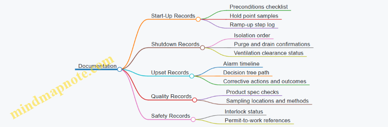
Step 7: Make It Usable
Finally, test the SOP with a tabletop exercise. Pick one start-up, one normal shutdown, and one upset scenario. Ask the team to follow the steps and record where they hesitate. If the SOP says “verify,” specify what “verify” means (a reading, a sample, a checklist item) and where it’s recorded.
This approach produces an SOP that guides action from first checks to final safe state, with enough structure to keep decisions consistent and enough detail to keep operations grounded.