Deep-Sea Engineering and Autonomous Underwater Systems
1. Scope of Deep Ocean Operations and System Requirements
1.1 Defining Operational Missions and Performance Targets
A deep-ocean mission starts as a plain question: what must the system do, where, and with what level of certainty? For an AUV that also supports sonar imaging and subsea infrastructure workflows, the answer must be specific enough to drive engineering requirements, not just planning documents.
Mission Scope and Success Criteria
Begin by writing a mission statement with three parts: objective, environment, and deliverable.
- Objective states the operational intent, such as “inspect a pipeline segment for coating damage” or “map a seafloor corridor for subsea cable routing.”
- Environment captures depth range, expected currents, visibility constraints for optical sensors, and acoustic conditions that affect sonar.
- Deliverable defines what leaves the system, such as georeferenced sonar mosaics, a set of inspection reports, or a trajectory with quality flags.
Success criteria should be measurable. Instead of “good image quality,” define thresholds like minimum usable range, required overlap between tracks, and allowable geolocation error for features of interest.
Example: Turning an Inspection Goal into Metrics
Suppose the objective is to inspect a 2 km pipeline reach. A practical set of targets could be:
- Coverage: 80% along-track overlap and 30% cross-track overlap for consistent mosaics.
- Geolocation: feature positions within 2 m horizontal error for engineering review.
- Imaging: minimum signal-to-noise ratio at the expected standoff distance.
- Completeness: at least 95% of the planned corridor receives usable data.
These metrics later become testable requirements for navigation, sonar calibration, and mission control.
Performance Targets That Map to Engineering
Performance targets should be organized into a hierarchy: mission-level outcomes, system-level capabilities, and component-level limits.
A useful way to avoid gaps is to cover five categories every time:
- Navigation accuracy for the deliverable’s coordinate frame.
- Survey geometry for coverage and overlap.
- Sensing performance for detection and imaging quality.
- Operational endurance for time-on-task and recovery margins.
- Reliability and safety for abort conditions and fault tolerance.
Mind Map: Mission to Requirements
Translating Targets into Constraints
Targets become actionable when you express them as constraints on mission planning parameters.
- Track spacing and speed determine overlap and the time available for each segment.
- Standoff distance affects sonar resolution and the expected signal level.
- Sampling cadence links to onboard storage and processing time.
- Control limits define how aggressively the vehicle can correct for current without losing coverage.
A common mistake is to set a navigation error target without specifying the operating conditions under which it must hold. For instance, “2 m horizontal error” should state whether it applies during steady current, during turns, or only after acoustic updates.
Example: Coverage Planning with Overlap
If the sonar footprint width at the chosen standoff is 120 m, and you require 30% cross-track overlap, then the cross-track spacing should be:
- Spacing = 120 m × (1 − 0.30) = 84 m
Now add along-track overlap. If the along-track footprint length is 200 m and you require 80% overlap, then the distance between successive pings or track lines should be 200 m × (1 − 0.80) = 40 m. These numbers directly influence vehicle speed and mission duration.
Operational Assumptions and Evidence
Every mission definition includes assumptions that must be documented because they determine what “meets target” means.
Record assumptions such as:
- expected current direction and magnitude bands
- sound speed profile source and update method
- expected acoustic visibility for positioning
- availability of surface support for acoustic modem windows
Then attach evidence requirements: what data will prove the system met the targets. For example, geolocation error can be supported by comparing logged navigation solutions against known checkpoints, while coverage completeness can be supported by track geometry and data usability flags.
A Practical Checklist for Writing the Mission Definition
- Objective and deliverable are stated in one paragraph.
- Success criteria are numeric and tied to the deliverable.
- Targets are mapped to navigation, survey geometry, sensing, endurance, and reliability.
- Constraints on speed, standoff, overlap, and sampling cadence are derived.
- Assumptions are listed with the evidence used to validate them.
When this is done, later sections can focus on how to engineer the system to meet the targets, rather than arguing about what the mission was supposed to accomplish.
1.2 Environmental Loading Profiles for Pressure Current and Temperature
Deep-ocean systems experience loads that change with depth, location, and time. A “loading profile” is a structured description of those loads so engineering models, control logic, and test plans can agree on what “normal” and “unfriendly” look like.
Foundational Concepts for Loading Profiles
Start with three basics: pressure, current, and temperature. Pressure is mostly a function of depth, but it also matters how quickly it changes during descent, ascent, or vehicle maneuvers. Current is a vector field that varies with depth and can change direction across a water column. Temperature affects buoyancy, material properties, and electronics thermal behavior.
A useful profile has four layers: (1) spatial dependence (depth and lateral position), (2) temporal dependence (steady, tidal, seasonal, event-driven), (3) uncertainty bounds (measurement error and natural variability), and (4) engineering translation (how the load becomes stress, force, heat, or sensor bias).
Pressure Loading with Depth and Transients
Hydrostatic pressure increases approximately linearly with depth. For engineering, the key is not just the peak value but the rate of change. Fast pressure transients can couple into mechanical compliance and sensor readings, especially when the vehicle or payload has internal cavities.
A practical way to build a pressure profile is to combine: depth-time data from mission planning, a depth sensor model, and a structural model that uses pressure as boundary loading. For example, if an AUV descends from 50 m to 200 m over 20 minutes, the pressure change is slow enough that structural response is dominated by the final pressure, not dynamic effects. If the vehicle performs a rapid dive during obstacle avoidance, the same final pressure may be less critical than the transient.
Current Loading as Forces and Flow Conditions
Current loads are more than “speed.” They include direction, turbulence intensity, and how current interacts with the vehicle geometry. A loading profile for current should specify velocity magnitude and direction versus depth, plus a turbulence or variability measure if you have it.
Translate current into forces using drag and lift models. For a first-pass example, assume a cylindrical hull segment with drag coefficient Cd. If current at the hull depth is 0.6 m/s and the projected area is 0.08 m², the drag force scales with 0.5·rho·Cd·A·V². The profile becomes meaningful when you also include how V changes with depth: a vehicle trimmed for one depth may see a different current at another, changing both speed control effort and power draw.
Temperature Loading for Buoyancy and Thermal Limits
Temperature profiles determine buoyancy and thermal gradients. Even if the vehicle’s average temperature is stable, local gradients can stress materials and shift sensor offsets.
Build a temperature profile by specifying temperature versus depth and, when relevant, time variation. A simple example: suppose the water column has a thermocline around 80 m. If the vehicle crosses that layer, buoyancy changes can require ballast or trim compensation. Meanwhile, electronics may experience different heat rejection conditions as surrounding water temperature changes.
Integrated Workflow from Measurements to Engineering Inputs
- Collect baseline data: depth, expected current profiles, and temperature versus depth from available surveys or operational records.
- Define scenario envelopes: create at least three cases such as typical, high-current, and cold-water. Each case should include uncertainty bounds.
- Convert to engineering loads: pressure to external pressure boundary conditions, current to hydrodynamic forces and moments, temperature to buoyancy terms and thermal boundary conditions.
- Check coupling effects: current affects power and thus internal heat; temperature affects buoyancy and thus control effort; pressure affects structural margins.
- Validate with sanity checks: confirm that predicted forces and thermal loads are consistent with observed power consumption or prior sea trials.
Mind Map: Environmental Loading Profile Structure
Example: Building a Three-Case Profile for Mission Planning
Assume a survey mission with a planned depth band from 60 m to 140 m. Create three cases:
- Typical: current profile moderate and aligned with the planned heading; temperature decreases gradually with depth.
- High-Current: same temperature profile as typical, but current magnitude increased within uncertainty bounds and direction rotated by a few degrees, forcing higher drag and more yaw control effort.
- Cold-Water: temperature shifted lower by a measured offset; current remains typical so you can isolate thermal and buoyancy effects.
For each case, generate depth-time traces, then compute pressure at each depth, drag forces from current at the vehicle’s effective depth, and buoyancy/thermal boundary conditions from temperature. The result is a consistent set of inputs that can feed structural checks, propulsion sizing, and control tuning without mixing incompatible assumptions.
Advanced Details Without the Guesswork
When you have limited measurements, avoid pretending the profile is exact. Use uncertainty bounds to prevent brittle designs. For current, direction uncertainty matters because it changes the moment balance and can increase control activity even if speed remains similar. For temperature, thermocline thickness controls how quickly buoyancy and thermal conditions change; a thin thermocline produces sharper transitions than a broad one.
Finally, keep the profile tied to the engineering translation. A profile that only lists “temperature at depth” but never states how it becomes buoyancy or thermal limits is incomplete. The best profiles make the path from water column physics to system constraints explicit, so later sections can reuse the same assumptions consistently.
1.3 System Architecture Tradeoffs for Payload Range and Endurance
Payload range and endurance are not separate knobs; they are coupled outcomes of how you allocate mass, volume, power, and acoustic or electrical bandwidth across the vehicle. A good architecture starts with a simple question: what must be true for the mission to succeed at the farthest point, not just at the start of the dive?
Foundational Constraints That Drive Architecture
Begin with three hard limits.
First, energy. If your mission requires sustained propulsion plus periodic high-power tasks (sonar imaging, acoustic positioning, compute bursts), then average power matters more than peak power. A practical rule is to budget energy for the worst-case duty cycle, not the best-case one.
Second, mass and volume. Batteries, pressure housings, and ballast are not interchangeable. If you increase payload mass, you often need more buoyancy control authority, which can add actuators, sensors, and control margin.
Third, hydrodynamics. Drag grows with speed and with how “busy” the hull is aerodynamically underwater. Adding external hardware can increase wetted area and flow disturbance, which increases propulsion power for the same speed.
A concrete example: two AUVs both carry a 2 kg sonar payload. One mounts it flush with the hull; the other uses a protruding fairing for easier maintenance. The second may require a lower cruise speed to meet the same endurance, even if the sonar itself is identical.
Architecture Patterns for Range and Endurance
Most architectures fall into a few patterns, each with predictable tradeoffs.
Energy-first pattern. The vehicle is designed around a conservative cruise profile and a power-efficient propulsion chain. High-power tasks are scheduled in short windows. This pattern tends to maximize endurance but can reduce effective survey time if imaging must be continuous.
Task-first pattern. The vehicle is designed to sustain payload operation, such as long-duration imaging or frequent acoustic updates. Propulsion is sized to support the duty cycle, and energy storage is increased. This pattern can reduce range if the added mass increases drag and buoyancy control effort.
Balanced pattern. The vehicle uses moderate cruise speed, selective sensor activation, and adaptive mission timing. It aims to meet both imaging coverage and navigation accuracy without assuming every segment is identical.
A useful way to choose is to map mission phases to power and performance needs: transit, station-keeping or slow survey, imaging bursts, and recovery. The architecture should match those phases, not the average of them.
Payload Range Tradeoffs Through Power and Drag
Payload range is constrained by how much energy remains when you arrive at the farthest waypoint and still have enough margin to complete the final imaging or inspection.
Three common levers affect this.
-
Cruise speed selection. Higher speed reduces time but increases drag and propulsion power. If your propulsion efficiency drops at higher load, the energy penalty can be worse than the simple speed-to-power intuition.
-
Propulsion efficiency and control. Thruster choice and control strategy affect how smoothly the vehicle holds speed and heading. Poorly tuned control can cause oscillations that waste energy.
-
Hull and appendage design. Fairings, sensor mounts, and cable routing change flow behavior. Even small increases in drag can matter over long missions.
Example: if you increase cruise speed by 20% and drag rises roughly with the square of speed, propulsion power can rise by more than 40%. If your mission energy margin is tight, you may lose the ability to run the sonar at the required settings near the end of the route.
Endurance Tradeoffs Through Duty Cycle and Scheduling
Endurance is the ability to keep the system operating safely for the required duration. The architecture determines how much of the mission uses “expensive” power.
A practical scheduling approach is to separate tasks into three tiers.
- Tier 1: Always-on. Navigation sensors, baseline compute, depth control, and safety monitoring.
- Tier 2: Periodic. Acoustic positioning, communications bursts, and moderate-rate logging.
- Tier 3: Burst. High-rate sonar imaging, intensive processing, or rapid actuation.
If Tier 3 dominates energy, the architecture must either increase energy storage or reduce the fraction of time spent in Tier 3. Reducing imaging duty cycle can be done without losing coverage by adjusting track spacing or using overlap rules that match the sensor’s resolution.
Example: instead of continuous imaging, the mission can image only during straight segments with stable attitude, while turning segments are used for navigation stabilization and lower-rate logging.
Mind Map: Payload Range and Endurance Tradeoffs
Integrated Example: Choosing Between Two Architectures
Consider a survey requiring 6 hours total operation with 2 hours of high-rate sonar imaging.
Architecture A uses a larger battery and a streamlined hull. It cruises at a moderate speed and runs sonar in scheduled bursts. The advantage is predictable energy margin at the end of the route; the risk is that imaging coverage depends on careful timing and stable attitude during burst windows.
Architecture B uses a smaller battery and a more complex mounting that improves access to the sonar. It must increase cruise speed to meet the total time, and it runs sonar more continuously. The advantage is simpler mission timing; the risk is that higher drag and tighter energy margins reduce the ability to maintain imaging settings late in the mission.
The decision comes down to which failure mode is less acceptable: missing imaging coverage due to scheduling constraints, or losing imaging quality due to energy depletion and reduced propulsion headroom.
Practical Checklist for Architecture Decisions
- Profile power by mission phase, not by component alone.
- Estimate end-of-mission energy margin under worst-case duty cycle.
- Treat drag as a system property influenced by mounts and routing.
- Ensure buoyancy and control authority scales with added payload mass.
- Validate with sea trials that measure propulsion power at the chosen cruise profile.
When these steps are followed, the architecture stops being a collection of parts and becomes a coherent plan for how the vehicle spends energy to earn range and endurance.
1.4 Interfaces Between AUV Navigation Sonar Imaging and Subsea Infrastructure
AUV navigation, sonar imaging, and subsea infrastructure only work as one system when their interfaces are defined in measurable terms. “Interface” here means more than cables and connectors: it includes coordinate frames, timing, data formats, uncertainty handling, and operational constraints that let an inspection result land in the right place on the asset.
Foundational Interface Concepts
Start with three shared reference ideas.
- Spatial reference: Navigation outputs position and attitude in a defined frame (often local vehicle, then mapped to a geodetic or site frame). Sonar imaging outputs pixels or beams that must be transformed into the same frame as the asset model.
- Temporal reference: Sonar pings, navigation estimates, and any motion compensation must be aligned to a common time base. If timestamps drift, the “same” point in space becomes a smeared point in the final product.
- Uncertainty reference: Each interface should carry not only a value (range, pose, intensity) but also an estimate of confidence. This prevents downstream decisions from treating uncertain geometry as exact.
A simple example: an AUV performs a close pass over a pipeline. If the lever-arm between the navigation sensor and the sonar transducer is wrong by 5 cm, the georeferenced track can miss a weld seam by several pixels, even when the navigation solution looks stable.
Interface Map from Vehicle to Asset
The interface chain typically looks like this: vehicle state estimation → sonar measurement formation → georeferencing → asset coordinate mapping → deliverables.
Mind Map: Interface Chain
Spatial Interfaces and Coordinate Frames
Define frames explicitly and keep them consistent across software and documentation.
- Vehicle frame: origin and axes fixed to the hull.
- Sensor frames: sonar and navigation sensors each have their own origin and axes.
- Site or geodetic frame: used for mapping to subsea infrastructure.
- Asset frame: used by the pipeline or structure model.
The key interface artifact is the transform set: a chain of rigid-body transforms that converts sonar measurements into the asset frame. Each transform must include a clear definition of origin, axis direction, and units.
Easy example: If the sonar is mounted 0.12 m forward and 0.03 m above the navigation IMU, the transform from IMU frame to sonar frame must reflect that lever arm. During georeferencing, the vehicle pose is applied to the sonar origin, not the IMU origin.
Temporal Interfaces and Synchronization
Timing interfaces are often the hidden source of “why does the image look slightly off?” issues.
- Use a common clock for navigation and sonar acquisition.
- Ensure the sonar ping time is the time the acoustic event occurs, not the time the processing finishes.
- Interpolate navigation pose to the ping time, rather than using the nearest sample.
Easy example: Suppose navigation updates at 50 Hz (20 ms spacing) and the AUV turns quickly. If sonar pings are stamped 10 ms late, the attitude used for motion compensation can be biased enough to shift features laterally.
Data Interfaces and Calibration Contracts
Treat calibration parameters as part of the interface contract, not as “setup notes.” At minimum, the system should exchange or store:
- Mounting offsets between navigation sensors and sonar transducer.
- Beam geometry parameters for mapping from beam angles to rays.
- Sound speed model inputs used for range-to-distance conversion.
- Timing offsets between ping emission and recorded timestamps.
A practical practice: version your calibration set and record which version was used for each mission. That way, when an inspection needs reprocessing, you can reproduce the same geometry.
Easy example: If a transducer is reinstalled after maintenance, the mounting offsets change. Without a versioned calibration record, reprocessed images might disagree with the original deliverable even though the navigation log is unchanged.
Uncertainty Interfaces and Quality Gates
Uncertainty should flow through the interface so that deliverables include meaningful confidence.
- Attach pose covariance to navigation outputs.
- Propagate mounting offset tolerances into georeferenced pixel uncertainty.
- Track sound speed uncertainty, especially when the vehicle crosses thermoclines.
Quality gates prevent silent failures. For instance, if the AUV attitude exceeds a configured limit, the system can flag the affected frames as lower confidence rather than pretending they are equivalent.
Easy example: During a shallow descent, the AUV may pitch more than expected. If motion compensation assumes a stable attitude, the system should mark those frames with reduced confidence so that feature measurements are weighted appropriately.
Operational Interfaces with Subsea Infrastructure
Subsea infrastructure imposes constraints that must be reflected in the AUV-sonar interface.
- Clearance constraints: minimum standoff distance to avoid shadowing and to keep the sonar within its calibrated range.
- Asset coordinate alignment: the asset model must define how its geometry relates to the site frame.
- Inspection intent: if the goal is weld inspection, the interface should prioritize image products with sufficient resolution and consistent georeferencing.
Easy example: If the pipeline model is aligned to a site survey grid, the AUV navigation solution must be mapped into that same grid. Otherwise, “correct” sonar images will still land in the wrong location on the asset.
Integrated Example Workflow
- Mission planning sets a survey track and standoff distance.
- Navigation logs pose with timestamps and covariance.
- Sonar records pings with ping-time stamps and raw measurement data.
- The system interpolates pose to ping time, applies mounting transforms, and converts sonar measurements into rays.
- Sound speed and beam geometry convert rays into 3D points.
- Points are transformed into the asset frame and assembled into georeferenced images.
- Deliverables include confidence flags derived from uncertainty propagation and operational constraints.
When these interfaces are defined and enforced, the final inspection product is not just an image; it is a measurement tied to the asset with traceable geometry and time.
1.5 Verification Requirements for Safety Reliability and Data Quality
Verification is how you prove the system does what the mission needs, not what the requirements sheet hopes it will do. For deep-sea AUV navigation, sonar imaging, and subsea infrastructure support, verification must cover three things at once: safety (no hazardous behavior), reliability (repeatable performance under stress), and data quality (measurements that can be trusted and used).
Start with a Traceable Requirements Map
Build a requirements-to-evidence chain before testing. Each requirement should point to measurable acceptance criteria and a verification method. For example, if a navigation requirement states “maintain depth within ±0.5 m,” the acceptance criteria must specify the test conditions (sea state, speed, payload configuration) and the metric definition (time window, filtering method, and whether overshoot counts).
A practical approach is to classify requirements into: (1) safety constraints, (2) performance targets, and (3) data integrity rules. Safety constraints include limits on thruster commands, power system behavior, and fail-safe states. Performance targets include navigation accuracy and sonar image quality metrics. Data integrity rules include time synchronization, sensor calibration validity, and completeness of logged metadata.
Define Safety Verification Through Hazard Scenarios
Safety verification is scenario-based. Start from hazards such as uncontrolled ascent/descent, loss of steering authority, runaway power draw, or corrupted command packets. Then define what “safe” looks like for each scenario.
Example: If a hazard is “loss of depth control,” verification should confirm the vehicle transitions to a defined safe mode, such as holding last known safe depth band or surfacing behavior when permitted. Acceptance criteria should specify maximum rate of depth change, minimum time spent in safe mode, and whether the system continues to log fault codes.
Prove Reliability with Stress, Not Just Success
Reliability verification answers: “If we run this many times, does it keep working?” Deep-sea systems face pressure, temperature gradients, vibration, and long-duration power cycling. Verification should therefore include:
- Environmental stress: pressure cycling, thermal soak, and vibration profiles matching handling and launch conditions.
- Operational endurance: repeated missions that exercise navigation, sonar pinging, and data storage.
- Fault injection: controlled sensor dropouts, checksum failures, and actuator saturation to confirm graceful degradation.
Example: For sonar imaging, reliability is not only “images appear.” It includes consistent ping timing, stable gain settings, and correct handling of missing navigation messages without producing misleading georeferenced outputs.
Validate Data Quality with Measurable Evidence
Data quality verification ensures that outputs are usable for engineering decisions. Define metrics that connect to the mission deliverables.
For navigation data quality, verify time alignment between navigation and sonar, depth reference correctness, and coordinate frame consistency. For sonar data quality, verify calibration status, beam geometry assumptions, and image quality metrics such as contrast stability and consistent speckle behavior under known conditions.
Example: If georeferenced sonar products require motion compensation, verification should include a test where the vehicle follows a known trajectory. The acceptance criteria should quantify residual misregistration in meters and confirm that the product includes the calibration and sound speed profile used.
Use a Verification Matrix Across Levels
Verification should be layered so failures are found early and fixed cheaply.
- Component level: sensor calibration checks, electronics self-tests, and power rail stability.
- Subsystem level: navigation estimator performance with recorded sensor streams, sonar signal chain checks, and communications link behavior.
- System level: full mission rehearsals with integrated logging, safety mode triggers, and end-to-end deliverable generation.
A verification matrix should list each requirement, the evidence source, the test setup, and the pass/fail criteria. This prevents the common failure mode where “it worked once” becomes the only evidence.
Mind Map of Verification Coverage
Verification Requirements Mind Map
Example Acceptance Criteria Set
Use acceptance criteria that are specific enough to be repeatable.
- Safety: In a depth-control fault injection, the vehicle must enter safe mode within 2 s, limit depth rate to ≤ 0.3 m/s, and log the fault code within the next 100 ms.
- Reliability: Over 10 endurance missions under nominal conditions, navigation solution availability must be ≥ 95%, and sonar ping timing jitter must remain within a defined bound.
- Data quality: For a georeferencing test with a known trajectory, residual misregistration must be ≤ 0.5 m (or the mission-justified threshold), and the output must include the sound speed profile identifier and calibration version.
Verification Evidence That Survives Real Use
Finally, verification evidence must be reproducible and interpretable. Require that logs include timestamps, sensor calibration identifiers, software versioning, and the exact configuration used for each run. If a result cannot be traced back to its inputs, it cannot be trusted—no matter how impressive the plot looks.
2. Hydrodynamics and Mechanical Design for AUVs
2.1 Hull Forms Drag Reduction and Flow Separation Control
A hull form’s job is simple to state and hard to execute: it must move water out of the way with as little energy loss as possible, while keeping the boundary layer attached so the flow doesn’t start “throwing tantrums” at the surface. Drag is not one thing; it’s the sum of frictional resistance from viscosity and pressure resistance from how the flow accelerates, decelerates, and separates.
Foundations: What Creates Drag
Start with the boundary layer, the thin region near the hull where velocity changes from zero at the wall to free-stream speed. Two mechanisms dominate:
- Frictional drag grows with wetted area and with how turbulent the boundary layer becomes. Smoother surfaces and favorable pressure gradients help keep friction lower.
- Pressure drag appears when the flow separates, leaving a low-pressure wake behind the hull. Separation is often the difference between a quiet, streamlined wake and a messy one.
A practical mental model is to treat the hull as a sequence of pressure changes. If the hull causes the pressure to rise along the surface, the boundary layer may lose momentum and separate.
Flow Separation Control: The Pressure Gradient Story
Flow separation is driven by the boundary layer’s ability to resist an adverse pressure gradient. An adverse pressure gradient means pressure increases in the direction of flow, which slows the near-wall fluid. When the near-wall fluid can’t overcome that slowdown, it separates.
Hull designers manage this by shaping the longitudinal pressure distribution:
- Accelerate gently where needed so the boundary layer gains momentum.
- Avoid strong deceleration in regions where the boundary layer is already thick or slow.
- Use curvature and taper to keep the pressure gradient favorable or only mildly adverse.
A useful rule of thumb for intuition: if the hull “pinches” too quickly, the flow decelerates too fast, and separation becomes more likely.
Hull Form Choices That Reduce Drag
Wetted Area and Form Factor
Frictional drag scales with wetted area and how long the boundary layer stays attached. For a given displacement, a slimmer hull tends to reduce wetted area, but it can also change the pressure distribution and stability. The goal is not minimum area at any cost; it’s a balanced form that keeps both friction and pressure drag under control.
Nose and Midbody Shaping
The bow and forward sections set the initial boundary layer state. A smooth, gradual entry helps the flow attach early. The midbody is where designers often fight the tradeoff between carrying volume and maintaining a favorable pressure gradient.
Afterbody and Wake Management
The afterbody controls how the flow recovers and how the wake forms. A well-shaped afterbody reduces the size and strength of the separated region. Even if some separation is unavoidable, reducing its extent and keeping it predictable lowers pressure drag.
Systematic Design Workflow
- Define operating regime: speed range, Reynolds number band, and whether the hull will see waves or currents.
- Choose a baseline geometry: start with a known family (e.g., streamlined displacement or semi-planing shapes) that matches the mission.
- Map pressure gradient along the hull: use CFD or towing-tank data to identify where adverse gradients become strong.
- Check boundary layer attachment: look for separation indicators such as reversed flow near the surface.
- Refine curvature and transitions: adjust radii, taper rates, and chine/keel lines to smooth deceleration.
- Validate with drag breakdown: confirm whether improvements came from reduced friction, reduced pressure drag, or both.
Example: A Simple Geometry Change That Helps
Suppose a hull has a noticeable drag rise at higher speed. A common cause is separation on the afterbody due to excessive deceleration. If the afterbody transitions from a fuller section to a narrower one too abruptly, the pressure increases sharply and the boundary layer loses momentum.
A practical fix is to increase the length of the taper and reduce the taper angle, keeping the same overall volume. This spreads the deceleration over a longer distance, making the adverse pressure gradient less severe. The result is often a smaller separated region and a lower pressure drag component, even if wetted area increases slightly.
Mind Map: Hull Forms and Separation Control
Quick Checks During Iteration
When comparing two hull variants, don’t just look at total drag. Track whether the change reduced pressure drag (often tied to separation behavior) or friction drag (often tied to wetted area and surface condition). If total drag drops but the wake looks larger, you may have traded one problem for another—use the boundary layer and pressure gradient evidence to keep the improvement grounded.
2.2 Propulsion Selection Thrusters and Efficiency Under Load
Propulsion selection for an AUV starts with a simple question: what thrust must the vehicle produce at the worst moment, not the average one? In deep water, “worst” often means a combination of higher drag (speed, payload, fouling), unfavorable attitude (trim changes), and power limits (battery voltage sag and thermal constraints). The thruster you pick must deliver the required thrust across that operating envelope while keeping efficiency high enough that the mission energy budget still closes.
Foundational Concepts for Thruster Choice
Thrust requirement comes from drag and mission profile. Drag grows roughly with the square of speed, so a small speed increase can noticeably raise thrust demand. A practical approach is to compute drag at several speeds using your hull form and appendage configuration, then add a margin for uncertainties like sensor fairings, cable drag, and slight misalignment of the flow.
Efficiency is not a single number. Thruster efficiency depends on operating point: advance speed, inflow conditions, propeller loading, and whether the propeller is partially ventilated or cavitating. “Best efficiency” at one speed can become poor efficiency at another, especially when the vehicle must hold depth and heading against currents.
Propulsor type shapes controllability. Fixed-pitch propellers are efficient near their design point but can be less flexible. Variable pitch is more complex and heavier. Thrusters with ducting can improve effective thrust in some regimes, but they also add drag and can be sensitive to mounting and flow quality.
Thruster Types and How They Behave Under Load
Open-water propellers. These are common because they are efficient and relatively straightforward. Under load, the propeller absorbs more torque to produce thrust, which raises motor current and losses. If the motor reaches its current limit, thrust will flatten even if the controller keeps commanding it.
Ducted propellers. Ducts can increase thrust at low speeds by shaping the flow, which helps during slow survey segments or station-keeping. The trade is added structure and potential flow separation if the duct experiences disturbed inflow.
Thruster pods and integrated modules. These simplify installation and alignment, but the pod’s hydrodynamic drag and the propeller’s interaction with the hull can shift the efficiency curve. Treat the pod as a system, not just a motor plus propeller.
Efficiency Under Load: The Operating-Point View
A useful way to reason about efficiency is to track power from battery to shaft to water. Motor electrical power splits into useful shaft power and losses (copper and iron). Shaft power then splits into thrust-producing work and propeller losses (viscous effects, tip losses, and cavitation-related inefficiencies).
When the vehicle accelerates or fights a current, the propeller moves to a higher loading condition. That increases torque demand and can push the propeller toward cavitation. Cavitation is not only a noise issue; it can reduce thrust and increase unsteady loads that stress bearings and mounts.
Selection Workflow That Avoids Common Traps
- Define the thrust envelope. Use mission speed, expected current range, and worst-case attitude. Include a margin for drag model error.
- Choose a propeller diameter and pitch family. Larger diameter can improve efficiency at lower RPM, but it may be limited by clearance and structural constraints.
- Map motor limits to thrust limits. Convert motor current and voltage limits into maximum shaft power, then into maximum thrust using propeller curves.
- Check cavitation margin. Ensure the operating point stays below cavitation risk for the expected speed and pressure conditions.
- Validate with system-level tests. Bench tests with a dynamometer help, but sea trials confirm real inflow and mounting effects.
Example: Sizing for a Current-Fighting Segment
Assume a vehicle needs 120 N thrust at cruise speed in calm water, and the mission includes a segment where a current adds an extra 30 N of effective drag. The thrust requirement becomes 150 N. If your propeller curve shows that 150 N occurs at a shaft power of 1.8 kW, then the motor and controller must sustain that power with battery voltage sag.
Now include efficiency: suppose propeller efficiency at that point is 0.65 and motor efficiency is 0.90. The electrical power becomes:
- Water useful power: 150 N × speed (use your cruise speed)
- Shaft power: useful thrust power divided by propeller efficiency
- Electrical power: shaft power divided by motor efficiency
If the computed electrical power exceeds your available battery power during the segment, you must either reduce speed, increase propeller diameter (if feasible), change pitch, or accept a shorter segment duration. The key is that the decision is driven by the operating point, not by the propeller’s best-case efficiency.
Mind Map: Thrusters and Efficiency Under Load
Practical Notes for Better Results
Thruster controllers should be tuned to avoid hunting around the propeller’s most inefficient region. If your vehicle frequently transitions between slow and fast segments, consider selecting a propeller family whose efficiency curve is reasonably flat across those points. Finally, treat propeller inflow quality as part of propulsion design: a small change in mounting or hull flow can shift the effective operating point enough to matter for energy use.
2.3 Buoyancy Systems Ballast and Variable Trim Mechanisms
Buoyancy is what keeps an AUV from turning every dive into a negotiation with gravity. In practice, you design buoyancy so the vehicle can hold a commanded depth, recover from disturbances, and still have margin for payload changes and mission variability.
Foundational Concepts for Buoyancy Control
Start with the forces. Net vertical force is the difference between buoyancy and weight, plus any hydrodynamic vertical components. For slow, controlled motion, you can treat hydrodynamic vertical forces as small compared to buoyancy and weight.
A simple mental model helps: if buoyancy exceeds weight, the vehicle rises; if weight exceeds buoyancy, it sinks. Depth control then becomes a matter of adjusting the net vertical force until it matches the commanded depth behavior.
Ballast Systems Fixed Buoyancy and Controlled Weight
Fixed buoyancy systems use a known displaced volume and a known mass. They are reliable and simple, but they require careful mass budgeting because you cannot “dial out” a mismatch mid-mission.
A common approach is to set the vehicle slightly buoyant and use ballast for fine control. Ballast can be implemented as:
- Solid ballast for permanent trim and center-of-mass placement.
- Disposable ballast for one-time adjustments, such as launch configuration changes.
- Variable ballast for continuous or stepwise control, which is where the real flexibility comes from.
A practical example: you plan a survey with a payload that consumes power but not mass. If your vehicle is neutrally buoyant at the start, battery mass changes are small enough that depth control remains stable. If your mission includes consumables like expendable weights or variable fluid loads, you need variable ballast or you’ll spend the mission fighting a slow drift.
Variable Trim Mechanisms for Depth Stability and Handling
Variable trim is about changing the vehicle’s effective weight distribution and sometimes its overall buoyancy. The goal is not only to move up or down, but to keep the vehicle controllable when it pitches, accelerates, or encounters currents.
Two mechanisms dominate:
Internal Ballast Tanks and Pumped Fluid
A variable ballast tank changes buoyancy by moving fluid between a tank and the surrounding structure. You can implement it as a pump-driven system or a gravity-assisted system with valves.
Key design details:
- Tank volume and stroke determine how much buoyancy change you can generate.
- Pump sizing affects how quickly you can respond without cavitation or excessive noise.
- Valve timing and hysteresis matter because depth control depends on repeatable force.
Easy example: suppose your vehicle needs a small net force change to counter a current-induced sink rate. If your ballast system can produce that net force with a few percent of tank volume change, you can use short ballast adjustments rather than large moves that overshoot.
Movable Mass Systems for Center of Mass Control
Movable mass shifts the center of mass to improve pitch control and reduce control effort. This is especially useful when the vehicle must maintain a stable attitude for imaging or sonar.
Key design details:
- Actuator range sets how much trim authority you have.
- Friction and backlash create dead zones that show up as sluggish depth or pitch response.
- Locking behavior matters when the vehicle is stationary; you want the mass to stay put.
Easy example: if your vehicle’s payload is slightly top-heavy, a movable mass can shift downward to restore neutral pitch behavior. That reduces how hard the control system must work, which in turn reduces power draw and improves repeatability.
Coupling Buoyancy and Control Loops
Buoyancy changes are not instantaneous. Pumps have dynamics, valves have delays, and fluid movement has time constants. If your control loop assumes immediate force response, you’ll see oscillations or slow settling.
A systematic way to design the coupling:
- Measure the ballast-to-depth response during controlled tests.
- Identify the effective time constant for net force changes.
- Tune the depth controller to avoid commanding faster changes than the mechanism can deliver.
A concrete example: if ballast adjustments take 2–3 seconds to fully affect buoyancy, a depth controller with a 0.2-second update rate may still be fine, but the control gains must reflect the slower plant response.
Practical Design Constraints and Failure Modes
Buoyancy systems must be robust to real-world issues:
- Air ingestion and trapped gas can reduce effective tank volume and cause unpredictable buoyancy.
- Leakage changes neutral buoyancy over time.
- Stiction in valves creates inconsistent step sizes.
- Sensor bias in depth and attitude can mask buoyancy errors.
Mitigations often include careful venting, leak testing, and calibration routines that relate commanded ballast position to measured depth response.
Mind Map: Buoyancy Systems Ballast and Variable Trim Mechanisms
Example Workflow for Commissioning Buoyancy Authority
- Set initial neutral buoyancy using solid ballast and known fluid fill states.
- Calibrate variable ballast by commanding small tank volume changes and recording depth response.
- Validate trim authority by shifting movable mass in steps and checking pitch stability.
- Tune control gains using the measured response time, then run a repeatability test with identical commands.
If the same ballast command produces slightly different depth outcomes, you don’t “fix it with control gains.” You first identify whether the mechanism has hysteresis, whether valves stick, or whether trapped gas is changing effective volume.
Summary of What “Good” Looks Like
A well-designed buoyancy and trim system provides predictable net force, stable attitude, and repeatable response under mission conditions. It supports depth holding without excessive control effort, and it behaves consistently enough that your navigation and imaging workflows can rely on the vehicle’s motion rather than constantly compensating for it.
2.4 Structural Design for External Pressure and Fatigue Life
External pressure is the quiet boss of deep water: it compresses everything, squeezes seals, and turns small design shortcuts into big maintenance bills. Structural design for an AUV or subsea housing starts with pressure loads, then moves to stress paths, then to fatigue life under realistic cycling.
Foundational Loads and Pressure Modeling
Begin by defining the pressure environment as a function of depth and time. Use hydrostatic pressure as the baseline: \(p=\rho g h\). For operational profiles, include depth excursions from mission logs or conservative envelopes. If the vehicle experiences pitching and heaving, pressure is still mostly hydrostatic, but local pressure gradients can appear around appendages and sensor pods.
Next, decide what “external pressure” means structurally. For a pressure hull, the load is nearly uniform over the wetted surface. For external frames, fairings, and battery pods, pressure acts as distributed load plus drag-induced bending. A practical approach is to separate components into pressure boundary elements and non-boundary structures.
Example: A cylindrical pressure hull with end caps sees uniform external pressure, so hoop stress dominates. A thruster guard ring sees pressure plus flow-induced forces, so bending and local stress concentrations matter more than pure hoop stress.
Stress Paths and Failure Modes
Uniform pressure produces predictable primary stresses, but real failures often start at geometric discontinuities: fillets, penetrations, weld toes, stiffener terminations, and mounting bosses. Map stress paths from load application to supports. If you can’t trace where the load goes, the structure will surprise you later.
Key failure modes to design against:
- Yielding or buckling under maximum depth.
- Fatigue cracking at stress raisers under repeated pressure cycling and vibration.
- Seal and interface damage from differential deformation.
For thin-walled shells, buckling is often the governing limit rather than material yield. For thick sections, yielding and fatigue may dominate.
Buckling Resistance for Shells and End Caps
Buckling capacity depends on geometry, boundary conditions, and imperfections. Use shell theory or validated finite element analysis to estimate critical buckling pressure. Then apply safety factors that reflect uncertainty in thickness, fabrication tolerances, and end-cap stiffness.
Imperfections are not optional in deep-ocean structures. A small out-of-roundness can reduce buckling margin. A good design workflow includes:
- Define manufacturing tolerances.
- Model initial geometric imperfections within those tolerances.
- Check buckling under worst-case boundary conditions.
Example: If end caps are assumed perfectly fixed in analysis but are actually bolted with compliance, buckling pressure can drop. Modeling end-cap flexibility often explains why a “safe” design fails in sea trials.
Fatigue Life Under Pressure Cycling and Vibration
Fatigue life is driven by stress range and number of cycles. External pressure cycling comes from depth changes, while vibration adds high-frequency stress fluctuations at local hotspots.
A systematic method:
- Convert mission depth profiles into pressure cycles.
- Translate pressure cycles into stress cycles at critical locations using structural analysis.
- Combine with vibration-induced stress ranges if the structure experiences resonant or near-resonant excitation.
Use an S-N approach for metallic components and a strain-life approach when mean stress effects are significant or when you have limited data. For welded joints, treat the weld toe as a hotspot and use appropriate notch factors or hotspot stress methods.
Example: A pressure hull may see low stress range from slow depth changes, but a welded stiffener toe can experience larger local stress range due to stiffness mismatch. The hull survives, the toe cracks.
Design Details That Control Fatigue
Fatigue is won or lost in details:
- Fillet radii at transitions reduce stress concentration.
- Smooth load paths avoid abrupt stiffness changes.
- Penetration reinforcement prevents local bending.
- Surface finish and corrosion protection reduce crack initiation.
Also manage mean stress. If the structure always operates near a high fraction of allowable stress, fatigue life shortens even if the stress range is modest.
Materials, Thickness, and Manufacturing Tolerances
Select materials based on strength, toughness, corrosion behavior, and weldability. Thickness is not just “more is safer.” Extra thickness can increase mass and change buckling behavior, while also shifting stress distributions.
Manufacturing tolerances must be part of the design. If thickness variation is ±10%, buckling and fatigue margins change. Include measured fabrication capability in the safety factors.
Example: A design that assumes nominal thickness might pass analysis, but if the as-built thickness at a stiffener termination is consistently low, the local buckling margin and fatigue hotspot stress both worsen.
Verification Through Analysis and Testing
Verification should connect analysis to measurable outcomes.
- Structural analysis: buckling checks, stress maps, and hotspot evaluation.
- Pressure testing: proof pressure and controlled cycling to validate deformation and detect leaks.
- Fatigue-relevant checks: inspect known hotspots after cycling and after vibration exposure.
Use strain gauges or displacement measurements at critical locations during proof tests. If measured deformation differs from predicted deformation, update the model before trusting fatigue calculations.
Mind Map: Structural Design Flow for Pressure and Fatigue
Example: Pressure Hull with Stiffeners and a Penetration
Consider a cylindrical hull with external stiffeners and a sensor penetration. The uniform external pressure drives hoop stress, while the stiffeners and penetration introduce local bending and stress concentration.
A practical design sequence:
- Run a global model to confirm hoop stress and overall buckling margin.
- Refine the region around the penetration and stiffener terminations to extract hotspot stress ranges.
- Convert the mission depth profile into pressure cycles and compute fatigue damage at the hotspot.
- Modify geometry if the hotspot stress is dominated by a sharp transition, such as adding a larger fillet radius or changing stiffener termination details.
- Validate with proof pressure deformation measurements and post-test inspection of the penetration region.
This approach keeps the design grounded: you don’t just “check strength,” you identify where cracks would start and ensure the structure is built to resist that exact behavior.
2.5 Sealing and Materials Selection for Long Duration Wet Operation
Long-duration wet operation is mostly a sealing problem wearing a materials problem’s clothes. Pressure, temperature swings, chemistry, and mechanical motion all attack the same weak points: interfaces, penetrations, and anything that must move while staying watertight.
Core Sealing Concepts for Wet Environments
A seal’s job is to maintain a pressure-tight boundary while accommodating deformation. In deep water, external pressure can be hundreds of times atmospheric, so the seal must resist both compression and shear. The most common failure modes are extrusion of soft elastomers into gaps, loss of compression due to creep, and chemical swelling that changes dimensions.
A useful starting rule is to separate sealing into three layers. First, use a primary barrier that carries the pressure load. Second, add a secondary barrier that catches leaks from the primary. Third, include a controlled drainage or leak detection path so a small breach does not turn into a full flood.
Materials Selection Principles
Materials must match the environment and the mechanical role. Elastomers provide compliance, but they age: oxygen, dissolved gases, and hydrocarbons can change hardness and elasticity. Metals provide stiffness and dimensional stability, but they can corrode or gall under load.
For elastomers, select based on compatibility with expected fluids and temperature range. If the system uses hydraulic oils, cable jackets, or potting compounds, treat those as part of the chemical exposure list. For metals, consider galvanic couples between dissimilar alloys, especially where seawater can bridge them through moisture films.
A practical method is to map each material to its contact partners: seal-to-housing, seal-to-shaft, seal-to-connector potting, and any elastomer-to-elastomer interface. Then verify that each pair avoids swelling, adhesion, or accelerated corrosion.
Seal Geometry and Compression Management
Seals fail when they are either under-compressed or over-compressed. Under-compression leaves leakage paths; over-compression increases extrusion risk and accelerates creep. Groove design matters because it controls how the seal deforms under pressure.
Use a gland that supports the seal cross-section and limits extrusion. For dynamic seals, include a wear surface strategy: a hard, smooth counterface reduces abrasion and keeps friction stable. For static seals, focus on surface finish and flatness so the seal can form a continuous contact band.
A simple example: a circular O-ring in a poorly machined groove may seal at first, then leak after a few thermal cycles because the contact band shifts. Fixing the groove finish often improves long-term performance more than changing the elastomer alone.
Penetrations and Cable Sealing Strategies
Penetrations are where design intent meets reality. Cable entries experience bending during handling, then vibration during operation. A robust approach uses strain relief so the seal does not carry bending loads.
Common strategies include compression glands with controlled torque, potting around conductors to eliminate voids, and connector designs that use redundant sealing surfaces. If you pot, ensure the potting compound does not shrink away from the cable jacket; shrinkage creates a capillary path.
A concrete workflow is to pressure-test each penetration subassembly before final integration. That way, you isolate whether the leak is in the connector interface, the gland, or the internal potting.
Dynamic Versus Static Sealing
Static seals handle housings, bulkheads, and sensor windows. Their main enemies are creep and chemical aging. Dynamic seals handle shafts, moving doors, and any mechanism that must operate underwater. Their main enemies are wear, friction-induced heating, and debris.
For dynamic applications, consider sealing with a combination of a primary lip and a secondary barrier. The secondary barrier can be a dry cavity with monitoring, or a second elastomer that catches leakage from the first. Even if the primary lip wears, the secondary layer buys time and prevents immediate flooding.
Surface Preparation and Assembly Controls
Even the best materials fail if assembly is sloppy. Cleanliness prevents particles from becoming leak paths. Lubricants must be compatible with the elastomer and the environment; a lubricant that works on land can swell the seal in seawater.
Assembly controls include torque verification, alignment checks, and avoiding nicking during installation. A tiny cut in an O-ring can become a leak channel under pressure. Use installation tools that minimize stretching and avoid sharp edges.
Mind Map: Sealing and Materials Selection
Example: Window Seal for a Sonar Housing
Imagine a sonar transducer window mounted in a pressure housing. The window must resist pressure while maintaining acoustic performance. Start with a static seal between window frame and housing: choose an elastomer compatible with seawater and the potting compound, and design the gland to prevent extrusion.
Add a secondary barrier by using a secondary gasket or a controlled cavity behind the window. Then include a drainage path or a sensor to detect moisture. During assembly, ensure the window seating surfaces are flat and free of machining debris. Finally, pressure-test the window subassembly at a level that exercises the seal without risking the transducer.
Example: Cable Penetration with Redundant Sealing
For a cable entry, use a compression gland for mechanical retention and a separate sealing interface for watertightness. Add strain relief so bending loads do not transfer into the elastomer. If the design uses potting, confirm that the potting compound bonds to the cable jacket without voids.
Pressure-test the penetration module before connecting it to the rest of the electronics. If a leak appears, you can distinguish whether it originates at the gland, the connector interface, or inside the potting region by repeating tests with controlled disassembly.
Practical Acceptance Checks
A long-duration seal design should include measurable acceptance criteria: allowable leak rate, compression set limits, and post-test inspection for extrusion, swelling, or surface damage. Record torque values, surface finish targets, and assembly cleanliness standards so the same results can be reproduced across builds.
3. Power Systems and Energy Management for Autonomous Underwater Vehicles
3.1 Battery Chemistry Selection and Operating Constraints
Choosing a battery chemistry for an AUV is mostly about matching three realities: the chemistry’s voltage behavior, the energy you can actually extract under load, and how the battery survives deep-water temperature and pressure conditions. The “best” chemistry is the one that meets mission energy at the required power profile while staying within safe voltage, temperature, and charge limits.
Foundational Constraints That Drive Chemistry Choice
Start with the mission energy requirement and the power profile. If your vehicle needs high peak power for bursts of thrust or sonar transmit, the chemistry must tolerate current spikes without excessive voltage sag. Voltage sag matters because many motor controllers and compute rails have minimum operating voltages; once you cross those thresholds, performance drops or the system resets.
Next, account for deep-water temperature. Battery capacity is temperature-dependent, and internal resistance rises as temperature drops. That combination reduces usable capacity and increases voltage sag at the same load. A practical approach is to define a “cold-case” temperature and compute the minimum expected pack voltage during the worst segment of the mission.
Finally, consider charge and cycle constraints. Some chemistries prefer partial cycling, others tolerate deeper cycles better, and many have strict limits on maximum charge voltage and allowable charge current. Even if you never fully charge in the field, you still need a charging strategy that won’t slowly push the chemistry toward unsafe operating regions.
Chemistry Families and What They Trade
Lithium-ion chemistries are common because they offer high energy density and manageable packaging. Within that family, the key differences are stability characteristics, voltage curves, and how they behave under low temperature and high current.
Lithium iron phosphate is often chosen when safety margin and cycle life matter more than maximum energy density. Its voltage is lower than some other lithium-ion types, which can increase the number of cells needed for a given bus voltage. That can affect mass and packaging, but it also tends to be more forgiving in terms of abuse tolerance.
Nickel-based lithium-ion variants can provide higher energy density, which helps when you’re constrained by volume. The trade is that they can be more sensitive to temperature and charging conditions, so your battery management system (BMS) and thermal design must be more disciplined.
Lithium polymer can be attractive for packaging flexibility, but it still needs careful thermal control and robust cell protection. In practice, the chemistry choice is inseparable from how the cells are mounted, insulated, and monitored.
Operating Constraints You Must Design Around
1) Voltage window and sag under load Define the minimum allowable pack voltage for propulsion and electronics. Then model the expected voltage drop using internal resistance and current draw. A simple sanity check: if your peak current causes the pack to dip below the controller’s minimum, you either need a different pack configuration, more cells, or a different chemistry with lower internal resistance.
2) Temperature limits for charge and discharge Discharge limits are about performance and safety; charge limits are often stricter. Many lithium chemistries should not be charged below a certain temperature because lithium plating risk rises. That means your charging workflow must include temperature conditioning or a charging inhibit logic.
3) State of charge estimation accuracy AUV batteries live in a world of partial discharge, temperature variation, and current pulses. State-of-charge (SoC) estimation must remain stable under those conditions. If SoC estimation drifts, the BMS may either cut off early (wasting energy) or allow deeper discharge than intended (risking damage).
4) Depth of discharge and cycle life Even when a chemistry can technically handle deep discharge, cycle life may suffer. For mission planning, it’s often better to cap usable depth of discharge and treat the remaining capacity as a safety buffer for unexpected currents, colder-than-modeled water, or navigation detours.
Integrated Example: Choosing Between Two Pack Options
Assume the AUV requires a 48 V bus and electronics must not drop below 42 V during peak thrust. Option A uses a chemistry with a higher nominal cell voltage but higher internal resistance at cold temperature. Option B uses a lower-voltage nominal chemistry with lower cold internal resistance.
You compute the worst-case pack voltage during the peak segment:
- If Option A’s predicted sag dips below 42 V, it fails the controller constraint even if it meets energy on paper.
- If Option B maintains voltage margin but requires more cells for the same bus voltage, you compare the added mass against the mission’s payload and volume limits.
Then you check charge constraints. If Option A requires strict charging above a higher temperature threshold, you must ensure the charging workflow can condition the pack reliably. If the facility can’t guarantee that, Option A becomes operationally risky even when the mission discharge looks fine.
The final selection is the one that satisfies voltage margin under peak load, stays within temperature-safe charge and discharge limits, and supports dependable SoC estimation for the planned depth of discharge.
3.2 Power Distribution Design for High Current Loads and Transients
High-current loads in an AUV—thrusters, pumps, and sometimes sonar transmitters—create two design problems at once: steady power delivery and short-duration electrical stress. Good power distribution treats both as first-class requirements, then proves the result with measurements rather than hope.
Foundational Concepts for Power Distribution
Start with the load reality. A “high current” thruster rarely draws a perfectly constant current; it ramps, reverses, and saturates. That means your distribution network must handle both:
- DC voltage drop so the controller sees the expected bus voltage.
- Transient behavior so voltage dips and ringing do not reset electronics or distort sonar timing.
A practical way to reason about this is to model the distribution path as an impedance chain: source internal resistance, busbar and cable resistance, connector contact resistance, switch and protection elements, then the load. The transient voltage at the load is approximately the transient current times the effective impedance, plus any inductive effects from wiring geometry.
Architecture Choices and Their Tradeoffs
A typical architecture uses a main energy bus feeding power rails for subsystems, with local power stages near high-current loads.
- Star distribution for high-current branches: run separate returns to a common node to reduce shared impedance. Example: two thrusters each get their own return conductor back to the main node rather than sharing a thin segment of return under the avionics bay.
- Local bulk energy near the load: place capacitors close to the thruster driver so the driver sees a low-impedance source during current steps.
- Segregated power domains: keep sensitive analog and digital rails physically and electrically separated from the thruster power path, then connect them through controlled regulation.
A useful rule of thumb is to minimize the “loop area” of the high-current path. Large loop areas convert current steps into magnetic fields that couple into nearby sensors and cables.
Designing for Voltage Drop Under Steady Load
Compute worst-case current and allowable bus sag. For example, if the thruster driver requires at least 36 V at its input and the battery nominal is 40 V, you might allow 2 V total sag across the distribution path. If the thruster branch current is 120 A, the allowable effective resistance is roughly 2 V / 120 A ≈ 0.017 Ω. That number tells you how aggressively you must size conductors and connectors.
Then validate with a simple measurement plan:
- Measure resistance from the bus node to the driver input using a four-wire method.
- Apply a controlled load step on a test bench and record bus voltage at the driver terminals.
If the measured sag exceeds the budget, the fix is usually mechanical and electrical: thicker conductors, better crimp quality, shorter runs, or fewer series protection elements.
Designing for Transients and Switching Stress
Transients come from two sources: the load itself (current steps) and the power electronics (switching edges). Your distribution network must prevent three common failures:
- Controller resets from undervoltage at the logic rail.
- False sensor readings from ground bounce.
- Excess EMI from ringing that couples into signal wiring.
Bulk Capacitance and Placement
Bulk capacitors reduce voltage droop during current steps. The key is placement: a capacitor that is electrically “far” behaves like a capacitor with extra series inductance. Place bulk capacitance at the driver input, then add smaller high-frequency capacitors in parallel to handle faster edges.
Example: a thruster driver draws 120 A and current ramps in 5 ms. If you estimate the droop due to capacitance as ΔV ≈ I·Δt/C, then C ≈ I·Δt/ΔV. If you want less than 0.5 V droop, C ≈ 120 A · 0.005 s / 0.5 V = 1.2 F. In practice you rarely get that with capacitors alone, so you combine capacitance with reduced impedance conductors and a battery management strategy that supports the step.
Snubbers and Damping
When inductance and capacitance form a resonant pair, you get ringing. Damping can be achieved with RC snubbers across switching elements, ferrite beads in the right place, or controlled gate drive shaping in the driver. The goal is not “no ringing,” but “ringing that stays within voltage and EMI limits.”
Protection Coordination Without Nuisance Trips
Protection elements—fuses, breakers, current sensors, and TVS devices—must be coordinated so they protect hardware without interrupting mission-critical operation.
- Fuses and breakers: choose time-current curves that tolerate startup and brief transients.
- Current sensing: place sensors so they measure the branch current accurately, not a distorted version caused by shared return paths.
- TVS and surge suppression: size for the expected energy and clamp level at the protected node.
Example: if a thruster driver draws a brief inrush that is higher than the steady current, a protection device with a slow response might be fine, while a fast electronic trip could nuisance-trip during every maneuver.
Grounding and Return Path Discipline
Grounding is where many designs quietly lose. Treat the return path as part of the power system, not an afterthought.
- Use a single-point reference for sensitive electronics when feasible.
- Route sensor grounds separately from high-current returns until the chosen reference node.
- Avoid daisy-chaining grounds through connectors that also carry thruster current.
A quick sanity check: if you can measure a voltage difference between “ground” points during a thruster step, you have ground bounce. Fix it by rerouting returns, adding local decoupling, or changing the star node location.
Verification Through Measurements
Design reviews are good; oscilloscope traces are better.
Use a test setup that reproduces the real current step and wiring geometry. Measure:
- Bus voltage at the source and at the driver input.
- Logic rail voltage and reset events.
- Current waveform at the branch.
- Noise on a representative sensor line.
Then compare to your impedance-based expectations. If the measured droop is larger than predicted, suspect connector resistance, unexpected inductance from cable routing, or insufficient local capacitance.
Mind Map: Power Distribution for High Current Loads and Transients
Example: Thruster Branch with Local Decoupling and Star Returns
A thruster driver is fed from the main bus through a dedicated branch. The branch uses a short, thick conductor pair to minimize resistance and inductance, with a star return back to the main node. At the driver input, bulk capacitors and smaller decouplers are mounted close to the driver power pins. During bench testing, a current step is applied and bus voltage is measured at both the battery node and driver input. If the driver input droop stays within the controller’s minimum voltage and the logic rail shows no reset, the distribution network is doing its job—quietly, reliably, and without turning the rest of the vehicle into a noise antenna.
3.3 Thermal Management for Electronics and Power Modules
Deep water is a great place to test electronics—because it’s also a great place to remove heat in the least forgiving way. Thermal management in an AUV is about controlling temperature rise, keeping gradients small, and ensuring components survive both steady operation and short high-load events.
Foundational Principles of Underwater Heat Transfer
Start with the heat path: junction heat flows through package materials into the enclosure, then into the surrounding water. In deep operation, convection is often limited by vehicle speed and boundary layer effects, so conduction design inside the vehicle becomes the main lever.
A practical way to reason about thermal design is to treat it like a chain of resistances. Each interface adds resistance: chip to substrate, substrate to heat spreader, spreader to enclosure, enclosure to water. If you reduce only one link, the rest still bottleneck the heat.
Example: Suppose a power module dissipates 120 W during a thruster transient. If the enclosure-to-water path has high thermal resistance, the enclosure temperature rises quickly even if the module-to-enclosure interface is perfect. The fix is not just better mounting paste; it’s also improving heat spreading area and ensuring the enclosure surface is in good thermal contact with the water.
Thermal Targets and Operating Margins
Thermal targets should be expressed as component limits with margins for uncertainty. Use datasheet maximum junction temperatures and then subtract margin for calibration error, sensor placement error, and worst-case ambient conditions.
A useful operational rule is to define two regimes:
- Steady-state: average dissipation during a mission segment.
- Transient: short bursts from control loops, power electronics switching, or sonar bursts.
Example: A navigation computer may run at 20 W steady, but a motor driver might spike to 200 W for a few seconds. Your design must keep the steady-state temperature safe and also prevent transient overshoot from exceeding allowable junction temperature.
Mechanical Coupling Heat Conduction
The most reliable thermal improvement is mechanical coupling that stays consistent over time. Bolted interfaces, spring preload, and controlled surface flatness reduce thermal contact resistance. Thermal pads and greases can help, but they must be chosen for pressure, shear, and long-duration stability.
Key practices:
- Use a heat spreader when the module footprint is small relative to the enclosure.
- Ensure uniform clamping force to avoid hot spots.
- Avoid trapped air at interfaces; even small voids can dominate thermal resistance.
Example: If a DC-DC converter is mounted directly to a thin aluminum wall, the wall may flex and reduce contact pressure after vibration. Adding a thicker spreader plate and using a defined preload bolt pattern can stabilize contact and reduce temperature cycling.
Enclosure-Level Heat Spreading and Surface Effectiveness
Once heat reaches the enclosure, the goal is to spread it so the hottest region doesn’t exceed limits. Thick walls can store heat, but they also increase conduction resistance. Thin walls conduct better but may suffer from local hot spots and mechanical stress.
Surface effectiveness matters because water cooling is the final sink. Increase effective area using fins or larger contact surfaces, but keep hydrodynamic drag and structural constraints in mind.
Example: Two designs both dissipate 80 W. Design A uses a small electronics bay with a limited outer surface. Design B uses a larger outer panel area for the same bay, even if the panel is slightly thicker. Design B often wins because it reduces enclosure-to-water thermal resistance.
Thermal Sensing Placement and Interpretation
Thermal sensors are not just for logging; they guide protection logic. Place sensors where they represent the limiting temperatures: near power module bases, on heat spreaders, and on the enclosure outer surface.
Avoid relying on a single sensor far from the heat source. A sensor on the outer shell might miss a hot spot inside the enclosure.
Example: If you place only a temperature sensor on the outer hull, a power module could be running 15–25°C hotter than the hull due to internal conduction limits. Add at least one sensor on the heat spreader or module mounting plate.
Power Electronics Switching Losses and Control of Hot Spots
Power modules generate heat not only from conduction losses but also from switching losses that depend on current, switching frequency, and load waveform. Thermal design should account for the worst electrical operating point, not just average current.
Mitigation tactics:
- Use appropriate switching frequency and gate drive settings to balance efficiency and heat.
- Distribute heat-generating components to avoid stacking hot regions.
- Route high-current conductors to reduce additional resistive heating.
Example: A thruster controller might be efficient at nominal speed but dissipate more during low-speed high-torque maneuvers. If your mission includes harbor-like operations, include those load cases in thermal calculations.
Protection Logic and Safe Operating Behavior
Thermal management includes what the system does when temperatures rise. Implement thresholds for warning and shutdown with hysteresis to prevent rapid cycling.
A common strategy is to reduce load before shutdown. For example, limit thruster command magnitude or reduce sonar duty cycle when module temperatures approach limits.
Example: If the heat spreader sensor reaches a warning threshold, the controller can cap peak current for the next control interval. This reduces junction temperature rise while keeping the vehicle operational.
Mind Map: Thermal Management System
Example Workflow for a Thermal Design Check
- Estimate dissipation for steady and transient mission segments.
- Build a simple thermal resistance chain from module junction to water.
- Choose interface materials and mounting approach to meet contact resistance assumptions.
- Select enclosure surface area and wall thickness to keep enclosure temperatures within safe bounds.
- Place sensors to validate the model at the limiting locations.
- Implement threshold-based load reduction and verify behavior in bench tests.
Example: During a sonar survey, the vehicle runs a 60 W average electronics load plus 40 W intermittent sonar processing. Your thermal check should include the intermittent peak and confirm that the power module junction temperature stays below the limit even if the sonar burst overlaps a thruster control transient.
Diagram: Thermal Resistance Chain
    flowchart LR
  A[Component Junction] --> B[Package and Substrate]
  B --> C[Interface Material]
  C --> D[Heat Spreader]
  D --> E[Enclosure Wall]
  E --> F[Outer Surface]
  F --> G[Surrounding Water]
  G --> H[Ambient Temperature Sink]
3.4 Energy Budgeting for Navigation Sonar and Communications
Energy budgeting is the practice of turning “how much power we can carry” into “how long we can do the mission without running out.” For navigation, sonar imaging, and communications, the key is to account for both average draw and short bursts, because underwater systems often spend energy in spikes: a ping, a transmit burst, a high-rate data write, then a quiet coast.
Step 1: Define Mission Energy Consumers
Start by listing every energy-consuming subsystem and when it runs.
- Navigation: IMU sampling, depth/pressure sensing, motor control loops, and any acoustic ranging receiver.
- Sonar imaging: transducer drive pulses, beamforming/processing, and any motion compensation compute.
- Communications: acoustic modem transmit, receive listening, and any surface buoy or shipboard relay interface.
A practical way to avoid missing items is to build a “mode table” with the mission timeline split into modes like: transit, survey pinging, imaging burst, and comms window.
Step 2: Convert Power into Energy per Mode
Use energy per mode rather than one global number. For each mode, compute:
- Energy = average power × duration
- For bursty loads, compute energy from pulse counts: Energy = (pulse energy × number of pulses) + overhead energy
Example: Suppose the sonar transducer is driven with 200 ms of total transmit time per minute, and the rest of the minute is receive and processing. If transmit power is 600 W during the 200 ms and processing is 40 W for the full minute, then per minute energy is:
- Transmit: 600 W × 0.2 s = 120 J
- Processing: 40 W × 60 s = 2400 J
- Total ≈ 2520 J per minute
This approach prevents a common mistake: treating a pulsed transmitter like a steady load.
Step 3: Include Control, Housekeeping, and Losses
Even when sonar and comms are “off,” the vehicle still spends energy.
- Control and estimation: motor driver overhead, navigation compute, and sensor polling.
- Housekeeping: telemetry framing, storage writes, and watchdog tasks.
- Conversion losses: battery to DC bus to motor driver to transducer. If your measured efficiency is 85%, divide required bus energy by 0.85.
Example: If your calculated subsystem energy for a mode is 10 kJ at the DC bus, and the measured conversion efficiency from battery to bus is 0.85, battery energy needed is 10/0.85 ≈ 11.8 kJ.
Step 4: Model Communications Windows Correctly
Acoustic modems often have three distinct behaviors: listening, receiving, and transmitting. Transmit is usually the dominant burst.
- Listening: lower power, continuous during comms windows.
- Receiving: moderate power, depends on packet rate and decoding.
- Transmitting: high power for the duration of the packet plus ramp-up.
Example: A comms window lasts 5 minutes. The modem listens for the full 5 minutes at 15 W, and transmits 30 packets. If each packet transmission plus overhead is 0.8 s at 120 W, then:
- Listening energy: 15 W × 300 s = 4500 J
- Transmit energy: 120 W × (30 × 0.8 s) = 2880 J
- Total ≈ 7380 J
Now compare this to sonar energy. If sonar pinging is frequent, comms may be a smaller slice; if sonar is sparse, comms can become the limiting factor.
Step 5: Add Margin and Validate with a Budget Sheet
A budget without margin is a budget that fails quietly. Add margin for:
- Battery capacity reduction under load and temperature
- Sensor and modem retries due to packet loss
- Unexpected mode extensions, like longer survey lines
A simple validation loop:
- Build the mode table and compute energy per mode.
- Sum total energy for the mission.
- Compare against usable battery energy at the expected depth and temperature.
- If the margin is too small, adjust mode durations, ping rates, or comms frequency.
Mind Map: Energy Budgeting Inputs and Outputs
Example: One-Page Budget with Mode Breakdown
Assume a 2-hour mission with these modes:
- Transit: 60 minutes, navigation + low compute at 35 W
- Survey pinging: 50 minutes, sonar processing at 45 W plus pulsed transmit averaging 120 J/min
- Imaging burst: 10 minutes, sonar processing at 70 W plus higher transmit averaging 300 J/min
- Communications windows: 10 minutes total, modem listen at 15 W plus transmit bursts averaging 2500 J per window
- Housekeeping and control overhead: add 8 W across all time
Compute each energy term, then sum and apply conversion efficiency. The final check is whether the resulting battery energy stays below usable capacity with margin. If not, the most controllable knobs are usually ping rate, imaging burst duration, and comms window frequency.
Step 6: Translate Budget into Operational Constraints
Once you have energy per mode, you can set constraints that are easy to follow during planning:
- Maximum ping rate that keeps sonar transmit energy within the budget
- Maximum comms frequency that avoids repeated retries
- Minimum transit time between imaging lines to prevent “energy creep”
This is where budgeting becomes operational rather than theoretical: you’re not just estimating energy, you’re deciding what the mission is allowed to do.
3.5 Health Monitoring for Voltage Current Temperature and Fault Isolation
Health monitoring in an AUV power system is about answering three questions quickly and correctly: What is happening right now, what is likely to happen next, and how do we keep the vehicle safe when something goes wrong. The monitoring scope should cover voltage, current, and temperature across the battery, power distribution, motor drives, and critical electronics, then translate measurements into actionable fault isolation steps.
Foundational Signals and What They Mean
Start with the measurement set and the physical meaning of each signal.
- Voltage indicates state of charge trends, regulator behavior, and open/short conditions in wiring or connectors. A sudden drop under load often points to excessive internal resistance or a contact issue.
- Current reveals load demand, drive efficiency, and short-circuit signatures. A current spike that appears simultaneously across multiple rails can indicate a shared fault upstream.
- Temperature captures both steady dissipation and abnormal heat generation. A localized hot spot near a power module is more informative than a single averaged sensor.
A practical rule: treat each signal as a clue, not a verdict. The same voltage symptom can come from different causes, so the system needs cross-checking.
Measurement Architecture and Data Quality
Health monitoring works only if the data is trustworthy.
- Sensor placement: Put temperature sensors on power semiconductors, battery cells or cell groups, and the enclosure near high-loss components. For current, measure at the battery output and at major downstream rails if possible.
- Sampling and filtering: Use a sampling rate high enough to catch fast transients from thrusters and motor drives. Apply filtering that preserves step changes; for example, a short moving average for display and a separate faster path for fault detection.
- Calibration and scaling: Verify ADC scaling and shunt calibration in a controlled load test. A monitoring system that is consistently “off” will still detect faults, but thresholds become harder to tune.
Fault Isolation Logic That Uses Multiple Clues
Fault isolation should be deterministic and explainable. Build it as a decision tree driven by measurement patterns.
Core patterns to detect
- Undervoltage: Battery voltage falls below threshold during load. Check whether current rises abnormally and whether temperature rises near the battery or power stage.
- Overcurrent: Current exceeds limit. Determine whether the overcurrent is localized to a rail (downstream short) or appears at the battery output (upstream short or drive failure).
- Overtemperature: Temperature exceeds limit. Confirm whether the heat is localized (one module) or distributed (overall power dissipation). Then correlate with current to distinguish “too much load” from “bad thermal path.”
Isolation steps
- Classify severity: Decide whether the fault is “monitor-only,” “reduce load,” or “shutdown.” Severity should depend on both magnitude and duration.
- Identify fault domain: Battery-side, power conversion, motor drive, or electronics rail. Use which measurements move together.
- Confirm with secondary evidence: For example, if a rail voltage collapses, verify whether its current sensor shows a corresponding rise.
- Apply containment: Reduce thruster command, disable a rail, or switch to a safe mode. Containment should be tied to the isolated domain.
Thresholding and Timing Rules
Thresholds should reflect real operating behavior, not just absolute limits.
- Use two-level thresholds: a warning threshold for early intervention and a hard threshold for protection.
- Use time qualification: require the condition to persist for a minimum duration to avoid reacting to brief transients.
- Use rate-of-change checks: a rapid voltage sag with a slower temperature rise often indicates electrical issues rather than thermal runaway.
Example: If battery voltage drops below warning during a thruster ramp but returns within the qualification window, log it and reduce ramp aggressiveness. If it stays low and battery-side temperature rises, treat it as a battery or contact problem and limit power more strongly.
Mind Map: Monitoring and Isolation Flow
Example: Distinguishing a Rail Short from a Battery Contact Issue
Assume the vehicle commands a thruster burst.
- Observation A: Battery voltage sags, battery current spikes, and a battery-side temperature sensor rises quickly.
- Isolation: This pattern suggests increased internal resistance or a contact issue at the battery output, because the battery-side measurements move together.
- Action: Reduce thruster ramp rate, limit peak current, and keep the vehicle in a controlled survey mode while logging the event.
Now consider a different case.
- Observation B: One downstream rail voltage collapses, its rail current rises sharply, while battery voltage and battery current remain within expected bounds.
- Isolation: The fault is likely localized to that rail’s power conversion stage or wiring, not the battery.
- Action: Disable the affected rail, switch to redundant power paths if available, and continue mission segments that do not require the disabled subsystem.
Example: Overtemperature Without Overcurrent
If a power module temperature exceeds the warning threshold while current remains normal, the likely cause is thermal path degradation: poor mounting pressure, degraded thermal interface material, or airflow obstruction inside the enclosure. The isolation step should therefore focus on thermal coupling rather than electrical load reduction. Containment can be a temporary load reduction plus a safe-mode check, while the system logs the temperature rise rate and the stable current level.
Logging and Operator-Readable Fault Records
Fault isolation is only useful if the record is actionable. Each event should log: the triggering condition, the measured values at trigger time, the qualification duration, the inferred fault domain, and the containment action taken. Use consistent identifiers so post-mission review can correlate events across voltage, current, and temperature channels.
A good monitoring system makes the next step obvious: it tells you what failed, where it failed, and what the vehicle did about it—without forcing the reader to guess.
4. Sensor Suite Engineering for Navigation and Mapping
4.1 Inertial Measurement Units and Attitude Estimation Inputs
An AUV’s attitude estimate is only as good as the measurements fed into it. In deep water, where GPS is unavailable and acoustic updates may be intermittent, the Inertial Measurement Unit (IMU) becomes the backbone for roll, pitch, and yaw (or heading) estimation. This section focuses on what IMUs measure, how those measurements are modeled, and how to turn raw sensor outputs into reliable attitude inputs.
What an IMU Measures
An IMU typically combines:
- Accelerometers measuring specific force: the sum of non-gravitational acceleration and the negative gravity vector.
- Gyroscopes measuring angular rate: how fast the body frame rotates relative to an inertial reference.
- Optional magnetometers measuring the local magnetic field direction for heading reference when available.
A useful mental model is that accelerometers tell you “how you’re being pushed,” while gyros tell you “how you’re turning.” Attitude estimation fuses both, because turning alone drifts over time, and acceleration alone is ambiguous when the vehicle is maneuvering.
Coordinate Frames and Sign Conventions
Attitude algorithms depend on consistent frames. Common choices include:
- Body frame fixed to the vehicle.
- Navigation frame aligned with Earth axes (often NED: North-East-Down).
- Sensor frame aligned with the IMU package.
Even if the IMU is physically mounted rigidly, the sensor axes may not align perfectly with the body axes. That misalignment is handled by a rotation (a 3×3 matrix or equivalent quaternion). Sign mistakes are a classic failure mode: a single flipped axis can turn “turn left” into “turn right,” and the filter will confidently converge to the wrong answer.
Gyroscope Inputs Angular Rate with Bias
Gyros output angular rate plus errors. A standard input model is:
- Measured rate = true rate + bias + noise
Bias is slow-changing and can be treated as a state in the estimator. Noise is typically modeled as random walk or white noise depending on the sensor and processing. Practically, you want to:
- Calibrate gyro bias at startup when the vehicle is stationary.
- Keep the bias state updated during motion using the filter’s correction from other sensors (like accelerometers and magnetometer when appropriate).
Example: If your gyro bias is off by 0.5 °/s, then after 10 seconds of uncorrected integration the attitude error can reach about 5 degrees. In deep-water missions, that’s not a rounding error; it’s a navigation problem.
Accelerometer Inputs Specific Force with Gravity
Accelerometers measure specific force, not “acceleration.” When the vehicle is not accelerating translationally, the accelerometer output aligns with gravity. During maneuvers, the accelerometer includes both gravity and dynamic acceleration, which can mislead attitude estimation if treated as pure gravity.
A systematic approach is to:
- Use gyros for short-term attitude propagation.
- Use accelerometers for long-term correction of roll and pitch when dynamic acceleration is limited.
- Detect high-dynamics intervals and reduce accelerometer influence.
Example: During a tight turn, centripetal acceleration can be comparable to gravity. If the filter assumes accelerometer magnitude equals gravity, it may “tilt” the attitude estimate toward the turn rather than toward the true gravity direction.
Attitude Estimation Inputs What the Filter Actually Needs
Most attitude filters (complementary, EKF, or similar) require inputs in consistent units and timing:
- Gyro rates in rad/s.
- Accelerometer specific force in m/s².
- Optional magnetometer field direction in a consistent frame.
- Time synchronization between sensors.
Timing matters because attitude propagation integrates angular rate over time. If the IMU timestamps drift relative to other sensors, the estimator will apply corrections at the wrong attitude.
Calibration and Mounting Effects
IMU calibration is not just “run a tool and hope.” You need to account for:
- Bias for each axis.
- Scale factors and axis non-orthogonality.
- Misalignment between sensor axes and vehicle body axes.
A practical workflow is:
- Perform static bias calibration in a controlled environment.
- Estimate scale and misalignment using known orientations.
- Apply the resulting transformation so that filter inputs are expressed in the body frame.
Example: If the IMU is rotated 2 degrees relative to the vehicle frame and you ignore it, roll and pitch estimates will show a persistent offset that looks like a “mystery trim problem.”
Error Handling and Quality Gating
Attitude estimation improves when the system knows when not to trust a sensor. Common gating signals include:
- Accelerometer norm deviating from expected gravity magnitude beyond a threshold.
- Sudden gyro spikes indicating vibration or electrical noise.
- Magnetometer disturbances detected by inconsistent field magnitude or heading jumps.
Example: If the vehicle is vibrating near a thruster, the accelerometer may show high-frequency noise. A simple norm-based gate can prevent the filter from treating vibration as real tilt.
Mind Map: IMU Inputs for Attitude Estimation
Example: From Raw IMU Data to Attitude Inputs
Suppose the IMU provides:
- Gyro readings in degrees per second for axes \( g_x, g_y, g_z \).
- Accelerometer readings in g-units (a_x, a_y, a_z).
A typical input preparation step is:
- Convert gyro to rad/s: ω = (π/180)·g.
- Convert accelerometer to m/s²: f = 9.80665·a.
- Rotate sensor-frame vectors into body frame using the calibrated misalignment matrix R_sb.
- Apply bias correction to gyro: ω_corrected = ω - b_g.
Example: If you forget the g-to-m/s² conversion, the accelerometer magnitude will be off by a factor of 9.81, and the filter will either overreact to accelerometer corrections or ignore them entirely depending on tuning.
Summary of the Input Discipline
Reliable attitude estimation is mostly discipline: consistent frames, correct units, calibrated biases, synchronized timestamps, and sensor-quality awareness. Once those inputs are trustworthy, the estimator can do its job—propagate attitude through turns and settle roll and pitch toward gravity without being tricked by motion.
4.2 Pressure Depth Sensors and Calibration Procedures
Why Depth Sensors Matter
Depth is the backbone of underwater navigation because it anchors the vertical component of the vehicle’s position. In practice, depth errors propagate into attitude-to-position transforms, sonar georeferencing, and even control stability when depth-hold loops rely on the same measurement. A good depth sensor is not just “accurate”; it is repeatable, stable over temperature, and predictable under pressure cycling.
Pressure Sensor Fundamentals
Most deep-ocean depth sensors use a pressure transducer that converts hydrostatic pressure into an electrical signal. The key relationship is:
- Hydrostatic pressure: \(P = \rho g h\)
- Depth: \(h = (P - P_{offset})/(\rho g)\)
Where \(\rho\) is seawater density and \(P_{offset}\) accounts for reference pressure and sensor zero. Because \(\rho\) changes with salinity and temperature, “depth from pressure” is best treated as a calibrated mapping rather than a single universal constant.
Sensor Types and Practical Implications
A common choice is a piezoresistive or capacitive pressure element sealed behind a diaphragm. The electronics typically include a bridge, amplifier, and temperature measurement. Two practical implications follow:
- Temperature affects both the pressure element and the electronics gain.
- Long cables and connector corrosion can add drift or noise, so calibration should include the full measurement chain.
Calibration Goals and Acceptance Checks
Calibration aims to produce a function that maps raw sensor output to depth with quantified uncertainty. A systematic procedure usually targets:
- Zero offset at known reference pressure
- Scale factor (slope) across the operating range
- Temperature compensation behavior
- Linearity and hysteresis under increasing and decreasing pressure
A simple acceptance check is to verify that residual errors stay within a chosen band at multiple depths, not just at the endpoints.
Calibration Setup and Measurement Chain
Use a pressure reference that is traceable and stable. The sensor should be mounted so that it experiences the same pressure as the reference point. Include:
- A temperature sensor close to the pressure element
- Stable power and logging hardware
- Controlled pressure ramp rates to limit dynamic effects
If the sensor is integrated into the vehicle, calibrate with the same cable length and connector type used in operations.
Stepwise Calibration Procedure
- Warm-up and stabilization: Power the system long enough for electronics and the pressure element to reach thermal equilibrium.
- Zero calibration: Record sensor output at a known low-pressure reference. If using a depth tank, treat the reference as a measured pressure, not “assumed zero.”
- Multi-point pressure calibration: Apply several pressure levels spanning the operational range. For each level, record steady-state readings after the output settles.
- Up and down sweeps: Repeat the pressure points while increasing and then decreasing pressure to reveal hysteresis.
- Temperature sweep: Repeat a subset of pressure points at different temperatures to characterize temperature dependence.
- Fit the calibration model: Use a model that matches observed behavior. Often a linear or piecewise-linear mapping with temperature terms is sufficient.
- Validate: Hold out one or two depths as check points and confirm residual errors.
Calibration Model Example
A practical model is:
- \(h = a,V + b + c,(T - T_0)\)
Where \(V\) is sensor voltage (or digital output), \(T\) is temperature, and \(a,b,c\) are fitted coefficients. If hysteresis is significant, you can store separate coefficients for increasing vs decreasing pressure, or include a hysteresis term.
Mind Map: Pressure Depth Calibration Workflow
Example: Interpreting Residuals
Suppose a sensor shows small errors at mid-depth but larger errors near the surface. That pattern often indicates a poor zero reference or a nonlinearity near low pressure. A fix is to add more calibration points near the surface and re-fit the model, rather than forcing a single global linear fit.
Example: Hysteresis Handling in Control Loops
If increasing pressure yields depth readings consistently higher than decreasing pressure by a few centimeters, depth-hold control can “chase” the bias during maneuvers. A straightforward mitigation is to use the calibration coefficients corresponding to the current pressure direction, or to apply a smoothing filter that reduces rapid switching between up/down models.
Case Study: Tank Calibration with Temperature Variation
In a depth tank, the water temperature may drift during the session. Record temperature continuously and fit temperature terms using the same time window as the pressure readings. If you ignore temperature drift, the fit may incorrectly attribute thermal effects to pressure scaling, causing errors when the vehicle later operates at a different temperature.
Calibration Documentation Essentials
Record the following with each calibration run:
- Reference pressure method and uncertainty
- Sensor serial number and mounting configuration
- Temperature range and stabilization time
- Pressure points used for fitting and check points used for validation
- Final coefficients and the residual error summary
This documentation makes it possible to compare later recalibrations and to explain why a depth bias changed, without guessing.
4.3 Doppler Velocity Logs and Acoustic Doppler Integration
A Doppler Velocity Log (DVL) estimates a vehicle’s velocity by measuring the Doppler shift of acoustic pulses reflected from the seafloor or other surfaces. In deep water, where GPS is unavailable, DVL often becomes the velocity “backbone” that keeps navigation from drifting. The key idea is simple: if you know the sound speed and you measure how fast the range to the bottom is changing, you can convert that into velocity in the DVL’s measurement frame.
Foundational Concepts for Doppler Velocity
DVLs typically transmit short acoustic beams downward or at an angle. Each beam returns echoes with a frequency shift caused by relative motion between the vehicle and the reflecting surface. The DVL estimates range rate for each beam, then solves for the vehicle’s velocity components.
Two practical details matter immediately:
- Beam geometry controls observability. With four beams, you can usually solve for three velocity components (surge, sway, heave) plus some robustness to noise. With fewer valid beams, the solution becomes less stable.
- Sound speed affects scaling. The Doppler shift-to-velocity conversion depends on the assumed sound speed. If the sound speed is wrong, the velocity magnitude will be biased even if the frequency measurement is correct.
DVL Measurement Frames and Coordinate Transformations
A DVL reports velocity in its own coordinate frame, which is fixed to the vehicle. Navigation, however, uses an earth-referenced frame (for example, NED: North East Down). Integration therefore requires careful handling of lever arms and attitude.
A typical workflow is:
- Measure vehicle attitude from an IMU.
- Transform DVL velocity from the DVL frame to the body frame.
- Apply rotation from body to earth frame.
- Use lever arm effects if the DVL is not at the IMU reference point.
A quick mental check helps: if the vehicle yaws right, the DVL’s “forward” velocity component should rotate accordingly in the earth frame. If it doesn’t, the transformation chain or mounting angles are wrong.
Bottom-Track Versus Water-Track
DVLs can operate in two modes:
- Bottom-track: beams lock onto the seafloor. This is usually the most accurate for deep operations when the bottom is within range.
- Water-track: beams track scatterers in the water column when the bottom is too far or acoustically unreliable.
Water-track can still be useful, but the reference is no longer the ground. The DVL then measures velocity relative to moving scatterers, so integration must treat it as a relative measurement with larger uncertainty. A practical example: during a long descent where the bottom is out of range, water-track can keep the velocity estimate coherent until bottom-track becomes available.
Acoustic Doppler Integration into Navigation Filters
Most AUV navigation systems use a state estimator such as an Extended Kalman Filter or factor-graph style estimator. The DVL provides velocity measurements that update the filter.
Integration steps that avoid common mistakes:
- Time alignment. DVL processing introduces latency. If you feed the filter with timestamps that don’t match the vehicle state time, you get systematic errors that look like “mysterious drift.”
- Measurement covariance tuning. DVL noise is not constant. It depends on beam lock quality, bottom geometry, and signal strength. Use quality indicators to scale the covariance.
- Outlier handling. When beams lose lock or return multipath echoes, the velocity can jump. Reject updates when beam confidence drops below a threshold.
A concrete example: imagine a survey pass where the vehicle passes over a sloped seabed. Bottom-track remains available, but the effective beam angles relative to the surface change. If you keep covariance fixed, the filter may over-trust the DVL and fight the IMU. If you scale covariance with beam quality, the estimator naturally weights the DVL less during the slope transition.
Sound Speed and Beam Geometry Practices
Sound speed is the quiet source of big errors. A DVL can use an onboard sound speed estimate, but the best practice is to base it on a measured or modeled sound speed profile for the operating depth.
Beam geometry practices:
- Mounting verification: confirm the DVL-to-IMU rotation matrix using a calibration procedure. A small mounting angle error can bias horizontal velocity.
- Range setting: ensure the DVL’s operating range covers the expected bottom distance with margin. If the bottom is near the edge of the range gate, occasional weak returns can create intermittent outliers.
Mind Map: Doppler Velocity Logs and Acoustic Doppler Integration
Example: Stationary Bias Check and Filter Sanity
Before a mission, place the vehicle in a controlled stationary condition (or use a tethered test). If the DVL is bottom-tracking, the measured velocity should hover near zero in the earth frame after transformations.
If you see a consistent bias in one axis, treat it as a calibration issue rather than “noise.” For instance, a persistent sideways velocity often points to a mounting angle or lever arm sign error. Once corrected, the filter should stop compensating with IMU integration, which reduces drift during the first minutes of the mission.
Example: Integrating DVL During Descent and Bottom Acquisition
During descent, bottom-track may not be available immediately. A robust approach is to:
- Use water-track with higher covariance until bottom-track locks.
- When bottom-track becomes valid, smoothly transition the measurement weighting rather than abruptly switching.
This prevents the estimator from making a large correction at the moment of lock acquisition. The result is a trajectory that remains continuous and easier to validate against planned depth and speed profiles.
4.4 Magnetometers and Magnetic Compensation for Vehicle Mounting
Magnetometers measure the local magnetic field vector, which helps estimate heading when other sensors drift. In deep water, the trick is not the magnetometer itself—it’s the vehicle’s own magnetic personality. Thrusters, wiring, steel structures, and even fasteners can bias the readings. The goal of this section is to make the magnetometer behave like a calm observer of Earth’s field rather than a gossip columnist about nearby metal.
Foundational Concepts for Magnetic Heading
A magnetometer outputs a 3D vector m in the sensor frame. Heading estimation typically compares this vector to a reference model of Earth’s field B. If the vehicle adds a bias b (from permanent magnetization or induced effects), the measured vector becomes:
m = R · B + b + n
where R is the rotation from Earth frame to sensor frame and n is noise. Magnetic compensation aims to estimate and remove b, and to ensure R is correct by aligning frames.
A practical implication: if you mount the magnetometer close to a current-carrying cable, the bias may change with operating state. That means compensation must account for both static offsets and state-dependent effects.
Mounting Geometry and Frame Alignment
Start with mechanical decisions that reduce the problem before you solve it in software.
- Distance from magnetic sources: Place the magnetometer as far as practical from thruster motors, power electronics, and large current loops. If you can’t increase distance, reduce current loop area and route cables away from the sensor.
- Orientation control: Define a clear sensor-to-vehicle coordinate relationship. Use a rigid mount with repeatable alignment marks so the sensor doesn’t rotate during maintenance.
- Avoid ferromagnetic surprises: Even if a component is “non-magnetic,” it may become magnetized after handling or assembly. Treat the mounting region as a magnetic zone to be characterized.
Frame alignment matters because a small mounting rotation can masquerade as a heading error. The compensation pipeline assumes the sensor axes are known relative to the vehicle axes.
Magnetic Bias Sources and Their Signatures
Magnetic bias typically comes in two flavors.
- Permanent bias: Caused by magnetized materials or permanent magnet components. It is mostly constant over time.
- Induced bias: Caused by currents in nearby conductors. It changes with thruster commands, power modes, and sometimes with cable routing.
A useful diagnostic is to log magnetometer data while holding the vehicle stationary and stepping thruster power through a few levels. If the heading estimate shifts with power, you have induced bias. If it stays constant, permanent bias dominates.
Static Compensation Workflow
Static compensation estimates a bias vector b₀ that you subtract from measurements.
- Collect data at multiple headings: Rotate the vehicle slowly on a test fixture or turntable. Keep the vehicle stationary relative to the environment so induced effects are minimal.
- Fit the bias: For each orientation, transform the expected Earth field into the sensor frame using your attitude estimate or a calibration reference. The residuals reveal the bias.
- Validate: After applying m_corrected = m − b₀, the corrected vector should show consistent magnitude and direction behavior across headings.
Easy example: if the raw magnetometer shows a consistent offset of +12 µT on one axis across all headings, subtracting that axis bias reduces heading ripple without affecting pitch and roll behavior.
State-Dependent Compensation Workflow
Induced bias requires compensation that depends on vehicle state, often thruster command or measured current.
- Choose state variables: Start with thruster PWM or commanded thrust, and optionally motor current if available.
- Model bias as a function: A simple linear model often works: b = b₀ + K·u, where u is a normalized command or current.
- Fit coefficients: Use logged data from multiple operating points while keeping attitude as stable as possible.
- Apply during navigation: Compute the bias estimate from the current state and subtract it before heading calculation.
Easy example: if increasing thruster command by 50% shifts the magnetometer X-axis by +3 µT, a linear coefficient can remove most of that shift during real missions.
Calibration Quality Checks
Compensation is only useful if it improves heading stability.
- Residual magnitude consistency: After correction, the corrected magnetic vector should vary smoothly with heading rather than showing axis-specific jumps.
- Heading repeatability: Repeat the same heading test multiple times. If heading differs between runs, you likely have frame misalignment or time-varying induced effects not captured by your model.
- Cross-axis coupling: If pitch or roll changes cause heading errors even when yaw is constant, check sensor mounting rotation and lever-arm effects in the attitude solution.
Mind Map: Magnetometer Mounting and Compensation
Example: Practical Mounting and Calibration Plan
A common approach is to mount the magnetometer near the vehicle’s centerline, away from the thruster motor housings, and route power cables along a different side of the hull. During commissioning, you perform a stationary multi-heading calibration with thrusters off to estimate b₀. Then you repeat a shorter calibration with thrusters at a few fixed command levels to fit K for induced bias. During operations, the navigation software subtracts b₀ + K·u before computing heading from the corrected vector.
The result is not magic; it’s accounting. The magnetometer stops reacting to the vehicle’s own electromagnetic footprint and starts reflecting the environment, which is exactly what you want when the ocean is doing its best to be electrically complicated.
4.5 Cameras and Imaging Sensors for Co-Registration with Sonar
Co-registration means the camera and sonar “agree” on where a feature is in 3D space. In practice, you get there by controlling three things: geometry (mounting and timing), physics (sound speed and optics), and data handling (how you store and align measurements). A good workflow starts simple: first align coordinate frames, then align timestamps, then correct for motion, and only then worry about image quality.
Foundational Geometry and Coordinate Frames
Every sensor reports in its own coordinate frame. Define at least four frames: Earth (navigation), vehicle body, camera frame, and sonar frame. The core outputs you need are the rigid transforms between frames: rotation and translation. A practical rule: measure lever arms (camera-to-IMU and sonar-to-IMU offsets) with a tape and calipers, then refine with calibration targets.
Easy example: If the camera is 12 cm forward of the sonar and 3 cm above it, then a point at the same depth will appear shifted laterally in the camera view relative to the sonar return. Co-registration must remove that shift using the known translation and the vehicle attitude.
Mounting Alignment and Calibration Targets
Mounting errors are the most common reason co-registration “almost works.” Use a planar target for coarse alignment and a 3D target for refinement. For underwater use, targets should be high-contrast and robust to biofouling; matte surfaces reduce glare and specular hotspots.
Easy example: Place a checkerboard-like target at a known distance from the vehicle. Capture synchronized camera frames while the vehicle holds steady depth and heading. Estimate camera intrinsics and the camera-to-body rotation by minimizing reprojection error.
Time Synchronization and Sensor Triggering
Even perfect geometry fails if timestamps drift. Prefer hardware triggering or a shared clock. If you must rely on software timestamps, measure the offset by observing a fast event visible to both sensors, such as a moving calibration target or a controlled light flash that correlates with sonar ping timing.
Easy example: If the camera lags sonar by 80 ms, and the vehicle moves 0.5 m/s, the apparent feature location shifts by about 4 cm. That is large enough to break pixel-to-range alignment.
Motion Compensation for Vehicle Attitude and Velocity
Between the sonar ping and the camera exposure, the vehicle may rotate and translate. Use navigation outputs to interpolate pose at the exact measurement times. Apply the transform chain: Earth → body → sensor frames, then project the 3D point into the camera image.
Easy example: During a slow survey line, roll and pitch can still change by a few degrees. A 2° pitch error at a 2 m standoff can move projected features by several centimeters, which you will see as a consistent misalignment across the image.
Optical Imaging Constraints Underwater
Cameras introduce their own physics: refraction at the port, limited depth of field, particulate backscatter, and lighting geometry. Choose lens and aperture to balance sharpness and noise. Use strobes or continuous lights with controlled angles to reduce specular reflections on the housing window.
Easy example: If you illuminate from directly behind the camera axis, you often get bright window reflections that obscure the target. Off-axis lighting typically improves usable contrast for feature matching.
Mapping Between Sonar Returns and Camera Pixels
Sonar imaging often produces intensity maps in a sensor-specific geometry. To co-register, you need a mapping from sonar image coordinates to 3D rays or point estimates. For many systems, you can treat each sonar pixel as a range bin along a beam direction, then intersect with the camera projection model.
Easy example: For a narrow-beam sonar, approximate each beam as a ray from the sonar origin. Convert the ray direction into Earth coordinates using the interpolated pose, then project the corresponding 3D point into the camera image.
Data Products and Practical Acceptance Checks
Define deliverables early: synchronized image sequences, pose logs, calibration parameters, and co-registered overlays. Acceptance checks should be quantitative: reprojection error for camera calibration, residual alignment error between sonar-derived points and image features, and consistency across multiple standoff distances.
Easy example: If co-registration residuals shrink when you apply the measured time offset and lever arm corrections, you have evidence that the remaining error is mostly optical blur or sonar resolution rather than a hidden geometry mistake.
Mind Map: Co-Registration Pipeline
Example: A Minimal Co-Registration Workflow
- Measure lever arms and define initial transforms between camera, sonar, and the navigation reference.
- Calibrate camera intrinsics using a planar target in a controlled environment.
- Capture a synchronized dataset while holding a stable pose near a target.
- Estimate time offset by maximizing alignment between sonar-derived features and camera observations.
- Interpolate vehicle pose at ping and exposure times, then project sonar-derived rays into the camera image.
- Compute residual misalignment and iterate on transforms until residuals are consistent across distances.
5. AUV Navigation Fundamentals for Deep Water
5.1 Coordinate Frames and Transformations for Vehicle and Earth References
Autonomous underwater navigation depends on a simple idea: every measurement lives in some coordinate frame, and you must know how to convert it into the frame used by your navigation solution. If you get the frames wrong, the math will still run—just not in the way you intended.
Coordinate Frames You Will Actually Use
Start with three common frames.
- Body frame (B): Fixed to the vehicle. Axes align with the vehicle’s geometry, so thruster commands and attitude estimates naturally live here.
- Navigation frame (N): A local frame used for position and velocity. In deep water, a common choice is East-North-Up (ENU) or North-East-Down (NED) anchored to a reference point near the mission area.
- Earth frame (E): A global reference tied to Earth. For many systems this is Earth-Centered, Earth-Fixed (ECEF), which avoids singularities that appear in latitude-longitude representations.
A fourth frame often appears implicitly.
- Sensor frame (S): Fixed to a sensor mount (e.g., sonar transducer, camera, or IMU). Even if the sensor is rigidly mounted, its axes rarely align perfectly with the body axes.
Rotations from Body to Navigation
Attitude describes how the body frame is oriented relative to the navigation frame. You typically represent this with a rotation matrix R_n^b that maps a vector expressed in body coordinates into navigation coordinates:
- If v_b is a vector in body frame, then v_n = R_n^b v_b.
The rotation matrix is built from yaw-pitch-roll (or equivalent) angles, but the key engineering point is consistency: the order of rotations and the axis conventions must match your IMU output and your navigation math. A frequent failure mode is using the right angles with the wrong multiplication order.
A practical check: if the vehicle is level and heading is zero by your convention, then the body x-axis should map to the navigation “forward” direction. If it doesn’t, you have a sign or axis mapping problem.
Transformations Including Translation Lever Arms
Sensors are not located at the vehicle’s origin. If a sensor measures a point or a velocity at its own location, you must account for the lever arm.
Let p_b^s be the sensor position relative to the body origin, expressed in body coordinates. If you know the vehicle position p_n^b and attitude R_n^b, then the sensor position in navigation coordinates is:
- p_n^s = p_n^b + R_n^b p_b^s.
For velocity, the translation term matters when angular rates are present. If the sensor is offset from the rotation center, then the sensor velocity includes a rotational component:
- v_n^s = v_n^b + ω_n^b × (R_n^b p_b^s).
This is why “it looks fine at rest” can turn into “the sonar points are smeared” once the vehicle pitches and rolls.
Earth Frame to Navigation Frame
To convert global position into a local navigation frame, you need a reference origin (lat/long/alt) and a mapping from ECEF to ENU or NED. The mapping is a rotation that depends on the reference latitude and longitude.
A systematic workflow looks like this:
- Convert the vehicle’s global position to ECEF coordinates p_e.
- Choose a local tangent-plane origin p_e0 near the mission.
- Compute the local rotation R_n^e from ECEF to ENU/NED at that origin.
- Compute local position p_n = R_n^e (p_e − p_e0).
For deep ocean operations, the local frame stays valid over the mission extent, so you avoid the complexity of repeatedly redefining the frame mid-mission.
Mind Map: Coordinate Frames and Transformations
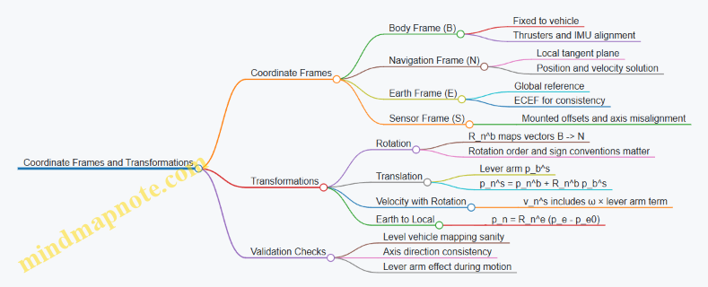
Example: Converting a Sonar Point from Sensor to Navigation
Assume the sonar returns a range measurement along the sonar’s beam direction. You first express the beam direction as a unit vector in the sensor frame u_s. If the sonar range is r, then the measured point relative to the sensor origin is:
- p_s^m = r u_s.
Convert to body coordinates using the fixed rotation R_b^s from sensor axes to body axes:
- p_b^m = R_b^s p_s^m.
Then include the sensor lever arm p_b^s to get the point relative to the body origin:
- p_b^m,body = p_b^s + p_b^m.
Finally rotate into navigation coordinates and add the vehicle position:
- p_n^m = p_n^b + R_n^b p_b^m,body.
If you skip the lever arm step, the point will be systematically displaced, which is especially noticeable when the vehicle is turning or when the sonar is mounted far from the vehicle origin.
Example: Debugging a Frame Sign Error
Suppose your navigation solution shows the vehicle moving north when it is actually moving east. A quick diagnosis is to test the rotation mapping with a known attitude: set pitch and roll to zero, set yaw to a value you can verify from heading, and transform a body-axis unit vector. If the transformed vector lands on the wrong navigation axis, you likely have a swapped axis convention (e.g., ENU vs NED) or a yaw sign mismatch.
Once you correct the frame mapping, the rest of the pipeline—lever arms, sonar georeferencing, and trajectory reconstruction—starts behaving like physics again.
5.2 Dead Reckoning With Inertial and Velocity Measurements
Dead reckoning estimates position by integrating measured motion over time. In deep water, it is often the backbone between acoustic fixes, because it keeps working when acoustics are quiet. The trick is to integrate the right quantities in the right frames, and to manage the inevitable drift with practical checks.
Core Idea and State Variables
A typical navigation state includes position p in a local Earth frame (often NED: North East Down), attitude R (vehicle orientation), and velocity v in the same Earth frame. The inertial sensors provide angular rate ω and specific force f. Specific force is not “acceleration”; it is what remains after gravity is removed, so you must add gravity back in the correct direction.
A simple continuous model looks like:
- Attitude update from gyro: orientation changes according to ω.
- Velocity update from accelerometer: v̇ = a = R · f + g.
- Position update from velocity: ṗ = v.
In discrete time with step Δt, you apply these updates repeatedly. Each step introduces small errors; over long missions, those errors accumulate.
Frames and Transformations That Actually Matter
Most navigation bugs come from mixing frames. Use a consistent convention:
- Gyro measures angular rate in the body frame.
- Accelerometer measures specific force in the body frame.
- Velocity and position are maintained in the navigation frame.
So you convert body-frame specific force into navigation-frame acceleration using the current attitude estimate R. If you get the rotation direction wrong, the vehicle will “accelerate” sideways in a way that no amount of tuning can fix.
Attitude Propagation from Gyro
Gyro integration updates orientation. In practice, you also estimate and correct gyro bias b_g. A common discrete form is:
- ω_corrected = ω_meas − b_g
- Update attitude using ω_corrected and Δt
Bias is the silent drift source. Even a small bias causes attitude errors that later corrupt gravity compensation and velocity integration.
Velocity Integration from Accelerometer
Accelerometer gives specific force f_meas. After bias correction b_a, compute:
- f = f_meas − b_a
- a_nav = R · f + g_nav
- v_k = v_{k-1} + a_nav · Δt
Gravity direction depends on your navigation frame. In NED, gravity is typically positive down, so g_nav = [0, 0, g]. If your frame differs, the sign flips.
Position Integration and Numerical Stability
Position update is straightforward:
- p_k = p_{k-1} + v_k · Δt
Use the same Δt as your sensor sampling. If you resample, do it carefully; uneven time steps distort integration. A practical approach is to run the inertial propagation at the IMU rate and only update slower outputs (like logging) at a lower rate.
Practical Error Sources and How to Spot Them
- Gyro bias: attitude slowly “leans,” causing gravity to be projected incorrectly.
- Accelerometer bias: velocity drifts even when the vehicle is stationary.
- Timing mismatch: if Δt is wrong by a few percent, drift grows faster than expected.
- Magnetometer absence: without absolute attitude references, yaw can wander; roll and pitch still matter because they affect gravity compensation.
A quick sanity check during a hover or slow maneuver: if the estimated velocity keeps growing while the vehicle is physically steady, bias or timing is the likely culprit.
Mind Map: Dead Reckoning with Inertial and Velocity Measurements
Example: Short Dive Segment with IMU Only
Assume a vehicle starts at known position and level attitude. During a 30-second segment, it performs a gentle descent with nearly constant pitch and thrust. If you integrate accelerometer-derived acceleration, you should see velocity evolve smoothly rather than oscillate wildly.
A concrete workflow:
- Initialize attitude using the start condition (level roll/pitch, yaw arbitrary if no magnetometer).
- Propagate attitude using gyro at IMU rate.
- Compute acceleration in NED: a_nav = R·f + g.
- Integrate velocity and then position.
- At the end of 30 seconds, compare the predicted depth rate against the pressure-derived depth change. If the mismatch is large, the gravity compensation or timing is off.
Example: Blending Velocity Measurements for Drift Control
When a Doppler Velocity Log (DVL) is available, it measures velocity relative to the seabed or water column, typically in a sensor frame. Convert it to the navigation frame and use it to correct the integrated velocity.
A simple integrated approach is to treat DVL as a periodic “velocity truth”:
- Run inertial propagation continuously.
- When DVL provides v_dvl, compute the velocity error e_v = v_est − v_dvl.
- Apply a correction to the velocity state (and optionally to attitude if the error pattern suggests misalignment).
This reduces velocity drift and indirectly improves position accuracy, because position depends on velocity integration.
Example: Detecting Frame Mistakes Using Gravity Projection
Suppose roll and pitch are near zero, but the estimated velocity grows during a stationary test. If you temporarily set gravity to zero in the computation, the drift pattern changes dramatically. That behavior indicates gravity projection is involved, pointing toward attitude errors or a sign convention mismatch in g_nav.
Summary of the Section
Dead reckoning with inertial and velocity measurements is a disciplined integration problem: attitude from gyro, acceleration from accelerometer plus gravity, velocity from acceleration, and position from velocity. The system works best when you keep frame conventions consistent, use accurate timing, and validate against simple physical checks like stationary drift and pressure-consistent depth change.
5.3 Acoustic Positioning With Ranges and Time of Flight
Acoustic positioning uses sound travel time to estimate distance, then combines multiple distances to infer position. In deep water, the main constraint is that sound speed is not constant, so the “range from time of flight” step must be done with care.
Core Idea from Time of Flight to Range
A transmitter emits a pulse, a receiver detects it, and the elapsed time is the time of flight (ToF). If the effective sound speed along the path is \(c_{eff}\), then the measured range is:
\[ r = c_{eff} \cdot \Delta t \]
The receiver’s clock and the transmitter’s clock rarely match perfectly, so the measured \(\Delta t\) includes a timing bias. Practical systems handle this by using known transceiver roles, calibration offsets, or two-way ranging.
Example: One-Way Range with a Known Speed Profile
Assume a vehicle receives a pulse from a fixed beacon. You have a sound speed profile (SSP) from CTD data and a ray-tracing model that gives \(c_{eff}=1480,\text{m/s}\) for the expected depth band. If the detected ToF is \(\Delta t=0.250,\text{s}\), then:
\[ r = 1480 \times 0.250 = 370,\text{m} \]
If the SSP were off by 1%, the range error would also be about 1%, which is a useful rule of thumb when you decide how often to update the SSP.
From Range to Position Using Geometry
With one range you know a sphere around the beacon. With two ranges you get the intersection of two spheres, typically a circle. With three non-collinear beacons you can solve for a 3D point. In practice, you estimate position by minimizing the mismatch between measured ranges and predicted ranges from candidate positions.
Example: Three-Beacon Trilateration with Least Squares
Let beacons be at known coordinates \(\mathbf{p}_i\). For a candidate vehicle position \(\mathbf{x}\), predicted ranges are \(\hat r_i = |\mathbf{x}-\mathbf{p}_i|\) if you approximate straight-line propagation, or predicted travel times converted to ranges if you model sound speed. You then minimize:
\[ J(\mathbf{x}) = \sum_i w_i,(r_i-\hat r_i)^2 \]
Weights \(w_i\) reflect measurement quality, such as signal-to-noise ratio (SNR) or detection confidence.
Handling Sound Speed Variability
Sound speed depends on temperature, salinity, and pressure, and the path bends due to refraction. If you ignore this and use a single average speed, you can get systematic bias even when ToF detection is accurate.
Practical Approach
- Measure or estimate an SSP for the mission area.
- Use ray tracing to compute travel time for a given candidate position.
- Convert travel time to an effective range or directly fit travel times in the solver.
Example: Why Straight-Line Assumptions Fail
Two vehicles at the same depth can have different horizontal ranges but similar ToF if the sound channel guides energy. A straight-line model would interpret the ToF as a shorter or longer distance than reality, shifting the estimated position along the direction that best matches the biased ranges.
Timing Bias and Ranging Modes
One-Way Ranging
One-way ranging needs synchronized clocks or a calibrated offset. If the timing bias is \(b\), then \(\Delta t_{meas}=\Delta t_{true}+b\), producing a range error \(c_{eff}b\).
Two-Way Ranging
Two-way ranging reduces sensitivity to clock offsets by using a reply. A common pattern is: beacon sends, vehicle replies after a known processing delay, beacon measures the round-trip time, and the system solves for range while canceling much of the bias.
Example: Two-Way with Known Reply Delay
If the vehicle waits \(T_{proc}\) between receiving and replying, then the remaining time is split into outbound and inbound travel times. Even with imperfect clock alignment, the algebra is designed so the bias terms cancel to first order.
Detection and Signal Processing for Reliable ToF
ToF accuracy depends on how precisely you detect the pulse arrival. A typical workflow is matched filtering or correlation with the known transmit waveform, then picking the peak time.
Example: Correlation Peak Picking
If the transmitted pulse is known, you correlate the received signal with the template. The peak location gives an arrival time estimate. If multipath causes multiple peaks, you choose the peak consistent with the expected travel geometry and depth band, not just the strongest one.
Mind Map: Acoustic Ranging and Position Solving
Worked Mini-Scenario from Detection to Position
Suppose an AUV receives pulses from three beacons at known coordinates. For each beacon, you compute ToF from correlation peaks, then convert to travel times using ray tracing with the current SSP. You run a least-squares solver that predicts travel times for candidate positions and adjusts \(\mathbf{x}\) to minimize residuals. Finally, you check residual patterns: if one beacon consistently has a larger residual, you down-weight it rather than forcing the solution to fit a bad measurement.
Common Failure Modes and How to Avoid Them
- Using the wrong SSP: update SSP inputs when the water column changes significantly; otherwise you get consistent bias.
- Picking the wrong correlation peak: multipath can create plausible but incorrect arrivals; use geometry and expected depth band.
- Assuming straight-line propagation everywhere: in refracting environments, straight-line models can produce systematic shifts.
- Ignoring timing mode differences: one-way and two-way ranging have different bias behavior; apply the correct model for the chosen mode.
Acoustic positioning is therefore a chain: detect ToF reliably, map ToF to travel time using sound speed physics, then solve position with geometry and measurement weighting. When each link is treated explicitly, the final position estimate behaves predictably rather than mysteriously.
5.4 Simultaneous Localization and Mapping With Practical Constraints
Simultaneous Localization and Mapping (SLAM) means estimating the vehicle pose while building a map of the environment, using the same sensor stream. In deep water, the “same stream” is often acoustic, and acoustics have long travel times, sparse updates, and occasional dropouts. Practical SLAM therefore starts with a simple rule: only claim what the sensors can support, and make the rest explicit as uncertainty.
Foundational Idea with AUV Constraints
AUV SLAM typically treats the problem as state estimation. The state includes pose (position and orientation) and map parameters (features or occupancy). Each new measurement updates the state, and the motion model predicts the next state between measurements.
In deep ocean operations, three constraints dominate:
- Latency: acoustic ranges and bearings arrive late, so the filter must account for time alignment.
- Observability limits: some motions do not change what the sensors can measure, so the map may drift without certain maneuvers.
- Outliers: multipath and reverberation can produce false feature matches, so robust gating is essential.
A practical SLAM workflow therefore uses a prediction-update cycle with careful time handling and conservative data association.
Mind Map: Practical SLAM Pipeline
Time Alignment and Measurement Handling
If a sonar-derived feature is timestamped at the moment it was received, but the vehicle moved since it was emitted, the update must be applied to the pose at the measurement’s effective time. A common approach is to maintain a short pose history buffer. When a measurement arrives, the filter rewinds to the corresponding time, applies the update, then re-propagates to the current time.
Easy example: suppose the AUV travels at 1 m/s and an acoustic measurement has a 2.5 s latency. That is 2.5 m of motion. If you update “now” instead of “then,” the residual will look like a map error, and the filter may incorrectly warp the map to fit the wrong pose.
Observability with Realistic Maneuvers
SLAM needs enough excitation to separate pose errors from map errors. In underwater surveys, straight-line motion with limited yaw changes can leave certain degrees of freedom weakly constrained.
Practical constraint: design the mission pattern to create parallax. For example, if you are mapping a set of seabed features with a forward-looking sonar, include gentle cross-track offsets or alternating headings so the same feature appears from different viewpoints. Even small yaw oscillations can improve the geometry of feature observations.
Easy example: a vehicle that only moves forward and keeps constant heading may estimate depth reasonably from pressure and attitude, but horizontal position can drift because the sonar returns do not change enough to constrain lateral translation.
Data Association and Robust Gating
SLAM fails gracefully when it refuses bad matches. Data association decides which measurement corresponds to which map feature. In deep water, reverberation can generate plausible but wrong echoes.
A practical method uses three layers:
- Prediction gating: only consider features that fall within a predicted uncertainty ellipse or ellipsoid.
- Appearance or geometry checks: compare expected range, bearing, and feature descriptors.
- Robust loss: downweight measurements with large residuals rather than letting them dominate.
Easy example: if a landmark is predicted to be 30 m away with a 2 m standard deviation, then a candidate at 45 m should be rejected or heavily downweighted. Otherwise, one outlier can pull the map and cause a chain reaction of incorrect associations.
Map Representation That Matches the Job
Different maps behave differently under constraints.
- Landmark-based maps store feature parameters and their uncertainty. They work well when features are stable and repeatable.
- Pose graphs store relative constraints between poses. They are often easier to manage when feature tracking is intermittent.
- Local submaps limit the scope of mapping so the system does not try to maintain a single global map under long dropouts.
Easy example: during a long acoustic blackout, a pose graph can still connect poses using inertial constraints, while landmark updates resume when sonar returns become reliable.
Consistency Checks and Practical Acceptance
A filter can produce numbers that look smooth while being wrong. Consistency checks catch this by monitoring residual statistics.
Use residual monitoring with thresholds tied to expected noise. If residuals grow persistently, it usually means one of these is happening: time alignment is off, gating is too loose, or the motion model is missing a systematic effect (like thruster bias).
Easy example: if depth and attitude are stable but SLAM residuals spike only when the vehicle turns, the issue may be lever-arm miscalibration between the IMU and sonar, causing systematic geometry errors during rotations.
Fallback Modes When SLAM Is Weak
Practical SLAM includes explicit behavior when conditions degrade. If feature matches are scarce, the system can switch to localization-only using the existing map, or it can freeze map updates and keep pose estimation conservative.
Easy example: if fewer than a minimum number of gated features are matched in a window, stop adding new landmarks. Continue predicting pose from inertial and pressure, and resume full SLAM only when enough reliable observations return.
Summary of Practical Constraints
Deep-water SLAM succeeds when it respects latency, manages observability through mission geometry, rejects outliers with strict gating, and chooses a map representation that tolerates intermittent sensing. The goal is not a perfect global map; it is a trustworthy pose and a map whose uncertainty matches the evidence.
5.5 Navigation Data Logging and Post Mission Trajectory Reconstruction
AUV navigation only becomes trustworthy after you can replay it. Navigation data logging captures the raw ingredients—sensor measurements, timestamps, vehicle states, and mission context—so post mission trajectory reconstruction can produce a corrected path with traceable assumptions.
Foundations of Navigation Logging
Start by deciding what “truth” means for your mission deliverable. For many surveys, you need a trajectory that is consistent with the navigation solution used during processing, plus enough metadata to reproduce it. That means logging not only the estimated pose (position and attitude), but also the measurements that drove the estimator.
A practical logging set includes:
- Time base: a monotonic clock for internal ordering and a mapping to an absolute time reference if available.
- Sensor measurements: IMU samples, pressure, velocity estimates, magnetometer readings, and any acoustic ranges or fixes.
- Vehicle state: thruster commands, actuator saturation flags, control mode, and estimated speed.
- Calibration and geometry: lever arms between sensors, mounting angles, and any sound speed parameters used for acoustic processing.
- Quality flags: sensor health indicators, dropout markers, and synchronization status.
Easy example: if your IMU timestamps drift by 20 ms over a long run, the reconstructed trajectory will still look smooth, but sonar motion compensation will smear. Logging the time mapping lets you correct the drift instead of guessing.
Logging Architecture and Timing Discipline
Trajectory reconstruction lives or dies on timing. Use a single time base for all logged streams, then record the conversion parameters for any external time sources. When sensors run at different rates, log each sample with its own timestamp rather than resampling blindly.
A simple rule: never infer time during post processing. If you must resample, do it explicitly and log the resampling method.
Mind Map: Navigation Data Logging
Data Integrity and Storage Strategy
Deep ocean missions are not gentle on storage. Use chunked logs with checksums so you can detect partial corruption. Include a schema version so post processing knows how to interpret fields.
Easy example: if a log file ends mid-chunk, checksums prevent you from accidentally treating trailing zeros as real sensor data.
Post Mission Trajectory Reconstruction Workflow
Reconstruction typically proceeds in stages: synchronize, clean, estimate, and validate.
Synchronize and Align Streams
Confirm that sensor timestamps align with navigation solution timestamps. If you logged both raw measurements and estimator outputs, compare them to detect systematic delays.
Easy example: if pressure changes appear 0.5 s late relative to IMU vertical acceleration, you likely have a buffering delay. Correcting that delay improves depth consistency.
Clean and Gate Measurements
Apply gates based on physical plausibility and sensor health flags. For instance, discard magnetometer samples during known magnetic interference windows flagged by onboard diagnostics.
Keep the gating transparent: record which samples were rejected and why, so the final trajectory can be explained.
Recompute the Navigation Solution
Run the estimator again using the logged measurements and the same configuration used during the mission, then apply any corrections that were not available in real time. Common corrections include refined lever arms, updated sound speed for acoustic processing, and improved calibration parameters.
A useful practice is to separate measurement processing from state estimation. That way, you can reprocess acoustic ranges without rewriting the entire estimator.
Validate Against Observables
Validation should use independent checks:
- Consistency: compare reconstructed motion against logged control actions and measured accelerations.
- Loop closure: if the mission includes repeated passes, verify that trajectory segments agree within expected uncertainty.
- Residual analysis: inspect residuals for acoustic ranges or velocity updates; large residuals often point to synchronization or sound speed errors.
Easy example: if range residuals grow with depth, the sound speed model used during acoustic processing may be biased for the actual water column.
Example: From Raw Logs to a Usable Trajectory
Imagine a mission that includes an AUV survey with acoustic fixes and sonar imaging. During the mission, the onboard system logs:
- IMU at 200 Hz
- pressure at 10 Hz
- acoustic ranges at irregular intervals
- estimator pose at 20 Hz
- lever arm and mounting metadata
Post mission, you:
- Align timestamps using the logged time mapping.
- Remove IMU samples marked as saturated.
- Recompute acoustic fixes using the logged sound speed profile parameters.
- Run the estimator offline to produce a smoothed trajectory.
- Export the trajectory at a fixed rate for sonar motion compensation.
The key is that the exported trajectory is not just “a path,” but a path with documented assumptions, measurement sources, and quality indicators.
Mind Map: Trajectory Reconstruction
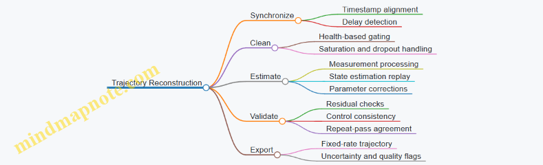
Deliverables and Traceability
Your final deliverables should include:
- A reconstructed trajectory with timestamps and coordinate frame definition.
- Uncertainty or quality indicators per segment.
- A processing log describing configuration versions, gating rules, and any parameter updates.
Easy example: if a segment has poor acoustic residuals, mark it so downstream sonar georeferencing can down-weight or exclude it rather than silently mixing good and questionable data.
A good navigation log makes post mission work deterministic: you can reproduce the trajectory, explain it, and connect it directly to the measurements that created it.
6. Guidance Control and Mission Execution for Autonomous Vehicles
6.1 Control Loops for Depth Heading and Speed Regulation
Depth, heading, and speed control are the three “keep the vehicle honest” loops that turn navigation targets into actuator commands. In deep water, the loops must handle changing buoyancy, current disturbances, and sensor noise without fighting each other. A practical approach is to run three nested layers: (1) sensing and state estimation, (2) guidance that produces desired depth, heading, and speed, and (3) control loops that regulate each variable using thrusters and control surfaces.
Foundational Control Concepts
A control loop repeatedly compares a measured value to a desired setpoint, computes an error, and drives actuators to reduce that error. For underwater vehicles, the measured depth comes from pressure sensors, heading from a magnetometer plus inertial fusion, and speed from Doppler velocity log or acoustic velocity estimates. The actuators typically include forward/aft thrusters for surge speed, and lateral thrusters or rudders for yaw and depth via pitch or vertical thrust.
A key detail is that the vehicle dynamics are coupled: changing depth can slightly change heading due to hydrodynamic forces, and changing speed affects both depth and heading through drag and flow angle. Good loop design acknowledges coupling by keeping bandwidths separated: the fastest loop regulates the most directly actuated variable, while slower loops avoid injecting oscillations into faster ones.
Depth Regulation Loop
Depth control usually regulates vertical position (or pitch-compensated depth) using vertical thrust and/or pitch control. A common structure is PID with feedforward buoyancy compensation.
- Setpoint: desired depth from guidance.
- Measurement: filtered pressure depth.
- Error: depth error with sign consistent with the actuator convention.
- Feedforward: estimate required vertical force to counteract net buoyancy.
- PID terms:
- Proportional reduces immediate error.
- Derivative damps vertical motion (useful when depth changes quickly).
- Integral removes steady-state bias from buoyancy drift.
Example: If the vehicle is slightly positively buoyant, the integral term will gradually increase downward thrust until depth error stays near zero. Without integral action, the vehicle would hover above the target depth by a small but persistent offset.
Heading Regulation Loop
Heading control regulates yaw angle using differential thrust, rudder, or both. The loop benefits from a yaw-rate term because heading changes are often driven by rotational dynamics.
- Setpoint: desired heading from the path-following guidance.
- Measurement: fused yaw angle.
- Error: wrapped heading error in the range -180° to 180° to avoid “long way around” turns.
- Controller: PID on heading plus a yaw-rate feedback term (often implemented as derivative on yaw angle or explicit rate feedback).
Example: During a survey turn, the guidance updates heading smoothly. The controller should command a yaw moment that respects actuator limits; if thrusters saturate, the integral term should be limited or paused to prevent windup.
Speed Regulation Loop
Speed control regulates surge velocity using forward/aft thrusters. Because speed estimates can be noisy, the loop should filter velocity measurements and avoid overreacting to short spikes.
- Setpoint: desired speed from mission profile.
- Measurement: Doppler velocity or acoustic velocity estimate.
- Controller: PID with anti-windup and a thrust slew-rate limit.
Example: If the velocity sensor momentarily drops quality during a rough acoustic environment, a well-designed loop will not slam thrust to chase the transient. Filtering plus rate limiting keeps the vehicle stable while the estimator recovers.
Bandwidth Separation and Loop Interaction
A simple rule of thumb is to make the speed loop faster than the depth loop, and the depth loop faster than the heading loop, or at least ensure that one loop’s corrections do not dominate the others. In practice, you tune using step tests in a controlled environment: command a small change in setpoint and observe overshoot, settling time, and oscillation frequency.
Mind Map: Control Loop Design Flow
Practical Tuning Procedure
- Tune one loop at a time: lock other setpoints to constant values and excite only the target variable with a small step.
- Start with proportional gain: increase until you see a stable response with modest overshoot.
- Add derivative or rate feedback: reduce overshoot and oscillation.
- Add integral carefully: increase until steady-state error is acceptable, then back off if oscillations grow.
- Implement anti-windup: when actuators saturate, clamp or freeze the integral term.
- Validate with disturbances: apply small changes that mimic current or buoyancy shifts and confirm the loop returns to setpoint without sustained oscillation.
Example: If depth oscillates after a step command, reduce derivative noise sensitivity first (filtering), then lower proportional gain. If the oscillation persists, increase derivative damping slightly and re-check actuator saturation.
Minimal Pseudocode for Loop Execution
loop at control_rate:
  depth_meas = filter(pressure_depth)
  yaw_meas   = fused_yaw
  v_meas     = filter(surge_velocity)

  depth_sp = guidance_depth()
  yaw_sp   = guidance_heading()
  v_sp     = guidance_speed()

  depth_err = depth_sp - depth_meas
  yaw_err   = wrap180(yaw_sp - yaw_meas)
  v_err     = v_sp - v_meas

  u_depth = buoy_ff(depth_meas) + PID_depth(depth_err)
  u_yaw   = PID_yaw(yaw_err, yaw_rate_meas)
  u_speed = PID_speed(v_err)

  u = mix_actuators(u_depth, u_yaw, u_speed)
  u = apply_saturation_and_antiwindup(u)
  send_to_thrusters(u)
This structure keeps each loop understandable while still respecting the reality that underwater vehicles are coupled, noisy, and sometimes stubborn—like a cat that refuses to be moved until you stop trying.
6.2 Waypoint Guidance and Path Following for Survey Patterns
Waypoint guidance tells the vehicle where to go; path following tells it how to move smoothly between points while keeping the survey geometry intact. In deep water, the “how” matters because currents, sensor latency, and vehicle dynamics can turn a neat plan into a drifting scribble. The goal is to convert a planned survey pattern into a sequence of feasible commands that respect vehicle limits and still produce the required coverage.
Core Concepts for Survey Patterns
A survey pattern usually combines straight legs and turns. Each leg has a target track line, and each turn has a controlled transition so the vehicle does not overshoot into the next leg. Two practical ideas keep the system grounded:
- Cross-track error measures how far the vehicle is from the desired line. If you keep this small, your swath stays where you planned.
- Along-track progress measures how far you have moved along the line. This prevents the common failure mode where the vehicle oscillates around a waypoint but never commits to the leg.
A simple mental model: the guidance law continuously decides whether to “stay on the line” or “finish the leg and start the turn.” That decision uses geometry and vehicle state, not just distance to the next waypoint.
Waypoint Types and How Vehicles Should Treat Them
Use different waypoint behaviors for different parts of the pattern:
- Transit waypoints are used to route the vehicle between survey areas. They can be treated with looser tolerances.
- Leg waypoints define the endpoints of a survey line. The vehicle should aim to follow the line segment, not just reach the endpoint.
- Turn waypoints define where the vehicle should begin and end a heading change. The vehicle should use a turn radius or a heading transition window.
A concrete example: for a parallel-track bathymetry survey, each leg is a line between two leg endpoints. The turn waypoints are placed so the vehicle can rotate and re-enter the next leg without cutting across the swath.
Geometry That Drives Guidance
For each leg, represent the desired path as a line segment with an associated heading. Compute:
- Closest point on the segment to the vehicle position.
- Cross-track error as the perpendicular distance to that closest point.
- Along-track coordinate as the distance along the segment to the closest point.
Then define a leg completion condition. A robust condition is not “distance to endpoint < threshold” alone. Instead, complete the leg when the along-track coordinate passes the endpoint (with a small margin) and the vehicle’s cross-track error is within tolerance. This reduces late turns caused by current-induced drift.
Path Following Control Strategy
A common structure is a two-layer approach:
- Guidance layer converts the survey geometry into a desired heading and/or desired velocity vector.
- Control layer tracks those commands using depth, heading, and speed controllers.
For survey patterns, heading control is often the key lever. A practical guidance law uses cross-track error to generate a heading correction:
- If cross-track error is positive, steer to reduce it.
- If cross-track error is small, steer primarily to maintain the leg heading.
To avoid aggressive steering near the endpoints, taper the correction as you approach the leg completion region. That taper can be based on along-track distance to the endpoint.
Turn Handling Without Cutting Corners
Turns are where coverage often breaks. If you simply command the next waypoint heading, the vehicle may cut across the next leg, leaving a gap.
Two practical methods:
- Arc-based turns: enforce a minimum turn radius by commanding a heading rate or by using a circular arc between leg headings.
- Heading transition windows: define a region around the turn waypoint where the vehicle transitions heading while still respecting a cross-track tolerance.
Example: in a lawnmower pattern, the vehicle finishes leg A, then transitions to the opposite heading for leg B. Place the turn waypoint so the arc re-enters leg B with acceptable cross-track error. The vehicle then “locks onto” leg B rather than crossing it.
Mind Map: Waypoint Guidance and Path Following
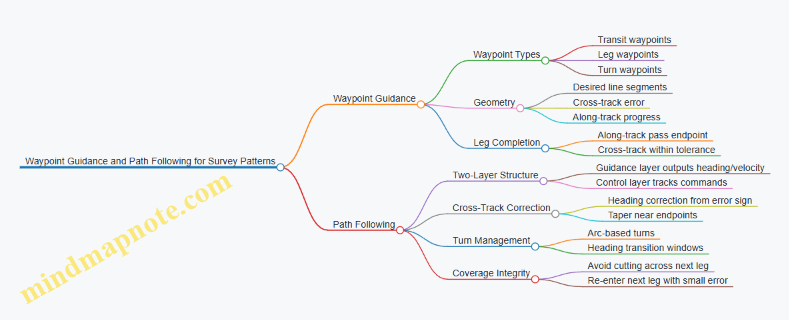
Example: Parallel-Track Survey with Controlled Re-Entry
Assume a vehicle must follow parallel lines spaced by a fixed swath. Plan each leg with endpoints and compute the closest-point projection during the mission.
- While on a leg, command heading using cross-track error correction plus a baseline leg heading.
- Define leg completion when along-track coordinate exceeds the endpoint margin and cross-track error is below a set limit.
- For the turn, command a heading transition that respects a minimum turn radius.
- When entering the next leg, reinitialize the closest-point projection to the new segment so the cross-track controller “grabs” the correct line.
This sequence prevents the classic failure where the vehicle reaches the next waypoint early, then drifts across the leg boundary and forces a coverage gap that is hard to fix later.
Practical Tuning Notes That Prevent Common Bugs
- Thresholds must match vehicle dynamics: if cross-track tolerance is too tight, the vehicle will hunt; too loose, coverage shifts.
- Use consistent coordinate frames: cross-track error depends on correct transforms between navigation solution and planned path.
- Account for latency: if sensor updates arrive late, increase damping by reducing correction gain or tapering earlier near endpoints.
When these pieces align, waypoint guidance becomes more than “go here next.” It becomes a controlled way to preserve the survey pattern under real-world disturbances.
6.3 Fault Handling for Sensor Dropouts and Actuator Limits
Fault handling in an AUV is mostly about making the vehicle behave predictably when information or authority disappears. The goal is not to “fix” the fault instantly; it is to keep the system within safe operating bounds while preserving enough data to understand what happened.
Foundations of Fault Handling
Start with three layers of defense: detection, containment, and recovery.
- Detection answers “Is something wrong?” using consistency checks rather than single thresholds. For sensor dropouts, check both freshness (time since last valid sample) and plausibility (values consistent with recent motion).
- Containment answers “What should the vehicle do right now?” by switching to a conservative control mode that respects actuator limits.
- Recovery answers “Can we return to normal?” by requiring the fault to clear for a sustained period and by verifying that the system state is still coherent.
A practical example: if the Doppler velocity log stops updating, depth and heading can still be controlled using IMU and pressure, but speed control must stop relying on the missing velocity estimate.
Sensor Dropout Handling
Sensor dropouts come in two flavors: intermittent (brief gaps) and persistent (long absence). Treat them differently.
- Intermittent dropout strategy: hold the last good value for a short window and increase uncertainty in the estimator. For instance, if pressure depth is valid but IMU-derived vertical acceleration drifts, the estimator can down-weight the stale depth correction while continuing to propagate motion.
- Persistent dropout strategy: switch to a mode that does not require the missing sensor. If the magnetometer is unavailable, heading can be stabilized using gyro integration plus a slow correction from other cues, but you should reduce reliance on absolute heading for tight path following.
Detection should include a “stale data” timer. If the sensor timestamp is older than a configured limit, mark it invalid. Then run plausibility checks: for example, if a velocity sensor reports a sudden jump that would require an impossible acceleration given thruster limits, treat it as a dropout or outlier.
Actuator Limit Handling
Actuator limits are not faults by themselves; they become faults when the controller keeps demanding impossible commands. The key is to prevent integrators and estimators from “believing” the vehicle followed commands that it could not.
Use command saturation awareness: when thruster commands hit max output, freeze or back-calculate the integrator term in the relevant control loop. A simple rule: if depth controller saturates for longer than a short duration, stop integrating depth error and switch to a safer depth-hold strategy using a reduced-gain controller.
Also monitor rate limits and current draw. If current spikes persist while output is saturated, you may be seeing a mechanical restriction or propulsor cavitation. Containment should reduce commanded speed and increase spacing from obstacles.
Integrated Detection to Control Mode Switching
A clean way to implement this is a small state machine that maps faults to control modes.
- Nominal: full sensor set, full control authority.
- Degraded Navigation: one or more sensors invalid, but enough information remains for stable motion.
- Degraded Control: actuator saturation or repeated saturation detected; reduce aggressiveness.
- Safe Recovery: navigation uncertainty is high or multiple faults exist; hold conservative depth/heading and minimize motion.
When switching modes, preserve continuity. For example, if speed control is degraded, keep the vehicle at the last commanded speed only if it is within safe bounds; otherwise ramp down using a bounded deceleration profile.
Fault Handling Mind Map
Example: IMU-Dependent Navigation with Doppler Dropout
Assume the Doppler velocity log drops out for 20 seconds.
- Detection: freshness timer expires; velocity becomes invalid.
- Containment: switch to Degraded Navigation. Depth and heading control remain active using IMU and pressure. Speed control changes from “track desired speed” to “track desired thrust level” or “hold low speed” using conservative assumptions.
- Estimator: increase process noise for velocity states so the filter does not over-trust stale propagation.
- Recovery: when Doppler resumes and passes plausibility checks, require it to remain valid for a short confirmation window, then ramp speed control back to normal.
The vehicle stays stable because the controller stops pretending it knows velocity when it does not.
Example: Thruster Saturation During Depth Hold
Suppose depth controller saturates repeatedly while descending against a current.
- Detection: saturation counter exceeds threshold.
- Containment: enter Degraded Control. Freeze depth integrator and reduce commanded descent rate.
- Recovery: if saturation clears and depth error decreases without oscillation, return to nominal with a slower gain schedule.
This prevents the classic failure mode where the integrator winds up, then causes a sudden overshoot when the actuator finally regains authority.
Practical Implementation Checklist
- Use freshness timers for every critical sensor.
- Add plausibility checks tied to physical acceleration limits.
- Track saturation duration per actuator and per control loop.
- Freeze or back-calculate integrators when saturation persists.
- Log mode transitions and fault flags with timestamps.
- Require sustained sensor validity before returning to nominal.
Done well, fault handling turns “bad data” into a controlled situation rather than a surprise. The vehicle may not do everything you wanted, but it will do the same safe thing every time.
6.4 Real Time Mission Management for Waypoint Timing and Coverage
Real time mission management is what turns a planned route into an executed survey that actually meets coverage requirements. In deep water, the vehicle cannot “just try again” easily, so the mission controller must continuously reconcile three things: where the AUV is, what it is doing right now, and what coverage gaps would result if it keeps doing that.
Foundational Concepts for Timing and Coverage
A waypoint plan usually includes more than a list of coordinates. It often specifies a speed or loiter behavior, a depth band, and a coverage pattern such as a lawnmower grid. Timing enters because the vehicle must keep a predictable track spacing relative to sonar footprint and vehicle motion. If the vehicle arrives late, it may still follow the same geometric path, but the along-track sampling can drift, creating uneven image density.
Coverage is best treated as a set of constraints rather than a single metric. Typical constraints include:
- Cross-track spacing between parallel legs.
- Along-track sampling driven by speed and sensor update rate.
- Minimum standoff to avoid collisions with seabed features or infrastructure.
- Time windows for acoustic positioning availability or shipboard operations.
A practical approach is to define a “coverage budget” per segment: how much along-track distance you can afford to deviate before the sonar sampling becomes too sparse.
Real Time State Estimation Inputs
Mission management depends on a reliable state estimate. The controller should use a fused navigation solution (position, velocity, attitude) and also track uncertainty. Uncertainty matters because it changes how aggressively you can correct. For example, if position uncertainty is large, snapping to the next waypoint can cause oscillations and wasted distance.
A simple but effective rule is: use uncertainty to scale corrections. When uncertainty is high, reduce lateral correction gains and prioritize stable depth and heading control until the estimate tightens.
Waypoint Timing Logic That Doesn’t Waste Distance
Waypoint timing logic should be based on predicted arrival time, not on a stopwatch. For each upcoming waypoint, compute a predicted time-to-go using current speed and a conservative turn model. Then compare it to the planned time-to-go.
If the AUV is early, you have options that preserve coverage:
- Reduce speed slightly while maintaining depth and heading stability.
- Add a short loiter that does not break the pattern alignment.
- Delay the turn initiation so the vehicle enters the next leg at the correct lateral position.
If the AUV is late, you must decide whether to recover coverage or preserve safety. Common recovery actions include:
- Increase speed within allowable limits.
- Start the next leg sooner by reducing the turn radius margin.
- Skip a non-critical waypoint that does not affect leg alignment.
The key is to tie each action to a coverage impact estimate. If skipping a waypoint only shifts along-track sampling by a small amount, it may be acceptable; if it breaks cross-track spacing, it is not.
Coverage-Aware Segment Control
Instead of treating each waypoint as an independent target, manage the mission as segments between waypoints. For each segment, maintain a running estimate of covered distance along the intended track direction. Then enforce sampling constraints by adjusting speed or by triggering a “leg switch” when the covered distance reaches the planned value.
This is especially useful for lawnmower patterns. The vehicle can switch from one leg to the next when it has covered the required along-track distance, even if the exact waypoint time is slightly off.
Handling Acoustic Updates and Timing Jitter
Acoustic positioning updates can arrive irregularly. When an update is late, the controller should avoid sudden jumps in the estimated position. A robust method is to keep the mission controller operating on the current best estimate, then apply corrections smoothly when new data arrives.
A practical tactic is to separate two loops:
- Fast control loop for depth, heading, and speed.
- Mission management loop for waypoint switching and coverage accounting.
The mission loop can run at a slower rate and use the latest navigation state, while the fast loop prevents abrupt motion.
Mind Map: Real Time Mission Management
Example: Timing Recovery on a Two-Leg Survey
Assume a lawnmower survey with two parallel legs. The plan sets a target speed of 1.2 m/s and expects each leg to be 600 m long, so the planned leg duration is 500 s. The sonar update rate implies along-track sampling requires staying within ±5% of that distance.
During execution, the AUV reaches the start of Leg 2 early by 20 s. The mission manager predicts that if it keeps 1.2 m/s, it will cover 24 m extra, which exceeds the sampling tolerance. It chooses a speed trim to 1.15 m/s for the first 200 m, then returns to 1.2 m/s. Coverage accounting confirms the covered distance lands within tolerance when the leg switch trigger is reached.
Now consider the opposite case: Leg 2 starts late by 35 s because the vehicle waited for an acoustic update. If the controller simply follows the waypoint time, it would cover too little distance and create a gap. Instead, it increases speed to 1.35 m/s within allowable limits and switches to the next leg when the covered distance reaches the planned 600 m target. The waypoint time is no longer the primary constraint; coverage distance is.
Example: Skipping a Non-Critical Waypoint
Suppose a waypoint exists only to smooth a turn, not to define leg alignment. If the AUV is late and already within acceptable cross-track spacing, the mission manager can skip the smoothing waypoint and command a direct transition to the next leg heading. The safety gate checks that the turn does not violate minimum standoff and that actuator limits are not exceeded. If those checks pass, the mission preserves coverage density while reducing unnecessary maneuvering distance.
Practical Decision Checklist
At each mission-management cycle, apply this order:
- Confirm safety constraints and standoff margins.
- Update navigation state and uncertainty.
- Predict time-to-go for the next waypoint.
- Update covered along-track distance for the current segment.
- Choose an action that corrects coverage distance first, then timing.
- Hand off commands to the fast control loop with smooth transitions.
This structure keeps the vehicle from “chasing the clock” while still respecting the timing realities of deep ocean operations.
6.5 Control System Validation With Bench Tests and Sea Trials
A control system is only as trustworthy as the tests that prove it behaves the way the model says it will. Validation should start with repeatable bench conditions, then move to sea trials where hydrodynamics, sensor noise, and disturbances show up for real.
Build a Testable Control Objective
Before any hardware test, translate requirements into measurable control outcomes. For depth and heading loops, define targets such as settling time, overshoot, steady-state error, and tolerance to disturbances. For example, if the mission needs depth hold within ±0.5 m, that number becomes a pass/fail criterion rather than a vague goal.
A practical way to keep tests honest is to list the loop structure and what each loop is responsible for. Depth hold typically uses an outer loop that commands vertical speed or pitch, and an inner loop that controls actuators like ballast valves or thruster thrust. If the inner loop is sloppy, the outer loop will compensate and look “stable” while wasting energy.
Bench Tests for Controller Logic and Actuator Response
Bench tests should isolate the control software from the ocean while still exercising the real sensors and actuators.
Start with actuator characterization. Command step inputs to each actuator channel and record the response: time constant, dead time, saturation behavior, and hysteresis. A simple example is a thruster command from 20% to 40% duty cycle. If the thrust rises slowly and saturates early, the controller gains must respect that limit.
Next, validate sensor processing and timing. Many control issues are timing issues wearing a control-theory costume. Verify that IMU updates, depth readings, and control loop execution are synchronized and that filtering introduces predictable delay. A good bench check is to inject a known depth signal into the depth estimator and confirm the controller sees the expected value at the expected time.
Then test closed-loop behavior with a hardware-in-the-loop setup. Use a simulator or a controlled plant model to emulate vehicle dynamics. Run a depth step and a heading step, and compare measured responses to the predicted ones. If the measured overshoot is larger, check for unmodeled actuator delay or incorrect sign conventions in the transformation between sensor frames and control frames.
Safety Limits and Fault Injection
Bench validation must include constraints and fault handling. Confirm that saturation logic behaves correctly: when the controller hits actuator limits, it should not keep integrating error indefinitely. Anti-windup behavior is easy to miss until you see a slow recovery after a disturbance.
Fault injection can be simple and still valuable. For instance, simulate a depth sensor dropout for 2 seconds and verify the controller switches to a safe fallback mode without producing large transients. Similarly, clamp the estimated velocity to a plausible range and confirm the guidance layer does not command aggressive maneuvers based on bad state.
Sea Trials for Real Hydrodynamics and Disturbances
Sea trials validate the full loop under real disturbances: current, waves, and vehicle-to-vehicle variability in drag and added mass.
Start with low-risk conditions. Conduct shallow, calm-water tests first, focusing on depth hold and heading hold at modest speeds. Use a consistent procedure: same initial conditions, same command sequence, and the same logging configuration. If you change too many variables at once, you will not know which change caused the behavior.
Then run disturbance tests. A straightforward example is to introduce a controlled thruster pulse to create a known perturbation and observe how quickly the controller returns to setpoint. Measure the response in both the controlled variable domain (depth or heading) and the actuator domain (thruster command, ballast command). If depth recovers but actuator commands oscillate, you may have a loop interaction problem.
Finally, validate guidance-to-control coupling. When the guidance layer commands a path or waypoint, the control system must track without excessive oscillation. A practical test is a straight-line segment followed by a gentle turn. If the vehicle overshoots the turn and then “hunts” for the path, the guidance gains or the control bandwidth mismatch is likely the culprit.
Acceptance Criteria and Evidence Packaging
Define acceptance criteria before testing. For each test, record the command, measured state, actuator outputs, and relevant diagnostics like estimator covariance or filter residuals. Evidence should support traceability: you should be able to connect a requirement like “depth hold within ±0.5 m” to a specific dataset.
A simple reporting structure works well:
- Test objective and setup
- Input sequence and timing
- Key metrics and pass/fail thresholds
- Notable deviations and likely causes
- Actions taken and re-test results
Mind Map: Control System Validation Flow
Example: Depth Hold Validation Sequence
- Bench: command a small depth step, record actuator response, and confirm the controller does not saturate for the chosen step size.
- Bench: inject a timing delay equal to the measured estimator delay and confirm overshoot stays within the threshold.
- Sea: repeat the same depth step at low speed in calm water, then repeat with a larger step that still avoids saturation.
- Sea: apply a short perturbation pulse and verify return-to-setpoint time and actuator effort remain within limits.
If any step fails, the next test should target the most likely mismatch: actuator delay, estimator timing, sign conventions, or loop bandwidth interaction. That keeps debugging focused instead of turning validation into a guessing game.
7. Sonar Imaging System Design and Signal Processing
7.1 Sonar Types and Use Cases for Deep Ocean Imaging
Deep ocean imaging starts with a simple question: what kind of “picture” do you need, and how far can you afford to see it? Sonar answers that question by trading off range, resolution, coverage geometry, and tolerance to motion and sound-speed variation. The main sonar types used with AUVs and subsea operations are classified by how they transmit and receive sound, and by how they form images.
Foundational Concepts for Choosing a Sonar Type
A sonar system has three core behaviors: it emits acoustic energy, it listens for echoes, and it converts echo timing and strength into geometry and intensity. In deep water, sound travels with refraction, so the same target can appear at different apparent ranges unless you correct for sound-speed structure. Also, the vehicle’s motion matters: if the platform moves while the sonar is “building” an image, you must compensate using navigation data.
Resolution depends on bandwidth and beamwidth. Bandwidth helps separate closely spaced targets in range, while beamwidth controls angular detail. Range depends on source level, absorption, spreading, and noise. In practice, you choose a sonar type that matches the imaging goal and the vehicle’s ability to maintain stable motion and accurate positioning.
Mind Map: Sonar Types and Deep Ocean Imaging Use Cases
Active Imaging Sonar for Direct Geometry
Forward-Looking Imaging Sonar
Forward-looking sonar projects a fan or narrow beams ahead of the vehicle. It is most useful when you need immediate shape information: checking for protruding rocks, verifying clearance near an asset, or guiding a vehicle through a constrained corridor. Because the sonar is close to the vehicle’s path, small attitude errors can shift where echoes land in the image. A practical best practice is to treat forward-looking sonar as a “near-field truth source” and ensure tight time synchronization between navigation and sonar ping times.
Example: During a subsea cable inspection, the AUV approaches a section with known seabed irregularities. The forward-looking sonar highlights a cluster of boulders, allowing the mission planner to adjust the path before the vehicle reaches the tightest clearance.
Side-Scan Sonar for Seabed and Corridor Mapping
Side-scan sonar sends pulses to the left and right and records echo intensity versus time, producing a characteristic image where bright returns often indicate hard or rough surfaces. It is widely used for seabed mapping and for surveying along a pipeline corridor. The key operational requirement is consistent altitude and stable track: if the vehicle climbs or descends rapidly, the slant range changes and the image scale becomes uneven.
Example: For a pipeline corridor survey, the AUV maintains a constant height above the seabed using depth and altitude control. The side-scan image reveals a trench edge and scattered debris, which can then be measured in the georeferenced mosaic.
Multibeam Sonar for Bathymetry and Dense Coverage
Multibeam sonar forms many beams across a swath, enabling efficient bathymetry and detailed seabed characterization. Compared with side-scan, multibeam provides more direct geometry for each beam, which supports surface modeling. However, it is less forgiving: calibration of beam angles, timing, and mounting offsets matters, and motion compensation must be robust.
Example: When mapping a large area for subsea infrastructure siting, multibeam provides a continuous elevation grid. The resulting surface model helps identify suitable anchor locations and detect uneven terrain that could affect installation.
Passive Sonar for Listening Without Transmitting
Passive sonar does not emit sound; it listens for acoustic sources. This can be useful when you need quiet operations or when transmitting would be undesirable. The trade is that you typically do not get direct range from a single sensor. Instead, you rely on geometry, multiple sensors, or known source characteristics.
Example: During a sensitive survey near active equipment, the system uses passive listening to monitor background activity while the AUV performs low-interference navigation and collects imaging with an active sonar only when needed.
Practical Selection Checklist for Deep Ocean Imaging
- Define the deliverable: corridor image, seabed mosaic, or bathymetric surface.
- Match resolution needs to bandwidth and beamwidth: narrow features require tighter angular control and sufficient bandwidth.
- Account for motion: if the vehicle cannot hold stable altitude or attitude, prefer sonar modes and processing that tolerate motion with strong compensation.
- Plan for sound-speed correction: include sound-speed profiling and apply refraction-aware processing.
- Verify timing and mounting: ensure lever arms and time offsets are measured so georeferencing does not smear features.
With these choices made early, the sonar type becomes a predictable tool rather than a mystery box. The rest of the imaging workflow—beamforming, motion compensation, and georeferencing—then follows logically from the physics of the chosen sonar.
7.2 Transducer Selection Beam Pattern and Mounting Effects
A sonar transducer is not just a “sound source.” It is a shaped acoustic radiator whose beam pattern is determined by geometry, frequency, and mounting. In deep water, where range is long and multipath can be stubborn, the beam pattern and how the transducer sits on the vehicle often decide whether you get crisp returns or a blurry mess.
Beam Pattern Basics You Can Use Immediately
Start with three practical beam metrics: beamwidth, sidelobe level, and directivity index.
- Beamwidth tells you how wide the main lobe is. Narrower beams improve angular discrimination, but they also reduce coverage when the vehicle yaws or rolls.
- Sidelobes are the “extra” lobes outside the main beam. High sidelobes can pick up echoes from off-axis clutter, which looks like false targets or elevated background.
- Directivity index summarizes how strongly the transducer focuses energy in its main direction compared to an omnidirectional radiator.
A simple rule of thumb: if you need to separate two nearby objects in angle, you want a narrower main lobe and controlled sidelobes. If you need broad coverage for search, you accept wider beams and focus on robust detection thresholds.
Frequency, Aperture, and Tradeoffs
Beam pattern is tightly linked to frequency and effective aperture.
- Higher frequency generally narrows the beam and improves fine detail, but it attenuates faster with range and can be more sensitive to small mounting misalignments.
- Lower frequency extends range and tolerates rougher conditions, but the beam becomes wider, so angular resolution drops.
- Effective aperture depends on transducer face size and mounting constraints. If the transducer is partially blocked by a fairing or recessed, the effective aperture shrinks and the beam widens.
Example: Suppose you are imaging a pipeline inspection area. If the vehicle must keep a safe standoff distance, a slightly higher frequency can help resolve small surface features, but only if the mounting keeps the beam aligned and the sidelobes are not feeding clutter from the hull.
Mounting Effects That Change the Beam in Real Life
Mounting can alter the beam through three mechanisms: acoustic impedance mismatch, mechanical baffling, and array-like behavior from structure.
-
Impedance mismatch The transducer face couples into water through a boundary layer: housing, potting, fairing material, and any protective window. If the acoustic impedance of these layers does not match water well, energy reflects back into the transducer or spreads into unwanted directions.
Easy check: compare expected beamwidth from datasheets to measured beamwidth in a tank. If measured beams are wider, coupling is likely poorer than assumed.
-
Mechanical baffling and recessing A flush mount behaves differently than a recessed mount. Recessing can create a cavity that acts like a baffle, changing the near-field and effectively reshaping the beam.
Example: A transducer mounted behind a thick fairing lip may show a “clean” main lobe in the forward direction but elevated sidelobes at angles where the fairing blocks or reflects energy.
-
Structure-borne vibration and scattering The vehicle hull can vibrate due to transducer drive and can scatter acoustic energy. This can create additional lobes or a background that correlates with vehicle motion.
Practical mitigation: isolate the transducer mechanically where possible and keep the mounting geometry consistent across vehicles in a fleet, so calibration remains transferable.
How Beam Pattern Interacts with Vehicle Motion
Even a perfect beam pattern is only useful if the vehicle keeps the beam pointed where you need it. Roll and pitch change the beam axis relative to the target.
- With a narrow beam, small attitude errors can move the main lobe off target, reducing return strength sharply.
- With a wider beam, you get more stable coverage, but clutter acceptance increases.
A useful workflow is to define an “attitude tolerance cone” based on expected roll/pitch during the survey. Then choose beamwidth so the main lobe stays within that cone for the majority of the mission.
Mind Map: Transducer Beam Pattern and Mounting Effects
Example: Choosing Between Two Mounting Approaches
Assume two candidate mounts for the same transducer face: flush and recessed behind a fairing window.
- The recessed mount may protect the transducer and reduce drag, but it can widen the beam and raise sidelobes due to cavity effects.
- The flush mount may couple more efficiently and keep the beam closer to the predicted pattern, but it can be more exposed to flow-induced vibration.
Decision logic: if your mission depends on resolving small targets at a consistent standoff distance, prioritize the mount that preserves beamwidth and sidelobe behavior under measured conditions. If your mission is broad-area search where angular precision is less critical, a wider beam with higher sidelobe tolerance can still work, provided your detection thresholds account for the extra off-axis energy.
Summary Checks Before You Lock the Design
- Confirm beamwidth and sidelobe behavior with measurements, not only datasheets.
- Verify that the mounting materials and geometry preserve coupling and do not reshape the near-field unexpectedly.
- Match beamwidth to expected attitude variation so the main lobe stays on target often enough to matter.
- Treat hull scattering as a calibration variable, especially when vehicle motion changes during the survey.
When these checks are done, transducer selection becomes a controlled engineering choice rather than a hopeful guess.
7.3 Range Resolution and Frequency Selection for Target Separation
Range resolution is the ability to distinguish two reflectors that are separated along the line of sight. In underwater sonar, that “line of sight” is shaped by beam geometry and sound propagation, but the core driver is the transmitted signal bandwidth. A simple rule of thumb helps anchor the rest: wider bandwidth gives finer range resolution, because the sonar can better separate echoes that arrive at slightly different times.
Foundational Timing to Resolution
Start with time-of-flight. If two targets are separated by distance \(\Delta R\), their echoes arrive separated by \(\Delta t = 2\Delta R / c\), where \(c\) is sound speed and the factor of 2 accounts for the round trip. A receiver cannot reliably separate echoes closer than the time span of the system’s effective pulse. That effective pulse width is tied to the signal bandwidth \(B\). For many practical pulse-like waveforms, the approximate range resolution is:
\[\Delta R \approx \frac{c}{2B}\]
Example: if \(c = 1500,\text{m/s}\) and \(B = 10,\text{kHz}\), then \(\Delta R \approx 1500/(2\cdot 10{,}000) = 0.075,\text{m}\). If you increase bandwidth to \(B = 30,\text{kHz}\), the resolution improves to about \(0.025,\text{m}\). That’s the basic lever: bandwidth buys separation along range.
Frequency Selection Beyond Resolution
Frequency selection is not just about bandwidth; it also affects absorption, noise, transducer efficiency, and beam behavior.
- Absorption and link budget: Higher frequencies attenuate more in seawater, reducing usable range. Lower frequencies travel farther but typically support narrower bandwidth for a given transducer and hardware constraint.
- Noise environment: Ambient noise depends on frequency and sea state. At some frequencies, shipping and surface noise dominate; at others, turbulence and thermal noise matter more. The “best” frequency is the one where your signal-to-noise ratio supports the resolution you need.
- Transducer and array constraints: A transducer’s bandwidth and matching determine how much of the theoretical bandwidth you can actually transmit and receive. Array elements also impose practical limits on usable frequency for beamforming.
- Target scattering behavior: Real targets are not perfect point reflectors. Their reflectivity varies with frequency because scattering depends on target size relative to wavelength. A frequency that gives great resolution might under-illuminate a target if the scattering is weak.
Practical Waveforms and Effective Bandwidth
Range resolution depends on effective bandwidth, not just the center frequency. For chirps (linear frequency modulated pulses), the transmitted bandwidth \(B\) sets the compressed pulse width after matched filtering. For single-frequency pulses, the bandwidth is narrow and resolution is coarse.
A useful mental model: the receiver’s matched filter “compresses” energy into a shorter time window. The shorter window corresponds to finer range discrimination. If the system uses matched filtering, you should treat the resolution as governed by the chirp bandwidth and processing, not by the raw pulse length alone.
Tradeoffs That Show Up in the Field
Consider two design goals: separating two closely spaced objects and reaching them at a useful standoff range.
- To separate closely spaced targets: increase bandwidth (often by using a chirp with a wider sweep) and ensure the transducer can support it.
- To reach them: choose a frequency band that maintains adequate signal level after propagation losses and absorption.
These goals can conflict. A common engineering compromise is to pick a frequency band where the transducer can provide the needed bandwidth while still maintaining acceptable range performance.
Mind Map: How Frequency and Bandwidth Shape Separation
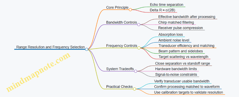
Example: Choosing Between Two Bands
Suppose you need to separate two reflectors 5 cm apart at a standoff where sound speed is about 1500 m/s.
- Required resolution: \(\Delta R \le 0.05,\text{m}\)
- Using \(\Delta R \approx c/(2B)\):
- \(0.05 \approx 1500/(2B)\) → \(B \approx 15,\text{kHz}\)
Now compare two candidate center frequencies:
- Band A: 30 kHz center, transducer supports 20 kHz bandwidth, but absorption is higher.
- Band B: 10 kHz center, transducer supports only 10 kHz bandwidth, but absorption is lower.
Band A meets the resolution requirement (20 kHz gives \(\Delta R \approx 1500/(2\cdot 20{,}000)=0.0375,\text{m}\)). Band B does not (10 kHz gives \(0.075,\text{m}\)), even if it reaches farther. If the targets are within Band A’s practical range, Band A is the correct choice for separation.
Example: When Resolution Is Theoretical but Not Achieved
Even if \(B\) suggests fine resolution, real systems can blur peaks due to:
- Motion and attitude errors: if the platform changes during the pulse or between navigation updates, the apparent range can smear.
- Sound speed mismatch: incorrect \(c\) distorts time-to-range conversion.
- Multipath and reverberation: multiple paths can create overlapping echoes that look like closely spaced targets.
- Processing mismatch: if the matched filter assumes a different chirp slope or timing than what was actually transmitted, the compressed pulse broadens.
A practical workflow is to validate separation using calibration targets at known ranges and verify that the measured peak spacing matches the predicted \(\Delta R\). If it doesn’t, the fix is usually in waveform/processing alignment, timing, or environmental modeling rather than in “picking a different frequency” blindly.
Summary for Selection Decisions
To separate targets along range, prioritize effective bandwidth and ensure your waveform and processing realize it. Then choose the center frequency that keeps absorption and noise within a link budget that still supports the required bandwidth. The best design is the one where the resolution you compute is the resolution you measure.
7.4 Beamforming and Matched Filtering for Improved Detection
Foundational Goal and Signal Model
Beamforming and matched filtering both aim to improve detectability of a target echo in noise, but they act at different stages. Beamforming combines signals across an array to emphasize energy arriving from a chosen direction; matched filtering then processes the time (or range) dimension to maximize the signal-to-noise ratio for a known waveform shape.
A practical sonar model starts with a received signal at array element m:
- (x_m(t) = s(t-\tau_m(\theta)) + n_m(t))
Here, (s(t)) is the transmitted/expected echo shape, \(\tau_m(\theta)\) is the propagation delay from the target direction \(\theta\) to element m, and \(n_m(t)\) is noise plus clutter. The key is that the delay term changes across elements, so a directionally correct combination can add the echo coherently while noise adds incoherently.
Beamforming Basics with Directional Delay-and-Sum
The simplest beamformer is delay-and-sum. For a steering direction \(\theta_0\), compute delays \(\hat{\tau}_m(\theta_0)\) and form:
- \(y(t)=\sum_{m=1}^{M} x_m(t+\hat{\tau}_m)\)
If \(\theta_0\) matches the true target direction, the echo terms align in time and add constructively. If not, the echo smears, reducing peak amplitude and widening the effective response.
Easy example: Suppose you have 16 elements and a target echo that lasts 2 ms. If your steering direction is correct, the echo peak in \(y(t)\) becomes about 16 times stronger in amplitude (and roughly 256 times in power, ignoring losses). If steering is off by enough that delays misalign by half the echo duration, the peak drops sharply because parts of the echo no longer overlap.
Beam Pattern and Tradeoffs You Can Actually Feel
Beamforming creates a main lobe and sidelobes. Main-lobe width depends on array aperture and element spacing; sidelobes depend on weighting.
- Uniform weighting: narrow main lobe, higher sidelobes.
- Tapered weighting (e.g., Hann-like): wider main lobe, lower sidelobes.
In deep water, sidelobes matter because clutter and multipath can leak into the beam. A lower sidelobe level can reduce false alarms even if the main lobe is slightly wider.
Concrete example: If a strong seabed return sits just outside the main lobe, uniform weighting may still admit enough sidelobe energy to create a detection peak. Tapering can suppress that leakage, letting the target echo stand out.
From Beamforming Output to Detection Statistics
After beamforming, you typically have a single-channel time series \(y(t)\). Detection often uses a matched filter or correlator to produce a range profile.
A matched filter is optimal (in the classical sense) when the noise is white and the signal shape is known. It computes correlation with the expected waveform:
- \(z(t)=\int y(\tau), s^*(\tau-t), d\tau\)
In discrete time, this is convolution with a time-reversed conjugated template.
Matched Filtering with Practical Templates
In sonar, the “template” is rarely the raw transmitted pulse alone. It often includes expected effects:
- pulse length and chirp rate (if applicable)
- transmit-receive filtering
- approximate propagation and system delays
- expected phase behavior for the imaging mode
Easy example: If your transmitted pulse is a linear chirp, the matched filter effectively performs de-chirping. A target echo that arrives with the correct time shift produces a sharp correlation peak; noise produces smaller, more spread values.
Combining Beamforming and Matched Filtering Systematically
A robust workflow is:
- Choose steering angles based on the navigation estimate and expected target region.
- Beamform to produce \(y(t)\) for each steering direction (or for a small set of beams).
- Apply matched filtering to each beamformed signal to obtain \(z(t)\), often interpreted as a range profile.
- Threshold using a noise-aware rule so the false alarm rate is controlled.
This separation is useful because beamforming handles spatial selectivity, while matched filtering handles waveform selectivity.
Mind Map: Beamforming and Matched Filtering Flow
Example: Two Targets and Why Weighting Matters
Consider two reflectors: one target at the steering direction and one strong clutter source slightly off-axis.
- With uniform weighting, the off-axis clutter can land in the sidelobes, producing a correlation peak that competes with the target.
- With tapered weighting, sidelobe energy drops, so the matched filter peak for the true target becomes the dominant peak.
The matched filter alone cannot fix spatial leakage; beamforming must reduce it first. Conversely, beamforming alone cannot sharpen a smeared echo caused by waveform mismatch; matched filtering must align the time-frequency structure.
Example: Template Mismatch and Peak Broadening
If the matched filter template uses the wrong chirp rate or an incorrect pulse length, the correlation peak broadens and its maximum value decreases. In practice, this shows up as:
- lower peak-to-noise ratio
- increased sensitivity to small timing errors
- more ambiguous peaks when multiple echoes overlap
A practical mitigation is to build templates that reflect the actual transmit waveform and the system’s effective filtering, then verify by checking that known calibration echoes produce narrow, repeatable peaks.
Summary of What Each Stage Does
Beamforming selects where energy is coming from; matched filtering selects what waveform shape you are looking for. When both are aligned—steering direction and template shape—detections become sharper, sidelobe clutter becomes less competitive, and range estimates become more stable.
7.5 Quality Metrics for Sonar Images Including Contrast and Speckle
A sonar image is only useful if you can explain why it looks the way it does. Quality metrics give you that explanation in numbers: they separate “the target is there” from “the image is just noisy,” and they help you compare settings across missions.
What Quality Means in Sonar Imaging
Quality usually has three layers. First is signal integrity, meaning the image contains energy where it should and not where it shouldn’t. Second is visual separability, meaning targets stand out from background clutter. Third is metric stability, meaning the same scene produces similar scores when the vehicle repeats the survey line.
A practical rule: pick metrics that match your decision. If you are detecting objects, prioritize separability and false-alarm control. If you are measuring dimensions, prioritize geometric consistency and speckle behavior. If you are creating mosaics, prioritize temporal consistency and normalization.
Contrast Metrics That Actually Help
Contrast answers: “How much brighter or darker is the target region than its surroundings?” For sonar, brightness depends on processing choices like gain, compression, and normalization, so metrics should be computed on a consistent scale.
Local contrast is computed around a region of interest (ROI). A common choice is the contrast-to-background ratio:
- Let \(\mu_t\) be the mean intensity in the target ROI.
- Let \(\mu_b\) be the mean intensity in a nearby background ROI.
- Use \(C = (\mu_t - \mu_b) / (\mu_b + \epsilon)\) to avoid division by zero.
Example: Suppose a pipeline inspection ROI has mean intensity 0.62 and background mean 0.40 after log compression. With \(\epsilon\) negligible, \(C \approx (0.62-0.40)/0.40 = 0.55\). If you change beamforming settings and C drops to 0.25, you likely reduced target separability even if the image still “looks fine” to the eye.
For scenes with uneven illumination, use contrast in matched windows: compute background statistics in windows that share the same range and incidence angle as the target window. This prevents you from rewarding images that merely brighten one side of the swath.
Speckle Metrics That Separate Texture from Structure
Speckle is the granular interference pattern common in coherent imaging. It can hide small targets, but it also carries information about scattering. The key is to measure speckle without confusing it with real edges.
A foundational metric is speckle contrast, often expressed as the coefficient of variation:
- In a homogeneous patch, compute mean \(\mu\) and standard deviation \(\sigma\).
- Speckle contrast \(S = \sigma / (\mu + \epsilon)\).
Example: Take a patch on open seabed with no visible objects. If \(S\) is 0.35, the texture is moderate. If \(S\) rises to 0.55 after changing processing, the image likely became less coherent or less averaged, which can increase false detections.
To avoid treating edges as “speckle,” compute \(S\) only in homogeneous masks. You can build masks from a simple threshold on local gradients: exclude pixels where gradient magnitude exceeds a chosen limit.
Combining Metrics into a Decision Score
Contrast and speckle measure different things, so combine them into a score that reflects your goal. One simple approach is a separability index:
- Compute contrast \(C\) between target ROI and matched background ROI.
- Compute speckle contrast \(S_b\) in the background.
- Use \(Q = C / (S_b + \epsilon)\).
Example: If contrast improves from 0.30 to 0.45 but background speckle also increases from 0.25 to 0.50, then \(Q\) changes from 1.20 to 0.90. The metric says the image is less reliable for detection, even though the target looks brighter.
Mind Map of Quality Metrics Workflow
Mind Map: Quality Metrics for Sonar Images
Systematic Validation with Repeatability Checks
Metrics are only meaningful if they behave predictably. Run a repeatability check on the same static scene or calibration target.
- Normalization check: verify that changing display scaling does not change metric values. If it does, compute metrics on linear or consistently log-scaled intensity.
- Range consistency check: compute contrast and speckle per range band. A metric that only improves at short range is not a general improvement.
- Mask robustness check: slightly perturb ROI boundaries and confirm scores do not swing wildly. Large swings usually mean the metric is sensitive to a few outlier pixels.
A good final test is boring: if two processing settings produce similar images, your metrics should agree. If the images look different, your metrics should explain whether the difference is contrast improvement, speckle increase, or both.
8. Sonar Calibration and Georeferenced Imaging Workflows
8.1 Time Synchronization Between Navigation and Sonar Data Streams
Time synchronization is the quiet difference between a clean georeferenced sonar product and a blurry one. The goal is simple: every navigation sample used to motion-compensate sonar must correspond to the correct instant of each sonar ping, with a known and bounded timing error.
Foundational Concepts for Timing Alignment
Start with three clocks that rarely agree: the vehicle computer clock, the sonar controller clock, and the data logging clock. Even if they all run “on time,” they may drift by milliseconds over a mission, which is enough to shift a platform by meters at survey speeds.
Define the timing chain explicitly:
- Ping time reference: when the transmit event occurs (or when the first sample is valid).
- Navigation time reference: when IMU, DVL, and attitude estimates are stamped.
- Transport latency: delays from sensor acquisition to logging and to storage.
A practical rule: treat timestamps as measurements with uncertainty, not as perfect truth. Your workflow should carry that uncertainty through to the final georeferencing.
Timestamp Sources and What They Actually Mean
Not all timestamps are created equal. A sonar packet timestamp might reflect when the packet arrived at the logger, not when the ping was transmitted. Likewise, navigation timestamps might be assigned at sensor readout rather than at the fusion output.
To avoid guessing, capture these facts during integration:
- Whether sonar timestamps correspond to transmit, receive window start, or packet creation.
- Whether navigation timestamps correspond to raw sensor time, filter output time, or logging time.
- Whether any resampling occurs between sensor acquisition and the logged navigation stream.
Building a Timing Model from Measurable Offsets
A robust approach uses a timing model with two parts: a constant offset and a possible drift.
- Constant offset: the fixed difference between sonar ping time and navigation time.
- Drift: slow clock rate mismatch, modeled as a linear term over the mission.
You can estimate both using a controlled event. For example, trigger a known action that affects both streams at the same moment, such as a mechanical switch that produces a detectable change in vehicle attitude and a simultaneous marker in the sonar log. If you cannot create a shared event, use a repeatable acoustic trigger and a synchronized electrical marker.
Practical Synchronization Workflow
A systematic workflow keeps the steps auditable:
- Collect raw timestamps for sonar pings and navigation outputs, including any “arrival” timestamps.
- Identify the correct reference for each stream (transmit vs receive window start; filter output vs sensor readout).
- Estimate offset by aligning a marker event across streams.
- Check drift by repeating alignment at multiple times during the same mission segment.
- Resample navigation to ping times using interpolation consistent with your motion model.
- Apply motion compensation using the resampled navigation state.
- Validate by checking image sharpness and consistency of track geometry.
Interpolation choice matters. If you interpolate attitude and velocity independently, you can introduce small inconsistencies. Prefer interpolating the full navigation state vector produced by your estimator, or interpolate components with a consistent kinematic model.
Mind Map: Timing Synchronization Components
Example: Aligning a Ping with an Attitude Step
Assume the sonar log stores a timestamp labeled ping_tx_time, while navigation logs store attitude_time from the estimator output. During a test, you command a small, fast pitch change using a control input that produces a visible step in attitude.
- Locate the attitude step time in the navigation stream.
- Find the sonar ping whose
ping_tx_timeis closest to that step. - Compute the offset as:
offset = attitude_step_time - ping_tx_time
- Repeat at two or three moments later in the run.
- If offsets differ, fit a drift term and update your timing model.
After applying the model, motion-compensated sonar should show reduced smear around edges that were previously blurred. If smear remains, the issue may be interpolation mismatch or an incorrect timestamp semantic, not just offset.
Example: When Timestamps Are “Arrival Times”
Suppose the sonar timestamp is actually the time the packet reached the logger. In that case, the offset will vary with link load or buffering. You’ll notice that the estimated offset changes when you alter logging rates or communications.
The fix is to use a ping reference that is generated at the sonar controller, or to record controller-side markers that allow you to reconstruct transmit timing. If you cannot, you must treat timing uncertainty as larger and propagate it into georeferencing error budgets.
Validation Checks That Catch Common Mistakes
After synchronization, perform checks that are quick but revealing:
- Monotonicity: timestamps should increase without jumps.
- Residual error: after applying offset and drift, the marker alignment should be consistent.
- Sensitivity test: shift the timing model by a small amount (for example, a fraction of the interpolation interval) and observe whether image focus degrades predictably.
These checks confirm that your pipeline is using the intended references and that the remaining timing error is within the bounds your system can tolerate.
8.2 Geometric Calibration for Mounting Offsets and Lever Arms
Geometric calibration turns “where the sensor is bolted” into “where the sensor actually measures,” in the same coordinate system as navigation. In sonar imaging, small mounting errors can create consistent distortions: a beam that should point at a fixed direction instead traces a slightly shifted path, and motion compensation then faithfully compensates the wrong geometry. The goal is to estimate the rigid-body transform between the navigation reference frame (often the IMU body frame or vehicle reference frame) and the sonar reference frame.
Foundational Frames and Rigid Transforms
Start by naming frames clearly. Typical frames include:
- World or Earth frame: used for georeferencing.
- Vehicle body frame: fixed to the hull.
- Navigation reference frame: often coincident with the IMU body frame.
- Sonar sensor frame: fixed to the transducer or sonar head.
The rigid transform from navigation frame to sonar frame is defined by a rotation and a translation:
- Rotation captures angular misalignment (roll/pitch/yaw mounting errors).
- Translation captures lever arms (offsets in x, y, z).
A practical rule: if you can physically measure the lever arm distances but not the angles, you still calibrate both. Angles can be inferred from data even when distances are known.
Lever Arms Why They Matter
Lever arms matter because navigation states are measured at one point (IMU location), while sonar measurements originate at another point (transducer location). During motion, the vehicle rotates and translates; the sonar “sees” from a different point, so the apparent target location shifts.
Easy example: imagine a vehicle pitching by 2° while the sonar is 0.3 m forward of the IMU. The sonar line of sight sweeps a slightly different arc than the IMU-based motion model predicts. If you ignore the lever arm, the motion compensation will produce a systematic smear that looks like a consistent blur across the track.
Rotation Offsets and Lever Arm Coupling
Rotation and translation are coupled in the math: a small rotation error changes how translation projects into the sensor’s line of sight. That’s why calibration should estimate the full transform rather than treating offsets independently.
A concrete way to see coupling: if the sonar is rotated by a small yaw error, the effective forward lever arm contributes to lateral error. So even “purely forward” offsets can create sideways image shifts when angles are wrong.
Calibration Inputs and Measurement Strategy
Use two categories of information:
- Mechanical measurements: initial guesses for translation and rotation from drawings and alignment marks.
- Data-driven constraints: observations that reveal the true geometry.
For data-driven constraints, choose scenarios where the environment provides stable reference features. Common choices include planar targets, corner reflectors, or repeatable bottom features along a straight or circular track.
A systematic workflow:
- Collect a dataset with controlled vehicle motion (e.g., straight lines at constant depth and speed).
- Ensure navigation is as consistent as possible so geometry errors stand out.
- Compute residuals between predicted sensor observations (using current transform) and measured observations.
Estimation Method from Residuals
Model the sonar measurement as a function of vehicle pose and the sensor transform. Then adjust the transform parameters to minimize residuals.
A practical parameterization:
- Translation: \(t = [t_x, t_y, t_z]\)
- Rotation: small-angle approximation \(\delta\theta = [\delta\phi, \delta\theta, \delta\psi]\) around roll, pitch, yaw.
Iterate until residuals stop improving. Keep the optimization constrained to physically plausible ranges so it doesn’t “explain away” navigation errors as geometry.
Step-by-Step Procedure
- Define the nominal transform from CAD and installation measurements.
- Verify axis conventions: confirm which direction is positive in each frame and how rotations are applied.
- Collect calibration runs with repeatable motion and clear features.
- Compute initial residuals using the nominal transform.
- Estimate transform updates using an optimization loop.
- Cross-check on a second dataset with different headings or speeds.
- Lock the final transform and use it for all subsequent georeferencing.
Mind Map: Geometric Calibration Flow
Example: Calibrating a Forward and Downward Offset
Assume the sonar is nominally 0.25 m forward and 0.10 m down from the IMU. During a straight-line survey, the georeferenced point cloud shows a consistent lateral bias that grows with pitch changes.
Interpretation:
- The forward/downward translation is likely close, but the rotation about yaw or pitch may be off.
- If the bias correlates with pitch, a pitch rotation error is a strong suspect.
Action:
- Start with translation fixed at measured values.
- Estimate rotation offsets using the dataset.
- Then re-estimate translation with rotation fixed, because once rotation is correct, translation errors show up more cleanly.
This two-stage approach reduces the chance of trading rotation error for translation error.
Example: Using Two Headings to Separate Errors
Run two calibration lines at the same speed and depth but with headings differing by 90°. If a lateral shift reverses sign between the two headings, it indicates a rotation-related error in the sensor frame. If the shift stays in the same direction, it points more toward translation or a frame convention issue.
The key is that geometry errors behave differently under heading changes, so multiple headings provide independent constraints.
Practical Quality Checks
After calibration, verify:
- Residuals decrease across the whole track, not just one segment.
- The estimated transform remains stable across repeated runs.
- The final transform produces consistent image sharpness when motion compensation is applied.
If residuals improve but image sharpness worsens, the transform may be compensating for navigation inconsistencies rather than true mounting geometry. In that case, revisit navigation alignment and frame conventions before trusting the transform.
8.3 Sound Speed Profiling and Refraction Correction Methods
Sound speed in seawater is not constant. Temperature, salinity, and pressure change it with depth, so an acoustic ray bends instead of traveling in a straight line. Sound speed profiling (SSP) gives you a depth-dependent sound speed function, which you then use to correct travel time, slant range, and georeferencing for sonar and acoustic positioning.
Foundations: What SSP Actually Provides
An SSP is typically represented as a set of depth–sound speed pairs, such as from a CTD cast or an onboard sensor. For each acoustic path, you need to know how sound speed varies along the ray. If you assume a constant sound speed, you can still compute a range, but the result will be biased when the water column has gradients.
A practical way to think about it: the sonar “listens” for echoes at a time delay. The conversion from time delay to distance depends on how fast sound travels along the path. SSP improves that conversion by making the speed model match the environment.
Building an SSP from Measurements
Start with a profile of temperature T(z), salinity S(z), and pressure p(z). Convert these to sound speed c(z) using a standard seawater equation of state. In operations, you often store c(z) on a grid (for example every 1 m or 5 m). Then you interpolate c(z) for the depths encountered by the acoustic ray.
Key operational details:
- Match timing: use the SSP closest in time to the mission segment you are correcting.
- Match location: if currents or fronts exist, a profile from far away can be worse than a simple average.
- Handle gaps: if the CTD has missing depths, interpolate carefully and flag the uncertainty.
Refraction Correction: From Straight-Line to Ray Paths
In a constant sound speed model, the acoustic path is a straight line and travel time t relates to range R by R = c·t. With SSP, the path bends. The most common correction approach is ray tracing: you compute the ray trajectory through the layered sound speed field and integrate slowness along that trajectory.
A systematic workflow:
- Choose a sound speed model: layered or continuous interpolation of c(z).
- Define geometry: transducer position and initial launch angle.
- Compute ray: step through depth layers, updating the ray direction according to Snell-like behavior in a stratified medium.
- Integrate travel time: sum dt = ds / c(z) along the ray.
- Invert for range: given a measured travel time, find the corresponding horizontal/vertical separation that produces that time under the ray model.
This is why SSP matters even when your sonar is “just” doing imaging: the mapping from time to distance controls where features land in the image.
Mind Map: Sound Speed Profiling and Refraction Correction
Example: Correcting a Single Echo Range
Assume a sonar measures an echo at time delay t = 0.250 s. If you used a constant sound speed c = 1500 m/s, you would compute R = 375 m. Now suppose your SSP shows a strong negative sound speed gradient in the upper 100 m, causing rays to bend toward slower layers and lengthen the path.
Using ray tracing with the SSP, you compute that the same travel time corresponds to a slant range of 360 m instead of 375 m. That 15 m difference is not cosmetic: it shifts where the echo appears in the image and affects any downstream measurement like target size or standoff distance.
Example: Georeferencing a Sonar Track with Motion Compensation
When you georeference sonar returns, you combine:
- vehicle pose from navigation (position, attitude, velocity)
- sensor mounting geometry (lever arms)
- acoustic propagation model (SSP and refraction)
A common mistake is to apply motion compensation using the navigation time but use an SSP sampled at a different time window. The result is a subtle mismatch: the vehicle pose corresponds to one environment, while the acoustic path corresponds to another. The fix is to time-align SSP selection to the sonar ping window and to interpolate c(z) consistently for each ping.
Validation: Checking That the Correction Works
Use calibration targets or known geometry where possible. Compare:
- predicted travel times from the SSP model to measured times
- predicted ranges to known standoff distances
Then inspect residuals by depth and bearing. If residuals grow with depth, your SSP may be stale or poorly interpolated. If residuals vary with bearing, the issue may be transducer mounting angles or assumptions about stratification.
Practical Method Selection
If the water column is nearly uniform, a constant sound speed model may be adequate and faster. If you see strong gradients or thermoclines, ray tracing with SSP becomes necessary. The decision is not about perfection; it’s about whether the correction changes your measured quantities by more than your tolerance.
In short: SSP provides the environment model, refraction correction provides the physics-based mapping from time to distance, and validation ensures the math matches what the ocean actually did to your sound.
8.4 Motion Compensation for Vehicle Attitude and Velocity Effects
Motion compensation is the step that turns “where the vehicle was” and “how it moved” into “where each sonar sample actually came from.” Without it, even a well-calibrated sonar can produce images that look smeared, stretched, or oddly shifted—especially when the vehicle is pitching, rolling, or changing speed during the ping.
Foundational Idea: Time, Pose, and Sample Geometry
A sonar ping is not a single instant. The transducer emits energy, then receives echoes over a time window. During that window the vehicle continues to move, so the transducer’s pose changes. Motion compensation models this by mapping each received sample to a transducer position and orientation at the sample time.
Start with three inputs:
- Attitude: roll, pitch, yaw from an IMU (often at high rate).
- Velocity: either from a DVL, estimated velocity, or a combination with filtering.
- Timing: synchronization between navigation timestamps and sonar sample times.
A practical rule: if your timing is off by 10 ms and your vehicle speed is 1 m/s, you introduce about 1 cm of range-to-position error per 10 ms. That may sound small, but it compounds with beam geometry and can bias georeferencing.
Attitude Effects: Why Roll and Pitch Matter More Than You Think
Attitude affects motion compensation in two ways:
- Beam pointing: the transducer’s acoustic axis rotates with the vehicle.
- Lever arms: the sonar is mounted away from the IMU reference point, so rotation changes the transducer location.
Compute the transducer pose at each sample time using the rigid-body transform:
- Rotate the lever arm from vehicle frame into navigation frame using the attitude at that time.
- Add it to the IMU position to get transducer position.
A simple example: the sonar is 0.3 m forward of the IMU. If pitch changes by 2 degrees during a ping, the forward lever arm projects into vertical displacement of roughly 0.3·sin(2°) ≈ 1 cm. That is enough to shift features in the image plane.
Velocity Effects: Range Migration and Image Smear
Velocity affects the mapping from echo time to spatial location. If you assume the vehicle is stationary during the ping, the echo is effectively “assigned” to the wrong origin point. The result is range migration (targets appear at incorrect along-track positions) and smear (edges lose sharpness).
Use a motion model over the ping window. Common choices:
- Piecewise linear: interpolate position and attitude between navigation samples.
- Constant-velocity: good for short windows and steady speed.
- Interpolated trajectory: preferred when DVL and IMU rates are high and stable.
A concrete workflow:
- Build a time series of vehicle pose at navigation timestamps.
- For each sonar sample time, interpolate pose to that exact time.
- Use the interpolated pose as the origin for converting echo time to range and then to 3D coordinates.
Sound Speed and Refraction Coupling
Motion compensation does not live alone. Sound speed affects where echoes land in space. If you use a sound speed profile (SSP) to convert travel time to range, then the motion-compensated origin must be consistent with the same coordinate assumptions.
A practical approach:
- Apply refraction correction using the SSP to compute the ray path.
- Then place the ray origin at the motion-compensated transducer position.
If you instead apply refraction with a fixed origin while the vehicle is moving, you introduce a subtle mismatch between ray geometry and platform motion.
Implementation Mind Map
Mind Map: Motion Compensation Inputs and Outputs
Worked Example: Small Pitch Change During a Ping
Assume:
- Vehicle speed: 1.2 m/s
- Ping duration window for relevant samples: 0.05 s
- Pitch changes by 1.5 degrees over the window
- Sonar lever arm: 0.25 m from IMU
Along-track displacement during the window is about 1.2·0.05 = 0.06 m. If you treat the vehicle as stationary, points can shift by centimeters along-track, which is visible in many inspection mosaics.
The lever-arm-induced vertical shift is about 0.25·sin(1.5°) ≈ 0.0065 m, or 6.5 mm. That can bend the apparent alignment of features across adjacent pings.
Now apply motion compensation:
- Interpolate attitude and position at each sample time.
- Recompute transducer origin per sample.
- Convert echo times using the SSP.
The result is a point cloud where edges from successive pings line up more consistently, and the mosaic looks less “stretched” in the direction of travel.
Diagnostics and Quality Checks
Motion compensation should be measurable, not just believed. Use these checks:
- Cross-ping alignment: compare repeated features (e.g., corners or targets) across adjacent pings.
- Edge sharpness: quantify gradient strength in the image plane before and after compensation.
- Residual consistency: after georeferencing, compute the spread of points that should coincide (like a flat plate or known geometry).
If alignment improves but edges still look smeared, the culprit is often timing offset or an overly simple motion model. If edges sharpen but features shift systematically, suspect lever-arm sign errors or frame convention mistakes.
Common Failure Modes and How to Avoid Them
- Timestamp mismatch: sonar sample times are referenced to ping start, while navigation times are referenced to IMU update times. Fix by explicitly defining the mapping and verifying with a known event.
- Frame convention confusion: swapping NED and ENU, or using yaw sign incorrectly, rotates the beam the wrong way.
- Lever arm applied in the wrong frame: rotating the lever arm with attitude in the wrong coordinate system produces consistent but wrong offsets.
- Over-smoothing velocity: aggressive filtering can lag the trajectory, reintroducing smear.
Motion compensation is essentially careful bookkeeping: every echo sample gets the correct transducer pose at the correct time, then the acoustics model places it in space. When those pieces agree, the sonar image stops arguing with the navigation track.
8.5 Producing Georeferenced Products for Survey and Inspection
Georeferenced products turn raw navigation and sonar measurements into outputs you can measure against real-world coordinates. The goal is simple: every pixel (or point) in your sonar image should be tied to a position in a chosen coordinate frame, with a stated uncertainty and a clear processing chain.
Choose Coordinate Frames and Product Targets
Start by locking down three things before processing anything: the earth reference frame, the local vehicle-to-sensor geometry, and the deliverable type.
- Earth frame: Common choices include a projected coordinate system for local work or a geographic frame for broader context. Pick one and keep it consistent across missions.
- Vehicle and sensor frames: Define the sensor’s lever arms and boresight angles relative to the navigation solution frame. Even a small mounting offset can shift features by meters at long ranges.
- Product targets: Decide whether you need a georeferenced mosaic, point cloud, track with overlays, or inspection measurements like distances and heights.
Example: For a pipeline inspection, you might produce a georeferenced mosaic at a fixed ground sampling distance, then compute coating thickness proxies from measured feature heights. For a seafloor survey, you might prioritize a point cloud with per-point uncertainty.
Build a Processing Chain That Keeps Time Honest
Georeferencing fails most often when timestamps drift or when data streams are aligned loosely. A robust chain treats time as a first-class input.
- Ingest navigation: Use the navigation solution time series with attitude, position, and velocity.
- Ingest sonar: Use sonar pings with their own timestamps and any internal timing offsets.
- Synchronize: Apply time alignment so each ping is paired with the correct navigation state.
- Correct sound propagation: Apply sound speed profile and refraction correction so slant range maps to ground range correctly.
- Apply motion compensation: Use vehicle attitude and velocity during the ping to reduce blur and smear.
Example: If your sonar logs pings at the start of transmission but your navigation solution is time-tagged at the end of the previous update, you can see consistent “ghosting” in mosaics. Fixing the time offset usually sharpens edges without changing any other parameter.
Convert Sonar Measurements into Spatial Points
How you map sonar data depends on the sonar model and output type.
- For image mosaics: Convert each pixel’s bearing and range to a 3D ray, intersect it with a surface model or terrain plane, then project onto the map grid.
- For point clouds: Convert each detected return (or beam sample) into a 3D point using the same ray-to-space intersection.
Ray intersection needs a surface assumption. Common options include:
- Flat or locally planar surface for short-range inspections.
- Digital terrain model for seafloor work.
- Iterative refinement where an initial surface estimate is updated using the new points.
Example: For a wall inspection, intersecting rays with a vertical plane aligned to the structure can produce more stable coordinates than intersecting with a generic seafloor model.
Manage Uncertainty and Quality Flags
A georeferenced product should include more than coordinates; it should include confidence.
Track uncertainty sources:
- Navigation position and attitude uncertainty
- Sound speed profile uncertainty
- Mounting lever arm and boresight calibration uncertainty
- Timing uncertainty
- Beam geometry and model mismatch
Then propagate these into a practical output metric, such as per-point covariance or a simpler “quality flag” derived from conditions like low confidence navigation or poor sound speed fit.
Example: If the vehicle is near a sharp turn, attitude uncertainty increases. Flagging those pings prevents the mosaic from looking crisp in the middle of a maneuver and smeared at the edges.
Create Mosaics with Consistent Gridding and Radiometry
Mosaics require two decisions: how to grid the world and how to blend overlapping returns.
- Gridding: Choose a map resolution that matches your expected ground footprint. Too fine creates holes; too coarse hides structure.
- Blending: Use weighted averaging based on incidence angle, range, or quality flags. Keep radiometry consistent by applying gain normalization and any range-dependent corrections.
Example: When overlapping passes cover the same area, blending by quality prevents a single noisy pass from dominating contrast. A simple rule is to weight by inverse variance derived from your uncertainty estimate.
Validate with Geometric Checks and Known Features
Validation should be measurable, not vibes.
- Check alignment: Compare mapped features across multiple passes. Edges should line up within stated uncertainty.
- Check scale: Measure known distances between targets (e.g., markers, pipeline supports) and compare to expected values.
- Check vertical consistency: For seafloor products, verify that repeated observations of the same patch agree.
Example: If a pipeline support bracket appears at two different elevations in the mosaic, the cause is often sound speed mismatch or incorrect surface intersection assumptions.
Mind Map: Georeferenced Product Workflow
Example: From Ping to Mosaic Tile
A practical pipeline for a single mosaic tile:
- Select pings whose estimated coverage overlaps the tile bounds.
- For each ping, synchronize time to navigation and apply motion compensation.
- Convert each beam sample into a ray using the sonar geometry.
- Intersect rays with a terrain model or local plane.
- Transform intersection points into the chosen earth frame.
- Bin points into the tile grid and blend using weights from quality flags.
- Output the tile with metadata: coordinate system, grid resolution, and uncertainty summary.
This approach keeps the chain consistent across tiles, so the final mosaic behaves like a single product rather than a patchwork of slightly different assumptions.
9. Underwater Communications and Data Management for Operations
9.1 Acoustic Modems Link Budget and Throughput Constraints
Acoustic modems carry commands and telemetry through water, where radio waves are a no-go and sound is the messenger. A link budget answers a simple question: will the receiver get enough signal to decode the message with an acceptable error rate? Throughput constraints answer the next question: how much useful data can you move given the time it takes to send, wait, and recover from errors.
Link Budget Foundations
Start with the received signal level. A common structure is:
- Transmit source level (how strong the modem emits)
- Spreading loss (energy spreads as distance increases)
- Absorption loss (sound energy converts to heat, strongly frequency dependent)
- Transmission loss due to environment (multipath, scattering, and boundary effects)
- Receiver sensitivity (minimum level for reliable detection)
- Implementation margins (coding gain, processing gain, and calibration uncertainty)
A practical way to compute it is to work in decibels end-to-end. For example, if a modem transmits at 190 dB re 1 µPa at 1 m, and the path is 5 km, spreading loss alone is 20 log10(5000) ≈ 74 dB. If absorption at the chosen frequency is 30 dB over that range, the basic path loss is about 104 dB before environmental effects. The received level is then 190 − 104 = 86 dB re 1 µPa, minus any additional losses from mounting, beam pattern mismatch, and water conditions.
Receiver sensitivity depends on bandwidth, modulation, and coding. If the modem needs, say, 75 dB re 1 µPa for the target bit error rate at your chosen settings, you have 11 dB of margin. That margin must cover more than just math: temperature and salinity affect sound speed and absorption, and transducer alignment affects effective radiated level.
Frequency Choice and Absorption Tradeoffs
Frequency is the knob that changes everything. Higher frequencies can support higher data rates because they allow narrower bandwidth and finer time-frequency structure, but absorption rises quickly with frequency. Lower frequencies travel farther with less absorption but often require longer symbols and narrower bandwidth to maintain reliability.
A concrete example: if you double frequency, absorption can increase enough to erase your margin even if your modem’s modulation can handle the higher rate. So you should treat throughput as a coupled outcome of frequency, coding, and packet timing, not as a standalone “bits per second” number.
Noise, Multipath, and SNR
Signal-to-noise ratio (SNR) is the real currency. Noise includes ambient sources like shipping and wind-driven surface noise, plus self-noise from the platform. Multipath creates constructive and destructive interference, which can temporarily boost or wreck your SNR.
To keep the link stable, you typically rely on:
- Matched filtering or coherent detection when the modem can estimate timing and phase
- Forward error correction to correct errors without retransmission
- Interleaving to spread burst errors from multipath
If you ignore multipath, you might pass link budget calculations on paper and still see packet loss in the field. That’s why environmental transmission loss and margins matter.
Throughput Constraints from Packet Timing
Even with a good SNR, throughput is limited by time. Acoustic channels are slow and have long propagation delays. A simple packet exchange includes:
- Transmit packet
- Propagation delay to the receiver
- Receiver processing time
- Propagation delay back for acknowledgments, if used
- Possible retransmissions
For a 5 km one-way path, propagation delay is roughly 5,000 / 1,500 ≈ 3.33 s. If you use stop-and-wait acknowledgments, each successful exchange can consume multiple seconds even when the raw data rate is high. That’s why many systems send larger payloads per packet and reduce acknowledgment frequency.
Throughput also depends on overhead. Headers, preambles, synchronization sequences, and guard times consume bandwidth. If your modem uses a narrow bandwidth for reliability, symbol duration increases, reducing the net payload rate.
Mind Map: Link Budget to Throughput
Example: Choosing Settings for a Survey Mission
Assume an AUV at 5 km from a surface buoy. You need periodic status updates and occasional mission commands. You compare two modem configurations:
- Configuration A: higher frequency, higher raw rate, but higher absorption
- Configuration B: lower frequency, lower raw rate, but better margin
If Configuration A yields only 2–3 dB margin, a small drop in SNR from multipath can push packets below the sensitivity threshold, causing retransmissions. Those retransmissions cost far more time than the raw-rate advantage. Configuration B, with a healthier margin, may deliver fewer errors and fewer retransmissions, producing higher net throughput even if its nominal bit rate is lower.
A good operational practice is to size packets so that one successful exchange carries all the information needed for the next control interval. That reduces the number of stop-and-wait cycles and makes the system behave more predictably under long propagation delays.
Practical Checklist for Engineers
- Compute received level using spreading and absorption at the planned frequency.
- Include environmental loss terms or conservative margins based on expected conditions.
- Verify receiver sensitivity for the chosen modulation and coding.
- Estimate net throughput using packet timing, not just modem bit rate.
- Prefer fewer, larger packets when acknowledgments are expensive in time.
- Use coding and interleaving settings that match the expected error pattern.
When link budget and throughput are treated together, the modem stops being a mysterious black box and becomes a controllable part of the system design—one that you can reason about with numbers and packet timing.
9.2 Surface Buoy and Shipboard Integration for Command and Telemetry
Surface buoy and shipboard integration is the part of the system that turns “the vehicle is out there” into “we can talk to it, and we can trust what we hear.” The goal is simple: provide a reliable acoustic-to-radio bridge, manage timing and addressing, and ensure that command and telemetry paths are both observable and safe.
Foundational Concepts for the Link
Start with three roles. The AUV sends short status packets acoustically to the buoy. The buoy relays those packets over radio to the ship. The ship sends commands back the same way, with the buoy acting as the protocol translator and timing anchor.
A practical integration rule is to treat the buoy and ship as separate systems with their own failure modes. If the radio link drops, the ship must stop issuing commands and the buoy must continue to listen for acoustic traffic. If the acoustic link is weak, the buoy must avoid flooding the ship with partial data and instead report link quality and packet counts.
System Architecture and Data Flow
A typical architecture includes: an acoustic modem on the buoy, a radio modem on the buoy, a shipboard gateway computer, and a mission control application. The gateway computer handles message framing, authentication checks, and routing to the correct vehicle session.
Mind Map: Surface Buoy and Shipboard Integration
Timing, Addressing, and Session Management
Timing issues show up as “the command arrived, but the vehicle ignored it.” To prevent that, commands should carry a sequence number and a validity window. The buoy should stamp messages with receive time and forward time so the ship can compute round-trip latency and detect stale packets.
Addressing should be explicit. Use a vehicle identifier plus a session identifier so that a command intended for one mission does not get applied to another vehicle or another launch. Session identifiers can be generated at launch and included in both telemetry and command headers.
Reliability Strategy Without Overcomplication
Reliability is not the same as “always deliver.” Acoustic links can be intermittent, so the buoy should buffer outgoing acoustic transmissions briefly and apply a retransmission policy based on packet type.
- Telemetry packets: forward as soon as received, but include counters so the ship can see gaps.
- Commands: retransmit only when the ship confirms that the command was not acknowledged, and stop retransmitting if the command validity window expires.
A simple backpressure approach prevents the buoy from overwhelming the ship. If the radio link is slow, the buoy can downsample noncritical telemetry (for example, send summary statistics instead of full sensor logs) while still forwarding critical health flags.
Safety Gating for Commands
Command safety is where integration details matter most. The ship should only send commands that pass three checks: correct vehicle and session ID, correct sequence number progression, and an operator-approved command class.
Command classes help separate “configuration” from “motion.” For example, a depth limit update might be allowed with standard gating, while a mission abort or actuator override requires an additional confirmation step. The buoy should also enforce a local safety gate: if acoustic link quality is below a threshold, it should avoid sending commands that are likely to be corrupted.
Observability and Diagnostics
Operators need clarity, not raw packet dumps. The gateway should present a compact status panel: acoustic link quality, radio link state, last telemetry time received, packet loss counters, and the most recent command acknowledgement.
On the engineering side, log everything with consistent identifiers: message IDs, sequence numbers, timestamps, and error codes. When something goes wrong, the logs should answer three questions quickly: Did the ship send it? Did the buoy receive it? Did the AUV acknowledge it?
Example: A Command Round Trip with Acknowledgement
Imagine the ship issues a “change survey depth” command at 10:15:00 on 2026-03-11. The gateway assigns sequence number 42 and session ID S7, then sends the framed command over radio to the buoy.
The buoy receives it at 10:15:02, validates IDs, and transmits acoustically. The AUV acknowledges with telemetry that includes the command sequence number 42. The buoy forwards the acknowledgement over radio, and the ship marks the command as complete.
If the ship does not receive the acknowledgement within the validity window, it reports “command not acknowledged” and stops retransmission. The vehicle continues its last safe behavior, because the command was never confirmed.
Practical Integration Checklist
- Verify message framing and checksums end to end.
- Confirm sequence numbers and validity windows are enforced at both buoy and ship.
- Test buffer behavior during radio dropouts.
- Validate operator command gating by command class.
- Run a dry acoustic test with a known responder to confirm acknowledgement handling.
- Confirm logs include message IDs, timestamps, and error codes for every hop.
9.3 Onboard Data Storage Design for High Rate Sonar Logging
High-rate sonar logging is mostly a storage problem disguised as a signal problem. If you design the storage system around the sonar’s data rate and the vehicle’s operating realities, you avoid the classic failure mode: the sonar keeps producing data, but the storage system can’t keep up, so you lose frames or corrupt files.
Foundational Requirements for Storage
Start with three numbers from the sonar and mission plan: sustained data rate, worst-case burst rate, and maximum continuous logging time. Sustained rate is what you expect during steady operation; burst rate covers short periods like high ping rates, wide beam modes, or increased metadata frequency. Continuous logging time is constrained by battery and thermal limits, but storage must be sized for the longest realistic run.
Next, define what “successful logging” means. For example, you may require that every ping has a timestamp, navigation state, and a complete image payload. If you can tolerate losing a few pings, you can trade strict completeness for higher throughput. Most teams choose completeness for sonar imagery because missing pings break downstream mosaicking and motion compensation.
Storage Architecture and Data Flow
A robust onboard design separates concerns into a fast ingest path and a durable commit path.
- Ingest buffer: A RAM ring buffer absorbs short bursts while the storage subsystem catches up.
- Packetization layer: Each ping becomes a self-contained record with a header and payload.
- Write scheduler: A controller decides when to flush buffers to nonvolatile storage.
- Commit and indexing: The system writes an index so you can recover cleanly after power loss.
A practical rule: size the RAM buffer for the maximum burst duration you want to survive without dropping data. If your sonar bursts at 120 MB/s for 2 seconds, and your sustained rate is 80 MB/s, the buffer must cover the 40 MB/s gap for 2 seconds, plus overhead. That’s 80 MB just for the gap, before metadata and alignment.
File Format and Record Design
High-rate logging benefits from a record-oriented format rather than a single monolithic file. Each record should include:
- Record ID: monotonically increasing ping counter.
- Timestamp: synchronized to the same clock domain used by navigation.
- Navigation snapshot: position/attitude values used for later motion compensation.
- Sonar parameters: frequency, gain mode, beam settings, and range window.
- Payload: raw or lightly processed sonar image data.
Keep headers small and fixed-size so parsing is predictable. Variable-length fields are fine for metadata, but the payload should be aligned for efficient writes.
Write Strategy and Wear Considerations
Nonvolatile storage is not magic; it has limits on write amplification and erase cycles. Use a strategy that reduces small random writes.
- Append-only segments: Write sequentially into time-ordered segments.
- Segment size: Choose a segment size that matches your storage’s optimal write granularity.
- Batch commits: Flush in batches so you don’t force frequent metadata updates.
- Power-loss safety: Maintain a small “segment footer” that marks the segment as complete.
If power is removed mid-write, you should be able to detect the last complete segment and ignore the partial one. That keeps recovery deterministic.
Integrity Checks Without Killing Throughput
Integrity checks must be cheap enough to run at the sonar’s rate. A common approach is:
- CRC per record: detect corruption at record granularity.
- Optional stronger hash per segment: verify the whole segment during post-processing.
CRC per record lets you discard only the damaged pings instead of losing an entire segment. If you include the CRC in the record header, recovery tools can scan forward and stop at the first invalid record.
Example Storage Sizing and Buffering
Assume a mission mode logs sonar imagery at 90 MB/s sustained, with a 10% overhead for headers and alignment. That becomes 99 MB/s effective. For a 45-minute continuous run:
- 45 minutes = 2700 seconds
- 99 MB/s × 2700 s ≈ 267,300 MB ≈ 261 GB
Add margin for filesystem overhead, occasional bursts, and safety headroom. A practical target is 1.2× the computed size, giving about 313 GB. If you want to keep recovery simple, allocate storage in fixed segments and reserve a small portion for indexes and logs.
Mind Map: Storage Design for High Rate Sonar Logging
Operational Practices That Prevent Surprises
Before launch, compute capacity using the mission’s actual sonar mode settings, not a best-case assumption. During the mission, log storage health signals such as current write throughput, buffer fill level, and the number of records written per segment. After recovery, run a deterministic scan that validates segment footers and CRCs, producing a list of missing or corrupted record IDs.
A small but effective habit: keep the storage system’s behavior observable. If the buffer fill level rises, you want a clear indicator of whether the cause is burst rate, filesystem stalls, or a write scheduler configuration issue. That turns a “we lost data” event into a diagnosable engineering problem.
9.4 Network Protocols for Command Routing and Status Reporting
Command routing and status reporting are the two halves of a reliable underwater workflow: one tells the vehicle what to do, the other tells you what it actually did. In deep operations, the network is usually intermittent, links are slow, and messages can arrive late or out of order. Protocol design therefore focuses on three things: message identity, deterministic handling, and bandwidth-aware payloads.
Foundations for Command and Status Messaging
Start with a shared message envelope used by both directions. Each message should carry a unique identifier, a sequence number, a timestamp from the sender, and a message type. The vehicle uses these fields to detect duplicates and to decide whether to apply a command or ignore it. The operator side uses them to correlate status with the command that triggered it.
A practical rule: commands should be idempotent whenever possible. If the same “start survey pattern” command is received twice, the vehicle should either treat the second copy as a no-op or confirm that it is already executing the requested pattern. This avoids the classic underwater problem where retries turn into repeated actions.
Command Routing Model
Use a routing model that separates intent from execution. The operator sends a command that describes intent (what to do), while the vehicle acknowledges receipt and later reports execution state (what it is doing now). This separation prevents the operator from assuming that “received” means “completed.”
A simple state machine on the vehicle helps. For example: Idle → Armed → Executing → Completed or Faulted. Commands are accepted only in compatible states. If a command arrives while the vehicle is not in the right state, the vehicle responds with a status message explaining the mismatch.
Status Reporting Semantics
Status messages should be structured by granularity. High-frequency telemetry is for local control and can be stored onboard, while network status is for operator awareness and mission management. Network status should include:
- Current mission state (from the state machine)
- Active command identifier and sequence number
- Key health flags (power, navigation solution quality, sonar readiness)
- Progress markers (e.g., waypoint index, coverage percentage bucket)
- Error codes with short human-readable text
To keep payloads small, use compact encodings for health flags and progress buckets, and reserve verbose text for faults.
Bandwidth-Aware Message Scheduling
Underwater links often force tradeoffs between timeliness and completeness. A good protocol schedules messages by priority:
- Safety-critical commands and fault acknowledgements
- Command receipt acknowledgements
- State transitions and progress updates
- Periodic summaries
On the vehicle, implement a queue with a maximum depth. If the queue fills, drop low-priority updates first while keeping the last known state transition. On the operator side, accept out-of-order status but always apply the highest sequence number per command identifier.
Acknowledgement and Retry Strategy
Use acknowledgements for command receipt, not for every internal step. The vehicle sends an ACK that includes the command identifier and the sequence number it accepted. If the operator does not receive the ACK within a timeout, it retries the same command identifier rather than generating a new one. The vehicle then recognizes the duplicate and re-sends the ACK without re-triggering execution.
For status, avoid “chatty” acknowledgements. Instead, include enough context for the operator to reconcile: command identifier, sequence number, and mission state.
Mind Map: Command Routing and Status Reporting
Example: Command Routing with Duplicate Handling
Assume the operator sends a command to start a survey. The command has identifier CMD-7F2A and sequence number 104. The vehicle receives it, transitions from Armed to Executing, and sends an ACK:
- ACK payload:
CMD-7F2A,seq=104,accepted=true,vehicleState=Executing
If the ACK is lost and the operator retries, it sends the same CMD-7F2A with seq=104. The vehicle checks its duplicate cache and replies with the same ACK content, without restarting the survey.
Example: Status Reporting for Progress and Faults
During execution, the vehicle periodically sends a compact status update:
vehicleState=ExecutingactiveCommand=CMD-7F2AprogressBucket=3(e.g., 30–40% of the planned track)healthFlags=OK_NAV|OK_POWER|SONAR_READY
If sonar readiness fails, the next status message includes:
vehicleState=FaultedactiveCommand=CMD-7F2AerrorCode=SONAR_INIT_FAILerrorText=Transducer self-test did not pass
The operator then knows the command was accepted but could not complete due to a specific subsystem issue, and can decide whether to re-issue a corrected command or request a recovery action.
Example: Operator Side Reconciliation Rules
When multiple status messages arrive out of order, the operator applies this rule per command identifier: keep the status with the highest sequence number. If a status arrives with a lower sequence number than the last recorded one for CMD-7F2A, it is marked as stale and ignored for mission state updates, though it can still be logged for traceability.
A small but important detail: the operator should treat “Completed” as a state transition, not as a single message. If “Completed” arrives, the operator records completion time from the vehicle timestamp and stops expecting progress updates for that command sequence.
9.5 Data Integrity Checks for Transfers and Post Processing
Data integrity is what keeps “the right data” from turning into “the data that looks right.” In deep-sea operations, integrity checks must cover both the bits moving between systems and the meaning of those bits after processing. The goal is simple: detect corruption, mismatches, and silent failures early enough that you can fix the pipeline before you trust the results.
Foundational Integrity Concepts
Start with three layers of integrity.
- Transport integrity ensures the file arrived intact. Use checksums and verify file sizes and counts.
- Semantic integrity ensures the data still matches the mission context. Confirm timestamps, sensor IDs, and coordinate frames.
- Processing integrity ensures the pipeline produced consistent outputs. Validate intermediate products and cross-check derived quantities.
A practical example: after a mission, you transfer a sonar log plus navigation packets. A checksum mismatch catches a corrupted transfer. A semantic check then confirms the sonar timestamps align with the navigation time base. Finally, processing checks ensure the motion-compensated sonar image uses the same lever-arm and sound-speed model that were recorded during the run.
Transfer Integrity Checks
During transfer, perform checks in this order.
- Manifest verification: create a manifest listing every expected file, its byte size, and a checksum (e.g., SHA-256). After transfer, recompute and compare.
- Chunked verification for large logs: for multi-gigabyte sonar logs, verify in chunks so a failure doesn’t force a full retransfer.
- Atomic file handling: write to a temporary name during transfer, then rename only after verification passes. This prevents post-processing from reading half-copied files.
- Metadata sidecar validation: verify that the accompanying JSON or XML metadata files exist and match the log’s declared sensor suite and sampling rates.
A concrete workflow: if the manifest says sonar_2026-03-11T1042Z.bin should be 1,842,110,208 bytes and its checksum is ..., the post-transfer script compares both. If size matches but checksum fails, you retransfer; if checksum matches but metadata is missing, you stop and request the missing sidecar.
Post-Processing Integrity Checks
After transfer, integrity shifts from bytes to meaning.
- Timestamp consistency: verify monotonicity where expected, detect clock jumps, and confirm that sonar and navigation streams share a common time reference. If the system uses a known offset, check that the offset applied matches the recorded configuration.
- Sensor identity and calibration linkage: confirm that each data stream references the correct sensor serial number and calibration version. A common failure is mixing calibration files from different vehicle builds.
- Range and unit sanity: check that depth values fall within plausible limits, that attitude angles are in degrees or radians as expected, and that velocity magnitudes are consistent with the vehicle’s propulsion limits.
- Completeness checks: confirm that the number of samples per segment matches the declared sampling rates within tolerance.
- Derived product cross-checks: for sonar imaging, compare motion-compensated outputs against raw motion signals. If the vehicle speed is near zero but the compensated image shows large smear, the pipeline likely used the wrong lever-arm or time alignment.
Mind Map: Data Integrity Checks
Example: Minimal Integrity Gate
Use a staged “gate” so you fail fast.
- Transfer gate: manifest checksum pass for every file; metadata sidecars present.
- Stream gate: timestamps monotonic within segments; sample counts within tolerance.
- Meaning gate: calibration version matches sensor serial; lever-arm and sound-speed model IDs match the run record.
- Output gate: derived products pass sanity thresholds (e.g., depth histogram not empty; motion-compensation smear metric within expected bounds).
If any gate fails, stop processing and record the failure reason in a run report. That report should include the specific file name, the check that failed, and the observed values (e.g., expected vs actual checksum, or detected timestamp gap duration). This turns integrity checks into something you can troubleshoot without guessing.
Example: Timestamp Gap Detection and Handling
Suppose navigation packets show a 2.4-second gap while sonar continues logging. The timestamp consistency check flags a discontinuity. The post-processing pipeline then marks the affected sonar frames as “uncompensated” or “low confidence” rather than silently interpolating. The output still gets generated, but the integrity report clearly indicates which frames should be excluded from engineering conclusions.
10. Offshore Subsea Infrastructure Engineering for Deep Water
10.1 Subsea System Components for Pipelines and Umbilicals
Subsea pipeline and umbilical systems are built from a small set of repeatable component types: a pressure boundary, protection layers, routing and support hardware, and termination interfaces that connect to topside or subsea equipment. The trick is making these parts work together under pressure, current, fatigue, and installation constraints—without relying on “it should be fine” assumptions.
Core Pipeline Components
Pressure Boundary and Pipe Body
The pressure boundary is the pipe itself, typically a steel tube with a controlled wall thickness and material properties matched to temperature and pressure. A practical way to think about it is: the pipe must resist hoop stress from internal pressure and external collapse risk from hydrostatic pressure. For an easy example, imagine a small-diameter line carrying water at moderate pressure; even if the internal pressure is not huge, the external pressure at depth is, so the design checks include both loading directions.
Corrosion Control Coatings and Cathodic Protection
Pipelines need corrosion control because seawater is patient and relentless. Coatings reduce contact and slow corrosion, while cathodic protection (often sacrificial anodes or impressed current systems) shifts the electrochemical conditions so the pipe is less likely to corrode. A common best practice is to treat coating damage as a normal event: design the cathodic protection system so it still provides protection where coatings are holidays or mechanically damaged.
Thermal Insulation and Flow Assurance Layers
If the fluid temperature matters, insulation and sometimes heating elements are added. Insulation can be as simple as a jacketed layer, but it must be mechanically protected and compatible with the pipeline’s thermal expansion. A concrete example: a line carrying warm process fluid may require insulation so the fluid does not cool below a threshold that would increase viscosity or cause hydrate risk. The insulation design then becomes part of the mechanical design because it changes buoyancy and affects support loads.
External Protection Rock Dump and Concrete Coatings
Where the seabed is rough or where fishing gear risk exists, additional protection is used. Rock dumping adds abrasion resistance and helps manage span exposure, while concrete coatings provide impact resistance and can add weight for stability. The key integration point is that protection changes the pipeline’s hydrodynamic behavior, so span lengths and vortex-induced vibration checks must reflect the final installed mass and surface roughness.
Umbilical Components and Their Roles
Power Conductors and Signal Elements
Umbilicals bundle multiple functions: electrical power conductors, fiber optics for data, and sometimes hydraulic lines. Each element has its own insulation and strength requirements, but they share the same outer mechanical envelope. A useful example is a subsea control umbilical for a valve system: power feeds actuators, fiber carries control and sensor data, and the overall umbilical must keep these paths reliable under bending and tension.
Strength Members and Mechanical Envelope
Strength members—such as wire armors or other load-bearing structures—carry tension and limit strain. The mechanical envelope protects internal elements from seawater ingress and mechanical damage. In practice, designers ensure that bending during installation does not exceed allowable strain for the most fragile element, often the fiber or thin insulation layers.
Terminations and Wet-Mate Interfaces
Terminations are where reliability is won or lost. Wet-mate connectors must maintain electrical isolation, sealing integrity, and mechanical alignment while handling repeated mating cycles and subsea tolerances. A straightforward example: if a connector relies on a seal compression range, then installation tooling and ROV guidance must control connector approach angles and standoff distances so the seal lands correctly.
Routing, Support, and Installation Hardware
Spools, Flexibles, and Joints
Pipelines are assembled from sections and joined using welding procedures qualified for the material and thickness. Where flexibility is required—such as near terminations—flexible jumpers or spool pieces are used. The integration best practice is to treat joints as fatigue-critical details, not just “welds that hold pressure.”
Supports, Clamps, and Spans
Supports manage free spans and reduce fatigue from vortex shedding. Clamps and hangers must be designed for the pipeline’s outer diameter, coating thickness, and thermal expansion. For an easy example, if a pipeline is laid with a long unsupported span, current-induced oscillations can grow over time; adding supports or adjusting routing reduces the span length and shifts the fatigue risk.
Anchors, Tethers, and Protection Along the Route
Anchors and tethers secure the system against movement from current and installation handling. Route protection can include mattresses, rock placement, or engineered covers. The practical point is that protection must be continuous where abrasion risk exists; gaps become the “weak link” that concentrates wear.
Mind Map: Subsea Pipeline and Umbilical Components
Example Integration Walkthrough
Consider a subsea system connecting a pipeline to a subsea manifold using a short pipeline section plus an umbilical for control. The pipeline section includes a pressure boundary, coating, and possibly insulation depending on fluid temperature. The route is planned to keep spans within fatigue limits, and protection is added where seabed abrasion is likely. The umbilical is selected so its strength members limit strain during installation, and its wet-mate termination is matched to the manifold connector geometry. During commissioning, the team verifies that sealing compression and electrical continuity are correct, because connector issues often show up as intermittent faults rather than immediate failures.
Component Selection Checklist
A reliable component set is consistent across disciplines: materials match temperature and pressure, coatings match installation methods, corrosion protection matches coating quality assumptions, supports match the final installed mass, and terminations match the actual landing tolerances. If any one of these is treated as “someone else’s problem,” the system will eventually remind you—usually at the least convenient time.
10.2 ROV and AUV Compatible Interfaces for Inspection Workflows
Inspection workflows live or die by interfaces: the mechanical way a vehicle connects to a subsea asset, the electrical and data way it exchanges commands and measurements, and the operational way crews coordinate launch, navigation, and deliverables. “Compatible” does not mean identical hardware everywhere; it means the workflow can be executed with predictable behavior across ROV and AUV modes.
Foundational Interface Concepts for Inspection Workflows
Start with three layers that must agree with each other.
-
Physical coupling layer: how the vehicle reaches the asset and how it attaches or aligns. For ROVs, this often involves docking frames, guide funnels, or alignment marks. For AUVs, it usually means repeatable standoff distances and visual or sonar-based alignment rather than hard docking.
-
Functional interface layer: what the vehicle can do once it is in position. Examples include pan-tilt camera control, sonar scan triggering, lighting control, and sensor calibration routines.
-
Data and control layer: how commands are issued and how measurements are time-stamped, logged, and later mapped to coordinates.
A practical rule: if the workflow requires a human to “figure it out” during the mission, the interface design is incomplete.
Mechanical Compatibility Patterns
Docking and Alignment for ROVs
ROVs can use mechanical aids that reduce pilot workload. A common pattern is a guide funnel plus hard stop: the funnel centers the connector, and the hard stop prevents over-insertion. The workflow benefit is simple: the ROV pilot can align quickly, and the system can assume a known pose for imaging.
Standoff and Repeatability for AUVs
AUVs typically avoid hard docking. Instead, design the inspection around repeatable geometry: fixed standoff targets, known mounting offsets, and vehicle attitude constraints. For example, if a sonar imaging task needs a 2.0 m standoff, the mission plan should enforce speed and depth bands that keep the vehicle within a tolerance envelope.
Shared Reference Features
Whether the vehicle is tethered or autonomous, shared reference features make workflows consistent. Examples include high-contrast markers for optical alignment, acoustic reflectors for sonar alignment, and standardized coordinate fiducials on the asset.
Electrical and Data Interface Design
Command and Trigger Semantics
Define triggers in a vehicle-agnostic way. Instead of “press this button,” specify event semantics such as “start image burst when within 0.5 m of target” or “log sonar line when heading is within 10 degrees.” ROV systems can translate these events into operator actions or software triggers; AUV systems can translate them into onboard autonomy logic.
Time Synchronization and Metadata
Inspection deliverables require consistent timing. A robust approach is to ensure every sensor sample carries:
- a monotonic timestamp from the vehicle timebase
- the navigation solution identifier (or equivalent)
- the sensor configuration state (gain, range, exposure, beam settings)
This prevents the classic failure mode where images and navigation are “close enough” but not close enough for engineering-grade measurements.
Connector and Cable Strategy
For ROVs, use connectors that are keyed and mechanically strain-relieved so that misalignment becomes a physical impossibility. For AUVs, the “connector” is often the data link to the onboard computer; still, the same principle applies: avoid ambiguous states by using explicit configuration messages and acknowledgments.
Workflow Integration from Mission Planning to Deliverables
Mission Planning Inputs
A compatible workflow starts with a single inspection definition that includes:
- target geometry and required standoff or docking pose
- sensor modes and required resolution
- acceptable tolerances for navigation and attitude
- deliverable types (images, mosaics, point clouds, defect reports)
Execution Differences Without Workflow Breakage
ROV execution can be operator-driven with assisted alignment. AUV execution can be autonomy-driven with preplanned patterns. The interface layer should absorb these differences so the deliverable pipeline remains consistent.
Deliverable Mapping and Quality Checks
After the mission, validate that each measurement can be mapped to the asset coordinate system. A simple quality check is to verify that fiducial detections exist for each segment and that sensor configuration states match the expected mode.
Mind Map: ROV and AUV Compatible Interfaces
Example: Same Inspection Task, Two Vehicle Modes
Consider a subsea valve inspection requiring high-resolution close images and a sonar scan for geometry confirmation.
-
ROV mode: The ROV docks using a guide funnel and hard stop, then triggers a camera burst at a known pose. The operator confirms pose visually, but the system logs the exact sensor configuration and timestamps automatically.
-
AUV mode: The AUV follows a planned track at a 2.0 m standoff. When onboard logic detects the acoustic reflector pattern, it triggers the camera burst and sonar scan using the same event semantics as the ROV workflow. The deliverable pipeline later uses the logged configuration and navigation solution IDs to produce a consistent mosaic.
The key compatibility outcome is that both modes generate measurements with the same metadata structure and mapping assumptions, so engineering review does not require mode-specific manual reconciliation.
Example: Interface Failure and How Compatibility Prevents It
A common failure is “images look fine, but measurements don’t align.” This happens when timestamps are missing or sensor settings are not recorded. Compatibility fixes it by enforcing metadata completeness: every burst includes configuration state and a timebase reference, and every segment includes fiducial evidence for coordinate mapping.
When the interface layer is designed this way, the workflow becomes predictable: ROVs and AUVs may execute differently, but the inspection output remains consistent enough for engineering decisions.
10.3 Corrosion Protection Coatings Cathodic Systems and Materials
Deep-water subsea hardware lives in a harsh neighborhood: seawater is conductive, oxygen can be present near the surface but scarce at depth, and biofouling can change local chemistry. Corrosion protection is therefore not a single product choice; it is a system choice that coordinates coatings, cathodic protection, materials, and inspection.
Foundations of Corrosion Control in Seawater
Corrosion is driven by electrochemical reactions. On a metal surface, anodic sites dissolve while cathodic sites reduce species in the water. Coatings reduce the area exposed to seawater, but they are not perfect barriers; holidays, pinholes, and mechanical damage create small “windows” where corrosion can start. Cathodic protection addresses those windows by forcing the protected metal to behave as a cathode, shifting the corrosion reactions to a controlled sacrificial or impressed-protection mechanism.
A practical rule: treat coatings as the first line of defense and cathodic protection as the second line that manages defects. When both are designed together, you avoid the common failure mode where coatings underperform and cathodic protection is either insufficient or misapplied.
Coating Systems for Subsea Assets
Subsea coatings typically include a surface preparation step, a primer, one or more intermediate layers, and a topcoat. The primer’s job is adhesion and corrosion inhibition at the metal interface; intermediate layers manage barrier properties and stress; the topcoat provides abrasion resistance and, when needed, ultraviolet stability for any above-water exposure.
Surface preparation quality strongly affects coating life. For example, if a steel surface has mill scale or salts left from cleaning, the primer may adhere poorly. In service, seawater can creep under the coating at those weak points, forming a corrosion “undercut” that looks like coating failure but is actually adhesion failure.
Coating Defect Management
Coating defects are inevitable, so design for them. Holiday detection during fabrication and controlled repair procedures during installation reduce defect density. A simple example: if a connector housing is repaired with a patch that is not blended into the surrounding coating system, the patch edge becomes a stress concentrator and a likely path for water ingress.
Cathodic Protection Approaches
Cathodic protection is implemented either with sacrificial anodes or with impressed current systems.
Sacrificial Anodes
Sacrificial anodes are made from metals that are more easily oxidized than the protected structure. As they corrode, they supply electrons to the structure, reducing its tendency to dissolve. The anode material choice matters: aluminum, zinc, and magnesium alloys are used depending on water conditions and required potential range.
Example: if an anode is sized too small for the structure’s exposed area and coating condition, the protected potential may drift toward less negative values. Corrosion then concentrates at coating defects where current demand is highest.
Impressed Current Systems
Impressed current systems use an external power source and inert or semi-inert anodes. They can provide higher current where needed and are useful for large structures or where coating performance is variable.
Example: if current distribution is uneven due to poor anode placement or shielding by geometry, some regions may be overprotected while others remain underprotected. Overprotection can also cause coating damage through excessive potential shifts, so the system must be tuned.
Material Selection and Compatibility
Materials and coatings must be compatible with each other and with cathodic protection. Galvanic interactions can occur when dissimilar metals are electrically connected. For instance, a stainless component electrically coupled to carbon steel can experience accelerated corrosion if the potential relationship is not managed.
Coating compatibility also matters. If a coating system is designed for one substrate type but applied to another without proper primers, adhesion and barrier performance can degrade. A good practice is to define coating qualification by substrate and surface condition, not just by “steel” in general.
Designing the Coating and Cathodic Protection Together
Design starts with estimating current demand. Current demand depends on exposed area, coating quality, seawater resistivity, temperature, and geometry. Coating quality is often expressed through effective coating resistance or defect density assumptions.
A systematic workflow looks like this:
- Define protected surface areas by material and coating type.
- Specify coating system performance targets and repair standards.
- Determine cathodic protection method and anode placement strategy.
- Set target protection potentials and monitoring points.
- Validate with calculations and then confirm with commissioning measurements.
Example: if a pipeline has a high-quality coating but a known risk area at a field joint, you can allocate more protection current or add localized anodes near that region rather than overdesigning the entire system.
Monitoring, Commissioning, and Maintenance
Cathodic protection is verified using potential measurements at reference electrodes and current output checks for impressed systems. Monitoring points should be placed where they represent the structure’s electrical behavior, not just where access is convenient.
Coating inspection complements electrical monitoring. Visual checks after handling and installation identify mechanical damage. For subsea operations, the goal is to correlate electrical readings with physical condition: if potentials indicate underprotection but no visible damage is found, the issue may be electrical continuity, anode wiring, or unexpected coating defects.
Mind Map: Corrosion Protection Coatings Cathodic Systems and Materials
Example: Coordinated Protection for a Subsea Connector Housing
Consider a steel connector housing with a multi-layer coating and a cathodic protection design. During fabrication, holiday testing identifies a small number of defects, which are repaired using the same coating system and approved blending procedure. During installation, handling marks are documented and repaired before final closure.
For cathodic protection, sacrificial anodes are placed to ensure electrical coverage of the housing and any high-defect zones near interfaces. Commissioning potential measurements are taken at designated points on the housing body and near the interface region. If potentials are less negative than expected at the interface point, the likely causes are increased current demand from coating damage or reduced electrical continuity at the interface, so troubleshooting focuses there rather than assuming a general system failure.
10.4 Installation Considerations for Anchors Tethers and Moorings
Deep-sea infrastructure is only as reliable as the way it gets there. Anchors, tethers, and moorings must survive handling, deployment, and the first moments after they become load-bearing. This section treats installation as a sequence of measurable states: pre-rigging, deployment, set-up, load transfer, and verification.
Foundational Concepts for Installation Success
Start by defining what “installed correctly” means in engineering terms. For anchors, it usually means the holding capacity is achieved and the anchor geometry is stable on the seabed. For moorings and tethers, it means the line is properly oriented, tensioned within limits, and free of harmful twists or slack pockets.
A practical way to keep the process grounded is to map each component to its dominant failure mode during installation:
- Anchors: insufficient penetration, poor seabed contact, or unexpected soil response.
- Tethers and mooring lines: kinking, abrasion at fairleads, excessive bending radius violations, or uneven tension leading to snatch loads.
- Connectors and terminations: misalignment, improper torque, or damage from handling.
Deployment Planning and Load Path Control
Installation is mostly about controlling the load path. Before any line leaves the vessel, confirm the intended sequence of tensioning and slack management. If the line is allowed to free-fall and then catch, the resulting snatch load can exceed design limits even when steady-state loads are fine.
A simple example: suppose a tether is deployed with a controlled pay-out system. If the pay-out rate is too slow, the line can snag on a guide or fairlead, creating a localized bend and abrasion. If it is too fast, the line can go slack, then re-tension abruptly when it contacts the seabed or a buoyancy element. Either way, the installation plan should specify acceptable ranges for pay-out rate, winch tension, and line angle.
Anchors Installation Considerations
Seabed Characterization and Set Verification
Anchors depend on seabed conditions, so installation should include a plan for confirming the anchor’s interaction with the bottom. Even when geotechnical data exists, the installation phase is where reality shows up. Use a set verification method aligned with anchor type, such as:
- monitoring penetration or set depth,
- tracking load build-up during pull-out testing if available,
- comparing measured tension-time behavior against expected curves.
Handling and Orientation
Many anchor issues are mechanical rather than geotechnical. Ensure the anchor is correctly oriented for deployment and that lifting gear does not induce permanent deformation. For example, if an anchor is stored with a particular stow orientation, verify that the deployment rig preserves that orientation rather than flipping it during release.
Moorings and Tethers Installation Considerations
Pay-Out, Tension, and Snatch Load Avoidance
Mooring lines should be deployed with tension control that prevents both slack and excessive tension. Slack invites entanglement and seabed dragging; excessive tension can exceed bending and fatigue limits at fairleads.
A concrete rule of thumb for planning: define a “tension window” that keeps the line taut enough to avoid snagging but low enough to respect minimum bending radius at all contact points. Then instrument the system so the crew can see when the process drifts out of that window.
Fairleads, Bend Radius, and Abrasion Control
Contact points are where installation damage hides. Fairleads and sheaves should be inspected for wear, and the line should be routed to avoid sharp edges. If a tether passes over a roller or through a guide, confirm the effective bend radius under expected tension.
Twist Management and Line Straightness
Twist is a quiet enemy. If a line is wound or coiled in a way that introduces torsion, it can unwind unevenly during deployment, causing localized stress and unpredictable geometry. During installation, manage rotation by controlling how the line is handled on deck and how it is released.
Terminations Connectors and Load Transfer
Terminations are the last mile. Verify that connectors are assembled with correct alignment and that any locking features are engaged before load transfer. During load transfer, watch for sudden tension jumps that indicate mis-seating or partial engagement.
A useful installation practice is to stage load transfer in steps. For instance, apply a small initial tension to seat the termination, hold briefly to confirm stability, then increase to the target tension. This reduces the chance that a hidden misalignment becomes a permanent one.
Verification and Acceptance During Installation
Installation verification should be immediate and evidence-based. Typical checks include:
- measured line length and geometry,
- tension readings at key stages,
- visual inspection of line routing and fairlead contact,
- post-deployment ROV checks where applicable.
If the system includes an acoustic or optical verification step, align it with the installation timeline so the crew can act on discrepancies rather than logging them for later.
Mind Map: Anchors Tethers and Moorings Installation
Example: Controlled Pay-Out for a Tether
A tether is deployed from a vessel using a winch and pay-out system. The plan sets a tension window of 20–35 kN at the fairlead to keep the line taut without exceeding bend limits. During deployment, the operator notices tension dropping below 20 kN when the line angle increases. Instead of continuing at the same pay-out rate, the crew slows pay-out to restore tension, preventing slack-induced seabed contact. After the tether reaches the target depth, load transfer is performed in two steps: a seating tension hold followed by ramp-up to the final tension. The acceptance check confirms that the tension-time curve matches the expected shape and that the line remains properly routed through the fairlead.
Example: Anchor Set Verification Using Load Build-Up
An anchor installation includes a pull-down phase where the winch tension is recorded continuously. The expected behavior is a gradual increase as the anchor contacts the seabed, followed by a steeper rise when penetration begins. If the measured curve shows early plateauing, the crew flags a potential insufficient set and pauses further load application pending additional checks such as ROV confirmation of contact and seabed conditions. The installation proceeds only after the observed behavior aligns with the set verification criteria.
10.5 Mechanical Handling Interfaces for Connectors and Manifolds
Mechanical handling interfaces are the “last mile” between subsea hardware and the tools that move it. For connectors and manifolds, the interface must survive handling loads, align reliably under imperfect conditions, and seal consistently once the system is made up. The goal is simple: when a connector meets a manifold, the mechanical path to correct engagement must be shorter than the path to misalignment.
Foundational Interface Requirements
Start with three baseline requirements that drive everything else: alignment, load path clarity, and sealing integrity.
Alignment means the connector must guide itself into the manifold’s mating geometry even when the vehicle, ROV, or installation frame introduces small offsets. A practical example is a funnel lead-in on a connector nose: it converts lateral offset into controlled centering before the sealing surfaces touch.
Load path clarity means you should be able to trace where forces go during make-up. If the connector is pulled into place by a latch, the latch must not be the only element resisting bending. For instance, a well-designed connector uses a primary mechanical shoulder to take axial load, while the seal handles only sealing—not structural bending.
Sealing integrity means the seal must see the right compression range and the right surface condition. A common best practice is to design for a “compression window” and include hard stops that prevent over-compression when the ROV applies extra force.
Connector to Manifold Geometry and Make-Up Mechanics
Connectors typically mate to manifolds through a combination of guide features, engagement features, and sealing features.
Guide features include chamfers, lead-ins, and alignment keys. A simple example is a two-stage guide: first a wide chamfer to catch the connector, then a narrower pilot to establish concentricity before seal contact.
Engagement features include threads, bayonet-style lugs, or latch mechanisms. For subsea handling, latches often reduce sensitivity to rotation and can be easier for an ROV to actuate consistently. However, latches must be designed so that partial engagement cannot create a “looks connected, isn’t connected” state. A mechanical indicator—such as a visible or sensor-detectable position change—helps the operator confirm full make-up.
Sealing features include elastomeric O-rings, metal-to-metal seals, or face seals. The interface should ensure that the seal is compressed by the intended mechanism. For example, a face seal should be backed by a rigid seat so that connector flex during handling does not change compression.
Handling Loads and Tooling Interfaces
Mechanical handling interfaces must account for the loads applied before and during make-up: lifting, transport, ROV grasping, and tool actuation.
A robust approach is to separate “handling surfaces” from “sealing surfaces.” Handling surfaces—such as lifting lugs, guide rails, or temporary transport collars—should carry contact loads from slings and grippers. Sealing surfaces should be protected by caps or recessed geometry so that incidental contact does not nick or contaminate them.
Tooling interfaces should be repeatable. If a manifold uses a specific make-up tool, the tool should have a kinematic constraint that prevents it from pushing the connector off-axis. A concrete example is a tool with a centered drive shaft and a floating outer ring that stays aligned even if the ROV’s approach angle varies.
Contamination Control and Surface Protection
Subsea connectors are unforgiving about surface damage and debris. Mechanical handling interfaces should include protection that is active during handling and passive during deployment.
Active protection includes removable caps that lock in place during transport and are designed to be removed by the same ROV tool that later performs make-up. Passive protection includes recessed seal pockets that reduce exposure to sand or cable debris.
A practical check is to define acceptable surface conditions and incorporate them into the assembly process. For example, a connector inspection step can verify that seal grooves are free of particulate and that mating faces have no scoring beyond a defined limit.
Mechanical Interface Verification and Acceptance
Verification should cover both geometry and function.
Geometry verification includes checking that alignment features produce the intended centering behavior. A simple method is a gauge-based test that simulates connector approach offsets and confirms that the pilot engages before seal contact.
Functional verification includes make-up force limits and seal compression confirmation. If you can’t measure compression directly, you can measure proxy parameters such as actuator travel, latch position, or tool torque-to-travel relationships.
Acceptance criteria should be explicit about what “good” looks like: full engagement indicators, no seal extrusion beyond limits, and no evidence of damage on sealing surfaces after make-up.
Mind Map: Connector and Manifold Handling Interfaces
Example: Designing for Misalignment During ROV Make-Up
Assume an ROV approaches a manifold with a lateral offset of a few millimeters and a slight angular error. A two-stage guide can handle this: the wide chamfer captures the connector, while the pilot engages only when the connector is nearly centered. The seal then compresses only after the pilot seats, reducing the chance that the seal contacts at an angle.
To prevent over-force, the make-up tool should bottom out against a hard stop that limits actuator travel. Finally, the latch should provide a detectable full-engagement position so the operator can confirm completion without relying on “feel.”
Example: Protecting Seals During Handling
If a connector is transported on a frame, the frame should contact dedicated handling collars rather than the seal nose. During deployment, a cap can remain in place until the ROV tool removes it as part of the make-up sequence. After make-up, the interface should show no seal extrusion beyond the defined limit and no scoring on the mating faces.
Summary of Practical Interface Rules
Design the mechanical interface so that alignment happens before sealing, load-bearing features are not the seal, and tooling constraints make correct engagement repeatable. When those rules are followed, connectors and manifolds behave like a well-matched set of gears: they meet, they seat, and they stay put.
11. Integration of AUV Navigation Sonar and Subsea Asset Workflows
11.1 Defining Survey Objectives for Asset Inspection and Mapping
A good survey objective is specific enough to drive engineering decisions, yet simple enough that the team can verify it in the field. For deep-sea asset inspection and mapping, start by translating “what we need to know” into measurable outcomes that connect directly to navigation accuracy, sonar imaging settings, and subsea deliverables.
Foundational Objective Types
Most missions fit one or more of these objective types:
- Locate and characterize: Determine where an asset is and describe its geometry or condition. Example: “Confirm the position of a subsea valve and estimate its opening state from visible features.”
- Inspect and detect: Find defects or anomalies. Example: “Detect coating damage patches on a pipeline segment within a defined corridor.”
- Measure and quantify: Produce dimensions or changes over time. Example: “Measure seabed trench width changes along a baseline line.”
- Map and register: Build a consistent spatial product. Example: “Create a georeferenced mosaic of a manifold face with stable alignment to existing survey control.”
Each type implies different evidence requirements. Detection needs repeatable imaging conditions; measurement needs calibrated geometry and motion compensation; mapping needs consistent georeferencing.
Turning Objectives into Acceptance Criteria
Convert each objective into acceptance criteria that can be checked after the mission. Use three layers: coverage, resolution, and confidence.
- Coverage defines where the AUV must go. Example: “Inspect a 30 m long pipeline segment with a 5 m lateral buffer on both sides.”
- Resolution defines what details must be visible. Example: “Resolve 2 cm features on the pipe surface using side-looking sonar at the planned standoff.”
- Confidence defines how sure you must be. Example: “At least 95% of the corridor area must have usable imagery with minimal shadowing.”
A practical trick: write acceptance criteria in the same units your engineers use—meters for distances, centimeters for feature sizes, and percentages for coverage quality.
Mapping the Objective to Vehicle and Sensor Constraints
Objectives must respect the physics of deep water. Navigation uncertainty affects where the sonar image lands; vehicle speed affects image blur; standoff affects both resolution and shadowing.
- If the objective is small-feature detection, tighten standoff and reduce speed where feasible.
- If the objective is wide-area mapping, prioritize stable coverage and accept that fine details may require a second pass.
- If the objective is georeferenced products, ensure the navigation plan supports the required registration accuracy, not just raw trajectory length.
Example objective refinement:
- Vague: “Inspect the manifold.”
- Better: “Inspect the manifold exterior within a 10 m radius, producing a georeferenced mosaic where bolt patterns are visible and located within 0.5 m of the reference frame.”
Defining the Survey Area and Geometry
Define the survey area using geometry that supports planning:
- Corridors for pipelines and umbilicals.
- Polygons for irregular structures.
- Surfaces and faces for manifolds, frames, and equipment housings.
- Baselines for change detection.
For each geometry, specify:
- Boundaries (what is included and excluded)
- Clearance constraints (minimum standoff from hazards)
- Orientation preferences (e.g., favoring side-looking sonar angles)
Example: “Survey a corridor centered on the pipeline axis, 30 m long, 6 m wide, excluding the last 2 m near a known snag hazard.”
Selecting Evidence Types and Deliverables
Objectives should state what evidence will be produced and how it will be packaged.
- Evidence types: sonar intensity mosaics, feature picks, cross-sectional profiles, change maps, and annotated defect candidates.
- Deliverables: georeferenced images, measurement tables, and a quality report that states coverage and confidence.
A simple deliverable rule: every acceptance criterion must have a corresponding output artifact. If you require “95% usable imagery,” the quality report must compute that percentage from defined criteria.
Mind Map: Survey Objective Definition
Example: From Objective to Plan Inputs
Objective: “Detect coating damage on a 30 m pipeline segment and produce a georeferenced mosaic for engineering review.”
Acceptance criteria:
- Coverage: 30 m length with 5 m lateral buffer on both sides.
- Resolution: resolve 2 cm damage patches.
- Confidence: at least 95% of the corridor area has usable imagery with limited shadowing.
Geometry: corridor centered on pipeline axis; exclude 2 m near a snag hazard.
Evidence: georeferenced sonar mosaic plus a defect candidate list with locations in the reference frame.
Constraint linkage: choose standoff and speed to support the 2 cm resolution requirement, and ensure navigation supports the mosaic registration tolerance.
When objectives are written this way, the rest of the mission planning becomes a chain of accountable decisions rather than a collection of disconnected settings.
11.2 Mission Planning for Coverage Patterns and Clearance Constraints
Coverage planning is where “we can map it” becomes “we mapped it correctly.” For subsea asset inspection, the vehicle must follow a pattern that hits required viewpoints while respecting clearance limits around structures, cables, and seabed features. The planning process starts with geometry and ends with a mission script that the vehicle can actually fly.
Start with Coverage Objectives and Sensor Footprints
Define what “covered” means in measurable terms: minimum ground sample distance for imaging, required overlap between adjacent tracks, and acceptable gaps near edges. Convert these into a sensor footprint model using sonar or camera geometry and expected vehicle altitude or standoff distance. A practical habit is to compute footprint size at the planned standoff and then derive track spacing from overlap.
Example: If your imaging sonar yields a usable swath width of 6 m at the chosen standoff and you require 70% overlap, the track spacing is 6 m × (1 − 0.70) = 1.8 m. This number becomes a constraint for the path generator rather than a “nice-to-have.”
Choose Coverage Patterns That Match Geometry
Common patterns map to different failure modes.
- Lawnmower (boustrophedon) works well for rectangular or bounded areas because it minimizes turns and keeps track spacing consistent.
- Spiral or concentric rings fit around cylindrical assets where you want uniform radial viewpoints.
- Corridor passes fit long linear features like pipelines when you need consistent standoff along a centerline.
Pattern choice should consider how the vehicle behaves during turns. If turns reduce altitude control quality or increase yaw error, you may need to widen the buffer near structures or shorten segments so the vehicle spends less time maneuvering.
Translate Clearance Constraints into Hard Boundaries
Clearance constraints are not just “stay away.” They must be expressed in the vehicle’s planning frame and tied to measurable quantities.
Key constraints include:
- Minimum standoff from the asset surface or cable envelope.
- Minimum clearance above seabed to avoid grazing or snag risk.
- Maximum allowable altitude if imaging quality degrades with distance.
- Attitude limits that prevent the sensor from pointing into the structure.
A robust approach is to build a 3D “no-go volume” around the asset and seabed features. Then plan the path centerline and altitude profile so the vehicle remains outside that volume even with navigation uncertainty.
Example: If the navigation system has a 1σ horizontal uncertainty of 2 m and you want a conservative 3σ buffer, add 6 m to the minimum standoff when defining the no-go boundary. This turns uncertainty into geometry the planner can enforce.
Account for Vehicle Dynamics and Control Limits
Coverage patterns often assume instantaneous motion, but AUVs do not. Convert path geometry into feasible segments by checking:
- Minimum turn radius based on yaw rate and speed.
- Depth/altitude slew limits so the vehicle can reach the planned standoff before entering the survey area.
- Thruster saturation during combined speed and maneuvering.
If the vehicle cannot meet the planned standoff at the start of a track, you should add a lead-in segment that allows stabilization before the first “counted” swath.
Plan for Entry Exit and Coverage Quality at Edges
Edges are where coverage claims break. Near boundaries, you need a strategy for partial swaths.
- Extend beyond the boundary by at least half a swath width so the outermost valid region still receives full overlap.
- Use a boundary-aware trimming rule that removes points that violate clearance rather than blindly keeping them.
- Define a “coverage acceptance band” where small deviations are allowed, but only if they do not violate clearance.
Example: For a 6 m swath, extend the pattern boundary by 3 m, then trim any segments that would enter the no-go volume. This keeps the interior coverage consistent while preventing edge violations.
Validate the Plan with a Coverage Simulation Loop
Before field execution, run a simulation that checks both geometry and sensor coverage.
- Trajectory feasibility check: does the vehicle follow the path within control limits?
- Clearance check: does the simulated vehicle remain outside the no-go volume under worst-case uncertainty?
- Coverage check: compute overlap along the path and flag gaps.
A simple rule: if any track segment fails clearance in simulation, do not “fix it later” by adjusting after the fact. Adjust the pattern spacing, standoff, or altitude profile until the plan passes.
Mind Map: Coverage Patterns and Clearance Constraints
Example: Lawnmoower Plan with Clearance Trimming
Assume a rectangular inspection zone 40 m by 20 m, swath width 6 m, and 70% overlap. Track spacing is 1.8 m, giving about 12 tracks across the 20 m dimension. You extend the boundary by 3 m on each side to preserve edge coverage. Then you define a no-go volume around the structure with a minimum standoff of 8 m plus a 6 m uncertainty buffer, and you trim any waypoints that would violate it. Finally, you add a lead-in segment so the vehicle reaches the planned altitude before the first counted track.
The result is a mission that is both geometrically consistent and operationally survivable: coverage is computed from footprints, and clearance is enforced from volumes, not from hope.
11.3 Data Fusion Between Navigation Tracks and Sonar Observations
Data fusion here means turning two imperfect stories into one consistent map: the vehicle’s navigation track (position, attitude, velocity) and the sonar observations (ranges, angles, and image intensity). The goal is not just to “place” pixels, but to ensure the geometry behind those pixels matches the vehicle motion and the sound path.
Foundations: What Must Be Aligned
Start with three coordinate frames that must agree through transformations:
- Vehicle frame: where the sonar transducer is mounted and where attitude is defined.
- Navigation frame: the earth-fixed frame used by the navigation solution.
- Sonar measurement frame: where each beam or pixel is described by a bearing and a time-of-flight (or equivalent).
A practical best practice is to treat every transformation as a logged, versioned parameter set. For example, if the lever arm between IMU and sonar is updated, you should be able to re-run the fusion and see the change in georeferenced outputs.
Step 1: Synchronize Time Before Geometry
Sonar pings and navigation estimates rarely share the same clock. Even a small offset can shift features by meters at speed.
A simple example: the vehicle cruises at 1.5 m/s. A 0.2 s timing error moves the platform about 0.3 m along-track. If your sonar footprint is only a few meters across, that’s enough to blur edges or misplace a pipeline segment.
Systematic approach:
- Estimate the time offset using a known event, such as a ping triggered by a command timestamp.
- Apply the offset to navigation samples so each sonar ping uses the correct pose.
- Interpolate navigation state to the ping time using a consistent method (linear for position, spherical interpolation for attitude).
Step 2: Convert Sonar Measurements into Rays
For each ping, convert beam measurements into a set of rays in the sonar frame. Depending on sonar type, you may use:
- Range and bearing for beamformed systems.
- Pixel-to-ray mapping for imaging sonars.
Then apply the transducer mounting geometry:
- Rotate from sonar frame to vehicle frame.
- Translate using lever arms.
- Rotate from vehicle frame to navigation frame using the fused attitude.
A concrete example: if the sonar is pitched down by 10 degrees relative to the vehicle, ignoring that mounting angle shifts the apparent seafloor line. The error grows with range because the ray direction is wrong, not just the origin.
Step 3: Apply Sound Speed and Motion Compensation
Sound speed affects where a ray intersects the world. If you use a single constant sound speed when the water column has a gradient, the intersection point drifts.
A practical workflow:
- Use a sound speed profile from CTD or an onboard estimator.
- Correct for refraction when mapping rays to points.
- Compensate for vehicle motion during the ping window by using the pose at ping start, mid, and end, then blending.
Example: during a 0.5 s ping sequence, the vehicle turns slightly. If you assign one pose to the entire sequence, the resulting image smears in the direction of the turn.
Step 4: Fuse into a Georeferenced Product
Fusion output can be a point cloud, a raster grid, or both. A robust method is to accumulate observations into a grid using a weighting scheme.
Weighting example:
- Higher weight for beams with stronger signal-to-noise.
- Lower weight for beams near the edge of the beam pattern.
- Reduce weight when navigation uncertainty is high (for instance, when acoustic fixes are sparse).
Then perform a consistency check by comparing overlapping passes. If two survey lines image the same feature, their fused positions should cluster rather than form parallel ghost copies.
Mind Map: Data Fusion Pipeline
Example: Pipeline Inspection with Overlapping Passes
Imagine a survey over a subsea pipeline where you want the sonar image to land on a known corridor. You run two passes with a small cross-track offset.
- After time alignment, you fuse each pass into a grid.
- In the overlap region, you compute the difference between corresponding edges, such as the strongest intensity ridge.
- If the edges are consistently shifted in one direction, the likely cause is a systematic lever arm or attitude bias.
- If the shift varies with range, the likely cause is sound speed mismatch or missing refraction correction.
This is where integrated thinking pays off: navigation errors and sonar mapping errors produce different spatial signatures. Treat the residual pattern as a diagnostic, not just a number.
Validation: What “Good” Looks Like
Good fusion has three properties:
- Geometric consistency: repeated features land in the same place across passes.
- Temporal consistency: ping-to-pose mapping does not introduce discontinuities.
- Uncertainty-aware behavior: areas with poor navigation or weak beams contribute less to the final product.
A final, practical habit is to store the fusion parameters alongside the output. When someone asks why a corridor edge moved after a reprocessing run, you can answer with specifics instead of guesswork.
11.4 Deliverable Generation for Engineering Review and Maintenance
Deliverables turn raw mission data into decisions. For engineering review and maintenance, the goal is simple: someone who was not on the mission should be able to (1) understand what happened, (2) verify it met requirements, and (3) maintain the system without guessing.
Foundational Inputs and Traceability
Start with a deliverable inventory that maps each requirement to evidence. A practical approach is to create a “traceability spine” that every deliverable references:
- Mission plan version and configuration snapshot
- Vehicle configuration record including software build, sensor serial numbers, and mounting offsets
- Environmental log used during the mission (sound speed profile, temperature, pressure)
- Raw data products with checksums and timestamps
- Derived products with processing parameters and versioned algorithms
A small but effective habit: include a one-page “configuration summary” at the front of the package. When maintenance teams ask, “Which sonar firmware was running?”, you can answer without hunting.
Deliverable Package Structure
A maintenance-friendly package usually has five layers, ordered from most human-readable to most auditable:
- Executive Summary for Engineering Review: what was attempted, what succeeded, what failed, and why.
- Evidence and Metrics: requirement-by-requirement tables with pass/fail and supporting plots.
- Operational Record: timeline of mission events including mode changes, alarms, and operator interventions.
- Data Products: navigation tracks, georeferenced imagery, and intermediate processing outputs.
- Maintenance and Troubleshooting: wear indicators, fault history, and recommended inspection actions.
Keep each layer consistent in naming and numbering so that future missions can be compared without re-learning the folder structure.
Engineering Review Content That Actually Gets Used
Engineering review deliverables should answer three questions quickly.
1. Did the system meet performance targets? Include metrics that match the acceptance criteria. For example:
- Navigation: horizontal/vertical error statistics against ground truth or acoustic fixes
- Control: depth and heading regulation error distributions
- Sonar imaging: image quality metrics such as effective resolution and coverage completeness
2. What changed during the mission? Provide a mode timeline. If the vehicle switched from one navigation source to another, show the exact timestamps and the reason code.
3. What is the evidence trail? For each derived product, list processing parameters (e.g., motion compensation settings, sound speed model used, beamforming configuration) and the software version that produced it.
Maintenance Content That Prevents Repeat Failures
Maintenance deliverables should be written like a checklist for the next technician, not like a report for the last engineer.
Include:
- Fault and Alarm Log: fault codes, severity, first occurrence time, and recovery behavior
- Health Monitoring Trends: battery voltage under load, IMU bias drift indicators, and thruster current signatures
- Inspection Recommendations: what to check first, where to look, and what “normal” looks like
Concrete example: if a sonar mount shows repeated attitude-dependent artifacts, the deliverable should recommend inspecting the mounting fasteners and checking lever-arm calibration, then include the exact lever-arm values used during processing.
Mind Map: Deliverable Generation Flow
Example: Evidence Table and Cross-Links
Use a consistent table format so reviewers can jump from requirement to plot to raw evidence.
| Requirement ID | Metric | Acceptance | Result | Evidence Figure |
|---|---|---|---|---|
| NAV-01 | Vertical error RMSE | <= 2.0 m | 1.6 m | Fig 5-3 |
| CTRL-02 | Depth hold error 95% | <= 0.5 m | 0.42 m | Fig 6-1 |
| SON-03 | Coverage completeness | >= 90% | 93% | Fig 7-4 |
Quality Checks Before Release
Before packaging, run three checks:
- Timestamp alignment: confirm navigation and sonar streams share the same time base after synchronization.
- Parameter disclosure: verify every derived product lists the processing configuration.
- Traceability links: ensure each metric points to the exact figure and the exact raw dataset.
A deliverable that fails these checks forces maintenance to guess, and engineering review to re-run processing. The package should be ready to use on day one, not day two.
11.5 Operational Checklists for Launch Recovery and Post Mission Handling
Operational checklists are the bridge between engineering intent and field reality. They reduce “tribal knowledge” by turning common failure points into repeatable steps, with clear ownership and evidence of completion.
Launch Day Foundations
Start with a short pre-launch alignment so the team agrees on what “ready” means. Confirm the mission plan version, the vehicle configuration (payload, sonar mode, logging settings), and the expected operating envelope (depth range, speed, acoustic windows). Then verify that the vehicle state matches the plan: battery charge level, ballast/trim position, and sensor health indicators.
A practical example: if the sonar is configured for a specific frequency and range gate, the checklist should require a quick sanity check of the selected mode on the topside console before launch. This prevents a classic mismatch where the vehicle logs data correctly, but the operator expects a different imaging configuration.
Launch Checklist
- Vehicle physical readiness: confirm external connectors are seated, protective covers removed, and any transducer covers stowed. Record the serial numbers of key components if your organization tracks them.
- Leak and seal indicators: check dry-mate indicators, pressure hull status flags, and any onboard moisture sensors. If a sensor reports a marginal condition, stop and resolve before launch.
- Power and thermal state: verify battery pack status, charge acceptance, and that thermal control is in the expected mode.
- Navigation and time synchronization: confirm GNSS is not required for underwater navigation but time alignment between navigation logs and sonar logs is. Require a “time sync complete” flag before launch.
- Mission parameter confirmation: verify waypoint list, survey pattern type, altitude/clearance constraints, and abort thresholds.
- Acoustic readiness: if acoustic positioning or modem links are used, run a link test and record modem status.
- Launch procedure: document launch time, initial depth target, and first-command acknowledgement.
A small but important detail: after the first descent command, the checklist should require a brief observation window to confirm depth control response. If depth oscillation is visible, you want to catch it early rather than after the vehicle has already committed to a survey line.
Recovery Checklist
Recovery is where good data can still be ruined by sloppy handling. The checklist should separate “vehicle retrieval” from “data preservation,” so one does not accidentally overwrite the other.
- Approach and retrieval plan: confirm the recovery zone, tether plan if applicable, and expected vehicle surface behavior.
- Last-known state verification: check the final navigation solution status and confirm the vehicle is in a recoverable mode.
- Acoustic and comms status: verify modem link if used for final commands. If comms are lost, follow the predefined safe recovery procedure.
- Surface handling: secure the vehicle without twisting cables or stressing connectors. Avoid pulling on any tether attachment that is not designed for side loads.
- Power-down sequence: follow the specified order for powering down subsystems to prevent corrupted logs.
- Log integrity check: confirm onboard storage files are closed cleanly and that the expected file set exists.
Example: if the vehicle uses separate partitions for navigation and sonar, the checklist should require a quick file count or checksum verification so you do not discover missing sonar frames only after the team has left the site.
Post Mission Handling
Post mission handling turns raw logs into traceable evidence. The checklist should include both technical steps and documentation steps.
- Data transfer and naming: copy logs to a designated storage location using a consistent naming scheme that includes mission ID and timestamp. Verify transfer completeness.
- Quick-look review: run a minimal review that checks depth trace continuity, navigation track plausibility, and sonar image presence for each planned segment.
- Event log review: scan for warnings such as sensor dropouts, thermal limits, modem retries, and control saturation.
- Maintenance inspection: inspect external surfaces, transducer mounts, and any areas exposed to debris. Record findings with photos if your process supports it.
- Battery and ballast assessment: check battery health indicators and verify ballast/trim mechanisms for smooth movement.
- Connector and cable inspection: look for corrosion, abrasion, and strain marks. Clean and re-cap as specified.
- De-brief and action items: document what was executed, what deviated, and what corrective actions are required. Assign owners and due dates.
A concrete example of evidence: if a sonar calibration offset is suspected, the checklist should require capturing the vehicle attitude and mounting reference at recovery, plus the exact sonar mode used during the mission. That combination makes later calibration work reproducible.
Mind Map: Operational Checklists
Example Checklist Snippet for One Mission
Use the same structure every time, even when the mission is routine.
- Launch: Mission ID confirmed; sonar mode verified; time sync flag present; link test passed; first descent acknowledged.
- Recovery: Surface command acknowledged; power-down sequence completed; expected log files present; file integrity verified.
- Post Mission: Transfer complete; quick-look shows all planned segments; warnings reviewed; maintenance inspection notes recorded; action items assigned.
12. Testing Validation and Acceptance for Deep Ocean Systems
12.1 Test Plans for Requirements Traceability and Acceptance Criteria
A good test plan starts by treating requirements like invoices: every line item must be accounted for, and nothing gets paid twice. In deep-ocean systems, the “invoice” is a chain from mission need to measurable acceptance criteria, then to test evidence that proves the chain holds under realistic constraints.
From Requirements to Measurable Acceptance Criteria
Begin with a requirements breakdown that separates intent from measurement. For each requirement, define:
- Acceptance metric: what number or pass/fail condition will be checked.
- Test condition: environment, configuration, and tolerances.
- Evidence type: log files, calibration reports, video, or computed metrics.
- Traceability key: a unique identifier that appears in the test record.
Example: If a navigation requirement says “maintain accurate track,” convert it into something testable such as “horizontal position error ≤ X meters (95th percentile) during a defined survey pattern, using specified sensor inputs and sound speed model.” Then define the test condition: e.g., repeat runs, fixed mounting offsets, and a known reference trajectory.
Test Strategy That Matches Risk and Coupling
Deep-sea systems couple mechanics, sensing, and control. A test strategy should therefore avoid “single-point” thinking. Use a layered approach:
- Unit and interface tests for sensors, signal chains, and control loops.
- Integration tests for navigation + sonar time alignment and motion compensation.
- System tests for end-to-end mission execution and deliverable generation.
- Operational tests for launch, recovery, and data handling under realistic constraints.
A practical rule: if two subsystems share timing, coordinate frames, or mounting geometry, test them together early. Otherwise you discover late that the math is correct but the clocks are not.
Traceability Matrix That Actually Gets Used
Create a traceability matrix that maps each requirement to:
- Verification method: analysis, inspection, test, or demonstration.
- Test case IDs: which specific procedures generate evidence.
- Acceptance criteria: the exact thresholds.
- Evidence artifacts: file names or report sections.
Keep it simple enough that a reviewer can follow it in one pass. If a requirement has no direct test case, document the alternative verification method and the evidence it produces.
Test Case Design with Repeatability
Each test case should include:
- Purpose: what requirement(s) it verifies.
- Setup: hardware configuration, calibration state, and software version.
- Stimulus: what inputs are applied (trajectories, acoustic patterns, simulated targets).
- Procedure: step-by-step actions with stop conditions.
- Data capture: sampling rates, time sync method, and logging checklist.
- Pass/Fail logic: how metrics are computed and thresholds applied.
Example: For sonar imaging acceptance, define a calibration target transect and specify the expected beam footprint coverage. Then compute image quality metrics such as contrast-to-noise and target localization error, using the same processing pipeline every run.
Evidence Management and Configuration Control
Evidence becomes unreliable when versions drift. Treat software, firmware, and processing parameters as configuration items. Record:
- build identifiers and parameter files
- sensor calibration timestamps and versions
- environment notes such as water temperature and sound speed model used
When evidence is stored, include a manifest that lists which requirement IDs each artifact supports. This prevents the classic failure mode: “the data exists” but nobody can prove what it was used for.
Acceptance Criteria for Navigation and Sonar Together
For coupled performance, acceptance criteria should reflect the deliverable, not just intermediate signals. For instance:
- Navigation acceptance: trajectory accuracy relative to reference under defined motion profiles.
- Sonar acceptance: imaging quality and target localization accuracy.
- Integrated acceptance: georeferenced product correctness, including motion compensation effectiveness.
Example: If the deliverable is a georeferenced inspection map, acceptance can require that the mapped target positions fall within a specified radius of reference points after applying the same time synchronization and sound speed correction used in production.
Mind Map of Requirements Traceability and Acceptance
Mind Map: Test Plans for Traceability and Acceptance
Example Traceability Slice for One Mission Requirement
Assume a requirement: “Georeferenced sonar target positions shall be accurate within 2.0 m (95th percentile) for a defined transect.”
- Acceptance metric: 95th percentile horizontal error ≤ 2.0 m.
- Test condition: fixed mounting offsets, specified sound speed profile, and time sync verified.
- Test cases:
- TC-NAV-014 verifies trajectory accuracy against reference.
- TC-SND-009 verifies sonar time alignment using a known ping schedule.
- TC-IMG-021 verifies motion compensation by comparing localized target positions.
- Evidence artifacts: navigation logs, sonar ping timestamps, processing outputs, and an error distribution report.
This slice shows the point of traceability: the acceptance criterion is one number, but the evidence is a chain that explains how that number was earned.
Review Checklist for Acceptance Readiness
Before signing off, verify that:
- every requirement ID appears in the traceability matrix
- every acceptance criterion has a defined computation method
- every test case records configuration and calibration state
- evidence artifacts match the naming in the matrix
- reviewers can reproduce the metric from the stored inputs
If any item is missing, the plan should specify what gets corrected and how the corrected evidence will be re-linked to the requirement.
12.2 Laboratory Verification for Sensors Electronics and Signal Chains
Laboratory verification is where you prove that each sensor and its electronics behave as specified before anyone asks them to survive pressure, motion, and long missions. The goal is simple: confirm that the signal you think you are measuring is the signal you actually measure, with known error sources and repeatable procedures.
Foundations of Signal-Chain Verification
Start by mapping the signal chain end to end: sensor element, analog front end, digitization, time synchronization, data transport, and software scaling. A useful rule is to verify in the same order the signal travels. If you jump to software scaling first, you may end up “fixing” a hardware mismatch with a software patch.
Define measurable requirements for each stage. Examples include depth sensor linearity within a tolerance, IMU bias stability over a fixed interval, sonar receiver noise floor under a controlled input, and ADC gain/offset accuracy. For each requirement, define a test stimulus and an expected response shape, not just a pass/fail number.
Instrumentation and Test Setup
Use calibrated instruments where they matter: precision power supplies, stable reference voltages, function generators or pulse generators, and oscilloscopes or logic analyzers for timing. Keep cabling consistent and document connector types and lengths, because impedance and grounding paths can change behavior.
A practical setup includes:
- A controlled power source with current limiting to prevent damage during wiring mistakes.
- A reference clock source for timing checks.
- A signal injection path that can feed the analog front end directly when possible.
Stepwise Verification Workflow
Power Integrity and Protection Behavior
Verify that the electronics start cleanly and recover predictably from brownouts. Measure rail voltages at the point of load, not just at the supply output. Confirm that protection circuits behave as intended by inducing small, safe disturbances and observing whether the system resets, latches faults, or continues.
Example: If the analog front end uses separate analog and digital rails, check that the analog rail remains within tolerance during digital activity. A common failure mode is digital noise coupling into the analog rail, which later appears as elevated noise in the sensor output.
Analog Front End Gain Offset and Linearity
Inject known signals into the front end or use a sensor simulator. Sweep across the expected operating range and record gain and offset. Look for nonlinearity near extremes, where amplifiers may saturate or where sensor elements show mechanical or electrical limits.
Example: For a pressure sensor interface, apply a set of reference voltages corresponding to known pressures. Plot measured pressure versus applied pressure and compute residual error. If residual error curves upward at high pressure, you likely have front-end headroom issues.
Noise Floor and Bandwidth
Measure noise with the input set to a defined condition: shorted input for electronics-only tests, or a stable simulator output for full chain tests. Capture spectra if you can, because “more noise” is vague, while “noise concentrated in a specific band” points to a specific coupling mechanism.
Also verify bandwidth. If the system expects a certain frequency response for motion compensation, confirm that the analog filters and digital processing preserve that band.
Example: If sonar receiver processing expects a particular pulse shape, verify that the front-end bandwidth supports the rise time of the injected pulse. A slow rise time often means the filter is too aggressive or the input impedance is mismatched.
Digitization Accuracy and Timing
Check ADC gain and offset using precision references. Then verify sampling timing: confirm that sample timestamps align with the reference clock and that there is no systematic jitter that would break motion compensation.
Example: If the IMU timestamps are off by a constant offset relative to sonar pings, motion compensation will smear features even if each sensor is individually “accurate.” Confirm alignment by injecting a known timing marker into both acquisition paths.
Data Transport and Software Scaling
Validate that raw data values survive transport without corruption. Confirm endianness, scaling factors, and unit conversions. Then test the software pipeline with recorded raw data and compare computed outputs against expected values from the simulator.
Example: A scaling bug can look like a calibration drift. If the same raw ADC counts map to different physical units depending on mission mode, you have a configuration path problem, not a sensor problem.
Mind Map: Laboratory Verification
Worked Example: Electronics-Only Sonar Receiver Chain
- Inject a calibrated pulse into the receiver input at several amplitudes.
- Verify that the measured peak amplitude scales linearly until the expected limit.
- Measure noise with the input shorted and confirm the noise floor matches the electronics-only expectation.
- Confirm timing by aligning the injected pulse trigger with the recorded sample index.
- Feed the same recorded raw data into the processing code and verify that the computed envelope or matched-filter output matches the expected shape.
If any step fails, isolate the stage: if timing is correct but amplitude is wrong, focus on gain/offset and bandwidth; if amplitude is correct but the processed shape is wrong, focus on sampling alignment and filter settings.
Documentation and Traceability
Record test conditions, instrument models, calibration status, and firmware or configuration identifiers. Store raw measurement files alongside computed results so the chain can be re-evaluated without repeating every experiment. A good lab report includes plots of residual error, noise spectra when available, and a clear mapping from each requirement to the evidence that supports it.
12.3 Sea Trial Procedures for Navigation Performance and Stability
Sea trials prove that navigation and control behave the same way in the real ocean as they did in the lab, just with more variables and fewer do-overs. The goal is to measure performance, isolate causes of error, and confirm stability margins under realistic disturbances such as current, waves, and sensor noise.
Trial Preparation and Safety Boundaries
Start by locking the test envelope: depth range, speed range, maximum turn rates, and allowable thruster or control surface limits. Write down what “safe” means in operational terms, not just in theory. For example, define a maximum allowable attitude error during manual recovery, and specify who can abort the run.
Next, verify data integrity before the first dive. Confirm time synchronization across navigation computer, IMU, pressure sensor, Doppler or acoustic inputs, and sonar timing if applicable. A simple check is to log a short burst while the vehicle is stationary on the launch platform; the depth and attitude should show consistent trends, and velocity estimates should hover near zero with no systematic drift.
Baseline Calibration Checks Before Maneuvers
Navigation performance depends on correct sensor calibration and correct mounting geometry. Before sea maneuvers, run a “still-water” calibration pass: record IMU bias stability, pressure sensor offset, and magnetometer behavior near the vehicle’s own magnetic environment.
A practical example: if the magnetometer shows a slowly changing heading while the vehicle is held still, you may be seeing thermal effects or nearby ferromagnetic components shifting with temperature. Note the pattern, then repeat after a short wait so you can distinguish transient behavior from true bias.
Instrumentation and Logging Strategy
Use logging that supports later diagnosis, not just later reporting. Capture raw sensor streams, estimated states, control commands, and health flags at a consistent rate. Include event markers for mode changes such as “autonomous depth hold,” “acoustic ranging active,” or “mission pattern start.”
A useful rule: if you cannot reconstruct why the controller chose a command, you cannot debug it. For instance, if depth control oscillates, you need the measured depth, estimated depth, controller output, and actuator saturation flags.
Test Sequence from Simple to Challenging
Run trials in a progression that reduces ambiguity.
- Station Keeping at Multiple Depths: Hold position relative to the launch frame or maintain a fixed depth and heading for several minutes. This checks stability, sensor noise handling, and control loop tuning.
- Straight-Line Runs With Constant Speed: Command a fixed speed and heading while recording track error. This reveals bias in velocity estimation and systematic heading errors.
- Controlled Turns and Spiral Patterns: Execute step changes in heading and observe overshoot, settling time, and whether the vehicle maintains depth during turns.
- Current and Disturbance Exposure: Repeat the same maneuvers with different current conditions if possible, or by changing heading relative to the current.
- Acoustic Positioning Stress Tests: If acoustic positioning is used, test range availability, multipath sensitivity, and the effect of intermittent measurements on the navigation solution.
A concrete example: during a spiral, if the vehicle maintains depth but the horizontal track “walks” after acoustic dropouts, the issue is likely not depth control but the navigation filter’s handling of measurement gaps.
Metrics to Compute During Each Run
Define metrics before the trial so you do not argue later.
- Depth Stability: mean error from commanded depth, standard deviation, and maximum excursion.
- Heading Stability: mean heading error, overshoot, and settling time after a command change.
- Track Quality: cross-track error and along-track drift relative to a reference track or surface positioning.
- Navigation Consistency: compare estimated uncertainty to observed errors; large mismatch suggests filter tuning problems.
- Actuator Usage: time spent near saturation, which often correlates with oscillations or degraded tracking.
Data Reduction and Root Cause Workflow
After each run, perform a structured review.
- Segment the timeline by mode and events.
- Plot measured vs estimated states for depth, attitude, and velocity.
- Check residuals for acoustic or Doppler inputs; persistent bias in residuals points to calibration or sound speed mismatch.
- Inspect control effort vs error; if error remains while effort saturates, the controller is asking for more authority than the vehicle can provide.
- Confirm timing alignment by checking correlations between sensor changes and estimator updates.
If a heading error grows during turns, verify whether the magnetometer is being disturbed by thruster currents or whether the IMU-to-body rotation is correct. The fix depends on which residuals change first.
Mind Map: Sea Trial Navigation Performance and Stability
Example Trial Plan with Concrete Steps
On 2026-03-15, run a two-depth campaign.
- Depth 1: hold commanded depth for 10 minutes, then execute a 30-degree heading step and hold for 5 minutes.
- Depth 2: repeat the same sequence after a short surface interval to capture any thermal or sensor drift.
For each run, compute depth mean error, depth standard deviation, heading overshoot, and settling time. If depth stability is good but heading overshoot increases at Depth 2, focus on actuator authority and any depth-dependent hydrodynamic effects rather than on sensor bias.
Acceptance Criteria and Documentation
Close the trial by mapping results to predefined thresholds. Record not only whether the vehicle passed, but which measurements drove the decision. Include a short “what changed” log: sensor health flags, acoustic availability, current direction notes, and any observed saturation events. This keeps the next trial focused on the right problem instead of re-litigating the same mystery.
12.4 Sonar Performance Verification with Calibration Targets and Transects
Purpose and Success Criteria
Sonar performance verification answers two practical questions: “Can the system measure what it claims to measure?” and “Does it do so consistently across the operating envelope?” Start by defining measurable acceptance criteria tied to your mission deliverables. Typical targets include range accuracy, bearing accuracy, image sharpness, detection probability at specified ranges, and repeatability across multiple runs. A good rule is to separate calibration (making measurements geometrically and acoustically consistent) from verification (proving the system meets the criteria under realistic conditions).
Foundational Concepts You Must Control
Deep-water sonar behavior depends on geometry, acoustics, and motion. Geometry includes transducer mounting offsets, beam angles, and the lever arms between the sonar and navigation sensors. Acoustics includes sound speed, absorption, and multipath effects from the seafloor and surface. Motion includes vehicle attitude changes and speed variations during the scan. If you do not control these inputs, you can still produce pretty images, but you cannot attribute performance to the system.
Calibration Targets and Why They Work
Use calibration targets that provide known geometry and reflectivity. Common choices are corner reflectors, flat plates with known orientation, and spheres with predictable scattering. Corner reflectors are especially useful because they return strong, directionally stable echoes, making them ideal for verifying range and bearing. Flat plates help validate angular response and image focus, while spheres can support consistency checks across angles.
A practical example: place a corner reflector at a surveyed location and record sonar data while the vehicle performs short, controlled passes at different headings. If the measured bearing consistently centers on the reflector direction and the measured range aligns with the surveyed distance after sound speed correction, you have strong evidence that your imaging geometry and timing are correct.
Transect Design for Verification
Transects are planned vehicle paths that expose the sonar to controlled variations in range, aspect angle, and motion. Design transects so that each run covers a distinct “slice” of the envelope. For instance, one transect can emphasize near-to-mid range, another can emphasize mid-to-far range, and a third can vary aspect angle by approaching the target from different headings.
Keep transects repeatable: hold depth within a tight band, maintain speed limits, and use consistent start/stop points. If you cannot keep speed constant, log it and use it in motion compensation during processing. A simple but effective approach is to run three passes over the same target location: one centered, one offset to port, and one offset to starboard. This reveals whether errors are systematic (mounting or timing) or localized (beam steering or processing).
Data Collection Checklist That Prevents “Mystery Errors”
Before you start, verify time synchronization between navigation and sonar. During the run, confirm that sound speed profiles are recorded or that a reliable estimate is available for the correction model. After the run, check that raw data includes the full time window around each target echo and that metadata captures transducer settings such as frequency, pulse length, and gain.
A small example: if you change gain between runs, you must treat image contrast metrics separately from detection metrics, because gain changes can mimic performance differences.
Processing Steps from Raw Echoes to Performance Metrics
- Apply sound speed correction to convert time-of-flight into range consistently.
- Apply geometric corrections using mounting offsets and attitude/position estimates.
- Perform motion compensation so that target echoes align in the image plane.
- Extract metrics such as peak location error, point spread function width, and detection thresholds.
- Compare against acceptance criteria for each range bin and aspect angle.
When extracting metrics, avoid mixing coordinate frames. For example, bearing error should be computed in the same frame used for target placement, not in a vehicle-centric frame that changes with attitude.
Mind Map: Verification Workflow
Example: Turning Measurements into Decisions
Suppose a corner reflector is surveyed at 1200 m. After processing, you compute a mean range error of +6 m and a standard deviation of 2 m across five passes. If your acceptance criterion is ±10 m with repeatability better than 5 m, range performance passes. Next, compute bearing error: if mean bearing error is 0.3° with a spread of 0.2°, you can attribute remaining error to beamwidth and attitude noise rather than gross timing.
If range error is small but bearing error is large, focus on mounting offsets and lever arms. If bearing error is stable but range error shifts with depth, revisit sound speed correction and absorption assumptions.
Common Failure Modes and How to Spot Them
- Timing mismatch: produces consistent range bias across targets; often correlates with changes in processing delays.
- Incorrect lever arms: creates bearing-dependent errors; the reflector appears shifted more at certain headings.
- Unmodeled sound speed variation: causes range error that grows with distance or changes between runs.
- Motion compensation gaps: broadens the image and increases point spread function width without necessarily shifting the mean.
Verification Output That Stays Useful
Deliver a structured report per target and per transect: raw data summary, processing configuration, sound speed model used, metric tables by range bin, and a clear pass/fail statement against each criterion. Include at least one visualization that shows measured target position versus surveyed position, because it makes systematic errors obvious even when numbers look “almost fine.”
12.5 Documentation Packages for Maintenance Training and Field Support
A maintenance and field-support documentation package should let a technician answer three questions quickly: What is this system? What can go wrong? What do I do next, in the right order? The package below is organized to move from fundamentals to operational detail, so training and troubleshooting do not rely on tribal knowledge.
Documentation Package Goals and Audience
Start by stating the intended readers and their typical tasks. For example, a launch-and-recovery operator needs checklists and safety steps, while a maintenance technician needs component-level procedures and test acceptance criteria. A good package also separates “what to do” from “why it matters,” so the same document can support both training and on-shift execution.
System Overview Pages That Prevent Confusion
Include a one-page system overview with a block diagram, major subsystems, and the data flow between navigation, sonar, and power. Add a short “normal operating state” section that lists expected indicators such as depth hold behavior, sonar logging status, and power rail health. A simple example: if the vehicle enters a low-power mode after a long idle, the overview should say which indicator confirms it and which actions are safe.
Maintenance Philosophy and Safety Controls
Define the maintenance philosophy in plain terms: preventive inspections, condition-based checks, and corrective actions. Then document safety controls that are not optional, such as pressure-hull handling rules, connector mating procedures, and lockout steps for power systems. A practical example is a connector inspection workflow that specifies how to verify pin cleanliness before mating, because a “looks fine” connector can still cause intermittent faults.
Training Materials with Progressive Skill Building
Training should be staged so learners build competence without skipping steps.
Training Path from Basics to Troubleshooting
- Orientation: Identify subsystems, learn the normal indicator set, and practice safe handling.
- Routine Maintenance: Perform scheduled inspections, clean and reseal as required, and record results.
- Functional Checks: Run built-in tests and verify sensor health against acceptance thresholds.
- Fault Isolation: Use symptom-to-procedure mapping, then validate the fix with a repeatable test.
A concrete example: during routine maintenance, trainees learn how to log sonar transducer mounting checks. Later, during fault isolation, they use the same log fields to decide whether a suspected imaging artifact is mechanical (mounting) or signal-chain (electronics).
Field Support Playbooks That Match Real Work
Field support documents should be written like a decision tree you can follow while wearing gloves.
Incident Intake and Triage
Provide an “incident intake” form template that captures mission context, timestamps, observed symptoms, and last known good configuration. Include a triage matrix that routes issues into categories such as navigation drift, sonar image artifacts, power anomalies, or communications dropouts.
Example: if sonar images show reduced contrast, the triage matrix should first ask whether sound speed profile data was recorded, then whether motion compensation inputs were present, and only then whether the transducer mounting was disturbed.
Stepwise Troubleshooting Procedures
Each troubleshooting procedure should include:
- Symptom definition and what “good” looks like
- Preconditions and required tools
- Step-by-step actions
- Expected measurements with acceptance ranges
- Re-test instructions after each corrective action
- “Stop conditions” that prevent damage
Keep procedures consistent in format so technicians can scan quickly. For instance, every power-related procedure should start with verifying safe discharge status before touching any connector.
Configuration Management and Traceability
Document how software versions, calibration files, and hardware revisions are tracked. Include a configuration record template that ties together vehicle serial number, firmware build, sonar calibration set, and navigation filter parameters. A simple example: if a navigation improvement changes the filter behavior, the package should show how to confirm the correct parameter set before blaming the inertial sensors.
Maintenance Logs and Evidence Standards
Define what evidence is required for each maintenance action. For example, after resealing a housing, the technician should record torque values, seal inspection results, and a leak-check outcome. For sonar calibration-related work, specify which calibration target measurements must be captured and how to store them so they can be compared later.
Mind Map: Documentation Package Structure
Example: One Page Template for a Troubleshooting Procedure
Use a consistent one-page layout so technicians can print and annotate.
- Procedure Title: Sonar image contrast reduced
- Symptoms: Low contrast, speckle dominates, targets hard to separate
- Preconditions: Sound speed profile recorded; motion compensation inputs present
- Tools: Calibration target, laptop/terminal, inspection light
- Steps:
- Verify sound speed profile file exists for the mission segment
- Confirm navigation solution timestamps align with sonar ping times
- Inspect transducer mounting for looseness or recent handling
- Run built-in sonar signal chain test
- Expected Results: Signal chain test within acceptance range; mounting inspection passes
- Acceptance Criteria: Contrast metric above threshold on calibration transect
- Re-test: Repeat calibration transect after any mechanical adjustment
- Stop Conditions: Do not open pressure housing unless leak-check plan is available
Documentation Package Assembly and Versioning
Finally, specify how the package is assembled and updated. Include a revision history page, a document index, and a rule that every field change must update the relevant procedure, configuration record template, and troubleshooting mapping. If a technician updates a connector cleaning step, the package should also update the incident intake prompts so the same issue is captured consistently next time.