Foundations of Tidal, Wave, and Ocean Energy Conversion
1. Marine Energy Conversion Fundamentals
1.1 Scope of Tidal Wave and Ocean Energy Systems
Marine energy conversion covers devices that extract usable electricity from moving water. In practice, “tidal” and “wave” are the two main buckets, while “ocean” is a broader umbrella that includes other water-motion sources such as currents. The scope is not just about the energy source; it also includes how the energy becomes electrical power, how the hardware survives the marine environment, and how the system connects to a grid.
What Counts as Tidal Energy
Tidal energy refers to power extracted from predictable water motion driven by astronomical tides. The resource is typically characterized by current speed and direction that vary over time, often with strong seasonal and spring-neap patterns. A tidal stream system usually looks like a turbine in a current, but the scope also includes devices that use oscillating motion or other hydrodynamic interactions with tidal flows.
A useful way to set boundaries is to ask what the device “sees” most of the time. If the dominant input is a steady-ish current that changes slowly compared with the device’s rotation or control cycle, the system behaves like a current turbine. If the dominant input is rapidly varying flow direction or strong acceleration, the control and structural design must account for that variability.
What Counts as Wave Energy
Wave energy refers to power extracted from surface gravity waves. Waves are not a single speed or direction; they are a spectrum of frequencies and heights. A wave energy converter may be a floating or near-surface body that moves with waves, or it may interact with waves through an opening, flap, or oscillating structure. The scope includes how the device converts motion into electricity, which often requires power take-off mechanisms and control strategies that respond to changing wave conditions.
A practical distinction: tidal systems often face long-duration repeating patterns, while wave systems face rapid changes. That difference affects how you measure the resource, how you size components, and how you plan operations.
What Counts as Ocean Energy
Ocean energy is the wider category. It includes tidal and wave, but also other mechanisms such as ocean currents, salinity gradients, and thermal gradients. In this book’s scope, the emphasis stays on marine resource utilization technologies that produce electricity through mechanical-to-electrical conversion pathways. That means the core focus is on water motion interacting with engineered structures and then being converted into electrical power.
System Boundary from Resource to Grid
A complete marine energy system can be described as a chain of transformations:
- Resource generation in the ocean (tides, waves, currents).
- Hydrodynamic interaction with the device (forces, pressures, motions).
- Conversion to mechanical power (turbine rotation, linear motion, or oscillation).
- Conversion to electrical power (generator and power electronics).
- Delivery to the grid (subsea cables, transformers, protection, synchronization).
- Survival and maintainability (mooring, corrosion control, inspection access).
Each link has its own constraints. For example, a device may be efficient hydrodynamically but still underperform if the electrical chain limits power at certain operating points or if the mooring system introduces excessive motion.
Core Performance Metrics
The scope includes how performance is measured and compared.
- Resource metrics: current speed distributions for tidal, wave spectra for wave.
- Device metrics: capture width ratio for tidal stream, capture factor or absorbed power metrics for wave.
- Energy metrics: annual energy production based on measured or modeled conditions.
- Electrical metrics: power factor, harmonic distortion, and availability.
- Reliability metrics: downtime, failure rates, and maintainability.
A simple example helps: if two designs absorb the same peak power, the one with higher average absorbed power over the full operating range usually produces more annual energy. That is why “peak” alone is not a complete story.
Mind Map: System Scope
Example: Comparing Tidal and Wave System Boundaries
Imagine two teams planning measurements.
- The tidal team focuses on current speed at the rotor depth, plus turbulence and directionality, because the device’s power depends strongly on how often the current falls within its efficient operating range.
- The wave team focuses on wave height and spectral content over time, because the device’s motion and absorbed power depend on frequency components that may change within hours.
Both teams still need electrical and structural constraints, but the measurement priorities differ because the resource varies differently.
Integrated Best-Practice Scope Checks
To keep the scope coherent, a project should explicitly verify four items early:
- Resource-to-device match: the measured resource aligns with the device’s operating region.
- Conversion chain consistency: hydrodynamic absorbed power can be delivered through the electrical chain without frequent clipping or unsafe operating points.
- Survivability versus productivity: extreme-load design does not force overly conservative operating limits that erase energy gains.
- Maintainability realism: inspection and repair assumptions match the access and logistics constraints of the site.
These checks prevent a common mismatch: a design that looks strong in one domain but fails when the full system boundary is applied.
1.2 Energy Forms in Marine Environments and Conversion Pathways
Marine energy conversion starts with a simple question: what kind of motion or gradient does the sea provide, and how do we turn that into electricity without asking the ocean to cooperate on our schedule? This section organizes marine energy into energy forms, then maps each form to practical conversion pathways.
Energy Forms in Marine Environments
Marine environments offer several usable “inputs,” each with its own typical time scales, spatial scales, and engineering implications.
Tidal Currents
Tidal energy comes from periodic horizontal flow driven by astronomical tides. The key feature is that current speed changes predictably, which helps with planning power output and scheduling maintenance. The conversion target is kinetic energy in moving water.
Surface Gravity Waves
Wave energy is stored in the motion of water particles and the pressure variations associated with waves. Waves are not just “bigger water”; they are organized energy that can be described statistically using wave height and period. The conversion target is oscillatory motion and pressure forces.
Wind-Driven Currents and Residual Flows
Beyond tides, currents can arise from winds, density differences, and basin-scale circulation. These flows may be less periodic, but they can still be steady enough for conversion if the site is well characterized.
Ocean Stratification and Gradients
Some ocean energy forms come from gradients rather than motion. Examples include temperature differences (thermal gradients) and salinity differences (chemical potential). These pathways convert energy through thermodynamic cycles or electrochemical processes.
Buoyancy and Pressure Differences
Certain concepts exploit buoyancy changes or pressure variations. Even when the driving mechanism is not “waves” or “currents,” the conversion still relies on a controlled flow path and a way to extract work.
Conversion Pathways from Input to Electricity
A conversion pathway is the chain of transformations from marine input to electrical output. A good pathway keeps the chain short, matches the device dynamics to the input, and manages losses where they are unavoidable.
Mechanical to Electrical Through a Generator
Many marine systems use a mechanical intermediate: motion from water forces drives a rotor, which drives a generator. The pathway typically includes:
- A hydrodynamic interface that converts water motion into mechanical force or motion
- A power take-off (PTO) that controls the mechanical behavior
- A generator and electrical conditioning that produce usable grid-compatible power
Direct Electrical Conversion
Some designs aim to convert motion or pressure directly into electrical energy using electromechanical or electrochemical elements. Direct approaches can reduce mechanical complexity, but they often require careful control of materials, sealing, and operating conditions.
Thermodynamic Conversion for Gradient Energy
For thermal or salinity gradient energy, the pathway includes a working fluid, heat or mass exchange, and a cycle that produces mechanical work. The engineering focus shifts from hydrodynamics to heat transfer, membrane or fluid handling, and efficiency under real seawater conditions.
Matching Energy Forms to Device Behavior
The ocean input has a “shape” in time and space, and the device has a “shape” in response. Matching means aligning:
- The dominant frequency or period of the input with the device’s natural response
- The expected force or pressure range with structural and control limits
- The spatial scale of flow features with the device footprint and mooring constraints
A practical way to think about this is to treat each energy form as a signal with statistics. The device is a filter plus a converter: it does not capture every detail, but it captures enough of the energy-bearing components to produce power.
Mind Map: Energy Forms and Conversion Pathways
Example: Choosing a Pathway for a Site
Imagine a site with strong tidal currents and moderate wave heights. A tidal converter targets the predictable current cycles, while a wave device would need to handle more variable oscillatory loading. If the goal is steady generation for a local load profile, the tidal pathway usually offers a more repeatable input. If the goal is to maximize total annual energy, a combined approach can be justified, but the key is that each device must be evaluated against its own input statistics and its own mechanical and electrical constraints.
Example: Converting Wave Statistics Into Design Requirements
Suppose you have wave records summarized as significant wave height and peak period. The device does not “see” a single wave; it experiences a distribution of forces. Designers use these statistics to estimate expected motion ranges, PTO torque or force demands, and survival loads. Then they set control strategies so the PTO does not fight the device motion in a way that wastes energy or overloads components.
Summary of the Conversion Logic
Energy forms define the input physics—currents, waves, gradients, or pressure differences. Conversion pathways define how that input becomes electricity—mechanical generation, direct conversion, or thermodynamic cycles. The best designs match device response to input statistics, manage losses at each transformation step, and keep the chain from sea to grid understandable and controllable.
1.3 Power Extraction Principles and Performance Metrics
Power extraction starts with a simple question: how much energy can a device take from moving water without breaking the laws of physics or the site’s operating envelope? The answer depends on the resource, the conversion mechanism, and how the device is controlled.
From Resource Kinematics to Available Power
For tidal stream and current systems, the kinetic energy flux is the baseline. If water of density \(\rho\) moves at speed \(v\) through an effective swept area \(A\), the available power is
\[P_{\text{avail}} = \tfrac{1}{2} \rho A v^3\]
The cubic dependence on velocity is why small measurement errors in current speed matter. A 5% speed bias changes \(v^3\) by about 15%. That is not a rounding issue; it affects expected annual energy.
For waves, the “available power” is not a single speed but a spectrum of wave energy. A wave energy converter (WEC) interacts with wave elevation and particle motion, so the input is typically expressed using significant wave height and spectral period, then converted into an incident wave power per meter of crest. The key idea is the same: the device can only extract a fraction of what the environment carries.
The Extraction Limit and the Conversion Fraction
A turbine-like device cannot extract all kinetic energy from a flow passing through it. The practical limit is captured by the thrust and momentum balance between the device and the flow. In idealized form, the maximum fraction of kinetic power that can be extracted is bounded (often discussed via actuator disk theory). Real devices fall below the ideal due to losses: wake mixing, tip losses, drag on non-ideal surfaces, electrical and hydraulic losses, and control choices.
This motivates the power coefficient \(C_P\), defined as
\[C_P = \tfrac{P_{\text{out}}}{P_{\text{avail}}}\]
A good best-practice mindset is to treat \(C_P\) as a performance “fingerprint” that depends on operating conditions and control settings, not as a constant.
How Control Shapes Power and Loads
Power extraction is not only about aerodynamics or hydrodynamics; it is also about how the device chooses its operating point.
- Tidal stream turbines often use variable speed and blade pitch or generator torque control. The goal is to keep the device near an optimal tip-speed ratio or maintain a target thrust level.
- Wave energy converters use control to manage motion and power take-off damping. The same wave conditions can yield different power depending on how the system trades absorbed energy against motion limits and survivability constraints.
A practical example: if a tidal turbine is tuned to maximize \(C_P\) at a moderate current, it may produce less energy at higher speeds if the control shifts to protect against excessive thrust or fatigue. That is why performance metrics must include both energy and mechanical stress.
Performance Metrics That Actually Help Engineering
A complete performance picture uses multiple metrics that connect physics to decisions.
- Power curve: \(P_{\text{out}}(v)\) or \(P_{\text{out}}(H_s, T_p)\). This is the backbone for energy yield.
- Capacity factor: \(\text{CF} = \tfrac{E_{\text{annual}}}{P_{\text{rated}}\cdot 8760}\). It translates the power curve into a yearly fraction of rated output.
- Annual energy production: computed by integrating the power curve over the site’s resource distribution.
- Availability and uptime: fraction of time the system is able to generate. A device with a great power curve but frequent outages will disappoint.
- Specific energy: energy per unit swept area or per unit installed capacity, useful for comparing layouts and array density.
- Thrust and torque envelopes: maximum and fatigue-relevant statistics, because power without structural sanity is just a spreadsheet.
Mind Map: Power Extraction and Metrics
Example: Turning a Power Curve into Expected Energy
Suppose a tidal turbine has a measured power curve that reaches 1.2 MW at 2.0 m/s and then holds near rated with control limiting thrust. If the site has a distribution of current speeds, you compute expected energy by weighting each speed bin by its probability and multiplying by the corresponding \(P_{\text{out}}\). A common best practice is to propagate uncertainty: if current speed measurements are biased high, the \(v^3\) relationship can inflate \(P_{\text{avail}}\) and therefore \(E_{\text{annual}}\). Even a careful power curve can be undermined by a sloppy resource dataset.
Example: Coupling Power and Loads
Consider two control strategies for the same tidal rotor. Strategy A targets maximum \(C_P\) at moderate speeds, producing higher power but increasing thrust peaks. Strategy B slightly reduces power at those speeds to keep thrust within a fatigue-friendly range. The best practice is to compare not just energy, but energy per unit fatigue damage or energy per unit allowable lifetime usage. That turns “more power” into a decision that survives contact with maintenance schedules and component replacement intervals.
Example: Wave Metrics Beyond Peak Power
For waves, peak power at a single sea state is rarely enough. A WEC may absorb strongly at one combination of \(H_s\) and \(T_p\), but operate inefficiently at others. The integrated metric should be energy over the full wave climate, using the device’s power capture behavior across the spectrum. This is where a power matrix approach—power as a function of multiple wave parameters—prevents the common mistake of designing for the most dramatic day rather than the most typical one.
1.4 System Components from Resource to Grid Interface
A marine energy project is easiest to reason about when you treat it as a chain with clear boundaries: resource physics creates mechanical motion, motion becomes electrical power, and electrical power becomes grid-compliant energy. The system components below follow that chain from the first interaction with water to the point where power leaves the marine site.
Resource Interface and Mechanical Capture
The resource interface is the part that “meets” the moving water. For tidal stream, this is typically a rotor and nacelle that convert current speed into shaft torque. For wave energy, it is usually a buoy or flap that turns wave-induced motion into mechanical movement through linkages.
Best-practice design starts with defining what the device can control. Some systems regulate generator speed directly; others regulate mechanical loading by changing how the capture geometry behaves. A practical example: if a tidal rotor is allowed to spin freely at high current, it may produce more power but also increase thrust and fatigue. If it is constrained to a target operating point, it trades peak power for longer component life and more predictable electrical output.
Power Take-Off and Conversion to Electrical Motion
Power take-off (PTO) is the mechanical-to-electrical bridge. Common PTO elements include:
- Gear trains or direct-drive couplings to match rotor speed to generator speed.
- Hydraulic systems for wave devices that need force control rather than pure speed control.
- Clutches and brakes for safe shutdown and controlled restart.
A useful way to think about PTO is as a “translation layer” with losses and constraints. If a wave device produces irregular motion, the PTO must handle frequent changes in torque demand. A practical example: a hydraulic PTO can smooth short-term motion by using accumulator volume, but it introduces additional components that require inspection and leak management.
Generator and Local Electrical Generation
The generator converts mechanical input into alternating current (AC) or direct current (DC) depending on the electrical architecture.
Two common approaches:
- Synchronous or induction generators that naturally produce AC at a frequency related to rotor speed.
- Permanent magnet generators paired with power electronics to produce controlled electrical output.
Best practice is to specify the generator not just by rated power, but by how it behaves across operating conditions. For instance, a generator that is efficient at nominal speed may be inefficient during partial loading, which matters because marine devices often spend significant time below peak resource.
Power Electronics and Control for Stable Output
Power electronics make the electrical side behave like a polite neighbor to the grid. They typically include:
- Rectifiers to convert generator output to DC (when using variable-speed generation).
- Inverters to convert DC to grid-synchronized AC.
- DC-link components that buffer power fluctuations.
Control systems coordinate PTO behavior and electrical conversion. A practical example: during a tidal current ramp, the controller can adjust generator torque to keep the device near an efficient operating point while limiting electrical current to protect cables and converters.
Step-Up Transformation and Protection
Marine devices are often connected to medium-voltage networks. A transformer steps voltage up from generator-level values to transmission-level values suitable for export cables.
Protection is not optional paperwork; it is what keeps faults from turning into expensive underwater fireworks. Typical elements include:
- Circuit breakers and contactors for isolation.
- Fuses and surge protection for component-level safety.
- Grounding and insulation monitoring to detect insulation degradation.
A practical example: if a cable develops a partial insulation fault, insulation monitoring can flag rising leakage current early, allowing maintenance before a full short circuit.
Export Cables and Subsea Electrical Interface
Export cables carry power from the device array to a shore or platform connection point. Their design must account for:
- Thermal limits from current and losses.
- Mechanical loading from currents, waves, and installation tension.
- Electrical performance such as voltage drop and reactive power effects.
Best practice includes planning for how the cable will be installed and repaired. If the cable route is complex, spares and repair procedures should be considered alongside electrical sizing, because a cable that is electrically perfect but mechanically hard to service becomes a reliability problem.
Grid Interface and Synchronization
At the grid interface, the system must meet grid requirements for voltage, frequency, harmonic distortion, and fault behavior. Synchronization is handled by the control system and grid-tied converters.
A practical example: if the grid voltage dips due to a nearby fault, the converter control must decide whether to ride through, reduce current, or disconnect. The correct behavior depends on the grid code and the protection coordination plan.
Monitoring, Telemetry, and Operational Modes
Monitoring ties the whole chain together. Sensors and telemetry typically cover:
- Hydrodynamic and mechanical signals such as thrust, rotor speed, and PTO pressures.
- Electrical signals such as current, voltage, power factor, and converter temperatures.
- Health indicators such as insulation resistance and vibration.
Operational modes define what the system does under normal and abnormal conditions. A practical example: in a controlled shutdown, the controller may reduce torque, apply braking, and keep monitoring active long enough to confirm that the device is safe and stable.
Mind Map: System Components from Resource to Grid Interface
Integrated Example: From Current Speed to Grid Power
Assume a tidal stream device in a moderate current. The rotor converts current speed into shaft torque, the PTO conditions that torque into generator input, and the generator produces variable electrical output. Power electronics rectify and invert to produce grid-compatible AC, while control adjusts torque to maintain an efficient operating point and protect against overcurrent. A step-up transformer raises voltage for export cables, protection devices isolate faults, and the grid interface synchronizes output so the shore connection sees stable voltage and frequency. Meanwhile, monitoring logs thrust, converter temperatures, and insulation status so maintenance decisions are based on measured behavior rather than guesses.
1.5 Practical Example: Mapping Resource to Electrical Output
This example turns a tidal-site resource description into an expected electrical energy output, using a clear chain: resource statistics → hydrodynamic power → electrical conversion → availability and losses. The goal is not a perfect prediction; it is a defensible estimate with visible assumptions.
Step 1: Choose a Resource Metric That Matches the Converter
For a tidal stream turbine, a common starting point is the current speed distribution at hub height. Suppose measurements over a representative period show that current speed (v) follows a Weibull-like behavior, and you summarize it with a set of bins (for example, 0–0.5 m/s, 0.5–1.0 m/s, etc.). Best practice is to keep the binning consistent with how you will apply the turbine power curve.
Example input (binned probability):
- 0–0.5 m/s: 5%
- 0.5–1.0 m/s: 10%
- 1.0–1.5 m/s: 20%
- 1.5–2.0 m/s: 25%
- 2.0–2.5 m/s: 20%
- 2.5–3.0 m/s: 15%
Also define the turbine power curve \(P_t(v)\) and cut-in/cut-out speeds. If the curve is given as discrete points, interpolate between them.
Step 2: Convert Current Speed to Turbine Mechanical Power
For each speed bin, compute the expected turbine power:
\[ \mathbb{E}[P_t] = \sum_i P_t(v_i),p_i \]
where \(v_i\) is a representative speed for bin \(i\) (often the bin midpoint) and \(p_i\) is the probability of that bin.
Example power curve values (illustrative):
- 1.0 m/s: 0 kW (below cut-in)
- 1.5 m/s: 200 kW
- 2.0 m/s: 450 kW
- 2.5 m/s: 600 kW
- 3.0 m/s: 600 kW (rated)
Using midpoints, you assign \(P_t(v_i)\) per bin and compute the mean mechanical power. This step is where many errors hide, so keep units consistent and confirm that the curve already accounts for basic hydrodynamic effects (for instance, whether it is measured at the same turbulence conditions as your site data).
Step 3: Apply Electrical Conversion Efficiency and Power Conditioning Losses
Mechanical power becomes electrical power through drivetrain and generator efficiency, plus losses in power electronics and cabling.
A practical approach is to use an overall efficiency factor \(\eta_{el}(v)\) or a constant \(\eta\) if you lack detailed dependence. Then:
\[ P_{el}(v)=P_t(v),\eta_{el}(v) - P_{loss,aux} \]
Example assumptions:
- Electrical efficiency: \(\eta_{el}=0.92\) across most of the operating range
- Auxiliary consumption: 5 kW constant when the system is available
Then for each bin, compute expected electrical power. If the turbine is off below cut-in, auxiliary power may still apply depending on your control strategy; document that choice.
Step 4: Include Availability and Operational Constraints
Electrical output is not just physics; it is also time. Availability \(A\) captures downtime from planned maintenance and unplanned faults.
Example:
- Availability: \(A=0.90\)
- Mean electrical power during available time: \(\overline{P_{el}}\)
Annual energy estimate:
\[ E_{year}=\overline{P_{el}}\times A\times 8760,\text{hours} \]
If you have separate availability for different operating states (for example, reduced power during certain conditions), apply state-weighted availability rather than one blanket number.
Step 5: Sanity Check with a Simple Loss Budget
Before finalizing, compare the result to a quick upper bound. The maximum possible electrical power is the rated electrical power times availability. If your computed mean power is higher than that bound, you likely mixed mechanical and electrical ratings or misapplied the power curve.
A compact loss budget helps catch unit and logic mistakes:
- Resource limitation: probability of being above cut-in
- Hydrodynamic-to-mechanical: power curve shape
- Mechanical-to-electrical: efficiency \(\eta\)
- Electrical-to-grid: cabling and converter losses
- Time limitation: availability \(A\)
Mind Map: Resource to Electrical Output Chain
Example Summary with One Computation Loop
- For each speed bin, read \(P_t(v_i)\).
- Compute \(P_{el,i}=P_t(v_i)\times\eta - P_{aux}\).
- Compute \(\overline{P_{el}}=\sum_i P_{el,i},p_i\).
- Compute \(E_{year}=\overline{P_{el}}\times A\times 8760\).
If you keep the steps modular, you can swap in improved site statistics or a refined efficiency model without rewriting the whole workflow. That modularity is the practical difference between a calculation you can defend and one you can only hope is right.
2. Ocean and Coastal Hydrodynamics for Energy Conversion
2.1 Water Motion Types Relevant to Energy Harvesting
Energy harvesting in the ocean starts with a simple question: what kind of water motion can push, lift, or compress a device in a predictable way? In practice, “water motion” is not one thing. It is a mix of currents, waves, turbulence, and near-bed effects that change with depth, location, and time. A good design begins by separating these motions so you can match the right physics to the right hardware.
Core Motion Categories
Currents are bulk flows driven by tides, winds, density differences, or large-scale circulation. For energy conversion, currents matter because they provide sustained velocity that can act on a turbine, a drag-based rotor, or a flow-through generator.
Waves are oscillatory motions caused by wind and other forcing. They move water particles in loops near the surface and in more complex patterns with depth. Waves are important because they create time-varying velocities and pressures that can excite moving bodies or drive pressure differentials.
Turbulence and mixing are the small-scale, irregular components of motion. They influence fatigue loading, power fluctuations, and the effectiveness of flow control surfaces. Turbulence is not usually the main energy source, but it strongly affects reliability.
Near-bed boundary layer effects describe how flow changes close to the seabed due to friction and roughness. Even if the “free-stream” current is known, the velocity at the device location can be reduced or reshaped by the boundary layer.
How Motions Combine in Real Sites
At most marine sites, currents and waves coexist. A tidal current can carry a wave field, changing wave direction and local particle velocities. Meanwhile, wave-induced orbital motion can increase turbulence and alter the effective drag on structures. The key is to treat the total motion as a superposition: a mean flow plus oscillatory components plus irregular fluctuations.
A practical way to think about it is to define a reference frame. If you measure velocity relative to the seabed, you will see tidal current plus wave-driven oscillations. If you measure relative to a moving water mass, the mean component changes. Device performance depends on the velocity that the device “feels,” so the reference frame should match the modeling and instrumentation plan.
Motion Descriptions That Map to Device Physics
- Steady or slowly varying flow supports conversion methods that rely on sustained thrust or lift. Examples include tidal stream turbines and current-driven pumping concepts.
- Periodic oscillation supports conversion methods that rely on motion response, such as wave energy converters that harvest from heave, pitch, or surge.
- Intermittent extremes matter for survivability. Even if average power is modest, peak velocities, accelerations, and pressures can govern structural design.
- Vertical structure with depth matters because many devices sit below the surface where particle motion differs from surface behavior. Wave orbital velocities decay with depth, while currents often vary more smoothly.
Mind Map: Water Motion Types Relevant to Energy Harvesting
Example: Separating Motions for a Tidal Stream Site
Suppose you have a site where a tidal current of 1.2 m/s is expected at 20 m depth, and you also observe waves with significant wave height of 1.5 m. A turbine model needs a velocity time series at the rotor plane.
A straightforward approach is:
- Treat the tidal component as a slowly varying mean velocity that reverses with the tide.
- Treat the wave component as an oscillatory addition that changes the instantaneous velocity and increases turbulence.
- Combine them into a single time series for hydrodynamic loading.
Even if the wave contribution to average velocity is smaller than the tidal current, it can still increase peak loads and power fluctuations. That is why “average power” and “design loads” should be computed from the same combined motion model, not from separate assumptions.
Example: Depth Matters for Wave-Driven Devices
Consider a wave energy converter mounted at 15 m depth. Surface waves might have particle motion amplitudes that are large near the surface, but orbital velocities decay with depth. If you ignore this and use surface-derived velocities directly, you will overestimate excitation and under-design the control system.
A better method is to convert wave measurements into depth-specific kinematics using the local water depth and wave frequency content. Then you can estimate the device-relevant motion and the resulting power take-off demands.
Practical Takeaway
Water motion types are best handled as a structured set: currents for sustained flow, waves for oscillatory excitation, turbulence for variability and fatigue, and boundary layers for depth-dependent velocity changes. Once you can describe how these components appear in measurements and how they act on a device, the rest of the design process becomes a matter of matching physics to hardware—without guessing what the water is doing.
2.2 Tides Currents and Residual Flows
Tidal energy sites are shaped by two related ideas: the predictable rise and fall of water level, and the less obvious but equally important horizontal motion that follows it. Currents are what turbines and wave-energy devices actually “see,” so this section focuses on how tides create current speed and direction, how that motion varies through time, and how to separate the repeating tidal signal from the slower background flow.
Tidal Currents from Water-Level Change
A tide is often described by a time-varying sea surface elevation. When that elevation changes across a coastline, strait, or shelf, pressure gradients form. Those gradients drive horizontal flow, which can be strong in narrow channels and weak on open coasts. A practical way to think about it is to treat the system as a conveyor belt: the water level difference acts like the belt’s slope, and the current is the belt’s speed.
In many locations, current direction reverses with the tide. That reversal is not perfectly symmetric: friction, bathymetry, and channel geometry can cause the flood (rising) and ebb (falling) currents to differ in peak speed, duration, and even the timing of maximum flow. For design, you want both the magnitude and the timing, because power extraction depends on how long the current stays near the turbine’s efficient operating range.
Flood Ebb Cycles and Current Profiles
Currents are rarely uniform with depth. Near the seabed, friction reduces speed and increases shear, while higher in the water column the flow can be faster and smoother. A common engineering approach is to represent the vertical profile using a shear model, then use it to estimate the speed at the device hub height. This matters because a turbine rated for a certain hub-height speed can underperform if the actual profile is flatter or steeper than assumed.
A useful best practice is to compute separate statistics for flood and ebb. For example, if flood peaks at 2.0 m/s for 1.5 hours and ebb peaks at 2.4 m/s for 1.0 hours, the energy yield will not be captured by a single “average current.” Instead, you compare the distribution of speeds over time for each phase and then map those to the device’s power curve.
Residual Flow and Why It Exists
Even after removing the repeating tidal component, many sites retain a background current called residual flow. Residual flow can come from wind-driven circulation, density differences, river discharge, and large-scale ocean dynamics. It is usually slower than peak tidal currents, but it can shift the effective operating conditions.
Residual flow is important because it changes the fraction of time the current aligns with the turbine’s preferred direction. It can also bias the mean speed used for array layout and control strategies. A simple analogy: tides are the tide clock, while residual flow is the “tilt” of the whole system.
Separating Tidal and Residual Components
To separate tidal and residual components, you typically use time-series decomposition. The goal is to model the predictable tidal part and subtract it from measured currents, leaving the residual. In practice, you also need to handle measurement gaps and sensor orientation changes.
A systematic workflow is:
- Collect current measurements at one or more depths with consistent orientation.
- Estimate the tidal component using harmonic analysis or a fitted periodic model.
- Subtract the tidal component to obtain residual time series.
- Summarize residual statistics by direction and speed, not just by magnitude.
Direction statistics matter because residual flow can be steady but not aligned with the tidal axis. If you only report residual speed, you may miss that the residual rotates the current ellipse.
Mind Map: Tides Currents and Residual Flows
Example: Interpreting Flood Ebb Asymmetry
Suppose you measure current speed and direction at hub height for 30 days. You find that flood currents are mostly eastward and ebb currents mostly westward, but flood peaks at 2.0 m/s while ebb peaks at 2.5 m/s. If you compute only the overall mean speed, you might conclude the site is “balanced.” A better approach is to compute energy-relevant metrics separately: the time-weighted distribution of speeds during flood and during ebb, then compare each to the turbine’s power curve.
If the turbine is bidirectional, you can use both phases. If it is directional, you may need to account for the fact that the stronger phase may not match the preferred direction, reducing effective operating time.
Example: Residual Flow Shifts Effective Direction
Imagine the tidal axis is along a channel, but residual flow adds a steady component that is 20° off-axis. During periods when the tidal current is moderate, the combined vector may fall outside the turbine’s optimal yaw range. During peak tidal currents, the tidal component dominates and the misalignment matters less. This is why residual statistics should be paired with tidal phase information, not treated as a single constant offset.
Practical Takeaways for Design Use
For tidal sites, treat current direction reversal, flood-ebb asymmetry, and vertical shear as first-class inputs. For residual flow, report both speed and direction distributions, then use decomposition results to understand how often the current vector falls within the device’s effective operating window. When you do this, the measured current record becomes a usable engineering input rather than just a plot with good intentions.
2.3 Waves Kinematics and Spectral Descriptions
Waves transport energy without transporting much net mass. For wave energy conversion, the useful question is not “what do waves look like,” but “what kinematic quantities drive forces and power extraction.” This section builds from basic motion descriptions to spectral representations that engineers use to estimate expected loads.
Wave Motion Basics
A simple way to describe a wave is with a surface elevation function \(\eta(x,t)\). For a monochromatic (single-frequency) wave, a common form is \(\eta(x,t)=a\cos(kx-\omega t+\phi)\), where \(a\) is amplitude, \(k\) is wavenumber, \(\omega\) is angular frequency, and \(\phi\) is phase.
From this, you get the kinematics that matter for devices:
- Particle velocity and acceleration: Under linear wave theory, horizontal and vertical velocities scale with \(\omega a\) and decay with depth. Acceleration scales with \(\omega^2 a\), which is why higher-frequency waves often drive larger dynamic loads.
- Pressure variation: Pressure under a wave is tied to the wave elevation and depth. For submerged components, pressure and velocity jointly determine hydrodynamic forces.
- Orbital motion: Near the surface, fluid particles move in approximately circular or elliptical paths; deeper down, the motion becomes smaller and more horizontally biased.
A practical best practice is to keep a “quantity map” in mind: elevation \(\eta\) is what you measure easily, but force-relevant quantities are velocity, acceleration, and pressure at the device location.
Dispersion Relation and Depth Effects
The relationship between frequency and wavelength comes from the dispersion relation. For water depth \(h\), wavenumber \(k\) satisfies
\[\omega^2=gk\tanh(kh)\]
Two limiting cases help intuition:
- Deep water \((kh\gg 1)\): \(\tanh(kh)\approx 1\), so \(\omega^2\approx gk\). Wavelength shortens as frequency increases.
- Shallow water \((kh\ll 1)\): \(\tanh(kh)\approx kh\), so \(\omega^2\approx gk^2h\). Waves become more “depth-controlled,” and kinematics change more slowly with depth.
Example: If two sites have the same wave period but different depths, the same measured period can correspond to different wavelengths and different near-bed velocities. That difference propagates into force estimates and mooring loads.
From Time Series to Spectra
Real seas are irregular, so engineers describe waves statistically. Instead of a single \(\omega\), you use a wave spectrum \(S(\omega)\) or \(S(f)\) that distributes energy across frequencies.
Key definitions:
- Significant wave height \(H_s\): linked to spectral energy by \(H_s\approx 4\sqrt{m_0}\), where \(m_0\) is the zeroth spectral moment.
- Spectral moments \(m_n\): \(m_n=\int_0^\infty \omega^n S(\omega),d\omega\). Moments connect to characteristic periods and to how strongly different frequencies contribute to motion.
A best practice is to treat the spectrum as a “budget.” If your device responds strongly to high-frequency motion, you care about how much energy sits in the upper part of \(S(\omega)\), not just \(H_s\).
Directional Waves and Kinematic Components
Many marine sites have waves arriving from multiple directions. Directional spectra add \(\theta\) dependence: \(S(\omega,\theta)\). For a device, direction matters because:
- Projected velocities change with heading.
- Excitation forces depend on how wave-induced pressure and velocity align with the device geometry.
A simple integrated view is to decompose the wave field into components relative to the device axes, then compute kinematics at the relevant points.
Mind Map: Kinematics to Spectra Workflow
Example: Estimating Motion-Relevant Quantities from a Spectrum
Suppose you have a measured spectrum \(S(\omega)\) at a site and you want a characteristic measure of acceleration at a depth \(z\). Under linear theory, acceleration magnitude scales with \(\omega^2\) times a depth-dependent factor. A practical approach is to compute a frequency-weighted moment that emphasizes acceleration:
- Compute \(m_2=\int \omega^2 S(\omega),d\omega\).
- Use \(m_2\) as a proxy for how strongly the wave field can drive dynamic response.
Then apply the depth factor for the device location (from the linear kinematics expressions). This keeps the workflow systematic: spectrum gives frequency weighting; depth gives spatial scaling; together they produce kinematics that can be fed into force models.
Practical Checks That Prevent Common Mistakes
- Units consistency: \(S(\omega)\) vs \(S(f)\) changes scaling because \(\omega=2\pi f\).
- Location consistency: spectrum measured at one depth or buoy location must be mapped to the device kinematics location.
- Depth regime awareness: using deep-water approximations in shallow water can misestimate velocities and pressures.
These checks are not glamorous, but they are the difference between “a model that behaves” and “a model that matches the physics.”
2.4 Boundary Layers and Near Bed Flow Effects
Tidal streams and wave-driven motions both create velocity gradients near the seabed. The boundary layer is the region where the flow “feels” the bottom through friction, so the velocity profile changes with height above the bed. For energy converters, this matters because the power depends strongly on the local flow speed and turbulence intensity where the device sits.
From Ideal Profiles to Real Near-Bed Flow
Start with the simplest picture: far from the bed, the flow can be treated as nearly uniform over the device scale. Near the bed, no-slip physics forces the velocity to drop to nearly zero at the boundary. The result is a shear layer that thickens or thins depending on how quickly the flow accelerates and reverses.
A practical way to think about it is to separate two effects:
- Mean shear: the average velocity decreases toward the bed.
- Unsteady shear: in waves and oscillatory tidal components, the shear changes over time.
In tidal streams, the boundary layer often reaches a quasi-steady state during each tidal phase. In waves, the boundary layer can repeatedly grow and collapse within each wave cycle, which changes the effective velocity seen by a device.
Boundary Layer Thickness and Flow Regimes
Boundary layer thickness is not a single universal number; it depends on roughness, viscosity, and the timescale of the motion. Two regimes are commonly useful:
- Laminar-like behavior: rare in typical marine energy sites because turbulence dominates.
- Turbulent boundary layer: the usual case, where friction is controlled by turbulent mixing rather than molecular viscosity.
A simple engineering check is to compare the device height above the bed with the expected boundary layer thickness. If the device is well above the boundary layer, the flow is closer to the outer profile. If it is within the boundary layer, small changes in height can cause large changes in local speed.
Roughness and the Velocity Log Law
The seabed is rarely smooth. Bed roughness elements—sand ripples, gravel, rock outcrops—raise friction and steepen the near-bed velocity gradient. In turbulent flow over rough beds, the velocity profile is often approximated by a logarithmic form in the region where viscosity is not the main player.
What you use in practice is not the exact formula so much as the workflow:
- Estimate bed roughness length from sediment type and ripple geometry.
- Choose an appropriate rough-wall velocity profile model.
- Compute the velocity at the device hub height.
Example: Suppose a tidal turbine is mounted 8 m above a sandy bed with moderate ripples. If a roughness estimate increases due to seasonal sediment disturbance, the near-bed shear increases and the velocity at hub height decreases. The turbine’s power can drop more than linearly because power scales with velocity cubed in many operating regions.
Oscillatory Boundary Layers Under Waves
Waves add a time-varying component to the flow. The near-bed region responds with an oscillatory boundary layer whose thickness depends on the oscillation frequency. During the onshore part of the cycle, the boundary layer can thicken; during the offshore part, it can thin again.
This creates two consequences for wave energy converters and any device exposed to wave orbital motion:
- Phase-dependent velocity: the speed near the bed is not just smaller or larger; it changes sign and magnitude over the wave period.
- Enhanced near-bed turbulence: shear and turbulence production can be stronger than in steady flow.
Example: A near-bed wave energy device that relies on relative water motion may experience reduced effective orbital velocity if the boundary layer is thick and friction-damped. If the device is designed assuming a free-stream orbital velocity, the predicted power can be optimistic.
Turbulence, Mixing, and Effective Flow Speed
Energy conversion performance depends not only on mean velocity but also on turbulence intensity and intermittency. Near the bed, turbulence is generated by shear and by roughness wakes. This affects:
- Hydrodynamic loading on blades, arms, or mooring-attached components.
- Control behavior for variable-speed systems, because fluctuating inflow can trigger different operating points.
A useful best practice is to treat “effective inflow” as a combination of mean and fluctuation statistics. For design, you can use conservative turbulence levels derived from site measurements or validated models, then check sensitivity by varying those inputs within plausible bounds.
Practical Modeling Workflow for Near-Bed Effects
A systematic approach avoids the common mistake of using one profile everywhere.
- Define the device reference height above bed and the vertical extent of key components.
- Characterize bed roughness using sediment and ripple observations or conservative assumptions.
- Separate mean and oscillatory components for sites with significant wave action.
- Compute velocity profiles for tidal-like and wave-like conditions.
- Extract effective velocities at component locations and feed them into power and load calculations.
- Validate with measurements such as ADCP profiles, focusing on the vertical gradient near the bed.
Mind Map: Boundary Layers and Near Bed Flow Effects
Example: Height Sensitivity for a Tidal Device
Consider two identical turbines placed at different elevations above the same seabed. If the boundary layer is thick enough that both heights lie within the shear region, the higher turbine sees a larger velocity and also a different turbulence level. The result is not just a higher mean power; it can also change fatigue-driving load spectra because the inflow fluctuations differ with height.
A good design habit is to run a small “height sweep” during early engineering: compute effective velocities at several plausible mounting heights, then quantify how power and loads shift. This turns boundary-layer uncertainty from a vague concern into a measurable design trade.
2.5 Practical Example: Deriving Flow and Wave Parameters for Design
A design starts with inputs that are simple enough to use in calculations but faithful enough to represent the site. Here’s a systematic workflow for deriving tidal stream flow parameters and wave parameters from measured or modeled data, with practical checks so you don’t accidentally design for the wrong “average.”
Define the Design Time Window
Pick a time window that matches the engineering question. For tidal devices, you often need statistics over a spring–neap cycle and a representative year. For waves, you typically use a long-term sea state distribution (often built from buoy records or hindcasts) and then extract design conditions.
Best practice: write down what “design” means for your calculations: mean power, extreme loads, fatigue damage, or survivability. Each one uses different statistics.
Derive Tidal Stream Flow Parameters
Start with a time series of current speed and direction at the device depth.
- Choose the reference depth and coordinate system. Use the hub depth (or swept area centroid) and define flow direction relative to the turbine axis or converter orientation.
- Compute speed statistics by phase. Split the record into tidal phases (e.g., flood and ebb, or bins by tidal phase angle). For each bin, compute mean speed, turbulence intensity, and direction spread.
- Extract design speeds. Common choices are:
- Rated-region speed: the speed near where power output is expected to be high.
- Annual energy speed distribution: the full probability distribution of speed.
- Extreme current speed: a high quantile for load cases.
Easy example: Suppose you have 30 days of current data at hub depth. You bin by flood/ebb and compute that flood mean speed is 1.2 m/s with a standard deviation of 0.3 m/s. If your turbine is aligned to the dominant flood direction, you use the flood bin for performance modeling and include direction spread as a reduction factor in effective inflow.
Convert Flow Statistics Into Design Inputs
Most converter models need a small set of parameters.
- For power estimation: use a speed probability distribution \(P(U)\) and a power curve \(P_{device}(U)\). Then expected power is the integral of \(P_{device}(U),P(U)\).
- For thrust and loads: use speed quantiles and apply hydrodynamic scaling consistent with your device class (e.g., thrust often scales roughly with \(\rho U^2\) times an effective area and coefficient).
Best practice: keep density \(\rho\) and water level assumptions consistent with the same dataset. If you change salinity or temperature, update \(\rho\) so your scaling doesn’t drift.
Derive Wave Parameters for Design
Wave design inputs usually come from a wave spectrum or from parameters derived from it.
- Select the wave measurement point and transform to the device location. If you use a buoy elsewhere, apply a transformation method so the spectrum matches local depth and sheltering.
- Compute the significant wave height \(H_s\). It is tied to spectral energy: \(H_s\) is proportional to the square root of zeroth spectral moment.
- Compute peak period \(T_p\) and/or energy period \(T_e\). For many WECs, the motion response depends on the spectral shape, not just a single period.
- Build a long-term sea state distribution. Bin sea states by \(H_s\) and \(T_p\) (or \(T_e\)) and assign occurrence probabilities.
Easy example: A buoy record yields a long-term distribution where the bin \(H_s=3.0\text{ m}\) and \(T_p=8\text{ s}\) occurs 2% of the time. If your WEC response model gives expected absorbed power \(P_{abs}(H_s,T_p)\), then long-term mean power is the probability-weighted sum across bins.
Link Waves to Hydrodynamic Inputs
For wave-body interaction, you typically need:
- Spectral moments (or a discretized spectrum)
- Wave direction distribution (if relevant)
- Water depth and draft for dispersion and kinematics
Best practice: verify that your wave spectrum discretization resolves the frequency range where your device has strong response. A coarse spectrum can underpredict peak motions.
Integrated Mind Map
Mind Map: Deriving Flow and Wave Parameters for Design
Quick Consistency Checks Before You Start Calculations
- Units and reference frames: confirm that current direction is defined relative to the device axis, and wave periods match the same convention used in your response model.
- Energy vs extremes: don’t reuse an extreme quantile as if it were a mean-energy input.
- Depth alignment: ensure the current speed is at hub depth and wave parameters correspond to the local depth at the device.
Mini Worked Summary
- From current data: compute \(P(U)\) and a high-speed quantile \(U_{ext}\).
- From wave data: compute \(H_s\) , \(T_p\) , and a sea-state distribution with probabilities.
- Feed power models with distributions and feed load models with appropriate quantiles and spectral moments.
That’s the whole trick: reduce messy marine measurements into a small, consistent set of parameters that match the physics your design calculations actually use.
3. Marine Resource Assessment and Site Characterization
3.1 Measurement Campaign Planning and Instrument Selection
A measurement campaign is a controlled argument: you state what you need to know, choose instruments that can answer it with acceptable uncertainty, and design the schedule so the data are usable for engineering decisions. For marine energy sites, the “what” usually includes resource magnitude, variability, and extremes; the “how” includes sampling strategy, sensor placement, calibration, and data handling.
Define Measurement Objectives and Decision Links
Start by translating engineering decisions into measurable quantities. For tidal stream projects, you typically need current speed and direction statistics at the rotor depth, plus turbulence indicators for fatigue and control design. For wave energy, you need wave elevation time series and spectra, often with directional information if the converter is sensitive to heading.
A practical way to keep the campaign grounded is to write a one-page decision map:
- Decision: choose device rating and control strategy
- Required inputs: mean and distribution of resource, plus short-term variability
- Measurement outputs: time series of velocity or surface elevation, with metadata on location and sensor height
- Acceptance criteria: uncertainty bounds that do not dominate the energy yield estimate
Choose Measurement Duration and Sampling Plan
Marine resources behave differently across minutes, hours, and seasons. Your sampling plan should capture the fastest dynamics relevant to the device while still covering enough time to estimate statistics reliably.
For waves, sampling must resolve the highest frequency of interest without aliasing. A common rule of thumb is to sample at least twice the highest frequency you intend to analyze, but in practice you also need margin for filtering and sensor response. For tides and currents, the key is capturing the full tidal cycle and any subtidal variability that affects mean flow.
A systematic approach is to set three time scales:
- Event scale: the shortest process that affects power or loads
- Cycle scale: the repeating pattern you must capture (tidal cycle, storm passage)
- Statistical scale: the period needed for stable estimates of means and percentiles
Example: If your tidal device operates at a depth where current direction can shift during slack water, you need continuous velocity and direction through the full cycle, not just peak-flow windows.
Select Instruments Based on Measurement Physics
Instrument selection should follow the measurement target, not the other way around.
For current velocity and direction
- Acoustic Doppler Current Profilers (ADCPs) measure velocity profiles across depth. They are strong for mapping flow at multiple elevations, which helps when you later decide rotor hub height or array layout.
- Single-point current meters are simpler and cheaper but require careful placement and may miss vertical shear.
Best practice: match the instrument’s measurement range and resolution to expected velocities. If the sensor saturates during peak flow, you lose exactly the data you most want.
For wave elevation and kinematics
- Pressure sensors measure wave-induced pressure and convert it to surface elevation using water depth and calibration assumptions.
- Wave buoys or surface-following sensors can provide elevation directly, but they require robust mounting and careful handling of motion artifacts.
Best practice: verify that the sensor response and mounting do not introduce significant phase lag or bias at the frequencies you will analyze.
For turbulence and extremes
- Turbulence metrics often require higher sampling rates and careful sensor mounting to avoid flow disturbance.
- Extreme events require survivability planning and data recovery strategies, because the worst moments are also the moments most likely to break equipment.
Plan Sensor Placement and Geometry
Placement determines whether your data represent the resource the device actually sees.
For tidal stream measurements, you must decide whether to measure at rotor hub height, across a vertical profile, or both. If the site has strong shear, a single height can misrepresent the effective velocity at the rotor. Direction matters too: if the flow rotates with depth, you need enough vertical resolution to capture that.
For wave measurements, the location relative to the device and the seabed depth affects how waves transform. If the converter is near a coastline or in complex bathymetry, you should account for refraction and local amplification by placing sensors where the wave field is representative.
Calibration, Metadata, and Data Quality Checks
A measurement campaign is only as good as its calibration trail.
- Calibrate sensors before deployment and record calibration coefficients, dates, and conditions.
- Log sensor orientation, mounting geometry, and any known offsets.
- Track time synchronization across instruments; even small clock drift can corrupt directional or phase-sensitive analyses.
Data quality checks should be planned before deployment:
- Identify dropouts, spikes, and periods of sensor saturation.
- Confirm that measured signals align with expected physical behavior (for example, tidal periodicity in current speed).
- Use consistency checks between instruments when possible, such as comparing surface elevation trends with pressure-derived elevation.
Mind Map: Measurement Campaign Planning and Instrument Selection
Example: Building a Campaign Plan for a Tidal Site
Assume you need current statistics at a rotor hub depth of 25 m in a site with expected vertical shear.
- Objective: estimate mean speed and direction distribution at 25 m, plus turbulence indicators.
- Strategy: deploy an ADCP to measure a vertical profile spanning at least 10 m above and below the hub depth, and run continuously through multiple tidal cycles.
- Sampling: choose a velocity sampling rate that resolves turbulence without overwhelming storage, and ensure time synchronization.
- Placement: mount the ADCP so the beam geometry covers the rotor depth with minimal shadowing from the mooring.
- Quality: calibrate pre-deployment, record orientation, and plan checks for saturation during peak flow.
The result is a campaign that produces engineering-ready inputs rather than a pile of data with unclear meaning. When objectives, sampling, placement, and quality checks are aligned, the uncertainty budget becomes manageable—and the data stop arguing with your model.
3.2 Data Quality Control and Uncertainty Handling
Marine resource assessment lives or dies by measurement discipline. A current meter that drifts by a few centimeters per second can quietly bias energy estimates, and a wave buoy that mislabels timestamps can scramble spectra. This section gives a systematic workflow to keep data trustworthy and to carry uncertainty through to engineering outputs.
Data Quality Control Foundations
Start with a clear separation between three ideas: (1) data validity, meaning the measurement is physically plausible; (2) data quality, meaning the measurement is precise enough for the intended use; and (3) uncertainty, meaning how much error remains after quality control.
A practical mindset is to treat each sensor stream as a suspect witness. You check consistency with physics, with neighboring sensors, and with the device’s own diagnostics.
Mind Map: Data Quality Control Workflow
Stepwise Quality Control Checks
1) Metadata and time integrity first. Before touching values, verify timestamps are monotonic and match the expected sampling interval. If a buoy logs in local time while the analysis uses UTC, the resulting spectra can look “reasonable” but correspond to the wrong sea state.
2) Sanity checks with hard limits. Apply simple bounds based on site knowledge and instrument specifications. For example, if a current meter reports speeds beyond the plausible range for the deployment region, flag those samples. Similarly, detect flatlines where the signal stays constant for long periods; that often indicates a stalled rotor or a stuck pressure transducer.
3) Gap handling with explicit rules. Decide how to treat missing segments. For tidal currents, short gaps may be interpolated only if the gap is smaller than a chosen fraction of the dominant period. For wave spectra, interpolation across gaps can distort frequency content, so it’s often better to exclude affected windows and keep a clear record of coverage.
4) Outlier detection that respects time structure. Use methods that don’t treat each sample independently. A single spike in wave elevation might be a sensor glitch, but a cluster of spikes could indicate biofouling or intermittent submergence. A robust approach is to compare each window’s statistics against neighboring windows and against the sensor’s own historical behavior.
5) Physical plausibility and cross-checks. For tidal streams, direction should rotate smoothly through the tidal cycle. If direction jumps abruptly while speed remains stable, suspect heading errors or magnetic interference. For waves, the energy distribution across frequencies should be consistent with the measured significant wave height; if the spectrum implies a height far from the time-domain estimate, flag the window for review.
Uncertainty Handling That Survives Real Calculations
Uncertainty is not a single number you tack on at the end. It should be built from identifiable sources and then propagated.
Common uncertainty sources include calibration offsets, sensor alignment errors, sampling and windowing effects, and processing choices such as detrending and binning for spectra.
A clean workflow is:
- Quantify each source as a standard uncertainty (or confidence interval) for the measured quantity.
- Choose a propagation method based on the transformation complexity.
- Track correlations when errors are linked, such as a shared clock drift affecting multiple channels.
Example: Uncertainty Through a Simple Power Estimate
Suppose you estimate tidal power using a measured current speed \(v\) and a power curve that depends on \(v^3\) (a common starting point for intuition). Let the quality control produce a standard uncertainty \(u_v = 0.05,\text{m/s}\) around a mean speed \(\bar{v} = 1.20,\text{m/s}\).
If power scales as \(P \propto v^3\), then the relative uncertainty in power from speed alone is approximately:
- \(u_P / P \approx 3,u_v/\bar{v} = 3\times 0.05/1.20 \approx 0.125\)
So the speed uncertainty contributes about 12.5% relative uncertainty in power for that operating point. If you also have uncertainty in device efficiency or rotor area, you combine those contributions using an appropriate rule (often root-sum-of-squares when independent).
Example: Wave Spectra Windowing and Coverage
For wave energy, you typically compute spectra over fixed windows. If quality control flags 20% of windows due to spikes or submergence issues, you should report both the mean spectral estimate and the coverage fraction. The coverage fraction matters because excluding windows can bias the result toward calmer conditions if the exclusions correlate with storms.
A practical rule is to compute the final energy metric using only accepted windows, then quantify uncertainty using the variability across accepted windows. This keeps the uncertainty tied to what the data actually supports.
Practical Reporting for Engineering Use
When you deliver processed resource statistics, include:
- Data coverage by time and by operating regime.
- QC flags that explain why data was excluded.
- Uncertainty bands for key derived quantities such as speed distributions or spectral moments.
A good QC report makes it obvious which assumptions are doing the heavy lifting. If the uncertainty is dominated by calibration, that’s a different engineering conversation than if it’s dominated by missing data or processing choices.
3.3 Resource Statistics for Tidal and Wave Inputs
Resource statistics turn raw measurements into design-ready inputs: they tell you how often the site delivers usable energy, how variable it is, and how that variability affects expected power and loads. For tidal and wave systems, the key is to separate what repeats predictably from what fluctuates randomly, then express both in forms engineers can use.
Foundational Idea: What “Statistics” Means for Energy
A tidal or wave resource is not a single number. It is a distribution of conditions over time. For tidal stream, the distribution is often expressed in terms of current speed and direction; for waves, it is expressed through wave height, period, and direction, typically summarized by a spectrum.
Best practice is to define the “design input variables” before you start crunching data. For example:
- Tidal: speed at hub height (or swept area), plus direction bins.
- Waves: significant wave height Hs, peak period Tp (or energy period Te), and mean wave direction.
Then you compute statistics that match how the device converts energy. A turbine cares about speed and angle; a wave energy converter cares about wave energy content across frequencies.
Data Preparation and Time Alignment
Before statistics, you need consistent time handling. Measurements from ADCPs, wave buoys, or pressure sensors must be aligned to a common time base and corrected for known biases.
A practical workflow:
- Convert all timestamps to a single time zone and sampling interval.
- Remove obvious outliers using physical checks (e.g., negative wave heights, impossible current speeds).
- Fill short gaps only when the gap is small relative to the variability timescale; otherwise, keep a “missing data” mask so you don’t accidentally invent energy.
Example: If a buoy drops data for 3 hours during a storm peak, you should not smooth it away. Instead, you treat that period as missing and quantify how it affects the final distribution.
Tidal Statistics: Speed, Direction, and Recurrence
Tidal currents have strong periodic structure. That structure is useful, but it can also mislead if you treat every hour as independent.
A systematic approach:
- Compute current speed distributions conditioned on tidal phase or time within the tidal cycle.
- Compute direction distributions, often in bins (e.g., 0–30°, 30–60°) because devices rarely respond equally to all angles.
- Combine these with a recurrence model so you can estimate how often a given speed range occurs.
Common statistics to produce:
- Exceedance curves: probability that speed exceeds a threshold.
- Directional joint distributions: probability of speed in each direction bin.
- Seasonal variation summaries: how the distribution shifts between months.
Easy example: If your turbine starts producing at 1.0 m/s and reaches rated power at 2.5 m/s, you can use the exceedance curve to estimate the fraction of time above each threshold. Directional bins then tell you whether the turbine is aligned often enough to matter.
Wave Statistics: From Time Series to Spectral Energy
Wave energy depends on the full spectrum, not just a single height. Still, design often uses simplified parameters derived from the spectrum.
A systematic approach:
- Convert the time series into a wave spectrum S(f) or S(ω).
- Compute summary parameters such as Hs and energy periods.
- Build a joint distribution of Hs and period (and direction if available).
Key statistics to produce:
- Hs exceedance curves.
- Joint distributions of Hs and Te or Tp.
- Directional spreading summaries, often reduced to mean direction plus a spread metric.
Easy example: Two sites can have the same Hs distribution but different period distributions. A wave energy converter tuned to longer periods will extract more energy at the site with the longer-period tail, even if Hs looks similar.
Joint Statistics and Device-Relevant Inputs
For both tidal and wave, the device response depends on more than one variable. You should therefore compute joint statistics that match the converter’s input variables.
For tidal arrays, direction and speed joint statistics matter because wake effects and yaw misalignment change effective inflow. For wave devices, the joint distribution of height and period matters because it shapes the frequency content the power take-off sees.
A practical best practice is to create “resource bins” that map directly to how you will later evaluate power and loads. For instance:
- Tidal bins: speed ranges (e.g., 0.5 m/s steps) × direction bins.
- Wave bins: Hs ranges × period ranges × direction bins.
Then you compute the probability of each bin from the historical dataset.
Mind Map: Resource Statistics Workflow
Example: Turning Statistics Into Engineering Inputs
Suppose you have a tidal turbine with cut-in at 1.2 m/s and rated at 2.8 m/s. After processing a year of data, you produce an exceedance curve for speed and a directional joint distribution.
You then compute:
- Fraction of time speed is between 1.2 and 2.8 m/s.
- Fraction of time speed exceeds 2.8 m/s.
- For each speed bin, the probability that direction falls within the turbine’s effective yaw range.
That yields a set of weighted inflow conditions you can use consistently in later power and load calculations. The statistics are no longer abstract; they become the “menu” your device model will order from.
Quality Checks That Prevent Silent Errors
Resource statistics fail quietly when assumptions are inconsistent. Use checks that catch those failures:
- Verify that derived parameters (Hs, periods, speed) reproduce known behavior from the raw data.
- Confirm that bin probabilities sum to 1 within numerical tolerance.
- Compare seasonal subsets to ensure you didn’t accidentally mix different measurement heights or sensor calibrations.
A final sanity check is simple: if your statistics suggest the site is mostly calm but the raw record contains frequent high-energy events, something went wrong earlier in preparation or binning.
3.4 Environmental Constraints for Deployment Planning
Environmental constraints are the practical limits that shape where, how, and when a tidal or wave energy project can be installed and operated. They come from three places: the physical environment that drives loads, the biological environment that must be protected, and the regulatory environment that turns protection into enforceable requirements. Good planning treats these constraints as design inputs, not paperwork afterthoughts.
Start with the baseline: what the site already does. For marine energy, “baseline” means more than averages. You need the typical range and the extremes that control survivability and safe operations. For example, a wave site with a high mean significant wave height can still be manageable if the extreme tail is well characterized and the device has a clear storm operating strategy. Conversely, a site with modest averages can be problematic if short-duration peaks coincide with maintenance windows.
Next, translate environmental information into constraints that engineers and operators can use. A useful method is to map each constraint to a decision it affects. If the constraint is turbidity, it affects installation methods and timing. If the constraint is seabed mobility, it affects foundation choice and scour protection. If the constraint is marine mammal presence, it affects noise mitigation and shutdown triggers.
Physical Environmental Constraints
Physical constraints include hydrodynamics, meteorology, and seabed conditions. Key items are current speed and direction variability for tidal devices, wave height and period distributions for wave devices, and extremes for both. You also need water depth, bathymetry gradients, and near-bed flow because they influence scour and cable exposure. For moorings and anchors, seabed type matters: cohesive clays behave differently from sands under cyclic loading.
A concrete example: suppose your tidal array is planned in a channel with strong seasonal current reversal. If you only design for peak speed, you may miss fatigue from frequent direction changes that increase vortex shedding and cyclic loading on blades and support structures. Planning should therefore include directional statistics, not just magnitude.
Biological Environmental Constraints
Biological constraints focus on avoiding harm to marine life and minimizing disturbance. The planning core is timing and method. Timing means identifying periods of higher sensitivity such as migration, spawning, or breeding. Method means controlling noise, vibration, sediment disturbance, and physical interactions like collision risk.
A practical example is installation noise. If surveys show a seasonal presence of a protected species, you can schedule pile driving or high-energy activities outside peak presence windows. If that is not possible, you can plan operational controls such as soft-start procedures, exclusion zones, and monitoring-triggered pauses.
Sediment disturbance is another common constraint. During trenching or anchoring, suspended sediment can reduce light and affect benthic habitats. Planning should specify allowable turbidity levels, monitoring locations, and contingency actions if thresholds are exceeded.
Regulatory and Operational Constraints
Regulatory constraints convert environmental goals into measurable requirements. They often specify monitoring frequency, reporting cadence, permitted activities, and limits on operational parameters. Operational constraints then turn those limits into procedures: what to do when thresholds are approached, how to document compliance, and who has authority to stop work.
A useful planning practice is to define “constraint thresholds” that are operationally actionable. For instance, if a noise limit is expressed as a maximum sound level at a monitoring station, the procedure should state the measurement method, the decision rule for pausing, and the communication path to the vessel and control room.
Integrated Constraint Planning Mind Map
Example Constraint Register and Response Logic
A constraint register is a table-like list of “constraint → evidence → threshold → affected activity → response.” Even if you keep it in a spreadsheet, the logic should be explicit.
Example entries:
-
Constraint: Elevated turbidity during trenching.
- Evidence: Baseline turbidity and sediment plume modeling.
- Threshold: Maximum allowable turbidity at specified monitoring points.
- Affected activity: Trenching and cable laying.
- Response: Pause work, adjust method, and resume only after readings return below threshold.
-
Constraint: Marine mammal presence during pile driving.
- Evidence: Seasonal survey results and planned activity schedule.
- Threshold: Presence within an exclusion zone.
- Affected activity: High-energy installation steps.
- Response: Soft-start, maintain exclusion zone, and stop work if monitoring confirms continued presence.
-
Constraint: Extreme sea state affecting safe operations.
- Evidence: Extreme wave and current statistics.
- Threshold: Sea state criteria for vessel operations and device shutdown.
- Affected activity: Installation, maintenance, and commissioning.
- Response: Implement storm mode and suspend non-essential operations.
A small but important planning detail: ensure the thresholds are consistent across documents. If the permit says one turbidity limit and the method statement uses another, the response procedure becomes ambiguous at the worst possible moment. Consistency is not glamorous, but it prevents avoidable confusion when conditions change.
3.5 Practical Example: Building a Site Dataset for Engineering Design
A good site dataset is not “everything you measured.” It is a curated set of variables, time bases, and uncertainty statements that let you compute design inputs consistently. For a tidal-and-wave project, you typically need (1) resource time series, (2) environmental context, (3) metocean extremes, and (4) metadata that explains how each number was produced.
Step 1: Define the Engineering Questions
Start by writing the calculations you must support. For example:
- Tidal stream: expected annual energy, turbine operating envelope, and fatigue-relevant load spectra.
- Waves: power capture estimates, extreme wave kinematics for survivability, and wave-induced motions.
- Coupling: how wave conditions coincide with currents for combined loading.
This step prevents a common mistake: collecting wave data that is great for wave height statistics but unusable for motion response because the spectrum is missing.
Step 2: Choose Variables and Time Bases
Create a variable list with units and sampling expectations.
- Tidal current: speed and direction at one or more depths, typically as time series.
- Wave: significant wave height, peak period, and either full spectra or enough parameters to reconstruct them.
- Water level: tide elevation or sea surface height for depth correction.
- Temperature and salinity: for density and viscosity assumptions in hydrodynamics.
- Wind: useful for wave generation checks and for operational planning.
Use a consistent time base. If you have hourly wave parameters but 10-minute current measurements, keep both, but store them with explicit timestamps and time zones.
Step 3: Ingest Raw Data and Normalize
Normalize means making the dataset internally consistent.
- Convert all timestamps to a single time zone.
- Convert depths to a common datum (e.g., relative to mean sea level) so “current at 10 m below surface” stays meaningful.
- Standardize direction conventions (e.g., meteorological vs oceanographic). A 180° flip can silently ruin array wake studies.
Step 4: Quality Control with Traceable Rules
Quality control should be rule-based, not vibes-based.
- Flag missing data segments and record the reason (instrument downtime vs sensor saturation).
- Apply range checks (e.g., current speed cannot be negative; direction must be within 0–360°).
- Use physical consistency checks: if wave height spikes while peak period collapses unrealistically, mark the interval for review.
Keep both “raw” and “cleaned” versions. Engineering calculations should reference the cleaned set, but audits should be able to trace back.
Step 5: Build Derived Quantities Needed for Design
Derived quantities turn measurements into engineering inputs.
- Tidal current speed at hub depth: interpolate between measured depths using water level-corrected geometry.
- Current direction statistics: compute mean direction and variability for yaw control assumptions.
- Wave spectra: if only Hs and Tp are available, reconstruct a parametric spectrum using a chosen formulation and document it.
- Density: compute seawater density from temperature and salinity for thrust and power calculations.
Step 6: Compute Statistics and Extremes with Uncertainty
You need both central tendencies and tail behavior.
- Annual energy: integrate power estimates over time, not just average speed.
- Extreme waves: compute return-period estimates using a consistent method for the chosen variable set.
- Uncertainty: store confidence intervals or at least a qualitative uncertainty level derived from data coverage and QC flags.
Step 7: Ensure Coincidence for Combined Loading
Combined loading requires pairing wave and current states.
- Use time-aligned windows (e.g., nearest-neighbor within ±10 minutes) to create joint states.
- If alignment gaps are frequent, quantify how much of the joint dataset is missing so later results don’t pretend the ocean was fully cooperative.
Step 8: Package the Dataset for Reproducible Engineering Runs
A practical dataset includes:
- A data dictionary: variable names, units, sampling interval, datum, and direction convention.
- QC flags: per timestamp and per variable.
- Processing log: what transformations were applied and why.
- Summary outputs: key statistics and plots for quick sanity checks.
Use a naming convention that encodes datum and depth, such as current_speed_mps_depth10m_MSL.
Mind Map: Site Dataset Building Workflow
Example: A Minimal Dataset Schema
Below is a compact structure that keeps engineering calculations honest.
Example: A Concrete Sanity Check
Pick one day with stable conditions and verify three things:
- Current direction changes smoothly except during flagged intervals.
- Wave height and period move together in a physically plausible way.
- Depth-corrected hub speed does not jump when water level changes slightly.
If any of these fail, fix the processing before computing design loads. The dataset should be boringly consistent; that’s the point.
4. Tidal Energy Conversion Technologies
4.1 Tidal Stream Energy Converter Concepts and Operating Modes
Tidal stream energy converters harvest kinetic energy from moving water, typically using a rotor that turns as currents pass through it. The core idea is simple: current flow produces hydrodynamic forces on blades or other lifting surfaces, those forces create torque on a shaft, and the shaft drives a generator. The engineering work is in making that chain efficient, survivable, and controllable across changing flow speeds and directions.
Core Converter Concepts
Most tidal stream converters fit one of a few mechanical patterns.
Horizontal-axis turbines resemble wind turbines but operate underwater. A rotor with blades aligned to the flow produces lift and drag forces, with torque mainly coming from lift. The rotor is usually mounted on a nacelle attached to a support structure, and it may include a yaw system if the site has meaningful directional variability.
Vertical-axis turbines use a rotor whose axis is roughly vertical. This can reduce sensitivity to flow direction, but it changes the force balance and often complicates control and efficiency across a wide range of current speeds.
Ducted or shrouded concepts place the rotor inside a structure that can guide flow and reduce losses. The duct can also protect the rotor from debris, but it adds hydrodynamic drag and structural load.
Oscillating or multi-body concepts convert flow-induced motion into electricity using mechanisms such as linkages and power take-off units. These can be attractive where steady flow is limited, but they require careful fatigue management because motion can be cyclic even when currents are steady.
A practical best practice is to treat the converter as a system with three coupled behaviors: hydrodynamics (how the rotor interacts with flow), drivetrain and electrical conversion (how torque becomes power), and control (how the system responds to changing currents). When one part is optimized in isolation, the others often pay the bill.
Operating Modes and Control Logic
Tidal currents vary over time, so converters typically operate in multiple modes rather than one fixed setting.
Start-up and synchronization: At low speeds, the rotor may not produce enough torque to overcome mechanical friction and generator load. Many designs therefore use a controlled start-up strategy, such as gradually increasing generator torque or using a low-resistance path until the rotor reaches a stable operating region.
Power capture region: As current speed rises, the control system aims to keep the rotor at an efficient operating point. For turbine-like devices, this often means maintaining a target relationship between blade pitch (if adjustable) and flow speed, or maintaining a target tip-speed ratio through variable generator loading.
Rated power and current limiting: Beyond a certain speed, the converter must avoid excessive loads and protect components. Control shifts from maximizing energy capture to limiting power and thrust. This can be done by pitching blades toward feather, adjusting generator torque, or using passive features that reduce effective rotor loading.
Park and survival: During extreme currents, storms, or maintenance windows, the device enters a survival state. Depending on design, this may involve pitching to a low-load position, braking the rotor, or aligning the device to reduce hydrodynamic forces.
A concrete example helps: imagine a horizontal-axis turbine with variable pitch. At moderate currents, pitch is adjusted to keep the rotor producing high lift at the desired angle of attack. When currents rise toward the rated region, pitch increases to reduce lift and cap thrust. If currents exceed a threshold, pitch moves further toward feather and the generator applies braking torque to keep rotational speed within safe limits.
Hydrodynamic Performance in Plain Terms
Two quantities guide early design decisions: power coefficient (how much of the available kinetic power is captured) and thrust (the force pushing on the rotor and support). For a given current speed, higher power coefficient is good, but it often comes with higher thrust. Control can trade between them by changing rotor operating conditions.
Another best practice is to account for wake effects and array interactions even at the concept stage. A turbine does not harvest from a uniform flow forever; downstream devices see reduced and distorted velocities. Operating modes that look efficient for a single unit may underperform in an array because the effective inflow is different.
Mind Map: Concepts and Operating Modes
Example: Mapping Modes to Current Speed
Consider a site where current speed rises from 0.8 m/s to 2.2 m/s during a tidal cycle. A turbine might behave like this:
- Below ~1.0 m/s, it stays in a low-load state because available torque is insufficient.
- Between ~1.0 and ~1.6 m/s, it enters the power capture region, using pitch or generator torque to keep the rotor near its efficient operating point.
- Between ~1.6 and ~2.0 m/s, it approaches rated power, so control shifts to limiting thrust while maintaining acceptable power.
- Above ~2.0 m/s, it caps power more aggressively and transitions toward survival settings if thresholds are exceeded.
This mode mapping is not just a control diagram; it directly determines expected energy yield, fatigue loading, and how often the device spends time in high-stress conditions.
4.2 Turbine Hydrodynamics and Thrust and Torque Relationships
From Flow Field to Blade Loads
A tidal stream turbine converts kinetic energy in moving water into mechanical power. The water’s velocity field is not uniform: it has shear, turbulence, and a free-surface or seabed influence depending on site depth. The turbine “sees” an effective inflow velocity at each blade element, typically written as the local relative velocity between the flow and the rotating blade.
A practical starting point is the blade element momentum idea: the flow slows down as it passes the rotor, and the rotor extracts momentum. The extraction shows up as thrust (axial force) and torque (tangential moment). The key is that thrust and torque are not independent; both come from the same pressure and shear forces on the blades.
Thrust and Torque Definitions That Actually Matter
Thrust is the net force in the flow direction, usually denoted \(T\). Torque is the net moment about the rotation axis, denoted \(Q\). Mechanical power is then \(P_{mech}=\omega Q\), where \(\omega\) is rotational speed.
For a turbine of swept area \(A\) in a stream with density \(\rho\) and far-upstream velocity \(U\), the available kinetic power scales like \(\tfrac{1}{2}\rho A U^3\). The extracted power is smaller because the flow cannot be stopped without infinite losses; it must pass through the rotor at some reduced speed.
Momentum Theory with a Reality Check
A common model introduces an axial induction factor \(a\), representing how much the rotor slows the flow. The local velocity through the rotor becomes \(U(1-a)\). Under ideal assumptions, thrust and power coefficients relate to \(a\):
- Thrust coefficient \(C_T=\tfrac{T}{\tfrac{1}{2}\rho A U^2}\)
- Power coefficient \(C_P=\tfrac{P}{\tfrac{1}{2}\rho A U^3}\)
In idealized actuator-disk form, \(C_T\) and \(C_P\) are linked through \(a\). Real turbines deviate because blades are finite, tip losses exist, and the wake is not uniform. Still, the induction factor remains a useful bridge between “what the flow does” and “what the rotor forces do.”
Blade Element Forces and Their Mapping to Thrust and Torque
At a blade radius \(r\), the blade element experiences lift \(dL\) and drag \(dD\) from the local angle of attack. The element’s relative wind speed depends on both inflow and rotation:
\(V_{rel}=\sqrt{U_{ax}^2+U_{tan}^2}\), where \(U_{tan}=\omega r\) (adjusted for any swirl model).
The inflow angle \(\phi\) is set by the ratio of axial to tangential components. The pitch angle \(\beta\) defines the angle of attack \(\alpha=\beta-\phi\). Lift contributes to both thrust and torque depending on geometry, while drag mainly reduces efficiency and adds extra loading.
A clean way to keep the bookkeeping straight is to project forces:
- Differential thrust \(dT\) comes from the component of blade forces aligned with the flow.
- Differential torque \(dQ\) comes from the component aligned with rotation, multiplied by radius.
Integrating \(dT\) and \(dQ\) from root to tip yields total thrust and torque.
Tip Losses, Hub Effects, and Wake Nonuniformity
Near the blade tip, the pressure difference drives flow around the tip, reducing effective circulation. This lowers torque and can change the thrust distribution. Near the hub, finite blade thickness and root geometry can create different stall behavior than at mid-span. Wake nonuniformity matters because the next blade passage encounters a distorted inflow, which affects instantaneous torque ripple even if average power is steady.
Example: Computing Torque from Local Lift and Drag
Assume a blade element at radius \(r=5,\text{m}\) with relative speed \(V_{rel}=6,\text{m/s}\). Let the element have lift \(dL=120,\text{N}\) and drag \(dD=20,\text{N}\). If the inflow angle is \(\phi=20^\circ\), the thrust component is approximately \(dT\approx dL\cos\phi + dD\sin\phi\), and the torque component is \(dQ\approx r(dL\sin\phi - dD\cos\phi)\).
Using \(\sin 20^\circ\approx 0.342\) and \(\cos 20^\circ\approx 0.940\):
- \(dT\approx 120(0.940)+20(0.342)\approx 120.!!!+6.8\approx 126.8,\text{N}\)
- \(dQ\approx 5,[120(0.342)-20(0.940)]\approx 5,(41.0-18.8)\approx 111,\text{N·m}\)
If the turbine rotates at \(\omega=2,\text{rad/s}\), the element contributes \(dP_{mech}=\omega dQ\approx 222,\text{W}\). Summing across elements gives total torque and power, and the same integration naturally produces thrust.
Example: How Pitch Changes Thrust and Torque Together
Increasing pitch angle \(\beta\) raises angle of attack \(\alpha\) for a given inflow angle \(\phi\). At moderate \(\alpha\), lift increases, so torque typically rises faster than thrust because torque depends on the tangential projection of lift. If pitch pushes the blade toward stall, lift drops and drag rises; thrust may remain high or even increase slightly while torque falls. That “torque drops first” behavior is a useful operational signal when interpreting measured \(T\) and \(Q\) together.
Practical Takeaway for Design and Testing
A consistent hydrodynamic model should reproduce the coupled nature of thrust and torque: both originate from the same lift and drag distributions, and both respond to induction, pitch, and tip-speed ratio. When measured thrust and torque disagree with the expected coupling, the likely causes are usually inflow misestimation, incorrect induction assumptions, or unmodeled losses such as tip effects and wake distortion.
4.3 Array Effects and Flow Interaction Between Devices
When multiple tidal stream devices share the same channel, each one changes the flow field seen by its neighbors. The result is rarely “sum of singles.” Instead, the array creates a combined wake pattern that can reduce available power locally while sometimes improving it elsewhere through redistribution of momentum. Good array design treats interaction as a controllable part of the system, not an annoying side effect.
Foundational Ideas for Array Interaction
A single device extracts kinetic energy from the flow, which slows the water in its immediate vicinity. Downstream, that energy extraction appears as a wake with reduced velocity and increased turbulence. In an array, wakes overlap, so the effective inflow to a downstream device is already modified.
Two concepts keep the reasoning grounded:
- Thrust loading and blockage: The device’s thrust determines how strongly it slows the flow. In a constrained channel, the same thrust produces larger velocity changes because there is less lateral space for the flow to bypass.
- Momentum redistribution: Flow can be diverted around the array, accelerating in bypass regions. A downstream device might see lower velocity because it sits in a wake, or it might see higher velocity if it is positioned in a bypass jet.
How Wakes Overlap in Real Arrays
Wake overlap depends on spacing, depth placement, and the channel’s turbulence and shear.
- Streamwise spacing: If devices are too close, the downstream unit operates on a partially recovered wake. If spacing is larger, the wake has more distance to mix and recover, but the array footprint grows.
- Cross-stream spacing: Lateral separation determines whether wakes merge into a broader low-velocity region or remain distinct. In practice, channel banks and bed roughness can bias wake spreading.
- Vertical placement: Tidal streams often have strong vertical shear. A device near the bed may experience a thicker boundary layer and a wake that mixes differently than a device near mid-depth.
A simple way to picture this: imagine each turbine leaves behind a “shadow” of reduced speed. Overlap turns multiple shadows into one larger shade, and the shade’s shape depends on where the shadows land.
Modeling Interaction Without Getting Lost
Array analysis typically combines device-level hydrodynamics with flow-field effects. A practical workflow is:
- Start with a single-device thrust curve as a function of operating condition.
- Represent the wake using an empirical or semi-empirical model that includes wake expansion and velocity deficit.
- Superpose wakes at the location of each device to estimate local inflow.
- Iterate operating points because control changes thrust, which changes wake strength.
This approach avoids pretending the wake is perfectly known. It also makes the key dependency explicit: local inflow depends on upstream decisions.
Control Choices That Change Array Outcomes
Array interaction is not only geometry; it is also control. If upstream devices run at high thrust, they deepen the wake and can reduce downstream power. If they run more conservatively, they may allow partial recovery for neighbors.
A useful best practice is to evaluate array-level energy, not just each device’s local efficiency. For example, a control strategy that slightly reduces upstream power can increase total array power if it prevents excessive wake overlap at downstream locations.
Practical Example: Spacing and Power Trade-Off
Consider three devices aligned with the flow in a channel. Assume each device has a thrust coefficient that increases as it extracts more power. If the first device is placed close enough that its wake has not recovered by the second device location, the second device’s effective inflow velocity drops. Since available power scales roughly with the cube of velocity, even a modest velocity reduction can cause a large power drop.
Now compare two layouts:
- Tight spacing: Device 2 sits in Device 1’s wake. Device 3 sits in a wake that is already influenced by both upstream units. Total array power may be limited by compounded velocity deficits.
- Moderate spacing: Device 2 sees a partially recovered wake, and Device 3 sees a weaker deficit. The array footprint is larger, but total energy can improve because the downstream devices are not forced to operate on “pre-slowed” flow.
The key lesson: spacing changes the wake recovery time, and wake recovery time changes the power curve you actually get.
Mind Map: Array Effects and Flow Interaction
Best Practices for Integrated Array Reasoning
- Compute local inflow at every device before comparing power. It is the common currency for interaction.
- Use an array objective function that sums energy across devices, because “best for one” can be “worst for all.”
- Check sensitivity to spacing and depth with a small set of layout variations. If results flip quickly with minor changes, the site likely has strong shear or confinement effects that demand more detailed modeling.
- Treat control as part of the layout. A layout that looks good under one operating assumption can underperform under another.
Case-Style Example: Wake Superposition with Control Iteration
Imagine two devices separated by a distance where the wake deficit at Device 2 is sensitive to thrust. If Device 1 operates at a higher thrust setting, the wake deficit at Device 2 increases, reducing Device 2’s power and potentially changing its optimal operating point. A simple iteration loop captures this:
- Assume Device 2 operates at a chosen setting.
- Estimate Device 1 thrust and compute wake deficit at Device 2.
- Update Device 2 local inflow and recompute its thrust and power.
- Repeat until thrust and power estimates stabilize.
This is not about perfect prediction; it is about ensuring the interaction logic is consistent with how control actually changes thrust.
4.4 Mooring and Support System Fundamentals for Tidal Sites
A tidal energy converter needs a support system that does two jobs at once: keep the device in the right place relative to the flow, and survive the forces that come with that flow. In practice, “mooring” is the part that restrains motion, while “support” includes the structure that carries loads into the seabed or into a floating platform. Good designs start with motion requirements, then translate them into line forces, stiffness, and damping.
Core Requirements and Design Inputs
Begin with the motion envelope. For a tidal stream turbine, excessive surge, sway, heave, pitch, or yaw can reduce power, increase fatigue, and complicate electrical and hydraulic connections. Designers typically set allowable offsets and angular motions based on performance sensitivity and clearance constraints.
Next, define the load drivers. The main contributors are thrust from the rotor, hydrodynamic drag on the device and nacelle, current profile effects, wave and wind loads (often smaller than current for many tidal sites but not always), and inertial effects from any platform motion. A practical best practice is to separate “steady” loads from “dynamic” loads so you can see which parts of the system need stiffness and which need energy dissipation.
Finally, gather site-specific inputs: water depth, seabed type, current speed distribution, turbulence intensity, and extreme current conditions. Even if you have a good resource model, you still need a conservative current time history for fatigue and an extreme condition set for ultimate limit checks.
Mooring System Architecture
Most tidal mooring systems fall into a few patterns. A common approach is a multi-line mooring that constrains horizontal motion while allowing controlled vertical compliance. For devices that are fixed to the seabed, the “mooring” becomes a structural foundation and connection system, but the same logic applies: stiffness where you need it, flexibility where you can afford it.
Key architectural choices include:
- Number of lines and geometry: More lines can distribute load and reduce peak tension in any one line.
- Line type: Chain, wire rope, synthetic rope, or hybrids each trade strength, stretch, and fatigue behavior.
- Attachment points: Where the lines connect to the device affects load paths and fatigue hotspots.
- Buoyancy and weight distribution: These set the static equilibrium and influence how the system responds to current changes.
A useful mental model is to treat the mooring as a spring-damper system. The line stiffness controls how much the device moves under thrust, while damping reduces oscillations that would otherwise drive fatigue.
Load Path and Force Translation
Thrust from the turbine acts on the rotor and is transmitted through the hub, shaft, and support frame into the mooring or foundation. The mooring then converts that force into tension along each line and reaction forces at the anchors.
To keep reasoning systematic, translate loads in steps:
- Rotor thrust to device net force using thrust coefficients and operating conditions.
- Device net force to mooring line tensions using static equilibrium for the mean position.
- Dynamic excitation to tension fluctuations using a coupled motion model or a simplified response model with appropriate added mass and drag.
- Tension to fatigue damage using stress ranges at critical sections and a fatigue model consistent with the line material.
A best practice is to verify the load path with a “sanity check” calculation. For example, if the turbine produces a large thrust and the mooring geometry is symmetric, the mean tensions should be of the same order across lines. If one line carries dramatically more, you likely have a geometry or attachment assumption that will create fatigue trouble.
Anchors and Seabed Interaction
Anchors must resist both ultimate loads and cyclic loading. The seabed response depends on soil type, embedment, and scour. For soft sediments, anchors may rely on holding capacity and embedment; for rockier bottoms, they may rely more on mechanical engagement.
Design checks typically include:
- Ultimate capacity under extreme current and device position.
- Fatigue capacity under tension cycles from tidal variability and turbulence.
- Scour and exposure for anchors and near-bed cables.
A practical example: if you expect strong near-bed currents, you should plan for cable protection and consider how scour could reduce effective embedment over time. Even without discussing timelines, the engineering implication is straightforward: less embedment means less margin.
Compliance, Damping, and Fatigue
Mooring compliance is not automatically good or bad. Too stiff a system can transmit higher dynamic loads into the device and increase fatigue in structural joints. Too compliant a system can allow large excursions that increase hydrodynamic drag and create additional dynamic excitation.
Damping comes from line material hysteresis, seabed friction, and hydrodynamic drag on the lines. In simplified design workflows, you can approximate damping effects by calibrating the response model against expected motion behavior.
Fatigue is usually driven by tension range and stress concentration at terminations. Terminations are where small geometry changes create big stress changes, so they deserve careful attention in both modeling and inspection planning.
Example: Translating Thrust to Line Tension
Assume a device experiences a mean thrust of 1.2 MN under a design operating current. If the mooring uses four identical lines arranged symmetrically, a first-order static estimate gives about 0.3 MN mean tension per line, ignoring buoyancy and vertical components. Then you refine the estimate by including the actual equilibrium geometry, line angles, and any vertical load components.
For fatigue, suppose the tension in each line fluctuates with a peak-to-peak range of 60 kN due to turbulence and operational control. The design task becomes ensuring that the fatigue damage computed from that stress range stays within allowable limits for the target service life, while ultimate checks confirm that maximum tension under extreme conditions remains below the line’s breaking strength with appropriate safety factors.
Mind Map: Mooring and Support System Fundamentals
Mind Map: Practical Checks That Prevent Costly Surprises

A well-designed mooring system is easiest to understand as a chain of translations: currents create thrust and drag, thrust creates motion and line tension, tension creates stresses, and stresses create fatigue damage. When each translation step is explicit and checked with simple estimates, the design becomes both more reliable and easier to defend.
4.5 Practical Example: Selecting a Tidal Converter Configuration
Selecting a tidal converter configuration is mostly a disciplined matching exercise: you align the device’s hydrodynamic behavior with the site’s flow regime, then check that the electrical, structural, and operational choices stay consistent with the same assumptions. A good workflow starts with what you know (resource statistics and constraints), then narrows to what you can build and maintain (loads, mooring, access), and only then optimizes the details.
Step 1: Translate Site Flow Into Design Inputs
Begin with a site dataset that includes current speed distribution, directionality, turbulence indicators if available, and seasonal variation. Convert that into a practical set of design points: for example, choose representative speeds such as 0.5 m/s (low), 1.5 m/s (typical), and 2.5 m/s (high), plus an extreme operational speed for control limits.
Best practice: keep the same speed bins for every subsystem. If the electrical model uses 10-minute averages but the hydrodynamic model uses instantaneous peaks, you’ll end up “optimizing” mismatched quantities.
Step 2: Choose Converter Class Based on Flow and Layout
Tidal stream devices commonly fall into a few configuration families: horizontal-axis turbines, vertical-axis turbines, oscillating foils, and ducted or shrouded concepts. For this example, assume a site with strong unidirectional flow and limited space for a large footprint. That points toward a horizontal-axis turbine in a single-row or staggered array.
Best practice: decide early whether you are designing for peak power capture or for smoother power delivery. A turbine with aggressive control may harvest more at high speeds but can increase load cycling.
Step 3: Define the Operating Strategy and Control Envelope
Pick an operating mode set that matches the expected current range. A typical approach is:
- Below cut-in speed: turbine idle or minimal drag state.
- Between cut-in and rated: variable speed with pitch or blade angle control to track optimum tip-speed ratio.
- Above rated: maintain rated power by reducing effective rotor power coefficient.
Easy example: if your rotor can safely operate up to 2.5 m/s, but your site has occasional 3.0 m/s events, you set the control to cap power and loads at the safe limit, while the mechanical system handles the remaining hydrodynamic forces through design margins.
Step 4: Convert Hydrodynamics Into Electrical Energy Yield
Use a power curve model that maps current speed to electrical power. For a first-pass configuration selection, you can use a simplified turbine power relation with a capped region:
- Below rated: power rises with speed according to the chosen control law.
- Above rated: power plateaus.
Best practice: include array interaction early. Even a modest wake deficit can reduce average power more than it reduces peak power, which matters for annual energy.
Step 5: Check Loads, Mooring, and Survivability Together
A configuration that looks great on energy can fail on survivability if it creates high thrust or unfavorable fatigue cycles. For a turbine, thrust generally scales strongly with flow speed, so you must evaluate:
- Extreme thrust at the design survival condition.
- Fatigue damage from the full operational speed distribution.
- Mooring line tensions and dynamic amplification under current and wave coupling.
Easy example: if you increase rotor diameter to capture more power, you may also increase thrust enough to require thicker mooring components. That can reduce net energy by increasing installation complexity and reducing available operating time due to maintenance constraints.
Step 6: Compare Candidate Configurations Using a Consistent Scorecard
Create a scorecard that uses the same assumptions for each candidate. Example candidates:
- Candidate A: 20 m rotor, fixed pitch with variable speed.
- Candidate B: 18 m rotor, active pitch control.
- Candidate C: 20 m rotor with partial shroud to reduce wake losses.
Scorecard categories:
- Annual energy capture (from the same site bins).
- Load severity metrics (extreme thrust and fatigue proxy).
- Mooring feasibility (max tension and allowable motions).
- Power conditioning compatibility (expected generator operating range).
- Operational practicality (access windows and inspection intervals).
A slightly playful rule: if one candidate wins on energy but loses on three other categories, it’s probably not a “better” configuration—just a different problem.
Mind Map: Configuration Selection Logic
Example: A Concrete Selection Outcome
Assume the site’s typical speed bin is 1.5 m/s and the rated speed is targeted near 2.0 m/s. Candidate A (20 m rotor, fixed pitch) yields higher power at 1.5 m/s but produces larger thrust growth as speed approaches rated. Candidate B (18 m rotor, active pitch) slightly reduces mid-speed power but caps thrust more effectively, lowering fatigue proxy and easing mooring tension margins. Candidate C (shrouded) improves wake recovery in a small array but adds complexity to hydrodynamic loading and maintenance access.
If the mooring design for Candidate A requires a near-limit tension margin, while Candidate B stays comfortably within allowable tension and motion limits, Candidate B is the better configuration even if its annual energy is marginally lower. The selection is then consistent: the same control choices that smooth thrust also reduce the downstream burden on mooring and structural fatigue.
Step 7: Lock Assumptions and Document the Configuration Rationale
Once you choose the configuration, freeze the key assumptions: speed bins, control envelope, array spacing, and the load cases used for survivability and fatigue. Then document the “why” in plain terms: which site features drove the choice and which constraints prevented alternatives.
Best practice: write the rationale so a different engineer can reproduce the selection without guessing what you assumed about control behavior or wake losses.
5. Wave Energy Conversion Technologies
5.1 Wave Energy Converter Classes and Motion Capture Mechanisms
Wave energy converters (WECs) turn wave motion into electricity, but they do it by combining two ideas: a mechanical “motion capture” stage and an electrical “power take-off” stage. Motion capture is the part that decides what the device responds to—heave, pitch, surge, sway, or rotation—and how efficiently that motion is converted into useful mechanical work.
Core Motion Capture Concepts
Most WECs start with a simple mapping: wave kinematics create forces and moments on a structure, the structure moves, and that motion drives a generator through a power take-off (PTO). The capture efficiency depends on matching the device’s natural response to the wave spectrum. A practical way to think about this is to treat the device like a spring-mass-damper system: too stiff means it barely moves; too soft means it moves but wastes energy in large motions that the PTO can’t control well.
Motion capture mechanisms also differ in how they “see” the water. Some devices interact with the water surface directly, others work with the orbital motion near the seabed, and others use a moving body that traps water or air. These choices affect the dominant motions and the instrumentation needed to measure them.
Main WEC Classes by Motion Type
-
Point Absorbers focus on capturing energy from a localized region of the wave field. They typically move in heave (vertical translation) and sometimes pitch. Because they are compact, they often rely on a strong PTO response to extract power from relatively small displacements.
-
Attenuators are long, floating structures aligned with wave propagation. They primarily capture energy through relative pitch motion along the length, like a segmented beam that bends as waves pass.
-
Oscillating Wave Surge Converters capture energy through horizontal surge motion. The device’s geometry and mooring arrangement create a restoring force that converts wave-driven horizontal forces into PTO motion.
-
Terminator Devices (often called overtopping or shoreline-facing types in broad categories) capture energy by interacting with waves at a boundary, using water flow, pressure, or overtopping to drive turbines or hydraulic systems.
-
Submerged or Near-Bed Concepts capture energy from orbital velocities and pressure variations below the surface. Their motion may be smaller, but the hydrodynamic forces can still be significant.
A good best practice is to classify a design by its dominant motion first, then check whether the PTO and control strategy are built around that motion. If the PTO is optimized for heave but the device mostly surges, you’ll see poor energy conversion even if the structure survives.
Motion Capture Mechanisms
Motion capture mechanisms are the mechanical interfaces between wave-induced motion and the PTO. Common mechanisms include:
- Hydraulic PTOs: motion drives a pump or piston, producing pressurized fluid that turns a motor. This is often robust for variable motion amplitudes, but it requires careful sealing and pressure control.
- Direct-drive electrical PTOs: motion drives a generator through gears or linear actuators. This can reduce intermediate losses, but it demands precise alignment and careful handling of marine loads.
- Rotary PTOs: pitch or surge motion rotates a shaft connected to a generator. Rotary systems are mechanically straightforward, yet they must manage backlash and friction that can eat into efficiency.
- Linear PTOs: heave or vertical motion drives a linear actuator or linear generator. Linear systems can match the motion well, but they need guidance mechanisms to prevent side loading.
A simple example: if a point absorber’s heave motion is measured to be small during calm seas, a hydraulic PTO with a controllable valve can maintain useful pressure swings. A fixed-ratio gear train might instead operate inefficiently because it cannot adapt to the motion amplitude.
Wave Energy Converter Classes and Motion Capture Mind Map
Mind Map: Wave Energy Converter Classes
Mind Map: Motion Capture Measurement

Practical Example: Choosing Sensors for the Dominant Motion
Suppose you have a heaving point absorber. The minimum sensible measurement set is: (1) a displacement measurement for heave, (2) PTO force or pressure measurement, and (3) a timing reference so you can compute phase relationships. With those, you can verify whether the PTO is absorbing energy when the body velocity is high. If you only measure displacement and generator electrical power, you may miss a control issue where the PTO is “fighting” the motion instead of damping it.
For an attenuator, you’d add orientation sensing along the length or at least pitch at representative points, because relative pitch is the key driver. For a surge converter, you’d prioritize horizontal displacement and mooring tension proxies, since the restoring and damping come from the mooring and the PTO’s interaction with surge.
The integrated takeaway is straightforward: WEC classes differ mainly in the motion they exploit, and motion capture mechanisms must be engineered and measured to match that motion. When the sensing and PTO control are aligned with the dominant motion, the device can convert wave energy with fewer surprises and fewer “mystery losses.”
5.2 Hydrodynamic Modeling of Wave Body Interaction
Hydrodynamic modeling explains how incoming waves push on a wave energy converter (WEC) and how the device pushes back on the water. The goal is not just to predict motion, but to connect motion to absorbed power through forces, pressures, and flow around the body.
Core Modeling Assumptions and What They Mean
Start with the water-wave description. For many WEC problems, the wave field is treated as linear and the fluid as inviscid for the wave propagation part, while viscous effects are handled separately where needed. Linear wave theory lets you represent irregular seas as a sum of sinusoidal components, which is essential for computing power over a spectrum.
Next, decide what “interaction” means for your device. Interaction can be dominated by body motion (radiation) and by scattering of the incident wave by the body. A practical modeling workflow separates these contributions so you can check each one against intuition and measurements.
Governing Equations and the Practical Form
In potential-flow modeling, the fluid velocity derives from a velocity potential that satisfies Laplace’s equation in the fluid domain. Boundary conditions enforce no flow through the body surface and match the free-surface behavior. In frequency-domain approaches, you solve for each wave frequency and then superpose results for irregular seas.
A common outcome is a force model on the body written in terms of added mass, radiation damping, and excitation forces. This is where modeling becomes usable: you can compute motion from the force balance and then compute absorbed power from the power take-off (PTO) forces and velocities.
Radiation, Added Mass, and Excitation Forces
Added mass represents how the body must accelerate some surrounding water. Radiation damping represents energy carried away by waves generated by the moving body. Excitation force represents the direct push from the incident wave.
A good modeling practice is to verify sign and magnitude trends. For example, as frequency increases, radiation effects often become more significant for many geometries, changing the phase between force and motion. If your computed excitation force phase behaves wildly compared to expectations, it usually points to a boundary condition or meshing issue rather than “physics being weird.”
Boundary Conditions That Control Accuracy
The free surface boundary condition is the most sensitive part of the setup. You also need correct treatment of the far-field boundary so outgoing waves do not reflect back into the computational domain. For time-domain simulations, you must ensure the numerical scheme preserves wave energy reasonably; for frequency-domain methods, you must ensure the radiation condition is enforced.
Meshing, Domain Size, and Convergence Checks
Hydrodynamic results depend strongly on discretization. Use convergence studies: refine the mesh and enlarge the domain until key outputs stabilize, such as excitation force magnitude and radiation damping. A practical rule is to track convergence for at least two frequencies—one near the expected operating band and one outside it—because errors can hide in the corners.
From Motion to Absorbed Power
Once you have the complex force coefficients and the PTO model, you solve the equation of motion. The PTO typically introduces a controllable damping and sometimes stiffness. Absorbed power is the average of PTO force times body velocity over a cycle.
A concrete example: consider a heaving point absorber with a PTO that acts like a linear damper. If the PTO damping is too small, the body moves a lot but absorbs little because the damper does not extract energy efficiently. If the PTO damping is too large, motion is suppressed and the damper has less velocity to work with. The model helps you quantify this trade-off by showing how absorbed power varies with frequency and PTO setting.
Irregular Seas and Spectral Integration
Real wave conditions are irregular, so you compute response statistics by integrating frequency-domain results over a wave spectrum. The absorbed power in a sea state becomes an integral of absorbed power per frequency component weighted by the spectrum.
A modeling best practice is to keep the chain consistent: if you compute hydrodynamic coefficients in the frequency domain, use the same frequency grid and ensure the PTO model does not introduce discontinuities across frequencies.
Mind Map: Hydrodynamic Modeling Workflow
Example: Building a Minimal Frequency-Domain Model
Assume you have a single-degree-of-freedom heaving device. Compute excitation force, added mass, and radiation damping for a set of frequencies. Then define the PTO as a linear damper with coefficient \( B_{pto} \). For each frequency, solve the complex motion amplitude from the force balance and compute absorbed power as the cycle-averaged product of PTO force and velocity.
To keep the model honest, compare the predicted motion amplitude and phase against a simple sanity check: near resonance, motion should peak and the phase between excitation and motion should shift. If it does not, revisit the sign conventions and the radiation damping extraction.
Example: Diagnosing Common Modeling Mistakes
If excitation force magnitude looks reasonable but radiation damping is negative, the issue is usually a sign convention or an incorrect radiation condition implementation. If both are off, the far-field boundary or mesh quality is likely the culprit. If absorbed power peaks at an implausible frequency, check that the PTO model and the hydrodynamic coefficients are aligned on the same frequency definitions and units.
Summary of the Modeling Logic
Hydrodynamic modeling starts with wave and fluid assumptions, produces frequency-dependent force coefficients, couples them to the device dynamics and PTO, and then integrates over a wave spectrum for irregular seas. When you follow that chain carefully and run convergence checks, the model becomes a reliable calculator rather than a black box.
5.3 Power Take Off Architectures and Control Interfaces
Power take-off (PTO) is the bridge between a marine energy converter’s mechanical motion and usable electrical power. In practice, it also decides how the device behaves in waves or currents: whether it “chases” energy, limits loads, or prioritizes survivability. A good PTO design starts with two foundational choices: the mechanical interface (how motion is converted into torque or pressure) and the electrical interface (how variable generation is conditioned for grid or local loads).
PTO Architecture Building Blocks
A typical PTO chain has four stages. First is the motion input from the converter’s moving parts. Second is the energy conversion stage, which might be hydraulic (pressure), mechanical (rotation), or electromechanical (direct generator torque). Third is power conditioning, which shapes voltage, current, and frequency. Fourth is control and protection, which keeps the system within safe operating limits.
A practical best practice is to map each stage to a measurable signal. For example, if the PTO uses a generator, you measure generator speed, electrical power, and stator currents. If it uses hydraulics, you measure accumulator pressure, pump flow, and valve positions. This turns “control” from a black box into a set of cause-and-effect relationships.
Mechanical-to-Electrical Conversion Options
Direct Drive Electromechanical PTO
In direct drive, the moving structure drives a generator through gears or a coupling. The control objective is usually to set generator torque as a function of speed and measured motion. A simple and effective approach is torque control: command a torque that extracts energy when motion is favorable and reduces torque when loads rise.
Easy example: imagine a wave device whose buoy rises and falls. If you command torque proportional to the buoy’s velocity, the generator resists motion more when the buoy moves quickly, extracting more power during those intervals. When the buoy slows, the commanded torque drops, reducing unnecessary resistance.
Gearbox and Generator Variants
A gearbox changes the relationship between device motion and generator speed, which affects both efficiency and control bandwidth. Higher gear ratios can improve generator operating range but can increase mechanical losses and wear. A best practice is to include a drivetrain efficiency model in control design so that the controller does not assume perfect conversion.
Hydraulic PTO with Electrical Generation
Hydraulic PTO uses a pump to convert motion into fluid pressure, then drives a hydraulic motor coupled to an electrical generator. The hydraulic side often includes an accumulator to smooth pressure fluctuations.
Easy example: if wave motion causes rapid reversals, a hydraulic system can use valve control and accumulator buffering to avoid harsh pressure spikes. The electrical generator then sees a more regular torque demand.
Linear-to-Hydraulic or Linear-to-Electrical
Some converters produce linear motion. Linear PTO can be implemented with hydraulic cylinders or linear generators. The control interface must handle force control rather than torque control, which changes how you define “optimal extraction.”
Control Interfaces and Signal Flow
Control interfaces define how measurements become actuator commands. A systematic way to design this is to define three control loops: motion/load limiting, power extraction, and electrical regulation.
- Motion and load limiting loop keeps mechanical stresses within limits. Inputs can include displacement, velocity, and strain or load sensors.
- Power extraction loop decides how much energy to take. It typically uses motion state and generator or hydraulic variables.
- Electrical regulation loop ensures the electrical output meets grid or local requirements, often through a power converter.
A best practice is to ensure the electrical loop has the fastest response, while the mechanical loop is slower and acts as a supervisor. This prevents the electrical system from fighting the mechanical system.
Common Control Strategies
Torque or Force Feedback Control
This strategy commands generator torque (or PTO force) based on measured motion and electrical state. It is robust because it reacts directly to what the device is doing.
Easy example: if measured load exceeds a threshold, the controller reduces commanded torque by a fixed percentage until loads return to a safe band.
Impedance and Damping Emulation
Impedance control makes the PTO behave like a chosen mechanical resistance and compliance. In wave energy, this often means emulating damping so the device extracts energy while avoiding excessive motion.
Easy example: if the device oscillates too much, increase emulated damping so the PTO resists motion more strongly, reducing peak displacement.
Hydraulic Valve and Pressure Control
For hydraulic PTO, valve control and pressure regulation determine how energy is captured and how loads are limited. The controller can prioritize pressure stability to protect components.
Easy example: when accumulator pressure drops below a setpoint, the controller adjusts valve duty cycle to restore pressure, preventing cavitation risk.
Mind Map: PTO Architectures and Control Interfaces
Example: Selecting a PTO Control Interface for a Wave Device
Suppose a wave converter uses a hydraulic PTO. The motion produces oscillatory cylinder displacement. The control interface can be organized as follows: the motion and load limiting loop monitors displacement and a structural load proxy, then caps the allowable pressure rise rate. The power extraction loop commands a target hydraulic pressure level that corresponds to a desired electrical power range, while the electrical regulation loop controls the generator-side converter to maintain grid-compliant current.
The key integration detail is that the hydraulic pressure command should be rate-limited by the mechanical supervisor. That prevents the electrical system from demanding extraction during moments when the structure is already near its load limit. In other words, the PTO does not just “take power”; it takes power without breaking the device doing it.
5.4 Survivability Design Loads and Operational Limits
Survivability design loads answer a simple question: what forces and motions can the device experience while still meeting a defined “safe” outcome? Operational limits answer a different question: what conditions allow the device to produce power without exceeding those same safety boundaries. Good practice keeps these two ideas connected by using the same load cases, but with different acceptance criteria.
Core Concepts for Loads and Limits
Start with the resource-driven reality: tidal currents, wave kinematics, and extreme weather all create time-varying loads. A survivability design process therefore uses (1) environmental inputs, (2) hydrodynamic and structural response models, and (3) limit states that map response to allowable damage or failure.
Operational limits are usually expressed as envelopes of controllable variables (rotational speed, generator torque, pitch/heave/heave damping, braking state) and uncontrollable variables (current speed, significant wave height, wave period, water depth, and site-specific extremes). The key is that control actions must be able to move the device from “operating” to “survival” quickly enough.
Mind Map: Survivability Loads and Operational Limits
Step 1: Define Survivability Outcomes
Choose explicit outcomes before calculating anything. For example, a common survivability target is “no structural collapse under extreme loads,” which might allow yielding in non-critical members but forbids loss of mooring integrity. If the design also requires safe restart after an event, then you add acceptance criteria for residual deformation and electrical subsystem protection.
A practical example: suppose a wave energy converter has a hinged flap. You might allow plastic rotation in a hinge pin during an extreme storm, but you still require that the mooring line tension stays below a level that prevents anchor pullout or excessive slack-to-tension cycling.
Step 2: Build Load Cases with Consistent Combinations
Extreme marine conditions rarely occur in isolation. A survivability load case typically combines:
- A wave state (often represented by significant wave height and spectral shape)
- A current state (tidal speed and direction)
- A water level state (affecting submergence and wave kinematics)
- Wind and surface effects when relevant to exposed structures
Best practice is to use a small set of well-justified combinations rather than a huge list. For each combination, define the directionality: wave-current alignment can increase or reduce peak forces depending on the device geometry and control state.
Example: for a tidal stream turbine, the worst thrust may occur at peak current, but the worst bending moment on a support can occur when current direction produces maximum lateral loading while the rotor is partially loaded due to control actions.
Step 3: Convert Environment to Forces and Motions
Use response models that match the device physics. For tidal turbines, thrust and torque depend on inflow speed and rotor operating point; for wave devices, hydrodynamic excitation depends on wave spectrum and body motion. In both cases, mooring dynamics matter because they couple device motion to line tension.
A useful operational check is to compute response in two stages: first, estimate peak hydrodynamic loads; second, propagate those loads through the mooring and structure to obtain tensions, stresses, and displacements. This prevents the common mistake of treating mooring tension as a simple static multiplier.
Step 4: Apply Limit States for Survivability
Use limit states that cover both strength and fatigue:
- Ultimate strength: prevent catastrophic failure such as fracture, collapse, or anchor failure.
- Yielding and buckling: ensure that plasticity or instability stays within tolerable bounds.
- Fatigue: limit cumulative damage from storm and operational cycles.
- Serviceability motion limits: control excessive displacements that can cause contact, loss of electrical clearances, or unacceptable mooring geometry.
Example: if a device’s survivability hinges on mooring integrity, then ultimate strength and fatigue of the line must be checked together. A design might pass ultimate tension but fail fatigue due to repeated tension cycling during frequent moderate storms.
Step 5: Set Operational Limits That Lead to Survival
Operational limits should be derived from the same response quantities used in survivability checks. Create three regions:
- Normal operation: control maintains power capture while staying comfortably below limit state thresholds.
- Curtailment: control reduces loads by changing operating point (e.g., reducing torque or changing damping).
- Shutdown and survival mode: braking, locking, or control reconfiguration to minimize peak loads and prevent runaway motion.
A concrete example for a wave converter: when significant wave height rises, the controller can reduce power take-off so the device motion does not exceed serviceability limits. If the wave state crosses a higher threshold, the system switches to a survival configuration that increases effective damping or locks the motion, trading power production for safer response.
Step 6: Verification Through Monitoring Thresholds
Finally, operational limits must be enforceable. Define sensor inputs (current speed, wave height proxies, device motion, mooring tension estimates) and set thresholds with hysteresis so the system does not chatter between regions.
Example: if mooring tension is estimated from line angle and platform motion, validate that estimate against measured tension during commissioning. Then set the shutdown threshold with margin so that even sensor noise and short-lived peaks do not push the device into an unsafe region.
5.5 Practical Example: Converting Wave Spectra to Expected Power
Wave energy converters rarely “see” a single wave height. They experience a sea state described by a spectrum: energy distributed across frequencies. The practical goal is to turn that spectrum into an expected electrical power by combining (1) the wave energy available at the site, (2) the device’s frequency-dependent capture, and (3) the time-averaging needed for power.
Step 1: Start with a Wave Spectrum That Has Units You Can Trust
Assume you have a measured or modeled surface elevation spectrum \(S_\eta(f)\) in \(\text{m}^2/\text{Hz}\). For a quick sanity check, the integral \(\int_0^\infty S_\eta(f),df\) should give the variance \(\sigma_\eta^2\) in \(\text{m}^2\). If you instead have a spectrum in angular frequency \(\omega\), convert using \(f=\omega/(2\pi)\) and \(S_\eta(f)=S_\eta(\omega),2\pi\).
Step 2: Convert Surface Elevation Spectrum to Wave Energy Flux
For linear waves, the mean energy flux per unit crest width is \[ P_\text{wave}(f)=E(f),c_g(f) \] where \(E(f)\) is energy density and \(c_g(f)\) is group velocity. A common relationship is \[ E(f)=\rho g,S_\eta(f) \] so the spectral wave power density becomes \[ \frac{dP_\text{wave}}{df}=\rho g,S_\eta(f),c_g(f) \] Here \(\rho\) is water density and \(g\) is gravity. You compute \(c_g(f)\) from the dispersion relation for the local depth \(h\). In deep water, \(c_g\approx c/2\), but in shallow water you should use the full depth-dependent expression.
Step 3: Apply Device Capture Using a Frequency-Dependent Response
For a wave energy converter, the key quantity is how much of the incident wave energy it can capture at each frequency. A practical way to represent this is a capture factor \(C(f)\) (dimensionless), defined so that the captured power spectral density is \[ \frac{dP_\text{cap}}{df}=C(f),\frac{dP_\text{wave}}{df} \] In many designs, \(C(f)\) is derived from hydrodynamic analysis and power take-off modeling, then validated against tests. If you only have a measured or simulated capture width \(w_c(f)\), convert using the incident energy flux per unit width.
Step 4: Include Electrical Efficiency and Power Take-Off Limits
Not all captured mechanical power becomes electricity. Use an overall efficiency \(\eta_\text{el}(f)\) that can be constant or frequency-dependent: \[ \frac{dP_\text{el}}{df}=\eta_\text{el}(f),\frac{dP_\text{cap}}{df} \] Also include operational constraints. If the device has a maximum electrical power \(P_\text{max}\), the final expected power is not just an integral; it’s an average of a capped response. A simple engineering approximation is to compute the uncapped expected power first, then apply a conservative cap based on how often the sea state drives the device near saturation.
Step 5: Integrate over Frequency to Get Expected Power
The expected electrical power for the sea state is \[ P_\text{exp}=\int_0^\infty \eta_\text{el}(f),C(f),\rho g,S_\eta(f),c_g(f),df \] If you have discrete frequency bins \(f_i\) with spacing \(\Delta f\), use a sum: \[ P_\text{exp}\approx \sum_i \eta_\text{el}(f_i),C(f_i),\rho g,S_\eta(f_i),c_g(f_i),\Delta f \]
Worked Example with Reasonable Numbers
Suppose you have a spectrum sampled at \(f=[0.05,0.10,0.15,0.20],\text{Hz}\) with \(\Delta f=0.05,\text{Hz}\). Let \(\rho=1025,\text{kg/m}^3\) and \(g=9.81,\text{m/s}^2\). Assume shallow-to-intermediate depth so you compute \(c_g\) from dispersion and obtain \(c_g=[1.8,2.6,3.1,3.4],\text{m/s}\). Let the measured spectrum be \(S_\eta=[0.20,0.35,0.25,0.10],\text{m}^2/\text{Hz}\). Assume capture factor \(C(f)=[0.05,0.10,0.08,0.03]\) and electrical efficiency \(\eta_\text{el}=0.85\) constant.
Compute each bin’s contribution: \[ \rho g S_\eta c_g \Delta f \] For \(f=0.10\): \(1025\cdot 9.81\cdot 0.35\cdot 2.6\cdot 0.05\approx 459,\text{W/m}\). Multiply by \(C=0.10\) and \(\eta=0.85\) to get about \(39,\text{W/m}\) from that bin. Repeat for all bins and sum. With the provided values, the total comes out around \(70\) to \(90,\text{W/m}\) of crest width for this sea state. If your device rated power is, say, \(500,\text{kW}\) and your effective width is \(W\), then \(P_\text{exp}\approx (80,\text{W/m})\times W\).
Mind Map: Converting Wave Spectra to Expected Power
Practical Checks That Prevent “Correct Math, Wrong Result”
First, verify units at each step: \(S_\eta\) times \(\rho g\) gives \(\text{N/m}^2\) per Hz, and multiplying by \(c_g\) and \(df\) yields watts per meter. Second, confirm that \(C(f)\) is bounded and behaves sensibly near resonance and away from it. Third, if you apply a power cap, document the rule used to approximate saturation; otherwise two analysts can both be “right” while producing different expected power.
6. Ocean Energy Conversion Beyond Tides and Surface Waves
6.1 Ocean Current Energy Conversion Fundamentals
Ocean current energy conversion turns moving seawater into electricity by extracting a portion of the flow’s kinetic energy. Unlike waves, currents are driven by large-scale circulation and tides, so the resource can be steady enough to support continuous operation—provided the site is characterized correctly and the device is designed for the actual flow regime.
Core Idea and Energy Accounting
The starting point is the kinetic energy flux in a moving stream. If a device “sees” an effective swept area A and the local current speed is v, then the available power scales with v³. That cubic relationship explains why small changes in current speed matter a lot. In practice, the device cannot capture all the kinetic energy; it slows the flow and leaves a wake behind. The fraction captured is limited by fluid mechanics and by how the device is shaped, controlled, and installed.
A useful way to think about performance is as a chain of efficiencies: resource availability (how often the current is within operating range), hydrodynamic capture (how much kinetic energy becomes mechanical power), electrical conversion (generator and power electronics), and system losses (electrical, hydraulic, and control-related). Good designs make each link measurable rather than assumed.
Flow Types and What They Mean for Design
Ocean currents relevant to energy conversion include:
- Tidal currents: periodic acceleration and reversal, often with strong seasonal and spring-neap variability.
- Residual currents: slower, more persistent flows from regional circulation.
- Jet-like flows: narrow, high-speed channels where shear and turbulence can be significant.
Each type changes the control strategy. For example, a device facing reversing flow needs either bidirectional operation or a mechanism that can tolerate negative torque without excessive wear.
Device Interaction with the Flow
Most current energy converters use a rotor or hydrofoil system that extracts momentum from the water. The rotor creates a pressure difference across its disk, producing thrust and torque. The thrust matters because it loads the support structure and mooring, while the torque matters because it drives the generator.
Two practical design constraints often compete:
- High capture vs. manageable wake: extracting more energy usually increases wake losses and can reduce performance of downstream devices in an array.
- Tip speed ratio vs. cavitation risk: higher rotational speed can improve efficiency, but it can also increase local pressure drops and bubble formation.
Power Curves and Operating Regions
A device’s power curve is not just a “best-case” number. It reflects how control sets rotor speed and blade pitch (if applicable) to keep the rotor near its efficient operating point. Typical regions include:
- Cut-in: below a threshold speed, the generator and drivetrain cannot produce useful power.
- Rated region: control maintains near-maximum capture efficiency.
- Rated power limit: when loads become too high, control reduces capture to protect components.
- Cut-out or survival mode: during extreme currents, the device may feather, brake, or lock to reduce damage.
A best practice is to connect the power curve to measured current statistics from the site. If you only use a single “design speed,” you will misestimate annual energy production.
Site Characterization Inputs
To convert a current resource into expected energy, you need more than average speed. Key inputs include:
- Speed distribution: how often the current falls into each speed bin.
- Directionality: how frequently the flow aligns with the device.
- Shear profile: speed variation with depth, which affects where the rotor operates.
- Turbulence intensity: influences fatigue loads and efficiency.
- Extreme events: informs survival limits and mooring design.
A simple but effective workflow is to compute expected power by combining the device power curve with the site’s speed histogram, then adjust for direction and depth effects.
Mind Map: Ocean Current Conversion Fundamentals
Example: Estimating Expected Power from a Speed Histogram
Assume a device power curve that yields these approximate outputs at different current speeds (per unit device):
- 0.8 m/s: 0 kW (below cut-in)
- 1.2 m/s: 30 kW
- 1.6 m/s: 70 kW
- 2.0 m/s: 100 kW (near rated)
Now suppose a site histogram (time fraction) for those speed bins is:
- 0.8–1.0 m/s: 10%
- 1.0–1.4 m/s: 25%
- 1.4–1.8 m/s: 35%
- 1.8–2.2 m/s: 30%
A straightforward estimate uses bin midpoints: 0.9, 1.2, 1.6, and 2.0 m/s. Expected average power is then:
- 0.10×0 + 0.25×30 + 0.35×70 + 0.30×100
- = 0 + 7.5 + 24.5 + 30
- = 62 kW average
This method is intentionally simple, but it highlights why the speed distribution matters. If the histogram shifts toward higher speeds, the v³ scaling boosts energy quickly; if it shifts toward lower speeds, the cut-in region can cause a sharp drop.
Example: Why Shear Changes the Effective Current
Consider a rotor mounted at a depth where the surface current is 2.0 m/s, but the speed at rotor depth is 1.4 m/s due to shear. If the device power at 2.0 m/s is 100 kW and at 1.4 m/s is closer to 70 kW, the energy loss is not just 30%—it can be worse once you include how often the rotor experiences speeds near cut-in. This is why depth placement and shear measurement are not “nice-to-have” details; they directly affect the power curve you should use.
Summary of What Must Be True
Ocean current energy conversion is fundamentally a controlled momentum extraction problem. To make it work in the real ocean, you need (1) a device that converts thrust and torque efficiently, (2) control logic that respects operating and survival regions, and (3) site data that captures speed distribution, direction, and shear so the predicted power matches what the device will actually experience.
6.2 Salinity Gradient and Thermal Energy Conversion Basics
Salinity gradient and thermal energy conversion both harvest energy from differences in the marine environment. The key idea is simple: when two fluids have different chemical potential (salinity) or different temperature (thermal), a device can extract work by moving matter or heat in a controlled way. The “conversion” part is where engineering choices determine how much of the available difference becomes electricity.
Salinity Gradient Conversion from Chemical Potential
A salinity gradient exists when seawater of different salt concentrations meets, such as where rivers mix with ocean water or where brackish and marine waters interface. Salt dissolved in water changes the chemical potential of water molecules. In practice, the device creates a controlled path for water to move from low salinity to high salinity while preventing salt from mixing freely.
Two common mechanisms are used in principle:
- Osmosis-driven systems use selective membranes so that water flux occurs due to the gradient.
- Pressure-retarded osmosis uses external pressure to slow the osmotic flow, turning part of the pressure difference into usable work.
A helpful mental model is to treat the gradient like a “tilted balance.” If you allow free mixing, the tilt disappears and no work remains. If you guide the mixing through a membrane and a power take-off, you can harvest some of the tilt before it levels out.
Best Practice: Define the Gradient and the Boundary Conditions
Before discussing membranes or power electronics, specify the inlet salinities, flow rates, and how the device is fed. For example, if you have 10 m³/h of brackish water at 15 g/L mixing with 10 m³/h of seawater at 35 g/L, the available driving force depends on how often the device sees those concentrations and how much dilution occurs inside the system. A design that ignores mixing losses will overestimate power.
Thermal Energy Conversion from Temperature Difference
Thermal energy conversion uses the fact that warm and cold seawater have different temperatures, which means different heat content and different ability to produce work. The device typically operates like a heat engine: it absorbs heat from the warm side, rejects heat to the cold side, and converts the temperature difference into mechanical work.
The practical constraint is that the temperature difference in the ocean is often modest. That means the theoretical ceiling for efficiency is low, so the engineering focus shifts to minimizing losses: heat exchanger effectiveness, pumping power, and heat leak paths.
A basic cycle can be described without naming every variant:
- Warm water provides heat to a working fluid.
- The working fluid changes state or expands, producing mechanical work.
- Cold water removes heat so the cycle can repeat.
- Pumps and heat exchangers consume power, reducing net output.
Best Practice: Track Net Power, Not Just Heat Flow
Suppose a system transfers 5 MW of heat from warm water to a working fluid. If the temperature difference is small, the fraction that becomes work might be only a few percent. If pumping and heat exchanger losses consume 0.3 MW, the net electrical output could be far lower than what “heat in” alone suggests. Net power is the quantity that matters for sizing and economics, and it depends on both thermodynamics and hydraulics.
Coupling with Marine Fluids and Practical Constraints
Both conversion types face similar marine realities:
- Fouling and scaling reduce membrane performance or heat exchanger effectiveness.
- Mixing and short-circuiting reduce the effective gradient or temperature difference.
- Biofouling and debris increase pressure drop and maintenance frequency.
- Salinity and temperature stratification variability changes operating conditions.
A systematic way to handle these is to define an “effective driving force” at the device, not just the nominal environmental values. For salinity systems, effective driving force is reduced by internal concentration polarization and leakage. For thermal systems, it is reduced by heat exchanger approach temperatures and by heat losses.
Mind Map: Salinity Gradient and Thermal Basics
Example: Comparing Two “Driving Forces” with Simple Numbers
Consider two scenarios to see why net power depends on more than the headline difference.
-
Salinity gradient example: If a membrane system sees a 20 g/L salinity difference but experiences significant internal polarization, the effective gradient across the membrane might be only 12 g/L. That reduction directly lowers water flux and therefore the extractable work.
-
Thermal example: If warm water is 25°C and cold water is 10°C, the nominal difference is 15°C. But if heat exchangers require approach temperatures of 3°C on each side, the effective temperature difference driving the cycle might be closer to 9°C, reducing the fraction of heat that becomes work.
In both cases, the “real” driving force is the one across the conversion interface, after losses and constraints.
Mind Map: What to Specify in Early Design
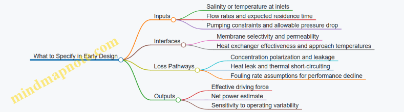
Case-Style Example: A Practical Check Before Selecting Hardware
Before choosing a membrane material or a working fluid, run a consistency check using the same workflow for both conversion types:
- Compute the available driving force from the measured inlet conditions.
- Apply a conservative reduction factor for internal losses (polarization, approach temperature).
- Estimate net power by subtracting pumping and auxiliary loads.
- Confirm that the required flow rates are compatible with marine constraints like pressure drop and intake clogging.
This keeps the design grounded in what the device can actually exploit, rather than what the ocean conditions suggest on paper.
6.3 Buoyancy Driven And Pressure Driven Conversion Mechanisms
Buoyancy driven and pressure driven converters both turn marine motion into electricity, but they start from different physical “handles.” Buoyancy driven systems exploit changes in the body’s displaced volume as it moves up and down. Pressure driven systems exploit pressure differences across a membrane, piston, or turbine runner created by wave or current flow.
Core Idea Buoyancy Driven Conversion
A buoyancy driven device typically has a floating or partially submerged body connected to a power take-off (PTO). When waves or heave motion change the body’s immersion, the displaced volume changes, so the buoyant force changes too. That varying force can be converted into mechanical motion at the PTO.
A simple way to picture it: imagine a buoy that rises and falls. As it rises, it displaces less water and buoyant force drops. As it falls, it displaces more and buoyant force rises. If the PTO resists motion with an appropriate force profile, the net work over a cycle becomes electrical energy.
Key design practice is matching the PTO’s effective damping to the motion. Too little damping and the device mostly “floats through” the waves with little energy extraction. Too much damping and the device motion is suppressed, reducing the buoyancy variation available to do work. Designers often express this as an energy balance between incoming wave power, hydrodynamic losses, and PTO absorption.
Core Idea Pressure Driven Conversion
Pressure driven devices use a pressure field difference between two sides of a flow path. In wave energy, pressure can be created by oscillating water columns or by forcing water through a duct. In current energy, pressure differences can arise across a turbine or through a controllable flow restriction.
A common architecture is a chamber connected to the sea surface or seabed. As waves raise and lower the water level, the pressure in the chamber changes. That pressure acts on a piston or membrane, producing a stroke. The stroke drives a hydraulic or mechanical power train.
The key design practice is controlling the pressure-volume relationship. If the chamber is too “stiff,” pressure changes are large but the volume flow is small, limiting energy. If it is too “soft,” volume flow is large but pressure may be insufficient to move the PTO effectively. Good designs manage this with geometry, compliance elements, and valves or control logic.
How Buoyancy and Pressure Couple to Motion
Buoyancy driven systems convert motion to force through displacement. Pressure driven systems convert pressure to force through area. The difference matters for scaling.
- Buoyancy driven: force scales with displaced volume change, which depends on immersion geometry and wave-induced motion.
- Pressure driven: force scales with pressure change times effective piston or membrane area, which depends on chamber dynamics and flow resistance.
In practice, both mechanisms include hydrodynamic added mass and damping. Added mass is the “extra inertia” of moving water with the body. Damping includes radiation losses and viscous effects. These terms shape the phase relationship between excitation and PTO motion, which is crucial because power depends on force and velocity being in the right relationship.
Mind Map: Conversion Mechanism Relationships
Example: Buoyancy Driven Heave with PTO Damping
Consider a floating buoy that heaves with a dominant wave frequency. The buoy’s vertical motion produces a buoyant force variation. If the PTO applies an opposing force proportional to velocity (a damping-like behavior), the instantaneous power is the product of opposing force and velocity. Over a cycle, the average power increases when the PTO force is well phased with the heave velocity.
A practical best practice is to tune the PTO damping so that the device’s motion is reduced only as much as needed. For instance, if measurements show the buoy’s heave amplitude is already small due to strong radiation damping, increasing PTO damping further may reduce motion without adding much absorbed power. In that case, the operating point should be shifted toward lower damping or adjusted with control to avoid “over-braking.”
Example: Pressure Driven Oscillating Water Column with Chamber Tuning
Imagine an oscillating water column with a chamber above the sea. Incoming waves push water into the chamber, compressing air or water trapped in the upper section. The pressure difference acts on a piston or drives an air turbine.
If the chamber volume is large, pressure changes are modest and the turbine sees limited torque. If the chamber volume is too small, pressure spikes but flow rate drops because the system cannot exchange volume quickly. The best practice is to choose chamber geometry and internal flow resistance so that pressure and flow are both sufficient across the expected wave spectrum. Designers often validate this by comparing measured pressure time series and flow rates with model predictions, then adjusting resistance elements to align the operating point.
Practical Comparison for Choosing a Mechanism
Buoyancy driven converters are often well suited when the site provides strong vertical motion and when a floating or semi-submerged structure can be maintained reliably. Pressure driven converters are often well suited when wave-induced pressure variations can be captured efficiently through chambers, ducts, or flow paths.
In both cases, the “conversion mechanism” is only half the story. The other half is the PTO operating point and the hydrodynamic environment that sets phase and losses. A device that looks good on paper can underperform if the PTO damping or pressure-flow tuning is mismatched to the actual sea state.
6.4 Intake and Flow Conditioning Considerations
Intake and flow conditioning turn a marine resource into something a power conversion system can use consistently. The intake’s job is not just to “get water in,” but to deliver flow with predictable velocity, turbulence level, and debris content while staying within allowable pressure losses and structural limits.
Intake Objectives and Constraints
Start with three measurable objectives: (1) capture the intended flow cross-section, (2) limit energy lost to friction and fittings, and (3) protect downstream components from damage and fouling. These objectives compete with constraints such as allowable head loss, maximum approach velocity to reduce erosion, and survivability during storms when flow reverses or accelerates.
A practical way to reason about tradeoffs is to treat the intake as a pressure-loss budget. If the converter needs a minimum flow speed at the device face, then every meter of pipe length, every bend, and every screen restriction consumes part of that speed. When the budget is tight, the intake must be shaped to reduce losses rather than relying on larger pumps or aggressive control.
Flow Conditioning Elements
Flow conditioning typically includes screens, flow straighteners, diffusers, and sometimes a settling section. Each element targets a specific problem.
Screens and debris management. Marine debris ranges from sand and shell fragments to floating plastics. Screens reduce the risk of blade strikes and clogging, but they also add head loss. A good practice is to size openings based on the smallest particle that would cause unacceptable damage, then verify that the resulting pressure drop remains within the intake budget at expected peak flow.
Flow straightening. Turbulence and swirl can reduce turbine efficiency and increase cyclic loads. Flow straighteners—such as honeycomb structures or vanes—reduce non-uniformity, but they can also trap debris. The best designs balance straightening effectiveness with cleanability and acceptable added drag.
Diffusers and contraction sections. A diffuser can lower velocity and recover static pressure, which helps with cavitation risk and reduces noise. However, diffusers can separate if the angle is too aggressive. A conservative approach is to use gentle area changes and to confirm separation margins with simple flow checks or model tests.
Hydrodynamic Performance Checks
Intake performance is usually evaluated using three linked quantities: approach velocity distribution, head loss, and turbulence intensity. Approach velocity distribution matters because many converters respond nonlinearly to local speed. Head loss matters because it reduces the effective energy available. Turbulence intensity matters because it affects fatigue and control stability.
A systematic workflow is to define a target “device-face” condition, then back-calculate allowable intake losses. For example, if the converter requires 2.0 m/s at the device face and the intake budget allows only a 5% speed reduction, then the intake must be designed so that the pressure drop corresponds to that limit under normal operating flow.
Cavitation and Erosion Risk Management
Cavitation risk rises when local pressure drops below vapor pressure plus a safety margin. Intakes can create low-pressure zones at edges, in corners, and around screen elements. Erosion risk rises with high near-wall velocities and abrasive particles.
Mitigation is practical and specific: use rounded leading edges, avoid sharp contractions, and place screens where flow is relatively uniform. For erosion-prone regions, consider sacrificial wear surfaces or replaceable inserts so maintenance can be targeted without replacing the entire intake structure.
Fouling and Cleanability by Design
Fouling changes the intake over time by reducing effective area and increasing pressure drop. Design for cleanability means access for inspection, predictable maintenance intervals, and geometry that discourages long-term buildup.
A simple example: if a screen is the primary restriction, then the intake should allow safe removal or backflushing without dismantling the whole assembly. If backflushing is not feasible, then the screen should be replaceable as a module, and the intake should include lifting points and clearances for maintenance vessels.
Integration with Mooring and Structural Loads
Intake structures experience hydrodynamic forces that interact with the mooring and support system. A common mistake is to size the intake for normal flow but ignore extreme conditions where debris, waves, and current combine. The intake should be treated as part of the overall load path, including added mass and drag.
A useful practice is to align intake geometry with expected flow direction under both operating and extreme states. If the intake faces can become partially shielded or exposed during current reversal, then the design should still maintain acceptable pressure losses and avoid creating vortex shedding hotspots.
Mind Map: Intake and Flow Conditioning Considerations
Example: Designing a Screened Intake for a Tidal Stream Device
Assume a tidal stream site where the device needs 2.0 m/s at the rotor plane. The intake budget allows a 5% reduction in effective speed, so the intake must limit pressure losses accordingly.
- Choose screen opening size to block particles that could damage blades, then estimate pressure drop at the expected maximum approach velocity.
- If the pressure drop exceeds the budget, first reduce losses by improving flow alignment and using a smoother screen frame rather than shrinking openings.
- Add a short settling section upstream of the screen to reduce large-scale non-uniformity, which lowers local velocities at the screen.
- Provide a maintenance plan: modular screen panels with lifting points and clear access so pressure drop can be restored without major disassembly.
This sequence keeps the design grounded in measurable limits: the rotor gets the speed it needs, the screen does not consume the intake budget, and maintenance can actually be performed.
6.5 Practical Example: Comparing Conversion Pathways for a Site Constraint
You have a coastal site with two constraints that matter immediately: (1) the seabed is shallow enough that moorings and foundations must be compact, and (2) the grid connection is limited in capacity, so you need a conversion pathway that produces steady power during the most common operating conditions. The goal is not to “pick the best technology,” but to compare tidal stream, surface wave, and ocean current options using the same site-limited logic.
Step 1: Translate Site Constraints Into Engineering Questions
Start by turning constraints into questions you can answer with calculations or at least consistent assumptions.
- Compact mooring and foundation requirement becomes: “Which device type needs the smallest footprint and lowest vertical clearance?”
- Limited grid capacity becomes: “Which pathway yields the highest fraction of energy during moderate conditions, not only during extremes?”
- Harsh marine environment becomes: “Which pathway tolerates higher downtime without losing too much annual energy?”
A useful habit is to write these as a checklist and keep it visible while comparing pathways.
Step 2: Build a Minimal Site Dataset
Use a small set of inputs that drive both energy and engineering feasibility.
- Tidal stream: representative current speed distribution (or binned speeds), typical directionality, and spring-neap variability.
- Waves: wave height and period statistics, plus a simple sea-state frequency table (bins).
- Ocean current: if present, a depth-averaged speed profile or at least a representative speed and thickness of the energetic layer.
- Bathymetry and clearance: water depth, seabed slope, and any known obstructions.
- Installation and operations limits: maximum allowable footprint, typical vessel access, and acceptable maintenance window.
Even a “good enough” dataset works here because you are comparing pathways consistently.
Step 3: Compare Conversion Pathways Using Consistent Metrics
Use three metrics that connect physics to engineering reality.
- Energy capture under moderate conditions: estimate power in the most frequent bins, not just peak bins.
- Footprint and structural complexity: count major subsystems that scale with size (turbine diameter, wave buoy size, mooring length, foundation type).
- Operational availability sensitivity: identify which pathway is most affected by downtime during storms or fouling.
For a quick, transparent comparison, you can use a simplified expected-power calculation:
- For each pathway, compute expected power as a weighted sum over bins:
- tidal: weighted by current-speed bins and device power curve
- wave: weighted by sea-state bins and device response-to-power mapping
- current: weighted by current-speed bins and conversion efficiency
Then adjust for feasibility using a feasibility factor that penalizes footprint and downtime risk.
Step 4: Mind Map of the Comparison Logic
Mind Map: Comparing Conversion Pathways for a Site Constraint
Step 5: Worked Example with Plausible Numbers
Assume the grid can accept 1.0 MW export, and you want to maximize annual energy without exceeding the export limit.
- Tidal stream: current speeds cluster around moderate values, and the device can be tuned so that the power curve reaches useful output before the highest speeds. The main engineering burden is ensuring the mooring and foundation fit the compact requirement.
- Wave energy: wave power is concentrated in a few energetic sea states. If the device must enter a survival mode during storms, the output can drop for long periods, which matters when grid capacity is limited.
- Ocean current: if the energetic layer is thin, the rotor or conversion element must be placed precisely, increasing installation complexity. If the layer is thick, it can behave more like a steady source, but only if the device fits the footprint.
Now apply the metrics:
- Moderate-condition energy: tidal stream typically scores well because tidal cycles repeat predictably and often keep the device operating through moderate bins.
- Footprint and complexity: wave systems can be bulky in the vertical direction, while tidal stream devices can be compact if the foundation choice is compatible with the seabed.
- Availability sensitivity: wave devices often have more frequent operational mode changes tied to sea state; tidal stream devices usually have fewer “all-or-nothing” shutdown periods.
A simple ranking emerges: tidal stream first, ocean current second if the energetic layer is thick enough, and wave third if vertical clearance and survivability modes reduce moderate-bin output.
Step 6: Make the Decision Actionable
Turn the ranking into a design implication.
- If tidal stream wins, the next step is to refine array spacing and confirm that mooring loads remain within the compact foundation envelope.
- If ocean current is close behind, the key check is whether the energetic layer thickness allows the conversion element to be positioned without violating clearance.
- If wave is last, the decision is not “wave is bad,” it’s “this site constraint set makes moderate-bin output too low relative to feasibility penalties.”
This approach keeps the comparison grounded: you are matching physics to constraints, using the same bin-weighted logic for every pathway, and letting the site limitations do the talking.
7. Electrical Generation and Power Conditioning for Marine Systems
7.1 Generator Types and Electrical Output Characteristics
Marine energy converters rarely produce steady power. The generator you choose has to tolerate changing torque, varying flow or wave motion, and electrical constraints at the grid connection. The goal of this section is to connect generator type to the shape of electrical output you can expect, and then to the control and protection choices that follow.
Core Generator Output Characteristics
A generator converts mechanical power into electrical power. What matters for marine systems is how electrical output responds when mechanical input changes.
- Voltage and frequency behavior: Some generators naturally maintain frequency with a tight mechanical speed requirement; others allow speed variation and instead rely on power electronics to produce grid-suitable output.
- Torque-speed relationship: The mechanical side of the converter imposes a torque curve. If the generator prefers a narrow speed range, the system must control the converter to stay near that range.
- Efficiency across operating points: Marine devices spend time away from their best-efficiency point, so part-load behavior matters.
- Fault current and protection coordination: Grid codes and protection schemes depend on how much current the generator can deliver during disturbances.
A practical way to think about output is to separate it into two layers: electrical machine behavior (what the generator produces at its terminals for a given speed and excitation) and power conditioning behavior (what the system does to make that output usable for the grid).
Generator Types and Where They Fit
Synchronous Generators
Synchronous generators produce AC output whose frequency is tied to rotor speed. They can be built with different excitation methods, but the key characteristic is that the machine synchronizes its electrical behavior to the mechanical rotation.
- Typical electrical output: Three-phase AC with frequency proportional to speed.
- System implication: If the converter speed varies, the electrical frequency varies too unless you add power electronics or use a mechanical arrangement that keeps speed near synchronous.
- Control implication: Reactive power control is often a central feature, since excitation affects terminal voltage.
Easy example: If a tidal turbine slows during slack water, a synchronous generator without speed control will output lower-frequency AC. A grid connection that expects fixed frequency cannot accept that directly, so you either keep speed nearly constant or condition the power.
Induction Generators
Induction generators rely on rotor currents induced by the stator magnetic field. They do not require external rotor excitation in the same way as synchronous machines.
- Typical electrical output: Three-phase AC at stator terminals, with frequency tied to grid and slip.
- System implication: The machine draws magnetizing reactive power from the grid, which affects voltage support and protection planning.
- Control implication: Speed variation changes slip, which changes torque and current draw.
Easy example: During a stronger current, the turbine torque increases. The induction generator responds by reducing slip, which shifts current and reactive power demand. The grid sees those changes, so the electrical design must account for them.
Doubly Fed Induction Generators
A doubly fed induction generator uses a partial-scale power converter on the rotor side, allowing the machine to operate over a wider speed range while keeping stator output closer to grid frequency.
- Typical electrical output: Stator side is synchronized to grid frequency; rotor-side converter handles the difference between rotor speed and synchronous speed.
- System implication: The converter rating can be smaller than full-scale, because only a fraction of power flows through the electronics.
- Control implication: Rotor current control becomes the lever for torque and reactive power.
Easy example: If the turbine speed varies by ±30% around a nominal value, the stator still outputs near fixed grid frequency, while the rotor converter manages the speed mismatch.
Permanent Magnet Synchronous Generators
Permanent magnet synchronous generators use rotor magnets instead of field windings. They often pair well with full-scale converters.
- Typical electrical output: Machine-side AC frequency follows rotor speed.
- System implication: With a full-scale converter, the system can accept variable speed and still deliver grid-suitable output.
- Control implication: Torque control is tied to current vector control, and the converter must manage voltage and current limits during transients.
Easy example: A wave energy device can change its motion cycle by cycle. With a full-scale converter, the generator can spin at whatever speed the motion provides, while the converter shapes the electrical output for the grid.
Mind Map: Generator Choice Logic
Practical Selection Example for Output Compatibility
Suppose you have a tidal site where turbine speed varies noticeably with flow, and the grid connection requires fixed frequency and controlled reactive power.
- If you choose a synchronous generator without a converter, you must keep speed close to synchronous, which may force the turbine to operate away from its optimal hydrodynamic point.
- If you choose an induction generator, you can keep stator frequency aligned to the grid, but you must manage reactive power draw and ensure voltage stability during disturbances.
- If you choose a doubly fed induction generator, you can allow wider speed variation while keeping stator output near grid frequency, using the rotor converter to control torque and reactive power.
- If you choose a permanent magnet synchronous generator, you typically use a full-scale converter so the grid sees a consistent voltage and frequency even when the mechanical input swings.
The best choice is the one that matches the converter’s mechanical variability to the electrical conditioning you can afford and control. In other words: don’t start with the generator name; start with the output shape your grid needs, then work backward to the machine and converter combination that produces it.
7.2 Power Electronics for Variable Speed Marine Generation
Marine converters rarely behave like a steady wall socket. Tidal current speed changes with the tide, wave power swings with the sea state, and ocean currents can vary over minutes. Variable-speed generation lets the electrical system follow those changes efficiently, but it also demands power electronics that can handle wide input ranges, harsh environments, and grid requirements.
Core Job of the Power Electronics Chain
A typical chain takes variable mechanical power from a turbine or generator, conditions it electrically, and produces grid-compliant voltage and frequency. The main functions are:
- Rectify or convert variable-frequency AC to a controllable DC link.
- Invert the DC link to grid-synchronous AC.
- Regulate current and voltage to control torque, manage power, and limit stresses.
- Provide protection for faults, overcurrent, and abnormal marine operating conditions.
A practical mental model is “mechanical control first, electrical control second.” The turbine control sets a target torque or speed; the power electronics then enforce electrical conditions that make that torque achievable.
Variable Speed Options and Where They Fit
Variable-speed marine generation usually uses one of these architectures:
- Synchronous generator with converter: Often uses a full converter to decouple generator speed from grid frequency.
- Induction generator with converter: Can use partial or full conversion depending on design goals.
- Permanent magnet generator with full converter: Common when you want strong controllability and compact machines.
Best practice is to choose the architecture based on what you need to control. If you must tightly regulate torque across a wide speed range, full conversion is the straightforward path. If you only need modest speed variation, partial conversion can reduce component count, but it limits how independently you can control power.
DC Link and Why It Matters
The DC link is the buffer between the variable generator side and the grid side. It smooths power fluctuations and provides energy storage for short transients.
- Capacitance sizing affects how much the DC voltage droops during gusts of power.
- Inductor and filter design affects current ripple and electromagnetic stress.
- Control of DC voltage prevents the grid-side inverter from “fighting” the generator-side converter.
A simple example: suppose the turbine suddenly accelerates and electrical power rises. Without adequate DC-link energy and control bandwidth, the DC voltage can spike, forcing protective shutdown. With proper DC-link sizing and control, the system temporarily absorbs the imbalance and then settles to the new operating point.
Generator-Side Conversion Control
On the generator side, the converter controls current waveforms to regulate torque and speed.
- For AC machines, control is often implemented in a rotating reference frame (commonly d-q control) to separate flux-producing and torque-producing components.
- For permanent magnet machines, the d-axis current often relates to torque directly, while the q-axis current sets torque magnitude.
A concrete control practice is to enforce current limits that reflect both electrical ratings and mechanical stress constraints. For instance, if the turbine experiences high thrust, you may cap generator current to reduce torque and avoid excessive hydrodynamic loading.
Grid-Side Inversion and Grid Compliance
The grid-side inverter must deliver power at the correct voltage and frequency and manage reactive power.
Key requirements typically include:
- Synchronization to grid phase for stable current injection.
- Current control loops that track active power and reactive power commands.
- Protection behavior during voltage dips, frequency deviations, and islanding risk.
A useful example is reactive power management. If the marine system injects too much reactive current, it can increase losses in cables and transformers. If it injects too little, voltage regulation can suffer. Power electronics let you choose a reactive power strategy that matches the grid connection design.
Protection and Fault Handling That Doesn’t Waste Time
Marine faults can be fast: insulation degradation, cable faults, converter overtemperature, or sensor failures. Power electronics should respond with:
- Overcurrent detection with controlled shutdown or current limiting.
- DC-link overvoltage and undervoltage protection.
- Thermal monitoring and derating logic.
- Grid fault ride-through behavior aligned with the connection agreement.
A practical best practice is to coordinate protection thresholds with mechanical limits. If the converter trips instantly on a minor transient, the turbine may experience repeated start-stop cycles that increase fatigue. If the converter rides through too aggressively, it may over-stress the generator and drivetrain. Coordination turns protection into a controlled response rather than a blunt instrument.
Mind Map: the Converter System
Worked Example: From Speed Change to Grid Power
Assume a tidal turbine increases rotor speed due to a stronger current. The turbine controller asks for higher torque, which increases generator-side current. The DC-link voltage tends to rise because generator power momentarily exceeds what the grid-side inverter can export. The DC voltage controller responds by adjusting grid-side current commands so the inverter exports more active power. Once the DC voltage returns to its setpoint, the system settles at a new operating point with stable grid current.
The key point is that the system does not “guess” the grid power. It measures DC voltage and current, then uses control loops to balance power flow between generator and grid.
Design Checklist for Practical Implementation
- Define the speed range and expected power swing from resource data.
- Choose converter architecture based on required decoupling and torque control.
- Size DC link and filters for transient energy and ripple limits.
- Implement coordinated current limits that reflect mechanical loading constraints.
- Ensure grid synchronization and current control bandwidth match grid requirements.
- Coordinate protection actions with ride-through behavior to avoid unnecessary trips.
When these pieces work together, variable-speed marine generation becomes less about “making power” and more about managing energy flow and stress—quietly, continuously, and with good manners toward both the turbine and the grid.
7.3 Grid Connection Requirements and Synchronization Methods
Connecting a marine energy converter to the grid is mostly an exercise in timing, protection, and predictable behavior under messy real-world conditions. The goal is simple: when the device is online, its electrical output must match the grid’s voltage and frequency closely enough to avoid harmful currents, and it must disconnect quickly when conditions are unsafe.
Grid Connection Requirements
Grid codes typically require three categories of performance: steady-state synchronization, dynamic ride-through behavior, and protection coordination.
Steady-state synchronization means the converter must control its output so that the grid sees either (a) a current source that stays within allowed current magnitude and phase error, or (b) a voltage source that matches grid voltage within tight limits. For tidal and wave systems, the challenge is that the mechanical input varies; electrical control must translate that variability into controlled electrical behavior.
Dynamic ride-through behavior addresses what happens during voltage dips, frequency excursions, or brief disturbances. A practical best practice is to define operating modes for each disturbance class, then test them with staged faults so the protection system and the control system agree on who “wins” during the event.
Protection coordination ensures the converter does not rely on the grid to clear faults. Typical elements include fast current limiting, transformer and cable protection, anti-islanding detection, and coordinated overcurrent or distance protection upstream. A useful rule of thumb: if a fault would create large fault current through the converter, the converter must either block output quickly or limit current before upstream protection clears.
Synchronization Methods
Synchronization is about phase alignment and controlled connection. There are two common approaches depending on the converter type.
Grid-following control is common for variable-speed generation with power electronics. The converter measures grid voltage phase and commands output current with a controlled phase angle. This method is straightforward because the grid sets the reference; the converter tracks it.
Grid-forming control is used when the converter can establish voltage and frequency locally. In marine systems, this is less common for export to a strong grid, but it matters for weaker grids or islanded operation tests. Even then, the converter must still respect limits on voltage magnitude, frequency ramp rates, and harmonic content.
Practical Synchronization Workflow
A systematic workflow reduces surprises:
- Pre-connection checks: verify grid voltage magnitude, frequency range, and phase stability. If the grid is noisy or unbalanced, the control should use filtering and measurement windows that avoid reacting to short spikes.
- Soft-start of electrical output: ramp current or voltage setpoints gradually so the inrush and transient torque do not create large electrical stress.
- Phase alignment: for grid-following, lock the current phase to the grid voltage using a phase-locked loop or equivalent estimator, then confirm phase error is within the allowed band.
- Connection and monitoring: after closing the breaker, monitor current, DC-link voltage, and protection signals. If any limit is exceeded, the system should open promptly.
- Anti-islanding verification: ensure the anti-islanding scheme detects loss of grid and triggers disconnection within the required time.
Mind Map: Synchronization and Connection Logic
Example: Current-Phase Alignment for Grid-Following
Assume the converter uses grid-following current control. The controller measures grid voltage \( v_g \) and estimates its phase φ. It then commands converter current (i) with a target phase angle θ relative to (v_g). If θ is set to achieve unity power factor, the current phase should be near the grid voltage phase.
A practical best practice is to define a maximum phase error band, such as a few degrees, and refuse connection if the measured phase error is outside that band for a minimum time window. This avoids “connecting on a lucky measurement” when the phase estimator is still settling after a disturbance.
Example: Coordinated Response During a Voltage Dip
During a voltage dip, the grid voltage magnitude drops while the grid phase continues. A well-coordinated system does two things: it limits current to avoid exceeding converter and cable ratings, and it follows the ride-through behavior required by the grid code. If the dip is within the allowed duration, the converter stays connected and adjusts current magnitude according to the specified control law. If the dip exceeds the allowed duration or violates voltage thresholds, protection clears the connection.
The key integration detail is that the control system and protection system must share the same thresholds and timing assumptions. If the control tries to ride through but protection trips immediately, the ride-through requirement is effectively not met, and the device will disconnect more often than intended.
7.4 Power Quality Control and Protection Coordination
Power quality in marine energy systems is less about sounding “clean” and more about staying within what the grid and the equipment can tolerate. Marine converters often produce variable voltage and frequency at the generator terminals, so the power conditioning chain must both shape the output and protect itself during faults, abnormal sea states, and switching events.
What “Power Quality” Means at the Grid Interface
At the point of common coupling, the grid expects stable voltage magnitude, controlled frequency, and limited harmonic distortion. For a marine system, the practical power-quality targets usually include:
- Voltage and frequency compliance: the delivered active power should not force the grid voltage outside limits.
- Harmonic distortion control: inverter switching can create harmonics; filters and modulation strategies reduce them.
- Flicker and rapid voltage changes: control loops that chase fluctuating resource power can cause short-term variations.
- Fault ride-through behavior: during grid voltage dips, the system must avoid tripping immediately while still protecting semiconductors.
A helpful mental model is to separate quality (how the output looks under normal operation) from protection (what happens when something goes wrong). Good coordination ensures the protection actions do not create worse power-quality problems than the original disturbance.
Protection Philosophy for Variable Marine Generation
Protection coordination starts with identifying credible fault paths and deciding which device should act first. Typical protection layers include:
- Converter-side protection for overcurrent, overvoltage, undervoltage, and semiconductor temperature limits.
- AC-side protection for short circuits, earth faults, and abnormal grid conditions.
- System-level protection for loss of synchronization, islanding, and unsafe operating states.
A best practice is to define protection actions in terms of energy and stress, not just electrical thresholds. For example, a short circuit can overheat a power module in milliseconds, so the converter must respond quickly, while slower breakers can handle upstream isolation.
Coordination Between Converter Control and Protective Devices
The converter control system and protective relays must agree on priorities. If the control loop tries to “fix” a fault while protection trips, you get unnecessary outages and extra stress.
Key coordination rules:
- Fast current limiting first: during a grid fault, the converter should limit current to protect the semiconductors.
- Grid synchronization checks: if the phase reference becomes unreliable, the system should transition to a safe state rather than injecting uncontrolled current.
- Defined trip hierarchy: the fastest action should be the one that prevents device damage; upstream isolation should follow only if the fault persists.
Example: Current Limit Versus Breaker Trip
Suppose a downstream cable fault causes a sudden voltage dip. The inverter detects the abnormal voltage and commands a current limit. If the fault clears quickly, the current returns to normal without opening the breaker. If the fault persists, the AC protection clears the fault and the converter enters a restart sequence. The coordination goal is to avoid opening the breaker for events that the converter can safely ride through.
Harmonic Control and Protection Interaction
Harmonic filters and modulation strategies reduce distortion, but they also affect protection behavior. For instance, a filter capacitor can contribute to transient overvoltage during switching, and filter resonance can amplify certain frequencies.
Practical measures:
- Use measured current feedback for protection rather than relying on filtered signals that may lag.
- Set harmonic-related limits conservatively so protection does not confuse normal switching harmonics with a true overcurrent condition.
- Coordinate filter bypass or switching states with protection logic to prevent nuisance trips during normal operating transitions.
Protection Settings That Match Marine Operating Reality
Marine systems face changing impedance, cable lengths, and resource-driven operating points. Protection settings should reflect these variations.
Best practices:
- Time-current coordination: choose trip times so the converter survives short disturbances while upstream devices clear sustained faults.
- Temperature-aware limits: current limits should reflect thermal headroom, especially after high sea-state operation.
- Voltage-dependent behavior: undervoltage and overvoltage thresholds should align with the converter’s modulation limits and DC-link protection.
Example: Undervoltage Event During High Wave Power
During a wave-driven power surge, the converter may draw higher current. If the grid voltage sags, the inverter’s available modulation margin shrinks. A coordinated undervoltage scheme can first reduce active power and limit current, then trip only if voltage remains below the safe operating envelope long enough to threaten the DC link or semiconductor temperatures.
Mind Map of Power Quality Control and Protection Coordination
Mind Map: Power Quality Control and Protection Coordination
Putting It Together in a Simple Coordination Workflow
A systematic workflow keeps the design from becoming a pile of unrelated settings:
- Define grid interface requirements for voltage, frequency, harmonics, and ride-through.
- List credible fault scenarios and identify the expected current and voltage waveforms.
- Assign protection responsibilities by speed and energy-stress severity.
- Verify control-protection interaction using simulated events: current limiting, synchronization loss, and filter switching.
- Finalize settings with marine operating ranges for impedance variation and thermal state.
When this workflow is followed, the system behaves predictably: it shapes power quality during normal operation and responds to faults in a way that protects hardware without creating unnecessary grid disturbances.
7.5 Practical Example: Designing a Power Conditioning Chain for a Converter
A tidal or wave converter rarely produces grid-ready electricity directly. The conditioning chain’s job is to shape electrical output, protect equipment, and meet grid requirements while staying efficient across changing marine conditions. A good design starts with three questions: What does the generator output look like across operating points, what does the grid require at the connection point, and what must be protected during abnormal events.
Step 1: Start with Converter Output Behavior
Assume a variable-speed permanent-magnet generator (common for tidal stream and some wave systems). Its electrical frequency and voltage magnitude vary with rotor speed and load. In practice, you treat the generator as a source with a wide operating envelope rather than a single operating point.
Best practice: define an operating map before choosing electronics. For example, pick three representative states: low flow (reduced speed), rated flow (near design speed), and high flow (where control may limit power). For each state, estimate generator line-to-line voltage range and current range. Even rough numbers help you size semiconductor ratings and filter components.
Step 2: Choose a Conditioning Topology
A typical chain is:
- Rectification to DC (often a three-phase diode bridge for simplicity, or an active rectifier for tighter control).
- DC link to buffer power and smooth ripple.
- Inversion to AC with grid synchronization (usually a voltage-source inverter).
- Filtering and protection to meet harmonic limits and survive faults.
If you need smooth torque control and predictable power factor behavior, an active rectifier is usually worth the extra complexity. If the converter control already manages torque well and you want fewer controllable degrees of freedom, a diode bridge can work, but you accept more variability in DC voltage.
Step 3: Design the DC Link for Energy Smoothing
The DC link capacitor reduces ripple current and helps the inverter maintain a stable DC voltage. The key relationship is that capacitor current depends on power pulsations from the rectifier and generator speed variation.
Easy example: Suppose the converter produces 500 kW peak electrical power at rated, and the rectifier introduces a DC ripple at twice line frequency. If you target a DC voltage ripple of 5% around a nominal DC voltage, you can estimate required capacitance using the allowable energy swing:
- Choose nominal DC voltage, e.g., 1.2 kV.
- Allow ripple, e.g., 5% → 60 V peak-to-peak.
- Estimate energy swing per ripple cycle and solve for capacitance.
You then verify that the capacitor can handle RMS ripple current without overheating. This is where “it works on paper” designs often stumble.
Step 4: Size the Inverter and Control Loops
The inverter must deliver the required AC voltage and current at the grid frequency. For a 400 V AC grid interface, you may use a transformer or multilevel strategy depending on your DC link voltage.
Control approach:
- Outer loop: regulates DC voltage or active power.
- Inner loop: controls inverter current to shape output and limit harmonics.
- Synchronization: phase-locked loop or grid-forming method ensures correct timing.
Best practice: keep the control bandwidth separation clear. If the inner current loop is too slow, ripple and harmonics increase. If the outer loop is too fast, it can fight the current loop and cause oscillations.
Step 5: Add Filtering and Harmonic Management
Even with current control, switching creates harmonics. A common solution is an LCL filter between inverter and grid.
Easy example: If you target a cutoff frequency well below the switching frequency but above the fundamental, you can reduce harmonic injection. You also damp resonance using resistive damping or active damping. The damping choice affects both harmonic performance and stability margins.
Step 6: Protection and Ride-Through Behavior
Protection is not optional; it’s part of the power conditioning chain.
Include:
- DC-side overvoltage and undervoltage protection to prevent inverter stress.
- AC-side overcurrent protection with fast interruption.
- Grid fault detection and controlled shutdown or current limiting.
- Surge protection for lightning-induced transients and switching events.
Best practice: coordinate protection settings with the converter’s mechanical control. If the electrical side trips but the turbine keeps accelerating, you can create repeated stress cycles.
Mind Map: Power Conditioning Chain Design Logic
Step 7: Put It Together with a Concrete Example
Assume:
- Generator peak electrical power: 500 kW
- Nominal DC link voltage: 1.2 kV
- Target DC ripple: 5%
- Switching frequency: 2 kHz
- Grid interface: 400 V AC, 50 Hz
A practical chain might be:
- Active rectifier to regulate DC voltage under varying generator speed.
- DC link sized to keep ripple within 5% and limit capacitor RMS current.
- Voltage-source inverter with current control feeding an LCL filter.
- Transformer or step-up stage to match inverter voltage to grid level.
- Protection set to trip on sustained overcurrent and clamp DC overvoltage.
Verification checklist:
- At low flow, confirm DC voltage regulation holds enough to avoid inverter saturation.
- At rated flow, confirm current control meets harmonic limits and power tracks the converter command.
- During a simulated grid voltage dip, confirm the inverter limits current and the protection logic behaves predictably.
When these checks pass, the chain is not just “designed”; it’s engineered to behave across the real operating messiness of marine power.
8. Structural Design and Marine Engineering for Reliability
8.1 Load Cases for Tidal and Wave Energy Devices
Load cases are the “storyboards” that translate ocean motion into forces, moments, and stresses your structure must survive. A good load-case set is systematic: it starts with what the environment can do, then maps those conditions to device states, and finally turns the result into design actions for analysis and verification.
Foundations of Load Case Thinking
A load case is defined by three ingredients: (1) environmental inputs, (2) operational state of the device, and (3) modeling assumptions that determine how loads are computed. For tidal devices, the environment is often described by current speed and direction over a tidal cycle. For wave devices, it is described by wave spectra, water depth, and wave directionality. In both cases, you also need the device state: operating, idling, starting, stopping, parked, or in survival.
Best practice is to keep the load-case definitions traceable. If a load case is “Extreme current with turbine braking,” you should be able to point to the current statistic used, the braking control mode, and the hydrodynamic model settings that convert flow into thrust and torque.
Core Environmental Inputs
For tidal stream devices, typical environmental variables include mean current, turbulence intensity, shear profile, and direction changes. You also need water level if it changes submergence and therefore hydrodynamic coefficients.
For wave energy devices, the key inputs are wave height, period (or frequency content), wave direction, and water depth. Because wave loads depend on phase, you generally treat wave conditions through time-domain simulations with many realizations or through frequency-domain approaches with appropriate phase assumptions.
A practical way to avoid gaps is to separate “resource description” from “design extremes.” Resource description supports energy yield and fatigue distributions; design extremes support ultimate strength and survivability.
Device States and How They Change Loads
Device states determine how the power take-off and control system behave, which changes hydrodynamic forces. Examples:
- Operating state: blades or buoyant structures interact with the flow or waves under active control, producing thrust and cyclic loading.
- Idling state: the device is not extracting power, often with a different pitch/yaw or PTO damping.
- Start and stop: transient control actions can create short-lived but high loads, especially when braking engages.
- Survival state: the device is configured to reduce loads, such as stowing, locking, or changing orientation.
A simple check: if your control logic changes the effective damping or blade pitch, you must reflect that in the load-case definition rather than reusing the operating hydrodynamics.
Load Case Categories
A complete set usually includes:
- Serviceability and fatigue: frequent or representative conditions that drive cumulative damage.
- Ultimate strength: rare but high loads that test structural capacity.
- Accidental and operational transients: events like loss of control, sudden PTO changes, or temporary mooring tension changes.
- Installation and recovery: loads during towing, lifting, and connection/disconnection.
Even if your chapter focuses on 8.1, the categories matter because they determine which response metrics you compute: stress ranges for fatigue versus peak internal forces for ultimate checks.
Mind Map: Building a Load Case Set
Example: Tidal Load Cases That Don’t Miss the Transients
Consider a tidal stream turbine with a yaw system and blade pitch control.
- Fatigue load case: representative current bins across the tidal cycle, using operating control with normal yaw tracking. Compute thrust and bending moment time histories, then extract stress ranges at critical welds.
- Ultimate load case: extreme current speed with the turbine in survival yaw orientation and maximum thrust reduction achieved by control. Use a conservative control response time so the device does not instantly reach the survival configuration.
- Transient load case: sudden loss of PTO torque leading to rapid pitch change and braking engagement. Model the time-dependent thrust rise and include the resulting mooring tension change.
A common mistake is to treat “extreme current” as if the device is always in steady operating mode. Transients are where control dynamics and inertia show up.
Example: Wave Load Cases with Phase Sensitivity
For a wave energy converter with a hinged body and PTO damping:
- Fatigue load case: multiple wave realizations for a moderate sea state, using the PTO damping corresponding to normal power capture. Extract cyclic hinge moments and deck reactions.
- Ultimate load case: a high sea state with direction aligned to maximize response amplitude. Use enough realizations to capture phase-dependent peaks, then select the governing response for structural checks.
- Survival load case: stowed configuration with reduced motion, using PTO bypass or locked damping. Confirm that the stowed configuration does not create new load paths that bypass the intended load reduction.
Practical Checklist for Completeness
- Every load case states the environment, device state, and control/PTO mode.
- Fatigue and ultimate cases are not mixed: they use different selection criteria and different response metrics.
- Transients are explicitly included for start/stop and control failures.
- Installation and recovery loads are treated as separate load cases, not as afterthoughts.
- The load-case set is small enough to analyze, but structured enough to justify why it covers the important physics.
8.2 Fatigue And Fracture Mechanics for Marine Components
Marine energy devices live a double life: they see repeated loading during normal operation, and they also face rare but severe events like storms, start-stop cycles, and accidental impacts. Fatigue and fracture mechanics explain how those histories translate into crack initiation, crack growth, and eventual failure. The practical goal is not to predict a single “failure date,” but to ensure the probability of unacceptable damage stays within design limits over the intended service life.
Mind Map: Fatigue and Fracture Mechanics Workflow
Foundational Concepts for Fatigue
Fatigue is damage accumulation under cyclic stress. A component can fail even when the peak stress is below the material’s static strength because microscopic cracks form at stress concentrators and grow with each cycle. In marine hardware, the usual stress concentrators are weld toes, holes, transitions, and contact points in joints.
A common starting point is the S-N curve, which relates stress range to cycles to failure. For design, engineers often use a stress range rather than a single stress value because fatigue is driven by the alternating part of the loading. Mean stress matters too: if the component spends more time at higher stress levels, cracks tend to grow faster. That’s why mean stress correction methods are used to convert a measured or simulated stress history into an equivalent fatigue-driving stress.
Load Spectra Construction That Actually Works
Fatigue calculations require a load history that represents reality. The best practice is to build a load spectrum from measured or modeled operational states, then combine them with extreme-event contributions using a consistent cycle counting method. Rainflow counting is frequently used for irregular time histories, because it extracts cycles with appropriate amplitudes and mean levels.
A practical example: suppose a tidal support beam experiences alternating bending from current fluctuations. You simulate or measure bending moment time series for several sea states, convert them to stress at critical locations, then count cycles. You might find that a small number of high-amplitude cycles contribute disproportionately to damage. That observation is not a surprise; fatigue damage scales strongly with stress range, so the spectrum shape matters as much as the average level.
Crack Initiation: Where Fatigue Starts in Marine Hardware
Cracks usually initiate at the surface where stress concentration is highest. Weld toes are notorious because geometry creates a local notch effect and residual stresses from welding can raise the effective mean stress. Surface roughness and corrosion pits further intensify local stress, which is why corrosion-fatigue is treated as a distinct mechanism rather than an afterthought.
A simple example: a steel bracket with a small surface pit under cyclic tension can fail sooner than predicted by a clean-surface S-N curve. The pit acts like a tiny crack starter, reducing the initiation life. In design practice, this is handled by using appropriate detail categories, applying corrosion allowances carefully, and considering inspection intervals that can catch early cracking.
Crack Growth Mechanics for When Cracks Are Already There
Once a crack exists, growth is governed by the stress intensity factor range, ΔK, which depends on crack size, geometry, and applied loading. The Paris law is a widely used relation for the mid-growth regime, where crack growth rate scales with a power of ΔK.
However, marine loading is variable amplitude. That means crack growth is not simply “Paris law times number of cycles.” Engineers account for thresholds (below which cracks grow very slowly) and overload effects (which can temporarily retard growth). The result is that damage accumulation must be computed with a method that respects the sequence of cycles, not only their counts.
A concrete example: if a component sees mostly moderate cycles but occasionally experiences a storm-induced overload, the overload can reduce the effective growth rate for subsequent cycles. A calculation that ignores overload sequence may overestimate damage if it assumes every cycle is in the same growth regime.
Fracture Mechanics: When Failure Becomes Unavoidable
Fracture mechanics addresses what happens when a crack reaches a critical size. Two key material properties are fracture toughness and ductility. For ductile steels, fracture often involves stable crack growth followed by tearing, while brittle fracture can occur if the temperature and stress state make the material unable to deform.
Design verification typically compares the driving force for crack growth against the material’s resistance. For marine components, the stress state can be complex due to bending plus axial load, and the crack may be oriented relative to welds or rolling direction. That’s why geometry-specific analysis is used for critical details rather than relying on generic assumptions.
Damage Accumulation and Verification Logic
A standard approach is to compute fatigue damage using Miner’s rule as a baseline, then refine with mean stress corrections and crack growth models where needed. Miner’s rule sums fractional damage from counted cycles and assumes linear accumulation. It can be acceptable for preliminary design, but for critical components with variable amplitude and overloads, crack growth-based verification provides a more faithful picture.
A practical example workflow: (1) identify critical locations like weld toes and transitions, (2) obtain stress histories from structural analysis under representative operational states, (3) count cycles and compute equivalent stress ranges, (4) estimate initiation and growth contributions, and (5) check that the combined damage stays below acceptance criteria with appropriate safety factors.
Marine-Specific Modifiers That Change the Math
Corrosion changes the geometry and effective crack initiation behavior by creating pits and thinning sections. Residual stresses from welding can shift mean stress and influence crack opening behavior. Added mass and hydrodynamic drag affect the dynamic stress distribution, which changes both stress ranges and the likelihood of overload cycles.
A final sanity check is often overlooked: compare predicted hot spots with inspection access and likely damage patterns. If the analysis says a crack should start at a location that cannot be inspected, the design needs either improved detailing or a different verification strategy. In marine engineering, “the calculation is correct” is only half the story; “the component can be managed” is the other half.
8.3 Corrosion Protection and Material Selection Practices
Marine energy devices live in a hostile neighborhood: saltwater, oxygen, biofouling, cyclic loading, and crevices created by seals and joints. Corrosion control is therefore a system decision, not a single material choice. The goal is to prevent loss of section, avoid sudden failures from localized attack, and keep electrical and mechanical interfaces stable over time.
Foundations of Corrosion Modes in Seawater
Start by matching the expected environment to the dominant corrosion mode.
- Uniform corrosion: slow, predictable metal loss. It matters for long-term thickness reduction.
- Galvanic corrosion: two dissimilar metals electrically connected in seawater. The less noble metal becomes the “sacrificial” one.
- Crevice corrosion: oxygen-starved pockets under gaskets, washers, or deposits. It often accelerates once initiated.
- Pitting and stress corrosion cracking: localized attack that can be small in area but large in consequence, especially under tensile stress.
- Microbiologically influenced corrosion: biofilms change local chemistry and oxygen availability.
Example: A stainless fastener clamping a carbon-steel bracket can corrode rapidly if the joint traps seawater and creates a crevice. The corrosion rate is often limited by how well the joint is insulated and sealed, not by the stainless grade alone.
Material Selection Logic for Marine Hardware
Material selection should follow a chain: service environment → mechanical demands → corrosion risk → manufacturability and inspection.
- Define the exposure zones: splash, tidal, submerged, and internal dry spaces. Corrosion behavior changes sharply across these.
- Set mechanical requirements: fatigue strength, impact resistance, and allowable deflection for moorings, housings, and turbine components.
- Choose corrosion-resistant alloys or coatings: stainless steels, nickel alloys, duplex stainless, aluminum alloys (with care), and coated carbon steels.
- Plan for joining methods: welding, brazing, bolting, and bonded joints can create heat-affected zones or galvanic couples.
- Design for inspection: if you cannot see it, you cannot manage it. Provide access for thickness checks and coating condition surveys.
Example: For a tidal turbine hub, a duplex stainless may be selected for corrosion resistance, but the welding procedure must preserve the intended microstructure. Otherwise, the “good” material becomes “good-looking” while corrosion finds the weakened region.
Corrosion Protection System Design
Treat corrosion protection as layered defense.
- Material choice: pick alloys that resist the expected chemistry.
- Coatings and barriers: use primers and topcoats matched to surface prep and immersion conditions.
- Cathodic protection: apply sacrificial anodes or impressed current to shift metal potential.
- Electrical isolation: prevent unintended galvanic paths through insulating washers, sleeves, and controlled bonding.
- Water management: avoid crevices that trap seawater; design drainage and sealing so joints do not become stagnant reservoirs.
Example: A coated steel structure with cathodic protection still needs coating holiday control. If coating damage exposes steel, cathodic protection can slow corrosion at the exposed spots, but only if electrical continuity and anode placement are correct.
Mind Map: Corrosion Control Workflow
Practical Examples That Tie It Together
Example 1: Fastener and Joint Strategy
- Use compatible materials for bolts and plates to reduce galvanic potential.
- Add insulating washers where dissimilar metals must meet.
- Ensure gasket design avoids trapped seawater pockets.
- Specify torque procedures that maintain seal compression without over-stressing.
Example 2: Coating and Cathodic Protection Coordination
- Coatings reduce current demand, but they must be defect-tolerant.
- CP design should assume coating imperfections rather than perfect coverage.
- Electrical continuity checks prevent “floating” sections that receive little protection.
Example 3: Hotspot Identification for Inspection
- Focus on crevices, weld toes, under deposits, and areas with trapped water.
- Plan thickness checks at locations where stress and flow combine to accelerate localized attack.
Advanced Details Without the Mystery
- Surface preparation matters: coating performance depends on cleanliness and profile; poor prep turns a coating into a decorative film.
- Welding and heat-affected zones: corrosion resistance can degrade locally if procedures are not qualified for the alloy and environment.
- Crevice geometry control: small changes in gasket compression or overlap length can shift oxygen availability and corrosion behavior.
- Monitoring is part of design: include test points for CP potential and access for coating condition checks so verification is possible during operations.
Summary of Best Practices
Choose materials based on exposure zones and mechanical needs, then add layered protection through coatings, electrical isolation, cathodic protection, and geometry that avoids crevice traps. Verify the system through inspection points and monitoring locations that match the corrosion hotspots you identified during design.
8.4 Hydrodynamic Drag and Added Mass Effects in Structures
Hydrodynamic drag and added mass are two different ways the surrounding water “pushes back” on a marine structure. Drag is mostly about energy loss through turbulence and flow separation. Added mass is about inertia: the structure must accelerate some volume of water as it moves, even if the water never fully detaches from the structure.
Foundational Picture of Fluid Forces
A practical way to organize forces is to split them into components that scale with velocity and components that scale with acceleration.
- Drag-related forces scale primarily with relative velocity between structure and flow. They grow quickly as speed increases, and they depend strongly on shape and surface roughness.
- Added-mass-related forces scale primarily with acceleration. They matter most when the structure undergoes rapid motion, such as wave-induced oscillations.
In design, you rarely treat them separately in the final equations, but you can reason about them separately first, then combine them in load cases.
Drag: From Flow Regimes to Force Magnitudes
Drag force is often modeled as:
- Quadratic drag: \(F_D \propto \rho A C_D v^2\)
- Linear drag: \(F_D \propto v\) (more common at low Reynolds numbers)
For marine energy devices, quadratic drag is usually the workhorse because Reynolds numbers are typically high. The drag coefficient \(C_D\) is not a constant; it changes with Reynolds number, surface roughness, and—crucially—whether the flow separates.
A concrete example: imagine two cylindrical members of equal diameter. One has a smooth finish; the other has marine growth. The rough one tends to trigger earlier separation and higher effective drag coefficient. Even if the member diameter is unchanged, the drag load can increase enough to shift fatigue damage because drag acts repeatedly during operational cycles.
Added Mass: Inertia of the Moving Water
Added mass represents the extra force needed to accelerate the surrounding fluid. A common form is:
\(F_A = m_a, a\)
where \(m_a\) is the added mass (often expressed as a fraction of displaced mass). Added mass depends on geometry and motion direction. For bluff bodies, added mass can be significant because the flow must reorganize around the moving surface.
Example: consider a mooring buoy or a wave-energy float undergoing heave motion. When the float accelerates upward, nearby water must accelerate too. That “extra inertia” shows up as an additional dynamic load that can be comparable to drag at certain frequencies.
How Drag and Added Mass Combine in Motion
When a structure moves relative to water, the total hydrodynamic force is a sum of drag-like and inertia-like terms. In oscillatory motion, drag often produces a force that is roughly in phase with velocity magnitude (and can be out of phase with displacement), while added mass produces a force that is closely tied to acceleration.
This matters for resonance. If the structure’s natural frequency aligns with wave excitation, added mass changes the effective dynamic response by altering the inertia term. Drag changes damping, which can reduce peak amplitudes but may increase mean and cyclic loads depending on the motion pattern.
Mind Map: Hydrodynamic Drag and Added Mass
Systematic Modeling Workflow for Structures
- Identify the dominant motion mode. A current-dominated structure experiences mostly steady relative velocity, so drag dominates. A wave-driven float experiences oscillatory motion, so added mass and drag both matter.
- Select a force model consistent with the regime. Use quadratic drag when velocities are high and Reynolds numbers are in the typical marine range. Use inertia-based added mass terms for acceleration-driven loads.
- Account for geometry and orientation. A member aligned with flow behaves differently from one at an angle. For arrays, wake interactions can change local velocities and effective drag.
- Build load cases that reflect reality. Operational cases should include representative sea states and current profiles. Extreme cases should include combined wave-current conditions where possible.
- Check sensitivity. Because \(C_D\) and \(m_a\) are coefficient-like quantities, small modeling changes can shift peak loads and fatigue damage. Sensitivity checks prevent “single-number” false confidence.
Example: Comparing Two Load Drivers in a Simple Member
Consider a vertical structural member subjected to a wave-induced horizontal oscillation. If the oscillation amplitude is small but the frequency is high, acceleration is large, and added mass can contribute a noticeable portion of the peak force. If the same member experiences a stronger current with slower motion, velocity is higher while acceleration is lower, and drag becomes the primary contributor.
A good modeling habit is to compute both contributions for the same motion time series. Even if the final design uses a combined force model, seeing which term dominates at each phase of motion helps you interpret results and avoid surprises.
Practical Notes for Reliable Structural Loads
- Drag is sensitive to surface condition. Roughness changes \(C_D\), so include realistic assumptions for marine growth or protective coatings in the load basis.
- Added mass is sensitive to motion direction. Use motion components that match the structure’s degrees of freedom rather than assuming one coefficient fits all.
- Arrays and wakes change local flow. A member downstream of another may see reduced or redirected velocity, altering both drag and the effective inertia response.
When you treat drag and added mass as separate physical mechanisms first, then combine them in load cases, the structural design becomes easier to reason about—and harder to accidentally overfit to a single coefficient choice.
8.5 Practical Example: Building a Simplified Structural Load and Fatigue Workflow
This example shows a compact workflow you can use to estimate structural loads and fatigue damage for a tidal-stream device. The goal is not perfect prediction; it is a defensible, repeatable process that connects resource conditions to structural stress cycles.
Step 1: Define Geometry, Materials, and What You Will Stress
Start with a minimal structural model: a representative member (e.g., a blade root spar, hub arm, or support strut) with length, cross-section, and material properties. Choose a stress measure that you can compute from bending and axial forces, such as maximum von Mises stress at a critical section.
Easy example: Assume a steel strut with a circular hollow section, outer diameter 0.25 m, wall thickness 0.02 m, and yield strength 350 MPa. You will compute bending stress from a lateral force at the top of the strut.
Step 2: Build a Load Case Set from Operational States
Create load cases that cover the main operating regimes: normal operation, reduced power, start/stop, and extreme conditions. For each case, specify:
- Water speed or current profile (or a representative velocity)
- Turbine operating state (yaw alignment, rotor speed, thrust coefficient)
- Environmental modifiers (density, turbulence intensity)
- Duration or cycle count assumptions
Best practice: Keep load cases mutually exclusive and clearly labeled. If two cases share the same thrust coefficient and only differ in duration, merge them and scale the cycle count.
Step 3: Convert Hydrodynamic Loads Into Structural Forces
Use a simplified force model to map current and device thrust into forces on the structural member. For a tidal-stream turbine, a common starting point is:
- Thrust force: \(F_T = \tfrac{1}{2}\rho A C_T U^2\)
- Lateral force on a member: \(F_L = F_T \cdot k\) where \(k\) represents how thrust translates into bending at the member location (from geometry and load path).
Easy example: Let \(\rho=1025,\text{kg/m}^3\), rotor swept area \(A=20,\text{m}^2\), thrust coefficient \(C_T=0.8\), and current speed \(U=2.0,\text{m/s}\). Then \(F_T\approx 0.5\cdot1025\cdot20\cdot0.8\cdot(2.0)^2\approx 32800,\text{N}\). If \(k=0.6\), then \(F_L\approx 19700,\text{N}\).
Step 4: Compute Stress for Each Load Case
For bending-dominated behavior, bending stress at the outer fiber is: \[\sigma = \frac{M c}{I}\] where \(M = F_L L\), \(c\) is outer radius, and \(I\) is second moment of area.
Easy example: If strut length \(L=6,\text{m}\), outer radius \(c=0.125,\text{m}\), and hollow-section \(I=\tfrac{\pi}{64}(D^4-d^4)\), compute \(\sigma\) for each load case. Store results as stress ranges or stress amplitudes.
Step 5: Turn Operational Variability Into Stress Cycles
Fatigue needs cycles. Convert time-varying conditions into a cycle spectrum using one of two simplified approaches:
- Discrete cycle counting: Define representative stress levels for each operational state and assign cycle counts.
- Rainflow on a reduced history: If you have a short time series, reduce it to a manageable set of turning points and apply rainflow.
Best practice: If you use discrete counting, document the mapping from operational states to stress levels and cycle counts. For example, “normal operation produces stress amplitude \(\sigma_a=120,\text{MPa}\) for 300 days per year.”
Step 6: Apply an S-N Curve and Compute Damage
Use an S-N relationship appropriate for welded or base material details. Compute damage per load case using Miner’s rule: \[D = \sum_i \frac{n_i}{N_i(\sigma_i)}\] where \(n_i\) is the number of cycles at stress amplitude \(\sigma_i\), and \(N_i\) is cycles to failure from the S-N curve.
Easy example: Suppose your stress amplitude for normal operation is 120 MPa and the S-N curve gives \(N=2\times10^7\) cycles at that amplitude. If you estimate 5 million cycles per year at that level, then annual damage is \(D_{year}=5\times10^6/2\times10^7=0.25\). Repeat for other load cases and sum.
Step 7: Check Limits and Iterate the Model
Do two checks:
- Strength check: Compare peak stress to allowable limits with appropriate safety factors.
- Fatigue check: Ensure total damage over the design life stays below the target threshold.
If fatigue is too high, iterate in a controlled way: adjust the load translation factor \(k\), refine the critical section, or improve the structural detail category (e.g., better weld geometry). Don’t change everything at once; otherwise, you lose the reason for improvement.
Mind Map: Simplified Structural Load and Fatigue Workflow
Example: Minimal Spreadsheet-Style Workflow
| Load Case | Current Speed U (m/s) | CT | k | Force FL (N) | Stress Amplitude σa (MPa) | Cycles ni (per year) |
|---|---|---|---|---|---|---|
| Normal | 2.0 | 0.8 | 0.6 | 19700 | 120 | 5,000,000 |
| Reduced | 1.2 | 0.6 | 0.6 | 7128 | 45 | 2,000,000 |
| Extreme | 2.5 | 0.9 | 0.7 | 50500 | 210 | 50,000 |
Compute \(N_i\) from the S-N curve for each \(\sigma_a\), then sum \(D=\sum n_i/N_i\). If \(D\) exceeds the target, refine the load translation and critical detail category first, because those usually drive the biggest swing in fatigue.
9. Mooring Anchoring and Subsea Infrastructure
9.1 Mooring System Components and Configuration Choices
A mooring system is the part of a marine energy project that translates ocean forces into controlled motion and manageable loads. The goal is not “holding still,” but keeping the device within safe operating limits while maintaining acceptable fatigue, survivability, and installability.
Core Components
Mooring line: The primary load-carrying element. Common choices include chain, wire rope, and synthetic rope. Chain is heavy and damps motion well; wire rope is flexible and efficient; synthetic rope reduces weight and can add compliance, which may lower peak loads but can increase dynamic motion.
Anchors: The connection to the seabed. Options include drag embedment anchors, suction anchors, and pile anchors. The right choice depends on soil type, water depth, and installation method. For example, drag anchors can work well in many sands and silts, while suction anchors require suitable seabed conditions and specialized equipment.
Connectors and terminations: Shackles, swivels, thimbles, wire rope clips, and chain links transfer load and allow controlled rotation. Swivels matter when the device experiences yaw or when wave-current coupling would otherwise twist the line.
Buoyancy and floatation: Buoys or syntactic foam elements tune the line’s vertical profile. Adding buoyancy can reduce seabed contact and improve catenary shape, but it also changes the load distribution and can affect extreme-load behavior.
Fairleads and chafe protection: Fairleads guide the line and reduce bending stresses. Chafe guards protect against abrasion where the line contacts structure or seabed features. A small improvement here can prevent a large failure mode.
Subsea hardware: Items like shackles, hang-off points, and instrumentation mounts live in the harshest environment. Their corrosion allowance and material selection must match the rest of the system.
Configuration Choices
Catenary mooring: Uses line weight to form a sagging curve. It provides strong damping and is often used where water depth is moderate and seabed conditions support anchor performance. A practical way to think about it: the catenary “spends” some energy by stretching and lifting the line as loads change.
Taut or near-taut mooring: Uses higher pretension so the line is relatively straight. It can reduce horizontal excursion but tends to transmit higher dynamic loads to the anchor and structure. This configuration is common when depth is large or when the device must stay tightly positioned.
Semi-taut mooring: A compromise where part of the line behaves like a catenary and part behaves like a taut segment. It can be useful when you want moderate damping without fully relying on seabed contact.
Single-point vs. multi-point mooring: Single-point systems are simpler but concentrate loads. Multi-point systems distribute forces and can reduce device rotation, though they add complexity in installation and load balancing.
Systematic Selection Logic with Examples
Start with site and device constraints, then map them to configuration.
- Water depth and allowable excursion
- Example: If the device must keep a narrow operating range for power take-off alignment, a near-taut or semi-taut layout can reduce horizontal drift compared with a deep catenary.
- Seabed conditions
- Example: In soft clay, a drag anchor may not develop the embedment needed for reliable holding. A suction anchor or pile anchor could be more appropriate, provided the seabed and installation approach support it.
- Load character and fatigue sensitivity
- Example: If the device experiences frequent current reversals, line compliance can reduce peak tension but may increase cyclic motion at the device. You would compare fatigue damage from tension cycles for each candidate line type and geometry.
- Installation practicality
- Example: A multi-point system can require careful tensioning to avoid uneven load sharing. If vessel time is limited, a simpler single-point configuration may be favored even if it is less forgiving under certain load cases.
Practical Component-Level Best Practices
- Chafe protection is not optional: If a line segment can contact a fairlead or seabed feature, include guards and verify contact locations under expected line shapes.
- Use swivels where rotation is likely: If the device yaw couples to the mooring, twisting can increase wear and reduce effective fatigue life.
- Match materials to the environment: Corrosion allowance, coating strategy, and sacrificial protection should be consistent across line, connectors, and hardware.
- Tune buoyancy to the load case: Buoyancy that looks good for normal operation can shift extreme-load behavior. Check both.
A good configuration is the one that keeps tensions within safe limits for both routine and extreme conditions while staying buildable and maintainable. In other words: the ocean will do what it does, so the mooring should be designed to do its job quietly and reliably.
9.2 Anchor Types and Soil Interaction Fundamentals
Anchors for tidal and wave energy systems do more than “hold position.” They must resist a mix of forces: steady tension from mooring lines, cyclic loads from waves, and direction changes from tidal current. Soil interaction is the part that turns those forces into capacity, and it depends on soil type, embedment, installation method, and the anchor’s geometry.
Anchor Types and What They’re Good At
Drag anchors rely on the anchor’s shape and the soil’s resistance to being pushed or dragged. They are common where seabed conditions allow large bearing areas. A practical way to think about them: if you can imagine dragging a heavy object across a rough floor, you can picture how drag anchors mobilize resistance.
Fluke anchors (including plate and “fluke” designs) use flukes that penetrate and then generate holding capacity through bearing and shear along the fluke surfaces. They tend to perform well when they can embed sufficiently and when the soil can provide shear strength.
Suction anchors use pressure differential to “grab” the seabed. They are often effective in sands where suction can create a strong seal. The key operational detail is that installation and retrieval change the soil state, so capacity depends on how the anchor is seated.
Gravity anchors depend on weight and base area. They are straightforward conceptually: the anchor resists motion by its mass and the friction between base and soil. They can be limited by required mass and seabed bearing capacity.
Pile anchors transfer load through structural elements into deeper, stronger layers. They are less sensitive to near-surface seabed variability, but they require installation equipment and careful handling of driving or drilling effects.
Soil Interaction Fundamentals
Soil resistance to anchor motion is usually described through three mechanisms: bearing, friction, and shear.
- Bearing is the normal stress the soil can support under the anchor’s base or fluke.
- Friction is the tangential resistance along contact surfaces.
- Shear is the soil’s ability to resist sliding or failure planes forming around the anchor.
In practice, anchors mobilize these mechanisms as the anchor moves slightly. That “small movement” matters: capacity is not instantaneous. For design, engineers use load–displacement behavior to estimate how much movement is needed to mobilize a target fraction of ultimate capacity.
Soil type controls which mechanism dominates. Dense sand often supports strong bearing and friction, while soft clay may govern through shear strength and progressive failure. Layering complicates everything: an anchor that embeds into a soft layer may mobilize less capacity than expected even if the deeper layer is strong.
Installation Effects That Change Capacity
Installation is part of the design, not a footnote. Penetration depth for flukes, embedment for drag anchors, and seating conditions for suction anchors all affect the failure mechanism.
A simple example: if a fluke anchor is installed with insufficient penetration, the fluke may behave more like a shallow plate than a fully mobilized fluke. The result is lower shear and bearing mobilization, which can reduce capacity and increase sensitivity to cyclic loading.
For drag anchors, the seabed disturbance during dragging can either help (by creating a stable trench) or hurt (by leaving loose material that reduces effective contact). For suction anchors, the seal quality and the time under suction influence how much soil is mobilized.
Cyclic Loading and Direction Changes
Tidal and wave systems rarely apply one steady direction of load. Cyclic loading can degrade capacity in some soils by remolding the failure zone, while in other cases it can stabilize the anchor position after initial settling. Direction changes also matter because the anchor may not mobilize the same failure plane each cycle.
A practical check is to compare the expected mooring line tension direction range with the anchor’s geometry. If the load swings significantly, a design that assumes a single “worst-case” direction may miss the true mobilization pattern.
Mind Map: Anchor Types and Soil Interaction
Example: Choosing an Anchor Based on Soil Profile
Assume a site with a thin soft clay layer over dense sand. If you select a gravity anchor, the base may sit mostly in soft clay, limiting bearing and friction. A fluke anchor might penetrate into the soft layer but not reach the dense sand, leading to a shallow failure mechanism. A pile anchor, by contrast, can transfer load through the soft layer into the dense sand, reducing sensitivity to the near-surface weakness.
The best practice is to treat the soil profile as a map of failure mechanisms. You want the anchor’s mobilized zone to overlap the soil strength that actually provides capacity, not just the soil that happens to be under the anchor at installation.
Example: Embedment Sensitivity for Fluke Anchors
If a fluke anchor is designed assuming a target embedment depth, but installation conditions reduce penetration by half, the failure plane can shift. The anchor may then mobilize less shear area and lower bearing pressure, which reduces ultimate capacity and increases the displacement needed to reach it. In design terms, that means you either improve installation assurance or adjust the capacity model to reflect the reduced embedment scenario.
Practical Takeaways for Design and Installation
Anchor selection should be tied to soil mechanisms, not just anchor “type.” Installation method must be consistent with the capacity assumptions, and cyclic load direction should be checked against how the anchor mobilizes its failure mechanism. When those pieces align, the anchor behaves like a predictable part of the system rather than a variable that surprises you later.
9.3 Cable and Riser Behavior Under Marine Loading
Cable and risers live a double life: they must be flexible enough to follow the sea’s motion, yet stiff enough to keep the electrical and mechanical functions where you need them. Their behavior is governed by geometry, material properties, and the way loads are applied through time.
Foundational Concepts That Control Response
A cable or riser under marine loading experiences axial tension, bending from lateral forces, and contact or near-contact with the seabed or other structures. The key modeling choice is whether you treat it as a simple spring, a beam, or a full flexible body. For engineering design, the common practical approach is to use a catenary or taut-line baseline for static shape, then add dynamic effects from waves and currents.
Start with the load sources. Current produces drag that scales with projected area and the square of velocity. Waves add oscillatory particle motion and can induce additional drag and inertia. Gravity and buoyancy set the baseline weight and effective submerged weight, which strongly affects sag and therefore bending moments.
A simple but useful check is to compare the axial tension level to the bending stiffness. If tension is high, the line tends to straighten and bending is reduced; if tension is low, sag increases and bending concentrates where the line transitions from seabed contact to free span.
Static Shape and Tension Distribution
For a seabed-supported cable, the catenary shape determines how tension varies along the length. Near the ends, tension is typically higher; in the middle, tension can drop as the line sags. That tension distribution matters because fatigue damage depends on curvature and stress cycles, not just peak tension.
For a buoyancy-supported riser, the effective submerged weight is reduced by buoyancy modules or inherent buoyancy. This changes the equilibrium profile and shifts where bending occurs. A riser that is too buoyant can lift off the seabed and increase dynamic motion; one that is too heavy can increase seabed interaction and wear.
Dynamic Loading and Motion Coupling
Dynamic behavior comes from the coupling between fluid forces and structural motion. As the line moves, the relative velocity between fluid and structure changes, which changes drag. In waves, the kinematics can be approximated by local water particle velocities and accelerations, then applied to the line segments.
Two dynamic effects are especially important. First, vortex-induced vibration can occur when flow speed and diameter produce a favorable shedding frequency. Second, wave-induced fatigue can arise from cyclic curvature changes even when the line does not fully resonate.
A practical best practice is to compute a curvature time series from the predicted deflected shape, then translate curvature into stress range using the section properties. This avoids the common mistake of using tension cycles alone as a fatigue proxy.
Bending, Contact, and Wear Mechanisms
Bending stress is tied to curvature: tighter bends mean higher stress. For cables, bending can be localized at touch points, fairleads, clamps, or where the line transitions from seabed contact to free span. For risers, bending can also concentrate near terminations and at buoyancy module interfaces.
Contact introduces additional mechanisms. If the line rubs against the seabed, it can experience abrasion and localized heating. If it contacts other structures, it can also suffer fretting and coating damage. Even without full contact, near-contact can produce intermittent impacts that increase stress cycles.
A simple field-informed example: if you observe a cable with polished spots at a consistent location, it often indicates repeated contact at a particular span region. Design response is then to adjust routing, add protection, or change buoyancy so the contact point migrates or disappears.
Advanced Details Engineers Actually Use
- Hydrodynamic coefficients and drag models: Use coefficients appropriate for the Reynolds regime and surface roughness. A drag model that is too optimistic can underpredict lateral deflection and curvature.
- Added mass and damping: These affect inertia-driven motion. Higher added mass increases dynamic bending demands for the same wave kinematics.
- Boundary conditions: Seabed stiffness, touchdown behavior, and termination flexibility change the effective constraints. Treating a termination as perfectly fixed when it is not can misplace peak bending.
- Nonlinear geometry: Large deflections make linear beam assumptions unreliable. Nonlinear analysis is often needed when sag is significant or when the line is close to contact.
Example: From Current Profile to Stress Cycles
Imagine a seabed-supported cable with a mid-span sag region. You estimate current speed at depth, compute drag per segment, and solve for the static profile. Then you run a time-domain simulation using wave-current kinematics to obtain deflected shapes over time. From each time step, you compute curvature along the line and extract the stress range at the critical location.
A practical sanity check: if the critical stress location in the simulation does not match the location of maximum curvature in the static profile, revisit boundary conditions and contact assumptions. The sea is not required to be consistent, but your model should be.
Mind Map: Cable and Riser Behavior Under Marine Loading
Quick Design Checklist for This Section
- Confirm the baseline profile using correct submerged weight and boundary conditions.
- Use hydrodynamic coefficients consistent with the expected flow regime.
- Evaluate fatigue using curvature-derived stress ranges, not only tension cycles.
- Identify and protect likely contact zones, especially near transitions and terminations.
- Validate that predicted critical locations align with the modeled geometry and constraints.
9.4 Installation Methods and Tensioning Procedures
Installation is where design meets reality: the mooring system must be placed, tensioned, and verified so it behaves as assumed in load cases. The core idea is simple—control geometry and tension during deployment so the line ends up in the intended configuration under the intended water level, current, and vessel motion.
Foundational Concepts for Installation
A mooring system has three geometry drivers: water depth, horizontal offset, and line sag. Tensioning sets the starting point for those drivers. If you tension too little, the line can end up too slack, increasing dynamic excursions and changing the effective stiffness. If you tension too much, you may preload components beyond what the design assumed, shifting fatigue damage into the wrong operating regime.
Installation method choices mainly affect three things: how accurately you can control line length during pay-out, how repeatable the tension is between units, and how well you can manage slack and snags. A good procedure treats these as measurable variables, not “operator judgment.”
Installation Methods by System Type
Bottom-anchored catenary and semi-taut systems typically require careful control of pay-out and tension while the vessel moves slowly to avoid sudden slack take-up. The usual workflow is: deploy the anchor, pay out the line while monitoring length, then apply controlled tension to seat the system.
Taut and near-taut systems rely more on maintaining near-straight geometry. Here, tensioning is less about “settling” and more about achieving a target line angle and top connection load. Because the line is stiffer, small errors in length or tension can produce larger changes in geometry.
Floating buoys and surface expressions add another layer: the buoy position depends on wind, waves, and vessel drift. The installation plan should specify acceptable ranges for buoy offset and heading during tensioning, not just a single “final” value.
Tensioning Procedures That Stay Repeatable
A tensioning procedure should define three numbers and the method to reach them: target top tension, acceptable tolerance, and the tensioning stage sequence. Staging matters because the mooring does not jump from “slack” to “final” in a single step; it passes through intermediate configurations as the line takes load.
A practical staged approach:
- Pre-tension check: confirm all connections are made, shackles are correctly oriented, and any retrieval aids are secured.
- Controlled take-up: apply tension gradually while monitoring line length and top connection load.
- Seat and verify: continue until the system reaches the intended geometry indicators (for example, measured offset and line segment behavior).
- Lock-in: finalize the top connection and record the achieved tension and configuration.
To keep the procedure grounded, use a measurement plan. Top tension is usually measured via load cells or inferred from winch load with calibration. Line length is tracked via winch encoder and pay-out marks. Geometry can be checked using acoustic positioning, surface tracking, or subsea transponders depending on site conditions.
Mind Map: Installation and Tensioning Workflow
Example: Semi-Taut Installation with Two Tension Stages
Assume a semi-taut system with a target top tension of 120 kN and an allowable tolerance of ±10 kN. The procedure uses two stages to avoid overshoot.
-
Stage 1: Take-up to 70 kN
- Pay out the line until the anchor is seated and the line is tensioned enough to remove major slack.
- Increase winch tension slowly while monitoring top load and pay-out length.
- Stop at 70 kN, then hold briefly to let the line settle and the buoy position stabilize.
-
Stage 2: Raise to 120 kN
- Resume take-up at a controlled rate.
- Watch for changes in line behavior that indicate geometry is approaching the design configuration.
- Stop when the top tension reaches 120 kN within tolerance.
After locking the top connection, record: achieved tension, total pay-out length, measured offset, and any deviations from the planned sequence. If the achieved tension is low but geometry looks acceptable, the next step is not “hope”—it is to compare the as-installed configuration to the design assumptions used for load cases.
Example: Taut System Tensioning with Geometry First
For a taut system, the line angle is sensitive. Suppose the design assumes a top line angle that corresponds to an effective horizontal offset of 35 m. During tensioning, you prioritize achieving the offset and line angle indicators first, then confirm tension.
- Use positioning to track buoy offset during take-up.
- Apply tension in small increments, pausing to allow the system to respond.
- Accept only configurations where both offset and top tension fall within their tolerances.
This approach prevents a common failure mode: meeting tension while the line angle is wrong because the vessel drift or pay-out error changed the geometry.
Practical Controls During Installation
Connection orientation is a quiet but important detail. A shackle or swivel installed with the wrong orientation can alter load paths and complicate later inspection. Similarly, slack management prevents sudden load spikes when the line transitions from slack to tension.
Measurement calibration is also part of the procedure. If winch load is used as a proxy for top tension, confirm the calibration before the installation run and document it in the installation log. That way, the “numbers” you record mean the same thing across units.
Finally, the installation log should capture the sequence, not just the outcome. Two installations can end with the same final tension, yet one may have experienced larger transient loads due to faster take-up or delayed seating. Recording the sequence helps interpret fatigue-relevant differences in as-installed behavior.
9.5 Practical Example: Sizing a Mooring Line for Operational and Extreme Conditions
A mooring line has two jobs that pull in opposite directions: keep the device within acceptable offsets during normal operations, and survive extreme events without exceeding strength or causing unacceptable geometry changes. The sizing workflow below treats those as separate checks, then reconciles them into one line design.
Step 1: Define the Design Envelope
Start with three sets of conditions for the same site and device:
- Operational: typical current and wave conditions used for power production.
- Storm: elevated loads that may occur several times over the device lifetime.
- Extreme: the rare event used for ultimate survival.
Example inputs for a tidal stream device:
- Water depth: 40 m
- Target maximum horizontal offset during operational: 3 m
- Target maximum offset during storm: 6 m
- Extreme event: peak current 2.0 m/s and significant wave height 6 m
- Allowable line tension limits: keep below a fraction of breaking load in operational and storm; use ultimate capacity with safety factors for extreme
Step 2: Choose Line Type and Initial Geometry
Pick a line construction that matches the expected motion and seabed interaction. For a first pass, assume a catenary or taut-leg style based on depth and expected tension.
A practical habit: sketch the geometry and decide what you want to control.
- If you want seabed touchdown to help limit motion, use a catenary with a planned slack region.
- If you want predictable stiffness and minimal seabed contact, use a more taut configuration.
Example assumption: a catenary mooring with a 30 m suspended length and 10 m near-bed portion.
Step 3: Convert Hydrodynamic Loads Into Line Tension
You need a load model that turns device forces into mooring forces. A common approach is to compute device drag and lift from current and wave kinematics, then map those forces to the mooring line using static equilibrium (for operational and storm) and dynamic amplification factors (for extreme).
Operational check example:
- Estimated resultant horizontal force on the device: 120 kN
- Vertical force component: 20 kN
- Assume the mooring shares the horizontal load between two lines, so each line sees ~60 kN mean tension
Extreme check example:
- Peak horizontal force on the device: 260 kN
- Apply a dynamic factor of 1.3 for extreme wave-current coupling
- Each line peak tension target: (260 kN × 1.3) / 2 ≈ 169 kN
Step 4: Apply Tension Limits with Safety Factors
Use different criteria for different conditions:
- Operational: limit mean and cyclic tension to reduce fatigue damage. A typical practice is to keep working tension below ~25–35% of breaking load for fatigue-sensitive designs.
- Storm: allow higher tension but still avoid entering a regime where geometry changes drastically or fatigue accelerates.
- Extreme: check ultimate capacity and ensure the line does not fail. Use a safety factor on breaking load and confirm that the line remains within allowable strain.
Example sizing target:
- Choose a line with breaking load BL = 600 kN.
- Operational working tension: 60 kN → 10% of BL (comfortable for fatigue).
- Storm tension estimate: 110 kN → 18% of BL.
- Extreme peak tension: 169 kN → 28% of BL.
This looks conservative on tension alone, so you also verify geometry and fatigue, because a line can be strong yet still misbehave if it goes slack or touches the seabed too often.
Step 5: Verify Offset and Geometry
Run a catenary equilibrium calculation (or a mooring analysis tool) to confirm that the chosen line stiffness and weight produce the required offsets.
Operational geometry goal: offset ≤ 3 m.
- If the model predicts 4 m, increase line stiffness (heavier line, different material, or shorter suspended length) or adjust anchor position.
Extreme geometry goal: avoid excessive angle changes and ensure the line does not reach a near-vertical configuration that spikes tension.
- If extreme analysis shows tension far above the target, revisit dynamic factor assumptions and line length.
Step 6: Fatigue sanity check
Even if operational tension is low, cyclic loading from waves and current shear can drive fatigue. Use a fatigue model that accounts for stress range at critical locations (often terminations and splices).
A simple practical check:
- Estimate dominant cycle tension range from wave-induced device motion.
- Confirm that the predicted damage fraction over the design life stays below the allowable limit.
If fatigue is too high, common fixes include reducing cyclic stress range (stiffer mooring, different damping) or improving termination details.
Mind Map: Mooring Line Sizing Workflow
Example: One-Line Summary with Numbers
- Assume two-line mooring, catenary geometry, 40 m depth.
- Operational mean tension per line: 60 kN.
- Storm tension per line: 110 kN.
- Extreme peak tension per line: 169 kN using dynamic factor 1.3.
- Select line with BL = 600 kN.
- Confirm operational offset ≤ 3 m and extreme geometry does not force tension above the ultimate check.
- Run fatigue at terminations; if damage is excessive, adjust stiffness or termination design.
The key point is that sizing is not just picking a breaking load. You size the line so that tension, geometry, and fatigue all agree with the operational and extreme requirements, using the same assumptions throughout the workflow.
10. Operations Maintenance and Asset Management
10.1 Maintenance Planning and Preventive Maintenance Strategies
Preventive maintenance is the disciplined habit of doing the right work before a failure forces the wrong work. For marine energy systems, that means planning around access limits, corrosion risk, and the fact that “routine” still happens in saltwater and storms.
Start with What Can Be Maintained
A maintenance plan begins with a clear inventory of maintainable items: turbine or wave power modules, power take-off components, electrical enclosures, subsea connectors, mooring hardware, and structural interfaces. For each item, define:
- Maintenance boundary: what is reachable by divers, ROV, or surface technicians.
- Failure modes that matter: electrical insulation breakdown, bearing wear, seal leakage, cable damage, and corrosion-driven thinning.
- Evidence available: what you can measure (temperature, vibration, insulation resistance, leak indicators) versus what you can only infer.
A practical rule: if you cannot describe how you would detect a problem, you cannot justify a preventive task.
Build a Maintenance Strategy Map
Preventive maintenance usually combines time-based tasks and condition-based tasks. Time-based work is useful when degradation is slow and predictable, like periodic inspection of accessible seals. Condition-based work is better when degradation depends on operating intensity, like bearing wear accelerating with higher loads.
A good plan assigns each task to one of three categories:
- Inspect to confirm condition.
- Service to restore function.
- Replace to avoid reaching an unacceptable failure probability.
Define Task Intervals with Real Constraints
Intervals should reflect both physics and logistics. Marine systems often have long lead times for parts and limited weather windows for vessel work.
Use a simple interval workflow:
- Baseline interval from manufacturer guidance or prior projects.
- Adjust for duty cycle using measured operating hours and load levels.
- Adjust for environment using corrosion severity and exposure to sand, biofouling, or high wave agitation.
- Set a “do not wait” threshold based on condition indicators that trigger earlier action.
Example: If insulation resistance trends downward faster during high-humidity periods, you shorten the inspection interval for cable terminations during those operational windows.
Create a Preventive Maintenance Schedule
A schedule is not just a list of jobs; it is a coordination tool. Group tasks by access method and vessel time. For instance, if an ROV visit is required to inspect subsea connectors, bundle connector inspection with any tasks that can be performed during the same dive window.
A typical cadence might look like:
- Weekly or monthly: surface checks, visual inspections, basic electrical readings.
- Quarterly: deeper inspections of accessible seals and housings, insulation resistance tests.
- Semiannual or annual: planned service of wear components, calibration checks, and full functional tests.
Use Checklists That Prevent “Good Enough” Work
Checklists should be specific enough to reduce ambiguity. Each checklist item should include:
- What to look for (leak marks, corrosion patterns, abnormal noise signatures).
- How to measure (units, acceptable ranges, pass/fail criteria).
- What to do next (repair action, escalation to engineering review, or part replacement).
Example: For a seal inspection, specify the exact location to inspect, the expected appearance, and the threshold for “replace now” versus “monitor.”
Plan Spares and Logistics Like a System
Spares planning prevents maintenance from stalling. Maintain a bill of spares tied to the maintenance schedule, including:
- critical spares with long procurement times,
- consumables like gaskets and corrosion inhibitors,
- test equipment calibration status,
- packaging and handling requirements for subsea components.
A simple best practice: keep a “minimum viable kit” for each access method so a planned visit does not become a partial job.
Track Work Orders and Learn from Results
Preventive maintenance becomes better when it is measured. After each task, record:
- actual work duration and access time,
- measurements and observed condition,
- deviations from the plan,
- parts used and any rework.
Then update intervals using evidence. If a quarterly bearing inspection consistently finds no wear beyond baseline, you can justify extending the interval for that item—while still keeping a condition trigger for early action.
Mind Map: Preventive Maintenance Planning Flow
Example: Turning a Maintenance Task Into a Decision
Suppose a plan includes quarterly insulation resistance testing for a subsea junction box.
- Inspect step: measure insulation resistance at defined temperatures and record values.
- Decision rule: if resistance drops below a set threshold or the rate of decline exceeds the baseline, escalate to seal inspection and connector rework.
- Service step: if inspection confirms contamination or moisture ingress, replace affected seals and perform a post-service test.
- Replace step: if degradation repeats after service, replace the junction box module rather than repeating the same repair.
This structure prevents “test-only” maintenance from becoming a recurring ritual.
Example: Bundling Work to Reduce Access Time
If an ROV visit is scheduled for connector inspection, include:
- connector visual inspection,
- cable strain relief check,
- cleaning of accessible surfaces if fouling is present,
- verification of any installed leak indicators.
The key is to ensure each bundled task is feasible within the same access window, with clear acceptance criteria for each measurement. That keeps the plan realistic and reduces the number of mobilizations.
10.2 Inspection Methods for Subsea and Surface Components
Inspection is the bridge between “it worked last time” and “we know why it might not work next time.” For marine energy systems, the bridge has two lanes: surface checks that catch obvious issues early, and subsea inspections that confirm what the water and time have been doing to the hardware.
Foundational Inspection Logic
Start with a simple chain: identify critical components → define failure modes → choose inspection methods that can see the failure mode → set acceptance criteria → record results in a way that supports trending. For example, if a mooring shackle is prone to fatigue cracking, you need an inspection method that can detect surface-breaking cracks, not just general corrosion.
A practical best practice is to separate inspections by purpose:
- Condition discovery: find unknown defects (e.g., after installation or after a major event).
- Condition verification: confirm a suspected issue (e.g., after a fault code or unusual vibration).
- Condition trending: measure change over time (e.g., coating thickness loss or biofouling growth rate).
Surface Component Inspection Methods
Surface components include buoys, deck equipment, cable terminations above the waterline, and topside electrical cabinets. These are usually easier to access, so the inspection cadence can be tighter.
Visual inspection is the workhorse. Use consistent lighting, angles, and distance so that “looks worse” becomes “looks worse by X.” A concrete example: when checking a buoy’s external coating, photograph the same panel area each visit and compare blistering size and edge creep. If you only note “coating degraded,” you lose the ability to correlate degradation with operating conditions.
Thermal inspection helps locate electrical hotspots in junction boxes and generator enclosures. A simple method is to scan during a stable operating window and compare readings across phases and similar components. If one cable gland runs consistently hotter, the likely cause is poor contact pressure or moisture ingress.
Electrical and functional checks verify that protection devices behave as expected. For instance, confirm insulation resistance on cable runs and verify that residual current devices trip within specified limits. Treat these as measurements, not rituals: record the baseline and the drift.
Subsea Component Inspection Methods
Subsea inspections must work around limited visibility, pressure, and access constraints. The goal is to obtain evidence that maps to specific failure modes.
ROV visual inspection is common for subsea structures, cable routes, and mooring hardware. To make it effective, plan the camera path so you can capture both the “front” and “shadow” sides where cracks and corrosion can hide. A good example is inspecting a fairlead: take overlapping images while the ROV holds a steady standoff distance, then review for abrasion marks, paint loss, and deformation.
Ultrasonic testing can detect wall thinning and some internal defects in accessible geometries. For subsea pipes or structural members, ultrasonic thickness gauging is most useful when you can reach the same measurement points repeatedly. Marking measurement locations on drawings and using a repeatable ROV positioning method prevents “apples-to-oranges” comparisons.
Magnetic particle or eddy current methods may be used on certain ferromagnetic or conductive components when access and surface condition allow. For example, eddy current can be useful for detecting surface cracks in cables or metallic housings, but it requires controlled surface cleanliness and known probe orientation.
Cable and connector inspection often relies on a combination of visual checks and electrical tests. For subsea terminations, look for signs of water ingress, damaged armor, and strain relief distortion. If you also run continuity and insulation checks (where feasible), you can separate “cosmetic damage” from “functional degradation.”
Mind Map: Inspection Methods and What They Catch
Examples That Tie Method to Failure Mode
Example: Mooring Chain Link Inspection
- Failure mode: fatigue cracking at high-stress regions.
- Method: ROV close-up imaging with controlled standoff, plus targeted surface crack screening where geometry allows.
- Acceptance: crack length threshold and location relative to welds or stress concentrators.
- Trending: compare crack indicators against the same link positions across visits.
Example: Subsea Cable Armor Abrasion
- Failure mode: progressive wear leading to insulation damage.
- Method: ROV inspection along the route with overlapping images, then thickness or wear assessment on reachable segments.
- Acceptance: abrasion depth and exposed layers criteria.
- Trending: track abrasion area growth rate rather than single-visit severity.
Advanced Details Without the Guesswork
To avoid inspection “blind spots,” define inspection coverage: which components are examined, which are sampled, and which are excluded due to access limits. Then define evidence quality: image resolution, lighting conditions, ROV standoff distance, and measurement repeatability.
Finally, make documentation decision-ready. Each finding should include: component ID, location reference, method used, measurement values (if any), uncertainty or limitations, and the mapped failure mode. When you do this, the next inspection is not starting from scratch; it’s continuing a conversation with the hardware.
10.3 Reliability Metrics and Failure Mode Documentation
Reliability work starts with a simple rule: measure what you can act on. For marine energy assets, “act on” usually means changing design margins, maintenance intervals, inspection focus, or operating limits. Reliability metrics translate observed behavior into decisions, while failure mode documentation preserves the reasoning chain from symptom to cause.
Foundational Concepts for Reliability Metrics
A failure is an event where a component can no longer perform its required function within specified limits. Reliability metrics come in two flavors: time-based and event-based. Time-based metrics answer “how long until trouble,” while event-based metrics answer “how often trouble happens.”
Start with the system boundary. Decide whether you are tracking the whole device, a subsystem (power take-off, electrical cabinet, mooring), or a component (bearing, cable termination). Mixing boundaries makes metrics look precise while hiding the real source of variation.
A practical best practice is to define success criteria in operational terms. For example, “available” can mean the unit can generate power above a minimum threshold for a sustained period, not merely that it is physically present. This prevents counting a device that is technically intact but unable to export power.
Core Reliability Metrics Used in Marine Assets
Availability is the fraction of time the asset is capable of performing its mission. A common structure is:
- Planned downtime excluded or included based on your reporting policy.
- Unplanned downtime counted from the moment the asset fails to meet the success criteria.
Mean Time Between Failures (MTBF) summarizes average time between failure events. It depends on how you define “failure event” and whether you treat repeated trips as separate failures or as one incident with multiple recoveries.
Mean Time To Repair (MTTR) measures how quickly you restore function after a failure. In marine contexts, MTTR often includes vessel time, mobilization, and subsea access delays, so it should be tracked separately from pure repair time.
Failure Rate can be expressed per unit time or per operating cycle. For wave converters with frequent starts and stops, cycle-based rates can be more informative than calendar time.
Survival and Degradation Indicators complement failure metrics. Examples include insulation resistance trends, corrosion coupon readings, or vibration signatures that shift before a hard failure.
Failure Mode Documentation That Engineers Can Use
Failure mode documentation is a structured record of how things fail, why they fail, and what you do about it. The goal is not to write a novel; it is to make the next investigation faster.
Use a consistent template with these fields:
- Failure Mode: what fails (e.g., “hydraulic seal leakage”).
- Failure Mechanism: how it fails (e.g., “abrasive wear from particulate ingress”).
- Detection Method: how you know it is happening (e.g., “pressure decay rate”).
- Impact: what it breaks in the system (e.g., “loss of damping control”).
- Severity: effect on safety, generation, and repair effort.
- Occurrence: estimated frequency under stated operating conditions.
- Detection Difficulty: likelihood of catching it before it becomes a failure.
- Corrective Actions: design changes, maintenance steps, or operating adjustments.
A useful best practice is to link each failure mode to measurable evidence. If the documentation says “corrosion,” it should also specify what corrosion looked like, where it occurred, and what measurements supported the conclusion.
Mind Map for Reliability Metrics and Failure Mode Documentation
Example: Turning an Incident Into Metrics and Documentation
Suppose a tidal array experiences repeated generator trips due to overheating in a power electronics module. The failure mode entry records:
- Failure mode: “module thermal shutdown.”
- Mechanism: “cooling channel fouling reducing heat transfer.”
- Detection method: “temperature sensor reaching trip threshold; fan current drop.”
- Impact: “loss of generation until restart and cooldown.”
- Severity: “high for availability; low for safety if protections function.”
- Corrective actions: “add filtration step to intake flow conditioning; revise cleaning interval.”
Then metrics update follows the same logic:
- Availability decreases by the unplanned downtime duration.
- MTBF counts the incident as one failure event if the unit remains non-operational until repaired.
- MTTR is split into “on-site access time” and “repair time,” so you learn whether the bottleneck is logistics or workmanship.
Finally, inspection triggers are refined. If temperature rise rate is a reliable early indicator, you document a threshold for maintenance action before thermal shutdown occurs.
Systematic Workflow for Consistent Reliability Records
- Define the reporting boundary and success criteria.
- Choose metrics that match the failure behavior you expect.
- Use a fixed failure mode template for every incident.
- Attach evidence to each root-cause claim.
- Update metrics and maintenance actions after incident review.
- Keep the documentation consistent across devices so comparisons are meaningful.
This approach keeps reliability reporting from becoming a spreadsheet exercise. It turns each failure into a measurable event, a traceable explanation, and a concrete change you can verify later.
10.4 Spare Parts Logistics and Vessel Scheduling Basics
Spare parts logistics for marine energy systems is mostly about timing: when a component fails, when you can reach it, and when you can install a replacement without turning a repair into a long science project. Vessel scheduling is the other half of the equation, because the ship is usually the most expensive “moving part” in the plan.
Core Concepts That Drive the Plan
Start with three inputs: failure modes, access constraints, and lead times. Failure modes tell you what to stock and how urgently you need it. Access constraints define when the site can be worked safely, such as sea-state limits, daylight windows, and subsea visibility requirements. Lead times cover manufacturing, coating or inspection steps, and shipping time, which can easily dominate the calendar.
A practical best practice is to classify spares by repair impact. For example, a failed subsea connector might stop production immediately, while a worn non-critical sensor might allow limited operation until the next planned visit. This classification determines whether you keep the part on hand locally, ship it to a regional hub, or rely on procurement.
Spare Parts Catalog and Criticality
Build a spares catalog that maps each replaceable item to a maintenance action. Include part identity, compatible variants, installation method, and the “time-to-replace” target. Then add a criticality score based on downtime impact and safety impact.
Easy example: Suppose a wave energy converter uses a hydraulic power unit with a pressure sensor. If the sensor failure triggers a shutdown, it’s critical. If the system can run in a reduced mode, it’s still important but not always urgent. The catalog should reflect that difference so the logistics plan doesn’t treat every sensor like a main bearing.
Inventory Levels and Where Parts Live
Use three inventory tiers.
- On-site or near-site spares for items that must be replaced quickly to restore generation.
- Regional spares for items that can tolerate a short delay but still need fast turnaround.
- Procurement spares for low-frequency items where waiting is acceptable.
A simple rule of thumb is to stock “repair-critical” items at tier 1 and “inspection-critical” items at tier 2. For tier 3, keep documentation ready: drawings, material specs, and acceptance test procedures so ordering doesn’t stall at the last minute.
Lead Time Management with Realistic Buffers
Lead time is not just shipping. It includes manufacturing, quality checks, and any required coating, welding, or calibration. Add buffers for paperwork and inspection scheduling.
Example: A replacement mooring component might require dimensional verification and corrosion protection steps before it’s ready to install. If the supplier quotes 6 weeks but the inspection slot is 2 weeks later, your effective lead time is 8 weeks. Your schedule should reflect the effective lead time, not the optimistic quote.
Vessel Scheduling Basics That Prevent Delays
Vessel scheduling starts with a work scope that is specific enough to estimate durations. Break the scope into tasks: mobilization, subsea or surface operations, installation, testing, and demobilization. Then assign each task a duration range and identify the critical path.
A common best practice is to schedule a “float” window for weather and operational holds. For marine work, the sea state can change faster than a procurement system can deliver a replacement. Float time reduces the chance that a minor delay forces a full reschedule.
Example: If you plan to replace a subsea cable termination and then run a functional test, treat the test as a separate task with its own time allowance. If the test reveals a wiring or sealing issue, you want enough time to correct it without rushing the vessel back out.
Mind Map: Integrated Logistics and Scheduling Logic
Example Workflow for a Replacement Visit
- Trigger and confirm: Identify the failed component and verify the diagnosis using onboard or subsea measurements.
- Check compatibility: Confirm the replacement part matches the installed variant, including connector type and software configuration.
- Verify readiness: Ensure the spare has passed acceptance checks and includes the correct documentation pack.
- Lock the schedule: Reserve vessel time with a float window and confirm weather criteria for the planned operations.
- Run a pre-job checklist: Tools, consumables, test equipment, and procedures should be verified before departure from port.
- Execute and test: Perform installation, then run the agreed functional tests before the vessel demobilizes.
- Close the loop: Record spare usage, update the catalog, and capture any deviations so the next visit is faster.
Practical Controls That Keep Costs Predictable
Track spare consumption and repair outcomes. If a part fails repeatedly, the issue may be installation technique, operating conditions, or a mismatch in expected tolerances. Also, keep a “tooling list” separate from the parts list; missing a specialized tool can be as disruptive as missing the part itself.
Finally, treat the schedule as a system output, not a wish. When the work scope, lead times, and vessel durations are connected with clear assumptions, the plan becomes easier to execute and easier to adjust without chaos.
10.5 Practical Example: Creating a Maintenance Plan for a Multi Unit Array
A multi unit marine energy array behaves like a small city: many assets, shared constraints (vessels, weather windows, spare parts), and maintenance work that must be scheduled so the whole system stays safe and productive. This example builds a practical plan from first principles, then turns it into a repeatable workflow.
Step 1: Define the Maintenance Goals and Boundaries
Start with three measurable goals:
- Safety: no work that exceeds allowable conditions for divers, ROVs, or lifting operations.
- Availability: keep each unit within an acceptable downtime budget.
- Reliability: reduce repeat failures by fixing root causes, not just symptoms.
For boundaries, list what you can realistically access:
- On-site access: surface vessel access for topside checks, ROV access for subsea components.
- Intervention depth: which tasks require full retrieval versus which can be done in place.
- Operational windows: define “workable sea states” for each task category.
Example: If your array has 12 tidal units, you might plan in-place inspections for all units quarterly, but full component swaps only during two annual retrieval campaigns.
Step 2: Build the Asset Register and Criticality Ranking
Create an asset register that includes, for each unit, the components that fail in different ways:
- Power train: generator, gearbox or direct drive coupling, bearings.
- Hydrodynamic interfaces: turbine blades, hub, seals.
- Mooring and electrical: mooring lines, terminations, subsea cables, junctions.
- Control and sensing: controller, sensors, comms links.
Then rank criticality using a simple matrix:
- Consequence: safety risk, environmental risk, grid risk.
- Detectability: how quickly you can notice degradation.
- Repairability: how hard it is to fix.
Example: A subsea cable fault scores high consequence and low detectability, so it gets more frequent monitoring and faster response thresholds.
Step 3: Choose Maintenance Actions and Intervals
Use three layers of maintenance:
- Condition monitoring: continuous or periodic measurements.
- Preventive maintenance: scheduled inspections, lubrication checks, seal inspections.
- Corrective maintenance: repairs triggered by thresholds.
A good practice is to tie each action to a failure mode and a detection method.
Example mapping:
- Bearing wear → monitor vibration and temperature; inspect during planned visits.
- Seal degradation → monitor leak indicators and inspect seals during retrieval or in-place seal checks.
- Mooring fatigue → inspect line tension trends and visual condition; plan targeted replacements.
Step 4: Plan Work Packages and Sequencing Across the Array
For multi unit arrays, sequencing matters because vessel time is the bottleneck.
Create work packages:
- WP-A: In-place inspection and sensor health check.
- WP-B: ROV visual inspection of blades, hub, and cable terminations.
- WP-C: Component swap requiring partial retrieval.
- WP-D: Full retrieval and overhaul.
Then schedule by criticality and access constraints. A common approach is “staggered waves” so you never need the same specialized task on all units at once.
Example: In a quarterly cycle, do WP-A on all units, then select 3 units for WP-B based on the highest risk scores.
Step 5: Define Acceptance Criteria and Documentation
Every maintenance task needs clear pass/fail criteria:
- Measurements: vibration limits, temperature ranges, insulation resistance thresholds.
- Visual checks: corrosion grading, coating integrity, blade damage severity.
- Electrical checks: continuity, polarity verification, protection device status.
Document consistently:
- Work performed, parts used, measurements before/after, photos, and any deviations.
Example: If a seal inspection shows minor scoring, record the location and severity grade, then set a shorter follow-up interval for that unit.
Step 6: Create a Spares and Logistics Plan
Spares should match the repair strategy:
- High downtime impact: keep spares on hand (e.g., critical sensors, fuses, common connectors).
- Low frequency: hold spares via vendor lead times.
Example: Keep a small kit for subsea termination repairs and a larger set for generator service components, because generator downtime usually dominates the schedule.
Step 7: Put It Together as a Repeatable Calendar
Use a baseline cycle and a trigger system.
- Monthly: review condition monitoring trends and alarms.
- Quarterly: WP-A for all units; WP-B for selected units.
- Semiannual: targeted seal and mooring checks on the highest criticality units.
- Annual: WP-D for a planned subset; WP-C as needed.
- Trigger-based: corrective work when thresholds are exceeded.
Example: If vibration rises above a defined limit for two consecutive monitoring windows, schedule WP-B within the next workable sea-state window.
Mind Map: Maintenance Plan Structure for a Multi Unit Array
Example: A One-Unit Maintenance Record That Supports Array-Level Decisions
For one unit, record:
- Before: vibration trend, temperature, insulation resistance, seal leak indicators.
- During: ROV findings on blade coating and hub corrosion grade.
- After: post-maintenance measurements and updated risk score.
Then roll up to the array level by comparing units with similar operating conditions. If three units show the same corrosion pattern at the same depth, you adjust the preventive interval and the inspection focus for the next cycle.
This is the key integration: the plan is not just a calendar of tasks. It is a closed loop where monitoring data drives work packages, work packages produce evidence, and evidence updates the next schedule.
11. Environmental and Regulatory Engineering for Marine Deployment
11.1 Environmental Baselines and Monitoring Requirements
A credible environmental baseline is the reference point that lets you distinguish device effects from normal variation. In marine energy projects, “normal” can change with tides, seasons, storms, and even day-to-day weather patterns. Monitoring requirements translate that baseline into a practical plan: what to measure, where to measure it, how often, and how you will interpret the results.
Baseline Goals and Decision Boundaries
Start by defining what decisions the baseline must support. Typical decisions include siting confirmation, design constraints, and operational limits. A baseline should therefore answer three questions: (1) what is already there, (2) how it varies naturally, and (3) how confident you are in those statements. A simple best practice is to write a “decision boundary” for each environmental receptor, such as benthic habitat condition or underwater noise levels, and specify the measurement outputs that will be used to judge compliance.
Receptors and Pathways
Environmental monitoring is most efficient when it follows pathways from activity to impact. For example, construction can increase suspended sediment, which can affect light availability and benthic organisms. Device operation can introduce underwater noise and electromagnetic fields, and it can change local flow patterns that influence sediment transport. Begin with a receptor list, then map each receptor to plausible pathways and measurable indicators.
Site Characterization Before Deployment
A baseline campaign should cover spatial coverage and temporal coverage. Spatial coverage means sampling across gradients such as near-field versus far-field, and across habitat types if they exist. Temporal coverage means capturing at least one full cycle of the dominant driver, often tidal cycles and seasonal conditions. A practical approach is to schedule baseline sampling so that the same instruments and protocols are used throughout, reducing the chance that differences come from measurement changes rather than environmental changes.
What to Measure and Why
Choose indicators that are both ecologically meaningful and measurable with defensible methods.
- Water quality: temperature, salinity, dissolved oxygen, turbidity, and nutrients. These help interpret biological responses and sediment behavior.
- Sediment and benthos: grain size, suspended sediment concentration, and benthic community metrics. These connect construction and mooring disturbance to habitat change.
- Biology: presence and relative abundance of key species or functional groups, plus habitat condition metrics.
- Underwater noise: ambient sound levels and, where relevant, frequency bands tied to marine life sensitivity.
- Currents and waves: not just for engineering, but because they control dispersion and resuspension.
A useful rule of thumb is to include at least one “supporting physical variable” for each biological receptor, so you can explain why a biological metric did or did not change.
Monitoring Design and Sampling Strategy
Monitoring requirements should specify sampling locations, measurement duration, and data handling.
- Near-field and far-field stations: near-field stations capture potential effects; far-field stations help quantify natural variability.
- Replication and consistency: repeat measurements at the same locations using the same gear settings when possible.
- Event-based triggers: turbidity spikes or construction phases may require higher-frequency sampling during specific windows.
- QA and QC: include instrument calibration checks, duplicate samples where feasible, and clear criteria for rejecting questionable data.
Interpreting Baseline Variability
Baseline data are not a single number; they are a distribution. When you compare post-deployment measurements to baseline, you need a method that accounts for seasonal shifts and tidal patterns. A straightforward best practice is to predefine comparison logic, such as using baseline percentiles for noise levels or using seasonal subsets for water quality.
Compliance-Oriented Reporting
Monitoring reports should be structured around receptors and pathways, not around instrument lists. Each receptor section should state: baseline findings, variability drivers, monitoring results during each project phase, and how the results relate to the decision boundary. Include uncertainty statements that reflect measurement limits and natural variability.
Mind Map: Environmental Baselines and Monitoring Requirements
Example: Baseline Plan for Turbidity and Benthic Effects
Assume a tidal array with near-bed moorings and expected seabed disturbance during installation. A baseline plan could include two near-field stations and two far-field stations. Measure turbidity continuously at near-field stations during installation windows, while far-field stations run continuously to capture weather-driven changes. Collect benthic samples at the same stations before installation and again after a defined settling period. If turbidity increases near-field during installation but returns to baseline ranges afterward, and benthic metrics show no meaningful shift beyond baseline variability, the monitoring results support the conclusion that the disturbance was temporary and within expected natural variation.
Example: Baseline Noise Monitoring for Ambient Variability
For underwater noise, baseline monitoring should capture typical ambient levels across tide states and weather conditions. Use fixed hydrophones at representative locations and record long enough to characterize daily and seasonal patterns. After deployment, compare operational noise levels against baseline distributions in the same frequency bands. If operational noise remains within baseline variability, you can document that the project did not introduce a sustained increase beyond natural fluctuations.
Practical Checklist for Baseline Credibility
Define receptors and pathways first, then select indicators that match them. Ensure spatial and temporal coverage is sufficient to represent natural variability. Predefine comparison logic and QA/QC criteria so that interpretation is consistent across project phases.
11.2 Noise Vibration and Electromagnetic Considerations
Noise, Vibration, and Electromagnetic Considerations
Marine energy devices sit in a place where sound travels well, structures flex under cyclic loads, and electrical systems must coexist with sensitive sensors and subsea equipment. Treat noise, vibration, and electromagnetic effects as one engineering chain: mechanical motion creates acoustic and structural vibration, electrical switching can create electromagnetic interference, and both can couple into control and measurement.
Foundational Concepts and Coupling Paths
Noise is unwanted sound pressure in water, typically produced by moving parts, cavitation, turbulent flow, and impacts. Vibration is the structural motion that can be measured as acceleration, velocity, or displacement, and it often originates from periodic forces such as blade passing, wave-induced body motion, or generator torque ripple. Electromagnetic considerations cover how currents and voltages in cables and converters can generate fields that interfere with instrumentation or protection systems.
A practical way to connect them is to track force to motion to signal. For example, a tidal turbine experiences fluctuating hydrodynamic torque; that torque drives generator torque ripple; the resulting mechanical vibration can modulate the housing and nearby sensors; and the same electrical system that produces power can inject high-frequency noise into sensor wiring if grounding and shielding are handled poorly.
Noise in Water and How It Shows Up
Start with the main sources you can actually control:
- Hydrodynamic noise from turbulence and flow separation around blades or struts.
- Cavitation noise when local pressure drops below vapor pressure, often tied to high loading and poor surface condition.
- Impulsive noise from impacts, debris strikes, or intermittent contact in mooring and drivetrain elements.
Best practice is to define noise-relevant operating states rather than measuring only at “rated” power. A simple example: if a turbine spends much of its time at partial load, measure and model noise at those loads too, because cavitation risk can peak at specific tip-speed ratios even when average power is lower.
Vibration Control Through Mechanical Design
Vibration management begins with identifying dominant excitation frequencies:
- Rotational harmonics such as blade passing frequency for turbines.
- Wave and current excitation for floating or oscillating wave energy converters.
- Control-induced excitation from actuator motion or power electronics torque commands.
Then you choose mitigation in the right order. First reduce excitation where possible: smoother blade loading, careful alignment, and avoiding resonance-prone operating points. Next manage the structure: stiffness distribution, damping elements, and isolation between rotating machinery and the main structure. Finally, instrument correctly so you can verify the outcome.
A concrete example: if accelerometers show a strong peak at a blade passing harmonic, check whether the peak aligns with a resonance mode of the housing. If it does, adjust stiffness or add damping rather than only changing control gains, because control changes may reduce torque ripple but can leave structural resonance untouched.
Electromagnetic Interference and Grounding Discipline
Electromagnetic issues usually appear as measurement errors, nuisance trips, or degraded communication quality. The common culprits are:
- Conducted noise traveling along power and sensor cables.
- Ground loops created by multiple grounding paths.
- Poor shielding continuity where cable shields are interrupted or incorrectly terminated.
- Switching transients from inverters and converters.
A best-practice workflow is to separate power and signal physically and electrically. Route sensor cables away from high-current runs, use twisted pairs for low-level signals, and bond shields at the correct ends to control where current flows. In subsea systems, “correct” often means consistent bonding strategy across the entire cable run and termination hardware.
Example: if a current sensor reading shows periodic spikes synchronized with switching frequency, verify whether the sensor cable shares a conduit with the converter output. If it does, reroute or add filtering and shielding continuity checks before changing sensor hardware.
Mind Map: Noise, Vibration, and Electromagnetic Considerations
Integrated Testing and Evidence Collection
Testing should connect the three domains with shared evidence. Use a measurement plan that includes: hydro-acoustic monitoring for noise, accelerometers and strain gauges for vibration, and logging of electrical switching states alongside sensor outputs for electromagnetic effects. Then correlate events.
Example workflow: during a controlled run, record turbine RPM, converter switching state, and accelerometer spectra. If a noise increase coincides with a vibration peak at a blade harmonic and also with a specific electrical operating mode, you have a clear chain: hydrodynamic loading drives vibration, vibration can change flow conditions near blades, and the electrical mode may be contributing to control torque ripple.
Practical Checklists for Engineering Teams
- Noise checklist: define operating states, include partial-load measurements, and document cavitation indicators.
- Vibration checklist: identify excitation frequencies, compare them to structural modes, and verify mitigation with spectra.
- Electromagnetic checklist: enforce cable separation, confirm shielding continuity, and test sensor readings for switching-synchronized artifacts.
When these checklists are used together, the system stops treating noise, vibration, and electromagnetic effects as separate chores. Instead, you get a single, traceable explanation for what the device is doing and why the measurements look the way they do.
11.3 Marine Life Interaction Mitigation Measures
Marine life mitigation is easiest when you treat it like engineering: define what “interaction” means, measure it, set thresholds, then choose actions that reduce risk without breaking the energy system. The goal is not to eliminate all contact—water is busy—but to prevent harmful outcomes such as injury, chronic stress, or habitat degradation.
Foundational Concepts for Interaction Risk
Start by separating interaction pathways into three buckets. First, physical contact risk occurs when animals encounter moving parts, intakes, or mooring hardware. Second, behavioral disruption includes avoidance, attraction to lights, or changes in migration routes. Third, environmental change covers noise, electromagnetic fields, sediment disturbance, and altered flow patterns that can affect feeding or breeding.
A practical best practice is to map each pathway to a specific mechanism. For example, “noise” becomes “source level at a given frequency band,” and “sediment disturbance” becomes “turbidity duration and spatial footprint.” This turns vague concerns into parameters you can actually manage.
Systematic Mitigation Hierarchy
Use a hierarchy that moves from prevention to reduction to compensation. Prevention means siting and design choices that avoid sensitive areas and reduce exposure time. Reduction means operational controls and physical barriers that lower encounter probability or severity. Compensation is rarely the first choice, but it can include habitat restoration when impacts are unavoidable and quantified.
A simple example: if a tidal site overlaps a known migration corridor, prevention might involve shifting the array footprint to a less used channel. If that is not possible, reduction could include limiting operation during peak passage windows and using turbine control strategies that reduce strike risk.
Design Measures That Reduce Contact and Exposure
For tidal and current devices, strike risk mitigation often focuses on controlling blade speed and operating region. A common approach is to define a “safe operating envelope” tied to measured or modeled animal presence. For instance, if monitoring indicates a peak of a target species during certain tidal phases, the controller can reduce rotational speed or temporarily pause in the highest-risk window.
For wave and buoy systems, contact risk is usually lower for moving internal parts but still exists for mooring lines and exposed structures. Streamlining and fairing mooring components reduces snagging and abrasion. Keeping line angles and slack within design limits also reduces the chance that animals become entangled in slack segments.
Intake-related risks require careful attention. If a system uses any form of intake or flow-through component, best practice is to minimize suction velocity and provide screens or bypass flows sized to reduce impingement. A clear example is designing intake velocities so that animals can detect and avoid the flow field rather than being pulled in.
Noise, Vibration, and Electromagnetic Considerations
Noise mitigation begins with source control. Choose installation methods that reduce impulsive sounds, such as using techniques that avoid unnecessary hammering where feasible. For operational noise, select generator and hydraulic components with attention to tonal emissions and cavitation-prone regimes.
For electromagnetic effects, the mitigation is mostly about layout and grounding. Use cable routing and shielding practices that limit stray fields near sensitive habitats. Verification should rely on measurements at representative depths and distances, not just lab assumptions.
A useful rule of thumb for planning: if you can’t explain how a mitigation changes a measurable parameter—sound level, frequency content, turbidity duration—then it’s not yet a mitigation, it’s a hope.
Operational Controls and Monitoring Integration
Mitigation becomes robust when operations and monitoring share the same decision logic. Build a monitoring plan that supports real-time or near-real-time actions. For example, if acoustic monitoring detects elevated presence of a target species, the control system can adjust operating mode to reduce exposure.
A systematic workflow is: define triggers, define actions, define recovery. Triggers might be thresholds on detection confidence or observed animal density. Actions could be reduced speed, altered phase scheduling, or temporary shutdown. Recovery defines how quickly the system returns to normal operation after conditions improve.
Installation and Maintenance Practices
Installation is often the highest-impact phase because it combines physical disturbance with elevated noise. Use staged deployment to limit the duration of seabed disturbance. Plan vessel routes to avoid unnecessary passes near sensitive areas.
Maintenance can also create repeated disturbance. A best practice is to schedule interventions to minimize repeated turbidity events and to use containment or silt management measures when work is near the seabed.
Mind Map: Mitigation Measures and Their Mechanisms
Example: Turning Mitigation Into a Decision Rule
Suppose a tidal array uses rotational control. The site team defines a risk window based on seasonal migration and local observations. During that window, the controller runs at a reduced speed when detection confidence exceeds a set threshold. If detections drop below the threshold for a defined period, the system returns to normal operation.
To keep this from becoming a spreadsheet exercise, the team also verifies that the reduced-speed mode still meets grid requirements for the planned operating period. If it does not, the mitigation plan must be redesigned—either by changing the operating schedule, adjusting array layout, or refining the trigger thresholds.
Verification and Documentation
Mitigation measures should be documented as testable statements: what parameter changes, by how much, and when. Verification then checks whether outcomes match expectations, such as reduced encounter rates, lower turbidity duration, or fewer detections during high-risk operations. When results differ, the response should be procedural—update triggers, refine control logic, or adjust installation methods—rather than simply repeating the same plan with a different label.
11.4 Permitting Documentation And Compliance Workflow
Permitting for tidal, wave, and other ocean energy systems is mostly paperwork with a purpose: it proves you understand the site, the risks, and how you will operate without turning the ocean into a surprise science project. A good workflow starts with clear jurisdiction mapping, then builds a documentation package that matches what reviewers need to evaluate impacts, mitigation, and compliance.
Core Workflow from Scope to Submission
Step 1: Identify Jurisdictions and Decision Makers
Start by listing every authority that could regulate your project: marine planning bodies, environmental agencies, maritime safety regulators, and local coastal authorities. Assign one owner per authority so questions do not bounce between teams.
Example: If your device array sits in a tidal channel, you may need both a marine works authorization and an environmental permit. The works permit focuses on construction methods and navigational safety, while the environmental permit focuses on ecological effects and monitoring.
Step 2: Translate Project Design Into Reviewable Claims
Reviewers do not evaluate “technology.” They evaluate claims like “noise levels stay below thresholds during pile driving” or “turbidity returns to baseline within a defined window.” Convert design parameters into measurable statements.
Best practice: Maintain a “claims register” that links each claim to a document section, a method, and acceptance criteria.
Step 3: Build the Documentation Package in the Same Order Reviewers Think
Most packages follow a pattern: baseline conditions → impact pathways → mitigation → monitoring → compliance and reporting.
A practical document set usually includes:
- Project description and layout
- Construction and installation methods
- Operations and maintenance approach
- Environmental baseline summary
- Impact assessment with quantified effects
- Mitigation measures and implementation plan
- Monitoring plan and adaptive triggers
- Decommissioning plan
- Compliance plan with reporting cadence
Step 4: Define Mitigation as Actions with Evidence
Mitigation is not a list of intentions. It is a set of actions tied to triggers, responsible parties, and verification.
Example: For underwater noise, mitigation might include seasonal timing, soft-start procedures, and shutdown criteria if monitoring indicates exceedance. The documentation should specify how you will measure, who decides, and what happens next.
Step 5: Create a Compliance Matrix
A compliance matrix maps permit conditions to operational procedures, monitoring methods, and records.
Example: If a permit requires monthly reporting of monitoring results, the matrix should specify data sources, analysis steps, sign-off roles, and the submission deadline.
Mind Map: Permitting Documentation and Compliance Workflow
Integrated Example: From Baseline to Monitoring Commitments
Assume the project includes a tidal array with seabed anchors and periodic maintenance. The baseline section should describe existing benthic habitats, current patterns, and seasonal biological presence. The impact assessment then connects installation activities to pathways: seabed disturbance from anchoring, potential changes in sediment resuspension, and noise during installation.
Mitigation measures should be written as operational steps. For instance, if turbidity is expected during installation, the plan should specify silt curtain use (if applicable), installation timing relative to sensitive periods, and the method for measuring turbidity at defined locations.
The monitoring plan then turns those steps into a compliance mechanism. It should state what is measured, where, how often, and what thresholds trigger corrective actions. Finally, the compliance matrix ensures the monitoring results feed into the reporting schedule required by the permit.
Review Readiness and Version Control
Permitting reviews often involve information requests. Treat each response as a controlled update: record what changed, why it changed, and which permit condition or claim it supports. A simple versioning rule helps: every document revision should carry a revision identifier and a short change summary.
Example: If reviewers ask for clarity on shutdown criteria during noise exceedance, you update the mitigation section, the monitoring plan, and the compliance matrix together, so the package stays consistent.
Practical Submission Checklist
Before submission, verify that every permit condition you expect has a corresponding section in the package and that each monitoring requirement has a defined data path to reporting. If you can’t point to where a requirement is handled, it will eventually show up as a question from the reviewer—usually at the least convenient time.
11.5 Practical Example: Preparing an Engineering Summary for Permitting Review
An engineering summary for permitting is the document that helps reviewers answer one question: “Do you understand the site, the device, the risks, and the controls well enough to operate safely and responsibly?” The trick is to be specific without drowning the reader in calculations. Below is a systematic, ready-to-adapt structure using a tidal stream project as the running example.
Step 1: Start with a Clear Project Snapshot
Open with a short description that anchors everything else.
- Project purpose: generate electricity from tidal currents.
- Location: define the study area and the deployment footprint.
- Device overview: turbine type, rated power, rotor diameter, number of units.
- Deployment approach: installation method and expected operational window.
- Key interfaces: export cable route concept and grid connection point.
Example text: “The project deploys three horizontal-axis tidal stream turbines within a defined lease area. Each unit is rated at 1.2 MW and connected to a subsea export cable that routes to an onshore grid connection. Installation is planned using a lift-and-place vessel with pre-laid cable sections.”
Step 2: Summarize Site Conditions Using Design-Relevant Facts
Permitting reviewers care about the inputs that drive loads and environmental interactions.
- Hydrodynamics: tidal range, peak current speeds, turbulence indicators, seasonal variability.
- Waves and extremes: wave climate used for survivability checks.
- Seabed and geology: soil type for anchors and foundation assumptions.
- Water depth and bathymetry: for clearance and mooring geometry.
Best practice: present a small table of “design drivers” rather than listing every dataset.
Step 3: Explain the Conversion System in Plain Terms
Describe how energy becomes electricity and what that implies for safety.
- Energy capture: how the turbine extracts power from flow.
- Control strategy: how the system responds to high currents and abnormal conditions.
- Power take-off: generator and converter arrangement at a high level.
- Electrical protection: fault detection and safe shutdown logic.
Example text: “The turbines operate in controlled variable-speed mode. When current exceeds a defined threshold, the control system reduces torque to limit loads and transitions to a safe state. Electrical protection includes overcurrent and ground-fault detection with automatic isolation.”
Step 4: Map Risks to Controls with Measurable Outcomes
This is where the summary earns its keep. For each risk category, state the control and the acceptance criterion.
- Structural failure risk: fatigue and extreme load margins; inspection intervals.
- Mooring and anchoring risk: proof testing, line tension limits, redundancy.
- Environmental impact risk: noise mitigation during installation, operational monitoring triggers.
- Navigation and safety risk: marking, exclusion zones, and emergency procedures.
Example text: “Mooring design targets a minimum safety factor under combined current and wave loading. During operations, tension monitoring flags deviations beyond preset bands, prompting controlled shutdown and inspection.”
Step 5: Include a Concise Environmental Management Summary
Keep it factual and tied to actions.
- Baseline: what was measured and when.
- Potential effects: installation disturbance, underwater noise, habitat interactions.
- Mitigation measures: timing windows, soft-start procedures, exclusion zones.
- Monitoring plan: what is measured, where, and what triggers corrective action.
Use a short “if-then” style so reviewers can see decision logic.
Step 6: Provide a Permitting-Ready Compliance Checklist
End with a structured list that mirrors typical permit review questions.
- device description complete
- site characterization complete
- design basis and load cases documented
- environmental mitigation and monitoring described
- emergency response and shutdown described
- cable route and installation method described
- stakeholder and navigation considerations addressed
Engineering Summary Mind Map
Mind Map: Engineering Summary Content Flow
Example: One-Page Summary Skeleton
Engineering Summary for Permitting Review
Project: Tidal Stream Generation (Three Turbines)
Date: 2026-04-05

1. Project Snapshot
- Location: [lease area description]
- Devices: [type, rated power, rotor size]
- Operations: [deployment and shutdown logic]

2. Site Conditions Used for Design
- Peak current: [value range]
- Wave climate: [extreme condition basis]
- Water depth and seabed: [summary]

3. Conversion System Overview
- Turbine control: [variable-speed and safe-state]
- Electrical protection: [isolation and fault handling]

4. Risk Controls and Acceptance Criteria
- Structural: [fatigue and extreme margins]
- Mooring: [safety factor and tension limits]
- Environmental: [noise mitigation and monitoring triggers]
- Navigation: [marking and exclusion zone]

5. Environmental Management
- Baseline: [what was measured]
- Mitigation: [installation timing and soft-start]
- Monitoring: [locations and trigger actions]

6. Compliance Checklist
- [itemized completeness list]
Step 7: Use a Consistent “Design Basis” Statement
Close the document with a short paragraph that ties the whole summary together: what assumptions were used, what standards or internal criteria were applied, and where the detailed calculations live. Reviewers don’t need the math here; they need confidence that the math exists and matches the narrative.
Example text: “The design basis uses the site-specific hydrodynamic and wave extremes summarized above. Load cases include combined current and wave conditions, and fatigue checks are based on the operational control strategy described in Section 3. Detailed calculations and drawings are provided in the supporting appendices referenced by this summary.”
12. System Integration Testing and Performance Verification
12.1 Test Planning for Components and Full Systems
A good test plan answers four questions in order: what you will measure, how you will measure it, what “good” looks like, and what you will do when reality disagrees. For marine energy conversion, that last part matters because water is not a lab tank and the ocean does not care about your schedule.
Test Objectives and Acceptance Criteria
Start by separating objectives into component-level and system-level goals.
- Component objectives focus on repeatable behavior: generator efficiency curves, power electronics temperature limits, sensor accuracy, and structural load paths under controlled conditions.
- System objectives focus on integrated performance: energy capture under representative resource states, survivability under extreme load cases, and safe grid interaction.
Define acceptance criteria as measurable thresholds, not vibes. For example, specify limits for:
- Electrical: voltage and frequency bounds at the grid interface, harmonic limits, protection trip times.
- Mechanical: allowable deflection ranges, fatigue-relevant stress ranges, mooring tension envelopes.
- Control: response time to setpoint changes, stability margins, and fault-handling behavior.
A practical best practice is to write criteria in the same units used by the test instrumentation. If the plan says “low noise,” the plan is not ready.
Test Levels and Logical Flow
Plan tests in a sequence that reduces risk while increasing realism.
- Bench tests verify subsystems without hydrodynamics: PTO control loops, generator commutation, converter protection logic.
- Tank or flume tests validate hydrodynamic-to-PTO coupling using scaled or representative motion.
- Subscale integrated tests confirm end-to-end power capture and data integrity with simplified structures.
- Full-scale system tests verify integrated performance, survivability, and commissioning readiness.
This ordering prevents expensive surprises like discovering that a control mode behaves differently once the device motion includes real-world phase lags.
Instrumentation Plan and Data Integrity
A test plan should list sensors, sampling rates, calibration steps, and how data will be validated.
- Core measurements: device motion (where applicable), flow or wave parameters, electrical output (voltage, current, frequency), temperatures, and key control signals.
- Environmental measurements: wave elevation and spectrum proxies, current speed and direction, and weather conditions that affect loads.
- Health monitoring: insulation resistance checks, leak detection status, and connector integrity indicators.
Data integrity is not optional. Include procedures for:
- Time synchronization across instruments so you can correlate events like trips or load spikes with electrical behavior.
- Calibration traceability for sensors that influence acceptance decisions.
- Data quality checks such as missing channel detection and sanity bounds on derived quantities.
Test Matrix Design
A test matrix turns objectives into a set of scenarios. Use a small number of scenarios that cover the operating envelope rather than trying to test everything.
For tidal stream systems, a matrix often includes:
- multiple current speeds and directions,
- start-up and shut-down sequences,
- partial-load and full-load control modes,
- fault injection cases like sensor dropout or converter current limit events.
For wave energy converters, include:
- representative sea states defined by wave spectra bins,
- motion and PTO control modes,
- survivability conditions using extreme wave realizations,
- post-extreme recovery behavior.
A simple rule: every acceptance criterion should map to at least one test scenario. If a criterion has no scenario, it will be argued later.
Safety, Fault Handling, and Test Readiness
Write a readiness checklist that covers both people and hardware.
- Safety: lockout/tagout steps, emergency stop pathways, and safe handling of high-voltage equipment.
- Fault handling: define what protections must do, what the system must log, and how it should recover.
- Pre-test verification: insulation checks, sensor sanity checks, and control mode confirmation.
Include a “stop criteria” section that tells the team when to halt a test due to unsafe conditions or invalid data.
Mind Map: Component and System Test Planning
Example: A Minimal Yet Complete Test Plan Segment
Suppose the acceptance criterion states: “Converter must trip within 100 ms when current exceeds the limit, and it must log the event.” A minimal plan segment includes:
- Setup: bench test with a programmable load that forces current above the limit.
- Instrumentation: current sensor with known bandwidth, event timestamp channel, and data logger synchronization.
- Procedure: apply overcurrent for a controlled duration, then return to nominal.
- Pass/Fail: trip time measured from current crossing to protection output, and confirmation that the log contains the overcurrent flag and timestamp.
- Stop criteria: if temperatures exceed a defined threshold before the trip occurs, abort and review protection settings.
This structure keeps the test from turning into a “we think it worked” situation.
Example: Full-System Scenario Coverage
For a full system power capture test, define scenarios that cover:
- Normal operation at two or three resource levels,
- Transition behavior when switching control modes,
- One representative fault that should lead to safe operation rather than uncontrolled shutdown,
- One survivability check that validates safe state after extreme loading.
If you can’t describe how each scenario supports a specific acceptance criterion, the matrix is missing a link.
Reporting and Traceability
Finally, plan the output before you start testing. A complete report package should include:
- test configuration and calibration records,
- scenario definitions and environmental conditions,
- raw data availability and processing steps,
- results against acceptance criteria,
- a list of deviations with their impact on conclusions.
A slightly playful but effective standard is to require that every deviation has a measurable consequence or a documented justification. Otherwise, the report becomes a story instead of evidence.
12.2 Instrumentation for Performance and Condition Monitoring
Performance and condition monitoring is where marine energy systems stop being a set of calculations and start being a measurable machine. The goal is simple: measure what matters, at the right place, with the right timing, and with enough redundancy to survive the ocean’s habit of being inconvenient.
Core Measurement Goals
Start by separating two measurement types.
- Performance monitoring answers: “How much energy did we convert, and how efficiently?” Typical outputs include electrical power, converter efficiency proxies, and resource-to-output relationships.
- Condition monitoring answers: “Is something degrading or about to fail?” Typical outputs include temperatures, vibration, strain, insulation resistance, and corrosion indicators.
A practical best practice is to define each sensor with a single primary purpose, then allow secondary uses only if they do not compromise the primary measurement. For example, a strain gauge on a mooring attachment is primarily for load verification; it can also help detect abnormal slackening patterns, but it should not be expected to replace a dedicated corrosion sensor.
Instrumentation Architecture
A robust architecture usually follows a chain: sensor → signal conditioning → data acquisition → time synchronization → storage and telemetry → data validation.
- Sensor placement should reflect the physics. Measure hydrodynamic loads near structural interfaces, not at a convenient location. Measure electrical quantities at the power electronics output, not only at the grid connection.
- Signal conditioning matters because marine signals are noisy and long-cable. Use appropriate filtering and scaling, and document the conversion from raw counts to engineering units.
- Time synchronization is essential for correlating events like wave impacts, control actions, and electrical transients. A common approach is to synchronize acquisition clocks to a reference and log the offset.
Mind Map: What to Measure and Why
Sampling Strategy That Doesn’t Waste Data
Use two sampling regimes.
- Slow channels (seconds to minutes) capture trends: temperatures, insulation resistance, average power, and control states.
- Fast channels (kHz to tens of kHz) capture events: impacts, cavitation-like signatures, and sudden load changes.
A concrete example: if you sample strain at 1 kHz but only log once per minute, you lose the event shape and end up with averages that hide fatigue-relevant peaks. Instead, log fast data in short windows triggered by thresholds (for example, strain rate or accelerometer peaks), while keeping continuous slow logging for context.
Sensor Selection with Integrated Examples
Electrical Measurements
Measure three-phase voltage and current and compute real power. Add DC link voltage and current if the converter uses a rectifier/inverter chain. This lets you distinguish “resource limited” operation from “electrical limitation” operation.
Example: if electrical power drops while generator speed remains stable and temperatures rise, the issue is likely in power electronics or control limiting rather than insufficient flow.
Structural and Mechanical Measurements
Use strain gauges at load paths and accelerometers near joints where impacts concentrate. Include at least one reference channel (like a temperature-compensated strain gauge or a nearby accelerometer) to help separate true mechanical changes from sensor drift.
Example: a gradual increase in baseline strain at the same operating point can indicate loosening or settlement in a mounting interface, even if peak events look unchanged.
Environmental and Integrity Measurements
Add water ingress detection in sealed enclosures and log it as a discrete state. For insulation health, track insulation resistance periodically and record the test conditions.
Example: a sudden insulation resistance drop paired with a water ingress flag is more actionable than resistance alone, because it points directly to sealing integrity rather than a slow thermal aging process.
Data Validation and Sensor Health
Instrumentation fails quietly unless you design for detection.
- Implement range checks for each channel (engineering limits and plausible operating ranges).
- Add sensor health flags based on signal characteristics: flatlines, excessive noise, or repeated dropout.
- Validate units and scaling immediately after installation using a known reference action. For instance, command a controlled change in generator torque setpoint and verify that measured current and speed respond in the expected direction.
Practical Event Logging Workflow
When an event occurs, you want enough data to explain it later.
- Pre-trigger buffer: store a few seconds before the trigger.
- Post-trigger buffer: store enough time to capture recovery.
- Store event metadata: operating mode, control states, and resource proxy values.
This approach keeps storage manageable while preserving the details needed to connect cause and effect. It also prevents the classic “we have the average, but not the story” problem.
12.3 Commissioning Procedures and Acceptance Criteria
Commissioning is where design intent meets reality. The goal is not to “make it work,” but to prove that it works as specified, under the conditions that matter, with evidence that survives a skeptical audit.
Commissioning Workflow from System Readiness to Evidence
Start with readiness checks that prevent wasted effort. Confirm that all mechanical interfaces are assembled to drawing tolerances, that electrical terminations are torqued and sealed, and that software versions match the configuration baseline. Then verify that instrumentation is calibrated or traceable, because acceptance criteria without trustworthy measurements is just a confident guess.
Next, perform a staged commissioning sequence:
- Dry and bench checks: Validate control logic, sensor scaling, interlocks, and protection trip paths using simulated inputs.
- Harbor or nearshore functional tests: Run the power take-off and generator chain at low energy. Confirm directionality, phase rotation, and basic efficiency behavior.
- Grid interface verification: Test synchronization, ramp rates, reactive power behavior, and protection coordination with the grid operator’s requirements.
- Site commissioning: Execute controlled operational tests in real resource conditions, then repeat key tests after any parameter changes.
A practical best practice is to use a commissioning log that ties each test to a requirement and records the exact configuration used. If you later change a control gain, you want to know which acceptance tests were performed before and after.
Acceptance Criteria That Are Measurable and Actionable
Acceptance criteria should be written so that a test engineer can say “pass” or “fail” without interpreting poetry. Use three categories: performance, safety, and availability.
Performance criteria should include:
- Power output within a defined band versus resource input. For tidal stream, compare measured electrical power to expected power curves using the measured current speed at the turbine location. For wave devices, compare power to a wave energy metric derived from the measured spectrum.
- Efficiency or conversion behavior using normalized metrics, such as electrical power per unit of extracted hydraulic power proxy.
- Control response such as start-up time, shutdown behavior, and tracking of setpoints.
Safety criteria should include:
- Protection trips that operate within specified time windows for overcurrent, overvoltage, overspeed, and abnormal sensor states.
- Fail-safe behavior when communications are lost, including whether the system enters a safe operating mode or stops.
- Mechanical limits such as maximum allowable loads, pitch/heave constraints, or brake engagement performance.
Availability criteria should include:
- Successful run rate during the commissioning window.
- Mean time to recover after a controlled fault.
- Repeatability of key tests across multiple runs.
A useful rule of thumb is to define acceptance thresholds with enough margin to account for measurement uncertainty, but not so much margin that the criteria become meaningless.
Mind Map: Commissioning Evidence and Decisions
Example: A Commissioning Test Matrix with Clear Pass/Fail
Example: Suppose a tidal stream converter has an acceptance requirement for grid-connected power delivery.
- Test: Controlled run at a target current speed band.
- Measured inputs: Current speed at hub height proxy, electrical active power, grid voltage and frequency.
- Pass criterion: Average active power within a defined percentage band of the expected curve, and power factor within a specified range.
- Safety checks during the run: No protection trips other than planned mode transitions; trip timing within limits if a simulated fault is injected.
If the average power is low but no safety issues occur, the decision is not “it failed” by default. The evidence package should specify whether the deviation is consistent with measurement uncertainty, sensor misalignment, or a control tuning issue, and then define the retest scope.
Example: Handling Deviations Without Losing the Plot
On 2026-04-05 (a typical commissioning planning date), a wave energy device may show a consistent underperformance during one test window due to a sensor dropout that was later corrected. The acceptance decision should be based on data quality rules: if the resource metric is unreliable for that interval, exclude it from performance acceptance calculations but still use it to validate safety and control behavior. This keeps acceptance criteria honest while still extracting value from the test.
Evidence Package and Final Acceptance Decision
The final acceptance package should include the test procedures, raw and processed data, calibration traceability, configuration snapshots, and a requirement-to-test mapping. Each deviation should state the requirement impacted, the observed magnitude, the likely cause category, and the corrective action. Final acceptance is then a structured decision: pass where evidence meets criteria, fail where it does not, and retest only where the evidence gap is real—not where someone simply wants a better story.
12.4 Performance Verification Using Measured Data
Performance verification turns “it should work” into “it did work,” using measured data that is traceable to the energy conversion chain. The goal is not to prove perfection; it is to quantify how close the system operated to its design expectations, and to explain deviations with evidence.
Verification Foundations and Success Criteria
Start by defining what “performance” means for the specific device type. For tidal stream, it is typically electrical energy versus flow speed and direction, plus availability and survival behavior. For wave energy, it is often power versus wave conditions and device motion, plus capture efficiency proxies. For any ocean energy system, success criteria should include:
- Energy output accuracy: measured mean power and energy yield within a stated tolerance.
- Conversion behavior: the shape of the power curve and control response under varying conditions.
- Mechanical and electrical health: temperatures, insulation indicators, vibration or strain trends, and protection events.
- Uncertainty transparency: documented measurement uncertainty so comparisons are fair.
A practical best practice is to write a one-page “verification map” that links each success criterion to sensors, data processing steps, and acceptance thresholds.
Measurement Plan and Data Integrity
Measured data is only useful if it is trustworthy. Build the measurement plan around three categories: resource, device response, and electrical output.
- Resource measurements: current speed and direction (for tidal), wave elevation and spectra (for wave), plus water level or depth references.
- Device response measurements: rotational speed, generator torque, PTO hydraulic pressures, body motion, strain gauges, or thrust estimates.
- Electrical measurements: voltage, current, frequency, power at the converter output, and grid-side quantities.
Data integrity checks should run before analysis. Confirm sensor calibration dates, verify time synchronization, and flag periods with known disturbances such as maintenance interventions or abnormal sensor saturation. A simple rule helps: if a data channel is missing more than a small fraction during a candidate test window, exclude that window from curve fitting and document why.
From Raw Signals to Comparable Metrics
Measured signals must be converted into metrics that match the design model inputs. This is where many verification efforts quietly stumble.
- Time alignment: synchronize all channels to a common clock. If current and power are offset by even a few seconds, the power curve can smear.
- Filtering and averaging: choose averaging windows consistent with the physics. For tidal, short-term fluctuations can be averaged over intervals that still preserve changes in flow. For wave, use windowing that respects wave periods and spectral estimation.
- Power calculation: compute electrical power from measured voltage and current, and cross-check with any internal power estimates.
- Operational state labeling: tag data by control mode, curtailment status, and protection events. A power curve that mixes normal operation with fault recovery is like averaging apples and spreadsheets.
Mind Map: Performance Verification Workflow
Example: Verifying a Tidal Power Curve
Assume a tidal stream device with a target power curve defined versus current speed. The verification steps look like this:
- Select test windows where the device is in normal control mode and no protection trips occurred.
- For each window, compute mean current speed at the rotor plane (or the closest validated proxy) and compute mean electrical power over the same interval.
- Bin the data by current speed, using bins wide enough to contain enough samples but narrow enough to preserve curve shape.
- Compare the measured binned power to the design curve and compute residuals.
A concrete best practice is to also plot residuals versus direction. If the device is directionally sensitive, the “wrong” bins will show systematic bias rather than random scatter.
Example: Explaining Deviations Without Guesswork
Suppose measured power is consistently lower than predicted at moderate flows. Instead of assuming underperformance, test likely causes with measured evidence:
- If generator torque is lower while rotor speed matches expectations, the limitation may be electrical or control-side.
- If PTO pressures are higher but power is lower, losses may have increased due to cavitation, friction, or hydraulic inefficiency.
- If loads are higher than expected, the device may be operating off-design due to flow misalignment or array interaction.
Each hypothesis should be tied to at least one sensor channel and a measurable signature.
Advanced Details: Uncertainty and Acceptance
Quantify uncertainty by combining measurement uncertainty (sensor accuracy, calibration, synchronization) with processing uncertainty (averaging window choice, binning strategy, and state classification). Then apply acceptance criteria to metrics rather than to individual points. For example, require that the measured mean power in each bin falls within a tolerance band, and that the integrated energy over a representative operating period matches within an overall tolerance.
Finally, document the verification in a structured way: what data was used, what was excluded, how metrics were computed, and how uncertainty was handled. When the report is clear, the numbers become usable for engineering decisions rather than just historical records.
12.5 Practical Example: Building a Verification Matrix for Power and Loads
A verification matrix is a structured checklist that ties each requirement to a measurable test, the instrumentation needed, acceptance criteria, and the evidence you will keep. The goal is simple: when someone asks, “Did it meet the power and load requirements, and how do you know?”, you can answer with traceable results.
Step 1: Start with Requirements and Translate Them Into Measurable Targets
Pick a small set of requirements for this example:
- Power performance: average electrical power during a defined operating window.
- Load performance: fatigue-relevant load ranges at critical structural locations.
- Survivability: extreme load response under an identified storm or current event.
Best practice is to write each requirement in a way that can be measured without interpretation. For instance, “meet rated power” becomes “average grid-delivered active power ≥ X kW over Y minutes while operating in mode Z.”
Step 2: Define Test Scenarios That Exercise the Physics
Create scenarios that map to how the device actually behaves:
- Steady resource: near-constant current or wave conditions to validate power conversion.
- Ramp resource: increasing and decreasing resource to validate control response.
- Extreme event: short-duration high-load conditions to validate survivability instrumentation and load capture.
A practical trick: include at least one scenario where the device is intentionally not at peak efficiency, because control limits and protection logic often show up there.
Step 3: Choose Measurements and Instrumentation with Clear Roles
For power verification, you typically need:
- Grid-side active power (kW) and voltage/current quality indicators.
- Converter status signals (operating mode, setpoints, protection flags).
For load verification, you need:
- Strain gauges or load cells at critical points.
- Motion measurements if relevant (platform motion, nacelle pitch/roll, rotor speed).
- Environmental measurements (current speed, wave elevation or spectrum proxies).
Keep the roles explicit: environmental sensors explain “why loads changed,” while structural sensors prove “how loads changed.”
Step 4: Build the Matrix with Evidence and Acceptance Criteria
Below is an example matrix you can copy and adapt.
| Requirement | Test Scenario | What You Measure | Acceptance Criteria | Evidence to Store |
|---|---|---|---|---|
| Avg power meets target | Steady resource | Grid active power, mode, rotor speed | Avg power ≥ X kW over Y minutes; mode stable | Time series, summary stats, mode logs |
| Power tracks setpoint | Ramp resource | Active power vs setpoint, response time | Settling time ≤ T; no sustained deviation | Control logs, power traces |
| Fatigue load range within design | Steady resource | Strain-derived equivalent load range | Load range ≤ design limit for counted cycles | Rainflow counts, strain calibration report |
| Extreme load captured correctly | Extreme event | Peak strain/load, sensor health | Peak within ±Z% of expected envelope; no sensor dropout | Raw strain, sensor health flags |
| Protection triggers safely | Ramp to high resource | Trip/protection event timing | Trip occurs before exceeding load threshold | Event timeline, alarms |
Step 5: Add a Traceability Layer for Calibration and Data Quality
A matrix without data quality checks is like a map without a legend. Add rows for:
- Sensor calibration: date, method, uncertainty.
- Time synchronization: clock alignment between power and strain systems.
- Data completeness: minimum sampling rate and acceptable gaps.
Use a consistent reference date for calibration records; for example, if you need one, use 2026-04-05.
Step 6: Validate the Matrix Itself Before Full-Scale Testing
Run a short “dry verification” session:
- Confirm that each measurement channel is present and labeled.
- Confirm that acceptance criteria can be computed automatically from stored data.
- Confirm that evidence files are named consistently so you can retrieve them later.
If you cannot compute a criterion from raw data, fix the instrumentation plan now, not after the test.
Mind Map: Verification Matrix Workflow
Example: Converting a Load Requirement Into a Computable Criterion
Suppose the requirement is “fatigue-relevant equivalent load range must not exceed \(L_{design}\) .” You can implement it as:
- Convert strain to stress using gauge factor and geometry.
- Compute equivalent load range using the chosen fatigue metric.
- Count cycles over the defined operating window.
- Compare the resulting equivalent range to \(L_{design}\) .
The key is that the matrix specifies the metric and window, not just the word “fatigue.”
Mind Map: Evidence and Acceptance Logic

A good matrix ends up being boring in the best way: it turns engineering judgment into repeatable calculations, and it makes the “how did you decide?” question answerable with files, not memories.