Subsea Factory Engineering
1. Scope and System Boundaries for Subsea Factories
1.1 Defining Subsea Factory Functions and Interfaces
A subsea factory is a set of manufacturing and processing capabilities placed on or near the seabed, where the environment limits access, maintenance time, and human intervention. Defining its functions and interfaces early prevents the common failure mode: equipment that can do the job in isolation, but cannot exchange materials, utilities, data, or commands reliably when everything is connected.
Core Functions and What They Produce
Start by listing functions in terms of inputs and outputs, not in terms of machines. A useful pattern is: Material in → Processing → Material out plus evidence.
- Manufacturing functions convert raw feed into a shaped or assembled product. Example: a deposition module that turns feedstock into a repaired section.
- Processing functions change properties without necessarily changing geometry. Example: a controlled heating step that sets a polymer coating thickness.
- Handling functions move items between steps. Example: a robotic tool that transfers coupons from a staging rack to a processing cradle.
- Quality functions generate evidence that the output meets requirements. Example: metrology that records dimensions and surface indicators for each batch.
- Support functions provide utilities and services. Example: filtration, chemical dosing, cooling circulation, and power conditioning.
For each function, define:
- Input types (solids, liquids, gases, electrical power, control signals, reference data).
- Output types (processed product, byproducts, utility consumption, measurement records).
- Acceptance criteria (what “good” looks like, expressed as measurable limits).
- Operational constraints (pressure, temperature, allowable dwell time, motion limits, and maximum exposure to contaminants).
A practical example: if a module needs a stable chemical concentration, the function definition must include the expected concentration range at the module inlet, not just the chemical name.
Interface Types and Their Responsibilities
Interfaces are the contracts that let separate subsystems work together. In subsea factories, interfaces must be explicit about timing, failure behavior, and data meaning.
Material Interfaces
Material interfaces cover physical streams and item flows.
- Fluid interfaces specify pressure rating, allowable flow range, cleanliness level, and sampling points.
- Item interfaces specify mechanical coupling geometry, alignment tolerances, and safe handling envelopes.
Example: a transfer line interface should state not only nominal flow rate, but also the maximum allowable particulate size and the required flush procedure before switching products.
Utility Interfaces
Utility interfaces include power, cooling, purge gas, and chemical supply.
- Electrical interfaces define voltage/current ranges, protection coordination, and grounding expectations.
- Thermal interfaces define heat removal capacity and allowable temperature gradients.
Example: if a processing module relies on cooling circulation, the interface definition should include minimum flow and maximum inlet temperature, because “cooling present” is not the same as “cooling effective.”
Control and Command Interfaces
Control interfaces define how commands are issued and how the system confirms state.
- Command interface specifies command IDs, parameter schemas, and authorization rules.
- State interface specifies the set of states and transitions, including what happens during degraded operation.
Example: a “start batch” command should require that prerequisites are satisfied (valves positioned, sensors healthy, interlocks cleared) and should return a confirmation that includes a traceable batch identifier.
Data and Evidence Interfaces
Data interfaces define what measurements are produced and how they are interpreted.
- Measurement interface specifies sensor channels, sampling rates, units, calibration status, and time synchronization method.
- Evidence interface specifies which data fields are required for acceptance and how they are stored.
Example: for a dimensional check, the interface should state whether the output is raw point clouds, derived dimensions, or both, and what calibration version was used.
Interface Mapping from Requirements to Reality
Once functions and interface types are defined, map them to physical assets.
- Functional-to-asset mapping: each function must have a responsible module or subsystem.
- Interface-to-connection mapping: each interface must point to a specific connection type (umbilical segment, manifold port, docking interface, network endpoint).
- Failure mapping: for each interface, define what “safe” means when communication or supply is lost.
A simple check: if you cannot draw a line from a requirement (e.g., “chem concentration within range”) to a specific measurement and control action, the interface definition is incomplete.
Mind Map: Subsea Factory Functions and Interfaces
Example: Defining a Repair Deposition Function
Define the deposition function as:
- Input: prepared substrate, feedstock, shielding purge, cooling circulation.
- Output: repaired geometry plus a measurement record.
- Acceptance criteria: deposition height within tolerance, surface indicator within limit, and no unacceptable void signature.
- Constraints: maximum substrate temperature and allowable purge flow range.
Then define interfaces:
- Material interface: feedstock delivery pressure range and required filtration level.
- Utility interface: cooling minimum flow and electrical protection behavior during faults.
- Control interface: start/stop commands gated by interlocks and sensor health.
- Data interface: required channels for layer monitoring and the exact evidence fields stored for acceptance.
When these are written as contracts, integration becomes a matter of verifying that each subsystem honors its part—rather than negotiating meaning after the first wet test.
1.2 Mapping Manufacturing and Processing Workflows Underwater
Mapping an underwater manufacturing or processing workflow is the step where you turn “we can do the operations” into “we can do them reliably at depth.” The goal is a complete, traceable chain from inputs to outputs, including what happens when something goes wrong. A good map also tells you what must be measured, where decisions are made, and which actions are safe to run autonomously.
Foundational Workflow Elements
Start by listing the workflow at a level that any engineer can read without knowing your control software. Use five core elements:
- Inputs: materials, fluids, tools, and identification data (batch tags, part IDs, lot numbers).
- Transformations: the actual manufacturing or processing steps (cutting, mixing, deposition, separation, curing).
- Utilities: power, cooling, purge gas, chemicals, and circulation water.
- Quality Checks: metrology and in-process verification that gates progression.
- Outputs: processed product, waste streams, and records.
A practical example: a subsea filtration-and-recovery workflow might take in a contaminated process fluid, run separation, measure turbidity and particle size, and then output cleaned fluid plus a solids concentrate.
From High-Level Steps to Execution Units
Next, convert the workflow into execution units that match how subsea systems actually operate. Each unit should have:
- Entry conditions (what must be true before starting)
- Actions (what equipment runs)
- Exit conditions (what must be true to proceed)
- Data outputs (what gets logged)
For instance, a “mixing” unit might require verified chemical concentration and correct valve positions before starting pump circulation. It should exit only after temperature and conductivity stabilize within limits.
Decision Points and Gating Logic
Underwater operations need explicit gates because you cannot rely on easy human intervention. Identify decision points where the workflow must branch:
- Start gates: confirmation of tool engagement, pressure within range, and correct batch ID.
- Quality gates: metrology results that either allow continuation or trigger rework.
- Safety gates: interlocks that force safe states on abnormal readings.
Example: during additive deposition, a layer-quality gate might compare measured bead geometry against a tolerance band. If the deviation is too large, the workflow could repeat the layer with adjusted parameters or switch to a conservative fallback recipe.
Mapping Interfaces Between Modules
A workflow map should show how modules hand off work. In subsea systems, interfaces are usually physical and data-based:
- Physical interfaces: couplings, umbilical connections, alignment features, and fluid ports.
- Data interfaces: recipe selection, sensor streams, and event acknowledgments.
A simple way to keep this coherent is to define a “handoff packet” for each transition: required identifiers, expected sensor ranges, and the next module’s required configuration.
Handling Utilities and Waste Streams
Utilities are not background services; they are part of the workflow. Map them alongside transformations so you can verify pressure, flow, and chemical availability at the right times.
Also map waste streams explicitly. Example: a neutralization step might generate a brine waste that must be routed to a storage container with a verified valve lineup. If the waste routing is wrong, the process can still “complete” while producing the wrong outcome.
Mind Map: Workflow Mapping Underwater
Example Workflow Map for a Subsea Processing Train
Consider a three-module train: conditioning → separation → verification.
-
Conditioning module
- Entry: batch ID verified, chemical valves in commanded positions.
- Action: circulate with controlled temperature and mixing speed.
- Exit: conductivity and temperature within limits; log stabilization time.
-
Separation module
- Entry: conditioning exit flag received; differential pressure within operating window.
- Action: run filtration cycle; manage backflush timing.
- Exit: flow rate and turbidity trend meet acceptance criteria; route solids to concentrate tank.
-
Verification module
- Entry: concentrate tank valve lineup confirmed.
- Action: perform particle size measurement and surface inspection if applicable.
- Exit: pass flag releases product; fail flag triggers rework recipe or safe stop.
This structure keeps the workflow map honest: every step has measurable entry and exit criteria, every interface has a defined handoff, and every quality check has a clear effect on what happens next.
1.3 Establishing System Boundaries for Equipment and Utilities
System boundaries are the rules for what your subsea factory includes, what it excludes, and where responsibility shifts between subsystems. In practice, boundaries prevent two common problems: duplicated work (two teams design the same interface) and missing work (nobody owns a failure mode because it “belongs” elsewhere).
Foundational Boundary Concepts
Start with three layers of boundaries.
-
Physical boundary: the physical extent of equipment and piping that you design, fabricate, and qualify. For example, you may include the processing skid, its local manifolds, and the first isolation valves, but exclude the long-distance export pipeline.
-
Functional boundary: which functions are owned by which subsystem. A typical example is separating “process control” from “utility generation.” The process controller may own recipe sequencing and quality checks, while the utility subsystem owns chemical dosing control loops.
-
Interface boundary: where signals, fluids, and mechanical connections cross. Interfaces must be explicit: pressure/temperature ranges, allowable flow rates, signal types, connector standards, and failure response.
A useful rule is to define boundaries at points where the system can be safely stopped, isolated, and inspected. If you cannot clearly isolate a hazard, your boundary is probably too fuzzy.
Boundary Inputs from Requirements
Begin from requirements, not from hardware. Translate each requirement into a boundary decision.
- Throughput and batch size determine how much utility capacity must be available at the boundary. If the process needs 20 m³ of wash water per batch, the boundary must include the storage and transfer equipment that guarantees that volume.
- Quality constraints determine which measurements must be inside the boundary. If product acceptance depends on outlet composition, the sampling and analysis path must be owned up to the point where results are produced.
- Safety and operability determine isolation scope. If a leak must be contained within a module, your boundary should include the containment volume and the valves that isolate upstream sources.
Defining Equipment Boundaries
For each equipment item, specify four boundary attributes.
- Start point: where the equipment begins. Example: a reactor module boundary starts at the inlet isolation valve and ends at the outlet isolation valve.
- End point: where the equipment hands off. Example: the module ends at the flange where the next skid’s piping begins.
- Operating envelope: the conditions the equipment is designed to handle at the boundary. Example: inlet pressure 30–60 bar, temperature 5–25°C, and maximum solids concentration.
- Failure response: what happens when something goes wrong. Example: on loss of utility pressure, the module closes inlet and outlet valves and transitions to a safe hold state.
A concrete example: Suppose you have a subsea filtration unit. If the boundary includes the filter housing but not the backflush pump, then the filtration unit must define the required backflush pressure and flow at its inlet, and it must specify how it behaves if backflush is unavailable.
Defining Utility Boundaries
Utilities are where boundaries often get messy because they span multiple physical systems. Treat each utility as a “contract” with clear terms.
- Power utility boundary: define voltage, frequency (if applicable), and protection behavior at the equipment terminals. Example: the equipment boundary includes surge protection up to the equipment-side terminals, while the distribution system owns upstream breakers.
- Hydraulic and pneumatic boundary: define actuation pressure ranges and acceptable response times. Example: valve actuators require 150–180 bar hydraulic pressure within 2 seconds to meet a safety interlock timing.
- Chemical utility boundary: define concentration limits, mixing requirements, and allowable contamination. Example: dosing lines must deliver a specified concentration at the injection point, not just “nominal” concentration at a tank.
- Thermal utility boundary: define heat transfer assumptions. Example: if cooling relies on a utility loop, the boundary must state the inlet coolant temperature and allowable temperature rise.
Interface Boundary Specification
Interfaces should be documented in a consistent template so they can be reviewed and tested. Include:
- Fluid interfaces: line size, material class, pressure rating, temperature range, and maximum allowable leak rate.
- Electrical interfaces: connector type, signal voltage levels, grounding method, and fault behavior.
- Control interfaces: command/feedback signals, interlock logic ownership, and timing expectations.
- Data interfaces: which variables are published, sampling rates, and how missing data is handled.
A small but practical example: If a valve position feedback signal is used for interlocks, the boundary must specify whether the signal is “raw sensor,” “validated state,” or “latched safety state.” Otherwise, two subsystems may interpret the same signal differently during a fault.
Mind Map: System Boundaries for Equipment and Utilities
Example Boundary Decisions in One Module
Consider a subsea module that performs mixing and then transfers product to a storage line.
- The mixing equipment boundary includes the mixer vessel, its local inlet/outlet isolation valves, and the internal sensors required to confirm mixing completion.
- The utility boundary for wash water includes the wash water injection valve and the required flow/pressure at that injection point, but excludes the upstream chemical storage.
- The handoff boundary for product transfer is the flange at the module outlet isolation valve. Downstream piping and storage are owned by the next subsystem.
This structure makes testing straightforward: you can verify mixing quality using measurements inside the mixing boundary, then verify transfer readiness using the defined handoff conditions at the outlet flange.
Boundary Review Checklist
Before freezing the design, confirm that every boundary has an owner and a test method.
- Can you isolate each hazard within the boundary?
- Are all required measurements inside the boundary where decisions are made?
- Are interface assumptions stated as ranges, not slogans?
- Do failure responses match across connected subsystems?
- Can commissioning teams test each interface without guessing?
When these questions are answered, system boundaries stop being paperwork and start behaving like engineering tools.
1.4 Selecting Operational Modes for Remote and Autonomous Execution
Operational mode is the contract between what the subsea factory can do and what the rest of the system must be ready to tolerate. The goal is not “more autonomy,” but the right allocation of responsibility across control, safety, communications, and human oversight.
Foundational Concepts for Mode Selection
Start by separating three layers that often get mixed in discussions:
- Control responsibility: who decides the next action when conditions change.
- Safety responsibility: who guarantees safe outcomes when something goes wrong.
- Execution authority: who can command actuators and start sequences.
A practical way to choose a mode is to list the factory’s “decision moments.” For example, a mixing step might require a decision at the moment flow rates stabilize; a cutting step might require a decision when tool load crosses a threshold. If the decision moment depends on measurements that arrive late or intermittently, you either buffer the decision locally or require human confirmation.
Mode Taxonomy and What Each Mode Means
Use a simple taxonomy that maps to real subsea constraints:
- Local manual: an operator commands actions directly. Best for commissioning, unusual repairs, and debugging.
- Remote supervised: the operator issues high-level commands; the subsea controller executes a validated sequence and reports progress.
- Autonomous sequenced: the controller runs predefined recipes with local interlocks and bounded recovery actions.
- Autonomous conditional: the controller chooses among recipe branches based on local measurements.
A key rule: safety interlocks should not depend on communications. If a valve must close to prevent overpressure, that action belongs to the safety layer that runs locally.
Communications and Latency Constraints
Communications quality determines how much the system can rely on timely feedback from the surface. Treat the link as a variable, not a constant. For example:
- If telemetry updates arrive slowly, the operator cannot reliably supervise fast control loops.
- If command acknowledgements are delayed, the operator cannot safely “step through” every actuator action.
So the mode selection should push fast loops and immediate safety actions into local control, while keeping slower, human-relevant decisions in supervised or conditional autonomy.
Safety and Interlock Allocation
Operational modes must specify what happens during abnormal conditions. A good baseline is:
- Hard interlocks: immediate, local actions such as shutdown, venting, or stopping motion.
- Soft constraints: local alarms and recipe holds that require operator review.
- Recovery actions: bounded retries that do not mask persistent faults.
Example: During a filtration cycle, a differential pressure sensor indicates clogging. In autonomous sequenced mode, the controller can pause the cycle, run a short backflush routine, and then either resume or require operator confirmation based on measured recovery.
Recipe Design and Bounded Autonomy
Autonomy works best when the factory is organized around recipes with explicit bounds. Each recipe step should declare:
- Inputs required to start the step
- Exit criteria that define completion
- Abort criteria that trigger safe stop
- Recovery options with limits
Example: A deposition repair recipe might include a “tool approach” step that requires alignment confidence above a threshold. If confidence is low, the controller can request a re-try within a small number of attempts, then stop and request operator intervention.
Human Oversight and Operational Roles
Even in autonomous conditional mode, humans still matter. Define roles such as:
- Operator: approves recipe selection, authorizes start windows, and reviews holds.
- Maintenance engineer: approves parameter changes and recovery logic updates.
- System controller: executes steps, monitors interlocks, and records outcomes.
A simple practice is to require operator authorization for any change that affects safety margins, such as pressure setpoints, maximum motor currents, or valve timing.
Mind Map: Operational Mode Selection
Operational Mode Selection Mind Map
Example Decision Workflow
Consider a subsea processing train that performs mixing, separation, and packaging.
- Mixing step: autonomous sequenced mode. The controller regulates flow and mixing time locally, with hard interlocks for overpressure and dry-run prevention.
- Separation step: autonomous conditional mode. The controller selects a branch based on measured composition after mixing, but it only chooses among branches that have been validated for safe operation.
- Packaging step: remote supervised mode. The operator approves the batch start and confirms that the system is in the correct state before sealing, since this step may involve consumables and physical handling that benefits from human confirmation.
This structure avoids the common failure mode where everything is either fully manual or fully autonomous, leaving no clear boundary for safety, authority, and decision timing.
Validation Requirements Tied to Mode
Operational mode selection should be backed by evidence that matches the responsibilities. If the mode includes autonomous conditional branching, you need test records that show each branch’s abort and recovery behavior under representative sensor faults. If the mode is remote supervised, you need proof that the surface command set cannot bypass safety interlocks and that the controller’s sequence execution remains deterministic within defined tolerances.
A final practical check is to ask, for each step: “If communications vanish right now, does the system still behave safely and predictably?” If the answer is no, the mode is not matched to the step’s risk and timing.
1.5 Documenting Requirements Through Engineering Specifications
Subsea factories live or die by clarity. When teams are split across disciplines and time zones, “we’ll figure it out later” becomes expensive underwater. Engineering specifications turn intent into testable statements: what the system must do, under which conditions, and how success is proven.
From Needs to Requirements
Start with a simple chain: operational needs → system requirements → subsystem requirements → verification criteria. Each step should reduce ambiguity rather than add it.
- Operational needs describe why the factory exists. Example: “Process produced water into a discharge-compliant stream.”
- System requirements state measurable outcomes. Example: “Reduce oil-in-water concentration to ≤ 20 mg/L at 95% confidence.”
- Subsystem requirements constrain how equipment achieves the outcome. Example: “Filtration module must achieve target removal across 10–30 bar differential pressure range.”
- Verification criteria define proof. Example: “Demonstrate compliance using representative feed samples during wet-run testing.”
A practical rule: every requirement should answer five questions—who/what, does what, under which conditions, to what level, and how it is verified.
Writing Requirements That Survive Reality
Subsea environments add constraints that often get lost in early documents. Specifications should explicitly capture them.
Define Operating Conditions
Include ranges for pressure, temperature, salinity, flow rate, and duty cycle. Example: “Valve actuation shall complete within 2 s for hydraulic supply pressure 250–320 bar at 4–10 °C.” This prevents “it worked in the lab” from becoming a permanent excuse.
Specify Interfaces Like You Mean It
Interfaces include mechanical coupling, electrical signals, data formats, and fluid boundaries.
- Mechanical: bolt pattern, alignment tolerance, allowable misalignment.
- Electrical: voltage/current limits, signal types, connector pinouts.
- Data: message timing, units, scaling, error handling.
- Fluids: allowable contaminants, viscosity limits, pressure/temperature envelopes.
Example: “Process controller shall accept flow-rate input in kg/h with resolution 0.1 kg/h and shall reject values outside 0–5000 kg/h.”
Make Safety Requirements Testable
Safety instrumented functions should be written as cause-and-effect statements with defined thresholds and response times.
Example: “If leak detection sensor reports concentration above alarm threshold for 3 consecutive samples, the system shall close isolation valves within 5 s and log the event.”
Engineering Specifications as Living Documents
A specification is not a single PDF. It is a structured set of statements tied to design artifacts and test records.
Use a Consistent Template
A good template keeps authors honest and reviewers fast.
- Requirement ID and owner
- Requirement text in shall form
- Rationale summary
- Assumptions and exclusions
- Verification method and acceptance criteria
- Traceability links to upstream needs and downstream design
Traceability Without Spreadsheet Pain
Traceability should be directional and auditable: need → requirement → design → test. If a requirement cannot be traced to a need, it must justify itself as a constraint (for example, regulatory or safety).
Mind Map: Engineering Specification Structure
Example: Turning a Process Goal into Specifications
Goal: “Autonomously produce a consistent polymer solution for downstream mixing.”
- System requirement: “Maintain polymer concentration within 2% of setpoint during continuous operation.”
- Subsystem requirement: “Dosing pump shall deliver 0.5–50 L/h with flow accuracy ±1% across 10–40 °C and supply pressure 200–300 bar.”
- Interface requirement: “Controller shall compute concentration using sensor inputs with unit scaling and shall flag sensor disagreement when readings differ by more than 3% for 10 s.”
- Verification criteria: “During wet-run, demonstrate concentration compliance for at least 8 hours with representative feed; acceptance requires ≥ 95% of samples within tolerance.”
Notice how each layer narrows the “how” while preserving the “what” and “how we prove it.”
Review Checklist for Requirement Quality
Before freezing a specification, reviewers should confirm:
- No requirement is vague (no “adequate,” “as needed,” or “where possible”).
- Every requirement has a verification method and acceptance criteria.
- Units and reference frames are explicit.
- Interface definitions include error handling, not just nominal behavior.
- Safety functions include thresholds, timing, and logging expectations.
A small, consistent habit helps: write the verification step first, then back into the requirement. If you can’t test it, you probably didn’t specify it.
Example: A Short Requirement Set for a Subsea Isolation Function
- R-ISO-001: “Upon leak alarm, isolation valves shall close within 5 s.”
- R-ISO-002: “Leak alarm shall trigger when sensor concentration exceeds threshold for 3 consecutive samples.”
- R-ISO-003: “System shall log alarm, sensor values, and valve command state with timestamp resolution 1 s.”
- V-ISO-001: “Verify using simulated leak signal during wet-run; acceptance requires closure time ≤ 5 s for 20 trials.”
This style keeps the specification readable and makes the test plan feel like a natural consequence rather than a separate document.
2. Subsea Site Engineering and Infrastructure Integration
2.1 Seabed Surveys and Geotechnical Design Inputs
Subsea Site Engineering and Infrastructure Integration
Seabed Surveys and Geotechnical Design Inputs
A subsea factory starts with the ground it sits on. Seabed surveys and geotechnical design inputs turn “the seabed is there” into numbers you can design against: bearing capacity, settlement limits, scour risk, and how utilities will be routed without surprises. The goal is simple—collect the right measurements at the right resolution, then translate them into engineering parameters that downstream design can use.
Survey Objectives and What They Must Answer
Begin by stating what the factory needs from the seabed. Typical objectives include:
- Site suitability: Can the seabed support equipment loads and dynamic effects?
- Topography and clearance: Where are high spots, trenches, and obstructions that affect layout and installation?
- Soil and rock characterization: What are the stratigraphy layers, strength, and compressibility?
- Seabed stability: Is there active erosion, sediment transport, or scour around existing features?
- Utility routing constraints: Where can pipelines, cables, and umbilicals be buried or protected?
A practical way to keep this systematic is to create a “parameter list” early. Each parameter should have a definition, unit, acceptable uncertainty, and the design use case. For example, “undrained shear strength for bearing checks” is not the same as “shear strength for slope stability.”
Survey Program from Broad Coverage to Targeted Detail
A good program moves from wide-area mapping to localized investigation.
- Desk study and constraints: Review bathymetry, existing assets, and historical metocean conditions. This prevents you from designing a foundation for a seabed that later turns out to be crossed by an old pipeline corridor.
- Geophysical mapping: Use multibeam bathymetry for surface shape and side-scan or sub-bottom profiling for buried features. The output is a map of “what you see” and “what might be under it.”
- Geotechnical sampling: Combine CPT (cone penetration tests), boreholes, and sampling where needed. CPT is efficient for continuous profiles; boreholes provide direct samples and lab testing.
- Ground truth and calibration: Tie geophysical anomalies to actual soil conditions. If side-scan shows a linear feature, you need to confirm whether it is a cable, a rock outcrop, or a sedimentary boundary.
- Repeatability checks: Where operations are sensitive to small elevation changes, re-survey critical zones to confirm that the seabed hasn’t shifted since the first campaign.
Geotechnical Inputs and How They Become Design Parameters
Geotechnical design relies on converting measurements into parameters used by foundation and installation models.
Key inputs typically include:
- Stratigraphy: Layer thicknesses and boundaries.
- Strength parameters: Undrained and drained shear strength, friction angle, and cohesion.
- Stiffness and compressibility: Young’s modulus or constrained modulus, plus consolidation properties for settlement predictions.
- Unit weight and buoyancy effects: For effective stress and uplift checks.
- Permeability and drainage: For consolidation rate and pore pressure dissipation.
- Scour and erosion indicators: Grain size distribution, critical shear stress, and evidence of past scour.
A common best practice is to document not only the parameter values but also the assumptions behind them. For instance, if you use correlations to convert CPT results into undrained strength, record the correlation basis and the confidence level.
Mind Map: Seabed Surveys and Geotechnical Design Inputs
Example: Turning Survey Results into Foundation Checks
Assume a processing module train requires a foundation that must resist vertical load and limit settlement. The survey program yields:
- A stratigraphy profile with a soft upper layer over denser material.
- CPT-derived undrained shear strength values with a stated uncertainty band.
- Consolidation properties from lab tests on recovered samples.
From these, you compute:
- Bearing capacity using the appropriate strength mode for the loading duration.
- Settlement using stiffness and consolidation parameters, with a limit tied to equipment alignment tolerances.
- Installation effects by checking whether the placement method could disturb the soft layer beyond acceptable thresholds.
If the soft layer thickness varies across the site, you do not average it away. Instead, you define design zones and assign conservative parameters to each zone, so the foundation design remains consistent with the actual ground variability.
Example: Utility Routing with Burial and Protection Constraints
For a cable route, the survey identifies a shallow trench and a buried obstruction signal. Geotechnical inputs include near-surface soil type and expected trench stability. The integrated decision might be:
- Route the cable to avoid the trench edge where lateral soil movement could expose the cable.
- Where burial is required, specify a target cover depth based on soil stability and expected erosion.
- If burial is not feasible over a localized hard feature, specify protection measures that match the measured rock or stiff layer properties.
Deliverables That Keep the Project Moving
The survey is successful when it produces usable outputs for design and installation. Typical deliverables include:
- A georeferenced bathymetry and feature map.
- Stratigraphy cross-sections tied to sampling locations.
- Parameter tables with units, uncertainty, and design use.
- Scour and erosion assessment inputs.
- A utility routing constraint map.
A small but effective habit is to include a “parameter trace” in the report: measurement method → processing steps → final parameter → design check it feeds. That trace prevents the classic problem where the numbers exist, but nobody can explain where they came from when a design assumption is challenged.
2.2 Layout Planning for Processing Trains and Handling Paths
A subsea processing train is only as autonomous as its layout. Layout planning decides where materials, tools, and utilities move, how often they must be accessed, and what the control system can reliably “see” and verify. The goal is to minimize cross-traffic between flows that should never meet, while keeping the paths short enough that sensors and actuators can do their jobs without heroic assumptions.
Foundations for a Layout That Works
Start with the processing sequence, not the hardware. Convert the process description into a step list with inputs, outputs, and required utilities per step. For each step, note whether it is continuous (steady flow) or batch (discrete lot). Continuous steps prefer straight, low-dead-volume routing; batch steps benefit from clear staging zones where a lot can be isolated, measured, and released.
Next, define handling modes. Typical modes include:
- In-line processing where the product stream moves through modules.
- Discrete handling where items or containers are moved between modules.
- Tool-centric operations where a robotic system swaps tools to perform tasks.
Each mode implies different path geometry. In-line layouts tolerate tight spacing because the product moves; discrete handling needs clearance for grippers, alignment, and safe tool standoff.
Processing Train Layout Principles
A practical layout uses a repeatable module pattern. Place modules in the order of the process steps, but allow “buffer space” between modules for valves, sample points, and maintenance access. Buffers prevent the common failure mode where a module must be removed and the entire train becomes a jigsaw puzzle.
Use three zones:
- Process zone for modules and in-line piping.
- Handling zone for robotic approach paths, docking points, and temporary staging.
- Service zone for umbilical terminations, filter change interfaces, and instrumentation access.
Keep the process zone compact and the handling zone generous. A compact process zone reduces pipe length and pressure drop; a generous handling zone reduces the number of special-case robot motions.
Handling Path Planning for Autonomous Operations
Handling paths should be planned like collision-free traffic lanes. Define approach vectors for each task: where the robot comes from, how it aligns, and where it retreats. Then enforce a clearance envelope around each docking and coupling point.
A useful method is to assign each handling task a “path signature”:
- Start pose relative to a known reference feature.
- Approach corridor with minimum clearance.
- Docking window where alignment tolerances are met.
- Action region where the tool engages.
- Exit corridor that avoids sweeping across active couplings.
This prevents the layout from being “technically reachable” but operationally fragile.
Integrated Layout Constraints
Layout constraints come from utilities and safety, not just geometry. Route power and control cabling so they do not share physical corridors with high-movement handling paths. If a cable must cross a handling corridor, add mechanical protection and plan a robot behavior that never drags or brushes near it.
For fluids, avoid routing that forces product lines to pass behind maintenance interfaces. A line that blocks a filter change is a layout bug with a long warranty period.
Also plan for sensor placement. Measurement points need stable reference conditions. For example, place sampling ports where flow is representative and where the robot can access the port without entering a region reserved for active valves.
Mind Map: Layout Planning
Example Layout Reasoning for a Three-Module Train
Consider a train with conditioning, reaction, and separation modules. Conditioning requires chemical dosing and mixing; reaction requires stable temperature and agitation; separation requires filtration and a sample check.
A workable layout places conditioning first in the process zone, followed by reaction, then separation. Between conditioning and reaction, include a short buffer area for a dosing valve cluster and a sampling port. Between reaction and separation, reserve space for filter housing access and a robot docking point for filter element handling.
For handling paths, define a docking point aligned with the filter change interface. The robot approach corridor should run parallel to the in-line product piping so the robot does not need to cross the piping corridor during tool exchange. The exit corridor should lead back to a “home” reference feature that the vision system can recognize consistently.
Finally, route power and control cabling along the service zone perimeter. This keeps the robot’s approach corridor free of cable hazards and reduces the chance that a tool swap drags across a protected conduit.
Practical Checks Before Finalizing the Layout
Before drawings are frozen, run three checks: (1) every handling task has a complete path signature with clearance, (2) every maintenance action has an unobstructed access route, and (3) every measurement point is reachable without entering a region reserved for active couplings or moving tools. If any check fails, adjust zoning first, then module spacing, and only then consider complex robot workarounds.
2.3 Foundation Design for Loads from Equipment and Motions
A subsea factory foundation has two jobs: keep the equipment where it belongs, and keep the loads from turning into a slow-motion maintenance bill. Because the ocean adds motion, buoyancy changes, and long load paths, the foundation design must start with a load map and end with a verified structural path.
Start with Load Cases and Load Paths
Foundation work begins by listing what can push, pull, or twist the equipment. Typical load categories include:
- Operational loads from process equipment, such as pump torque, agitator thrust, and reaction forces from valves and actuators.
- Environmental loads from waves, currents, and vessel motions during installation and operations.
- Accidental loads such as dropped tools, impact during maintenance, or temporary misalignment of a robotic handling interface.
Then define the load path: equipment → base frame → foundation interface → seabed soil or rock → global structure. A common best practice is to draw one load path per load case and verify that each path has a clear “handoff” at interfaces. If you cannot point to the interface where load transfer happens, you cannot reliably size it.
Example: A processing module with a rotating mixer produces a cyclic horizontal force. If the module base frame is bolted to a grout pad, the design must confirm how shear transfers through bolts and grout, and how uplift is prevented when cyclic loading slightly changes contact pressure.
Translate Motions into Structural Demands
Subsea motion comes from currents, wave-induced vessel motion during installation, and dynamic response of the structure itself. Convert motion into structural demands using a consistent chain:
- Determine expected motions at the equipment location.
- Convert motions into relative displacements between equipment and foundation.
- Translate displacements into forces through stiffness models.
A practical approach is to use equivalent stiffness for the interface. For example, grout pads behave differently in compression versus shear, and bolt groups have load sharing that depends on preload and deformation. Treating the interface as a single rigid connection often underestimates shear and overestimates stability.
Example: If the foundation is stiff in vertical direction but flexible in shear, the same current-driven sway can create larger bending moments at the equipment skirt than a “fully rigid” assumption would predict.
Choose Foundation Type and Interface Strategy
Foundation types include gravity-based pads, piles, suction caissons, and rock anchors, each with different stiffness and failure modes. The interface strategy matters as much as the foundation type.
- Grout pads provide a continuous load transfer surface but require careful surface preparation and grout quality control.
- Bolt and flange interfaces simplify replacement, but they concentrate stress and require corrosion-resistant detailing.
- Separable interfaces for modularity must still prevent fretting and water ingress.
A best practice is to align the interface choice with the maintenance concept. If the equipment is intended to be swapped by a remotely operated system, the foundation should support repeatable alignment and predictable re-torque or re-seating behavior.
Example: A module designed for robotic replacement uses a keyed base plate and controlled bolt pattern. The foundation design includes features that limit misalignment so that the robot does not “fight” the structure during docking.
Model Soil and Rock Interaction Without Hand-Waving
Soil-structure interaction is where good intentions go to die. Use geotechnical inputs to model:
- Bearing capacity and settlement under vertical loads.
- Lateral resistance under current-induced sway.
- Cyclic degradation if relevant to the load history.
For rock, consider jointing, local crushing, and the effectiveness of grout or bearing pads. For soil, consider stiffness variation with depth and the effect of scour.
A systematic check is to compare model outputs against simple bounds: if the predicted settlement is orders of magnitude larger than the allowable equipment alignment tolerance, the model assumptions need revision before you trust the detailed finite element results.
Design for Uplift, Sliding, and Overturning
Even if the equipment is heavy, subsea foundations can face uplift and overturning from hydrodynamic forces and buoyancy changes. Design the foundation for three primary stability modes:
- Sliding resistance against lateral forces.
- Uplift resistance against net upward forces.
- Overturning resistance against moment-induced rotation.
Use load combinations that reflect operational and installation phases, not only steady-state operation. Installation often governs because the structure may be partially supported and exposed to higher relative motions.
Example: During installation, a partially grouted pad may experience temporary uplift. The design includes temporary restraint assumptions and a staged grouting plan so the final condition is not treated as the only condition.
Detail Corrosion and Fatigue at the Interface
Foundation design is not only structural; it is also about keeping the interface functional. Key details include:
- Coatings and cathodic protection continuity across the equipment-to-foundation boundary.
- Drainage paths to avoid trapped water and crevice corrosion.
- Fatigue-sensitive stress concentrations at bolt holes, weld toes, and transitions.
A useful rule of thumb is to treat every interface as a potential fatigue hotspot. If cyclic loads exist, verify fatigue categories for the connection details rather than assuming “the foundation is massive, so fatigue is fine.”
Verify with Acceptance Criteria and Instrumentation
Define measurable acceptance criteria tied to the design intent:
- Maximum allowable settlement and rotation.
- Maximum interface shear and bearing stresses.
- Alignment tolerances for docking and robotic handling.
Where feasible, include instrumentation such as strain gauges on base frames or displacement monitoring points. Even a small set of measurements during commissioning can confirm that the load path behaves like the model.
Mind Map: Foundation Design Workflow
Example: Designing a Module Base for Current-Induced Sway
A module base experiences lateral current force and a small rotational motion at the interface. The design process:
- Compute lateral force and overturning moment for the governing load case.
- Model interface shear stiffness to estimate additional bending at the equipment skirt.
- Check sliding and uplift margins using the final installed condition.
- Verify bolt group load sharing and fatigue at the base frame weld toe.
- Set alignment tolerances so robotic docking remains within limits after settlement.
The result is a foundation that is not just “strong,” but predictable: the equipment stays aligned, the connection details survive cyclic loading, and the interface remains corrosion-resistant and serviceable.
2.4 Umbilicals and Manifold Integration for Power and Fluids
Subsea factories rarely “plug in and go.” Umbilicals and manifolds are the physical agreement between remote power, control signals, and process fluids. Good integration makes that agreement measurable: you can trace every conductor and every fluid path from shore or host to the exact actuator, sensor, or processing module it serves.
Foundational Concepts for Integration
An umbilical typically combines multiple functions in one cable bundle: electrical power conductors, fiber-optic or copper control/telemetry paths, and one or more fluid lines (often hydraulic, chemical, or utility water). A manifold is the distribution and switching hub that terminates those paths and routes them to equipment with the right pressure, isolation, and monitoring.
Start with a simple rule: every load needs a defined source, a defined isolation method, and a defined monitoring point. For example, a remotely actuated valve needs power for its actuator, a control command path, a return or feedback path, and a way to isolate and depressurize the fluid or hydraulic supply feeding it.
Umbilical Functional Partitioning
Treat the umbilical as separate “lanes” even though it is one physical item. Partitioning reduces integration mistakes and simplifies testing.
- Power lane: conductors sized for steady load and starting/transient conditions, with insulation and protection coordination.
- Control lane: signal paths for commands, position feedback, and safety-related status.
- Fiber lane: high-noise-tolerant telemetry and time-synchronized measurement where required.
- Fluid lanes: lines for hydraulic actuation, chemical injection, or utility circulation, each with compatible materials and pressure ratings.
A practical example: if a manifold supplies hydraulic pressure to multiple valve actuators, keep the hydraulic lines grouped by pressure class. Mixing pressure classes in one routing scheme forces extra regulators and increases the chance of misconnection during maintenance.
Manifold Termination and Routing Logic
Manifold integration is mostly about disciplined routing. Each termination should map to a single equipment interface with clear labeling and test access.
A typical manifold includes:
- Inlet terminations for umbilical power, signals, and fluid lines.
- Distribution blocks that split power to local power converters or directly to loads.
- Fluid headers with isolation valves, check valves, and pressure relief where appropriate.
- Sensor ports for pressure, temperature, and flow confirmation.
- Drain and vent paths to support safe depressurization.
Example: for a chemical injection line, the manifold should include an isolation valve close to the termination, a check valve to prevent backflow, and a pressure sensor upstream of the injection point. During commissioning, you can then verify that injection pressure reaches the target without contaminating the umbilical-side volume.
Isolation, Segregation, and Safe Depressurization
Isolation is not just “a valve exists.” It is a set of actions that ensures the system can be made safe in a predictable order.
Use a layered approach:
- Electrical isolation at the manifold or local distribution point for each load group.
- Fluid isolation close to the umbilical termination to limit the volume that can be pressurized.
- Pressure relief or controlled venting to remove stored energy.
- Verification using sensors or indicators that confirm the isolated state.
Concrete example: if a hydraulic supply line feeds a processing module’s clamp actuator, the manifold should allow the line to be isolated and then depressurized through a controlled path. Without a controlled vent, maintenance teams end up relying on “wait and hope,” which is exactly the kind of uncertainty that causes delayed troubleshooting.
Monitoring and Testability by Design
Integration should enable tests without dismantling the system.
- Electrical: include test points for insulation resistance, continuity checks, and current draw verification at commissioning.
- Fluid: include pressure and temperature sensors at key junctions, plus flow measurement where it affects process outcomes.
- Signals: ensure that command and feedback paths can be loop-tested from the control system.
A useful practice is to define “minimum testable sets.” For instance, a valve group might require: (a) actuator power verification, (b) command-to-position feedback verification, and (c) hydraulic pressure confirmation at the manifold header.
Mind Map: Umbilical and Manifold Integration
Example Integration Walkthrough
Consider a manifold that supplies hydraulic pressure to two subsea valve clusters and injects a chemical into a processing loop.
- Umbilical lanes: hydraulic lines are grouped by pressure rating; chemical line is separate with compatible materials.
- Manifold routing: hydraulic headers split to each valve cluster through isolation valves; chemical injection passes through an isolation valve and check valve.
- Monitoring: pressure sensors are placed on the hydraulic header and on the chemical line upstream of the injection point.
- Safe maintenance: maintenance mode isolates hydraulic and chemical at the manifold, then depressurizes through controlled vent paths.
- Commissioning tests: verify actuator response using command and position feedback, confirm hydraulic pressure at each cluster, and confirm chemical injection pressure without backflow.
This approach keeps the system understandable under pressure—literally and operationally—because every path has a purpose, a boundary, and a way to prove it is behaving.
2.5 Corrosion Control and Protective Coatings for Site Assets
Subsea assets live in a hostile neighborhood: seawater brings oxygen, salts, microbes, and constant wetting. Corrosion control is therefore not a single coating choice; it is a system that starts with material selection and ends with inspection evidence.
Foundational Corrosion Mechanisms and What They Mean for Coatings
Three mechanisms dominate most subsea site assets.
1) Uniform corrosion slowly reduces thickness. Coatings help by limiting water and ions reaching the metal surface, but they do not stop corrosion if the coating is damaged or poorly bonded.
2) Galvanic corrosion happens when dissimilar metals share an electrical path in seawater. Coatings can reduce the electrical connection, but they must be continuous at interfaces like flanges, fasteners, and cable terminations.
3) Crevice and underfilm corrosion occurs where water is trapped under a coating edge, gasket, or lap joint. This is why surface preparation and coating edge details matter as much as the coating itself.
A practical rule: treat coating integrity as the primary barrier, and treat cathodic protection as the backup barrier.
Surface Preparation That Determines Coating Performance
Coatings fail most often because the surface was not ready.
Start with inspection of existing conditions: identify coating remnants, rust, mill scale, salt deposits, and biological growth. Then choose a preparation method that matches the asset geometry.
- Abrasive blasting is effective for flat and accessible surfaces, but it must remove all loose material and create a consistent profile for adhesion.
- Mechanical cleaning (wire brushing, grinding) can work for small areas, but it must reach the same cleanliness standard as blasting.
- Salt removal is critical even when the metal looks clean. Residual chloride salts can accelerate corrosion under a coating.
After preparation, control time-to-coat. The longer the delay, the more the surface recontaminates, especially in humid environments.
Coating System Selection for Subsea Service
A coating system is usually a stack, not a single layer.
1) Primer provides adhesion and corrosion inhibition. For steel, primers often include corrosion-inhibiting pigments or chemically active layers.
2) Intermediate layer builds thickness and improves barrier properties.
3) Topcoat provides chemical resistance, UV stability if applicable, and mechanical protection.
For subsea site assets, also consider mechanical damage modes: abrasion from suspended solids, impacts during installation, and wear at contact points. A thicker system can help, but only if it remains well-bonded and properly cured.
Coating Details That Prevent Underfilm Corrosion
The coating system is only as good as its edges.
- Coating over welds and heat-affected zones requires attention to surface profile and cleanliness. Weld spatter and sharp transitions create stress concentrations and weak adhesion.
- Sealant and coating transitions should avoid creating pockets where water can sit. For example, a coating edge should be feathered rather than left as a sharp step.
- Fasteners and interfaces need a plan. If bolts pass through coated surfaces, use compatible materials and ensure the coating is continuous around the interface.
A simple example: if a flange is coated but the bolt heads are left bare, the bolt heads become local corrosion sites and can also drive galvanic effects through the flange assembly.
Cathodic Protection Coordination with Coatings
Coatings and cathodic protection (CP) work together.
Coatings reduce the current demand on CP, but they also change where current concentrates. If a coating has holidays or thin spots, CP current will preferentially flow there.
Best practice is to design CP and coating together:
- Ensure CP targets the correct structures and electrical bonds.
- Use coating thickness and expected holiday density to estimate current demand.
- Verify CP effectiveness with measurements at representative points, not just at the most convenient location.
Holiday Detection and Acceptance Testing
Before an asset is declared ready, you need evidence that the barrier is continuous.
Common methods include:
- Spark testing for conductive coatings to locate pinholes and holidays.
- Ultrasonic thickness measurements to confirm system build.
- Adhesion testing where feasible, recognizing that subsea-ready acceptance may require sampling.
When a holiday is found, repair must follow a defined procedure: clean the defect area, apply the correct repair material, and re-test the repaired region.
Inspection and Maintenance Planning for Autonomy
Even with good coatings, subsea inspection is about finding the early signs of trouble.
Plan inspection around likely failure points:
- coating edges near joints and penetrations
- areas exposed to abrasion or flow-induced wear
- zones with repeated mechanical handling
A useful maintenance example: if an ROV inspection finds a small coating blister near a cable gland, the repair plan should include checking for underfilm corrosion around the blister perimeter, not just patching the visible spot.
Mind Map: Corrosion Control and Protective Coatings
Example: Flange Coating with Bolt Interfaces
Suppose a steel flange assembly is coated for corrosion protection.
- Prepare the flange faces and bolt holes to the same cleanliness standard.
- Apply primer and full coating system to the flange surfaces, including around welds.
- Ensure coating continuity around bolt holes by using compatible sealants or coating transitions designed for penetrations.
- Treat bolt heads and washers with a coating or material compatibility plan so they do not become local corrosion drivers.
- Perform holiday detection on the coated flange surfaces, then repair any defects before CP commissioning.
This approach prevents the common failure pattern: coating damage at edges leads to underfilm corrosion, which then accelerates at fastener interfaces where water can linger.
3. Autonomous Control Architecture and Safety Management
3.1 Control System Topologies for Subsea Execution
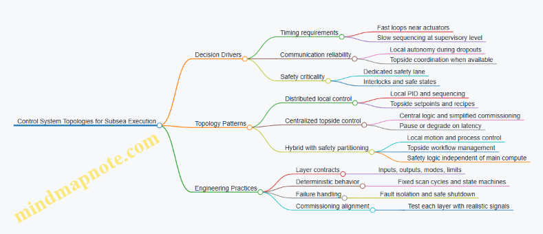
Subsea factories need control topologies that survive long cables, intermittent communications, and harsh environments. The topology you choose determines where decisions are made, how safety is enforced, and how quickly the system can recover when something goes wrong.
Foundational Concepts for Choosing a Topology
Start with three questions. First, what must keep running even if communications drop? Second, what actions are safety-critical and must not depend on remote commands? Third, what timing requirements exist for control loops, such as pressure regulation or valve sequencing?
A practical rule: push fast, deterministic control close to the actuators, and keep slower coordination higher in the system. In subsea hardware, “close” usually means the local controller inside the subsea module or the nearest topside controller with direct I/O.
Common Subsea Control Topologies
Distributed Local Control with Topside Coordination
In this topology, each processing module has a local controller that drives its valves, pumps, and sensors. Topside provides setpoints, recipes, and supervisory sequencing.
Example: A filtration skid maintains differential pressure using local PID loops. Topside sends a target pressure band when a batch starts. If telemetry is delayed, the skid still regulates within the band because the loop runs locally.
Best practice: define a clear contract between layers. The local controller accepts setpoints and mode commands, while it owns actuator timing, interlocks, and safe shutdown behavior.
Centralized Topside Control with Subsea I/O
Here, topside controllers read all sensor signals and command all actuators through subsea I/O. This can simplify commissioning because logic is centralized.
Example: A simple chemical dosing manifold uses topside logic to open valves in a timed sequence. If communications degrade, the system may pause because the controller depends on timely I/O.
Best practice: use this topology only when safety and control timing can tolerate communication latency. For anything that must react within seconds, local control is usually the safer choice.
Hybrid Control with Safety Partitioning
Hybrid topologies combine local control for fast loops with topside coordination for workflow. Safety functions are partitioned so they do not rely on the same compute path as normal control.
Example: A robotic handling cell executes motion steps locally, while topside coordinates which cell gets which part. Safety interlocks such as emergency stop and hard limits are implemented in dedicated safety logic that directly monitors sensors and commands safe states.
Best practice: treat safety as a separate “lane.” Even if the main controller resets, safety logic should remain capable of forcing a safe condition.
Mind Map for Control Topology Decisions
Systematic Design Flow from Requirements to Implementation
- Classify functions by time and safety. Pressure regulation and valve timing are typically fast; batch sequencing and reporting are slower. Safety interlocks are always fast and independent.
- Assign ownership by layer. Local controllers own actuator commands and loop execution. Topside owns recipe selection, batch orchestration, and operator interaction.
- Define modes and transitions. Use explicit modes such as Manual, Automatic, Hold, and Safe. Transitions should be deterministic and logged.
- Specify fault reactions. For each fault, define whether the system holds, retries, isolates, or shuts down. A common pattern is: hold process outputs to the last safe state, then isolate the failing module.
- Validate with realistic signal paths. Test with representative sensor dynamics and actuator response times, not idealized step changes.
Example: Valve Sequencing in a Hybrid Topology
Consider a subsea reactor feed valve that must open only when two conditions are true: upstream pressure is within range and a downstream temperature sensor indicates readiness.
- Local controller runs the sequencing state machine.
- It reads both conditions locally and enforces interlocks before commanding the valve.
- Topside provides the “batch start” command and the target pressure band.
If temperature telemetry is delayed, the local controller does not guess. It either waits in a Hold state or transitions to Safe based on a timeout rule you define during design.
Example: Local Autonomy During Communication Loss
A module that performs mixing can continue its mixing cycle without topside updates. The local controller uses a stored recipe with time-based steps and sensor-based stop conditions.
Best practice: store only what is needed for safe completion, and require topside confirmation for actions that change the process envelope, such as switching to a different chemical recipe.
Summary of Topology Tradeoffs
Distributed local control improves responsiveness and resilience. Centralized topside control can be simpler but often struggles with latency and autonomy. Hybrid topologies are common because they let you keep fast control and safety near the hardware while still coordinating the overall factory workflow from topside.
3.2 Deterministic Sequencing for Manufacturing and Processing Steps
Deterministic sequencing means the subsea factory follows the same step order every time, with explicit rules for when to advance, pause, retry, or stop. Underwater, you cannot rely on “operator intuition” to fix timing problems, so the sequence must be both predictable and inspectable. A good starting point is to treat each manufacturing or processing step as a state transition with clear entry conditions, actions, and exit conditions.
Step Modeling with States and Guards
Model the workflow as a finite set of states: Idle, Ready, Execute, Verify, Transfer, Hold, Recover, and Stop. Each transition is guarded by measurable conditions. For example, a “Mix” step should not begin just because the recipe says so; it should begin only when pressure, temperature, and valve positions match the step’s requirements.
A practical guard set for subsea work includes:
- Resource availability: required utility pressure and flow present.
- Equipment readiness: actuator homed, tool latched, pump primed.
- Process readiness: sensors stable for a minimum dwell time.
- Safety permissives: interlocks satisfied and no active fault that blocks the step.
Example: A “Filtration” step advances from Execute to Verify only after differential pressure reaches a target band and remains within tolerance for a defined window. That window prevents the system from accepting transient spikes caused by initial flow settling.
Sequencing Patterns That Prevent Surprises
Use a small set of sequencing patterns repeatedly so engineers can reason about behavior quickly.
- Precondition then Execute: verify prerequisites first, then run the action.
- Execute then Verify: run the step, then confirm output quality or physical completion.
- Timeout with Defined Recovery: every step has a maximum duration and a recovery path.
- Idempotent Retries: a retry must not corrupt the process state. If it can, add a “Reset” sub-step.
Example: For a “Valve Swap” operation, a retry should not simply re-command the same motion. Instead, the sequence should include a “Confirm Position” verification and, if mismatched, a “Re-home Actuator” action before retrying.
Recipe Structure with Explicit Advancement Rules
A deterministic recipe is more than a list of steps; it is a table of rules. For each step, define:
- Inputs: required fluids, utilities, and tool configuration.
- Parameters: setpoints and allowable ranges.
- Duration policy: fixed time or event-driven completion.
- Verification criteria: what must be true to advance.
- Failure handling: what to do on timeout, sensor disagreement, or safety block.
Event-driven completion is often better than fixed time for subsea processes because it adapts to actual conditions. For instance, “Heat to Temperature” should complete when temperature crosses the threshold and stays there for a dwell period, not when a stopwatch ends.
Handling Sensor Disagreement Deterministically
Sensors rarely fail gracefully. Deterministic sequencing treats disagreement as a first-class condition. Define a rule such as: if two temperature sensors differ by more than X for Y seconds, the step transitions to Recover and selects a safe fallback strategy.
Example: During “Chemical Conditioning,” if conductivity and temperature disagree, the system can pause mixing, hold valves in a safe configuration, and request a controlled purge before resuming. The key is that the behavior is specified, not improvised.
Mind Map: Deterministic Sequencing Elements
Mind Map: Example Sequence for a Processing Batch

Diagram: State Transition View for One Step
stateDiagram-v2
  [*] --> Idle
  Idle --> Ready: Preconditions met
  Ready --> Execute: Safety permissive true
  Execute --> Verify: Action complete or event reached
  Verify --> Transfer: Verification criteria satisfied
  Verify --> Recover: Timeout or sensor disagreement
  Recover --> Ready: Recovery successful
  Recover --> Stop: Safety block persists
  Transfer --> Idle: Batch step complete
Concrete Example: “Heat to Temperature” Step Specification
A deterministic “Heat to Temperature” step can be written as: enter Execute only when heater interlock is satisfied and cooling loop flow is within range. During Execute, sample temperature at a fixed interval and compute a moving average. Transition to Verify when the moving average crosses the setpoint minus tolerance. Transition to Transfer only after the temperature remains within the target band for the dwell time. If the moving average fails to reach the threshold before timeout, transition to Recover and perform a controlled cooling-and-retry sequence that first checks for heater power delivery and sensor plausibility.
This approach keeps the system’s behavior consistent across batches, while still responding to real conditions. It also makes troubleshooting straightforward: when something goes wrong, you can point to the exact guard or verification that failed, rather than guessing what the system “probably meant.”
3.3 Safety Instrumented Functions and Interlock Design
Safety Instrumented Functions, or SIFs, are the parts of the control system that take a process to a safer state when specific conditions occur. In a subsea factory, “safer” usually means stopping energy input, isolating hazardous media, and preventing uncontrolled motion—while keeping the system predictable enough that recovery is possible.
Foundational Concepts for SIFs
A SIF is defined by three elements: a safety function, a set of safety inputs, and the required safety output action. For example, a “High-Pressure Overfill Protection” function might require that when tank level exceeds a threshold and pressure rises above a limit, the system closes an inlet valve and stops the transfer pump.
Interlocks are the practical mechanism that enforces safe sequencing. A SIF reacts to abnormal conditions; interlocks prevent unsafe actions during normal operation. In subsea work, both are needed because remote operation can’t rely on a human noticing a subtle mismatch in time.
A good starting practice is to write each SIF as a short sentence with measurable triggers and explicit outputs:
- Trigger: what exact signals indicate the unsafe condition?
- Action: what exact actuators move, and to what state?
- End state: what does “safe” look like after the action?
Designing SIF Inputs and Signal Quality
Safety inputs must be chosen for both relevance and reliability. If a trigger depends on a sensor that can drift or get fouled, the SIF becomes a “sometimes works” system, which is the opposite of what you want.
Use diverse sensing where it matters. For a pressure-related SIF, combine a pressure transmitter with a second independent measurement path such as a different transmitter location or a separate pressure sensing element. Where diversity isn’t practical, improve robustness with diagnostics: plausibility checks, stuck-signal detection, and range monitoring.
Signal conditioning should be deterministic. Filtering is fine, but it must be bounded and documented so the SIF response time is known. A common subsea pitfall is over-filtering a signal and accidentally delaying the safety action beyond the process’s tolerance.
Interlock Logic for Safe Sequencing
Interlocks should be organized by intent: start permissives, motion permissives, and release conditions. For instance, a robotic handling interlock might require:
- Start permissive: tool changer latch status is “locked”
- Motion permissive: gripper pressure is within range and camera-based alignment confidence is above threshold
- Release condition: only allow tool exchange when the gripper is stationary and the latch is confirmed unlocked
Keep interlock logic simple enough to test. If the logic becomes a maze, the test plan becomes a maze too, and nobody enjoys that.
A practical rule: interlocks should fail safe. If a required status signal is lost, the system should default to preventing the unsafe action rather than guessing.
Safety Output Actions and State Definitions
Outputs must be defined as states, not intentions. “Stop the pump” is ambiguous if the pump can coast, so specify the actuator command and the expected physical outcome.
Typical subsea SIF output actions include:
- De-energize a motor starter or close a normally closed valve
- Command an emergency shutdown sequence that includes venting or depressurization
- Block motion by removing drive enable signals to actuators
For valves, define whether the safe state is “fail closed” or “fail open,” and ensure the actuator design matches the safety case. For example, a chemical injection line might be safer when isolated by closing valves, while a pressure relief function might require opening a relief path.
Managing SIF Reset, Proof Testing, and Bypass
Reset rules prevent accidental re-entry into a hazardous condition. After a SIF trip, require that:
- The unsafe condition is cleared
- The system is in a known safe configuration
- Operators can confirm the reset permissive states
Bypass is sometimes necessary for commissioning or maintenance, but it must be controlled. A bypass should be explicit, time-limited where possible, and logged with the reason and the affected safety function.
Proof testing verifies that the safety function still works. Design for testability by including test modes, partial stroke tests for valves, and diagnostic checks for sensors. For example, a valve SIF can be validated by commanding a short, controlled movement during a maintenance window, then verifying position feedback.
Mind Map: SIF and Interlock Design
Example: Overpressure Protection SIF with Interlocks
Consider a subsea processing module with a transfer pump feeding a reaction vessel.
SIF: Overpressure Protection
- Trigger: vessel pressure > P_high for longer than T_high and pump discharge flow > F_min
- Action: stop pump and close inlet valve to isolate the vessel
- End state: vessel pressure allowed to stabilize while preventing further inflow
Interlocks: Transfer Start Permissives
- Inlet valve must be confirmed “open” before pump start
- Pressure sensor must be healthy and within calibration diagnostics
- Vessel level must be within an acceptable range to avoid overfill
Interlocks: Transfer Stop Release
- If the pump is commanded to stop, allow only a controlled depressurization sequence before any valve reconfiguration
This combination works because the interlocks prevent the unsafe setup, while the SIF handles the case where the setup still goes wrong due to a fault or an unexpected operating condition.
Example: Robotic Tool Exchange Interlocks
For a tool exchange operation, define interlocks that prevent motion during uncertain alignment.
- Start permissive: tool carriage is docked and latch status is “locked”
- Motion permissive: gripper pressure is within range and alignment confidence is above threshold
- Release condition: only unlock the latch when the gripper is stationary and holding the tool
If any required status signal is lost, the system blocks motion and keeps the latch state unchanged. That way, the robot doesn’t “continue anyway,” which is a surprisingly common failure mode when logic is written for convenience rather than safety.
3.4 Fault Detection Isolation and Recovery for Subsea Operations
Fault detection isolation and recovery (FDIR) is the part of a subsea factory that keeps production from turning into a long, expensive scavenger hunt. The goal is simple: detect an abnormal condition early, isolate the affected function so it can’t corrupt other steps, and recover in a controlled way that preserves safety and product quality.
Foundational Concepts for Subsea FDIR
Start with three layers of intent. First, detection: decide what “abnormal” means using thresholds, rate-of-change checks, and consistency rules across sensors. Second, isolation: prevent propagation by shutting valves, freezing actuators, or switching to a safe mode. Third, recovery: return to a known-good state using a defined sequence, not operator improvisation.
A subsea environment adds constraints that shape the design. Sensors can drift, communication can be delayed, and physical access is slow. So FDIR must rely on local measurements and local logic, with telemetry used for confirmation and recordkeeping.
Detection Strategy That Avoids False Alarms
Good detection is mostly about reducing ambiguity. Use a layered approach:
- Primary limits: hard bounds for pressure, temperature, motor current, flow rate, and valve position.
- Dynamic checks: detect stuck actuators by comparing commanded position to measured position over time.
- Cross-sensor consistency: for example, if pump speed increases but flow stays flat, treat it as a likely blockage or cavitation condition.
- State-aware thresholds: the same pressure might be normal during startup but abnormal during steady processing.
Example: During a filtration step, the system commands a pump ramp. If differential pressure rises faster than expected while flow remains below the minimum, the detection logic flags “filter loading” rather than “pump failure.” That distinction matters because isolation actions differ.
Isolation Logic That Prevents Cascading Failures
Isolation should be deterministic and minimal. Define isolation boundaries by function, not by hardware. A “processing train” might include pumps, valves, heaters, and sensors; isolating the train means stopping its inputs and preventing backflow.
Common isolation actions include:
- Close upstream valves to stop the supply of process fluid.
- Vent or drain to reduce pressure hazards and protect equipment.
- Freeze downstream actuators to avoid moving parts into unsafe positions.
- Switch to bypass paths when available, so other non-affected steps can continue.
Example: If a heater temperature sensor disagrees with the control loop, isolation might stop heating while allowing circulation to continue. That avoids overheating while still keeping the fluid moving to prevent settling.
Recovery Sequencing That Uses Known-Good States
Recovery is not “try again.” It is a sequence that returns the system to a defined state with explicit exit criteria.
A practical recovery pattern:
- Enter safe mode: halt the affected action, maintain safe pressures, and keep monitoring.
- Confirm the fault: require the abnormal condition to persist for a short validation window.
- Perform a corrective action: clear a blockage by reversing flow briefly, reset an actuator, or reinitialize a control loop.
- Re-test: run a short, low-risk test segment and verify key measurements.
- Resume: continue the processing step only if quality-relevant metrics are within limits.
Example: For a stuck valve, recovery might command a small oscillation pattern within mechanical limits, then verify position feedback. If feedback still fails, the system transitions to “manual intervention required” rather than repeatedly stressing the actuator.
Mind Map: Subsea FDIR Flow
Example: End-to-End FDIR for a Processing Step
Consider an autonomous batch where a chemical conditioning module mixes reagents, then holds temperature for a fixed time.
- Detection: During mixing, the system expects a rise in conductivity and a stable motor current. If conductivity fails to change while motor current increases, detection flags “mixing ineffective” rather than “no flow.”
- Isolation: The module stops mixing, closes reagent inlet valves, and keeps circulation running to prevent stratification.
- Recovery: The system performs a short agitation reversal, then re-runs a low-risk mixing test for a brief interval. If conductivity response returns and motor current normalizes, it resumes the hold step. If not, it marks the batch as nonconforming and prevents downstream processing from using the conditioned fluid.
This approach keeps the system honest: it distinguishes between symptoms, isolates the right function, and only resumes when measurements indicate the process is back on track.
Verification That FDIR Works When It Matters
FDIR logic should be validated with scenarios that mirror real subsea behavior: sensor drift, intermittent communication, and partial actuator response. Use recorded test logs to confirm that each fault leads to the intended isolation action and that recovery never bypasses safety checks.
A good sanity check is to ask: if the fault happens at the worst moment in the step, does the system still reach a safe state and produce an auditable record of what it did? If the answer is yes, the FDIR design is doing its job.
3.5 Verification and Validation of Control Logic With Test Records
Subsea control logic has two jobs: produce correct actions and do so safely when sensors lie, valves stick, or communications hiccup. Verification answers “did we build the logic right?” while validation answers “did we build the right logic for the job?” The trick is to treat both as evidence-producing activities, not as one-time checkboxes.
Foundational Concepts for Evidence
Start by writing control logic requirements in testable terms. A requirement like “maintain pressure” becomes measurable: target band, allowable deviation, response time, and acceptable oscillation. Then define the control outputs that must be exercised: valve commands, pump start/stop, interlock states, and shutdown triggers.
Next, define the test record structure before running tests. A good record ties together: configuration (software version, parameter set), stimulus (inputs and timing), expected behavior (pass criteria), and observed behavior (logged signals). If you cannot reproduce the run from the record, the record is not evidence.
Verification Strategy from Unit to System
Verification proceeds in layers so failures are easier to localize.
Unit-Level Verification
Unit tests focus on pure logic: state machine transitions, limit checks, and interlock evaluation. Use deterministic inputs and verify outputs at each step. For example, if a pressure sensor reading crosses a high limit, the logic should set the correct alarm flag and command the correct valve state within a specified time.
Integration-Level Verification
Integration tests combine modules: control loops with actuator models, interlocks with command arbitration, and sequencing with timing constraints. Here, you verify signal mapping and timing alignment. A common failure is correct logic paired with wrong scaling or swapped channels, which unit tests won’t catch.
System-Level Verification
System tests run the full control application with realistic I/O interfaces and fault injection. Validate that the system behaves correctly under combinations: low power, degraded sensor, and a stuck actuator. The goal is to confirm that the logic’s safety paths override normal operation.
Validation Strategy Using Operational Scenarios
Validation uses scenarios that represent how the factory is actually operated. Build scenarios from operating procedures: start-up, steady processing, batch changeover, and controlled shutdown.
A practical approach is to define scenario “contracts.” Each contract lists: initial conditions, sequence of operator or autonomous commands, expected state progression, and acceptance criteria for outputs and alarms. For example, during start-up the logic should not allow processing commands until prerequisites are satisfied: utilities within range, interlocks cleared, and communication health verified.
Test Records That Make Results Reproducible
A test record should read like a recipe with a timestamped log. Include:
- Identity: test ID, requirement IDs covered, software build, and parameter set.
- Configuration: hardware revision, simulated vs. real I/O, and any calibration constants.
- Stimulus: input values, timing, and injected faults.
- Expected Results: pass/fail criteria for each monitored signal.
- Observed Results: recorded traces, event logs, and any deviations.
- Disposition: pass, fail, or inconclusive with a clear reason.
When a test fails, the record should help you answer three questions quickly: what changed, where the logic diverged, and whether the failure is safety-relevant.
Example Mind Map for Coverage and Evidence
Mind Map: Verification and Validation Evidence Flow
Example Test Case with Clear Pass Criteria
Consider a sequencing rule: “When processing temperature exceeds the upper limit, pause the feed and keep agitation running until temperature returns within the safe band.”
- Stimulus: apply a temperature ramp that crosses the upper limit at t=120 s, then returns within band at t=190 s.
- Expected Results:
- At t=120 s ± 2 s: feed command transitions to paused.
- Agitation remains commanded ON throughout the pause window.
- At t=190 s ± 2 s: feed command resumes only if interlocks remain clear.
- Alarm flag sets at the same time as the pause command.
- Observed Results: compare logged feed command, agitation command, alarm flag, and temperature trace.
- Disposition: pass if all timing and state conditions meet criteria; otherwise fail with a note identifying the first violated condition.
Practical Checklist for Test Records
Before closing a test, confirm that another engineer could rerun it using only the record. If the record lacks software build identity, parameter values, or stimulus timing, it will be hard to reproduce the outcome. Also ensure that each test record maps back to the requirements it covers, so coverage is measurable rather than hopeful.
A final sanity step is to review the event timeline: control actions should align with sensor changes and interlock states in a way that matches the intended sequence. If the timeline looks “almost right,” it usually isn’t—subsea systems punish small timing mismatches.
Use a consistent date format in records, such as 2026-03-25, to keep audit trails readable and searchable.
4. Power Systems and Energy Distribution for Subsea Operations
4.1 Power Source Selection and Electrical System Sizing
Subsea factories live under constraints that make “just add more power” a bad plan: long cable runs, limited space, harsh environments, and the need to keep critical functions alive during disturbances. Power source selection and electrical system sizing are therefore one integrated decision, not two separate checklists.
Foundational Requirements That Drive the Choice
Start by defining what must run, when it must run, and what happens when power is interrupted.
- Load inventory: Break loads into categories—process equipment (pumps, heaters, mixers), automation (controllers, drives, valves), sensing (instrumentation and metrology), and safety (shutdown valves, emergency actuation, safety PLC I/O). For each load, record rated power, duty cycle, start-up behavior, and acceptable voltage or frequency tolerance.
- Operational modes: At minimum, define normal production, controlled shutdown, and safe state. A heater that is allowed to stop during a fault is sized differently than a valve actuator that must complete a stroke.
- Power quality needs: Some loads tolerate dips; others require tight regulation. Drives and converters often dominate the power quality discussion because they draw non-sinusoidal currents and can create harmonics.
- Environmental and installation constraints: Cable ampacity, insulation temperature rise, and allowable voltage drop are physical limits. If the cable is long, voltage drop can force you toward higher distribution voltage or local conversion.
A practical rule: if you can’t explain the load behavior during start-up and shutdown in plain language, you can’t size the system reliably.
Power Source Options and How to Select Among Them
Common subsea power sources include shore power delivered through umbilicals, subsea generation (diesel or gas turbines are typical in other offshore contexts but are harder subsea), and hybrid approaches with energy storage.
Shore Power Through Umbilicals
Shore power is usually the baseline because it avoids maintaining rotating machinery underwater. Selection hinges on distribution voltage and losses.
- Higher voltage distribution reduces current for the same real power, which reduces I²R losses and cable heating.
- Local conversion near the subsea equipment can provide the lower voltages needed by drives and electronics.
Subsea Energy Storage for Ride Through
Energy storage is not a replacement for the main source; it’s a bridge.
- Use it to cover short disturbances so safety actions can complete.
- Size it based on the energy required for the longest “must-act” interval, not on the average load.
Hybrid Selection Logic
Choose shore power for steady production, add local conversion for usable voltages, and include storage only where it materially improves safe-state completion or reduces nuisance trips.
Electrical System Sizing Method That Avoids Surprises
Sizing should follow a sequence that respects both steady-state and transient behavior.
Step 1: Compute Real Power and Apparent Power
- Real power (P) comes from motor mechanical output, heater resistive power, and converter losses.
- Apparent power (S) depends on power factor and converter behavior.
For motors, include starting current and acceleration time. For drives, include harmonic effects when selecting transformers, switchgear, and cable ratings.
Step 2: Apply Demand and Diversity
Not every load runs at full power simultaneously. Use operational schedules to compute a realistic maximum demand.
Example: If two pumps each draw 30 kW but only one runs at a time during normal processing, the maximum demand is closer to 30 kW plus the smaller auxiliary loads, not 60 kW.
Step 3: Size Conductors for Thermal Limits
Cable ampacity must satisfy steady current and transient heating.
- Use allowable temperature rise and insulation limits.
- Include derating for burial, grouping, and ambient seawater temperature.
If the cable is already near thermal limits, increasing voltage or moving conversion closer to the load can be more effective than simply increasing conductor cross-section.
Step 4: Check Voltage Drop Under Worst-Case Conditions
Voltage drop affects torque margin for motors and regulation for converters.
- Evaluate at maximum demand and during start-up where applicable.
- Ensure the minimum voltage at the equipment terminals stays within tolerance.
Step 5: Select Protection and Coordination
Protection must clear faults without causing unnecessary shutdowns.
- Coordinate fuses, breakers, and protective relays with cable withstand and downstream equipment limits.
- For drives, ensure that protective settings account for inrush and ride-through behavior.
A good coordination test is simple: can you describe which protective device trips for a cable-to-ground fault at the far end, and what the subsea equipment does immediately after?
Worked Example for Integrated Sizing
Assume a subsea processing skid with:
- One 30 kW pump motor (typical duty)
- One 15 kW mixing motor
- Instrumentation and controls at 2 kW
- A heater at 10 kW that runs intermittently
- Drive-based actuation and valves totaling 3 kW average
- Maximum demand: heater on during peak, pumps and mixer running → P ≈ 30 + 15 + 10 + 2 + 3 = 60 kW real power.
- Demand diversity: if heater and mixer never overlap in some modes, peak could drop to 45 kW; keep the sizing tied to the defined operational mode.
- Starting behavior: motor starting current can be several times rated current. Protection and cable thermal checks must include this transient.
- Voltage drop and conversion: if the umbilical run is long, distribute at a higher voltage and convert locally to the motor drive DC link or required AC levels.
The key outcome is not the exact voltage number; it’s that the sizing process ties voltage selection to cable heating, voltage drop, and transient protection behavior.
Mind Map: Power Source Selection and Electrical System Sizing
4.2 High Voltage Distribution and Protection Coordination
High-voltage distribution in a subsea factory is less about “getting power there” and more about ensuring that faults are detected, isolated, and contained without turning the rest of the system into a fuse. Coordination means the protection devices on each side of a boundary agree on what counts as a fault, how fast it must be cleared, and what happens to the remaining loads.
Foundational Concepts for Coordination
Start with the power path. A typical subsea chain is: incoming supply → subsea switchgear → distribution feeders → load transformers or converters → motor drives, heaters, and auxiliary systems. Each boundary should have a defined protection role.
Next, define fault types and locations. For coordination work, treat faults as categories: phase-to-phase, phase-to-ground, three-phase, and arcing faults. Then map likely fault locations: cable terminations, switchgear compartments, busbars, and load interfaces. This mapping drives both device selection and settings.
Finally, establish the coordination objective. In practice, the objective is selective clearing: the closest upstream device to the fault clears first, while downstream devices remain closed. If selectivity is impossible for some fault modes, the objective shifts to safe de-energization of the smallest practical area.
Protection Roles Across the Distribution Chain
A clean way to coordinate is to assign roles by layer.
- Main protection clears faults on the incoming side and limits the maximum fault energy seen by the rest of the factory.
- Feeder protection isolates a specific branch so other feeders keep running.
- Load-side protection protects transformers, drives, and capacitors from internal faults and abnormal currents.
- Backup protection provides clearance if the primary device fails.
A simple example: a feeder short at a motor drive output should trip the feeder breaker or feeder fuse first. The main breaker should only trip if the feeder device fails to operate within its backup time window.
Setting Philosophy and Time-Current Coordination
Protection coordination is built on time-current curves. The key is to ensure that for every fault current level, the primary device operates before the backup device.
Use three practical checks:
- Normal load and starting currents must not cause nuisance trips. Motor starting can create high currents for seconds, so feeder settings must account for inrush and acceleration behavior.
- Cable and component thermal limits must not be exceeded during fault clearing. Even if selectivity is achieved, the fault duration must keep conductor temperature rise within limits.
- Arc and transient behavior must be handled. Subsea faults can involve arcing at terminations, so protection that relies only on steady-state current may be too slow or too insensitive.
A concrete coordination example: suppose a feeder has an overcurrent relay with instantaneous pickup for high fault currents and a time-delayed element for lower faults. The main protection uses a slower time curve. For a phase-to-ground fault at the feeder end, the feeder’s instantaneous element clears quickly; for a weaker fault, the time-delayed element clears within the main device’s backup window.
Voltage Level, Insulation, and Protection Interaction
High-voltage distribution choices affect protection behavior through insulation strength and fault impedance. Higher system voltage typically increases insulation requirements and changes how faults develop. In subsea environments, moisture ingress and contamination at terminations can create partial discharges that evolve into more severe faults.
Coordination must therefore consider not just current magnitude, but also fault signatures. Where available, incorporate protection functions that respond to ground faults, negative-sequence currents, and sensitive earth fault conditions. These functions reduce the chance that a “small” fault grows while the system waits for a large overcurrent.
Coordination of Switching Devices and Current-Limiting Elements
Switchgear selection matters because it determines the clearing mechanism. Circuit breakers clear by opening contacts; fuses clear by melting and current interruption. Current-limiting fuses can reduce peak fault current and energy delivered to downstream equipment.
A typical coordination pattern is: fuse on a branch for fast energy limitation, breaker upstream for isolation and system restoration. The fuse clears first for most faults; the breaker provides backup and isolates the branch if the fuse does not clear.
When coordinating breakers and fuses, verify that the breaker’s interrupting rating and the downstream equipment’s withstand rating are not exceeded for the worst-case fault energy.
Subsea-Specific Constraints That Affect Settings
Subsea systems introduce constraints that are easy to overlook:
- Long cable runs increase capacitance and affect transient currents, which can influence ground-fault detection.
- Temperature effects change conductor resistance, shifting current levels for the same fault impedance.
- Remote operation means you want fewer trips that require intervention, but you also need robust isolation when a fault occurs.
A practical approach is to use as-built cable parameters and measured insulation characteristics during commissioning, then confirm that protection pickup thresholds remain valid across expected operating temperatures.
Mind Map: High Voltage Protection Coordination
Example: Coordinated Clearing for a Feeder Ground Fault
Assume a feeder supplies a transformer feeding a motor drive. A phase-to-ground fault occurs near the feeder end.
- The feeder’s ground-fault function detects the signature and trips the feeder breaker quickly.
- The main breaker remains closed because its backup time window is longer.
- The transformer and drive see a reduced fault duration, limiting thermal stress.
- After isolation, the control system logs the event with the feeder identifier so restoration targets only the affected branch.
This example works because coordination is not just “fast”; it is fast in the right place, with the right signature, and with upstream devices held back long enough to preserve selectivity.
Example: Coordination for Motor Starting Without Nuisance Trips
During normal operation, the motor drive draws high current during acceleration. Feeder overcurrent protection must tolerate this without tripping.
A practical method is to set the time-delayed pickup above the expected starting current envelope, then use an instantaneous element for high-magnitude faults. If a fault occurs, the current rises beyond the instantaneous threshold and clears immediately. If the motor is merely starting, the current stays within the tolerated region and the time-delayed element does not trip.
The result is a protection scheme that behaves differently for “normal stress” versus “abnormal failure,” which is exactly what coordination is meant to achieve.
4.3 Local Power Conversion and Conditioning for Loads
Local power conversion and conditioning turns the factory’s distributed energy into the right electrical “diet” for each subsea load. The key idea is simple: keep the long-distance distribution robust, then do the careful work near the equipment that actually needs it.
Foundational Requirements for Subsea Loads
Start by listing each load’s electrical needs: voltage level, current profile, allowable ripple, start-up surge limits, and grounding expectations. A pump motor might tolerate brief dips, while a control electronics supply may require tight regulation and low noise. Next, define the operating envelope: ambient temperature range, expected water ingress risk, and the maximum voltage variation at the load terminals during faults elsewhere in the system. This prevents the common mistake of designing a converter that meets nominal conditions but fails during real subsea disturbances.
Conversion Topologies and Where They Fit
Local conversion usually falls into three patterns.
AC to DC for electronics and drives. If the distribution is AC, rectification and filtering produce DC rails. For sensitive electronics, add regulation stages and noise filtering. For motor drives, the DC link must handle current ripple without overheating.
DC to DC for distributed control and sensors. If the distribution is already DC, step-down converters create multiple rails (for example 24 V for solenoids and 12 V or 5 V for logic). Choose converter types based on load transients: a buck converter with adequate control loop bandwidth prevents overshoot when a valve coil energizes.
Inversion for AC loads. Some loads require AC at a specific frequency. Use an inverter stage sized for continuous power and starting surges, then condition the output with filtering to keep motor and transformer losses predictable.
Conditioning for Stability, Noise, and Ride-Through
Conditioning is not just “smoothing.” It is about ensuring the load sees stable voltage and current under disturbances.
Input filtering and surge handling. Place EMI/EMC filters and transient suppression close to the converter input. In subsea systems, cable inductance and switching events can create spikes that propagate if not contained.
Regulation and control loop behavior. A converter’s control loop must remain stable across load changes and temperature. Practical best practice is to specify worst-case component tolerances and verify loop margins with the actual output capacitor and wiring inductance.
Output filtering for ripple and noise. Use output capacitors and, when needed, LC or RC filters to meet ripple requirements. For example, a metrology sensor supply may need low-frequency stability to avoid measurement drift during pump starts.
Energy storage for short interruptions. Add local bulk capacitance or a small ride-through module so brief upstream dips do not reset controllers. Size it from the load’s hold-up energy: energy equals average power times required hold-up duration, adjusted for converter efficiency.
Protection and Selectivity at the Local Level
Local conditioning must fail safely and predictably.
Current limiting and fusing. Use fuses or electronic current limiting sized to protect wiring and converter semiconductors without nuisance trips. Selectivity matters: a downstream fault should not force an upstream shutdown.
Isolation and grounding strategy. Decide whether the load is galvanically isolated from the distribution. Isolation can reduce ground loop currents and improve noise immunity, but it adds leakage considerations and insulation monitoring requirements.
Thermal protection. Include temperature sensing on power stages and enforce derating rules. Subsea cooling can be limited by fouling and flow conditions, so thermal margins should be conservative.
Example: Designing a 24 V Control Rail for Valve Actuation
Assume a subsea control rail must power valve coils and nearby sensors. The distribution provides 400 V DC.
- Conversion: Use a DC-to-DC buck stage to generate 24 V. Select a converter rated for the coil’s peak current, not just its average.
- Input conditioning: Add a transient suppressor and input filter to handle switching spikes from other loads.
- Output conditioning: Provide bulk capacitance for coil energization and a smaller low-noise stage for sensor power. This prevents coil current steps from injecting ripple into measurement circuits.
- Protection: Add a fast-acting fuse upstream of the converter and a current limit inside the converter to protect against short circuits.
- Hold-up: Compute hold-up energy for the controller so it does not reset during brief upstream dips. If the controller must remain alive for 50 ms at 10 W, the required stored energy is about 0.5 J, then divided by efficiency to size capacitors.
Mind Map: Local Conversion and Conditioning Flow
Practical Integration Checks
Before finalizing the design, verify that the converter’s output remains within limits during the load’s worst-case sequence: for instance, a valve energizes while a pump starts and the upstream distribution experiences a transient. Then confirm that protection actions are selective by simulating a downstream short and observing which upstream elements remain energized. If the local rail can ride through brief disturbances without resetting control electronics, you have achieved the real goal: stable power where it matters, without making the whole factory pay for one problem.
4.4 Energy Storage Integration for Ride Through and Shutdown
Energy storage in a subsea factory is less about “having extra power” and more about buying time. That time is used to finish safe sequences, keep critical sensors alive, and move actuators to known positions before the main power collapses. The integration goal is simple: when power dips or disappears, the system must transition predictably, not randomly.
Foundational Requirements for Ride Through
Start by defining what “ride through” means in your context. A practical requirement set includes: minimum energy to cover the longest critical action, maximum allowable voltage or frequency deviation for control electronics, and the time budget for orderly shutdown. For example, if a processing module needs 90 seconds to purge lines and park valves, the storage system must supply control power, communication links, and valve actuation power for that 90-second window.
Next, identify the load classes. Control and safety electronics are usually continuous loads; pumps, heaters, and robotic drives are burst loads. A good design separates these so the storage sizing is not inflated by short, high-power events that can be deferred until after the main power returns.
Storage Technology Selection and Fit
Common subsea storage options include batteries and supercapacitors, sometimes combined. Batteries provide higher energy density for longer ride-through durations. Supercapacitors provide high power for short bursts, such as valve strokes or brief motor inrush support.
A typical integrated approach is: supercapacitors handle the first seconds of a power interruption while power electronics ride through their own control loops, and batteries cover the remainder until shutdown completes. This reduces battery peak current stress and improves reliability.
Power Electronics and Energy Management
Energy storage rarely connects directly to the main bus. Instead, it feeds a controlled DC link or local essential bus through power conversion. The essential bus supplies safety PLCs, instrumentation, and selected actuators.
Key design practices include:
- Undervoltage detection with deterministic thresholds so the system enters the correct mode without oscillation.
- Current limiting to prevent storage from collapsing under sudden load steps.
- State-of-charge estimation using measured voltage and current, filtered to avoid false triggers.
Example: if the essential bus voltage drops below a threshold for longer than a defined debounce time, the controller switches from “process mode” to “shutdown mode,” then commands valves to their safe positions in a fixed sequence.
Ride Through Control Sequence
A ride-through sequence should be written like a checklist with timing. One effective structure is:
- Detect event: main power undervoltage or loss.
- Freeze nonessential actions: stop new process steps that would require additional energy.
- Maintain essential functions: keep sensors sampling and safety interlocks active.
- Execute safe actions: purge, depressurize, park moving equipment, and log the event.
- Confirm completion: verify valve positions and pressure targets using feedback.
Concrete example: during a loss of main power, a chemical mixing skid stops adding reagents, continues circulation for 20 seconds to prevent stratification, then isolates the mixing vessel and vents to a controlled receiver until pressure reaches a defined safe band.
Shutdown Energy Budgeting
Shutdown sizing is an accounting exercise. Build an energy budget that includes:
- essential electronics consumption over the full shutdown duration,
- actuator energy for each stroke and any holding requirements,
- communication and data logging overhead,
- losses in converters and cabling.
A useful method is to compute energy per phase: \(E = \sum (P_i \times t_i) + \text{loss margin}\). The margin covers converter inefficiency and aging effects. If your shutdown includes a valve stroke that draws 200 W for 5 seconds, that’s 1,000 J for that action, before accounting for losses.
Protection, Isolation, and Safety Integrity
Storage integration must respect safety integrity. Include isolation devices so a failed storage path cannot backfeed faults into the essential bus. Use fusing and protective relays sized for worst-case fault currents.
Also ensure that safety functions do not depend on a single measurement. For instance, shutdown mode should be triggered by both bus voltage and a power-loss signal from the upstream distribution, with logic that fails safe if either signal is invalid.
Mind Map: Energy Storage Integration for Ride Through and Shutdown
Example: Storage Sizing for a Purge and Valve Parking Task
Assume a shutdown duration of 120 seconds. Essential electronics draw 60 W continuously, and two valves each require 150 W for 4 seconds during parking. Converter losses add 10%.
Energy for electronics: 60 W × 120 s = 7,200 J. Valve energy: 2 × (150 W × 4 s) = 1,200 J. Total before losses: 8,400 J. With 10% losses: 9,240 J. If the storage system is sized with a practical margin of 25% to cover aging and temperature effects, the usable energy target becomes about 12,000 J.
This is the point where integration becomes concrete: the storage capacity is not a generic number, but a direct consequence of the shutdown checklist and its timing.
4.5 Grounding Bonding and Surge Protection for Subsea Equipment
Subsea grounding and bonding are about giving fault current a predictable path and keeping exposed metal at safe potentials. Surge protection is about limiting the voltage stress that fast transients impose on insulation, sensors, and power electronics. In practice, these goals are achieved as a system: equipotential bonding, controlled earthing, and coordinated surge devices sized for the actual wiring and environment.
Foundational Concepts for Subsea Electrical Safety
Start with what “ground” means underwater. The seawater environment is conductive, but its conductivity varies with salinity, temperature, and local flow. So you should not treat seawater as a stable reference node. Instead, you design a defined conductive network using metallic structures, armor, shields, and dedicated bonding conductors.
A useful mental model is three layers:
- Equipotential bonding ties all reachable metal together so a person touching any part sees minimal potential difference.
- Fault current return provides a low-impedance path so protective devices operate within required times.
- Surge energy control clamps fast transients so insulation and electronics survive long enough to keep operating.
Equipotential Bonding Strategy for Metallic Structures
Bonding should be continuous and mechanically robust. Use bolted or welded connections designed for corrosion resistance and for the number of expected maintenance cycles. Where you have removable modules, include bonding jumpers or sliding contacts that maintain low resistance under vibration and thermal cycling.
A practical example: if a subsea processing skid has a steel frame, instrument housings, and cable trays, you bond the frame to the main bonding network and bond each instrument housing to the same network. That way, a cable shield fault does not create a local “floating” metal island.
Bonding conductor sizing should be based on both steady-state and fault conditions. For fault current, the conductor must handle the thermal and electromagnetic effects long enough for upstream protection to clear. For steady-state, it must keep touch potentials within limits.
Earthing and Reference Management for Control and Power
Because seawater is not a stable reference, you manage reference points inside the system. Common approaches include:
- Single-point reference for sensitive measurement circuits, with bonding that prevents ground loops.
- Distributed bonding for power structures, where the priority is equipotential behavior.
A concrete example: a subsea controller measures a differential signal from two sensors. If each sensor housing is bonded through different paths with different impedances, the differential reading can shift during transients. You reduce that by bonding sensor returns to a common reference node and keeping shield termination consistent.
Surge Protection Coordination Across Power and Signal Paths
Surges arrive from multiple mechanisms: lightning-induced transients, switching events, and faults that create steep voltage gradients. Surge protection must be coordinated so that energy is absorbed in stages rather than dumped into the first device it meets.
Use a layered approach:
- Primary protection near the interface limits the largest surge energy.
- Secondary protection closer to equipment reduces residual voltage.
- Tertiary protection at the equipment input protects the final electronics.
For power circuits, surge devices are typically MOVs, gas discharge devices, or surge arresters, selected for voltage ratings and energy handling. For signal circuits, use components suited to low-voltage transients, such as transient voltage suppressors and shielded surge arresters.
A practical example: a 24 VDC sensor supply feeding a subsea transmitter. If you only protect the supply at the topside end, a fast transient can couple through the cable capacitance and stress the transmitter input before the topside device responds. Adding a local clamp at the subsea junction box reduces the peak at the transmitter pins.
Cable Shield Termination and Bonding Details
Cable shields are both protective and noisy. Termination choices affect surge performance and electromagnetic compatibility.
Best practice is to terminate shields to the bonding network in a controlled way. Use 360-degree termination where possible to reduce impedance and improve high-frequency behavior. If you must use pigtails, keep them short because inductance turns a surge into a voltage spike.
Example: a long armored cable from a subsea manifold to a sensor. If the shield is bonded at only one end, the shield can float during transients and increase common-mode voltage. Bonding at both ends through appropriate surge and bonding design reduces that risk while still managing loop currents.
Mind Map: Grounding, Bonding, and Surge Protection System
Verification and Acceptance Tests That Actually Matter
Verification should confirm both electrical performance and physical integrity. Start with continuity and resistance measurements of the bonding network, including removable interfaces. Then perform insulation withstand tests appropriate to the equipment and cable types.
For surge protection, test using representative cable lengths and termination methods, because surge behavior depends heavily on wiring inductance and capacitance. A good acceptance record includes device identification, installation torque or weld procedure, and measured bonding resistance at commissioning.
Example: Coordinated Protection for a Subsea Junction Box
Consider a junction box that distributes power and signals to multiple subsea sensors.
- The steel enclosure is bonded to the main bonding network.
- Each cable entry uses a shield termination method that maintains low impedance at high frequency.
- Power inputs include a primary surge device at the box inlet, with secondary clamping near the distribution rails.
- Signal pairs include local clamps referenced to the box bonding node, with consistent polarity and shield handling.
If a transient couples onto one cable, the surge energy is first limited at the inlet, then reduced at the rail, and finally clamped at the equipment input. Meanwhile, the enclosure stays at a controlled potential because all reachable metal shares the same equipotential bonding path.
5. Process Fluid Handling and Utility Networks
5.1 Utility Taxonomy for Water Chemicals and Gases
A subsea factory needs utilities that are predictable, measurable, and compatible with equipment materials. “Utility taxonomy” means you classify water, chemicals, and gases by function first, then by delivery form, then by control and monitoring needs. This keeps design decisions consistent from piping layout to control logic.
Utility Functions and Why They Matter
Start with what each utility must do:
- Conditioning utilities change water chemistry so downstream process steps behave consistently. Example: adjusting pH before a precipitation step.
- Cleaning utilities remove residues and biofouling from surfaces and lines. Example: flushing a transfer line after a batch.
- Reaction utilities provide reactants or catalysts. Example: supplying oxidant for controlled conversion.
- Quench and cooling utilities remove heat or stop reactions. Example: cooling a thermal module’s effluent.
- Support gases provide inerting, purging, or controlled atmospheres. Example: nitrogen purging to prevent oxygen-sensitive reactions.
- Process gases participate directly in a step. Example: carbon dioxide for pH control or gas-phase stripping.
A simple best practice is to write one sentence per utility: “This utility ensures X outcome by doing Y under Z constraints.” If you can’t, the taxonomy is missing a functional layer.
Delivery Forms and Compatibility Layers
Utilities arrive as one of a few delivery forms, each with different risks:
- Single-phase liquids (treated water, chemical solutions) are governed by concentration control and corrosion compatibility.
- Two-phase or gas-liquid mixtures require careful venting and separation. Example: sparging a liquid with gas for stripping.
- Compressed gases are governed by pressure regulation, leak detection, and moisture control.
For subsea use, compatibility is not just “will it corrode.” It includes:
- Material pairing between utility and wetted surfaces.
- Solubility and scaling behavior, such as calcium carbonate precipitation when pH and temperature shift.
- Contaminant tolerance, like how trace oxygen affects an inerting strategy.
Concrete example: if you classify “treated water” only as water, you may miss that the same line might later carry a cleaning solution with higher oxidizer content. The taxonomy should separate “process water” from “cleaning water” even if both are delivered through similar hardware.
Taxonomy Mind Map
Utility Taxonomy Mind Map
Control and Monitoring by Utility Type
Once categorized, each utility gets a control “minimum set.” A practical baseline looks like this:
- Water utilities: measure at least one chemistry indicator (commonly conductivity or pH) and one cleanliness indicator (often turbidity or filter differential pressure upstream). Example: if conductivity rises during a run, you can infer salt ingress or dosing drift.
- Chemical utilities: control dosing by concentration and verify with periodic sampling. Example: for an acid dosing line, track injection flow and confirm pH at the process inlet rather than trusting the tank concentration alone.
- Gas utilities: control pressure and dryness, then monitor oxygen or moisture where it matters. Example: for nitrogen purging, an oxygen sensor at the purge outlet confirms the purge is actually doing its job.
A key best practice is to prevent cross-mixing. Use physical separation in manifolds where feasible, and enforce procedural interlocks that block simultaneous dosing into the same header.
Example Utility Set for a Subsea Processing Train
Imagine a processing train that includes conditioning, reaction, and cleaning:
- Process water: pH-adjusted water for stable reaction conditions.
- Reactant chemical: a controlled oxidant solution for conversion.
- Support gas: nitrogen for inerting the reaction chamber headspace.
- Quench utility: neutralization solution to stop the reaction quickly.
- Cleaning water: a flushing and cleaning solution to remove residues.
The taxonomy keeps these distinct even if they share similar pumping hardware. In the control system, each utility maps to its own set of sensors, dosing limits, and allowed sequencing steps.
Integrated Design Checks
Before finalizing drawings, run three checks:
- Functional coverage: every process step has a utility mapped to it, not just “some water.”
- Compatibility coverage: each utility has a material and scaling/corrosion assumption recorded.
- Control coverage: each utility has a measurable variable that proves it is performing.
If any utility fails a check, the taxonomy is incomplete, and the system will eventually pay for it—usually in the form of unreliable batches or maintenance-heavy troubleshooting.
5.2 Piping Layout Design for Pressure Drop and Reliability
A subsea piping layout has two jobs that fight each other: keep pressure losses low enough for stable process control, and keep the system reliable enough that valves, pumps, and sensors keep doing their work after years of saltwater and vibration. Good layouts treat pressure drop as a design constraint and reliability as a layout constraint, then reconcile them with clear rules.
Foundational Principles for Pressure Drop
Pressure drop comes from friction along straight runs, local losses at fittings and valves, and elevation changes. Start by writing the governing flow equation for each line, then separate the contributors so you can see what you are paying for. A practical approach is to budget losses: allocate a maximum allowable total drop for each process function, then split it across segments based on length and expected velocity.
A simple example: if a chemical injection line must deliver at a minimum pressure at the injection point, you can compute the required upstream pressure by summing friction and local losses. If you reduce pipe diameter to save space, friction loss rises sharply with velocity, and the injection point may fall below the required pressure even though the upstream pump still runs.
Layout Rules That Reduce Losses
- Minimize unnecessary length. Route along the shortest practical path between equipment skids, manifolds, and injection points, while respecting bend radii and tool access.
- Prefer gentle transitions. Use long-radius bends and avoid sudden area changes. A short, sharp elbow can add local loss comparable to several meters of straight pipe.
- Control velocity. Choose pipe sizes so velocities stay within your process comfort zone for the fluid type. High velocity increases friction and can accelerate erosion in elbows and reducers.
- Keep fittings consistent. Standardize on a limited set of elbows, tees, and reducers so you can predict losses and avoid “mystery hardware” during installation.
Reliability-Driven Layout Decisions
Reliability is not just about corrosion rating; it is about how the layout behaves under maintenance, thermal effects, and flow transients.
- Avoid trapped volumes. Dead legs can accumulate solids, promote corrosion, and complicate purging. If a branch is intermittent, design it so it can be drained or flushed.
- Design for isolation. Place isolation valves so you can isolate a section without draining the entire train. This reduces downtime and limits the amount of work during remote intervention.
- Support and protect the pipe. Proper supports reduce fatigue from thermal cycling and dynamic loads. Over-constrained runs can create stress at flanges; under-supported runs can sag and stress equipment nozzles.
- Plan for thermal expansion. Include expansion loops or bends where needed, and ensure the layout does not force movement into instrument connections.
Integrated Design Workflow
A systematic workflow keeps the layout from becoming a “draw-first” exercise.
- Define hydraulic intent. Identify each line’s function: transfer, injection, purge, sampling, or return. Set minimum and maximum allowable pressures at key nodes.
- Create a node list. Mark equipment nozzles, manifold ports, valve stations, and instrument taps as nodes. This makes later calculations traceable.
- Build a segment model. Break the piping into segments with known lengths, diameters, and fitting counts. Assign each segment a friction factor model appropriate to the fluid and expected regime.
- Run pressure drop checks. Verify that the worst-case operating condition still meets pressure requirements at the control points.
- Apply reliability constraints. Review the same layout for dead legs, isolation coverage, support locations, and access clearances.
- Iterate with trade-offs. If pressure drop is too high, first try routing and fitting reductions before changing diameter. If reliability is weak, fix trapped volumes and isolation first, then revisit hydraulics.
Mind Map: Layout Trade-Offs
Example: Injection Line Routing and Valve Placement
Consider a subsea chemical injection line from a manifold to a reactor inlet. The process requires a minimum injection pressure to overcome backpressure and ensure mixing. You have two routing options: a direct route with two long-radius bends, or a longer route that avoids a support obstruction but adds extra fittings and a higher number of local losses.
You compute pressure drop for both. The longer route may still “fit” hydraulically at nominal flow, but it can fail under a higher-viscosity condition because friction loss scales with velocity and fluid properties. After selecting the direct route, you place an isolation valve near the manifold and another near the reactor inlet so you can service the line without disturbing the rest of the train. Finally, you ensure the branch can be purged by arranging a drain or flush connection at the low point, preventing stagnant pockets.
Case Study: Reliability Review of a Branch with a Dead Leg
A sampling branch is added to monitor a process stream. The initial layout includes a tee with a short run to a sensor, then a capped end for future expansion. During commissioning, the line shows inconsistent readings because the capped section traps small amounts of solids and intermittently releases them during flow changes.
The fix is layout-based: remove the capped dead leg, re-route the sensor takeoff so the branch can be purged, and add a small drain path to clear the lowest point. The pressure drop impact is minor compared to the reliability gain, because the corrected branch reduces both local losses from unnecessary fittings and the operational variability caused by stagnant volume.
5.3 Pumping Strategies for Subsea Circulation and Transfer
Subsea pumping is less about “moving fluid” and more about managing pressure, reliability, and control under constraints like limited access, long umbilicals, and harsh environments. A good strategy starts with the job: circulation for heat or chemical conditioning, transfer between modules, or batch filling and draining. Each job has a different tolerance for pressure swings, solids, and response time.
Foundational Concepts for Choosing a Pumping Approach
Begin by separating the hydraulic roles. Circulation typically maintains flow through a loop to control temperature, mixing, or chemical uniformity. Transfer typically pushes fluid from a source tank or manifold to a destination, often with a defined volume and a defined end condition.
Next, define the pressure landscape. Subsea systems must overcome static head, friction losses in piping, and any pressure requirements at process equipment. A practical way to reason is to treat the system as two parts: a “required pressure” curve driven by process needs and a “available pressure” curve driven by the pump and its control method. If the curves intersect poorly, you get unstable flow, cavitation risk, or chronic underperformance.
Finally, decide how the pump will be controlled. Fixed-speed pumping with throttling can work, but it wastes energy and can create unnecessary heat and wear. Variable-speed control is often cleaner because it matches flow to demand, but it requires careful electrical and control design to avoid oscillations.
Pump Placement and System Layout
Pump placement influences both performance and maintainability. Locating pumps close to the process loop reduces friction losses and improves control authority. However, proximity can increase exposure to process contaminants, so filtration and strainer design must match the pump’s tolerance.
For transfer lines, consider whether the pump should be upstream or downstream of sensitive equipment. If the destination equipment is sensitive to pressure spikes, placing the pump upstream and using controlled ramping can reduce stress. If the source is sensitive to cavitation, you may need suction-side measures like positive suction head management or careful line sizing.
Selecting Pump Types for Subsea Service
Centrifugal pumps are common for clean or moderately contaminated fluids because they provide smooth flow and are efficient over a range. For higher solids or viscous slurries, positive displacement pumps can handle variable loads better, but they may require pressure relief strategies and careful handling of compressibility.
For seawater cooling or general circulation, you often want robust materials and coatings, plus a design that tolerates biofouling and debris. For chemical dosing loops, the pump must handle compatibility and avoid dead legs that lead to concentration gradients.
A simple rule of thumb: if the fluid can tolerate shear and is mostly single-phase, centrifugal is usually simpler. If the fluid includes significant solids or needs near-constant volumetric delivery, positive displacement may be safer.
Managing Cavitation and Suction Conditions
Cavitation is the quiet failure mode that turns into noise, vibration, and eventual damage. The key is ensuring the pump inlet pressure stays above the fluid’s vapor pressure plus a safety margin across all operating points.
In subsea systems, suction pressure can drop due to elevation changes, friction losses, and transient events like valve operations. Mitigation strategies include increasing suction line diameter to reduce friction, using suction strainers with predictable pressure drop, and controlling valve opening rates so the system doesn’t “snap” into a low-pressure condition.
When the fluid is volatile or the system experiences frequent start-stop cycles, suction-side pressure control becomes part of the pumping strategy, not an afterthought.
Control Strategies for Stable Flow and Safe Transients
A stable control strategy matches pump output to system demand while limiting pressure transients. For circulation loops, flow setpoints can be tied to temperature or mixing requirements. For transfer operations, flow setpoints can be tied to volume tracking and destination pressure limits.
Use ramping on variable-speed drives to avoid sudden pressure jumps. For fixed-speed pumps, prefer controlled valve actuation over aggressive throttling, because throttling can create heat and can worsen cavitation margins if it drives suction pressure down.
Include interlocks that stop the pump when suction conditions are unsafe, when differential pressure across strainers indicates blockage, or when downstream pressure exceeds equipment limits.
Mind Map: Pumping Strategy Design
Example: Circulation Loop for Chemical Conditioning
Assume a chemical conditioning loop that must keep a target flow through a small reactor module to maintain mixing and reaction completion. The loop includes a pump, a strainer, a short run to the reactor, and a return line.
A practical approach is to set a minimum flow to avoid concentration gradients and a maximum flow to prevent excessive shear or erosion. The pump runs at variable speed to hold flow as the reactor pressure drop changes with fouling. The strainer differential pressure is monitored; when it rises beyond a threshold, the control system reduces speed to maintain suction margin and triggers a maintenance action.
Valve operations are ramped so that when the reactor isolation valve opens, the suction pressure doesn’t dip below the cavitation margin. This keeps the pump quiet and extends seal life.
Example: Transfer Operation Between Manifolds
For transferring a defined volume from a source tank to a destination manifold, the strategy often uses a flow-controlled ramp-up, a steady delivery phase, and a controlled ramp-down. The ramp-up reduces pressure spikes in the destination piping. The steady phase tracks delivered volume using flow measurement and compensates for small changes in line pressure.
During ramp-down, you avoid closing valves instantly. Instant closure can create water hammer-like pressure transients that stress fittings and can dislodge debris into strainers. A short controlled closing window keeps pressure within the equipment limits while still achieving the required end condition.
In both examples, the pumping strategy is not just pump selection. It is the combined behavior of hydraulics, control, and safety limits working together so the system performs predictably when conditions change.
5.4 Valve Selection and Actuation for Remote Operation
Remote subsea valves are less forgiving than their topside cousins: you cannot “just take a look,” and you cannot easily fix a jammed actuator with a wrench. Good selection starts with what the valve must do, then matches the actuation method to the environment, the control philosophy, and the maintenance reality.
Foundational Requirements for Remote Valve Choices
Begin by writing the valve’s job in three lines: normal function, abnormal conditions, and acceptable failure behavior. For example, a production isolation valve might normally open to allow flow, must close on loss of control power, and may fail “closed” to protect downstream equipment.
Next, translate the job into measurable requirements:
- Pressure and temperature envelope: choose a pressure class and materials that survive static pressure and any thermal swings from process fluids.
- Flow regime and throttling needs: decide whether the valve is primarily for isolation (tight shutoff) or for regulation (stable control with acceptable noise and wear).
- Leakage tolerance: specify allowable leakage rate or class, especially for valves that isolate hazardous or expensive fluids.
- Cycle frequency and duty: a valve that cycles daily needs different wear planning than one that operates only during commissioning.
A practical habit: define a “worst-case actuation” scenario. Example: if the valve must close during a power loss, confirm that the actuator can still complete the stroke within the required time using the available energy source.
Valve Types That Fit Subsea Service
Valve selection is mostly about matching flow behavior and sealing to the process.
- Ball valves work well for on-off isolation with low pressure drop when properly sized. They can be compact, but sealing performance depends on correct seat design and torque margins.
- Gate valves provide good isolation with low flow restriction, but they are typically slower and less suitable for frequent throttling.
- Globe valves are common for throttling and control because they handle pressure drop and provide predictable flow characteristics.
- Plug and control valves can manage variable flow, but they require careful attention to cavitation, noise, and trim wear.
For remote operation, also consider end-to-end accessibility. A valve that is hard to reach for inspection should be chosen only if its failure modes are acceptable and its actuation system is robust.
Actuation Methods and Their Tradeoffs
Actuation is where remote operation either becomes reliable or becomes a maintenance headache.
Hydraulic Actuation
Hydraulic actuation uses a power fluid to move the actuator. It is effective when you have a stable hydraulic supply and want strong force capability.
- Best fit: systems with centralized hydraulic power and clear routing.
- Key checks: hydraulic pressure availability, hose/umbilical routing losses, and response time under worst-case conditions.
Example: If a valve must close within 10 seconds, compute whether the hydraulic supply pressure at the actuator still exceeds the minimum required force after accounting for line losses and temperature effects.
Pneumatic Actuation
Pneumatic actuation can be used with subsea compressors or gas supplies, but compressibility affects response time and stroke repeatability.
- Best fit: applications where slower response is acceptable and the gas supply is reliable.
- Key checks: pressure stability, moisture control, and how the system behaves during gas loss.
Example: A valve that must “fail safe” on gas loss should be paired with a spring-return or accumulator arrangement that guarantees the required stroke completion.
Electric Actuation
Electric actuators are attractive when you want direct control and straightforward diagnostics, but they must be sized for torque, duty cycle, and thermal constraints.
- Best fit: where electrical power is available and you can support motor control and monitoring.
- Key checks: motor starting torque, gear efficiency, and how the system handles stalled conditions.
Example: For a high-torque ball valve, verify that the motor and gearbox can overcome maximum differential pressure plus friction, not just the nominal torque.
Fail-Safe Energy Storage
Many subsea valves use stored energy to achieve a safe state during loss of control. Common approaches include springs, accumulators, or both.
- Best fit: any valve where “no power” must still lead to a defined outcome.
- Key checks: stored energy capacity, leakage rates over time, and the time-to-stroke under low-energy conditions.
Sizing and Performance Calculations That Prevent Surprises
Valve sizing is not only about flow; it is also about actuation torque/force.
- Determine maximum differential pressure across the closed valve. This drives seating loads and friction.
- Estimate actuator output required to overcome seating force and stem friction.
- Apply margins for manufacturing tolerances, aging, and lubrication changes.
Example: If a valve’s maximum differential pressure doubles during a transient, the required closing torque may increase nonlinearly due to friction and seal behavior. Your actuator sizing should reflect the maximum credible differential, not the average operating condition.
Control, Feedback, and Remote Operability
Remote operation depends on more than moving the valve; it depends on knowing what state it is in.
- Position indication: use limit switches or position sensors that remain reliable under subsea conditions.
- Command logic: define how the control system interprets “open,” “close,” and “in transit.”
- Interlocks: prevent conflicting commands, such as opening a valve while downstream pressure indicates it should remain isolated.
A simple best practice: require the control system to confirm state change within a defined time window. If the valve does not reach the expected position, the system should flag a maintenance action rather than repeatedly commanding motion.
Mind Map: Valve Selection and Actuation for Remote Operation
Example: Selecting a Remote Isolation Valve
Assume a subsea isolation valve must close on loss of control and limit leakage to a defined class. Start with a valve type that suits isolation, such as a ball valve, then confirm the maximum differential pressure and seating load. Choose an actuator method that can deliver the required closing force within the time window using fail-safe energy storage. Finally, specify position feedback and a control timeout so the system can detect a partial stroke and stop repeated commands.
This approach keeps the selection systematic: requirements drive valve type, valve type drives actuation force needs, actuation drives energy storage and timing, and timing drives control logic and feedback requirements.
5.5 Instrumentation for Flow Pressure Temperature and Composition
Subsea process control lives or dies by measurement quality. In a factory on the seabed, the sensors must survive pressure, chemistry, vibration, and long cable runs—while still producing signals that control logic can trust. This section builds a practical measurement chain: what to measure, how to measure it reliably, how to condition the signal, and how to use it in control and diagnostics.
Foundational Measurement Goals
Start by separating three roles of instrumentation:
- Control variables drive actuators. Flow rate and pressure often set the pace; temperature and composition shape product quality.
- Constraint variables protect equipment. Pressure limits prevent overloading; temperature limits prevent polymerization, coking, or material damage.
- Diagnostic variables explain why performance changes. Trends in sensor health, fouling indicators, and plausibility checks help you avoid “mystery failures.”
A simple example: if a subsea transfer line suddenly shows lower flow, you need to know whether the cause is a valve issue, a pump issue, a blockage, or a sensor drift. Good instrumentation supports that separation.
Flow Measurement Under Subsea Constraints
Flow is usually measured using differential pressure (DP) devices, turbine meters, or Coriolis meters.
- DP flow meters are robust and common. They require stable upstream/downstream piping conditions and careful calibration. In subsea service, pay attention to gas entrainment and two-phase flow, because DP can misrepresent actual mass flow.
- Turbine meters provide good resolution for single-phase liquids but can be sensitive to debris and flow profile disturbances.
- Coriolis meters directly measure mass flow and density, which helps with composition-related control. They are more complex and require vibration-aware installation.
Best practice: pair flow measurement with line pressure and temperature so you can detect implausible combinations. For instance, if flow increases while pressure drop decreases and temperature rises, that may indicate reduced viscosity or partial bypass rather than a simple valve change.
Pressure Measurement for Control and Protection
Pressure sensors are typically strain-gauge or piezoresistive types, often with remote electronics. The key design choices are:
- Range selection: choose a range that covers normal operation with margin for transients.
- Reference and mounting: ensure the sensor sees the correct point in the process line, not a dead leg.
- Signal filtering: apply filtering that removes noise without masking real pressure dynamics needed for control.
Example: for a subsea reactor feed line, you may use pressure to maintain a target inlet pressure. If the sensor is mounted after a check valve, backflow events can distort readings. Moving the sensor upstream or adding a second measurement point can prevent control oscillations.
Temperature Measurement for Process Quality
Temperature sensors include RTDs and thermocouples, with RTDs favored for stability. Subsea temperature measurement must handle:
- Thermal lag from sensor placement in flowing media.
- Self-heating from excitation current.
- Cable effects that can shift resistance or introduce noise.
Best practice: place temperature sensors where the fluid is well mixed and away from stagnant zones. If you must measure near a heat exchanger, consider measuring both inlet and outlet temperatures so you can compute heat transfer performance and detect fouling.
Composition Measurement and Practical Alternatives
Direct composition measurement is harder than flow and temperature. Common approaches include:
- Inline density and refractive index proxies.
- Gas analyzers for specific components.
- Sampling with subsea conditioning when direct inline measurement is impractical.
A practical integrated strategy is to use composition proxies for control and reserve higher-fidelity confirmation for batch verification. Example: if you control a polymer blend using density and temperature, you can keep the process stable while using periodic sampling to confirm that the proxy remains valid.
Signal Conditioning and Data Integrity
Instrumentation is only as good as the signal chain:
- Transmitter placement reduces susceptibility to noise. Where possible, locate transmitters near sensors.
- Analog-to-digital conversion must match sensor scaling and filtering requirements.
- Calibration and traceability must be planned for subsea realities, including drift and replacement cycles.
Data integrity checks prevent bad measurements from driving bad actions:
- Range checks reject impossible values.
- Rate-of-change checks catch spikes.
- Cross-sensor plausibility compares flow, pressure drop, and temperature against expected relationships.
Mind Map: Instrumentation Chain for Subsea Control
Example Integrated Measurement Set for a Transfer Line
Imagine an autonomous subsea transfer line that moves a liquid from a processing module to a storage tank. A reliable measurement set includes:
- Flow: DP meter with upstream strainer management and periodic fouling assessment.
- Pressure: two pressure points to compute differential pressure across the line and detect blockage.
- Temperature: inlet temperature for viscosity-related control and outlet temperature for heat loss detection.
- Composition proxy: density-based estimate to confirm blend stability.
Control logic can then use flow and pressure to regulate transfer rate, while temperature and density proxies guard against off-spec conditions. If flow drops but pressure differential increases, the system can infer restriction rather than sensor drift, because the pressure evidence agrees with the flow trend.
Example: Sensor Health Through Consistency Checks
A common failure mode is gradual drift in one sensor. Consistency checks reduce the chance that drift silently corrupts control:
- If temperature rises while density proxy indicates cooling, the system flags a measurement inconsistency.
- If pressure drop changes without corresponding flow change, the system checks for fouling or valve sticking.
These checks don’t require perfect models; they require coherent relationships. When the relationships break, you get a clear maintenance target instead of a vague “process instability” message.
6. Materials Processing Equipment Design Underwater
6.1 Mechanical Processing Modules for Cutting Forming and Separation
Mechanical processing modules are the underwater “hands” that turn raw subsea feed into usable intermediate products. In practice, a module is more than a cutter or a press: it includes the mechanical frame, actuation, tooling interfaces, utilities, sensing, and a control sequence that makes the motion repeatable at depth. A good design starts with the module’s job description, then works backward to forces, clearances, wear surfaces, and what the autonomy system needs to know.
Module Foundations and Functional Decomposition
Begin by separating the module into five functional blocks.
- Tooling and process zone: the cutting edge, forming die, separation screen, or clamp surfaces that contact the material.
- Actuation and transmission: hydraulic cylinders, electric drives, gearboxes, linkages, and any compliant elements that prevent shock loads.
- Structure and alignment: frames, guide rails, bearings, and datum features that keep the tool path consistent.
- Utilities and environment interface: power, hydraulic lines, flushing flow, and seals that manage seawater ingress.
- Sensing and control hooks: position feedback, load or torque measurement, and interlocks that define safe operating windows.
A practical example is a subsea cutting module for cable sheathing. The process zone is the blade and an anvil; actuation is a cylinder driving a scissor linkage; structure provides a fixed datum for the anvil; utilities include a small flushing flow to clear debris; sensing includes blade travel and cutting load to confirm completion.
Cutting Modules for Controlled Material Removal
Cutting underwater is mostly about managing three things: force, debris, and tool condition.
- Force management: The module must limit peak cutting loads so the structure and seals survive repeated cycles. Designers often use a staged cut, where the first pass scores and the second pass completes. This reduces sudden load spikes and makes the load profile easier to monitor.
- Debris management: Chips and fragments can jam mechanisms or foul separation downstream. A common best practice is to provide a directed flushing path that moves debris away from the tool pivot and into a capture zone.
- Tool condition monitoring: Cutting performance degrades as edges dull. Even without fancy metrology, load and travel signatures can indicate edge wear. If the same material requires more travel or higher load for the same cut, the module can flag the need for inspection.
Example: A cutting module for polymer-coated metal rods uses a replaceable blade cartridge. The cartridge seats against a hardened anvil surface with a keyed alignment feature. During operation, the controller checks that the blade reaches a target travel at a load below a threshold; otherwise it aborts and triggers a debris flush.
Forming Modules for Shaping and Joining Preparation
Forming includes bending, crimping, pressing, and shaping that prepares material for later joining or processing. Underwater, forming modules must handle springback, material variability, and tool wear.
- Springback control: The module can compensate by over-traveling slightly or by using a die geometry that constrains the final shape. Position feedback is critical because the same stroke length does not always yield the same final geometry when material properties vary.
- Material variability: Subsea feed can differ in stiffness and thickness. A robust approach is to measure forming force or actuator pressure and use it to confirm that the material reached the intended deformation regime.
- Tool wear and surface finish: Forming tools experience sliding contact and localized stress. Replaceable die inserts reduce downtime because the module can be serviced without redesigning the whole frame.
Example: A crimping module for small subsea connectors uses a two-stage press. Stage one brings the connector into alignment; stage two applies the final crimp force. The module records peak actuator pressure for each cycle, creating a simple “fingerprint” that helps detect gradual die wear.
Separation Modules for Sorting and Stream Conditioning
Separation modules convert a mixed stream into fractions using mechanical principles such as screening, sieving, gravitational or flow-assisted separation, and magnetic or mechanical capture. The key design challenge is preventing clogging.
- Geometry that discourages bridging: Screen openings and flow paths should reduce the chance that particles span across gaps. Slightly tapered or stepped openings can help.
- Self-cleaning motion: Many separation modules include a periodic vibration or reciprocation of the screen to dislodge trapped solids. The motion must be controlled so it does not loosen fasteners or damage bearings.
- Capture and routing: Separated fractions must be routed to the correct downstream container or processing step. A module that separates correctly but misroutes is still a failure.
Example: A separation module for removing solids from a process feed uses a rotating perforated drum with a flushing manifold. The controller schedules short flush pulses between batches, and it monitors differential pressure across the drum to detect clogging early.
Integrated Module Interfaces and Control Sequences
Mechanical modules should expose standardized interfaces so the autonomy system can treat them consistently.
- Mechanical interface: tool cartridges or end-effectors should seat using repeatable datums and quick-connect fasteners.
- Utility interface: flushing flow rates and hydraulic pressures should be defined as operating windows.
- Control interface: each module should provide a clear state model such as ready, in motion, process complete, fault, and requires service.
A typical cutting cycle illustrates the integration. The controller verifies tool alignment status, applies flushing, drives the cut with a monitored load profile, confirms completion by travel and load signature, then performs a post-cut flush and transitions to ready.
Mind Map: Mechanical Processing Modules
Design Checks That Prevent Common Underwater Failures
Before finalizing drawings, verify that the module can survive the real cycle: peak loads, repeated actuation, debris exposure, and seal duty. A simple checklist helps: confirm the tool path has clearance under worst-case alignment tolerance; ensure debris has a defined exit route; verify that sensing signals are stable enough to distinguish a normal cycle from a jam; and ensure that any cartridge replacement can restore the same alignment without re-tuning thresholds.
6.2 Thermal Processing Modules for Heating and Controlled Cooling
Thermal processing modules turn electrical or chemical energy into controlled temperature histories for subsea materials. In a subsea factory, the module must do three things reliably: transfer heat to the workpiece, remove heat when cooling is required, and keep temperatures uniform enough that the product meets spec. The module design starts with the thermal goal, then works outward to hardware, instrumentation, and control logic.
Thermal Goals and Process Windows
A thermal module is defined by a temperature profile, not a single setpoint. For example, a polymer composite may need a ramp to 120°C, a hold for 20 minutes, then a controlled cool to prevent warping. A metal heat-treatment step might require a faster cool rate through a critical range. The process window should specify:
- Maximum and minimum allowable temperatures at the workpiece surface and core.
- Ramp rates for heating and cooling.
- Hold durations.
- Acceptable gradients across the part.
A practical best practice is to translate these requirements into a heat-transfer budget. If the part must reach 120°C in 30 minutes, you can estimate required heat flux using part mass, heat capacity, and expected losses to surrounding water and module structure.
Heating Mechanisms and Their Subsea Tradeoffs
Common heating approaches for subsea modules include resistive heating, induction heating, and circulating hot fluids.
- Resistive heating uses heaters bonded to a thermal interface plate. It is straightforward to control but needs careful insulation to avoid wasting power and to protect nearby materials.
- Induction heating couples electromagnetic energy into conductive workpieces. It can be efficient but requires coil design that tolerates pressure, water ingress risk, and variable part positioning.
- Hot-fluid heating circulates heated process fluid through channels or jackets. It supports uniform heating and easy integration with a thermal power unit, but it adds pumping and heat-exchanger complexity.
A simple example: if you are heating small batches of coupons, resistive heating with a clamped thermal interface plate can be efficient. If you are processing larger assemblies with irregular geometry, hot-fluid heating often produces more uniform temperatures.
Controlled Cooling Strategies
Cooling is not just “turn off the heat.” Controlled cooling requires a defined heat removal rate and a predictable boundary condition.
Cooling options include:
- Forced convection to process water using a heat exchanger. This is common because the surrounding environment provides a stable sink.
- Recirculating coolant loops where a pump drives coolant through a radiator or subsea heat exchanger.
- Two-stage cooling where you use a fast initial cool to reach a target range, then switch to slower cooling to manage gradients.
Example: for a polymer, you might cool quickly from 120°C to 80°C to reduce cycle time, then slow down to 60°C to avoid internal stress. Implementing this as two cooling modes reduces overshoot and improves repeatability.
Thermal Interface and Uniformity
Uniformity depends on how heat reaches the workpiece. Thermal interface design often matters more than heater power.
Best practices include:
- Use a compliant thermal interface layer when surface contact varies, such as a thin conductive pad or controlled contact grease where compatible.
- Ensure clamping force is repeatable. A loose clamp can create hot spots; a too-strong clamp can deform parts.
- Design for contact area. A larger interface reduces local gradients.
A concrete example: if a part sits on a flat plate, adding a shallow recess that centers the part can improve contact consistency across batches.
Instrumentation and Sensing Placement
Temperature control requires sensors that represent the part, not just the heater.
Typical sensor types:
- Thermocouples or RTDs embedded near the workpiece surface.
- Infrared sensing is usually impractical subsea due to water and window fouling, so contact sensing dominates.
Placement rules of thumb:
- Place at least one sensor at the expected hottest region and one at a representative cooler region.
- Route sensor leads with strain relief and avoid sharp bends.
- Include a sensor for the thermal boundary condition, such as coolant inlet temperature.
Example: in a heating-and-cooling cycle, the controller needs both part temperature feedback and coolant temperature feedback to avoid chasing disturbances.
Control Logic for Temperature Profiles
A robust controller follows the temperature profile while respecting actuator limits. The module should implement:
- Ramp control to meet target slopes.
- Hold control using closed-loop regulation.
- Cooling mode switching based on measured temperature thresholds.
A practical approach is a two-loop structure: an outer loop computes the required heating or cooling power to track the profile, and an inner loop regulates heater power or valve/pump speed to achieve the requested power.
Mechanical Integration and Safety Considerations
Thermal modules must be mechanically stable under pressure and vibration, and they must fail safely.
Key design elements:
- Thermal insulation to reduce heat loss and protect nearby components.
- Pressure-tolerant heater housings and sealed electrical feedthroughs.
- Over-temperature protection independent of the main controller.
- Leak containment for hot-fluid systems.
Example: if a heater controller fails, a separate thermal cutoff should remove power when a sensor exceeds a hard limit, preventing runaway heating.
Mind Map: Thermal Module Design
Example Module Sequence for a Heating and Cooling Cycle
A typical cycle for a subsea batch process might be:
- Clamp the part and verify sensor readings are within plausible ranges.
- Heat with resistive heaters or hot-fluid flow until the part reaches the first ramp target.
- Hold at the processing temperature for the required duration while maintaining tight regulation.
- Switch to cooling mode by increasing coolant flow or opening a heat-exchanger bypass.
- Apply a second cooling stage when the part enters the controlled range, reducing cooling power to limit gradients.
- End the cycle only after the part temperature is within the acceptance band and the module boundary temperatures have stabilized.
This sequence keeps the module from “overshooting and correcting,” which is a common source of uneven product quality in thermal processes.
6.3 Chemical Processing Modules for Mixing Reaction and Conditioning
Chemical processing underwater is less about “making chemistry happen” and more about making it happen reliably when you cannot easily reach in, adjust, or clean up. A mixing-reaction-conditioning module is typically built as a sequence of controlled steps: prepare inputs, mix to a known state, run the reaction under defined conditions, then condition the output so it meets the next module’s requirements.
Foundational Concepts for Module Behavior
Start with the three behaviors you must control: composition, temperature, and residence time. Composition is governed by metering accuracy and mixing completeness. Temperature is governed by heat transfer area, allowable gradients, and insulation or cooling paths. Residence time is governed by flow rates, hold-up volumes, and any bypass or dead zones.
A practical way to design the module is to define “state points” at boundaries between steps. For example, define a mixing outlet state where all reactants have the same bulk composition, then define a reaction outlet state where conversion has reached a target range, then define a conditioning outlet state where pH, solids content, or viscosity is within limits.
Mixing Module Design and Control
Mixing underwater usually uses one of two approaches: static mixing elements or mechanical mixing. Static mixers are compact and have no moving parts, which helps reliability. Mechanical mixers improve mixing quality when viscosity is high or when you need rapid homogenization.
Best practice is to size mixing for worst-case viscosity and for the smallest expected droplet or jet size from injection. A simple example: if you inject a chemical stream through a small orifice into a larger carrier flow, the jet can remain segregated if the momentum is too high or if the mixing time is too short. The fix is not “more flow” but a controlled injection strategy: use staged injection points, reduce jet velocity, or add mixing elements downstream.
Control-wise, mixing modules benefit from a “meter-then-mix” philosophy. Meter each input to a target flow, verify with flow measurement, then mix in a section sized for the required mixing time. If you skip verification, you end up tuning reaction performance by guessing composition.
Reaction Module Design for Controlled Conversion
Reactions underwater are constrained by heat transfer and by the need to avoid runaway conditions. The module should include a reaction chamber with known volume and a heat management system sized for the reaction enthalpy and allowable temperature rise.
A common pattern is a jacketed or coil heat exchanger around a stirred or plug-flow chamber. Stirred chambers reduce concentration gradients, while plug-flow chambers can be easier to model for certain kinetics. Choose based on whether the reaction is sensitive to local concentration.
Safety instrumented functions should be designed around reaction boundaries. For instance, if temperature must not exceed a limit, then the module should include independent temperature sensing and a shutdown path that stops reagent injection and initiates safe quenching or dilution. The goal is to prevent the module from continuing a reaction state that violates the defined state points.
Example: Suppose you are conditioning a stream by neutralization. If the acid injection continues after a temperature sensor indicates overheating, you can worsen the condition. A robust design ties injection control to both temperature and flow confirmation, so the module stops adding reactant when either signal indicates the process is not in the expected envelope.
Conditioning Step for Output Readiness
Conditioning makes the reaction output usable for downstream processing. Typical conditioning actions include pH adjustment, dilution, solids settling or filtration, degassing, and viscosity control.
Conditioning is where you often correct for real-world deviations. If mixing is slightly imperfect, conditioning can still bring the output into specification by adjusting a measurable property. The key is to measure the property you will control. For pH control, include robust pH sensing and ensure the sensor is protected from fouling and chemical attack.
A practical example is a two-stage conditioning approach. First, perform rapid dilution to bring temperature and concentration into a safe handling range. Second, perform fine adjustment of pH or composition in a smaller, more controlled volume. This reduces the risk of overshooting because the second stage has less “chemical leverage” than the first.
Integrated Module Architecture and Data Flow
An integrated module treats mixing, reaction, and conditioning as a single controlled system with clear boundaries and consistent data. Flow meters and temperature sensors feed control logic. Property sensors at the conditioning outlet confirm that the module achieved the required state point.
The module should also log the inputs and measured outputs for each batch or continuous run. That record becomes the evidence that the module stayed within its defined operating envelope.
Mind Map: Chemical Processing Module Responsibilities
Example: End-to-End Neutralization and Conditioning Sequence
- Meter an acid stream and a base stream to target flow rates, then route them into a mixing section sized for the worst-case viscosity.
- Send the mixed stream into a reaction chamber with heat management sized for the expected temperature rise.
- Monitor temperature and stop reagent injection if limits are approached, then initiate dilution to move the system back into a safe envelope.
- Condition the output by rapid dilution followed by fine pH adjustment in a smaller controlled volume.
- Confirm pH and temperature at the conditioning outlet before releasing the stream to the next module.
This sequence keeps the module’s logic consistent: each step produces a measurable state that the next step assumes, rather than hoping the chemistry behaves itself.
6.4 Filtration Separation and Solids Handling for Subsea Streams
Subsea filtration is less about “catching particles” and more about keeping the whole processing chain stable. A filtration system must handle solids that arrive with the stream, prevent those solids from damaging pumps and valves, and still produce a filtrate that downstream steps can tolerate. The design starts with what the solids are, where they will go if you do nothing, and how you will remove them without creating a new failure mode.
Foundational Concepts for Subsea Solids
Solids Characterization That Drives Design
Begin with three measurements: particle size distribution, solids concentration, and solids properties. Size distribution tells you whether the target is coarse straining or fine filtration. Concentration determines how quickly the filter will load. Properties such as hardness, abrasiveness, and tendency to agglomerate decide whether you need mechanical robustness, chemical conditioning, or both.
A practical example: if produced water contains sand with a broad size range, a coarse strainer reduces the load on a finer filter. If the stream contains fine scale that cakes, a fine filter may clog quickly unless you manage differential pressure and provide a reliable backflush or bypass strategy.
Filtration Modes and What They Mean Underwater
Common modes include surface filtration (particles sit on a medium), depth filtration (particles are trapped within a porous matrix), and straining (particles are separated by openings). Under pressure and at depth, the “mode” matters because it changes how clogging behaves. Surface filtration often shows a rapid differential pressure rise once the surface is covered. Depth filtration can tolerate some loading but may still foul as pores fill.
Solids Handling as a System, Not a Component
A filter is only half the job. The other half is what happens to the captured solids: where they accumulate, how they are drained, and how they are removed or isolated. In subsea systems, you also need to consider that backflush water, drain lines, and valves become part of the solids management loop.
Mind Map: Filtration and Solids Handling Logic
Systematic Design Flow from Stream to Hardware
Step 1: Choose the Separation Train
Most subsea designs use a train rather than a single filter. A coarse strainer protects pumps and reduces the solids load. A finer stage then targets the remaining particles that would harm downstream equipment.
Example: for a subsea chemical dosing skid, a coarse strainer prevents abrasive particles from wearing metering components. A finer filter ensures the dosing line sees low turbidity so mixing remains consistent.
Step 2: Size the Filter Using Loading and Pressure Limits
Filter sizing must account for how fast differential pressure rises under expected solids loading. Use the worst-case solids concentration and the expected run time between cleaning events. Set allowable differential pressure based on pump head margin and the risk of bypassing or damaging seals.
A simple rule of thumb for thinking: if you cannot define a cleaning interval that keeps differential pressure within limits, you do not yet have a complete design.
Step 3: Design Cleaning and Solids Discharge Paths
Cleaning methods include backflush, forward purge, or periodic isolation and drain. Underwater, cleaning must be coordinated with available utility pressure and with the routing of backflush effluent.
Example: if backflush returns to a collection tank, ensure the tank has a known capacity and that the return path does not create a new plugging location. If you backflush into the same line you are trying to protect, you may simply move the fouling downstream.
Step 4: Prevent Air and Gas Problems
Gas entrainment can reduce effective filtration and cause unstable differential pressure readings. Include venting where appropriate and ensure that sensors are mounted to avoid gas pockets. For streams that may contain dissolved gases, consider how temperature and pressure changes during operation affect bubble formation.
Step 5: Add Instrumentation for Actionable Control
At minimum, install differential pressure measurement across each filtration stage and flow measurement upstream. Differential pressure alone can be misleading if flow changes; together they tell you whether the filter is loading or the system is operating differently.
Example: if differential pressure rises while flow remains constant, the filter is likely fouling. If both differential pressure and flow drop, the issue may be upstream throttling or a valve position change.
Advanced Details That Avoid Common Failure Modes
Caking and Agglomeration Management
Fine solids can form cakes that resist backflush. Mitigation options include selecting a medium with appropriate pore structure, using chemical conditioning when compatible, and designing cleaning cycles that include sufficient flow and duration.
Example: if scale-forming solids are present, a filter that works during initial operation may clog rapidly after a few cycles. In that case, the design should include a way to manage chemistry upstream so the filter sees solids that remain removable.
Bypass and Isolation Logic
A bypass path can protect downstream equipment when the filter is near its differential pressure limit. However, bypass must be controlled so that downstream quality requirements are not silently violated.
Example: implement logic that allows bypass only when differential pressure is within a defined band and when downstream turbidity or particle counts are acceptable. If you cannot measure downstream quality, use conservative differential pressure thresholds.
Solids Collection Volume and Drain Strategy
Captured solids need a place to go. Design the collection volume to handle the expected solids mass between maintenance actions. Provide drain and vent paths that allow trapped fluid to clear, reducing the chance of stagnant zones that promote further deposition.
Example: Two-Stage Subsea Filtration for Produced Water
A two-stage train might include a coarse strainer followed by a fine filter. The coarse stage handles sand and larger debris, reducing wear on pumps. The fine stage targets smaller particles that would foul heat exchangers.
Operationally, the system monitors differential pressure across each stage. When the fine filter approaches its limit, the controller initiates a backflush using available utility pressure. The backflush effluent routes to a solids collection path with a defined capacity. If backflush does not restore differential pressure within a set time, the system isolates the fine stage and uses bypass to keep critical equipment running while the subsea team prepares a remote intervention.
This approach keeps the filtration train predictable: solids are separated, captured, and removed through defined routes, while instrumentation ensures the system takes action based on measured conditions rather than assumptions.
6.5 Example Module Design Package From Requirements to Drawings
A good subsea processing module design package is less about producing a stack of documents and more about proving that every drawing traces back to a requirement. The example below shows a systematic path from a clear need to fabrication-ready drawings, using a single module: a subsea filtration and solids-handling skid that supports autonomous processing.
Start with Requirements That Can Be Measured
Begin with a requirement set that includes performance, interfaces, and constraints. For this example, the module must:
- Filter produced fluid to a target particle size of 50 µm nominal.
- Handle a design flow rate of 2.0 m³/h at an inlet pressure of 20 bar.
- Operate at 60 m water depth with external hydrostatic pressure and internal pressure containment.
- Permit remote cleaning by backflush using a utility line.
- Survive an unmanned 12-month interval with inspection intervals defined by condition monitoring.
Each requirement should map to measurable verification methods. For instance, “filter to 50 µm” becomes a testable differential pressure curve and a particle retention verification plan.
Translate Requirements into Engineering Functions
Convert requirements into functions, then into design parameters. The filtration module functions are:
- Receive flow and distribute it uniformly across the filter element.
- Separate solids while limiting pressure drop.
- Contain pressure and resist fatigue from pressure cycling.
- Enable backflush and manage effluent routing.
- Provide sensors and data points for autonomous control.
A practical way to avoid gaps is to create a function-to-parameter table during early design. Example parameters include allowable pressure drop at design flow, maximum element differential pressure, backflush flow rate, and sensor placement locations.
Define Interfaces and Physical Boundaries
Subsea modules fail quietly when interfaces are vague. Lock down:
- Mechanical interfaces: mounting pattern, bolt size, lifting points, and envelope dimensions.
- Fluid interfaces: inlet/outlet sizes, flange standards, and backflush routing.
- Electrical interfaces: power and signal connectors, grounding scheme, and sensor wiring routes.
- Control interfaces: I/O list for valves, pump control (if present), and differential pressure sensors.
For example, the module envelope might be limited to 1.2 m × 0.8 m × 0.9 m to fit a handling tool’s reach envelope. That constraint then drives component selection and internal layout.
Build the Architecture and Select Components
Architecture choices should be justified by the requirement set. A common subsea approach is:
- A strainer or pre-filter stage to protect the main filter element.
- A main filter housing with replaceable element cartridges.
- A backflush valve set and effluent return path.
- Differential pressure measurement across the element.
Component selection should include materials and actuation method. For instance, if the module must tolerate chemical exposure during backflush, choose wetted materials with compatible corrosion resistance and confirm elastomer compatibility for seals.
Create a Traceable Design Package Structure
A traceable package typically includes:
- Requirements traceability matrix linking each requirement to a design feature and verification method.
- Interface control documents for mechanical, fluid, and electrical connections.
- Calculations for pressure containment, structural loads, and pressure drop.
- Process and instrumentation diagrams for fluid routing and sensor placement.
- Manufacturing drawings with bill of materials and welding/inspection notes.
- Test procedures for factory acceptance and hydrostatic/functional checks.
The key is that drawings should not introduce new requirements. If a drawing implies a new constraint, it must be added to the requirements baseline.
Mind Map of the Package Flow
Mind Map: Module Design Package Flow
Example Traceability from Requirement to Drawing
Take the requirement: “Permit remote cleaning by backflush.” The design feature is a backflush valve block with a defined actuation method and a check valve to prevent backflow into the inlet line.
- Requirement: remote backflush capability.
- Design feature: backflush valve block with check valve and drain routing.
- Verification: functional test that confirms backflush flow reaches the filter element and that reverse flow is blocked.
- Drawing outputs: a valve block assembly drawing, a piping layout drawing, and an instrumentation wiring diagram showing the valve actuation signal and position feedback.
This is where many teams stumble: they draw valves but forget to show how the control system confirms valve position. In the package, the position sensor becomes a named item on the wiring diagram and a line item in the I/O list.
From Concept Layout to Fabrication Drawings
A practical drawing progression looks like this:
- Concept layout: envelope, major components, and rough fluid paths.
- Preliminary design: sizing, material selection, and first-pass P&ID.
- Detailed design: final internal routing, sensor locations, and valve selection.
- Fabrication drawings: assembly drawings, part drawings, weld callouts, and inspection requirements.
For the filtration module, the final drawings should include:
- General arrangement drawing with lifting points and handling clearances.
- Filter housing assembly drawing with pressure boundary callouts.
- Backflush valve block assembly drawing with flow direction arrows.
- Piping and instrumentation diagram showing differential pressure sensor taps.
- Wiring diagram showing sensor signal types and connector pinouts.
- Bill of materials with part numbers, materials, and inspection levels.
The package is complete when every drawing item can be traced to a requirement or an interface definition, and every verification step is linked to a requirement. That’s the boring part that keeps subsea work from becoming expensive improvisation.
7. Additive Manufacturing and Repair Workflows Subsea
7.1 Feedstock Preparation and Delivery for Subsea Deposition
Subsea deposition depends on feedstock that arrives at the deposition head in the right physical state, with the right chemistry, and with predictable flow behavior. Feedstock preparation is where you prevent most downstream surprises, because once material is underwater, you cannot “stir it better” or “dry it more.” Delivery is where you preserve that preparation through pressure, temperature, and time.
Foundational Requirements for Subsea Feedstock
Start with three measurable targets: (1) composition within tolerance, (2) particle or droplet condition within tolerance, and (3) delivery stability over the operating window. For powders, that means moisture content, particle size distribution, and flowability. For slurries, it means solids concentration, viscosity range, and settling behavior. For wire or pellets, it means surface condition and dimensional consistency.
A practical way to make these targets concrete is to define an “acceptable deposition window.” For example, if the deposition process tolerates only a narrow viscosity range, you treat temperature and residence time in the delivery line as first-class design parameters, not afterthoughts.
Feedstock Conditioning Before Delivery
Conditioning converts raw material into a deposition-ready form.
Moisture and Volatile Control
Moisture is a common failure mode for powders and reactive chemistries. Prepare feedstock in a controlled environment, then package it to limit re-exposure. In operations, you track moisture with sampling plans that match the batch size and the consequences of being off-spec. A simple rule: if a small deviation can cause nozzle blockage, sampling must be frequent enough to catch it before the batch is committed.
Particle Size and Flowability Conditioning
For powders, sieving or classification aligns particle size distribution with the deposition head’s flow regime. Flowability improves when you control agglomeration and electrostatic effects. A straightforward example: if the deposition head uses a metering screw, you verify that the powder’s bulk density and angle of repose stay within limits across the expected temperature range.
Slurry Stabilization
For slurries, conditioning includes mixing procedures and stabilizer selection. You also define a maximum allowable settling time before delivery. Example: if the slurry is prone to settling, you design the delivery system so that agitation is maintained until the moment of deposition, and you set a hard limit on how long the system can sit idle.
Chemical Compatibility Checks
If the feedstock reacts with carrier fluids or line materials, you treat compatibility as a materials engineering problem. You verify seals, tubing elastomers, and any wetted metals against the feedstock chemistry and temperature. This is not paperwork; it prevents slow degradation that later shows up as viscosity drift or contamination.
Delivery System Design for Predictable Flow
Delivery must preserve conditioning while handling subsea constraints: hydrostatic pressure, limited access, and long run times.
Carrier Fluid and Pressure Management
Choose a carrier fluid or transport method that supports stable flow. For pneumatic transport, you control gas dryness and regulate pressure so the powder experiences consistent drag and avoids excessive segregation. For hydraulic or pump-driven transport, you manage pressure drops to keep viscosity and shear within the deposition head’s operating limits.
A useful practice is to compute a “pressure-to-flow sensitivity.” If a small pressure change causes a large flow change, you add regulation and monitoring closer to the deposition head.
Thermal Control and Residence Time
Temperature affects viscosity, reaction rates, and sometimes particle behavior. You design for the worst-case residence time in the line, including startup and recovery after a pause. Example: if the slurry viscosity increases as it cools, you either insulate the line, add controlled heating, or ensure the system circulates until temperature stabilizes.
Line Layout and Avoiding Traps
Subsea lines should minimize dead legs and low points where material can accumulate. You also consider cleaning strategy: the system should be able to flush to a defined cleanliness state without leaving pockets. Example: if a branch creates a low point, you either redesign the geometry or include a purge sequence that reliably clears that region.
Instrumentation and Verification During Delivery
You verify feedstock condition indirectly through delivery measurements.
- For powders: monitor carrier gas flow, pressure, and deposition head feed rate; add blockage detection based on pressure transients.
- For slurries: monitor pump speed, differential pressure, and temperature; infer viscosity changes from pressure-flow relationships.
- For reactive chemistries: monitor key temperatures and, where feasible, conductivity or other indicators tied to composition.
Verification should be tied to actions. If a sensor indicates out-of-range behavior, the system should switch to a defined safe mode such as pausing deposition and initiating a controlled purge.
Integrated Mind Map
Mind Map: Feedstock Preparation and Delivery for Subsea Deposition
Example Workflow for a Powder Deposition Run
- Receive powder and verify moisture content against the batch tolerance.
- Condition powder by classification to match the deposition head’s metering behavior.
- Package and stage the powder to minimize re-exposure to humidity.
- Start delivery with carrier gas regulation and confirm stable pressure and feed rate.
- Monitor for pressure transients that indicate partial blockage; if detected, pause and purge.
- Record the delivery measurements with the batch identifier so the deposition quality record ties back to preparation.
This workflow keeps the chain of custody tight: preparation defines what you can deposit, delivery preserves it, and instrumentation proves the system stayed within the acceptable deposition window.
7.2 Deposition Head Design for Pressure and Thermal Constraints
A subsea deposition head has two jobs that fight each other: it must hold a stable process while the surrounding pressure and temperature conditions try to change everything. The design starts with a clear pressure boundary and a thermal budget, then turns those into mechanical layout, materials, and control-friendly interfaces.
Pressure Constraints and Load Paths
Begin by defining the pressure envelope at the head exterior and at every internal compartment. Treat pressure as a load that flows through seals, housings, and fasteners. A practical approach is to separate the head into three zones: the process zone (where deposition happens), the fluid boundary zone (where process media and purge flows live), and the electronics/actuation zone.
For each zone, specify whether it is exposed to ambient seawater pressure or isolated. If isolated, decide whether the internal volume is oil-filled, gas-filled, or pressure-balanced. Pressure-balanced designs reduce differential stress across seals, but they require careful control of pressure equalization paths so they do not become contamination routes.
Seal selection should be driven by differential pressure, motion, and chemical exposure. For example, a static face seal near the process zone can be paired with a dynamic rotary seal only where tool motion truly exists. If the deposition head uses a coaxial nozzle with a rotating feed mechanism, keep the rotating elements out of the highest chemical exposure region and use a purge barrier to protect the seal faces.
A useful design check is to compute worst-case differential pressure across each seal and then verify that the seal compression remains within the manufacturer’s range after housing deformation. Housing deformation matters because subsea pressure can slightly ovalize thin sections, changing seal contact pressure.
Thermal Constraints and Heat Flow Management
Thermal design begins with identifying where heat is generated: electrical heaters, plasma or arc sources, resistive elements, and exothermic chemical reactions if used. Next, map where heat must go: into the workpiece, into process gas or liquid, into the housing, and into the surrounding seawater.
Because seawater cooling is strong and variable, treat the thermal boundary condition as a range, not a single value. A deposition head that works at one flow rate may overheat when the ambient flow slows. To manage this, design for conservative maximum surface temperatures on the housing and for stable nozzle temperatures at the deposition interface.
Heat flow management is usually a mix of thermal insulation and thermal conduction. Insulation reduces heat loss to seawater, but it can trap heat and raise internal temperatures that stress electronics. A common compromise is to thermally isolate the nozzle region from the electronics region using low-conductivity spacers, while providing a controlled conduction path to a heat-spreading element that keeps the housing gradient reasonable.
Nozzle and Deposition Interface Geometry
The nozzle geometry controls both pressure drop and thermal stability. A narrow passage increases flow resistance, which can raise local temperatures and make purge effectiveness sensitive to small flow changes. A wider passage reduces pressure drop but may reduce shielding effectiveness at the deposition point.
Design the nozzle with a predictable flow regime by selecting an orifice diameter and length that yields stable purge coverage. Then verify that the nozzle-to-workpiece standoff distance can be maintained by the robot or positioning system. If standoff varies, the deposition head should tolerate it without turning purge into a random variable.
For thermal stability, include features that reduce hot spots, such as gradual transitions in wall thickness and smooth internal surfaces that avoid flow separation. If the process uses a heated substrate or preheat, incorporate a temperature sensor near the nozzle region and place it where it measures the relevant thermal state rather than the average housing temperature.
Materials and Compatibility Under Combined Stress
Materials must survive pressure, temperature, and chemical exposure at the same time. Choose corrosion-resistant alloys or coatings for seawater exposure, but also consider thermal expansion mismatch between nozzle components and the housing. Mismatch can create seal leakage or nozzle warping.
A practical method is to pair materials with similar coefficients of thermal expansion in the regions that affect seal compression and alignment. Where mismatch is unavoidable, use compliant interfaces such as controlled-thickness flex features that absorb differential expansion without distorting the nozzle axis.
Integrated Design Example
Consider a deposition head that uses a heated nozzle and a purge flow to protect the deposition zone. The design sets an external pressure rating based on the maximum operating depth and then isolates the electronics compartment with a pressure-balanced oil-filled volume. The nozzle region is exposed to process media and purge, so it uses a static face seal at the boundary to the oil-filled housing.
Thermally, the nozzle heater is mounted to a heat-spreading ring that conducts heat away from the heater but keeps the electronics side below a target limit. A temperature sensor is placed on the nozzle wall near the orifice to control heater power based on interface temperature, not housing temperature.
Finally, the nozzle passage is sized so purge flow remains within a stable operating window even when the ambient seawater flow changes. The result is a head that maintains deposition conditions while keeping seal compression and internal temperatures inside safe ranges.
Mind Map: Deposition Head Design for Pressure and Thermal Constraints
7.3 Layer Monitoring And Quality Assurance Measurements
Layer monitoring is the difference between “it looks right” and “it will behave right.” In subsea additive manufacturing, you must measure the layer while the process is still correctable, not after the part is already locked in by the next layers.
Foundational Measurement Goals
Start with three goals that drive everything else:
- Geometric fidelity: confirm the deposited layer thickness, bead width, and surface profile match the plan.
- Material integrity: detect signs of poor fusion, contamination, or incorrect thermal history.
- Process stability: verify that key inputs—powder feed, energy delivery, shielding conditions, and motion—remain within limits.
A practical way to keep the goals from becoming vague is to map each goal to a measurable signal and a decision rule. For example, if you care about fusion quality, you need a fusion proxy (like melt pool temperature or acoustic signature) and a threshold that triggers a corrective action.
Layer Monitoring Architecture
A subsea layer monitoring setup typically combines in-situ sensing with time-aligned process data. The sensing must be synchronized to the layer timeline so you can attribute anomalies to a specific segment of the layer.
A robust architecture includes:
- Triggering: start-of-layer and end-of-layer markers from the motion controller.
- Sensing channels: optical or acoustic signals for surface and melt behavior, plus electrical or thermal signals from the energy source.
- Context data: powder feed rate, travel speed, energy settings, and shielding flow or local environment parameters.
- Data reduction: compute layer-level metrics (not just raw waveforms) so decisions are fast.
Mind Map: Layer Monitoring and Quality Assurance
Geometric Measurements That Actually Help
Geometric checks should be designed around what you can correct. If the layer is too thick, you can often reduce energy or adjust deposition rate on the next pass. If the layer is too thin, you may need to increase deposition or slow travel.
Common geometric measurement approaches include:
- Surface profile estimation using optical cues through a controlled viewing window. The key is to measure relative changes layer-to-layer, not absolute perfection.
- Bead width inference from image features or sensor response tied to the melt track footprint.
- Layer thickness confirmation using a height proxy derived from sensor distance and known tool geometry.
Example: Thickness Correction Loop
Suppose the layer thickness metric for Layer 12 averages 6% above target. The decision rule might be:
- If thickness error is between 3% and 8%, adjust energy by -2% and reduce travel speed by +1% for the next segment.
- If thickness error exceeds 8%, pause and perform an inspection of the viewing window and sensor alignment.
This keeps the response proportional and prevents “fixing” the wrong problem.
Material Integrity Proxies
Material integrity is harder to measure directly underwater, so you use proxies that correlate with fusion quality.
Good proxies share two traits: they respond quickly to process changes, and they are stable enough to compare across layers.
Examples of integrity proxies:
- Melt pool behavior from acoustic signatures: consistent fusion tends to produce repeatable patterns, while poor fusion often changes amplitude or timing.
- Thermal or electrical signatures: energy delivery that deviates from expected ranges can indicate powder starvation, poor coupling, or shielding issues.
- Contamination indicators: changes in signal noise characteristics can flag unexpected water ingress or feed irregularities.
Example: Fusion Quality Index
Define a fusion quality index (FQI) from normalized acoustic energy and a thermal proxy. If FQI drops below a threshold for more than a specified track length, treat the segment as suspect and either:
- re-run the segment with adjusted parameters, or
- add a targeted inspection step before continuing.
The threshold should be based on calibration runs and early production layers, not on guesswork.
Process Stability Metrics
Stability metrics prevent slow drift from becoming a silent defect.
Typical stability checks include:
- Feed rate consistency: monitor variance and detect intermittent starvation.
- Energy delivery repeatability: track deviations in delivered power or coupling indicators.
- Motion consistency: confirm travel speed and path execution match the planned trajectory.
A useful technique is to compute a stability index per segment and require it to remain within bounds for the layer to be considered “in control.”
Calibration, Drift, and Quality Gates
Calibration is not a one-time event. Underwater optics can fog, acoustic coupling can change, and sensor offsets can drift.
Implement:
- Pre-run calibration: verify sensor alignment and baseline response using a controlled reference target or known process condition.
- In-run drift monitoring: track baseline shifts and pause if drift exceeds a limit.
- Layer-level quality gates: each layer must pass geometric and integrity checks before the next layer proceeds.
Example: Layer Quality Gate Policy
For each layer segment, apply:
- Gate 1: geometric error within tolerance.
- Gate 2: FQI above minimum.
- Gate 3: stability index within control limits.
If Gate 1 fails but Gates 2 and 3 pass, adjust geometry-related parameters next segment. If Gate 2 fails, prioritize fusion correction and consider pausing for inspection.
Measurement Data Handling for Decisions
Raw sensor streams are useful for troubleshooting, but the control system needs compact metrics. Store both:
- Layer metrics for fast decision-making and traceability.
- Segment-level raw windows around anomalies for later root-cause analysis.
This approach keeps the system responsive while still giving engineers enough evidence to fix the real cause, not just the symptom.
7.4 Post Deposition Conditioning and Surface Finishing Steps
Post deposition work is where a printed part stops being “a shape” and becomes “a component.” Underwater, the goal is the same as on land: control residual stresses, stabilize the microstructure, and bring surfaces to the required functional condition. The difference is that every step must tolerate pressure, limited access, and remote handling.
Conditioning Objectives and Acceptance Targets
Start by translating part requirements into measurable targets. Typical objectives include: reducing residual stress to prevent warping during later handling, achieving a consistent surface roughness for sealing or sliding, and removing loosely bonded powder or spatter that can trap fluid and accelerate corrosion. A practical approach is to define acceptance criteria for three layers: macro geometry (dimensional tolerance), micro surface (roughness and waviness), and chemistry (oxide state or contaminant level). For example, a subsea valve seat may require low roughness on the sealing land while allowing rougher surfaces on non-contact flanks.
Stress Relief and Thermal Conditioning
Thermal conditioning is often the first conditioning step because it changes the internal stress state. In subsea settings, heating must be uniform enough to avoid new gradients. A common method is controlled heating using a localized heater band or an external jacket that circulates a conditioning fluid. The process plan should specify ramp rates, soak time, and cool-down method, because the “soak” is not just time—it is the period where diffusion and stress relaxation occur.
Example: For a stainless steel deposition, a staged ramp reduces thermal shock. If the part is clamped to a fixture, the fixture material and thermal expansion must be considered; otherwise, the fixture becomes an unintended stress generator.
Surface Cleaning and Debris Removal
After thermal conditioning, surfaces still need cleaning. Residual powder, loose oxides, and deposition spatter can interfere with coatings and sealing. Cleaning is usually a sequence: dry removal (brushing or air/water jet), wet cleaning (chemically compatible wash), and final rinse. Underwater, the rinse step is critical because trapped cleaning agents can leave residues that later react with the environment.
Best practice: use a two-stage rinse where the first rinse removes bulk contaminants and the second rinse is a lower-conductivity or filtered fluid to reduce ionic residue. A simple indicator is rinse conductivity trending toward a stable baseline before the part is considered “clean enough” for finishing.
Controlled Surface Finishing Methods
Finishing methods should match the functional surface. Three categories cover most subsea needs.
- Abrasive finishing for roughness reduction and removal of surface irregularities. Remote abrasive tools must control contact pressure to avoid gouging.
- Machining or milling for dimensional accuracy on sealing faces and critical interfaces. Tool paths should compensate for expected material shrinkage after conditioning.
- Polishing or lapping for fine roughness where sealing performance depends on surface conformity.
Example: A printed flange face may be milled to a target flatness, then lightly lapped to achieve a consistent contact pattern. Skipping the light lapping can leave micro-high spots that concentrate leakage.
Coating Preparation and Application Readiness
If a protective coating is required, finishing must prepare the surface for adhesion. That means removing contaminants and achieving a surface profile that the coating system can anchor to. For corrosion protection, the coating process plan should include surface roughness range, cleanliness level, and drying or curing conditions compatible with the subsea environment.
Best practice: treat coating readiness as a gate. If cleaning and finishing are performed in multiple sessions, re-check cleanliness before coating rather than assuming the part stayed clean while waiting for the next tool exchange.
Quality Checks During and After Finishing
Quality checks should be embedded into the workflow, not bolted on at the end. During finishing, monitor tool wear and contact behavior using force/torque trends and surface measurement snapshots. After finishing, verify geometry and roughness at locations tied to function.
Example: For a threaded component, measure pitch diameter and flank roughness separately. A part can meet average roughness while still having localized high spots on thread flanks that cause galling.
Mind Map of Post Deposition Conditioning and Surface Finishing
Integrated Example Workflow for a Sealing Surface
Consider a printed seat insert that must seal reliably. First, apply stress relief with controlled heating and cooling to reduce warping risk. Next, clean to remove powder and oxides, using a rinse sequence that minimizes ionic residue. Then finish the sealing land by milling to reach the required geometry, followed by light lapping to set the final roughness. Finally, run targeted checks on flatness and roughness at the sealing band, and confirm cleanliness before any coating or elastomer contact step. This order matters: finishing without conditioning can chase geometry; coating without cleaning can fail adhesion; inspection without function-linked locations can miss the real leakage path.
7.5 Example Repair Procedure for Wear and Corrosion Damage
Purpose and Repair Scope
This procedure repairs localized wear and corrosion on a subsea processing module component while preserving the surrounding integrity. Typical targets include valve seats, pump impellers, heat exchanger tube sheets, and structural brackets exposed to flow and chemical contact. The scope is limited to damage that can be cleaned, measured, and restored within defined dimensional tolerances; if damage exceeds those limits, the component is replaced rather than “patched and prayed.”
Safety and Work Preparation
Start with a work permit that lists energy sources, chemical hazards, and mechanical hazards. Verify isolation points for power, hydraulics, and process fluids. Confirm that the component is depressurized and drained, then establish a controlled cleaning area to prevent debris from entering adjacent flow paths.
A practical rule: if you cannot explain how you will prevent contamination of seals and mating surfaces, you do not yet have a repair plan.
Inspection and Damage Characterization
Perform a structured inspection sequence:
- Visual inspection for pitting, undercut corrosion, fretting marks, and coating loss.
- Dimensional checks using calibrated gauges or metrology targets.
- Surface condition mapping to identify whether corrosion is uniform, localized, or crevice-driven.
- Thickness or material loss assessment where applicable.
Record findings in a repair log that ties each observation to a location coordinate on the component. This makes later measurements defensible and keeps rework from turning into a guessing game.
Decision Gate for Repair Method
Choose the repair method based on damage type and required restoration:
- Wear without significant material loss: surface build-up or coating restoration.
- Corrosion with material loss: material removal to sound substrate, then build-up and finishing.
- Corrosion under coatings: remove coating beyond the affected boundary, then treat the substrate.
Set acceptance criteria before work begins, including minimum remaining thickness, allowable roughness, and dimensional limits for clearances.
Cleaning and Surface Preparation
Clean to remove salts, biofouling, and loose corrosion products. Use a controlled method appropriate to the material and coatings. After cleaning, perform surface preparation:
- Remove damaged material to reach sound substrate.
- Create a surface profile suitable for bonding or deposition.
- Degrease and dry to prevent trapped contaminants.
Example: for a valve seat with pitting, remove material until the pit boundaries are eliminated, then re-profile the seat to restore sealing geometry.
Repair Execution
Select one of the following execution paths.
Build-Up and Re-Profile
For localized wear or corrosion, apply a build-up process (e.g., welding or additive deposition) using qualified parameters. Control heat input to minimize distortion and avoid altering adjacent heat-treated regions.
After build-up:
- Machine or grind to near-net shape.
- Inspect for porosity, lack of fusion, and surface defects.
- Finish to final geometry with controlled tool paths.
Coating Restoration
For corrosion where substrate integrity is acceptable, restore coating systems. Ensure surface roughness and cleanliness match the coating specification. Apply coating in a way that avoids holidays and ensures coverage at edges and transitions.
Post-Repair Inspection and Acceptance
Perform verification steps aligned to the decision gate:
- Dimensional verification for sealing faces, clearances, and alignment.
- Surface inspection for remaining pits, cracks, or unfilled voids.
- Roughness and finish checks to confirm flow and sealing performance.
- Non-destructive checks where required by the repair method.
Acceptance is not “looks fine.” It is “meets the numbers recorded in the plan.”
Reassembly, Functional Checks, and Documentation
Reassemble with verified fasteners, seals, and torque procedures. Conduct functional checks that match the component’s role:
- For valves: stroke verification and leak checks.
- For rotating parts: run-up checks for vibration and smooth motion.
- For heat transfer surfaces: verify flow path cleanliness and absence of debris.
Document everything: pre-repair measurements, material removal extent, deposition or coating parameters, inspection results, and final acceptance evidence.
Mind Map: Repair Procedure Flow
Example: Valve Seat Wear and Pitting Repair
A valve seat shows localized pitting and a measurable loss of sealing surface height. The repair plan removes material to sound substrate, deposits build-up to restore the seat profile, then machines to final geometry. After finishing, the seat is inspected for remaining pits and measured for sealing face width and concentricity. The valve is reassembled with new seals, then a leak check is performed at the specified test conditions. The final report includes the pre- and post-repair dimensions, deposition parameters, and inspection results tied to the seat location coordinates.
8. Robotic Handling and Tooling for Autonomous Operations
8.1 End Effector Design for Grasping Lifting and Tool Exchange
An end effector is the part that actually touches the work, so it must translate uncertain underwater conditions into repeatable contact. Design it as a small system: mechanical interface, sensing and control, actuation, and a tool exchange mechanism that can be verified remotely.
Foundational Requirements for Underwater Grasping
Start with what the gripper must do in the worst case. Define the target object envelope, allowable contact forces, and the maximum misalignment you expect from the robot’s positioning. A practical way to set force limits is to relate them to the object’s failure modes: brittle fracture, plastic deformation, or surface damage. For example, if you’re handling a valve wheel, you may allow only light clamping to avoid bending the stem.
Next, decide whether the end effector should be compliant or rigid. Compliance helps when object geometry varies or when the robot approaches with small errors. A simple example is a three-finger gripper with spring-loaded fingertips: each finger can seat on a surface even if one corner is slightly off.
Finally, plan for the underwater environment. Seawater changes friction, adds biofouling risk, and can trap debris between surfaces. That means your grasp surfaces should be replaceable, textured for predictable friction, and shaped to shed trapped particles.
Grasping Mechanisms and Contact Strategy
Choose a grasping mechanism based on object shape and required retention time.
- Parallel jaw clamping works for flat or near-flat faces. Use hardened pads with a sacrificial wear layer.
- Three- or four-finger grasping suits irregular parts. Finger pads should be curved to conform without concentrating stress.
- Magnetic or electroadhesive approaches can help for ferromagnetic parts, but you still need mechanical retention for safety.
- Suction can handle smooth, flat surfaces, but it is sensitive to surface roughness and leaks.
A good design practice is to specify a “contact sequence.” For instance, approach with a low-force touch sensor, confirm contact, then increase force only after the gripper is seated. This reduces the chance of crushing a corner during the first contact.
Lifting Interfaces and Load Paths
Lifting is not just about holding; it’s about transferring load into the robot without overstressing the end effector. Design a clear load path from the object into the tool body, then into the robot wrist.
Use a lifting feature that matches the object’s geometry: a clamp around a handle, a cradle under a flange, or a hook engaging a defined slot. Avoid relying on friction alone for lifting. For example, if you lift a cylindrical spool, a cradle with two contact points plus a restraint strap is safer than a single clamp pad.
Also account for dynamic effects. Even slow robot motion can create acceleration loads. Add mechanical stops so that if the gripper closes unexpectedly, the stops limit force and prevent finger overtravel.
Tool Exchange Design for Remote Operations
Tool exchange must be repeatable with limited visibility and with the robot’s positioning uncertainty. Use a standardized coupling interface so the robot can align and lock without “fine hand” adjustments.
A robust coupling typically includes:
- Kinematic alignment features such as tapered pilots or keyed geometry.
- A positive lock like a latch or bayonet mechanism that can be confirmed by position sensors.
- A release mechanism that can be actuated reliably under load.
- A self-cleaning or debris-tolerant geometry so trapped particles do not prevent seating.
Example: a bayonet-style coupling with tapered entry guides can tolerate slight angular misalignment. The tapered pilots start alignment, while the bayonet rotation provides the final seating. Add a mechanical indicator that the robot can sense indirectly, such as a change in latch position.
Sensing and Verification Without Drama
Because you cannot “look closely,” you must verify grasp and exchange through measurable signals.
- Jaw position and motor current indicate clamp state and detect jams.
- Force sensing can be as simple as strain gauges in the tool body, but ensure the signal is filtered for noise.
- Latch position sensors confirm tool exchange completion.
- Contact detection can be done with limit switches or analog thresholds on actuator effort.
Verification practice: after each grasp, run a short “hold test” by commanding a small motion attempt. If the object slips, the actuator effort rises or jaw position deviates. This is quick and catches weak grasps early.
Mind Map: End Effector Design Flow
Example: Gripper with Tool Exchange Coupling
Consider a gripper that can switch between a clamp tool and a lifting cradle. The clamp tool uses three fingers with replaceable pads. The cradle tool uses two side supports plus a restraint strap.
The coupling interface is a keyed bayonet with tapered entry guides. During exchange, the robot approaches, the tapered pilots start alignment, then the bayonet rotates to seat. Latch sensors confirm lock engagement. After locking, the robot performs a short motion test: it commands a small lift attempt and checks that actuator effort remains within a normal band. If the effort spikes, it aborts and retries the exchange rather than attempting a full lift.
This approach keeps the end effector predictable: the mechanical design handles alignment and load transfer, while the sensing design confirms that the robot actually achieved the intended state.
8.2 Tooling Interfaces for Standardized Coupling and Alignment
Standardized tooling interfaces make autonomous subsea work predictable. The core idea is simple: every coupling point should have a repeatable geometry, a clear alignment method, and a measurable acceptance criterion. When these three are designed together, the robot spends less time “trying” and more time “doing.”
Interface Foundations
Start with a coupling taxonomy that matches how the tool will be handled. For subsea factories, you typically need three interface roles:
- Mechanical coupling to carry load and resist rotation.
- Fluid or electrical connection to transfer utilities without cross-talk.
- Data and sensing interface to confirm the tool is seated correctly.
A practical baseline is to define a primary datum (the feature that establishes position), a secondary datum (the feature that controls orientation), and a tertiary datum (the feature that prevents over-constraint). For example, a tool docked to a processing module might use a tapered guide as the primary datum, a keyway as the secondary datum, and a compliant bumper as the tertiary datum.
Standardized Geometry and Tolerances
Geometry standardization is not about making everything identical; it’s about making the “critical-to-fit” features consistent. Use a two-tier tolerance strategy:
- Fit features that must align for coupling to engage.
- Non-critical features that can vary without breaking function.
A common best practice is to set tighter tolerances on the guiding surfaces and looser tolerances on housings that only protect internal components. If you tighten everything, you increase manufacturing cost and reduce the chance of successful docking after wear.
Alignment Aids That Work Underwater
Alignment aids should tolerate misalignment, not punish it. Three mechanisms cover most cases:
- Self-centering guides such as chamfers or funnels that funnel the tool into the correct axis.
- Kinematic keys that constrain rotation with minimal contact area.
- Compliant features like spring-loaded pilots that absorb small positional errors.
Example: a robotic gripper approaches a tool changer. The changer has a funnel-shaped lead-in and a short pilot pin. Even if the robot is off by a few millimeters, the funnel guides the pilot pin into the correct axis. The pilot pin then triggers a latch only after the tool reaches the correct depth.
Latching, Locking, and Verification
A standardized interface needs a latch that is both robust and verifiable. Design the latch sequence so that verification can be done with simple signals:
- Mechanical state: latch engaged or not (e.g., a microswitch or magnet sensor).
- Depth confirmation: tool seated to a target insertion depth.
- Connection integrity: utility coupler pressure test or continuity check.
Keep the verification logic deterministic. For instance, require all three conditions—depth within tolerance, latch engaged, and utility continuity—before enabling any processing motion. This prevents “half-seated” conditions that can cause leaks or misalignment.
Utility Coupling Without Cross-Talk
When interfaces carry utilities, separation matters. Use physical segregation and keyed mating to prevent incorrect connections. A good pattern is:
- Primary mechanical coupling engages first.
- Utility couplers engage next.
- Data handshake confirms the correct tool identity.
Example: a chemical mixing tool docks to a module. The fluid couplers are keyed so the reagent lines cannot swap. After docking, the controller runs a short pressure/flow check to confirm the correct line is connected before starting mixing.
Acceptance Criteria and Wear Tolerance
Define acceptance criteria that can be measured subsea. Typical criteria include:
- Insertion depth range.
- Latch sensor state stability over a short dwell time.
- Utility coupler leak check pass/fail.
- Optional alignment measurement using onboard sensing.
Wear tolerance should be built into the interface geometry. If the guiding surfaces wear, the interface should still self-center within the acceptance window. That means the “self-centering” features should be long enough to average out minor surface loss.
Mind Map: Tooling Interfaces for Standardized Coupling and Alignment
Example: Docking Sequence for a Tool Changer
A tool changer interface can follow a simple, testable sequence:
- Robot aligns using the tool’s approach funnel.
- Pilot engages and centers the tool axis.
- Latch engages; latch sensor confirms engagement.
- Controller checks insertion depth.
- Utility coupler continuity and a short pressure check confirm correct connection.
- Only then does the system enable tool motion.
This sequence is easy to troubleshoot because each step has a distinct measurable outcome. If step 4 fails, you know it’s a seating-depth issue rather than a latch or utility problem.
Example: Designing for Misalignment
Assume the robot can have a lateral error of 5 mm at initial contact. Instead of designing a narrow slot that requires near-perfect alignment, use a funnel lead-in with a length that converts lateral error into a controlled angular correction. Pair it with a short pilot that only needs to enter a small capture hole. The result is a coupling that succeeds across the robot’s real positioning error, not just its best-case repeatability.
8.3 Motion Planning for Subsea Kinematics and Clearance Control
Subsea motion planning is less about “where the robot can go” and more about “what it can do without touching anything it shouldn’t.” Clearance control is the bridge between kinematics (how joints move) and geometry (how close tools get to structures, cables, and each other). A good plan starts with a geometry model, then chooses a motion strategy that respects constraints, and finally produces a trajectory that can be executed safely under uncertainty.
Foundational Geometry and Kinematic Models
Begin with three coordinate frames: the vehicle or ROV frame, the robot base frame, and the task frame attached to the worksite. Even if the robot is fixed to the seabed, you still need a task frame because the workpiece and fixtures define the “real” geometry.
Next, build a collision model that is intentionally conservative. Use simplified shapes for obstacles: cylinders for pipes, boxes for frames, and envelopes for cable bundles. For the robot, represent links and the tool as swept volumes rather than thin lines. A practical rule: if your model can’t explain why a clearance margin exists, it’s too detailed in the wrong place.
Finally, define kinematic limits: joint ranges, velocity and acceleration limits, and any non-linear constraints such as cable-driven tendon routing or actuator stroke limits. Underwater, you also need to account for compliance and backlash; even if you don’t model it explicitly, you must reserve clearance margin.
Clearance Margins and Constraint Types
Clearance control typically includes three constraint categories.
-
Hard collisions: contact is forbidden. These constraints are enforced by collision checking with a safety buffer.
-
Soft proximity limits: being too close is allowed but discouraged because it increases risk of snagging or measurement error. These are enforced by cost functions or penalty terms.
-
Task constraints: the tool must maintain orientation or approach angle to ensure proper alignment. For example, a connector insertion may require a specific axial approach and limited lateral offset.
A useful way to compute the buffer is to combine sources of uncertainty: pose estimation error, actuation repeatability, and model simplification error. If your pose estimate is uncertain by ±5 mm and your model simplification adds ±3 mm, a 10 mm buffer is often justified for a first pass, then tightened after commissioning data.
Planning Strategy from Simple to Robust
Start with a collision-free path in a reduced representation, then refine it.
-
Phase 1: Approach path. Plan a path for the tool center point (TCP) that avoids obstacles while keeping orientation within allowable bounds. Use waypoints that are easy to reason about, such as “above the fixture,” “aligned laterally,” and “ready-to-insert.”
-
Phase 2: Insertion or interaction motion. Replace generic motion with a constrained motion primitive. For insertion, use a straight-line or screw motion along the insertion axis with bounded lateral error.
-
Phase 3: Retraction and tool exchange. Plan a retreat that clears the interaction region before any large reorientation. This prevents the tool from sweeping through the work envelope during rotation.
Each phase should be validated with collision checking at multiple time steps, not just at the trajectory endpoints. A trajectory that is safe at keyframes can still clip an edge between them.
Handling Subsea Uncertainty Without Guessing
Uncertainty management should be systematic, not magical. Use three mechanisms.
-
Conservative envelopes: inflate obstacles and the tool volume by the buffer.
-
Robust sampling: if the robot pose estimate has a distribution, sample plausible poses and verify the trajectory remains collision-free across samples.
-
Execution monitoring: during motion, check real-time signals such as joint currents, proximity sensors, or vision-based alignment. If a threshold is exceeded, stop and switch to a recovery routine.
A simple example is connector alignment. If the connector requires a 2 mm lateral tolerance, plan the insertion only after the alignment sensor confirms the offset is within tolerance. If not, re-run the approach phase rather than forcing insertion.
Mind Map: Motion Planning and Clearance Control
Example: Safe Tool Approach to a Tight Manifold
Assume a manipulator must connect a hose to a manifold port. The manifold has nearby pipes that create a narrow corridor.
-
Model: represent each nearby pipe as a cylinder envelope and the tool as a swept volume along its approach direction.
-
Buffer: set a 10 mm clearance buffer based on pose uncertainty and model error.
-
Approach waypoints: plan TCP waypoints at (a) 150 mm above the port, (b) laterally aligned at a safe height, and (c) at 30 mm above the insertion plane.
-
Orientation constraint: keep the tool axis within ±5° of the insertion axis during the corridor traversal.
-
Insertion primitive: once at 30 mm above the plane, execute a straight-line insertion down to the target depth while continuously checking collision clearance.
-
Retraction: retract upward before rotating the wrist to avoid sweeping the tool through the corridor.
If the execution monitor detects increased joint effort during insertion, stop immediately and re-run alignment rather than continuing. That single decision prevents a small misalignment from turning into a collision.
Example: Clearance-Aware Trajectory Refinement
A common failure mode is generating a smooth trajectory that “just barely” clears obstacles at endpoints. Refinement fixes this by re-checking collisions at intermediate times and by enforcing minimum clearance constraints.
Use a time step small enough that the tool cannot move more than half the clearance buffer between checks. If the maximum TCP speed is 20 mm/s and the buffer is 10 mm, checking every 0.25 s limits motion to 5 mm per step, which is a reasonable starting point for refinement.
The result is a trajectory that is not only kinematically feasible but also geometrically defensible, with clearance margins that match how the system actually behaves.
8.4 Vision and Sensing for Localization and Task Confirmation
Subsea autonomy needs two things from sensing: a reliable estimate of where the robot is, and a trustworthy confirmation that the intended task happened. Vision and other sensors work best when you treat them as a system with explicit failure handling rather than a single “camera that sees.”
Foundational Concepts for Localization
Localization is the process of estimating pose—position and orientation—relative to a reference frame. In subsea factories, the reference frame can be the seabed grid, a fixed structure datum, or a docking interface coordinate system. Pose estimates are only useful if you know their uncertainty, because uncertainty drives how conservative the robot must be.
A practical approach is to separate localization into layers:
- Global alignment: coarse placement using features that are visible from a distance.
- Local refinement: precise alignment near the worksite using close-range sensing.
- Task confirmation: evidence that the robot achieved the goal, not just that it moved.
Sensor Roles and Fusion Strategy
Vision provides rich geometry but is sensitive to lighting, turbidity, and surface reflectivity. Acoustic sensing is robust over distance but has lower spatial detail. Inertial sensing gives smooth motion estimates but drifts over time. The integrated strategy is to use each sensor where it performs best.
A common fusion pattern is:
- Inertial dead-reckoning predicts motion between updates.
- Vision or acoustic measurements correct the prediction when features are detectable.
- Task confirmation sensors validate the final state using tight acceptance criteria.
Keep the fusion logic simple and testable. For example, if vision confidence drops below a threshold, the system should fall back to a safer mode such as holding position and requesting a re-acquisition rather than guessing.
Vision Pipeline for Subsea Feature Detection
A subsea vision pipeline should explicitly handle three stages: detection, pose estimation, and verification.
- Detection: identify features such as fiducial markers, edges of machined surfaces, or structured patterns on docking plates.
- Pose estimation: compute the transform from image coordinates to the worksite frame using calibrated camera intrinsics and known marker geometry.
- Verification: confirm that the estimated pose is consistent with expected constraints, such as allowable approach angles and tool clearance.
Easy-to-understand example: suppose a robot must dock a tool to a receptacle. The receptacle has a ring of high-contrast markers. The robot first detects the ring from a distance to get coarse alignment, then moves closer for refined pose estimation, and finally checks that the tool tip is centered within a tolerance band before actuating the latch.
Task Confirmation Evidence Design
Task confirmation should not rely on the same measurement used for motion planning. Instead, use independent evidence that the physical state changed.
Examples of confirmation evidence:
- Mechanical state: latch engagement detected by a position sensor or current signature change in an actuator.
- Geometric state: post-move camera check that the tool is seated and aligned.
- Process state: flow or pressure signatures indicating that a valve opened and stabilized.
A good rule is to define acceptance criteria in measurable terms. For instance, “tool seated” might mean: camera-estimated insertion depth exceeds 90% of the target range, latch sensor reports engaged, and no abnormal motor current spike occurred during actuation.
Mind Map: Vision and Sensing Workflow
Advanced Details Without the Mystery
Calibration discipline matters more than fancy algorithms. Camera intrinsics and extrinsics must be validated for the actual pressure and housing conditions. A simple test is to place a known target at multiple positions within the expected working volume and verify that estimated pose errors stay within your tolerance budget.
Lighting and contrast can be engineered. If markers are used, choose materials and coatings that remain distinguishable under expected illumination and water conditions. Even a basic “marker with a matte finish” can reduce false detections compared to glossy surfaces that produce glare.
Occlusion planning prevents dead ends. Tool bodies, hoses, and bubbles can block the view. Design the approach so that the robot can acquire features before it enters the tightest clearance zone, then rely on confirmation sensors once occlusion becomes likely.
Example: Autonomous Tool Docking with Confirmation
- The robot approaches the docking station and uses a wide-view camera to detect the marker ring.
- It computes a coarse pose and moves to a pre-dock pose that maintains clearance.
- It transitions to a close-view camera for refined pose estimation.
- It checks constraints: insertion axis alignment within tolerance and lateral offset within bounds.
- It actuates the latch.
- It confirms task completion using both the latch sensor and a post-action camera check of seated alignment.
- If confirmation fails, it does not retry blindly. It re-acquires the marker ring and repeats the approach from the pre-dock pose.
This structure keeps localization and confirmation honest: the robot may be able to see where it is, but it still earns permission to proceed only when the physical evidence matches the plan.
8.5 Example Handling Sequence for Consumables and Replacement Parts
A good consumables and replacement handling sequence does three things in order: it prevents wrong parts from entering the process, it keeps the robot and tooling from colliding with the worksite, and it proves the part is actually installed and functional. The sequence below assumes an autonomous subsea workcell with a tool changer, a gripper, a docking interface, and a consumables magazine.
Foundational Inputs and Constraints
Start by defining what the system must know before it moves. The robot needs: (1) part identity (barcode or RFID tag read at the magazine), (2) part orientation constraints (keyed couplings or alignment pins), (3) installation acceptance criteria (torque range, seal compression indicator, or sensor confirmation), and (4) safety limits for motion (keep-out zones around live utilities and sharp edges). A practical best practice is to store these as a single “job card” generated from the work order, so the robot does not improvise during the job.
Step-by-Step Handling Sequence Example
Step 1: Plan the pick and verify location. The job card selects the target consumable or replacement part and the required tool. The robot moves to a pre-pick pose, then performs a short localization routine using fiducials on the magazine frame. Example: if the magazine has four slots, the robot confirms the slot index before it extends the gripper.
Step 2: Read identity and confirm compatibility. The robot reads the part tag and compares it to the expected part number and revision. If the tag is unreadable, the robot retries with a different sensor angle; if still failing, it parks and requests human intervention. Example: a seal kit might be revision-specific because the elastomer hardness differs.
Step 3: Pick with controlled force and record the grasp. The gripper closes using a force-limited profile, then the system logs grasp force and gripper travel. This creates an audit trail and helps diagnose future failures. Example: if a filter element is slightly warped, the grasp profile will differ from the nominal pattern.
Step 4: Tool change and alignment check. If the job requires a different end effector, the robot docks at the tool changer, verifies the coupling alignment, and confirms the tool identity. Example: a torque tool is not interchangeable with a press tool even if both “fit” physically.
Step 5: Transit through keep-out zones. The robot follows a precomputed path that avoids utilities and fragile components. It also enforces a clearance margin that accounts for positioning uncertainty. Example: the path may route above a manifold where hoses hang, rather than threading between them.
Step 6: Dock at the installation interface. The robot approaches the target station using a two-stage motion: coarse approach to a docking pose, then fine alignment using local markers or mating geometry. Example: keyed couplings reduce reliance on vision alone.
Step 7: Install with acceptance sensing. Installation method depends on the part type:
- Consumables like cartridges: insert to a stop, then verify seat position using a displacement sensor.
- Replacement parts like valve modules: engage the coupling, then apply controlled torque or actuation steps.
The system checks acceptance criteria immediately after installation. Example: a cartridge might require a minimum insertion depth and a pressure differential test during the next purge.
Step 8: Perform a functional check. The robot triggers the local process sequence needed to prove the part works. Example: after installing a filter cartridge, the system runs a short flow test at reduced rate and checks for expected pressure drop.
Step 9: Stow used items and clean the interface. The robot returns the removed part to a designated bin and wipes or flushes the interface if the design includes a cleaning step. Example: removing a sensor module may leave residue; a quick flush prevents false readings on the next calibration.
Step 10: Update records and close the job. The system writes a completion record containing part identity, installation parameters, functional test results, and any deviations. This record is what maintenance and commissioning teams use later.
Mind Map: Handling Sequence Logic
Example Variations That Still Fit the Same Sequence
If the part is a consumable cartridge, the functional check is often a short flow or purge test. If the part is a mechanical module, the functional check may include a motion cycle and a sensor sanity check. In both cases, the sequence stays consistent: verify identity, control motion, install with acceptance sensing, then prove function.
Common Failure Points and Built-In Safeguards
Wrong part selection is handled by tag verification before any motion beyond the pre-pick pose. Misalignment is handled by two-stage docking and keyed interfaces. Installation errors are handled by immediate acceptance sensing and a functional check that uses conservative operating conditions. Finally, traceability is handled by recording grasp parameters and installation metrics, not just a simple pass/fail flag.
9. Metrology and in Process Quality Control
9.1 Measurement Strategy for Dimensional and Surface Quality
A subsea factory can’t “eyeball” quality, so the measurement strategy must be planned like a control system: define what matters, measure it reliably, and connect results to actions. Dimensional quality answers “did we hit the shape,” while surface quality answers “did we create the right interface for corrosion resistance, bonding, or flow.” The strategy below starts with fundamentals and ends with an execution-ready plan.
Define Quality Characteristics and Acceptance Criteria
Start by listing measurable characteristics tied to function. For dimensions, typical targets include thickness, diameter, flatness, and alignment between mating features. For surface quality, typical targets include roughness, waviness, coating thickness, and defect presence such as pits or delamination.
Convert each characteristic into an acceptance criterion with units and tolerance. Example: for a deposited repair bead, require height within ±0.2 mm and surface roughness Ra within 3–6 µm. If a criterion is hard to measure directly, define a measurable proxy that correlates to performance, such as coating thickness measured by eddy current instead of long-term corrosion rate.
Choose Measurement Methods by Geometry and Environment
Subsea measurement is constrained by pressure, limited access, and optical or acoustic interference. Select methods based on geometry, material, and expected surface condition.
- Dimensional metrology: laser scanning for accessible surfaces, structured light for controlled standoff distances, or acoustic/ultrasonic methods for hidden interfaces.
- Surface metrology: stylus profilometry is usually impractical subsea; use optical profilometry where light paths are stable, or replica/transfer methods when direct measurement is unreliable.
A practical rule: pick at least one method that is robust to fouling and one that is sensitive to the specific defect mode you care about. If you only measure “average roughness,” you may miss localized pits that drive corrosion.
Build a Measurement Plan with Sampling Logic
Not every point needs the same scrutiny. Use a sampling plan that reflects process risk.
- Critical-to-quality features get dense sampling, such as edges, interfaces, and load paths.
- Noncritical fields get sparse sampling, such as broad flat areas where variation is low.
- Time-based sampling ties to process stages, like “after deposition,” “after machining,” and “after coating.”
Example: for a repair workflow, measure bead height densely along the centerline and sparsely across the sides, then verify coating thickness at the same locations to ensure the repair and protection layers align.
Control Measurement Uncertainty and Repeatability
A measurement strategy is only as good as its uncertainty budget. Break uncertainty into contributors: sensor noise, positioning error, standoff variation, calibration drift, and environmental effects like turbidity or acoustic attenuation.
Use a repeatability check before production: run the same target feature multiple times without changing the part. If repeatability is worse than the tolerance margin, you must improve fixturing, standoff control, or method selection.
Example: if laser scanning standoff varies by ±10 mm due to tool compliance, incorporate that into the uncertainty model or add a mechanical reference surface to stabilize distance.
Design Fixtures and Reference Frames for Repeatable Alignment
Subsea measurement often fails because the part moves relative to the sensor. Build reference frames into the process.
- Use datums and hard stops for repeat placement.
- Include fiducials or reference marks on the workpiece or tooling.
- Ensure the same reference frame is used for both manufacturing and measurement steps.
Example: a robotic handling cell can place a component against a fixed shoulder and clamp, then the metrology tool measures relative to that shoulder. This reduces the need for complex coordinate transformations.
Integrate Measurement into the Process Loop
Measurement should not be a post-mortem. Integrate it so results can trigger actions.
- In-process checks: after deposition, measure bead height to decide whether to add another pass.
- Post-process checks: after machining, measure final dimensions and surface roughness to confirm acceptance.
Define decision rules that are deterministic and auditable. Example: if bead height exceeds +0.2 mm, route to a corrective machining step; if roughness exceeds the upper limit, route to surface conditioning.
Manage Data Quality and Traceability
Store raw data and derived metrics together. Raw point clouds, profiles, and images allow reprocessing when calibration models improve. Derived values should include the calibration version and reference frame used.
A simple but effective practice: record a “measurement context” bundle with each dataset, including sensor ID, calibration status, standoff estimate, and the datum definition used for alignment.
Mind Map: Measurement Strategy for Dimensional and Surface Quality
Example: Repair Bead Measurement Workflow
- Place the part against a fixed datum shoulder and clamp.
- After deposition, scan the bead centerline and key edges; compute height relative to the datum.
- Measure surface roughness on the same locations using an optical method with controlled standoff.
- Apply decision rules: height out of tolerance triggers corrective machining; roughness out of tolerance triggers surface conditioning.
- After coating, verify coating thickness at the same measurement points to confirm protection coverage.
This workflow keeps measurement tied to the same references used for manufacturing, which is the quiet difference between “data collected” and “quality proven.”
9.2 Sensor Selection for Optical Acoustic and Electrical Methods
Choosing sensors for subsea metrology is mostly about matching what you need to measure with what the environment allows you to measure. Optical, acoustic, and electrical methods each trade off range, resolution, robustness, and calibration effort. The best selection starts with a measurement plan: define the quantity, required accuracy, update rate, operating pressure, expected fouling, and allowable downtime for calibration.
Measurement Requirements That Drive Selection
Start by writing the measurement as a performance statement. For example: “Measure surface roughness on a deposited bead with ±0.5 µm uncertainty over a 20 mm field of view, at a cadence of 1 measurement per layer.” Then translate that into sensor needs:
- Spatial resolution: optical methods win for fine geometry; acoustic methods can cover larger areas with lower detail.
- Signal-to-noise: electrical sensors are often stable but can drift with temperature and aging; optical sensors can be sensitive to turbidity and reflections.
- Update rate: electrical and acoustic can be fast; optical may be limited by illumination and exposure settings.
- Environmental tolerance: pressure, vibration, biofouling, and chemical exposure determine packaging and cleaning strategy.
Optical Methods Selection
Optical sensors measure light reflected, transmitted, or emitted. They are strong for dimensional checks, surface inspection, and alignment.
When to choose optical
- You need high lateral resolution for edges, gaps, bead geometry, or surface texture.
- You can control the optical path using standoff distance, shielding, and illumination geometry.
Key selection criteria
- Wavelength and illumination: choose wavelengths that work with your target reflectivity and minimize backscatter from suspended particles.
- Optical geometry: fixed-angle setups are simpler; scanning setups can improve coverage but add motion complexity.
- Field of view and standoff: larger standoff increases coverage but reduces resolution.
- Contamination handling: plan for lens windows, wipers, or purge flows. A sensor that cannot be cleaned is just a sensor that will eventually measure “the ocean.”
Easy example
If you are verifying a deposited layer width, a structured-light or confocal approach can give repeatable edge detection. Use a fixed standoff and a reference target mounted near the work zone so you can correct for window fouling by comparing measured reference features.
Acoustic Methods Selection
Acoustic sensors infer structure from sound propagation and echoes. They are useful when optical access is limited or when you need to measure through opaque media.
When to choose acoustic
- You need range and penetration through turbid water or where light is unreliable.
- You can accept lower spatial resolution in exchange for robustness.
Key selection criteria
- Frequency: higher frequency improves detail but attenuates faster; lower frequency travels farther.
- Beam pattern and angle: narrow beams improve localization; wider beams tolerate misalignment.
- Coupling and mounting: subsea acoustic performance depends on consistent transducer coupling and stable mounting.
- Multipath and reflections: design for predictable geometry to reduce ambiguous echoes.
Easy example
For locating a tool tip relative to a target plate when the water is cloudy, a time-of-flight acoustic measurement can provide a stable distance estimate. Use a known plate thickness and a fixed transducer position so the echo timing maps directly to range.
Electrical Methods Selection
Electrical sensors measure electrical properties such as resistance, capacitance, inductance, voltage, current, and impedance. They are often used for proximity, strain, temperature, and electrical characterization.
When to choose electrical
- You need repeatable contact or near-contact measurements.
- You want sensors that are less sensitive to optical fouling.
Key selection criteria
- Measurement principle fit: inductive for conductive targets, capacitive for dielectric sensitivity, strain gauges for force proxies.
- Temperature compensation: include sensors and algorithms that account for thermal drift.
- EMI and grounding: subsea power and switching can inject noise; shielding and cable routing matter.
- Mechanical integration: mounting stiffness and alignment affect calibration.
Easy example
To confirm clamp engagement, a simple electrical continuity or contact-resistance check can be more reliable than a vision system. Pair it with a force proxy (strain or load cell) so you can distinguish “touching” from “clamped.”
Cross-Method Selection Logic
Many subsea tasks benefit from combining methods. Use optical for fine geometry, acoustic for coarse positioning, and electrical for confirmation and safety interlocks.
- Optical + Electrical: optical measures shape; electrical verifies contact state.
- Acoustic + Optical: acoustic provides initial alignment; optical refines edges.
- Electrical + Acoustic: electrical confirms actuation; acoustic verifies distance when optical is blocked.
Mind Map: Sensor Selection Workflow
Practical Selection Checklist
Before finalizing a sensor, confirm these points in your design record: what signal you expect, what failure mode produces a misleading reading, how you detect that failure, and how you recover without manual intervention. A good sensor choice is not just “accurate on paper”; it is accurate after pressure, vibration, fouling, and the occasional awkward alignment.
Example Integrated Selection for a Subsea Processing Step
For layer-by-layer additive deposition, use optical to measure bead width and height, acoustic to verify tool-to-work distance when visibility is reduced, and electrical contact sensing to confirm nozzle engagement. This combination reduces the chance that one environmental limitation turns your measurement into a guess.
9.3 Calibration Procedures and Traceability Underwater
Calibration underwater is less about “getting a number” and more about proving that the number still means what it used to mean. The core idea is simple: you establish a known reference, you measure the device response under controlled conditions, and you record enough metadata to reproduce the logic later—without needing the original operator’s memory.
Foundational Concepts for Underwater Traceability
Traceability means every calibration result can be linked to a reference standard with an unbroken chain of comparisons. Underwater, that chain has extra links: pressure effects, temperature gradients, sensor drift, and the fact that the calibration environment is rarely identical to the operating environment.
A practical approach starts with three definitions:
- Reference standard: the physical instrument or material property used as the truth source.
- Calibration model: the relationship between measured signals and corrected values, including uncertainty.
- Traceability record: the dataset that ties reference, model, and conditions together.
Example: A pressure sensor used for process control is calibrated against a calibrated pressure controller. The record must capture the controller’s calibration status, the water temperature, the pressure ramp profile, and the sensor’s mounting orientation.
Calibration Planning and Risk-Based Scope
Before any hardware is touched, define what “good” means. For each measurement channel, specify:
- Calibration interval and triggers (time-based, event-based, or after maintenance)
- Acceptance criteria (tolerance on bias, linearity, and repeatability)
- Environmental correction needs (temperature, salinity, hydrostatic pressure)
- Data retention requirements (how long raw and processed data are stored)
A useful rule: calibrate the smallest set of parameters that actually affect control decisions. If a temperature sensor only feeds a compensation term, you still calibrate it—but you may not need to re-characterize every nonlinearity if the compensation model already accounts for it.
Underwater Calibration Workflow
A systematic workflow prevents “calibration by vibes.”
-
Pre-check and configuration lock
- Verify firmware version, sensor range settings, and wiring/connector integrity.
- Record the exact channel mapping used by the control system.
- Example: If a sensor range was changed during a prior intervention, the same raw signal could map to different engineering units.
-
Reference setup and environmental characterization
- Establish the reference standard and measure ambient conditions that influence both reference and device.
- Underwater, temperature is often the biggest silent contributor. Measure it at the sensor location, not just at a nearby bulkhead.
-
Data acquisition with controlled excitation
- Use repeatable stimulus patterns: pressure steps, flow setpoints, or known electrical inputs.
- Capture raw signals at a defined sampling rate and time alignment.
- Example: For a flow meter, run a short sequence of stable flow plateaus rather than a continuous ramp; this makes repeatability easier to quantify.
-
Model fitting and uncertainty calculation
- Fit the correction model (offset, gain, polynomial, or lookup table) using the collected data.
- Compute uncertainty components: reference uncertainty, repeatability, temperature influence, and fitting residuals.
- Example: If the residuals grow at high pressure, you may need a segmented model or a different functional form.
-
Verification run and acceptance decision
- Apply the new calibration to a separate verification set, not the same points used for fitting.
- Decide pass/fail against acceptance criteria.
- Example: A bias that is acceptable at mid-range might still be unacceptable at the extremes where control margins are tight.
-
Seal the calibration state and update the system
- Store calibration coefficients with effective dates and identifiers.
- Update the control system parameters only after verification passes.
- Keep the previous calibration set available for rollback.
Traceability Records That Actually Help Later
A traceability record should answer: “What was compared to what, under which conditions, using which model, and with what uncertainty?” Include:
- Device identifiers and serial numbers
- Reference standard identifiers and their calibration status
- Environmental measurements used for corrections
- Raw data files or hashes, plus processed results
- Calibration model version and parameter set
- Operator and procedure identifiers
A good record format supports audits and troubleshooting. If a sensor later drifts, you can compare the new calibration outcome to the historical model and identify whether the drift is bias-like, gain-like, or temperature-coupled.
Mind Map for Calibration and Traceability Underwater
Example: Pressure Sensor Calibration with Traceability
A pressure sensor is calibrated on 2026-03-25 using a reference pressure controller. The procedure records controller serial number, its last calibration status, and the water temperature at the sensor housing. The team applies pressure steps across the operating range, fits an offset-and-gain model, and calculates uncertainty from reference error and repeatability. A verification set at three intermediate points is then used to confirm bias stays within tolerance. Finally, the calibration coefficients are stored with a model version identifier, and the control system is updated only after the verification pass.
The result is not just a corrected reading. It is a chain of evidence that explains why the reading is trustworthy, and what would need to change if the environment or configuration changes later.
9.4 Data Acquisition Timing and Synchronization for Control Loops
Subsea control loops live or die by timing. Sensors report at one moment, actuators respond at another, and the controller makes decisions in between. Good timing design makes those moments predictable, measurable, and consistent across the whole chain.
Foundational Timing Concepts
A control loop has three time anchors: sampling, computation, and actuation. Sampling is when each sensor value is captured. Computation is when the controller turns those values into commands. Actuation is when the command reaches the physical device and produces a measurable effect.
In practice, you rarely get perfect simultaneity. Different sensors may have different update rates, different communication paths, and different internal conversion times. The goal is not to pretend everything happens at once; the goal is to align timestamps to a common time base and then design the controller to tolerate the remaining offsets.
Time Base and Timestamping Strategy
Start by defining a single time base for the entire acquisition system, typically the controller clock or a disciplined reference distributed to acquisition units. Every sensor sample should carry a timestamp from the same time base, ideally captured as close as possible to the measurement instant.
A common best practice is “timestamp at the edge”: the acquisition module stamps the sample when it is read from the sensor interface, not when it later arrives at the controller. This reduces ambiguity when network latency varies.
Example: A pressure sensor and a temperature sensor are polled over different links. If the controller timestamps on receipt, the pressure reading might appear 80 ms “newer” simply because its link is faster. With edge timestamping, both readings reflect their true capture times, and the controller can account for the difference.
Synchronization Methods for Multi-Sensor Loops
There are three practical synchronization levels.
-
Synchronous sampling: all sensors are triggered so they sample at the same cycle boundary. This is best when sensors support hardware triggering.
-
Asynchronous sampling with timestamp alignment: sensors run independently, but each sample is timestamped. The controller selects the most recent sample set that matches the desired control cycle.
-
Rate matching: sensors run at different rates, and the controller uses interpolation, hold-last-value, or filtering to produce consistent inputs.
Best practice: document which method you use per sensor. A loop that mixes methods without stating it becomes a debugging puzzle.
Jitter, Latency, and Their Control Impacts
Jitter is variation in the time between expected and actual sampling or actuation events. Latency is the average delay from measurement to command output. Both affect stability margins.
A simple way to reason about it: if your controller assumes a fixed sample period but the actual period varies, the effective loop gain changes cycle to cycle. That can show up as oscillation, sluggish response, or excessive actuator hunting.
Example: A valve position controller expects a 200 ms update. If network congestion occasionally stretches updates to 260 ms, the controller may overshoot because it is effectively applying older information for longer than designed.
Designing the Acquisition Pipeline
Treat the acquisition pipeline as a chain of bounded delays.
- Sensor interface layer: define conversion times and communication timeouts.
- Acquisition module: enforce deterministic readout order and buffering rules.
- Transport layer: specify maximum message delay and retransmission behavior.
- Controller input stage: define how samples are selected for each cycle.
- Actuation output stage: define command buffering and when the actuator latches the new setpoint.
Best practice: use explicit buffering policies. For each control cycle, decide whether you use the latest complete sample set, a time-windowed average, or a prediction based on the last two samples.
Mind Map: Timing and Synchronization for Control Loops
Example: End-to-End Timing Budget for a Subsea Processing Module
Assume a control cycle of 100 ms. You can build a timing budget that stays within that cycle.
- Sensor conversion and interface read: 20 ms worst case
- Acquisition module edge timestamp and packaging: 2 ms
- Transport and message delivery: 30 ms worst case
- Controller input selection and computation: 25 ms
- Actuation command latching: 10 ms
Total worst case: 87 ms, leaving 13 ms slack. That slack is where you absorb occasional small variations without breaking the cycle assumption.
The key verification step is to measure the real end-to-end timing distribution under representative conditions, then confirm that the controller’s configured sample period matches the observed cycle timing.
Verification and Operational Checks
Timing verification should include both static and dynamic checks.
- Static: confirm timestamp source alignment and that actuator latching occurs at the expected cycle boundary.
- Dynamic: record time-stamped samples and commands for multiple cycles, then compute jitter and latency statistics.
A practical rule: if you cannot explain where the time goes in the pipeline, you cannot fix it. Timing problems are usually not “mystical”; they are bookkeeping errors, buffering surprises, or mismatched assumptions about when data becomes valid.
9.5 Example Quality Control Plan for Batch Processing Runs
A batch processing run is a controlled sequence that starts with a defined recipe, proceeds through timed and measured steps, and ends with acceptance criteria that decide whether the batch is released. In a subsea factory, the plan must also account for remote verification, sensor drift under pressure, and the fact that “fixing it later” is usually expensive.
Batch Scope and Quality Objectives
Define what “quality” means for the batch output before choosing measurements. For example, a chemical conditioning batch might require:
- Target composition range for the final fluid
- Acceptable temperature history during reaction
- Limited solids content after filtration
- Traceable evidence that each step executed within tolerance
A practical best practice is to map each quality objective to one or more measurable indicators, then to one control action. If an indicator can’t be measured subsea, the plan should specify an indirect indicator (such as valve position plus flow rate) and the uncertainty budget for that inference.
Quality Control Mind Map
Step-by-Step Control Strategy
Use a three-layer approach: prevention, detection, and release.
-
Prevention through recipe and equipment readiness
- Confirm feedstock identity using stored lot IDs and pre-run checks of tank levels and valve actuation readiness.
- Verify sensor calibration status and last maintenance date. If a temperature sensor is outside its calibration window, the plan should either block the run or switch to a validated redundant sensor.
- Example: If the plan requires reaction at 45.0°C ± 1.0°C, you also specify the allowable sensor bias and the control loop response time.
-
Detection during the run with hold points
- Insert hold points at transitions where the process changes state, such as “after dosing complete” and “after filtration stabilized.”
- Example: After dosing, require that integrated flow matches the recipe mass within ±2% and that the dosing valves reached commanded positions within a defined time window.
- For temperature, check both absolute value and trend slope. A sensor that reads correctly but drifts slowly can still cause an off-spec reaction.
-
Release decision with acceptance criteria
- Acceptance criteria should include both final product specs and evidence that each critical step stayed within tolerance.
- Example criteria for a batch:
- Final composition within ±1.5% relative of target
- Temperature maintained between 44.0°C and 46.0°C for the full residence time
- Filtration differential pressure within a band that indicates stable solids removal
- All critical measurements recorded with valid timestamps and sensor health flags
Example Measurement Plan for One Batch
Assume a batch with three critical steps: dosing, reaction, and filtration.
-
Dosing
- Measure: flow rate from inline meters; valve position feedback.
- Control action: stop dosing if cumulative mass deviates beyond ±2%.
- Example: If cumulative mass reaches 98% of target early, the system pauses and requests operator confirmation before continuing.
-
Reaction
- Measure: temperature at two points (inlet and reactor zone) plus mixing pump speed.
- Control action: adjust heating power to maintain temperature band; alarm if mixing speed drops.
- Example: If inlet temperature is within band but reactor zone lags, the plan triggers a mixing check rather than blindly increasing heat.
-
Filtration
- Measure: differential pressure trend and outlet conductivity or turbidity proxy.
- Control action: hold filtration until the trend stabilizes; then proceed to discharge.
- Example: If differential pressure rises faster than the historical pattern for clean feed, the batch is flagged for review before discharge.
Data Integrity and Outlier Handling
Quality control fails quietly when data is unreliable. Require:
- Time synchronization for all sensor streams
- Audit trail of recipe version, setpoints, and control actions
- Explicit rules for outliers, such as “single-sample spikes are ignored if the sensor health flag is normal and neighboring samples are consistent.”
A simple rule set works well: classify each measurement as valid, suspect, or invalid based on health flags and continuity checks. Release decisions should only use valid data, while suspect data triggers hold-point review.
Release, Rework, and Documentation
Define three outcomes:
- Pass: all critical steps within tolerance and final specs met.
- Rework allowed: only if the plan identifies a reversible deviation, such as a short dosing pause that can be corrected without changing the reaction chemistry.
- Reject: if critical evidence is missing or if deviations affect irreversible transformations.
For documentation, store a batch quality record that includes the recipe ID, calibration status, hold-point results, and the final acceptance decision. If a temperature sensor was calibrated on 2026-03-20, that date is recorded alongside the calibration certificate ID so the evidence is complete without extra detective work.
10. Data Management and Communications for Subsea Factories
10.1 Data Architecture for Process Control and Maintenance Records
A subsea factory lives or dies by data that is both timely and trustworthy. Data architecture is the plan for how measurements, commands, events, and maintenance facts are represented, stored, and linked so operators can run the process and engineers can learn from what happened. The goal is simple: every control decision has the evidence it needs, and every maintenance action leaves a trail that can be audited.
Foundational Data Categories
Start by separating data by purpose, not by where it comes from.
- Process control data: sensor readings, computed variables, actuator states, and setpoints used in control loops.
- Operational events: mode changes, alarms, interlock trips, recipe step transitions, and operator actions.
- Maintenance records: inspections, work orders, parts used, test results, and post-maintenance verification.
- Engineering context: equipment identity, configuration versions, calibration certificates, and procedure identifiers.
A practical rule: if the data is needed to decide what the system should do next, it belongs in the control category. If it explains why a decision was made later, it belongs in events or maintenance.
Data Model and Identifiers
Use a consistent identity scheme so records from different subsystems can be joined without guesswork.
- Asset identity: a stable equipment ID for every pump, valve, sensor, module, and manifold.
- Tag identity: a stable tag name for each measurement and command point.
- Batch or run identity: a unique run ID for each manufacturing or processing campaign.
- Recipe step identity: a step ID that maps to procedure text and expected ranges.
Example: a valve tag might be VLV-TRN3-014_POS. When a run starts, the system records RUN-2026-03-18-001 and links it to the valve’s configuration version and calibration state. Later, maintenance can answer: “Was this valve operating under the calibration that was valid at the time of the run?”
Time, Ordering, and Traceability
Subsea systems often face delayed telemetry and intermittent connectivity. Architecture should therefore treat time as a first-class field.
- Timestamping: record both source time (when measured) and ingest time (when received).
- Sequence numbers: attach an incrementing sequence to event streams so ordering can be reconstructed.
- Correlation keys: include run ID, recipe step ID, and alarm/event IDs.
This prevents a common failure mode: logs that look correct when viewed alone but cannot be aligned across control, events, and maintenance.
Storage Tiers and Retention
Use multiple storage tiers so you don’t force every query to scan everything.
- Hot store: recent control variables and event streams for active operations.
- Warm store: summarized run data and alarm histories for engineering review.
- Cold store: immutable maintenance records, calibration certificates, and configuration snapshots.
Retention should match the decision horizon. Control tuning needs high-resolution data for short windows; maintenance audits need long-term integrity.
Data Quality Rules
Define quality checks that are explicit and testable.
- Range checks: reject impossible values (e.g., negative pressure where not allowed).
- Staleness checks: mark measurements as invalid if they exceed a defined age.
- Consistency checks: verify relationships (e.g., flow computed from differential pressure matches expected bounds).
- Calibration validity: flag readings when calibration is expired or missing.
Example: if a temperature sensor is stale during a heating step, the system can still log the condition as an event and record the fallback behavior used by the controller.
Linking Maintenance to Process Outcomes
Maintenance records should not be isolated documents. They must connect to the process data that motivated the work.
- Link each work order to the run IDs and alarm IDs that triggered it.
- Record before and after test results with the same tag identities used in control.
- Store the procedure ID and parts used so configuration can be reconstructed.
This enables straightforward questions: “Did the replacement reduce the frequency of a specific interlock trip?” without manual spreadsheet archaeology.
Mind Map of the Data Architecture
Mind Map: Data Architecture for Process Control and Maintenance Records
Example Integrated Record Flow
During a processing run, the controller logs control variables at high rate to the hot store while emitting events at step boundaries. If an interlock trips, the event record includes run ID, recipe step ID, the interlock name, and the sensor quality flags that were active at the moment of the trip. After recovery, the system continues the run or safely terminates based on the defined logic.
Later, a maintenance work order is created. The work order references the same run ID and interlock event ID, records the inspection findings, and stores the replacement part IDs and post-maintenance test results using the same tag identities. When engineers review the run, they can see the exact chain: sensor quality → interlock event → maintenance action → test outcome, all tied together by identifiers and time.
10.2 Telemetry Bandwidth Management for High Rate Measurements
High-rate measurements in a subsea factory create a simple problem: you can’t send everything, all the time, to everyone, over a limited link. Bandwidth management is the discipline of deciding what to measure, what to transmit, when to transmit it, and how to keep the control system safe when data is missing.
Start with Measurement Intent and Control Criticality
Begin by classifying each signal by its role. A pressure sensor used for a safety interlock is not the same as a sensor used to trend pump efficiency.
- Safety-critical signals: must be available for safety instrumented functions. They typically stay local to the controller, with only status and diagnostics transmitted.
- Control-critical signals: needed for closed-loop control. They must be transmitted with bounded latency, or the loop must run locally.
- Quality and maintenance signals: useful for monitoring, tuning, and troubleshooting. They can be sampled less often or compressed.
Example: A batch reactor temperature sensor feeds a local control loop at 10 Hz. The factory sends the current value at 1 Hz plus alarms, while it sends full-resolution traces only during abnormal events.
Define Data Rates, Payload Sizes, and Link Budget
Telemetry bandwidth is not just “bits per second.” You need a link budget that includes framing overhead, acknowledgements, encryption overhead (if used), and worst-case burst traffic.
A practical approach is to compute:
- Raw sample rate (samples/second)
- Bytes per sample (including timestamp, sensor ID, and encoding)
- Effective payload fraction (after protocol overhead)
- Worst-case concurrent streams (normal + alarms + retries)
Then compare the total to the link’s usable throughput.
Example: If a stream is 50 samples/s, each sample encodes to 12 bytes, and overhead reduces payload to 70%, the effective usage is 50 × 12 × 0.7 = 420 bytes/s. Multiply by the number of simultaneous streams and add alarm bursts.
Use Sampling Strategies That Match What You Need
Bandwidth improves when sampling matches signal behavior.
- Uniform sampling for signals that change predictably and require consistent timing.
- Event-triggered sampling for signals that are quiet most of the time, such as vibration that spikes during a jam.
- Adaptive sampling where the rate increases when a threshold is crossed.
Example: Flow meter readings are steady, so transmit at 1 Hz. During a valve actuation, increase to 20 Hz for 30 seconds to capture the transient.
Apply Compression and Encoding Without Breaking Semantics
Compression should reduce bytes while preserving meaning.
- Delta encoding for slowly varying signals.
- Quantization for measurements where engineering tolerances allow it.
- Run-length encoding for repeated states like valve positions.
Keep a clear mapping from encoded values to engineering units so that downstream interpretation remains deterministic.
Example: Valve position is an enumerated state. Instead of sending raw analog values, send state changes only, with a timestamp.
Prioritize with Scheduling and Backpressure
When bandwidth is tight, you need a policy for what gets sent first and what gets dropped.
A common pattern is priority queues:
- Safety status and alarm summaries at highest priority.
- Control-critical snapshots next.
- Maintenance trends last.
Add backpressure rules so producers don’t flood the system. If the queue grows beyond a limit, reduce sampling rate for non-critical streams rather than letting memory fill.
Example: If the telemetry link degrades, the system continues sending alarm states and last-known control values, while it downshifts trend sampling from 1 Hz to 0.2 Hz.
Manage Time Stamps and Synchronization
High-rate data is only useful if timestamps are consistent.
- Use a common time base at the subsea controller.
- Transmit timestamps with each sample or with periodic sync markers.
- Ensure that dropped packets do not cause misleading time gaps in reconstructed traces.
Example: For a 50 Hz trace, include a sequence number. If packet 120–121 are missing, the receiver can mark the gap rather than interpolate blindly.
Mind Map: Bandwidth Management Decisions
Example Integrated Telemetry Policy for a Processing Train
Consider a subsea processing train with three streams: reactor temperature (control-critical), pump vibration (quality/maintenance), and safety interlock status (safety-critical).
- Reactor temperature: run the control loop locally at 10 Hz; transmit current value at 1 Hz plus alarm thresholds.
- Pump vibration: transmit RMS at 0.5 Hz; when vibration exceeds a threshold, transmit a 20 Hz window for 10 seconds.
- Safety interlock status: transmit state changes immediately; do not rely on telemetry for the interlock action.
This policy keeps the link stable during normal operation, preserves the evidence needed for troubleshooting during anomalies, and avoids the classic mistake of treating every signal as equally urgent.
Validation Through Stress Tests and Acceptance Criteria
Finally, verify the policy with tests that simulate realistic contention.
Set acceptance criteria such as:
- Maximum latency for control-critical snapshots.
- Maximum queue depth for non-critical streams.
- Guaranteed delivery of alarm summaries.
- Defined behavior when packets are dropped.
Example: During a simulated alarm burst, confirm that safety status changes arrive within the required time window and that trend sampling downshifts rather than accumulating unbounded backlog.
10.3 Command Authorization and Secure Session Handling
Subsea factories send commands over long, latency-heavy links where mistakes are expensive and visibility is limited. Command authorization answers one question: “Who is allowed to do what, to which device, under which conditions?” Secure session handling answers the second: “How do we keep commands intact, attributable, and usable only within the right time window?” Together, they prevent accidental actuation, limit the blast radius of faults, and make post-incident analysis possible.
Foundations: Identity, Permissions, and Intent
Start with a clear separation between identity and intent. Identity is the authenticated operator, service, or automated controller. Intent is the specific action requested, such as “start batch run,” “open valve V-12 to 30%,” or “acknowledge alarm A-07.” Authorization rules should be expressed in terms of intent parameters, not just command names.
A practical example: a maintenance technician may be allowed to request “inspect” and “read diagnostics,” but not “change setpoints.” The system should enforce this even if the technician’s workstation is compromised, because the permission check happens on the receiving side, not only at the user interface.
Authorization Model for Subsea Command Paths
Use a policy model that maps:
- Subject: operator role or automated service identity
- Resource: device, module, or data stream
- Action: allowed operation type
- Conditions: state and context constraints
Conditions are where subsea reality matters. For instance, “open valve” might be allowed only when the module is in a safe mode, pressure is within a valid range, and the command is consistent with the current process step.
Example rule set for a valve actuator:
- Action:
SetValvePosition - Resource:
Valve V-12 - Conditions:
ModuleState == Processing,PressureWithinLimits == true,SessionRole == ProcessController
If any condition fails, the command is rejected with a reason code that is specific enough for troubleshooting but not so detailed that it reveals internal logic.
Secure Session Handling Lifecycle
A secure session is a bounded period during which a client and the subsea controller agree on how to authenticate and protect messages. The lifecycle typically includes: session establishment, command exchange, and session termination.
-
Session establishment: The client requests a session using mutual authentication. The subsea controller verifies the client identity and checks whether the requested session role is permitted for the target equipment.
-
Session keys and message protection: Once established, commands are protected with integrity checks so corrupted or altered messages are detected. Encryption is used when confidentiality matters, such as when commands include proprietary process parameters.
-
Replay resistance: Each command includes a monotonically increasing sequence number or a nonce tied to the session. The receiver rejects duplicates or out-of-order messages.
-
Time bounding: Sessions expire after a defined duration or after inactivity. This limits the usefulness of captured traffic.
-
Termination: Sessions end on explicit logout, loss of link recovery, or safety-triggered shutdown. After termination, previously captured commands must not be accepted.
Command Validation Beyond Authorization
Authorization answers “allowed,” but validation answers “safe and coherent.” Even authorized commands should be checked for:
- Schema correctness: required fields present, units valid, ranges within engineering limits
- State coherence: command matches the current module step and interlock status
- Rate limits: prevent rapid toggling that could stress actuators
Example: An authorized “set temperature” command arrives with a value in °F instead of °C. Range checks catch it, and the system rejects the command before it reaches the heater control loop.
Practical Example: Start Batch Run with Guardrails
A process controller requests StartBatchRun for a specific train. The authorization engine verifies:
- The controller identity is allowed to start runs
- The target train is the correct resource
- The module state is
Ready - Interlocks indicate all safety conditions are satisfied
Then the command validator checks:
- Batch recipe identifier exists and matches the train configuration
- Expected utility availability flags are true
- The command rate is within limits
If all checks pass, the subsea controller executes the first step and returns an acknowledgment that includes the session identifier and the command sequence number. If a check fails, the response includes a failure category such as PermissionDenied, StateMismatch, or ValidationError.
Mind Map: Command Authorization and Secure Session Handling
Implementation Notes That Matter in Practice
Make authorization decisions deterministic and auditable. Every accepted command should be logged with subject identity, resource, action, session identifier, and sequence number. Every rejected command should be logged with the failure category and the specific validation gate that failed. This keeps troubleshooting grounded: you can see whether the issue was permissions, state, or message integrity.
Finally, ensure that acknowledgments are protected the same way as commands. If the link is noisy, an unprotected acknowledgment can cause the sender to assume success when it did not happen, which is how “helpful” systems accidentally create confusion.
10.4 Logging Traceability and Audit Trails for Compliance
Subsea factories live under constraints that make “we’ll figure it out later” a bad plan. When something goes wrong, you need to answer three questions quickly: what happened, why it happened, and who approved the configuration that made it possible. Logging traceability and audit trails provide that evidence chain.
Core Concepts for Traceability
Traceability starts with a stable identifier strategy. Every log event should be tied to a specific asset, process step, and configuration version. For example, if a mixing module runs a 12-minute cycle, the log should reference the module ID (asset), the recipe step ID (process), and the recipe hash or version (configuration). This prevents the classic failure mode where logs exist but cannot be matched to the controlling logic.
Audit trails add governance. They record not only operational events, but also changes: configuration edits, software deployments, calibration updates, and permission grants. A useful rule is that any action that could change outcomes must have an auditable record, even if the action is later rolled back.
Event Taxonomy and What to Log
A practical event taxonomy keeps logs consistent and searchable.
- Process events: step start/stop, parameter setpoints, batch or lot identifiers.
- Control events: mode transitions, interlock activations, controller state changes.
- Quality events: metrology results, acceptance pass/fail, measurement calibration references.
- Maintenance events: inspections, component replacements, torque or seal verification records.
- Security events: authentication events, role changes, command authorization decisions.
Example: During a subsea filtration run, log the flow setpoint, actual flow trend summary, differential pressure limits, and the exact filter cartridge part number used. If the run is accepted, the audit trail should show the measurement basis for acceptance.
Traceability Links Across Systems
Traceability is not a single log file; it is a set of links. Use correlation identifiers that travel across layers: control logic, data acquisition, storage, and operator interfaces.
A typical chain looks like this:
- Operator or automation requests a job with a recipe version.
- Control system executes steps and emits events with the job ID.
- Metrology system records measurements referencing the same job ID and calibration ID.
- Storage system writes immutable records with timestamps and integrity checks.
If a metrology reading fails acceptance, the audit trail should still show the job context and the calibration basis, not just the failure flag.
Integrity, Ordering, and Time Handling
Logs must be tamper-evident and time-consistent. Use monotonic sequence numbers per device to preserve ordering even when network latency varies. Store both device time and a synchronized reference time, then record the synchronization method used.
Example: If a subsea controller logs “interlock opened,” store the device timestamp, the sequence number, and the synchronization status (e.g., “synced via master clock” or “unsynced”). During audits, this prevents disputes about whether events were recorded in the correct order.
Access Control and Nonrepudiation
Audit trails should reflect who did what and under what authorization. Implement role-based access so that only approved roles can change recipes, calibration constants, or safety logic parameters. Record authorization decisions, not just the resulting action.
Example: When a technician updates a calibration constant, the log should include the calibration record ID, the new value reference, the approval identity, and the reason code. If the change is rejected, record the rejection decision and the reason.
Practical Compliance Workflow
A compliant workflow ties evidence to decisions.
- Before execution: verify configuration version, safety settings, and calibration validity windows.
- During execution: record step transitions, parameter changes, and interlock outcomes.
- After execution: record acceptance results, deviations, and any corrective actions.
Use a “minimum necessary” approach: log enough to reconstruct decisions, but avoid dumping raw sensor streams for every event. For high-rate data, store summaries plus references to the raw data location.
Mind Map: Logging Traceability and Audit Trails
Example Audit Trail Record Set
Consider a filtration job “JOB-1842” using recipe version “RCP-7.3.1” on filter module “FM-02.” The audit trail should include:
- Job start event: job ID, recipe version, operator authorization ID.
- Step events: step IDs with start/stop times and setpoint values.
- Interlock events: any limit crossings with the exact threshold reference.
- Metrology events: differential pressure measurement summary with calibration ID.
- Acceptance event: pass/fail decision with the acceptance criteria reference.
- Change events (if any): calibration or configuration edits with approver identity.
When an auditor asks, “Why was this run accepted?” the evidence chain should answer without requiring interpretation of missing context. The logs should already contain the decision inputs, the configuration basis, and the authorization trail.
10.5 Example Data Package for Commissioning and Acceptance Testing
A commissioning and acceptance data package is the “paper trail” that proves the subsea factory can run safely, produce within spec, and recover predictably when something goes wrong. The package should be organized so an auditor, an operator, and a controls engineer can each find what they need without guessing.
Package Purpose and Entry Criteria
Start by stating what “acceptance” means in measurable terms. For example, define pass/fail criteria for:
- Process outputs such as yield, purity, or particle size distribution.
- Control behavior such as settling time, overshoot limits, and interlock response time.
- Safety behavior such as proof-test results and shutdown sequence timing.
- Reliability behavior such as mean time between recoverable faults during a defined test window.
Include entry criteria that prevent “testing the wrong thing.” Examples:
- All mechanical interfaces torqued and documented.
- All sensors calibrated with traceability records.
- All software builds uniquely identified and traceable to requirements.
Data Package Structure
Use a consistent folder and naming scheme. A practical structure is:
- Test Plan and Configuration Baseline
- Instrumentation and Calibration Records
- Control System Evidence
- Process Evidence
- Safety Evidence
- Communications and Data Integrity Evidence
- Deviations and Waivers
- Final Acceptance Summary
Each section should contain both raw data and a short interpretation summary. Raw data supports re-analysis; summaries reduce the “hunt for meaning.”
Example Test Campaign and What to Record
Consider a commissioning campaign for an autonomous processing train that includes fluid handling, a processing module, and robotic handling for consumables.
A. Dry Run Evidence
- I/O mapping verification: confirm every commanded actuator has a corresponding feedback signal.
- Control loop checks: record step responses for key loops (pressure, temperature, flow).
- Interlock timing: trigger each safety function in a controlled manner and record timestamps.
B. Wet Run Evidence
- Process start-up sequence: record state transitions from power-up to stable operation.
- Batch run data: capture setpoints, measured values, and quality metrics at defined sampling intervals.
- Recovery behavior: induce a recoverable fault (for example, a temporary flow deviation) and record the recovery path.
C. Acceptance Evidence
- Demonstrate repeatability: run at least two batches with the same recipe and compare quality metrics.
- Demonstrate boundary handling: test one controlled edge condition such as reduced utility pressure within allowed limits.
Mind Map: Example Data Package for Commissioning and Acceptance
Data Fields and Templates That Prevent Confusion
For each test, record a minimum set of fields:
- Test identifier, date, site, and equipment serial numbers.
- Software build IDs for control logic and any supervisory components.
- Recipe or procedure version used.
- Start and end timestamps for each phase.
- Sampling plan details: which variables, sampling rate, and averaging method.
- Data completeness metrics: missing samples count and reasons.
Example date to use in forms: 2026-03-25.
Example Acceptance Summary Entry
Write the final summary as a table-like narrative with explicit outcomes. Example entries:
- Control Performance: Pressure loop settling time met the threshold of 8 s for all runs; maximum overshoot remained below 5%.
- Safety Functions: Each safety instrumented function produced the required shutdown sequence within the specified response window; proof-test results matched expected ranges.
- Process Output: Batch yield and purity met acceptance limits; particle size distribution stayed within the defined band.
- Recoverability: The induced flow deviation triggered the correct recovery sequence and returned to stable operation without manual intervention.
- Data Integrity: Time synchronization error remained within the allowed tolerance; no unresolvable gaps occurred in quality-critical signals.
Common Failure Modes in Data Packages
Avoid these recurring problems:
- Missing traceability between software build and test results.
- Calibration records that exist but are not linked to the specific sensor IDs used.
- Event logs without consistent timestamps across subsystems.
- Summaries that state “passed” without listing the thresholds and measured values.
A good package makes it hard to argue with the evidence, and easy to understand why the system behaved as it did.
11. Reliability Engineering and Maintainability by Design
11.1 Failure Mode Analysis for Subsea Equipment and Utilities
Failure mode analysis for subsea factories is about turning “what could go wrong” into “what we will detect, prevent, and recover from,” using evidence from design, testing, and operating data. The goal is not to list failures for their own sake; it is to connect each failure mode to a specific mechanism, a measurable symptom, and an engineering response.
Foundations for Subsea Failure Mode Analysis
Start with the system boundary: equipment modules, utility networks, and the interfaces between them. For subsea utilities, include power distribution, hydraulic or pneumatic actuation if present, chemical injection lines, and any shared manifolds. Then define operating states such as normal production, start-up, shutdown, and maintenance mode. A failure mode that is harmless during production can become critical during start-up when valves move and temperatures are changing.
Next, identify failure mechanisms rather than only symptoms. Examples include corrosion thinning, seal extrusion, fatigue cracking from cyclic pressure, sensor drift from biofouling, and clogging from solids or scale. Mechanisms matter because they determine what you can measure and what mitigation actually works.
Structured Workflow from Components to Consequences
A systematic workflow keeps the analysis from becoming a pile of disconnected notes.
- Break down the system into functions and components. A processing module might include a pump, a heater, a filter, control valves, and a control cabinet.
- List plausible failure modes for each component. For a pump: loss of prime, bearing wear, impeller erosion, motor insulation degradation, or control valve misposition.
- Assign local effects such as reduced flow, unstable temperature, increased pressure drop, or loss of actuation.
- Map to system-level consequences like inability to meet batch quality, inability to maintain safe pressure, or loss of containment.
- Identify detection methods such as differential pressure trends, motor current signatures, valve position feedback, or temperature ramp-rate checks.
- Define mitigations including design changes, operational limits, redundancy, and recovery actions.
A practical tip: write each failure mode as a cause-to-effect chain. “Seal wear leads to leakage into the motor cavity, which increases insulation moisture and triggers a trip” is more actionable than “seal failure.”
Mind Map: Failure Mode Analysis Structure
Examples That Tie Mechanisms to Engineering Responses
Example 1: Differential Pressure Rise Across a Filter
- Failure mechanism: solids accumulation and scale formation.
- Failure mode: filter partially blocked.
- Local effect: increased differential pressure and reduced downstream flow.
- Consequence: heater underperformance and batch quality drift.
- Detection: monitor differential pressure trend and compare to expected flow-pressure curve.
- Mitigation: schedule backflush or swap procedure; add bypass logic that maintains minimum flow for safe temperature control.
Example 2: Valve Position Mismatch
- Failure mechanism: actuator seal wear or linkage stiffness from corrosion products.
- Failure mode: valve command does not match position feedback.
- Local effect: wrong flow path, leading to unintended mixing or bypass.
- Consequence: incorrect reagent dosing and potential containment boundary stress.
- Detection: cross-check commanded position vs. position sensor; add time-to-position plausibility checks.
- Mitigation: interlock dosing logic to require verified position; isolate the affected line and continue with a degraded recipe if allowed by safety limits.
Example 3: Motor Insulation Degradation in Wet-Connected Equipment
- Failure mechanism: moisture ingress through cable terminations or housing seals.
- Failure mode: insulation resistance drops, increasing leakage current.
- Local effect: nuisance trips or loss of torque.
- Consequence: inability to circulate utilities, leading to unsafe temperature or pressure conditions.
- Detection: insulation resistance trending where feasible, plus motor current signature monitoring.
- Mitigation: enforce pre-start checks; implement controlled shutdown that maintains safe pressure and prevents overheating.
Advanced Details Without the Guesswork
For subsea utilities, include common-cause failures. A single umbilical power conductor issue can affect multiple loads, and a shared manifold leak can create cascading pressure and contamination problems. Model dependencies explicitly: which systems share power, which share chemical lines, and which share control signals.
Also treat diagnostics as part of the design. A failure mode without a detection path is just a delayed surprise. Good detection uses redundancy in measurement, not redundancy in hope: for instance, confirm flow using both a flow sensor and a pump speed-current relationship.
Finally, ensure recovery actions are defined with clear triggers. A safe recovery might mean isolating a line, switching to a redundant pump, or entering a controlled shutdown sequence that preserves containment and prevents thermal runaway. Each trigger should be tied to a measurable condition and a documented response.
Practical Output of the Analysis
The analysis should produce a table-like set of decisions: failure mode, mechanism, local effect, consequence, detection, mitigation, and verification evidence. When this is done consistently, commissioning becomes less about “did it work” and more about “did the system behave exactly as the failure logic predicted.”
11.2 Redundancy Strategies for Critical Components and Paths
Redundancy in a subsea factory is not “more stuff.” It is a deliberate choice about what must keep working, what can tolerate interruption, and what failure modes must be prevented from cascading. The goal is to preserve safe operation and acceptable production output when a component, sensor, actuator, or communication path fails.
Foundational Concepts for Redundancy
Start by classifying criticality. A component is critical if its failure can cause loss of containment, unsafe energy release, uncontrolled process conditions, or inability to reach a safe state. Then define the acceptable response: immediate shutdown, controlled degradation, or continued operation with reduced performance.
Next, map redundancy to failure paths. In subsea systems, failures often propagate through shared utilities such as power distribution, hydraulic actuation, control networks, and common process manifolds. Redundancy must therefore cover both the “thing” and the “path” that carries energy, signals, or fluids.
Finally, design for diagnosability. Redundancy without good detection turns a manageable fault into a mystery. If the system cannot identify which redundant element is healthy, it cannot switch cleanly.
Redundancy Patterns That Actually Help
Active-Active for Continuous Control
Use active-active when the process must keep running and the control loop can tolerate parallel computation. Two controllers run the same control logic, each driving its own actuator set or command channel. A voting mechanism selects the command that matches expected behavior.
Example: A subsea dosing system for chemical conditioning uses two independent flow controllers. If one sensor drifts, the voting logic rejects the outlier and continues dosing using the other sensor and its actuator path.
Active-Standby for High-Certainty Switching
Use active-standby when switching latency is acceptable and the standby can be kept in a ready state. The standby element is powered, calibrated, and periodically exercised with low-impact tests.
Example: A filtration skid has two parallel filter trains. One train runs while the other remains pressurized and monitored. When differential pressure rises beyond a threshold, the system switches to the standby train and initiates a cleaning cycle on the isolated train.
N+1 for Utility and Transport Paths
For utilities like power conversion, pumping, and heat exchange, N+1 means one extra capacity unit sized to cover the loss of a single unit. This avoids overloading the remaining equipment during fault handling.
Example: Two pumps supply circulation to a processing module. Each pump is sized for the full required flow at reduced efficiency. A third pump provides N+1 coverage so the system can maintain flow while one pump is isolated for inspection.
Segregation for Shared Manifolds and Networks
Redundancy fails when both “redundant” elements share the same upstream failure. Segregate critical paths by using independent manifolds, separate protection devices, and isolated communication routes.
Example: Two valve banks that control different process stages should not share the same hydraulic supply line without isolation valves and check valves. If a leak occurs, segregation limits the affected stage.
Switching Logic and Safety Interlocks
Redundant elements must switch under clear rules. The switching logic should be deterministic, based on health signals that are independent of the failed element.
A practical approach is three-stage decisioning:
- Detect: confirm a fault using multiple indicators such as sensor plausibility and actuator response.
- Isolate: close valves or disable outputs to prevent further damage.
- Transfer: command the redundant element and verify that process variables move toward expected ranges.
Example: For a temperature control loop, the system detects a heater underperformance by comparing commanded power to measured temperature rise rate. It isolates the heater output, transfers control to a parallel heater path, and confirms that temperature slope returns within tolerance.
Mind Map: Redundancy Strategies
Verification Through Fault Injection
Redundancy must be proven with tests that simulate realistic faults. Use fault injection at the control level first, then at the hardware level. Validate that the system selects the correct redundant path, maintains safe conditions, and records enough information to support troubleshooting.
Example: Inject a stuck-at fault on one pressure sensor during a controlled test. Confirm that the system detects inconsistency, switches to the redundant sensor path, and logs the event with timestamps and the health metrics used for the decision.
Common Pitfalls to Avoid
Redundancy often fails due to shared dependencies. A classic example is two redundant controllers both relying on the same power converter without independent protection, so a single converter fault disables both. Another pitfall is switching based on a single sensor reading; if that sensor is the fault source, the system may “confirm” the wrong state.
Good redundancy is boring in the best way: it keeps the system safe, limits the scope of the fault, and makes the recovery steps repeatable.
11.3 Spares Strategy and Consumables Planning for Autonomy
Autonomy under the ocean is mostly a planning problem: you cannot “send someone tomorrow,” so you design the system so it can keep producing while parts are unavailable. A spares strategy is the set of rules that decides what to stock, where to store it, how to qualify it, and how to use it without turning maintenance into a second job.
Foundations for Spares and Consumables
Start by separating items into three buckets.
-
Spares are replaceable components that restore function after failure, such as pump cartridges, valve actuators, sensor heads, or control module boards.
-
Consumables are items that are consumed by operation or maintenance, such as filter elements, seals, gaskets, calibration fluids, and cleaning media.
-
Service kits are bundles that include the right mix of spares and consumables for a specific task, like “replace a flow meter and reseal the manifold.” This bundling prevents the classic failure mode: you have the part, but not the seals, or you have the seals, but not the correct torque spec for the job.
A practical spares plan begins with a task-based view. List the maintenance actions that the autonomous factory must perform, then map each action to required parts and consumables. For example, if the factory periodically backwashes a filter train, the plan should include the filter element replacement and any required cleaning consumables, not just the filter hardware.
Demand Modeling Without Overcomplication
You need a way to estimate how many replacements will be required over a mission interval. Use a simple structure:
- Failure rate for each spares item (from vendor data, field history, or test results).
- Repair time and access constraints that determine whether the system can wait for a replacement.
- Operational intensity such as number of process cycles, starts, or thermal excursions.
For consumables, replace “failure rate” with usage rate. A seal set might be replaced every N valve cycles, while a filter element might be replaced based on differential pressure thresholds. The key is to tie replacement triggers to measurable operating conditions so the plan matches reality.
Criticality and Stocking Policies
Not everything deserves the same inventory. Apply a criticality ranking based on:
- Process impact if the item fails (does production stop, degrade, or continue?).
- Repair feasibility underwater (can the autonomous system physically replace it, and can it verify the result?).
- Time-to-recovery if the item is missing.
Then choose a stocking policy.
- Full redundancy for items whose failure stops the factory and whose replacement can be done quickly. Example: two parallel pumps with independent power and control paths.
- Limited spares for items that degrade performance but do not fully stop output. Example: a spare sensor head for a non-critical measurement used for trend monitoring.
- Consumable-first for items that are consumed by routine maintenance. Example: filter elements stocked to match the expected backwash schedule.
A good rule of thumb is to stock enough to cover the longest interval during which the factory can continue operating safely while awaiting replacement actions.
Storage, Handling, and Qualification
Spares are only useful if they remain usable when needed. Plan storage around three constraints: environment, compatibility, and traceability.
- Environment: temperature, pressure, humidity, and chemical exposure. Even sealed components can degrade if packaging is wrong.
- Compatibility: materials must match the process fluids and the expected cleaning chemicals. A seal that survives seawater may not survive a specific solvent.
- Traceability: each item should carry an identifier that links it to its qualification record, part number, and any shelf-life limits.
Qualification should include both “it works on the bench” and “it works after storage.” For example, a valve actuator spares kit should be tested for actuation response after the planned storage duration and after exposure to the relevant packaging environment.
Example Spares and Consumables Set for a Filter Backwash Task
Assume an autonomous processing train uses a filter cartridge that is backwashed when differential pressure exceeds a threshold.
- Consumables: filter elements, backwash rinse fluid, O-ring seals for the cartridge housing, and a cleaning wipe or swab compatible with the housing material.
- Spares: cartridge housing quick-connect coupler components, differential pressure sensor head (if used for control), and a spare backwash valve actuator.
- Service kit: a single “Filter Backwash Service Kit” containing the exact seals and elements required for one cartridge change, plus a checklist for the autonomous replacement sequence.
The integrated planning benefit is straightforward: the autonomous system can execute the task with minimal decision-making because the kit defines what “done” looks like.
Mind Map: Spares Strategy and Consumables Planning
Operational Checks That Keep the Plan Honest
A spares plan should include verification that the inventory matches the maintenance reality. Track three metrics during commissioning and early operations: kit completeness at first use, successful replacement verification rate, and actual consumable usage versus planned usage. If any of these drift, update the triggers or the kit contents so the system stops “learning” the hard way.
11.4 Maintenance Procedures for Remote Inspection and Replacement
Remote maintenance is mostly about reducing uncertainty: you cannot “just look” or “just swap” like you would onshore. The procedures below treat inspection, decision-making, and replacement as one continuous workflow, so the team always knows what evidence is needed and what action follows.
Foundational Principles for Remote Work
Start with a clear maintenance objective for each task. If the objective is condition assessment, the procedure must specify what measurements confirm degradation. If the objective is restoration, the procedure must specify acceptance criteria for the installed part.
Remote work also needs a repeatable access plan. Every procedure should state the access method (ROV intervention, subsea manipulator, or internal service port), the required clearances, and the expected time window for each step. For example, if a valve actuator is buried under a cable bundle, the procedure should include a “clearance verification” step before any attempt to disconnect lines.
Finally, define the evidence chain. A remote task should record: what was observed, how it was observed, what was compared to baseline or limits, and what decision was made. This prevents the classic failure mode where the team replaces parts without proving the fault.
Remote Inspection Procedure Structure
Use a consistent sequence for inspection so technicians can build confidence quickly.
-
Pre-Task Readiness: confirm system state, power availability for sensors, and the latest as-built configuration. Example: before inspecting a pump seal housing, verify the correct serial number and the correct sensor mapping so the temperature reading is tied to the right component.
-
Visual and Positional Verification: establish that the tool is aligned with the target. Example: when checking a flange for leakage signs, first confirm the camera framing and that the lighting angle can reveal wetness patterns.
-
Targeted Measurements: collect only what supports the decision. Example: for a suspected fouling issue, prioritize differential pressure across the filter and flow-rate evidence rather than taking a long list of non-decisive readings.
-
Condition Assessment Against Criteria: compare measurements to predefined limits. Example: if vibration data indicates cavitation risk, the procedure should specify the threshold and the required confirmation measurement.
-
Action Recommendation: choose between clean, adjust, repair, or replace. Example: if corrosion is localized to a bracket, the procedure should recommend replacement of the bracket rather than the entire module.
Replacement Procedure with Remote Constraints
Replacement is a chain of mechanical, hydraulic, and electrical steps. Each step must include a “stop condition” so the team can pause safely.
-
Isolation and Depressurization: confirm valves are in the correct state and pressure is relieved. Example: for a line replacement, verify both upstream and downstream isolation to avoid trapped pressure during disconnection.
-
Disconnection and Capture: remove connectors and secure them to prevent loss. Example: when disconnecting an umbilical segment, use a tethered handling method and document connector orientation before separation.
-
Removal of the Faulted Component: define the exact grasp points and lifting method. Example: for a filter cartridge, specify whether the ROV should pull axially or rotate to avoid damaging the housing seat.
-
Inspection of Mating Surfaces: check seals, threads, and alignment features. Example: if an O-ring shows a nick, the procedure should require replacement of the seal kit rather than reusing it.
-
Installation and Torque/Engagement Verification: remote work needs measurable confirmation. Example: after installing a flange, verify engagement depth using a camera-based reference mark and confirm the connector latch state.
-
Reconnection and Leak/Function Checks: perform a controlled test. Example: after restoring a valve actuator, run a short stroke test and confirm position feedback matches command.
-
Closeout Documentation: record part numbers, installation evidence, and test results. Example: include a photo set showing the installed label and the final connector state.
Decision Logic for When to Replace
Replacement should be triggered by evidence, not by suspicion.
- Replace when acceptance criteria fail and the failure mode is consistent with the observed symptoms.
- Repair or clean when the criteria fail but the damage is superficial and reversible.
- Escalate when evidence is insufficient, such as when the camera cannot confirm seal condition.
Mind Map: Remote Inspection and Replacement Workflow
Example: Filter Module Cartridge Replacement
A filter cartridge shows rising differential pressure and reduced flow. The inspection confirms differential pressure exceeds the limit and the camera shows partial blockage.
The procedure isolates the filter train, confirms pressure relief, and removes the cartridge using axial extraction to protect the seat. Before installing the new cartridge, the team inspects the seal groove for debris and replaces the seal kit. After installation, they verify engagement depth against a reference mark and run a short flow stabilization test. The closeout record includes the cartridge part number, seal kit batch, engagement evidence, and the post-install differential pressure trend.
Example: Valve Actuator Replacement After Position Mismatch
A valve reports position feedback that lags command during stroking. Inspection verifies that the actuator housing is intact and the wiring routing matches the as-built diagram. The replacement procedure isolates the actuator supply, disconnects the connector with orientation marks, and removes the actuator using the specified lift points.
After installation, the team performs a controlled stroke test and checks that feedback matches command within the defined tolerance. If the mismatch persists, the procedure stops and escalates rather than repeating replacement, because the fault may be in the valve linkage or sensor signal path.
Procedure Quality Checks
Before releasing a procedure for use, validate three things: the evidence required for decisions is measurable remotely, the replacement steps include verification points that can be captured on record, and every step has a stop condition tied to safety or quality. This keeps remote maintenance from turning into a “try and hope” exercise, which is a hobby best left to land-based DIY projects.
11.5 Example Reliability Case Study for a Processing Module Train
A processing module train is a chain of subsea units that must run in a coordinated way: utilities supply power and fluids, modules transform the material, and handling equipment moves workpieces or process streams. Reliability work starts by treating the train like a system, not a collection of parts.
Foundational Reliability Targets and Operating Assumptions
The case study uses a practical target set for a remote subsea run lasting 30 days. The train must achieve:
- Availability: 99.0% for the run window, allowing planned maintenance windows.
- Safety: no hazardous release beyond defined limits, even during faults.
- Throughput: stable output rate within ±5% of plan.
Assumptions are explicit so the reliability model doesn’t quietly change under your feet. For example, the train is assumed to experience steady-state operating conditions for 18 hours per day, with the remaining time reserved for cleaning cycles and controlled transitions.
System Breakdown and Failure Mode Coverage
The train is decomposed into functional blocks:
- Utility interface block: power conversion, chemical dosing, and utility valves.
- Processing block: primary module(s) performing separation, reaction, or conditioning.
- Handling block: robotic handling or transfer pumps and associated valves.
- Sensing and control block: instrumentation, local controllers, and safety interlocks.
- Containment and isolation block: seals, pressure boundaries, and isolation valves.
Each block gets failure modes mapped to effects. A useful rule is to write the effect in operational terms. For instance, “valve actuator fails” becomes “cannot achieve required flow rate, causing process deviation and potential overpressure upstream.” This keeps reliability actions tied to what operators actually see.
Reliability Model and Data Inputs
A reliability model combines component-level failure rates with system-level logic. The case study uses three categories:
- Wear-out contributors: seals, bearings, and moving linkages.
- Random failures: electronics faults, sensor drift beyond tolerance.
- Common-cause contributors: shared power supply, shared control network, shared chemical line.
To avoid pretending you have perfect data, the model uses conservative priors and then updates them with test evidence from qualification and commissioning. For example, if a pressure sensor shows a higher-than-expected drift rate during accelerated testing, the model increases the probability of out-of-tolerance readings and therefore the likelihood of a controlled stop.
Design Actions That Reduce Both Frequency and Consequence
Reliability improvements are grouped into frequency reduction and consequence reduction.
- Frequency reduction examples
- Redundant sensing for critical measurements: two sensors feed a voting scheme so a single sensor fault triggers a graceful transition rather than a full stop.
- Valve health monitoring: actuator current signatures detect sticking early, enabling a planned cleaning cycle.
- Consequence reduction examples
- Isolation valves with fail-safe positions: if a downstream module trips, isolation limits the amount of material that can migrate into an unsafe state.
- Controlled shutdown sequences: the control logic ensures pumps ramp down in a defined order to prevent pressure spikes.
A small but important detail: the shutdown sequence is treated as a reliability feature. A “safe stop” that causes a stuck valve is not safe in practice.
Verification Through Fault Scenarios
The case study defines fault scenarios that represent realistic operational interruptions. Each scenario includes detection, isolation, recovery, and operator-visible outcomes.
Example scenario: chemical dosing line fault.
- Detection: flow and concentration sensors disagree beyond threshold for a defined time.
- Isolation: close upstream dosing valve and open a bypass to maintain minimal circulation.
- Recovery: attempt one reset of the dosing actuator, then require operator intervention if the fault persists.
- Outcome: process deviation stays within the allowed band for the remainder of the run window.
This structure prevents “recovery” from meaning “try something and hope.” Every recovery action has a measurable success condition.
Mind Map: Reliability Case Study Logic
Example Results and Acceptance Criteria
After integrating the design actions, the model is used to compute expected unplanned stops and their durations. The acceptance criteria are tied to scenario outcomes rather than abstract reliability numbers.
- Sensor fault scenarios: single-sensor faults trigger a controlled transition with no loss of containment and no more than a defined throughput reduction.
- Actuator faults: valve health monitoring reduces the probability of a stuck condition during critical steps.
- Utility faults: isolation logic limits upstream pressure excursions and prevents cascading trips.
The final check is consistency between the model and evidence. If a test shows that a particular recovery step takes longer than assumed, the scenario timing is updated and the availability calculation is re-run.
Practical Takeaway for Engineers
Reliability for a subsea processing module train is strongest when it is written as a chain of operational cause-and-effect statements: what fails, how it is detected, what is isolated, what recovery is attempted, and what success looks like. When those steps are explicit, the train behaves predictably even when it doesn’t behave perfectly.
12. Commissioning Testing and Operational Readiness
12.1 Factory Acceptance Testing for Subsea Manufacturing Systems
Factory Acceptance Testing (FAT) proves that the subsea manufacturing system works as designed before it ever touches seawater. The goal is not to “see it run,” but to confirm that the system can execute manufacturing and processing steps safely, repeatably, and with traceable evidence. A good FAT plan treats the system like a small factory with a nervous safety brain: process logic, utilities, sensing, actuation, and data logging must all agree.
Foundational Concepts and Test Philosophy
Start by locking the test scope to the factory build. FAT typically covers:
- Mechanical and electrical integration of modules (processing, handling, utilities interfaces).
- Control logic behavior under normal and abnormal conditions.
- Safety instrumented functions using factory test rigs and simulated signals.
- Data capture and traceability for every manufacturing-relevant event.
A practical rule: every requirement that can be verified in the factory should be verified in the factory. If a requirement depends on seawater conditions, FAT should still verify the parts that are independent, such as control sequencing, interlocks, and sensor plausibility.
Test Readiness and Evidence Strategy
Before running tests, confirm three things:
- Configuration control: software versions, parameter sets, wiring revisions, and calibration certificates are frozen.
- Test instrumentation: measurement ranges, accuracy, and sampling rates are documented so results can be interpreted.
- Acceptance criteria: each test has pass/fail thresholds tied to manufacturing outcomes, not just “no alarms.”
Example: If a deposition module must achieve a target bead width, FAT should define measurable proxies available in the factory, such as bead geometry on test coupons and the corresponding process parameter logs.
System-Level FAT Flow
Run FAT in layers so failures are easier to diagnose.
- Static checks: continuity, insulation resistance, torque verification, valve stroke checks, and sensor health.
- Dry functional tests: actuators cycle, control sequences run, and data logging captures every step.
- Utility simulation tests: pumps, heaters, and chemical dosing are exercised using factory rigs that mimic pressure/flow/temperature profiles.
- Safety and interlock tests: deliberate faults confirm the system transitions to safe states.
- Integrated manufacturing runs: complete representative production recipes on test articles.
A small but effective habit: after each layer, perform a “results-to-requirements” review. It prevents the common problem where tests are executed but acceptance evidence is missing for the specific requirement that failed.
Mind Map: FAT Coverage and Evidence
Detailed Test Categories with Examples
Control Sequencing and Recipe Execution
Verify that each manufacturing recipe step triggers the correct actuation and waits for the correct conditions. Example: A processing recipe might require “pressurize to setpoint, hold for dwell time, then start mixing.” FAT should confirm that the system does not start mixing until the pressure sensor reading is within tolerance for a defined stability window.
Sensor Plausibility and Calibration Use
Sensors must not only be accurate, but also behave correctly in the control logic. Example: If a temperature sensor reports out-of-range values, the system should flag the condition and prevent the process from entering a parameter window that could damage equipment or compromise quality.
Safety Instrumented Functions
Test safety functions using simulated inputs and factory-safe conditions. Examples include:
- Emergency stop behavior: verify that motion halts and valves move to defined safe positions.
- Interlock enforcement: confirm that a handling motion cannot start when a guard condition is not satisfied.
- Fault isolation: inject a sensor fault and verify that the system transitions to a safe mode without corrupting recipe state.
Integrated Manufacturing Runs on Test Articles
Choose representative recipes that exercise the full chain: handling, processing, metrology, and data capture. Example: For a batch processing run, FAT should confirm that each batch ID is linked to:
- the process parameter log,
- the metrology results,
- the final disposition (pass/fail),
- and any alarms raised during the run.
Acceptance Reporting and Closure
Conclude FAT with an acceptance summary matrix mapping each requirement to:
- test case ID,
- evidence location (log file, report number, measurement record),
- result (pass/fail),
- and corrective actions for any nonconformances.
A clean closure package makes commissioning smoother because it shows what is already proven and what remains dependent on subsea conditions. The best FAT reports read like a set of answers to specific questions, not a pile of logs.
12.2 Site Acceptance Testing for Integrated Subsea Functionality
Site Acceptance Testing (SAT) proves that the whole subsea factory behaves correctly when everything is connected: power, utilities, control, safety systems, mechanical handling, and process equipment. The goal is not to re-test every component in isolation; it is to verify end-to-end functionality against the integrated acceptance criteria defined earlier in the project.
Acceptance Scope and Entry Criteria
Start with a clear boundary between what is SAT versus what is commissioning. SAT typically covers integrated sequences that cross equipment and control domains, such as “start-up to first product,” “normal batch completion,” and “safe shutdown on a defined fault.” Entry criteria should include installed configuration verification, as-built documentation availability, and completion of factory acceptance testing results with recorded deviations.
A practical rule: if a test requires a capability that is not yet installed or not yet configured, it belongs to commissioning, not SAT. For example, if a particular sensor channel is still bypassed for calibration, you can test the control logic path but you should not claim full process quality acceptance.
Test Planning and Traceability
Build a test matrix that maps each integrated requirement to:
- Preconditions (utilities available, valves in a known state, robot homed)
- Stimulus (commands, simulated sensor values, controlled flow rates)
- Expected outcome (state transitions, interlock behavior, data logging)
- Evidence (screenshots, event logs, trend captures, actuator position records)
Traceability matters because subsea failures often show up as subtle mismatches: a valve reaches the commanded position but the downstream pressure never stabilizes, or a safety function trips correctly but the system does not enter the required safe state.
Foundational Verification Before Integrated Sequences
Before running full sequences, verify the “plumbing” that makes integration possible:
- Time and data alignment: confirm that timestamps across control, safety, and process data are consistent enough to correlate events.
- Signal health: check that each critical analog and discrete input reports plausible values and that scaling matches the control configuration.
- Actuation authority: confirm that remote commands can move actuators and that feedback signals update within defined tolerances.
Example: During signal health checks, a temperature sensor might report values but with swapped units. The integrated sequence would still run, yet the process would fail quality checks. Catching this early saves time and prevents confusing results later.
Integrated Functional Test Sequences
Run SAT sequences in a controlled order: normal operation first, then boundary conditions, then fault handling.
- Normal operation sequence: execute a representative manufacturing or processing batch with conservative setpoints. Verify state machine transitions, recipe step completion, and correct routing of fluids and materials.
- Boundary condition sequence: test at the edges of allowed operating ranges, such as minimum flow rate or maximum allowable pressure drop. Confirm that control loops remain stable and that the system still logs the correct process variables.
- Fault and recovery sequence: inject defined faults that should trigger safety instrumented functions or controlled degradations. Verify that the system isolates the fault, enters the correct safe state, and records the event with enough detail to support root-cause analysis.
A good integrated test includes both “what happened” and “what the system did next.” For instance, if a pump trips due to a current limit, the expected outcome is not only that it stops, but also that downstream valves reposition to prevent backflow and that the recipe pauses or aborts according to the defined logic.
Evidence Collection and Acceptance Criteria
For each test, collect evidence that supports pass/fail decisions:
- Event timeline showing command issuance, actuator feedback, and safety trips
- Trend data for key process variables during the sequence
- Confirmation of interlock activation and safe state entry
- Verification that data logging includes required tags and identifiers
Acceptance criteria should be quantitative where possible. For example, “valve position reaches 95% of target within 10 seconds” is more actionable than “valve moved correctly.”
Mind Map: SAT Execution Flow
Example SAT Scenario and Expected Outcomes
Scenario: Start a processing batch that requires coordinated fluid routing and robotic handling.
- Preconditions: utilities connected, robot homed, valves in known positions, recipe loaded.
- Stimulus: issue “start batch” command.
- Expected outcomes:
- State machine transitions in the correct order (routing, conditioning, handling, processing, completion)
- Actuator feedback confirms each valve and pump reaches commanded states
- Process variables reach stability within defined tolerances before the next step begins
- Data logs capture step start/stop times and key measurements
Fault injection: During conditioning, simulate a loss of flow indication.
- Expected outcomes:
- Safety or controlled logic triggers according to the defined fault classification
- System isolates the affected path to prevent unintended processing
- Recipe pauses or aborts with a clear event record
- Operators can identify the fault from the log without needing additional interpretation
Documentation and Final Acceptance
After completing the matrix, review deviations with a focus on whether they affect integrated functionality or only non-critical presentation. A deviation that changes timing margins for an interlock response is a functional issue; a deviation limited to a cosmetic label in a trend display is usually not. Final acceptance should be based on the integrated criteria being met with documented evidence, not on the absence of surprises.
12.3 Dry Run and Wet Run Test Procedures for Control and Safety
A dry run proves that the control system can command actions in the right order, under the right conditions, without relying on seawater, pressure, or real process chemistry. A wet run proves that the same logic still behaves correctly when the environment adds friction, delays, and real fluid behavior. The two tests should share the same test cases and acceptance criteria so you can trace a failure to either logic, integration, or environment.
Foundational Setup and Test Readiness
Start with a single test matrix that lists each commanded action, its prerequisites, its expected feedback, and the safety response if feedback is missing. For example, a “start circulation” command should require: power available, pump permissive true, valve position within tolerance, and pressure sensor healthy. If any prerequisite fails, the expected response is not “do nothing,” but a specific safe state such as “hold command and raise a diagnostic.”
Before any motion, verify instrumentation health using a checklist: sensor range and plausibility, signal polarity, scaling, and time synchronization. A simple but effective example is to compare two independent temperature sensors on the same utility line; if they disagree beyond a set band, you stop and fix wiring or calibration rather than guessing during control testing.
Dry Run Procedure for Control Logic and Safety
Dry run uses a simulated or bench environment for actuators and sensors. The goal is to validate sequencing, interlocks, and fault handling.
- Initialize and baseline: Load the exact software build, confirm configuration hashes, and record initial states of all I/O points.
- Run nominal sequences: Execute the full manufacturing or processing cycle in steps. After each step, confirm that the controller transitions state and that the expected outputs match the commanded values.
- Validate interlocks with controlled violations: For each safety instrumented function, force a single condition to fail. Example: command a valve open while the pressure permissive is false; acceptance is that the valve command is blocked and a specific alarm is latched.
- Test timeouts and degraded modes: Simulate a stuck actuator by holding feedback constant. Acceptance is that the controller detects the mismatch within the defined time window and initiates the correct recovery action.
- Confirm logging and traceability: Every step should produce a timestamped record of inputs, outputs, state transitions, and safety events.
A practical acceptance example: if a pump start requires “valve open” feedback, then during dry run the pump must never reach “running” state when valve feedback is held at “closed.” That single rule catches a surprising number of integration mistakes.
Wet Run Procedure for Control, Safety, and Process Behavior
Wet run uses real or representative fluids and real subsea hardware. The goal is to validate that the same control logic works with pressure effects, flow dynamics, and real actuator response.
- Pre-wet checks: Verify leak monitoring channels, confirm umbilical continuity, and run low-energy functional checks such as local valve stroking at safe pressure.
- Establish safe operating envelopes: Define maximum allowable pressure, temperature, and flow rates for each phase. Example: during initial circulation, cap flow to a value that prevents cavitation while still providing measurable sensor response.
- Execute the same stepwise sequences: Run the nominal cycle with the same state transitions as dry run. After each step, confirm that measured feedback reaches the expected band, not just that commands were issued.
- Repeat interlock tests with environmental realism: Instead of forcing a sensor to fail, you can induce conditions that naturally trigger interlocks. Example: restrict flow using a controlled valve position so pressure rises; acceptance is that the controller transitions to the defined safe state and does not continue processing.
- Test recovery actions: After a fault, confirm that the system returns to a safe baseline and requires the correct operator or supervisory reset path.
Wet run should include at least one “slow response” scenario. For instance, if a valve takes longer to reach position due to real hydraulic load, the controller must still behave correctly: it should wait within the allowed tolerance, then alarm and stop if the timeout is exceeded.
Mind Map: Dry Run and Wet Run Test Coverage
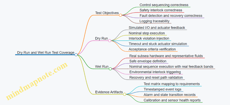
Example Test Case Walkthrough for Control and Safety
Case: Start Circulation
- Prerequisites: Utility valve feedback “open,” pump permissive true, pressure sensor healthy.
- Dry run: Hold valve feedback at “closed” while issuing “start pump.” Expected: pump command blocked, safety alarm latched, state remains “ready.” Then set valve feedback to “open” and confirm pump transitions to “running” only after permissive conditions are satisfied.
- Wet run: Run with a capped flow setting. Expected: pressure rises within the defined time band, pump remains in “running,” and no interlock trips occur. Next, partially restrict flow to force pressure into the interlock threshold; expected: controller stops the pump and transitions to “safe hold,” with a diagnostic that identifies the triggering condition.
Evidence Review and Pass Fail Logic
A test passes only when three layers agree: the commanded intent (what the controller tried to do), the observed behavior (what the hardware and sensors actually did), and the safety response (what happened when something was wrong). If any layer conflicts, the failure record should specify whether the issue is in control logic, integration wiring, sensor scaling, actuator dynamics, or safety configuration.
12.4 Performance Verification for Process Output and Quality Metrics
Performance verification answers two practical questions: did the subsea factory produce the required output, and did it do so within quality limits while staying safe and stable? In subsea work, “performance” is not just throughput; it includes repeatability under pressure, consistent chemistry, and predictable handling of solids and interfaces.
Define Output Metrics Before You Measure
Start by translating requirements into measurable metrics with clear acceptance criteria. For each product stream, specify:
- Output rate: e.g., kilograms per hour of processed material.
- Yield: fraction of input converted into acceptable product.
- Quality attributes: composition, particle size distribution, moisture, surface condition, or purity.
- Process stability: allowable drift of key variables such as temperature, pressure, residence time, and mixing intensity.
Example: If the process is chemical conditioning followed by filtration, define quality as both filtrate clarity (e.g., turbidity threshold) and target concentration (e.g., mass fraction range). Throughput alone is insufficient if concentration drifts during long runs.
Build a Verification Plan from Process Logic
A good plan mirrors the process sequence. For each step, decide what to verify and where to sample.
- Pre-run checks: calibration status, sensor health, actuator response, and baseline fluid properties.
- In-process checks: measurements that confirm the step is behaving correctly.
- Post-run checks: final product sampling and mass balance closure.
Example: For a thermal step, verify heater power delivery and temperature control during the step, then confirm product properties after cooling. If you only check the final temperature, you may miss a control oscillation that still averages out.
Select Quality Metrics That Survive Real Subsea Constraints
Subsea environments complicate measurement. Choose metrics that are robust to sensor noise, fouling, and limited sampling opportunities.
- Prefer metrics with direct physical meaning rather than indirect proxies.
- Use redundant measurement paths when feasible, such as two sensors for the same variable with different failure modes.
- Define sampling plans that account for stratification and mixing delays.
Example: If solids settle quickly, a single grab sample can misrepresent the batch. Instead, specify sampling timing relative to mixing completion and include a settling-time window.
Verify Measurement Integrity and Traceability
Before judging product quality, confirm the measurement system is trustworthy.
- Calibration verification: confirm sensor response within tolerance at the start of the run.
- Drift monitoring: track baseline changes during the run.
- Traceability: record calibration identifiers, test conditions, and data timestamps.
Example: A pressure sensor that drifts by a small amount can shift valve control behavior, which then changes residence time and affects product quality. Verification should catch this chain early.
Perform Statistical Acceptance with Clear Rules
Use a structured approach so acceptance is not a subjective “looks good.”
- Choose a sampling frequency that matches process dynamics.
- Apply acceptance rules such as mean and variability limits, or percentile-based limits for distributions.
- Separate process capability from run performance: capability is about the process under stable conditions; run performance is what happened in this specific test.
Example: For particle size distribution, require that the median stays within a band and that the fraction above a maximum size remains below a threshold. This prevents a run from passing due to average agreement while the tail distribution violates specs.
Close the Loop with Mass Balance and Error Budgets
Quality verification should include accounting for inputs and outputs.
- Create an error budget for each quality attribute, combining sensor uncertainty, sampling variability, and model assumptions.
- Use mass balance closure to detect hidden losses or bypasses.
Example: If yield is low, mass balance can distinguish between conversion failure and measurement bias. If total input and recovered output disagree beyond the error budget, treat it as a verification failure even if some quality samples look acceptable.
Mind Map for Performance Verification Flow
Example Verification Package for a Batch Processing Run
Assume a batch produces conditioned product through mixing, filtration, and final conditioning.
- Pre-run: confirm mixing motor current response, verify temperature sensor calibration ID, and check valve stroke counts.
- In-process: record mixing temperature and pressure every minute; sample filtrate turbidity at two time points to capture early and late behavior.
- Post-run: measure final concentration and particle size distribution from a composite sample; compute yield from measured input mass and recovered product mass.
- Acceptance: require concentration within range, turbidity below threshold, median particle size within band, and yield above minimum. Also require mass balance closure within the error budget.
If turbidity passes but yield fails, the verification report should flag a likely loss mechanism or sampling bias rather than treating the run as partially successful. In subsea operations, “partial success” is often just the start of a bigger problem.
12.5 Example Commissioning Checklist for End-to-End Autonomy
This checklist is written for a subsea factory that runs a repeatable manufacturing or processing job with minimal human intervention. It assumes you already have a defined product recipe, a control architecture, and a safety concept. The goal is to prove the system can execute the full sequence: from receiving a job command to producing a verified output, while staying inside safety limits.
Pre-Commissioning Readiness
- Verify configuration integrity: Confirm the deployed software versions match the approved build list. Example: compare the control system “software manifest” against the release record before any wet testing.
- Confirm mechanical readiness: Check that all connectors, seals, and tool couplings are installed with the specified torque and inspection marks. Example: record a photo of each coupling location after final tightening.
- Validate utility availability: Ensure power, communications, and required fluids are reachable at the subsea interface. Example: run a short “utility health” cycle that measures voltage, flow, and pressure without starting process steps.
- Establish a commissioning log discipline: Every test step must record inputs, outputs, alarms, and operator actions. Example: use a single line per step with a unique step ID so later troubleshooting is fast.
Dry Run Verification of Control and Safety
- Run control sequence in simulation mode: Execute the manufacturing recipe with simulated sensor values to confirm step ordering and timing. Example: confirm that the system refuses to start heating until mixing reaches the required temperature band.
- Prove interlocks and safety instrumented functions: Trigger each interlock condition one at a time and confirm the correct safe state. Example: block a valve feedback signal and verify the system transitions to “hold” rather than continuing.
- Check fault detection and isolation: Induce representative faults such as sensor dropout, actuator stall, or communication loss. Example: disconnect a temperature sensor input and confirm the system selects the defined fallback strategy.
- Validate manual override behavior: Confirm that local manual commands cannot bypass safety logic. Example: allow a technician to jog a robot axis while still enforcing motion limits.
Wet Run Readiness and Controlled Start
- Perform a staged wet start: Begin with low-energy, low-risk operations such as instrument checks and leak tests. Example: pressurize a small utility loop first, then expand to full operating pressure.
- Confirm sensor plausibility underwater: Compare redundant measurements and check for physically impossible values. Example: if flow rate increases while pump speed decreases, flag the run for review.
- Validate actuation response: Measure valve response time, pump ramp behavior, and robotic motion timing. Example: record the time from command to confirmed position for each critical valve.
End-to-End Job Execution with Quality Proof
- Execute the full recipe once in “verification mode”: The system runs the entire sequence but may stop before final discharge or product release. Example: stop after final metrology and confirm all quality gates pass.
- Check each process gate: For every step, confirm entry conditions and exit conditions. Example: before separation, verify solids concentration is within the recipe window; after separation, verify target recovery or residue limits.
- Capture traceability data: Ensure the job ID links to every sensor record, alarm, and operator action. Example: store metrology results with timestamps aligned to control events.
- Perform a controlled output acceptance: Use the defined acceptance criteria for the output form. Example: if the product is a machined component, verify dimensions and surface condition against the spec thresholds.
Commissioning Acceptance and Handover
- Complete a commissioning summary: List pass/fail status for each checklist item, plus deviations and corrective actions. Example: if a valve response time is slow, record the measured delay and the mitigation applied.
- Confirm readiness for autonomous operation: Verify the system can start, run, and stop safely without live operator intervention. Example: run a full job with the operator only monitoring alarms and quality gates.
- Close out safety documentation: Ensure safety function test results are filed and mapped to the safety concept. Example: attach the test evidence for each safety instrumented function.
- Lock configuration and permissions: Prevent unapproved changes to recipe parameters and control logic. Example: require a change ticket for any parameter that affects quality gates.
Mind Map: End-to-End Autonomy Commissioning Flow
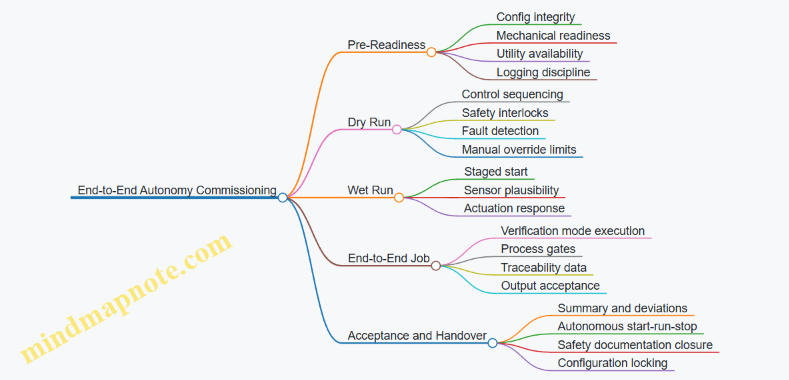
Example: One Job Run Checklist Snapshot
- Job ID created and logged
- Recipe loaded and validated
- Interlocks confirmed green
- Utility health cycle passed
- Step 1: entry conditions met
- Step 2: gate passed with measured values recorded
- Fault injection test not performed during verification run
- Final metrology within acceptance thresholds
- System transitions to safe stop and records completion
Example: Commissioning Date Reference
Use a fixed commissioning reference date such as 2026-03-25 for labeling the commissioning batch in the job traceability record.