Digital Scent Technology Overview
1. Scope and System Requirements for Digital Scent
1.1 Defining Digital Scent Technology and Its Boundaries
Digital scent technology is the engineering of smell experiences using three linked parts: an odor source, a control method, and a representation of “what to smell” that can be scheduled and reproduced. In practice, it means you can take an intended odor event—like “fresh coffee at the start of a scene”—and translate it into device commands that produce a repeatable output at the right time and location.
A useful boundary is to separate odor generation from odor representation. Odor generation is the physical act of releasing volatile compounds (or mixtures that approximate them). Odor representation is the data model that describes the target smell in a way a system can render. Many systems fail not because the hardware is weak, but because the representation is vague, inconsistent, or impossible to map to the device.
Another boundary is to distinguish digital scent from general “fragrance effects.” A digital scent system includes a control loop that can vary output based on interaction or scene timing, and it includes a method to keep those variations consistent. If a device only supports a single “on” button for one cartridge, it is an effect, not a digital scent system.
What Counts as Digital Scent
Digital scent typically includes:
- A library or mapping from encoded odor events to device-ready parameters.
- Timing control so odor onset and decay align with user actions or scene cues.
- Repeatability controls such as calibration, normalization, or feedback from flow/temperature sensors.
- Context-aware rendering for mixed reality, where placement and intensity depend on user position and environment.
A concrete example: a training app wants “burnt plastic” when a virtual circuit overheats. The system stores an encoded profile for burnt plastic, schedules it when the overheating threshold is crossed, and uses device calibration to ensure the same perceived intensity across sessions.
What Does Not Count
The following are common misunderstandings:
- Single-shot scent cards without timing or control are not digital scent.
- Purely visual “smell cues” (text, icons, or animations) are not digital scent because no odor is generated.
- Pre-recorded audio-style playback of odor without a representation that maps to device parameters is incomplete; it may be a sequence of releases, but not a reproducible encoding.
Core Boundaries You Should State Up Front
- Scope of fidelity: The system should define whether it aims for “recognizable category” (like coffee vs. tea) or “fine-grained similarity” (specific roast notes). Different goals require different encoding and calibration effort.
- Scope of interaction: Decide whether smell changes only with scene events, or also with continuous user actions like turning a head.
- Scope of environment: Smell behavior depends on airflow, room volume, and leakage. A boundary statement clarifies whether the system assumes a controlled chamber or a typical room.
- Scope of safety: Odor delivery must be constrained by exposure limits, ventilation assumptions, and cleaning procedures.
Mind Map: Digital Scent System Boundaries
Example: Boundary Check for a VR Experience
Suppose a VR museum exhibit includes “sea breeze” near a virtual ship. A boundary check asks:
- Representation: Is “sea breeze” stored as an encoded profile with parameters that can be rendered, or is it just a label?
- Control: Does the system trigger onset when the user approaches, and does it control intensity rather than only turning a fan on?
- Repeatability: After cleaning and calibration, does the same approach produce comparable output across sessions?
- Environment: Is the exhibit in a controlled airflow area, or does the system assume a typical room with variable leakage?
If any of these answers are “no,” the project may still be enjoyable, but it is not a well-defined digital scent system.
Example: Encoding vs. Generation in One Sentence
If you can swap the odor source hardware while keeping the encoded “burnt plastic” profile and still render a comparable smell after calibration, you have a clearer separation between representation and generation. If swapping hardware breaks the experience completely, the representation is probably too tied to one device’s quirks.
Summary Boundary Statement
Digital scent technology is the controlled, encoded, and reproducible generation of smell events for interactive systems, with explicit limits on fidelity, interaction, environment assumptions, and safety constraints.
1.2 Smell Use Cases in Virtual and Mixed Reality Experiences
Smell in virtual and mixed reality is most useful when it answers a concrete question the user is already asking. In practice, that means the scent must be tied to an event, a location, or a decision, and it must change in a way the user can notice without guessing. The goal is not to make everything smell like the real world; it is to add information that improves understanding, navigation, or training.
Mind Map: Smell Use Cases by User Goal
Navigation and Wayfinding
A common pattern is using scent as a “soft landmark.” For example, an escape-room style MR experience can place a subtle citrus note near an exit door. When the user turns toward the correct corridor, the scent intensity rises with distance, then fades after passing the doorway. This supports wayfinding without requiring the user to read text or follow a glowing arrow.
A useful design constraint is to keep the scent distinct from nearby cues. If the corridor also contains a cleaning-supply smell, the system should either avoid overlap or schedule one cue at a time. Otherwise, users may learn the wrong association and confidently walk into the wrong room.
Training and Skill Practice
Smell can represent categories that are hard to show visually. In a maintenance training simulation, a “burning plastic” profile can appear when a virtual circuit overheats. The scent is not meant to be identical to the real hazard; it is meant to be consistent enough that trainees learn the relationship between a condition and a response.
Another training example is procedure verification. During a virtual cooking class, the system can release a “toasted aroma” cue at the moment a timer reaches the recommended browning window. The user still follows the visual cues, but the scent provides an extra confirmation channel that reduces timing errors.
For quality inspection, scent can act like a checklist item. In a virtual brewery tasting lab, different fermentation stages can be represented by distinct odor profiles. The learner selects the stage that matches what they smell, then receives feedback tied to the specific stage they chose.
Storytelling and Environmental Context
Smell can anchor a scene when visual information is ambiguous. In a mixed reality museum guide, a workshop exhibit can emit a faint wood-and-resin profile when the user approaches a specific bench. The scent helps the user understand what they are looking at even if labels are out of view.
Character-triggered cues work similarly. If a virtual character carries a distinct scent, releasing it only when the character is within a short range supports attention and improves spatial coherence. The key is to avoid constant emission; continuous scent becomes background noise and loses meaning.
Interaction and Feedback
Scent is also a feedback channel for actions. A VR game can release a short “fresh paint” note when a user successfully applies a patch to a wall. The scent should be brief and synchronized with the completion event, then purged quickly so the next action starts from a clean baseline.
Proximity-based cues are effective for object interaction. In an MR assembly task, a “lubricant” scent can appear when the user brings a tool to the correct joint. If the user moves away, the scent fades, reinforcing correct placement without requiring extra on-screen prompts.
Accessibility and Multimodal Support
Smell can support users who rely less on vision by adding timing and location cues. For example, a VR navigation training for low-vision users can use distinct scent zones to indicate intersections. The system should pair scent with consistent spatial rules, such as “scent increases when facing the correct direction,” so users can build reliable mental maps.
Research and Evaluation
In evaluation studies, smell use cases often focus on measuring whether scent improves task performance. A simple experiment can compare two versions of a VR training: one with visual-only cues and one with an added scent cue at the moment of correct action. The outcome measures can be completion time, error rate, or confidence calibration.
Example: Mapping Use Case to Design Decisions
| Use Case | What the User Needs To Know | Scent Behavior | Example Implementation Detail |
|---|---|---|---|
| Wayfinding | Which corridor is correct | Intensity rises with distance, fades after passing | Calibrate so the cue is noticeable at 2–3 meters but not at 10 meters |
| Hazard Training | When a condition becomes dangerous | Short onset, then steady until resolved | Trigger at threshold crossing, stop immediately when the user fixes the issue |
| Procedure Timing | Whether browning window is reached | One-time pulse or short plateau | Release for 5–8 seconds aligned to the timer event |
| Interaction Feedback | Did the action succeed | Brief confirmation, then purge | Emit only on success events to avoid learning noise |
1.3 Core System Requirements for Encoding, Playback, and Control
A digital scent system has three jobs: turn an odor intent into an encoded representation, render that representation on hardware, and coordinate timing with the VR or mixed reality experience. If any one job is sloppy, the result is usually the same: the smell arrives late, fades too quickly, or doesn’t match what the user expects.
Encoding Requirements
Encoding requirements define what information must be captured so playback can be repeatable.
- Odor identity and mixture definition: The system must store which odorants are included and how they combine. Example: a “coffee” profile might include roasted notes plus a caramel-like note, each with a target relative strength.
- Perceptual scaling parameters: Because concentration does not map linearly to perceived intensity, the encoding should include a scaling rule or calibration reference. Example: “low intensity” might correspond to a specific calibration setting rather than a raw concentration value.
- Timing metadata: The encoding must specify onset, duration, and decay behavior. Example: a “fresh bread” cue might be configured to peak quickly and then taper over 3–5 seconds.
- Constraints for device compatibility: The encoded profile should include or reference limits such as maximum simultaneous channels or supported mixture sizes. Example: if the device can only mix two odorants at once, the encoding must avoid profiles that require more.
Playback Requirements
Playback requirements define what the hardware and software must achieve physically and measurably.
- Deterministic command execution: When the control layer says “start at time T,” the output should begin within a known tolerance. Example: a system might target a ±50 ms start window for onset.
- Flow and mixing stability: Odor delivery depends on airflow and mixing. The system should control or measure airflow so the same command produces similar output. Example: if airflow drops, the same “medium” setting should automatically compensate.
- Cross-contamination management: Mixtures and residues can linger. The system must support purge or cleaning cycles and track which odorants were used recently. Example: after “solvent-like” notes, the system should run a purge before “citrus” to prevent lingering bitterness.
- Output calibration and normalization: Each channel and cartridge should be calibrated so “intensity level 3” means the same thing across sessions. Example: a calibration curve can map a requested level to a device-specific drive value.
- Thermal and operational limits: Hardware must avoid conditions that degrade performance or safety. Example: if a heater or pump has a maximum duty cycle, the playback scheduler should enforce it.
Control Requirements
Control requirements define how the system coordinates VR events, user movement, and device state.
- A timing model that matches perception: The control layer should schedule odor events relative to VR timestamps and account for known device latency. Example: if hardware latency is 300 ms, the system triggers the command 300 ms before the visual cue.
- State management and feedback: The system should track device status such as “ready,” “purging,” “mixing,” and “fault.” Example: if a sensor reports low flow, the controller can pause new odor events rather than sending commands that will underperform.
- Spatial and intensity mapping hooks: Even if the first version is simple, the control layer should accept inputs like distance or direction so intensity and timing can be adjusted. Example: when a user walks closer to a virtual candle, the controller increases intensity and shortens the time to peak.
- Concurrency rules: The system must define what happens when multiple odor cues overlap. Example: it can either blend if supported, queue them, or prioritize one cue based on a rule set.
- Fail-safe behavior: On faults, the system should move to a safe output state, typically stopping odor emission and purging if needed. Example: if a cartridge is empty, it should stop and report the issue rather than emitting an incorrect substitute.
Mind Map: Core System Requirements
Example: A Minimal End-to-End Requirement Set
Suppose a VR scene includes a “rain on pavement” cue that should start when the user looks at a window, peak quickly, and fade without contaminating the next cue.
- Encoding: Store a mixture definition for “rain” (two odorants), an intensity scaling reference, and a timing profile with onset at 0 s, peak at 1 s, and decay to near-zero by 6 s.
- Playback: Use calibrated drive values for the two odorants, enforce a purge rule after rain playback, and verify airflow is within tolerance before emitting.
- Control: Trigger the odor command 300 ms before the visual event to match perceived onset, queue the next odor cue if it overlaps, and stop emission if flow feedback drops.
Example: Concurrency Rules That Prevent Surprises
If a user triggers “coffee” and then quickly triggers “citrus,” the system needs a defined overlap policy.
- Blend policy: If both odorants can be mixed simultaneously, the controller schedules a combined mixture with a capped total intensity.
- Queue policy: If mixing is limited, the controller finishes the first cue’s decay window before starting the second.
- Priority policy: If one cue is marked “critical” (e.g., a safety-related odor), it interrupts non-critical playback and initiates a purge afterward.
These policies should be explicit in the system requirements so the behavior is consistent, testable, and not dependent on who clicked what first.
1.4 Performance Metrics for Smell Fidelity and User Experience
Smell performance is tricky because “correct” is not a single number. A good metric set separates physical output quality (what the device emits) from perceptual outcome (what the user experiences) and then ties both back to task success (what the user needs to do in VR/MR).
Fidelity Metrics That Measure What You Actually Emit
Odor concentration accuracy checks whether the delivered intensity matches the intended level. A practical approach is to define a small set of target levels (for example, low/medium/high) and measure each with an appropriate sensor or lab method, then compute error per level. Example: if “medium” is calibrated to 60 units and the device outputs 48–52 units across trials, you can quantify systematic under-delivery.
Timing accuracy matters because smell onset and decay are part of the cue. Measure the time from the command to first detectable odor at the delivery point, plus the time to reach a stable plateau. Example: in a cooking simulation, if the “fresh bread” cue starts 600 ms late, users may still smell it, but the event no longer lines up with the visual action.
Mixture composition stability evaluates whether multi-odor profiles remain consistent across repeated plays. Even if each odorant is correct individually, the mixture can drift due to cartridge aging, partial clogging, or imperfect mixing airflow. Example: a “citrus + wood” profile might keep citrus stable while wood fades, shifting the perceived balance.
Cross-contamination index estimates how much a previous odor lingers into the next one. You can test by playing odor A, waiting a fixed purge time, then playing odor B and measuring residual A. Example: if “coffee” leaves a trace that makes “mint” feel muted, you’ll see it as elevated residual A.
Perceptual Metrics That Measure What Users Experience
Similarity ratings capture how close the perceived smell is to a reference. Use a structured scale with clear anchors, such as “same as reference,” “close but different,” and “clearly different.” Example: participants compare the rendered odor to a real reference smell and rate both identity and intensity.
Detection and recognition rates measure whether users can tell that an odor is present and whether they can identify it. Example: in a training scenario, you might require at least 80% recognition for “smoke” before allowing a safety drill to proceed.
Confusability matrices show which odors get mixed up with which. This is more useful than a single average score because smell systems often fail in predictable pairs. Example: “lemon” and “lime” may be consistently confusable, while “lemon” and “burnt rubber” are not.
Intensity perception error compares intended intensity levels to perceived ones. Example: if users rate “high” as only “medium,” you know the issue is not timing or identity—it’s scaling.
User Experience Metrics That Tie Smell to Outcomes
Task performance impact links smell to what users do. Choose a task where smell is relevant: locating a source, selecting an item, or confirming an event. Example: in a VR kitchen, users might need to identify “spoilage” from smell; you measure accuracy and time-to-decision with and without smell.
Discomfort and annoyance track whether odor delivery causes irritation, fatigue, or repeated “too strong” complaints. Example: after each session, ask for a simple 1–5 discomfort rating and record whether users request earlier termination.
Adaptation and habituation effects measure how quickly users stop noticing an odor. This is not inherently bad, but it changes how you schedule cues. Example: if “campfire” becomes undetectable after 3 minutes, you may need shorter exposures or fewer repeated triggers.
Spatial plausibility checks whether users accept the smell’s location. Example: if the system claims “smell comes from the left,” but users consistently point elsewhere, you’ll see it in localization error.
Mind Map for Metric Selection
Example Metric Set for a Single VR Scenario
For a “detect the gas leak” training module, a sensible minimum set is:
- Timing accuracy: onset within ±200 ms of the visual alarm.
- Concentration accuracy: medium level perceived as “clearly present” by at least 90% of users.
- Cross-contamination index: residual from the previous odor below a predefined threshold so “gas” is not masked.
- Recognition rate: at least 85% correctly identify “gas leak” when prompted.
- Discomfort rating: median ≤ 2/5, with a clear rule for stopping if discomfort spikes.
This combination prevents a common failure mode: a system that emits something strong and on time but still gets the wrong smell, or a system that gets the smell right but makes users uncomfortable enough to stop paying attention.
1.5 Safety, Compliance, and Risk Controls for Odor Delivery
Digital scent systems turn chemicals into user-facing experiences, so safety is not a “nice to have.” It is a design constraint that affects hardware choice, software behavior, and operational procedures. The goal is simple: prevent harmful exposure, avoid unsafe mixtures, and keep the system predictable.
Risk Inventory and Hazard Scoping
Start with a structured inventory of what can go wrong. Consider the odorants themselves, the carrier air, the delivery mechanism, and the user environment.
- Chemical hazards: irritants, allergens, toxicants, flammables, and reactive compounds.
- Physical hazards: hot surfaces, moving parts, pressurized reservoirs, and pinch points.
- Operational hazards: wrong cartridge installed, stale cartridges, clogged nozzles, and failed purge cycles.
- Environmental hazards: poor ventilation, high humidity, and accumulation in small rooms.
A practical approach is to assign each odorant a risk category based on available safety data, then require stronger controls for higher-risk categories. If you cannot classify an odorant confidently, treat it as high risk until you can.
Engineering Controls That Reduce Exposure
Engineering controls should work even when software misbehaves.
-
Closed-loop delivery volume control
- Use measured ejection pulses with a maximum dose per event.
- Example: If a VR scene triggers “campfire,” cap the total ejection time so the system cannot keep spraying when the user stays in the scene.
-
Fail-safe shutoff and interlocks
- Add hardware interlocks for airflow sensors, reservoir pressure, and temperature limits.
- Example: If airflow drops below a threshold, the controller stops ejection and enters a safe state rather than continuing to push odor into a stagnant chamber.
-
Purging and flushing cycles
- Define purge behavior after each odor event and after errors.
- Example: After “cleaning solvent” odor, run a short purge to reduce lingering vapors before the next scene.
-
Cartridge and connector design
- Use keyed cartridges or unique mechanical interfaces so the wrong chemical cannot be installed.
- Example: A “mint” cartridge physically cannot connect to a “solvent” port.
-
Material compatibility and corrosion control
- Select tubing and seals that resist permeation and degradation by the odorants.
- Example: If an odorant slowly permeates through a seal, you will see background smell even when the system is “off,” which is both a comfort and safety issue.
Software Controls That Keep Behavior Predictable
Software should enforce safety limits and prevent unsafe sequences.
-
Dose budgeting per session
- Track cumulative ejection time or estimated delivered volume.
- Example: If a user triggers multiple “food” events quickly, the system reduces intensity or blocks further ejections after a threshold.
-
State machine for safe transitions
- Only allow ejection in a “ready” state, and require purge before switching odorants.
- Example: Switching from “ammonia-like” to “citrus” requires a purge state; the system does not jump directly.
-
User-triggered consent and pause behavior
- Provide a clear way to pause odor delivery and ensure the pause triggers a safe stop and purge.
- Example: A “mute scents” button immediately halts ejection and prevents queued odor events.
-
Error handling with safe defaults
- If a sensor fails or a command cannot be verified, default to no ejection.
- Example: If the airflow sensor reports “unknown,” the system refuses to deliver.
Compliance and Documentation Practices
Compliance is easier when you can show your work.
-
Maintain an odorant dossier
- For each odorant: hazard classification, maximum dose assumptions, storage conditions, and disposal method.
-
Define operational limits
- Document maximum room size assumptions, ventilation requirements, and acceptable operating temperature ranges.
-
Labeling and traceability
- Ensure cartridges are labeled with identifiers that match the software library.
- Example: The system logs “cartridge ID 12A used for event 104” so you can trace incidents.
-
Training and maintenance logs
- Record cartridge changes, cleaning schedules, and calibration dates.
- Example: If a nozzle is cleaned, note the date and the technician so you can correlate performance changes with safety checks.
Mind Map: Safety Controls for Odor Delivery
Example: Safe Switching Between Two Odors
Imagine a mixed reality scene that transitions from “spice” to “bleach-like cleaning.” A safe system does not just stop one and start the other.
- It verifies airflow is within range.
- It stops ejection and enters a purge state.
- It waits for a defined purge duration.
- It confirms the system is back in “ready.”
- It then delivers the next odor with a capped dose.
If any step fails, the system skips the second odor rather than trying to “catch up.” That one design choice prevents a common failure mode: unintended overlap that can increase irritation risk and confuse users.
Verification and Ongoing Safety Checks
Safety controls must be tested, not assumed.
- Purge effectiveness tests: confirm background odor drops to an acceptable baseline.
- Sensor fault injection: simulate airflow or temperature sensor failures and verify the system refuses to eject.
- Cross-contamination checks: run back-to-back odor events and measure whether the first odor persists into the second.
When verification is documented, you can confidently explain why the system behaves safely under normal use and under faults.
2. Human Olfaction Fundamentals for Engineering Smell
2.1 Olfactory Receptor Activation and Perceptual Implications
Smell starts with receptors, but what you perceive is not a direct readout of “which receptor fired.” Your brain interprets patterns of receptor activation, and those patterns are shaped by chemistry, timing, and context.
How receptor activation happens
Olfactory receptor neurons sit in the nasal epithelium. Each neuron expresses one type of olfactory receptor, and that receptor binds certain odorant molecules. Binding is not a simple on/off event; it depends on how well a molecule fits the receptor’s binding site, how long it stays there, and how many molecules reach the receptor surface.
A practical way to think about it: the odorant is the “key,” the receptor is the “lock,” and the fit determines how strongly and how quickly the neuron responds. But the brain never sees the key directly. It only receives signals from many receptor types at once.
Pattern coding instead of single-molecule labeling
Because each odorant can activate multiple receptor types, and each receptor type can respond to multiple odorants, perception is driven by a distributed activation pattern. For example, a “citrus” impression often involves several receptors responding to different volatile components, not one magic receptor.
This is why two mixtures can smell similar even when they contain different chemicals: they can produce comparable activation patterns across receptor populations.
Concentration changes the shape of the pattern
Increasing odor concentration generally increases firing rates and recruits additional neurons. That means the percept can shift with concentration, not just intensify. A molecule that reads as “fresh” at low levels can become “sharp” or “solvent-like” at higher levels because the activation pattern changes across receptor types.
Example: If you compare the smell of a cleaning alcohol at a low sniff versus a strong sniff, the stronger exposure tends to emphasize receptors associated with more irritating or high-volatility components, even if the same base chemical is present.
Timing matters because odor delivery is transient
Odorants arrive in pulses as air moves through the nose and as the mixture evaporates. Receptor neurons respond over time, and the pattern evolves during the sniff.
Two percepts can differ even when the average concentration is the same, if one stimulus arrives quickly and another arrives slowly. Rapid onset can feel “brighter” or more attention-grabbing because early receptor activation dominates the brain’s interpretation.
Example: A scent released from a spray often produces a fast rise and decay. A scent released from a slow-release source may feel smoother because the receptor activation pattern changes more gradually.
Mixtures create overlapping receptor responses
When multiple odorants are present, their receptor activations overlap. The resulting pattern is not a simple sum of “parts.” Interactions can occur at the receptor level (different molecules compete for binding) and at the system level (different odorants change airflow and evaporation behavior).
Example: Consider a mixture of vanillin-like sweetness plus a smoky component. Even if each component alone activates distinct receptor sets, the mixture can produce a new combined pattern that reads as “warm” rather than “sweet” or “smoky” separately.
Perceptual implications for encoding and reproduction
For digital scent systems, receptor activation implies three engineering constraints.
- You need mixture-level fidelity, not just single-chemical fidelity. If you encode only one dominant chemical, you may reproduce intensity but miss the activation pattern that creates the intended percept.
- You must control timing and concentration delivery. Receptor activation patterns evolve during a sniff, so playback should match onset and decay characteristics, not only the final odor “strength.”
- You should expect non-linear percept shifts. Because concentration and mixture composition change which receptor populations contribute, perceptual similarity is not guaranteed by matching chemical lists alone.
Mind Map: Olfactory Receptor Activation and Perceptual Implications
Worked Example: From receptor pattern to a percept
Suppose you want a “fresh laundry” impression. If you reproduce only a single volatile associated with a clean note, you may get a recognizable smell but it can feel flat. Adding a second component that activates a different subset of receptors can reshape the overall activation pattern, producing a more complete percept. If you also deliver the mixture with a slow onset, the activation pattern evolves more gradually, which often reads as smoother rather than sharp.
In short, receptor activation is the first step, but perception is the interpretation of a changing pattern across many receptor types. That’s why smell reproduction works best when it treats odor as a time-varying mixture, not a static label.
2.2 Odor Perception Variables That Affect Reproduction
Reproducing smell in virtual or mixed reality is less about “playing a file” and more about matching how people notice and interpret odor over time. Several variables change what a user perceives even when the same odorant mixture is delivered.
Concentration and Perceptual Scaling
Odor perception is not linear with concentration. A small increase can be barely noticeable, while a larger jump can suddenly feel stronger or even different. This happens because receptors saturate and because the brain compares the current signal to recent exposure.
Example: If you calibrate a “coffee” profile at a medium intensity, then double the delivered concentration, users may report “more coffee” but also “burnt” or “stronger roast,” because different components become more salient at higher levels.
Practical implication: Treat intensity as a perceptual target, not a numeric knob. Use a few intensity steps during calibration and record which step corresponds to “subtle,” “present,” and “noticeable.”
Mixture Balance and Component Salience
A mixture can smell different from its parts because some components dominate perception. Even when total concentration stays constant, shifting the ratio changes which notes stand out.
Example: A “citrus” blend might include lemon-like and orange-like components. If the lemon-like component is slightly higher, users may describe it as “sharp” and “clean.” If the orange-like component is higher, the same blend can shift toward “round” and “sweet.”
Practical implication: Store mixture profiles with ratio information and verify them with human judgments, not only chemical measurements.
Volatility and Temporal Evolution
Odorants evaporate at different rates. When released, the composition of what reaches the nose changes over time, even if the delivered liquid or cartridge output is constant.
Example: A “fresh paint” scent may start with a solvent-like sharpness and later settle into a softer, resin-like impression. If your playback timing holds the same output for too long, users may experience the later phase more strongly than intended.
Practical implication: Encode not just “what” but “when.” Use onset, peak, and decay timing so the user encounters the intended phase during the VR event.
Adaptation and Odor History
The olfactory system adapts quickly. After exposure, sensitivity drops, and the same odor can feel weaker or even absent. Adaptation also depends on what came immediately before.
Example: If a user smells “campfire” and then, a few seconds later, “vanilla,” the vanilla may seem muted until the campfire fades. In a session, the order of scenes can change perceived intensity.
Practical implication: Design smell timelines with spacing and consider “reset” intervals. When switching odors, include a brief gap or a controlled purge so the next note is not competing with residual perception.
Individual Differences in Sensitivity
People vary in receptor genetics, nasal physiology, and learned associations. Some users detect certain odorants at lower levels; others may not detect them reliably.
Example: Two users can both rate “smoke” as present, but one may describe it as “wood” while the other describes it as “burnt plastic,” because their sensitivity to specific components differs.
Practical implication: Use a calibration routine per user or per session group. For interactive experiences, consider offering intensity adjustment so users can reach a comfortable detection level.
Context and Cross-Modal Expectation
What users expect affects what they report. Visual cues, scene semantics, and even airflow from head movement can bias perception.
Example: If a VR scene shows a bakery, users may interpret a mild sweet odor as “bread,” while the same odor in a workshop scene might be labeled “cleaning solution.”
Practical implication: Align odor events with visual and narrative cues. If the system can’t guarantee perfect timing, prioritize consistency between the odor onset and the most relevant visual moment.
Environmental Conditions and Delivery Path
Temperature, humidity, and airflow influence how quickly odorants reach the nose and how they disperse. Delivery hardware also matters: where the plume goes, how it mixes, and how much reaches the user’s breathing zone.
Example: In a cooler room, a scent may feel weaker because volatility drops. With a strong airflow, the same scent can arrive faster but dissipate sooner, changing the perceived duration.
Practical implication: Keep environmental variables controlled during testing. In mixed reality, account for head motion and ensure the plume remains in the user’s effective zone.
Mind Map: Variables Affecting Odor Reproduction
Example: Turning Variables into a Reproduction Checklist
When authoring a smell event, confirm these items in order: (1) the target intensity step, (2) the mixture ratio that produces the intended note balance, (3) the onset/peak/decay timing to match volatility, (4) the spacing from the previous odor to reduce adaptation effects, (5) whether the user group is likely to detect the key components, (6) whether the visual moment supports the odor label, and (7) whether room conditions and delivery placement are consistent.
If any one item is off, users may still detect an odor, but the perceived identity, timing, or duration can shift—exactly the mismatch that makes smell feel “wrong” even when the hardware is working.
2.3 Temporal Dynamics of Smell Detection and Adaptation
Smell perception is time-sensitive in ways that matter for encoding and playback. A good smell system treats timing as part of the signal, not just a schedule for when to turn a device on.
Detection Windows and Onset Timing
Most odor experiences have a noticeable onset: the moment when the brain decides “something is there.” In practical terms, that decision depends on how quickly odor molecules reach the user’s nose and how rapidly the system ramps concentration.
A useful engineering approach is to model three phases for each odor event:
- Ramp-up: from device activation to reaching a perceptible concentration.
- Steady: the interval where concentration stays near the target.
- Decay: after shutdown, when concentration drops but the user may still detect the odor.
Example: Suppose you want a “fresh coffee” note for 2 seconds in VR. If the device takes 0.6 seconds to reach a detectable level, then the user effectively experiences only about 1.4 seconds of “on.” If you instead schedule 2 seconds plus a 0.6-second lead-in, the perceived onset aligns with the visual cue.
Onset timing also interacts with attention. If the user is looking away or engaged in a task, detection can lag even when the odor arrives on time. That means your timing strategy should include a small buffer for attention shifts, especially for short events.
Adaptation and Sensory Fatigue
Adaptation is the reduction in perceived intensity after repeated exposure. It can happen within seconds, and it affects both detection and discrimination.
There are two common adaptation patterns you’ll see in smell playback:
- Within-event adaptation: intensity drops during a single prolonged exposure.
- Between-event adaptation: a second odor in a sequence feels weaker or less distinct.
Example: If you play “lemon” for 6 seconds and then switch to “orange” after 1 second, the orange may seem muted because the olfactory system is still downshifting from lemon. Increasing the gap can restore sensitivity, but too large a gap can break the intended narrative timing.
A practical rule is to treat adaptation as a function of exposure history, not just the current odor. Systems that ignore history often overestimate how much intensity the user will perceive.
Persistence, Carryover, and Perceptual Overlap
Odor persistence is the lingering sensation after the device stops. Even if the airflow clears quickly, the user’s perception can remain for a while due to ongoing receptor activity and lingering molecules in the delivery path.
Carryover creates perceptual overlap when events are close together. Overlap can be helpful when you want blending, but harmful when you need crisp transitions.
Example: You want a “soap” cue followed by “smoke” within 3 seconds. If the soap’s decay tail overlaps with smoke onset, the user may report “soapy smoke” rather than two distinct notes. The fix is not only to shorten soap duration; it’s to manage the decay tail by adding a purge interval or by scheduling smoke onset later than the visual transition.
Modeling Temporal Behavior for Encoding
To encode smell events reliably, you need a timing model that maps device commands to perceived intensity over time. A simple model uses three parameters per odor event:
- Time-to-detect: when intensity crosses a perceptual threshold.
- Time-to-peak: when intensity reaches the target level.
- Half-life of decay: how quickly intensity falls after shutdown.
You can estimate these parameters by running a controlled sequence and asking users to rate intensity at fixed time points. Even a small calibration dataset helps you avoid “turn it on for X seconds” thinking.
Mind Map: Temporal Dynamics of Smell Detection and Adaptation
Example: Scheduling a Two-Note Sequence
Goal: “Rose” then “Cedar” with a clear separation, while the visuals switch at t=2.0s.
- Measure or estimate that rose reaches detectability at +0.4s and decays with a noticeable tail lasting ~1.0s.
- Start rose at t=1.6s so the onset matches the visual cue at t=2.0s.
- If cedar should feel distinct, schedule cedar onset after rose’s tail is mostly gone. For instance, start cedar at t=3.3s instead of t=2.0s.
- Keep cedar duration short enough to avoid within-event adaptation dominating the perceived intensity.
The key idea is that the timeline you author should be based on perceived phases, not just device on/off time.
Example: Handling Short, Repeated Cues
Goal: Provide three quick “mint” puffs during a single interaction.
If you play three identical pulses back-to-back, the second and third may feel weaker due to adaptation. A workable approach is to:
- Use slightly longer pulses for later cues, or
- Insert a brief gap that allows partial recovery, or
- Reduce intensity targets for later cues if the system can’t fully recover.
The best choice depends on whether the experience needs consistent detection (“I should notice mint each time”) or consistent intensity (“mint should feel the same each time”).
2.4 Mixture Perception and Why Linear Models Fail
A mixture is not just “more of each ingredient.” Human smell is shaped by how volatile molecules arrive over time, how receptors respond in overlapping ways, and how the brain interprets patterns rather than single signals. That’s why linear models—where mixture intensity equals a weighted sum of component intensities—often miss what people actually report.
What Linear Models Assume
A typical linear approach treats each odorant as an independent contributor. If odorant A produces intensity 0.6 and odorant B produces intensity 0.4, a linear model might predict a mixture intensity of 1.0 (or some scaled version). This implies three things:
- Independence: A’s effect doesn’t change when B is present.
- Additivity: The mixture’s percept is the sum of component percepts.
- Constant scaling: The mapping from concentration to perceived strength is the same in isolation and in mixtures.
Real mixtures break all three.
Receptor-Level Interactions
Olfactory receptors respond to molecular features, and many receptors are activated by multiple odorants. When odorants share receptor targets, their combined presence can produce non-additive outcomes. Two common patterns show up in practice:
- Competitive effects: If two odorants vie for the same receptor activation pathway, the mixture can feel weaker than the sum.
- Synergistic effects: If odorants jointly drive a receptor pattern that the brain interprets as “stronger” or “more complex,” the mixture can feel stronger than the sum.
Even when the total number of activated receptors increases, the distribution across receptors matters. Linear models that only track overall intensity ignore distribution changes.
Mixture Perception Is Pattern-Based
People rarely describe mixtures as “A plus B.” They describe them as a new percept with its own character. That suggests the brain uses a pattern of receptor activity, not a single scalar. Two mixtures can have the same predicted linear intensity but different perceived qualities because their receptor activation patterns differ.
A practical example: imagine a “citrus” note built from multiple volatiles. If one component is reduced, a linear model might predict a proportional drop in “citrus strength.” In reality, the percept can shift toward “sharp” or “soapy,” because the balance of receptor activations changes.
Temporal Dynamics and Adaptation
Smell is time-sensitive. Odorants differ in volatility and diffusion, so their arrival at the nose is staggered. Mixtures therefore create a time course: an early phase dominated by fast volatiles and a later phase dominated by slower ones.
Linear models often assume a single static concentration. But perception depends on onset, decay, and adaptation. If odorant A strongly adapts receptors early, it can reduce how much odorant B contributes later, even if B’s concentration is unchanged. The result is a mixture that doesn’t scale linearly with component amounts.
Nonlinear Concentration–Perception Mapping
Even for a single odorant, perceived intensity typically follows a nonlinear relationship with concentration. A linear model can still be made to work over a narrow range, but mixtures push you across ranges quickly. When you combine components, the effective concentration of shared receptor activators can move into a region where the concentration–perception curve bends.
So the failure isn’t only “mixtures are special.” It’s also that the mapping from concentration to perception is already nonlinear, and mixtures change the concentration distribution.
A Concrete Failure Example
Consider a simplified scenario with two components:
- Odorant A: “sweet” note, strong early impact.
- Odorant B: “woody” note, slower onset.
A linear model might predict that doubling both concentrations doubles perceived intensity. In a real delivery system, A arrives first and can partially adapt the relevant receptors. When B arrives, the receptors are less responsive than they would be in isolation. The mixture can end up feeling less intense than predicted and more “balanced” than either component alone.
Mind Map: Why Linear Models Fail
Practical Modeling Implication
If you’re building an encoding approach, treat mixture behavior as context-dependent. A robust strategy is to model mixtures using measured mixture outcomes (or receptor-pattern proxies) rather than relying purely on component intensities. Even a simple correction term—based on whether components share perceptual roles—can outperform a straight weighted sum.
Example: A Better Than Linear Check
Suppose you have component-only calibration curves for A and B. Before using linear additivity, run a small mixture test at two ratios (e.g., 80/20 and 50/50). If the measured mixture intensity deviates consistently from the predicted value, you can introduce a mixture-specific correction factor for that pair. The key is that the correction is grounded in observed mixture behavior, not assumed independence.
2.5 Practical Design Constraints Derived From Human Physiology
Human olfaction is not a simple “more airflow equals more smell” system. It’s a set of biological filters with timing, adaptation, and mixture effects. When you design digital scent for VR or mixed reality, these constraints become practical rules you can test.
Timing Constraints from Olfactory Adaptation
Olfactory receptors adapt quickly when exposed to a steady stimulus. In practice, this means a long, constant odor often feels weaker over time than a sequence with controlled onsets and pauses.
Example: If you render “fresh coffee” as a continuous plume for 20 seconds, many users report it fades halfway through. A better approach is to pulse: 1–2 seconds on, 1 second off, then repeat. The goal is not to “game” perception; it’s to match how the sensory system re-detects changes.
Design constraint checklist:
- Prefer short bursts over constant output for interactive events.
- Align odor onset with the visual cue that triggers attention.
- Avoid stacking multiple strong odors without a reset period.
Intensity Is Nonlinear and Context Dependent
Perceived intensity depends on concentration, but also on background odors, room airflow, and the user’s recent exposure. Two users can experience the same device output differently because their baseline environment differs.
Example: In a lab with a faint cleaning-solution smell, a “lemon” odor may be perceived as sharper or even “off” compared to the same session in a neutral room. Your encoding should assume that the environment is part of the input.
Practical constraint:
- Treat intensity targets as ranges, not single values.
- Use a calibration step per session to set a baseline output level.
Mixture Constraints and the Limits of Additivity
Olfaction does not behave like volume mixing. Adding odor A and odor B does not guarantee the perceived result equals “A plus B.” Mixtures can suppress, enhance, or shift character.
Example: Combining “vanilla” and “almond” may produce a result that users describe as “marzipan-like,” which is not a straightforward sum of two separate notes. If your system assumes linear additivity, you’ll get consistent technical output but inconsistent perceptual outcomes.
Design constraint:
- Validate mixture recipes with perceptual tests, not only chemical ratios.
- Keep mixture complexity manageable; fewer components often yield more predictable character.
Spatial Constraints from Nasal Flow and Localization
Users localize smell sources using airflow patterns and timing differences between the nostrils. In a headset setup, the airflow path and device placement matter as much as the encoded “direction.”
Example: If the device always delivers from the same physical location, users may still report “front” or “side” depending on head turns and airflow direction. But they will not reliably perceive arbitrary 3D positions.
Practical constraint:
- Design for plausible localization within the physical delivery geometry.
- Use head-tracked timing more than absolute direction claims.
Physiological Limits on Detection and Comfort
There are thresholds for detection and thresholds for discomfort. A design that aims for “realistic” intensity can exceed comfort limits, especially with repeated exposures.
Example: A “burnt rubber” odor might be detectable at low levels, but repeated pulses can become unpleasant even if each pulse is brief. Comfort is not just about peak intensity; it’s also about cumulative exposure and user sensitivity.
Design constraint:
- Use conservative maximum outputs and enforce cooldowns between strong odors.
- Provide user controls that allow early termination of odor playback.
Individual Variability and Attention Effects
Olfactory sensitivity varies across people due to genetics, health, smoking history, allergies, and even temporary factors like nasal congestion. Attention also changes perception: when users focus on smell, they detect more detail.
Example: In the same scene, one user identifies “citrus” quickly while another only notices “something fresh.” If your system relies on fine-grained character recognition, you’ll see inconsistent results.
Practical constraint:
- Choose design targets that tolerate variability, such as “category-level” recognition.
- Keep odor events short and tied to clear narrative or visual triggers.
Mind Map: Human Physiology Constraints
Example: Constraint-Driven Odor Event Design
A “forest” scene includes “pine” and “earthy soil.” Instead of one continuous blend, schedule three short pine pulses and one soil pulse, each separated by a neutral interval. Keep the maximum output conservative, and trigger the first pine pulse exactly when the user’s gaze lands on the tree. If the user opts out or shows discomfort, stop further pulses and revert to neutral output.
This approach respects adaptation, avoids uncontrolled intensity buildup, and reduces mixture unpredictability by limiting how often complex blends are presented at once.
3. Odor Representation and Encoding Models
3.1 Choosing an Encoding Strategy Based on Target Fidelity
Encoding strategy is the practical decision about what you store, how you scale it, and how you translate it into device commands. “Target fidelity” is not one number; it’s a bundle of expectations such as perceived similarity, timing accuracy, and consistency across sessions. The right encoding approach depends on which of those expectations matter most for your experience.
Start with Fidelity Targets You Can Actually Measure
Pick fidelity goals that map to observable outcomes.
- Perceptual similarity: Users should recognize the intended smell or judge it as close to a reference.
- Temporal behavior: Onset, peak, and decay should align with the VR event timeline.
- Intensity consistency: The same scene should feel similar in strength across devices and sessions.
- Mixture correctness: Multi-note scents should not collapse into a single “blob” impression.
A useful rule: if you cannot measure a target, you cannot justify a complex encoding.
Choose an Encoding Family That Matches Your Mixture Complexity
Most encoding strategies fall into a few families. Each family has a different cost profile and failure mode.
-
Single-odor mapping (one note per event)
- Best when each event can be represented by one dominant odorant or one calibrated mixture.
- Example: “Coffee” as a single library entry triggered when the cup appears.
- Common failure: users notice missing sub-notes when the scene expects layered complexity.
-
Feature-based encoding (multiple perceptual attributes)
- Best when you want control over perceived dimensions like “woody vs. citrus” and “fresh vs. stale,” even if you cannot reproduce exact chemistry.
- Example: encode “citrus brightness” and “herbal dryness” separately, then combine them into a final playback profile.
- Common failure: attribute weights drift if your calibration does not cover the full operating range.
-
Mixture component encoding (store multiple odorants and their proportions)
- Best when you need compositional control, such as blending “floral” and “green” notes that vary by scene.
- Example: encode a “garden path” as 60% green leaf, 30% wet soil, 10% floral, then adjust proportions as the user moves.
- Common failure: cross-contamination and nonlinear perception can make proportional changes feel inconsistent.
-
Device-calibrated library encoding (store what the device can reliably output)
- Best when your priority is repeatability on real hardware rather than theoretical chemical accuracy.
- Example: build a library of 30 calibrated profiles, each with a known playback recipe and measured output.
- Common failure: limited flexibility when you need a new scent not in the library.
Match Encoding Complexity to the Scene’s Interaction Pattern
Encoding that works for static scenes may fail for interactive ones.
- Discrete events: If smells trigger at specific moments (e.g., opening a door), single-odor or device-calibrated library encoding often suffices.
- Continuous modulation: If intensity changes smoothly with distance or gaze, feature-based or mixture component encoding with careful timing control is usually safer.
- Rapid switching: If you need frequent changes, keep the number of components small and design for predictable purge and mixing behavior.
Use a Fidelity Budget to Prevent Overengineering
A fidelity budget is a constraint on how much complexity you can afford.
- Hardware limits: number of channels, mixing time, and purge effectiveness.
- Calibration effort: how many profiles you can measure and validate.
- Authoring workload: how many parameters content creators can manage without mistakes.
If your budget is tight, prefer an encoding that reduces degrees of freedom. Fewer parameters means fewer ways to be wrong.
Mind Map: Encoding Strategy Selection
Encoding Strategy Selection Mind Map
Example: Choosing for Three Different VR Scenarios
Example: Museum Exhibit With Fixed Labels
- Fidelity priority: perceptual similarity and stable intensity.
- Interaction: discrete events when the user approaches a display.
- Choice: device-calibrated library encoding.
- Why: you can validate a small set of profiles and ensure consistent playback.
Example: Cooking Simulation With Adjustable Heat
- Fidelity priority: temporal behavior and mixture correctness as ingredients change.
- Interaction: continuous modulation as the user “cooks.”
- Choice: mixture component encoding with a limited component set.
- Why: you need proportional changes, but you keep components few to reduce contamination and timing drift.
Example: Escape Room With Directional Clues
- Fidelity priority: perceived intensity and timing tied to spatial cues.
- Interaction: rapid switching between clues.
- Choice: feature-based encoding for intensity shaping plus strict timing rules.
- Why: you avoid large component blends while still controlling how strong the smell feels at the moment of discovery.
Practical Checklist Before You Commit
- Identify which fidelity target is highest priority.
- Estimate how many independent parameters you can calibrate reliably.
- Decide whether you need compositional control or just repeatable recognition.
- Define a validation plan that matches your chosen encoding family.
A good encoding strategy is the simplest one that meets your fidelity targets on real hardware, not the most detailed one on paper.
3.2 Feature-Based Representations for Odor Characterization
Feature-based representations describe an odor using measurable attributes rather than trying to store the “whole smell” directly. In practice, you pick a set of features that correlate with how people perceive odor quality and intensity, then encode each odor as a vector of feature values. The representation is only as useful as the features you choose, so the goal is to select features that are (1) observable or inferable from chemical inputs, (2) stable enough for repeatable playback, and (3) meaningful for perceptual similarity.
What Features Mean in Odor Systems
A feature is a single axis of description. Examples include “perceived citrusness,” “smokiness,” “sweetness,” or “metallic sharpness.” In a system pipeline, features can come from different sources:
- Chemical-derived features: computed from odorant identity, concentration, and volatility.
- Instrument-derived features: measured via sensors or chromatography outputs.
- Perceptual features: obtained from human ratings on controlled scales.
A common mistake is mixing feature types without tracking what each feature represents. If one feature is a human rating and another is a sensor reading, the model may learn shortcuts that fail when conditions change.
Choosing Feature Sets That Behave
Start with a small, interpretable set. For odor characterization, a practical feature set often includes:
- Valence-like attributes: whether the odor is generally pleasant or unpleasant (useful for user-facing tuning).
- Intensity: perceived strength, typically nonlinearly related to concentration.
- Quality descriptors: categories like floral, woody, citrus, or burnt.
- Temporal features: onset speed and persistence, which matter for VR timing.
Even if you later add more features, the initial set should support basic tasks: retrieving similar odors, predicting intensity changes, and scheduling playback timing.
Mind Map: Feature-Based Odor Characterization
Encoding Odors as Feature Vectors
Once features are defined, each odor (or mixture) becomes a vector. For mixtures, you need an aggregation rule. A simple baseline is weighted summation, where each odorant contributes to features proportionally to its effective concentration. But odor perception is not linear, so you usually apply transformations:
- Nonlinear intensity mapping: convert concentration to perceived intensity using a curve.
- Dominance effects: some notes dominate quality even when they are not the highest concentration.
- Suppression and masking: one odorant can reduce the perceived strength of another.
A feature-based approach handles these effects by letting the aggregation rule be feature-specific. For example, intensity might use a nonlinear sum, while “citrusness” might use a max-like dominance rule.
Example: Citrus vs. Woody Mixtures
Assume you define four features: intensity (I), citrusness (C), woody (W), and smokiness (S). You then characterize three mixtures:
- Mixture A: lemon-like blend
- Mixture B: pine-like blend
- Mixture C: campfire-like blend
You might end up with vectors like:
- A = [0.72, 0.85, 0.10, 0.05]
- B = [0.65, 0.15, 0.80, 0.10]
- C = [0.90, 0.05, 0.25, 0.88]
Now retrieval is straightforward: compute distance in feature space. If your VR scene asks for “wood warmth,” you can select the closest vector to a target feature profile rather than matching exact chemical recipes.
Example: Feature-Specific Aggregation for Mixtures
Suppose a mixture contains odorants o1 and o2. Let each odorant have a contribution to each feature. A practical rule is:
- Intensity: apply a nonlinear transform to each odorant’s effective concentration, then sum.
- Quality descriptors: use a dominance rule like “take the strongest contributor after scaling.”
This prevents a minor component from dragging the quality descriptor in the wrong direction. It also makes debugging easier: if a mixture is perceived as “too smoky,” you can inspect which odorant is dominating the smokiness feature.
Mind Map: Feature Engineering Decisions
Practical Debugging with Features
Features give you leverage when something goes wrong. If users report that a “floral” scene smells correct but too weak, you adjust the intensity mapping without touching the quality descriptors. If the smell is strong but wrong, you inspect the quality feature contributions and the aggregation rule. This separation of concerns is the main engineering advantage of feature-based representations: they turn vague “it smells off” feedback into targeted parameter changes.
3.3 Concentration, Volatility, and Perceptual Scaling
A smell you perceive is not just “more of the same.” Two knobs—how much material is present (concentration) and how readily it escapes into air (volatility)—interact with how your nose converts molecules into a percept. In practice, encoding systems need a scaling model that maps an intended percept to device commands that produce the right air-phase exposure over time.
Concentration and Why It Does Not Scale Linearly
Concentration refers to how much odorant is available to evaporate and mix into the air near the user. If you double the delivered amount, you do not necessarily double perceived intensity. Reasons include receptor saturation, mixture interactions, and adaptation during the exposure.
A concrete example: suppose you render “coffee” by ejecting a blend. If you increase the blend’s concentration by 2×, users may report “stronger” but not “twice as strong.” They may also shift the perceived balance toward the more dominant components, because higher amounts can change which molecules reach effective receptor activation first.
A practical implication for encoding: treat concentration as a perceptual control variable, not a physical one. Your encoding layer should include a calibration curve that converts a target intensity level (e.g., 0–5) into a device-specific dose.
Volatility and Air-Phase Timing
Volatility describes how easily an odorant transitions from liquid or solid storage into gas. Two odorants can have the same chemical “amount” in a reservoir, yet produce very different air-phase concentrations because one evaporates quickly while the other lags.
Example: consider a “citrus” profile using a fast-evaporating component (bright top note) and a slower component (support note). If you eject both at the same time, the fast component peaks early and fades quickly, while the slow component rises later. Users experience this as a change in character over time, even if the mixture composition stays constant.
For encoding, volatility means you should schedule delivery with timing granularity. A single “on” command rarely produces the intended temporal profile. Instead, you often need short pulses, staggered releases, or controlled airflow to shape the air-phase curve.
Perceptual Scaling as a Mapping Problem
Perceptual scaling is the mapping from physical delivery (dose over time) to perceived attributes such as intensity, pleasantness, and character. A useful starting point is to model intensity as a function of air-phase concentration integrated over an exposure window.
A simple, workable approach:
- Define an exposure window length that matches typical detection and adaptation times for your system.
- Convert device output into an estimated air-phase concentration over time.
- Use a non-linear mapping from integrated exposure to an intensity score.
Example with numbers: if your calibration shows that an intensity score of 3 corresponds to an integrated exposure of 40 “units,” and score 4 corresponds to 60 units, then the jump from 3→4 requires 50% more exposure. That non-linearity is exactly why linear scaling feels wrong to users.
Mixtures: Scaling One Note Changes the Whole
In mixtures, concentration and volatility scaling can alter relative dominance. If you increase concentration uniformly, the most volatile component may still dominate early, but the slower components may become more noticeable later. If you scale only one component, you can change perceived character without much change in overall intensity.
Example: a “forest” blend might include a pine-like component (more volatile) and a woody component (less volatile). Increasing only the woody component can raise the “depth” users report while leaving the initial “freshness” similar. That behavior is useful for interactive scenes where you want character shifts without constant intensity changes.
Calibration Workflow That Respects Scaling
A calibration plan should separate three tasks: measuring device output, fitting perceptual scaling, and validating mixture behavior.
- Measure output: for each odorant, record how device commands translate into air-phase concentration proxies over time.
- Fit scaling: for each odorant, fit a non-linear curve from integrated exposure to intensity ratings.
- Validate mixtures: test a few mixture levels that vary both concentration and timing, then adjust the mapping so mixture dominance matches user reports.
Mind Map: Concentration, Volatility, and Scaling
Example: Building a Two-Level Intensity Control
Assume you want two intensity levels for a single odorant: “Low” and “High.” Calibration yields:
- Low intensity score 2 corresponds to integrated exposure 30.
- High intensity score 4 corresponds to integrated exposure 70.
If your device command “A” produces integrated exposure 30, and command “B” produces integrated exposure 70, you should not assume B is 2.33× A in command duration or reservoir volume. Instead, you choose B based on the fitted scaling curve so that the percept lands where you intend.
Now add volatility: if the odorant is fast-evaporating, command A might be a short pulse, while command B might require a slightly longer pulse to avoid overshooting the peak and triggering adaptation too early. The goal is not only the total exposure, but the timing of that exposure.
Example: Timing Control for a Citrus Profile
You want the “top note” to appear quickly, then settle into a softer base. Use two components:
- Component 1: high volatility, short pulse.
- Component 2: lower volatility, delayed release.
If you deliver both simultaneously, users may report a muddier character because the base rises while the top is still peaking. If you delay Component 2 by a calibrated offset, the top note can peak and fade while the base rises, producing a clearer progression.
The key idea across these examples is consistent: concentration sets how much is available, volatility sets when it arrives, and perceptual scaling turns the resulting air-phase exposure into the intensity and character users actually report.
3.4 Mixture Encoding Approaches for Multi-Note Scents
Multi-note scents are mixtures where each “note” contributes a different part of the perceived odor. Encoding them well means you can reproduce the intended blend without accidentally turning it into a single flat smell. The main challenge is that perception is not a simple sum of concentrations; interactions change how notes appear, fade, and mask each other.
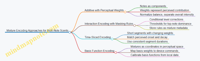
Additive Mixture Encoding with Perceptual Weights
A practical starting point is an additive model: represent a mixture as a set of notes, each with a target intensity weight. Instead of treating weights as chemical concentration, treat them as perceptual contribution. You can implement this by calibrating each note’s “effective intensity” in your playback hardware.
Example: Suppose you want a “citrus-wood” blend with notes A (citrus) and B (cedar). You might store a mixture as:
- Citrus note weight: 0.7
- Cedar note weight: 0.3
During encoding, you convert weights into device commands using each note’s calibrated output curve. If citrus tends to dominate at low levels, the calibration will naturally reduce the cedar’s command level so the perceived balance stays stable.
Best practice: keep the weights normalized (sum to 1) for authoring, then allow a separate “overall intensity” scalar for the whole mixture. This prevents authors from accidentally changing balance when they only meant to change loudness.
Component-Interaction Encoding Using Masking Rules
Mixtures often behave differently because one note can mask another. Masking rules capture this by adjusting note levels when certain combinations occur. The encoding stores both the base note weights and conditional corrections.
Example: In many systems, a strong “top” note can reduce the perceived presence of a “base” note. If you encode a three-note blend—top (A), middle (B), base (C)—you can apply a rule like:
- If A is above a threshold, reduce C by a fixed fraction.
This rule is not about chemistry; it’s about what users perceive in your setup. You can derive thresholds and correction factors from short psychophysical sessions where participants compare blends at different component levels.
Best practice: store masking rules as explicit metadata alongside the mixture. That way, you can reproduce the same behavior even if you later adjust device calibration.
Time-Sliced Mixture Encoding for Sequential Note Emergence
Even when the final mixture is constant, the perceived order matters because notes have different onset and decay characteristics. Time-sliced encoding represents a multi-note scent as a sequence of short segments where component levels change.
Example: For a “fresh laundry” blend, you might want the “clean” note to appear first, then the “soft” note to settle in. Encode it as three segments:
- Segment 1 (0–2 s): high A, low B
- Segment 2 (2–5 s): medium A, medium B
- Segment 3 (5–8 s): low A, higher B
Each segment uses the same mixture notes but different weights. This approach also helps with hardware limitations: if your device can’t deliver a perfect instantaneous mixture, time slicing compensates by matching perceived timing.
Best practice: keep segment durations consistent across mixtures so you can reuse authoring templates and avoid “timing drift” between assets.
Mixture Encoding as Basis Functions
Instead of encoding each note directly, you can encode mixtures using a small set of basis functions that approximate perceptual dimensions. Each mixture is a weighted combination of basis functions, and each basis function maps to device commands.
Example: If you find that your system’s perceptual space is well approximated by two dimensions—“freshness” and “warmth”—you can store mixtures as coordinates in that space. A “citrus-cedar” mixture might be (freshness 0.8, warmth 0.4). Then a mapping layer converts those coordinates into note-level commands.
Best practice: basis functions should be derived from your own calibration data, not assumed from generic odor taxonomies. The mapping layer is only as good as the measurements behind it.
Mind Map: Mixture Encoding Approaches
Example: Three Notes with Balance, Masking, and Timing
Consider notes A (top), B (middle), and C (base). You want a blend that feels balanced at steady state but still shows A early.
- Authoring representation
- Base weights: A 0.55, B 0.30, C 0.15
- Overall intensity: 0.9
- Masking rule: if A > 0.5, reduce C by 20%
- Time slicing
- Segment 1 (0–2 s): A 0.70, B 0.20, C 0.10
- Masking applies: C reduced further by 20%
- Segment 2 (2–5 s): A 0.55, B 0.30, C 0.15
- Masking applies at the threshold
- Segment 3 (5–8 s): A 0.35, B 0.35, C 0.30
- Masking does not apply: A is below threshold
- Device command conversion
- Convert each segment’s perceptual weights into note output levels using each note’s calibrated intensity curve.
- Apply masking corrections before conversion so the device sees the intended perceptual balance.
This structure keeps the blend readable: authors can adjust balance, timing, and masking separately without accidentally changing everything at once.
3.5 Validation Protocols for Encoded Odor Data
Encoded odor data is only useful if it predicts what the user will smell. Validation checks that prediction at three levels: the encoding itself, the translation into device commands, and the perceptual outcome. A good protocol is specific enough to catch errors, but simple enough to run repeatedly.
Define What “Valid” Means
Start by writing acceptance criteria in plain language. For example: “When odor profile A is played at intensity level 2, at least 70% of participants correctly identify it among three options, and the perceived onset time is within ±1.5 seconds of the target.” This turns validation from a vibe into measurable outcomes.
Create a validation matrix with rows for odor profiles and columns for checks. Include:
- Encoding integrity: mixture components, concentrations, and timing fields are present and within allowed ranges.
- Playback integrity: device commands match the encoded profile and timing.
- Perceptual integrity: users perceive the intended odor quality and intensity.
Validate Encoding Integrity with Deterministic Checks
Before any hardware runs, validate the data structure and math.
Use deterministic rules that fail fast:
- Component completeness: every mixture must list all required odorants and their concentration units.
- Range checks: concentrations must be within the library’s calibrated bounds.
- Normalization checks: if the encoding uses relative scaling, confirm the scaling sums correctly.
- Timing checks: onset, duration, and inter-odor gaps must be non-negative and ordered.
Example: If a profile encodes “citrus” as 60% limonene and 40% linalool but the library defines linalool max at 0.8 g/L and the encoding requests 1.2 g/L, the profile fails encoding integrity even if the device could technically output it.
Validate Translation Integrity with Command Audits
Translation integrity ensures the pipeline turns encoded profiles into device actions without silent drift.
Run a command audit by logging the generated device commands and comparing them to expected values derived from the encoding:
- Mixture selection: the same odorants are chosen.
- Flow rates and valve states: values match the encoding-to-device mapping.
- Scheduling: the command timeline aligns with the encoded onset and duration.
- Purge behavior: cross-odor gaps include required purge or dilution steps.
A practical approach is to compute a “command checksum” per profile: a hash of the ordered command list. If the checksum changes after a software update, you investigate before running user tests.
Validate Perceptual Outcomes with Controlled User Tests
Perceptual validation is where encoding earns its keep. Use controlled conditions to reduce noise.
Recommended test structure:
- Use a small set of reference profiles first (e.g., 6 odors) to keep sessions manageable.
- Include both identification and intensity ratings.
- Randomize order and include blanks (no odor) to measure false positives.
- Control ventilation and waiting time between trials so adaptation doesn’t dominate.
Example protocol for one odor profile:
- Present the target odor at three intensity levels (1, 2, 3).
- For each level, run 5 trials with randomized order and 2 blanks.
- Collect: (a) forced-choice identification among three options, (b) intensity rating on a 0–10 scale, (c) onset timing estimate by the participant.
Interpretation rules should be explicit. For instance, if intensity ratings increase monotonically with level for most participants, intensity mapping is behaving. If identification accuracy collapses at level 3, the issue may be saturation, mixture imbalance, or timing mismatch.
Use Similarity Metrics That Match the Task
Different tasks need different metrics.
- For forced-choice identification: use accuracy and confusion matrices to see which odors are mistaken for which.
- For intensity: use correlation with target level and compute mean absolute error.
- For timing: compare onset estimates to target onset and report median error.
A confusion matrix is especially useful because it tells you whether the encoding is “off by a little” or “off by category.” If “lavender” is consistently confused with “eucalyptus,” the encoding likely misrepresents mixture balance rather than just intensity.
Mind Map of Validation Steps
Example: A Validation Run That Catches a Real Error
Suppose a citrus profile passes encoding integrity and command audit, but user identification accuracy is near chance.
You then check perceptual timing. If onset estimates cluster 3–4 seconds late, the issue is likely scheduling: the device commands may be correct, but the pipeline’s synchronization with the VR event is delayed. After adjusting the synchronization offset, identification accuracy improves while intensity ratings remain stable. That outcome narrows the root cause to timing alignment rather than mixture composition.
Document Results for Repeatability
Validation is only as good as its record. For each odor profile and device configuration, store:
- Encoding version and library version
- Calibration date and airflow/room notes
- Command audit logs or checksums
- User test design details and sample counts
- Metrics and pass/fail outcomes
When a profile fails, the documentation should make it clear which layer failed first: encoding integrity, translation integrity, or perceptual outcome. That prevents “fixing everything” and helps the next run be faster and more reliable.
4. From Chemical Inputs to Encoded Smell Profiles
4.1 Mapping Chemical Descriptors to Perceptual Attributes
Chemical descriptors tell you what molecules are present and in what rough conditions, but perception is what the user experiences. Mapping is the translation layer between “what’s in the mixture” and “what the nose reports,” and it has to handle three realities: mixtures interact, intensity is not linear, and people vary.
What “Chemical Descriptor” Means in Practice
A chemical descriptor can be a name (e.g., limonene), a functional class (terpene, aldehyde), a physical property (boiling point, vapor pressure), or a measured concentration. In smell systems, you usually start with a library entry that includes at least one of: odorant identity, volatility-related parameters, and a baseline perceptual profile.
A key design choice is whether your descriptor set is “chemical-first” or “perception-first.” Chemical-first means you store molecules and later infer perception. Perception-first means you store perceptual attributes and later fit chemicals to them. For encoding and playback, chemical-first is common because it supports repeatable preparation and calibration.
What “Perceptual Attribute” Means in Practice
Perceptual attributes are structured descriptions of what users report. Common attribute types include:
- Quality: the category-like feel (citrus, smoky, floral).
- Valence: generally pleasant vs. unpleasant.
- Intensity: how strong it seems.
- Temporal character: fast onset, lingering, or fading.
- Complexity: how many “notes” seem to be present.
Not every attribute is equally measurable. Intensity and quality are usually easiest to operationalize; temporal character requires careful timing control in playback.
The Mapping Pipeline
A practical mapping pipeline turns chemical descriptors into perceptual attributes using a small set of rules and a calibration dataset.
- Normalize the input: convert concentrations to a consistent basis (e.g., relative to a reference odorant) and standardize temperature assumptions.
- Estimate volatility-driven availability: vapor pressure and boiling point influence how much odorant reaches the olfactory receptors during the exposure window.
- Apply perceptual weighting: each odorant contributes to perceptual attributes with weights that are learned or curated.
- Handle mixture interactions: treat interactions as adjustments to weights or as overrides for certain attribute combinations.
- Scale intensity perceptually: apply a non-linear mapping so that doubling concentration does not double perceived strength.
A good sanity check is to test single-odorant playback first. If your mapping cannot predict the perceived quality and intensity of a single component, mixture tuning will be guesswork.
Mind Map: Chemical to Perceptual Translation
Example: Citrus Mixture with Two Odorants
Suppose your library includes limonene and linalool. Chemical descriptors might include: limonene as a terpene with relatively high volatility, and linalool as a terpene alcohol with different vapor behavior.
A simple mapping approach could look like this:
- Quality mapping: limonene strongly supports “citrus,” while linalool supports “floral/woody” and adds complexity.
- Intensity mapping: both contribute, but limonene’s higher volatility increases early intensity. Linalool may contribute more to later persistence.
- Mixture interaction: the combination might shift perceived quality from “pure citrus” toward “citrus-floral.” In practice, you implement this as a small adjustment to the quality weights when both odorants are present.
Concrete outcome: if limonene alone is rated as “citrus, medium intensity,” and linalool alone is “floral, low-to-medium intensity,” the mixture should land in “citrus-floral, medium intensity with longer decay.” If your playback produces “citrus only” or “too strong too fast,” the issue is likely in volatility availability estimation or intensity scaling.
Example: Smoke-Like Notes Without Overfitting
Smoke-like perception often comes from multiple chemical contributors rather than one dominant odorant. If you map every chemical to a separate quality label, you risk overfitting to a specific dataset.
A better strategy is to define a small set of perceptual attributes and constrain mapping:
- Use quality categories that are stable across users (e.g., smoky, burnt, woody).
- Use intensity scaling that is non-linear and calibrated.
- Treat “complexity” as a derived attribute from the number of active odorants and their relative weights.
Then, when you test a new mixture, you verify that predicted quality shifts are plausible without requiring a new rule for every pair.
Practical Rules That Prevent Common Mistakes
- Don’t assume linearity: perceived intensity typically follows a compressive curve.
- Separate availability from contribution: volatility affects how much reaches receptors; contribution affects what that odorant “means.”
- Calibrate with the same timing model you will play back: if your mapping assumes a certain onset window, playback timing must match.
- Keep interaction rules minimal: start with pairwise adjustments, then expand only when tests show systematic errors.
When mapping is done carefully, chemical descriptors become usable inputs rather than trivia. The goal is not perfect prediction for every user and every environment; it’s consistent, explainable translation that supports repeatable encoding and playback.
4.2 Selecting and Characterizing Odorants for Libraries
A smell library is only as useful as the odorants it contains and the way those odorants are characterized. “Selecting” means choosing compounds that can be delivered reliably by your hardware and that map to perceptual targets users can actually distinguish. “Characterizing” means measuring enough properties to reproduce the same perceptual outcome across sessions, devices, and mixture contexts.
Selecting Odorants with Delivery in Mind
Start with delivery constraints before you think about scent aesthetics. Many odorants differ in how easily they vaporize, how strongly they adsorb to surfaces, and how stubbornly they linger in tubing. If your system uses cartridges and a carrier airflow, prefer odorants with stable volatility under your operating temperature range. If your system uses heated elements, verify that the odorant does not decompose or produce off-notes at the required temperatures.
A practical selection checklist:
- Physical stability: Does the odorant remain consistent over storage time and repeated heating or pumping?
- Chemical compatibility: Does it react with tubing materials, seals, or cleaning agents?
- Adsorption behavior: Does it stick to surfaces and cause ghosting in later scenes?
- Safety profile: Is it manageable within your exposure controls and documentation workflow?
- Perceptual usefulness: Can it support the perceptual goals of your application (e.g., “fresh,” “smoky,” “citrus”) with enough discriminability?
Example: Suppose you want a “laundry fresh” note. You might choose a blend dominated by a moderately volatile aldehyde-like component plus a supporting ester-like component. If the dominant component adsorbs heavily to plastic tubing, you will see carryover after short scenes. In that case, you either switch to a less adsorptive odorant or you redesign the delivery path and cleaning routine.
Characterizing Odorants for Repeatable Playback
Characterization should capture both device-relevant properties and perception-relevant properties.
Device-relevant properties include:
- Volatility and emission rate: How quickly the odorant reaches a usable concentration after activation.
- Thermal sensitivity: How output changes with temperature or heater duty cycle.
- Flow dependence: How the emitted concentration scales with airflow and mixing chamber conditions.
- Surface interactions: How quickly the system clears after ejection.
Perception-relevant properties include:
- Odor quality descriptors: A small set of consistent labels that trained panelists can agree on.
- Intensity scaling: How perceived strength changes with concentration.
- Detection and discrimination thresholds: The concentration range where users can reliably notice and differentiate it.
- Mixture behavior: Whether it suppresses, enhances, or blends with other components.
A useful way to organize characterization is to define a reference operating point for each odorant: a specific command setting (or cartridge state), an airflow regime, and a timing profile. Then you measure output and perception at that reference point and at one or two nearby levels.
Building a Library Taxonomy
Libraries work better when odorants are grouped by how they behave in mixtures and how they are likely to be used.
- Anchor notes: Components that define the main identity and are stable across sessions.
- Support notes: Components that add nuance but can be swapped with minimal perceptual change.
- Accent notes: Low-concentration components used for short-lived effects (e.g., “smoke edge,” “mint snap”).
- Background notes: Components intended to persist or fill gaps during longer scenes.
Example: For a “forest after rain” scene, you might treat “earthy” as an anchor note, “green” as a support note, and “cool” as an accent note. During authoring, you can keep the anchor fixed while adjusting support and accent levels to match the scene’s timing without rewriting the entire mixture.
Mind Map: Odorant Selection and Characterization
Example: Turning a Candidate Odorant into a Library Entry
- Pick a candidate based on your target descriptor and delivery feasibility.
- Define a reference operating point: e.g., command level 60%, airflow 1.2 L/min, 800 ms ejection, 200 ms mixing.
- Measure emission behavior: record onset time, relative output consistency across five trials, and clearance time.
- Measure perception: collect intensity ratings at three concentrations around the reference point and record a short descriptor set.
- Test mixture behavior: combine the candidate with one likely partner odorant at two ratios and note whether the identity stays stable or shifts.
- Document constraints: include warnings like “high carryover in short scenes” or “intensity saturates quickly,” so authors can use it correctly.
A library entry that omits clearance time is like a recipe that lists ingredients but not cooking duration. The smell might be “right,” but it will show up in the wrong place and the wrong moment.
4.3 Handling Solvents, Carriers, and Contaminants
Solvents and carriers are the “transport layer” for odorants: they help deliver molecules to the air stream at a controlled rate. Contaminants are the “uninvited guests” that ride along and change what users perceive. In digital scent systems, these details matter because odor perception is sensitive to both concentration and mixture composition, and because hardware surfaces can quietly accumulate residues.
Solvents and Carriers: What They Do in Practice
A solvent is a liquid that dissolves or disperses odorants so they can be metered reliably. A carrier is the medium that carries odorant molecules into the airflow path during playback. In many systems, the carrier is effectively the air plus any vaporized fraction from the liquid reservoir.
A practical example: suppose you want a “fresh citrus” note. If you dissolve the citrus odorant in a solvent with high volatility, more of the solvent evaporates quickly, which can shift the initial smell toward a sharp, solvent-like top note. If you choose a lower-volatility solvent, the citrus note may rise more slowly and feel smoother, but it may also reduce peak intensity if the delivery system cannot vaporize enough odorant.
Key handling goals:
- Stable dosing: the odorant concentration in the reservoir should remain consistent over time.
- Predictable vaporization: the fraction that becomes airborne should be repeatable.
- Low residue formation: surfaces should not build sticky films that later release “ghost notes.”
Contaminants: Where They Come From
Contaminants enter through three common routes.
-
Cross-contamination from shared hardware If the same nozzle, mixing chamber, or tubing is used for multiple odorants, residual vapor can remain after playback. Even a small amount can matter because odorants often have low detection thresholds.
-
Impurities in materials Cartridges, tubing, seals, and even cleaning wipes can contain trace fragrances or plasticizers. These can leach into the airflow, especially when heated or repeatedly cycled.
-
Residual solvent effects Solvents can leave behind non-volatile residues. Later, when the system heats or flushes, those residues can re-evaporate and blend with the next odor.
A concrete example: you run “lavender” followed by “peppermint.” If lavender uses a solvent that leaves a faint film, the first seconds of peppermint may include a muted floral undertone. Users may not name it, but they will notice that the transition feels “off.”
Mind Map: Solvents, Carriers, and Contaminants
Mitigation Strategies That Actually Reduce Errors
1. Choose materials that minimize absorption and odor carryover. Some plastics and elastomers absorb odorants and then release them slowly. For example, if a tubing material absorbs a woody odorant, the next session may start with a background “woodiness” even when you think the system is idle. Using low-absorption materials for the delivery path reduces this memory effect.
2. Separate pathways when you can. If your design allows it, dedicate reservoirs or delivery channels to odor families. Even partial separation can reduce cross-talk. If you cannot fully separate, plan for stronger purge cycles between dissimilar odorants.
3. Use a purge strategy matched to the chemistry. A purge is not just “run air longer.” The purge medium and duration should clear both volatile odorant and any solvent fraction that could leave residue. For instance, if a solvent is mostly volatile, a shorter purge may remove it effectively. If it leaves residue, you may need a cleaning step that targets residue rather than relying on airflow alone.
4. Manage reservoirs to prevent concentration drift. Reservoirs can change composition as the more volatile components evaporate during idle time. A simple example: if you prepare a mixture and leave it for hours, the effective odorant-to-solvent ratio may shift, altering intensity and timing. Keeping reservoir handling consistent—sealed storage, controlled fill timing, and documented replacement intervals—improves repeatability.
5. Verify with quick “transition checks.” Before a full user session, run short transitions between the most common pairs in your content. If “lavender to peppermint” shows a persistent floral tail, you have evidence of residue or cross-contamination. This is faster than waiting for user feedback and gives you a clear target for cleaning or purge adjustments.
Example Workflow for a Two-Odor Sequence
Imagine a VR scene that alternates between “citrus” and “cedar.”
- Pre-run check: run citrus alone for a fixed duration, then stop and wait the system’s standard settle time.
- Transition test: play cedar immediately after citrus with your normal purge.
- Assess: if cedar starts with a citrus top note, increase purge time or adjust cleaning for the delivery path.
- Confirm: repeat the transition test after the change to ensure the fix doesn’t create the reverse problem.
This workflow treats solvents, carriers, and contaminants as measurable contributors to output rather than background assumptions. When you control them, your encoded odor profiles behave more like the ones you authored.
4.4 Building Odor Profiles for Repeatable Playback
Repeatable playback starts with repeatable odor profiles. An odor profile is a structured description of what to emit, when to emit it, and how to reproduce it with the same perceived result across sessions. The goal is not to store “chemicals,” but to store a recipe that survives real-world variation in airflow, device output, and user context.
What an Odor Profile Must Contain
A useful profile includes five layers:
- Identity: a stable name or ID for the target scent.
- Composition: the odorants (or odorant surrogates) and their intended relative amounts.
- Timing: onset, steady duration, and decay behavior.
- Delivery parameters: flow rate targets, mixing strategy, and any device-specific constraints.
- Quality targets: acceptance criteria tied to measurable outputs (for example, flow and ejection timing) and perceptual checks.
A common mistake is treating “composition” as the whole profile. If you only store ratios but ignore timing and delivery parameters, you will get inconsistent intensity and different perceived blends.
Choosing a Profile Granularity
Profiles can be built at different levels:
- Single-note profiles for calibration and debugging.
- Blend profiles for user-facing scents.
- Scene profiles that include multiple emissions and transitions.
For repeatability, start with single-note profiles to establish baseline behavior. Then build blend profiles using those calibrated building blocks. Finally, assemble scene profiles that reuse the same blend profiles rather than re-authoring everything from scratch.
Mind Map: Odor Profile Components
Building Composition with Calibration in Mind
Composition should be expressed in a way that matches how the device actually outputs odorants. If the device uses cartridges with limited resolution, store amounts as device-ready units (for example, “ejection time at calibrated concentration” rather than abstract percentages). This reduces rounding differences between authoring tools and playback firmware.
A practical approach:
- Calibrate each odorant’s output so you can map a control command to an estimated emitted strength.
- Choose relative amounts for the blend based on perceptual balancing tests.
- Convert those relative amounts into device commands using the calibration mapping.
Example: Suppose “citrus” is built from limonene and a small amount of a secondary note. You might decide the secondary note should be subtle. Instead of storing “limonene 90%, secondary 10%,” store “limonene command A, secondary command B,” where A and B are derived from each odorant’s calibrated strength.
Timing: Onset and Decay Are Part of the Blend
Perception changes with time. Two profiles with identical composition can feel different if one ramps up slowly and the other snaps on. For repeatability, define timing as curves or step segments.
A simple timing model uses three segments:
- Onset: ramp from 0 to target output over a fixed time.
- Hold: maintain near-target output for a set duration.
- Decay: stop ejection and allow a controlled purge or natural fade.
Example: For a “coffee” note, you may prefer a slightly slower onset to avoid sharp top notes. That preference becomes a timing choice: onset ramp 1.5 seconds, hold 3 seconds, decay 2 seconds with a defined purge interval.
Delivery Parameters That Prevent Cross-Contamination
Repeatability depends on what happens between emissions. If you reuse the same channels for different odorants, you need a purge strategy that is consistent.
Define:
- Purge duration after each emission.
- Mixing behavior during transitions.
- Minimum separation between two profiles that share odorants.
Example: If “mint” and “vanilla” share a carrier, you can keep the carrier warm and reduce purge time, but you still need a consistent purge for the odorant channels to prevent residual mint from tinting vanilla.
Example: A Repeatable Blend Profile Schema
Odor Profile: Citrus Clean
- Composition
- Limonene: command A (calibrated strength unit)
- Secondary note: command B (subtle balance)
- Timing
- Onset: ramp 1.0s
- Hold: 3.0s
- Decay: 2.0s with purge
- Delivery Parameters
- Flow target: 0.8 L/min
- Mixing chamber: standard setting
- Quality Targets
- Ejection timing tolerance: ±50 ms
- Flow tolerance: ±5%
- Validation
- Baseline perceptual check: pass
- Repeatability check: pass
Mind Map: Validation Workflow
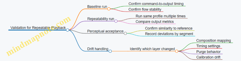
Case Study: Fixing Inconsistent Intensity
A team notices that “citrus clean” feels weaker in later trials. The first check is output timing: if onset and hold durations match, the issue is likely delivery or purge.
They compare purge duration across runs and find the purge was shortened during testing to speed up sessions. That change reduced how fully the previous odorant cleared from the mixing path. The fix is to restore the purge interval and re-run the blend. After that, intensity returns to baseline because the blend starts from the same “clean air” condition each time.
Repeatable odor profiles are built from explicit layers—composition, timing, delivery, and quality targets—then validated as a whole. When you treat transitions and purge as first-class parts of the profile, the system stops behaving like it is guessing.
4.5 Documenting Uncertainty in Chemical-to-Perceptual Mapping
Chemical-to-perceptual mapping rarely behaves like a clean lookup table. The same odorant can smell different across people, concentrations, and contexts because perception depends on physiology, mixture interactions, and delivery timing. Documenting uncertainty is how you keep those differences from turning into silent bugs.
What Uncertainty Means in Practice
In this context, uncertainty is the gap between what your encoding model predicts and what users actually perceive. It shows up as:
- Concentration uncertainty: the delivered vapor concentration may differ from the intended value due to airflow, temperature, and device variability.
- Mixture interaction uncertainty: components can suppress or enhance each other, so the percept of a mixture is not the sum of parts.
- Perceptual mapping uncertainty: the same chemical features can map to different percept labels depending on the person and the label scheme.
- Temporal uncertainty: onset and decay affect detection and identification, especially when scents are short-lived.
A useful documentation goal is not to eliminate uncertainty, but to make it measurable, traceable, and actionable.
Uncertainty Types to Record
Record uncertainty at the level where it originates, so downstream teams know what they can safely adjust.
-
Input uncertainty
- Chemical identity and purity: note if odorants are blends, contain stabilizers, or have batch variability.
- Carrier and solvent: document what fraction is carrier and whether it can contribute its own smell.
-
Model uncertainty
- Mapping method: whether the model is feature-based, rule-based, or derived from sensory panels.
- Confidence basis: how many samples, how consistent the panel was, and how the mapping was calibrated.
-
Output uncertainty
- Predicted percept label stability: whether the model tends to produce the same label across similar inputs.
- Similarity ambiguity: whether the odor is often confused with a neighboring category (e.g., “woody” vs “cedar-like”).
A Documentation Template That Works
Use a structured record per odorant or mixture profile. Keep it short enough to maintain, but explicit enough to debug.
- Profile ID and version
- Chemical composition
- odorants, concentrations or relative ratios, carrier type
- purity notes and batch ID
- Encoding assumptions
- volatility scaling method
- mixture interaction handling (if any)
- Uncertainty summary
- concentration delivery variability range
- percept label confidence or similarity distribution
- temporal assumptions for onset and decay
- Evidence summary
- number of sensory sessions
- participant count and selection criteria
- measurement method for delivery and timing
- Known failure modes
- e.g., “label confusion at low intensity” or “carrier odor dominates at short pulses”
- Mitigations
- e.g., “use longer pulse width” or “apply normalization based on device calibration”
Mind Map: Uncertainty Documentation Flow
Mind Map: Evidence to Confidence
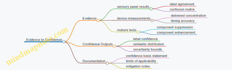
Concrete Example: Citrus Mixture with Label Confusion
Suppose you encode a mixture intended to smell like “lemon peel.” Your mapping model predicts a strong “citrus” label, but sensory tests show frequent confusion between “citrus” and “clean/soapy” at lower intensities.
Document it like this:
- Uncertainty summary
- concentration delivery variability: ±20% around target
- label stability: high at medium intensity, lower at low intensity
- similarity ambiguity: citrus ↔ clean/soapy increases when pulse width is under 0.8 seconds
- Evidence summary
- 3 sensory sessions, 18 participants
- confusion matrix shows citrus predicted as clean/soapy in 35% of low-intensity trials
- Known failure modes
- “short pulses reduce perceived peel character”
- Mitigations
- set minimum pulse width to 1.0 seconds for lemon peel scenes
- avoid using the profile for “subtle background” moments
This turns uncertainty into a design constraint you can apply consistently.
Concrete Example: Single Odorant with Batch Variability
If a single odorant is used as a “rose” note, but different batches vary in purity, the percept can drift. Record the batch ID and purity range, then attach uncertainty to the mapping record.
- Input uncertainty: purity varies between 95–98% across batches
- Model uncertainty: mapping evidence collected on batch A only
- Output uncertainty: label confidence decreases for batches outside the evidence range
- Mitigation: require a quick re-calibration run or restrict the profile to the validated batch range
How Uncertainty Documentation Prevents Bugs
When uncertainty is recorded, teams can set acceptance criteria that match reality. For instance, you can require that a profile meets a percept similarity threshold at the intended intensity and pulse width, rather than assuming the same chemical recipe always yields the same percept. That’s the difference between “it usually works” and “it works for the conditions we documented.”
5. Smell Playback Hardware Architecture
5.1 Odor Ejection Mechanisms and Their Tradeoffs
Odor ejection is the part of a smell system that turns an encoded “what” and “when” into actual molecules leaving a device. The mechanism you choose determines how quickly odor starts, how cleanly it stops, how much it costs to maintain, and how much effort you need to prevent cross-contamination.
Core Mechanism Types
Heated vaporization uses a heat source to push volatile odorants into the airflow. It can produce fast onset for compounds that vaporize readily, but it also risks degrading sensitive chemicals and can leave residue on heater surfaces. A practical tradeoff is that you gain responsiveness while accepting more frequent cleaning and careful material selection.
Air-assisted atomization breaks a liquid mixture into fine droplets and carries them out with airflow. Droplet size matters: smaller droplets evaporate faster, which can improve perceived timing, but they also increase the chance of clogging and require robust filtration and maintenance. If your odorant mixture includes heavier components, atomization may produce a slower, thicker “tail” unless you tune airflow and mixing.
Direct liquid injection dispenses a controlled amount of liquid into a mixing chamber, where it evaporates or entrains into the airstream. This can be easier to calibrate by volume, but it often creates longer persistence because evaporation continues after ejection stops. It’s a good fit when you can tolerate a decay curve rather than needing a sharp cutoff.
Solid cartridge sublimation releases odorants from a solid or porous medium. It can be mechanically simple and reduce liquid handling, yet it tends to have slower ramp-up and ramp-down because mass transfer is limited by surface area and diffusion. Cartridge systems also make it easier to swap odor “assets,” but you still need to manage how fully the cartridge clears between uses.
Membrane or microfluidic dispensing uses small channels or membranes to meter tiny quantities. This can improve repeatability and reduce waste, but it increases sensitivity to viscosity changes, particulate contamination, and manufacturing tolerances. In practice, it rewards disciplined cleaning and consistent odorant preparation.
Tradeoffs That Matter in Real Systems
Onset sharpness vs. persistence. Users notice when smell appears, but they also notice when it refuses to leave. Heated vaporization and atomization often give sharper onset; direct injection and sublimation often extend persistence.
Cross-contamination vs. cleaning burden. If the mechanism leaves residue, the next odor may inherit a faint “ghost.” Systems with more residue-prone components usually require more frequent purging cycles or physical cleaning.
Control granularity vs. complexity. Microfluidic and membrane approaches can meter precisely, but they add failure modes like clogging. Simpler mechanisms may be easier to repair, yet they can be harder to tune to consistent output.
Energy and thermal management. Heating-based methods need temperature control to avoid drift. Thermal gradients can also affect airflow mixing, which changes perceived intensity even when the command signal is identical.
Mind Map: Mechanism Selection Drivers
Example Scenarios with Mechanism Fit
Example: “Coffee” cue in a short VR scene. If the scene needs the smell to appear quickly when the player opens a cup and then fade before the next location, heated vaporization or well-tuned atomization is often the better starting point. You still need a purge strategy, but the mechanism’s ability to stop producing vapor sooner helps keep the timeline believable.
Example: “Rain on pavement” with a lingering ambience. If the experience benefits from a smell that stays present for several seconds, direct liquid injection or sublimation can work well because the evaporation tail becomes part of the intended effect. The key is to calibrate the decay curve so the persistence matches the scene pacing.
Example: Alternating “lemon” and “pine” in rapid succession. Cross-contamination becomes the main constraint. Mechanisms that leave less residue and can be purged effectively are favored. If you must use a residue-prone approach, you compensate with stronger cleaning intervals and conservative scheduling so the system has time to clear.
Practical Selection Checklist
- Decide whether you need a sharp cutoff or a controlled decay.
- Identify odorant volatility and sensitivity to heat or shear.
- Estimate maintenance tolerance for your deployment context.
- Plan for purging and verify that the next odor starts clean.
- Choose a mechanism whose failure modes you can detect and recover from during normal operation.
A good mechanism is the one that matches your timing requirements and your odor chemistry, not the one that looks simplest on a diagram. The tradeoffs are predictable once you map them to onset, persistence, and contamination behavior.
5.2 Airflow, Mixing Chambers, and Delivery Path Design
Airflow is the part of a smell system that behaves like physics, not like software. If you treat it as a controllable “volume knob,” you’ll get inconsistent results. If you treat it as a flow network with measurable losses, you can design for repeatability.
Airflow Goals and Constraints
A practical delivery system usually needs three things at once: (1) fast onset, (2) predictable intensity, and (3) clean separation between odor events. Onset depends on how quickly odor molecules reach the user’s nose. Intensity depends on how much odor-laden air is delivered and for how long. Separation depends on how quickly the delivery path clears.
The main constraints are pressure limits, turbulence, and condensation. Many odorants are carried by a carrier gas or air stream; if the path cools below the odorant’s effective volatility range, you can get residue that later “leaks” into the next event. Even when you don’t see visible residue, you can still get memory effects.
Mixing Chamber Design
A mixing chamber’s job is to turn a controlled amount of odorant into a stable gas mixture before it enters the delivery path. The chamber should reduce sensitivity to small changes in ejection timing.
Key design choices:
- Mixing method: Static mixing elements (simple baffles) encourage laminar-to-turbulent transition without moving parts. Moving fans can improve mixing but add vibration and extra control variables.
- Residence time: Too short and the mixture is uneven; too long and you add delay. A good target is the shortest time that still yields consistent concentration at the chamber outlet.
- Geometry: A chamber with a short, wide section can reduce pressure drop but may create dead zones. Dead zones act like storage, releasing odor later.
- Surface materials: Smooth, non-porous internal surfaces reduce adsorption. Porous materials can “store” odorant molecules and slowly release them.
A simple way to reason about chamber performance is to treat it as a concentration filter. If your ejection produces a concentration pulse, the chamber should output a pulse with a similar shape every time, just scaled to the requested intensity.
Delivery Path Design
The delivery path connects the mixing chamber to the user. It should minimize losses and avoid unpredictable flow behavior.
Design priorities:
- Minimize bends and sudden expansions: Sharp turns can create recirculation pockets that trap odorant.
- Keep tubing length consistent: If you change length, you change delay and clearing time.
- Control cross-sectional area: Narrow sections increase pressure sensitivity and can amplify small flow errors.
- Avoid leaks and unintended mixing: Any gap between the intended flow and the surrounding air becomes a dilution path.
A useful mental model is a “flow highway” with toll booths. Each restriction (tube bends, valves, filters) costs pressure and adds delay. If you know the costs, you can compensate by adjusting ejection duration or flow rate.
Flow Control and Feedback
Even with good hardware, airflow varies with temperature, filter loading, and user movement. Add feedback where it matters: measure flow rate near the chamber outlet or in the delivery path upstream of the user.
Practical feedback strategy:
- Calibrate at a known flow: Record the relationship between commanded intensity and measured flow.
- Use flow as the primary control variable: Keep concentration changes tied to a stable flow profile.
- Detect abnormal clearing: If the system fails to return to baseline quickly, treat it as a contamination or clogging condition.
Example: Designing for Fast Onset and Clean Clearing
Suppose you want a “coffee” cue that should start within ~300 ms and stop without lingering.
- Use a mixing chamber with short residence time and smooth interior surfaces.
- Choose a delivery path with minimal bends and a fixed length.
- Implement a two-phase command: first, run odorant ejection while maintaining a steady flow; second, switch to a purge-only phase using the same flow rate.
Concrete check: after each event, measure baseline odor sensor output (or a proxy like VOC concentration) at a fixed sampling point in the path. If baseline recovery is slow, reduce residence time, shorten the path, or improve purge routing.
Example: Preventing Cross-Contamination Between Odors
If you alternate between “lemon” and “smoke,” cross-contamination often comes from residue in dead zones.
- Remove or redesign any low-flow regions in the chamber outlet.
- Ensure valves fully seal and that purge air routes through the same path the odor used.
- Use a purge phase long enough to clear the delivery path volume, not just the chamber.
A quick calculation: delivery path volume equals cross-sectional area times length. Purge time should be long enough to exchange that volume several times, accounting for mixing inefficiency.
Mind Map: Airflow, Mixing, and Delivery Path
Design Checklist for Implementation
- Chamber outlet concentration is consistent for repeated ejections at the same flow.
- Delivery path has no obvious dead zones or hard-to-purge segments.
- Purge clears the path volume, not just the chamber.
- Flow measurement is placed where it reflects what the user receives.
- Baseline recovery time is stable across odor types.
When these conditions hold, airflow stops being a source of mystery and becomes a predictable part of the smell rendering pipeline.
5.3 Sensor Integration for Flow, Temperature, and Feedback
Smell playback is a control problem disguised as a hardware problem. Sensors turn “we fired the pump” into “we delivered the right amount at the right time, with the right conditions.” The goal is not perfect chemistry; it’s repeatable delivery that matches the encoded timeline.
What You Measure and Why
Flow sensors answer: did the system actually move air through the mixing chamber and out to the user path? Without flow measurement, a partially clogged nozzle can look identical to a correctly working one from the software side.
Temperature sensors answer: did the carrier air and/or odor mixture stay within the range that your calibration assumes? Temperature shifts change volatility and can alter how quickly the odor reaches the user.
Feedback answers: did the device behave as expected during the last command? Feedback can include pressure, valve state confirmation, fan tachometer readings, or odor output proxies like optical/ionization sensors where available.
A practical rule: measure the variables that most strongly affect delivery timing and concentration, then add redundancy for the failure modes you see most often.
Sensor Placement That Actually Helps
Place flow sensing where it represents the air that will carry odor to the outlet. A common mistake is measuring flow at the pump inlet while the mixing chamber has its own restrictions.
Temperature sensing should be near the mixing chamber outlet or in the delivery duct close to where the user-facing air stream forms. If you measure temperature only at the reservoir, you’ll miss the heating or cooling that happens during mixing.
Feedback signals should confirm the actuators you rely on: valve open/closed, pump running, fan speed, and any purge cycle completion. If you only measure “system on,” you can’t distinguish a stuck valve from a software timing issue.
Signal Conditioning and Timing Alignment
Sensors produce noisy signals and different latencies. Flow sensors might update at 100 Hz, temperature at 10 Hz, and valve state changes are effectively event-based. Your control logic needs a common timeline.
Use a timestamped data pipeline: every sensor sample gets a time tag from the same clock domain as your playback scheduler. Then resample or interpolate to the scheduler’s control step.
Also filter carefully. A moving average on flow can hide short delivery failures; a median filter can reduce spikes without erasing step changes. The key is to filter for noise, not for convenience.
Control Loop Structure for Smell Delivery
A simple architecture works well:
- Pre-check: verify airflow path is clear and fan/pump are within expected ranges.
- Ramp: bring flow to target and stabilize temperature.
- Pulse: open odor valves for the commanded duration while monitoring flow and temperature.
- Purge: clear the path using a known purge profile.
- Post-check: confirm actuators returned to safe states and flow dropped as expected.
If any step fails, the system should stop the current odor event and either retry with a corrected purge or mark the event as failed for that session.
Mind Map: Sensor Integration
Example: Calibrated Pulse with Flow and Temperature Guardrails
Assume your calibration says a “citrus burst” requires:
- Target flow: 2.0 L/min at the outlet
- Temperature window: 30–35°C during the pulse
- Pulse duration: 400 ms
During playback, the controller:
- Starts the fan and waits until flow is within ±10% of 2.0 L/min.
- Waits until temperature enters 30–35°C, but caps the wait at 250 ms to avoid stalling the VR timeline.
- Opens the odor valve for 400 ms.
- Monitors flow for dropouts; if flow falls below 1.6 L/min mid-pulse, it ends the pulse early and triggers a purge.
This approach prevents a common failure: the valve opens correctly, but the airflow collapses due to a partial blockage, leading to a weak or delayed smell.
Example: Feedback-Driven Valve Fault Detection
A valve command says “open for 100 ms.” The feedback channel reports valve current or a limit switch state.
- If the valve state does not change within 30 ms, the system flags a stuck valve.
- If the valve closes late, the system flags a leaky valve and uses a longer purge to reduce cross-contamination.
Because the feedback is tied to the actuator, you can diagnose faults without guessing whether the issue is software timing, wiring, or mechanical wear.
Diagram: Sensor-Guided Playback Flow
    flowchart TD
  A[Start odor event] --> B[Pre-check sensors]
  B -->|Flow/Temp OK| C[Ramp to targets]
  B -->|Not OK| X[Abort and log]
  C --> D[Stabilize temperature]
  D --> E[Pulse odor valves]
  E --> F{Flow stable during pulse?}
  F -->|Yes| G[Purge cycle]
  F -->|No| H[Early stop and purge]
  G --> I[Post-check actuators]
  H --> I
  I --> J[Mark success or failure]
  J --> K[Return to idle]
Practical Integration Checklist
- Use outlet-representative flow measurement, not inlet-only.
- Place temperature sensing where mixing and delivery conditions form.
- Confirm actuator state with feedback, not just command issuance.
- Timestamp everything to the same scheduler clock.
- Filter noise without smoothing away step changes.
- Define explicit abort and purge behaviors for sensor out-of-range events.
When these pieces are in place, sensor integration stops being “extra instrumentation” and becomes the mechanism that makes odor playback dependable.
5.4 Cartridge, Reservoir, and Refill System Considerations
A smell system is only as repeatable as its fluid handling. Cartridges and reservoirs decide how consistently odorants reach the ejection stage, how quickly the system recovers after a change, and how safely operators can refill without cross-contaminating notes.
Cartridge Selection and Layout
Cartridges are typically small, sealed odorant containers paired with a delivery interface. Choose a cartridge format that matches your odor library size and change frequency.
Key considerations:
- Seal integrity and vapor loss: Many odorants are volatile, so cartridges should minimize headspace and use materials compatible with the odorants. If you notice gradual intensity drop over days, it’s often a sealing or material issue.
- Wetting and flow behavior: Some odorants cling to surfaces, causing delayed onset. A cartridge design that promotes consistent wetting of the delivery path reduces “first puff is weak” problems.
- Mechanical coupling repeatability: The cartridge-to-device connection should align reliably so the same internal volume and flow path are used each time. A loose fit can create variable mixing and inconsistent output.
Example: A “citrus” cartridge that uses a porous wick can produce a slower onset than a cartridge that feeds a smooth microchannel. If your VR scene expects a sharp burst when a door opens, the wick-based cartridge may require longer precharge or different timing.
Reservoir Sizing and Buffering
Reservoirs act as a buffer between odor storage and the ejection hardware. They help stabilize flow during rapid scene changes.
Key considerations:
- Buffer volume vs. response time: Larger reservoirs reduce refill frequency but increase the time constant for changes. Smaller reservoirs respond faster but run out sooner.
- Thermal stability: Reservoir temperature affects vapor pressure and thus output intensity. If your device sits near a heat source, the same command can yield different results.
- Mixing uniformity: If the reservoir contains multiple odorants or carrier mixtures, ensure the system avoids stratification. Even simple agitation or circulation logic can improve consistency.
Example: In a mixed reality museum guide, you may trigger “paper” and “ink” smells in quick succession. A reservoir that’s too small forces frequent refills and can interrupt playback, while an oversized reservoir can blur the boundary between notes unless timing is tuned.
Refill Workflow and Cross-Contamination Control
Refilling is where many systems lose consistency. The goal is to keep each odorant note isolated and to ensure the same fill procedure produces the same output.
Key considerations:
- Dedicated cartridges or strict cleaning: If you reuse cartridges, you need a cleaning and purge procedure that removes prior odor residues. For many odorants, “rinse and hope” is not enough.
- Purge strategy: Purging should clear the delivery path and mixing chamber, not just the cartridge. Track purge duration and airflow conditions as part of the procedure.
- Labeling and lot tracking: Record odorant batch, fill date, and cartridge ID. This makes it possible to diagnose whether a change in performance comes from the odorant itself or from the device.
- Operator steps that reduce mistakes: Use keyed cartridge shapes or color-coded interfaces so the wrong cartridge cannot be inserted. Human error is predictable; design around it.
Example: Suppose you refill a “forest” cartridge after “smoke.” Even if the smoke seems gone, trace residues can shift the perceived mixture. A purge that targets the mixing chamber and a short “burn-in” sequence before the next session can prevent the first minutes from being misleading.
Compatibility and Materials
Cartridges, tubing, seals, and adhesives must be compatible with both odorants and carriers.
Key considerations:
- Absorption and swelling: Some plastics absorb odorants, reducing available concentration and increasing variability over time.
- Seal chemistry: Elastomers can react with certain compounds, changing flow resistance and causing leaks.
- Outgassing: Materials that outgas can add background odor that becomes noticeable when the intended smell is subtle.
Example: A system that uses a soft silicone seal might work well for one odorant family but show slower onset for another because the seal absorbs the more hydrophobic component.
Monitoring, Maintenance, and Failure Modes
A refill system should detect problems early and guide maintenance.
Key considerations:
- Leak detection and pressure/flow feedback: If the system can measure flow rate or pressure drop, it can flag clogged paths or partial cartridge seating.
- Clogging and residue buildup: Over time, odorants can leave residues that narrow channels. Maintenance intervals should be based on observed performance drift, not just calendar time.
- End-of-life behavior: Define what “empty” means. Some cartridges stop abruptly; others degrade gradually. Knowing the pattern helps you schedule refills without ruining a session.
Example: If a cartridge’s output gradually weakens, you can schedule a refill after a threshold is crossed. If it stops abruptly, you need a conservative refill margin or a backup cartridge.
Mind Map: Cartridge, Reservoir, and Refill System Considerations
Example: A Practical Cartridge Refill Checklist
Use a repeatable checklist so the system behaves the same after every refill.
- Verify cartridge ID and odorant lot.
- Confirm cartridge seating alignment using the same insertion force.
- Fill to a documented level or volume.
- Run the purge sequence that clears the mixing chamber.
- Perform a short verification playback at a fixed intensity and timing.
- Record results and any deviations in a session log.
This checklist prevents the two most common issues: silent cross-contamination and “it worked yesterday” variability caused by inconsistent purge or fill steps.
5.5 Calibration Workflow for Consistent Output
Consistent smell output is mostly about controlling three things: what you command, what the device actually emits, and how you verify it. Calibration turns those three into a repeatable routine rather than a one-time “it seems close enough” moment.
Calibration Goals and What to Measure
Start by deciding what “consistent” means for your system. For many VR projects, consistency is less about matching a chemical concentration and more about producing the same perceived intensity and timing across sessions.
Measure these outputs:
- Onset time: time from command to first detectable odor.
- Peak intensity: relative strength at the top of the pulse.
- Decay curve: how quickly the odor fades.
- Carryover: how much remains when the next odor should start.
- Mixture stability: whether multi-odor profiles keep their balance.
A practical trick: pick one “reference odor” per device channel (or per cartridge) and treat it as your calibration anchor.
Mind Map: Calibration Workflow
Step 1: Prepare a Stable Test Environment
Calibration is sensitive to airflow and temperature. Before you measure anything, standardize the conditions you can control: keep the delivery path clear, use the same ventilation state, and avoid running other odor tests in parallel.
If your system has a mixing chamber, ensure it is at the same operating state each time. For example, if the device warms up to a steady fan speed, wait for that steady state before starting the first pulse.
Step 2: Run a Baseline Single-Pulse Test
Choose a reference odor and command a short pulse at a known setting. Record:
- the command timestamp,
- the device telemetry (fan speed, valve open time, heater state if present),
- and an output proxy.
An output proxy can be a gas sensor, a photoionization detector, or a consistent measurement method your team trusts. If you only have human detection, you can still calibrate, but you’ll need tighter protocols and more repetitions.
Example: Command a 500 ms pulse at “level 3” and measure onset at 1.2 s, peak at 2.0 s, and return near baseline by 6.5 s. Those numbers become your first baseline.
Step 3: Build Command-to-Output Response Curves
Repeat the baseline test at multiple command levels (for instance, levels 1 through 5). For each level, extract onset, peak, and decay metrics.
Then create a simple mapping from desired intensity to command level. Keep it practical: a piecewise linear mapping is often enough.
Example mapping rule:
- If you want ~70% of reference peak, use level 4.
- If you want ~40%, use level 2.
The key is that the mapping is derived from your device’s behavior, not from assumptions about chemistry.
Step 4: Set Timing Parameters for VR Synchronization
Your VR app needs a predictable relationship between an event and the odor reaching the user.
Compute a command offset:
- If onset consistently occurs 1.2 s after command, and your VR event time is when the user should perceive the smell, then schedule the command 1.2 s earlier.
Next, set pulse duration and inter-odor delays using decay curves:
- If the odor fades to near baseline by 6.5 s, and you need a clean transition at 7.0 s, schedule the next odor no earlier than 6.5 s plus a safety margin.
Example: If you trigger odor A at t=0 and odor B at t=8.0, and A’s carryover is unacceptable when B starts before 7.2 s, then enforce a minimum delay of 7.2 s between A command and B command.
Step 5: Validate Repeatability Across Sessions
Run the reference odor at the same desired intensity in a new session (different day, same device state). Compare:
- onset difference (e.g., within ±0.2 s),
- peak difference (e.g., within ±10% of reference peak),
- carryover (e.g., sensor baseline within a threshold).
If repeatability fails, don’t immediately change the mapping. First check operational differences: reservoir fill level, purge duration, fan speed calibration, or whether the device was allowed to reach steady state.
Step 6: Calibrate Mixtures Without Guessing
Mixtures are where “it sort of works” usually breaks. A reliable approach is component-first calibration.
- Calibrate each component odor to a target intensity using the response curves.
- Define mixture scaling rules that preserve balance.
- Validate the mixture with a dedicated test pulse.
Example: If component X at level 3 gives 60% intensity and component Y at level 2 gives 50%, and your mixture target is “X-dominant,” you might start with X at level 3 and Y at level 1. Then verify whether the balance matches your intended perceptual profile using your output proxy and, if needed, controlled user checks.
Step 7: Lock, Version, and Document the Calibration
Store calibration parameters with a version identifier and tie them to device settings. A calibration that silently changes because someone updated a firmware parameter is the kind of bug that wastes weeks.
Document at minimum:
- reference odor identity and batch (if applicable),
- command-to-output mapping parameters,
- timing offsets and minimum delays,
- mixture scaling rules,
- acceptance thresholds for onset, peak, decay, and carryover.
A good calibration record lets you answer one question quickly: “If the smell timing feels off today, which parameter changed?”
Practical Acceptance Checklist
Before you call calibration “done,” verify:
- reference odor produces the same onset and peak within thresholds,
- decay reaches baseline before the next scheduled odor,
- carryover stays below your defined limit,
- mixture balance matches the intended profile for at least one representative mixture.
If any item fails, adjust the specific parameter that controls it—timing offsets for onset, pulse duration for decay, purge delay for carryover, and mixture scaling for balance.
6. Encoding-to-Playback Translation Pipelines
6.1 Defining an End-to-End Smell Rendering Pipeline
An end-to-end smell rendering pipeline turns an authored “smell event” into timed odor output that a user can perceive in the right place and at the right intensity. The pipeline is easiest to reason about when you treat it like a conveyor belt with explicit handoffs: authoring, encoding, scheduling, device translation, delivery, and verification.
Pipeline Goals and Non-Goals
Goals
- Keep smell timing aligned with VR events (onset, peak, and decay).
- Produce consistent output across sessions by using calibration data.
- Prevent unintended mixing by controlling sequencing and purge behavior.
- Support spatial rendering by mapping head/hand pose to delivery parameters.
Non-Goals
- Perfect chemical fidelity to every real-world odor molecule.
- Instantaneous changes at arbitrary times without physical constraints.
End-to-End Stages
Smell Event Authoring
A smell event is a structured record created by the experience designer or toolchain. It includes the odor asset identifier, intended start time, duration or envelope, and optional spatial anchors (e.g., “near the left hand”).
Example: A cooking scene triggers “garlic_brown_sauce” at 12.0s for 3.5s with a “near mouth” anchor so the user perceives it as coming from the tasting moment.
Odor Asset Selection and Encoding
The odor asset maps to an encoded smell profile: a mixture recipe (odorants), concentration targets, and a perceptual envelope model. Encoding should also include device-agnostic parameters like relative intensity steps.
Example: “garlic_brown_sauce” is encoded as three odorants with a concentration ratio and an intensity curve that ramps to 70% peak by 1.2s, then decays.
Scheduling and Synchronization
The scheduler converts event time into device-ready timing. It accounts for known device latency (ejection delay), minimum pulse widths, and any required purge time between mixtures.
Example: If the device needs 250 ms to reach stable output, a 12.0s authored onset becomes 11.75s for the ejection command so the perceptual onset lands at 12.0s.
Spatial Rendering Parameterization
Spatial rendering turns pose into delivery parameters. A common approach is to compute a target direction and intensity scaling based on distance and occlusion heuristics, then translate that into airflow routing or mixing chamber settings.
Example: When the user turns their head away, the system reduces intensity by 30% and shifts routing to the nearest outlet to keep the perceived source direction plausible.
Translation into Device Commands
This stage converts encoded profiles into concrete commands: which reservoirs to open, for how long, with what mixing airflow, and in what order. It also enforces safety constraints like maximum total output per minute.
Example: For a three-odorant mixture, the command sequence might open odorant A for 600 ms, then B and C in a controlled overlap window to reduce cross-contamination.
Odor Delivery and Control Loop
The delivery controller runs the commands and monitors feedback signals such as flow rate and temperature. If feedback deviates beyond tolerance, it can adjust subsequent pulses or abort the remainder of the event.
Example: If flow drops during a long session, the controller shortens later pulses to avoid under-delivery while keeping the envelope shape consistent.
Verification and Logging
Verification checks that the system behaved as intended. It records the commanded parameters, measured feedback, and any corrections. This log becomes the basis for later quality assurance.
Example: After playback, the system flags that the garlic event’s peak was 15% low due to a flow sensor reading, so the next session can apply a normalization factor.
Mind Map: End-to-End Smell Rendering Pipeline
Concrete Example: One Smell Event Through the Pipeline
Scenario: A “fresh coffee” smell triggers when the user picks up a cup.
- Authoring: Event starts at the “grip” timestamp, duration 2.8s, anchor at the cup position.
- Encoding: Asset specifies two odorants with a ratio and an envelope that peaks at 1.0s.
- Scheduling: If ejection delay is 180 ms and minimum pulse is 120 ms, the system schedules the first pulse 180 ms early and splits the envelope into two pulses.
- Spatial Parameterization: Cup is 0.35 m from the face; intensity scales to 0.8 and routing favors the outlet aligned with the cup direction.
- Command Translation: Reservoir A opens for 520 ms, then A+B overlap for 260 ms, then a short purge to prevent lingering.
- Delivery Control: Flow sensor confirms stable output; if flow is low, overlap time is reduced to preserve peak timing.
- Verification: Logs show peak timing within ±50 ms and intensity within ±10% of target.
Practical Design Checks
- Timing budget: List every known delay and minimum constraint so the scheduler can meet the envelope shape.
- Mixture hygiene: Define explicit purge rules between different odor assets, not just between identical ones.
- Pose handling: Decide what happens when tracking is lost—freeze spatial parameters or fall back to a default outlet.
- Observability: Ensure logs capture enough detail to explain mismatches without requiring guesswork.
This pipeline structure keeps smell rendering deterministic where it can be, and measurable where it must be.
6.2 Timing, Scheduling, and Synchronization with VR Events
Smell playback only feels “synchronized” when the timing matches how people perceive cause and effect. In practice, you synchronize three clocks: the VR render clock (frame time), the device command clock (when you tell the odor hardware what to do), and the physical odor clock (when molecules actually reach the user’s nose). This section focuses on making those clocks agree enough that the experience feels intentional.
Timing Targets That Users Actually Notice
Start by choosing what “on time” means for each event type.
- Onset timing: When the odor first becomes detectable after an in-world action. If you trigger at the same frame as the visual event, you may still be late physically.
- Peak timing: When intensity is highest. Peak often matters more for “this is that smell” recognition than for simple presence.
- Duration timing: How long the odor stays above a noticeable threshold. Too short feels like a glitch; too long feels like a lingering mistake.
A practical rule: treat onset and duration as separate parameters in your authoring tools, even if your hardware uses a single ejection window.
Scheduling Strategies for Reliable Playback
A good scheduler prevents two common issues: missed commands (because the frame loop stutters) and overlapping mixtures (because multiple events fire close together).
-
Event queue with timestamps
- Author smell events with a target timestamp relative to the VR timeline.
- Convert those timestamps into device commands using a fixed offset for physical delay.
- Keep a priority queue sorted by target time.
-
Lookahead dispatch
- Instead of sending commands exactly at the target moment, dispatch them slightly early based on measured device latency.
- This reduces sensitivity to frame drops.
-
Resource locking for odor channels
- If your system uses a limited number of valves or reservoirs, treat each channel as a resource.
- When two events want the same channel, decide whether to queue, blend, or cancel based on your design intent.
-
Cross-contamination guardrails
- After a strong odor, enforce a purge or cooldown window before a contrasting odor.
- Scheduling should include these “no-go” intervals so you don’t rely on luck.
Synchronization with Head-Motion and Interaction
Odor placement depends on where the user is looking and moving, but smell delivery has inertia. You can still synchronize well by separating when you eject from where you aim.
- Eject timing: Trigger based on the VR event timeline.
- Aim update timing: Update airflow direction or mixing parameters at a higher rate than ejection, but only within a safe window.
Example: A “coffee steam” interaction.
- Visual: cup lifts at time t = 12.0s.
- Smell onset target: t = 12.4s (includes physical delay).
- Aim updates: every frame from t = 12.2s to t = 12.8s, so the plume follows head motion while the odor is actually traveling.
If you update aim too late, the plume may miss the intended direction even though the odor starts on time.
Handling Frame Jitter and Latency
VR systems can vary frame-to-frame. Your smell scheduler should be robust to that variation.
- Use monotonic time for scheduling so system clock adjustments don’t shift odor timing.
- Measure device latency: the time from “command issued” to “odor begins.” Store it per device and per odor channel if needed.
- Apply a per-event offset: different odorants may have different rise times due to volatility and mixing behavior.
Example: A “rain on pavement” scene.
- You record that the first detectable onset occurs about 250 ms after command for the “wet earth” cartridge.
- During playback, you schedule ejection commands at event_time - 0.25s.
- If the user pauses the scene (time dilation), you pause the smell timeline too, rather than letting smell continue on real time.
Mind Map: Timing and Synchronization Workflow
Example Timeline: Door Opening with Two Smells
Scenario: A door opens, revealing “clean laundry” first, then “fresh paint” after a short delay.
- t = 5.00s: Door begins opening.
- Laundry onset target: t = 5.35s.
- Laundry duration: 1.2s.
- t = 6.10s: Paint smell begins.
- Paint onset target: t = 6.45s.
- Enforce purge window: 0.3s between laundry end and paint start.
Scheduling outcome:
- Laundry command is issued at 5.35s - laundry_latency.
- Paint command is issued at 6.45s - paint_latency.
- If the user reopens the door quickly, the scheduler uses the overlap policy: cancel paint if laundry is still active, because mixing would create an unintended “laundry-paint” hybrid.
Practical Checklist for Authoring and Runtime
- Author onset and duration separately.
- Use a monotonic timeline and a device-latency offset.
- Dispatch with lookahead to survive frame jitter.
- Lock odor channels and enforce purge windows.
- Update aim during a defined window, not indefinitely.
- Test with real head motion, not just stationary playback.
6.3 Converting Encoded Profiles into Device Commands
An encoded odor profile is only useful once it becomes a concrete set of device actions: which odorant(s) to release, when to release them, how long to run the actuator, and how to manage airflow so the user receives the intended mixture at the intended time. This section focuses on the translation step between “what the experience wants” and “what the hardware can do.”
Command Translation Goals
The conversion layer should satisfy four practical goals.
- Determinism: the same encoded profile should produce the same command sequence under the same device configuration.
- Timing fidelity: onset and decay should align with VR event timing, not with the device’s internal delays.
- Mixture correctness: the system should avoid accidental cross-contamination and should respect mixture ordering constraints.
- Graceful degradation: if a device cannot produce a requested mixture, it should choose the closest feasible option rather than failing silently.
Input and Output Contracts
Treat conversion as a function with explicit inputs and outputs.
-
Inputs:
- Encoded profile: odor IDs, mixture weights or concentration targets, and timestamps.
- Device capability map: which odorants are supported, maximum flow rates, actuator limits, and mixing chamber behavior.
- Calibration parameters: per-odorant gain curves and timing offsets.
- Session constraints: maximum total output per second, safety limits, and ventilation mode.
-
Outputs:
- A command list:
select odorant,set flow,open valve,close valve,purge,wait, with durations. - A metadata block: expected delivered mixture, confidence, and any substitutions.
- A command list:
Conversion Pipeline
A reliable pipeline usually has five stages.
- Normalize the request: convert mixture weights into device-friendly targets (for example, map “relative intensity” to an absolute dose estimate).
- Quantize to hardware steps: if the device supports only discrete flow levels or valve timing increments, round with a rule that minimizes perceptual error.
- Schedule events: convert profile timestamps into actuator commands using measured timing offsets.
- Plan mixture sequencing: decide whether to blend in the chamber, sequence odorants, or use a pre-mix cartridge strategy.
- Insert purge and safety gaps: add purge intervals when switching odorants or when airflow must stabilize.
Mixture Sequencing Rules
Mixtures can be delivered in at least three ways, and the conversion layer should pick one based on device constraints.
- Parallel blending in a mixing chamber: multiple valves open during the same window. Best when the chamber mixing time is short and stable.
- Sequential dosing: odorants are released one after another with controlled overlap. Best when chamber mixing is slow or when you want to reduce cross-contamination risk.
- Cartridge or reservoir switching: swap a preloaded mixture. Best for fixed mixtures with strict timing needs.
A simple rule set that works well in practice:
- If two odorants share the same reservoir and the device supports simultaneous output, blend in parallel.
- If they require different reservoirs, sequence them with a purge gap sized to the measured carryover.
- If the requested mixture exceeds per-second output limits, scale down all components proportionally and keep the relative ratios.
Mind Map: Command Conversion
Example: Single Note with Timing Offsets
Suppose the encoded profile requests odor OAK at t=2.000s for 0.800s of perceived presence. Calibration shows the valve opening latency is +120ms, and the device needs +60ms to reach target flow.
- Requested onset:
2.000s - Actuator start time:
2.000s - 0.120s - 0.060s = 1.820s - Command duration:
0.800smapped to actuator open time using the per-odorant gain curve (assume linear mapping here for simplicity): open for0.800s
Resulting command sequence (conceptual):
wait until 1.820sset flow to OAK targetopen valve OAKwait 0.800sclose valve OAKoptional purge for 0.200s(only if the next event needs a different odor)
Example: Two-Note Mixture with Substitution
Encoded profile requests ROSE and CITRUS at ratio 70/30 starting at t=5.000s for 1.000s. The device supports simultaneous blending only for ROSE, while CITRUS requires a different reservoir.
Conversion decisions:
- Use sequential dosing: release
ROSEandCITRUSwith overlap limited by reservoir switching. - Apply a purge gap after switching reservoirs. Assume measured carryover requires
0.150spurge. - If
CITRUSis not available in the current cartridge set, substitute with the closest supported citrus-like odorBERGAMOTat the same relative ratio but mark substitution in metadata.
A concrete schedule might look like:
t=4.820s: startROSEdosing (accounting for latency)t=5.300s: switch toCITRUSdosing after purge gapt=5.820s: close valves and begin stabilization purge if the next event differs
The key is that the conversion layer records what it actually did: the delivered mixture is not just “what was requested,” it is “what the device can deliver given constraints,” plus the timing that makes it perceptually align with the VR timeline.
6.4 Managing Mixture Sequencing and Cross-Contamination
Mixture sequencing is the order and timing of odor components you play, while cross-contamination is what happens when remnants of one component leak into the next. In practice, both are the same problem viewed from different angles: you want each note to start cleanly and end cleanly, even though the hardware and air do not reset instantly.
Why Sequencing Matters
Most odor playback systems share a delivery path: a reservoir, a mixing chamber, tubing, and a nozzle or outlet. When you switch from mixture A to mixture B, the air in that path still contains some fraction of A. If you start B immediately, you effectively play a blended “A+B” that the encoding never asked for.
A good sequencing strategy reduces three failure modes:
- Residual carryover: leftover vapor from the previous component.
- Temporal smearing: the onset of the next note ramps up too early or too late.
- Perceptual masking: a strong note dominates and makes weaker notes harder to detect.
Managing Cross-Contamination with Practical Rules
Use these rules as defaults, then tune with calibration.
-
Group by volatility and strength
- Play higher-volatility components earlier so they clear the path before lower-volatility notes.
- If one component is consistently dominant (for example, a “sharp” top note), place it so it does not sit between two subtle notes.
-
Insert purge or idle intervals where it counts
- An idle interval is not just waiting; it gives airflow time to replace the air in the delivery path.
- Use shorter intervals between similar notes, longer intervals between notes that are known to leave strong residues.
-
Avoid rapid alternation of incompatible notes
- If two components are chemically or behaviorally “sticky” in your setup, alternating them creates a persistent blend.
- Prefer a sequence that plays one region of the odor profile, then moves on.
-
Use “one change at a time” transitions
- When possible, change only one variable between consecutive steps: either concentration, or which odorants are active, or the airflow level.
- This makes it easier to attribute any artifact to a specific change.
-
Account for mixture overlap intentionally
- Some overlap is useful for natural transitions, but it should be controlled.
- Treat overlap as a deliberate design parameter, not an accident of timing.
Mind Map: Sequencing and Cross-Contamination Controls
Example: Controlled Transition for a Two-Note Scene
Suppose you want a “citrus top note” followed by a “woody base note.” Your encoding says: play citrus at 0–2 s, then woody at 2–6 s.
A naive implementation might start woody exactly at 2.0 s. If citrus lingers in the path, the first second of woody will smell like citrus-woody, which can be acceptable once or twice but becomes inconsistent across sessions.
A better approach:
- Play citrus 0–2 s.
- Keep airflow at a clearing level from 2.0–2.6 s.
- Start woody at 2.6 s.
If your system can measure or estimate clearing time, you can set the 0.6 s interval to the minimum value that yields stable onset. If you cannot measure it, you can still find it empirically by repeating the same transition and checking whether the woody onset is consistent.
Example: Three-Component Mixture with Intentional Overlap
You want a blend of three components: A (strong), B (medium), C (light). Your goal is a smooth ramp where A leads, B follows, and C arrives last.
Instead of starting all three at once, use a staged sequence:
- A active from 0–3 s.
- At 1.5 s, start B while A is still active.
- At 2.5 s, start C while A and B are active.
Then end notes in reverse order:
- Stop C at 5 s.
- Stop B at 5.5 s.
- Stop A at 6 s.
This reduces the chance that C’s light character gets overwhelmed by A’s dominance, and it limits how long each component remains in the path before the next one begins.
Example: Detecting Cross-Contamination in a Simple Test
To verify that your purge interval is doing its job, run a short sequence:
- Play A for 2 s.
- Purge/idle for X seconds.
- Play B for 2 s.
- Purge/idle for X seconds.
- Play A for 2 s.
If the second A playback still carries B’s signature, then X is too short or the ordering is wrong for your delivery path. If the second A playback is clean but B’s onset is contaminated, then the issue is likely the transition into B rather than residual after B ends.
Implementation Notes for Robust Sequencing
- Treat purge time as a parameter per transition pair, not a single global constant.
- Keep a small “transition matrix” in your project notes: for each pair of notes, record the ordering and the purge interval that produced stable results.
- When you change hardware settings (airflow, nozzle position, cartridge type), re-check the most sensitive transitions first.
With these controls, mixture sequencing becomes predictable: each note begins when you intend it to begin, and the next note does not inherit the previous one’s leftovers.
6.5 Error Handling and Recovery During Playback
Smell playback fails in predictable ways: a command arrives late, a cartridge is empty, airflow is off, or the system mixes two odor streams when it should keep them separate. Good error handling treats smell like a timed output device, not a “best effort” effect.
Error Categories and What They Mean
- Timing errors: the odor command triggers too early/late relative to the VR event.
- Delivery errors: the device cannot reach the commanded flow or temperature, or the ejection motor stalls.
- Content errors: the requested odor profile is missing, mapped to the wrong cartridge, or contains an invalid mixture.
- State errors: the playback controller believes it is in one mode while the hardware is in another (for example, “ready” vs “purging”).
- Safety errors: a threshold is exceeded (over-temperature, blocked vent, or unexpected pressure rise).
Each category should map to a response policy: retry, skip, degrade, or stop.
Recovery Policies That Keep Users Oriented
Timing errors should trigger a “time correction” step before any retry. If the system is behind by 120 ms, it can either fire immediately (risking mismatch) or skip the onset and play only the decay portion (risking a weaker cue). A practical rule is: if the onset is already missed beyond a tolerance window, skip onset and log the miss.
Delivery errors should use bounded retries. For example, attempt up to two re-primes of the airflow path, then fall back to a reduced-intensity playback mode if available. If the device still cannot reach the target flow, skip the odor rather than repeatedly hammering the hardware.
Content errors should fail fast. If a mixture references an odorant not present in the library, do not guess. Instead, substitute a pre-approved “closest match” profile only when the system has an explicit mapping; otherwise, skip and continue the timeline.
State errors require a state reconciliation step. The controller should query hardware status, then re-enter a known safe mode. If the system cannot confirm the state, it should stop playback for that odor event and purge the line if the safety policy allows.
Safety errors must stop playback and enter a safe condition. The system should also prevent subsequent odor events from starting until the operator or supervisory logic clears the fault.
Mind Map: Playback Error Handling
Concrete Example: Late Onset with Graceful Degradation
Assume the VR scene schedules “coffee” at t = 10.000 s. The command reaches the controller at t = 10.140 s.
- The controller compares the current time to the scheduled onset.
- If the lateness is within a small tolerance (say 50 ms), it triggers immediately.
- If it exceeds tolerance (140 ms), it skips the onset and starts the decay phase at the correct relative time so the user still gets a cue, just not the full ramp.
This avoids a common failure mode: repeated retries that cause the smell to appear at the wrong moment and then linger into unrelated actions.
Concrete Example: Cartridge Empty During a Multi-Note Sequence
A “campfire” profile might be a sequence: smoke → wood → ember. The smoke note starts correctly, but the wood note fails because the cartridge is empty.
A good recovery sequence is:
- Detect content/delivery failure for the wood note.
- Mark the note as skipped in the timeline state.
- Continue to the ember note only if the ember uses a different cartridge and the system can confirm availability.
- Purge only if the failure could leave residual vapor in the line.
This keeps the experience coherent: you don’t stall the entire scene waiting for a refill, and you don’t accidentally blend “wood” residue into “ember.”
Concrete Example: State Mismatch After Pause/Resume
During a pause, the system may enter a “hold” mode and stop ejection while leaving airflow running for a short purge. When resuming, the controller might still think it is in “ready.”
Recovery:
- On resume, the controller queries hardware state.
- If it detects purge is still active, it waits for purge completion or times out and then performs a controlled purge.
- Only after the state is confirmed does it resume the smell timeline.
The key is to treat pause/resume as a synchronization boundary, not a minor interruption.
Observability That Helps Debugging Without Flooding Logs
For each odor event, record:
- Command id and scheduled onset time
- Actual onset time and delta
- Target vs measured flow (or the nearest available proxy)
- Failure category and recovery action taken
Keep logs structured so you can filter by category. That way, you can answer questions like “Are timing misses correlated with a specific scene transition?” without reading a novel of text.
Practical Guardrails
- Never retry indefinitely; retries should be bounded and time-aware.
- Prefer skipping a note over replaying it at the wrong time.
- Purge only when needed; unnecessary purging can erase subsequent cues.
- After a safety stop, block new odor events until the system confirms a safe condition.
These rules make recovery predictable for both users and engineers, which is the least exciting kind of reliability—and the most useful.
7. Spatiotemporal Rendering in Mixed Reality
7.1 Spatial Smell Placement Models for Head and Hand Tracking
Spatial smell placement is about deciding where an odor source appears to be, how strong it feels at the user’s location, and how quickly it changes as the user moves. In practice, you build a model that converts tracking data (head pose, hand pose, and sometimes controller aim) into a delivery plan for the odor hardware.
Coordinate Frames and What They Mean
Start by defining frames clearly. A common setup uses:
- World frame: the room coordinate system used by the VR runtime.
- Head frame: head position and orientation from the headset.
- Hand frame: hand position and orientation from controllers or hand tracking.
- Device frame: the physical odor emitter’s position relative to the headset or room.
A placement model should always answer: “Given a target source in world space, what does the user perceive at this moment?” That perception depends on both geometry (distance and direction) and timing (odor onset and decay).
Head-Relative Models
Head-relative models keep the odor source fixed relative to the user’s head. This is useful when you want the smell to feel like it’s coming from “the scene” but you cannot reliably place it in the room.
Head-locked source: place the virtual odor origin at a fixed offset from the headset, such as 0.25 m forward and slightly above eye level. The intensity then follows a simple rule: constant intensity while the user stays within a small head movement envelope, with a gentle fade when the head turns sharply.
Why it works: the user’s brain expects stable cues from the head-centered viewpoint. Even if the odor is not truly directional, stability reduces confusion.
Easy example: a “menu scent” that indicates navigation focus. When the user looks around, the scent stays near the center of view, so it doesn’t feel like it teleports across the room.
World-Relative Models
World-relative models place the odor source at a fixed point in the room or at a tracked object. The smell intensity is computed from the user’s position relative to that source.
A practical intensity function uses distance attenuation:
- Compute d = distance from user (often head position) to source.
- Map d to intensity using a curve such as inverse-square-like behavior, then clamp to a minimum and maximum.
Add directionality by using the angle between the user’s forward vector and the source direction. If your hardware can’t truly steer odor, directionality can still be approximated by modulating intensity and timing based on angle.
Easy example: a bakery counter scent placed at a fixed world coordinate. As the user walks closer, the odor strengthens. When they turn away, it weakens, even if the emitter is stationary.
Hand-Relative Models
Hand-relative models are for smells that should feel attached to an object the user holds, such as a “spice vial” or “fresh paint brush.” The odor source follows the hand pose.
Two common variants:
- Hand origin model: odor origin equals the controller or palm position.
- Aim model: odor origin equals a point along the controller’s forward direction (for example, 0.15 m ahead), which better matches how users expect a tool to emit.
Easy example: when the user “sprays” perfume, the odor origin follows the hand aim point. If the user points at a wall, the smell feels like it’s directed toward that surface.
Spatiotemporal Delivery Rules
Spatial placement is incomplete without timing. Odor systems typically have onset delay, a finite emission duration, and a decay tail.
A robust rule set:
- Onset scheduling: start emission when the user’s head enters a “relevance region” around the source (distance and angle thresholds).
- Duration control: emit for a short window tied to interaction time, not continuous time, to avoid lingering confusion.
- Decay management: stop emission before the next event so the tail doesn’t overlap unrelated cues.
Easy example: for a “door opens” smell at a doorway, trigger emission when the user’s head is within 1.5 m and within ±45° of the doorway normal. Emit for 0.8 s, then allow decay to finish before any other nearby scent triggers.
Mind Map: Placement Model Decisions
Example: Choosing a Model for Three Interactions
1. Smell indicates where the user is looking
- Use a head-relative head-locked source.
- Keep intensity stable to avoid “smell drift” during head turns.
2. Smell marks a physical location in the room
- Use a world-relative fixed source.
- Use distance attenuation and angle modulation to reduce mismatch when the user turns away.
3. Smell follows a held object
- Use a hand-relative aim model.
- Trigger emission when the hand is moving or when the user performs the interaction, so the scent doesn’t feel glued to the controller.
Quick Validation Checks
After implementing a placement model, verify three behaviors with short test sessions:
- Walk test: move toward and away from a world source; intensity should change smoothly.
- Turn test: rotate left and right while staying in place; direction-based modulation should feel consistent.
- Manipulation test: move the hand source around; the odor should track the intended emission point without excessive lag.
These checks catch the most common issues: wrong frames, intensity mapping that saturates too early, and timing that causes overlapping tails.
7.2 Directionality and Perceived Source Localization Methods
Directionality is what makes a smell feel like it comes from somewhere, not just “in the room.” Localization is the user’s perceived source position relative to their head and body. In smell systems, both are constrained by airflow, device placement, and the fact that odors arrive as a cloud, not a laser pointer.
What Users Actually Localize
Most people localize smell using a mix of cues:
- Relative intensity: stronger near the source, weaker farther away.
- Arrival timing: earlier arrival can suggest a closer or more direct path.
- Head motion changes: turning the head changes which device outputs first and how the cloud sweeps across the nose.
- Breathing and sniffing: sniff rate affects how quickly the odor reaches the olfactory epithelium.
A key engineering implication: you rarely get “true direction” from a single static emission. You get it from how the odor cloud changes as the user moves.
Directionality with Multi-Emitter Strategies
If your hardware has multiple odor outlets, you can approximate direction by choosing which outlet(s) fire based on the target source direction.
Simple method: nearest-outlet selection
- Compute the target direction in the user’s head frame.
- Pick the outlet whose physical direction best matches.
- Fire a short pulse, then stop.
Example: A “campfire” smell should come from the left side of a virtual street.
- When the user’s head yaw is 20° left, select the left outlet.
- When the head yaw crosses toward center, switch to the middle outlet.
- Keep pulse duration constant, but adjust intensity by outlet calibration.
This works best when outlets are spaced enough that the cloud reaches the nose with noticeably different timing.
Better method: weighted blending
- Use weights based on angular difference between target direction and each outlet.
- Fire multiple outlets with proportional strengths.
Example: A “fresh bread” smell comes from a window at 35° right.
- Outlet A at 30° right gets weight 0.7.
- Outlet B at 60° right gets weight 0.3.
- Both emit within the same short time window.
Weighted blending reduces abrupt jumps when the user turns, but it increases cross-contamination risk if outlets share airflow paths.
Directionality with Single-Emitter Systems
With one outlet, you cannot directly choose a direction. You can still create perceived localization by controlling when and how long the odor is present relative to head motion.
Method: head-locked pulsing with motion gating
- Keep the outlet fixed.
- Only emit when the user’s head orientation indicates the target direction is “facing” the outlet.
- Use short pulses to make onset timing salient.
Example: A “sea breeze” smell should feel like it comes from behind.
- If the user turns their head toward the back direction, emit a pulse.
- If they turn forward, stop emission.
This produces a consistent percept: the smell appears when the user looks toward the intended source. It’s not perfect physics, but it is consistent interaction design.
Localization Models That Match Human Perception
Localization is often modeled as a mapping from device outputs to a perceived source position. Two practical approaches are common.
1) Intensity-gradient model
- Assume perceived direction correlates with relative intensity across outlets.
- Use calibration curves to convert “commanded dose” into “delivered strength.”
Example: If the right outlet delivers 30% more effective concentration than the left, the perceived source shifts right by a corresponding fraction of the outlet spacing angle.
2) Arrival-time model
- Assume perceived direction correlates with which outlet’s cloud reaches the nose first.
- Introduce small, controlled delays between outlets.
Example: For a target at 15° right, fire the right outlet slightly earlier than the left by a delay that matches measured travel time through your delivery path.
Arrival-time modeling is sensitive to airflow changes, so it benefits from feedback sensors (flow or temperature) and conservative delay ranges.
Mind Map: Directionality and Localization Methods
Practical Implementation Notes
- Use short pulses for direction cues: onset timing is easier to notice than steady-state presence.
- Avoid rapid outlet switching: if you switch every frame, users perceive flicker rather than direction.
- Calibrate “effective strength,” not just commanded output: delivery path losses can invert expected intensity differences.
- Test with head turns, not static poses: localization is interaction-driven; a static test often hides the real behavior.
Example Workflow for a Directional Smell Event
- Determine target direction in head coordinates.
- Choose strategy: nearest-outlet (simple) or weighted blending (smooth).
- Convert desired direction into outlet weights and a pulse schedule.
- Apply calibration to translate weights into commanded doses.
- Validate with head-turn tests, checking whether perceived source tracks the intended direction.
When these steps are followed, directionality becomes a controllable design variable rather than a hope-and-pray side effect of airflow.
7.3 Distance and Intensity Mapping for Realistic Perception
Distance and intensity mapping is the part of smell rendering that answers two practical questions: “How strong should it feel?” and “Where should it seem to come from?” In mixed reality, those answers must stay consistent as the user moves, otherwise the brain quickly flags the mismatch.
Intensity Mapping That Matches Perceived Strength
Start with a simple rule: intensity should drop with distance, but not in a way that looks linear. Human perception of odor strength is closer to a compressive response, so a linear falloff often feels too abrupt near the source and too weak far away.
A practical approach is to compute a normalized distance factor, then apply a perceptual curve. For example:
- Compute distance d from the estimated odor source point to the user’s head position.
- Clamp d to a minimum and maximum range to avoid extreme values.
- Use an inverse-like curve for physical plausibility, then apply a power curve for perception.
A concrete example: a “fresh coffee” smell is authored to be clearly noticeable at 1.0 m. If the user steps back to 2.0 m, you might reduce intensity to about 35–45% rather than 50% or 25%. That range comes from the fact that perceived strength doesn’t track concentration linearly.
Intensity should also consider airflow direction. If the user is downwind, the odor should feel stronger than the same distance upwind. Even if you don’t model wind explicitly, you can approximate it using the user’s head orientation and a simple “delivery direction” vector from the device.
Distance Mapping That Avoids “Floating” Smells
Distance cues come from timing and intensity together. If intensity drops instantly when the user moves, the smell can feel like it is “teleporting” rather than emanating from a location.
Use a two-stage update:
- Spatial update: update the target intensity based on distance and direction.
- Temporal smoothing: ramp the delivered output toward the target over a short window.
A short ramp prevents harsh jumps when the user crosses a threshold. For instance, when the user moves from 0.9 m to 1.1 m, the system should not switch from “strong” to “weak” in a single frame. A 200–400 ms smoothing window often reads as continuous rather than discrete.
Mind Map: Distance and Intensity Mapping
Example: Coffee Source with Reference Distance
Assume the authoring tool defines “coffee noticeable” at 1.0 m with a target intensity of 0.8 on a 0–1 scale. Let the system use a distance factor like:
- d = 0.5 m → intensity ≈ 1.0 (clamped)
- d = 1.0 m → intensity = 0.8
- d = 2.0 m → intensity ≈ 0.4
- d = 3.0 m → intensity ≈ 0.25
Notice what this does: it keeps the smell present as the user walks away, but it makes the change feel gradual and believable. If you instead used a strict inverse-square without perceptual compression, the 2.0 m value would often feel too low.
Example: Campfire Smoke with Directional Delivery
For a campfire, the user’s position relative to the device matters. If the device delivers odor along a nozzle axis, treat that axis as the “delivery direction.” When the user’s head points toward the axis, increase intensity slightly; when it points away, reduce it.
A simple rule of thumb:
- If the angle between head forward direction and delivery axis is small, multiply intensity by ~1.1.
- If the angle is large, multiply by ~0.8.
This doesn’t need to be physically perfect. It just needs to be consistent so the user learns that turning their head changes the smell strength in a coherent way.
Example: Corridor Trail with Spatial Smoothing
Imagine a corridor where “baked bread” should feel strongest near a doorway and fade as the user walks past. If you update intensity purely from instantaneous distance, the smell can flicker as the user’s head tracking jitters.
Use smoothing on both distance and intensity targets. For instance, compute distance from a smoothed head position (low-pass filtered), then ramp intensity toward the new target. The result is a trail that feels like it occupies space rather than appearing only when the tracking is perfectly aligned.
Practical Calibration Checklist
- Pick a reference distance per odor (often 1 m or 2 m) where the smell should be clearly noticeable.
- Choose near and far clamps to prevent intensity from exploding or vanishing.
- Tune the distance curve so that doubling distance produces a noticeable but not dramatic drop.
- Add temporal smoothing so motion feels continuous.
- Validate with at least two movement patterns: slow walking and head-turning while staying in place.
When these pieces work together, the user experiences distance as a stable property of the scene, not as a side effect of how quickly the system updates numbers.
7.4 Temporal Effects Including Onset, Decay, and Persistence
Temporal behavior is where smell systems either feel “attached” to the scene or feel like a background effect. The goal is not just to turn odor on and off, but to match three time phases: onset (how quickly it becomes noticeable), decay (how quickly it fades), and persistence (how long it lingers after the device stops).
Onset Timing and Noticeability
Onset depends on both the device and the user’s breathing and attention. A common mistake is to schedule odor at the same moment as the visual event. In practice, you need an offset that accounts for transport time from the ejection point to the user’s nose.
A practical way to reason about onset is to split it into two delays:
- Ejection delay: time from command to first effective emission.
- Transport delay: time for the odor-laden air to reach the user’s breathing zone.
Example: In a VR cooking scene, the “fresh bread” cue appears when the oven door opens. If your system emits reliably 200 ms after the command, and typical transport to the nose takes another 300 ms, you should trigger the odor about 500 ms before the door opens. You can verify this by running a simple test: trigger the odor at different offsets while a tester watches a neutral visual marker and reports the moment they first notice the smell.
Onset also changes with intensity. Stronger concentrations often become noticeable faster, but they can also create a “snap” effect that feels detached from the scene. A good compromise is to use a slightly earlier trigger for lower-intensity cues and a slightly later trigger for higher-intensity cues, then keep the same rule across the experience.
Decay Curves and Perceptual Fade
Decay is rarely a straight line. Many systems show a fast drop right after emission stops, followed by a slower tail caused by residual vapor in tubing, mixing chambers, and the user’s local air.
To model this, treat decay as two components:
- Active decay: the portion driven by airflow and mixing after the device stops.
- Residual decay: the portion driven by remaining odor in hardware and local environment.
Example: Suppose you emit a “coffee” mixture for 1.0 s. If you stop the device and the smell is still noticeable 10 s later, you likely have a long residual tail. You can reduce it by shortening emission duration, increasing purge airflow between events, or using a delivery profile that ramps down rather than cutting abruptly.
A useful authoring practice is to define a target perceptual window instead of a fixed emission duration. For instance, you may want “lavender” to be noticeable for 2–3 s after onset, not necessarily emitted for that entire time. Then you tune emission length and purge timing to hit that window.
Persistence and Cross-Event Contamination
Persistence is the smell that remains after the intended cue ends. It matters most when events happen close together or when the next odor is supposed to be clearly different.
Persistence problems show up as:
- Smell carryover: the next cue starts with a “hint” of the previous one.
- Masking: a strong odor makes a weaker one hard to detect.
- Context drift: the user’s perception feels inconsistent with what the scene shows.
Example: In a mixed reality museum walkthrough, a “paint” smell plays when the user approaches a restoration exhibit, followed by “wood” when they move to a display case. If the paint persists, wood may feel “painted,” even if the wood mixture is correct.
A simple scheduling rule helps: enforce a minimum odor separation time between different cues. You can estimate it empirically by running a two-cue test: play odor A, stop, then play odor B at increasing delays. Record the earliest delay where B is perceived without A’s influence. Use that delay as the separation time for similar intensity levels.
Practical Timing Profiles
Instead of using only “on” and “off,” many experiences benefit from a three-part emission profile:
- Pre-onset ramp: short, lower output to reduce snap.
- Peak window: higher output during the perceptual onset target.
- Tail control: reduced output or early stop to manage decay.
Example: For a “rain on pavement” cue, you might ramp for 300 ms, peak for 600 ms, then stop 200 ms before the scene expects the smell to end. This can produce a smoother perceptual fade while limiting persistence.
Mind Map: Temporal Effects
Example Timeline: Two Odors with Controlled Separation
Assume you want odor A (“citrus”) to feel present during a hand-to-object interaction, and odor B (“mint”) to feel distinct right after.
- Visual interaction starts at t = 0.0 s.
- Odor A onset target: first noticeable at t = 0.6 s.
- Trigger odor A command at t = 0.1 s (to cover ejection + transport).
- Emit odor A for 1.0 s, then stop.
- Determine empirically that odor separation time is 3.0 s for your setup.
- Trigger odor B command at t = 4.0 s, so B starts after A’s influence drops below noticeable levels.
This timeline is not about perfect chemistry; it’s about controlling what the user can perceive at each moment.
7.5 Environmental Context Controls for Mixed Reality
Mixed reality smell rendering is less about “placing an odor in space” and more about controlling the conditions that let the user’s nose receive it the way the system intends. The environment affects airflow, dilution, and how quickly an odor fades, so good controls treat the room like part of the rendering pipeline.
Environmental Inputs That Actually Matter
Start by measuring or estimating a small set of variables that strongly influence delivery:
- Air movement: HVAC vents, ceiling fans, open doors, and even a person walking can move odor plumes. If you can’t measure it directly, you can still detect instability by watching how quickly the same odor output changes across repeated trials.
- Ventilation rate: Higher ventilation typically shortens persistence. That means the same timeline can feel too brief in one room and too lingering in another.
- Temperature and humidity: These affect volatility and perceived intensity. A warm, humid room often produces stronger early notes and a different decay curve.
- Background odors: Coffee, cleaning products, and cooking smells compete with your target. The system should either avoid those conditions or compensate by changing intensity and timing.
- Surface absorption: Porous materials and soft furnishings can trap odor molecules, extending tail effects. Hard, non-porous surfaces tend to be more predictable.
A practical approach is to define an “environment profile” for each session based on quick checks and a short calibration routine.
Control Strategy: Treat Odor Like a Signal
Use closed-loop thinking without overcomplicating it. The system should:
- Detect context: Determine whether the room is stable enough for the planned smell timeline.
- Select a rendering preset: Choose intensity and duration parameters that match the context.
- Adjust in real time: Apply small corrections when airflow changes or when the user’s position shifts relative to vents.
- Fail gracefully: If conditions are too unstable, reduce odor output or suppress non-critical cues.
This keeps the experience consistent even when the room is not.
Mind Map: Environmental Context Controls
Concrete Controls and Examples
1. Airflow stability gating If the system detects strong airflow changes (for example, a door opens or the HVAC cycles), it can delay odor onset until conditions settle. Example: In a museum gallery, the HVAC turns on periodically. Without gating, the same “fresh paint” cue arrives early and then disappears too quickly. With gating, the system waits for a stable window and then plays the cue with the intended onset and decay.
2. Ventilation-aware timeline scaling Define two presets: “low ventilation” and “high ventilation.” Example: A cooking-themed scene uses a “garlic” cue. In a low-ventilation lab, the cue can last 6 seconds with a 2-second tail. In a high-ventilation room, the same cue might need 4 seconds with a shorter tail to prevent lingering odor from overlapping the next event.
3. Background odor compensation Before the experience starts, run a brief baseline check by emitting a neutral purge and measuring how quickly the device output clears. Example: If the room smells faintly of detergent, the system can reduce intensity for “clean linen” cues to avoid making the background feel louder than the authored content.
4. Temperature and humidity intensity adjustment Use a simple scaling rule: warmer conditions increase early intensity, so reduce the initial output slightly. Example: During a winter demo, the room is cooler and drier. The same “citrus” cue may feel weak unless you increase output or extend duration by a small amount.
5. Spatial context with vent direction When vents blow toward the user, odors can arrive from the wrong direction or too quickly. Example: In a mixed reality training room, the device is mounted near a workstation. If a vent blows across the user’s face, the system should either shift the emission timing later or reduce intensity so the cue doesn’t “snap” into perception.
Authoring Rules That Keep Timelines Honest
Environmental controls work best when content authors follow constraints:
- Prefer shorter, cleaner cues for high-ventilation spaces.
- Avoid stacking multiple strong odors close together when the room has porous materials.
- Use neutral transitions (brief purge or reduced output) between major cues to prevent tail overlap.
Minimal Implementation Checklist
- Define room profiles using a small set of measurable signals.
- Map each profile to a rendering preset with intensity, duration, and onset offsets.
- Add a stability gate for airflow changes.
- Include a baseline clearing step to reduce background interference.
These controls make the environment a managed variable rather than an unpredictable co-author of the smell experience.
8. Calibration, Compensation, and Quality Assurance
8.1 Establishing Ground Truth for Odor Output
Ground truth is the set of measurements that tell you what your device actually releases, not what you intended to release. For odor output, “what” includes concentration over time, mixture composition, and delivery timing relative to the VR event. “Ground truth” also includes the conditions under which those measurements were taken, because airflow and temperature quietly change everything.
What to Measure and Why
Start with three layers of truth:
- Device output truth: how much odorant mass (or proxy signal) leaves the device per command.
- Airborne truth: how the odor concentration evolves in the delivery zone where the user inhales.
- Perceptual truth: how users report similarity or detectability under controlled conditions.
You do not need all three for every project, but you need at least one objective layer to avoid “it smells right to me” as a measurement method.
A practical minimum is device output truth plus timing truth. Timing truth matters because humans notice onset and decay, even when the odor identity is roughly correct.
Measurement Setup That Doesn’t Lie
Use a repeatable test rig:
- Delivery zone: a fixed location relative to the user’s expected nose position, marked on a jig.
- Controlled airflow: either a consistent fan setting or a ducted path so the same plume behavior repeats.
- Temperature and humidity logging: record them because volatility changes with conditions.
- Command logging: store every odor command with timestamps from the same clock used by the VR system.
For device output truth, you can use one of these approaches:
- Mass proxy: measure reservoir mass before and after a run, then divide by number of ejections.
- Flow proxy: measure actual flow rate through the mixing chamber and assume known odorant concentration in the cartridge stream.
- Sensor proxy: use an inline gas sensor tuned to your odorants or a general VOC sensor for relative comparisons.
Sensors are imperfect, but they are consistent. Consistency is what you need for ground truth.
Ground Truth Mind Map
Building Command-to-Output Curves
Ground truth becomes useful when you convert it into a mapping from command parameters to measured output. A common mapping is a curve for each odorant (or each cartridge) that relates command duration or valve opening time to output mass proxy.
Example: Suppose your device uses a valve-open time t to eject an odorant. Run a series of tests at fixed airflow and temperature:
t = 50 ms, 100 ms, 150 ms, 200 ms- For each
t, measure reservoir mass change over 10 trials.
You might find that output is roughly linear up to 150 ms, then saturates due to mixing limits. Your ground truth mapping should reflect that saturation, so later commands do not assume linear scaling.
Capturing Timing Truth
Timing truth is about onset and decay. Measure concentration (or sensor proxy) in the delivery zone and record:
- Onset delay: time from command start to first detectable rise.
- Peak time: time to maximum.
- Decay time: time to return near baseline.
Example: If onset delay is consistently 300 ms, then a VR event that triggers at “door opening” should schedule odor command 300 ms earlier to align perceived onset with the visual cue.
Do not assume the delay is constant across all command sizes. Larger ejections can change mixing dynamics, so measure timing for at least two representative command levels.
Acceptance Criteria and Repeatability
Ground truth is not a one-time measurement. Define acceptance criteria before you test:
- Repeatability: e.g., output mass proxy varies by no more than 10% across trials.
- Timing tolerance: e.g., onset delay varies by no more than 20 ms.
- Baseline stability: e.g., sensor baseline returns within a fixed window after each run.
Example: If your acceptance criteria fail because baseline never returns, you likely have residual odor in the mixing path. Ground truth then includes a cleaning or purge step as part of the measurement protocol.
A Concrete Ground Truth Runbook
- Fix delivery zone and airflow.
- Log temperature and humidity.
- Run a calibration series for each odorant at two command levels.
- Record device output proxy and delivery-zone sensor proxy.
- Compute command-to-output mapping and timing profiles.
- Validate with 10 additional trials at one mid-level command.
- Store results with the exact test conditions.
When you later compare two devices or two cartridges, you compare apples to apples: same mapping method, same delivery zone, same airflow regime, and the same timing alignment rules.
8.2 Device-to-Device Variability and Normalization Techniques
Even when two odor devices use the same cartridge and the same software command, the delivered smell can differ. Variability comes from hardware tolerances (heater and fan output), fluid behavior (cartridge viscosity and residual liquid), and airflow paths (tube length, leaks, and mixing chamber geometry). Normalization is the practice of turning “what the device tends to do” into “what the experience needs,” so the same encoded odor profile produces comparable perceptual results.
Sources of Variability You Can Measure
Start by separating variability into three buckets.
- Output amount variability: the same command yields different total emitted mass or vapor concentration.
- Timing variability: onset is earlier or later, and decay is faster or slower.
- Mixture variability: when multiple odorants are used, the relative proportions can shift due to different vapor pressures, valve response, or cross-contamination.
A practical way to catch these quickly is to run a repeatable test sequence on each device and record airflow, temperature, and valve actuation timing. If you only measure “did it smell,” you will end up normalizing by vibes.
Normalization Strategy Overview
Normalization usually combines device characterization with runtime compensation.
- Characterize each device with a small set of calibration odors and timing patterns.
- Fit a mapping from commanded parameters to measured delivery proxies.
- Apply the mapping at runtime to adjust command amplitude and duration.
The key is to normalize against something measurable, not against user reports alone. User perception is the end goal, but it is too noisy to serve as the sole control signal.
Device Characterization Protocol
Use a consistent test harness.
- Choose 3–6 representative odor profiles: one “light,” one “medium,” one “heavy,” plus one multi-note mixture.
- For each profile, test multiple command levels (for example, 30%, 60%, 90% intensity) and multiple pulse durations.
- Record at least: fan/airflow setpoint, actual airflow if available, heater/driver temperature, valve open time, and a proxy for emitted concentration (for example, photoionization sensor, VOC sensor, or a calibrated gravimetric/flow-based proxy).
Then compute per-device parameters such as effective intensity scaling and time constant for decay.
Normalization Methods That Work in Practice
Intensity Scaling
If device A emits 20% more proxy signal than device B for the same command, scale the command for device A downward. A simple model is:
effective_signal ≈ k_device * command_level
Where k_device is estimated from calibration runs. This is often enough for single-note odors.
Timing Compensation
If onset is late, you can shift the command earlier relative to the VR event. If decay is too fast, you can lengthen the pulse or add a short “tail” pulse.
A compact approach is to estimate a decay time constant tau_device from the proxy signal after the pulse. Then choose pulse duration so the proxy reaches a target decay point at the same time across devices.
Mixture Proportion Correction
Mixtures are trickier because each odorant behaves differently. A practical method is to calibrate each mixture note’s contribution using single-note tests and then solve for mixture scaling factors.
For example, if a two-note mixture is commanded as 50% A and 50% B, but device measurements show A is consistently overrepresented, apply a per-device correction to the A valve duration while keeping B unchanged (or vice versa). This keeps the mixture’s relative balance closer to the intended profile.
Mind Map: Normalization Workflow
Example: Two Devices, One Command
Assume both devices receive the same encoded odor profile: command level 70% for 1.2 seconds.
- Device 1 calibration shows
k_device = 1.10(it emits 10% more proxy signal). - Device 2 calibration shows
k_device = 0.92.
If the target proxy signal corresponds to “nominal” device behavior, normalize by scaling command levels:
- Device 1 adjusted level =
70% / 1.10 ≈ 64% - Device 2 adjusted level =
70% / 0.92 ≈ 76%
Now consider timing. If Device 1’s decay is faster (smaller tau_device), you might extend duration slightly, for example from 1.2s to 1.3s, while Device 2 might stay at 1.2s. The point is not to make both devices identical in every physical detail; it’s to align the delivered proxy curve to the target curve.
Example: Mixture Balance Correction
A two-note mixture uses valves A and B. Intended ratio is 50/50. Calibration on Device 3 shows that when commanding 50/50, the proxy indicates A contributes 60% and B contributes 40%.
A simple correction is to reduce A’s effective contribution. If you scale A’s valve duration by 0.83 (so 60% becomes 50%), you can keep B at its nominal setting. After applying the correction, rerun the same mixture command and confirm the proxy ratio returns close to 50/50.
Verification and Acceptance Checks
Normalization should be validated with repeatability tests, not just one pass. For each device, rerun the calibration sequence and compute how close the proxy signal curves are to the target curve. Also check that the same device produces consistent results across multiple runs, because a device that is stable but biased is easier to normalize than one that is unstable.
A good normalization system ends with a simple promise: when the encoded odor profile says “this should happen,” each device adjusts its commands so the delivered signal follows the same shape and timing, within defined tolerances.
8.3 Compensating for Airflow and Room Conditions
Airflow and room conditions decide whether your odor output behaves like a controlled signal or like a polite suggestion. Even if your device is calibrated, the air path between the ejection point and the user’s nose changes with HVAC flow, open doors, ceiling fans, and the user’s head position.
Why Airflow Breaks “Same Command, Same Smell”
Odor delivery depends on three coupled variables: how fast the carrier air moves, how turbulence mixes the plume, and how quickly the odor is diluted by the room. A command that produces the right concentration at one airflow rate can arrive too early, too weak, or not at all when the room’s ventilation changes. The effect is strongest for short pulses because the plume has less time to stabilize.
Measure the Room, Not Just the Device
Treat the room as part of the system model. During setup, record a small set of environmental signals that correlate with plume behavior:
- Airflow direction and strength near the user position (even a simple handheld anemometer helps).
- Air temperature and relative humidity, since they affect volatility and perceived intensity.
- Background odor level (smells from cleaning products, cooking, or nearby materials).
A practical rule: if you can feel airflow on your face at the user’s head position, your odor plume will also be affected.
Build a Compensation Strategy
Compensation usually has two layers: a static adjustment for typical conditions and a dynamic adjustment for session-level changes.
- Static adjustment: calibrate under the same HVAC mode you will use during sessions. If you calibrate with the HVAC off and run with it on, you are compensating for the wrong baseline.
- Dynamic adjustment: during each session, estimate airflow state and adjust timing and output volume.
You can implement dynamic adjustment without fancy sensors by using a repeatable “airflow check” routine.
Airflow Check Routine with a Simple Proxy
Use a non-odor proxy that responds quickly to airflow, such as a visible vapor source or a safe, low-impact tracer. The goal is not to measure concentration precisely, but to estimate plume travel time and mixing.
Procedure
- Place the proxy at the ejection location.
- Observe how long it takes to reach a marked point at the user’s nose height.
- Repeat three times and compute an average travel time.
- Compare the travel time to the baseline travel time from calibration.
If travel time increases, the plume is slower or more mixed; you can compensate by delaying the onset relative to the VR event and slightly increasing pulse duration.
Timing Compensation: Align Onset and Peak
Many systems fail because they align the command time with the VR event time, not the odor arrival time. Use a timing offset derived from plume travel time.
- If plume arrives early: reduce pulse duration or add a start delay.
- If plume arrives late: add a start delay and consider a longer pulse to reach peak at the intended moment.
Keep the adjustment bounded. Large timing changes often indicate a different airflow regime, not just a small drift.
Intensity Compensation: Adjust Duration Before Volume
When airflow increases, odor can be diluted before it reaches the user. A common mistake is to increase output volume aggressively. A safer approach is to adjust pulse duration first, because it changes the delivered mass while keeping peak behavior closer to your calibrated profile.
A simple control heuristic:
- If intensity is consistently low at the user position, increase duration in small steps.
- If intensity is consistently high or lingering too long, decrease duration or shorten the decay window.
Room Geometry and User Position
Room conditions include geometry. A plume behaves differently near walls, corners, and furniture because reflections and eddies form local circulation.
- Mark a user “sweet spot” and keep head tracking aligned to it.
- Avoid placing the ejection point where airflow from vents crosses the plume path.
- If you must support multiple positions, calibrate a small set of zones and select the closest match.
Humidity and Temperature Effects
Humidity and temperature influence volatility and how quickly odor components evaporate and mix. You don’t need a full physical model to benefit from practical handling:
- Record temperature and humidity at session start.
- If conditions differ from calibration by a noticeable margin, apply a small intensity scaling and re-check onset timing.
Example: HVAC on vs HVAC Off
Baseline calibration: HVAC on, travel time 0.9 s, pulse duration 300 ms.
Session: HVAC off, travel time 1.3 s.
Observed: odor arrives late and peak feels weaker.
Compensation:
- Add a start delay of +0.4 s.
- Increase pulse duration from 300 ms to 360 ms.
- Keep volume constant initially to avoid overshoot.
After adjustment, the odor peak aligns with the intended VR moment and the perceived intensity stabilizes.
Example: Ceiling Fan Creates a Cross-Flow
Baseline: still air, stable plume.
Change: ceiling fan on, cross-flow causes lateral spreading.
Observed: odor appears but directionality feels wrong and it lingers.
Compensation:
- Reduce pulse duration to limit the time the plume is carried past the user.
- Increase start delay slightly so the peak occurs when the plume is most aligned.
- If available, reposition the ejection point or adjust the user sweet spot to reduce cross-flow intersection.
Mind Map: Airflow and Room Compensation
Practical Acceptance Checks
After compensation, verify three things in the actual room: onset timing, peak intensity, and decay length. If any one of these drifts sharply, treat it as a room regime change and re-run the airflow check rather than continuing to tweak commands blindly.
8.4 Repeatability Testing and Acceptance Criteria
Repeatability means the same encoded odor profile produces the same perceptual outcome when you run it again under controlled conditions. In practice, you’re testing both the device’s physical output and the pipeline’s timing and mixture logic. A good test plan separates these sources of variation so you can set acceptance criteria that are specific enough to be actionable.
What to Measure
Start with measurable outputs that correlate with user perception.
- Output consistency: delivered flow rate, ejection duration, and mixture ratios (as close as you can measure them).
- Temporal consistency: onset time relative to the VR event, rise time, and decay time.
- Cross-contamination control: residual odor level after a purge or after switching between two mixtures.
- Perceptual consistency: similarity ratings or detection/identification outcomes across repeated trials.
A practical approach is to define two layers of acceptance: engineering pass/fail (device behavior) and user pass/fail (perception).
Test Setup That Doesn’t Lie
Use a fixed environment and a fixed procedure.
- Environmental controls: keep room temperature and airflow stable; record them anyway.
- Device state: start each run from the same cartridge fill level and same preheat or warm-up condition.
- Positioning: keep the user’s nose position and airflow path consistent, or use a standardized sampling fixture.
- Timing discipline: trigger odor playback from the same synchronization mechanism used in the real system.
If you skip these, your acceptance criteria will end up measuring “how the room felt” rather than how the device performed.
Repeatability Test Matrix
Cover the main axes of variation without exploding the number of trials.
- Odor profiles: choose a small set that represents typical complexity (single-note, two-note, and a higher-mixture case).
- Runs: repeat each profile across multiple runs on different days.
- Within-run repeats: repeat the same profile multiple times back-to-back to isolate short-term stability.
- Switching tests: run A then B then A to quantify carryover.
A simple matrix might be: 3 profiles × 5 runs × 3 within-run repeats × 2 switching orders.
Acceptance Criteria That Are Specific
Set criteria at three levels: timing, output, and perception.
Timing Acceptance
Use tolerances around event alignment.
- Onset error: absolute difference between commanded onset and measured onset must be within a small window.
- Duration error: ejection duration must stay within a percentage of the target.
- Decay window: time to reach a defined low threshold must be consistent.
Example: if your system targets onset at 500 ms after a VR event, you might accept onset within ±50 ms and duration within ±10%.
Output Acceptance
Define consistency using repeat-run statistics.
- Flow or proxy signal: mean delivered flow per run must be within a tolerance, and run-to-run standard deviation must be below a threshold.
- Mixture ratio proxy: if you can’t measure chemical concentration directly, use device-level proxies such as valve open time linearity and reservoir pressure stability.
- Residual after purge: residual signal after purge must be below a defined level.
Example: residual after switching from profile A to B must be low enough that A is not detectable in a forced-choice test.
Perception Acceptance
Perception criteria should match the intended use.
- Similarity score stability: repeated trials of the same profile should cluster tightly.
- Identification consistency: if the experience expects users to recognize a smell, require a minimum identification rate.
- Confusability limits: define which other profiles are allowed to be confused and which are not.
Example: for a training scenario where users must distinguish “coffee” from “citrus,” require identification accuracy above a set threshold in repeated trials.
Mind Map: Repeatability Testing
Example: Setting Criteria for a Two-Note Profile
Suppose profile A is “lavender + mint” and you expect a stable percept across sessions.
- Engineering layer: run A 15 times across 3 days.
- Timing: accept onset within ±50 ms and ejection duration within ±10%.
- Output: accept delivered flow proxy mean within ±8% of target and standard deviation below a set value.
- Carryover: run A → B → A where B is a strong contrasting odor; require residual A not detectable in a forced-choice test.
- Perception: collect similarity ratings for A across repeats; accept if the within-profile variance stays below your threshold and the mean similarity remains above your minimum.
If timing passes but perception fails, you likely have mixture mapping or cross-contamination issues. If timing fails, you fix synchronization and scheduling before touching odor profiles.
Example: Acceptance Criteria Template
Use a consistent structure so teams can compare results.
- Profile ID: A
- Timing: onset ±50 ms, duration ±10%
- Output: flow proxy mean ±8%, residual after purge below detection threshold
- Perception: similarity variance ≤ V, identification accuracy ≥ P
- Run count: N total, M within-run repeats
- Pass rule: all timing checks pass AND at least X% of perception trials meet thresholds
This template keeps “it seems fine” out of the decision process and makes failures diagnosable.
Reporting and Decision Rules
For each profile, report results per layer and define what happens on failure.
- Hard fails: timing misalignment beyond tolerance, residual carryover above detection threshold.
- Soft fails: perception variance slightly above target; allow retesting after calibration or cleaning.
- Root-cause tagging: label failures as likely timing, likely output, or likely perception mismatch based on which layer broke.
Repeatability testing is successful when the acceptance criteria tell you exactly what to fix, not just whether you passed.
8.5 Building a Traceable QA Record for Each Odor Profile
A traceable QA record is a single source of truth that answers three questions: what odor profile was intended, what the device actually produced, and what you did when results drifted. Think of it as a lab notebook entry that can survive handoffs between authors, technicians, and QA reviewers.
What to Record for Every Odor Profile
Start with an immutable identity. Use a stable profile ID that never changes, even if you later improve calibration. Then capture:
- Intended profile: odor name, constituent odorants (or encoded features), target mixture ratios, and the intended timing pattern (onset, hold, decay).
- Device configuration: cartridge/slot mapping, reservoir levels at start, airflow setpoints, mixing chamber settings, and firmware/software version.
- Calibration state: calibration date, calibration method, and the specific calibration parameters used for this run.
- Execution log: timestamped commands sent to the device, any retries, and any detected faults.
- Measured output: airflow/temperature readings during playback, plus any sensor-derived proxies you trust.
- Perceptual checks: structured user or panel ratings with the exact rubric version, and the number of raters.
- Acceptance decision: pass/fail criteria, the outcome, and the reason for any deviation.
- Corrective actions: what changed, who approved it, and whether the profile ID was kept or superseded.
A QA record becomes truly traceable when every field links back to a specific run and a specific configuration.
Mind Map: Traceable QA Record Contents
Example: QA Record Template for a Single Profile
Below is a practical template you can copy into your internal system. The goal is consistency, not elegance.
Profile ID: ODOR-CHAMOMILE-014
QA Record Version: 3
Intended Pattern: 2s onset, 6s hold, 4s decay
Intended Composition:
- Odorant A: chamomile extract (ratio 0.60)
- Odorant B: apple ester (ratio 0.25)
- Odorant C: clean woody note (ratio 0.15)

Device Configuration:
- Device Serial: DEV-0192
- Cartridge Slots: A=2, B=5, C=1
- Airflow Setpoint: 1.8 L/min
- Mixing Chamber Temp: 32 C
- Firmware: 4.7.1
- Control Software: 2.3.0

Calibration State:
- Calibration Date: 2026-03-10
- Method: flow-normalized cartridge characterization
- Parameters Used: FN=0.92, TC=1.05

Execution Log:
- Run ID: RUN-2026-03-22-1031
- Start Conditions: reservoir levels OK
- Faults: none
- Retries: 0

Measured Output:
- Flow Avg: 1.79 L/min (target 1.80)
- Temp Avg: 31.6 C (target 32)

Perceptual Checks:
- Panel Size: 8
- Rubric Version: R-odor-2026-01
- Ratings: pleasantness 4.2/5, chamomile likeness 4.0/5
- Confusability: low with ODOR-APPLE-009

Acceptance:
- Criteria: likeness >= 3.8, flow within ±5%, no major faults
- Result: PASS

Corrective Actions:
- None
Example: Handling a Drift Without Losing Traceability
Suppose a later run shows the chamomile likeness rating dropping from 4.0 to 3.4 while airflow remains within tolerance. Your QA record should capture the investigation path without rewriting history.
- Record the run outcome and the exact measured traces.
- Note whether the calibration state changed since the last pass.
- If you adjust mixing chamber temperature or cartridge slot mapping, create a new QA record version tied to the same Profile ID, unless the intended profile itself changed.
- If the intended composition changes (for example, you replace odorant B), keep the old profile ID as-is and create a new profile ID for the new intended composition.
This separation prevents a common failure mode: fixing the device while accidentally changing the product.
Practical Mind Map: Approval and Change Control
Keeping the Record Useful over Time
A QA record should be readable in one sitting. Use consistent units, avoid free-form notes for critical fields, and store the rubric version alongside the ratings so you can interpret scores later. When a profile passes, the record should still explain why it passed; when it fails, it should explain what evidence drove the decision.
9. Evaluation Methods for Smell Encoding and Reproduction
9.1 Designing Psychophysical Tests for Odor Fidelity
Designing psychophysical tests for odor fidelity means answering a simple question: when users smell what the system outputs, how close is it to what the system intended? The trick is to measure the right thing with the right controls, so the results reflect odor perception rather than device quirks, timing artifacts, or guessing.
What to Measure
Start by choosing a primary outcome and one or two supporting outcomes.
- Odor similarity: How similar is the perceived odor to the target? Use rating scales or pairwise comparisons.
- Discriminability: Can users tell two different encoded odors apart? Use forced-choice tasks.
- Detection and confusion: What odors are mistaken for what? Use confusion matrices from multi-class choices.
- Temporal fidelity: Does the onset and decay match the intended timeline? Use time-locked judgments.
A practical approach is to pick one task that is easy to run repeatedly (pairwise similarity or forced choice) and one task that checks timing (onset/decay judgments).
Test Design Basics That Prevent False Results
Odor experiments are sensitive to context, so controls matter.
- Randomization: Randomize trial order to avoid learning effects.
- Blinding: If possible, keep the participant unaware of which condition is being tested.
- Inter-trial interval: Use a consistent break long enough for odor adaptation to stabilize.
- Single-variable changes: When testing fidelity, change only the encoding or playback parameter under study.
- Counterbalancing: Rotate left-right or A-B labels so “first option” bias doesn’t masquerade as fidelity.
A slightly playful but effective rule: if the participant could guess the condition from non-odor cues (noise, airflow changes, timing), your test is measuring those cues.
Stimulus Construction and Trial Types
Create stimuli that map cleanly to the fidelity question.
- Target vs. rendered: Compare the intended odor profile to the device output.
- Same vs. different encodings: Include “same encoding, different playback” to separate device variability from encoding error.
- Anchor odors: Add a clearly different reference odor to calibrate the participant’s use of the scale.
Use at least three odor classes in a session: one target, one close competitor, and one clearly distinct anchor. This makes the task informative instead of purely noisy.
Example Mind Map
Mind Map: Psychophysical Tests for Odor Fidelity
Example Test Protocol: Pairwise Similarity
This protocol is good when you want a continuous sense of fidelity.
- Training: Present three trials using known targets and rendered outputs. Give feedback only here.
- Main trials: For each trial, present two smells: A is the target, B is the rendered output. Ask: “How similar are A and B?”
- Scale: Use a 7-point scale from “not similar” to “very similar.”
- Counterbalance: Randomize whether A is target or rendered.
- Timing: Keep delivery duration and inter-trial interval constant across all trials.
Concrete example: if you test two encoding settings for the same odor, you run 30 trials per setting with the same participant session. The setting with higher average similarity and lower variance is likely closer in perceptual space.
Example Test Protocol: Forced Choice Discrimination
This protocol is good when you need clear separation between conditions.
- Present three odors in a trial: one target and two candidates.
- Ask the participant to choose which candidate matches the target.
- Use a fixed number of trials per odor pair.
- Compute accuracy and confusion patterns.
Concrete example: if “citrus” and “lemon” are close in your encoding library, you expect systematic confusions between them. That’s not a failure; it’s a map of perceptual overlap that helps refine encoding.
Training, Adaptation, and Participant Handling
Training should teach the task, not the answer. Keep training short and consistent.
Adaptation is real: repeated exposure can reduce sensitivity and change perceived intensity. Use rest breaks, and avoid stacking trials that all share the same dominant odorant family.
Data Quality Checks
Before interpreting fidelity, verify that the participant is engaged and the task is functioning.
- Response consistency: Look for unusually flat or extreme use of the scale.
- Chance-level performance: For forced-choice tasks with known distinct anchors, accuracy should exceed chance.
- Outlier trials: Flag trials with delivery failures or obvious participant noncompliance.
If you skip these checks, you may “measure” fidelity that is actually just inconsistent participation.
Putting It Together
A strong odor fidelity test usually combines one similarity task with one discrimination task, includes anchors and close competitors, and uses strict controls for timing and labeling. When those pieces are in place, the results can tell you whether the system is failing at encoding, playback, or both—without guessing.
9.2 Measuring Similarity, Confusability, and Detection Thresholds
Measuring smell performance is less about “getting the right answer” and more about mapping how people confuse one odor for another, and when they notice anything at all. Similarity, confusability, and detection thresholds are three complementary lenses: similarity describes how close two odors feel, confusability describes how often one is mistaken for another, and detection thresholds describe the minimum intensity that reliably produces a “yes, I smell something” response.
What You Measure and Why
Similarity is usually computed from perceptual ratings or similarity judgments. If participants say Odor A and Odor B feel close on a scale, you can treat that as a distance in perceptual space.
Confusability is measured from categorical responses. If participants label odors from a fixed set, the confusion matrix shows which pairs get mixed up.
Detection thresholds are measured from yes/no or forced-choice tasks. They answer: at what delivered concentration (or device command level) does detection become reliable?
A practical rule: use similarity for design and encoding choices, use confusability for library organization and playback safety margins, and use detection thresholds for deciding whether a commanded odor will be noticeable.
Mind Map: Core Metrics and Data Sources
Similarity Measurement with Concrete Examples
Example: Pairwise similarity ratings. Present two odor stimuli (A then B) and ask participants to rate perceived similarity from 0 to 100. Repeat across many pairs. Convert ratings into distances by using distance = 100 - similarity. If A and B are consistently rated as similar, their distance will be small.
To keep results usable, control for intensity: if one odor is always stronger, similarity may reflect strength rather than identity. A simple mitigation is to either match intensity during stimulus preparation or include intensity as a covariate in analysis.
Example: Same-different judgments. Instead of a numeric scale, ask “Are these the same odor?” with a confidence option. This yields a similarity boundary without requiring participants to quantify how similar they are.
Confusability Measurement with Confusion Matrices
Example: Forced-choice labeling. Provide a set of N odor options. On each trial, play one target odor and ask participants to select the best match. Build an N×N confusion matrix where rows are true odors and columns are chosen odors.
Interpretation details that matter:
- Diagonal entries are correct identification rates.
- Off-diagonal entries show which odors are mistaken for which.
- Row-normalization answers “given the true odor, how likely is each choice?”
- Column-normalization answers “given a chosen label, what true odors does it come from?”
Example: Pairwise confusability score. For each odor pair (A, B), compute the probability that A is labeled as B and the probability that B is labeled as A. If either direction is high, treat the pair as perceptually overlapping.
A useful design application: if two odors are highly confusable, don’t place them as distinct “notes” in the same moment of playback unless your goal is to intentionally blur them.
Detection Thresholds That Don’t Lie
Detection tasks should separate “something is present” from “what it is.”
Example: 2AFC detection. Each trial contains two intervals: one with odor and one with clean air (order randomized). Participants choose which interval contained odor. This reduces bias from guessing because chance performance is 50%.
Example: Method of constant stimuli. Choose several intensity levels (including a blank). Run multiple trials per level. Fit a detection curve (probability of correct detection vs. intensity). The threshold can be defined as the intensity where detection reaches a chosen criterion, such as 75% correct.
Key controls:
- Keep sniff timing consistent, since people sniff harder when they expect an odor.
- Use a clean-air baseline that matches the device’s airflow and temperature behavior.
- Avoid long sessions where adaptation changes sensitivity.
Mind Map: Trial Design Choices
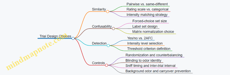
Putting It Together in Practice
Suppose your library contains three odors: Basil, Citrus, and Smoke. Similarity ratings might show Basil and Citrus are close, while Smoke is far. Confusability might reveal that Basil is often labeled as Citrus, but Smoke is rarely confused with either. Detection thresholds might show Smoke requires a higher command level to be noticed.
That combination tells you something actionable: you can safely use Smoke as a distinct cue only when you can deliver enough intensity, while Basil and Citrus should be treated as overlapping options if you need reliable identification.
Minimal Reporting Checklist
When you report results, include: the task type (similarity, confusability, detection), the stimulus set size, how intensity was handled, the randomization method, and the threshold criterion or similarity/confusion summary metric. Without those details, the numbers are hard to interpret and easy to misapply.
9.3 User Study Protocols for VR and Mixed Reality Contexts
User studies for smell rendering need two kinds of evidence: whether the smell matches the intended percept, and whether the experience is usable without causing confusion, discomfort, or workflow breakage. The protocol below is designed for VR and mixed reality (MR) where timing, spatial placement, and user movement all affect what people notice.
Study Goals and Hypotheses
Start by writing goals that map directly to measurable outcomes.
- Fidelity goal: Users can identify or rate the intended odor with higher scores than a baseline condition.
- Timing goal: Odors delivered at the correct moment produce higher similarity ratings than early or late delivery.
- Spatial goal: Users report more accurate source direction or distance when spatial rendering is enabled.
- Usability goal: Users complete tasks with acceptable workload and no meaningful increase in discomfort.
Example hypotheses:
- “When odor onset is synchronized to the visual event, similarity ratings increase by at least 1.0 point on a 7-point scale.”
- “When airflow direction cues are consistent with head motion, perceived source direction error decreases.”
Participant Planning
Recruit participants with a mix of olfactory ability and VR familiarity.
- Screening: Exclude known anosmia/hyposmia, strong nasal allergies on session day, and recent respiratory infections.
- Olfactory baseline: Use a simple odor identification check (a short set of familiar scents) to categorize participants into higher and lower baseline performance.
- VR/MR experience: Record headset exposure hours so you can interpret learning effects.
A practical target is 24–40 participants per major condition set. If you run multiple odor types, keep the number of conditions per participant manageable to avoid fatigue.
Experimental Design
Use within-subject designs when possible, but counterbalance order to reduce adaptation and expectation.
- Conditions: At minimum include the intended condition and one or more control conditions (e.g., no odor, delayed odor, swapped odor).
- Counterbalancing: Randomize condition order per participant using a Latin-square style schedule.
- Session structure: Break sessions into blocks of 6–10 trials with short rest periods.
Example trial set:
- Visual event: “open a drawer” in VR.
- Odor conditions: intended odor, no odor, and delayed odor by 2 seconds.
- Task: identify odor category and rate similarity.
Task Design and Questionnaires
Choose tasks that force attention to the smell without turning the study into a memory contest.
- Identification task: “Which of these three labels best matches what you smelled?”
- Similarity rating: “How close was it to the expected smell?” on a 7-point scale.
- Localization task (MR/VR): “Where did it seem to come from?” with a constrained response method (e.g., choose among 5 directions and 3 distances).
- Comfort and usability: Collect ratings for irritation, headache, nausea, and perceived control of the experience.
Keep questions consistent across trials. If you change the prompt mid-study, you’ll measure prompt effects instead of smell effects.
Trial Procedure and Timing Controls
Timing is the silent variable in smell studies.
- Pre-trial baseline: Present a neutral visual scene for 5–10 seconds before odor delivery.
- Odor delivery window: Use a fixed delivery duration and a fixed delay relative to the visual event.
- Inter-trial interval: Provide enough time for odor to clear. If you cannot guarantee clearing, include a “cooldown” block with no odor.
- Response timing: Let participants respond after a defined window (e.g., 8 seconds) to avoid rewarding fast guesses.
Example procedure for a single trial:
- Visual scene appears.
- After 3 seconds, odor onset occurs (or not, for control).
- Participant completes identification and similarity rating.
- Neutral scene returns for 15 seconds.
Data Collection and Quality Checks
Record both perceptual and operational data.
- Perceptual: identification choice, similarity score, localization selection, confidence rating.
- Operational: actual device command timestamps, airflow sensor logs, and any playback errors.
- Attention checks: Include occasional “no odor” trials to verify participants are not guessing.
Define exclusion criteria before the study starts, such as failure to follow instructions or repeated missing responses.
Mind Map: User Study Workflow
Example: Comparing Timing in VR
Design a timing study with three conditions: intended onset, 1-second early, and 2-second late.
- Stimulus: Same visual event across all trials.
- Task: Similarity rating plus a binary “did it match the moment?” question.
- Analysis: Compare similarity scores across timing conditions and test whether baseline olfactory ability changes the pattern.
If early delivery produces high similarity but low “moment match,” you’ve learned that perceptual content and temporal alignment are separable.
Analysis Plan and Reporting
Report results in a way that supports design decisions.
- Primary metrics: similarity score and identification accuracy.
- Secondary metrics: localization error, comfort ratings, and confidence.
- Stratification: analyze by olfactory baseline group to avoid averaging away meaningful differences.
- Effect sizes: include them so you can judge practical impact, not just statistical significance.
Keep the reporting consistent with the hypotheses. If timing is the target, don’t let localization questions become the main outcome unless you planned for it.
9.4 Statistical Analysis for Perceptual Outcomes
Statistical analysis turns “people said it smelled right” into measurable claims about odor fidelity, timing, and consistency. The key is matching the analysis to the outcome type and the experimental design, then reporting uncertainty in a way that supports decisions.
Choosing the Right Outcome Metrics
Start by classifying each dependent variable:
- Similarity ratings (e.g., 1–7 “how similar is this to the reference?”): typically treated as approximately continuous, analyzed with models that account for repeated measures.
- Confusion outcomes (e.g., forced-choice identification among odor categories): analyzed as accuracy, confusion matrices, or multinomial models.
- Detection thresholds (e.g., smallest concentration detected): analyzed with psychometric functions and threshold estimates.
- Temporal judgments (e.g., perceived onset time): analyzed with error distributions and mixed models, not just averages.
A practical rule: if the same participant evaluates multiple odors or conditions, you almost certainly need a repeated-measures approach.
Mind Map: Analysis Workflow for Perceptual Outcomes
Example: Similarity Ratings with Repeated Measures
Imagine a study with 24 participants rating similarity between a reference odor and three playback conditions: A (baseline), B (slightly delayed), C (lower intensity). Each participant rates all conditions.
A simple approach is an ANOVA, but mixed-effects modeling is usually safer because it can handle missing trials and participant-to-participant variability. The model includes:
- Fixed effects: condition
- Random intercept: participant
- Optional random slopes: condition per participant
Report the estimated mean difference between conditions with 95% confidence intervals. If condition B differs from A by 0.3 points on a 7-point scale with a confidence interval that crosses zero, you should treat it as “no clear evidence of difference,” not “it’s probably fine.”
Minimal Analysis Pseudocode
For each rating y:
  Fit mixed model: y ~ condition + (1|participant)
Compute:
  Pairwise contrasts A vs B, A vs C
  Report effect size and 95% CI
Check:
  Residual plots for outliers
  Sensitivity with robust variance if needed
Example: Identification Accuracy with Confusion Matrices
Suppose participants choose the closest odor label among five categories. Accuracy alone hides structure. A confusion matrix shows which odors are mistaken for which.
Analysis steps:
- Compute the confusion matrix per condition.
- Summarize with per-class recall and overall accuracy.
- Use a multinomial logistic model or a set of one-vs-rest logistic models to test whether playback changes the probability of correct identification.
When you compare conditions, correct for multiple comparisons. Otherwise, you can “find” differences that are just noise wearing a lab coat.
Example: Detection Thresholds with Psychometric Fits
For detection thresholds, raw concentration values are not linear with perceived intensity. Fit a psychometric function such as a logistic curve to the proportion detected across concentrations.
Report:
- Threshold at a defined detection probability (e.g., 50%)
- Slope indicating how quickly detection rises
- Confidence intervals for both
If the threshold shifts but the slope stays similar, the device may be consistently underpowered rather than producing erratic outputs.
Multiple Comparisons and Correction
Perceptual studies often test many odors, conditions, and metrics. Use a correction strategy aligned to your question:
- Family-wise control when you must limit false positives across many pairwise tests.
- False discovery control when you expect some true effects and want to balance sensitivity.
Always state what the “family” is. Comparing every condition against every other odor without defining the family is how results become hard to interpret.
Reporting That Keeps Results Honest
A good results section includes:
- Sample sizes per condition and participant
- The model used and why it matches the outcome type
- Effect sizes, not only p-values
- Confidence intervals for key contrasts
- How missing data were handled
If you report only p-values, you force readers to guess the magnitude. If you report only means, you hide uncertainty. The sweet spot is both.
9.5 Interpreting Results to Improve Encoding and Playback
Interpreting evaluation results is less about finding a single “best” setting and more about mapping failures to causes. When you do that well, you can improve encoding and playback without guessing.
Turning Raw Scores into Diagnoses
Start by separating three layers: what the user perceived, what the device produced, and what the system intended. If users report “campfire” but the device output was closer to “smoke,” the mismatch is likely in encoding-to-playback translation or mixture selection. If users report weak intensity across the board, the issue may be delivery timing, airflow, or calibration drift.
A practical workflow:
- Create a confusion table from similarity judgments or forced-choice results. Rows are intended odors, columns are perceived odors.
- Add intensity and timing columns from your device logs (e.g., ejection duration, fan speed, onset delay).
- Compute per-pair patterns: which intended odors are consistently confused with which perceived odors.
If “lavender” is often confused with “soap,” but both are consistently rated at lower intensity, you might be seeing a concentration scaling problem rather than a mixture composition problem.
Using Error Patterns to Choose the Next Fix
Not all errors are equal. Treat each common pattern as a clue:
- Systematic bias: the same intended odor is always perceived as a particular neighbor. This often points to encoding representation issues (wrong mixture weights, missing components, or incorrect perceptual scaling).
- Random spread: perceptions vary widely for the same intended odor. This suggests playback variability (inconsistent mixing, cartridge temperature differences, or airflow instability).
- Threshold behavior: users only detect the odor when intensity is high. This points to calibration gaps, carrier losses, or timing that misses the user’s sniff window.
- Temporal mismatch: users report the odor “too early,” “too late,” or “lingering.” This points to onset/decay modeling, valve timing, or persistence control.
Mind Map: From Results to Root Causes
Example: Confusion Between Two Mixtures
Suppose your confusion table shows that “orange peel” is frequently perceived as “lemon zest,” while “orange peel” is rated correctly in intensity. That combination is a strong hint: the delivery is working, but the encoded mixture is too close in perceptual space.
A targeted next step is to compare the encoded feature vectors for both odors. If your encoding uses a small set of components, check whether both mixtures share the same dominant note and differ only in a minor component. If so, the minor component may be underrepresented after playback losses.
You can test this hypothesis by increasing only the minor component’s encoded weight by a small step, then re-running the same forced-choice task. If the confusion rate drops without changing intensity ratings, you likely fixed the mixture composition rather than the delivery.
Example: Weak Detection with Correct Labels
Now consider a different outcome: users correctly identify “coffee,” but detection rates are low and intensity ratings are consistently below target. Confusion is low, so perceptual mapping is probably fine. The problem is likely that the device is not delivering enough odorant mass at the user’s sniff time.
Use device logs to check onset delay and ejection duration. If onset delay is longer than your event timing model assumes, the user may sniff after the peak concentration. In that case, adjust scheduling so ejection starts earlier relative to the VR event.
Then verify with repeatability tests: run the same odor profile multiple times and measure whether intensity variance shrinks. If variance remains high, calibration and mixing stability are the next suspects.
Example: Temporal Complaints That Point to Persistence
If users report “the smell stays after it should be gone,” you should not immediately change encoding. First, inspect the playback pipeline for purge behavior and residual vapor handling. A common issue is that the system stops ejection but does not actively clear the mixing chamber or delivery path.
A focused test is to keep the encoded profile identical and vary only the purge duration. If lingering decreases while identification stays stable, you improved temporal rendering without disturbing mixture fidelity.
Making Improvements Without Overfitting
After each change, re-test using the same evaluation structure but focus on odor pairs that previously failed. Keep unrelated parameters fixed so you can attribute improvements to the specific adjustment. If you change encoding and timing at the same time, you lose the ability to tell whether the fix worked for the right reason.
Finally, record the “reasoning trail” in your QA notes: error pattern → likely cause → single change → expected outcome. This prevents the next iteration from turning into a guessing game where everyone is technically busy but nobody learns.
10. Data Formats, Metadata, and Interoperability
10.1 Requirements for Smell Data Interchange in Pipelines
Smell data interchange is the part of a system that makes one team’s odor assets usable by another team’s rendering pipeline. If the interchange format is vague, you get mismatched timing, wrong intensities, and “it smells different on my machine” bugs that are hard to reproduce.
What Must Be Interchanged
A smell asset needs enough information to reproduce a specific perceptual event, not just a list of chemicals. In practice, interchange requirements fall into five buckets:
- Identity: stable IDs for odorants, mixtures, and authored “smell events.”
- Composition: how the mixture is defined (odorants, ratios, and any carrier/solvent assumptions).
- Timing: onset, duration, and any fade or hold behavior.
- Intensity Control: how “strength” is represented and how it maps to device output.
- Device Capability Binding: what the target hardware can actually render (max flow, supported odorants, mixing limits).
Concrete example: a “fresh coffee” event authored for one device might specify a 1.0 intensity scale. Another device might only support a subset of odorants and interpret intensity as a different physical quantity. Without explicit binding, the second device will render something else.
Canonical Units and Scales
Interchange formats must define units for every numeric field. For smell systems, the safest approach is to separate authored perceptual intensity from device command values.
- Authored intensity: a normalized scale (for example, 0–1) defined by the authoring pipeline.
- Device output: physical or device-native values (for example, flow rate, valve open time, or cartridge power level).
Concrete example: if a pipeline stores “concentration_mg_per_m3,” but the playback device uses “valve_ms,” you still need a documented mapping layer. The interchange format should carry both the authored intensity and the mapping version used.
Timing Semantics That Survive Translation
Timing fields should specify whether they represent:
- Event time (when the smell should start relative to VR frame time)
- Delivery profile (how the output changes over the smell’s lifetime)
- Persistence behavior (how long the system should consider the odor “active” for subsequent mixing)
Concrete example: “onset=0ms, duration=800ms” is not enough if the device has a 150ms warm-up delay. Interchange should include either device compensation parameters or a clear statement that onset is defined at the authored perceptual level rather than at the valve level.
Metadata That Prevents Silent Mismatch
Interchange should include metadata that lets a pipeline reject incompatible assets rather than guess.
Required metadata fields typically include:
- Schema version and asset version
- Authoring pipeline ID and mapping version
- Supported odorant list or a reference to a library entry
- Constraints such as maximum simultaneous mixtures and cross-contamination handling rules
Concrete example: if an asset assumes “mixture A and B can overlap,” but the target device requires purge between them, the renderer should fail fast or automatically split the timeline with an explicit rule.
Interchange Schema Mind Map
Mind Map: Smell Data Interchange Requirements
Example Interchange Payload
The following example shows a minimal, device-aware smell event. The key idea is that it carries both authored intent and the mapping needed to render it.
{
  "schemaVersion": "1.0",
  "assetVersion": "3",
  "eventId": "evt-coffee-001",
  "mixtureId": "mix-coffee-std",
  "timing": {
    "onsetMs": 1200,
    "durationMs": 800,
    "profile": "fadeOut"
  },
  "intensity": {
    "authoredScale": "0to1",
    "value": 0.72,
    "mappingVersion": "map-v5"
  },
  "deviceBinding": {
    "targetDeviceId": "dev-odor-42",
    "maxSimultaneousMixtures": 2
  },
  "validation": {
    "units": "explicit",
    "status": "ready"
  }
}
Validation Rules That Keep Pipelines Honest
Interchange should define validation outcomes as part of the format. A renderer should:
- Check schema and asset versions.
- Verify units and intensity scale names.
- Confirm the target device supports the mixture’s odorants.
- Ensure timing semantics match the renderer’s interpretation.
- Apply constraint rules for overlap and purge.
Concrete example: if an event uses a “fadeOut” profile but the device only supports “step” output, validation can either reject the asset or require a deterministic conversion rule. Either way, the behavior must be explicit so results are reproducible.
10.2 Metadata Fields for Odorants, Mixtures, and Timing
Metadata is what lets odor assets move cleanly between authoring tools, rendering pipelines, and playback hardware. Without it, you end up guessing: which bottle was used, how strong it was calibrated, and whether the timing was meant for “start now” or “arrive later.” The fields below are practical and designed to support repeatable playback.
Odorant Metadata Fields
Use odorant-level metadata for single ingredients in a library.
- Odorant Identifier: A stable ID like
odorant:vanillin_01so references don’t break when names change. - Chemical or Material Descriptor: Store what you know (e.g., vanillin, limonene) and what you don’t (e.g., “proprietary blend”). Keep it factual.
- Carrier and Solvent: Record the delivery medium used during calibration and playback, such as ethanol-based carrier or water-based emulsion.
- Physical Form: Liquid, gel, solid, or aerosolized concentrate. This affects vaporization behavior and device settings.
- Lot or Batch: Calibration and output can drift across batches. Batch IDs let you trace differences.
- Safety Classification: A simple internal category that maps to allowed devices, ventilation requirements, and handling steps.
- Calibration Parameters: At minimum, store the mapping between commanded drive (or pump duty cycle) and measured output (e.g., relative intensity units).
- Stability Notes: Include “shelf time since opening” or “max cycles” if your hardware or formulation has limits.
Example odorant record fields for a library entry:
odorant_id:odorant:vanillin_01descriptor:vanillincarrier:ethanolphysical_form:liquidbatch:VAN-2026-02calibration:{ intensity_per_command: 0.42, units: rel_intensity }
Mixture Metadata Fields
Mixture-level metadata describes how multiple odorants combine into one authored “smell.”
- Mixture Identifier:
mixture:campfire_smoke_01for consistent referencing. - Composition List: Each component odorant with a fraction or target concentration. Use one method consistently.
- Mixing Basis: Specify whether fractions are by volume, mass, or “relative drive units.” This prevents silent unit mismatch.
- Per-Component Calibration Link: Reference the odorant calibration used when the mixture was authored.
- Expected Output Profile: Store a target intensity curve over time (onset, plateau, decay) measured under defined conditions.
- Cross-Contamination Constraints: If the system requires purging between mixtures, store the purge requirement and minimum dwell time.
- Authoring Notes for Rendering: Keep short, operational guidance like “use with airflow mode A” or “avoid rapid re-triggering.”
Example mixture composition:
- Components: vanillin (sweet note), guaiacol (smoky note), cellulose-based carrier (for slow release)
- Basis: relative concentration
- Composition:
{ vanillin: 0.35, guaiacol: 0.10, carrier: 0.55 } - Output profile: onset 0.8 s, plateau 2.5 s, decay 6 s
Timing Metadata Fields
Timing metadata is where many systems fail, because “when the user perceives it” is not the same as “when the command is sent.” Store timing in multiple layers.
- Event Time Reference: Choose one:
command_time,device_ejection_time, orperception_estimate_time. Document the choice. - Trigger Offset: A numeric delay from the VR event to the device command. Example: “start ejection 300 ms before the visual cue.”
- Onset Duration: How long it takes to reach a defined intensity threshold.
- Peak Time Window: The expected time range where intensity stays near maximum.
- Decay Model Parameters: Store either a simple decay constant or a sampled curve.
- Persistence and Re-Trigger Rules: Define what happens if the same mixture is requested again before it fully decays.
- Synchronization Tolerance: A small tolerance value used by the renderer to avoid jittery re-scheduling.
Mind Map for Metadata Coverage
Metadata Fields Mind Map
Example: One Mixture with Timing and Links
A practical way to keep everything consistent is to treat the mixture as the authored unit, while odorants and timing provide the operational truth.
- Mixture:
mixture:campfire_smoke_01 - Composition basis: relative concentration
- Components:
odorant:vanillin_01fraction 0.35odorant:guaiacol_02fraction 0.10
- Timing:
- Event reference:
command_time - Trigger offset:
-0.30 srelative to the visual “flame appears” event - Onset duration:
0.8 s - Peak window:
2.0–3.0 s - Decay: exponential with
tau = 2.2 s - Re-trigger rule: ignore requests until intensity drops below 20% of peak
- Event reference:
This structure makes it possible for a renderer to schedule commands correctly, for QA to compare measured output to expected curves, and for hardware to apply the right calibration without guessing.
10.3 Versioning, Provenance, and Traceability of Odor Assets
Odor assets are easy to treat like static files, but they behave more like recipes with hardware-specific constraints. Versioning, provenance, and traceability keep teams from accidentally mixing “what we authored” with “what the device actually delivered.”
Versioning Odor Assets
Use versioning at three levels: the odor definition, the encoding parameters, and the playback profile.
- Odor definition version changes when the intended percept changes, such as swapping an odorant, adjusting mixture ratios, or updating the perceptual label mapping.
- Encoding version changes when the representation changes, such as switching from a feature vector to a mixture list, or changing how intensity is scaled.
- Playback profile version changes when device-facing parameters change, such as nozzle mapping, airflow targets, or timing offsets.
A practical rule: if a change would alter what a user smells, it increments the odor definition version; if it would alter how the system commands the hardware, it increments the playback profile version.
Example: A “Citrus Peel” asset is authored as a mixture of odorants A/B/C. You later correct the ratio of B from 0.20 to 0.25. That is an odor definition version bump. If you keep the same mixture but adjust the device’s mixing chamber dwell time from 120 ms to 150 ms, that is a playback profile version bump.
Provenance Records That Survive Handoffs
Provenance answers: where did this asset come from, who touched it, and what evidence supports it. Store provenance as structured metadata, not as a comment buried in a ticket.
Include:
- Source: lab batch identifier, cartridge lot, or supplier batch ID.
- Authoring method: how the mixture was created (manual formulation, measured dilution series, or calibration-derived mapping).
- Calibration context: device model, firmware version, and calibration session ID.
- Measurement evidence: which evaluation method produced the mapping (e.g., panel similarity scores, sensor-based flow verification, or both).
Example: “Citrus Peel v1.2” includes provenance stating it was formulated using cartridge lot L-441 and calibrated on device D-07 with firmware 3.4.1. If someone later reports a mismatch, you can reproduce the exact conditions rather than arguing about “the general setup.”
Traceability from Asset to Playback Event
Traceability connects an odor asset to a specific playback event in a session. This is crucial when debugging user reports or comparing two builds.
Track these identifiers:
- Asset ID and asset versions (odor definition, encoding, playback profile).
- Runtime parameters used during the session, such as intensity multiplier, onset delay, and any environment compensation flags.
- Hardware execution logs: command timestamps, valve open durations, airflow setpoints, and any fault codes.
- Session context: VR scene ID, event ID, and user/session ID.
Example: During a training simulation, a user reports “burnt plastic” instead of “fresh coffee.” The trace shows the event used “Coffee v2.0” but the playback log indicates a purge step was skipped after a previous “solvent” odor. The asset itself is fine; the session trace reveals the operational mistake.
Mind Map: Versioning, Provenance, Traceability
Example: A Minimal Metadata Schema
A compact schema helps teams implement governance without turning it into a bureaucracy project.
{
  "assetId": "odor.citrus.peel",
  "odorDefVersion": "1.2",
  "encodingVersion": "0.9",
  "playbackProfileVersion": "2.1",
  "provenance": {
    "sourceBatchId": "L-441",
    "authoringMethod": "measured_dilution_series",
    "calibration": {"deviceId": "D-07", "firmware": "3.4.1", "sessionId": "cal-2026-02-14"}
  },
  "trace": {
    "sessionId": "vr-8f3a",
    "sceneId": "kitchen_training",
    "eventId": "evt-112",
    "runtime": {"intensity": 0.8, "onsetMs": 120},
    "hardwareLogRef": "log-2026-03-02T10:22:11Z"
  }
}
Operational Practices That Keep Data Honest
- Immutable asset versions: once published, do not edit the same version; create a new one.
- Change logs tied to versions: record what changed and why, using the same version identifiers.
- Validation gates: require that a playback profile references an existing, calibrated odor definition version.
- Session trace completeness checks: ensure every playback event stores the asset versions and runtime parameters.
These practices make governance practical: when something smells “off,” you can pinpoint whether the issue is in the recipe, the encoding, the device profile, or the session execution.
10.4 Mapping Encoded Assets to Specific Device Capabilities
Encoded smell assets are only useful if they can be rendered by the actual hardware in the room. Mapping is the step that turns an abstract “odor profile” into concrete device actions that the system can execute reliably. The goal is simple: every asset should declare what it needs, and every device should declare what it can do, so the runtime can choose the right playback plan.
Capability Inventory for Smell Devices
Start by listing device capabilities in a way that matches how playback is controlled. Typical capability fields include:
- Odorant channels: number of independently controlled outputs.
- Mixture limits: maximum number of simultaneously active odorants (or maximum total flow).
- Timing resolution: smallest controllable step for on/off or flow changes.
- Flow and mixing behavior: whether the device supports stable mixing or only burst ejection.
- Output range: minimum and maximum effective intensity per channel.
- Purging and recovery time: how long it takes to clear a channel after changing odorants.
- Spatial constraints: whether delivery is directional, head-mounted, or room-based.
Example: A device with 4 channels and a “two-at-a-time” mixture limit can render a 3-note scent only by sequencing notes, not by playing them simultaneously.
Asset Requirements and Compatibility Rules
Each encoded asset should include requirements that reflect perceptual intent and playback constraints. Useful requirement fields:
- Odorant set: which odorants or mixture components are required.
- Concurrency: which components must overlap in time.
- Intensity curve: target relative intensity over time, not just a single level.
- Temporal shape: onset, plateau, and decay expectations.
- Spatial intent: where the source should appear (head-locked, hand-locked, world-anchored).
Then define compatibility rules that are explicit and testable. For instance:
- If an asset requires 3 simultaneous components but the device allows 2, the mapper must either reject the asset or convert it into a sequenced approximation.
- If the asset’s timing resolution is 10 ms but the device only supports 50 ms steps, the mapper must quantize event times and adjust intensity ramps accordingly.
Mapping Strategy: Choose, Transform, or Reject
A practical mapper usually follows three paths.
- Choose: If the device can represent the asset directly, use a direct translation.
- Transform: If the device cannot represent it exactly, apply controlled transformations.
- Reject: If the mismatch would break the intended perceptual timing or safety constraints, do not play it.
Example transformation rules:
- Channel remapping: If the device has different channel assignments, map odorants to available channels using a stable ordering.
- Intensity normalization: Scale the asset’s intensity curve so the peak stays within device output range.
- Temporal quantization: Round event times to the device’s timing grid, then recompute ramp durations to preserve overall “amount delivered.”
- Mixture reduction: For assets requiring more simultaneous components than allowed, keep the most perceptually dominant components and sequence the rest with a short crossfade window.
Mind Map: Mapping Encoded Assets to Device Capabilities
Example: Direct Mapping vs Transformation
Scenario A: Direct Mapping
- Asset: “Citrus burst” uses odorants A and B, overlapping for 1.2 s, with a peak intensity of 0.7.
- Device: 4 channels, supports two-at-a-time mixtures, timing step 10 ms, intensity range 0.0–1.0.
- Result: Map A→channel 1, B→channel 2, keep the intensity curve, schedule events at 10 ms resolution.
Scenario B: Transformation Needed
- Asset: “Forest blend” uses odorants A, B, C with all three overlapping for 0.8 s.
- Device: 4 channels but only two-at-a-time mixtures.
- Result: Choose the two dominant components (say A and B) for the overlap window, then sequence C immediately after with a purge-aware gap. The mapper records that the blend is an approximation so evaluation can interpret results correctly.
Example: Command Plan Output Structure
A mapped playback plan should be explicit enough for the runtime to execute without guessing. Include:
- Channel assignment: which odorant goes to which channel.
- Event timeline: timestamped commands (on/off or flow level).
- Purge steps: required delays and purge commands between odorant changes.
- Scaling factors: how intensity was normalized.
Example plan fields:
assetId: forest_blend_v3deviceId: room_unit_04channelMap: {A:1, B:2, C:3}events: [{t:0.00, ch1:0.6, ch2:0.5}, {t:0.80, ch3:0.4, purgeBefore:true}]notes: mixture reduced from 3-way overlap to 2-way overlap
Mapping is not just a conversion step; it’s a contract between what the asset author intended and what the device can actually do. When the contract is explicit, playback becomes predictable, debugging becomes faster, and evaluation results become easier to interpret.
10.5 Practical Examples of Structured Smell Asset Schemas
A structured smell asset schema is just a consistent way to describe what to play, how to play it, and how to verify it. The trick is to keep the schema strict enough that devices can interpret it the same way, while still being practical for authors who are not writing firmware.
Example: Minimal Odor Asset Schema
Use this when you have one device type, one delivery method, and a single mixture per event.
- assetId: stable identifier for the odor content (not the playback instance)
- name: human-readable label for authors
- libraryVersion: version of the odor library used to calibrate this asset
- mixture: list of odorants with relative amounts
- rendering: timing and intensity mapping rules
- deviceProfile: which hardware assumptions this asset expects
- qa: acceptance checks and how to measure them
Concrete example fields:
mixture:[{odorantId: "vanillin", amount: 0.6}, {odorantId: "ethyl butyrate", amount: 0.4}]rendering:onsetMs: 250,holdMs: 800,decayMs: 500,intensityScale: "perceptual"deviceProfile:delivery: "fan-mixed", mixingVolumeMl: 120, targetFlowSccm: 180qa:repeatability: ">= 0.85 correlation", method: "panel similarity"
Why this works: the schema separates “what the smell is” (mixture) from “how it is delivered” (rendering + deviceProfile). That separation prevents authors from accidentally changing playback behavior when they only meant to swap odorants.
Example: Multi-Note Timeline Asset Schema
Use this when an experience needs a sequence like “citrus peel → floral body → woody base.” The schema should represent each note as a playable segment with explicit transitions.
- timeline: ordered segments
- transitionRules: how to handle overlap and cross-contamination
- spatial: optional placement constraints for mixed reality
Concrete example timeline:
- Segment A: citrus note,
onsetMs: 0,holdMs: 600 - Segment B: floral note,
onsetMs: 500,holdMs: 700 - Segment C: woody note,
onsetMs: 1100,holdMs: 900 - Transition rule:
overlapMs: 100,purgeBetweenNotes: false,maxCarryoverPercent: 8
Why this works: overlap is declared as a parameter, not left to device defaults. If a device changes its mixing behavior, you can update deviceProfile and keep the timeline intent intact.
Example: Device-Aware Asset with Capability Mapping
Use this when you must support multiple hardware variants. The schema should include capability requirements and mapping instructions.
- capabilityRequirements: what the asset needs
- mapping: how to translate the asset into device commands
- fallbackBehavior: what to do if a capability is missing
Concrete example:
- Requirements:
maxSimultaneousOdorants: 6,supportsFanMixing: true,supportsPerceptualIntensity: true - Mapping: if a device only supports 3 odorants at once, split the timeline into two sub-events with the same perceptual intensity target.
- Fallback: if perceptual intensity is unavailable, use concentration scaling and mark qa expectations accordingly.
Why this works: you avoid silent mismatches where the asset “plays” but does not match the intended perceptual outcome.
Mind Map: Structured Smell Asset Schema Components
Mind Map: Authoring Workflow from Asset to Playback
Example: QA Metadata That Prevents Confusion
A common failure mode is treating calibration as a one-time event. Add QA metadata that ties the asset to a measurement context.
Include:
calibrationMethod: e.g., “panel similarity with fixed airflow”calibrationDate: date of last calibrationexpectedOutputRange: acceptable intensity boundsmeasurementProtocolId: which protocol produced the acceptance thresholds
Why this works: when someone reports “the smell feels weaker,” you can compare the runtime device conditions and the asset’s expected output range without guessing.
Example: Schema Snippet for a Timeline Asset
{
  "assetId": "smell.citrus_floral_woody.v3",
  "libraryVersion": "lib-2026-01",
  "deviceProfile": {"delivery": "fan-mixed", "targetFlowSccm": 180},
  "timeline": [
    {"note": "citrus", "onsetMs": 0, "holdMs": 600, "decayMs": 400},
    {"note": "floral", "onsetMs": 500, "holdMs": 700, "decayMs": 450},
    {"note": "woody", "onsetMs": 1100, "holdMs": 900, "decayMs": 600}
  ],
  "transitionRules": {"overlapMs": 100, "purgeBetweenNotes": false},
  "qa": {"repeatability": ">=0.85", "metric": "panel_similarity"}
}
This snippet shows the core idea: the timeline expresses intent, deviceProfile expresses assumptions, and qa expresses what “good” means in measurable terms.
11. Practical Implementation Patterns and Reference Workflows
11.1 Building a Minimal Viable Smell System for Prototyping
A minimal viable smell system should answer three questions quickly: Can you reliably output a chosen odor? Can you trigger it at the right time relative to VR events? Can you keep the result consistent enough that users notice the intended change rather than device quirks?
1) Define the smallest useful experience
Start with one interaction and one odor. For example, a VR scene where the user opens a drawer and a “paper + citrus” smell plays for 2–3 seconds. Keep the spatial complexity low at first: deliver from a single fixed outlet near the user’s face level, and ignore directionality.
A good minimal target is a binary percept: “odor present” versus “odor absent.” Once that works, you can add intensity control and multiple notes.
2) Choose a delivery approach you can calibrate
For prototyping, prioritize hardware that is easy to measure and repeat. A practical pattern is a cartridge or reservoir feeding a controlled ejection mechanism into a small mixing path.
Your prototype should include:
- A single odor channel (one mixture or one cartridge)
- A controllable ejection duration (for onset and cutoff)
- A way to measure or infer airflow so you can reproduce timing
- A purge or flush method to reduce lingering
Example: Use a short ejection pulse into a mixing chamber, then route the mixed air to a nozzle aimed at the user’s breathing zone. Even if the nozzle is imperfect, consistent airflow makes the output predictable.
3) Build the smallest control loop
Treat smell playback like audio playback: you need a scheduler, a device command layer, and a feedback or at least a logging trail.
A minimal control loop can be event-driven:
- VR event fires at time T
- System schedules odor start at T + latency_offset
- System schedules odor stop at T + latency_offset + pulse_duration
- System logs actual command times and device state
If you cannot measure actual ejection time, you can still calibrate an effective latency by testing with a stopwatch and repeating the same pulse pattern.
4) Create a tiny odor library with one profile
Build one odor profile with explicit parameters. Keep the profile format simple: odor_id, mixture recipe reference, pulse_duration_ms, and purge_duration_ms.
Example odor profile fields:
- odor_id: “drawer_citrus_paper”
- pulse_duration_ms: 1800
- purge_duration_ms: 2500
- max_retrigger_rate_s: 10
The max retrigger rate prevents the system from stacking pulses faster than the purge can clear residual vapor.
5) Calibrate with a repeatable test protocol
Calibration should produce numbers you can reuse, not just “it seems right.” Use a small set of trials:
- Baseline: odor off for 3 seconds
- Pulse: odor on for your chosen duration
- Repeat: run the same pulse 5 times
Ask a small internal panel to rate “odor present” on a 0–3 scale and note whether onset feels early/late. If onset is consistently late, adjust latency_offset. If odor lingers after cutoff, increase purge_duration_ms or shorten pulse_duration_ms.
6) Mind map for the minimal system
Mind Map: Minimal Viable Smell System
7) Example prototype build plan
Week 1: Hardware bring-up and purge verification
- Confirm you can trigger a single pulse and then clear it
- Record purge effectiveness by running pulse → wait → pulse again
Week 2: Timing calibration with VR synchronization
- Set latency_offset so odor onset aligns with the drawer opening
- Use a fixed pulse_duration_ms and adjust only one parameter at a time
Week 3: Acceptance criteria and basic UX wiring
- Define pass/fail: at least 4 out of 5 trials rated “odor present” and minimal lingering in the next 3-second window
- Wire the VR event to the smell scheduler and ensure logs capture every trigger
8) Minimal acceptance criteria that keep you honest
A prototype is “minimal viable” when it meets criteria like:
- Odor presence: 80% of trials show clear detection
- Timing: onset occurs within a chosen window relative to the VR event
- Lingering: odor is mostly absent in the next baseline segment
- Stability: the same command sequence yields similar outcomes across repeats
If any criterion fails, adjust the parameter that most directly affects it: onset timing via latency_offset, lingering via purge_duration_ms, and presence via pulse_duration_ms or mixture delivery consistency.
11.2 Creating an Odor Library with Repeatable Calibration
A good odor library is not just a list of smells. It is a set of odor “recipes” plus the measurements that prove each recipe behaves the same way on the same device. Repeatable calibration means you can run the same timeline twice and get the same perceived result often enough to trust it for testing and authoring.
Define Library Scope and Naming
Start by deciding what “library” covers: single-note odors, multi-note blends, or both. Then set naming rules that encode what matters for playback. A practical pattern is: [family]-[note]-[strength]-[version]. Example: citrus-limonene-0.6-v3. The version changes when you change calibration constants, not when you merely adjust authoring timelines.
Keep a “do not mix silently” rule: if two odorants share a reservoir or share a purge path, mark that relationship in metadata so authors know which combinations require extra cleaning time.
Choose Calibration Targets That Match Your Use
Calibration should be anchored to targets you can measure. For each odor recipe, define:
- Target onset time: time from command to first detectable output.
- Target intensity window: acceptable range of output strength over a short interval.
- Target decay behavior: how quickly output drops after the command ends.
A simple approach is to pick one reference interval for intensity, such as 2–4 seconds after onset, and one reference interval for decay, such as 6–8 seconds after onset. This avoids the common mistake of calibrating to a single peak value that may not align with perception.
Build a Calibration Matrix
Create a matrix that lists each odor recipe against each device parameter that can drift. Typical parameters include:
- airflow rate or fan speed setting
- mixing chamber temperature (if present)
- valve open duration mapping
- purge duration
- cartridge fill level or reservoir pressure
For each recipe, you want a mapping from command parameters → measured output. If you only calibrate one setting, you will later discover that small airflow differences shift onset and intensity.
Run Stepwise Calibration with Controlled Variables
Use a stepwise workflow so you can attribute changes to one cause at a time.
- Baseline purge: run the purge routine and confirm the output is near zero.
- Single-odor calibration: calibrate each note independently first. This makes blend calibration easier because you can reuse the note-level behavior.
- Blend calibration: combine notes using the same command scheduling logic you will use in VR timelines.
- Repeatability check: run the same recipe multiple times without changing anything, then compare measured onset, intensity window, and decay.
A concrete example: Suppose citrus-limonene-0.6-v3 uses a valve open duration of 120 ms. You might find that on a different day the onset shifts by 0.4 seconds due to airflow drift. Instead of changing the recipe, update the calibration constant that converts “120 ms command” into “effective output timing” for that device state.
Record Calibration Constants and Evidence
For each recipe, store:
- the command parameters used during calibration
- the measured onset, intensity window, and decay metrics
- the device configuration snapshot (airflow setting, purge routine ID, cartridge ID)
- the acceptance criteria used to mark the calibration as valid
Evidence matters because it prevents silent regressions. If a later calibration changes the constants, you can explain why the library version changed and how it affects playback.
Mind Map: Odor Library Calibration Workflow
Example: Calibrating a Two-Note Blend
Assume you have two calibrated notes:
- citrus-limonene-0.6-v3
- floral-linalool-0.4-v3
You want citrus-floral-0.5-v1 as a blend. Start by authoring the blend timeline using the same valve scheduling style you used for single notes (for example, sequential pulses with a fixed gap). Then measure the blend’s onset and intensity window.
If the blend onset is earlier than either note, it usually means the mixing chamber is reaching effective concentration faster due to combined airflow demand or reduced purge influence. Fix it by adjusting the blend’s command timing, not by changing the note-level calibrations. After adjustment, rerun the repeatability check to confirm the blend behaves consistently across multiple trials.
Example: Acceptance Criteria That Prevent “Good Enough” Drift
Set explicit pass/fail thresholds. For instance:
- Onset time must be within ±0.2 seconds of the target.
- Intensity window mean must be within ±10% of the calibrated value.
- Decay must drop below a defined fraction within a fixed time.
If a recipe fails, treat it as a calibration issue, not an authoring issue. Authors should not compensate for a broken recipe by stretching timelines; that creates inconsistent behavior across devices and sessions.
Practical Checklist for Authors and Engineers
- Recipes are versioned and include device configuration snapshots.
- Blends are built from calibrated notes using the same scheduling logic.
- Purge routines are treated as part of the recipe behavior.
- Calibration evidence is stored with measured metrics and acceptance criteria.
- Repeatability checks are run after any change to hardware settings or purge logic.
11.3 Authoring Smell Timelines for Interactive VR Events
A smell timeline is a schedule that turns “what the user is experiencing” into “what the device should output,” with explicit timing, intensity, and stop conditions. In interactive VR, the timeline must survive interruptions: head turns, teleportation, pauses, and scene transitions. The simplest reliable approach is to treat each odor event as a small state machine with three phases: request, render, and release.
Event Inputs That Drive Timeline Decisions
Start by listing the triggers that can start or stop an odor. Common triggers include proximity to an object, gaze dwell, entering a room, picking up an item, and completing a task step. Each trigger should map to an odor “intent” with parameters: odor profile ID, target intensity, onset delay, duration, and a cancellation rule.
Example: When the user approaches a bakery counter, the system requests “warm bread” with a 0.3 s onset delay, 4.0 s duration, and a rule that cancels immediately when distance exceeds the threshold for 0.5 s. That rule prevents flicker when the user hovers near the boundary.
Timeline Authoring Rules That Prevent Artifacts
Use consistent timing semantics across the project. A practical convention is:
- Onset delay: time from trigger acceptance to first ejection.
- Render duration: time during which the device outputs the mixture.
- Tail handling: time after render duration during which lingering perception is expected.
Because smell devices often have physical delays and persistence, you should separate “device output time” from “perceptual presence.” If you only schedule output, users will notice mismatches when they move quickly.
A second rule is to define cancellation behavior for every event. If a new odor starts while another is active, decide whether to crossfade, hard-switch, or queue. Hard-switch is easiest but can feel abrupt; crossfade reduces discontinuity but requires overlap control to avoid unintended mixtures.
A Practical Timeline Template
Author timelines as a sequence of odor events with explicit device commands. Keep each event small so you can reuse it across interactions.
Event template fields
trigger: what starts itprofile: which odor profile to useintensity: target level (0–1)onsetDelayMs: delay before outputrenderMs: output durationtailMs: expected perceptual persistencecancelRule: how to stop or replace
Example: A “coffee pour” event might have onsetDelayMs = 150, renderMs = 1200, tailMs = 2500, and cancelRule = “stop when user looks away for 300 ms.”
Mind Map: Smell Timeline Components
Example: Interactive Room Entry with Layered Odors
Scenario: Enter a “kitchen” scene. The system should start a background smell, then add a localized note when the user approaches the stove.
-
Kitchen background event
- Trigger: scene entry
- Profile: “clean kitchen”
- onsetDelayMs: 0
- renderMs: 6000
- tailMs: 3000
- cancelRule: stop on scene exit
-
Stove localized event
- Trigger: distance < 1.5 m to stove for 800 ms
- Profile: “warm food”
- intensity: 0.7
- onsetDelayMs: 200
- renderMs: 2500
- tailMs: 2000
- cancelRule: replace background note with reduced intensity (0.3) when user leaves
The key detail is the replacement rule: it avoids a sudden drop to zero when the user moves away from the stove, while still letting the background remain.
Example: Gaze-Based Dwell for a Single Object
Scenario: A character’s letter emits a faint paper-and-ink smell when the user reads it.
- Trigger: gaze on letter for 1200 ms
- onsetDelayMs: 100
- renderMs: 1800
- tailMs: 1500
- cancelRule: stop when gaze leaves for 250 ms
The short “leave” dwell prevents rapid start-stop if the user’s head jitters. The longer “read” dwell ensures the smell doesn’t fire during casual glances.
Implementation Notes for Authoring Consistency
When you implement timelines, treat each event as owning its own parameters and cancellation rule. A central scheduler should resolve conflicts deterministically: if two events overlap, apply the overlap policy defined per event pair. This keeps behavior predictable and makes it easier to debug why a smell did or didn’t play during a specific interaction.
Finally, log timeline decisions with timestamps: trigger acceptance, cancellation, and actual device output start/stop. That record is what turns “it felt off” into a concrete timing mismatch you can correct.
11.4 Handling User Variability and Session-Level Differences
Smell systems behave like other sensory channels: the same stimulus can land differently depending on the person and the moment. In practice, you manage variability by separating what you can control (device timing, airflow, calibration) from what you can measure (user state, session conditions) and then designing your workflow so the system degrades gracefully.
Sources of Variability You Should Expect
Olfactory sensitivity varies. Some users detect faint odors quickly; others need stronger concentrations or longer exposure. A simple example: a “fresh coffee” cue that feels obvious to one user may be barely noticeable to another, even when the device output is identical.
Adaptation and fatigue change perception. After repeated exposures, many people become less responsive to the same odor. Example: in a guided VR cooking demo, the “baking bread” smell may feel strong at the first step but noticeably weaker by the third repetition.
Nasal and health factors matter. Congestion, allergies, dry air, and recent colds can reduce odor perception. Example: the same user reports “nothing” on a day with a stuffy nose, but “clear and accurate” on a normal day.
Context and attention shift outcomes. Users who are focused on a task may notice smells less than users who are explicitly told to look for them. Example: during a fast-paced puzzle, a subtle “smoke” cue might be missed unless it is timed with a clear event.
Individual odor familiarity changes interpretation. People map odors to different mental labels. Example: “lemon cleaner” might be interpreted as “dish soap” by one user and “laundry” by another.
Session-Level Differences That Break Consistency
Room airflow and ventilation change delivery. A door opening mid-session can pull odor away or spread it. Example: a smell that lingers correctly in a closed room may dissipate too fast in a room with HVAC cycling.
Device state drifts over time. Cartridge temperature, residual vapor, and pump performance can shift during long runs. Example: after an hour of continuous use, the same command produces a slightly weaker output.
Cross-contamination accumulates. Even with purging, tiny residues can carry over. Example: a “mint” cue can leave a faint background that makes the next “rose” feel less distinct.
User behavior affects exposure. Breathing rate, head movement, and distance from the delivery path change effective dose. Example: a user leaning away during playback receives less odor than intended.
A Practical Strategy for Managing Variability
Use a two-layer approach: baseline calibration for the device and session calibration for the user and environment.
-
Baseline device calibration ensures the same encoded profile produces consistent output on that hardware. Keep this stable and repeatable.
-
Session calibration adjusts for the current run. Start each session with a short “check sequence” that uses neutral, low-risk odors and measures whether the user can detect them.
A concrete check sequence might include:
- One mild odor to confirm detection.
- One “no odor” interval to confirm the user notices absence.
- One quick repeat to estimate adaptation within the session.
Mind Map: Variability Handling Workflow
Runtime Controls with Easy Examples
Intensity scaling per user. After the check sequence, set a per-user gain that maps “detected” to a target intensity. Example: if the user misses the mild odor, increase the next cue by one step in your intensity ladder.
Timing adjustments for adaptation. If the user reports the second exposure is weaker, insert a longer gap before the next similar cue. Example: in a multi-step “forest walk,” delay the second “pine” note so it doesn’t compete with the first.
Purge between critical transitions. For cues that must be distinct, add a purge interval after each. Example: switching from “cleaning solvent” to “food aroma” without purging can cause a blended perception.
Distance-aware delivery. If your system supports it, align delivery with the user’s typical head position during key events. Example: trigger the odor slightly earlier when the user is likely to move toward the source.
Session Feedback Without Overcomplicating It
Keep feedback lightweight: a short rating after a small set of cues is enough to adjust the remainder of the session. Example: ask “Did you notice it?” (yes/no) and “Was it too strong or too weak?” (three options). This avoids long questionnaires and still captures the two most actionable variables: detectability and intensity.
Handling Edge Cases
If a user reports persistent non-detection across multiple check cues, treat the session as “low-olfaction mode”: reduce reliance on subtle smells and reserve stronger cues for key moments. Example: use smell for major events only, while keeping minor details visual.
If a user reports discomfort, stop odor delivery immediately and switch to non-odor cues for the rest of the session. Example: replace “burning” with a visual warning and a brief, odor-free pause.
The goal is not to make every user experience identical; it’s to make the system predictable enough that the experience remains coherent even when the person’s senses and the room conditions are not.
11.5 Troubleshooting Common Failure Modes in Smell Rendering
Smell rendering fails in predictable ways: the device outputs the wrong odor, the timing is off, the intensity is inconsistent, or the user perceives something different than expected. A good troubleshooting flow starts with what you can measure (flow, timing, cartridge state) before you change the encoding.
Symptom First, Likely Cause Second
Use this quick triage to avoid random knob-turning.
-
No smell at all
- Cartridge empty or wrong slot selected.
- Pump/valve not firing due to a control mapping error.
- Air path blocked by condensation or residue.
- Safety interlock preventing output.
-
Wrong smell
- Odor library index mismatch between authoring and device.
- Cartridge swapped or mislabeled during refill.
- Cross-contamination from previous mixture.
-
Smell is too weak
- Under-delivery: insufficient pump duration or flow rate.
- Odorant degraded from heat or long storage.
- Excess dilution from airflow settings.
-
Smell is too strong or lingering
- Over-delivery: pump duration too long.
- Insufficient purge between events.
- Delivery path mixing chamber not reaching target conditions.
-
Smell timing feels wrong
- Event scheduling mismatch between VR timeline and device command.
- Latency in control loop or serial/USB buffering.
- Onset delay from airflow ramp-up.
-
Smell feels “off” even when it matches the label
- Mixture ratio mismatch due to concentration scaling errors.
- Temperature/humidity differences changing volatility.
- User adaptation effects causing reduced sensitivity.
Mind Map of Failure Modes
Practical Debugging Workflow
-
Confirm the command path. Trigger a single odor from a minimal scene and verify the device receives the correct odor ID and duration. If the device logs show the wrong ID, stop and fix the mapping.
-
Validate cartridge selection. Physically inspect the installed cartridges and confirm the software slot assignment matches the physical labels. A surprising number of “wrong smell” issues are just swapped cartridges.
-
Run a single-odor baseline. Play one odor at a known calibrated setting. Record onset time, peak intensity (subjective rating is fine for early debugging), and decay time. If the baseline is wrong, the issue is hardware delivery or calibration, not encoding.
-
Test purge behavior. After the baseline, play a second odor that should be clearly different. If the second odor is contaminated, increase purge time or verify that the purge valve and airflow direction are correct.
-
Measure timing alignment. Compare the VR event timestamp with the actual firing timestamp from device logs. If there is consistent offset, adjust scheduling or add a fixed delay compensation.
-
Check mixture math. For multi-odor scenes, verify that concentration scaling and mixture ratios are applied in the same units used during calibration. A unit mismatch can produce “almost right” odors that still fail evaluation.
Example: The Case of the “Almost Right” Citrus
A team reports that a citrus scene smells like citrus but with a faint “burnt” note. They first run a single-odor baseline for citrus at the calibrated setting. The baseline is clean, so the odor library entry is correct.
Next they run the scene’s mixture sequence with logging enabled. The logs show citrus is followed by a cleaning purge command, but the purge duration is shorter than the value used during calibration. The second odor in the sequence is being partially carried into the citrus onset window.
Fix: restore purge duration to the calibrated value and ensure the purge command is scheduled before the next odor’s onset, not merely after the previous one’s nominal end. After the change, the citrus onset matches the baseline and the “burnt” note disappears.
Example: Timing Drift in Fast Interactions
In a fast-paced VR interaction, users report that the smell arrives late during quick turns. Single-odor tests in a slow scene look fine. Device logs reveal that commands are queued and executed in bursts when the scene triggers multiple events within a short window.
Fix: throttle smell commands so only one odor event is active per rendering window, and align the smell onset to the first command execution time rather than the scene’s scheduled time. After throttling, onset timing becomes consistent even when the user moves quickly.
What to Record During Every Test
Keep a small test record for each run:
- Odor IDs and mixture ratios used
- Cartridge slot mapping and refill date
- Pump/valve durations and airflow settings
- Device log timestamps for command receipt and firing
- Onset time, peak intensity rating, and decay duration
- Purge duration and whether cross-odor contamination is observed
This turns troubleshooting from guesswork into a repeatable process. When the next failure appears, you can compare it to the last known-good baseline instead of starting over.
12. Safety Engineering for Odor Delivery Systems
12.1 Hazard Identification for Odorants and Carriers
Hazard identification starts with a simple question: what can harm a person, a device, or the environment when an odor is released? In digital scent systems, the answer is rarely “the smell itself.” More often it’s the odorant chemistry, the carrier medium, the delivery conditions (heat, airflow, pressure), and the cleaning gaps between sessions.
Odorant Hazards
Odorants can pose risks in several categories, and you should treat each category as a separate checklist item.
- Acute irritation and sensitization: Some compounds irritate eyes or airways, and repeated exposure can increase sensitivity. Example: a strong citrus-like aldehyde may feel “pleasant” but still trigger coughing in users with reactive airways.
- Toxicity via inhalation: Even if an odor is detectable at low levels, toxicity can occur at higher concentrations or with poor ventilation. Example: a solvent-like note that smells “clean” can still be harmful if the system overshoots the intended dose.
- Skin and eye hazards: Concentrated odorants or residues from cartridges can contact skin during maintenance. Example: a technician refilling a reservoir without gloves can get a sticky residue on hands, then rub eyes.
- Flammability and reactivity: Many odorants are volatile organic compounds. Some can react with oxidizers or form irritating byproducts under heat. Example: a highly volatile terpene may increase fire risk if the device uses hot components near the cartridge.
- Odor masking effects: A pleasant odor can reduce user awareness of a real hazard. Example: if a leak occurs, the scent may delay detection of a solvent spill.
Carrier Hazards
Carriers are the “delivery helpers,” but they can be the main hazard source.
- Solvent or carrier toxicity: Carriers may be less noticeable than odorants but still irritate or depress the nervous system at sufficient exposure. Example: a carrier used to dissolve a fragrance concentrate can cause throat irritation even when the odorant dose is correct.
- Volatility and unintended exposure: A carrier that evaporates quickly can spread beyond the target zone. Example: a system that vents into a room can create lingering background odor after the session.
- Residue and cross-contamination: Carriers can leave films in tubing and nozzles, which then mix with the next odor. Example: a sweet carrier residue can make the next “fresh” scent appear darker and also increase irritation.
- Cleaning chemistry hazards: Purging and cleaning often use chemicals that are safer than the odorants, but still require handling controls. Example: an alcohol-based purge can irritate eyes and require ventilation.
Delivery Condition Hazards
Even a safe odorant can become risky under the wrong operating conditions.
- Overdose from timing errors: If the playback controller triggers too long, concentration rises. Example: a timeline bug causes a “campfire” profile to run twice, leading to stronger-than-expected smoke-like irritation.
- Airflow and mixing failures: Poor mixing can create local high concentrations near the nozzle. Example: a clogged mixing chamber produces a sharp burst that users near the device experience as harsh.
- Temperature effects: Heating can increase volatility and change chemical composition. Example: warming cartridges to improve flow can also increase the rate of release and irritation.
- Pressure and leaks: Leaks can expose users and staff to concentrated vapors. Example: a loose fitting during cartridge swap releases a short plume that is stronger than the intended dose.
Risk Identification Workflow
A practical workflow keeps hazard identification grounded in evidence.
- Inventory inputs: List each odorant and carrier by name, concentration, and physical form.
- Map hazards to exposure routes: Inhalation, skin contact, eye contact, ingestion (usually accidental), and environmental release.
- Define operating envelopes: Record normal temperature, airflow, dose duration, and maximum output.
- Identify failure modes: Timing faults, clogs, leaks, incorrect cartridge installation, and incomplete purging.
- Assign controls per hazard: Ventilation requirements, dose caps, sensor checks, maintenance PPE, and cleaning procedures.
Mind Map: Hazard Identification for Odorants and Carriers
Example: Hazard Checklist for a “Cedar” Profile
Assume a cedar-like odorant dissolved in a carrier.
- Odorant: Check for airway irritation potential and flammability class.
- Carrier: Confirm whether it is a solvent with known eye/throat irritation.
- Delivery: Verify dose duration caps prevent overshoot.
- Mixing: Confirm mixing chamber cleanliness reduces burst release.
- Maintenance: Require gloves and eye protection during cartridge swaps.
- Cleaning: Use a purge procedure that removes residue without leaving irritating films.
Example: Failure Mode to Hazard Mapping
If the system detects a flow drop and compensates by extending ejection time, you must treat that as a hazard pathway, not a convenience.
- Failure mode: Flow sensor reads low due to partial clog.
- System behavior: Controller increases ejection duration.
- Hazard: Higher local concentration near the nozzle.
- Control: Trigger a “stop and purge” state when flow deviates beyond a threshold, then prompt maintenance.
Hazard identification is complete when each hazard has a clear exposure route, a plausible failure pathway, and a concrete control that can be checked during operation and maintenance.
12.2 Exposure Limits, Ventilation, and Operational Controls
Odor delivery is a controlled exposure problem, not just a rendering problem. The goal is to keep concentrations low enough to avoid irritation and unsafe exposure, while still producing a perceptible signal for the experience.
Exposure Limits That Match Real Use
Start with the specific chemicals you plan to use, then translate any allowable exposure guidance into operational limits you can enforce. In practice, you’ll need three layers:
- Substance limits: what’s considered safe for the chemical itself (often expressed as time-weighted or short-term exposure thresholds).
- Mixture limits: how multiple odorants combine, since “safe individually” does not always mean “safe together.”
- Device limits: what your hardware can actually deliver, including worst-case output and variability.
A practical method is to define a maximum dose per event and a maximum cumulative dose per session. For example, if your device can output a short pulse that produces a peak concentration, you cap the pulse energy so the peak stays under the short-term threshold. Then you cap the number of pulses so the session total stays under the time-weighted threshold.
Ventilation That Controls Concentration, Not Just Smell
Ventilation is about removing odor molecules from the breathing zone. “Room smells less” is not a measurement; it’s an outcome. Use ventilation controls that target concentration reduction:
- Supply and exhaust placement: place exhaust so it pulls air from where users breathe, not only from the far side of the room.
- Air exchange rate: higher exchange reduces lingering odor, but it can also change delivery effectiveness. You should test with the same airflow settings you will use operationally.
- Local extraction: for systems that use cartridges or reservoirs, extraction near the source prevents leaks from becoming background contamination.
A simple operational rule: if you can’t reliably clear the odor between sessions, you don’t have a ventilation plan—you have a hope plan.
Operational Controls That Prevent Accidental Overexposure
Operational controls are the “seatbelts” that work even when someone makes a mistake.
Event Gating and Rate Limits
Implement software and hardware gating so the system refuses to exceed safe delivery patterns. Examples:
- Minimum interval between odor events to prevent accumulation.
- Maximum events per minute and maximum events per session.
- Fail-closed behavior: if sensors or calibration checks fail, the system stops delivery rather than guessing.
Interlocks and Hardware Safeties
Use physical interlocks where they matter:
- Door or occupancy interlock: odor delivery only when the space is in the correct state.
- Flow verification: if airflow is below a threshold, delivery is blocked because mixing and dilution won’t meet your assumptions.
- Leak detection or pressure monitoring: if the system can’t maintain expected pressure/flow, it should stop.
User Controls and Session Management
Operational safety also includes user-facing steps:
- Consent and opt-out: allow participants to skip odor content without penalty.
- Clear start/stop procedures: staff should know how to halt delivery and initiate purge.
- Post-session purge: define a purge time based on ventilation performance, not on “it seems gone.”
Mind Map: Exposure Limits, Ventilation, Operational Controls
Example: Turning Limits into Device Rules
Suppose your short-term exposure guidance corresponds to a maximum peak concentration in the breathing zone. You run a calibration test at the intended airflow and measure peak concentration for a known pulse duration. If a 200 ms pulse reaches 80% of the allowed peak, you set the operational cap to 150 ms to keep margin for variability. Then you set a session cap by counting pulses: if 10 pulses reach 90% of the time-weighted allowance, you cap at 8 pulses per session and enforce a minimum interval so the system doesn’t stack lingering odor.
Example: Ventilation Settings That Support Consistent Playback
If you deliver an odor pulse and then immediately deliver another, the second pulse rides on residual concentration. You can either increase the minimum interval or increase ventilation between events. In a controlled test, you measure how long it takes for the background concentration to drop below a defined baseline. That measured clearance time becomes your operational interval rule.
Example: Staff Checklist for Safe Operation
A short checklist reduces human error:
- Confirm ventilation mode and airflow status.
- Verify device calibration status for the active odor cartridges.
- Check that the session dose counter is reset.
- Confirm purge procedure and timer.
- During the session, stop delivery immediately if airflow verification fails.
- After the session, run the defined purge time before the next group.
These controls keep exposure predictable. Predictability is what makes safety engineering more than a policy document.
12.3 Cleaning, Purging, and Cross-Use Contamination Prevention
Cross-use contamination happens when residue from one odor session carries into the next. In practice, it shows up as “ghost notes” (a faint background smell), timing drift (the next odor starts late), or intensity inflation (the next odor feels stronger than authored). Preventing it is mostly about controlling three things: what touches the odor path, how you remove what’s left, and how you prove it worked.
Cleaning Principles That Match Real Hardware
Start by separating components into three categories.
- Contact surfaces: anything the odor-laden air or liquid passes through, such as mixing chambers, tubing, valves, nozzles, and cartridge interfaces.
- Non-contact surfaces: housings and external panels that may get dust or condensation but do not carry odor flow.
- Support systems: fans, heaters, filters, and sensors that influence airflow and temperature but may also trap residue.
A cleaning plan should specify which category is cleaned, how often, and what “clean” means. For example, wiping external panels is not a substitute for purging the mixing chamber after a strong solvent-like odor.
Purging Strategies That Remove Residue
Purging means flushing the odor path with a carrier air stream (or an approved cleaning gas) long enough to reduce leftover molecules below a practical threshold.
A useful rule is to purge based on odor strength and volatility, not just time. Heavy, low-volatility compounds tend to cling to surfaces and require longer flushing. Light, fast-evaporating compounds usually clear sooner.
Example: If you switch from a “pine resin” profile to “clean linen,” a short purge may still leave resin-like background. Increase purge duration and confirm with a test run that the first seconds of “linen” are not contaminated.
Purging should also be consistent. If purge duration varies randomly, you can’t compare sessions or debug issues. Keep purge parameters tied to odor classes (for instance, “high cling,” “moderate cling,” “low cling”) and log which class was used.
Cross-Use Prevention Through Operational Discipline
Even with good purging, cross-use prevention improves when you reduce unnecessary transitions.
- Group similar odors: If your experience includes multiple “citrus” moments, play them back-to-back before moving to “smoke” or “spice.”
- Use a neutral buffer: Insert a known neutral odor or clean-air state between very different odor classes. The buffer acts like a controlled reset.
- Avoid rapid alternation: Switching every few seconds increases the chance that residue accumulates faster than purging can remove it.
Example: In a training simulation, you might alternate “coffee” and “metallic workshop” every 10 seconds. Instead, schedule the scene so each odor class runs in blocks, with a neutral buffer between blocks.
Cleaning Workflow with Verification
A practical workflow has three phases: purge, clean, verify.
- Purge: Flush the odor path after the session ends or after a high-risk odor.
- Clean: For components that can be disassembled or wiped safely, remove visible residue and clean according to the device’s material compatibility. Avoid harsh solvents on parts that can absorb odor compounds.
- Verify: Run a short “blank” playback and check for ghost notes.
Verification should be objective where possible. Use a standardized blank odor (or clean-air mode) and record whether users report any background smell. If you have a sensor for airflow and temperature, confirm those are stable too; inconsistent airflow can mimic contamination by changing delivery timing.
Mind Map: Cleaning, Purging, and Cross-Use Prevention
Example: High-Risk Odor Transition Plan
Suppose your system will play “burnt sugar” followed by “fresh air”.
- Mark “burnt sugar” as high cling due to caramelized, heavier notes.
- After “burnt sugar,” run a purge sized for high cling.
- Insert a neutral buffer state for a fixed duration.
- Verify by playing “fresh air” and checking the first 5–10 seconds for any lingering sweetness.
If contamination persists, increase purge duration for that odor class and inspect contact surfaces for residue that purging alone may not remove.
Logging That Makes Problems Traceable
Contamination prevention fails when you can’t connect symptoms to actions. Log at least:
- Odor sequence and transition points
- Odor class for each profile
- Purge duration and buffer usage
- Verification outcome for blanks
This turns “it smells off today” into a specific, fixable statement like “high-cling transitions used the short purge preset.”
12.4 User Guidance, Consent, and Accessibility Considerations
User guidance is part of the safety system, not an afterthought. Smell delivery changes the user’s environment, so instructions should be specific, short, and tied to what the user will feel and do.
Consent That Matches the Experience
Consent should be granular enough to reflect real choices. A single “agree” checkbox is usually too vague because users may want to opt out of intensity changes, odor persistence, or any smell at all.
A practical approach is a two-step prompt:
- Step 1: “Do you want smell effects in this experience?”
- Step 2: “If yes, do you want automatic intensity adjustments or fixed intensity?”
Example: In a cooking simulation, the default can be “smell effects on,” but users can switch to “smell effects off” before entering the scene. If they choose “on,” they can also select “fixed intensity” to avoid sudden changes when they move between rooms.
Consent should also be revocable during the session. Provide a visible control that immediately stops future odor ejections and clears any active delivery schedule.
Clear Onboarding Without Guesswork
Guidance should explain three things: what will happen, how long it may last, and what the user can do if it feels wrong.
Include a “what to expect” line near the smell toggle:
- “Odors may start a moment after you trigger events and may linger briefly.”
Include a “what to do” line:
- “If you feel discomfort, use Stop Smell Effects. You can re-enable later.”
Example: In a museum-style mixed reality guide, the app can show a small icon next to each smell trigger in the UI. When the user taps the trigger, a short message appears: “Starting scent. You can stop at any time.”
Discomfort, Allergy, and Sensitivity Controls
Not all users have the same sensitivity. Guidance should encourage users to self-identify without requiring medical disclosure.
Use a simple pre-check:
- “If you have allergies or strong sensitivities, consider turning smell effects off.”
Then add operational controls:
- A global intensity slider with a safe minimum.
- A “quiet mode” that reduces frequency of odor events.
- A “single-shot mode” that prevents repeated ejections when the user stays in the same area.
Example: In a navigation training app, the system can detect repeated triggers from the same waypoint. In quiet mode, it limits the odor to one ejection per waypoint per session.
Accessibility for Diverse Sensory Needs
Smell effects should not be the only channel for meaning. Every scent cue should have a non-olfactory equivalent such as text, color, audio, or haptic feedback.
A good rule is: “If smell is optional, the experience must still make sense without it.”
Example: In a VR escape room, a “smoke” odor cue can be paired with a visual warning label and a distinct sound. Users who disable smell still understand the hazard and can proceed safely.
Also consider users with reduced ability to perceive odors. Provide a way to confirm that smell effects are enabled, such as a brief test sequence with an easy-to-recognize odor and a “did you notice it?” prompt.
Timing, Persistence, and User Control
Odor onset and decay can be slower than visual and audio cues. Guidance should set expectations so users do not interpret delayed smell as a malfunction.
Use consistent behavior:
- When the user triggers an event, the system should follow a predictable delay.
- When the user stops smell effects, the system should stop scheduling new ejections immediately.
Example: If a “fresh paint” cue is tied to opening a door, the system can show a countdown icon that matches the odor onset delay. If the user exits the room before the onset, the system should cancel the pending ejection.
Mind Map: User Guidance, Consent, and Accessibility
Example Interaction Flows
Example: “Scent Off by Default” onboarding
- User enters the app.
- UI shows: “Smell effects are optional.”
- Default is off.
- User can enable smell effects and choose fixed intensity.
- A short test cue plays once.
- User confirms “noticed” or “not noticed,” and the app keeps the setting.
Example: “Stop Smell Effects” during discomfort
- User feels discomfort.
- They press a large on-screen button labeled “Stop Smell Effects.”
- The system halts future ejections and cancels queued events.
- The UI changes to “Smell effects stopped,” with an option to re-enable later.
Practical Wording Guidelines
Keep labels concrete and action-oriented. Prefer “Stop Smell Effects” over “Reduce odor impact,” and prefer “Smell effects may linger briefly” over “Smell may be present.”
Avoid medical claims. Guidance should focus on user choices and operational controls rather than promising specific health outcomes.
12.5 Documentation and Maintenance Procedures for Safe Operation
Safe smell systems fail in predictable ways: a valve sticks, a cartridge leaks, a sensor drifts, or a user runs a session without the expected purge. Documentation and maintenance are how you keep those failures from becoming surprises.
Documentation That Matches Real Work
Maintain a single “source of truth” document set that mirrors the actual operating flow.
- System description sheet: device model, odorant cartridge types, carrier/air supply method, maximum flow rates, and the approved odorant list.
- Operating procedure: step-by-step startup, session start, session end, and shutdown. Include what “normal” looks like (for example, expected sensor ranges and typical purge duration).
- Cleaning and purge procedure: specify when to purge (after each session, after cartridge swaps, after any fault), what to purge with, and how to verify completion.
- Maintenance schedule: list tasks by time and by usage cycles, such as weekly filter checks or per-cartridge replacement intervals.
- Fault response guide: map each alarm to actions, including when to stop playback, when to purge, and when to require service.
- Change log: record firmware changes, calibration updates, cartridge library edits, and any hardware replacements.
A good test for documentation quality is simple: a new operator should be able to follow it without guessing. If they need tribal knowledge, the document is missing a step.
Maintenance Procedures That Prevent Contamination
Cross-contamination is usually a maintenance problem before it becomes a safety problem.
- Cartridge handling: store cartridges sealed, label them with odorant ID and install date, and keep a “used” bin to prevent accidental reinstallation.
- Swap workflow: require a purge before removing a cartridge and a verification purge after installation. If the system supports it, run a short “blank” cycle to confirm airflow without odorant.
- Nozzle and mixing path care: inspect delivery nozzles for residue buildup. Residue can cause slow release and lingering odor after shutdown.
- Filter and tubing checks: replace filters on schedule and inspect tubing for discoloration or stiffness that suggests chemical degradation.
Calibration and Verification Records
Calibration is only useful if you can prove it happened.
- Calibration log: record date, operator, calibration method, sensor readings before and after, and pass/fail criteria.
- Odor output verification: for each odorant profile, store the expected playback parameters and the measured output indicators (such as flow stability and timing consistency).
- Acceptance thresholds: define what “good enough” means. For example, allow a small timing deviation but require immediate service if flow drops below a minimum.
Keep logs structured so they can be scanned quickly during troubleshooting. A messy spreadsheet is still a spreadsheet, but it slows down safe decisions.
Maintenance Mind Map
Example: End-of-Session Checklist
Use a checklist that can be completed in under five minutes.
- Confirm playback ended normally.
- Run the configured purge cycle.
- Verify sensor readings are within the expected post-purge range.
- Record purge duration and any deviations.
- If a cartridge was swapped during the session, note the cartridge IDs and install time.
- If any alarm occurred, attach the fault code to the session record.
This prevents the common “we purged, probably” situation.
Example: Cartridge Swap Record Entry
When swapping cartridges, record enough detail to reproduce the state later.
- Old cartridge ID and removal time.
- New cartridge ID and install time.
- Purge method used before removal.
- Purge method used after installation.
- Verification result for blank cycle or airflow-only test.
- Operator initials.
If a user reports an unexpected odor later, you can trace it to the exact swap and the exact purge.
Record Retention and Access
Store records so they are available during audits and internal reviews.
- Retention window: keep logs long enough to cover the expected lifetime of cartridges and maintenance intervals.
- Access control: restrict edits to authorized staff and preserve original entries.
- Versioning: when procedures change, keep the previous version with an effective date.
Fault Escalation and Service Boundaries
Define clear stop conditions.
- Stop playback and initiate a safe purge when flow sensors disagree with commanded output.
- Stop and lock out the system when repeated faults occur within a short window.
- Require service when hardware inspection is needed, such as persistent residue, valve sticking, or sensor replacement.
A system that keeps running through faults is not “robust”; it is just quiet about its problems.