Through-Wall Imaging and Non-Intrusive Detection Essentials
1. Scope and Use Cases for Non-Intrusive Detection
1.1 Defining Through-Wall Imaging and Non-Intrusive Detection
Through-wall imaging (TWI) and non-intrusive detection are ways to infer what is on the other side of a barrier without cutting, drilling, or removing material. The “through-wall” part is about geometry and signal propagation: energy leaves a sensor, travels through or around a wall, and returns with enough information to estimate where something is. The “non-intrusive” part is about constraints: you avoid physical contact with the interior, minimize disruption, and operate safely within practical access limits.
At a high level, these systems do three jobs in sequence: (1) measure signals that have interacted with the wall and any hidden objects, (2) convert those measurements into an image or localization estimate, and (3) decide what the result means for the task at hand. The tricky part is that the wall is not a neutral window. It reflects, absorbs, scatters, and sometimes routes energy in ways that can mimic or mask targets. Good definitions therefore include both the sensing mechanism and the interpretation goal.
What Counts as Through-Wall Imaging
A useful definition is: TWI produces spatial information about hidden structures using signals that have passed through a barrier or traveled along paths that include the barrier. Spatial information can be a heatmap, a set of candidate locations, or a depth estimate relative to a wall plane.
A simple example: a handheld RF scanner sweeps a wall with a known antenna pattern. If the processing highlights a consistent “hot spot” at a particular location across multiple passes, the system is doing more than measuring “something is there.” It is estimating where.
What Counts as Non-Intrusive Detection
Non-intrusive detection is broader than TWI. It includes any method that avoids opening the wall, such as using RF sensing, acoustic sensing, thermal imaging, or electromagnetic induction from the surface. In this book’s context, the emphasis is on RF and advanced sensing, but the definition of non-intrusive still matters: the method must work with limited access and without altering the hidden region.
A practical example: before drilling for a cable route, a technician uses a surface scan to flag likely voids or embedded metallic objects. The goal is actionable guidance, not a perfect picture of the interior.
Core Building Blocks
Sensing
Sensing is the choice of energy type and how it is emitted and received. In RF TWI, you choose frequency content, transmit power (within safety limits), antenna characteristics, and measurement timing. In non-RF sensing, you choose modalities like thermal contrast or vibration response, but the same logic applies: the measurement must be sensitive to the property you care about.
Propagation Through Barriers
Propagation describes how signals change between sensor and target. Walls can introduce attenuation, multipath reflections, and phase shifts. Reinforcement bars, studs, and cavities create structured effects that can either help (strong contrasts) or hurt (clutter and ambiguity).
Reconstruction and Interpretation
Reconstruction turns measurements into spatial estimates. Interpretation turns those estimates into decisions: “likely void,” “likely metallic object,” or “inconclusive.” In practice, interpretation must include uncertainty. A system that always outputs an image without confidence is like a map with no scale.
Mind Map: Definitions and Boundaries
A Concrete Example: From Measurement to Meaning
Imagine scanning a plaster wall to locate a concealed pipe. The sensor collects RF data as the antenna moves or as the system sweeps frequency. Raw data might show peaks caused by the wall’s internal structure, not the pipe. Reconstruction uses a model of expected propagation and geometry to focus energy back into likely target locations.
Then interpretation applies rules: if the candidate location appears consistently when you change scan angle slightly, and if the signature resembles what pipes tend to produce (for example, stronger response at certain orientations), the system flags it. If the candidate shifts unpredictably with small changes, the system labels the result inconclusive rather than forcing a conclusion.
Practical Boundaries You Should Define Up Front
A definition is only useful if it sets boundaries. For TWI and non-intrusive detection, define:
- What you are estimating: presence, location, size proxy, or material class.
- What you are allowed to do: surface-only operation, limited scan area, no wall opening.
- What “good” means: repeatability, localization accuracy, and acceptable false alarms for the task.
- What you will report: an image, a list of candidates, and confidence or uncertainty.
If you can state these four items clearly, you have a working definition. If you can’t, the system may still produce pictures, but it won’t reliably produce answers.
1.2 Mapping Detection Goals to Observable Quantities
A detection goal is a human statement like “find a person behind a wall” or “locate a void near the corner.” An observable quantity is what your sensors can actually measure: received signal strength, phase change, time-of-flight, angle of arrival, or image-domain contrast. Mapping between them is the difference between a system that sounds capable and one that produces usable evidence.
Start with a goal written in three parts: target type, target location requirement, and acceptable uncertainty. For example: “Locate a metallic pipe segment behind drywall, within 10 cm laterally and 20 cm in depth.” That statement immediately suggests which observables matter: lateral position comes from angular diversity (array geometry or scanning), depth comes from propagation model fit (frequency sweep or time-domain behavior), and “metallic” hints at stronger contrast in reflection and scattering.
Goal Decomposition Into Measurable Variables
Break the goal into variables that correspond to measurement degrees of freedom:
- Where: lateral coordinates and depth.
- What: material class or object signature.
- How sure: decision threshold and uncertainty bound.
- When: measurement time window and motion tolerance.
Each variable maps to a sensor-side lever:
- Where → geometry and reconstruction: beam steering, synthetic aperture coverage, and imaging grid resolution.
- What → contrast mechanism: reflection strength, phase shift, polarization response, or frequency-dependent attenuation.
- How sure → statistics and calibration: noise model, background subtraction, and confidence scoring.
- When → acquisition strategy: dwell time, averaging, and synchronization.
A practical habit: write the mapping as a checklist of “if I change X, what observable should move?” If the answer is “nothing,” you likely chose an observable that cannot support the goal.
Observable Quantities That Actually Move
For through-wall radio frequency sensing, common observables include:
- Received power vs. frequency: reveals frequency-dependent attenuation and resonant-like behavior from interfaces.
- Phase vs. frequency or time: supports depth-related constraints when the propagation model is stable.
- Cross-channel correlation: helps separate coherent structure from random noise.
- Angle-dependent response: beamformed peaks shift with target position.
- Image-domain intensity or likelihood maps: reconstruction outputs that can be thresholded.
For non-RF sensors (used alongside RF), observables might be thermal gradients, acoustic reflections, or electromagnetic induction changes. The mapping logic stays the same: define the goal variable, then identify which physical effect produces a measurable change.
From Observables to Decisions
Mapping is not complete until you define the decision rule. A typical workflow is:
- Measure raw data (e.g., complex samples across antennas and frequencies).
- Calibrate to remove systematic bias (antenna offsets, cable loss, reference wall response).
- Reconstruct or score candidate locations/material hypotheses.
- Threshold or rank candidates using a rule tied to uncertainty.
Example: Suppose the goal is “detect a void.” A void often reduces effective permittivity and changes scattering at the interface. The observable might be a localized drop in reconstructed likelihood compared to the background model. The decision rule could require the void score to exceed the background mean by a fixed number of standard deviations computed from calibration scans.
Mind Map: Mapping Detection Goals to Observable Quantities
Example: Turning a Goal Into a Measurement Plan
Goal: “Find a concealed electrical box behind plaster and estimate its approximate position.”
- Target type suggests a box produces stronger reflections and different phase behavior than empty wall cavities.
- Location requirement suggests you need angular diversity: either multiple antenna positions or a scanning path that covers enough baselines.
- Uncertainty suggests you should quantify variability using repeated scans of the same wall area.
Observable mapping:
- Use phase-consistent reconstruction to constrain depth.
- Use beamformed peaks to constrain lateral position.
- Use background subtraction from a known “no-box” region to reduce false alarms.
If repeated scans show that the box score fluctuates widely even after calibration, the mapping is telling you something important: either the goal’s uncertainty requirement is too tight for the current observables, or the acquisition needs longer dwell/averaging to stabilize the decision.
Example: A Quick Consistency Check
Write two candidate observables and ask which one supports the goal variable.
- If the goal is depth, an observable that only changes with angle will not help much unless your geometry couples angle to depth through a known model.
- If the goal is material, an observable that depends only on range may confuse different materials that share similar attenuation.
This check prevents the classic mismatch: collecting data that looks impressive but cannot be tied to the specific uncertainty you promised to meet.
1.3 Selecting Constraints for Range Resolution and Coverage
Range resolution and coverage are the two knobs you turn first, because they determine what you can see and how much wall you can scan before the data becomes unmanageable. Start with a simple idea: resolution is about separating two nearby features in distance, while coverage is about the total spatial region you can measure with acceptable confidence.
Mind Map: Constraints That Shape Resolution and Coverage
Foundational Step Define the Target Geometry
Write down three numbers before touching hardware: (1) the smallest depth separation you must distinguish, (2) the depth interval you care about, and (3) the approximate size of the objects or voids. For example, if you need to separate two studs behind drywall that are 38 mm apart, your depth resolution requirement should be comfortably smaller than 38 mm, not equal to it. If your targets might be anywhere from 20 mm to 150 mm behind the wall, your coverage constraint is that the system must produce usable measurements across that depth span.
Bandwidth Sets Range Resolution
For many radio-frequency ranging approaches, range resolution is primarily tied to effective bandwidth. A practical rule of thumb is that finer resolution requires larger bandwidth, because the system can distinguish returns that arrive at slightly different times.
Example: Suppose you want about 10 mm depth separation. If your method behaves like a time-of-flight system in the relevant medium, you can estimate the needed bandwidth from the relationship between time resolution and bandwidth. If the required bandwidth looks too large for your hardware or regulatory limits, you adjust the requirement: either accept coarser separation, change the sensing modality, or narrow the depth interval so you can focus on fewer ambiguous returns.
Coverage Depends on Depth Reach and Spatial Sampling
Coverage is not just “how far the signal goes.” It also includes whether you sample the scene densely enough to reconstruct location without leaving gaps.
Depth reach: Your signal must remain above a detection threshold after propagation losses and after accounting for clutter such as reflections from the wall surface and internal layers. If the wall is thick or contains metal, attenuation and multipath can reduce usable signal strength at deeper ranges.
Spatial sampling: If you scan with too large a step size, you may cover a wide area but still miss targets because the imaging reconstruction cannot form a consistent spatial map. A simple check is to ensure the scan step is smaller than the effective beam footprint on the wall, with overlap that supports stable reconstruction.
Example: If your beam footprint at the wall is roughly 60 mm wide, stepping 80 mm across the wall gives you coverage in the “map” sense but creates blind spots in the “reconstruction” sense. Stepping 40–50 mm improves overlap and typically reduces artifacts.
Choose Center Frequency and Trade Penetration Against Clutter
Center frequency influences both penetration and how strongly the environment responds. Lower frequencies often penetrate better through lossy materials, while higher frequencies can provide finer spatial detail but may suffer more attenuation and stronger sensitivity to small structural features.
Example: If you are imaging through a concrete wall with embedded rebar, higher frequencies may produce strong surface and near-wall reflections that dominate the received signal. In that case, you might reduce the center frequency or adjust processing to suppress direct-path and near-surface clutter, so deeper returns have a chance to contribute.
Translate Requirements Into Acquisition Constraints
Once you have resolution and coverage targets, convert them into acquisition limits.
- Dwell time and averaging: More averaging can improve SNR, but it increases acquisition time. If you must scan an entire room, you may need to accept a slightly lower SNR threshold and rely on robust reconstruction.
- Dynamic range: Strong reflections from the wall surface can saturate receivers, hiding weaker deeper echoes. You may need attenuation, gain scheduling, or a measurement sequence that avoids saturation.
- Data volume: Higher sampling rates and dense scan grids increase storage and processing time. If your pipeline cannot handle the data, your “coverage” becomes theoretical.
Example: If your receiver saturates at the first strong reflection, you can still meet coverage by using a two-pass approach: one pass optimized for near-surface stability and another pass with adjusted gain for deeper returns.
Quick Back-of-Envelope Validation
Before committing to a full scan plan, run a simple sensitivity check: estimate attenuation across the depth interval, compare it to your detection threshold, and verify that the expected signal-to-noise ratio remains adequate at the farthest depth. Then check that your scan step size and aperture geometry support the spatial coverage you want.
If the numbers don’t work, change one constraint at a time: reduce the required resolution, narrow the depth interval, adjust center frequency, or increase averaging within the time budget. This is usually faster than redesigning the entire system after you discover the mismatch in the field.
1.4 Establishing Safety, Access, and Operational Requirements
Before you scan a wall, you need a plan for people, equipment, and the building itself. Through-wall imaging is non-intrusive, but it still involves transmitters, cables, positioning, and data handling. Treat safety and operations as part of the measurement chain, not a paperwork afterthought.
Safety Foundations for People and Equipment
Start with a simple risk inventory: who could be harmed, what could be damaged, and what could go wrong during setup, operation, and teardown. Then translate that inventory into concrete controls.
Access control means defining who is allowed in the scan area and how you prevent accidental contact with antennas, tripods, or power supplies. A practical example is marking a “no-step” zone around the device base and requiring a spotter when the operator is working near stairs, ladders, or narrow corridors.
RF safety requires checking transmitter power, duty cycle, and operating frequency against applicable exposure limits. Even if your system is low power, you still need a procedure for verifying that the antenna is not pointed at people at close range for extended periods. A straightforward control is to use a fixed scan stance and a physical barrier or tape line that keeps bystanders outside the minimum distance.
Electrical safety covers cable routing, strain relief, and grounding. If you run a long cable across a walkway, you reduce trip hazards by using cable ramps and securing connectors so they cannot wiggle loose mid-scan.
Data handling safety matters because scans can reveal sensitive layouts. Define who can access raw data, how it is stored, and how long it is retained. A practical rule is to store raw measurements separately from processed images and to restrict processed outputs to the minimum set of stakeholders.
Operational Requirements That Keep Measurements Honest
Operational requirements are the “how” that prevents avoidable measurement errors.
Environmental conditions should be recorded at the start of each session: temperature range, humidity if relevant, and whether the area is occupied by active RF sources (radios, Wi-Fi routers, industrial equipment). For example, if a nearby elevator motor starts during a scan, you may see periodic interference that looks like structure.
Positioning and repeatability require a method for placing the antenna and defining the scan grid. Use a consistent reference point on the wall, such as a marked corner or a measured offset from a door frame. If you cannot mark the wall, use a removable template held against the surface.
Operational cadence sets expectations for scan duration and breaks. If the system uses a laptop plus a power amplifier, define a maximum continuous run time and a cooling pause. This prevents thermal drift that can shift calibration.
Interference management includes deciding whether to pause other equipment during scans. If you cannot pause, document what is running and capture a short “background” measurement before the main scan.
Documentation and Approval Workflow
A good workflow reduces confusion when multiple people are involved.
- Pre-scan briefing: confirm roles, boundaries, and the stop condition.
- Site check: verify power availability, cable paths, and the scan reference point.
- Safety verification: confirm RF distance controls and that bystanders are outside the defined area.
- Calibration and baseline: run the system’s standard calibration routine and a brief background capture.
- Scan execution: log start/stop times, grid parameters, and any anomalies.
- Post-scan teardown: secure cables, remove markers, and confirm data integrity.
Use a dated record for traceability. For example, a scan plan created on 2026-04-06 can include the safety boundaries, scan grid dimensions, and the operator list.
Mind Map: Safety, Access, and Operational Requirements
Example: Wall Scan with Shared Workspace
Imagine a scan in a corridor where maintenance staff pass through. You set a tape line that keeps bystanders outside the minimum RF distance, route the cable through a ramp, and assign one spotter to watch the boundary during the first minute of operation. You also capture a 10-second background measurement before starting the grid scan, then pause nearby equipment if feasible. After the scan, you confirm that the raw dataset is stored under restricted permissions and that the processed image is labeled with the grid reference used for positioning.
Example: Safety Stop Condition
Define a stop condition that is easy to apply: if someone crosses the boundary, if a cable connector loosens, or if the operator loses the reference point alignment, the scan stops immediately. This prevents “almost correct” data that wastes time later and keeps the process consistent across operators.
1.5 Documenting System Requirements and Acceptance Criteria
Good documentation turns “we think it will work” into “we can prove it did.” For through-wall imaging, requirements must cover not only performance, but also how measurements are taken, how results are judged, and what happens when conditions are messy.
Start with Measurable Goals
Begin by translating the detection goal into observable outputs. For example, if the goal is “find a concealed object behind drywall,” the system should produce an output that can be evaluated: an estimated location (x, y, z or range-angle), a confidence score, and a detection/no-detection decision.
A practical requirement set includes:
- Target definition: size, material class, and approximate depth range.
- Operational envelope: wall type, thickness range, and allowed scan geometry.
- Performance outputs: localization error, detection probability, false alarm rate.
- Acquisition constraints: dwell time per position, number of scan points, and acceptable motion tolerance.
Example: “For a 10 cm metal cylinder located 5–20 cm behind drywall, the system shall localize the cylinder center within 5 cm (95% of trials) when scanned from 0.5–2 m with a 10 cm step.”
Define Acceptance Criteria as Testable Rules
Acceptance criteria specify pass/fail thresholds and the test method that produces the evidence. Avoid vague language like “high accuracy.” Instead, define:
- Metrics: localization error (e.g., Euclidean distance), detection probability, false alarm rate.
- Statistical basis: number of trials, confidence level, and how outliers are handled.
- Test conditions: fixed antenna height, fixed frequency sweep settings, and controlled placement tolerances.
- Decision logic: how confidence scores map to “detected.”
Example decision rule: “A target is declared detected if the peak feature score exceeds threshold T and the peak lies within the target’s expected depth band.”
Capture Assumptions and Boundaries
Every requirement rests on assumptions. Document them explicitly so later troubleshooting doesn’t turn into guesswork.
Common assumptions to record:
- Calibration state: whether the system is calibrated before each session.
- Positioning accuracy: how the scanner pose is measured and its typical error.
- Material variability: whether wall properties are treated as fixed or measured.
- Clutter handling: whether the system expects direct-path dominance or relies on processing to suppress it.
Example assumption: “Wall thickness is measured within ±2 mm; antenna orientation error is ≤3°; processing uses the measured thickness as an input.”
Document the Measurement Procedure
Requirements should include the “how,” because acceptance depends on repeatability.
Include a procedure outline:
- Pre-scan checks: verify antenna connections, confirm frequency plan, and log environmental conditions.
- Calibration: specify reference target or calibration artifact and the exact steps.
- Scan pattern: define grid spacing, overlap, and scan duration.
- Data integrity checks: record missing samples, saturation events, and timing offsets.
- Processing settings: list key parameters like windowing, filtering, and reconstruction grid.
Example: “If any channel saturates for more than 1% of samples, the dataset is rejected and the scan is repeated.”
Use a Requirements Traceability Mind Map
A traceability structure helps ensure every requirement has an acceptance test and every test maps back to a goal.
Provide Evidence Artifacts and Naming Conventions
Acceptance is easier when evidence is consistent. Define what gets stored and how it’s labeled.
Minimum evidence artifacts:
- Raw measurement files with timestamps and channel metadata.
- Calibration logs and calibration parameters.
- Pose/position data for each scan point.
- Processing configuration snapshot.
- Output products: reconstructed images, peak lists, and final decisions.
Example naming rule: YYYYMMDD_Site_WallType_TargetDepth_ScanID_ConfigID.
If a date is required for a test record, use a fixed example like 2026-04-10 for template demonstrations.
Write a Compact Acceptance Criteria Table
A table makes reviews faster and reduces interpretation drift.
| Requirement ID | Acceptance Metric | Threshold | Test Method | Evidence |
|---|---|---|---|---|
| R-LOC-01 | 95% localization error | ≤ 5 cm | 30 trials with known placements | pose logs, recon outputs |
| R-DET-01 | Detection probability | ≥ 0.9 | ROC-style threshold sweep | peak scores, decision logs |
| R-FA-01 | False alarm rate | ≤ 0.05 per scan | clutter-only runs | outputs, peak lists |
Keep It Cohesive with a Single Source of Truth
Finally, ensure requirements, procedures, and acceptance criteria live together in one coherent document set. When a parameter changes, update the requirement reference and the acceptance test settings together, so the system doesn’t “meet criteria” only because the criteria were quietly altered.
A good rule of thumb: if someone else can reproduce the test from your document alone, your acceptance criteria are doing their job.
2. Electromagnetic Fundamentals for Radio Frequency Imaging
2.1 Maxwell Equations and Wave Propagation in Materials
Maxwell’s equations describe how electric fields E and magnetic fields H are created and how they change in space and time. For through-wall imaging, the key idea is simple: once you know how fields propagate in a material, you can predict what a sensor will measure after the wave has crossed interfaces, encountered losses, and bounced off boundaries.
Maxwell’s Equations in Matter
In differential form, Maxwell’s equations are:
- Gauss’s law for electricity: \(\nabla \cdot \mathbf{E} = \rho/\varepsilon\)
- Gauss’s law for magnetism: \(\nabla \cdot \mathbf{B} = 0\)
- Faraday’s law: \(\nabla \times \mathbf{E} = -\partial \mathbf{B}/\partial t\)
- Ampère–Maxwell law: \(\nabla \times \mathbf{H} = \mathbf{J} + \partial \mathbf{D}/\partial t\)
To connect these to materials, use constitutive relations:
- \(\mathbf{D} = \varepsilon \mathbf{E}\)
- \(\mathbf{B} = \mu \mathbf{H}\)
- \(\mathbf{J} = \sigma \mathbf{E}\)
Here \(\varepsilon\) is permittivity, \(\mu\) is permeability, and \(\sigma\) is conductivity. In many building materials at RF, \(\mu\) is close to \(\mu_0\), while \(\varepsilon\) and \(\sigma\) vary more noticeably.
From Maxwell to Wave Equations
Take the curl of Faraday’s law and substitute Ampère–Maxwell. After algebra, you get a wave equation for E in a homogeneous medium:
\[\nabla^2 \mathbf{E} = \mu\varepsilon, \frac{\partial^2 \mathbf{E}}{\partial t^2} + \mu\sigma, \frac{\partial \mathbf{E}}{\partial t}\]
The extra term involving \(\sigma\) is what makes waves attenuate in lossy materials. If \(\sigma = 0\), the equation reduces to the familiar lossless form.
Plane Waves and Propagation Constants
Assume a plane wave traveling in the +z direction with time dependence \(e^{j\omega t}\). The field behaves like:
\[\mathbf{E}(z) \propto e^{-\gamma z}\]
where the propagation constant \(\gamma\) is:
\[\gamma = \alpha + j\beta\]
- \(\alpha\) is the attenuation constant (how fast amplitude decays)
- \(\beta\) is the phase constant (how fast phase advances)
For a medium with \(\varepsilon\) and \(\sigma\), \(\gamma\) depends on frequency \(\omega\). A practical takeaway: higher \(\sigma\) and higher frequency generally increase attenuation, which is why signal strength drops faster through wet or conductive layers.
Intrinsic Impedance and Energy Flow
The ratio of electric to magnetic field magnitudes for a plane wave is the intrinsic impedance \(\eta\):
\[\eta = \sqrt{\frac{\mu}{\varepsilon_c}}\]
where \(\varepsilon_c\) is the effective complex permittivity that accounts for loss. \(\eta\) matters because it controls how much of the incident wave couples into the material and how reflections behave at interfaces.
Mind Map: Maxwell to Propagation
Example: What Conductivity Does to a Wave
Consider two slabs with the same permittivity \(\varepsilon\) but different conductivities \(\sigma_1\) and \(\sigma_2\). A sensor measures received amplitude after a fixed thickness \(L\). In a simple model, the amplitude scales roughly like \(e^{-\alpha L}\). If \(\sigma_2 > \sigma_1\), then \(\alpha\) increases, so the received signal drops faster. This is the physics behind why a damp wall or a metal-rich region tends to reduce usable range.
Example: Why Interfaces Reflect
At a boundary between medium 1 and medium 2, the tangential components of E and H must match. Since each medium has its own intrinsic impedance \(\eta\), a mismatch forces part of the wave to reflect. For imaging, this reflection is not just a nuisance: it can create strong echoes from rebar, studs, or void edges, which later processing can interpret as structure.
Practical Modeling Assumptions
For through-wall imaging, you often start with piecewise-homogeneous regions: treat each material layer as uniform, then apply boundary conditions at interfaces. This keeps the math manageable while still capturing the dominant effects: propagation loss inside each layer and reflections at boundaries.
When you build your measurement model, the chain is consistent: Maxwell’s equations → wave equation → propagation constant and impedance → interface reflections and transmission. Once that chain is clear, the rest of the imaging workflow becomes a matter of using the right approximations for the materials you actually have.
2.2 Permittivity Conductivity and Permeability in Practice
Through-wall imaging lives and dies by how materials respond to electromagnetic fields. Three parameters capture most of what you need for practical modeling: permittivity (how electric fields polarize matter), conductivity (how easily charge moves and dissipates energy), and permeability (how magnetic fields respond). In real walls, these parameters vary with frequency, moisture, temperature, and even how the material is formed—so the best practice is to treat them as measured, not guessed.
Mind Map: Material Parameters and Their Effects
Permittivity in Practice
Permittivity is often written as ε = ε′ − jε″. The real part (ε′) sets how much the material slows the wave; the imaginary part (ε″) represents energy loss tied to polarization mechanisms. A useful mental model: if you increase ε′, the wave travels more slowly, so the same physical distance produces more phase delay. That phase delay matters because many imaging methods rely on consistent timing or phase alignment across scan positions.
Easy example: Suppose two wall sections have the same thickness, but one has higher ε′ due to denser concrete or added moisture. The higher-ε′ section produces a larger phase shift. If you calibrate using the lower-ε′ section, your reconstructed target location can shift because the algorithm interprets the phase delay as a different path length.
Conductivity in Practice
Conductivity, σ, controls how quickly fields decay. In many building materials, σ is low enough that permittivity dominates phase behavior, but σ still strongly affects amplitude through attenuation. Conductivity is also the parameter most sensitive to moisture and contamination. Dry drywall and wet drywall can differ enough that the same transmitter power yields noticeably different received signals.
Easy example: Place a transmitter-receiver pair on opposite sides of a gypsum board. When the board is dry, you might see a clear echo-like feature at a certain frequency. After the board absorbs moisture, the received amplitude drops and the feature broadens because the signal-to-noise ratio falls and the effective bandwidth of usable information shrinks.
Permeability in Practice
Permeability matters most for materials that are not “magnetically boring.” For typical concrete, wood, and drywall, μ is close to μ0, so you can often treat permeability as constant. Metals and ferromagnetic components can have much higher effective permeability and also introduce strong conductivity effects, which dominate attenuation and reflection.
Easy example: A steel stud behaves like a strong reflector and absorber. Even if you model ε and σ reasonably, ignoring the magnetic response can still mispredict how much energy returns to the receiver, especially at lower frequencies where metal behavior is less purely “skin-depth only.”
How the Three Parameters Combine
For a homogeneous medium, the propagation constant γ captures both phase and attenuation. A practical takeaway is that you should expect two simultaneous effects:
- Phase distortion from ε′ (and any loss-related contribution).
- Amplitude decay from σ and ε″.
When you move from one material to another, the wave also encounters an impedance mismatch, which drives reflection and transmission. Imaging algorithms often assume a forward model; if your model uses wrong ε, σ, or μ, the mismatch shows up as systematic localization error or reduced contrast.
Practical Measurement Workflow
Best practice is to measure or estimate parameters in the same way you will use them.
- Choose a frequency band first. Parameters are frequency-dependent, so “one number” for ε or σ across a wide sweep is usually a lie.
- Measure relative changes before absolute values. For example, compare dry vs. damp samples at the same frequency to quantify how σ changes.
- Use calibration targets to validate the forward model. A simple metal plate at a known location can reveal whether your assumed ε′ and σ produce the correct phase and amplitude.
Easy example: If you cannot measure ε directly, you can still fit an effective ε′ and σ by matching measured phase delay and attenuation through a known slab thickness. Once that effective model matches the slab, you can apply it to more complex wall sections with the same material composition.
Interface Effects You Can’t Ignore
Even if you know bulk parameters, through-wall imaging is dominated by interfaces: rebar-to-concrete, drywall-to-air gaps, and insulation-to-stud cavities. Reflection depends on the contrast in effective impedance, which is influenced by ε, σ, and μ. Multiple reflections create multipath, which can look like ghost targets unless your processing accounts for it.
Easy example: In a wall with an air gap behind drywall, the air has much lower permittivity than the surrounding materials. The resulting impedance mismatch creates a strong reflection at the gap boundary, often producing a prominent feature in the image. If you treat the wall as uniform, the algorithm may interpret that boundary reflection as a target.
Practical Modeling Rules of Thumb
- If the material is non-magnetic, treat μ as approximately constant unless you have evidence otherwise.
- If moisture varies, treat σ as the primary uncertainty and expect amplitude changes first.
- If you see consistent range or phase bias across scan positions, suspect ε′ mismatch.
- If you see contrast collapse, suspect σ or ε″ mismatch and verify signal-to-noise and calibration.
These rules keep your modeling grounded: you’re not chasing perfect material physics, you’re building a forward model that matches the measurements you actually collect.
2.3 Reflection Transmission and Attenuation at Interfaces
When an electromagnetic wave hits an interface—say air to drywall, or concrete to rebar—part of the wave reflects and part transmits. The split depends on how the materials differ in impedance, and the transmitted wave then attenuates as it propagates through the second medium. A useful way to think about it is: reflection is an immediate “decision” at the boundary, while attenuation is the “cost” paid after the wave enters the next material.
Interface Boundary Conditions and Impedance
At the boundary, the tangential components of the electric and magnetic fields must match. In practice, this leads to Fresnel-type relations that express reflection and transmission in terms of wave impedance. For a plane wave in a homogeneous medium, the intrinsic impedance is
- \(\eta = \sqrt{\frac{j\omega\mu}{\sigma + j\omega\epsilon}}\)
where \(\epsilon\) is permittivity, \(\sigma\) is conductivity, \(\mu\) is permeability, and \(\omega\) is angular frequency. If conductivity is small compared to \(\omega\epsilon\), the impedance is mostly set by permittivity; if conductivity is large, the impedance becomes more resistive and attenuation increases.
A quick sanity check: if two media have identical impedance, reflection goes to zero and transmission is complete. If one medium is much “stiffer” electrically than the other, reflection grows.
Reflection Coefficients for Normal Incidence
For normal incidence, the electric-field reflection coefficient is
- \(\Gamma = \frac{\eta_2 - \eta_1}{\eta_2 + \eta_1}\)
and the transmission coefficient is
- \(T = \frac{2\eta_2}{\eta_2 + \eta_1}\)
The reflected power fraction is \(|\Gamma|^2\) (for plane-wave assumptions). This is where best practices start: if you can estimate \(\epsilon\) and \(\sigma\) for each layer, you can predict whether the boundary will “bounce” your signal or let it through.
Transmission and Power Flow
Transmission is not just “what fraction of the field continues.” Power flow depends on both the field amplitude and the medium’s propagation characteristics. In layered materials, the transmitted wave may also experience a phase shift, which matters for coherent imaging where multiple paths interfere.
For imaging systems, the practical takeaway is simple: boundary reflections create early echoes and multipath. Those echoes can be helpful (they provide structure cues) or harmful (they mask weaker target returns). Your processing strategy should treat the interface as a predictable source of structure, not as random noise.
Attenuation in the Transmitted Medium
After crossing the interface, the wave propagates with a complex propagation constant
- \(\gamma = \alpha + j\beta\)
where \(\alpha\) is the attenuation constant and \(\beta\) is the phase constant. The field magnitude decays roughly like \(e^{-\alpha z}\). In low-loss dielectrics, attenuation is often modest; in lossy conductors or wet materials, \(\alpha\) can become large, shrinking the usable range.
A concrete example: suppose a signal enters a medium with higher conductivity. Even if transmission at the boundary is decent, the wave can lose most of its strength within a short distance, so the interface reflection might be the dominant contribution you measure.
Multiple Interfaces and Thin Layers
Real walls are stacks: drywall, air gaps, insulation, concrete, and sometimes metal lath. Each interface creates its own reflection and transmission, and thin layers can cause interference between reflections. This is why two walls that have the same overall thickness can behave differently: the internal layer ordering changes the phase relationships.
For a thin layer of thickness \(d\), the round-trip phase is \(2\beta d\). If that phase aligns with the receiver’s coherent processing, reflections can add; if it misaligns, they can partially cancel. In practice, this means you should expect frequency-dependent behavior: changing frequency changes \(\beta\), which changes whether reflections reinforce or oppose.
Mind Map: Interface Reflection, Transmission, and Attenuation
Example: Air to Drywall to Concrete
Assume a wave travels from air into drywall and then into concrete. The air-to-drywall interface likely has moderate impedance mismatch, so some energy reflects, producing an early return. The drywall-to-concrete interface can reflect more strongly if concrete is more lossy or has different effective permittivity.
Now consider attenuation: even if the boundary transmission is not terrible, concrete’s higher loss can increase \(\alpha\), reducing the amplitude reaching deeper structures. In an imaging workflow, you can use this to set expectations: early strong peaks often correspond to boundary reflections, while deeper features require either stronger transmitted energy, better dynamic range, or processing that can separate coherent target echoes from clutter.
Example: Metal Rebar as a Strong Reflector
Metal has very high conductivity, which makes its impedance much lower than that of typical building materials. At a metal boundary, \(|\Gamma|\) tends to be large, so most incident energy reflects. The transmitted component into metal is small and quickly attenuates, so the receiver mostly sees reflections from the metal surface and from subsequent interfaces.
This is why rebar often appears as crisp structural cues in through-wall imaging: it behaves like a boundary that “returns” energy efficiently. The same logic helps interpret results around other conductive elements like pipes or wiring conduits.
Practical Best Practices for Interfaces
- Estimate material parameters per layer: even rough \(\epsilon\) and \(\sigma\) estimates let you predict whether reflection or attenuation will dominate.
- Treat early returns as interface signatures: label them during calibration so later processing can suppress or exploit them intentionally.
- Account for phase shifts: coherent imaging depends on phase; ignoring phase can turn constructive interference into cancellation.
- Expect frequency dependence: if your system sweeps frequency, interface interference patterns can shift, changing apparent target contrast.
- Use layered models for stacks: a single-interface model often underestimates multipath when walls include thin layers or air gaps.
2.4 Polarization Effects and Antenna Orientation
Polarization describes how an electromagnetic wave’s electric field points as it travels. In through-wall imaging, polarization matters because the wall and its internal features (rebar, studs, voids, ducts) can change the field direction and strength. Antenna orientation controls which polarization you launch and which you can receive, so it directly affects signal-to-noise and the sharpness of reconstructed features.
Foundational Polarization Concepts
Start with the simplest case: a linearly polarized wave has its electric field aligned along one direction. If the receiving antenna is aligned with that direction, it couples strongly; if it is orthogonal, coupling drops dramatically. A practical way to remember this: antennas “prefer” the field direction they are built to respond to.
Real systems rarely stay perfectly aligned. Even small rotations can reduce coupling because the received voltage scales with the projection of the incident electric field onto the antenna’s effective polarization axis. For linear polarization, that projection follows a cosine relationship, so a 30° misalignment reduces coupling to about 0.87 of the field projection and about 0.75 in power.
Why Walls Make Polarization Interesting
When a wave hits an interface, boundary conditions force the tangential electric field components to satisfy continuity rules. In layered materials, the wave can experience different phase shifts for different components, which can rotate the effective polarization. Metal-rich environments add another twist: currents induced on conductive surfaces can re-radiate fields with altered directions, creating cross-polar components.
In practice, you’ll see polarization effects as:
- Reduced direct-path amplitude when antenna polarization doesn’t match the dominant transmitted component.
- Increased “smearing” in images when cross-polar energy contributes inconsistently across scan positions.
- Strong dependence on wall orientation relative to the antenna axes.
Antenna Orientation as a Control Knob
Most through-wall setups use linearly polarized antennas or antenna elements whose response is dominated by a single axis. Orientation is then a two-part decision:
- Transmit polarization axis: the direction of the antenna’s main electric field.
- Receive polarization axis: the direction the receiver is sensitive to.
If transmit and receive axes are parallel, you maximize co-polar coupling. If they are perpendicular, you emphasize cross-polar coupling, which can be useful when the wall tends to rotate polarization or when you want to suppress certain direct-path components.
A systematic workflow is to treat orientation as a measurement variable, not a guess. Record data at a few deliberate angles (for example 0°, 45°, 90° relative to a known reference on the wall). Then compare the strength and stability of peaks in the processed image. Stable peaks across angles often indicate geometry-driven features; angle-sensitive peaks often indicate polarization-driven coupling.
Mind Map: Polarization and Orientation
Concrete Example: Choosing Between Co-Polar and Cross-Polar
Imagine scanning a drywall wall with a suspected void behind it. You place a linearly polarized antenna pair facing the wall. At 0° orientation (co-polar), you observe a strong broad response that looks like it follows the wall surface and clutter. When you rotate both antennas by 90° (cross-polar), the broad response drops, but a narrower peak associated with the void becomes more prominent.
What’s happening is not magic; it’s coupling selectivity. The void region may generate or preserve a polarization component that aligns better with the cross-polar configuration, while the direct-path and surface reflections align more with the co-polar case. The key is to evaluate the processed image, not just raw received power, because processing steps like coherent summation and matched filtering can change how polarization differences appear.
Concrete Example: Orientation Errors and Their Symptoms
Suppose your antenna mount has a small tilt error so the effective axis is rotated by 15° from what you think you set. In a co-polar configuration, you’ll see a consistent reduction in received amplitude and a corresponding drop in detection margin. In an imaging pipeline, that reduction can also lower the contrast between target peaks and background clutter, especially if your processing expects a certain signal strength for stable reconstruction.
A quick sanity check is to repeat a short scan without moving the antennas physically, only re-verify the orientation reference. If the image changes more than expected, treat orientation verification as part of calibration rather than an afterthought.
Practical Rules of Thumb
- Align transmit and receive polarization axes when you want maximum coupling to the dominant transmitted component.
- Use cross-polar measurements when clutter dominates co-polar responses or when you suspect polarization rotation through the wall.
- Treat orientation as a controlled variable: measure at a few angles and choose the configuration that yields consistent, localized peaks.
- Verify the physical reference on the wall so “0°” means the same thing every time.
With these habits, polarization stops being a mysterious footnote and becomes a measurable lever for cleaner through-wall detection.
2.5 Modeling Path Loss and Link Budget for Imaging
Path loss modeling answers a practical question: how much signal power reaches the receiver after traveling through walls, air, and clutter. For imaging, you also need to translate that received power into whether your processing can form a usable pixel or voxel. A link budget is the bookkeeping tool that connects physics to measurement limits.
Path Loss Basics That Actually Matter
Start with a baseline path loss model that separates distance effects from material effects. A common form is
- Free-space loss: power spreads as distance increases.
- Additional loss: absorption and scattering from materials and interfaces.
- Multipath effects: constructive and destructive interference that changes the received waveform, not just its average power.
For imaging, average power alone is not enough because coherent processing depends on phase stability. Still, average power is the first gate: if the received signal is buried in noise, no amount of clever reconstruction can recover it.
From Path Loss to Received Power
Use a link budget equation that tracks power from transmitter to receiver. A typical received power estimate is:
- Prx = Ptx + Gtx + Grx − Lpath − Lmisc (in dB)
Where:
- Ptx is transmit power.
- Gtx/Grx are antenna gains in the relevant directions.
- Lpath includes free-space loss plus material losses.
- Lmisc covers implementation losses like cables, connectors, and mismatch.
A concrete example: suppose you transmit 10 dBm with 6 dBi transmit gain and 6 dBi receive gain. If the path loss through the wall and geometry totals 80 dB, and miscellaneous losses sum to 2 dB, then:
- Prx = 10 + 6 + 6 − 80 − 2 = −60 dBm
That number becomes the anchor for signal-to-noise calculations.
Link Budget with Noise and Bandwidth
Noise power depends on bandwidth. For a receiver with noise figure, the noise floor is:
- N = kTB + NF (in dB form)
Where k is Boltzmann’s constant, T is noise temperature, B is effective noise bandwidth, and NF is receiver noise figure.
Example with easy arithmetic: assume B = 1 MHz, T ≈ 290 K, and NF = 5 dB. The thermal noise for 1 MHz is about −114 dBm (before NF). After adding NF, the noise floor is roughly −109 dBm. With Prx = −60 dBm, the power SNR is about 49 dB. That’s comfortably high for detection, but imaging may still fail if phase coherence is poor or if the signal is intermittent due to multipath.
Imaging-Specific SNR: Coherent Processing Counts
Imaging often uses coherent summation across frequency bins, time snapshots, or array elements. Coherent processing can improve effective SNR, but only if the model matches reality well enough.
A useful rule of thumb is to separate:
- Detection SNR: can you tell signal from noise at a given pixel candidate?
- Localization SNR: can you estimate position/shape without the solution jumping around?
If you average N independent snapshots, noise power drops by about 10 log10(N) in dB for power averaging. For coherent summation, the improvement can be stronger, but only when phase alignment is correct. This is why link budgets for imaging should include not just power, but also assumptions about coherence time and motion tolerance.
Modeling Material Loss Without Getting Lost
Material loss is often represented with an effective attenuation term. In practice, you can model it as:
- Lmaterial = α(f) · d
Where α(f) is frequency-dependent attenuation and d is thickness. For reinforced structures, the “material loss” picture is incomplete because rebar introduces strong reflections and shadowing. In those cases, treat the wall as both an attenuator and a multipath generator.
A practical workflow is to estimate effective path loss empirically at a few frequencies using a known transmitter-receiver setup, then reuse those fitted values in the link budget. This keeps the model grounded in the actual building rather than in generic material tables.
Mind Map: Path Loss and Link Budget for Imaging
Example: Choosing Bandwidth and Scan Settings
Assume you can choose between B = 1 MHz and B = 10 MHz by changing your processing window. With the same received power Prx = −60 dBm:
- For 1 MHz, noise floor is about −109 dBm → SNR ≈ 49 dB.
- For 10 MHz, noise floor rises by 10 dB to about −99 dBm → SNR ≈ 39 dB.
The wider bandwidth may improve range resolution in imaging, but the link budget tells you the cost: lower SNR. A good imaging plan balances these so that the reconstruction has enough signal support per pixel.
Example: When Multipath Breaks the Simple Budget
Suppose your average received power matches the budget, but the imaging output shows ghost targets. That often indicates that the received waveform is not consistent with the assumed propagation model. In link-budget terms, the “missing” factor is not average power; it’s coherence and model mismatch. You can address this by tightening motion control, improving calibration, or adjusting the processing to be robust to phase variation—while keeping the same power-based budget as the first sanity check.
3. Signal Chains and Measurement Architectures
3.1 Transmit Receive Architectures for Imaging Systems
A through-wall imaging system is only as good as its measurement architecture. The transmit-receive (T/R) design determines what signals you can measure, how repeatable those measurements are, and how well you can separate useful echoes from clutter and direct coupling.
Core Building Blocks
Most imaging architectures share four elements: a transmitter that generates a known waveform, a receiver that captures the returned energy with controlled gain and bandwidth, a switching or isolation strategy that prevents the receiver from being overwhelmed by the transmitter, and a timing method that aligns measurements to the geometry.
A practical way to think about T/R is to ask three questions. First, is the system measuring one location at a time or sweeping across many positions? Second, is the receiver capturing a full waveform or only a few summary values? Third, how does the system handle the fact that the transmitter and receiver are often physically close and therefore strongly coupled?
Continuous Wave Versus Pulsed Measurements
In continuous-wave (CW) imaging, the transmitter emits a steady tone or a slowly varying frequency. The receiver measures amplitude and phase changes caused by reflections and propagation differences. CW can be simple, but it often struggles when you need fine range discrimination unless you add frequency stepping or modulation.
In pulsed imaging, the transmitter emits short bursts. The receiver captures time-of-flight information, which naturally supports range separation. Pulsed systems require careful control of receiver recovery time and dynamic range because the early-time region can be dominated by direct coupling.
A concrete example: if you are scanning a wall for a void behind drywall, pulsed measurements let you gate out early energy that corresponds to direct leakage and focus on later arrivals that are more likely to have traversed the wall.
Single-Channel Sequential Scanning
The simplest architecture uses one transmit element and one receive element. You move the antenna (or the array steering) to sample different spatial points. This approach is easy to calibrate because each measurement is structurally similar.
Best practice: keep the mechanical motion and timing consistent. If your position sensor reports coordinates with jitter, you can still succeed, but you must record the actual pose for each shot so reconstruction can account for it.
Example workflow: transmit a known waveform, record the received trace, apply a time gate to suppress early coupling, then store the trace with pose metadata. Repeat for each scan point.
Multi-Channel Simultaneous Reception
A more capable architecture uses multiple receivers to capture signals from the same transmit event. This can reduce motion sensitivity because all channels share the same transmit timing.
However, multi-channel designs introduce two new constraints: channel-to-channel gain/phase consistency and synchronization. If one channel has a 3 dB gain error and a small phase offset, beamforming and coherent summation will produce biased peaks.
Best practice: perform a channel calibration routine using a reference path. Even a simple setup with a stable reflector can help you estimate relative gain and phase across channels.
Example: with a small receive array, you can steer beams in software by applying phase shifts across channels, improving angular localization without physically moving the antenna as often.
Full Duplex, Half Duplex, and Isolation Strategy
T/R isolation is the quiet hero of imaging. Full duplex means transmit and receive occur at the same time; half duplex means transmit and receive are separated in time.
Full duplex can reduce total acquisition time, but it demands strong isolation through antenna separation, shielding, circulators or switches, and receiver protection. If isolation is insufficient, the receiver saturates and the early-time region becomes unusable.
Half duplex is often more forgiving. You transmit, wait for the system to settle, then receive. The tradeoff is longer acquisition time, which matters when the environment is changing.
Example: if you are imaging through a metal-studded wall, multipath and strong reflections can cause receiver overload. A half-duplex schedule with a conservative transmit power and a measured recovery delay can prevent saturation and preserve phase information.
Coherent Versus Non-Coherent Reception
Coherent reception preserves phase relationships between the transmitted waveform and the received signal. This is essential for methods that rely on matched filtering, coherent summation, or phase-based localization.
Non-coherent reception uses magnitude-only features such as envelope energy. It can work for coarse detection, but it typically yields lower localization precision because phase cues are discarded.
Best practice: if your reconstruction method assumes phase consistency, design the receiver chain to maintain it. That means stable local oscillator behavior, controlled group delay across the signal path, and careful handling of temperature-induced drift.
Timing, Synchronization, and Metadata
Imaging reconstruction depends on knowing when each sample was taken relative to the transmit event and the scan pose. Even if your waveform is perfect, timing errors smear the effective impulse response.
A systematic approach is to store three timestamps per measurement: transmit start time, receiver sampling start time, and pose timestamp. If you use a scanning rig, also store the motion controller state or at least the commanded position.
Example: two measurements taken at the same nominal location but with slightly different pose timing can produce inconsistent peaks. Recording pose timing lets you correct for that mismatch during reconstruction.
Mind Map: Transmit Receive Architectures
Example: Choosing an Architecture for a Wall Scan
Suppose you need to detect a hidden void behind drywall and you can tolerate a few seconds per scan line. A pulsed, half-duplex, single-channel sequential architecture is often a strong starting point: it naturally supports range gating, avoids receiver saturation from direct coupling, and keeps calibration straightforward.
If you later need faster acquisition because the environment is not stable, you can move to a multi-channel simultaneous reception design while keeping the same waveform and half-duplex timing. The key is to preserve coherent phase relationships by calibrating relative channel gain and phase before you trust the reconstructed image.
3.2 Coherent Versus Non-Coherent Measurement Strategies
Coherent and non-coherent measurement strategies differ mainly in what the receiver preserves: phase information or only magnitude-related statistics. That choice shapes everything downstream—how you form images, how you calibrate, and how sensitive you are to motion and timing errors.
Core Idea: What “Coherent” Preserves
Coherent measurement keeps a stable relationship between the transmitted waveform and the received signal. Practically, that means the system uses a reference oscillator (or an equivalent timing method) so the receiver can estimate phase and then combine measurements in a way that adds constructively when the geometry matches.
A simple example: imagine scanning a wall with a narrowband tone. If you record the complex baseband signal (I and Q), then a target at a particular location produces a consistent phase progression across scan positions. When you later sum across positions using the correct phase model, the target response strengthens while unrelated clutter tends to average out.
Core Idea: What “Non-Coherent” Preserves
Non-coherent measurement discards phase and focuses on energy, power, or magnitude. The receiver may still use frequency sweeps or multiple pulses, but it combines results using operations like averaging magnitudes or computing power spectral densities rather than complex summation.
Example: you transmit a chirp and record only the envelope or magnitude of the returned signal. A target still increases energy in the correct range bins, but you cannot exploit phase consistency to sharpen spatial focus. The result is often more forgiving to timing drift, but less selective.
Measurement Chain Consequences
Coherent systems typically require:
- A stable local oscillator and careful timing alignment.
- Calibration that accounts for phase offsets across channels and scan positions.
- A processing model that matches the propagation and system response.
Non-coherent systems typically require:
- Less stringent phase stability.
- Strong control of gain variation because magnitude-based metrics can be biased by receiver drift.
- Robust clutter handling since phase-based cancellation is unavailable.
A practical rule of thumb: if your platform position changes during acquisition, coherent processing can lose focus unless you compensate; non-coherent processing usually degrades more gracefully.
How Coherence Affects Imaging Math
In coherent imaging, the reconstruction often relies on summing complex responses aligned by a forward model. If the assumed phase differs from the true phase by Δφ, the coherent sum scales roughly like cos(Δφ) in the simplest case, so small phase errors can noticeably reduce contrast.
In non-coherent imaging, the reconstruction often uses magnitude or power maps. Misalignment mainly affects how energy spreads across bins rather than how it cancels. That means you may see broader peaks rather than sharp losses in peak height.
Noise and Dynamic Range Behavior
Coherent processing can improve effective signal-to-noise ratio when phase is correct because it performs coherent integration across measurements. However, it can also amplify systematic phase errors: a consistent wrong phase model produces a consistent wrong focus.
Non-coherent processing generally averages noise power, which reduces variance without relying on phase. The trade is that you do not get the same integration gain from phase alignment.
Motion, Timing, and Synchronization
Consider a through-wall scan where the antenna is moved by a motorized rail. If the rail motion is smooth and the timing reference is stable, coherent processing can use the known scan geometry to maintain phase consistency.
If the antenna is handheld or the wall environment introduces intermittent changes, phase coherence can break between measurements. In that case, non-coherent strategies can be more reliable because they do not require phase continuity.
Decision Checklist with Integrated Examples
Use coherent measurement when:
- You can maintain stable timing and reference generation.
- You can calibrate phase offsets across channels.
- You need sharper localization and can tolerate more careful setup.
Use non-coherent measurement when:
- Motion or timing uncertainty is significant.
- You need simpler acquisition and robust operation.
- You can accept lower spatial selectivity in exchange for stability.
Example workflow: start with non-coherent energy maps to verify coverage and detect obvious target regions. Then, if the data show consistent geometry and stable acquisition conditions, run coherent processing on the same dataset to refine localization.
Mind Map: Coherent Versus Non-Coherent Measurement Strategies
Example: Two Receivers on the Same Scan
Imagine two receivers capturing the same wall scan at the same positions. Receiver A records I/Q and supports coherent summation; Receiver B records only envelope magnitude and supports energy averaging. If the scan timing is consistent, Receiver A yields a tighter target peak because phase alignment reinforces the correct location. If the scan timing jitters, Receiver A’s peak spreads or drops in contrast, while Receiver B still shows a detectable energy rise at the target region.
The best choice is not a philosophical one; it’s a measurement reality check. Coherent methods reward careful synchronization and calibration, while non-coherent methods reward operational stability and simpler processing assumptions.
3.3 Sampling, Bandwidth, and Dynamic Range Considerations
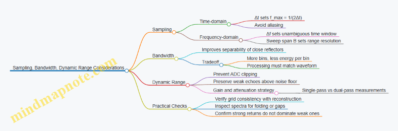
Sampling, bandwidth, and dynamic range are the three knobs that decide whether your through-wall measurement is crisp, stable, and actually useful. Sampling sets how finely you capture time or frequency; bandwidth sets how much detail you can resolve; dynamic range sets how well you can see weak echoes without being blinded by strong ones.
Sampling Foundations for Measurable Echoes
Start with what you measure: either time-domain waveforms (sampled over time) or frequency-domain sweeps (sampled across frequency). In both cases, the sampling grid must be consistent with the features you want.
For time-domain sampling, the sampling interval \(\Delta t\) determines the highest frequency you can represent: \(f_{\max}=\tfrac{1}{2\Delta t}\). If your transmitted pulse or system response contains higher frequency content than \(f_{\max}\), you get aliasing—false structure that can look like a target.
For frequency-domain sampling, the frequency step \(\Delta f\) and sweep span \(B\) determine the time window and resolution of the reconstructed response. A smaller \(\Delta f\) gives a longer unambiguous time window; a larger \(B\) gives finer range resolution. A practical way to remember it: frequency sampling controls “how far you can see without wrapping,” while bandwidth controls “how tightly you can separate two close reflectors.”
Bandwidth as a Resolution Budget
Bandwidth is not just a number on a spec sheet; it is a resolution budget that interacts with propagation loss and clutter. Wider bandwidth improves range resolution, which helps separate reflections from, say, a stud cavity and a deeper void. But wider bandwidth also spreads energy across more bins, so each bin may have less signal strength.
A concrete example: suppose you want to distinguish two reflectors separated by 5 cm. A rough range-resolution target is on the order of \(\Delta R \approx \tfrac{c}{2B}\). Solving for \(B\) gives \(B \approx \tfrac{c}{2\Delta R}\). With \(\Delta R=0.05,\text{m}\), \(B\) is about 3 GHz. If your hardware can only deliver 500 MHz, you should expect the two reflectors to blur together unless you rely on additional processing constraints (like geometry priors or multi-angle fusion).
Bandwidth also affects processing choices. If you use matched filtering, the filter length and frequency grid must match the transmitted waveform and sampling scheme. A mismatch can reduce peak sharpness even when the raw data is “correct.”
Dynamic Range as the Fight Between Strong and Weak
Dynamic range is the ability to represent both large and small signals without clipping or burying the small ones in noise. In practice, it is limited by ADC quantization, receiver noise figure, and any analog saturation before digitization.
A useful mental model: your strongest return might come from a nearby wall surface or a metal feature; your weakest return might be a reflection from a small object behind drywall. If the strong return uses most of the ADC range, the weak return may occupy only a few quantization levels, making it hard to detect reliably.
Example scenario: you set receiver gain so the strongest reflection peaks at 90% of ADC full-scale. If the weak target echo is 30 dB below that strong return, it will be around 0.09% of full-scale. Depending on ADC resolution and noise, that may still be measurable, but the detection threshold must be set carefully to avoid false alarms from quantization noise and residual clutter.
To manage dynamic range, you can adjust gain, reduce transmitted power, or change the measurement mode. For instance, you might run two passes: one optimized for strong reflections to estimate geometry, and another with lower gain or different attenuation to preserve weak echoes. The key is to keep the sampling grid identical so you can compare or fuse results without re-tuning everything.
Integrated Mind Map for Sampling, Bandwidth, and Dynamic Range
Practical Example Workflow for Choosing Settings
- Decide the target separation you must resolve (e.g., 5 cm) and estimate the required bandwidth using \(\Delta R \approx \tfrac{c}{2B}\).
- Choose sampling so the frequency grid covers the bandwidth without gaps and the time window is long enough to include expected multipath delays.
- Set gain so the strongest expected return stays below clipping while leaving enough headroom for weak echoes. If you cannot satisfy both, plan a second measurement with different gain or attenuation.
- Validate by checking whether reconstructed peaks sharpen as expected when you increase bandwidth or refine sampling; if not, suspect a grid mismatch or saturation.
When these three knobs are aligned, your data stops being “technically recorded” and starts being “usefully interpretable.”
3.4 Calibration Workflows for Repeatable Measurements
Repeatable through-wall measurements start with a simple idea: every scan should be comparable to the last one. Calibration is the set of steps that makes that true by correcting for system drift, geometry changes, and measurement chain imperfections. Think of it as turning “whatever happened today” into “the same measurement, on purpose.”
Calibration Goals and What They Fix
A good workflow targets four error sources:
- Timing and synchronization errors: phase drift or misalignment between transmit and receive.
- Amplitude and gain errors: uneven response across frequency, temperature, or cable paths.
- Positioning and geometry errors: antenna height, tilt, and scan grid offsets.
- Environmental variability: humidity, wall surface condition, and coupling changes.
A practical rule: calibrate what you can control, measure what you cannot, and record everything so you can explain differences later.
Step 1: Define a Calibration Reference Setup
Choose a reference that is stable and easy to reproduce. For RF through-wall work, a common approach is to use a known reflector (metal plate or corner reflector) placed at a fixed location relative to the antenna mount.
Example: Place a small metal plate at the same distance from the antenna as the typical target region. Mark the antenna mount position on the floor and use a rigid spacer to maintain height. If you can’t keep the environment stable, keep the reference stable.
Step 2: Perform System Warm-Up and Baseline Checks
Many measurement chains behave differently when cold. Start the system, allow it to reach thermal equilibrium, then run a baseline capture of the reference reflector.
Baseline checks should include:
- Repeatability test: run 3–5 captures back-to-back and confirm the variation is within your expected noise floor.
- Frequency response sanity: verify that the measured spectrum shape matches the expected trend (no sudden notches unless you know why).
If baseline variation is large, fix that first. Calibration cannot compensate for a measurement chain that is unstable.
Step 3: Calibrate the Measurement Chain
This step corrects amplitude and phase errors introduced by cables, connectors, and front-end electronics.
A straightforward workflow uses a two-stage correction:
- Reference normalization: divide measured data by a baseline capture taken with the same setup.
- Phase alignment: estimate a phase offset using the reference reflector peak and apply it consistently across the scan.
Example: If the reference reflector peak amplitude drops by 2 dB after a temperature change, normalization restores the relative scale so imaging differences come from the scene, not the electronics.
Step 4: Calibrate Geometry and Scan Coordinates
Geometry errors are the sneaky ones because they look like “real” structure in the image.
Use a repeatable coordinate method:
- Establish a scan origin on the wall or floor.
- Use a template or jig so antenna position and orientation repeat.
- Measure antenna height and tilt once per session, not per scan.
Example: If your antenna is consistently tilted by 2°, the backprojection can shift features. Correcting tilt at the start of the session prevents systematic mislocalization.
Step 5: Validate with a Known Target Scenario
Before scanning unknown areas, run a validation scan where the target is known. The goal is not perfection; it’s confirming the workflow produces consistent localization.
Example: Place a small metal object behind a drywall section at a known grid coordinate. Run the full scan protocol and check that the reconstructed peak falls within your tolerance window.
Step 6: Record Calibration Metadata and Apply It Automatically
Repeatability depends on traceability. Store metadata with every dataset:
- calibration reference ID and capture time
- temperature or warm-up duration
- antenna height, orientation, and scan origin
- normalization and phase correction parameters
Then apply corrections automatically during processing so you don’t rely on memory. Humans are good, but they are not consistent.
Mind Map: Calibration Workflow for Repeatable Measurements
Example: End-to-End Session Workflow
- Start system, warm up for a fixed duration.
- Capture reference reflector data 3 times; compute mean and variation.
- Compute normalization factors and phase offset from the reference peak.
- Verify antenna height and tilt using the jig.
- Run a validation scan with a known object behind a representative wall section.
- If validation passes, scan the unknown region using the same grid.
- Save calibration metadata with every dataset and apply corrections during reconstruction.
This workflow keeps the “what changed?” question answerable: if the image changes, it’s because the scene changed, not because the measurement chain wandered.
3.5 Data Logging Metadata and Traceability for Experiments
Good imaging results are not just about clean signals; they’re about being able to explain how a particular image was produced. Metadata and traceability turn “it looked good” into “it looked good because…”. This section builds from the basics of what to record, to how to structure it, to how to verify it during and after experiments.
What Metadata Must Capture
Start with four categories that cover almost every through-wall imaging workflow.
-
Acquisition context: where and when the measurement happened, and under what operating mode. Example: record the wall ID, sensor position reference, and whether you used a stepped-frequency sweep or a time-domain pulse.
-
System configuration: what the hardware and software were set to. Example: store transmit center frequency, bandwidth, number of frequency steps, pulse repetition interval, antenna model, and gain settings.
-
Calibration state: what corrections were applied and which calibration artifacts were used. Example: log the calibration run ID for antenna phase alignment and the date of the calibration dataset (e.g., 2026-04-12).
-
Data provenance: how raw data became processed outputs. Example: record the processing version, the exact windowing function, and whether clutter suppression used a direct-path subtraction.
A practical rule: if you cannot reproduce the same processing pipeline and configuration, you do not yet have traceability.
Traceability as a Chain of Custody
Traceability is easiest to manage when you treat data like a chain of custody.
- Raw: immutable measurement files captured from the instrument.
- Derived: intermediate products such as range FFTs, beamformed cubes, or intermediate images.
- Final: the outputs used for detection decisions.
Each stage should reference the stage(s) before it. Example: a final heatmap file should point to the raw capture ID and the processing configuration ID that produced it.
Metadata Schema That Stays Useful
A schema should be consistent across experiments and readable by humans during troubleshooting. Use a small set of required fields and a larger set of optional fields.
Required fields (minimum viable traceability):
experiment_idcapture_idtimestamp_utcsite_or_wall_idsensor_idsrf_parameters(center frequency, bandwidth, sweep type)positioning_reference(coordinate frame definition)calibration_idsprocessing_versionsoftware_build_hashdata_format_version
Optional fields that often save time:
- environmental notes (temperature, humidity)
- operator name or team
- known anomalies (e.g., “antenna cable swapped”)
- masking parameters used for reconstruction
Mind Map: Metadata and Traceability
Verification During Logging
Metadata is only helpful if it’s correct. Add checks at two points: right after capture and right before processing.
- Integrity checks: compute checksums for raw files so you can detect silent corruption. Example: if a raw file hash changes, you know the file was altered or truncated.
- Completeness checks: validate that required metadata fields exist before processing starts. Example: if
calibration_idsis missing, stop and request the calibration reference. - Consistency checks: confirm that RF parameters match the processing assumptions. Example: if the processing expects stepped-frequency data but the capture mode is time-domain, flag it.
Example: One Capture to One Final Output
Imagine a wall scan where you sweep from 2.4 to 2.6 GHz in 201 steps, using a fixed antenna height and a known coordinate frame.
capture_id:CAP-2026-04-12-0142rf_parameters: center 2.5 GHz, bandwidth 200 MHz, stepped-frequencypositioning_reference:FRAME-WALL-A, origin at the left corner markercalibration_ids:CAL-ANT-PHASE-2026-04-12andCAL-RX-GAIN-2026-04-10processing_version:PROC-1.7.3software_build_hash:b41c9e2
When you generate the final image, the output file includes references to capture_id and processing_version, plus the exact processing parameters used for reconstruction. If someone later asks why a target appears shifted, you can check whether the coordinate frame definition changed, or whether a different calibration run was used.
Example: Minimal Metadata Record
{
  "experiment_id": "EXP-2026-04-12-09",
  "capture_id": "CAP-2026-04-12-0142",
  "timestamp_utc": "2026-04-12T14:32:10Z",
  "site_or_wall_id": "WALL-A",
  "sensor_ids": ["ANT-01", "RX-02"],
  "rf_parameters": {
    "mode": "stepped_frequency",
    "center_hz": 2500000000,
    "bandwidth_hz": 200000000,
    "steps": 201
  },
  "positioning_reference": "FRAME-WALL-A",
  "calibration_ids": ["CAL-ANT-PHASE-2026-04-12"],
  "processing_version": "PROC-1.7.3",
  "software_build_hash": "b41c9e2",
  "data_format_version": "DFV-2"
}
This record is small enough to be practical, but it still supports the full chain of custody from raw capture to final output.
Operational Best Practices That Keep Traceability Intact
- Use stable IDs for captures and calibration runs; never rely on filenames alone.
- Freeze configuration snapshots at capture time; do not let later software edits silently change interpretation.
- Store metadata alongside data in a consistent folder structure so humans can find it during troubleshooting.
- Treat raw files as immutable and log any reprocessing as a new derived set.
When these practices are followed, the dataset becomes self-explanatory, and the experiment stops being a one-time event.
4. Antennas and Arrays for Through-Wall Sensing
4.1 Antenna Types for Imaging and Scanning
Through-wall imaging lives or dies by how well an antenna can trade off three things: how it illuminates the wall, how it separates echoes from clutter, and how repeatable the measurements are when you move or rotate the sensor. Antenna choice is therefore not just a hardware detail; it shapes the entire measurement geometry and the processing assumptions.
Foundational Antenna Roles in Imaging
An imaging system typically needs one or more antennas to perform these roles:
- Transmit illumination: radiate energy into the wall so that hidden objects produce measurable secondary scattering.
- Receive sensitivity: capture weak echoes with low noise and stable phase response.
- Spatial sampling: change the effective viewpoint across a scan so that processing can reconstruct location.
A useful way to think about antenna types is by how they control beam shape and phase stability. Narrower beams can improve angular discrimination, but they also demand more careful placement and calibration. Wider beams cover more area per measurement, but they mix more paths and clutter.
Common Antenna Types and What They’re Good At
Horn Antennas
Horn antennas provide a relatively well-defined beam and predictable radiation patterns. They are often used when you want stable illumination and consistent coupling to the environment.
Easy example: If you scan a hallway wall with a horn mounted on a fixed bracket, each position produces a similar beam footprint. That consistency makes it easier to compare measurements across the scan grid.
Best fit: controlled scanning setups where you can maintain alignment and where the beam width helps reduce ambiguity.
Directional Patch Arrays
Patch arrays can form beams electronically or mechanically (depending on design). They are compact and can be arranged to support scanning without moving the entire antenna.
Easy example: Place a small patch array at one location and step the beam direction across a few angles. You get multiple “views” without changing the sensor-to-wall distance.
Best fit: systems where you want repeatable geometry and efficient angular sampling.
Yagi-Uda and Log-Periodic Antennas
These antennas are directional and relatively simple to deploy. They can be effective for scanning when you need a strong signal in a preferred direction.
Easy example: Point a Yagi at the wall and perform a raster scan by moving only the receiver position. The directionality reduces energy that would otherwise bounce around and confuse the image.
Best fit: practical field work where robustness matters and you can accept a narrower operating bandwidth.
Dipole and Monopole Antennas
Dipoles and monopoles are often used as baseline sensors because they are straightforward and cover polarization effects clearly.
Easy example: Use a dipole and rotate it 90 degrees between scans. If a target produces a stronger response in one polarization, you learn something about how it couples to the field.
Best fit: polarization studies, calibration routines, and simpler scanning geometries.
Planar Antenna Arrays for Beamforming
Planar arrays support beamforming and can improve imaging by controlling the phase across elements. With proper calibration, they can reduce sidelobes and improve contrast.
Easy example: During processing, you can combine element signals to focus on a particular direction, then repeat for other directions. The scan becomes a sequence of controlled viewpoints.
Best fit: imaging systems that can afford calibration effort and want better angular discrimination.
Selection Criteria That Actually Matter
When choosing an antenna type for imaging and scanning, evaluate these criteria in order:
- Radiation pattern stability: Does the beam behave the same across the scan? If not, processing may interpret pattern changes as target changes.
- Polarization control: Can you align polarization with the expected coupling mechanism? Even a simple rotation step can improve interpretability.
- Bandwidth and matching: Poor matching increases reflections at the antenna feed and can distort amplitude and phase.
- Phase coherence: Imaging often assumes consistent phase relationships across measurements. Arrays and coherent systems benefit most from stable phase response.
- Mechanical practicality: If the antenna is hard to mount consistently, the “best” antenna becomes the least useful.
Mind Map: Antenna Types and Imaging Implications
Practical Example Workflow for Choosing an Antenna
Suppose you need to scan a concrete wall for a concealed object using a grid of measurement points. Start by deciding whether you will move the antenna position, steer angles, or both. If you can maintain a fixed height and orientation, a horn or directional antenna can give consistent illumination across the grid. If you need to minimize mechanical movement, a patch array or planar array can provide multiple angles from fewer physical positions.
Then run a short polarization check: take two scans with orthogonal polarization (or rotate the antenna by 90 degrees). If one polarization produces a cleaner response pattern, keep that polarization for the full scan. Finally, verify repeatability by measuring a known reference reflection at a consistent location; if it changes significantly between positions, the antenna mounting or phase coherence is likely the limiting factor.
This approach keeps antenna selection grounded in measurement behavior rather than assumptions, and it makes the later reconstruction steps less fragile.
4.2 Array Geometry and Beamforming Basics
Array geometry is the “where” and beamforming is the “how.” Together they determine which directions your system emphasizes, which it suppresses, and how cleanly it can form an image through a wall.
Array Geometry Fundamentals
Start with the array elements as points in space. For element i at position \(\mathbf{r}_i=[x_i,y_i,z_i]\), the key quantity is the extra distance a wavefront travels to reach that element compared to a reference point. If a plane wave arrives from direction \(\hat{\mathbf{u}}\), the relative path difference is
\[\Delta d_i = -\hat{\mathbf{u}}\cdot \mathbf{r}_i\]
The minus sign is just a convention: what matters is that elements “ahead” of the wavefront see the wave earlier.
Two geometry choices dominate practical systems:
- Linear arrays: elements along one axis. Good for scanning in one angular dimension.
- Planar arrays: elements on a plane. Enables 2D angular control, which helps when wall clutter creates ambiguous features.
A third choice is aperture size: the span from the first to last element. Larger apertures generally narrow the main lobe of the beam, improving angular resolution, but they also complicate calibration and increase hardware count.
Steering and Phase Alignment
Beamforming works by applying complex weights to each element’s received signal and summing. For a narrowband signal at center frequency f with wavenumber \(k=2\pi/\lambda\), the ideal steering weight for direction \(\hat{\mathbf{u}}\) is a phase term that compensates for \(\Delta d_i\):
\[w_i(\hat{\mathbf{u}})=e^{j k \hat{\mathbf{u}}\cdot \mathbf{r}_i}\]
If you steer correctly, signals from that direction add in phase; signals from other directions add with varying phase and partially cancel.
A concrete example: suppose you have 8 elements spaced by \(d=\lambda/2\) along the x-axis. For a target direction at angle \(\theta\) from broadside, \(\hat{\mathbf{u}}\cdot \mathbf{r}_i = x_i\sin\theta\). The phase progression across elements becomes \(e^{j k x_i\sin\theta}\). When \(\theta\) matches the true arrival direction, the sum peaks; when it doesn’t, the peak shifts and the sidelobes rise.
Beam Patterns and Resolution
The beam pattern is the response as a function of angle. For a uniform linear array with N elements and spacing d, the main-lobe width depends on aperture \(L=(N-1)d\). A useful rule of thumb is that the first nulls occur near angles where the phase progression across the aperture reaches \(\pm\pi\). That means wider apertures produce tighter beams.
However, spacing also matters. If d exceeds \(\lambda/2\), grating lobes appear: extra directions where the phase alignment looks “correct” even though it shouldn’t. In through-wall imaging, grating lobes are especially annoying because they can mimic real target locations.
Practical Weighting and Calibration
Ideal weights assume perfect knowledge of element positions and identical gains. In reality, you need calibration:
- Gain calibration: equalize amplitude so one element doesn’t dominate the sum.
- Phase calibration: correct systematic phase offsets due to cable lengths, electronics, and mounting tolerances.
- Position sanity checks: verify spacing and alignment; a small tilt can bias the steering angle.
A simple best practice is to measure a known reflector in free space or a controlled environment, then adjust per-element complex weights so the beam peaks at the expected direction. Even if the wall changes the propagation, this step makes your geometry-based steering trustworthy.
Mind Map: Array Geometry and Beamforming Basics
Example: Steering a Linear Array Through a Wall
Imagine a 1D array of 8 elements spaced at \(\lambda/2\) along x. You form beams for angles \(\theta\) from -60° to +60° in 1° steps. For each steering angle, you compute the phase weights and sum the received signals.
In a through-wall scenario, the “arrival direction” of energy is not purely geometric because reflections and multipath exist. Still, the beamforming step remains useful: it converts messy multi-path energy into angle-dependent measurements. When you later do imaging, you treat those measurements as evidence tied to the assumed propagation model.
A practical check: if you see strong peaks at angles that correspond to grating-lobe conditions, reduce spacing or constrain steering to avoid ambiguous directions. If peaks shift when you slightly move the array, revisit phase calibration and mounting alignment.
Summary of What to Get Right
- Geometry sets the phase relationships across elements.
- Beamforming weights align phases for a chosen direction.
- Aperture controls angular resolution; spacing controls grating lobes.
- Calibration turns the math into something your wall won’t immediately ruin.
4.3 Matching, Impedance, and Radiation Pattern Control
Matching is the quiet hero of through-wall imaging: it reduces wasted power, stabilizes the measurement, and makes the antenna behave predictably across frequency. Impedance control is how you stop the system from “arguing” with itself, while radiation pattern control is how you decide where the system looks and how cleanly it focuses.
Matching Foundations for Predictable Measurements
An RF chain has an input impedance at the antenna terminals and a source impedance at the transmitter output. When they don’t match, part of the signal reflects back, creating standing waves and frequency-dependent gain. In practice, that shows up as inconsistent image brightness across scan positions.
A useful mental model: matching turns the antenna into a load that the transmitter can “see” as close to its intended impedance. For a typical 50 Ω system, you aim for an antenna input impedance near 50 Ω over the operating band.
What You Measure
- Return loss (S11): lower magnitude means less reflection.
- VSWR: a simple reflection ratio; high VSWR means more power bouncing around.
- Bandwidth of matching: matching that only works at one frequency can still ruin imaging if your waveform spans a band.
Practical Example
Suppose you sweep 2.4–2.6 GHz for a wall scan. If S11 is excellent at 2.5 GHz but poor at the edges, your effective transmit power and receive sensitivity vary across the sweep. A straightforward best practice is to check S11 across the entire sweep range and adjust matching components (or antenna geometry) until the worst-case return loss is acceptable.
Impedance Matching Networks and Their Tradeoffs
Matching networks convert between impedances using reactive components (inductors, capacitors, transmission-line sections). The goal is not magic; it’s controlled transformation.
Common Approaches
- Direct feed: simplest, works when antenna impedance already sits near 50 Ω.
- L-section or pi networks: good for narrow-to-moderate bandwidth.
- Transmission-line transformers: often used when you need smoother behavior across frequency.
Best Practice Example
If your antenna is slightly capacitive at the low end of the band, an L-network can add inductive reactance to counter it. You tune using measured S-parameters, then verify the match after assembly, because cable routing and connector quality can shift the impedance.
Radiation Pattern Control for Imaging Geometry
Even with perfect matching, imaging quality depends on how the antenna illuminates space. The radiation pattern determines which paths contribute to the received signal and how strongly.
Key Pattern Quantities
- Main lobe direction: where energy goes.
- Beamwidth: affects spatial resolution and overlap between scan points.
- Side lobes: can create ghost responses from unintended reflections.
- Polarization: mismatch reduces coupling and can look like “missing targets.”
Polarization Example
If your transmitter and receiver are cross-polarized relative to the target orientation, coupling drops. In a wall scan, that can make a metal object appear weaker than a nearby void. A practical step is to keep antenna polarization consistent with your scanning plan and verify it by measuring received amplitude from a known reflector at a few angles.
Controlling Pattern Through Placement and Orientation
Radiation patterns are not only antenna properties; they change with the environment. Nearby metal edges, wall curvature, and mounting hardware can distort the pattern.
Systematic Placement Workflow
- Define the scan coordinate frame: where “forward” is for each antenna.
- Set a consistent stand-off distance: the gap between antenna and wall affects coupling.
- Lock orientation: use a repeatable mount so the polarization axis doesn’t drift.
- Measure a reference response: a fixed reflector or calibration target at a known location.
Example: Reducing Side-Lobe Clutter
If your pattern has strong side lobes, reflections from corners can dominate. You can reduce this by aiming the main lobe away from the corner during each scan point, then relying on overlap to recover coverage. The result is fewer spurious peaks without changing the processing pipeline.
Mind Map: Matching, Impedance, and Radiation Pattern Control
Integrated Checklist for Field-Ready Control
- Confirm S11 across the full sweep band, not just the center frequency.
- Tune matching using measured S-parameters, then validate after mounting and cabling.
- Keep polarization consistent with your scan plan and verify using a simple angled reflector test.
- Use a repeatable stand-off distance and orientation so the pattern doesn’t wander between measurements.
- Reduce clutter by aiming the main lobe to minimize strong side-lobe paths from corners and edges.
4.4 Placement, Height, and Orientation for Stable Imaging
Stable through-wall imaging is mostly about repeatability. If the antenna pose changes between scans, the reconstruction changes too—sometimes more than the object does. This section treats placement, height, and orientation as a single measurement geometry problem: you want the same transmit/receive paths and the same beam footprint each time.
Foundational Geometry: What Must Stay Consistent
Start with three invariants: (1) the antenna-to-wall distance, (2) the antenna height relative to a fixed reference on the wall, and (3) the antenna pointing direction relative to the wall normal. A practical way to think about it: your system “sees” a weighted average of paths; small pose changes shift which paths dominate.
A simple example: you scan the same wall twice with a handheld antenna. On the first pass, the antenna is slightly angled upward. On the second pass, it’s level. Even if the object is unchanged, the strongest reflections and multipath contributions move, and your image peaks can drift.
Placement: Distance and Lateral Position
Placement has two components: distance from the wall and lateral offset along the wall.
Distance from the wall affects coupling and near-field behavior. If you can’t keep a fixed standoff, at least record it and keep it within a tight band. For an easy rule of thumb, choose a standoff that is large enough to reduce direct coupling variations, but small enough to maintain signal strength.
Lateral position affects which parts of the wall are illuminated. If you’re building an image grid, define the grid in wall coordinates and keep the antenna center aligned to grid points. A helpful practice is to mark a baseline line on the wall and use a tape measure or a rail to place the antenna at known offsets.
Example: Suppose you plan a 5×5 scan with 10 cm spacing. If one row is shifted by 2 cm, the reconstruction grid no longer matches the actual measurement geometry, and features can appear “smeared” or displaced.
Height: Using a Reference That Survives Real Life
Height errors are common because people don’t naturally agree on “where the antenna is.” Fix this by using a physical reference: a ruler, laser line, or a marked rail.
Measure height to the antenna phase center (or the best available proxy). If you don’t know the phase center, be consistent: measure to the same mechanical point on the antenna housing every time.
A concrete workflow:
- Choose a wall reference line (e.g., 0 cm at floor, or a marked datum).
- Set antenna height using a rigid spacer or a clamp.
- Verify height before each scan row.
Example: If your target is at mid-wall height, a 5 cm height mismatch can change the effective incidence angle enough to alter which reflections are strongest.
Orientation: Wall Normal, Polarization, and Rotation Control
Orientation includes three angles: yaw (left-right), pitch (up-down), and roll (rotation around the antenna axis). For many RF imaging setups, polarization alignment is a major driver of signal strength.
Yaw and pitch determine the incidence direction and the beam footprint. Keep yaw aligned to the wall normal if you want consistent path weighting. Keep pitch consistent to avoid changing the balance between direct leakage and reflected energy.
Roll matters when the antenna has polarization sensitivity. If the antenna is rotated 90 degrees, the received signal can drop dramatically even when the object is unchanged.
Practical control methods:
- Use a mounting bracket with detents for yaw and pitch.
- Use a bubble level for pitch.
- Use a marked orientation ring on the antenna mount for roll.
Example: In a drywall scenario, a small roll change can reduce the signal-to-noise ratio enough that thresholding misses a target region entirely.
Integrated Setup Checklist for Repeatable Scans
Treat each scan as a “pose contract.” If you can’t guarantee the contract, you must at least measure deviations.
- Standoff: same distance from wall for all grid points.
- Grid alignment: antenna center aligned to marked wall coordinates.
- Height: fixed datum and consistent measurement point.
- Yaw/pitch: aligned to wall normal with mechanical stops.
- Roll: fixed polarization orientation with a visual index.
- Verification: quick check at the start of each row, not just at the beginning.
Mind Map: Placement, Height, and Orientation
Example: Two-Pass Scan with Controlled Pose
On Pass A, you set standoff to 30 cm using a spacer, clamp the antenna at 120 cm height to a wall rail, and align yaw to the wall normal using a bracket detent. On Pass B, you repeat the same steps but intentionally rotate roll by 10 degrees. The image difference is not random: the strongest peaks shift in amplitude and sometimes in location because polarization changes alter which multipath components dominate. The takeaway is simple: if you want stable imaging, control pose first, then interpret the scene.
4.5 Practical Antenna Selection for Concrete, Wood, and Metal
Antenna choice is mostly about matching your measurement goal to what the wall does to the signal. In practice, you’re balancing three things: (1) how much energy couples into the wall, (2) how well you can form a useful spatial response, and (3) how stable the setup stays when the environment refuses to cooperate.
Start with What You Need to See
First decide whether you’re trying to detect a target presence, estimate a rough location, or produce an image-like map. Then translate that into antenna requirements:
- Need coarse localization: prioritize stable beam direction and manageable sidelobes.
- Need fine localization: prioritize aperture size and controlled phase across the array.
- Need weak-target sensitivity: prioritize receiver noise performance and antenna gain at the chosen band.
A simple rule of thumb: if you can’t keep the antenna position and orientation consistent, the “best” antenna won’t help much.
Concrete: Rebar, Rough Surfaces, and Lossy Paths
Concrete is often the toughest case because it combines attenuation with scattering from aggregates and reinforcement. For concrete, antenna selection usually favors moderate bandwidth and robust coupling.
- Single-element horn or patch: good when you can keep a fixed standoff and want repeatable pointing.
- Broadband dipole or log-periodic: useful when you need flexibility across frequencies to find a band with better penetration.
- Array with beamforming: beneficial when you can afford more setup complexity and want to suppress clutter from strong surfaces.
Easy example: If you’re scanning a concrete wall for a void behind it, start with a directional antenna (horn or patch) at a frequency where the received signal is measurable but not dominated by surface reflections. Then compare with a broadband dipole: if the dipole improves detection but smears localization, you’ve learned that bandwidth helps sensitivity while narrowing helps spatial focus.
Wood: Lower Loss, More Geometry Sensitivity
Wood typically attenuates less than concrete, but it introduces strong effects from framing, studs, and air gaps. That means antenna choice should emphasize controlled polarization and consistent stand-off.
- Polarization-aligned patch or dipole: helps when studs create direction-dependent coupling.
- Small array or scanning element: helps separate target echoes from structural reflections.
Easy example: Suppose you’re detecting a concealed object behind drywall over wood studs. If you rotate a linearly polarized antenna by 90 degrees and the signal drops sharply, you’ve confirmed polarization sensitivity. In that case, keep the antenna orientation fixed during the scan and use the same orientation for every measurement.
Metal: Reflection-Dominated Behavior and Multipath
Metal surfaces can act like mirrors for RF, creating strong direct reflections and multipath. Antennas that rely on “clean” propagation may struggle because the strongest return may not be the target.
- Directional antennas with narrow beamwidth: reduce the amount of metal-reflected energy entering the receiver.
- Antenna arrays with beamforming: can steer nulls away from the metal-dominated paths.
- Shielded or well-matched elements: reduce unintended coupling to nearby hardware.
Easy example: If a metal plate is near the antenna, a wide-beam antenna may produce a strong peak even when no target exists. Switching to a narrower beam and adjusting standoff often makes the peak less “always-on,” which improves decision-making.
Matching Antenna Type to Frequency Band
Antenna bandwidth and element size are tied to frequency. Higher frequencies often improve angular resolution but can suffer more attenuation and more sensitivity to small structural features.
Practical selection steps:
- Pick a band where you can measure a stable return through the wall.
- Use the antenna’s bandwidth to avoid “dead zones” where the match is poor.
- Verify that the antenna pattern doesn’t change dramatically across your chosen band.
Mind Map: Antenna Selection Logic
Practical Selection Checklist
Use this checklist at the bench before you trust it on a wall:
- Pattern sanity: confirm the antenna has a predictable main lobe at the operating band.
- Polarization control: mark the antenna orientation so every scan uses the same reference.
- Standoff repeatability: measure the distance from antenna face to wall and keep it consistent.
- Match quality: verify return loss or standing-wave behavior is acceptable across the band you plan to use.
- Clutter test: with no target, record a baseline at the same points you’ll later scan.
Example: Choosing Between Three Antennas
You have three options for a wall inspection: a horn (directional), a dipole (broadband), and a small phased array (beamforming). You’re targeting a concealed void behind concrete.
- Start with the horn to establish a stable, directional response.
- Add the dipole to see whether a broader frequency span improves detectability.
- If localization is inconsistent due to clutter, move to the array and use beamforming to reduce energy from dominant surface paths.
This sequence is deliberate: it separates “can we detect anything?” from “can we place it?” and then from “can we suppress the stuff that keeps pretending to be the target?”
5. Propagation Through Common Building Materials
5.1 Material Characterization and Measurement Methods
Material characterization is the part where you stop guessing what the wall is doing and start measuring it in a way your imaging algorithm can actually use. In through-wall sensing, you typically need three things: (1) electromagnetic properties that affect propagation, (2) geometric and layering information that affects paths and interfaces, and (3) measurement repeatability so your model doesn’t drift between scans.
What You Measure and Why It Matters
Start with the properties that control wave behavior. For radio frequency work, the most useful parameters are relative permittivity (εr), conductivity (σ), and sometimes magnetic permeability (μr, usually near 1 for common building materials). These parameters determine attenuation, phase delay, and how strongly signals reflect at boundaries.
A practical way to think about it: if εr is wrong, your reconstructed positions shift; if σ is wrong, your signal strength and contrast change; if layer thickness or interfaces are wrong, multipath patterns don’t match your forward model. So characterization is not just “material ID,” it’s “model inputs with uncertainty.”
Measurement Planning and Setup
Before any measurements, define the measurement geometry you will reuse. Through-wall imaging is sensitive to antenna height, polarization, and distance to the material. A simple best practice is to mark a fixed coordinate frame on the test surface and keep antenna orientation consistent across all samples.
For repeatability, record: antenna type, center frequency (or sweep range), polarization, incident angle, distance, and environmental conditions like temperature and humidity. Even if you don’t model temperature explicitly, you’ll want to know when it changed.
Core Measurement Methods
Transmission Measurements Through Known Paths
If you can place antennas on opposite sides of a material slab, transmission is the cleanest route to estimate effective attenuation and phase delay. Use a reference path in air (or a calibration fixture) to normalize system response.
Easy example: measure S21 through a 10 cm drywall panel and compare it to S21 through a 10 cm air gap. The ratio gives you a first-order estimate of loss and phase shift per thickness. Repeat with two thicknesses (e.g., 5 cm and 15 cm) to separate thickness effects from system drift.
Reflection Measurements at Interfaces
When transmission is hard, reflection helps estimate boundary behavior. Place the antenna so the wave hits the surface at a controlled angle, then measure S11. Reflection magnitude and phase relate to impedance mismatch, which depends on εr and σ.
Easy example: measure S11 on bare concrete and on concrete with a thin plaster layer. The difference in phase slope across frequency tells you how the added layer changes effective boundary conditions.
Resonant or Cavity Methods for Small Samples
For small material coupons, resonant methods can estimate εr and loss tangent by observing resonance frequency shifts and Q-factor changes. This can be more accurate for lab samples, but it requires careful fixture design.
Easy example: place a dielectric sample in a simple resonator fixture and record the resonance peak frequency and bandwidth. Convert those changes to εr and effective loss, then verify by predicting transmission through a slab of the same thickness.
Time-Domain Characterization for Layered Structures
If your imaging system uses time-domain signals, you can characterize layers by measuring early arrivals and their delays. A layered wall often produces distinct echoes at interfaces.
Easy example: send a short pulse toward a wall section and record the reflected waveform. Identify peaks corresponding to the first interface and subsequent layers. Those time markers give thickness constraints you can feed into the forward model.
Turning Measurements Into Model Parameters
Raw measurements rarely map directly to εr and σ without a model. A common workflow is: choose a forward model (even a simplified one), fit parameters to measured S-parameters or time traces, and validate by predicting a second measurement condition.
A simple fitting discipline prevents “parameter cosplay.” Fit on one geometry (e.g., normal incidence, one distance), then predict another geometry (e.g., slightly different antenna spacing). If the prediction fails, the model is missing something—often interface roughness, effective thickness, or polarization dependence.
Uncertainty, Repeatability, and Data Hygiene
Characterization must include uncertainty. At minimum, capture variability from repeated measurements: reposition the antenna within a small tolerance, repeat the sweep, and compute spread in extracted parameters.
Also watch for measurement artifacts:
- Cable and connector drift: re-check calibration if you change temperature or move hardware.
- Antenna coupling: near-field coupling can masquerade as material effects; keep distances consistent.
- Surface contact and air gaps: especially for layered samples, small gaps can dominate results.
Mind Map: Material Characterization Workflow
Integrated Example: Characterizing a Concrete Wall Section
-
Measure transmission through a concrete coupon of known thickness to estimate an effective attenuation per centimeter and phase delay. Normalize S21 against an air reference.
-
Measure reflection on the wall surface with and without a thin finishing layer to capture boundary changes. Use the phase response across frequency to refine effective εr.
-
If the wall is layered, use time-domain echoes to estimate interface delays and constrain layer thickness. Feed those thicknesses into the forward model.
-
Validate by predicting S21 for a second thickness or a slightly different antenna spacing. If predicted contrast is too high or too low, adjust σ first; if reconstructed positions shift, adjust εr and interface placement.
This approach keeps characterization tied to imaging reality: every extracted parameter earns its place by improving prediction under a new measurement condition, not just by matching one dataset.
5.2 Concrete Rebar and Reinforced Structure Effects
Reinforced concrete changes through-wall imaging in a very specific way: it adds strong, conductive scatterers (steel) inside a lossy dielectric (concrete). The result is not just “more attenuation,” but a mix of reflection, shadowing, and multipath that can either help you localize targets or confuse your reconstruction.
Foundational Behavior of Steel Inside Concrete
Steel bars behave like elongated conductors. At radio frequencies, they reradiate energy and create strong reflections, especially when the bar orientation aligns with the incident field polarization and the observation direction. Concrete, by contrast, mainly absorbs energy and adds phase delay through its permittivity and loss tangent.
A practical way to think about it: concrete sets the overall “brightness” of the scene, while rebar sets the “texture.” If you ignore rebar, your forward model assumes a smooth slab and your inverse step tries to explain steel-induced artifacts as if they were hidden objects.
What You Actually See in Measurements
In a typical scan, rebar effects show up as:
- Localized bright streaks or arcs in imaging outputs, often corresponding to bar ends, intersections, or near-parallel segments.
- Depth-dependent clutter where the strongest steel reflections dominate the dynamic range, masking weaker signals behind the reinforcement.
- Angle-dependent responses where the same bar appears stronger at some scan positions and weaker at others due to geometry and polarization.
A simple example: if you scan a wall with a rebar grid, you may notice that the “grid pattern” becomes clearer when you change antenna height or lateral position, even though the wall itself is unchanged. That’s geometry and multipath doing their job.
Orientation and Polarization Effects
Rebar is rarely a single bar; it’s a network. Each bar has an orientation, and each orientation interacts differently with the incident field. When the antenna polarization couples well to the bar’s effective current path, the reflection strength increases.
For an easy mental model, imagine two cases:
- A bar roughly aligned with the dominant electric field component: stronger coupling, stronger reflection.
- A bar mostly orthogonal to that component: weaker coupling, more subtle contribution.
This matters for best practices: keep antenna polarization consistent across a dataset, and record antenna orientation so you can interpret changes as physics rather than “mystery variation.”
Reinforcement Geometry and Its Imaging Consequences
Rebar geometry includes spacing, diameter, cover depth (distance from surface), and layering (single mat vs multiple mats). These parameters control three imaging behaviors.
- Cover depth controls apparent depth: steel reflections arrive earlier or later depending on path length through concrete. If your reconstruction grid assumes wrong cover depth, steel can “move” in the image.
- Spacing controls periodic clutter: regular spacing can produce repeating patterns that look like multiple targets.
- Layering controls interference: two mats at different depths can create constructive or destructive interference in coherent processing.
Example: a wall with two reinforcement layers can produce a strong response at two depth bands. If you threshold blindly, you might report two “objects” where there are none.
Modeling Strategy for Robust Reconstruction
A systematic approach is to treat rebar as a structured scatterer rather than noise.
- Step 1: Estimate reinforcement layout using drawings when available, or infer it from repeated scan signatures. Even coarse estimates help.
- Step 2: Incorporate steel as high-contrast elements in the forward model. You don’t need perfect metallurgy; you need the geometry and relative strength.
- Step 3: Use residual analysis: after reconstruction, check whether the strongest artifacts correlate with expected bar locations. If they do, your model is doing the right kind of work.
Practical Best Practices in the Field
- Vary scan positions with overlap so multipath patterns average out. If you only sample a narrow strip, rebar artifacts can masquerade as localized targets.
- Use consistent antenna height. Small height changes alter the coupling to bars and can shift bright features.
- Record polarization and orientation. Without that metadata, you lose the ability to separate “physics changes” from “setup changes.”
- Apply target selection rules that penalize periodicity when appropriate. A true hidden object often produces a less regular pattern than a rebar grid.
Mind Map: Concrete Rebar Effects on Through-Wall Imaging
Example: Distinguishing Rebar from a Hidden Void
Suppose you scan a concrete wall and see a strong response at a depth band consistent with rebar cover. To test whether it’s steel or a void, you can:
- Compare responses across adjacent scan lines. Rebar signatures tend to follow the grid-like geometry and remain correlated with bar locations.
- Check for polarization sensitivity. If the feature strength changes strongly with antenna orientation, it likely couples to conductive bars.
- Look for persistence at expected bar intersections. Steel intersections often produce stronger localized reflections than a void of similar size.
If the feature stays aligned with the inferred reinforcement pattern and shows strong orientation dependence, treat it as rebar-driven clutter and adjust your reconstruction or decision thresholds accordingly.
5.3 Drywall Insulation and Void Impacts on Signals
Drywall is thin, but it rarely behaves like a simple flat sheet. In through-wall imaging, the drywall layer mainly sets the “front door” boundary conditions, while insulation and voids inside the cavity shape how energy spreads, attenuates, and reflects. The practical goal is to predict which effects dominate so you can choose frequencies, scan geometry, and processing steps that match the wall’s internal structure.
Foundational Signal Effects in Cavity Walls
Start with the cavity as a three-part system: drywall surface, cavity air (or partial fill), and insulation material. Each part contributes differently.
- Drywall surfaces create a strong impedance contrast with air, so you often see a noticeable front-wall reflection. This can be useful as a timing anchor, but it can also mask weaker echoes from deeper features.
- Insulation changes the effective permittivity and loss. Fibrous materials typically increase attenuation and can reduce coherent buildup in beamforming, especially when the material is uneven.
- Voids behave closer to air gaps: lower loss, lower permittivity, and stronger specular reflections at void boundaries. A void can therefore produce a clearer “edge” echo than the surrounding insulation, even if it is small.
A simple mental model: drywall is the loud neighbor at the door; insulation is the carpet that absorbs footsteps; a void is a hallway that bounces sound back toward you.
Drywall Insulation: Attenuation and Coherence Loss
Insulation affects signals in two ways: amplitude reduction and phase consistency.
- Amplitude reduction comes from dielectric loss and scattering within the material. Even if the insulation is mostly air-filled, the fibers and trapped moisture (if present) increase effective loss.
- Phase consistency matters for imaging. If the insulation properties vary across the beam footprint, different rays accumulate slightly different phase errors. In coherent processing, those errors reduce the summed peak, making targets look weaker or broader.
Easy example: Suppose you scan the same location twice, once with a cavity that is well-filled with insulation and once with a partially filled cavity. In the insulation-filled case, the overall signal-to-noise ratio drops and the reconstructed target region spreads. In the partially filled case, you may see sharper contrast because the dominant path includes a more uniform air-like region.
Voids: Boundary Reflections and Multipath
Voids introduce additional interfaces: drywall-to-void, void-to-insulation, and void-to-air pockets. These interfaces create extra reflections and multipath paths.
- Small voids often act like localized scatterers, producing weaker but more localized artifacts.
- Large voids can behave like a quasi-flat reflector, producing stronger echoes and sometimes a “ghost” structure in backprojection if the processing assumes a uniform medium.
Easy example: If a void is roughly planar and parallel to the wall, you may observe an echo that stays at nearly the same depth across neighboring scan positions. That stability is a clue that the void boundary is dominating rather than a random scatterer.
Frequency Dependence and Practical Tradeoffs
Drywall and insulation losses generally increase with frequency, while resolution improves with bandwidth. The result is a trade: higher frequencies can separate features spatially but may not penetrate as well through lossy insulation.
Rule-of-thumb workflow:
- If the wall is insulation-heavy and echoes from deeper regions are weak, prioritize lower frequencies or narrower bandwidth to improve penetration and stability.
- If voids are expected and you need sharper localization, use higher frequencies only if you still see usable reflections beyond the front wall.
Geometry and Scan Planning for Cavity Effects
Cavity-induced artifacts often correlate with geometry.
- Angle of incidence: A void boundary that is nearly perpendicular to the dominant ray direction reflects more strongly back. Changing antenna angle can help distinguish a void echo from diffuse insulation scattering.
- Antenna footprint: If your beam footprint is larger than the void, the void echo is diluted. If it is smaller, the void can stand out.
Easy example: When scanning across a stud bay, you may see alternating stronger and weaker responses. The stud bay often contains different cavity fill conditions than the stud itself, so the imaging output can “strip” along the building’s structural rhythm.
Mind Map: Drywall Insulation and Void Impacts on Signals
Integrated Example Workflow for a Stud Bay
- Collect baseline scans at multiple antenna angles across a stud bay.
- Identify the front-wall reflection and use it as a depth reference.
- Compare echo strength and depth stability across positions.
- If deeper echoes weaken smoothly, insulation loss is likely dominating.
- If deeper echoes appear at consistent depth in a localized region, a void boundary is likely contributing.
- Adjust processing assumptions by using a more conservative medium model for insulation-heavy areas and focusing on boundary-consistent features for void-like echoes.
This approach keeps the reasoning grounded: you treat drywall as the boundary, insulation as the attenuator and phase disruptor, and voids as the interface generator that often leaves the clearest fingerprints.
5.4 Metal Surfaces and Multipath Dominated Environments
Metal surfaces change the game because they reflect energy strongly and often with phase shifts. In through-wall imaging, that reflection creates multipath: the same target contribution arrives through multiple paths, while clutter reflections from the wall and metal fixtures compete for attention. The practical goal is to separate “useful structure” from “repeatable echoes.”
Core Mechanisms Behind Multipath
Start with what metal does to an incident wave. A smooth metal face behaves like a strong reflector, so energy bounces back with high amplitude. If the surface is not perfectly smooth, micro-roughness spreads energy into angles rather than sending it back as a single clean ray. In a building, you rarely have just one reflecting surface; you have metal studs, rebar, pipes, door frames, and sometimes HVAC components. Each reflection adds another delayed and angled copy of the signal.
Multipath becomes dominant when the direct path is weak or blocked. For example, if the wall attenuates the direct signal heavily, the reflected paths can become the largest contributors to the received waveform. That is when imaging algorithms that assume a relatively simple propagation model start producing ghost features.
Foundational Observations You Can Measure
Before processing, check the received data for signatures of multipath. A simple time-domain view often shows multiple peaks rather than one. In frequency-domain data, multipath can appear as deep notches or rapid ripple across frequency, caused by constructive and destructive interference.
A useful rule of thumb: if the waveform changes significantly when you move the antenna by a small distance, you are likely seeing strong interference patterns rather than stable propagation. That sensitivity is not a failure; it’s a clue that geometry and phase are doing most of the work.
Practical Best Practices for Robust Imaging
1. Treat Metal as a Known Reflector, Not Just Noise. If you can identify likely metal locations (door frames, conduit runs, access panels), incorporate them into your forward model or at least into your masking strategy. For instance, when scanning near a metal door jamb, expect strong early reflections; you can downweight early-time bins that correspond to the jamb and focus on later bins where target echoes may appear.
2. Use Calibration Moves That Probe Interference. Perform a short calibration scan with the same antenna motion pattern you will use in the field. Then compare the “empty wall” response to the response with a known target placed at a consistent location. If a feature appears in both, it is probably a metal-driven echo. If it appears only with the target, it is more likely target-related.
3. Control Antenna Orientation and Height Consistently. Metal reflections are angle-sensitive. A small tilt can change the dominant reflection path and shift interference fringes. Keep the antenna mount fixed, and record orientation so you can repeat scans with the same geometry.
4. Apply Windowing and Gating in Time or Range. When multipath produces strong early peaks, gating can reduce clutter. Example: if the first 2–3 ns correspond to wall and frame reflections, apply a gate that starts after that region. This does not remove multipath entirely, but it reduces the strongest competing components.
5. Prefer Coherent Summation When Phase Is Reliable. If your system maintains stable phase across the measurement, coherent methods can reinforce target contributions while averaging down inconsistent clutter. If phase stability is poor, coherent summation can amplify artifacts, so you may need more conservative processing.
Example: Interpreting a Metal-Frame Scan
Imagine scanning a wall segment where a metal conduit runs vertically. You observe three prominent peaks in the range profile: one very early, one mid-range, and one late. The early peak is consistent across repeated scans without a target, so it likely comes from the conduit or frame. When a small object is placed behind the wall at a known depth, the mid-range peak grows and shifts slightly with antenna position, while the early peak remains nearly unchanged. In processing, you would gate out the early region, then focus reconstruction on the depth band around the mid-range peak.
To avoid overconfidence, you also check lateral behavior: a true target echo should move predictably across scan positions, while a fixed reflector echo often stays tied to the metal geometry.
Mind Map: Metal Surfaces and Multipath Dominance
Advanced Details Without the Mystery
Multipath is not just “more clutter”; it changes the effective point spread function. With strong metal reflections, sidelobes can become structured, forming consistent false regions that repeat across scans. That is why gating, calibration, and geometry control matter: they reduce the chance that the algorithm locks onto a repeatable reflector pattern.
Finally, remember that metal can create both helpful and harmful effects. A strong reflector can provide a stable reference for phase alignment, but only if you can separate it from the target region. The workflow above aims to make that separation practical: measure, identify stable echoes, gate, reconstruct, and verify movement with known target placement.
5.5 Building Layout Effects on Imaging Geometry
Building layout changes the geometry of what you can see, how signals travel, and where reconstruction algorithms place energy. Even with a perfect wall model, the floor plan decides the angles, path lengths, and multipath structure that your measurements contain. The goal is to treat layout as part of the measurement system, not as background noise.
Foundational Geometry: What Layout Changes
Start with the simplest imaging assumption: a known transmitter and receiver position, a known wall plane, and a target location in a defined coordinate system. In practice, layout adds three geometry shifts.
-
Coordinate alignment drift: If the wall you scan is not aligned with your coordinate axes, the reconstructed target will appear rotated or shifted. A quick example: you measure a corridor wall, but your “north” axis is actually 7° off because you aligned the rig to a doorway instead of a marked grid.
-
Effective propagation paths: Layout determines whether signals mainly cross the wall directly or bounce off adjacent surfaces like floors, ceilings, and perpendicular walls. In a room corner, a “through-wall” target can be dominated by energy that never truly crosses the wall in the direct sense.
-
Occlusion and accessible viewpoints: You may not be able to place the antenna at the ideal height or distance because furniture, doors, and safety barriers block access. This changes the baseline and viewing angles, which directly affects localization.
Layout-to-Measurement Mapping
Treat each scan as a set of rays. Layout controls which rays exist.
-
Corridors: Long, narrow spaces encourage repeated reflections between parallel walls. Example: scanning a door-adjacent wall in a hallway often produces ghost features at consistent offsets because the corridor acts like a reflection channel.
-
Rooms with corners: Corner geometry creates strong multipath from the perpendicular wall. Example: a target behind a partition may appear smeared along the bisector direction because energy couples into both walls.
-
Openings and recesses: Windows, vents, and recessed niches create additional interfaces. Example: a shallow recess can behave like a secondary “boundary,” shifting apparent range for features located near the recess edge.
-
Multiple walls in series: If the signal must cross more than one partition, the effective attenuation and phase behavior change. Example: scanning from one room into another through a thin interior wall can look fine, but scanning into a third room through two partitions yields weaker, less stable reconstructions.
Practical Geometry Controls
Use layout-aware controls to keep reconstructions honest.
-
Define a consistent coordinate system: Anchor your axes to fixed building references such as floor level and a marked wall edge. Example: measure antenna height from the floor, not from the rig base, because floor finishes can vary by a few centimeters.
-
Record the actual scan footprint: Store transmitter/receiver positions for every measurement. Example: if you stop the scan early to avoid a doorway, do not pretend the missing positions were collected; reconstruction should reflect the true sampling.
-
Use overlap planning: Plan adjacent scan lines so that the viewing angles overlap enough to constrain the inverse problem. Example: if you scan only one side of a wall, a target near the wall edge may be underconstrained; adding a second adjacent line improves stability.
-
Segment the scene by surfaces: If the building has distinct planes—main wall, perpendicular wall, floor—treat them as separate geometric elements in your forward model. Example: in a corner, modeling the perpendicular wall as a generic “clutter region” often produces less consistent localization than explicitly including it as a boundary.
Advanced Details: Geometry Effects on Resolution and Artifacts
Layout affects both resolution and the shape of artifacts.
-
Viewing angle limits: With narrow access, the system sees the target from a limited set of angles, which increases uncertainty in cross-range localization. Example: scanning a wall from a single doorway produces tight range estimates but broader lateral spread.
-
Edge diffraction and boundary coupling: Wall edges and junctions can create localized responses that reconstruction may interpret as point targets. Example: a junction near the scan boundary can generate a bright spot that stays fixed across multiple passes, indicating a geometry-driven artifact.
-
Multipath coherence: When reflections are strong and repeatable, artifact locations can appear stable. Example: in a corridor, the same “false target” may recur at the same reconstructed coordinates because the path length difference stays nearly constant.
Mind Map: Building Layout Effects on Imaging Geometry
Example: Corridor Scan with a Doorway Constraint
A team scans a wall from one side of a corridor because a door blocks the opposite side. They align coordinates to the floor and a marked wall edge, then collect two overlapping scan lines from the doorway area. The first scan shows a bright spot near the wall edge that does not move when they slightly shift the antenna height. After segmenting the perpendicular surfaces and including the corridor floor and adjacent wall as explicit boundaries, the bright spot reduces while a weaker interior feature becomes more consistent across passes. The takeaway is simple: layout-driven geometry effects can masquerade as targets unless you control coordinates, sampling, and surface modeling together.
6. Imaging Modalities and Core Processing Techniques
6.1 Time Domain and Frequency Domain Imaging Approaches
Through-wall imaging often starts with a simple question: what does the wall do to a signal, and how can we infer hidden structure from that change? Two main approaches answer it from different angles. Time domain imaging asks how echoes and delays appear after a pulse. Frequency domain imaging asks how the wall’s response varies across frequency. Both can produce spatial reconstructions, but they differ in measurement setup, processing steps, and the kinds of errors you notice first.
Time Domain Imaging Approach
Time domain systems transmit a short pulse (or a coded pulse) and measure the received waveform. The key observable is the time-of-flight of energy components. If a target or interface reflects part of the signal, it contributes a delayed feature in the received trace. In practice, the wall creates many delays due to reflections, scattering, and multipath, so imaging is less about finding one “perfect echo” and more about separating consistent paths.
A practical workflow looks like this:
- Acquire waveforms at multiple antenna positions or angles.
- Window and align traces to a reference event, such as the direct path or a calibration reflector.
- Select time gates that correspond to plausible propagation through the wall.
- Backproject or beamform using the gated data to form an image.
Easy example: imagine scanning a doorway with a handheld pulsed radar. The strongest early return is often the direct coupling between antennas. Later returns may include wall interfaces and any object behind the wall. If you gate out the early region, you reduce direct-path clutter and let weaker delayed components contribute to the reconstruction.
Time domain strengths are intuitive: delays map naturally to range, and gating can suppress unwanted components. The tradeoff is that short pulses require sufficient bandwidth to resolve closely spaced features, and timing errors directly blur the image.
Frequency Domain Imaging Approach
Frequency domain systems sweep a carrier across a band and measure the complex response at each frequency. The observable is how amplitude and phase change with frequency. Those changes encode propagation effects such as attenuation, dispersion, and interference.
A common workflow:
- Measure S-parameters or complex transfer functions across frequency.
- Calibrate to remove system response and antenna coupling.
- Transform the frequency response into a delay profile using an inverse transform.
- Image using the resulting delay-domain data or by frequency-domain beamforming.
Easy example: suppose you sweep 1–3 GHz through a wall. If a hidden void causes additional reflections, the interference pattern across frequency shifts. When you convert the sweep to a delay profile, that shift appears as energy at a specific delay. You can then gate and backproject similarly to the time domain case.
Frequency domain strengths include stable measurement of complex values and often better control over calibration. The tradeoff is that sweep nonlinearity, phase wrapping, and limited bandwidth can distort the delay-domain representation.
How They Relate
Time and frequency approaches are connected by transforms. A pulse in time corresponds to a broad spectrum in frequency; a frequency sweep corresponds to a time-domain response after transformation. That means many processing ideas transfer: gating, coherent summation, and reconstruction grids can be shared.
The main difference is where you “pay” for resolution. In time domain, bandwidth comes from the pulse shape. In frequency domain, bandwidth comes from the sweep span. Either way, limited bandwidth sets the sharpness of delay features, and that sharpness limits range resolution.
Mind Map: Imaging Domain Choices
Example: Choosing a Domain for a Concrete Wall
Consider a concrete wall with rebar. Rebar often creates strong multipath and narrowband-like interference patterns. If you use time domain, you can gate around delays that are consistent with paths passing through the wall thickness rather than along the surface. If you use frequency domain, you can calibrate the complex response and then transform to delay, where the rebar-related clutter tends to cluster at certain delays. In both cases, the best results come from matching the gate to the geometry and measurement setup, not from assuming the strongest feature is the target.
Practical Integration Tips
- Use a reference event for alignment in both domains, such as direct coupling or a known calibration reflector.
- Treat gating as a hypothesis test: start with a conservative window, then tighten it based on how stable the image features are across adjacent antenna positions.
- Check consistency across positions: true structure-related features should move predictably with scan geometry, while random noise and calibration artifacts tend to behave less consistently.
Time domain and frequency domain imaging are two ways to observe the same physics. The choice mainly determines how you represent the data and where errors show up first. Once you translate both into delay-domain thinking—either directly or via transformation—the reconstruction steps become much easier to reason about.
6.2 Synthetic Aperture Concepts for Spatial Reconstruction
Synthetic aperture is a way to turn many small measurements taken from different positions into an image with the spatial detail you would normally get from a much larger antenna. The “aperture” is synthetic because the system never physically has a huge array; instead, it synthesizes one through motion or scanning.
Core Idea and Why It Works
In a through-wall imaging setup, each transmit-receive position produces a measurement that depends on the target’s location and the wave paths through the wall. If you collect measurements while moving an antenna (or a small array) across a line or grid, you get multiple views of the same scene. Spatial reconstruction then combines these views by aligning them to what the data would look like if a target were at a candidate location.
A helpful mental model: treat each measurement as a “vote” for where a reflector could be. When the candidate location matches the true geometry, the votes add coherently; when it doesn’t, they smear or cancel. Coherence is the whole game, so timing, phase stability, and calibration matter.
Geometry of the Synthetic Aperture
You choose an aperture path: a straight line, a raster grid, or a curved trajectory. For each position, you record the signal and the exact antenna pose. Reconstruction uses a forward model that predicts the phase and amplitude contribution from each candidate point.
Key geometric quantities:
- Aperture length controls cross-range resolution. Longer aperture generally sharpens left-right detail.
- Step size controls aliasing and grating lobes. Too large a step causes multiple candidate locations to explain the data equally well.
- Look angle and standoff affect how sensitive the measurements are to cross-range position.
From Measurements to Spatial Reconstruction
The reconstruction pipeline typically looks like this:
- Collect data at positions along the aperture path.
- Calibrate phase and amplitude so that measurements are comparable across positions.
- Choose a reconstruction grid in the wall coordinate system.
- Compute predicted responses for each grid point and each aperture position.
- Sum contributions across positions using a coherent rule.
A common coherent rule is matched filtering: for each grid point, you apply the conjugate of the predicted phase history and sum across the aperture. The result is an image intensity map where peaks correspond to likely reflector locations.
Mind Map: Synthetic Aperture Workflow
Practical Example: A Line Scan Backprojection
Assume you scan an antenna along a horizontal line in front of a wall. You record complex samples at each step for a narrow frequency band.
For a candidate point
- compute the distance from each antenna position to the point,
- convert that distance to a predicted phase shift,
- multiply the measured complex sample by the conjugate of that predicted phase,
- sum across all positions.
If the candidate point matches the true target, the phase shifts align and the sum magnitude grows. If the candidate point is off, the phase alignment breaks and the sum spreads into a lower-intensity region.
A subtle but important detail: you need the correct coordinate transform between the antenna pose and the reconstruction grid. If the grid is shifted by even a small amount, the predicted phase history changes, and the coherent sum loses sharpness.
Advanced Detail: Sampling and Grating Lobes
Synthetic aperture behaves like an array in the cross-range direction. If your step size is too large relative to wavelength and geometry, you can get multiple apparent locations that satisfy the same phase progression. These show up as secondary peaks, often called grating lobes.
A practical rule of thumb is to choose step size so that the phase change between adjacent positions for a typical target depth does not jump by more than about half a cycle. In practice, you verify this by reconstructing a known target and checking whether the main peak is clean or accompanied by strong replicas.
Advanced Detail: Coherence and Phase Errors
Coherent summation is sensitive to phase errors that vary with position. Common sources include:
- inconsistent timing between transmit and receive,
- drift in oscillator phase,
- pose measurement noise,
- imperfect calibration of cable delays.
If phase errors are random, they reduce peak height and broaden the image. If they have a systematic trend (for example, a consistent pose bias), the peak shifts. That’s why calibration and pose accuracy are not “setup chores”; they directly determine whether the synthetic aperture adds up or just averages.
Interpreting the Output
The reconstructed image is not a literal photograph; it’s an intensity map produced by your model and summation rule. Peaks indicate locations that best match the assumed propagation geometry. To interpret results reliably, you compare peak locations across nearby grid resolutions and check that the strongest peaks remain stable under small reconstruction parameter changes.
When you see a peak that moves wildly with minor grid adjustments, it often means the model mismatch is dominating. When the peak stays put and sharpens with better calibration or denser aperture sampling, it’s behaving like a real reflector rather than a modeling artifact.
6.3 Backprojection and Matched Filtering Methods
Backprojection and matched filtering are two ways to turn measured signals into spatial images. Backprojection focuses on “where could the signal have come from?” by accumulating energy along geometric paths. Matched filtering focuses on “does the signal look like what we expect?” by correlating measurements with a predicted waveform. In practice, many through-wall imaging pipelines use both ideas: matched filtering cleans up the data, then backprojection places the evidence into space.
Core Idea of Backprojection
Backprojection starts with a forward model: for a candidate point in the scene, you can predict the time delay (or frequency-dependent phase) between each transmitter and receiver. For each measurement, you compute what the contribution would be if the target were at that candidate point, then sum contributions over all antenna positions.
A simple mental model: imagine you have a stack of “time-of-flight” slices. Each slice says how strong the signal was at a particular delay. Backprojection takes each candidate location, converts it into the delay it would produce, and pulls the corresponding slice value into that location. If many antenna positions agree, the location accumulates high intensity.
Geometry and Delay Computation
For monostatic sensing (same antenna transmits and receives), the round-trip distance from antenna position \(\mathbf{r}*m\) to candidate point \(\mathbf{x}\) is \(R_m=|\mathbf{x}-\mathbf{r}*m|\). The predicted delay is \(\tau_m=2R_m/c\). For bistatic sensing (separate transmit and receive), use \(R_m=|\mathbf{x}-\mathbf{r}*{t,m}|+|\mathbf{x}-\mathbf{r}*{r,m}|\).
The key best practice is to keep coordinate frames consistent. If your antenna positions are in a local building coordinate system but your reconstruction grid is in another, you will get “confidently wrong” images—strong peaks where nothing is.
Matched Filtering as a Measurement Cleanup
Matched filtering computes a correlation between the measured signal and a reference waveform. In through-wall imaging, the reference is often the expected received signal for a hypothesized target response, including the predicted delay and phase.
A practical example: suppose you transmit a known pulse \(s(t)\). After recording \(y_m(t)\) at antenna position \(m\), you form a delayed reference \(s(t-\tau_m)\) and compute \(\int y_m(t), s^*(t-\tau_m), dt\). If the target is at \(\mathbf{x}\), then \(\tau_m\) aligns the pulse energy and the correlation becomes large.
This is where matched filtering and backprojection meet: the correlation score becomes the “evidence value” you backproject into \(\mathbf{x}\).
Systematic Pipeline from Data to Image
- Preprocess: remove DC offsets, apply windowing, and optionally normalize channels so one antenna does not dominate purely due to gain.
- Choose a representation: time-domain delays for pulsed systems, or frequency-domain phase terms for stepped-frequency systems.
- Compute predicted delays: for each grid point and each antenna position.
- Apply matched filtering: correlate (or phase-compensate and sum) for each grid point.
- Backproject: sum evidence across antenna positions to form the image intensity.
- Postprocess: apply dynamic range control and suppress obvious artifacts (for example, strong direct-path leakage).
A useful rule of thumb: if your matched filtering step is weak (poor alignment, wrong reference), backprojection will still produce an image, but it will look like a blurry vote count rather than a focused localization.
Mind Map: Method Relationships
Example: Small 2D Grid with Delay Alignment
Consider a 2D wall plane where you scan along a line of antenna positions \(\mathbf{r}_m\). You define a reconstruction grid of candidate points \(\mathbf{x}_k\). For each \(\mathbf{x}_k\):
- compute \(\tau_{m,k}=2|\mathbf{x}_k-\mathbf{r}_m|/c\)
- correlate \(y_m(t)\) with \(s(t-\tau_{m,k})\) to get a score \(q_{m,k}\)
- sum \(I_k=\sum_m q_{m,k}\)
If you accidentally use \(c\) instead of an effective propagation speed that matches your dominant material path, the peak will shift and broaden. The image still “works,” but the peak-to-true-location error grows.
Practical Notes on Resolution and Artifacts
Resolution is governed by bandwidth (time-domain sharpness) and aperture (how widely you view the scene). Backprojection tends to smear along directions where the geometry provides less angular diversity. Matched filtering tends to suppress components that do not match the expected waveform shape, but it cannot fix a wrong delay model.
A final sanity check: run a reconstruction on a known empty region and verify that the intensity distribution is low and relatively uniform. If you see structured peaks everywhere, the issue is usually preprocessing, reference waveform mismatch, or coordinate errors—not the wall being “mysterious.”
6.4 Beamforming and Coherent Summation Strategies
Beamforming is the practice of combining signals from multiple antenna elements (or multiple measurement positions) so that energy arriving from a chosen direction and path history adds up, while other contributions partially cancel. Coherent summation is the core mechanism: you add complex-valued measurements with phase alignment, so the sum magnitude grows when the phase is correct.
Foundational Idea of Coherent Addition
A single measurement can be modeled as a complex sample: \(x = A e^{j\phi} + n\), where \(A\) is amplitude, \(\phi\) is phase, and \(n\) is noise. If you have \(M\) sensors observing the same target contribution with the same phase after compensation, then the coherent sum is \(S = \sum_{m=1}^{M} x_m e^{-j\hat{\phi}_m}\). When \(\hat{\phi}_m\) matches the true phase, the target term adds like \(M A\), while uncorrelated noise tends to add more like \(\sqrt{M}\). That difference is why coherent strategies improve detectability.
A practical way to think about it: beamforming is not magic phase guessing; it is phase bookkeeping. You compute what phase each channel should have for a hypothesized location, then you rotate each channel by the negative of that phase before summing.
Phase Compensation from Geometry and Timing
For a hypothesized target point \(\mathbf{r}\), the expected propagation delay from sensor \(m\) is \(\tau_m(\mathbf{r})\). If your system uses frequency-domain data at frequency \(f\), the phase rotation is often written as \(e^{-j2\pi f \tau_m}\). For time-domain data, you can apply a fractional delay via interpolation or by transforming to a domain where delays become phase ramps.
The key best practice is to keep the coordinate frames consistent. If your antenna positions are in meters but your delay model assumes centimeters, the beam will “steer” to the wrong place even if everything else is correct. A quick sanity check is to test a known reflector or a calibration target and verify that the peak appears where the geometry predicts.
Beamforming Weighting and Tradeoffs
Once you can align phases, you choose weights \(w_m\) to control sidelobes and robustness. A simple choice is uniform weights, \(w_m=1\), which maximizes coherent gain but can produce higher sidelobes. Tapered weights reduce sidelobes at the cost of some mainlobe width.
A concrete example: suppose you have a linear array of 16 elements. Uniform weighting might yield a narrow mainlobe but noticeable “ghost” peaks from multipath. Applying a mild taper (for instance, a cosine-like roll-off) often reduces those ghosts because the far-off contributions no longer add as strongly.
Coherent Summation Inside Imaging Pipelines
In through-wall imaging, you typically evaluate many hypotheses across an image grid. For each grid point \(\mathbf{r}_k\), you compute predicted delays \(\tau_m(\mathbf{r}_k)\), rotate each channel accordingly, and sum. The resulting image value might be \(|S(\mathbf{r}_k)|\) or \(|S(\mathbf{r}_k)|^2\), depending on how you want contrast to behave.
A systematic workflow looks like this:
- Preprocess each channel to remove obvious artifacts (DC offsets, known system delays).
- Calibrate phase so that “zero delay” is truly zero across channels.
- For each grid point, compute delays from geometry.
- Apply phase rotations at the measurement frequencies (or delays in time).
- Sum coherently using chosen weights.
- Post-process the image with consistent scaling so thresholds behave predictably.
Mind Map: Beamforming and Coherent Summation
Example: Steering to a Known Target Through a Wall
Imagine a two-antenna setup measuring a wall from the same side. You collect frequency sweeps and store complex spectra for each antenna. Choose a grid point on the far side where a small metal plate is expected.
For each frequency bin \(f_i\), compute \(\tau_1(\mathbf{r}_k)\) and \(\tau_2(\mathbf{r}_k)\). Rotate channel 2 by \(e^{-j2\pi f_i(\tau_2-\tau_1)}\) so that both channels are aligned relative to channel 1 for that hypothesis. Then sum the aligned complex values across antennas (and across frequencies if your processing supports it). If the plate is near \(\mathbf{r}_k\), the aligned phases reinforce and the magnitude at that grid point rises.
If the peak appears shifted, the most common causes are geometry mismatch (antenna positions), incorrect wall thickness in the delay model, or uncorrected channel phase offsets. The fix is usually not “more processing,” but correcting the phase model inputs so the rotations match reality.
Example: Reducing Multipath Ghost Peaks with Weighting
Suppose your imaging map shows a strong main peak plus several weaker peaks that repeat at similar offsets. Those are often sidelobes or multipath contributions that partially align for some grid points. Switching from uniform to a tapered weighting reduces the contribution of edge elements that are more sensitive to phase errors and multipath.
A practical check: compare two images computed with different weight profiles but the same delay model. If the main peak location stays stable while the ghost peaks shrink, you’ve improved sidelobe behavior rather than accidentally changing the geometry. That stability is a good sign that your beamforming is doing coherent alignment for the intended path.
6.5 Handling Clutter and Direct Path Suppression
Through-wall imaging often fails for a simple reason: the strongest signal is usually not the hidden object. It’s the direct path (line-of-sight leakage) and other clutter such as wall-to-wall reflections, antenna coupling, and multipath. The goal of direct path suppression is to reduce those dominant components while preserving weaker, spatially informative echoes.
Foundational Idea: What Counts as Clutter
Clutter is anything that produces energy in the same measurement channels as the target but does not carry the target’s spatial signature. Direct path suppression focuses on the most repeatable clutter term: energy that arrives with nearly fixed delay and phase across scans.
A practical mental model: your measurement is a sum of (1) direct leakage, (2) structured reflections from known surfaces, and (3) target-dependent scattering. If you remove (1) and reduce (2) without damaging (3), the imaging stage has a fighting chance.
Direct Path Suppression Methods
Reference Subtraction Using a Calibration Scan
Take a “no-target” or “empty” scan under the same geometry and settings. Subtract it from the target scan after aligning time/frequency axes.
Easy example: you scan a wall with an array at fixed height. First, you record data with no object behind the wall. Later, you repeat the scan with a small metal can behind a stud bay. Subtracting the empty scan removes stable leakage and many surface reflections, leaving differences that correlate with the can.
Best practice: ensure the antennas and positioning are repeatable. If the array shifts by even a few millimeters, subtraction leaves residuals that look like ghost targets.
Gating in Time Domain
If the direct path arrives earlier than target echoes, apply a time gate to keep only the later portion. This is common in pulsed or wideband measurements where delay separation exists.
Easy example: you observe a strong early peak in the range profile at 2–3 ns, while target returns appear after 8 ns. You keep samples after 7 ns and discard the early region. You just turned a messy scene into a cleaner one.
Caution: if the target is close to the wall or the medium causes slow propagation, the target may overlap the direct path. In that case, gating can remove real signal.
Frequency-Domain Notch Filtering
Direct path leakage often behaves like a narrowband or structured component across frequency. If you see a consistent spectral feature that does not change with target presence, you can attenuate that band.
Easy example: across multiple scans, a narrow frequency ripple appears at the same bins. You apply a notch window around those bins before imaging. The target’s broader spectral behavior remains.
Caution: notches reduce information. Use them when the clutter feature is stable and clearly separable.
Clutter Reduction Beyond Direct Path
Direct path suppression is necessary but not sufficient. Multipath from corners, pipes, and metal fasteners can create structured clutter.
Spatial Filtering with Beamforming Consistency
Beamforming can suppress energy that does not match the expected spatial steering. If you form images using coherent summation, clutter that arrives from inconsistent angles tends to average out.
Easy example: when scanning, you steer beams across a grid. A strong reflection from a fixed corner appears in many adjacent pixels, but it does not align with the target’s expected scattering pattern. Coherent summation at the target pixel produces a sharper peak than at clutter pixels.
Polarization and Antenna Coupling Control
A surprising amount of clutter comes from antenna coupling and polarization mismatch. Adjusting polarization or using isolation techniques can reduce leakage.
Easy example: if your transmit and receive antennas are cross-polarized, direct coupling often drops. The imaging peak for a behind-wall object may drop too, but the signal-to-clutter ratio can improve.
Mind Map: Clutter Handling Workflow
Integrated Example: From Raw Data to Cleaner Imaging
- Acquire a calibration scan with the same antenna placement and settings.
- Align and subtract the calibration data from the target scan to remove stable leakage.
- Apply a time gate that keeps the later portion of the range profile where target echoes dominate.
- Beamform and image using coherent summation so spatially inconsistent clutter averages down.
- Check residuals: if you still see a strong early-range ghost in the image, your subtraction alignment or gating boundary is off.
Practical Validation Checks
- Stability test: if a clutter feature changes wildly between scans, subtraction may introduce artifacts. In that case, rely more on gating or spatial filtering.
- Peak sanity: a real target typically produces a localized peak that moves consistently with scan position. Clutter often produces broad, stationary patterns tied to surfaces.
- Energy accounting: suppression should reduce total energy in the clutter-dominated region more than in the target-dominated region. If both drop equally, you may be removing signal along with clutter.
Handled well, clutter suppression turns a wall from a loud background into a predictable medium. The imaging algorithm then gets to do the job it was designed for: separating spatially meaningful echoes from everything else.
7. Inversion and Reconstruction for Hidden Object Localization
7.1 Forward Models and Inverse Problem Formulation
A through-wall imaging system starts with a simple idea: you transmit a known signal, measure what comes back, and use physics to explain how hidden objects could have changed that return. The “forward model” is the physics-based mapping from scene parameters to measurements. The “inverse problem” is the task of estimating scene parameters that best explain the measurements. If you keep those roles separate, the math stays honest and the workflow stays debuggable.
Forward Model: From Scene to Measurements
Let the scene be described by parameters \(\theta\). In practice, \(\theta\) might include target location, shape, and material properties, or it might be a discretized reflectivity field on an imaging grid. The measurement system produces data \(\mathbf{y}\) from \(\theta\) through a forward operator \(\mathcal{F}\):
\[\mathbf{y} = \mathcal{F}(\theta) + \mathbf{n}.\]
Here \(\mathbf{n}\) is measurement noise and unmodeled effects like imperfect coupling, small positioning errors, and clutter that the model does not explicitly represent.
A practical forward model usually has three layers:
- Propagation and interaction physics: how waves travel through materials and scatter from objects.
- System response: antenna patterns, transmit waveform, receiver filtering, and sampling.
- Geometry mapping: how a candidate scene point projects into expected delays, angles, and phase shifts.
Example: Discretized Reflectivity Field
Instead of treating the scene as a continuous object, discretize space into grid cells. Assign each cell a reflectivity value \(x_k\). Stack them into \(\mathbf{x}\). The forward model becomes a linear(ish) system:
\[\mathbf{y} \approx \mathbf{A}\mathbf{x} + \mathbf{n}.\]
\(\mathbf{A}\) contains predicted responses for each grid cell under the chosen measurement setup. For a single transmitter-receiver pair, each row of \(\mathbf{A}\) corresponds to one measurement sample (for example, a frequency bin or a time sample). For multiple antenna positions, rows accumulate across scans.
A good forward model is not perfect; it is consistent with how the data were collected. If your system uses stepped frequencies, your model should predict frequency-dependent phase and attenuation. If your system uses time-domain pulses, your model should predict arrival times and pulse distortion.
Inverse Problem: From Measurements to Scene Estimates
The inverse problem asks for \(\hat{\theta}\) (or \(\hat{\mathbf{x}}\)) that makes the forward model match the measurements. In the discretized case, you solve:
\[\hat{\mathbf{x}} = \arg\min_{\mathbf{x}} ; |\mathbf{y} - \mathbf{A}\mathbf{x}|^2 + \lambda,\mathcal{R}(\mathbf{x}).\]
The first term enforces data consistency. The second term, \(\mathcal{R}(\mathbf{x})\), regularizes the solution so it does not chase noise. The parameter \(\lambda\) controls the balance.
Why Regularization Matters
Through-wall imaging is typically ill-posed: many scenes can produce similar measurements, especially when walls introduce multipath and attenuation. Regularization adds a preference, such as:
- Sparsity: assume only a few grid cells contain meaningful reflectors.
- Smoothness: assume targets occupy contiguous regions.
- Energy control: prevent unreasonably large reflectivity values.
Example: Sparse Target Localization
Suppose you expect a small object like a pipe segment or a concealed cavity edge. A sparse prior encourages solutions where only a few cells have nonzero \(x_k\). In practice, you might use an \(\ell_1\)-style penalty or an iterative reweighting scheme. The key is that the forward model \(\mathbf{A}\) defines what “nonzero” means in measurement space.
Mind Map: Forward and Inverse Logic
Integrated Workflow: Building \(\mathbf{A}\) Without Getting Lost
A reliable workflow starts with measurement bookkeeping. First, define the measurement vector \(\mathbf{y}\) exactly: which samples, what ordering, and what preprocessing (windowing, normalization, background subtraction). Next, define the scene representation: grid resolution, coordinate origin, and whether \(x_k\) represents reflectivity, contrast, or another parameter.
Then build \(\mathbf{A}\) by simulating the response of each grid cell under the measurement conditions. For each transmitter-receiver pair and each sampling index, compute the expected phase and amplitude contribution. If you include material effects, keep them consistent with how you characterized the wall. Finally, solve the inverse problem with a regularizer that matches your expectations about target extent.
Example: Residual-Driven Sanity Check
After solving for \(\hat{\mathbf{x}}\), compute the residual \(\mathbf{r} = \mathbf{y} - \mathbf{A}\hat{\mathbf{x}}\). If the residual is large in a structured way (for example, always high at certain frequencies), it often indicates a mismatch in the forward model, such as incorrect antenna orientation or an overlooked preprocessing step. If the residual is small but the image is noisy, the regularization may be too weak or the grid may be finer than the system can support.
Forward models and inverse formulations are not separate tasks; they are two halves of the same contract between physics and measurements. When the contract is written clearly, the reconstruction becomes a controlled inference problem rather than a guessing game with a fancy output image.
7.2 Regularization Methods for Stable Reconstructions
Regularization is what you do when the inverse problem is too eager. Without it, small measurement noise can produce large, physically implausible changes in the reconstructed scene. With it, you trade a bit of “perfect fit” for a reconstruction that behaves sensibly.
The Core Idea of Regularization
Start with a forward model: measurements \(y\) are related to an unknown reflectivity or property field \(x\) through \(y \approx A x\). In practice, \(A\) is imperfect and \(y\) includes noise, so solving \(A x = y\) directly is unstable. Regularization replaces the raw fit with a constrained compromise:
\[ \hat{x} = \arg\min_x ; |A x - y|_2^2 + \lambda,\mathcal{R}(x) \]
Here, \(\mathcal{R}(x)\) penalizes undesirable solutions, and \(\lambda\) controls how strongly you enforce that preference. A useful mental model: the first term says “match the data,” and the second says “don’t make the solution misbehave.”
Regularization Types That Map to Real Expectations
Tikhonov Regularization
Tikhonov uses a quadratic penalty, typically \(\mathcal{R}(x)=|Lx|_2^2\). If \(L=I\), you get ridge regression that discourages large amplitudes. If \(L\) is a discrete gradient operator, you discourage rapid spatial changes, producing smoother images.
Easy example: Suppose you reconstruct a wall slice and the result shows bright speckles everywhere. If those speckles are not consistent across repeated measurements, a gradient-based Tikhonov penalty often suppresses them by preferring gradual spatial variation.
Total Variation Regularization
Total variation (TV) penalizes the sum of absolute gradients, \(\mathcal{R}(x)=|\nabla x|_1\). Unlike quadratic smoothing, TV tolerates sharp edges while reducing noise in flat regions.
Easy example: If a hidden object boundary is expected to be relatively crisp—like a cavity edge or a distinct interface—TV can preserve that boundary while still reducing grainy artifacts.
Sparsity and Sparse Priors
If you expect only a few localized targets, you can encourage sparsity. A common choice is \(\mathcal{R}(x)=|x|_1\), which penalizes the number of nonzero elements.
Easy example: In a scan where you know there is at most one small void in the region of interest, \(\ell_1\) regularization tends to concentrate energy into a small area rather than spreading it across the entire grid.
Choosing the Regularization Strength \(\lambda\)
The value of \(\lambda\) determines the balance. Too small: you overfit noise and get unstable reconstructions. Too large: you oversmooth and erase real structure.
A practical approach is to use a discrepancy principle when you have an estimate of noise level \(\sigma\): pick \(\lambda\) so that \(|A\hat{x}-y|_2\) is consistent with the expected noise magnitude. If you do not have \(\sigma\), you can use a stability check: vary \(\lambda\) over a range and select the smallest value that yields reconstructions that stop changing dramatically under small perturbations of the data.
Mind Map: Regularization Methods for Stable Reconstructions
Worked Example: Comparing Two Penalties
Consider a 2D grid reconstruction where the true scene contains a small void producing a localized contrast pattern. You run the same measurement pipeline twice: once with Tikhonov smoothing and once with TV.
- Tikhonov outcome: The void location may appear, but its contrast spreads into neighboring pixels. The background becomes smoother, yet the object boundary looks slightly blurred.
- TV outcome: The void appears with a sharper boundary. Noise in uniform regions is reduced, but you may see mild “staircasing” where gradients become piecewise constant.
Both are stable, but they encode different assumptions: Tikhonov assumes smoothness everywhere; TV assumes flat regions separated by edges.
Implementation Notes That Prevent Common Failure Modes
- Scale \(A\) and \(y\): If the measurement units or scaling differ across experiments, \(\lambda\) becomes meaningless. Normalize so that the data misfit term has comparable magnitude.
- Use the right operator \(L\): If you use gradient-based Tikhonov, ensure the gradient matches your grid spacing and coordinate convention.
- Check residual behavior: A stable reconstruction should not require an unrealistically tiny residual. If the residual is far below what noise would allow, you are likely overfitting.
Regularization is not a magic fix; it is a disciplined way to say what kinds of reconstructions are acceptable. Once you align \(\mathcal{R}(x)\) with the structure you expect—smooth, edge-rich, or sparse—the reconstruction stops chasing noise and starts reflecting the scene.
7.3 Imaging Grid Design and Coordinate System Alignment
A reconstruction pipeline can be mathematically correct and still produce a blurry or shifted result if the imaging grid and coordinate system are inconsistent. The grid is the set of candidate points where you ask, “Could there be something here?” Coordinate alignment is how you ensure those candidate points match the real world where the measurements were taken.
Start with the Reconstruction Model
Your forward model predicts measurements from a set of candidate locations. That model assumes a specific coordinate frame: where the wall plane is, where the antenna array origin sits, and how axes point. Before choosing grid spacing, write down the frame explicitly:
- World frame: a fixed reference tied to the site (often with axes aligned to wall and floor).
- Sensor frame: a frame attached to the antenna or array (useful for beamforming and calibration).
- Imaging frame: the coordinate system used by the reconstruction algorithm.
A practical rule: pick one frame as the “truth” (usually world), then transform everything else into it.
Define the Wall Plane and Imaging Volume
Most through-wall imaging assumes a wall plane where the medium changes abruptly. Define:
- Wall plane: a point on the wall and a normal vector.
- Imaging volume: a 3D box or a 2D slice region you will reconstruct.
If you reconstruct a 2D slice, you still need a thickness parameter because real objects have extent. A common approach is to reconstruct on a plane (e.g., x–z at y = y0) and later interpret peaks with respect to that plane.
Example: You scan a wall at y = 0. You decide to reconstruct a vertical slice spanning x from 0.2 m to 1.2 m and z from 0.3 m to 2.0 m. Your imaging grid lives in (x, z) but the algorithm still needs a consistent mapping to the 3D world coordinates (x, y=0, z).
Choose Grid Resolution Using Geometry, Not Hope
Grid spacing controls both resolution and computation. Too coarse: targets smear or split. Too fine: runtime grows and noise creates false structure.
Use two linked ideas:
- Spatial sampling: grid spacing should be small enough to represent the smallest meaningful displacement in the imaging plane.
- Model mismatch tolerance: if your antenna position uncertainty is ±1 cm, grid spacing much smaller than 1 cm often just interpolates uncertainty.
Example: If your positioning system has 8 mm repeatability and your wall-normal depth is fixed, choose grid spacing around 5–10 mm in the imaging plane. Then verify by running a reconstruction on a known target and checking whether the peak location changes smoothly with small grid shifts.
Align Coordinate Axes with Measurement Data
Coordinate alignment usually fails in three places: axis direction, origin choice, and handedness.
- Axis direction: confirm which direction is positive for each axis. A sign flip can mirror the image.
- Origin choice: antenna coordinates must be expressed relative to the same origin used by the grid.
- Handedness: mixing right-handed and left-handed conventions can rotate the scene by 180° or swap axes.
A quick sanity check is to reconstruct a simple reflector (or a known feature) and verify that it appears on the expected side of the wall.
Use Rigid Transforms for Sensor to World Mapping
Most systems use a rigid transform from sensor coordinates to world coordinates:
- rotation matrix R
- translation vector t
Then a sensor point p_s maps to world point p_w as: p_w = R p_s + t.
Example: Your antenna position is measured in a local tripod frame. You measure the tripod’s pose relative to the wall using three reference points. From those points you compute R and t, then transform every recorded antenna location into world coordinates before reconstruction.
Mind Map: Grid and Alignment Checklist
Example Workflow for a Consistent Grid
- Fix the world frame: set wall plane and define x along the wall, z vertical, y normal.
- Transform antenna positions: convert every recorded sensor location into world coordinates using R and t.
- Set the imaging volume: choose a slice or box aligned to the wall plane.
- Pick grid spacing: start near the positioning uncertainty scale, then refine if peaks are unstable.
- Run a controlled reconstruction: use a known reflector or a repeatable internal feature to confirm that peaks land where geometry predicts.
- Lock the convention: once validated, keep the same grid and coordinate conventions for subsequent runs so comparisons are meaningful.
When these steps are consistent, the reconstruction behaves like a measurement tool rather than a guessing game. The grid becomes a well-defined question, and coordinate alignment ensures the answer refers to the same physical space you scanned.
7.4 Resolution Limits and Uncertainty Quantification
Resolution limits tell you what you can separate; uncertainty quantification tells you how confident you are when you claim you separated it. In through-wall imaging, both are shaped by the same ingredients: bandwidth, aperture, geometry, noise, and how well your forward model matches reality.
Resolution Foundations for Hidden-Object Localization
Start with the idea of a point target. If you place a tiny object at a location, the imaging system does not return a single pixel; it returns a blurred response called the point spread function. The width of that response sets the practical resolution.
Range resolution is mainly controlled by the effective bandwidth and the waveform processing. For a simple time-delay interpretation, doubling bandwidth roughly halves the delay bin size, which tightens range separation. A concrete example: if your processing uses a 500 MHz effective bandwidth, your delay bin is about 2 ns; in free space that corresponds to about 0.6 m of one-way path length. In a wall, the mapping from delay to physical distance changes because the wave speed is lower and varies by material.
Cross-range (angular) resolution depends on aperture size and observation geometry. A larger effective aperture gives a narrower beam in angle, which sharpens lateral localization. Example: if you scan an antenna across a 1 m span and your wall-to-target distance is 3 m, the angular span is about 18 degrees; the resulting lateral resolution is on the order of (distance × beamwidth). If you halve the scan span, you typically double the lateral blur.
Depth resolution is usually worse than range and cross-range because many imaging setups have limited sensitivity to out-of-plane position. If your data are dominated by a single propagation path, depth changes can look similar to range or angle shifts. A practical symptom: two targets at different depths can produce nearly overlapping peaks, especially when the wall thickness and material properties are uncertain.
Uncertainty Sources and How They Enter the Math
Uncertainty comes from both measurement noise and model mismatch.
- Noise and quantization: receiver noise, ADC quantization, and phase noise broaden the reconstructed peak and can create spurious sidelobes. If you increase averaging, random noise decreases, but systematic phase errors do not.
- Positioning and timing errors: small errors in antenna location, orientation, and synchronization shift the assumed geometry. Example: a 5 mm positioning bias can translate into a noticeable lateral shift when the wall-to-target distance is only a few meters.
- Material parameter uncertainty: permittivity and conductivity affect attenuation and phase velocity. If your model assumes the wrong wall properties, the forward model’s predicted phase history is off, which moves the reconstructed maximum.
- Calibration drift: imperfect gain/phase calibration changes relative amplitudes across channels and scan positions, affecting both peak height and centroid.
A useful mental model is to treat the reconstruction as a function of parameters:
- measured data → reconstruction image
- reconstruction peak location → estimated target coordinates Each step has its own uncertainty.
Uncertainty Quantification Methods That Actually Work
1. Local peak uncertainty from image statistics
Estimate uncertainty by examining the neighborhood around the detected peak. For instance, fit a simple quadratic surface to the log-magnitude of the image around the maximum. The curvature relates to how sharply the system responds; flatter curvature means larger uncertainty. Example: if the fitted curvature is small along one axis, your uncertainty ellipse will be elongated in that direction, reflecting weaker sensitivity.
2. Monte Carlo perturbation of inputs
Create many synthetic reconstructions by perturbing inputs within measured bounds: add noise consistent with your measured SNR, jitter antenna positions by the known positioning error, and vary material parameters within their calibration range. Then compute the spread of estimated target coordinates. This is often the most intuitive method because it mirrors how errors occur in practice.
3. Model-based covariance from linearization
When the reconstruction is near a solution, you can approximate how small parameter changes affect the predicted data. This yields a covariance estimate for the target parameters. It is efficient, but it depends on the linearization being valid and the model being close.
Resolution Versus Uncertainty: A Practical Distinction
Resolution tells you the smallest separation you can distinguish; uncertainty tells you how much the estimated location can move even when there is only one target.
Example scenario: suppose your lateral resolution is 0.25 m, but your uncertainty (from Monte Carlo) is 0.15 m. Two targets separated by 0.3 m might still be separable, but you should expect overlap in the reconstructed peaks and report a larger combined ambiguity. If uncertainty is 0.35 m, separation claims become unreliable even if the nominal resolution looks fine.
Mind Map: Resolution Limits and Uncertainty Quantification
Example: Reporting Resolution and Uncertainty Together
Imagine a scan where the reconstructed peak for a suspected void has a lateral point spread width of about 0.30 m. You run Monte Carlo with measured SNR, a 5 mm positioning tolerance, and permittivity variation within your calibration bounds. The resulting coordinate spread is 0.12 m laterally and 0.20 m in depth. Your report should state: lateral resolution is 0.30 m, while uncertainty is 0.12 m laterally and 0.20 m in depth. If a second candidate target is 0.25 m away laterally, you can note that it lies within the resolution blur and that the uncertainty further increases the chance of peak merging.
This pairing—nominal resolution from system response and uncertainty from error propagation—keeps claims grounded. It also prevents the common mistake of treating a sharp-looking image as automatically precise.
7.5 Practical Reconstruction Workflows with Example Datasets
A reconstruction workflow is easiest to trust when it is repeatable: the same inputs, the same processing steps, and the same checks. The goal of this section is to show a complete path from raw measurements to a spatial image, using two small example datasets that differ in how the data was collected.
Mind Map: Reconstruction Workflow
Example Dataset A: Frequency Sweep Backprojection
Dataset A simulates a typical scan where you measure complex S-parameters across a frequency band for multiple antenna positions. Suppose you have 41 antenna positions along a line, 201 frequency points, and you want to image a 0.6 m by 0.6 m region behind a wall.
Step 1: Calibrate and align phases. Use a reference measurement taken with a known reflector at a fixed location. For each antenna position, divide the measured complex response by the reference response magnitude and subtract the reference phase trend. A practical check: after calibration, the reference reflector should appear as a strong peak at the expected grid location for most antenna positions.
Step 2: Prepare the data for range focusing. Apply a window to reduce sidelobes in the frequency domain, then convert to a time-like representation if your backprojection expects it. If you stay in frequency, you can still backproject by computing the expected phase delay for each grid point and summing the complex contributions.
Step 3: Build the imaging grid. Choose grid spacing based on the smallest wavelength in your band and your expected uncertainty in wall thickness. A simple rule of thumb is to start with a spacing that yields 3–5 samples across the smallest resolvable feature, then refine only if compute time allows.
Step 4: Backproject and score. For each grid point, compute the predicted travel path from each antenna to that point and back (or to the assumed reflection interface). Multiply the calibrated measurement by the conjugate of the predicted phase term, then sum across antennas and frequencies. The output is a score map where peaks correspond to candidate object locations.
Step 5: Suppress direct path and wall clutter. If the wall produces a dominant return, subtract a baseline map created from an empty-room or “no target” scan. If you do not have that, you can estimate a direct-path component by averaging contributions near the wall plane and subtracting it from the score map.
Step 6: Validate with peak stability. Reconstruct using two slightly different frequency sub-bands (for example, lower half and upper half). A real target should remain near the same grid cell, while clutter often shifts more.
Example Dataset B: Time-Domain Matched Filtering with Regularization
Dataset B uses time samples from a pulsed system. You have 25 antenna positions, 1024 time samples per position, and a known approximate wall thickness. The key difference is that time-domain data benefits from explicit gating.
Step 1: Gate the useful portion. Convert raw time samples into a window that starts after the wall’s earliest strong reflection and ends before late multipath dominates. A concrete example: if the wall reflection arrives around sample 180, gate from 200 to 650.
Step 2: Matched filter the gated signal. Build a template from a reference reflection measured at the same antenna positions. Correlate each gated trace with the template to emphasize consistent echoes and reduce random noise.
Step 3: Regularize the inversion. Instead of a pure backprojection sum, use a regularized approach that penalizes overly sharp solutions. In practice, this means you tune a regularization weight so that isolated noise spikes do not become peaks. A good sanity check is that the reconstructed energy spreads across nearby grid cells rather than collapsing into a single pixel.
Step 4: Reconstruct on the same grid as Dataset A. Keep the grid identical so you can compare results fairly. If Dataset B produces a broader peak, that often indicates the regularization is doing its job.
Mind Map: Reconstruction Checks
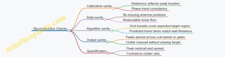
Workflow Summary You Can Actually Repeat
- Calibrate using a reference measurement and align phase.
- Clean and gate the data so the reconstruction sees the right echoes.
- Use a forward model consistent with your geometry assumptions.
- Reconstruct on a grid chosen for resolution and uncertainty.
- Suppress clutter using a baseline subtraction or a direct-path estimate.
- Validate by stability across sub-bands or gates and by comparing peak location to expected ground truth.
If you follow those steps in order, you will usually get reconstructions that are not just pretty maps, but maps you can defend with specific checks and measurable outcomes.
8. Feature Extraction and Interpretation of Imaging Outputs
8.1 Converting Images to Detectable Features
Turning an imaging output into something you can actually detect is mostly about choosing the right representation. An “image” might be a grid of intensities, a stack of range slices, or a reconstructed reflectivity map. Your job is to convert that grid into features that survive noise, clutter, and small alignment errors.
From Pixel Values to Physical Meaning
Start by deciding what each pixel value represents. In many through-wall pipelines, the pixel intensity is proportional to one of these: (1) matched-filter response, (2) backprojected energy, or (3) estimated reflectivity after inversion. If you treat all three as the same, you’ll pick thresholds that don’t behave.
A practical rule: normalize before you threshold. For each scan, convert raw intensities into a comparable scale using a robust baseline such as the median and a spread estimate like the median absolute deviation. Example: if your target response is a few decibels above typical clutter, robust normalization keeps the threshold stable even when the wall or antenna coupling changes slightly.
Feature Types That Work in Practice
Not every feature is equally stable. Choose features that match the physics and the expected target geometry.
Point-Like Features
Use when the target is small relative to the resolution cell. Typical examples include a tool head, a cable segment, or a compact object. Convert the image into candidate points by finding local maxima after smoothing with a kernel matched to your point spread function.
Line-Like Features
Use when the target extends across multiple pixels. Examples include a wire, a pipe edge, or a long tool. Extract oriented responses by applying directional filters (e.g., steerable filters) and then selecting peaks in orientation-consistent neighborhoods.
Region-Like Features
Use when the target occupies an area, such as a cavity boundary, a void region, or a larger object. Segment by thresholding on normalized intensity, then refine with morphological operations to remove speckle and fill small holes.
Shape and Consistency Features
Use when you can exploit geometry. For instance, a void boundary often produces a coherent ring or contour across adjacent slices. Instead of trusting a single slice, require consistency across a small stack of neighboring depths or frequencies.
Mind Map: Feature Conversion Pipeline
Candidate Generation Without Overreacting to Noise
A common failure mode is generating too many candidates, then drowning in false positives. Use a two-stage approach.
-
Coarse candidate generation: smooth the image lightly, then find peaks above a permissive threshold. This stage should aim for high recall.
-
Refinement and scoring: for each candidate, compute a small set of features: peak height above baseline, local contrast (peak minus local median), and neighborhood coherence (how many adjacent pixels support the same structure).
Example: suppose you expect a small tool head. For each candidate peak, take a 5×5 neighborhood. Compute contrast as (center − median(neighborhood)). A true target tends to keep contrast high even if the exact peak location shifts by a pixel due to positioning error.
Thresholding That Doesn’t Collapse Under Clutter
Thresholds should be tied to the normalized representation and to the measurement context.
- Global thresholding works when clutter statistics are stable across the image.
- Adaptive thresholding works when clutter varies spatially, such as near edges, corners, or antenna coupling regions.
A simple integrated method: compute a normalized score map, then set the threshold using a target false-alarm rate estimated from a “no-target” region of the same scan. For instance, if you know a section of the wall has no hidden object, use it to estimate the score distribution and choose a cutoff that yields few peaks there.
Example: From a Reconstructed Grid to Detectable Points
Assume your reconstruction produces a 2D grid of normalized intensity values.
- Apply a PSF-matched smoothing kernel so that true peaks broaden consistently.
- Find local maxima.
- Keep only maxima where normalized intensity exceeds the adaptive threshold.
- Score each remaining point using local contrast and neighborhood coherence.
- Output a ranked list of candidate locations with their scores.
This produces a feature set you can feed into later stages like clustering, tracking, or evidence reporting.
Feature Quality Checks
Before you declare victory, verify that your features behave sensibly.
- Shift sensitivity: nudge the image by a fraction of a pixel and confirm candidate scores don’t swing wildly.
- Peak shape: true targets usually produce a compact, coherent peak; random clutter often yields irregular, isolated spikes.
- Spatial plausibility: if your system geometry constrains where objects can appear, discard candidates that violate those constraints.
When these checks pass, your “image” has become a set of reliable, interpretable features rather than just pretty numbers.
8.2 Thresholding and Statistical Decision Rules
Thresholding turns a messy measurement into a yes/no statement: “target present” or “target absent.” The trick is choosing a threshold that matches your measurement noise, your clutter level, and your tolerance for false alarms. In through-wall imaging, you usually have many pixels or range-angle bins, so the decision rule must handle both per-bin statistics and the fact that you will test thousands of bins.
Foundational Concepts for Thresholding
Start with a simple model for one bin. Let the measured value be \(Y\). Under the null hypothesis \(H_0\) (no target), \(Y\) is dominated by noise and clutter. Under the alternative \(H_1\) (target present), \(Y\) shifts upward, or changes shape, relative to \(H_0\).
A practical threshold rule is:
- Declare target if \(Y \ge T\).
- Otherwise declare no target.
If \(Y\) is approximately Gaussian under \(H_0\), then \(T\) can be set from a desired false-alarm probability \(P_{FA}\). For example, if \(Y|H_0 \sim \mathcal{N}(\mu_0, \sigma_0^2)\), then \(T = \mu_0 + z_{1-P_{FA}}\sigma_0\), where \(z\) is the standard normal quantile.
In imaging pipelines, \(Y\) is often a magnitude, power, or matched-filter score. Those are frequently non-Gaussian, so you either estimate the \(H_0\) distribution empirically or transform the score into something closer to Gaussian (for instance, by using log-power or normalized residuals).
Per-Bin Versus Global Decisions
A per-bin threshold controls false alarms in one bin. But if you evaluate \(N\) bins, the probability of at least one false alarm grows. A common approach is to control the expected number of false alarms by using a per-bin \(P_{FA}\) that is small enough for your bin count.
A simple approximation is:
- Expected false alarms \(\approx N,P_{FA}\).
If you want fewer than 0.5 false alarms on average and you have \(N=10{,}000\) bins, then choose \(P_{FA} \approx 5\times 10^{-5}\). This is not perfect, because bins are correlated, but it gives a defensible starting point.
Estimating Noise and Clutter Statistics
You need \(\mu_0\) and \(\sigma_0\) (or the full \(H_0\) distribution). In practice, you estimate them from regions that are likely target-free. For through-wall imaging, that can mean:
- Using bins outside the plausible target region defined by geometry.
- Using early time windows or frequency slices where the target signature is not expected.
- Using multiple frames and treating consistent clutter patterns as part of \(H_0\).
A good habit is to compute thresholds separately for different parts of the image if the noise floor varies with range or angle. One global threshold can quietly punish distant bins.
Statistical Decision Rules That Work in Practice
Neyman-Pearson Style Thresholding
When you can model the likelihood ratio \(\Lambda(Y)=\frac{p(Y|H_1)}{p(Y|H_0)}\), the optimal rule for a fixed \(P_{FA}\) is to threshold \(\Lambda\). In imaging, you rarely have perfect \(p(Y|H_1)\), so you approximate by using a score that makes targets stand out under \(H_1\) and then calibrate \(H_0\) empirically.
Constant False Alarm Rate Style Calibration
If you cannot trust parametric noise models, you can calibrate a threshold directly from the empirical distribution of \(Y\) under \(H_0\). For instance, if you collect many frames without targets, sort the scores, and pick \(T\) as the \((1-P_{FA})\) quantile. This automatically handles non-Gaussian tails.
Likelihood Ratio with Normalized Scores
A common engineering compromise is to normalize the score by an estimate of local variance. If \(S\) is your raw score and \(\hat{\sigma}\) is a local noise estimate, use \(Z = (S-\hat{\mu})/\hat{\sigma}\). Then threshold \(Z\) using a standard normal quantile. This reduces sensitivity to slow gain changes and uneven coupling.
Mind Map: Thresholding Workflow
Example: Choosing a Threshold from Target-Free Data
Suppose you compute a matched-filter score \(S\) for each bin. You have 200 scans of the same wall with no targets. For a chosen region of interest, you gather all \(S\) values and build an empirical distribution.
You want \(P_{FA}=10^{-4}\) per bin. With \(N=8{,}000\) bins in the region, the expected false alarms are \(N,P_{FA}=0.8\), which is usually manageable if you later cluster detections.
From the sorted target-free scores, pick \(T\) as the value exceeded by only 1 in 10,000 samples. Then declare detections where \(S\ge T\). If the resulting detections are concentrated in one corner, that suggests your \(H_0\) sample did not match the local noise floor, so you should re-estimate \(T\) per subregion.
Example: Normalization to Fix Uneven Noise Floors
In many setups, bins at larger range have lower signal-to-noise. If you use a single threshold on raw \(S\), distant bins will rarely exceed it. Instead, estimate \(\hat{\sigma}(r)\) as a function of range from target-free data, compute \(Z=(S-\hat{\mu}(r))/\hat{\sigma}(r)\), and threshold \(Z\). Now the threshold corresponds to a consistent false-alarm probability across range bins.
Practical Decision Output Beyond Yes/No
Even if the final product is a binary detection map, it helps to compute a simple confidence measure such as \(C = S - T\) or \(C = Z - z_{1-P_{FA}}\). This does not replace validation, but it makes it easier to tune thresholds and to understand whether a detection is barely above the line or comfortably above it.
8.3 Clustering and Region Proposal Techniques for Targets
Clustering turns a noisy imaging map into a small set of candidate target regions. Region proposal then converts those candidates into shapes you can score, compare, and report. The key idea is to treat “pixels above threshold” as a starting guess, not as the final answer.
Foundational Setup for Clustering
Start with a 2D or 3D image volume produced by your imaging step (for example, backprojection or matched filtering). Convert it into a detection score map S(x) where larger values mean “more target-like.” Before clustering, apply two practical steps:
- Normalize within a scan so different sessions are comparable. A simple approach is z-score normalization using the map mean and standard deviation computed over a region that excludes obvious direct-path artifacts.
- Suppress obvious non-target structure using a mask. For example, if you know the wall thickness band where clutter dominates, zero out scores there so clusters don’t form around the wall itself.
A concrete example: in a through-wall scan of a doorway, the direct reflection can create a bright stripe. If you don’t mask it, clustering will happily group that stripe into a “target” region with high confidence.
Clustering Methods That Work on Score Maps
Use clustering on connected components or on feature vectors derived from the score map.
Connected-Component Clustering
- Threshold S(x) at T to get a binary map.
- Find connected regions in 2D slices or 3D neighborhoods.
- Filter regions by size, shape, and internal consistency.
Example: choose T as the 95th percentile of scores in the masked volume. A small cluster of 30–200 voxels that persists across adjacent slices is more plausible than a single-voxel spike.
Density-Based Clustering
When targets are weak and fragmented, density-based methods can group scattered high-score points.
- Extract candidate points where S(x) exceeds a lower threshold T_low.
- Cluster points using a radius ε and minimum points minPts.
Example: a buried pipe might produce a thin, broken signature. Connected components may split it into many tiny regions, while density-based clustering can merge them if the gaps are small.
Model-Based Region Proposal
Instead of clustering raw pixels, propose regions using simple geometric templates.
- Assume targets occupy roughly compact volumes.
- Fit bounding boxes or ellipsoids to high-score neighborhoods.
Example: for a handheld object, a compact ellipsoid proposal often outperforms arbitrary blob shapes when the imaging grid is coarse.
Region Proposal from Clusters
Once you have clusters, convert each into a region proposal with measurable attributes:
- Spatial extent: bounding box or convex hull.
- Peak location: argmax of S(x) within the region.
- Support: number of voxels/points above T.
- Contrast: region mean score minus local background mean.
- Shape sanity: aspect ratio limits to reject long streaks.
A practical rule: require both support and contrast. A region with a single bright voxel has high peak but low support, which is usually not a stable target.
Scoring and Ranking Proposals
Rank proposals using a composite score that penalizes clutter-like shapes.
- Start with a base score such as region mean or sum of scores.
- Add penalties for extreme elongation or for regions touching masked-out boundaries.
Example: if a cluster touches the direct-path stripe mask boundary, reduce its score even if it has a high peak, because the stripe often leaks into the imaging map.
Mind Map: Clustering to Region Proposals
Example Workflow with Numbers
Suppose your score map has been normalized. You mask a direct-path stripe and compute T as the 97th percentile of remaining scores.
- Threshold at T to get initial connected components.
- Keep components with voxel counts between 50 and 800.
- For each kept component, compute contrast using a ring-shaped neighborhood around the component’s bounding box.
- Rank by
score = mean_region + 0.5 * contrast.
If two regions have similar scores, prefer the one whose peak is more central within the region extent. That simple tie-breaker reduces cases where a cluster is mostly background with one lucky bright point.
Common Failure Modes and Fixes
- Over-thresholding: targets split into fragments. Fix by using T_low with density-based clustering, then merge proposals.
- Under-thresholding: clutter merges into one giant region. Fix by tightening the mask or increasing T for connected components.
- Grid artifacts: repeated patterns create periodic clusters. Fix by filtering proposals whose shape matches known artifact geometry, such as long thin streaks aligned with the scan axis.
8.4 Distinguishing Material Signatures From Geometry
When an image shows a bright or dark region, you still have to answer a harder question: is that region caused by the object’s shape, or by the object’s material properties? In practice, geometry and material both affect the measurement, so the goal is not to “pick one,” but to separate their contributions using consistent cues.
Foundational Idea: What Each Cue Tends to Affect
Geometry primarily changes where energy appears to come from. That means it influences:
- Location and extent of reconstructed features across scan positions.
- Apparent boundaries that shift predictably when you change viewpoint or beam angle.
- Phase consistency for features that behave like coherent reflectors.
Material primarily changes how energy is attenuated, refracted, or re-radiated. That means it influences:
- Relative strength across frequency bands or waveform types.
- Contrast behavior when the same physical location is measured under different polarization or incidence.
- Texture-like variation inside a region that remains spatially stable.
A useful mental model is: geometry decides where a feature lands; material decides how strongly it shows up and how that strength changes.
Step 1: Build a Geometry-First Consistency Check
Start by testing whether the feature behaves like a geometric reflector.
Practice: Take three scans with small changes in antenna position or steering angle. For each scan, track the feature’s centroid and boundary.
- If the feature’s centroid moves in a way that matches the imaging model’s expected viewpoint dependence, geometry is likely dominant.
- If the feature stays locked in place while its intensity changes, material effects are more likely.
Easy example: A metal pipe behind drywall often produces a strong edge response. When you shift the antenna laterally, the pipe’s apparent position in the reconstruction follows the expected parallax. The shape is doing the heavy lifting.
Step 2: Build a Material-First Contrast Check
Next, test whether the feature’s intensity pattern changes in a way consistent with material properties.
Practice: Repeat the measurement using two frequencies (or two bandwidth settings) while keeping geometry as constant as possible.
- If the same region brightens or fades systematically with frequency, material attenuation or permittivity effects are likely.
- If the region’s intensity stays nearly proportional while geometry cues still shift, geometry dominates.
Easy example: A void or air gap often produces a stronger contrast at frequencies where the wall’s effective loss is higher. The void’s location stays stable, but its contrast relative to surrounding plaster changes.
Step 3: Use Polarization and Incidence Sensitivity
Material response depends on how fields couple to it. Geometry alone cannot explain strong polarization dependence.
Practice: Measure with two orthogonal antenna polarizations (or rotate the antenna by 90 degrees) at the same positions.
- If the feature’s contrast flips sign or changes dramatically, the material’s electromagnetic response is likely responsible.
- If contrast changes are minor but boundaries remain consistent, geometry is more likely.
Easy example: Reinforcing rebar can show direction-dependent coupling. The “same” bar can appear more pronounced under one polarization because the induced currents align better.
Step 4: Separate Boundary Edges from Interior Texture
Geometry tends to create sharp boundaries; material tends to create smoother interior variations.
Practice: Compare edge strength to interior variance.
- Compute an edge metric (gradient magnitude) along the feature boundary.
- Compute interior variance after masking out the boundary band.
If edges are strong but interior variance is low, geometry is likely dominant. If interior variance is high while the boundary is stable, material heterogeneity is likely.
Easy example: A cable bundle can create a textured interior signature due to multiple conductors and local coupling, even when the overall outline is fairly stable.
Step 5: Apply a Forward-Model Sanity Test
Even a simple forward model can help. You do not need perfect physics; you need consistency.
Practice: Create two candidate explanations for the same feature:
- Geometry-only: same material parameters, vary shape/position.
- Material-only: same shape, vary material parameters.
Run both through the imaging pipeline (or a simplified surrogate) and compare which one reproduces the observed changes across scans, frequencies, and polarizations.
Easy example: If geometry-only reproduces centroid shifts but fails to match frequency-dependent contrast, you can treat material as the missing ingredient.
Mind Map: Material Versus Geometry Separation
Integrated Example: A Feature That Won’t Behave
Suppose a reconstruction shows a bright blob behind a wall.
- Across three lateral positions, the blob’s centroid shifts in a way consistent with parallax: geometry is involved.
- When you switch frequency, the blob’s brightness changes nonlinearly: material is also involved.
- With polarization rotation, the blob contrast changes more than the boundary shape: material coupling is significant.
The conclusion is not “it’s geometry” or “it’s material.” It’s a mixed case: the object’s shape sets the location, while its material response sets the contrast behavior.
Practical Decision Output
For each detected feature, record three observations:
- Location behavior: stable or parallax-consistent.
- Contrast behavior: frequency-dependent and/or polarization-dependent.
- Texture behavior: edge-dominant or interior-variant.
This turns interpretation into a checklist. The image becomes less like a guess and more like a set of measurable tendencies—still imperfect, but grounded in evidence.
8.5 Generating Evidence Reports With Confidence Metrics
A good evidence report does two things at once: it tells a clear story about what was measured, and it quantifies how much you should trust the story. In through-wall imaging, the “story” is usually a location hypothesis (where something might be), plus supporting observations (what the imaging and processing produced). The “trust” part is confidence metrics tied to measurable factors like signal-to-noise ratio, calibration quality, and reconstruction stability.
Evidence Report Structure
Start with a compact header so the reader can reproduce the conditions without hunting through notes.
- System and configuration: sensor model, antenna/array geometry, frequency sweep or waveform, sampling rate, and any gating/windowing used.
- Environment and constraints: wall type, approximate thickness, known metal reinforcements if available, and scan geometry (positions, angles, spacing).
- Calibration record: last calibration date, calibration target used, and calibration residual summary (for example, mean magnitude error across a reference set).
- Data provenance: file identifiers, timestamps, and whether any preprocessing steps were applied (filtering, normalization, motion correction).
Then present the results in a way that separates raw observations from interpretation.
- Observations: peak locations in the reconstructed image, top-N candidate regions, and any intermediate maps used for decision-making (for example, confidence heatmaps or residual maps).
- Interpretation: the selected hypothesis, the reasoning chain from observations to hypothesis, and what would falsify it.
- Confidence metrics: numeric scores with definitions, uncertainty bounds, and the conditions under which the score is valid.
Finally, include a short “limitations” section that is specific, not generic. For example: “Direct-path leakage likely inflated the top candidate score because the scan angle produced a strong specular reflection.”
Confidence Metrics That Actually Mean Something
Use confidence metrics that correspond to failure modes you can explain.
-
Signal Quality Confidence
- Example: compute an SNR-like metric from the reconstructed domain (peak-to-sidelobe ratio). If the peak-to-sidelobe ratio is low, the image is telling you less than you want.
- Easy example: two scans of the same wall. Scan A has a strong, narrow peak; Scan B has a broad peak with similar background. The report assigns higher confidence to A because the peak is more distinguishable.
-
Reconstruction Stability Confidence
- Example: run the reconstruction with small, controlled perturbations (slight grid shift, minor regularization change, or bootstrap resampling of measurement noise). Confidence increases when the same location remains dominant.
- Easy example: if the top candidate stays in the same grid cell across perturbations, confidence rises; if it jumps around, confidence drops.
-
Calibration and Model Consistency Confidence
- Example: compare measured reference responses to the forward model used in reconstruction. Large residuals reduce confidence because the model is not matching the environment.
- Easy example: if a calibration target produces a systematic amplitude bias, confidence is reduced for absolute magnitude-based decisions.
-
Decision Rule Confidence
- Example: if you use a thresholding rule, report the threshold basis (for example, percentile of background distribution) and the resulting false-alarm estimate.
- Easy example: if the threshold is set at the 99th percentile of background, the report states that the expected false-alarm rate under those conditions is about 1%.
Combine these into a single confidence score only if you also provide the components and their definitions. A single number without components is just a fancy guess.
Mind Map: Evidence Report with Confidence Metrics
Example Evidence Report Snippet
Below is a compact example that shows how the metrics connect to the narrative.
- Hypothesis: Candidate region centered at (x=1.20 m, y=0.35 m) with estimated depth band 0.10–0.25 m.
- Observations: Top-3 peaks at grid cells [1.20,0.35], [1.18,0.37], [1.25,0.33]. Peak-to-sidelobe ratio = 6.2 dB.
- Stability: Across 50 perturbation runs, the top candidate remained in the same cell 41/50 times; mean location drift = 0.03 m.
- Calibration consistency: Reference residual magnitude averaged 8% after applying the calibration correction.
- Decision rule: Threshold set using background distribution; estimated false-alarm probability = 0.02 under the same scan geometry.
- Confidence score: 0.78, computed from weighted components (signal quality 0.35, stability 0.35, calibration 0.20, decision rule 0.10).
- Uncertainty bounds: Position uncertainty ±0.05 m in-plane; depth band uncertainty widened to 0.08–0.30 m due to multipath indicators.
- Limitations: Strong specular reflection from a nearby metal element likely increased sidelobe structure, so confidence is higher for in-plane localization than for depth.
This style keeps the report grounded: every claim has a measurable anchor, and every confidence number comes with the knobs that produced it.
9. Multi-Sensor Fusion with Non-RF Modalities
9.1 Complementary Roles of RF and Non-RF Sensors
RF through-wall imaging measures how radio waves propagate, reflect, and attenuate across materials. Non-RF sensors measure other physical effects—acoustic, thermal, optical, magnetic, or mechanical—often with different sensitivities to the same hidden feature. Using both is not about redundancy; it’s about covering different “failure modes” of each measurement.
Start with what each sensor type tends to “see” well. RF is sensitive to dielectric changes, conductive objects, and geometry that perturbs wave paths. A metal conduit, a void, or a cavity filled with different moisture can shift RF amplitude and phase patterns. Non-RF sensors are often better at detecting localized phenomena that RF may miss or smear, such as surface vibrations from a tapping test, temperature gradients near a concealed cavity, or magnetic anomalies from embedded ferromagnetic components.
A practical way to think about complementarity is to map sensor outputs to physical mechanisms:
- RF mechanisms: propagation loss, multipath, polarization effects, and boundary reflections.
- Non-RF mechanisms: mechanical coupling, thermal conduction, optical contrast, magnetic permeability, and acoustic scattering.
When you combine them, you reduce ambiguity. RF alone can confuse “a void” with “a different material layer” because both can alter attenuation. Non-RF can break the tie by responding differently to the same candidate location.
Mind Map: Complementary Roles of RF and Non-RF Sensors
Example: RF-First Then Non-RF Confirmation
Imagine inspecting a wall for a concealed utility void behind drywall. You run an RF scan and obtain a cluster of high-likelihood pixels roughly centered at a specific grid coordinate. RF suggests a candidate cavity, but the confidence is moderate because the wall contains mixed materials.
Next, you apply a non-RF check at the same coordinate. If you use an acoustic tapping approach, you listen for changes in resonance or damping that correlate with an air gap. If the tapping response shows a distinct attenuation pattern at the candidate location, you treat the RF cluster as more credible. If the acoustic response matches the surrounding wall, you downgrade the cavity hypothesis and consider alternatives such as a denser material pocket that produced RF contrast.
This workflow works because RF and acoustic sensing respond to different properties: RF is influenced by electromagnetic boundary conditions, while acoustic response depends on mechanical coupling and cavity compliance.
Example: Non-RF Finds a Candidate, RF Resolves Depth and Geometry
In another scenario, a magnetic sensor detects a localized ferrous anomaly near the wall surface. The magnetic reading alone cannot reliably indicate whether the object is a fastener, a conduit, or a deeper embedded component.
You then perform an RF scan focused on that region. RF can help by showing how the anomaly perturbs wave paths across the wall thickness. If the RF data indicates a conductive object signature consistent with a through-wall path, you classify it as a likely embedded conduit. If RF shows only a shallow boundary effect, you treat it as a surface fastener or thin metal layer.
Here, non-RF provides a targeted hypothesis, and RF provides spatial context that non-RF lacks.
Integrated Decision Logic
To keep the combination systematic, use explicit rules rather than “eyeballing.” A simple approach is:
- Generate RF candidate regions using a threshold on likelihood or matched-filter response.
- Collect non-RF indicators at candidate coordinates and nearby offsets to estimate local contrast.
- Apply a gating rule: accept a candidate only if non-RF evidence exceeds a minimum contrast relative to a local baseline.
- Resolve conflicts: if RF and non-RF disagree, report the most likely explanation that satisfies both mechanisms, or mark the location as uncertain.
For example, if RF indicates a void-like signature but non-RF acoustic response shows no cavity-like damping, you label the result as “RF-ambiguous” rather than forcing a single conclusion.
Practical Integration Checklist
- Use a shared grid so both sensors reference the same physical points.
- Calibrate each sensor independently before combining outputs.
- Record environmental conditions that affect non-RF signals, such as ambient vibration or airflow.
- Keep scan paths consistent so you can compare like with like.
- Store raw measurements alongside processed maps so you can re-run decision thresholds without re-scanning.
With these steps, RF and non-RF sensors stop competing and start collaborating: RF narrows the search using electromagnetic behavior, and non-RF either confirms the physical mechanism or points to a different explanation.
9.2 Synchronization and Time Alignment Across Sensors
When you fuse RF imaging with other sensing modalities, the hardest part is rarely the math—it’s making sure every sensor is talking about the same moment in time. If one device’s “time zero” drifts by even a few microseconds, your fused location can smear into a confident-looking mess.
Foundational Timing Concepts
Start by separating three ideas: triggering, time stamping, and alignment.
- Triggering answers: what starts the measurement?
- Time stamping answers: what time does each sample claim it represents?
- Alignment answers: how do you map timestamps from different sensors onto a shared timeline?
A practical rule: treat each sensor as having its own clock, its own latency, and its own sampling grid. Your job is to estimate the mapping between those grids.
Clock Sources and Synchronization Modes
Most systems fall into one of these modes:
- Common hardware trigger: all sensors start from the same electrical pulse. This reduces uncertainty in start time, but you still must handle per-sensor latency and sample-to-sample timing.
- Common clock (timebase): sensors share a clock reference. This improves long recordings, but you still need to align phase offsets and pipeline delays.
- Independent clocks with post alignment: sensors run freely and you align after the fact using markers. This is common when you can’t wire triggers, but it demands careful marker design.
Example: Two Sensors with Different Latencies
Sensor A timestamps at the ADC readout. Sensor B timestamps at the end of a processing buffer. Even if both are triggered together, B’s timestamps are systematically late. You can correct this by estimating a constant offset using a shared event marker (like a controlled pulse or a mechanical tap).
Time Stamping Strategy That Actually Works
Time stamps must be tied to a known point in the acquisition chain. Pick one convention and stick to it:
- Edge-based stamping: timestamp the trigger edge and propagate through known pipeline delays.
- Sample-based stamping: timestamp each sample using the sampling interval and the first sample time.
If you only store “start time” and ignore pipeline delay, fusion errors often look like spatial shifts rather than obvious timing mistakes.
Alignment Workflow from Basics to Robustness
A systematic workflow prevents guesswork.
-
Collect synchronization markers
Use a marker that is visible to all sensors. Examples include a brief RF excitation, a digital GPIO pulse captured by both systems, or a physical event recorded by both modalities. -
Estimate coarse offset
Compute the time difference between marker occurrences. For independent clocks, this gives you an initial offset. -
Estimate drift if needed
Over long sessions, sampling rates may differ slightly. If you observe marker times separating nonlinearly, fit a linear drift model:- shared_time = a * sensor_time + b
-
Resample or map to a common grid
Choose a fusion grid (often the RF slow-time or the non-RF frame time). Then convert each sensor’s samples to that grid using interpolation consistent with your signal bandwidth. -
Validate alignment with a sanity check
After alignment, a known target should appear at consistent coordinates across modalities. If it “breathes” between frames, your alignment is incomplete.
Mind Map: Synchronization and Time Alignment
Worked Example: Marker-Based Alignment with Drift
Assume you have:
- RF sensor A sampling at 1 kHz slow-time frames.
- Non-RF sensor B producing frames at nominal 30 Hz.
- Both record a marker pulse at the start and again at the end of a 10-minute scan.
If the marker separation in A is 600,000 ms and in B is 599,400 ms, B’s clock is running fast by 600 ms over 10 minutes. Fit a linear mapping using the two marker times, then resample B frames onto A’s timeline. After resampling, the fused target centroid should stop drifting across the scan.
Practical Best Practices
- Log raw marker timestamps before any processing so you can re-estimate offsets later.
- Quantify timestamp resolution. If one sensor timestamps in 1 ms steps and another in 10 µs steps, your alignment floor is set by the coarser one.
- Keep latency models explicit. Document whether timestamps refer to trigger edge, first sample, or buffer completion.
When synchronization is done carefully, fusion becomes a matter of consistent geometry and signal interpretation rather than chasing artifacts that look like physics but are really timing.
9.3 Spatial Registration and Coordinate Transformations
Spatial registration is the step that makes multiple sensor views agree on where things are. In multi-sensor through-wall detection, you typically have different coordinate frames: each sensor has its own origin, axes, scale, and sometimes its own notion of “up.” If you skip registration, fusion becomes a polite disagreement—each sensor reports a target, but the targets don’t land in the same place.
Foundational Concepts
Coordinate Frames and Transforms
A coordinate frame is defined by an origin and three axes. A spatial transform maps points from one frame to another. In practice, you’ll use rigid transforms for most setups: rotation plus translation. If your sensors have different scale (for example, due to calibration errors or image-to-world scaling), you may add a uniform scale factor.
A point in frame A, written as \(p_A\), maps to frame B as: \(p_B = R p_A + t\) where \(R\) is a 3×3 rotation matrix and \(t\) is a 3×1 translation vector.
Homogeneous Coordinates for Convenience
Homogeneous coordinates let you combine rotation and translation into a single matrix. This is handy when you chain transforms across multiple frames.
\[ \begin{bmatrix} p_B \\ 1 \end{bmatrix} = \begin{bmatrix} R & t \\ 0 & 1 \end{bmatrix} \begin{bmatrix} p_A \\ 1 \end{bmatrix} \]
Practical Registration Workflow
Step 1: Define Frames Explicitly
Name frames clearly, such as:
- \(W\): world or site frame
- \(R\): RF sensor frame
- \(I\): imaging sensor frame (camera, IR, or other)
- \(T\): target or wall plane frame
Then decide what you want to fuse in. Most teams choose \(W\) or a wall-plane frame \(T\) because it keeps geometry consistent.
Step 2: Measure Extrinsics Between Sensors
Extrinsics are the transform parameters between sensor frames. You can estimate them using a calibration rig with known markers or a set of measured points.
Easy example: place three non-collinear markers on a rigid board. Measure their coordinates in \(R\) using the RF system’s positioning reference, and in \(I\) using the imaging system. With three points, you can solve for rotation and translation (assuming no scale mismatch).
Step 3: Register to a Common Surface Frame
For through-wall work, a wall plane frame often simplifies interpretation. Define \(T\) so that:
- \(T_x\) and \(T_y\) lie along the wall
- \(T_z\) points normal to the wall
If your sensors are mounted at different heights and angles, projecting detections onto \(T\) reduces confusion. A detection at a 3D point becomes a 2D location on the wall plane plus a depth estimate if available.
Step 4: Apply Transforms to Detections and Uncertainties
Registration isn’t only about point locations. If you have covariance (uncertainty) for each detection, transform it too. For a rigid transform, covariance rotates with \(R\): \(\Sigma_B = R \Sigma_A R^T\) This matters because fusion should trust some measurements more than others.
Step 5: Validate with Residual Checks
After transforming, compute residuals between expected marker locations and transformed observations. A small residual across multiple points indicates the transform is consistent. If residuals grow with distance from the calibration region, you likely have a scale or lens/antenna model mismatch.
Mind Map: Spatial Registration and Coordinate Transformations
Example: Two Sensors Fusing a Hidden Void
Assume the RF system outputs a 3D point \(p_R\) in its frame, and the imaging system outputs a 3D point \(p_I\) in its frame. You want both in \(W\).
- Use calibration to obtain \(T_{WR}\) and \(T_{WI}\), where each is a homogeneous transform.
- Convert points:
- \(p_W = T_{WR} \cdot p_R\)
- \(p_W = T_{WI} \cdot p_I\)
- Convert \(p_W\) into wall-plane coordinates by applying \(T_{TW}\) (or equivalently by using the wall plane basis vectors). The fused result becomes a consistent wall location.
If the void is near the wall center, both sensors should agree closely. If one sensor is farther off-axis, its uncertainty may be larger; covariance-aware fusion will naturally reduce its influence.
Common Pitfalls and How to Avoid Them
- Mixing axis conventions: one system might use right-handed coordinates while another uses left-handed. Fix this at the transform definition stage, not after fusion.
- Using a transform for the wrong reference: ensure the transform maps the detection’s reference point (antenna phase center, pixel ray intersection, or estimated target centroid) rather than a random mounting point.
- Ignoring unit consistency: millimeters versus meters can produce transforms that look “reasonable” but yield huge residuals.
Summary of the Integrated Approach
Registration becomes reliable when you (1) define frames explicitly, (2) estimate extrinsics from measured correspondences, (3) project detections into a shared wall-plane or world frame, (4) transform uncertainties alongside positions, and (5) validate with residual checks. Once these steps are consistent, fusion stops being a negotiation and becomes a calculation.
9.4 Fusion Strategies for Consistent Localization
Consistent localization means different sensors agree on the same target position in a shared coordinate system, with comparable uncertainty. The trick is not “averaging everything,” but aligning measurements, weighting them by reliability, and enforcing geometric consistency.
Foundational Alignment and Common Coordinates
Start by defining a single world frame for the site. For each sensor, record a rigid transform from its local frame to the world frame using the same reference markers throughout the session. A practical habit: store transforms with timestamps and verify them by re-measuring a known point (like a marked corner) after any repositioning.
Next, align time. If one sensor integrates over a window while another provides near-instant snapshots, you must map each measurement to a common time basis. A simple approach is to tag each measurement with the start and end of its acquisition window, then fuse using the overlap interval.
Finally, align representations. RF imaging often yields a probability-like intensity map over space, while non-RF sensors may output detections (points, boxes, or tracks). Convert both into a common form: either spatial likelihoods on a grid or a set of candidate hypotheses with associated covariance.
Fusion as Hypothesis Scoring
A reliable pattern is hypothesis scoring: generate candidate target locations from each modality, then score them jointly.
-
Generate candidates per sensor
- RF: find peaks in the reconstructed image or local maxima after clutter suppression.
- Non-RF: use thresholded detections or track extrapolation to produce candidate positions.
-
Quantify uncertainty per candidate
- RF peaks: estimate spread from the local curvature of the response surface or from the width of the matched-filter peak.
- Non-RF detections: use the sensor’s reported covariance or empirical spread from repeated measurements.
-
Score candidates with a shared likelihood
- Convert each candidate into a likelihood in world coordinates.
- Combine likelihoods by multiplying (or summing log-likelihoods).
A concrete example: suppose RF suggests a target at (x=2.1, y=0.6, z=1.2) with larger uncertainty along depth, while a ground-penetrating or acoustic-like sensor suggests (2.0, 0.7, 1.1) with tighter lateral uncertainty. Joint scoring will favor the location that best satisfies both, not the one that looks strongest in only one modality.
Consistency Checks That Prevent “Confident Wrong” Results
Even good fusion can go wrong when one sensor produces structured false positives. Add consistency checks before finalizing.
- Gating by distance and covariance: reject candidate pairs whose Mahalanobis distance exceeds a threshold derived from expected noise.
- Geometry gating: enforce that the target lies in physically plausible regions given line-of-sight constraints and wall thickness.
- Support gating: require that at least two sensors provide non-trivial support for the same neighborhood.
These checks are boring in the best way: they stop a single sensor’s artifact from dominating the final estimate.
Weighting Strategies That Behave Well
Weighting should reflect uncertainty and measurement quality, not raw signal strength.
- Uncertainty-weighted fusion: when fusing two Gaussian estimates, the combined mean is a covariance-weighted average.
- Quality-weighted fusion: if a sensor’s data quality degrades (for example, due to poor coupling or noisy positioning), inflate its covariance rather than forcing a fixed weight.
- Robust fusion: if one modality occasionally produces outliers, use a robust loss that reduces the influence of candidates far from the consensus.
Mind Map: Fusion Strategies for Consistent Localization
Example: Two-Sensor Localization Through a Wall
Assume you have RF imaging and a non-RF sensor that provides a surface-projected detection.
- RF produces a 3D likelihood grid over a volume behind the wall.
- Non-RF produces a 2D point on the accessible side.
- Lift non-RF to 3D by mapping the point through a known wall thickness model, producing a candidate at a nominal depth with depth uncertainty.
- Score candidates: compute the RF likelihood at the lifted point and multiply by the non-RF likelihood.
- Gate: if the lifted point is too far from RF’s top peak in Mahalanobis terms, discard and instead search nearby candidates.
- Fuse: compute the final mean and covariance from the joint likelihood around the accepted neighborhood.
The result is stable: if RF is strong but non-RF is noisy, the fused uncertainty grows appropriately; if RF is ambiguous, the non-RF support narrows the solution.
Practical Output and Traceability
Return not only a fused location but also the fused uncertainty and a short explanation of which sensors contributed most. Keep per-sensor likelihood values for the final neighborhood so you can diagnose cases where one modality consistently disagrees. This turns “it didn’t work” into “RF peaked here, non-RF supported there, and gating rejected the mismatch,” which is exactly the kind of clarity you want when the wall is doing its best to be mysterious.
9.5 Example Fusion Pipelines for Hidden Void and Utility Detection
A good fusion pipeline starts by agreeing on what “the same thing” means across sensors. In this example, we combine RF through-wall imaging with a non-RF modality that is sensitive to surface or near-surface changes, such as acoustic/ultrasonic or thermal/IR. The goal is not to average everything together; it is to produce one consistent set of candidate locations with a confidence score that reflects agreement and disagreement.
Pipeline Overview
- Acquire synchronized measurements from each sensor while recording geometry and environmental conditions.
- Preprocess each sensor stream to produce comparable intermediate representations (for example, probability-of-presence maps).
- Register to a common coordinate frame so that a voxel or pixel refers to the same physical location.
- Fuse at the evidence level using rules that reward consistent localization and penalize contradictions.
- Post-process candidates with spatial constraints and sanity checks to reduce false positives.
- Validate with ground truth from controlled openings or known utility traces.
Mind Map: Evidence-Level Fusion Flow
Step 1: Preprocessing That Produces Comparable Maps
RF preprocessing typically includes time/frequency selection, direct-path suppression, and a reconstruction step that yields a spatial map. For a simple example, assume the RF reconstruction outputs a grid where each cell has a value proportional to “reflective anomaly likelihood.”
For the non-RF modality, preprocessing should produce a map with the same grid meaning. If the non-RF sensor measures surface contrast, convert it into a probability-of-presence map by normalizing against a baseline region on the same wall. A practical trick: use a “no-known-target” patch to estimate mean and variance, then convert deviations into probabilities.
Step 2: Registration with Uncertainty, Not Just Geometry
Registration aligns the two maps. Use the wall coordinate frame: define an origin at a known corner, x along the horizontal scan direction, y vertical, and z into the wall. Then apply transforms from each sensor’s pose.
To avoid silent errors, carry a simple uncertainty model. For example, if the RF antenna position has ±5 mm uncertainty and the non-RF sensor has ±8 mm, represent that as a blur kernel applied to each map before fusion. This makes the fusion tolerant to small misalignment while still penalizing large disagreements.
Step 3: Evidence Fusion with Agreement Scoring
A straightforward evidence fusion rule is to combine probabilities while explicitly measuring agreement. One workable approach:
- Compute RF evidence \(P_{rf}(x,y,z)\) and Non-RF evidence \(P_{nr}(x,y,z)\).
- Compute an agreement mask by checking whether both maps have local maxima within a tolerance radius.
- Fuse using a weighted product or weighted sum, but multiply by the agreement mask so that “both sensors point to the same place” matters.
Here is a compact pseudocode sketch:
for each grid cell c:
  rf = P_rf[c]
  nr = P_nr[c]
  agree = 1 if maxima_nearby(c, tol) else 0
  fused[c] = agree * (w1*rf + w2*nr)

candidates = peak_pick(fused, min_distance)
clusters = cluster_by_proximity(candidates)
for each cluster:
  score = max(fused in cluster)
  consistency = agreement_fraction(cluster)
  report location = cluster centroid
Step 4: Candidate Post-Processing for Voids vs Utilities
Hidden voids and utilities often differ in how they appear across modalities.
- Voids: RF may show a strong anomaly due to impedance contrast, while non-RF may show weaker surface effects unless the void affects coupling or surface response.
- Utilities: RF may show a consistent signature along a path, and non-RF may show localized surface changes aligned with that path.
Use this without guessing too hard. Add two simple checks:
- Spatial coherence: utilities tend to form elongated clusters; voids tend to be more compact.
- Cross-modality consistency: if RF is strong but non-RF is absent everywhere in the neighborhood, lower confidence rather than declaring “no target.”
Mind Map: Fusion Decision Logic
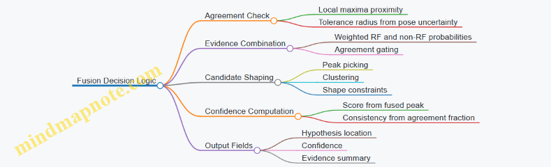
Example Run: One Void and One Utility
Assume a wall scan produces two RF peaks: one near (x=0.42 m, y=0.95 m) and another near (x=0.70 m, y=0.60 m). The non-RF map shows a strong localized response near the second peak and a mild, broader response near the first.
After registration blur, the agreement check passes for both peaks if the tolerance is set to 12 mm. Fusion then yields:
- Candidate A near the first RF peak: moderate fused score, lower agreement fraction, compact cluster shape. Label as “void-like” with reduced confidence.
- Candidate B near the second RF peak: higher fused score, high agreement fraction, elongated cluster shape. Label as “utility-like” with higher confidence.
The final report should include the fused confidence and a short evidence summary: which sensor(s) contributed most and whether the sensors agreed on location within tolerance. That keeps the pipeline honest and makes review practical.
10. Practical Field Deployment and Measurement Protocols
10.1 Site Survey and Environmental Condition Recording
A good wall scan starts before the first measurement. The goal of a site survey is to turn a messy physical space into a measurement plan you can actually follow: where you will stand, what you will measure, what might interfere, and how you will record enough context to interpret results later.
Define Survey Objectives and Measurement Boundaries
Start by writing down the detection objective in plain terms: locate a void behind a wall, confirm the presence of a utility conduit, or estimate whether a cavity exists near a known feature. Then set boundaries: which walls are in scope, what access points are allowed, and what constraints exist on height, distance, and scan time.
Easy example: If the objective is “find a void behind drywall,” your boundaries might be “one interior wall, accessible from one side, scanning at 0.8–1.6 m height, no drilling.” That immediately affects antenna height choices and scan grid spacing.
Walkthrough Notes That Matter for RF Imaging
During the walkthrough, capture details that directly affect propagation and clutter.
- Wall construction: drywall over studs, masonry, concrete with rebar, plaster, or mixed layers.
- Known penetrations: outlets, conduits, HVAC runs, plumbing chases.
- Surface conditions: paint type, moisture stains, exposed metal fasteners.
- Geometry: corners, adjacent rooms, floor-to-ceiling height, and any large furniture that blocks line of sight.
- Operational constraints: whether you can pause power tools, whether someone will move during acquisition.
Easy example: If you see a metal conduit near the scan area, record its approximate location and orientation. Later, when you see a strong reflector, you can decide whether it is a target or just the conduit doing its job.
Environmental Condition Recording That Supports Interpretation
Record environmental variables that influence noise, drift, and propagation.
- Temperature and humidity: note approximate values and whether conditions are stable during the scan.
- Time-of-day and occupancy: note if people are present, doors open, or HVAC cycles change.
- Electromagnetic activity: note nearby radios, Wi-Fi routers, industrial equipment, or large power supplies.
- Vibration and motion: note foot traffic, machinery, or unstable mounting surfaces.
Easy example: If the scan is repeated and the second run shows a higher noise floor, check whether a nearby HVAC unit started cycling. Even without perfect causality, the recorded context helps you choose the better dataset.
Site Coordinate Setup and Reference Marking
You need a consistent coordinate system so your scan grid and later reconstructions align.
- Choose a reference corner or a known feature (e.g., outlet centerline).
- Define axes: typically horizontal along the wall and vertical upward.
- Mark measurement points with tape or removable markers.
- Record the exact reference you used, including any offsets.
Easy example: If you use the center of an outlet as (0,0), record that the outlet is 1.1 m above the floor and that your first scan line starts 0.3 m to the left.
Scan Planning Based on Access and Expected Propagation
Translate survey findings into a practical scan plan.
- Coverage: ensure overlap between adjacent scan positions so features do not “fall between” measurements.
- Angle diversity: if possible, vary antenna angle by moving laterally or using a second stance.
- Distance to wall: keep it consistent; if you must change distance, record it for each run.
- Height strategy: scan at multiple heights when the target could be above or below typical clutter.
Easy example: For a suspected void near the middle of a wall, plan two height bands (e.g., 0.9–1.2 m and 1.3–1.6 m) rather than relying on a single height that might align with studs.
Data Logging Checklist During the Survey
Before measurements begin, confirm that your logs will capture what you need.
- Device identifiers and firmware/software version
- Antenna model and any settings used
- Calibration status and last calibration time
- Positioning method (manual marks, laser range, tripod, handheld)
- Environmental notes and any changes during acquisition
- File naming convention tied to site and run
Easy example: If you later compare two runs and one uses a different antenna orientation, your log should make that difference obvious without hunting through notes.
Mind Map: Site Survey Inputs and Outputs
Example: One Wall, One Outlet, Two Runs
A team inspects an interior drywall wall. The outlet is used as the reference at 1.1 m above the floor. They record that the wall likely contains metal conduit near the outlet and that the room has moderate humidity.
Run A: They scan from 0.8–1.6 m height with consistent stance distance, while the HVAC is off. The log records temperature and humidity at the start.
Run B: They repeat the same grid after HVAC turns on. The survey notes that foot traffic increased briefly. When interpreting results, they treat the higher noise floor in Run B as a contextual factor rather than an unexplained imaging failure.
Common Survey Mistakes and How to Avoid Them
- No reference feature: reconstructions won’t line up; always anchor to a physical point.
- Unrecorded antenna height changes: record height bands and any deviations.
- Ignoring nearby metal: note conduits, fasteners, and outlet boxes.
- Logs that stop after setup: record changes during acquisition, not just before.
A site survey is not paperwork for its own sake. It is the difference between “we saw something” and “we can explain what we saw, and why it might be real.”
10.2 Scan Planning for Coverage and Overlap Requirements
Scan planning is where “we can detect something” becomes “we can detect it reliably.” Coverage defines how much of the region you actually illuminate, while overlap defines how many independent looks each point receives. Together they control missed targets, false alarms, and how consistent your reconstructions look across a wall.
Coverage Fundamentals for Spatial Assurance
Start by defining the scan volume in the same coordinate system you will use for imaging. If your wall is 3 m wide and 2.5 m tall, treat it as a 2D surface for planning unless you truly scan in depth. Then choose a grid of measurement points.
A practical rule: spacing between adjacent scan positions should be small enough that the imaging footprint from one position overlaps the next. If your system’s effective lateral resolution is 10 cm at the target depth, a common starting point is 5–8 cm step size. This is not a law of physics; it’s a planning choice that you later confirm with a simple test target.
Example: You plan to scan a 2 m × 2 m area using a 0.07 m step. That yields about \((\frac{2}{0.07} + 1)^2 ≈ 820\) positions. If that’s too many for your time budget, increase step size carefully and compensate with more overlap in the direction where resolution is worse.
Overlap Requirements for Robust Reconstruction
Overlap matters because through-wall imaging often suffers from clutter, multipath, and imperfect knowledge of material properties. Multiple looks let the processing average out random errors and reinforce consistent features.
Plan overlap in two directions: along the scan path and between parallel paths. Along-path overlap is usually easier to manage because you control step size directly. Between-path overlap is where gaps sneak in, especially when you rotate the array or change height mid-scan.
A useful planning target is 50–70% overlap of the effective footprint. If you don’t know the footprint, estimate it from your system’s beamwidth and the expected range to the target. For instance, if the beamwidth at the wall corresponds to a 20 cm footprint at the depth of interest, a 0.06 m step gives 70% overlap.
Path Strategy and Directional Consistency
Choose a path pattern that minimizes unplanned variation. A serpentine path reduces repositioning time and keeps your array orientation consistent from one row to the next. If you must change orientation, do it at row boundaries and log the change so your processing can account for it.
Also decide whether you will scan in one pass or multiple passes. One pass is simpler; multiple passes can improve coverage uniformity when the wall has strong edges or when you expect targets at different depths.
Example: For a wall with a doorway opening, you might do two passes: one centered on the doorway region and one offset to cover the adjacent studs where multipath can create misleading streaks.
Edge Coverage and Margin Planning
Targets near boundaries are common in real inspections, so plan margins beyond the region of interest. If your region is 2 m wide, consider scanning 10–20 cm beyond each side. The margin helps because imaging footprints extend beyond the nominal grid, and it reduces the chance that a target is partially illuminated.
Practical Constraints That Affect Coverage
Coverage is limited by time, battery, and mechanical stability. Positioning errors act like additional “jitter” that effectively reduces overlap. If your positioning system has ±5 mm uncertainty, you should not plan step sizes that are only slightly larger than your expected footprint.
Environmental factors also matter. If you expect strong metal reflections, you may need denser overlap to distinguish consistent target features from repeatable clutter.
Mind Map: Scan Planning Logic
Example: Turning Requirements Into a Grid
Suppose you need to cover a 1.8 m × 2.2 m area. Your estimated footprint at the target depth is 18 cm laterally, and you want ~60% overlap. That implies step ≈ 18 cm × (1 − 0.60) = 7.2 cm.
Add 15 cm margins on all sides, making the scanned area 2.1 m × 2.5 m. With 7.2 cm steps, the number of positions is about (2.1/0.072 + 1) × (2.5/0.072 + 1) ≈ 30 × 35 ≈ 1050 positions. If that’s too many, increase step to 8.5 cm and plan a second pass offset by half a step in the direction with the most uncertain resolution.
Quality Gate Before You Commit
Before scanning the full wall, do a short dry run over a representative subregion. Confirm that reconstructed features appear at the expected locations and that there are no obvious “dead zones” where the footprint coverage drops. If you see gaps, adjust step size or margins immediately rather than compensating later in processing.
10.3 Handling Motion, Vibration, and Positioning Errors
Through-wall imaging is picky about geometry. A small shift in antenna position, a slight wall-to-antenna angle change, or a bit of vibration during a sweep can smear features and create false “blobs.” The goal is not to eliminate motion entirely, but to measure it, model its impact, and design acquisition so the errors average out or can be corrected.
Foundational Error Sources and What They Do
Start by separating three error types:
- Positioning errors: antenna location and orientation differ from the assumed scan grid. This mainly causes spatial misregistration, so targets appear shifted or stretched.
- Motion errors: the antenna moves during a measurement sweep (even if the start and end positions match). This causes phase inconsistency across frequency bins or time samples.
- Vibration errors: periodic or quasi-periodic oscillation from footsteps, machinery, or building settling. This often produces ringing artifacts and “ghost” sidelobes.
A practical rule: if your imaging pipeline assumes a fixed geometry per sweep, then any motion within that sweep becomes an unmodeled geometry term.
Measurement Strategy That Makes Errors Manageable
- Define the unit of correction: decide whether you correct per scan point, per frequency sweep, or per time window. For most field setups, correcting per scan point is the sweet spot.
- Use a stable reference frame: place a rigid reference marker on the antenna mount or rig. Track that marker, not the antenna body, so the tracked point matches the actual radiating point as closely as possible.
- Shorten the time window per measurement: if you can reduce sweep duration, motion during the sweep shrinks. Even a modest reduction can noticeably sharpen peaks.
- Record timestamps and sensor streams: store motion sensor data with precise timing so you can align it to the RF acquisition.
Positioning and Orientation Control
Positioning errors are often dominated by how you place the rig, not by the sensor itself. Use a repeatable workflow:
- Grid alignment: establish a wall coordinate system once, then reuse it. A simple tape-and-mark approach works if you always reference the same corner.
- Orientation checks: measure antenna tilt and yaw at each scan point. If you cannot measure both, measure the one that most affects coupling, usually tilt.
- Repeatability test: at one location, place the rig, measure, remove, and place again. The spread tells you your effective positioning noise.
Example: If your grid spacing is 5 cm and your placement repeatability is 1 cm, then your effective spatial uncertainty is 20% of the grid step. That level often turns a sharp target into a smeared region unless you correct or oversample.
Motion Within a Sweep and Phase Consistency
When motion occurs during a sweep, the phase history no longer matches the assumed geometry. You can mitigate this by:
- Detecting motion: compute the magnitude of motion from the tracked reference. If it exceeds a threshold, flag the sweep.
- Segmenting acquisition: split a long sweep into shorter segments and treat each segment as its own geometry.
- Applying motion compensation: if you have time-stamped position, update the forward model per segment.
Example: Suppose the antenna oscillates by 2 mm at a few hertz while you sweep. If your imaging uses phase-sensitive coherent summation, that 2 mm can shift the apparent range/angle enough to broaden the response. Segmenting the sweep into windows shorter than the oscillation period reduces the phase mismatch.
Vibration Handling Through Practical Controls
Vibration is tricky because it can be both periodic and direction-dependent.
- Decouple the rig: use a stable base and avoid contact points that transmit footfalls.
- Stabilize before acquisition: wait a short settling time after moving the rig. The exact wait time is empirical; the goal is to start acquisition when motion energy is low.
- Use overlap and redundancy: scan with overlap so that a few corrupted points do not dominate the reconstruction.
Example: If you scan a 1 m by 1 m area with 5 cm spacing, and vibration corrupts every fifth point, overlap can still preserve consistent features because neighboring points contribute similar evidence.
Mind Map: Motion, Vibration, and Positioning Errors
A Concrete Field Workflow Example
At each scan point, do the following:
- Place the rig using the wall coordinate marks.
- Verify tilt with a simple inclinometer and yaw with a visual reference line.
- Start motion tracking and wait for settling.
- Acquire a short sweep window.
- Compute motion magnitude during the window; if it exceeds your threshold, mark the point for re-acquisition.
- Store RF data with synchronized motion data so the reconstruction can update geometry per segment.
If you keep the sweep windows short and enforce a motion threshold, most artifacts shift from “mysterious imaging weirdness” to “known bad points,” which you can handle systematically.
Quick Checklist for Error Control
- Track a rigid reference marker with timestamps.
- Keep sweep windows short enough to limit motion.
- Measure tilt and yaw when orientation matters.
- Use settling time after any rig movement.
- Flag sweeps with excessive motion and re-acquire.
- Use overlap so localized corruption does not dominate the image.
10.4 Quality Checks for Data Integrity and Calibration Drift
Quality checks keep your measurements honest when the system, environment, and operator all change slightly over time. The goal is simple: confirm that what you think you measured is what you actually measured, and detect when calibration has drifted enough to matter.
Foundations of Data Integrity
Start with a clear definition of “good data.” For through-wall imaging, good data typically means consistent timing, stable gain, correct sensor positioning, and traceable calibration parameters.
- Timing integrity: Verify that transmit start, receive window, and any motion encoder timestamps align. A common failure mode is a silent offset that shifts phase relationships and smears reconstructions.
- Amplitude integrity: Check that the received signal level stays within expected bounds for a known reference target or calibration reflector.
- Spatial integrity: Confirm that the scan coordinates match the physical placement. If the antenna height or orientation changes, the imaging grid must reflect it.
- Metadata integrity: Ensure every file includes acquisition settings, calibration version, and environmental notes. Missing metadata is like missing units—everything still runs, but interpretation becomes guesswork.
Calibration Drift: What It Looks Like
Calibration drift rarely announces itself. It shows up as small, repeatable changes: gain slowly creeping, phase offsets shifting, or timing skew increasing. Drift can be caused by temperature changes, component aging, cable movement, or power supply variation.
Use a practical rule: if drift changes the calibration residual beyond your tolerance, you must either recalibrate or adjust the processing pipeline.
Mind Map: Quality Checks and Drift Control
Step-by-Step Quality Check Workflow
Perform checks in layers so you catch problems early and avoid wasting compute time.
1. Pre-scan sanity checks
- Confirm the system configuration matches the planned acquisition settings: frequency range, sweep length, sampling rate, and averaging count.
- Run a short “reference capture” against a known reflector or calibration target. Example: place a small metal plate at a fixed distance from the antenna in free space, then record one sweep.
- Record ambient temperature and any recent cable or connector changes.
2. In-scan consistency checks
- For each sweep, verify that the noise floor stays within a band. Example: if the noise floor rises by 6 dB compared to the baseline, stop and check for loose connections or a changed attenuation setting.
- Compare repeated sweeps at the same position. Example: if the peak amplitude varies more than your threshold, treat the sweep as suspect and inspect trigger timing and gain control.
3. Post-scan integrity checks
- Validate coordinate mapping by checking a known feature location. Example: if your wall has a consistent corner or fixture, confirm that the reconstructed geometry aligns with expected placement.
- Confirm that the calibration parameters used during processing match the calibration run that produced them. Example: if the file says “calibration v3” but the processing uses v2, the output may still look plausible while being wrong.
Drift Monitoring with Simple Metrics
Track a few metrics that directly reflect calibration health.
- Amplitude residual: difference between measured reference response and the stored calibration response.
- Phase residual: phase difference at a selected frequency bin or time sample.
- Timing skew indicator: a derived measure from trigger-to-receive alignment.
Example decision rule: if amplitude residual exceeds 3 dB or phase residual exceeds a set angle threshold for two consecutive reference captures, flag the dataset and schedule recalibration.
Example: Reference-Based Drift Detection in Practice
Suppose you run a wall inspection scan and also take a reference capture before and after the scan.
- Baseline reference capture: peak amplitude = 0.80 V, phase at 2.4 GHz = 12°.
- After-scan reference capture: peak amplitude = 0.92 V, phase = 19°.
Compute residuals: amplitude residual = +1.2 dB (since 20·log10(0.92/0.80) ≈ 1.2 dB), phase residual = +7°. If your tolerance is 3 dB and 5°, you flag the scan for recalibration or reprocessing with updated calibration parameters.
Mind Map: Decision Rules and Actions
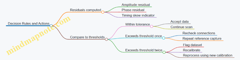
Practical Notes That Prevent Common Failures
- Keep reference captures short but consistent: same placement, same orientation, same averaging.
- Don’t average away problems. If the reference residual is unstable, averaging can hide the symptom while preserving the error.
- Treat metadata as part of the measurement. If you can’t reproduce the calibration context, you can’t trust the result.
A good quality check system is boring in the best way: it produces clear accept or flag outcomes, and it tells you why.
10.5 Step-by-Step Example Protocol for a Wall Inspection
This protocol shows a complete, repeatable workflow for inspecting a single wall segment to locate likely voids, utilities, or concealed objects using through-wall sensing. It assumes you already chose a sensing mode and have a calibrated system; the goal here is to make the field work consistent enough that results can be compared across scans.
Define the Inspection Target and Boundaries
Start by writing down what “success” means before you touch the equipment.
- Target types: voids behind drywall, embedded conduits, or a concealed cavity.
- Wall segment: specify width and height in meters, and mark a reference corner.
- Constraints: note access points, allowable dwell time, and any known metal fixtures.
Example: Inspect a 1.5 m by 2.2 m wall panel. You expect a conduit run near 0.6 m above the floor and want to detect a possible void behind a patch.
Prepare the Site and Record Conditions
Good measurements start with boring documentation.
- Photograph the wall with a visible scale and reference corner.
- Record temperature and humidity if available.
- Note recent construction activity, wet patches, or loose coverings.
- Confirm the wall is stable and not vibrating from nearby equipment.
Best practice: Use the same camera angle and keep the reference corner in every photo so later comparisons are straightforward.
Establish a Coordinate Frame and Scan Grid
Create a grid tied to the physical wall.
- Choose a grid spacing that matches your expected lateral resolution.
- Mark grid points with removable tape.
- Define axes: x along the wall width, y along height, and z as the sensor-to-wall normal.
Example: Use 10 cm spacing on a 1.5 m width, giving 16 points across. If your sensor height is fixed, y is handled by the grid; otherwise, record sensor height at each row.
Perform a Quick System Health Check
Before scanning, verify that the system behaves predictably.
- Run a short calibration capture using your standard procedure.
- Check signal-to-noise level and confirm the noise floor is stable.
- Verify timing and positioning inputs are being logged correctly.
Example: If the noise floor jumps by more than a set threshold between two consecutive checks, pause and investigate cables, grounding, or positioning drift.
Acquire Baseline Measurements
Baseline data helps you separate “wall-only” effects from target effects.
- If possible, scan an adjacent region you believe is empty.
- If not, perform a “near-field” baseline at the same grid but at a different sensor orientation or height.
Example: Scan the left half of the panel first as baseline, then scan the full grid. Later, subtract or compare features that appear in both halves.
Execute the Main Scan with Controlled Motion
Consistency matters more than speed.
- Move the sensor smoothly between grid points.
- Keep orientation fixed unless your plan requires multi-angle coverage.
- At each grid point, record the full acquisition set (all frequencies, sweeps, or time windows).
Best practice: Use a checklist per point: position confirmed, orientation confirmed, acquisition started, acquisition completed, data saved with correct filename.
Apply On-Site Quality Checks Immediately
Do not wait until the end to discover a problem.
- Inspect raw traces for clipping, dropouts, or unexpected saturation.
- Confirm that metadata matches the intended grid point.
- Look for gross misalignment between consecutive points.
Example: If one row shows systematically lower amplitude, verify sensor height and check whether you accidentally changed the antenna angle.
Process Data with a Reproducible Pipeline
Use the same processing steps for baseline and main scans.
- Apply calibration corrections.
- Perform imaging reconstruction or feature extraction using your chosen method.
- Generate intermediate outputs: range profiles, beamformed maps, and confidence scores.
Best practice: Keep processing parameters in a run log so another operator can reproduce the same results.
Interpret Results Using Evidence Rules
Turn images into decisions using simple, consistent criteria.
- Identify candidate regions that exceed a threshold relative to baseline.
- Require spatial consistency across neighboring grid points.
- Cross-check with expected geometry (for example, conduit runs often form continuous lines).
Example: A candidate void should appear as a localized anomaly that persists across multiple adjacent points, not as a single-pixel blip.
Document Findings and Plan Follow-Up Actions
Write down what you found, where it is, and how confident you are.
- Provide coordinates in the wall frame.
- Include the acquisition settings and processing run ID.
- Note any ambiguous areas and the reason for ambiguity.
Example: “Candidate cavity at x=0.92 m, y=1.35 m, confidence 0.72 based on baseline-relative contrast and spatial persistence.”
Mind Map: Wall Inspection Protocol
Example: One Grid Point to the Final Candidate
At grid point (x=0.60 m, y=1.10 m), you acquire the full measurement set, confirm no saturation in the raw trace, and verify metadata matches the intended coordinates. Processing produces a localized anomaly in the reconstructed map that is absent in the baseline region. When the anomaly repeats in the neighboring points (within your grid spacing tolerance) and aligns with the expected conduit direction, you mark it as a candidate and assign confidence based on contrast and persistence.
Example: Minimal Field Checklist
- Reference corner marked and photographed
- Grid points taped and numbered
- Calibration check passed
- Baseline captured (or orientation baseline captured)
- Per point: position, orientation, acquisition, save confirmation
- Post-row: raw trace sanity check
- End: processing run logged and outputs archived
11. Validation, Ground Truth, and Performance Evaluation
11.1 Defining Metrics for Detection Localization and Imaging Quality
Good metrics turn “it looks like something” into “we can measure how well it worked.” For through-wall imaging, you typically care about three things: where the target is, whether it is detected at all, and how trustworthy the image is when you interpret it.
Core Metrics for Localization
Localization metrics measure error in position and orientation, not just whether a bright spot exists.
Position error (range and cross-range). Define a coordinate frame tied to the scan geometry. For each true target, compute the Euclidean distance between the estimated and true location in the imaging plane. If your system outputs depth or range, compute a separate range error as well.
Angular error. If the system estimates direction (bearing/elevation), measure the angular difference between estimated and true rays. This matters when the same target can appear at different image locations depending on angle.
Localization success rate. Choose a tolerance radius, such as “within 10 cm in the imaging plane,” then report the fraction of targets that meet it. This is more actionable than average error alone.
Example. Suppose you scan a wall and know a small metal can is behind a stud bay. If your estimated peak lands 7 cm from the true can center, it counts as a success under a 10 cm rule. If it lands 18 cm away, it fails even if the image looks convincing.
Detection Metrics That Don’t Lie
Detection metrics quantify whether the system separates target returns from clutter and noise.
Probability of detection (Pd). For a set of trials with targets present, Pd is the fraction where the algorithm declares a detection.
Probability of false alarm (Pfa). For trials with targets absent, Pfa is the fraction where the algorithm still declares a detection.
Receiver operating characteristic. Sweep a decision threshold and plot Pd versus Pfa. This shows the tradeoff between catching targets and raising alarms.
Signal-to-clutter ratio at decision time. Instead of only using raw image intensity, compute a ratio using a local neighborhood around the candidate peak versus a background region. This helps when overall brightness changes across scans.
Example. If you set a threshold so that Pfa is 1% on empty-wall scans, you can then report Pd on scans with known targets. If Pd is low, the issue is not “bad luck,” it’s a measurable separation problem.
Imaging Quality Metrics for Interpretability
Imaging quality metrics describe how stable and meaningful the reconstructed image is.
Point spread function width. For a known point-like reflector, measure the mainlobe width and sidelobe level in the reconstructed image. Narrow mainlobes improve localization; low sidelobes reduce ghost peaks.
Dynamic range and contrast. Compute the ratio between the strongest target-related response and the typical background level. Contrast is often more informative than absolute intensity.
Resolution and uncertainty. Report effective resolution (e.g., full width at half maximum) and uncertainty bounds for estimated positions. Uncertainty should reflect both measurement noise and modeling mismatch.
Repeatability. Re-run the same scan conditions and measure variance in estimated target location and detection score. Repeatability catches calibration drift and positioning errors.
Example. If two scans of the same empty wall produce occasional peaks at similar locations, those peaks inflate false alarms. Repeatability plus Pfa tells you whether the system is consistently “confused” or just occasionally noisy.
Metrics That Tie Together Localization and Detection
A practical evaluation often uses a combined view.
Detection-to-localization consistency. For each trial, record whether a detection occurred and whether the estimated location is within tolerance. This yields a joint success rate.
Localization conditional on detection. Report localization error only for trials where detection was declared. This prevents mixing “no detection” failures with “detected but inaccurate” failures.
Error decomposition. Separate error sources: geometry/pose error, material-model mismatch, and algorithmic regularization effects. Even a simple decomposition helps you target fixes.
Mind Map: Metrics and How They Connect
Example Metric Set for a Wall Inspection Trial
Use a consistent protocol so metrics are comparable across runs.
- Collect N trials with targets present and N trials with targets absent.
- For each trial, compute a detection score from the reconstructed image.
- Sweep threshold to obtain Pd and Pfa.
- For detected targets, compute position error and angular error.
- Report: ROC summary (Pd at a fixed Pfa), localization success rate within tolerance, and imaging quality indicators (PSF width, sidelobe level, repeatability).
Example. If Pd at Pfa = 1% is 0.8, localization success within 10 cm is 0.65, and PSF sidelobes are high, you can interpret the gap: the system detects often, but ghost structure is degrading localization accuracy.
Practical Metric Definitions to Write Down
To avoid metric confusion, define these explicitly in your evaluation plan.
- Coordinate frame and units for position error.
- Tolerance radius for localization success.
- How detection is declared from the image (thresholding rule).
- Background region definition for clutter/contrast calculations.
- How uncertainty is computed (from repeated scans, bootstrap, or model-based propagation).
When these are specified, results become reproducible and disagreements become technical rather than interpretive.
11.2 Ground Truth Collection Methods and Documentation
Ground truth is the “known answer” your system will be judged against. In through-wall imaging, that answer is rarely a single number; it’s a set of spatial locations, object extents, and material facts tied to a coordinate frame. The goal of this section is to make that set trustworthy, repeatable, and easy to audit.
Define Ground Truth Scope and Acceptance
Start by writing down what you will treat as truth. For localization tasks, ground truth often includes target centroid coordinates and approximate size. For detection tasks, it includes presence or absence within a defined region of interest (ROI). For material inference, it includes material class labels and, when possible, measured properties.
A practical acceptance rule prevents arguments later. Example: “A target is considered found if the reconstructed peak lies within 5 cm of the centroid and the ROI overlap exceeds 70%.” If you cannot measure that overlap reliably, reduce the claim to what you can support.
Choose a Coordinate Frame and Lock It Early
Pick one coordinate system for the whole experiment: typically a wall-referenced frame with axes aligned to the wall plane. Document the origin, axis directions, and units. Then physically enforce it.
Example: Place three non-collinear fiducials on the wall surface (or on a rigid plate mounted to the wall). Measure their positions once with a tape measure plus a level for rough alignment, then refine with a total station or laser rangefinder if available. Every scan uses the same fiducials so you can transform sensor coordinates into the wall frame.
Select Ground Truth Measurement Methods
Use methods that match the target type.
- Direct measurement for accessible targets: If you can place a target and later remove it, measure its position and dimensions before and after the scan. This reduces the chance that the target moved during setup.
- Non-destructive verification for embedded targets: When targets are inside walls, use complementary sensing that does not disturb the structure. For instance, if you can access a cavity from another side, measure there and map back through the known geometry.
- Reference geometry for voids and interfaces: For voids, ground truth often comes from controlled inserts (foam blocks, removable spacers) whose dimensions are known precisely.
Example: To validate void detection, build a test panel with a removable rectangular cavity. Measure the cavity dimensions with calipers, then record the cavity center relative to the fiducials.
Document Target Specifications with Uncertainty
Ground truth should include uncertainty, not just values. Record measurement method, instrument resolution, and how you estimated error.
A simple uncertainty table works well:
| Quantity | How Measured | Typical Uncertainty |
|---|---|---|
| Target centroid | Fiducial-based transform | ±2–5 mm |
| Target size | Calipers or CAD | ±1–3 mm |
| Wall thickness | Tape/scan | ±2–10 mm |
Example: If wall thickness is measured with a tape measure through a small opening, treat it as a coarse value and avoid claiming fine depth accuracy.
Capture Material Facts and Environmental Conditions
Through-wall imaging depends on materials and conditions. Record:
- Wall build-up order (e.g., drywall, stud cavity, insulation)
- Reinforcement presence and approximate spacing
- Surface finish and moisture state if relevant
- Temperature and humidity at the time of measurement
Example: If a wall contains metal studs, note their spacing and whether they are aligned with the scan direction. Even if you cannot model them perfectly, you can explain why certain artifacts appear.
Create a Ground Truth Data Package
A ground truth package should be self-contained. Include:
- A “truth manifest” describing targets, ROI definitions, and coordinate frame
- A measurement log with timestamps, operator, and instrument identifiers
- The raw measurement outputs used to compute truth (or a clear summary if raw files are too large)
- A mapping file that links sensor poses to the wall frame
Example: Store a JSON manifest with target entries: id, type, centroid (x,y,z), size (dx,dy,dz), ROI bounds, and uncertainty fields.
Mind Map: Ground Truth Collection Methods and Documentation
Example Workflow for a Controlled Wall Test
- Build a wall section with a known cavity and fixed fiducials.
- Measure fiducials and cavity center in the wall frame; record uncertainties.
- Record wall thickness and build-up order.
- Run scans using the same fiducial-based transform for every pose.
- Produce a ground truth manifest with target centroid, size, ROI bounds, and uncertainty.
- During evaluation, compare reconstructed peaks to centroid distance and ROI overlap, using the acceptance rule you wrote at the start.
This workflow keeps the “known answer” grounded in measurable facts, with enough uncertainty detail to interpret mismatches without inventing explanations.
11.3 Controlled Experiments With Known Targets
Controlled experiments turn “it looks like something” into “we can measure how well the system finds it.” The goal is not to mimic every real building; it is to isolate variables so performance claims have a clear cause.
Define the Experiment Objective
Start by choosing one primary question and one secondary question. Primary questions usually target localization accuracy, detection probability, or false-alarm rate. Secondary questions often target robustness to small changes like antenna height or slight wall moisture.
Example objective: “When a known metal pipe is placed behind drywall, how accurately does the system estimate its center location and orientation?” Secondary objective: “How does performance change if the pipe is shifted 5 cm laterally?”
Select Known Targets and Ground Truth
Known targets must be measurable independently of the imaging system. Use targets with stable geometry and repeatable placement.
Common target set:
- A cylindrical metal rod with known diameter and length.
- A dielectric block with known permittivity proxy (or at least known material label and thickness).
- A void cavity created by a removable insert behind a wall panel.
Ground truth methods:
- For fixed targets, record placement using a physical template and measure offsets from a reference corner.
- For removable targets, photograph the setup before closing the wall and log the insert coordinates.
Best practice: include at least one “boring” target that should not be detected strongly (e.g., a low-contrast dielectric slab) to quantify false alarms.
Build a Test Matrix That Controls Variables
A test matrix lists what changes and what stays fixed. Keep the number of variables small per run.
A practical matrix:
- Geometry: target depth (3 levels), lateral offset (3 levels).
- Environment: one wall type per batch.
- System settings: one frequency sweep per batch.
Hold constant:
- Antenna model and orientation reference.
- Scan grid spacing.
- Triggering and timing method.
Example: Run 3 depths × 3 offsets = 9 target positions, each repeated 5 times. That gives enough data to estimate variability without turning the lab into a full-time job.
Standardize Setup, Calibration, and Repeatability
Repeatability is where controlled experiments succeed or fail.
Checklist for each session:
- Mark a coordinate origin on the wall and keep it unchanged.
- Use the same antenna mounting hardware and record antenna height.
- Perform a calibration measurement on a reference surface or empty wall segment.
- Verify that the positioning system reports the same coordinates when you return to the start point.
Example: If your positioning system has a 2 mm repeatability limit, treat that as part of the uncertainty budget rather than pretending it is zero.
Define Pass/Fail Criteria and Metrics
Choose metrics that match the objective.
- Detection probability: fraction of runs where the target is declared present.
- False-alarm rate: fraction of runs where the system declares a target in empty regions.
- Localization error: distance between estimated and true target center.
- Orientation error: angular difference for targets where orientation is meaningful.
Decision rule example:
- Declare a detection if the peak response in the target neighborhood exceeds a threshold set from empty-wall runs.
- Report localization error only for runs that pass the detection rule.
Run the Experiment with Consistent Data Capture
Use a fixed acquisition script so each run differs only by the intended variable.
Operational practices:
- Randomize the order of target positions to reduce systematic drift effects.
- Keep environmental conditions logged (temperature, humidity, and any power-supply changes).
- Save raw data plus processing parameters so results can be reproduced.
Example: Alternate between “target present” and “target absent” runs every other scan to prevent threshold bias from creeping upward.
Analyze Results with Uncertainty and Error Attribution
Controlled data lets you separate measurement noise from modeling mismatch.
A systematic analysis flow:
- Compute detection outcomes per run.
- For detected runs, compute localization error in the wall coordinate system.
- Compare error distributions across depths and offsets.
- Attribute large errors to specific causes by checking residual patterns.
Example attribution:
- If localization error grows mainly with depth, the issue is likely signal attenuation and reduced effective aperture.
- If error spikes at certain lateral offsets, the cause may be scan-grid alignment or antenna orientation inconsistency.
Mind Map: Controlled Experiments with Known Targets
Example: Depth and Offset Study for a Metal Rod
Setup:
- Wall: one consistent drywall assembly.
- Target: metal rod diameter and length recorded.
- Coordinates: origin at a marked corner.
Matrix:
- Depths: 5 cm, 10 cm, 15 cm.
- Offsets: -10 cm, 0 cm, +10 cm.
- Repeats: 5 runs per position.
Evaluation:
- Use empty-wall runs to set a threshold.
- For each detected run, compute localization error in centimeters.
Expected outcome pattern to look for (without guessing):
- If detection probability drops with depth, attenuation is dominating.
- If localization error is symmetric around zero offset, alignment is likely stable.
- If errors cluster at one offset sign, investigate coordinate transforms and antenna orientation.
This structure keeps the experiment honest: you know what changed, you know where the target really was, and you can explain the results using measurable factors rather than vibes.
11.4 Error Analysis for Range Angle and Material Uncertainty
Error analysis turns “the image looks plausible” into “we know what could be wrong and by how much.” In through-wall imaging, two error sources dominate: geometric errors (range and angle) and propagation-model errors (material properties). The goal is to quantify how these uncertainties move peaks in the reconstructed space and how that movement affects detection decisions.
1) Start with the Measurement Geometry
Range and angle errors come from how you measure position and how you map measurements into an imaging grid.
- Range error typically arises from timing offsets, frequency sweep nonlinearity, and calibration drift in the transmit-receive chain. A simple way to reason about it: if the system’s effective time reference is off by \(\Delta t\), then the apparent path length shifts by \(\Delta R \approx c,\Delta t/2\) for a monostatic setup.
- Angle error comes from antenna placement uncertainty, orientation errors, and beamforming assumptions. If the antenna is rotated by a small angle \(\Delta\theta\), the reconstructed target direction shifts roughly proportionally to \(\Delta\theta\) for narrow beams.
A practical habit: record the position/orientation used for each scan point, not just the nominal values. Even a “small” 5 mm placement error can matter when the wall-to-target distance is only a few tens of centimeters.
2) Separate Propagation-Model Uncertainty from Reconstruction Math
Material uncertainty affects the forward model: how signals attenuate, reflect, and scatter through the wall. Common uncertain parameters include effective permittivity and conductivity, plus the presence of rebar, voids, or air gaps.
Instead of treating material uncertainty as one blob, split it into two effects:
- Amplitude bias: wrong attenuation changes peak height and can push threshold-based detection toward false negatives.
- Phase or delay bias: wrong effective propagation speed shifts the apparent range, which moves peaks in the imaging grid.
A concrete example: if the wall is modeled as slightly less lossy than it really is, the reconstruction may place a target closer than it is because the assumed path delay is too small.
3) Build a Sensitivity Chain
A systematic workflow is to compute how small parameter changes move the reconstructed peak.
- Choose a representative target location in your imaging grid.
- Perturb geometry inputs (position, orientation) within measured bounds.
- Perturb material inputs within plausible bounds derived from calibration or prior measurements.
- Reconstruct for each perturbation and measure the peak shift.
You can summarize results with:
- Range shift \(\Delta r\) and angle shift \(\Delta\phi\)
- Peak amplitude change \(\Delta A\)
- Localization spread as the standard deviation across perturbations
This is essentially “error propagation by simulation,” and it avoids pretending the system is perfectly linear.
4) Mind Map of Error Sources and How They Show Up
Mind Map: Error Analysis for Range, Angle, and Material Uncertainty
5) Example: Quantifying Range and Angle Spread
Assume you reconstruct a point target using a grid with 1 cm range bins and 2° angular bins.
- Geometry perturbations: position uncertainty of 5 mm and orientation uncertainty of 1.5°.
- Material perturbations: effective permittivity varied by ±5% and effective conductivity by ±20% (chosen to match calibration scatter).
Run 200 perturbation reconstructions. You might observe:
- Median peak shift of 0.6 cm in range and 1.1° in angle.
- Peak amplitude standard deviation of 0.25 in normalized units.
Interpretation: the localization spread is not just grid quantization; it is driven by both geometry and material. If your detection threshold is set near the mean peak amplitude, the amplitude spread can flip decisions even when the peak location is stable.
6) Example: How Material Error Can Mimic Geometry Error
Suppose you see a consistent bias where peaks appear closer to the antenna than expected.
- If timing calibration is correct, the bias likely comes from effective delay error in the wall model.
- If the bias changes sign when you rotate the antenna, geometry or multipath structure is more likely.
A simple diagnostic is to compare reconstructions using two different wall parameter sets that preserve attenuation but change phase. If range bias persists while amplitude stays similar, phase/delay uncertainty is the culprit.
7) Turn Uncertainty Into a Confidence Region
Finally, convert the measured localization spread into a confidence region aligned with your decision process.
- Define a region in the range-angle plane that contains, for example, 90% of perturbed peak locations.
- Report whether the region overlaps the expected target location or a known reference.
This makes performance evaluation concrete: you are not only saying “we detected it,” but also “we detected it with a known tolerance to geometry and material uncertainty.”
11.5 Reporting Results With Reproducible Test Conditions
Reproducible reporting turns a good measurement into something others can repeat without guessing. The goal is simple: if someone reruns your protocol with the same inputs, they should see the same outcomes within stated tolerances.
Reporting Structure That Matches the Experiment
Start with a short “what we did” summary, then expand into the exact conditions that affect the signal. A practical order is: objective, setup, procedure, data handling, results, and verification. Keep the summary readable, but ensure every number in the results section can be traced back to a parameter in the setup or procedure.
Test Date, Location, and Environmental Conditions
Record the test date (use a fixed example date such as 2024-04-12), site type (lab, corridor, room), and any constraints (occupied building, limited access). Then log environmental variables that measurably influence propagation and electronics: ambient temperature, humidity, and whether HVAC or doors were active during acquisition. If you used a controlled fixture, describe it as precisely as the wall.
Example: “Temperature 21–22°C, humidity 40–45%, doors closed, HVAC off during scans.” This is boring in the best way: it tells readers what to control.
Equipment Configuration and Calibration State
List the measurement chain in a way that someone can rebuild it. Include:
- Transmit settings: center frequency or sweep range, bandwidth, modulation type, transmit power, dwell time.
- Receive settings: gain, noise figure if known, sampling rate, number of averages, windowing.
- Timing and synchronization: trigger source, synchronization method, and any latency compensation.
- Positioning: coordinate system definition, sensor mounting offsets, and positioning method (manual marks, encoder, laser range).
Calibration must be reported as a state, not a vague promise. State what was calibrated (e.g., frequency response, phase alignment, antenna port match), when it was last performed, and how you verified it before the run. If you used a reference target, describe its dimensions and placement.
Geometry, Target Definition, and Ground Truth
Reproducibility depends on geometry more than people expect. Report:
- Wall type and thickness, and whether reinforcement is present.
- Scan path: start/end coordinates, step size, scan speed, and coverage area.
- Target definition: what counts as a “hit,” including size thresholds and acceptable localization error.
Ground truth should be documented with the same care as the measurement. If you used a known cavity, specify its dimensions and how its location was measured (e.g., from drawings, from destructive verification, or from a reference survey).
Data Handling and Processing Parameters
Processing choices can shift results even when acquisition is identical. Report the full processing parameter set:
- Preprocessing: filtering, normalization, windowing, outlier handling.
- Imaging: algorithm name, grid resolution, coordinate transforms, and any regularization settings.
- Decision rules: thresholding method, false-alarm control approach, and how confidence scores were computed.
Include file naming conventions and the mapping from raw files to processed outputs. If you downsampled or cropped, state the exact criteria.
Results Presentation with Uncertainty
Present results with both central estimates and uncertainty. For localization, include error statistics such as mean absolute error and spread (e.g., standard deviation or percentile ranges). For detection, report metrics that match your decision rule: detection rate at a specified false-alarm rate, or precision/recall computed consistently.
Also report failure modes. If some scans are unusable due to positioning drift or saturation, list the criteria used to exclude them. Exclusion rules should be deterministic, not “we felt like it.”
Mind Map: Reproducible Reporting Checklist
Example: Minimal Yet Complete Results Block
Objective: Localize a concealed void behind a 15 cm masonry wall using a fixed scan grid.
Test Context: 2024-04-12, indoor corridor, temperature 21–22°C, humidity 40–45%, HVAC off, doors closed.
Setup: Center frequency 2.45 GHz, sweep 2.40–2.50 GHz, transmit power 10 dBm, bandwidth 20 MHz, sampling rate 200 MS/s, 16 averages. Positioning via encoder with origin at the lower-left corner of the wall coordinate frame; antenna height 1.20 m with measured offset of +3 mm.
Calibration State: Frequency response calibration performed the same day; verification using a reference reflector showed phase error within ±5° across the sweep.
Geometry and Ground Truth: Wall thickness 15 cm masonry, reinforcement present per drawings. Void dimensions 0.30 m × 0.20 m × 0.10 m; ground truth from as-built measurements with ±5 mm coordinate uncertainty.
Processing: Bandpass filter 2.40–2.50 GHz, imaging grid 5 mm spacing, regularization parameter λ = 0.02, decision threshold set to achieve 1% false-alarm rate on background scans.
Results: Void centroid localization error mean 12 mm, 90th percentile 22 mm. Detection rate 9/10 scans. Excluded 1 scan due to encoder reset detected by discontinuity in position logs.
This format is compact, but every number has a home. When readers can trace outcomes back to conditions, reproducibility stops being a hope and becomes a property.
12. System Design for Robust Non-Intrusive Detection
12.1 Selecting Frequency Bands and Tradeoffs for Penetration
Frequency selection is the first knob you turn when you want signals to travel through a wall and still carry enough detail to locate hidden objects. The core tradeoff is simple: lower frequencies generally penetrate better, while higher frequencies usually provide finer spatial detail. The trick is matching the band to the wall materials, the object size, and the measurement geometry so your system can see something meaningful rather than just “something.”
Foundational Concepts for Band Selection
Start with how frequency interacts with materials. In many building materials, the signal experiences attenuation that grows with frequency because losses increase with how charges and dipoles respond to the changing electric field. Conductive elements like rebar and metal fixtures add additional loss and scattering, often creating strong multipath and clutter that can mask weaker target echoes.
Next, connect frequency to resolution. In imaging, resolution is tied to the effective bandwidth and the wavelength. A shorter wavelength (higher frequency) can support tighter angular discrimination and smaller features, but only if the signal survives the wall and the system can maintain adequate signal-to-noise ratio (SNR). If the higher-frequency components die out, your “resolution” becomes theoretical rather than practical.
Finally, consider coupling and antennas. Antenna size relative to wavelength affects radiation efficiency and beam shape. If the antenna is too small for the chosen band, you lose power and distort the assumed beam pattern, which then feeds errors into imaging reconstruction.
Tradeoffs That Actually Matter in Practice
Penetration vs. Detail: If your target is small and you need precise localization, you may want a higher band. If the wall is thick or highly lossy, you may need to drop frequency to keep enough energy at the receiver.
Attenuation vs. Clutter: Higher frequencies can increase scattering from surface roughness and internal interfaces. That can raise clutter levels even when penetration is acceptable, so you may need stronger processing or better geometry.
Bandwidth vs. Stability: Wideband operation can improve range resolution, but it also increases calibration burden because phase and gain must remain consistent across the band. A narrower band can be easier to calibrate and more stable, at the cost of coarser range discrimination.
Regulatory and hardware limits: Transmit power, receiver noise figure, and available components constrain which bands are feasible. A band that looks good on paper can fail because the system cannot deliver enough effective radiated power or because the receiver saturates.
A Systematic Selection Workflow
- Characterize the wall class: Identify whether the wall is mostly concrete, masonry, drywall with cavities, or mixed construction. Note likely conductive elements such as rebar density or metal studs.
- Estimate attenuation: Use prior measurements or quick pilot scans to compare received power across candidate bands. You are looking for usable SNR, not maximum penetration.
- Match target scale: Choose a band where the wavelength is not wildly larger than the object features you want to detect. For example, if you care about a small void or a thin conduit, you typically need enough frequency content to produce distinguishable reflections.
- Check antenna feasibility: Confirm that your antenna array elements are practical for the band and that beamforming assumptions match the real radiation pattern.
- Plan bandwidth and calibration: Decide whether you will use a single band or multiple bands. If you use multiple bands, ensure your calibration and synchronization strategy can compare results fairly.
- Run a “visibility test”: Perform a short scan with a known reflector or a controlled target. Evaluate whether the target appears above clutter and whether the phase behavior is stable enough for imaging.
Mind Map: Frequency Band Selection Logic
Example: Choosing Between Two Candidate Bands
Suppose you are scanning a reinforced concrete wall for a small cavity behind drywall on the far side. You test two bands: a lower band (better penetration) and a higher band (better detail).
- In the lower band, the received signal is strong enough that the direct path and a few reflections are visible. The cavity echo is present but smeared, and the reconstruction shows broad regions rather than a crisp location.
- In the higher band, the cavity echo becomes more distinct in the frequency response, but the clutter from rebar reflections rises too. The cavity still localizes, yet the confidence drops unless you improve geometry overlap or use a stricter decision rule.
A practical resolution is to use the higher band for localization refinement and the lower band to stabilize detection. Even if you do not fuse bands formally, you can use the lower band to confirm that the wall is “transparent enough” for imaging and then rely on the higher band for tighter placement.
Example: Bandwidth Choice for Range Discrimination
If you need to separate two objects at different depths, wider bandwidth helps because it improves range discrimination. However, if your calibration across the full band is imperfect, phase errors can smear the depth estimate.
A common compromise is to choose a band where the system can maintain stable gain and phase across the intended bandwidth. For instance, you might keep a moderate bandwidth that still provides useful depth separation while ensuring your calibration procedure produces consistent results across repeated scans.
Practical Checklist for Finalizing the Band
- The selected band yields measurable SNR after wall attenuation.
- The antenna and array geometry are appropriate for the wavelength.
- The bandwidth is wide enough for the depth or range separation you need, and narrow enough for stable calibration.
- Pilot scans show target visibility above clutter, not just received power.
- The expected clutter behavior matches your processing approach, so the reconstruction does not confuse multipath with targets.
12.2 Designing for Dynamic Range and Noise Performance
Dynamic range is the span between the smallest signal you can trust and the largest signal you can measure without distortion. Noise performance is how reliably your system separates real echoes from random variation. In through-wall imaging, this matters because echoes are weak, multipath is common, and reflections can vary dramatically across scan positions.
Foundational Concepts That Drive Design
Start with three numbers: receiver noise floor, expected echo strength, and maximum interference level. The receiver noise floor is set by thermal noise, front-end noise figure, and bandwidth. Expected echo strength depends on path loss, wall material, and antenna pattern. Maximum interference level comes from direct coupling, leakage, strong reflectors, and any motion-induced changes.
A practical way to think about it: if your noise floor is too high, you lose weak targets; if your interference is too high, you saturate or compress the receiver and create false structure.
Noise Sources and Where They Enter
Noise is not one thing; it’s a stack. Thermal noise is unavoidable and scales with bandwidth. Front-end noise figure adds extra noise beyond thermal. Phase noise and oscillator jitter smear coherent measurements, which can reduce the benefit of averaging. Quantization noise appears when the ADC resolution is insufficient for the signal scale.
A simple example: suppose you widen bandwidth to improve range resolution. Thermal noise rises with bandwidth, so the signal-to-noise ratio (SNR) may not improve. The design task is to choose bandwidth that supports the imaging method while keeping SNR acceptable.
Dynamic Range Budgeting with Realistic Limits
Dynamic range is limited by saturation and by the smallest measurable level. In a receiver chain, the limiting element is often the first stage that can overload: the LNA, mixer, or ADC input.
Build a budget in this order:
- Estimate strongest expected input at the receiver during worst-case coupling.
- Check headroom for linear operation at that input.
- Determine the smallest echo you must detect at the farthest or most lossy positions.
- Ensure the ADC and processing chain can represent that smallest echo above the noise floor.
Concrete example: if your strongest coupling is 20 dB above the weakest target echo, you need enough headroom to avoid compression while still resolving the weak echo. If the ADC full-scale range is set for the strong coupling, the weak echo may occupy only a tiny fraction of codes and become quantization-limited.
Bandwidth, Averaging, and the SNR Trade
Averaging reduces random noise but not deterministic interference. If your measurement includes repeated sweeps, coherent averaging improves SNR more than non-coherent averaging, provided phase alignment is stable. If phase is unstable, averaging can help less than expected.
Example: you average 16 sweeps. If noise is truly random and phase-stable for coherent summation, SNR can improve by about 12 dB. If phase drifts, the improvement might be closer to 6 dB, and the reconstructed image may show smeared artifacts.
Bandwidth selection should match the imaging approach. Frequency-stepped methods often use narrower effective bandwidth per step, while time-domain methods may rely on pulse bandwidth. In both cases, keep an eye on how bandwidth changes noise floor and on how it interacts with the wall’s dispersive behavior.
Front-End Linearity and Overload Control
Overload control is about preventing gain compression and intermodulation. Use appropriate attenuation before sensitive stages, select an LNA with sufficient linear range, and ensure mixers and filters are not driven beyond their linear region.
A practical tactic: include a switchable attenuator or variable gain mode. During calibration or when scanning near strong reflectors, reduce gain to protect linearity. When scanning in quieter regions, increase gain to recover sensitivity.
ADC and Quantization Strategy
ADC performance is governed by full-scale range, effective number of bits, sampling rate, and input drive. If the ADC input is too small, quantization noise rises relative to the signal. If it is too large, clipping destroys waveform shape and can create spurious peaks.
Example: if the target echo is 30 dB below full-scale, and you have limited effective bits, the echo may land near the quantization noise. A better approach is to set gain so that typical echoes sit in the mid-range of the ADC codes, while still leaving headroom for occasional strong coupling.
Mind Map: Dynamic Range and Noise Performance
Integrated Example Workflow
- Measure receiver noise floor at the chosen bandwidth with antennas terminated or in a controlled low-reflection setup.
- Estimate strongest coupling by placing antennas in the worst expected geometry and recording peak levels.
- Choose gain so the strongest coupling stays below compression limits with headroom, while the weakest target echo remains above the noise floor by a comfortable margin.
- Validate with a known reference reflector placed at a representative distance and orientation.
- Run a short scan sequence and verify that averaging improves SNR as expected and that reconstructed peaks do not grow when only noise should be present.
If any step fails, adjust bandwidth, gain staging, attenuation, or averaging strategy. The goal is not to maximize numbers on a spec sheet; it’s to ensure the imaging output changes when real structure changes, and stays stable when it shouldn’t.
12.3 Power, Thermal, and Duty Cycle Constraints in Operation
Power, thermal load, and duty cycle are the three knobs that quietly decide whether a through-wall system works for five minutes or five hours. The goal is to design operation so the electronics stay within safe limits while still collecting data with the timing and signal quality you need.
Foundational Constraints and Why They Matter
Start with three measurable limits:
- Electrical power: available supply voltage/current and allowable peak draw.
- Thermal limits: maximum junction temperature for semiconductors and maximum surface temperature for enclosures.
- Duty cycle: fraction of time the system transmits or runs high-power processing.
A simple way to think about it: power determines heat generation; heat determines temperature rise; temperature rise changes component behavior (gain, noise figure, oscillator stability), which then changes measurement quality.
Power Budgeting with Realistic Peaks
Even if average power looks fine, many systems fail on peak events. For example, a transmitter might draw 2 A for 50 ms during a burst, even if the average over a minute is only 0.2 A.
A practical workflow:
- List each high-current block: RF power amplifier, synthesizer, ADC/DAC, compute module, fans/heat pumps.
- Record peak and steady-state current for each block.
- Sum peaks for the worst-case operating mode.
- Verify the supply can handle the peak without voltage droop that shifts frequency or compresses the RF chain.
Example: If your supply droops by 5% during bursts, the oscillator may shift by tens of kHz. That can smear coherent processing unless your calibration and frequency tracking account for it.
Thermal Modeling That Matches How You Actually Operate
Thermal behavior is not instantaneous. Use a two-part model:
- Transient heating during bursts.
- Cooling between bursts.
A useful operational metric is temperature rise per cycle. Suppose the system runs 100 ms transmit bursts every 1 s. The average power might be modest, but the junction temperature can still climb if the cooling time constant is longer than the 1 s period.
Best practice: measure it once, then design around it.
- Run a representative burst pattern.
- Log temperature at the hottest point (often near the RF amplifier or power regulator).
- Repeat with a slightly higher duty cycle to find the knee where temperature rise accelerates.
Duty Cycle Planning for Signal Quality
Duty cycle affects more than safety. It also affects:
- Receiver stability: gain and noise figure can drift with temperature.
- Timing consistency: burst-to-burst latency can change the effective sampling window.
- Calibration validity: if calibration assumes a stable thermal state, you must either keep the state stable or recalibrate.
A systematic approach is to define three phases in each scan:
- Warm-up: bring electronics to a repeatable thermal state.
- Acquisition: run bursts at a controlled duty cycle.
- Recovery: allow cooling enough to prevent drift from accumulating.
Example: If you observe that coherent summation quality drops after 200 bursts, you can either reduce duty cycle or insert a recovery pause every N bursts. The trick is to choose N based on measured drift, not guesswork.
Control Strategies That Keep Everything Inside Limits
Use layered controls rather than a single “limit switch.”
- Software gating: enforce maximum burst count per minute.
- Adaptive burst scheduling: reduce burst length when temperature approaches a threshold.
- Hardware protection: current limiting and thermal shutdown as a last resort.
A simple scheduling rule:
- If temperature is below \(T_{low}\) , run the nominal burst.
- If between \(T_{low}\) and \(T_{high}\) , shorten bursts or increase spacing.
- If above \(T_{high}\) , pause acquisition and cool.
This prevents sudden thermal collapse that would ruin the dataset mid-scan.
Mind Map: Power, Thermal, and Duty Cycle Constraints
Example: Burst Pattern Selection for a Wall Scan
Assume you need 500 bursts per scan. You test two patterns:
- Pattern A: 100 ms bursts every 1 s.
- Pattern B: 80 ms bursts every 0.8 s with a 30 s recovery after 200 bursts.
If Pattern A reaches the thermal knee after 250 bursts, you’ll see drift and inconsistent imaging. Pattern B may use slightly less total transmit time but keeps temperature in the stable region, producing a cleaner dataset and fewer “mystery” reconstruction artifacts.
The operational lesson is straightforward: choose duty cycle based on measured thermal behavior, then verify that the resulting temperature stability preserves the assumptions behind your calibration and processing.
12.4 Software Architecture for Acquisition Processing and Storage
A through-wall system lives or dies by its software’s ability to keep data consistent from the first trigger to the final report. The architecture should separate concerns: acquisition control, signal processing, metadata management, and storage. When those parts are loosely coupled, you can swap processing methods without rewriting the acquisition layer—like changing the recipe without changing the kitchen.
Core Architecture Principles
Start with a clear data contract. Every measurement should produce: raw samples, timing information, sensor configuration, and environmental context. The software should treat these as first-class objects rather than side files. A practical rule: if you cannot reproduce a result from the stored package alone, the architecture is missing something.
Next, design for deterministic execution. Acquisition threads should never wait on heavy processing. Instead, they publish “measurement jobs” to a queue. Processing workers consume jobs, compute outputs, and write results back with the same identifiers. This prevents dropped triggers when the CPU is busy.
Finally, enforce versioning. Store software version, processing configuration, and calibration identifiers alongside the data. If you later adjust a calibration constant, you want the system to keep the old constant tied to the old dataset.
Data Flow from Trigger to Stored Product
A typical pipeline looks like this:
- Acquisition Controller arms devices, sets transmit parameters, and starts synchronized capture.
- Timestamping Layer records trigger time, sample clock status, and any synchronization offsets.
- Raw Data Writer streams samples to disk immediately to avoid memory pressure.
- Metadata Builder collects configuration, antenna geometry, and material assumptions used for processing.
- Processing Orchestrator runs the chosen processing chain on a worker pool.
- Result Writer stores intermediate products needed for debugging and final outputs for interpretation.
A useful sanity check is to compute a lightweight checksum or energy statistic during acquisition and store it with the raw chunk. If a later stage fails, you can still verify whether the raw data was intact.
Mind Map: Acquisition Processing and Storage
Storage Strategy That Helps Debugging
Use a container format that supports chunking and random access. Store raw samples in fixed-size blocks aligned to acquisition bursts. Keep intermediate products separate from raw data so you can regenerate them without re-capturing. For example, if you change the imaging grid resolution, you should only need to recompute the final reconstruction, not the raw stream.
A practical naming scheme prevents confusion during multi-day campaigns. Include run_id, wall_id, and scan index in every stored object name. Also store a “channel map” that records which physical antenna or port corresponds to each data channel. Without it, the system may still run, but the results will be quietly wrong.
Processing Orchestration and Quality Gates
Processing should be modular. Each stage consumes inputs and produces outputs with explicit shapes and units. A prefilter stage might output a calibrated complex spectrum; a beamforming stage might output a spatial cube; an inversion stage might output an image grid plus uncertainty estimates.
Quality gates stop bad data from polluting later stages. Example gates:
- Clipping detection: if receiver ADC saturates, flag the chunk and skip reconstruction.
- Timing sanity: if sample clock drift exceeds tolerance, mark the chunk as unreliable.
- Energy bounds: if measured energy is near zero, likely the transmit path was misconfigured.
These checks should be cheap enough to run inline, not after the fact.
Example: Minimal End-to-End Workflow
Below is a compact pseudo-implementation of the job model. It shows the separation between acquisition and processing, and it highlights where metadata and checksums attach.
on_trigger(scan_id):
  cfg = snapshot_system_config()
  run_id = current_run_id()
  chunk_id = allocate_chunk_id()

  raw = stream_samples_to_disk(chunk_id)
  checksum = checksum_of(raw)

  meta = build_metadata(run_id, scan_id, cfg, chunk_id, checksum)
  enqueue_job(job_id=chunk_id, meta=meta)

worker(job):
  raw = load_raw(job.chunk_id)
  if not quality_pass(raw, job.meta):
    write_flag(job.chunk_id, "rejected")
    return

  products = processing_chain(raw, job.meta)
  write_intermediate_and_final(job.chunk_id, products, job.meta)
Example: Metadata That Prevents “It Worked Yesterday”
Suppose you adjust antenna height by 2 cm during a site visit. If the metadata builder records antenna pose per scan, the processing stage can use the correct geometry. If it does not, the system may still produce images, but target locations will drift. The architecture should make geometry changes traceable at the same granularity as the scan.
Operational Considerations for Storage Reliability
Write raw data first, then metadata, then enqueue processing. If power is lost mid-scan, you can detect incomplete chunks by missing checksums or incomplete metadata records. On restart, the system should resume by scanning for completed chunk markers and re-enqueueing only what is missing.
Finally, keep an audit trail that ties every stored output to its inputs. That means storing the processing configuration snapshot and calibration identifiers used to generate each final product. When a result looks odd, you can answer “which settings made it” without guessing.
12.5 End-to-End Example System Build and Integration Checklist
This checklist walks through a complete build from requirements to a working scan workflow. It’s written as if you’re assembling one system for a real wall inspection, then integrating it so the same procedure produces repeatable results.
Start with a Build-Ready Requirements Sheet
- Write down the target wall types, typical distances, and what “success” means (e.g., detect a void of a given size at a given range).
- Convert goals into measurable constraints: required bandwidth, expected penetration loss, and acceptable localization error.
- Choose a test date for your first integration run, such as 2026-04-06, and record it in your lab notebook so later results can be compared.
Select Hardware Blocks and Define Interfaces
- RF front end: transmitter, receiver, and switching (if you alternate antennas).
- Antenna system: single antenna or array, including mounting hardware and repeatable positioning.
- Positioning: encoder or tracked mount for scan geometry.
- Compute and storage: acquisition PC with enough disk for raw data and metadata.
- Define interfaces early: trigger signals, synchronization method, and how you will store calibration parameters.
Build the RF Signal Chain with Calibration in Mind
- Verify the frequency plan: center frequency, sweep span, and sampling rate.
- Confirm gain staging so you don’t saturate the receiver during strong reflections.
- Add a calibration path: a known reference reflector or loopback so you can separate system drift from wall changes.
- Use a repeatable warm-up procedure before measurements so gain and phase settle.
Assemble Antennas and Mounting for Stable Geometry
- Mount antennas so orientation is repeatable across sessions; mark reference axes.
- Measure and record antenna height and lateral offsets relative to the coordinate origin.
- If using an array, label each element and verify element-to-channel mapping before any imaging.
Implement Acquisition Software and Data Hygiene
- Acquisition should write raw samples plus metadata: frequency sweep parameters, antenna pose, temperature if available, and calibration IDs.
- Add sanity checks: expected power levels, sweep completion, and timestamp alignment.
- Keep raw data immutable; generate derived products in a separate folder with versioned processing settings.
Integrate Processing Pipeline from Calibration to Images
- Calibration step outputs correction factors used by the imaging step.
- Imaging step outputs intermediate products (e.g., beamformed maps) before final thresholding.
- Detection step produces structured results: target candidates, confidence score, and uncertainty estimate.
- Ensure coordinate consistency: the same pose definition used in acquisition must match the reconstruction grid.
Run a Controlled Commissioning Sequence
- Start with a “known geometry” target: a flat reflector or a simple void mock-up.
- Confirm that the system localizes it at the expected position and that the image peak behaves consistently when you repeat the scan.
- Then test with a realistic wall section and compare results across multiple days to confirm drift handling.
Validate with Ground Truth and Document the Evidence
- Record ground truth using a method that matches the target type (e.g., measured void dimensions or known embedded objects).
- Evaluate detection performance with metrics tied to your success criteria.
- Store everything needed to reproduce one run: configuration files, calibration IDs, and processing parameters.
Mind Map: End-to-End Integration Flow
Example: Integration Checklist for One Wall Scan
- Before scan: verify sweep parameters, confirm calibration ID, and check antenna pose markers.
- During scan: ensure each position step triggers acquisition and that no sweep is skipped.
- After scan: confirm raw files exist for every pose, then run calibration-to-image processing with the same configuration.
- Decision gate: if the known reflector peak shifts beyond your tolerance, stop and fix geometry or synchronization before interpreting wall results.
Example: Minimal Data Record Template
- Run ID, calibration ID, frequency plan, antenna model and channel map
- Pose origin definition, pose per step, and timing reference
- Receiver gain settings and any saturation flags
- Processing version and parameter set used to generate the final detection list
This structure keeps the system understandable: each stage produces outputs that the next stage can trust, and each stage leaves enough evidence to explain why an image looks the way it does.