Electrolytic Iron Production
1. Scope and Definitions for Electrolytic Iron Production
1.1 What Electrolytic Iron Production Means in Practice
Electrolytic iron production is the making of iron by driving a controlled electrical current through an electrolyte that contains iron ions. In practice, the “electrolytic” part is not a vague label—it is a specific chain of events: iron ions move through the liquid, electrons arrive at the cathode, and metallic iron forms where the electrons meet the ions. The “production” part means you end up with a usable solid product, not just a chemical change in a beaker.
A helpful way to picture the process is as a set of roles. The electrolyte provides a conductive path and a chemical environment where iron can exist as ions. The cathode is the place where iron ions gain electrons and become iron atoms. The anode is where the complementary reaction happens, often producing oxygen or another gas depending on the electrolyte system. Between them, the cell voltage is the sum of several losses: the electrolyte’s resistance, the reaction barriers at each electrode, and the extra voltage needed to keep the reactions going at the chosen current.
Core Process Blocks in Plain Terms
- Prepare the electrolyte so it contains the right concentration of iron species and stays within an operating window for conductivity and stability.
- Run the cell at a chosen current density and temperature so deposition proceeds at a predictable rate.
- Manage the chemistry as ions are consumed and byproducts accumulate, using monitoring and purification steps.
- Collect and condition the product by separating deposited iron from the electrolyte and preparing it for downstream use.
Each block has practical “best practice” implications. For example, if the electrolyte concentration drifts low, deposition slows and the cell may become less efficient. If impurities build up, they can co-deposit or interfere with iron nucleation, changing the deposit texture and making later separation harder.
What “Iron Deposition” Looks Like
At the cathode, iron ions are reduced to iron metal. The deposit can be smooth, powdery, or dendritic depending on current density, temperature, ion composition, and how mass transport behaves near the electrode surface. This matters because deposit morphology affects how easily the iron can be washed, how much electrolyte residue sticks to it, and how uniform the product is.
A concrete example: imagine two runs at the same total current. In one run, the electrolyte is well mixed and the iron ion concentration near the cathode stays relatively steady. In the other run, mixing is poor and the near-cathode region becomes depleted. The second run often shows a rougher deposit because the reaction becomes limited by ion supply, pushing the system toward less controlled growth.
Why the Anode Reaction Matters
The anode is not just a “return electrode.” Its reaction determines what leaves the cell with the offgas and what species remain in the electrolyte. If oxygen evolves, you must handle gas safely and prevent it from disrupting deposition. If other byproducts form, they can change pH, alter corrosion behavior of cell materials, or create new impurities that later require removal.
A practical example: if the anode reaction produces species that increase corrosion of hardware, you may see gradual changes in cell performance—higher voltage for the same current, more contamination in the electrolyte, and more frequent maintenance.
Mind Map: Electrolytic Iron Production in Practice
A Simple Walkthrough Example
Consider a small pilot cell. Operators start by charging the electrolyte to a target iron-ion concentration and verifying conductivity. They set a current density and stabilize temperature. As the run proceeds, iron ions near the cathode are consumed, so the system relies on transport from the bulk electrolyte to keep deposition steady. Meanwhile, the anode reaction generates offgas that must be vented and captured without letting bubbles interfere with the cathode surface.
After a set operating time, the deposited iron is removed and washed to reduce electrolyte residue. The electrolyte is then sampled to check whether iron concentration and impurity levels remain within acceptable ranges. If not, the next batch includes purification or makeup steps so the next deposition run starts from a known baseline.
In short, electrolytic iron production is a controlled electrochemical conversion with measurable inputs and outputs. When the cell chemistry, electrical conditions, and mass transport are aligned, iron deposits form reliably and can be conditioned into consistent product. When they are not, the symptoms show up quickly: changed voltage behavior, altered deposit texture, and electrolyte contamination that makes separation and quality control more difficult.
1.2 Distinguishing Electrolytic Routes From Smelting and Refining
Electrolytic iron production starts with an electrochemical idea: you drive iron ions to the cathode using electrical current, then you collect the deposited metal. Smelting and refining start with a different idea: you separate iron from ore by chemical reduction and then you clean up the product by physical or chemical treatment. The easiest way to tell them apart is to track where the “work” happens—at an electrode interface versus in a furnace or during downstream purification.
Foundational Differences That Matter
Reaction location is the first discriminator. In electrolytic routes, the key reduction step occurs at the cathode surface, where iron species gain electrons and become solid iron. In smelting, reduction occurs in the bulk of a high-temperature reactor, where reducing agents react with ore minerals throughout the charge. Refining typically happens after iron is already present as a metal or slag, focusing on removing impurities rather than forming iron from ore.
Energy form is the second discriminator. Electrolysis uses electricity directly for electron transfer. Smelting uses thermal energy to enable reactions and phase changes, with chemical energy often supplied by a reductant. Refining uses a mix of heat and chemistry to adjust composition and remove contaminants.
Mass balance structure is the third discriminator. Electrolytic routes require a feed of iron-bearing species in an electrolyte and a controlled supply of supporting ions. Smelting requires ore, fluxes, and a reductant, producing slag and offgas. Refining requires a metal feed and then generates slag, dross, or offgas depending on the impurity removal method.
Mind Map: the Decision Path
Practical Examples That Make the Distinction Concrete
Example: Starting from iron ore. If you begin with hematite or magnetite and end with solid iron by depositing it from an electrolyte, you are using an electrolytic route. The ore must be converted into an electrolyte-compatible iron species first, then the electrochemical step produces the metal. If instead you heat ore with a reductant until iron forms in the furnace and separates from slag, that is smelting.
Example: Starting from hot metal. If the input is already metallic iron (or iron-rich alloy) and the process focuses on removing carbon, sulfur, phosphorus, or other impurities, you are in refining territory. Electrolysis is not the primary mechanism here because the iron is already in metallic form.
Example: Where the byproducts come from. Electrolytic cells generate byproducts tied to electrode reactions and electrolyte chemistry. Smelting generates byproducts tied to combustion and high-temperature gas-phase reactions, plus slag from gangue and fluxes. Refining generates byproducts tied to impurity partitioning into slag or gas.
A Simple “Classification Checklist”
Use this sequence when you read a process description:
- What is the immediate feed to the main conversion step? Soluble iron species in an electrolyte points to electrolysis; ore charge points to smelting; molten metal points to refining.
- What interface is doing the conversion? A cathode surface doing electron-driven deposition points to electrolytic production.
- What are the dominant byproduct streams? Electrolyte residues and electrode-related gases suggest electrolysis; slag and offgas from ore reduction suggest smelting; impurity slag/dross suggests refining.
- What energy input is explicitly driving the conversion? Electricity driving electron transfer suggests electrolysis; heat enabling reduction suggests smelting; heat plus chemical treatments for cleanup suggests refining.
Common Confusions and How to Resolve Them
A frequent confusion is mixing “electrochemical” with “electrolytic iron production.” Electrochemical methods can exist in many contexts, but electrolytic iron production specifically means iron is formed by electrode-driven deposition from an electrolyte. Another confusion is assuming refining is always downstream of smelting. In practice, iron can be produced by multiple upstream routes, and refining can be applied to metal from any route; what matters is whether the process is primarily impurity removal rather than iron formation.
Finally, remember that these categories are about dominant mechanisms, not labels. A plant can include conversion, deposition, and cleanup steps, but the classification comes from which step actually creates iron and which step mainly improves its composition.
1.3 Defining Carbon-Free Metallurgy in Material Accounting Terms
Carbon-free metallurgy is a bookkeeping definition: it specifies which carbon-containing inputs and outputs are counted, how they are measured, and what accounting boundary makes a product eligible. In material accounting terms, the goal is not to claim “no carbon exists anywhere,” but to ensure that the net carbon impact attributable to producing a unit of iron is zero under a defined method.
Foundational Accounting Boundary
Start with the accounting boundary, because it determines what “counts.” A practical boundary for iron production usually includes:
- Direct process emissions: carbon dioxide (CO₂) released within the electrolytic cell system due to chemical reactions.
- Upstream emissions from carbon-containing inputs: CO₂ associated with producing any carbonaceous materials used in the process, such as carbon anodes, binders, or carbon-based additives.
- Energy-related emissions: CO₂ associated with electricity and heat used by the plant, allocated to the iron output.
A product can be called carbon-free only if the accounting method treats each counted category as zero (or cancels to zero) for the defined boundary.
Example: Boundary Choice That Changes the Result
If a plant uses electricity with a grid-average emission factor, energy-related emissions are not zero, so the iron cannot be carbon-free under a strict accounting method. If the plant instead uses electricity with an emission factor treated as zero by the chosen method, the same physical process may qualify. The chemistry inside the cell did not change; the accounting boundary did.
Defining “Carbon” and “Zero” in the Ledger
Material accounting needs two definitions: what forms of carbon are included, and what “zero” means.
What Counts as Carbon
In iron production ledgers, carbon typically includes:
- CO₂ directly emitted or captured.
- Carbon in feedstocks that eventually oxidizes to CO₂ during processing.
- Carbon in residues that leave the system and are later oxidized, depending on the chosen treatment of downstream fate.
Some methods also track carbon monoxide (CO) and non-CO₂ greenhouse gases if they are produced and attributable, but for iron electrolytic routes, the dominant concern is CO₂.
What “Zero” Means
“Zero” can be interpreted as:
- Net-zero within the boundary: emissions minus removals attributable to the product equal zero.
- Zero gross emissions: every counted emission category is individually zero.
For carbon-free metallurgy, the simplest and most auditable interpretation is zero gross emissions for all counted categories. That avoids debates about whether a removal elsewhere “pays for” emissions inside the boundary.
The Mass Balance Logic for Carbon-Free Claims
Carbon-free claims become credible when they follow a mass balance logic: carbon enters the accounting boundary through defined inputs and leaves through defined outputs.
Ledger Structure
A clean ledger for one tonne of iron can be written as:
- Carbon In = carbon in carbonaceous inputs + carbon in any carbon-containing process chemicals + carbon in energy carrier accounting (if electricity is treated via an emission factor).
- Carbon Out = CO₂ emitted in the process + CO₂ associated with energy + carbon leaving as residues that will oxidize.
Then apply the rule: Carbon In − Carbon Out = 0 under the chosen boundary.
Example: Carbon in a “Non-Carbon” Looking Input
Suppose a plant uses a polymer binder in electrode cleaning or a carbon-containing additive for electrolyte stabilization. Even if the additive is used in small mass fractions, it introduces carbon into the boundary. If that carbon later oxidizes or is counted as oxidizable carbon, it breaks the carbon-free condition unless the accounting method treats that carbon as zero by design (for example, by using a non-carbon alternative) or by excluding it under a justified boundary.
Allocation and Attribution Rules
Accounting becomes tricky when the plant produces more than one output or when streams are shared.
Shared Streams
If the plant captures oxygen or other byproducts, the carbon-free status of iron depends on whether any carbon-containing byproduct streams exist. Oxygen itself is not carbon, but shared purification chemicals might be.
Co-Products and Allocation
If multiple products share electricity, heat, or purification steps, the ledger must allocate those energy-related emissions to each product. Carbon-free metallurgy requires that the allocation method does not assign non-zero emissions to iron.
Example: Allocation That Keeps Iron Eligible
If electricity is treated as zero-emission under the method, allocation details do not matter for energy-related carbon. But if electricity is not zero, allocation can make iron eligible or ineligible depending on the chosen split.
Mind Map: Carbon-Free Metallurgy in Material Accounting
Integrated Example: A Complete Accounting Walkthrough
Consider a plant producing iron via electrolysis and using no carbonaceous additives in the electrolyte or hardware. The plant uses electricity treated as zero-emission under its accounting method. Under these conditions, the carbon ledger shows:
- Carbon In from carbonaceous inputs: 0
- Carbon Out as process CO₂: 0
- Carbon Out as energy-related CO₂: 0
Therefore, Carbon In − Carbon Out = 0, and the iron qualifies as carbon-free under the defined boundary and definitions.
If any one element changes—such as introducing a carbon-containing additive, using electricity with a non-zero emission factor, or counting oxidizable carbon in residues—the ledger no longer balances to zero, and the carbon-free claim fails for that product under the same method.
1.4 Core Process Blocks and Their Typical Interfaces
Electrolytic iron production is easiest to understand as a chain of blocks that pass both material and information. Each block has inputs, outputs, and a set of “interfaces” where chemistry, electricity, and control signals meet. If you keep those interfaces explicit, troubleshooting stops being guesswork.
Block 1: Feed Preparation and Iron Source Conditioning
This block prepares the iron-bearing stream so the cell sees a predictable chemistry. Typical tasks include dissolving or conditioning iron salts, setting initial concentration, and removing solids that would foul flow paths. A practical interface is the sampling point: the rest of the plant needs a reliable reading of iron concentration and major impurities before the stream enters the cell.
Example: If the feed contains suspended particles, they can settle in manifolds and cause local current spikes. A simple filtration step plus a “before cell” concentration check prevents the cell from inheriting the problem.
Block 2: Electrolytic Cell Reaction Zone
The cell is where electrical energy drives iron deposition at the cathode and produces the corresponding anode reaction products. The interface here is both electrical and chemical: current distribution depends on conductivity, temperature, and hydrodynamics, while deposition depends on local ion availability.
Example: When temperature rises, conductivity often increases, which can lower ohmic losses but also changes mass transport. Operators typically watch cell voltage and deposition appearance together because either one can signal an interface mismatch.
Block 3: Electrode Handling and Product Collection
After deposition, the system must separate deposited iron from the electrolyte without contaminating either stream. Interfaces include mechanical transfer points, washing stages, and the timing of cathode removal. If the electrolyte film on the cathode is not managed, product quality varies even when the cell chemistry is stable.
Example: A short rinse with controlled electrolyte composition can reduce trapped salts on the iron surface. The rinse becomes an interface decision: it trades small losses in electrolyte for more consistent downstream behavior.
Block 4: Electrolyte Conditioning and Purification
This block restores electrolyte properties by removing impurities and adjusting concentration. Interfaces include return lines to the cell, purge streams, and purification feed points. Purification must be coordinated with the cell’s operating window; removing too aggressively can starve the cathode of iron ions.
Example: If chloride accumulates, it can alter deposition morphology and corrosion behavior. A controlled purge plus makeup feed keeps chloride within a target range while maintaining iron availability.
Block 5: Energy Supply and Electrical Distribution
Power electronics and wiring deliver current to the cell and measure key electrical signals. The interface is the set of measurement points used by control loops: current, voltage, and sometimes ripple or power factor. Electrical distribution also affects uniformity; poor busbar design can create uneven current density.
Example: Two cells with identical chemistry can produce different deposition if one has higher resistance in its bus connections. Comparing voltage drops across known segments helps isolate the interface.
Block 6: Offgas and Byproduct Handling
Depending on anode chemistry and cell design, gases may form and must be captured and treated. The interface includes gas collection manifolds, pressure monitoring, and any scrubbing system that returns cleaned gas or condensate. Gas handling also influences cell operation because backpressure and gas-liquid contact can change effective mass transport.
Example: If gas collection is partially blocked, bubbles can linger near electrodes, increasing local gradients and roughening deposition.
Block 7: Instrumentation, Control, and Data Logging
This block ties everything together by enforcing operating targets. Interfaces include sensor locations, control setpoints, and alarm thresholds. Good control is not just “more sensors”; it is sensors placed where they represent the process the controller is trying to manage.
Example: Measuring temperature in a stagnant corner can mislead the controller. A temperature probe near the flow path better reflects the interface between electrolyte circulation and reaction zone.
Mind Map: Core Process Blocks and Interfaces
Typical Interface Map for Daily Operation
| Interface | What Crosses It | What Can Go Wrong | Simple Check |
|---|---|---|---|
| Feed-to-Cell | iron concentration, solids level | fouling, concentration drift | pre-cell filtration + concentration sample |
| Cell-to-Product | trapped electrolyte, surface salts | inconsistent product quality | rinse step consistency |
| Cell-to-Electrolyte Return | composition after reaction | impurity buildup | impurity trend vs purge rate |
| Power-to-Cell | current and voltage distribution | uneven deposition | compare cell voltage behavior across runs |
| Gas-to-Treatment | offgas flow and pressure | backpressure, rough deposits | pressure/flow alarms |
| Sensors-to-Controller | temperature, current, composition | misleading control actions | verify sensor location relevance |
Example: One Integrated Operating Cycle
Start with conditioned electrolyte entering the cell at a known concentration and low solids. The power supply sets current, while instrumentation logs voltage and temperature to confirm the cell stays within its electrical and thermal operating window. Cathodes are removed on a schedule that matches deposition rate, then rinsed to standardize salt carryover. The electrolyte is returned to conditioning where impurities are removed and concentration is corrected, using purge and makeup to maintain balance. Offgas is captured continuously, and pressure monitoring ensures gas handling does not interfere with deposition.
When each interface is treated as a contract—what goes in, what comes out, and how it is measured—the system becomes predictable enough to optimize without guesswork.
1.5 Key Performance Metrics for Iron Production Systems
Electrolytic iron production is a system, not a single reaction. The best performance metrics connect what you measure in the cell to what you ultimately ship as iron, while keeping energy, materials, and reliability in the same picture.
Core Output Metrics That Tie to Product
Start with the simplest question: how much iron do you produce per unit time?
- Iron production rate: mass of deposited iron per hour (kg/h). Example: if a cathode stack deposits 12.5 kg over 6 hours, the rate is 2.08 kg/h.
- Current efficiency: fraction of electrical charge that becomes iron rather than side products. Example: if you pass 1000 Ah and the measured iron corresponds to 920 Ah worth of iron deposition, current efficiency is 92%.
- Specific energy consumption: electrical energy per kilogram of iron (kWh/kg). Example: if the cell averages 3.2 kW over 10 hours and produces 32 kg, then energy is (3.2×10)/32 = 1.0 kWh/kg.
These three metrics form a practical triangle: production rate depends on current and efficiency; energy depends on voltage and current; efficiency depends on chemistry and operation.
Electrical Metrics That Explain Why the Cell Behaves
Electrical measurements tell you whether the cell is wasting charge or wasting voltage.
- Cell voltage: average operating voltage (V). Track both mean and variability; a stable mean with rising variance often signals uneven current distribution.
- Current density: current per electrode area (A/m²). Example: a 0.5 m² cathode at 800 A gives 1600 A/m².
- Power density: electrical power per electrode area (W/m²). This helps compare cells of different sizes.
- Ohmic loss indicator: the portion of voltage associated with electrolyte resistance and contact resistances. Example: if voltage jumps when electrolyte conductivity drops, the culprit is often resistive, not kinetic.
A useful habit is to record voltage at a fixed current density and temperature. If voltage rises at constant current density, you likely changed resistance, electrode condition, or mass transport.
Electrochemical Metrics That Capture Reaction Quality
Iron deposition quality is not only about quantity; it affects downstream handling.
- Faradaic efficiency by reaction pathway: current split between iron deposition and competing reactions. Example: if hydrogen evolution increases, current efficiency falls and gas handling loads rise.
- Deposit morphology indicators: measurable proxies such as deposit density, adhesion, and surface roughness. Example: a deposit that flakes during washing reduces effective yield even if current efficiency looks fine.
- Impurity incorporation rate: how much unwanted species enter the deposit. Example: if nickel in the electrolyte rises and the deposit nickel content increases, you can expect higher refining or lower product value.
Mass Balance Metrics That Keep You Honest
Electrolytic systems are prone to “looks good on paper” errors. Mass balance metrics prevent that.
- Electrolyte consumption rate: how quickly key ions or supporting salts are depleted or lost to sludge. Example: if iron concentration drops faster than expected from deposition, you may be losing iron to side precipitation.
- Sludge and residue generation: mass of solids per ton of iron. Example: if you generate 18 kg of sludge per ton, you can estimate washing losses and disposal volume.
- Recycle loop performance: how well purification returns electrolyte to target composition. Example: if purification returns 85% of lost metal to the main loop, you can quantify makeup requirements.
Reliability Metrics That Matter for Continuous Operation
A cell that performs well for a day but fails weekly is not a good system.
- Availability: fraction of scheduled time the cell produces within spec. Example: 20 hours producing out of 24 hours scheduled gives 83.3% availability.
- Unplanned downtime frequency: events per month. Example: three trips per month often correlate with a specific failure mode like anode passivation or instrumentation drift.
- Ramp and recovery behavior: how quickly performance returns after a disturbance. Example: if current efficiency takes 6 hours to stabilize after a temperature adjustment, that affects operating schedules.
Mind Map of Performance Metrics
Mind Map: Key Performance Metrics for Electrolytic Iron Systems
Example Metric Set for a Single Operating Point
Suppose a plant runs a cathode area of 1.0 m² at 1200 A and averages 2.35 V. Over 8 hours it produces 60 kg of iron.
- Production rate: 60/8 = 7.5 kg/h.
- Energy: power is 2.35×1200 = 2820 W = 2.82 kW; energy is 2.82×8 = 22.6 kWh; specific energy is 22.6/60 = 0.377 kWh/kg.
- Current efficiency: compute from measured iron mass versus theoretical charge for Fe deposition; if the measured iron corresponds to 1080 A effective deposition out of 1200 A, current efficiency is 90%.
This set is coherent: voltage and current explain energy, iron mass explains yield, and efficiency explains whether the system is converting charge into iron or into side reactions.
Practical Measurement Discipline
To make metrics actionable, measure them in consistent units and at consistent operating conditions. Record temperature, electrolyte conductivity, and electrode status alongside electrical data. When a metric changes, you want to know whether it is a chemistry shift, a resistance shift, or a mechanical/handling shift—because each one points to a different fix.
2. Iron Chemistry in Electrochemical Systems
2.1 Iron Oxidation States and Their Relevance to Electrolysis
Iron in electrolytic production is not just “iron.” It is a set of oxidation states that decide what ions exist in the electrolyte, which reactions are thermodynamically possible, and what products actually form at the electrodes. In practice, you can think of oxidation state as the electrolyte’s bookkeeping system: it tells you what charge balance must be maintained and what species can be reduced or oxidized.
Foundational Map of Oxidation States
Iron commonly appears as Fe(0), Fe(II), Fe(III), and sometimes in intermediate or complexed forms depending on the chemistry of the electrolyte. For electrolytic iron production, the most relevant are Fe(II) and Fe(III) because they are typically present as dissolved ions or hydrolyzed species.
- Fe(0) is metallic iron, the target at the cathode.
- Fe(II) is a reduced ionic state that can be converted to Fe(0) at the cathode.
- Fe(III) is a more oxidized ionic state that may either be reduced to Fe(II) first or directly to Fe(0) depending on conditions.
A key operational point: oxidation state controls solubility and speciation. Fe(III) often forms hydrolysis products more readily than Fe(II), which can increase sludge formation and reduce current efficiency.
How Oxidation State Controls Electrode Reactions
At the cathode, iron ions gain electrons and move toward Fe(0). The simplest idealized reductions are:
- Fe(II) + 2e⁻ → Fe(0)
- Fe(III) + 3e⁻ → Fe(0)
Real systems rarely behave like a single clean step. Instead, you often see a sequence such as Fe(III) reducing to Fe(II) near the cathode surface, followed by Fe(II) reduction to metal. This matters because the local concentration of Fe(II) at the electrode can become the rate-limiting factor, even if the bulk electrolyte contains mostly Fe(III).
At the anode, oxidation occurs to balance charge. Depending on electrolyte and cell design, the anode may evolve oxygen (in aqueous systems) or participate in other oxidation processes. The oxidation state of iron still matters because it sets the electron demand on the cathode and therefore the overall current and voltage requirements.
Speciation and Hydrolysis as the Practical Twist
Oxidation state is not only about “how many electrons.” It also determines what the ions look like in water. In aqueous electrolytes, Fe(III) tends to hydrolyze, forming species that can precipitate or adsorb onto surfaces. Fe(II) is generally more stable against hydrolysis, which is why many electrolytic workflows aim to maintain a controlled Fe(II)/Fe(III) ratio.
A concrete example helps: imagine two electrolytes with the same total iron concentration. In one, iron is mostly Fe(II). In the other, it is mostly Fe(III). Under similar current density, the Fe(III)-rich electrolyte is more likely to generate insoluble hydroxide-like material near the cathode, which can block active sites and increase overpotential. The result is often lower deposition rate and more residue.
Mind Map: Oxidation State Relevance
Example: Tracking Oxidation State Through a Simple Balance
Suppose you start with an electrolyte containing iron mostly as Fe(III). As electrolysis proceeds, the cathode consumes iron species by reduction. If the bulk replenishes Fe(III) faster than Fe(III) can convert to Fe(II) near the surface, you can end up with a local Fe(III)-rich boundary layer. That boundary layer increases the chance of hydrolysis and surface fouling.
A best-practice response is to monitor and manage the Fe(II)/Fe(III) ratio so the cathode boundary layer stays dominated by the more deposition-friendly species. In operational terms, this often means adjusting feed composition and controlling conditions that influence redox balance and hydrolysis.
Advanced Detail Without the Mystery
Oxidation state also affects electron transfer kinetics. Even if two reactions are thermodynamically feasible, the one with slower electron-transfer steps will dominate the observed rate. Fe(III) reduction can be slower than Fe(II) reduction under many practical conditions, so the system behaves as if Fe(II) were the “real reactant” at the cathode.
Finally, oxidation state influences mass transport sensitivity. If Fe(II) is depleted at the electrode faster than it is replenished from the bulk, deposition slows and side reactions become more prominent. That is why oxidation state management is inseparable from current density, mixing, and electrolyte composition control.
2.2 Thermodynamic Baselines for Iron Species in Electrolytes
Thermodynamics tells you what reactions are allowed and what direction they prefer, even before you worry about electrode surfaces or stirring. For electrolytic iron production, the practical goal is to connect iron’s oxidation states in solution to the cell voltage you must apply, and to understand which species are stable under typical operating conditions.
Core Idea: Free Energy and Reaction Direction
For any electrochemical half-reaction, the sign of the Gibbs free energy change, ΔG, predicts spontaneity under specified conditions. Electrochemistry links ΔG to the equilibrium potential through:
- ΔG = −n F E
Here, n is the number of electrons transferred and F is Faraday’s constant. If E is positive for the written reaction direction, ΔG is negative and the reaction is thermodynamically favored. If E is negative, the reaction is thermodynamically uphill.
Oxidation States and the Species You Actually Care About
Iron can exist in multiple oxidation states, but electrolytic iron processes typically revolve around soluble Fe(II) and Fe(III) ions, plus hydrolyzed or complexed forms depending on electrolyte chemistry. The key baseline is that the cathode wants to reduce iron ions to metallic iron, while the anode produces the counter-reaction (often oxygen evolution in aqueous systems).
A useful way to keep the bookkeeping straight is to track the dominant soluble iron species at operating pH and composition. For example, in moderately acidic aqueous electrolytes, Fe(II) and Fe(III) are more likely to remain as ions or simple complexes, whereas at higher pH they can shift toward hydroxides and precipitates. Thermodynamics captures this through equilibrium constants and activity terms.
Equilibrium Potentials and Nernst Dependence
For a generic reduction:
- \(Fe^{z+} + n e^- → Fe(s)\)
The equilibrium potential depends on the ion activity. The Nernst form is:
- E = E° − (RT/nF) ln Q
where Q is the reaction quotient. In practice, Q often reduces to a ratio involving iron ion activity and any competing species that appear in the half-reaction. This is where “thermodynamic baselines” become operational: if your electrolyte has lower effective \(Fe^{z+}\) activity, the equilibrium potential shifts, and you need more applied voltage to drive the same net deposition rate.
Linking Half-Reactions to Cell Voltage
A full cell voltage baseline comes from combining cathode and anode equilibrium potentials:
- E_cell,eq = E_cathode,eq − E_anode,eq
This baseline is not the voltage you measure during operation, because real cells include overpotentials and ohmic losses. Still, the equilibrium voltage is the anchor that tells you whether the process is fundamentally feasible at your chosen conditions.
A concrete example: if the cathode equilibrium potential for \(Fe^{2+}/Fe\) is relatively negative under your conditions, and the anode equilibrium potential for oxygen evolution is relatively positive, the equilibrium cell voltage may be modest. That doesn’t mean the process fails; it means you should expect a significant fraction of the applied voltage to be consumed by kinetic and transport effects.
Activities, Not Concentrations
Thermodynamics uses activities, not raw concentrations. Activities account for non-ideal behavior, especially in concentrated electrolytes where ions interact strongly. A practical implication is that two electrolytes with the same nominal Fe concentration can yield different equilibrium potentials if their ionic strength differs.
To keep this grounded, think of activity as “effective concentration” after accounting for how crowded the solution is. Higher ionic strength typically reduces activity coefficients, shifting equilibrium potentials and sometimes changing which iron species dominate.
Hydrolysis and Precipitation Baselines
Even if Fe(II) or Fe(III) is initially added, hydrolysis equilibria can convert dissolved iron into hydroxide species. Thermodynamically, this is captured by equilibria like:
- \(Fe^{3+} + 3 H2O ⇌ Fe(OH)3(s) + 3 H^+\)
When the solution pH rises or when water activity and ion strength change, the equilibrium can move toward solids. In a cell, precipitation affects more than chemistry: it changes the available soluble iron activity, which shifts the cathode equilibrium potential and can foul electrodes.
Mind Map: Thermodynamic Baselines for Iron Species
Example: Interpreting a Measured Shift in Deposition Behavior
Suppose you observe that, at the same applied current density, deposition becomes less efficient after electrolyte concentration drifts downward. Thermodynamically, the \(Fe^{z+}\) activity decreases, which increases the magnitude of the Nernst term and shifts the cathode equilibrium potential. Even before considering kinetics, the cell now has a smaller thermodynamic driving force for the net reduction. The result is a higher likelihood of competing reactions and a greater fraction of voltage spent overcoming non-equilibrium effects.
Example: pH Control as a Thermodynamic Stabilizer
If pH slowly increases due to imperfect buffering, Fe(III) hydrolysis equilibria can move toward insoluble hydroxides. Thermodynamically, that reduces soluble iron activity and can change the dominant iron species. The cathode then “sees” a different chemical environment than intended, so the baseline equilibrium potential shifts and deposition quality can degrade. In other words, pH control is not just a comfort feature; it is a way to keep the electrolyte on the intended side of equilibrium.
2.3 Mass Transport Constraints in Concentrated Electrolytes
In electrolytic iron production, the electrochemical reaction happens at the electrode surface, but the ions that enable that reaction must arrive there. In concentrated electrolytes, ion movement is not just “slower”; it becomes structured by crowding, viscosity, and gradients that form during operation. When transport cannot keep up, the cell voltage rises, deposition quality changes, and side reactions gain a foothold.
Foundational Picture of Transport
Start with a simple sequence: bulk electrolyte contains dissolved iron species, diffusion carries them toward the cathode, and convection helps by stirring or flow. Near the electrode, a thin region develops where concentration changes rapidly with distance. This is the diffusion layer. Its thickness depends on hydrodynamics and cell geometry, so two cells with the same chemistry can behave differently.
A useful mental model is a “supply line.” If the reaction demand at the surface is modest, diffusion replenishes ions smoothly. If demand increases—often by raising current density—the surface concentration drops. Once the concentration at the surface approaches a limiting value, transport becomes the bottleneck.
Concentration Polarization and Limiting Current
As iron species are consumed at the cathode, a concentration gradient forms. The resulting concentration polarization adds an extra voltage term beyond the pure electrochemical overpotential. The practical consequence is that the cell looks like it is “fighting” the current.
The limiting current concept captures this. At the limiting current, diffusion can no longer supply enough ions to sustain the imposed current. In concentrated electrolytes, the limiting behavior can appear earlier than expected because the effective diffusion coefficient is reduced by crowding and because viscosity increases.
A concrete example: imagine two electrolytes both containing the same nominal iron concentration, but one is more concentrated overall with additional salts. The more concentrated one often has a lower effective diffusion coefficient for the iron species. Even if the bulk concentration is high, the transport rate through the diffusion layer is reduced, so the limiting current is lower.
How Crowding Changes Ion Motion
Concentrated electrolytes alter transport in several linked ways:
- Reduced effective diffusivity: ions interact more strongly and move through a more viscous medium.
- Modified migration: electric fields drive charged species, but the local composition changes conductivity and activity.
- Non-ideal activity effects: the “driving force” for transport and reaction depends on chemical potential, not just concentration.
These effects mean that using a single diffusion coefficient from dilute-solution data can mislead. In practice, transport parameters must reflect the actual electrolyte composition and temperature.
Boundary Layer Thickness and Hydrodynamics
The diffusion layer is not fixed. Stirring, gas evolution, and flow channel design change how quickly fresh electrolyte reaches the electrode. In iron deposition, hydrogen evolution at the cathode can create bubbles that disturb flow. That can improve mixing, but it can also block active area intermittently, producing local current spikes.
A practical takeaway: when you see deposition becoming uneven at higher current, check whether hydrodynamics are changing at the same time. Unevenness can be transport-limited even if the average concentration in the tank looks fine.
Advanced Details: Coupled Transport and Reaction
Mass transport constraints are coupled to reaction kinetics. If the surface reaction is fast relative to transport, the surface concentration drops sharply. If kinetics are slower, the system may remain transport-friendly even at higher current.
In concentrated electrolytes, the coupling is stronger because the same concentration gradients also affect local speciation and conductivity. That means the local current distribution can shift: regions with thinner diffusion layers or better mixing carry more current, which further increases local consumption.
Mind Map: Mass Transport Constraints in Concentrated Electrolytes
Example: Diagnosing Transport Limitation in Operation
Suppose a cell is run at increasing current density while monitoring cell voltage and observing deposition morphology. If voltage rises sharply and the deposit becomes rough or dendritic, transport limitation is a likely contributor. A simple check is to compare behavior at the same current density but different flow rates. If increasing flow reduces the voltage rise and improves uniformity, the diffusion layer was too thick and transport was limiting.
A second check is electrolyte composition. If you increase total salt concentration to improve conductivity, you might expect lower voltage. But if the added salts significantly reduce effective diffusivity or increase viscosity, the limiting current can drop, negating the benefit. In that case, the cell may show earlier concentration polarization even though bulk conductivity improved.
Practical Best Practices for Managing Transport
- Control hydrodynamics consistently: keep flow patterns stable so the diffusion layer thickness does not wander.
- Use current density targets tied to transport: avoid operating near the limiting regime where small disturbances cause large concentration swings.
- Measure temperature and composition together: transport parameters depend strongly on both, so treat them as a coupled set.
- Watch for local effects: uneven deposits often signal non-uniform mass transport, not just average chemistry.
Mass transport constraints are easiest to manage when you treat the electrode surface as a demand point and the electrolyte as a supply system. Once you do that, the symptoms—voltage growth, morphology changes, and sensitivity to flow—stop being mysterious and start being predictable.
2.4 Kinetic Considerations for Iron Electrode Reactions
Kinetics answers a practical question: even if thermodynamics says iron can form, what controls how fast it actually does? In electrolytic iron production, the rate is governed by the electrode reaction steps, the availability of reactants near the surface, and how easily electrons and ions move through the interfacial region. The result is that cell performance often changes more with current density and surface conditions than with bulk composition alone.
Reaction Pathways and Rate-Determining Steps
Iron deposition commonly involves reduction of iron ions to metallic iron at the cathode. A simplified sequence is:
- Iron ion approaches the cathode surface.
- The ion is reduced by electron transfer.
- The newly formed iron atom either grows into a nucleus or dissolves back if conditions favor it.
At moderate conditions, the overall rate is frequently limited by one or more electron-transfer steps at the interface. When electron transfer is slow, increasing current forces the system to operate at higher overpotential, which changes the balance between deposition and competing reactions.
A useful mental model is to treat the electrode as having a “reaction resistance” in addition to the solution resistance. Solution resistance affects voltage through ohmic drop, while reaction resistance shows up as extra overpotential needed to drive the same current.
Overpotential as a Kinetic Lever
Overpotential is the extra voltage beyond the equilibrium potential required to sustain a given current. Kinetics connects overpotential to current through relationships that, in their simplest form, resemble exponential behavior: small changes in overpotential can produce large changes in current when the reaction is activation-controlled.
In practice, you see this when the same electrolyte and temperature produce different deposition rates after a surface change. For example, a freshly cleaned cathode may accept current efficiently, while a cathode with oxide or adsorbed impurities may require more overpotential to reach the same deposition rate.
Charge Transfer and Electron Transfer Steps
Electron transfer at the cathode depends on how iron species interact with the surface and how water and other ions reorganize near the interface. If the iron ion must shed hydration shells or if intermediate species form transiently, the reaction becomes slower.
A concrete example: suppose two cathodes have identical geometry and are operated at the same bulk concentration and temperature. The cathode with a surface that promotes strong adsorption of iron intermediates can show faster deposition at the same current because the electron-transfer step proceeds with less interfacial reorganization.
Mass Transport and Concentration Polarization
Even if electron transfer is fast, the reaction can stall when reactants cannot reach the surface quickly enough. As current increases, iron ions near the cathode are consumed faster than they are replenished from the bulk, creating a concentration gradient.
This produces concentration polarization: the effective concentration at the surface drops, which reduces the reaction rate unless overpotential increases further. A practical sign is that voltage rises sharply at higher current densities while deposition quality may worsen due to local depletion and increased likelihood of side reactions.
A simple example helps: imagine a narrow channel cell with limited mixing. At low current, the surface concentration stays close to bulk. At higher current, the surface concentration falls, and the system begins to behave as if the electrolyte were “weaker,” even though the bulk analysis looks fine.
Side Reactions and Their Kinetic Competition
Iron deposition competes with other cathodic processes, most notably hydrogen evolution when water is involved. Hydrogen evolution has its own kinetic pathway and can become significant when overpotential is high or when local conditions favor it.
Kinetic competition matters because it changes both efficiency and deposit morphology. More hydrogen means more gas bubbles at the surface, which can block active sites, disturb current distribution, and lead to rough or porous deposits.
A practical example: if you increase current density to push throughput, you may observe a higher fraction of gas evolution. Even if iron still deposits, the deposit may become less dense because the growing surface is intermittently covered by bubbles and because local pH and ion composition shift near the interface.
Nucleation, Growth, and Surface Morphology
Kinetics also controls how iron nucleates and grows. Nucleation requires overcoming an energy barrier to form stable initial clusters. Once nuclei form, growth can be limited by either electron supply at the interface or by transport of iron species to the growing sites.
This is why two operating points with the same average current can yield different deposit structures. If the system operates at conditions that favor many small nuclei, the deposit tends to be finer and denser. If conditions favor fewer nuclei with faster growth, the deposit can be coarser and more prone to defects.
Mind Map: Kinetic Controls on Iron Deposition
Worked Example: Separating Kinetic and Transport Effects
Consider two runs at the same temperature and bulk iron concentration.
- Run A uses a lower current density. Voltage is moderate and changes slowly with time. Deposit is dense.
- Run B uses a higher current density. Voltage increases more than expected and rises as operation continues. Deposit becomes rougher and gas evolution is more noticeable.
A consistent interpretation is that Run A is closer to activation-controlled behavior, where overpotential primarily drives electron transfer. Run B shifts toward transport limitation and kinetic competition: local depletion increases concentration polarization, and higher overpotential accelerates hydrogen evolution. The deposit morphology follows because nucleation and growth are now influenced by both reduced iron availability at the surface and intermittent gas coverage.
Practical Takeaways for Kinetic Management
To manage kinetics effectively, treat the electrode as a system with multiple resistances: reaction resistance at the interface and transport resistance in the boundary layer. Surface preparation and stable operating conditions reduce unnecessary overpotential. Hydrodynamics and current density selection prevent local depletion from forcing the process into a regime where side reactions and poor morphology become likely.
2.5 Impurity Chemistry That Affects Iron Deposition
Iron deposition in electrolytic cells is rarely a single-reaction story. Impurities change what ions are available, how fast they move, and which reactions compete at the cathode surface. The result is often visible as altered deposit density, roughness, or unexpected color and cracking—sometimes even when the current and temperature are held constant.
Impurities as Competing Electrochemical Actors
At the cathode, iron ions are reduced, but other species can also be reduced or can block active sites. A simple way to think about it is: the cathode surface has limited “real estate,” and impurities can either occupy it directly or change the local chemistry so iron reduction becomes less favorable.
Common impurity categories include:
- More easily reduced metal ions that plate before iron.
- Less easily reduced metal ions that still adsorb or form films.
- Anions and complexing species that shift iron speciation.
- Hydrolysis-prone species that generate local pH gradients and precipitates.
Example: If a small concentration of a more noble metal ion is present, it can deposit as fine particles early in the run. Those particles can act as nucleation sites, sometimes improving initial coverage, but they can also create galvanic micro-sites that later roughen the deposit.
Speciation Shifts and Complexation Effects
Iron in many electrolytes exists as a mixture of hydrated ions and complexes. Impurities that bind iron can change the fraction of electroactive species. When the electroactive form decreases, the same applied current must be supported by slower pathways, increasing overpotential and often worsening morphology.
Complexation can also change mass transport. If iron is tied up in a larger complex, diffusion slows and the concentration near the cathode drops more quickly.
Example: Suppose an impurity anion forms a stable complex with Fe(II). During operation, the cathode consumes Fe(II) near the surface. If complexed iron cannot replenish quickly, the local Fe(II) level falls, and the cathode shifts toward side reactions that consume protons or water.
Local pH, Hydrolysis, and Precipitation Pathways
Even when the bulk electrolyte pH is controlled, the cathode region can become more basic due to reaction stoichiometry and transport limits. Impurities that hydrolyze or form insoluble salts then precipitate locally.
These precipitates can be beneficial in tiny amounts (they can moderate nucleation), but excessive formation leads to insulating films and uneven current distribution.
Example: If an impurity forms a hydroxide that is sparingly soluble, it may precipitate as a thin layer on the cathode. The cell voltage rises because current must pass through a less conductive film, and the deposit becomes patchy.
Adsorption and Surface Blocking Mechanisms
Some impurities adsorb strongly to the cathode surface. This can reduce the number of active sites for iron reduction, even if the bulk chemistry suggests plenty of iron is available.
Surface-active species can also change the growth mode. Iron may shift from smooth layer-by-layer growth to dendritic or granular growth when adsorption alters step-edge kinetics.
Example: A trace organic contaminant or a strongly adsorbing anion can cause “early passivation.” The first minutes show a low deposition rate, followed by sudden changes when the surface chemistry evolves.
Mass Transport and Diffusion Layer Distortion
Impurities affect deposition not only by chemistry but by transport. Higher ionic strength changes conductivity and diffusion coefficients. Viscosity changes alter the thickness of the diffusion layer.
If impurities increase solution resistance, the ohmic drop grows, and the effective cathode potential becomes less uniform across the electrode. That non-uniformity promotes uneven deposition.
Example: Two electrolytes with the same iron concentration can behave differently if one contains more inert salts. The inert salts can raise conductivity but also change diffusion layer behavior, shifting where iron is depleted first.
Practical Diagnostics for Impurity-Driven Deposition Issues
When deposition quality changes, the fastest path to the cause is to connect symptoms to mechanisms.
- Voltage drift upward with stable current suggests film formation or reduced electroactive iron.
- Increased roughness without major voltage change suggests adsorption effects or competing metal deposition.
- Color changes in deposit often indicate co-deposition of other metals.
- Sludge formation in the bulk points to hydrolysis or speciation instability.
Example: If sludge increases while the cathode voltage also rises, prioritize checking hydrolysis-prone impurities and complexing agents before chasing electrode hardware.
Mind Map: Impurity Chemistry Pathways to Deposition Changes
Integrated Example Workflow for Root Cause Isolation
Imagine a run where deposit density drops and the cathode voltage rises gradually over several hours. Start by confirming that iron concentration and temperature are stable. Next, check for increased sludge or precipitate in the electrolyte, which points to hydrolysis or speciation drift. If sludge is present, test whether impurity anions or metal ions that form insoluble species are elevated. If sludge is absent but roughness increases, focus on adsorption or co-deposition: verify impurity metal levels and look for deposit color changes. Finally, compare current distribution across the electrode; if edge regions show worse deposition, transport and ohmic effects from impurity-driven conductivity changes are likely contributing.
This workflow works because each observation maps to a mechanism: voltage drift aligns with films or reduced electroactive iron, while morphology shifts without sludge aligns with adsorption or competing deposition.
3. Electrolyte Selection and Cell Architecture
3.1 Electrolyte Classes Used for Iron Deposition
Electrolyte choice is the quiet driver of iron deposition. It sets which iron species are available, how fast they move, how much energy is lost as heat, and how easily impurities get trapped in the deposit. In practice, most iron deposition electrolytes fall into a few classes, each with a distinct “personality” in terms of chemistry and cell behavior.
Core Electrolyte Requirements for Iron Deposition
An electrolyte must provide soluble iron in a form that can reach the cathode, carry current efficiently, and remain stable under the cell’s operating voltage. For iron, the cathode reaction depends on the local availability of iron ions and on how strongly the electrolyte resists side reactions such as hydrogen evolution. On the anode side, the electrolyte must tolerate oxygen or other byproducts without rapidly degrading or generating problematic precipitates.
Aqueous Sulfate Electrolytes
Aqueous sulfate systems are common because sulfate salts dissolve well and support good conductivity. Iron is typically supplied as Fe(II) or Fe(III) salts, with Fe(II) often being the more directly useful species for deposition. A practical advantage is straightforward make-up: you can replenish iron and supporting ions by adding salts, then correct concentration using routine sampling.
Best-practice example: If your deposit is porous and hydrogen is high, you can often improve conditions by increasing iron ion concentration slightly and tightening temperature control. The goal is to raise the fraction of current that goes to iron rather than water reduction.
Chloride-Based Electrolytes
Chloride electrolytes can also dissolve iron effectively and can yield smooth deposits under the right conditions. Their downside is that chloride can promote corrosion of cell hardware and can increase the risk of unwanted reactions that create volatile or hard-to-handle species. Chloride systems also tend to be more sensitive to contamination, because small impurity changes can shift deposition behavior.
Best-practice example: When switching to chloride, treat materials compatibility as part of the electrolyte selection, not an afterthought. Use corrosion-resistant components and establish a cleaning and passivation routine so the cell starts from a predictable baseline.
Nitrate and Other Oxygenated Anion Systems
Nitrate-based electrolytes provide strong ionic conductivity and can keep iron soluble, but nitrate can participate in side chemistry depending on electrode potentials and operating conditions. In some setups, nitrate systems are used when the process needs specific solubility and buffering behavior, but they require careful monitoring to prevent accumulation of species that affect deposition quality.
Best-practice example: If you observe gradual changes in deposit composition over time, check whether anion balance is drifting. Even when iron concentration looks stable, changing nitrate-related chemistry can alter current efficiency and deposit morphology.
Mixed-Anion and Buffered Electrolytes
Many real systems use mixtures of anions to balance conductivity, solubility, and stability. Buffering can help maintain pH near a target range, which matters because iron speciation changes with pH. When pH drifts, iron may hydrolyze and form solids that lower effective ion concentration and increase sludge formation.
Best-practice example: Use a two-step control mindset—first stabilize pH with buffering, then control iron concentration. If you only correct iron concentration while pH is wandering, you may chase symptoms while the root cause keeps generating precipitates.
Non-Aqueous and Hybrid Electrolytes
Non-aqueous or hybrid electrolytes can reduce hydrogen evolution and change deposition pathways, but they introduce new constraints: higher purity requirements, different conductivity behavior, and more demanding handling. These systems are less forgiving of contamination and often require tighter control of water content.
Best-practice example: If water ingress is suspected, track it directly rather than inferring from deposit behavior. Water can quietly shift speciation and increase gas evolution, even when iron concentration appears correct.
Mind Map: Electrolyte Classes for Iron Deposition
Case Study: Choosing an Electrolyte Based on Deposition Symptoms
Suppose a pilot cell shows rising sludge and a drop in current efficiency. Start by checking whether pH is drifting and whether iron is hydrolyzing into solids. If sludge correlates with pH excursions, a buffered mixed-anion approach often fixes the root cause by keeping iron in solution. If pH is stable but corrosion is severe and deposit quality fluctuates, chloride may be the culprit, and switching to a sulfate-based system plus corrosion-resistant hardware can restore steadiness.
The practical takeaway is simple: electrolyte class determines the chemistry at the cathode and the stability of the bulk solution. Once you map symptoms to chemistry—pH-driven hydrolysis, anion drift, corrosion, or water sensitivity—you can choose the electrolyte class with fewer surprises and more predictable deposition.
3.2 Solvent and Salt Roles in Conductivity and Stability
Electrolytic iron production depends on an electrolyte that can carry current efficiently and keep iron chemistry from turning into a mess. Two ingredients do most of the work: the solvent (often water) and the dissolved salts (which provide ions and control chemical activity). Think of the solvent as the road and the salts as the traffic that makes the road useful.
Solvent as the Conduction Medium
A solvent enables ionic conduction by solvating ions. In water-based systems, dissolved species are surrounded by water molecules, forming hydration shells. These shells reduce the energy penalty for moving ions through the liquid and help maintain a stable distribution of charge.
Conductivity is not just “more ions equals better.” Mobility matters too: ions that are strongly bound to solvent molecules move more slowly. For example, if you compare a small, weakly hydrated ion to a larger, strongly hydrated one, the smaller ion typically contributes more to conductivity at the same concentration.
Stability also starts with the solvent’s chemical limits. Water can participate in side reactions, especially at high potentials. If the electrolyte’s composition pushes the cell toward conditions where water reduction or oxidation becomes favorable, you get extra gas evolution and changes in pH near the electrodes. Those local pH shifts can alter iron speciation and deposition behavior.
Salt as the Ionic Backbone
Salts provide the ions that actually carry charge. In practice, the “supporting electrolyte” ions are chosen to be electrochemically tolerant in the operating voltage window. They should not be consumed at the electrodes in significant amounts, or else the electrolyte composition drifts.
Salt selection also affects iron chemistry indirectly. Even if the salt is not the iron source, it changes the ionic strength of the solution. Higher ionic strength compresses the electrical double layer at electrode surfaces, which can influence how easily ions approach the cathode and how thick the interfacial region becomes.
Conductivity Tradeoffs with Concentration
Increasing salt concentration usually increases conductivity at first because more charge carriers are available. Past a point, additional salt can reduce ion mobility through stronger ion–ion interactions and more structured solvation. The result is a curve: conductivity rises, then levels off or even declines slightly.
Stability Through Buffering and Speciation Control
Many salts are chosen to manage pH and iron speciation. If iron exists as different hydrolyzed forms depending on pH, then controlling local pH near the electrodes helps keep iron in the intended form for deposition. A practical way to see this is to imagine two beakers with the same iron concentration: one with a salt system that resists pH change, and one without. During electrolysis, the unbuffered beaker develops stronger pH gradients, which can cause precipitation or poor deposition.
Interfacial Effects at the Electrodes
Solvent and salt together determine what happens right at the electrode surface. The electrode does not “see” the bulk solution; it sees a thin region where electric fields and concentration gradients are strongest.
- Double-layer structure: Salt concentration and ion identity shape how charges arrange near the electrode.
- Mass transport: Viscosity and ion interactions affect diffusion and migration of iron species.
- Local chemistry: Near the cathode, consumption or generation of protons changes pH, which can shift iron speciation.
A useful operational rule is to treat conductivity and stability as coupled. A formulation that gives high conductivity but weak chemical control can still fail because iron speciation drifts or precipitates.
Mind Map: Solvent and Salt Roles in Conductivity and Stability
Example: Two Electrolytes with Different Salt Systems
Consider a lab-scale cell where iron is supplied as an aqueous iron salt. Electrolyte A uses a supporting salt that provides ions with good electrochemical tolerance and moderate buffering capacity. Electrolyte B uses a salt that increases conductivity but does not resist pH change well.
During operation, both electrolytes may start with similar bulk conductivity. After some time, electrolyte B shows more variation in deposition quality: the cathode surface becomes less uniform, and the electrolyte develops signs of iron hydrolysis products. Electrolyte A maintains steadier deposition because its salt system dampens pH swings, keeping iron in the intended soluble form.
Example: Interpreting Conductivity Measurements
If conductivity drops over a run, it can mean several things: dilution from make-up errors, accumulation of poorly soluble species, or changes in ion composition due to side reactions. A stable supporting electrolyte should keep conductivity relatively steady when operating conditions are constant. When it does not, the electrolyte is telling you that either the ion inventory is changing or the solution is becoming less able to carry charge.
Summary of Best-Practice Logic
Choose a solvent that supports ion solvation without excessive side reactions in the operating window. Choose salts that provide stable charge carriers and control local chemistry so iron stays in the right soluble forms. Then verify the coupling by tracking conductivity alongside deposition behavior and pH trends, because the electrolyte’s job is both electrical and chemical.
3.3 Water Management and Its Impact on Electrolyte Behavior
Water is not just a solvent in electrolytic iron cells; it is an active participant that shapes conductivity, speciation, gas evolution, and even how cleanly iron deposits. Good water management means you control where water goes, how much is present, and how it changes during operation.
Foundational Concepts of Water in Iron Electrolytes
Most iron electrolyte systems rely on water to dissolve salts and support ionic conduction. In practice, water also participates in side reactions at the electrodes. At the cathode, water can be reduced to produce hydrogen, which competes with iron deposition. At the anode, water oxidation can generate oxygen or other oxygen-containing species depending on the electrolyte composition and operating conditions. The result is that “more water” does not automatically mean “better performance”; it can increase competing reactions and alter deposit morphology.
Water also affects speciation. Dissolved iron can exist in multiple forms depending on pH and local conditions near the electrodes. Even if bulk pH is controlled, the thin boundary layer near the cathode can shift quickly due to reaction-driven changes. Water availability influences how quickly those local shifts occur and how strongly hydrolysis and precipitation tendencies appear.
Water Balance: Inputs, Outputs, and Where It Hides
A practical water balance tracks four things: water added with make-up salts, water consumed or transformed in reactions, water removed with purge or bleed streams, and water redistributed between bulk electrolyte and deposits or sludges.
A simple way to think about it: every time you run current, you are forcing electrochemical reactions that can either consume water (net) or generate gas that carries water vapor out of the cell. Evaporation is often underestimated because it depends on temperature, airflow, and cell geometry. If you keep temperature stable but increase ventilation, you may still lose more water than expected.
Example: Suppose a cell runs at constant current and temperature, but the cooling loop flow rate drops slightly. The cell temperature rises by a few degrees, evaporation increases, and the electrolyte concentration creeps upward. Higher concentration can raise conductivity but also changes iron speciation and increases the likelihood of unwanted precipitation, which then clogs flow paths.
Conductivity, Activity, and Current Efficiency
Ionic conductivity depends on both ion concentration and the mobility of ions, which is influenced by the solvent environment. Water content changes the “effective” activity of ions, not just their nominal concentration. In concentrated electrolytes, water becomes less available for solvation, and ion pairing or hydrolysis can become more significant.
Current efficiency is sensitive to water-driven side reactions. If water reduction to hydrogen becomes more favorable, some of the applied current no longer produces iron. This typically shows up as lower iron mass per unit charge and more gas volume than expected.
Best practice: Track both electrical output and gas evolution. If iron deposition rate stays steady while gas volume rises, you likely have increased water participation at the cathode.
Local pH Gradients and Hydrolysis Control
Even with a well-mixed bulk electrolyte, the cathode boundary layer can become more basic due to reaction pathways that consume protons or generate hydroxide equivalents. Higher local pH promotes iron hydrolysis and can lead to basic iron species that either reduce deposition quality or form sludge.
Water management intersects with this because water availability affects how quickly hydroxide can accumulate and how easily hydrolyzed species can remain dissolved versus precipitating.
Example: If you observe a gradual increase in sludge formation while bulk pH is unchanged, check whether water loss has increased effective concentration. Higher effective concentration can intensify hydrolysis even when your bulk pH meter reads the same.
Temperature, Evaporation, and Mixing
Temperature controls evaporation rate and also changes reaction kinetics. Higher temperature can increase deposition rates but may worsen side reactions and accelerate corrosion or electrode degradation. Mixing determines how quickly the boundary layer is refreshed; poor mixing makes local water and ion gradients persist longer.
Best practice: Use mixing and temperature control together. For instance, if you increase current density, you may need stronger electrolyte circulation to prevent local depletion or accumulation of water-related species.
Monitoring and Control Methods That Actually Work
Water management is easiest when you measure it directly rather than inferring it from performance alone.
- Mass-based concentration checks: Periodically weigh electrolyte inventory or use density measurements to detect water loss.
- Conductivity trends: Conductivity can indicate concentration shifts, but interpret it alongside temperature and composition.
- Gas composition and volume: Rising hydrogen fraction often signals increased water reduction.
- Sludge rate and particle size: Faster sludge formation can indicate hydrolysis intensified by concentration changes.
Example: A plant notices that conductivity rises slowly over several days. Density confirms water loss, and hydrogen fraction increases. The corrective action is to restore water balance via controlled make-up and adjust temperature and ventilation to reduce evaporation.
Mind Map: Water Management in Electrolytic Iron Cells
Integrated Practice Summary
Treat water management as a closed loop: measure water-related indicators, connect them to likely mechanisms, and correct the balance using controlled make-up plus operational adjustments. When you do that, you reduce hydrogen competition, stabilize iron speciation, and prevent sludge from turning your cell into an expensive filter.
3.4 Cell Designs for Managing Heat and Current Distribution
Heat and current distribution are the two knobs that quietly decide whether an electrolytic iron cell behaves like a controlled lab instrument or like a temperamental kettle. The goal is simple: keep temperature uniform enough that reaction rates stay predictable, and keep current density uniform enough that deposition stays dense rather than lacy or patchy.
Foundational Constraints
Start with what the cell “feels” internally. Current spreads through electrolyte according to conductivity and geometry, but it also prefers the shortest electrical paths. That means edges and thinner regions often get more current, unless the design counteracts it. Heat is generated mainly by electrical losses (I²R) and by any reaction enthalpy that shifts with conditions. Even if the chemistry is stable, temperature gradients change viscosity, diffusion, and local overpotential, which then feeds back into where current goes.
A practical design mindset is to treat the cell as a coupled system: electrical resistance and thermal resistance are linked through the same physical layout. If you reduce resistance in one region, you also change where heat is produced.
Geometry Choices That Shape Current
Current distribution is strongly influenced by electrode spacing, electrode area, and the presence of current collectors. Narrow gaps reduce ohmic drop, but they also reduce the “buffer” that smooths out uneven current. Wider gaps can help uniformity but increase voltage and heat.
A common baseline is to use a uniform electrode gap and to avoid abrupt changes in flow area near the electrodes. If the gap varies by even a few millimeters across a large plate, the local current density can shift enough to change deposition morphology.
Current collectors should be designed to minimize current crowding. A thick, well-connected collector reduces lateral voltage gradients, but it must also be mechanically stable so it does not warp under thermal load. If the collector is too thin or poorly bonded, the effective current path becomes uneven, and the cathode surface inherits that unevenness.
Thermal Management Through Flow and Heat Paths
Temperature uniformity comes from two mechanisms: removing heat and preventing hot spots from forming. Heat removal is usually handled by circulating electrolyte and by external cooling plates or jackets.
Electrolyte flow should be arranged so that it sweeps the electrode surfaces without creating stagnant zones. Stagnant zones become both mass-transport bottlenecks and heat traps. A useful rule of thumb is to design flow so that the boundary layer thickness stays similar across the electrode face.
External cooling should be placed close enough to reduce thermal resistance, but not so close that it distorts the electrolyte gap or encourages localized boiling or gas accumulation. Cooling channels that run behind the cathode can work well, but they must be balanced so that coolant temperature and flow rate do not vary across the width.
Coupling Design: Keeping Electrical and Thermal Maps Aligned
If a region is electrically “favored,” it will also tend to generate more heat because I²R scales with local current. That means your thermal design must not only remove heat, but also avoid amplifying the same spatial pattern.
One integrated approach is to use symmetric electrode layouts and symmetric cooling. Symmetry reduces the chance that one side of the cell becomes the default current path. Another approach is to introduce controlled resistance shaping, such as using insulating spacers or tailored current collector thickness, so that the electrical field becomes more uniform.
Mind Map: Heat and Current Distribution Design
Example: Plate Cell with Balanced Cooling and Edge Control
Imagine a rectangular cathode with a uniform gap to the anode. If you cool only one side, the cooled side becomes slightly lower temperature, which can reduce local overpotential and attract more current. That extra current increases local heat, partially canceling the cooling advantage but often leaving a persistent gradient.
A better layout uses cooling channels behind both sides of the cathode, with equal coolant flow resistance. To address edge effects, the design can include insulating edge guards or adjust the current collector so that the effective electrical path length near the perimeter matches the interior. The result is that deposition thickness and surface smoothness become more consistent from center to edge.
Example: Flow-First Design for Avoiding Stagnant Hot Spots
Consider a cell where electrolyte enters near the center and exits near a corner. The corner often becomes a low-flow region. Even if the average temperature is acceptable, the corner can run hotter and show rougher deposition because diffusion supply is weaker.
Reversing the flow path to create a more uniform velocity field across the electrode face reduces both mass-transport limitations and heat accumulation. In practice, designers often validate this by placing thermocouples at multiple points and checking whether temperature differences correlate with deposition quality.
Verification Loop That Closes the Design
Design choices should be checked with measurements that reflect the coupled nature of the problem. Temperature mapping across the electrode face reveals whether cooling and flow are balanced. Current distribution can be inferred from deposition thickness patterns on test coupons or from electrical measurements that detect lateral voltage gradients.
When you see a mismatch—say, uniform temperature but uneven deposition—it usually points to electrical distribution issues like current collector bonding or gap variation. When you see uneven temperature but uniform deposition, it suggests the thermal gradient is not yet strong enough to affect kinetics, but it still matters for long-term stability and impurity behavior.
A good cell design makes the electrical and thermal “maps” agree: where current goes, heat is removed; where heat is removed, the electrolyte conditions remain similar. That alignment is what turns a complex electrochemical process into something you can operate reliably.
3.5 Materials Compatibility Between Electrolyte and Cell Hardware
Electrolytic iron cells are chemical systems first and electrical systems second. Compatibility between electrolyte and hardware determines whether you get stable deposition or a slow parade of corrosion, scaling, and clogged flow paths. The goal is simple: keep the electrolyte’s chemistry, the cell’s materials, and the operating conditions in a “no-surprises” zone.
Start with the Electrolyte’s “Aggression Profile”
Before choosing metals or polymers, map what the electrolyte can do. Three mechanisms dominate: (1) corrosion from ions and pH, (2) chemical attack from dissolved oxidants or reductants, and (3) physical fouling from precipitates.
A practical way to reason is to list the electrolyte components and ask what each one does to common hardware materials. For example, if the electrolyte is chloride-bearing, stainless steels may pit under stagnant conditions. If the electrolyte contains sulfate, scale can form on cooler surfaces and create under-deposit corrosion. If the electrolyte is water-rich, hydrogen evolution at unintended sites can embrittle susceptible alloys.
Example: Suppose your cell uses an acidic iron salt solution. You might select a stainless steel for current collectors, but if the design leaves dead zones where solution stagnates, local chemistry can shift and accelerate pitting. The “material choice” problem becomes a “flow and geometry” problem.
Choose Materials by Function, Not by Brand
Hardware in a cell has different jobs, so it should have different material requirements.
- Current collectors and busbars: Must handle electrical load and resist corrosion where wetting is continuous.
- Electrode frames and gaskets: Must tolerate wet/dry cycling, compression, and chemical exposure at edges.
- Flow channels and manifolds: Must resist erosion and scaling, especially where velocity is high.
- Insulators and seals: Must maintain dielectric properties while resisting swelling or chemical permeation.
A single “best” material rarely fits all roles. Compatibility is a system decision.
Match Electrolyte to Metals Using Corrosion Modes
Corrosion is not one thing. Common modes include uniform corrosion, pitting, crevice corrosion, galvanic corrosion, and stress corrosion cracking. Each mode has a different trigger.
- Uniform corrosion scales with overall aggressiveness and temperature.
- Pitting and crevice corrosion often depend on oxygen gradients and stagnant crevices.
- Galvanic corrosion appears when dissimilar metals are electrically connected in the presence of electrolyte.
- Stress corrosion cracking needs both stress and a compatible chemical environment.
Example: If you bolt a carbon steel bracket to a stainless steel frame and both are wetted, the less noble metal can corrode preferentially. Even if the stainless steel is “corrosion resistant,” the joint can become the weak link.
Control Contact Points and Galvanic Pairs
Compatibility improves dramatically when you treat joints as electrochemical components.
Best practices include:
- Use insulating gaskets or sleeves between dissimilar metals.
- Prefer similar corrosion potentials for electrically connected parts.
- Ensure fasteners are made from compatible alloys rather than “whatever was in the drawer.”
- Avoid bare metal-to-bare metal contact in wetted zones.
Example: A titanium-coated current collector can work well, but if the coating is interrupted at a weld and the exposed substrate contacts a different metal, corrosion can concentrate at the defect line.
Design for Crevice-Free Wetting and Cleanability
Crevices trap electrolyte and create oxygen and ion concentration gradients. Those gradients can turn a “stable” material into a pitting starter.
Design tactics:
- Use continuous welds or gasket geometries that avoid narrow gaps.
- Provide drainage so solution does not sit in low points.
- Choose surface finishes that reduce nucleation sites for scale.
- Ensure that cleaning methods can reach corners without damaging coatings.
Example: A gasket that compresses unevenly can form a thin crevice. Even a small crevice can cause under-deposit corrosion after a few cleaning cycles.
Validate with Practical Tests and Acceptance Checks
Compatibility is best confirmed with targeted tests that mirror your operating conditions.
- Coupon exposure tests in the actual electrolyte at expected temperature.
- Joint tests that include fasteners and interfaces, not just flat coupons.
- Flow and stagnation checks to see whether dead zones accelerate corrosion.
- Post-test inspection for pitting depth, coating blistering, and gasket swelling.
Example: If your cell has a recirculation loop, test a coupon in both high-flow and low-flow regions. The low-flow region often reveals problems first.
Mind Map of Compatibility Decisions
Mind Map: Materials Compatibility Between Electrolyte and Cell Hardware
Quick Integrated Example from Materials to Layout
Imagine selecting stainless steel for electrode frames and a polymer gasket for sealing. A compatibility failure can still happen if the gasket creates a narrow crevice at the frame edge. The electrolyte stagnates there, oxygen gradients form, and pitting starts under the deposit layer. The fix is not only “change the metal.” It is to redesign the gasket compression geometry, add drainage, and isolate any dissimilar fasteners so the joint does not become the corrosion hotspot.
In other words, compatibility is achieved by aligning chemistry, materials, and geometry into one coherent set of constraints.
4. Electrode Materials and Surface Engineering
4.1 Cathode Requirements for Dense Iron Deposition
Dense iron deposition starts with a simple idea: the cathode surface must encourage iron to arrive, stick, and grow into a compact layer rather than a powdery mess. “Dense” is not a vibe; it’s a set of measurable outcomes tied to surface chemistry, geometry, and operating conditions.
Foundational Requirements for Cathode Behavior
A cathode must support uniform current distribution so the local deposition rate stays steady across the surface. If current concentrates at edges or defects, those spots grow faster, roughen, and trap electrolyte, which then feeds more uneven growth. In practice, this means the cathode should be mechanically straight, well aligned, and designed to minimize sharp corners and crevices.
The cathode surface also needs the right wetting behavior. Iron ions and supporting electrolyte must form a stable liquid film at the interface; if the surface repels the electrolyte or forms stagnant pockets, mass transport becomes uneven. A straightforward check is to observe whether the electrolyte spreads consistently across the cathode during commissioning, without persistent dry patches.
Finally, the cathode must resist corrosion and maintain its surface properties over time. Even if the bulk electrolyte is stable, the interface experiences high local potentials and reactive species. A cathode that slowly changes its surface roughness or chemistry will gradually change deposition morphology.
Surface Chemistry and Energy Control
Dense iron deposition depends on how readily iron nucleates and how smoothly it grows. Too little nucleation can lead to sparse islands that later coalesce into rough layers. Too much nucleation can create many small grains that still pack well, but only if growth remains controlled.
Surface energy and functional groups influence nucleation. For example, a cathode with a hydrophilic, clean surface often promotes consistent wetting and reduces the chance of gas bubbles sticking and blocking active sites. Conversely, oily residues or oxide films can create local differences in interfacial resistance, which show up as streaks or bands in the deposit.
A practical best practice is to standardize cathode cleaning and pre-conditioning. One workable workflow is: rinse, degrease, rinse again, then perform a brief electrolyte soak before applying full current. The goal is not perfection; it’s repeatability.
Geometry, Roughness, and Current Distribution
Microscale roughness affects how current lines “choose” where to deposit. A rough surface can increase effective area and encourage nucleation, but excessive roughness can also trap electrolyte and promote dendritic growth patterns. The sweet spot is usually moderate smoothness with controlled texture.
Geometry matters at the macroscale. If the cathode is a plate, spacing to the anode should be uniform, and the cathode should be mounted so it does not flex under thermal load. Thermal expansion can shift gaps by small amounts, but electrochemical systems notice small changes.
A useful rule of thumb for design review is to ask: “Where could current crowd?” Common answers include edges, weld seams, and contact points to busbars. Those areas should be either shielded or engineered so they do not become unintended deposition hotspots.
Electrical Contact and Mechanical Stability
Dense deposition fails quickly when electrical contact resistance varies across the cathode. A slightly loose clamp can create a local voltage drop, leading to different deposition rates and a non-uniform layer. Mechanical stability also matters because vibration or movement can intermittently change contact pressure.
Best practice: use corrosion-resistant contact hardware, ensure consistent torque or clamping force, and keep contact points outside the main deposition zone when possible. If contact points must be within the zone, they should be shaped to reduce current crowding.
Operating Coupling That Affects Cathode Performance
Even a perfect cathode can produce poor deposits if operating conditions are mismatched. High current density can exceed the rate at which iron ions arrive at the surface, causing concentration gradients that favor rough growth. Temperature influences viscosity and mass transport; it also affects how quickly the electrolyte composition near the cathode changes.
A practical approach is to treat cathode requirements and operating targets as a coupled system: start with a moderate current density, confirm uniform deposition visually and by thickness mapping, then adjust while keeping the cathode surface clean and stable.
Mind Map: Cathode Requirements for Dense Iron Deposition
Example: Diagnosing Non-Dense Deposits
Suppose deposits show a rough, powdery texture near the cathode edges but look smoother in the center. A systematic check starts with current distribution: inspect edge geometry for sharp corners and confirm uniform spacing to the anode. Next check surface cleanliness: compare deposits from a freshly cleaned cathode area versus an area that was only rinsed. If the roughness correlates with contact points, measure or inspect electrical contact tightness and corrosion at clamps.
If the issue persists after mechanical and cleaning fixes, the operating coupling is likely at fault. Reduce current density slightly and observe whether the deposit becomes more compact while maintaining uniform coverage. The cathode requirements are met, but the system is asking for more iron than the interface can supply evenly.
4.2 Anode Requirements for Oxygen or Other Byproduct Evolution
Anode design in electrolytic iron production is mostly about one thing: controlling what happens when you push current through an electrolyte. At the anode, iron is not the main actor; instead, water or other species oxidize to form oxygen (or, in some chemistries, alternative byproducts). The anode must therefore support stable oxidation, resist corrosion, and keep the cell’s electrical performance predictable.
Foundational Requirements for Oxygen Evolution
Reaction Pathways and What They Imply
When oxygen evolution occurs, the dominant reaction is typically water oxidation. That means the anode environment is exposed to oxygen bubbles, local pH shifts near the surface, and aggressive oxidizing conditions. Even if the bulk electrolyte looks calm, the anode boundary layer can be very different. A practical takeaway: anode materials must tolerate both chemical attack and the mechanical effects of gas formation.
Electrical Behavior That Keeps the Cell Stable
Oxygen evolution is sensitive to overpotential. If the anode has high catalytic resistance, the cell voltage rises and more energy becomes heat. If the anode surface changes during operation, the overpotential drifts, and so does the deposition quality at the cathode. Best practice is to treat anode performance as a time-dependent variable, not a one-time material choice.
Gas Management at the Surface
Oxygen bubbles can block active sites and increase local current density. That can trigger uneven conditions that later show up as higher cell voltage and more impurities in the product. A good anode design promotes bubble release and minimizes stagnant gas pockets.
Material Selection for Oxygen Evolution
Corrosion Resistance Under Oxidizing Conditions
Oxygen evolution makes the anode environment harsh. Materials must resist dissolution, passivation breakdown, and surface reconstruction. In practice, the anode should maintain a stable surface chemistry so that its catalytic activity does not swing wildly.
Catalytic Activity Without Unwanted Side Reactions
An anode that is too reactive can accelerate formation of undesired oxidized species that contaminate the electrolyte or interfere with iron deposition. The goal is “enough” catalytic activity for efficient oxygen evolution, while keeping side reactions limited.
Mechanical Robustness and Surface Stability
Gas evolution imposes cyclic stress. Anode coatings or surface layers must adhere well and survive thermal and chemical cycling. If the surface layer peels or cracks, the cell often experiences a sudden voltage increase followed by accelerated degradation.
Operating Conditions That Shape Anode Performance
Current Density and Bubble Dynamics
Higher current density generally increases oxygen generation rate, which can worsen bubble coverage and mass transport limitations near the anode. A systematic approach is to select current density based on both electrochemical efficiency and observed bubble behavior, not only on average cell voltage.
Temperature and Electrolyte Composition
Temperature affects reaction kinetics and gas solubility. Electrolyte composition affects conductivity and the formation of intermediate species. A practical example: if the electrolyte becomes more contaminated with species that oxidize readily, the anode may produce additional byproducts, raising impurity levels even when oxygen evolution still looks “normal” at the gas outlet.
pH Gradients at the Anode Boundary Layer
Even when bulk pH is controlled, the anode boundary layer can shift due to oxygen evolution and local consumption or production of ions. Materials and coatings must tolerate these gradients without losing integrity.
Monitoring and Diagnostics for Anode Health
Electrical Indicators
Track anode-related voltage contributions indirectly through overall cell voltage and its drift over time at constant operating conditions. A sudden change often points to surface damage, coating loss, or altered bubble behavior.
Gas and Impurity Indicators
Gas flow rate and oxygen purity (when measured) help confirm that the anode is behaving as expected. On the electrolyte side, monitor impurity trends that correlate with anode degradation, such as increased dissolved metals from corrosion.
Simple Field Example
If cell voltage rises gradually over weeks while cathode deposition quality remains stable, the anode may be slowly losing catalytic activity or accumulating surface deposits. If voltage rises quickly and deposition quality worsens at the same time, suspect coating failure or severe bubble blockage.
Mind Map: Anode Requirements for Oxygen or Other Byproduct Evolution
Example: Designing for Oxygen Evolution in a Practical Cell
Start with a target operating window: choose current density and temperature that keep oxygen bubbles from forming persistent coverage on the anode. Select an anode material or coating known to resist oxidizing corrosion and maintain stable catalytic behavior. Then verify performance with routine monitoring: record cell voltage at fixed settings, track electrolyte impurity levels, and observe gas evolution patterns. If voltage drifts upward while impurities remain low, focus on surface fouling or catalytic decline; if impurities rise, prioritize corrosion and coating integrity.
Summary of What “Good” Looks Like
A suitable anode for oxygen or other byproduct evolution provides efficient oxidation with controlled side reactions, resists corrosion under oxidizing and pH-gradient conditions, and manages oxygen bubbles so the cell stays electrically stable. When you pair material choice with disciplined monitoring, anode issues become measurable rather than mysterious—like most good engineering, it’s less about guessing and more about watching the right signals.
4.3 Coatings and Surface Treatments for Reaction Control
Electrode coatings and surface treatments are the practical way to control where and how iron forms. In electrolytic iron production, the same current that drives deposition can also drive unwanted side reactions, uneven nucleation, and corrosion of the electrode surface. A good coating doesn’t just “protect”; it shapes the local electrochemistry by changing wettability, ion access, electron pathways, and the stability of the interface.
Foundational Idea: What a Coating Changes at the Interface
A coating can influence four things in a controlled sequence:
- Mass transport: how easily Fe species and supporting ions reach the surface.
- Electron transfer: how readily electrons move through or across the coating.
- Nucleation behavior: whether iron starts as many small nuclei or fewer large ones.
- Stability: whether the surface resists dissolution, passivation, or mechanical shedding.
A useful mental model is to treat the interface like a layered “traffic system.” If the coating slows ion movement too much, deposition becomes diffusion-limited and rough. If it blocks electron transfer, current efficiency drops. If it is unstable, it becomes a source of contamination and fluctuating performance.
Coating Categories and What They’re Good At
Conductive protective layers are designed to keep electron transfer easy while reducing corrosion. They are often thin enough to avoid large ohmic penalties.
Ion-selective or ion-transport layers aim to moderate the local composition near the cathode. Even when the bulk electrolyte is stable, the boundary layer can shift during operation; coatings can reduce those swings.
Catalyst-modifying layers tune reaction pathways. For iron deposition, the goal is not to “speed everything up,” but to favor iron formation over competing reactions that consume current.
Wetting and nucleation-control layers change how the electrolyte spreads and how iron nuclei form. This is where morphology control starts: smoother wetting can promote uniform nucleation, while overly hydrophobic surfaces can trap gas and create current hot spots.
Mind Map: Coatings and Surface Treatments for Reaction Control
Practical Selection Workflow
Start with the electrolyte and operating window, because coatings fail in ways that match the chemistry. A coating that survives in one salt system may dissolve or swell in another.
- Match conductivity to current density: if the coating adds significant resistance, the cell voltage rises and deposition shifts toward less desirable regimes.
- Check chemical compatibility: coatings must resist the dominant ions and any oxidizing or reducing species present at the interface.
- Plan for mechanical stress: iron deposition can lift or crack coatings if adhesion is weak or if deposition stresses concentrate.
- Decide on the morphology target: dense, fine-grained iron usually benefits from higher nucleation density and stable wetting.
A simple example: if you observe needle-like deposits and frequent short-term efficiency drops, you likely have uneven nucleation and local depletion. A surface treatment that improves wetting and supports uniform nucleation can be more effective than simply increasing agitation.
Example: Two Coating Strategies and Their Expected Outcomes
Example 1: Conductive protective layer on a corrosion-prone cathode
- Setup: Apply a thin conductive protective layer to a substrate that otherwise shows gradual surface degradation.
- Expected control: Reduced corrosion products entering the electrolyte, more stable deposition over time.
- Easy-to-check indicators: steadier voltage at constant current, fewer changes in deposit color and texture, and reduced buildup of stray particulates.
Example 2: Wetting and nucleation-control treatment for morphology stability
- Setup: Use a surface treatment that improves electrolyte spreading and reduces gas trapping at the cathode.
- Expected control: More uniform nucleation sites, fewer localized current hot spots, and less roughness.
- Easy-to-check indicators: smoother deposit surface under the same current density, reduced frequency of visible gas-related defects, and improved repeatability between runs.
Validation: How to Know the Coating Is Doing the Right Job
Validation should connect coating properties to measurable outcomes:
- Electrochemical behavior: compare polarization curves before and after coating to see whether electron transfer and reaction selectivity improved.
- Morphology and adhesion: inspect deposit texture and perform simple adhesion checks after controlled cycling.
- Operational stability: run at constant current for a defined period and track voltage drift and impurity indicators in the electrolyte.
If voltage rises quickly after coating, suspect added resistance or poor contact. If voltage stays stable but deposits become rough, suspect wetting or nucleation mismatch. If performance degrades after some time, suspect chemical instability or mechanical delamination.
Common Failure Modes and What to Adjust
- Poor adhesion: leads to flaking and contamination; improve surface preparation and coating curing/activation steps.
- Over-thick layers: increase resistance; reduce thickness or use a more conductive formulation.
- Incompatible chemistry: coating dissolves or reacts; switch to a chemically resistant class and re-check electrolyte compatibility.
- Gas trapping: causes localized deposition and roughness; adjust surface energy and consider how the coating interacts with gas evolution at the interface.
A good coating is boring in the best way: it makes the interface behave consistently, so the process can be controlled by current, temperature, and electrolyte composition rather than by unpredictable surface changes.
4.4 Wetting and Nucleation Effects on Iron Morphology
Iron morphology in electrolytic cells is strongly shaped by two coupled ideas: how the electrolyte wets the cathode surface, and how iron nuclei form and grow once local conditions permit deposition. If wetting is poor, the surface behaves like a collection of dry islands; if nucleation is sluggish, deposition waits for rare favorable spots and then grows unevenly. Together they decide whether you get smooth, compact iron or rough, porous, or dendritic structures.
Wetting Foundations for Cathode Surfaces
Wetting is governed by surface energy and interfacial forces between the cathode, the electrolyte, and any adsorbed species. In practice, the cathode surface is rarely perfectly clean; it carries oxide films, adsorbed ions, and micro-roughness. These features change the effective contact between liquid electrolyte and the metal.
A useful mental model is to compare two surfaces under the same current density: one that lets electrolyte spread into thin layers, and one that traps gas bubbles or forms thicker stagnant films. The first supports more uniform ion access to the cathode. The second creates local depletion zones where iron ions are scarce, pushing deposition to the edges of wetted regions.
Surface Roughness and Micro-Topography
Micro-roughness increases real contact area, but it can also amplify local current density. Peaks tend to receive more current because the electric field lines concentrate there. If those peaks are also poorly wetted, they become hotspots for early nucleation and later uneven growth.
Adsorbed Layers and Ion Specificity
Even when the bulk electrolyte composition is correct, the cathode boundary layer can differ. Adsorbed anions or water-related species can alter the local interfacial energy, changing wetting and the ease of electron transfer. The result is that the same applied voltage can produce different morphologies depending on prior cleaning and conditioning.
Nucleation Mechanisms That Control Early Growth
Nucleation is the start of deposition: the first stable iron clusters that survive dissolution and coarsening. Two limiting behaviors are common.
Instantaneous Versus Progressive Nucleation
In instantaneous nucleation, many nuclei form quickly once the potential is sufficiently negative. This tends to produce finer grains and smoother deposits because growth starts across many sites.
In progressive nucleation, nuclei appear over time as conditions gradually become favorable. This often yields a broader distribution of grain sizes and can increase roughness if later-forming nuclei grow into already-occupied space.
Overpotential and Local Supersaturation
Nucleation depends on the balance between driving force and the ability of iron ions to reach the surface. Higher overpotential increases the driving force for electron transfer, but it also increases hydrogen evolution risk in aqueous systems. Hydrogen bubbles can disrupt wetting and physically block deposition sites, shifting nucleation from a distributed pattern to a patchy one.
Coupling Wetting and Nucleation into Morphology Outcomes
Wetting affects where deposition can begin; nucleation determines how many beginnings occur and how they compete.
Case Pattern 1: Smooth Deposit Through Stable Wetting
If the cathode is well-conditioned, electrolyte spreads uniformly, and hydrogen coverage is low, nucleation sites are numerous and evenly distributed. Iron then grows laterally as well as vertically, producing compact morphology. A practical example is a cathode that has been cleaned to remove oxide and then preconditioned at low current to establish a stable boundary layer before ramping to production current.
Case Pattern 2: Rough or Porous Deposit from Patchy Wetting
If wetting is inconsistent, deposition starts at wetted edges and at micro-peaks where current density is higher. Nuclei form there first, consuming local iron ions and leaving the surrounding areas underfed. The deposit grows into voids and can trap electrolyte residues, increasing porosity.
Case Pattern 3: Dendritic Growth from Local Hotspots
Dendrites often reflect a feedback loop: a protrusion increases local electric field, which increases local deposition rate, which further changes surface geometry and wetting. If nucleation is sparse, early protrusions dominate and suppress competing growth sites.
Mind Map: Wetting and Nucleation Pathways
Practical Example Workflow for Controlled Morphology
- Prepare the cathode surface by removing oxide and residues so the electrolyte can wet consistently.
- Condition at low current to establish a stable boundary layer and reduce the chance of sudden, localized nucleation.
- Ramp current density gradually to avoid abrupt changes in overpotential that can trigger hydrogen bubble coverage.
- Observe early deposit texture on a small test area; if you see patchy initiation, adjust cleaning or ramp rate before scaling.
This workflow works because it addresses both sides of the problem: it improves wetting first, then encourages nucleation to start broadly rather than at a few lucky spots.
4.5 Managing Electrode Degradation and Performance Drift
Electrode degradation in electrolytic iron cells is usually not a single failure mode. It is a slow change in surface chemistry, surface geometry, and local current distribution. Performance drift shows up as rising cell voltage, changing iron morphology, increased impurity co-deposition, or more frequent cleaning needs. The practical goal is to detect the drift early, identify which mechanism is driving it, and respond in a way that restores stable deposition without damaging the rest of the system.
What Degradation Looks Like in Real Operation
Start with observable symptoms and map them to likely causes.
- Rising cell voltage at constant current often indicates increased resistance: scale growth, fouling films, or contact degradation.
- More powdery or dendritic iron suggests altered nucleation and mass transport at the cathode surface.
- Higher oxygen or hydrogen byproduct fraction points to surface changes that shift competing reactions.
- Increased iron contamination with electrolyte residues can come from roughening, poor wetting, or trapped films.
A useful habit is to log symptoms alongside operating setpoints (current density, temperature, electrolyte composition, agitation). If voltage rises while temperature and composition stay steady, the electrode is the prime suspect.
Core Degradation Mechanisms
Most electrode drift can be grouped into four mechanisms.
- Surface film growth: insoluble salts, hydroxides, or oxide-like layers form and increase local resistance.
- Mechanical roughening: repeated deposition and stripping cycles change surface texture, affecting nucleation.
- Interfacial chemistry shifts: adsorption of impurities or additives changes the reaction pathway.
- Contact and hardware issues: loosening, corrosion at current collectors, or gasket wear changes current distribution.
Each mechanism has a signature. Film growth tends to raise voltage smoothly and reduce effective active area. Roughening often changes morphology first. Contact issues can create uneven deposition patterns and localized hot spots.
A Systematic Monitoring Strategy
Monitoring should be simple enough to run daily and structured enough to support diagnosis.
- Electrical trend tracking: record cell voltage at fixed current density and temperature. Plot voltage versus time and versus electrolyte conductivity.
- Deposition quality checks: use consistent sampling and visual grading of morphology, plus a quick impurity screen when available.
- Electrolyte-side indicators: track impurity levels that are known to affect deposition and film formation.
- Surface inspection cadence: schedule short inspections during planned downtime to avoid “surprise” failures.
Mind the difference between global and local drift. A uniform voltage rise suggests bulk resistance or film growth. Localized morphology changes suggest current distribution problems or localized fouling.
Root Cause Mind Map
Mind Map: Electrode Degradation and Performance Drift
Cleaning and Regeneration Practices
Cleaning is not just “scrub and hope.” It should be targeted to the suspected mechanism.
- If voltage rises and deposits look coated: treat as film growth. Use a cleaning step that removes salts or hydroxide-like layers without attacking the electrode substrate. After cleaning, re-establish baseline operation at controlled current density to avoid immediate re-fouling.
- If morphology changes without a strong voltage trend: treat as surface roughening or nucleation shift. Adjust current density and agitation to restore stable deposition, then schedule a controlled surface regeneration if quality does not recover.
- If deposition becomes uneven: treat as contact or current distribution issues. Inspect current collectors, bus connections, and gaskets. Cleaning alone will not fix a poor electrical contact.
A practical example: a cell shows a 0.15 V increase over two weeks at constant current density. Conductivity is stable, but cathode deposits show a thin, matte residue. The likely driver is film growth. The corrective action is a targeted cleaning to remove the residue, followed by a short stabilization run while monitoring voltage and morphology.
Operating Adjustments That Reduce Drift
Before major maintenance, small operating changes can slow degradation.
- Current density discipline: avoid frequent large swings. Sudden increases can accelerate film formation and roughening.
- Temperature control: stable temperature reduces variability in reaction rates and solubility, which helps keep deposition consistent.
- Electrolyte agitation consistency: mass transport stability reduces local concentration gradients that promote uneven deposition.
- Impurity management: if impurity levels rise, deposition quality often drifts quickly. Tightening purification frequency can prevent the electrode from “learning” a bad surface chemistry.
Performance Drift Verification After Maintenance
After any cleaning or repair, verify recovery with a short, structured check.
- Confirm that voltage returns to the historical baseline range at the same current density and temperature.
- Confirm that morphology grading returns to the prior standard using the same sampling method.
- Confirm that impurity co-deposition indicators are not worse than before maintenance.
If voltage improves but morphology does not, the issue may be nucleation behavior or surface texture rather than resistance. If morphology improves but voltage keeps rising, the electrode may still be accumulating insulating films.
Example Decision Flow
    flowchart TD
A[Observe drift symptoms] --> B{Voltage rising?}
B -->|Yes| C{Conductivity stable?}
C -->|Yes| D[Likely film growth or contact resistance]
C -->|No| E[Likely electrolyte condition change]
B -->|No| F{Morphology changed?}
F -->|Yes| G[Likely roughening or interfacial chemistry]
F -->|No| H[Check current distribution and hardware]
D --> I[Targeted cleaning then stabilization run]
E --> J[Correct electrolyte management]
G --> K[Adjust operating conditions then inspect surface]
H --> L[Inspect and repair contacts or gaskets]
I --> M[Verify baseline voltage and morphology]
J --> M
K --> M
L --> M
Managing electrode degradation is mostly disciplined observation plus targeted action. When you connect symptoms to mechanisms, you spend less time cleaning the wrong thing and more time restoring stable deposition with predictable results.
5. Current Distribution and Cell Operation Fundamentals
5.1 Ohmic Losses and How They Shape Cell Voltage
Ohmic losses are the part of the cell voltage that gets spent simply to push current through resistive paths. In an electrolytic iron cell, that means the electrolyte, current collectors, electrode gaps, and any contact resistances. If you treat the cell like a circuit, the total cell voltage is the sum of several terms, and the ohmic term is the one that scales most predictably with current.
The Voltage Budget from First Principles
A practical way to think about cell voltage is:
- Thermodynamic voltage: the minimum voltage needed for the overall redox change.
- Kinetic overpotentials: extra voltage needed because reactions are not instantaneous.
- Concentration overpotentials: extra voltage needed when reactants are depleted near the electrode.
- Ohmic losses: voltage lost to resistance, typically written as iR.
Ohmic losses show up as heat. That heat is not optional; it is the bill you pay for moving charge through materials that resist current.
Where Resistance Lives in an Electrolytic Iron Cell
Resistance is not one thing; it is a network of resistances in series. The main contributors are:
- Electrolyte resistance: depends on conductivity, temperature, and geometry.
- Electrode and current collector resistance: depends on material resistivity and thickness.
- Contact resistance: depends on surface condition, pressure, and corrosion films.
- Inter-electrode spacing and flow paths: geometry changes the effective current path.
A useful rule: if you double the current and the voltage rises by about the same amount each time, you are seeing strong ohmic dominance. If the voltage rise changes shape with current, concentration and kinetics are also pulling their weight.
The Core Relationship iR and How Geometry Matters
Ohmic loss is often modeled as:
- V_ohmic = i · R_total
- R_electrolyte ≈ ρ · L / A
Here, ρ is electrolyte resistivity, L is the effective distance between electrodes, and A is the effective cross-sectional area for current flow. This is why small design choices matter:
- Increasing electrode spacing increases L, raising resistance.
- Reducing effective wetted area reduces A, raising resistance.
- Poor wetting or gas coverage on electrodes can reduce the effective conductive area, increasing apparent resistance.
Example: Spacing Change
Suppose an electrolyte has resistivity that yields R_electrolyte = 0.20 Ω at a given spacing. If you increase spacing so that L doubles while A stays the same, R_electrolyte doubles to 0.40 Ω. At a current of 500 A, the ohmic loss increases from 100 V to 200 V. That is not a small adjustment; it changes power draw and can push the cell into a different operating regime.
Temperature Effects and Practical Control
Electrolyte resistivity typically decreases with temperature. That means raising temperature reduces ohmic losses, but it also affects reaction kinetics and gas solubility. In practice, you manage temperature to keep ohmic losses low without creating instability.
A simple operational check is to record cell voltage at constant current while stepping temperature in small increments. If voltage drops roughly linearly with temperature, ohmic resistance is a major contributor. If voltage changes nonlinearly, other terms are changing too.
Contact Resistance and Why “Good Enough” Isn’t
Contact resistance can be surprisingly large because current must pass through microscopic asperities and any oxide or corrosion film. Two identical electrodes can behave differently if one has better pressure distribution or cleaner surfaces.
Best practice is to treat contacts as process-critical hardware:
- Use consistent clamping force and alignment.
- Maintain surface preparation procedures for electrodes and current collectors.
- Inspect for corrosion films that increase resistance.
Example: Contact Degradation
Imagine a contact resistance that grows from 0.005 Ω to 0.020 Ω over time. At 300 A, the ohmic loss from that contact rises from 1.5 V to 6 V. That voltage increase can look like “the cell is getting worse,” even if electrolyte composition is unchanged.
Separating Ohmic Losses from Other Voltage Terms
To isolate ohmic losses, operators often use current interruption or pulse tests. The idea is that immediately after changing current, the voltage response contains a fast component associated with resistance, while slower components reflect concentration and kinetics.
A Quick Diagnostic Workflow
- Measure voltage at several current levels and check whether V increases linearly with current.
- Hold current constant and step temperature slightly; observe whether voltage shifts mainly with temperature.
- Inspect and standardize contacts if voltage drift appears without electrolyte composition changes.
- Confirm with a pulse or interruption test when you need to quantify the ohmic component.
When these steps agree, you can confidently attribute a measured voltage change to resistance rather than guessing. That clarity is the difference between fixing the cell and just watching it complain.
5.2 Overpotential Components And How to Separate Them
When you measure cell voltage, you get a stack of contributions: the thermodynamic requirement plus several “extra” losses. Overpotential is the extra part, and it’s useful because it can be split into components you can actually act on.
Overpotential as a Voltage Budget
Start with the practical decomposition:
- Equilibrium voltage: set by the iron redox couple and electrolyte conditions.
- Overpotential: the difference between measured potential and equilibrium.
- Ohmic drop: voltage lost to ionic resistance in the electrolyte and electronic resistance in hardware.
A common mistake is to lump everything into “overpotential.” Instead, treat ohmic losses separately (from current and resistance measurements), then analyze the remaining overpotential.
The Three Main Components
After removing ohmic drop, the remaining overpotential typically includes:
- Activation overpotential: energy barrier for charge transfer at the electrode surface.
- Concentration overpotential: limitation from mass transport, often expressed as depletion near the cathode.
- Interfacial or film-related effects: resistance or altered kinetics due to surface films, roughness evolution, or adsorbed species.
You can separate these by changing one operating variable at a time and observing how the voltage responds.
Mind Map: Overpotential Separation Workflow
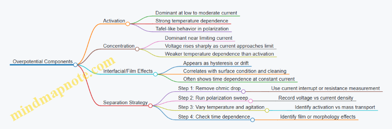
Step 1: Remove Ohmic Drop
Measure the instantaneous voltage drop when current is interrupted. The immediate jump approximates the ohmic component. Subtract it from the measured cell voltage to obtain an estimate of non-ohmic overpotential.
Example: If the cell voltage is 2.10 V at 500 A/m² and the current-interrupt method estimates an ohmic drop of 0.35 V, the non-ohmic overpotential is about 1.75 V. All subsequent separation targets this 1.75 V, not the full 2.10 V.
Step 2: Use Polarization Curves to Identify Activation vs Concentration
Run a controlled current density sweep (steady temperature, fixed agitation). Plot non-ohmic overpotential versus current density.
- Activation-dominated region: overpotential increases gradually with current. If you repeat at different temperatures, the slope changes noticeably.
- Concentration-dominated region: overpotential increases rapidly as current approaches a limiting value. Increasing agitation (or improving mass transfer) shifts the onset to higher current.
Example: At 200–400 A/m², doubling temperature from 45°C to 55°C reduces non-ohmic overpotential by a large margin. That points to activation control. If, above 700 A/m², agitation changes the voltage strongly while temperature changes it only slightly, concentration effects are taking over.
Step 3: Add Agitation and Temperature as Diagnostic Knobs
- Agitation changes mass transport: higher flow reduces boundary layer thickness and delays depletion.
- Temperature changes kinetics: charge transfer rates typically respond strongly.
Example: Keep current density fixed at 650 A/m². If increasing stirring speed reduces overpotential by 0.15 V but raising temperature by 5°C reduces it by 0.03 V, concentration overpotential is the main culprit.
Step 4: Detect Interfacial or Film Effects with Time Tests
At constant current density, record overpotential versus time. Film-related effects often show:
- Drift: overpotential slowly increases as deposits or films build.
- Hysteresis: the path differs between ramp-up and ramp-down.
- Recovery after cleaning: a fresh surface returns the overpotential closer to the initial value.
Example: At 500 A/m², non-ohmic overpotential rises by 0.10 V over 30 minutes, then drops back after a standardized rinse and restart. That pattern is consistent with interfacial resistance or surface coverage effects, not purely activation or concentration.
Practical Separation Summary
To separate components in a way that leads to action:
- Subtract ohmic drop using current interruption or resistance estimation.
- Use polarization sweeps to locate activation vs concentration regions.
- Use temperature and agitation tests to confirm which region dominates.
- Use time dependence and cleaning response to identify interfacial/film contributions.
If you do this consistently, “overpotential” stops being a single number and becomes a set of levers you can tune—current density, temperature, agitation, and surface management—without guessing.
5.3 Current Density Selection and Its Practical Constraints
Current density is the knob that sets how fast iron ions are reduced at the cathode. Choose it well, and you get dense, adherent deposits with manageable voltage and stable operation. Choose it poorly, and you trade away either product quality or energy efficiency—sometimes both.
Foundational Link Between Current Density and Deposition
At the simplest level, higher current density means more electrons delivered per unit area per unit time. For iron deposition, that translates into a higher deposition rate, but only if ions can reach the cathode fast enough. If ion supply lags behind electron demand, the local electrolyte near the cathode becomes depleted, and side reactions become more likely.
A practical way to think about it is as a three-way balance:
- Electrons arrive because you set the current density.
- Ions arrive because mass transport can replenish the near-cathode region.
- Reactions proceed because the electrode kinetics and overpotentials allow the reduction to occur.
When any one of these lags, the system compensates by changing the reaction pathway or increasing losses.
The Constraint Map: Mass Transport, Kinetics, and Ohmic Loss
Mass transport constraint shows up as concentration gradients. As current density rises, the diffusion layer effectively “thickens” in terms of how far ions must travel to sustain the reaction. The result is a higher concentration polarization, which increases cell voltage and can shift deposit morphology from smooth to rough.
Kinetic constraint is about how readily the cathode surface supports the iron reduction reaction. Even if ions are present, insufficient catalytic behavior or unfavorable surface conditions can require higher overpotential, again raising voltage and sometimes promoting hydrogen evolution.
Ohmic constraint is the resistance to current flow through electrolyte and cell components. Higher current density increases the iR drop, which reduces the fraction of voltage available for useful electrochemical work.
A useful mental model is that voltage rises with current density due to multiple contributions. Your job is to pick a current density where the voltage increase is justified by acceptable deposition quality.
Practical Selection Workflow
- Start with a target deposition rate based on production needs and acceptable residence time for washing and handling.
- Check electrolyte transport capacity by ensuring agitation, flow, or cell hydrodynamics can keep the near-cathode concentration from collapsing.
- Estimate voltage sensitivity by observing how cell voltage changes with step changes in current density during stable operation.
- Validate deposit quality using simple, direct checks: adhesion after mechanical handling, surface roughness, and presence of visible gas pitting.
- Lock in a working window rather than a single value, because small variations in temperature, concentration, and spacing shift the constraints.
Examples That Make the Tradeoffs Concrete
Example: Low Current Density That Looks Safe but Underperforms
A pilot cell runs at a modest current density and produces smooth deposits. However, the deposition rate is slow enough that the cathode spends too long in contact with electrolyte containing impurities. The result is a higher fraction of trapped electrolyte residues and more variability in composition across the deposit thickness. The fix is not necessarily to jump to the maximum; instead, increase current density until the deposition rate improves while deposit adhesion remains strong.
Example: High Current Density That Causes Roughness and Gas Pitting
Another run increases current density to shorten cycle time. Voltage rises faster than expected, and the deposit becomes dull with localized rough patches. Microscopic inspection shows gas bubbles interfering with nucleation and growth. This is a sign that mass transport and/or kinetics are no longer keeping up. The practical response is to reduce current density and, if needed, improve hydrodynamics or electrode surface condition.
Example: Current Density Limited by Cell Geometry
In a larger cell, current distribution becomes less uniform due to electrode spacing and edge effects. Even if the average current density is acceptable, local peaks can exceed the transport limit near edges. The deposit then shows edge roughening while the center looks fine. The fix is often geometric: adjust electrode spacing, improve busbar design, or use current distribution features rather than simply lowering the global current density.
Mind Map: Current Density Constraints
Advanced Details Without the Mystery
Operating window thinking matters because current density interacts with temperature and concentration. Warmer electrolyte lowers viscosity and can improve transport, allowing a higher current density before polarization becomes severe. Higher bulk concentration can also delay depletion, but it may increase impurity activity or change precipitation behavior, so the window should be validated with deposit checks.
Uniformity beats averages. If the cell has nonuniform current distribution, the limiting behavior occurs at the local maxima. That is why edge quality often tells the truth faster than bulk measurements.
Quality checks should be tied to the failure mechanism. If roughness correlates with visible gas, the constraint is likely transport or kinetics near the cathode surface. If deposits are smooth but adhesion is poor, the issue may be surface chemistry or trapped residues rather than purely current density.
In practice, selecting current density is less about finding a single best number and more about choosing a value that keeps the system inside its constraint envelope while producing deposits that are easy to handle and consistent from batch to batch.
5.4 Temperature Control Strategies for Stable Operation
Temperature control is the quiet workhorse behind stable iron deposition. It affects electrolyte conductivity, reaction kinetics, gas solubility, and the way impurities behave at the electrode surface. If temperature drifts, the cell voltage and deposit morphology usually follow—often before you notice the product quality.
Foundations: What Temperature Changes in an Electrolytic Iron Cell
Start with three linked effects.
- Electrical behavior: As temperature rises, ionic conductivity typically increases, which reduces ohmic drop. That can lower cell voltage at the same current, but it can also encourage higher local reaction rates.
- Electrochemical kinetics: Reaction rates generally increase with temperature, changing the balance between desired iron deposition and competing reactions.
- Mass transport and gas behavior: Warmer electrolytes can reduce viscosity and shift diffusion rates. Gas bubbles can detach differently, changing local current distribution and deposit texture.
A practical implication: you should treat temperature as a control variable that influences both global performance (voltage, current efficiency) and local outcomes (nucleation, roughness, and impurity co-deposition).
Control Targets and How to Choose Them
Pick a temperature setpoint that supports stable deposition without pushing competing reactions too hard. Then define acceptable bands.
- Setpoint: Choose based on prior runs or pilot data, aiming for a region where voltage is not overly sensitive to small changes.
- Band: Use a narrow operating window for production. In early commissioning, widen the band temporarily to avoid chasing noise.
- Gradient limits: Control not only the bulk temperature but also the temperature near the electrodes. A small bulk drift can hide a larger local hot spot.
A simple rule of thumb for instrumentation: if you only measure bulk temperature, you must assume the electrode region could be several degrees different under high current or poor mixing.
Heat Sources and Heat Removal Paths
Identify where heat comes from.
- Joule heating: Current through electrolyte and hardware generates heat proportional to electrical resistance.
- Reaction enthalpy: Electrochemical reactions contribute heat, usually smaller than Joule heating but not negligible.
- Auxiliary loads: Pumps, heaters, and recirculation systems add or remove heat.
Then map how heat leaves.
- Heat exchangers in recirculation loops
- Jacketed cell walls
- Cooling plates near current collectors
- Evaporation and offgas condensation, which can be significant in water-containing systems
Integrated best practice: design the cooling path so that the hottest region has the shortest thermal distance to a heat sink.
Measurement Strategy That Prevents False Confidence
Use at least two temperature measurements.
- Bulk electrolyte sensor: Tracks overall thermal state.
- Near-electrode or inlet/outlet sensors: Reveal gradients and heat exchanger effectiveness.
If you have a recirculation loop, measure inlet and outlet temperatures. The difference gives you a direct handle on heat removal performance.
Example: If bulk temperature is stable but inlet-outlet delta increases, the system may be losing mixing or fouling the heat exchanger. Voltage might remain steady for a while, but deposit morphology can shift due to local conditions.
Control Loops That Actually Hold Temperature
Use a layered approach.
- Primary control: Maintain bulk temperature using a heater/cooler valve or pump speed.
- Secondary control: Adjust recirculation flow to manage gradients and bubble behavior.
- Protection logic: Hard limits that reduce current or stop operation if temperature rises beyond safe bounds.
A common failure mode is tuning the primary loop too aggressively. That can cause oscillations: the controller overshoots, then corrects, then overshoots again. The deposit then experiences alternating conditions that can worsen roughness.
Practical Tuning Using Step Tests
When commissioning, run a controlled step test.
- Apply a small change in cooling duty or flow.
- Record temperature response and cell voltage response.
- Estimate time constants and delay.
From this, set controller parameters so the loop responds faster than slow drift but not faster than measurement noise.
Example: If temperature responds within 30 seconds but voltage responds within 2 minutes, prioritize temperature stability first, then verify that voltage and current efficiency remain steady.
Handling Transients During Start Up and Current Changes
Temperature control must respect that start-up is not steady state.
- Preheat or pre-cool the electrolyte to near the setpoint before applying full current.
- Ramp current gradually so heat generation increases smoothly.
- Stabilize mixing early; poor circulation during start-up can create localized hot zones.
Example: If you jump directly to high current, Joule heating spikes immediately. Even if the bulk sensor lags, the electrode region may already be in a different deposition regime, leading to early roughness that persists.
Mind Map: Temperature Control for Stable Iron Deposition
Case Example: Diagnosing a Temperature-Related Deposit Shift
Suppose deposit roughness increases while bulk temperature appears unchanged.
- Check inlet-outlet delta: if it increased, cooling effectiveness may be reduced.
- Inspect recirculation flow: reduced flow can raise electrode-region temperature without moving the bulk sensor much.
- Compare voltage noise: higher noise can indicate local boiling or bubble detachment changes.
Corrective action should target the thermal gradient first: restore flow, clean heat exchanger surfaces, and confirm that near-electrode conditions return to the prior stable range.
Operating Checklist for Temperature Stability
- Setpoint and allowable band defined
- Bulk and loop temperatures monitored continuously
- Cooling duty and flow adjusted to prevent gradients
- Current ramps used during start-up and major changes
- Overtemperature interlocks tested and documented
- After any maintenance, repeat a short step test to confirm response behavior
5.5 Operating Procedures for Start Up and Steady State
Start-up and steady state are not separate jobs; they are one continuous workflow with different priorities. During start-up, the goal is to reach stable electrical and chemical conditions without creating runaway deposition, excessive gas evolution, or electrolyte imbalance. During steady state, the goal is to keep those conditions stable while production slowly consumes reactants and generates byproducts.
Start Up Objectives and Readiness Checks
Before energizing the cell, confirm that the mechanical and chemical “plumbing” is ready. Verify that the electrolyte circulation path is open, pumps are primed, and filters are installed correctly. Check that temperature control is active and can hold setpoint within a narrow band. Confirm that the gas handling system is connected and leak-tested, because offgas behavior is part of the process, not an afterthought.
Next, verify electrical readiness. Inspect electrode spacing and ensure fixtures are tightened to prevent drift under thermal expansion. Confirm that the power supply can ramp current smoothly and that measurement leads are connected to the correct terminals. If you use reference measurements for voltage drop, ensure they are zeroed or baseline-corrected.
Finally, do a chemical sanity check. Measure initial electrolyte composition and impurity levels. If the electrolyte contains unexpected metals or high levels of species that promote side reactions, deposition quality will suffer even if the current looks “normal.”
Stepwise Start Up Procedure
- Establish electrolyte conditions: Set concentration and temperature to target values. Circulate long enough to homogenize, especially after any make-up additions.
- Start low-current ramp: Begin at a reduced current density and ramp gradually. This limits sudden changes in local concentration at the cathode and reduces the chance of uneven nucleation.
- Stabilize voltage and temperature: Watch cell voltage and temperature together. A rising voltage at constant current can indicate increasing resistance from gas coverage or precipitation; a falling voltage can indicate improved wetting or, sometimes, a shift toward more conductive but less desirable chemistry.
- Confirm deposition behavior: During early operation, inspect representative cathode coupons or sampling areas. Look for uniformity and avoid excessive roughness that can trap electrolyte and increase ohmic losses.
- Bring gas handling into normal regime: Ensure offgas flow and pressure remain within designed limits. If gas collection is too weak, bubbles can blanket the electrode and distort current distribution.
- Reach steady setpoints: Once voltage, temperature, and deposition appearance are stable, increase to the planned operating current density.
A practical example: if the cell is designed for 2.0 A/dm², ramp from 0.5 to 1.0 A/dm² in small increments, hold for 10–20 minutes at each step, and only proceed when voltage drift is small and temperature control remains stable.
Steady State Operating Logic
Steady state is maintained by balancing three things: electrical input, chemical consumption, and thermal removal. Current drives deposition and byproduct formation; deposition changes surface conditions; chemical changes alter conductivity and reaction pathways.
Use a simple control philosophy: measure frequently, adjust gently, and change one lever at a time when troubleshooting. Typical levers include current density, temperature setpoint, electrolyte flow rate, and make-up or purification rates.
Mind map below summarizes the steady state loop.
Mind Map: Start Up to Steady State Control
Monitoring Cadence and Acceptance Criteria
During steady state, define what “stable” means numerically for your cell. For example, set acceptance criteria such as: cell voltage drift less than a specified threshold over a defined interval, temperature within a tight band, and offgas flow within expected limits for the applied current.
Product checks should be scheduled so they catch drift early. A common approach is to sample deposition morphology at regular intervals and verify iron purity and impurity levels from representative product batches.
Troubleshooting with Minimal Guessing
If voltage rises while current is constant, first check for gas coverage changes by reviewing offgas behavior and electrode wetting conditions. If voltage rises without corresponding offgas changes, investigate electrolyte resistance and precipitation by checking conductivity and visual signs of solids.
If deposition becomes rough or uneven, reduce the chance of local concentration depletion by increasing electrolyte flow slightly or adjusting temperature to improve mass transport. Avoid large current changes as the first response; roughness often reflects transport and nucleation conditions rather than a simple “too much current” problem.
Example Operating Schedule
On a typical day, you might start with readiness checks, then ramp current in stages, then hold at steady setpoints for production. During production, run continuous monitoring for voltage, temperature, and offgas, while performing periodic electrolyte sampling and product checks. If you need to adjust make-up or purification, do it slowly and confirm the effect by observing both electrical behavior and product quality, not just one signal.
6. Electrolyte Management and Purification Workflows
6.1 Electrolyte Make Up and Concentration Control Methods
Electrolytic iron cells behave like chemistry plus bookkeeping. You can’t just “add more electrolyte” and hope for the best; you must keep iron species, supporting ions, water content, and trace impurities within ranges that match the cell’s current density and temperature. Concentration control is the practical bridge between lab recipes and steady production.
Electrolyte Make Up Foundations
Start with a defined electrolyte recipe expressed as target concentrations and allowable tolerances. In practice, you also define which species are measured directly (for example, total dissolved iron) and which are inferred (for example, free acid from titration). A good make-up plan includes:
- Mass-balance targets for iron source, counter-ions, and any complexing agents.
- Solubility and compatibility checks so salts dissolve without forming unwanted precipitates.
- Water management rules because evaporation and drag-out change concentration even when you think you are “closed loop.”
A simple make-up example: suppose the target is 1.0 mol/L Fe²⁺ in a sulfate-based electrolyte. You dissolve the iron source into deionized water, add the supporting sulfate to the target level, then adjust acidity to the specified range. After mixing, you sample and verify iron concentration and acidity before charging the cell. If you skip verification, you may start operation with the wrong iron level and spend the first hours correcting it.
Concentration Control Strategy
Concentration control is easiest when you separate it into three coupled tasks: measurement, correction, and prevention of drift.
-
Measurement
- Iron concentration: typically measured by titration or spectrometric methods.
- Acidity or alkalinity: tracked by titration because it affects speciation and deposition behavior.
- Conductivity: used as a fast proxy for ionic strength, but it must be calibrated against actual composition.
- Water content indicators: tracked indirectly via density, conductivity trends, or periodic gravimetric checks.
-
Correction
- Additions should be staged to avoid overshoot. For example, add concentrated iron solution in small increments, mix thoroughly, and re-sample.
- Neutralization or acid adjustment is done using titration targets, not guesswork. If acidity is too low, iron speciation shifts and deposition can become less uniform.
-
Prevention of Drift
- Minimize drag-out by controlling cell hydrodynamics and rinse steps.
- Control evaporation with covers and temperature management.
- Manage purge and recycle so impurities do not accumulate faster than you can remove them.
Practical Control Loops for Iron and Supporting Ions
A concentration control loop is more reliable when it uses a clear decision rule. For instance, you can define a band for iron concentration, such as 0.98–1.02 mol/L. When a sample falls below the band, you add iron source solution; when it rises above, you increase purge or adjust recycle ratio.
Supporting ions and acidity often drift together because corrections for one can affect the other. Example: if you add iron sulfate to raise Fe²⁺, you also raise sulfate concentration. If sulfate is already near its upper limit, you may instead add an iron source that contributes less sulfate, or you may correct sulfate via controlled purge and make-up. The goal is to keep the electrolyte within a multivariable window, not just fix one number.
Water and Density Management
Water loss changes effective concentration and can shift deposition morphology. In many plants, the most actionable approach is to track density or conductivity continuously and verify with periodic chemical analysis. A workable method is:
- Use continuous conductivity to detect drift.
- Trigger sampling when conductivity deviates beyond a set threshold.
- Adjust water by adding deionized water when drift indicates concentration increase.
Example: if conductivity increases while temperature is stable, the electrolyte is likely becoming more concentrated due to evaporation or reduced make-up water. Adding deionized water lowers concentration and restores conductivity, but you still confirm iron concentration by sampling.
Impurity-Aware Make Up and Correction
Trace impurities can change deposition quality even when iron concentration is correct. Common issues include residual metals that co-deposit or anions that affect conductivity and speciation. Make-up should therefore include:
- Feedstock specification for iron source and salts.
- Pre-treatment steps such as filtration to remove particulates that seed unwanted deposits.
- Periodic impurity checks aligned with the correction schedule.
Example: if nickel is present at low levels and begins to rise due to recycle contamination, you may see changes in deposit texture. The fix is not to chase texture alone; you trace the impurity source in the recycle stream and adjust purification or purge rate.
Mind Map: Make Up and Concentration Control
Example Workflow for a Stable Make Up and Start
- Prepare make-up water and dissolve salts to reach supporting ion targets.
- Add iron source to reach an initial Fe²⁺ level slightly below target.
- Mix, then sample for iron concentration and acidity.
- Adjust iron in small increments until within the target band.
- Start the cell and begin continuous conductivity monitoring.
- Schedule the first impurity check after the electrolyte has equilibrated with the cell hardware.
This workflow reduces overshoot and prevents the common “start fast, correct later” pattern that wastes energy and produces inconsistent early deposits.
6.2 Monitoring Techniques for Composition and Contamination
Electrolyte performance depends on composition staying within a narrow band and contamination staying low enough that it doesn’t change deposition behavior. Monitoring is not just measurement; it’s a feedback system that connects what you see in samples to what you do in the cell.
Define What “Good” Looks Like
Start by listing the electrolyte variables that directly affect iron deposition and cell stability. Typical targets include iron ion concentration, acidity or alkalinity (depending on the electrolyte family), total dissolved salts, water content, and conductivity. Then define contamination categories: dissolved metals that compete for deposition, anions that change speciation, and solids that cause localized current spikes.
A practical way to make this concrete is to set two thresholds per variable: a “watch” level that triggers increased sampling and a “action” level that triggers correction. For example, if conductivity drifts upward, you might first verify temperature and then check salt concentration; only after confirming the drift is real do you adjust make-up additions.
Build a Sampling Plan That Matches Cell Dynamics
Electrolyte composition can change on different timescales. Near the cathode, concentration gradients form quickly; in the bulk tank, changes are slower and depend on circulation and mixing.
Use a three-tier sampling approach:
- Fast checks for electrical and bulk indicators that change within hours (e.g., conductivity, pH, temperature).
- Routine samples for composition that changes over days (e.g., iron concentration, major ions).
- Event-driven samples when something unusual happens (e.g., after maintenance, after a filter change, or after a gas-handling upset).
Example: if deposition suddenly becomes rough, you don’t wait for the next daily lab run. You take an immediate conductivity and pH check, then pull a targeted sample for impurity screening.
Measure Composition Using Complementary Methods
No single measurement tells the whole story, so combine methods that cover different chemistry.
Conductivity and temperature provide a fast proxy for total ionic strength. Because conductivity depends on temperature, always record both and use a consistent temperature correction.
pH or acidity helps track speciation and side reactions. In many iron systems, pH shifts can indicate dilution, wrong make-up additions, or contamination with basic or acidic residues.
Iron concentration is best confirmed with a quantitative method such as titration or spectrometric analysis. Titration is often fast and robust for routine control; spectrometry can catch subtle shifts and is useful when titration chemistry becomes less reliable due to interfering species.
Major anions and salts can be monitored by targeted assays. This matters because some anions influence solubility and can change deposition morphology even when iron concentration looks fine.
Detect Contamination Without Waiting for Product Problems
Contamination monitoring should focus on what causes deposition defects: competing metal ions, particulate solids, and organic or reducing contaminants.
Dissolved metal impurities are typically monitored by periodic screening. If you know the likely sources—electrode wear, upstream feed impurities, or corrosion products—you can prioritize those metals.
Particulate contamination is monitored by filtration checks and turbidity or particle counts where available. Solids can create local high-current areas, leading to dendrites or poor adhesion.
Organic and reducing contaminants are harder to measure directly, so you watch indirect indicators: changes in current efficiency trends, unexpected color changes in electrolyte, or shifts in measured redox behavior.
Example: after a gasket replacement, you might see a temporary change in impurity profile. The monitoring plan should include an event-driven sample right after restart so you can separate “normal drift” from “new contamination source.”
Use Control Charts and Material Balance Logic
Measurements become useful when they are interpreted. Plot key variables over time and separate random noise from systematic drift.
A simple rule: if conductivity and pH move together, suspect dilution or make-up composition errors; if conductivity drifts alone, suspect salt concentration or temperature correction issues.
Tie monitoring to material balance. If you add a known amount of make-up and remove a known amount via bleed or product separation, the iron concentration should follow a predictable path. When it doesn’t, either mixing is poor, sampling is biased, or losses are occurring through side reactions or carryover.
Mind Map of Monitoring Techniques and Actions
Mind Map: Monitoring Composition and Contamination
Worked Example of an Integrated Monitoring Response
Assume a routine shift finds conductivity higher than the watch threshold while pH remains stable. First, verify temperature correction and check whether the sensor calibration is due. If corrected conductivity is still high, pull a routine composition sample and confirm iron concentration and major salt levels.
If iron concentration is unchanged but salts are elevated, the most likely cause is make-up addition imbalance or reduced bleed rate. Adjust make-up dosing and restore the bleed schedule. If iron concentration also trends down, investigate whether carryover or side reactions increased; then schedule an impurity screening sample to rule out contamination that could be changing deposition efficiency.
This sequence keeps you from “chasing numbers.” You measure quickly, confirm with composition assays, and only then choose the correction that matches the observed pattern.
6.3 Purification Steps for Removing Metal and Nonmetal Impurities
Purification in electrolytic iron production is the part where chemistry stops being theoretical and starts being practical. The goal is simple: remove dissolved metals that co-deposit or poison the cathode, and remove nonmetal species that change solution behavior, increase voltage losses, or create unwanted deposits. A good workflow treats purification as a sequence of targeted separations, each chosen to match the impurity’s chemistry and the plant’s constraints.
Purification Objectives and Impurity Map
Start by classifying impurities into two groups. Metal impurities often include ions that can plate alongside iron or form mixed deposits. Nonmetal impurities include anions and dissolved gases that affect conductivity, mass transport, and side reactions. The purification plan should connect each impurity class to a removal mechanism.
Mind Map: Purification Logic
Step 1: Confirm Impurity Speciation and Where It Lives
Before removing anything, determine whether an impurity is truly dissolved, present as colloids, or associated with suspended solids. A quick operational approach is to pair a filtered sample (for dissolved ions) with an unfiltered sample (for total). If an impurity appears mainly in the unfiltered fraction, filtration or clarification should come before chemical treatment.
Example: If sulfate-like species rise after agitation changes, check whether they are tied to fine solids. In that case, a clarification step reduces chemical consumption later.
Step 2: Clarification and Solid-Liquid Separation
Clarification removes suspended solids that can seed rough deposition and trap impurities. Common methods include settling, filtration, and centrifugation. The key best practice is to match the cutoff to the deposit risk: too coarse a filter leaves seed particles; too fine a filter clogs quickly and forces frequent downtime.
Example: If cathode deposits become mottled after a maintenance shutdown, inspect whether solids carryover increased. A short clarification campaign often restores stable deposition without changing the main chemistry.
Step 3: Precipitation and Selective Removal of Metal Ions
Many metal impurities can be reduced in concentration by converting them into insoluble forms. The choice depends on pH, oxidizing conditions, and complexation. In practice, operators adjust pH to a narrow window where iron remains soluble enough for the process, while specific impurity ions precipitate.
Best practice: do jar tests with the actual electrolyte composition. Complexing agents can shift solubility dramatically, so lab-only recipes often disappoint.
Example: Suppose nickel ions are causing a darker, harder deposit. A controlled pH adjustment that precipitates nickel hydroxide while keeping iron in solution can reduce co-deposition. The precipitate is then removed by filtration.
Step 4: Ion Exchange and Selective Adsorption for Trace Control
After bulk removal, trace impurities still matter because small concentrations can noticeably affect deposit quality. Ion exchange resins or selective sorbents can target specific ion types. The integrated workflow is to place ion exchange after clarification and after the main precipitation step, so the media is not overloaded with solids.
Best practice: track resin loading and breakthrough using routine sampling. When breakthrough begins, the resin is no longer selective and can even reintroduce impurities.
Example: If chloride levels remain high and contribute to localized corrosion on hardware, a selective anion exchange step can reduce chloride without disturbing iron concentration.
Step 5: Electrochemical Polishing and Controlled Bleed-and-Feed
Some impurities are best handled by electrochemical behavior rather than purely chemical solubility. A small polishing cell can remove residual metal ions by controlled deposition onto a sacrificial cathode, followed by separation of the deposit. In parallel, bleed-and-feed manages impurities that accumulate from make-up streams.
Best practice: bleed rate should be tied to measured impurity buildup, not just time. This prevents wasting electrolyte and energy.
Example: If a feedstock contains trace copper that steadily accumulates, a bleed-and-feed strategy combined with periodic polishing can keep copper below the co-deposition threshold.
Step 6: Nonmetal Removal by Conditioning and Gas Management
Nonmetal impurities often include anions and dissolved gases. Conditioning can include pH correction, removal of dissolved gases by controlled stripping, and adjustment of oxidizing conditions to keep nonmetal species in forms that are easier to remove.
Example: If oxygen or other dissolved gases increase side reactions and raise cell voltage, degassing the electrolyte before it enters the main cell can reduce variability.
Step 7: Sludge Handling and Preventing Recontamination
Every removal step creates a solid stream or a spent media stream. The best practice is to prevent these solids from returning to the electrolyte loop. Use dedicated tanks, clear labeling, and controlled transfer lines. Also, dewater and dispose of sludge in a way that avoids leaching back into process water.
Mind Map: Purification Step Sequencing
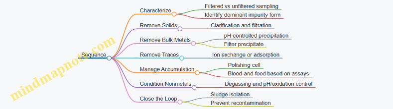
Step 8: Verification Through Mass Balance and Quality Checks
Purification is only “done” when measurements confirm it. Use a simple mass balance: compare impurity concentration and flow rates before and after each step. Then confirm product impact by checking deposit composition and morphology indicators.
Example: If iron purity improves but deposit roughness worsens, the issue may be residual solids or an unaddressed nonmetal species. That feedback loop is the reason purification steps are sequenced rather than applied randomly.
Integrated Example Workflow
A practical integrated sequence looks like this: clarify the electrolyte to remove seed solids, run a pH-controlled precipitation to knock down dominant metal impurities, polish with ion exchange for trace control, and apply bleed-and-feed to prevent accumulation from make-up. Finish with conditioning for nonmetal species and verify with both electrolyte assays and deposit checks. This order minimizes media fouling, reduces chemical waste, and keeps the main cell chemistry stable.
6.4 Handling Sludges and Precipitates Without Process Loss
Sludges and precipitates form when dissolved species exceed solubility, when local pH shifts near electrodes, or when impurities react faster than the main deposition pathway. The goal is simple: remove solids safely while keeping valuable ions in the process loop and preventing “silent” losses that show up later as higher energy use or lower iron yield.
Foundational Concepts for Solid Formation
Start by mapping what “solid” means in your system. In electrolytic iron production, solids can be:
- Electrolyte precipitates from solubility limits (often driven by concentration and temperature).
- Impurity solids from contaminants reacting with the electrolyte.
- Electrode-adjacent deposits that detach and become sludge.
A practical rule: if solids appear after a change in current density, temperature, or electrolyte concentration, treat the cause as upstream. If solids appear after a change in feed purity or make-up water quality, treat the cause as contamination.
Capture and Segregation That Preserves Valuable Ions
Solid handling should separate three streams: (1) recoverable electrolyte, (2) recoverable metal-bearing solids, and (3) truly waste solids.
- Use staged settling or filtration rather than one-pass removal. Early stages catch coarse particles and reduce filter loading, which lowers pressure drop and avoids bypassing.
- Minimize hold-up time in sludge tanks. Long residence increases adsorption of iron species onto solids, making later recovery harder.
- Rinse with controlled electrolyte, not plain water. A rinse that matches the bulk electrolyte composition reduces desorption losses and keeps iron in the liquid phase.
Example: If your sludge contains iron hydroxide-like material, a rinse using the same acid/salt strength as the bulk electrolyte can keep dissolved iron from re-precipitating during washing. Water rinses often shift pH locally and worsen iron loss.
Recovery Loops for Process Ions
Once solids are separated, decide what to do based on composition.
- If solids are mainly electrolyte precipitate: treat them as a concentration management issue. Dissolve them back into the electrolyte using a controlled neutralization or acidification step, then re-check conductivity and ion balance.
- If solids are metal-bearing with recoverable iron: use a dissolution step that targets iron species while leaving inert impurities behind.
- If solids are impurity-dominated: remove them as waste, but first wash to recover entrained electrolyte.
Example: Suppose analysis shows high iron content in sludge but low impurity content. A targeted dissolution step can return iron to the electrolyte, while a subsequent filtration removes remaining insolubles. The key is to measure iron concentration before and after dissolution so you can close the mass balance.
Preventing Adsorption and Entrapment Losses
Two common “process loss” mechanisms are adsorption (iron species stick to solids) and entrapped liquid (electrolyte trapped in sludge pores).
Mitigations:
- Control ionic strength during washing so the driving force for adsorption is reduced.
- Use dewatering steps that match your solids’ compressibility. Centrifugation can reduce entrained liquid faster than gravity settling for fine particles.
- Track wash efficiency by sampling the wash liquor for iron and key ions.
Example: If wash liquor iron concentration is consistently high, your rinse volume is too small or the rinse composition is mismatched. Increase rinse volume slightly or adjust rinse chemistry, then confirm by comparing iron in wash liquor versus iron in final waste.
Systematic Workflow for Sludge Handling
A reliable workflow keeps decisions tied to measurements.
- Characterize: sample sludge for iron content, major anions/cations, and impurity markers.
- Classify: label solids as recoverable precipitate, metal-bearing solids, or impurity waste.
- Separate: settle/filtrate to reduce solids load on downstream equipment.
- Wash: rinse with electrolyte-matched solution; collect wash liquor for return or treatment.
- Recover or Dispose: dissolve recoverable fractions with controlled chemistry; filter off inert residue.
- Close the Balance: compare iron in incoming electrolyte, dissolved iron after recovery, and iron in final waste.
Mind Map: Sludge Handling Without Process Loss
Example: Closing the Loop with a Simple Mass Balance
Assume you remove 100 kg of wet sludge containing 20 kg of entrained electrolyte and 5 kg of iron as solids. After dewatering, you wash with 30 kg of rinse solution and recover 4.6 kg of iron back into the electrolyte via dissolution. If final waste contains 0.4 kg of iron, your recovery is 5.0 kg total minus 0.4 kg = 4.6 kg, or 92%. That number is actionable: if recovery drops, check whether adsorption increased (often due to longer residence time) or whether washing chemistry shifted.
Advanced Details That Matter in Practice
- Sampling discipline: take samples from the same physical location each time (sludge tank bottom versus overflow) because concentration gradients are real.
- Equipment compatibility: avoid materials that catalyze unwanted side reactions or adsorb iron species.
- Operational triggers: treat sudden sludge rate increases as a signal to check current distribution, temperature stability, and feed purity—because solids rarely “arrive” without a reason.
Handled this way, sludge becomes a managed stream rather than a leak. You remove solids, recover what’s valuable, and document the balance so the process stays honest.
6.5 Recycle Streams and Their Material Balance Requirements
Recycle streams keep an electrolytic iron plant stable, but they also make accounting harder. The goal is simple: every kilogram that leaves one unit must either become product, leave the system, or return somewhere with a known composition. When you can write that story cleanly, you can control concentration, impurity buildup, and yield.
Foundational Idea: Define the System Boundary
Start by choosing a boundary that matches your reporting. For example, you might define the boundary as “cell stack plus electrolyte purification loop plus product washing,” excluding upstream power generation and downstream steelmaking. Everything inside the boundary must balance: mass in equals mass out plus accumulation. If you cannot state what is inside, you will end up balancing the wrong things.
A practical rule: pick one “accounting time window” (often one shift or one day) and treat it consistently across make-up, recycle, and product removal. If you change the window, your balance will still be correct, but your control actions will feel random.
What to Recycle and Why
Common recycle streams include:
- Electrolyte recycle from cell effluent back to the cell after purification.
- Rinse water recycle from product washing, after filtration and impurity management.
- Sludge return or controlled bleed streams that prevent impurity accumulation.
Each stream has a purpose. Electrolyte recycle reduces make-up needs and stabilizes ionic strength. Rinse recycle reduces water use, but it can drag dissolved impurities back into the loop. Sludge handling is the opposite: it is where impurities go to die, unless you intentionally bleed it.
Material Balance Framework That Works in Practice
Use three linked balances: overall mass, component mass, and charge balance (as a consistency check).
-
Overall mass balance
Track total liquid flow rates: make-up, recycle, product wash water, and any purge. -
Component mass balances
Choose components that matter for control. Typical choices are iron species (or iron concentration), key anions/cations that define electrolyte chemistry, and impurity ions that cause deposition defects. -
Charge balance check
Electrolysis changes oxidation states, so electrical current must correspond to chemical change. You don’t need perfect electrochemical modeling for control, but you do need internal consistency: if the iron concentration change implied by current disagrees with measured concentration change, your sampling or assumptions are off.
Example: One-Day Balance with Purge
Assume a daily window with:
- Make-up electrolyte: 10,000 kg/day at 50 g/L Fe equivalent
- Cell liquid flow through stack: 30,000 kg/day, with 2,000 kg/day removed as wash-and-drain stream
- Purge: 1,000 kg/day from the recycle loop to prevent impurity buildup
- Purified recycle returned: remainder of loop flow
To compute the iron component balance, you write:
- Iron in from make-up = iron in with recycle + iron in with purge (if purge carries iron) + iron in with wash stream
- Iron out as product deposition and any iron leaving with drained streams
In a simplified control scenario, you measure iron concentration in make-up, in recycle after purification, and in the drained stream. Then you solve for the implied iron deposited. If the implied deposited iron is inconsistent with product mass, you investigate either deposition yield assumptions or measurement bias.
Mind Map: Recycle Streams and Balance Elements
Advanced Details Without Hand-Waving
Sampling alignment matters. If you sample recycle concentration at the purification outlet but your purge is taken upstream, the purge composition may differ. The balance will still close mathematically, but it will close using the wrong numbers.
Purges are component-selective in effect. A purge removes all dissolved species in proportion to their concentrations. That means the purge rate needed to control one impurity may be excessive for another. The best practice is to base purge decisions on the impurity that most strongly affects deposition quality, while confirming that iron and key electrolyte ions remain within target ranges.
Solids and entrained liquid must be treated explicitly. If product separation leaves behind liquid trapped in deposits, that liquid carries electrolyte back into the system. Either measure the trapped liquid composition or include a correction term based on measured wash volumes and residual moisture.
Practical Checklist for Balance Closure
- Define the boundary and time window.
- List every inlet and outlet stream across the boundary.
- Choose component set for control, not for curiosity.
- Ensure sampling points match the stream locations.
- Use charge balance as a consistency check, not as a substitute for measurements.
- Close the balance for iron and at least one impurity; if it fails, fix data first.
When these steps are followed, recycle becomes a controlled tool rather than a bookkeeping headache. The plant still runs on electricity and chemistry, but your decisions run on numbers that agree with each other.
7. Iron Product Formation and Downstream Handling
7.1 Deposition Morphology and Its Influence on Product Quality
Deposition morphology is what the iron “looks like” as it forms on the cathode: smooth layers, branching growth, porous networks, or compact grains. That appearance matters because it controls how much of the deposited iron is electrically useful, how easily it can be separated from the electrolyte, and how consistently the product meets downstream requirements.
Foundational Link Between Morphology and Quality
At the cathode, iron ions arrive by mass transport, then electrons drive reduction at the surface. The local balance between ion supply, electron availability, and surface kinetics determines where growth happens first and how it spreads. If growth is uniform, you get dense deposits with predictable composition and low trapped electrolyte. If growth is uneven, you get roughness, voids, and inclusions that can later show up as poor mechanical performance or inconsistent chemistry.
A practical way to think about morphology is to track three outcomes: (1) surface roughness, (2) internal porosity, and (3) impurity incorporation. Roughness affects effective surface area and current distribution; porosity affects washing efficiency and residual salt content; impurity incorporation affects both corrosion behavior and alloying response.
Morphology Drivers You Can Control
Current density and its local peaks. Higher current density increases the driving force for reduction, but it also increases the risk that ion supply cannot keep up everywhere. When ion depletion occurs near protrusions, those protrusions keep growing while recessed regions lag, producing dendritic or sponge-like structures.
Electrolyte composition and conductivity. Concentration of iron species and supporting ions affects both mass transport and ohmic drop. Poor conductivity increases local voltage gradients, which can intensify non-uniform growth.
Temperature and viscosity. Temperature changes diffusion rates and solution viscosity. Warmer electrolyte often improves ion transport, but it can also change evaporation and water balance, indirectly shifting morphology.
Hydrodynamics and mixing. Stirring or flow reduces boundary-layer thickness. Better mixing tends to smooth growth by keeping ion concentration more uniform at the cathode surface.
Electrode surface condition. Surface roughness, oxide films, and wetting behavior influence nucleation. A surface that nucleates many sites evenly can suppress runaway growth at a few points.
What Different Morphologies Mean for Product Quality
Dense, fine-grained deposits. These typically wash cleanly and retain less electrolyte. They also provide a more stable surface for subsequent deposition cycles, reducing drift in current efficiency.
Columnar or granular growth. This can be acceptable when porosity is low, but it may trap small pockets of electrolyte between grains. Quality checks should focus on residual salt content and consistency across the deposit thickness.
Dendritic growth. Dendrites increase surface area and create deep crevices. Those crevices can trap impurities and make washing less effective. They also raise the chance of mechanical fragility during handling.
Porous or sponge-like deposits. Porosity increases residual moisture and salt retention. Even if chemical assays look fine, the physical structure can cause variability in downstream melting or forming due to uneven drying and fluxing behavior.
Mind Map: Morphology to Quality Pathways
Integrated Example: Diagnosing a Morphology Shift
Suppose a batch that previously produced compact deposits starts showing rough, branching features near the edges of the cathode. A systematic check begins with current density distribution: edge regions often experience different current density due to geometry and field lines. Next, verify electrolyte concentration and mixing intensity. If mixing was reduced or feed concentration drifted, ion depletion near protrusions becomes more likely, which promotes dendritic growth.
Then check electrode surface condition. If the cathode developed an oxide film or changed wetting due to cleaning differences, nucleation may shift from many evenly distributed sites to fewer preferential sites. That change alone can convert a dense deposit into a rough one even when electrical settings are unchanged.
Finally, connect morphology to measurable quality outcomes. Branching deposits typically increase residual salt after washing because crevices hold electrolyte. If downstream melting shows inconsistent impurity levels or variable flux requirements, the morphology-to-residual-link is a strong candidate explanation.
Practical Best Practices Embedded in the Workflow
- Treat current density as a local variable, not just a setpoint. Use geometry-aware operation and verify uniformity across the cathode surface.
- Maintain electrolyte composition with tight control. Small concentration shifts can change mass transport enough to alter growth mode.
- Keep hydrodynamics consistent. Mixing changes can move the system from uniform deposition to protrusion-driven growth.
- Standardize cathode preparation. Cleaning and surface condition should be repeatable so nucleation behavior stays stable.
- Measure quality in ways that reflect morphology. Residual salt, moisture, and thickness uniformity are more informative than a single bulk chemical assay when deposits vary structurally.
7.2 Separation of Deposited Iron from Electrolyte Residues
Electrolytic iron rarely leaves the cell as a clean, ready-to-use metal. More often, it is deposited as a porous or layered structure that traps electrolyte between grains and within surface roughness. Separation is the step that turns “electrochemically produced iron” into “metallurgically usable feed,” while keeping electrolyte losses low and preventing contamination of the product.
Foundational Idea: What Must Be Separated
Deposited iron and electrolyte residues are linked by three physical realities. First, electrolyte films cling to the deposit surface. Second, capillary forces hold liquid in pores and crevices. Third, dissolved and suspended impurities can co-travel with the liquid phase during washing. A good separation workflow targets all three without mechanically tearing the deposit into fines that are hard to recover.
Mind Map: Separation Workflow and Decision Points
Step 1: Mechanical Release and Minimizing Fines
Separation begins at the cathode. If the deposit is brittle, aggressive scraping creates dust that increases surface area and traps more electrolyte. If it is ductile or sponge-like, gentle mechanical release followed by controlled agitation reduces fragmentation. A practical rule is to match the release method to the deposit morphology: use low shear for porous deposits and slightly higher shear only when the deposit detaches cleanly.
Example: In a pilot cell, operators compare two routines: (a) high-speed scraping into a hopper and (b) slow detachment with a rinse-assisted lift. The second routine typically yields fewer fines, which later reduces filtration load and lowers the amount of electrolyte trapped in the product bed.
Step 2: Solid-Liquid Separation by Filtration or Settling
Once released, the deposit is separated from the bulk electrolyte using either filtration or settling/decanting. Filtration is faster and better for fine particles, but it can clog if sludges are present. Settling is gentler but slower and less effective when the deposit contains fine fractions.
Best practice: choose filtration media based on expected particle size and sludge content. A coarse pre-filter can capture larger solids, while a finer stage polishes the liquid. This staged approach prevents the main filter from becoming a sludge sponge.
Step 3: Washing Sequence That Targets Trapped Electrolyte
Washing is where most carryover is controlled. The goal is to replace electrolyte in pores with a wash liquid that either dissolves fewer impurities or can be removed more easily. Two common strategies are water-based washing and wash solutions tuned to reduce specific anions or metal impurities.
A systematic washing sequence uses multiple stages rather than one long wash. Each stage reduces the concentration of residual salts in the deposit, and the final stage uses the cleanest wash to minimize residual conductivity.
Example: Suppose the deposit pores contain a concentrated sulfate-rich electrolyte. A three-stage wash can be arranged so that the first wash removes most of the bulk liquid, the second reduces remaining salt concentration, and the third targets residual ions. Operators monitor conductivity of each wash filtrate; when the conductivity drop between stages becomes small, additional washing yields diminishing returns.
Step 4: Treating the Wash Liquids and Maintaining Electrolyte Balance
Wash filtrates are not waste by default. They contain iron traces, dissolved salts, and sometimes suspended solids. Returning them to the electrolyte loop can reduce chemical consumption, but only if impurity levels remain within acceptable limits.
Best practice: separate dissolved impurities from suspended solids. Suspended solids can be removed by settling or filtration, while dissolved species are handled by the electrolyte purification workflow. This prevents reintroducing sludge into the cell.
Step 5: Drying and Handling Without Recontamination
After washing, drying removes residual moisture so the product can be weighed, alloyed, or briquetted. Drying conditions matter: overly hot drying can cause salt crystallization on surfaces, which later increases corrosion risk and complicates downstream processing. Controlled drying that limits salt migration helps keep the product surface cleaner.
Example: If a deposit is dried too quickly at high temperature, salts can migrate to the surface and form a crust. A slower drying profile or staged drying can reduce crust formation, improving product consistency.
Quality Checks That Confirm Separation Success
Separation quality is verified through simple, direct measurements. Conductivity of wash filtrates indicates how effectively salts are removed. Product testing for residual anions and trace metals confirms impurity carryover. A mass balance closes the loop: iron recovery should be high, and electrolyte losses should be explainable by entrainment and purge.
Common Failure Modes and How to Prevent Them
- Excess fines: caused by harsh detachment; prevention is morphology-matched release.
- Filter clogging: caused by sludge-rich deposits; prevention is staged filtration and pre-removal of solids.
- High residual conductivity: caused by insufficient wash stages or overly viscous trapped liquid; prevention is multi-stage washing with appropriate wash conditions.
- Salt crusting after drying: caused by rapid drying and salt migration; prevention is controlled drying and minimizing residual brine.
When these elements are treated as one connected workflow—mechanical release, solid-liquid separation, staged washing, liquid treatment, and careful drying—separation becomes predictable rather than mysterious. The deposit stops being a “wet electrochemical artifact” and becomes a stable input for the next metallurgical step.
7.3 Washing and Drying Protocols for Consistent Metallurgical Inputs
Consistent metallurgical inputs start after deposition. The “as-deposited” iron is a mix of metal, electrolyte residues, and fine solids that can quietly change chemistry and behavior in downstream steps. Washing and drying are the controlled way to remove those residues without stripping away the product or altering its surface in ways that later cause variability.
Foundational Goal and What You Are Removing
Washing targets three categories of carryover: dissolved salts, entrained electrolyte droplets, and loosely attached particulates. A simple way to think about it is: if a later furnace or melting step sees extra chloride, sulfate, or hydroxide, it will treat your iron like it brought its own chemistry. That can shift melting behavior, slag formation, and corrosion risk.
A practical check is to define acceptance criteria in terms of measurable residue rather than “looks clean.” For example, you can track conductivity of the final wash, mass loss after drying, and chloride content on a representative sample.
Washing Workflow from Coarse Removal to Chemical Cleanup
A robust washing workflow usually uses staged washing rather than one heroic rinse.
-
Initial Rinse to Remove Bulk Electrolyte
Use a low-solids rinse liquid compatible with your electrolyte system. The purpose is to remove droplets and loosely held electrolyte. Keep agitation gentle enough to avoid detaching product flakes or creating fines. -
Main Wash for Salt Reduction
Apply a controlled wash volume and contact time. Counterintuitively, more agitation is not always better: strong mixing can increase surface wetting and trap salts in pores. Instead, use steady mixing and ensure the wash liquid can actually reach the product surface. -
Final Rinse to Stabilize Residue Chemistry
The final rinse is where you “lock in” consistency. Use the same rinse composition and temperature each batch, and collect the final rinse for conductivity or ion checks.
A concrete example: if your electrolyte contains chloride, you might run three stages—initial rinse, main wash, final rinse—then measure chloride in the final rinse. If chloride remains high, you adjust wash volume or contact time rather than changing everything at once.
Drying Principles That Prevent Hidden Variability
Drying removes water and volatile residues, but it can also create new variability if done inconsistently.
- Temperature Control: Too hot too fast can cause surface oxidation and cracking, increasing surface area and changing how the product interacts with fluxes later.
- Time Control: Under-drying leaves bound moisture, which later becomes steam and disrupts melting or mixing.
- Atmosphere Control: If your process allows, use an atmosphere that limits unwanted oxidation. Even without special gases, consistent airflow and humidity matter.
A practical drying approach is stepwise: warm-up at a moderate temperature to drive off free water, then a hold at a higher setpoint to reach target mass stability. Mass stability means repeated weighings show no meaningful change.
Mind Map: Washing and Drying Decision Logic
Example: Batch Protocol with Measurable Checks
Assume you deposit iron on cathode substrates and then detach product for washing.
- Sampling Plan: Take one representative sample per batch for final rinse testing and one for drying mass stability.
- Washing: Perform three stages with fixed wash volumes and the same temperature. Record stage times and agitation settings.
- Final Rinse Test: Measure conductivity of the final rinse. If it exceeds your threshold, repeat the main wash stage with the same parameters and re-test.
- Drying: Use a two-step ramp. Weigh after warm-up, then after the hold. Stop when mass change between weighings is within your tolerance.
This example works because it ties actions to measurements. If conductivity is high, you adjust washing. If mass change persists, you adjust drying time or airflow.
Advanced Details That Matter in Real Equipment
- Drainage and Hold-Up: Product geometry affects trapped liquid. If your product forms pockets or crevices, increase drainage time between stages so the next wash liquid actually contacts the surface.
- Foaming and Wetting: Some rinse liquids foam or wet differently. If you see persistent foaming, reduce agitation and confirm that the wash still reaches surfaces.
- Handling After Washing: Delay between washing and drying can allow salts to re-distribute as water evaporates. Keep the interval consistent and document it.
- Substrate Effects: If product is washed while still attached to a cathode, the cathode material can influence wetting and residue retention. Treat the cathode as part of the system and keep it consistent.
When washing and drying are treated as a controlled chemical and physical process—rather than a cleaning chore—you get metallurgical inputs that behave predictably. That predictability is what makes downstream steps simpler, not just cleaner.
7.4 Alloying Pathways Using Controlled Additions
Alloying in electrolytic iron production is less about “mixing metals” and more about controlling what ions are available at the cathode at the moment iron is growing. The practical goal is to steer composition while keeping deposition stable, because adding alloying species can change conductivity, mass transport, and the balance between smooth deposition and unwanted side reactions.
Foundational Idea: Composition Is Set at the Cathode
In an electrolytic cell, the deposited solid reflects the relative rates of competing cathodic reactions. For iron-based alloys, the baseline is iron deposition, then alloying elements are introduced either as dissolved ions in the electrolyte or as soluble precursors that generate ions under operating conditions. A controlled addition strategy therefore starts with two questions: which ionic forms will actually be present, and how their electrochemical behavior compares to iron.
Best practice: treat alloying as an ion-management problem. For example, if you want a small nickel content, you add a nickel salt that dissolves cleanly into Ni²⁺ (or a closely related species) and confirm that it remains stable in the working electrolyte. If the nickel forms insoluble hydroxides at your pH, your “addition” becomes a sludge problem, not an alloying problem.
Step 1: Choose Alloying Targets and Define Acceptable Tolerances
Before selecting chemicals, define the target composition range and the acceptable deviation. A useful way to think is in terms of “composition control bandwidth.” If your downstream product can tolerate ±0.2 wt% of a minor element, you can use simpler control loops. If the tolerance is ±0.02 wt%, you need tighter monitoring of electrolyte composition and deposition rate.
Example: Suppose you target 1.0 wt% Cu in an iron deposit. If your deposition rate is steady but copper concentration in the electrolyte drifts, the deposit will drift too. In that case, you set a concentration control interval and sampling frequency that match the drift rate.
Step 2: Map Electrochemical Compatibility
Each alloying ion has its own reduction potential and kinetics. Some ions reduce readily and may co-deposit even if you add only a small amount. Others reduce slowly and may require higher overpotential, which can also increase hydrogen evolution and roughen the deposit.
Best practice: compare the alloying ion’s tendency to deposit versus its tendency to stay in solution. A quick operational check is to run a short deposition at the intended current density with and without the additive, then measure deposit composition and surface morphology. If the deposit becomes porous or powdery, the additive may be shifting the reaction balance.
Step 3: Design the Addition Method So It Matches the Cell’s Mixing Reality
Controlled additions can be done as batch dosing to the electrolyte tank, continuous dosing into the recirculation line, or stepwise dosing during a run. The “right” method depends on how quickly the electrolyte composition becomes uniform.
Example: If your cell has strong recirculation, continuous dosing into the return line can keep the bulk concentration stable. If mixing is weak, batch dosing can create local concentration gradients near the cathode, leading to streaky composition and inconsistent deposition.
Step 4: Manage Side Effects on Deposition Quality
Alloying additions can change:
- Mass transport: viscosity and ionic strength affect diffusion layers.
- Current efficiency: more competing reactions can reduce the fraction of charge that becomes metal.
- Deposit morphology: nucleation and growth can shift, changing grain size and roughness.
Best practice: monitor at least three signals during alloying runs: electrolyte additive concentration, cell voltage at constant current, and deposit morphology (even a simple visual/weight check). If voltage rises while current efficiency drops, you likely increased resistance or promoted side reactions.
Step 5: Close the Loop with Measurement and Correction
A practical control loop uses measured deposit composition to correct the next dosing plan. Because deposition integrates conditions over time, you should align sampling with the period that represents the deposit you will test.
Example: If a run produces deposits averaging 0.85 wt% of a target element instead of 1.00 wt%, you adjust the next dosing amount based on the measured deviation and the known deposition time. The correction should also consider whether the electrolyte concentration drifted during the run.
Mind Map: Controlled Alloying Workflow
Example: Nickel Microalloying with Controlled Additions
- Target: 0.5 wt% Ni in the iron deposit.
- Additive choice: a nickel salt that remains soluble under operating conditions.
- Compatibility check: run a short deposition at the planned current density and confirm Ni appears in the deposit without major morphology changes.
- Addition method: continuous dosing into the recirculation line to keep bulk Ni²⁺ stable.
- Control signals: track cell voltage and current efficiency; if hydrogen evolution increases, reduce dosing rate or adjust operating parameters.
- Feedback: analyze deposit composition, then correct the next dosing setpoint.
Example: Copper Microalloying and Morphology Guardrails
Copper often deposits at low concentrations, but it can also affect nucleation behavior. A controlled addition approach uses small stepwise increases in Cu concentration, with deposit morphology checks after each step. If the deposit shifts from dense to dendritic or powdery, you stop increasing Cu and instead refine the dosing rate and electrolyte conditions so copper contributes to alloying without destabilizing growth.
Controlled alloying is therefore a sequence: define tolerances, ensure ions are available, verify electrochemical compatibility, add in a way that respects mixing, guard deposition quality, and use measurement to correct the next run. When these steps are followed, alloying becomes repeatable rather than mysterious—like getting the same seasoning effect every time, not just hoping the soup tastes right.
7.5 Quality Testing Methods for Iron and Iron Based Products
Quality testing for electrolytic iron is easiest when you treat it as a chain: you verify the incoming electrolyte and operating conditions, then confirm what the cathode produced, and finally prove that the downstream product meets its intended use. The trick is to test in a sequence that prevents “passing” a sample that was never representative.
What Quality Means for Electrolytic Iron
Start with a short list of measurable targets. For iron, the usual categories are composition, structure, cleanliness, and performance-relevant properties. Composition answers “what is in it,” structure answers “how it is arranged,” cleanliness answers “what is stuck to it,” and performance properties answer “how it behaves when used.”
A practical example: if your iron is destined for alloying, composition and impurity levels matter most. If it is destined for powder metallurgy feed, particle morphology and oxygen contamination become more important. Testing should match the product’s job description, not just the lab’s convenience.
Sampling Strategy That Doesn’t Lie
Representative sampling prevents false confidence. Deposited iron can vary across a cathode due to current distribution, local mass transport, and temperature gradients.
Use a sampling plan that covers spatial variation. For instance, if a cathode is divided into four quadrants, take small coupons from each quadrant and combine them into a composite sample for bulk composition. For surface cleanliness, sample from the same locations but keep surface swabs separate so you can detect localized contamination.
A simple rule: if you can’t explain where each sample came from, you can’t interpret the result.
Composition Testing for Iron and Impurities
The core composition check is typically done with methods such as:
- ICP-OES or ICP-MS after dissolving a known mass of iron to quantify trace metals.
- Combustion or inert gas fusion for carbon and related light elements when relevant.
- XRF for faster screening of major and many minor elements.
Example workflow: dissolve a weighed iron coupon, dilute to a calibrated range, run ICP-MS for trace impurities, and compare to acceptance limits. If results show a systematic deviation across multiple coupons, treat it as a process signal rather than a one-off lab error.
Oxygen, Hydrogen, and Moisture Related Cleanliness
Electrolytic iron can carry oxygen-containing species and adsorbed water, especially if washing and drying are inconsistent. These affect oxidation behavior and downstream processing.
Common checks include:
- Loss on drying to quantify residual moisture.
- Thermal analysis to estimate oxygen-related mass changes.
- Inert atmosphere oxygen measurement when available.
Example: two batches with similar metal composition can behave differently in storage. If one batch has higher loss on drying, it likely has more surface-bound water or hydroxide residues, which can accelerate rusting.
Microstructure and Morphology Verification
Structure matters because deposition conditions influence grain size, porosity, and surface roughness. Useful methods include:
- Optical microscopy for general morphology.
- Scanning electron microscopy for pore and surface features.
- X-ray diffraction for phase identification and texture.
Example: if cathode conditions produced a porous deposit, you may see higher surface area and faster oxidation. Even if composition is correct, morphology can change handling and reactivity.
Mechanical and Process Performance Tests
Depending on product form, test properties that connect to use. For iron sheets or compacted forms, consider hardness or tensile testing. For powder-like products, consider flowability, bulk density, and particle size distribution.
Example: if powder flow is poor, downstream feeders can jam even when composition is perfect. A particle size distribution test can explain the issue without guessing.
Acceptance Criteria and Statistical Handling
Acceptance criteria should be defined for each test category, not only for final composition. Use control charts or at least batch-to-batch comparison to detect drift.
A practical approach: set “must-pass” limits for critical impurities, “should-pass” targets for cleanliness metrics, and “informational” tests for microstructure that help diagnose root causes.
Mind Map of Quality Testing Logic
Mind Map: Quality Testing for Electrolytic Iron
Integrated Example for a Batch Release Decision
Suppose a batch is released based on three checkpoints:
- Composition: ICP-MS shows impurities within limits.
- Cleanliness: loss on drying is slightly higher than the historical mean but still within the “should-pass” range.
- Structure: microscopy shows a more porous deposit than usual.
Instead of treating this as a pass/fail mystery, you connect the results. Higher moisture plus porosity often points to washing or drying inconsistency and can explain oxidation sensitivity during storage. The batch can still pass release if acceptance criteria allow it, but the process team can adjust washing time or drying conditions for the next run.
Documentation That Makes Results Usable
Record the sampling location, sample mass, preparation steps, instrument settings where relevant, calibration identifiers, and raw results. When a later batch fails, good records let you compare like with like instead of starting from scratch.
A clean lab report is not bureaucracy; it is the difference between learning and guessing.
8. Energy Integration and Electrical System Design
8.1 Electrical Power Requirements and Load Profiles
Electrolytic iron cells turn electrical energy into chemical work plus heat and losses. To size the power system correctly, you need two linked views: (1) the electrical demand at the cell terminals and (2) how that demand changes over time as the plant starts, runs, and recovers from disturbances.
Foundational Power Quantities
The instantaneous electrical power is
- Cell power: \(P_{cell}=V_{cell}\times I\)
- Current: \(I=J\times A\), where \(J\) is current density and \(A\) is active area.
For energy accounting, convert to specific energy using production rate. A practical approach is to compute energy per kilogram of deposited iron from measured voltage and current over a defined operating window, then reconcile with mass balance.
Voltage is not a single number in real operation. It is the sum of:
- Thermodynamic voltage tied to the targeted iron redox state and electrolyte conditions.
- Ohmic losses from electrolyte resistance, current collectors, and contact resistances.
- Overpotentials at cathode and anode, which depend on current density, temperature, and surface condition.
This decomposition matters because load profile behavior often comes from the parts that change fastest: contact resistance, temperature, and concentration gradients.
Load Profile Shapes You Actually See
A plant’s load profile is rarely flat. Typical phases include:
- Start-up: current ramps from near zero to the setpoint. Voltage may be higher at first due to cooler electrolyte and changing wetting of electrodes.
- Steady operation: current is held near constant, while voltage slowly drifts as deposits, impurities, and temperature evolve.
- Control interventions: brief adjustments to current density or temperature to correct deposition quality or electrolyte composition.
- Recovery after disturbances: after a short interruption, the system may require a controlled re-ramp to avoid shocks in temperature and gas evolution.
For power system design, you care about peak demand, ramp rates, and the duration of each operating state.
Sizing Electrical Infrastructure
Power equipment is rated by current and voltage, but also by thermal limits and switching behavior.
- Transformer and switchgear sizing: use the maximum continuous current and the highest expected short-term current during ramping.
- Rectifier sizing: consider both maximum DC output and allowable overload during start-up and recovery.
- Cabling and busbars: size for current and temperature rise; contact resistance changes can dominate losses if maintenance is neglected.
A useful rule of thumb for planning is to treat the load profile as a set of time blocks. For each block, compute average power and energy, then sum. This avoids the common mistake of using only the steady-state point.
Example Calculation with a Time Block Method
Assume a plant has one electrolytic line with these blocks:
- Start-up: 10 minutes at \(I=8,\text{kA}\), average \(V_{cell}=2.2,\text{V}\)
- Steady run: 6 hours at \(I=10,\text{kA}\), average \(V_{cell}=2.0,\text{V}\)
- Recovery: 5 minutes at \(I=9,\text{kA}\), average \(V_{cell}=2.1,\text{V}\)
Compute energy per block:
- Start-up energy: \(E=2.2\times 8000\times (600/3600)\) kWh
- Steady energy: \(E=2.0\times 10000\times (21600/3600)\) kWh
- Recovery energy: \(E=2.1\times 9000\times (300/3600)\) kWh
Then sum to get total kWh for the cycle. In practice, you would use measured voltage and current traces rather than averages, but the block method shows why ramping and recovery matter.
Mind Map: Electrical Demand Drivers
Advanced Details That Affect Real Power
- Contact resistance drift: a small increase in contact resistance raises voltage drop, which increases power and heat. This can show up as a gradual rise in average voltage even when current is constant.
- Temperature coupling: electrolyte resistance decreases with temperature, but temperature is also influenced by \(I^2R\) heating. Control loops must avoid oscillations that create repeated ramp-like load changes.
- Current sharing across stacks: if multiple cells share a rectifier, unequal resistances cause uneven current distribution. The plant may meet production targets but still exceed local thermal limits.
- Measurement strategy: voltage should be measured at the cell terminals or with a consistent lead compensation method. Measuring only at the rectifier output can hide losses in cables and busbars.
Practical Operating Window for Planning
When defining the load profile for electrical design, specify:
- minimum and maximum current setpoints
- ramp rates used by the control system
- expected duration of start-up and recovery
- allowable voltage range and how it triggers interventions
A well-defined window turns “power requirement” from a single number into a predictable set of operating states—exactly what electrical equipment needs to be sized without surprises.
8.2 Power Supply Types and Their Compatibility With Electrolysis
Electrolytic iron cells behave like a load with both electrical and chemical “personality.” The power supply must deliver the right current shape, voltage range, and control response so the cell stays within safe operating limits while deposition quality remains stable.
Foundational Requirements for Electrolysis Power
Start with what the cell demands:
- Current delivery: Electrolysis is fundamentally current-driven; deposition rate tracks current (with efficiency losses).
- Voltage headroom: Cell voltage includes thermodynamic potential, overpotentials, and ohmic drops. If the supply cannot provide enough voltage at the chosen current, the cell simply cannot run.
- Control bandwidth: When concentration, temperature, or gas evolution changes, the cell impedance shifts. The supply should correct quickly enough to prevent runaway voltage or current.
- Ripple and stability: Excess ripple can worsen morphology and promote uneven deposition. Stability matters more than “low ripple” marketing claims; what matters is whether the supply maintains current under real load disturbances.
A practical way to think about compatibility is to match the supply’s control mode to the cell’s dominant variability.
Power Supply Types and Where They Fit
Constant Current Rectifiers
Constant current (CC) supplies regulate current and allow voltage to float. They are a common match for electrolysis because current is the primary process variable.
- Compatibility strengths: Good for maintaining deposition rate when cell voltage drifts due to temperature or electrolyte conductivity changes.
- Compatibility risks: If the cell impedance rises sharply, the supply may hit its voltage limit. The current may then collapse or the system may trip.
Example: A pilot cell runs at 2.0 kA with a target current density. As the electrolyte warms, conductivity increases and cell voltage drops. A CC supply keeps current at 2.0 kA, so deposition continues without manual retuning.
Constant Voltage Supplies with Current Limiting
Constant voltage (CV) supplies hold voltage and rely on current limiting to prevent excessive current. This can work when the cell impedance is relatively stable and the control system can manage current.
- Compatibility strengths: Useful when you want to cap maximum voltage for equipment protection.
- Compatibility risks: If the cell impedance decreases, current can rise, potentially increasing hydrogen or oxygen evolution and degrading deposit quality.
Example: If a cell’s electrolyte becomes more conductive after purification, a CV supply may push current above the intended range unless current limiting is tight and fast.
Programmable Rectifiers with Closed-Loop Control
These supplies combine power electronics with control logic that can regulate current, voltage, or both, often with programmable profiles.
- Compatibility strengths: Better handling of start-up ramps, periodic cleaning cycles, and compensation for measured disturbances.
- Compatibility risks: More configuration complexity. Poor tuning can cause oscillations between supply control and cell response.
Example: During start-up, a programmable CC profile ramps current over 10 minutes to avoid sudden gas evolution that can disturb wetting and nucleation.
Inverter-Based Power Systems
Inverter-based systems convert AC to DC with high-frequency switching and typically provide flexible control.
- Compatibility strengths: Often offer fast dynamic response and good integration with monitoring systems.
- Compatibility risks: Switching ripple and electromagnetic noise must be managed so sensors and cell hardware remain stable.
Example: A plant uses inverter-based supplies with filtered outputs. Temperature sensors remain stable because wiring and grounding are designed to reduce noise coupling.
Compatibility Checks That Prevent Headaches
Use a short checklist before selecting a supply:
- Voltage compliance: Confirm the maximum expected cell voltage at the chosen current, including worst-case cold electrolyte and higher resistance.
- Current regulation accuracy: Verify the supply maintains current within the tolerance needed for consistent deposition.
- Protection behavior: Determine what happens when the supply hits voltage limits, when a short occurs, or when sensors fail.
- Ramp capability: Ensure the supply can follow the required current ramp without overshoot.
- Ripple tolerance: Confirm ripple is within what your deposition process can tolerate, ideally validated with test runs.
Mind Map: Power Supply Compatibility with Electrolysis
Example: Choosing Between CC and Programmable CC
Suppose you run two operating modes: steady deposition and periodic electrolyte conditioning.
- If you only need steady operation, a constant current rectifier can be sufficient, provided voltage compliance is verified.
- If conditioning requires controlled ramps and repeatable current profiles, a programmable CC supply reduces manual intervention and helps keep deposition morphology consistent between cycles.
In both cases, the decisive factor is not the name on the front panel; it’s whether the supply’s control behavior matches how the cell impedance and gas evolution change during real operation.
8.3 Measuring and Reporting Energy Efficiency in Practice
Energy efficiency in electrolytic iron production is not a single number; it’s a set of measurements that must agree with each other. The goal is to report a value that a reader can reproduce: what energy was counted, what product mass was credited, and what losses were excluded.
Start with Clear Boundaries for What You Count
Begin by defining the system boundary in plain language. For example, you might report:
- Cell electrical efficiency: electrical energy delivered to the cell divided by energy content of the produced iron (or by a reference electrochemical requirement).
- Plant energy efficiency: electrical energy plus major thermal utilities consumed by the production line.
A practical boundary choice is to separate cell-only from cell-plus-utilities. If you don’t, readers will argue about whether pumps, heating, and gas handling were included. A good rule: if the equipment is required to keep the cell producing iron at steady quality, it belongs in the plant boundary.
Measure the Right Energy Inputs
For cell electrical energy, measure at the power supply output using calibrated instruments:
- Voltage and current: record at a frequency that captures operating changes, not just averages.
- Power: compute from measured V and I, then integrate over time.
For utilities, measure where possible rather than estimating. Typical utility categories include:
- Cooling water or air handling power
- Heating for electrolyte make-up or temperature maintenance
- Compressed air or vacuum power for gas handling
- Pumping for circulation and purification
If you must estimate, document the method and the assumptions in the report appendix, not inside the main efficiency number.
Define the Product Basis for Efficiency
Efficiency depends on what mass you credit. Choose one basis and stick to it:
- Mass of deposited iron recovered as product
- Mass of iron in final washed and dried form
- Mass of iron credited after accounting for losses (for example, material lost in sludges)
A simple example: if 1,000 kg of iron is deposited but 20 kg is lost during washing and handling, reporting efficiency on the 1,000 kg basis will look better than what customers receive. Reporting on the 980 kg basis is usually more honest and operationally useful.
Use Electrochemical References to Separate Loss Types
A useful reporting approach is to show two related metrics:
- Current efficiency: fraction of charge that ends up as iron rather than side reactions.
- Energy efficiency: how much electrical energy is required per unit of iron, relative to a reference.
Current efficiency is often computed from Faraday’s law using measured charge and the credited iron mass. Energy efficiency then incorporates the actual cell voltage and time-integrated power.
Mind Map: Measuring and Reporting Energy Efficiency
Example Calculation with a Consistent Story
Assume a production period where the power supply delivers an integrated electrical energy of 5.40 GJ to the cell. The washed and dried iron product recovered is 300 kg.
-
Specific electrical energy
- \(5.40,\text{GJ} / 300,\text{kg} = 18.0,\text{MJ/kg}\)
- Report this as a direct, auditable metric.
-
Current efficiency support
- Measure total charge passed during the same period.
- Use credited iron mass to compute the fraction of charge that produced iron.
- Report current efficiency alongside energy per kg so readers can tell whether high energy use came from voltage losses or from side reactions.
If you only report MJ/kg, two different problems can look the same. Pairing MJ/kg with current efficiency prevents that confusion.
Data Quality Rules That Prevent “Average” from Lying
Energy efficiency is sensitive to how you choose time windows.
- Use steady-state windows for the main metric, defined by stable current, stable temperature, and stable electrolyte composition.
- Keep start-up and shut-down energy in a separate line item so it doesn’t distort the main number.
Calibration matters. If voltage and current sensors drift, the integrated energy drifts too. A good reporting practice is to state the calibration date and the instrument uncertainty range in the report’s measurement summary.
Reporting Template That Stays Understandable
A clean report presents one main efficiency number plus the minimum supporting data needed to interpret it:
- System boundary definition
- Time window definition
- Energy inputs included
- Product basis and loss accounting
- Main metric (for example, MJ/kg)
- Supporting metric (current efficiency)
- Measurement uncertainty statement
A slightly playful but effective habit: write the boundary and product basis as one sentence each. If you can’t, the report is probably mixing definitions, and the number will be hard to trust.
8.4 Thermal Integration Between Cell and Auxiliary Equipment
Thermal integration is the practice of treating the electrolytic cell and its supporting systems as one heat-moving network. The goal is simple: keep electrolyte temperature, current efficiency, and deposition quality within targets while minimizing wasted energy and avoiding equipment stress. In practice, you do this by mapping heat sources and sinks, selecting a heat-transfer path, and then controlling temperatures with feedback that matches the slowest thermal dynamics.
Foundational Heat Flows You Must Account For
Start with a heat ledger. The cell generates heat mainly from electrical losses (ohmic heating) and from any enthalpy changes tied to reactions and concentration shifts. Auxiliary equipment adds or removes heat: pumps warm the electrolyte slightly, heat exchangers move heat between streams, and any recirculation loop redistributes temperature gradients.
A useful rule is to separate “where heat is created” from “where heat is removed.” If you only size cooling capacity without understanding where heat is created, you end up with local hot spots that degrade deposition even when the bulk temperature looks fine.
Choosing Heat Transfer Paths That Match the Process
Most plants use one or more of these paths:
- Direct loop cooling: a heat exchanger on the main recirculation line removes heat continuously.
- Cell jacket or plate cooling: heat is removed through hardware in contact with the cell.
- Batch temperature conditioning: heating or cooling is applied during start-up, shutdown, or electrolyte make-up.
A practical best practice is to use the main recirculation loop for steady-state control and reserve jacket cooling for smoothing gradients. This reduces the risk of uneven cooling surfaces and makes temperature measurement more representative of the bulk electrolyte.
Instrumentation That Prevents “Looks Fine” Failures
Thermal integration fails when the control system trusts the wrong temperature. Place sensors so they represent the electrolyte that actually feeds the cathode region. Typical choices include:
- Inlet and outlet temperatures across the heat exchanger to compute heat removal rate.
- Loop temperature near the cell inlet to control bulk conditions.
- Localized temperature near the hottest expected region when geometry allows.
If you only measure one point, you can accidentally correct the wrong variable. For example, a heat exchanger may keep the outlet at target while the cell interior runs hotter due to poor mixing.
Control Strategy from Fast to Slow Dynamics
Thermal systems often have layered time constants. Electrical losses respond quickly to current changes, while electrolyte mixing and hardware heat capacity respond more slowly.
A systematic approach is:
- Feed-forward on current: estimate additional ohmic heat from current and adjust coolant flow before the temperature drifts.
- Feedback on temperature: use a PID loop to fine-tune coolant flow or heat exchanger duty.
- Gradient management: if you have multiple sensors, control based on the maximum or on a weighted average that penalizes hot spots.
This prevents the controller from chasing a lagging signal, which otherwise causes oscillations in coolant flow and unnecessary wear.
Mind Map: Thermal Integration System View
Example: Sizing and Verifying a Heat Exchanger Loop
Assume a cell recirculation loop removes heat through a plate heat exchanger. You measure electrolyte inlet temperature \(T_{in}\), outlet temperature \(T_{out}\), electrolyte mass flow ᵢ, and specific heat \(c_p\). The removed heat rate is:
- \(Q = ᵢ × c_p × (T_{out} - T_{in})\)
You then compare (Q) to the estimated heat generation from electrical losses at the operating current. If the exchanger can remove the required heat at the expected coolant temperature difference, you have a steady-state path.
Verification is not just steady-state. Run a controlled current step and observe whether the cell inlet temperature returns to setpoint without overshoot. If it overshoots, your feedback tuning is too aggressive for the loop time constant, or your sensor location is too far from the mixing point.
Example: Start-Up Conditioning Without Overshooting
During start-up, electrolyte properties may differ from steady-state due to temperature and concentration equilibration. A common mistake is to jump directly to full coolant flow, which can create a cold boundary layer near the exchanger while the cell interior lags.
A better procedure is staged control:
- Heat or cool the recirculation loop toward a safe intermediate temperature.
- Ramp coolant duty gradually while monitoring cell inlet temperature.
- Only then transition to steady-state control once the temperature gradient between inlet and outlet stays within a narrow band.
This keeps deposition conditions stable from the moment current begins.
Advanced Integration Detail: Mixing, Fouling, and Thermal Stress
Even with correct heat balance, mixing determines whether the cell sees uniform temperature. Ensure recirculation flow is sufficient to suppress stratification, especially when viscosity changes with temperature.
Heat exchangers also foul. Fouling reduces heat transfer coefficient, which shows up as rising \( T_{out}-T_{in} \) for the same coolant conditions. Integrate a performance check into operations: periodically compare measured heat removal to expected values and adjust cleaning schedules based on actual thermal performance rather than calendar time.
Finally, thermal stress matters. Rapid coolant changes can cycle the cell hardware temperature. Use rate limits on coolant flow changes and ensure the controller output respects mechanical constraints.
Mind Map: Practical Checks That Keep Integration Stable
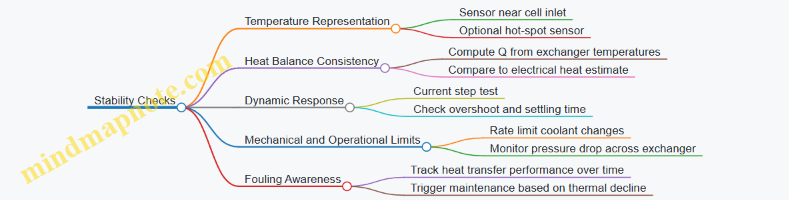
Thermal integration is successful when the cell temperature behaves predictably under normal current changes and during start-up transitions. When you connect heat accounting, sensor placement, and control timing, the system stops “guessing” and starts managing heat like a measurable resource.
8.5 Example Energy and Material Balance for a Defined Production Target
This example shows how to turn a production target into a practical energy and material balance for an electrolytic iron line. The goal is not to predict a perfect plant outcome; it is to build a consistent accounting framework that you can later calibrate with measured cell voltage, current efficiency, and electrolyte losses.
Step 1: Define the Production Target and Product Basis
Assume the plant must produce 10,000 kg of iron per month as deposited metal. Convert to moles for stoichiometry:
- Molar mass of Fe: 55.845 kg/kmol
- Iron production: 10,000 kg / 55.845 kg/kmol = 179.0 kmol Fe
Choose an operating window. For a monthly basis, assume 30 days and 24 hours/day, so total time is 720 hours.
Step 2: Convert Iron Mass to Required Charge
Iron deposition from aqueous electrolytes is commonly represented as:
- \(Fe^{2+} + 2e^- → Fe(s)\)
Each kmol of Fe requires 2 kmol of electrons, which corresponds to a charge of:
- Faraday constant: 96,485 kC per kmol \(e^-\)
- Charge per kmol Fe: 2 × 96,485 kC = 192,970 kC
Total charge for 179.0 kmol Fe:
- Q = 179.0 × 192,970 kC = 34,540,000 kC
Convert kC to kWh using electrical energy relation. First compute average current from charge and time, then compute energy from voltage.
Step 3: Choose Realistic Operating Efficiencies
Two factors determine how much charge becomes product:
- Current efficiency (CE): fraction of charge that deposits iron rather than side reactions.
- Cell voltage (Vcell): average operating voltage including ohmic and kinetic losses.
For a worked example, assume:
- CE = 0.85
- Average Vcell = 2.10 V
Required electrical charge becomes:
- Q_elec = Q / CE = 34,540,000 kC / 0.85 = 40,635,000 kC
Step 4: Compute Average Current and Power
Convert charge to ampere-hours (Ah). Since 1 C = 1 A·s, and 1 kC = 1000 C:
- Total charge in A·s: \(40,635,000\text{ }kC × 1000 = 4.0635×10^{13} C\)
- Total time: \(720 h = 2.592×10^6 s\)
- Average current: \(I = Q/t = 4.0635×10^{13} / (2.592×10^6)\) = 15.7 MA
Average electrical power:
- \(P = V × I = 2.10 V × 15.7×10^6 A\) = 33.0 MW
Monthly electrical energy:
- E = P × time = 33.0 MW × 720 h = 23,800 MWh
Specific energy per kg Fe:
- 23,800,000 kWh / 10,000 kg = 2,380 kWh/kg Fe
This number is intentionally high compared with some industrial claims because the example uses a simplified single-cell voltage and a single CE value; in practice, you would refine Vcell with measured current density and electrolyte resistance, and you would include stack-level voltage and power factor details.
Step 5: Material Balance on Iron Ions and Electrolyte Losses
Start with the stoichiometric requirement of \(Fe^{2+}\).
Stoichiometric \(Fe^{2+}\) consumed equals deposited \(Fe^{2+}\) moles, so:
- \(Fe^{2+}\) required = 179.0 kmol
Now include electrolyte losses. Suppose the process loses iron from the electrolyte via drag-out, purification losses, and non-productive deposition. Represent this with an electrolyte iron loss fraction (Lf) relative to deposited iron. Assume Lf = 0.05.
- Total \(Fe^{2+}\) that must be supplied = 179.0 × (1 + 0.05) = 188.0 kmol
Convert to mass of \(Fe^{2+}\) as elemental Fe basis (same molar mass):
- 188.0 kmol × 55.845 kg/kmol = 10,500 kg Fe equivalent
If you supply iron as FeSO4·7H2O or another salt, you would convert using the salt’s molar mass and hydration state. The key is to keep the accounting consistent: either track everything as elemental Fe equivalents or track each chemical species explicitly.
Step 6: Build a Consistent Accounting Table
Use a simple structure: inputs, outputs, and internal transfers.
| Stream | Basis | Amount |
|---|---|---|
| Deposited iron | Product | 10,000 kg |
| \(Fe^{2+}\) supplied | Electrolyte makeup | 10,500 kg Fe eq |
| \(Fe^{2+}\) lost | Drag-out and purification | 500 kg Fe eq |
| Electrical energy | Utility input | 23,800 MWh |
Mind Map: Energy and Material Balance Logic
Step 7: Practical Checks That Prevent Silent Errors
- Charge-to-mass check: If you compute deposited mass from measured current and CE, it should match the target within the expected operating variability.
- Voltage realism check: If Vcell is far from what your cell design and electrolyte resistance suggest, the energy result will be misleading even if the stoichiometry is correct.
- Electrolyte loss check: If the required makeup iron implies an implausible purification rate or drag-out rate, revisit the assumed Lf and the sampling basis.
Example: How a Small CE Change Moves Energy
If CE improves from 0.85 to 0.90 while everything else stays the same, the required electrical charge scales by 0.85/0.90.
- New energy ≈ 23,800 MWh × (0.85/0.90) = 22,460 MWh
That is a reduction of 1,340 MWh/month, which corresponds to 134 kWh/kg Fe for this example basis. The point is simple: energy accounting is extremely sensitive to CE because CE sits directly in the denominator of charge required for a fixed product mass.
9. Gas Handling and Byproduct Capture Systems
9.1 Identifying Expected Byproducts From Electrode Reactions
Electrolytic iron cells turn electrical energy into chemical change. The “expected byproducts” are the species formed alongside iron at the electrodes, plus any secondary products created when those species react with the electrolyte, water, or impurities. Identifying them early matters because they drive gas handling design, electrolyte purification needs, and product quality.
Foundational Reaction Map
Start with the electrode reactions you intend to run. For iron deposition, the cathode reaction is typically the reduction of an iron ion to solid iron. The byproducts then come from what else is reduced or oxidized under the same conditions.
At the cathode, common competing pathways include:
- Hydrogen evolution when water is available and the potential is sufficiently negative.
- Reduction of dissolved impurities such as certain metal ions that may plate before or alongside iron.
- Consumption of supporting ions indirectly, when side reactions change local pH and shift solubility.
At the anode, common pathways include:
- Oxygen evolution if water oxidation dominates.
- Chlorine or related halogen species if chloride is present and the anode environment favors halogen oxidation.
- Anode corrosion products when the anode material participates in reactions or forms soluble species.
A practical way to keep this systematic is to separate “primary electrode byproducts” from “secondary chemistry.” Primary byproducts are created directly at the electrode surface. Secondary products form when those primary species dissolve, react, or precipitate in the bulk electrolyte.
Mind Map: Byproduct Sources and Consequences
Stepwise Identification Workflow
-
List the intended cathode and anode reactions. Write the net iron deposition reaction and the dominant anode reaction assumed by the process design.
-
Inventory what can participate. Check electrolyte composition for water content, halides, and known impurity metals. Even “trace” chloride can matter because it changes anode chemistry.
-
Compare operating potentials to competing reaction thresholds. If the cathode potential is pushed far enough, hydrogen evolution becomes likely. If the anode potential favors water oxidation, oxygen dominates; if halides are present, halogen formation can compete.
-
Account for local conditions near electrodes. Bulk electrolyte may look stable, but near the cathode pH can rise due to hydrogen evolution or ion consumption patterns. Higher local pH can cause iron hydroxide or basic salts to form, which then show up as sludge.
-
Translate primary byproducts into measurable plant outputs. Hydrogen and oxygen affect offgas flow and flammability controls. Halogen species require corrosion-resistant ducting and scrubbing chemistry. Sludge formation affects filtration and electrolyte makeup rates.
Concrete Examples
Example: Chloride-containing electrolyte with oxygen evolution at the anode. If chloride is present, anode oxidation can produce chlorine or related oxidized chlorine species. Even if oxygen is the main product, small fractions of chlorine can dissolve into the electrolyte, increasing corrosivity and changing purification targets. In practice, you would expect higher anode corrosion rates and a need for tighter control of chloride concentration in recycle.
Example: High current density leading to hydrogen evolution at the cathode. When current density approaches the mass-transport limit for iron ions, the cathode surface sees less iron availability. Water reduction becomes a more competitive pathway, generating hydrogen bubbles. Those bubbles can disrupt deposition morphology, trap electrolyte in the iron product, and increase washing demand. Offgas systems must therefore be sized for hydrogen, not just for “inert” venting.
Example: Impurity metals in feed. Suppose nickel is present at low levels. If its reduction potential is favorable under your operating conditions, nickel can co-deposit. The byproduct here is not a gas but a compositional contaminant that changes downstream alloying behavior and may increase corrosion resistance issues in the product. You would identify this by tracking impurity concentrations in electrolyte before and after operation and by analyzing product composition.
Practical Checklist for Expected Byproducts
- Gases: Hydrogen at the cathode; oxygen at the anode; halogens if halides are present.
- Solids: Basic iron compounds or hydroxide-related sludge from local pH shifts.
- Dissolved species: Corrosion products from anode dissolution; dissolved oxidized halogen species.
- Contaminants: Co-deposited impurity metals that originate from feed and recycle.
Once you can name these categories for your specific electrolyte and operating window, the rest of the chapter’s topics—offgas capture, purification, and product quality—become straightforward engineering choices rather than surprises.
9.2 Gas Collection Methods for Minimizing Contamination
Gas collection in electrolytic iron cells is mostly about controlling where the gas goes, how it contacts liquids, and how quickly it leaves the reaction zone. Contamination happens when offgas carries droplets, entrained electrolyte mist, or fine solids into the downstream line. The goal is to remove the gas from the cell fast enough to limit entrainment, then clean it using staged separation that matches the particle size and liquid properties.
Foundational Principles for Clean Offgas
Start with the two main contamination pathways. First, mechanical entrainment: bubbles rise and drag electrolyte droplets and sludgy particles into the headspace. Second, re-dissolution and carryover: soluble species can dissolve into the gas-phase moisture film and later reappear downstream. Minimizing both requires controlling gas velocity, pressure drop, and the geometry of the gas path.
A practical way to think about it is to treat the offgas line as a sequence of “contact opportunities.” Every bend, sudden expansion, or high-velocity section increases the chance that droplets detach and travel. So the best designs keep the gas path short, smooth, and consistently sized, with separation steps placed where droplets are most likely to fall out.
Cell Headspace Design and Capture Geometry
Begin at the cell. Use a gas outlet located to avoid direct bubble plumes when possible, and ensure the outlet is above the liquid level to reduce direct splash. If the cell has a cover or hood, keep the cover tight enough to prevent ambient air ingress, because dilution changes condensation behavior and can increase moisture carryover.
Gas velocity matters. Too low, and the gas lingers, allowing more time for moisture pickup and for fine aerosols to form. Too high, and you increase droplet entrainment. A good rule is to design for stable flow that avoids “jetting” from the outlet; the outlet should feel like a gentle draw, not a firehose.
Primary Separation Using Knockout and Demisters
The first line of defense is a knockout (KO) vessel or droplet separator placed close to the cell. Its job is to slow the gas and give droplets a chance to fall. KO sizing is based on residence time and expected droplet loading, which depends on current density and electrolyte volatility.
After the KO, use a demister to catch smaller aerosols. Common choices include mesh pads or structured media. Mesh pads are effective for fine droplets but can foul if solids load is high, so they pair well with upstream KO performance and good electrolyte filtration.
A simple operational check is to compare pressure drop across the demister over time. If pressure drop rises quickly, you likely have aerosol or solids breakthrough and should inspect KO performance and upstream filtration.
Secondary Cleaning with Scrubbers and Condensers
If the offgas contains soluble contaminants or if moisture carryover remains significant, add a secondary stage. A condenser targets water vapor and reduces downstream corrosion and mist formation. Condensation also helps keep later scrubber media from clogging.
For soluble species, a wet scrubber can remove them by mass transfer into a controlled liquid. Scrubber design should match the gas composition and the solubility of the target contaminants. Use a recirculating scrubber liquor with filtration to prevent captured solids from building up and re-entraining.
Keep scrubber liquid management disciplined. Track scrubber liquor conductivity, pH, and solids content so you can adjust bleed-and-bleedback rates. If you do not, the scrubber becomes a contamination reservoir rather than a cleanup step.
Minimizing Contamination in the Piping and Valves
Even with good separators, piping can undo your work. Use smooth bends with generous radii and avoid long horizontal runs where condensate can pool and later aerosolize. Provide low-point drains so condensed liquid can be removed without opening the system.
Valves and fittings are common leak and mist sources. Choose components rated for the expected chemical environment and ensure seals are compatible with scrubber liquor if any backflow occurs. Install check valves where reverse flow is possible, especially during power interruptions.
Integrated Mind Map for Gas Collection
Mind Map: Gas Collection Methods for Minimizing Contamination
Example: Two-Stage System for Stable Cleanliness
Consider a cell where offgas visibly carries a light mist during steady operation. The first step is to add or improve a KO vessel directly at the cell outlet, with a short vertical drop section so droplets can fall before the gas accelerates into the line. Next, place a demister downstream and monitor its pressure drop.
If mist persists, add a condenser before any long ducting. This reduces moisture availability for aerosol formation and lowers corrosion risk. Finally, if analysis shows dissolved electrolyte species in the collected gas, add a scrubber stage with recirculating liquor and a small filtration loop to keep solids from building up.
The integrated logic is simple: KO reduces the bulk of droplets, demister captures what remains, condenser controls moisture, and scrubber handles dissolved contaminants. When each stage is tuned and monitored, contamination drops without turning the system into a maintenance-heavy science project.
9.3 Scrubbing and Conditioning for Safe Downstream Use
Electrode reactions produce offgas that must be cleaned before it reaches any downstream step, whether that is a vent stack, a gas-to-liquid contactor, or a heat recovery unit. Scrubbing and conditioning are not the same thing: scrubbing removes contaminants, while conditioning makes the remaining gas safe and stable for the next boundary. A good workflow starts with knowing what you have, then choosing the simplest unit operation that removes it without creating new problems.
Foundational Inputs and Targets
Begin by defining the downstream “acceptance conditions” in plain terms: maximum allowable particulates, limits on corrosive species, moisture range, and acceptable oxygen or hydrogen levels for the chosen equipment. For electrolytic iron systems, the offgas composition often includes oxygen and/or other evolved gases plus entrained mist and fine aerosols. Even when the main gas is benign, the droplets can carry electrolyte components that cause corrosion and scaling.
A practical target-setting approach is to map each contaminant to a removal mechanism:
- Mist and aerosols are removed by droplet capture (cyclones, demisters, packed scrubbers).
- Soluble gases are removed by absorption in a liquid phase (acid/base scrubbing depending on chemistry).
- Reactive traces are reduced or neutralized by controlled chemistry in the scrub liquor.
Scrubbing Train from Coarse to Fine
Use a staged train so each unit does what it is best at. A common sequence is:
- Pre-separation for large droplets and bulk particulates.
- Gas-liquid contact for soluble species and remaining aerosols.
- Polishing to protect downstream equipment.
For example, if the offgas carries visible mist during start-up, a pre-separator reduces the load on the main scrubber. That prevents the scrubber liquor from rapidly accumulating solids and keeps pressure drop stable.
Key operating parameters are chosen to balance capture efficiency and energy use:
- Gas velocity in demisters and cyclones controls droplet carryover.
- Liquid-to-gas ratio controls absorption capacity and wetting.
- pH and alkalinity control whether soluble species stay in solution or precipitate.
Conditioning for Safe Downstream Boundaries
After scrubbing, condition the gas to match the next equipment’s needs. Conditioning often includes:
- Moisture control so downstream piping and heat exchangers do not frost or corrode.
- Temperature adjustment to keep scrubbed gas within safe material limits.
- Residual chemistry control to avoid carryover of scrub liquor.
A simple example: if a heat exchanger follows the scrubber, you may need a demister or a short residence section to reduce liquid carryover. Otherwise, the exchanger surfaces become a “deposit magnet,” and maintenance turns into a recurring hobby.
Scrubber Liquor Management That Prevents Secondary Problems
Scrubbers create a new liquid stream: the scrub liquor. Treat it as a process stream, not a sink.
Core best practices:
- Circulation control keeps contact conditions steady and reduces localized pH swings.
- Filtration or settling removes captured solids before they build up in the contact zone.
- Make-up and bleed strategy prevents excessive concentration of dissolved salts.
For instance, if the scrub liquor becomes too concentrated, it can promote scaling on packing and nozzles. A controlled bleed rate paired with measured conductivity or ion balance keeps the system in a workable window.
Monitoring and Verification Without Guesswork
Verification should include both gas-side and liquid-side checks.
Gas-side indicators:
- Differential pressure across scrubber internals to detect fouling.
- Outlet particulate measurement to confirm polishing effectiveness.
- Moisture or dew point checks to ensure conditioning meets downstream needs.
Liquid-side indicators:
- pH and alkalinity to confirm absorption chemistry.
- Conductivity or total dissolved solids to manage concentration.
- Suspended solids to decide when filtration or bleed is required.
A useful operational pattern is to link each measurement to an action threshold. If differential pressure rises faster than expected, inspect demister performance or packing wetting before the system compensates by consuming more energy.
Mind Map: Scrubbing and Conditioning Logic
Example: Start-Up Mist Control with a Two-Stage Approach
During start-up, gas flow and chemistry stabilize over minutes to hours, and mist generation is often highest early on. A two-stage approach reduces risk:
- Stage 1: pre-separator/demister captures large droplets so the main scrubber does not get overwhelmed.
- Stage 2: main scrubber absorbs soluble species while maintaining a controlled pH.
Conditioning then dries the gas to the dew point range required by downstream piping. If outlet moisture remains high, the first response is to check demister performance and liquid carryover, not to increase scrubber liquid rate blindly.
Example: Choosing Chemistry Based on What You Actually Remove
If analysis shows that a corrosive soluble component is present, select scrub liquor chemistry that keeps it dissolved rather than precipitated in the contact zone. For instance, maintaining appropriate alkalinity can prevent formation of hard solids that clog packing. The operational check is simple: if pressure drop rises while pH drifts, the system may be shifting from absorption to precipitation.
By treating scrubbing and conditioning as a controlled chain—capture, absorb, polish, then condition—you keep downstream equipment clean, reduce corrosion drivers, and make safety checks measurable rather than hopeful.
9.4 Ventilation and Offgas Monitoring Requirements
Electrolytic iron cells can release oxygen or other gases from electrode reactions, plus water vapor and aerosolized electrolyte mist. Ventilation and monitoring are the two halves of the same job: ventilation keeps the room safe and limits corrosion, while monitoring proves the system is doing that job consistently.
Foundational Goals for Ventilation
Start with three measurable goals. First, keep gas concentrations below occupational limits by removing offgas at the source. Second, prevent electrolyte mist from settling on equipment by capturing it before it spreads. Third, maintain stable cell operation by avoiding excessive backpressure that can disturb gas evolution.
A practical way to connect these goals to design choices is to treat the cell hood or enclosure as a controlled “capture zone.” Air should flow into the capture zone, not out of it. That means the exhaust rate must exceed any air leakage into the room, and the ducting must be arranged to avoid dead zones where mist can accumulate.
Ventilation System Layout and Capture Strategy
Use local capture rather than room-wide dilution. For a typical setup, place a hood or ventilated enclosure over the cell, connect it to a dedicated exhaust duct, and include a mist management stage before the exhaust fan.
Mist management is not optional. Even when gas volume is modest, aerosol can carry dissolved salts and metals that corrode ductwork and contaminate filters. A common approach is a demister or mesh pad upstream of a scrubber or filter stage, followed by a controlled pressure drop element so the system remains predictable.
To keep backpressure low, design the duct path with smooth turns, adequate diameter, and a pressure relief strategy for abnormal conditions. If the enclosure pressure rises, gas can find alternative paths through seals, which defeats the capture zone.
Offgas Monitoring What to Measure and Why
Monitoring should cover three categories: airflow, gas composition, and system health.
Airflow verification confirms capture. Use differential pressure across the enclosure or hood face, or measure exhaust flow directly with a calibrated flow element. If airflow drops, the system may still “look fine,” but mist and gases will spread.
Gas composition confirms safety and reaction behavior. For oxygen evolution, oxygen sensors can be used where appropriate, but the key is to monitor the specific hazard relevant to your chemistry and electrode reactions. Pair gas sensors with a sampling method that avoids sensor fouling, such as drawing from a protected sampling port with a short, heated or filtered line.
System health checks ensure the monitoring signals are trustworthy. Include checks for filter loading, scrubber differential pressure, and fan status. A sensor that is reading “normal” while the sampling line is blocked is a classic failure mode.
Monitoring Placement and Sampling Integrity
Place sampling points where the gas is representative of the offgas stream leaving the capture zone, not where mist has already condensed. If you sample too close to the cell, you may overload the line with droplets; too far downstream, and you may dilute or mix with room air.
Sampling integrity also depends on maintaining stable flow through the sampling line. Use a small pump or controlled aspiration flow, and include a way to detect blockage, such as a differential pressure switch across the sampling filter.
Operational Checks and Response Actions
Define acceptance criteria for ventilation and monitoring before commissioning. For example, set a minimum enclosure differential pressure or minimum exhaust flow, and require an interlock that prevents cell operation if the criterion is not met.
Response actions should be specific and procedural. If airflow falls below the setpoint, pause the process, verify filter loading, check duct dampers, and inspect for enclosure leaks. If gas composition indicates abnormal oxygen evolution patterns, verify current distribution and electrode condition, then confirm that the ventilation system is still capturing correctly.
Mind Map: Ventilation and Offgas Monitoring Requirements
Example: Enclosure Differential Pressure Interlock
Assume a cell enclosure is designed to maintain inward airflow. During commissioning, you measure differential pressure between the enclosure interior and the room. You set an interlock at a value that corresponds to reliable capture under normal operating conditions.
If the differential pressure drops below the interlock threshold, the control system stops the cell current and triggers an alarm. Operators then check for common causes: a loaded mist filter, a partially closed damper, or a door left open. After correcting the cause, they confirm the differential pressure returns to the acceptable band before restarting.
Example: Sampling Line Blockage Detection
A sampling line draws offgas through a small filter to protect sensors. Add a differential pressure switch across that filter. If the filter clogs, the switch triggers an alarm indicating that sensor readings may no longer represent the offgas stream. The process is paused until the sampling line is cleaned or replaced and the differential pressure returns to normal.
9.5 Example Offgas System Sizing for a Laboratory Scale Cell
This section walks through a practical sizing workflow for an offgas system on a laboratory electrolytic iron cell. The goal is to size the gas capture and treatment so that (1) the cell atmosphere stays controlled, (2) the exhaust is safely handled, and (3) the system can be built and tested without guesswork.
Foundational Inputs for Sizing
Start with what the cell actually produces. In many iron electrolysis setups, the cathode reaction forms iron while the anode reaction evolves a gas such as oxygen (or another gas depending on electrolyte chemistry). You size the offgas system from the expected gas generation rate, then add a safety margin for imperfect capture.
Key inputs:
- Current (A) and operation time (s or h). Example: 10 A for 2 hours.
- Faradaic efficiency for gas evolution (dimensionless). Example: 0.9 for the fraction of current producing the intended gas.
- Stoichiometry linking electrons to gas molecules. For oxygen evolution: 4 e⁻ per O₂.
- Capture factor representing how much of the generated gas is actually captured. Example: 0.85 with a well-designed hood and local enclosure.
- Gas conditions at the cell outlet: temperature and pressure. Example: 25 °C and 1 atm.
Step 1: Compute Theoretical Gas Generation
For oxygen evolution, the molar rate of O₂ is:
- Moles O₂ per second = (I × η) / (4 × F)
Where F is Faraday’s constant (96485 C/mol e⁻).
Example calculation:
- I = 10 A
- η = 0.9
- mol O₂/s = (10 × 0.9) / (4 × 96485) ≈ 2.33 × 10⁻⁵ mol/s
Convert to volumetric flow at 25 °C and 1 atm using the ideal gas law (molar volume ≈ 24.47 L/mol):
- Q_theoretical ≈ 2.33 × 10⁻⁵ × 24.47 ≈ 0.00057 L/s
- Q_theoretical ≈ 2.05 L/h
That number is small, which is why capture design matters: leaks and entrainment often dominate over the pure electrochemical gas volume.
Step 2: Apply Capture Factor and Add Margin
Captured flow:
- Q_captured = Q_theoretical × capture factor
- Q_captured ≈ 2.05 L/h × 0.85 ≈ 1.74 L/h
Add a practical margin for variability in bubbling, splashing, and transient operation. A common lab approach is a 3× flow margin for commissioning, then you verify with measurements.
- Q_design ≈ 1.74 L/h × 3 ≈ 5.2 L/h
Convert to m³/h for equipment selection:
- 5.2 L/h = 0.0052 m³/h
In practice, you will likely choose a small blower or regulated vacuum that can provide a stable flow in the tens of L/h range to maintain negative pressure at the enclosure. The design flow above is the minimum gas-handling requirement; the blower flow is often higher to overcome line losses and ensure consistent capture.
Step 3: Size the Enclosure and Ducting
Use a local capture hood or a sealed cell enclosure with a controlled exhaust port. The enclosure should prevent backflow when the blower cycles.
Sizing logic:
- Keep duct runs short to reduce pressure drop.
- Use smooth tubing and avoid sharp bends.
- Ensure the exhaust port is positioned where bubbles rise and where vapor can escape.
A simple commissioning check is to place a strip of lightweight tissue near the exhaust opening and confirm it consistently draws inward during operation.
Step 4: Select Treatment Based on Gas Identity
For oxygen-only evolution, treatment may be minimal if the lab ventilation is adequate and the enclosure prevents release. If the electrolyte can generate additional reactive species (for example, acid mist or other gases), treatment must include a condensation/mist stage and then a scrubber stage appropriate to the chemistry.
A typical laboratory stack for mixed offgas includes:
- Mist knockdown (coalescing filter or demister)
- Condensation trap (if water vapor is significant)
- Scrubber (only if required by gas composition)
- Final exhaust to the facility system
Mind Map: Offgas System Sizing Workflow
Example: Laboratory Build and Verification Plan
Assume the cell runs at 10 A with oxygen evolution and a target design captured flow of ~5 L/h. Choose a small diaphragm pump or regulated blower that can be set to 30–60 L/h at the exhaust port, then throttle with a needle valve or mass-flow controller if available.
Verification steps:
- Measure actual exhaust flow with an inline flow meter.
- Confirm enclosure negative pressure during operation.
- Observe for visible mist at the exhaust line; if present, increase mist knockdown capacity.
- If gas composition is uncertain, take a short sample using appropriate in-house analytical methods and confirm the treatment assumptions.
Step 5: Turn Sizing into Operating Limits
Finally, translate the sizing into operational guardrails:
- Do not exceed the current used in the sizing basis without re-checking flow and treatment capacity.
- Keep the enclosure sealed and the exhaust path unobstructed.
- Treat any sudden change in bubbling intensity as a reason to re-verify exhaust flow.
For the example cell, the system is sized to handle the expected oxygen generation with margin, while the enclosure and mist control address the practical realities that dominate in small setups.
10. Process Control Instrumentation and Data Practices
10.1 Sensor Selection for Temperature Voltage and Current
Choosing sensors for an electrolytic iron cell is less about buying the fanciest part and more about matching what you measure to what you must control. Temperature, voltage, and current are the three signals that most directly shape deposition quality, efficiency, and safety. The trick is to measure them in a way that survives real-world conditions: splashes, electrical noise, drifting electrolytes, and long cable runs.
Foundational Signal Roles
Temperature sensors tell you whether reaction rates and transport conditions are staying within your operating window. Voltage sensors help you separate useful electrical driving force from losses you cannot control, and they support energy accounting. Current measurement is the backbone for mass balance because deposition rate scales with charge.
A practical rule: if a sensor cannot support both control and verification, you usually end up with two sensors anyway—one for control, one for audit. Plan for that early.
Temperature Sensing
What Temperature Means in a Cell
In an electrolytic cell, “temperature” is not a single truth. There is bulk electrolyte temperature, local hot spots near current collectors, and temperature gradients across the cell wall. For control, you typically want bulk electrolyte temperature. For diagnosing issues like poor mixing or localized resistance, you want at least one additional spot measurement.
Sensor Types and Placement
- Thermocouples are rugged and tolerate harsh environments. Use them where you can protect the junction from splatter and where you can tolerate some drift.
- RTDs (resistance temperature detectors) offer better stability and repeatability, which helps when you compare runs.
Placement matters more than brand. Mount sensors away from direct gas impingement and ensure good thermal contact with the medium you care about. If you measure near a wall, you may track wall temperature rather than bulk electrolyte.
Wiring and Noise
Temperature signals are low-level. Use shielded twisted pairs, route them away from high-current conductors, and ground shields at one end to reduce noise injection.
Voltage Sensing
What Voltage You Actually Need
Cell voltage includes contributions from electrode overpotentials, ohmic drops in electrolyte and hardware, and contact resistances. For control, you want a stable measurement of the cell’s electrical driving condition. For diagnostics, you want to know whether changes come from electrolyte resistance or from electrode behavior.
Differential Measurement
Always measure voltage differentially across the cell terminals or across a defined segment of the circuit. Single-ended measurements invite ground offsets and misleading readings when the power supply floats or when other equipment shares a ground.
Filtering and Response Time
Voltage can fluctuate with bubble coverage and current distribution. A control loop often benefits from modest filtering, but too much filtering delays response and can worsen oscillations. Choose filtering based on your control update rate.
Current Sensing
Why Current Measurement Must Be Accurate
Current determines charge throughput. If current is biased by even a few percent, your predicted deposition yield and energy per ton will be off. Current also feeds interlocks that prevent unsafe operating conditions.
Common Approaches
- Shunt resistors provide direct current-to-voltage conversion. They are straightforward and accurate when properly sized and cooled.
- Hall-effect sensors avoid inserting resistance into the circuit and can be easier to retrofit, but they require careful calibration and attention to temperature effects.
Bandwidth and Saturation
Current measurement must handle the full operating range without saturation. Bandwidth should be sufficient to capture meaningful changes for control, but not so high that noise dominates.
Integrated Selection Workflow
Use a structured process so you do not end up with sensors that measure the right quantities but at the wrong times or in the wrong locations.
- Define control objectives: what must be regulated (deposition quality, stability, safety limits).
- Define measurement granularity: fast enough for control, stable enough for reporting.
- Map sensor locations to physical phenomena: bulk temperature, terminal voltage, total current.
- Select sensor type by environment: splashes, corrosion risk, vibration, and cleaning cycles.
- Plan wiring and grounding: separate signal and power paths, use shielding, and verify grounding strategy.
- Set calibration and verification: define how you will check drift and measurement bias.
Mind Map: Sensor Selection Logic
Example: Choosing Sensors for a Control Loop
Assume you run a cell where deposition stability depends on maintaining bulk electrolyte temperature and limiting current to avoid excessive gas evolution.
- Temperature: place an RTD in the well-mixed region of the electrolyte and add one thermocouple near a current collector as a diagnostic. Filter the temperature signal lightly so the controller reacts to real drift, not momentary disturbances.
- Voltage: measure differential voltage across the cell terminals. Use a moderate low-pass filter so bubble-induced spikes do not cause control chatter.
- Current: use a shunt sized for the maximum operating current with adequate thermal management. Feed the current signal directly to the interlock path with minimal filtering, while the control loop can use a slightly filtered version.
The result is a system where the controller sees stable, meaningful signals, while the interlocks and audit measurements remain trustworthy.
Example: Debugging a Measurement Mismatch
If energy per ton looks inconsistent while deposition morphology remains stable, suspect measurement bias rather than chemistry. Check whether voltage is measured differentially across the intended terminals and whether current sensing is calibrated at operating temperature. If temperature readings show a wall-to-bulk gradient, confirm sensor placement and mixing assumptions. Often, the “problem” is that the sensor is faithfully measuring a different physical location than the one your control model assumes.
10.2 Sampling Plans for Electrolyte and Product Streams
A sampling plan is a map of decisions: what to sample, when to sample, how to sample, and how to turn samples into actions. In electrolytic iron production, the tricky part is that “the tank” is not the same thing as “the chemistry at the electrode,” and “the product” is not the same thing as “the deposit you can see.” A good plan reduces that mismatch.
Start with Measurement Goals
Define goals before choosing sampling points. Typical goals include:
- Confirming electrolyte composition stays within deposition-ready limits.
- Detecting impurity buildup that changes deposit morphology.
- Verifying product quality targets like iron purity and surface condition.
- Supporting process control loops by providing data with known timing and uncertainty.
A practical way to connect goals to sampling is to list each control-relevant variable (for example Fe species concentration, chloride level, sulfate level, dissolved impurities, water content) and assign it a decision rule: “If it crosses X, do Y.” The sampling plan exists to feed those rules.
Identify Sampling Locations and Representativeness
Electrolyte sampling points should represent the bulk chemistry that feeds the cell, while product sampling points should represent the deposit that will be processed downstream.
For electrolyte, common locations include:
- Inlet line to the cell, representing what reaches the electrodes.
- Recirculation loop, representing mixed bulk conditions.
- Post-treatment tank outlet, representing purified feed.
For product, sampling points include:
- Deposited iron sheet or plate after removal.
- Washed solids after the washing step, representing what will be dried and tested.
- Slurry or residue streams if they are recycled or disposed.
Representativeness improves when you standardize flow conditions during sampling. If the recirculation pump speed changes, the “same” sample can become a different mixture.
Choose Sampling Frequency with a Two-Layer Approach
Use two layers: routine sampling and event-driven sampling.
Routine sampling catches slow drift. A typical pattern is daily checks for major composition and weekly checks for less frequent impurity trends. Event-driven sampling triggers when operating conditions change, such as:
- A step change in current density.
- A temperature setpoint adjustment.
- A change in make-up water or salt addition rate.
- Any abnormal voltage behavior suggesting altered mass transport.
This approach prevents over-sampling during stable operation while still catching chemistry shifts when they matter.
Define Sample Volume, Container, and Handling
Sample volume must be enough for repeat tests and rechecks. Container choice matters because some ions can adsorb to surfaces or react with residues.
Best practices that are easy to apply:
- Use clean, labeled containers dedicated to electrolyte chemistry.
- Rinse sampling lines with a small purge volume before collecting the analytical sample.
- Seal immediately to limit evaporation and atmospheric contamination.
- Keep temperature consistent between sampling and analysis when possible.
For product samples, standardize the mass and area taken from a plate so that thickness and surface variability do not masquerade as chemistry changes.
Build a Chain of Custody and Data Traceability
Every sample should have a unique identifier linked to:
- Cell number and operating conditions.
- Time of sampling and time of analysis.
- Operator and sampling method.
- Any deviations, such as delayed analysis or unusual handling.
Traceability prevents “mystery failures” where the data exists but cannot be trusted.
Use a Sampling Plan Template That Supports Control
A sampling plan should specify acceptance criteria and actions. For example, if chloride exceeds a threshold, you might increase purification throughput or adjust make-up composition. The plan should also state how quickly results must be available to influence the next operating window.
Mind Map: Sampling Plan Logic
Concrete Example: A Weekly Impurity Trend with Daily Guardrails
Assume you track a dissolved impurity that affects deposit smoothness. You set daily guardrails for a related indicator (for example conductivity or a proxy ion) and weekly direct measurement for the impurity.
- Daily: sample from the recirculation loop and measure the proxy. If it exceeds the guardrail, you pull an additional direct impurity sample immediately.
- Weekly: sample from the post-treatment outlet to confirm purification performance.
- Action: if the weekly impurity rises while the proxy stays stable, you investigate analytical bias or sampling handling; if both rise, you adjust purification or make-up composition.
This example shows why frequency alone is not enough: the plan must connect measurements to decisions.
Concrete Example: Product Sampling That Avoids “Looks Fine” Errors
For product testing, take samples from multiple positions on a plate rather than one corner. Edge regions often experience different current distribution, which can change deposit density and trapped electrolyte residues.
A simple method:
- Mark three zones on each plate: center, mid-edge, and edge.
- Take a fixed mass or fixed area from each zone.
- Combine or test separately depending on your acceptance criteria.
If your acceptance criteria are based on average purity, combining can be appropriate. If morphology defects trigger rejection, test zones separately so you can locate the problem source.
Common Failure Modes and How the Plan Prevents Them
- Sampling too far from where control decisions are made: fix by aligning sampling points with the decision variable.
- Inconsistent line purging: fix by standardizing purge volume and documenting deviations.
- Delayed analysis without temperature control: fix by specifying maximum hold times.
- Product sampling that ignores spatial variability: fix by zoning and fixed sampling geometry.
A sampling plan is successful when the data can be used without second-guessing. When it’s written clearly, operators can follow it, analysts can trust it, and process control can act on it.
10.3 Control Loops for Stabilizing Concentration and Current Density
Stable electrolytic iron production is mostly about keeping two things from drifting: the electrolyte composition (especially iron species and key supporting ions) and the electrical driving conditions (current density and the resulting overpotentials). A good control system treats these as coupled variables: changing current density alters local concentration near electrodes, and changing concentration changes conductivity and reaction rates. The trick is to control both without creating a tug-of-war.
Foundational Measurements and What They Really Mean
Start with signals that can be trusted. Measure bulk electrolyte temperature, cell voltage, current, and at least one concentration proxy (for example, iron ion concentration via titration or inline spectroscopy). Use conductivity as a secondary indicator because it responds quickly to ionic strength changes. For current density, compute it from measured current and electrode area, then correct for any effective area changes due to wetting or electrode spacing.
A practical rule: if a sensor is slow or noisy, don’t force it into the fastest loop. Use fast electrical signals for fast control, and slower chemical measurements for slower correction.
Control Architecture That Avoids Coupling Chaos
Use a layered structure:
- Fast inner loop: holds current density (or cell voltage) near a setpoint.
- Slower outer loop: adjusts electrolyte make-up or purification rate to restore bulk concentration.
- Supervisory logic: limits actions when the system is outside safe operating envelopes.
This separation prevents the outer loop from chasing short-term fluctuations that are caused by mass transport and bubble behavior.
Inner Loop for Current Density Stability
The inner loop typically manipulates power supply output. Two common approaches are:
- Current control: keep current constant and accept voltage changes as a diagnostic.
- Voltage control with current limiting: keep voltage near a target while enforcing a maximum current to protect electrodes.
In either case, include a deadband around the setpoint to avoid constant micro-adjustments. Also filter the measured current density signal with a short moving average so the controller doesn’t react to electrical ripple.
Example: If current density is set to 300 A/m² and cell voltage rises by 0.2 V over several minutes, the inner loop will maintain current, while the voltage trend flags increasing ohmic resistance or concentration depletion. That information can feed the outer loop or supervisory alarms.
Outer Loop for Concentration Restoration
Bulk concentration changes come from three places: feed addition, purification removal, and consumption/production at electrodes. The outer loop should adjust make-up flow rates and purification duty cycles based on bulk concentration error.
A simple and effective method is PI control on concentration error with constraints:
- Actuator limits: cap make-up and purification rates.
- Rate limits: prevent sudden composition jumps.
- Hold conditions: pause concentration correction during start-up or when the cell is not in steady electrical operation.
Example: Suppose iron ion concentration is 1.0 M target and measured at 0.92 M. The controller increases make-up flow by a small step, then waits for the bulk measurement to reflect the change. If the concentration overshoots, reduce the make-up gain or increase the measurement-to-actuation delay.
Managing Mass Transport Coupling
Even with perfect bulk control, local depletion near the cathode can cause deposition quality issues. To reduce coupling, incorporate a feed-forward term into the inner loop: when current density increases, temporarily adjust electrolyte flow rate or agitation to maintain boundary layer conditions.
Example: If you raise current density from 250 to 300 A/m², increase electrolyte circulation slightly so the limiting current is not approached. The controller doesn’t need to “know” diffusion coefficients; it just needs a consistent relationship between flow and observed voltage/concentration proxies.
Supervisory Logic and Safety Interlocks
Supervisory logic prevents controllers from doing the wrong thing for the right reason. Implement rules such as:
- If cell voltage exceeds a threshold at constant current, reduce current density.
- If temperature deviates beyond tolerance, hold concentration control actions to avoid compounding effects.
- If concentration sensor quality drops (missing data, out-of-range), switch to a conservative operating mode using last known good values.
This is where you keep the system from turning into a well-instrumented mess.
Mind Map: Control Loop Design
Worked Example: Coordinated Tuning Workflow
- Tune the inner loop first using current steps while keeping concentration actions fixed. Confirm that current density tracks setpoint with minimal oscillation.
- Observe voltage response to steps. If voltage rises sharply, increase inner-loop stability margins or improve electrolyte mixing.
- Then enable the outer loop with small concentration setpoint changes. Verify that bulk concentration returns to target without overshoot.
- Add supervisory limits so that if voltage indicates depletion or resistance growth, the system reduces current density rather than forcing concentration correction.
A well-tuned system shows a pattern: electrical variables settle quickly, chemical variables correct more slowly, and the supervisory layer quietly prevents the controllers from fighting each other.
10.4 Troubleshooting Based on Electrical and Chemical Indicators
Troubleshooting electrolytic iron cells works best when you treat electrical signals and chemical measurements as two views of the same system. Electrical indicators tell you what the cell is doing right now; chemical indicators tell you what the cell is becoming over time. The goal is to connect symptoms to causes without guessing.
Foundational Logic for Interpreting Indicators
Start with the simplest question: is the cell underperforming because it cannot push current, because it pushes current inefficiently, or because it pushes current into the wrong reactions.
- Voltage too high at stable current usually points to increased resistance or larger overpotentials.
- Current too low at stable voltage usually points to insufficient conductivity, poor wetting, or electrode blockage.
- Voltage and current both drift often indicates changing electrolyte composition, temperature, or fouling.
- Product quality shifts while electrical values look steady often indicates chemistry problems like impurity-driven co-deposition or altered speciation.
A practical habit: log every reading with time, current density, temperature, and the last electrolyte adjustment. Without that context, the same symptom can mean different things.
Electrical Indicators and What They Mean
Electrical indicators are most useful when you separate them into components.
- Ohmic resistance rise shows up as a voltage increase that correlates with temperature drops or concentration changes. Example: if temperature falls by 3–5 °C and voltage rises immediately, suspect conductivity loss or poor heat transfer.
- Overpotential changes show up as voltage changes that do not track temperature. Example: if temperature is constant but voltage climbs over hours, suspect electrode surface changes such as passivation, scaling, or gas coverage.
- Current distribution issues show up as uneven deposition. Example: if one edge of the cathode grows rough deposits while the center remains smooth, suspect flow maldistribution, spacer misalignment, or local blockage.
Chemical Indicators and What They Mean
Chemical indicators confirm whether the electrolyte and interfaces are behaving.
- Iron concentration drift affects deposition rate and efficiency. Example: if iron concentration drops while current remains constant, you may be losing iron to side reactions or to sludge formation.
- Impurity buildup can change deposition morphology and reduce current efficiency. Example: rising nickel or copper in solution often correlates with darker, rougher deposits.
- pH and speciation shifts can change which species are reduced. Example: if pH rises due to inadequate control, you may see altered iron speciation and more competing reactions.
- Gas composition and rate indicate whether the anode reaction is behaving as expected. Example: higher-than-normal oxygen evolution can increase local turbulence and affect cathode morphology.
Mind Map: Electrical and Chemical Troubleshooting Path
Systematic Troubleshooting Workflow
Use a short sequence so you do not chase your tail.
- Stabilize operating conditions: confirm temperature control and that current density matches the setpoint.
- Classify the symptom: choose one primary category—resistance, overpotential, current distribution, or chemistry.
- Check the fastest corroborating measurement:
- For resistance: conductivity and temperature.
- For overpotential: electrode inspection and gas behavior.
- For distribution: deposition pattern and flow indicators.
- For chemistry: iron concentration, impurity panel, and pH.
- Apply one corrective action at a time and watch for response within a defined window. Example: after cleaning and restoring wetting, voltage should drop quickly if the issue was interface resistance.
Example: Voltage High with Stable Temperature
You observe voltage rising by 0.3–0.5 V over several hours while temperature stays within ±1 °C.
- Electrical interpretation: likely overpotential increase or electrode surface change.
- Chemical check: sample electrolyte for iron concentration and impurity levels to rule out chemistry drift.
- Interface check: inspect cathode for scaling or persistent gas coverage.
- Most common fix: clean electrodes and verify that electrolyte is fully wetting the cathode surface. If the cell uses spacers or flow channels, confirm they are not partially blocked.
After correction, you expect voltage to return toward baseline at the same current density. If it does not, the problem may be deeper than surface fouling, such as persistent impurity effects or anode behavior changes.
Example: Current Efficiency Drop with Stable Voltage
Voltage looks steady, but iron yield per ampere-hour drops and deposits become darker.
- Electrical interpretation: resistance and overpotential may be unchanged, so look for chemistry.
- Chemical check: measure impurity concentrations and iron speciation indicators. If impurities increased, co-deposition can consume current without producing the desired iron morphology.
- Corrective action: purify the electrolyte or adjust the bleed-and-recycle strategy so impurity levels fall while maintaining iron concentration.
Example: Edge Roughness with Uniform Average Readings
Average voltage and current look fine, yet the cathode edges show rough, porous growth.
- Electrical interpretation: current distribution is not uniform.
- Chemical check: confirm electrolyte composition is uniform across the cell; local depletion can happen even when bulk samples look normal.
- Mechanical and flow checks: verify flow paths, spacer alignment, and that the cathode is evenly spaced from the anode.
Fixing geometry and flow often restores uniform deposition without changing bulk chemistry.
Practical Notes for Reliable Diagnosis
- Do not rely on one number. A single voltage reading can be caused by temperature, wetting, or fouling.
- Use patterns over time. Rapid changes suggest interface or wetting; slow changes suggest chemistry or accumulation.
- Tie actions to measurements. If you clean electrodes, re-check voltage and deposition morphology after the next stable operating period.
This approach keeps troubleshooting grounded: electrical tells you where the system is resisting or misbehaving, chemistry tells you why, and targeted checks prevent unnecessary rework.
10.5 Example Control Strategy for Maintaining Deposition Quality
A deposition-quality control strategy should treat “good iron” as a measurable outcome, not a vibe. In electrolytic iron production, deposition quality typically means: (1) the deposit is dense rather than powdery, (2) composition stays within limits, (3) surface roughness and thickness are stable, and (4) the cell runs without drifting into gas-heavy or impurity-driven regimes.
Foundational Control Variables and What They Really Mean
Start by mapping each controllable input to the deposition outcome it most strongly influences:
- Current density (A/m²): sets the rate of iron reduction relative to mass transport. Too high invites concentration depletion and rough, dendritic growth.
- Electrolyte temperature (°C): affects conductivity, viscosity, and reaction kinetics. Small shifts can change both voltage and morphology.
- Electrolyte composition and impurity levels: govern competing reactions and co-deposition risk. Even “minor” impurities can change deposit texture.
- Hydrodynamics and mixing: control boundary-layer thickness near the cathode, which strongly affects concentration gradients.
- Electrode spacing and alignment: influence current distribution and local current density hotspots.
A practical strategy uses a layered approach: fast electrical control to keep the cell in a stable operating window, medium-speed chemical control to maintain composition, and slower mechanical/hydraulic checks to prevent drift.
Layered Control Architecture
Layer 1: Fast electrical stabilization
Use a power supply in constant-current mode with a supervisory loop that watches voltage and current efficiency indicators. Voltage is a proxy for ohmic resistance and reaction regime. If voltage rises at constant current, it often signals increased resistance (temperature drop, fouling, or concentration changes) or a shift toward less favorable deposition.
Example rule set
- Maintain setpoint current density.
- If cell voltage exceeds a threshold for more than a short dwell time, reduce current density by a small step (e.g., 3–5%) and log the event.
- If voltage returns to normal within a defined recovery window, resume the original setpoint gradually.
This prevents the common failure mode: pushing current while the system is already moving into a rough-deposition regime.
Layer 2: Medium-speed electrolyte composition control
Composition control should be tied to sampling and mass balance, not guesswork. Use a control schedule that matches process dynamics: for instance, daily sampling for major ions and more frequent checks for impurities that affect morphology.
Example rule set
- Keep iron ion concentration within a target band using controlled additions and bleed-and-replace logic.
- When impurity concentration trends upward, increase purification throughput (e.g., filtration or ion removal) rather than compensating by changing current density.
Changing current density to “fix” impurity effects usually just changes the symptom.
Layer 3: Slower hydrodynamic and thermal management
Temperature and mixing should be stabilized because they influence both voltage and mass transport. Use feedback from temperature sensors near the cell and verify mixing effectiveness with periodic checks.
Example rule set
- Maintain temperature within a narrow band using heat exchange control.
- If temperature is stable but voltage drifts, suspect fouling, gas coverage, or concentration gradients rather than blaming the heater.
Mind Map: Deposition Quality Control Strategy
A Concrete Example Control Sequence
Assume a production cell targeting a stable deposit thickness over a shift. The operator sets a current density setpoint and the system runs in constant-current mode.
- At start of shift, the controller confirms temperature is within band and mixing is active. It then enables the current setpoint.
- During operation, voltage is monitored continuously. If voltage rises above the threshold for longer than the dwell time, the controller reduces current density in steps until voltage returns to the normal band.
- At scheduled sampling times, electrolyte composition is checked. If iron concentration is trending low, the system increases controlled replenishment. If a morphology-sensitive impurity rises, purification duty is increased.
- After any intervention, the controller logs the cause category (electrical drift vs chemical drift) and the action taken, so the next shift starts with the right assumptions.
The key is that each action has a reason and a measurable outcome. Electrical control handles fast instability; chemical control handles composition drift; thermal and mixing control prevent slow creeping changes.
Practical Diagnostics That Prevent “Control Fighting”
Avoid scenarios where multiple loops counteract each other. For example, if voltage rises due to impurity-driven changes, reducing current density may temporarily lower voltage but does not remove the impurity. In that case, the correct response is to increase purification while keeping current density within the stable window.
A simple discipline helps: when voltage and composition indicators disagree, prioritize the variable with the clearest mechanistic link to deposition morphology—impurity removal for impurity-driven roughness, and thermal or mixing correction for transport-driven roughness.
11. Scale Up from Bench to Pilot Production
11.1 Scaling Laws for Current Distribution and Heat Transfer
Scaling an electrolytic iron cell is mostly a story about how electricity and heat “choose” paths. If you scale geometry without respecting those paths, you get uneven current density, local overheating, and deposition that looks like it was drawn with a shaky hand.
Foundational Scaling Concepts
Current Distribution as a Field Problem
Current spreads through the electrolyte and across electrode surfaces. In a larger cell, the same total current does not guarantee the same current density everywhere because resistive paths grow with distance and geometry.
A practical way to think about it: the cell voltage is the sum of contributions, and each contribution depends on where current travels. The electrolyte’s ohmic resistance increases with path length and decreases with cross-sectional area. When you scale up, path lengths typically increase faster than cross-sectional area, so voltage drops and current distribution can shift.
Heat Transfer as a Balance Problem
Heat is generated mainly by electrical losses (ohmic heating and overpotential-related dissipation) and removed by conduction through walls, convection to cooling media, and sometimes evaporation or gas-liquid effects. Larger cells often have a higher heat generation rate per unit volume but a less favorable heat removal area per unit volume.
A useful rule of thumb: if heat generation scales with volume while heat removal scales with surface area, then larger cells tend to run hotter unless you increase cooling area, improve mixing, or reduce current density.
Scaling Laws You Can Use Without a PhD
Ohmic Scaling for Electrolyte Paths
For a simplified electrolyte region, resistance scales roughly like:
- \(R \propto L/A\) where \(L\) is characteristic path length and \(A\) is effective cross-sectional area.
If you scale linear dimensions by a factor \(k\):
- \(L \to kL\)
- \(A \to k^2A\) So \(R \to R/k\) for a purely geometric scaling of a uniform slab. Real cells deviate because current also spreads in 3D, electrode spacing may not scale the same way, and flow patterns change. The takeaway is still solid: spacing and conductivity dominate, not just total size.
Heat Scaling for Volume and Surface
A simplified thermal balance gives:
- Heat generation \(\propto V\propto k^3\)
- Heat removal \(\propto A\propto k^2\) So the temperature rise tends to scale like \(\Delta T \propto k\) if cooling conditions are unchanged.
This is why “same current density, bigger cell” often fails: the cell needs more heat removal capacity per added volume.
Dimensionless Groups for Better Predictions
Instead of relying on one-off proportionalities, engineers often use dimensionless groups to compare regimes:
- Peclet number for whether convection dominates over diffusion in electrolyte transport.
- Biot number for whether internal conduction limits heat removal.
- Nusselt number for how effectively flow enhances convection.
You don’t need to compute them perfectly to use them as a checklist: if mixing is worse in the larger cell, temperature and concentration gradients get worse too.
Mind Map: What Changes When You Scale
Example: Two Cells with the Same Current Density
Assume you scale from a small cell to a larger one by doubling linear dimensions (\(k=2\)). If you keep the same current density and electrolyte conductivity, the total current increases with electrode area ( \(I \propto k^2\)).
Now consider heat. Electrical losses per unit volume are roughly tied to current density and local resistance, so total heat generation grows with volume ( \(Q_{gen} \propto k^3\)). Heat removal grows with surface area ( \(Q_{rem} \propto k^2\)).
If cooling hardware and flow patterns are unchanged, the larger cell’s temperature rise tends to be about twice as high. That temperature rise matters because conductivity and reaction kinetics shift with temperature, which then feeds back into current distribution. The “simple” scaling choice (same current density) becomes a coupled electrical-thermal problem.
Example: Fixing the Problem with Design Levers
To keep temperature rise and current uniformity within bounds, you typically adjust one or more levers:
- Increase cooling surface area or improve thermal contact so heat removal scales closer to generation.
- Increase electrolyte flow rate or redesign flow paths to maintain similar mixing intensity.
- Reduce electrode spacing or optimize current collector geometry to shorten high-resistance paths.
- Use segmented current collectors or busbar layouts that reduce edge-driven current crowding.
A good scaling test is to compare not only average temperature and average current density, but also the spread: the maximum-to-average ratio across the electrode face. That ratio is where scaling mistakes show up first.
Practical Scaling Checklist
- Keep electrolyte conductivity and spacing comparable in the active region.
- Match mixing intensity so concentration and temperature gradients scale reasonably.
- Ensure heat removal capacity per unit volume increases with size.
- Validate current uniformity using mapped measurements, not just total current.
When these four items are satisfied, scaling becomes less of a gamble and more of a controlled engineering exercise—still challenging, but at least it stops being mysterious.
11.2 Mechanical Design Considerations for Larger Cells
Mechanical design for larger electrolytic iron cells is mostly about keeping the electrochemistry where you want it: stable, uniform, and reachable by maintenance. As cell size grows, small geometric errors turn into big current-density differences, and thermal gradients become structural loads.
Foundational Geometry and Current Uniformity
Start with the electrical reality: current follows the path of least resistance. Larger cells therefore need mechanical features that preserve uniform spacing between electrodes and predictable flow paths.
Key mechanical choices include:
- Electrode spacing control: Use rigid frames and repeatable spacers so the gap doesn’t drift with temperature. For example, if a lab cell tolerates a 1 mm gap variation, a larger cell might need sub-millimeter control because current density scales with local gap.
- Electrode planarity: Warping changes local overpotential and deposition morphology. A practical approach is to design for stiffness first, then add compliance only where it prevents damage during thermal cycling.
- Busbar alignment: Misalignment can create uneven current entry into the electrode surface. A simple check is to map the busbar-to-electrode contact points and ensure they are symmetric about the cell centerline.
Thermal Loads and Structural Stiffness
Electrolysis generates heat from electrical resistance and reaction overpotentials. In larger cells, heat removal is harder, so temperature gradients create expansion differences.
Design practices that keep the gap stable:
- Thermal expansion allowances: Choose materials with compatible coefficients of thermal expansion for frames, supports, and electrode holders.
- Heat path planning: Route cooling channels so they reduce gradients across the electrode plane, not just the average temperature.
- Support strategy: Use supports that constrain bending but allow controlled movement where expansion would otherwise buckle components.
Example: If the cathode frame expands more than the spacer structure, the gap near the hotter edge shrinks first, increasing local current density and accelerating uneven deposition. The mechanical fix is to align expansion behavior, not to “chase” the chemistry later.
Fluid Dynamics, Flow Distribution, and Mechanical Integration
Electrolyte flow affects mass transport and also exerts forces on hardware. Larger cells require flow distribution that matches the electrode surface area.
Mechanical integration points:
- Manifold design: Ensure inlet and outlet manifolds distribute flow evenly. A common failure mode is short-circuiting where fluid takes the easiest route, leaving dead zones.
- Channel sizing and pressure drop: Mechanical design must hit a target pressure drop that supports the intended flow regime. If pressure drop is too low, mixing is weak; too high, pumps and seals suffer.
- Erosion and corrosion allowances: Place sacrificial wear surfaces where high-velocity jets occur, and design for replacement without dismantling the entire cell.
Mechanical Strength, Vibration, and Handling Loads
Even if the cell is “static,” it experiences loads from pumps, thermal cycling, and maintenance actions.
Design considerations:
- Load cases: Include hydrostatic pressure, buoyancy effects on components, and the weight of deposited material during cleaning.
- Vibration damping: Avoid resonant support structures near pump frequencies. A simple mitigation is to stiffen supports and add damping where feasible.
- Lifting and access: Provide lifting points and clearances so electrodes can be removed without bending busbars or damaging coatings.
Sealing, Containment, and Replaceable Components
Electrolyte leaks are both a safety issue and a process issue because they change local chemistry and electrical paths.
Mechanical best practices:
- Seal placement: Put seals where they see predictable temperatures and minimal mechanical shear.
- Replaceability: Design electrode holders, gaskets, and wear plates as modular parts. For instance, if a gasket fails, you should be able to replace it without re-machining electrode alignment.
- Drain and purge paths: Provide mechanical routes for complete draining and controlled purging so residues don’t accumulate in hidden corners.
Maintenance-Oriented Alignment and Verification
Large cells need alignment methods that can be verified repeatedly.
Practical verification tools:
- Reference surfaces: Use machined datum points for electrode spacing checks.
- Gap measurement strategy: Combine fixed mechanical stops with periodic measurement to confirm the gap hasn’t drifted.
- Contact quality monitoring: Ensure electrical contact surfaces remain clean and mechanically stable; poor contact increases local heating and accelerates degradation.
Mind Map: Mechanical Design Considerations for Larger Cells
Example: Designing for Stable Electrode Gap
A team plans a scale-up where electrode area doubles. They keep the same nominal gap but change the frame material to match thermal expansion of the electrode holder. They also add symmetric busbar contact points and a manifold that targets equal inlet velocity across the electrode plane. During commissioning, they measure gap variation at multiple points and confirm it stays within the mechanical tolerance across the operating temperature range. The result is not just “better deposition,” but fewer corrective adjustments during routine operation because the geometry stays consistent.
Example: Modular Wear Plate Replacement
In a larger cell, high-velocity regions near inlets cause gradual erosion. The design includes a replaceable wear plate mounted with accessible fasteners and a drain path that isolates the plate area. When wear is detected, maintenance removes only the plate and gasket set, preserving electrode alignment and reducing downtime. The mechanical design choice directly supports consistent flow distribution and stable deposition conditions.
11.3 Managing Variability in Feedstock and Electrolyte Composition
Electrolytic iron production behaves like a system of coupled balances: chemistry sets what can deposit, transport sets how fast it arrives, and electricity sets how hard the cell tries. Variability in feedstock and electrolyte composition shifts all three, so the goal is not to eliminate variation, but to measure it early and route it into predictable operating responses.
Foundational View of Variability
Start by separating variability into three sources.
-
Feedstock variability changes the incoming iron species and the impurity load. For example, a batch with higher chloride content can increase corrosion risk and alter deposition morphology.
-
Electrolyte variability changes the working solution composition inside the cell loop. Even if the feed is stable, evaporation, bleed-and-replace, and recycle streams can drift concentration and pH.
-
Operational variability changes effective conditions, such as temperature gradients and mixing intensity, which can make the same bulk composition behave differently at the electrode.
A practical best practice is to treat composition as a controlled variable with a sampling plan, not as a one-time lab check. If you only sample at the start of a shift, you are measuring yesterday’s chemistry.
What to Measure and Why It Matters
Build a minimal but sufficient measurement set around the deposition reaction and the main impurity pathways.
- Iron concentration and speciation: determines available reducible species. If iron activity drops, the cell may compensate by increasing overpotential, which can raise hydrogen evolution.
- Acidity or pH proxy: affects hydrolysis and side reactions. A small pH shift can change which species dominate near the cathode.
- Conductivity and temperature: conductivity controls ohmic losses; temperature changes both kinetics and transport.
- Key anions and cations: chloride, sulfate, and alkali metals often influence corrosion and deposit quality.
- Trace impurities: nickel, copper, and other metals can co-deposit or catalyze unwanted reactions.
A concrete example: suppose incoming feed has 20% higher chloride than the previous batch. If you only adjust iron concentration to match a target, the chloride remains higher and can increase pitting on cell hardware. If you also track chloride and route it to a purification step, you keep both deposition and equipment health stable.
Systematic Workflow for Managing Variability
Use a repeatable sequence that connects measurements to actions.
- Characterize incoming streams with fast tests for iron content, conductivity, and the most sensitive impurity indicators.
- Map the composition to cell impact using simple rules of thumb tied to your operating window. For instance, if conductivity drops by a known amount, you expect higher cell voltage at the same current.
- Apply corrective actions at the right location in the loop: adjust make-up, increase purification throughput, or change bleed rate.
- Verify with in-cell indicators such as voltage trend, gas evolution rate, and deposit morphology. These are not substitutes for chemistry, but they confirm whether the chemistry changes are actually reaching the electrode environment.
A helpful practice is to define “decision thresholds” before you need them. For example, if chloride exceeds a set limit, you route the batch to a dilution-and-purify path rather than feeding it directly to the main electrolyte.
Mind Map: For Variability Management
Example: Chloride Spike and Controlled Response
Imagine a production run where a new feed batch increases chloride concentration. If you keep the same bleed rate and purification settings, chloride accumulates in the loop. Over several hours, you observe a gradual rise in cell voltage and a shift toward rougher deposits.
A controlled response looks like this:
- At receipt: run a quick chloride test and compare to the decision threshold.
- In the loop: reduce direct feed to the main tank and route the batch to a dilution-and-purify path.
- During operation: increase purification throughput for the chloride removal step and adjust bleed rate to prevent accumulation.
- Verification: confirm that voltage stabilizes and deposit morphology returns to the expected range.
This approach prevents the system from “learning the hard way” through corrosion and poor product.
Advanced Details That Prevent Hidden Drift
Even with good incoming characterization, electrolyte composition can drift due to internal transfers.
- Recycle stream composition: if recycle is not perfectly mixed, local pockets can develop different impurity concentrations, leading to inconsistent deposition. Ensure mixing and sampling represent the tank average.
- Sludge handling effects: purification produces residues that can carry entrained electrolyte. If you do not account for entrainment, you reintroduce impurities and water balance errors.
- Speciation changes: iron may shift between forms depending on acidity and temperature. Track the proxies you can measure reliably, and interpret them with your established chemistry behavior.
A final best practice is to keep a “composition-to-response” log. When you later see a voltage or morphology change, you can quickly determine whether it matches a known composition shift or whether something else, like temperature or mixing, is the real driver.
11.4 Commissioning Protocols and Acceptance Testing Criteria
Commissioning is where theory meets stubborn reality: pumps cavitate, sensors drift, and current distribution behaves differently once the cell is actually full of electrolyte. A good protocol prevents “we think it works” from turning into “it worked until we noticed.” The goal is to verify that each subsystem performs to defined limits, then confirm the integrated process produces iron with stable quality.
Commissioning Foundations and Readiness Checks
Start with prerequisites that reduce rework. Confirm mechanical integrity (cell seals, busbar torque, electrode alignment), electrical safety (interlocks, insulation resistance, grounding continuity), and instrumentation functionality (signal ranges, calibration dates, alarm thresholds). A practical readiness checklist should include a dry run of the control system: verify that commands map to the correct actuators and that every alarm condition triggers the expected response.
Next, establish a baseline for “normal.” Before introducing full electrolyte inventory, run a low-risk electrolyte circulation test at reduced current or with dummy loads where applicable. Record steady-state values for temperature, conductivity, flow rate, and voltage response. This baseline becomes the reference for acceptance tests later.
Stepwise Commissioning Sequence
- Initial Electrolyte Conditioning: Fill and condition the electrolyte to target concentration and temperature. Mix until composition is uniform, then verify with sampling. If purification equipment is present, confirm it can reach operating setpoints without causing unacceptable losses.
- Hydraulic Stabilization: Run circulation and confirm no dead zones by checking return temperatures and flow indicators. Verify that gas handling paths are clear so offgas does not back up into the cell.
- Low Current Verification: Apply current at a fraction of nominal. Watch for abnormal voltage spikes, unexpected temperature rise, or rapid changes in pH or conductivity. These are early indicators of poor wetting, shorts, or incorrect electrode spacing.
- Transition to Operating Window: Increase current density gradually while maintaining temperature and electrolyte composition within limits. Confirm that deposition remains uniform across the cathode surface.
- Steady-State Operation: Hold the process at target conditions long enough to demonstrate stability. Stability is not “it ran for a while”; it is “key variables stayed within bounds.”
Acceptance Testing Criteria That Actually Mean Something
Acceptance criteria should be measurable, tied to product quality, and separated by subsystem.
Electrical and Control Acceptance
- Voltage-current behavior must be consistent with expected ohmic and kinetic ranges.
- Control loops must track setpoints without sustained oscillation.
- Alarm response must be verified: each alarm triggers the correct action and logs correctly.
Electrolyte and Mass Balance Acceptance
- Electrolyte composition must remain within defined tolerances during steady-state operation.
- Flow rates and temperatures must match design targets to support predictable deposition.
- Material balance checks should close within an agreed tolerance, accounting for sampling and hold-up.
Deposition and Product Acceptance
- Iron deposition must be dense enough to reduce rework in downstream separation.
- Morphology should be consistent across the cathode area, with no persistent regions of poor deposition.
- Impurity levels in the product must meet the defined specification for the intended downstream use.
Safety Acceptance
- Interlocks must prevent unsafe states, including incorrect polarity, loss of cooling, or offgas system failure.
- Emergency shutdown must bring the system to a safe condition within the specified time.
Mind Map: Commissioning and Acceptance Logic
Example: A Practical Acceptance Test Run
On 2026-03-25, a pilot cell commissioning run can be structured as follows. First, perform low current verification until temperature and voltage settle for a defined period (for example, a full hour of stable readings). Then ramp to the target current density in controlled steps, pausing at each step to confirm that temperature rise rate and voltage response remain within limits.
During the steady-state hold, take scheduled electrolyte samples and one product sample set. Evaluate deposition uniformity by simple visual inspection plus a standardized thickness or mass measurement method. Finally, run a control and safety audit: trigger each alarm condition in a controlled manner (where permitted) and confirm that the system responds exactly as specified, including data logging.
Evidence Package and Sign-Off Criteria
Sign-off should be based on an evidence package, not memory. Include: test logs with timestamps, calibration records for instruments used in acceptance measurements, sampling sheets, mass balance calculations, and a summary table mapping each acceptance criterion to the measured result. If any criterion fails, the protocol should specify whether the system is returned to a safe state for corrective action or whether the test can be repeated after a defined troubleshooting step.
11.5 Example Pilot Scale Mass Balance and Operating Schedule
This example shows a practical way to plan a pilot run: start with a target production rate, translate it into electrolyte consumption, then schedule operations so the cell stays within workable ranges for current, temperature, and composition.
Step 1: Define the Pilot Target
Assume the pilot aims to deposit 1.0 metric ton of iron per month as compact cathode product. For planning, use a deposition efficiency of 95% (the rest becomes side reactions or losses). That means the theoretical iron required from charge is:
- Required deposited iron: 1.0 t
- Iron from charge before losses: 1.0 / 0.95 = 1.053 t
Convert to moles using iron molar mass 55.845 g/mol. This gives about 18.9 kmol Fe deposited from charge.
Step 2: Convert Iron to Required Charge
Iron deposition is a two-electron process: Fe²⁺ + 2e⁻ → Fe(s). The required total charge is:
- Q = n·F·2
- Q ≈ 18.9 kmol × 2 × 96485 C/mol ≈ 3.64×10¹² C per month
If the pilot runs 20 days per month with 20 hours/day of electrolysis, total operating time is 400 hours. The average current is then:
- I = Q / t ≈ 3.64×10¹² C / (400×3600 s) ≈ 2.53×10⁶ A
To make that manageable, the pilot would use multiple parallel cells or a larger electrode area. The mass balance logic stays the same regardless of how current is distributed.
Step 3: Electrolyte Consumption and Make-Up
Let the electrolyte contain Fe²⁺ at an average concentration of 1.5 mol/L in an effective working volume of 10 m³ (10,000 L). The total Fe²⁺ inventory is 15 kmol, which is far less than the monthly requirement (~18.9 kmol). Therefore, the system must be continuously fed with Fe²⁺-bearing solution and/or periodically replenished.
A simple planning rule is to compute net Fe²⁺ needed from charge and then add a small allowance for analytical uncertainty and dead volume. For this example:
- Net Fe²⁺ required from charge: 18.9 kmol
- Add 2% planning allowance: 19.3 kmol Fe²⁺
At 1.5 mol/L, the make-up volume is:
- Volume = 19.3 kmol / (1.5 mol/L) ≈ 12.9 m³ per month
If the pilot also removes impurities and replaces some electrolyte during purification, schedule additional make-up tied to the purification fraction.
Step 4: Monthly Mass Balance Summary
The pilot’s monthly iron and electrolyte accounting can be summarized as follows.
| Stream | Amount | Basis |
|---|---|---|
| Deposited iron | 1.0 t | Target |
| Iron from charge | 1.053 t | 95% efficiency |
| Fe²⁺ consumed | 19.3 kmol | Charge + 2% allowance |
| Fe²⁺ make-up solution | 12.9 m³ | 1.5 mol/L average |
| Electrolyte inventory | 10 m³ | Working volume |
This table implies the electrolyte is not “used up” in one pass; instead, it is continuously refreshed while the cell cycles through steady composition.
Step 5: Operating Schedule That Matches the Chemistry
A schedule should prevent two common failure modes: (1) Fe²⁺ concentration drifting too low, and (2) impurity buildup changing deposition behavior.
Assume the pilot uses a daily routine with a weekly purification day.
Daily Electrolysis Block
- Start-up checks: verify temperature control, electrode spacing, and current ramp limits.
- Electrolysis window: 20 hours/day at a stable current setpoint.
- Continuous make-up: feed Fe²⁺ solution to maintain target concentration.
- Continuous bleed/purge: small controlled purge to manage impurities.
- End-of-day stabilization: hold at a reduced current for 30–60 minutes to reduce concentration gradients.
Weekly Purification Day
- Stop electrolysis for a defined window.
- Withdraw a purification fraction of electrolyte (example: 10–20% of working volume).
- Treat to remove impurities and restore Fe²⁺ concentration.
- Return treated electrolyte and resume electrolysis.
Example Week Layout
- Mon–Fri: electrolysis with continuous make-up and small purge
- Sat: purification and electrolyte adjustment
- Sun: maintenance and inspection, with optional short electrolysis if composition targets are met
Mind Map: Pilot Mass Balance and Schedule
Example: How the Schedule Prevents Drift
If the pilot runs 400 hours/month, the average current is fixed by the charge requirement. Continuous make-up ensures Fe²⁺ concentration stays near the planning value (1.5 mol/L). The small purge prevents impurity accumulation from silently shifting deposition morphology. The weekly purification day resets the impurity baseline so the next five electrolysis days start from a known composition rather than a slow slide.
Step 6: What to Record During the Run
To keep the mass balance honest, log these items at least daily: average current, cell temperature, measured Fe²⁺ concentration, purge rate, make-up rate, and deposited iron mass. When the month ends, compare measured Fe²⁺ make-up (converted to kmol) against the charge-based requirement. If they differ, the gap points directly to efficiency changes, analytical bias, or unaccounted hold-up volumes.
12. Safety Engineering and Quality Assurance for Electrolytic Iron Plants
12.1 Hazard Identification for Electrolytes and Electrical Systems
Hazard identification for electrolytic iron production starts with a simple rule: list what can go wrong, then map each failure to a specific mechanism, a specific location, and a specific control. In practice, that means separating chemical hazards from electrical hazards, then reconnecting them where they interact—because the most interesting problems usually happen at the boundary.
Foundational Scope and Boundaries
Begin by defining the system boundary: electrolyte storage, mixing and dosing, cell stack, offgas handling, product washing, and electrical power distribution. Include normal operation, start-up, shutdown, maintenance, and cleaning. A good hazard list also includes “boring” states like idle equipment with energized busbars, because energized does not mean actively working.
A practical method is to create a process map and mark where energy and chemicals meet. For example, the cell region is where electrical energy drives electrochemical reactions, while the electrolyte region is where corrosive and reactive species are present. The hazard identification should explicitly connect these two regions.
Mind Map: Hazard Sources and Controls
Hazard Identification Mind Map
Chemical Hazard Identification for Electrolytes
Start with the electrolyte’s physical behavior. Corrosive liquids create hazards not only through direct contact but also through aerosols during agitation, sampling, or venting. Identify where mist can form: pumps, valves, sampling ports, and any vent that can “burp” during pressure changes.
Next, identify chemical reactivity pathways. A common example is contamination that shifts reaction pathways and increases gas evolution. If a cleaning solution or rinse water enters the cell region, it can change conductivity and pH, which can alter deposition behavior and increase offgas generation. In hazard terms, that is a “control-to-chemistry” link: the control action (cleaning) changes the chemistry (electrolyte composition), which changes the hazard profile (gas and mist).
Finally, identify material compatibility hazards. Electrolytes can degrade seals, gaskets, and coatings, turning a contained system into a leaking one. A systematic hazard list should include “failure of containment” as a distinct event, not just “corrosion.”
Electrical Hazard Identification for Power and Distribution
Electrical hazards are easiest to underestimate because they often look tidy. Identify energized components at every voltage level: rectifiers, busbars, switchgear, cell connections, and any auxiliary power used for pumps or sensors.
Shock hazards come from direct contact or conductive paths created by wet surfaces. Arc flash hazards come from faults and short circuits, especially where current paths are close and access is possible. A practical approach is to treat each access point as a potential fault exposure: panels, maintenance covers, and cable terminations.
Overheating hazards deserve equal attention. Loose connections can heat under load, and heat can accelerate insulation aging. The hazard identification should therefore include thermal monitoring points and inspection intervals for terminations.
Interaction Hazards Where Chemistry Meets Electricity
The highest-risk interaction is electrolyte leakage into electrical enclosures. Even small leaks can create conductive films that reduce insulation resistance and increase fault probability. Another interaction is condensation from offgas systems: moisture can migrate onto control cabinets, where it may not be obvious until insulation performance degrades.
To capture these interactions, hazard identification should include “environmental ingress” events: leaks, condensation, and cleaning residues. Then link each event to a detection method and a response method.
Integrated Examples of Hazard Statements and Controls
Example 1: Sampling Port Mist
- Hazard statement: Sampling can generate corrosive mist that irritates eyes and airways.
- Mechanism: Pressure release and splashing at the port.
- Controls: Use a closed sampling system with a drip catch, perform sampling under local exhaust, and require chemical splash PPE.
Example 2: Electrolyte Leak Near Rectifier
- Hazard statement: A leak can create a conductive path that increases shock risk and insulation failure.
- Mechanism: Electrolyte film bridges insulation gaps.
- Controls: Install drip trays and leak detection, route cables away from spill paths, and require lockout with verification before opening enclosures.
Example 3: Fault Current During Maintenance
- Hazard statement: Maintenance access can expose energized conductors or create an unintended current path.
- Mechanism: Incomplete isolation or interlock bypass.
- Controls: Permit to work, lockout-tagout with measured verification of de-energization, and physical barriers for exposed sections.
Systematic Output for the Hazard Register
A complete hazard identification output should be structured as: event, location, mechanism, consequences, existing controls, and verification method. Verification matters because controls that are not tested become decorative. For instance, grounding is only a control if continuity checks are documented, and leak detection is only useful if alarms are tested and acted upon.
When the hazard register is assembled, review it in two passes: one focused on chemical containment and exposure routes, and one focused on electrical isolation, fault exposure, and thermal integrity. The final pass checks the interaction points so the list reflects how the plant actually behaves, not just how it is drawn.
12.2 Containment Ventilation and Emergency Response Planning
Containment and ventilation are the two halves of the same job: keep hazardous substances where you can manage them, and move them to a controlled path when you cannot. In an electrolytic iron plant, the main drivers are corrosive electrolyte mist, oxygen or other evolved gases, and hydrogen risk where applicable. Planning starts with a simple rule: design for normal operation first, then define what changes during upset conditions.
Foundational Concepts for Containment
Containment means physical barriers plus pressure control. A practical baseline is to treat the cell hall as the primary containment boundary and the local enclosures around cells as secondary boundaries. Local enclosures reduce the area that must be protected and make it easier to capture mist at the source.
Pressure control is the next layer. If the hall is kept at a slight negative pressure relative to adjacent clean areas, air tends to flow inward rather than outward. That directionality matters because it determines where leaks go when seals age or panels are opened for maintenance.
A good planning habit is to map “where air should flow” under three states: normal, maintenance access, and emergency release. For example, during normal operation, air flows from hall to local capture points; during maintenance access, the local enclosure remains active and the hall pressure setpoint is adjusted to prevent backflow; during emergency, capture systems switch to a higher duty mode.
Ventilation System Design Logic
Ventilation planning should be tied to specific release modes. Common release modes include electrolyte mist from splashing or boiling, gas release from abnormal current distribution, and accidental spill vaporization. Each mode needs a capture strategy.
Use local exhaust ventilation at likely generation points: around cell tops, vent headers, and any open electrolyte handling stations. Size the system so that capture velocity is adequate at the opening geometry you actually have, not the one you wish you had. Then add hall exhaust as a backup layer.
Filtration and scrubbing are selected based on what you capture. Mist typically needs demisting and corrosion-resistant media; gases may require neutralization or oxidation steps depending on chemistry. The key operational detail is differential pressure monitoring across filters and scrubbers. If pressure drop rises, capture performance falls, so alarms should be tied to action thresholds.
Emergency Response Planning Structure
Emergency response planning should be written as a sequence of decisions, not a list of heroic actions. Start with triggers, then define immediate actions, then define recovery steps.
Triggers should be measurable: sustained negative pressure loss, offgas flow outside expected bands, scrubber differential pressure above limit, or gas detection alarms. For example, if hall pressure rises toward neutral while a cell enclosure door is closed, the likely cause is a fan failure or damper misposition; the immediate action is to stop nonessential operations, confirm fan status, and keep local enclosures running.
Immediate actions should prioritize people and containment. Evacuate or shelter based on the specific hazard zone, not on a generic “evacuate everything” rule. If hydrogen is possible, treat ignition control as part of the response: stop ignition sources, verify ventilation is in emergency mode, and ensure electrical systems are operated according to the plant’s hazardous area classification.
Recovery steps should include verification. After an upset, confirm that pressure direction is restored, that scrubbers are operating within normal parameters, and that gas concentrations are back within safe limits before resuming work.
Mind Map: Containment Ventilation and Emergency Response
Example Emergency Scenario and Response Sequence
Scenario: A demister unit shows rising differential pressure, and hall pressure trends upward toward neutral while a cell enclosure remains closed.
- Trigger recognition: Differential pressure alarm plus pressure trend sustained for a defined time window.
- Immediate action: Switch ventilation to emergency mode for the affected zone and confirm fan and damper positions.
- Containment priority: Keep the local enclosure exhaust running; do not open the enclosure unless required and only after verifying capture performance.
- People protection: If gas detectors show no abnormal readings, restrict access to the zone and keep nonessential personnel out; if detectors alarm, apply the site’s hazard-zone procedure.
- Recovery: Replace or bypass the blocked demister only after confirming safe operating conditions and restoring normal pressure direction.
Operational Best Practices That Make Planning Work
Write procedures so they can be executed under stress: each step should reference a specific instrument reading and a specific action. Assign roles for ventilation control, gas monitoring, and communications so that “who does what” is not decided during the event. Finally, test the logic: run drills that include fan failure, blocked filtration, and enclosure access so the team learns how the system behaves when reality refuses to cooperate.
12.3 Handling of Reactive Materials and Cleaning Procedures
Handling Reactive Materials and Cleaning Procedures
Electrolytic iron systems handle materials that can react with water, air, or each other, and they also generate residues that cling to hardware. Good cleaning is not just “making things look tidy”; it prevents corrosion, avoids contamination of electrolyte, and keeps current paths predictable. This section lays out a systematic workflow: identify reactivity, prepare for safe handling, clean in the right order, verify cleanliness, and document what happened.
Foundational Reactivity Concepts for Plant Operations
Reactive materials in this context include concentrated salts and acids or bases used to maintain electrolyte chemistry, oxidizing or reducing species that may form at electrodes, and metal-containing sludges that can trap electrolyte. Reactivity is driven by three practical factors: moisture sensitivity, compatibility with metals and elastomers, and the presence of dissolved ions that can catalyze unwanted reactions.
A simple rule helps planning: treat every residue as “electrolyte with extra steps.” That means you assume it contains dissolved ions until tests prove otherwise. Another rule: never mix cleaning chemicals “because it worked once.” Even when both chemicals are common, their combination can create heat, gas, or insoluble salts that are harder to remove than the original residue.
Pre-Job Preparation and Material Compatibility Checks
Before any cleaning, isolate the equipment electrically and hydraulically. Then confirm the state of the system: electrolyte drained or displaced, gas lines purged, and pressure relieved. Next, check compatibility between cleaning agents and wetted surfaces. For example, gasket materials that tolerate salts may still fail under strong oxidizers, and some coatings that resist chloride solutions may blister under alkaline cleaners.
A practical checklist for each cleaning job:
- Identify the residue type: salt crust, metal hydroxide, iron-rich sludge, or mixed scale.
- Identify the last operating electrolyte composition and pH range.
- Choose a cleaning agent that dissolves the residue without attacking the substrate.
- Plan rinse water quality and capture method.
Cleaning Workflow That Prevents Cross-Contamination
Cleaning should proceed from “easy to remove” to “chemically bound,” while keeping rinse streams contained.
- Drain and capture: Remove bulk electrolyte and collect it for proper treatment or recycle. This prevents dilution of residues into rinse water.
- Initial rinse: Use controlled rinse to remove loose salts. Collect the rinse in labeled containers so you can manage it as waste or return it if it meets reuse criteria.
- Targeted dissolution: Apply a cleaning agent matched to the residue chemistry. For salt crusts, mild dissolution often works; for hydroxide-rich deposits, an appropriately chosen alkaline or acidic step may be needed.
- Mechanical assistance: Use non-sparking tools and approved brushes only after chemical loosening. Scrubbing dry scale can smear it into crevices.
- Final rinse and neutralization: Rinse until conductivity and pH stabilize. If neutralization is required, do it as a separate step with full mixing and containment.
- Drying and inspection: Dry to prevent flash corrosion and to verify that no film remains that could seed deposition.
A small but important detail: clean in the same direction as fluid flow during operation. If you clean “against the grain,” you can push residues into seals and corners.
Mind Map: Cleaning Logic and Safety Controls
Examples of Cleaning Decisions in Realistic Scenarios
Example: Salt Crust After Electrolyte Drift
If conductivity rose during operation and the cell was later shut down, you may find a salt crust near current collectors. Start with a controlled rinse to remove loose salts, then use a mild dissolution step that targets the dominant salt species. After rinsing, verify conductivity returns to the expected baseline for clean surfaces.
Example: Iron-Rich Sludge in Low-Flow Corners
Sludge often forms where flow is slow and gas bubbles disrupt circulation. For these corners, use chemical loosening first, then gentle mechanical removal. Avoid aggressive scraping that can damage the surface and create micro-roughness, which later increases deposition irregularity.
Example: Residue That Changes Color During Cleaning
Color shifts can indicate that the cleaning agent is reacting with residue rather than dissolving it cleanly. Stop the process, reassess compatibility and residue chemistry, and adjust the cleaning plan. Continuing without understanding the reaction can create new insoluble compounds.
Verification, Documentation, and “Stop Rules”
Verification is the difference between “we cleaned it” and “we restored it.” Use measurable stop rules: conductivity and pH stabilization after final rinse, plus a consistent visual inspection under the same lighting conditions each time.
Document each cleaning run with chemicals, concentrations, contact times, temperatures, and observations about residue behavior. If a cleaning step required extra time or changed color unexpectedly, record it so the next cleaning can be planned with fewer surprises.
Finally, define stop rules for safety and quality: if gas evolution becomes vigorous, if temperature rises beyond the expected range, or if surfaces show signs of attack, halt and reassess before proceeding.
12.4 Quality Assurance for Product Traceability and Documentation
Quality assurance for electrolytic iron is mostly paperwork with teeth: it proves what you made, how you made it, and whether it met the rules at the time you made it. Traceability matters because deposition quality can shift with electrolyte composition, current distribution, and impurity carryover—even when the cell looks “normal” on a quick glance.
Foundational Traceability Concepts
Start with a clear identity for every unit of product. Define a batch as the smallest meaningful production grouping based on operational continuity (for example, a fixed run window with consistent operating setpoints and electrolyte lot tracking). Assign a unique batch ID and link it to:
- Electrolyte lot IDs and any purification or dilution events
- Cell ID and operating window timestamps
- Key electrical records (current, voltage, power supply settings)
- Sampling results for electrolyte and product
A practical rule: if you cannot point to the batch ID and list the evidence in under five minutes, the system is not yet traceable.
Documentation That Matches Real Operations
Good documentation mirrors the plant’s workflow. Use controlled documents with versioning so that “the procedure” and “the procedure you actually used” never drift apart.
Core records to maintain for each batch:
- Batch traveler: what was planned and what happened, including deviations.
- Run log: time-stamped operational data and operator actions.
- Sampling plan and results: electrolyte composition, impurity levels, and product checks.
- Nonconformance records: what failed, how it was contained, and disposition.
- Release record: the decision basis for accepting the batch.
Example: If a deposition run shows higher-than-usual voltage at constant current density, you document the observation, confirm whether it correlates with electrolyte conductivity changes, and record any corrective actions. Later, when product morphology tests show increased porosity, you can connect the dots without guessing.
Evidence Chain and Data Integrity
Traceability is only as strong as the integrity of the data. Treat measurements like ingredients: they need provenance, calibration status, and context.
For each critical measurement, record:
- Instrument ID and calibration due date
- Sampling method and sample container type
- Measurement method and acceptance criteria
- Who performed the test and when
When data is collected automatically, still capture the human layer: operator verification that the data stream is valid (for example, confirming sensor ranges and alarms). If a sensor was out of range for 20 minutes, you mark the affected interval so batch conclusions do not accidentally rely on bad inputs.
Mind Map: Traceability and Documentation
Systematic Workflow from Batch Start to Release
- Pre-run setup verification: confirm cell readiness, electrolyte lot IDs, and that instruments are within calibration status. Record the checklist results.
- In-process monitoring: log electrical parameters continuously and electrolyte checks at defined intervals. If a deviation occurs, document it immediately and link it to the batch ID.
- Sampling and testing: collect electrolyte and product samples using the approved method. Record chain-of-custody details so samples can be traced back to the batch.
- Review and reconciliation: compare run logs, sampling results, and any deviations. If the data conflicts, you document the resolution path rather than forcing a conclusion.
- Release decision: approve only when the batch meets acceptance criteria and the record set is complete. If a record is missing, the batch is not released until the gap is resolved.
Example: A batch is flagged because sulfur in the product exceeds the limit. The review checks electrolyte impurity trends, verifies whether purification steps were completed for the electrolyte lot, and confirms whether any sampling interval was skipped. The final disposition is recorded with the evidence trail.
Documentation Practices That Prevent Common Failure Modes
- Avoid “floating” notes: keep deviations in the traveler, not in personal notebooks.
- Use consistent timestamps: align operator logs with system time so intervals match.
- Separate observation from conclusion: write what happened first, then the decision basis.
- Close the loop on nonconformance: containment actions and final disposition must be recorded, not just identified.
Integrated Example of a Traceability Record Set
For a batch produced on 2026-03-25, the release package includes: traveler with batch ID, run log with continuous current and voltage, electrolyte lot IDs and purification timestamps, sampling results for iron species and key impurities, product test results for composition and morphology, and a signed release record. If a deviation occurred at 10:40, the record set includes the deviation entry, the corrective action, and the reconciliation showing which test results remain valid for release.
This structure turns documentation into a decision tool: it supports consistent release decisions, enables targeted investigations, and makes “what happened” answerable without guesswork.
12.5 Example Standard Operating Procedures for Routine Cell Operation
Purpose and Scope
This procedure describes a repeatable routine for operating an electrolytic iron cell day-to-day. It covers pre-start checks, controlled operation, routine monitoring, and end-of-run actions. The goal is simple: keep current, temperature, and electrolyte composition within defined windows so iron deposits consistently and the cell stays safe.
Roles and Responsibilities
Operators perform the checks, record measurements, and execute the steps in order. A supervisor reviews logs for out-of-range conditions and signs off on any deviations. Maintenance handles hardware issues and verifies repairs before returning the cell to service.
Operating Limits and What “In Range” Means
Before starting, confirm the cell’s acceptance limits for:
- Electrical: target current and allowable voltage band.
- Thermal: electrolyte temperature setpoint and allowable drift.
- Electrolyte: iron concentration, acidity or supporting electrolyte level, and impurity thresholds.
- Hydraulics: circulation flow rate and pressure drop.
- Gas handling: offgas flow and pressure indicators. If any limit is unknown, stop and obtain the approved operating sheet.
Mind Map: Routine Cell Operation Flow
Pre-Start Checks
- Safety systems: confirm ventilation is running, emergency stops are functional, and gas monitoring indicators show normal status.
- Electrical readiness: verify busbar connections are tight, insulation is intact, and no visible corrosion exists at terminals.
- Electrolyte confirmation: measure iron concentration and supporting electrolyte level using the approved sampling method. Record pH or acidity proxy as specified.
- Temperature and circulation: start circulation and confirm flow rate is stable. Heat control should reach the setpoint without overshoot.
- Cell hardware condition: check cathode and anode surfaces for damage or excessive scaling. If scaling is present, follow the cleaning SOP before proceeding.
Start-Up Sequence
- Set targets: enter the planned current and temperature setpoints into the control system.
- Ramp current: increase current gradually to the operating value. This reduces sudden gas evolution and helps the electrolyte reach uniform conditions.
- Stabilize temperature: hold the ramp until temperature is within the allowable band for at least 10 minutes.
- Verify early deposition: during the first hour, watch for stable voltage behavior and consistent deposition appearance through the approved observation method.
Steady Operation
Perform these checks at the specified frequency (example: every 30 minutes for electrical and temperature, every 2–4 hours for electrolyte sampling).
- Electrical: record current and cell voltage. A rising voltage at constant current often signals increased resistance from temperature drift, fouling, or concentration changes.
- Thermal: log temperature and coolant or heater status. If temperature trends upward, reduce heat input before it forces higher resistance.
- Electrolyte: sample and analyze iron concentration and impurity indicators. Use the results to decide whether to adjust make-up additions or trigger purification steps.
- Gas handling: confirm offgas flow remains steady and no alarms appear. Sudden changes can indicate electrode wetting issues or blockage.
- Cathode condition: inspect for signs of uneven deposition such as patchiness or excessive roughness. If observed, adjust current density or circulation within the approved bounds.
Response to Deviations
Use a “stop and diagnose” mindset when the deviation is outside limits.
- Electrical out-of-band: first verify temperature and circulation. If both are normal, pause additions and check for scaling or short-lived gas behavior.
- Temperature drift: correct heat input or coolant flow. Do not compensate by changing current until temperature returns to range.
- Composition shift: confirm sampling validity, then adjust make-up or purification. Avoid chasing the numbers by rapidly changing operating conditions.
- Gas anomalies: check ventilation and offgas line indicators. If gas handling is abnormal, reduce current to a safe level and follow the cell-specific gas response steps.
End-of-Run Shut-Down and Cleanup
- Controlled current reduction: lower current gradually to prevent sudden changes in deposition and gas evolution.
- Stabilize and isolate: maintain circulation briefly as specified, then stop once the electrolyte is within the safe handling temperature.
- Rinse and isolate: perform rinsing steps for the cell hardware and isolate the electrolyte stream according to the plant’s waste and recovery rules.
- Record final data: log final current, voltage, temperature, electrolyte analysis results, and any deviations with their corrective actions.
- Prepare for next run: confirm cathode and anode condition, verify that sensors are calibrated for the next shift, and ensure the cell is left in the defined safe state.
Example Routine Log Entry
- Start time: 09:00
- Target current: 10,000 A; actual average: 9,980–10,020 A
- Voltage: stable within the approved band
- Temperature: 55.0 °C setpoint; logged 54.6–55.4 °C
- Electrolyte sample: iron concentration within limit; impurity indicator below threshold
- Deviations: none
- End time: 17:00; final readings recorded
Example Mind Map: Deviation Handling
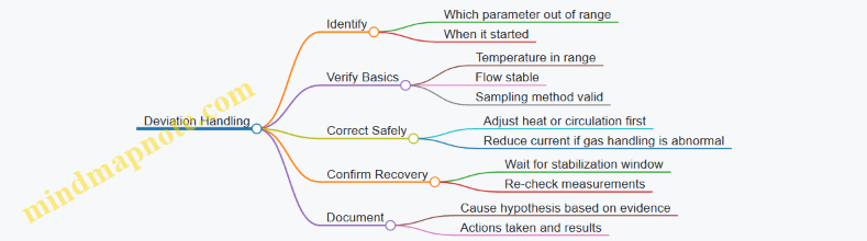
Completion Criteria
The shift is complete when the cell is in the defined safe state, all required measurements are recorded, and any deviations have documented corrective actions and confirmation that parameters returned to within limits.