Energy Harvesting Technologies Explained
1. Energy Harvesting Fundamentals
1.1 Define Energy Harvesting and Distinguish It from Energy Storage
Energy harvesting is the process of converting energy that already exists in the environment into usable electrical power. The key word is conversion: you start with motion, heat, or light, and you end with electricity that can run a circuit. Energy storage, by contrast, is the process of holding electrical energy for later use. Storage does not create energy; it buffers it.
A simple way to separate the two is to ask two questions. First: “Where does the energy come from?” Harvesting answers that. Second: “How long can the system keep operating when the source is weak or absent?” Storage answers that. A device can do one without the other, but most real systems use both because ambient sources are irregular.
Core Definitions in Practical Terms
Energy harvesting typically includes a transducer and a power-conditioning path. The transducer turns an environmental input into electrical output. Power conditioning then rectifies, regulates, and manages that output so it matches the needs of the load or the storage element.
Energy storage typically includes a component that stores charge or chemical energy, plus charge management circuitry. Storage smooths out gaps between energy arrivals and provides current bursts when the load wakes up.
Why the Distinction Matters
If you mix up harvesting and storage, you can mis-size the system. For example, a harvester might produce only a few microwatts on average, but the load might require tens of milliwatts for a short time. Storage is what makes that mismatch survivable.
Another common confusion is efficiency accounting. Harvesting efficiency describes how much of the environmental input becomes electrical output at the harvester terminals. Storage efficiency describes how much of that electrical energy remains after charging and later discharging. Both matter, but they apply to different stages.
Mind Map: Harvesting Versus Storage
Concrete Example: Door Sensor with Intermittent Motion
Imagine a wireless door sensor that wakes when the door moves. The motion harvester produces electrical energy only during movement. If the sensor tried to power itself directly from the harvester output, it would likely fail because the electrical output is brief and may not reach the voltage level needed for the radio.
With storage, the harvester charges a supercapacitor during motion. Later, when the sensor needs to transmit, it draws from the stored energy. In this setup, the harvester answers “How do we get energy from the door movement?” Storage answers “How do we run the radio after the movement ends?”
Concrete Example: Thermoelectric Module and the Heat-Flow Reality
A thermoelectric generator converts a temperature difference into electricity. If the temperature gradient collapses, the harvester output drops immediately. Storage can keep the system running for a while, but it cannot compensate for a complete absence of heat flow indefinitely.
This is the practical boundary: storage can delay downtime, not eliminate it. The harvester determines whether energy is available at all; storage determines how long the system can tolerate the gaps.
A Quick Distinction Checklist
- If the component converts motion, heat, or light into electrical output, it is part of energy harvesting.
- If the component stores electrical energy for later discharge, it is part of energy storage.
- If the system still works when the ambient source is absent, storage is doing the work during that interval.
- If the system cannot generate electricity when the ambient source is present, the harvesting stage is the limiting factor.
Mini-Model: Energy in, Energy Out
Think in terms of energy flow over time. Harvesting produces electrical energy from an external input, but it is often intermittent and low power. Storage accumulates that energy and releases it to the load. The load’s energy demand is met only when the harvested energy, after conversion and storage losses, exceeds the load’s consumption over the relevant time window.
1.2 Identify Ambient Energy Sources and Match Them to Device Types
Before picking a harvester, list what energy is actually present in the environment and what the device needs to do with it. “Ambient” usually means the source is not under your control, so the match is about timing, magnitude, and electrical behavior—not just physics.
Step 1: Classify the Source by How It Changes over Time
Motion, heat, and light each vary differently:
- Motion changes with movement events and often comes in bursts.
- Heat depends on temperature gradients and can be steady or intermittent depending on contact and airflow.
- Light depends on illumination level, angle, and whether something blocks it.
A good match starts with the device’s duty cycle. A sensor that wakes for 50 ms every minute can tolerate intermittent energy; a device that must stream continuously cannot.
Step 2: Map Source Characteristics to Harvester Types
Use this practical mapping to avoid common mismatches.
| Ambient Source | Typical Variability | Best-Fit Harvester Types | Device Types That Fit Well |
|---|---|---|---|
| Human motion (walking, tapping, vibration) | Bursty, event-driven | Piezoelectric, electromagnetic, hybrid motion | Footstep counters, door sensors, wearable buttons |
| Machinery vibration | Periodic with load changes | Piezoelectric, electromagnetic | Condition monitoring, rotating equipment tags |
| Temperature difference (skin-to-air, pipe-to-room) | Often steady with slow changes | Thermoelectric | Temperature logging, valve position tags |
| Rapid heating/cooling cycles | Transient spikes | Pyroelectric, phase-change concepts | Surface-touch indicators, intermittently heated surfaces |
| Indoor lighting (office, hallway) | Slow changes, often dim | Photovoltaic, photosensor-based | Low-power beacons, occupancy sensing |
| Sunlight | Strong but angle-dependent | Photovoltaic | Outdoor signage, field instruments |
| Flicker and shadowing from movement | Fast interruptions | Photovoltaic with storage, photosensor harvesting with buffering | Devices that can buffer energy and tolerate brief outages |
Step 3: Match Electrical Output to Power Management Needs
Even when the physics is right, the electrical interface can make or break the design.
- Piezoelectric and electromagnetic motion often produce higher voltage but limited energy per event, so the power stage must handle intermittent input efficiently.
- Thermoelectric output is typically low voltage and low power, so the system must minimize losses and use careful thermal-to-electrical conversion.
- Photovoltaic and photosensor harvesting can produce usable power under light, but the output depends heavily on optical conditions and requires conversion that works across a wide input range.
A simple rule: if the harvester output is low voltage, your rectifier and converter losses matter more than you expect.
Mind Map: Source-to-Device Matching Logic
Example: Choosing Motion vs Light for a Hallway Sensor
A hallway occupancy sensor must report when someone enters and then sleep. If the sensor is mounted near a door and people pass by irregularly, motion energy is likely bursty but frequent enough. If it is mounted high on a wall where people rarely get close, motion coupling may be weak. In that case, indoor light harvesting becomes more reliable because illumination is present most of the day.
Practical check: estimate how often the device must transmit and compare that to expected energy events. If motion events are rare or weak, the system will spend more time waiting for enough energy than it spends sensing.
Example: Choosing Thermoelectric vs Pyroelectric for a Pipe Tag
A tag on a warm pipe in a building experiences a temperature difference relative to the room. That gradient changes slowly, so a thermoelectric approach matches the steady nature of the input. If instead the tag is attached to a surface that gets heated briefly and then cools quickly, the temperature change happens in short intervals, which is where pyroelectric behavior can be advantageous.
Practical check: measure or approximate the temperature profile over time. If the gradient is mostly constant, thermoelectric is a cleaner match; if the device sees sharp temperature swings, pyroelectric extraction can align better with the timing.
Example: Matching Light Harvesting to a Power Budget
Two devices both “need 10 mW average,” but one can buffer energy and the other cannot. A photovoltaic system can handle brief shading if storage is sized so the device can keep running during outages. A photosensor-based approach can be effective when light is low but must still be paired with conversion that works at the actual photocurrent levels.
Practical check: treat light as a time series. If the device’s operation window overlaps with frequent shadowing, you need either more storage or a different source.
Step 4: Use a Simple Selection Checklist
- What sources are present where the device will be installed?
- How does the source change over time relative to the device’s wake and transmit schedule?
- Does the harvester’s electrical output match the power stage’s loss tolerance?
- Is the device allowed to buffer energy during interruptions?
When these answers line up, the “match” is not just plausible—it’s testable.
1.3 Quantify Power Budgets with Realistic Load Profiles
A power budget is only useful if it matches how the device actually behaves. “Average power” is a start, but the real constraint is usually the peak current during a burst, the energy during long quiet periods, or both. The goal of this section is to turn a vague requirement like “runs for months” into numbers you can design around.
Step 1: List Loads as Events, Not Just Components
Treat each activity as an event with a duration and a current. Typical event categories include sensing, processing, radio transmit/receive, display updates, and sleep. For each event, record:
- Current during the event I_event
- Duration of the event t_event
- Frequency of the event (N per day or per hour)
Example: A motion tag that wakes on motion, samples an accelerometer, sends a short radio packet, then returns to sleep.
Step 2: Compute Energy per Event
Energy per event is:
- E_event = V * I_event * t_event
If you prefer to work in power first, use P_event = V * I_event, then E_event = P_event * t_event. Use the supply voltage your power stage actually delivers to the load, not just the battery nominal voltage.
Example numbers (3.3 V system):
- Sleep: I_sleep = 5 µA, continuous
- Wake + sample: I_sample = 2 mA, t_sample = 20 ms
- Radio transmit: I_tx = 40 mA, t_tx = 80 ms
- Total wake time is not “sum of currents,” it’s the sum of time spent in each mode.
Step 3: Convert to Daily Energy and Average Power
For event-based loads:
- E_day = E_sleep + Σ(E_event * N_event)
- E_sleep = V * I_sleep * 86400
- Average power: P_avg = E_day / 86400
Example: Suppose the device transmits 60 times per day.
- E_sleep = 3.3 V * 5e-6 A * 86400 s = 1.43 kJ/day
- E_sample = 3.3 * 2e-3 * 0.02 = 0.132 mJ per wake
- E_tx = 3.3 * 40e-3 * 0.08 = 10.56 mJ per transmit
- E_day = 1.43 kJ + 60*(0.132 mJ + 10.56 mJ) = 1.43 kJ + 634 mJ ≈ 2.06 kJ/day
- P_avg = 2.06 kJ / 86400 s ≈ 23.8 mW
This average power is what your energy harvesting system must supply over time, after accounting for conversion losses.
Step 4: Check Peak Current and Minimum Energy Windows
Energy budgets don’t guarantee the device can start. Many harvesters produce energy slowly, but the load may demand a fast current spike. You must check:
- Peak current requirement I_peak
- Minimum energy needed to cross the power-stage threshold E_start
- Storage capacity to ride through low-input intervals
Example: If the radio needs 40 mA for 80 ms, the storage must provide that current without the voltage collapsing below the regulator’s dropout. A quick sanity check uses required energy during the burst:
- E_burst = V * I_tx * t_tx = 3.3 * 0.04 * 0.08 = 10.56 mJ If your storage can’t deliver that, the radio will brown out even if the average power looks fine.
Step 5: Include Realistic Duty Cycles and “Hidden” Costs
Common omissions:
- Wake-up overhead: interrupts, clock start, and sensor warm-up
- Radio receive windows: listening for acknowledgments
- Debug or calibration modes: sometimes left enabled during testing
A practical habit is to measure current profiles with a current probe or a shunt and then map the waveform into events. If you can’t measure yet, start with conservative durations and currents, then tighten later.
Mind Map: Power Budget Inputs and Outputs
Example: From Requirements to a Load Table
Requirement: “Send one status update every 10 minutes, and sample temperature each time.” Assume 3.3 V.
Event table:
- Sleep: 5 µA, 24 hours
- Temperature sample: 2 mA for 15 ms, 144 times/day
- Radio transmit: 40 mA for 70 ms, 144 times/day
Compute:
- E_sleep = 3.3 * 5e-6 * 86400 = 1.43 kJ/day
- E_sample/day = 3.3 * 2e-3 * 0.015 * 144 ≈ 0.143 kJ/day
- E_tx/day = 3.3 * 40e-3 * 0.07 * 144 ≈ 1.33 kJ/day
- E_day ≈ 2.90 kJ/day, P_avg ≈ 33.6 mW
Peak check:
- E_burst = 3.3 * 0.04 * 0.07 ≈ 9.24 mJ per transmit
- Ensure storage and power stage can deliver 40 mA for 70 ms without voltage collapse.
A good power budget ends with two numbers: the average power you need over a day (or the relevant cycle) and the burst energy/current you must survive during each active window.
1.4 Select System Architectures for Intermittent Energy Availability
Intermittent energy means the input power arrives in bursts, pauses, or slow ramps. The architecture’s job is to turn that messy input into a predictable supply for sensing, computing, and communication—without wasting most of the harvested energy in conversion losses or protection circuits.
Start with Operating Modes and Energy “Weather”
Before choosing circuits, write down the device’s modes: idle sensing, active measurement, radio transmit, and sleep. Then estimate how energy arrives for each source.
A practical way to reason is to create a simple table of “energy weather” for each mode:
- Motion: short peaks during movement, near-zero otherwise.
- Heat: slower changes; power depends on temperature gradient and thermal contact.
- Light: often steady indoors, bursty outdoors due to angle and shading.
Example: A door sensor might wake from motion, sample a switch state, and transmit once. If the motion harvester only produces energy during a door swing, the system must store enough energy to finish the transmit even after the swing ends.
Choose Between Direct-Run and Store-Then-Run
There are two common architectural families.
Direct-run powers the load as soon as input is available. It’s simple, but it couples your load timing to the harvester’s instantaneous output.
Store-then-run uses an energy buffer so the load runs on stored energy. It decouples timing and usually improves reliability.
Best practice: If your load includes a high-energy step (radio transmit, heater, display), prefer store-then-run. If your load is tiny and tolerant of delays (a low-rate sensor read), direct-run can work.
Use a State Machine with Explicit Guard Conditions
Intermittent energy systems should not “hope” they have enough power. They should check.
A robust pattern is a state machine with guard conditions based on buffer voltage or an energy estimate.
- Sleep: minimal draw.
- Harvesting: buffer charges.
- Ready: buffer voltage indicates enough energy for the next action.
- Execute: run the action with a fixed energy budget.
- Recover: if energy drops early, return to harvesting.
Example: For a motion sensor, set a “ready” threshold slightly above the minimum voltage required for the radio’s transmit peak current. If the threshold is not met, skip transmit and only log locally.
Pick Buffer Type and Size to Match the Load Shape
Energy buffers are not interchangeable because loads draw power in different shapes.
- Supercapacitors: good for fast bursts and many charge-discharge cycles. They tolerate frequent harvesting pauses.
- Batteries: good for long-term storage and stable voltage, but require careful charging control.
Example: A light-harvested tag that transmits once per minute can use a small supercapacitor if indoor light is steady and the transmit burst is short. A thermoelectric sensor that only slowly accumulates energy may need a larger buffer to cover the time between temperature changes.
Decide How to Combine Multiple Energy Sources
Multi-source systems can be wired in ways that either cooperate or fight.
Common approaches:
- Parallel with isolation: each source charges the same buffer through isolation elements (prevents one source from discharging another).
- Separate buffers with a selector: each source has its own buffer, and the system chooses which buffer to use.
- Hybrid: one source charges the main buffer, another directly supports short bursts.
Best practice: If one source is “strong but brief” (motion) and another is “weak but steady” (light indoors), use isolation and a main buffer that the steady source can keep topped up. Then let the brief source cover the extra energy needed for a transmit.
Mind Map of Architecture Choices
Mind Map: System Architectures for Intermittent Energy
Example: Motion-Triggered Sensor with a Radio
Assume the device must transmit 200 ms at a peak current that the harvester cannot sustain continuously.
- Use store-then-run.
- Add a supercapacitor sized so the buffer voltage stays above the radio’s minimum during the transmit window.
- Implement a state machine: only enter “Execute” when buffer voltage exceeds the transmit-ready threshold.
- If the threshold is missed, skip transmit and return to harvesting.
This avoids the common failure mode where the system starts transmitting, the buffer sags, and the radio resets mid-packet.
Example: Thermoelectric Sensor with Slow Energy Accumulation
Thermoelectric output depends on temperature gradient and contact quality, so energy arrival can be gradual.
- Use a larger buffer than you would for motion.
- Prefer a longer measurement interval so the system can accumulate enough energy for the next action.
- Use guard conditions so the system does not attempt a high-energy step until the buffer indicates readiness.
The architecture here is less about reacting instantly and more about making sure the next action completes once started.
Quick Selection Checklist
- Does the load include a peak current event? If yes, store-then-run.
- Is energy arrival bursty or slow? Size the buffer and thresholds accordingly.
- Are multiple sources present? Add isolation or separate buffers to prevent backflow.
- Can you define a “ready” condition that correlates with successful execution? If not, refine the buffer sensing or reduce the action’s energy budget.
1.5 Establish Efficiency Metrics and Measurement Practices
Efficiency in energy harvesting is not one number. It’s a chain of conversions, each with its own losses, plus a measurement method that can accidentally “lose” power in the lab. The goal of this section is to define metrics that map to real behavior and to describe measurement practices that produce numbers you can trust.
Define Efficiency Metrics That Match the Conversion Chain
Start by separating three layers of efficiency.
- Transduction efficiency: how well the harvester turns the physical stimulus into electrical power at its electrical terminals.
- Example: A piezo element converts vibration into charge; transduction efficiency depends on mechanical coupling, resonance, and charge extraction.
- Power conversion efficiency: how well the power electronics convert the harvester’s electrical output into usable energy for the load or storage.
- Example: A buck converter may be efficient at mid input voltage but wasteful near startup or at very low input power.
- System efficiency: how much energy ends up doing useful work compared to the energy available from the environment.
- Example: If your device wakes a sensor, transmits once, then sleeps, system efficiency includes the energy spent on switching, sensing, and communication.
Use metrics that reflect these layers:
- Instantaneous power efficiency: \(\eta(t)=\frac{P_{out}(t)}{P_{in}(t)}\) when both are measurable.
- Energy efficiency over a cycle: \(\eta_{cycle}=\frac{E_{out}}{E_{in}}\) where \(E=\int P,dt\). This is often more stable than instantaneous ratios.
- Harvesting yield: energy delivered to storage per unit time under a defined stimulus profile, such as “per hour of indoor light” or “per minute of walking.”
A practical rule: if you cannot measure \(P_{in}\) directly, report efficiency as a conversion ratio between measurable electrical quantities (for example, harvester electrical output vs. storage charge energy) and label it clearly.
Choose Measurement Points That Avoid Hidden Losses
Decide where “input” and “output” are measured. Common measurement points are:
- Harvester electrical terminals: best for transduction efficiency.
- Converter input and output: best for power conversion efficiency.
- Storage terminals: best for system-level yield.
Hidden loss examples:
- Measuring at the converter input but forgetting rectifier diode drops can make the converter look worse than it is.
- Measuring storage current without accounting for voltage-dependent charge acceptance can make the storage look inefficient.
Use consistent wiring and measurement bandwidth. For intermittent harvesters, a slow multimeter can miss peaks and undercount energy.
Establish a Stimulus Profile and Keep It Repeatable
Efficiency depends on how the stimulus is applied.
- For motion: define amplitude, frequency, and direction. A piezo harvester tuned for 2 Hz may look “inefficient” at 5 Hz.
- For heat: define temperature gradient and thermal contact quality. A loose clamp changes thermal resistance and shifts output.
- For light: define illuminance, spectrum if relevant, and angle.
Repeatability practice: run at least three trials and report mean and spread. If spread is large, fix the stimulus or the mechanical/thermal contact before trusting any efficiency number.
Measure Energy Correctly Under Intermittent Operation
Many harvesters produce bursts. In that case, measure energy rather than relying on average power alone.
Recommended practice
- Log voltage and current at the measurement point.
- Compute energy by numerical integration over the full event window.
- Ensure the sampling rate captures the fastest relevant switching or waveform features.
Example Suppose a harvester delivers 40 mW peak for 10 ms every second. Average power is 0.4 mW, but energy per second is \(40,\text{mW}\times 10,\text{ms}=0.4,\text{mJ}\). If your load only wakes during those bursts, energy per event is the metric that predicts battery or supercapacitor behavior.
Use Calibration and Sanity Checks
Calibration prevents “measurement efficiency” from becoming the dominant error.
- Calibrate current shunts or current probes using a known load.
- Verify voltage probe grounding and avoid ground loops.
- Sanity check by comparing computed energy to what the storage voltage change implies.
Example sanity check If storage energy increases by \(\Delta E=\tfrac{1}{2}C(V_2^2-V_1^2)\) for a capacitor, but your logged energy at the converter output is far higher, you likely have measurement range issues, bandwidth limits, or a mismatch in where you measured.
Mind Map of Efficiency and Measurement
Mind Map: Efficiency Metrics and Measurement Practices
A Compact Example Workflow
- Pick the metric: start with energy delivered to storage per event.
- Instrument the system at the storage terminals and at the converter output.
- Apply a repeatable stimulus profile for at least three trials.
- Integrate logged waveforms to compute \(E_{storage}\) and \(E_{conv,out}\).
- Compute conversion ratio \(\eta_{conv}=E_{conv,out}/E_{harv,out}\) if harvester output is logged too.
- If results vary widely, fix contact quality or mechanical alignment before comparing designs.
This approach keeps the numbers tied to what the device actually experiences, and it makes it easier to explain why one design performs better without guessing where the losses went.
2. Motion Energy Harvesting with Electromagnetic and Piezoelectric Converters
2.1 Model Mechanical Excitation and Convert It into Electrical Work
Mechanical-to-electrical energy harvesting is mostly bookkeeping: you start with motion, translate it into mechanical power at the transducer, then translate that into electrical power at the terminals. The tricky part is that real motion is rarely a clean sine wave, and the transducer rarely behaves like an ideal spring.
Mechanical Excitation as Inputs
Treat the mechanical side as a source of displacement, velocity, or force. Pick the variable you can measure or estimate.
- Displacement input: common for piezo beams and resonant structures. Example: a door-mounted sensor that deflects a springy arm by a few millimeters during each opening.
- Velocity input: common for electromagnetic generators where induced voltage relates to speed. Example: a wheel with a magnet moving past a coil.
- Force input: common when the motion is constrained and you can estimate contact forces. Example: a footstep pressing on a pad.
A practical modeling workflow starts with a motion record. If you have a time series \(x(t)\), compute velocity \(v(t)=dx/dt\) and acceleration \(a(t)=d^2x/dt^2\). If you only have peak values, you can still estimate energy per event, but you must be explicit about assumptions.
Energy per Event and Average Power
For intermittent motion, energy per event is often more useful than average power.
-
Energy per event: \[ E_{mech} = \int F(t),dx(t) \] If you know force and displacement, this integral is direct. If you only know displacement and the structure behaves approximately linear, you can approximate force as \( F \approx kx \) and get \(E \approx \int kx,dx = \tfrac{1}{2}k x_{pk}^2\) for a full cycle.
-
Average mechanical power: \[ P_{avg} = E_{mech} \cdot f_{event} \] where \(f_{event}\) is events per second.
A key best practice is to separate motion energy from transducer energy. Motion energy includes what you lose in bearings, friction, and compliance elsewhere. Your model should include those losses, or you will overestimate electrical output.
Mechanical Model of the Transducer Interface
Most harvesters can be approximated as a mass-spring-damper system with an electromechanical coupling term.
- Mass \(m\): effective moving mass.
- Stiffness \(k\): spring constant of the structure and mounting.
- Mechanical damping \( c_m \): losses in material and friction.
- Electrical damping \( c_e \): the part of damping caused by electrical load extraction.
The transducer converts mechanical motion into electrical effects by adding an electrical load that changes the effective damping. That is why “same motion, different load” can produce different harvested power.
From Mechanical Power to Electrical Power
Mechanical power delivered to the transducer is the rate of work done on the mechanical port.
- Instantaneous mechanical power: \[ P_{mech}(t) = F(t),v(t) \]
- Average mechanical power over an interval: \[ P_{mech,avg} = \frac{1}{T}\int_0^T F(t),v(t),dt \]
Electrical power depends on the transducer type.
- Electromagnetic: induced voltage \(V\) is proportional to velocity. Electrical power into a load \( R_L \) is \(P_{elec}=V^2/R_L\) after accounting for coil resistance and back-emf effects.
- Piezoelectric: charge and voltage relate to strain and stress. Electrical power depends on the charge extraction circuit and the effective electrical damping.
A concrete modeling habit: compute power in two steps—first power at the mechanical port, then power delivered to the electrical load. If the second step is missing, you will treat the transducer like a perfect energy converter, which it is not.
Mind Map of the Modeling Chain
Example: Door Opening as a Motion Event
Assume a door-mounted harvester experiences a displacement pulse: the arm moves from 0 to \( x_{pk}=3,\text{mm} \) and returns over about \( 0.6,\text{s} \). If the effective stiffness is \( k=200,\text{N/m} \) and the motion is roughly symmetric with small losses in the structure itself, the mechanical energy per event is approximately
\[ E_{mech} \approx \tfrac{1}{2}k x_{pk}^2 = \tfrac{1}{2}\cdot 200\cdot (0.003)^2 = 0.0009,\text{J} \]
If the door opens \(f_{event}=0.2,\text{Hz}\) (one opening every 5 seconds), then
\[ P_{mech,avg} \approx 0.0009\cdot 0.2 = 0.00018,\text{W} = 0.18,\text{mW} \]
Now include extraction efficiency. Suppose the electrical load and transducer coupling capture only 30% of mechanical energy as electrical power due to damping and conversion losses. Then
\[ P_{elec,avg} \approx 0.3\cdot 0.18,\text{mW} = 0.054,\text{mW} \]
This example shows why you should model both the mechanical energy available and the fraction that becomes electrical power. The motion might look “small,” but the energy per event can still be meaningful; the load might look “reasonable,” but it can drastically change how much energy is actually extracted.
Example: Resonant Tuning and Load-Dependent Damping
Consider a resonant electromagnetic generator tuned near the dominant motion frequency. If you increase the electrical load resistance, the electrical damping decreases, so the system moves more but extracts less electrical power per cycle. If you decrease the resistance too far, electrical damping increases, the motion amplitude drops, and electrical power can also fall. Modeling helps you find the balance by predicting how the load changes the effective damping and therefore the mechanical power delivered to the transducer.
A practical best practice is to run a sensitivity check: vary \(k\) and \( c_m \) within plausible tolerances and observe how the predicted electrical power changes. If the result swings wildly, you need a more robust mechanical design or a better estimate of the real damping.
2.2 Electromagnetic Generators Design and Key Loss Mechanisms
Electromagnetic generators turn mechanical motion into electrical power using electromagnetic induction. The core design goal is simple: maximize useful electrical output while keeping mechanical losses low enough that the harvester still “pays” for the energy it takes from the environment.
Generator Types and What They Imply
Most small motion harvesters use either a moving-magnet or moving-coil approach.
- Moving magnet: a magnet moves relative to a stationary coil. This is common because the coil can be packaged easily and the moving mass can be kept compact.
- Moving coil: the coil moves through a magnetic field. This can reduce some parasitics, but it often complicates wiring and mechanical integration.
A practical rule: choose the configuration that minimizes friction and wiring complexity for your mechanical layout, then optimize the magnetic circuit for the motion you actually expect.
Electromagnetic Design: The Induction Chain
Induced voltage depends on three linked factors: magnetic flux density, rate of change of flux, and effective coil turns.
- Magnetic flux density (B): stronger fields increase induced voltage, but magnets saturate nearby iron and too-tight gaps can increase mechanical drag.
- Rate of change: if the motion is slow or mostly linear with little flux variation, voltage drops. That’s why geometry matters as much as magnet strength.
- Coil turns and geometry: more turns increase voltage, but they also increase resistance and parasitic capacitance, which can reduce power at higher frequencies.
A useful design workflow is to start with the expected displacement and frequency, then estimate the induced open-circuit voltage waveform. After that, you size the coil resistance and the electrical load so the generator operates near the point where electrical damping helps rather than hurts.
Key Loss Mechanisms and How They Show Up
Losses are not just “waste”; they change the generator’s behavior, including its effective damping and the voltage you can actually rectify.
-
Copper (Ohmic) loss: coil resistance converts electrical power into heat. It reduces terminal voltage under load and lowers harvested energy. Example: if your coil is 200 mΩ and the load draws 50 mA peak during part of the cycle, the instantaneous loss is I²R = 0.05² × 0.2 = 0.0005 W at that moment.
-
Core and magnetic losses: if you use iron cores, hysteresis and eddy currents can consume power, especially at higher motion frequencies. Example: a laminated core reduces eddy currents compared to a solid core, which can matter when the harvester sees rapid motion.
-
Mechanical losses: bearing friction, air drag, and internal damping reduce the mechanical energy available for induction. Example: a poorly aligned guide rail can add enough friction that the harvester’s electrical output drops even though the magnetic design looks fine.
-
Magnet losses and demagnetization risk: strong fields can push magnets toward operating limits, and temperature can reduce magnet strength. Even without “catastrophic” failure, weaker magnet flux reduces induced voltage.
-
Electrical damping mismatch: the generator’s electrical load reflects back as damping. If the load is too high, the generator produces voltage but little current; if too low, it drags mechanically. Example: a rectifier plus storage capacitor can make the effective load vary during the cycle, so the “best” load is not a single resistor value.
-
Eddy currents in nearby conductors: aluminum housings or conductive brackets near the moving magnet can create opposing fields. Example: placing a magnet near a thick metal plate can reduce output without any obvious electrical reason.
Electrical Interface: Load Matching Without Overpromising
Electromagnetic generators are often modeled as a voltage source in series with coil resistance. The harvested power depends on how the rectifier and storage stage draw current.
A practical approach is to treat the electrical interface as a load that changes with time. During motion peaks, the generator can deliver higher current; during low-voltage parts of the cycle, the rectifier may stop conducting.
To design for this, you can:
- estimate the generator’s peak open-circuit voltage and internal resistance
- choose a rectifier with low forward loss for the expected voltage range
- ensure the storage stage doesn’t demand more current than the generator can supply during short motion events
Mind Map: Electromagnetic Generator Design and Losses
Example: Why “More Turns” Can Reduce Power
Suppose you increase coil turns by 30%. Induced voltage rises roughly proportionally, but coil resistance also rises. If resistance increases from 200 mΩ to 260 mΩ, and the rectifier and storage stage effectively limit current, the extra voltage may not translate into more harvested energy. The generator might spend more of the cycle at voltages that don’t overcome rectifier thresholds, especially if motion amplitude is modest.
A better strategy is to compare power at the expected motion amplitude rather than comparing open-circuit voltage. Measure or simulate the terminal voltage under a realistic rectifier and storage load, then compute energy per cycle.
Example: Detecting Eddy Currents in a Metal Housing
If output is lower than expected, check for conductive structures near the moving magnet. A simple test is to temporarily insert a non-conductive spacer between the magnet path and the housing wall. If power increases noticeably, you likely had eddy-current drag. After confirming, you can redesign with increased clearance, thinner conductive sections, or non-conductive materials.
Design Takeaway
Good electromagnetic generator design is a balancing act between magnetic strength, coil resistance, and the electrical interface that turns induced voltage into usable current. Loss mechanisms are easiest to manage when you treat the generator as a coupled mechanical-electrical system, not a standalone coil with a magnet attached.
2.3 Piezoelectric Harvesters Design and Charge Collection Basics
Piezoelectric harvesters turn mechanical strain into electrical charge. The core design job is to make the mechanical part produce useful strain at the right frequency, then make the electrical part collect that charge efficiently without wasting it in the wrong places.
Piezoelectric Transduction Essentials
A piezo element behaves like a charge source in parallel with a capacitance. When it bends or compresses, it generates charge proportional to strain. That means your electrical output depends on both the mechanical strain level and the electrical load you connect.
Two practical implications follow. First, the piezo’s capacitance is not a small detail; it sets how much charge becomes voltage under a given load. Second, the harvester’s “best” electrical behavior changes with frequency because the mechanical system and the electrical interface interact.
Mechanical-to-Electrical Matching with a Simple Model
A common starting point is to treat the piezo as a capacitance Cp with a charge source that depends on strain. If you connect a load, the voltage across the piezo rises when the load is high impedance and drops when the load is low impedance. Power is maximized when the electrical damping introduced by the interface helps the mechanical system extract energy, rather than simply shorting the piezo.
A quick mental check: if your interface makes the piezo behave like a near-short circuit, you may get large current but low voltage, and the power can still be poor because the mechanical system loses energy in a way that doesn’t translate to usable electrical work.
Charge Collection with Rectification
Piezo output is typically alternating polarity. To store energy, you need rectification. The simplest approach is a full-wave bridge rectifier, which flips negative voltage so the storage element always sees the same polarity.
However, bridge rectifiers have diode drops, and those drops matter when the piezo voltage is modest. Two design practices help:
- Use low-threshold switching: Replace standard diodes with MOSFET-based synchronous rectification or low-loss switches when voltages are small.
- Control the conduction window: Ensure the rectifier conducts only when the piezo voltage exceeds the threshold needed to move charge into the storage path.
Energy Storage and the “Don’t Starve the Piezo” Rule
After rectification, energy goes into a storage element such as a capacitor or supercapacitor. If the storage voltage is too high, the piezo may not be able to push charge into it, even when it is generating charge internally.
A practical rule: design the storage voltage range so that the piezo interface can still transfer charge during typical operating motion. For intermittent motion, consider a storage capacitor that can accept energy in small bursts, then feed the load when enough energy accumulates.
Interface Topologies That Matter
1. Direct Rectifier Into Storage
This is the simplest: full-wave rectification into a capacitor. It works well when piezo voltages are high enough to overcome switch losses.
2. Synchronized Switching for Better Utilization
Synchronized switching changes the electrical boundary condition at the right moment in the AC cycle. The goal is to keep the piezo from “wasting” energy by letting it discharge into the wrong impedance.
3. Resonant or Buck-Style Power Stages
These can improve efficiency when you need a regulated output, but they add complexity and require careful tuning to the piezo’s operating range.
Example: Designing a Charge Collection Stage for a Low-Voltage Piezo
Assume a piezo element that produces about 5 V peak-to-peak under expected motion. A standard diode bridge might lose roughly 1.4 V per conduction path (two diode drops in a bridge), leaving little voltage headroom for charging.
A better approach is a MOSFET-based full-wave rectifier with low on-resistance. If the MOSFET drop is, say, 0.2 V at the relevant current, the piezo can still charge the storage capacitor effectively.
Design steps:
- Estimate the minimum piezo voltage during normal motion.
- Estimate the storage capacitor voltage you expect at the moment of charging.
- Choose a rectifier whose effective voltage loss is small compared to the available headroom.
- Verify with a bench test using the same mechanical excitation you plan to use in the product.
Mind Map: Piezo Charge Collection Design
Example: Checking Whether Your Interface Can Actually Charge
Suppose your storage capacitor sits at 3.8 V during operation. Your piezo produces 4.0 V peak and the rectifier has an effective loss of 0.3 V at the charging current. The available headroom is 4.0 V − 3.8 V − 0.3 V = −0.1 V, meaning charging barely happens or stops.
The fix is not “try harder”; it’s to change one of the constraints:
- Reduce storage voltage by using a larger capacitance with a lower initial charge strategy.
- Lower interface losses with better switching.
- Increase piezo voltage by adjusting mechanical resonance or geometry.
This kind of arithmetic is boring, but it prevents a common failure mode: a design that looks fine on paper yet never transfers meaningful charge in the real operating range.
2.4 Interface Circuits for Piezo Energy Extraction Under Variable Loads
Piezo harvesters are happiest when the electrical load “looks right” to the mechanical motion. Under variable loads—different user activity, changing mounting conditions, or intermittent system wake-ups—the interface circuit must keep the piezo from either wasting energy as heat or starving it by presenting an incorrect impedance.
What “Variable Load” Means in Practice
A piezo element produces charge when it bends. The interface decides what happens to that charge: it can be collected into a useful voltage, dissipated, or partially stored. In real systems, the load is not constant because the rest of the device cycles between sleep, sensing, and radio transmission. That means the effective electrical demand seen by the piezo changes over time.
A useful mental model is: the piezo behaves like a current source in parallel with a capacitance. If the circuit clamps the voltage too tightly, the piezo current has nowhere to go except through losses. If the circuit lets the voltage rise too high without drawing current, the piezo current drops and you get less energy overall.
Core Interface Goals
- Match energy extraction to available motion. When motion is weak, you want the circuit to draw current at lower voltages. When motion is strong, you must avoid overvoltage.
- Minimize conversion losses. Rectifiers and switching stages should not burn most of the harvested energy.
- Provide a stable output for the power stage. The downstream regulator and storage need a predictable input range.
Rectification and Storage: The Baseline That Still Matters
The simplest interface is a bridge rectifier feeding an energy storage element (often a supercapacitor). This works because piezo output is alternating in polarity. The bridge ensures the storage sees a unidirectional voltage.
Best practice: use a rectifier topology that fits your voltage level. If the piezo voltage is low, diode drops can be a large fraction of the output. In that case, consider a synchronous rectifier or a low-drop implementation. If the piezo voltage is high, diode losses shrink relative to the available voltage.
Example: A small piezo attached to a door hinge produces brief pulses when the door opens. With a bridge rectifier and a supercapacitor, the system can accumulate energy during the pulse and then power a short sensing burst. If the supercapacitor is too large, the voltage rise per pulse is small and the regulator may never reach its minimum operating point.
Impedance Matching via Active Control
For better extraction, the interface can emulate an “optimal” electrical load. The key idea is that the piezo’s electrical impedance affects the mechanical damping. Too much damping reduces motion; too little damping reduces charge flow.
A practical approach is switching between capture and relaxation states. During capture, the circuit draws current to keep the piezo voltage near a target range. During relaxation, it stops drawing current so the piezo can recharge or the system can process stored energy.
Example: A wearable motion harvester might experience frequent small movements and occasional larger ones. If you always draw aggressively, small movements produce little energy because the piezo voltage never rises enough to overcome losses. If you always draw gently, large movements waste potential because the circuit clamps too early. A state machine that adjusts the draw based on measured piezo voltage (or storage voltage) improves consistency.
Charge Extraction with Resonant and Buck-Style Stages
Some interfaces use a resonant or quasi-resonant approach to transfer energy efficiently from the piezo capacitance into a storage element. Others use a buck-like converter that periodically transfers energy when the piezo voltage reaches a threshold.
Best practice: choose thresholds that align with the piezo’s typical peak voltage. If the threshold is above what weak motion can reach, the circuit does nothing until strong motion arrives, which can be too late for intermittent events.
Example: A floor tile harvester might generate higher voltage when someone steps firmly. If the interface only transfers energy when the piezo exceeds 20 V, light steps contribute nothing. Lowering the threshold increases participation, but you must ensure the converter still operates efficiently at the lower voltage.
Overvoltage Protection Without Killing Harvesting
Piezo interfaces often need protection because open-circuit voltage can be high. A common mistake is using a simple zener clamp that burns energy continuously during strong motion.
Better approach: use a clamp that only engages when necessary, and prefer energy-aware methods. For instance, you can route excess energy into storage through controlled switching rather than dissipating it.
Example: In a vibration environment, the piezo can spike above the regulator’s maximum input. A hard clamp limits the spike but wastes the energy that could have been stored. A controlled transfer stage can cap the voltage while still moving energy into the supercapacitor.
Practical Interface Architectures
1) Bridge Rectifier Plus Storage
- Works well for moderate voltage and simple systems.
- Add a controlled clamp to prevent excessive voltage.
2) Synchronized Rectification or Low-Loss Switching
- Reduces diode drops.
- Useful when piezo voltage is low.
3) Thresholded Energy Transfer with State Control
- Draws energy only when piezo voltage is in a useful range.
- Helps when motion is intermittent.
4) Active Impedance Matching
- Uses sensing and switching to emulate an effective load.
- Improves extraction across a wider range of motion amplitudes.
Mind Map: Piezo Interface Under Variable Loads
Example: A Simple State-Controlled Interface
Below is a conceptual control flow that avoids drawing energy when the piezo voltage is too low and prevents overvoltage when motion is strong.
Measure piezo voltage Vp and storage voltage Vs.
If Vp < V_low:
  Keep switches open to avoid losses.
Else if Vp between V_low and V_high:
  Enable energy transfer to storage.
Else if Vp > V_high:
  Enable protection path that transfers excess energy
  or limits voltage with minimal dissipation.
Update state and repeat on a fast timer.
This kind of logic is often enough to make extraction behave sensibly across changing motion and intermittent system demand.
Quick Design Checklist
- Confirm the piezo’s typical peak voltage under weak and strong motion.
- Ensure rectifier losses are small compared to the piezo voltage range.
- Set energy-transfer thresholds so weak motion contributes.
- Use overvoltage protection that limits voltage without permanently wasting energy.
- Size storage so the system can complete its wake cycle before the next energy burst.
2.5 Practical Mounting, Damping, and Resonance Tuning for Real Environments
Real environments rarely match the tidy assumptions of a lab setup. Mounting stiffness, added mass, friction, and temperature changes all shift the mechanical resonance and reduce how much motion reaches the transducer. The goal is simple: make the harvester experience the motion you think it will, and keep losses predictable.
Mounting That Transfers Motion Instead of Stealing It
Start with a mechanical “motion path.” If the harvester is bolted to a surface, the surface must actually move in the direction that excites the transducer.
- Use a rigid base for the fixed side. A loose bracket behaves like a spring in series, lowering effective stiffness and often detuning the system.
- Minimize compliance in the mounting interface. Rubber pads and soft adhesives can be useful for vibration isolation, but they also reduce transmitted acceleration. If you need isolation, isolate the whole assembly, not just the transducer.
- Avoid over-tightening. Excess clamp force can warp thin frames or change piezoelectric preload, altering output and sometimes causing hysteresis.
- Control added mass. A heavy enclosure can lower resonance frequency by increasing the moving system’s effective mass. If you must add mass, measure the shift rather than guessing.
Example: A piezo cantilever mounted to a plastic housing underperforms compared to a metal test rig. The plastic flexes, so the cantilever sees less strain. Switching to a stiffer mounting plate increases strain for the same external motion, improving output without changing electronics.
Damping That Limits Losses Without Killing Output
Damping converts mechanical energy into heat. Some damping is unavoidable, but too much damping reduces peak response and lowers harvested energy.
- Separate damping sources. Air drag, internal material losses, friction at joints, and electrical damping from the interface circuit all contribute.
- Reduce friction where motion is intended. If you use a sliding mass or a linkage, lubricate appropriately and keep contact surfaces smooth. Dry friction can turn smooth oscillation into stick-slip.
- Use damping intentionally for stability. For systems that experience irregular motion, moderate damping can prevent large excursions that cause impacts or fatigue.
- Match damping to the motion profile. If excitation is mostly low-frequency and intermittent, heavy damping can be worse than light damping because it prevents energy from building.
Example: A spring-mass electromagnetic harvester mounted with a felt pad shows lower output. The pad adds strong damping and reduces the amplitude of the moving mass. Replacing the pad with a thin, stiff spacer restores oscillation while still preventing rattling.
Resonance Tuning with Real Constraints
Resonance tuning is about aligning the system’s natural frequency with the dominant excitation frequency range. In practice, you tune for a band, not a single point.
- Tune stiffness first. For a simple spring-mass system, increasing stiffness raises resonance frequency; reducing stiffness lowers it. In cantilevers, geometry changes (length, thickness) are the main tuning knobs.
- Tune mass second. Adding a proof mass lowers resonance frequency. Keep added mass symmetric to avoid side loading.
- Tune damping last. Once resonance is near the target, adjust damping to control amplitude and bandwidth.
- Account for directionality. Many harvesters assume motion along one axis. If the real motion is angled, the effective excitation component drops.
Example: A motion harvester designed for footsteps is mounted on a strap that moves in multiple directions. The resonance frequency shifts and the effective excitation component decreases. Adding a guide that constrains motion along the intended axis improves consistency, even if the resonance frequency remains unchanged.
A Practical Tuning Workflow
- Measure the excitation spectrum. Use a phone accelerometer or a simple IMU on the mounting surface to estimate dominant frequencies during typical use.
- Estimate the current resonance. Gently excite the harvester in a controlled way and observe the decay rate and oscillation frequency.
- Adjust one parameter at a time. Change stiffness or geometry first, then mass, then damping. If you change everything at once, you won’t know what worked.
- Verify under representative mounting. Test with the final enclosure and fasteners. A “bench mount” can overestimate performance.
- Check for mechanical limits. Ensure the maximum displacement stays within safe bounds to avoid impacts and fatigue.
Mind Map: Mounting, Damping, Resonance
Quick Reference: What Usually Goes Wrong
- Soft mounting materials reduce strain or coil motion.
- Hidden compliance in brackets creates a second spring in series.
- Friction in moving parts turns oscillation into intermittent motion.
- Resonance tuned to the wrong axis because the device is mounted at an angle.
- Electrical interface mismatch increases effective damping and reduces mechanical amplitude.
Example: An electromagnetic harvester shows low output only when connected to the power stage. The interface circuit effectively loads the generator, increasing electrical damping. Adjusting the electrical load behavior restores mechanical amplitude and improves net harvested energy.
Summary
Good tuning is not just “set resonance to frequency.” It is ensuring the harvester experiences the right motion, controlling damping so energy can build without causing impacts, and validating performance with the actual mounting hardware and constraints that will be present in the field.
3. Motion Energy Harvesting with Electrostatic and Hybrid Approaches
3.1 Electrostatic Harvesters Operation and Capacitance Variation Requirements
Electrostatic energy harvesting turns mechanical motion into electrical energy by changing a capacitor’s geometry. The core idea is simple: when capacitance changes, charge and voltage can be managed so that electrical work is extracted instead of just moving energy back and forth.
How the Energy Gets Out
An electrostatic harvester typically uses a variable capacitor, such as a fixed plate facing a movable plate. As the gap changes, capacitance changes. The electrical energy available depends on how you control the capacitor’s charge or voltage during the motion.
There are two common operating styles:
- Charge-controlled approach: You trap charge on the capacitor during part of the motion. When capacitance increases, voltage drops, and the energy difference can be delivered to a circuit.
- Voltage-controlled approach: You keep the capacitor at (approximately) a fixed voltage using a power stage. When capacitance increases, the electrical energy drawn from the source can be converted to useful output.
In practice, most designs use a switching interface that approximates one of these behaviors at the right times.
Capacitance Variation Requirements
The mechanical motion must produce enough capacitance change to overcome losses in switching, leakage, and parasitic capacitances. A useful way to think about it is through the ratio between the variable capacitance and the total capacitance seen by the circuit.
Key requirements:
- Large relative capacitance swing: If the capacitance barely changes, the harvested energy is small even if the motion is frequent.
- Low parasitic capacitance: Parasitics add a “background” capacitance that dilutes the effect of the variable gap.
- Sufficient gap sensitivity: For parallel plates, capacitance roughly follows the inverse of gap. That means small gaps are powerful, but they also increase pull-in risk and fabrication sensitivity.
- Timing alignment with motion: The circuit must switch when the capacitor is at the right capacitance level. Switching too early or too late reduces the net energy.
A practical metric is the capacitance change ratio:
- Let Cmax be the capacitance at minimum gap and Cmin at maximum gap.
- The useful swing is often characterized by Cmax/Cmin and the absolute capacitance level.
If Cmax/Cmin is close to 1, you will spend most of your effort moving charge around without extracting much net energy.
Operation Sequence with Switching
A typical charge-controlled sequence looks like this:
- Charge phase at low capacitance: The capacitor is charged when the gap is large (Cmin). Voltage rises because capacitance is small.
- Isolation phase during motion: The circuit isolates the capacitor so charge stays approximately constant while the plates move toward smaller gap.
- Energy transfer at high capacitance: As capacitance increases to Cmax, voltage drops. The drop drives current through the interface to deliver energy to the output.
The interface must also handle leakage so that charge doesn’t leak away during the isolation phase. Leakage is especially important at higher temperatures.
Mind Map: Capacitance Variation to Energy Output
Concrete Design Example: Estimating Whether the Swing Is Enough
Assume a parallel-plate variable capacitor with an effective area A and gap d. If the gap changes from dmax = 200 µm to dmin = 100 µm, then capacitance roughly doubles because capacitance is inversely proportional to gap.
- Cmax/Cmin ≈ dmax/dmin = 200/100 = 2
That ratio is a decent starting point. Now include parasitics: suppose the total parasitic capacitance from wiring and electrodes is Cpar = 0.5 Cmin. Then the effective swing seen by the circuit is reduced.
- Effective capacitance at low gap: Ceff,min = Cmin + Cpar = 1.5 Cmin
- Effective capacitance at high gap: Ceff,max = Cmax + Cpar = 2 Cmin + 0.5 Cmin = 2.5 Cmin
- Effective ratio: Ceff,max/Ceff,min = 2.5/1.5 ≈ 1.67
Even though the geometric ratio was 2, the parasitics pull it down to about 1.67. That reduction directly lowers the net energy per cycle.
Example: Timing Sensitivity with a Simple Thought Experiment
Imagine the circuit charges the capacitor at the wrong time. If it charges when the gap is already partially closed, the capacitor is closer to Cmax than Cmin. The voltage you build up during charging is smaller, so the later voltage drop during energy transfer is also smaller.
A practical takeaway: the interface should be synchronized to the mechanical position or at least to a repeatable phase of the motion. If the motion is irregular, you’ll see cycle-to-cycle variation in output power.
Checklist for Capacitance Variation Requirements
- Target a meaningful Cmax/Cmin rather than a tiny gap change.
- Minimize parasitic capacitance in layout and packaging.
- Ensure the mechanical system can reach the intended minimum gap without sticking.
- Design switching so charge is held long enough to matter, but not so long that leakage dominates.
- Validate with measurements of capacitance vs. displacement, not just geometry calculations.
3.2 Voltage Conversion Strategies for Electrostatic Energy Capture
Electrostatic harvesters turn motion into a changing capacitor. The hard part is not making capacitance change; it’s converting that changing capacitance into usable voltage and current without throwing away the charge you worked for. Voltage conversion strategies mainly differ in how they manage charge transfer during the “capacitance up” and “capacitance down” phases.
Core Idea: Control Charge, Then Control Voltage
An electrostatic harvester can be operated in two broad modes:
- Constant-charge mode: you isolate the capacitor so its charge stays roughly fixed while capacitance changes. Voltage rises when capacitance decreases.
- Constant-voltage mode: you keep the voltage across the capacitor nearly fixed using an external circuit. Current flows as capacitance changes.
Most practical circuits mix these behaviors using switches and rectifiers so that energy is extracted during the most favorable phase.
Strategy 1: Synchronous Charge Transfer with Switches
This approach uses a controlled switch network to move charge between the harvester capacitor and an energy storage element.
How it works (conceptually):
- During the phase where capacitance increases, the circuit connects the harvester to a reference so charge can be accumulated.
- When capacitance decreases, the circuit disconnects and routes the stored charge so the voltage across the storage element increases.
Why it helps: you can time the switching so that charge transfer happens when the voltage difference is largest, which improves conversion efficiency.
Example: A device uses a variable capacitor that changes from 2 pF to 5 pF as a mass moves. The circuit targets a storage capacitor at 10 V.
- In the “capacitance increases” phase, the harvester is connected to a charging node so it collects charge.
- In the “capacitance decreases” phase, the harvester is switched so the charge is dumped into the 10 V storage capacitor through a rectifying path.
If you switch too early or too late, the harvester voltage won’t align with the storage voltage, and the charge transfer becomes inefficient.
Strategy 2: Resonant or Quasi-Resonant Rectification
Instead of aggressively timing switches, this strategy uses circuit dynamics to encourage energy flow at the right moments.
How it works: the harvester capacitor and an inductor or resonant network form a temporary energy exchange loop. Diodes or controlled rectifiers then capture the energy into storage.
Why it helps: it reduces sensitivity to exact switching timing, which matters when motion frequency varies.
Example: Suppose the harvester’s mechanical motion produces a capacitance waveform that is not perfectly periodic. A resonant network is tuned so that when the harvester voltage rises, it forward-biases a rectifier into a storage capacitor. The inductor limits current spikes and helps the rectifier see a consistent polarity.
Practical best practice: choose component values so the resonant frequency is within the range of expected motion frequencies, but not so broad that the rectifier conducts during the wrong phase.
Strategy 3: Voltage Multiplication Using Step-Up Stages
Some designs accept that the harvester voltage may be modest and use a step-up stage to reach a usable level.
How it works: a rectifier and multiplier network (often diode-capacitor style) stacks voltage peaks into higher DC levels.
Why it helps: it can be simpler than synchronous switching when the harvester voltage swing is small.
Example: If the harvester produces peaks around 2–3 V, a two-stage multiplier can raise the DC level toward 6–9 V under light load. The tradeoff is that diode drops and leakage reduce efficiency, especially at low input power.
Best practice: use low-leakage capacitors and diodes with low forward voltage, and verify performance at the actual expected duty cycle. A multiplier that looks fine on paper can underperform when the harvester spends most of its time at low voltage.
Strategy 4: Energy Extraction with Active Rectifiers
Active rectifiers replace passive diodes with controlled switches that reduce losses.
How it works: the circuit senses polarity or voltage level and turns on the appropriate switch so current flows only when it is useful.
Why it helps: diode conduction losses can be significant when harvester currents are small.
Example: A MOSFET-based synchronous rectifier can reduce the effective voltage drop compared to a diode. If the harvester voltage rises above the storage capacitor by a small margin, the MOSFET turns on to transfer charge. When the voltage equalizes, it turns off to prevent reverse conduction.
Best practice: include a small dead-time or control hysteresis so the switch doesn’t chatter near the equalization point.
Mind Map: Voltage Conversion Choices
Worked Example: Choosing Between Two Approaches
Assume a harvester produces a capacitance change from 1 pF to 4 pF and the motion cycle repeats at 50 Hz. You want to charge a 100 µF storage capacitor from 0 V to 5 V.
- If you can measure or reliably predict the motion phase, synchronous charge transfer can be efficient because it transfers charge when the harvester voltage is highest relative to the storage capacitor.
- If motion frequency varies and phase detection is unreliable, resonant rectification can be more robust because the circuit encourages energy capture when voltage rises, even if the exact timing shifts.
In both cases, the storage capacitor voltage matters: as it rises, the harvester must generate a larger voltage difference to push charge. That’s why conversion circuits often include mechanisms to keep extraction efficient across a range of storage voltages.
Practical Checklist for Conversion Circuits
- Verify the harvester voltage swing relative to the target storage voltage.
- Account for parasitic capacitances that reduce effective capacitance change.
- Measure conversion efficiency at the expected load, not just at open-circuit.
- Watch leakage paths in multipliers and storage capacitors.
- Ensure switching or rectification doesn’t conduct during the “wrong” phase.
Electrostatic conversion is essentially a timing and loss-management problem. Once you treat it that way, the circuit choices become straightforward: either you time the charge transfer precisely, or you shape the circuit dynamics so energy naturally flows at the right moments.
3.3 Hybrid Harvesters Combining Multiple Transduction Mechanisms
Hybrid harvesters combine two or more energy conversion methods in one device so the system can produce power when any single source is weak. The key design job is not “adding more parts,” but managing how mechanical, thermal, or optical inputs share the same enclosure, wiring, and power electronics.
Why Hybrid Works in Real Use
A motion harvester might be quiet when a device sits still, while a thermoelectric section can still generate power from a temperature difference. A light harvester can help during daytime, but motion can cover gaps when lighting is poor. Hybrid designs reduce long idle periods by giving the power system multiple ways to meet the load’s minimum energy needs.
The practical constraint is that each transduction mechanism has its own electrical behavior. Piezoelectric outputs are often high-voltage and current-limited; thermoelectrics behave like a resistive source with a voltage that depends on temperature gradient; photovoltaics depend on illumination and angle. If you connect these sources without care, one can drag down the others or waste energy in conversion.
Architecture Options That Actually Fit on a Board
1) Separate Harvest Channels With Shared Storage Each mechanism has its own rectifier and DC-DC stage (or at least its own front-end), then the outputs feed a common energy storage node. This is the most predictable approach because each channel can be optimized for its source.
2) Shared Rectification With Source-Aware Switching If one mechanism dominates most of the time, you can simplify hardware by using a shared rectifier and selecting which source is connected. This reduces parts but requires careful isolation so the “off” source does not load the “on” source.
3) Mechanical Co-Location With Electrical Separation For motion plus thermal, you can mount a thermoelectric module near the moving structure so it experiences the same environment, while the motion converter uses a separate mechanical path. The goal is to avoid coupling that changes resonance or heat flow unintentionally.
Mind Map: Hybrid Harvester Design Flow
Example: Motion Plus Thermoelectric for a Door Sensor
Goal: A sensor needs power for periodic radio bursts. When the door is opened, motion occurs briefly; when it’s closed, motion stops but the indoor/outdoor temperature difference may remain.
Mechanics: Use a small piezoelectric cantilever driven by door movement. Place a thermoelectric module so one side contacts an interior plate and the other side contacts an exterior-facing surface. Keep the thermoelectric mounting independent of the cantilever’s clamping force so resonance doesn’t drift.
Electrical front-ends:
- Piezo channel: use a rectifier and a storage-oriented converter designed for intermittent pulses.
- Thermoelectric channel: use a converter that can operate efficiently at the thermoelectric’s typical voltage range.
Isolation: Add ideal-diode-style switching or FET-based isolation so the thermoelectric does not sink piezo pulses, and the piezo does not clamp the thermoelectric voltage.
Power budget practice: Measure energy per door event from the piezo channel, then measure steady power from the thermoelectric channel under representative temperature gradients. Size storage so the radio burst can be supported even if only one channel is active.
Example: Motion Plus Photovoltaic for a Hallway Switch
Goal: The switch should work reliably under varying lighting. People move at irregular times, and indoor lighting can be dim or blocked.
Mechanics: Mount a small photovoltaic area on the switch face. Add a motion harvester that triggers when the user presses or swings the switch mechanism.
Electrical strategy:
- Photovoltaic channel: operate near a fixed point if full MPPT is too heavy, but verify that the chosen operating point still yields usable power across angles.
- Motion channel: extract energy from short events and route it to storage quickly.
Cross-loading control: Use separate converters or at least separate rectification so the PV does not see reverse currents during motion events.
Load behavior: Implement a simple rule: the system attempts a radio transmission when storage voltage crosses a threshold, regardless of which channel charged it. This avoids “source guessing” and keeps the logic tied to measurable energy availability.
Common Failure Modes and How to Avoid Them
-
One Source Silences Another: If isolation is missing, a low-impedance source can clamp the voltage of a higher-impedance one. Fix by isolating channels and validating with oscilloscope captures during transitions.
-
Thermal Coupling Breaks Mechanical Performance: If the same structure is used for both heat flow and mechanical motion, contact pressure changes can alter resonance. Fix by separating mounting paths and controlling contact pressure.
-
Storage Node Becomes a Bottleneck: A single storage element can be too slow to accept pulses efficiently. Fix by checking charge acceptance and converter efficiency at the storage voltage range.
Hybrid harvesters succeed when each mechanism keeps its electrical identity while sharing a common energy goal. The design is mostly about interfaces, isolation, and measurement discipline—less about cleverness, more about making the system behave predictably under messy real inputs.
3.4 Mechanical Design Constraints Including Friction, Wear, and Fatigue
Mechanical energy harvesters live and die by the parts that touch. In motion-based harvesters, friction turns useful motion into heat, wear changes the motion over time, and fatigue limits how long the structure can survive repeated cycles. The goal is not “zero losses”; it’s predictable losses and predictable lifetime.
Friction: Where Motion Goes to Disappear
Friction shows up in three common places: sliding interfaces, rolling contacts, and internal damping in compliant structures. A practical way to reason about it is to separate “static friction” (the threshold to start moving) from “kinetic friction” (the resistance during motion).
- Sliding contacts: If your harvester uses a slider or rubbing seal, static friction can prevent the harvester from starting at low excitation. A simple check is to compare the expected peak force from the excitation to the estimated breakaway force. If the excitation is only slightly above that threshold, you’ll see intermittent operation.
- Rolling contacts: Bearings reduce friction but add complexity. Misalignment increases friction and can create uneven wear. If you can’t guarantee alignment, a flexure-based approach may be more repeatable even if it has higher internal damping.
- Compliant flexures: Flexures avoid contact wear, but they add hysteresis. That hysteresis behaves like friction: energy is dissipated each cycle.
Best practice example: Suppose a piezoelectric cantilever is driven by a cam. If you add a dry friction pad to control motion, you might reduce peak strain (good for survival) but also raise the start threshold (bad for low-speed operation). A better approach is to tune the mechanical stiffness and damping so the harvester starts reliably without relying on friction pads.
Wear: How Small Changes Become Big Performance Shifts
Wear is not only material loss; it also changes geometry, stiffness, and alignment. In harvesters, that matters because electrical output depends on strain, displacement, or relative motion.
Key wear mechanisms to plan for:
- Abrasive wear: Fine particles (dust, grit) act like sandpaper. If the harvester is in a dusty environment, sealing and surface finish selection matter more than the transducer choice.
- Adhesive wear: Soft materials can transfer to harder surfaces, increasing friction over time. This is common with polymer-on-metal contacts under load.
- Fretting wear: Tiny oscillations at a contact interface can damage surfaces even when average motion is small. This often occurs where parts are clamped or where a pin “micro-slides.”
Best practice example: If you use a pin-and-slot linkage, avoid relying on a single tight clamp to prevent micro-sliding. Add a controlled clearance design and ensure the contact surfaces are either lubricated appropriately or made from compatible materials that tolerate dry operation.
Fatigue: The Cycle Budget
Fatigue failure depends on stress amplitude and the number of cycles. For mechanical harvesters, cycles can be high because the device may operate whenever motion occurs, even if each event is brief.
Design steps that keep fatigue under control:
- Identify the highest-stress locations. Corners, holes, and transitions concentrate stress. In flexures, the root of the cantilever is usually the critical region.
- Reduce stress concentration. Fillets, smooth transitions, and avoiding sharp edges can significantly lower peak stress.
- Limit strain amplitude. For piezo harvesters, strain is often proportional to output. If you cap strain mechanically, you protect both the structure and the piezo.
- Choose materials and surface conditions that match the environment. Corrosion pits can become fatigue crack starters.
Best practice example: A metal spring that flexes millions of times should not be designed with a sharp drilled hole near the bend. Replacing the hole edge with a larger radius or moving the hole away from the bend can reduce peak stress enough to extend lifetime.
Mind Map: Friction, Wear, and Fatigue Constraints
Practical Example: Choosing Between Contact and Flexure
Imagine two ways to convert motion into piezo strain: a sliding contact that pushes a piezo stack, or a flexure that bends and strains the piezo directly.
- The sliding contact can be efficient at high motion but risks start-threshold issues from static friction and long-term drift from wear at the contact.
- The flexure avoids contact wear but introduces hysteresis and fatigue risk at the flexure root.
A good decision comes from matching constraints to the environment. If the device will see dust and frequent small motions, flexures often behave more predictably. If the device sees large, infrequent motions and you can control alignment and lubrication, a contact mechanism may be acceptable.
Quick Checklist for Constraint-Aware Mechanical Design
- Estimate whether excitation exceeds static friction or breakaway force.
- Prevent grit ingress where sliding contacts exist.
- Avoid micro-sliding at clamped interfaces; control clearance and alignment.
- Locate peak stress regions and smooth transitions.
- Mechanically cap strain to protect both structure and transducer.
- Plan a cycle test that matches the expected motion pattern, not just a single “max” event.
3.5 Validation Methods Using Bench Tests and Field-Representative Motion
Validation is where “it should work” becomes “it did work under conditions that resemble reality.” For motion energy harvesters, the key is to test the full chain: mechanical excitation, electrical extraction, power management, and the load behavior. A bench test is not a replacement for field-representative motion; it’s a way to isolate variables so you can explain results instead of guessing.
Bench Test Setup That Matches the Real Mechanical Interface
Start by reproducing how the harvester is mounted and excited. If the device is bolted to a surface, clamp it to a rigid fixture with the same bolt pattern and torque. If it’s strapped, use a strap material and tension that produce similar stiffness and damping. Then choose an excitation method that matches the motion type:
- For vibration harvesters, use a shaker with a controlled acceleration profile.
- For impact harvesters, use a drop-weight or solenoid impactor with a repeatable strike location.
- For motion-based generators, use a motorized cam or belt mechanism to reproduce stroke length and direction.
Measure the excitation at the harvester, not just at the shaker. A small accelerometer near the mounting point helps you confirm that the fixture isn’t filtering the motion.
Electrical Extraction Verification Under Controlled Load
Electrical performance depends on how the harvester output is rectified, stored, and loaded. Validate the extraction stage with a load that represents your system’s behavior. If your device charges a storage element and then powers a sensor burst, emulate that with a programmable load profile:
- A low draw during “sleep”
- A higher draw during “wake”
- A recovery period that matches the expected duty cycle
Record voltage and current waveforms across the rectifier and the storage element. If you only measure average power, you can miss clipping, diode conduction losses, or charge starvation.
Field-Representative Motion That Respects Real Motion Statistics
Field-representative motion means more than “random movement.” It means using motion traces or motion envelopes that match how the device is actually used. A practical approach is to capture motion with an accelerometer on a prototype mounted exactly like the final product, then replay the motion in a controlled rig.
If replay equipment is limited, approximate the motion with a sequence of repeatable events: typical step frequency, typical impact intensity, and typical duration. The goal is to cover the range you expect, including the “boring” low-energy periods that often dominate average performance.
Mind Map for Validation Workflow
Example: Validating a Piezo Harvester with a Burst Load
Suppose the harvester charges a supercapacitor and powers a radio burst. On the bench, drive the harvester with a shaker at several frequencies and amplitudes that cover the expected motion range. For each condition, run a load profile that matches the radio burst timing: for example, 30 ms sleep draw, 5 ms transmit draw, then 1 s recovery.
Compute energy per burst by integrating power into the storage element during the burst window. If energy is inconsistent across trials, inspect the waveform for intermittent rectifier conduction or insufficient voltage headroom. Then adjust the interface (for example, rectifier type or storage voltage target) and re-test using the same load profile.
Example: Validating an Electromagnetic Generator with Impact Events
For an impact-based generator, use a drop-weight rig with a fixed drop height and a guide that ensures the same strike location and angle. Record the displacement or acceleration at the mount during each impact. Then measure the electrical output into a storage emulator.
A common failure mode is that the mechanical impact energy is repeatable, but the electrical extraction isn’t because the load is too heavy during the short high-current window. Use a programmable load to sweep effective load resistance during the impact and identify the range that maximizes energy delivered to storage.
Acceptance Criteria and Debugging Logic
Define pass/fail criteria before testing. Typical criteria include minimum energy delivered per motion event, acceptable storage charge time, and no overvoltage beyond component ratings. When results miss targets, debug systematically:
- Confirm mechanical excitation at the harvester mount.
- Check electrical waveforms for clipping or poor rectification.
- Verify the storage element behavior under repeated cycles.
- Inspect mounting contact and alignment for changes in damping.
This sequence prevents the classic trap of changing electrical settings when the mechanical interface is the real culprit.
4. Thermal Energy Harvesting with Thermoelectrics
4.1 Thermoelectric Principles and Material Parameters That Matter
Thermoelectric generators turn a temperature difference into electrical power. The core idea is simple: charge carriers in a material respond to both a thermal gradient and an electric field. The details that matter are not just “how good the material is,” but how its properties combine with real-world heat paths and contacts.
The Three Effects You Actually Use
- Seebeck effect: A temperature difference creates a voltage. The proportionality constant is the Seebeck coefficient \(S\) (units: V/K). A useful sanity check is that \(S\) is typically on the order of tens to hundreds of microvolts per kelvin for common thermoelectric materials.
- Peltier effect: The reverse process. When current flows, heat is absorbed or released at junctions. This matters because it changes the temperature distribution inside the module during operation.
- Joule heating: Current also produces heat \(I^2R\). Even if the Seebeck effect is strong, high electrical resistance can waste the generated power.
A thermoelectric material is judged by how well it converts heat flow into electrical power while minimizing internal losses.
The Material Parameters That Drive Performance
The most common single-number figure of merit is
\[ ZT = \frac{S^2,\sigma,T}{\kappa} \]
where \(\sigma\) is electrical conductivity, \(T\) is absolute temperature, and \(\kappa\) is total thermal conductivity (electronic plus lattice contributions). In practice, you rarely optimize just one parameter; you balance them.
Seebeck Coefficient \(S\)
A larger magnitude of \(S\) increases the voltage produced per kelvin. But materials with high \(S\) often have lower carrier concentration, which can reduce conductivity. Example: if you double \(S\) but conductivity drops by a factor of four, the \(S^2\sigma\) term may not improve.
Electrical Conductivity \(\sigma\)
Higher \(\sigma\) reduces electrical resistance and Joule losses. However, increasing carrier concentration can lower \(S\). This is why thermoelectric materials are engineered around carrier transport rather than simply “making it conductive.”
Thermal Conductivity \(\kappa\)
Thermal conductivity determines how easily heat leaks through the material without producing electricity. Lower \(\kappa\) helps because it forces more of the heat flow to pass through the thermoelectric conversion process. But if \(\kappa\) is too low, temperature gradients can become uneven, especially near contacts.
The Power Factor \(S^2\sigma\)
The power factor is the electrical part of \(ZT\). It tells you how much electrical output you can get per unit thermal leakage, before considering thermal conductivity. Example: two materials at the same temperature can have similar \(S^2\sigma\), but the one with lower \(\kappa\) yields higher \(ZT\) and typically better device-level power.
How These Parameters Become Device Behavior
A thermoelectric module is not a single material slab. It has geometry, contacts, and heat spreading. The material parameters influence the module through effective properties.
- Geometry scaling: Voltage scales with the number of thermocouples and the temperature difference across each leg. Resistance scales with leg length and cross-sectional area.
- Heat path reality: The temperature difference across the thermoelectric legs is rarely the same as the temperature difference between the environment and the cold side. Thermal resistances in heat sinks and interfaces reduce the usable \(\Delta T\).
- Contact quality: Poor interfaces add thermal resistance and can also increase electrical resistance, both of which reduce output.
Mind Map: Thermoelectric Principles and Material Parameters
Example: Reading Material Parameters Like a Checklist
Suppose you compare two candidate materials for a leg operating around \(T = 350,K\).
- Material A: \(S = 200,\mu V/K\), \(\sigma = 1.0\times10^5,S/m\), \(\kappa = 1.2,W/m\cdot K\)
- Material B: \(S = 150,\mu V/K\), \(\sigma = 2.0\times10^5,S/m\), \(\kappa = 0.9,W/m\cdot K\)
Compute the power factor term \(S^2\sigma\):
- A: \((200^2)\times 1.0 = 40{,}000\) in relative units
- B: \((150^2)\times 2.0 = 45{,}000\) in relative units
So B looks slightly better electrically. Now include thermal conductivity in \(ZT\):
- A: \(40{,}000/1.2 \approx 33{,}333\)
- B: \(45{,}000/0.9 = 50{,}000\)
Even with a smaller \(S\), B’s lower \(\kappa\) and higher \(\sigma\) can produce a higher \(ZT\). The practical takeaway is that you should not judge materials by a single parameter; the combined terms decide.
Example: Why High \(ZT\) Can Still Underperform
Imagine a material with excellent \(ZT\) values, but the module is mounted with a thick, resistive thermal interface. The heat sink and interface might reduce the temperature difference across the legs from the intended \(\Delta T\) to a much smaller value. Since voltage and power depend strongly on \(\Delta T\), the device can deliver less power even when the material itself is strong. In other words: material parameters set the ceiling, but the system heat path sets how close you get to it.
4.2 Heat Flow Path Design Including Thermal Resistance Matching
Thermoelectric (TE) modules turn a temperature difference into electrical power, so the heat flow path is the whole story. If you accidentally design a path that wastes the temperature difference, the TE module will dutifully produce less power while you keep paying for the hardware.
The Core Idea
A TE module sits between a hot side and a cold side. Heat must flow through the module and the surrounding materials. The temperature difference across the TE legs is not the same as the temperature difference between the environment and the heat sink. The difference you want is the one that actually appears across the TE module’s effective thermal resistance.
A practical way to think about it is as thermal resistors in series:
- Hot-side path resistance: from the heat source to the TE hot plate
- TE module resistance: internal conduction plus contact effects
- Cold-side path resistance: from the TE cold plate to the heat sink or ambient
When resistances are mismatched, most of the temperature drop happens somewhere you don’t care about.
Thermal Resistance Matching
“Matching” doesn’t mean making all resistances equal. It means allocating the total thermal resistance so that a large fraction of the temperature drop occurs across the TE module.
A useful target is to make the hot-side and cold-side path resistances comparable to the TE module’s effective resistance. If one side is much larger, it dominates the temperature drop and starves the TE module.
A simple rule of thumb for design intuition:
- If the TE module’s effective thermal resistance is R_TE, aim for hot-side and cold-side resistances on the order of R_TE, not 10× smaller or 10× larger.
This is especially important because TE performance depends on the temperature difference across the TE legs, not the ambient-to-ambient difference.
Mind Map: Heat Flow Path Elements
Heat Flow Path Design Mind Map
Concrete Example: Interface Thickness That Eats Your ΔT
Assume a TE module with effective thermal resistance R_TE. You mount it between a heat source plate and a cold heat sink plate.
- Case A: You use a thermal interface material (TIM) layer that is thin and well-compressed, giving R_hot ≈ R_TE and R_cold ≈ R_TE.
- Case B: You use a thicker TIM layer or a poorly compressed stack, making R_hot ≈ 5R_TE while R_cold ≈ R_TE.
In Case B, most of the temperature drop occurs across the hot-side TIM layer. The TE module sees a smaller temperature difference, so electrical output drops even if the heat source is still hot.
A quick measurement-based sanity check: place temperature sensors on the hot plate and cold plate surfaces near the TE module. If the hot plate temperature barely rises above the heat source interface temperature, your hot-side path is the bottleneck.
Concrete Example: When the Cold Side Is the Limiter
Sometimes the TE module is fine, but the cold side can’t remove heat. Suppose R_hot ≈ R_TE, but the cold-side path resistance is dominated by convection from the heat sink, making R_cold much larger than R_TE.
Then the cold plate temperature climbs toward the hot plate temperature. The TE module’s ΔT shrinks, and power falls.
To diagnose this, measure:
- Hot plate temperature \( T_H \)
- Cold plate temperature \( T_C \)
- Ambient temperature \( T_A \)
If T_C is much closer to T_H than to T_A, the cold-side thermal resistance is too high. The fix is to reduce cold-side resistance by improving conduction to the heat sink (plate thickness, contact quality) or improving convection (surface area, airflow), while keeping the TE module interfaces consistent.
Practical Design Steps
- Define the temperature difference you care about. Use ΔT_TE = T_H_plate − T_C_plate, not ΔT_ambient.
- Estimate thermal resistances. Treat hot path, TE module, and cold path as series elements.
- Control the interfaces. TIM thickness, surface flatness, and compression force strongly affect contact resistance.
- Check spreading resistance. If plates are too thin or the TE footprint is large relative to conduction area, heat “bottlenecks” laterally.
- Measure and iterate. After assembly, re-measure T_H_plate and T_C_plate under operating load.
Common Failure Modes
- TIM too thick or uneven: creates large hot-side resistance and reduces ΔT_TE.
- Insufficient compression: increases contact resistance and makes performance inconsistent.
- Heat sink too small for the load: cold-side resistance dominates and collapses ΔT_TE.
- Sensors in the wrong place: measuring ambient or far-away surfaces leads to incorrect conclusions about what the TE module is actually experiencing.
Thermal resistance matching is less about chasing a perfect ratio and more about preventing one part of the stack from hogging the temperature drop. When you design the path so the TE module gets the ΔT it deserves, the rest of the power budget stops feeling like guesswork.
4.3 Module Layout, Hot Cold Side Management, and Contact Engineering
A thermoelectric (TE) module turns a temperature difference into electrical power, but it only does so if the heat actually flows through the TE legs in the intended direction. Module layout is therefore less about “putting the module somewhere” and more about controlling thermal paths, contact resistance, and mechanical stability.
Module Layout Principles
Start with the heat-flow map. The hot side should present a low thermal resistance path from the heat source into the TE ceramic plates, while the cold side should do the same toward a heat sink or ambient radiator. If you route heat through long, thin, or poorly coupled materials, the TE module sees a smaller temperature gradient than you think.
A practical layout uses three layers on each side: a heat spreader, the TE module, and a heat sink interface. The heat spreader reduces local hot spots from uneven contact pressure. For example, if you mount a TE module directly onto a small metal pipe, the pipe’s curvature can create a few high-pressure points and many low-pressure gaps. A thin copper or aluminum spreader plate evens out the pressure and improves contact.
Mechanical compression matters because TE contacts are not magically gap-free. Use a clamping structure that maintains force across temperature cycles. Springs or Belleville washers can help keep pressure stable when materials expand differently.
Hot Side Management
The hot side is where you control the temperature you can afford. If the heat source is intermittent, the hot side may experience spikes that do not translate into sustained power. Layout can reduce this mismatch by adding thermal capacitance on the hot side.
Example: a TE module attached to a small resistor. Without a spreader, the resistor heats quickly and the TE module lags, so the temperature difference is smaller during the early phase. Adding a 1–3 mm aluminum spreader plate increases the thermal mass, smoothing the hot-side temperature rise and improving the time-integrated gradient.
Also consider hot-side heat spreading direction. If the heat source is planar, align the spreader so heat enters evenly across the module area. If it is a point source, use a spreader with a larger footprint than the TE module to avoid edge-dominated heating.
Cold Side Management
The cold side is often the limiting factor because it must reject heat continuously. A heat sink’s job is not just to be “big,” but to match the expected heat flow and airflow conditions.
Example: passive cooling for a wearable. If you use a large finned heat sink but mount it with a thick, compliant pad that adds thermal resistance, the fins never get the heat. In that case, a thinner, higher-conductivity interface material and a firm clamp can outperform a “bigger” sink.
Cold-side convection depends on surface area and contact quality. Ensure the heat sink base plate makes uniform contact to the TE module. Uneven pressure creates a patchy thermal gradient: some legs run hotter, others cooler, and the module’s effective performance drops.
Contact Engineering
Contact resistance is the silent power thief. It comes from microscopic gaps, surface roughness, and imperfect wetting of interface materials. The goal is to minimize the thermal resistance between the TE ceramic plates and the surrounding metal.
Use a thermal interface material (TIM) appropriate to the temperature range and mechanical constraints. Common choices include thin thermal pads or thermal grease. Grease can fill micro-gaps well, but it can pump out under repeated cycling if the clamp force is low. Pads are more stable mechanically but can be thicker than ideal, which increases resistance.
A good rule is to keep the TIM thickness as small as practical while still filling surface irregularities. If you can see daylight between parts during assembly, no TIM will fully fix it.
Surface preparation helps. Clean metal surfaces remove oxides and contaminants that prevent good contact. For aluminum, a light abrasion followed by immediate assembly can improve wetting and reduce variability.
Electrical insulation is also part of contact engineering. TE modules are electrically active, and the metal plates can be at different potentials depending on wiring. Use insulating layers where required, especially if the heat sink is grounded or touches other conductive structures.
Mind Map: Hot Cold Side and Contacts
Example: Layout That Actually Works
A compact TE module is mounted between a hot metal block and a finned heat sink. The hot block has a smaller contact area than the TE module. The fix is a copper spreader plate that is larger than the TE footprint, clamped with a spring washer to maintain force. A thin thermal pad is used on the cold side because the system cycles repeatedly; the pad thickness is kept minimal, and the heat sink base is lapped flat to improve uniform contact.
During testing, the measured temperature difference across the TE module increases compared to a baseline where the module was clamped directly to the hot block. The improvement is not because the TE material changed; it is because the thermal path became more direct and the contact resistance dropped.
Example: Diagnosing Uneven Temperature Gradients
If one edge of the TE module is significantly hotter than the other, the issue is usually mechanical or contact-related rather than electrical. Check for uneven clamp pressure, warped heat sink bases, or TIM that was applied too thick or inconsistently. Reassemble with a uniform clamping pattern and verify that the spreader plates are flat and aligned.
When the temperature gradient becomes uniform across the module, the electrical output typically stabilizes because the legs are no longer operating under mismatched conditions.
4.4 Electrical Interfaces for Thermoelectric Output Under Load Variation
Thermoelectric generators (TEGs) behave like a voltage source with an internal resistance that depends on temperature difference and device selection. The electrical interface’s job is simple to state and fiddly to execute: it must convert the TEG’s changing voltage and current into a usable power level while keeping losses low and protecting the device from bad operating points.
How Load Variation Changes TEG Operating Point
A TEG’s open-circuit voltage rises with temperature difference, but once you connect a load, current flows and the voltage drops. If the load is too heavy, the TEG current increases and the voltage collapses, reducing delivered power. If the load is too light, current is small and power again drops. The sweet spot depends on the effective load resistance seen by the TEG.
A practical way to think about it: the interface should present an “effective resistance” that tracks the TEG’s internal resistance as conditions change. Since temperature difference and internal resistance drift with real-world heat flow, the interface must either adapt or accept a predictable efficiency loss.
Interface Options and When They Make Sense
Direct Resistive Load
A resistor across the TEG is the simplest interface. It works as a baseline and for quick measurements, but it rarely matches the optimum point across temperature changes. Use it when you need a rough power estimate or a controlled test load.
Example: A lab setup uses a 10 Ω resistor across a TEG. At one temperature difference the TEG delivers 20 mW, but when the temperature difference drops, the same resistor may deliver only 8 mW because the TEG’s internal resistance shifts.
Buck Converter with Synchronous Rectification
A buck converter can regulate output voltage, which is helpful when the downstream electronics require a stable rail. The tradeoff is that the converter’s input current draw changes with load and duty cycle, which changes the TEG operating point.
Best practice: choose a converter designed for low input voltages and wide input ranges, and verify its behavior at the minimum expected TEG voltage. Many converters behave poorly when the input is near their undervoltage threshold, causing output dropouts.
Boost Converter for Low TEG Voltage
If the TEG voltage is below the system rail, a boost converter is needed. Boost stages often have higher losses at low power, so efficiency can be worse when the temperature difference is small.
Best practice: include a power budget that accounts for converter efficiency at the lowest expected power, not just at nominal conditions.
Buck-Boost Converter for Wide Input Variation
When the TEG voltage swings widely, a buck-boost converter can keep the output regulated across more conditions. This reduces the need to “guess” the operating point, but it can add complexity and component count.
Best practice: measure converter efficiency versus input voltage and load current using a programmable load or electronic load. Then compare that curve to the TEG’s expected operating range.
Protection and Loss Control That Actually Matter
Reverse Polarity and Startup Transients
TEGs can be wired incorrectly or experience momentary polarity changes if the system uses switching. Add a diode or ideal diode controller to prevent reverse current.
Example: During a hot-to-cool transition, the TEG voltage can drop quickly while the storage capacitor holds charge. Without proper isolation, current can flow back into the TEG.
Overvoltage and Overcurrent Limits
Even though a TEG is not a battery, it can still generate enough voltage to stress downstream components. Use input clamps or converter protections sized for the maximum expected temperature difference.
Best practice: set limits based on measured maximum open-circuit voltage under your real thermal boundary conditions.
Input Filtering and EMI
A TEG interface often includes a small input capacitor and sometimes an LC filter. Too much capacitance can increase startup current spikes into the converter. Too little can cause ripple that reduces effective power.
Best practice: start with the converter’s recommended input capacitor values, then adjust based on measured ripple and startup behavior.
Mind Map: Electrical Interface Design Under Load Variation
Example: Choosing an Interface for a 3 V Nominal TEG
Assume a TEG that produces 0.8 V to 3.5 V depending on temperature difference, and the system needs 3.3 V to run a microcontroller plus sensors.
- If you use a buck converter, it may fail when the TEG voltage falls below its minimum input voltage. That causes brownouts even if the TEG still produces some power.
- A boost converter can run when the TEG is below 3.3 V, but at very low power the boost efficiency may be poor.
- A buck-boost converter can keep the output regulated across the full input range, but you must verify that its efficiency at the lowest expected TEG power is acceptable.
Best practice: sweep the TEG voltage range with an electronic load that emulates different operating points, record output power and efficiency, and select the interface that meets your minimum power requirement without frequent dropouts.
Example: Using Storage to Reduce Sensitivity to Load Changes
If the downstream electronics draw power in bursts, the interface can be designed to charge a storage element (like a supercapacitor) during favorable TEG conditions, then supply the bursts from storage.
Example: A sensor node wakes every minute for 200 ms. The TEG interface charges a supercapacitor when heat flow is steady, then a regulator powers the wake event. This reduces the need for the converter to operate efficiently at every instant of the burst, which often improves overall energy delivery.
Mind the detail: storage charging current changes the TEG operating point, so you still need to verify that the charging mode doesn’t pull the TEG into a consistently poor region. The interface should be tuned so charging occurs at a reasonable average operating point, not just at maximum instantaneous power.
4.5 Thermal Characterization Techniques for Accurate Power Estimation
Thermoelectric power depends on temperature difference, heat flow paths, and electrical loading. Accurate estimation starts by measuring the right temperatures and separating “what the module sees” from “what the environment does.” A good workflow produces repeatable results across multiple thermal cycles and load conditions.
Thermal Quantities You Must Measure
Measure three temperatures, not two: the module hot-side surface temperature, the module cold-side surface temperature, and the ambient temperatures near each side. Surface temperatures matter because contact resistance can create a temperature drop that never reaches the module. Ambient temperatures help you interpret heat losses through the fixture.
Also record the electrical operating point. For thermoelectrics, output power is not a fixed property of the module; it changes with load. So you need at least one of these: open-circuit voltage and short-circuit current, or a sweep of load resistance to find maximum power.
Fixture Design That Makes Data Trustworthy
A thermoelectric test fixture should minimize uncontrolled heat paths. Use thermal interface materials consistently and apply repeatable clamping force. If you use springs or screws, measure the clamping force or at least standardize torque and assembly time.
Insulate the sides of the module to reduce lateral heat spreading. If you mount the module on a metal plate, treat the plate as part of the thermal circuit: its thickness and thermal conductivity affect how quickly the module reaches steady state.
Step-by-Step Measurement Procedure
- Precondition the system by running the hot and cold sources until temperatures stabilize. “Stable” means the module surface temperatures change less than a small threshold over a defined time window.
- Measure surface temperatures using thermocouples or thin-film sensors placed as close as practical to the module surfaces. If sensors are embedded in the plates, calibrate the temperature offset by comparing to a sensor placed directly on the surface during a one-time check.
- Run a load sweep at each chosen temperature difference. Sweep load resistance across a range that includes the expected maximum power region. Record voltage and current simultaneously.
- Repeat for multiple temperature differences so you can see how performance scales with ΔT.
A practical rule: if your measured maximum power changes significantly between repeated runs at the same ΔT, the issue is usually contact quality, sensor placement, or insufficient settling time.
Steady-State vs Transient Testing
Steady-state testing is straightforward but slow. Transient testing can be faster if you model the thermal capacitances of the fixture and sources. For most lab setups, steady-state is the safer choice for accurate power estimation.
If you do transient tests, log temperatures at a high enough rate to capture the module’s thermal time constant. Then fit the temperature evolution to extract effective thermal resistances. Without that, you risk treating a momentary ΔT as the operating ΔT.
Converting Measurements into Power and Efficiency
Compute electrical power as \(P = VI\) for each load point. For power estimation, the key thermal input is the heat flow into the hot side, \(\dot{Q}_H\). You rarely measure \(\dot{Q}_H\) directly, so estimate it using a thermal resistance model.
A common approach is to treat the module and interfaces as series thermal resistances. Use measured surface temperatures to estimate the temperature drop across interfaces, then infer heat flow from the hot-side temperature and the known thermal resistance of the fixture path.
Validate your heat-flow estimate by checking energy balance: the heat leaving the hot fixture should roughly match the heat absorbed by the cold fixture plus losses. If the mismatch is large, your insulation or sensor placement is likely misleading the thermal circuit.
Mind Map: Thermal Characterization Workflow
Example: Contact Resistance Error and How to Catch It
Suppose you measure ΔT using plate thermocouples 2 mm away from the module. You find ΔT = 20°C and compute expected power from module datasheet curves. In a repeat test, maximum power is 25% lower.
To diagnose, place sensors directly at the module surfaces (or add a thin thermocouple on the interface layer during a controlled test). You discover the module sees ΔT = 15°C because the interface drop is 5°C. The electrical sweep is fine; the thermal input was wrong.
Fix by standardizing clamping force and interface material thickness, then re-run the load sweep at the corrected module ΔT.
Example: Heat Flow Estimation Using Series Thermal Resistances
You measure hot-side surface temperature \(T_H\) and cold-side surface temperature \(T_C\). You also characterize the fixture path thermal resistance \(R_{fix}\) by running a calibration test with a dummy thermal load.
Model the total thermal resistance as \(R_{tot} = R_{fix} + R_{interfaces} + R_{module,eff}\). Then estimate heat flow as \(\dot{Q}*H \approx (T_H - T*{cold-source})/R_{tot}\). Use the same \(\dot{Q}_H\) estimate to compute efficiency \(\eta = P/\dot{Q}_H\) for each load point.
If efficiency varies wildly with load at fixed ΔT, the heat-flow estimate is inconsistent with the electrical operating point. In that case, refine the thermal model using surface temperatures and re-check interface drops.
Quality Criteria for “Accurate Enough”
Aim for repeatability: maximum power should land within a small band across repeated runs at the same module ΔT. Ensure your steady-state criterion is strict enough that ΔT drift does not shift the maximum power point. Finally, confirm that your heat-flow estimate passes a basic energy-balance sanity check so efficiency calculations aren’t built on a thermal accounting error.
5. Thermal Energy Harvesting with Pyroelectric and Phase-Change Concepts
5.1 Pyroelectric Operation and Temperature-Change Driven Energy Capture
Pyroelectric materials generate charge when their temperature changes. The key quantity is not the absolute temperature, but the change over time: a fast temperature step produces more current than a slow drift, even if the total temperature change is the same. That’s why pyroelectric harvesters often behave like “temperature-change sensors” with power output.
Core Operation
A pyroelectric element has built-in polarization. When temperature rises, the polarization changes, which forces charges to appear on the electrodes. When temperature falls, the polarization changes again, reversing the charge flow. If you connect the electrodes to a circuit, the changing charge becomes current.
A practical way to reason about it is to separate the physics from the electronics:
- Physics side: temperature change creates charge. The amount depends on material properties and the temperature swing.
- Circuit side: the circuit decides what fraction of that charge becomes usable energy, and how much is lost as heat in resistances or as charge that leaks away.
What “Temperature Change” Means in Practice
Temperature change can come from many sources: a warm object moving away, a surface cooling after sun exposure, a device body heating from nearby electronics, or a thermal gradient that periodically relaxes. The important part is that the element experiences a time-varying temperature at its active region.
To make this concrete, imagine a small pyroelectric film attached to a metal plate. If the plate is heated for 30 seconds and then allowed to cool for 30 seconds, the film experiences two temperature transitions. The output is typically strongest during the transitions, not during the steady hold.
Energy Conversion Path
The simplest mental model is: charge generated → current through the circuit → voltage across a load → energy delivered.
A common interface uses a high-value resistor or a charge-collecting network so the element can develop voltage while still allowing charge to flow. If the circuit is too resistive, voltage rises but current is tiny. If it’s too conductive, charge leaks quickly and less energy is captured.
A useful design practice is to treat the pyroelectric element as a charge source with an effective capacitance. Then you can estimate how much voltage swing you can expect for a given charge and capacitance, and how that voltage interacts with the power stage.
Timing and Waveform Effects
Pyroelectric output is sensitive to how quickly temperature changes. A sharp change produces a higher current peak, which can be easier to rectify and store. A slow change produces a small current that may never exceed the thresholds of the power electronics.
This leads to a practical rule of thumb: if your environment changes slowly, you may need to engineer the thermal path so the element sees faster transitions. That can be done by reducing thermal mass near the element, improving thermal contact where you want quick heating or cooling, or adding a thermal “switch” layer that changes the effective heat flow path.
Example: Cooling-Only Energy Capture
Suppose you mount a pyroelectric element on the outside of a small enclosure. During the day it warms up, and at night it cools. You can capture energy primarily during the cooling transition.
A straightforward approach:
- Thermal contact: ensure consistent contact between the enclosure wall and the pyroelectric element so the temperature at the element tracks the wall.
- Electrical interface: use a charge-collecting circuit that can handle the expected voltage swing without clamping too early.
- Load behavior: choose a load that draws energy during the cooling transient rather than expecting steady power.
If the enclosure cools by 10°C over 2 hours, the temperature change rate is low, so the output current will be small. If you instead create a faster cooling event—say, by exposing the enclosure to airflow for 2 minutes—the same 10°C change happens over a shorter time, producing a larger current pulse and more usable energy.
Example: Two-Phase Heating and Cooling
If you can alternate heating and cooling, you get two charge events: one for heating and one for cooling. The circuit must be able to capture both polarities or at least capture the net energy efficiently.
A practical method is to use a rectifying interface so that charge flow in either direction contributes to charging a storage element. The design goal is to avoid wasting energy by shorting the element during one half-cycle.
Mind Map: Pyroelectric Operation and Temperature-Change Capture
Quick Design Checklist
- Confirm the element experiences temperature transitions, not just steady temperature.
- Estimate the temperature change rate to predict current peaks.
- Select an interface that avoids both excessive leakage and over-clamping.
- Match the load and storage behavior to transient energy, not continuous power.
- Validate with a test where you control heating/cooling timing so you can see the output during transitions.
5.2 Circuit Considerations for Pyroelectric Charge Extraction
Pyroelectric materials generate charge when temperature changes. The circuit’s job is to turn that charge into usable energy while preventing the harvester from “self-canceling” by leaking charge away too quickly. The key design choice is whether you treat the output as a current source (charge flowing during a temperature ramp) or as a charge packet that must be collected before it disappears.
Core Electrical Model for Pyroelectric Output
A practical model is a current source in parallel with a capacitance (the pyroelectric element’s dielectric) and a large but finite leakage resistance. During a temperature change, the current is approximately proportional to the rate of temperature change. The element’s capacitance means the output voltage can rise quickly if you keep the load impedance high.
Best-practice implication: if your temperature change is slow, the current is small and the leakage path becomes a bigger fraction of the total. That pushes you toward circuits that either present a high impedance during the ramp or actively manage the charge.
Charge Extraction Topologies
High-Impedance Charge Sensing
The simplest approach is to measure voltage across the element using a high-input-impedance buffer (often a charge amplifier). This works well when you can tolerate high voltages and when leakage is low.
Easy example: a small pyroelectric disk connected to a low-bias op-amp configured as a charge amplifier. When a warm finger approaches, the temperature rises, the element produces charge, and the amplifier output steps. You then rectify or digitize that signal depending on your system.
Tradeoff: high impedance improves retention but increases sensitivity to noise and static charge. You also need careful guarding and PCB cleanliness.
Direct Charge-to-Storage via Switched Collection
A more energy-harvesting-friendly approach is to periodically connect the pyroelectric element to a storage capacitor through a controlled switch. The switch closes during the temperature event window, allowing charge to transfer; it opens afterward to stop leakage.
Easy example: place a MOSFET across a resistor network so that, when a temperature change is detected (or on a fixed schedule), the element is connected to a storage capacitor for a few milliseconds. After the event, the switch opens and the capacitor holds the collected charge.
Tradeoff: you must manage switch timing and parasitic capacitances. If the switch closes too early or too late, you collect less charge.
Synchronous Rectification for Bidirectional Temperature Changes
Pyroelectric output polarity flips depending on whether temperature increases or decreases. If you want energy from both directions, you need a circuit that can handle both polarities without losing charge.
Easy example: use a full-wave bridge made from diodes or MOSFETs so that regardless of polarity, the storage capacitor charges with the same sign. For low-voltage systems, MOSFET-based rectifiers usually reduce losses compared to diode bridges.
Tradeoff: bridge elements add capacitance and leakage paths, which can reduce effective charge transfer.
Interface Components That Matter
Load Impedance and Time Constants
The element capacitance \( C_p \) and the effective load resistance \( R_L \) set a time constant \( \tau = R_L C_p \). If the temperature ramp duration is much shorter than \( \tau \), most charge becomes voltage. If the ramp is much longer, charge leaks into the load and less energy reaches storage.
Best-practice rule of thumb: choose a load that is high enough to preserve charge during the ramp, but not so high that the voltage exceeds device limits.
Voltage Limiting and Protection
Pyroelectric elements can generate high open-circuit voltages. You need clamping to protect the interface electronics.
Easy example: place a fast TVS diode or a pair of back-to-back zeners across the element output node. The clamp limits peak voltage during rapid temperature changes while still allowing charge transfer.
Tradeoff: clamps conduct during the event, which can steal energy if the clamp threshold is too low.
Leakage Management
Leakage comes from the element itself, PCB contamination, and component leakage. Guard rings, conformal coating where appropriate, and selecting low-leakage switches/buffers can noticeably improve harvested energy.
Easy example: compare two prototypes: one with a bare high-impedance node and one with a guarded trace and clean solder mask. The guarded version typically shows slower voltage decay between temperature events.
Practical Extraction Workflow
- Measure element capacitance and leakage at operating temperature range.
- Estimate temperature ramp rate from your mechanical/thermal setup.
- Pick a target extraction window based on how long the temperature change lasts.
- Choose topology: high-impedance sensing for signal capture, switched collection for energy storage, or bidirectional rectification for both heating and cooling.
- Add protection sized for expected peak voltage.
- Validate with a controlled thermal stimulus and log voltage decay between events.
Mind Map: Pyroelectric Charge Extraction Circuit Considerations
Worked Example: Switched Collection for a Small Element
Assume a pyroelectric element with capacitance \( C_p = 50,\text{nF} \). Your temperature event lasts about 20 ms, and you want the element voltage to not decay significantly during that window. If you connect it to a storage capacitor through a switch, the effective resistance during the event should be large enough that \(\tau = R_L C_p\) is comfortably greater than 20 ms.
If you aim for \( \tau \approx 200,\text{ms} \), then \( R_L \approx \tau / C_p = 0.2 / 50\text{e-9} = 4,\text{M}\Omega \). In practice, the switch on-resistance and any series resistors set the effective \( R_L \), so you choose a switch with low leakage and moderate on-resistance, then verify the result by measuring voltage decay with the switch held on and off.
This is the circuit’s “quiet win”: you’re not trying to force maximum voltage at all costs. You’re shaping the electrical environment so the charge has time to move into storage before leakage and parasitics take their share.
5.3 Managing Transient Thermal Events and Duty-Cycle Effects
Thermoelectric (TE) harvesters rarely see steady heat flow. Real systems experience short thermal events: a person walks past, a surface warms after sunlight, or a hot object is briefly touched. Managing these transients is mostly about two things: predicting how long useful temperature difference lasts, and ensuring the electronics behave correctly when power comes and goes.
Understanding Transient Heat Flow
A TE module’s output depends on the temperature difference between its hot and cold sides. During a transient, that difference rises and falls with thermal time constants in the heat path, the module, and the environment. A practical way to reason about it is to treat the system like a “thermal RC circuit”: heat capacity stores energy, and thermal resistance controls how quickly it moves. If the heat path is too resistive, the module warms slowly and produces little power before the event ends. If the path is too conductive, the module may track the hot side quickly but also dumps heat into the cold side, shrinking the temperature difference.
Easy example: A TE module mounted on a wall experiences a 10-minute warm-up from a nearby heater. If the thermal path to the cold side is stiff (high thermal resistance), the module may reach a meaningful temperature difference only after several minutes, so the first part of the event is mostly wasted. If the cold side is well-coupled (lower resistance), the module may reach peak difference sooner, but the cold side warms too, reducing the gradient faster.
Duty Cycle Effects on Power Electronics
Duty cycle is the fraction of time the system is “on” in terms of electrical load and sensing activity. With TE harvesters, duty cycle interacts with transient thermal behavior because the load can change the effective electrical operating point, which changes how much electrical power is extracted.
A common pitfall is designing the load to draw power continuously. When the thermal event is short, continuous draw forces the system to brown out before the temperature difference has time to build. Instead, you want a load pattern that matches the thermal envelope: store energy when power is available, then spend it in short bursts.
Easy example: Suppose your device measures once per minute and transmits right after. During a brief warm event, you might buffer energy in a supercapacitor. Then you can power the measurement and radio in a short window, even if the TE output collapses immediately after.
Practical Control Strategy
Use a two-layer approach: (1) energy-aware load scheduling, and (2) safe power-stage behavior during low input.
- Energy-aware scheduling: Gate high-energy actions (radio transmit, high-rate sensing) behind an energy threshold. The threshold should be based on the energy needed for the action plus a margin for conversion losses.
- Safe power-stage behavior: Ensure the converter and storage do not oscillate when input power hovers near the minimum operating point. Add hysteresis so the system doesn’t repeatedly enable and disable.
Easy example: If your converter starts only when the TE voltage exceeds a minimum, set the firmware so it attempts a transmit only after the storage voltage indicates enough headroom. That way, you avoid “trying to transmit” during the converter’s unstable region.
Mind Map: Transient Thermal Events and Duty Cycle
Measuring and Verifying the Behavior
To manage transients, you need timing data, not just average power. Measure (or estimate) the temperature difference over time and correlate it with storage voltage and load events.
A simple test setup uses two thermistors on the module sides and logs storage voltage while you apply a controlled thermal event (for example, a heated plate moved into place for a fixed duration). Then you check whether your scheduled actions complete before the storage voltage drops below the minimum required.
Easy example: If your radio needs 50 mJ to transmit and your storage is a 1 F supercapacitor charged from 2.0 V to 2.5 V, the stored energy change is 0.5·C·(V2^2−V1^2)=0.5·1·(6.25−4)=1.125 J. Even with conversion losses, you have room for multiple transmissions, but only if the warm event lasts long enough to recharge between bursts.
Design Rules That Actually Help
- Size the thermal path so the module reaches useful temperature difference within the event duration.
- Prefer burst loads with energy thresholds over continuous loads.
- Add hysteresis in both power electronics and firmware decisions.
- Validate with time-based tests that mirror your real event lengths.
When you treat transients as a timing problem—thermal rise time, thermal decay time, and electrical energy scheduling—the system stops being “mysteriously inconsistent” and becomes predictable enough to design around.
5.4 Phase-Change Heat Capture Using Practical Thermal Switching Structures
Phase-change materials (PCMs) can store heat at nearly constant temperature while they melt or solidify. The trick is not the PCM itself; it’s the thermal switching structure that decides when heat flows into the PCM, when it flows out, and how you avoid wasting time and area.
What “Thermal Switching” Means in Practice
A thermal switch is a mechanical or material arrangement that changes thermal conductance between a heat source and a PCM. In a simple setup, you want three behaviors:
- During heating, conduct heat into the PCM quickly.
- After the PCM reaches its phase-change range, reduce heat flow so you don’t keep overheating it.
- During cooling, provide a controlled path to extract stored heat.
A good switch is repeatable, not just effective once. That means it should tolerate many cycles without losing contact pressure, warping, or degrading seals.
Switching Structure Options That Actually Work
1) Contact-Based Switching With Spring-Loaded Interfaces Use a spring to press a high-conductivity plate against the PCM container when heating is needed. When the system cools or the control signal changes, a latch releases and the contact gap increases, dropping conductance.
Easy example: a small wearable module where a spring-loaded copper plate touches a PCM slab only when a nearby heater warms the plate. When the heater turns off, the plate separates slightly, reducing heat leakage into the PCM.
Key design details:
- Include a compliant layer (thin graphite sheet or thermal pad) to handle surface roughness.
- Keep the gap small enough to switch fast, but large enough to reduce conduction meaningfully.
- Design the latch so it doesn’t creep under repeated thermal cycling.
2) Phase-Change Switching With a Secondary PCM Layer A secondary PCM can act like a thermal valve. Below its melt temperature, it has low thermal conductivity; above it, it becomes more conductive as it melts.
Easy example: stack two PCMs. The inner PCM stores energy around 45°C. Surround it with a “gate” PCM that melts at 40°C. When the environment rises above 40°C, the gate melts and improves heat transfer into the storage PCM. When temperatures fall below 40°C, the gate solidifies and reduces heat flow.
Key design details:
- Choose gate and storage melt ranges with enough separation to create a clear on/off window.
- Ensure the gate PCM volume is small enough that it doesn’t dominate the energy budget.
3) Heat Pipe or Vapor Chamber Switching With Condensation Control Heat pipes naturally conduct strongly when there is a temperature gradient that drives evaporation and condensation. You can “switch” by arranging the geometry so that the condensation region is thermally isolated until you want extraction.
Easy example: place a heat pipe between a hot surface and the PCM. During heating, the condensation end is thermally coupled to a heat sink, so the pipe transports heat into the PCM. During cooling, decouple the condensation end with an insulating standoff or a movable thermal strap.
Key design details:
- Avoid trapping non-condensable gas during assembly.
- Keep the pipe orientation and wick structure consistent with the intended gravity conditions.
Mind Map: Thermal Switching Building Blocks
Example: Designing a Contact-Based Switch for a 50°C PCM
Assume a PCM that melts around 50°C with a useful plateau from 48–52°C. You want it to absorb heat when the source is above ~52°C and stop absorbing when it’s near the plateau.
A practical approach:
- Use a heater plate that contacts the PCM container through a thin thermal pad.
- Add a spring that maintains contact pressure only while a small control element holds the latch engaged.
- When the PCM surface temperature reaches ~52°C, release the latch so the contact gap increases.
Concrete reasoning:
- The thermal pad reduces sensitivity to surface roughness, so switching performance doesn’t depend on perfect machining.
- The gap increase reduces conduction enough that the PCM doesn’t keep climbing far above its plateau.
- During cooling, you can re-engage contact when you want heat extraction, or keep it separated if you want to slow discharge.
Example: Gate PCM Selection for a Clear Switching Window
Suppose storage PCM melts at 55°C. Choose a gate PCM that melts at 50°C.
Concrete reasoning:
- When the environment rises to 50°C, the gate starts melting and conductance increases, letting heat reach the storage PCM.
- Between 50–55°C, the gate is already conductive while the storage PCM is still solid, so heat transfer ramps up smoothly.
- Above 55°C, the storage PCM begins melting and stores energy; the gate may remain conductive, but the system’s overall heat flow is limited by the storage plateau and the external heat source.
This structure gives you a predictable “start absorbing” temperature without requiring complex actuators.
Practical Testing Checks
- Measure interface temperatures on both sides of the switch, not just the PCM bulk.
- Track conductance drift across cycles by logging heating and cooling time constants.
- Verify that the switch reduces heat flow enough to matter at the plateau, using a controlled heat input.
A thermal switch is successful when the PCM temperature history matches your intent: absorb during the right interval, then hold steady instead of slowly creeping upward or leaking heat away.
5.5 Build and Test Procedures for Thermal Transients in Controlled Setups
Thermoelectric harvesters care about what happens during temperature changes, not just steady-state gradients. A controlled setup should therefore measure temperature, heat flow proxies, and electrical output while you repeat the same transient profile multiple times.
Test Goals and What to Measure
Start by writing down three measurable outcomes:
- Transient power: energy delivered during a defined heating/cooling window.
- Response time: how quickly the electrical output follows the temperature change.
- Repeatability: whether the same transient produces the same energy within a tolerable band.
Minimum instrumentation:
- Two temperature sensors: one on the hot side interface and one on the cold side interface.
- A way to log electrical output: voltage across a known load or current into a controlled converter.
- Optional but helpful: a reference thermistor near each interface to detect sensor drift or poor contact.
A practical rule: sample fast enough that you capture the slope of the temperature curve, not just the endpoints. If your transient lasts 30–60 seconds, logging every 100–200 ms is usually enough to see the shape.
Controlled Thermal Transient Setup
Use a heat source with stable control and a heat sink with stable removal. The goal is not perfect physics; it’s repeatable boundary conditions.
Hot side options:
- A resistive heater block with closed-loop temperature control.
- A circulating fluid plate with a thermostat.
Cold side options:
- A finned heat sink with a controlled fan speed.
- A Peltier cooler in constant-temperature mode (more complex, but controllable).
Interface quality matters more than people expect. Use the same contact method every time: consistent clamping force, the same thermal paste or pad type, and the same assembly torque. If you change paste thickness or clamp pressure, your transient response changes even if the heater and sink controls are identical.
Build Procedure for Repeatable Contact
- Prepare surfaces: clean mating faces so thermal paste behaves consistently.
- Apply thermal interface material: use a measured amount or a pre-cut pad to reduce variability.
- Clamp consistently: mark the clamp position and use a torque tool if available.
- Place sensors correctly: attach sensors to the interface plate, not to the air near it.
- Route wires: keep thermally conductive wiring away from the hot/cold measurement points.
If you see temperature sensors reading different values than the interface plate you expect, check whether the sensor is actually bonded or just pressed against a surface.
Transient Profiles and How to Choose Them
Pick transient shapes that match your intended operating mode. Common profiles:
- Step: hot side jumps to a setpoint, then holds briefly.
- Ramp: hot side temperature increases linearly.
- Pulse: heat applied for a fixed duration, then removed.
For each profile, define:
- Start temperature on both sides.
- Target hot-side temperature and cold-side temperature control mode.
- Duration of the heating window.
A good practice is to run a short “dry” trial to confirm the transient duration and sensor response before you connect the electrical load.
Electrical Load and Data Logging
Thermoelectric output depends on load. For transient testing, choose one of these approaches:
- Fixed resistive load: simplest for comparing runs.
- Controlled DC-DC input: closer to real operation, but more variables.
Use the same load setting for all runs in a test series. Log:
- Temperature hot and cold.
- Output voltage and current (or voltage across a known resistor).
- Load switching state if your power stage gates power.
Compute instantaneous power and integrate over the transient window to get delivered energy.
Mind Map: Thermal Transient Test Flow
Example: Step Transient with Fixed Load
Assume a module clamped between a heater plate and a cold sink. You want to test a 20-second heating pulse.
- Set both sides to 25°C.
- Apply heater control to reach 45°C on the hot interface.
- Hold until the hot interface reaches 45°C, then keep for 20 seconds.
- Remove heater power and let the cold sink stabilize.
- Log temperatures and output into a fixed 10 Ω load.
Analysis steps:
- Identify the start time when hot interface crosses 30°C.
- Integrate electrical power from that time to the end of the 20-second window.
- Compare energy across at least 5 repeats.
If energy varies widely, inspect contact repeatability first. A small change in thermal interface thickness can shift the effective thermal resistance and alter the temperature difference during the window.
Example: Ramp Transient to Estimate Response Time
Use a ramp because it makes response time easier to see.
- Start at 25°C on both sides.
- Ramp hot interface at 0.5°C/s up to 40°C.
- Keep cold side at 25°C with active control.
- Log output power.
Compute response time as the delay between the hot-side temperature reaching a chosen fraction of its final value and the electrical power reaching the same fraction of its peak. If the delay is inconsistent between runs, sensor placement or contact quality is likely drifting.
Troubleshooting Checklist for Common Failures
- Temperature difference looks right, power is low: check electrical wiring, load value, and power-stage settings.
- Power peaks early then collapses: likely contact thermal resistance is changing during the transient; verify clamping and interface material.
- Temperature curves are noisy: improve sensor mounting and reduce wire motion.
- Heater overshoots: retune heater control or shorten the step duration.
A controlled transient test is successful when you can repeat the same energy within a reasonable spread and explain the remaining variation using measurable factors like interface contact and sensor lag.
6. Light Energy Harvesting with Photovoltaics
6.1 Photovoltaic Fundamentals Including Spectral Response and Losses
A photovoltaic (PV) cell turns light into electrical current through a semiconductor junction. When photons hit the material, they can create electron-hole pairs if the photon energy is high enough. The cell then separates those charges using the internal electric field, producing current that a circuit can draw as voltage.
How Spectral Response Shapes Output
Not all light produces the same result. A cell’s spectral response describes how efficiently it converts different wavelengths into current. Two practical reasons matter most:
- Bandgap threshold: If a photon’s energy is below the semiconductor bandgap, it won’t create useful charge carriers. That sets a cutoff wavelength.
- Excess energy loss: If a photon has more energy than the bandgap, the extra energy becomes heat instead of additional electrical output.
A simple way to think about it: the cell is picky about both “too little energy” and “too much energy.”
Example: Indoor vs Outdoor Light
Suppose you power a small sensor indoors under warm white lighting. Indoor sources often have lower intensity and different spectral composition than sunlight. Even if the illuminance looks “bright,” the PV may produce less current because:
- The spectrum may contain fewer photons near the cell’s most efficient wavelengths.
- The total photon flux is lower, so fewer carriers are generated.
A good best practice is to estimate energy using irradiance and spectrum, not just lux. Lux weights light by human vision, which is not the same weighting PV cells use.
Core Loss Mechanisms You Will Actually See
Real PV output is lower than the ideal because several loss paths compete with charge generation and collection.
Optical Losses
- Reflection: Some light bounces off the surface instead of entering the semiconductor.
- Absorption in non-active layers: Light can be absorbed before reaching the junction.
- Shading and soiling: Even partial blockage reduces current because PV cells behave like current sources with limited bypass paths.
Best practice: treat small shadows seriously. A tiny obstruction can reduce current more than you expect, especially in series-connected strings.
Electrical Losses
- Recombination: Generated carriers can recombine before being collected.
- Resistive losses: Current flowing through internal resistance causes voltage drop.
- Mismatch and interconnect losses: In modules, cells may not receive identical light, and interconnects add additional resistance.
Thermal and Voltage Losses
As temperature rises, PV voltage typically drops. That reduces power even if current stays similar. In practice, mounting and airflow affect temperature, so “same light, different placement” can change output.
Connecting Spectral Response to Real Measurements
Spectral response is usually measured as external quantum efficiency (EQE): the fraction of incident photons at each wavelength that become collected electrons. If you know EQE and the light spectrum, you can predict current.
Example: Using EQE Conceptually
Imagine two light sources with the same total irradiance. If one source emits more photons in wavelengths where EQE is high, it will generate more current. The other source may waste photons in regions where EQE is low.
This is why a PV system can behave differently under different lamps even when the “brightness” feels comparable.
Mind Map: Photovoltaic Spectral Response and Losses
A Quick Design Checklist for This Section
- Verify whether your light source is closer to sunlight or to typical indoor lamps.
- Use irradiance and spectrum when possible, not only lux.
- Plan for optical losses: avoid shading, protect from dust, and consider surface reflections.
- Expect temperature to reduce voltage; design mounting to control heat buildup.
If you keep these points straight, PV behavior stops feeling mysterious. It becomes a predictable chain: photons → carrier generation → collection → voltage and current, with losses at each step.
6.2 Selecting Cell Types for Indoor and Outdoor Light Conditions
Choosing a photovoltaic cell type is mostly about matching the cell’s strengths to the light you actually have. Indoor lighting is usually dimmer and spectrally different than sunlight. Outdoor lighting is brighter, more directional, and harsher on materials. The goal is to pick a cell that converts the available photons into usable electrical power with the least fuss.
Mind Map: Cell Type Selection for Indoor and Outdoor
Indoor Lighting: What Changes and What to Optimize
Indoor sources like LED bulbs and fluorescent fixtures often provide lower irradiance than outdoor sun, and the spectrum can be narrower than daylight. In practice, that means you should care about performance at low light levels, not just the headline efficiency under standard test conditions.
Amorphous silicon thin film tends to perform relatively well under diffuse or lower-intensity lighting. It also tolerates being used in smaller areas where you can’t easily increase the illuminated area. A practical example: a ceiling-mounted sensor powered by light from a nearby hallway. The light is mostly diffuse and the sensor is rarely in direct line-of-sight to a lamp. A thin-film cell can be a good fit because it doesn’t require perfect alignment.
Crystalline silicon (especially monocrystalline) can work indoors too, particularly when the device is placed near a window or under strong office lighting. The catch is that crystalline cells often show a bigger drop in output when irradiance is low. Example: a key fob placed on a desk near a bright lamp. If the fob spends time within a few tens of centimeters of the lamp, monocrystalline can deliver enough energy; if it sits across the room, output may fall below what the power management can reliably use.
Multi-junction cells are typically unnecessary for most indoor harvesting designs because they cost more and require careful optical and electrical matching. They can make sense when you have strict space limits and can control the light path, but for most products, simpler cells win on total system practicality.
Outdoor Lighting: What Changes and What to Optimize
Outdoor conditions bring higher irradiance and more directional light. That usually favors monocrystalline silicon, which generally offers strong efficiency and predictable behavior. It also tends to maintain good output across a range of outdoor lighting angles, especially when paired with a reasonable panel orientation.
Polycrystalline silicon can be a cost-effective choice when you can accept slightly lower efficiency. Example: a garden moisture sensor in a shaded spot near a fence. If the panel area can be larger, polycrystalline can still produce enough energy because the system benefits from more capture area rather than squeezing performance from a small cell.
Thin-film outdoor use is often about mechanical flexibility or tolerance to partial shading. Thin-film cells can be useful when you need a flexible panel that conforms to a surface or when the device will be partially blocked by leaves or structures. Example: a wearable patch that harvests from daylight through clothing gaps. The light is not consistent, so a cell type that doesn’t demand perfect illumination can reduce the “all-or-nothing” behavior.
Matching Cell Output to Power Electronics
Cell selection isn’t only about conversion efficiency. It’s also about how the cell’s voltage and current behave under your operating light levels.
- If your power management expects a certain input voltage range, choose a cell whose open-circuit voltage and operating voltage under indoor light can reach it.
- If you use a boost converter, you can often tolerate lower voltage, but you still need enough current to avoid converter starvation.
Example workflow: Suppose you have a device that wakes every 10 minutes and needs 50 mJ per wake. You estimate indoor irradiance at the installation location, then check the cell’s datasheet output at that irradiance (not just at standard test conditions). If the cell’s power is marginal, increase illuminated area or adjust duty cycle rather than assuming “higher efficiency” alone will fix it.
Concrete Selection Checklist
- Start with the light scenario: indoor LED vs fluorescent, near-window vs far-from-window, outdoor sun vs shade.
- Use datasheet curves at relevant irradiance: confirm output at low light for indoor and at high irradiance for outdoor.
- Check temperature coefficient for outdoor use so you understand how hot panels behave.
- Consider packaging and mounting: cell type matters less if the panel is shaded, dirty, or poorly sealed.
- Prototype with your power management and measure harvested energy over a day or two.
A good cell choice feels boring in the best way: it produces enough power in the real lighting you have, with margins that survive imperfect placement and occasional shading.
6.3 Optical Coupling Design Including Lenses, Diffusers, and Shading
Optical coupling is the part of a light-harvesting design that decides how much of the available light actually reaches the photosensor, and how consistently it does so. The goal is not maximum brightness; it’s predictable power at the sensor under the lighting conditions you expect.
Start with Geometry and Acceptance Angle
Before choosing any lens or diffuser, define the sensor’s “acceptance angle”: the range of incident angles that still produces useful photocurrent. A simple way to reason about it is to imagine the sensor as a target and the optics as a funnel. If most of the light in your environment arrives outside that funnel, you’ll get sporadic power.
Best practice: measure or estimate the dominant angles of light for your use case. For an indoor device on a desk, light often comes from overhead fixtures with some lateral spread. For a device near a window, angles can vary widely as the sun moves.
Example: A photodiode module aimed at a ceiling light might work well with a narrow acceptance angle. The same module placed on a wall near a window may underperform because the incident angles shift with the user’s position.
Lenses for Concentration and Angle Control
A lens can increase irradiance at the sensor by concentrating light. It also changes the angular distribution: rays that would miss the sensor can be redirected toward it.
Key design choices:
- Focal length and distance: the lens must be positioned so the sensor sits near the intended focus plane.
- Field of view: a lens can trade concentration for a narrower field. Narrow field means more sensitivity to alignment.
- Surface quality and coatings: scattering from rough surfaces and reflections from uncoated interfaces reduce net gain.
Best practice: treat lens gain as a system property, not a lens property. If your device can’t maintain alignment, the “extra” light the lens could collect may never arrive.
Example: Suppose you add a small convex lens to boost indoor performance. If the device is frequently rotated, the lens may concentrate light when aligned and starve the sensor when not. In that case, a diffuser or wider optical path can outperform a lens.
Diffusers for Consistency
A diffuser spreads light across angles and reduces sensitivity to small movements. It typically lowers peak irradiance but improves uniformity.
How to choose a diffuser:
- Diffusion mechanism: matte plastics and etched films scatter differently; the scattering profile affects how much light reaches the sensor at different angles.
- Thickness and haze: thicker or more strongly scattering diffusers increase angular spread but can add absorption and reduce total transmission.
- Placement: putting the diffuser close to the sensor can help smooth angular variations; placing it farther can change the effective mixing.
Best practice: pick a diffuser based on the variability you see, not on theoretical transmission alone. If your sensor power swings wildly when the device tilts a few degrees, a diffuser is often the simplest fix.
Example: A wearable sensor experiences frequent orientation changes. Adding a diffuser over the photodiode may reduce maximum power under direct lighting, but it can prevent long “dark” intervals caused by angle mismatch.
Shading for Noise Rejection and Safety Margins
Shading is used to block unwanted light paths, not to “make it darker.” The most common reasons are:
- Avoiding direct glare: direct reflections can saturate the sensor or create large current spikes.
- Reducing sensitivity to stray light: light entering from behind or from off-axis directions can dominate.
- Improving repeatability: a consistent optical environment makes power budgeting easier.
Practical shading elements include hoods, baffles, and apertures. Their geometry determines which angles are allowed.
Best practice: design shading around the sensor’s field of view. If the sensor is meant to “see” overhead light, block lateral and behind-the-sensor rays that would otherwise dominate.
Example: A device mounted inside a housing might receive strong light from a nearby indicator LED. A small internal baffle can block that direct path while still allowing ambient light to reach the sensor.
Combine Optics with a Simple Optical Budget
Treat the optical path as a chain of factors:
- Incident light at the device surface
- Geometric capture (affected by acceptance angle and shading)
- Transmission through lens/diffuser materials
- Reflection losses at interfaces
- Sensor responsivity converting irradiance to current
Best practice: compare options using measured irradiance at the sensor plane, not only at the device surface. Two designs can have the same “ambient lux” but different delivered power.
Mind Map for Optical Coupling Decisions
Optical Coupling Design Mind Map
Quick Design Workflow with Examples
- Define the sensor’s target angles. If you expect mostly overhead light, plan for a narrower acceptance angle.
- Choose lens or diffuser based on alignment risk. If the device will rotate often, start with a diffuser; if alignment is stable, a lens can help.
- Add shading to remove dominant stray paths. Use a hood or baffle to block known glare sources.
- Verify with measurements at the sensor plane. Record power across orientations to confirm the design improves consistency.
Example workflow: A desk-mounted sensor that’s usually horizontal can use a modest lens to increase indoor capture. A handheld sensor that tilts frequently benefits more from a diffuser plus a simple hood that blocks light from behind the device.
6.4 Maximum Power Point Tracking and Fixed-Point Alternatives
A photovoltaic (PV) panel’s voltage and current depend on light level and temperature, so the “best” operating point moves around. Maximum power point tracking (MPPT) is the method that keeps the operating point near where the product of voltage and current is largest. Fixed-point alternatives skip the tracking loop and instead aim for a reasonable operating voltage using simpler control.
How MPPT Finds the Sweet Spot
MPPT works by adjusting the electrical load seen by the panel. In a typical buck or buck-boost converter, the controller changes duty cycle so the panel voltage moves toward the maximum power point (MPP). The key idea is that the controller does not need to know the MPP voltage directly; it only needs a rule for how to move when power increases or decreases.
A practical MPPT loop measures panel voltage and either panel current or output power. Then it perturbs the operating point slightly and observes the resulting power change. If power increases, the controller continues in that direction; if power decreases, it reverses or reduces the step. This “nudge and observe” approach is easy to implement and robust when the light changes gradually.
Perturb and Observe with Real-World Guardrails
Perturb-and-observe (P&O) is common because it is straightforward: change duty cycle, measure power, decide whether to keep going. The guardrails are what make it behave well.
- Use a small perturbation step to reduce oscillation around the MPP.
- Slow down the loop when conditions are stable to avoid wasting energy in constant hunting.
- Detect large light changes and temporarily increase step size or reset the direction logic.
Example: Suppose a solar-powered sensor wakes every 10 minutes, then stays active for 30 seconds. During the active window, the load is fairly constant, so the MPPT loop can run at a moderate rate. When the load is off, the panel voltage may float upward; the controller should either pause MPPT or switch to a safe operating mode to avoid unnecessary oscillation.
Incremental Conductance for Faster Response
Incremental conductance (IncCond) uses the relationship between power and voltage: at the MPP, the derivative of power with respect to voltage is zero. In practice, the controller estimates whether the slope is positive or negative by comparing changes in current and voltage. This can reduce oscillation and respond better to rapid changes, but it requires more careful measurement and filtering.
Example: In a wearable device, motion can cause quick shading changes. IncCond can be more stable than P&O because it uses both current and voltage trends rather than only the last perturbation direction.
Fixed-Point Alternatives That Work Without Tracking
Fixed-point methods trade efficiency for simplicity. They assume the MPP voltage stays near a chosen value over the expected operating range.
-
Fixed resistive loading: A resistor sets a constant operating point. This is simple but usually inefficient because the PV curve is not a straight line, and the MPP shifts with light and temperature.
-
Fixed voltage regulation: A converter regulates the panel to a target voltage, such as 80% of the panel’s nominal MPP voltage. This can be implemented with a basic voltage loop and a current limit.
-
Switched fixed points: The controller selects among a small set of duty cycles or target voltages. It can use a coarse “scan” at startup or when output power drops.
Example: A garden light might only need to charge a supercapacitor. At startup, the controller can try three target voltages for a short time each (for instance, low, mid, high). It then keeps the setting that produced the highest charging current. After that, it holds the chosen point until the next wake cycle.
Choosing Between MPPT and Fixed-Point
A useful decision rule is to compare the energy you gain from better tracking against the complexity cost.
- If your load is intermittent and the device spends long periods at low power, MPPT can still pay off because it improves charging efficiency during short illumination windows.
- If your system already has a large energy buffer and the PV input is relatively stable (for example, consistent indoor lighting), fixed-point regulation may be adequate.
- If measurement quality is poor, MPPT can misbehave. In that case, fixed-point can be more predictable because it relies on fewer signals.
Practical Implementation Notes
Regardless of method, measurement matters.
- Measure panel voltage with a divider sized to keep ADC inputs within range, and calibrate for divider tolerance.
- Measure current either with a shunt plus amplifier or with an integrated current-sense approach, and filter lightly to avoid control jitter.
- Ensure the converter can handle the full input voltage range without saturating its switch or inductor.
Example: If your PV voltage can exceed the converter’s nominal input limit during bright conditions, add protection logic to clamp duty cycle or disable the converter when voltage is too high. Otherwise, the controller may chase an MPP that the power stage cannot safely deliver.
Mind Map: MPPT and Fixed-Point Control
Example: A Simple Fixed-Point Charging Strategy
A supercapacitor charger can use a fixed-voltage target to avoid full MPPT complexity.
- Choose a target panel voltage based on the panel’s nominal MPP voltage under typical conditions.
- Regulate the converter so the panel voltage stays near that target.
- Limit charging current to protect the converter and capacitor.
- If charging current drops below a threshold, re-run a short three-point scan to pick a better target.
This approach keeps control logic small while still adapting when the environment changes enough to move the true MPP away from the original guess.
6.5 Estimating Energy From Measured Illumination and Geometry
Estimating harvested energy from light starts with a simple idea: power depends on how much light reaches the device, how efficiently the device turns that light into electricity, and how that illumination changes with angle and distance. The tricky part is that “measured illumination” usually comes from a lux meter, which reports human-perceived brightness, not the exact spectrum your cell sees. You can still get useful results if you treat lux as an input to a conversion step and then validate with a quick electrical measurement.
Step 1: Convert Illumination to Optical Power on the Surface
A lux meter gives illuminance E_v in lux (lm/m²). For a photovoltaic (PV) cell, what matters is irradiance E_e in W/m² over the cell’s spectral response. A practical approach is to use a conversion factor k that maps lux to irradiance for your lighting type and geometry:
- E_e ≈ E_v × k
For many common indoor sources, k is often on the order of 0.008 to 0.02 W/m² per lux, but the exact value depends on spectrum. Instead of guessing, measure electrical output once under your real lighting and back-calculate an effective k.
Example: A desk lamp produces 500 lux at the device plane. If you use k = 0.015, then E_e ≈ 500 × 0.015 = 7.5 W/m² incident on the cell.
Step 2: Account for Geometry and Shading
Illuminance at the device plane already includes distance and some obstruction, but geometry still matters when you move the sensor or when the light source is directional.
Key geometry effects:
- Incidence angle: If the light hits at angle θ, the projected area scales roughly with cos(θ). For a small cell, you can approximate incident power as E_e × cos(θ).
- Partial shading: If a fraction f of the cell area is shaded, the effective incident power is (1 − f) times the unshaded value. In series strings, shading can be worse than proportional due to bypass behavior, so keep your estimate conservative.
- Optics and encapsulation: Lenses, diffusers, and cover glass reduce transmission. Use a transmission factor T (0 to 1) for the optical path.
Example: The cell sees 7.5 W/m² at normal incidence, but in use it sits at 30° tilt. With cos(30°) ≈ 0.866, and a cover transmission T = 0.9, the incident irradiance becomes 7.5 × 0.866 × 0.9 ≈ 5.85 W/m².
Step 3: Convert Incident Power to Electrical Power
Electrical output depends on cell efficiency and operating point. A simple first estimate uses an effective conversion efficiency η_eff:
- P_e ≈ E_e × A × η_eff
Where A is the active cell area. η_eff is lower than datasheet peak efficiency because of temperature, non-ideal operating voltage, and mismatch between the illumination spectrum and the cell’s response.
Example: If A = 25 mm² = 25×10⁻⁶ m² and η_eff = 0.18, then P_e ≈ 5.85 × 25×10⁻⁶ × 0.18 ≈ 26.3 µW.
Step 4: Integrate over Time to Get Energy
Illumination is rarely constant. If you have a time series of lux readings E_v(t), compute energy by integrating power:
- E_harv = ∫ P_e(t) dt
In practice, use time bins. For each interval i of duration Δt_i, compute P_e,i and sum E_harv ≈ Σ P_e,i × Δt_i.
Example: Suppose the device spends 8 hours at 500 lux, 8 hours at 200 lux, and 8 hours at 50 lux. Using the earlier k and geometry factors already applied into η_eff and incident irradiance:
- At 500 lux: P_e ≈ 26.3 µW
- At 200 lux: scale linearly with lux → 10.5 µW
- At 50 lux: 2.6 µW
Energy per day:
- E ≈ (26.3×8 + 10.5×8 + 2.6×8) µW·h
- E ≈ (210.4 + 84 + 20.8) µW·h = 315.2 µW·h
Convert to joules if needed: 1 µW·h = 3.6 mJ, so 315.2 µW·h ≈ 1.13 J/day.
Mind Map: Estimating Energy from Illumination and Geometry
Example: Back-Calculating an Effective Conversion Factor
If you can measure PV output current or power once, you can reduce uncertainty. Suppose your earlier estimate predicted 26.3 µW, but the measured maximum power under the same lighting is 20 µW. That suggests your combined conversion (k and η_eff) is high by a factor 20/26.3 ≈ 0.76. Multiply k or η_eff by 0.76 and reuse the corrected value for other lux levels under the same lighting setup.
Practical Checklist for Reliable Estimates
- Measure lux at the actual device plane, not at a nearby desk surface.
- Record the angle between the light source and the cell during measurements.
- Include cover transmission and any diffuser losses as a single factor.
- Use time-binned lux to compute energy, not just average lux.
- Validate with one electrical measurement and adjust the effective conversion factor.
With these steps, you can turn a lux reading and a few geometry details into a power and energy estimate that’s consistent enough for design decisions and sizing.
7. Light Energy Harvesting with Photosensors and Alternative Optical Converters
7.1 Photodiode and Phototransistor Harvesting Basics
Photodiodes and phototransistors turn light into electrical current. In harvesting systems, that current is only useful after you convert it into a usable voltage and manage it with a power stage. The good news: the basic physics is simple, and the practical differences between the two devices explain most design choices.
Photodiode Operation and Output Shape
A photodiode is a two-terminal device that generates current when illuminated. In typical harvesting use, you bias it in reverse (or near zero bias) so the current is roughly proportional to light intensity over a useful range.
Key terms you’ll see on datasheets:
- Responsivity (A/W): how much current you get per watt of optical power at a given wavelength.
- Dark current: the small current when no light is present; it sets a noise floor.
- Junction capacitance: affects speed and how quickly the device responds to changing light.
Practical implication: a photodiode behaves like a current source with a parallel capacitance and a non-ideal diode. That means the output current can be steady under constant light, but voltage depends on the load and the conversion circuit.
Example: Suppose a photodiode has responsivity 0.4 A/W at your light wavelength. If it receives 50 µW of optical power, the photocurrent is about 20 µA. If your power stage needs a higher voltage to charge a storage element, you must use a rectifier and DC-DC stage that can operate at microamp-to-milliamp levels.
Phototransistor Operation and Gain
A phototransistor is a transistor whose base region is illuminated. Light creates a photocurrent that is amplified by the transistor action, so the output current can be much larger than a photodiode under the same illumination.
What changes compared to a photodiode:
- Higher sensitivity: often useful for dim indoor light.
- More nonlinearity: gain depends on illumination and operating point.
- Slower response: the device capacitances and carrier storage can limit speed.
Practical implication: phototransistors can produce more current, but the output is less predictable across lighting conditions. For harvesting, that unpredictability matters because power stages often assume a certain input behavior.
Example: If a phototransistor produces 10× the current of a photodiode at the same light level, you may be able to start charging storage sooner. However, if the gain collapses at different angles or spectra, your energy yield can vary more than you expect.
Choosing Between Photodiodes and Phototransistors
Use a photodiode when you want predictable behavior and good speed. Use a phototransistor when you need extra current at low light and can tolerate more variation.
A simple decision checklist:
- Lighting stability: stable illumination favors photodiodes.
- Ambient variability: changing angles and shadows often favor circuits that can handle wide input ranges.
- Power stage compatibility: some converters work better with current-like sources; others tolerate voltage-like behavior.
- Bandwidth needs: if you only care about energy over seconds, speed is less critical.
Mind Map: Device Behavior and Design Inputs
Mind Map: Circuit-Level Consequences

Concrete Example: Estimating Harvestable Power
Assume you have a dim indoor environment where the optical power on the sensor is 100 µW. If you use a photodiode with responsivity 0.3 A/W, the photocurrent is 30 µA.
If your power stage can convert that current with an effective voltage of 2.5 V into storage, the ideal electrical power is roughly:
- P ≈ I × V = 30 µA × 2.5 V = 75 µW
Real systems will be lower due to conversion losses and the fact that voltage is not constant. Still, this estimate helps you size the storage and decide whether you need a higher-sensitivity device or more optical area.
Practical Layout and Measurement Notes
For both devices, keep optical coupling consistent: sensor area, lens or diffuser presence, and placement relative to light sources strongly affect results. Measure under the same conditions you expect in operation, because “same lux” does not guarantee the same spectral content or angle.
When testing, record both photocurrent (or output current) and the storage charging behavior. A device can look strong on a bench current measurement but still underperform if the power stage cannot raise voltage efficiently at that operating point.
7.2 Rectification and Power Conversion for Low-Light Operation
Low-light harvesting is mostly a problem of getting usable current from tiny, irregular photocurrents. Rectification turns an AC-like photocurrent into a DC-ish supply, but the real constraint is the voltage drop and leakage of the parts doing the rectifying. In low light, every millivolt and every microamp matters.
What Rectification Must Achieve
A photodiode or phototransistor produces a current that depends on illumination and device bias. To power electronics, you need:
- A path that converts current into voltage without wasting too much at low levels.
- A way to handle polarity and intermittency so the storage element charges.
- A conversion stage that does not require a high input voltage to start.
A helpful mental model is to treat the harvester as a current source with a limited compliance voltage. If your rectifier and converter demand more voltage than the harvester can provide, the system will look “dead” even though light is present.
Rectification Options and Practical Tradeoffs
Passive Rectification with Diodes
Passive diode bridges are simple, but they often lose too much voltage. In low light, the diode forward drop can exceed the available voltage across the device and load. A single diode drop can be the difference between charging and not charging.
Best practice: use single-diode or synchronous-style approaches only when you can confirm the available voltage headroom is larger than the diode drop at the expected photocurrent.
Synchronous Rectification with MOSFETs
Synchronous rectification replaces diode drops with MOSFET conduction. The conduction loss is then dominated by the MOSFET’s on-resistance and the current level. This can significantly improve efficiency at low power, but it requires a control method.
Best practice: if you do not have a dedicated controller, use a self-driven or simple gating scheme that activates only when the input voltage rises enough to justify switching. Otherwise, gate drive overhead can erase the benefit.
Active Full-Wave Rectification with Low-Threshold Circuits
Active circuits can reduce effective voltage loss by using transistors configured to conduct with lower threshold requirements. The catch is that they still have leakage and bias currents, which become a large fraction of the harvested power in dim conditions.
Best practice: measure the converter’s quiescent current and ensure it is small compared to the harvested current at your dimmest operating point.
Power Conversion: From Rectified Voltage to Usable Supply
Rectification alone rarely gives a stable voltage. You typically need a DC-DC stage and a storage element.
Buck-Style Conversion with Low Start-Up Requirements
Buck converters can be efficient when input voltage is comfortably above the output plus losses. In low light, input voltage may hover near the minimum operating point, so the converter may skip pulses or never start.
Best practice: choose a conversion topology that can start at low input voltage, or design the system so the storage element charges first and the converter runs only when enough energy is accumulated.
Energy Storage First, Regulation Second
A common approach is to rectify and charge a capacitor or supercapacitor directly, then regulate when the storage voltage reaches a threshold. This avoids forcing the converter to operate at the edge of its start-up range.
Best practice: set the regulation threshold based on the load’s minimum supply requirement, not on the converter’s marketing “typical” behavior.
Example: Photodiode Charging a Supercapacitor in Dim Light
Assume a photodiode produces a photocurrent of 5 µA at a given illumination level. You connect it to a rectifier and charge a 10 mF supercapacitor.
- If you use a diode with a 0.3 V drop at the relevant current, the available voltage for charging shrinks. The capacitor may charge slowly or not at all if the photodiode compliance voltage is limited.
- If you use a low-loss rectifier that reduces the effective drop to 0.05 V, the capacitor sees more of the photodiode’s voltage headroom.
A simple way to estimate charging time is to use energy: the capacitor energy is \(E=\tfrac{1}{2}CV^2\). If you need to reach 2.0 V from 0 V with C=10 mF, then \(E=0.5\cdot0.01\cdot(2^2)=0.02,J\). With harvested power \(P\approx I\cdot V_{cap}\) (roughly increasing as the capacitor voltage rises), the time will be on the order of seconds to minutes depending on illumination and losses. The exact number comes from measurement, but the direction is clear: reducing rectifier loss increases both the voltage and the effective power.
Example: Handling Flicker and Motion-Induced Shadowing
Indoor light can flicker, and a device can move so the light level changes abruptly. Rectification plus storage smooths these changes.
Best practice: choose a storage size that prevents the supply from dropping below the load’s brownout threshold during brief dips. For instance, if your load needs 1.8 V to operate and your rectifier can charge a capacitor to 2.2 V, then a short shadow event that drops the capacitor by 0.4 V may still keep the system running.
Mind Map: Low-Light Rectification and Conversion
Quick Design Checklist
- Confirm the photodiode or sensor can generate enough voltage to overcome rectifier losses at your dimmest target.
- Compare converter quiescent current to harvested power at low illumination.
- Use storage to avoid running regulation at the edge of start-up.
- Validate with measurements at the actual light level and geometry, not only under bright bench illumination.
7.3 Concentration and Light Management Without Overcomplicating Packaging
Concentrating light can raise the power you get from a small harvester area, but it also makes the system more sensitive to alignment, shading, and surface cleanliness. The goal is to improve the light-to-electrical conversion while keeping the enclosure simple enough to survive real handling.
Concentration Options That Stay Practical
Start with the simplest approach: use a larger collection area than the cell, then reduce the optical losses with basic geometry. A diffuser or light guide can spread incoming light so the cell sees a steadier intensity, which helps when the device moves.
If you want concentration, prefer designs that tolerate misalignment. A compound parabolic concentrator (CPC) can collect light over a range of angles without requiring pinpoint pointing. Compared with a tight lens-and-tracker setup, it trades some peak gain for easier packaging.
For indoor use, concentration often matters less than uniformity. Many indoor sources are diffuse, and the main limitation becomes how much of the room’s light reaches the cell. In that case, a matte reflector behind the cell and a controlled opening angle can outperform a more complex concentrator.
Packaging Choices That Reduce Losses
Optical surfaces are where good intentions go to lose power. Every interface adds reflection and absorption unless you manage it.
Use these rules of thumb:
- Minimize air gaps. If you must separate surfaces, keep the gap small or use an index-matching adhesive. Air gaps create extra reflections and can trap dust.
- Control the front surface. A cover window should be optically clear, with a surface finish that avoids strong specular glare. A mild anti-reflective coating helps, but even without it, choosing the right material and thickness reduces unwanted reflections.
- Keep the optical path short. Longer paths increase the chance of dust settling and create more opportunities for misalignment.
- Design for cleaning. If the device will be wiped, use a cover that tolerates it and avoid micro-textures that clog.
A useful sanity check is to treat the packaging like an optical filter. If your cover blocks part of the spectrum or adds haze, the cell’s effective response drops even when the illuminance looks fine.
Angle Management Without a Tracker
Most energy-harvesting products do not have the luxury of perfect pointing. Angle management means shaping what angles you accept and how you distribute that light.
A practical method is to define an acceptance cone. For example, if the device is mounted on a wall and you expect light from above, you can shape the opening so the cell mostly sees that region. This can be done with a simple hood or baffle.
Then decide whether you want concentration or smoothing:
- Smoothing reduces sensitivity to small movements. A diffuser or light guide helps when the device experiences frequent angle changes.
- Concentration increases peak output but makes performance more dependent on alignment. If you use a concentrator, pair it with a mechanical feature that limits how the device can be rotated.
Example: Simple Hood and Reflector for Indoor Light
Suppose you have a small photovoltaic cell and you mount it near a desk. You can improve energy without adding optics by doing two things:
- Add a hood that blocks light from directions you don’t expect, such as from behind the user.
- Add a reflector behind the cell to redirect light that would otherwise pass through.
Concrete setup:
- Cell area: 1 cm²
- Mounting: vertical, facing a desk
- Hood: a shallow cavity with an opening angle that roughly matches the desk’s illumination direction
- Reflector: a matte white surface behind the cell
What you measure matters. Record power under several desk positions and compare before/after. You’ll usually see a bigger improvement when the device is partially shaded, because the hood reduces the fraction of light that hits the cell at grazing angles.
Example: CPC-Style Concentration for Outdoor Motion
For outdoor use, you might want more gain from a small cell. A CPC-like concentrator can collect light over a range of angles.
Concrete packaging approach:
- Use a concentrator with a fixed geometry that mates to the cell holder.
- Add a front cover that is optically clear but not overly thick.
- Include a mechanical stop so the concentrator cannot rotate relative to the cell.
Then test under different sun angles. The key is to verify that the concentrator’s acceptance range matches the device’s expected orientation changes. If the device can flip, you may need a symmetric design or a mounting constraint.
Mind Map: Concentration and Light Management Without Overcomplicating Packaging
Quick Design Checklist
Before you commit to a concentrator, confirm you can answer these:
- Does the packaging preserve optical clarity after handling and cleaning?
- Is the optical alignment constrained by hardware, not careful assembly?
- Do you have a measurement plan that covers the angles you actually expect?
- Are you improving uniformity when uniformity is the real problem?
If those boxes are checked, concentration and light management can be effective without turning the enclosure into a precision optical instrument.
7.4 Handling Flicker, Motion-Induced Shadowing, and Angle Dependence
Photovoltaic energy harvesting from light is often limited less by the electronics and more by what the light is doing: it changes over time (flicker), it gets blocked (shadowing), and it arrives from different directions (angle dependence). The goal of this section is to make those behaviors predictable enough that your power budget and power management can handle them.
Flicker and Temporal Variations
Many indoor light sources modulate intensity. A simple fluorescent or LED driver can create a repeating pattern where the illuminance rises and falls faster than your device’s measurement interval. If your harvester sees that modulation, the output power also modulates, which can cause load brownouts when the system is near its minimum operating energy.
Best practice: measure with the right time scale. If you only measure average illuminance, you miss the low points. A practical approach is to record illuminance (or harvester voltage) at a time resolution that is comfortably shorter than the flicker period. Then compute not just the mean, but the minimum sustained level over the time window your load needs to run.
Easy example. Suppose your device wakes, takes a sensor reading, and transmits for 200 ms. If the light flicker has a 100 ms period, then during some 200 ms windows the light may spend more time near the dim phase. You can model this by taking the measured power trace and integrating energy over 200 ms windows. If the worst 200 ms window provides less energy than your required budget, you either need to buffer more energy (larger storage) or schedule the wake-up to coincide with brighter portions.
Motion-Induced Shadowing
Shadowing is not just “on/off.” It can be partial, moving across the sensor area, and it can happen during motion events that also affect your mechanical or thermal harvesters. The result is a sudden drop in photocurrent and a corresponding drop in available power.
Best practice: design for energy continuity, not constant power. Instead of assuming the harvester always provides enough power, assume it will sometimes dip. Use energy storage so the load runs from stored energy during shadow events.
Easy example. A small solar harvester on a wearable might be fully lit when the wearer’s arm is down, but partially blocked when the arm rises. If your harvester output drops by 70% for 1 second, then a load that needs 50 mJ per second will fail unless storage can cover that 1-second gap. You can estimate required storage energy as:
- Required storage energy ≈ load energy during shadow − harvested energy during shadow
Then include conversion losses and storage efficiency by adding a margin.
Best practice: add mechanical strategies that reduce shadow depth. If the light source is overhead, orient the cell so it has a wider acceptance angle. If the device is handheld, use a diffuser or a slightly larger active area so partial blocking still leaves some illuminated pixels.
Angle Dependence and Geometric Losses
Angle dependence comes from two effects: the optical projection of light onto the cell and the way the cell’s internal response changes with incidence angle. Even if the cell material is unchanged, the effective irradiance on the surface drops as the cosine of the incidence angle.
Best practice: treat angle as a power multiplier. If you know the nominal irradiance at normal incidence, you can approximate the irradiance at angle θ as proportional to cos(θ). This is a good first-order model for many practical setups.
Easy example. If your cell is rated for 500 lux equivalent at normal incidence and your device tilts so the light arrives at 60°, then cos(60°)=0.5. Your effective irradiance is roughly half, so your harvested power is also roughly halved after accounting for conversion efficiency.
Best practice: validate with geometry that matches the real use. Angle dependence is often worse than the cosine model when there are reflections, housings, or internal shading. A simple validation method is to place the device in a fixed light field and step through angles while logging harvester output. Record both the steady-state voltage/current and the energy delivered over a realistic duty cycle.
Mind Map: Flicker, Shadowing, and Angle Dependence
Practical Mini-Workflow
- Characterize the light behavior by logging illuminance or harvester output over time while reproducing the expected motion and angles.
- Compute energy for the load’s time windows rather than relying on averages.
- Size storage to cover the worst dips so the load never depends on a single bright moment.
- Adjust geometry to reduce the severity of angle and shadow losses, then re-check the worst-case energy windows.
This approach keeps the system grounded in what the light actually does, which is usually more helpful than optimizing for the best-case conditions.
7.5 Measurement Workflows for Indoor Lighting and Outdoor Variability
Measuring harvested light energy is mostly about controlling three variables: where the light comes from, how much of it reaches the device, and what the power stage does with it. A good workflow separates those questions so you can tell whether low output comes from weak light, poor optical coupling, or conversion losses.
Step 1: Define the Measurement Goal
Start by deciding what you need to predict.
- Per-session energy: total energy over a day or a work shift.
- Instantaneous power: what the harvester can deliver at a given moment.
- Minimum guaranteed power: the floor under worst-case conditions.
Example: If a sensor transmits every 10 minutes, you care about energy per 10-minute window, not just peak power.
Step 2: Choose the Right Measurement Points
Measure at two places when possible.
- At the harvester output (photovoltaic terminals or rectifier input) to capture optical and electrical conversion.
- At the regulated load (after the power management stage) to capture system behavior.
If you only measure at one point, you’ll end up guessing where the losses are. For instance, indoor light might look strong at the PV terminals, but the buck converter could be inefficient at the low input voltage.
Step 3: Instrumentation Setup That Doesn’t Lie
Use instruments that match the signal level.
- For PV: measure voltage and current with a setup that can handle low currents without large offset errors.
- For rectified sensors: measure DC output power and ripple, because ripple can affect downstream charge control.
Practical practice: Place the device on a non-reflective surface and keep cables short. Long leads add stray capacitance and can distort low-light readings.
Step 4: Indoor Lighting Workflow
Indoor lighting is usually stable in spectrum and direction, but it changes with occupancy and fixtures.
A. Map the lighting geometry
- Mark the device position relative to fixtures.
- Measure at multiple heights if the product can be moved (desk vs. shelf).
B. Record illumination over time Use a lux meter or photodiode reference sensor to log illumination at the device location. Then measure harvested power at representative time points.
C. Validate with a simple correlation Create a quick table: illumination level → measured harvester power. You’re not trying to build a perfect model; you’re checking whether power scales sensibly.
Example: If illumination drops by 50% but harvested power drops by 80%, the mismatch might be optical (angle or shading) or electrical (converter efficiency at lower input).
Step 5: Outdoor Variability Workflow
Outdoor conditions vary in spectrum, angle, and cloud cover. The workflow should capture those changes without turning the test into a weather report.
A. Measure at fixed orientations Test the device at several angles that match real mounting options.
- Flat horizontal
- Tilted toward the sky
- Tilted away from the sky
B. Use time windows instead of single snapshots Measure power in intervals (for example, every 5–10 minutes) and integrate energy over the window.
C. Separate direct and diffuse light A practical method is to repeat the same test with a simple shade that blocks direct sun while allowing diffuse light. Compare the two results to understand how much of your energy budget depends on direct rays.
Example: A device that performs well under direct sun but collapses under diffuse-only conditions may still be fine if it’s mounted where direct sun is common.
Step 6: Convert Measurements into Energy Metrics
Once you have power vs. time, compute energy.
- Energy over interval: \(E = \sum P(t),\Delta t\)
- Average power: \( P_{avg} = E/T \)
Then compare energy to your load schedule. If your load draws power in bursts, also check the minimum energy needed to survive the longest gap between harvest events.
Step 7: Common Failure Modes and How to Catch Them
- Angle sensitivity: indoor lamps and outdoor sun create strong directionality. If output changes sharply when you rotate the device slightly, you need to measure at the actual mounting angle.
- Shading from the device itself: cables, housings, and mounting brackets can cast shadows. Measure with the real enclosure installed.
- Converter inefficiency at low input: the harvester may generate power, but the power stage may not pass it. Measure both harvester terminals and regulated output.
Mind Map: Measurement Workflow for Indoor and Outdoor
Example: Indoor Desk Sensor Measurement
Place the device at the intended desk location and log illumination for one workday. Measure harvested power at three times: start of shift, mid-day, and end of shift. If mid-day power is much higher than start/end, your energy budget will be dominated by the mid-day window. That means your firmware should schedule transmissions to avoid relying on the lowest-power periods.
Example: Outdoor Mounted Beacon Measurement
Mount the device at the real tilt angle and measure power every 5 minutes for a day. Repeat once with a shade that blocks direct sun. If the shaded run still provides enough energy for the beacon’s duty cycle, the design is robust to cloud cover; if not, you can identify that the system depends on direct sunlight and adjust the measurement-based operating schedule accordingly.
8. Power Management Circuits for Harvesting Systems
8.1 Rectification, Buck Conversion, and Synchronous Switching Choices
Harvesters rarely deliver a clean DC voltage. Motion and thermal sources often produce AC or pulsed outputs, while light sources can be current-like and vary with illumination. The job of this section is to turn whatever the harvester gives into a usable supply without wasting too much energy in the first few centimeters of the power chain.
Rectification Choices That Match the Source
Start by classifying the harvester output:
- AC-like output: piezo and many electromagnetic generators produce alternating voltage. You need a bridge or a controlled rectifier.
- Current-like output: some photovoltaic and photodiode setups behave more like a current source into a load. You still typically rectify, but the “shape” of the current matters more than the polarity.
For AC-like sources, the simplest option is a diode bridge. It works, but it drops voltage across two diode junctions at any moment. That matters when the harvester voltage is only a few volts peak.
A practical alternative is synchronous rectification using MOSFETs. Instead of paying a fixed diode drop, you pay an on-resistance drop that can be much smaller at low voltages. The tradeoff is control complexity: you must switch in sync with the input polarity or zero-crossing behavior.
Buck Conversion: Step-Down Without Step-Over Losses
After rectification, you usually have a DC bus that may be higher than your system rail. A buck converter reduces it efficiently, but only if the converter is configured correctly.
Key design choices:
- Continuous vs. discontinuous conduction: At very low power, many bucks enter discontinuous mode. That can be fine, but it changes ripple and efficiency. Your power budget should include the “small power” region, not just the peak.
- Switching frequency: Higher frequency reduces inductor size but increases switching losses. For energy harvesting, where power can be intermittent, the best frequency is often the one that keeps efficiency reasonable across the expected operating range.
- Inductor selection: Inductor current ripple affects both efficiency and output ripple. If ripple is too large, your load may brown out even when average power seems adequate.
A useful rule of thumb for early sizing: estimate the minimum input voltage that still allows the buck to regulate. If your rectified voltage frequently falls below that, you’ll spend more time in dropout than in regulation.
Synchronous Switching: When It Helps and When It Doesn’t
Synchronous switching can mean two things in practice:
- Synchronous rectification at the input stage (replacing diode drops).
- Synchronous buck operation (using a MOSFET instead of a diode on the low side).
For energy harvesting, the first one is often the bigger win when input voltages are low. The second one helps when the buck output current is high enough that diode conduction losses are significant.
Synchronous rectification is most beneficial when:
- The harvester voltage is low enough that diode drops consume a large fraction of it.
- The source impedance is high, so the system is sensitive to voltage loss.
It is less beneficial when:
- The input voltage is already high relative to diode drops.
- The control overhead and gate drive losses outweigh the saved conduction loss.
Mind Map: Rectification and Conversion Decisions
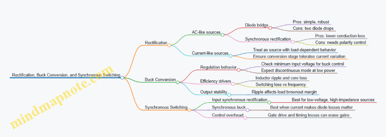
Example: Piezo Harvester with Low Voltage Peaks
Assume a piezo element produces about 6 V peak open-circuit, but the source impedance is high. A diode bridge might drop roughly 1.2 V total (two diodes). That leaves only a few volts for the buck input, and the buck may fail to regulate during much of the cycle.
If you use synchronous rectification, the conduction loss could be modeled as I × Rds(on). Even with a modest current, the voltage loss can be far smaller than diode drops. The result is a higher effective rectified voltage and more time spent in regulation.
To make this work, you need a control method that turns the MOSFETs on when the input polarity is correct. In many designs, a simple comparator-based polarity detector is enough because the piezo waveform is slow compared to typical switching frequencies.
Example: Photovoltaic Input with a Buck That Needs Headroom
A small PV panel might produce a rectified voltage that hovers around your target rail plus some margin. If the buck requires, say, 0.5 V of headroom to stay in regulation, then clouds or angle changes can push the input below that threshold.
In that case, the “best” rectifier is not the one with the lowest conduction loss; it’s the one that preserves voltage and avoids unnecessary drops. You might still use a diode bridge if the PV voltage is high enough, but you should verify the minimum operating illumination and the buck’s dropout behavior.
Practical Checklist for Choosing the Right Combination
- Estimate the minimum rectified voltage under worst-case conditions.
- Compute how much of that voltage is lost in rectification (diodes vs MOSFET Rds(on)).
- Confirm the buck can regulate at that minimum input voltage and at the expected load current.
- Check output ripple and ensure the load has enough margin to avoid resets.
- Only add synchronous control where it saves more loss than it costs in drive and timing.
When these steps are done in order, the design stops being a guessing game. You end up with a power chain that wastes less energy where the harvester is weakest: at low voltage and low power.
8.2 Energy Storage Selection Including Supercapacitors and Batteries
Energy harvesting systems rarely deliver steady power. Storage is what turns “sometimes” into “enough to do the job.” The trick is choosing storage that matches your input pattern, your load behavior, and your acceptable tradeoffs in size, cost, and lifetime.
What Storage Must Solve
Start with two questions: how much energy you need per operation, and how long you can wait between harvesting bursts. A door sensor that wakes for 2 seconds every minute needs a different storage strategy than a tracker that transmits for 30 seconds after each motion event.
A practical way to size storage is to compute energy per cycle:
- Energy per wake = (average power during wake) × (wake duration)
- Energy per cycle = energy per wake + (any standby losses)
- Required storage energy = energy per cycle ÷ (allowable depth-of-discharge factor)
Then translate energy into voltage range. Many power management ICs need a minimum input voltage to regulate correctly, so storage must hold enough voltage above that threshold during the load event.
Supercapacitors: Fast, Tolerant, and Usually Smaller Than You Think
Supercapacitors are excellent when your harvester produces short bursts and your load draws power quickly. They can accept many charge/discharge cycles with little wear, and they tolerate frequent energy “top-ups.”
Key characteristics to plan around:
- Voltage droop is real: capacitance stores energy as ½CV², so voltage falls as energy is used.
- Equivalent series resistance matters: high ESR reduces usable power and increases heat.
- Leakage exists: self-discharge can matter if your device sleeps for long periods.
Easy example: Suppose your system needs 3.0 V for a 1-second radio transmit at 50 mW, and you can allow the storage voltage to drop from 3.3 V to 3.0 V during the transmit. The energy needed is 50 mJ. For a single capacitor, the usable energy is:
- Usable energy = ½C(Vmax² − Vmin²)
- 0.05 J = ½C(3.3² − 3.0²) ≈ 0.5C(10.89 − 9.00) ≈ 0.5C(1.89)
- C ≈ 0.05 / 0.945 ≈ 0.053 F = 53 mF
That’s a rough sizing, but it shows the main point: voltage range drives capacitor size more than people expect.
Batteries: Higher Energy Density, Slower to Change, More Care Required
Batteries store more energy per volume and can support longer runtimes with less voltage droop. They are a better fit when your device needs energy over longer intervals or when harvesting is intermittent and infrequent.
Key characteristics to plan around:
- State-of-charge is not linear: voltage can stay flat for a while, then drop quickly near empty.
- Charge control is mandatory: batteries dislike being overcharged or charged too aggressively.
- Cycle life depends on depth-of-discharge: using the full range often shortens lifetime.
Easy example: A coin-cell-like battery at 3.0 V nominal must power a sensor that consumes 20 mW for 0.5 seconds once per minute. Energy per minute is 10 mJ. If you plan for 10,000 cycles and want to use only 30% of the battery’s usable capacity to preserve life, you can estimate required usable energy and then convert to capacity at the battery’s operating voltage. The exact numbers depend on chemistry, but the workflow stays the same: energy per cycle × number of cycles ÷ usable fraction.
Choosing Between Them by Load Shape
Use this decision logic:
- If your load is short and power-hungry, and you can tolerate voltage droop, supercapacitors often win.
- If your load needs longer runtime or you want a stable energy reserve over time, batteries often win.
- If your harvester is weak or sporadic, batteries reduce the risk of “never quite enough.”
Hybrid Storage: When One Isn’t Enough
Many real designs use both: a supercapacitor for burst power and a battery for energy buffering. The supercapacitor handles fast current spikes, while the battery charges slowly and covers longer gaps.
A common architecture is:
- Harvester → charge management → battery (slow energy)
- Battery → DC/DC or regulator → supercapacitor (or direct load)
- Load bursts draw from the supercapacitor to reduce stress on the battery and improve efficiency
This can also simplify power management because the burst current no longer has to come through the battery’s internal resistance.
Mind Map: Storage Selection Checklist
Practical Design Practices
- Define an explicit voltage window for the load event. For capacitors, energy scales with V², so “3.3 V to 3.0 V” is not the same as “3.1 V to 3.0 V.”
- Check peak current, not just average power. Radio bursts can demand current that stresses ESR and converter limits.
- Use depth-of-discharge intentionally for batteries. If you only need a small fraction of capacity, you can often trade runtime for longer life.
- Include protection behavior in the plan. Storage selection is incomplete without overvoltage/undervoltage handling and safe charging limits.
Example: Two Storage Choices for the Same Load
Assume the same 50 mW for 1 second transmit and a minimum operating voltage of 3.0 V.
- Supercapacitor-only: You size capacitance using the usable energy between Vmax and Vmin. You then verify that ESR and converter losses don’t drop the voltage below 3.0 V during the transmit.
- Battery-only: You size capacity based on energy per cycle and cycle count, then ensure the regulator can supply 50 mW during the burst without the battery voltage sagging too far.
If the harvester charges slowly, a battery-only design may still work, but a supercapacitor can reduce burst stress and improve reliability during marginal charging periods.
Summary Decision Rule
Pick supercapacitors when your system needs burst power and can tolerate voltage droop. Pick batteries when you need energy over longer intervals and want a larger reserve. Use hybrids when you want both: burst handling without stressing the energy source.
8.3 Charge Control, Overvoltage Protection, and Safe Startup Behavior
Charge control is the part of an energy-harvesting system that decides what to do when the input is too small, just right, or too large. Overvoltage protection is what keeps the storage element and the power-management IC from getting stressed when the harvester output spikes. Safe startup behavior is how the system avoids “boot loops” and brownouts when energy arrives in bursts.
Charge Control Goals and Operating Modes
A practical charge controller usually supports three modes:
- Harvesting mode: Convert harvester output into a controlled charge current or controlled voltage.
- Hold mode: Stop charging when the storage reaches a target level, while still allowing the system to draw power.
- Recovery mode: Resume charging after the storage voltage drops below a threshold.
A simple best practice is to define two thresholds: a charge enable threshold (below it, charging is allowed) and a charge stop threshold (above it, charging is blocked). This hysteresis prevents rapid on-off cycling when the input hovers near the boundary.
Overvoltage Protection That Matches Real Failure Paths
Overvoltage can come from several places: a harvester that produces higher-than-expected voltage, a rectifier that leaves the storage node floating during startup, or a converter that overshoots during load transients. Protection should therefore be layered.
Layer 1: Electrical limits in the power stage
- Use a converter or regulator with defined maximum input and output ratings.
- Ensure the converter’s control loop is stable with the storage element’s equivalent series resistance (ESR) and capacitance.
Layer 2: Storage protection
- For supercapacitors, add a clamp path so the voltage cannot exceed the capacitor’s rated maximum.
- For batteries, use a charge controller that enforces charge termination and prevents reverse current.
Layer 3: Fast clamp for spikes
- Add a transient suppressor (for example, a TVS diode) sized for the expected spike energy and waveform.
- Place it so the spike current returns to the correct ground reference, not through sensitive analog nodes.
A concrete example: suppose a piezo harvester can generate 30–60 V open-circuit during impacts, but your storage is a 3.0 V supercapacitor. The charge controller should include a front-end that limits the voltage reaching the converter input, and the converter should include output limiting so the storage node never exceeds its maximum.
Safe Startup Behavior for Energy-Constrained Systems
Safe startup is about sequencing. Many harvesting systems fail not because the energy is insufficient, but because the system tries to start the load before the power rails are stable.
Key practices:
-
Use a “power-good” gate for the load
- The MCU and radio should only wake when the storage voltage is above a minimum operating level.
- If the storage voltage falls mid-transmission, the system should stop the radio first, then let the MCU finish gracefully.
-
Avoid charging and heavy load draw at the same instant
- If your converter supports it, schedule charging to occur when the load is off.
- If not, ensure the charge loop can tolerate the load step without overshoot.
-
Provide a defined startup state for the converter
- Some converters require an enable pin or a soft-start capacitor. Tie these to a known state so the converter does not start in an undefined configuration.
-
Use hysteresis for wake and sleep decisions
- Wake threshold should be higher than the sleep threshold.
- This prevents rapid toggling when energy input is intermittent.
Mind Map: Charge Control and Startup Safety
Example: Designing Thresholds and Hysteresis
Assume a 3.3 V system rail powered from a storage element. Let the storage be allowed to charge up to 3.2 V and be considered “usable” for the load above 3.0 V.
- Charge stop threshold: 3.2 V
- Charge enable threshold: 3.0 V
- Wake threshold for load: 3.05 V
- Sleep threshold for load: 2.90 V
This separation ensures that:
- Charging stops before the storage reaches the absolute maximum.
- The load does not wake at the exact moment charging stops.
- The system can ride through small dips without immediately shutting down.
Example: Handling a Piezo Spike Without Storage Overshoot
A piezo harvester can produce brief high-voltage pulses. If you connect it directly to a converter input, the converter may see a spike that exceeds its absolute maximum rating.
A robust approach is:
- Rectify and limit the harvester output into a controlled intermediate node.
- Feed the charge controller from that intermediate node.
- Clamp the intermediate node with a fast suppressor so the converter input never sees the raw piezo peak.
Then verify with a scope capture at three points: harvester rectifier output, converter input, and storage node. The storage node should show no overshoot beyond its target maximum even during the largest impact.
Practical Validation Checklist
- Confirm hysteresis prevents charge-controller chatter near thresholds.
- Verify overvoltage clamps do not conduct continuously under normal operation.
- Check converter stability with the actual storage capacitance and ESR.
- Test startup with the worst-case energy arrival pattern: short bursts, then silence.
- Ensure the load gating prevents brownouts from causing repeated resets.
8.4 Load Switching, Power Gating, and Efficient Wake-Up Strategies
Energy harvesting systems rarely have steady power. They get bursts, then quiet periods. Your job is to make the device do useful work during the bursts and stay nearly silent when energy is scarce. Load switching and power gating are the practical tools for that.
Load Switching Basics for Real Loads
A “load” is anything that draws current: a sensor, an analog front end, a microcontroller, a radio, an LED, or even a voltage regulator’s quiescent path. Load switching means you connect and disconnect those loads under control.
Best practice: switch at the highest level that still meets your needs. If you only need to power the radio, don’t cut power to the whole system. If you need the MCU to keep time or retain state, keep the MCU domain alive and gate only the radio and sensors.
Example: A motion node that wakes on an accelerometer interrupt. The accelerometer runs from a low-power domain. When motion is detected, the MCU wakes, powers the sensor interface for a short measurement window, then gates the sensor again before sending data.
Key design checks:
- Inrush current: capacitors and radios can demand a sudden current spike. Your switch must handle it without large voltage droop.
- Leakage: a “turned off” load can still leak through switch body diodes, ESD structures, or pull-ups. Measure or estimate leakage at the actual voltage.
- Control timing: if you gate too quickly, the load may not settle before you sample.
Power Gating with Domains and States
Power gating is load switching with a goal: create power states that match the energy you actually have. A simple three-state model works well:
- Active: loads needed for sensing and communication.
- Standby: minimal logic and wake sources.
- Off: everything possible is off, except what must remain alive to detect wake conditions.
Best practice: define state transitions using energy thresholds, not time alone. Harvesting inputs vary with motion, temperature gradients, and lighting. If you wake based only on a timer, you may start a radio transmission when the energy buffer is too low.
Example: Use a storage capacitor or supercapacitor as the energy buffer. When its voltage rises above a “ready” threshold, the system enters Active. After the work is done, it returns to Standby and waits for the next threshold crossing.
Efficient Wake-Up Strategies That Don’t Waste Energy
Wake-up is where many systems quietly lose energy. The MCU can spend more energy waking up than doing the actual measurement.
A good wake-up strategy includes:
- A wake source that costs little (interrupts from a sensor, a comparator, or a GPIO event).
- A fast path to the first useful action (avoid long boot sequences when you only need a short measurement).
- A decision step before expensive work (check buffer voltage and only then power the radio).
Example: A light-harvesting tag that wakes when a photodiode indicates sufficient illumination. The photodiode output feeds a low-power comparator. When the comparator trips, the MCU wakes, immediately reads the buffer voltage, and only powers the radio if the voltage is above the transmission threshold.
Choosing Switches and Regulators for the Job
For gating, you typically choose between:
- High-side or low-side switching using MOSFETs or load switches.
- Regulator enable pin control to shut down downstream rails.
Best practice: prefer a load switch or a MOSFET arrangement that minimizes leakage and provides a clean off state. If you use a regulator enable pin, confirm that the regulator truly shuts down and that its output doesn’t backfeed through internal paths.
Also consider the “off” behavior of your storage element. If the storage capacitor is connected through a switch, you must ensure the system can still reach the thresholds needed for wake decisions.
Mind Map: Load Switching and Wake-Up Flow
Load Switching and Power Gating Mind Map
Example: A Threshold-Gated Radio Transmission
Assume a storage capacitor feeds a buck regulator for the MCU and a separate rail for the radio. You define:
- V_ready: minimum buffer voltage to start a measurement and power the radio.
- V_tx: minimum buffer voltage to complete a transmission.
- Hysteresis: a small gap between turn-on and turn-off thresholds.
Flow:
- Wake from a sensor interrupt.
- Read buffer voltage.
- If buffer < V_ready, return to Standby.
- If buffer ≥ V_ready, power the sensor, take the measurement, then gate the sensor.
- If buffer ≥ V_tx, power the radio and transmit.
- After transmission, gate the radio and return to Standby.
This avoids the common failure mode where the system wakes, powers everything, then resets mid-transmission because the buffer sagged.
Practical Checklist for Efficient Gating
- Use interrupt-driven wake sources instead of periodic polling.
- Gate sensors and radios separately from the MCU domain.
- Add hysteresis to threshold comparisons to prevent rapid on/off cycling.
- Verify off-state leakage with the actual wiring, not just the schematic.
- Confirm regulator enable and switch off behavior under worst-case voltages.
- Measure settling time after enabling a rail before sampling.
When load switching and wake-up are designed as a state machine driven by energy thresholds, the system becomes predictable. Predictability is what lets you spend energy where it matters and stop spending it where it doesn’t.
8.5 Designing for Efficiency Across Wide Input and Output Ranges
Harvesting systems rarely see a steady input. Motion can be bursty, light can be angled or shaded, and thermal gradients can drift. Efficiency across a wide input and output range means the power stage wastes less energy when conditions change, and it still delivers usable voltage/current to the load.
Start with a Range Map, Not a Single Operating Point
A common mistake is optimizing for one “typical” input. Instead, define three bands for each harvester: low, nominal, and high. Then define the load’s required output bands: minimum voltage to run, preferred voltage for best efficiency, and maximum voltage you must not exceed.
For example, suppose a harvester produces 0.2–2.0 V depending on conditions, while the device needs 3.0–3.6 V to run. Your converter must handle low input without stalling, and it must avoid excessive losses at high input. The range map becomes the checklist for every component choice.
Choose Conversion Topologies That Behave Well at the Edges
Different converter styles trade efficiency for robustness.
- Buck converters tend to be efficient when input is comfortably above the regulated output, but they can struggle when input falls near the output.
- Boost converters can work at low input, yet they may waste more power when input is high because the duty cycle shrinks and switching losses remain.
- Buck-boost converters handle wide input-to-output ratios, but they often have higher baseline losses than a simple buck when conditions are favorable.
A practical approach is to use a topology that matches the dominant ratio band. If most energy arrives when input is far below the target output, a boost or buck-boost is usually worth the extra complexity. If input is usually above the target, a buck-first approach can be more efficient.
Design for Efficiency Losses You Can Actually Measure
Efficiency drops for predictable reasons:
- Switching losses grow with switching frequency and input voltage.
- Conduction losses grow with current and resistances (inductor DCR, switch RDS(on), diode losses).
- Control losses include quiescent current and the cost of maintaining regulation.
- Rectification losses matter for low-voltage motion and light where forward drops are a big fraction of the signal.
When you test, measure input power and output power across the range bands, not just at one point. If you cannot measure both sides, at least log input voltage/current and output voltage/current with a consistent measurement method.
Use Energy Storage as a “Buffer with Rules”
Storage doesn’t just smooth energy; it changes the operating point of the converter.
- Supercapacitors often pair well with converters that need a stable input for regulation. They can reduce converter stress during bursts, but their leakage and voltage droop affect long idle periods.
- Batteries can accept energy at a wider range, but charge control must prevent overvoltage and manage current limits.
The key is to set storage thresholds that keep the converter in its efficient region. For instance, you can allow the storage to charge up to a “start” threshold, run the load until a “stop” threshold, and avoid frequent on/off cycling.
Mind the Load Profile, Not Just the Average Power
A load that wakes for 50 ms every second can be efficient to run, yet inefficient to power if the converter must repeatedly reconfigure or if the storage voltage collapses between bursts.
A useful rule: compute energy per event, not just power. If the device consumes 30 mA at 3.3 V for 50 ms, that’s 4.95 mJ per event. Add converter overhead and include the energy needed to recharge storage between events. Then verify the converter can deliver that energy without dropping below the load’s minimum voltage.
Mind Map: Efficiency Across Wide Ranges
Example: Motion Harvester with Burst Energy
Assume a piezo interface produces a rectified DC that varies from 0.3 V (light motion) to 1.2 V (strong motion). The load needs 3.3 V.
- If you use a buck converter, it will not regulate at 0.3–1.2 V because the input is below the output.
- A boost converter can regulate at low input, but at 1.2 V it may run with higher current ripple and switching losses.
A practical design is to charge a supercapacitor from the harvester using a rectifier and a stage that can operate at low voltage, then run a buck from the supercapacitor to 3.3 V when the supercap reaches the start threshold. This keeps the buck in its efficient region and limits how long the boost must work at high input.
Example: Light Harvester with Shading
A photovoltaic source might deliver high current under direct light and drop sharply under partial shading. If the converter tries to regulate continuously, it may spend time in inefficient control modes.
Instead, set storage thresholds so the system only regulates the output when the PV has provided enough energy to keep the storage voltage within a tight window. During low-light periods, the system can remain in a low-power state while the storage slowly accumulates energy. When light returns, the output stage starts from a known voltage, reducing the time spent in inefficient transitions.
Efficiency Checklist for Wide Ranges
- Converter can start and regulate in the low input band without excessive current draw.
- Storage thresholds prevent frequent start/stop cycles.
- Losses are measured across bands, not inferred from one operating point.
- Load energy per event fits within the storage recharge time and voltage limits.
- Rectification and interface losses are included in the power budget.
When these items are satisfied, the system spends less time “trying” to regulate under conditions where it cannot, and more time delivering energy where it matters.
9. System Integration for Motion Heat and Light in One Product
9.1 Choosing Single-Source Versus Multi-Source Architectures
Choosing between single-source and multi-source energy harvesting is mostly about how predictable your inputs are and how much engineering effort you can spend on power management. A single-source architecture is simpler, but it can stall when that one input disappears. A multi-source architecture adds complexity, yet it can keep the system alive through partial conditions.
Single-Source Architectures
A single-source design uses one harvesting path—motion, heat, or light—and routes its electrical output into a power management stage. This approach is attractive when the energy source is consistently present during the device’s operating window.
Best-fit situations
- Motion energy when the device is attached to something that moves regularly, like a door handle or wearable strap.
- Light energy when the device sits under stable indoor lighting or near a known illumination source.
- Thermal energy when there is a persistent temperature gradient, like a sensor near a warm pipe.
Core design choices
- Pick the harvester type that matches the dominant input. For example, if motion is intermittent but strong, a resonant piezo or electromagnetic generator may outperform a weak, broadband approach.
- Size the storage and load duty cycle around the worst-case energy availability. If your device must transmit once every minute, you design for the minute with the least energy, not the average.
- Keep the power path short. Fewer stages usually means fewer conversion losses and fewer failure points.
Easy example A small motion sensor that wakes up only when a person approaches can use a motion harvester alone. The firmware can measure, transmit, then sleep. If the door is rarely touched, the device simply stays off until motion happens again. That’s acceptable when “off” is not a safety issue.
Multi-Source Architectures
A multi-source design combines two or three harvesting inputs. The key question is whether you want the system to keep operating when any one source is missing, or whether you only need backup energy for occasional gaps.
Two common ways to combine sources
- Parallel energy paths into shared storage: each harvester has its own rectifier and converter, then both feed the same supercapacitor or battery.
- Shared intermediate bus: multiple harvesters are conditioned to a common voltage range before charging storage.
Best-fit situations
- Motion plus light for devices that are moved during the day and left in light between uses.
- Motion plus thermal for environments where temperature gradients exist but are weak, while motion provides bursts.
- Light plus thermal when one source is seasonal or angle-dependent.
Core design choices
- Ensure each harvester’s power stage can tolerate the other source’s behavior. For instance, if one converter clamps voltage while another tries to charge, you can get wasted energy or oscillations.
- Decide how the system prioritizes energy. A simple rule like “charge storage whenever possible” often works, but you must define what happens when storage is full.
- Budget losses separately. Two harvesters do not automatically double energy because each conversion stage has its own inefficiencies.
Easy example A cabinet sensor uses motion energy to wake and send a short status update. If the cabinet is opened infrequently, light energy from a nearby window can slowly charge the storage so the next opening has enough energy to transmit even if the motion burst is small.
Mind Map: Architecture Tradeoffs
A Practical Decision Checklist
- Define acceptable downtime: If the device can be off until the next event, single-source is often enough. If it must respond reliably, multi-source becomes more attractive.
- Compare worst-case energy, not average energy: A single-source system fails when the input is absent during the critical interval.
- Count conversion stages: Multi-source can add stages; if each stage is inefficient, the combined output may not be as helpful as expected.
- Check interaction risk: If two harvesters share storage, confirm their charge control behavior doesn’t fight.
- Match architecture to physical constraints: If you cannot place multiple harvesters without interfering with each other, single-source may be the only realistic option.
Quick Rule of Thumb
If your device’s required actions happen only when one input is reliably present, choose single-source. If the device must survive gaps in that input while another source is intermittently available, choose multi-source and design the power stage so the sources cooperate instead of compete.
9.2 Combining Harvesters Without Creating Electrical Conflicts
When you combine multiple energy harvesters, the main risk is not “not enough power.” It’s electrical conflict: two sources fighting over voltage, current, or timing. The fix is usually straightforward once you decide what each harvester is allowed to do.
Start with a Power-Path Decision
Pick one of these roles for each harvester:
- Direct contributor: feeds the power-management input whenever it has energy.
- Pre-stage contributor: charges a local storage element first, then the storage feeds the system.
- Occasional contributor: only connects when its output is clearly above the system’s current level.
A good rule: if you cannot describe when each harvester is “allowed” to connect, you will end up with accidental backfeeding or oscillation.
Prevent Backfeeding with Diodes or Ideal-ORing
Backfeeding happens when one harvester’s output drives another harvester’s circuitry in reverse. The symptom is a harvester that “works” on the bench but drains the other source in real use.
Two common approaches:
- Simple diode ORing: easy, but the forward drop reduces harvested voltage, especially harmful for low-voltage sources like small thermoelectrics.
- Ideal diode or controller-based ORing: lower loss, but requires a proper controller and careful layout.
Example: A small thermoelectric module (low voltage) and a photovoltaic panel (higher voltage) both connect to the same storage. Without ORing, the panel can push current into the thermoelectric when the panel is dark, wasting energy and heating the module. With diode ORing, the thermoelectric only sees current when it is actually producing.
Avoid Voltage Clashes with “Who Sets the Bus”
If two harvesters connect directly to a shared node, they may try to enforce different voltages. Even if both are “DC,” their internal behavior differs: piezo interfaces can look like a pulsed source, PV looks like a current-limited source, and thermoelectrics behave like a voltage source with internal resistance.
A clean design chooses a single “bus manager” that regulates the system input, while harvesters feed through controlled stages.
Example: Piezo harvesting often uses a rectifier plus a converter that expects a certain input range. If you connect PV directly to the same node without isolation, the PV can shift the piezo converter’s operating point, lowering piezo energy extraction. The fix is to isolate each harvester with its own rectification and conversion stage, then combine at the storage or at a regulated input.
Use Storage as the Conflict Buffer
Energy storage is not just for runtime; it’s also a mechanical shock absorber for electrical behavior.
- Connect each harvester to its own charge path into a shared storage element (supercapacitor or battery).
- Let the power-management system draw from storage with a stable policy.
This prevents harvesters from directly interacting with each other’s instantaneous output.
Example: Motion (piezo) produces short bursts, while light (PV) is steadier. If both feed the same converter input directly, the piezo bursts can cause converter input voltage swings that reduce PV efficiency. If both charge the same capacitor through separate paths, the capacitor smooths the bursts and the converter sees a calmer input.
Match Interface Types to Input Behavior
Not all harvesters should be combined at the same electrical layer.
- PV: often best combined after a PV-specific stage (rectification and MPPT or fixed operating point logic).
- Thermoelectric: benefits from a dedicated interface that handles low voltage and polarity constraints.
- Piezo: needs a rectifier and often an energy extraction strategy tuned to its waveform.
Example: If you try to “OR” raw PV and raw piezo outputs before rectification, you can create unintended current paths through the piezo rectifier during PV conduction. Separate the rectification and then combine at a controlled node.
Add Simple Rules for Safe Switching
If you use load switches or connection control, define these rules:
- Only connect a harvester when its output is above the storage voltage by a margin.
- Ensure the switch body diode or parasitic paths do not create backfeeding.
- Confirm startup order: a storage element can be at 0 V, so “above by a margin” logic must still allow initial charging.
Mind Map: Electrical Conflict Sources and Fixes

Case Study: Motion and Light with a Shared Storage Node
Goal: A device uses piezo motion and indoor PV to charge a supercapacitor, then powers a sensor.
Naive wiring: PV and piezo rectifiers both connect to the supercapacitor through a single node.
Observed issue: When motion stops, the piezo path still shows small leakage, and the capacitor voltage rises more slowly than expected.
Reasoning: The PV output can forward-bias parts of the piezo rectifier network, creating a reverse current path. Also, piezo bursts can momentarily pull the node, shifting PV’s effective operating point.
Corrected approach:
- Keep PV rectification and conversion in its own path.
- Keep piezo rectification and conversion in its own path.
- Combine at the supercapacitor using ORing that blocks reverse current.
- Let the system draw from the supercapacitor with a stable power-management policy.
Result: each harvester charges the storage when it can, and neither one “borrows” energy from the other when it shouldn’t.
9.3 Mechanical Integration for Co-Located Motion, Thermal, and Optical Capture
Co-locating motion, thermal, and optical harvesting is mostly a mechanical problem: you’re trying to place three energy paths in the same physical space without turning them into three separate failure modes. The goal is simple—each subsystem should “see” the stimulus it needs, while the others don’t steal its mechanical or optical budget.
Start with Three Interfaces and One Mechanical Skeleton
Treat each harvester as having an interface that must be satisfied:
- Motion interface: a predictable displacement/force at the transducer.
- Thermal interface: a stable temperature gradient across the thermal element.
- Optical interface: a defined light collection geometry and surface condition.
Then build one mechanical skeleton that provides alignment and repeatability. A good skeleton uses the same datum points for all three: for example, a mounting plate corner for optical alignment, and a central boss for mechanical motion reference.
Best practice example: If you mount a piezo stack and a thermoelectric module on the same carrier, keep their contact surfaces flat and separated by a thin thermal isolation layer. That way, vibration doesn’t conduct heat in a way that collapses the temperature gradient.
Separate What Must Be Separated
Mechanical coupling is the silent saboteur. Motion harvesting often benefits from compliance and damping, while thermal harvesting benefits from controlled thermal resistance.
Use separation strategies:
- Thermal isolation: thin polymer standoffs or low-conductivity spacers between hot-side and cold-side structures.
- Mechanical decoupling: compliant mounts that reduce vibration transfer into the thermal path.
- Optical shielding: matte baffles or light-absorbing walls to prevent stray reflections from changing the optical input.
Best practice example: Put the optical window on a slightly raised bezel so it doesn’t share the same flexing region as the motion element. Even small flex can change the incidence angle and create large power swings.
Manage Shared Constraints: Mass, Stiffness, and Clearance
All three harvesters compete for the same mechanical budget.
- Mass: heavier assemblies reduce acceleration at the motion transducer.
- Stiffness: too stiff a mount can shift resonance away from real motion.
- Clearance: optical windows need protection without blocking light.
A practical approach is to define a single “mechanical envelope” and then allocate zones:
- Zone A for the motion element and its moving features.
- Zone B for thermal hot/cold interfaces with minimal airflow disruption.
- Zone C for the optical collection area with a protective cover.
Best practice example: If you must add a protective cover, choose a cover thickness and material that stays optically consistent across temperature. Otherwise, thermal expansion can alter focus or introduce micro-gaps that change reflection.
Build a Thermal Path That Doesn’t Care About Vibration
Thermal gradients are fragile. Vibration can change contact pressure, which changes thermal resistance.
Use a thermal path design that includes:
- Defined contact pressure using springs or compliant pads.
- Consistent contact area with flatness requirements.
- Thermal resistance budgeting so you know which interface dominates.
Best practice example: For a thermoelectric module, use a spring-loaded cold plate so the contact pressure stays stable even when the motion element flexes.
Build an Optical Path That Doesn’t Care About Motion
Optical harvesting is sensitive to angle, shadowing, and surface contamination.
Mechanical integration should include:
- A fixed optical axis relative to the enclosure.
- A window that stays aligned even when the motion element moves.
- A shadow map: identify where moving parts block the sensor during typical motion.
Best practice example: If the device rotates, mount the optical sensor on a rigid “camera-like” stalk tied to the enclosure, not to the moving mass.
Wiring and Strain Relief as Part of the Mechanical Design
Mechanical integration fails when cables become springs.
- Route wires through strain-relief channels so they don’t tug on transducers.
- Keep thermoelectric and sensor wiring away from high-strain regions.
- Use slack loops sized for the maximum motion stroke.
Best practice example: For a piezo element, anchor the cable to the enclosure at two points and keep the piezo leads short. Long leads turn into antennas and also add unwanted mechanical loading.
Mind Map: Co-Located Integration Checklist
Example: One Enclosure with Three Zones
Imagine a small device mounted on a door that experiences opening motion, ambient temperature differences, and indoor light.
- Zone A (motion): a piezo element on a compliant flex arm with a known stroke limit.
- Zone B (thermal): a thermoelectric module clamped between a hot-side plate near the door surface and a cold-side plate exposed to indoor air, with spring-loaded contact pads.
- Zone C (optical): a photodiode behind a fixed window on the enclosure wall, with a baffle that blocks light from the moving arm.
During door movement, the flex arm moves but the window stays rigid. During temperature changes, the spring-loaded pads maintain contact pressure so the thermal gradient doesn’t collapse. During normal lighting, the baffle reduces angle-dependent reflections so the photodiode sees a more consistent illumination pattern.
The result is not “three harvesters in one box.” It’s one enclosure that preserves three different kinds of input conditions while preventing mechanical and optical cross-talk.
9.4 Environmental Protection Including Water, Dust, and Temperature Cycling
Energy-harvesting products often live in places where the environment does not care about your power budget. Protection is not just about keeping water out; it’s about preventing performance drift, mechanical degradation, and electrical failures that quietly reduce harvested energy over time.
Water Protection That Preserves Electrical Performance
Start with the failure modes. Water can cause short circuits, corrosion of exposed conductors, and leakage currents that steal power from high-impedance circuits.
Best practice: design for the most likely ingress path, not the most dramatic one. For example, if the device is mounted under a desk lip, water may enter from the side during cleaning rather than from direct spray. Use a gasketed enclosure with a drain path so any water that gets in can exit instead of pooling around the harvester.
Concrete example: a small motion harvester in a hallway sensor. The enclosure uses a silicone gasket around the lid and a bottom vent membrane that allows pressure equalization but blocks liquid water. The power management board is conformally coated only on the soldered areas, leaving connector contacts uncoated for reliable mating.
Electrical best practice: avoid relying on coating alone for insulation. If the harvester output is high impedance, even tiny leakage can matter. Add creepage and clearance spacing between exposed nodes, and route the rectifier and storage circuitry away from any area where condensation could form.
Dust Protection That Prevents Mechanical and Optical Degradation
Dust is abrasive, conductive in the wrong form, and good at settling into moving parts. It also reduces optical coupling for light harvesters by scattering and shading.
Best practice: separate “dust-tolerant” from “dust-sensitive” zones. Keep the harvester’s mechanical interface either sealed or designed to tolerate fine particles. For light harvesting, treat the optical window as a replaceable consumable rather than a permanent miracle.
Concrete example: an indoor light-harvesting tag placed near a dusty workshop bench. The photovoltaic surface sits behind a clear cover with an anti-soiling coating. The cover is mounted with a simple snap-fit so it can be swapped after heavy dust exposure. The electronics compartment is sealed with a membrane vent to reduce pressure-driven ingress.
Electrical best practice: if dust can become conductive (for instance, with humidity), increase insulation margins and use conformal coating on the board. For connectors, use seals or choose housings that maintain contact pressure over time.
Temperature Cycling That Avoids Cracks, Drift, and Loose Connections
Temperature cycling stresses materials differently: metals expand, plastics flex, and solder joints fatigue. The result can be intermittent connections, changes in thermal contact for thermoelectrics, and altered optical alignment.
Best practice: design the mechanical stack-up to reduce differential strain. Use compliant mounting features where appropriate, and avoid rigidly bonding dissimilar materials without a stress-relief layer.
Concrete example: a thermoelectric module attached to a heat spreader. If you rigidly glue the module to both sides, cycling can pump stress into the module leads. A better approach is to use a controlled thermal interface material on the hot and cold sides and a mounting frame that allows slight movement while maintaining pressure. This keeps thermal resistance stable and reduces lead fatigue.
Electrical best practice: strain-relief the wires and keep solder joints away from direct mechanical flex. If the device has a moving cover, route cables with slack and use tie-down points so motion does not translate into connector stress.
Mind Map: Environmental Protection Priorities
Practical Verification Steps That Catch Real Problems
- Water ingress check: run a controlled spray or splash test that matches the device’s mounting orientation. After the test, measure leakage current in the power stage and inspect for corrosion at edges.
- Dust exposure check: simulate dust loading by applying a fine particulate layer to the optical window and seams. Verify that harvested power does not drop beyond your acceptable margin.
- Temperature cycling check: cycle between your expected minimum and maximum temperatures with dwell times long enough for the enclosure to reach equilibrium. Then perform continuity checks on harvester leads and connectors, and re-measure power output.
Concrete example: a multi-source device that combines motion and light. After temperature cycling, the motion harvester may still work, but the optical window alignment can shift slightly, reducing light-harvested energy. A simple post-test measurement of harvested power under a fixed illumination setup quickly separates mechanical drift from electrical failure.
The goal is not to make the device “indestructible.” It’s to ensure the protection strategy matches the actual ingress paths and the mechanical realities of the materials you chose.
9.5 End-to-End Power Budgeting with Realistic Operating Modes
Power budgeting is where “it should work” becomes “it does work.” The goal is to account for energy from motion, heat, and light, then map it to what the device actually does in each operating mode. A good budget includes time fractions, start-up costs, conversion losses, and the energy needed for the worst day of the week, not the best.
Step 1: Define Operating Modes That Match Reality
Start by listing the device’s distinct behaviors and how long each lasts. For example, a motion-heat-light sensor might have:
- Sleep: low-power monitoring, no radio.
- Wake on Motion: brief sensor read, then decide whether to transmit.
- Transmit: radio on for a fixed packet window.
- Status Blink: optional LED pulse if energy is available.
Best practice: measure or estimate mode durations from firmware behavior, not from intuition. If your radio takes 120 ms to send and you retry twice, that’s 240 ms of radio time per event.
Step 2: Compute Energy per Mode
For each mode, compute energy as:
- E_mode = V * I_avg * t_mode If your system uses a regulated rail, use the rail voltage and average current at that rail. If you only have input-side current, convert carefully using measured efficiency.
Example: Suppose the device runs from a 3.3 V rail.
- Sleep: 3.3 V, 5 µA, 10 s per cycle → E_sleep = 3.3 * 5e-6 * 10 = 165 µJ
- Wake read: 3.3 V, 1 mA, 20 ms → E_read = 3.3 * 1e-3 * 0.02 = 66 µJ
- Transmit: 3.3 V, 30 mA, 200 ms → E_tx = 3.3 * 30e-3 * 0.2 = 19.8 mJ
- LED pulse: 3.3 V, 10 mA, 5 ms → E_led = 3.3 * 10e-3 * 0.005 = 165 µJ
If one event occurs every 60 s, then per-minute energy is:
- E_total = E_sleep + E_read + E_tx + E_led
- E_total = 165 µJ + 66 µJ + 19.8 mJ + 165 µJ ≈ 20.2 mJ
Step 3: Convert Harvested Power into Usable Energy
Harvesters rarely deliver constant power. Use average harvested power over the same cycle as your operating modes.
A practical approach:
- Estimate P_in_avg from each source (motion, thermal, light) using measured or modeled duty cycles.
- Apply conversion efficiency: P_usable = P_in_avg * η_total
- Include storage and regulator losses: η_total might be 0.5 to 0.9 depending on architecture and load switching.
Example: Over one minute, suppose:
- Motion harvesting average: 0.25 mW
- Thermal harvesting average: 0.05 mW
- Light harvesting average: 0.10 mW
- Total input average: 0.40 mW
- Total efficiency: 0.75 Then usable average power is 0.40 * 0.75 = 0.30 mW. Energy available per minute:
- E_avail = 0.30 mW * 60 s = 18 mJ
Your budget needs E_total ≤ E_avail with margin for variability and measurement error. Here, 20.2 mJ exceeds 18 mJ, so you must change something.
Step 4: Add a Margin and Identify the Bottleneck
Margin is not a vibe; it’s a buffer for uncertainty. Use at least one of:
- Reduce transmit frequency
- Shorten radio time or reduce retries
- Gate the LED behind a “energy available” check
- Increase sleep duration
- Improve conversion efficiency or reduce regulator losses
In the example, the transmit energy dominates. Cutting transmit time from 200 ms to 120 ms reduces E_tx proportionally:
- New E_tx = 3.3 * 30e-3 * 0.12 = 11.88 mJ New E_total ≈ 12.3 mJ, which fits under 18 mJ with room for losses.
Step 5: Model Storage as a Buffer, Not a Magic Battery
Energy storage smooths intermittent harvesting. Use a simple state-of-charge check:
- E_storage_next = E_storage_now + E_avail - E_total Then ensure storage never drops below the minimum required for safe operation, including brownout margins.
Mind Map: End-to-End Power Budgeting
Example: Budgeting a Multi-Source System with Mode Gating
Assume the device transmits only if it has enough energy since the last event. A simple gating rule:
- If storage energy is above a threshold, allow transmit.
- Otherwise, record locally and wait for the next wake.
This changes the average energy per event because failed transmit attempts are avoided. It also prevents the system from repeatedly waking and draining storage during low-light or low-motion periods.
Concrete practice: implement a “budget-aware” decision in firmware using a storage voltage estimate or an energy counter updated from measured charge/discharge. Then log mode counts (sleep, wake, transmit) to confirm that the real operating mode mix matches the budget.
10. Sensing, Communication, and Load Design for Energy-Constrained Devices
10.1 Selecting Sensors and Estimating Their Energy per Measurement
Energy harvesting systems live and die by measurement energy. A sensor that seems “small” on a datasheet can dominate your power budget once you include wake-up time, analog settling, and the cost of communication. This section gives a practical way to pick sensors and estimate energy per measurement so your design decisions stay grounded.
Step 1: Define What “One Measurement” Means
A measurement is not just “read a value.” Decide the full sequence your firmware performs:
- Wake sensor and any front-end circuitry
- Configure measurement mode and range
- Wait for stabilization or ADC settling
- Take samples and compute (or average)
- Optionally calibrate or compensate
- Power down or return to a low-power state
Example: A light sensor might require 5 ms to stabilize after enabling the LED or changing gain. If you count only the ADC conversion time, you’ll underestimate energy by orders of magnitude.
Step 2: Choose Sensors by Output Rate and Interface Cost
Start with the sensor’s electrical behavior, not just its accuracy.
- Output type: analog voltage, digital bus, pulse/frequency, or event interrupt
- Interface: I2C/SPI/UART often costs energy in both the sensor and the MCU due to clocking and bus activity
- Conversion style: continuous vs. triggered vs. burst sampling
- Data handling: raw samples vs. built-in filtering
A sensor with built-in averaging can reduce MCU compute time, but it may increase sensor active time. The “cheapest” option is the one with the smallest total energy for your exact measurement sequence.
Step 3: Estimate Energy per Measurement with a Simple Budget
Use this structure:
Energy per measurement = Σ \( Power_i × Time_i \)
Break it into phases:
- Wake and configuration: sensor enable, register writes, bus setup
- Stabilization: time until the signal is valid
- Acquisition: ADC conversion(s) or digital read
- Processing: filtering, scaling, compensation
- Shutdown: any tail time before power-down takes effect
Example: Suppose a temperature sensor sequence is:
- Enable sensor: 0.8 mA for 2 ms
- Stabilize: 0.2 mA for 8 ms
- Read via I2C: 3 mA for 1 ms (includes MCU bus activity)
- Process locally: 5 mA for 0.3 ms
- Power down tail: 0.1 mA for 0.2 ms
Energy per measurement (in mJ) can be approximated using average current times voltage. If your system runs at 3.3 V:
- Total charge time = (0.8×2 + 0.2×8 + 3×1 + 5×0.3 + 0.1×0.2) ms = (1.6 + 1.6 + 3 + 1.5 + 0.02) ms·mA = 7.72 ms·mA
- Energy = V × (I·t) = 3.3 V × 7.72×10^-3 A·s = 0.0255 J = 25.5 mJ
That number is big enough to force a low measurement frequency or a different sensor/interface approach.
Step 4: Account for Sampling Strategy and Averaging
Averaging reduces noise but increases time.
- If you average N samples, acquisition time often scales roughly with N.
- Some sensors offer hardware averaging; that can be cheaper than waking the MCU repeatedly.
Example: If a motion sensor provides event interrupts, you can avoid periodic sampling. You measure only when motion occurs, then read a few samples to estimate intensity.
Step 5: Include “Hidden” Costs
Common energy surprises:
- ADC settling after switching channels or changing gain
- Voltage reference startup time
- Pull-ups and bus activity on I2C/SPI
- Sensor warm-up for optical or thermal sensors
- Calibration routines that run every measurement instead of once at startup
Example: An optical sensor might require enabling an LED driver and waiting for the photodiode output to settle. If you reuse the same LED timing but change the gain range, you must re-check settling time.
Mind Map: Sensor Selection and Energy Estimation
Example: Choosing Between Two Sensors for the Same Quantity
You need a humidity reading.
- Sensor A: digital humidity sensor with 10 ms conversion time and I2C read
- Sensor B: analog humidity sensor requiring ADC sampling and a longer stabilization due to RC filtering
If Sensor A conversion is 10 ms at 0.5 mA and the I2C read plus MCU activity is 1 ms at 5 mA, then the dominant term is 10 ms × 0.5 mA. Sensor B might require 50 ms stabilization at 0.2 mA plus ADC sampling at 2 mA for 2 ms, but the MCU may also spend longer waiting for the analog front-end to settle.
Even if Sensor B has lower sensor current, the longer stabilization can still win against it. The decision should be based on total energy per measurement sequence, not just sensor current.
Practical Checklist for This Section
- Define the exact firmware sequence for one measurement.
- Break energy into wake, stabilize, acquire, process, and shutdown.
- Include MCU and bus activity, not only sensor power.
- Treat averaging and settling time as first-class energy terms.
- Verify assumptions with a quick bench measurement of one full cycle.
When you do this consistently, sensor selection becomes a budgeting exercise rather than a guessing game. Your power budget stops being a spreadsheet fantasy and starts matching what the device actually does.
10.2 Radio Duty Cycling and Energy Cost of Communication Events
Radio use is usually the biggest energy line item in a harvested-power device. Duty cycling helps, but only if you count the real costs: transmit time, receive listening time, wake-up overhead, and the energy spent when packets fail and must be retried.
Energy Cost Model for Radio Events
A practical way to reason about radio energy is to break it into event types:
- Transmit event: energy during the actual on-air transmission plus any preamble or ramp-up time.
- Receive event: energy while the receiver is on, including time spent waiting for a packet.
- Idle listening: energy when the radio is not actively receiving but still checks for activity (depends on the chip and mode).
- Retry event: extra transmit and receive time after a failed attempt.
- Wake-up overhead: energy to power up the radio, reconfigure registers, and stabilize clocks.
A simple budgeting equation for one successful message can look like:
- E_total ≈ E_tx(attempts) + E_rx(listen) + E_wake + E_retry(extra attempts)
The key nuance: “successful message” is not the same as “one transmit.” If your link is marginal, retries can dominate.
Duty Cycling Strategies That Actually Reduce Energy
-
Sleep most of the time, wake briefly to transmit
- Use when you can tolerate delayed delivery or you control the schedule.
- Example: a door sensor wakes every 10 minutes, sends one packet, then returns to sleep.
-
Scheduled receive windows
- Instead of listening continuously, the receiver turns on only during expected windows.
- Example: a hub listens for 200 ms after each expected sensor report, then sleeps again.
-
Acknowledged transmissions with bounded retries
- Acknowledgements prevent silent failures, but they add receive time at the sender and transmit time at the receiver.
- Example: sender transmits, waits 30 ms for ACK, retries up to 3 times.
-
Carrier sensing or channel checks when supported
- Useful in shared environments, but it can cost energy if it keeps the radio awake too long.
- Example: check the channel for 5 ms before transmitting; if busy, back off and try again later.
Concrete Example: Budgeting a Sensor Message
Assume a small node with these measured or datasheet values:
- Transmit current: 60 mA
- Receive current: 20 mA
- Sleep current: 5 µA
- Packet on-air time: 8 ms
- Wake-up time: 2 ms
- ACK wait time: 30 ms
- Retries: average 1 retry (so 2 attempts per successful message)
For one successful message:
- Per attempt transmit energy: (60 mA) × (2 ms wake + 8 ms on-air)
- Per attempt receive energy: (20 mA) × (30 ms ACK wait)
- Two attempts: multiply transmit and ACK wait by 2
Even without exact voltage, the relative impact is clear: the 30 ms ACK wait at 20 mA is often larger than the 8 ms on-air time at 60 mA. That’s why duty cycling must include receive windows and ACK timing, not just transmit duration.
Mind Map: Radio Duty Cycling Decisions
Example: Choosing Between Two Schedules
- Schedule A: send every 60 seconds, receiver listens continuously for 60 seconds.
- Schedule B: send every 60 seconds, receiver listens for 200 ms right after each expected send.
If the receiver listens continuously, it pays receive current for the entire minute. With a 200 ms window, the receiver pays receive current for only 0.2 seconds per minute. The sender’s transmit energy is similar in both cases, so the receiver’s duty cycle dominates the difference.
Practical Best Practices for Communication Events
- Measure packet success rate under real conditions and use it to estimate retries; guessing retries is the fastest way to miss your power budget.
- Keep ACK wait time tight so the sender doesn’t sit in receive mode longer than needed.
- Avoid “always-on” receive unless you truly need low latency; scheduled windows usually win on energy.
- Treat retries as first-class citizens in your calculations, not an afterthought.
- Use energy per successful message as the comparison metric, not energy per attempt.
Quick Checklist for Duty Cycling
- What is the receiver doing when the sender is asleep?
- How long is the radio awake per attempt, including wake-up?
- What is the average retry count, and how does it change with distance?
- Are you optimizing for energy per delivered packet, not just fewer transmissions?
- Do your assumptions match measured behavior over multiple cycles?
10.3 Firmware Techniques for Energy-Aware Sampling and Transmission
Energy harvesting systems rarely deliver steady power. Firmware has to treat energy like a budget with receipts: measure what you can, spend only when you can, and avoid wasting cycles when the input is weak. The goal is not to “optimize everything,” but to make behavior predictable under changing conditions.
Energy-Aware State Machine
A practical approach is a small state machine driven by two signals: available energy (or a proxy) and system readiness (sensor and radio availability).
- Sleep: clocks off, wake on timer or interrupt.
- Sense: power up sensors, take one or more samples, then power down.
- Prepare: format data, compute a compact payload, and decide whether to transmit.
- Transmit: enable radio, send, then confirm success or fall back.
- Store: if transmission is skipped, write to local buffer.
Best practice: keep transitions explicit and logged during development. If you ever wonder why data stopped, you want to know whether the system was waiting for energy, blocked by a sensor warm-up, or stuck retrying a radio.
Sampling Strategy That Matches Energy
Sampling is where energy disappears quietly. A few rules keep it under control.
- Sample less often when energy is low: use a variable sampling interval tied to the energy proxy.
- Batch samples: if you already woke up, take multiple readings before returning to sleep.
- Use early exit: for threshold sensors, stop after you detect the event.
- Control sensor warm-up: many sensors draw more power during startup than during steady measurement.
Example: a motion node using an accelerometer can wake on motion interrupt, then take 3 samples at 50 ms spacing to estimate movement magnitude. If the energy proxy is low, it sends only a single “event detected” flag instead of the full magnitude estimate.
Transmission Scheduling and Retry Discipline
Radio transmission is usually the biggest power event. Firmware should avoid repeated retries that burn energy without improving outcomes.
- Send only when the energy proxy is above a threshold that covers worst-case transmit time.
- Limit retries: cap the number of attempts per wake cycle.
- Use backoff: if acknowledgments fail, wait longer before the next attempt.
- Prefer short payloads: compress or quantize values so the radio stays on for less time.
Example: if acknowledgments are unreliable in a noisy environment, send a compact packet with a sequence number and rely on the receiver to detect gaps. Retries can be reduced to one per wake cycle, which prevents the transmitter from draining the energy buffer.
Energy Proxy Design
You rarely measure “available energy” directly. Instead, use a proxy that correlates with whether the system can complete its next action.
Common proxies:
- Storage voltage level (supercapacitor or battery).
- Estimated harvested power from recent measurements.
- Time-to-wake success (how often you can complete a cycle without brownout).
Best practice: calibrate thresholds experimentally. A voltage threshold that works on your desk might fail in a colder room because leakage and internal resistance change.
Data Buffering and Loss Handling
When energy is scarce, you need a plan for what happens to data.
- Ring buffer for small records with overwrite policy.
- Queue with drop rules for larger records.
- Store-and-forward only for data that must not be lost.
Example: temperature readings every minute can overwrite older values because the receiver mostly cares about trends. A “door opened” event should be stored until successfully transmitted, even if it means dropping intermediate temperature samples.
Timing Control and Brownout Avoidance
Firmware must ensure that it does not start an operation it cannot finish.
- Guard critical sections: once you start a transmit, avoid long computations that could delay completion.
- Use a “commit point”: write state to nonvolatile memory before the risky operation, so you can resume after a reset.
- Detect reset cause: on boot, check whether the last reset was a brownout and adjust behavior (e.g., lower sampling rate).
Mind Map: Energy-Aware Firmware Flow
Example: Minimal Pseudocode for Energy-Aware Cycle
loop:
  proxy = read_energy_proxy()
  if proxy < sense_threshold:
    sleep_until_interrupt_or_timer()
    continue

  samples = take_samples(batch_count(proxy))
  payload = format_payload(samples)

  if proxy >= transmit_threshold:
    ok = transmit_with_limited_retries(payload)
    if not ok:
      store_payload(payload)
  else:
    store_payload(payload)

  sleep_until_next_schedule(proxy)
Example: Threshold-Based Sampling and Payload Choice
- If proxy is high: take 5 samples, compute average and peak, send both.
- If proxy is medium: take 2 samples, send average only.
- If proxy is low: take 1 sample, send a quantized bucket.
This keeps the system responsive without pretending it can always afford the same level of detail. The receiver can interpret the payload type based on a small header field.
Practical Development Checks
During bring-up, verify three things with instrumentation:
- Energy proxy vs. success: confirm that transmit threshold correlates with successful completion.
- Cycle time accounting: measure how long sensing and formatting take relative to the energy window.
- Buffer behavior: ensure drop rules match expectations under forced low-energy tests.
When these checks pass, the firmware becomes boring in the best way: it behaves consistently, even when the environment changes.
10.4 Using Local Storage and Buffering to Handle Energy Bursts
Energy harvesting rarely delivers a steady stream. Motion can be intermittent, thermal gradients can collapse when the environment equalizes, and light can dip when someone walks by. Local storage and buffering turn those bursts into a usable supply for sensing and communication.
What Local Storage Actually Does
Local storage stores energy when it is available and releases it when the load needs it. In practice, you use it to:
- Smooth short gaps between harvest events
- Absorb brief power spikes from radios or heaters
- Provide a stable “enough voltage” window for power management
A useful mental model is a bathtub. The harvester is the faucet, the storage is the tub, and the load is the drain. Buffering doesn’t create energy; it changes timing.
Choosing Storage Type
Pick storage based on how often you need to act and how quickly you must recover.
- Supercapacitors: Good for frequent bursts and fast charge/discharge. They tolerate many cycles and handle power spikes well. They also have higher self-discharge than batteries, so they need periodic replenishment.
- Rechargeable batteries: Good for longer-term energy availability and lower self-discharge. They can be slower to accept charge at very low input power, and they require careful charge control.
A practical rule: if your device wakes often and transmits in short bursts, supercapacitors are a strong fit. If you need to survive long quiet periods, add battery capacity or use a hybrid approach.
Buffering Strategy Layers
Most systems benefit from three layers:
- Energy storage (supercap or battery)
- Power conversion (buck/boost or buck-boost)
- Load scheduling (decide when to measure and transmit)
If you skip layer 3, you can end up with a system that has energy in the storage but still fails because the radio fires at the wrong time.
State of Charge Without Fancy Math
You often can’t measure “state of charge” directly. Instead, measure what matters: storage voltage and the power manager’s ability to sustain the load.
Use these practices:
- Define voltage thresholds for safe operation, limited operation, and shutdown.
- Log voltage at key events (harvest start, before radio transmit, after transmit) to build an empirical map.
This approach is simple and works because the load cares about voltage and available current, not theoretical charge.
Example: Radio Bursts with Supercapacitor Buffer
Assume a sensor node that measures every 10 minutes but transmits for 2 seconds when it wakes. The radio needs 60 mA at 3.3 V during transmit.
- Compute transmit energy:
- Power ≈ 3.3 V × 0.06 A = 0.198 W
- Energy ≈ 0.198 W × 2 s = 0.396 J
- Add overhead for conversion losses and measurement: assume 1.5× margin → about 0.6 J.
- Size the supercapacitor using the energy relation for a capacitor:
- \(E = \tfrac{1}{2} C (V_{max}^2 - V_{min}^2)\)
If you can use 3.3 V down to 2.7 V:
- \(V_{max}^2 - V_{min}^2 = 10.89 - 7.29 = 3.60\)
- \(C = 2E / 3.60 = 1.2 / 3.60 = 0.333 F\)
So a capacitor around 0.33 F is a starting point. Real designs use more because losses and threshold behavior are not ideal.
Buffering practice: only transmit when the storage voltage is above a “ready” threshold, and avoid starting the radio if you cannot finish the 2-second burst.
Example: Thermal Harvester with Duty-Cycled Sensing
Thermoelectric output can be weak and slow to change. A common pattern is to measure less often and only when the thermal gradient is meaningful.
Buffering practice:
- Use a low-power “watch” mode that periodically checks storage voltage.
- When voltage rises above a ready threshold, take a measurement and store it locally.
- Transmit only when the storage voltage stays above the transmit threshold long enough to complete the radio event.
This prevents the system from spending harvested energy on repeated failed wake attempts.
Mind Map: Local Storage and Buffering
Practical Buffering Checklist
- Choose thresholds based on measured voltage sag during the real load, not bench ideal values.
- Ensure the power manager can handle the storage’s voltage range without oscillation.
- Schedule work in energy-sized chunks so you don’t strand the system mid-task.
- Prefer “measure then transmit later” when communication is the biggest energy consumer.
When local storage is treated as a timing tool rather than a magic energy reservoir, the system becomes predictable: it either has enough energy to finish a task, or it waits until it does.
10.5 Verifying System Behavior with Instrumented Power Logging
Instrumented power logging answers a simple question: “What actually happened to the energy budget during real operation?” Harvesting systems often look fine on a bench and then behave differently in the field because timing, startup transients, and load patterns matter as much as average power.
What to Measure
Log at least four signals so you can connect cause to effect:
- Input energy indicators: harvester voltage/current (or rectified output) to see when energy is available.
- Storage state: supercapacitor voltage or battery voltage to track energy buffering.
- Power stage behavior: regulator output voltage and enable/wake signals to confirm the power path.
- Load activity: sensor sampling timestamps and radio transmit windows (or GPIO toggles that bracket them).
A practical rule: if you can’t align load events to power changes within a few milliseconds, you don’t have enough timing resolution.
Logging Setup That Doesn’t Lie
Start with measurement points that minimize ambiguity:
- Measure before the energy storage element to capture charging behavior.
- Measure after the regulator to capture what the load actually sees.
- Use a single time base across channels so event alignment is trustworthy.
If you use a current shunt, place it where the current is representative of the system’s main draw. For example, measuring only the MCU rail can miss radio spikes if the radio draws from a different rail.
A Minimal Instrumentation Plan
Use this baseline when you want clarity without turning the device into a lab instrument.
- Storage voltage: sample at 10–100 Hz.
- Input or rectified output: sample at 1–10 kHz if motion/heat/light changes quickly.
- Load markers: toggle a GPIO at the start and end of each measurement and each transmit.
- System log: record firmware state transitions with timestamps.
Then correlate the GPIO markers with the power traces.
Mind Map: Instrumented Power Logging Workflow
Example: Motion-Triggered Sensor with Radio Bursts
Suppose a node wakes on motion, samples a sensor, then transmits. You log:
- Storage voltage at 50 Hz.
- Regulator output at 1 kHz.
- GPIO markers for sensor and radio.
What you look for:
- Charge-to-wake link: the regulator should enable only after storage voltage rises enough to support the radio burst.
- Brownout margin: during the radio window, storage voltage should not dip below the MCU brownout threshold.
- Energy per cycle: integrate regulator output power during sensor and radio windows, then compare to the energy gained during the preceding charging interval.
If the radio window causes a sharp storage dip followed by a reset, the firmware may be enabling the radio too early. The fix is not “use more power,” but to adjust the wake threshold or add a brief delay until storage voltage recovers.
Example: Thermal Harvester with Intermittent Heat Flow
Thermoelectric output can be slow to change. You log:
- Hot-side and cold-side temperatures (or a proxy like thermistor readings).
- Rectified output voltage.
- Storage voltage.
Common verification checks:
- Thermal lag awareness: storage voltage may rise after temperature gradients stabilize. Your load schedule should respect that delay.
- Contact quality detection: if temperature changes but rectified output stays flat, the issue is often thermal resistance at contacts, not firmware.
When you see storage voltage rising but load still failing, the problem is usually power-stage enable logic or load gating, not the harvester.
Example: Light Harvesting Under Indoor Flicker
Indoor lighting can create periodic variations. You log:
- Photovoltaic output or rectified voltage at 5–10 kHz.
- Storage voltage at 100 Hz.
- Radio transmit GPIO.
Verification steps:
- Confirm that transmit windows avoid the lowest illumination troughs.
- If transmissions cluster at the same phase of the light cycle, your energy thresholds may be too tight, causing repeated “almost enough” behavior.
A simple mitigation is to require a higher storage voltage before enabling the radio, even if that reduces the number of transmissions. The goal is fewer failures, not more attempts.
Turning Logs into Decisions
Use three concrete outputs from your analysis:
- Event timeline: a plot or table listing charge intervals, regulator enable windows, and load bursts.
- Energy accounting: energy consumed per event and energy gained per charging interval.
- Invariant checks: rules like “no load burst occurs when storage voltage is below X” and “no resets occur during radio windows.”
When an invariant fails, the log tells you where to look: input availability, power conversion, storage behavior, or load timing.
Practical Pitfalls to Watch
- Averaging hides failures: average power can look fine while peak dips cause resets.
- Measurement loading: some probes or shunts can affect low-power circuits; verify with a control run.
- Time alignment errors: if GPIO timestamps don’t match the power trace time base, you’ll chase the wrong cause.
Instrumented power logging is less about collecting lots of data and more about collecting the right signals with enough timing precision to connect energy availability to what the device actually did.
11. Testing, Characterization, and Validation Protocols
11.1 Building Test Setups for Motion Excitation and Repeatability
A motion harvester test setup has two jobs: reproduce the same mechanical input every time, and measure enough electrical output to compare designs fairly. If either job is sloppy, you end up comparing “how you tested” instead of “how the harvester performs.”
Define the Excitation You Actually Want
Start by writing the excitation as a measurable target: frequency range, motion amplitude, directionality, and duty cycle. For example, a wearable might see short bursts of walking at roughly 1–3 Hz with irregular steps, while a machine-mounted sensor might see steady vibration at a narrow band.
Translate that into test parameters:
- Kinematics: displacement (peak-to-peak), velocity, or acceleration.
- Boundary conditions: how the harvester is constrained and where the force is applied.
- Duration and repetition: number of cycles and rest intervals.
A practical rule: choose the parameter you can control directly. If your shaker controls acceleration, don’t pretend you controlled displacement.
Choose a Mechanical Excitation Method
Common options differ in how well they control repeatability.
- Electrodynamic shaker: best for controlled sinusoidal or swept-frequency vibration. Use when you need repeatable frequency response.
- Cam or crank mechanism: good for repeatable periodic motion with defined displacement profiles. Use when you need a specific stroke shape.
- Impact or drop tests: useful for shock harvesting, but repeatability depends heavily on alignment and energy consistency.
- Human-motion rigs: realistic for wearables, but variability is high unless you instrument the motion and trigger measurements consistently.
For motion-to-electric transducers, the most important mechanical detail is how the harvester is coupled to the driver. A loose clamp or inconsistent preload can change the effective stiffness and damping, shifting resonance and output.
Build a Repeatable Mounting and Load Path
Repeatability often fails at the mount.
- Use a rigid fixture with the same torque pattern every time. Mark fasteners so you can reassemble consistently.
- Control preload for spring-mass systems. If the harvester uses a diaphragm or cantilever, preload changes the operating point.
- Minimize parasitic motion. If the fixture flexes, some input energy goes into the fixture instead of the harvester.
- Align the force direction. For piezo beams, off-axis loading can reduce effective strain.
A simple check: record the harvester’s strain proxy (or output voltage) while you slightly adjust alignment. If output changes dramatically, your setup is too sensitive for fair comparisons.
Instrument the Motion with Sensors That Match Your Control
Measure the excitation at the harvester, not just at the shaker table.
- Accelerometer: mounted close to the harvester to capture local vibration.
- Laser displacement sensor: useful when you need displacement control.
- Load cell: helpful for force-driven tests.
Use the same sensor placement for every run. If you move the accelerometer between samples, you change the local mass and sometimes the coupling.
Use a Consistent Electrical Loading Strategy
Motion tests are meaningless without a defined electrical condition.
- Measure open-circuit voltage to compare transduction behavior.
- Measure into a known load (resistive or rectifier + storage) to compare usable power.
- Keep the power stage fixed across samples when possible.
If you must test multiple load conditions, do it systematically: start with a baseline load that matches expected operating voltage, then sweep.
Mind Map: Motion Excitation and Repeatability
Example: Shaker-Based Sinusoidal Test with Defined Acceleration
- Mount the harvester on a rigid plate using the same fastener torque each time.
- Attach an accelerometer near the harvester mounting point.
- Drive the shaker with a sine at a chosen frequency and set the target acceleration amplitude.
- Record: accelerometer signal, harvester voltage across the rectifier input, and current into a fixed load.
- Run a warm-up segment, then collect data for a fixed number of cycles.
Why the warm-up? Many mechanical systems settle as friction and contact conditions stabilize. If you skip it, early cycles can bias results.
Example: Cam Mechanism Test for a Fixed Stroke
A cam provides repeatable displacement, but the harvester still needs consistent preload and alignment.
- Use a displacement sensor to verify the stroke profile at the harvester coupling point.
- Keep the cam speed constant and measure actual cycle timing.
- Use the same number of cycles per run and include rest time if the harvester heats up or friction changes.
Example: Impact Test with Energy Consistency Checks
Impact tests often fail because the energy varies.
- Use a guided drop with a fixed release mechanism.
- Measure impact velocity with a sensor gate so you can reject runs outside tolerance.
- Record output for multiple impacts and report the distribution, not just the average.
Practical Repeatability Checklist
- Same assembly steps and torque.
- Same sensor placement.
- Same electrical load and power stage.
- Same cycle count and timing.
- Local motion measured near the harvester.
- Alignment verified before each batch.
When these are controlled, differences in output can be attributed to the harvester design rather than the test bench doing its own improvisation.
11.2 Thermal Testing for Temperature Gradients and Contact Quality
Thermoelectric and other thermal harvesters live or die by two things: how much temperature difference you actually create across the device, and how consistently you transfer heat into and out of it. A test that looks “close enough” on paper can still produce misleading power results if contact resistance dominates.
Define What You Mean by Temperature Gradient
Start by separating three temperatures you may be tempted to treat as one: the hot-side surface temperature, the cold-side surface temperature, and the temperatures at the thermoelectric module’s internal junctions. In practice, you usually measure surface temperatures with sensors, then infer the gradient across the active material.
A useful best practice is to report both the measured surface gradient and an estimated module gradient. For example, if the hot plate is at 60°C and the cold plate is at 20°C, you might measure 58°C and 22°C at the module surfaces. That gives a 36°C surface gradient, not the 40°C plate-to-plate gradient. When you later compare builds, you want the same measurement method every time.
Build a Test Stack That Minimizes Unknowns
Your thermal path is a stack of resistances: heater plate to interface material to module to interface material to cold plate. Any extra layer—air gaps, uneven pressure, thick adhesive, or a misaligned clamp—adds resistance and reduces effective gradient.
Use a repeatable stack-up and document it like a recipe. Include: plate flatness, interface material type and thickness, clamping force method, and sensor placement. If you change any one of those, treat it as a new test condition.
Concrete example: if you use thermal grease, keep the application method consistent. A “thin smear” is not a measurement. Instead, use a controlled amount (for instance, a fixed dispense volume) and a consistent torque or clamp force so the grease spreads to a similar thickness.
Measure Contact Quality Without Guessing
Contact quality shows up as contact resistance, which you can infer by comparing temperature drops across known thermal resistances.
A practical approach is to measure temperatures at both sides of the interface layer. If you have access to two sensors—one near the hot interface and one near the module surface—you can estimate how much of the total temperature drop occurs at the interface versus inside the module.
If you cannot place sensors at the interface, you can still detect poor contact by running a pressure sweep. Keep heater and cold plate setpoints fixed, vary clamping force, and observe whether the measured module gradient increases and then saturates. Saturation suggests you reached a contact regime where additional force mostly improves uniformity rather than reducing large gaps.
Control Pressure, Flatness, and Alignment
Thermal contact is strongly pressure-dependent. Too little force leaves micro-gaps; too much can warp parts or squeeze interface materials into nonuniform layers.
Alignment matters because modules are thin and sensitive to bending. A slight tilt can create one side with good contact and the other side with poor contact, producing a gradient that looks plausible but is spatially uneven.
Best practice: use a flat reference surface and verify plate/module parallelism. If you have access to a dial indicator or a simple feeler gauge, check that the module sits without rocking.
Concrete example: with a clamped sandwich, place a thin sheet of thermal paper or a removable marker film between plates during setup. After tightening, inspect for uneven transfer. It’s a quick sanity check before you spend time on power measurements.
Use Sensor Placement That Matches the Claim
Sensor placement is where many thermal tests quietly go wrong. If you measure on the plate but the interface resistance changes between runs, your inferred module gradient changes even if the plate setpoints are identical.
Prefer sensors mounted close to the module surfaces. Use thin, well-bonded thermocouples or RTDs, and insulate them from the environment so they track the local surface rather than ambient air.
A good reporting practice is to include sensor type, mounting method, and approximate sensor-to-surface thermal coupling. If you use tape or epoxy, keep it consistent.
Validate with a Simple Thermal Balance Check
Before trusting power output, do a thermal balance check: estimate heat flow from heater power and compare it to the expected heat flow based on measured gradients and your estimated thermal resistances.
Even a rough check helps catch cases where heat is bypassing the intended path (for example, through wiring, mounting posts, or a loose clamp). If the inferred heat flow is wildly inconsistent, fix the stack before interpreting electrical results.
Mind Map: Thermal Testing for Temperature Gradients and Contact Quality
Example: Pressure Sweep to Separate Contact Loss from Module Behavior
Set heater and cold plate to fixed values, then run clamping force at three levels: low, medium, and high. For each level, record hot-side surface temperature, cold-side surface temperature, and module surface temperatures if available.
If the module gradient increases significantly from low to medium and then changes little from medium to high, you likely moved from “gap-dominated” contact to “interface-dominated” contact. Use the medium force for repeatability. If the gradient keeps rising with force, your contact is still unstable, and electrical power comparisons across builds will be unreliable.
Example: Detecting Heat Bypass Through Mounting Hardware
If you see a larger-than-expected temperature difference across the module for a given heater power, suspect bypass heat paths. Inspect mounting posts, wiring routes, and any gaps that allow conduction around the intended stack. Add insulation or redesign the mechanical supports so the dominant heat path goes through the module and its interfaces.
A quick check is to repeat the test with the module removed but the same stack and clamping hardware in place. If the heater power still produces a meaningful temperature change at the cold side, you have a bypass path that must be corrected.
11.3 Optical Testing for Spectral Conditions and Angle of Incidence
Optical testing answers two practical questions: “What wavelengths are present?” and “How much of that light actually reaches the sensor or harvester at the angles you will see in the field?” If you measure only one of these, you can end up with a power budget that looks fine on the bench and disappoints in real use.
Spectral Conditions That Affect Output
Start by identifying the spectral sensitivity of your optical energy harvester. A photovoltaic cell and a photodiode do not respond equally across the spectrum; indoor lighting often has a different mix of wavelengths than sunlight. Even when total illuminance looks similar, the electrical output can differ because the device converts some wavelengths more efficiently than others.
A practical workflow:
- Characterize the light source spectrum using a spectrometer or a calibrated spectral measurement setup.
- Measure illuminance and correlated color temperature (if you have it) to document the lighting condition.
- Convert spectrum to expected device response by applying the device’s spectral responsivity curve (or cell quantum efficiency curve).
- Validate with electrical measurements at a few representative angles and distances.
Easy-to-understand example: Suppose you test under two lamps that both read 500 lux at the sensor plane. If one lamp emits more in the wavelengths where your cell is less efficient, you might see lower harvested power even though the lux reading matches. The fix is not “use higher lux,” it’s “use the right spectrum for your use case” and verify with electrical output.
Angle of Incidence and Geometric Losses
Angle of incidence (AOI) changes both the optical path and the effective area. Many devices also have angle-dependent reflectance losses at the surface, plus packaging effects like cover glass, encapsulant, or lens curvature.
Test AOI systematically rather than by eyeballing. Use a fixture that holds the light source position and rotates the device (or vice versa) with a known angle scale. Record at least these angles: 0°, 15°, 30°, 45°, and 60°. If your product will often be tilted, add intermediate angles around the expected operating range.
Concrete example: A small solar harvester mounted on a moving enclosure might spend most of its time around 30° tilt. If you only test at 0°, you may overestimate energy by a large margin. AOI testing often reveals that the “missing” power is simply optical—less light enters the active region.
Measurement Setup and Repeatability
Optical tests are sensitive to alignment. A few setup practices prevent confusing results:
- Fix the sensor plane: mark the exact location of the active area and keep it at a constant distance from the light source.
- Control stray light: use a matte black shroud around the device and fixture to reduce reflections.
- Use consistent aperture geometry: if the light source is large, the apparent spectrum and intensity at the sensor can change with distance and angle.
- Log temperature: some optical setups warm the device, which can shift electrical behavior.
If you are measuring harvested power, also control the electrical operating point. For photovoltaics, the output depends on load and maximum power tracking behavior. For photodiodes, the bias and conversion circuit matter. Keep the electrical configuration identical across spectral and angle tests.
Mind Map: Optical Testing Inputs and Outputs
Example Test Plan for a Photovoltaic Harvester
- Pick three light conditions: one indoor lamp, one daylight-simulating source, and one outdoor reference.
- Measure spectrum for each condition and record illuminance at the device plane.
- For each condition, sweep AOI at 0°, 30°, and 60°.
- Measure electrical output under the same load strategy each time.
- Create two plots: harvested power vs AOI for each light condition, and harvested power vs illuminance for a fixed AOI.
Interpretation rule of thumb: if power changes strongly with AOI but not much with illuminance scaling, geometry and reflectance dominate. If power changes with light condition even at matched illuminance, spectrum mismatch dominates.
Example: Diagnosing a “Good Lux, Bad Power” Result
You measure 800 lux and get low harvested power. First, confirm AOI: if the device is tilted relative to the lamp, effective light coupling can drop. Next, check spectrum: indoor sources can be heavy in wavelengths your cell converts poorly. Finally, verify electrical setup: if the load is not near the cell’s intended operating region, you may measure a low output even when optical input is adequate. This sequence keeps you from chasing the wrong problem first.
11.4 Electrical Characterization of Harvesters and Power Stages
Electrical characterization answers a simple question: “What electrical behavior do I actually get from this harvester and its power stage, under conditions that resemble real use?” The trick is to measure the right quantities in the right order, because many power-stage problems look like harvester problems.
Measurement Goals and What to Record
Start by defining the electrical outputs you care about for each energy source.
- Harvester open-circuit behavior: open-circuit voltage vs. excitation level (motion speed, temperature gradient, irradiance).
- Harvester load behavior: voltage and current vs. load resistance or input operating point.
- Power-stage conversion behavior: input voltage/current, output voltage/current, and efficiency vs. operating point.
- System-level behavior: energy delivered to the storage or load during real duty cycles.
A practical best practice is to record data in three layers: (1) harvester-only, (2) harvester plus rectifier/converter, (3) full chain including storage and load switching. If you skip a layer, you often end up guessing which block is misbehaving.
Electrical Test Setup and Instrumentation
Use instrumentation that matches the expected voltage and current ranges.
- For voltage: measure at the harvester terminals and again at the converter input to catch connector and rectifier losses.
- For current: prefer a current-sense method that doesn’t add significant series resistance; otherwise you’ll “improve” efficiency by accidentally limiting current.
- For power: compute power from measured V and I at the same reference points and time alignment.
- For dynamic behavior: if the input is intermittent, capture waveforms with enough bandwidth to see rectification and switching events.
A small but important detail: many harvesters produce signals with DC offsets or ringing. If you measure only average values, you can miss a converter’s minimum input requirement.
Characterizing Motion Harvesters
Motion harvesters often behave like a source with internal impedance that changes with excitation.
- Sweep load resistance (or equivalent input impedance) while stepping excitation amplitude or frequency.
- Extract the effective Thevenin model: open-circuit voltage and internal resistance near the operating region.
- Identify the power peak: the load that maximizes harvested power at the harvester terminals.
Example: A piezo harvester connected to a rectifier may show a power peak at a load that is not the same as the rectifier’s optimal input. If the rectifier clamps too early, the harvester never reaches the voltage needed for maximum power. You’ll see this as a mismatch between harvester-only power curves and power-stage output curves.
Characterizing Thermal Harvesters
Thermoelectric generators are sensitive to thermal contact quality, but electrical characterization still matters.
- Measure Seebeck-like open-circuit voltage under a stable temperature gradient.
- Measure I–V curve by applying electrical loads while keeping the thermal gradient constant.
- Compute electrical power vs. load and compare it to the converter’s operating constraints.
Example: If a thermoelectric module is wired with long thin leads, the electrical characterization will show lower delivered power even when the temperature gradient is correct. Measuring at the module terminals reveals whether the loss is in the wiring or in the power stage.
Characterizing Light Harvesters
For photovoltaics and photosensors, electrical behavior depends on illumination level and spectrum.
- For PV: record I–V curves at several irradiance levels and temperatures if possible.
- For photodiodes/phototransistors with rectification: measure rectified output power vs. load or converter input condition.
Example: Under indoor lighting, a fixed-load test can hide the real issue: the converter may require a minimum input voltage to start, so the system delivers almost nothing even though the harvester can produce current. Measuring converter input voltage during the same illumination sweep exposes this.
Power Stage Efficiency and Operating Point Mapping
Efficiency is not a single number; it depends on input conditions.
- Define conversion efficiency as output power delivered to storage/load divided by input power from the harvester at the converter input.
- Sweep input operating points by varying excitation level and load conditions.
- Plot efficiency vs. input voltage (or vs. input power) to identify where the converter performs well.
Debugging with Cause–Effect Checks
When results don’t match expectations, use targeted checks.
- Wiring and connector losses: compare harvester-terminal measurements to converter-input measurements.
- Rectifier or diode conduction limits: look for waveform clipping or reduced rectified voltage.
- Minimum input voltage or current: verify whether the converter enters regulation during the excitation window.
- Storage interaction: measure converter output before and after the storage element; a storage with high effective series resistance can reduce delivered energy.
Example: A system might show good harvester power on paper but low stored energy. If converter output voltage collapses when the storage is connected, the issue is often storage ESR or charge-control behavior, not the harvester.
Example Test Plan for One Harvester Chain
Run a structured sequence so you can attribute differences.
- Harvester-only sweep: measure V and I at terminals across excitation levels.
- Converter input sweep: connect converter, measure its input V and I.
- Converter output sweep: measure regulated output V and delivered current.
- Storage/load test: connect storage and a representative load profile; measure energy delivered per cycle.
If step 1 shows a strong power peak but step 3 shows low output power, the converter is the bottleneck. If step 3 is fine but step 4 is poor, the storage/load interface is the bottleneck. This “layered attribution” keeps you from chasing ghosts with the wrong instrument.
11.5 Acceptance Criteria and Debugging Root Causes of Underperformance
Acceptance criteria turn “it seems weak” into measurable pass/fail outcomes. Start by defining what “underperformance” means for each energy path and for the full device.
Define Acceptance Criteria That Match Real Use
- Energy delivered per operating cycle: Specify required charge or energy to complete one duty cycle (measure → process → communicate → sleep). Example: a motion sensor must power a 10 ms radio burst every 60 s; acceptance is “radio burst succeeds in at least 99% of cycles.”
- Minimum harvested power under representative conditions: Use test conditions that resemble the field. Example: for indoor light harvesting, test at the same illuminance range and viewing angles the device will see.
- Startup and brownout behavior: Define how the system should behave when energy is scarce. Example: if storage is below a threshold, the device should stay in a low-power state and avoid partial radio transmissions.
- Efficiency targets for each stage: Set limits for conversion stages (rectifier, DC-DC, charge control, load switching). Example: if the harvester produces 1.0 mW at the input, the power delivered to the storage should be within a defined fraction.
- Mechanical and thermal stability: For motion and thermal harvesters, acceptance includes performance consistency across temperature range and after repeated cycles. Example: piezo output should not drop more than a set percentage after 100,000 flex cycles.
Create a Debugging Mind Map
Mind Map: Underperformance Debugging Flow
Debugging Root Causes with Concrete Examples
1. “The harvester makes power, but the device still fails.”
- Likely cause: conversion or storage stage inefficiency.
- Example: a thermoelectric module produces a usable open-circuit voltage, but the charge controller clamps early due to an overly conservative input range. Fix by measuring the harvester voltage under load and verifying the charge controller’s operating window.
2. “Output looks fine on the bench, but it collapses under real motion.”
- Likely cause: mismatch between test excitation and real mechanical conditions.
- Example: a piezo harvester tuned for a narrow vibration frequency range performs well on a shaker table, but real motion has lower amplitude and different waveform. Acceptance should include a frequency sweep or multiple motion profiles, not a single point.
3. “The system reaches threshold sometimes, then stops.”
- Likely cause: leakage, protection thresholds, or load spikes.
- Example: a supercapacitor slowly discharges through a power-gated regulator that isn’t truly off. Measure storage voltage decay with the load disabled; if decay is faster than expected, inspect regulator enable pins, indicator LEDs, and ESD paths.
4. “Radio transmissions are missed even though energy seems sufficient.”
- Likely cause: transient current draw exceeds what the storage can supply at that moment.
- Example: the device wakes and immediately transmits, but the storage ESR causes a voltage dip below the radio’s minimum. Fix by adding a short settling delay, reducing peak current (lower TX power or longer preamble), or improving storage sizing and ESR.
5. “Thermal harvesting underperforms despite a big temperature difference.”
- Likely cause: heat flow path resistance dominates.
- Example: a thermoelectric module is clamped with uneven pressure, creating a high thermal contact resistance. Acceptance should include contact quality checks and thermal resistance measurement using controlled heat sinks.
Practical Acceptance Tests That Catch Root Causes Early
- Stage-by-stage energy accounting: Measure harvester output, post-rectifier/DC-DC output, and storage charge gain during a single duty cycle.
- Worst-case condition tests: Run at the lowest expected light angle, smallest temperature gradient, or lowest motion amplitude.
- Repeatability checks: Repeat the same scenario multiple times; underperformance that appears only occasionally often points to threshold crossings or timing issues.
- Instrumentation points: Place measurement probes at the harvester terminals, after the conversion stage, and at the storage terminals to avoid “mystery losses.”
Root Cause Confirmation Rules
- Change one variable at a time and observe which stage’s numbers move.
- If a symptom is present, the stage that should supply the missing energy will show a measurable shortfall.
- Once fixed, re-run the original acceptance tests, not just the one scenario that looked better.
12. Practical Design Examples and Component Selection Workflows
12.1 Example: Motion Harvester Design from Mechanical Constraints to Power Output
Step 1: Start with the Real Mechanical Story
Assume the device must run from a door-mounted motion sensor that experiences short, irregular pushes. You can’t design for “average motion” because the harvester will mostly see either nothing or a brief burst.
Define the mechanical constraints first:
- Stroke: maximum relative displacement between mass and frame (e.g., 2 mm).
- Force: approximate peak force from a push (e.g., 1–3 N at the mounting point).
- Frequency content: not just a single Hz value; note whether motion is slow (human push) or fast (vibration).
- Available space: envelope limits for generator and spring.
- Orientation and mounting: vertical vs horizontal affects gravity assist and damping.
A quick sanity check: if the available stroke is smaller than the harvester’s effective motion range, you’ll end up with a generator that never reaches useful electrical output.
Step 2: Choose the Transduction Path
For motion harvesting, two common choices are electromagnetic and piezoelectric.
- Electromagnetic tends to like larger displacements and can be forgiving with irregular motion if the mechanical system is tuned.
- Piezoelectric can work well with small motion but often needs careful electrical loading and mechanical resonance control.
Example decision for the door push case:
- Stroke is small (2 mm), and motion is bursty.
- Piezoelectric is a strong candidate because it can generate voltage from small strain.
Step 3: Build a Mechanical Model That Matches Reality
Use a simple mass-spring-damper model:
- Mass m (proof mass)
- Spring constant k
- Damping c (includes mechanical losses and any added damping)
- Excitation force F(t) from the door motion
Target a resonance that overlaps the dominant energy content of the push. Since pushes are not steady sine waves, you’re aiming for “resonance near the typical burst energy,” not perfect tuning.
Practical best practice: include an adjustable element early, like a spring with selectable stiffness or a movable mass, so you can tune after measuring actual motion.
Step 4: Translate Mechanical Output to Electrical Output
For a piezo harvester, the key chain is:
- Motion → strain in the piezo stack
- Strain → charge generated
- Charge → voltage across the piezo capacitance
- Voltage → usable power after rectification and power management
A useful design habit is to compute power at the electrical interface, not just open-circuit voltage. Open-circuit voltage can look great while delivered power is mediocre.
Example numbers (illustrative):
- Piezo capacitance C_p = 20 nF
- Effective strain under a burst yields a charge Q = 5 µC
- Peak voltage estimate: V_oc ≈ Q / C_p = 250 V (rectifier and interface will clamp this)
Now estimate energy per burst. If the burst lasts 50 ms and the electrical interface delivers an average power P_avg during that window, then energy is E = P_avg × 0.05 s. That energy must cover sensing and communication costs.
Step 5: Design the Electrical Interface for the Load You Actually Use
A common failure mode is using a rectifier and storage that “works” on paper but wastes energy during low-to-mid voltage operation.
Best practice for bursty motion:
- Use a rectifier suited to the expected voltage range.
- Add a power stage that can draw energy efficiently when the harvester voltage is not at its peak.
- Ensure the storage element doesn’t cause the harvester to see an overly heavy load.
Example interface approach:
- Full-wave bridge rectifier to handle polarity changes.
- A buck or buck-boost stage to regulate charging of a supercapacitor.
- A charge controller that prevents overvoltage and manages the harvester’s operating point.
Step 6: Iterate with Measurement, Not Guesswork
Build a test rig that reproduces the door push motion:
- Use a fixture that clamps the harvester exactly as it will be installed.
- Measure displacement (or acceleration) and electrical output simultaneously.
- Record energy per burst into a known load or into a controlled storage capacitor.
A simple acceptance criterion:
- After N pushes, the storage voltage must rise enough to power one full sensing cycle.
Mind Map: Motion Harvester Design Flow
Example: Turning Constraints into a Concrete Prototype Plan
- Pick piezo due to small stroke.
- Choose a mechanical resonance near the typical push energy content by starting with a mid-range spring and adding a small proof mass.
- Prototype the electrical stage with a rectifier and a charging path to a supercapacitor sized for one sensing cycle.
- Measure energy per burst by logging storage voltage rise and estimating energy from capacitor voltage change.
- Tune mechanically if energy per burst is low: adjust stiffness first, then proof mass, then damping.
If the storage voltage barely moves after a push, don’t immediately blame the piezo. Check whether the mechanical system is spending most of the burst away from resonance, and verify that the electrical interface isn’t clamping too aggressively during the early part of the burst.
12.2 Example: Thermoelectric Design from Heat Path to Electrical Interface
A practical thermoelectric (TE) design starts with the heat path, because the TE module can only convert the heat that actually reaches it. Then you choose the electrical interface so the module sees a load that matches its voltage and current behavior.
Mind Map: Thermoelectric Design Flow
Step 1: Define the Heat Path Like You Mean It
Assume you want to harvest from a warm surface (hot side) to a cooler enclosure (cold side). Pick target temperatures you can actually measure: for example, hot side 55°C, cold side 30°C. The tempting mistake is to assume the module sees the full 25°C. In reality, thermal resistances steal some of that gradient.
Use a simple mental model: the module sits between two thermal resistances (hot-side path and cold-side path). If each side has comparable thermal resistance, the module might only see about half the system ΔT. A quick check is to place thermocouples as close as possible to the module faces, not just on the external surfaces.
Best practice example: If your module is sandwiched between a steel plate and an aluminum heat spreader, the interface material matters. A thin thermal interface material (TIM) layer can reduce contact resistance, but only if you clamp consistently. If you loosen the clamp, you often see ΔT across the module drop more than you expect.
Step 2: Choose a Module Based on Real ΔT
Thermoelectric modules are usually characterized by their maximum current, open-circuit voltage, and internal resistance. You don’t need the full datasheet math to start; you need the operating point.
Concrete example: Suppose your measured ΔT across the module is 12°C under load conditions. If the module’s open-circuit voltage is roughly proportional to ΔT, you might expect a modest voltage, such as 1–3 V depending on couples and geometry. The internal resistance then determines how much current flows when you connect a load.
If your storage system requires 3.3 V or 5 V, you’ll likely need a power converter. If the module voltage is too low, a converter with a high start-up threshold will sit idle. That’s why measuring open-circuit voltage at the module terminals is not optional.
Step 3: Model the Electrical Interface
A TE module behaves like a voltage source with internal resistance. The electrical interface should do three things:
- Convert the module’s variable voltage/current into a stable charging voltage.
- Avoid wasting power in quiescent consumption.
- Protect against overvoltage when ΔT increases.
Best practice example: If you connect the module directly to a supercapacitor through a simple diode, you might get charging only when the module voltage exceeds the diode drop plus capacitor voltage. That can leave a lot of usable energy on the table when ΔT is small.
Step 4: Pick a Converter Strategy That Matches Your Voltage Range
Case example A: Low ΔT, low voltage output
- If open-circuit voltage is around 1–2 V, choose a converter designed for low input operation.
- Use synchronous or low-loss rectification to reduce forward losses.
- Add overvoltage protection so a larger ΔT event doesn’t stress the storage stage.
Case example B: Moderate ΔT, higher output
- If open-circuit voltage is comfortably above your storage target, a simpler buck or buck-boost can work.
- Still measure the operating point: the module’s maximum power occurs at a specific load, not at open-circuit.
Step 5: Validate with a Small, Controlled Test
Before building the final enclosure, do a bench test that separates thermal and electrical issues.
Minimum measurement set:
- ΔT across the module faces
- Open-circuit voltage at module terminals
- Charging voltage and current into the intended storage element
Best practice example: If charging current is far lower than expected, check whether ΔT collapsed under electrical loading. Some systems look fine at open-circuit, then lose gradient when the module draws current because the heat path is too resistive.
Mind Map: Electrical Interface Decisions

Quick Design Checklist
- Place temperature sensors at the module faces, not just at the enclosure walls.
- Clamp with consistent force and use a TIM layer appropriate for the contact area.
- Measure open-circuit voltage at the module terminals under representative ΔT.
- Select a converter that starts at the lowest expected module voltage.
- Include overvoltage and reverse polarity protection.
- Validate charging current into the real storage element, not just module output voltage.
12.3 Example: Photovoltaic Design from Illumination Data to Energy Yield
You start with illumination data, not with a solar panel fantasy. The goal is to estimate energy delivered to your power system over time, then size the panel and power electronics so the numbers work in the real lighting you measured.
Step 1: Turn Illumination Measurements into Irradiance
If your data is in lux, convert to irradiance using a practical approximation: for typical indoor white light, 1,000 lux is often around 5–10 W/m² of optical power. Use the range as a sanity check, not as a precise truth. If you have spectral data or measured irradiance directly (W/m²), use that instead.
Example: Suppose you measured a desk lamp environment with these time blocks:
- 8 hours at 500 lux
- 2 hours at 2,000 lux
- 14 hours at 50 lux
Using 1,000 lux ≈ 7 W/m², the irradiance blocks become:
- 500 lux → 3.5 W/m²
- 2,000 lux → 14 W/m²
- 50 lux → 0.35 W/m²
Step 2: Choose Panel Area and Estimate Electrical Power
A photovoltaic module’s output depends on irradiance, temperature, and conversion efficiency. For a first-pass design, use an effective efficiency that already accounts for real-world losses: angle, wiring, temperature, and the fact that indoor light is not the same spectrum as standard test conditions.
A reasonable starting point for indoor PV is an effective efficiency of 10–20% of the optical power on the active area, depending on cell type and optics. Keep it conservative if you don’t have measured IV curves for your exact lighting.
Example: Assume effective efficiency η = 15% and active area A = 20 cm² = 0.002 m².
Instantaneous electrical power estimate:
- At 3.5 W/m²: P = 3.5 × 0.002 × 0.15 = 0.00105 W = 1.05 mW
- At 14 W/m²: P = 14 × 0.002 × 0.15 = 0.0042 W = 4.2 mW
- At 0.35 W/m²: P = 0.35 × 0.002 × 0.15 = 0.000105 W = 0.105 mW
Step 3: Compute Energy Yield per Day
Energy is power integrated over time. Multiply each power estimate by its duration.
Example daily energy:
- 8 hours × 1.05 mW = 8 × 1.05 = 8.4 mWh
- 2 hours × 4.2 mW = 2 × 4.2 = 8.4 mWh
- 14 hours × 0.105 mW = 14 × 0.105 = 1.47 mWh
Total ≈ 18.27 mWh/day.
Now account for power electronics and storage losses. If your MPPT and conversion chain is 80–90% efficient in the relevant operating region, apply a factor like 0.85.
Net ≈ 18.27 × 0.85 = 15.53 mWh/day delivered to the storage/load system.
Step 4: Match Yield to Load with Realistic Operating Modes
Your load rarely runs continuously. If your device wakes every 10 minutes, measures for 2 seconds, transmits for 1 second, and sleeps the rest, the average energy per cycle matters more than peak power.
Example: If your average consumption is 2 mWh/day, you have margin. If it’s 14 mWh/day, you’re in the zone where small changes in angle, shading, or lamp usage can tip the system into undercharging.
A practical best practice is to compute two yields:
- “Typical” yield using your measured average lux
- “Low” yield using a lower block or reduced lamp time
Then size so typical covers the load with margin, and low still charges at least enough to prevent long-term drift.
Step 5: Validate with a Simple Electrical Check
Before buying hardware, verify that the panel voltage range makes sense for your power stage. Indoor PV often produces lower current and voltage than outdoor conditions, and some MPPTs behave poorly at very low power.
Example check:
- If your converter needs a minimum input voltage to regulate, ensure the panel’s open-circuit voltage under your lowest lux block exceeds that threshold with margin.
- If you can’t measure IV curves, use datasheet values cautiously and plan to test the first prototype under your measured lighting.
Mind Map: Photovoltaic Design from Illumination Data to Energy Yield
Example: Sizing Area from Target Daily Energy
Suppose you need 25 mWh/day net, and your net efficiency factor is 0.85. Using the earlier irradiance schedule, your net energy for A = 20 cm² was 15.53 mWh/day.
Area scales roughly linearly with energy in this first-pass model, so:
- Required area A_req = 20 cm² × (25 / 15.53) ≈ 32.2 cm²
A practical move is to round up to a standard size and then re-check voltage and current limits for your converter at the lowest lux block.
The result is a design that starts from measured lighting, produces a daily energy number you can compare to your load, and ends with a voltage/current sanity check so the electronics don’t get surprised.
12.4 Example: Multi-Source System Integration with Power Budget and Storage Sizing
You have three harvesters: motion (piezo or electromagnetic), thermal (thermoelectric), and light (photovoltaic or rectified photosensor). The job is not to “add their powers.” It’s to ensure the device can run its tasks when any one source is weak, and to size storage so short energy gaps don’t reset the system.
Step 1: Define Operating Modes and Energy Needs
Start with a small set of modes that match real behavior:
- Sleep: MCU in low-power state, wake sources enabled.
- Sense: sample sensors and compute minimal data.
- Transmit: radio on for a known duration.
- Housekeeping: read voltages, log status, manage power switches.
Example energy budget (per cycle):
- Sleep: 50 µA for 10 s → 0.5 mC at 3.3 V → 1.65 mJ
- Sense: 10 mA for 200 ms → 2 mC → 6.6 mJ
- Transmit: 40 mA for 80 ms at 3.3 V → 10.7 mC → 35.3 mJ
- Housekeeping: 5 mA for 50 ms → 0.25 mC → 0.83 mJ
Total per cycle: 44.4 mJ. If you transmit every 60 s, your average required power is about 0.74 mW.
Step 2: Convert Each Harvester to “Usable Energy per Cycle”
For each source, estimate energy delivered to the storage node over the same cycle window. Use measured or estimated power at the storage voltage, not at the raw generator.
A practical way is to compute energy from average power:
- Motion: average 0.3 mW over 60 s → 18 mJ
- Thermal: average 0.1 mW over 60 s → 6 mJ
- Light: average 0.6 mW over 60 s → 36 mJ
If all sources are active, total harvested energy might exceed 44.4 mJ. But real life includes “one source is quiet” periods. So you also compute worst-case subsets:
- Light only: 36 mJ (short by 8.4 mJ)
- Motion only: 18 mJ (short by 26.4 mJ)
- Thermal only: 6 mJ (short by 38.4 mJ)
That gap is what storage must cover.
Step 3: Decide How Sources Share Power
Use a power path that prevents one harvester from back-feeding another. A common approach is:
- Each harvester has its own rectifier and DC-DC stage (or a shared stage with isolation).
- Outputs feed a storage bus through ideal diode controllers or OR-ing FETs.
- A buck/boost then supplies the system rail from the storage bus.
Rule of thumb: if you can’t guarantee isolation, assume the weakest source will get dragged down by the strongest one.
Step 4: Size Storage Using Energy Gap and Voltage Window
Storage sizing depends on the usable voltage range of your system regulator.
Let:
- \( E_{req} \) = energy gap you must cover when harvest is insufficient \(J\)
- \( V_{max} \) = storage upper voltage
- \( V_{min} \) = storage lower voltage where the system still runs
- \(C\) = capacitance \(F\) for a supercapacitor
For a capacitor, the stored energy is \(E = \tfrac{1}{2} C (V^2)\). So the usable energy between voltages is:
\[E_{usable} = \tfrac{1}{2} C (V_{max}^2 - V_{min}^2)\times \eta\]
Where \(\eta\) lumps in conversion and regulator losses.
Example: suppose you want to cover the “light only” shortfall of 8.4 mJ, but you also include margin for conversion losses. Use \(\eta = 0.8\). Choose \(V_{max}=4.2,V\) and \(V_{min}=3.3,V\).
\[E_{usable} = 0.5,C(4.2^2-3.3^2)\times 0.8\] \[8.4,mJ = 0.5,C(17.64-10.89)\times 0.8\] \[8.4,mJ = 0.5,C(6.75)\times 0.8 = 2.7C\] \[C \approx 3.11,mF\]
So a 3.3 mF supercapacitor class part is a starting point. If you need to survive “motion only” gaps, the required energy is much larger, and you either increase capacitance or reduce transmit frequency.
Step 5: Add a Control Strategy That Matches the Math
Storage sizing works only if the firmware respects the voltage window.
- Wake only when storage voltage is above a threshold.
- If voltage is low, do sense-only and skip transmit.
- Use a simple energy accounting variable: subtract estimated energy per mode from a “budget” updated from measured storage voltage.
This keeps behavior consistent with the budget rather than hoping the harvester will “come through.”
Mind Map: Multi-Source Integration Workflow
Example: Putting It Together with One Concrete Cycle
Assume transmit is required every 60 s, but only if storage can support it.
- If light is present, harvested energy is ~36 mJ, leaving ~8.4 mJ to be supplied by storage.
- If light is absent but motion is present, harvested energy is ~18 mJ, leaving ~26.4 mJ. The storage voltage will drop more, so the controller either delays transmit or reduces duty cycle.
- Thermal alone provides ~6 mJ, so transmit is skipped and the device logs locally.
This is why storage sizing must be tied to mode gating: the system becomes predictable instead of “sometimes it works.”
Quick Checklist for Integration
- Confirm each source can’t back-feed another.
- Budget energy per mode at the actual system rail voltage.
- Compute energy gaps for worst-case source combinations.
- Size storage for the voltage window your regulator can tolerate.
- Gate transmit based on measured storage voltage, not optimism.
12.5 Component Selection Checklist for Efficient, Robust Builds
Use this checklist like a pre-flight inspection. Each item has a reason, and each reason points to a measurable outcome.
Start with the Load and Energy Budget
- List operating modes: wake, measure, communicate, idle, and sleep. Example: a sensor node that measures every 10 minutes but transmits only once per hour needs a different storage size than one that transmits every 10 minutes.
- Compute energy per mode: multiply current by voltage and time, then sum. Example: if a radio draws 40 mA at 3.3 V for 200 ms, that transmit costs about 2.7 mJ.
- Check minimum input conditions: identify the worst-case harvest window. Example: indoor light might be steady, but motion energy can be intermittent and bursty.
Choose the Harvester and Interface Correctly
- Match transducer output to the power stage: piezo and electrostatic outputs often need specialized rectification and control; thermoelectrics behave like a current-limited source.
- Select rectification topology by source type: Example: a piezo often benefits from a bridge or synchronized extraction approach to avoid wasting charge during polarity reversals.
- Verify voltage range and ripple tolerance: Example: a buck converter that needs 0.6 V headroom may fail to start when the harvester is weak.
Pick Energy Storage with the Right Job
- Decide what storage is for: smoothing, buffering bursts, or holding energy long enough to complete a transaction.
- Supercapacitor for burst buffering: Example: if communication happens in short bursts, a supercap can supply peak current without stressing the harvester.
- Battery for long hold time: Example: if the device must survive long low-light periods, a battery-like storage option reduces the risk of repeated brownouts.
- Size storage using depth-of-discharge limits: Example: if your regulator stops at 2.7 V and starts at 3.0 V, don’t assume the full nominal capacity is usable.
Select Power Management Parts with Startup in Mind
- Choose a regulator that starts under your lowest voltage: Example: if the harvester can only reach 2.9 V during weak motion, a regulator requiring 3.2 V input will never run.
- Confirm quiescent current: Example: a “sleep” current of 10 µA can erase the benefit of harvesting if the system idles for hours.
- Add overvoltage and reverse protection: Example: a supercap can be overcharged if the power stage lacks a proper clamp.
Protect the System from Real-World Nuisance
- Use input filtering appropriate to the source: Example: thermoelectric interfaces may need thermal and electrical filtering to prevent oscillation when the temperature gradient fluctuates.
- Control inrush current: Example: charging a large capacitor directly can trip protection circuits or cause resets.
- Plan for connector and cable losses: Example: a long cable to a remote light sensor can add resistance that reduces available voltage.
Component Selection Checklist for the “Small Stuff”
- Diodes and switches: prefer low forward drop parts for rectifiers; verify switching losses at your expected input frequency.
- Inductors and capacitors: check ripple current ratings and temperature derating. Example: a capacitor rated at 85°C may lose effective capacitance at 105°C.
- Resistors in sensing paths: Example: a divider that draws 1 mA continuously is a battery killer; use higher values or duty-cycle the measurement.
- ESD and surge handling: Example: outdoor light sensors need protection that doesn’t clamp normal operating signals.
- Thermal interfaces: Example: thermoelectric modules are sensitive to contact resistance; a “good enough” thermal pad can cut power by more than you expect.
Validate with a Build-Ready Test Plan
- Measure at the right nodes: Example: don’t only measure harvester output; measure the regulator input and the storage voltage during real bursts.
- Test worst-case conditions: Example: low light plus motion shadowing can reduce harvested energy more than either condition alone.
- Confirm brownout behavior: Example: ensure the MCU resets cleanly and doesn’t corrupt data when storage dips.
Mind Map: Component Selection Flow
Example: Quick Selection for a Motion Plus Light Node
- Storage: choose a supercap for burst buffering of radio transmissions.
- Power stage: pick a regulator with low startup threshold and low sleep current.
- Rectification: use a motion-appropriate rectifier so piezo output is not wasted during polarity changes.
- Sensors: duty-cycle the light sensor divider or use a sensor interface that doesn’t burn current continuously.
- Validation: log storage voltage during transmit to confirm it stays above the regulator cutoff.
Example: Thermoelectric Interface Component Sanity Checks
- Thermal path: verify contact quality and thermal resistance assumptions before picking electrical parts.
- Electrical interface: ensure the power stage can operate with the thermoelectric’s typical voltage and current behavior.
- Capacitors: select capacitors with adequate ripple current and temperature derating.
- Protection: include safeguards for startup and transient gradients so the system doesn’t oscillate or reset.
Final Checklist Summary
- Budget energy per mode and include worst-case harvest.
- Match harvester output to the power stage’s startup and operating range.
- Size storage for buffering and cutoff behavior, not nominal capacity.
- Use low quiescent currents and proper protection.
- Validate with measurements at regulator input and storage voltage during real bursts.