Nuclear Fusion Explained
1. Foundations of Nuclear Fusion and Energy Release
1.1 What Fusion Means and How It Differs from Fission
Fusion is the process of combining light atomic nuclei into a heavier nucleus. When the final nucleus is more tightly bound than the starting nuclei, the mass difference shows up as released energy. In practical terms, fusion is about getting enough collisions between light ions that the strong nuclear force can take over, overcoming the electrical repulsion that normally keeps nuclei apart.
Fission is the opposite direction: a heavy nucleus splits into two (or more) lighter nuclei. If the products are more tightly bound than the original nucleus, the mass difference again becomes energy. So both processes convert nuclear binding energy into heat and radiation, but they do it by moving in different directions on the chart of nuclear stability.
The Core Physics Idea
Nuclei are positively charged, so they repel each other via the Coulomb force. To fuse, two light nuclei must get close enough that the strong nuclear force becomes attractive. That requires high temperatures or other mechanisms that produce fast ions. Higher temperature means more ions have enough energy to reach the short-range “close enough” distance during collisions.
A useful way to picture it is as a two-step gate:
- Approach gate: ions must overcome repulsion long enough to get within nuclear-force range.
- Binding gate: once close, the strong force rearranges nucleons into a more stable configuration, releasing energy.
Fusion reactions typically involve hydrogen isotopes because they are light and can reach favorable binding-energy outcomes.
What Energy Looks Like
In fusion, the released energy is carried mainly by the reaction products. For example, in the deuterium–tritium reaction, most energy appears as fast neutrons and some as charged particles. Those fast particles deposit their energy into surrounding material through collisions, turning into heat.
In fission, energy is shared among fission fragments, emitted neutrons, and prompt gamma rays. The neutrons can trigger further fissions in a chain reaction, which is why reactor design focuses heavily on controlling neutron populations.
A Quick Comparison That Actually Helps
| Feature | Fusion | Fission |
|---|---|---|
| Starting nuclei | Light (often hydrogen isotopes) | Heavy (like uranium or plutonium) |
| Main barrier | Coulomb repulsion between light nuclei | Coulomb repulsion is less central; nucleus is already heavy and unstable |
| How energy is released | Products become more tightly bound | Fragments become more tightly bound |
| Neutron role | Often produced, but not usually used for a self-sustaining chain in the same way | Neutrons commonly sustain a chain reaction |
| Typical control challenge | Maintain conditions for fusion reactions to occur | Manage reactivity and power via neutron economy |
Mind Map: Fusion Versus Fission
Concrete Example: Why Temperature Matters in Fusion
Imagine two hydrogen isotopes, deuterium and tritium. At room temperature, their ions move slowly, so collisions are mostly “near misses”: they approach, feel repulsion, and separate before the strong force can act. If you raise the temperature, the ion energy distribution shifts so that a larger fraction of collisions reach the short-range region where fusion can occur. The reaction rate rises because the probability of successful close-range encounters increases.
Now compare that with fission. A heavy nucleus like uranium-235 can be induced to split by absorbing a neutron. The splitting releases more neutrons, and those can induce additional splits. The system’s behavior depends on whether the average number of neutrons that cause new fissions stays above, at, or below the level needed for a sustained chain reaction.
A Practical Engineering Takeaway
Fusion is fundamentally about creating and maintaining a state where many light ions collide with enough energy and appropriate timing. Fission is fundamentally about managing neutron-driven multiplication in a material that can sustain a chain reaction. Same broad theme—nuclear binding energy to usable energy—but different “levers”: fusion leans on collision conditions, while fission leans on neutron economy.
If you keep that distinction in mind, later topics like confinement, reaction rates, and power balance become easier to follow, because each concept answers a specific question about which levers matter most.
1.2 Binding Energy, Mass Defect, and Q Value Calculations
Fusion is often introduced as “mass turning into energy,” but the useful part for engineering is the arithmetic: how much energy you get per reaction, and how that connects to measurable masses. This section builds that chain step by step, from binding energy to mass defect to the Q value.
Binding Energy and Why It Matters
A nucleus is not just a pile of protons and neutrons; it is a bound system. The binding energy is the energy required to separate the nucleus into its free nucleons. If the binding energy is large, the nucleus is stable against breaking apart.
A practical way to connect binding energy to calculations is through energy–mass equivalence:
- If a nucleus is bound, its total mass is slightly smaller than the sum of the masses of its separated nucleons.
- That missing mass corresponds to the binding energy.
For a nucleus with mass number \(A\) and atomic number \(Z\), define the binding energy \(B\) as
\[ B = \left(Z m_p + (A-Z) m_n - m_{nucleus}\right)c^2 \]
where \(m_p\) and \(m_n\) are proton and neutron masses, and \(m_{nucleus}\) is the nuclear mass.
Easy example: If you compare two nuclei and one has a larger binding energy per nucleon, it means it is “more tightly held.” In fusion, you typically move toward higher binding energy per nucleon for light elements, so energy is released.
Mass Defect from Nucleons to Nucleus
The mass defect is the difference between the mass of separated components and the mass of the bound system:
\[ \Delta m = \left(Z m_p + (A-Z) m_n\right) - m_{nucleus} \]
Then the binding energy is
\[ B = \Delta m,c^2 \]
In practice, nuclear data tables often provide atomic masses rather than nuclear masses. Atomic masses include the electrons, so you must be consistent about electron bookkeeping when computing reaction energies.
A clean rule for many fusion reactions is: if you use atomic masses for reactants and products with the same total number of electrons on both sides, electron masses cancel. For common fusion reactions involving light nuclei, this is usually straightforward.
Q Value as the Energy Released per Reaction
The Q value is the net energy change of a nuclear reaction. For a reaction
\[ \text{Reactants} \rightarrow \text{Products} \]
the Q value is
\[ Q = \left(m_{initial} - m_{final}\right)c^2 \]
If \(Q>0\), the reaction releases energy; if \(Q<0\), energy must be supplied.
Using Atomic Masses
When atomic masses are used, write
\[ Q = \left(M_{reactants} - M_{products}\right)c^2 \]
where \(M\) are atomic masses. This works when the electron count is the same on both sides, or when the difference is negligible compared with nuclear mass differences.
Easy example: Consider the deuterium–tritium fusion reaction:
\[ \mathrm{D} + \mathrm{T} \rightarrow \mathrm{He} + n \]
Using atomic masses for D, T, He, and n (with consistent conventions), you compute \(Q\) from the mass difference. The result is about 17.6 MeV per reaction, meaning each fusion event releases that amount of energy into the kinetic energy of the products.
From Q Value to Product Energies
Energy released becomes kinetic energy of the outgoing particles. Momentum conservation splits the energy between products inversely with their masses (more precisely, according to kinematics). For D–T fusion, the neutron typically carries most of the kinetic energy because it is lighter than the helium nucleus.
This matters for engineering because neutron energy influences shielding thickness, material damage rates, and detector design. The Q value tells you the total; kinematics tells you how it is partitioned.
Mind Map: the Calculation Chain
A Worked Mini-Template for Any Fusion Reaction
To compute Q for a reaction, follow a consistent checklist:
- Write the balanced reaction with correct isotopes.
- Choose mass type (atomic masses are common) and keep it consistent.
- Compute the mass difference \(\Delta m = m_{initial} - m_{final}\).
- Convert to energy using \(Q = \Delta m c^2\). In nuclear physics units, \(1,\text{u}c^2 \approx 931.5,\text{MeV}\).
- Interpret the sign: positive Q means energy release.
- Use kinematics to split Q into product kinetic energies if needed.
Quick example (symbolic): If you find \(m_{initial} - m_{final} = 0.0189,\text{u}\), then \[ Q \approx 0.0189\times 931.5,\text{MeV} \approx 17.6,\text{MeV} \]
That’s the same scale as D–T fusion, and it shows why small mass differences produce large energies.
Summary
Binding energy explains why nuclei have smaller masses than their free nucleons. Mass defect quantifies that missing mass. The Q value turns the mass difference between reactants and products into the energy released per reaction, which then becomes kinetic energy of the fusion products—an input that directly connects nuclear physics to measurable engineering consequences.
1.3 Common Fusion Reactions and Their Reactant Requirements
Fusion reactions are specific nuclear pairings that trade mass for energy when the nuclei get close enough to overcome electric repulsion. In practice, “reactant requirements” means the mix of fuel species, the temperature range where the reaction rate becomes useful, and the constraints on density and confinement that determine whether enough reactions occur per second.
The Big Picture: What “Reactant Requirements” Really Means
A fusion reaction needs three ingredients working together: (1) the right nuclei in the plasma, (2) enough thermal energy that many collisions reach the effective interaction region, and (3) a plasma environment where those collisions happen frequently enough. The first ingredient is chemistry-like: you choose fuel isotopes. The second is physics-like: you need temperatures high enough that the Maxwellian tail supplies a steady stream of near-barrier collisions. The third is engineering-like: you need density and confinement so the reaction rate integrated over time produces net power.
Deuterium–Tritium Reaction
The most widely used reaction for near-term fusion concepts is:
- D + T → He-4 + n + 17.6 MeV
Reactant requirements:
- Fuel species: deuterium and tritium must both be present. A practical plasma is usually a D–T mixture rather than pure D or pure T.
- Temperature scale: the reaction rate peaks at relatively “moderate” fusion temperatures compared with many alternatives, because the D–T pair has a favorable balance of cross section and Coulomb barrier.
- Energy partition: most of the energy leaves as a fast neutron, which matters for how you extract heat and how you design surrounding materials.
Easy example: Imagine two crowds of particles. Deuterium is one crowd, tritium the other. Even if the average particle energy is not enough to “force” fusion, the high-energy tail provides a fraction that fuses. The D–T choice makes that fraction larger than for many other fuel pairs at comparable temperatures.
Deuterium–Deuterium Reaction
The D–D family has two main branches:
- D + D → T + p + 4.0 MeV
- D + D → He-3 + n + 3.3 MeV
Reactant requirements:
- Fuel species: only deuterium is needed initially, but the reaction products include tritium and helium-3, which then become additional reactants.
- Temperature scale: D–D requires higher temperatures than D–T to reach comparable reaction rates because the effective cross section is smaller for the same thermal conditions.
- Secondary fuel buildup: the presence of tritium (from the first branch) can increase the overall reaction rate if the plasma conditions allow D–T reactions to occur as well.
Easy example: Start with a single ingredient, deuterium. The first fusion events “manufacture” tritium and helium-3 inside the plasma. Those newly created species can then participate in further reactions, but only if the temperature and confinement keep them from simply cooling the plasma or escaping the reaction zone.
Deuterium–Helium-3 Reaction
A key alternative reaction is:
- D + He-3 → He-4 + p + 18.3 MeV
Reactant requirements:
- Fuel species: deuterium and helium-3 must both be present at significant fractions.
- Temperature scale: this reaction typically needs higher temperatures than D–T because the helium-3 nucleus is more strongly repelling to deuterium than tritium is.
- Energy partition: most energy leaves as a fast proton rather than a neutron, which changes how energy is deposited in the plasma and how surrounding components are loaded.
Easy example: Think of helium-3 as a “harder-to-approach” partner. The payoff is that the main energy-carrying product is charged, so it can deposit energy more locally. The trade is that you must heat the plasma enough that enough D–He-3 collisions occur.
Proton–Boron-11 Reaction
Another prominent reaction is:
- p + B-11 → 3 He-4 + 8.7 MeV
Reactant requirements:
- Fuel species: protons and boron-11 must both be present.
- Temperature scale: this reaction generally requires very high temperatures to achieve useful reaction rates.
- Energy partition: the products are charged helium nuclei, which strongly affects how energy is distributed and how the plasma responds.
Easy example: If D–T is like a “shorter hurdle,” p–B-11 is like a “taller hurdle.” You can still get over it, but you need a much larger fraction of particles in the high-energy tail.
Mind Map: Reaction Families and What They Need
A Practical Way to Compare Reactant Requirements
When comparing reactions, focus on three questions. First, what fuel species must be present at the same time? Second, what temperature range makes the reaction rate large enough to matter? Third, where does the energy go—neutrons, protons, or charged products—because that determines how the plasma stays hot and how components absorb heat.
Example comparison: If you choose D–T, you accept neutron-dominated energy deposition and the need for both deuterium and tritium. If you choose D–He-3, you trade neutron load for charged-particle energy deposition, but you must heat more aggressively and manage helium-3 as a reactant. If you choose D–D, you start with only deuterium, but you rely on reaction branches to generate additional species that then shape the overall reaction mix.
1.4 Plasma States and Why Fusion Requires Ionized Matter
Fusion is a nuclear process, but the “fuel” has to be in a state where nuclei can get close enough to feel the strong nuclear force. In ordinary matter, nuclei are separated by electrons and atomic spacing, so they mostly bounce off each other. Fusion becomes possible when the material is ionized into a plasma: a gas-like mixture of free electrons and ions that can be heated and confined.
What Counts as Plasma
A plasma is not just “hot gas.” It is a medium where a significant fraction of particles are charged and can respond collectively to electric and magnetic fields. A practical way to think about it is: if electrons are no longer bound to atoms in the way they are in a neutral gas, the system behaves like a plasma.
Ionization happens when thermal energy is high enough to remove electrons from atoms. For hydrogen isotopes used in fusion, the ionization threshold is relatively low compared with many heavier elements, which is one reason hydrogen plasmas are common in fusion research.
From Neutral Gas to Ionized Mixture
Start with a neutral gas at room temperature: atoms are electrically neutral overall, and collisions mostly shuffle momentum without creating long-lived charge separation. As temperature rises, electrons gain enough energy to escape bound states. Once ionization becomes substantial, the plasma contains:
- Ions: the positively charged nuclei (for fusion fuels, typically deuterium and tritium ions).
- Electrons: free electrons that move much faster due to their lower mass.
Even though the plasma is full of charges, it tends to remain nearly neutral on large scales because electrons and ions rearrange to cancel net charge. That near-neutrality is not a contradiction; it’s a consequence of how charges move to reduce electric fields.
Why Ionization Matters for Fusion
Fusion requires two things at the same time: high relative kinetic energy and a way to keep nuclei close long enough to overcome the Coulomb repulsion.
-
High kinetic energy: Heating a plasma raises the temperature of ions and electrons. In a neutral gas, heating mostly increases random motion of atoms, but nuclei remain shielded by electron clouds and are not free to interact directly.
-
Close approach probability: In an ionized plasma, nuclei are not locked inside intact atoms. They move as ions and can approach each other more directly. The electrons still influence motion through electric screening, but they do not “glue” nuclei together the way bound electrons do.
A useful mental model is to compare two scenarios:
- Neutral gas: nuclei are embedded in atoms; collisions are dominated by atomic structure.
- Plasma: nuclei are ions moving in a sea of electrons; collisions are dominated by Coulomb interactions between charged particles.
Fusion is driven by the tail of the velocity distribution: a small fraction of collisions have enough energy to get close. Ionization is what makes those collisions between bare nuclei (or nearly bare nuclei) physically relevant.
Plasma States and How They Relate to Fusion Conditions
Plasma behavior depends on how strongly particles interact and how well the system screens electric fields. Three linked ideas matter for fusion:
- Temperature sets the energy available for ion-ion collisions.
- Density sets how often collisions occur.
- Confinement sets how long the plasma stays hot enough and dense enough.
As temperature increases, ionization fraction rises, and the plasma becomes a better environment for fusion reactions. As density increases, collision frequency increases, but too much density can also increase radiative losses and complicate transport. Confinement determines whether the plasma can maintain the needed combination of temperature and density long enough for fusion power to matter.
Mind Map: Plasma States and Fusion Relevance
Example: Why “Hot Gas” Isn’t Enough
Imagine heating a neutral hydrogen gas. At moderate temperatures, atoms are still largely intact, and electrons remain bound. Collisions between atoms are frequent, but the nuclei are not free to approach each other as effectively because atomic structure and electron clouds dominate the interaction.
Now consider the same gas after it becomes significantly ionized. Electrons are free, ions move independently, and the dominant interaction between nuclei is the Coulomb force between charges. That is exactly the interaction fusion must overcome, using the high-energy tail of ion-ion collisions.
Example: Screening and the “Not Quite Bare” Reality
Even in a plasma, ions do not interact in a vacuum. Electrons rearrange around ions, partially reducing the effective electric repulsion at some distances. This screening changes the collision dynamics, which is why fusion modeling uses plasma-specific physics rather than vacuum nuclear cross sections alone.
The takeaway is simple: ionization is required so that nuclei participate in the right kind of collisions, but plasma electrons also modify those collisions. Fusion engineering is about managing both effects—enough ionization for the right collision environment, and enough confinement and heating to make the fusion-relevant collisions occur often enough.
1.5 From Reaction Rate to Power Density Using Basic Models
Fusion power density starts with a microscopic event rate and ends as a macroscopic heat source. The bridge is mostly bookkeeping: how many reactions happen per second in each cubic meter, how much energy each reaction releases, and what fraction of that energy stays in the plasma.
Step 1: Start with Reaction Rate per Volume
For a plasma with deuterium and tritium, the volumetric reaction rate is commonly written as
\[ R = n_D n_T \langle \sigma v \rangle \]
Here, \(n_D\) and \(n_T\) are number densities (particles per cubic meter), and \(\langle \sigma v \rangle\) is the Maxwellian-averaged product of fusion cross section \(\sigma\) and relative speed \(v\). The angle brackets matter: the plasma is not a single-speed beam, so the reaction probability is averaged over the velocity distribution.
Easy example: suppose \(n_D = n_T = 5\times 10^{19},\text{m}^{-3}\) and \(\langle \sigma v \rangle = 1\times 10^{-22},\text{m}^3/\text{s}\). Then \[ R = (5\times 10^{19})^2(1\times 10^{-22}) = 2.5\times 10^{17},\text{reactions}/\text{m}^3/\text{s}. \]
That number is already impressive, but it still has no units of power.
Step 2: Convert Reaction Energy into Power Density
For the D-T reaction, the released energy is about 17.6 MeV per fusion event. In joules, that is \[ E_{\text{fus}} \approx 17.6\times 10^6,\text{eV}\times 1.602\times 10^{-19},\text{J/eV} \approx 2.82\times 10^{-12},\text{J}. \]
The fusion power density produced in the plasma volume is \[ P_{\text{fus}} = R,E_{\text{fus}}. \]
Continuing the example: \[ P_{\text{fus}} = (2.5\times 10^{17})(2.82\times 10^{-12}) \approx 7.1\times 10^{5},\text{W/m}^3. \]
So the same microscopic rate becomes hundreds of kilowatts per cubic meter.
Step 3: Account for Energy Deposition Fraction
Not all fusion energy heats the plasma. In D-T fusion, most energy is carried by 3.5 MeV alpha particles and 14.1 MeV neutrons. Neutrons escape or deposit energy elsewhere, while alphas slow down in the plasma and can provide self-heating.
A simple model uses an alpha heating fraction \(f_\alpha\) (often near 0.2 for D-T when you account for where energy goes). Then \[ P_{\text{heat}} = f_\alpha,P_{\text{fus}}. \]
Example: if \(f_\alpha = 0.2\), then \(P_{\text{heat}} \approx 1.4\times 10^{5},\text{W/m}^3\). This is the part that can help maintain the temperature without external power.
Step 4: Relate Power Density to Temperature Balance
A basic energy balance compares heating to losses. A common starting point is \[ P_{\text{loss}} \approx \frac{3n k_B T}{\tau_E}. \]
Here, \(n\) is total particle density, \(T\) is temperature (often treated as a single effective temperature in basic models), \(k_B\) is Boltzmann’s constant, and \(\tau_E\) is energy confinement time.
For a quick consistency check, if heating exceeds losses, temperature can be sustained. If not, external heating must cover the gap.
Mind Map: Reaction Rate to Power Density
Step 5: Why \(\langle \sigma v \rangle\) Controls Everything
In practice, \(n_D n_T\) sets the scale, but \(\langle \sigma v \rangle\) is the temperature-sensitive lever. Fusion cross sections rise steeply with energy because nuclei must get close enough to overcome Coulomb repulsion. In a thermal plasma, that “close enough” probability is captured by the averaged \(\langle \sigma v \rangle\).
Example: if temperature increases so that \(\langle \sigma v \rangle\) doubles while densities stay fixed, then \(R\) doubles and so does \(P_{\text{fus}}\). That linear scaling is why temperature control is so central: it changes the reaction rate directly.
Step 6: A Compact Worked Summary
Given \(n_D\), \(n_T\), \(\langle \sigma v \rangle\), and \(f_\alpha\):
- Compute \(R = n_D n_T \langle \sigma v \rangle\).
- Convert \(E_{\text{fus}}\) to joules.
- Compute \(P_{\text{fus}} = R E_{\text{fus}}\).
- Compute \(P_{\text{heat}} = f_\alpha P_{\text{fus}}\).
- Compare \(P_{\text{heat}}\) to a loss estimate like \(P_{\text{loss}} \approx (3 n k_B T)/\tau_E\).
That’s the whole pipeline: from collision statistics to a heat source term, then to a temperature balance. The math is simple enough to do by hand, but the assumptions—especially about deposition and effective temperature—are where real engineering judgment shows up.
2. Plasma Physics Essentials for Fusion Devices
2.1 Debye Screening, Quasineutrality, and Plasma Parameters
Debye Screening and Why Plasmas Don’t Keep Secrets
In a fusion plasma, charges are constantly moving and interacting. If you place a test charge into the plasma, the surrounding electrons and ions respond by rearranging themselves. The key idea is that the plasma does not allow electric fields to remain long-range. Instead, the field is “screened” over a characteristic length called the Debye length.
Debye Screening from Force Balance
Consider a test charge (q) inserted into a plasma with electron temperature \( T_e \) and ion temperature \( T_i \). Nearby, electrons and ions shift slightly in density. The shift is small when the potential energy \( e\phi \) is much less than thermal energy \( k_B T \). In that regime, the plasma response is approximately linear, and the electrostatic potential decays roughly like an exponential with distance.
A practical way to remember the Debye length is: it measures how far thermal motion can “spread out” the charge rearrangement before electrostatic forces pull it back into place.
Debye Length and Plasma Parameter
For a quasi-neutral plasma with electrons and ions, the Debye length is
\[ \lambda_D = \sqrt{\frac{\varepsilon_0 k_B T_e}{n_e e^2}}\quad \text{(electron contribution)} \]
If both species contribute, the combined form uses both temperatures and densities. The important part for intuition is the scaling:
- Higher temperature increases \(\lambda_D\) because particles move more energetically and resist being tightly organized.
- Higher density decreases \(\lambda_D\) because more charges are available to neutralize the disturbance.
Now define the plasma parameter \(\Lambda\), roughly the number of particles inside a Debye sphere:
\[ \Lambda \sim n_e \frac{4\pi}{3}\lambda_D^3 \]
When \(\Lambda \gg 1\), many particles collectively screen the charge, and the plasma behaves like a weakly coupled medium. When \(\Lambda\) is not large, individual particle interactions matter more than collective screening.
Quasineutrality and Its Limits
Quasineutrality means that on length scales much larger than \(\lambda_D\), the net charge density is nearly zero:
\[ n_i \approx n_e \quad \text{for scales } L \gg \lambda_D. \]
This does not mean the plasma has exactly zero charge everywhere. It means that any local charge imbalance is confined to thin regions near boundaries or within gradients, typically on the order of \(\lambda_D\). A useful mental model is that the plasma “allows” small charge separation only when it helps satisfy boundary conditions or supports electric fields needed for transport.
From Microscopic Screening to Macroscopic Parameters
To connect these ideas to fusion-relevant behavior, compare two length scales:
- Debye length \(\lambda_D\): how quickly electric fields are screened.
- System scale \(L\): how quickly macroscopic quantities like density and temperature change.
If \(\lambda_D \ll L\), then quasineutrality holds almost everywhere, and you can treat the plasma as locally neutral while still allowing electric fields to exist through small gradients.
Examples with Numbers
Example 1: Screening length in a hot, moderately dense plasma Let \(T_e = 10,\text{keV}\) and \(n_e = 10^{20},\text{m}^{-3}\). Using the scaling \(\lambda_D \propto \sqrt{T_e/n_e}\), you get a Debye length on the order of \(10^{-5}\) to \(10^{-4}\) m. If the device scale is meters, then \(\lambda_D \ll L\), so quasineutrality is an excellent approximation.
Example 2: When quasineutrality becomes less accurate Suppose density drops or temperature rises so that \(\lambda_D\) grows. If \(\lambda_D\) approaches the scale of interest—say, the thickness of a boundary layer—then charge separation can no longer be ignored. In that case, you must solve for the electric potential more explicitly rather than assuming \(n_i \approx n_e\) everywhere.
Mind Map: Debye Screening and Quasineutrality
A Clean Summary You Can Use in Calculations
When modeling fusion plasmas, start by estimating \(\lambda_D\). If \(\lambda_D\) is tiny compared with the gradients you care about, quasineutrality is a reliable simplification and you can focus on transport and stability using nearly neutral density profiles. If \(\lambda_D\) is not tiny, you must account for electric potential and charge separation explicitly, because the plasma can no longer screen disturbances quickly enough on the relevant length scale.
2.2 Temperature, Density, and the Meaning of Confinement
Temperature and density tell you how hard the plasma is trying to make fusion. Confinement tells you how long it gets to try before it cools, spreads out, or loses particles. In practice, these three knobs are linked: changing one often forces you to manage the others.
Temperature and Why It Matters
Fusion reactions require ions to get close enough for the strong nuclear force to take over. In a plasma, that closeness is probabilistic: higher temperature increases the fraction of ions with enough kinetic energy to overcome the Coulomb barrier.
A useful mental model is a “speed distribution” rather than a single speed. Even at moderate temperature, some ions are fast; raising temperature shifts the distribution so that the fast tail grows. For many fusion reactions, the reaction rate rises steeply with temperature, so small temperature improvements can produce outsized changes in fusion power.
Temperature is not just “how hot it feels.” In a magnetized plasma, ions and electrons can have different temperatures because heating methods often target one species. If ions are colder than electrons, the fusion rate may be limited even when electron temperature looks impressive.
Example: Temperature as a Tail-Boost
Imagine two plasmas with the same density. Plasma A has a lower temperature, so only a tiny fraction of ions are energetic enough. Plasma B has a slightly higher temperature, and the energetic fraction increases. Even if most ions still cannot fuse, the increased tail can raise the overall fusion rate noticeably.
Density and Why It Matters
Density controls how many potential fusion partners are available. For a given temperature, higher density increases the number of ion pairs per unit volume, which increases the total reaction rate per unit volume.
But density is not free. Higher density can increase radiative losses and collisional transport, and it can make it harder to keep the plasma stable. Also, density affects how quickly energy spreads through collisions, which changes how heating translates into the ion temperature that actually drives fusion.
Example: Density as “More Targets”
If you keep temperature fixed and double the density, you roughly double the number of ion pairs available to react. The fusion power density rises accordingly, unless losses rise enough to cancel the gain.
The Meaning of Confinement
Confinement is about keeping the plasma’s useful conditions—especially temperature and density—inside the device long enough for fusion to matter. There are two common ways to lose: energy loss (cooling) and particle loss (density drop). Either one reduces the reaction rate.
A standard performance idea is energy balance: heating power goes in; losses carry energy out. If the plasma loses energy faster than it is replenished, temperature falls and fusion power drops. If losses are slow enough, temperature can be maintained.
Confinement is often summarized by a confinement time, which is the characteristic time for the plasma to lose a significant fraction of its stored energy. You can think of it like a bathtub: temperature corresponds to how much “thermal content” is in the tub, heating is the faucet, and losses are the drain.
Example: Confinement as a Drain Rate
Two plasmas have the same temperature and density. Plasma A has a short confinement time, so the drain is fast and the temperature collapses. Plasma B has a longer confinement time, so the heating can keep the tub from emptying.
Putting Them Together: Reaction Rate and Power Density
Fusion power density depends on both temperature and density. A simplified picture is:
- Reaction rate per volume grows with density squared because two reactants are needed.
- It also grows strongly with temperature because the reaction probability depends on the energy distribution.
- Confinement determines whether temperature and density can be sustained against losses.
This is why experiments focus on maintaining the right combination rather than maximizing only one parameter.
Mind Map: Temperature, Density, and Confinement
Practical Measurement Logic
To interpret results, you connect what you measure to what you control.
- If temperature rises while confinement time stays poor, losses are still winning; the system may only be temporarily boosted.
- If density rises but temperature falls, the plasma may be loading the system with more particles than it can heat effectively.
- If both temperature and density are stable while losses are reduced, confinement is doing its job.
Example: Reading a Simple Trend
Suppose an experiment increases heating power. If temperature increases but density does not, the plasma may be energy-limited rather than particle-limited. If density increases too, you must check whether the added density increases radiation or transport enough to offset the heating benefit.
Summary
Temperature shapes how many ions can fuse; density sets how many fusion opportunities exist per unit volume. Confinement determines how long the plasma maintains those conditions against cooling and particle loss. Together, they decide whether fusion power is merely possible or actually sustained.
2.3 Collisions, Transport, and Mean Free Path Regimes
Fusion plasmas are not “gas” in the everyday sense. They are ionized, magnetized, and full of long-range Coulomb forces. Collisions still matter, but their role changes depending on how far particles travel before their velocities are meaningfully altered. That single idea—how the mean free path compares to device length scales—organizes most transport physics.
Collisions in a Magnetized Plasma
A collision in a plasma is usually not a dramatic “hit.” It is a small-angle Coulomb deflection that accumulates over many encounters. Two practical consequences follow.
First, the collision frequency depends on density and temperature: higher density means more encounters per second, while higher temperature means particles move faster and deflect less per encounter. Second, because the forces are long-range, the relevant “collision” is often better described as a gradual diffusion in velocity space rather than a single event.
A useful mental model is to separate two effects:
- Pitch-angle scattering changes the direction of motion relative to the magnetic field.
- Energy exchange changes particle speeds and therefore the temperature profile.
In many fusion conditions, pitch-angle scattering is faster than energy exchange for the same species, so direction randomization can happen before significant thermal equilibration.
Mean Free Path and Regime Sorting
The mean free path is the typical distance a particle travels before collisions significantly change its velocity. Compare it to a characteristic length scale, such as the size of the confinement region or the distance a particle streams along a field line before leaving.
This comparison yields three common regimes:
- Collisional regime: mean free path is short. Particles undergo many scattering events over the relevant distance, so transport resembles diffusion.
- Semi-collisional regime: mean free path is comparable to the length scale. Transport becomes mixed: some diffusion-like behavior, some streaming.
- Collisionless or weakly collisional regime: mean free path is long. Particles stream along field lines with limited scattering, and transport is dominated by geometry and orbit structure.
A quick example: imagine electrons moving along a magnetic field line. If collisions are frequent, their parallel velocity is repeatedly randomized, and the net flow is small. If collisions are rare, electrons can carry heat and particles along the field line efficiently until something interrupts their motion, such as magnetic trapping or loss to the wall.
Transport: From Microscopic Motion to Macroscopic Flux
Transport describes how density, momentum, and energy move through the plasma. In fusion devices, the magnetic field strongly constrains motion, so transport is anisotropic.
- Along the field: particles can stream relatively easily, especially in weakly collisional conditions.
- Across the field: motion is harder because guiding centers drift due to field inhomogeneity and electric fields, and collisions can enable cross-field diffusion.
A practical way to connect collisions to transport is to think in terms of effective scattering rates. Collisions reduce the “memory” of a particle’s initial direction and therefore reduce directed streaming. That reduction lowers parallel heat flux and can increase the relative importance of cross-field mechanisms.
Collisions, Trapping, and Loss Mechanisms
Magnetic fields in fusion devices are not uniform. As particles move into regions of stronger field, their pitch angle can change so that they become trapped rather than passing. Collisions then control how trapped particles behave.
- In a collisional regime, trapped particles can scatter into passing orbits, replenishing populations and smoothing gradients.
- In a weakly collisional regime, trapped particles remain trapped longer, and transport depends more on orbit dynamics and the detailed magnetic geometry.
Loss to the wall or divertor is also shaped by collisions. If collisions are frequent, particles can scatter into loss cones more effectively. If collisions are rare, only particles already near loss-cone angles contribute significantly.
Mind Map: Collisions and Transport Regimes
Example: Regime Change by Temperature
Consider a simplified scenario where density stays fixed but temperature increases.
- Higher temperature increases particle speed.
- Faster particles experience smaller fractional deflections per encounter.
- The mean free path grows.
So the plasma transitions from more diffusion-like transport toward more streaming-like transport along field lines. In practice, this changes how quickly a temperature gradient relaxes and how strongly heat flux aligns with magnetic geometry.
Example: Regime Change by Density
Now keep temperature fixed and increase density.
- More particles per unit volume means more encounters per second.
- Collision frequency rises.
- Mean free path shrinks.
Transport becomes more collisional: parallel streaming is suppressed, and diffusion-like behavior becomes more prominent. This also affects how efficiently trapped populations are scattered into passing or loss trajectories.
Summary of the Regime Logic
Collisions set the rate at which particles lose directional and energetic memory. Mean free path compares that rate to the device’s relevant length scales. Transport then follows from the combination of anisotropic motion in magnetic fields and the orbit structure created by trapping. Once you keep those links straight, the rest of fusion transport modeling becomes less like guesswork and more like bookkeeping.
2.4 Magnetohydrodynamics and the Role of Conducting Fluids
Magnetohydrodynamics, or MHD, treats a plasma as a conducting fluid that carries charge and momentum together. This is useful because many fusion-relevant behaviors are dominated by large-scale motion and magnetic-field evolution rather than by individual particle trajectories. The key idea is simple: if the plasma conducts electricity well enough, then electric currents flow in response to electric fields and motion, and those currents reshape the magnetic field.
Core Assumptions and What They Buy You
MHD typically assumes the plasma can be described by bulk density, velocity, pressure, and a magnetic field. It also assumes a “single-fluid” picture where ions and electrons share a common bulk motion closely enough for the phenomena of interest. In fusion devices, this works well for many macroscopic instabilities and equilibrium questions, especially when you care about how fields and flows evolve over times longer than microscopic collision times.
A practical way to remember the payoff: MHD gives you coupled equations for momentum and magnetic-field evolution. Those equations let engineers reason about stability, transport drivers, and how control actuators affect the plasma.
The MHD Picture of Forces
The momentum balance in MHD can be summarized as a competition between pressure gradients, inertia, gravity if relevant, and electromagnetic forces. The electromagnetic force is the Lorentz force, which in fluid form becomes a combination of magnetic pressure and magnetic tension. Magnetic pressure pushes plasma away from strong-field regions, while magnetic tension tries to straighten bent field lines.
A concrete example: imagine a slightly kinked magnetic field line in a tokamak. If the line is bent, tension acts like a restoring force, but pressure gradients and current-driven effects can overpower that restoring tendency. Whether the kink grows or settles depends on the balance captured by the MHD equations.
Conducting Fluids and the Induction Equation
The “role of conducting fluids” becomes explicit through the induction equation, which governs how the magnetic field changes in time. In ideal MHD, conductivity is treated as infinite, so the magnetic field is frozen into the fluid: field lines move with the plasma flow. In resistive MHD, finite conductivity allows field lines to slip and reconnect.
A simple analogy: ideal MHD is like dye in a moving stream that stays attached to the flow. Resistive MHD is like dye that can slowly diffuse through the stream, letting structures change topology over time.
In fusion plasmas, resistivity is small but not zero. That smallness matters because many stability and relaxation processes depend on how quickly magnetic structures can change through resistive effects.
Magnetic Reynolds Number and When Ideal MHD Works
Whether ideal or resistive behavior dominates is often summarized by the magnetic Reynolds number, which compares advection of magnetic field to resistive diffusion. Large values mean the field is carried along with the flow; smaller values mean diffusion can smear out gradients.
Example: if a control system changes a boundary condition faster than resistive diffusion can act, the plasma responds more like ideal MHD. If the timescale is long, resistive effects can relax current profiles and alter equilibrium.
Ohm’s Law in MHD and Current Closure
MHD uses a fluid form of Ohm’s law to relate electric fields, currents, and plasma motion. In the simplest resistive MHD form, the electric field in the plasma frame is proportional to current density via resistivity. This closes the system: currents determine how the magnetic field evolves, and the evolving magnetic field feeds back into forces.
A practical engineering consequence: when you shape current profiles with heating and current drive, you are indirectly setting the current density distribution that appears in the Lorentz force and in the resistive term of Ohm’s law.
Stability, Modes, and the Language of Perturbations
MHD stability analysis studies what happens when you slightly disturb an equilibrium. You linearize the MHD equations around a steady state and ask whether perturbations decay, oscillate, or grow. Growing perturbations correspond to unstable modes.
Example: tearing modes involve a breakdown of magnetic surfaces due to reconnection-like behavior. In resistive MHD, the growth rate depends strongly on resistivity, which is why resistive physics cannot be ignored when analyzing these modes.
Energy Principles and Why They Matter
An energy-based viewpoint helps interpret stability without solving every time-dependent detail. If a perturbation can lower the system’s potential energy while conserving constraints, it tends to grow. If it raises energy, it tends to be damped.
Example: magnetic tension resists bending, so perturbations that increase bending energy are harder to sustain. Pressure-driven effects can counteract that resistance by providing free energy from pressure gradients.
Mind Map: MHD and Conducting Fluids in Fusion
Worked Mini-Example: From Conductivity to a Stability Outcome
Suppose a plasma has a current gradient that supports a particular magnetic configuration. If resistivity is effectively low on the timescale of a disturbance, the system behaves closer to ideal MHD, and magnetic surfaces remain more intact. If resistive diffusion can act during the disturbance, current can rearrange and reconnection-like processes become possible, changing the stability outcome.
That is the practical meaning of “conducting fluids” here: conductivity controls how tightly the magnetic field is tied to the plasma motion, and that linkage determines whether perturbations are suppressed by field-line rigidity or allowed to grow through resistive restructuring.
2.5 Kinetic Effects and Distribution Functions in Plasmas
So far, many fusion arguments use fluid-style quantities like temperature, density, and pressure. Kinetic theory adds the missing detail: it tracks how particles are distributed in velocity space. That distribution matters because fusion rates, transport, and wave-particle interactions depend on the shape of the velocities, not just their averages.
Distribution Functions as the Core Object
A distribution function f(v) describes how many particles occupy a small volume of velocity space. In a simple, spatially uniform plasma, f depends on velocity v and time t. In more realistic cases, it also depends on position r, giving f(r, v, t).
A useful mental model is a “velocity histogram” that lives in 3D velocity space. If the histogram is Maxwellian, the plasma has a thermal equilibrium look. If it is distorted—say, by heating, beams, or strong gradients—then the histogram develops tails and anisotropies that change reaction rates and transport.
Maxwellian Distributions and Their Limits
For a plasma in local thermal equilibrium, the velocity distribution is Maxwell-Boltzmann:
- Faster particles are exponentially less common.
- The mean kinetic energy relates directly to temperature.
Fusion reactions often depend strongly on relative speed, so even modest deviations from Maxwellian behavior can shift effective reaction rates. A classic example is a high-energy tail produced by auxiliary heating: the bulk temperature might look unchanged, but the tail contributes disproportionately to rates.
Moments and How Fluid Quantities Emerge
Fluid quantities are moments of the distribution. For example, density is the zeroth moment, flow velocity is the first moment, and temperature relates to the second moment (after subtracting bulk flow).
This is why kinetic effects can be “invisible” to fluid models: if two distributions share the same low-order moments, a fluid description can look identical even while the high-energy tail differs. Fusion engineering cares about those tails.
The Boltzmann Equation and Kinetic Evolution
The kinetic evolution is governed by a transport equation for f. In plasmas, the key ingredients are:
- Streaming in real space due to particle velocities.
- Acceleration in velocity space from electric and magnetic fields.
- Collisions that drive the distribution toward equilibrium.
A practical takeaway: if collisions are frequent, the distribution relaxes toward Maxwellian. If collisions are rare, the distribution retains memory of how it was heated or injected.
Collisions, Mean Free Path, and Regimes
Whether kinetic effects are important depends on the ratio of mean free path to system size. When the mean free path is small, collisions quickly isotropize velocities and thermalize energy. When it is large, anisotropies and non-thermal features persist.
A concrete example: consider a neutral beam injected into a magnetized plasma. Beam ions start with a directed velocity. Collisions gradually spread their velocities, but if the collision time is long compared with the confinement time, the ion distribution remains non-Maxwellian and can drive additional transport.
Anisotropy in Magnetized Plasmas
Magnetic fields constrain motion. Particles spiral along field lines, so it is natural to describe the distribution using parallel and perpendicular velocities relative to the magnetic field.
This leads to anisotropic distributions f(v∥, v⊥). Temperature becomes direction-dependent: T∥ and T⊥. Such anisotropy affects:
- Pressure tensor components.
- Stability thresholds for certain instabilities.
- How energy is redistributed by collisions.
A simple example: if heating preferentially increases perpendicular energy (common in some wave heating scenarios), then T⊥ rises faster than T∥ until collisions and field-aligned transport reduce the imbalance.
Resonances and Wave-Particle Interactions
Kinetic theory explains why waves can be effective even when fluid models predict only modest changes. A wave interacts strongly with particles whose motion matches a resonance condition involving frequency and particle motion along the field.
When resonance occurs, particles are preferentially accelerated or decelerated, reshaping f. That reshaping can be targeted: for instance, heating can be designed to deposit energy where it improves the distribution relevant to fusion reactions.
From Distribution Shapes to Transport
Transport is not just diffusion of density; it is transport of energy and momentum carried by particles with different velocities. In kinetic terms, the flux depends on how f deviates from equilibrium.
A useful decomposition is:
- Equilibrium part: close to Maxwellian.
- Perturbation part: driven by gradients, fields, and waves.
The perturbation determines fluxes. If the perturbation creates a skewed high-energy tail, energy transport can increase even if density gradients look similar.
Mind Map: Kinetic Effects and Distribution Functions
Example: Beam Ions and a Non-Maxwellian Tail
Imagine a beam injects ions with a narrow range of initial speeds. Immediately after injection, f has a bump at beam velocity. Collisions then:
- Spread the bump into a broader tail.
- Reduce anisotropy between v∥ and v⊥.
- Gradually move the distribution toward a Maxwellian.
If the collision time is long, the tail survives. Because fusion reaction rates weight higher relative speeds more strongly, the effective contribution from beam ions can exceed what a Maxwellian with the same average temperature would predict.
Example: Why Two Plasmas Can Share Temperature Yet Differ
Consider two plasmas with the same density and the same measured temperature from low-order moments. If one plasma has a high-energy tail and the other does not, their Maxwellian fits to the core might look similar. Kinetic theory predicts different fusion reactivity and different energy transport because the tail changes the weighting of velocity-dependent processes.
In short, kinetic effects matter when the distribution’s shape, anisotropy, or non-thermal features influence the physics you care about—reaction rates, stability, and transport—rather than just the averages.
3. The Lawson Criterion and Fusion Performance Metrics
3.1 Deriving the Lawson Criterion from Reaction Rates
Fusion power is often summarized by a single requirement: the plasma must spend enough time and have enough density to let fusion reactions occur faster than energy is lost. The Lawson criterion is the clean way to express that requirement using reaction rates and an energy balance.
Start with Reaction Rate per Volume
Consider a plasma containing species 1 and 2 that fuse through a reaction with cross section \(\sigma(E)\). For a thermal plasma, the reaction rate per unit volume is
\[ R = n_1 n_2 \langle \sigma v \rangle \]
Here \(n_1\) and \(n_2\) are number densities, and \(\langle \sigma v \rangle\) is the Maxwellian average of cross section times relative speed. For the common deuterium-tritium (D-T) reaction, \(n_D\) and \(n_T\) appear similarly, and \(\langle \sigma v \rangle\) is a strong function of temperature because the cross section rises rapidly with energy.
Example: If \(n_D = n_T = 5\times 10^{19},\text{m}^{-3}\) and \(\langle \sigma v \rangle = 1\times 10^{-22},\text{m}^3/\text{s}\), then \[ R = (5\times 10^{19})^2(1\times 10^{-22}) = 2.5\times 10^{17},\text{reactions}/\text{m}^3/\text{s}. \] Each reaction releases energy \(E_{\text{fus}}\) (for D-T, about 17.6 MeV), so the fusion power density is \(P_{\text{fus}} = R,E_{\text{fus}}\).
Convert Reaction Rate into Fusion Power Density
Write \[ P_{\text{fus}} = n_1 n_2 \langle \sigma v \rangle E_{\text{fus}}. \] In practice, not all released energy stays in the plasma. Charged fusion products deposit their energy locally, while neutrals escape. This is handled by introducing an energy confinement fraction \(f\) (often called the fraction of fusion energy that heats the plasma). Then \[ P_{\text{heat}} = f,P_{\text{fus}}. \] For D-T, \(f\) is close to 1 because most energy is carried by charged alpha particles that slow down in the plasma.
Example: If \(f=0.9\), then \(P_{\text{heat}}\) is 90% of the raw fusion power density.
Write the Energy Balance Using Confinement Time
Let the plasma thermal energy content be \(W\) (joules). A standard way to model losses is \[ \frac{dW}{dt} = P_{\text{in}} + P_{\text{heat}} - P_{\text{loss}}. \] Define the energy confinement time \(\tau_E\) by the loss term \[ P_{\text{loss}} = \frac{W}{\tau_E}. \] This definition is deliberately simple: it treats the plasma as if it loses energy at a rate proportional to how much energy it currently contains.
For “ignition” or net self-heating, the fusion heating must at least balance losses, so set \(P_{\text{in}}=0\) and require \[ P_{\text{heat}} \ge \frac{W}{\tau_E}. \] Rearranging gives \[ P_{\text{heat}},\tau_E \ge W. \]
Express Thermal Energy in Terms of Temperature and Density
For a fully ionized plasma with electron and ion temperatures near each other (a common simplifying assumption in the Lawson derivation), the thermal energy is proportional to total particle density times temperature. A typical form is \[ W \approx 3 n k_B T,V \] where \(n\) is a representative number density (for D-T, related to \(n_D\) and \(n_T\)), \(T\) is temperature, \(k_B\) is Boltzmann’s constant, and \(V\) is volume.
Substitute \(P_{\text{heat}} = f,n_1 n_2 \langle \sigma v \rangle E_{\text{fus}}\) and \(W\approx 3 n k_B T V\). After canceling \(V\), the inequality becomes a condition on density, temperature, and confinement time.
Arrive at the Lawson Criterion Form
For D-T, using \(n_D=n_T=n/2\) so \(n_1 n_2 = n^2/4\), the requirement can be written as \[ n,\tau_E \ge \frac{3 k_B T}{f, (n_1 n_2/n^2),\langle \sigma v \rangle E_{\text{fus}}} \] The exact prefactors depend on how you define \(n\) and whether you include separate electron and ion temperatures, but the structure is consistent: the product of density and confinement time must exceed a temperature-dependent threshold.
A common way to present it is through the “triple product” form: \[ n T \tau_E \gtrsim \text{constant depending on reaction and energy fraction}. \] The constant is chosen so that fusion heating matches losses for the assumed thermal model.
Example: If you increase temperature, \(\langle \sigma v \rangle\) rises quickly, so the required \(n\tau_E\) drops. If you lower temperature, the reaction rate falls and you must compensate with higher density or longer confinement.
Mind Map: From Reaction Rates to the Lawson Criterion
Practical Interpretation Without Hand-Waving
The Lawson criterion is not a magic number; it is a bookkeeping statement. Reaction rates tell you how fast fusion energy is created per cubic meter. The energy confinement time tells you how fast the plasma leaks its stored thermal energy. When the fusion heating rate times the confinement time is large enough to cover the stored energy, the plasma can sustain itself against losses.
Example: Suppose two operating points have the same \(\langle \sigma v \rangle\) (same temperature). If one has half the density, then it produces half the fusion power density, so it must have roughly twice the confinement time to satisfy the same inequality.
That’s the core logic: density sets how many reactants are available, temperature sets how likely they are to fuse, and confinement time sets how long the plasma keeps the energy long enough for fusion heating to matter.
3.2 Interpreting Triple Product and Its Practical Measurement
The triple product is a compact way to express whether a fusion plasma is “doing enough” work: it combines density, temperature, and confinement time into a single figure of merit. In its common form for magnetically confined plasmas, it is written as
Tritple Product ≈ n · T · τ
where n is the relevant particle density (often electron density), T is the plasma temperature (typically in energy units like keV), and τ is an effective energy confinement time. The idea is simple: higher density increases collision opportunities, higher temperature increases reaction probability, and longer confinement reduces energy losses. The practical part is interpreting what you measure and how you avoid fooling yourself.
What the Triple Product Really Measures
Start from the energy balance viewpoint. If fusion power is to be significant, the plasma must sustain enough fusion reactions before energy leaks away. Reaction rate scales strongly with temperature, while confinement time captures how quickly energy escapes. Density matters in two ways: it directly scales the number of reacting pairs and it also affects transport and radiation losses, which is why the “n” in the triple product is not just a convenient knob.
A useful mental model is to treat the triple product as a “budget multiplier.” If you double density but confinement time drops by more than a factor of two, the triple product may not improve. That’s why interpreting experimental results requires checking whether the three ingredients are consistent with the same underlying plasma regime.
Practical Measurement Inputs
In experiments, you rarely measure n, T, and τ in isolation. Instead, you reconstruct profiles and then compute volume-averaged quantities.
- Density (n): typically from interferometry, Thomson scattering, or reflectometry. The key nuance is choosing the density that matches the model used for fusion reactivity and energy balance. For many analyses, an electron density profile is used as a proxy for ion density.
- Temperature (T): usually from Thomson scattering for electron temperature and from spectroscopy or charge-exchange for ion temperature. The nuance is that fusion reactions depend on the ion temperature for many reaction channels, so electron temperature alone is not always sufficient.
- Confinement time (τ): derived from power balance or from stored energy divided by net loss power. Stored energy comes from equilibrium reconstruction plus pressure profiles; net loss power comes from heating power minus measured losses (including radiation and charge-exchange).
A common best practice is to compute the triple product using the same definitions across shots, including consistent averaging volumes and consistent treatment of impurities.
Mind Map: Triple Product Measurement Workflow
Example: From Measured Profiles to Triple Product
Assume a plasma where the following volume-averaged quantities are reconstructed over the same flux surface region:
- n = 5.0 × 10^19 m⁻³
- T = 8 keV (effective temperature used for reactivity)
- τ = 0.30 s (effective energy confinement time)
Then the triple product is
n · T · τ = (5.0 × 10^19) · 8 · 0.30 = 1.2 × 10^20 keV·s·m⁻³
Interpreting this number is not about memorizing a threshold. It’s about checking whether the computed τ is consistent with the measured heating and losses. If you later discover that radiation was underestimated, τ would be too large, and the triple product would look better than the plasma actually supported.
Example: A Subtle Trap with Temperature
Suppose electron temperature is measured as Te = 10 keV, but ion temperature is Ti = 6 keV. If the analysis uses T = Te while the fusion reactivity is sensitive to Ti, the triple product is inflated. A practical mitigation is to compute two versions—one using Ti-based T and one using Te-based T—and then report the difference as a systematic uncertainty tied to temperature equilibration assumptions.
Uncertainty Handling That Actually Helps
Triple product uncertainty is usually dominated by τ and by the temperature definition. A straightforward best practice is to propagate uncertainties from:
- Profile reconstruction (measurement noise and calibration)
- Averaging choices (volume or flux surface region)
- Power balance terms (especially radiation and charge-exchange)
If the uncertainty band is wide, the triple product may still be useful for comparing shots within the same diagnostic and analysis pipeline, because many systematic effects cancel.
Mind Map: Interpreting Meaningfully

When you interpret triple product this way, it becomes a practical diagnostic of whether the plasma’s density, temperature, and confinement are working together rather than just appearing impressive on paper.
3.3 Energy Balance in Magnetically Confined Plasmas
Energy balance is the bookkeeping that tells you whether a magnetically confined plasma can sustain itself. In practice, it connects three things: how much power you put in, how much power the plasma loses, and how quickly the plasma’s stored energy changes. If the stored energy is steady, the balance becomes a simple equality; if it’s changing, the difference shows up as a time derivative.
Core Energy Terms and What They Mean
Start with the plasma’s internal energy, \(W\), which is mainly thermal energy of ions and electrons. The energy equation can be written in words as: rate of change of stored energy equals absorbed heating minus total losses.
- Absorbed heating power \(P_{\text{in}}\): neutral beam power, radio-frequency power, and any other driver, after accounting for how much actually couples to the plasma.
- Radiation losses \(P_{\text{rad}}\): photons emitted by plasma processes, including line radiation and bremsstrahlung.
- Transport losses \(P_{\text{trans}}\): energy carried out by particles and heat through turbulent and neoclassical transport.
- Charge-exchange and shine-through effects: not always listed separately, but they reduce effective absorbed power and can add additional loss channels.
A useful split for magnetically confined plasmas is:
Total loss power \(P_{\text{loss}} = P_{\text{rad}} + P_{\text{trans}}\).
Steady State Versus Evolving Plasmas
In many experiments, the plasma is close to steady on the timescale of interest, so \(dW/dt \approx 0\). Then:
\(P_{\text{in}} \approx P_{\text{loss}}\).
If the plasma is ramping up or relaxing, \(dW/dt\) matters. A positive \(dW/dt\) means losses are temporarily smaller than input; a negative \(dW/dt\) means the plasma is cooling faster than it is heated.
A concrete example: suppose a discharge is heated with 20 MW of coupled power. If diagnostics show radiation of 3 MW and transport of 16 MW, then losses sum to 19 MW. The remaining 1 MW shows up as increasing stored energy, which typically appears as rising temperature profiles.
Transport Losses Through the Lens of Confinement
Transport losses are often expressed using an effective confinement time. For thermal energy, a common form is:
\(P_{\text{trans}} \approx W/\tau_E\).
Here, \(\tau_E\) is not a single microscopic timescale; it’s a lumped parameter that represents how efficiently the plasma holds onto energy. If \(\tau_E\) increases while heating stays fixed, the plasma can reach higher temperatures because it loses energy more slowly.
Example with numbers: take \(W = 2,\text{MJ}\). If \(\tau_E = 0.2,\text{s}\), then \(P_{\text{trans}} \approx 10,\text{MW}\). If improved transport raises \( \tau_E \) to 0.25 s, transport drops to 8 MW. With the same heating, the plasma either needs less input to maintain steady state or it can run hotter.
Radiation Losses and Why They Don’t Behave Like Transport
Radiation depends strongly on plasma composition and temperature. Line radiation can dominate at lower temperatures, while bremsstrahlung becomes more important at higher temperatures and densities. This means radiation can change quickly when density or impurity content changes.
A practical example: if a small increase in impurity concentration raises radiation from 3 MW to 5 MW, then transport must drop by 2 MW to keep steady state. If transport doesn’t change, the plasma will cool, and temperatures will fall until the balance is restored.
Putting It Together with a Simple Energy Balance Workflow
A systematic way to use energy balance in analysis is:
- Compute absorbed heating \(P_{\text{in}}\) from power sources and coupling estimates.
- Measure radiation \(P_{\text{rad}}\) using spectroscopy and bolometry.
- Infer transport \(P_{\text{trans}} = P_{\text{in}} - P_{\text{rad}} - dW/dt\).
- Cross-check inferred transport against profile-based models or confinement-time estimates.
If the inferred transport is inconsistent with measured temperature and density gradients, the issue is usually one of: heating coupling misestimation, radiation calibration, or an incorrect assumption about \(dW/dt\) during the time window.
Mind Map: Energy Balance in Magnetically Confined Plasmas
A Compact Worked Example
Assume a time window where \(dW/dt\) is small. Diagnostics give:
- Coupled heating \(P_{\text{in}} = 18,\text{MW}\)
- Radiation \(P_{\text{rad}} = 4,\text{MW}\)
Then transport losses are \(P_{\text{trans}} = 14,\text{MW}\). If the measured stored energy is \(W = 1.4,\text{MJ}\), the implied confinement time is \(\tau_E \approx W/P_{\text{trans}} = 0.10,\text{s}\). If a transport model predicts a much shorter \(\tau_E\), the mismatch points to either an undercounted heating coupling or an overestimated loss mechanism in the model.
Energy balance is powerful because it turns many measurements into a single consistency check. When the numbers close, you can trust the interpretation of profiles and transport; when they don’t, the imbalance tells you where to look.
3.4 Confinement Time Definitions and Experimental Determination
Confinement time is the bookkeeping variable that turns “the plasma stayed hot long enough” into a number you can compare across experiments. The key idea is simple: define how quickly the plasma loses energy, then measure the relevant energy content and the loss rate. The details differ depending on whether you track total energy, particle content, or a specific species.
What Confinement Time Means
Start with an energy balance for a confined plasma volume: stored energy decreases because energy leaves the system and because power is not perfectly deposited where you think it is. In the simplest form, the stored energy (W) and the net loss power \( P_{loss} \) relate through
\[ \tau = \frac{W}{P_{loss}} \]
This is not a single universal time; it is a family of times that correspond to different definitions of (W) and different interpretations of what counts as “loss.” A practical way to avoid confusion is to always state three things: what is stored (thermal energy, particle energy, or both), what is counted as loss (radiation, transport, charge exchange, etc.), and what region is included (core only, whole plasma, or a flux-surface average).
Energy Confinement Time and Its Measurement
Energy confinement time, often written \(\tau_E\), is based on the plasma’s thermal energy and the net power crossing the boundary of the region you define. In experiments, \(W\) is estimated from measured temperature profiles and density, while \(P_{loss}\) is inferred from the difference between applied heating power and measured losses.
A common experimental workflow looks like this:
- Measure electron and ion temperature profiles and density profiles.
- Compute stored thermal energy \(W\) as a volume integral of \(\tfrac{3}{2} n_e T_e + \tfrac{3}{2} n_i T_i\) (or an equivalent model using measured ratios).
- Estimate radiated power \(P_{rad}\) using spectroscopy and bolometry.
- Estimate power leaving through transport and other channels by using \(P_{loss} \approx P_{in} - P_{rad} - P_{other}\), where \(P_{other}\) includes power sinks like charge exchange or shine-through corrections.
Example: A Core Energy Balance Check
Suppose a discharge has 10 MW of net heating power into the plasma core region you are analyzing. Bolometry indicates 2 MW of radiated power from that same region. If charge exchange and other sinks contribute 0.5 MW, then \(P_{loss} \approx 10 - 2 - 0.5 = 7.5\) MW. If the computed stored thermal energy in that region is 30 MJ, then
\[ \tau_E = \frac{30\ \text{MJ}}{7.5\ \text{MW}} = 4\ \text{s}. \]
That number is only meaningful if the region definition and power accounting match the energy integral. Changing the analyzed radius without updating the power partition can shift \(\tau_E\) even when the plasma physics is unchanged.
Particle Confinement Time and Density Evolution
Particle confinement time focuses on how quickly particles are removed. A standard definition uses the density evolution equation for a given species:
\[ \frac{dN}{dt} = S - \frac{N}{\tau_p} \]
Here \(N\) is the number of particles in the chosen region, \(S\) is the source rate (fueling, recycling, beam fueling), and \(\tau_p\) is the particle confinement time. In steady state, \(dN/dt \approx 0\), so \(\tau_p \approx N/S\). In non-steady phases, you fit the time trace of \(N(t)\) to extract \(\tau_p\).
Example: Extracting \(\tau_p\) From a Density Ramp
During a controlled fueling ramp, assume the measured total number of deuterons in the core region is 5×10^20. If the effective source rate into that region is 2×10^20 s^-1 and the density is roughly steady over the fit window, then \(\tau_p \approx 5/2 = 2.5\) s. If the density is still rising, you must include \(dN/dt\) in the fit; otherwise you will overestimate the confinement time.
Confinement Time for Heat and Transport Models
Transport models often use flux-surface-averaged heat fluxes and define a local or profile-based confinement measure. A useful mental model is that energy confinement time is a global summary, while transport coefficients determine how energy moves across radius.
To connect them, experiments frequently compute a “global” \(\tau_E\) and compare it to a transport-based estimate derived from measured gradients and inferred heat fluxes. This is where experimental determination becomes more than arithmetic: you must ensure that the heat flux used in the model corresponds to the same power balance region as the stored energy.
Mind Map: Confinement Time Definitions and Determination
Practical Consistency Rules
Confinement time numbers can disagree for reasons that have nothing to do with confinement physics. The most common culprits are mismatched regions (core radius in \(W\) but different radius in \(P_{loss}\)), inconsistent power accounting (forgetting a sink term), and using a steady-state formula during a transient.
A good habit is to run a “sanity check” calculation: verify that \(W\) and \(P_{loss}\) are computed from the same time window and the same spatial region, and confirm that the inferred \(\tau\) is stable when you slightly adjust analysis boundaries. If it swings wildly, the issue is usually bookkeeping, not confinement.
3.5 Gain and Breakeven Metrics for Interpreting Results
Fusion experiments are often summarized with two numbers: how much energy the plasma produces and how much energy the experiment had to supply. “Gain” and “breakeven” are the shorthand, but they only make sense once you know what counts as input, what counts as output, and how losses are treated.
What “Gain” Means in Practice
A useful starting point is to separate the energy story into three buckets:
- Fusion output power: energy carried by fusion products (mostly fast neutrons for D-T).
- External input power: heating and current-drive power delivered to the plasma.
- Losses: everything that prevents fusion power from translating into net energy, including radiation, transport to walls, and inefficiencies in converting delivered power into plasma heating.
The simplest gain metric is the power gain ratio:
- Q = P_fusion / P_input
If Q = 1, fusion power equals external input power. If Q = 2, fusion power is twice the input power. This is easy to compute, but it can mislead if P_input is not defined consistently across experiments.
Example: Suppose an experiment delivers 20 MW of heating power and measures 40 MW of fusion power. Then Q = 2. If the reported input excludes auxiliary systems that consume electricity elsewhere, the “real-world” energy balance is different even though Q is unchanged.
Breakeven and Why It’s Not Just a Single Number
Breakeven is the point where the system’s net energy balance stops being negative. In the most common experimental sense, it corresponds to Q ≈ 1 for steady-state power balance.
However, there are two practical reasons breakeven can be defined more carefully:
-
What is included in P_input
- Some definitions use only the power coupled into the plasma.
- Others use the power at the wall-plug level or include conversion losses.
-
Time structure and energy accounting
- In pulsed systems, you may compare total energy delivered during a pulse to total fusion energy produced.
To keep the logic straight, it helps to define two related metrics:
- Power breakeven: based on instantaneous or averaged powers during the burn window.
- Energy breakeven: based on integrated energies over the pulse or discharge.
Example: A pulsed device might have Q > 1 during the peak but still have energy breakeven below 1 if the pulse includes long preheating and ramp phases that don’t produce fusion.
The Integrated Picture: From Plasma to Measured Quantities
Measured fusion power is inferred from neutron production. For D-T, the fusion reaction rate determines neutron rate, and neutron rate determines fusion power. The key is that the inferred P_fusion depends on diagnostic calibration and assumptions about plasma conditions.
Meanwhile, P_input depends on:
- Coupling efficiency: how much of the injected power actually heats the plasma.
- Geometry and alignment: beam overlap with the plasma and RF resonance conditions.
- Operational mode: whether the device is optimizing for confinement, stability, or current drive.
A good interpretation workflow is:
- Compute P_fusion from neutron diagnostics and reaction-rate models.
- Compute P_input from delivered power and coupling models.
- Form Q and compare to breakeven thresholds.
- Check whether the dominant uncertainties could shift Q across the threshold.
Uncertainty Budgets That Actually Matter
A Q value is only as meaningful as its uncertainty. The most common contributors are:
- Neutron diagnostic calibration and background subtraction.
- Plasma profile reconstruction used to convert measurements into reaction rate.
- Coupling efficiency uncertainty for heating systems.
- Time averaging choices that define the “burn window.”
If the uncertainty range straddles Q = 1, the experiment has not clearly demonstrated breakeven in the chosen definition. If the uncertainty is small and Q is well above 1, the result is robust.
Example: If Q = 0.95 ± 0.10, breakeven is plausible but not confirmed. If Q = 1.30 ± 0.05, breakeven is supported under the same accounting rules.
Mind Map: Gain and Breakeven Interpretation
Example: Two Experiments, Same Q, Different Meaning
Consider two experiments that both report Q = 1.2.
- Experiment A defines P_input as coupled plasma heating and uses a short burn window.
- Experiment B defines P_input as wall-plug delivered power and uses a longer window including ramp-up.
Even with the same Q, the underlying energy accounting differs. The correct comparison is not “which is bigger,” but “which definition is being used.” That’s why interpreting results requires reading the metric definition as carefully as the number.
A Practical Checklist for Reading Q
- Is Q defined using coupled or delivered input power?
- Is Q based on power or energy balance?
- What is the burn window or averaging interval?
- Which uncertainties dominate, and do they move Q across 1?
- Are the diagnostic assumptions consistent with the reported plasma conditions?
When these points are aligned, gain and breakeven become more than slogans: they become a compact summary of a full energy accounting chain.
4. Magnetic Confinement Concepts and Tokamak Operation
4.1 Magnetic Field Geometry and Particle Guiding Centers
Magnetic confinement works because charged particles spiral around magnetic field lines while their slow drift motion is shaped by the field geometry. The key idea is that the particle does not follow the field line exactly; instead, it follows a helical path whose center—called the guiding center—moves through space in a way determined by gradients and curvature of the magnetic field.
Magnetic Field Geometry Basics
A magnetic field in a fusion device is usually described as a vector field B(r) with a dominant direction and varying magnitude. Two geometric features matter most:
- Field-line direction: where the unit vector b = B/|B| points.
- Field strength variation: how |B| changes across space and along the field.
In a tokamak, the field has toroidal and poloidal components. In a stellarator, the field is more three-dimensional, but the same local physics applies: particles experience a local direction b and a local magnitude B.
Guiding Center Motion and the Separation of Scales
The guiding-center approximation assumes a clear scale separation:
- The particle’s gyroradius ρ is much smaller than the scale length over which B changes.
- The particle’s gyroperiod is much shorter than the time over which the guiding center evolves.
A practical way to picture this is to imagine walking while looking at a moving target: your feet (the fast gyration) trace small loops, while your overall progress (the guiding center) responds to the larger landscape (field gradients and curvature).
Particle Motion: From Helix to Guiding Center
A charged particle with velocity v can be decomposed into components parallel and perpendicular to the magnetic field:
- v∥ along b
- v⊥ perpendicular to b
The perpendicular component causes circular motion with cyclotron frequency Ω = qB/m. The parallel component makes the helix advance along the field. The guiding center is the center of that circular motion, located at the instantaneous position around which the particle gyrates.
Magnetic Moment and Adiabatic Invariance
When the field changes slowly compared to the gyro motion, the magnetic moment
- μ = m v⊥² / (2B)
is approximately conserved. This conservation is the reason particles can be reflected by regions of stronger magnetic field. If B increases along the path, maintaining μ forces v⊥ to increase and v∥ to decrease; eventually v∥ reaches zero and the particle turns around.
A simple example: take a ball rolling on a track that narrows. As the track constricts, the ball’s effective motion along the track slows and can reverse. In the magnetic case, the “narrowing” is the increase in B.
Trapped and Passing Particles
Whether a particle is trapped or passing depends on the pitch angle, often expressed as the ratio of perpendicular to total velocity. In a mirror-like situation, particles with pitch angles above a threshold become trapped, oscillating between two mirror points. Those below the threshold are passing, moving around the device along the field.
A concrete tokamak-style example: near the outboard midplane, the magnetic field magnitude is typically lower than near the inboard side. Particles moving from low-B to high-B regions can mirror, creating trapped populations that strongly influence transport.
Drift Motion from Geometry
Even if μ is conserved, the guiding center does not stay fixed relative to the field. Two main drift effects arise from geometry:
- Gradient-B drift: due to spatial variation in B.
- Curvature drift: due to the field lines bending.
These drifts are opposite for opposite charge signs and depend on v⊥ and v∥. In a tokamak, the combined effect produces a net drift that can be thought of as an average motion around the torus. The exact direction depends on whether the particle is trapped or passing and on the relative sizes of v⊥ and v∥.
Mind Map: Magnetic Geometry to Guiding Center Outcomes
Example: Mirror Reflection in a Simplified Field
Assume a particle moves into a region where B increases. Start with a pitch angle such that v∥ is nonzero. As the particle approaches the mirror point, μ conservation implies:
- v⊥² ∝ B
- v∥² = v² − v⊥²
So as B grows, v⊥² grows and v∥² shrinks. At the mirror point, v∥ = 0, and the particle reverses direction along the field. This is the microscopic mechanism behind trapped-particle populations that shape macroscopic transport.
Example: Why Guiding Centers Matter for Engineering
Suppose you want to predict where fast ions deposit energy. If you track full helices, you must resolve the cyclotron motion, which is computationally expensive. Guiding-center theory instead evolves the slow motion of the guiding center while accounting for μ and drift effects. That lets you estimate orbit shapes and deposition patterns using geometry and field profiles, which is exactly the kind of information engineering systems need when designing heating and shielding.
4.2 Tokamak Configuration, Toroidal and Poloidal Fields
A tokamak confines a hot, ionized gas using magnetic fields that guide charged particles along curved paths. The key idea is that the magnetic field lines form nested surfaces shaped like donuts, so particles tend to stay near a given surface instead of wandering across it. In practice, the field is built from two components that work together: a toroidal field that wraps around the donut’s long way, and a poloidal field that wraps around the short way.
Core Geometry and Field-Line Topology
Imagine a torus with major radius \(R\) (from the center of the donut to the tube center) and minor radius \(a\) (the tube radius). The toroidal magnetic field \(B_\phi\) points in the torus’s long direction. The poloidal magnetic field \(B_\theta\) points around the tube. When both exist, a field line does not stay purely toroidal or purely poloidal; it spirals, tracing a helix on the surface.
A useful way to quantify this spiral is the safety factor \(q\), which relates how many toroidal turns a field line makes per poloidal circuit. Roughly, higher \(q\) means the helix is “more toroidal,” while lower \(q\) means it winds more poloidally. This matters because many stability properties depend on where resonances occur, which are tied to \(q\) values.
Toroidal Field Construction and Its Consequences
The toroidal field is produced by external magnets (often superconducting coils) arranged around the torus. Because the torus curvature changes the distance from the coil set, \(B_\phi\) typically decreases with radius like \(1/R\). That radial variation is not a nuisance; it creates predictable drift behavior and helps define the equilibrium.
A concrete example: if you place a compass near a current-carrying wire, the field direction is set by the current. In a tokamak, the “current” is effectively the magnet system that creates a strong, mostly toroidal field. Charged particles then experience a Lorentz force that makes them gyrate around the local field direction, so their guiding centers follow the helical field lines.
Poloidal Field Generation and Plasma Current
The poloidal field is largely produced by the plasma current itself. The plasma acts like a current-carrying loop, generating a magnetic field that circles the torus’s cross-section. This is why tokamaks historically use a large central solenoid or transformer action to drive plasma current: the changing magnetic flux induces current, which then sustains the poloidal field.
A practical consequence is that the plasma current is not just a “parameter”; it reshapes the magnetic configuration. The poloidal field strength grows with current, which changes the pitch of the field-line helix and shifts the \(q\) profile.
Combined Field and Magnetic Surfaces
When \(B_\phi\) and \(B_\theta\) coexist, the magnetic field lines lie on surfaces labeled by a flux coordinate. In an idealized picture, these surfaces are nested and closed, which supports confinement. In real devices, imperfections and turbulence cause deviations, but the baseline geometry still matters.
A simple mental model: take a sheet of paper wrapped into a cylinder. The toroidal direction is like the long direction along the cylinder, and the poloidal direction is like the short direction around it. A field line is like a thread that winds around the cylinder; it stays on the same “sheet” if the winding is consistent.
Shaping, Flux Surfaces, and Edge Behavior
Tokamak plasmas are not perfectly circular. Elongation stretches the plasma vertically, and triangularity pushes it toward a more D-shaped cross-section. These shapes modify the magnetic shear and the distribution of curvature and gradients, which influences stability and transport.
At the edge, the divertor region is designed so that field lines intersect material surfaces in a controlled way. The goal is to manage heat and particles without letting them hit the main chamber walls. The edge magnetic geometry therefore couples configuration choices to engineering outcomes like heat flux distribution.
Mind Map: Tokamak Configuration and Field Components
Example: Reading the Configuration from q and Pitch
Suppose two operating points have the same plasma current but different toroidal field strengths. If \(B_\phi\) increases while current stays fixed, the field-line pitch becomes more toroidal, and the safety factor \(q\) generally increases. That shift changes where resonant surfaces appear, which affects stability and how the plasma responds to perturbations. In other words, configuration is not a static drawing; it is a set of relationships that determine how the plasma “sees” the magnetic geometry.
Example: Why Divertor Geometry Depends on Field Lines
If the edge flux surfaces are arranged so that field lines intersect the divertor plates at shallow angles, heat spreads over a larger area and the peak heat load is reduced. If the geometry is less favorable, the same total power can concentrate into a smaller region. This is why tokamak configuration choices for poloidal field and shaping are tightly linked to how the edge connects to material surfaces.
4.3 Plasma Current, Safety Factor, and Magnetic Surfaces
A tokamak is a machine for organizing charged particles into a controlled geometry. Two ideas do most of the work here: the plasma current shapes the magnetic field, and the safety factor describes how field lines wind around the torus. Together they determine the structure of magnetic surfaces, which are the “roads” along which particles and heat preferentially travel.
Plasma Current as a Field-Shaping Tool
Plasma current, usually driven by transformer action in early phases and by non-inductive methods in steady operation, produces a poloidal magnetic field. The toroidal field comes from external magnets, while the poloidal field comes largely from the plasma itself. The combined field makes helical trajectories for charged particles.
A useful mental model is to compare field-line geometry to a screw thread. If you increase plasma current, you increase the poloidal component, so the “pitch” of the helix changes. That pitch is not just a geometric curiosity: it changes how easily field lines can connect across the plasma and how strongly instabilities can couple to the equilibrium.
Example: Current Profile and Helical Pitch
Imagine two plasmas with the same toroidal field but different current profiles. In one case, current is peaked near the center; in the other, it is flatter. The poloidal field is stronger where current is larger, so the helix pitch varies with radius. Field lines near the core wind differently than those near the edge, which is why stability and transport often depend on radius rather than being uniform.
Safety Factor as Field-Line Winding Measure
The safety factor, q, is defined so that it counts how many toroidal turns a field line makes for each poloidal turn (or equivalently, how many poloidal turns per toroidal turn, depending on convention). In practice, q is a function of radius and is central because many magnetohydrodynamic (MHD) instabilities resonate at specific rational values of q.
A common simplified relationship is that q increases when the toroidal field is strong or when the poloidal field is weak. Since the poloidal field is tied to plasma current, q typically decreases when current is increased for fixed geometry. The exact mapping depends on geometry and current distribution, but the direction of the effect is robust.
Example: Rational q and Resonant Surfaces
Suppose q(r) crosses 2 at some radius. Field lines there close after a specific number of toroidal and poloidal turns, forming a rational surface. If an MHD mode has the matching helicity, it can interact strongly with that surface. This is why controlling the q profile is a stability engineering task, not just a diagnostic exercise.
Magnetic Surfaces and Why They Matter
Magnetic surfaces are nested, flux-surface-like regions where the magnetic field lines lie on the same surface. In an idealized axisymmetric equilibrium, these surfaces are well defined and provide an organizing principle for transport: particles and heat move much more easily along field lines than across them.
When magnetic surfaces exist, cross-field transport is limited by mechanisms such as collisions and turbulence. When surfaces break down, field lines can wander across radii, and transport can increase sharply. In other words, magnetic surfaces are the difference between “mostly along the rails” and “sometimes off-road.”
Example: From Surfaces to Stochasticity
Consider a region where q has a strong gradient and an instability drives magnetic perturbations. If the perturbations are large enough to destroy the nested surfaces near a rational q, field lines can become stochastic in that region. The result is enhanced radial mixing because field lines no longer remain confined to a single flux surface.
Connecting q Profile to Surface Quality
The q profile influences where rational surfaces occur and how close they are to each other. If q changes rapidly with radius, rational surfaces are separated in a way that can affect mode overlap and the likelihood of surface destruction. If q is shaped so that problematic rational values are avoided or isolated, magnetic surfaces can remain intact.
This is also why equilibrium reconstruction matters: q is not measured directly everywhere; it is inferred from magnetic measurements and model assumptions. The quality of the reconstructed equilibrium determines how confidently you can say where surfaces exist and where they might be vulnerable.
Mind Map: Plasma Current, Safety Factor, Magnetic Surfaces
Practical Engineering Takeaways
- Treat plasma current as a geometry-shaping input: it changes the poloidal field and therefore the field-line pitch.
- Treat q as a stability map: rational q values mark where resonant interactions are likely.
- Treat magnetic surfaces as the transport gate: intact surfaces support controlled confinement, while broken surfaces enable radial mixing.
When you put these together, the tokamak equilibrium stops being a static picture and becomes a controllable relationship between current, winding, and surface structure.
4.4 Heating and Current Drive Methods in Tokamaks
Tokamaks need two things at once: enough particle energy to raise fusion reaction rates, and a controlled plasma current to shape the magnetic geometry. Heating supplies energy; current drive supplies current without relying solely on the plasma’s natural tendency to act like a transformer secondary. The trick is that the two goals are coupled through plasma response: the same waves that heat electrons or ions also change transport and can drive current.
Heating Basics That Set Up Current Drive
Most tokamak heating starts by depositing power into a specific particle population. In practice, the deposition profile matters as much as the total power. A simple way to think about it: if power lands too far from where current is needed, you get heat without useful current drive.
A useful mental model is “resonant interaction plus slowing down.” Waves interact strongly where their frequency matches a plasma resonance condition, then the energized particles slow down through collisions. The slowing-down process spreads energy, but the initial absorption location still leaves a fingerprint in the radial power deposition.
Example: Suppose you want current near the core. If you use a method that deposits power at mid-radius, the driven current peaks away from the center. You might still raise temperature, but the magnetic safety factor profile may not match the target equilibrium.
Neutral Beam Injection
Neutral beam injection (NBI) accelerates ions to high energy, neutralizes them, and injects them into the plasma. Inside the plasma, the neutrals are ionized and the resulting fast ions carry energy and momentum. Those fast ions then slow down, transferring energy to the plasma.
NBI can drive current because the injected ions have a preferred direction. As they slow down, their distribution becomes asymmetric in velocity space, producing a net toroidal current.
Best-practice reasoning: Choose beam energy and injection geometry so that the fast-ion slowing-down length overlaps the region where you want current. If the ions stop too quickly, the current drive is weak and heating becomes edge-biased.
Example: A beam aimed to maximize core deposition will typically require careful tuning of beam energy and tangency radius. If you keep the same beam energy but shift the injection angle, the deposition can move outward, changing both heating and current drive efficiency.
Electron Cyclotron Resonance Heating
Electron cyclotron resonance heating (ECRH) uses microwaves tuned near electron cyclotron frequencies. Absorption is strongest where the magnetic field strength satisfies the resonance condition. Because tokamak magnetic fields vary with radius, ECRH naturally produces a localized deposition profile.
ECRH can also drive current through “quasilinear” effects: resonant electrons gain energy and develop a shifted distribution. With the right polarization and launch geometry, that shift can be asymmetric in the toroidal direction, producing current.
Best-practice reasoning: Use polarization and steering to control whether the wave preferentially interacts with electrons moving in the desired direction. Also, account for how the resonance layer moves with magnetic equilibrium changes.
Example: If the plasma current or magnetic field changes during a discharge, the resonance layer can drift radially. Operators compensate by adjusting steering mirrors or frequency to keep deposition near the intended radius.
Lower Hybrid Current Drive
Lower hybrid current drive (LHCD) targets electrons using waves near the lower hybrid frequency. The key feature is that LH waves can launch with high parallel refractive index, enabling strong interaction with electrons that have the right velocity component along the magnetic field.
Current drive efficiency depends on how well the wave spectrum overlaps the electron velocity distribution where absorption occurs. The wave also heats electrons, but the current drive is often the primary goal.
Best-practice reasoning: Manage the launched spectrum and phasing so that the absorption occurs where the electron population can sustain the desired current profile. Avoid situations where the wave is absorbed too shallowly or too deeply, which reduces net driven current.
Example: If the density rises, the refractive properties change and the wave may refract differently, shifting where it deposits power. A practical response is to retune launcher settings to restore the intended absorption location.
Ion Cyclotron Resonance Heating
Ion cyclotron resonance heating (ICRH) uses radio-frequency waves tuned to ion cyclotron harmonics. Absorption occurs where the resonance condition matches the local magnetic field and wave frequency. ICRH can heat ions efficiently and, with appropriate phasing, can drive current.
Current drive from ICRH comes from momentum transfer to ions and from how ion heating modifies distribution functions that contribute to toroidal current. The method is sensitive to plasma composition and resonance location.
Best-practice reasoning: Select frequency and harmonic number to place the resonance where fast-ion or ion heating is useful, while keeping unwanted absorption channels under control.
Example: In a mixed hydrogen-deuterium plasma, the resonance conditions differ for species. If you ignore composition, you may heat the “wrong” ions more than expected, altering both temperature profiles and current drive effectiveness.
Putting It Together in a Coherent Control Strategy
Tokamak operation typically combines methods. A common integrated approach is to use one system for bulk heating and another for current drive shaping. The goal is to match the current profile to the equilibrium requirements while controlling temperature gradients that affect stability and transport.
Example: Use NBI to raise ion temperature and provide a baseline current contribution, then add LHCD to tailor the electron current profile near the mid-radius. If diagnostics show the current profile is too peaked, adjust LHCD deposition inward by retuning spectrum and launcher angles.
Mind Map: Heating and Current Drive in Tokamaks
Quick Comparison Mindset
When choosing a method, ask three practical questions: Where does the power deposit? Which particle population is most affected? How sensitive is the deposition to density and magnetic equilibrium? Answering those questions consistently prevents the classic failure mode: heating that looks impressive on paper but doesn’t produce the current profile you actually need.
4.5 Typical Operating Scenarios and Their Control Requirements
Tokamaks rarely run in a single “set-and-forget” mode. Instead, they move through repeatable scenarios: startup, ramp-up, steady operation, and recovery from disturbances. Each scenario has its own control targets, actuator limits, and failure modes. The goal is not just to reach a desired plasma state, but to keep it there while the machine and plasma push back.
Scenario 1: Startup and Early Ramp-Up
Startup begins with a cold, low-density plasma where magnetic flux and current must be established before strong confinement can be expected. Control focuses on creating a stable current path and avoiding early instabilities.
Key control objectives:
- Establish plasma current using the transformer action, then transition to additional current drive.
- Maintain workable density and temperature so heating power is not wasted on radiation losses.
- Keep the plasma position and shape within safe bounds to prevent coil overloading.
Practical example:
If the plasma current rises too quickly while density is low, the heating can produce sharp gradients that trigger fast magnetohydrodynamic activity. A common mitigation is to coordinate the timing of gas puffing (to raise density) with the ramp rate of current and heating power, so the plasma forms with smoother profiles.
Scenario 2: Current Ramp and Shape Control
As current increases, the equilibrium must be shaped to support confinement and stability. Shape control is a continuous job because small changes in current distribution shift the magnetic surfaces.
Key control objectives:
- Track the desired plasma boundary using feedback from magnetic sensors.
- Regulate elongation and triangularity to manage stability margins.
- Coordinate heating and current drive so the internal current profile evolves as planned.
Practical example:
Suppose the controller holds the plasma boundary correctly but the internal current profile drifts. The boundary can look fine while stability limits are approached internally. This is why profile-sensitive diagnostics and model-based control targets matter: they prevent “looks-good” equilibria that are actually close to trouble.
Scenario 3: Achieving Confinement Regimes
Once the plasma is hot enough, the machine aims for a confinement regime where energy losses are reduced and performance metrics stabilize. Control shifts from “can we form the plasma?” to “can we keep the profiles in the right neighborhood?”
Key control objectives:
- Manage heating power partition between electrons and ions.
- Control density to balance radiative cooling against sufficient collisionality for confinement.
- Use feedback on temperature and pressure gradients to avoid runaway transport.
Practical example:
If density is too high, radiation can steal energy and the temperature drops, which then changes transport and heating absorption. A density feedback loop that uses real-time radiation or spectroscopy signals can prevent the system from settling into a low-temperature, high-radiation state.
Scenario 4: Steady Operation and Profile Maintenance
In steady operation, the plasma is held near a target equilibrium while actuators compensate for slow drifts and disturbances. The control problem becomes multi-input and multi-output: position, shape, current profile, and power deposition must all stay aligned.
Key control objectives:
- Maintain plasma current and safety factor profile within stability limits.
- Keep heating deposition aligned with the desired radial location.
- Suppress or manage known instabilities through active feedback.
Practical example:
A small misalignment in heating deposition can shift where power is deposited, altering gradients and triggering transport changes. Operators often manage this by adjusting the actuator settings while monitoring profile proxies, such as temperature gradient indicators and equilibrium reconstruction outputs.
Scenario 5: Transient Events and Recovery
Transient events include edge-localized activity, sudden changes in confinement, and disruptions that require rapid mitigation. Recovery is not only about restoring parameters; it is also about preventing damage and protecting components.
Key control objectives:
- Detect the onset quickly using fast diagnostics.
- Reduce or redistribute power to limit heat loads.
- Adjust plasma current and shape to move away from unstable regions.
Practical example:
If edge activity increases, the divertor heat flux can rise sharply. A practical control response is to lower heating power and adjust fueling so the edge conditions move back toward a safer operating point, while the system transitions to a controlled shutdown if needed.
Mind Map: Control Requirements Across Operating Scenarios
Scenario Control Checklist for Operators and Engineers
- Confirm the equilibrium target is consistent with stability constraints, not just boundary tracking.
- Coordinate density, heating, and current ramp rates so absorption and transport stay predictable.
- Use layered control: fast loops for position and disturbance rejection, slower loops for profile shaping.
- Define recovery actions with clear thresholds so the system transitions cleanly rather than improvising.
A good way to think about these scenarios is as different “control contracts.” Startup contracts with formation physics, steady operation contracts with stability and profile maintenance, and recovery contracts with protection limits. When the contract changes, the control targets and acceptable actuator behavior change too—so the control system must be designed to switch modes without creating new problems.
5. Magnetic Confinement Concepts and Stellarator Operation
5.1 Helical Field Geometry and Rotational Transform
Helical field geometry describes magnetic fields whose direction twists around the device axis as you move along it. In a stellarator, this twist is built into the external coils, so the field lines follow a helical path without needing a large plasma current to create the main confinement field. The key payoff is that the field line mapping can be engineered to control how particles sample space, which directly affects transport.
A useful starting point is the idea of nested magnetic surfaces. Even when the field is helical, most of the plasma volume is organized into surfaces labeled by a flux-like coordinate. On each surface, a field line can be described by how it winds in two angles: a poloidal angle and a toroidal angle. If you track a field line as it goes around toroidally, the poloidal angle changes too, because the field has both toroidal and poloidal components. That coupling is what makes the geometry helical.
Rotational transform quantifies the twist rate of these field lines. A standard way to express it is through the safety-factor-like relation, often written as a ratio between toroidal and poloidal winding. In practice, the rotational transform is the number of poloidal turns a field line makes per toroidal circuit, or equivalently the inverse ratio depending on convention. The important point is that it is not just a geometric curiosity: it sets where resonances occur.
Mind Map: Helical Geometry to Rotational Transform
From Geometry to Field-Line Winding
Imagine a field line on a surface. If the field were purely toroidal, the line would stay at a fixed poloidal angle and no helical winding would occur. If the field had a poloidal component, the line would drift in poloidal angle as it moves toroidally. The helical geometry is essentially the spatial pattern of that drift.
Now consider how the winding changes with radius. Near the core, the geometry and field strength differ from the edge, so the winding ratio changes with the surface label. That radial dependence is the rotational transform profile. A simple mental model is to picture a set of concentric rings, where each ring has a different “gear ratio” between toroidal and poloidal motion.
Resonances and Why Rational Surfaces Matter
Rotational transform determines when a field line closes on itself after a finite number of toroidal and poloidal turns. When the transform takes a rational value, the field line repeats its path, creating a resonance condition. These rational surfaces can be sites where certain perturbations couple strongly to the plasma motion.
To see the practical consequence, consider particle motion that is not perfectly locked to a single field line. Real particles have finite gyroradius and drift, so they sample neighborhoods around the field line. If the field-line mapping repeats in a resonant way, particles can experience correlated kicks over many turns, which tends to increase transport.
Rotational Transform Shear and Transport Reduction
Rotational transform shear is the radial derivative of the transform profile. If the transform changes rapidly with radius, then neighboring field lines separate in phase as you move outward. That reduces the chance that a particle keeps receiving correlated resonant interactions. In other words, shear helps “dephase” the motion.
A concrete example: suppose two field lines start close together on the same surface. With low shear, they remain close in the angle mapping for a long distance, so any perturbation they encounter stays aligned. With higher shear, the mapping diverges sooner, so the perturbation averages out more effectively.
Engineering the Transform Profile
In stellarators, the rotational transform profile is shaped by the coil geometry and the resulting magnetic field harmonics. Designers choose coil parameters so that the transform is smooth, avoids problematic resonance conditions in key regions, and provides adequate shear where it matters.
A practical way to think about this is to treat the transform as a target function. The coil system is then adjusted so the computed field-line winding matches the desired profile. Because the plasma itself modifies the field through pressure and current effects, the final transform is not purely “coil-only,” but the coil geometry sets the baseline mapping.
Example: Reading a Transform Profile
Suppose a transform profile increases from 0.8 at mid-radius to 1.2 near the edge. Somewhere in between, it may cross a rational value like 1.0 or 4/3. If those crossings occur in regions where the plasma is sensitive to perturbations, transport can rise. If the crossings are narrow and the shear is strong, the resonant influence is more localized and less effective at driving large-scale transport.
Example: Shear as a Dephasing Mechanism
Take two nearby surfaces with transform values differing by a small amount. After many toroidal turns, the accumulated poloidal phase difference grows roughly in proportion to the transform difference times the number of turns. If the shear is larger, that transform difference is larger for the same surface separation, so the phase difference grows faster. Faster growth means less coherent sampling of resonant structures.
Mind Map: What Rotational Transform Controls

Rotational transform is therefore the bridge between geometry and physics: it converts coil-shaped magnetic structure into a quantitative description of how field lines map angles across the plasma. Once you can interpret the transform profile and its shear, you can reason about why certain regions behave more quietly and others require more careful control.
5.2 Neoclassical Transport and Why Stellarators Differ
Neoclassical transport describes how particles and heat drift across magnetic field lines when the plasma is close to equilibrium but not perfectly collisionless. The key idea is that even when collisions are weak, they still matter: they let particles sample different parts of their drift orbits, which changes how quickly they move radially.
Core Picture of Neoclassical Transport
Start with a magnetized particle. It spirals around magnetic field lines, so its motion along the field is fast, while motion across the field is slower and tied to drifts. In a perfectly symmetric field, many drifts cancel in a way that reduces net radial transport. In a real device, symmetry is imperfect, so drifts don’t cancel perfectly.
Neoclassical theory focuses on three ingredients:
- Magnetic geometry: field strength and curvature vary along the field line.
- Particle motion classes: trapped particles bounce between mirror points, while passing particles circulate.
- Collisions: small-angle scattering and pitch-angle changes allow particles to move between regions of phase space.
A useful mental model is a “staircase” in phase space. Without collisions, a particle stays on its orbit and repeatedly samples the same regions. With collisions, it gradually steps to neighboring orbits, and each step can shift the particle’s average radial position.
Why Stellarators Differ from Tokamaks
Tokamaks have axisymmetry: the magnetic field is the same after rotating around the torus. Stellarators are typically nonaxisymmetric, meaning the field varies with toroidal angle. That difference changes how particles drift and how trapped-passing boundaries behave.
In a tokamak, neoclassical transport is strongly shaped by the poloidal variation of the magnetic field and by the presence of a large plasma current that helps define the equilibrium. In a stellarator, the equilibrium is produced mainly by external coils, so the magnetic field’s three-dimensional structure is “baked in.”
Two consequences follow.
Trapped Particle Behavior Is More Intricate
In both device types, trapped particles exist because the field strength increases toward certain regions. But in a stellarator, the location and depth of magnetic wells vary along the field line in a way that depends on toroidal angle. That means the bounce motion and the drift motion are coupled more strongly.
A concrete example: imagine two trapped particles with the same energy and magnetic moment. In an axisymmetric tokamak, their average radial drift can be similar if they share the same pitch. In a stellarator, the same pitch can correspond to different effective wells because the field strength pattern changes as the particle moves toroidally.
Collisional Effects Change the Transport Scaling
Neoclassical transport depends on how collisions randomize the particle’s pitch angle and energy. In simplified terms, the radial flux can scale differently in different collisionality regimes. Stellarators often operate with geometry that alters the effective “trapping fraction” and the way particles transition between trapped and passing states.
A practical way to see this: consider a device where the magnetic wells are shallow in some toroidal sectors and deeper in others. Collisions can push particles into deeper wells more often than in a uniform-well case, increasing the time particles spend trapped and changing the net radial step per collision.
From Orbits to Fluxes
Neoclassical transport is usually computed by solving a drift-kinetic equation with a collision operator. The result is a distribution function that is slightly perturbed from a Maxwellian. The radial particle flux comes from correlating that perturbation with the radial component of drift.
Even without equations, the logic is clear:
- Geometry sets the drift velocities and the trapped/passing structure.
- Collisions set how quickly particles move between phase-space regions.
- The perturbed distribution sets how much asymmetry remains to drive flux.
Mind Map: Neoclassical Transport in Stellarators
Example: Sector-Dependent Trapping and Net Radial Steps
Take a simplified stellarator picture with two toroidal sectors. In sector A, the magnetic field has a stronger well, so trapped particles bounce with a longer bounce time and spend more of their orbit where curvature drifts point one way. In sector B, the well is weaker, so the same particles may become effectively passing or have shorter bounce times.
Now add weak collisions. A particle does not instantly jump sectors, but collisions change its pitch angle over time. Each time it re-enters a different sector’s effective trapping condition, its orbit-averaged radial position shifts. The net radial flux is the cumulative effect of many small orbit-averaged shifts, weighted by how often collisions move particles into the sector-dependent trapped conditions.
Summary
Neoclassical transport is fundamentally about how magnetic geometry and weak collisions combine to produce a small but persistent asymmetry in particle orbits. Stellarators differ because their nonaxisymmetric fields make trapped-passing structure and drift-bounce coupling depend on toroidal position, which changes both the orbit-averaged radial steps and the collisional pathways that connect phase-space regions.
5.3 Modular Coil Design and Field Optimization Principles
Modular coil design means building a magnet system from repeatable coil “tiles” that can be manufactured, assembled, and tuned with less pain than one monolithic structure. In stellarators, this approach is especially useful because the magnetic field must be shaped in three dimensions, and small geometric changes can have outsized effects on particle trajectories.
Core Design Goals
A good modular design balances four constraints: (1) magnetic field quality, (2) mechanical integrity, (3) manufacturability, and (4) maintainability. Field quality is usually expressed through how well the coil set reproduces a target magnetic configuration, such as the desired rotational transform and flux-surface structure. Mechanical integrity covers stresses from electromagnetic forces and thermal cycles. Manufacturability pushes you toward repeatable coil forms and tolerances that can actually be achieved. Maintainability matters because coils are not immortal; modularity makes replacement feasible without rebuilding the entire device.
A practical way to keep these constraints from fighting is to define a “design envelope” early: allowable coil positions, maximum deviation from nominal geometry, and acceptable ranges of current and cooling performance. Then the optimization problem becomes: find coil parameters that meet field targets while staying inside that envelope.
Coil Modularity Choices
Modularity can be implemented at multiple levels. You can split the device into toroidal periods, then split each period into poloidal segments, and finally split each segment into individual coils. More modules increase flexibility but also increase the number of interfaces, alignment tasks, and control variables.
A useful rule of thumb is to choose the smallest module size that still keeps alignment manageable. If each module needs its own precise survey and shimming, the “optimization” shifts from field physics to project logistics.
Parameterization for Optimization
Field optimization needs a parameterization that is both expressive and stable. Common parameters include:
- Coil centerline shape coefficients (how the conductor path is described)
- Radial and vertical offsets of each module
- Rotation angles between modules
- Current scaling factors to compensate for small geometry errors
The key is to avoid parameters that are too correlated. If two parameters always change the field in nearly the same way, the optimizer will waste effort and produce solutions that are hard to interpret. A quick sanity check is to compute the sensitivity of the field metric to each parameter and look for near-duplicates.
Field Metrics and What They Measure
Optimization requires a scalar metric. Typical metrics include how closely the computed field matches the target configuration and how well it preserves desired properties across the plasma volume.
One metric might focus on the rotational transform profile, another on the shape of magnetic surfaces, and another on the magnitude of unwanted field components. The important detail is that each metric should be tied to a physical consequence. For example, if a metric penalizes deviations that increase ripple, it should connect to how that ripple affects particle confinement and transport.
Optimization Workflow That Doesn’t Get Lost
A systematic workflow looks like this:
- Define the target configuration and the plasma volume where it must hold.
- Choose a parameterization for the modular coils.
- Compute a baseline field and evaluate field metrics.
- Run an optimization loop that adjusts parameters within the design envelope.
- Validate the optimized coil set with higher-fidelity modeling and check sensitivity to manufacturing tolerances.
The “within the design envelope” step is not optional. Without it, the optimizer can find mathematically good solutions that require impossible machining.
Tolerance-Aware Design
Modular coils are assembled from parts, so errors are inevitable: conductor placement tolerances, support deformation, and thermal expansion. Tolerance-aware design treats these as bounded perturbations.
A concrete example: suppose each module’s vertical position can be set within ±0.5 mm. You can model a worst-case shift pattern and see whether the field metric still stays within acceptance. If it does not, you either tighten tolerances, add adjustable shims, or change the parameterization so the optimizer prefers solutions that are less sensitive.
Mind Map: Modular Coil Design and Field Optimization
Example: Two-Stage Optimization with Assembly Adjustments
Consider a modular coil set where the initial optimization uses ideal geometry. After fabrication, you discover that module placement will be adjusted during assembly using shims.
Stage 1: Optimize the nominal coil parameters to meet field metrics with margin.
Stage 2: Add shim variables to the parameterization and re-optimize under the shim limits. This produces a solution that is robust to realistic assembly changes.
A simple acceptance test is to compare the field metric before and after applying the shim limits. If the metric collapses, the design is too fragile. If it stays stable, you’ve turned “manufacturing reality” into an input rather than a surprise.
Example: Sensitivity Screening to Avoid Parameter Confusion
Suppose you include both a radial offset parameter and a current scaling parameter for each module. If sensitivity analysis shows they produce nearly identical changes to the chosen field metric, the optimizer may trade one for the other unpredictably.
A practical fix is to reduce the parameter set: keep the one that is easier to control in hardware. For instance, if current scaling is limited by power supply constraints but radial shimming is feasible, you keep radial offsets and remove current scaling from the optimization variables.
This keeps the solution interpretable: when the optimizer says “move module A up,” you can actually do that, and you can predict the field response without guessing which knob it used.
5.4 Heating and Diagnostics in Nonaxisymmetric Devices
Nonaxisymmetric fusion devices, like stellarators, use magnetic fields whose geometry changes around the torus. That single fact reshapes both heating and diagnostics: power deposition is not just a function of energy, but also of where the field lines carry particles, how resonances line up locally, and how measurement sightlines intersect the plasma.
Heating in Nonaxisymmetric Geometry
1) Start with What “Heating” Means in Practice
Heating is energy transfer from a driver to plasma particles, usually electrons first, then ions through collisions. In nonaxisymmetric fields, the same injected power can produce different local temperature profiles because particle orbits sample different regions as they move along the helical field.
Easy example: Imagine two identical wave launchers aimed at the same radius. In an axisymmetric device, the magnetic surfaces are symmetric, so the deposition pattern is similar in angle. In a stellarator, the field strength and curvature vary with angle, so the resonance condition can be met more strongly in some toroidal locations than others.
2) Resonance and Accessibility Constraints
Most wave heating relies on resonance: the wave frequency matches a particle motion frequency. In nonaxisymmetric devices, the resonance condition depends on local magnetic field magnitude and direction, so “good” launch angles are those that create resonance where the plasma is dense enough and the wave can propagate without being absorbed too early.
Best practice: Treat the heating design as a coupled problem: wave propagation, absorption, and resulting distribution functions. A practical workflow is to compute where the wave power is absorbed, then check whether that absorption produces the target electron or ion temperature gradients without creating overly sharp local peaks.
3) Power Deposition Mapping to Diagnostics
Heating is not complete until you can measure its effects. Because deposition is angle-dependent, diagnostics must be interpreted with geometry in mind. A line-integrated signal can look “flat” even when local heating is strongly structured.
Easy example: A spectrometer views a chord through the plasma. If heating concentrates in a region that the chord only partially intersects, the measured temperature may underestimate the peak. The fix is to use synthetic diagnostics: forward-model what the diagnostic would see given the computed deposition.
Diagnostics That Match Nonaxisymmetry
1) What Makes Diagnostics Harder
Nonaxisymmetry breaks simple symmetry assumptions. Equilibrium reconstruction and profile inference must account for 3D magnetic geometry, not just a radius label. That affects both the mapping from measured signals to plasma parameters and the uncertainty budget.
Best practice: Use diagnostics in pairs: one that constrains geometry or equilibrium, and one that constrains temperature or density. For instance, magnetic measurements help define the flux surfaces, while spectroscopy constrains the thermal state on those surfaces.
2) Core Diagnostic Categories and What They Tell You
- Equilibrium and magnetic structure: magnetic probes, flux loops, and interferometric constraints support reconstruction of 3D surfaces.
- Temperature and rotation: spectroscopy (including Doppler broadening and charge-exchange features) provides local or chord-averaged temperature and flow.
- Density and line-integrated quantities: interferometry and reflectometry constrain electron density profiles that strongly influence wave absorption.
- Fusion-rate related signals: neutron and gamma diagnostics provide fusion activity, which depends on both temperature and confinement.
3) Synthetic Diagnostics as a “Sanity Check”
Synthetic diagnostics convert a modeled plasma state into predicted detector signals using the actual viewing geometry. This is especially important when heating is localized in angle.
Easy example: If a model predicts a hot spot at a specific toroidal angle, a chord that misses that region will measure a lower temperature. Synthetic diagnostics prevent you from “correcting” the model by forcing agreement where the diagnostic simply cannot see the hot spot.
Integrated Mind Map
Mind Map: Heating and Diagnostics Coupling in Nonaxisymmetric Devices
A Practical Example Workflow
- Choose a heating scenario (wave frequency, polarization, launch geometry) and compute wave propagation and absorption in the 3D magnetic field.
- Translate absorption into particle distributions using a kinetic or reduced model, then compute resulting temperature and rotation profiles.
- Reconstruct equilibrium using magnetic and interferometric constraints so the modeled surfaces match the experimental geometry.
- Run synthetic diagnostics for each temperature/density diagnostic channel, including chord geometry and instrument response.
- Compare and iterate by adjusting only the parameters that are physically tied to heating power deposition (e.g., launch alignment, density profile inputs), not by forcing agreement with signals that the diagnostic cannot observe.
This approach keeps the logic tight: heating determines where energy goes, diagnostics determine what you can actually see, and nonaxisymmetry determines why those two must be connected through geometry-aware modeling.
5.5 Steady State Operation Constraints and System Integration
Steady state in a fusion device means the plasma properties repeat with small drift over many confinement times, while the engineering systems keep up with continuous heat, particle, and control demands. In a tokamak, the plasma current and pressure profiles must be maintained without relying on a one-off transient. In a stellarator, the magnetic geometry can support long pulses, but the plasma still needs continuous fueling, exhaust, and power deposition.
A useful way to think about steady state is as a set of coupled loops. The plasma loop sets temperatures, densities, and stability margins. The power loop supplies heating and current drive (or the equivalent steady-state support). The particle loop manages fueling and exhaust. The materials loop handles heat flux and neutron damage. The control loop measures, estimates, and adjusts actuators so the other loops stay within safe operating windows.
System Integration Map
Mind Map: Steady State Coupling
Constraint 1: Power Balance That Doesn’t Drift
In steady state, the plasma must satisfy an energy balance where heating power equals losses plus any stored energy changes. Practically, this means the heating deposition and transport must match the evolving profiles as density and impurities vary. A simple example: if fueling increases density while heating power stays fixed, the radiated fraction can rise and the electron temperature can drop. Lower temperature changes resistivity and affects current drive efficiency, which then shifts the current profile. That shift can move the plasma toward a stability boundary even if the total power balance looked fine at the start.
Integration best practice: treat heating, fueling, and impurity control as one coupled problem. Operators often use a target setpoint for electron temperature and density profiles, then adjust heating deposition and fueling to keep both near their desired shapes rather than only matching a single global metric like total power.
Constraint 2: Particle Balance and Divertor Load
Steady state requires continuous removal of helium ash and excess particles. The divertor is the bottleneck because it must handle heat flux and particle flux without exceeding material limits. If the exhaust capacity is insufficient, density rises, the plasma edge cools, and the radiative losses can increase. That can spread the heat load and worsen erosion.
Concrete example: suppose the divertor pumping and gas puffing are tuned so that the strike point footprint stays within a target region. If a control action increases density quickly, the same strike point may now carry a higher particle flux. Even if the strike point position is correct, the divertor can still exceed a heat flux limit because the plasma edge conditions changed.
Integration best practice: coordinate edge control (density and impurity) with strike point control. Use diagnostics that can estimate edge temperature and radiation fraction, not just core density, so the divertor load is managed directly.
Constraint 3: Stability Margins and Control Authority
Steady state operation is constrained by the ability to avoid or mitigate instabilities such as tearing modes, edge-localized modes, and disruptions. Many instabilities depend on profile gradients and current density distribution, which are influenced by heating deposition and current drive.
Example: if current drive is shifted too far off-axis to chase a desired temperature profile, the resulting current density profile may reduce the margin against a tearing mode. The plasma might remain stable for a while, then transition when small drifts accumulate. The key point is that stability is not only about instantaneous values; it’s also about how quickly the control system can correct deviations.
Integration best practice: define control bandwidths and actuator authority so the system can respond faster than the instability growth and profile drift timescales. This includes ensuring that the actuators used for profile shaping do not conflict with actuators used for position and density control.
Constraint 4: Timing, Latency, and Interlocks
A control system is only as good as its measurement and timing. Equilibrium reconstruction and profile inference can take time, and actuator effects can be delayed by transport and plasma response. Interlocks handle fast hazards, while feedback handles slower regulation.
Example: a fast protection interlock might trip when a magnet signal indicates an abnormal condition. Meanwhile, a slower feedback loop might be trying to correct density using fueling adjustments. If the feedback loop is not aware of the interlock logic, it can keep commanding changes that are immediately overridden, creating oscillations in the operating point.
Integration best practice: separate responsibilities clearly. Interlocks should be conservative and independent. Feedback loops should use filtered, validated estimates and should include logic to pause or retune when interlock states change.
Constraint 5: Shared Limits Across Subsystems
Subsystem limits often share a common cause. RF power coupling limits can restrict heating deposition, which then affects current drive and stability. Coolant temperature limits can restrict allowable heat flux, which then constrains divertor operation and impurity levels. Even the available fueling rate can be limited by gas handling and pumping capacity.
Example: if divertor heat flux is near its limit, operators may reduce impurity seeding to avoid excessive radiation. But reduced impurity can raise edge temperatures, which can increase sputtering and change the impurity mix again. The system can end up chasing its own tail unless the integration plan includes a consistent set of constraints.
Integration best practice: define a single set of operating envelopes that combine physics and engineering limits, then map each actuator to the constraints it most strongly affects.
Putting It Together: A Practical Steady State Workflow
- Establish target core profiles and edge conditions that satisfy stability and power balance.
- Choose heating and current drive settings that support the target current density profile.
- Set fueling and impurity control to maintain density and radiation fraction compatible with divertor limits.
- Verify exhaust performance by checking edge diagnostics and divertor load indicators.
- Confirm control loop stability by observing response to small deliberate perturbations.
- Ensure interlocks and feedback logic are consistent so protection actions do not destabilize regulation.
When these steps are integrated, steady state becomes less about “holding a number” and more about maintaining a coherent set of relationships among profiles, power deposition, exhaust, and stability.
6. Inertial Confinement Fusion and Target Physics
6.1 Target Design Basics and Symmetry Requirements
In inertial confinement fusion, the target is a carefully shaped “container” for fuel, designed to convert driver energy into a nearly uniform inward push. The core idea is simple: fusion yield depends on reaching high density and temperature at the same time and in the same place. The hard part is that any unevenness in the inward motion creates low-density regions, mixes cold material into the hot spot, or both.
What Symmetry Means in Practice
Symmetry is not just aesthetic roundness. It is the requirement that the implosion produces similar inward velocity and compression across the fuel surface. If one side accelerates faster, it can punch through, leaving a distorted hot spot. A useful mental model is a water balloon: squeeze it evenly and the pressure rises uniformly; squeeze it unevenly and the shape collapses into a lopsided mess.
Two symmetry levels matter:
- Geometric symmetry: the initial shape and material distribution of the target.
- Dynamic symmetry: the time-dependent drive and resulting implosion flow.
Target Architecture and Key Interfaces
A typical indirect-drive target has an outer radiation case and an inner fuel capsule. The driver heats the case; the case emits x-rays that ablate the inner surface of the capsule. Ablation produces a recoil force that drives the capsule inward.
The design must manage three interfaces:
- Ablation front: where material turns into plasma and carries away energy.
- Shell interior: where the inward-moving shell mass accumulates.
- Hot spot boundary: the region where compressed fuel begins to burn and where mixing is most damaging.
A practical best practice is to treat these interfaces as “control points.” If you can predict how each interface moves and how instabilities grow there, you can reason about symmetry requirements rather than hoping for the best.
How Symmetry Requirements Translate into Engineering Constraints
Symmetry requirements show up as tolerances on:
- Drive uniformity: the x-ray or laser power must be distributed so the ablation pressure is nearly constant over the capsule surface.
- Timing: the implosion must reach peak compression when the hot spot is ready to ignite; mistimed drive can create a shell that is still converging or already decompressing.
- Material uniformity: thickness variations and density gradients seed asymmetries that grow during acceleration.
A simple example: imagine a capsule with a 1% thickness variation on one hemisphere. During acceleration, that region experiences a slightly different ablation history, producing a small velocity difference. Instability growth amplifies that difference, so the final density nonuniformity can become several times larger than the initial defect.
Instability Growth and Why Symmetry Is Hard
Even with excellent initial geometry, perturbations exist from surface roughness, manufacturing tolerances, and nonuniform drive. During acceleration, the ablation front can be susceptible to perturbations that grow into “fingers” or “spikes.” During deceleration, other modes can grow as the shell tries to slow down while still converging.
Symmetry requirements therefore include not only “uniform compression” but also suppression of perturbation growth. Ablation helps because it tends to smooth the interface, but it cannot fix everything if the drive is uneven or the shell is too thin in places.
Mind Map: Target Design Basics and Symmetry Requirements
A Concrete Example Workflow
Start with a target specification: capsule radius, shell thickness, and fuel layering. Next, set tolerances for thickness and density uniformity based on how perturbations would grow under the planned drive. Then, design the drive geometry and timing so that the ablation pressure is as uniform as practical across the capsule surface.
Finally, validate the symmetry plan by checking whether the predicted implosion flow keeps the hot spot boundary stable and minimizes mixing. If the model shows that a small initial defect produces a large density asymmetry at stagnation, the fix is usually one of three things: improve target uniformity, improve drive uniformity, or adjust the drive timing and pulse shape to reduce instability growth.
Summary of the Core Requirement
A good target design makes symmetry a measurable property: it specifies what must be uniform, when it must be uniform, and how the system limits the growth of imperfections. In ICF, symmetry is the difference between a capsule that compresses and a capsule that actually burns.
6.2 Laser or Ion Beam Energy Deposition Mechanisms
Energy deposition is where driver physics turns into target physics. In inertial confinement fusion, the goal is not just “make heat,” but to place energy in the right region, at the right time, with the right spatial uniformity. That combination controls compression symmetry, shock timing, and ultimately whether the fuel reaches conditions for significant fusion.
Core Idea of Deposition
A laser or ion beam enters a target and transfers energy to plasma through a chain of interactions: electromagnetic fields or particle slowing create local heating; heating changes opacity and electron temperature; those changes alter how much of the driver is absorbed where. The deposition profile is therefore dynamic: it evolves as the target surface ablates and the surrounding plasma expands.
A useful mental model is “where does the driver stop?” For lasers, the stopping distance is set by absorption mechanisms and plasma density gradients. For ion beams, it is set by collisional stopping power and the beam’s energy spread.
Laser Energy Deposition Pathways
Laser deposition is often described in terms of absorption at or near the critical surface, where the plasma frequency matches the laser frequency. In practice, multiple effects matter:
- Absorption in underdense plasma: As the target heats, a low-density corona forms. Some laser energy is absorbed before reaching the densest region.
- Absorption near the critical density: The strongest coupling frequently occurs around the critical surface, where electromagnetic waves can be absorbed or converted.
- Absorption in the ablation region: Once ablation starts, the density and temperature profiles shift, changing where absorption occurs.
Common absorption mechanisms include inverse bremsstrahlung and resonance-related processes. Inverse bremsstrahlung scales with electron-ion collision rates, so it becomes more effective when the plasma is denser and cooler than the laser wavelength would otherwise suggest.
Ion Beam Energy Deposition Pathways
Ion beams deposit energy primarily through Coulomb collisions with electrons and ions in the target material and surrounding plasma. The beam slows down as it travels, producing a Bragg-like peak in deposited energy for many conditions. Two practical consequences follow:
- Penetration depth depends on ion energy: Higher beam energy pushes the deposition deeper, which can help couple energy to the ablator/fuel interface but can also worsen uniformity if the beam optics are imperfect.
- Stopping depends on charge state and plasma conditions: As ions traverse changing density and temperature, effective stopping power changes, so the deposition profile is not fixed.
Ion beams also create secondary electrons and heating that can broaden the deposition region, which can be beneficial for smoothing small-scale nonuniformities but harmful if it reduces the sharpness needed for clean shock formation.
Timing and Shock Formation
In both laser and ion-beam schemes, deposition must drive a sequence of pressure waves. A common target strategy uses an initial “foot” to precondition the ablator and reduce instabilities, followed by a main drive that launches the compression shocks.
If energy is deposited too early or too shallow, the ablator can expand excessively, lowering compression efficiency. If deposition is too late or too deep, the shock can arrive out of sequence, degrading symmetry and mixing.
A practical engineering check is to compare the expected deposition depth and time scale with the target’s hydrodynamic response time. That response time is set by sound speed and thickness, so the deposition profile must be matched to those scales rather than treated as an isolated radiation problem.
Uniformity and Smoothing
Uniformity is not only about average intensity. Small spatial variations in deposition create local pressure differences, which seed hydrodynamic instabilities during acceleration and compression.
- Lasers can suffer from beam nonuniformity and plasma-induced changes to the optical path. The deposition profile can become “lumpy” if absorption is sensitive to local density gradients.
- Ion beams can suffer from beam transport errors and space-charge effects, which can distort the beam footprint.
Smoothing strategies aim to reduce the growth of perturbations by broadening or time-averaging the effective drive. The key is to smooth without erasing the intended shock timing.
Mind Map: Energy Deposition Mechanisms
Example: Comparing Depth Control
Consider two drivers aimed at the same ablator thickness.
- A laser tuned such that absorption peaks near the critical surface will tend to deposit energy in a layer that moves as the corona expands. If the pulse is lengthened, the critical region can shift, changing the effective depth.
- An ion beam with higher initial energy will penetrate further before stopping, shifting deposition toward the interface. If the beam energy spread is large, the deposition profile becomes wider, which can reduce peak pressure but may improve perturbation smoothing.
In both cases, the “depth knob” is not independent of time: the plasma state evolves, and the target response reshapes the density profile that the driver sees.
Example: Foot and Main Drive Logic
Suppose the target needs a preconditioning foot to stabilize early acceleration.
- If the foot deposition is too strong, it can overheat the ablator, increasing expansion and weakening the later compression.
- If the foot deposition is too weak, perturbations grow during the early phase, and the main drive cannot fully correct the damage.
The same logic applies to ion beams: the early part of the beam pulse must create the right initial pressure gradient, not just any initial heating.
Practical Engineering Takeaway
Treat deposition as a coupled problem: driver physics sets an initial absorption or stopping profile, and target hydrodynamics reshapes the plasma that the driver interacts with. Good designs therefore specify deposition in terms of both where energy goes and when it goes, then check that the resulting pressure history matches the desired shock sequence.
6.3 Compression Dynamics and Shock Timing Constraints
In inertial confinement fusion, the goal is simple to state and hard to execute: compress a fuel capsule fast enough and uniformly enough that fusion reactions occur before the system blows itself apart. Compression dynamics describe how the capsule radius, density, and temperature evolve during the driver pulse. Shock timing constraints describe when shocks must form, propagate, and merge so the inner fuel reaches the right conditions with minimal mix and minimal asymmetry.
Core Picture of Implosion Stages
A typical indirect-drive or direct-drive implosion can be organized into stages. First, the outer ablator is heated and becomes a plasma that accelerates inward. Second, a shock forms in the ablator and later in the fuel, converting kinetic energy into internal energy. Third, the inward-moving material converges near the center, ideally producing a near-uniform hot spot surrounded by colder, dense fuel.
A useful mental model is to track two things: the shock front position and the shell thickness remaining behind it. If the shock arrives too early, it can overheat the fuel before sufficient compression. If it arrives too late, the shell may not compress enough before the hot region forms. Either way, the final density and temperature miss the target.
Shock Formation and Propagation
Shock formation depends on how quickly the ablator pressure rises compared with the time it takes material to respond. A steep pressure rise creates a discontinuity-like structure: the shock. As it propagates, it compresses the material and increases entropy. In the ablator, this can be beneficial because it helps drive strong inward motion. In the fuel, it must be timed so that the compressed state is achieved near peak convergence.
Propagation speed is not constant. It depends on local density and temperature, and it changes as the shock moves through different layers. That is why “timing” is not just a single number; it is a schedule that must remain consistent as conditions evolve.
Timing Constraints as a Matching Problem
Shock timing constraints can be expressed as matching conditions between three clocks:
- Driver pulse clock: the time history of energy deposition.
- Shock travel clock: the time for shocks to traverse ablator and fuel.
- Convergence clock: the time for the shell to reach minimum radius.
The constraint is that the main fuel-shock convergence and the hot-spot formation should occur close to the time of peak compression. A practical way to see this is to imagine the hot spot as a “window” in time: it must open when density is high and close before hydrodynamic expansion reduces density.
Why Uniformity Matters for Shock Merging
Even if the average timing is correct, small asymmetries can spoil the outcome. Perturbations on the shell surface seed nonuniform shock arrival. When shocks do not merge smoothly, the hot spot can become elongated or layered. That increases the surface area of the hot region relative to its volume, which enhances energy loss and reduces effective confinement.
A second issue is mix. If instabilities grow during acceleration and deceleration phases, ablator material can contaminate the fuel. Shock timing influences the growth window: earlier or later deceleration changes how long perturbations have to amplify.
Practical Example with a Simplified Timeline
Consider a capsule with an ablator thickness such that the ablator shock needs a travel time of about 5 ns, and the fuel shock needs about 2 ns to reach the inner region where the hot spot forms. If the driver pulse launches the ablator shock at time 0, then fuel shock arrival is around 7 ns. If peak convergence occurs at 7.5 ns, the hot spot forms slightly before maximum density, which is usually workable because the compressed state persists for a short interval.
Now shift the driver so the ablator shock launches 0.5 ns later. Fuel shock arrival becomes 7.5 ns, and peak convergence might already be passing. The hot spot then forms when density is lower, reducing fusion yield. The same shift earlier can also hurt: the hot spot forms while the shell is still accelerating, so it expands sooner relative to peak compression.
Mind Map: Shock Timing Constraints
Engineering Levers That Follow from the Physics
The driver pulse shape is the most direct lever because it sets the pressure rise and therefore the shock launch time and strength. Layer thickness and material properties affect shock travel times by changing how quickly the shock traverses each region. Drive uniformity constrains asymmetry so that shock arrival remains close to spherical.
A good engineering practice is to treat timing as a coupled system rather than a single target. When you adjust the pulse, you should expect changes in both shock strength and convergence behavior, so the “correct” adjustment is the one that keeps the three clocks aligned together.
6.4 Instabilities in Implosions and Mitigation Strategies
In inertial confinement fusion, a target implodes to raise density and temperature fast enough that fusion happens before the fuel flies apart. The implosion is not a smooth squeeze; it is a dynamic fluid problem with interfaces, shocks, and strong gradients. Instabilities appear when small perturbations grow faster than the drive can “average them out.” The goal of mitigation is not to make the target perfectly symmetric, but to keep the perturbations from reaching amplitudes that spoil compression.
Core Instability Mechanisms
Rayleigh Taylor Instability
Rayleigh Taylor instability (RTI) occurs when a dense material is accelerated by a lighter one. In an implosion, the ablator is pushed inward by the drive, and the interface between ablator and fuel experiences an effective acceleration. If the interface has a small surface ripple, the ripple grows into bubbles and spikes.
A useful mental model is a rubber sheet being pushed from one side: if the push is perfectly uniform, the sheet stays flat; if the push has a tiny unevenness, the sheet develops protrusions. In a target, the “sheet” is the ablator–fuel interface, and the “push” is the pressure from ablation.
Richtmyer Meshkov Instability
Richtmyer Meshkov instability (RMI) is triggered by an impulsive acceleration, usually from a shock passing through a perturbed interface. A shock gives the perturbation a velocity kick, and the interface then evolves as the flow stretches and rolls.
This matters because many implosions use a sequence of shocks to shape the density profile. Each shock can amplify existing roughness, so the timing and strength of shocks are part of the stability plan.
Kelvin Helmholtz Instability
Kelvin Helmholtz instability (KHI) grows when there is velocity shear across an interface. In an implosion, shear can arise from nonuniform ablation, asymmetries in the drive, or differential flow between layers. KHI tends to create small-scale mixing that can erode the clean separation between hot spot and surrounding material.
How Instabilities Are Measured and Modeled
Engineers track instability risk using two linked ideas: growth rate and available time. Growth rate depends on acceleration, density contrast, and perturbation wavelength. Available time is the interval over which the interface is unstable, often tied to shock timing and the duration of peak acceleration.
A practical workflow is:
- Identify dominant interfaces and when they are accelerated or shocked.
- Estimate which perturbation wavelengths matter most for those times.
- Compare predicted growth to an allowable perturbation amplitude that would degrade compression.
Mitigation Strategies That Work with the Physics
Drive Shaping and Acceleration Control
RTI is strongly influenced by the acceleration history. If the acceleration is high for long enough, perturbations have time to grow. Drive shaping aims to reduce the effective acceleration at the most sensitive times and to keep the interface “stable enough” during peak growth windows.
Example: Suppose a target has a known interface roughness with a characteristic wavelength. If you reduce the peak acceleration by adjusting the pulse shape, the RTI growth over that window can drop even if the roughness is unchanged.
Ablation Stabilization
Ablation can stabilize interfaces because mass is blown off the surface, smoothing perturbations. The ablation front acts like a self-cleaning layer: spikes get eroded faster than valleys can deepen.
Example: If two neighboring regions of the ablator have slightly different thickness, the region that ablates more strongly tends to lose material faster, which can reduce the contrast that would otherwise seed stronger RTI.
Shock Timing and Multi-Shock Design
RMI is sensitive to shock strength and timing. Multi-shock designs can be arranged so that the interface experiences a controlled sequence rather than a single harsh impulse.
Example: If a first shock is used to precondition the density profile, then a later shock can be timed to minimize the net impulsive growth at the most critical interface.
Symmetry Management and Mode Filtering
Even if the target is manufactured well, the drive can introduce low-mode asymmetries (like a slightly elliptical illumination). Those asymmetries can seed larger-scale flows that later feed smaller-scale instabilities.
Mitigation uses mode filtering through careful beam geometry and target alignment, plus control of how energy is deposited across the surface.
Example: If a drive pattern has a dominant low-order asymmetry, the implosion can develop a corresponding deformation. Reducing that deformation lowers the shear and mixing that would otherwise trigger KHI.
Material and Surface Quality Control
Initial perturbations come from manufacturing roughness, layer thickness variations, and density nonuniformities. Since instability growth amplifies what is already there, improving initial surface quality reduces the starting amplitude.
Example: If the ablator–fuel interface roughness is halved, then even with the same growth rate, the final perturbation amplitude is also halved, which can be the difference between “mixing stays tolerable” and “hot spot quality collapses.”
Mind Map: Instabilities and Mitigation in Implosions
Worked Example: Choosing a Mitigation Priority
Imagine two issues in a target: (1) interface roughness is moderate, and (2) the drive pulse produces a long interval of high acceleration. If you only improve roughness, RTI still has time to grow. If you only shorten the high-acceleration interval, the instability starts smaller and also has less time. In practice, the best mitigation plan addresses both the starting amplitude and the growth window, because instability amplitude at stagnation is the product of “how big it starts” and “how much it grows.”
Practical Checklist for Stability During an Implosion
- Identify which interface is accelerated and when.
- Map shock events to the interfaces they cross.
- Check whether the drive introduces low-mode asymmetry that can create shear.
- Ensure the pulse shape limits the time spent in the most unstable acceleration regime.
- Confirm that manufacturing tolerances keep initial perturbations within an acceptable starting range.
6.5 Yield Scaling with Driver Parameters and Target Properties
Yield scaling is the practical art of turning “how hard we drive the target” and “what the target is made of” into an estimate of how many fusion reactions occur. For inertial confinement fusion, the key idea is that yield depends on the time-integrated product of density and temperature, shaped by how well the implosion compresses the fuel and how long it stays hot.
Core Scaling Picture
A useful starting point is the reaction-rate form
- Fusion power density scales roughly like \(n_i n_j \langle \sigma v \rangle(T)\).
- For a single dominant reaction, \(\langle \sigma v \rangle\) is a steep function of temperature, so small temperature changes can matter a lot.
- Total yield is the volume integral of reaction rate over time, which can be approximated by an effective “hot spot” model.
In that model, the yield behaves like
- \(Y \propto \int n^2 \langle \sigma v \rangle(T), dV, dt\).
To make this computable, scaling laws replace the integral with characteristic values: peak density, peak temperature, hot-spot volume, and confinement time. That’s where driver parameters and target properties enter.
Driver Parameters That Matter
Driver parameters describe how energy is delivered and how symmetrically it is delivered.
- Total absorbed energy: More absorbed energy generally increases implosion velocity and the ability to form a denser, hotter hot spot.
- Pulse shape and timing: The drive must accelerate the shell, then time the deceleration so the fuel stagnates near maximum compression. A mistimed pulse can produce either under-compression (not enough density) or premature disassembly (not enough confinement time).
- Absorption efficiency: If the driver couples poorly to the ablator, less energy reaches the shell motion. Scaling must include an efficiency factor, not just the nominal laser or beam energy.
- Symmetry quality: Imperfect symmetry seeds low-mode distortions and mixes cold material into the hot spot. Yield scaling often treats this as an effective reduction in hot-spot density and temperature.
Easy example: If you double the driver energy but also increase asymmetry so the hot spot becomes smaller and cooler, the yield might increase less than expected because \(\langle \sigma v \rangle(T)\) is temperature-sensitive and \(n^2\) is density-sensitive.
Target Properties That Matter
Target properties determine how the shell converts drive into compression and how it resists instabilities.
- Ablator composition and thickness: These set how energy is absorbed, how efficiently momentum is transferred, and how the shell decelerates. A thicker or higher-Z ablator can change both the acceleration and the stability.
- Fuel type and initial density: Higher initial fuel density can help reach higher stagnation density, but it also changes how heat and mix behave.
- Shell mass and radius: These affect the characteristic implosion velocity and the time scale of stagnation.
- Initial surface roughness: Roughness grows during acceleration and deceleration. Scaling typically folds roughness into an “effective instability growth” term that reduces hot-spot quality.
- Equation of state and opacity: These govern how pressure builds and how radiation transport redistributes energy during the drive.
Easy example: A target with slightly rougher interfaces can lose more yield than a modest reduction in driver energy because the hot spot is where the reaction rate is most sensitive.
A Practical Scaling Workflow
A systematic way to apply scaling is to map driver and target inputs to hot-spot parameters.
- Estimate implosion velocity from absorbed energy and shell mass.
- Estimate stagnation density from velocity, shell geometry, and deceleration dynamics.
- Estimate hot-spot temperature from the balance between compression work and energy losses.
- Estimate confinement time from the hot-spot size and expansion rate.
- Apply reaction-rate sensitivity using \(\langle \sigma v \rangle(T)\) to convert temperature into reaction rate.
This workflow keeps the logic consistent: energy and symmetry shape the dynamics, dynamics shape density and temperature, and density and temperature shape yield.
Mind Map: Yield Scaling Inputs and Outputs
Example: Comparing Two Design Choices
Consider two targets driven with the same absorbed energy.
- Design A has slightly higher stagnation density but lower temperature due to stronger radiation losses.
- Design B has slightly lower density but higher temperature due to better insulation and reduced mix.
Because yield scales with \(n^2\) and \(\langle \sigma v \rangle(T)\), the outcome depends on which effect dominates the product \(n^2 \langle \sigma v \rangle(T)\). If the temperature difference moves \(\langle \sigma v \rangle\) by a large factor, Design B can win even with modestly lower density. If the temperature stays in a flatter part of the reaction-rate curve, density tends to dominate.
Summary of the Scaling Logic
Yield scaling is not a single formula; it’s a chain of cause and effect. Driver parameters set the shell’s motion and the symmetry of the implosion. Target properties set how that motion turns into compression while resisting instabilities and energy losses. The resulting hot-spot density, temperature, and confinement time determine the reaction-rate integral, and the steep temperature dependence makes careful temperature estimation essential. In short: good scaling is basically good bookkeeping of how energy becomes a hot, dense region that lasts long enough to do the physics.
7. Heating, Current Drive, and Power Coupling Engineering
7.1 Neutral Beam Injection and Beamline Engineering Basics
Neutral beam injection (NBI) heats fusion plasmas by delivering fast particles that can penetrate magnetic fields before they reionize and transfer energy to the plasma. The engineering trick is simple to state and hard to execute: you must create a high-power beam of neutral atoms, guide it through a complex beamline, and then manage the consequences when it finally meets the plasma.
Core Idea from Neutral Atoms to Plasma Heating
A neutral beam starts as ions, typically deuterium or hydrogen. These ions are accelerated to high energy, then passed through a neutralizer where a fraction becomes neutral atoms. Only the neutrals ignore magnetic field lines and travel deep into the plasma. Once inside, they are reionized by collisions, producing fast ions that follow magnetic field lines and slow down through Coulomb interactions, raising electron and ion temperatures.
A useful mental model is “energy bookkeeping.” Each injected particle carries kinetic energy. After reionization, that energy is redistributed through collisions. The beam power delivered to the plasma depends on neutral fraction, beam attenuation, and how much of the slowing-down energy actually thermalizes rather than escapes.
Beamline Architecture and Signal Flow
An NBI system is usually organized as a chain of subsystems that convert electrical power into beam power, then into plasma heating:
- Ion source produces a stable beam of ions with acceptable emittance.
- Acceleration sets the beam energy and current.
- Neutralization converts ions to neutrals.
- Beam transport steers and focuses the neutral beam through vacuum.
- Beam diagnostics measure energy, profile, and losses.
- Protection systems manage stray power and limit component damage.
Each stage has a “failure mode.” For example, poor ion-source stability creates current ripple that becomes heating ripple. Misaligned optics increases halo particles, which then strike beamline components and create activation and downtime.
Ion Source and Acceleration Basics
The ion source must provide a beam with low divergence and consistent current. In practice, the beam quality is judged by emittance and energy spread. A beam with larger emittance spreads more in the beamline, increasing the fraction of particles that miss the intended aperture.
Acceleration uses high-voltage systems that demand careful insulation and control of electrical breakdown. Engineers treat the high-voltage section like a precision instrument: surfaces, vacuum quality, and conditioning procedures all affect reliability.
Neutralization and Why It Matters
Neutralization is not 100% efficient. The neutral fraction depends on neutralizer gas pressure, beam energy, and geometry. If neutralization is too low, fewer particles reach the plasma; if too high, the beam attenuates before it arrives.
A concrete example: suppose you accelerate 100 kW of ion beam power and neutralize 50% into neutrals. Even before considering losses, only about 50 kW is available as neutral beam power. If beamline transmission is 90%, the delivered neutral power becomes 45 kW. The rest is lost to reionization in the beamline or absorbed by components.
Beam Transport Optics and Apertures
Neutral atoms still have finite divergence because they originate from a finite source and pass through apertures. Beamline optics—often electrostatic and magnetic elements depending on the stage—shape the beam so that the neutral core overlaps the desired plasma region.
Apertures are both friends and enemies. They define the beam footprint and protect components, but they also clip the beam halo. Halo particles are especially important because they can carry a disproportionate share of the lost power.
Engineers therefore design a “loss budget”: expected losses at each aperture and component are estimated so that peak heat loads remain within material limits.
Beam Energy, Penetration, and Deposition
Beam energy determines how far fast ions can slow down inside the plasma. Higher energy generally penetrates deeper, shifting where heating occurs. Deposition profiles also depend on plasma density and temperature because reionization and slowing-down rates change with local conditions.
A practical way to think about deposition is to compare the beam’s characteristic slowing-down length to the plasma size. If the slowing-down length is much smaller than the plasma minor radius, energy deposits near the edge. If it is comparable, heating becomes more volume-filling.
Diagnostics and Feedback for Stable Operation
Because NBI performance is sensitive to alignment and plasma conditions, diagnostics are essential. Typical measurements include:
- Beam energy via spectroscopy or time-of-flight methods.
- Beam profile using scintillators or wire-based systems at controlled locations.
- Beam current using calorimetry or electrical measurements at beamline stages.
- Loss monitoring with sensors near apertures and beam dumps.
These measurements support operational feedback. If beam profile drifts, optics adjustments can restore overlap with the target region. If energy shifts, reionization and deposition change, so the system must correct or at least quantify the impact.
Mind Map: Neutral Beam Injection System
Example: Estimating Delivered Neutral Power
Assume an ion beam current and voltage produce 120 kW of ion power. The neutralizer converts 35% into neutrals. Beamline transmission for the neutral core is 92%, and there is an additional 5% loss from reionization in the transport region.
Delivered neutral power ≈ 120 kW × 0.35 × 0.92 × (1 − 0.05) ≈ 120 × 0.35 × 0.92 × 0.95 ≈ 36.7 kW.
This kind of back-of-the-envelope calculation is not a substitute for detailed modeling, but it quickly identifies which knob matters most: neutral fraction, transmission, or transport losses.
Mind Map: Engineering Levers and Their Effects

Summary of What “Good NBI” Means
Good neutral beam injection delivers the right energy to the right place with predictable losses. That requires coordinated control of beam quality, neutralization efficiency, transport optics, and diagnostics—because small deviations early in the chain often show up as large heating errors or component damage later.
7.2 Radio Frequency Heating and Resonance Conditions
Radio frequency (RF) heating transfers energy from an electromagnetic wave to plasma particles. The key idea is simple: the wave frequency and the plasma’s characteristic frequencies must line up so that particles can absorb energy efficiently. The engineering part is making that alignment happen across a real plasma that is not perfectly uniform.
Core Mechanism of RF Absorption
RF heating relies on resonant interaction. In practice, the plasma absorbs power where the wave’s dispersion relation permits a resonant response. Two ingredients matter most:
- Frequency selection: the RF frequency determines which particle motion can resonate.
- Spatial matching: the resonance condition is satisfied at specific locations because plasma density and magnetic field vary with position.
A useful mental model is a “moving target.” Even if you choose a single frequency, the resonance layer moves as density profiles evolve. That’s why control systems and diagnostics are not optional accessories.
Resonance Conditions in Magnetized Plasmas
In a magnetized plasma, charged particles spiral around magnetic field lines. Their motion introduces characteristic frequencies that the wave can couple to.
Cyclotron Resonances
For electrons and ions, the cyclotron frequency is set by the magnetic field strength. When the RF frequency matches a harmonic of that cyclotron frequency, energy transfer can be strong.
- Electron cyclotron resonance (ECR): targets electrons, often producing rapid electron heating.
- Ion cyclotron resonance (ICR): targets ions, typically with different accessibility and damping behavior.
Because the magnetic field varies across the device, the resonance occurs at a surface where the local field makes the cyclotron condition true.
Plasma Frequency and Cutoffs
Waves also face density-related constraints. At sufficiently high density, some wave modes cannot propagate and instead reflect. This creates cutoff layers that bound where the wave can travel.
A practical consequence: the resonance layer must be reachable by the propagating wave. If the density profile shifts so that the cutoff moves, the wave may never reach the intended absorption region.
Doppler and Transit Effects
Particles do not sit still; they move along and across magnetic field lines. Their motion can shift the effective resonance through Doppler-like effects and finite orbit widths. This is why absorption is not a mathematical delta function at one point; it has a finite width that depends on temperature and geometry.
From Dispersion to Location of Absorption
The wave’s dispersion relation links frequency, magnetic field, and plasma density. In engineering terms, you treat the plasma as a medium with position-dependent properties.
A systematic workflow looks like this:
- Choose the RF frequency and polarization based on the target species and desired absorption location.
- Compute propagation accessibility using the expected density profile and magnetic geometry.
- Identify resonance layers where the cyclotron or harmonic condition is met.
- Estimate damping and absorption width using temperature-dependent broadening.
- Plan power deposition so the heating profile supports the stability and performance goals.
Mind Map: Radio Frequency Heating and Resonance
Concrete Example: Matching a Resonance Layer
Suppose you select an RF frequency intended to match an electron cyclotron harmonic. The resonance condition depends on the local magnetic field magnitude, so the resonance occurs where B(x) satisfies the required value.
Now imagine the plasma density increases. Two things can happen:
- The wave may encounter a cutoff earlier, preventing it from reaching the resonance location.
- Even if it still reaches the resonance, the absorption region can shift because the wave’s effective path and damping change.
A practical best practice is to compute both the resonance location and the propagation accessibility using the current density profile, then update the plan when the profile changes. In experiments, this is often done by iterating between equilibrium reconstruction and RF modeling, guided by measured reflectometry or other indicators of density.
Concrete Example: Why Polarization and Launch Geometry Matter
Two launchers can use the same frequency but different antenna phasing and polarization. The wave mode content changes, which alters the dispersion relation and therefore where the wave can propagate and where it couples to resonant motion.
A simple check is to verify that the chosen polarization produces the intended coupling to the target resonance rather than to a nearby mode that damps elsewhere. If the heating ends up too far from the core, the plasma may not benefit where you need it, even though the total absorbed power looks healthy.
Best Practices for Resonance-Driven Heating
- Treat resonance as a layer, not a point: absorption width matters for stability and for avoiding overly localized heating.
- Account for profile evolution: density and temperature change during operation, moving resonance accessibility.
- Validate with deposition-sensitive diagnostics: compare predicted deposition profiles with measurements that respond to where energy goes.
- Use conservative margins: launcher alignment and magnetic field calibration have uncertainty, so you design so the resonance remains accessible within expected variation.
Summary of the Section
RF heating works when wave frequency, polarization, and plasma conditions align so that particles can absorb energy resonantly. Resonance conditions determine where absorption is possible, while cutoffs and dispersion determine whether the wave can reach those locations. Engineering success comes from matching these conditions across a nonuniform plasma and verifying the resulting power deposition with diagnostics.
7.3 Electron Cyclotron Resonance Heating Implementation
Electron Cyclotron Resonance Heating (ECRH) uses microwaves injected into a magnetized plasma so that the wave frequency matches the electron cyclotron frequency. In practice, the “match” is not a single global condition: the resonance occurs on a surface where the local magnetic field satisfies the frequency relation. That simple idea drives the whole implementation: choose frequency, shape the magnetic field geometry, steer the beam, and verify that the deposited power lands where it should.
Core Resonance Condition and What It Means
For non-relativistic electrons, the cyclotron frequency is approximately
\[ f_{ce} \approx \frac{eB}{2\pi m_e} \]
So a fixed microwave frequency corresponds to a required magnetic field magnitude. Because tokamak magnetic fields vary with position, the resonance forms a layer rather than a point. Implementation therefore includes a mapping step: compute where the resonance layer intersects the plasma volume for the chosen frequency and magnetic configuration.
A practical best practice is to treat the resonance location as a controllable variable. If the resonance layer is too close to the edge, power can be lost to the scrape-off layer; if it is too deep, absorption may be weaker or shift with changing plasma parameters. Beam steering and frequency selection are the two knobs that move the deposition.
Wave Launch, Polarization, and Mode Selection
ECRH waves are launched with a specific polarization so they couple efficiently to the plasma’s electromagnetic modes. The key engineering detail is that the plasma is not a vacuum: density and magnetic field alter the wave’s dispersion, which changes where the wave can propagate and how it reaches resonance.
A systematic workflow is:
- Choose frequency and polarization.
- Estimate the plasma density profile to ensure the wave can reach the intended region.
- Use ray or full-wave modeling to predict the propagation path and absorption.
- Confirm that the predicted absorption overlaps the target region.
Easy-to-understand example: imagine shining a flashlight through fog. If the fog is too dense, the light never reaches the far wall. In ECRH, “fog density” is the plasma refractive behavior; if it blocks or refracts the wave away from the resonance, the heating won’t show up where you want.
Beam Steering and Deposition Control
Steering is done by adjusting the launcher angles and sometimes the polarization launch parameters. In a tokamak, the magnetic field strength increases toward the inboard side, so the same frequency can resonate at different radii depending on where the beam travels.
A concrete example: suppose you want to heat near mid-radius rather than the core. You can steer the beam so that its ray path intersects the resonance layer at the desired location. If the plasma current changes, the equilibrium shifts and the resonance layer moves; steering must be re-optimized or the frequency adjusted.
Absorption Mechanisms and Efficiency Checks
Once the wave reaches the resonance layer, electrons absorb energy through cyclotron interaction. Absorption is influenced by electron temperature, relativistic corrections, and the velocity distribution. That means the resonance condition is slightly “blurred” in practice.
Implementation best practice: perform an efficiency sanity check using power balance logic. If the deposited power is correct but the measured temperature rise is smaller than expected, the mismatch is often one of these:
- The resonance layer was not where the model predicted.
- The wave was partially reflected or absorbed before reaching the target.
- The plasma density profile differed from the assumed one.
Diagnostics and Feedback Loops
ECRH implementation is incomplete without measurement. Typical checks include:
- Electron temperature profile changes versus time.
- Hard X-ray or bremsstrahlung signatures that indicate where energetic electrons appear.
- Equilibrium reconstruction inputs that confirm magnetic geometry.
A simple feedback strategy is to compare measured temperature response with modeled deposition for the same equilibrium. If the response peaks at a different radius, you adjust steering angles or frequency and re-run the deposition model.
Mind Map: ECRH Implementation
Example: A Practical Implementation Sequence
- Pick a frequency corresponding to a magnetic field magnitude that occurs near mid-radius in the current equilibrium.
- Estimate density so the wave can propagate to the resonance layer.
- Use modeling to predict the absorption radius and width.
- Launch with a polarization that couples to the intended mode.
- Measure the electron temperature response and compare the peak radius to the predicted deposition.
- If the peak is shifted outward, steer inward or adjust frequency so the resonance layer intersects deeper.
This sequence keeps the reasoning tight: every adjustment has a clear physical target—where the resonance layer is, and where the wave actually deposits energy.
7.4 Lower Hybrid and Ion Cyclotron Heating Considerations
Lower hybrid (LH) and ion cyclotron resonance heating (ICRH) are two ways to put radio-frequency power into a plasma so that ions do more of the work. The main engineering question is simple: can you deliver power at the right frequency and wave spectrum so that the plasma absorbs it where you want, without cooking your antennas or losing too much power in the scrape-off layer?
Foundational Picture of Wave–particle Energy Transfer
In both LH and ICRH, absorption happens when the wave phase speed matches particle motion closely enough for resonant or near-resonant interactions. For LH waves, the relevant motion is often tied to electrons moving along magnetic field lines while ions gain energy through the overall wave dynamics and mode conversion. For ICRH, the resonance is more directly with ion cyclotron motion: ions absorb when the wave frequency is near an integer multiple of their cyclotron frequency in the local magnetic field.
A practical rule: absorption is not only about frequency. It also depends on the plasma density profile, magnetic field strength, and the wave’s parallel and perpendicular refractive indices. That is why both systems are designed around ray tracing and full-wave modeling, then verified with diagnostics that can see where power actually goes.
Lower Hybrid Heating Essentials
LH heating typically uses frequencies between ion and electron cyclotron scales, producing waves with large perpendicular wavenumber. This helps the wave interact with ions indirectly while keeping the wave accessible from the antenna.
Key considerations include:
- Accessibility and launch geometry: The antenna must launch a spectrum that can propagate to the target region. If the launched spectrum is too narrow or the launch angle is off, the wave may reflect or damp before reaching useful radii.
- Density limits and cutoffs: LH waves face density-dependent propagation constraints. A common best practice is to plan for the expected density range during the discharge and to verify that the chosen frequency remains above the relevant cutoff for the intended path.
- Power deposition profile: You want deposition that supports the desired ion temperature gradient without creating excessive edge heat flux. This is managed by adjusting frequency, antenna phasing, and plasma shape.
Example: Suppose you aim to deposit LH power around mid-radius. If the density rises during the shot, the same frequency may shift the absorption toward the core or toward a cutoff layer. Operators mitigate this by using real-time density measurements to select frequency and by choosing a launch spectrum that is robust to modest profile changes.
Ion Cyclotron Heating Essentials
ICRH is often described as “frequency equals cyclotron condition,” but the real story is more precise. The resonance condition depends on the local magnetic field, so the same frequency resonates at different radii as the equilibrium evolves.
Key considerations include:
- Ion species and harmonic selection: The wave frequency is chosen to match the cyclotron frequency of the dominant ion species or a harmonic. In mixed plasmas, absorption can split across species, changing the effective heating location.
- Damping mechanisms: Absorption can occur through cyclotron resonance and through transit-time or finite-orbit effects. The damping strength depends on ion temperature and distribution shape.
- Antenna loading and edge protection: ICRH antennas sit close to the plasma edge. If the edge plasma becomes too conductive or too dense, antenna currents and sheath effects can increase, raising thermal and electrical stress.
Example: If a discharge has a stronger-than-expected edge density pedestal, the antenna may see higher loading, reducing delivered power to the core. A mitigation practice is to coordinate ICRH timing with edge conditions, using equilibrium reconstruction and edge density diagnostics to avoid periods when the antenna impedance becomes unfavorable.
Integrated Engineering Workflow
A systematic workflow ties both systems together:
- Choose target heating radius and ion species goal. Decide whether you want core ion temperature rise, profile shaping, or current-drive assistance.
- Select frequency and launch parameters. Use expected magnetic field and density ranges to ensure propagation and resonance overlap.
- Model deposition and power coupling. Ray tracing for accessibility and full-wave or kinetic models for absorption location.
- Plan for profile evolution. Build operating windows that tolerate realistic changes in density and magnetic field.
- Validate with deposition-sensitive diagnostics. Compare predicted and measured temperature response and, where available, inferred absorption profiles.
Mind Map: Lower Hybrid and Ion Cyclotron Heating Considerations
Quick Comparison for Decision-Making
LH heating is often favored when you need strong coupling and flexible deposition using wave accessibility constraints. ICRH is often favored when you want a more direct resonance with specific ion species and harmonics, accepting that antenna loading and edge conditions can strongly affect delivered power.
Example: In a scenario where edge conditions are stable but the density profile varies, LH may be easier to keep on-target by adjusting launch parameters. In a scenario where the magnetic field is well controlled and the ion composition is known, ICRH can provide more predictable resonance placement, provided antenna loading is managed.
7.5 Power Coupling Efficiency, Impedance, and Plasma Loading
Power coupling is the practical bridge between an RF or beam generator and a plasma that refuses to be treated like a simple resistor. Efficiency is not just “how much power you send”; it is “how much of that power actually turns into useful heating where you intended.” The key players are coupling efficiency, effective impedance seen by the source, and plasma loading that changes as the plasma evolves.
Mind Map: Power Coupling Efficiency, Impedance, and Plasma Loading
From Forward Power to Absorbed Power
A common starting point is the RF power balance. If the generator sends forward power \(P_f\) and the system reflects \(P_r\), then the net power entering the coupling structure is \(P_{net}=P_f-P_r\). The coupling efficiency for heating is then \(\eta_c = P_{abs}/P_f\), where \(P_{abs}\) is the power actually absorbed by the plasma in the intended region.
A useful mental model: reflection is like sending water into a hose with a kink. The generator still “works,” but the plasma receives less. The reflected fraction is captured by the reflection coefficient \(\Gamma\), with \(P_r = |\Gamma|^2 P_f\). Even if \(P_{net}\) is large, absorption can be reduced if the power is deposited too far from the core or if it couples to modes that damp weakly.
Effective Impedance and Why Matching Is Not Optional
For RF heating, the plasma plus antenna plus transmission line behaves like a complex load. The effective impedance \(Z_{pl}\) changes with plasma density, temperature, and magnetic configuration. The matching network is designed so that the source sees an impedance close to its characteristic impedance \(Z_0\). When \(Z_{pl}\neq Z_0\), the mismatch increases \(|\Gamma|\), raising reflected power.
A practical example: during a density ramp, the same frequency can move from “well-coupled” to “poorly coupled.” The antenna current distribution and the wave accessibility change, so the plasma loading shifts the impedance. That is why matching networks are often adjustable and why operators tune during the ramp rather than only at the start.
Plasma Loading as a Moving Target
Plasma loading is the way the plasma changes the electromagnetic boundary conditions at the antenna. It affects:
- Antenna fields and current drive: the plasma response modifies the local fields, which changes how much power reaches the resonant or absorption region.
- Wave propagation and absorption: the same launched wave can experience different damping depending on density and temperature.
- Edge losses: power can be lost to the scrape-off layer before reaching the core, especially when the edge density or impurity content changes.
A concrete scenario: suppose you tune for good coupling at a mid-radius density. If the edge density rises, more power may be absorbed near the wall-facing region. Your reflected power might still look acceptable, but the heating profile shifts outward, reducing the fraction of power that contributes to core temperature rise.
Engineering Practices That Keep Coupling Stable
1) Use reflection measurements as the first diagnostic. Track \(S_{11}\) or reflected power versus time during a discharge. If reflected power rises while forward power stays constant, the impedance mismatch is worsening.
2) Tune with a matching strategy tied to plasma state. Instead of a single static match, use a procedure that accounts for density and magnetic configuration. A simple approach is to adjust matching elements at a few points along the density ramp, then interpolate.
3) Validate with power deposition proxies. Reflection alone does not guarantee useful heating. Use diagnostics that indicate where energy goes, such as temperature profile evolution, fluctuation signatures, or charge-exchange-derived changes in ion behavior.
Example: Interpreting a Coupling Efficiency Drop
Imagine an RF system where \(P_f=1.0,\text{MW}\). Initially, \(P_r=0.1,\text{MW}\), so \(P_{net}=0.9,\text{MW}\). Later, \(P_r\) increases to \(0.3,\text{MW}\), giving \(P_{net}=0.7,\text{MW}\). If the absorbed fraction of net power stays similar, heating power drops by about 22%.
Now consider a second case: \(P_r\) remains near 0.1 MW, but core temperature rise slows. That points to a deposition-profile shift rather than a mismatch problem. The plasma loading may still be “matched” in terms of reflection, but the wave absorption may be occurring too far from the core.
Example: Beam Coupling and Plasma Loading
For neutral beam injection, the coupling efficiency depends on how much of the beam power is converted into fast ions and then deposited. Plasma loading shows up through changes in beam attenuation and shine-through. If the plasma density increases, more beam particles are neutralized or scattered before reaching the intended deposition region, reducing effective heating even if the beam optics are unchanged.
A simple check is to compare expected deposition radius from beam optics with inferred fast-ion behavior from diagnostics. If the deposition shifts outward while beam energy and geometry are constant, the plasma loading is altering the effective path length and interaction probability.
Mind Map: Quick Checks During Operation
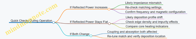
Summary of the Integrated Logic
Power coupling efficiency is determined by both reflection losses and how the plasma absorbs the delivered power. Effective impedance explains why matching must respond to plasma conditions, while plasma loading explains why the same “matched” system can still heat the wrong region. Good engineering practice therefore combines real-time reflection monitoring with deposition-aware validation, so the system is not only well-matched, but also well-aimed.
8. Confinement Quality, Transport, and Turbulence Control
8.1 Transport Mechanisms in Magnetized Plasmas
Transport is how particles and energy move across magnetic field lines and through the plasma’s gradients. In magnetized plasmas, motion parallel to the field is usually much faster than motion across it, so the key engineering question becomes: what processes still allow cross-field transport, and how large are they compared with the confinement requirement.
Core Picture of Magnetized Transport
Start with the simplest ordering: a charged particle spirals around magnetic field lines with a small gyroradius, then drifts due to field inhomogeneities. If the magnetic field were perfectly uniform and the plasma perfectly collisionless, guiding centers would stay on their field lines and cross-field transport would be tiny. Real plasmas break those idealizations through collisions, turbulence, and geometry.
A useful mental model is to separate transport into three layers:
- Microscopic motion: gyration, guiding-center drifts, and parallel streaming.
- Mesoscopic transport: how those motions produce fluxes driven by gradients.
- Macroscopic profiles: how fluxes reshape density and temperature over time.
A gradient-driven flux is often written in the form
- Particle flux: \(\Gamma = -D,\nabla n + V,n\)
- Heat flux: \(q = -\chi,\nabla T + \text{(pinch terms)}\)
Here \(D\) and \(\chi\) are effective diffusion coefficients, and \(V\) represents drift-like convection. The “effective” part matters: turbulence and collisions both contribute, but the plasma only cares about the net flux.
Collisional Transport and Neoclassical Effects
Collisions randomize particle velocities and allow slow cross-field motion even without turbulence. In a magnetized plasma, the collision frequency sets how quickly parallel momentum and energy are redistributed. That redistribution then couples to drift motion, producing neoclassical transport.
Neoclassical transport is geometry-sensitive because trapped particles bounce in regions of weaker magnetic field. In a tokamak, the combination of toroidal curvature and field variation creates different populations: passing and trapped. Each population has different drift patterns, so the resulting flux depends on safety factor, magnetic shear, and collisionality.
Easy example: Imagine two groups of particles in a “magnetic bottle.” Passing particles slide along the field and sample the whole device, while trapped particles bounce back and forth near the midplane. If collisions are rare, trapped particles stay trapped longer, so their contribution to cross-field transport is limited. If collisions are frequent enough, trapped particles scatter into passing orbits, increasing cross-field transport.
Turbulent Transport and Fluctuation-Driven Fluxes
Turbulence is the dominant cross-field transport mechanism in many operating regimes. It creates fluctuating \(\tilde{n}\) and \(\tilde{T}\) that correlate with \(\tilde{\phi}\) (electrostatic potential) or magnetic fluctuations. Those correlations produce a net flux even when the mean \(E\times B\) drift is small.
A standard decomposition is:
- Mean flux comes from mean gradients.
- Turbulent flux comes from correlations like \(\langle \tilde{n}\tilde{v}_r\rangle\).
Because the turbulence is driven by gradients, transport is often nonlinear: increasing temperature gradient can increase turbulent intensity, which then increases heat flux. That feedback shapes the steady-state profiles.
Easy example: Consider a hallway with moving people. If the hallway is calm, people mostly follow the rules and move predictably. If someone starts a small crowd-surge, the average motion changes even if the average “intent” is unchanged. In plasmas, the “crowd-surge” is the turbulence, and the net effect is a larger effective \(\chi\).
Transport Regimes and Scaling Logic
Transport size depends on which physics dominates:
- Low collisionality: trapped-particle effects and turbulence can both matter, but neoclassical may be limited by long orbit lifetimes.
- High collisionality: collisions enhance neoclassical scattering, often increasing effective diffusion.
- Strong gradients: turbulence thresholds are crossed, and turbulent transport rises sharply.
Engineers usually don’t need every microscopic detail to start; they need the ordering. For example, if measured heat flux scales strongly with gradient in a way consistent with turbulent transport, then improving confinement means reducing the gradient drive or stabilizing the turbulence, not just changing average density.
Mind Map: Transport Mechanisms
Putting It Together with a Concrete Scenario
Suppose a device increases auxiliary heating power. Initially, temperature rises near the core, steepening \(\nabla T\). If neoclassical transport alone dominated, the heat flux would change smoothly with collisionality and geometry. Instead, many experiments show that once gradients become large enough, turbulent transport increases, raising the effective \(\chi\) until the system reaches a new balance where heating power matches total losses.
That balance is the practical meaning of transport mechanisms: they determine how quickly the plasma “pushes back” against imposed gradients. In modeling and control, the goal is not to pick a favorite mechanism, but to identify which one sets the net flux under the current operating conditions.
8.2 Neoclassical Transport and Its Dependence on Geometry
Neoclassical transport describes how particles and heat move in a magnetized plasma when collisions are present but the plasma is still “well organized” by magnetic fields. The key idea is simple: in a perfectly symmetric magnetic field, many particle drifts cancel out over a bounce or transit. Real fusion devices are not perfectly symmetric, so geometry decides how much cancellation you get, and collisions decide how quickly particles sample different parts of phase space.
Core Geometry Ingredients
Neoclassical theory starts from how guiding centers move. A particle follows a magnetic field line while its drift motion depends on field strength variation and curvature. Two geometric features dominate:
- Magnetic field strength variation along the field creates a mirror effect. Particles with large enough pitch angle reflect, producing trapped orbits.
- Curvature and gradient of the magnetic field create drifts that differ for trapped and passing particles.
A practical mental model is to imagine a marble rolling through a wavy channel. If the channel is symmetric, the marble’s sideways tendency averages out. If the channel’s shape changes with position, the averaging is incomplete, and collisions then “reset” the marble’s direction, letting a net drift accumulate.
Trapped Versus Passing Particles
In toroidal devices, particles split into:
- Passing particles that circulate around the torus.
- Trapped particles that bounce between mirror points.
Geometry controls the trapped fraction through the magnetic field’s variation. Stronger variation increases trapping, which changes transport because trapped particles experience different drift paths and spend more time in regions where the field is weaker or stronger.
A concrete example: in a tokamak with stronger poloidal field shaping, the magnetic field magnitude varies more along a field line. That increases the number of trapped orbits, which typically raises the sensitivity of transport to collisionality and to the details of the flux-surface geometry.
Collisions and Collisionality Regimes
Neoclassical transport depends on collisionality, often expressed as a dimensionless ratio comparing collision frequency to the rate of parallel motion along the field. Three regimes matter conceptually:
- Low collisionality: particles complete many bounces or transits before collisions significantly change their pitch angle. Transport is limited by how geometry causes drift averaging.
- Intermediate collisionality: collisions gradually mix pitch angles, letting particles sample different drift orbits. This is where geometry effects often show up clearly.
- High collisionality: collisions dominate pitch-angle evolution, and transport becomes closer to a diffusion picture with geometry entering through effective transport coefficients.
Example: if you increase density while keeping temperature fixed, collisionality rises. In many configurations, that shifts the dominant transport mechanism from drift-averaging limitations toward collision-driven diffusion, changing the measured heat flux scaling with temperature.
How Geometry Enters Through Flux Surfaces
Neoclassical transport is not only about “toroidal vs stellarator.” It depends on how flux surfaces are shaped and how field lines wind through them. Important geometric quantities include:
- Magnetic shear, which measures how rapidly the field-line pitch changes with radius.
- Bounce-averaged drift differences between trapped and passing particles.
- Orbit topology, which depends on whether particles remain on nested surfaces or explore more complex regions.
In a tokamak, magnetic shear and circular-to-elongated shaping change the fraction and properties of trapped orbits. In a stellarator, nonaxisymmetry changes the entire orbit structure, so the same “collisionality knob” can produce different transport responses.
Mind Map: Geometry to Transport Chain
Putting It Together with a Worked Example
Consider a simplified comparison between two flux surfaces at the same radius in a tokamak-like device. Surface A has weaker magnetic field variation along field lines than Surface B. Surface B therefore has a larger trapped fraction.
- With more trapped particles, the plasma’s effective drift averaging is less complete because trapped orbits experience stronger bounce-averaged drift differences.
- At low collisionality, trapped particles keep their pitch angles longer, so geometry-driven drift differences persist, increasing transport.
- At higher collisionality, collisions scatter pitch angles more frequently, partially smoothing orbit differences. Transport may still be higher than in Surface A, but the scaling with collisionality changes.
This is why neoclassical transport is often described as “geometry plus collisionality plus orbit class.” If any one of those is missing, the explanation feels incomplete.
Practical Implications for Modeling
When building or interpreting neoclassical predictions, the geometry must be represented accurately enough to capture orbit topology and trapped-passing boundaries. Small errors in shaping or equilibrium reconstruction can shift trapped fractions and drift averages, which then changes predicted heat flux and particle flux. That is also why neoclassical calculations are sensitive to the chosen equilibrium and to how flux surfaces are parameterized.
In short: neoclassical transport is the accounting system for how magnetic geometry controls orbit-averaged motion, while collisions control how quickly particles move between those orbit classes.
8.3 Turbulence Driven Transport and Basic Instability Types
Turbulence matters because it turns “nice” average plasma profiles into messy, correlated fluctuations. Those fluctuations move particles, heat, and momentum across magnetic field lines far faster than simple collisional transport would. The practical engineering goal is not to eliminate every wiggle, but to keep the turbulence from becoming the dominant transport channel.
Core Idea of Turbulent Transport
Start with a quantity like ion temperature. In a magnetized plasma, the mean temperature varies with radius, but turbulence adds fluctuations around that mean. The radial heat flux is well represented by the correlation between the fluctuating radial velocity and the fluctuating temperature:
- If hotter-than-average regions tend to move outward, the correlation is positive and heat flows outward.
- If the correlation changes sign, the net flux can reduce.
A useful mental model is a crowd moving through a doorway: if the “fast people” consistently head outward, the flow is large; if they mix randomly, the net flow is smaller. In plasmas, the doorway is the radial direction, and the “fast people” are the correlated fluctuations.
From Microphysics to Transport Models
Turbulence is driven by free energy gradients, such as:
- Temperature gradients that feed ion-scale instabilities.
- Density gradients that feed drift-wave-like behavior.
- Velocity shear that can suppress or reshape turbulent eddies.
A standard modeling workflow is:
- Identify the dominant gradient and scale.
- Determine the likely instability family.
- Estimate how fluctuations saturate, often by balancing drive against nonlinear decorrelation.
- Convert the resulting fluctuation statistics into transport coefficients or direct flux predictions.
A practical best practice is to connect models to measurements using profile gradients and fluctuation diagnostics. For example, if measured turbulence levels rise sharply when the ion temperature gradient increases, that supports a gradient-driven instability picture rather than a purely collisional one.
Basic Instability Types and What They Do
Most turbulence in fusion-relevant plasmas is associated with a few recurring instability families. Each has a characteristic “signature” in scale, frequency, and dependence on gradients.
Ion Temperature Gradient Instability
This family is driven by ion temperature gradients. It typically produces turbulence that transports heat strongly and can also move particles. A simple example: imagine a steep temperature ramp near the core. As the ramp steepens, the drive increases, and the turbulence correlation between radial motion and temperature fluctuations grows, raising heat flux.
Engineering implication: profile control systems that flatten the ion temperature gradient can reduce the dominant drive, but they must do so without triggering other constraints like stability limits or power balance issues.
Trapped Electron Mode Turbulence
Here the free energy comes from density gradients and electron-related dynamics. Trapped electrons respond differently to fields than passing electrons, so the turbulence can be sensitive to density profile shape. Example: if the density gradient becomes steeper in a region where electrons are more likely to be trapped, the turbulence can intensify even if the ion temperature gradient is unchanged.
Engineering implication: density peaking and fueling strategies affect turbulence levels, so transport control is not only about heating.
Drift Wave and Density Gradient Turbulence
Drift-wave-like behavior is often present when density gradients exist. It tends to produce particle transport and can contribute to heat transport indirectly. Example: if density fluctuations correlate with radial electric field fluctuations, the resulting E×B-driven motion can carry particles outward or inward depending on the phase relationship.
Engineering implication: controlling the radial electric field profile can change turbulence character, not just its magnitude.
Microtearing and Electromagnetic Effects
When magnetic fluctuations become important, tearing-like microstructures can appear, often affecting electron heat transport. Example: if electromagnetic fluctuations increase, electron thermal transport can rise even when electrostatic measures look similar.
Engineering implication: stability and transport are coupled; a “good” electrostatic picture may miss an electromagnetic channel.
Kelvin Helmholtz and Shear Suppression
Velocity shear can suppress turbulence by stretching turbulent eddies until they decorrelate. Example: if the E×B flow shear increases across a narrow radial region, turbulent structures may become thinner and less effective at transporting heat.
Engineering implication: shear is a tool, but it must be generated and maintained without causing other instabilities or excessive control effort.
Mind Map: Turbulence Drivers and Instability Types
A Concrete Example of How Instability Choice Changes Transport
Consider two operating points with the same average temperature but different gradient shapes. In the first, the ion temperature gradient is moderate and the density gradient is steep. Turbulence may be dominated by trapped electron or drift-wave-like behavior, producing substantial particle transport and a different heat-flux balance. In the second, the density gradient is flatter while the ion temperature gradient is steeper. Ion temperature gradient turbulence becomes more likely, and heat transport tends to increase more strongly with the steepened ion gradient. The key is that turbulence is not determined by a single number; it depends on which gradient provides the free energy and which instability family can access it.
Practical Checks for Identifying Dominant Turbulence
A reliable workflow uses three categories of evidence:
- Profile evidence: compare measured gradients to thresholds implied by instability theory.
- Fluctuation evidence: check whether fluctuation frequencies and spatial scales match the expected family.
- Flux evidence: see whether changes in heating or fueling correlate with changes in the predicted flux channel.
When these lines agree, the transport model becomes more than a guess. When they disagree, the mismatch usually points to the wrong dominant instability family, missing electromagnetic effects, or an incorrect assumption about saturation and correlation structure.
8.4 Profile Control Using Shaping and Auxiliary Systems
Profile control means steering plasma temperature and density profiles so the device stays in a favorable operating window for confinement and stability. In practice, you are not “aiming for a perfect curve”; you are managing gradients, because gradients drive transport, instabilities, and power-flow patterns.
Foundational Idea: Profiles, Gradients, and Transport
A magnetically confined plasma can be thought of as a set of coupled balances: heating and particle sources compete with transport losses. Transport is strongly sensitive to local gradients, so small changes in shaping or auxiliary power can shift the dominant transport regime.
A useful mental model is the steady-state balance for a generic quantity \(X\) (temperature or density):
- Sources add \(X\).
- Transport removes \(X\) through a flux that depends on gradients.
- Geometry sets how those gradients map onto magnetic surfaces.
If you increase heating at mid-radius, you often steepen the temperature gradient there, which can either improve confinement (if turbulence is suppressed) or worsen it (if turbulence is enhanced). Profile control is the art of choosing the direction that improves the overall energy balance.
Shaping: Changing Geometry to Reshape Flux Paths
Shaping modifies the magnetic equilibrium and therefore the mapping between heating deposition, particle orbits, and transport channels.
Key Shaping Levers
- Plasma cross-section and elongation: affects stability boundaries and how pressure gradients relate to magnetic curvature.
- Triangularity: changes the effective drift and can influence neoclassical transport.
- Current and pressure profiles through equilibrium control: determines safety factor \(q\) and magnetic shear, which strongly affects stability and turbulence.
Easy Example
Suppose two discharges have the same total heating power. In one, the equilibrium has stronger magnetic shear near mid-radius. That often changes how perturbations grow and can reduce the tendency for certain instabilities to flatten profiles. The result can be a higher core temperature even without changing total power, because the transport “path” is altered by equilibrium.
Auxiliary Systems: Where the Power and Particles Go
Auxiliary systems add controlled sources. The goal is to place those sources so they counteract unwanted flattening or prevent excessive edge gradients.
Heating and Current Drive as Profile Tools
- Neutral beam injection: deposits energy and momentum; momentum can help shape rotation and current profile.
- Radio frequency heating: deposits energy at targeted radii depending on frequency and magnetic field.
- Lower hybrid and ion cyclotron heating: can drive current and modify electron or ion temperature gradients.
Particle Control
- Gas puffing and pellet injection: control density profile shape and edge fueling rate.
- Impurity control: affects radiation losses, which indirectly reshape temperature profiles.
Easy Example
If density rises too much, electron temperature often drops because more energy goes into ionization and because radiative losses increase. A practical response is to reduce edge fueling or shift fueling inward with pellets, aiming for a density profile that supports confinement rather than one that simply increases total particle content.
Integrated Control Strategy: From Targets to Actuators
A systematic approach uses three layers: measurement, control targets, and actuator selection.
Step 1: Define Profile Targets
Targets are usually expressed as constraints on:
- core temperature gradient (to manage turbulence)
- edge temperature and density gradients (to manage heat flux and stability)
- current profile shape or magnetic shear (to manage MHD stability)
Step 2: Choose Actuators That Affect the Right Radius
- If you need to change mid-radius \(T_e\), prefer heating deposition that peaks there.
- If you need to reduce edge gradients, adjust fueling and edge heating balance.
- If you need to change stability via shear, use current drive or equilibrium shaping.
Step 3: Close the Loop with Feedback
Feedback uses real-time diagnostics to adjust actuators. A common pattern is:
- measure profile proxies (or reconstructed profiles)
- compare to targets
- adjust actuator power, fueling rate, or equilibrium parameters
Mind Map: Profile Control Using Shaping and Auxiliary Systems
Case Study: A Coherent Control Sequence
Consider a discharge where the core temperature starts to flatten while edge heat flux rises.
- Check density profile: if density is creeping up, reduce edge fueling or shift fueling inward.
- Rebalance heating deposition: move heating deposition slightly toward mid-radius to rebuild the temperature gradient where transport is most sensitive.
- Adjust equilibrium shaping or current drive: if stability indicators suggest reduced magnetic shear, modify current profile shape to restore the favorable shear region.
The key is that each action targets a different part of the coupled balance: density affects radiation and ionization, heating deposition affects local gradients, and shear affects stability and turbulence pathways. When these levers are coordinated, the plasma stops “fighting back” by pushing gradients into an unfavorable regime.
8.5 Practical Diagnostic Inputs for Transport Model Validation
Transport models only earn their keep when they can reproduce measured profiles and fluxes without “fitting the universe.” The practical workflow is to (1) choose diagnostics that constrain the specific terms in your transport equations, (2) translate raw signals into physically comparable quantities, and (3) validate models with uncertainty-aware consistency checks.
What Transport Models Actually Need
Most transport models reduce to a few coupled ingredients: particle and energy fluxes, source terms, and profile evolution. In practice, you validate against quantities that map to these ingredients.
- Profiles: electron temperature, ion temperature, density, and rotation where available.
- Fluxes: heat fluxes (electron and ion), particle fluxes, and sometimes momentum flux.
- Geometry and equilibrium: magnetic surfaces, safety factor, shaping parameters, and local gradients.
- Inputs to transport closures: turbulence proxies, collisionality, effective charge, and impurity content.
A useful rule of thumb: if your model predicts a flux, you should have at least one diagnostic path that can infer that flux or its divergence.
Diagnostic Categories That Constrain Transport
Equilibrium and Geometry Inputs
Magnetic equilibrium reconstruction provides the mapping from diagnostic coordinates to flux surfaces. Without it, “the same radius” becomes a moving target.
Example: A spectroscopic line-of-sight measurement gives an emission location. If the equilibrium shifts the flux-surface radius by even a few percent, the inferred temperature gradient can change enough to alter predicted transport.
Profile Diagnostics for Gradients
Transport closures are gradient-sensitive. You therefore want diagnostics that are accurate in the gradient region, not just at the core.
- Thomson scattering for electron temperature and density profiles.
- Charge exchange or spectroscopy for ion temperature and flow.
- Interferometry for line-integrated density, combined with inversion to get radial profiles.
Best practice: validate profile inversion against independent constraints such as edge density from reflectometry or radiation-based impurity estimates.
Heat Flux Inference from Power Balance
Heat flux is often inferred rather than directly measured. The most robust approach uses power balance and local gradient information.
- Electron heat flux from measured temperature profiles and known sources/sinks.
- Ion heat flux from ion temperature profiles and charge-exchange-based constraints.
Example: If auxiliary heating is predominantly electron-coupled, electron heat flux inferred from power balance should show a clear outward trend consistent with the measured temperature pedestal slope. If not, either the source partition is wrong or the inferred gradients are biased.
Particle Transport Constraints
Particle transport validation benefits from impurity and main-ion diagnostics.
- Impurity spectroscopy for effective charge and impurity density profiles.
- Charge exchange for main-ion density and sometimes flux-related quantities.
- Recycling and edge diagnostics for boundary conditions.
Best practice: treat impurity transport as a first-class constraint. Even if the model focuses on main ions, impurity-driven changes to radiation and collisionality can indirectly reshape main-ion transport.
Mind Map: Diagnostic Inputs for Transport Validation
A Systematic Validation Workflow
- Reconstruct equilibrium and map diagnostics to flux surfaces. Use the same reconstruction settings for all diagnostics in the comparison window.
- Convert raw signals into profiles with uncertainty. Keep track of calibration, inversion regularization, and line-of-sight geometry effects.
- Infer fluxes using power balance with explicit source terms. Include auxiliary heating deposition and radiation losses consistently with the model.
- Compute model-predicted flux divergences and compare to profile evolution. If your model predicts fluxes but not the observed profile time evolution, the mismatch is usually in either source partitioning or transport coefficients.
- Perform consistency checks. For example, the inferred heat flux should align with the measured temperature gradient trends across the same radial region.
Example: Validating Electron Transport with a Heat Balance Loop
Suppose you have electron temperature and density profiles plus auxiliary heating power. You infer electron heat flux from power balance using measured profiles and estimated radiation losses. Then you run the transport model with the same equilibrium and gradients.
- If the model reproduces the shape of the inferred electron heat flux but not the magnitude, the likely culprit is incorrect heating deposition or radiation loss modeling.
- If it reproduces magnitude but not shape, the likely culprit is biased temperature gradients or an incorrect transport closure dependence on gradient scale length.
This loop is simple, but it forces the model to match both the “where” and the “how much,” not just one.
Common Failure Modes to Watch
- Misaligned radii: equilibrium mapping differences can masquerade as transport physics.
- Biased gradients: smoothing or inversion choices can shift gradient scale lengths.
- Wrong source partition: assuming all heating goes to electrons when it does not will break flux inference.
- Overconfident equilibrium: treating equilibrium as exact ignores reconstruction uncertainty that can dominate gradient comparisons.
When diagnostics are used this way—profiling, flux inference, and uncertainty-aware comparisons—the transport model stops being a story and becomes a measurable hypothesis.
9. Instabilities, Disruptions, and Stability Engineering
9.1 MHD Stability Concepts and Mode Classification
Magnetohydrodynamics (MHD) treats a plasma as a conducting fluid coupled to magnetic fields. Stability questions then become: if the plasma is nudged, do the perturbations shrink back, stay bounded, or grow until they change the operating state? In fusion devices, this matters because growing modes can trigger large transport, degrade confinement, or lead to disruptions.
Core Assumptions and What They Buy You
MHD assumes the plasma is sufficiently collisional or that macroscopic behavior can be captured by fluid moments. It also assumes a single-fluid description: electrons and ions share bulk motion, while current comes from relative motion encoded in conductivity. This framework is not meant to predict every microscopic detail; it’s meant to classify macroscopic instabilities and identify which equilibrium features they depend on.
A useful mental model is a magnetized fluid sheet. If the equilibrium has “bad geometry” for the current and pressure profiles, the sheet can bend or twist in ways that reduce energy. Stability analysis asks whether those energy-lowering motions are available.
Energy Principle and the Stability Test
A common way to classify MHD stability is through an energy principle: perturbations are stable if they increase the system’s potential energy for all allowed displacements. If there exists any displacement that decreases energy, the corresponding mode can grow.
Practically, this becomes a mode classification problem. You identify the displacement pattern, then check whether it taps free energy from pressure gradients, current gradients, or magnetic shear.
Mode Classification by Geometry and Symmetry
In toroidal devices, perturbations are labeled by how they vary around the torus and along the poloidal direction.
- Toroidal mode number (n) counts how many “ripples” fit in the toroidal direction.
- Poloidal mode number (m) counts ripples poloidally.
- Resonant surfaces occur where the safety factor q satisfies a resonance condition, often written as q = m/n for idealized cases.
A mode near a resonant surface can couple strongly to the equilibrium current and pressure, making it more likely to grow.
Ideal vs Resistive Behavior
MHD modes are often grouped by whether they rely on resistivity.
- Ideal MHD modes can grow even if resistivity is very small, because they do not require magnetic field lines to reconnect.
- Resistive MHD modes require finite resistivity to allow reconnection or tearing-like behavior at resonant surfaces.
This distinction is not academic. It determines which control levers matter: ideal modes respond strongly to pressure and current profile shaping, while resistive modes are sensitive to resistive time scales and local current gradients.
Mind Map: MHD Stability Concepts and Mode Classification
Example: Reading a Mode Label Like a Map
Suppose diagnostics show a perturbation with n = 2 and m = 3. The resonance condition suggests q ≈ 3/2 at the relevant radius. If the equilibrium q-profile crosses 1.5, that location becomes a prime suspect for where the mode energy couples into the plasma. If the q-profile is shifted so it no longer crosses that value within the plasma core, the same perturbation pattern may weaken or move to a different radius.
This is why stability analysis is inseparable from equilibrium reconstruction: the mode label is only half the story; the q-profile is the other half.
Example: Ideal vs Resistive in Practice
Consider two scenarios with the same pressure and current profiles but different effective resistivity (for instance, due to temperature changes). An ideal mode classification predicts similar growth behavior because it does not rely on resistive reconnection. A resistive mode classification predicts growth changes because the reconnection rate depends on resistive time scales. Observing which behavior matches the data helps sort the instability family.
Advanced Details Without the Fog
Once you know the family, you can refine classification by asking what the perturbation does to magnetic topology and flow.
- Magnetic shear affects how field lines twist relative to each other, shaping where resonances are strong and how perturbations align with equilibrium.
- Pressure-driven effects can create ballooning-like displacements that bulge outward where pressure gradients are steep.
- Current-driven effects can create kink-like distortions that twist the plasma column.
In a stability workflow, you start with equilibrium profiles, identify candidate resonant surfaces, classify whether the mode is ideal or resistive, and then connect the expected displacement pattern to observed signatures such as magnetic fluctuations and changes in transport.
Example: A Systematic Classification Checklist
- Identify dominant n and m from fluctuation spectra.
- Compute where q(r) ≈ m/n.
- Check whether the mode growth correlates with profile changes that affect pressure gradients or current gradients.
- Compare sensitivity to resistivity-related conditions to decide ideal vs resistive family.
- Map the expected displacement to measured spatial localization and transport response.
When these steps agree, the classification is not just a label; it becomes a consistent explanation for why the plasma either resists the perturbation or lets it grow.
9.2 Tearing Modes, Sawtooth Oscillations, and Their Impacts
Tearing modes and sawtooth oscillations are two closely related ways a magnetically confined plasma can “rearrange” its internal magnetic structure. The common thread is that the plasma current profile and pressure gradients can become mismatched with the stability requirements of the magnetic geometry. When that happens, magnetic islands or rapid core relaxations appear, and the resulting transport changes can be measured within milliseconds.
Core Concepts Before the Instability Shows Up
A tokamak plasma has nested magnetic surfaces, but the surfaces are not perfectly rigid. The safety factor profile, q(r), tells you how many toroidal turns a field line makes per poloidal turn. If q crosses a rational value m/n, the plasma can resonate with an m/n perturbation. A tearing mode is essentially a resonant response that forms a magnetic island around that rational surface.
Sawtooth oscillations are a different-looking behavior: the core temperature rises gradually, then drops quickly, then repeats. The usual picture is that a sufficiently steep pressure gradient drives a fast relaxation when the internal kink condition is met near the q=1 surface. That relaxation flattens the temperature and pressure profiles in the core, which changes the current profile and can also affect nearby tearing activity.
Tearing Modes: From Resonance to Magnetic Islands
A practical way to think about tearing modes is to separate two ingredients: (1) a resonant perturbation at a rational surface, and (2) a mechanism that allows reconnection to proceed. In the simplest terms, the plasma needs a current perturbation that is phase-aligned with the magnetic perturbation. If the current profile is steep enough, the mode can grow and form islands.
Easy example: Imagine a rubber sheet with a small notch at a specific location. If you tug the sheet periodically at the notch’s natural rhythm, the notch region can widen. In a plasma, the “tug” is the resonant perturbation at m/n, and the “widening” is the island growth.
Impacts: Magnetic islands increase local transport by breaking the smoothness of magnetic surfaces. Even if the island is confined to a narrow radial band, it can degrade confinement by flattening temperature gradients across the island width. Islands can also seed further instabilities by changing local current and pressure profiles.
Sawtooth Oscillations: Core Relaxation and Profile Flattening
Sawtooth behavior is often described as a slow build-up followed by a fast crash. During the slow phase, heating and transport gradually steepen the core profiles. Once the internal kink stability threshold is crossed, the core undergoes a rapid reconfiguration that flattens temperature and pressure inside the affected region.
Easy example: Think of a sponge soaking up water. As long as the sponge is absorbing slowly, the moisture gradient increases. When the sponge reaches a threshold, water redistributes quickly, reducing the gradient. In the plasma, the “water” is the pressure/temperature gradient, and the “redistribution” is the fast relaxation.
Impacts: The immediate effect is a drop in core temperature and a change in current profile. Because tearing modes depend on current and q-profile details, sawtooth crashes can either suppress or trigger tearing activity depending on how the relaxation shifts the q=1 region and nearby rational surfaces.
Coupling Between Sawteeth and Tearing Modes
The coupling is not automatic, but it is common. A sawtooth crash can alter the current profile so that the drive for a tearing mode changes. Conversely, persistent tearing activity can modify the current profile enough to change the internal kink threshold. In experiments, this shows up as correlations between sawtooth timing and the appearance or growth rate of specific island modes.
Mind Map: Tearing Modes and Sawtooth Oscillations
Example: Interpreting a Mode-Linked Sawtooth Event
Suppose diagnostics show that the core temperature rises for 50 ms, then drops sharply. At the same time, magnetic diagnostics indicate an m/n island near a rational surface slightly outside the q=1 region. The sequence can be interpreted as follows: the slow phase steepens profiles until the internal kink triggers the sawtooth crash. The crash relaxes the core and changes the current profile, which shifts the local stability of the nearby rational surface. If the island amplitude grows after the crash, the relaxation likely increased the tearing drive there; if it decays, the relaxation likely reduced the drive.
Practical Takeaway for Engineering Stability
From an engineering perspective, the key is that both phenomena are profile-driven. Tearing modes respond to how current and q align with rational surfaces, while sawtooth oscillations respond to how pressure gradients and current shear satisfy the internal kink condition. That means mitigation strategies must be consistent with the measured profile evolution, not just the instantaneous mode amplitude. When you treat them as coupled profile dynamics, the behavior becomes less mysterious and more actionable.
9.3 Disruption Physics and Thermal Mechanical Consequences
A disruption is a rapid loss of the plasma’s ability to maintain stable confinement. In a tokamak, it often starts with a stability problem in the magnetohydrodynamic (MHD) system and ends with a sudden change in current, temperature, and heat-flux patterns. The key engineering point is that the plasma does not “turn off” politely; it transfers energy and momentum to surrounding structures on timescales that can be shorter than many mechanical response times.
Foundational Chain from Instability to Energy Deposition
The disruption chain begins with a mode that grows because the plasma current profile and pressure gradients no longer satisfy stability conditions. As the mode amplitude increases, magnetic surfaces break down and transport rises sharply. Two consequences follow in parallel: (1) the confinement of heat deteriorates, and (2) the current channel can reorganize or collapse.
A practical way to think about it is to separate three clocks:
- Magnetic evolution clock: how quickly the current and field topology change.
- Thermal diffusion clock: how quickly heat spreads in the plasma and then into materials.
- Mechanical response clock: how quickly structures expand, bow, or crack under thermal and electromagnetic loads.
Disruptions are dangerous when the magnetic evolution clock is much faster than the thermal and mechanical clocks, because energy is deposited before structures can distribute it.
Thermal Consequences for First Wall and Divertor
Once confinement degrades, power that previously spread over flux surfaces can concentrate along new paths. In tokamaks, the divertor is the usual target for this concentration. The heat-flux profile can become narrow, raising peak surface temperatures and thermal stresses.
A simple example helps: imagine a heat load that is normally spread over a 10 cm wide region. If the effective width shrinks to 1 cm during a disruption, the peak heat flux can increase by roughly a factor of 10, even if the total energy deposited is similar. That peak matters because thermal stress scales with temperature gradients, not just with average heating.
Electromagnetic effects also contribute. As the plasma current decays, induced currents appear in nearby conductors. These currents create additional forces and can couple to the same regions that already see concentrated heat.
Mechanical Consequences from Rapid Loading
Thermal expansion is slow compared to the timescale of a disruption, so the surface layer can try to expand while the bulk material resists. This mismatch generates stress. If the stress exceeds material limits, you get cracking, delamination, or erosion that can progress with repeated events.
There is also a fatigue-like mechanism even without catastrophic failure. Repeated disruptions can cycle thermal loads, causing microstructural changes and weakening. Engineers therefore treat disruption mitigation as a lifetime management problem, not only a single-event safety problem.
Current Quench and Runaway Electrons
Many disruptions include a current quench, where the plasma current drops quickly. During this phase, the electric field can become large enough to accelerate a subset of electrons. If these electrons form a runaway population, they can carry energy to the wall in a highly localized pattern.
The thermal-mechanical consequence is straightforward: a narrow beam-like deposition produces steep temperature gradients. Even if the total runaway energy is smaller than the thermal energy of the plasma, the localization can dominate peak stress.
Mitigation Levers and What They Change Physically
Mitigation strategies aim to reduce either the peak heat flux, the total deposited energy, or the localization.
- Slowing the current quench spreads energy over a longer time, giving structures more time to conduct heat inward.
- Distributing the deposition changes where the power lands, often by controlling magnetic topology during the disruption.
- Reducing runaway formation lowers the chance of a sharply localized energy channel.
A useful engineering check is to ask: does the mitigation change the deposition width, the deposition time, or both? Each has a different impact on peak temperature and stress.
Mind Map: Disruption Physics to Consequences
Example: Comparing Two Hypothetical Quenches
Consider two disruptions with the same total energy deposited into the divertor. In Case A, the deposition occurs over 1 ms with a 1 cm effective width. In Case B, it occurs over 5 ms with a 2 cm effective width. Case B reduces peak heat flux because the energy is spread over a longer time and a wider region. That combination lowers peak temperature and reduces thermal stress, even though the total energy is identical. This is why mitigation often targets quench duration and deposition geometry, not only total disruption severity.
Mind Map: What to Measure During a Disruption
Disruption physics and thermal-mechanical consequences are tightly coupled: instability changes magnetic topology, topology changes where energy goes, and energy deposition patterns determine stress. When you track the chain from current quench to deposition width and time, the engineering choices become concrete rather than abstract.
9.4 Control Systems for Stability Monitoring and Mitigation
Stability control in a fusion plasma is less about “stopping” instabilities and more about keeping the operating point inside a region where growth is slow, feedback authority is sufficient, and actuators do not create new problems. A useful mental model is a loop: measure the plasma state, estimate what is about to happen, decide what to do, and actuate with constraints.
Core Control Loop from Signals to Actions
- Measure: Use real-time diagnostics to track equilibrium, profiles, and mode activity. Typical signals include magnetic pickup coils, soft X-ray arrays, interferometry, reflectometry, and divertor probes.
- Estimate: Convert raw signals into quantities tied to stability, such as current density profile, safety factor trends, and mode amplitude or phase.
- Decide: Select a mitigation strategy based on thresholds, mode identification, and actuator availability.
- Actuate: Apply control actions such as changes to heating/current drive, magnetic perturbations, or plasma shape parameters.
- Constrain: Enforce limits on power deposition, coil currents, and allowable profile changes to avoid secondary instabilities.
A practical example: if magnetic sensors show a rising tearing mode amplitude, the controller may increase localized current drive at the rational surface while simultaneously reducing global current ramp rate. The first action targets the mode’s driver; the second reduces the background conditions that make the mode keep growing.
Monitoring Strategy That Separates Noise from Meaning
Good monitoring starts with signal hygiene. Many stability indicators are indirect, so the controller must handle delays and measurement noise.
- Time alignment: Diagnostics often have different sampling rates and latencies. If you ignore this, feedback can “chase” an already-past event.
- Filtering with intent: Use filtering that preserves phase information when phase is used for feedback. A controller that only tracks amplitude can miss whether the mode is rotating or locked.
- Feature extraction: Instead of feeding raw waveforms, compute features like mode amplitude, frequency, and phase relative to a reference.
Example: A soft X-ray channel may saturate during bursts. A robust controller detects saturation and switches to alternative channels or reduces trust weight for that channel rather than blindly continuing.
Estimation Layers from Equilibrium to Mode Identification
Controllers typically use layered models.
- Equilibrium estimation: Reconstruct magnetic surfaces and pressure/current profiles to locate rational surfaces.
- Transport-aware profile estimation: Update profiles using simplified transport models so the controller knows how quickly profiles will respond to actuators.
- Mode identification: Determine which instability family is present by combining frequency, spatial localization, and polarization signatures.
Example: If a controller assumes the wrong rational surface location, it may drive current in the wrong region. The mode amplitude might still drop briefly due to indirect effects, but the system becomes harder to stabilize consistently.
Mitigation Actions and How They Map to Instability Drivers
Mitigation is most effective when the action targets the driver rather than only the symptom.
- Profile control: Adjust heating/current drive to shape pressure and current density gradients.
- Magnetic control: Use feedback on external coils or resonant magnetic perturbations to influence mode structure.
- Rotation and shear management: Modify torque or heating deposition to change flow shear, which can slow growth.
- Ramping and scenario management: Change ramp rates to avoid crossing stability boundaries too quickly.
Example: For a sawtooth-like event driven by central current/pressure conditions, a mitigation strategy might preemptively alter central heating so the system reaches the next regime with less violent relaxation. The controller does not need to prevent every event; it needs to keep the event within acceptable limits for heat loads and component stress.
Feedback Types and When Each Makes Sense
- Threshold-based control: Simple and reliable for events with clear indicators. It works best when actuator response is fast compared to instability growth.
- Proportional-integral-derivative control: Useful for continuous regulation of mode amplitude or profile targets.
- Model-predictive control: Applies when constraints are tight and actuator effects are coupled. It can plan around limits like maximum heating deposition.
Example: If divertor heat flux constraints are strict, a controller may use model-predictive logic to reduce heating deposition before a predicted peak, rather than waiting for the peak to appear.
Constraints That Keep Mitigation from Creating New Instabilities
Actuators are not free. Common constraints include:
- Power and particle deposition limits: Avoid localized overheating or excessive impurity influx.
- Current drive and coil slew limits: Respect hardware bandwidth so commands remain physically achievable.
- Profile gradient limits: Large, fast changes can trigger other modes.
A simple rule of thumb: if mitigation requires a change larger than the plasma can respond to smoothly, the controller should slow down the approach or use a different actuator.
Mind Map: Stability Monitoring and Mitigation Control
Example: A Complete Mitigation Sequence for a Growing Mode
Suppose mode amplitude rises and the estimated rational surface is confirmed.
- The controller detects a sustained amplitude increase over a short window, not a single spike.
- It verifies sensor health and aligns the mode phase with the magnetic reference.
- It identifies the mode family by frequency and localization.
- It applies localized current drive near the rational surface while reducing the global ramp rate.
- It monitors for secondary indicators, such as pressure gradient changes and divertor heat flux proxies.
- If the mode amplitude stalls but heat flux rises, it reduces the deposition and shifts to a more conservative profile adjustment.
This sequence shows the core idea: monitoring prevents false triggers, estimation prevents wrong targeting, decision logic chooses an action that matches the driver, and constraints keep the fix from becoming the next problem.
9.5 Feedback and Feedforward Techniques for Plasma Control
Plasma control is easiest to understand as a timing problem: disturbances appear, the plasma responds, and actuators must correct the response before it grows into a loss of confinement or a stability limit. Feedback handles what you can measure after the fact; feedforward handles what you can predict before the plasma reacts. In practice, good control systems use both, with feedback doing the fine work and feedforward handling known coupling paths.
Core Concepts and Signal Flow
A useful mental model is a closed loop: sensors estimate state, a controller computes corrections, actuators apply changes, and the plasma evolves. For tokamaks, typical controlled variables include plasma current profile, edge density, heat flux proxies, and stability indicators such as mode amplitudes. Actuators include heating power, current drive, gas puffing, and magnetic field trims.
Feedback is most reliable when the measurement is fast enough and the actuator effect is sufficiently repeatable. If the sensor lags by a large fraction of the instability growth time, the controller will “chase” the error rather than suppress it. Feedforward is most reliable when the disturbance-to-actuator mapping is consistent, such as when a known heating schedule causes predictable profile shifts.
Feedback Control for Stability and Profile Shaping
Start with the simplest feedback: proportional-integral control on a scalar error. For example, suppose you want to keep edge density near a target to manage divertor heat loads. Let the error be e(t)=n_edge_target−n_edge_measured. Proportional action reduces immediate deviation; integral action removes steady offset caused by unmodeled fueling efficiency.
A more realistic approach uses multiple loops. One loop regulates a profile parameter (like electron temperature gradient proxy) while another loop regulates a stability metric (like a mode amplitude). These loops should be designed so they do not fight each other. A practical rule is to separate timescales: fast loops handle stability indicators, slower loops handle profile targets.
When the plasma exhibits nonlinear behavior, linear controllers can still work if you design around an operating point and update gains conservatively. Gain scheduling is a common technique: controller gains change with plasma current or heating power so the loop remains stable across the operating range.
Feedforward Control for Known Couplings
Feedforward uses a model or empirical mapping from planned inputs to expected plasma response. Consider a heating power step. Even if feedback will correct later, the initial transient can trigger an instability or create an overshoot in edge temperature. Feedforward can pre-compensate by adjusting gas puffing or magnetic shaping in anticipation.
A concrete example is current profile control. If you increase neutral beam power, the current drive efficiency and resulting current profile evolution are not instantaneous. A feedforward term can adjust the timing and magnitude of auxiliary actuators so the current profile stays near the desired shape during the ramp.
Feedforward is also useful for actuator constraints. If an actuator has a known dead time or saturation limit, the controller can shape the command so the plasma sees the intended effective change rather than the raw command.
Combining Feedback and Feedforward Without Chaos
The combined command is typically u(t)=u_ff(t)+u_fb(t). The key is to ensure the feedforward does not overwhelm feedback. One practical method is to let feedforward handle the bulk correction and limit feedback authority with saturation-aware logic. Another method is to filter feedforward signals so they do not inject high-frequency content that the actuators cannot reproduce.
A simple sanity check is to test each component separately in simulation or controlled experiments: first run feedback alone, then feedforward alone, then both together. If the combined response is worse than either alone, the interaction is likely due to phase mismatch or inconsistent scaling.
Mind Map: Feedback and Feedforward Plasma Control
Example: Edge Density Regulation with Anticipatory Heating Compensation
Assume you run a discharge where heating power ramps from P1 to P2 over 2 seconds. Edge density tends to drop during the ramp, increasing divertor heat flux risk. A feedback loop uses a fast edge diagnostic proxy sampled at 1–5 ms to regulate n_edge toward a target.
Feedforward adds a compensating gas puff profile based on the expected density drop per unit heating power change. During the ramp, the feedforward increases fueling slightly ahead of the measured density decline. Feedback then corrects residual error caused by shot-to-shot variability in fueling efficiency and transport.
If you only use feedback, the controller may respond after the density has already fallen, forcing larger corrective gas commands that can overshoot. If you only use feedforward, variability in transport can leave a steady offset. The combined approach reduces both the transient overshoot and the steady error.
Example: Stability Mode Suppression with Timescale Separation
Suppose a tearing mode proxy grows on a timescale of tens of milliseconds. A fast feedback loop uses the mode amplitude estimate to adjust a magnetic trim that changes the relevant resonant condition. A slower loop simultaneously regulates the current profile target using heating and current drive.
Timescale separation prevents the slow loop from reacting to short-lived mode fluctuations. Without it, the slow loop may alter the current profile while the fast loop is trying to suppress the mode, creating unnecessary coupling and larger oscillations.
Practical Checklist for Implementing Control Logic
- Verify measurement latency relative to instability growth time.
- Identify actuator delays and saturation limits.
- Separate loops by timescale so each loop addresses the right physics.
- Use feedforward for known schedule-driven effects, not for unknown disturbances.
- Test feedback-only, feedforward-only, and combined behavior to catch interaction issues early.
When these pieces fit together, the plasma sees commands that are both timely and physically consistent, which is exactly what you want when the system is trying to do its own thing.
10. Materials, Neutronics, and Component Lifetime Constraints
10.1 Fusion Neutron Spectra and Damage Mechanisms
Fusion neutrons are the main carriers of energy in many practical concepts because they escape magnetic fields and deposit their energy in surrounding structures. The spectrum matters because it sets how much energy is available for displacement damage, how much goes into heating, and which nuclear reactions produce gas and radioactivity.
Fusion Neutron Spectra Fundamentals
Most fusion concepts aim for deuterium–tritium (D–T) reactions. The dominant neutron is produced at a characteristic energy near 14.1 MeV. In a real device, the spectrum is not perfectly monoenergetic: plasma ion temperatures broaden the neutron energy distribution, and secondary reactions can add lower-energy components.
A useful mental model is to separate three contributions:
- Primary D–T neutrons: set the high-energy peak and dominate displacement damage rates.
- Down-scattered neutrons: appear after neutrons collide with nuclei in the surrounding material, producing a softer tail.
- Reaction-produced neutrons: can occur when high-energy neutrons induce secondary reactions, changing the local spectrum.
A simple engineering takeaway follows: if you only assume a single neutron energy, you will misestimate both the displacement damage and the production of certain isotopes that depend strongly on energy.
Damage Mechanisms from Neutrons
Neutron damage is not one effect; it is a chain of events. A fast neutron transfers energy to a lattice atom, creating a recoil atom. That recoil can displace atoms from their lattice sites, leaving behind vacancies and interstitials. These defects can cluster, migrate, and interact, changing material properties.
The main mechanisms to track are:
- Displacement damage: quantified by how many atoms are displaced per unit time and how effectively damage survives recombination.
- Gas production: helium and hydrogen are created by nuclear reactions, and they can form bubbles that weaken materials.
- Activation: neutron capture and transmutation create radioactive isotopes, affecting maintenance and shielding requirements.
- Swelling and embrittlement: defect clusters and gas bubbles can increase volume and reduce ductility.
A practical example helps: imagine two materials exposed to the same neutron fluence. Material A has a higher threshold for certain reactions, so it produces less helium; Material B produces more helium and forms bubbles earlier. Even if both receive similar displacement damage, their long-term mechanical behavior can diverge.
Quantifying Damage with Energy-Dependent Metrics
Engineers often use fluence and damage functions that weight neutron energy. The key idea is that not all neutron energies are equally effective at producing displacements or gas.
- Displacement damage is commonly expressed through a damage metric that scales with neutron energy and material response.
- Gas production is computed from reaction cross sections that vary strongly with neutron energy.
- Activation depends on capture and other reaction channels, again energy dependent.
Because the neutron spectrum is shaped by both the source and the surrounding geometry, the same component can experience different spectra at different locations. That is why “one number for the whole blanket” rarely survives contact with reality.
Mind Map: Neutron Spectrum to Material Response
Example: Why Spectrum Details Change Predictions
Consider a structural steel component near the plasma-facing region. If you assume only 14.1 MeV neutrons, you may overpredict reactions that require high-energy thresholds and underpredict those driven by the down-scattered tail. If you include transport effects, you get a mixed spectrum: the high-energy peak still drives displacement, while the softer tail can contribute disproportionately to certain capture-driven activation channels.
A second example uses gas production. Helium generation often depends on specific reaction channels whose cross sections rise and fall with energy. A small change in the local spectrum shape—caused by different thicknesses, materials, or angles of incidence—can shift the helium production rate enough to alter swelling and embrittlement timelines.
Engineering Implications for Damage Modeling
To model damage reliably, you need a consistent chain:
- Source spectrum from the fusion reaction and plasma conditions.
- Transport through geometry to determine the spectrum at the component.
- Energy-weighted reaction rates for displacement, gas, and activation.
- Defect evolution assumptions that connect microscopic damage to macroscopic property changes.
The chain is only as strong as its weakest link. If the spectrum at the component is wrong, every downstream calculation inherits the error—sometimes in a direction that is hard to notice until you compare to measured activation or property shifts.
Summary
Fusion neutron spectra are shaped by the primary D–T reaction and by transport-driven secondary components. Those spectra control energy-dependent nuclear reactions that create displacement damage, gas, and activation. Because damage metrics weight neutron energy differently, accurate spectrum modeling at the component location is essential for credible lifetime and performance estimates.
10.2 Radiation Effects on Metals, Ceramics, and Composites
Radiation effects start with a simple chain: a fusion neutron hits a material atom, transfers energy, and creates damage. That damage then changes microstructure, which changes properties like strength, thermal conductivity, and dimensional stability. The tricky part is that the same neutron environment can produce different outcomes depending on whether the material is metallic, ceramic, or composite.
Radiation Damage Fundamentals
Neutrons are electrically neutral, so they don’t slow down by ionization the way charged particles do. Instead, they interact through nuclear collisions, producing energetic recoils. Those recoils displace atoms from their lattice sites, forming point defects (vacancies and interstitials) and defect clusters. A useful mental model is “damage density” rather than “damage count”: two materials can receive the same number of displacements but end up with different defect survival because of how defects move and recombine.
A second ingredient is transmutation. Some neutron reactions change the element itself, creating new isotopes and sometimes helium or hydrogen. Helium is especially mischievous in metals because it tends to form bubbles that weaken grain boundaries.
Metals Under Neutron Irradiation
In metals, the lattice is held together by metallic bonding, so defects strongly affect dislocation motion. Irradiation typically increases strength and hardness at first because defect clusters pin dislocations. The downside is that the same pinning can reduce ductility, making components more prone to cracking under thermal cycling.
Helium and hydrogen production can drive bubble formation and embrittlement. Grain boundaries act like highways for defect transport, so damage that accumulates at boundaries can degrade fracture toughness.
Thermal conductivity often drops because phonon scattering increases when the microstructure becomes defect-rich. That matters for heat removal: even if the metal survives mechanically, hotter surfaces can follow.
Example: Consider a steel component exposed to a neutron field while undergoing repeated heat-up and cool-down. Early in life, irradiation hardens the steel, so it resists plastic deformation. Later, embrittlement and reduced ductility mean the same thermal strain produces higher stress concentration, raising the risk of crack initiation at surface roughness or weld defects.
Ceramics Under Neutron Irradiation
Ceramics are typically brittle and rely on a stable crystal structure for mechanical integrity. Neutron damage disrupts that structure by creating point defects and, at higher doses, amorphization or microcracking. Because ceramics have limited ability to plastically relax stress, irradiation-induced swelling or cracking can translate directly into loss of stiffness and strength.
Ceramics also suffer from changes in thermal conductivity and elastic moduli. Defect scattering of phonons reduces heat conduction, which can raise local temperatures. If the ceramic includes grain boundaries or pores, irradiation can change how those features interact with stress.
Example: A polycrystalline ceramic with grain boundaries can experience irradiation-enhanced microcracking. Under a fixed thermal gradient, the cracks can grow in a way that increases effective thermal resistance, which then increases the temperature gradient further. The feedback loop is mechanical and thermal, not magical.
Composites and Interfaces
Composites combine phases, such as a fiber reinforcement in a matrix. Radiation effects then occur in each phase and at interfaces. Interfaces are often the weak link because they concentrate stress and control load transfer.
In fiber-reinforced systems, neutron damage can degrade fiber strength and matrix toughness. If the matrix swells or loses thermal conductivity, the fiber may see higher stress and poorer heat removal. Interface debonding can occur when irradiation changes bonding chemistry or creates voids.
A practical way to think about composites is “damage partitioning”: the overall behavior depends on how much damage each constituent accumulates and how well the structure redistributes stress.
Example: A carbon-based composite used near a divertor-like heat flux may experience both irradiation damage and thermal gradients. If the matrix loses toughness, fibers can no longer bridge cracks effectively, so a small defect becomes a through-thickness crack.
Mind Map: Radiation Effects and Property Impacts
Engineering Translation: From Damage to Design Decisions
Radiation effects rarely act alone. In fusion-relevant environments, mechanical loading from thermal gradients and electromagnetic forces combines with irradiation hardening and embrittlement. That combination changes failure modes: ductile yielding can give way to brittle fracture or delayed cracking.
Design best practices follow from this logic. Use materials with microstructures that tolerate defect accumulation, control weld quality because defects become crack starters, and plan for thermal management since reduced conductivity can raise peak temperatures. For composites, treat interfaces as primary design objects, not afterthoughts.
Example: If a component must maintain tight clearances, swelling and creep under irradiation can shift dimensions. A design that allows for controlled expansion and uses compliant mounting can prevent contact stresses that would otherwise amplify cracking risk.
10.3 Activation, Transmutation, and Waste Handling Requirements
Why Activation Matters for Fusion Components
Fusion neutrons (especially 14.1 MeV from D-T reactions) can knock nuclei out of their original states. The result is activation: the component becomes radioactive because some target atoms transform into radioactive isotopes. Activation is not just a “how hot is it” problem; it is a “how long until it is safe to touch” problem.
A practical way to think about it is to separate three time scales. First is prompt radiation during operation. Second is short-term decay heat and dose rate after shutdown. Third is long-term residual radioactivity that drives maintenance schedules, remote handling needs, and waste classification.
Core Concepts That Drive Requirements
Activation depends on neutron spectrum, material composition, and geometry. Neutron spectrum matters because different energies open different reaction channels. Material composition matters because trace elements can dominate activation in some regimes. Geometry matters because it affects self-shielding and how activation products are distributed through thickness.
Transmutation is the material’s “identity change” under neutron bombardment. It includes:
- Neutron capture producing heavier isotopes.
- (n,2n) and (n,p) reactions changing mass and charge.
- Inelastic scattering that can create metastable states.
Waste handling requirements follow from the activation inventory and how it evolves with time. The same component can be classified differently depending on cooling time, clearance criteria, and regulatory thresholds.
Activation Inventory and Decay Behavior
Engineers typically compute an activation inventory using reaction cross sections and neutron transport through the component. The output is a list of isotopes with production rates and decay constants. From that, you estimate:
- Contact dose rate for maintenance planning.
- Decay heat for thermal management.
- Gamma and neutron emission for shielding design.
A simple example: if a steel component contains cobalt as an impurity, neutron capture can create Co-60, which has a long half-life and strong gamma lines. Even small impurity levels can create a maintenance bottleneck because the dose rate drops slowly.
Waste Categories and Handling Logic
Waste handling requirements are usually organized by activity level and physical form. The key is that “waste” is not one thing; it includes:
- Activated structural components (large masses, complex shapes).
- Contaminated consumables (filters, gloves, tools).
- Dust and residues from cleaning and maintenance.
- Coolant and tritium-bearing waste streams where applicable.
The handling logic is straightforward: determine the isotopic inventory, compute dose rates and heat after specified cooling times, then map results to classification rules. If a component can meet clearance limits after adequate cooling, it may be handled as non-radioactive waste; otherwise it goes to licensed disposal routes.
Tritium and Activation Interactions
Tritium is a special case because it is both a fuel and a radiological hazard. Neutron activation can also create tritium in lithium-containing blankets via breeding reactions, and tritium can migrate into materials. That means waste handling must track both activation products and tritium inventory.
A concrete example: if a maintenance task involves removing a blanket module, the team needs a workflow that accounts for both external gamma dose from activation and internal dose from tritium retained in surfaces or permeated into materials. The order of operations matters because ventilation and containment controls reduce airborne tritium exposure.
Shielding and Remote Maintenance Requirements
Activation drives shielding thickness and access control. If dose rates remain high after shutdown, remote handling becomes mandatory. Requirements often specify:
- Cooling time targets before hands-on work.
- Remote tooling reach and payload limits.
- Hot cell or shielded bay design for component cutting and packaging.
A useful engineering habit is to treat maintenance as a sequence of dose-limiting steps. For instance, you might cut a component into smaller segments to reduce dose rates during transport, but cutting can also increase airborne contamination risk if residues are present.
Mind Map: Activation, Transmutation, and Waste Handling Requirements
Example Workflow for a Blanket Structural Component
- Define the neutron environment at the component location using transport calculations.
- Select material composition including impurities and weld contributions.
- Compute activation inventory for relevant isotopes and their decay.
- Evaluate dose rate and decay heat at shutdown and after planned cooling times.
- Set maintenance constraints such as remote handling requirements and shielding needs.
- Determine waste classification for segments, residues, and any tritium-bearing materials.
- Write handling procedures that match the dominant hazard at each step: external dose early, internal contamination controls where tritium is present.
Key Requirements Checklist
- Activation calculations include impurities and realistic weld/heat-affected zones.
- Waste classification uses cooling-time-specific results, not just shutdown values.
- Tritium accounting is integrated with activation-based dose planning.
- Maintenance and cutting procedures are consistent with both radiological and contamination controls.
- Packaging and transport assumptions match the computed dose rates for the actual segment geometry.
Closing Integration
Activation, transmutation, and waste handling are one system: neutron physics determines isotopes, isotopes determine dose and heat, and dose and heat determine how people and equipment must interact with hardware. When the chain is modeled end-to-end, requirements become measurable rather than mysterious.
10.4 Divertor and First Wall Heat Flux Engineering Constraints
A fusion reactor’s divertor and first wall are the “hot face” of the machine: they intercept particles and energy that the plasma can’t keep to itself. Engineering constraints come from the same physics that sets the plasma boundary—heat flux is localized, transient, and coupled to particle flux—so the material system must survive both thermal loads and the way those loads are delivered.
Heat Flux Basics and Why Geometry Matters
Heat flux at the wall is not just “how hot the plasma is.” It depends on how the plasma connects to the surface through magnetic field lines, how far the strike point moves, and how the divertor spreads power across tiles. A useful mental model is to treat the divertor as a moving target: if the strike point sweeps quickly, the same total power can be distributed over a larger area, reducing peak temperature rise. If it stays fixed or moves slowly, the peak load can exceed what even robust materials can tolerate.
Example: Suppose the plasma deposits 10 MW into a divertor region. If that power spreads over 1,000 cm², the average is 10 kW/cm². If the strike region contracts to 200 cm², the average becomes 50 kW/cm², and the peak temperature rise grows nonlinearly because thermal resistance and surface-to-bulk conduction set the temperature gradient.
Constraint 1: Peak Surface Temperature and Thermal Stress
The first wall and divertor must limit peak surface temperature to avoid melting, excessive creep, and rapid degradation. But temperature alone is not enough: steep temperature gradients create thermal stress, which can crack brittle layers or fatigue ductile components through cyclic expansion and contraction.
A practical engineering workflow is to map expected heat flux profiles to temperature fields, then convert those to stress and strain using the material’s temperature-dependent properties. The constraint is satisfied only if the combined thermal-mechanical response stays below allowable limits for the relevant lifetime mode.
Example: If a tile experiences a short heat pulse, the surface may heat faster than the bulk can conduct. The surface temperature can spike while the bulk lags, producing high tensile stress near interfaces. Designing for conduction paths and compliant layers can reduce stress concentration even when the average temperature looks acceptable.
Constraint 2: Cyclic Loading, Fatigue, and Lifetime Accounting
Divertor loads are rarely steady. Plasma instabilities, control actions, and changes in operating conditions can shift the strike point and alter the heat flux profile. Even if each pulse is below a “melting” threshold, repeated cycling can accumulate damage through low-cycle fatigue, thermal fatigue, and progressive microstructural changes.
Engineers therefore track not only maximum temperature but also the number of cycles at given load ranges. A common best practice is to define operational regimes with distinct heat flux statistics, then run thermal-mechanical simulations for each regime and combine them into a lifetime usage model.
Example: Two operating modes might have the same mean heat flux, but one has frequent moderate pulses while the other has rare high pulses. The rare high pulses can dominate peak stress and crack initiation, so lifetime accounting must weight the tail of the load distribution.
Constraint 3: Heat Flux Spreading, Cooling, and Interface Integrity
Divertor tiles typically rely on internal cooling channels and engineered interfaces to move heat away. Cooling constraints include maximum coolant temperature rise, pressure drop, and boiling margins. Interface integrity matters because thermal contact resistance can change with surface roughness, clamping force, and irradiation damage.
Best practice is to treat the cooling system and the tile as a coupled thermal circuit: heat flux enters the surface, spreads through the tile, crosses interfaces, and exits via coolant. If any link in the chain degrades, the surface temperature rises even when the coolant flow rate is unchanged.
Example: If contact resistance increases due to surface degradation, the same incident heat flux can produce a higher temperature gradient across the interface. That can raise both peak tile temperature and thermal stress at the interface, accelerating failure.
Constraint 4: Particle-Induced Erosion and Material Surface Evolution
Heat flux is accompanied by particle flux: ions, neutrals, and impurities strike the surface. Particle bombardment can sputter material, erode coatings, and change surface roughness, which feeds back into heat transfer and local power deposition. In addition, deposition of eroded material can alter the divertor surface and affect how power is absorbed.
Engineering constraints therefore include allowable erosion rates and acceptable changes in surface morphology over the operational cycle. Mitigation often combines material selection, surface engineering, and control of plasma conditions that influence where and how particles land.
Example: A surface that becomes rough can increase local absorption and reduce effective spreading, raising peak temperatures for the same incident power. That means erosion and thermal loading are not independent problems.
Constraint 5: Alignment, Control, and Strike Point Management
Because the strike point location controls the heat flux footprint, mechanical alignment and plasma control are part of the heat flux engineering system. Small misalignments can shift the footprint onto different tile regions, changing both peak loads and cooling effectiveness. Control actions that move the strike point can reduce peak stress, but they must be coordinated with the thermal time constants of the tiles.
Example: If the strike point moves faster than the tile can thermally respond, the load averages out. If it moves slowly, the tile experiences a near-steady hot spot. The control strategy must match the thermal response timescale.
Mind Map: Divertor and First Wall Heat Flux Constraints
Example: From Heat Flux Profile to Engineering Decision
- Start with an expected heat flux footprint from plasma boundary conditions.
- Convert that into a surface heat input over the tile area, including time dependence.
- Compute transient temperature fields in the tile and interfaces using temperature-dependent material properties.
- Translate temperatures into stress and strain, then compare with allowable limits for the relevant lifetime mode.
- Check cooling margins for coolant temperature rise and heat transfer capability.
- Include particle-driven erosion effects by updating surface assumptions and reassessing peak absorption.
- If any constraint fails, iterate on footprint spreading (geometry and plasma control), tile thermal conduction paths, cooling design, or interface engineering.
This chain of steps is the core reason heat flux engineering is constraint-heavy: the “right” answer must satisfy thermal, mechanical, cooling, and surface-evolution limits simultaneously, not one at a time.
10.5 Qualification Testing Using Irradiation and Thermal Cycling
Qualification is the process of proving that a component will survive the fusion environment with an acceptable margin. For fusion hardware, “survive” means more than passing a single stress test: it includes radiation damage, thermal fatigue, and changes in mechanical and thermal properties that occur together. A good qualification plan starts with a clear mapping from service conditions to test conditions, then uses staged experiments to build confidence without pretending the first test is the whole story.
Service Conditions to Test Conditions
Begin by listing the dominant loads and mechanisms for the component. For example, a first-wall or divertor armor tile experiences (1) neutron irradiation that creates displacement damage and gas production, (2) cyclic heat flux that drives thermal strain, and (3) constraints from joints, brazes, or claddings that turn temperature changes into stress.
Translate those into test targets:
- Radiation metrics: displacement per atom (dpa), helium and hydrogen production, and irradiation temperature range.
- Thermal metrics: peak surface temperature, temperature swing per cycle, cycle frequency, and dwell time at extremes.
- Mechanical metrics: allowable changes in strength, ductility, fracture toughness, and thermal conductivity.
A practical best practice is to define acceptance criteria in measurable terms before testing. For instance, instead of “no cracking,” specify a detectable crack size threshold under microscopy and a maximum change in thermal conductivity after post-irradiation annealing.
Irradiation Testing Foundations
Irradiation qualification aims to reproduce the material state the component will reach in service. The key idea is that radiation effects depend on both dose and temperature, so the irradiation temperature is not a detail—it is part of the material “recipe.”
A systematic approach uses three layers:
- Baseline property characterization of the as-received material and any joining layer.
- Irradiated property characterization after exposure at representative dpa and temperature.
- Post-irradiation thermal conditioning to capture what happens during real thermal cycles.
Example: Suppose a tungsten-based armor is expected to operate around 600–900°C. You would irradiate specimens at a matching temperature band, then measure hardness, tensile behavior, and thermal conductivity. If thermal conductivity drops sharply, you connect that to heat-flux limits and thermal stress calculations for the component.
Thermal Cycling Foundations
Thermal cycling testing targets fatigue and cracking driven by repeated temperature gradients. The most common failure mode is not uniform heating; it is differential expansion between layers and between the hottest region and the cooler backing structure.
A good thermal cycling test includes:
- Controlled temperature profile that matches the expected gradient, not just the peak temperature.
- Representative constraint conditions so the specimen experiences realistic stress.
- Interim inspections after selected cycle counts to detect early damage.
Example: For a brazed joint, cycling a free-standing coupon may show little cracking because it can expand. Cycling a constrained stack that mimics the joint restraint can reveal interface debonding and crack initiation at realistic stress levels.
Coupling Irradiation with Thermal Cycling
In service, irradiation and thermal cycling occur together, but experiments often separate them because combined testing is expensive. The qualification strategy therefore uses a coupling logic:
- Irradiate to the target dose at representative temperature.
- Perform thermal cycling on irradiated specimens to evaluate how radiation-altered properties affect fatigue and fracture.
- Use the results to update component-level models.
Example: If irradiation increases brittleness, the same thermal strain range that was safe for unirradiated material may become unsafe. Thermal cycling on irradiated specimens quantifies the new strain-to-failure relationship.
Mind Map: Qualification Test Workflow
Acceptance Criteria and Uncertainty Handling
Qualification is only as strong as its decision rules. Acceptance criteria should cover both performance and evidence quality. For instance:
- Performance: no through-thickness cracking, limited interface damage, and acceptable property retention.
- Evidence: sufficient specimen numbers, defined measurement uncertainty, and traceable calibration.
A useful best practice is to track uncertainties separately for each step: irradiation dose uncertainty, temperature nonuniformity, thermal cycling temperature measurement error, and microscopy detection limits. Then you propagate them into the final margin.
Integrated Example: From Specimen Results to Component Limits
Imagine a layered armor tile with a tungsten surface and a structural backing. Qualification proceeds as follows:
- Irradiate coupons at the expected temperature band to representative dpa.
- Measure post-irradiation thermal conductivity and mechanical properties.
- Cycle irradiated coupons with a constrained fixture that reproduces joint restraint.
- Identify the strain range where cracking initiates and where it becomes unacceptable.
- Feed those results into a component thermal-stress model to set allowable heat-flux and cooldown rates.
The key is that the specimen tests do not merely “show damage or no damage.” They produce quantitative thresholds that can be used to set operational limits with justified margins.
Documentation That Makes Results Usable
Finally, qualification testing must be documented so another engineer can reproduce the logic. Include specimen configurations, irradiation parameters, thermal cycling profiles, inspection methods, and raw-to-processed data paths. When the documentation is complete, the qualification becomes a reusable engineering asset rather than a one-time report.
11. Tritium Fuel Cycle and Breeding Blanket Engineering
11.1 Tritium Inventory Accounting and System Boundaries
Tritium inventory accounting is the bookkeeping layer that turns “we made some fusion reactions” into “we can measure, balance, and safely manage the fuel.” The core idea is simple: define what counts as your system, track every way tritium enters, leaves, and changes form, and reconcile measured inventories against calculated flows.
System Boundaries and What They Include
Start by drawing a boundary around the physical and functional parts that can hold tritium. In practice, boundaries are not just walls; they are also time windows and measurement scopes.
A useful boundary definition includes:
- Physical regions: blanket, divertor, first wall, vacuum vessel, piping, processing skids, and storage beds.
- Chemical and physical forms: molecular tritium (T2), tritiated water (HTO), tritiated hydrocarbons (if present), and tritium in metal lattices.
- Operational states: normal operation, maintenance access, pump-down, bakeout, and recovery after a fault.
- Time basis: continuous accounting during steady operation, and discrete accounting per campaign during shutdown.
A good boundary choice prevents “double counting.” For example, if tritium is extracted from the blanket into a processing skid, the blanket inventory should decrease while the skid inventory increases, but only one of them should be treated as “in the system” at any moment.
Inventory Categories and Accounting Variables
Treat inventory as a set of state variables. A practical decomposition is:
- In-vessel inventory: tritium retained in plasma-facing components and the vacuum vessel.
- Ex-vessel inventory: tritium in transfer lines, processing equipment, and storage.
- In-process inventory: tritium temporarily held in separators, catalysts, or beds during processing.
- Measured inventory vs. model inventory: measurements constrain the model; the model fills gaps between measurements.
For each category, define:
- Mass of tritium (or equivalent) in each form.
- Location (which boundary region).
- Uncertainty (measurement error and model error).
The Core Balance Equation
The accounting backbone is a mass balance over a defined period:
Inventory at end = Inventory at start + Inputs − Outputs + Internal transfers
Internal transfers cancel if they stay inside the boundary, but they matter if you split the system into sub-boundaries (for example, blanket vs. processing skid). This is where the “system boundaries” part becomes operationally important.
Mind Map: Accounting Flow and Boundaries
Inputs, Outputs, and Internal Transfers
Inputs include injected fuel and any makeup from processing. In a real facility, “fuel injection” is not a single number; it is a time series with known flow rates and valve states.
Outputs include extraction streams, controlled releases, and waste handling routes. Even when releases are regulated and small, they must be included as outputs from the boundary.
Internal transfers are the tricky part because they can look like outputs and inputs if boundaries are drawn poorly. A clean approach is to define sub-boundaries and then sum them, ensuring internal transfers cancel at the full-system level.
Example: A Simple Campaign Reconciliation
Assume a campaign boundary from the end of one maintenance window to the start of the next. You track three inventory buckets: in-vessel, processing skid, and storage beds.
- Start inventories: in-vessel 120 g, skid 8 g, beds 15 g.
- Inputs: fuel injection adds 300 g to the in-vessel bucket.
- Internal transfers: 285 g is extracted from in-vessel to the skid; 270 g is processed from skid to beds.
- Outputs: 10 g leaves the system via a controlled waste stream.
End inventories predicted by balance:
- In-vessel: 120 + 300 − 285 = 135 g
- Skid: 8 + 285 − 270 = 23 g
- Beds: 15 + 270 = 285 g
- Total end = 135 + 23 + 285 = 443 g
Total start + inputs − outputs = (120 + 8 + 15) + 300 − 10 = 433 g.
The 10 g mismatch is not a mystery; it signals either an unmodeled output (for example, a purge not included) or an internal transfer that crossed the boundary definition (for example, a line segment treated inconsistently). The reconciliation step is where you force the accounting to “close” by checking boundary assumptions and measurement coverage.
Measurement Hooks and Uncertainty Discipline
Inventory accounting is only as good as its uncertainty budget. Measurements typically include gas sampling for T2, water sampling for HTO-related species, and model-based inference for tritium retained in metals. Each measurement must be tied to a location and form, or it becomes a number with nowhere to live.
A practical discipline is to compute a balance residual and then attribute it to categories: measurement error, model error, and boundary mismatch. If the residual is consistently biased in one direction, it usually points to a systematic boundary definition issue rather than random noise.
Practical Checklist for Defining Boundaries
- Write down the boundary regions and list every component that can hold tritium.
- Specify which chemical/physical forms are tracked in each region.
- Define the time windows for each accounting period.
- Decide how sub-boundaries are handled so internal transfers cancel correctly.
- Require every input and output stream to be labeled as inside or outside the boundary.
- Use reconciliation residuals to test boundary assumptions, not just to “adjust numbers.”
11.2 Breeding Reactions and Neutron Multiplication Concepts
Practical fusion power needs more tritium than a reactor can produce from its own tiny starting inventory. The core idea is breeding: use fusion neutrons to convert lithium into tritium inside a blanket surrounding the plasma. In the most common approach, the blanket contains lithium-bearing material and a neutron multiplier that can increase how many neutrons are available for further breeding.
Breeding Reaction Basics
The dominant breeding reaction is:
- Neutron + Lithium-6 → Tritium + Helium-4 + Energy
Lithium-6 is the key isotope because it has a large probability of capturing fusion neutrons. Lithium-7 is far less effective for direct tritium production, so blanket designs focus on enriching or efficiently using Li-6 in the breeding zone.
A useful mental model is a “neutron budget.” Each fusion reaction produces one neutron. Some neutrons escape the blanket, some are absorbed in non-breeding materials, and some are captured by Li-6 to create tritium. Breeding performance depends on the fraction that ends up in the Li-6 capture channel.
Neutron Multiplication and Why It Matters
Neutron multiplication means using interactions that generate extra neutrons, increasing the number available for Li-6 captures. A common mechanism is fast-neutron multiplication through reactions in materials with suitable cross sections. The practical effect is that one fusion neutron can lead to more than one neutron that continues through the blanket.
This matters because tritium breeding is not just about producing tritium once; it is about sustaining a steady-state tritium inventory while accounting for losses. Multiplication can reduce the required blanket thickness or improve breeding margin, but it also changes the neutron spectrum and heat deposition patterns.
Spectrum Shaping and Capture Efficiency
The neutron spectrum in the blanket is not uniform. Fast neutrons tend to penetrate deeper, while slower neutrons have different capture probabilities. Lithium-6 capture is sensitive to neutron energy, so blanket designers aim for a spectrum that balances penetration with capture.
A simple example: imagine two blankets with the same lithium amount. If one blanket leaves more neutrons in an energy range where Li-6 capture is less likely, it will produce less tritium even though the neutrons still pass through the lithium region. Conversely, a blanket that moderates neutrons too strongly might increase capture in lithium but also increase absorption in structural materials, reducing net breeding.
Blanket Zones and Reaction Pathways
Most blanket concepts separate functions into zones:
- Breeding zone where Li-6 capture occurs
- Neutron multiplication zone if multiplication is used
- Shielding zone to protect magnets and structures
- Coolant and heat extraction paths
Neutron multiplication often occurs in a region optimized for fast interactions, while breeding is optimized for Li-6 capture. The geometry and material choices determine how neutrons slow down, where they are absorbed, and how much energy ends up as heat.
Mind Map: Breeding Reactions and Neutron Multiplication
Example: Comparing Two Blanket Strategies
Consider a simplified comparison with the same lithium mass. Strategy A uses only breeding without multiplication. Strategy B includes a multiplication material that increases the number of neutrons reaching the breeding zone.
If Strategy B increases the effective neutron flux through lithium by, say, 30%, then the tritium production rate can rise by a similar factor, assuming capture probabilities remain comparable. However, multiplication also tends to increase fast neutron fluence in structures, which can raise damage rates and shift where heat is deposited. So the “win” is not free: improved tritium production must be balanced against component lifetime and thermal constraints.
Integrated View: From Reactions to Inventory
Breeding is ultimately an inventory problem. Tritium produced in the blanket must be extracted and processed, while losses occur through permeation, holdup in materials, and decay or handling inefficiencies. Neutron multiplication and spectrum shaping influence the production rate and spatial distribution of tritium, which then affects extraction practicality.
A coherent design therefore links three layers: nuclear reaction probabilities (Li-6 capture and multiplication), transport behavior (how neutrons move and change energy), and system-level accounting (how produced tritium becomes usable inventory). When these layers align, the blanket can sustain tritium generation with manageable losses, even as operating conditions change the neutron environment.
11.3 Blanket Architecture and Coolant Integration Basics
A fusion blanket has two jobs that must cooperate: it slows down and absorbs fusion neutrons, and it carries away the heat those neutrons deposit. The architecture is usually described in layers, but the real design is a set of coupled engineering choices: neutron transport, heat removal, tritium breeding, structural strength, and maintainability.
Core Functions of a Blanket
Neutrons leave the plasma with high energy and enter the blanket. As they scatter and slow down, they deposit energy in the material. If the blanket includes lithium, some neutrons can trigger reactions that produce tritium. The coolant then removes the resulting heat, while structural materials keep everything aligned under thermal gradients and mechanical loads.
A practical way to think about the blanket is as a heat engine with a neutron “front end.” The neutron side determines where energy is deposited; the coolant side determines how quickly that energy can be removed without exceeding temperature limits.
Layered Architecture from Neutron Entry to Heat Extraction
A common conceptual stack is:
- Neutron-First Layer: Often a material chosen to manage neutron slowing and reduce peak damage in sensitive components.
- Breeding Region: Lithium-bearing material where tritium is produced. This region is designed to balance breeding performance with acceptable temperatures and swelling.
- Multiplier or Reflector Elements: Optional components that can increase neutron economy by scattering or multiplying neutrons, depending on the chosen chemistry and materials.
- Structural Support and Backing: Materials that carry loads and provide mechanical integrity.
- Coolant Channels: Paths that remove heat from the breeding and structural regions.
The key integration point is that coolant channels are not an afterthought. Their geometry affects heat transfer coefficients, pressure drop, and the local temperature field, which in turn affects material lifetime and tritium release.
Coolant Integration Principles That Actually Matter
Coolant selection and channel design are constrained by three realities: neutron environment, heat transfer, and compatibility with tritium and structural materials.
- Heat Transfer: Higher flow rates reduce peak temperatures but increase pumping power and complicate piping.
- Pressure Drop: Narrow channels can improve heat removal but raise pressure losses, which can dominate the system’s hydraulic design.
- Neutron-Induced Changes: Neutrons can alter material properties and can also change coolant behavior through radiation effects.
- Tritium Management: If tritium is produced in or near the coolant-contacting region, the design must control permeation and retention.
A simple example: imagine two channel layouts with the same total coolant flow. If one layout has twice the number of channels with half the hydraulic diameter, the surface area increases and heat transfer improves, but the pressure drop rises sharply. The “best” choice is the one that keeps temperatures within limits while staying within allowable pumping power and mechanical stress.
Channel Geometry and Temperature Uniformity
Blanket heat removal is often limited by the hottest location, not the average. Channel geometry influences the hottest spot through conduction paths in the solid and through how uniformly heat is distributed across the breeding region.
Designers typically aim for:
- Short Conduction Paths from the energy-deposit region to the coolant surface.
- Controlled Wall Thickness so that thermal stresses do not exceed allowable limits.
- Predictable Flow Distribution so that one channel does not quietly become the “overachiever” that runs hotter.
A useful mental model is to treat each coolant channel as a resistor network: heat enters the solid, spreads by conduction, then exits through the channel wall. If one resistor becomes too large—often due to poor flow distribution or thick walls—the temperature rise concentrates there.
Tritium Breeding Region Integration
In lithium-containing regions, the coolant must be positioned so that it removes heat without creating unacceptable tritium permeation pathways. If tritium is produced in a solid breeder, it may need a transport mechanism to reach a collection surface. That transport is affected by temperature and by how close the breeder is to coolant-contacting structures.
A concrete example: if the breeder is separated from coolant by a thin structural wall, the wall temperature becomes a critical control variable. Too cool, and tritium release can be inefficient; too hot, and structural lifetime drops. The coolant design therefore sets the operating window for both thermal limits and tritium handling.
Mind Map: Blanket Architecture and Coolant Integration
Example: Comparing Two Coolant Channel Designs
Consider two designs with the same total coolant flow and similar solid materials.
- Design A uses fewer, larger channels. Heat transfer is adequate, but conduction paths to the channel wall are longer in some regions, which can raise peak temperatures.
- Design B uses more, smaller channels. Heat transfer improves and peak temperatures drop, but pressure drop increases, and the thinner walls can raise thermal stress sensitivity.
The integrated decision is therefore not “which transfers heat better,” but “which keeps the entire coupled system within temperature, stress, and tritium-handling constraints.”
Summary of the Integration Logic
Blanket architecture starts with where neutrons deposit energy and where lithium sits for tritium production. Coolant integration then shapes the temperature field and the mechanical stress distribution, while also influencing tritium transport and permeation. When these pieces are designed together, the blanket behaves like a controlled heat exchanger under a hostile neutron load—less mysterious than it sounds, and much more measurable than it looks.
11.4 Tritium Extraction Methods and Separation Constraints
Tritium extraction is the step where a blanket’s “tritium-bearing” material is converted into a form that can be purified, metered, and sent to the fuel cycle. The core constraint is simple: tritium is chemically similar to hydrogen, but operationally it behaves like a radioactive contaminant that must be contained, measured, and kept from spreading into places where it would be hard to recover.
What You Are Extracting and Why It Matters
In a typical breeding blanket, tritium is produced when fusion neutrons interact with lithium. It then appears in multiple chemical forms depending on blanket design: dissolved in liquid metals, trapped in ceramics, adsorbed on surfaces, or present as tritium gas in pores. Extraction methods are therefore chosen to match the dominant “residence state.” A practical way to think about it is to treat extraction as three linked processes: release from the host, transport to a collection system, and chemical separation into a controlled stream.
Example: If tritium is mainly dissolved in a liquid metal, you first need a way to move it out of the liquid into a gas phase. If it is mainly trapped in a solid, you may need controlled heating or sweeping to promote release.
Release Mechanisms and Extraction Pathways
Most extraction schemes rely on one of these release pathways:
- Thermal release: heating the tritium-bearing material to increase diffusion and desorption rates.
- Chemical exchange: using a reactive environment so tritium forms a volatile species that can be removed.
- Sweep gas transport: flowing a gas that captures tritium released from surfaces or pores.
- Permeation through membranes: using materials that preferentially allow hydrogen isotopes to pass.
Each pathway has a “knob” you can tune—temperature, gas composition, pressure difference, or contact time—but tuning also changes constraints like corrosion, mechanical stress, and impurity generation.
Example: Raising temperature can improve release, but it can also increase tritium inventory in unwanted locations by accelerating diffusion into structural materials.
Separation Constraints That Drive Design
Separation is not only about purity; it is about controlling where tritium goes and how reliably you can measure it.
Key constraints include:
- Isotope separation selectivity: You want tritium-enriched streams without losing tritium to waste lines. Separation factors depend on chemistry and phase behavior, not just on isotope mass.
- Impurity management: Blanket coolants, corrosion products, and hydrogen isotopes from other systems can contaminate the extraction stream. Separation steps must tolerate realistic impurity loads.
- Containment and permeation control: Even after extraction, tritium can permeate through seals, piping walls, and instrument housings. Materials selection and leak-tight design are part of “separation,” not an afterthought.
- Radiological and safety limits: Systems must keep tritium concentrations below operational thresholds, which affects allowable holdup volumes and the design of detritiation and monitoring.
- Mass balance closure: You need enough measurement points to reconcile tritium produced, extracted, purified, and sent onward. Without closure, you cannot tell whether losses are real or just unmeasured.
A Systematic Extraction Flow
A coherent extraction train typically follows a sequence: collection → purification → isotopic conditioning → metering and transfer. Collection captures tritium from the blanket region into a dedicated processing loop. Purification removes chemical and particulate impurities that would foul downstream equipment. Isotopic conditioning adjusts the chemical form and isotopic composition into what the next fuel-cycle stage expects.
Example: If the downstream stage requires tritium as a specific gas mixture, the conditioning step must convert extracted tritium into that mixture while minimizing tritium holdup in intermediate vessels.
Mind Map: Extraction and Separation Logic
Example: How Constraints Show Up in a Real Train
Suppose a blanket produces tritium that is captured by a sweep gas. The sweep stream then enters a purification section. If moisture is high, it can form reactive species that degrade catalysts or increase adsorption on surfaces, reducing recovery. The design response is not just “dry it more,” but to place moisture control where it prevents both performance loss and tritium holdup. Similarly, if permeation through a heat exchanger wall becomes significant, you may need a different wall material or a geometry that reduces surface area exposed to tritium-bearing gas.
Measurement and Mass Balance Closure
Separation constraints are only enforceable if you can measure. A workable approach is to instrument the system so that every major step has an input and output measurement: flow rates, tritium concentration, and where relevant, chemical form indicators. When the numbers don’t close, you can’t tell whether the issue is extraction inefficiency, separation losses, or measurement bias.
Example: If recovery drops after a maintenance interval, mass balance can distinguish whether tritium is being lost in a specific segment (like a purifier) or whether the monitoring calibration changed.
Practical Takeaway
Tritium extraction methods are chosen by the blanket’s dominant tritium residence state, but separation constraints determine whether the chosen method actually works in a real system. The best designs treat release, purification, and containment as one integrated problem: improve recovery without increasing holdup, keep impurities from degrading separation performance, and measure enough to close the tritium accounting.
11.5 Fuel Cycle Balance Using Mass and Throughput Calculations
A practical fuel cycle is easiest to reason about when you treat it like a set of connected “accounting boxes.” Each box has an inventory (how much tritium is present) and a throughput (how much moves per unit time). The goal of 11.5 is to compute whether the system can sustain a target tritium inventory while meeting extraction and processing limits.
Core Definitions and Boundaries
Start by defining the system boundary: what counts as “in inventory” and what counts as “in process.” A typical boundary includes:
- In-vessel inventory: tritium stored in plasma-facing components, coolant, and permeable surfaces.
- Processing inventory: tritium held in detritiation beds, compressors, storage beds, and holdup volumes.
- External inventory: tritium in transport cylinders or buffer storage.
Then define these quantities:
- Tritium inventory \(I\) in grams.
- Neutron production rate \(\dot{N}_n\) and breeding rate \(\dot{M}_b\) in grams per day.
- Extraction rate \(\dot{M}_e\) in grams per day.
- Loss rate \(\dot{M}_\ell\) from permeation, decay handling losses, and process inefficiencies.
- Consumption rate \(\dot{M}_c\) from fusion reactions.
A simple mass balance over a time interval \(\Delta t\) is:
\[ I_{\text{end}} = I_{\text{start}} + (\dot{M}_b - \dot{M}_e - \dot{M}_\ell - \dot{M}_c),\Delta t \]
In steady operation, \(I_{\text{end}} \approx I_{\text{start}}\), so the net production must match net demand plus losses.
Mind Map: Fuel Cycle Accounting
From Breeding to Usable Tritium
Breeding calculations often give a gross tritium generation rate based on neutron flux and blanket reaction cross sections. Not all of that becomes usable tritium immediately. The usable amount depends on:
- Neutron-to-tritium conversion (reaction rate).
- Transport and retention in blanket materials.
- Extraction efficiency of the detritiation system.
- Holdup time before tritium reaches processing.
A useful way to connect these is to write:
\[ \dot{M}_e = \eta_{\text{ext}},\dot{M}_{\text{avail}} \]
where \(\dot{M}*{\text{avail}}\) is the tritium generation rate that is actually extractable on the timescale of interest, and \(\eta*{\text{ext}}\) is the extraction efficiency.
Throughput Constraints and Residence Time
Even if the average extraction rate is sufficient, throughput limits can break steady operation. Detritiation beds and compressors have finite capacity, and tritium can spend time in holdup volumes.
Model this with a simple residence-time idea: if a fraction of tritium is delayed by time \(\tau\), then the extraction stream is shifted relative to the breeding stream. For a first-pass balance, you can treat the system as having an effective delay and ensure the inventory margin covers the mismatch.
Example Calculation with Inventory Margin
Assume a steady fusion demand of \(\dot{M}_c = 0.50\) g/day. Suppose the blanket produces \(\dot{M}*b = 0.80\) g/day gross. Let process losses be \(\dot{M}*\ell = 0.05\) g/day. The steady-state requirement is:
\[ \dot{M}_e = \dot{M}_b - \dot{M}_\ell - \dot{M}_c = 0.80 - 0.05 - 0.50 = 0.25\ \text{g/day} \]
Now check extraction efficiency. If the extractable availability is \(\dot{M}_{\text{avail}} = 0.30\) g/day, then:
\[ \eta_{\text{ext}} = \dot{M}_e/\dot{M}_{\text{avail}} = 0.25/0.30 \approx 0.83 \]
So the detritiation system must achieve about 83% effective extraction on the relevant timescale.
Finally, include a holdup mismatch. If the effective delay is \(\tau = 10\) days, then during startup or disturbances the inventory can temporarily need to cover roughly:
\[ \Delta I \approx (\dot{M}_e - \dot{M}_{\text{avail}})\tau \]
Using the numbers above, \(\dot{M}*e - \dot{M}*{\text{avail}} = 0.25 - 0.30 = -0.05\) g/day, so \(\Delta I \approx -0.5\) g. That means you need at least about 0.5 g of buffer inventory beyond the nominal steady value to avoid running short.
Practical Validation Checks
- Unit consistency: keep everything in g/day (or convert once and stick to it).
- Stream-by-stream accounting: if you have multiple extraction streams (coolant, purge gas, surface release), sum their throughputs before comparing to \(\dot{M}_e\).
- Efficiency realism: treat \(\eta_{\text{ext}}\) as an effective number that includes losses in transfer, not just bed capture.
- Inventory margin: ensure the computed buffer covers the largest plausible delay or transient imbalance.
When these checks agree, the fuel cycle balance stops being a spreadsheet exercise and becomes a constraint set: breeding must be high enough, extraction must be fast enough, and holdup must be small enough—or the inventory must be large enough to bridge the gap.
12. Diagnostics, Data Acquisition, and Experimental Validation
12.1 Core Diagnostic Categories and Measurement Objectives
Fusion experiments are only as useful as the measurements that constrain them. Core diagnostics aim to answer a small set of questions: What are the plasma profiles? How much fusion is happening? What is the plasma doing minute-to-minute? And what is the machine experiencing at the boundaries? This section organizes the main diagnostic categories around those objectives, then shows how measurements connect to engineering decisions.
Measurement Objectives That Drive Diagnostic Choices
Start with the simplest objective: determine the plasma state. That means measuring temperature and density profiles, plus flow and composition where relevant. Next comes performance: quantify fusion reaction rate and energy confinement indicators. Then comes control: detect instabilities, disruptions, and changes in equilibrium quickly enough to guide mitigation. Finally, there are boundary and component objectives: measure heat loads, particle fluxes, and impurity sources that affect lifetime.
A practical rule helps avoid diagnostic sprawl: each diagnostic should either (1) constrain a model input, (2) validate a model output, or (3) provide feedback signals for control. If it does none of these, it usually becomes expensive decoration.
Mind Map: Core Diagnostic Categories and Their Objectives
Plasma Profiles and Their Measurement Targets
Electron temperature is commonly inferred from spectral line ratios or from continuum emission. A useful mental model is that different radiation components respond differently to temperature, so combining channels reduces ambiguity. For example, if one diagnostic is sensitive mainly to hotter regions while another weights cooler regions, their disagreement can reveal calibration issues or non-Maxwellian effects.
Electron density is often obtained from interferometry or reflectometry. Interferometry measures phase shift, which scales with line-integrated density; reflectometry measures cutoff or resonance positions, giving more localized information. A simple example: if the interferometer reports a stable line-integrated density while reflectometry shows a rapidly changing edge cutoff, the plasma likely has evolving profile peaking rather than a global density change.
Ion temperature and flow are typically accessed through Doppler broadening and Doppler shifts in spectroscopy. The objective is not just “temperature exists,” but “temperature where it matters.” If the measurement is dominated by the edge, it may not constrain core transport models well. That’s why many experiments use multiple viewing chords and then reconstruct radial profiles.
Impurities matter because they radiate energy and can cool the plasma. Spectral diagnostics identify impurity species and estimate concentrations. A concrete example: if a particular impurity line intensity rises while electron temperature drops, the data support a scenario where increased radiation losses are driving cooling, not merely a measurement artifact.
Fusion Activity Diagnostics and What They Quantify
Neutron diagnostics are the workhorse for fusion rate. The primary objective is to measure the neutron production rate and, when possible, its spectrum. The spectrum can help separate contributions from different reaction channels and can constrain plasma ion temperature through Doppler broadening.
A straightforward example: suppose two neutron detectors see the same total count rate but different time histories during a transient. That can indicate changes in plasma position relative to detector sightlines or changes in the spatial distribution of fusion emission, not just a uniform reaction-rate change.
Gamma diagnostics can complement neutron measurements by providing additional information about reaction products and background. Their objective is usually cross-checking and improving model constraints, especially when neutron signals are limited by geometry or shielding.
Equilibrium and Geometry Constraints
Even perfect profile measurements can be misleading if the plasma geometry is wrong. Equilibrium reconstruction uses magnetic measurements to infer flux surfaces and current-related quantities. The diagnostic objective here is to provide consistent inputs for mapping measured profiles onto a common radial coordinate.
A practical example: if a diagnostic chord is assumed to intersect a certain flux surface radius but the equilibrium reconstruction shifts the magnetic axis, the inferred profile can develop a systematic offset. That’s why equilibrium diagnostics and profile diagnostics are treated as a coupled system.
Stability and Transient Detection
Stability diagnostics aim to identify modes and their timing. Magnetic probes and soft X-ray imaging are common tools for detecting MHD activity, while fast signals from other channels help detect disruptions and rapid edge events.
The objective is measurement with enough time resolution to support cause-and-effect reasoning. For instance, if a mode appears after a control action, the data can test whether the action suppressed the mode or simply occurred during a naturally evolving phase.
Boundary Diagnostics and Engineering Relevance
Boundary diagnostics measure heat flux and particle flux to the divertor and first wall. Infrared thermography and surface probes can estimate heat loads, while particle diagnostics infer recycling and impurity sources.
A concrete example: if heat flux measurements show a localized peak moving across the divertor while spectroscopy indicates rising impurity emission, the combined data support a link between strike-point motion and impurity generation. That connection is essential for component lifetime engineering.
Data Integrity Objectives That Prevent Misleading Conclusions
Calibration and uncertainty budgets are not paperwork; they are how you keep measurements honest. Cross-validation is the final objective: when two diagnostics measure the same quantity through different physics, agreement increases confidence, while disagreement points to specific failure modes like miscalibration, chord misalignment, or model mismatch.
In short, core diagnostics form a measurement chain: geometry and equilibrium mapping enable profile inference; profiles constrain transport and radiation; fusion diagnostics validate reaction-rate models; stability and boundary diagnostics connect plasma behavior to machine stress. When the chain is consistent, the experiment becomes interpretable rather than merely noisy.
12.2 Magnetic Diagnostics and Equilibrium Reconstruction Inputs
Magnetic diagnostics answer a simple question with a lot of engineering behind it: what magnetic field structure is the plasma actually producing, and how does that structure relate to pressure and current profiles? Equilibrium reconstruction turns those measurements into a consistent picture of flux surfaces, safety factor, and current density—while enforcing physics constraints so the result doesn’t depend on which sensor you happened to trust most.
Core Measurement Targets
Start with what reconstruction needs. Most equilibrium models assume axisymmetry for tokamaks or use specialized formulations for nonaxisymmetric devices. Either way, the reconstruction requires:
- Magnetic field geometry: poloidal and toroidal field components, plus how they vary with position.
- Plasma current distribution: inferred from how the field changes across the vessel.
- Flux surface labeling: a mapping from measured fields to a normalized flux coordinate (often called \(\psi_N\) or \(\psi\)).
- Boundary constraints: the plasma boundary shape and location relative to the vessel.
A practical way to think about this is to treat the plasma as a set of current-carrying sheets. The magnetic sensors measure the field those sheets create at known locations, and reconstruction finds the sheet arrangement that best matches the measurements.
Magnetic Diagnostics Inputs
External Magnetic Probes
External magnetic probes measure field components outside the plasma. Typical examples include:
- Mirnov coils for time-varying signals tied to MHD activity.
- Flux loops that measure the change in poloidal flux over a discharge.
- Rogowski coils for total plasma current.
For equilibrium reconstruction, the most important external inputs are usually static or slowly varying components of poloidal flux and the current normalization from total current. Flux loops are especially valuable because they directly constrain the poloidal flux evolution, which strongly anchors the reconstructed equilibrium.
Internal Magnetic Probes and Motional Effects
Some devices use internal sensors, but even when probes are external, the plasma’s motion matters. If the plasma boundary shifts, the measured fields change even without a change in current profile. Reconstruction therefore benefits from synchronized measurements of plasma position and shape so the model can separate “current changed” from “plasma moved.”
A concrete example: if a flux loop indicates the poloidal flux change is consistent with the current ramp, but the boundary moves inward, the same current can still produce different local fields at the probe locations. Without position inputs, the reconstruction may compensate by adjusting current profile shape.
Magnetic Equilibrium Constraints
Equilibrium reconstruction does not just fit measurements; it also enforces constraints such as:
- Force balance consistency between pressure gradients and magnetic shear.
- Current profile parameterization that keeps the solution physically plausible.
- Boundary matching so the last closed flux surface aligns with the measured plasma edge.
These constraints reduce sensitivity to noise and missing sensors. The tradeoff is that the chosen parameterization can bias results if it is too rigid.
Data Conditioning and Uncertainty Handling
Before reconstruction, magnetic data must be conditioned:
- Coordinate alignment: sensor positions must be mapped into the same geometric frame as the equilibrium model.
- Signal filtering: remove high-frequency components not relevant to the equilibrium time slice.
- Calibration and drift correction: flux loop offsets and probe gains affect absolute flux levels.
Uncertainty matters because reconstruction typically minimizes a weighted mismatch. If one probe has underestimated noise, it can dominate the fit and pull the equilibrium toward an incorrect solution. A good practice is to propagate calibration uncertainties into the measurement covariance so the solver knows which measurements are trustworthy.
Equilibrium Reconstruction Inputs in Practice
A typical workflow for a tokamak equilibrium time slice looks like this:
- Select a time window where the plasma is quasi-steady.
- Use flux loops to set poloidal flux evolution and absolute scaling.
- Use total current to normalize current-related quantities.
- Use external probe fields to constrain the spatial structure.
- Use plasma boundary shape from imaging or other shape diagnostics to anchor the edge.
- Run the equilibrium solver with parameterized profiles and enforced constraints.
If the solver reports a poor fit, the first checks are usually sensor timing, coordinate transforms, and whether the boundary input matches the magnetic boundary implied by the flux measurements.
Mind Map: Magnetic Diagnostics to Reconstruction Inputs
Example: Why Flux Loops Matter
Suppose two reconstructions use the same external probe signals but differ in flux loop calibration by a constant offset. The external probes constrain the shape of the magnetic field pattern, but the flux loop sets the absolute poloidal flux level. With the wrong offset, the solver may still match probe fields reasonably while producing a shifted \(\psi\) scale, which then changes derived quantities like the mapping between \(\psi\) and current density. The mismatch can be subtle in the fit metric but obvious when comparing inferred current profile shapes against independent current-related constraints.
Example: Separating Motion from Current Changes
During a discharge, the plasma boundary can move due to control actions. If you reconstruct equilibrium using probe data without boundary position inputs, the solver may interpret the field changes caused by boundary motion as a change in current profile. Adding boundary shape and position measurements forces the reconstruction to attribute the observed field shift to geometry first, leaving current profile adjustments for what the magnetic data truly require.
12.3 Spectroscopy and Charge Exchange Measurements
Spectroscopy and charge exchange (CX) measurements turn “what the plasma is doing” into numbers you can use in an energy balance, transport model, or stability analysis. The core idea is simple: atoms or ions that interact with the plasma carry information about temperatures, flows, and sometimes impurity content. The practical challenge is separating that information from geometry, backgrounds, and instrument response.
Foundational Concepts for Interpreting Spectra
Spectroscopy measures light emitted by excited species. In a fusion plasma, the most useful signals often come from:
- Impurity line radiation from partially ionized atoms or ions (e.g., carbon, oxygen, tungsten). These lines map electron temperature and radiation power when modeled correctly.
- Hydrogen and deuterium Balmer lines and related features, which can constrain electron temperature and neutral populations.
- Doppler broadening and Doppler shifts that encode ion temperature and bulk flow along the line of sight.
A key modeling step is the emissivity: how many photons per unit volume per unit time a transition produces. Emissivity depends on electron density and temperature, ionization balance, and excitation rates. In practice, you rarely measure emissivity directly; you measure spectral radiance and then infer emissivity using calibration and line-of-sight integration.
Mind Map: Spectroscopy and CX Measurement Chain
Doppler Broadening and Shifts for Ion Temperature and Flow
When ions emit (directly or after CX), their motion changes the observed wavelength. For a line centered at rest wavelength \(\lambda_0\):
- A Doppler shift \(\Delta\lambda\) corresponds to the line-of-sight velocity \(v_{\parallel}\).
- A Doppler width corresponds to the velocity spread, which is tied to ion temperature (and sometimes non-thermal broadening).
A practical example: suppose your spectrometer measures a hydrogen line with a center shifted by a small fraction of \(\lambda_0\). If you know the viewing angle relative to the magnetic field and the expected mapping from velocity components to the line of sight, you can convert the shift into a toroidal or poloidal flow estimate. The “gotcha” is that the plasma has multiple ion populations along the chord; you must interpret the signal as a weighted average unless you have strong spatial resolution.
Charge Exchange Measurements as a Velocity Diagnostic
CX is especially valuable because it can measure ion velocity distributions rather than only electron-driven excitation. The typical approach uses a neutral beam or a neutral gas. Fast ions in the plasma undergo charge exchange with neutrals, producing excited neutrals that emit light. The emitted photon carries the velocity information of the parent ions.
Example: Separating Thermal and Beam-Driven Contributions
Consider a CX diagnostic viewing a region where both thermal ions and beam ions exist. The beam ions have a different velocity distribution, so their CX emission produces a different Doppler profile. By fitting the spectrum with two components—each with its own centroid and width—you can estimate how much of the signal comes from thermal ions versus beam ions. This is not just curve-fitting for fun; it prevents you from misreading beam-driven broadening as a higher thermal ion temperature.
Practical Spectral Line Identification and Modeling
Spectral lines must be identified before you can interpret them. That means:
- Wavelength calibration using known reference lines.
- Instrument response correction so measured intensities reflect true photon counts.
- Line selection that avoids blends when possible.
- Collisional-radiative modeling to connect line intensity ratios to temperature and density.
A concrete workflow for impurity lines:
- Choose a set of lines from the same element but different ionization stages.
- Measure intensity ratios along a chord or at multiple radii.
- Use an ionization balance model to infer electron temperature and impurity charge state distribution.
If two lines overlap, you can either fit them simultaneously with known relative shapes or select alternative lines with better separation. The best practice is to plan for blending early, because post-hoc “we’ll just ignore it” usually turns into systematic error.
Uncertainty Handling That Actually Matters
Spectroscopy and CX measurements are sensitive to several error sources:
- Calibration uncertainty in wavelength affects flow estimates.
- Spectral resolution affects how well you separate thermal width from instrumental broadening.
- Background subtraction affects line intensity and thus inferred temperatures.
- Geometry and viewing angle affect mapping from measured Doppler quantities to plasma velocity components.
A useful rule of thumb: if your inferred ion temperature changes significantly when you vary the background model within reasonable bounds, then the measurement is background-limited, not physics-limited. That tells you where to focus improvements—often stray light control or better chord selection.
Integrating Spectroscopy and CX with Other Diagnostics
Spectroscopy and CX do not live alone. Their outputs become more reliable when cross-checked with:
- Equilibrium reconstruction for geometry mapping.
- Magnetic diagnostics for locating where along the chord the signal originates.
- Neutron or other fusion-rate indicators for consistency in overall power balance.
A coherent analysis uses spectroscopy for impurity and electron-related constraints, while CX provides ion temperature and flow information. Together, they help distinguish whether a change in performance comes from altered heating, modified transport, or changes in plasma composition—without guessing.
12.4 Neutron Diagnostics and Fusion Rate Determination
Neutrons are the fusion experiment’s “honest bystander”: they escape the magnetic fields and carry information about the reaction rate with minimal distortion. In most fusion plasmas, the neutron signal is dominated by a small set of reactions, so the main job of neutron diagnostics is to convert what a detector counts into how many fusion reactions happened in the plasma.
Core Idea from Counts to Fusion Rate
A detector records a count rate, not a reaction rate. The bridge is a chain of factors:
- Reaction rate in the plasma produces a neutron emission rate.
- Neutron transport spreads neutrons through space and attenuates them in materials.
- Detector geometry and efficiency determine what fraction of those neutrons reach and trigger the detector.
- Electronics and background subtraction turn raw counts into net fusion-related counts.
A practical workflow starts with a simple equation and then adds realism.
Minimal Relationship
Let R be the fusion reaction rate (reactions per second). Let Y be the neutron yield per reaction (for D-T, Y ≈ 1 neutron per reaction). The total neutron emission rate is Y·R. If a detector subtends a solid angle fraction and has an efficiency, the expected count rate is proportional to Y·R.
In practice, you also include attenuation and scattering, which is why “solid angle times efficiency” is the starting point, not the finish line.
Detector Types and What They Measure
Neutron diagnostics come in two broad flavors: neutron rate and neutron spectrum.
- Rate detectors focus on counting neutrons with minimal spectral detail. They are used to infer the total fusion rate.
- Spectral detectors measure energy information, which helps separate reaction channels and reduces systematic uncertainty when backgrounds or mixed fuels are present.
A common example is a scintillator or gas-based detector that produces a pulse when a neutron interacts. The pulse height distribution can be used to discriminate neutron events from gamma background.
Geometry, Solid Angle, and Attenuation
Even if the detector is perfectly efficient, geometry limits what it sees. The detector’s location relative to the plasma determines the solid angle. If the plasma is extended, the emission point is not a single point, so you must integrate over the plasma volume or use an effective emission radius.
Materials between the plasma and detector—shielding, structural components, and ports—can scatter or absorb neutrons. Attenuation is energy-dependent, so you need either a transport model or calibration that captures the relevant neutron energy.
Example: A Single-Point Approximation
Suppose a detector is located far from the plasma and the neutron energy is fixed (as in D-T). If you approximate the plasma as a point source at radius r0, then the expected count rate scales with \(1/d^2\), where d is the distance from the source to the detector. If you later refine the plasma shape, the inferred fusion rate changes by the ratio of the refined geometric factor to the point-source factor.
This is why experiments often report a “geometry factor” with an uncertainty rather than pretending the plasma is a dot.
Background Subtraction and Timing
Neutron detectors see more than fusion neutrons. Background can come from:
- Environmental neutrons from surrounding materials and cosmic-ray induced processes.
- Beam-related or RF-related secondaries that produce neutrons indirectly.
- Gamma contamination that can mimic neutron pulses if discrimination is imperfect.
A robust approach uses time windows aligned with the plasma conditions. For example, if the fusion power is only present during a heating interval, you can compare counts during the interval to counts in a nearby interval with similar detector settings but no fusion.
Example: Windowed Net Counts
Let N_on be the number of counts during the fusion-active time window and \(N_{off}\) be the counts during a background window of equal duration. The net counts are \(N_{net} = N_{on} − N_{off}\). Dividing by the window duration gives a net count rate, which then maps to fusion rate through the detector response model.
From Detector Response to Fusion Rate
The mapping from net count rate to fusion rate is usually expressed as:
- \(R = N_{net} / (Y · ε_{eff} · G · T)\)
where:
- \(ε_{eff}\) is the effective detection efficiency including interaction probability and pulse discrimination acceptance.
- \(G\) is the geometry factor including solid angle and plasma-volume weighting.
- \(T\) is a transmission factor capturing attenuation and scattering effects.
Because \(ε_{eff}\), \(G\), and \(T\) are not perfectly known, the fusion rate uncertainty is built from their uncertainties and from counting statistics.
Uncertainty Budget Logic
Counting statistics follow Poisson behavior, so the relative statistical uncertainty is roughly \(1/\sqrt{N_{net}}\). Systematic uncertainties come from calibration of detector efficiency, modeling of geometry and transport, and background subtraction stability.
A good practice is to propagate uncertainties through the full equation rather than reporting only a single “total error” without showing which terms dominate.
Mind Map: Neutron Diagnostics to Fusion Rate
Mind Map: Practical Corrections and Checks
Example: Putting It Together in One Calculation
Imagine a D-T plasma where the neutron yield per reaction is Y = 1. A detector records N_on counts during a 10 ms fusion window and \(N_{off}\) counts during a matched 10 ms background window. If \(N_{on} = 2.40×10^5\) and \(N_{off} = 2.00×10^4\), then \(N_{net} = 2.20×10^5\) and the net count rate is \(2.20×10^7 s^{-1}\).
If the combined response factors are \(ε_{eff} = 0.015\), \(G = 2.5×10^{-4}\), and \(T = 0.80\), then the inferred fusion rate is:
\(R = \frac{N_{net}}{Y · ε_{eff} · G · T · window_{duration}}\)
Equivalently, using count rate:
\(R = \frac{\text{count rate}}{Y · ε_{eff} · G · T}\)
The numerical result follows directly, and the uncertainty is then computed from counting statistics plus the fractional uncertainties in \(ε_{eff}\), \(G\), and \(T\).
Key Takeaways for Reliable Fusion Rates
Neutron diagnostics are reliable when the experiment treats the conversion from counts to fusion rate as a structured correction chain. The most common failure modes are sloppy geometry assumptions, untracked background drift, and efficiency calibrations that do not match the detector’s operating conditions. When those are handled carefully, the neutron signal becomes a quantitative measure of fusion reactions rather than just a number on a screen.
12.5 Uncertainty Budgets, Calibration, and Cross Validation Methods
A fusion experiment is a chain of measurements: plasma conditions, diagnostic signals, calibration constants, and finally the inferred quantities like fusion rate, temperature, or density. Uncertainty budgeting is how you keep that chain from quietly turning into a chain of guesses.
Core Idea of Uncertainty Budgets
Start by separating uncertainty sources into categories:
- Measurement noise: random fluctuations in detector output.
- Calibration uncertainty: imperfect knowledge of conversion factors (gain, responsivity, wavelength-to-energy mapping).
- Model uncertainty: approximations in forward models used to infer plasma parameters.
- Systematic effects: geometry misalignment, stray light, background subtraction choices, time-base errors.
A practical budget lists each source, assigns a magnitude, and specifies whether it is statistical, systematic, or both. Then you combine them using a consistent rule: typically root-sum-square for independent components, and worst-case or correlation-aware handling when sources share common inputs.
Stepwise Construction of a Budget
- Define the output quantity: for example, fusion reaction rate \(R\) from neutron counts, or electron temperature \(T_e\) from spectroscopy.
- Write the inference path: signal \(S\) → calibrated signal \(S_c\) → intermediate quantities → final parameter \(y\).
- Compute sensitivity: estimate how \(y\) changes with each input. A simple approach uses numerical perturbations: change one input by its uncertainty and rerun the inference.
- Combine uncertainties: if inputs are independent, use \(\sigma_y = \sqrt{\sum_i \sigma_{y,i}^2}\). If two terms share a calibration constant, treat them as correlated.
- Report uncertainty with context: state whether it is per time slice, per shot, or averaged over a window.
Calibration Practices That Actually Matter
Calibration is not a one-time ceremony; it is a living process tied to operating conditions.
Detector gain and linearity: Use reference signals spanning the expected dynamic range. If the detector response is slightly nonlinear, fit a correction curve and include the fit uncertainty in the budget.
Time alignment: Many fusion inferences assume diagnostic timing matches plasma evolution. Verify alignment using events with known timing signatures, such as fast changes during heating ramps.
Background subtraction: Neutron and x-ray signals often sit on backgrounds from scattered radiation or ambient activation. Calibrate background using dedicated intervals and propagate the uncertainty from the background estimate into the final rate.
Geometry and viewing: For line-integrated diagnostics, small misplacement of chords or camera alignment can bias inferred profiles. Include geometry uncertainty by perturbing the viewing model within measured tolerances.
Cross Validation Methods That Reduce Model Risk
Cross validation checks whether different diagnostics and different inference paths agree within their uncertainty budgets.
Same quantity, different diagnostics: Example: electron density from interferometry compared with density inferred from Stark broadening or from charge-exchange emission modeling. Agreement supports both calibration and model assumptions.
Different quantities, consistent physics: Example: if \(T_e\) and \(n_e\) imply a certain pressure profile, compare it with equilibrium reconstruction constraints. Even when each diagnostic has its own quirks, the combined physics can expose inconsistencies.
Closure tests with synthetic data: Create simulated signals using a known plasma profile, run the full inference pipeline, and verify that the recovered parameters match the truth within the predicted uncertainty. This is especially useful for model uncertainty.
Mind Map: Uncertainty Budget Workflow
Example: Neutron Rate Uncertainty Budget
Suppose neutron rate \(R\) is inferred from a detector count rate \(C\) over a time window \(\Delta t\): \(R \propto C / (\epsilon A)\), where \(\epsilon\) is efficiency and \(A\) is an effective acceptance factor.
- Counting statistics: \(\sigma_C = \sqrt{C}\) (Poisson).
- Efficiency calibration: \(\sigma_\epsilon\) from calibration runs.
- Acceptance model: \(\sigma_A\) from geometry and shielding uncertainties.
- Background: subtract background counts \(C_b\) with uncertainty \(\sigma_{C_b}\).
You propagate these through \(R\) using sensitivity: perturb \(C\), \(\epsilon\), \(A\), and \(C_b\) by their uncertainties and recompute \(R\). If \(\epsilon\) also affects another neutron-based diagnostic, mark that correlation so combined results don’t pretend the same calibration error is two independent mistakes.
Example: Cross Validation for Temperature Inference
Electron temperature can be inferred from spectroscopy and also constrained by transport-consistent modeling.
- Build a temperature uncertainty from calibration (wavelength-to-energy), background (spectral continuum), and model (line shape, atomic data assumptions).
- Compare the spectroscopy \(T_e\) time evolution with the value that best satisfies energy balance constraints using the same heating power and density evolution.
- If the two disagree beyond combined uncertainty, inspect the largest budget term first: often it is background handling or line-shape modeling rather than the detector gain.
Practical Reporting Rules
Report uncertainty in a way that supports decisions:
- Provide a breakdown table or structured list of dominant terms.
- State correlation assumptions when combining diagnostics.
- Use consistent time windows across diagnostics to avoid “agreement” caused by averaging away real differences.
When budgets are built this way, cross validation stops being a vibe check and becomes a controlled experiment on your own measurement chain.