Lithium Sulfur Batteries with Solid Electrolyte Protection
1. Fundamentals of Lithium Sulfur Cell Chemistry and Failure Modes
1.1 Cell Architecture and Electrochemical Reactions in Lithium Sulfur Systems
A lithium sulfur cell is easiest to understand by separating three roles: lithium provides electrons and Li ions, sulfur provides the active material that stores charge, and the electrolyte decides which reactions are allowed to happen. In a typical setup, the cathode is a composite containing sulfur and conductive carbon, the anode is lithium metal, and the electrolyte is a solvent system that can dissolve or react with sulfur species. When protection layers are added later, they mainly change what reaches the sulfur and what gets blocked from leaving.
Core Cell Architecture
Cathode side. The cathode usually contains sulfur (often as S8), conductive carbon to maintain electronic pathways, and a binder to hold the structure. Even before any protection is considered, the cathode must support two transport processes at once: electrons through the carbon network and ions through whatever electrolyte phase wets the cathode pores. If either pathway is missing, you get “unused sulfur,” which shows up as lower capacity rather than a dramatic voltage change.
Anode side. Lithium metal supplies Li and electrons. Its surface is reactive, so the electrolyte can form a passivation film. That film can be helpful by reducing continuous electrolyte consumption, but it can also increase resistance if it grows too thick or uneven.
Separator and electrolyte. The separator keeps electrodes apart while allowing ionic transport. In lithium sulfur systems, the electrolyte chemistry strongly influences whether sulfur species stay near the cathode or migrate. That migration is not just a nuisance; it changes where reactions occur, which changes both efficiency and degradation.
Electrochemical Reactions in Plain Terms
Lithium sulfur discharge is often described as a sequence of transformations from solid sulfur to soluble polysulfides and then to lithium sulfide. A common way to write the overall reaction is:
- Overall discharge: S8 + 16 Li → 8 Li2S
In practice, the path is stepwise. During discharge, sulfur is reduced to intermediate polysulfides, which may dissolve and move through the electrolyte. As discharge continues, these intermediates convert toward shorter-chain species and finally precipitate as Li2S near the cathode region.
A simplified reaction chain looks like this:
- S8 → Li2Sx (where x decreases as discharge proceeds)
- Li2Sx → Li2S (final solid product)
Each step matters for cell behavior. Longer-chain polysulfides tend to be more soluble, so they can travel farther before converting. Shorter-chain species are less mobile and more likely to deposit near where they formed.
Where Reactions Actually Happen
A useful mental model is “reaction zones.”
- Cathode reaction zone: where sulfur and early polysulfides are reduced.
- Electrolyte reaction zone: where dissolved polysulfides can be reduced or oxidized away from the cathode.
- Anode reaction zone: where lithium can react with sulfur species that arrive at the anode.
When the cathode reaction zone dominates, capacity is used efficiently. When the electrolyte and anode zones contribute significantly, you typically see lower coulombic efficiency because some charge cycles through side reactions rather than reversible sulfur conversion.
Mind Map: Cell Architecture and Reactions in Lithium Sulfur
Example: Tracking Discharge with a Simple Capacity Picture
Imagine a cathode with good carbon connectivity and electrolyte wetting. Early in discharge, sulfur near the cathode surface converts to polysulfides, which can dissolve and partially move. If the cathode still has accessible pores and electronic pathways, those intermediates can re-enter the cathode region and continue reducing toward Li2S. The voltage curve stays relatively smooth because the dominant reactions remain spatially organized.
Now imagine the same cathode but with poor wetting. Sulfur particles deeper in the cathode do not see enough electrolyte, so they cannot convert. You may still observe a similar initial voltage drop, but the total capacity is lower because part of the sulfur never participates. This is not a “mystery.” It is simply a transport mismatch between electrons, ions, and reactive species.
Example: Why Reaction Zones Matter for Efficiency
Suppose dissolved polysulfides migrate to the anode. Instead of being oxidized back at the cathode during charge, they can react with lithium at the anode during discharge or form products that are harder to reverse. The cell still moves charge, but not through the intended S8/Li2S conversion. The result is a coulombic efficiency loss that often correlates with stronger polysulfide mobility.
In short, lithium sulfur cell architecture determines where sulfur chemistry can occur, and the reaction sequence determines what species are available to move. Once those two ideas are clear, later sections about solid electrolyte protection and cathode stabilization become much more concrete.
1.2 The Role of Polysulfides in Capacity Loss and Self Discharge
Lithium–sulfur cells rely on sulfur chemistry, but the same chemistry that enables high capacity also creates mobile intermediates. During discharge, sulfur is reduced stepwise to form soluble lithium polysulfides, typically written as Li2Sx where x ranges from about 4 to 8. These species can move within the cathode and electrolyte, and that mobility is the root of both capacity loss and self discharge.
Foundational Pathway from Sulfur to Polysulfides
In a simplified view, discharge converts S8 to higher-order polysulfides first, then to lower-order polysulfides, and finally to Li2S near the end of discharge. The key practical detail is that the intermediate polysulfides are not equally stable or equally reactive. Higher-order species tend to be more soluble, so they can leave the cathode region before they fully convert. Lower-order species are less soluble and more likely to deposit, but they still require the right local environment to do so.
A useful mental model is “reaction locality.” If the cathode contains enough conductive pathways and interfacial contact, polysulfides can be converted where they are formed. If not, they drift away and later react elsewhere, which is where the trouble starts.
Capacity Loss Mechanisms
1) Shuttle and Reversible Redox Loss
Polysulfides that dissolve from the cathode can migrate to the anode. There, they can be reduced again, consuming lithium and producing new species that diffuse back toward the cathode. This shuttle loop does not necessarily contribute to net capacity during a full cycle. Instead, it increases the amount of active material that is cycled without being effectively stored as solid Li2S.
Example: Imagine a cathode with sulfur particles that are well connected at the start of discharge but gradually lose contact as the electrode swells and contracts. Early on, polysulfides form and deposit locally. Later, when contact degrades, more polysulfides dissolve and migrate. During charge, those migrated species can be re-oxidized, but the re-oxidation may occur at a different location than the original deposition, leading to incomplete utilization and lower reversible capacity.
2) Loss of Active Material Through Irreversible Conversion
Not all polysulfide reactions are reversible under practical conditions. Some dissolved species can react to form Li2S on surfaces where it is difficult to re-mobilize during charge. If Li2S forms as electrically isolated islands, it can become “stuck,” reducing the fraction of sulfur that can participate in later cycles.
Example: If Li2S deposits on the anode surface or on poorly conductive regions of the cathode, it may not reconnect to the electronic network. Even if the chemistry is thermodynamically possible, the kinetics and transport constraints prevent full re-oxidation, so capacity fades.
3) Interfacial Polarization and Kinetic Bottlenecks
Polysulfide mobility changes local concentration gradients. When dissolved species accumulate, the cathode experiences altered reaction driving forces. Additionally, the conversion between different polysulfide orders depends on interfacial contact and catalytic effects. If the solid–liquid interface is unstable, polarization rises, and the cell reaches cutoff voltages earlier.
Example: A cell with high sulfur loading may show a smooth voltage curve initially, then develop a sharper polarization near the end of discharge. That pattern often indicates that lower-order conversion and Li2S deposition are limited by local transport and interface quality, not just by overall conductivity.
Self Discharge Mechanisms
Self discharge occurs when the cell loses capacity while sitting idle. Polysulfides enable self discharge because they can undergo redox reactions without an external circuit.
1) Chemical Reduction at the Anode
Even at open circuit, the anode can reduce dissolved polysulfides. This consumes lithium and changes the composition of the electrolyte. The result is a drop in available charge when the cell is later connected.
Example: After a rest period, a cell that previously had a high state of charge may show a noticeable voltage decline and reduced capacity on the next cycle. The decline is not just “voltage relaxation”; it reflects chemical consumption of active lithium by polysulfides.
2) Concentration-Driven Reactions in the Electrolyte
Polysulfides can also react among themselves or with electrolyte components, shifting the distribution of x in Li2Sx. This changes how much of the electrolyte is in forms that can later be converted efficiently at the cathode.
Mind Map: Polysulfide Effects
Practical Takeaway for Solid Electrolyte Protection
Polysulfides are not merely “unwanted byproducts.” They are the moving intermediates that determine where reactions occur, whether they repeat cleanly each cycle, and how much charge disappears during rest. Solid electrolyte protection strategies aim to control this mobility and stabilize the cathode interface so that polysulfide conversion happens locally and reversibly, rather than by wandering off and doing chemistry elsewhere.
1.3 Cathode Degradation Mechanisms Including Volume Change and Conductivity Loss
Lithium–sulfur cathodes degrade mainly because the active material does not stay put. During discharge, sulfur is converted to soluble and solid lithium polysulfides; during charge, the reverse happens. The catch is that these transformations involve large volume and composition changes, and the cathode’s ability to move ions and electrons depends on maintaining good contact pathways.
Volume Change and Contact Loss
When sulfur turns into lithium sulfides, the solid phase fraction and local lattice structure change. Even if the overall reaction is reversible, the cathode microstructure is not. Particles expand, contract, and sometimes crack, which breaks the physical connections between active material, conductive additive, and current-collecting surfaces.
A simple way to picture it: imagine a sponge made of conductive beads with sulfur “islands” embedded inside. Early cycling keeps the islands connected. Later, repeated expansion and contraction creates tiny gaps at island boundaries. Those gaps are small enough to be invisible to the eye, but large enough to interrupt electron pathways.
Volume change also affects the ion side. In many cathode designs, ion transport relies on a tortuous network of pores and interfaces. As particles swell, pores can narrow; as they crack, new pores can form but may not connect to the right places. Either way, the effective transport resistance rises.
Conductivity Loss Through Microstructural Evolution
Conductivity loss has two intertwined causes: electronic percolation and interfacial resistance.
Electronic percolation means there must be continuous routes for electrons through the conductive network. If the network is just barely connected, small mechanical damage can disconnect it. Conductive carbon can also be physically separated from sulfur-rich regions as those regions move or fracture.
Interfacial resistance rises when the interfaces between conductive additive and active material become less favorable. Polysulfides and sulfur species can deposit on surfaces, forming layers that are poorly conductive electronically and unevenly wet by the electrolyte. Even when the bulk conductive additive remains intact, a thin insulating film at many contact points can raise the overall resistance.
Polysulfide-Driven Effects That Feed Back Into Degradation
Polysulfides are not only a shuttle problem; they also participate in cathode-side chemistry. Soluble species can migrate and then re-deposit elsewhere, changing local composition. That redeposition can coat conductive particles, block pores, or create regions with different reaction kinetics.
A practical example: if you cycle a cathode with high sulfur loading but limited ion-accessible porosity, polysulfides generated near the current collector may re-deposit deeper in the cathode where contact is already fragile. The result is a “reaction zone drift,” where the cell keeps reacting but with worse utilization because the newly active regions are less electrically connected.
How These Mechanisms Show Up in Performance
Volume change and conductivity loss typically produce a characteristic pattern: increasing polarization and declining capacity retention even when the electrolyte is stable. Early cycles may look reasonable because contact pathways still exist. As cycling proceeds, the same current demands more voltage because the effective resistance grows.
You can also see it in rate behavior. A cathode suffering mainly from conductivity loss often shows a stronger drop in capacity at higher current densities, because electrons and ions must travel through more resistive pathways.
Mind Map: Cathode Degradation Mechanisms
Example: What Happens When Contact Is Marginal
Consider a cathode where conductive additive content is tuned to just meet percolation at the start of cycling. After several cycles, sulfur-rich particles crack. The cracks create micro-gaps that interrupt electron flow. The cell still produces some capacity because ions can reach parts of the cathode, but electrons cannot efficiently reach those reaction sites. The voltage curve becomes more sloped, and the coulombic efficiency may remain acceptable while capacity still drops.
Example: What Happens When Pores Collapse
Now consider a cathode with limited pore volume. During discharge, swelling reduces pore cross-sections. Ion transport slows, so the reaction becomes concentrated near regions where electrolyte access remains best. As cycling continues, those regions become more coated and resistive, while deeper regions contribute less. The capacity fade is then driven by both transport limits and increasing interfacial resistance.
Practical Takeaway for Mechanism-Based Interpretation
When you observe capacity fade, treat it as a microstructure story: volume change explains why contact and pore networks deteriorate; conductivity loss explains why the remaining contact is not enough to sustain low resistance. Polysulfide chemistry ties the two together by redistributing material and altering interfaces. If you can link your performance trend to one of these pathways, you can interpret the “why” without guessing.
1.4 Anode Side Reactions Including Passivation and Shuttle Induced Damage
Lithium metal anodes in lithium–sulfur cells face two recurring problems: surface passivation that raises resistance, and shuttle-driven damage that turns “lost active material” into “damaged electrode.” These effects are linked, because shuttle species change the anode surface chemistry, and the passivation layer changes how easily shuttle species can reach reactive lithium.
Anode Baseline Chemistry and Why It Matters
Lithium reacts readily with electrolyte components, especially at fresh surfaces created by cycling. In a lithium–sulfur cell, the anode is not only exposed to the electrolyte; it is also exposed to sulfur-derived species that can migrate from the cathode. Even if the cathode is well stabilized, some soluble species typically reach the anode, so the anode must be designed to tolerate both electrolyte decomposition and chemical exposure.
A useful mental model is to separate anode-side processes into three layers: (1) immediate surface reactions that form an interphase, (2) transport through that interphase, and (3) mechanical evolution of lithium morphology that changes the available surface area.
Passivation Layer Formation and Its Consequences
Passivation is often described as “good” because it can form a protective solid electrolyte interphase (SEI) that slows further electrolyte decomposition. The catch is that the SEI can become too resistive or too fragile.
What Builds the SEI
During discharge and charge, lithium plating and stripping repeatedly expose new lithium surface. Each exposure triggers electrolyte reduction and SEI growth. In practice, the SEI composition depends on electrolyte formulation and on the local potential at the anode. If the SEI forms unevenly, current concentrates at defects, accelerating localized growth.
How Passivation Shows Up in Data
You can usually spot passivation through increasing impedance and a gradual shift in voltage response. A simple example: if early cycles show low polarization but later cycles show higher overpotential at the same current, the anode interphase is likely thickening or cracking, forcing repeated reformation.
When Passivation Becomes Harmful
Passivation becomes harmful when it either blocks lithium-ion transport or cracks during cycling. Cracking exposes fresh lithium again, causing a cycle of “break → re-form,” which consumes electrolyte and increases resistance. In lithium–sulfur systems, this can also reduce coulombic efficiency because more lithium is tied up in side reactions rather than reversible plating/stripping.
Shuttle Induced Damage Mechanisms
Shuttle refers to soluble sulfur species migrating between electrodes. On the anode side, shuttle species can cause damage in two main ways: chemical reactions that consume lithium and changes to the SEI that make it less protective.
Direct Chemical Consumption of Lithium
Some sulfur species can react with lithium metal without requiring electrochemical control. This reaction consumes lithium and produces new products that may deposit on the anode surface. A concrete example: if polysulfide species reach the anode during rest, they can still react, so you may observe self-discharge even when no current is flowing.
SEI Modification by Sulfur Species
Shuttle species can alter SEI chemistry. Instead of a stable, ion-conductive layer, the SEI may incorporate sulfur-containing components that are less uniform or less conductive. This can increase interfacial resistance and promote further cracking.
Morphology and Contact Loss
Lithium morphology evolves under cycling. If shuttle reactions create deposits or change wetting, they can worsen contact between lithium and the current collector or between lithium and the SEI. The result is higher local current density during plating, which encourages dendritic or mossy growth patterns and accelerates failure.
Interplay Between Passivation and Shuttle
Passivation and shuttle are not separate villains; they interact. A thicker or more defective SEI can allow more shuttle species to reach reactive lithium through pores and cracks. Conversely, shuttle-induced chemical changes can make the SEI more brittle, increasing crack frequency.
A practical way to connect these ideas is to track performance across two conditions:
- During cycling: rising polarization and impedance suggest passivation growth or cracking.
- During rest: voltage drift and capacity loss suggest chemical shuttle reactions.
If both increase together, the likely story is that shuttle species are both consuming lithium and destabilizing the SEI.
Mind Map: Anode Side Reactions
Example: Interpreting a Simple Test Sequence
Run a short cycling protocol at a fixed current, then include a rest period between charge and discharge. If you see:
- impedance rising cycle-by-cycle, and
- additional voltage drift during rest, then the anode is likely experiencing both passivation growth and shuttle-driven chemical consumption. If rest drift is small but polarization still rises, passivation cracking or thickening is the dominant contributor.
Practical Takeaways for Anode Protection
Even without changing the cathode, you can reduce anode-side damage by focusing on SEI stability and limiting shuttle arrival at the anode. The most actionable approach is to ensure the anode interphase remains uniform and mechanically resilient, because that reduces both electrolyte decomposition and the ability of shuttle species to reach reactive lithium through defects.
1.5 Practical Diagnostics for Identifying Dominant Degradation Pathways
Lithium–sulfur cells fail in patterns, not mysteries. The goal of diagnostics is to identify which pathway is dominating right now so you can fix the right knob: chemistry, interface, transport, or mechanics. A good workflow starts with what you can measure quickly, then narrows down with targeted tests.
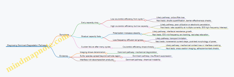
Step 1: Build a Symptom Profile from Routine Data
Start with three baseline plots from the same cycling protocol across at least two cells per condition.
- Capacity fade curve: Does capacity drop fast early, or slowly over many cycles?
- Voltage profile shape: Are plateaus shrinking uniformly, or does one region collapse?
- Coulombic efficiency trend: Is inefficiency constant, spiking, or mostly absent until later?
Easy example: If coulombic efficiency is high for 10–20 cycles and then declines sharply, you likely have an interface or mechanical contact issue that worsens after repeated expansion/contraction. If coulombic efficiency is low from cycle 1, polysulfide loss or poor initial passivation is a prime suspect.
Step 2: Separate Loss Mechanisms Using Targeted Electrochemical Clues
Use a small set of diagnostic tests that map to specific failure modes.
-
Rate capability with fixed cutoff
- If performance collapses at higher current but recovers when current is lowered, transport limitations dominate.
- If performance stays poor at all rates, interfacial reaction or electronic pathways are likely damaged.
-
Incremental current steps
- Track polarization growth. Rapid polarization increase often signals rising interfacial resistance or loss of ionic/electronic percolation.
-
Rest-step analysis
- During rest, voltage relaxation can indicate ongoing chemical conversion or concentration gradients.
- Strong relaxation that grows with cycling suggests that active species remain trapped or that shuttle-related chemistry is still active.
Easy example: Suppose your protected cathode shows a stable initial plateau, but polarization increases steadily with cycle number. That pattern fits interfacial resistance growth more than pure shuttle loss.
Step 3: Use Impedance to Pinpoint Where Resistance Is Growing
Electrochemical impedance spectroscopy (EIS) is most useful when you compare relative changes over cycling.
- High-frequency intercept: often linked to electronic/ohmic contributions.
- Mid-frequency arc: commonly associated with charge transfer at interfaces.
- Low-frequency tail: often reflects diffusion or mass transport through porous networks and interfaces.
Easy example: If the low-frequency tail grows while the high-frequency intercept stays similar, the dominant issue is likely transport through the cathode/protection stack rather than bulk electrolyte resistance.
Step 4: Confirm with Post-Test Evidence That Matches the Hypothesis
Electrochemistry tells you what changed; post-mortem tells you why.
- Cross-section imaging: Look for delamination, cracking, or loss of contact at the solid electrolyte protection interface.
- Surface chemistry mapping: Identify sulfur species distributions. Broad, cathode-side presence of soluble species suggests insufficient suppression.
- Elemental gradients: Interdiffusion or decomposition products concentrated near interfaces point to chemical instability.
Easy example: If imaging shows a clean gap at the protection interface and EIS shows rising mid-frequency resistance, you likely have mechanical contact loss driving interfacial degradation.
Step 5: Create a Decision Mind Map to Choose the Next Test
Use the mind map below to connect symptoms to likely pathways and the next diagnostic action.
Mind Map: Diagnosing Dominant Degradation Pathways
Step 6: Apply a Minimal “Two-Cell” Comparison Strategy
You do not need a lab full of experiments. Compare two conditions that differ in one protection variable, then run the same diagnostic set.
- Condition A: baseline protection stack
- Condition B: modified cathode stabilization or interlayer thickness
Easy example: If Condition B reduces coulombic inefficiency early but still shows rising low-frequency diffusion resistance, then you improved suppression but not transport. Your next change should target pore/ion pathways rather than chemistry.
Step 7: Translate Diagnostics Into a Single Dominant Pathway Statement
End each diagnostic cycle with one sentence that names the dominant pathway and the supporting evidence.
Example statement formats:
- “Dominant pathway is interfacial resistance growth, supported by increasing mid-frequency EIS arc and polarization rise with stable coulombic efficiency.”
- “Dominant pathway is transport limitation, supported by worsening rate capability and growth of the low-frequency diffusion tail.”
This keeps the work grounded: you’re not collecting data for its own sake; you’re selecting the next fix with your eyes open.
2. Solid Electrolyte Protection Concepts and Design Requirements
2.1 Protection Objectives Including Polysulfide Blocking and Interfacial Stabilization
Lithium–sulfur cells lose performance mainly because sulfur species wander and because interfaces stop behaving nicely. In a solid-electrolyte protected design, the goal is simple to state and tricky to execute: keep polysulfides from escaping the cathode region, and keep the solid electrolyte interface chemically and mechanically stable so ion transport stays predictable.
Polysulfide Blocking Objectives
Polysulfides form during discharge as sulfur chains dissolve or migrate through the electrolyte. When they reach the anode, they can be reduced again, consuming active material without contributing to the intended cathode reaction. This shows up as lower capacity, reduced coulombic efficiency, and a voltage profile that looks like the cell is “working” while quietly wasting sulfur.
A protection layer can block polysulfides in two complementary ways:
- Physical restriction: reduce the pathways available for sulfur species to move. In practice, this means designing a barrier with controlled tortuosity and thickness so that migration length is longer than the typical residence time of reactive species.
- Chemical restraint: reduce the tendency of polysulfides to adsorb, dissolve, or react outside the cathode. This is achieved by materials that either bind polysulfides more strongly than the electrolyte does or catalyze conversion back toward insoluble forms within the cathode region.
A useful mental model is to treat polysulfide loss as a “leak.” Blocking objectives aim to shrink the leak rate and to keep the cathode reaction zone as the place where polysulfides spend their time.
Interfacial Stabilization Objectives
Even if polysulfides are blocked, the solid electrolyte interface can still degrade. The interface is where three things must coexist: ionic conduction, electronic blocking, and mechanical contact. When any one of these fails, resistance rises and side reactions become more likely.
Interfacial stabilization targets three failure modes:
- Interfacial resistance growth: caused by poor contact, interphase formation that is too resistive, or loss of ionic pathways. The symptom is increasing polarization during cycling.
- Chemical instability: solid electrolyte components can react with sulfur species or with cathode additives, forming products that are either electronically conductive or poorly ion-conducting.
- Mechanical mismatch: sulfur cathodes expand and contract as they cycle. If the protection layer cannot accommodate this strain, microcracks or delamination can form, creating new transport shortcuts.
A practical way to define success is to require that the interface remains “functionally the same” over cycling: similar impedance behavior, stable voltage plateaus, and no sudden jump in polarization.
Integrated Design Logic
Protection objectives should be treated as a coupled system rather than two separate checklists.
- If a barrier is too dense, it may block polysulfides but also impede ion transport, shifting the bottleneck from chemical loss to transport resistance.
- If a barrier is too ion-permissive, it may allow polysulfides to pass or enable interfacial reactions.
- If interlayers improve contact but are chemically reactive, they can become a new source of degradation.
So the design logic is: block sulfur species without starving ions, and stabilize the interface without creating new reactive surfaces.
Mind Map: Protection Objectives
Example: Translating Objectives Into a Simple Stack
Consider a cathode region that contains sulfur, a conductive network, and a solid electrolyte. A protection approach can be organized as a thin interlayer at the cathode–electrolyte boundary plus a barrier within or adjacent to the cathode.
- Barrier within the cathode: designed to slow polysulfide migration by increasing tortuosity. A practical check is to compare discharge utilization at low and moderate current densities; if blocking is effective, utilization should not collapse at higher rates due to uncontrolled leakage.
- Interlayer at the interface: designed to maintain ionic contact and suppress resistive interphase growth. A practical check is to track impedance before and after cycling; stabilization should show a gradual change rather than a step increase.
If both objectives are met, the cell should show improved coulombic efficiency and a more stable voltage curve, while impedance growth remains limited.
Example: What “Good Blocking” Looks Like in Data
When polysulfide blocking is working, the coulombic efficiency during cycling tends to stay closer to unity, and the capacity fade rate is reduced. The voltage curve also tends to show less evidence of cathode material being consumed elsewhere. If instead the interface is unstable, you may see coulombic efficiency that is not terrible but polarization rises quickly, indicating that ions are struggling to move through a changing interface.
In other words, blocking and interfacial stabilization leave different fingerprints. A well-designed protection system aims to reduce both sets of fingerprints at once.
2.2 Compatibility Constraints for Solid Electrolytes with Sulfur Cathodes
Solid electrolytes can protect lithium-sulfur cells only if they survive contact with sulfur species, keep ionic pathways open, and maintain mechanical contact during cycling. Compatibility is not a single property; it’s a set of constraints that show up as specific failure modes: poor wetting, interphase decomposition, electronic leakage, and loss of ionic transport.
Core Compatibility Constraints
Chemical stability against sulfur species
Sulfur cathodes generate multiple species during discharge, including S8, long-chain polysulfides, and shorter sulfur intermediates. A solid electrolyte must resist reacting with these species at the cathode interface. A practical way to think about it is to compare the electrolyte’s chemical reactivity with the cathode’s “active chemistry” rather than with pure sulfur alone. For example, an electrolyte that looks stable in dry conditions can still react when it meets sulfur intermediates that are more chemically aggressive.
Electrochemical stability against cell potentials
Even if the electrolyte is chemically stable, it can still decompose electrochemically when the cathode potential swings. Compatibility therefore depends on the electrolyte’s stability window relative to the operating voltage range of the cell. If decomposition occurs, it often creates an insulating layer that raises interfacial resistance and reduces utilization.
Interfacial contact and mechanical compliance
Solid electrolytes are rigid compared with liquid electrolytes. During cycling, the cathode experiences volume change as sulfur converts and the solid network reorganizes. If the electrolyte cannot maintain contact, gaps form and ionic current drops. A simple diagnostic is to compare impedance before and after cycling: if bulk resistance stays similar while interfacial resistance rises sharply, contact loss is often the culprit.
Ionic conductivity under realistic interfaces
Bulk ionic conductivity is not enough. The interface can have different defect chemistry, grain boundary effects, and reaction products that reduce effective ionic transport. A compatible electrolyte should preserve ionic conduction at the interface, not just in the interior.
Electronic blocking and leakage control
Some solid electrolytes allow unwanted electronic pathways, especially if they become partially reduced or if interphase products are electronically conductive. Electronic leakage can mimic good ionic transport while still causing self-discharge. In practice, compatibility requires both ionic conduction and electronic insulation across the operating range.
Mind Map: Compatibility Constraints
Systematic Compatibility Checks
Step 1: Screen for chemical and electrochemical mismatch
Start with a controlled contact test: place the solid electrolyte in contact with a sulfur-containing cathode component under the same temperature and pressure conditions used in cell assembly. Then check whether the interface forms new phases or shows signs of reaction. If you observe rapid interphase growth, the electrolyte is chemically incompatible for that cathode chemistry.
Step 2: Measure interfacial resistance evolution
Run a short cycling protocol that isolates interface behavior. Track impedance at the beginning and after a small number of cycles. If interfacial resistance increases quickly while bulk resistance changes little, the electrolyte is likely decomposing or losing contact.
Step 3: Confirm electronic blocking using self-discharge behavior
A compatible electrolyte should not enable significant electronic leakage. One practical approach is to compare capacity after rest periods: if the cell loses capacity during rest without meaningful electrochemical cycling, electronic leakage or shuttle-like behavior may be present.
Example: Diagnosing Incompatibility in a Cathode Stack
Imagine a cell where the electrolyte has decent bulk ionic conductivity. After assembly, initial performance looks fine. After several cycles, capacity retention drops and voltage polarization increases.
- If impedance shows a strong rise in interfacial resistance, the likely issue is interphase decomposition or contact loss.
- If post-mortem imaging shows a reacted layer at the electrolyte surface, chemical incompatibility is the main driver.
- If the interface looks intact but performance still degrades, mechanical mismatch or grain-boundary transport limitations may be dominating.
This kind of “evidence-first” reasoning keeps compatibility work grounded: you’re not guessing whether the electrolyte is “good” or “bad,” you’re identifying which constraint is being violated.
Practical Design Implications
Compatibility constraints guide how you build the cathode-electrolyte interface. If chemical stability is marginal, you can’t fix it purely with pressure; you need an interlayer that changes the interface chemistry. If mechanical compliance is the issue, you need a contact strategy that tolerates cathode volume change. If electronic leakage is present, the electrolyte or its interphase must restore electronic insulation. Compatibility is therefore a design problem with measurable checkpoints, not a single material label.
2.3 Transport Requirements for Ionic Conductivity and Electronic Blocking
A solid electrolyte protection layer has two jobs that must cooperate: move lithium ions fast enough to support the cathode reactions, and stop electrons from taking shortcuts that would trigger unwanted chemistry. If ions crawl, voltage rises and utilization drops. If electrons leak, the layer becomes a highway for parasitic reactions and the cathode loses active material even when the cell is “resting.”
Ionic Conductivity Requirements
Ionic transport in a solid layer is governed by the effective ionic conductivity, which depends on the material’s intrinsic mobility and the microstructure. In practice, the microstructure matters as much as the chemistry. Grain boundaries can be more resistive than grains, and poor contact between particles can add tortuous pathways.
A useful way to reason about this is to compare the ionic resistance of the protection layer to the rest of the cell. When the protection layer is thin and well-contacted, its contribution to total resistance is small, so the cell can sustain higher current densities without large polarization. When it is thick or poorly bonded, the layer dominates the impedance and the cell behaves as if the cathode is “underpowered,” even when the cathode formulation is fine.
Example: Suppose you have two protection layers made from the same electrolyte material. Layer A is 20 µm and well-pressed; Layer B is 60 µm with visible voids at interfaces. Even if the material conductivity is identical, Layer B has roughly three times the thickness-related resistance, plus extra resistance from voids and contact gaps. The result is higher overpotential at the same current, which can reduce sulfur utilization because the cathode reactions stop earlier in the voltage window.
Electronic Blocking Requirements
Electronic blocking is about preventing electronic percolation through the protection layer. If electrons can move, they can reduce sulfur species or react with the electrolyte, producing capacity loss and interphase growth. The key is not just “low electronic conductivity,” but the absence of continuous electronic pathways.
In solid systems, electronic leakage can occur through intrinsic electronic conductivity, defects, or electronic conduction via additives and conductive fillers. Even small amounts of conductive carbon or metal contamination can create percolating networks, especially if the layer is thin and interfaces are rough.
Example: Imagine a protection layer that includes a small fraction of conductive additive to improve contact. If the additive forms a connected network, the layer may still look uniform, but electrons can travel across it. During rest, sulfur species can keep reacting because electrons are available, so you observe self-discharge and a drop in open-circuit voltage over time.
Coupled Transport and Interfacial Effects
Ionic and electronic transport are coupled through interfaces. A protection layer that blocks electrons but has poor ionic contact can still fail, because ions must cross the interface to reach the cathode. Conversely, a layer with good ionic conductivity but high electronic leakage can fail even if the interface is perfect.
Interfacial resistance is often dominated by contact quality and interphase formation. If the layer does not conform to the cathode surface, micro-gaps form and ions must detour through longer paths. If the layer reacts aggressively with sulfur species, it can thicken or become less conductive, increasing ionic resistance over cycling.
Example: Two stacks use the same protection material. Stack A is assembled with strong mechanical contact, producing low interfacial impedance. Stack B is assembled with looser contact, leaving microscopic gaps. Stack B shows higher polarization immediately and also faster degradation, because the local current density concentrates where contact exists, accelerating interphase growth.
Practical Design Checks
A systematic checklist helps translate transport requirements into measurable targets.
- Measure impedance contributions: Use electrochemical impedance to separate bulk and interfacial resistance trends when comparing layer thickness and processing.
- Verify electronic blocking indirectly: Track self-discharge and changes in open-circuit voltage during rest periods; large changes suggest electronic leakage or ongoing parasitic reactions.
- Control additives and contamination: Avoid conductive percolation routes in the protection layer and keep processing steps clean.
- Engineer contact: Use processing that improves conformity and reduces voids, because contact gaps behave like extra resistors.
Mind Map: Transport Requirements for Ionic Conductivity and Electronic Blocking
Example: Interpreting a “Good Ionic, Bad Electronic” Outcome
If a protection layer shows low polarization at moderate current but the cell loses voltage during rest and capacity fades quickly, the likely issue is electronic leakage rather than ionic transport. The ionic pathways are doing their job, so the cell can charge and discharge. The problem is that electrons are also getting through, enabling parasitic reactions when the cell is not actively driving the desired cathode chemistry.
In contrast, if the cell holds voltage during rest but polarization rises sharply with current and utilization drops, the likely issue is ionic resistance from thickness, poor contact, or grain-boundary dominated transport. The electrons are not the main culprit; the ions simply cannot reach the reaction sites fast enough.
These two patterns—rest behavior for electronic blocking and current-dependent polarization for ionic transport—provide a practical way to connect transport requirements to observable outcomes without guessing.
2.4 Mechanical Requirements Including Interfacial Contact and Stress Tolerance
Solid electrolyte protection is not just chemistry; it is also contact mechanics. If the solid electrolyte (or its protective interlayer) loses intimate contact with the cathode during cycling, ionic transport becomes patchy and the protection layer stops doing its job. The mechanical goal is simple to state and tricky to execute: maintain stable interfaces while accommodating volume change, binder softening, and thermal or pressure variations.
Foundational Mechanical Loads in Solid Electrolyte Protected Lithium Sulfur Cells
Start by identifying what pushes and pulls the stack. During charge, sulfur species convert and the cathode composite expands and contracts. Even if the bulk cathode thickness change is modest, local mismatch at particle scale can create gaps. Meanwhile, the solid electrolyte is typically stiffer than the cathode composite, so stress concentrates at the interface.
A practical way to think about loads is to separate them into three categories:
- Normal pressure from cell assembly and any stack compression.
- Interfacial shear caused by uneven expansion across the cathode plane.
- Thermal stress from temperature changes during testing.
A useful sanity check is to ask: if you remove compression, does the interface still look continuous? If the answer is “not really,” then your design must rely on mechanical compliance or on interlayers that can maintain contact under reduced pressure.
Interfacial Contact as a Transport Requirement
Ionic conduction through a solid electrolyte is sensitive to contact because current must cross the solid-solid boundary. When contact is incomplete, the effective resistance rises sharply, and the cell compensates by increasing polarization. That polarization then accelerates chemical degradation at the interface.
Contact quality depends on three things:
- Surface roughness and asperities that determine real contact area.
- Conformability of the interlayer or protective coating.
- Stability under cycling so that contact does not degrade after the first few cycles.
Easy example: imagine two surfaces pressed together. If only 20% of the area touches, the rest behaves like a thin gap. Even a small gap can dominate resistance because ionic transport across a gap is far worse than through the solid. Your mechanical design should therefore aim to maximize real contact area early and keep it from collapsing later.
Stress Tolerance and Interphase Integrity
Stress tolerance is about preventing mechanical failure modes that break the electrical and ionic pathways. Common failure modes include:
- Cracking in the solid electrolyte or interlayer.
- Delamination at the cathode-protection interface.
- Particle debonding where cathode particles lose contact with the protective layer.
- Interlayer pulverization when the coating is too brittle.
The key mechanical mismatch is modulus. A stiff electrolyte against a softer cathode can be fine if the interface is engineered to distribute strain. If not, the interface becomes the stress concentrator.
Easy example: if your interlayer is a brittle ceramic with high modulus and low fracture toughness, it may form a good initial barrier. But during cycling, the cathode expands locally, and the brittle layer can crack. Once cracked, the barrier becomes discontinuous, and polysulfide suppression weakens because the “blocked” path is no longer continuous.
Design Levers for Contact and Stress Management
Use mechanical levers that directly address the failure modes above.
- Interlayer thickness and compliance: A slightly thicker interlayer can accommodate strain, but too much thickness increases ionic resistance. Choose a thickness that balances strain accommodation with acceptable transport.
- Particle size and packing: Smaller particles can fill voids and improve contact, but they can also increase surface area and stress concentration. Aim for dense packing without creating overly brittle agglomerates.
- Binder selection and distribution: A binder that maintains integrity under cycling helps keep the cathode composite cohesive. If the binder softens and flows, it can change contact pressure distribution.
- Stack compression strategy: Assembly pressure affects initial contact. However, too high pressure can crush porous structures and reduce long-term stability. Too low pressure leads to gaps. The best approach is to design so that modest pressure loss does not immediately destroy contact.
Measurement and Validation Practices
Mechanical requirements should be validated with measurements that connect mechanics to electrochemistry.
- Interfacial resistance tracking: Monitor impedance before and after cycling. A rapid rise often signals contact loss or interlayer cracking.
- Thickness and mass change checks: Track cathode thickness evolution and compare it with expected expansion from sulfur conversion.
- Post-mortem microscopy: Look for delamination, crack networks, and void formation at the interface.
- Compression sensitivity tests: Run a small matrix of assembly pressures and observe how early-cycle polarization changes. If performance collapses at lower pressure, the design is not mechanically robust.
Mind Map: Mechanical Requirements for Interfacial Contact and Stress Tolerance
Example: Diagnosing Contact Loss Versus Chemical Degradation
Suppose two protected cathode designs show similar initial capacity, but one loses performance quickly. If impedance after a few cycles shows a strong increase in interfacial resistance while voltage profiles show earlier polarization, the likely issue is mechanical contact degradation. If, instead, impedance stays stable while voltage gradually shifts, the dominant problem may be chemical interphase growth or transport limitations within the cathode composite. This distinction matters because mechanical fixes focus on contact maintenance, while chemical fixes focus on interphase chemistry and polysulfide interactions.
2.5 Selection Criteria for Materials and Architectures for Solid Electrolyte Protection
Choosing materials and architectures for solid-electrolyte protection is mostly about managing three things at once: chemical compatibility, transport pathways, and mechanical contact. If you pick for only one of these, the other two usually find a way to ruin your day.
Start with Protection Goals and Failure Signatures
Begin by mapping the dominant failure you want to prevent. If your cell shows fast capacity fade at moderate current, polysulfide migration and interfacial reactions are likely. If it shows rising resistance and sudden cutoff, contact loss or interphase cracking is common. This goal-to-failure link determines whether you prioritize chemical blocking, ionic conduction, or mechanical compliance.
A practical example: if your voltage curve has a persistent polarization increase from the first cycles, you likely have interfacial resistance growth. In that case, you should select architectures that maintain contact and limit interphase thickening, not just materials that “chemically look stable.”
Chemical Compatibility and Interphase Stability
Solid electrolytes must tolerate sulfur species, lithium metal, and any interfacial products formed during cycling. Selection criteria include:
- Stability window against sulfur reduction/oxidation: the electrolyte should not react strongly with sulfur or polysulfides.
- Reaction products that remain ionically conductive or at least thin: a stable product that blocks ion flow is still a problem.
- Low reactivity with lithium at the operating potential: otherwise, you get rapid interphase growth or lithium consumption.
Example: suppose you compare two candidate electrolytes with similar ionic conductivity. The one that forms a thin, dense interphase that still conducts lithium ions tends to preserve cycling better than the one that forms a thicker, insulating layer even if its initial impedance is lower.
Transport Requirements for Ionic Conduction and Electronic Blocking
Protection architectures should allow lithium ions to move while limiting electronic leakage that can accelerate shuttle-like chemistry. Use these criteria:
- Ionic conductivity at the relevant temperature and pressure/contact state
- Electronic conductivity suppression so polysulfides do not gain an easy electronic path
- Effective transport through the whole stack, not just the bulk electrolyte
A simple check: if you measure impedance and see that the electrolyte bulk resistance is small but the interfacial resistance dominates, then improving ionic conductivity alone won’t fix the problem. Your selection should shift toward interlayers, surface treatments, or contact architectures.
Mechanical and Interfacial Contact Requirements
Solid electrolytes are rarely the only mechanical component. The architecture must maintain intimate contact despite cathode volume change and thermal or pressure variations.
Key criteria:
- Elastic compliance and fracture resistance to reduce cracking at the interface
- Ability to conform under assembly pressure without creating large voids
- Interphase toughness so the protective layer does not become a brittle separator
Example: a rigid electrolyte that cracks at the cathode interface can still be chemically compatible. Once cracks form, local current concentrates, interphase thickens, and the cell fails even though the chemistry “should have worked.”
Architecture Selection Based on Where Protection Must Act
Architectures differ in how they place the protective function:
- Barrier-first designs: prioritize polysulfide blocking near the cathode
- Interphase-first designs: prioritize stable interfacial chemistry and thin reaction layers
- Contact-first designs: prioritize mechanical coupling and low interfacial resistance growth
A useful selection rule: if your cathode is high loading and the electrolyte contact is uneven, contact-first architectures usually outperform barrier-only approaches because they reduce the number of “bad contact zones” where reactions concentrate.
Mind Map: Selection Criteria for Solid Electrolyte Protection
A Systematic Selection Workflow with Concrete Checks
- Define the dominant failure signature from early cycling and impedance trends.
- Screen materials by chemical compatibility using interphase behavior as the deciding metric, not just stability claims.
- Verify transport balance by checking whether bulk or interfacial resistance dominates.
- Stress-test contact assumptions by selecting architectures that tolerate volume change without losing area contact.
- Choose the architecture that targets the failure location: cathode-side barriers for migration, interlayers for interphase control, and compliant coupling layers for contact preservation.
Example: if impedance shows interfacial resistance growth and post-test imaging shows partial delamination, then your next iteration should focus on contact-first or hybrid architectures with improved interfacial coupling, even if the electrolyte’s bulk conductivity is excellent.
Practical Decision Matrix for Shortlisting
Use a shortlist that scores each candidate across four criteria: chemical stability, ion transport effectiveness, electronic blocking, and mechanical integrity. A candidate that is mediocre in all four can still lose to one that is strong in the two criteria matching your observed failure mode. The goal is not perfection everywhere; it’s preventing the specific failure mechanism you can already see.
3. Solid Electrolyte Materials and Interphase Engineering
3.1 Classification of Solid Electrolytes by Conduction Mechanism and Stability Window
Solid electrolytes are best understood as two coupled stories: how ions move through the material, and how the material survives the chemical environment created by lithium, sulfur, and intermediate polysulfides. Classifying by conduction mechanism tells you what transport to expect; classifying by stability window tells you what reactions to fear.
Conduction Mechanism: What Moves and How
Most solid electrolytes fall into three practical conduction families.
- Lithium-ion conductors move Li⁺ through a lattice or through hopping sites. In these materials, the anion framework is relatively fixed, so ionic conductivity depends strongly on defect concentration and temperature-activated hopping.
- Lithium-metal conductors are less common in sulfur cell contexts, but the key idea is that lithium transport is not just ionic hopping; it can involve more complex interfacial processes that affect plating/stripping behavior.
- Mixed conductors conduct both ions and electrons to some degree. This can reduce polarization at interfaces, but it also increases the risk of electronic leakage that undermines cathode protection.
A simple way to connect mechanism to cell behavior is to ask: “If I double the thickness of the electrolyte layer, what happens to resistance?” For ion-only conductors, resistance typically scales up strongly with thickness, so interfacial engineering matters more. For mixed conductors, the electronic component can partially compensate, but it can also accelerate unwanted side reactions.
Stability Window: What the Material Can Tolerate
The stability window is the range of potentials and chemical conditions where the solid electrolyte does not decompose. In lithium–sulfur systems, the relevant stressors are not just voltage; they include reactive sulfur species, interfacial contact pressure, and local chemical gradients.
A practical classification uses two overlapping views:
- Electrochemical stability: whether the electrolyte resists oxidation at high cathode potentials and reduction near the lithium anode.
- Chemical stability: whether the electrolyte resists reaction with sulfur, polysulfides, or sulfur-derived species that can reach the interface even when bulk transport is blocked.
If you want an easy mental model, treat the stability window like a “do-not-touch” zone. Conduction mechanism tells you how quickly ions can reach interfaces; stability window tells you whether those interfaces become chemically busy.
Mind Map: Conduction and Stability Classification
Example: Choosing Between Two Electrolytes
Consider two solid electrolytes used as a protection layer between a sulfur cathode and a lithium anode.
- Electrolyte A is a lithium-ion conductor with high ionic conductivity but a narrow electrochemical stability window on the cathode side. In cycling, it may initially look fine because ions move well. After some time, decomposition products form at the cathode interface, increasing interfacial resistance and reducing sulfur utilization.
- Electrolyte B is a mixed conductor with moderate ionic conductivity but better electrochemical stability. It may show lower initial polarization. However, if its electronic conductivity is significant, it can provide a pathway for electronic leakage, which can reduce the effectiveness of polysulfide suppression by enabling side reactions at the cathode.
The point is not that one is always better; it’s that classification predicts which failure mode is more likely to dominate.
Example: Stability Window as a Contact-Driven Problem
Even if a solid electrolyte is chemically stable in bulk, the interface can be different. Imagine a thin electrolyte interlayer that is well bonded to the cathode. If the interlayer is too thin, local chemical gradients can still drive reactions at pinholes or imperfect contact regions. Classification by stability window helps you set expectations, but conduction mechanism helps you estimate how quickly reactive species can reach those sensitive spots.
Practical Classification Workflow
To classify a candidate solid electrolyte for lithium–sulfur protection, use a two-step checklist.
- Identify the conduction family by measuring temperature-dependent conductivity and checking whether electronic conduction is negligible. If electronic conduction is measurable, treat it as a risk factor for cathode stabilization.
- Map the stability window to the cell’s operating potentials and chemical environment. Then judge whether decomposition would occur at the cathode interface, the anode interface, or both.
When these two classifications agree—good ionic transport and adequate stability at the relevant interfaces—you get a solid foundation for cathode protection. When they conflict, you can still use the material, but you must design around the likely dominant failure mode rather than hoping it won’t show up.
3.2 Surface Chemistry and Interphase Formation at Solid Electrolyte Interfaces
Solid electrolyte protection works only if the solid electrolyte actually “behaves like an electrolyte” at the specific contact it shares with the sulfur cathode. That behavior is set by surface chemistry: what functional groups, ions, and defects are present right before assembly, and what new species form once current starts flowing. The interphase is the thin, often non-uniform region where those chemistry changes meet mechanical contact and ion transport.
Interphase Formation: What Changes and Why
At the solid electrolyte–cathode boundary, three processes typically occur in parallel.
-
Chemical reactions at the interface. Even if the bulk materials are stable, the interface can be less so because surface atoms have unsatisfied bonds and higher chemical potential. Common outcomes include formation of sulfide-rich or oxide-rich interfacial layers, depending on the electrolyte chemistry and residual species.
-
Ion redistribution and defect creation. Lithium ions and vacancies can migrate into the interphase, changing local stoichiometry. This can either improve ionic conductivity (by creating mobile charge carriers) or worsen it (by forming electronically blocking, ion-poor phases).
-
Interfacial contact evolution. Pressing, thermal steps, and cycling can change contact area and pressure. A chemically “good” interface can still fail if the contact becomes patchy, because current then concentrates into fewer spots.
A useful mental model is to treat the interphase as a series of resistive and reactive layers: some parts mainly resist ion flow, others mainly block electrons, and some mainly react with sulfur species.
Surface Preparation: The Starting Line Matters
Surface chemistry begins before any electrochemistry.
-
Remove moisture and loosely bound contaminants. Many solid electrolytes and cathode components are sensitive to water and air exposure. A simple example: if a cathode powder is stored in humid air, it can carry hydroxylated species that later react with the solid electrolyte surface, creating an insulating film.
-
Control surface roughness and particle contact. Rough surfaces increase real contact area but also increase the number of high-energy sites that react. If you polish a solid electrolyte pellet to a smoother finish, you may reduce interphase growth rate but also reduce contact area; the net effect depends on how the cathode is pressed.
-
Match surface chemistry to the intended interphase. If your protection strategy relies on forming a lithium-ion-conducting interlayer, the electrolyte surface should not be dominated by species that drive the formation of an electronically insulating but ion-blocking layer.
Interphase Chemistry: Typical Pathways
Interphase formation is often governed by which species are most mobile and which reactions are thermodynamically favorable.
-
Lithium exchange and interfacial lithiation. When the cell is assembled, lithium chemical potentials differ across the boundary. This can drive lithium into the solid electrolyte surface region, altering local phases.
-
Reaction with sulfur species. Polysulfides and sulfur vapor-like species can reach the interface if transport control is incomplete. When they do, they can form new compounds at the boundary. A practical example: if the cathode contains a high fraction of easily released polysulfides, the interphase may become sulfur-rich and thicker, increasing interfacial resistance.
-
Formation of electronically blocking layers. Some interphase products are beneficial because they suppress electron leakage that accelerates shuttle-like chemistry. The catch is that blocking layers must still allow lithium-ion transport; otherwise, you trade one failure mode for another.
Interphase Structure: Thickness, Uniformity, and Transport
Interphase performance depends on more than average thickness.
-
Thickness gradients. Interfaces often show thicker regions near pores or imperfect contact points. Those thicker zones dominate impedance because current prefers the lowest-resistance paths.
-
Uniformity across the contact area. A thin, uniform interphase can yield stable impedance, while a patchy interphase produces time-dependent resistance changes during cycling.
-
Grain-boundary coupling. If the solid electrolyte has grain boundaries that are chemically reactive, the interphase can extend along those paths. That can increase effective interfacial area but also create additional resistive regions.
How to Evaluate Interphase Formation in Practice
You can infer interphase formation without guessing.
-
Baseline impedance before cycling. Measure impedance after assembly and after a short rest. A rapid rise suggests early interphase growth or poor contact.
-
Impedance evolution during cycling. If interfacial resistance increases steadily, interphase growth is likely continuing. If it spikes after certain voltage regions, reactions may be tied to specific electrochemical states.
-
Post-mortem chemical mapping. After disassembly, compare the solid electrolyte surface chemistry with the cathode-side chemistry. If sulfur-rich products appear on the solid electrolyte surface, transport control at the cathode side is insufficient.
Mind Map: Surface Chemistry and Interphase Formation
Example: Interphase That Helps vs Interphase That Hurts
Consider two assemblies that use the same solid electrolyte but different cathode-side preparation.
-
Assembly A: Cathode is dried thoroughly and pressed to achieve consistent contact. During cycling, interfacial impedance rises slowly and stabilizes. Post-mortem analysis shows a thin interphase with lithium-ion-conducting characteristics and limited sulfur-rich products on the electrolyte surface.
-
Assembly B: Cathode contains residual moisture and releases more polysulfides. Interfacial impedance increases quickly, and the rise correlates with voltage regions where polysulfides are most active. Post-mortem analysis shows a thicker, sulfur-rich interphase on the solid electrolyte surface, consistent with ongoing interfacial reactions and reduced ion transport.
The difference is not magic; it’s chemistry meeting contact. Control the starting surface, limit reactive sulfur arrival, and verify the interphase through impedance behavior and post-mortem chemistry.
3.3 Protective Coatings and Interlayers for Sulfur Cathode Contact Stabilization
Solid electrolyte protection is only as good as the contact it maintains. In lithium–sulfur cells, the sulfur cathode expands and contracts during cycling, while the solid electrolyte (or its protective layer) can be brittle and slow to re-wet. Protective coatings and interlayers are the “middle layer” engineering that keeps ionic pathways open and prevents chemical contact damage at the solid electrolyte–cathode interface.
Core Job Description of Coatings and Interlayers
A useful coating or interlayer must do three things at the same time:
- Maintain contact under volume change. When the cathode swells, the interface should not separate into gaps that raise interfacial resistance.
- Reduce chemical side reactions. The layer should limit direct contact between reactive sulfur species and the solid electrolyte surface.
- Support ion transport. It cannot be an insulating blanket; it must allow lithium-ion movement through the interface region.
A practical way to think about it: the interlayer is not a “barrier only,” it is a controlled interface region with tuned chemistry and mechanics.
Foundational Design Choices
Coating vs Interlayer
- Protective coating is typically thin and applied directly to the solid electrolyte surface or to cathode particles. It aims to control the first few nanometers to micrometers where reactions start.
- Interlayer is thicker and often engineered as a composite layer between cathode and solid electrolyte. It can provide mechanical compliance and a more forgiving contact interface.
If you have frequent loss of contact during cycling, an interlayer usually solves the mechanical part better than a very thin coating.
Mechanical Compliance and Interfacial Wetting
Solid electrolytes often crack or lose contact when the cathode expands. Interlayers can be designed with a soft phase (for compliance) plus a hard phase (for structural integrity). For example, a composite interlayer can include an ion-conducting ceramic for transport and a polymer-derived or elastomeric component that improves conformal contact during assembly. The key is to ensure the soft component does not create a permanent electronic path or dissolve into the cathode.
Chemical Compatibility and Reaction Control
Sulfur species can react with many solid electrolytes, forming resistive interphases. A protective coating can be chosen to be chemically stable against polysulfides and against the electrolyte’s own decomposition products. A simple screening approach is to test interlayer materials in a controlled environment that mimics polysulfide exposure, then measure interfacial resistance growth after contact.
Material Building Blocks and Their Roles
Ion-Conducting Interlayers
Ion-conducting interlayers reduce the “contact resistance tax.” A good target is an interlayer that has ionic conductivity comparable to the solid electrolyte in the operating temperature range. If the interlayer is too resistive, you will see higher polarization even when contact looks visually intact.
Electronic Blocking and Mixed Conductivity Control
You want to avoid electronic leakage that can accelerate shuttle-like behavior. Many designs aim for ionic conduction with minimal electronic conduction. A quick diagnostic is to compare open-circuit voltage stability and self-discharge behavior between cells with and without the interlayer.
Adsorptive or Reactive Surface Layers
Some coatings are designed to interact with polysulfides at the interface, reducing their ability to migrate into the solid electrolyte. The trick is to keep this interaction from consuming the coating too quickly. In practice, you look for a coating that forms a stable, thin interphase rather than a thick, continuously growing reaction product.
Integrated Mind Map
Mind Map: Protective Coatings and Interlayers for Sulfur Cathode Contact Stabilization
Example: A Coating-First Stack That Fails for the Right Reason
Suppose you apply a very thin protective coating on the solid electrolyte surface to block polysulfides. After a few cycles, the cell shows rising polarization and reduced utilization, but coulombic efficiency is only moderately improved. Post-mortem inspection reveals micro-gaps at the interface.
Interpretation: the coating controlled chemistry, but it did not provide enough mechanical compliance. The fix is to keep the coating for chemical control and add a thicker ion-conducting interlayer that can deform slightly and maintain contact.
Example: Interlayer Composite with a Contact-Repair Role
A composite interlayer can be built from an ion-conducting ceramic matrix plus a small fraction of a compliant phase that improves conformal contact. During assembly, the compliant component helps the layer conform to cathode roughness and solid electrolyte surface asperities. During cycling, it reduces the tendency for delamination when the cathode expands.
To verify it is doing the intended job, compare three cells:
- No interlayer
- Ceramic-only interlayer
- Ceramic–compliant composite interlayer
If cell (3) shows lower interfacial resistance growth and more stable voltage profiles, the composite is successfully stabilizing contact without introducing excessive electronic leakage.
Practical Checklist for Building and Testing
- Ensure the coating or interlayer is uniform; patchy coverage creates local current hotspots.
- Confirm ionic transport is sufficient; if polarization rises early, the layer is likely too resistive.
- Use post-mortem inspection to distinguish contact loss from chemical consumption.
- Keep assembly pressure and surface cleanliness consistent; otherwise, you will confuse contact quality with material performance.
Protective coatings and interlayers work best when they are designed as an integrated interface region: chemistry that survives polysulfide exposure, mechanics that tolerate cathode expansion, and transport that keeps lithium-ion pathways open.
3.4 Grain Boundary Effects and Their Impact on Interfacial Resistance
Solid electrolytes are not single crystals; they are mosaics of grains separated by grain boundaries. Those boundaries often decide whether ions move smoothly or get stuck at the solid–solid interface. In protected lithium–sulfur cells, grain-boundary behavior matters twice: first inside the solid electrolyte, and then at the solid electrolyte–cathode contact where interfacial resistance is measured.
Core Concepts of Grain Boundaries
Grain boundaries are regions with disrupted atomic order. Compared with grain interiors, they typically have:
- Different defect concentrations (vacancies, interstitials, trapped charges)
- Different local chemistry (segregated impurities or reaction products)
- Different free volume and mobility pathways
A useful mental model is to treat ion transport as a series of resistors. Grain interiors provide one resistance, and grain boundaries add another. Even if the bulk conductivity is good, grain boundaries can dominate the effective conductivity when they are more resistive.
How Grain Boundaries Increase Interfacial Resistance
Interfacial resistance at the cathode contact is not only about chemistry at the surface. It also depends on how easily ions can arrive at that surface. Grain boundaries can raise interfacial resistance through three main mechanisms.
-
Ion depletion near the interface
If grain boundaries trap mobile ions, the region near the cathode contact can become ion-poor. The interface then behaves like a bottleneck: ions must cross both the grain boundary network and the interfacial layer. -
Space-charge layers from trapped charge
Charged defects at grain boundaries can create local electric fields. These fields can repel or attract ions, effectively adding an extra barrier. The effect is strongest when the defect charge state changes with potential during cycling. -
Reaction products that form at boundaries
During assembly or cycling, small amounts of reactive species can migrate along grain boundaries more easily than through the bulk. If those species react with the solid electrolyte, they can form resistive interphases that extend laterally along boundaries.
Foundational Transport Picture
Start with bulk transport: ions move through a network of sites. Grain boundaries alter that network by changing site availability and activation energy. When you measure impedance, the “interfacial” contribution often includes both true interface effects and near-surface grain-boundary effects. That is why two samples with the same surface coating can show different contact resistance.
Advanced Details That Matter in Lithium–Sulfur Cells
Grain Boundary Orientation Relative to the Contact
In a pressed or infiltrated stack, the contact plane is fixed, but grain orientations vary. Some grain boundaries intersect the contact plane at shallow angles, creating percolation paths that are either favorable or harmful. A sample with a small fraction of highly resistive boundary orientations can still perform poorly if those boundaries form continuous barriers across the current path.
Percolation of Conductive Pathways
If the solid electrolyte has mixed conduction quality, grain boundaries can fragment the ion-conducting network. The effective resistance then scales nonlinearly with boundary fraction. Practically, this means that modest changes in sintering conditions can cause large shifts in interfacial resistance.
Coupling with Cathode Volume Change
Lithium–sulfur cathodes change volume during cycling. That mechanical motion can open or close contact microgaps. When microgaps exist, ions must rely more heavily on lateral transport through the solid electrolyte. Grain boundaries become more important under these conditions because lateral transport often routes through boundary networks.
Mind Map: Grain Boundaries and Interfacial Resistance
Example: Interpreting Impedance When Grain Boundaries Dominate
Suppose two solid electrolyte pellets are coated with the same protective interlayer and assembled with identical pressure. Sample A shows lower bulk resistance but higher interfacial resistance than Sample B. A straightforward explanation is that Sample A has grain boundaries that trap ions more strongly near the surface. The bulk measurement averages over the whole pellet, while the interface measurement is sensitive to the near-surface region where ion depletion and space-charge effects are strongest.
Example: Boundary-Driven Interphase Growth
During assembly, trace reactive species can be present in small amounts. If those species preferentially migrate along grain boundaries, they can form a thin resistive film that spreads laterally. Even if the surface coating is intact, the boundary network under the contact can become partially blocked, raising interfacial resistance over the first few cycles.
Practical Takeaways for Systematic Control
- Treat grain boundaries as part of the transport path to the interface, not as a separate bulk issue.
- Expect impedance “interfacial” features to include near-surface grain-boundary contributions.
- When comparing designs, keep sintering and processing consistent, because grain boundary structure can change without obvious surface differences.
- Use microstructural evidence (grain size distribution and boundary density) to interpret resistance changes rather than relying on surface appearance alone.
3.5 Practical Material Characterization for Electrolyte Protection Performance
Solid-electrolyte protection only “works” if it changes what happens at interfaces and inside the cathode during cycling. This section gives a practical characterization workflow that starts with what you can measure directly, then connects those measurements to the failure modes you care about.
Define What Success Looks Like
Start by translating protection goals into measurable targets:
- Lower interfacial resistance growth: impedance should not steadily climb with cycle number.
- Reduced polysulfide activity at the cathode surface: fewer soluble sulfur species should appear in electrolyte extracts.
- Stable ionic transport through the protected cathode: rate tests should show less polarization increase.
- Mechanical integrity at the interface: fewer cracks, delamination, or loss of contact area.
A simple example: if your protection layer is meant to block polysulfides, you should see both (1) reduced soluble sulfur in extracts and (2) less capacity loss at the same current density.
Baseline Material Checks Before Assembly
Before you test protection performance, confirm the materials are what you think they are.
- Particle and film morphology: use SEM for surface texture and thickness uniformity.
- Composition and bonding: use XPS to verify expected chemical states at the protection layer surface.
- Bulk ionic conduction: measure ionic conductivity of the solid electrolyte and any interlayer separately.
Example: if XPS shows the protection layer surface is heavily oxidized, it may form a resistive interphase that looks like “good blocking” but actually kills ion transport.
Interface Chemistry That Explains Performance
Interfacial chemistry is where protection layers earn their keep.
- XPS depth profiling or angle-resolved XPS: compare protected vs unprotected cathode surfaces after controlled exposure to sulfur species.
- FTIR or Raman mapping: track sulfur-related vibrational signatures on the cathode surface.
- Time-controlled exposure tests: expose cathode stacks to a defined sulfur/polysulfide solution for a fixed time, then characterize.
Example: if the protected cathode shows weaker sulfur-related peaks after exposure, you can connect that to reduced shuttle-driven loss during cycling.
Interfacial Resistance Growth with Electrochemical Impedance
EIS is the fastest way to see whether protection improves the interface or just changes the chemistry.
- Run EIS at the same state of charge and temperature for every sample.
- Fit spectra using a consistent equivalent circuit across samples.
- Track interfacial resistance and charge-transfer-related elements versus cycle number.
Practical tip: if your equivalent circuit changes between samples, your “improvement” may be an artifact of fitting rather than a real physical change.
Polysulfide Suppression Measured Directly
To verify blocking or adsorption, measure soluble sulfur species.
- Electrolyte extraction after cycling: dissolve the cathode and quantify sulfur species in the extracted solution.
- UV-Vis or ICP-based quantification: choose a method that matches your sulfur species and detection limits.
- Mass balance sanity check: compare extracted sulfur to expected sulfur inventory.
Example: two protection layers might both reduce capacity fade, but only one reduces extracted polysulfides significantly. That difference tells you whether the benefit comes from true suppression or from simply slowing reaction kinetics.
Transport and Kinetics Through Rate and Relaxation Tests
Material characterization should connect to transport.
- Rate capability: compare voltage polarization growth across current densities.
- Relaxation after current steps: observe how quickly voltage returns, which reflects kinetic and transport contributions.
- Temperature series: repeat a small set of tests at two temperatures to separate ionic transport limits from interfacial reaction limits.
Example: if higher current density mainly increases polarization but relaxation behavior stays similar, the issue is often transport through the protected cathode rather than a sudden interfacial chemistry failure.
Mechanical and Contact Integrity After Cycling
Protection layers can block chemistry but still fail mechanically.
- Cross-sectional SEM: look for delamination, voids, and crack paths.
- Focused ion beam milling: inspect interlayer thickness changes and contact loss.
- Thickness and roughness before vs after: quantify whether the protection layer densifies or fractures.
Example: if EIS shows resistance jump at mid-life and microscopy shows interfacial cracking at the same time, you have a direct cause-and-effect chain.
A Mind Map for Turning Measurements Into Decisions
Mind Map: Characterizing Electrolyte Protection Performance
Example Workflow for One Protection Layer
- Verify materials: SEM for thickness uniformity; XPS for expected surface states.
- Run a short exposure test: expose cathode to sulfur species for a fixed time; measure sulfur signatures.
- Assemble and cycle: include an unprotected control.
- Track EIS every N cycles: confirm interfacial resistance growth is slower.
- Extract electrolyte at end of test: quantify soluble sulfur species.
- Post-mortem microscopy: confirm contact integrity where EIS changes.
If the protection layer reduces extracted polysulfides but EIS still worsens rapidly, the likely culprit is a resistive interphase or contact loss rather than insufficient chemical blocking.
4. Cathode Stabilization Strategies for High Loading and High Areal Capacity
4.1 Cathode Formulation Variables Including Sulfur Loading and Binder Selection
Cathode formulation is where “solid electrolyte protection” either gets a fair fight or gets sabotaged before the first cycle. Two variables dominate early outcomes: sulfur loading (how much active material you pack in) and binder selection (how well the cathode holds together while interfaces breathe and shrink).
Sulfur Loading from Practical Targets to Measurable Consequences
Start with a clear target: areal capacity, not just mass fraction. A useful way to think is that sulfur loading sets the amount of reaction per unit area, while transport limits decide how much of that reaction you can actually use.
Foundational rule: higher sulfur loading increases energy density, but it also increases the distance ions and electrons must travel through a composite that is not perfectly uniform. In a solid-electrolyte-protected design, the protection layer can block polysulfide escape, yet it cannot fix a cathode that is too thick or too poorly connected.
How to Choose a Starting Loading
Pick a baseline areal sulfur loading that matches your test geometry and current density. Then vary one factor at a time.
- Low loading example: ~1–2 mgS/cm². Expect easier wetting and lower interfacial stress; capacity is often limited by utilization rather than transport.
- Moderate loading example: ~3–4 mgS/cm². You begin to see whether your conductive network and ion pathways are truly continuous.
- High loading example: ~5–7 mgS/cm². Capacity may drop unless binder, porosity, and protection interfaces are tuned together.
What Changes When Loading Increases
- Electronic percolation becomes harder. If the conductive additive content or dispersion is marginal, higher loading amplifies dead zones.
- Ionic transport becomes more sensitive to pore structure. Even with solid electrolyte protection, the cathode still needs ion-accessible pathways.
- Mechanical mismatch becomes more obvious. Volume change during cycling stresses particle contacts and binder bridges.
A practical check is to compare initial discharge capacity at the same current density across loadings. If the initial capacity collapses sharply with loading, you likely have transport or connectivity issues rather than a protection-layer problem.
Binder Selection from Adhesion to Interphase Stability
Binders do more than hold particles together. In lithium–sulfur cathodes, they influence: (i) electronic contact stability, (ii) interfacial resistance growth, and (iii) how the cathode tolerates repeated expansion and contraction.
Binder Roles You Can Actually Observe
- Mechanical integrity: prevents cracking and delamination that would increase contact resistance.
- Interfacial compatibility: affects how the binder and sulfur species interact near the solid electrolyte interface.
- Polysulfide interaction: some binders can adsorb or interact with sulfur species, changing how much material remains where it should.
Common Binder Types and Practical Selection Logic
- PVDF-based binders: often provide robust adhesion and are easy to process. They can be a good baseline when you need structural stability, but you must ensure they do not hinder ionic access.
- Water-soluble binders like CMC/SBR: useful for processing control and uniform films. They can improve dispersion, yet you must manage their decomposition behavior under cell conditions.
- Polymeric binders with polar groups: may improve interfacial wetting and sulfur species retention. The tradeoff is that too much binder can dilute the active material and block ion pathways.
Binder Content Example and Its Tradeoffs
Use binder content as a dial, not a guess.
- Low binder example: ~2–5 wt%. Cathode may be fragile; cycling can create microcracks that raise impedance.
- Moderate binder example: ~5–10 wt%. Often a workable compromise for adhesion without excessive dilution.
- High binder example: >10 wt%. Mechanical stability may improve initially, but ionic transport can suffer because the binder occupies space that could be pores or conductive pathways.
A simple diagnostic is to measure electrode thickness and mass loading before and after calendaring. If thickness changes significantly or the electrode becomes brittle, binder content or dispersion is likely off.
Integrated Formulation Workflow That Avoids Guesswork
- Fix geometry and target areal capacity. Convert to sulfur loading.
- Choose a binder baseline for adhesion. Start with a moderate binder content that you can reproduce.
- Tune conductive additive dispersion. If binder is correct but capacity is low, connectivity is usually the culprit.
- Check porosity and thickness consistency. High loading without controlled structure is a recipe for transport-limited behavior.
- Evaluate with the same current density across variations. Otherwise you mix transport and kinetics effects.
Mind Map: Cathode Formulation Variables
Example: A Controlled Two-Step Formulation Adjustment
If you start at ~3 mgS/cm² with a moderate binder content and see low utilization, increase sulfur loading only after confirming that the initial impedance and electrode integrity are stable. Then, when you raise loading to ~5 mgS/cm², adjust binder content slightly downward if the electrode becomes overly dense, or upward if it cracks during handling. The key is to treat binder and loading as coupled variables that both affect transport and mechanics, not separate knobs you can spin independently.
4.2 Conductive Network Design for Electronic Percolation Under Cycling
A lithium-sulfur cathode needs two kinds of pathways at the same time: ions must move through the solid electrolyte protection region, and electrons must move through the cathode’s conductive network. Under cycling, the “electron road” can break when particles lose contact, when insulating decomposition products build up, or when volume change pushes the network out of alignment. The goal of conductive network design is simple: keep electronic connectivity high enough that the electrochemical reactions stay distributed rather than collapsing into a few active zones.
Core Concepts for Electronic Percolation
Electronic percolation means there is a continuous route for electrons from the current collector to the reaction sites. In practice, you design for a percolating network at the start of cycling and then for resilience during cycling. Two rules help:
- Connectivity beats conductivity alone. A high-conductivity additive that sits in isolated islands does little. What matters is whether islands touch often enough to form a continuous path.
- Contact stability matters as much as particle mixing. Cycling changes geometry. If the network relies on fragile point contacts, it will fail early.
A useful mental model is to treat the cathode as a 3D map of “touching” conductive particles. Cycling adds stress that turns some touches into gaps. Your design should start with enough redundancy that losing a fraction of contacts still leaves at least one continuous route.
Network Architecture Choices
Start with the conductive additive system. Common options include carbon black, conductive carbon fibers, and conductive polymers or composites. The best choice depends on how you want the network to behave under compression and shear.
- Carbon black style networks form many small contacts. They can percolate at relatively low additive content, but they are sensitive to binder distribution and particle agglomeration.
- Fiber or whisker style networks create longer-range connections. They can maintain connectivity when the cathode structure deforms, but they may require careful dispersion to avoid clumps.
- Hybrid networks combine short-range contact density with long-range bridging. This often improves robustness without demanding excessive additive loading.
Binder and Wetting as Hidden Network Designers
Conductive networks are not only made of conductive particles. The binder controls how particles pack, how they adhere to each other, and how they stay attached after volume change.
A practical approach is to choose a binder that can do three jobs:
- Hold conductive particles together so contacts survive cycling.
- Maintain mechanical coupling between cathode and the solid electrolyte protection region.
- Avoid becoming an electronic insulator at the interface through thick, poorly distributed layers.
Example: If you increase binder content to improve mechanical integrity, you may also increase the fraction of insulating material between conductive particles. The result can be a cathode that looks mechanically stable but shows higher impedance and lower utilization. The fix is not “less binder always,” but “binder that distributes thinly and consistently,” often achieved by tuning slurry viscosity and mixing time.
Percolation Under Cycling: What Actually Breaks
During cycling, three failure modes commonly disrupt electronic pathways:
- Loss of contact due to volume change. Sulfur conversion involves significant expansion and contraction. Conductive particles that were just barely touching can separate.
- Insulating film growth on conductive surfaces. Decomposition products can coat conductive additives, raising local resistance even if the network remains physically connected.
- Local current crowding. If only a few regions remain electronically connected, current concentrates there, accelerating degradation and further isolating other regions.
Designing for cycling means you should aim for a network that is not only percolating, but also evenly distributed so current does not concentrate.
Mind Map: Conductive Network Design Under Cycling
Example: Tuning Additive Loading Without Guesswork
Suppose you start with a cathode formulation where conductive additive content is just enough to percolate at room temperature. You then cycle at a fixed current and observe increasing polarization and reduced capacity. A systematic adjustment is:
- Increase conductive additive in small steps while keeping binder solids and mixing protocol constant.
- Track impedance growth rather than only final capacity. If impedance rises quickly, the network is losing connectivity or being coated.
- If impedance rises but capacity drops less than expected, the issue may be local current crowding rather than total network failure. In that case, switching from purely particulate carbon to a hybrid (adding a small fraction of fibers) can improve bridging.
Concrete outcome: a hybrid network often reduces the rate of impedance growth because fibers maintain longer conductive paths when particles separate. You still need to watch total additive loading because too much conductive material can dilute sulfur and lower energy density.
Example: Mixing Protocol as a Network Stability Tool
Two slurries with the same composition can behave differently if dispersion differs. If conductive particles form agglomerates, you get “conductive islands” surrounded by insulating regions. Under cycling, islands may remain connected internally but fail to connect to the rest of the network.
A practical workflow is to standardize mixing energy and time, then verify dispersion by consistent electrode microstructure. If you see large conductive clusters, reduce agglomeration by improving solvent wetting and mixing sequence rather than immediately changing chemistry.
Validation Strategy for Percolation Resilience
To confirm that your network stays percolating under cycling, use measurements that reflect electronic connectivity:
- Impedance trends across cycles: a slower growth rate suggests better contact retention and less insulating buildup.
- Rate capability at fixed capacity targets: if performance collapses at higher current, electronic or interfacial resistance is limiting.
- Consistency across electrodes: large variation indicates dispersion or thickness nonuniformity, which undermines percolation.
A well-designed conductive network is boring in the best way: it keeps the electrochemical reaction distributed, so cycling doesn’t turn the cathode into a few isolated islands.
4.3 Porosity and Pore Network Engineering for Ion Transport and Wetting
Porosity is the “plumbing” of a solid-electrolyte-protected lithium sulfur cathode: it sets how ions move, how liquid-like species can wet surfaces during fabrication, and how contact evolves when the cathode swells and relaxes. The goal is not maximum porosity; it is the right pore geometry for ion pathways that stay connected while the cathode cycles.
Foundational Concepts for Ion Transport and Wetting
Start with two linked requirements. First, ions must travel through a continuous path of solid electrolyte and/or ion-conducting regions. Second, sulfur species and electrolyte must access reactive surfaces without leaving isolated pockets behind.
A useful mental model is to treat the cathode as a network of pores and solid phases. If pores are too small or disconnected, wetting during assembly is incomplete and interfacial contact becomes patchy. If pores are too large or tortuous, ion transport becomes slow even if wetting looks good.
Wetting is governed by capillary pressure and surface energy balance. In practice, you can see the outcome indirectly: poor wetting often shows up as higher interfacial resistance and lower initial utilization, even when the chemistry is otherwise correct.
Designing the Pore Network Geometry
Porosity has three geometry knobs: volume fraction, pore size distribution, and connectivity. Connectivity matters more than average pore size because ions need percolating pathways.
-
Target pore size for infiltration and contact formation: During fabrication, the protective layer and solid electrolyte must penetrate enough to establish contact with sulfur-rich regions. If the pore size distribution is dominated by very fine pores, infiltration can stall. If it is dominated by very large pores, the solid phases become too sparse to maintain continuous ion pathways.
-
Control tortuosity to reduce transport losses: Tortuosity increases the effective path length for ions. A cathode with the same porosity but higher tortuosity typically shows lower rate capability because concentration gradients build up.
-
Engineer connectivity with a percolation mindset: A small fraction of dead-end pores can consume volume without helping transport. The practical approach is to aim for a pore network that connects the current collector side to the electrolyte side through multiple routes.
Practical Levers in Cathode Fabrication
You can tune the pore network using formulation and processing choices that directly affect packing and phase separation.
-
Particle size ratio: Mixing larger and smaller particles can create interstitial voids that are large enough for infiltration but still maintain a connected solid skeleton. Example: if sulfur host particles are large, adding a controlled fraction of smaller conductive particles can fill some voids while preserving a connected pore network.
-
Binder and pore former selection: A pore former that burns out or dissolves after drying can create pores, but its removal can also collapse the structure if the green body is too weak. Example: using a pore former with a narrow size distribution tends to produce more uniform pores, which makes wetting behavior more predictable.
-
Calendering and pressing pressure: Pressing improves contact but can close pores. Example: if you press too hard, you may reduce interfacial resistance initially, yet later cycling can reveal transport limitations because the pore network no longer supports ion access to reactive surfaces.
-
Layer-by-layer architecture: A gradient in porosity can help. Example: a more porous region near the electrolyte interface can improve wetting and contact formation, while a slightly denser region near the current collector can support electronic pathways.
Linking Pore Structure to Measurable Performance
To avoid guessing, tie pore engineering to observables.
-
Initial impedance and its evolution: A well-wetted pore network often yields lower initial interfacial resistance. If resistance rises quickly during cycling, it can indicate pore closure, contact loss, or formation of isolated regions.
-
Utilization at low and moderate rates: If utilization is low at modest current, ion transport through the pore network is likely limiting, not just reaction kinetics.
-
Mass transport signatures in voltage profiles: When transport is constrained, voltage curves show stronger polarization and earlier deviation from expected behavior.
Mind Map: Porosity and Pore Network Engineering
Example Workflow for a Stable Pore Network
-
Define the target pore role: Decide whether pores mainly support electrolyte access, ion pathways, or both. For many protected cathodes, pores must do both, but the balance can be shifted by layer design.
-
Choose a formulation strategy: Use particle size ratio to create a connected void network, then add a pore former only if you need additional porosity beyond what packing provides.
-
Set pressing pressure conservatively: Start with a pressure that improves contact without collapsing the pore network. Then verify by impedance and utilization rather than relying on appearance.
-
Validate with structured comparisons: Keep chemistry and loading constant while varying only pore-related parameters. Example: compare two cathodes that differ only in pore former content; if the higher-porosity one wets better but shows worse rate performance, tortuosity or loss of ion connectivity is the likely culprit.
A good pore network is the one that stays useful after cycling. That means it supports wetting early and preserves connected ion pathways later, even as the cathode’s internal structure changes.
4.4 Host Materials and Adsorption Sites for Polysulfide Suppression
Polysulfide suppression in lithium sulfur cells is mostly about controlling where polysulfides go after they form. A “host” material helps by offering adsorption sites that bind polysulfides strongly enough to slow migration, yet not so strongly that the cathode chemistry becomes unusable. Think of it as a parking system: the host should hold cars (polysulfides) in the right place long enough for the cell to convert them, without turning the lot into a permanent storage unit.
Foundations: What Adsorption Sites Must Achieve
A useful host material must satisfy three practical requirements.
- Chemical affinity: Sites should interact with sulfur species through polar interactions, Lewis acid–base behavior, or specific functional groups. This reduces the concentration of free polysulfides that can diffuse.
- Transport compatibility: Adsorption should not block ion pathways. If the host is too dense or too insulating, the cathode becomes kinetically limited even if polysulfides are well trapped.
- Reversibility across cycling: During discharge, polysulfides form and should be captured; during charge, the captured species must be able to react back toward sulfur. Strong binding that never releases can lower utilization.
A simple way to check these requirements is to compare two measurements: (a) how much polysulfide remains in the electrolyte after cycling, and (b) whether the cathode still reaches high sulfur utilization at the same current density.
Host Material Classes and Their Typical Site Types
Hosts can be grouped by the nature of their adsorption sites.
- Polar hosts: Oxides, nitrides, and polar carbons provide surface polarity that stabilizes polysulfides via dipole interactions.
- Heteroatom-doped carbons: Nitrogen, sulfur, oxygen, and phosphorus dopants create localized charge density and Lewis basic/acidic regions.
- Metal-containing hosts: Oxides, sulfides, and single-atom-like motifs can provide stronger binding through coordination chemistry.
- Porous scaffolds: High surface area supports more adsorption sites, but pore size and tortuosity determine whether trapped species can still participate in redox.
A practical rule: more adsorption sites usually helps suppression, but only if the sites are accessible to polysulfides and the host still supports electron and ion transport.
Designing Adsorption Sites Without Breaking Transport
Adsorption sites are not just “more is better.” Site distribution and accessibility matter.
- Site density vs. accessibility: If sites are buried inside micropores that electrolyte cannot wet, they won’t contribute. A host with moderate surface area but good wetting can outperform a high-area host with poor infiltration.
- Pore size selection: Mesopores often balance accessibility and confinement. Too small can trap species in a way that slows conversion; too large can reduce confinement effectiveness.
- Electronic conductivity: Many hosts are improved by pairing adsorption functionality with a conductive network. Otherwise, the cathode may show low shuttle but also low rate capability.
A concrete example: suppose you compare two carbon hosts. Host A has higher surface area but is mostly microporous and poorly wetted. Host B has slightly lower surface area but a broader pore distribution that electrolyte can access. In many cases, Host B shows better cycling because the adsorption sites are actually used.
Site Chemistry: How Binding Strength Translates to Performance
Binding strength should be tuned to the cell’s operating window.
- Too weak: Polysulfides remain mobile, leading to high self-discharge and low coulombic efficiency.
- Too strong: Polysulfides may be immobilized but not converted efficiently, lowering voltage efficiency and utilization.
To reason about this without guesswork, match site chemistry to the dominant polysulfide species expected under your conditions. Lower current densities allow more time for conversion, so moderately strong adsorption may be sufficient. Higher current densities demand faster kinetics, so sites that slow conversion too much can hurt.
Practical Example Workflow for Host Selection
- Choose a host class based on desired site chemistry. For instance, heteroatom-doped carbon targets polar and Lewis-type interactions.
- Check accessibility by ensuring the host’s pore structure can be wetted by the electrolyte used in your solid electrolyte protection scheme.
- Balance conductivity by confirming the host is integrated into the cathode’s electronic network.
- Validate suppression using an electrolyte analysis method that quantifies polysulfide content after cycling.
- Validate reversibility by tracking sulfur utilization and voltage profiles at the same areal loading.
If suppression improves but utilization drops, the likely issue is overly strong or inaccessible adsorption. If utilization stays high but suppression is weak, the issue is insufficient affinity or poor confinement.
Mind Map: Host Materials and Adsorption Sites
Example: Tuning a Carbon Host by Site and Pore Balance
Consider two carbon hosts used in the cathode composite.
- Host 1 is nitrogen-doped with many adsorption sites but dominated by micropores. Electrolyte wetting is limited, so only a fraction of sites interact with polysulfides. Result: moderate suppression, but cycling still shows noticeable self-discharge.
- Host 2 uses a similar doping level but with a pore structure shifted toward mesopores. More sites are accessible, and polysulfides are confined near the cathode reaction zone. Result: stronger suppression and higher coulombic efficiency, with utilization remaining stable because the host does not overly block transport.
This comparison highlights the central idea: adsorption sites work only when they are both chemically appropriate and physically reachable.
4.5 Practical Cathode Fabrication Workflows for Reproducible Testing
Reproducible cathode testing starts before you mix anything. The goal is to control four variables that quietly dominate results: sulfur mass fraction, cathode thickness and loading uniformity, conductive network percolation, and the solid-electrolyte contact quality. If those are stable, performance differences usually reflect chemistry and interfaces rather than fabrication randomness.
Define Test Targets Before Mixing
Start by writing down the target areal capacity (mAh/cm²), sulfur loading (mgS/cm²), and cathode thickness (µm). Then set a tolerance you can actually hit. For example, if you need 4.0 mgS/cm², decide whether ±0.2 mgS/cm² is acceptable. This tolerance becomes your acceptance rule during weighing and caliper checks.
A practical workflow uses a “single-cathode recipe sheet” per batch: exact masses, target slurry viscosity range, drying temperature, and pressing force. Keep it paper-simple so the next run matches the last one.
Prepare Materials with Controlled Moisture and Particle Handling
Solid-electrolyte protected systems are sensitive to moisture because it can change interfacial chemistry and promote unwanted side reactions. Use a dry environment for powder handling and assembly. Even if your powders are “dry enough,” keep handling time consistent.
Particle handling matters too. If you pre-sieve sulfur host materials or conductive additives, do it every time with the same mesh size. Otherwise, you change packing density and pore connectivity without noticing.
Slurry Formulation with Repeatable Mixing Energy
Choose a binder system and solvent that are compatible with your protection layer and drying step. The repeatability lever is mixing energy and time. For instance, mix at a fixed rotation speed for a fixed duration, then record the slurry appearance: flow behavior, visible agglomerates, and whether it settles quickly.
A simple acceptance check: after mixing, take a small aliquot and weigh it after drying to confirm solids content. If solids content drifts, your sulfur loading will drift even when you “weighed correctly.”
Coat or Press with Thickness and Loading Verification
For reproducible areal loading, prefer a method that allows mass-per-area control. If you coat, measure wet thickness and then confirm dry mass per area. If you press, measure the pressed thickness and then verify mass per area from a representative sample.
Uniformity is not optional. When you cut electrodes, measure thickness at multiple points. If thickness varies, your ionic pathways vary, and the same cathode recipe will behave like three different recipes.
Drying and Calendering That Do Not Rewrite Your Microstructure
Drying removes solvent and can change binder distribution. Use the same drying temperature, duration, and airflow conditions. If you dry longer “because it seems wet,” you may alter binder migration and pore structure.
Calendering improves contact but can also reduce porosity. Use a fixed pressure and record the resulting thickness. If you need higher compaction for one batch, resist the urge to compensate by changing pressure again; instead, adjust formulation so compaction response stays consistent.
Build the Solid Electrolyte Contact Stack Consistently
Cathode stabilization depends on the interface, so treat the stack as part of the fabrication workflow. Apply the same surface preparation to the cathode and the same protection-layer deposition method. If you use a coating or interlayer, keep its thickness target and drying step consistent.
During assembly, control alignment and pressing force. A small change in contact pressure can shift interfacial resistance enough to masquerade as cathode chemistry effects.
Batch Acceptance Criteria and Troubleshooting
Before cycling, run quick checks that catch fabrication drift.
- Mass per area check: confirm sulfur loading within tolerance.
- Thickness map: verify variation stays within your set limits.
- Baseline impedance: compare to the batch average; large deviations usually indicate contact or drying issues.
If a batch underperforms, inspect in this order: loading first, then thickness uniformity, then drying history, then interface assembly pressure. This order prevents you from chasing chemistry when the problem is geometry.
Mind Map: Practical Cathode Fabrication Workflow
Example: A Reproducible Batch Checklist
Use a one-page checklist per batch.
- Confirm target: 4.0 mgS/cm², thickness 120 µm, tolerance ±0.2 mgS/cm².
- Weigh powders using the same balance and record masses.
- Mix slurry at the same speed for the same time; verify solids content by drying an aliquot.
- Form electrodes and measure thickness at 5 points; reject if variation exceeds your limit.
- Dry using the same temperature and duration; document start and end times.
- Calender to the same final thickness.
- Assemble stack with the same interlayer method and pressing force.
- Run baseline impedance; flag any electrode with a large deviation before cycling.
This workflow keeps the “what changed?” question answerable. When results differ, you can point to the intended variable rather than the fabrication gremlins.
5. Interfacial Engineering Between Solid Electrolyte Protection and Cathode
5.1 Contact Formation Methods Including Pressing Coating and Infiltration
Solid electrolyte protection only works if ions can move where they need to, and if the protected cathode surface stays in contact during cycling. Contact formation is therefore not a “setup detail”; it determines interfacial resistance, wetting of pores, and how well the stack survives volume change. The goal is simple: create continuous, low-resistance pathways across every interface—solid electrolyte to interlayer, interlayer to cathode, and cathode to current collector—without trapping voids that later become failure sites.
Foundational Concepts for Contact Quality
Start with three measurable realities.
-
Real contact area is smaller than apparent area. Even polished-looking pellets have microscopic gaps. Under pressure, asperities deform, but only if the materials can accommodate stress without cracking.
-
Interfacial resistance is dominated by the worst contact spots. A few poorly contacting regions can dominate the total impedance, especially at moderate temperatures where ionic conductivity is limited.
-
Porosity is a double-edged sword. Pores help accommodate volume change and provide pathways, but they also create places where solid electrolyte particles may not fully infiltrate, leaving dry regions.
A practical way to think about contact is as a “stack of interfaces.” If any interface has poor contact, the next layer cannot compensate.
Pressing Methods for Mechanical Coupling
Pressing aims to increase real contact area and reduce interfacial voids by applying controlled force.
What to control:
- Pressure magnitude and duration: Too little pressure leaves gaps; too much can crack brittle layers or deform the cathode structure.
- Surface flatness and particle size: Rough surfaces reduce effective contact. Smaller particles can conform better, but they may also increase tortuosity.
- Interlayer presence: A thin, compliant interlayer can improve conformity and reduce shear stress during cycling.
Easy example: Imagine two surfaces: a rigid ceramic sheet and a powder cathode. If you press without an interlayer, the ceramic touches only the highest powder peaks. Add a thin, ion-conducting interlayer and press again: the interlayer can flow or rearrange slightly, filling micro-gaps and lowering impedance.
Common workflow:
- Dry and handle components to avoid moisture-related chemistry changes.
- Ensure electrode thickness uniformity so pressure distributes evenly.
- Apply pressure in a controlled sequence, allowing stress relaxation before final assembly.
Coating Methods for Conformal Coverage
Coating creates a thin protective or conductive layer that improves contact by covering rough surfaces and bridging micro-voids.
Two coating roles appear in practice:
- Interfacial coating: A layer between solid electrolyte and cathode to improve wetting and reduce chemical mismatch.
- Barrier coating: A layer that suppresses polysulfide migration while still allowing ionic transport.
What to control:
- Coating thickness: Too thin leaves pinholes; too thick increases ionic path length and can raise resistance.
- Solvent and drying behavior: Drying can cause shrinkage and cracking. Matching drying kinetics to the substrate helps maintain continuity.
- Adhesion: Poor adhesion leads to delamination under cycling stress.
Easy example: If you coat a porous cathode with a slurry and dry quickly, the coating may form a skin that bridges pores but leaves internal voids. A slower drying profile or a coating formulation that wets pores more effectively can produce a more continuous internal layer.
Infiltration Methods for Pore-Level Contact
Infiltration targets the pore network. Instead of relying only on surface contact, infiltration fills pores so ions can travel through the cathode structure without “dry islands.”
What to control:
- Infiltration medium viscosity and wetting: Better wetting reduces trapped air.
- Infiltration time and penetration depth: Short times can leave incomplete filling.
- Solidification or curing method: The infiltrated phase must form a stable, ion-conducting pathway.
Easy example: Consider a cathode with interconnected pores. If infiltration only coats the outer surface, the center remains poorly connected. If infiltration penetrates and solidifies inside pores, the center becomes electrically and ionically reachable, improving utilization and reducing localized degradation.
Mind Map: Contact Formation Strategy
Integrated Example Stack and How to Evaluate It
A common integrated approach is: pressing for macroscopic contact, coating for interfacial conformity, and infiltration for pore-level connectivity.
Example stack concept:
- Apply a thin interfacial coating on the cathode to improve wetting and provide a stable interface.
- Infiltrate a fraction of the pore network with an ion-conducting phase to reduce dry islands.
- Use controlled pressing during assembly to ensure intimate contact between the solid electrolyte and the coated/infiltrated cathode.
Evaluation logic:
- If initial impedance is high and localized, suspect poor surface conformity or pinholes in coating.
- If impedance rises quickly during early cycling, suspect incomplete pore infiltration or weak adhesion leading to contact loss.
- If performance is stable but utilization is low, suspect transport limitations from insufficient infiltration depth or overly thick layers.
Contact formation is a balancing act between mechanical conformity, chemical compatibility, and transport pathways. When each method is chosen for the specific gap it addresses—surface gaps for pressing, micro-gaps for coating, and pore voids for infiltration—the stack behaves like a system rather than a pile of parts.
5.2 Interfacial Resistance Sources and Mitigation Through Surface Preparation
Solid electrolyte protection works only if ions can cross the interfaces without paying an unreasonable “tax.” That tax shows up as interfacial resistance, which can dominate the cell even when the bulk electrolyte is highly conductive. Surface preparation is the practical lever because it controls contact quality, chemical compatibility, and the thickness and composition of interphases.
Foundational Sources of Interfacial Resistance
Interfacial resistance typically comes from four coupled causes: poor physical contact, insulating interphase layers, unfavorable chemistry at the interface, and transport bottlenecks created by roughness or pore blockage.
-
Contact resistance from imperfect contact
Even when electrodes are pressed together, microscopic gaps remain. Under load, asperities deform, but if the solid electrolyte surface is too rough or too brittle, the real contact area stays small. The result is a resistance that behaves like a “thin insulating film,” even if no film is intentionally present. -
Interphase resistance from reaction products
Solid electrolytes and sulfur cathodes can react to form products that are not ionically conductive enough. A thin layer can be helpful if it is stable and ion-conducting; a thicker or poorly conducting layer raises resistance quickly. -
Chemical mismatch and wetting issues
Surface energy affects whether the cathode side forms intimate contact with the protection layer. If wetting is poor, the interface becomes a patchwork of good and bad contact regions, which increases resistance and makes it sensitive to pressure. -
Transport bottlenecks from roughness and blocked pathways
Rough surfaces can trap electrolyte and create tortuous current paths. In porous cathodes, surface treatments can also change how liquid-like species infiltrate during assembly, which affects ionic pathways through the protected region.
Surface Preparation Principles That Reduce Resistance
Surface preparation aims to increase real contact area, control interphase chemistry, and keep transport pathways open.
A. Clean surfaces to remove insulating contaminants
Dust, residual binders, and oxidation films can add an insulating layer. A simple workflow is to handle components in a dry environment, then use a controlled cleaning step that removes organics without leaving residues. The goal is not “perfectly shiny,” but “chemically consistent.”
B. Control surface roughness to balance contact and transport
Too smooth can reduce mechanical interlocking; too rough can trap voids and increase tortuosity. A practical target is moderate roughness that supports contact under pressure while not creating deep valleys that remain unfilled.
C. Promote a controlled interphase rather than a chaotic one
Surface treatments can encourage formation of a thin, stable interphase. For example, pre-coating the solid electrolyte with a compatible thin layer can reduce direct contact between reactive species and limit uncontrolled reactions.
D. Ensure mechanical conformity under assembly pressure
Surface preparation should be paired with assembly conditions. If the surface is brittle or poorly matched in stiffness, even good chemistry won’t prevent contact loss during cycling.
Mind Map: Interfacial Resistance and Surface Preparation
Example: Cleaning and Interphase Control in a Two-Step Stack
Consider a common failure: the cell shows a high initial impedance that drops after a few cycles, then rises again. A practical surface-preparation fix is to separate cleaning from interphase control.
- Clean the solid electrolyte surface to remove loosely bound organics and surface oxidation. Use a method that leaves no polymer residue.
- Apply a thin, compatible interlayer on the solid electrolyte before assembling the cathode-protection stack. The interlayer should be ionically compatible and mechanically stable.
- Assemble under consistent pressure so the interlayer can conform and fill micro-gaps.
If the interlayer is doing its job, impedance should be lower immediately after assembly and should not show large pressure sensitivity. If impedance still spikes, the issue is likely contact mechanics or an interphase that is too resistive.
Example: Roughness Tuning for Reduced Pressure Sensitivity
A second common symptom is that interfacial resistance changes dramatically when pressing pressure changes. That usually points to poor contact formation.
A systematic approach is to prepare three surface states: relatively smooth, moderately textured, and overly rough. Assemble identical stacks at the same pressure and measure interfacial resistance. The best surface state is the one that minimizes resistance while keeping it stable across small pressure variations. If the smooth surface performs poorly, it likely lacks mechanical interlocking; if the rough surface performs poorly, it likely traps voids or blocks pathways.
Practical Checklist for Surface Preparation
- Confirm surfaces are free of residues that can form insulating films.
- Choose a roughness level that supports contact without creating deep void traps.
- Use interlayers to control interphase chemistry at the solid electrolyte boundary.
- Keep assembly pressure and contact time consistent so comparisons are meaningful.
- Validate with impedance measurements that isolate interfacial contributions before cycling.
Surface preparation is not a cosmetic step; it is the interface’s way of negotiating terms. When cleaning, roughness, and interphase control are aligned, interfacial resistance becomes smaller, less erratic, and easier to interpret.
5.3 Managing Volume Change Effects at the Cathode Protection Interface
Volume change is the quiet saboteur of lithium sulfur cells. During discharge, sulfur species convert and the cathode composite reorganizes; during charge, it tries to reverse. At the cathode protection interface, that “trying” often becomes a mismatch: the protection layer and the cathode matrix expand and contract differently, and the solid electrolyte protection can lose intimate contact. The result is higher interfacial resistance, uneven current distribution, and faster degradation of both the protection layer and the cathode.
Start with What Moves and Why
In a protected cathode, three regions matter mechanically: the sulfur-rich composite, the conductive network, and the protection layer that interfaces with the solid electrolyte. The sulfur-rich region experiences the largest effective strain because the active material undergoes phase and morphology changes. The conductive network is usually more compliant than the protection layer, so it can accommodate some deformation, but it also risks cracking if the strain localizes. The protection layer is often denser and stiffer, so it can maintain chemical stability while still failing mechanically.
A practical way to reason about this is to treat the interface like a contact patch. If the contact patch area shrinks or becomes patchy, ionic pathways narrow and electronic pathways can become locally imbalanced. That imbalance shows up as voltage hysteresis and a growing impedance arc in electrochemical impedance spectroscopy.
Design the Interface for Contact Maintenance
The goal is not to prevent all deformation; it is to keep enough contact for ion transport and to avoid delamination. Three levers work together.
-
Interfacial compliance matching: Use a protection layer stack where the layer closest to the cathode can deform more than the layer closest to the solid electrolyte. In practice, this can mean a thin, more compliant interlayer under a chemically robust barrier.
-
Controlled thickness: Too thick increases the chance of cracking under strain; too thin may not survive chemical exposure or may not provide continuous coverage. A useful starting point is to target a thickness that is comparable to the scale of cathode microstructural rearrangement, then verify with post-test microscopy.
-
Stress distribution through graded interfaces: A sharp boundary between materials with very different modulus concentrates stress. Grading composition or porosity across a short distance reduces stress peaks.
Use a Simple Mechanics Check Before Fabrication
Before optimizing chemistry, do a “contact survival” check. Imagine the interface under cyclic strain: if the protection layer is much stiffer than the cathode composite, it will experience higher shear stress at the edges of contact. That shear stress can initiate cracks at the interface, especially where there are pores or voids.
A practical workflow:
- Map the cathode surface roughness and porosity after coating.
- Ensure the protection layer can conform during assembly pressure.
- Verify that the interface remains continuous after a short cycling test, not only after long cycling.
Assembly Pressure and Contact Mechanics
Assembly pressure is a mechanical tool, not just a convenience. Higher pressure can improve initial contact, but it can also compact the cathode and change pore structure, which affects ion transport. The best pressure is the one that maintains contact through cycling without pushing the cathode into a permanently altered state.
A concrete example: if you observe a rapid impedance rise in the first few cycles, it often indicates that the interface was not mechanically stable from the start. Reducing voids at the interface and improving conformity can help more than simply increasing pressure.
Interlayer Architecture That Handles Expansion
A common failure pattern is delamination at the protection layer edges, where strain concentrates. To counter this, design the protection interface so that the interlayer can “flow” slightly during early cycling while still blocking polysulfide transport.
One effective architecture is a three-part stack:
- Cathode-facing compliant interlayer to accommodate strain and maintain contact.
- Chemically stable barrier to limit polysulfide migration.
- Solid-electrolyte-facing contact layer to reduce interfacial resistance.
The compliant interlayer should be thin enough to avoid becoming an ion-transport bottleneck, and its microstructure should support wetting or intimate contact formation.
Mind Map of Volume Change Management
Mind Map: Managing Volume Change Effects at the Cathode Protection Interface
Example: Diagnosing and Fixing a Contact-Loss Interface
Suppose a protected cathode shows good initial capacity but impedance rises sharply after 10–20 cycles. Microscopy reveals that the protection layer has separated in a ring-like pattern near the cathode edges. The ring pattern suggests strain concentration at boundaries and incomplete conformity during assembly.
A targeted fix:
- Add a thin cathode-facing compliant interlayer to reduce shear stress at the interface.
- Improve surface preparation to reduce voids before applying the barrier.
- Keep barrier thickness within a range that avoids cracking.
After the change, impedance grows more slowly and the voltage profile becomes more stable, consistent with a larger and more persistent contact patch.
Practical Checklist for the Interface
- Confirm the protection layer remains continuous after short cycling.
- Tune compliance and thickness together, not separately.
- Reduce interfacial voids before assembly; pressure cannot fix everything.
- Use impedance and microscopy together to distinguish chemical degradation from mechanical contact loss.
When volume change is treated as a contact mechanics problem rather than a purely chemical one, the interface stops being the weakest link and starts behaving like a system component.
5.4 Adhesion and Mechanical Coupling Strategies for Long Cycle Life
Long cycle life in solid-electrolyte-protected lithium–sulfur cells is often won or lost at interfaces. Adhesion determines whether the protective layer stays where it should, and mechanical coupling determines whether it can keep making contact as the cathode expands, contracts, and reorganizes during cycling. Think of it as two problems: staying attached, and staying electrically/ionically connected.
Foundational Concepts for Interface Stability
Adhesion is the resistance to separation between two materials. In practice, it is shaped by surface chemistry, roughness, and the ability of the interlayer to conform under pressure. Mechanical coupling is the ability of the stack to distribute stress without creating gaps at the solid electrolyte–cathode boundary.
A useful mental model is “contact area over time.” If the contact area shrinks due to cracking, delamination, or particle rearrangement, interfacial resistance rises and the cell starts behaving like it has a bigger internal “tax.” The goal is to prevent that tax from compounding cycle after cycle.
Adhesion Mechanisms and How to Engineer Them
-
Chemical affinity at the interface
A protective interlayer that can form stable bonds or strong polar interactions with both the solid electrolyte and the cathode host tends to resist peeling. A practical way to test this is to compare interfacial impedance before cycling and after a short mechanical stress step (for example, repeated compression and release). If impedance rises sharply, adhesion is likely weak. -
Mechanical interlocking through controlled roughness
Smooth surfaces can look good during assembly but fail when the stack flexes. Introducing controlled roughness—enough to create anchoring points but not so much that it traps voids—improves resistance to delamination. A simple example: a thin interlayer coating applied to a mildly rough cathode surface typically maintains contact better than the same coating on a polished surface. -
Interlayer compliance to accommodate volume change
Lithium–sulfur cathodes undergo significant volume change. A brittle interlayer can crack, while an overly soft one can flow and create uneven contact. The sweet spot is a mechanically compatible interlayer that can deform without losing integrity. In testing, you can look for stable impedance growth rather than a sudden jump that indicates interfacial separation.
Mechanical Coupling Strategies That Keep Contact Alive
-
Stack pressure management
Solid-state cells rely on maintaining interfacial pressure. If pressure is too low, gaps form; if too high, you risk crushing particles and increasing contact resistance in a different way. A practical approach is to standardize compression during assembly and verify it with thickness measurements of the finished stack. Then, during cycling, track impedance trends to confirm that pressure is not drifting due to creep or relaxation. -
Particle-scale stress distribution
Stress concentrates at sharp asperities and at boundaries between stiff and soft regions. Designing the cathode microstructure to avoid abrupt stiffness transitions helps. For example, mixing a small fraction of a more compliant conductive additive can reduce local stress peaks, improving the durability of the electrolyte–cathode contact. -
Crack arrest through layered architecture
If cracking occurs, you want it to stop short of the critical interface. Layered architectures can route cracks into less harmful regions. A practical example is placing the most brittle component away from the solid electrolyte boundary and using a tougher interlayer near the interface.
Mind Map: Adhesion and Mechanical Coupling
Example Workflows for Practical Implementation
Example: Comparing Two Interlayer Coatings
Prepare two otherwise identical cells: one with a thin interlayer that is chemically compatible with the solid electrolyte, and one with a similar thickness but weaker interfacial affinity. Assemble both under the same compression. Run a short cycling protocol and monitor impedance. If the weaker coating shows a faster impedance rise or a step change, adhesion is insufficient and mechanical coupling cannot compensate.
Example: Pressure Standardization and Thickness Verification
Assemble multiple stacks using the same spacer thickness and compression force. Measure final stack thickness after assembly and after a rest period. If thickness relaxes significantly, the effective pressure at the interface drops, which often correlates with earlier contact loss. Adjusting spacer design or using a more stable compression scheme can improve repeatability.
Practical Checklist for Long Cycle Life
- Confirm interfacial impedance growth is gradual, not step-like.
- Standardize compression and verify stack thickness after assembly.
- Use surface preparation that improves anchoring without trapping voids.
- Choose an interlayer that is neither brittle nor overly compliant.
- Design cathode microstructure to reduce local stress peaks.
When adhesion and mechanical coupling are treated as measurable design variables—not just assembly details—the interface stops being the weak link and starts behaving like a stable system component.
5.5 Example Interfacial Stack Designs and How to Evaluate Them
Interfacial stacks are where solid electrolyte protection either earns its keep or quietly sabotages performance. The goal is simple: maintain ionic contact to the cathode while preventing polysulfide escape and limiting interfacial resistance growth. Below are three practical stack designs, each followed by an evaluation workflow that ties measurements to specific failure modes.
Mind Map: Interfacial Stack Design Logic
Example: Stack a Inert Barrier with Wetting Assist
Concept: Use a thin, electronically insulating barrier to slow polysulfide migration, plus a wetting/ionic-bridging layer to reduce contact resistance.
Stack sketch (conceptual):
- Cathode surface conditioned for uniform roughness
- Thin barrier layer that blocks polysulfide mobility
- Thin ionic-bridging interlayer that improves contact
- Solid electrolyte pressed against the interlayer
Why it works: The barrier reduces lateral polysulfide movement, while the bridging layer provides a continuous ionic pathway where the solid electrolyte meets the cathode-side stack.
How to evaluate it:
- Baseline impedance: Measure EIS after assembly and after a short formation cycle. Track the interfacial resistance component rather than only total resistance.
- Contact sensitivity test: Repeat assembly with slightly different pressing pressures. If performance changes strongly with pressure, contact quality dominates.
- Shuttle indicator: Compare coulombic efficiency at low and moderate current densities. A barrier that suppresses migration should improve efficiency without causing a large rate penalty.
- Post-mortem check: Inspect the interface for gaps, delamination, or localized discoloration. If gaps appear, the barrier may be too brittle or too thick.
Example: Stack B Reactive Interphase That Forms a Stable Film
Concept: Allow controlled interphase formation at the cathode-protection interface so the chemistry becomes less reactive over time.
Stack sketch (conceptual):
- Cathode with tailored surface chemistry
- Reactive protection layer that forms a stable interphase
- Solid electrolyte pressed directly to the interphase
Why it works: Instead of trying to stop every chemical interaction, the stack encourages formation of a film that is less permeable to polysulfides and more compatible with the solid electrolyte.
How to evaluate it:
- Interphase growth tracking: Run EIS at multiple cycle counts (for example, after 1, 10, and 30 cycles). A reactive film should show resistance that stabilizes rather than continuously increases.
- Voltage profile consistency: Look for reduced growth in polarization over cycling. If hysteresis increases steadily, the interphase may be thickening or cracking.
- Rate stress test: Cycle at two current densities with the same areal capacity. If the stack is truly interphase-stabilized, the rate penalty should be moderate and repeatable.
- Chemical mapping: After cycling, map sulfur species and key elements across the interface. A stable film should correlate with reduced polysulfide signatures near the solid electrolyte.
Example: Stack C Composite Protection with Conductive Pathways
Concept: Combine polysulfide suppression with a conductive network so the cathode-side stack does not become an electronic bottleneck.
Stack sketch (conceptual):
- Cathode with a tuned conductive network
- Composite protection layer containing ionic-conducting regions and electronically insulating regions
- Solid electrolyte
Why it works: Polysulfide suppression is not enough if the protection layer blocks electron flow needed for utilization. A composite approach can keep the electrochemical reaction zone active.
How to evaluate it:
- Utilization under load: Compare capacity at the same areal loading across stacks. If Stack C improves utilization while maintaining efficiency, the conductive pathways are doing their job.
- Impedance decomposition: Use EIS fitting to separate charge-transfer and diffusion-related contributions. A protection layer that is too resistive will show increased charge-transfer resistance.
- Thickness sensitivity: Fabricate two variants with different protection-layer thickness. If performance collapses when thickness increases, ion transport through the layer is limiting.
- Mechanical robustness: Cycle with a fixed protocol but vary the cathode thickness. If cracking scales with thickness, the protection layer may be mechanically mismatched.
Mind Map: Evaluation Workflow and Evidence Mapping
Practical Comparison Checklist
When comparing stacks, keep the cathode formulation and areal capacity constant, then change only the interfacial stack. A good stack shows three consistent patterns: interfacial resistance that does not steadily climb, coulombic efficiency that improves or stays high, and post-mortem evidence that the interface remains bonded and chemically coherent. If one metric improves while another collapses, the stack is solving the wrong problem—or solving it in a way that creates a new one.
6. Polysulfide Transport Control with Solid Electrolyte Barriers
6.1 Mechanisms of Polysulfide Migration and Their Dependence on Cell Conditions
Polysulfide migration is the set of processes that moves sulfur species from the cathode reaction zone toward the anode side. In lithium–sulfur cells with solid electrolyte protection, the goal is not to stop every molecular motion, but to reduce the fraction of polysulfides that reach the anode and react there. Migration is driven by concentration gradients, electric fields, and the availability of pathways through pores, grain boundaries, and interphases.
Core Migration Pathways
Polysulfides can move in three main ways, often simultaneously:
- Diffusion through pores and voids: If the cathode contains connected free volume, dissolved or partially solvated polysulfides can spread from high concentration near the cathode surface to lower concentration elsewhere.
- Migration under electric fields: Charged species respond to the local potential gradient. Even when net transport is small, field-driven motion can bias where species accumulate.
- Permeation through solid protection layers: Solid electrolyte protection can block by being electronically insulating and by limiting chemical affinity. However, if the protection layer has defects, cracks, or insufficient tortuosity, polysulfides can still pass.
A useful mental model is to treat the cell as a set of resistors for mass transport: diffusion resistance comes from pore geometry and tortuosity, while “electrochemical bias” comes from the local potential distribution.
How Cell Conditions Change the Dominant Mechanism
Polysulfide migration depends strongly on operating and construction conditions. The same protection design can behave differently if any of these variables shift.
State of Charge and Reaction Front Location
During discharge, sulfur species evolve from higher-order to lower-order polysulfides. The concentration of reactive intermediates is highest near the reaction front. If the reaction front spreads deeper into the cathode, the region producing polysulfides also expands, increasing the amount available to migrate.
Example: In a cathode with uneven sulfur distribution, the reaction front concentrates near one side. That side generates more polysulfides locally, creating a steeper concentration gradient across the protection interface.
Current Density and Polarization
Higher current density increases overpotential. That changes both the rate of polysulfide formation and the local equilibrium at interfaces. Stronger polarization can also widen the region where concentration gradients are steep.
Example: At a higher C-rate, you may see faster voltage drop early in cycling. That often corresponds to a larger effective “generation zone,” which increases the flux of polysulfides toward any available transport pathways.
Temperature and Viscosity of Any Liquid-Like Phases
Even in solid systems, there can be thin interfacial films or partially mobile phases. Temperature increases mobility and can reduce effective viscosity, making diffusion faster.
Example: If a protection layer is assembled with imperfect contact, micro-gaps can trap thin films. Raising temperature can increase transport through those films more than through the bulk solid.
Pore Structure and Tortuosity in the Cathode
Migration is sensitive to whether pores are connected. Large, connected pores provide direct diffusion highways. High tortuosity forces longer travel paths and increases the chance that polysulfides react or are adsorbed before reaching the anode.
Example: Two cathodes with the same sulfur loading can show different migration if one has a continuous pore network while the other has isolated pores separated by dense regions.
Interfacial Contact Quality and Mechanical Stability
Solid protection layers work best when they maintain intimate contact under cycling. Poor contact creates gaps that act like low-resistance channels for transport.
Example: If the cathode expands during discharge and the protection layer cannot accommodate the strain, micro-cracks can form. Those cracks can dominate migration even if the bulk layer is otherwise effective.
Mind Map: Migration Drivers and Dependencies
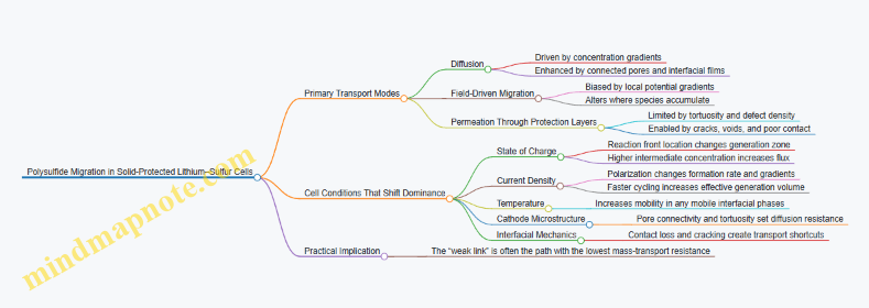
Putting It Together with a Simple Diagnostic Logic
When migration is high, the question is where the low-resistance pathway is. If performance loss tracks with current density, field and generation-zone effects are likely. If loss is sensitive to assembly quality or cycling-induced contact changes, mechanical pathways such as gaps and cracks are likely. If loss accelerates strongly with temperature, mobility in interfacial films or partially mobile phases is likely.
Example: Suppose two cells use the same protection material. The one with higher impedance growth early in cycling often indicates increasing interfacial resistance and contact degradation. That same cell typically shows stronger migration signatures because new shortcuts appear as contact worsens.
In short, polysulfide migration is not a single mechanism. It is a competition between transport modes and the cell’s evolving internal geometry and chemistry. Solid electrolyte protection reduces the available pathways, but cell conditions decide which remaining pathway becomes the main route.
6.2 Barrier Design Principles Including Thickness and Tortuosity Control
A solid-electrolyte barrier is not just a “wall.” It is a controlled path that slows polysulfide migration while still allowing the electrochemical reactions to proceed where they should. Two design knobs dominate: thickness (how far species must travel) and tortuosity (how crooked that travel becomes). Together, they set the effective transport resistance through the barrier.
Foundational Transport Picture
Start with a simple idea: polysulfides move by diffusion through pores, grain boundaries, or microcracks. If the barrier is thicker, the diffusion distance increases. If the barrier is more tortuous, the actual path length increases even if the geometric thickness stays the same. In practice, both effects show up as a higher concentration gradient requirement to achieve the same flux.
A useful mental model is to treat the barrier as having an effective diffusion coefficient smaller than the bulk value. Thickness and tortuosity both reduce the effective transport, which lowers shuttle-driven capacity loss. The trick is doing this without making ionic transport so difficult that the cathode becomes reaction-limited.
Thickness Control Without Starving the Cathode
Thickness is the most straightforward parameter to tune, but it has a predictable tradeoff.
- Too thin: polysulfides can cross before they are immobilized or consumed, so self-discharge and coulombic inefficiency rise.
- Too thick: ionic pathways through the barrier become sluggish, increasing interfacial resistance and reducing utilization.
A practical approach is to design thickness in steps and evaluate each step with the same cathode loading and current density. For example, if you are comparing barrier coatings, keep the cathode formulation and pressing pressure constant, then test three thickness levels such as “thin, medium, thick.” The best thickness is the one where coulombic efficiency improves while the discharge capacity remains close to the baseline.
Easy example: Suppose your baseline shows a noticeable voltage drop during discharge and a coulombic efficiency that falls below 98%. You apply a barrier coating. If the first coating is too thin, the efficiency barely changes. If the second coating is thicker, efficiency improves and the voltage profile stabilizes. If the third coating is thicker still, efficiency may remain high, but the discharge capacity drops because ionic transport through the barrier becomes the bottleneck.
Tortuosity Control Through Microstructure
Tortuosity is about geometry. A barrier with straight, well-connected pores offers a relatively direct route for polysulfides. A barrier with a more tortuous pore network forces longer, more winding paths.
You can influence tortuosity by controlling:
- Particle packing and sintering level: denser packing can reduce straight channels.
- Binder and pore former content: more tortuous pore networks can be created by adjusting how voids form.
- Grain boundary connectivity: barriers that interrupt continuous grain-boundary pathways reduce effective transport.
Easy example: Imagine two barriers with the same thickness. Barrier A has a uniform, connected pore network. Barrier B has pores that terminate more often and change direction frequently. Even if both have the same nominal thickness, Barrier B forces polysulfides to travel farther in practice, so the shuttle effect weakens.
Balancing Ionic and Electronic Pathways
A barrier that blocks polysulfides must not accidentally block the ions needed for sulfur redox. In many solid-electrolyte protection schemes, the barrier is designed to be ion-conducting but electron- and polysulfide-transport resistant.
Thickness and tortuosity affect different species differently. Polysulfides may be hindered by size, solvation, and adsorption, while ions may move through specific conduction pathways. That means you should evaluate barrier performance using both:
- Shuttle indicators such as coulombic efficiency and self-discharge behavior.
- Interfacial indicators such as impedance growth and polarization under the same current.
Mind Map: Thickness and Tortuosity Design Logic
Example: Stepwise Barrier Optimization Workflow
- Choose a baseline barrier chemistry that is known to be chemically compatible with the cathode and electrolyte.
- Prepare three thickness levels using the same deposition or coating method, aiming for clearly separated thickness values.
- Keep tortuosity roughly comparable by using the same processing conditions (same drying, same pressing, same thermal treatment).
- Run identical cycling protocols at a fixed current density and cutoff criteria.
- Select the thickness where coulombic efficiency improves without a meaningful loss in discharge capacity.
If the medium thickness works but the thick one fails, the failure mode is usually transport-limited ionic access. If the thin one fails but the medium succeeds, the failure mode is usually insufficient suppression of polysulfide crossing.
Practical Rules of Thumb for Thickness and Tortuosity
- Treat thickness as a first-pass filter for shuttle suppression, then refine tortuosity through microstructure control.
- Use paired metrics: one for shuttle (coulombic efficiency/self-discharge) and one for transport (polarization/impedance).
- When changing thickness, avoid changing too many other variables at once; otherwise, you will not know whether you tuned thickness, tortuosity, or both.
This is the core logic: thickness sets the distance, tortuosity sets the crookedness, and the best barrier is the one that makes polysulfide travel expensive while keeping ion travel affordable.
6.3 Chemical Interactions Including Adsorption and Reaction Pathways
Solid electrolyte protection works best when it does more than block polysulfides physically. It also changes what polysulfides “want” to do at the cathode–electrolyte interface. The key chemical interactions are adsorption on surfaces, interfacial reaction to form new species, and subsequent transport or passivation effects that alter the local reaction network.
Foundational Picture of Polysulfide Chemistry at Interfaces
Lithium–sulfur cathodes generate a family of sulfur species during discharge: S8 converts to soluble long-chain polysulfides first, then to shorter-chain polysulfides and finally to Li2S near the end of discharge. In a protected solid-electrolyte system, the interface becomes a “reaction crossroads” where species can either proceed toward Li2S formation, adsorb and linger, or react with protective layers.
A useful mental model is to track three fates for each incoming polysulfide molecule: (1) adsorption to a surface site, (2) chemical transformation at the surface, and (3) escape back into the cathode region. Adsorption alone can reduce shuttle by increasing residence time near the cathode, but it can also create a bottleneck if the adsorbed species cannot convert efficiently.
Adsorption Mechanisms and What They Change
Adsorption is governed by how well a surface stabilizes sulfur species relative to the surrounding electrolyte environment. In practice, adsorption strength depends on surface charge, polar functional groups, and the availability of binding sites.
Example: Polar Surface Anchoring
Imagine a protective interlayer containing polar groups that can coordinate sulfur species. A long-chain polysulfide arriving at the interface may bind through sulfur atoms, reducing its mobility. If the bound species can still react to form Li2S, the protection improves utilization. If not, the surface becomes a parking lot: polysulfides accumulate, local concentration rises, and side reactions increase.
Example: Conductive Host with Strong Binding
A conductive carbon-like host can adsorb polysulfides while also providing electron pathways. That combination often helps because the adsorbed species are more likely to undergo reduction steps needed to reach Li2S. If the host is poorly connected electronically, adsorption may still occur, but the reduction stalls.
Reaction Pathways at the Solid Electrolyte Interface
Once adsorption occurs, the next step is whether the species undergoes interfacial reduction, disproportionation, or decomposition. These pathways are influenced by local lithium activity, interfacial electronic structure, and the chemical stability of the solid electrolyte and its protective layer.
A common pathway is stepwise reduction: long-chain polysulfides reduce to shorter chains and then to Li2S. In a protected system, the interlayer can shift where these steps happen. If the interlayer is chemically compatible, it can act like a controlled reaction zone. If it is not, it can promote decomposition that consumes active sulfur and forms resistive products.
Example: Interlayer That Promotes Controlled Reduction
Consider a thin interlayer that is chemically stable but provides adsorption sites. A polysulfide binds, then receives electrons and lithium ions at the interface, converting toward Li2S. The result is a more localized deposition of Li2S that reduces long-range migration.
Example: Interlayer That Reacts Unhelpfully
Now consider an interlayer that reacts with polysulfides to form insulating compounds. The first few cycles may show good suppression because the layer initially captures species. Over time, the insulating products increase interfacial resistance, making it harder for subsequent species to reduce. The cell then shows higher polarization and lower utilization.
Interphase Formation and Its Dual Role
Interphase formation is the “paperwork” generated by repeated contact between polysulfides and protective materials. It can be beneficial when it creates a stable, ion-conducting, and electronically appropriate interface. It can be harmful when it forms thick, poorly conducting layers.
A practical way to reason about interphase quality is to ask two questions: Does the interphase allow lithium-ion transport to the reaction site? And does it avoid consuming sulfur species into nonproductive products? The best interphases tend to be thin enough that they do not dominate resistance, yet robust enough to survive volume changes and repeated cycling.
How to Diagnose Chemical Interactions in Practice
Chemical interactions leave fingerprints. If adsorption dominates, you often see reduced polysulfide mobility and changes in voltage profile shape without extreme resistance growth. If interfacial reactions dominate, you often see evidence of new interphase chemistry and a stronger link between cycle count and impedance increase.
Example Diagnostic Workflow
1. Compare cycling curves with and without the protective interlayer.
2. Track impedance growth trends across cycles.
3. After cycling, examine whether sulfur is concentrated near the interface or distributed deeper into the cathode.
4. Correlate sulfur distribution with signs of interphase formation.
Mind Map: Chemical Interactions Including Adsorption and Reaction Pathways
Putting It Together for Cathode Stabilization
In a well-designed protected system, adsorption should bring polysulfides close to the reaction zone, and interfacial chemistry should convert them toward Li2S without generating thick insulating products. When either step fails—adsorption is too strong without reduction, or interfacial reactions produce resistive layers—the protection becomes less about “stopping shuttle” and more about managing where and how sulfur is consumed. The goal is not just to trap polysulfides, but to steer their chemistry toward productive deposition.
6.4 Measuring Polysulfide Suppression Using Electrolyte Free and Extractive Methods
Polysulfide suppression is easiest to measure when you separate two questions: how much polysulfide leaves the cathode region, and how much of what leaves actually returns to the cathode during discharge. Electrolyte-free methods focus on the first question by preventing soluble species from being carried by a liquid electrolyte. Extractive methods focus on the second question by quantifying soluble sulfur species after cycling or during controlled contact.
What You Measure and Why It Matters
In a lithium sulfur cell, polysulfides can be suppressed by blocking migration, reducing solubility, or accelerating conversion at the cathode side. Each mechanism leaves a different fingerprint:
- Lower soluble polysulfide concentration in an electrolyte-contact region suggests stronger migration suppression.
- Higher coulombic efficiency with similar capacity suggests less polysulfide loss to shuttle reactions.
- Faster return of sulfur species to the cathode region suggests improved interfacial conversion rather than only physical blocking.
A practical approach is to report both a concentration metric (from electrolyte-free or extractive sampling) and a cell-level metric (from cycling). The concentration metric tells you where the chemistry went; the cell metric tells you what it did.
Electrolyte Free Contact Tests
Electrolyte-free contact tests use a controlled environment where polysulfides can interact with the solid electrolyte protection layer without being continuously transported by a bulk liquid electrolyte.
Core idea: create a donor side containing sulfur species and a receiver side containing the solid electrolyte protection region, then quantify sulfur species that appear on the receiver side after a fixed time.
Common setup pattern:
- Prepare a donor compartment with a known amount of sulfur species source.
- Place the solid electrolyte protection layer between donor and receiver.
- Use a receiver medium that does not dissolve polysulfides aggressively, so detected sulfur on the receiver side is meaningful.
- After a fixed contact time, extract sulfur from the receiver side and quantify it.
Easy-to-understand example:
- Donor side: sulfur species source is mixed with a non-dissolving carrier.
- Receiver side: a thin solid electrolyte protection sample is placed facing the donor.
- After 2 hours at controlled temperature, the receiver sample is rinsed, then sulfur is extracted and measured.
If the receiver-side sulfur is low, the protection layer is doing its job at blocking migration or limiting interfacial solubilization.
Extractive Quantification During Controlled Cycling
Extractive methods sample the liquid phase where polysulfides accumulate. The key is to standardize sampling so that differences reflect suppression rather than handling.
Core idea: after a defined cycling step or after a fixed open-circuit rest, extract the electrolyte and quantify polysulfide species.
Systematic workflow:
- Run a cell to a defined state, such as after a partial discharge where polysulfides are expected to be abundant.
- Stop the test at a fixed time and state of charge.
- Extract the electrolyte quickly under controlled conditions.
- Quantify polysulfide species using a method that distinguishes chain length or at least total soluble sulfur.
Easy-to-understand example:
- Compare two cells with identical cathode loading and current density.
- Cell A has no protection interlayer; Cell B has a protection layer.
- After the same partial discharge, extract electrolyte from both cells.
- If Cell B shows lower soluble sulfur concentration, it indicates reduced polysulfide presence in the liquid phase.
To avoid misleading results, keep the extraction timing consistent. Polysulfides do not wait politely for your pipette.
Mind Map: Measuring Polysulfide Suppression
Converting Measurements Into Suppression Metrics
Use at least one relative metric so results remain comparable across batches.
- Receiver Suppression Factor for electrolyte-free tests:
- Ratio of extracted sulfur on receiver side for protected vs unprotected samples.
- Soluble Sulfur Reduction for extractive tests:
- Percent reduction of total soluble sulfur in electrolyte for protected vs unprotected cells.
Easy-to-understand example:
- Unprotected receiver extraction yields 10 arbitrary units of sulfur.
- Protected receiver extraction yields 2 units.
- Receiver Suppression Factor is 0.2, meaning an 80% reduction.
Pair these with coulombic efficiency from cycling at the same cutoff criteria. If soluble sulfur is reduced but coulombic efficiency is unchanged, the protection may be shifting where loss happens rather than eliminating it.
Practical Controls That Prevent False Confidence
Three controls keep the story coherent:
- Blank extraction control: confirm that your extraction procedure does not introduce sulfur artifacts.
- Mass balance control: verify that sulfur source amount is consistent across samples.
- Interfacial contact control: ensure the protection layer is similarly pressed or infiltrated so differences are chemical, not mechanical.
A small but useful habit is to report contact time, temperature, and extraction timing together. When those variables drift, your suppression metric drifts too, like a shopping list that keeps changing mid-trip.
6.5 Practical Protocols for Quantifying Shuttle and Capacity Loss Contributions
Quantifying how much capacity loss comes from polysulfide shuttle versus other effects is mostly an exercise in controlled comparisons. The goal is to separate “loss caused by migrating species” from “loss caused by loss of active material, blocked transport, or interfacial degradation.” You do this by combining (1) a baseline cycling test, (2) shuttle-suppression conditions, and (3) post-test checks that confirm what changed.
Core Measurement Logic
Start with a simple accounting model for capacity loss over a cycle window:
- Total capacity loss = loss in delivered capacity relative to the reference cycle.
- Shuttle contribution = the portion that disappears when migration is blocked or chemically neutralized.
- Non-shuttle contribution = the remaining loss after shuttle is suppressed.
A practical way to implement this is to run three cell conditions under identical current, temperature, and pressure/contact scheme:
- Reference: standard solid electrolyte protection stack.
- Shuttle-blocked: add a polysulfide-trapping layer or stronger barrier that targets migration without changing the electrochemical window.
- Electrolyte-absent control: a configuration that prevents ionic conduction but still allows you to observe chemical interactions in a limited way, used only for interpreting species presence rather than capacity.
Use the same sulfur loading and areal capacity for all electrochemical tests, because shuttle effects scale with concentration gradients and utilization.
Mind Map: Quantification Workflow
Step-by-Step Protocol
1) Define a Stable Reference Window
Pick a cycle interval where the cell is not yet dominated by catastrophic failure. For example, use cycles 5–20 for the reference and shuttle-blocked comparisons. If the first few cycles show large formation effects, normalize to the capacity at cycle 5 rather than cycle 1.
Example: If delivered capacity at cycle 5 is 1.00 (normalized) and at cycle 20 is 0.80 for the reference, the reference loss over the window is 0.20.
2) Run Paired Cycling Tests
Cycle both reference and shuttle-blocked cells with identical rest times after charge and discharge. Rest matters because it changes how much time polysulfides have to migrate and react. Keep the same cutoff voltages, since shuttle can be sensitive to the degree of reduction/oxidation reached.
Record:
- Discharge capacity per cycle.
- Coulombic efficiency (CE) per cycle.
- Voltage profile features such as hysteresis and polarization slope.
3) Compute Shuttle Contribution from Capacity Differences
Let L_ref be the capacity loss fraction in the reference condition over the chosen window, and L_block be the capacity loss fraction in the shuttle-blocked condition.
- Shuttle fraction = (L_ref − L_block) / L_ref
- Non-shuttle fraction = 1 − shuttle fraction
Example: If L_ref = 0.20 and L_block = 0.12, then shuttle fraction = (0.20 − 0.12)/0.20 = 0.40. That means 40% of the loss over that window is consistent with migration-driven effects.
4) Use CE to Sanity-Check the Split
CE is not a perfect shuttle meter, but it helps catch mistakes. If shuttle is truly reduced, CE should improve or stabilize in the shuttle-blocked condition. If CE barely changes while capacity loss drops, the improvement likely comes from reduced chemical consumption of active material at interfaces rather than classic shuttle.
Example: Capacity loss drops by 30% but CE changes by only 1%. That pattern suggests the shuttle-blocking layer may also be modifying interfacial chemistry or transport, so interpret the shuttle fraction as “migration-consistent” rather than “pure shuttle.”
5) Confirm Species Suppression with Post-Test Sampling
After cycling, extract or probe the electrolyte-side species in a way that matches your cell design. For solid electrolyte systems, you can still compare:
- Presence of sulfur species associated with migrating intermediates.
- Changes in interphase chemistry at the cathode-protection interface.
A useful practical check is to compare the intensity of sulfur species signals in the shuttle-blocked condition relative to reference. If species suppression is weak, the computed shuttle fraction is likely underestimating shuttle’s role.
6) Separate Interfacial and Transport Losses
Non-shuttle loss often shows up as increasing interfacial resistance or reduced effective transport. Run impedance spectroscopy at the same state-of charge for both conditions. If the shuttle-blocked cell shows similar resistance growth as the reference, then the remaining loss is likely dominated by interfacial degradation rather than migration.
Example: Both conditions show comparable impedance rise, but only the reference shows strong migrating species. The capacity difference then maps well to shuttle.
Practical Reporting Template
Report results as:
- Window definition (cycles used, normalization point).
- L_ref and L_block with units or normalized fractions.
- Shuttle fraction and non-shuttle fraction.
- CE trend summary.
- Species suppression evidence.
- Impedance trend summary.
This keeps the story consistent: the numbers come from paired cycling, the interpretation comes from species and impedance, and the conclusions stay tied to what the measurements actually show.
7. Electrolyte Protection Under Realistic Operating Conditions
7.1 Influence of Temperature on Solid Electrolyte Conductivity and Interfaces
Temperature affects both how fast ions move through a solid electrolyte and how stable the interfaces are when sulfur chemistry starts doing its thing. In lithium–sulfur cells with solid electrolyte protection, you can think of temperature as changing two knobs at once: bulk ionic conductivity and interfacial resistance.
Temperature and Bulk Ionic Conductivity
Most solid electrolytes show thermally activated ionic transport. As temperature rises, the ionic conductivity typically increases because ions hop more easily between sites and grain boundaries become less resistive. A practical way to connect this to cell behavior is to separate the total resistance into bulk and interfacial parts. When bulk conductivity improves with temperature, the same current draws less voltage drop, so polarization decreases.
A concrete example: suppose your cell has a total resistance of 100 mΩ at 25°C, where 60 mΩ is bulk and 40 mΩ is interfacial. If temperature increases conductivity so that bulk resistance halves to 30 mΩ while interfacial resistance stays roughly constant, the total becomes 70 mΩ. That 30% reduction in resistance is noticeable in voltage profiles, especially at higher current densities.
Temperature and Interfacial Processes
Interfaces are where solid electrolytes meet cathode protection layers, binders, and current collectors. Temperature changes several interfacial phenomena:
- Interfacial contact quality: Thermal expansion mismatch can tighten contact in some stacks or worsen it in others. Even if the average contact area is unchanged, local gaps can open under cycling.
- Interphase growth and decomposition: Many solid electrolytes form thin interphases with reactive species. Higher temperature accelerates both formation and breakdown, which can increase resistance if the interphase becomes electronically conductive or poorly ion-conducting.
- Wetting and infiltration of protection layers: If the cathode protection includes pores or partially infiltrated regions, temperature can improve infiltration during assembly and early cycling, reducing void-related resistance.
- Reaction kinetics at boundaries: Charge transfer at the electrolyte–cathode interface can speed up with temperature, lowering activation overpotential until transport limitations dominate.
A useful mental model is to treat interfacial resistance as a sum of contact resistance, charge-transfer resistance, and diffusion-related contributions. Temperature may reduce charge-transfer resistance while simultaneously increasing interphase-related resistance. The net effect depends on which term is dominant.
Practical Measurement Strategy
To avoid guessing, measure temperature dependence in a way that separates bulk from interface.
- Step 1: Use impedance at multiple temperatures with the same stack pressure and identical assembly. Track how the high-frequency intercept (often tied to bulk) and the semicircle features (often tied to interfacial processes) shift.
- Step 2: Keep current density constant during electrochemical tests so that changes in voltage are attributable to resistance changes rather than different polarization regimes.
- Step 3: Watch for nonlinearity. If resistance drops at first and then rises at higher temperature, that pattern often signals interphase growth overtaking conductivity gains.
Example Temperature Profiles and What They Mean
Consider two cells with different solid electrolyte protection designs.
- Cell A shows steadily decreasing polarization from 25°C to 60°C. This suggests bulk conductivity improvement and no severe interphase penalty.
- Cell B improves from 25°C to 40°C, then polarization increases at 60°C. A common interpretation is that interphase formation or contact degradation accelerates at higher temperature, raising interfacial resistance.
In both cases, the voltage curve shape matters. If the early-cycle voltage drop improves but later-cycle performance worsens at high temperature, the interface is likely changing during cycling rather than only during measurement.
Mind Map: Temperature Effects on Solid Electrolyte Conductivity and Interfaces
Example Workflow for a Temperature Sweep
- Assemble cells with identical stack pressure and electrode thickness.
- Run impedance at 25°C, 35°C, 45°C, and 60°C.
- Identify whether bulk-like resistance decreases smoothly while interfacial features show a turning point.
- Perform a short constant-current discharge at each temperature to confirm the impedance trend matches real polarization.
This workflow keeps the interpretation grounded: temperature changes are not treated as magic, just as measurable shifts in resistance components and interface behavior.
7.2 Current Density Effects on Polarization and Degradation Onset
Current density sets the pace of lithium and ion transport through the solid electrolyte and across every interface. In lithium–sulfur cells with solid electrolyte protection, higher current density usually increases polarization first, then accelerates degradation once certain thresholds are crossed. The key is to separate what is happening electrochemically from what is happening mechanically and chemically.
Foundational Link Between Current Density and Polarization
Polarization is the extra voltage you pay beyond the equilibrium potential. It comes from several sources that scale differently with current density:
- Ohmic losses: voltage drop through solid electrolyte, current collectors, and contact resistances. These scale roughly linearly with current density.
- Charge-transfer losses: sluggish interfacial reactions at the cathode/electrolyte boundary. These often grow nonlinearly as overpotential increases.
- Mass-transport limitations: insufficient ion availability near reaction sites. In solid systems this can be driven by limited ionic conductivity, tortuosity, and poor contact that creates “dead” regions.
A practical way to see the separation is to compare low-current and high-current voltage curves at the same state of charge. If the voltage gap between currents grows linearly, ohmic effects dominate. If the gap widens faster at high current, interfacial kinetics or transport limitations are taking over.
How Polarization Triggers Degradation Onset
Degradation onset is not a single event; it is when the cell crosses from “losses are mostly reversible” to “losses start compounding.” Current density influences several degradation pathways:
-
Interfacial contact deterioration: Higher current increases local current density at imperfect contact spots. Those spots heat slightly, experience stronger electrochemical driving forces, and can develop microcracks or delamination at the solid electrolyte protection layer. Once contact area shrinks, resistance rises, which further increases polarization—a feedback loop.
-
Accelerated side reactions: Larger overpotentials increase the likelihood that reactive species form at interfaces. Even if the solid electrolyte blocks polysulfides, the protection layer and cathode surface can still undergo chemical changes when the local potential swings hard.
-
Nonuniform utilization and local depletion: Under high current, ion flux demand rises. If ion transport cannot keep up, some regions become depleted while others keep reacting. Depleted regions may stop contributing, while active regions experience higher local potentials and stronger stress from volume change.
-
Polysulfide-related effects despite protection: Solid electrolyte protection reduces migration, but it does not remove every pathway. When polarization is high, any residual transport or interfacial dissolution can become more damaging because the cell is operating at conditions that favor further reaction and deposition patterns.
Threshold Behavior and What to Measure
Many cells show a “knee” in performance: below a certain current density, capacity and coulombic efficiency degrade slowly; above it, both worsen quickly. The knee is often tied to one of these limiting factors:
- ionic conductivity and tortuosity limits in the solid electrolyte
- interfacial resistance growth from contact loss
- reaction kinetics at the cathode protection interface
To identify the knee systematically, use three measurements:
- Voltage vs. time at constant current: look for rapid voltage drift or sudden slope changes.
- Electrochemical impedance before and after a current step: rising interfacial resistance points to contact or interphase changes.
- Coulombic efficiency trend during a current-density ladder: a sharp drop suggests side reactions or increased irreversible consumption.
Example: Interpreting a Current-Density Ladder
Suppose you test at 0.1, 0.3, and 0.6 C (with the same areal capacity target). At 0.1 C, the discharge voltage is stable and the impedance after cycling is close to the baseline. At 0.3 C, the discharge voltage drops more and the impedance increases moderately, but coulombic efficiency remains acceptable. At 0.6 C, you see a pronounced voltage knee early in discharge, impedance rises strongly, and coulombic efficiency falls.
A consistent interpretation is:
- 0.1 C: ohmic and mild interfacial losses dominate; degradation is slow.
- 0.3 C: interfacial resistance growth begins; polarization is high enough to stress interfaces.
- 0.6 C: transport or contact failure becomes dominant; side reactions increase because overpotential is large and local conditions are harsher.
Mind Map: Current Density Pathways to Polarization and Degradation
Example: A Simple Diagnostic Decision Rule
If increasing current density causes voltage to drop smoothly and impedance rises mainly in the bulk-like part, focus on ionic conductivity and transport pathways. If voltage shows a knee and impedance rises mainly in the interfacial part, focus on contact integrity and protection-layer stability. If coulombic efficiency collapses while voltage knee appears early, treat the situation as side-reaction dominated rather than purely transport-limited.
Practical Takeaways for Solid Electrolyte Protected Cathodes
- Use a current-density ladder with impedance checks at each step to separate bulk, interface, and reaction contributions.
- Track whether degradation correlates with voltage knee timing; early knees usually indicate interfacial or transport bottlenecks.
- When comparing cathode protection designs, keep areal capacity target and electrode thickness consistent, because current density effects are strongly coupled to local utilization.
In short, current density is not just “more power.” It changes where the cell spends its voltage, and once that spending concentrates at fragile interfaces, degradation starts paying interest.
7.3 Effects of Areal Capacity and Sulfur Loading on Protection Effectiveness
Areal capacity (mAh cm⁻²) and sulfur loading (mgS cm⁻²) determine how much electrochemical work the cathode must do per unit area. In lithium sulfur cells with solid electrolyte protection, those quantities also determine whether the protection layer can keep interfaces stable while ions move and sulfur species are prevented from causing trouble.
Foundational Link Between Loading and Protection Demands
Protection effectiveness is not just “blocking polysulfides.” It also has to maintain low interfacial resistance and reliable ionic transport as the cathode thickens and the reaction zone shifts. When sulfur loading increases, the cathode requires more conversion per area, so the solid electrolyte protection must handle:
- Larger local concentration gradients of sulfur species.
- More pronounced volume change at the cathode during discharge.
- Greater sensitivity to any loss of contact or pore accessibility.
A simple way to picture this: imagine the protection layer as a bouncer at a club door. At low guest counts, the bouncer can manage with a relaxed posture. At higher counts, any small weakness—slightly misaligned door, worn shoes, or a crack in the wall—shows up as people slipping through.
Areal Capacity as a Proxy for Reaction Utilization
Areal capacity reflects how much of the cathode’s active material is actually used during cycling. Two cathodes can have the same sulfur loading but different areal capacity performance depending on transport limits and polarization. If the cell reaches cutoff voltage early, the reaction utilization is incomplete, and the protection layer may appear “effective” simply because less chemistry occurred.
To avoid that misleading outcome, compare cells at matched areal capacity targets rather than only matched sulfur loading. For example, if one design reaches 2.0 mAh cm⁻² before cutoff while another reaches 1.2 mAh cm⁻², the first may show better stability because it experienced a smaller fraction of its own potential degradation pathways.
Sulfur Loading Changes Geometry, Not Just Chemistry
Increasing sulfur loading typically increases cathode thickness and alters the internal architecture. That changes three practical factors:
- Ionic path length: Solid electrolyte protection relies on ionic transport through the cathode and interfaces. Thicker cathodes increase tortuosity and can raise polarization.
- Electronic percolation: Conductive networks must span the full thickness. If the network is tuned for low loading, higher loading can create regions that are electronically isolated, leading to uneven reaction and localized stress.
- Interfacial contact area: Protection layers work at interfaces. Higher loading can reduce effective contact if the stack compresses less uniformly or if binder distribution changes.
Concrete example: consider two cathodes with the same protection interlayer. The higher-loading cathode may show a similar initial impedance, but during cycling its voltage curve can develop a larger hysteresis because the reaction concentrates near better-connected regions. Those regions experience stronger local volume change, which can gradually degrade the protection interface.
How Protection Effectiveness Degrades with Higher Loading
As areal capacity and sulfur loading rise, failure often shifts from “global shuttle” to “interface and transport bottlenecks.” Common patterns include:
- Early capacity fade with stable initial coulombic efficiency: This suggests transport limitations and incomplete utilization, not just polysulfide migration.
- Rising interfacial resistance over cycles: This points to contact loss or interphase thickening at the protected interface.
- Greater sensitivity to current density: If higher loading makes the cell more polarization-limited, the same protection design can perform acceptably at one current but poorly at another.
Mind Map: Of Loading Effects on Protection
Example Comparison Workflow
Suppose you test two protected cathodes:
- Cathode A: 2.5 mgS cm⁻², target 1.5 mAh cm⁻².
- Cathode B: 4.0 mgS cm⁻², target 1.5 mAh cm⁻².
If both reach 1.5 mAh cm⁻², compare their voltage profiles at the same areal capacity points. If Cathode B shows higher hysteresis and faster impedance growth, the protection layer is likely being stressed by transport and contact issues rather than failing purely as a barrier. If Cathode B cannot reach 1.5 mAh cm⁻² without cutoff, then the apparent “protection success” is partly utilization-limited; the cell never fully engages the chemistry that would reveal shuttle or interface degradation.
Practical Takeaways for Interpreting Results
When areal capacity and sulfur loading increase, protection effectiveness must be judged using multiple signals, not a single metric. Use areal capacity-matched comparisons, monitor voltage shape and impedance trends, and interpret coulombic efficiency in context of utilization. This keeps the story consistent: protection layers can block migration, yet still lose performance if transport and contact cannot keep up with the amount of sulfur that must react per square centimeter.
7.4 Managing Moisture and Contaminants During Assembly and Testing
Moisture management is not a side quest in lithium sulfur with solid electrolyte protection—it directly controls interphase chemistry, ionic transport, and the stability of the cathode protection stack. In practice, you’re trying to prevent water from reaching three sensitive zones: the lithium metal anode surface, the solid electrolyte and its grain boundaries, and any cathode protection layers that rely on controlled surface chemistry.
Moisture Pathways and Why They Matter
Water can enter the cell during electrode drying, transfer, stack pressing, electrolyte filling, and even during measurement if the environment is not controlled. Once present, it can react with lithium to form insulating products, alter the solid electrolyte surface, and change the wetting behavior of cathode protection layers. The result is often a higher initial impedance, faster capacity fade, and inconsistent coulombic efficiency—especially when comparing cells assembled on different days.
A useful mental model is to treat moisture as a “contaminant with a schedule.” If your assembly steps are long, the risk grows with time exposed to ambient air. If your steps are short but involve poor sealing or leaky fixtures, the risk grows with repeated handling.
Foundational Controls Before You Touch Materials
Start with process discipline rather than heroics. Define a maximum exposure time for each component and keep it measurable. Use dry storage containers with desiccant and verify that the atmosphere is actually dry by tracking humidity indicators. For lithium metal, minimize handling time and avoid wiping that can smear surface films.
For cathode and solid electrolyte components, confirm that drying is complete and that the drying method matches the material. A common mistake is drying “until it looks dry,” then letting the sample sit in ambient air while you prepare other parts. Instead, stage your workflow so the sample goes from drying to assembly with minimal delay.
Cleanliness Targets for Interfaces
Contaminants are broader than water. Fine dust, binder residues, and residual solvents can block contact points or change local reaction pathways. Solid electrolyte protection layers are especially sensitive because performance depends on intimate contact and stable interphase chemistry.
A practical approach is to set cleanliness targets per interface:
- Lithium to separator or electrolyte: no visible residue, minimal handling, controlled transfer.
- Solid electrolyte to cathode stack: no loose powder that can create voids.
- Interlayers and coatings: consistent thickness and uniform coverage, without clumps.
If you see variability in thickness or surface texture, treat it as a contamination signal, not just a fabrication tolerance.
Assembly Workflow That Limits Exposure
Use a workflow that reduces both time and opportunities for contamination. Keep tools dedicated to dry-zone use, and avoid moving between wet and dry areas without a controlled transition. When stacking, ensure that pressing is done consistently so that trapped moisture pockets and loose particles don’t become permanent voids.
A simple example: if you assemble three cells back-to-back, prepare all cathode components first inside the dry environment, then assemble cell-by-cell without pausing to “just check something.” That one pause can dominate variability.
Testing Conditions That Reveal Hidden Moisture
Even if assembly is careful, testing conditions can expose problems. Temperature affects both conductivity and reaction kinetics, so compare cells tested under the same thermal profile. Humidity in the test environment can also matter if your setup allows gas exchange.
During early cycling, monitor initial impedance and the first few voltage profiles. A moisture-related failure often shows up as a rapid rise in resistance or an early mismatch between theoretical utilization and measured capacity. If one cell behaves differently from the rest, don’t average it away—trace it back to handling time, drying batch, or stack pressing parameters.
Mind Map: Moisture and Contaminant Control
Example: Diagnosing an Outlier Cell
Suppose three cells are assembled using the same cathode formulation and solid electrolyte protection stack. Two cells show stable early cycling, while one has higher initial impedance and lower coulombic efficiency.
A systematic check looks like this:
- Compare assembly logs for exposure time of the solid electrolyte and cathode components.
- Verify drying batch records for the cathode and any interlayers.
- Inspect the stack for signs of trapped voids or loose particles at the solid electrolyte interface.
- Confirm that the pressing force and dwell time were consistent.
If the outlier had a longer exposure window for the solid electrolyte, the most likely cause is altered interphase chemistry or contact loss, not a random electrochemical fluke.
Example: A Simple Exposure-Time Rule
Set a rule such as: “Cathode and solid electrolyte components must be assembled within a fixed time window after removal from dry storage.” Then enforce it with a timer and a checklist. The rule is boring, but it makes your results comparable, which is the real goal of moisture control.
7.5 Protocols for Building Comparable Cells Across Different Protection Designs
Comparing lithium–sulfur cells with different solid-electrolyte protection designs is mostly an exercise in removing accidental variables. If two cells differ in more than the protection stack, the performance gap is impossible to interpret. The goal is simple: make every other difference measurable, controlled, or explicitly reported.
1) Define the Comparison Scope Before You Touch Materials
Start by writing down what “comparable” means for your study. Decide whether you compare at fixed sulfur loading, fixed cathode thickness, fixed areal capacity, or fixed electrolyte-to-cathode ratio. Then lock those choices for the entire batch.
Example: If one design uses a thicker interlayer, you might keep cathode thickness constant and accept a different total stack mass. Alternatively, you might keep total stack mass constant and allow cathode thickness to vary. Pick one and stick to it, because both approaches answer different questions.
2) Standardize the Cathode Baseline So Protection Is the Only Moving Part
Use the same sulfur host, conductive additive, binder type, and target porosity across designs. If you must change the cathode to accommodate a protection layer, treat that as part of the design and document it.
A practical workflow:
- Prepare a single “base cathode slurry” recipe.
- Cast cathodes to the same target thickness and dry them using the same schedule.
- Measure thickness at multiple points and reject outliers.
Example: If you only measure thickness once, you may accidentally compare a thin cathode that wets easily against a thick one that traps voids. That difference can masquerade as “better protection.”
3) Control Protection Stack Geometry and Contact Formation
Protection designs often change interlayer thickness, surface roughness, and contact pressure. Those factors strongly affect interfacial resistance.
Use consistent stack geometry:
- Specify interlayer thickness targets and tolerances.
- Use the same deposition method and drying/curing conditions.
- Apply the same assembly pressure and dwell time.
Example: Two interlayers with identical chemistry can behave differently if one is pressed into better contact. Record the pressure and dwell time, and include a simple post-assembly impedance check to confirm the contact state.
4) Keep Electrolyte and Separator Conditions Identical
Even “solid” systems can vary in moisture sensitivity and interfacial wetting. Standardize:
- Solid electrolyte batch and pre-drying conditions.
- Any interfacial additives or wetting agents.
- Separator type and placement.
Example: If one batch of solid electrolyte was stored longer, it may develop different surface chemistry. That can change polysulfide interactions and interphase formation, confusing the comparison.
5) Use a Single Cell Format and a Single Current Protocol
Cell geometry affects ionic path length and electronic percolation. Choose one format and keep it constant: same electrode area, same current collector design, same tabbing method.
Then standardize the cycling protocol:
- Same formation steps.
- Same current density or same C-rate definition.
- Same rest times and cutoff criteria.
Example: If one design is tested at a lower current density, it may appear more stable simply because it generates less polarization and slower side reactions.
6) Build a Measurement Plan That Separates “Interfacial” from “Bulk” Effects
Before cycling, run a baseline impedance measurement at a consistent temperature and state of charge. During cycling, track:
- Coulombic efficiency trends.
- Voltage hysteresis growth.
- Capacity retention at fixed areal capacity.
After cycling, perform the same post-mortem sampling locations for every design.
7) Replicate Like a Grown-Up: Randomize and Document
Use at least three cells per design when possible. Randomize the order of assembly and testing to avoid systematic drift (for example, temperature changes in the lab or slight differences in press timing).
Document everything that could shift results:
- Batch IDs for sulfur, electrolyte, and interlayers.
- Thickness maps and average values.
- Assembly pressure and dwell time.
- Any deviations from the protocol.
Mind Map: Comparable Cell Protocol Workflow
Example: A Minimal Comparison Template
Use a single spreadsheet template for every design:
- Design ID and protection stack description.
- Cathode recipe ID and measured thickness stats.
- Solid electrolyte batch ID and pre-dry time.
- Interlayer thickness target and measured value.
- Assembly pressure and dwell time.
- Formation protocol ID and cycling current.
- Baseline impedance value at a fixed condition.
- Key outputs: first-cycle capacity, coulombic efficiency trend, capacity retention at fixed areal capacity.
If you follow this template, you can attribute differences to the protection design with far fewer “mystery variables.” The best part is that when something goes wrong, the log tells you where to look—before you start blaming chemistry for what was really a thickness error.
8. Electrochemical Testing Methods and Data Interpretation for Stabilized Cathodes
8.1 Cell Cycling Protocols Including Cutoff Criteria and Rest Steps
A cycling protocol is a set of rules that turns “we tested it” into “we can compare it.” For lithium sulfur cells with solid electrolyte protection, the rules matter even more because small differences in cutoff timing, rest duration, and current direction can change which degradation pathway dominates.
Core Cycling Goals
Start by deciding what you want the protocol to measure. If you want reaction utilization, you care about consistent cutoff criteria. If you want interfacial stability, you care about rest steps that let polarization relax and reactions settle. If you want rate behavior, you care about how quickly you move between current levels.
A practical approach is to separate three phases: formation, cycling, and diagnostic pauses. Formation establishes stable interfacial films; cycling evaluates performance under your chosen stress; diagnostic pauses reveal whether losses are mostly kinetic or mostly transport-related.
Cutoff Criteria That Actually Mean Something
Use cutoff criteria that map to physical limits rather than arbitrary numbers.
- Voltage cutoffs: Choose upper and lower voltage limits that prevent lithium plating and excessive cathode over-reduction. For solid-electrolyte-protected systems, keep the lower cutoff conservative because interfacial resistance can rise quickly and cause local overpotential.
- Capacity cutoffs: Define a maximum delivered or charged capacity per cycle. This prevents a cell from “finishing” early due to sudden impedance growth, which would otherwise make later cycles look artificially better.
- Current termination on polarization: If your setup allows it, terminate when the instantaneous voltage drop exceeds a threshold relative to a reference step. This catches cases where the cell is no longer following the intended reaction path.
Example: Suppose you target 1.0 mAh/cm² per cycle. You set a capacity cutoff at 1.05 mAh/cm² and a voltage window that matches your chemistry. If the cell reaches the capacity cutoff early, you record the delivered capacity and treat that cycle as a utilization-limited event, not a “normal” cycle.
Rest Steps That Separate Processes
Rest steps are not idle time; they are a measurement tool. During rest, concentration gradients and interfacial polarization relax, so the next step starts from a more comparable state.
Use two types of rests:
- Inter-step rests: Short rests between charge and discharge (or between current levels) to reduce transient effects.
- Inter-cycle rests: Longer rests after each full cycle to stabilize the baseline before the next cycle.
A systematic way to choose durations is to link them to the timescale of your relaxation. If you observe that voltage relaxation after a rest is still changing rapidly after your chosen duration, extend the rest. If it has flattened, you can shorten it to improve throughput.
Example: During early cycles, you rest 10 minutes between charge and discharge. If the open-circuit voltage keeps drifting for 30 minutes, you switch to 30 minutes for the remainder of the cycling test. This makes cycle-to-cycle comparisons fair.
A Systematic Cycling Workflow
- Formation step: Apply a low current with conservative cutoffs. Include a rest after each step so interphase formation is not confused with transport limitations.
- Baseline check: Run one short diagnostic cycle at the target current to confirm that the cell reaches the expected capacity before hitting cutoffs.
- Main cycling: Cycle at fixed current or fixed C-rate with consistent cutoff rules.
- Periodic diagnostic cycles: Every N cycles, insert a rest-heavy cycle or a stepwise current sequence to separate kinetic and transport contributions.
Mind Map: Cycling Protocol Logic
Example Protocol Template
Use a template that you can apply consistently across cells.
- Formation: 0.1C charge/discharge with voltage cutoffs and a capacity cutoff slightly above target; rest 30 minutes after each step.
- Baseline check: One cycle at 0.5C with the same cutoffs; rest 10 minutes between steps.
- Main cycling: Fixed current (e.g., 0.5C) for 50 cycles; rest 10 minutes between steps and 1 hour after each full cycle.
- Diagnostics: Every 10 cycles, run a stepwise current test (e.g., 0.2C then 0.5C) with the same rest durations.
Example: If a cell hits the lower voltage cutoff early during main cycling, you log “voltage cutoff reached” and the delivered capacity. In analysis, you treat that cycle as a different regime than cycles that hit the capacity cutoff, because the limiting mechanism likely changed.
Recording Cutoff Reasons Without Guessing
For each cycle, record:
- delivered and charged capacity
- whether termination was due to voltage or capacity
- the step where termination occurred
- the voltage relaxation trend during the rest
This turns your dataset into something you can interpret. Without cutoff reason logging, two cells can show the same average capacity while suffering from completely different failure modes—like two people taking different routes to the same destination, then arguing about traffic.
8.2 Interpreting Voltage Profiles for Reaction Utilization and Loss Mechanisms
Voltage profiles are the cell’s way of telling you what it actually did, not what the chemistry promised. In lithium–sulfur with solid electrolyte protection, the profile is shaped by three coupled realities: (1) where the redox reactions happen, (2) how quickly species and charge move through the stack, and (3) how interfaces change as cycling proceeds.
From Voltage Shape to Reaction Utilization
Start by mapping the voltage curve to the expected redox sequence. In a typical discharge, the cathode voltage drops as sulfur species are reduced stepwise; during charge it rises as species are re-oxidized. Reaction utilization is about how much of the sulfur inventory participates rather than sitting idle behind transport limits or blocked interfaces.
A practical way to quantify utilization from voltage is to compare the plateau behavior to the theoretical capacity window. If the curve maintains a relatively stable plateau while delivering near the targeted capacity, more of the sulfur is likely participating. If the voltage quickly departs from the plateau and polarization grows early, the cell is often hitting a limitation: ionic transport through the solid electrolyte path, electronic connectivity in the cathode, or interfacial reaction kinetics.
Mind Map: Voltage Profile Signals
Reading Key Features Systematically
Plateau Behavior and Its Meaning
A long, smooth plateau suggests that the dominant redox reaction can keep pace with the applied current. In contrast, a sloped plateau or early voltage “knee” often indicates that only part of the cathode is electrochemically active. For solid electrolyte protected designs, this can happen when the protected region is well stabilized but the unprotected or poorly contacted regions become electronically isolated or ionically inaccessible.
Example: Suppose two cells have the same sulfur loading and electrolyte protection concept. Cell A shows a discharge plateau that persists until ~90% of the intended capacity. Cell B shows a knee at ~50% capacity and then continues at a steeper decline. Even without measuring species directly, Cell B’s voltage shape strongly suggests reduced utilization, commonly from transport or contact limitations rather than a purely chemical failure.
Polarization and Hysteresis
Hysteresis is the voltage difference between discharge and charge at comparable states of charge. Larger hysteresis can reflect higher overall resistance and/or slower kinetics. If hysteresis grows with cycle number, the likely culprit is increasing interfacial resistance—often from contact degradation or interphase evolution at the solid electrolyte/cathode interface.
Example: If the first-cycle discharge and charge curves are close, but by the fifth cycle the charge voltage rises noticeably for the same delivered capacity, the cell is probably paying an increasing “tax” to drive the reverse reaction. That tax is usually resistance-related, not a sudden change in the fundamental redox chemistry.
Voltage Slopes as Transport Clues
Transport limitations often show up as stronger current dependence. When you increase current density, a transport-limited cell typically exhibits a larger voltage drop on discharge and a larger rise on charge, with the plateau shrinking or shifting.
Example: Run three rates at the same areal capacity target. If the plateau length decreases sharply with rate while the shape remains similar, ionic or mixed transport is likely limiting. If the plateau shape stays similar but the overall voltage shifts are modest, kinetics may be closer to the limiting factor.
Incremental Capacity Analysis Without Overcomplication
Incremental capacity analysis (ICA) uses the derivative of capacity with respect to voltage. Peaks in dQ/dV correspond to regions where the voltage changes slowly while capacity accumulates—often tied to dominant reaction steps. Loss mechanisms can smear, shift, or reduce these peaks.
A simple workflow:
- Choose a consistent discharge and charge basis (same cutoff criteria).
- Compute dQ/dV for each cycle.
- Compare peak positions and peak areas across cycles.
Example: If a peak associated with a reduction step becomes smaller over cycles while the total capacity also declines, the cell is not just losing efficiency; it is losing participation of that reaction region. If peaks shift without large area loss, the cell may be experiencing increased polarization rather than a complete loss of reaction pathways.
Connecting Voltage Features to Likely Mechanisms
Use a “feature-to-cause” mapping:
- Early knee + strong rate sensitivity: limited access to active sulfur (ionic/electronic transport or contact).
- Growing hysteresis with cycling: increasing interfacial resistance (contact loss or interphase growth).
- Plateau smearing without major hysteresis growth: reaction step overlap due to polarization, or partial utilization across a broader voltage range.
- Capacity loss with minimal voltage-shape change: possible inventory loss or side reactions that reduce available active material while leaving the remaining reaction regions similarly polarized.
A Quick Worked Interpretation Example
Imagine a protected lithium–sulfur cell tested at a fixed current. Discharge shows a plateau that ends early at ~60% of target capacity, followed by a steeper slope. Charge shows a similarly shortened effective region and a noticeably larger hysteresis than in cycle one.
A consistent interpretation is:
- Early plateau termination points to reduced reaction utilization, likely from transport/contact limits that prevent the full cathode from participating.
- Increased hysteresis by later cycles indicates that the interfacial resistance is rising, consistent with contact degradation or interphase evolution at the protected cathode interface.
- Together, the profile suggests a coupled problem: not only is less sulfur participating, but the pathways that enable participation are becoming harder to sustain.
That’s the core skill: treat the voltage curve as a structured diagnostic signal, not a single number. When you connect plateau behavior, polarization, hysteresis, and their evolution across cycles and rates, the dominant loss mechanism usually stops being mysterious and starts being measurable.
8.3 Coulombic Efficiency Analysis and Its Relation to Shuttle Suppression
Coulombic efficiency (CE) answers a simple accounting question: how much charge you put into the cell during discharge, compared to how much charge you get back during the next charge step. In lithium–sulfur systems, CE is tightly linked to shuttle suppression because parasitic redox reactions can move active sulfur species to the wrong electrode, consuming electrons without contributing to reversible capacity.
What Coulombic Efficiency Measures
CE is typically computed per cycle as:
- CE = (Discharge capacity) / (Charge capacity)
- If CE is near 100%, most of the charge passed during charge is recovered as discharge.
- If CE drops, some of the charge is spent on side reactions, commonly including polysulfide shuttling.
A useful mental model is to treat the cell as having two “charge budgets.” The first budget is the intended sulfur conversion. The second budget is the parasitic consumption of electrons by species that react at the wrong place or at the wrong time.
Why Shuttle Suppression Changes CE
In a lithium–sulfur cell, polysulfides can dissolve and migrate. When they reach the anode, they can be reduced again, forming new lithium sulfide and consuming lithium and electrons. Later, those products may not fully return to the cathode in the same electrochemical form, so the discharge capacity no longer matches the charge capacity.
Solid electrolyte protection aims to reduce this mismatch by:
- Blocking migration through physical barriers and tortuous pathways.
- Reducing chemical availability by adsorbing polysulfides or promoting conversion at the cathode side.
- Stabilizing interfaces so that the protected cathode does not continuously generate mobile species.
A Systematic CE Analysis Workflow
Start with a baseline, then separate “where the loss happens” from “how much loss happens.”
-
Measure CE per cycle using consistent cutoff voltages and current.
- Example: If cycle 1 CE is 98% and cycle 20 CE is 92%, the loss is not just initial conditioning; it is accumulating.
-
Compare CE to capacity retention.
- If capacity drops but CE stays high, the dominant issue may be transport limits or loss of utilization rather than shuttle-driven parasitics.
- If CE drops in parallel with capacity, shuttle-like side reactions are likely contributing.
-
Use rate and rest steps to diagnose mechanism.
- Example: Run a low-rate cycle followed by a higher-rate cycle. If CE improves at low rate, time-dependent shuttling and diffusion-driven migration are more influential.
- Add a rest after charge. If CE recovers slightly or the voltage relaxation changes, ongoing chemical conversion and migration during polarization can be involved.
-
Normalize by areal capacity and sulfur loading.
- Example: Two cells with the same CE but different sulfur loading can have different absolute shuttle activity. Reporting CE alongside areal capacity helps avoid false comfort.
Interpreting CE Curves Without Guesswork
CE curves often show one of three patterns:
- Early CE drop then stabilization: initial formation of interphases and wetting changes. Shuttle may be present, but the system is “learning” its interfaces.
- Gradual CE decline: progressive interfacial degradation or barrier loss that increases polysulfide mobility over time.
- Sudden CE collapse: a mechanical or interfacial failure that suddenly increases contact loss or allows rapid migration.
A practical trick is to pair CE with differential capacity or voltage profile shape. If CE declines while the discharge plateau shifts or broadens, it suggests altered reaction pathways, not only electron accounting.
Example: CE as Evidence of Shuttle Suppression
Consider two protected cathodes tested under identical conditions.
- Cell A (weak protection): CE starts at 97% and falls to 90% by cycle 30.
- Cell B (stronger protection): CE starts at 98% and remains above 95% through cycle 30.
If both cells show similar initial discharge capacity but Cell A loses CE faster, the simplest consistent explanation is that more polysulfide reaches the anode in Cell A, consuming electrons without returning them to the cathode reversibly.
Mind Map: Coulombic Efficiency and Shuttle Suppression
Practical Reporting Checklist
When you report CE, include enough context to make it interpretable:
- CE calculation method and cycle definition
- Current density and cutoff voltages
- Sulfur loading and areal capacity
- Whether rest steps were used
- CE trend over multiple cycles, not just the first cycle
With those details, CE becomes more than a number. It becomes a consistent indicator of whether your solid electrolyte protection is actually preventing the electron-consuming detours caused by polysulfide shuttle.
8.4 Rate Capability Testing for Transport Limited Versus Kinetics Limited Behavior
Rate capability testing answers a simple question: when you push current higher, what breaks first—ion movement through the cathode/protection stack, or the electrochemical steps at interfaces? In lithium sulfur with solid electrolyte protection, both can fail, but they fail in different ways. The trick is to design tests that make the failure mode visible.
Foundational Setup for Meaningful Rate Tests
Start with a consistent cell format so only the applied current changes. Use the same sulfur loading, same solid electrolyte protection architecture, and the same electrode thickness across all rates. Keep temperature constant and record it; solid electrolyte conductivity and interfacial contact both shift with temperature.
Define a baseline current density and then scale it. For example, test at 0.1C, 0.2C, 0.5C, and 1C, where C is based on the theoretical sulfur capacity. If you prefer areal current density, convert using the same areal capacity basis so comparisons remain fair.
What Transport Limited Looks Like
Transport limitation means the cell cannot supply enough reactive species to the reaction sites during the time window of the pulse. In practice, you see:
- Larger polarization growth as current increases, especially during the early part of discharge.
- A voltage profile that “bends” more strongly at higher rates.
- Lower utilization at high rate, even if the cell still has capacity at low rate.
A concrete example: suppose your 0.2C discharge reaches 80% of the low-rate capacity, but at 1C it reaches only 45%. If the voltage drop at 1C is steep and the discharge curve shows a pronounced slope change, transport is likely the bottleneck.
What Kinetics Limited Looks Like
Kinetics limitation means the reaction at the active interface cannot keep up. You see:
- A relatively similar shape of the voltage curve across rates, but with a systematic shift in overpotential.
- Strong sensitivity to interfacial contact quality and surface chemistry.
- Larger changes in impedance-related features than in diffusion-related features.
Example: if 0.2C and 0.5C show similar capacity utilization but different overpotentials, and post-test impedance indicates a dominant interfacial resistance increase, kinetics is likely limiting.
A Systematic Test Workflow
- Run a low-rate reference cycle to establish stable capacity and a consistent voltage window.
- Apply stepwise rate increases using the same cutoff criteria (same voltage limits and same capacity cutoff rules).
- Include short rest periods between steps to separate polarization from immediate transport depletion.
- Measure impedance at each rate step if your setup allows it, or at least after the rate step using a consistent relaxation time.
- Quantify utilization by comparing discharge capacity at each rate to the low-rate reference.
The rest period matters. If a voltage relaxes significantly after current stops, that often indicates concentration gradients or species distribution effects—classic transport behavior. If relaxation is small but the overpotential remains large, kinetics and interfacial charge transfer are more likely.
Mind Map: Rate Capability Diagnostics
Example: Interpreting Two Hypothetical Results
Result A: At 0.2C, discharge capacity is 1.0 (normalized). At 1C, it drops to 0.4. The 1C voltage curve shows a strong bend near the start of discharge, and after a 10-minute rest the voltage partially recovers.
Interpretation: transport limitation. The large utilization loss and voltage recovery after rest point to insufficient species transport and redistribution during the pulse.
Result B: At 0.2C, capacity is 1.0. At 1C, it drops to 0.85. The voltage curve shape remains similar, but the entire curve shifts downward. Impedance after the 1C step shows a larger increase in interfacial resistance than in diffusion-related components.
Interpretation: kinetics limitation. Capacity remains relatively high, while overpotential increases and interfacial resistance grows.
Common Pitfalls That Confuse the Diagnosis
- Changing cutoff rules across rates: capacity comparisons become meaningless.
- Ignoring relaxation time: transport effects can masquerade as kinetics if you stop too quickly.
- Mixing electrode thicknesses: thicker cathodes increase transport distance and bias the outcome.
- Letting temperature drift: solid electrolyte conductivity changes can look like rate limitation.
A good rate test is less about collecting more curves and more about making the curves answer a specific question: does the cell run out of transport, or does the interface refuse to react fast enough?
8.5 Post Test Analysis Workflows for Linking Performance to Mechanisms
A good post-test workflow turns “it got worse” into a short list of mechanisms that explain why. The goal is not to collect every possible measurement; it’s to connect performance metrics (capacity, efficiency, impedance, polarization) to physical changes (interfaces, transport paths, chemistry).
Start with a Mechanism-First Scorecard
Before opening the cell, write down what changed during cycling. Use a simple scorecard so later observations have a home.
- Capacity fade shape: steady decline vs sudden drop after a few cycles.
- Coulombic efficiency trend: stable near 100% vs drifting downward.
- Voltage profile shift: increasing overpotential at the same state of charge.
- Impedance growth: rise in high-frequency intercept vs mid-frequency arc changes.
- Rate sensitivity: does performance collapse more at high current or across all currents?
Example: If coulombic efficiency falls early while impedance stays flat, shuttle-related loss is likely dominating. If impedance rises while efficiency stays high, interfacial resistance or contact loss is more likely.
Preserve Samples Without Creating New Damage
Solid-electrolyte systems are sensitive to handling. Plan the disassembly so you don’t introduce artifacts that look like degradation.
- Record cell ID, cycling history, and test conditions.
- Use consistent disassembly timing and atmosphere handling.
- Photograph electrodes and separators before cleaning.
- If you need cross-sections, mark the same region across samples (for example, near the current collector edge).
Example: If one sample is exposed longer to ambient moisture, you may see extra surface decomposition that confuses the mechanism assignment.
Map Performance Metrics to Physical Hypotheses
Turn the scorecard into hypotheses that can be tested with specific observations.
- Polysulfide shuttle → sulfur species outside the cathode region, separator discoloration, reduced utilization.
- Cathode contact loss → increased interfacial resistance, cracking at the cathode–protection interface, loss of intimate contact.
- Interphase growth or decomposition → new interphase layers, thicker reaction products, altered impedance arc positions.
- Electronic/ionic transport limitation → gradients in sulfur conversion, thicker effective diffusion lengths.
Keep hypotheses mutually constrained: each observation should narrow the list rather than expand it.
Run a Structured Characterization Sequence
Use a sequence that matches what each tool can answer.
- Optical and SEM overview: cracks, delamination, pore collapse, particle agglomeration.
- Cross-section imaging: verify whether the protection layer remains continuous and well bonded.
- Elemental mapping: locate sulfur-rich regions and check whether they correlate with performance loss.
- Spectroscopy on interfaces: identify chemical states consistent with interphase formation or decomposition.
- Targeted impedance re-measurement on fresh assemblies when possible: separate contact resistance from bulk contributions.
Example: If sulfur mapping shows accumulation near the separator while cross-sections show intact cathode protection, shuttle is likely chemical/transport driven rather than purely mechanical.
Use a Decision Tree to Assign Dominant Mechanisms
A decision tree prevents “everything looks bad” from becoming “everything is the cause.”
- If coulombic efficiency drops early and sulfur is found outside the cathode → prioritize shuttle.
- If impedance rises strongly and cross-sections show loss of contact or cracks → prioritize interfacial mechanics.
- If voltage polarization increases without major sulfur redistribution → prioritize interphase growth or transport limitation.
Mind Map: Post Test Workflow Linking Metrics to Mechanisms
Evidence Traceability with a Simple Matrix
Create a one-page matrix that links each performance metric to each observation.
- Rows: capacity fade, efficiency loss, impedance rise, polarization shift.
- Columns: sulfur redistribution, crack/delamination, interphase chemistry, contact continuity.
- Mark each cell as supported, weakly supported, or not supported.
Example: Supported links might be “efficiency loss ↔ sulfur outside cathode,” while “capacity fade ↔ crack density” could be weak if cracks appear only in a small region.
Write the Mechanism Narrative as if You Had to Defend It
A defensible narrative is short and specific:
- What happened: cite the scorecard trends.
- Where it happened: cite spatial evidence (cathode region, interface, separator).
- What changed: cite structural or chemical observations.
- Why it explains the trend: connect the mechanism to the metric.
- What you ruled out: list one or two alternatives and why they don’t fit.
Example narrative: “Efficiency dropped early while impedance stayed nearly constant; sulfur mapping showed accumulation near the separator; cathode protection remained continuous in cross-section. This combination points to shuttle-driven loss rather than contact failure.”
Common Failure Points and How to Avoid Them
- Over-interpreting one tool: a single image rarely proves a mechanism.
- Ignoring spatial context: compare regions, not just averages.
- Mixing samples with different handling histories: keep handling consistent.
- Skipping the scorecard: without it, post-test observations become a scavenger hunt.
A workflow that is consistent, traceable, and evidence-based makes mechanism linking repeatable. And yes, it’s less glamorous than chasing new materials, but it’s far more useful when you need to explain why a protected cathode performed the way it did.
9. Post Mortem Characterization of Protected Cathodes and Interfaces
9.1 Surface and Cross Section Imaging for Morphology and Contact Changes
Surface and cross-section imaging is how you turn “it seems better” into “here is what changed.” In protected lithium sulfur cells, the most useful images are the ones that connect morphology to contact quality: where the solid electrolyte touches the cathode, where interfaces are clean or contaminated, and where mechanical mismatch creates gaps or cracks.
What You Are Looking For
Start with three questions that guide every imaging session. First, is there continuous contact at the solid electrolyte–cathode interface, or do you see voids and interfacial delamination? Second, did the protection layer stay where it was supposed to, or did it thin, smear, or react away? Third, do you see morphological signatures of volume change, such as particle cracking, loss of particle connectivity, or pore collapse.
A practical way to avoid aimless imaging is to define “contact” operationally. For example, you can treat contact as continuous if the interface region shows no persistent dark gaps across multiple fields of view, and as degraded if you repeatedly find interfacial voids aligned with the same cathode features.
Surface Imaging Workflow
Surface imaging typically uses SEM for morphology and EDS for elemental contrast. Begin with low magnification to locate representative regions, then move to higher magnification to inspect the interface plane.
-
Plan for contrast. Solid electrolytes and cathode composites often differ in average brightness and texture. Before you chase fine details, capture a few images at different accelerating voltages to confirm that your contrast is real, not an imaging artifact.
-
Inspect the interface edge. Look for a sharp boundary between the solid electrolyte protection region and the cathode host. A blurred boundary can indicate intermixing, while a stepped boundary can indicate incomplete wetting or poor pressing.
-
Check for surface residues. Even small amounts of binder-rich material or residual salts can change local contact. In EDS maps, residues often show up as localized enrichment of elements associated with binders or additives.
A simple example: if your cathode uses a polymer binder, and your protection layer is a ceramic interlayer, you may see polymer “islands” at the interface after assembly. Those islands can correlate with interfacial voids in cross-section images.
Cross Section Imaging Workflow
Cross sections answer the question surface images cannot: what is happening through the thickness. The key is sample preparation, because lithium sulfur materials are sensitive to handling.
-
Choose a sectioning method that preserves interfaces. Polishing can smear soft phases; fracture can open cracks that were not present in the cell. If you use fracture, document the fracture plane relative to the expected interface.
-
Use consistent thickness and orientation. Compare cells only when the cross-section plane is similar. Otherwise, you might mistake a geometric effect for a contact improvement.
-
Quantify voids and crack patterns. Even a basic count of voids per unit interfacial length, combined with their typical size, can be more informative than a single dramatic image.
A concrete example: suppose Cell A shows scattered interfacial voids, while Cell B shows fewer voids but larger cracks. If you only compare average brightness, you might conclude “better.” If you count voids and measure crack widths, you can see that Cell B trades small gaps for fewer but more damaging separations.
Connecting Morphology to Contact Changes
To connect images to mechanism, map what you see to likely causes.
- Interfacial voids often align with poor pressing, uneven cathode thickness, or protection layer shrinkage during drying.
- Cracks near the interface commonly reflect mechanical mismatch and volume change stress concentrated at the contact plane.
- Particle cracking within the cathode can reduce electronic pathways and increase local current density, which then accelerates further interfacial degradation.
When you interpret images, keep the “where” and “when” separate. A crack that appears only after cycling is different from a crack created during sectioning. Consistency across multiple samples and multiple locations is your best defense against confusing preparation artifacts with real failure.
Mind Map: Imaging Targets and Interpretation
Example Imaging Interpretation Table
| Observation in Images | Likely Contact Issue | What To Verify Next |
|---|---|---|
| Dark gaps along interface | Incomplete contact or shrinkage | Compare pressing pressure and interlayer thickness uniformity |
| Blurred boundary between layers | Intermixing or residue | Use EDS line scans across the interface |
| Cracks concentrated at interface | Mechanical mismatch during cycling | Check crack density across multiple regions |
| Particle cracking near pores | Volume-change stress and connectivity loss | Correlate with pore size distribution and cycling voltage behavior |
Practical Reporting Checklist
End each imaging section with a consistent set of details: imaging modality, accelerating voltage or equivalent settings, sectioning method, orientation relative to the interface, number of fields of view, and the specific contact metric you used. This keeps comparisons honest and prevents the classic problem of “great picture, unclear meaning.”
9.2 Spectroscopic Methods for Identifying Sulfur Species and Interphase Chemistry
Solid electrolyte protection works only if you can tell what chemistry is happening at the interface. Spectroscopy helps by identifying sulfur species, tracking their conversion states, and checking whether the solid electrolyte (or its interphase) is reacting in ways that raise resistance or consume active material.
Core Idea from Spectral Signals to Chemical Assignments
Start with a simple workflow: (1) choose a technique that is sensitive to sulfur bonding and local environment, (2) collect spectra from the cathode surface and, if possible, from cross-sections, (3) compare peak positions and shapes against reference states, and (4) confirm with at least one orthogonal method (for example, pairing sulfur-specific signals with elemental mapping).
A practical rule: sulfur species often overlap in energy, so you should treat peak fitting as a hypothesis generator, not a final verdict. Good practice is to report both the raw spectrum and the fitted components, and to justify constraints using chemistry you expect from the cell voltage window.
X-Ray Photoelectron Spectroscopy for Sulfur States and Interphase Clues
XPS is surface-sensitive and excellent for distinguishing sulfur oxidation states and bonding environments. For lithium–sulfur systems, you typically look for S 2p features associated with sulfide-like and polysulfide-like environments, plus higher-valence sulfur species that can appear when the surface has been exposed to air or when interphase reactions occur.
Example: After cycling a protected cathode, you compare S 2p spectra from an unprotected control and a protected stack. If the protected sample shows a higher fraction of lower-valence sulfur species at the surface, that can indicate stronger suppression of long-lived polysulfides near the electrolyte. If you also see new signals in the electrolyte-related elements (for instance, shifts in binding energy for oxygen or fluorine-containing components), that suggests interphase formation rather than just physical retention.
To avoid misleading conclusions, keep acquisition consistent: same sputter conditions if you use depth profiling, same charge compensation strategy, and the same calibration reference (commonly C 1s at 284.8 eV for insulating samples).
Raman Spectroscopy for Polysulfide Signatures and Conversion Progress
Raman is useful because many sulfur species have characteristic vibrational modes. It is also relatively fast, which makes it practical for comparing multiple cathode regions.
Example: Map Raman spectra across a cathode cross-section. Regions near the solid electrolyte interface often show different sulfur species than regions deeper in the cathode. If the protected design reduces the spatial spread of polysulfide-related Raman bands, you can connect that to barrier effectiveness. If bands shift toward more reduced species after cycling, you can infer that conversion proceeds differently at the interface.
Raman interpretation benefits from controlling laser power to limit local heating and from using consistent focusing conditions, since sulfur species can be sensitive to measurement-induced changes.
Solid-State NMR for Local Chemical Environments
Solid-state NMR can distinguish sulfur environments by chemical shift and, with suitable experiments, help separate overlapping species that are hard to resolve by XPS alone. It is especially helpful when you need evidence of specific bonding motifs in the interphase.
Example: If your protection layer is designed to form a stable interphase, NMR can show whether sulfur is chemically bound to interphase components rather than merely present as mobile species. When NMR indicates a dominant environment consistent with stable sulfur–host bonding, you gain confidence that the protection is doing chemistry, not just blocking.
NMR requires careful sample preparation and longer acquisition, so it is best used on representative samples rather than every test condition.
FTIR and Attenuated Total Reflectance for Interphase Functional Groups
FTIR can identify functional groups in the interphase, including species that arise from electrolyte decomposition or binder-related chemistry. While FTIR is not as direct for sulfur oxidation state as XPS, it is strong for confirming whether the interphase contains new chemical groups that correlate with impedance growth.
Example: Compare FTIR spectra of cycled protected and unprotected cathodes. If protected samples show stronger bands associated with interphase-derived functional groups and reduced bands associated with unreacted electrolyte components, that supports the idea that the protection layer changes decomposition pathways.
Depth and Spatial Resolution Strategy
Interphase chemistry is rarely uniform. Use a staged approach: surface spectroscopy first (XPS, FTIR), then spatially resolved mapping (Raman), then bulk or near-bulk local environment checks (NMR). For cross-sections, combine spectroscopy with imaging so you can link chemical signatures to physical location.
Mind Map: Spectroscopic Evidence Chain
Integrated Example Workflow for a Protected Cathode
- Collect XPS on fresh and cycled protected cathodes to track S 2p changes and interphase-related element binding energy shifts.
- Run Raman mapping on cross-sections to see whether polysulfide-related bands remain localized near the interface or spread through the cathode.
- Use FTIR to check whether electrolyte-derived functional groups appear or diminish after cycling.
- Select one representative cycled sample for solid-state NMR to confirm whether sulfur is chemically incorporated into the interphase rather than only present as residual species.
If all four steps point to reduced surface polysulfide persistence plus interphase functional group formation, you have a coherent chemical story. If only one technique shows the effect, you likely have a measurement artifact, a surface-only phenomenon, or a chemistry that does not survive deeper into the stack.
Practical Reporting Checklist
When you write results, include: the spectral region and calibration method, acquisition conditions, whether fitting constraints were chemistry-based, and which sample regions were measured. This keeps the chemistry traceable and makes comparisons between protected designs meaningful.
9.3 Elemental Mapping for Detecting Interdiffusion and Decomposition Products
Elemental mapping answers a simple question: where did each relevant element end up after cycling, and how did that distribution change compared with a fresh stack? In lithium–sulfur cells with solid electrolyte protection, the most useful maps are the ones that connect chemistry to transport and mechanical contact. If you only look at “what elements exist,” you’ll miss the story; if you look at “where they concentrate,” you can often identify the failure mode.
What You Map and Why
Start by listing the elements that can plausibly move or transform. Typical targets include sulfur (S), lithium (Li), the solid electrolyte cation (often a metal such as Si, P, Ge, or a transition metal depending on the electrolyte), oxygen (O), and any interlayer or coating elements (for example, carbon, nitrogen, fluorine, or metals used in protective layers). Then decide which spatial patterns matter.
A practical rule: map elements that can indicate (1) polysulfide-related transport, (2) solid electrolyte decomposition, and (3) interphase formation or loss of contact. For instance, sulfur enrichment near the solid electrolyte boundary suggests interfacial reaction or migration; oxygen and electrolyte-cation enrichment in the cathode region can indicate decomposition products migrating outward.
Baseline Design Before You Cycle
Elemental mapping is only as good as your baseline. Prepare at least three reference conditions: a fresh cathode stack (no cycling), a cycled stack that shows stable performance, and a cycled stack that shows rapid capacity fade. Keep assembly steps consistent so differences are attributable to cycling rather than handling.
Also record the stack geometry you will map. If the cathode thickness varies by even a few tens of micrometers, your “diffusion length” estimates become guesswork. Mark the region of interest during sectioning so the same interface is always analyzed.
Sample Preparation for Meaningful Maps
Interdiffusion is often subtle, so preparation artifacts are the main enemy. Use a sectioning method that minimizes smearing and preferential loss of volatile species. If you use focused ion beam milling, document the milling conditions because they can alter surface chemistry and redistribute light elements.
For lithium-containing materials, be aware that some imaging modes can undercount Li due to detection limits. That doesn’t make Li maps useless; it just means you should interpret Li trends alongside other elements rather than treating Li intensity as an absolute measure.
Interpreting Elemental Gradients
Elemental maps become informative when you convert “color differences” into gradients and boundaries.
- Sharp boundary with localized sulfur: suggests limited interfacial reaction and good blocking behavior. Sulfur stays near the cathode side, and electrolyte-side elements remain mostly confined.
- Broad sulfur penetration into the electrolyte: indicates interdiffusion or migration through imperfect barriers or along cracks and grain boundaries.
- Electrolyte-cation and oxygen appearing in the cathode region: points to decomposition products forming at the interface and migrating outward.
- Interlayer element spreading: can mean the protective layer is reacting or being physically displaced due to volume change and contact loss.
A useful sanity check is to compare maps with the expected stack order. If an element appears “behind” the interface relative to the known layering, it may reflect sectioning artifacts or redeposition.
Mind Map: Elemental Mapping Workflow
Example: Reading a Sulfur-to-Electrolyte Interface Map
Imagine two cross-sections of the same stack design.
-
Sample A shows stable cycling: sulfur intensity is high within the cathode region and drops quickly at the solid electrolyte boundary. Oxygen and electrolyte-cation signals remain mostly on the electrolyte side. The interlayer element, if present, stays near the interface without spreading deep into either phase.
-
Sample B shows fast fade: sulfur intensity forms a wider band that extends into the electrolyte. Oxygen and electrolyte-cation signals increase near the same band, and the interlayer element is reduced or redistributed. This combination supports a mechanism where the protection layer is no longer effectively blocking transport, and interfacial decomposition products are forming and moving.
To make this more than a visual impression, draw a line scan across the interface and plot normalized intensity versus distance. Even a simple profile can show whether the “reaction zone” thickness increased after cycling.
Example: Distinguishing Interdiffusion from Contact Loss
Contact loss can mimic chemical migration because poor contact changes local current distribution and reaction location. If you see sulfur enrichment that correlates with voids, cracks, or delamination features, the map likely reflects reaction localization due to mechanical separation. If sulfur enrichment occurs uniformly across the interface without corresponding structural discontinuities, interdiffusion through transport pathways becomes more plausible.
In practice, pair elemental maps with a structural image of the same region. The goal is not to prove a single cause from one dataset, but to ensure your chemical interpretation matches the physical reality of the interface.
Practical Output That Ties to Mechanism
End by summarizing each element’s spatial behavior in one sentence per element: where it starts, where it accumulates, and what that implies about interdiffusion or decomposition. Then link those statements to the observed performance trend, such as whether capacity loss aligns with increased reaction-zone thickness or with electrolyte-side decomposition signatures.
That’s the whole point of elemental mapping here: it turns “something degraded” into “which interface chemistry and transport pathway changed,” with evidence you can point to in the cross-section.
9.4 Mechanical and Structural Assessment Including Cracking and Delamination
Mechanical failure is often the quiet accomplice of electrochemical degradation in protected lithium sulfur cells. When interfaces lose contact, ionic pathways become patchy, local current spikes appear, and the chemistry at the cathode protection layer becomes harder to control. This section lays out a systematic way to assess cracking and delamination, starting from what to look for and ending with how to connect observations to performance.
What Cracking and Delamination Mean in Practice
Cracking usually refers to fracture within the cathode composite, the solid electrolyte protection layer, or the solid electrolyte itself. Delamination is separation between layers, typically at interfaces such as cathode-to-protection, protection-to-solid electrolyte, or solid electrolyte-to-current collector. In both cases, the electrochemical consequence is similar: effective contact area shrinks and transport becomes nonuniform.
A practical example: if a cell shows stable average capacity but rapidly increasing impedance after a few cycles, cross-sections often reveal narrow gaps at the protection interface. Those gaps can be thin enough to miss in surface imaging yet large enough to disrupt ion flow.
Foundational Observables and How to Measure Them
Start with three measurable categories: geometry, interface integrity, and mechanical damage distribution.
- Geometry: thickness changes, gap formation, and pore collapse. Measure electrode and layer thickness before and after cycling using consistent cut planes.
- Interface integrity: adhesion quality and contact continuity. Look for continuous bonding layers versus discontinuous regions.
- Damage distribution: where cracks start and how they propagate. Map damage density across the electrode area.
A simple workflow: mark a grid on the cathode pellet, then image multiple grid points after cycling. If damage concentrates near edges, you likely have stress gradients from clamping or uneven pressure.
Imaging Strategy from Low Effort to High Detail
Use a tiered approach so you don’t jump to expensive microscopy before you know where to look.
- Optical and stereomicroscopy: quick screening for visible cracks, edge separation, and gross delamination.
- Scanning electron microscopy: higher-resolution views of crack faces, particle pullout, and interfacial voids.
- Focused ion beam cross-sections: targeted cross-sections through suspected failure zones.
- X-ray computed tomography: useful for 3D gap networks when available, especially for thicker stacks.
Example: if optical images show a crack line but SEM shows no obvious interfacial gap along that line, the crack may be confined within the cathode composite rather than at the protection interface. That distinction matters for choosing mitigation.
Mind Map: Mechanical Failure Assessment
Mechanical and Structural Assessment Mind Map
Interpreting Crack Morphology Without Guessing
Crack shape and location often hint at the stress origin.
- Surface-parallel cracks suggest stress concentrated near the surface or within a layer with limited strain accommodation.
- Through-thickness cracks often indicate that the stack experiences tensile stress across layers, commonly from volume change mismatch or uneven pressure.
- Crack branching can correlate with heterogeneous microstructure, such as uneven particle packing or inconsistent protection-layer coverage.
A concrete example: if cracks repeatedly initiate at regions with lower protection-layer thickness, you can treat that as a coverage uniformity problem rather than a purely material toughness problem.
Quantifying Damage in a Way That Supports Decisions
Qualitative “cracked vs not cracked” is useful for screening, but decisions need numbers.
- Crack density: count cracks per unit area on a consistent imaging plane.
- Crack length distribution: track whether cracks are short and numerous or long and sparse.
- Delamination gap fraction: estimate the area fraction of interfacial voids from cross-sections.
- Through-thickness continuity: record whether gaps span the full layer thickness or only a partial region.
Keep the measurement consistent across samples by using the same magnification, same cut orientation, and the same grid scheme.
Connecting Mechanical Findings to Electrochemical Symptoms
Mechanical damage should map to specific performance changes.
- Impedance rise with stable capacity: often indicates growing interfacial resistance from partial delamination.
- Capacity fade with increasing hysteresis: can reflect progressive contact loss and transport constriction.
- Early performance drop: may point to assembly-induced gaps, such as insufficient pressure or poor interfacial wetting.
Example: if post-mortem shows interfacial voids concentrated near the current collector edge, and the voltage profiles show larger polarization early in discharge, the likely mechanism is current constriction caused by reduced effective contact area.
Practical Checklist for a Reliable Assessment
- Use the same electrode grid for pre- and post-cycling comparisons.
- Image multiple locations, not just the worst-looking region.
- Record stack pressure and assembly conditions for each sample.
- Pair each mechanical observation with an electrochemical symptom it can explain.
A good assessment ends with a clear statement: which interface failed, where it failed, and what transport consequence it likely caused. That’s enough to guide the next design iteration without turning the analysis into a guessing game.
9.5 Building Mechanism Maps from Combined Characterization Results
Mechanism maps are a practical way to connect what you measured to why the cell behaved that way. The goal is not to name every possible reaction; it’s to build a small, defensible set of dominant mechanisms that explain the performance curve and the post-mortem observations. A good map is systematic: it starts with electrochemical signatures, then links them to interfacial chemistry, transport changes, and mechanical damage.
Step 1: Convert Electrochemical Traces Into Mechanism Clues
Begin with three plots from the same test: voltage vs. capacity, differential capacity (dQ/dV) if available, and coulombic efficiency vs. cycle. Look for consistent patterns.
- Early capacity fade with stable coulombic efficiency often points to cathode utilization limits or rapid loss of active material due to contact or conductivity issues.
- Coulombic efficiency loss that grows with cycling suggests shuttle-related loss pathways or parasitic reactions that consume lithium.
- Voltage polarization that increases gradually is a common sign of rising interfacial resistance, often from interphase thickening, loss of ionic pathways, or mechanical contact degradation.
A simple example: if the first 10 cycles show a steep drop in discharge capacity while coulombic efficiency stays near constant, you should prioritize cathode-side stabilization and electronic/ionic percolation. If coulombic efficiency drops at the same time as a new low-voltage feature appears in dQ/dV, polysulfide transport and side reactions become higher priority.
Step 2: Translate Post-Mortem Observations Into Mechanism Candidates
Now map each characterization result to a mechanism category. Use a consistent vocabulary so you don’t accidentally mix “what you saw” with “what it means.”
- Morphology changes (cracking, delamination, pore collapse) map to mechanical contact loss and transport interruption.
- Elemental redistribution (sulfur species outside the cathode region, interdiffusion across interfaces) maps to polysulfide migration and interphase breakdown.
- Chemical state changes (spectroscopy shifts in sulfur species, new interphase components) map to interphase evolution and reaction pathways.
- Electrical/ionic indicators (impedance growth, local conductivity changes) map to interfacial resistance and transport bottlenecks.
Concrete example: if cross-sections show a clean separation between cathode and solid electrolyte after cycling, and impedance indicates a strong rise in interfacial resistance, the mechanism map should include “mechanical decoupling at the protection interface” rather than only “interphase instability.”
Step 3: Build a Mechanism Map with Evidence Weights
A mechanism map is easiest to maintain when each node has an evidence score. Use a 0–3 scale:
- 0: not observed
- 1: weak or ambiguous
- 2: consistent with multiple measurements
- 3: directly supported by at least one strong measurement
Then connect nodes with arrows that represent causal links you can justify. For instance, “polysulfide migration” can cause “interphase thickening” and “cathode active loss,” which then increases “interfacial resistance” and “polarization.”
Mind Map: Mechanism Map Construction Workflow
Step 4: Use a Worked Example to Show How the Map Narrows
Example scenario: After 50 cycles, discharge capacity drops by 35%. Coulombic efficiency declines from 99% to 96%. Impedance shows a growing high-frequency intercept and a larger semicircle in the interfacial region. Spectroscopy detects increased sulfur-containing species at the solid electrolyte surface, and microscopy shows microcracks near the cathode edge.
A coherent mechanism map would rank:
- Polysulfide migration and shuttle-driven parasitics (evidence: coulombic efficiency loss + sulfur redistribution).
- Interfacial resistance growth from interphase evolution (evidence: impedance growth + surface chemical changes).
- Mechanical contact loss at cathode edges (evidence: microcracks + increased polarization).
Notice what the map avoids: it doesn’t over-attribute the entire fade to “bulk cathode decomposition” because the strong coulombic efficiency trend and sulfur redistribution point to transport and interface reactions as primary drivers.
Step 5: Validate the Map Internally
Finally, check consistency across categories. If the map claims “mechanical contact loss,” you should be able to connect it to at least one electrochemical signature (often faster polarization growth) and one physical observation (cracks, delamination, or reduced contact area). If a category is supported by only one weak observation, keep it as a low-weight node rather than forcing it into the dominant explanation.
A mechanism map that passes this internal consistency check is ready to guide interpretation of future tests without turning into a guessing game. It’s basically a disciplined “if this, then that” chart—except the “that” is grounded in multiple measurements, not vibes.
10. Engineering for Energy Density Through Mass and Volume Accounting
10.1 Converting Laboratory Metrics Into Areal and Gravimetric Energy Density
Laboratory data often starts as voltage vs. time and capacity vs. mass of a single component. Energy density, however, cares about how much energy you can store per unit area (areal) and per unit total mass (gravimetric). The trick is to convert everything into consistent accounting units before you compare designs.
Start with the Right Baselines
First decide what you are normalizing to.
- Areal energy density uses active material area as the reference. It answers: “How much energy fits on a square centimeter?”
- Gravimetric energy density uses total cell mass as the reference. It answers: “How much energy per kilogram of the whole device?”
A common lab workflow reports:
- Specific capacity in mAh per gram of sulfur.
- Areal capacity in mAh per cm².
- Sometimes only one of these, plus a stack thickness.
If you only have sulfur-specific capacity, you can still compute areal energy density as long as you know sulfur loading in mg/cm².
From Capacity to Energy
Energy comes from integrating voltage over charge. In practice, you usually approximate using average discharge voltage.
- Areal capacity: \(Q_{areal} = \frac{m_{S} \cdot C_{sp,S}}{A}\)
- \(m_S\) is sulfur mass, \(C_{sp,S}\) is sulfur-specific capacity, and \(A\) is electrode area.
- Areal discharge energy density: \(E_{areal} = Q_{areal} \cdot V_{avg}\)
- Convert mAh to Ah and multiply by volts to get Wh.
Then divide by area to get Wh/cm².
For gravimetric energy density, you need total mass.
- Gravimetric discharge energy density: \(E_{grav} = \frac{E_{cell}}{m_{cell}}\)
- \(m_{cell}\) must include current collectors, electrolyte and protection layers, separators, packaging, and any inactive components you choose to count.
Mind Map: The Accounting Chain
Example: Areal Energy Density from Typical Lab Numbers
Assume:
- Sulfur loading: 4.0 mg/cm²
- Measured sulfur-specific discharge capacity: 650 mAh/g
- Average discharge voltage: 2.1 V
- Convert to areal capacity:
- \(Q_{areal} = 4.0,mg/cm^2 \times 650,mAh/g = 4.0\times10^{-3},g/cm^2 \times 650,mAh/g = 2.6,mAh/cm^2\)
- Convert to areal energy density:
- \(E_{areal} = 2.6,mAh/cm^2 \times 2.1,V = 5.46,mWh/cm^2 = 0.00546,Wh/cm^2\)
If your design includes solid electrolyte protection layers, the areal energy density can look better or worse depending on whether you keep sulfur loading constant and whether the voltage average changes due to added interfacial resistance.
Example: Gravimetric Energy Density with Explicit Mass Accounting
Suppose the cell active area is 10 cm² and you use the areal energy from above:
- Cell energy: \(E_{cell} = 0.00546,Wh/cm^2 \times 10,cm^2 = 0.0546,Wh\)
Now assume total cell mass is 18 g (including protection layers and inactive components you counted):
- \(E_{grav} = 0.0546,Wh / 0.018,kg = 3.03,Wh/kg\)
If instead you report only based on sulfur mass, you might get a much larger number. That’s not wrong, but it answers a different question. For fair comparisons, keep the same mass definition across designs.
Practical Rules That Prevent “Math That Lies”
- Use the same cycle point for capacity and voltage. Averages taken over different cutoff behavior produce inconsistent energy.
- Include protection layer mass consistently. If you add a barrier or interlayer, gravimetric energy density should reflect that added mass.
- Track whether capacity is based on sulfur or total cathode. Solid electrolyte protection can change utilization, so the normalization choice matters.
- Report both areal and gravimetric. Areal metrics show whether stabilization enables higher loading; gravimetric metrics show whether stabilization costs too much mass.
A Simple Checklist Before You Compare Two Designs
- Areal capacity computed from the same sulfur loading definition?
- Average discharge voltage computed over the same voltage window and cutoff?
- Total cell mass definition identical across both cells?
- Protection layers included in mass and thickness accounting?
- Same area used for Wh conversion?
Once these boxes are ticked, the energy density numbers become comparable, and the tradeoffs between cathode stabilization and added protection mass stop being a guessing game.
10.2 Accounting for Solid Electrolyte Protection Mass and Volume Penalties
Solid electrolyte protection helps the cathode behave better, but it also adds mass and volume. If you ignore those penalties, your energy density numbers will look great and then fail the first real stack build. This section gives a systematic way to account for protection mass and volume without getting lost in spreadsheet purgatory.
Core Idea: Separate “Active” from “Protective” Contributions
Start by defining what you are measuring.
- Gravimetric energy density uses total cell mass.
- Volumetric energy density uses total cell volume.
Then split the cathode-side stack into:
- Active cathode: sulfur plus conductive carbon plus binder.
- Protection elements: solid electrolyte layer(s), interlayers, coatings, and any barrier that sits between cathode and electrolyte.
- Supporting components: current collectors, separators, electrolyte reservoirs, and packaging.
Even if the protection is thin, it can matter because energy density is a ratio. A small mass increase can noticeably reduce Wh/kg.
Step 1: Define Geometry and Areal Basis
Use an areal basis so you can compare designs.
- Choose 1 cm² of cell area.
- Track thicknesses and densities for each layer.
For each layer i:
- Areal mass: \(m_i/A = \rho_i t_i\)
- Areal volume: \(V_i/A = t_i\)
Example: if a protection layer has thickness 20 µm and density 2.0 g/cm³, then
- \(m/A = 2.0,\text{g/cm}^3 \times 0.002,\text{cm} = 0.004,\text{g/cm}^2\) That is 4 mg/cm². Whether that is “small” depends on your sulfur loading and total cell mass.
Step 2: Compute Energy from Sulfur Utilization, Not Just Sulfur Mass
Energy per area is tied to how much of the sulfur actually participates.
- Let \(Q_{S}\) be theoretical capacity per gram of sulfur.
- Let \(u\) be utilization fraction.
- Let \(m_S\) be sulfur mass per area.
Then areal discharge capacity is \(u,Q_S,m_S\), and areal energy is that capacity times average discharge voltage (or integrate voltage over capacity if you have curves).
This matters because protection can improve utilization. A protection penalty that costs mass but increases utilization can still improve Wh/kg.
Step 3: Add Protection Mass and Volume Into the Denominators
For a 1 cm² basis:
- Total cell mass per area: \(m_{cell}/A = \sum_i \rho_i t_i\) plus any non-layer masses you include (tabs, casing).
- Total cell volume per area: \(V_{cell}/A = \sum_i t_i\) plus any void or packaging thickness you model.
Then:
- \(\text{Wh/kg} = \text{Wh per area} / (m_{cell}/A)\)
- \(\text{Wh/L} = \text{Wh per area} / (V_{cell}/A)\) with unit conversion.
A practical rule: if your protection layer thickness is uncertain, run a sensitivity range. Energy density often changes more with thickness than with density.
Step 4: separate “local” and “global” penalties
Protection can be local (only cathode-side) or global (it forces thicker separators, changes stack pressure, or requires extra current collector thickness).
- Local penalty: added layers on the cathode side.
- Global penalty: downstream changes in stack height or inactive material redistribution.
Example: a 30 µm interlayer might be local, but if it requires a thicker current collector to maintain contact pressure, the global penalty can dominate.
Step 5: Use a Penalty Ledger to Keep Accounting Consistent
Create a ledger that lists each layer, its thickness, density, and whether it is active, protective, or supporting. This prevents the common mistake of counting protection twice or forgetting packaging.
Mind Map: Solid Electrolyte Protection Penalties Accounting
Worked Example: Compare Two Protection Thicknesses
Assume:
- Sulfur loading: 4 mg/cm²
- Utilization: 70% for both designs
- Average voltage: same (so the numerator is equal)
- Only difference is protection thickness: 10 µm vs 30 µm
- Protection density: 2.0 g/cm³
Protection mass per area:
- 10 µm: \(2.0\times 0.001,\text{cm}=0.002,\text{g/cm}^2\) = 2 mg/cm²
- 30 µm: \(2.0\times 0.003,\text{cm}=0.006,\text{g/cm}^2\) = 6 mg/cm²
If the rest of the cell mass per area is, say, 40 mg/cm², then total mass becomes 42 mg/cm² vs 46 mg/cm². With equal energy numerators, Wh/kg drops by \(42/46\approx 0.913\), about a 9% decrease. That is the kind of “boring math” that keeps energy density claims honest.
Practical Takeaway
Treat protection as a line item in both the numerator and denominators. If protection improves utilization, include it in the energy numerator. If it adds thickness or forces extra inactive material, include it in the mass and volume denominators. When you do both, the trade-off stops being a mystery and becomes a controllable design variable.
10.3 Optimizing Sulfur Utilization While Maintaining Interfacial Stability
Sulfur utilization is the fraction of active sulfur that actually participates in the intended redox reactions during cycling. In lithium sulfur cells with solid electrolyte protection, the tricky part is that higher utilization often demands conditions that also stress interfaces. The goal is to raise utilization without letting the solid electrolyte protection layer lose contact, increase interfacial resistance, or allow unwanted sulfur species to bypass the intended pathways.
Foundational Tradeoffs That Set the Limits
Start with three coupled constraints.
-
Ionic access to sulfur: Solid electrolyte protection must provide ionic pathways to the reaction sites. If the effective ion-conducting network is sparse, only the sulfur near the best-connected regions reacts, and utilization stays low.
-
Electronic access to sulfur: Even if ions arrive, electrons must reach the same sulfur particles. A conductive network that is too thin or poorly percolated leads to partial utilization.
-
Interfacial stability: Cycling causes volume change and contact evolution. If the solid electrolyte protection layer or interlayer cracks, debonds, or chemically changes, the interface becomes a bottleneck. Utilization then drops because the cell “runs out of good contact” before sulfur is fully used.
A practical way to think about it: utilization is not only a chemistry question; it is also a geometry and contact question.
A Systematic Optimization Workflow
Step 1: Define Utilization Targets Using Areal Metrics
Instead of optimizing only for capacity per gram of sulfur, set targets using areal capacity and utilization fraction. For example, if you aim for 4 mAh/cm² areal capacity, you can estimate required sulfur loading and then check whether the measured discharge capacity approaches the theoretical value based on that loading. This prevents “high utilization on paper” that is actually low utilization masked by low loading.
Step 2: Tune Cathode Architecture for Simultaneous Ion and Electron Reach
A useful rule of thumb is to design the cathode so that typical sulfur particles are close enough to both ionic and electronic pathways. A concrete example:
- If sulfur particles are large, only the outer shell may be well connected.
- If you reduce particle size or increase the density of the ion-conducting phase, more of each particle becomes reachable.
- If you increase conductive additive content too much, you can dilute sulfur fraction and reduce energy density even if utilization improves.
So you optimize by balancing three fractions: sulfur fraction, ion-conducting fraction, and electronic-conducting fraction.
Step 3: Use Interfacial Stability Controls as Utilization Enablers
Interfacial stability is often treated as a separate problem, but it directly affects utilization. Consider two cathodes with the same architecture:
- Cathode A has good initial contact but the protection layer debonds after a few cycles. Utilization appears high in the first cycle, then collapses.
- Cathode B has slightly lower initial contact quality but maintains contact longer, leading to higher average utilization over the test window.
To improve stability, focus on contact formation quality, mechanical compliance of the protection stack, and chemical compatibility at the interface. Even small improvements in interfacial resistance growth can translate into more complete sulfur reaction because the cell spends less time in polarization-limited conditions.
Step 4: Match Current Density to the Effective Transport Budget
If you cycle at a current density that exceeds what the combined ionic and electronic networks can support, you get incomplete utilization. A simple example:
- At a moderate current, the voltage profile shows a broad but stable reaction region.
- At a higher current, the reaction region shortens and the cutoff is reached earlier.
You can treat this as a transport budget problem: utilization improves when the reaction can proceed without forcing the cell into polarization that limits how much sulfur can react.
Mind Map: Interlocking Levers for Utilization and Stability
Example: A Practical Tuning Sequence
Suppose your baseline cell shows 70% sulfur utilization in the first few cycles, then drops to 45% by mid-test.
- Check interfacial resistance growth: If impedance rises quickly, prioritize contact stability. Improve pressing/stack contact formation and ensure the protection layer remains mechanically coupled.
- Rebalance cathode connectivity: If resistance growth is moderate but utilization still lags, adjust the ion/electron network. For instance, slightly increase ion-conducting phase fraction or reduce sulfur particle size to shorten ion/electron travel distances.
- Re-run at a current density that matches the transport budget: If utilization is incomplete at higher rates, lower the rate for the same areal target to confirm whether the limitation is transport rather than chemistry.
The key is sequencing: fix contact first when utilization collapses over cycles, then tune connectivity, then tune operating conditions.
How to Know You Improved Utilization Without Breaking Stability
A good sign is not only higher discharge capacity, but also stable voltage profiles and slower interfacial resistance growth across cycles. If sulfur utilization rises while the interface metrics remain steady, you have improved access to reaction sites rather than merely shifting where the reaction happens. In other words, more of the sulfur is participating, and the cell is still willing to keep doing it.
10.4 Balancing Cathode Thickness Electrolyte Coverage and Transport Limits
Cathode thickness and solid-electrolyte coverage are linked through transport: ions must travel through the electrolyte phase and pores, while electrons must reach reaction sites through the conductive network. If you make the cathode thicker without improving ionic pathways, the inner regions become electrochemically “quiet” even if sulfur is still present. If you add electrolyte coverage to fix that, you may increase interfacial resistance and reduce the fraction of active material.
Core Idea: Match Three Length Scales
- Reaction depth: how far into the cathode the redox reactions remain active before polarization rises too much.
- Ionic path length: the effective distance ions must traverse through the solid electrolyte and any pore space.
- Electronic path length: the distance electrons can travel through the conductive network to reach the same reaction sites.
A practical rule is to design so that the reaction depth is limited by chemistry and interfacial kinetics, not by transport starvation. In other words, the “bottleneck” should be where you can afford it.
Cathode Thickness: What Changes as You Go Thicker
As thickness increases, two things happen at once:
- Ionic resistance grows nonlinearly if the ionic phase is discontinuous or poorly connected. Even small gaps in ionic pathways can dominate.
- Current distribution becomes uneven. Outer regions near the current collector often carry more current, leaving inner regions underutilized.
A simple diagnostic is to compare capacity retention at different areal loadings while keeping the same formulation. If thicker cathodes show a larger drop in utilization than thinner ones, transport limits are likely taking over.
Electrolyte Coverage: What “Enough” Looks Like
Coverage can mean different things: coating thickness on particles, volume fraction of solid electrolyte, or interlayer thickness between cathode and electrolyte. Regardless of definition, the goal is to ensure that most sulfur-containing regions have a short ionic route to the electrolyte.
A useful way to think about coverage is connectivity, not just fraction. Two cathodes can have the same electrolyte content, but one forms continuous ionic pathways while the other leaves isolated islands. The continuous one will show lower polarization and higher utilization.
The Balancing Workflow
Step 1: Start with a Target Utilization Metric
Pick a measurable target such as high first-cycle utilization at a fixed current density and cutoff voltage. Then treat thickness and coverage as knobs that must preserve that metric.
Step 2: Increase Thickness in Controlled Increments
Change cathode thickness while holding formulation constant. For each increment, record voltage profiles and capacity at the same current density. You are looking for the point where additional thickness no longer increases capacity proportionally.
Step 3: Add Coverage Only Where It Matters
If the thick cathode underperforms, improve ionic access rather than uniformly adding electrolyte everywhere. In practice, that can mean:
- Using a gradient where ionic phase content is higher near regions that otherwise become transport-limited.
- Designing a coated particle strategy so sulfur particles have shorter ionic distances to the electrolyte.
- Introducing an interlayer that reduces the ionic bottleneck at the cathode–electrolyte interface.
Step 4: Watch Interfacial Resistance as You Add Coverage
More electrolyte can reduce ionic path length, but it can also increase interfacial resistance if contact quality worsens or if the added phase is less conductive. Track impedance before and after cycling to separate “transport improvement” from “interface penalty.”
Mind Map: Thickness, Coverage, and Transport Limits
Example: Two Cathodes with the Same Sulfur Loading
Assume both cathodes have equal sulfur mass per area, but Cathode A is thinner with lower electrolyte coverage, while Cathode B is thicker with higher electrolyte coverage.
- Cathode A: Short ionic paths help utilization, but some sulfur sites may be electronically isolated if the conductive network is sparse. You might see moderate polarization and decent capacity.
- Cathode B: Higher electrolyte coverage reduces ionic starvation, but the thicker structure increases the chance of poor contact in deeper regions. If interfacial resistance rises, the voltage curve can show earlier steep polarization, and utilization may plateau.
The balancing win is when Cathode B’s increased thickness is offset by coverage improvements that preserve contact quality, so capacity scales more closely with sulfur content.
Example: A Quick “Bottleneck” Test Using Current Density
Run two current densities on the same cathode. If higher current density causes a sharp drop in utilization, ionic transport is likely limiting. If utilization stays relatively stable but voltage losses increase, interfacial kinetics or electronic access may be the dominant issue. Use this to decide whether to adjust thickness, coverage, or conductive network first.
Practical Takeaway
Treat thickness and coverage as a coupled system: thickness increases the demand for connected ionic pathways, while coverage improvements must not degrade interfacial contact. The best designs keep the reaction depth large enough that added sulfur actually participates, and they confirm that by measuring utilization and polarization trends rather than assuming the chemistry is the only limiter.
10.5 Example Energy Density Calculations for Representative Cell Stacks
Energy density math is where “it works in the lab” either becomes “it fits in a device” or becomes a cautionary tale. This section walks through a representative stack calculation from first principles, then shows how solid electrolyte protection changes the accounting.
Step 1: Define the Stack and What You Must Count
Start with a stack that has: (1) lithium metal anode, (2) solid electrolyte, (3) cathode with sulfur plus additives, and (4) current collectors. For energy density, you need areal capacity and total mass/volume per unit area.
Core quantities
- Areal capacity: \(Q_A = \text{(sulfur areal loading)} \times \text{(utilization)} \times \text{(theoretical specific capacity of sulfur)}\)
- Cell voltage: use an average discharge voltage over the chosen capacity window.
- Mass per area: sum masses of each layer per cm².
- Volume per area: sum thicknesses per cm².
A practical rule: do all calculations per 1 cm² first, then scale.
Step 2: Use a Representative Cathode Loading and Utilization
Assume a cathode with:
- Sulfur areal loading: 4.0 mg/cm²
- Sulfur utilization: 75% (meaning 75% of the theoretical sulfur capacity is actually delivered)
- Theoretical specific capacity of sulfur: 1672 mAh/g
Then areal capacity is: \[ Q_A = 4.0,\text{mg/cm}^2 \times 0.75 \times 1672,\text{mAh/g} \] Convert 4.0 mg/cm² to g/cm²: 0.004 g/cm². \[ Q_A = 0.004 \times 0.75 \times 1672 = 5.016,\text{mAh/cm}^2 \]
If average discharge voltage is 2.1 V, areal energy is: \[ E_A = Q_A \times V = 5.016,\text{mAh/cm}^2 \times 2.1,\text{V} \] \[ E_A = 10.534,\text{mWh/cm}^2 \]
Step 3: Account for Solid Electrolyte Protection Mass and Volume
Protection usually adds layers or increases thickness. Here’s a representative stack per cm²:
| Layer | Thickness (µm) | Density (g/cm³) | Areal mass (mg/cm²) |
|---|---|---|---|
| Lithium anode | 50 | 0.53 | 26.5 |
| Solid electrolyte | 100 | 2.0 | 200 |
| Protection interlayer | 10 | 2.5 | 25 |
| Cathode composite | 200 | 2.1 | 420 |
| Cathode current collector | 10 | 8.96 | 89.6 |
| Anode current collector | 10 | 8.96 | 89.6 |
Total areal mass: \[ M_A = 26.5 + 200 + 25 + 420 + 89.6 + 89.6 = 751.3,\text{mg/cm}^2 \] Total thickness: \[ T = 50 + 100 + 10 + 200 + 10 + 10 = 380,\mu\text{m} = 0.038,\text{cm} \] Volume per cm² is 0.038 cm³.
Step 4: Convert Areal Energy to Gravimetric and Volumetric Energy Density
Gravimetric energy density (Wh/kg): \[ E_g = \frac{E_A}{M_A} \times 1000 \] Use \(E_A\) = 10.534 mWh/cm² and \(M_A\) = 0.7513 g/cm². \[ E_g = \frac{10.534,\text{mWh/cm}^2}{0.7513,\text{g/cm}^2} \times 1,\text{Wh/1000 mWh} \times 1000,\text{g/kg} \] The conversion simplifies to: \[ E_g \approx \frac{10.534}{0.7513} = 14.03,\text{Wh/kg} \]
Volumetric energy density (Wh/L): \[ E_v = \frac{E_A}{\text{Volume per cm}^2} \times 1000 \] Volume per cm² = 0.038 cm³, and 1 L = 1000 cm³. \[ E_v = \frac{10.534,\text{mWh/cm}^2}{0.038,\text{cm}^3} \times \frac{1,\text{Wh}}{1000,\text{mWh}} \times 1000 \] So the factor cancels, leaving: \[ E_v \approx \frac{10.534}{0.038} = 277.2,\text{Wh/L} \]
Step 5: Show the Impact of Protection Layer Thickness
Now reduce the protection interlayer from 10 µm to 5 µm, keeping everything else constant.
- Interlayer areal mass drops from 25 mg/cm² to 12.5 mg/cm².
- Total mass becomes 738.8 mg/cm².
Energy stays the same (same areal capacity), so only energy density changes: \[ E_g \approx \frac{10.534}{0.7388} = 14.26,\text{Wh/kg} \] That’s a modest gain, but it’s real: protection layers often trade mechanical and chemical stability for mass/volume penalties.
Mind Map: Energy Density Accounting for Representative Stacks
Example: Quick Sanity Check Using Ratios
If you double the solid electrolyte thickness while keeping cathode utilization and voltage unchanged, areal energy stays fixed but mass increases, so \(E_g\) drops roughly in proportion to the mass increase. This ratio check catches arithmetic mistakes before you trust the final numbers.
11. Practical Design Case Studies for Solid Electrolyte Protected Lithium Sulfur Cells
11.1 Case Study: Design of a Cathode With Solid Electrolyte Interlayer for Shuttle Suppression
This case study shows one practical cathode design that uses a solid electrolyte interlayer to reduce polysulfide shuttle while keeping ionic pathways open. The goal is simple: stop soluble sulfur species from leaving the cathode region, without turning the cathode into an ion-blocking brick.
Starting Point and Design Targets
Assume a cathode built from sulfur, a conductive additive, and a binder, paired with a lithium metal anode and a solid electrolyte separator. In a typical failure mode, polysulfides form during discharge, dissolve or migrate, and then re-encounter the anode where they cause self-discharge and capacity loss.
Set measurable targets before choosing materials:
- Lower self-discharge: compare open-circuit voltage decay after a rest step.
- Higher coulombic efficiency: track charge lost to side reactions.
- Stable impedance: monitor interfacial resistance growth during cycling.
A solid electrolyte interlayer should do two things at once: block polysulfide migration and provide enough ionic conduction to sustain conversion reactions.
Mind Map: Cathode Interlayer Design Logic
Cathode Interlayer Design Mind Map
Step 1: Choose an Interlayer That Is Ion-Conducting and Polysulfide-Resistant
Pick a solid electrolyte material that conducts lithium ions and has limited chemical reactivity with sulfur species. In practice, the interlayer is not expected to be chemically inert; it should form a stable contact layer that discourages polysulfide mobility.
A useful screening approach is to compare two interlayers with the same thickness and processing: one with strong lithium-ion conductivity and one with weaker conductivity. If the shuttle suppression improves but the rate capability collapses, the interlayer is blocking ions rather than blocking polysulfides.
Step 2: Set Interlayer Thickness to Balance Blocking and Transport
Thickness is the most common “it works until it doesn’t” parameter. Too thin, and polysulfides can still find pathways. Too thick, and lithium ions struggle to reach sulfur.
A practical starting range is to fabricate three interlayers that differ by a factor of about two in thickness. Keep everything else constant, including cathode loading and pressing pressure. Then compare:
- Rest OCV decay: shuttle suppression should improve as thickness increases, up to a point.
- Overpotential at a fixed current: excessive thickness shows up as higher polarization.
Step 3: Engineer the Interface So the Interlayer Actually Contacts
Even a perfect material fails if it is not well coupled to the cathode. Interfacial gaps create local current starvation and encourage side reactions.
Use a controlled surface preparation on the cathode side: remove loose agglomerates, then apply the interlayer using a method that promotes conformal contact (for example, infiltration of a thin precursor followed by solidification, or a carefully pressed coating). After assembly, apply a consistent stack pressure during cell fabrication so the interlayer remains in contact during early cycling.
Step 4: Tune Cathode Formulation to Survive the Interlayer’s Presence
The interlayer changes how ions and electrons distribute. If the cathode conductive network is marginal, the interlayer can make the problem worse by increasing effective resistance.
Use a simple check: measure electronic percolation indirectly by comparing initial discharge utilization at low current. If utilization is low, increase conductive additive fraction or adjust particle size distribution so the network remains connected even as sulfur undergoes volume change.
Example: A Concrete Build and What You Should See
Design A: cathode with sulfur composite, plus a lithium-ion-conducting interlayer of moderate thickness.
Control: same cathode without the interlayer.
Test protocol: cycle at a fixed current, include a rest step after discharge, and record OCV decay and coulombic efficiency.
Expected observations:
- Control shows faster OCV decay during rest due to ongoing shuttle-driven reactions.
- Design A shows slower OCV decay because polysulfides are less able to migrate out of the cathode region.
- Design A may show slightly higher initial impedance than the control, but it should stabilize rather than continuously climb.
If Design A improves OCV decay but coulombic efficiency stays poor, the interlayer may be blocking migration without preventing interfacial reactions where polysulfides still form. In that case, revisit cathode formulation to reduce soluble species generation, for example by improving sulfur utilization uniformity and ensuring the conductive network supports full conversion.
Step 5: Diagnose Failure Modes Systematically
When results are mixed, map symptoms to causes:
- High polarization from the start: interlayer too thick or poor contact.
- Good polarization but poor coulombic efficiency: shuttle still occurs, likely via defects or insufficient chemical resistance.
- Performance degrades quickly after a few cycles: interlayer contact loss or cathode network fracture.
Use post-test cross-sectional imaging and impedance trends to confirm whether the interlayer remained coupled and whether interfacial resistance grew uniformly or localized.
Mind Map: Evaluation and Decision Flow
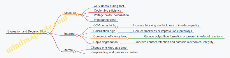
This case study emphasizes that shuttle suppression is not a single-material property. It emerges from the combined effect of interlayer transport, interfacial contact, and cathode formulation stability, all verified with rest behavior, efficiency, and impedance rather than just discharge capacity.
11.2 Case Study: Optimization of Barrier Thickness for Reduced Polysulfide Migration
Starting Point and What “Barrier Thickness” Actually Controls
In a solid-electrolyte-protected lithium sulfur cell, a “barrier” is the region that polysulfides must cross before reaching the lithium side. Thickness changes three things at once: (1) the diffusion path length for migrating species, (2) the ionic transport resistance through the barrier, and (3) the likelihood of interfacial defects that create shortcut paths. The goal is to reduce polysulfide migration without making the barrier so resistive that sulfur utilization collapses.
A practical way to frame the tradeoff is to treat the barrier as two resistances in series: one for ionic conduction (needed for the cathode reaction) and one for polysulfide transport (what you want to suppress). If the ionic resistance dominates, voltage polarization rises and the cell stops using sulfur efficiently. If polysulfide transport dominates, you lose active material to shuttle-like chemistry and capacity fades.
Baseline Stack and Measurable Targets
Assume a cathode protected by a solid electrolyte interlayer plus an additional barrier coating. Keep everything constant except barrier thickness: same sulfur loading, same current density, same electrolyte composition, and the same stack pressure. Define targets that are easy to measure:
- Coulombic efficiency during cycling (proxy for parasitic loss)
- Capacity retention over a fixed number of cycles
- Initial polarization at a set current (proxy for ionic resistance)
- Post-test sulfur species distribution at the anode side (proxy for migration)
Example baseline thicknesses: 10, 20, 30, and 40 µm. Use identical fabrication steps so thickness is the only meaningful variable.
Mind Map: Thickness Effects and How They Show Up in Data
Step 1: Verify That Thickness Changes Transport, Not Contact
Before interpreting electrochemistry, confirm that thicker barriers do not simply worsen contact. A quick check is to compare initial impedance spectra across thicknesses. If the dominant impedance increase scales with barrier thickness, ionic transport is likely the limiting factor. If impedance jumps irregularly, you may have fabrication variability such as poor interfacial wetting or trapped voids.
Concrete example: if 10 µm and 20 µm show similar impedance but 30 µm jumps sharply, the 30 µm barrier may have higher defect density or poorer contact rather than purely higher thickness.
Step 2: Track Polysulfide Suppression with a Migration-Sensitive Readout
To connect thickness to migration, use a readout that reflects polysulfide presence near the anode. One approach is to run identical cells for a short formation period, then stop and analyze sulfur species on the anode side. Even without fancy instrumentation, you can compare relative sulfur signal intensity across thicknesses.
Expected trend: migration signal should decrease as thickness increases, but only until defect-driven shortcuts become the dominant pathway. If 40 µm shows no further reduction compared to 30 µm, it suggests that migration is now governed by defects rather than diffusion length.
Step 3: Quantify the Ionic Penalty Through Polarization and Utilization
Now connect thickness to performance. Plot initial discharge voltage at a fixed current density and compute effective utilization from the delivered capacity relative to theoretical sulfur capacity. A barrier that is too thick will raise polarization, which can cause incomplete conversion of sulfur species and lower utilization.
Concrete example: suppose 10 µm delivers high initial capacity but coulombic efficiency is low. The 20 µm cell improves efficiency with only a modest polarization increase. The 30 µm cell shows further efficiency gains but also a noticeable drop in utilization. The 40 µm cell may have the best migration suppression, yet the delivered capacity falls enough that overall energy output worsens.
Step 4: Use a Simple Decision Rule to Pick the “Best” Thickness
A robust rule is to select the smallest thickness that achieves near-maximal migration suppression without a sharp utilization drop. Operationally:
- Identify the thickness where migration signal reduction plateaus.
- Identify the thickness where polarization begins to rise steeply.
- Choose the overlap region where both conditions are satisfied.
Example outcome: 20–30 µm might be optimal if migration suppression improves strongly from 10 to 20 µm, plateaus from 20 to 30 µm, and polarization steepens from 30 to 40 µm.
Step 5: Confirm Mechanism with Post-Test Evidence
After cycling, inspect the barrier and interfaces. Look for crack networks, delamination, or pore collapse. If thicker barriers show more cracking, migration may reappear through new pathways, explaining why migration suppression plateaus.
A useful sanity check is to compare the anode-side sulfur signal with the observed defect density. If sulfur signal remains low while defects increase, the barrier may still be diffusion-limited. If sulfur signal rises alongside defects, thickness alone is not the controlling factor.
Summary of the Case Study Logic
Barrier thickness is a balancing act between suppressing polysulfide migration and maintaining ionic transport. The best thickness is not the thickest one; it is the one that reduces migration until diffusion length stops being the limiting factor, while avoiding the point where ionic resistance and defects start to dominate. In practice, the 20–30 µm region often emerges as the sweet spot when fabrication quality is consistent and contact resistance is controlled.
11.3 Case Study: Conductive Network Tuning Under High Loading With Protection Enabled
This case study shows how to tune a cathode’s conductive network when sulfur loading is high and a solid-electrolyte protection layer is present. The goal is simple: keep electronic pathways available while the protection layer does its job of limiting polysulfide migration and stabilizing interfaces.
Starting Point: What High Loading Breaks
At high sulfur loading, three things happen at once. First, the ionic path through the cathode becomes longer and more tortuous, so regions near the current collector can react differently than regions deeper in the electrode. Second, the electronic network can become discontinuous when sulfur content rises and conductive additives are diluted. Third, the protection layer can add interfacial resistance if its contact with the cathode is uneven.
A practical way to frame the problem is to treat the cathode as two coupled networks: an ionic network that must reach active material, and an electronic network that must carry electrons to where reactions occur. When either network fails locally, you get partial utilization and a voltage profile that looks “fine” on average but hides dead zones.
Baseline Cathode Design and Protection Stack
Assume a cathode composite with sulfur, a solid electrolyte protection interlayer, and a conductive additive system. The protection layer is already chosen to reduce polysulfide transport and stabilize the solid electrolyte interface. The tuning task is therefore limited to the cathode’s conductive network and its contact quality.
Baseline choices:
- Sulfur loading: high enough to stress transport, not just “thicker electrode” in name.
- Conductive additive: a mix of carbon and a second conductive phase to improve percolation.
- Binder: selected to maintain mechanical integrity during volume change.
Baseline expectation: initial capacity may be acceptable, but utilization drops as cycling proceeds because electronic contact degrades where the electrode compacts or cracks microscopically.
Step 1: Diagnose Where Electronic Contact Fails
Before changing formulations, measure two signals that point to electronic limitations.
- Rate response shape: If capacity drops sharply at higher current densities while voltage polarization increases early, electronic pathways are likely insufficient.
- Spatial utilization proxy: After cycling, compare regions near the current collector versus deeper regions using cross-section imaging and elemental mapping. If deeper regions show less sulfur conversion, the electronic network is often the limiting factor.
A quick, easy example: run two cells with identical protection layers and sulfur loading. Cell A uses a lower conductive additive fraction; Cell B uses a higher fraction. If Cell B shows improved utilization at the same cutoff voltage and similar impedance growth, you have evidence that electronic percolation was the bottleneck.
Step 2: Tune Percolation Without Overloading the Cathode
Conductive additive tuning is not “more is better.” Too much additive can reduce the fraction of active material and can also change pore structure, harming ionic transport.
A systematic approach:
- Keep sulfur loading fixed.
- Vary conductive additive fraction in small steps.
- For each step, maintain similar particle size distribution and mixing protocol.
Example workflow:
- Prepare three cathodes: low, medium, high conductive additive fractions.
- Use the same protection-enabled stack and identical assembly pressure.
- Cycle with the same protocol and compare (a) initial utilization, (b) capacity retention, and (c) impedance growth.
Interpretation rule of thumb: if impedance growth is dominated by interfacial resistance, conductive tuning helps less; if impedance growth tracks with electronic limitation symptoms, conductive tuning helps more.
Step 3: Improve Network Connectivity with a Two-Phase Conductive Strategy
When sulfur loading is high, a single conductive additive often forms a network that is just barely connected. A two-phase strategy can create more robust pathways.
Example: combine a high-surface-area carbon with a conductive additive that forms longer-range contacts. The carbon can fill micro-gaps and improve local contact, while the second phase can bridge larger distances.
How to verify it without fancy equipment:
- Compare electronic conductivity trends using a simple electrode resistivity measurement on dried cathode films.
- Confirm that the improvement persists after compression and cycling, not just in the as-made state.
Step 4: Match Network Tuning to Protection Layer Contact
Protection enabled stacks can add an interfacial “bottleneck” if the cathode surface is rough or if the protection layer does not wet uniformly.
Practical tuning lever: adjust cathode surface preparation and calendering pressure so that the protection layer sees consistent contact. If you increase conductive additive but the protection layer contact is patchy, you’ll still get local reaction dead zones.
Example: two cathodes with the same conductive fraction. One is calendered to improve contact uniformity; the other is left looser. If the calendered one shows better utilization depth and lower impedance growth, the network tuning was only half the story.
Mind Map: Conductive Network Tuning Under High Loading with Protection Enabled
Step 5: Consolidated Example Results and Decision Logic
Consider a representative set of three cathodes with the same protection layer.
- Low conductive fraction: good early capacity but rapid drop at higher current; post-test shows deeper regions underutilized.
- Medium conductive fraction: improved high-rate capacity and more uniform conversion; impedance growth slows.
- High conductive fraction: best electronic connectivity initially, but capacity gain plateaus because ionic transport is hindered by reduced pore volume and higher tortuosity.
Decision: choose the medium fraction if it delivers the best balance of utilization depth and impedance growth. Then refine contact uniformity with calendering pressure rather than simply increasing conductive additive again.
Practical Takeaway
Conductive network tuning under protection enabled conditions is a balancing act between electronic percolation, ionic transport, and interfacial contact. The fastest path to a working design is to diagnose electronic limitation symptoms, tune percolation in controlled steps, and then ensure the protection layer actually contacts the cathode where reactions need to happen.
11.4 Case Study: Interfacial Contact Improvement Using Surface Preparation and Pressing
Problem Setup and What “Good Contact” Means
In solid-electrolyte protected lithium sulfur cells, interfacial contact is often the difference between “the chemistry works” and “the chemistry is stuck behind a gap.” The goal is to reduce interfacial resistance and prevent local current crowding that accelerates sulfur species decomposition near the interface.
For this case study, the cathode is a sulfur-rich composite pressed against a solid electrolyte. The protection layer is thin and intended to block polysulfide migration while still allowing ionic transport. Two failure symptoms are common: (1) a high initial impedance that grows quickly, and (2) voltage profiles that show early polarization even at moderate current.
Foundational Mechanisms Behind Contact Loss
Contact loss comes from three practical sources:
- Surface roughness and particle-scale gaps. Even if the stack looks flat, micro-asperities leave voids that behave like insulating layers.
- Interphase formation that is uneven. Surface reactions can create brittle or resistive products, especially where pressure is low.
- Mechanical mismatch during cycling. Volume change in the cathode can open or close contact depending on local stiffness.
A useful mental model is to treat the interface as parallel paths: well-contacted regions carry most current, while poorly contacted regions contribute little but still consume voltage through polarization.
Surface Preparation Workflow That Targets the Right Failure Mode
Surface preparation should be chosen based on what the interface is actually doing. In this case, the cathode surface shows contamination and binder-rich smearing after fabrication.
Step A: Controlled cleaning and drying. Remove loosely bound residues and moisture without changing particle morphology. A practical check is to compare mass before and after preparation and verify consistent drying time across batches.
Step B: Gentle surface activation. Use a mild treatment that increases surface energy so the protection layer wets more uniformly. The success criterion is not “more aggressive is better,” but improved wetting and reduced interfacial voids.
Step C: Surface planarity by controlled calendaring. Light calendaring can reduce large-scale waviness. Overdoing it can crush pores needed for ionic transport, so the target is planarity, not densification.
Example: If two cathode batches have the same sulfur loading but one shows higher impedance, compare their surface cleanliness by measuring contact resistance trends after identical pressing. The batch with binder smears typically shows a larger impedance spread.
Pressing Strategy That Balances Contact and Transport
Pressing improves contact by increasing real contact area, but it can also block ion pathways if it collapses the cathode pore network.
A systematic pressing plan uses three variables:
- Pressure level to increase contact area.
- Pressing time to allow stress relaxation and conformal contact.
- Stack temperature if the protection layer softens or partially flows.
Example: Start with a moderate pressure that does not collapse cathode porosity, then increase pressure in steps while monitoring impedance after assembly. If impedance drops initially and then plateaus, you likely reached sufficient contact without major pore damage.
Mind Map: Interfacial Contact Improvement Plan
Integrated Case Study Execution and Results Logic
Baseline: Assemble cells with identical materials but no surface activation and a single pressing condition. Expect higher initial impedance and larger cell-to-cell variation.
Iteration 1: Surface preparation only. Improve cleaning and mild activation while keeping pressing constant. If impedance decreases and voltage polarization becomes more consistent, the dominant issue was surface wetting and contamination.
Iteration 2: Pressing optimization on the improved surface. Sweep pressure and time. If impedance continues to drop with pressure up to a point and then stops improving, use the plateau condition. If impedance worsens at high pressure, the cathode pore network is likely being compressed, limiting ionic transport.
Iteration 3: Confirm mechanical coupling. After cycling, inspect whether contact remains uniform. A good sign is reduced evidence of delamination-like features and fewer localized reaction hotspots.
Practical Example: Interpreting Impedance Trends
- High initial impedance that improves after activation: likely poor wetting and interfacial contamination.
- Impedance decreases with pressure then increases at higher pressure: likely pore collapse or increased tortuosity.
- Impedance growth rate remains high despite low initial impedance: contact may be breaking during cycling, suggesting the need to adjust mechanical coupling or protection layer stiffness.
Takeaway Rules for This Case Study
- Fix wetting and cleanliness before turning the pressure knob.
- Use pressure sweeps with impedance as the primary metric, not just visual flatness.
- Preserve pore structure while increasing real contact area.
- Validate improvements by checking both initial impedance and its growth during cycling.
11.5 Case Study: Integrated Stack Evaluation With Performance And Failure Mode Comparison
This case study compares two integrated stack designs built around the same baseline cathode and electrolyte chemistry. The goal is not just to report capacity, but to connect performance differences to specific failure modes you can see in post-test evidence.
Step 1: Define a Common Baseline So Comparisons Mean Something
Both stacks use the same sulfur loading target, the same current collector geometry, and the same formation protocol. The only intentional change is the cathode-side protection stack:
- Stack A uses a thin solid-electrolyte protection interlayer with minimal mechanical compliance.
- Stack B uses a thicker protection layer plus a compliant interfacial layer to maintain contact during cycling.
A practical baseline check is to measure initial interfacial resistance at room temperature using a small AC perturbation. If Stack B starts with lower resistance, you must still verify that it is not simply better wetting from assembly artifacts.
Step 2: Build a Mind Map of What Can Fail
Mind Map: Integrated Stack Evaluation
Step 3: Run Electrochemical Tests That Separate Mechanisms
Use three cycling conditions that stress different parts of the stack.
- Low current, longer rest: emphasizes shuttle and chemical loss because the cell spends more time at intermediate potentials.
- Higher current pulses: emphasizes transport limits and interfacial kinetics because polarization rises quickly.
- Areal capacity matched cycling: ensures that one stack is not simply operating at a lower effective utilization.
In both stacks, track coulombic efficiency and the shape of the discharge plateau. If Stack A shows a gradual efficiency decline while voltage profiles remain similar, the likely culprit is active material loss rather than immediate contact failure.
Step 4: Compare Performance with Mechanism-Specific Signatures
Observed behavior in this case study
- Stack A delivers higher initial capacity but coulombic efficiency drops steadily after the first few cycles.
- Stack B starts slightly lower in capacity but maintains efficiency and shows slower growth in voltage hysteresis.
A useful interpretation rule:
- Efficiency loss without abrupt resistance jump often points to chemical loss pathways such as polysulfide migration.
- Hysteresis growth with stable efficiency early on often points to interfacial resistance increasing.
Stack A’s early efficiency decline aligns with insufficient polysulfide suppression at the cathode protection boundary. Stack B’s slower hysteresis growth aligns with better mechanical maintenance of contact.
Step 5: Post-Test Evidence That Confirms the Story
After cycling, compare three things in the same locations across both stacks.
- Cathode protection interface morphology: Stack A shows partial loss of intimate contact near the edges, consistent with mechanical mismatch. Stack B shows more uniform contact coverage.
- Sulfur species distribution: Stack A has stronger evidence of migrated sulfur species in regions away from the cathode, consistent with shuttle-driven loss. Stack B shows reduced off-cathode sulfur signatures.
- Interfacial thickness and cracking: Stack A exhibits microcracks that likely increase local resistance. Stack B shows fewer crack-like features and less evidence of delamination.
Step 6: Failure Mode Comparison Table
| Category | Stack A Symptom | Stack A Evidence | Stack B Symptom | Stack B Evidence |
|---|---|---|---|---|
| Active material loss | Efficiency declines early | Off-cathode sulfur signatures | Efficiency stays steadier | Reduced migrated sulfur |
| Interfacial resistance | Hysteresis grows later | Microcracks near interface | Hysteresis grows slower | Better contact retention |
| Mechanical integrity | Edge contact loss | Delamination-like regions | More uniform interface | Fewer crack features |
| Electronic isolation | Capacity fades with cycling | Conductive network disruption | Less severe fade | More stable transport paths |
Step 7: Integrated Conclusion You Can Use in Design Reviews
Stack A’s thin, stiff protection layer improves initial utilization but fails to maintain both chemical suppression and mechanical contact under cycling. Stack B trades a small amount of initial capacity for better interfacial stability, which preserves coulombic efficiency and slows resistance growth.
The key takeaway for future stack decisions is to treat performance as a bundle of coupled effects: chemical suppression, contact mechanics, and transport resistance. When you compare stacks, require both electrochemical signatures and physical evidence to agree on the failure mode, otherwise you are just measuring vibes with a voltmeter.
12. Assembly, Safety, and Reproducibility for Protected Lithium Sulfur Testing
12.1 Materials Handling and Assembly Controls for Moisture Sensitive Components
Moisture control starts before you touch any powder. In lithium–sulfur systems, water can react with lithium metal and with sulfur species, creating insulating byproducts and accelerating corrosion. The result is usually not a dramatic failure; it’s more like a slow leak in performance that shows up as higher impedance, lower coulombic efficiency, and inconsistent cycle-to-cycle behavior.
Core Principles for Moisture Control
- Keep exposure time short and measurable. Treat every open-lid moment like a stopwatch event. If you must stage multiple components, stage them in a single workflow so the “open time” is predictable.
- Control humidity at the point of use. A glovebox with a low dew point is useful, but what matters is the environment where assembly actually happens. Verify the dew point and ensure the chamber is stable before starting.
- Use sealed transfer paths. Move moisture-sensitive parts in sealed containers between storage and the glovebox. Avoid “temporary” placement on benches, even for a minute.
- Minimize thermal and pressure shocks. Rapid temperature changes can drive condensation inside containers. Let sealed containers equilibrate to the glovebox temperature before opening.
Materials Inventory and Handling Rules
Create a simple inventory list and assign each item a handling rule:
- Lithium metal: Store and transfer in sealed holders. Handle with tools that are dry and clean; avoid touching with bare gloves.
- Solid electrolyte and interlayers: Keep powders and films sealed. If a coating is involved, protect it from abrasion and keep it flat to preserve contact quality.
- Cathode components: Sulfur-containing cathodes and any sulfur-adjacent additives should remain sealed until assembly. If you use pre-made electrodes, confirm they were stored under the same moisture regime.
- Current collectors and separators: These are often overlooked. Even if they are not “powders,” they can absorb moisture and affect wetting and interfacial resistance.
A practical rule: if an item can absorb moisture by surface adsorption, treat it as moisture sensitive.
Assembly Workflow with Controls
A good workflow is a chain of small, verifiable steps. Here’s a systematic sequence that reduces variability.
- Pre-assembly checks. Confirm glovebox dew point, verify seals on transfer containers, and stage tools so you don’t search mid-assembly.
- Dry tool discipline. Use dedicated tweezers and spatulas for moisture-sensitive work. Wipe tools only if your glovebox protocol allows it; otherwise keep them sealed or stored in a dry container.
- Electrode staging. Lay out electrodes in a fixed order on a clean, dry surface. If electrodes are thin, keep them supported to prevent microcracks that later become high-resistance paths.
- Stack assembly. Build the stack in the same order every time. For solid electrolyte protection layers, ensure alignment and avoid trapped debris at interfaces.
- Sealing and final inspection. Seal the cell promptly. Inspect for visible misalignment, wrinkles, or particles at interfaces.
Example: A Controlled Assembly Day
Suppose you assemble three cells using the same cathode batch and solid electrolyte protection layer.
- You open the cathode container once, remove all needed electrodes, and reseal immediately.
- You keep lithium metal in its sealed holder until the moment it enters the cell.
- You record the approximate open time for each container and note any deviations, like a delayed seal.
After cycling, if one cell shows a sharp impedance rise early, you can correlate it with a longer open time or a sealing delay rather than guessing.
Mind Map: Moisture Sensitive Handling and Assembly Controls
Practical Checks That Catch Problems Early
- Baseline impedance screening: If one cell starts with a noticeably higher impedance than its peers, treat it as a handling issue until proven otherwise.
- Visual interface inspection: Particles or wrinkles at interfaces often trace back to assembly steps, not chemistry.
- Batch-to-batch comparability: If multiple cells from the same materials behave differently, focus on handling time, sealing delays, and transfer integrity.
Moisture control is less about perfection and more about repeatability. When your handling rules are consistent, performance differences can be attributed to the design variables you actually care about.
12.2 Cell Sealing and Current Collector Integration for Stable Measurements
Stable lithium–sulfur measurements depend on two boring-but-critical details: keeping the cell environment consistent, and making sure current collectors behave like predictable conductors rather than variable resistors. In solid-electrolyte-protected designs, sealing also protects interfaces from moisture and limits unwanted side reactions that can masquerade as “cathode degradation.”
Foundational Goals for Sealing and Current Collection
A good sealing and current-collector setup has four measurable outcomes:
- Consistent ionic and electronic pathways across repeated assemblies. If contact resistance changes, voltage curves shift even when chemistry is unchanged.
- Controlled atmosphere exposure during assembly and testing. Moisture can react with lithium and alter interphase chemistry.
- Mechanical stability under cycling. Volume change at the cathode can loosen contact unless the stack is held with the right compression.
- Reproducible electrical grounding. A current collector that is slightly misaligned can create local current crowding and uneven utilization.
A simple way to think about it: sealing prevents “environmental noise,” while current collector integration prevents “electrical noise.” Together they make your electrochemistry look like electrochemistry.
Sealing Strategy from Materials to Interfaces
Start with the materials that touch the electrolyte and lithium. Solid electrolytes and protective interlayers often tolerate heat differently, so choose sealing temperatures that do not crack brittle layers or drive unwanted interphase growth.
Core sealing principles:
- Use a barrier that blocks moisture and oxygen while allowing the cell to remain mechanically stable. Even a small leak can show up as rising self-discharge or drifting open-circuit voltage.
- Avoid direct chemical attack between sealants and lithium or sulfur species. A sealant that slowly reacts can create an internal “extra electrode.”
- Plan for compression transfer. If the seal deforms more than the stack, pressure relaxes and interfacial resistance rises.
Practical example: If you observe that impedance increases sharply after the first few cycles, check whether the seal is relaxing. A common fix is to adjust stack compression and ensure the seal supports the same load path each time.
Current Collector Integration That Minimizes Variable Resistance
Current collectors must provide low, stable electronic conduction and maintain uniform contact pressure to the solid electrolyte or protective layer.
Key integration steps:
- Surface preparation: Clean current collector surfaces to remove oxides and residues. A thin oxide layer can add contact resistance that changes with pressure.
- Flatness and alignment: Misalignment causes edge contact, which increases local current density and can accelerate degradation.
- Contact layer selection: If you use a compliant interlayer (for example, a thin conductive foil or coating), keep it thin enough to avoid becoming a variable “spring” that changes thickness during cycling.
Concrete example: Two cells with identical cathodes can show different coulombic efficiency if one current collector has a slightly rough surface. The rough one may create micro-gaps that intermittently contact during cycling, producing irregular polarization.
Compression, Stack Geometry, and Electrical Pathways
Compression is the bridge between mechanical sealing and electrical stability. Too little compression leads to poor interfacial contact; too much can crack brittle components or deform the solid electrolyte.
Systematic approach:
- Define a target compression range based on your stack materials.
- Measure stack thickness before sealing and after sealing to confirm load transfer.
- Use consistent spacer geometry so each assembly starts from the same mechanical baseline.
Example workflow: Record initial stack thickness, seal torque or clamp force, and final thickness. If final thickness varies by more than a small tolerance, treat the electrical data as suspect until mechanical variability is reduced.
Wiring, Tabs, and Measurement Integrity
Measurement stability also depends on how current is routed.
- Use short, rigid leads to reduce movement during cycling.
- Ensure consistent connection points so the effective current path length is the same across cells.
- Avoid strain on the current collector. A wire that pulls on the tab can gradually change contact pressure.
Mind Map: Cell Sealing and Current Collector Integration
Diagnostics for When Sealing or Current Collection Is the Culprit
When results drift, separate mechanical/electrical issues from chemistry.
- If impedance jumps early and then stabilizes, suspect contact resistance changes from compression relaxation or seal deformation.
- If open-circuit voltage drifts quickly before cycling, suspect environmental exposure or seal leakage.
- If voltage curves shift between otherwise identical cells, compare current collector alignment, surface preparation, and connection points.
Example: If only cells assembled with a particular sealant batch show faster self-discharge, the issue is likely seal chemistry or barrier performance rather than cathode formulation.
Example: A Stable Assembly Checklist
Before you start cycling, verify these items in order:
- Sealant and solid electrolyte are compatible at your assembly temperature.
- Current collector surfaces are cleaned and visually flat.
- Stack thickness and compression are within tolerance.
- Tabs and leads are secured so they cannot tug during handling.
- The cell shows no abnormal leakage indicators during a brief pre-test hold.
This checklist is intentionally mechanical. When the setup is consistent, the electrochemistry stops hiding behind artifacts.
12.3 Standardizing Electrode Loading Distribution and Thickness Measurement
Standardizing electrode loading distribution and thickness is how you stop “mystery performance” from masquerading as chemistry. In lithium–sulfur with solid electrolyte protection, small variations in sulfur mass per area and local thickness can shift current density, interfacial contact, and ion transport paths. The goal is not perfect uniformity; it’s repeatable uniformity with measurable tolerances.
Foundational Targets and What to Measure First
Start with two quantities that drive most downstream behavior:
- Areal sulfur loading (mgS/cm²): the mass of sulfur active material per geometric area.
- Electrode thickness (µm or mm): the physical distance that affects ionic path length and mechanical contact.
A practical workflow begins with defining acceptance windows. For example, set a target areal loading and require that measured values across the electrode stay within a chosen spread (e.g., ±5–10% depending on your fabrication capability). Then set a thickness target and require a similar spread. If you don’t set windows, you’ll only discover problems after cycling.
Mind Map: Loading Distribution and Thickness Control
Areal Loading Measurement That Doesn’t Lie
Areal loading standardization starts with a consistent area. Use a mask or die to define the exact region that will be weighed and later assembled. Exclude edges where material can pool or smear.
Example: You target 2.0 mgS/cm² on a 2.0 cm² electrode area. After drying, weigh the electrode within the masked region. If the sulfur fraction in your cathode composite is 60% by mass, and the total composite mass is 6.70 mg, then sulfur mass is 4.02 mg. Dividing by 2.0 cm² gives 2.01 mgS/cm². That’s close enough to proceed if your acceptance window allows it.
To check distribution, don’t rely on a single weight. Create a simple map: measure thickness at a grid of points, and for loading distribution, use either (a) multiple small die-cut samples from different regions for weighing, or (b) a method that can infer local mass from thickness plus known composition. The simplest reliable option is die-cut sampling for a few representative electrodes per batch.
Thickness Measurement with Grid Sampling
Thickness measurement should be repeatable and aligned with how the cell will be assembled. If your solid electrolyte layer is sensitive to contact pressure, thickness variation becomes a contact variation.
Example grid approach:
- Choose a 3×3 grid across the active area.
- Measure thickness at the nine points.
- Compute mean thickness and spread.
If the center is consistently thicker than the edges, you likely have coating edge effects or drying shrinkage gradients. If the pattern is irregular, you may have substrate non-flatness or inconsistent pressing.
Practical tip: Always measure after the same drying and conditioning steps. Thickness can drift slightly with humidity and handling, especially for composite electrodes with binders.
Linking Loading and Thickness to Local Current Density
Once you have maps, connect them to what the battery “feels.” Local thickness affects ionic path length; local loading affects how much active material must be served by the same ionic and electronic pathways.
Example: Suppose one region is 10% thicker and also 10% higher in sulfur loading. That region demands more reaction sites while also presenting a longer ion path. Even if the average loading is correct, the local mismatch can increase polarization and accelerate degradation at the interface.
This is why acceptance should be based on both mean values and spread. A mean-correct electrode with large spread is still a problem.
Feedback Rules for Common Failure Patterns
Use the measurement maps to decide what to fix.
- High loading at edges, low in center: check slurry mixing uniformity and coating flow stability; verify blade speed and gap.
- Thickness high at center, low at edges: check substrate flatness and press distribution; verify drying shrinkage conditions.
- Random variation across points: check measurement repeatability first, then inspect powder segregation risk during transfer.
Documentation That Makes Batches Comparable
Record batch ID, target loading, measured mean loading, loading spread, target thickness, measured mean thickness, thickness spread, and the grid map values. When you later compare cathode stabilization strategies, you’ll know whether differences come from chemistry or from “how the electrode was made.”
A good standardization process ends with a simple pass/fail rule. If the electrode meets both loading and thickness spread criteria, it goes into testing. If not, you fix the process and re-run. That’s the unglamorous part that keeps your results honest.
12.4 Quality Checks Including Impedance Screening and Baseline Cycling
Quality checks are where you catch problems that won’t show up in a single heroic cycle. The goal is simple: verify that your protected lithium–sulfur cell starts from a known, comparable electrical state, and that any later performance differences are caused by the design—not by assembly quirks.
Foundational Electrical Expectations
Before measuring anything, define what “good starting behavior” looks like for your architecture. In solid-electrolyte protected lithium–sulfur cells, the main electrical contributors are (1) ionic transport through the solid electrolyte and any interlayers, (2) interfacial resistance at the solid electrolyte–cathode side, and (3) electronic pathways that must be present in the cathode without shorting the stack. If your baseline impedance already looks abnormal, cycling will mostly amplify the issue.
A practical baseline target is not a single number; it’s a consistent impedance signature across replicate cells. For example, if three cells built with the same cathode loading show a high-frequency intercept that varies by 2×, you likely have inconsistent contact pressure, thickness, or interlayer coverage.
Impedance Screening Workflow
Step 1: Standardize Conditions
Measure impedance at a controlled temperature and with the same rest time after assembly. Even a short rest difference can change interfacial polarization. Use a fixed state of charge for the screening point, such as after a brief formation step that brings the cell to a reproducible voltage window.
Step 2: Choose Frequency Range and Perturbation
Use a frequency sweep that spans from high frequency (bulk and current-collector related contributions) down to the low-frequency region where interfacial processes dominate. Keep the AC perturbation small enough that the response stays linear; otherwise, you end up measuring “how the cell reacts to being poked,” not its baseline resistance.
Step 3: Interpret the Nyquist Shape
In many protected lithium–sulfur stacks, you’ll see a semicircle-like feature at mid-to-high frequencies and a larger low-frequency tail. The mid-to-high feature often correlates with interfacial charge transfer and contact quality, while the low-frequency tail can reflect slower transport and polarization relaxation.
A useful sanity check: compare the high-frequency intercept across cells. If one cell’s intercept is much larger, suspect poor electronic contact, thicker current-collector spacing, or an assembly defect that increases effective series resistance.
Step 4: Fit with Restraint
Equivalent circuit fitting can be helpful, but overfitting is a fast way to confuse yourself. Use a simple model that matches the number of visible features. If your fit requires five arbitrary elements to explain one broad arc, treat the fit parameters as descriptive, not diagnostic.
Baseline Cycling Protocol
Baseline cycling should be short, consistent, and designed to reveal early instability. The trick is to separate “normal early conditioning” from “assembly failure.”
Step 1: Use Identical Current and Cutoffs
Run a small number of cycles with the same current density and the same voltage cutoffs you will later use for comparisons. If one cell hits a cutoff early, don’t immediately assume chemistry failure; check whether its impedance already indicated high interfacial resistance.
Step 2: Track Coulombic Efficiency and Voltage Hysteresis
Coulombic efficiency (CE) during the first few cycles is a strong indicator of whether parasitic reactions are already active. Voltage hysteresis—difference between charge and discharge plateaus or average voltages—often grows when interfacial resistance increases or when contact degrades.
Example: If Cell A shows stable CE near your expected range but Cell B shows CE collapse and rising hysteresis by cycle 2, and Cell B also had a larger mid-frequency semicircle in impedance, you likely have interfacial contact issues rather than a purely cathode chemistry problem.
Step 3: Decide Pass or Fail Rules
Set clear acceptance criteria before you build the full dataset. For instance:
- Pass if high-frequency intercept is within a chosen tolerance across replicates.
- Pass if the first-cycle discharge capacity loss is within a defined band.
- Fail if CE drops sharply while impedance indicates abnormal interfacial resistance.
These rules keep you from “cherry-picking” cells that happen to look good by chance.
Mind Map: Impedance Screening and Baseline Cycling
Concrete Example: Two Cells with Different Outcomes
Cell A and Cell B are built with the same cathode formulation and the same solid-electrolyte protection layer. In impedance screening, Cell A shows a consistent high-frequency intercept and a mid-frequency arc of similar size to the replicate average. Cell B shows a noticeably higher high-frequency intercept and a broader mid-frequency feature.
During baseline cycling, Cell A maintains reasonable CE and stable hysteresis through the first few cycles. Cell B reaches a discharge cutoff earlier and shows CE collapse by cycle 2. The combined evidence points to a contact or series-resistance problem rather than a subtle cathode chemistry effect. You can then re-check stack pressure, interlayer coverage, and electrode thickness distribution before running the full test matrix.
12.5 Safety Practices for Lithium Sulfur Cell Fabrication and Testing
Lithium sulfur work is mostly about managing three hazards: reactive lithium, sulfur species that can irritate and stain, and electrical/thermal risks during testing. Good safety is not a separate activity; it is built into how you handle materials, assemble cells, and run experiments.
Core Hazard Map for Fabrication and Testing
Start by treating every step as a potential exposure point. Lithium metal and lithium-containing components require strict moisture and oxygen control, while sulfur powders and cathode slurries require dust control and skin/eye protection. Testing adds electrical hazards (short circuits, high current) and thermal hazards (overheating during abuse conditions or poor contact).
Mind Map: Safety Workflow
Glovebox and Dry Environment Discipline
If you use a glovebox, safety starts with consistency. Keep a single “clean side” for lithium-containing parts and a single “dirty side” for tools that touched cathode powders or separators. Before opening containers, confirm glove integrity and verify that seals and airlocks are functioning; a glovebox that looks fine can still leak through a slow tear.
A practical habit: stage everything before you start. Lay out tweezers, spatulas, and sample holders so you do not reach across open containers. For lithium metal, minimize time outside controlled conditions and avoid repeated opening of the same container, since each opening increases exposure risk.
Personal Protective Equipment and Handling Rules
Use eye protection at all times during powder handling, even if you are wearing a face shield; face shields are not a substitute for safety glasses. For sulfur-containing powders, use respiratory protection appropriate to your facility rules and keep airflow directed away from your breathing zone.
Gloves are not magic. Replace gloves when they show pinholes, swelling, or discoloration from electrolyte contact. Keep a small waste container labeled for sulfur and electrolyte-contaminated materials so you do not mix them with general lab waste.
Assembly Safety That Prevents Electrical Accidents
Many “safety incidents” in cell assembly are really preventable wiring mistakes. Route leads so they cannot touch the cell casing or each other under strain. Use insulated fixtures for holding cells during sealing and avoid metal-to-metal contact that can create a short.
When applying pressure or torque, use a repeatable method. Over-tightening can deform current collectors and create internal shorts; under-tightening can cause intermittent contact that heats locally during testing. If your stack uses spacers or gaskets, verify their placement before final closure.
Testing Setup with Built-In Limits
Before connecting a cell, set conservative current and voltage limits in the test software and confirm the limits match your hardware capability. A simple checklist prevents the classic “wrong channel” problem: verify the channel number, confirm the wiring map, and run a dry instrument check with a dummy load if your lab procedure allows it.
Monitor temperature during cycling, especially during formation or high-rate steps. If your setup lacks temperature sensing at the cell surface, treat the first run as a “slow and watchful” test and increase current only after stable behavior.
Abnormal Behavior Response Plan
Define stop conditions before you start. For example, stop immediately if you observe a sudden voltage collapse, a persistent voltage plateau inconsistent with prior cycles, or any sign of swelling, leakage, or unusual heating. Do not try to “fix” a failing cell by continuing the test; continuing often turns a manageable issue into a cleanup problem.
After stopping, keep the cell in a safe location per your facility protocol and allow it to cool before handling. If you must move it, use tools and containers designed for reactive battery materials.
Example: Safe Assembly and First Test Sequence
Example: You assemble a protected lithium sulfur coin cell.
- Stage all tools inside the glovebox and confirm glove integrity.
- Handle sulfur cathode materials with eye protection and dust control.
- Assemble with insulated fixtures and verify gasket alignment.
- Close the cell, then visually inspect for misalignment or damaged seals.
- In the tester, apply conservative current limits and a voltage cutoff.
- Run a short formation step while monitoring temperature.
- If voltage behavior is stable, proceed to the next step using the same limits.
Example: Spill and Contamination Control
Example: A small sulfur powder spill occurs on a bench.
- Avoid sweeping dry powder; use a controlled cleanup method to prevent airborne dust.
- Dispose of contaminated wipes and gloves in the labeled waste container.
- Wipe nearby surfaces that could later contact lithium components.
- Only resume lithium handling after the area is clean and dry.
Mind Map: What to Check Before You Start
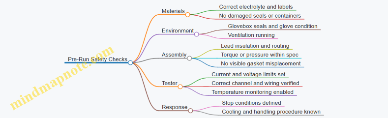
Safety in lithium sulfur cells is mostly boring in the best way: controlled environments, consistent handling, and test limits that prevent small mistakes from becoming big ones. When you treat each step as a checklist item, you spend less time troubleshooting and more time learning what your cathode stabilization is actually doing.