Sodium-Ion Battery Engineering
1. Scope and Engineering Requirements for Sodium-Ion Systems
1.1 Defining Performance Targets for Grid and Off-Grid Applications
Performance targets turn “we want a sodium-ion battery” into measurable engineering constraints. The trick is to define targets at two levels: system behavior (what the user sees) and cell behavior (what the battery must deliver to make that system behavior happen).
Foundational Concepts for Target Setting
Start with the load profile. A grid-connected system often cycles with daily demand peaks, while off-grid systems may run long, irregular discharge periods. From that, define three primary outputs:
- Energy delivered over a typical cycle (kWh).
- Power capability during the fastest meaningful load changes (kW).
- Usable lifetime under the expected depth of discharge and temperature range (cycles or years).
Then define constraints that prevent “technically works” designs:
- Voltage window the system can tolerate without tripping protections.
- Efficiency (round-trip and coulombic) because losses become heat and reduce usable energy.
- Safety limits including maximum temperature rise, current limits, and fault response behavior.
A practical way to avoid gaps is to write targets as “must meet” and “should meet.” Must-meet items are non-negotiable for acceptance testing; should-meet items guide optimization.
System-Level Targets for Grid Applications
Grid applications typically care about predictable response and repeatable performance. Define:
- Peak power for short bursts, such as smoothing a 1–5 minute ramp.
- Energy throughput for daily operation, such as supporting several charge-discharge events per day.
- State-of-charge operating band that the control system will use, for example keeping operation away from extremes to reduce stress.
Example: If the grid controller demands 500 kW for 3 minutes, the energy requirement is 500 kW × 0.05 h = 25 kWh for that event. If the battery must deliver that at a minimum system voltage, the cell voltage sag and current limits become hard constraints.
System-Level Targets for Off-Grid Applications
Off-grid systems often prioritize autonomy and robustness. Define:
- Run time at a specified load (hours at a given kW).
- Survivability across wider temperature swings and less controlled charging.
- Tolerance to imperfect inputs, such as solar variability or generator charging with less precise current control.
Example: A cabin system might need 2 kW for 6 hours, so energy delivered is 12 kWh. If the system uses a 90% usable energy factor due to voltage limits and reserve, the pack must store about 13.3 kWh nominal at the operating conditions.
Translating System Targets to Cell-Level Requirements
Once system targets are set, map them to cell requirements using a simple chain of constraints:
- Power requirement sets maximum allowable current per cell and limits on internal resistance growth.
- Energy requirement sets minimum usable capacity at the required C-rate and temperature.
- Lifetime requirement sets allowable degradation per cycle, which depends on depth of discharge and temperature.
A useful engineering habit is to compute “worst-case” current and “worst-case” capacity separately. Worst-case current might occur at low temperature (higher resistance), while worst-case capacity might occur at high temperature (accelerated side reactions) or at high C-rate (kinetic limits).
Target Tradeoffs and How to Make Them Explicit
Targets are rarely independent. For instance, pushing for high power usually increases current, which increases heat and can reduce effective capacity. To keep tradeoffs from becoming guesswork, define a small set of design points:
- Design point A for typical operation (mid temperature, moderate load).
- Design point B for peak power (low temperature or fastest ramp).
- Design point C for capacity verification (high temperature or longest discharge).
Each design point should specify: load profile, allowable voltage window, temperature, and required delivered energy or power.
Mind Map: Performance Target Definition
Example Target Set for Two Use Cases
Grid example (daily cycling):
- Must deliver 25 kWh per event at required voltage.
- Must provide 500 kW for 3 minutes.
- Must maintain efficiency within a specified band at the operating temperature.
- Must achieve a minimum cycle count at a defined depth of discharge.
Off-grid example (autonomy):
- Must run 2 kW for 6 hours with reserve.
- Must operate across a defined temperature range without violating voltage limits.
- Must tolerate charging current variation within a specified range.
- Must retain usable capacity after a defined number of seasonal cycles.
Acceptance Criteria That Prevent Surprise Failures
Finally, define acceptance tests that match the targets. If the target is “deliver 25 kWh at 500 kW bursts,” then acceptance should include both energy and power verification under the same voltage and temperature conditions. If the target is “6 hours at 2 kW,” acceptance should include the full discharge curve, not just a single snapshot. This keeps the battery from passing a test while failing the real job.
1.2 Translating System Requirements into Cell Level Specifications
System requirements start as “what the battery must do,” but cell specifications are “what the cell must survive and deliver.” The translation is easiest when you treat it like a requirements pipeline: define the duty, convert it into electrical and thermal stress, then map those stresses to measurable cell targets.
Step 1: Define the Duty Cycle and Operating Envelope
Begin with the system’s duty cycle: charge and discharge rates, rest periods, and the temperatures the pack will actually see. If the system says “daily cycling,” you still need numbers: for example, 1C charge for 1 hour, then 0.5C discharge for 2 hours, with 30 minutes rest between cycles. Also record the minimum and maximum allowable cell temperatures.
A practical way to avoid ambiguity is to write the operating envelope as constraints:
- Voltage limits at the pack level, including any margins for wiring and sensing errors.
- Current limits that reflect both normal operation and peak events.
- Temperature limits that include both steady-state and short transient behavior.
Step 2: Convert Pack Level Limits into Cell Level Targets
Pack voltage is the sum of cell voltages, so pack limits become per-cell limits with margin. If a pack requires 48 V nominal and uses 4 series cells, the nominal per-cell voltage is 12 V, but the usable per-cell voltage window must be narrower because cell voltage varies with state of charge, temperature, and aging.
Current translation is similar but not identical. In series, current is the same through each cell; in parallel, current divides. If the pack peak current is 200 A and the design uses 4 parallel strings, each string sees about 50 A, but you must also consider current sharing tolerances. A conservative engineering practice is to specify a per-cell maximum current that accounts for imbalance, not just the average.
Step 3: Map Electrical Stress to Cell Performance Metrics
Once you know the per-cell current and voltage window, define the cell metrics that must meet them.
Key metrics and what they mean:
- Capacity at a defined C-rate and temperature: example target might be 100 Ah at 0.5C and 25°C, with a specified retention after cycling.
- Power capability: specify maximum deliverable current while staying within voltage limits. Example: “At 1C discharge, voltage must stay above X V for the full depth of discharge.”
- Coulombic efficiency: define acceptable loss per cycle. Example: “≥ 99.5% average over 500 cycles at 0.5C.”
- Impedance growth: specify an allowable increase in resistance, because power fade often shows up as rising voltage drop under load.
A useful trick is to tie each metric to a measurable test method. If you can’t test it consistently, it’s not a specification yet.
Step 4: Translate Thermal Requirements into Design Constraints
Thermal requirements are not just “keep it cool.” They become constraints on heat generation and heat removal.
Compute or estimate heat generation using electrical losses: heat roughly scales with current and internal resistance, plus additional contributions from polarization. Then translate the pack’s cooling approach into a cell-level thermal boundary condition: what is the maximum cell surface temperature under worst-case current and ambient conditions?
Example: if the system allows a maximum cell temperature of 60°C and the ambient is 40°C, you have only 20°C of allowable rise. That number becomes a design constraint on allowable internal resistance and on how much heat the module can conduct away.
Step 5: Create a Requirements Matrix That Links Cause to Measurement
A requirements matrix prevents “specification drift,” where later teams optimize something that doesn’t actually satisfy the system.
| System Requirement | Cell-Level Specification | Test Condition | Acceptance Criteria |
|---|---|---|---|
| Peak power at pack level | Max current without voltage violation | 1C discharge at 25°C | Voltage stays within limit |
| Daily cycling | Capacity retention after cycles | 0.5C charge/discharge | ≥ target retention |
| Temperature safety | Max temperature rise | Worst-case ambient and load | Tcell ≤ limit |
| Usable energy | Energy delivered per cycle | Defined depth of discharge | ≥ target energy |
Mind Map: Requirements Translation Pipeline
Example: From a Simple Duty Cycle to Cell Targets
Assume a system requires: charge at 0.8C for 1 hour, rest 15 minutes, discharge at 1.0C for 1 hour, with ambient 10–35°C, and a maximum cell temperature of 55°C.
- Per-cell current: if the pack uses 3 parallel strings, and peak pack current is 150 A, each string is 50 A. If the cell nominal capacity is 100 Ah, 50 A is 0.5C, so you must check whether the system’s “1.0C” claim refers to pack-level or cell-level rate.
- Voltage window: choose per-cell charge and discharge voltage limits that include margins for temperature and measurement error.
- Capacity and power: specify that at 1.0C discharge (at the coldest allowed temperature), the cell must deliver the required energy without crossing the voltage floor.
- Thermal: use the allowable temperature rise to set an upper bound on internal resistance and polarization under the 1.0C load.
The result is a set of cell targets that are testable, stress-aligned with the duty cycle, and consistent with safety limits. That’s the whole point: the cell should be engineered to satisfy the system’s real workload, not just a spreadsheet version of it.
1.3 Comparing Sodium-Ion And Lithium-Ion Design Constraints
Sodium-ion and lithium-ion cells share the same basic job description—move ions between electrodes, keep electrons flowing through an external circuit, and survive repeated cycling. The differences show up in the constraints engineers must design around, especially for materials, interfaces, and system-level packaging.
Core Chemistry Constraints
Sodium is heavier than lithium, and that affects transport and kinetics. In practice, sodium-ion electrodes often need thicker active layers or different particle morphologies to reach usable capacity at reasonable loading. That choice then feeds into resistance and heat generation during fast charge or high current discharge.
Lithium-ion design constraints are usually dominated by lithium inventory management and interphase stability. Sodium-ion design constraints are more often dominated by how well the electrode structure tolerates sodium insertion and extraction without turning into a pile of disconnected particles.
A simple way to compare is to track three “bottlenecks”: ion transport through electrolyte and pores, charge transfer at the electrode surface, and structural stability of the host material.
Materials and Interface Constraints
Lithium hosts can be sensitive to electrolyte composition because the solid-electrolyte interphase (SEI) and cathode surface films strongly influence impedance growth. Sodium systems also form interphases, but the chemistry and growth behavior can differ enough that the same electrolyte strategy does not transfer cleanly.
For cathodes, many sodium-ion options rely on frameworks that can handle sodium motion with less structural collapse than some lithium cathodes under comparable stress. However, sodium-ion cathodes can still face voltage hysteresis and phase-related strain, which show up as capacity loss and increased polarization.
For anodes, lithium-ion commonly uses graphite, where lithium intercalation is well understood and tightly controlled. Sodium-ion typically uses hard carbon or other non-graphitic hosts, where sodium storage may involve multiple mechanisms. That complexity makes capacity balancing and formation protocols more sensitive to electrode formulation and electrolyte additives.
Electrical and Thermal Constraints
Because sodium-ion cells often use different electrode thicknesses, current collector choices, and electrolyte formulations, their internal resistance profile can differ across state of charge. Engineers must therefore design current limits and thermal management around where the cell is most resistive, not just around average performance.
A practical example: if a sodium-ion cell has higher resistance near the end of discharge, the same power request can produce more heat late in the cycle. That means the pack-level control strategy may need different current tapering rules than a lithium-ion pack, even when the nominal voltage range looks similar.
Mechanical and Manufacturing Constraints
Sodium-ion electrodes can experience different swelling and stress patterns due to host material behavior. That affects binder selection, electrode calendaring pressure, and the tolerance for manufacturing variation. A small shift in active material fraction can change pore connectivity, which then changes both rate capability and the stability of the interphase.
Lithium-ion manufacturing is also sensitive, but the “knobs” that most strongly affect performance can differ. For sodium-ion, engineers often spend more effort ensuring consistent electrode microstructure for sodium transport pathways.
Mind Map: Design Constraints Comparison
Example: Translating Constraints into Requirements
Consider a target: 1C charge and 1C discharge for 500 cycles with stable capacity. For lithium-ion, engineers may focus on controlling SEI growth and cathode surface stability through electrolyte selection and formation cycling. For sodium-ion, engineers may focus on ensuring the anode host delivers consistent sodium storage and that the cathode maintains structural integrity under sodium-driven strain.
Now add a packaging constraint: limited cooling capacity. A lithium-ion design might tolerate a certain peak temperature rise because its resistance profile is flatter across the discharge window. A sodium-ion design may require earlier current tapering because its resistance can spike at specific states of charge, increasing heat generation when the cell is already under mechanical and interfacial stress.
Example: Capacity Matching and Formation Sensitivity
In sodium-ion cells, capacity matching between anode and cathode can be more sensitive to formulation because the anode storage mechanism may not scale linearly with electrode loading. A small mismatch can cause the anode to reach unfavorable potentials sooner, accelerating impedance growth.
A concrete practice is to set formation cycles that deliberately build a stable interphase without pushing the cell into conditions that amplify side reactions. The acceptance criteria then include not only initial capacity but also early-cycle impedance trends, since that trend often predicts whether the cell will meet the cycling target.
Summary of the Comparison
Both chemistries require careful control of interfaces, transport, and mechanical stability. The difference is where the constraints concentrate: sodium-ion designs often need tighter attention to electrode microstructure, anode host behavior, and state-of-charge-dependent resistance, while lithium-ion designs more often emphasize lithium inventory control and SEI stability. In both cases, good engineering turns those constraints into measurable requirements—so the cell behaves predictably when it leaves the lab.
1.4 Establishing Test Standards for Capacity Power and Safety Metrics
Establishing Test Standards for Capacity, Power, and Safety Metrics
A sodium-ion cell is only as useful as the numbers you can reproduce. Test standards turn “it seems better” into measurable capacity, deliverable power, and safety behavior under defined conditions. The goal is not to mimic every real-world scenario; it is to create a consistent baseline that engineering teams can compare across materials, electrode batches, and manufacturing lots.
Capacity Metrics That Actually Mean Something
Start with capacity at a defined state of charge window and temperature. Use a formation-conditioned cell, then apply a standardized charge and discharge protocol.
Core capacity metrics
- Nominal capacity: capacity measured after formation and acceptance cycling, using a fixed current rate and cutoff criteria.
- Coulombic efficiency: ratio of discharge capacity to charge capacity over a defined cycle segment, reported separately for charge and discharge steps.
- Usable capacity: capacity within the voltage limits that you will also use in system operation.
Example practice If your cell is rated for a 2.0–3.8 V window, do not measure “capacity” using a wider window and then later restrict it. Measure within the same window you will use for power and energy calculations, or your numbers won’t reconcile.
Power Metrics That Separate Rate Capability from Voltage Drop
Power depends on both how much charge you can move and how quickly the cell can sustain voltage under load. Define power using discharge current and cutoff voltage, and report internal resistance indicators.
Core power metrics
- Discharge power at C-rate: power computed from measured voltage and current during a defined discharge segment.
- Voltage response under load: average voltage over a time window, not just the initial voltage.
- Resistance growth proxy: resistance extracted from EIS or pulse tests at a defined SOC and temperature.
Example practice When comparing two cathode batches, run both at the same SOC start point. If one batch begins at 90% SOC and the other at 70%, the “better power” result may just be a different operating point.
Safety Metrics That Are Measurable, Not Vague
Safety testing should cover electrical, thermal, and mechanical stress paths. The key is to define triggers, thresholds, and what constitutes failure.
Core safety metrics
- Thermal runaway indicators: temperature rise rate, maximum temperature, and whether venting or flame occurs.
- Overcharge and overdischarge behavior: voltage limits, current cutoffs, and post-test condition.
- Short-circuit response: temperature and current behavior under a defined external resistance or direct short protocol.
- Leakage and seal integrity: mass change, visual inspection criteria, and post-test electrolyte condition.
Example practice For overcharge, specify both the voltage limit and the maximum time allowed after reaching it. Otherwise, one lab may stop at 5 minutes and another at 30 minutes, and the results will not be comparable.
Standardizing Test Conditions for Reproducibility
A test standard is a bundle of constraints. If you omit one, you usually end up measuring something else.
Minimum condition set
- Temperature: report the cell temperature, not just the chamber setpoint.
- SOC and rest time: define equilibration time before measurement.
- Current definition: use C-rate or absolute current consistently, and state which one.
- Cutoff criteria: voltage cutoff and time cutoff must be explicit.
- Sample handling: moisture exposure limits and transfer time for electrolyte-filled cells.
Example practice If you use a 30-minute rest after charge to stabilize voltage, keep it identical across all lots. Voltage relaxation can otherwise masquerade as improved kinetics.
Mind Map: Test Standard Components
Integrated Example: A One-Page Acceptance Test Plan
Use a structured plan so the same steps can be repeated by different operators.
Acceptance test flow
- Preconditioning: rest at 25°C, then verify open-circuit voltage within a defined band.
- Capacity check: charge and discharge at a fixed current, measure usable capacity in the operating voltage window.
- Power check: perform a rate discharge segment at a higher current, compute average voltage over a fixed time window, and record resistance proxy at the same SOC.
- Safety screening: run a defined overcharge step with strict voltage and time triggers; stop on the first failure condition.
- Post-test inspection: check for leakage, seal deformation, and any abnormal appearance.
Example practice Set pass/fail thresholds relative to your baseline lot, not relative to “best ever.” For instance, require capacity within a specified percentage of the baseline mean and require resistance proxy within a defined limit. That keeps acceptance from drifting as people chase the newest batch.
Reporting Format That Prevents Misinterpretation
A good report includes the “why” behind the numbers: formation history, test conditions, and the exact protocol version. Include a short protocol identifier and the date of the standard revision, such as 2026-03-07, so teams can trace which method produced which results.
Finally, keep the language consistent: if you call something “usable capacity,” it must be tied to the same voltage limits used in power and safety tests. Otherwise, your metrics will look precise while describing different realities.
1.5 Building an Engineering Requirements Traceability Matrix
A Traceability Matrix is a structured way to prove that every engineering requirement has a clear origin, an implementation path, and a verification method. In sodium-ion battery engineering, it prevents the classic failure mode where a test exists but no one can explain what requirement it actually validates.
Start with a Requirements Backbone
Build the matrix around three columns that never change: Requirement, Design/Process Implementation, and Verification Evidence. Add a fourth column for Rationale and Source so you can trace why the requirement exists.
Use a consistent requirement ID format, for example: SI-REQ-01 for system-level targets, SI-CELL-07 for cell constraints, and SI-MFG-03 for manufacturing controls. Keep IDs stable across revisions; changing IDs breaks traceability faster than any spreadsheet typo.
Example: If the system target is “usable capacity ≥ 90% after 500 cycles,” create SI-CELL-12 for the cell-level capacity retention requirement, then map it to cathode loading control, electrolyte additive selection, and formation cycling parameters.
Define Requirement Types and Acceptance Criteria
Not all requirements are equal. Classify each requirement so verification is unambiguous:
- Performance requirements specify measurable outcomes (capacity, power, efficiency).
- Safety requirements specify limits and prohibited conditions (temperature rise, voltage bounds).
- Reliability requirements specify behavior over time or cycles.
- Manufacturing requirements specify process constraints (moisture limits, thickness tolerances).
For each requirement, write acceptance criteria as a testable statement. Avoid vague wording like “good wetting.” Replace it with something like “electrolyte uptake within X% of target mass gain after filling.”
Map Requirements to Design Elements
Once requirements are written, connect them to the smallest design element that can be changed. This is where teams often over-map. If you map a requirement to “electrolyte,” you still need a lever: salt identity, solvent ratio, additive type, target concentration, and allowable impurity range.
Example: A power requirement that depends on low resistance should map to electrode thickness, conductive additive fraction, current collector surface preparation, and formation protocol that stabilizes interfacial resistance.
Map Design Elements to Verification Methods
Verification methods should match the mechanism. Use a mix of fast screening and deeper validation:
- Cell-level tests for capacity, rate capability, and cycle retention.
- Electrochemical diagnostics for resistance growth and interfacial changes.
- Process qualification tests for moisture, coating mass, and dimensional tolerances.
- Safety tests for overcharge, short circuit behavior, and thermal response.
Example: If a requirement targets stable interfacial layers, pair a cycle test with a resistance trend check using EIS at defined states of charge. The cycle test proves outcome; EIS helps explain why.
Use a Mind Map to Keep the Logic Straight
Mind Map: Traceability Matrix Flow
Populate the Matrix with a Concrete Mini-Example
Below is a compact template you can expand into a spreadsheet. The key is that each row answers three questions: what, how, and how we know.
| Requirement ID | Requirement Statement | Implementation Lever | Verification Evidence |
|---|---|---|---|
| SI-CELL-12 | Capacity retention ≥ 90% after 500 cycles at 1C | Formation cycling protocol; electrolyte additive for stable interfaces | 500-cycle test report; EIS resistance trend at defined SOC |
| SI-CELL-19 | Voltage window maintained during charge/discharge | Voltage limits in BMS; cell voltage monitoring; electrode balancing | Charge/discharge test with logged voltage; BMS validation run |
| SI-MFG-04 | Electrode thickness within ±10 µm | Coating thickness control; calendaring parameters | In-process thickness measurements; SPC charts |
| SI-MFG-02 | Moisture in assembly environment ≤ 10 ppm | Dry room protocol; material bake and transfer controls | Moisture sensor logs; batch acceptance records |
Add Traceability Rules That Prevent Gaps
To keep the matrix from becoming a decorative document, enforce these rules during reviews:
- Every requirement row must include at least one verification method.
- Every verification method must reference the requirement ID(s) it supports.
- Every implementation lever must have a measurable control parameter.
- When a requirement changes, require a re-check of downstream mappings.
Example: If SI-MFG-04 thickness tolerance is tightened, you must confirm that the same verification evidence still applies or update the acceptance criteria and test plan accordingly.
Version Control and Review Cadence
Treat the matrix like a controlled engineering artifact. Use a revision field and a change reason so reviewers can see what moved and why. A practical cadence is a design review checkpoint and a manufacturing readiness checkpoint, each with a requirement-to-evidence audit.
Example: During a manufacturing readiness review, sample three recent batches and confirm that the process controls listed in the matrix were actually recorded and that the recorded values meet the acceptance criteria tied to the relevant requirements.
2. Electrochemistry Fundamentals for Sodium Storage
2.1 Sodium Ion Transport in Electrolytes and Electrodes
Sodium-ion transport is the quiet workhorse behind charge and discharge. If ions cannot move fast enough through the electrolyte and inside the electrode, the cell behaves like it is “full” but refuses to deliver power. Engineering starts by separating transport into three linked steps: (1) ion motion in the electrolyte, (2) ion crossing the electrode–electrolyte interface, and (3) ion diffusion through the electrode’s active material and pores.
Electrolyte Transport: Migration, Diffusion, and Convection
In a liquid electrolyte, sodium ions move by three mechanisms. Migration happens when an electric field pushes charged ions; diffusion happens when concentration gradients exist; convection happens when the fluid physically moves. In sealed batteries, convection is usually minimal after formation, so migration and diffusion dominate.
A practical way to reason about this is to imagine a sodium “traffic jam” near the electrode during high current. The electrode consumes Na⁺ at the interface, lowering local concentration. Diffusion tries to refill that region, while migration pulls ions toward the charged surface. The balance between these processes determines whether the electrolyte can sustain current without large concentration polarization.
Example: Estimating Electrolyte Limitation
Suppose a cell is tested at a higher C-rate. If voltage drops sharply at the start of discharge and recovers when current is reduced, electrolyte transport is often involved. A simple diagnostic is to compare the same cell at two currents while keeping temperature constant. If the voltage difference scales strongly with current, the electrolyte’s effective ionic conductivity and transport resistance are likely limiting.
Electrode Transport: Pores, Tortuosity, and Solid Diffusion
Inside an electrode, ions travel through a network of pores filled with electrolyte. The path is not straight; it is tortuous, meaning the effective diffusion length is longer than the physical thickness. Two electrode properties control this: porosity (how much space is available) and tortuosity (how winding the paths are). Higher porosity and lower tortuosity reduce transport resistance.
Once ions reach the active material particles, they must diffuse through the solid. This solid-state diffusion can be slower than transport in the liquid electrolyte, especially in materials where sodium motion requires hopping between specific sites. The result is a second “traffic jam,” this time inside particles.
Example: Why Thicker Electrodes Can Hurt Power
Consider two electrodes with the same active material and chemistry, but one is twice as thick. Even if the total capacity scales with thickness, the diffusion distance for ions increases. During high-rate discharge, the thick electrode can develop a larger concentration gradient within particles, causing earlier polarization and lower usable capacity.
Interface Transport: Charge Transfer and Interfacial Layers
At the electrode–electrolyte interface, ions must not only arrive but also participate in electrochemical reactions. This step is governed by charge-transfer kinetics and the presence of interfacial films. A resistive interfacial layer increases the voltage needed to drive the reaction.
A useful mental model is to treat the interface as an additional resistor in series with transport. When current increases, the interface contributes more to overpotential than transport alone, especially if the interfacial layer thickens or becomes less conductive.
Example: Linking EIS Features to Transport Steps
Electrochemical impedance spectroscopy often separates behavior into time constants. A low-frequency feature can reflect diffusion-related limitations, while a mid-frequency feature can relate to charge-transfer and interfacial resistance. If increasing current during tests makes the low-frequency response more dominant, diffusion limitations in pores or particles are likely contributing.
Coupled Transport: The Concentration Profile Story
Transport in electrolyte and electrode is coupled through the boundary condition at the interface: the reaction rate sets how quickly Na⁺ is consumed or produced locally. At higher current, the reaction rate increases, which steepens concentration gradients both in the electrolyte near the interface and within the electrode. That steepening increases polarization, which then reduces the effective driving force for further reaction.
This coupling explains why “more electrolyte” can help. Adding electrolyte volume can reduce the severity of concentration gradients near the electrode, lowering polarization and improving rate performance—up to the point where other resistances dominate.
Mind Map: Sodium Ion Transport Pathways
Engineering Practices That Follow from Transport
- Tune electrolyte-to-electrode ratio to reduce concentration gradients at the interface; a practical check is whether increasing electrolyte volume improves rate without changing chemistry.
- Use electrode thickness and particle size deliberately: thinner electrodes and smaller particles reduce diffusion distances, improving power at the cost of manufacturing and sometimes energy density.
- Control porosity and binder content so pores remain connected; disconnected pores trap electrolyte and increase effective tortuosity.
- Manage interfacial film formation through electrolyte formulation and formation protocols; lower interfacial resistance improves both power and cycling stability.
Example: A Systematic Transport-Based Design Check
Start with a target current and temperature, then ask three questions. Can the electrolyte supply Na⁺ fast enough to the interface (migration and diffusion)? Can the electrode pore network deliver ions to active particles (porosity and tortuosity)? Can the active material particles accept ions at the required rate (solid diffusion and interface kinetics)? If any answer is “no,” the cell will show polarization consistent with that bottleneck, and the fix should target the specific transport step rather than changing everything at once.
2.2 Interfacial Reactions at The Sodium Electrode And Cathode
Interfacial reactions are where the battery earns its keep. Bulk materials can store and transport sodium, but the actual charge transfer happens at the boundaries: solid electrode surfaces, liquid electrolyte, and the thin interphase layers that form there. In sodium-ion cells, these interfaces are especially influential because sodium metal is reactive and many cathodes rely on repeated insertion and extraction that continually reshapes the surface.
What Counts as an Interfacial Reaction
An interfacial reaction is any electrochemical or chemical process occurring at or near an electrode surface where electrons and ions meet. For the sodium electrode, the key events include sodium plating/stripping (if sodium metal is used) or sodium insertion/extraction into a host (if using hard carbon or other anodes). For the cathode, the key events include sodium deintercalation/intercalation and side reactions between the cathode surface and electrolyte.
A practical way to think about it is to separate three layers of behavior:
- Charge transfer: electron transfer coupled to sodium ion movement.
- Interphase formation: electrolyte decomposition products that create a passivation layer.
- Transport through the interface: ionic movement across the interphase and electronic movement through conductive pathways.
Sodium Electrode Interface Reactions
Sodium Metal Interfaces
When sodium metal is present, the interface reaction is dominated by plating and stripping. The ideal reaction is reversible sodium deposition and dissolution. The non-ideal part is that the electrolyte can decompose on fresh sodium surfaces, especially when local current density is high.
Two common interfacial issues follow:
- SEI growth on sodium: The solid electrolyte interphase forms from electrolyte reduction products. Its growth consumes electrolyte and increases resistance.
- Morphology and roughness effects: Uneven deposition increases surface area, which accelerates side reactions. A simple example is current crowding near edges of a rough surface: more area means more reaction sites, so the interphase thickens faster.
A useful engineering practice is to manage current density distribution. For instance, if you cycle a cell at a moderate rate but with a poorly wetted electrode, local dry spots can create higher local current density. The result is faster SEI growth even though the average current looks fine.
Host Anode Interfaces
With hard carbon or other host anodes, the interfacial reaction is sodium insertion/extraction plus SEI formation. The host surface still provides sites for electrolyte reduction, but the sodium is stored inside pores and near surface defects rather than as a metal film.
A concrete example: in a hard carbon electrode, the first cycles often show the largest irreversible capacity loss because the surface area accessible to electrolyte is highest during early wetting and initial structural rearrangements. After the interphase stabilizes, subsequent cycles typically show lower growth rates.
Cathode Interface Reactions
Cathode surfaces face a different set of constraints. Many cathodes operate by changing oxidation state and crystal structure during sodium extraction. Those changes can expose new reactive sites and alter how the electrolyte “sees” the electrode.
Intercalation Coupled Side Reactions
The desired cathode reaction is sodium deintercalation during charge and reintercalation during discharge. Side reactions occur when electrolyte components react with the cathode surface at the potentials and local environments present during cycling.
A systematic example is to compare two cathode particle sizes. Smaller particles provide more surface area, so interfacial side reactions can increase even if the bulk insertion kinetics are similar. That means a cathode can look electrochemically fine in a short test but degrade faster in long cycling because interphase growth continues.
Interphase Layer on Cathodes
Cathode interphases can be more complex than anode SEI because the cathode is often at higher potentials where electrolyte oxidation becomes relevant. The interphase may be electronically insulating, which can reduce effective utilization of active material. It can also crack or reform as the cathode lattice changes, repeatedly exposing fresh surface.
A practical diagnostic is to watch how impedance changes with cycling. If resistance rises steadily while capacity fades, interphase thickening and loss of interfacial contact are likely contributors.
How Interfacial Reactions Are Governed
Interfacial behavior is controlled by a few levers that show up across both electrodes:
- Potential and local overpotential: Higher overpotential increases the driving force for side reactions.
- Electrolyte composition and salt-to-solvent balance: Different components form different interphase chemistries.
- Wettability and contact quality: Poor wetting increases local current density and accelerates decomposition.
- Surface area and morphology: More area means more interphase formation per cycle.
- Mechanical stability: Cracking of interphase layers can create a cycle of reformation.
Mind Map: Interfacial Reactions at Sodium Electrode and Cathode
Example: Reading Interfacial Behavior from Simple Tests
Consider two cells with the same nominal capacity and electrolyte, cycled at the same average current.
- Cell A shows a large first-cycle irreversible loss and then moderate fading.
- Cell B shows smaller first-cycle loss but faster resistance growth.
A reasonable interpretation is that Cell A experiences stronger early interphase formation due to higher accessible surface during initial wetting or rougher sodium deposition. Cell B likely forms an interphase that is initially thinner but becomes less protective or less conductive over time, possibly due to mechanical cracking or poor interfacial contact.
This kind of reasoning matters because it connects what you see in data to what you should change in engineering: electrode wetting, formation protocol, particle size distribution, and current density uniformity.
2.3 Charge Transfer Kinetics and Overpotential Decomposition
Charge transfer kinetics describe how quickly electrons and sodium ions move across the electrode–electrolyte interface. When that interface is slow, the cell needs extra voltage to keep current flowing—this extra voltage is the overpotential. In sodium-ion cells, overpotential is not one single thing; it is a sum of contributions from several steps, and separating them helps you engineer the right fix.
The Interface Steps That Create Overpotential
A practical way to think about the interface is as a sequence:
- Ions reach the interface from the electrolyte.
- Ions cross the interface and enter or leave the electrode material.
- Electrons move through the electrode and current collector to the reaction site.
- Interfacial chemistry happens such as forming or modifying the solid electrolyte interphase (SEI).
Steps 1 and 3 are often discussed under transport and electronic conductivity, but step 2 is the core of charge transfer kinetics. When step 2 is rate-limiting, the reaction current grows slowly with applied voltage.
Kinetic Control Through Butler–Volmer Behavior
For many electrode reactions, the current density follows a Butler–Volmer relationship: the net reaction rate increases with overpotential because the forward and backward reaction rates become unbalanced. At small overpotentials, the response is roughly linear; at larger overpotentials, one direction dominates and the curve becomes more exponential.
A useful engineering interpretation is: kinetics set the slope of voltage versus current when other resistances are not dominating. If you measure polarization curves at different temperatures or scan rates, you can infer whether the interface is the bottleneck.
Decomposing Overpotential into Practical Terms
Overpotential can be decomposed into components that map to measurable behaviors:
- Ohmic overpotential: current times resistance from electrolyte, separator, contacts, and current collectors. It shows up as an immediate voltage drop when current steps.
- Charge transfer overpotential: voltage needed to drive the interfacial reaction at a given current. It grows with current even after the ohmic drop.
- Concentration overpotential: voltage needed to maintain ion concentration gradients near the interface. It becomes more noticeable at high current or when diffusion is slow.
- Interfacial film overpotential: voltage associated with SEI growth or changes in interfacial resistance, often evolving during cycling.
In real sodium-ion cells, these terms overlap. The trick is to design tests that separate them.
How to Identify Charge Transfer Dominance
A simple diagnostic sequence:
- Current step test: record the immediate voltage drop (ohmic) and the slower relaxation (kinetic and concentration).
- Electrochemical impedance spectroscopy: look for an interfacial semicircle whose size changes with state of charge and temperature.
- Temperature variation: if the polarization changes strongly with temperature while diffusion-limited behavior changes less, charge transfer is likely dominant.
Example: Suppose a hard-carbon anode shows a large immediate drop at high current but the remaining polarization is still substantial and strongly temperature-dependent. The immediate drop points to ohmic resistance, while the temperature sensitivity of the remaining part points to charge transfer limitations.
What Controls Charge Transfer Kinetics in Sodium-Ion Electrodes
Charge transfer depends on more than the reaction itself. Key levers include:
- Interfacial contact quality: pores, roughness, and binder distribution affect how much electrode area is actually electrochemically active.
- Electronic pathways: if conductive additive percolation is weak, electrons cannot reach reaction sites efficiently.
- Surface chemistry: functional groups and residual impurities can change the effective reaction barrier.
- SEI properties: a stable SEI can reduce side reactions, but an overly resistive SEI increases interfacial overpotential.
A concrete example: if electrode thickness increases without adjusting formulation, the electronic network may still percolate, but local current crowding can occur near the separator. That crowding increases local overpotential even if the average conductivity looks acceptable.
Mind Map: Overpotential Decomposition and Kinetic Levers
Example: Separating Kinetic and Concentration Contributions
Consider a cell tested at two current rates, C/5 and 2C. At C/5, the voltage drop after the initial ohmic step relaxes quickly, and impedance shows a moderate interfacial resistance. At 2C, the relaxation becomes slower and the concentration-related part grows, often visible as additional polarization that does not scale like a simple interfacial resistance.
If you then repeat at a higher temperature, and the interfacial semicircle shrinks substantially while the concentration signature improves less dramatically, you can conclude that charge transfer is a major contributor at both rates, while concentration becomes increasingly important at 2C.
Practical Takeaways for Engineering
When charge transfer kinetics dominate, improving interface accessibility and reaction pathways usually reduces overpotential more effectively than simply lowering bulk resistance. When concentration overpotential dominates, changing thickness, porosity, and particle size distribution matters more. The best designs treat overpotential as a budget with line items, then run tests that tell you which line item is overspent.
2.4 Solid State Diffusion and Phase Behavior in Host Materials
Solid-state sodium storage is often limited by how sodium moves inside host particles and how the host changes its structure while doing so. Diffusion controls how fast concentration gradients relax, while phase behavior controls how much of the material can reversibly host sodium without turning into a structural mess.
Foundations of Solid State Diffusion
In a host particle, sodium chemical potential varies with state of charge. That variation drives diffusion from regions of higher chemical potential to lower chemical potential. A practical way to think about it is: if the particle is thick, sodium must travel farther, so the same diffusion coefficient yields slower equilibration.
A common engineering simplification treats diffusion as Fickian within a particle. The characteristic diffusion time scales like the square of the diffusion length. For example, if you double the effective diffusion length, the diffusion time becomes about four times longer. This is why particle size and electrode thickness matter even when the electrolyte is perfectly conductive.
Diffusion is not always uniform. Near surfaces, sodium can exchange quickly with the electrolyte, creating steep gradients. Inside, diffusion may be slower, so the particle can behave like a “moving boundary” where only part of it is at a given composition during fast cycling.
Phase Behavior and Its Coupling to Diffusion
As sodium enters or leaves the host, the host may remain in a single phase or transform between phases. Two limiting cases are useful.
-
Single-phase solid solution: sodium composition changes continuously with minimal structural rearrangement. Diffusion and phase evolution are tightly coupled, and voltage changes tend to be smoother.
-
Two-phase transformation: the material separates into sodium-poor and sodium-rich regions. The interface between phases migrates as cycling proceeds. In this case, diffusion still matters, but the rate can also be limited by how fast the phase boundary moves and how coherently the lattice accommodates the change.
A key consequence is that two-phase systems often show flatter voltage plateaus during transformation, while single-phase systems show more gradual voltage slopes. Engineers use this difference to diagnose whether the host is transforming or mixing.
Thermodynamics Meets Kinetics
Phase behavior is governed by the free energy landscape of the host as a function of sodium content. If the free energy has a “double well” shape, the system prefers phase separation rather than uniform mixing. The boundary between stable compositions defines where two phases coexist.
Kinetics determine whether the system follows the thermodynamic preference. If diffusion is slow, the material can temporarily remain in a metastable composition, leading to hysteresis between charge and discharge. That hysteresis is not just a measurement artifact; it reflects real delays in reaching equilibrium structures.
Practical Modeling of Diffusion and Phase Evolution
For engineering design, you rarely need a full atomistic model to get useful insight. A layered approach works well.
- Diffusion-limited picture: assume a diffusion coefficient and compute how quickly the particle interior approaches surface composition.
- Phase-aware picture: incorporate an effective thermodynamic driving force for phase separation and allow an interface to move.
- Coupled picture: treat diffusion as feeding the phase boundary, so the overall rate is limited by the slower of diffusion supply and interface motion.
A simple diagnostic is to compare how capacity changes with current. If capacity drops sharply at higher rates, diffusion or interface motion is likely limiting. If capacity remains stable but voltage shifts, kinetic overpotentials at interfaces or within the host may dominate.
Mind Map: Solid State Diffusion and Phase Behavior
Example: Particle Size Effect on Rate Capability
Consider two cathode particles made of the same host material. Particle A has an effective diffusion length of 5 µm, and Particle B has 10 µm. If diffusion is the limiting step and the diffusion coefficient is unchanged, the characteristic diffusion time for B is about four times longer. In a fast charge, sodium at the surface can reach the target composition quickly, but the interior of B cannot. The result is lower utilization of the active material and a larger polarization contribution.
Example: Two-Phase Transformation and Hysteresis
Suppose a host undergoes a two-phase transformation between low-sodium and high-sodium structures. During charge, the phase boundary advances as sodium enters. During discharge, the reverse boundary must retreat. If diffusion through the particle and interface motion are not fast enough, the system may require a different overpotential to initiate the reverse transformation. That difference shows up as hysteresis: the charge and discharge voltage curves do not overlap even at the same nominal state of charge.
Example: Distinguishing Diffusion-Limited vs Phase-Boundary-Limited Behavior
Run a set of tests at increasing current while keeping temperature constant. If the voltage plateau length shrinks significantly at higher current, the phase boundary cannot traverse the particle fast enough, suggesting interface-limited behavior. If the plateau shape remains but the overall capacity drops, diffusion inside the particle is likely limiting how much of the material reaches the transforming compositions.
Summary of Design Levers
To engineer better sodium storage in host materials, you manage diffusion length scales and you respect phase behavior. Smaller particles reduce diffusion time, thinner electrodes reduce transport bottlenecks, and careful interpretation of voltage shape and hysteresis helps identify whether the limiting step is diffusion supply, interface motion, or both.
2.5 Coulombic Efficiency Loss Mechanisms and Their Root Causes
Coulombic efficiency (CE) is the fraction of charge you put into a cell that comes back as useful charge during discharge. In sodium-ion systems, CE losses usually come from “extra” sodium consumption or extra electron consumption that does not produce reversible capacity. A practical way to think about CE is: every irreversible side reaction steals some sodium and some electrons, and the stolen amount shows up as a gap between charge in and charge out.
Mind Map: Coulombic Efficiency Loss Mechanisms
Foundational CE Accounting and What “Loss” Means
CE is often computed as discharge capacity divided by charge capacity for a cycle. If CE is below 100%, the difference corresponds to net irreversible processes. For example, if you charge 100 mAh and discharge 97 mAh, the missing 3 mAh is not “lost to the universe”; it is tied to side reactions consuming sodium and/or electrons.
A key nuance: CE can look stable while capacity still fades, because different degradation modes can trade off. CE focuses on charge balance per cycle, so it is most sensitive to parasitic currents and irreversible sodium inventory changes.
SEI Growth on the Anode
The most common CE sink is solid electrolyte interphase (SEI) growth on the anode. In hard carbon anodes, the first cycles form a passivating film by reducing electrolyte components. After formation, the SEI should be relatively stable, but it can keep growing slowly if the electrolyte remains reactive at the anode potential.
Root causes that drive continued SEI growth include:
- Electrolyte reactivity: More easily reduced salts or solvents create more parasitic reduction.
- High anode potential excursions: If the anode spends time at potentials where electrolyte reduction is favorable, parasitic current persists.
- Large surface area and defects: Finer particles and rough surfaces increase the number of active sites.
Easy example: Suppose two cells use the same anode but one is cycled with a wider voltage window. The wider window pushes the anode to lower potentials more often, increasing electrolyte reduction events, so CE drops even if the cathode is unchanged.
Cathode Side Reactions
On the cathode side, CE losses can come from electrolyte oxidation and surface degradation. When the cathode operates at higher potentials, electrolyte components can oxidize, consuming electrons without delivering reversible sodium extraction.
Root causes include:
- High upper cutoff voltage: More time at high potential increases oxidation probability.
- Surface instability: Cathode particles can reconstruct, exposing fresh reactive sites.
- Catalytic surfaces: Certain surface chemistries accelerate parasitic reactions.
Easy example: If you raise the cathode cutoff by 0.2 V, you may see CE fall quickly in early cycles because oxidation starts immediately, even before major structural damage is visible.
Sodium Trapping and Irreversible Inventory Changes
Not all sodium that enters the anode is necessarily reversible. Some sodium can become trapped in deep sites, defects, or strongly bound adsorption states that do not fully participate in the discharge process.
Root causes include:
- Defect-rich microstructure: More trapping sites form during initial cycling.
- Inhomogeneous lithiation-like analog behavior: Local environments can differ across particles.
- SEI-mediated trapping: SEI growth can physically or chemically immobilize sodium.
Easy example: If a cell shows CE near 100% for a few cycles but then gradually declines, sodium trapping can be accumulating even while the main SEI formation phase seems complete.
Kinetic and Transport Effects That Create Parasitic Currents
CE is not purely chemistry; it is also how current distributes. When charge transfer is slow or sodium transport is uneven, the local overpotential increases. Higher local overpotential can make side reactions more favorable, turning a “rate problem” into a “CE problem.”
Root causes include:
- High polarization: Larger overpotentials increase parasitic reaction rates.
- Concentration gradients: Regions near interfaces can become sodium-poor or sodium-rich, changing local reaction pathways.
- Poor electrode percolation: If electronic or ionic pathways are uneven, micro-currents form.
Easy example: Two electrodes have the same average thickness, but one has slightly worse binder distribution. During fast charging, the poorly connected regions polarize more, and CE drops even though the bulk materials are identical.
Protocol and Measurement Artifacts
Sometimes CE “loss” is not chemistry. Aggressive current cutoffs, insufficient rest periods, or temperature differences can cause incomplete relaxation and apparent imbalance.
Root causes include:
- Current cutoff too early: You stop while polarization is still relaxing.
- No rest between steps: The cell may not reach a stable state before measuring capacities.
- Temperature drift: Reaction rates and resistances shift, changing the effective charge balance.
Easy example: If one test includes a 10-minute rest after charging and another does not, CE can differ by a few percent even with identical materials, because the voltage and reaction state at the moment of cutoff are not the same.
Practical Diagnostic Logic for Root Cause Isolation
A systematic approach is to separate “where the side reaction happens” from “why it happens.” First, compare CE trends with voltage window changes. If CE drops strongly when you increase the upper cutoff, cathode oxidation is likely. If CE drops when you extend the lower cutoff, anode SEI growth is likely.
Next, compare CE with current rate. If CE worsens sharply at higher rates, polarization and transport-driven parasitics are likely contributing. Finally, verify protocol consistency: repeat the same cycle with identical rest and temperature. If CE changes without any material change, measurement artifacts are in play.
Example: Interpreting a CE Drop in the First 10 Cycles
Imagine a cell where CE is 99.5% for cycles 1–3, then falls to 97.8% by cycle 10.
- If the voltage window is unchanged, the continued decline suggests ongoing SEI growth or sodium trapping.
- If CE correlates with longer time at low anode potentials, SEI growth is the dominant mechanism.
- If CE correlates with higher cathode potentials, cathode side reactions are likely.
This pattern-based reasoning turns CE from a single number into a map of which interface is misbehaving and which operating choice is feeding it.
3. Cathode Materials Selection and Electrode Design
3.1 Layered Prussian Blue Analogues and Oxide Cathodes Selection Criteria
Choosing a cathode for sodium-ion cells is mostly a set of trade-offs you can measure: how much sodium it can host, how fast it can move sodium ions during charge and discharge, how stable it stays under cycling, and how forgiving it is during manufacturing. Layered Prussian blue analogues (PBAs) and oxide cathodes both work, but they behave differently in ways that matter for engineering.
Foundational Differences That Drive Selection
PBAs are built from a framework that can insert and remove sodium with relatively low structural rearrangement. This often translates into good rate capability and predictable voltage plateaus. Oxide cathodes rely on transition-metal oxide lattices where sodium insertion changes the local environment more strongly; the payoff can be higher energy density, but the engineering burden is usually higher.
A practical way to start is to map your target operating window to the cathode’s typical behavior. If your system needs frequent cycling at moderate-to-high power, PBAs often reduce the risk of performance collapse from kinetic limitations. If your system prioritizes higher energy per mass and can tolerate tighter process control, oxide cathodes become more attractive.
Selection Criteria with Concrete Engineering Checks
-
Capacity and Voltage Profile
- PBA cathodes often show a clearer voltage plateau, which can simplify pack-level state-of-charge estimation.
- Oxides may show sloping voltage behavior, which can be fine, but it makes calibration and BMS tuning more sensitive to cell-to-cell variation.
- Example: If you design for a narrow usable voltage range, a PBA plateau that sits neatly inside that range can yield more consistent usable capacity.
-
Rate Capability and Transport Limits
- For PBAs, sodium diffusion through the framework and charge-transfer at the surface both influence power performance.
- For oxides, diffusion through the bulk and changes in electronic conductivity during cycling can become limiting.
- Example: In a lab test, compare capacity at C/10 and 2C. A cathode that loses little capacity at 2C is likely to meet power targets without forcing excessive electrode thickness.
-
Structural Stability and Cycling Mechanisms
- PBAs can suffer from framework degradation if the electrolyte chemistry promotes side reactions or if cycling drives unfavorable local environments.
- Oxides can experience surface reconstruction, microcracking, and transition-metal dissolution depending on composition and operating conditions.
- Example: If your cell will operate near the upper voltage limit, you should expect more aggressive surface changes. PBAs may show earlier capacity loss, while oxides may show resistance growth that hurts power.
-
Electrode Compatibility and Interface Behavior
- Both cathode types depend on forming a stable cathode–electrolyte interphase. The difference is that oxides often present more reactive surfaces under certain states of charge.
- Example: If you observe rising impedance after a few hundred cycles, check whether the cathode surface is reacting more than the anode. The cathode choice can shift where the problem shows up.
-
Manufacturing Robustness and Variability
- PBAs can be sensitive to moisture and handling because their synthesis and surface chemistry can affect how they interact with electrolyte.
- Oxides can be sensitive to calcination history, particle morphology, and residual impurities.
- Example: If your production line has wider variation in drying time or mixing intensity, pick the cathode that tolerates that variation with smaller performance spread.
Mind Map: Cathode Selection Logic
Example Decision Paths
Example 1: Moderate Power Cycling With Simple SoC Estimation
- Requirements: stable performance from 0.5C to 2C, and a voltage window that aligns with a plateau.
- Selection: start with a PBA because the plateau can keep the cell voltage more consistent across state-of-charge.
- Engineering check: verify that capacity at 2C remains within your allowable loss budget and that impedance growth stays slow enough to avoid power derating.
Example 2: Higher Energy Target With Tight Process Control
- Requirements: maximize energy per cell while accepting more complex calibration.
- Selection: consider an oxide cathode, but only after confirming that resistance growth and surface reactivity are manageable under your chosen upper cutoff voltage.
- Engineering check: run cycling at representative temperatures and track both capacity fade and resistance growth, not just one metric.
Practical Acceptance Tests That Tie Back to Selection
A selection is only as good as its acceptance criteria. For both PBA and oxide cathodes, include tests that reflect the failure modes you care about: high-rate capacity retention for kinetic limits, impedance growth for interphase and transport degradation, and performance spread across multiple production lots. If a cathode passes these checks consistently, it earns its place; if it only looks good under ideal lab conditions, it will likely punish you later in the cell line.
3.2 Particle Size Distribution and Its Impact on Rate Capability
Rate capability in sodium-ion cathodes is often limited by how quickly sodium ions and electrons can move through a real, messy electrode. Particle size distribution (PSD) is one of the most practical levers because it shapes both pathways: ions travel through pores and within particles, while electrons travel through the conductive network and across particle surfaces.
Foundational Link Between PSD and Rate
Start with two time scales. First, ion transport inside particles: smaller particles shorten the characteristic diffusion length, reducing the time needed for sodium to reach reaction sites. Second, ion transport through the electrode: smaller particles can increase surface area and pore volume, but they can also increase tortuosity if the electrode becomes too dense or binder-rich.
Now add electron transport. If particles are too large, the conductive additive may not form enough percolation contacts across the full particle population, so current crowds near easier-to-connect regions. If particles are too small, the electrode can become “powdery” in a bad way: more surface area consumes more conductive additive and binder, leaving less effective electronic pathways per unit mass.
Mind Map: PSD Levers and Rate-Limiting Steps
How PSD Shape Changes the Electrode Microstructure
PSD affects packing density and pore structure. A narrow PSD often packs more efficiently, which can reduce pore volume and slow electrolyte penetration. A broader PSD can fill voids more effectively, sometimes improving wetting and reducing dead volume. The catch is that “better packing” can also mean smaller pores and higher tortuosity, which slows ion movement through the electrode.
A useful engineering rule is to treat PSD as a knob that trades intraparticle diffusion against interparticle transport. If your cathode is diffusion-limited, you usually benefit from smaller particles or a distribution weighted toward smaller sizes. If your cathode is electrolyte-access limited, you may need a distribution that preserves enough pore connectivity.
Example: Narrow vs Broad PSD Under the Same Loading
Imagine two electrodes with identical active material mass loading and the same conductive additive fraction.
-
Electrode A: narrow PSD centered at 10 µm
- Intraparticle diffusion length is relatively long.
- During a fast charge, the outer regions of particles react first, creating stoichiometry gradients.
- The electrode shows a strong drop in usable capacity at higher C-rates because sodium cannot homogenize inside particles quickly enough.
-
Electrode B: broad PSD with many particles around 1–3 µm plus a tail up to 10 µm
- Smaller particles react quickly and provide early current pathways.
- Larger particles contribute more capacity at moderate rates but still lag at the highest rates.
- The overall response is smoother: capacity fades more gradually with rate because the electrode has multiple “reaction speeds” rather than one dominant diffusion length.
The key point is not that smaller is always better. Electrode B can outperform A because it reduces the fraction of material that is severely diffusion-limited, while still maintaining sufficient structural integrity and packing behavior.
Advanced Detail: Why Too Much Small Material Can Hurt
When you shift PSD toward very small particles, surface area rises. That can increase the number of reaction sites, but it also increases the demand for electrolyte wetting and conductive additive coverage. If the conductive network becomes discontinuous at the particle scale, electrons must travel longer distances through the binder-rich regions.
You can spot this failure mode experimentally: at higher rates, the voltage response may show increased polarization even if the electrode is well wetted. That suggests electron transport or interfacial contact resistance is becoming the bottleneck rather than ion diffusion.
Practical Engineering Practices for PSD Control
- Measure PSD consistently: Use the same dispersion protocol and measurement method for every batch. PSD is sensitive to agglomeration, and agglomerates can masquerade as large particles.
- Target a distribution, not a single size: For rate capability, a bimodal or broad PSD often reduces the fraction of material that is “too slow.”
- Re-optimize conductive additive after PSD changes: If you increase the fraction of small particles, the same additive loading may no longer provide adequate percolation.
- Check calendering response: PSD changes packing density, which changes how the electrode compresses. Compression affects pore structure and tortuosity, so the same calendering pressure can produce different ion transport.
Example: A Simple PSD Tuning Workflow
- Start with a baseline PSD and record rate performance at two or three C-rates.
- If high-rate capacity collapses sharply, bias the PSD toward smaller particles by adjusting milling or classification.
- If polarization increases without a proportional improvement in high-rate capacity, increase conductive additive or adjust binder content to restore electronic pathways.
- Repeat with the same electrode formulation except for the PSD-related change, so you can attribute improvements to the right mechanism.
This workflow keeps the reasoning grounded: PSD changes microstructure, microstructure changes transport, and transport determines which part of the cell “runs out of time” first.
3.3 Conductive Additives and Binder Systems for Sodium Cathodes
A sodium cathode needs three jobs done at once: electrons must travel through the composite, ions must reach active material surfaces, and the electrode must stay mechanically intact during cycling. Conductive additives and binders are the two levers that control those jobs in a practical, buildable way.
Conductive Additives: What They Actually Fix
Conductive additives form an electronic network that bridges particles and reduces contact resistance. In sodium cathodes, the active material often has limited intrinsic electronic conductivity, so the additive is not optional—it is the difference between “it works in a lab cell” and “it works when current increases.”
Start with the simplest rule: too little additive leaves isolated active islands; too much additive can dilute active material and increase tortuosity for ion transport. A useful engineering approach is to target a percolated network while keeping the composite mostly active. For example, if a cathode formulation is 80 wt% active, 10 wt% conductive carbon, and 10 wt% binder, you can expect a baseline network. If rate performance is poor, you adjust carbon upward in small steps (e.g., +2 wt%) and verify whether resistance drops without a matching loss in capacity.
Particle morphology matters. Carbon black tends to create dense contact points, while graphite-like carbons can improve electronic pathways but may wet differently. A practical check is to compare slurry viscosity and coating uniformity: if the slurry becomes difficult to coat at the same solids loading, you likely pushed the carbon too far or selected a carbon with poor dispersion behavior.
Binder Systems: Holding the Film Together Without Blocking Transport
Binders connect particles to each other and to the current collector. They also influence wetting, adhesion, and the evolution of interfacial layers during cycling. A binder that is too rigid can crack as the cathode expands and contracts; a binder that is too soft can allow particle detachment.
For sodium cathodes, binders are commonly chosen from polymer families that can dissolve or swell in the electrolyte environment to varying degrees. The key is not “best binder,” but “binder that survives the specific electrolyte and voltage window.” A good starting point is to select a binder that provides strong adhesion to the current collector and forms a stable film that does not excessively swell. You can evaluate this with simple tests: after coating and drying, measure peel strength or perform a controlled tape test; then compare mass change or thickness change after electrolyte soaking under representative conditions.
Integrated Formulation Logic
Conductive additive and binder must be engineered together because they compete for space and both affect dispersion. A systematic workflow looks like this:
- Choose a binder that gives adhesion and mechanical stability.
- Choose a conductive additive that disperses well in the chosen solvent system.
- Set a baseline solids loading and electrode thickness.
- Tune carbon content for electronic resistance using a resistance-focused diagnostic.
- Tune binder content for adhesion and cycling stability using a mechanical and electrochemical acceptance check.
A concrete example: suppose a cathode shows high polarization at moderate current. You first check whether the issue is electronic or ionic. If EIS indicates a large charge-transfer or electronic resistance component, increasing conductive additive by 2–3 wt% often helps. If EIS instead shows strong diffusion limitations, increasing carbon further may not help and can worsen ion access by increasing composite tortuosity.
Mind Map: Conductive Additives and Binder Systems
Example: Carbon and Binder Adjustment for Rate Capability
Imagine a sodium cathode that delivers only 70% of expected capacity at a higher current, while low-current capacity is near target. You run a quick diagnostic: EIS shows increased electronic resistance and a larger semicircle associated with interfacial processes.
Step 1: Increase conductive additive from 8 wt% to 10 wt% while keeping binder constant. Recoat and dry under the same conditions. If polarization decreases and the high-current capacity rises, the electronic network was the limiting factor.
Step 2: If high-current capacity improves but cycling shows early capacity fade, adjust binder. Reduce binder slightly (for example from 10 wt% to 9 wt%) if the electrode appears overly insulating, or increase binder if you observe cracking or particle loss. The decision is guided by post-test inspection: cracked films point to insufficient mechanical integrity; uniformly intact films with persistent polarization point back to electronic/ionic transport.
Example: Binder Choice Through Adhesion and Soak Behavior
Two binders are tested with the same active and carbon. Binder A forms a strong dry film but shows significant swelling after electrolyte soaking. Binder B shows minimal swelling and maintains thickness. In cycling, Binder B typically retains better contact between particles and the current collector, which reduces resistance growth. The lesson is straightforward: binder swelling changes the internal structure of the composite, and that structure controls both electron pathways and ion access.
Practical Takeaways
- Conductive additive content is a balancing act between percolation and active dilution.
- Binder selection is about adhesion and controlled swelling, not just “film strength.”
- Tune carbon for resistance and tune binder for mechanical integrity, using targeted diagnostics and simple physical checks.
When these two components are treated as a coupled system rather than separate ingredients, sodium cathodes become easier to reproduce and easier to scale from small cells to larger electrodes.
3.4 Electrode Formulation and Slurry Rheology for Scale Up
Scaling sodium-ion electrodes is mostly about controlling three things at once: how particles pack, how the slurry flows during coating, and how the dried film holds together. If any one of those drifts, you often see it later as poor capacity, uneven thickness, or cracks that appear as if they were invited.
Formulation Foundations for Reproducible Coating
Start with a formulation that you can reproduce by mass, not by “it looks right.” A typical cathode slurry recipe has four roles: active material, conductive additive, binder, and solvent. The active material sets capacity and voltage behavior; the conductive additive reduces electronic bottlenecks; the binder provides mechanical integrity; the solvent controls wetting and viscosity.
A practical way to lock down formulation is to define target solids content and a mixing order. For example, aim for a fixed solids fraction (by weight) and keep it constant across batches. Then mix conductive additive into the solvent first to wet it thoroughly, add active material next to avoid dry clumps, and finally add binder last so it dissolves or disperses without over-shearing.
Mind Map: Formulation Variables and Their Effects
Rheology Targets for Coating and Drying
Rheology is not just “thick or thin.” For coating, you want a slurry that flows under shear at the doctor blade or slot die, then relaxes to maintain a stable film. Two practical rheology metrics are viscosity at a representative shear rate and yield stress that indicates whether the slurry will slump or hold shape.
A simple bench check is to measure viscosity at a consistent temperature and record it alongside solids content. If viscosity rises between batches, suspect binder concentration drift, incomplete binder dissolution, or additive agglomeration. If viscosity drops, check for solvent loss during handling or an error in solids calculation.
Example: Diagnosing a Viscosity Jump
Suppose batch A coats smoothly, while batch B shows streaks and uneven thickness. You measure viscosity and find batch B is 30% higher. The fastest root-cause test is to compare dispersion quality: take a small sample, let it sit for 10 minutes, and observe whether particles settle or form a visible sediment layer. If sediment forms quickly, the mixing order or mixing time likely left binder or additive insufficiently wetted.
Mixing and Dispersion for Scale Up
At lab scale, you can “fix it” by extra mixing. At production scale, extra mixing can be the problem because it changes binder conformation and can break fragile particle structures. The goal is consistent dispersion with controlled shear.
Use a mixing protocol with three controls: mixing sequence, mixing time, and shear intensity. Keep temperature controlled because solvent viscosity and binder solubility both shift with temperature. Also standardize the order of additions so that binder does not start dissolving too early or too late.
Example: Mixing Sequence That Reduces Clumps
If you add active material directly to binder solution, you may trap dry active particles inside viscous binder, creating hard-to-wet clumps. A better sequence is to wet conductive additive first, then add active material gradually under agitation, and only then introduce binder solution. This reduces the chance of “floating islands” that later show up as thick spots after coating.
Binder and Additive Balance for Mechanical Integrity
Binder content affects adhesion and crack resistance, but too much binder can reduce ionic/electronic pathways by increasing inactive volume. Conductive additive content affects electronic percolation, but excessive additive can increase viscosity and create a fragile network that fractures during calendaring.
A useful engineering practice is to treat binder and additive as coupled variables. If you increase solids loading to improve throughput, you may need to adjust binder to maintain wetting and adhesion. If you increase conductive additive to improve rate performance, you may need to reduce solids or modify solvent to keep rheology within coating limits.
Example: Binder Starvation and Its Coating Symptoms
If binder is too low for the chosen solids loading, the dried film can appear uniform but fail during calendaring or show edge cracking. A quick check is to compare peel strength or observe whether the film surface becomes powdery after light handling. If it does, the binder network is likely insufficient to bridge particle contacts.
Solvent Handling and Contamination Control
Solvent evaporation during slurry preparation changes solids content and viscosity. Keep containers covered, standardize transfer steps, and record solvent batch identity if you have multiple lots. Moisture contamination can also change binder behavior and interfacial wetting, which then shows up as poor dispersion stability.
A practical control is to define an allowable viscosity window for acceptance. If a slurry is outside the window, do not “just coat it and hope.” Instead, adjust within a controlled range: verify solids content, confirm binder dissolution, and check for agglomerates.
Scale Up Checklist for Consistent Electrode Films
- Confirm solids loading by mass before mixing.
- Use a fixed mixing order and record mixing time and temperature.
- Measure viscosity at a consistent temperature and shear reference.
- Inspect dispersion stability after a short hold.
- Validate coating uniformity by thickness mapping on test strips.
- Verify dried film adhesion and crack resistance after calendaring.
Case Study: From Pilot to Production Coating
A pilot line used a slurry that coated evenly at moderate speed. When production speed increased, thickness variation rose and edge defects appeared. The formulation was unchanged, but the residence time between mixing and coating shortened, and solvent evaporation during handling became less controlled.
The fix was not a new recipe; it was tighter process control. The team standardized covered transfer, revalidated solids content at the start of coating, and adjusted mixing time to restore the same viscosity window. After that, thickness uniformity returned and the dried film showed the same adhesion behavior as the pilot line.
Summary of Engineering Logic
Electrode formulation and slurry rheology are a chain: composition determines dispersion, dispersion determines flow, flow determines coating uniformity, and uniformity determines film structure. Scale up succeeds when you control the chain with measurable targets rather than relying on “it seems similar.”
3.5 Practical Cathode Coating Parameters and Quality Checks
Cathode coating is where lab chemistry turns into a manufacturable electrode. The goal is simple: make a uniform, well-adhered film with the right thickness, porosity, and electrical pathways—then prove it with checks that catch problems early.
Coating Parameters That Actually Matter
Slurry Composition and Solids Target
Start by fixing the solids content and the active-to-carbon-to-binder ratio. A practical approach is to choose a target solids loading that gives stable viscosity during coating and avoids particle settling. For example, if your slurry separates after a few minutes, increase binder content slightly or adjust solvent fraction to improve wetting. If the slurry is too thick, you’ll get streaks and thickness variation; if it’s too thin, you’ll lose film integrity during drying.
Viscosity and Shear Stability
Measure viscosity at the coating temperature and confirm it doesn’t drift rapidly during mixing. A useful rule is to run a short “hold test”: mix for the same time as production, then coat a small strip. If thickness varies along the strip, your slurry is changing under shear or settling.
Coating Gap and Wet Thickness
The doctor blade or slot-die gap sets wet thickness. Use a calibration run: coat a short strip, weigh it, and calculate wet thickness from areal mass and solvent fraction. Then dry a sample and measure dry thickness. Adjust gap until the dry thickness lands in your design window.
Drying Profile and Solvent Removal
Drying is not just “until it looks dry.” Solvent removal affects binder distribution and particle packing. Use a staged temperature profile: a lower initial zone to prevent skin formation, followed by a higher zone to finish solvent removal. A concrete check is mass loss tracking: weigh coated coupons before and after each drying stage to confirm you’re removing solvent consistently.
Calendering Pressure and Porosity Control
Calendering improves particle contact and reduces resistance, but it can also crush pores and harm ion transport. Choose a pressure that reduces thickness to target while keeping a reasonable porosity. A quick sanity check is to compare electrode density and ionic performance proxies (for instance, early-cycle impedance trends) between two calendering pressures.
Quality Checks from Incoming Materials to Finished Electrode
Incoming Powder Verification
Before coating, verify particle size distribution and moisture content. Moisture can change slurry behavior and binder performance. If you see batch-to-batch viscosity swings, treat it as a material issue first, not a process issue.
Slurry Homogeneity Checks
Perform a simple settling test: after mixing, let the slurry sit for a defined time and observe whether the top layer clears. If it does, remixing time or solvent fraction needs adjustment. Also check pH or conductivity if your formulation uses salts that can shift with contamination.
Coated Film Uniformity
Measure thickness across the web using a non-contact gauge. Map thickness at multiple points and compute variation. If variation correlates with web speed or edge effects, adjust coating alignment and edge dams rather than changing chemistry.
Dry Film Adhesion and Mechanical Integrity
Use a tape test or controlled peel test on dried electrodes. Adhesion failures often come from binder under-drying, poor wetting, or contamination on the current collector. If adhesion is weak, confirm current collector surface cleanliness and revisit drying profile.
Binder Distribution and Microstructure
Inspect cross-sections or use microscopy to confirm binder forms a continuous phase rather than isolated clumps. If you see binder-rich regions, the slurry may be too viscous or mixing may be insufficient.
Electrical and Electrochemical Screening
Run quick electrical checks such as sheet resistance mapping. Then perform a short electrochemical screening on representative coupons to catch outliers. The point is not full qualification; it’s to identify coating defects that would otherwise show up later as unexplained impedance growth.
Mind Map: Cathode Coating Parameters and Quality Checks
Example: Parameter Set with Checks and Acceptance Criteria
Assume you target a dry cathode thickness of 80–90 µm. You run a calibration strip to link doctor blade gap to dry thickness, then you set a drying profile with staged temperatures and track mass loss to ensure consistent solvent removal. After drying, you map thickness at five positions across the strip; acceptance is that all points fall within the thickness window and the variation stays below a chosen limit.
Next, you run adhesion tests on three coupons. If any coupon peels in large flakes, you stop and check binder drying and current collector cleanliness. Finally, you measure sheet resistance and run a short electrochemical screening. If resistance is high across the whole strip, suspect calendering or conductive additive dispersion; if resistance is localized, suspect coating uniformity or edge effects.
Example: Diagnosing a Common Defect
If you observe streaks in thickness and higher impedance in the same regions, treat it as a coating uniformity problem first. Verify slurry homogeneity with a settling test, then check coating gap calibration and web alignment. If thickness is uniform but adhesion is poor, focus on drying profile and current collector surface preparation. If both thickness and adhesion are fine but impedance rises quickly, inspect binder distribution and calendering pressure, since ion/electron pathways can be disrupted even when the film looks acceptable.
4. Anode Materials and Sodium Metal Alternatives
4.1 Hard Carbon Structure and Sodium Storage Pathways
Hard carbon is the most common anode choice for sodium-ion cells that avoid sodium metal. It stores sodium through a mix of mechanisms that depend strongly on how the carbon is built: how ordered it is, how pores are shaped, and how sodium ions move from electrolyte to internal sites. The practical engineering goal is to make those sites plentiful and accessible while keeping the structure stable during repeated cycling.
Core Structure of Hard Carbon
Hard carbon is not one material with one recipe. It is a family of carbons with a disordered, partially graphitic framework. Two structural features dominate sodium storage:
- A disordered carbon matrix made of small graphene-like domains separated by defects and turbostratic stacking. This disorder creates a variety of local environments where sodium can reside.
- A pore and surface network that includes micropores and larger voids. These pores influence how sodium ions solvate, desolvate, and enter the carbon.
A useful mental model is to picture hard carbon as a sponge made of stacked-but-misaligned sheets. The “sponge” has both internal cavities and edge-like regions. Sodium ions can park near surfaces and also move into internal spaces when the local chemistry and geometry allow it.
Sodium Storage Pathways
Sodium storage in hard carbon is typically described as two main contributions plus a smaller set of interfacial effects.
Surface and Near-Surface Adsorption
At higher anode potentials (relative to the sodium metal reference), sodium ions tend to adsorb on accessible surfaces. This step is sensitive to surface area, functional groups, and how the electrolyte wets the carbon. Engineering implication: if the carbon is too hydrophobic or poorly dispersed in the electrode, the electrolyte may not reach the internal surfaces, and the “easy” capacity becomes smaller.
Easy example: If you compare two electrodes made from the same hard carbon powder but one uses a binder that improves wetting, the better-wetted electrode often shows higher initial capacity at the same formation protocol because more sodium ions can reach the active surfaces.
Micropore Filling and Sodium Insertion
As the potential lowers, sodium ions can enter micropores and fill them. This is not a simple “one-size-fits-all” insertion. The pore size distribution matters: pores that are too small can trap sodium without allowing stable accommodation, while pores that are too large reduce the benefit of confinement.
Inside micropores, sodium can adopt configurations that differ from bulk-like sodium. The confinement also affects the local solvation shell, which changes how easily sodium ions desolvate and settle.
Easy example: Consider two hard carbon batches with the same BET surface area but different micropore size distributions. The batch with a higher fraction of appropriately sized micropores often shows a smoother voltage profile and better utilization because more pores are “just right” for stable sodium accommodation.
Sloping Region and Structural Rearrangement
In many hard carbons, a sloping voltage region appears at lower potentials. This region is associated with additional sodium uptake that correlates with gradual structural changes and further filling of available sites. The exact microscopic picture varies by material, but the engineering takeaway is consistent: the slope reflects how the carbon’s internal landscape becomes progressively occupied.
Easy example: If you cycle a cell and observe that the sloping region capacity shrinks quickly, it often indicates that the internal sites are being lost or blocked, commonly due to interfacial layer growth or pore accessibility changes.
How Structure Controls Performance
Disorder and Defect Density
More disorder generally increases the number of potential adsorption and accommodation sites. However, too much disorder can also increase irreversible losses because the interfacial chemistry becomes more reactive.
Pore Size Distribution
Micropores drive much of the low-potential capacity. A narrow distribution can improve reproducibility, while a broad distribution can increase total capacity but may worsen cycle-to-cycle variation.
Surface Chemistry and Functional Groups
Oxygen-containing groups and edge sites influence electrolyte reduction and the formation of the solid electrolyte interphase (SEI). A thicker or more resistive SEI reduces power capability and can consume sodium inventory.
Mind Map: Hard Carbon Structure and Sodium Storage
Engineering Practices with Concrete Checks
-
Match electrode wetting to carbon porosity. If the carbon has many internal pores, poor wetting wastes capacity. A practical check is to compare slurry viscosity and electrode density across batches and confirm that the same formation protocol yields similar early-cycle coulombic efficiency.
-
Use voltage profile shape as a structural fingerprint. A strong adsorption contribution often shows up as a clearer higher-potential feature, while micropore filling and sloping uptake shape the lower-potential region. If the profile changes after a manufacturing step, the issue is often dispersion, drying, or contamination rather than the chemistry of sodium.
-
Track irreversible sodium loss. Hard carbon can store sodium, but it can also consume sodium to build SEI. Monitoring the difference between first discharge and first charge capacity helps separate “lost to SEI” from “lost to poor site utilization.”
Example: Interpreting a Capacity Split
Suppose a cell shows a large first discharge capacity but a noticeably smaller first charge capacity. If the voltage profile indicates a strong high-potential adsorption feature but the low-potential sloping region is truncated early, the likely story is that the electrolyte is forming an SEI quickly and blocking access to internal sites. In that case, the engineering response is to adjust electrolyte compatibility and formation conditions, and to verify that electrode drying and assembly did not introduce moisture that accelerates interfacial reactions.
Hard carbon works because its structure offers many ways for sodium to be accommodated without forming a single perfect crystal phase. Engineering success comes from controlling accessibility—how sodium ions reach sites—and stability—how those sites remain usable after the SEI does its job.
4.2 Alloying and Conversion Anode Options for Sodium Systems
Sodium-ion anodes often rely on materials that store sodium through more than one mechanism. Alloying anodes form new phases with sodium, while conversion anodes break down and rebuild compounds during cycling. Both approaches can deliver high specific capacity, but they also tend to create large volume changes, so engineering choices must manage stress, maintain electrical contact, and stabilize the solid-electrolyte interphase (SEI).
Foundational Concepts for Alloying and Conversion
Alloying storage is governed by phase formation and sodium diffusion into the host. During discharge, the host structure transforms into sodium-rich alloys; during charge, it reverses. The practical challenge is that the lattice expands and contracts, which can crack particles and detach them from the current collector.
Conversion storage is different: the active material reacts with sodium to form metallic sodium-containing products and an inert or partially inert matrix. On charge, the reverse reaction occurs, but the pathway may not perfectly retrace the discharge chemistry. That mismatch can lead to gradual loss of active material contact and changes in the SEI.
A useful engineering lens is to separate three jobs: (1) provide enough active material, (2) keep electrons and ions reaching it, and (3) prevent the SEI from repeatedly “starting over” after each volume swing.
Mind Map: Mechanisms and Engineering Levers
Alloying Anode Options and How They Work
Alloying candidates for sodium systems are typically based on elements that form sodium-containing alloys. The most common engineering pattern is to use a host that can alloy with sodium while keeping particle dimensions small enough to limit diffusion distances.
A practical example is an anode built from alloying nanoparticles embedded in a conductive carbon matrix. The carbon matrix serves two roles: it provides electronic pathways even when the particles crack, and it can accommodate some mechanical strain. To make this work, the electrode formulation must balance three components: active alloy particles, conductive carbon, and binder. If the binder is too stiff, cracks propagate quickly; if it is too weak, the electrode loses electrical integrity.
Alloying anodes also tend to consume sodium during SEI formation, which lowers initial coulombic efficiency. A common best practice is to manage the first-cycle behavior through electrolyte selection and additive use so that the SEI forms in a controlled way. For an easy-to-understand check, compare the first-cycle discharge capacity to the first-cycle charge capacity. A large gap indicates excessive irreversible sodium consumption, often tied to unstable SEI growth.
Conversion Anode Options and How They Work
Conversion anodes often use metal oxides, sulfides, or other compounds that react with sodium to produce metallic phases and a residual matrix. The residual matrix can be beneficial if it remains electronically connected and mechanically stable, but it can also become insulating if it thickens or separates from the conductive network.
A concrete example is a metal oxide anode where the oxide particles are coated or mixed with conductive carbon. During discharge, the oxide converts and the conductive carbon helps maintain electron access to the newly formed phases. During charge, the reverse reaction occurs, but the interface evolves. That evolution is why resistance growth is a frequent issue: as the SEI thickens and contact degrades, ionic and electronic transport slow down.
To engineer conversion anodes effectively, focus on three practical controls. First, keep particle size small enough that conversion products do not isolate from the carbon network. Second, design the electrode so that the conductive network is continuous even after cracking. Third, choose electrolyte conditions that limit repeated SEI reformation.
Systematic Design Workflow for Alloying and Conversion Anodes
- Start with a mechanism fit: if you need high capacity and can tolerate volume change, alloying or conversion can be appropriate. If you need gentler cycling, you would typically consider other anode families.
- Choose particle scale: smaller particles reduce diffusion length and can lower stress concentration. The tradeoff is higher surface area, which can increase SEI formation.
- Build a conductive scaffold: ensure electrons can travel through the electrode after cracking. This usually means a percolating carbon network and careful mixing.
- Select a compliant binder system: the binder must hold the electrode together while allowing strain. A stiff binder often leads to rapid loss of contact.
- Control SEI formation: use electrolyte composition and additives to reduce irreversible sodium loss and slow resistance growth.
- Validate with targeted tests: track initial coulombic efficiency, capacity retention at a fixed current, and resistance growth via impedance or voltage relaxation.
Example: Formulation Logic for a Conversion Oxide Anode
Suppose you are preparing a conversion-oxide electrode. You can reason about the formulation like this: if the oxide fraction is too high, the conductive network becomes discontinuous after conversion and cracking. If the conductive carbon fraction is too low, the electrode becomes resistive. If the binder fraction is too high, it can block ion pathways and increase polarization.
A balanced starting point is to aim for a conductive carbon content that supports a continuous electron pathway, then adjust binder to maintain mechanical integrity without choking transport. After assembly, evaluate the first-cycle coulombic efficiency gap and the trend of resistance growth. If resistance rises quickly, it often means the SEI is unstable or the conductive network is losing contact.
Example: Alloying Anode Particle Size Check
For an alloying anode, a simple diagnostic is to compare performance at two current rates. If higher-rate capacity collapses sharply, sodium diffusion into the alloy particles is likely limiting. If both rates show similar capacity but retention is poor, mechanical degradation or SEI instability is more likely. This separation helps you decide whether to adjust particle size, electrode architecture, or electrolyte/additive strategy.
Mind Map: Failure Modes and What They Suggest
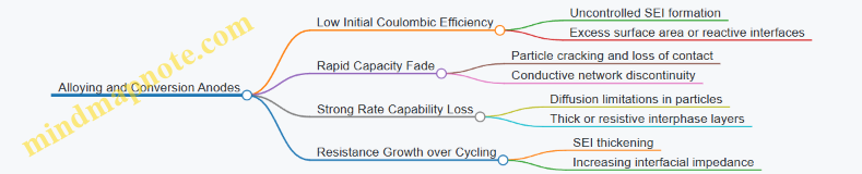
Engineering Takeaways
Alloying and conversion anodes can be high-capacity options for sodium systems, but they demand disciplined control of particle scale, conductive connectivity, mechanical compliance, and SEI formation. When you treat those as separate engineering levers and verify them with targeted measurements, the material behavior becomes predictable enough to design around rather than merely observe.
4.3 Anode Prelithiation Equivalent Strategies for Sodium Cells
Prelithiation is the idea of giving an anode a head start in charge so the cell does not waste its first cycles on forming interphases. Sodium cells need an equivalent strategy because the first sodium insertion and the first solid electrolyte interphase (SEI) formation consume sodium irreversibly. Without compensation, you typically see low initial coulombic efficiency, slower capacity stabilization, and sometimes a larger spread in formation results between batches.
Foundational Concept: Why Sodium Cells Need a Head Start
In a typical sodium-ion cell, the first discharge drives sodium into the anode while electrolyte components decompose to form the SEI. That SEI locks up some sodium and electrolyte fragments. The anode then cycles with a reduced “available” sodium inventory, so the first few cycles show a capacity deficit relative to later cycles.
A practical engineering goal is to make the anode’s initial irreversible loss predictable and small enough that the cell’s rated capacity and energy are not dominated by formation losses. The “equivalent” part means you’re not trying to preload lithium; you’re trying to preload sodium balance and interphase formation outcomes.
Mind Map: Prelithiation Equivalent Strategy Options
Sodium Inventory Compensation Methods
Electrochemical Pre-Sodiation
Electrochemical pre-sodiation means you insert sodium into the anode before assembling the full cell. A common workflow is to pre-sodiated anode electrodes in a half-cell environment, then assemble them into full cells with a cathode. The engineering benefit is controllability: you can target a specific amount of sodium uptake based on charge passed.
Easy-to-understand example: Suppose your anode loses 8% of its theoretical capacity in the first cycle due to SEI formation. If you pre-sodiated the anode by roughly 8% of its capacity (measured as added charge per gram), the full cell’s first discharge capacity deficit shrinks, and the subsequent cycles align more closely with the stabilized capacity.
Key practical detail: pre-sodiation must be uniform across the electrode thickness. If sodium insertion is surface-heavy, you can create local over-sodiation, which later shows up as higher impedance growth or early capacity fade.
Chemical Sodium Sources
Chemical pre-sodiation uses sodium-containing reagents to drive sodium into the anode without an external electrochemical circuit. This can reduce equipment complexity, but it introduces handling and compatibility constraints because reagents may react with electrolyte components or binders.
Easy-to-understand example: If a chemical method deposits sodium in a controlled manner, you can tune the extent by reagent concentration and exposure time. The tradeoff is that “tuning” is often less precise than charge-based electrochemical methods, so you validate with mass balance and electrochemical testing.
Key practical detail: any residual reagent or byproduct can interfere with SEI formation during full-cell assembly. That interference can erase the benefit of sodium compensation.
SEI Engineering as an Alternative or Complement
Prelithiation-equivalent strategies are not only about adding sodium. You can also reduce how much sodium is consumed by making the SEI form in a more efficient way.
Additive-Driven SEI Formation
Electrolyte additives can shift SEI chemistry toward products that are less sodium-consuming and more mechanically stable. The engineering logic is simple: if the SEI forms with fewer irreversible side reactions, the first-cycle coulombic efficiency improves even without pre-sodiation.
Easy-to-understand example: Consider two electrolyte formulations tested on the same anode. Formulation A yields a first-cycle coulombic efficiency of 85%, while formulation B yields 92%. If you then add a smaller amount of pre-sodiation when using formulation B, you avoid overcompensating and reduce the risk of anode stress.
Key practical detail: additives can also change wetting and interfacial impedance. You want a SEI that is both sodium-efficient and low-resistance.
Capacity Balancing Approaches
Extra Anode Capacity with Controlled Formation
Instead of pre-sodiating, you can design the cell so the anode has extra capacity relative to the cathode. During formation, the “extra” anode capacity covers the irreversible loss. This is conceptually straightforward and often easier to implement than pre-sodiation.
Easy-to-understand example: If the anode loses 8% in formation, you can set the anode-to-cathode capacity ratio so that the cathode’s rated capacity is still met after the initial loss. If the cathode is limiting, the cell’s first-cycle capacity deficit becomes less visible in the delivered energy.
Key practical detail: too much excess anode can increase inactive material fraction and reduce energy density. The best balance is found by measuring formation loss and then setting a ratio that meets both performance and manufacturing constraints.
Selection Criteria and Validation
Choose a strategy based on what you can measure and control.
- If you need tight control of initial capacity and can support extra process steps, electrochemical pre-sodiation is often the most direct.
- If you want to avoid extra steps but can tune electrolyte chemistry, SEI engineering is a strong complement.
- If manufacturing simplicity dominates, capacity balancing with a well-defined formation protocol can be the most robust.
Validate with three metrics: first-cycle coulombic efficiency, capacity stabilization after formation, and impedance growth trends. If the cell shows improved first-cycle efficiency but later resistance growth accelerates, the strategy likely changed SEI quality rather than just sodium inventory.
Practical Example Workflow for Engineering Decisions
- Measure first-cycle coulombic efficiency and capacity loss on the anode in a controlled half-cell setup.
- Test electrolyte additives that target SEI efficiency on the same anode.
- Decide whether to add pre-sodiation, capacity balancing, or both, based on how much loss remains after additive tuning.
- Assemble full cells and compare formation spread across multiple batches.
A good outcome looks boring in the best way: the first-cycle deficit shrinks, stabilized capacity matches the target, and the cell-to-cell variation narrows without introducing new impedance problems.
4.4 SEI Formation Control Through Electrolyte and Additives
SEI, the solid electrolyte interphase, is the thin layer that forms when electrolyte components react at the anode surface during early cycling. In sodium-ion cells, controlling SEI matters because it sets the baseline for ionic transport, corrosion rate, and long-term resistance growth. The goal is not to prevent SEI entirely; it is to form an SEI that is thin, stable, and ion-conductive while minimizing continuous electrolyte consumption.
Foundational Mechanisms and What You Can Control
SEI formation starts with electrolyte reduction at low potential near the anode. The first products can be electronically insulating but ion-permeable, which is ideal. If the SEI is too resistive or too porous, sodium keeps finding fresh surface and the layer keeps rebuilding. If the SEI is mechanically weak, it fractures under cycling-induced volume changes and exposes new reactive sites.
You can influence these outcomes through three levers:
- Electrolyte composition: which salts and solvents are available to reduce.
- Additives: which sacrificial or film-forming molecules preferentially reduce early.
- Operating conditions during formation: temperature, current rate, and voltage limits that shape the initial reaction pathway.
Electrolyte Choices That Steer SEI Chemistry
Start with the salt and solvent system because they determine the “default” reduction products. For sodium-ion cells, common practice uses sodium salts in ether-based or carbonate-based solvents, often with a small amount of co-solvent to tune viscosity and wetting. A practical engineering approach is to treat electrolyte selection as a balance between:
- Wetting and transport: better wetting reduces local current spikes that accelerate SEI growth.
- Reduction tendency: more easily reduced components can form SEI quickly, but may also create unstable layers.
- Interfacial stability: some solvent molecules produce SEI that is mechanically robust; others produce brittle films.
Easy example: If you switch from a higher-viscosity solvent blend to a lower-viscosity one, the same formation current often yields a more uniform current distribution across the electrode. That uniformity can reduce “hot spots” where SEI thickens rapidly, even if the chemical ingredients are similar.
Additives as Controlled Sacrifices
Additives are used to bias the earliest reduction reactions toward forming a protective SEI. The key is selectivity: the additive should reduce before the bulk solvent or salt does, so it becomes the main contributor to the interphase.
Common additive roles include:
- Film-formers: create inorganic-rich or polymer-like interphases that slow further reaction.
- SEI stabilizers: reduce continuous electrolyte decomposition by improving adhesion or reducing permeability.
- Gas suppressors: limit side reactions that generate gas and disrupt the interface.
Easy example: Suppose your cell shows rapid resistance increase after formation. You add a small fraction of a film-forming additive and keep everything else constant. If the additive works, you should see lower continuing electrolyte consumption during later cycling, often reflected as improved coulombic efficiency and slower impedance growth.
Formation Protocols That Prevent Runaway SEI Growth
Formation cycling is where most SEI “decisions” are made. Two parameters dominate:
- Current density: higher current increases overpotential and accelerates reduction reactions.
- Temperature: warmer conditions speed kinetics but can also increase side reactions.
A systematic formation approach is to use a moderate current, allow rest steps where appropriate, and cap the voltage window to avoid pushing the anode into overly aggressive potentials. Rest steps help concentration gradients relax, which reduces local over-reduction.
Easy example: If you run formation at the same total capacity but split it into two stages with a rest in between, the second stage often forms SEI on a more “settled” surface. That can reduce the thickness of the newly formed layer compared with a single uninterrupted ramp.
Mind Map: SEI Control Pathway
Practical Testing and Interpretation
To confirm that your electrolyte and additive strategy is working, track metrics that connect chemistry to performance:
- Initial coulombic efficiency: lower values often indicate excessive irreversible reactions.
- Electrochemical impedance spectroscopy trends: a rapid impedance jump during early cycling can signal thick or resistive SEI.
- Resistance growth slope: stable SEI typically shows slower, more predictable growth.
- Gas and swelling indicators: excessive gas can mean ongoing decomposition or unstable interphase.
Easy example: If two electrolyte formulations yield similar initial coulombic efficiency but one shows faster impedance growth after the first few cycles, the difference is often SEI structure. The better formulation may form a layer that is less permeable to electrolyte, even if the initial irreversible charge is comparable.
Engineering Checklist for SEI Control
- Choose an electrolyte blend that wets the electrode well and supports stable interfacial chemistry.
- Add a small amount of a film-forming additive that reduces early and preferentially.
- Use formation currents that limit overpotential-driven side reactions.
- Include rest steps when concentration gradients are likely.
- Validate with coulombic efficiency, impedance evolution, and signs of gas.
When these elements align, the SEI becomes a controlled boundary layer rather than a recurring project. That’s the practical win: fewer surprises, steadier resistance, and less electrolyte spent just to keep the interface alive.
4.5 Anode Balancing and Capacity Matching with Cathodes
Anode balancing is the art of ensuring the anode can supply sodium during discharge without running out early, while also avoiding excess anode that wastes volume and increases irreversible losses. In sodium-ion cells, this is especially important because hard carbon and other anodes can show significant first-cycle loss and evolving impedance. The goal is not “equal capacities on paper,” but “equal usable sodium inventory across the operating window.”
Core Concepts for Capacity Matching
Start with two capacities: the cathode’s reversible capacity and the anode’s reversible capacity after formation. During the first cycles, the anode typically forms an interphase and may trap sodium, so its effective capacity is lower than its nominal value. Capacity matching therefore uses effective anode capacity, not just material datasheet values.
A practical engineering approach uses areal capacities (mAh/cm²) because electrode thickness and loading vary. Define:
- Cathode areal capacity: based on active material loading, utilization, and target cutoff voltage.
- Anode effective areal capacity: based on measured first-cycle efficiency and subsequent cycle utilization.
Then choose an anode-to-cathode capacity ratio (often called excess capacity). If the anode is too small, the cell hits the anode cutoff early, leaving cathode material unused. If the anode is too large, you increase inactive mass and can worsen impedance growth due to thicker electrodes and higher tortuosity.
Stepwise Method for Systematic Balancing
-
Pick a target utilization strategy Decide how much of the cathode you want to use at the C-rate and temperature of interest. For example, if you expect 80% cathode utilization at 1C, you design around that number rather than assuming 100%.
-
Estimate cathode areal capacity Compute cathode areal capacity from loading and expected utilization. Example: cathode loading 4.0 mg/cm² with 120 mAh/g practical capacity gives 0.48 mAh/cm² at 100% utilization; at 80% utilization, you design for 0.38 mAh/cm².
-
Measure anode effective capacity from formation After formation, determine the anode’s usable capacity under the same cutoff and current density. If the anode shows 85% first-cycle efficiency and stabilizes near 90% utilization, you use the stabilized effective value for matching.
-
Choose a capacity ratio with margin Use a modest anode excess to cover cycle-to-cycle variability and gradual loss of anode efficiency. A common starting point is 5–20% anode excess depending on how stable the anode is and how tight your manufacturing tolerances are.
-
Convert capacity ratio into thickness or loading Adjust anode thickness or active loading to reach the required areal capacity. This is where many designs fail: the ratio is correct on a spreadsheet, but the electrode microstructure changes utilization.
-
Validate with a rate-matched test Run a short cycling protocol at the intended current density and temperature. Confirm that the cell reaches the cathode cutoff without prematurely hitting the anode cutoff.
Mind Map: Anode Balancing Logic
Example: Matching for a Moderate-Power Cell
Assume the cathode design targets 0.38 mAh/cm² areal capacity at 1C. The anode, after formation, provides 0.42 mAh/cm² at the chosen loading and cutoff. If you use a 10% anode excess margin, the required anode areal capacity is:
- Required anode capacity = 0.38 × 1.10 = 0.418 mAh/cm²
Your anode effective capacity is 0.42 mAh/cm², so the design is close. If the measured anode utilization later drops to 0.40 mAh/cm², the cell will likely underutilize the cathode at 1C. That’s why the validation step matters: you are checking the pair of electrodes under real constraints, not just their individual capacities.
Example: When Excess Anode Hurts
Consider a design that uses 30% anode excess to be “safe.” The extra anode increases electrode thickness, which can raise ionic resistance and slow sodium transport. At higher rates, the anode may still be “capacity-rich,” but the cell becomes power-limited because the anode cannot access its internal surface quickly. The result is a lower usable capacity at the same cutoff, even though the anode has spare theoretical capacity.
Advanced Details That Prevent Common Mismatches
- Utilization is not constant across rates: cathode and anode utilization both change with current density, so matching at one rate may not hold at another.
- First-cycle loss must be included: if you match using nominal anode capacity, the first discharge may look fine but later cycles can show imbalance as the anode inventory shrinks.
- Electrode density affects effective capacity: higher density can reduce porosity and slow transport, lowering utilization even when active mass is unchanged.
- Electrolyte volume and separator thickness matter: limited electrolyte can increase interfacial resistance, effectively reducing anode usable capacity.
Practical Acceptance Checks
A balanced design typically shows:
- Discharge endpoints governed by the cathode cutoff rather than anode depletion.
- Stable first-cycle efficiency and no sudden capacity loss after formation.
- Reasonable impedance growth without a strong rate-dependent capacity collapse.
If these checks fail, adjust the anode excess ratio and re-validate using areal capacity and rate-matched tests. The best balancing is the one that survives the real manufacturing spread, not just the idealized calculation.
5. Electrolyte Chemistry and Additive Engineering
5.1 Sodium Salt Selection and Solvent System Compatibility
Choosing the sodium salt and the solvent system is less about finding a “best” chemistry and more about matching three things: (1) how sodium ions move, (2) how the salt and solvent behave at the electrodes, and (3) how stable the electrolyte remains under real operating conditions. If any one of these is off, you’ll see it as poor wetting, fast resistance growth, or uneven interfacial layers.
Foundational Criteria for Sodium Salt Choice
Start with the salt’s role in three places: bulk transport, interfacial chemistry, and safety-relevant decomposition pathways.
-
Ion availability and dissociation: A salt that dissociates well increases ionic conductivity, but too much dissociation can also change the composition of the interphase. A practical check is to compare conductivity and viscosity of candidate electrolytes at the same salt concentration.
-
Anion stability and interphase contribution: The anion often participates in forming the solid electrolyte interphase (SEI) on the anode and the cathode interphase on the cathode. In sodium systems, the goal is not “no SEI,” but an SEI that is ion-conducting and electronically blocking.
-
Electrochemical stability window: The salt must resist oxidation at the cathode potential and reduction at the anode potential. A narrow stability window can create gas and rapid capacity loss.
-
Moisture sensitivity: Many salts and solvents react with trace water. Water can increase impedance and accelerate side reactions. Treat moisture as a measurable input, not a vague enemy.
Solvent System Compatibility with Salt and Electrodes
Solvents control viscosity, dielectric constant, and the solvation structure around Na⁺. That solvation structure affects both transport and interfacial reactions.
-
Wetting and electrode infiltration: If the electrolyte wets the electrode poorly, you get localized current density and early degradation. A simple engineering test is to measure contact angle on representative electrode surfaces and compare it across solvent blends.
-
Viscosity and ionic mobility: Higher viscosity slows Na⁺ transport, which shows up as worse rate performance and larger polarization. Balance viscosity with stability; a very low-viscosity system can be more reactive.
-
Solvation structure and SEI chemistry: Some solvents preferentially coordinate Na⁺ and influence which decomposition products form. You can observe this indirectly by tracking impedance growth during formation and by comparing the coulombic efficiency trend.
-
Cathode compatibility: Cathode surfaces can catalyze electrolyte decomposition. Solvent blends that are stable against oxidation reduce parasitic reactions, which helps maintain capacity at moderate-to-high voltage.
Practical Selection Workflow
Use a structured workflow so decisions don’t become guesswork.
-
Fix a target operating window: Choose the maximum charge voltage and minimum discharge voltage for the cell design. This sets the required electrochemical stability window.
-
Choose a baseline salt family: Select salts that are known to dissolve well in sodium-compatible solvents and that form manageable interphases.
-
Screen solvent blends by transport first: Compare conductivity and viscosity at the same salt concentration. Pick candidates that meet a minimum conductivity threshold while keeping viscosity reasonable.
-
Run formation-focused checks: Formation cycling reveals whether the anode interphase forms consistently. Look for stable coulombic efficiency and controlled impedance growth.
-
Verify interfacial stability at the cathode: Perform voltage-hold or cycling at representative cathode potentials to confirm oxidation stability.
Mind Map: Sodium Salt and Solvent Compatibility
Example: Comparing Two Electrolyte Candidates
Assume you’re targeting a moderate-power sodium-ion cell and you have two electrolyte candidates at 1 M salt concentration.
- Candidate A: Salt dissolves readily in a solvent blend with moderate viscosity.
- Candidate B: Salt dissolves less completely, but the solvent blend has lower viscosity.
A sensible test sequence is: measure conductivity and viscosity first. If Candidate B shows higher viscosity despite lower solvent viscosity, the incomplete dissolution is likely increasing effective viscosity and reducing free Na⁺. Next, run formation cycling and track coulombic efficiency. If Candidate A forms a stable SEI with slower impedance growth, it’s usually the better choice even if Candidate B looks attractive on paper. The key is that “fast ions in the bulk” doesn’t help if the interphase keeps changing.
Example: Moisture Control as a Compatibility Variable
Suppose two labs prepare the same nominal electrolyte. Lab 1 uses stringent moisture control; Lab 2 allows higher water exposure during assembly. Even with identical salt and solvent, Lab 2 often sees higher initial impedance and faster capacity fade because water alters the decomposition products and SEI structure. The engineering takeaway is straightforward: salt-solvent compatibility must be evaluated under controlled moisture conditions, or the results won’t transfer.
Engineering Checks That Tie Salt and Solvent Together
- Conductivity vs viscosity correlation: If conductivity doesn’t improve when viscosity decreases, solvation or dissolution is likely the limiting factor.
- Formation impedance slope: A steep impedance rise suggests unstable interphase formation, often linked to salt-anion or solvent decomposition behavior.
- Consistency across batches: If performance varies widely with the same recipe, the issue is frequently moisture handling or incomplete dissolution rather than the chemistry “mysteriously changing.”
In short, sodium salt selection and solvent compatibility are one decision, not two. The salt sets the interphase chemistry and stability constraints; the solvent sets transport and wetting. When both are aligned and moisture is controlled, the electrolyte behaves like a predictable component instead of a moving target.
5.2 Electrolyte Viscosity Conductivity and Wetting Requirements
Electrolyte performance is often summarized with two numbers—viscosity and ionic conductivity—but sodium-ion cells care about how those numbers show up at interfaces. Viscosity affects how quickly electrolyte penetrates pores and reaches electrode surfaces. Conductivity affects how much voltage you lose to ion transport during charge and discharge. Wetting ties both together by controlling whether the electrolyte actually contacts the places where current must flow.
Mind Map: Electrolyte Viscosity Conductivity and Wetting
Viscosity: From Filling Behavior to Transport Losses
Viscosity is measured directly, but its impact is easiest to see through a simple filling analogy. Imagine an electrode as a sponge with narrow channels. If the electrolyte is too thick, it may still be chemically correct, yet it fills slowly and leaves dry pockets. Those dry pockets create local current crowding, which then accelerates side reactions and increases resistance.
A practical rule is to treat viscosity as a “time-to-contact” parameter. During assembly, electrolyte must reach internal surfaces before the cell is sealed and formation cycling begins. In production, you can observe this indirectly by comparing early-stage impedance across lots: higher viscosity often correlates with larger initial resistance because the effective wet area is smaller.
Temperature matters because viscosity typically drops as temperature rises. That means a formulation that looks fine at room temperature can underperform in colder conditions if the cell relies on fast ion transport during high-rate operation.
Conductivity: Separating Bulk and Effective Resistance
Ionic conductivity is the property you want, but it is not the whole story. Bulk conductivity describes how easily ions move through the liquid phase. Effective resistance in a cell also includes tortuosity in the porous electrode and separator, plus any additional resistance from interfacial films.
To connect conductivity to cell behavior, use a resistance decomposition mindset. If conductivity is low, voltage loss grows with current because the electrolyte cannot supply ions quickly enough. If conductivity is adequate but resistance still rises, the limiting step may be interfacial—often tied to SEI growth or poor contact.
Salt concentration influences conductivity in two competing ways. Adding salt increases the number of charge carriers, but it can also increase ion pairing and reduce mobility. The “best” concentration is therefore not the maximum salt you can dissolve; it is the concentration that balances carrier availability with mobility.
Wetting: Contact Angle, Capillary Action, and Real Surfaces
Wetting is commonly reduced to contact angle, but in porous electrodes the more useful concept is capillary-driven infiltration. A liquid wets a surface when its surface tension and interactions with the solid allow it to spread rather than bead up. In pores, wetting determines whether capillary forces can pull electrolyte deep into the structure.
Two engineering levers control wetting. First, electrolyte surface tension and polarity determine how strongly the liquid interacts with electrode binders and current collector surfaces. Second, electrode surface energy and pore geometry determine how easily the electrolyte can spread and climb.
A concrete example: if an electrode binder formulation changes from a more wettable polymer to a less wettable one, the same electrolyte can show a higher contact angle and slower wicking. The cell then exhibits higher early impedance even if measured conductivity of the electrolyte is unchanged.
Contamination can also sabotage wetting. Residual moisture or processing residues can alter surface chemistry and create local gas formation during early cycling, both of which reduce effective contact area.
Integrated Engineering Controls
Solvent and Salt Selection
Choose solvent systems that provide a workable viscosity-conductivity balance. Then verify that the chosen salt concentration does not create excessive ion pairing. A formulation that is slightly lower in conductivity but significantly better in wetting can outperform in rate tests because it reduces effective interfacial resistance.
Additives for Interfacial Behavior
Additives can improve wetting and stabilize interfaces, but they must not raise viscosity too much. Treat additives as “small changes with big consequences”: even low concentrations can alter surface tension and interfacial chemistry, shifting how quickly electrolyte spreads and how uniformly SEI forms.
Electrode Preparation Compatibility
Electrode porosity, thickness, and binder content set the wetting demand. If the electrode is thicker or has smaller pores, the electrolyte must infiltrate more distance, making viscosity and wetting more critical. Matching electrolyte properties to electrode architecture is often more effective than trying to force a single formulation to work everywhere.
Validation: Measurements That Predict Cell Behavior
Start with direct measurements, then connect them to cell-level indicators.
- Measure viscosity at relevant temperatures and record how it changes with temperature.
- Measure ionic conductivity across the same temperature range.
- Measure contact angle on representative electrode surfaces and run a wicking test to estimate infiltration speed.
- In cell tests, track early-stage impedance and compare it to the wetting and conductivity metrics.
If you see high impedance despite acceptable conductivity, suspect wetting or interfacial contact. If you see both high viscosity and poor infiltration, suspect filling and effective contact area first. This ordering keeps troubleshooting efficient and avoids blaming the chemistry when the liquid simply never reached the places it needed to.
Example: Choosing Between Two Electrolytes
Suppose Electrolyte A has higher conductivity but also higher viscosity. Electrolyte B has slightly lower conductivity but wets the electrode better and infiltrates faster. In a moderate-rate test, A may look better at first because bulk transport is strong. In a thicker-electrode test, B often wins because the effective ion supply improves when electrolyte reaches internal surfaces quickly. The lesson is simple: conductivity matters most when contact is already good; wetting matters most when contact is the bottleneck.
5.3 SEI Formation Pathways and Additive Roles
SEI, the solid electrolyte interphase, forms when the electrolyte first meets the anode surface and the cell voltage drives reduction reactions. In sodium-ion systems, the same basic idea holds as in other alkali-ion batteries: the SEI must be ion-conductive enough for sodium to pass while being electronically insulating enough to stop continuous electrolyte breakdown. The engineering challenge is that SEI is not one material; it is a layered set of products whose composition depends on electrolyte chemistry, electrode surface state, and the early cycling protocol.
Foundational Pathways from First Contact to Stabilization
A practical way to think about SEI formation is as a sequence of events.
- Electrolyte reduction at the anode surface: Solvent and salt species react at low potential, producing inorganic and organic fragments.
- Transport-limited growth: Once a passivating layer forms, further reactions slow because sodium and reactive species must diffuse through the growing film.
- Stabilization or runaway: If the film is sufficiently insulating electronically, the reaction current drops and the SEI “settles.” If not, electrolyte keeps decomposing, consuming inventory and increasing resistance.
A simple engineering check is to compare early-cycle coulombic efficiency. If the first few cycles show large irreversible capacity, SEI growth is likely consuming electrolyte and active sodium.
Additive Roles Mapped to SEI Chemistry
Additives are small concentrations of molecules or salts designed to steer which reduction products dominate. They do not magically stop SEI; they change the balance between “fast film-forming but fragile” and “slower film-forming but robust.”
Common additive functions include:
- SEI-forming salts: They preferentially reduce to inorganic-rich layers that tend to be more electronically blocking.
- Film-forming co-solvents or molecules: They create polymeric or organic-rich SEI that can improve flexibility and reduce cracking.
- Wetting and interfacial modifiers: They help electrolyte spread on the electrode, reducing local hot spots where SEI forms unevenly.
A useful rule of thumb: inorganic-rich SEI often improves resistance stability, while organic-rich SEI often improves mechanical compliance. Many successful formulations aim for a mixed layer.
Mind Map: SEI Formation and Additive Mechanisms
Systematic Engineering Example: Choosing Additives by Failure Mode
Consider two common observations during early cycling.
Case A: Resistance jumps early. This often indicates SEI that forms but is too resistive or uneven. An additive strategy is to promote a more uniform, mixed SEI. For instance, pairing an SEI-forming salt (to increase inorganic blocking) with a film-forming organic component (to improve contact and reduce cracking) can reduce the “patchy” growth that causes localized current spikes.
Case B: Coulombic efficiency is low and keeps dropping. This suggests ongoing electrolyte reduction, meaning the SEI is not sufficiently insulating. Here, the additive role shifts toward stronger electronic blocking products. Increasing the fraction of inorganic SEI precursors can reduce continuous decomposition, but the tradeoff is that overly brittle layers may crack during sodium insertion, so the additive balance matters.
Advanced Details: Surface State and Formation Protocol
Even with the same electrolyte recipe, the anode surface state changes SEI pathways.
- Surface area and porosity: Higher surface area increases reaction sites, accelerating SEI growth. Additives may need to be tuned to avoid excessive consumption.
- Residual moisture and contaminants: Trace water can change reduction chemistry and increase gas-forming reactions, which can disrupt SEI continuity.
- Formation cycling: A controlled low-current formation step can limit the peak reduction rate, allowing additives to form the intended SEI rather than letting the electrolyte “take the fastest path.”
A practical formation approach is to start with a gentle current density and gradually increase it. The goal is not to slow everything forever, but to prevent the first SEI from becoming a rough, high-defect layer.
Quick Validation Checks That Tie Back to Additives
After formation, engineers typically look for three linked signals:
- Coulombic efficiency trend: It should improve and then stabilize as SEI growth slows.
- Impedance evolution: Resistance should rise initially and then change more slowly, indicating passivation rather than continuous breakdown.
- Voltage hysteresis: Large, persistent hysteresis can indicate unstable interfacial layers or thickening SEI.
When these signals align, the additive is doing its job: steering SEI formation toward a layer that is ion-transport-friendly and electronically blocking, without turning the early cycles into a chemistry experiment with no control knobs.
5.4 Electrolyte Stability Windows and Interfacial Constraints
An electrolyte is “stable” only relative to the voltages, temperatures, and electrode potentials it actually experiences. For sodium-ion cells, stability is constrained by two coupled realities: the electrolyte must not decompose in bulk, and it must form interphases that are thin enough to keep resistance low but robust enough to survive cycling.
Start with the Stability Window
A practical stability window is the range of electrode potentials where the electrolyte shows minimal net decomposition. Engineers usually treat it as a combination of two limits:
- Cathodic limit: where the electrolyte or its additives oxidize at the cathode surface.
- Anodic limit: where the electrolyte reduces near the sodium anode.
A useful mental model is to map the cell’s operating voltage to the approximate electrode potentials. If the cathode is driven to high potentials during charge, the cathodic limit becomes the first bottleneck. If the anode sees low potentials during discharge, the anodic limit dominates. The “window” is not a single number; it shifts with temperature, current rate, and interphase thickness.
Interfacial Constraints Are the Real Gatekeepers
Even if bulk decomposition is slow, interfacial reactions can still consume electrolyte and grow resistive layers. Three constraints matter most:
- Interphase formation rate: how quickly reduction products build on the anode and oxidation products build on the cathode.
- Interphase transport properties: whether sodium ions can pass through without excessive resistance.
- Interphase mechanical integrity: whether the layer cracks or detaches when volume changes occur.
A stable interphase is not necessarily the thinnest one. It is the one that stays chemically compatible and mechanically coherent under the cell’s cycling conditions.
What Changes the Stability Window in Practice
Stability depends on more than salt and solvent. Consider these levers:
- Electrolyte composition: different sodium salts and solvent mixtures change both ionic conductivity and the tendency to form protective films.
- Additives: small concentrations can steer interphase chemistry. The goal is to promote a film that conducts sodium ions while suppressing continuous electrolyte consumption.
- Water and impurities: trace moisture can trigger rapid side reactions, especially near the sodium anode, shrinking the effective anodic stability.
- Temperature: higher temperature accelerates both desired transport and undesired decomposition, often widening current but narrowing practical stability.
A simple example: if a cell is cycled at the same voltage but at higher temperature, you may see faster capacity fade even when initial coulombic efficiency looks fine. The interphase may form quickly, then become resistive as it thickens.
Interphase Chemistry and Thickness Control
Interphase growth is often self-limiting at first, then becomes problematic when the layer thickens or loses transport pathways. Engineers look for signs such as rising impedance and declining coulombic efficiency over time.
A concrete workflow for electrolyte screening is to run a short formation protocol and then compare:
- Initial impedance after formation
- Impedance growth rate over several cycles
- Coulombic efficiency trend during repeated charge-discharge
If impedance rises quickly while coulombic efficiency remains high, the layer may be growing without consuming too much charge. If coulombic efficiency drops early, side reactions are consuming electrolyte and producing additional products.
Mind Map: Stability Window and Interfacial Constraints
Example: Choosing a Voltage Limit Based on Interfacial Behavior
Suppose two electrolyte formulations are tested in otherwise identical cells. Electrolyte A shows lower initial impedance but faster impedance growth. Electrolyte B shows slightly higher initial impedance but slower growth.
A reasonable decision is to set the operating voltage limit using the behavior that best matches the interphase constraint. If the cell is expected to cycle many times, the slower impedance growth often wins because the interphase remains transport-friendly longer. If the application is shallow cycling, the lower initial impedance may dominate energy efficiency.
Example: Additive Selection as a Film-Quality Lever
Imagine an additive that preferentially reduces at the sodium anode and forms a compact, ion-conducting film. In testing, you might observe:
- Higher coulombic efficiency during early cycles
- Reduced impedance growth compared with a no-additive baseline
- Less sensitivity to small variations in moisture
The key is that the additive changes the interfacial reaction pathway, not just the bulk stability. That is why the same electrolyte can behave differently depending on electrode surface condition and formation protocol.
Practical Constraints to Keep the System Consistent
To make stability meaningful, the electrolyte must be evaluated under consistent conditions:
- Same electrode prep: surface area and roughness change local potentials.
- Same formation: interphase quality depends on early cycling history.
- Same temperature: stability window comparisons are temperature-dependent.
When these controls are respected, the stability window becomes a useful engineering boundary rather than a lab curiosity.
5.5 Practical Electrolyte Preparation Handling and Contamination Control
Electrolyte performance is often decided before the first cell is assembled. Sodium-ion electrolytes are sensitive to moisture, oxygen, and trace impurities that can trigger unwanted interfacial layers, gas formation, and conductivity loss. The goal of this section is simple: prepare electrolyte consistently, keep it dry and clean, and document every step so troubleshooting has something solid to point at.
Foundational Handling Principles
Start with a contamination map for your process. Moisture is the usual suspect, but oxygen, metal ions from tools, and residues from containers can also matter. Treat the electrolyte like a “reactive liquid” even when it looks stable in a bottle.
A practical baseline workflow:
- Pre-plan the materials list and verify container compatibility with the solvent and salt.
- Dry the workspace and control humidity using a monitored dry room or glovebox.
- Stage everything before opening any electrolyte components.
- Use dedicated tools and avoid cross-contact between dry and wet areas.
- Record batch identifiers, weights, and any deviations.
A small example: if you weigh salt on a balance that previously measured hydrated salts, you can transfer water films without noticing. The fix is not “be careful,” it is “separate equipment or clean and verify.”
Contamination Control Strategy
Contamination control works best when it is layered.
Layer 1: Environment control
- Keep relative humidity low and track it continuously.
- Minimize door openings and the time containers spend outside controlled conditions.
- Use desiccant and purge routines consistently, not “whenever it seems dry.”
Layer 2: Material control
- Store salts and solvents in sealed containers.
- Transfer components using dry, closed transfer methods when possible.
- Inspect stoppers, caps, and seals for wear; a cracked cap is a slow leak.
Layer 3: Tool and container control
- Use solvent-rinsed, dry-compatible vessels.
- Avoid metal tools that can shed ions; if stainless steel is used, keep it dedicated and clean.
- Label containers with the batch ID and the date of preparation using a fixed format. For example, use 2026-03-01 as a batch date marker in your lab records.
Electrolyte Preparation Workflow with Checkpoints
A systematic approach reduces both mistakes and variability.
Step A: Verify dryness of containers
- Containers should be dried and sealed until use.
- If you reuse vessels, define a cleaning and drying cycle and stick to it.
Step B: Weigh and dissolve in a controlled sequence
- Dissolve salt into solvent under stirring until fully homogeneous.
- Avoid prolonged exposure of the open vessel to the environment.
Step C: Filter and transfer
- If your process uses filtration, define pore size and filter compatibility.
- Transfer electrolyte into sealed, pre-labeled bottles for cell filling.
Checkpoint example: If conductivity measurements show a sudden drop for one batch, compare the time the solution spent mixing, the stirring duration, and whether the vessel was opened more than once. Those are the variables you can actually control.
Mind Map: Electrolyte Handling and Contamination Control
Practical Examples and What to Watch
Example 1: Moisture ingress during transfer A team prepares electrolyte, then leaves the bottle uncapped while labeling. The fix is to label before opening and to use a two-person workflow: one opens and pours, the other labels and seals. The improvement is measurable because the “open time” becomes consistent.
Example 2: Residue contamination from cleaning If a vessel was cleaned with detergent and only partially rinsed, trace residues can change wetting and interfacial behavior. A simple control is to run a blank check: prepare a small test electrolyte batch and compare its conductivity and appearance to a known-good baseline. If the new batch behaves differently, the cleaning step is the first suspect.
Example 3: Metal contamination from tools Using the same spatula for different salts can introduce trace ions. Even tiny amounts can alter SEI formation behavior. The control is straightforward: dedicate tools per chemistry family and store them in sealed bags inside the controlled environment.
Documentation That Actually Helps
A batch record should include: component lot numbers, masses, solvent volume, mixing time, filtration details, container IDs, and any deviations. When a cell shows early resistance growth, you want to answer one question quickly: did this batch experience a handling difference that could plausibly change interfacial chemistry? If the record is missing, you end up guessing.
A final practical rule: if you cannot explain a step in terms of contamination risk, you probably do not need to do it that way.
6. Cell Architecture and Current Collector Integration
6.1 Coin Pouch and Cylindrical Formats for Engineering Validation
Engineering validation needs a format that is repeatable, measurable, and forgiving enough to let you learn from mistakes. Coin pouches and cylindrical cells both serve that purpose, but they do it differently. Coin pouches are compact and great for fast iteration; cylindrical formats are easier to scale in mechanical handling and can better mimic real stack behavior.
Foundational Concepts for Format Choice
A cell format is not just a container. It changes current distribution, pressure on electrodes, electrolyte wetting, and how heat leaves the cell. Those effects can dominate early results if you do not control them.
Start by defining what you must measure reliably: capacity at a given C-rate, impedance growth, rate capability under load, and failure signatures such as sudden resistance jumps. Then decide whether you need pressure control and realistic current paths.
A practical rule: if your goal is to compare materials or electrolyte additives, coin pouches often give cleaner comparisons. If your goal is to validate mechanical stack behavior, gas management, or pressure-driven performance, cylindrical formats are usually the better engineering test.
Coin Pouch Engineering Validation
Coin pouch cells use a flat geometry that makes assembly and testing straightforward. The electrodes are thin, and the current collectors are close to the active area, which reduces the complexity of interpreting transport limits.
Key Design Variables
- Electrode area and thickness: Keep active area consistent across lots. If thickness varies, diffusion paths change and you will misattribute performance changes to chemistry.
- Electrode overlap and edge effects: Edges can concentrate current and accelerate side reactions. Use a consistent mask or tooling so the active region is well defined.
- Pressure and sealing: Coin pouches rely on controlled compression to maintain contact and reduce voids. Too little pressure increases contact resistance; too much can crack brittle electrodes.
- Electrolyte volume and wetting: Underfilling leads to dry spots and early impedance rise. Overfilling can increase swelling and stress at the seal.
Example: Comparing Electrolyte Additives
Prepare three coin pouches with the same cathode and anode formulations, differing only in electrolyte additive concentration. Run formation with identical current density and temperature. If the additive reduces impedance growth, you should see a slower rise in EIS resistance components after the same number of cycles. If performance changes immediately at the first discharge, suspect wetting or sealing differences rather than true interfacial chemistry.
Mind Map: Coin Pouch Validation Workflow
Cylindrical Engineering Validation
Cylindrical cells use a rolled or stacked geometry that better represents how electrodes behave under winding or stacking forces. They also provide more realistic current paths and mechanical constraints.
Key Design Variables
- Winding or stacking tension: This affects contact resistance and pore accessibility. Keep tension consistent or record it so you can normalize results.
- Current collector geometry: Tabs and collector surfaces influence current distribution. Use the same tab design when comparing chemistries.
- Separator placement and alignment: Misalignment can create local short risk or uneven ion transport.
- Pressure management: Cylindrical designs often include springs or end caps. Pressure changes can shift impedance and cycling stability.
Example: Validating Pressure Sensitivity
Build two cylindrical cells that are identical except for end-cap compression force. Run the same formation and then a rate ladder. If higher compression improves initial power but accelerates capacity fade, you likely reduced contact resistance at first while increasing mechanical stress on the electrode during cycling.
Bridging Coin and Cylindrical Results
Coin pouches and cylindrical cells can disagree because each format emphasizes different limitations. Use a structured comparison so you do not chase ghosts.
- Normalize by areal capacity and current density: Compare at the same current density and similar areal loading.
- Track impedance components consistently: Even if absolute values differ, the direction of change should match if the underlying mechanism is the same.
- Use the same electrolyte and electrode batches when possible: Batch-to-batch variability can hide format effects.
Mind Map: Cross-Format Comparison
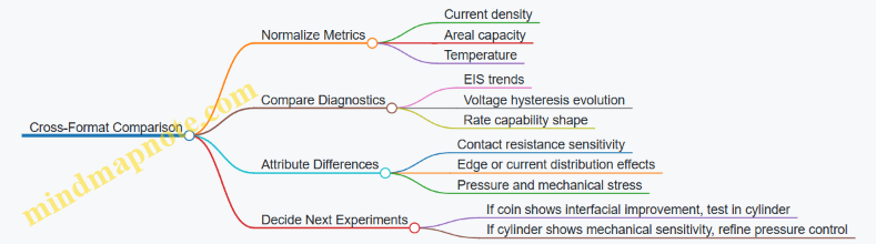
Practical Acceptance Criteria for Engineering Lots
For engineering validation, define pass/fail rules that are measurable and not overly strict. A reasonable set includes: formation reaching a target capacity window, impedance growth staying within a defined band after a fixed cycle count, and no evidence of seal leakage or abnormal swelling. When a lot fails, record which variable changed—compression, electrolyte volume, or electrode thickness—before you change chemistry. That habit saves time and prevents “fixing” the wrong problem.
6.2 Electrode Stack Design and Pressure Management
A sodium-ion cell’s electrode stack is not just a stack of materials; it’s a controlled mechanical system that must keep ionic paths short, electrical paths reliable, and interfaces stable. Pressure management is the lever that ties those goals together, because it governs contact resistance, pore accessibility, and how the stack tolerates swelling and shrinkage during cycling.
Stack Architecture and Load Paths
Start with the load path: current collectors clamp the stack, the separator sits between electrodes, and the electrolyte fills the voids. In a typical pouch or prismatic design, the stack is compressed so that:
- Electrode-to-separator contact is firm enough to avoid local gaps that increase resistance.
- Current collector surfaces stay in intimate contact with the electrode coatings.
- The separator is not crushed to the point of blocking electrolyte transport.
A practical way to reason about this is to treat the stack as a set of springs. The electrode layers compress, the separator compresses, and the current collectors flex slightly. If you increase clamp force too much, you reduce separator thickness and can reduce effective ionic conductivity by limiting pore volume.
Pressure Targets and How to Set Them
Pressure targets should be expressed as a range tied to measurable outcomes, not a single magic number. Use three checkpoints during development:
- Initial contact resistance: Measure impedance or DC resistance across a fresh stack at the intended pressure. If resistance drops with pressure and then plateaus, you’ve likely reached the “good contact” region.
- Separator integrity: After assembly, confirm separator thickness and porosity are within spec. A simple check is to compare separator mass per unit area before and after compression.
- Cycle stability: Track resistance growth and capacity retention under the same pressure. If pressure is too low, contact loss shows up as rising resistance early; if too high, you may see accelerated degradation from restricted transport or mechanical damage.
A useful engineering habit is to define a “pressure window” rather than a point value. For example, you might test three clamp forces that differ by a small step and select the window where resistance is low and separator properties remain unchanged.
Electrode Thickness, Porosity, and Compression Effects
Compression changes more than thickness. It alters:
- Electrode porosity: Lower porosity can slow ion transport through the electrolyte-filled pores.
- Tortuosity: When pores collapse or become less connected, ions take longer paths.
- Percolation of conductive additives: Excess compression can improve electronic contact in some regions, but it can also crack brittle regions during cycling.
To keep the design systematic, link thickness and pressure. If you choose thicker electrodes for energy, you typically need a pressure strategy that maintains contact without over-compressing the separator. That often means distributing force more evenly across the stack and avoiding local “hot spots” from uneven coating or current collector waviness.
Current Collector and Surface Preparation
Current collectors are part of the pressure story. Surface roughness and cleanliness affect how well the electrode coating wets and contacts the metal.
- Use consistent surface roughness: too smooth can increase contact resistance; too rough can concentrate stress.
- Control oxide and contamination: even a thin film can raise interfacial resistance.
- Ensure flatness: a bent current collector creates uneven pressure, which leads to localized high resistance and uneven aging.
A simple diagnostic is to compare resistance maps if you have access to segmented measurements. If not, you can still infer unevenness by checking whether impedance semicircles shift differently across repeated assemblies.
Separator Selection and Compression Tolerance
Separator choice must match the mechanical environment. A separator that is too stiff may resist compression but transmit stress into electrodes; one that is too soft may deform and reduce pore volume.
Design for “compression tolerance” by checking:
- Thickness change under load: measure before and after compression.
- Wetting behavior: compression can change how electrolyte spreads; ensure electrolyte can still penetrate quickly.
- Thermal and shutdown behavior: mechanical compression should not interfere with safety features.
Mind Map: Electrode Stack Design and Pressure Management
Example: Choosing a Pressure Window for a Pouch Cell
Assume you’re building a pouch cell with hard carbon anode and a sodium cathode. You have three candidate clamp forces: low, nominal, and high. You assemble identical stacks and measure:
- DC resistance across the stack at room temperature.
- Separator thickness after compression.
- Impedance after formation and after a fixed number of cycles.
If low force shows higher resistance and faster resistance growth, contact is insufficient. If high force shows separator thickness reduction beyond your spec and resistance growth accelerates after cycling, transport or mechanical damage is likely. The best choice is the window where resistance is low, separator properties stay within spec, and resistance growth is stable.
Example: Avoiding Local Pressure Hot Spots
Uneven coating thickness or slightly warped current collectors can create local regions that see higher stress. That can cause localized cracking in electrodes or premature interface degradation.
Mitigation steps:
- Use coating thickness control with tight tolerances.
- Inspect current collector flatness before assembly.
- Ensure consistent stack alignment so the clamp distributes force uniformly.
A quick check is to compare formation curves across multiple assemblies. Large spread in early resistance or polarization often points to mechanical non-uniformity rather than chemistry.
Practical Assembly Notes That Matter
Pressure management is only as good as the assembly repeatability. Control:
- Stack alignment and centering before clamping.
- Spacer thickness and compression stops so the final pressure is consistent.
- Seal and fixture deformation that can shift pressure distribution.
When these are controlled, pressure becomes a predictable design parameter rather than a source of random variation. That predictability is what lets you tune electrode thickness, separator choice, and electrolyte wetting without chasing ghosts.
6.3 Current Collector Materials and Surface Preparation
Current collectors are the quiet organizers of a sodium-ion cell: they carry electrons reliably, resist corrosion from electrolyte exposure, and provide a surface that electrodes can bond to without turning into a flaky science project. In practice, good collector engineering starts with choosing a compatible metal and ends with surface preparation that supports low contact resistance and stable wetting.
Current Collector Material Selection
Copper, nickel, stainless steel, and aluminum show up most often, but the “best” choice depends on which electrode it serves and how the electrolyte behaves.
For sodium-ion cells, the anode side typically uses a metal that tolerates contact with hard carbon and electrolyte additives without rapid corrosion. Nickel-based foils and stainless steel are common because they form relatively stable surfaces and can handle processing temperatures used in electrode fabrication.
The cathode side often uses stainless steel or nickel as well, especially when the cathode chemistry is sensitive to metal dissolution. Aluminum is sometimes considered for cathodes in lithium systems, but sodium-ion electrolytes and operating potentials can make aluminum less forgiving. The engineering rule is simple: if the metal dissolves into the electrolyte, you lose both performance and consistency lot-to-lot.
A practical selection workflow:
- List the electrode potential range and the electrolyte salt and additive set.
- Screen candidate metals for corrosion resistance and passivation behavior.
- Verify contact resistance after assembly and early formation cycles.
- Confirm mechanical compatibility with calendaring and stack pressure.
Surface Preparation Goals
Surface preparation is not about making the metal “clean” in a vague sense. It targets three measurable outcomes:
- Wetting and adhesion: the electrode coating must spread and bond without voids.
- Low interfacial resistance: roughness and oxide films can add resistance even if the bulk metal is fine.
- Stable interphase formation: the collector should not trigger aggressive reactions that thicken interfacial layers.
Think of it like installing a gasket: a perfectly flat surface is helpful, but the real win is a surface that mates consistently under pressure.
Surface Preparation Methods
Collectors usually arrive with rolling oils, oxides, and handling residues. Preparation methods aim to remove contaminants while avoiding damage.
1. Solvent degreasing
- Use a controlled solvent rinse and dry step to remove oils.
- Example: if you see inconsistent electrode adhesion during peel tests, start by checking whether the solvent step is being skipped or shortened.
2. Mild alkaline or acidic cleaning
- Brief chemical cleaning can remove oxides and improve surface energy.
- Example: if contact resistance spikes after formation, a too-aggressive etch can leave a porous surface that traps electrolyte and increases interfacial area unpredictably.
3. Mechanical conditioning
- Light abrasion or controlled surface roughening can improve mechanical interlock.
- Example: for thick electrodes, slightly higher roughness can reduce the chance of edge delamination under stack pressure.
4. Plasma or corona treatment
- These treatments increase surface energy and improve wetting without heavy material removal.
- Example: when binder systems are formulation-sensitive, plasma treatment can reduce variability in coating spreading.
5. Oxide management
- Many metals form oxides quickly in air. If the time between cleaning and coating is long, the benefit of cleaning fades.
- Example: a simple process control—coating within a fixed time window—often improves repeatability more than changing chemistry.
Quality Checks That Actually Matter
Surface prep should be validated with tests that connect to cell outcomes.
- Contact angle or wetting test on representative coupons.
- Adhesion testing such as peel strength or pull-off measurements.
- Surface roughness measurement to ensure you are not over-roughening.
- XPS or oxide thickness checks when available, mainly for root-cause work.
- Early formation contact resistance tracking using impedance measurements.
Mind Map: Current Collector and Preparation Flow
Example: Diagnosing High Contact Resistance
Suppose a production lot shows higher impedance after formation compared with prior lots, while electrode thickness and active material loading look normal.
A systematic check:
- Compare collector cleaning logs for solvent time, chemical concentration, and rinse steps.
- Measure wetting behavior on cleaned coupons; poor wetting often correlates with higher interfacial resistance.
- Inspect coating edges for voids or partial delamination.
- Check time-to-coating after cleaning; oxide regrowth can undo the preparation.
- If plasma is used, verify power and exposure time and confirm equipment calibration.
In many cases, the root cause is not the metal choice but a process drift: a shortened cleaning step, a longer delay before coating, or inconsistent drying that leaves residues.
Example: Choosing a Preparation Route for Nickel Foils
For nickel-based collectors, a common integrated approach is:
- Solvent degrease to remove oils.
- Mild chemical cleaning to reduce oxide and improve surface energy.
- Controlled drying to avoid water residues.
- Coating within a defined time window to limit oxide regrowth.
- Optional plasma treatment if binder wetting remains inconsistent.
This sequence balances removal of contaminants with minimal surface damage, which helps keep contact resistance stable across lots.
6.4 Separator Selection and Pore Structure Effects
A sodium-ion cell’s separator is not just a physical spacer. It sets the rules for ion transport, controls where the electrolyte can wet, and influences how quickly interfacial layers grow. The practical goal is simple: keep sodium ions moving while preventing electronic contact between electrodes, even when the cell swells slightly during cycling.
Separator Functions That Matter in Sodium-Ion Cells
First, the separator must provide ionic pathways. Sodium ions travel through the electrolyte-filled pores, so the separator’s pore size distribution and thickness directly affect effective ionic conductivity.
Second, the separator must block electrons. If the separator is too thin, too weak, or poorly wetted, local defects can form conductive bridges, especially near edges where manufacturing tolerances stack up.
Third, the separator must tolerate mechanical stress. During charge and discharge, electrode thickness and porosity change. A separator that cannot maintain contact without tearing can create intermittent gaps, which show up as rising resistance.
Pore Structure Fundamentals
Pore structure is usually described by three linked parameters: porosity, tortuosity, and pore size distribution.
- Porosity controls how much electrolyte volume is available. Higher porosity generally improves ion transport, but it can reduce mechanical strength.
- Tortuosity captures how winding the pore network is. Higher tortuosity slows ions and increases concentration gradients.
- Pore size distribution affects wetting and the likelihood of local dry-out. A narrow distribution can wet more uniformly, while a broad distribution may leave pockets that fill slowly.
A useful engineering mindset is to treat the separator as a “porous resistor.” When pore pathways are short and straight, the separator behaves like a lower-resistance medium. When pathways are long and tortuous, the same electrolyte becomes harder to use.
Wetting and Electrolyte Infiltration
Separator performance depends on how quickly electrolyte penetrates the pore network during filling and formation. If wetting is incomplete, ions must detour around dry regions, increasing impedance.
A practical check is to compare early-cycle impedance growth across lots. If one lot shows higher initial resistance and a slower stabilization, it often points to slower infiltration or weaker electrolyte affinity.
Thickness and Areal Loading Tradeoffs
Separator thickness affects both safety margin and transport. Thicker separators improve mechanical robustness and reduce the risk of shorting under compression, but they add ionic path length.
In engineering terms, you balance two constraints:
- Safety and durability: thicker, stronger separators reduce the chance of puncture and maintain separation under stack pressure.
- Power capability: thinner separators reduce ionic resistance and help maintain voltage under high current.
A good practice is to set a target separator areal density and then verify that formation and cycling do not cause excessive resistance growth. If resistance rises early, thickness may be too high, or wetting may be insufficient.
Mechanical Strength and Pore Collapse
Pore structure is not static. Under stack pressure, pores can deform, changing tortuosity and reducing permeability. If the separator is too soft, compression can collapse the pore network and increase impedance.
To manage this, engineers specify separator tensile strength and compressibility, then validate with compression tests that mimic the cell stack pressure. The goal is to ensure that the separator maintains a stable pore geometry through formation and normal cycling.
Edge Effects and Defect Sensitivity
Even if the separator is excellent in the center, edge regions can dominate failure risk. Misalignment, burrs, or uneven electrode coating can concentrate stress and create thin spots.
A systematic mitigation approach is:
- Control electrode-to-separator alignment during assembly.
- Use consistent winding or stacking tension.
- Inspect for separator wrinkles and pinholes.
- Confirm that electrolyte wetting reaches edges, not just the middle.
Mind Map: Separator Selection Drivers
Example: Choosing Between Two Separator Candidates
Assume two separators have the same thickness but different pore structures.
- Separator A: higher porosity, moderate tortuosity, slightly lower tensile strength.
- Separator B: lower porosity, lower tortuosity, higher tensile strength.
If you expect moderate current cycling and can control stack pressure tightly, Separator A may deliver better power because more electrolyte volume is available. If you expect higher compression or rougher assembly tolerances, Separator B may be safer because it resists pore collapse and maintains stable ionic pathways.
A simple validation plan is to run formation and then compare impedance at a fixed state of charge. If Separator A shows a larger impedance increase after a few cycles, it may be losing permeability due to mechanical deformation or incomplete wetting.
Example: Diagnosing Resistance Growth from Separator Issues
Suppose a production lot shows rising resistance after formation, while capacity fade remains modest.
Common separator-related causes include:
- Incomplete wetting leading to persistent dry regions.
- Pore collapse from excessive compression.
- Local defects causing intermittent current paths.
A targeted response is to measure separator wetting quality during filling, verify stack pressure against the assembly recipe, and inspect for pinholes or wrinkles. When the root cause is separator-related, the impedance pattern typically appears early and correlates with current stress during cycling.
Summary of Engineering Selection Rules
Pick separator pore structure to match your electrolyte wetting behavior, choose thickness to balance safety with ionic resistance, and confirm mechanical stability under the actual stack pressure. Then validate with early-cycle impedance trends and defect-focused assembly checks, because separator problems tend to show up where the cell is stressed the most.
6.5 Gas Management and Sealing Strategies for Reliability
Gas in sodium-ion cells is not a mystery; it is the byproduct of specific electrochemical and chemical events. Reliability improves when you (1) predict where gas comes from, (2) keep pressure within safe limits, and (3) prevent gas from turning into a permanent performance loss.
Gas Generation Fundamentals
Most gas originates from electrolyte decomposition and interfacial reactions that grow with time, temperature, and overcharge. In practical terms, you can treat gas generation as a rate that depends on three knobs: voltage stress, temperature, and how clean the interfaces are at assembly.
A useful engineering habit is to separate “early gas” from “late gas.” Early gas often appears during formation and the first cycles when SEI-like layers are still stabilizing. Late gas tends to correlate with aging: resistance growth, thicker interphases, and electrolyte consumption.
What Pressure Does to a Cell
Pressure affects reliability in two ways. First, it can deform pouch foils or stress seals, changing internal contact and raising resistance. Second, it can drive electrolyte wetting changes across the separator, which can increase local current density and accelerate further decomposition. In other words, gas is both symptom and cause.
Sealing Principles for Pouch and Coin Formats
Sealing is a mechanical and chemical barrier. Mechanically, it must resist creep and fatigue under thermal cycling. Chemically, it must tolerate electrolyte vapors and any reactive species that reach the seal region.
Pouch Cell Sealing Strategy
For pouch cells, the seal region is typically a heat-sealed polymer laminate or a welded/laminated edge system. Reliability improves when the seal design accounts for three realities: electrode swelling, electrolyte volume changes, and gas expansion.
A practical approach is to design for a controlled headspace and a predictable maximum internal pressure. That means you choose a target electrolyte fill fraction and a separator compression level so the cell can accommodate volume changes without forcing the seal to do all the work.
Coin Cell Sealing Strategy
Coin cells rely on gasket compression and metal can geometry. Reliability improves when you control gasket material properties and assembly torque so compression remains within a narrow window after cycling. If compression relaxes, gas can migrate more easily and the effective contact area can drop.
Gas Management Tactics
Gas management is not only about venting; it is about preventing gas from becoming a runaway process.
Headspace and Electrolyte Fill Control
Headspace provides room for gas expansion. Too little headspace forces pressure rise; too much headspace can increase electrolyte evaporation and worsen wetting stability. A simple example: if two otherwise identical prototypes differ by 10% electrolyte mass, you can often see a measurable difference in pressure rise rate during high-temperature storage because the gas-to-liquid ratio changes.
Formation and Preconditioning
Formation cycling is where you “pay down” early gas generation. The goal is to build stable interphases without pushing the cell into aggressive decomposition regimes. A common best practice is to use stepwise current or voltage limits during formation so the cell reaches a stable state before full-rate cycling begins.
Separator and Wetting Stability
Gas can create local dry zones if it displaces electrolyte. Separator selection and electrolyte wetting behavior matter here. A reliable workflow is to verify wetting uniformity after assembly by checking impedance spread across multiple cells from the same lot.
Controlled Pressure Relief
Some designs include pressure relief features. If used, they must be engineered so relief does not permanently compromise safety or electrical isolation. For example, a relief path that vents to the outside must still prevent electrolyte leakage onto conductive surfaces.
Mind Map: Gas Management and Sealing Reliability
Reliability Validation Workflow
A systematic test plan ties gas behavior to measurable outcomes.
- Baseline pressure proxy: Track resistance growth and impedance evolution during controlled cycling. If gas is driving wetting loss, impedance dispersion often increases before catastrophic failure.
- Thermal stress: Run storage at elevated temperature with a fixed state of charge. Pressure rise accelerates with temperature, so this test reveals seal weakness and interfacial instability.
- Leak and integrity checks: After cycling or storage, inspect for electrolyte residue near seal edges and verify electrical isolation. A small leak can look like a cleanliness issue, but it usually shows up as a resistance trend.
Example: Comparing Two Seal Setups
Consider two pouch prototypes built with the same electrodes and electrolyte chemistry. Prototype A uses a higher electrolyte fill fraction; Prototype B uses more headspace. During high-temperature cycling, Prototype A shows faster resistance growth and larger impedance spread. The likely cause is pressure-driven wetting disruption near the separator edges, which increases local current density and accelerates decomposition. Prototype B maintains more stable impedance distribution because the headspace buffers gas expansion and reduces seal stress.
Practical Checklist for Reliability
- Control electrolyte fill fraction and document it like a critical dimension.
- Use formation steps that limit early decomposition while still stabilizing interfaces.
- Verify wetting stability indirectly through impedance uniformity.
- Validate seal integrity under thermal cycling, not just at room temperature.
- If pressure relief exists, confirm it prevents leakage onto conductive paths.
Gas management and sealing are inseparable: sealing defines how pressure is handled, and gas generation defines how much pressure you must survive. When both are engineered together, reliability stops being a guessing game and becomes a set of controllable constraints.
7. Manufacturing Process Engineering for Sodium-Ion Cells
7.1 Electrode Coating Drying Calendaring and Thickness Control
Electrode coating is where chemistry meets geometry. If the coating dries unevenly or ends up too thick, you get the classic symptoms: higher resistance, poor utilization, and cells that behave like they were built on different planets. The goal of this section is to control three things in order: solvent removal during drying, microstructure development during calendaring, and final thickness and mass loading for predictable electrochemical performance.
Drying Fundamentals That Prevent Defects
Drying removes solvent and lets binders and active particles form a stable composite. Start with a drying plan that matches your solvent system and binder chemistry. A practical baseline is a staged temperature profile: lower temperature first to avoid skin formation, then higher temperature to finish solvent removal. Skin forms when the surface dries too fast, trapping solvent inside; later, that trapped solvent can create bubbles or voids.
A simple process check is mass tracking. Weigh coated strips at fixed intervals during drying and plot mass versus time. When the curve flattens, solvent removal is effectively complete. For example, if a cathode slurry-coated strip loses 60% of its initial mass in the first 10 minutes and only 2% more after 20 minutes, you can set the end point near the flattening region rather than using a fixed time that ignores batch-to-batch variability.
Drying also affects binder distribution. If the binder is not fully dissolved or if viscosity changes during drying, you can see streaks or local agglomeration. Keep slurry mixing consistent, and avoid long idle times between coating and the start of drying.
Calendaring Purpose and Mechanical Logic
Calendaring compresses the dried electrode to tune porosity, particle contact, and current collector-electrode interface. More compression is not always better. Excessive calendaring can reduce pore volume so much that electrolyte access suffers, especially for thicker electrodes.
Think of calendaring as setting a target porosity window. A useful engineering approach is to measure thickness and density after calendaring, then correlate with electrochemical metrics like initial resistance and capacity utilization. If you have two settings—light and heavy calendaring—compare them using the same formation and test protocol. The setting that yields lower resistance without sacrificing capacity is usually the right compromise.
A concrete example: suppose your target is 30–35% porosity for a sodium-ion cathode. Light calendaring yields 38% porosity and higher resistance; heavy calendaring yields 25% porosity and lower utilization due to limited wetting. The middle setting that lands near 32–34% porosity tends to be the practical sweet spot.
Thickness Control from Target to Tolerance
Thickness control is not just a measurement step; it’s a feedback loop. Define a target thickness and a tolerance band based on cell design. Then control thickness through three levers: coating gap, solids content, and calendaring pressure.
Start upstream. If slurry solids content drifts, the same coating gap produces different wet film thickness, which becomes different dried thickness. For example, a 2% absolute change in solids can translate into a noticeable mass loading shift. Track solids by weighing a known volume and drying a representative sample.
During coating, control the gap and verify it periodically. Use a thickness gauge to map thickness across the web. If you see edge-to-center variation, it often points to web tension issues or slurry viscosity gradients.
After calendaring, measure thickness at multiple positions. If thickness varies systematically, adjust calendaring pressure uniformity or roll alignment. If variation is random, look for local defects like particle clusters or binder streaks.
Quality Checks That Tie Process to Performance
Thickness and drying quality should be linked to simple diagnostics.
- Surface appearance: streaks, pinholes, and “orange peel” texture often indicate drying or slurry mixing problems.
- Mass loading: compare measured active material mass per area to the target. If thickness is correct but mass is low, you likely dried off too much or lost solids during handling.
- Wetting behavior: after electrolyte soaking, check how quickly the electrode becomes uniformly darkened or changes in appearance. Slow or patchy wetting often correlates with over-calendaring or incomplete drying.
Mind Map: Drying and Calendaring Control Flow
Example: Setting a Drying Endpoint and Calendaring Pressure
Assume you coat a cathode to a target dried thickness of 120 µm with a tolerance of ±5 µm.
- Drying endpoint: Run a strip test and weigh every 5 minutes. If mass loss slows from 12% at 10 minutes to 1% between 20 and 25 minutes, set the production drying time so that the strip reaches the flattening region, not necessarily the same absolute time.
- Calendaring pressure: Start with a baseline pressure that reduces thickness from 130 µm (post-dry) to 120 µm. Measure porosity or density proxies if available; otherwise, use thickness plus wetting uniformity. If wetting is patchy, reduce pressure to restore pore access.
- Thickness verification: After calendaring, measure at center and edges. If center is within tolerance but edges are thin, adjust web tension or coating gap stability rather than changing the entire process.
Practical Process Notes That Save Time
Keep the time between coating and drying start short and consistent. Use the same drying airflow and exhaust conditions across batches, since airflow affects solvent removal rate. Finally, treat thickness as a controlled variable with a tolerance, not a hopeful estimate; when it drifts, it usually traces back to solids content, coating gap, or calendaring pressure drift.
7.2 Dry Room Requirements and Moisture Management Protocols
Moisture control is not a “nice to have” in sodium-ion manufacturing; it is a direct driver of electrolyte decomposition, interphase instability, and inconsistent formation results. The goal is simple: keep water exposure low enough that the cell’s internal interfaces see predictable chemistry during assembly and early cycling.
Foundational Moisture Concepts That Matter
Water enters the process through air leaks, wet surfaces, operator clothing, and residual solvent in electrodes and binders. In dry rooms, the key metric is relative humidity (RH), but what matters for reactions is the absolute water content and the time spent above your target. A practical mindset is to treat moisture like a contaminant with a “dose”: higher RH and longer exposure both increase dose.
A useful engineering rule is to separate moisture control into three layers:
- Room environment (RH and airflow discipline)
- Material conditioning (drying, storage, and transfer)
- Process behavior (minimizing open time and controlling human factors)
Dry Room Requirements
Target RH and monitoring. Many facilities use RH setpoints that keep water low enough for stable electrolyte handling. Choose a target RH based on your electrolyte sensitivity and validate it with formation repeatability. Install calibrated RH sensors at multiple heights and locations, because stratification happens when doors open and when air is recirculated.
Air handling and pressure. Maintain positive pressure relative to adjacent non-controlled areas to reduce ingress when doors open. Use controlled airflows that avoid blowing directly across open containers, which can increase particulate and moisture variability.
Door discipline. Treat door openings as moisture events. Use interlocks and staged airlocks where possible. If you must use a single door, enforce a “batching” habit: plan movements so the door stays closed between transfers.
Surface and equipment cleanliness. Dry rooms still accumulate dust. Dust can hold moisture and can also interfere with wetting during electrolyte filling. Clean with methods compatible with your dry environment and verify that cleaning does not introduce residues that later affect wetting.
Moisture Management Protocols
Material drying and storage. Dry electrodes and separators according to your validated drying profile, then store them in sealed containers with desiccant or inert atmosphere. The transfer path should be short and predictable. If you see formation variability lot-to-lot, check whether storage time or container integrity changed.
Glovebox and transfer practice. Use gloveboxes for electrolyte filling and any step where containers are open. Keep containers capped except during the minimum handling time. Pre-stage tools so operators do not search mid-process.
Operator controls. Clothing and gloves are moisture sources. Require controlled gowning and glove change intervals. Train operators to avoid leaning over open containers and to keep movements smooth, because repeated glove contact with surfaces increases contamination risk.
Process timing and exposure logs. Record open-time for critical steps: electrode exposure to ambient, separator handling, electrolyte container open duration, and time between filling and sealing. These logs help you connect a performance shift to a specific operational change.
Mind Map: Moisture Control System
Example: Moisture Protocol for Electrode-to-Filling Transfer
Assume you dry electrodes, then move them to electrolyte filling. A workable protocol is:
- Dry electrodes to the validated endpoint, then cool in a sealed container.
- Store in a desiccated or inert environment until assembly.
- During transfer, keep containers closed and move directly to the glovebox.
- In the glovebox, open each container only when the next step is ready, and close immediately after removing the required quantity.
- Record the open-time per container and the total time from removal from storage to sealing.
If you later observe higher initial resistance or lower coulombic efficiency, compare open-time logs and container handling records first. Often the issue is not the room RH itself, but a few long open intervals during a specific shift.
Example: Diagnosing a Moisture-Related Formation Shift
Suppose Lot A and Lot B use the same electrode formulation and electrolyte recipe, but Lot B shows slower formation and lower early capacity. A systematic check looks like this:
- Compare RH sensor logs for the assembly window.
- Compare door opening counts and durations.
- Compare storage times for electrodes and separators.
- Review glovebox open-time logs for electrolyte containers.
- Inspect container seals and desiccant status for the affected lots.
If RH stayed stable but open-time increased, the likely cause is workflow timing rather than room control. If RH spiked during door openings, the likely cause is ingress during transfers.
Practical Checklist for Daily Operations
- Verify RH sensor calibration status before the shift.
- Confirm positive pressure indicators are within range.
- Stage tools and containers to minimize open time.
- Use sealed containers for any material leaving controlled storage.
- Log open-time for electrolyte and critical containers.
- Change gloves per your interval and after visible contamination.
- Inspect desiccant and container seals at defined frequencies.
Moisture management is a system, not a single setting. When you control dose through environment, handling, and timing, formation becomes repeatable—and your engineering time stops getting spent on mystery variability.
7.3 Cell Assembly Steps for Consistent Electrolyte Filling
Consistent electrolyte filling is mostly about controlling three variables: how much electrolyte enters, how evenly it wets the electrodes, and how little moisture and air get trapped. Sodium-ion cells are sensitive to interfacial chemistry, so “good enough” filling that works once can still produce lot-to-lot variation.
Foundational Setup Before Filling
Start with a controlled environment and a clear assembly sequence. Use a dry room with monitored dew point and keep all components sealed until use. Label every batch of electrodes and separators so you can trace filling outcomes back to coating lot, drying profile, and storage time.
A practical rule: treat electrodes like they are already “reacting” with the atmosphere. Even if the reaction is slow, the effect shows up later as inconsistent formation behavior and resistance growth.
Pre-Wetting and Handling of Electrodes
Before electrolyte contact, confirm electrode geometry and cleanliness. Remove visible particulates, verify thickness and mass targets, and ensure the stack is assembled without wrinkles or misalignment. Separator pores must be unobstructed; compressed or folded separators can create local dry zones.
If your process uses pre-wetting, do it consistently. For example, immerse the separator region briefly in electrolyte while keeping the rest of the assembly protected from prolonged exposure. The goal is uniform wetting without over-soaking and without trapping bubbles.
Assembly Orientation and Bubble Control
Electrolyte filling should minimize gas entrapment. Bubbles tend to cling to electrode edges and separator folds, then later release during cycling, causing local current spikes.
Use a repeatable orientation: keep the stack level during filling and avoid tilting that encourages gas migration. If you use vacuum-assisted filling, apply vacuum long enough to remove trapped air but not so long that the stack dries out or deforms.
Electrolyte Metering and Delivery
Measure electrolyte volume by mass or calibrated flow, not by “time in the reservoir.” Volume targets should account for cell format and expected uptake by separator and electrode porosity.
Example: if a pouch cell requires 18.0 g electrolyte for target wetting, set a process window such as 17.6–18.4 g and record the actual mass for each cell. Later, correlate mass deviation with formation capacity and early impedance to see whether your filling is under- or over-supplying.
Delivery method matters. A gentle flow reduces turbulence that can trap air. If using a needle or manifold, keep the inlet position consistent so the electrolyte front reaches the same regions first.
Vacuum Filling and Soak Steps
A typical sequence is: evacuate, fill, then allow a short soak for capillary infiltration. The soak time is not arbitrary; it compensates for slower wetting in thicker electrodes and higher tortuosity separators.
Example workflow for a pouch cell:
- Evacuate the filled assembly chamber to a defined setpoint.
- Introduce electrolyte until the target mass is reached.
- Maintain mild vacuum briefly to remove microbubbles.
- Release vacuum and soak for a fixed time to equalize wetting.
Track the soak outcome indirectly by weighing the cell before and after filling if your format allows, or by monitoring formation variability.
Sealing and Post-Fill Handling
After filling, seal promptly to limit moisture ingress. Ensure the sealing temperature and pressure are consistent so the gasket compresses uniformly. Uneven sealing can create pathways for gas exchange, which later appears as pressure drift and inconsistent impedance.
Handle filled cells with care: avoid mechanical shocks that can dislodge separator alignment or create voids. Store filled cells in a controlled environment until formation.
In-Process Checks That Catch Problems Early
You do not need fancy equipment to detect many filling issues. Use a layered inspection approach:
- Mass check: compare actual electrolyte mass to target.
- Visual check: inspect for obvious bubbles or dry edges where accessible.
- Dimensional check: verify pouch thickness and stack compression after sealing.
- Early electrical screening: run a brief impedance or open-circuit check to flag outliers.
Example acceptance logic: if electrolyte mass is within window but early impedance is high, suspect incomplete wetting or trapped gas rather than underfill.
Mind Map: Electrolyte Filling Consistency
Example: Diagnosing Underfill Versus Trapped Gas
If a batch shows reduced formation capacity across many cells, first check electrolyte mass distribution. Underfill often produces lower wetting coverage and slower interfacial stabilization.
If capacity is near nominal but early impedance is scattered, trapped gas is a common culprit. The pattern often correlates with a specific assembly station or operator technique, such as inconsistent stack leveling or variable vacuum duration.
The key is to connect each symptom to a filling variable you can measure, then tighten only that part of the process rather than changing everything at once.
7.4 Formation Cycling Procedures for Reproducible Performance
Formation cycling is the controlled first run of a sodium-ion cell that builds stable interphases and reveals early defects before you waste time on long cycling tests. The goal is not maximum capacity on day one; it is repeatable, measurable behavior across lots.
Foundational Principles for Formation
Formation changes the cell internally through two main pathways: (1) electrolyte reduction and interphase growth on the anode, and (2) cathode/electrolyte interfacial stabilization. Both pathways consume a portion of cyclable sodium and electrolyte, so formation must be designed around predictable “first-cycle” losses.
A practical way to think about formation is as a sequence of controlled stress levels. Start gently to establish wetting and initial interphase formation, then step up to the target operating window. If you jump too quickly, you often get thick, resistive layers and large irreversible capacity loss that later looks like “mysterious” degradation.
Mind Map: Formation Cycling Workflow
Pre-Checks That Prevent “Formation Surprises”
Before any cycling, equilibrate cells at the formation temperature for long enough that internal gradients settle. Then record initial open-circuit voltage and basic dimensions or stack pressure indicators if available. A cell that starts far outside the expected voltage range is often already compromised, and formation will only make the problem more expensive.
Moisture control matters because sodium systems are sensitive to side reactions. Use a consistent assembly environment and track moisture exposure time. Even if you cannot measure moisture directly inside the cell, you can standardize the process so formation results become comparable.
Formation Cycling Profile That Balances Stability and Throughput
Use a stepwise profile with explicit voltage cutoffs. A common structure is: low-rate conditioning, intermediate-rate stabilization, then a final ramp to the intended operating window.
Example formation profile for reproducible engineering validation:
- Step 0: Rest at formation temperature for 2–4 hours.
- Step 1: Charge at 0.05C to the upper voltage limit, then rest 30 minutes.
- Step 2: Discharge at 0.05C to the lower voltage limit, then rest 30 minutes.
- Step 3: Repeat Step 1–2 at 0.1C for two cycles.
- Step 4: Perform one cycle at the target formation rate (e.g., 0.2C) to confirm interphase stability.
Keep the rest periods consistent. Rest time affects relaxation and measured voltage hysteresis, which in turn affects how you interpret capacity and impedance.
Monitoring Signals That Actually Tell You Something
Track at least four signals each cycle: (1) charge and discharge capacity, (2) coulombic efficiency (CE), (3) voltage curve shape, and (4) time-resolved resistance via impedance at defined checkpoints.
CE is especially useful early on. During formation, CE often improves as interphase layers stabilize. If CE stays low or worsens after the intermediate-rate steps, you likely have ongoing electrolyte decomposition or poor electrode wetting.
Impedance checkpoints should be placed where they inform decisions, not where they create busywork. For example, measure after the first low-rate cycle and after the final formation-rate cycle. Compare the trend in interfacial resistance rather than chasing absolute values.
Acceptance Criteria and Lot-Level Reproducibility
Define acceptance criteria before running production lots. Typical criteria include bounds on irreversible capacity loss in the first few cycles, limits on the spread of CE across cells, and a maximum allowed resistance increase between checkpoints.
A simple reproducibility rule: if you see a wide distribution in early cycles, stop and diagnose before proceeding. Formation is not a “try harder” process; it is a controlled filter.
Troubleshooting with Clear Decision Points
If irreversible capacity loss is high from the start, check electrolyte handling, assembly dryness, and whether the cell reached proper wetting during early steps. If variance between cells is large, focus on process consistency: electrode thickness control, separator placement, and sealing integrity.
If you observe sudden voltage spikes or abnormal plateaus during charge or discharge, pause the run and inspect the voltage logging for cutoff behavior. Then verify that the voltage limits and current control are implemented consistently across instruments.
Example Mind Map: Formation Acceptance and Actions
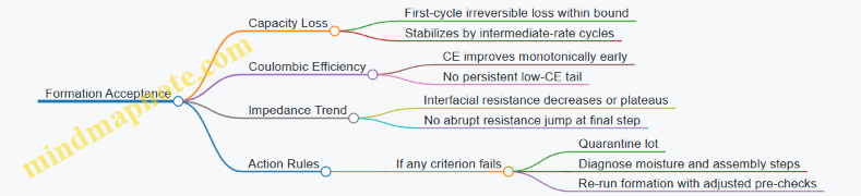
Practical Example: Interpreting a Two-Lot Comparison
Suppose Lot A and Lot B both pass voltage window limits, but Lot B shows higher irreversible capacity loss after Step 2 and a flatter CE improvement. The voltage curves may still look “reasonable,” yet the CE trend indicates ongoing side reactions. In that case, you would compare electrolyte batch records and assembly environment logs for differences in handling time and dryness, then rerun formation on a small sample set using the same profile.
Formation cycling becomes reproducible when the profile, monitoring, and acceptance criteria are treated as one system. When you change only one element—like current rate or rest time—rebaseline the criteria so you are not comparing apples to a slightly different fruit.
7.5 In Process Quality Assurance and Defect Detection Methods
In-process quality assurance (IPQA) is where you prevent defects from becoming “mystery performance problems” later. The goal is simple: catch deviations early, trace them to a step, and stop the line from producing a whole batch of the same wrong thing.
Quality Gates from Materials to Finished Cells
IPQA works best as a sequence of gates. Each gate checks a small set of high-leverage variables that strongly affect sodium-ion cell behavior: moisture exposure, electrode thickness and loading, electrolyte fill quality, and formation consistency.
A practical gate set looks like this:
- Incoming materials gate: verify sodium salt water content, solvent purity, separator basis weight, and conductive additive lot consistency.
- Electrode gate: confirm slurry solids, coating mass, drying endpoint, and calendering target density.
- Assembly gate: verify separator dryness, stack alignment, and electrolyte fill mass.
- Formation gate: confirm current profile execution, temperature control, and voltage cutoff behavior.
- Post-formation gate: check impedance trend and capacity retention against acceptance windows.
Mind Map: Defect Detection Coverage
Electrode Defects and How to Catch Them Early
Electrodes fail in predictable ways when process variables drift. Three common defect families are thickness/loading mismatch, drying residue, and poor contact.
Thickness and loading mismatch shows up as uneven current distribution. A simple detection method is mass-per-area measurement across multiple strips before assembly. For example, if a target dry mass is 8.0 mg/cm², measure at five positions per electrode. If one region is 10% low, you will often see higher local resistance and earlier polarization during formation.
Drying residue increases gas generation and thickens interfacial layers. You can catch it indirectly by tracking drying endpoint consistency and by monitoring solvent odor/volatiles in exhaust streams. If drying time is shortened to chase throughput, formation voltage curves often become noisy and impedance rises faster than normal.
Poor contact comes from calendering under-pressure or binder distribution issues. A fast check is to measure electrode density and compare it to historical distributions. If density is low by a small amount, the cell may still pass acceptance at first, then degrade quickly because ionic pathways are less stable.
Assembly Defects and Practical Detection
Assembly defects are often “invisible” until formation. Moisture exposure is the big one. Use dew point monitoring in the dry room and record it with each batch. If dew point spikes during a shift, treat it as a batch-level risk and tighten formation acceptance windows.
Electrolyte fill quality is another high-impact variable. Track fill mass and wetting time. A useful example: if two cells share the same electrode lot and stack dimensions, but one has 5% lower fill mass, it may still wet initially yet show higher resistance after formation. That pattern is a strong indicator that electrolyte quantity or sealing integrity is off.
Formation Monitoring That Actually Helps
Formation is not just a ritual; it is a diagnostic window. Keep formation equipment logs complete: current setpoints, temperature, and cutoff events. If a cell hits a voltage cutoff early, classify it immediately rather than waiting for later cycling.
A structured approach is to compare formation curves to a baseline band:
- Voltage rise too fast: often points to contact issues or low effective active material utilization.
- Voltage noise or irregular plateaus: can indicate wetting problems or inconsistent interfacial formation.
- Temperature excursions: may reflect abnormal internal resistance.
Early Impedance Signatures for Defect Classification
Electrochemical impedance spectroscopy (EIS) after formation is a practical defect classifier. Instead of chasing absolute numbers, compare to the lot’s trend.
Example workflow:
- Run EIS at a fixed state of charge and temperature.
- Extract a small set of features such as high-frequency intercept and a mid-frequency semicircle area.
- If the high-frequency intercept is elevated, suspect current collector contact or separator/electrode interface issues.
- If the mid-frequency feature grows, suspect interfacial layer formation differences.
Then link back to the most likely step using your gate records. This is where IPQA becomes efficient: the test result points to the step, and the step points to the likely cause.
Root Cause Loop and Line Discipline
When a defect is found, the response should be consistent:
- Contain: quarantine the batch or the affected sub-lot.
- Classify: map the signature to a defect family.
- Trace: review gate data from incoming materials through formation.
- Correct: adjust the specific work instruction parameter.
- Verify: run a small confirmation set and ensure signatures return to the baseline band.
A small but effective discipline is to require a “no data, no release” rule for gate metrics. If a measurement was skipped, the batch does not move forward. It’s less glamorous than troubleshooting later, but it saves time and prevents repeat defects from multiplying.
8. Modeling and Characterization for Design Verification
8.1 Electrochemical Models for Capacity and Rate Predictions
Purpose and Modeling Scope
Electrochemical models translate cell design and operating conditions into measurable outputs like capacity, voltage profiles, and rate limits. For sodium-ion cells, the key is to represent the coupled processes that set performance: ion transport in electrolyte and porous electrodes, charge transfer at interfaces, and solid-state diffusion inside active particles. A good model is not “more physics everywhere”; it is physics where it matters and parameters where you can measure them.
Mind Map: Capacity and Rate Prediction Chain
Foundational Building Blocks
Start with a voltage balance. At a given current, cell voltage is the difference between cathode and anode equilibrium potentials minus losses from transport and kinetics. A minimal but useful structure is:
- Open-circuit term: \(U_{c}(\theta_c) - U_{a}(\theta_a)\), where \(\theta\) is state of charge or stoichiometry.
- Ohmic losses: \(iR\) from current collectors, separator, and electrolyte.
- Kinetic losses: overpotentials from charge transfer, often represented with Butler–Volmer or a simplified symmetric form.
- Mass-transport losses: concentration polarization in electrolyte and diffusion limitations in particles.
Capacity prediction then follows from the condition that, during discharge, the model must reach the cutoff voltage before the theoretical charge throughput is exhausted. That is why cutoff voltages are part of the model inputs, not an afterthought.
Rate Limits from Time Scales
Rate capability is governed by competing time scales. If the current is high, concentration gradients grow faster than diffusion can smooth them.
A practical way to reason is to compare:
- Particle diffusion time: proportional to \(R_p^2/D_s\), where \(R_p\) is particle radius and \(D_s\) is solid diffusion coefficient.
- Electrolyte diffusion/transport time: related to separator thickness and effective ionic conductivity.
- Reaction time: linked to exchange current density and how quickly interfacial kinetics can respond.
When particle diffusion is slow, the model predicts larger kinetic and concentration overpotentials at high C-rate, which reaches cutoff earlier and reduces delivered capacity.
Example: A Two-Parameter Capacity Fit That Actually Works
Suppose you have discharge curves at 0.2C and 1C for a sodium-ion cell. You can fit a model in stages:
- Use the 0.2C curve to estimate the effective diffusion and OCV mapping because transport losses are smaller.
- Use the 1C curve to fit kinetic and transport parameters that control polarization.
A compact approach is to treat the voltage loss as:
- \(\eta_{kin} = i,R_{ct}(\theta)\) using an effective charge transfer resistance over the relevant SOC window.
- \(\eta_{mt} = i,R_{mt}(i,\theta)\) where \(R_{mt}\) increases with current due to concentration gradients.
Then capacity at a given current is found by integrating current over time until the simulated voltage hits the cutoff. The “easy example” check is scaling: if you double current, the model should not keep the same delivered capacity unless diffusion and kinetics are truly fast.
Advanced Details Without Losing the Plot
Once the minimal model matches discharge curves, you can refine it with spatial resolution:
- Porous electrode representation: use effective ionic conductivity and tortuosity to capture electrolyte concentration gradients across thickness.
- Solid diffusion in particles: include radial diffusion so the model predicts how utilization changes with particle size distribution.
- Coupled concentration and kinetics: exchange current density can depend on local surface concentration, which makes polarization depend on both SOC and current.
A common engineering pitfall is fitting parameters that compensate for missing physics. For example, using a single constant \(R_{ct}\) might fit one current but fail across current profiles because the real \(R_{ct}\) changes with surface concentration.
Calibration Loop with Measurable Tests
To keep the model grounded, calibrate with tests that isolate mechanisms:
- EIS helps separate ohmic, charge transfer, and diffusion-related contributions.
- Current pulses reveal how voltage relaxes, which is sensitive to diffusion time constants.
- Temperature sweeps constrain activation energies for transport and kinetics.
A model is “validated” when it predicts capacity and voltage shape across multiple currents and temperatures without refitting every time.
Example: Thickness Sensitivity Check
If you increase cathode thickness while keeping the same active material and formulation, the model should predict:
- higher polarization at high C-rate,
- earlier cutoff,
- reduced utilization of deeper regions in the porous electrode.
This check is useful because it ties design geometry directly to predicted capacity loss, not just to a fitted constant.
8.2 Equivalent Circuit Modeling for Parameter Extraction
Equivalent circuit modeling turns messy electrochemical behavior into a set of electrical elements you can fit to measurements. The goal is not to pretend the cell is a circuit; it is to create a consistent map from test data to parameters you can use for design checks.
Foundations: What Parameters You Can Extract
A practical sodium-ion cell model usually separates three effects:
- Ohmic resistance: electrolyte, current collectors, tabs, and contact resistances. This shows up as an immediate voltage drop when current steps.
- Charge transfer resistance: interfacial kinetics at electrode/electrolyte surfaces. This dominates the mid-frequency response.
- Mass transport limitation: diffusion and concentration gradients. This appears at low frequencies and often produces a Warburg-like trend.
A common starting point is the Randles family: a series resistor for ohmic drop, a parallel branch for charge transfer, and a diffusion element.
Step 1: Choose a Model Topology That Matches Your Test
Before fitting, match the topology to what your data can support.
- If you only have current steps and basic voltage response, you can estimate series resistance and a single effective polarization term.
- If you have EIS (electrochemical impedance spectroscopy), you can fit a richer model with separate time constants.
- If you see depressed semicircles in EIS, include constant phase elements (CPE) instead of ideal capacitors.
Mind Map: Modeling Choices and Parameter Targets
Step 2: Extract Rs from Time-Domain Data
For a current step, the voltage change at the moment of the step approximates the ohmic drop.
- Compute ΔV0 as the difference between the initial voltage and the voltage after the fast transient.
- Then estimate Rs ≈ ΔV0 / ΔI.
Example: If a 2 A step causes an immediate drop of 40 mV, then Rs ≈ 0.040 V / 2 A = 0.020 Ω. If you repeat this at multiple SOC points, Rs should vary smoothly; sharp jumps usually indicate measurement artifacts or contact issues.
Step 3: Fit EIS to Separate Kinetic and Transport Effects
A typical impedance form is:
- Series Rs plus
- Parallel Rct and CPE plus
- Diffusion element (often Warburg or a generalized diffusion impedance).
When fitting, use a consistent workflow:
- Fix Rs using the time-domain estimate or fit it with constraints.
- Fit the mid-frequency arc to obtain Rct and CPE parameters.
- Fit the low-frequency tail to obtain diffusion-related parameters.
Example workflow:
- At a given SOC, fit Rs first.
- Then fit Rct and CPE while keeping Rs fixed.
- Finally, add the diffusion element and refit all parameters.
This staged approach reduces parameter correlation, which is the main reason fits look good but predict poorly.
Step 4: Use Constraints to Prevent Nonsense Fits
Parameter extraction can wander if the model is too flexible.
- Constrain CPE exponent n between 0 and 1.
- Keep diffusion parameters positive.
- If you include an SEI/interphase branch, require it to be inactive at high SOC where the interphase is already established.
Mind Map: Parameter Correlation and How to Reduce It
Step 5: Validate the Model with Predictive Checks
A fit is only useful if it reproduces behavior outside the fitting window.
- Predict impedance at frequencies you did not emphasize during fitting and compare residuals.
- Predict voltage response for a current profile using the fitted parameters and check whether the polarization magnitude matches.
- Confirm trends: Rct should increase when kinetics slow (for example, at lower temperature or at SOC regions where the electrode is less favorable). Rs should track resistive contributions and remain comparatively stable unless contacts or electrolyte conditions change.
Example: A Minimal Randles-Style Fit for Parameter Extraction
Use a model with Rs, Rct, CPE, and a diffusion element. Fit in stages to reduce correlation.
    flowchart TD
A[Measure EIS at fixed SOC and temperature] --> B[Estimate Rs from current-step data]
B --> C[Fit mid-frequency arc for Rct and CPE]
C --> D[Add diffusion element and fit low-frequency tail]
D --> E[Validate residuals and predict impedance]
Practical Notes for Sodium-Ion Cells
Sodium-ion systems often show non-ideal interfacial behavior, so CPE terms are frequently more realistic than ideal capacitors. Also, diffusion-related parameters can shift with electrode thickness and porosity, so keep the model tied to the specific cell format you tested. If you change electrode loading or separator, treat extracted parameters as format-specific rather than universal constants.
8.3 Diffusion and Transport Modeling for Electrode Thickness Effects
Electrode thickness changes how ions and electrons share the workload. In sodium-ion electrodes, the limiting step often shifts with thickness: thin electrodes tend to be limited by reaction kinetics or electronic resistance, while thick electrodes more often become limited by ion transport through pores and solid particles. A good model keeps these pathways separate, then couples them through boundary conditions at the current collector and at the electrolyte-facing surface.
Core Modeling Picture
Start with a one-dimensional through-thickness coordinate \(x\), where \(x=0\) is the current collector side and \(x=L\) is the electrolyte-facing side. You then represent three coupled phenomena:
- Ionic transport in the electrolyte-filled pores: described by an effective diffusion coefficient \(D_{\text{eff}}\) that accounts for tortuosity and porosity.
- Solid-state diffusion inside active particles: described by a particle diffusion coefficient \(D_s\) and a characteristic diffusion length (often particle radius \(R_p\)).
- Charge transfer at the interface: represented by an interfacial kinetics law that links local overpotential to local surface concentration.
A practical modeling workflow uses an effective-medium approach for pores and a diffusion-in-particles approach for active material. You do not need full 3D geometry to see thickness effects; the 1D coupling already predicts the main trends.
Mind Map: Thickness Effects Modeling
Governing Equations in Plain Terms
For pore transport, a diffusion equation with an effective coefficient captures how concentration changes with \(x\). The key modeling choice is \(D_{\text{eff}}\), which typically scales with porosity and tortuosity. If you increase thickness while keeping the same formulation, the diffusion “distance” grows linearly, so the characteristic ionic transport time grows roughly with \(L^2\). That scaling is the reason thick electrodes can show larger polarization at the same current.
For solid particles, the diffusion equation is solved in the particle domain. The electrode-level coupling happens because the interfacial reaction consumes or produces sodium at the particle surface, which depends on the local electrolyte concentration and the local state of charge. In practice, you track a surface concentration \(c_{s,\text{surf}}(x)\) that feeds the kinetics.
Thickness Scaling and What It Means for Design
A useful engineering shortcut is to compare characteristic times:
- Pore transport time: \(\tau_{\text{pore}} \sim L^2 / D_{\text{eff}}\)
- Particle diffusion time: \(\tau_{\text{part}} \sim R_p^2 / D_s\)
If \(\tau_{\text{pore}} \gg \tau_{\text{part}}\), particles can equilibrate internally, but the electrolyte cannot supply ions fast enough through the thickness. You then see strong concentration gradients across \(x\), and deeper regions of the electrode contribute less to capacity.
If \(\tau_{\text{part}} \gg \tau_{\text{pore}}\), the electrolyte supplies ions, but particles cannot redistribute sodium quickly. In that case, thickness changes matter less than particle size and solid diffusion properties, though electronic resistance still affects power.
Example: Two Thicknesses at the Same Current
Assume a fixed formulation and particle size. Consider electrodes with \(L_1=50,\mu\text{m}\) and \(L_2=100,\mu\text{m}\). If \(D_{\text{eff}}\) is unchanged, then \(\tau_{\text{pore}}\) for the thicker electrode is about four times larger. In a model, this shows up as:
- Higher electrolyte concentration drop near the electrolyte-facing side during discharge.
- Lower reaction rate deeper in the electrode because interfacial kinetics slow when surface concentration falls.
- Greater overpotential contribution from transport, even if electronic resistance is unchanged.
A concrete way to validate this in simulation is to plot reaction rate \(j(x)\) and utilization fraction versus \(x\). For the thicker electrode, \(j(x)\) typically becomes more concentrated near one side, meaning the “effective active mass” is smaller than the geometric mass.
Example: When Electronic Resistance Starts to Compete
Thickness also increases electronic path length. If you include an electronic conductivity model, you can see a second effect: even if ions are available, electrons may not reach all regions without extra voltage drop. In the model, this appears as a spatially varying electronic potential, which shifts the local overpotential and changes \(j(x)\). The combined outcome is often a two-sided limitation: transport limits ion supply while electronic resistance limits current sharing.
Mind Map: Model Outputs to Watch
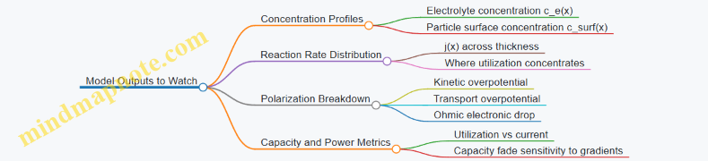
Practical Modeling Workflow
- Choose \(L\), porosity, tortuosity, and particle radius \(R_p\) from the formulation.
- Set \(D_{\text{eff}}\) and \(D_s\) from measured or literature-calibrated values, then run a baseline current.
- Solve for \(c_e(x)\) and \(c_{s,\text{surf}}(x)\), then compute \(j(x)\) using the interfacial kinetics.
- Repeat for multiple \(L\) values and compare \(j(x)\) shape and polarization contributions.
- Use the results to identify whether thickness is limited by pore transport, particle diffusion, or electronic conduction, based on which term dominates the overpotential map.
This approach turns thickness from a “bigger is better” knob into a measurable design variable: you can see where the electrode stops being fully used and quantify how much voltage penalty comes from transport distance.
8.4 Diagnostic Testing Using EIS GITT and Incremental Capacity Analysis
Diagnostic testing is where you stop guessing which step limits performance. Electrochemical Impedance Spectroscopy (EIS) tells you where resistance and interfacial losses sit at a given operating point. Galvanostatic Intermittent Titration Technique (GITT) maps how diffusion and polarization evolve with current pulses. Incremental Capacity Analysis (ICA) turns voltage–capacity curves into a set of peaks that correspond to changing processes during charge or discharge. Used together, they form a practical “triangulation” workflow: EIS for where losses live, GITT for how transport behaves, and ICA for how processes shift with state of charge.
Mind Map: Diagnostic Testing Workflow
EIS: What You Measure and How to Read It
EIS applies a small AC perturbation around a steady DC operating point. The key is to keep the perturbation small enough that the cell stays near its linear response. A typical workflow starts by selecting a state of charge where you want diagnosis—say, mid-discharge where polarization is noticeable but not extreme. Then you run a frequency sweep, often from high kHz down to mHz, and fit the spectrum to an equivalent circuit.
A common starting circuit for sodium-ion cells includes: an ohmic resistance (current collector, electrolyte bulk), a charge transfer resistance with a parallel constant phase element (CPE) to represent non-ideal interfacial capacitance, and a diffusion-related element that captures frequency-dependent mass transport. If you see the high-frequency intercept increase after cycling, that points to growing ohmic losses such as electrolyte degradation or contact resistance. If the mid-frequency semicircle grows, charge transfer limitations are likely worsening—often tied to interphase thickening or loss of active surface contact.
Example: Suppose a fresh cell and a cycled cell are tested at the same temperature and state of charge. The cycled cell shows a larger high-frequency intercept and a larger mid-frequency arc. The first suggests increased bulk/contact resistance; the second suggests slower interfacial kinetics. If the low-frequency tail also becomes more pronounced, diffusion limitations are likely contributing, not just surface effects.
GITT: Turning Relaxation into Transport Information
GITT alternates current pulses with relaxation periods. During the pulse, the cell polarizes; during relaxation, voltage relaxes toward a quasi-equilibrium value. The diffusion coefficient is not measured directly, but you can compute a proxy from how the relaxation voltage changes with time and current.
A systematic approach is to keep pulse duration and current density consistent across tests. Use short pulses early in the diagnostic process to avoid large state-of-charge drift. Then ensure relaxation is long enough to observe a meaningful voltage recovery; otherwise, you will confuse incomplete relaxation with genuine diffusion slowdown.
Example: If after cycling the relaxation curve shows the same initial polarization but a slower recovery, the diffusion-related limitation is more likely. If recovery is fast but the pulse polarization is higher, charge transfer or ohmic contributions are more likely. This distinction matters because EIS can tell you “where resistance is,” while GITT helps you decide “what transport step is slowing down.”
Incremental Capacity Analysis: Peaks as Process Markers
ICA uses a smooth derivative of voltage with respect to capacity. For a discharge curve, you compute dQ/dV or dV/dQ after resampling to uniform capacity increments. Peaks and shoulders correspond to changes in reaction mechanism, phase transitions, or shifts in polarization contributions as state of charge changes.
To keep ICA from becoming a noise amplifier, you smooth the derivative using a controlled window and apply the same processing settings to all datasets. Then compare peak positions and peak widths between fresh and aged cells.
Example: If a peak shifts to lower voltage during discharge and broadens, it often indicates increased polarization and/or altered reaction pathways. If peak height drops while peak position stays nearly constant, the process may still occur at similar potentials but with reduced reversibility or active utilization.
Integration: Making the Three Methods Agree
The most useful diagnostic outcome is a consistent story across methods.
- If EIS shows increased charge transfer resistance and ICA peaks broaden without major changes in diffusion proxy from GITT, the dominant issue is likely interfacial kinetics and active surface availability.
- If GITT diffusion proxy worsens and ICA peaks shift in a way consistent with stronger concentration polarization, diffusion or transport through pores and electrodes is likely limiting.
- If EIS ohmic resistance rises and ICA shows overall voltage offset with minimal peak shape change, contact resistance or bulk conductivity issues are likely.
Practical Checklist for Reliable Diagnostics
- Match temperature and state of charge across EIS, GITT, and ICA runs.
- Use consistent current magnitudes and pulse durations.
- Keep EIS perturbation small and verify linearity by checking repeatability.
- Process ICA derivatives with identical smoothing parameters.
- Fit EIS using the same circuit structure across datasets, then interpret parameter trends rather than chasing perfect fits.
When these steps are followed, EIS, GITT, and ICA stop being three separate plots and start acting like a single diagnostic instrument—each method answering a different question, with the combined result pointing to the actual limiting step.
8.5 Interpreting Data to Identify Limiting Steps in Cells
Interpreting battery data is mostly about asking one question: which physical process is slowest under the test conditions? In sodium-ion cells, the “slowest step” can shift between charge transfer at interfaces, sodium transport through electrolyte and porous electrodes, and structural or interfacial evolution during cycling. The trick is to use multiple diagnostics that each emphasize different bottlenecks, then cross-check them.
Start with a Test Map
Before touching plots, write down what each test is designed to stress.
- Rate tests (varying current) highlight transport limits and kinetic limits.
- Temperature sweeps separate thermally activated processes from purely resistive ones.
- EIS separates ohmic resistance from charge-transfer and diffusion-related contributions.
- GITT (current pulses with relaxation) isolates diffusion-like behavior.
- Incremental capacity and voltage relaxation reveal how polarization evolves with state of charge.
A practical workflow is: pick one representative formation-aged cell, run a baseline EIS at a few states of charge, then perform a rate ladder at the same states. If the limiting step changes with state of charge, you will see it as a consistent pattern across these measurements.
Mind Map: Limiting Steps from Measured Signatures
Use EIS Like a Map, Not a Mystery Box
EIS is most useful when you connect each frequency region to a process.
- High-frequency intercept approximates ohmic resistance (current collectors, electrolyte bulk, and contact resistances). If this term dominates, improving conductivity and contact quality helps more than changing electrode chemistry.
- Mid-frequency semicircle often corresponds to charge transfer plus some interfacial effects. If it grows with current or temperature sensitivity is high, charge transfer is likely limiting.
- Low-frequency tail is commonly associated with diffusion and/or distributed relaxation in porous electrodes and active material. If the tail changes strongly with state of charge or rate, diffusion-related limitations are likely.
Example: Suppose you run EIS at 20%, 50%, and 80% state of charge and fit a simple equivalent circuit. You observe that the high-frequency intercept is nearly constant across SOC, but the mid-frequency semicircle increases sharply near 80% SOC. Then a rate ladder shows the largest capacity loss at high SOC. The consistent pairing points to charge transfer limitation near high SOC, not bulk resistance.
Combine Rate Tests with Temperature Tests
A clean separation comes from temperature.
- If polarization decreases modestly with temperature and scales mostly with current, ohmic and geometric factors dominate.
- If polarization drops significantly at higher temperature and the fitted kinetic resistance decreases, charge transfer and interfacial kinetics dominate.
Example: Two cells have similar EIS high-frequency intercepts. Cell A shows a strong reduction in mid-frequency resistance when temperature rises from 10°C to 30°C, while Cell B barely changes. In a rate ladder, Cell A maintains higher capacity at high current. You can reasonably attribute the performance gap to kinetic limitation rather than electrolyte bulk resistance.
Use GITT to Estimate Whether Diffusion Is the Bottleneck
GITT provides apparent diffusion-like behavior by comparing voltage response during current pulses and relaxation.
- If the voltage during pulses shows large polarization and relaxation does not recover quickly, diffusion-related limitations are likely.
- If relaxation nearly returns to the baseline and pulse polarization is small, diffusion is probably not the dominant limit.
Example: During a GITT pulse at a fixed SOC, Cell C shows a long relaxation tail and a lower apparent diffusivity estimate than Cell D. In the rate ladder, Cell C loses capacity faster as current increases. The agreement across two tests supports diffusion limitation as the controlling step.
Track Aging to Separate “Today’s Limit” From “Tomorrow’s Problem”
Instantaneous limits can be different from aging mechanisms. To interpret degradation data, compare EIS and diagnostic curves before and after cycling.
- If the mid-frequency feature grows while the high-frequency intercept stays stable, aging is likely driven by interfacial layer thickening or kinetic degradation.
- If the high-frequency intercept grows, focus on contact degradation, electrolyte depletion, or increasing bulk resistance.
- If incremental capacity peaks shift and broaden, it often indicates changing reaction pathways or evolving phase behavior in the active materials.
Example: After 200 cycles, Cell E shows a larger low-frequency tail and reduced relaxation recovery, while the mid-frequency semicircle changes little. That pattern suggests transport limitations worsening, such as pore clogging or diffusion path changes, rather than a sudden loss of charge transfer capability.
A Practical Decision Checklist
When you need a single conclusion, use this order:
- Does voltage drop scale linearly with current? If yes, start with ohmic loss.
- Does EIS mid-frequency resistance dominate and vary with SOC? If yes, charge transfer is likely limiting.
- Does low-frequency behavior worsen with rate and SOC? If yes, diffusion/transport is likely limiting.
- Do these features change with cycling? If yes, identify which process is aging.
If you follow the checklist and the evidence points to different steps in different SOC regions, that is not a contradiction. It means the cell has multiple limiting regimes, and engineering choices should target the worst-case region under the intended operating profile.
9. Thermal Management and Safety Engineering
9.1 Heat Generation Sources And Temperature Rise Calculations
Heat in a sodium-ion cell is mostly the byproduct of electrical losses and chemical irreversibilities. Temperature rise then depends on how that heat moves through electrodes, electrolyte, casing, and surrounding air or coolant. The engineering job is to connect these two parts with numbers you can actually measure.
Heat Generation Sources
Start with the cell-level power balance. During charge or discharge, the electrical power input or output is not fully converted into useful work. The remainder becomes heat.
-
Ohmic heating
- Origin: ionic resistance in electrolyte and separator, electronic resistance in electrodes and current collectors.
- Simple model: \(Q_{ohm} \approx I^2 R\), where \(I\) is current and \(R\) is effective resistance at the operating temperature.
- Example: If \(I=20,A\) and \(R=15,m\Omega\), then \(Q_{ohm}=20^2\times0.015=6,W\).
-
Charge-transfer and interfacial heating
- Origin: overpotentials from reaction kinetics at electrode interfaces.
- Simple model: \(Q_{rxn} \approx I,\eta\), where \(\eta\) is the average overpotential.
- Example: If average overpotential is \(0.12,V\) at \(20,A\), then \(Q_{rxn}=20\times0.12=2.4,W\).
-
Entropic heating or cooling
- Origin: the reversible heat term tied to the entropy change with state of charge.
- Simple model: \(Q_{rev} = I,T,\frac{\partial U}{\partial T}\), where \(\frac{\partial U}{\partial T}\) is the entropic coefficient.
- Example: If \(\frac{\partial U}{\partial T}=-0.3,mV/°C\), \(I=20,A\), \(T=298,K\), then the sign indicates whether the process cools or heats. Use the sign carefully; it can partially offset other heat terms.
-
Side reactions and gas generation
- Origin: electrolyte decomposition, SEI growth, and any parasitic reactions.
- Practical approach: treat this as an additional heat fraction when you have post-test evidence (gas volume, impedance growth, capacity loss). For engineering calculations, you can bound it using measured coulombic inefficiency and additional resistance growth.
Temperature Rise Modeling
Once you have heat generation \(Q\) in watts, temperature rise follows from thermal resistance and heat capacity.
Steady-state estimate
- \(\Delta T = Q,R_{th}\), where \(R_{th}\) is thermal resistance from cell internal heat generation to the ambient or coolant.
- Example: If total heat is \(Q=8.4,W\) and \(R_{th}=2.0,K/W\), then \(\Delta T=16.8,K\).
Transient estimate
- Use a lumped thermal capacitance model: \(C_{th}\frac{d(\Delta T)}{dt} = Q - \frac{\Delta T}{R_{th}}\).
- The time constant is \(\tau = R_{th}C_{th}\). After about \(3\tau\), the temperature approaches steady state.
- Example: If \(R_{th}=2.0,K/W\) and \(C_{th}=500,J/K\), then \(\tau=1000,s\). A 30-minute test is long enough to nearly reach steady state.
Practical Calculation Workflow
- Choose the operating point: current profile, state of charge range, and ambient temperature.
- Compute heat terms: \(Q=Q_{ohm}+Q_{rxn}+Q_{rev}+Q_{parasitic}\). If you lack \(\frac{\partial U}{\partial T}\), start with \(Q_{ohm}+Q_{rxn}\) and later refine.
- Use measured resistance: estimate \(R\) from pulse tests or impedance at the same temperature.
- Select thermal path: determine \(R_{th}\) from a controlled heating test or calibrated thermal model.
- Check consistency: verify that predicted \(\Delta T\) matches thermocouple trends during a representative load.
Mind Map: Heat and Temperature Rise
Example: One Discharge Segment with Numbers
Assume a discharge segment at \(I=20,A\) with effective resistance \(R=15,m\Omega\), average overpotential \(\eta=0.12,V\), and entropic heating that is small enough to ignore for a first pass.
- \(Q_{ohm}=6,W\)
- \(Q_{rxn}=2.4,W\)
- Total \(Q\approx 8.4,W\)
If the cell-to-ambient thermal resistance is \(R_{th}=2.0,K/W\), then \(\Delta T\approx 16.8,K\). If ambient is \(25°C\), the predicted cell temperature is about \(42°C\) after reaching near steady state. If the segment is short compared to \(\tau\), the peak temperature will be lower; use the transient model to avoid overestimating stress.
Example: When the Sign of Entropic Heat Matters
If \(\frac{dU}{dT}\) is negative during discharge, \(Q_{rev}\) can reduce net heating. In practice, you still compute \(Q_{ohm}+Q_{rxn}\) first, then add \(Q_{rev}\) with the correct sign. This prevents the common mistake of treating all heat terms as always positive, which can lead to overly conservative thermal limits.
9.2 Thermal Conductivity Interfaces and Module Layout Choices
Thermal design starts with a simple question: where does heat go after it is generated inside the cell? In sodium-ion modules, the answer is rarely “straight through.” Heat must cross multiple interfaces—electrode stack to can, can to tab, tab to busbar, busbar to housing, and housing to whatever cooling path you use. Each interface adds thermal resistance, and the layout determines how much contact area you get, how consistently you press it, and how easily heat can spread laterally.
Interface Fundamentals That Matter in Practice
Thermal conductivity of bulk materials is only part of the story. At interfaces, the effective thermal resistance is dominated by contact quality: surface roughness, flatness, oxide films, voids, and the stability of pressure over time. Two modules can use the same aluminum baseplate and still behave differently if one has better clamping force distribution or a more forgiving stack-up tolerance.
A useful mental model is to treat each interface as a “thermal bottleneck.” If you reduce one bottleneck, the next one becomes the limiting step. That is why module layout choices—clamp paths, spacer thickness, and where you place thermal pads—must be made together with interface materials.
Choosing Thermal Paths with Module Layout
A module layout should create at least two heat spreading routes: one through the primary baseplate and another through lateral conduction to nearby cells. If you place cells in a tight grid but only connect heat to the baseplate at a few points, you create hot spots near those points and underutilize the rest of the metal.
Start with the heat generation map. Even without detailed electrochemical modeling, you can approximate where heat is likely to concentrate: near current collectors and tabs, and in cells that experience higher current due to wiring resistance or balancing behavior. Layout then decides whether you route cooling to the hottest region directly or spread heat first and cool second.
Contact Engineering for Reliable Thermal Interfaces
Thermal pads and greases can help, but they must be applied with the right assumptions. Pads fill voids, but they also add thickness, which increases conduction distance. Greases reduce void effects, but they can pump out under vibration or thermal cycling if the clamping pressure is not stable.
The most robust approach is usually a controlled stack-up: define the mechanical thicknesses so that clamping force reaches the intended level, and use interface materials that tolerate small variations. For example, if your cell-to-base contact relies on a single bolt per cell, the local pressure can be high while adjacent areas remain poorly contacted. A busbar-to-base design that uses a continuous clamping bar can improve uniformity.
Practical Example Layout with Two Interface Strategies
Consider a module with 12 prismatic cells arranged in a 3×4 grid on an aluminum baseplate.
Strategy A: Point Cooling. You place thermal pads only under the busbar region and clamp with four corner bolts. Heat spreads well near the busbar but poorly under the middle cells. In thermal tests, the center cells show higher peak temperature because their heat must travel laterally through the baseplate before reaching the cooled zones.
Strategy B: Distributed Spreading. You place thin thermal pads under the full cell footprint and use a perimeter clamp plus a mid-span stiffener so pressure is more uniform. Peak temperature drops because heat crosses interfaces over a larger area, and the baseplate spreads heat before it reaches the cooling plate.
Both strategies can work, but Strategy B reduces sensitivity to small manufacturing variations. It also makes the thermal design less dependent on one “perfect” contact spot.
Mind Map: Thermal Interfaces and Layout Decisions
Engineering Checks That Close the Loop
After you choose interface materials and layout, verify with measurements that isolate interface effects. Use a temperature map with sensors placed consistently on multiple cells, not just near the cooling boundary. Then vary clamping torque within the allowed tolerance range and observe whether temperature differences track with contact quality. If small torque changes cause large temperature shifts, your interface design is too sensitive.
Finally, confirm that your layout supports both thermal and electrical assembly. A design that improves thermal contact but forces awkward electrical clearances can lead to inconsistent clamping or added spacers, which quietly increases thermal resistance again. Good module layout is the one that keeps the mechanical stack-up stable while giving heat a short, wide path to the cooling surface.
9.3 Overcharge Overdischarge and Short Circuit Protection Design
Protection design starts with three “what can go wrong” events: charging too far, discharging too far, and current surges from wiring or internal faults. For sodium-ion cells, these events matter because interfacial layers and electrode structures are sensitive to voltage extremes, and short circuits turn chemical energy into heat fast.
Foundational Protection Targets
Set protection thresholds using cell-level test data, not guesses. Define:
- Overcharge limit as a maximum cell voltage that avoids accelerated cathode degradation and excessive electrolyte oxidation.
- Overdischarge limit as a minimum cell voltage that avoids deep anode depletion and unstable interphase growth.
- Short-circuit response as a maximum allowable current and a maximum time-to-interruption that keeps cell temperature within safe bounds.
A practical engineering move is to include margin bands: for example, trigger control at a conservative voltage, then rely on a secondary cutoff if the first stage fails. This two-step approach reduces the chance that a single sensor error causes a bad day.
Protection Architecture Overview
Use layered protection so that no single component must be perfect.
- Primary control: the Battery Management System (BMS) monitors voltage and current and commands charge/discharge enable.
- Secondary cutoff: independent hardware (often a fuse and/or a hardware cutoff switch) that trips if the BMS misses a condition.
- Fault interruption: a contactor, solid-state switch, or fuse designed to open under the expected fault current.
The key is coordination: the BMS should act quickly enough to prevent reaching the hardware trip region, while the hardware trip should be fast enough to prevent thermal runaway from a sustained short.
Voltage-Based Overcharge and Overdischarge
Voltage limits must be applied to the correct measurement points. In a pack, cell voltages are not identical, so you protect using the most extreme cell (highest for overcharge, lowest for overdischarge).
A systematic approach:
- Sense each cell voltage with adequate resolution and filtering.
- Validate readings by checking plausibility (e.g., no sudden jumps inconsistent with current).
- Apply hysteresis so the system doesn’t chatter around the threshold.
- Use time qualification so brief spikes don’t cause unnecessary shutdown.
Example: Suppose the overcharge trigger is set at 3.80 V per cell with a 10 s qualification and 3.75 V release. If a cell rises above 3.80 V for 10 s while charging, the BMS stops charge and opens the charge path. If the spike lasts only 1 s, the qualification prevents a shutdown.
For overdischarge, the same logic applies, but the release point should be higher than the trigger to avoid repeated cycling at the edge. Also consider that voltage sag under load can mimic low state; use current-aware filtering or sample during low-current windows when feasible.
Current-Based Short Circuit Protection
Short circuits are about current and time, not just voltage. A short can be external (wiring) or internal (cell failure). Your design should handle both with the same principle: limit energy delivered during the fault.
Use a three-part strategy:
- Detect: measure pack current with a sensor that can survive fault conditions and has enough bandwidth.
- Interrupt: open the current path using a device rated for the fault current.
- Limit energy: ensure the interrupt time keeps the integral of current-squared over time within safe bounds for the cell and interconnects.
Example: If the maximum prospective fault current is 800 A and the interrupt device clears in 5 ms, the energy stress is far lower than if clearing takes 50 ms. Even without exact thermal modeling, the time-to-open dominates.
Coordination with Fuses and Switching Devices
Fuses and switches must be selected as a coordinated set. A fuse that clears quickly for a hard short may still be too slow for a moderate fault that persists. Conversely, a switch that opens fast might not handle the fault current without arcing control.
A common coordination pattern:
- Fuse protects against catastrophic faults and provides a last-resort open.
- Contactor or solid-state switch provides fast interruption under detected abnormal current.
- BMS logic reduces the chance the system ever reaches the fuse’s operating region.
To keep this practical, specify device ratings using the worst-case pack voltage, maximum current, and expected fault duration from your mechanical and electrical layout.
Mind Map: Protection Design Flow
Example: Coordinated Thresholds and Actions
Assume a 16-cell series string. The BMS monitors each cell and controls a charge contactor.
- Overcharge: trigger at 3.80 V/cell for 10 s; release at 3.75 V/cell.
- Overdischarge: trigger at 2.60 V/cell for 5 s; release at 2.70 V/cell.
- Short circuit: if current exceeds 600 A for 2 ms, open the charge/discharge switch immediately; if current persists beyond the switch capability, the fuse clears.
During a test, you verify that the most extreme cell crosses thresholds only when expected, that qualification filters ignore brief spikes, and that the switch clears within the required time window.
Validation Checklist
- Threshold correctness: confirm limits match cell test behavior under realistic charge/discharge rates.
- Timing correctness: verify qualification windows with oscilloscope captures of sensor signals and switch actuation.
- Sensor robustness: confirm behavior under open-wire or stuck-sensor conditions using defined safe states.
- Fault interruption: test with representative fault currents and confirm the system reaches a stable safe state after interruption.
A well-designed protection system behaves predictably: it stops charging or discharging when limits are truly exceeded, and it interrupts short circuits quickly enough that heat generation stays within what the design can tolerate.
9.4 Abuse Testing Protocols for Mechanical and Electrical Events
Abuse testing checks whether a sodium-ion cell or module survives realistic mistakes and hard failures without turning them into a chemistry lesson. The goal is not to “see what happens,” but to verify that mechanical integrity and electrical protection work together under stress.
Foundations for Mechanical and Electrical Abuse
Start by defining what counts as mechanical abuse versus electrical abuse. Mechanical events include drop impacts, vibration, crush, tab bending, and separator deformation from swelling. Electrical events include short circuits, overcharge, overdischarge, reverse polarity, and insulation breakdown.
A useful protocol ties each event to a measurable outcome. For mechanical events, outcomes include loss of capacity, rise in internal resistance, separator damage indicators, and evidence of current collector deformation. For electrical events, outcomes include voltage collapse behavior, temperature rise rate, current limiting effectiveness, and post-test leakage or insulation failure.
Mind Map: Abuse Testing Coverage
Mechanical Abuse Protocols with Integrated Checks
Drop and impact. Use a repeatable drop height and orientation so the impact energy is comparable across lots. Mount the cell or module in a fixture that reflects real installation stiffness. After each impact, perform a quick electrical sanity check: open-circuit voltage stability, a short pulse resistance measurement, and a low-rate charge/discharge to confirm no immediate runaway-like behavior.
Vibration and rattle. Choose a vibration profile that stresses mounting and internal connections rather than just shaking the outside. Verify fastener torque before and after. During vibration, monitor for intermittent electrical contact by logging current noise during a small, controlled load. If the system supports it, add strain or displacement sensors near the tabs to catch bending before it becomes a short.
Crush and bending. Apply controlled compressive force and record force versus displacement. The key is to stop at a defined limit that represents worst-case handling or transport abuse, not random destruction. Afterward, inspect for separator deformation signs during teardown and correlate them with electrical changes such as increased resistance growth during a short cycling window.
Electrical Abuse Protocols with Protection Verification
External short circuit. Define the short resistance using a calibrated conductor or resistor so the event is repeatable. Start with a conservative current path that represents a plausible fault, then test higher severity only if the protection design is validated at lower severity. Log voltage collapse timing and temperature rise rate at multiple locations. A good protocol checks whether the protection triggers fast enough to prevent sustained high temperature.
Overcharge and overdischarge. Use BMS cutoff thresholds and verify they are consistent with cell-level limits. Test both “cutoff works” and “cutoff fails” scenarios in a controlled manner. For the failure scenario, the protocol should still include a hard stop based on temperature or current so the test ends before uncontrolled conditions.
Reverse polarity and miswiring. Simulate miswiring with a controlled polarity swap and include protection components in the test path. Monitor for weld heating and abnormal current spikes. After the event, confirm whether the cell can return to safe operation under normal charge limits or whether it shows permanent resistance increase.
Insulation and ground fault. Apply dielectric withstand tests and then perform a leakage current check under representative voltage. Mechanical deformation can reduce insulation margins, so pair insulation checks with at least one mechanical abuse condition to ensure the combined stress doesn’t create a hidden failure mode.
Instrumentation and Decision Rules
Use temperature sensors at locations that represent likely hot spots: near current collectors, tab regions, and the geometric center of the cell. Pair them with high-speed voltage and current logging so you can separate “fast electrical failure” from “slow thermal runaway-like progression.”
Acceptance criteria should be explicit. For example: no venting, no sustained current after protection trigger, no insulation breakdown beyond a defined leakage threshold, and no catastrophic resistance increase after a short post-test cycling window.
Example: Short Circuit Event Protocol
Setup. Place the cell in a fixture that prevents movement, connect a calibrated short path, and arm the data logger for voltage, current, and three temperature points.
Procedure. Apply the short for a defined maximum duration or until a temperature limit is reached. Record the time to protection action and the peak temperature.
Post-test. Measure open-circuit voltage, perform a low-rate resistance check, and run a short cycling window to confirm whether the event caused permanent performance loss.
Example: Crush Followed by Electrical Stress
Setup. Apply a controlled crush displacement to the module while recording force. Then run an electrical stress test such as a short pulse charge/discharge to detect resistance growth.
Procedure. If resistance rises sharply or temperature spikes during the electrical check, stop and proceed to teardown inspection for separator deformation and current collector contact changes.
Safety-First Execution Without Guesswork
Define stop conditions for every test: maximum temperature, maximum force, maximum time, and maximum allowable leakage. Ensure the test environment includes containment measures appropriate to the cell format. The protocol should be written so a different engineer can run it and get comparable results, even if they are less enthusiastic about the “abuse” part of the name.
9.5 Safety Validation Documentation and Failure Mode Traceability
Safety validation is only useful if someone else can follow your logic later—during a design review, an audit, or a post-incident investigation. This section builds a documentation workflow that ties hazards to tests, tests to acceptance criteria, and results back to specific failure modes.
Safety Documentation Foundations
Start with a single safety case document that references three core artifacts: (1) a hazard register, (2) a verification matrix, and (3) a failure mode traceability record. The hazard register lists credible hazards such as thermal runaway, venting with flame, electrical shock, and toxic decomposition products. The verification matrix maps each hazard to one or more tests and measurable pass/fail criteria. The traceability record links each test outcome to the failure modes that could explain it.
A practical habit: write acceptance criteria in the same units you will measure. For example, “no sustained flame longer than 10 s” is more actionable than “no fire.” Likewise, “cell temperature rise rate below X °C/min during abuse” is easier to compare across lots than “temperature stays low.”
Failure Mode Traceability Workflow
Use a structured chain: requirement → hazard → failure mode → test method → observable → criterion → evidence. Failure modes should be specific enough to guide investigation. Instead of “electrolyte failure,” use “electrolyte decomposition due to separator shrinkage under compression” or “SEI breakdown leading to rapid resistance growth.”
When you run tests, record evidence that supports the chain. Evidence includes instrument settings, sampling rates, sensor placement, environmental conditions, and the exact test termination logic. If a test ends early due to a safety interlock, document the reason and what that implies for coverage.
A simple traceability example: if a short-circuit test shows rapid voltage collapse and a temperature spike, you trace it to failure modes involving current collector contact, separator puncture, or internal dendrite-like pathways. Then you check whether the documentation includes separator integrity checks, stack pressure logs, and post-test microscopy notes.
Mind Map: Safety Validation Documentation
Mind Map: Failure Mode to Evidence Mapping
Example: Traceability Entry for an Abuse Test
Below is a compact template for a single verification record. It is intentionally boring: boring is what makes it auditable.
- Hazard: External short circuit leading to thermal runaway
- Failure Mode: Separator puncture from current collector burr
- Test Method: External short at specified resistance and duration
- Observable: Cell voltage collapse time and peak temperature
- Criterion: Peak temperature below limit; no sustained flame
- Evidence: Raw voltage and thermocouple data; post-test inspection photos
- Traceability Links: Design requirement ID; manufacturing burr control spec ID
Documentation Integrity Checks
Before sign-off, run three consistency checks. First, confirm every hazard has at least one verification path; “we think it’s unlikely” is not a verification method. Second, confirm every acceptance criterion is measurable with your instrumentation and sampling rate. Third, confirm the evidence folder contains the raw data, not only summary plots.
For traceability, require a one-to-many mapping: a single failure mode can explain multiple observables, but each observable must map back to at least one failure mode. If an observable cannot be mapped, treat it as a documentation gap and either add a failure mode hypothesis or refine the test instrumentation.
Date-Stamped Review Cadence
Use a consistent review cadence so safety documentation evolves with manufacturing changes. For example, perform a formal safety documentation review on 2026-03-01 after design freezes and again after any process change that affects electrode coating, separator handling, or stack pressure control. Each review should record what changed, what tests were rerun, and which traceability links were updated.
10. Cycling Performance Degradation and Failure Analysis
10.1 Capacity Fade Mechanisms in Sodium Storage Systems
Capacity fade is the slow loss of usable charge after repeated cycling. In sodium-ion cells, it usually comes from a few recurring themes: the active material becomes less accessible, the interfaces consume reactants, and transport becomes harder as internal resistance grows. The trick is to connect each symptom you measure—capacity drop, voltage hysteresis growth, and increased polarization—to the specific physical process causing it.
Foundational Capacity Accounting
A cell’s delivered capacity depends on how much of the cathode and anode can reversibly host sodium during charge and discharge. If the cathode loses reversible sodium sites, or the anode forms a thicker inactive interphase, the “available inventory” shrinks. If sodium can’t move fast enough through electrolyte and within particles, the cell may still have inventory, but it cannot access it within the test window.
A practical engineering way to separate these effects is to compare three quantities over cycle number: (1) discharge capacity at a fixed current, (2) charge capacity at the same current, and (3) voltage profiles. When charge capacity rises while discharge capacity falls, losses are dominated by irreversible consumption or growing overpotentials. When both charge and discharge capacities fall together, active material loss or loss of accessible sites is more likely.
Mind Map: Capacity Fade Root Causes
Cathode-Driven Capacity Fade
Cathodes can lose reversible capacity when sodium storage sites become less usable. In many sodium-ion cathodes, repeated cycling can trigger surface reconstruction or gradual loss of structural integrity. A common engineering signature is a growing separation between charge and discharge voltages at the same state of charge, because polarization increases as the surface becomes less reactive.
Particle cracking is another frequent contributor. When particles fracture, fresh surfaces form and react with electrolyte, which consumes sodium and builds interphases. Even if the bulk material remains intact, the newly created surfaces are often electrochemically “expensive,” so the cell spends more charge to achieve the same sodium insertion.
Anode-Driven Capacity Fade
Hard carbon anodes typically fade through interphase growth and loss of effective sodium storage. As cycling proceeds, the solid electrolyte interphase thickens and becomes less conductive, which increases the voltage needed to drive the same current. Over time, some pores and near-surface regions become clogged or less accessible, reducing the fraction of sodium that can reversibly cycle.
A useful diagnostic is to look for increasing irreversible capacity during the early part of cycling. If the first few tens of cycles show a steep decline, interphase formation and electrolyte decomposition are likely dominating. If the decline is slower and correlates with increasing polarization, transport and contact loss become more prominent.
Irreversible Sodium Consumption and Interphase Growth
Capacity fade is not only about losing active material; it is also about losing sodium to side reactions. Electrolyte decomposition at electrode surfaces consumes sodium and forms products that do not participate in reversible storage. This reduces the coulombic efficiency and gradually shifts the cell’s operating balance.
A concrete example: if a cell is cycled at a moderate current but at a higher upper cutoff voltage, the cathode surface sees stronger driving forces for side reactions. The result is often a faster capacity fade even when the cathode’s nominal capacity is unchanged. The cell’s voltage profile will typically show increased hysteresis, reflecting thicker interphases and higher reaction resistance.
Transport Limitations and “Accessible Capacity”
Even when active material remains, capacity can drop because sodium ions and electrons struggle to reach reaction sites. Thicker interphases increase ionic resistance, while contact loss between particles and the current collector increases electronic resistance. Both effects reduce utilization at practical charge/discharge rates.
An easy-to-understand test logic is rate sensitivity. If capacity loss is much worse at higher current than at lower current, transport limitations are likely a major contributor. If capacity loss is similar across rates, active material loss and irreversible consumption are more dominant.
Systematic Engineering Controls
Capacity fade is easier to manage when you control the stressors that accelerate each mechanism. Keep cycling within a reasonable state-of-charge window to reduce interphase growth. Avoid excessive upper cutoff voltage that increases cathode side reactions. Use formation protocols that build stable interphases without overreacting the electrolyte.
Finally, treat electrode balance as a first-class design variable. If the anode is undersized relative to the cathode, interphase growth consumes sodium faster than the anode can replenish it, and capacity fade accelerates. If the anode is oversized, the cathode may reach its limits sooner, also reducing utilization. Balanced capacity helps keep the cell operating where both electrodes remain in their most reversible regimes.
Example: Interpreting a Capacity Fade Pattern
Suppose a cell shows a steady capacity decline from 100% to 85% over 200 cycles, while coulombic efficiency stays near 99.5% after the first 20 cycles. The early drop suggests initial interphase formation, but the later steady decline points to gradual active site loss or increasing transport resistance rather than runaway irreversible consumption. If voltage hysteresis grows in parallel, interphase thickening and contact loss are likely the main drivers. If hysteresis stays stable but capacity still falls, accessible active sites in one electrode are being lost more directly.
10.2 Power Fade Mechanisms Including Resistance Growth
Power fade shows up as a cell that can no longer deliver the same current at the same voltage. In sodium-ion cells, the most common root cause is resistance growth, which turns “can do” into “can’t without a bigger voltage penalty.” Resistance growth is not one thing; it’s a bundle of contributors that add up during cycling.
Foundational View of Voltage Loss Under Load
When you draw current, the measured voltage drops due to several terms:
- Ohmic drop: current times bulk resistance of electrolyte, electrodes, and current collectors.
- Interfacial polarization: extra overpotential from charge-transfer limits and surface film behavior.
- Mass-transport limits: additional overpotential when sodium concentration gradients build up.
Power fade is often diagnosed by comparing voltage at a fixed state of charge and temperature across cycles. If the voltage sag increases with cycling, resistance growth is usually involved.
Mind Map: Resistance Growth Pathways
Ohmic Resistance Increase
Ohmic resistance rises when the pathways for ions and electrons become less effective. A practical example: imagine an electrode that initially wets well with electrolyte. After many cycles, interfacial films consume electrolyte and the remaining liquid struggles to maintain uniform wetting. The cell still has electrolyte, but the effective conductivity through pores drops.
Another contributor is contact resistance. Electrode stacks compress during assembly, but cycling can relax pressure slightly. Even a small increase in contact resistance between active material and current collector can noticeably increase voltage loss at higher currents.
A simple engineering check is to compare resistance inferred from current interruption tests at the same temperature and similar state of charge. If the resistance jump is larger at higher current, ohmic components are likely growing.
Interfacial Resistance Increase
Interfacial resistance is where “film growth” does most of its damage. On the anode side, sodium-ion cells form a passivation layer that limits further electrolyte decomposition. Over time, that layer can thicken or become less permeable, increasing impedance.
On the cathode side, surface films can also grow, especially when the cathode experiences repeated high-voltage exposure. The key mechanism is not just thickness; it’s also active area loss. If particles crack, the surface area may increase initially, but the electrically connected fraction can decrease later, leaving parts of the cathode that are electrochemically isolated.
A concrete example: during cycling at moderate current, a cathode may maintain capacity, but the voltage at the end of discharge becomes progressively lower. That pattern often indicates interfacial resistance growth rather than immediate loss of total lithium inventory.
Charge-Transfer Resistance Increase
Charge-transfer resistance reflects how easily sodium ions and electrons cross the electrode surface. Even if the bulk conductivity stays stable, kinetics can slow when surface chemistry changes. For instance, if the passivation layer becomes more resistive, the same current requires a larger overpotential.
This is why two cells with similar capacity fade can show very different power fade. Capacity depends on how much active material remains usable; power depends on how quickly it can be used.
Transport Resistance Increase
Transport resistance grows when ionic movement through the electrode and separator becomes harder. Pore blockage can occur as films accumulate inside the electrode microstructure. The result is a longer effective path for ions and a higher concentration gradient during current draw.
A helpful diagnostic is to run a set of constant-current discharges at different C-rates. If the voltage curves separate more at higher C-rate as cycling progresses, transport limitations are becoming more dominant.
How to Measure and Separate Contributors
Use a systematic test sequence:
- Fix temperature and state of charge for comparisons.
- Track voltage polarization at a constant current across cycles.
- Run EIS at the same conditions to separate bulk, interfacial, and charge-transfer contributions.
- Correlate EIS growth with the current-rate dependence of voltage sag.
If EIS shows a strong increase in the high-frequency intercept, bulk/ohmic effects dominate. If the mid-frequency semicircle grows, interfacial/charge-transfer effects dominate. If low-frequency features expand, transport limitations are likely increasing.
Example: Interpreting a Power Fade Signature
Suppose a cell maintains 80% of its capacity after 300 cycles, but its 1C discharge voltage drops by an additional 120 mV compared with cycle 1. EIS at the same state of charge shows the bulk resistance increased by 10 mΩ, while the interfacial semicircle resistance increased by 25 mΩ. The most likely explanation is interfacial film growth and/or loss of effective active area, not a sudden loss of sodium inventory.
A second example: if the voltage penalty is small at 0.2C but large at 2C, and EIS low-frequency impedance rises, transport resistance is likely the main driver. That points to pore blockage or reduced effective ionic conductivity rather than purely contact issues.
Engineering Practices That Reduce Resistance Growth
- Maintain consistent electrode wetting through controlled electrolyte filling and careful moisture management during assembly.
- Design for stable interfaces by selecting electrolyte/additive combinations that form passivation layers with low impedance growth.
- Control particle integrity via electrode formulation and drying conditions that reduce cracking and preserve electrical connectivity.
- Protect contact quality by managing stack pressure and minimizing variability in calendering and assembly.
Resistance growth is measurable, separable, and therefore engineerable. The trick is to treat power fade as a diagnostic target with multiple knobs, not as a single mysterious decline.
10.3 Mechanical Degradation From Volume Change and Cracking
Mechanical degradation is the part of sodium-ion failure that shows up even when the chemistry is behaving. During charge and discharge, sodium insertion and extraction change the dimensions of active materials. If the electrode stack cannot accommodate those changes, stresses build up, cracks form, and electrical contact degrades. The result is often a gradual capacity fade paired with rising resistance.
Foundations: Why Volume Change Creates Stress
Start with the simplest picture: an electrode is a composite of active particles, conductive carbon, binder, and pores. When the active particles expand, they push against neighboring particles and the binder network. Because the electrode is constrained by current collectors and by the surrounding layers, expansion turns into stress rather than free movement.
Two practical stress sources matter most:
- Particle-level mismatch: active particles expand while the surrounding matrix (binder and carbon network) expands less.
- Electrode-level constraint: the electrode thickness and adhesion to current collectors limit how much the whole layer can deform.
A useful engineering check is to compare strain per cycle to mechanical compliance. If the electrode formulation is stiff and adhesion is strong, it resists deformation and stress concentrates at weak interfaces.
Cracking Pathways in Sodium-Ion Electrodes
Cracks rarely appear as a single clean line. They usually evolve through stages:
- Initial microcracking inside active particles or at particle–binder interfaces.
- Crack propagation through the electrode thickness, often following regions with lower cohesion.
- Loss of electrical connectivity as conductive pathways break and contact resistance rises.
- Secondary effects where fresh surfaces increase interfacial layer growth, which further increases resistance.
In sodium-ion systems, hard carbon and some conversion/alloying anodes can show significant internal rearrangement. Cathodes can also crack if their particles undergo phase changes or if particle size distribution is broad.
Stress Concentration and the Role of Microstructure
Mechanical behavior is controlled by microstructure choices you can actually influence during engineering.
- Particle size and distribution: smaller particles reduce absolute expansion per particle but can increase the number of interfaces that must survive cycling. A narrow distribution can reduce uneven stress.
- Porosity and pore geometry: pores provide space for expansion. Too little porosity increases constraint; too much porosity reduces electrical percolation.
- Binder elasticity and adhesion: a binder that can stretch and maintain adhesion helps keep cracks from opening wide. Poor adhesion turns microcracks into electrically isolating gaps.
- Conductive network continuity: carbon additives form a percolating network. If cracks cut through that network, resistance jumps even if active material remains present.
A practical rule of thumb for engineering reviews: if resistance rises faster than capacity falls, suspect connectivity loss from cracking.
Practical Mitigation Strategies That Work Together
Mechanical mitigation is not one trick; it is a set of coordinated choices.
1) Formulation for Compliance
Use binder systems that balance strength and elasticity. In practice, engineers tune binder content and binder type so the electrode can deform without losing cohesion.
Example: If an electrode formulation shows early resistance growth at moderate cycling, reduce binder brittleness by adjusting binder chemistry or increasing binder fraction slightly, then verify that slurry coating and drying still produce uniform thickness.
2) Particle Engineering for Controlled Expansion
For active materials with large volume change, particle engineering focuses on reducing stress concentration.
Example: If hard carbon particles are too large, expansion creates larger internal stress gradients. Switching to a smaller median particle size can reduce cracking, but you must re-check electrode density and electronic percolation.
3) Electrode Architecture for Crack Arrest
Design the electrode to slow crack growth.
- Use thickness targets that avoid excessive constraint.
- Ensure consistent drying to prevent gradients that become crack initiation sites.
Example: Two electrodes with the same composition but different thicknesses can show different failure modes. The thicker one often cracks earlier because stress has more distance to accumulate before it can relax.
4) Interface Quality Control
Cracks often start at weak interfaces.
Example: If mixing or calendaring creates poor binder distribution, cracks initiate at binder-poor regions. Improving mixing time and controlling calendaring pressure can improve uniformity and reduce localized stress.
How to Diagnose Cracking Without Guessing
Mechanical degradation should be diagnosed with evidence, not vibes.
- Incremental capacity and resistance trends: rising internal resistance with only partial capacity loss suggests connectivity disruption.
- Post-mortem microscopy: cross-sections reveal crack density, crack depth, and whether cracks follow particle boundaries or binder-rich regions.
- Thickness and density checks: compare initial and post-cycle electrode thickness and mass changes to separate mechanical cracking from electrolyte loss.
A simple diagnostic workflow is to correlate electrochemical signatures with where cracks are. If cracks are shallow but resistance is high, the conductive network is likely severed near the surface or along a percolation path.
Mind Map: Mechanical Degradation from Volume Change and Cracking
Integrated Example: From Symptom to Root Cause
A cell shows capacity fade after 80 cycles, but internal resistance increases sharply by cycle 30. The electrode is disassembled and cross-sectioned. Cracks are visible near the mid-plane of the anode, and carbon-rich pathways appear discontinuous across crack faces.
The engineering response is systematic:
- Confirm mechanical constraint by checking electrode thickness and density uniformity.
- Adjust binder compliance to reduce crack opening.
- Re-tune conductive additive distribution so percolation survives crack formation.
- Re-run formation and cycling while tracking resistance growth rate to verify the connectivity hypothesis.
This approach keeps the focus on the mechanical chain: expansion creates stress, stress creates cracks, cracks break pathways, and broken pathways raise resistance.
10.4 Electrolyte Depletion and Interfacial Layer Thickening
Electrolyte depletion and interfacial layer thickening are two sides of the same coin: the electrolyte is consumed to form a passivation film, and the film then slows transport so the cell needs more voltage to do the same work. In sodium-ion systems, this often shows up as rising impedance, reduced power at the same current, and gradual capacity loss even when the bulk electrodes remain structurally intact.
Foundational Concepts That Control Both Failure Modes
Electrolyte depletion means the concentration of “active” electrolyte species near the electrode drops because decomposition products accumulate and solvent/salt are consumed. Interfacial layer thickening means the passivation layer grows thicker or becomes more resistive, increasing charge-transfer resistance and sometimes blocking ion pathways.
A useful mental model is a three-step loop at each electrode:
- Local potential and current drive electrolyte reduction or oxidation.
- Decomposition products form a solid interphase layer.
- The thicker layer increases resistance, shifting current distribution and accelerating further decomposition.
A practical engineering implication follows: if you only measure bulk capacity, you can miss early interfacial problems. If you measure impedance and voltage response during formation and early cycling, you can catch the “film growth” signature before it becomes irreversible.
Mind Map: Electrolyte Depletion and Interfacial Layer Thickening
Mechanisms in Detail with Concrete Examples
Where Depletion Starts
Depletion is most severe where the electric field and current density are highest. In a sodium-ion cell, that can be at electrode edges, at binder-poor regions, or where electrolyte wetting is incomplete. A simple example: if the cathode coating has small dry patches, the local current concentrates into fewer wetted pathways. Those regions see higher local overpotential, so electrolyte decomposition accelerates there first.
How Interphase Thickening Happens
Interphase growth is not just “more film.” It can be a change in film structure. Early in cycling, the film may be thin and ion-conductive enough to allow sodium transport. Over time, continued decomposition and product rearrangement can make the film denser or more resistive.
A concrete example is a film that initially allows sodium ions to pass through defects. As the film thickens, defects can be filled by decomposition products, increasing effective diffusion length. Even if the film remains chemically similar, the transport penalty grows.
Why the Two Effects Reinforce Each Other
As resistance rises, the cell needs higher voltage to maintain the same current. Higher local potential increases decomposition rates, consuming more electrolyte and generating more film. This positive feedback is why early interfacial control matters: once the loop is established, it becomes harder to slow down.
Diagnostics That Separate the Two Effects
Impedance spectroscopy (EIS) is the most direct tool. A typical pattern is an increase in the high-frequency intercept (often linked to electrolyte resistance) and growth of semicircle features (charge-transfer and interphase contributions). If the electrolyte is being depleted significantly, you often see a stronger electrolyte resistance component. If the interphase is dominating, the charge-transfer/interphase-related resistance grows more prominently.
Voltage relaxation after a current step helps too. If polarization relaxes quickly but impedance still rises, the film may be growing without fully blocking the immediate current path. If relaxation becomes sluggish, ion transport through the interphase is likely worsening.
Engineering Practices That Reduce Depletion and Thickening
Electrolyte Composition Control
- Use additives that preferentially form a stable interphase. Example: an additive that decomposes at slightly lower potential than the main solvent can “take the hit” first, producing a film that is more uniform and less resistive.
- Tune salt concentration to balance conductivity and film formation. Example: too low a salt concentration can reduce ionic strength near the interface, increasing local overpotential and decomposition. Too high can increase viscosity, slowing transport and indirectly raising polarization.
Electrode Interface Quality
- Improve wetting and uniformity. Example: optimizing slurry solids and drying can reduce coating cracking and improve electrolyte penetration, lowering current hot spots.
- Control surface area exposure. Example: excessive roughness increases reactive sites, so the same formation current consumes more electrolyte.
Formation and Operating Conditions
- Formation cycling should be controlled, not just “long enough.” Example: a gentler formation current density can reduce early hot spots, limiting initial film growth to a manageable level.
- Avoid unnecessary temperature excursions. Example: higher temperature increases decomposition kinetics; even if it improves conductivity, the interphase can grow faster than it stabilizes.
Example: Interpreting a Realistic Failure Signature
A cell shows stable capacity for 20 cycles, then power drops sharply at the same current. EIS reveals a steady impedance rise from cycle 5 onward, with a stronger growth in the interphase-related semicircle than in the electrolyte resistance. This points to interphase thickening as the dominant mechanism rather than bulk electrolyte conductivity loss. The engineering response is to adjust formation protocol and electrolyte additive strategy to produce a more stable, less resistive film, and to verify electrode wetting uniformity.
Summary of Cause to Action
Electrolyte depletion is driven by where decomposition happens and how much electrolyte is consumed; interfacial layer thickening is driven by how the film evolves and how it impacts ion transport. Measure impedance early, connect the trend to likely physical causes, and then adjust electrolyte formulation, electrode interface quality, and formation/operating conditions to break the feedback loop.
10.5 Post Mortem Analysis Workflow for Root Cause Identification
A good post mortem is a controlled investigation, not a scavenger hunt. The goal is to connect a specific symptom to a specific mechanism using evidence that survives simple counter-arguments. Start with what changed, when it changed, and where it shows up in the cell.
Define the Failure Statement and Boundaries
Write a failure statement that is measurable and bounded. Example: “After 220 cycles at 1C charge and 1C discharge, cell voltage rises faster during charge and EIS shows a 2.5× increase in charge-transfer resistance.” Then list what is known to be normal: storage temperature, rest times, formation protocol, and whether the issue appears in all cells or only a subset from one production lot.
A practical habit: capture the “failure window.” If the first noticeable deviation occurs at cycle 180, focus early-cycle data and avoid spending time on late-stage artifacts like severe gas generation.
Preserve Evidence and Prevent Contamination
Treat the cell like a sample, not a toy. Photograph external markings, record serial numbers, and store the cell in a safe condition before disassembly. During disassembly, minimize exposure to moisture and oxygen, since electrolyte and interfacial layers are sensitive. Label every component: tabs, current collectors, separator, and electrode pieces. If you mix parts from different cells, your root-cause logic becomes a guessing game.
Build a Timeline from Electrical and Thermal Logs
Collect the full history: charge/discharge curves, rest voltages, temperature traces, and any alarms. Convert raw logs into a timeline of events:
- First divergence in voltage or coulombic efficiency
- Any abnormal temperature rise
- Sudden resistance jumps
- Capacity drop onset
Example: If temperature spikes appear only after resistance increases, the resistance growth is likely the driver, not the consequence. If temperature rises first, you may be dealing with a thermal runaway precursor like internal shorting or poor heat sinking.
Map Symptoms to Candidate Mechanisms
Use a symptom-to-mechanism map to avoid random testing. For sodium-ion cells, common mechanism families include interfacial layer growth, loss of active material, lithium-free but still SEI-like interphase thickening, electrolyte depletion, mechanical cracking, and current-collector or tab issues.
Mind Map: Post Mortem Evidence to Mechanisms
Run Targeted Diagnostics in a Logical Order
Start with non-destructive or minimally destructive tests, then move to microscopy and chemistry.
-
Re-measure electrical behavior: confirm the symptom after rest and at multiple current rates. If the symptom disappears after a long rest, you may be seeing transient polarization rather than permanent loss.
-
EIS with consistent conditions: use the same temperature and SOC window as earlier tests. Fit spectra using a stable model so you can track parameter drift across time.
-
Electrode and separator inspection: look for localized discoloration, delamination, separator damage, and uneven wetting. A uniform change suggests chemistry or formulation; a localized defect suggests manufacturing variation or mechanical stress.
-
Interfacial and compositional checks: use elemental mapping and surface-sensitive observations to verify whether decomposition products concentrate near specific regions.
Example: If resistance growth correlates with visible loss of separator integrity near one edge, prioritize mechanical stress and assembly alignment over electrolyte chemistry.
Confirm Root Cause with a Minimal Reproduction Plan
Root cause is not “the most likely story.” It is the mechanism that explains all key observations without contradictions. A minimal reproduction plan uses one or two controlled variables.
Example plan: If post mortem shows thickened interphase on the anode and early coulombic inefficiency, run a small set of cells varying only electrolyte additive level or formation cutoff voltage. If the interphase thickness and early inefficiency move together, you have a coherent mechanism chain.
Rule Out Confounders and Document the Evidence Chain
Create an evidence chain table in your notes:
- Observation
- Measurement method
- Location in cell
- Mechanism hypothesis
- What would falsify it
- Decision
A simple rule: if a hypothesis cannot be tied to a specific location, time, or parameter shift, it stays in the “needs more evidence” pile.
Produce a Clear Corrective Action Link
Finish by connecting the root cause to a corrective action that changes a controllable process step. Example: If tab contact loss is implicated, corrective action targets tab welding parameters, inspection criteria, and assembly torque or pressure control. If interphase growth is implicated, corrective action targets formation protocol and electrolyte additive dosing tolerances.
Use a dated record for traceability such as “2026-03-01” for the investigation summary, and include the final decision rationale so future teams can understand why the conclusion was reached.
11. System Integration for Affordable Energy Storage
11.1 From Cell to Module to Pack Electrical Design Considerations
Designing electrical connections from cell to module to pack is mostly about controlling three things: current paths, voltage measurement points, and fault containment. Sodium-ion cells add a practical twist: their operating voltage windows and interfacial behaviors can make small connection resistances and measurement offsets show up as noticeable performance differences.
Cell-Level Electrical Choices That Scale Up
Start with the cell terminals and the current collectors. Use low-resistance, mechanically stable connections so the electrical design does not fight the chemistry. A common best practice is to specify a maximum allowable contact resistance per connection and then verify it during assembly with a simple four-wire resistance check on representative cells.
Example: If a cell-to-tab contact adds 0.2 mΩ and you have 100 cells in parallel at the module level, the effective added resistance can create uneven current sharing. That unevenness increases local heating and accelerates capacity loss. The fix is not “more torque” everywhere; it is consistent tab geometry, controlled compression, and a measured resistance acceptance criterion.
Module Electrical Topology and Its Consequences
A module typically arranges cells into series strings to reach the required voltage, while parallel groups set capacity and current capability. The electrical topology determines how faults propagate.
- Series strings set pack voltage. Any open circuit in one series element can stop the string.
- Parallel groups set current capability. Any short circuit in one parallel element can stress the rest of the group.
A practical design rule is to keep wiring lengths short and symmetric within a series string. Symmetry reduces voltage measurement skew and helps ensure that balancing currents do not fight unequal resistances.
Measurement Points and Balancing Strategy
For reliable state estimation, the system needs clear voltage measurement points. Two common approaches are:
- Per-series-string taps for BMS monitoring. This supports balancing and fault detection.
- Per-cell or per-group taps when the module is built from many small cells and the cost of extra sensing is justified.
Example: Suppose you measure only at the module terminals. A weak cell in the middle of a series string can drift without being seen until it triggers protection. Measuring at intermediate taps lets the BMS apply balancing before the cell reaches limits.
Fault Containment from Module to Pack
Electrical design should assume faults happen. The goal is to localize them so the pack can shut down predictably.
- Fuse or breaker placement: Put protective devices where they can isolate a series string or a parallel group without opening unrelated paths.
- Precharge path: Use a controlled precharge resistor and switching path so the pack does not slam into a large inrush current when connecting to the inverter or load.
- Contactor and wiring segregation: Keep high-current conductors physically separated from sense lines to reduce noise coupling.
Example: If sense leads run alongside the main bus, the voltage drop from bus current can appear as false cell imbalance. The fix is routing discipline plus differential sensing at the BMS inputs.
Busbar, Harness, and Compression Engineering
Electrical performance depends on mechanical choices. Busbars and harnesses must manage both resistance and thermal expansion.
- Resistance control: Use consistent cross-sectional area and avoid sharp transitions that increase current crowding.
- Thermal paths: Ensure heat can leave the connection area. A low-resistance joint that runs hot will still age quickly.
- Compression consistency: For tabbed connections, define a compression range and verify it with assembly tooling.
Example: Two joints with identical nominal resistance can diverge after cycling if one joint loses compression due to stack settling. A design that includes spring elements or controlled stack-up tolerances can prevent that drift.
Electrical Interface with the BMS
The BMS is not just a monitor; it is part of the electrical system. It needs:
- Accurate voltage sensing with defined input impedance and filtering.
- Balancing outputs sized for the expected imbalance currents.
- Current sensing (shunt or hall) placed so it measures the true pack current, not a partial path.
Example: If the current sensor is placed after a branch that feeds auxiliary loads, the BMS will miscompute coulomb counting. The result is a state-of-charge estimate that drifts even when cell voltages look reasonable.
Mind Map: Electrical Design Flow
Example: A Practical Module-to-Pack Electrical Layout
Consider a pack that uses multiple modules in series. Each module must present a stable voltage and a predictable fault behavior.
- Within each module, connect cells into series strings with equal-length conductors and defined voltage taps at string ends.
- Protect each series string with a fuse sized to clear faults without nuisance opening.
- At the module-to-pack interface, route main bus conductors separately from sense harnesses and use a precharge circuit before closing the main contactor.
- At the pack level, the BMS monitors module voltages and string taps, then coordinates contactor opening and balancing based on measured limits.
This approach keeps the electrical design consistent: the same principles that prevent uneven current at the cell level also prevent confusing measurement artifacts at the pack level. The result is a system that behaves the same way in the lab and in the field, which is the whole point of engineering.
11.2 Battery Management System Sensing and Balancing Requirements
A sodium-ion pack behaves like a system of coupled parts: cells with slightly different capacities, temperatures, and internal resistances. The job of sensing and balancing is to keep those differences from turning into uneven aging, premature shutdown, or safety limits being reached on one weak cell while others still have usable energy.
Sensing Foundations and What Must Be Measured
Start with the minimum set of measurements that map directly to safety and usable energy.
- Cell voltage: Needed for charge state estimation, overcharge and overdischarge protection, and balancing decisions. Use per-cell measurement for packs where cell-to-cell spread matters.
- Pack current: Required to compute coulomb counting and to interpret voltage changes under load.
- Temperature: At least one sensor per group of cells, plus additional sensors near expected hot spots. Temperature affects both resistance and the rate of side reactions.
- Isolation and leakage: For systems with exposed conductive parts, measure insulation resistance or implement equivalent detection.
A practical rule: every sensing channel should have a defined role in a constraint. If a sensor does not influence a decision, it is just decoration.
Sensing Accuracy and Timing Requirements
Voltage and current errors translate into state-of-charge errors. That matters because protection thresholds are typically conservative.
- Voltage resolution should be fine enough that the smallest meaningful cell-voltage difference can be detected. If balancing decisions are made in steps, the step size must exceed measurement noise.
- Current measurement bandwidth should capture the load transients that cause voltage sag. If the current sensor averages too slowly, the estimator will misattribute sag to state-of-charge.
- Sampling synchronization matters when estimating cell voltages under load. A common approach is to sample at a fixed time after current transitions, so comparisons are consistent.
State Estimation Inputs and Consistency Checks
Balancing depends on knowing which cells are ahead or behind. A simple estimator can work if it is fed consistently.
- Coulomb counting uses current integration, but it drifts. Periodic correction can be done using voltage relaxation windows when current is near zero.
- Voltage-based correction should be temperature-compensated. A cell at higher temperature may show lower apparent voltage under the same state-of-charge.
- Sanity checks prevent bad data from triggering wrong actions. Examples include rejecting impossible combinations such as a sudden voltage jump without a corresponding current event.
Balancing Requirements and Control Strategy
Balancing is not just about equalizing voltages once. It is about preventing persistent imbalance from growing.
- When to balance: Most systems balance during charge, when the pack approaches the upper voltage limit. If balancing is only done at the very end, the system may hit limits before the weakest cell is corrected.
- How to balance: Passive balancing uses bleed resistors to dissipate energy from higher-voltage cells. Active balancing transfers energy but requires more hardware and careful safety design.
- Balancing limits: Set a maximum balancing current or power per cell to avoid overheating and to keep the process predictable.
A useful control pattern is threshold plus hysteresis: start balancing when a cell exceeds a “start” threshold relative to the pack average, and stop when it falls below a “stop” threshold. This avoids constant on-off cycling.
Mind Map: Sensing and Balancing Requirements
Example: Passive Balancing with Relative Thresholds
Assume a 16-cell series string. During charging, the BMS computes the average cell voltage \( V_{avg} \). For each cell (i), it computes \(ΔV = (V_i - V_{avg})\).
- Start balancing if ΔV > 20 mV for at least 30 seconds.
- Stop balancing if ΔV < 10 mV.
- Limit bleed power so the cell temperature rise stays within a defined margin.
This relative approach handles packs where absolute voltage varies with temperature and measurement offsets. It also prevents balancing from chasing a single noisy reading, because the condition must persist.
Example: Temperature-Aware Balancing Decision
If two cells have the same measured voltage difference but one is 8°C hotter, the hotter cell may be closer to a reaction-limited regime. The BMS can reduce balancing power for that cell group when temperature exceeds a set point, while still allowing balancing on cooler cells. The result is safer operation and less thermal stress, without pretending the voltage difference is the only variable.
Fault Handling and What to Do When Sensing Fails
If a cell voltage channel is stuck or a temperature sensor is disconnected, balancing decisions become unreliable. The BMS should:
- Flag the fault and limit operation to safe modes.
- Avoid balancing based on suspect channels.
- Use remaining sensors to enforce conservative pack-level protection.
A good sensing system fails in a way that is boring: it stops doing risky things and records enough information to explain why.
11.3 Wiring Protection and Isolation Practices for Field Installations
Field wiring is where good cell engineering meets real-world physics: moisture, vibration, accidental shorts, and the occasional “someone swapped two connectors” moment. Wiring protection and isolation practices aim to keep faults local, prevent hazardous touch voltages, and ensure the battery management system can reliably detect abnormal conditions.
Foundational Principles for Safe Wiring
Start with three rules. First, design for the worst single fault: a conductor short, a connector loosening, or a separator failure that results in internal heating. Second, assume insulation will age and get wet, so protection must not rely on “perfect” insulation. Third, treat isolation as a system property: cable, connectors, enclosures, and monitoring all contribute.
A practical way to translate rules into design choices is to map each electrical node to its role. Battery terminals carry high current and must be protected by fusing and contactors. Intermediate nodes, like sense lines and temperature leads, must be protected from common-mode noise and accidental contact with power wiring. The chassis or enclosure is the safety reference and must be bonded consistently.
Isolation Strategy by Voltage Domain
Divide wiring into domains and apply isolation accordingly.
- Power domain: main positive and negative conductors, busbars, and contactor paths. Use physical separation, proper cable ratings, and overcurrent protection.
- Control and sensing domain: BMS sense lines, current shunt signals, and temperature sensors. Keep these away from power conductors and route them with shielding or twisted pairs when needed.
- Safety domain: protective earth bonding, insulation monitoring points, and any metal enclosure connections.
A common mistake is routing sense wires alongside high-current cables “because it fits.” Even when insulation is intact, shared impedance can create false readings that look like cell imbalance or sensor faults.
Protection Components and How They Work Together
Protection is most effective when layered.
- Overcurrent protection: Use appropriately rated fuses or breakers near the battery terminals. Place them so a short in the field wiring clears before excessive heating spreads.
- Switching and disconnect: A contactor or solid-state disconnect provides controlled isolation for maintenance and fault response. Ensure the BMS can command it and that the wiring supports fail-safe behavior.
- Surge and transient control: Add transient suppression where long cable runs can pick up surges. The goal is to protect the BMS inputs and contactor coils, not to “absorb everything.”
- Insulation monitoring: For systems with exposed conductive parts, insulation monitoring helps detect leakage paths early. It should be integrated with the fault handling logic so the system can stop safely.
Example: Clearing a Field Short Without Spreading Heat
Imagine a two-meter cable run from the battery to the inverter. If a conductor chafes and contacts the enclosure, the fault current depends on bonding and impedance. A correctly placed fuse at the battery terminal clears the fault quickly, while a delayed or remote fuse can allow the cable to heat and damage nearby insulation. The wiring layout and fuse placement are therefore part of the safety design, not an afterthought.
Routing, Separation, and Termination Practices
Use separation as your first line of defense.
- Physical separation: Maintain distance between power and sense wiring. Where crossing is unavoidable, cross at right angles.
- Cable selection: Choose jacket materials rated for temperature and moisture exposure. Use strain relief so connector stress does not transfer to terminals.
- Termination quality: Crimping must match the conductor size and tool specification. After assembly, verify torque or crimp pull strength per your process.
- Ingress protection: Use sealed glands and enclosures with appropriate sealing. Route cables downward where possible to reduce water tracking.
A slightly playful but useful check: tug-test every connector after installation. If it moves by hand, it will move under vibration, and vibration is just “tug-test, repeated.”
Fault Localization Through Enclosure and Bonding
Enclosures should guide faults into protective paths.
- Bonding: Bond metal enclosures to protective earth using a dedicated conductor. Avoid relying on mounting screws alone.
- Cable glands and strain relief: Ensure the gland grips the cable jacket, not the individual conductors.
- Segregated compartments: If the design allows, separate power wiring compartments from BMS electronics compartments.
Mind Map: Wiring Protection and Isolation Practices
Case Example: Sense Line Noise Causing False Faults
A site team reports frequent “cell imbalance” flags. The power cable and sense harness were bundled together for convenience. The current ripple from the inverter induced noise into the sense lines through shared impedance. The fix was not changing the chemistry; it was re-routing sense wires away from the power run, using twisted pairs for sense leads, and adding shielding termination at the BMS end. After the change, the imbalance flags aligned with actual load events and stopped appearing during steady operation.
Verification Checklist for Field Readiness
Before commissioning, verify that protection and isolation are measurable, not just “installed.” Confirm fuse ratings and placement, inspect cable routing and separation, verify bonding continuity, test insulation monitoring response using a controlled leakage simulation, and validate that the BMS can command a safe disconnect under fault conditions.
11.4 Performance Testing at Pack Level Under Representative Loads
Pack-level testing answers a simple question: do the cells behave the way the system needs them to behave when current paths, thermal gradients, and protection logic are all in the mix? The goal is not to measure everything at once; it is to measure the right things with enough structure that you can trace results back to design choices.
Define Representative Load Profiles
Start by translating real operating behavior into testable electrical patterns. Choose a small set of profiles that cover the pack’s expected current range and duty cycle.
- Profile A: Steady discharge for capacity verification under a constant current that matches typical use.
- Profile B: Pulse load for power capability and voltage recovery behavior.
- Profile C: Charge-discharge cycling for early degradation signals and interfacial stability.
Example: If the pack will run a 30-minute duty with short bursts, build a profile with 10 minutes at moderate current, 5 minutes at higher current, then repeat. Keep the total energy throughput consistent across lots so comparisons are meaningful.
Instrument the Pack Like You Mean It
Representative loads create multiple failure modes: voltage sag, uneven temperature rise, current imbalance, and protection trips. Instrumentation should capture these without drowning the test in data.
- Electrical: pack voltage, current, and at least one shunt-based current measurement near the pack terminals.
- Cell or group voltages: enough taps to detect imbalance across series strings.
- Temperature: sensors at the hottest expected locations and at least one location that represents the cold side.
- Protection signals: record BMS charge/discharge enable states, fault flags, and any contactor or MOSFET switching events.
Example: If the pack has four parallel groups, place sensors so you can see whether one group runs hotter while another group carries less current. That pattern often explains “mysterious” capacity loss.
Establish Test Conditions and Guardrails
Performance depends on starting state and boundary conditions. Lock them down.
- State of charge window: pick a narrow starting SOC band for comparisons.
- Preconditioning: if the pack is tested cold or warm, precondition to a defined temperature range.
- Thermal boundary: define ambient conditions and whether active cooling is on.
- Safety limits: set hard cutoffs for overvoltage, undervoltage, overtemperature, and current limits.
Example: For a discharge test, stop when any group voltage hits the lower limit, not just when the pack average hits it. Average values can hide a weak string.
Run the Electrical Tests Under Load
Use a structured sequence so each result has a clear interpretation.
- Rest period: measure open-circuit voltage after a defined rest to stabilize electrochemical conditions.
- Baseline load: apply Profile A to establish capacity and average voltage behavior.
- Power check: apply Profile B to evaluate voltage response during current steps.
- Cycling: apply Profile C for a limited number of cycles to detect early degradation.
Example: During pulse loads, record the voltage at multiple time points (immediately after step, after a short settling time, and near the end of the pulse). The shape of the voltage recovery helps separate resistive effects from slower polarization.
Evaluate Thermal Behavior and Current Sharing
Thermal and electrical imbalance often travel together. Analyze both.
- Temperature rise: compute ΔT relative to the measured starting temperature.
- Thermal gradients: compare hottest and coldest sensor readings.
- Group voltage spread: track how the voltage difference between groups evolves during the same load.
Example: If the hottest sensor rises faster while its group voltage sags more, you likely have higher local resistance or poorer contact in that group. If temperatures rise uniformly but voltage spread grows, the issue is more likely electrochemical imbalance.
Apply Acceptance Criteria That Match Engineering Intent
Acceptance criteria should be tied to measurable outcomes.
- Capacity retention: compare delivered ampere-hours or watt-hours to a target range.
- Power capability: verify that voltage stays above the minimum limit during pulses.
- Imbalance limits: set allowable group-to-group voltage spread at defined SOC and current levels.
- Thermal limits: enforce maximum temperature and maximum gradient.
- Protection behavior: ensure faults occur only under true limit violations and that recovery behavior is consistent.
Example: For a pack intended for moderate power cycling, you might accept a small capacity reduction but require strict pulse voltage compliance. That choice reflects the product’s operational risk profile.
Mind Map: Pack-Level Performance Testing Under Representative Loads
Example Test Plan for One Pack Lot
Use one pack as a pilot to confirm instrumentation placement and timing, then test the lot with the same script.
- Pilot: run Profile A and Profile B once to confirm sensor synchronization and that the BMS logs fault states correctly.
- Lot run: execute Rest → Profile A → Rest → Profile B → Rest → Profile C for a fixed number of cycles.
- Data review: check that every run meets the same stop conditions and that the group voltage spread is within limits at the same SOC points.
Example: If one unit trips protection early during Profile C, compare its group voltage spread and hottest temperature sensor trend to the pilot. If the trip correlates with a specific group’s voltage, you can focus troubleshooting on contact resistance, group balancing, or local thermal coupling.
Reporting Results So Engineering Can Act
A useful report connects numbers to design decisions.
- Provide plots of pack voltage vs time for each profile.
- Provide group voltage spread vs time for at least one representative profile.
- Provide temperature rise vs time for the hottest and coldest sensors.
- Summarize pass/fail against acceptance criteria and list the first observed deviation.
Example: If capacity is low but pulse voltage is fine, the likely issue is not gross resistance. That points attention toward SOC window control, formation variability, or early-cycle interfacial losses rather than contact integrity.
11.5 Cost Drivers and Practical Design Tradeoffs for Affordability
Affordability in sodium-ion systems is not one knob; it is a chain of decisions that either reduce cost directly or prevent expensive rework later. A practical way to engineer for cost is to start with the cost-per-useful-kilowatt-hour at the system level, then work backward to the cell design, manufacturing steps, and quality gates that protect yield.
Cost Drivers from Cell Chemistry to Pack Hardware
Active material cost matters, but it is rarely the whole story. A cathode that is cheap per kilogram can still be expensive if it requires thick electrodes, long formation cycles, or frequent replacement due to early capacity loss. For example, if a cathode needs a higher loading to reach target capacity, you may spend more on binder, conductive carbon, and current collector area even when the cathode powder itself is inexpensive.
Electrolyte and additives drive both material cost and process complexity. A more expensive additive can reduce formation time or stabilize the interface, which lowers scrap and improves first-pass yield. A simple example: if a baseline electrolyte requires two extra formation steps to reach acceptable impedance, the added labor and time can outweigh the additive price.
Manufacturing yield is often the hidden cost multiplier. Moisture control, electrode thickness uniformity, and sealing quality determine how many cells pass acceptance tests without rework. If a process change improves performance but increases defect rate, the net cost can rise even when materials get cheaper.
Energy efficiency and usable capacity affect cost-per-kWh. If a design has higher polarization, more energy is lost as heat during charge and discharge, reducing delivered energy. In a system that cycles daily, that inefficiency becomes a recurring cost through additional energy throughput and thermal management requirements.
Safety and protection hardware also contribute. A cell design that tolerates wider operating windows can reduce the strictness of protection thresholds and the margin needed for thermal components. The tradeoff is that safety margins must be justified by measured behavior, not assumptions.
Practical Tradeoffs That Engineers Actually Make
The most common tradeoffs can be organized as “cost vs. performance vs. manufacturability.”
- Higher energy density vs. thicker electrodes: Thicker electrodes can raise capacity but increase diffusion limits and impedance growth. If you push thickness too far, you may need more formation time and tighter quality screening.
- Lower impedance vs. interface stability: Additives and electrolyte choices can reduce resistance growth, but they may require more careful handling or longer stabilization steps.
- Cheaper materials vs. consistent performance: Using lower-cost powders or binders can increase variability. Variability forces wider acceptance bands, which can reduce average performance and increase warranty risk.
- Simpler manufacturing vs. defect control: Simplifying steps like drying or assembly can reduce labor, but if it increases voids, poor wetting, or seal failures, the cost returns as scrap.
Mind Map: Cost Drivers and Design Levers
Example: Turning Requirements into Costed Decisions
Suppose the system target is 1,000 cycles with a minimum delivered energy of 80% of nominal at a defined charge/discharge rate. A cost-focused engineering approach would:
- Translate the cycle requirement into cell constraints: decide allowable impedance growth and capacity fade limits that correspond to system energy delivery.
- Select electrode loading with a cost lens: if increasing cathode loading improves capacity but worsens impedance, you may end up losing usable energy under load. The “cheapest” option is the one that meets delivered-energy requirements, not the one with the lowest powder price.
- Budget formation time: if a formulation reduces formation steps by 30%, that labor and throughput improvement can be worth more than a modest additive cost increase.
- Set acceptance tests that prevent expensive failures: for instance, if a specific impedance threshold correlates with early capacity loss, use it as a gate. This reduces the number of units that pass early checks but fail later, which is where costs quietly accumulate.
Example: A Simple Cost Model for Tradeoff Discussions
A lightweight model helps teams avoid arguing in opinions. Track these terms per cell:
- Material cost (cathode, anode, electrolyte, separator, current collectors)
- Processing cost (drying, assembly, formation labor)
- Scrap cost (yield loss times downstream handling)
- Efficiency penalty (energy lost as heat that increases system operating cost)
Then compare two designs by computing cost per passed unit and cost per delivered kWh over the required cycle life. If Design B costs 5% more per cell but delivers 10% more usable energy at the required rate and passes acceptance more often, it is usually the affordability winner. The math is less glamorous than the debate, but it keeps everyone honest.
Engineering Practices That Keep Tradeoffs from Becoming Chaos
Use a requirements traceability matrix that includes cost impact for each requirement. Tie each acceptance test to a specific failure mode so that quality gates are not arbitrary. Finally, run small design-of-experiments around the most cost-sensitive variables—electrode thickness, formation protocol, and electrolyte additive dosage—because those are the knobs that most often move both performance and yield at the same time.
12. Practical Engineering Examples and Test Plans
12.1 Example Design of a Sodium Ion Cell for Moderate Power Cycling
This example designs a sodium-ion pouch cell aimed at moderate power cycling: frequent charge-discharge, reasonable energy, and robust repeatability. The design goal is not maximum energy density; it is stable performance under current pulses while keeping manufacturing practical.
Design Targets and Operating Window
Start with measurable targets so every later choice has a reason.
- Nominal capacity: 20 Ah per cell
- Nominal voltage window: 2.2 V to 3.8 V
- Moderate power cycling: 0.5 C charge and 1 C discharge for routine cycles
- Cycle life target for engineering validation: 500 cycles with capacity retention suitable for lab qualification
- Ambient temperature assumption: 20–30 °C with controlled test conditions
A simple sanity check: if the discharge is 1 C at 20 Ah, the discharge current is 20 A. That current drives electrode thickness limits, electrolyte wetting needs, and heat generation calculations.
Cell Chemistry Selection and Capacity Balancing
Choose a cathode family that supports sodium insertion with manageable voltage and kinetics. For a moderate-power design, a Prussian blue analogue cathode is a common starting point because it often delivers good rate behavior with simpler processing.
- Cathode: sodium insertion host with operating voltage around the mid-3 V range
- Anode: hard carbon with sodium storage via adsorption and pore filling
Capacity balancing prevents one electrode from hitting its limits early. Use a practical approach:
- Estimate cathode specific capacity at the target current.
- Estimate anode usable capacity after accounting for initial losses.
- Set electrode capacity ratio so the anode has slightly more capacity than the cathode.
Example ratio: if cathode delivers 120 mAh/g and anode usable capacity is 300 mAh/g, you might target an anode-to-cathode capacity ratio of about 1.1 to 1.2. That margin reduces the chance of anode overutilization during cycling.
Electrode Architecture and Thickness Choices
Moderate power cycling is often limited by transport rather than chemistry. Thicker electrodes store more energy but increase diffusion distance and ionic resistance.
- Cathode areal loading: pick a value that keeps ionic resistance manageable at 1 C
- Anode areal loading: slightly higher than cathode to preserve balance
- Porosity and binder content: tune for wetting and mechanical integrity
A practical rule for engineering iteration: start with conservative thickness, measure impedance and polarization at the target current, then adjust thickness in small steps. If the cell shows large voltage drop at 1 C, reduce thickness or improve electrolyte access rather than immediately changing chemistry.
Electrolyte and Additive Strategy for Stable Interfaces
The electrolyte must support sodium-ion transport and form a stable interphase on the anode. A typical engineering workflow is to select a sodium salt and solvent system that wets both electrodes well, then add a small amount of interfacial-forming additive.
- Electrolyte: sodium salt in an aprotic solvent blend
- Additive: chosen to promote a stable anode interphase
- Electrolyte amount: enough to avoid local depletion during cycling
Example practice: target a lean-but-not-starved electrolyte volume. If you start too lean, you may see rapid resistance growth. If you start too rich, you lose energy density and complicate thermal behavior.
Formation and Acceptance Testing
Formation is where the cell earns its right to be tested. The goal is to build a consistent anode interphase and stabilize cathode utilization.
- Formation cycling: low current steps followed by moderate current steps
- Rest periods: include relaxation to reduce misleading polarization
- Acceptance criteria: stable voltage profiles and controlled early impedance growth
Example acceptance thresholds for engineering validation:
- Coulombic efficiency above a set minimum after early cycles
- Impedance at a reference state that does not exceed a defined limit
- No abnormal swelling or leakage indicators during handling
Mind Map: Moderate Power Cell Design Flow
Example Test Protocol and Interpretation
Run a baseline cycle at the intended currents and compare voltage polarization and impedance trends.
- Cycle 1: 0.5 C charge to the upper voltage limit, rest, then 1 C discharge to the lower limit
- Cycle 2–5: repeat with consistent rest times
- EIS checkpoints: after formation and after a few cycles
If discharge voltage drops sharply at 1 C while EIS shows a growing high-frequency resistance, suspect electronic contact or electrolyte wetting issues. If polarization increases mainly at lower frequencies, suspect ionic transport limits from thickness, porosity, or interphase growth.
Summary of the Example Design Choices
This moderate power cell design uses a sodium insertion cathode and hard carbon anode, balances capacities with a modest anode excess, starts with transport-friendly electrode thickness, and uses formation plus impedance-based acceptance to ensure the cell is not just “working,” but behaving consistently under 1 C discharge.
12.2 Example Design of a Sodium Ion Cell for High Energy Density Targets
High energy density is mostly a geometry and balance problem: you want a lot of active material per unit mass and volume, but you also need enough ionic access and enough electrical pathways to avoid turning the cell into a slow-motion traffic jam. This example walks through a practical design path for a sodium-ion cell aimed at high gravimetric and volumetric energy, using a hard-carbon anode and a sodium-rich cathode.
Target Definition and Design Levers
Start with a clear target set so every later choice has a job.
- Nominal voltage target: 3.3–3.6 V class, set by cathode chemistry and operating window.
- Energy density target: choose a specific metric (Wh/kg active materials or Wh/kg cell). For this example, target ~160 Wh/kg at the cell level.
- Rate expectation: high energy designs often accept moderate power; set 1C discharge as the acceptance condition.
- Cycle life acceptance: define a minimum (for example, 500 cycles to a stated capacity retention) so you don’t optimize only the first discharge.
A useful rule: if you push energy by increasing electrode loading, you must compensate with better transport (thinner diffusion paths, improved wetting, and controlled interfacial layers).
Cell Format and Geometry Choice
Pick a format that supports consistent electrode thickness and pressure control.
- Format: pouch or prismatic for engineering validation.
- Electrode strategy: use thicker electrodes than moderate-power designs, but keep total ionic resistance in check.
- Typical starting point:
- Cathode areal capacity: 2.8–3.5 mAh/cm²
- Anode areal capacity: 3.2–4.2 mAh/cm² (slight excess to avoid anode starvation)
- Electrode thickness: start around 80–120 µm cathode and 100–160 µm anode after drying
Example calculation: if cathode loading is 3.2 mAh/cm² and average discharge voltage is 3.4 V, the cathode energy per area is about 10.9 mWh/cm². The rest of the cell mass and volume determine whether that becomes a high Wh/kg number.
Electrode Composition and Transport Balance
High energy density depends on maximizing active fraction while keeping percolation and wetting.
Cathode electrode formulation approach
- Active material: sodium-rich cathode (choose a chemistry with stable cycling in the chosen voltage window).
- Conductive additive: enough to maintain electronic pathways through thicker electrodes.
- Binder: selected for mechanical integrity and stable interfacial contact.
- Porosity target: aim for a pore structure that supports electrolyte penetration without excessive inactive volume.
Anode electrode formulation approach
- Hard carbon: primary active.
- Binder and conductive additive: tune to prevent cracking and maintain contact during cycling.
- SEI management: the anode side often dominates early losses; formulation and electrolyte additives must reduce irreversible consumption.
Integrated best practice: keep the electrode thickness increase and porosity decrease from happening at the same time. If you thicken electrodes for energy, you must preserve enough pore connectivity for sodium-ion transport.
Electrolyte and Additive Strategy
For high energy designs, electrolyte mass is a major penalty, so you want minimal excess while still achieving stable interfaces.
- Electrolyte-to-electrode ratio: start with a lean but safe baseline (for example, ~2.0–3.0 g electrolyte per Ah of cell capacity, adjusted after early formation data).
- Additives: use a small amount of interfacial-forming additives that reduce continuous SEI growth on the anode.
- Wetting check: confirm electrolyte uptake in thicker electrodes; poor wetting can erase the energy gain by increasing polarization.
A practical example: if formation shows a large voltage hysteresis increase after the first few cycles, reduce electrolyte lean-ness slightly or adjust additive level to stabilize interfacial resistance.
Formation and Acceptance Testing Plan
Formation is where high-energy designs either behave or quietly misbehave.
- Formation cycling: use controlled current steps with temperature control to avoid uneven SEI formation.
- Acceptance criteria:
- First-cycle coulombic efficiency above a defined threshold
- Stable voltage profile during the acceptance discharge
- Resistance growth rate within a specified limit
Example acceptance logic: if the cell meets energy target on day one but shows rapid resistance growth, the design likely has an interfacial imbalance rather than a bulk transport issue.
Mind Map: High Energy Density Cell Design Flow
Example Design Summary with Numbers
To make the example concrete, here is a reasonable starting set for a first prototype batch.
- Cathode: areal capacity 3.2 mAh/cm², thickness ~100 µm, porosity tuned for electrolyte penetration.
- Anode: areal capacity 3.7 mAh/cm² (about 15–20% excess), thickness ~130 µm.
- Cell: lean electrolyte ratio adjusted after wetting and formation results.
- Testing: formation with temperature control, then acceptance at 1C discharge and a defined rest protocol for consistent comparisons.
The key idea is simple: high energy density comes from stacking more active material, but the cell must still provide fast enough sodium-ion access and stable interfaces. When those two goals conflict, the diagnostics tell you which lever to move next.
12.3 Example Formation and Acceptance Test Plan for Production Lots
A production lot acceptance plan should answer two questions: does the cell meet the spec today, and is the manufacturing process stable enough that “today” is not a fluke. The plan below moves from foundational controls to higher-level electrochemical verification, using concrete pass/fail logic and example thresholds.
Mind Map: Formation and Acceptance Flow
Foundational Lot Controls
Start with controls that prevent “formation problems” from being caused by basic handling. For each lot, verify: (1) electrode coating mass per area and thickness within tolerance, (2) separator integrity and wetting readiness, (3) electrolyte fill volume and sealing integrity, and (4) moisture exposure history. A practical example is to log dry-room dew point and assembly start time; if dew point exceeds the limit for more than a defined window, flag the lot for tighter formation monitoring.
Formation Protocol Example
Use a formation sequence that limits lithium inventory loss while building stable interphases. The exact voltages depend on chemistry, but the structure is consistent.
Example formation steps for a sodium-ion cell
- Rest and wetting: After electrolyte fill, rest at a controlled temperature (for example 25–35°C) until pressure and temperature stabilize. This reduces early variability in wetting and ionic conductivity.
- Low-rate pre-charge: Apply a gentle current to reach a target upper voltage cutoff. Keep the current low enough that voltage rise is gradual; this helps avoid uneven interphase growth.
- Controlled charge-discharge cycles: Perform a sequence of charge/discharge cycles with decreasing current or fixed current depending on your spec. Include a mid-cycle diagnostic such as a brief impedance check or a voltage relaxation step.
- Temperature discipline: Formation temperature affects interphase thickness and resistance growth. Record temperature at the cell surface and in the chamber; reject runs where the chamber deviates beyond the allowed band.
- Final stabilization: Finish with a rest period and a final capacity measurement at a defined current.
Pass/fail logic during formation
- Voltage cutoff compliance: No cycle may exceed the defined upper voltage limit.
- Current compliance: If the measured current deviates beyond tolerance, treat the cycle as invalid.
- Early resistance screening: If impedance at a reference state jumps beyond a threshold relative to baseline, stop and investigate before proceeding to full acceptance.
Acceptance Tests for Production Lots
Acceptance should be efficient: enough tests to catch defects, not so many that you burn time on cells that already fail basics.
Capacity and Coulombic Efficiency
Measure capacity at a reference temperature and current. Use coulombic efficiency (CE) from charge and discharge coulombs over a defined cycle window.
Example thresholds
- Initial discharge capacity: ≥ 90% of lot reference mean (or a fixed spec value).
- CE over acceptance window: ≥ 99% for the final formation cycle or ≥ 98.5% if your spec allows early stabilization.
Rate Capability Snapshot
Run a short rate test at two currents: a moderate rate and a higher rate. The goal is to detect electrode or electrolyte issues that only show up under stress.
Example thresholds
- Moderate rate capacity: ≥ 85% of reference capacity.
- High rate capacity: ≥ 70% of reference capacity.
Impedance Screening
Use EIS at a consistent state of charge and temperature. Screen for outliers rather than chasing perfect models.
Example thresholds
- Charge-transfer resistance proxy: Must be below a defined limit or within a set multiple of the lot median.
- Consistency check: Reject if impedance is inconsistent across replicate samples.
Safety and Leakage Checks
Perform mechanical and electrical checks that are quick but meaningful: seal integrity verification, leakage current screening, and basic insulation resistance. These tests catch assembly defects that electrochemistry might not reveal immediately.
Data Review and Statistical Acceptance
Define sampling size and decision rules before testing. A simple approach is to test a fixed number of cells per lot and use both spec limits and outlier rules.
Example decision rule
- If any cell fails a safety or leakage criterion, reject the lot.
- Otherwise, accept if at least 90% of sampled cells meet capacity and CE thresholds, and no more than one cell exceeds the impedance outlier limit.
Example Documentation Package
For each lot, record: formation chamber logs, step-by-step cycle parameters, measured capacity and CE, impedance results at the same state of charge, and a traceability table linking each cell to assembly parameters. A clean traceability table prevents the classic “we know it failed, but we don’t know why” situation.
Example acceptance table fields
| Cell ID | Formation Temp | Final Capacity | CE | Rate Snapshot | Impedance Proxy | Safety Pass |
|---|
This plan keeps the logic tight: control the inputs, build interphases in a disciplined formation sequence, then accept using a small set of measurements that reliably expose manufacturing defects.
12.4 Example Failure Investigation Plan for Sudden Resistance Increase
A sudden resistance increase usually means something changed quickly: an interface got worse, a conductive path opened, or a measurement artifact slipped in. The plan below is built to move from fast verification to targeted root-cause checks, using sodium-ion cell realities like interphase growth, electrolyte wetting, and electrode cracking.
Define the Failure Signature
Start by pinning down what “sudden” means in your dataset. Collect the last three known-good points and the first bad point for:
- DC resistance or impedance at a fixed state of charge (SoC) and temperature
- Charge/discharge voltage response at the same current
- Cell temperature rise during the step
- Any concurrent events like pressure change, connector work, or storage time
Example: If the DC resistance jumps 40% between two formation cycles at the same SoC, treat it as an interface or contact problem first, not a slow capacity fade mechanism.
Confirm Measurement Integrity
Before touching chemistry, confirm the measurement chain.
- Verify test fixture cleanliness and torque on terminals
- Repeat the resistance measurement on the same cell with a different instrument channel
- Check for current step timing errors and temperature sensor drift
- Inspect for connector discoloration or loose tabs
Quick example: If only one channel shows the jump across multiple cells, the issue is likely instrumentation or wiring, not the cell.
Build a Minimal Evidence Set
Run a short, controlled diagnostic sequence to separate ohmic effects from interfacial effects.
- SoC normalization: bring the cell to the same SoC using a gentle current
- Temperature control: repeat at the same temperature window
- Step current test: measure voltage response at low and high current
- EIS at the same SoC: compare spectra shape, not just a single number
Interpretation guide:
- If voltage drop scales strongly with current, suspect contact resistance or electrolyte wetting
- If EIS shows a larger high-frequency intercept, suspect ohmic paths
- If low-frequency features grow, suspect diffusion limits or interphase thickening
Mind Map of Likely Causes
Mind Map: Sudden Resistance Increase
Targeted Checks in Order of Likelihood
Use the evidence set to choose the next action.
A. If high-frequency resistance increases Focus on ohmic paths:
- Inspect tab welds or crimp marks for micro-cracks
- Check for corrosion products at terminals
- Confirm separator integrity and alignment after disassembly
Example: A cell stored in a humid environment may show terminal corrosion that increases contact resistance without changing electrochemistry.
B. If EIS shows larger low-frequency impedance Focus on interfacial and transport:
- Look for signs of poor wetting: dry spots often correlate with higher polarization
- Compare EIS before and after a gentle rest period to see if relaxation behavior changed
- If available, compare with a sibling cell from the same lot to isolate manufacturing variability
Example: If resistance increases only after a rest, the interphase or wetting state likely changed during the rest window.
C. If voltage response shows early divergence under load Suspect mechanical contact loss:
- Check stack pressure indicators and spacer condition
- Inspect for electrode edge delamination or separator deformation
Root-Cause Confirmation with a Controlled Re-Test
Once you identify a suspect category, confirm it without guessing.
- Re-test after cleaning or re-torquing terminals to validate contact hypotheses
- If you suspect wetting, compare polarization response after a standardized conditioning step
- If you suspect mechanical issues, compare resistance after a controlled pressure adjustment protocol used in your process
Example: If re-torquing reduces resistance back near baseline, you have a contact problem, not a chemistry problem.
Document Findings as a Decision Tree
Record each decision point with the measured outcome.
    flowchart TD
A[Resistance jump observed] --> B[Verify measurement integrity]
B -->|Pass| C[Normalize SoC and temperature]
B -->|Fail| Z[Fix instrumentation or fixture]
C --> D[Step current test]
D --> E[EIS comparison high vs low frequency]
E --> F[High-frequency increase]
E --> G[Low-frequency increase]
F --> H[Inspect tabs current collector contact]
G --> I[Assess wetting and interphase behavior]
D --> J[Voltage divergence under load]
J --> K[Inspect mechanical pressure and alignment]
H --> L[Controlled re-test confirmation]
I --> L
K --> L
L --> M[Conclude root cause and update process controls]
Close the Loop with Process Control Updates
Finish by linking the root cause to a specific control action:
- If contact: tighten torque spec, add visual acceptance criteria for welds
- If wetting: tighten electrolyte handling and assembly timing limits
- If mechanical: adjust stack pressure targets and separator handling steps
Example: If the failure correlates with a particular assembly shift, update the checklist to include a terminal inspection step and a pressure verification step at the end of assembly.
12.5 Example Data Package for Engineering Review and Qualification
A qualification-ready data package is the engineering version of a well-labeled toolbox: every item has a purpose, a method, and a way to verify it. Below is a complete, example structure you can adapt for sodium-ion cell qualification, written so a reviewer can trace claims back to measurements.
Package Scope and Version Control
Start with a one-page summary that states what is being qualified, for which use case, and under what boundaries. Include a revision table so later changes don’t quietly invalidate earlier conclusions.
Example scope statement
- Product: Sodium-ion pouch cell, nominal 3.2 V, 20 Ah class
- Qualification goal: Demonstrate stable capacity and power retention under defined cycling and calendar aging
- Boundaries: Temperature range 0–45 °C, maximum charge current per spec, no mechanical abuse beyond controlled compression
Test Matrix and Acceptance Criteria
List tests in a matrix that ties each condition to an acceptance criterion. Reviewers like this because it prevents “we tested a lot” from turning into “we can’t prove the requirement.”
Example acceptance criteria
- Capacity retention: ≥ 85% after cycling block
- Resistance growth: ≤ 30% increase in DC resistance at end of test
- Safety: No venting, no flame, no current interruption events outside defined limits
- Coulombic efficiency: ≥ 99% averaged over the last third of cycling
Cell Definition and Traceability
Qualification depends on knowing what you actually tested. Provide a bill of materials summary at the engineering level and a traceability map from materials to cell serial numbers.
Include
- Electrode formulation targets and measured loading
- Electrolyte composition and additive identity
- Separator type and thickness
- Formation protocol parameters
- Assembly environment controls (humidity target and achieved range)
Measurement Methods and Calibration Records
For each measurement, specify the method, instrument model, calibration status, and sampling plan. This is where “trust me” becomes “show me.”
Example methods
- Capacity: constant-current/constant-voltage protocol with defined cutoff criteria
- DC resistance: pulse test at a fixed state of charge and temperature
- EIS: frequency range, amplitude, and state-of-charge selection
- Temperature: sensor placement and uncertainty estimate
Baseline Characterization Results
Baseline is not just a starting point; it’s the reference for later comparisons. Include both raw data and derived metrics.
Example baseline set
- Initial capacity and energy at reference temperature
- Initial DC resistance and EIS-derived charge transfer indicators
- First-cycle coulombic efficiency and voltage hysteresis
- Visual inspection outcomes and dimensional checks
Cycling and Aging Results with Reasoned Interpretation
Present results by block: formation, cycling, calendar aging, and any stress add-ons. Each block should include a short interpretation that points to the likely limiting mechanism without hand-waving.
Example interpretation pattern
- If capacity fades faster at high current, link to polarization and interfacial limitations
- If resistance rises early, connect to interphase growth or loss of effective conductivity
- If performance is stable but energy drops, check voltage window utilization and cutoff behavior
Failure Modes and Containment Evidence
Even when tests pass, document what was monitored and what did not occur. If any cell fails, include a structured post-event report.
Example containment evidence
- Vent detection method and threshold
- Current interruption behavior and timing
- Post-test inspection checklist and findings
Data Package Mind Map
Mind Map: Qualification Data Package Flow
Final Qualification Decision Page
Close with a decision table that maps each requirement to evidence. Add a deviations section that lists any protocol changes, missing data, or out-of-spec conditions, along with the impact assessment.
Example decision table fields
- Requirement ID
- Evidence artifact name
- Test condition reference
- Result value and uncertainty
- Pass/fail
- Notes on deviations
Example Artifact List
Use consistent file naming so reviewers can find things quickly.
00_Summary_RevA.pdf01_Test_Matrix.xlsx02_Traceability_Map.csv03_Calibration_Certificates.pdf04_Baseline_Characterization.xlsx05_Cycling_Block_Results.xlsx06_Aging_Block_Results.xlsx07_EIS_and_Resistance_Analysis.xlsx08_Safety_Monitoring_Report.pdf09_Post_Test_Inspection_Log.pdf10_Final_Qualification_Decision.pdf
Example Data Integrity Checks
Before signing off, verify that the dataset is internally consistent. A few checks prevent embarrassing contradictions.
Example checks
- Capacity computed from current integration matches reported capacity within tolerance
- State-of-charge references are consistent across DC resistance and EIS
- Temperature logs align with test timestamps and protocol steps
- Serial numbers in plots match the traceability map
This package format keeps the review grounded: every claim has a test condition, a measurement method, and a clear acceptance criterion.