Space-Based Solar Power
1. Foundations of Space Solar Power Systems
1.1 Core System Elements and Power Flow from Sunlight to Load
Space-based solar power is easiest to understand as a chain of energy transformations. Each link has a job, a loss mechanism, and a control knob. If you can trace a single watt from sunlight to a household outlet, you can design the whole system without guessing.
The Energy Chain in Plain Terms
Start with sunlight: photons arrive at the orbital platform and are captured by solar cells. The cells convert light into direct-current (DC) electricity. That DC power is conditioned into a stable bus for the wireless transmitter. The transmitter turns electrical power into an electromagnetic beam, which travels to a ground receiver. The receiver converts the incoming beam back into electrical power, then conditions it for the final load, such as an inverter feeding an AC grid or a DC bus for industrial equipment.
A useful mental model is “conversion plus control.” Conversion changes energy form; control keeps the system within safe and efficient operating points.
Orbital Platform Elements
Solar Arrays
Solar arrays are the primary power source. Their output depends on incident angle, temperature, and radiation-driven degradation. In practice, the platform maintains solar pointing so the array operates near its designed current-voltage region. A simple example: if the array is tilted away from the Sun by a few degrees, the reduced irradiance lowers current, and the power available to downstream electronics drops proportionally.
Power Conditioning and Distribution
The array output is not automatically “ready” for transmission hardware. Power conditioning units regulate voltage and current, manage transient behavior during load changes, and provide protections. A common best practice is to include a DC bus with controlled voltage so the transmitter sees a predictable input. Example: if the transmitter draws power in bursts for beam shaping, the bus capacitor and regulation loop limit bus droop so the transmitter does not momentarily underperform.
Energy Storage for Load Matching
Even if the platform is always illuminated, the wireless link can experience operational variations such as beam steering adjustments or receiver availability. Storage smooths these changes and helps maintain stable transmitter operation. Example: during a brief receiver acquisition window, the transmitter can continue at a controlled power level while the receiver locks in, rather than forcing a full shutdown.
Wireless Transmitter
The transmitter converts DC electrical power into either microwave or optical radiation. It also includes modulation and beam control interfaces. The key idea is that transmitter efficiency is not constant; it depends on operating point. Example: a microwave power amplifier might be most efficient near a particular output power, so the system may choose a slightly lower peak power to reduce overall losses and thermal stress.
Attitude and Pointing Control
Power generation and beam delivery both depend on pointing. Solar pointing affects array output; beam pointing affects received power. The platform control system coordinates these so that neither function “wins” at the expense of the other. Example: if the platform prioritizes beam alignment during a ground pass, it still must keep the arrays within an acceptable irradiance window.
Ground Segment Elements
Receiver Antenna or Optics
The receiver captures the incoming beam and concentrates it into a form suitable for conversion. For microwave systems, this is typically an antenna or phased array feeding a rectifying front end. For laser systems, it is a telescope-like optical collector with tracking. Example: if the receiver is misaligned by a fraction of the beam width, the captured power drops sharply, which is why receiver tracking and calibration are part of the core chain.
Power Conversion and Conditioning
The receiver converts received electromagnetic energy into DC or AC electrical power. For microwave, rectification is central; for laser, photovoltaic conversion or equivalent detection and conversion is used. After conversion, power conditioning filters ripple, regulates voltage, and provides protection for downstream equipment. Example: if rectification produces a pulsed DC waveform, a smoothing stage prevents excessive ripple current from stressing the load.
Grid Interface or Load Interface
Finally, the system delivers power to the load. If the load is an AC grid, an inverter and synchronization logic are required. If the load is DC, the interface focuses on voltage regulation and current limiting. Example: a grid-tied inverter must match frequency and phase; a DC industrial load must meet current and voltage tolerances.
Losses and Where They Matter
Every stage has losses: optical and electrical losses in arrays, conversion losses in conditioning and storage, transmitter inefficiency, propagation losses, receiver capture loss, and conversion losses at the receiver. The design implication is straightforward: you don’t optimize only the “best” component; you optimize the chain’s weakest link under realistic operating conditions.
Mind Map: Core Power Flow
A Concrete End-to-End Example
Assume the platform generates DC power from arrays and feeds a transmitter through a regulated DC bus. During a ground pass, the platform maintains beam pointing so the receiver captures most of the beam. The receiver converts the captured energy into DC, filters it to reduce ripple, and then an inverter synchronizes to the grid. If the receiver temporarily loses alignment, storage and control keep transmitter operation stable while the receiver reacquires; once alignment returns, delivered power ramps back to the commanded level without abrupt transients.
That example highlights the core system elements: generation, conditioning, transmission, capture, conversion, and interface—each with control that prevents the chain from breaking at the seams.
1.2 Energy Conversion Pathways and Their Practical Implications
Space-based solar power is really a chain of conversions. Each link has its own efficiency, noise or loss mechanisms, and control requirements. The practical implication is simple: the “best” pathway is the one whose losses you can manage with the mass, pointing accuracy, and ground infrastructure you actually have.
Conversion Chain Overview
Start with sunlight on the orbital platform. The energy becomes electrical power only after several steps:
- Photons to electricity via solar cells or optical-to-electrical conversion.
- Conditioning into a stable electrical bus for storage and for powering the transmitter.
- Radiation of energy as microwaves or laser light.
- Propagation through the atmosphere with attenuation and beam spreading.
- Reception and conversion back into electricity at the ground receiver.
- Power conditioning to match the load or grid interface.
A useful way to reason about pathways is to treat each step as a “loss budget line item.” If you can’t reduce a loss, you compensate with more input power—until mass, thermal limits, or pointing constraints stop you.
Electrical Pathways on the Orbital Platform
Most orbital platforms follow one of two internal architectures.
A. Direct Electrical Drive to a Microwave Transmitter
- Solar arrays produce DC power.
- Power conditioning creates the required voltage/current for RF amplifiers.
- Energy storage smooths load changes during attitude maneuvers and eclipse transitions.
- The RF chain converts electrical power to microwave power with efficiency that depends on amplifier type and operating point.
Practical implication: RF amplifiers like stable operating conditions. If the platform bus voltage swings, you either accept efficiency loss or add regulation hardware. Storage reduces bus ripple, which can improve both efficiency and transmitter stability.
B. Optical Drive to a Laser Transmitter
- Solar arrays feed DC power.
- Conditioning powers laser drivers.
- Laser output is shaped and expanded to manage divergence and coupling.
Practical implication: laser systems are less tolerant of misalignment. The conversion efficiency may be high, but the delivered power depends heavily on pointing and tracking performance and on atmospheric effects.
Wireless Transmission Modalities
Microwave and laser pathways differ in how they “pay” for delivery.
Microwave pathway:
- Beam spreading is relatively modest for large apertures.
- Atmospheric attenuation is typically lower than for many optical wavelengths, but weather and humidity still matter.
- Receiver coupling can be forgiving if the ground antenna has sufficient gain and tracking is manageable.
Practical implication: microwave links often trade higher transmitter power for easier alignment. The receiver can be designed as an antenna farm with power combining, which helps when individual elements have imperfect performance.
Laser pathway:
- Optical beams can be tightly focused, improving coupling when alignment is good.
- Atmospheric turbulence and absorption can cause rapid fluctuations in received power.
Practical implication: laser links often require active tracking and robust receiver optics. Even if the optical-to-electrical conversion is efficient, the system can lose power through pointing error and scintillation.
Ground Conversion Pathways
At the ground receiver, the pathway determines how you turn received energy into usable electricity.
Microwave reception with Rectennas:
- The receiver uses antennas to collect RF power.
- A rectifier converts RF to DC.
- Matching networks and rectifier design determine how well the rectenna performs across expected power levels.
Practical implication: rectennas are sensitive to input power density and impedance matching. A design that performs well at one power level may underperform at another, so the link budget and receiver operating range must be consistent.
Optical reception with Photovoltaics or Photodetectors:
- Photovoltaic receivers convert light to electricity directly.
- Photodetectors with conversion electronics can also be used, depending on the optical power and modulation needs.
Practical implication: optical receivers must handle variable irradiance. If the received power fluctuates, the electronics must avoid saturation and maintain stable output for the downstream power conditioning.
Mind Map: Energy Conversion Pathways
Worked Example: Choosing a Pathway by Loss Sensitivity
Assume the platform must deliver a fixed average power to a ground load. If you choose a microwave pathway, the dominant sensitivity often comes from RF amplifier efficiency and receiver coupling. If you choose a laser pathway, the dominant sensitivity often comes from pointing error, atmospheric fluctuations, and receiver saturation limits.
A practical selection method is to compare which uncertainties you can control more tightly:
- If you can maintain accurate pointing and tracking and design receivers for variable irradiance, laser reception can be effective.
- If you need robustness to alignment and want simpler ground coupling, microwave with rectenna or antenna-based reception can be easier to engineer.
Either way, the pathway choice is not just about peak efficiency. It’s about which losses are stable, which are controllable, and which ones force you to add mass or complexity elsewhere in the chain.
1.3 Reference Architectures for Orbital Platforms and Ground Receivers
A reference architecture is a “wiring diagram in words”: it states which subsystems exist, how power and control signals move between them, and what each interface must guarantee. For space-based solar power, the architecture must handle three realities at once: sunlight varies, the platform must point precisely, and the ground receiver must convert received RF or optical energy into usable electrical power.
Platform Reference Architecture
Start with the energy source and work outward.
-
Solar array and power conditioning: The array produces variable DC power. A power conditioning unit regulates the bus voltage so downstream electronics see a stable input. A simple example is a DC bus setpoint of 100 V with a converter that trims array output as illumination changes.
-
Energy storage and eclipse handling: During Earth shadow, the array output drops to near zero. Storage bridges the gap and also smooths short-term load steps. A practical practice is to size storage for the worst eclipse plus margin, then verify that converter control loops remain stable when input power collapses.
-
Attitude control and pointing: The platform must keep the beam aligned with the ground receiver. The architecture includes sensors (star tracker, sun sensors, inertial units) and actuators (reaction wheels or control moment gyros). A useful check is to translate allowable pointing error into a maximum beam loss budget before choosing control hardware.
-
Wireless transmitter chain:
- For microwave, the chain typically includes RF generation, amplification, and an antenna system with beamforming or fixed pattern control.
- For laser, the chain includes an optical source, beam expansion optics, and a pointing/tracking mechanism that controls where the beam lands.
-
Thermal control: High-power electronics and RF/optical components need heat rejection. The architecture specifies heat paths and temperature limits that protect both efficiency and reliability.
-
Command, telemetry, and safety interlocks: Control software coordinates pointing, power ramping, and fault responses. Interlocks prevent unsafe operation, such as transmitting when alignment is out of tolerance.
Ground Receiver Reference Architecture
The ground side mirrors the platform side, but with different constraints: atmospheric effects, site logistics, and grid integration.
-
Acquisition and tracking: The receiver must find the beam and keep it centered. For microwave, this can be antenna pointing plus calibration. For laser, it often includes optical tracking sensors and fast steering.
-
Energy capture and combining:
- Microwave receivers may use multiple elements whose outputs are combined to improve effective aperture.
- Laser receivers may use a collecting optic that focuses energy onto conversion electronics.
-
Conversion to electricity:
- Microwave uses rectenna-style conversion where RF power becomes DC through rectification and matching networks.
- Laser uses photovoltaic or photodetector conversion followed by power electronics.
-
Power conditioning and protection: The receiver output must match the load or grid interface. This includes DC-DC conversion, filtering, and protections like overcurrent and surge handling.
-
Measurement and metering: Delivered energy accounting requires calibrated sensors for received power and electrical output. A good practice is to define measurement uncertainty early, so later efficiency claims are grounded in numbers.
Integrated End-to-End Interfaces
Reference architectures succeed or fail at interfaces. The key ones are:
- Pointing interface: Platform pointing accuracy must meet receiver capture requirements. Example: if the receiver aperture corresponds to a 0.5 mrad acceptance angle at the site, the platform must maintain pointing error well below that during transmission.
- Power interface: The platform must ramp transmitter power in a way the receiver can handle without saturating. Example: receiver electronics might tolerate only a certain input power before rectifier efficiency drops.
- Timing and control interface: Beam control loops need synchronization so the receiver’s tracking state matches the transmitter’s operating mode.
- Safety interface: Both sides must share a common definition of “safe to transmit,” typically based on alignment and fault status.
Mind Map: Reference Architectures
Example Architecture Walkthrough
Consider a microwave architecture. The platform regulates a DC bus, powers an RF amplifier chain, and drives an antenna that forms a directed beam. The receiver site uses a tracking antenna to keep the beam centered, then combines element outputs into a rectenna input. A matching network maximizes conversion efficiency at the expected received power level, and a DC-DC stage conditions the output for the load. The transmitter ramps power only after the receiver reports alignment within tolerance, and both sides log received power and output energy for metering.
For a laser architecture, the same structure applies, but the capture and conversion blocks change: optical tracking maintains alignment, the collecting optic focuses energy onto conversion electronics, and power conditioning manages the electrical output for the grid or local loads. In both cases, the reference architecture is the same logic: stabilize inputs, control pointing, convert energy efficiently, and define interfaces so the system behaves predictably when conditions change.
1.4 System Performance Metrics Including Efficiency and Power Quality
A space-based solar power system has two jobs: convert sunlight into electrical power, and deliver that power to a ground load in a form the load can actually use. Performance metrics help you measure both jobs without mixing them up. Efficiency tells you how much energy you keep; power quality tells you how cleanly and reliably you deliver it.
Efficiency Metrics That Track Energy Kept
Start with the simplest accounting: input solar power versus delivered electrical power. In practice, you break that accounting into stages so you can find where losses hide.
Stage efficiency chain
- Solar array conversion efficiency: sunlight to DC bus power.
- Power conditioning efficiency: DC bus to the transmitter’s required electrical form.
- Transmission efficiency: transmitter output to received RF/optical power.
- Receiver conversion efficiency: received power to DC (or AC) output.
- Distribution efficiency: output conditioning and cabling to the final load.
A useful rule of thumb is that overall efficiency is the product of stage efficiencies. If one stage drops, the total drops even if the others look fine.
Example:
Assume stage efficiencies of 0.30 (arrays), 0.95 (conditioning), 0.70 (wireless link), 0.60 (receiver conversion), and 0.98 (distribution). Overall efficiency is:
- 0.30 × 0.95 × 0.70 × 0.60 × 0.98 ≈ 0.117 So about 11.7% of incident sunlight becomes delivered electrical power at the load.
Power availability versus efficiency
Efficiency alone can mislead when the system sometimes can’t transmit. Availability metrics capture time coverage and operational readiness.
- Eclipse handling efficiency: how much output is maintained during Earth shadow.
- Transmission duty factor: fraction of time the beam is on target and safe.
- Mean time between corrective actions: how often you must intervene to restore performance.
Power Quality Metrics That Track Usability
Power quality describes whether the delivered waveform and control behavior match what the load expects. Even with high efficiency, poor power quality can cause overheating, flicker, or protection trips.
Key power quality dimensions
- Voltage regulation: how tightly output voltage stays near its setpoint.
- Current regulation: how well current limits and control loops behave under load changes.
- Ripple and noise: periodic and broadband components on the output.
- Harmonic distortion: for AC outputs, how much energy appears at multiples of the fundamental.
- Transient response: overshoot and settling time after step changes.
- Power factor and reactive behavior: for grid-tied inverters, how real and reactive power are managed.
Example:
A ground receiver produces DC that feeds an inverter. If the DC ripple is too high, the inverter’s control loop may increase switching losses, raising temperature and reducing lifetime. Measuring ripple at the inverter input helps you decide whether to improve filtering at the receiver or adjust inverter control parameters.
Measuring Efficiency Without Guesswork
Efficiency measurements require consistent definitions. You need to specify what “input” and “output” mean and at what points in the chain.
Measurement points
- Input: solar array incident irradiance and array electrical terminals.
- Intermediate: transmitter DC bus power and RF/optical output power.
- Output: received power at the receiver terminals and delivered power after conditioning.
Practical practice
Use synchronized logging so you can correlate changes in pointing, atmospheric conditions, and load demand with efficiency drops. A common mistake is comparing measurements taken at different times or different control states.
Measuring Power Quality with Meaningful Tests
Power quality tests should reflect real operating conditions rather than only steady-state.
Test categories
- Steady-state characterization: ripple spectra, harmonic content, and regulation error.
- Load step tests: step the load and record overshoot, settling time, and any protection events.
- Link perturbation tests: introduce controlled variations in received power to verify control robustness.
- Start-stop tests: confirm that ramp-up and ramp-down do not create unsafe transients.
Example:
During beam acquisition, the received power can ramp quickly. If the receiver’s power conversion stage saturates, the output may momentarily exceed limits. A ramp-rate test reveals whether you need soft-start logic or additional buffering.
Mind Map: Efficiency and Power Quality Metrics
Putting Metrics Together into One Diagnostic View
When performance drops, you want to know whether the system lost energy, delivered it poorly, or both. A practical diagnostic approach is to compare three layers:
- Energy layer: efficiency chain and availability.
- Signal layer: received power stability and conversion behavior.
- Load layer: regulation, ripple, harmonics, and transient limits.
Example:
If delivered power falls but output voltage remains tightly regulated, the issue is likely upstream efficiency or link loss. If voltage regulation worsens while received power is stable, the receiver conversion or conditioning control is the likely culprit.
A Simple Metric Set That Works in Practice
For day-to-day engineering checks, a compact set of metrics is often more useful than a long list. Track:
- Overall efficiency (with stage breakdown)
- Availability during operational windows
- Output voltage regulation error
- Output ripple level and dominant frequency components
- Transient overshoot and settling time after load steps
This combination covers both “how much power you kept” and “how well you delivered it,” which is exactly what the system must do.
1.5 Mission Design Constraints Including Mass Power and Reliability
A space-based solar power mission lives or dies by constraints that show up early: how much mass you can afford, how much power you can reliably generate and deliver, and how likely the system is to keep working after launch, deployment, and years of harsh conditions. The trick is to treat these constraints as design inputs, not late-stage surprises.
Mass Budget as a Design Driver
Mass is not just “weight”; it is a chain reaction. Every kilogram you add to structures, thermal systems, or power electronics forces tradeoffs in propulsion margins, launch volume, array area, or redundancy.
A practical way to manage mass is to group it into functional buckets and assign each bucket a target share. For example:
- Arrays and their support structure: mass grows with area and stiffness requirements.
- Power conditioning and distribution: mass grows with current handling and protection.
- Wireless transmitter hardware: mass grows with RF/optical output and beam control.
- Receiver and ground interface: mass grows with antenna optics, tracking actuators, and conversion electronics.
Easy example: if your wireless transmitter needs more output power, you might increase amplifier size or add more elements to an array. Either choice increases mass, which may reduce the allowable spare mass for redundancy. That can then reduce reliability unless you compensate elsewhere.
Power Budget with Real Losses
Power budgets must include losses that are easy to forget: conversion efficiency, cable and bus losses, thermal derating, and duty-cycle effects from eclipses or beam scheduling. A clean approach is to separate “available generation” from “deliverable power.”
A simple accounting model:
- Solar array output at operating temperature and degradation state.
- Power conditioning efficiency to the DC bus.
- Conversion efficiency from DC bus to transmitter output.
- Wireless link efficiency including beam spreading, pointing loss, and atmospheric effects.
- Receiver conversion efficiency to usable electrical power.
Easy example: suppose the array can generate 100 kW at beginning of life. If conditioning is 95%, transmitter stage is 90%, and the link delivers only 70% of that to the receiver, then delivered power is 100 × 0.95 × 0.90 × 0.70 = 59.9 kW. If your load needs 60 kW with margin, you are already at the edge before considering eclipse storage or degradation.
Reliability as a System Property
Reliability is not a single number you sprinkle on at the end. It emerges from architecture choices: redundancy level, fault detection coverage, component stress margins, and maintainability assumptions.
Start with a reliability block mindset:
- Generation chain: arrays, harnesses, power conditioning.
- Transmission chain: beam steering, RF/optical sources, high-voltage or high-current stages.
- Control chain: attitude control, timing, beam control loops.
- Ground chain: receiver tracking, conversion, grid interface protection.
Then apply stress thinking. Components fail more often when they run near limits. So you design for margin in:
- Thermal headroom so electronics do not live at maximum temperature.
- Electrical headroom so voltage and current peaks stay within safe operating regions.
- Mechanical headroom so deployment and vibration do not create latent damage.
Easy example: if you size amplifiers to run at 95% of rated power continuously, you may meet the power budget but lose reliability margin. Reducing operating point to 80–85% can increase component lifetime, even if it requires more mass for additional amplifier capacity.
Integrated Tradeoffs and Constraint Loops
Mass, power, and reliability form a loop:
- More redundancy increases mass.
- More power output increases thermal load, which can reduce reliability.
- Better reliability often requires more margin, which can reduce delivered power unless you add array area.
The goal is to converge to a design where constraints agree. If they don’t, you adjust the architecture rather than only resizing components.
Mind Map: Mission Constraints and Their Interactions
Example: Constraint-Driven Design Adjustment
Assume a mission needs 50 kW delivered during scheduled transmission windows. Your first-pass design meets the link budget at beginning of life but leaves little margin for eclipse storage and degradation.
A constraint-driven fix might look like this:
- Add modest energy storage to cover eclipse gaps, but only if it does not force a large transmitter redesign.
- Reduce transmitter operating point to improve thermal reliability, accepting a small efficiency penalty.
- Reallocate mass from non-critical structure stiffness to higher-efficiency power conditioning, improving delivered power without increasing transmitter mass.
The key is that each change addresses a constraint directly: storage improves power availability, operating point improves reliability, and efficiency improvements recover delivered power while keeping mass under control.
Practical Checklist for Early Constraint Reviews
- Can you compute delivered power from generation to load using explicit loss terms?
- Does the design include margin for degradation and operational duty cycle?
- Are thermal and electrical operating points set with headroom, not just “meets spec” sizing?
- Does the reliability approach match the architecture, including fault detection and safe modes?
- Are mass allocations aligned with the functions that actually drive delivered power and survivability?
When these questions are answered consistently, the mission stops being a collection of separate subsystems and becomes a single constrained system with coherent tradeoffs.
2. Orbital Mechanics for Energy Platform Deployment
2.1 Orbit Selection Criteria for Continuous and Scheduled Power Delivery
Choosing an orbit for space-based solar power is mostly about timing: when the platform can see the Sun, when it can illuminate a specific ground receiver, and how much effort it takes to keep those conditions true. “Continuous” and “scheduled” delivery differ in how strict the timing must be, which directly changes the orbit choice.
Foundations: What “Delivery” Means in Orbital Terms
A power platform has two independent clocks. The first is solar availability: the platform must be illuminated to generate power. The second is link availability: the transmitter beam must reach the intended receiver with acceptable pointing and atmospheric loss.
For continuous delivery, you want both clocks to run with minimal interruptions. For scheduled delivery, you accept gaps in one or both clocks, as long as the delivered energy meets the mission plan.
A practical way to think about orbit selection is to separate three requirements: (1) sunlight duty cycle, (2) receiver visibility geometry, and (3) station-keeping effort. Each requirement can be quantified and compared across candidate orbits.
Sunlight Duty Cycle and Eclipse Behavior
The simplest criterion is the fraction of time the platform is in sunlight. In low Earth orbits, eclipses are frequent because the Earth blocks the Sun for a portion of each revolution. In higher orbits, eclipses can be reduced, but not eliminated, depending on inclination and the orbit’s relation to the Sun.
A useful rule of thumb is to compute eclipse duration per orbit and then convert it into a duty cycle. If your power system includes storage, you can tolerate shorter sunlight gaps, but the orbit still matters because storage mass and depth-of-discharge are not free.
For scheduled delivery, you can also align the orbit so that sunlight windows coincide with planned beam sessions. That reduces the need for deep storage cycling.
Receiver Visibility Geometry and Link Windows
Link availability depends on the receiver’s location and the platform’s ground track. Even if the platform is sunlit, the beam may not be usable if the receiver is outside the acceptable pointing envelope or if the propagation loss becomes too high.
For microwave links, the receiver can tolerate some pointing error, but not unlimited. For optical links, the allowable pointing and tracking error is typically tighter because the beam is narrower. Either way, orbit selection should be evaluated using link windows: time intervals when the platform-to-receiver geometry yields acceptable coupling.
A good practice is to define a “usable elevation” threshold for the receiver. For example, you might require a minimum elevation angle to limit atmospheric path length and reduce scintillation sensitivity. Then you can count how often the orbit provides those elevation conditions.
Continuous Delivery: Orbit Patterns That Reduce Interruptions
Continuous delivery usually implies a near-constant ability to illuminate at least one receiver site. This can be achieved by selecting an orbit that maintains a stable relationship between the platform and the Sun while also providing frequent receiver visibility.
Two common approaches are:
- Sun-synchronous or near-sun-synchronous orbits to keep solar illumination predictable across days.
- Higher-altitude orbits to reduce eclipse frequency and to slow the apparent motion of the platform across the sky, which can simplify tracking.
The trade is that higher altitude increases free-space path length, which affects link budget. So continuous delivery is not “free”; it shifts the burden from eclipse management to transmission efficiency.
Scheduled Delivery: Using Time Windows on Purpose
Scheduled delivery is more forgiving. You can choose an orbit that provides strong sunlight duty cycle even if receiver visibility is intermittent, then schedule beam sessions when geometry is favorable.
This approach pairs well with a power system that includes energy storage sized for the gap between sessions. The orbit selection criterion becomes: maximize the product of (sunlight availability) and (usable link window frequency) while minimizing station-keeping.
A concrete example: suppose you need 8 hours of delivered power per day. You can accept that the platform is sunlit more than 8 hours, but the beam is only usable during a subset of those hours. The orbit should be chosen so that those usable windows are consistent enough to support operations without excessive retasking.
Station-Keeping Effort and Operational Cost
Even if an orbit looks perfect on paper, it must stay that way. Station-keeping requirements come from perturbations such as atmospheric drag (for lower altitudes), Earth’s oblateness effects, and gravitational perturbations that change the ground track.
A practical selection method is to estimate how often you must correct inclination, altitude, or argument of latitude to maintain the desired sunlight and link geometry. Then compare that effort against the mission’s allowable propellant budget.
For continuous delivery, station-keeping is often worth more because geometry must remain stable day after day. For scheduled delivery, you can sometimes tolerate drift between sessions if the link windows remain within acceptable bounds.
Mind Map: Orbit Selection Criteria for Delivery
Example: Comparing Two Candidate Orbits Using a Single Metric
Consider two candidate orbits, A and B. Orbit A has fewer eclipses but provides usable receiver elevation only a few times per day. Orbit B has more frequent eclipses but offers longer link windows.
A simple integrated metric is delivered-availability fraction: the fraction of time when the platform is both sunlit and within the receiver’s usable geometry envelope. You can compute it by intersecting sunlight intervals with link windows over a representative day. Then you translate that fraction into operational implications: how much storage is needed, how often beam sessions must be started, and how sensitive the plan is to small tracking errors.
This method keeps the decision grounded in what the system actually experiences, rather than in orbit labels. It also makes it easier to explain tradeoffs to the rest of the design team, because the metric directly connects orbit behavior to delivered energy timing.
2.2 Launch and Transfer Planning Including Delta V Budgeting
Launch and transfer planning is where the physics meets the spreadsheet. You start with a target orbit for the platform, then work backward to find the sequence of burns that can place the spacecraft there with enough margin to handle real-world imperfections. The central tool is the delta V budget: the total velocity change required across all maneuvers, plus reserves.
Foundations of Delta V Budgeting
Delta V is not “fuel used.” It is the change in velocity your propulsion system must provide to reshape the spacecraft’s trajectory. A useful mental model is that each burn changes the orbit geometry or timing, and the sum of those changes must match the mission’s orbital requirements.
A practical budgeting workflow looks like this:
- Define the target orbit: altitude, inclination, and any constraints on eccentricity or orbital period.
- Choose a transfer strategy: direct injection, multi-burn phasing, or staged transfers.
- Compute maneuver delta V for each burn.
- Add margins for navigation error, burn execution error, and model uncertainty.
- Check propellant feasibility using the rocket equation and tank constraints.
A good habit is to keep the budget modular: each burn gets its own line item with an uncertainty estimate. That way, when something changes—like a different launch vehicle performance—you can see exactly what breaks.
Transfer Strategy and Burn Sequencing
Most orbital transfers are built from a few common building blocks:
- Launch vehicle injection: the upper stage places the spacecraft into an initial orbit or suborbital trajectory.
- Perigee or apogee raising: burns that reshape the orbit so the next maneuver happens at the right place.
- Plane alignment: inclination changes, often expensive, handled carefully to minimize delta V.
- Phasing: timing adjustments so the spacecraft arrives when the ground link geometry and station-keeping plan make sense.
A systematic approach is to write the sequence as “state transitions.” For example: “after stage separation, we are at orbit A; burn 1 creates orbit B; burn 2 circularizes at the target altitude.” Each transition has a delta V.
Delta V Budget Structure
A typical delta V budget for a platform deployment includes:
- Injection delta V: from the launch vehicle’s delivered state to the first useful orbit.
- Transfer delta V: raising/lowering maneuvers and phasing.
- Plane change delta V: inclination adjustment, ideally minimized.
- Circularization delta V: final orbit shaping.
- Contingency reserve: extra delta V for off-nominal conditions.
- Operational reserve: small margin for later corrections before the platform begins its regular energy delivery operations.
Even if you do not compute every term with perfect fidelity, the structure prevents the classic mistake: forgetting that “final orbit insertion” is not the same as “arriving near the target.”
Example Delta V Budget Calculation Workflow
Assume a spacecraft must reach a target orbit with a higher altitude than the launch injection. You can model the transfer as two burns:
- Burn 1 at perigee to raise apogee to the target altitude.
- Burn 2 at apogee to circularize.
Steps:
- Compute orbital velocities at perigee and apogee for the initial orbit.
- Compute the velocities required on the transfer ellipse at those points.
- Delta V for each burn is the difference between required and current velocity at that point.
- Add plane change if needed, ideally combined with one of the burns to reduce total cost.
A simple numerical illustration (not tied to a specific launch vehicle) might look like:
- Burn 1: 1.20 km/s
- Burn 2: 0.35 km/s
- Plane change: 0.10 km/s
- Reserves: 0.20 km/s
Total budget: 1.85 km/s. The key is that reserves are explicit, not an afterthought.
Mind Map: Launch and Transfer Planning
Advanced Details That Prevent Budget Surprises
Plane change handling: inclination changes are most efficient when the spacecraft is moving slowly, which usually means performing them near apogee for altitude-raising transfers. If the mission requires a specific inclination, you may combine a plane change with a raising or circularization burn to avoid paying twice.
Timing and phasing: even when delta V is correct, arriving at the wrong time can force extra maneuvers later. Phasing is often treated as a delta V term, but it is also a schedule constraint: the transfer must align with the availability of ground receiver geometry and the platform’s operational plan.
Execution realism: burns are not instantaneous. If your propulsion system has finite thrust, the spacecraft moves during the burn, which slightly changes the achieved orbit. Budgeting should reflect that by including an execution uncertainty term.
Margin discipline: reserves should be justified by error sources. A common approach is to allocate separate allowances for navigation uncertainty, burn execution error, and modeling mismatch, then combine them conservatively.
Practical Checklist for the Budget Review
- Every maneuver has a delta V line item and a reason.
- Plane change is minimized and accounted for explicitly.
- Circularization is treated as a separate step from “arrival near target.”
- Reserves are present and tied to error sources.
- Propellant feasibility is checked with the rocket equation, not just delta V totals.
When these pieces are consistent, the delta V budget becomes more than a number. It becomes a map of how the mission earns its final orbit, one controlled change at a time.
2.3 Attitude Control Requirements for Solar Pointing and Beam Stability
Space-based solar power platforms have two different “pointing jobs” that interact: keeping the solar arrays pointed to the Sun for power generation, and keeping the wireless transmit beam pointed to the ground receiver for power delivery. Attitude control requirements come from the allowable loss in delivered power and the allowable loss in generated power, then get translated into pointing error budgets, control-loop bandwidth, and actuator authority.
Foundational Requirements and How They Translate to Pointing Error
Start with the simplest rule: power delivered to the receiver drops when the beam center misses the receiver’s effective capture area. For a Gaussian-like beam, a small angular error can cause a noticeable reduction, especially when the beam is narrow. A practical way to build requirements is to define an end-to-end link loss budget, then isolate the portion attributed to pointing.
For solar pointing, the requirement is usually less about “beam capture” and more about maintaining array irradiance. If the array normal tilts away from the Sun direction, effective irradiance falls roughly with the cosine of the angle. That means solar pointing tolerances can be looser than beam pointing tolerances, but they still matter during maneuvers and disturbances.
A good integrated practice is to express both as angular errors in the same attitude frame: define a body-to-inertial attitude representation, then compute how errors in that representation map to (1) array power and (2) beam coupling efficiency.
Reference Frames and Control Objectives
You typically control attitude in an inertial or quasi-inertial frame using sensors and actuators. The control objective is often expressed as a target attitude that satisfies two constraints:
- Solar constraint: array boresight aligns with the Sun vector within a specified tolerance.
- Beam constraint: transmit antenna or optical axis aligns with the receiver line-of-sight within a specified tolerance.
When these constraints conflict, the system must prioritize based on mission phases. For example, during eclipse recovery you may accept slightly reduced beam coupling while you restore array power, but you still keep the beam within a safe envelope.
Disturbances That Drive the Requirements
Attitude control requirements are not written on a clean whiteboard; they are written against disturbances. Common contributors include:
- Gravity-gradient torques that depend on orbit and inertia distribution.
- Reaction wheel friction and saturation behavior.
- Aerodynamic drag in low-altitude phases, if applicable.
- Thermal distortions that shift the effective alignment between the optical/RF boresight and the mechanical reference.
- Flexible-body dynamics that introduce phase lag between actuator motion and boresight motion.
Each disturbance has a characteristic time scale. That time scale determines the needed control-loop bandwidth and the sampling rate of estimation.
Pointing Error Budget Structure
A systematic error budget separates pointing error into components:
- Sensing error from star tracker noise, Sun sensor quantization, and gyro bias.
- Estimation error from filter tuning and model mismatch.
- Control error from finite bandwidth and actuator limits.
- Alignment error between the sensor frame and the beam/array frame.
- Environmental error from thermal and structural effects.
Integrated best practice: treat alignment error as a slowly varying bias that can be calibrated, while treat control error as a dynamic term that must be reduced by bandwidth and actuator authority.
Control Loop Bandwidth and Stability Margins
Beam stability requirements usually force a higher bandwidth than solar pointing. The reason is simple: beam coupling is sensitive to instantaneous angular jitter, not just long-term average pointing.
A practical approach is to specify:
- Maximum allowable steady-state pointing error.
- Maximum allowable RMS jitter over a defined bandwidth.
- Maximum allowable overshoot during slews.
Then design the attitude control loop to meet these while maintaining stability margins. If the loop is too slow, jitter leaks through. If it is too aggressive, actuator saturation and structural modes can degrade performance.
Actuator Authority and Momentum Management
Even a perfect controller fails if actuators cannot generate the required torques. Reaction wheels provide fine control but accumulate momentum under persistent torques. Thrusters or control-moment gyros can unload momentum, but unloading events can create transient pointing disturbances.
Integrated practice: schedule momentum dumps during periods when beam coupling can tolerate brief reductions, and ensure the attitude controller has a defined “recovery profile” that returns to the beam pointing target without oscillation.
Sensor Suite and Estimation Strategy
A typical integrated strategy uses:
- Gyros for high-rate attitude propagation.
- Star tracker for absolute attitude reference.
- Sun sensors for coarse solar constraint and fallback modes.
Estimation must also account for frame alignment. If the beam boresight is not exactly coincident with the star tracker frame, the filter should include a calibration parameter or a correction model.
Example: Translating Beam Pointing to Angular Requirement
Assume the receiver effectively captures power within an angular radius where coupling drops beyond a certain offset. If your link budget allows at most 1 dB additional loss from pointing, you can map that loss to an angular mispointing limit using the beam pattern model. Then you set:
- Steady-state error target to be comfortably below that limit.
- Jitter RMS requirement so that the probability of exceeding the limit stays acceptably low.
A concrete workflow is to run a Monte Carlo simulation with sensor noise, gyro bias drift, and structural jitter, then adjust controller gains and alignment calibration until the simulated pointing loss stays inside the allocated budget.
Mind Map: Attitude Control Requirements for Solar Pointing and Beam Stability
Example: Integrated Operation During a Slew
During a receiver handoff, the platform must slew the beam while maintaining solar power. A workable integrated procedure is:
- Compute a slew profile that keeps beam pointing within the jitter envelope.
- Use the solar constraint as a soft constraint by allowing a temporary array tilt within its cosine-loss tolerance.
- Monitor wheel momentum and trigger a momentum dump only when the slew is in a low-sensitivity region of the beam coupling curve.
- After the slew, run a short settling phase with tighter control gains to remove residual bias without exciting structural modes.
This turns “two pointing jobs” into a coordinated control problem with explicit allowances, rather than a tug-of-war between subsystems.
2.4 Ground Track Coverage and Link Geometry for Receiver Access
Ground track coverage is the practical question behind “Can the receiver actually see the platform when it matters?” Link geometry is the engineering answer: the angles and distances that determine whether the beam lands on the receiver with enough power and acceptable quality.
Foundational Geometry Concepts
Start with the simplest picture: a platform in orbit moves relative to a fixed ground site. The receiver can access the platform only when the line of sight exists and the pointing requirements are within limits.
Two angles drive most decisions. First is elevation angle, measured from the local horizon to the platform. Higher elevation reduces atmospheric path length and makes pointing less sensitive to small errors. Second is azimuth, which matters when the receiver antenna has directionality or when the platform beam must avoid obstructions.
Distance matters too. Even if the platform is visible, the slant range changes continuously along the pass. For wireless power, slant range influences received power through free-space spreading and affects how much beam steering is required to keep the receiver illuminated.
Coverage Planning Using Pass Windows
A pass window is the time interval when the platform meets visibility and geometry thresholds. Typical thresholds include minimum elevation, maximum allowable pointing error, and receiver operational constraints such as safe beam dwell time.
A practical way to plan is to compute a “geometry envelope” for the receiver site. For each time step during an orbit, evaluate:
- Elevation angle at the receiver
- Slant range
- Relative azimuth
- Whether the platform attitude can keep the beam within its pointing budget
Then convert those results into an access schedule. For example, if the minimum elevation is 20°, the receiver might see the platform for 8 minutes per pass, but only 5 minutes meet the stricter pointing tolerance. That difference becomes a real constraint on delivered energy.
Link Geometry for Receiver Coupling
Once visibility is established, the link geometry determines coupling efficiency. For microwave systems, coupling depends on how well the beam footprint matches the receiver aperture and how accurately the beam is steered. For laser systems, coupling is even more sensitive because the receiver spot size and tracking errors combine.
A useful mental model is “effective misalignment.” Even if the platform points correctly, geometry introduces errors through:
- Platform-to-receiver line-of-sight changes during the pass
- Receiver pointing or mounting tolerances
- Beam steering quantization or control loop latency
Effective misalignment can be treated as an angular error budget. If the receiver aperture is small, a few tenths of a milliradian can noticeably reduce received power. If the aperture is larger, the same angular error may be absorbed with less penalty.
Mind Map: Coverage and Geometry Inputs
Example: Turning Geometry into an Access Window
Assume a receiver site requires elevation ≥ 25° to keep atmospheric loss and pointing sensitivity within limits. During a pass, elevation rises from 0° to 60° and then back down. If you sample every 10 seconds, you can mark the first and last times elevation crosses 25°.
Now add a second constraint: the platform beam pointing must stay within a maximum angular error. Suppose the pointing budget allows 0.5 mrad total error, and the geometry-induced component grows as elevation drops. If the geometry-induced error exceeds 0.5 mrad below 35° elevation, then the usable window is narrower than the visibility window.
The result is a two-stage filter:
- Visibility window from elevation ≥ 25°
- Usable link window from elevation ≥ 35° (or from a computed pointing margin)
This is the kind of “no surprises” discipline that prevents planning a pass that looks fine on a map but fails in the link budget.
Advanced Detail: Geometry Across Multiple Receivers
If you have more than one receiver site, you can reduce downtime by overlapping access windows. The key is to avoid assuming that “more sites” automatically means “more energy.” Each site has its own elevation profile, slant range behavior, and obstruction environment.
A systematic approach is to compute access windows for each site and then merge them into a schedule that respects platform pointing and safety constraints. If the platform can only dwell on one receiver at a time, the schedule becomes a sequencing problem: choose which site to serve when their windows overlap.
Mind Map: Link Geometry to Scheduling

Example: Receiver Selection During Overlap
Consider two receivers, A and B, whose usable windows overlap for 2 minutes. Receiver A has higher elevation during the overlap, so it offers better coupling margin. Receiver B has slightly lower elevation but a larger aperture, which partially compensates.
If your control system can switch receivers only at discrete times, you might serve A first until the coupling margin drops below a threshold, then switch to B. The decision is driven by geometry-derived margins, not by a fixed rule like “always pick the highest elevation.”
Practical Checklist for Receiver Access
- Confirm elevation thresholds are tied to both atmospheric and pointing needs.
- Use slant range and azimuth to compute coupling-relevant margins, not just visibility.
- Filter pass windows with the pointing budget so “seen” becomes “usable.”
- For multiple receivers, merge windows using geometry-derived margins and operational constraints.
When these steps are followed, ground track coverage stops being a map exercise and becomes a measurable, repeatable method for ensuring the receiver can actually access the platform with the required link geometry.
2.5 Station Keeping and Orbit Maintenance Using Practical Control Methods
Station keeping is the routine work that keeps an orbital energy platform where it needs to be: the right altitude, the right ground-track behavior, and the right pointing geometry for reliable power delivery. The practical goal is simple—limit drift caused by gravity-field imperfections, atmospheric drag, solar radiation pressure, and thruster imperfections—while spending as little propellant and operational time as possible.
Foundational Concepts for Orbit Maintenance
Start with what “drift” means in practice. For most station-keeping problems, you track a small set of orbital elements or state variables that map to mission needs. For example, a platform intended to maintain a stable receiver access window may care about:
- Altitude and eccentricity growth from drag or perturbations.
- Inclination and node drift that changes ground-track timing.
- Along-track phase drift that affects scheduling of beam access.
- Attitude-related pointing errors that can turn a small orbital error into a large power-delivery loss.
A useful mental model is a loop: measure → estimate → plan → execute → verify. Measurement comes from orbit determination (tracking data) and attitude sensors (star trackers, gyros). Estimation turns noisy measurements into a best estimate of current state and uncertainty. Planning chooses maneuvers that reduce predicted error at the right time. Execution performs the burn or control action. Verification checks that the maneuver produced the expected change.
Control Architecture That Works in Real Operations
Practical station keeping usually uses a two-layer control approach.
- Orbit control layer: decides when and how much to correct orbital elements.
- Attitude and pointing layer: ensures the platform’s solar arrays and transmitter optics remain aligned, even during burns.
A common best practice is to separate responsibilities so that orbit maneuvers do not accidentally create pointing problems. For instance, you can schedule burns during periods when the transmitter can tolerate reduced coupling, while still keeping the solar arrays within allowable pointing limits.
Practical Maneuver Planning Methods
Most platforms do not have the luxury of perfect models, so planning focuses on robustness.
1. Impulsive correction with a maneuver budget
You compute a target state at the next maintenance epoch, then choose a maneuver that reduces the error vector. A practical method is to use a delta-v budget per orbit period or per month. If the budget is tight, you prioritize the elements that most strongly affect receiver access and beam pointing.
2. Linearized guidance around the current orbit
Near the current state, you can approximate how a small burn changes orbital elements. This enables fast planning and frequent replanning. The key is to keep the linearization valid by limiting maneuver size or updating the plan after new tracking data.
3. Use of phasing maneuvers
When along-track timing matters, you may prefer a maneuver that changes mean motion slightly rather than trying to “fix everything” at once. A small change in semi-major axis can correct phase over multiple orbits, often with less total propellant than repeated large corrections.
Estimation and Uncertainty Management
Orbit determination outputs not only a best estimate but also uncertainty. Practical operations treat uncertainty as a first-class input.
- If uncertainty grows, you reduce the time between updates or increase the frequency of smaller corrections.
- If uncertainty is small, you can plan fewer maneuvers with tighter timing.
A concrete example: suppose predicted node drift will move the ground-track access window by 0.2 degrees over the next maintenance period. If your node uncertainty is ±0.15 degrees, a single correction at the end may miss the window. Instead, you can do a smaller mid-period correction to keep the predicted access within tolerance.
Thruster and Burn Execution Practicalities
Even a good plan can fail if execution is sloppy.
- Burn timing: start and stop times should be aligned to the estimated state epoch.
- Thrust calibration: use recent performance data to correct for temperature and propellant conditions.
- Attitude during burns: maintain a known attitude profile so the thrust direction is accurate.
A simple but effective practice is to model the maneuver as a sequence of short thrust segments rather than one ideal impulse. This helps capture attitude changes and reduces systematic errors.
Verification and Feedback Loops
After each maneuver, you verify with updated tracking and compare the observed state change to the predicted one.
- If the observed change is smaller, you may need to adjust thrust calibration or account for unmodeled losses.
- If the change is in the right direction but with a different magnitude, you refine the maneuver model.
- If the change is off in direction, you revisit attitude control and thrust vector alignment.
This is where “practical” really shows up: you do not just accept the new orbit; you learn from the discrepancy and update the next plan.
Mind Map: Station Keeping and Orbit Maintenance
Example: Two-Step Correction for Access Window Stability
Assume the platform must keep a receiver access window within a tolerance that corresponds to a maximum node error. You run orbit propagation to the next maintenance epoch and find the predicted node drift is 0.25 degrees. Your uncertainty at that epoch is ±0.12 degrees.
A practical approach is to schedule a first small correction now to reduce the drift rate, then re-estimate and plan a second correction closer to the access-critical time. This reduces the chance that uncertainty pushes the platform outside the window, while keeping total delta-v within the monthly budget. The verification step after the first burn updates the model so the second burn is not based on stale assumptions.
Example: Burn Scheduling to Protect Pointing
During an orbit correction, the platform may need to keep solar array pointing within allowable limits. If the transmitter can tolerate reduced coupling for a short interval, you schedule the burn during that interval. Meanwhile, the attitude controller maintains array alignment using a constrained attitude mode. After the burn, you return to the normal pointing profile and confirm that beam coupling metrics are back within target range.
This kind of scheduling turns station keeping from a purely orbital task into a coordinated operations procedure that respects the full system, not just the orbit elements.
3. Spacecraft Power Generation and Platform Subsystems
3.1 Solar Array Technologies Including Radiation and Degradation Considerations
Solar arrays in space are less like “panels” and more like a chain of carefully engineered compromises. You want high power per kilogram, stable output over years, and predictable behavior under radiation, thermal cycling, and mechanical stress. This section connects the array technology choices to the degradation mechanisms that actually limit lifetime.
Array Technology Foundations
Photovoltaic Cell Types
Most space solar power starts with silicon-based cells, then moves toward specialized structures for higher efficiency or better radiation tolerance.
- Single-junction crystalline silicon (c-Si): Mature manufacturing and predictable performance. Degradation is well characterized, but radiation can still reduce output over time.
- Multi-junction cells: Stack materials to capture more of the solar spectrum. They typically deliver higher efficiency, which helps when mass and area are constrained. Radiation effects are more complex because multiple junctions interact.
- Thin-film options: Can offer flexibility and potentially lower mass, but in practice they must be evaluated carefully for radiation response and long-term stability.
Module and Array Architecture
Cells rarely operate alone. They are integrated into modules with interconnects, coverglass or encapsulants, and bypass paths.
- Series strings: Simple and efficient, but one shaded or damaged cell can reduce string output unless bypass diodes are used.
- Parallel grouping: Improves fault tolerance but increases complexity in current sharing and protection.
- Interconnect design: Solder joints, conductive adhesives, and ribbon materials must survive vibration and thermal cycling without developing resistive hot spots.
Radiation Effects That Actually Matter
Radiation in space is not one thing; it’s a mix of particle types and energies that create different damage pathways.
Total Ionizing Dose
Ionizing radiation can change the electrical properties of materials in and around the cell, especially insulating layers and encapsulants. The practical symptom is a gradual shift in cell voltage and fill factor, which reduces power even if the cell still “works.”
Easy example: If a cell’s voltage drops by a few percent, the array’s power drops by roughly the same fraction because current is largely set by illumination and the operating point is constrained by the power electronics.
Displacement Damage
High-energy particles can knock atoms out of their lattice, creating recombination centers that reduce carrier lifetime. This effect often shows up as reduced short-circuit current and lower overall conversion efficiency.
Easy example: Imagine carriers recombining before they can be collected. The cell still produces current, but less of it reaches the external circuit.
Radiation-Induced Surface and Encapsulant Changes
Even if the semiconductor survives, the materials around it can degrade. Optical transmission through coverglass or encapsulants can decline, and microcracks can form under combined radiation and thermal stress.
Degradation Mechanisms Beyond Radiation
Radiation is important, but it’s not the only villain.
- Thermal cycling: Repeated expansion and contraction can stress interconnects and encapsulants.
- Micrometeoroid and debris impacts: Small punctures can create localized hot spots or electrical shorts.
- Contamination and outgassing: Deposits can reduce optical transmission, especially on cover surfaces.
- Mechanical fatigue: Deployment cycles and long-term vibration can loosen connections or damage thin structures.
Modeling Degradation Systematically
A good design process treats degradation as a chain of measurable steps rather than a single “lifetime number.”
- Define the radiation environment for the mission orbit, including particle types and expected dose rates.
- Translate environment to cell-level damage using radiation response models for the chosen cell technology.
- Convert cell degradation to module and array output by accounting for interconnect resistance growth and bypass behavior.
- Include thermal and optical losses that compound the electrical degradation.
Practical practice: Build a simple spreadsheet model with separate terms for ionizing dose loss, displacement damage loss, and optical transmission loss. Then validate each term against test data from representative coupons.
Radiation and Degradation Mitigation Practices
Material and Process Choices
- Radiation-tolerant cell designs: Some structures and doping profiles reduce sensitivity to displacement damage.
- Encapsulant selection: Materials with better optical stability and lower susceptibility to radiation-induced yellowing help preserve transmission.
- Interconnect robustness: Using proven solder or conductive adhesive systems reduces resistance growth and hot spot risk.
Mechanical and Thermal Design
- Thermal control strategy: Keeping array temperatures within a controlled range reduces stress and slows certain degradation pathways.
- Deployment and support design: Minimizing flexure at critical interconnect locations reduces fatigue.
Electrical Design for Fault Tolerance
- Bypass diodes: Prevent a damaged cell from dragging down an entire string.
- Current limiting and protection: Power electronics should handle degraded operating points without overstressing components.
Mind Map: Solar Array Technologies, Radiation, and Degradation
Worked Example: Turning Degradation into Design Margin
Suppose an array is required to deliver a minimum power at end of mission. You can allocate margin by separating losses:
- Start-of-life power: 100%
- Ionizing dose loss: 3%
- Displacement damage loss: 5%
- Optical transmission loss: 2%
- Interconnect resistance growth and thermal effects: 1%
Total modeled loss is 3% + 5% + 2% + 1% = 11%, leaving 89% of start-of-life power. If the required end-of-mission power is 85% of start-of-life, the design meets the requirement with 4% margin. The key is that each term is tied to a mechanism you can test or bound, not just a single “mystery factor.”
3.2 Power Conditioning Units for Stable DC Bus Operation
A space solar array rarely hands you a perfectly steady DC voltage. Between array current ripple, eclipse transitions, load steps, and radiation-driven component drift, the DC bus needs help. A Power Conditioning Unit (PCU) turns “whatever the array is doing” into “what the rest of the platform can tolerate,” while keeping efficiency and reliability in check.
What “Stable DC Bus” Means in Practice
Stability is not one number. In a platform, it usually includes:
- Voltage regulation within a defined band at the bus terminals.
- Current limiting so faults don’t turn into runaway power.
- Low ripple so downstream converters and motors don’t complain.
- Dynamic response that prevents bus sag during load steps.
- Predictable behavior during eclipses when generation collapses and storage takes over.
A useful mental model: the bus is a shared “water tank,” and the PCU is the plumbing with pressure control, safety valves, and a pump that knows when to switch modes.
Core Building Blocks and Their Roles
Most PCUs combine several functions, sometimes in separate boxes, sometimes integrated:
- Input regulation stage: typically a DC-DC converter that matches the solar array operating point to the bus requirement.
- Bus regulation and distribution: a controlled output stage that maintains bus voltage under varying load.
- Energy storage interface: bidirectional conversion for batteries or supercapacitors, handling eclipse ride-through and load transients.
- Protection and isolation: fast current limiting, fusing, and isolation to prevent a single fault from draining the whole system.
- Sensing and control: voltage/current measurement, temperature monitoring, and control loops tuned for the platform’s dynamics.
Control Architecture from Basics to Advanced Details
A stable bus needs control loops that don’t fight each other.
- Outer loop regulates bus voltage by commanding the input converter or storage current.
- Inner loop regulates converter current for fast response and predictable limits.
- Mode logic switches control priorities between “generation-dominant” and “storage-dominant” operation.
A practical best practice is to define loop bandwidth separation: the inner current loop responds quickly, while the outer voltage loop moves more slowly. That prevents oscillations that look like “the bus is stable… until it isn’t.”
Example: Load Step Without Bus Sag
Assume a bus at 28 V nominal. A payload draws an additional 20 A for 200 ms.
- If the PCU relies only on the solar array input converter, the bus may dip because the array current cannot instantly change.
- With storage support, the PCU can immediately supply the extra current from the battery through a controlled bidirectional converter.
- The voltage outer loop detects the sag, commands storage current for the duration of the step, and then gradually returns storage current to zero as the array catches up.
The key is that the storage interface is not just “backup power.” It is a dynamic actuator for bus stability.
Protection Strategy That Doesn’t Create New Problems
Protection must be selective and fast:
- Current limiting should be gradual enough to avoid repeated converter hiccups, but fast enough to cap fault energy.
- Isolation prevents a shorted load from dragging the bus down.
- Fault latching can be appropriate for hard failures, while transient faults may trigger retry logic.
A concrete example: if a DC-DC output stage shorts, the PCU should limit current at the bus interface and isolate the affected branch so the rest of the platform continues operating.
Component Choices That Affect Stability
Stability is influenced by hardware realities:
- Inductor and capacitor ESR/ESL affect ripple and transient response.
- Switching frequency impacts both ripple and control loop design.
- Radiation effects can shift transistor parameters and control IC offsets, so the sensing chain and control margins matter.
A practical approach is to design with measurable margins: verify that regulation remains within limits across expected temperature and component tolerance ranges.
Mind Map: Power Conditioning for Stable DC Bus
Example: Eclipse Transition Mode Switch
During eclipse entry, solar array current drops. A well-behaved PCU:
- Detects the generation decline using bus voltage trend and array input measurements.
- Switches control priority so the storage converter supplies the bus.
- Maintains voltage regulation while limiting storage current to protect battery health.
- Smoothly transitions back when sunlight returns, avoiding a sudden surge as the array reasserts control.
The “smoothly” part is where many designs stumble: without careful mode logic and current ramping, the bus can overshoot or oscillate right at the transition.
Practical Design Checklist for Stable Operation
- Define stability requirements as voltage band, ripple, and transient limits, not just “stable.”
- Separate control loop bandwidths and verify stability with expected load and source variations.
- Treat storage as a controlled dynamic element for transient support.
- Implement selective protection so faults don’t propagate across the bus.
- Validate with scenarios that match real events: load steps, eclipse entry, and a representative short-circuit.
When these pieces work together, the bus behaves like a well-managed supply line: predictable under normal changes, and disciplined when something goes wrong.
3.3 Energy Storage Integration for Load Matching and Eclipse Handling
Energy storage in space solar power is mostly about two jobs: smoothing the power your load sees and bridging the times when the arrays stop producing. In an orbital platform, those “off” periods happen during eclipse, but the “on” periods still vary because of pointing jitter, array temperature swings, and receiver operating modes. A good storage design treats these as predictable disturbances and manages them with clear control rules.
Foundational Concepts for Storage Use
Start with the power timeline. Arrays provide a near-continuous DC source when illuminated, but the platform must deliver a stable bus power to downstream converters and to the wireless transmitter chain. Storage sits between the generation side and the load side so the bus can remain within a target band.
A practical way to think about storage is as a buffer with three operating regions:
- Charge region when generation exceeds load demand.
- Hold region when generation roughly equals load.
- Discharge region during eclipse or peak load.
To size storage, you need the eclipse duration profile and the load power profile. Eclipse duration depends on orbit geometry, while load power depends on transmitter duty cycle and any housekeeping loads. Even if the transmitter is “always on,” its power may step between modes, so treat load as a time series rather than a single number.
Choosing Storage Type and Interface
Most platform designs use battery chemistry for energy storage because it can deliver high power quickly and tolerate repeated cycling. The key integration detail is the electrical interface to the DC bus.
Two common patterns are:
- DC-coupled battery with a bidirectional DC/DC converter so the battery can regulate bus voltage and current.
- Battery with a controlled charge/discharge path where the bus voltage is primarily regulated by power conditioning units and the battery follows.
DC/DC coupling is usually more flexible because it lets you enforce bus limits even when the battery state of charge (SoC) is near its extremes. The trade is complexity: more power electronics, more fault modes, and more validation work.
Eclipse Handling Strategy with Load Matching
Eclipse handling is easiest when you define a bus power target and a SoC reserve policy.
- Define a bus power band such as a tight range around the nominal transmitter input. The band width should reflect allowable converter ripple and receiver sensitivity to input variation.
- Set an SoC reserve that guarantees the platform can ride through the worst eclipse without hitting minimum allowable SoC.
- Plan charge during illumination so the battery reaches the reserve before eclipse begins.
A simple control logic works well:
- During illumination, run the arrays and converters to meet load while charging the battery only up to a ceiling SoC.
- As eclipse approaches, increase charging rate if needed to reach the reserve by the eclipse start time.
- During eclipse, discharge to keep the bus within the target band.
This avoids “surprise” behavior where the battery is full too late or empty too early.
Mind Map: Storage Integration Logic
Example: Sizing Storage from an Eclipse Window
Assume a platform needs a stable 200 kW DC bus for a transmitter chain plus 20 kW housekeeping, for a total load of 220 kW. Suppose eclipse lasts 35 minutes in the worst case. If you want to cover the full eclipse without load shedding, the required usable energy is:
- Energy = 220 kW × (35/60) h ≈ 128.3 kWh
Now include efficiency losses in the bidirectional converter and battery round-trip behavior. If you assume 90% effective discharge efficiency for the eclipse segment, the battery must provide:
- Required battery energy ≈ 128.3 / 0.90 ≈ 142.6 kWh
Finally, apply SoC limits. If only 80% of the nominal battery capacity is usable between your minimum and maximum SoC, then nominal capacity should be:
- Nominal capacity ≈ 142.6 / 0.80 ≈ 178.3 kWh
This is the core sizing loop: energy from load × time, then efficiency, then usable fraction.
Example: Control Rules That Prevent SoC Surprises
Consider a bus controller that uses two thresholds: Reserve SoC and Ceiling SoC.
- If SoC < Reserve SoC and illumination is available, charge aggressively but stop at Ceiling SoC.
- If SoC is between Reserve and Ceiling, charge only enough to cover any load steps.
- If SoC ≥ Ceiling SoC, stop charging and let arrays meet load directly.
During eclipse, discharge is allowed until SoC reaches Reserve SoC minimum. If the eclipse duration is longer than expected, the controller can reduce load in a defined order (for example, reduce transmitter duty cycle first, then housekeeping loads) while still keeping the bus within safe limits.
Advanced Integration Details That Matter in Practice
Two integration details often decide whether the design behaves nicely.
- SoC estimation quality: Battery management relies on estimating SoC from voltage, current, and temperature. If estimation is noisy, the controller may oscillate between charge and discharge. Filtering and model-based estimation reduce that.
- Thermal coupling: Battery temperature affects both usable capacity and internal resistance. During eclipse, less power is available for active thermal control, so thermal design must ensure the battery stays within its operating window.
A storage system that is electrically correct but thermally fragile will still fail the eclipse requirement.
Verification Checklist for Eclipse Readiness
Before hardware, validate with time-domain simulation using the actual eclipse start time, load steps, and converter limits. Then test fault handling in a controlled way: a converter current limit event, a sensor bias in SoC estimation, and a partial load reduction command. The goal is not to make the system “survive everything,” but to ensure it fails predictably and keeps the bus within defined bounds.
3.4 Thermal Control for Arrays and High Power Electronics
Thermal control keeps both solar arrays and high power electronics inside their allowed temperature ranges. The goal is not to make everything “cool,” but to manage heat so performance stays predictable and materials survive their mission life.
Foundational Heat Paths and Why Temperature Matters
Start with the basic accounting: heat is generated in electronics, absorbed by structures, and radiated to space. In orbit, conduction spreads heat through materials, convection is negligible, and radiation dominates. Temperature then becomes a direct consequence of how much heat each component produces and how effectively it can radiate.
A practical way to reason is to treat each major subsystem as a node with an energy balance. For a solar array, absorbed solar power and electrical conversion losses become heat that must leave through radiation. For power electronics, switching losses and resistive losses become heat that must be conducted to a heat spreader and then radiated.
Thermal Design Targets and Margins
Thermal design begins with constraints: maximum junction temperatures for semiconductors, allowable array operating temperature for efficiency and degradation, and minimum temperatures that prevent performance drift or mechanical issues. Margins matter because real hardware sees variations in sun angle, eclipse duration, and component tolerances.
A simple example: if a power module’s datasheet allows 125°C junction, you might design so the worst-case junction stays at 110°C. That 15°C buffer covers model uncertainty, manufacturing spread, and control loop imperfections.
Modeling the Thermal System Without Getting Lost
Thermal analysis typically uses a combination of steady-state and transient models. Steady-state checks cover typical sunlit conditions; transient checks cover eclipse entry, rapid load changes, and start-up sequences.
A good modeling practice is to verify heat flow direction before trusting numbers. If your model predicts the hottest spot is on the wrong side of a heat spreader, you likely have a sign error in boundary conditions or an incorrect contact assumption.
Solar Array Thermal Control Strategies
Solar arrays need temperature stability because efficiency and degradation depend on operating conditions. Common strategies include:
- Radiative control via surface properties: choosing coatings with appropriate absorptivity and emissivity. A higher emissivity surface helps shed heat.
- Heat spreading and conduction paths: using conductive backplanes or straps to reduce hot spots.
- Geometric control: panel orientation and spacing that influence view factors to deep space.
Example: if an array runs hotter than expected during prolonged sun, increasing effective emissivity on the back side can reduce peak temperature without changing electrical design.
High Power Electronics Thermal Control Strategies
High power electronics often generate concentrated heat. The typical chain is: junction heat → package → baseplate → heat spreader → radiator. The weak links are usually thermal interfaces and contact resistances.
Key practices:
- Minimize thermal interface resistance using properly specified gap fillers or solders where appropriate.
- Design for uniform spreading so one component doesn’t dominate the radiator.
- Account for radiator performance including emissivity, cleanliness, and mounting conduction.
Example: two power modules mounted on the same baseplate can show different temperatures if one has a slightly worse interface. Measuring interface resistance during assembly and using torque specs for mechanical clamps prevents “mystery hotspots.”
Control Methods and Operational Thermal Management
Thermal control is not only hardware; it includes operational choices. If the platform can vary power output or duty cycles, you can manage thermal peaks.
A straightforward approach is to define thermal operating modes. For instance, during eclipse recovery you may limit peak power until temperatures return to a safe band. This avoids exceeding junction limits while still delivering useful power.
Verification Through Test and Instrumentation
Verification should include both hardware-level temperature measurements and system-level thermal behavior.
- Instrument junction-adjacent points when possible, or use calibrated thermal sensors on representative locations.
- Use thermal vacuum testing to validate radiative assumptions.
- Check transient response by stepping loads and observing time constants.
Example: if a transient test shows a slower cool-down than the model predicts, the likely causes are underestimated contact resistances or radiator effective emissivity lower than assumed.
Mind Map: Thermal Control Workflow
Example: Building a Thermal Budget for One Electronics Module
- Identify the heat load: estimate module dissipation at maximum duty.
- Map the conduction path: baseplate and heat spreader materials, plus interface resistance.
- Select radiator area and properties: emissivity and effective view to space.
- Compute worst-case temperature: junction temperature = ambient-equivalent + thermal resistances × heat load.
- Validate with a transient test: confirm time constants match the model.
If the computed junction temperature is too high, the most common fixes are increasing radiator area, improving interface quality, or improving spreading so the radiator sees a more uniform heat flux.
Summary of Best Practices
Thermal control succeeds when heat paths are explicit, temperature limits are enforced with margins, and interfaces are treated as first-class design elements. Hardware choices and operational modes should be consistent with the same temperature budget, so the system behaves the same way in analysis and in test.
3.5 Structural and Mechanical Design for Deployment and Vibration Loads
A space solar platform has two mechanical jobs that fight each other: it must survive launch vibration, and it must deploy into a precise geometry without bending, twisting, or binding. The structure therefore gets designed as a system: load paths, stiffness targets, deployment kinematics, and interfaces to power and pointing hardware.
Structural Load Paths and Stiffness Targets
Start by mapping where forces enter and where they exit. Launch loads typically come through the spacecraft adapter into the main frame, then spread into ribs, spars, and corner brackets. A practical best practice is to define three stiffness targets early: (1) bending stiffness to keep array curvature within limits, (2) torsional stiffness to prevent panel twist that would mispoint the array normal, and (3) local stiffness at hinge and latch interfaces so deployment loads do not “print” into the deployed shape.
A simple example: if a hinge bracket is too flexible, the array may deploy correctly on the bench but later settle under thermal gradients, changing the pointing vector and reducing delivered power. Stiffness is not just about surviving; it is about holding geometry long enough for power and control loops to do their work.
Materials, Interfaces, and Damping Choices
Material selection is less about “strongest” and more about predictable behavior under temperature and repeated stress cycles. Aluminum alloys, titanium, and carbon-fiber composites each bring different stiffness-to-mass ratios and thermal expansion characteristics. The key is interface engineering: bolted joints, bonded joints, and flexures must be designed so that differential thermal expansion does not create stress concentrations.
Damping matters because vibration energy can excite structural modes that couple into deployment mechanisms. A practical approach is to include damping elements where they do not interfere with deployment motion, such as constrained-layer damping on non-moving panels or tuned mass dampers on the main frame.
Deployment Mechanisms and Kinematic Constraints
Deployment mechanisms include hinges, torsion springs, motor drives, burn-wire or latch releases, and sometimes sliding rails. The mechanical design must ensure that the deployed configuration is repeatable and that the mechanism does not rely on “luck” to land in the correct position.
Use kinematic constraints to separate degrees of freedom. For instance, a hinge provides rotation about one axis, while a guide rail constrains lateral motion. If you only constrain rotation, the array can experience side-slip during latch engagement, leading to misalignment and increased friction in subsequent operations.
A concrete example: consider a latch that engages at a specific over-center angle. If the structure flexes during deployment, the latch may miss by a small margin, forcing a reattempt or causing partial engagement. Designing the latch geometry with tolerance stack-up and adding mechanical stops that define the final position reduces this risk.
Vibration Environment Modeling and Mode Management
Vibration design begins with an environment definition: random vibration, sine bursts, and acoustic loads. Then you build a structural model that includes the main frame, deployment mechanisms, and any stiff appendages that can act like drumheads.
Mode management is the art of ensuring that critical modes are not excited excessively during launch. You do this by adjusting stiffness distribution, adding ribs, changing thicknesses, or altering mass placement. The goal is not to push every mode higher; it is to keep modes away from dominant excitation energy and to avoid modes that couple into deployment actuation.
A best practice is to correlate the model with test data early using a representative structural test article. Correlation prevents “model confidence” from becoming “model optimism.”
Joint Design for Launch and Deployment Loads
Joints are where many mechanical surprises hide. Bolted joints must be designed for preload retention under vibration and thermal cycling. Bonded joints must address surface preparation, cure quality, and peel stresses.
For deployment-related interfaces, use mechanical features that tolerate small misalignments: compliant shims, controlled-clearance fasteners, and alignment pins sized for repeatability. If you rely on a single tight tolerance, vibration can turn that tolerance into a manufacturing lottery.
Tolerance Stack-Up and Geometry Verification
Deployment accuracy depends on the sum of tolerances across hinges, brackets, latches, and mounting points. A systematic method is to build a tolerance stack-up model that includes manufacturing variation, assembly variation, and operational deflection.
Verification should be staged: first check component-level fit, then subassembly deployment geometry, and finally integrated deployment with measurement of key angles and clearances. A practical metric is to define allowable angular error at the array root and allowable gap variation at latch interfaces.
Mind Map: Structural and Mechanical Design Flow
Example: Designing a Hinge-Bracket for Deployment Under Vibration
Assume a hinge bracket must carry deployment torque and also survive random vibration without yielding or excessive flex. First, define the maximum deployment torque and the allowable angular deflection at the array root. Next, size the bracket cross-section so that local bending deflection stays within the latch engagement tolerance.
Then check the bracket’s local modes. If a bracket-local bending mode sits near a strong excitation band, stiffen the bracket locally or add a rib that increases stiffness without adding mass everywhere. Finally, verify joint preload retention by ensuring the bolt pattern and interface materials maintain clamping force after thermal cycling.
The result is a bracket that does not just “hold,” but holds in the exact way the deployment mechanism expects—because the structure and the mechanism are designed as one mechanical conversation.
4. Wireless Power Transmission Fundamentals
4.1 Transmission Modalities Including Microwave and Laser Approaches
Space-based solar power needs a way to move energy from an orbital platform to a ground receiver. The transmission modality is the “middle layer” between generation and delivery: it determines how much power arrives, how precisely it must be aimed, what the ground hardware looks like, and how the system behaves under weather and regulations.
Foundational Concepts
Start with three quantities: wavelength (or optical frequency), beam geometry, and receiver coupling.
- Wavelength sets beam behavior. Microwave systems use longer wavelengths, which generally makes beam steering and atmospheric effects more forgiving. Laser systems use much shorter wavelengths, which enables tighter beams but makes pointing and atmospheric turbulence more demanding.
- Beam geometry sets how much power lands on the receiver. A beam that spreads too quickly wastes power; a beam that stays narrow requires accurate pointing and tracking.
- Receiver coupling converts incident energy into electricity. Microwave coupling typically uses rectennas that convert RF power directly. Laser coupling typically uses photovoltaic or photodetector receivers that convert optical power.
A practical way to compare modalities is to track the chain: transmit power → beam spreading and steering losses → propagation losses → receiver conversion efficiency → delivered power. Each modality changes the shape of that chain.
Microwave Versus Laser at a Glance
Microwave transmission usually operates with phased arrays that shape the beam electronically. The ground receiver often uses an array of rectenna elements that sum power across the illuminated area.
Laser transmission typically uses an optical source and beam expansion optics. The ground receiver uses a collecting aperture and a conversion stage that turns optical power into electrical power.
Both modalities must manage the same engineering realities: pointing stability, power control, and safe operation. The difference is where the sensitivity shows up. Microwave links often care more about antenna pattern control and RF efficiency. Laser links often care more about optical alignment, atmospheric attenuation, and turbulence-induced beam wander.
Mind Map: Transmission Modalities
Transmission Modalities Mind Map
Microwave Approach: How It Works in Practice
A microwave platform forms a beam using a phased array. Each element contributes a small portion of the total field; phase control makes the fields add constructively in the desired direction and cancel elsewhere.
Best-practice example: Suppose the ground receiver is fixed at a known location. The platform can precompute the required beam steering angles from orbital geometry. During operation, the system uses telemetry to update the steering commands and keeps the beam within a specified pointing error budget. On the receiver side, the rectenna array is designed so that its effective collecting area and impedance matching remain adequate across the expected incident angles.
This approach naturally supports power shaping: if delivered power must follow a load profile, the platform can adjust transmit power or beamforming weights without changing the receiver hardware.
Laser Approach: How It Works in Practice
A laser platform produces an optical beam and expands it to reduce divergence. The ground receiver uses a collecting aperture and a conversion stage that turns optical power into electricity.
Best-practice example: Imagine a receiver aperture with a defined diameter. The platform chooses beam expansion so that, under typical atmospheric conditions, the beam spot size at the receiver is comparable to or slightly smaller than the aperture. Then the tracking system maintains alignment by measuring pointing error and correcting it continuously. If tracking bandwidth is too low, the beam can drift off the aperture and delivered power drops sharply.
Laser links also require careful handling of atmospheric effects. Turbulence can cause rapid fluctuations in received power even when average attenuation is acceptable, so the receiver and power conditioning chain must tolerate short-term variability.
Choosing a Modality by System Constraints
Instead of treating microwave and laser as competing “technologies,” treat them as different solutions to the same constraints.
- If the system prioritizes electronic steering and broader tolerance to pointing, microwave is often easier to operate.
- If the system prioritizes tight spatial concentration and optical collection, laser can be advantageous, but the alignment and atmospheric sensitivity must be engineered explicitly.
In both cases, the transmission modality is not just a component choice. It sets the receiver architecture, the control loop requirements, and the shape of the link budget. When you build the end-to-end model, you’ll see the modality’s fingerprints in the dominant loss terms—antenna pattern mismatch for microwave, and pointing plus atmospheric effects for laser.
4.2 Beam Formation and Steering for Efficient Receiver Coupling
Efficient receiver coupling starts with a simple goal: deliver as much of the transmitted power as possible into the receiver’s effective capture area and acceptance angle. In practice, that means shaping the beam so its intensity pattern matches the receiver optics or rectenna aperture, then steering it so the receiver stays within that pattern despite platform motion and pointing errors.
Beam Formation Principles
A beam is not just “a direction”; it is a spatial intensity distribution. For microwave links, the distribution is set by antenna aperture size, element spacing, and phase control. For laser links, it is set by the optical beam waist, divergence, and any beam expansion optics. The receiver coupling efficiency is strongly tied to the overlap between the transmitted intensity and the receiver’s collection region.
A useful mental model is the overlap integral: if the receiver “sees” only the edges of the beam, coupling drops quickly. That is why beam shaping often targets a flatter top profile or a controlled taper rather than a single narrow peak. A narrow peak can be efficient when pointing is perfect, but it punishes small errors.
Practical best practice: choose a beamwidth that balances two losses—geometric spreading and pointing loss. For example, if the receiver has a finite acceptance angle, a beam that is slightly wider than the receiver’s acceptance can reduce sensitivity to small angular errors.
Steering Architecture
Steering is usually implemented as a closed-loop system that combines coarse pointing and fine correction.
- Coarse pointing aligns the platform to the receiver region using attitude control and large-angle pointing actuators.
- Fine steering adjusts beam direction at higher bandwidth using phase shifters (microwave) or fast steering mirrors and gimbals (laser).
- Sensing provides error estimates from beacon signals, star trackers, inertial measurements, or receiver feedback.
Best practice: separate the control loops by bandwidth. Coarse loops handle slow drift; fine loops handle fast jitter. Mixing them without a bandwidth plan often creates oscillations or wasted actuator effort.
Microwave Beamforming Details
Microwave beam steering typically uses a phased array. The beam direction is controlled by applying progressive phase shifts across antenna elements. The array factor determines where the main lobe points and how much power appears in sidelobes.
Key design tradeoffs:
- Main-lobe width shrinks with larger effective aperture, improving coupling when pointing is accurate.
- Sidelobe level affects how much power misses the receiver and can increase interference risk.
- Quantized phase control introduces small pointing errors and pattern distortion.
Example: Suppose a phased array is designed for a main-lobe half-power beamwidth of 0.2°. If the pointing error standard deviation is 0.05°, most power remains near the receiver. If the pointing error grows to 0.15°, the receiver starts sampling the beam’s roll-off region, and coupling can drop dramatically even though the beam is still “roughly pointed.”
Laser Beam Steering Details
Laser coupling depends on maintaining alignment between the transmitted beam and the receiver’s collection optics. Because optical beams can have small divergence, even tiny angular errors can translate into large spot displacement at the receiver.
Steering methods include:
- Fast steering mirrors for high-bandwidth correction.
- Tracking mounts at the receiver site to reduce required transmitter correction.
- Beam expansion to reduce divergence and relax pointing requirements.
Best practice: treat divergence and pointing error as coupled. A beam expansion that reduces divergence can allow slower steering, which reduces actuator noise and control complexity.
Example: If a laser beam has divergence that produces a 1 m spot at the receiver, and the receiver’s effective collection diameter is 0.7 m, then a pointing error that shifts the spot by 0.3 m can cut overlap substantially. Increasing beam expansion to make the spot 1.4 m instead can improve robustness, even if peak intensity decreases.
Pointing Error Budget and Coupling Loss
To engineer coupling, build a pointing error budget that includes:
- platform attitude uncertainty
- sensor noise and bias
- control loop tracking error
- beamforming quantization or actuator nonlinearity
- mechanical flexure and thermal effects
Then convert angular error into expected coupling loss using the beam’s intensity pattern. For microwave arrays, this often uses measured or simulated array patterns. For laser links, it uses the optical spot profile and receiver aperture geometry.
A practical best practice is to validate the mapping from pointing error to coupling loss with a simple end-to-end test: inject known pointing offsets (or command known phase gradients) and measure delivered power at the receiver under controlled conditions.
Mind Map: Beam Formation and Steering
Example: Coupling-First Design Choice
Consider a microwave link where the receiver has a fixed effective aperture. If you tighten the array to create a narrower main lobe, you reduce geometric spreading loss but increase pointing sensitivity. If your pointing system can only guarantee moderate accuracy, a slightly wider beam can deliver higher average coupled power because it keeps the receiver within the flatter portion of the beam pattern.
In other words: “more narrow” is not automatically “more efficient.” The efficient choice is the one that matches the receiver’s acceptance and the real pointing error you can actually control.
4.3 Propagation Effects Including Atmospheric Losses and Scintillation
A wireless power beam leaving an orbital platform does not arrive unchanged. For ground links, the atmosphere acts like a variable filter: it absorbs some energy, scatters some energy out of the intended direction, and adds rapid fluctuations that make the received power wobble. The key is to separate these effects into (1) average attenuation and (2) time-varying fluctuations, then connect them to measurable quantities used in link budgets.
Atmospheric Losses: What Gets Removed from the Beam
Atmospheric losses are mostly about energy leaving the beam’s useful path. There are three common contributors.
Absorption by gases. Water vapor and other molecules absorb at specific frequencies. Even when absorption is not obvious to the eye, it can be significant for microwave bands near absorption lines or for optical wavelengths where molecular absorption can be strong. A practical best practice is to compute losses using a frequency- or wavelength-specific model rather than a single “weather factor.”
Scattering by aerosols and particulates. Dust, haze, and droplets scatter energy. For microwave links, scattering is usually smaller than absorption but can still matter in dusty conditions. For optical links, scattering can dominate because the beam interacts strongly with small particles relative to the wavelength.
Cloud and precipitation. Clouds are not just “more attenuation.” They also change the beam’s angular distribution, increasing the fraction that misses the receiver. Rain can add both absorption and scattering, and fog can be particularly punishing for optical links.
Geometry and path length. The slant path through the atmosphere grows as the elevation angle drops. A simple example: if the vertical path is 10 km and the link is at a low elevation, the slant path can become several times longer, multiplying absorption and scattering losses. This is why link budgets often show delivered power versus elevation angle.
Scintillation: Why Received Power Fluctuates
Scintillation is rapid intensity variation caused by refractive index fluctuations in the atmosphere. Turbulence creates moving “cells” with slightly different optical or electromagnetic properties. As the beam passes through, the wavefront phase changes, and interference at the receiver turns those phase variations into intensity variations.
Two regimes matter for system design.
Small-scale turbulence. When turbulence cells are small compared to the beam footprint, the receiver sees many independent phase patches. The result is a relatively smooth intensity distribution with moderate fluctuations.
Large-scale turbulence. When turbulence structures are comparable to or larger than the beam footprint, the beam experiences stronger focusing and defocusing. The received power can vary more dramatically, especially for narrow beams.
A useful mental model is to treat scintillation as a “fast gain” term multiplying the average received power. That gain term has a statistical spread, not a single value.
Connecting Effects to Link Budget Terms
In a link budget, atmospheric losses typically appear as an average attenuation factor, while scintillation appears as a margin or a statistical penalty.
- Average attenuation reduces the mean received power.
- Scintillation reduces reliability unless you add margin or use averaging over time.
A concrete example for microwave: suppose the average atmospheric attenuation at a given elevation is 2 dB. If scintillation causes a 95th-percentile fade of 3 dB over the receiver integration time, then the “effective” margin must cover both. Otherwise, the system may meet average power but miss during fades.
For optical, the same logic applies, but the scintillation behavior can be more severe because the beam is often narrower and more sensitive to phase distortions.
Mind Map: Atmospheric Losses and Scintillation
Example: Elevation Angle and Reliability Margin
Consider a microwave link at two elevations: 60° and 20°. The 20° case has a longer atmospheric path, so average attenuation increases. Now add scintillation: at lower elevation, turbulence is often more influential along the longer path, which can increase the probability of deep fades during short intervals.
A practical design approach is to compute delivered power at the elevation angles you actually plan to use, then apply a fade margin tied to the receiver’s integration time and required availability. If the receiver averages over a longer window, scintillation can average out; if it averages over a short window, fades are more likely to be seen directly.
Example: Receiver Integration Time as a Control Knob
Imagine two receivers with the same antenna and conversion efficiency but different integration times. The faster receiver responds to instantaneous intensity changes, so scintillation appears as rapid power swings. The slower receiver averages those swings, reducing the apparent variance. This does not remove the underlying turbulence; it changes how the receiver “samples” it. In practice, you match integration time to the control loop bandwidth and the power delivery requirements so the system doesn’t chase noise.
4.4 Receiver Coupling Mechanisms and Power Conversion to Usable Electricity
A wireless power link only earns its keep when the receiver turns incident RF or optical energy into stable electrical power. “Coupling” is the handshake between the transmitted beam and the receiver’s capture area, while “power conversion” is the receiver’s internal translation from electromagnetic power into DC (or grid-ready AC). Good design treats both as one system: coupling sets how much power arrives, and conversion sets how much of that power becomes usable electricity.
Receiver Coupling Mechanisms
1) What Coupling Means in Practice
Coupling is usually described as an efficiency term: the fraction of transmitted power that ends up in the receiver’s effective aperture (optical) or effective capture area (microwave). For microwave, the receiver’s antenna pattern and polarization alignment matter; for optical, the receiver’s optics, field of view, and pointing error dominate.
A simple mental model: imagine a bucket under a hose. The bucket’s size and shape determine how much water you catch (coupling), and the bucket’s drain and plumbing determine how much water becomes useful flow (conversion).
2) Microwave Coupling with Rectennas
Microwave receivers often use rectennas: antennas followed by rectifying circuits. Coupling depends on:
- Antenna gain and pattern: a phased array can shape the receive pattern to match the incoming beam.
- Polarization match: if the transmit polarization and receive polarization are misaligned, received power drops quickly.
- Impedance matching: the antenna and rectifier must present a load that the antenna “likes,” otherwise power reflects back.
Easy example: If a rectenna element is designed for a specific polarization and the incoming field is rotated by 45°, the received power can fall by roughly half (exact value depends on polarization purity and antenna design). That loss then propagates through the rectifier efficiency.
3) Optical Coupling with Photovoltaic Receivers
Optical receivers typically use telescopes or lenses to concentrate light onto photovoltaic (PV) cells or photodiodes. Coupling depends on:
- Optical throughput: lens transmission and mirror reflectivity.
- Spot size vs. receiver aperture: beam divergence and pointing error determine how much light lands on active area.
- Field of view and tracking: too narrow a field of view risks missing the beam; too wide reduces concentration.
Easy example: If the beam spot diameter at the receiver is larger than the active PV area, only the portion overlapping the active region contributes to current. The rest is effectively wasted, even if the receiver is “looking” in the right direction.
4) Coherent vs Noncoherent Reception
Microwave rectennas can benefit from coherent combining across elements when the receiver maintains phase relationships. Optical PV reception is typically noncoherent at the system level; the receiver converts intensity to current. Either way, the receiver must manage how incident power is distributed across elements to avoid local saturation or uneven conversion.
Power Conversion to Usable Electricity
1) Conversion Chain Overview
A practical receiver chain usually includes:
- Capture (antenna or optics)
- Front-end conditioning (matching network, filtering)
- Conversion (rectifier or PV)
- Power management (DC-DC conversion, regulation)
- Protection and metering (overvoltage, temperature, current limits)
The key is that each stage has its own efficiency and operating range. If coupling delivers power at a level outside the conversion stage’s sweet spot, total efficiency collapses.
2) Microwave Rectification Mechanics
Microwave conversion commonly uses diode-based rectifiers. The rectifier’s job is to turn an RF waveform into a DC voltage by exploiting nonlinear I–V behavior.
Key design levers:
- Matching network: transforms the antenna’s impedance to the rectifier’s optimum operating impedance.
- Harmonic management: rectifiers often rely on generating and using higher harmonics; circuit layout and component parasitics matter.
- Load selection: the DC load affects the RF-to-DC conversion efficiency.
Easy example: A rectifier tuned for a certain input power range may produce high efficiency at moderate power but become inefficient at very low power because the diode conduction is too weak to generate useful DC.
3) Optical Conversion Mechanics
PV-based optical receivers generate current proportional to incident light intensity, then use power electronics to regulate voltage and current.
Key design levers:
- Cell operating point: PV cells have a nonlinear I–V curve; maximum power point tracking (MPPT) is often used to keep operation near the best point.
- Thermal behavior: cell temperature changes voltage and efficiency.
- Concentration and uniformity: nonuniform illumination can create hot spots and reduce effective conversion.
Easy example: If a receiver concentrates light onto a small region, the local temperature rises faster than the rest of the module, reducing voltage and lowering conversion efficiency even if coupling is strong.
4) From DC Output to Grid-Ready Power
Wireless power receivers rarely stop at “some DC.” Loads often require regulated DC rails or AC via inverters.
Common practices:
- Use DC-DC conversion to regulate voltage despite variations from pointing and atmospheric conditions.
- Include current limiting and surge protection so transient coupling changes do not stress the conversion stage.
- Meter delivered power at the receiver output, not just at the RF/optical input.
Mind Map: Receiver Coupling and Conversion
Integrated Example: Coupling Loss Meets Conversion Limits
Assume a microwave receiver array is designed for high efficiency when incident RF power per element is within a target range. If pointing error reduces coupling, each element receives less power. The antenna still captures energy, but the rectifier may shift into a lower-efficiency region because diode conduction becomes weaker and matching is no longer optimal at the new effective operating point. The result is not just “less power,” but disproportionately lower delivered power. This is why receiver design couples mechanical pointing, RF matching, and conversion operating range into one set of requirements.
Practical Design Checklist
- Verify polarization and alignment assumptions match the receiver hardware.
- Design matching networks for the expected range of incident power, not only a single nominal point.
- Ensure the conversion stage output can be regulated across coupling variations.
- Meter delivered power at the receiver output to reflect real system performance.
- Include protection for transient coupling changes so the receiver stays within safe electrical and thermal limits.
4.5 Link Budget Construction from Transmit Power to Delivered Watts
A link budget is just an accounting system: start with what the platform can radiate, then subtract or multiply by every loss and gain until you reach the power actually delivered to the receiver load. For space-to-ground wireless power, the “loss list” is dominated by geometry, propagation, and conversion efficiency, while the “gain list” is dominated by antenna directivity (microwave) or optical collection (laser) and receiver conversion.
Step 1: Define the Reference Points
Pick consistent reference points so you don’t accidentally count the same effect twice. A practical convention is:
- Transmit power: RF/optical power at the transmitter output port.
- Transmit antenna gain: included as a directional gain relative to an isotropic radiator.
- Free-space propagation: handled as a path loss term.
- Receiver coupling: handled as an effective aperture or rectenna/photovoltaic collection efficiency.
- Delivered power: after rectification/conversion and any receiver-side power conditioning losses.
Example: If you already include transmitter feeder loss in the available transmit power, do not also subtract it again inside the antenna gain term.
Step 2: Choose the Core Link Equation
For microwave power transfer, a common starting point is the received power at the receiver input:
\[ P_{rx} = P_{tx} \cdot G_{tx} \cdot L_{tx,other} \cdot L_{prop} \cdot G_{rx} \cdot L_{rx,other} \]
Where:
- \(G_{tx}\) and \(G_{rx}\) are antenna gains (dimensionless).
- \(L_{prop}\) is the propagation loss (dimensionless, less than 1).
- \(L_{tx,other}\) and \(L_{rx,other}\) cover implementation losses like polarization mismatch, pointing loss, and mismatch losses.
For laser power transfer, the same bookkeeping idea applies, but you replace antenna gain with optical collection using beam divergence and receiver aperture overlap.
Step 3: Compute Free-Space Path Loss
Free-space path loss captures how power spreads with distance. For microwave links:
\[ L_{fs} = \left(\frac{4\pi R}{\lambda}\right)^2 \quad \Rightarrow \quad P_{rx} \propto \frac{1}{L_{fs}} \]
Here \(R\) is slant range and \(\lambda\) is wavelength. A quick sanity check: doubling range increases path loss by 6 dB for microwave, because \(L_{fs}\) scales with \(R^2\).
Step 4: Add Geometry and Pointing Losses
Even with perfect pointing, the receiver only captures a fraction of the transmitted energy. For microwave, pointing loss often appears as an additional term multiplying the effective gain, because the phased array may not illuminate the receiver direction perfectly.
For laser, pointing loss is usually expressed through overlap between the beam spot and the receiver aperture. A useful mental model is to treat the beam as a cone: larger divergence means a larger spot at the ground, which reduces the fraction intercepted.
Example: If the beam spot diameter at the receiver is twice the receiver aperture diameter, the intercepted fraction drops roughly with area ratio, so delivered power falls quickly even if the transmitter power is unchanged.
Step 5: Include Propagation Effects
Propagation is not just free space. For microwave, atmospheric attenuation and scintillation can be modeled as additional multiplicative losses. For laser, atmospheric absorption and scattering add losses, and turbulence adds time-varying coupling loss.
A practical approach is to separate:
- Deterministic losses: absorption, known attenuation.
- Stochastic losses: scintillation or turbulence, summarized by a fade margin or an effective coupling factor.
Step 6: Convert Received Power to Delivered Watts
Received power is not the same as delivered power. The receiver has conversion efficiency \(\eta\), plus internal losses in rectification and power conditioning.
\[ P_{del} = P_{rx} \cdot \eta_{conv} \cdot L_{pc} \]
Where \(L_{pc}\) is the power conditioning loss (DC-DC conversion, filtering, and any regulation overhead). For rectennas, \(\eta_{conv}\) depends on input power level because diode rectification is nonlinear; for photovoltaic receivers, efficiency depends on irradiance and operating point.
Example: If \(P_{rx}=10,\text{W}\), rectification efficiency is 40%, and power conditioning loss is 10%, then \(P_{del}=10\times0.40\times0.90=3.6,\text{W}\).
Step 7: Use dB Form Carefully
Engineers often switch to dB to simplify multiplication into addition. The rule is consistent:
- Gains add.
- Losses subtract.
A clean workflow is:
- Convert \(P_{tx}\) to dBW.
- Add \(G_{tx}\) and \(G_{rx}\) in dB.
- Subtract path loss and all loss terms.
- Subtract receiver-side losses and subtract \(-10\log_{10}(\eta)\) for efficiency.
Mind Map: Link Budget from Transmit Power to Delivered Watts
Worked Example: Microwave to Delivered Watts
Assume:
- \(P_{tx}=100,\text{W}\)
- \(G_{tx}=40,\text{dBi}\), \(G_{rx}=30,\text{dBi}\)
- Slant range \(R\) and wavelength \(\lambda\) give \(L_{fs}=10^{10}\) (100 dB path loss)
- Implementation losses: \(L_{impl}=3,\text{dB}\) total
- Rectification efficiency \(\eta_{conv}=0.45\)
- Power conditioning loss \(L_{pc}=0.90\)
Compute in linear form conceptually:
- Start with \(P_{tx}\).
- Apply gains and divide by path loss.
- Apply implementation losses.
- Multiply by \(\eta_{conv}\) and \(L_{pc}\).
If the combined gain and path loss yield \(P_{rx}=1.2,\text{W}\) after losses, then \(P_{del}=1.2\times0.45\times0.90=0.486,\text{W}\). The exact numeric value depends on \(R\) and \(\lambda\), but the structure stays the same: every term has a job, and the delivered watts come from the receiver conversion chain.
Common Pitfalls That Break Budgets
- Double counting: including feeder loss both in \(P_{tx}\) and again in an “antenna loss” term.
- Mixing references: using antenna gain defined at one polarization while the receiver assumes another.
- Confusing received power with delivered power: forgetting power conditioning losses or efficiency dependence on input level.
- Unit drift: using dB for some terms and linear for others without converting.
A good link budget ends with a single delivered-watts number and a traceable list of assumptions, so you can change one input—like range or pointing error—and immediately see which loss term moves.
5. Microwave Wireless Power Transmission Engineering
5.1 Frequency Selection and Band Allocation Considerations
Frequency choice is the first “knob” you turn that quietly affects almost everything else: antenna size, beam steering resolution, atmospheric losses, receiver design, and even the regulatory paperwork. For space-based solar power with wireless transmission, the goal is simple to state and tricky to execute: deliver usable power to a ground receiver with acceptable efficiency, safety margins, and manageable hardware complexity.
Foundational Constraints That Drive Frequency Choice
Start with the link geometry and the receiver coupling mechanism. A higher frequency generally allows tighter beam control and smaller antennas for the same physical aperture, but it also tends to increase sensitivity to pointing error and atmospheric effects. A lower frequency can be more forgiving in some propagation conditions, yet it may require larger antennas or more complex beam shaping to achieve the same power density at the receiver.
Next, consider the receiver architecture. Rectennas for microwave links rely on diode rectification and matching networks, which have practical bandwidth limits. Optical links use different physics, so this section focuses on microwave frequency selection, where the receiver’s impedance behavior across frequency directly impacts conversion efficiency.
Finally, include system-level constraints: available transmit power, amplifier efficiency, thermal design, and the feasibility of building phased arrays with the required element spacing and phase resolution.
Band Allocation Mind Map
Mind Map: Frequency Selection and Band Allocation
Stepwise Method for Choosing a Band
-
Fix the physical apertures and pointing concept. If the spacecraft uses a phased array, define the effective aperture and the beamwidth you need to concentrate power at the receiver. Beamwidth sets how much pointing error the system can tolerate.
-
Estimate free-space path loss and atmospheric loss separately. Free-space loss grows with frequency, so higher bands start at a disadvantage. Atmospheric loss can partially offset that disadvantage depending on absorption lines and weather conditions. Treat these as separate terms so you can see which one is dominating.
-
Map frequency to antenna and array behavior. For phased arrays, element spacing is tied to wavelength. Shorter wavelengths allow more elements in the same physical area, which can improve beam shaping, but it also increases the number of phase shifters and calibration points.
-
Check receiver conversion bandwidth. A rectenna’s matching network typically has a usable band where reflection is low and diode conduction supports efficient rectification. If you pick a band wider than the receiver can handle, you’ll “pay” with reduced conversion efficiency even if the link budget looks fine.
-
Validate safety and interference constraints. Higher frequencies can concentrate energy differently across the beam footprint and may change how exposure limits are evaluated. You also need to ensure the emission mask and sidelobe behavior fit within coordination requirements.
Concrete Example: Two Candidate Bands
Assume a spacecraft-to-ground link where the receiver aperture is fixed and the beam is formed by a phased array.
-
Candidate A: Lower microwave band
- Pros: often more forgiving for atmospheric absorption and can be easier to build with larger effective wavelengths.
- Cons: to achieve the same beamwidth, you may need a larger physical aperture or accept a wider beam, which reduces power density at the receiver.
-
Candidate B: Higher microwave band
- Pros: smaller wavelength can produce narrower beams with the same array size, improving power density.
- Cons: free-space path loss increases, and the receiver matching network must be designed for tighter frequency tolerances. Pointing errors can also translate into larger fractional power loss because the beam is narrower.
A practical way to compare is to compute a simplified delivered-power metric:
- Delivered power ≈ transmit power × (free-space loss × atmospheric loss × pointing loss) × receiver conversion efficiency.
Even if Candidate B wins on pointing loss, Candidate A can win overall if atmospheric loss or receiver conversion efficiency is significantly better.
Band Plan Details That Prevent Surprises
Once you select a center frequency, define an operating range rather than a single number. Oscillator stability, Doppler effects, and thermal drift can shift the carrier. If the receiver matching network is narrow, you must either tighten frequency control or design the matching network to maintain acceptable reflection across the expected deviation.
Also allocate margin for sidelobes and beamforming errors. Frequency affects how phase quantization maps into sidelobe levels. A band that looks good in an ideal link budget can underperform if the array calibration leaves residual phase errors.
In short: frequency selection is not a single choice but a chain of coupled constraints. When you treat propagation, antenna behavior, and receiver conversion as one system, the “best” band becomes the one that keeps delivered power high under real pointing and real weather—without turning the hardware into a museum exhibit.
5.2 Antenna Array Design Including Phased Array Beamforming
A phased array is a set of many small radiators whose signals are combined with controlled phase (and often amplitude) so the overall beam points where you want. In space-to-ground wireless power, the goal is simple: maximize power delivered to the receiver while keeping sidelobes low enough to avoid wasting energy and creating unnecessary exposure.
Array Fundamentals and What “Beamforming” Really Means
Start with the geometry. Each element sits at a known position on the platform. When you apply a phase shift to each element, you change the direction where their waves add constructively. A useful mental model is a “path difference” picture: if the phase progression matches the extra distance a wavefront travels toward the desired direction, the array sums in-phase there.
A practical design workflow begins with three choices:
- Operating frequency: sets wavelength, which sets element spacing and beamwidth.
- Array aperture size: larger aperture narrows the beam.
- Scan range: how far off boresight the beam must move to track the receiver.
Beamwidth is roughly inversely proportional to aperture. If you halve the aperture, you typically double the beamwidth, which increases receiver capture loss unless you compensate with higher transmit power.
Element Spacing and Grating Lobes
Element spacing is where good intentions meet physics. If spacing exceeds about half a wavelength, the array can produce grating lobes—extra directions where signals also add constructively. Those lobes are not “small side effects”; they can be comparable to the main beam for certain scan angles.
A good rule of thumb is to keep spacing at or below λ/2 for the scan region you care about. If you must use larger spacing for mechanical reasons, you compensate by limiting scan angle or using more sophisticated element patterns.
Choosing Array Topology
Two common topologies show up in high-power space systems:
- Uniform linear array: easiest to analyze, but limited in pointing flexibility.
- Planar arrays: support two-dimensional steering, which is helpful when the receiver moves in both azimuth and elevation.
Planar arrays are often implemented as a grid of elements with row/column control. That structure maps well to practical feed networks and calibration routines.
Beam Steering with Phase Shifts
For a narrowband system, steering is primarily phase control. If the desired beam direction is described by angles (θ, φ), then the required phase for element (m, n) follows from the dot product between the element position vector and the unit direction vector.
In practice, you also need amplitude control. Amplitude tapering (for example, using a cosine or Taylor-like taper) reduces sidelobes at the cost of a wider main lobe. This trade is central for power beaming: lower sidelobes mean less wasted radiated power and fewer unwanted hotspots.
From Ideal Phasing to Real Hardware
Real arrays have losses and imperfections:
- Phase quantization from finite-resolution phase shifters.
- Amplitude variation from component tolerances.
- Mutual coupling between nearby elements.
- Frequency dependence of matching networks.
A systematic approach is to treat the array as a calibrated system. You measure each element’s effective complex gain and store correction factors. Then beamforming uses corrected weights rather than assuming every element behaves identically.
A concrete example: suppose each phase shifter has 6-bit resolution (64 steps). If you command a phase that falls between steps, the resulting phase error can reduce peak gain and raise sidelobes. Calibration plus careful choice of quantization strategy (for instance, centering quantization around the commanded phase) keeps the loss predictable.
Tradeoffs: Efficiency, Sidelobes, and Scan
You can’t optimize everything at once. Three common constraints interact:
- Peak gain: favors uniform amplitude.
- Sidelobe level: favors tapering.
- Scan range: favors larger aperture and careful spacing.
A useful design habit is to define an explicit “receiver capture” metric: the fraction of transmitted power that lands within the receiver’s effective collection area after accounting for beam shape, pointing error, and atmospheric loss. Then you choose taper and scan limits that maximize this metric rather than merely minimizing sidelobes in an abstract plot.
Mind Map: Phased Array Beamforming Design
Example: Designing for a Fixed Receiver Spot
Assume a planar array must illuminate a ground receiver with a beam that can be steered within a small angular window. You choose element spacing at λ/2 and a planar aperture that yields a beamwidth slightly smaller than the receiver’s effective collection footprint at the expected slant range.
Next, you decide on tapering. If sidelobes are too high, you reduce amplitude uniformly to a tapered distribution. The main lobe broadens, but the receiver capture fraction can improve because less power spills outside the receiver area. Finally, you include pointing error: if the receiver tracking can be off by, say, a fraction of the beamwidth, you verify that the resulting gain drop is acceptable. If not, you adjust aperture size or taper strength.
Example: Quantized Phase Shifters and Expected Loss
If phase shifters have limited resolution, the beam peak gain typically drops and sidelobes rise. A practical mitigation is to calibrate the array and choose a phase step size that keeps the worst-case phase error small relative to the array’s sensitivity. You then verify the pattern by measuring the beam at a few representative steering angles, not just boresight.
Summary of the Design Logic
Good phased array design is a chain: geometry sets the possible beams, beamforming weights set the constructive addition, calibration makes the real hardware match the math, and performance metrics tie the beam pattern to delivered power. When those links are explicit, the array stops being a collection of parts and becomes a predictable power-delivery instrument.
5.3 High Power Microwave Sources Including Solid State and Tube Options
High power microwave transmitters for space-based solar power need two things at the same time: enough RF output to make the link budget work, and enough stability that the beamforming and receiver coupling don’t get surprised. The source is the heart of that trade. It sets the available power, the spectral purity, the efficiency, and how gracefully the system handles faults.
Source Requirements That Drive Architecture
A practical design starts with requirements that come from the end-to-end link. First, determine the required equivalent isotropically radiated power, then translate it into transmitter output power per element or per subarray. Next, specify spectral characteristics: phase noise affects coherent beamforming, and spurious emissions affect receiver rectenna efficiency and safety constraints. Finally, define operational behavior: how quickly the transmitter must ramp, what happens during a partial failure, and what level of output power regulation is needed to match ground receiver conditions.
A simple way to reason about stability is to separate amplitude and phase. Amplitude stability keeps delivered power predictable; phase stability keeps the beam pointed where the array expects it. If you’ve ever tried to keep a flashlight beam steady while your hand shakes, you’ve already met the same problem—just with microwaves and a lot more math.
Solid State Options
Solid state sources build power by combining many semiconductor devices. They are typically modular, which helps with redundancy and maintenance planning.
Power Scaling by Combining
Because individual transistors have limited output, solid state designs often use either:
- Series combining for voltage scaling in certain architectures.
- Parallel combining for power scaling, usually with hybrid couplers, power combiners, or corporate feed networks.
A key practice is to design the combining network so that phase and amplitude errors don’t turn into unwanted reflections. For example, if one amplifier channel is 1 dB weaker, the combined output may drop more than 1 dB depending on the combiner type. That’s why designers include calibration and monitoring points.
Efficiency and Thermal Reality
Solid state efficiency depends on operating point and modulation needs. Even when the average RF power is high, the thermal design must handle heat during worst-case duty cycles. In space, convection is not your friend, so heat has to move through conduction to radiators. A good rule of thumb is to treat thermal margin as a first-class requirement, not an afterthought.
Spectral Purity and Phase Noise
Semiconductor amplifiers can be very clean, but phase noise is shaped by device physics and by the oscillator that drives the chain. A typical architecture uses a low-noise reference oscillator, then distributes it to amplifier stages. If you distribute the reference with poor phase coherence, you can lose the very benefit you paid for.
Practical Example
Suppose you need 1 kW RF output. A tube might reach that directly, but a solid state approach could use multiple 50–100 W amplifier modules combined into a subarray. If each module has a built-in limiter and you can disable a failed module, the system can keep operating at reduced power rather than shutting down. That “graceful degradation” is often the deciding factor for reliability.
Tube Options
Traveling-wave tubes and related vacuum devices can produce high power with good linearity and robust operation under certain conditions.
Why Tubes Still Matter
Tubes can deliver large RF output with fewer stages, which can reduce some complexity in combining networks. They also tend to tolerate certain overload conditions differently than semiconductors, depending on the specific tube design and protection circuitry.
High Voltage and Control Complexity
The trade is that tubes require high-voltage power supplies and careful control of beam current and cathode conditions. The transmitter must manage warm-up, bias stability, and protection against arcing or abnormal operating points. In a space system, those requirements translate into additional subsystems and more stringent fault handling.
Efficiency and Longevity Considerations
Tube efficiency varies with operating mode. Longevity depends on how the tube is driven and how well the thermal and electrical environment is controlled. A practical best practice is to operate with conservative margins and to use current and voltage monitoring to detect drift early.
Practical Example
Imagine a transmitter that needs 5 kW RF output with tight spectral constraints. A tube-based chain might generate that power with fewer amplification stages, but the system must include a high-voltage regulation and interlock scheme. If the tube current rises unexpectedly, the protection logic should reduce drive power quickly to prevent damage. The control system becomes part of the “source” rather than a separate afterthought.
Choosing Between Solid State and Tube
The decision usually comes down to a few measurable factors:
- Power level per channel: tubes often win at very high single-channel power.
- Modularity and fault tolerance: solid state often wins because you can disable a bad module.
- Spectral and phase requirements: both can meet them, but the architecture of reference distribution and control loops is what matters.
- Mass and power of supporting electronics: tubes shift burden toward high-voltage supplies and protection.
- Thermal management: both require careful thermal design, but the heat paths and failure modes differ.
Mind Map: High Power Microwave Sources
Integrated Takeaway
A high power microwave source is not just an RF generator; it’s a system of amplification, reference coherence, thermal movement, and protection logic. Solid state designs typically manage power through modular combining and careful phase coherence, while tube designs manage power through high-voltage control and robust bias protection. Either way, the best architectures make it easy to keep the transmitter stable, measurable, and safe—so the rest of the wireless power chain can do its job without surprises.
5.4 Waveguide and Feed Network Design for Efficient Power Delivery
Efficient power delivery starts with a simple question: how do you move RF power from the source to the radiating aperture with minimal loss, stable phase, and predictable impedance? In a space-to-ground microwave link, the waveguide and feed network must also survive launch vibration, thermal cycling, and tight pointing-induced geometry changes. The goal is not just “high efficiency,” but efficiency that stays high when the platform is cold, hot, and slightly misaligned.
Foundational Concepts for Waveguide Power Delivery
A waveguide is a controlled path for electromagnetic energy. Its job is to carry power with low attenuation and to maintain a known field distribution. The feed network is the part that turns “one RF source” into “the right excitation across an antenna array,” usually with controlled amplitude and phase.
Key design variables are:
- Mode selection: You want the dominant propagating mode (often TE10 in rectangular waveguides) and you want to avoid higher-order modes that create pattern distortion.
- Impedance continuity: Discontinuities reflect power back toward the source, reducing delivered power and potentially stressing amplifiers.
- Phase control: For arrays, phase errors translate directly into beam pointing and sidelobe changes.
- Loss budgeting: Conductor loss, dielectric loss (if any), and mismatch loss all add up. A “small” mismatch can cost more than a “large” conductor loss if it repeatedly reflects.
Waveguide Geometry and Mode Control
Rectangular waveguides are common because they are straightforward to fabricate and analyze. The cutoff frequency sets the minimum frequency for low-loss propagation. A practical rule of thumb is to design so the operating frequency is comfortably above cutoff, leaving margin for manufacturing tolerances and temperature effects.
To keep the field in the intended mode:
- Use smooth transitions and avoid abrupt steps.
- Keep bends gentle and characterized, because bends can excite unwanted modes.
- Specify flange and joint tolerances tightly; tiny gaps can become leakage points at high power.
Example: Choosing a Waveguide Size
Suppose your operating band is centered at 5.8 GHz. If the TE10 cutoff is too close to 5.8 GHz, attenuation rises and phase velocity changes with frequency. If you select dimensions so TE10 cutoff is, say, 30–40% below the band, you reduce sensitivity to small frequency shifts and manufacturing variation. The result is a more stable phase response across the band.
Transitions, Flanges, and Low-Reflection Interfaces
Most real systems are a chain of components: amplifier output → transition → waveguide run → bends → power divider/combiner → array feed. Each interface is a potential reflection source.
Design practices that matter:
- Use matched transitions between coax and waveguide or between different waveguide sizes.
- Control flange flatness and bolt torque to maintain consistent contact pressure.
- Model gasket behavior if gaskets are used; their RF properties can shift with temperature.
Example: Reflection Budgeting
If your amplifier tolerates a maximum VSWR of 2:1, you can back-calculate the maximum allowable return loss at the amplifier output. Then you distribute that budget across transitions and joints. A common mistake is to optimize one transition while ignoring the cumulative effect of several “acceptable” mismatches.
Feed Network Architectures for Arrays
A feed network must distribute power to multiple radiating elements. Two common approaches are:
- Corporate feed: A tree of dividers that can provide uniform amplitude control.
- Series feed or traveling-wave concepts: Useful when you want a progressive phase distribution, though they require careful control of dispersion.
For corporate feeds, the main challenge is ensuring equal electrical lengths to each element (or each subarray) so phase stays aligned. That means you either:
- Use precision waveguide lengths and phase shifters, or
- Use a calibration approach with measured phase offsets.
Example: Phase Equalization with Electrical Length
If element-to-element phase error must stay under 2°, at 5.8 GHz that corresponds to a path length error on the order of tens of micrometers depending on the waveguide’s effective permittivity. This is why “cut it to the drawing” is not enough; you need metrology, controlled assembly, and verification.
Power Dividers and Combiners
Dividers can be implemented with waveguide junctions, directional couplers, or hybrid structures. The choice depends on bandwidth, isolation needs, and how much amplitude/phase control you require.
Design checks:
- Amplitude balance: Unequal division changes element weights and affects sidelobes.
- Isolation: Poor isolation can cause power to flow backward into earlier stages.
- Port match: Each port should see the intended impedance across the band.
Example: Directional Coupler for Monitoring
A directional coupler can sample forward power for protection and control. If the coupling factor varies with temperature, your monitoring becomes biased. The fix is to characterize coupling versus temperature and incorporate that into the control logic.
Loss Mechanisms and Efficiency Accounting
Waveguide loss is not just conductor roughness. It includes:
- Surface resistance changes with temperature and frequency.
- Joint losses at flanges and transitions.
- Mismatch losses from imperfect impedance continuity.
A systematic approach is to build a loss spreadsheet that separates:
- Propagation loss per meter,
- Additional loss per bend and transition,
- Mismatch loss from S-parameters,
- Any insertion loss from phase shifters or attenuators.
Then you compute delivered power at the aperture and compare it to the required effective radiated power.
Mechanical Integration and Thermal Effects
Waveguide networks live in the real world: they expand, contract, and vibrate. Thermal expansion changes physical lengths, which changes phase. If the platform cycles between hot and cold, phase drift can become a beam pointing drift.
Practical mitigations:
- Use materials with matched coefficients of thermal expansion where possible.
- Constrain mechanical interfaces to reduce stress-induced warping.
- Validate phase stability with thermal-vacuum style temperature sweeps and re-measure S-parameters.
Mind Map: Waveguide and Feed Network Design
Example: End-to-End Feed Network Verification Workflow
- Start with a target: required aperture phase uniformity and maximum allowable return loss at the amplifier.
- Build the chain model: waveguide runs, transitions, dividers, and expected S-parameters.
- Allocate budgets: loss and mismatch budgets per component so the total stays within limits.
- Prototype and measure: verify insertion loss, return loss, and phase across the band.
- Thermal re-check: repeat key measurements at hot and cold conditions to confirm phase stability.
When this workflow is followed, the feed network becomes a predictable component rather than a “black box that mostly works,” which is exactly what you want when the platform is far from easy access.
5.5 Receiver Rectenna Design Including Matching Networks and Rectification
A rectenna turns the received RF power into DC by combining an antenna with a rectifier. The antenna delivers a load-dependent RF voltage; the rectifier converts that voltage into DC current. The “matching network” is the translator between the antenna’s impedance and the rectifier’s nonlinear input so that most of the received power becomes usable DC rather than heat or reflected waves.
System Starting Point: Define What “Good” Means
Begin with three measurable targets: (1) high RF-to-DC conversion efficiency at the expected received power range, (2) acceptable DC output ripple for the downstream power conditioning, and (3) stable operation across angle and polarization variations. A practical rule is to design the matching network around the rectifier’s effective impedance at the power level where you expect the link to spend most of its time.
Antenna Output and Rectifier Input
The antenna can be modeled as a Thevenin source: an RF voltage with a series impedance. The rectifier input is not a simple resistor; it changes with input power because diodes conduct differently as the RF amplitude rises. That means a match that looks perfect at one power level can become mismatched at another.
A useful mental model: the matching network shapes the RF voltage waveform at the rectifier terminals. Higher peak voltage generally improves diode conduction and thus DC output, but it can also increase losses in the network and stress components. The goal is to maximize the rectifier’s DC output for the received power distribution, not just maximize S11 at a single frequency.
Matching Network Foundations
Most rectenna matching networks are narrowband because the rectifier’s behavior is frequency-selective and because the antenna is often narrowband. Common choices include:
- Lumped LC matching for compactness at a single band.
- Microstrip or coplanar waveguide matching for integration with phased-array receiver feeds.
- Harmonic-tuned matching when the rectifier benefits from controlling the impedance at harmonics of the fundamental.
The simplest starting point is a single-frequency impedance match: transform the antenna impedance to the rectifier’s small-signal input impedance. Then refine using nonlinear simulation or measurement to account for large-signal behavior.
Nonlinear Rectification Core
A typical rectifier uses a diode (often Schottky) with an RF choke or load network that separates RF and DC paths. The rectifier’s job is to rectify the RF voltage peaks into a DC current while filtering remaining RF components so the load sees mostly DC.
Key design knobs:
- Diode selection: lower turn-on voltage helps at low received power, while higher breakdown voltage supports higher peaks.
- RF choke and DC blocking: ensure the DC path is stable and the RF path is not shorted.
- Load network: sets the effective load seen by the diode and influences conversion efficiency.
Harmonics and Why They Matter
Even if your antenna is tuned to one frequency, the rectifier generates harmonics. If the matching network presents a favorable impedance at those harmonic frequencies, the diode can conduct more effectively during each RF cycle. This is why some rectenna designs include harmonic terminations or multi-section networks.
A practical example: if the diode conducts strongly only near the RF peaks, then shaping the impedance so that the voltage waveform “stays high” longer during the conduction window can improve DC output without increasing transmit power.
Mind Map: Matching and Rectification Flow
Example: Single-Section Matching That Doesn’t Lie
Suppose your antenna is designed for a 50 Ω feed and your rectifier input at low power behaves like 20 Ω resistive with some capacitance. A single L-section can transform 50 Ω to 20 Ω at the target frequency.
- Choose whether you need a step-down or step-up transformation.
- Compute the series and shunt reactances for the L-section.
- Include diode capacitance in the rectifier input model so the network resonates at the correct frequency.
- Measure conversion efficiency versus input power, not just S11.
What often surprises teams: the network can show excellent return loss at the design frequency while still underperforming at the expected received power because the diode’s effective impedance shifts as the RF amplitude increases.
Example: Two-Stage Matching for Better Low-Power Efficiency
If your link budget predicts low received power, you can use a two-stage approach:
- Stage 1: targets a match at the lower-power region using the rectifier’s small-signal impedance.
- Stage 2: provides additional voltage transformation and can be tuned to improve harmonic conditions.
You validate by sweeping input power into the rectifier and plotting efficiency. The best design is the one with the highest efficiency across the relevant power range, not the one with the deepest notch in S11.
Practical Design Checklist
- Confirm the rectifier model includes diode capacitance and package parasitics.
- Account for matching network insertion loss; at high power, losses can dominate.
- Ensure the DC filter does not load the RF path unexpectedly.
- Verify that the rectenna output remains stable under realistic modulation of received power due to pointing and link geometry.
A well-designed rectenna is less about “perfect matching” and more about shaping the RF-to-DC conversion so the diode sees the right voltage peaks at the right times, while the rest of the circuit quietly does its job: separating RF from DC, filtering ripple, and keeping the load happy.
6. Laser Wireless Power Transmission Engineering
6.1 Optical Source Selection Including Coherent Power Scaling Constraints
Optical wireless power transmission starts with a simple question: what kind of light source can produce enough optical power, with the right beam quality, while staying controllable and safe? The “coherent” part matters because phase coherence affects how tightly you can form and steer the beam, which in turn changes how much power actually reaches the receiver.
Coherence and Beam Quality Basics
Coherence describes whether the optical field has a stable phase relationship over time and across the beam. For power delivery, you care less about fancy interference patterns and more about practical beam metrics: divergence, spot size at the receiver, and how sensitive the beam is to pointing errors.
A useful mental model is to treat the optical source as setting the starting beam quality, then let optics and pointing determine the delivered spot. If the source has poor spatial coherence or a large effective source size, the beam will spread faster, forcing you to spend more power to achieve the same received irradiance.
Source Types and What They Trade
Common optical source categories include:
- Coherent laser sources: narrow linewidth and stable phase. They typically offer the best beam quality and smallest divergence for a given aperture.
- Broadband or partially coherent sources: easier to generate at high average power in some cases, but they usually require larger apertures or more complex optics to achieve comparable spot sizes.
For coherent power scaling, lasers are the main workhorse because they can be engineered for low divergence and stable pointing. The catch is that scaling power while keeping beam quality is not just “turn the knob up.”
Coherent Power Scaling Constraints
Scaling coherent optical power runs into constraints that show up as either optical quality degradation or control problems.
1. Thermal effects in the gain medium
As average power rises, the gain medium heats. Temperature gradients change the refractive index, which distorts the wavefront and increases effective divergence. A practical example: if a laser’s beam quality degrades by 20% due to thermal lensing, the receiver spot grows, and the delivered power density drops roughly with the area increase. That means you may need more optical power just to maintain the same received electrical power.
2. Nonlinear effects in the optical path
High optical intensity can trigger nonlinearities such as stimulated scattering or self-focusing in fibers or optics. Even if the laser itself is stable, the beam delivery optics can become the limiting factor. Example: a beam that is perfectly fine near the source can develop hotspots after passing through a component with insufficient thermal handling or a small beam diameter.
3. Phase noise and linewidth growth
Coherent systems can tolerate some phase noise, but phase noise couples into pointing and coupling efficiency when the receiver uses tight spatial filtering or when atmospheric turbulence adds additional phase fluctuations. Example: if the system relies on a narrow receiver acceptance angle, increased phase noise can reduce the fraction of power that stays within that acceptance.
4. Coherent combining limits
If you scale by combining multiple emitters, you must align phases and match spatial modes. The constraint is that combining efficiency drops when phase errors grow or when emitters drift. A concrete example: with two lasers, a relative phase error of 90 degrees can reduce the combined field amplitude significantly, turning a “double power” plan into something closer to “maybe 1.5×” depending on the combining scheme.
Selection Criteria That Actually Matter
When choosing an optical source for an orbital platform, selection should be driven by measurable constraints:
- Output power and wall-plug efficiency: higher electrical input can force larger thermal systems, which then affect beam quality.
- Beam divergence and M²: lower M² means you can achieve a smaller spot at the receiver for the same transmit aperture.
- Linewidth and phase stability: tighter linewidth helps maintain coupling into the receiver optics.
- Thermal robustness: the source should maintain beam quality across expected duty cycles and thermal environments.
- Control bandwidth: the platform needs to correct pointing and manage intensity without introducing oscillations.
Mind Map: Optical Source Selection and Coherent Scaling Constraints
Example: Why “More Power” Can Still Deliver Less
Suppose you increase laser output by 30% to compensate for atmospheric losses. If thermal lensing increases divergence so the spot area at the receiver grows by 40%, the received irradiance scales roughly as 1.3 / 1.4 ≈ 0.93. You spent more optical power and ended up with about 7% less irradiance. The fix is not necessarily “use less power,” but to improve thermal management, reduce intensity in sensitive optics, or choose a source architecture with better beam quality under load.
Example: Coherent Combining with Phase Error
Two identical emitters are coherently combined. If phase control is perfect, the field amplitude doubles and power ideally becomes 4× relative to one emitter’s field reference. If the relative phase error is 60 degrees, the combined field amplitude becomes proportional to |1 + e^{i60°}|, which equals √3, so power becomes about 3× rather than 4×. That gap is exactly the kind of loss you must budget when scaling coherent power using multiple emitters.
Coherent optical power scaling is therefore a balancing act between generating more optical power and preserving the beam properties that make that power useful at the receiver. The best source choice is the one that keeps beam quality stable under the platform’s thermal and control realities, not just the one with the highest rated output.
6.2 Beam Expansion and Divergence Control for Ground Coupling
Ground coupling depends on how much of the transmitted beam power lands inside the receiver’s effective collection area. Beam expansion reduces intensity at the transmitter but can also reduce pointing sensitivity by making the beam footprint larger and more forgiving. Divergence control determines how quickly that footprint grows with range, which is the main lever for matching a spaceborne transmitter to a ground receiver.
Foundational Geometry of Beam Footprints
Start with a simple picture: the beam leaves the platform with an initial spot size (or waist) and then spreads due to diffraction and any intentional optics. At a slant range R, the beam radius w(R) is often approximated as
w(R) ≈ w0 + θ·R
where w0 is the effective initial radius and θ is the full-angle divergence divided by two (use a consistent definition across your calculations). The receiver couples power based on overlap between the beam intensity profile and the receiver aperture. For a Gaussian-like beam, the overlap is strongly tied to the ratio of receiver radius to beam radius.
Practical best practice: compute coupling efficiency at three regimes—beam much smaller than receiver, beam comparable to receiver, and beam much larger than receiver—so you can see whether your design is limited by diffraction, pointing, or receiver size.
Choosing the Expansion Strategy
Beam expansion can be achieved by optical or RF beam-forming choices that trade peak intensity for footprint size.
- Set the initial beam size: A larger w0 lowers the rate at which the beam grows in the near field. This can reduce sensitivity to small pointing errors because the beam already covers the receiver.
- Control divergence: Divergence is the long-range growth rate. Lower divergence keeps the footprint from ballooning, which helps when you want high coupling without excessive transmitter power.
- Match to receiver aperture: The goal is not “largest possible footprint,” but “footprint that stays near the receiver size across the expected pointing and atmospheric error budget.”
Easy example: if the receiver effective radius is 0.5 m and your divergence would make the beam radius 2 m at the worst-case range, then only a small fraction of power overlaps the receiver. If instead the beam radius is 0.6 m, most power is captured even with modest pointing offsets.
Divergence Control Mechanisms
For laser systems, divergence is governed by beam quality and the optical system’s focusing. For microwave systems, divergence is governed by antenna aperture size and the beam-forming pattern.
Key mechanisms to manage:
- Aperture sizing: Larger apertures reduce diffraction-limited divergence. In practice, you balance aperture mass and deployment complexity against coupling efficiency.
- Beam shaping: Using a near-Gaussian main lobe with controlled sidelobes improves predictable coupling. Sidelobes waste power outside the receiver and can complicate safety and interference analysis.
- Mode quality and wavefront control: For optical beams, higher beam quality reduces effective divergence. For RF, phase errors across the aperture broaden the main lobe and raise sidelobes.
- Optical or RF alignment stability: Divergence control is only useful if the beam stays within the pointing control envelope; otherwise, you pay twice—first for spreading, then for misalignment.
Best practice: treat divergence and pointing as coupled variables in your calculations. A design that looks good on divergence alone can fail when pointing error shifts the beam center relative to the receiver.
Coupling Under Pointing and Range Uncertainty
Ground coupling efficiency should be evaluated with a realistic distribution of beam center offsets. A common approach is to model the received power as a function of radial offset ρ and beam radius w(R). For a Gaussian beam, the fraction of power within a circular aperture decreases as the beam center moves away.
Systematic workflow:
- Compute w(R) at nominal and worst-case slant ranges.
- Estimate pointing error statistics at the receiver plane.
- Integrate overlap over the pointing error distribution to get average coupling.
- Include atmospheric broadening or scattering as an additional effective increase in beam radius or as a loss term, depending on the modeling fidelity you use.
Easy example: suppose your nominal beam radius at the receiver is 0.7 m and the receiver radius is 0.5 m. If pointing error can shift the beam by 0.2 m RMS, the average overlap drops noticeably because the receiver is already smaller than the beam. If you instead design for a beam radius of 0.5 m at nominal, the same pointing error causes less relative loss.
Practical Design Rules of Thumb
These rules keep designs grounded in measurable quantities:
- Aim for a beam radius comparable to receiver radius at the typical operating geometry, not just at one “best” point.
- Use margin on divergence to cover manufacturing tolerances and thermal or mechanical changes that affect beam-forming.
- Limit sidelobes because they reduce effective coupling even when the main lobe seems well-sized.
- Validate with end-to-end overlap rather than only comparing beam size at one distance.
Mind Map: Beam Expansion and Divergence Control
Worked Example: Matching Footprint to Receiver
Assume a ground receiver effective radius of 0.5 m. You can choose divergence so that the beam radius at worst-case slant range is either 0.5 m or 1.5 m.
- Case A: w(R) = 0.5 m. The receiver radius matches the beam radius, so most power falls within the aperture when the beam center is near nominal. Pointing errors reduce overlap, but the system remains in the “comparable size” regime.
- Case B: w(R) = 1.5 m. The receiver captures only a small central portion of the beam. Even with perfect pointing, coupling is low; with pointing error, it drops further because the receiver samples only the beam’s tail.
The lesson is straightforward: divergence control is primarily about keeping the beam footprint in the receiver’s useful size range across the operating geometry, while expansion choices determine how forgiving the system is when the beam center wanders.
6.3 Pointing and Tracking Requirements for Tight Beam Alignment
Tight beam alignment is what turns “we can transmit power” into “we can deliver it consistently.” For space-based solar power, the challenge is that the transmitter platform and the ground receiver are both moving, while the beam must stay within a narrow angular window to avoid large efficiency losses.
Foundational Geometry and Why Small Errors Matter
Start with the basic mapping from angular error to spot displacement. If the beam is steered with an angular pointing error \(\Delta\theta\), the receiver-plane displacement is approximately \(\Delta x \approx R,\Delta\theta\), where \(R\) is the slant range. For a Gaussian-like beam, coupling efficiency drops as the receiver moves away from the beam center. A practical rule is to treat the allowable pointing error as the fraction of the beam’s effective radius you can tolerate.
Example: Suppose the effective beam radius at the receiver is 20 m and the receiver aperture is sized so that you want the beam center to stay within 5 m. If the slant range is 40,000 km, then \(\Delta\theta_{max} \approx 5/4\times10^7 = 1.25\times10^{-7}\) rad, or about 0.026 arcseconds. That’s tight enough that you must budget not only control error, but also measurement noise, thermal drift, and mechanical flex.
Pointing Error Budget from End-to-End
A useful approach is to build a pointing error budget that separates independent contributors. Each term should be expressed in angular units at the transmitter or as an equivalent displacement at the receiver.
Key contributors:
- Attitude knowledge error: how well the platform orientation is known.
- Attitude control error: how well the platform can hold the commanded orientation.
- Beam steering actuator error: residual error from gimbals, phased-array phase quantization, or optical steering.
- Thermal and structural drift: slow changes in alignment due to temperature gradients.
- Vibration and jitter: high-frequency motion that blurs the beam.
- Propagation-induced apparent motion: for optical and microwave, the medium can cause rapid fluctuations in received power.
Best practice: keep the budget in angular terms and combine uncorrelated components using root-sum-square. Then verify that the resulting total stays below the maximum allowable error derived from coupling efficiency.
Tracking Architecture for Moving Targets
Tracking is the closed-loop process that keeps the beam centered on the receiver. The architecture typically includes:
- Ephemeris and geometry prediction to compute the expected line-of-sight.
- Attitude and pointing command generation to translate line-of-sight into actuator commands.
- Sensing to measure residual pointing error.
- Control loops to correct the error.
For microwave phased arrays, sensing can be based on received beacon signals or on monitoring array phase and amplitude consistency. For laser systems, sensing often uses optical feedback from a beacon or from a coarse acquisition channel.
Acquisition, Coarse Pointing, and Fine Lock
Tight alignment usually requires staged operation:
- Coarse acquisition: bring the beam within a wide capture region using ephemeris-based pointing.
- Fine lock: switch to a higher-bandwidth loop that uses error signals derived from the receiver.
- Hold: maintain alignment during steady transmission.
Example: If your fine-lock capture range is ±50 arcseconds and your final requirement is ±0.03 arcseconds, you need a coarse stage that reliably lands inside the fine stage’s capture region. That means your coarse pointing error budget must be comfortably smaller than the capture range, with margin for ephemeris uncertainty.
Control Loop Bandwidth and Stability Constraints
The control loop must react fast enough to counter jitter and slow enough to remain stable. Bandwidth is constrained by actuator dynamics, sensor latency, and noise amplification.
Practical guidance:
- Use a two-loop structure: a slower loop for attitude stabilization and a faster loop for beam steering.
- Ensure the phase margin is adequate so that sensor noise does not cause oscillations.
- Include actuator saturation checks so that large transient errors do not “wind up” the controller.
Example: If the receiver’s pointing error signal updates at 1 kHz and the actuator can respond within a few milliseconds, a loop bandwidth around a few tens to a few hundred Hz is often reasonable. The exact value comes from measured actuator response and noise spectra.
Mind Map: Pointing and Tracking Requirements
Worked Example: Designing a Tight Alignment Requirement
Assume a slant range of 40,000 km, an effective beam radius of 20 m at the receiver, and a target coupling loss that corresponds to keeping the beam center within 25% of the radius, i.e., 5 m displacement. The maximum angular error is \(\Delta\theta_{max} \approx 5/4\times10^7\). Next, allocate margins:
- 40% to steady-state control and knowledge
- 30% to thermal drift over the operating window
- 30% to jitter and residual sensing noise
Then validate with a simulation that includes actuator limits and realistic sensor noise. If the simulated total exceeds the budget, reduce the requirement by improving sensing, increasing actuator authority, or widening the effective beam radius via beam shaping—each option has a cost, but the budget tells you where the cost matters.
Operational Checks That Prevent “Looks Aligned” Failures
Even when the beam appears centered, alignment can degrade due to subtle effects. Use operational checks such as:
- Coupling proxy monitoring: track received power or error-signal magnitude as a health indicator.
- Residual error statistics: verify that the distribution stays within the error budget, not just the mean.
- Mode transitions: confirm that acquisition-to-fine-lock switching does not introduce a transient overshoot.
The goal is simple: alignment should be measurable, repeatable, and bounded by the same error budget you used in design. When that’s true, tight beam alignment stops being a hope and becomes an engineering constraint you can test.
6.4 Atmospheric Effects Including Absorption Scattering and Turbulence
A ground link for space-based power has two jobs: deliver energy efficiently and keep the receiver within a predictable power envelope. The atmosphere mainly attacks those goals through absorption, scattering, and turbulence. Each effect changes the received power in a different way, so treating them separately makes the system easier to model and operate.
Absorption and Why Wavelength Matters
Absorption converts some beam energy into heat in the air. For optical links, absorption depends strongly on wavelength because molecules have specific spectral lines. For microwave links, absorption is usually smaller but not always negligible at higher frequencies and in humid conditions.
A practical way to think about absorption is as an exponential loss with path length:
- Longer slant paths lose more energy.
- Moisture and certain gases increase loss at particular wavelengths.
Example: If a laser beam is transmitted at a wavelength where water vapor absorbs, a receiver at a low elevation angle can see noticeably lower power than a receiver at higher elevation, even with the same platform pointing. The difference is mostly path length and atmospheric composition, not beam alignment.
Scattering and Beam Broadening
Scattering redirects energy away from the receiver. It comes from aerosols (dust, smoke, haze) and from molecules (Rayleigh scattering). Scattering also broadens the beam, which reduces the fraction of power that lands inside the receiver aperture.
Two operational consequences follow:
- Even perfect pointing cannot recover power that was scattered outside the receiver footprint.
- Receiver aperture size trades off against system mass and cost, but it also changes how sensitive the link is to scattering.
Example: In a hazy morning scenario, a receiver with a small aperture may experience a sharp drop in delivered power compared with a larger aperture, because the beam’s energy distribution spreads beyond the smaller collection area.
Turbulence and Random Fluctuations
Atmospheric turbulence is caused by spatial and temporal variations in refractive index. Those variations distort the wavefront and cause intensity scintillation, meaning the received power fluctuates around a mean value.
Turbulence affects the link through:
- Wavefront distortion, which increases pointing and coupling loss.
- Scintillation, which causes rapid power variations at the receiver.
A useful modeling approach is to separate mean loss from variability:
- Mean loss captures absorption and scattering.
- Variability captures turbulence-driven fluctuations.
Example: A receiver might be correctly aligned on average, yet still see power “spikes” and “dips” because the instantaneous wavefront focuses and defocuses across the aperture.
From Physics to Link Loss Terms
To integrate these effects into a system model, represent atmospheric transmission as a product of terms:
- Absorption term for molecular absorption.
- Scattering term for aerosol and molecular scattering.
- Turbulence term for additional coupling loss and scintillation statistics.
A simple workflow for engineering calculations:
- Compute slant path length from elevation angle.
- Apply absorption and scattering losses using wavelength-appropriate coefficients.
- Add turbulence as a statistical coupling loss and a scintillation margin.
Mind Map of Atmospheric Effects and System Impacts
Example: Estimating Delivered Power Envelope for a Laser Link
Assume a laser link with a known mean atmospheric transmission \( T_{mean} \) and turbulence-induced scintillation described by a fractional standard deviation σ. A receiver design typically needs both:
- Average delivered power: \(P_{avg} = P_{tx} \times T_{mean} \times \eta_{rx}\)
- Lower-bound operating power: \(P_{min} \approx P_{avg} \times (1 - kσ)\)
Here, \(\eta_{rx}\) includes receiver optics and conversion efficiency, and \(k\) is chosen to match the desired confidence level for operational stability.
Example: If haze increases scattering so that \(T_{mean}\) drops by 20%, the average delivered power falls by 20% regardless of turbulence control. If turbulence adds σ = 0.15 and you choose \(k=2\), the delivered power can dip by about 30% below the average during short intervals, so the power conditioning chain must handle that envelope without saturating or dropping below minimum load.
Practical Integration into Operations
Operationally, you can reduce turbulence impact by improving coupling stability, but you cannot “point away” absorption and scattering losses. That leads to a clean separation in procedures:
- Use pointing and tracking control to manage turbulence-driven coupling variability.
- Use link budgeting and receiver aperture choices to manage absorption and scattering mean losses.
Example: During a period of high haze, tracking may remain stable while delivered power still decreases. The correct response is to adjust power conditioning settings or accept reduced delivered power, not to chase pointing errors that are not the dominant cause.
6.5 Photovoltaic and Photodetector Receiver Architectures for Power Conversion
A laser or microwave beam delivers power as electromagnetic energy; the receiver’s job is to turn that energy into usable electrical power with predictable efficiency and stable output. In practice, “photovoltaic” and “photodetector” architectures differ mainly in how they convert incident radiation into charge, how they handle concentration and alignment errors, and how they manage heat and noise.
Core Receiver Requirements
Start with four constraints that drive architecture choice:
- Spectral and optical matching: The receiver’s active material must respond at the beam’s wavelength (laser) or at the effective frequency content (microwave-to-optical conversion is not assumed here; we focus on direct optical detection).
- Alignment tolerance: A tight beam means the receiver sees a rapidly changing spot size and intensity. The conversion chain must remain stable across that variation.
- Power handling and thermal path: High incident power can saturate detectors or overheat junctions. The thermal design must keep conversion efficiency from collapsing.
- Electrical output conditioning: The receiver must produce a DC bus (or a controlled AC) compatible with the platform’s power conditioning unit.
A useful mental model: treat the receiver as three blocks—optical capture, charge generation/rectification, and electrical conditioning—then design each block so its failure modes don’t all happen at once.
Photovoltaic Receiver Architectures
Photovoltaic (PV) receivers convert incident photons into DC power through a p-n junction. For wireless power, PV is often used in concentrated or quasi-concentrated regimes where the beam spot is smaller than the array area.
1. Single-Junction PV Cells
Single-junction cells are straightforward: incident light generates current, and the cell’s I–V curve sets the operating point. Best practice is to include a maximum power point tracking (MPPT) strategy or a fixed operating point chosen from expected intensity ranges. Example: if the receiver expects a 2:1 variation in received irradiance due to pointing jitter, choose an operating point where the I–V slope is not too steep; otherwise, small alignment changes cause large output swings.
2. Series-Connected Cell Strings with Bypass Paths
When cells are arranged in strings, partial shading or localized beam hot spots can reduce output. Bypass diodes prevent one under-illuminated region from dragging down the whole string. Example: if the beam occasionally lands near the edge of the active area, bypass diodes limit the penalty to the affected cells rather than the entire string.
3. Multi-Junction PV for Better Spectral Utilization
If the beam wavelength is fixed and known, multi-junction designs can improve conversion efficiency by better matching photon energy to junction bandgaps. The practical trade is complexity: more layers mean more interfaces and a more demanding thermal and fabrication process.
4. Concentrator-Integrated PV
A concentrator (optical element or engineered surface) increases irradiance on the cell, improving current generation. The receiver must then manage non-uniform illumination and ensure the concentrator does not create hot spots that exceed cell limits. Example: a simple lens-based concentrator can be paired with a cell layout that spreads current collection, reducing local overheating.
Photodetector Receiver Architectures
Photodetectors convert light into an electrical signal that can be rectified or processed. In wireless power contexts, the key distinction is whether the detector is used as a direct power converter (e.g., photodiode into a rectifying network) or as a signal source feeding a conversion stage.
1. Photodiode Plus Rectifier Chain
A common architecture uses a photodiode to generate photocurrent, then a rectifier and smoothing network to produce DC. The design challenge is that photodiodes have bandwidth and capacitance limits, and the rectifier must handle the expected photocurrent without introducing excessive losses.
Example: if the incident power produces a photocurrent that varies with pointing, the rectifier’s load line should be chosen so the output capacitor filters short-term fluctuations while still allowing the system to respond to longer-term changes.
2. Avalanche Photodiodes for Higher Sensitivity
Avalanche photodiodes (APDs) provide internal gain, which can help when received power is low. However, gain comes with higher noise and tighter operating conditions. Best practice is to include a bias control loop that maintains stable gain across temperature changes.
Example: if the receiver experiences temperature swings, a bias temperature compensation scheme keeps gain from drifting, preventing output ripple from masquerading as power variation.
3. Coherent Detection Style Architectures
Some receiver designs treat the incoming optical field as a signal and use mixing or interference to extract power. For power conversion, this typically requires careful phase and alignment control, so it’s most suitable when the system already maintains tight pointing and stable optical geometry.
Electrical Output Conditioning and Integration
Regardless of PV or photodetector choice, the electrical chain must translate the receiver’s native behavior into a stable bus.
- Impedance matching: For photodiode/rectifier chains, matching reduces conversion loss. For PV, the “matching” is effectively the operating point on the I–V curve.
- Filtering and energy buffering: A capacitor or small energy buffer smooths output against fast pointing-induced intensity changes.
- Protection: Include over-voltage and over-current protection so that misalignment events do not damage the receiver.
Example: during a brief alignment transient, the receiver might see a rapid irradiance increase. A protection scheme that clamps voltage while the control loop settles prevents the conversion stage from entering a damaging operating region.
Mind Map: Photovoltaic and Photodetector Receiver Architectures
Practical Example: Choosing Between PV and Photodetector
Suppose the beam wavelength is fixed and the receiver expects moderate-to-high received power with occasional pointing jitter. PV is often attractive because its I–V behavior naturally supports DC generation, and bypass diodes handle partial illumination gracefully. If instead the received power is low and the system must still produce usable DC, a photodiode-based rectifier with carefully chosen load and filtering can be more effective; if noise becomes limiting, APD gain with bias control can improve sensitivity.
In both cases, the “best” architecture is the one whose operating point stays inside safe and efficient regions across the expected intensity and temperature range—because the receiver should be boring in the best possible way.
7. Beam Safety and Electromagnetic Compatibility
7.1 Exposure Metrics and Measurement Methods for Human Safety
Human safety for wireless power transmission starts with a simple question: how much energy reaches the body, and how quickly? The answer depends on the transmission type (microwave or laser), the beam shape, and the exposure geometry. Safety work therefore uses metrics that map physical fields to biological effects, then measurement methods that can actually verify those metrics in real conditions.
Foundational Concepts for Exposure Metrics
Field Quantities and What They Mean
For microwave systems, the key measured quantity is the electromagnetic field strength, typically expressed as electric field (E) or power density (S). For laser systems, the key quantity is optical irradiance (power per area) and, for pulsed sources, how that power is distributed over time.
A practical way to remember the difference: microwaves “fill space” with fields, while lasers “paint an area” with light. That difference drives which instruments and averaging rules are used.
Time Averaging and Exposure Duration
Biological response depends on how long energy is applied. Safety metrics therefore include time-averaging windows. For example, a short burst may be less hazardous than a continuous exposure with the same peak field, but only if the metric’s averaging rules support that comparison. Measurement plans must match the metric’s time basis, not just the instrument’s display.
Spatial Averaging and Beam Size
Many limits are defined over a reference area. If the beam spot is smaller than the reference area, the effective exposure can be higher than a naive “peak over spot” calculation. Measurement methods must therefore either integrate over the reference area or use a validated method that accounts for spot size.
Microwave Exposure Metrics and Measurement Methods
Power Density and Electric Field Strength
Microwave exposure is commonly assessed using power density (W/m²) and/or derived quantities from electric field measurements. A typical measurement workflow is:
- Measure E-field at representative points in the beam footprint.
- Convert to power density using the appropriate relationship for the frequency and environment.
- Apply the metric’s spatial and temporal averaging rules.
Instrument Setup That Doesn’t Lie
A common failure mode is using a probe that is not calibrated for the frequency band or polarization. Another is placing the probe where it perturbs the field. To avoid this, measurement setups should:
- Use calibrated instruments covering the operating band.
- Maintain consistent probe orientation relative to polarization.
- Use a scanning grid fine enough to capture gradients near the beam center.
Example: Scanning a Microwave Beam Footprint
Suppose a platform transmits a narrow beam and you want to verify that exposure stays below a limit defined over a reference area. You would scan the receiver plane with a calibrated E-field probe on a grid, compute power density at each point, then average over the reference area region that corresponds to the beam’s worst-case alignment. If the worst-case average is below the limit with measurement uncertainty accounted for, the exposure metric is satisfied for that geometry.
Laser Exposure Metrics and Measurement Methods
Irradiance and Pulse Considerations
Laser safety metrics depend on whether the source is continuous or pulsed. For pulsed systems, the relevant quantity often includes energy per pulse and pulse duration, combined with time-averaging rules. Measurement therefore needs both optical power and temporal characterization.
Measuring Optical Irradiance Correctly
A practical approach is to measure irradiance at the receiver plane using:
- A calibrated power meter with an aperture matching the reference collection area, or
- An irradiance sensor that is calibrated for the wavelength and beam size.
If the beam is smaller than the sensor’s active area, the sensor may under-report peak irradiance. In that case, you either use a smaller-area sensor or apply a validated correction based on beam profile.
Example: Verifying a Pulsed Laser at a Fixed Distance
At a test range, you measure pulse energy and pulse duration with a calibrated photodetector, then measure spatial irradiance distribution using a sensor array or scanning head. You compute the metric’s time-averaged irradiance over the required window and compare it to the limit for the relevant exposure scenario. If the metric is satisfied for the worst-case pointing position within the allowed tolerance, the safety check is complete for that setup.
Uncertainty, Worst-Case Geometry, and Documentation
Measurement Uncertainty Accounting
Safety verification is not just “measured value < limit.” You must include uncertainty from calibration, sensor alignment, probe placement, and repeatability. A conservative comparison uses a margin so that even if the true exposure is higher within uncertainty bounds, the metric still remains below the limit.
Worst-Case Alignment and Human-Relevant Positions
Exposure is geometry-dependent. Measurement plans should cover:
- Beam center and near-center positions where gradients are highest.
- Representative heights and orientations corresponding to likely human presence.
- Conditions that maximize coupling, such as minimal atmospheric attenuation for the scenario being tested.
Example: Turning Measurements into a Safety Statement
You run a grid scan at the maximum expected beam power, compute the metric with the required averaging, and then apply uncertainty margins. You document the sensor calibration identifiers, scan spacing, averaging method, and worst-case region selection. The resulting record supports a clear pass/fail decision tied directly to the exposure metric.
Mind Map: Exposure Metrics and Measurement Workflow
Practical Checklist for Measurement Campaigns
- Confirm the metric’s time and spatial averaging definitions before selecting instruments.
- Use calibrated sensors for the exact operating band or wavelength.
- Plan a scan grid that captures beam gradients near the center.
- Compute the metric using the required averaging rules, not just raw peaks.
- Include uncertainty margins and document the full calculation chain.
- Verify worst-case geometry within allowed pointing and alignment tolerances.
When these steps are followed, the safety assessment becomes a measurable, repeatable process rather than a collection of “looks safe” observations.
7.2 Regulatory Frameworks for Wireless Power Emissions and Licensing
Wireless power from space-based platforms is regulated at two levels: the electromagnetic spectrum (what frequencies you use and how much energy you radiate) and the safety/compatibility rules (what effects your emissions may have on people and other systems). A licensing path is easiest when you treat compliance as an engineering input, not a paperwork afterthought.
What Regulators Typically Require
Start with the “three questions” most authorities ask.
-
Are you allowed to transmit at this frequency and power? Spectrum authorization defines permitted bands, emission masks, and coordination obligations.
-
Will your emissions exceed safety limits? Safety limits are usually expressed as exposure metrics derived from field strength or power density, with measurement and modeling methods.
-
Will you interfere with other services? Compatibility analysis checks cochannel and adjacent-channel impacts, including worst-case geometry and modulation assumptions.
A practical best practice is to create a compliance matrix that maps each subsystem output—RF/optical output power, beam pointing accuracy, duty cycle, and polarization—to the specific regulatory requirement it affects. For example, if your microwave beam can be steered, the “maximum exposure” case is not necessarily the maximum transmitter power; it’s the combination of power and pointing that yields the highest field at a given location.
Spectrum Authorization and Emission Control
Spectrum rules often specify:
- Authorized bands for the chosen microwave or optical approach.
- EIRP or equivalent radiated power limits and emission masks.
- Operational constraints such as geographic coordination, time limits, or maximum effective duty cycle.
For microwave systems, emission control is usually about controlling sidelobes and harmonics. A concrete example: if your transmitter uses a high-power amplifier with imperfect filtering, harmonics can land in bands used by other services. Compliance testing should therefore include harmonic measurements at representative operating points, not only at nominal output.
For optical systems, the “spectrum” concept becomes about wavelength allocation and optical power limits at the receiver and along the beam path. The engineering implication is similar: you must characterize the output spectrum and beam quality so that the modeled exposure uses realistic distributions rather than idealized beams.
Safety Limits and Exposure Modeling
Safety compliance typically requires demonstrating that exposure stays below established limits for relevant populations and scenarios. Regulators usually accept either direct measurement (hard for space-to-ground beams) or validated modeling.
A systematic modeling workflow looks like this:
- Define beam parameters: divergence, pointing error distribution, and temporal behavior.
- Define propagation assumptions: atmospheric attenuation and scattering models used consistently with the link budget.
- Define worst-case geometry: closest approach of the beam to controlled and uncontrolled areas.
- Compute exposure metrics over time, then compare to limits.
Example: Suppose a microwave platform has a pointing error standard deviation of 0.05 degrees and a control loop that occasionally produces larger excursions. The “worst-case” exposure might come from the tail of the pointing distribution, not from the mean. A good practice is to use a conservative statistical bound that matches how the control system actually behaves, supported by test data.
Interference Studies and Coordination
Interference analysis checks whether your emissions raise noise floors or cause harmful effects in other systems. The analysis typically includes:
- Victim receiver assumptions: receiver bandwidth, sensitivity, and filtering.
- Propagation and path loss for the relevant geometry.
- Antenna patterns: both your transmit pattern and the victim’s receive pattern.
- Worst-case scheduling: whether transmissions overlap with other users.
A concrete example for microwave: if multiple ground receivers are in the same region, the platform’s beam steering could increase interference to an unintended receiver even while the intended link remains within its power budget. Coordination requirements may therefore include constraints on simultaneous beam positions or operational windows.
For optical, interference is often about saturating sensors or affecting imaging systems. The compliance approach still uses geometry and beam parameters, but the “victim” set may include optical receivers with narrow fields of view.
Licensing Process and Documentation Package
Licensing generally expects a coherent set of documents that tie requirements to evidence. A typical package includes:
- System description: frequencies/wavelengths, modulation or beam characteristics, and operational modes.
- Technical justification: emission control measures and how limits are met.
- Safety analysis: exposure modeling methodology, assumptions, and results.
- Interference analysis: victim list, calculations, and mitigation measures.
- Operational procedures: how you prevent unsafe or noncompliant operation.
A best practice is to align the operational procedures with the compliance assumptions. If the safety model assumes a maximum effective duty cycle, the licensing package should include interlocks or control logic that enforce that duty cycle.
Mind Map: Regulatory Frameworks for Wireless Power Emissions and Licensing
Example: Compliance Matrix for a Microwave Platform
A compliance matrix can be as simple as a table in your internal design review.
- Input: transmitter output power, beam steering range, pointing error stats, duty cycle.
- Spectrum requirement: emission mask and harmonic limits.
- Safety requirement: maximum exposure metric at controlled/uncontrolled areas.
- Interference requirement: maximum allowable increase in noise floor at victim receivers.
Then you attach evidence: amplifier filtering test results, pointing control test logs, and modeled exposure outputs using the same beam parameters.
Example: Operational Enforcement for Duty Cycle Limits
If the licensing basis assumes a maximum duty cycle to control exposure and interference, the platform should enforce it in software and hardware. For instance, a beam-control controller can refuse beam-on commands when the cumulative on-time in a rolling window exceeds the licensed limit, and it can trigger a safe shutdown if the duty cycle counter disagrees with telemetry. This turns compliance from a document into a behavior.
7.3 Interference Analysis Including Cochannel and Adjacent Channel Effects
Interference analysis for wireless power links starts with a simple question: “How much of the receiver’s useful signal survives when other transmitters are present?” The answer depends on frequency selectivity, antenna patterns, receiver nonlinearity, and the way power is combined across the beam footprint. A good workflow keeps these factors separate, then recombines them into a single delivered-power estimate.
Start with Signal and Interference Definitions
Define the received useful power as \(P_s\). Define interference powers as \(P_{i,k}\) for each interfering transmitter \(k\). For many rectenna and optical-to-electric receivers, the key metric is not only signal-to-noise ratio but also the total RF/optical power incident on the rectifying element and the resulting DC output.
A practical first step is to compute incident RF power density \(S\) at the receiver aperture, then convert it to received power using effective area \(A_{eff}\): \(P= S,A_{eff}\). This makes cochannel and adjacent-channel effects comparable because both ultimately change the power arriving at the receiver.
Cochannel Interference Basics
Cochannel interference comes from transmitters operating on the same frequency (or within the receiver’s effective bandwidth). In a microwave system, if the receiver is narrow enough and the interfering signal is phase-random relative to the desired signal, the instantaneous RF voltage adds stochastically. For power delivery, the receiver’s rectification tends to respond to the envelope statistics, so the worst-case assumption is often “add powers” rather than “add voltages.”
A conservative engineering approximation is:
- Total incident power \(P_{tot}=P_s+\sum_k P_{i,k}\)
- Delivered DC is then computed using the receiver’s power-to-DC curve (or a linearized small-signal approximation if operating far from saturation).
Easy example: Suppose a rectenna is designed for \(P_s=10,\text{mW}\) incident. Two cochannel interferers each contribute \(P_{i}=2,\text{mW}\). Then \(P_{tot}=14,\text{mW}\). If the rectenna is still in its approximately linear region for DC output, the DC output rises with total incident power, but the delivered power may be “wrong” if the system expects a specific modulation-free waveform or if the receiver saturates. If it saturates, extra incident power can reduce incremental DC gain.
Adjacent Channel Interference Mechanics
Adjacent-channel interference is trickier because it depends on frequency selectivity and receiver filtering. Even if an interferer is offset by \(\Delta f\), some of its energy can still pass through due to:
- Finite receiver bandwidth and imperfect matching.
- Side lobes in antenna patterns and feed networks.
- Receiver nonlinearity that can mix frequencies and create in-band components.
For a linear receiver chain, adjacent-channel interference is often modeled by filtering the interferer’s spectrum. If the receiver has an effective bandwidth \(B_{rx}\) and the interferer’s spectrum overlaps it by a fraction \(\eta\), then \(P_{i,adj}=\eta,P_i\). In practice, \(\eta\) is determined by measured or simulated frequency response of the antenna, matching network, and any RF front-end.
Easy example: A receiver effectively passes 1 MHz around the carrier. An adjacent interferer is 5 MHz away but has a spectral skirt such that 1% of its power falls within the receiver passband. If \(P_i=100,\text{mW}\) at the receiver input, then \(P_{i,adj}=1,\text{mW}\). That number is small enough that the main concern becomes whether the receiver’s nonlinear elements generate mixing products.
Nonlinearity and Mixing Products
Rectennas and high-power RF front-ends are not perfectly linear. Nonlinearity can convert out-of-band interference into in-band effects through intermodulation. A common way to capture this without drowning in equations is to use an “effective interference-to-output” approach:
- Compute incident RF power from each interferer.
- Apply a receiver model that includes saturation and harmonic generation.
- Evaluate how the DC output changes when the interferer is present.
A useful rule of thumb: if the receiver is near saturation, small changes in incident power can cause disproportionate changes in DC output. That makes adjacent-channel interference more consequential than a purely linear bandwidth-overlap model would suggest.
Antenna Pattern and Spatial Filtering
Interference is not only spectral; it is spatial. The receiver antenna (or rectenna array) has sidelobes, and the platform beam has a main lobe and sidelobes. Cochannel and adjacent-channel interferers arriving from different directions can be attenuated by pattern nulls.
Easy example: If the desired platform is aligned with the receiver boresight, the receiver might see 0 dB pattern gain. An interferer arriving 20° off-axis might experience -15 dB pattern gain at the receiver. Even if the interferer transmits the same power, the received interference becomes 31.6× smaller, often dominating the interference budget more than the frequency offset itself.
Build a Systematic Interference Budget
A systematic budget keeps four layers separate:
- Propagation: path loss and shadowing for each interferer.
- Antenna coupling: transmitter beam sidelobes and receiver pattern gain.
- Spectral overlap: bandwidth overlap for adjacent-channel cases.
- Receiver response: nonlinear power-to-DC conversion and saturation.
Worked Scenario with Both Types
Assume the receiver expects \(P_s=10,\text{mW}\) incident. Two cochannel interferers contribute \(2,\text{mW}\) each, so \(P_{co}=4,\text{mW}\). One adjacent interferer contributes \(100,\text{mW}\) at the receiver input, but only 0.5% overlaps the passband, giving \(P_{adj}=0.5,\text{mW}\). Total incident power is \(P_{tot}=10+4+0.5=14.5,\text{mW}\).
If the receiver is linear up to 12 mW and then compresses, the cochannel portion pushes it into compression while the adjacent-channel contribution mostly changes the operating point slightly. That outcome is exactly why interference analysis must include receiver response, not just RF math.
Practical Best Practices for Clear Results
- Use a single consistent receiver model for both cochannel and adjacent-channel cases.
- Treat spectral overlap and spatial coupling as separate multipliers before combining them.
- Check two operating points: one in the linear region and one near expected saturation.
- Prefer measured frequency response for \(\eta\) when available; otherwise, use conservative overlap estimates.
With these steps, cochannel and adjacent-channel effects become two flavors of the same problem: how much extra incident energy and how much nonlinear conversion it produces at the receiver.
7.4 Shielding and Filtering Techniques for Platform and Receiver Electronics
High-power wireless power transmission forces a simple truth on designers: your electronics will see strong electromagnetic fields whether you want them or not. Shielding and filtering are the two practical tools for keeping those fields from turning into glitches, resets, or measurement errors. Shielding reduces field coupling; filtering prevents conducted noise from traveling along cables and power rails.
Foundational Coupling Paths and What Each Fixes
Start by mapping where interference enters.
- Radiated coupling reaches electronics through space. Shielding is the primary defense.
- Conducted coupling travels through power and signal lines. Filtering and proper grounding are the primary defense.
- Common-mode coupling appears when both conductors in a cable move together relative to ground. Good cable routing and common-mode chokes help.
- Differential-mode coupling appears as a voltage difference between conductors. Differential filters and twisted pairs help.
A useful rule of thumb: if the noise is strongest when you move the cable relative to the platform structure, you’re dealing with radiated or common-mode effects. If the noise follows the power rail, treat it as conducted.
Shielding Fundamentals That Actually Matter
Shielding works by providing a low-impedance path for induced currents and by attenuating fields. In practice, performance depends more on seams and terminations than on the bulk material.
-
Material choice and thickness
- Use conductive enclosures with adequate thickness for the frequency range of interest.
- For higher frequencies, surface conductivity and continuity dominate. Thin metal that is continuous can outperform thicker metal with poor seams.
-
Seams, joints, and penetrations
- Treat every seam as a potential leak. Overlap joints, use conductive gaskets, and avoid paint layers on mating surfaces.
- For cable penetrations, use feedthroughs or bulkhead connectors designed for RF continuity.
-
Grounding strategy
- Create a controlled reference: a single-point or star-like scheme for sensitive analog grounds, and a separate, robust chassis reference for high-current sections.
- Avoid “ground loops by accident” where shield currents return through signal ground.
-
Enclosure partitioning
- Separate high-power RF/optical driver electronics from low-level measurement circuits with physical barriers.
- Use internal bulkheads to shorten coupling paths.
Filtering Techniques for Power and Signal Integrity
Filtering is not just adding capacitors. It’s building a predictable impedance profile so noise sees a wall instead of a path.
Power Rail Filtering
- Input stage: place bulk capacitance near the entry point to handle low-frequency ripple.
- Mid-frequency stage: add ceramic capacitors close to the load to reduce rail impedance.
- High-frequency stage: use ferrite beads or small inductors with care, because they can resonate with capacitor networks.
Example: if a receiver front-end shows gain jitter when the transmitter ramps, measure noise on the DC bus at the front-end connector. If the jitter correlates with rail spikes, add a local LC or ferrite-based filter at the front-end power input, not just at the main bus.
Signal Line Filtering
- Differential filtering: use RC or LC filters in series with the signal path when bandwidth allows.
- Common-mode filtering: use common-mode chokes on multi-conductor cables feeding sensitive ADCs or control loops.
Example: if both ADC inputs shift together while the differential signal remains stable, the interference is likely common-mode. A common-mode choke plus improved shield termination usually fixes more than a differential RC filter.
Cable and Connector Practices
- Use twisted pairs for differential signals to reduce loop area.
- Route sensitive lines away from high-current and high-field regions.
- Terminate shields correctly: 360-degree termination where possible, and avoid leaving long pigtails that defeat the shield’s purpose.
Mind Map: Shielding and Filtering Workflow
Practical Example: Receiver Chain Under High RF Environment
Consider a receiver front-end feeding an ADC and a digital control loop. During transmitter operation, you observe two symptoms: ADC baseline wander and occasional control-loop misbehavior.
- Probe locations: measure noise at the front-end power input and at the ADC reference pin. If the baseline wander tracks the front-end rail noise, prioritize local power filtering.
- Shield continuity check: inspect enclosure seams around the front-end module. A single discontinuity can create a strong coupling slot at the operating frequency.
- Cable mode diagnosis: compare noise on both ADC inputs relative to shield. If they move together, add a common-mode choke on the affected cable and ensure the shield terminates at the bulkhead.
- Filter placement: move any added capacitors from the main bus to the load-side connector. The wiring inductance between bus and load can undo the benefit.
When these steps are followed in order, you typically reduce both conducted and radiated effects without over-filtering the signal path.
Validation and Acceptance Checks
Validation should be measurement-driven:
- Confirm that noise reduction occurs at the load, not just at the power entry.
- Verify that filters do not introduce unacceptable phase delay or bandwidth limits in control loops.
- Check that shielding improvements do not create new ground paths that increase common-mode noise.
Done carefully, shielding and filtering become a system: enclosures stop fields, filters stop currents, and grounding keeps the whole arrangement from turning into a very expensive antenna.
7.5 Operational Controls Including Beam Interlocks and Safe Shutdown Procedures
Operational controls are what keep a high-power beam from becoming a high-power surprise. The goal is simple: detect unsafe conditions early, prevent beam emission when conditions are not met, and bring the system to a known safe state in a predictable sequence.
Foundational Control Concepts
Start with three layers that work together.
- Permissive conditions: Beam emission is allowed only when required states are true, such as correct pointing, verified receiver alignment mode, and stable power bus voltage.
- Interlocks: Hard stops that immediately inhibit transmission when a safety-critical condition is violated, such as loss of attitude control or a beam steering actuator fault.
- Shutdown sequencing: A controlled ramp-down that avoids abrupt transients, followed by a post-shutdown verification that the system remains safe.
A practical way to design this is to write down the “beam enable chain” as a checklist. If any item fails, the chain breaks and the transmitter stays off.
Beam Enable Chain and Permissive Logic
A typical enable chain for either microwave or laser transmission includes:
- Platform health: power conditioning units within limits, thermal control stable, and no latched faults in RF/optical drivers.
- Attitude and pointing: pointing error below a threshold for the chosen beam mode, with a valid star tracker or equivalent attitude solution.
- Steering authority: actuators not saturated, with encoder feedback consistent with commanded motion.
- Ground receiver readiness: receiver site in the correct mode, with tracking locked for optical systems or antenna pointing verified for microwave.
- Timing and synchronization: beam control loop running, with no loss of command timing.
Example: If the platform reports a pointing error of 0.2° while the allowed limit is 0.05°, the permissive logic blocks beam enable even if the transmitter is otherwise healthy. This prevents “almost aligned” operation from becoming “aligned enough to matter.”
Interlock Categories and Trigger Conditions
Interlocks should be grouped by what they protect.
- Attitude and pointing interlocks: triggered by loss of attitude solution, excessive pointing error, or steering actuator fault.
- Power and driver interlocks: triggered by overcurrent, overtemperature, undervoltage on the DC bus, or RF/optical driver mismatch indicators.
- Beam control interlocks: triggered by beam steering loop instability, loss of tracking lock, or invalid beam mode selection.
- Safety boundary interlocks: triggered by computed or measured exposure boundary violations, including unexpected beam direction or receiver site mismatch.
Example: For a microwave phased array, if the beamforming controller detects a phase calibration mismatch beyond tolerance, it can inhibit transmission because the beam may broaden or shift, changing where power lands.
Safe Shutdown Procedures
Shutdown should be deterministic: the same inputs produce the same outputs.
1. Normal shutdown
- Command beam off using the transmitter’s controlled gating.
- Ramp down driver power to a predefined safe level.
- Keep attitude control active until the beam steering system reports it is in a safe stow position.
- Verify that driver status indicates “no emission” and that power bus voltages are within safe ranges.
2. Fault shutdown
- Interlock triggers inhibit emission immediately.
- The system transitions to a fault-handling state that logs the trigger reason.
- Attitude control may switch to a safe mode depending on fault type, but beam steering should not resume until permissive conditions are restored.
3. Post-shutdown verification
- Confirm that the enable chain is broken (for example, a fault latch remains set or a permissive flag is cleared).
- Confirm that thermal and power subsystems are stable enough to avoid re-energizing hazards.
Example: If an overtemperature interlock triggers, the system should not attempt automatic restart. It should require a deliberate operator or automated recovery step that re-checks thermal sensors and driver limits.
Operational Runbook Structure
A runbook should separate operator actions from system actions.
- Pre-beam checks: verify permissive conditions and record key measurements.
- Beam-on confirmation: verify that the system reports emission inhibited-to-enabled transition correctly.
- During-beam monitoring: watch interlock counters, pointing error statistics, and thermal margins.
- Stop conditions: define what constitutes a stop beyond interlocks, such as repeated near-threshold pointing error.
Example: If pointing error repeatedly approaches the limit within a short window, the runbook can require a controlled beam-off and re-acquisition step, even if interlocks never triggered.
Mind Map: Beam Interlocks and Safe Shutdown
Example: End-to-End Control Flow
A concise control flow helps teams implement consistently.
- Operator selects beam mode and receiver site.
- System evaluates permissives; if any fail, it stays in inhibited state.
- When permissives pass, the system transitions to beam-on and starts monitoring interlock margins.
- If an interlock triggers, emission is inhibited immediately.
- The system logs the trigger, transitions to fault state, and requires permissive restoration before any re-enable.
This structure keeps safety decisions close to the hardware signals, while still giving operators clear, actionable states to work with.
8. Ground Segment Design for Power Reception and Distribution
8.1 Receiver Site Selection Including Terrain and Infrastructure Requirements
A ground receiver site is where the wireless link becomes real electricity. Good selection reduces losses, simplifies operations, and prevents “we can receive power, but we can’t safely use it” surprises.
Foundational Constraints and What They Mean on the Ground
Start with three constraints that directly shape site choice: line-of-sight geometry, environmental exposure, and power-handling logistics.
Line-of-sight geometry matters because the receiver must couple to the incoming beam. For microwave systems, this means the site should minimize obstructions along the dominant beam direction and avoid terrain features that create shadowing during scheduled passes. For laser systems, the same idea applies, but atmospheric turbulence and local aerosols become more noticeable, so the site should also support stable optical pointing and tracking.
Environmental exposure affects both performance and maintenance. Wind loads influence antenna or telescope stability; dust and precipitation affect optical surfaces and RF radomes; thermal cycling stresses mounts and cabling. A site that is “open” on a map can still be harsh in practice if it sits in a wind corridor or collects fine dust.
Power-handling logistics determine whether the receiver can deliver usable power continuously. You need space for the receiver hardware, power conditioning equipment, protection gear, metering, and safe routing to the grid or local load. If the nearest grid interconnection is far, the cost and complexity shift to transmission lines and switching equipment.
Terrain Selection Criteria That Actually Reduce Loss
Use terrain as a loss-control tool, not just a location label.
- Obstruction profile: Choose a site with a clear horizon in the receiver’s expected pointing azimuth and elevation ranges. A practical method is to mark the beam direction envelope and check for ridges, tall structures, and nearby trees that could intrude during operation.
- Ground roughness and reflectivity: For microwave receivers, nearby reflective surfaces can create multipath that changes received power and can complicate calibration. For optical receivers, reflective surfaces can increase stray light and raise background noise for sensors.
- Drainage and soil stability: Receiver mounts need stable foundations. Poor drainage leads to soil movement and alignment drift. Soil that supports heavy equipment access also reduces downtime during maintenance.
- Access and staging: You will need periodic transport for spare parts, calibration tools, and protective covers. A site that requires specialized access vehicles can still work, but the operational plan must match reality.
Infrastructure Requirements for Reliable Operations
Receiver hardware is only half the system; the rest is the ground support stack.
Electrical infrastructure should include:
- A dedicated power path for receiver electronics and control systems.
- Protection and isolation devices sized for the expected operating currents and fault conditions.
- Grounding and bonding that meet safety requirements and reduce noise coupling into measurement circuits.
Communications and timing should include:
- A stable network path for telemetry, command, and monitoring.
- Timing synchronization for coordinated beam control and data logging.
- Local network redundancy if the site is remote.
Mechanical and environmental support should include:
- Weather protection strategies such as radomes, covers, or enclosures designed for the specific exposure profile.
- HVAC or passive thermal management where electronics require tighter temperature control.
- Cable routing that avoids sharp bends, water traps, and places where animals or debris can damage insulation.
Example: Comparing Two Candidate Sites
Consider two locations with similar distance to the grid.
- Site A is on a flat plateau with good horizon clearance but experiences strong seasonal winds. The advantage is consistent line-of-sight; the tradeoff is higher mechanical stress. The best practice is to design mounts for wind loading and include a maintenance schedule that checks alignment after high-wind events.
- Site B sits in a shallow valley. It has calmer winds and easier access, but nearby terrain creates partial shadowing during some receiver pointing angles. The best practice is to map the obstruction envelope against the planned operational schedule and verify that the remaining windows still meet the required energy delivery profile.
Mind Map: Receiver Site Selection Factors
Practical Checklist for Site Walkdowns
During a site walkdown, verify the basics with measurements and observations:
- Confirm horizon clearance across the planned pointing envelope.
- Inspect nearby vegetation growth patterns and seasonal changes.
- Check drainage paths after rainfall and identify areas that stay wet.
- Verify that heavy equipment can reach foundation locations.
- Walk the cable route and identify water traps, abrasion points, and places needing conduit.
- Confirm that the electrical room or container location supports safe separation between power electronics and sensitive measurement equipment.
A receiver site is successful when it supports the full chain: stable alignment, safe power conversion, and maintainable hardware. If any link in that chain is forced into a corner by terrain or infrastructure, the site will eventually pay the bill.
8.2 Microwave Receiver Systems Including Antenna Farms and Power Combining
A microwave receiver for space-based solar power has one job: turn a weak, narrowband beam into usable electrical power with predictable quality. The “antenna farm” approach does this by using multiple receiving elements and combining their outputs in a controlled way, so the system tolerates pointing errors, improves effective sensitivity, and keeps the power delivered to the grid or local loads stable.
Receiver Architecture from Signal Capture to Delivered Power
Start at the antenna. Each element produces a voltage proportional to the incident field and the element’s gain pattern. That raw RF signal then passes through low-noise amplification and filtering before being combined with other elements. Combining can happen at RF, at intermediate frequency, or after conversion to baseband. The choice affects noise performance, calibration effort, and how easily you can correct for element-to-element differences.
A practical rule: combine signals as late as you can while still meeting noise and dynamic range requirements. Late combining reduces the number of components that must handle high RF power and makes it easier to isolate faults to a specific element.
Antenna Farm Design Principles
An antenna farm is a set of receiving antennas arranged so that their combined pattern covers the expected beam footprint and pointing uncertainty. The farm’s geometry determines three key behaviors:
- Effective collecting area: More elements increase sensitivity, but only if their signals are combined coherently or with a combining method that preserves SNR.
- Beam pattern shape: The farm pattern should be smooth around the expected arrival direction to avoid sharp nulls that would cause power dips.
- Mutual coupling and isolation: Closely spaced elements can “talk” to each other, creating correlated noise and pattern distortion. Isolation networks or spacing strategies reduce this.
A simple example: if the platform beam is expected to land within a 0.2° radius on the ground receiver, you can choose element spacing and combining weights so that the farm’s effective gain drops gradually across that region rather than abruptly.
Combining Strategies and Their Tradeoffs
1. Power combining (incoherent) sums powers from each element. It is robust and tolerant of phase errors, but it does not fully exploit coherent gain.
2. Coherent combining sums complex voltages, requiring phase alignment. It can deliver higher effective gain, but it demands calibration and stable phase references.
3. Hybrid approaches use coherent combining within sub-arrays and then power combine sub-array outputs. This reduces the calibration burden while still improving sensitivity.
A concrete workflow for coherent combining:
- Measure each element’s complex response using a known test signal.
- Derive per-element phase and gain corrections.
- Apply corrections in the RF/IF domain or in digital processing after downconversion.
- Re-check calibration periodically using internal references and monitoring of receiver health.
Signal Chain Details That Matter
Each element’s signal chain typically includes:
- Low-noise amplifier: Sets the system noise figure. Place it early to avoid losing SNR in lossy components.
- Bandpass filtering: Rejects out-of-band interference and reduces noise bandwidth.
- Downconversion: Converts RF to IF/baseband for easier combining and control.
- Gain control and limiting: Protects mixers and ADCs from unexpected power excursions.
- Combining and power estimation: Produces both delivered power and diagnostic metrics.
Example: Suppose one element experiences a small gain drop due to a connector issue. In power combining, the total power decreases slightly and may be hard to attribute. In coherent combining with per-element monitoring, the phase/gain correction model flags the anomaly because the element’s complex contribution no longer matches the expected pattern.
Calibration and Monitoring for Stable Combining
Calibration is not a one-time event; it’s a process. Temperature changes alter amplifier gain and phase, and mechanical drift can shift the effective antenna pattern. A reliable receiver includes:
- Reference tone injection or internal calibration paths.
- Per-element health metrics such as gain, noise figure proxies, and phase residuals.
- Combiner status checks that detect saturation, abnormal noise, or broken channels.
A useful operational practice: compute a “combining efficiency” metric from the measured complex sum versus the expected sum. When efficiency falls, you know the issue is in combining alignment or element performance, not in the external link.
Example Antenna Farm Layout with Sub-Array Combining
Consider an antenna farm with 16 elements arranged as four sub-arrays of four elements. Each sub-array uses coherent combining to maximize sensitivity where the beam is expected. The four sub-array outputs are then power combined to reduce the impact of any single sub-array calibration drift.
If one element in a sub-array degrades, coherent combining within that sub-array will show a phase residual increase and a drop in sub-array combining efficiency. The system can then reduce that sub-array’s weight or flag it for maintenance while still delivering power from the remaining sub-arrays.
This structure keeps the receiver both sensitive and manageable: coherent gain where it helps, and fault tolerance where it matters.
8.3 Optical Receiver Systems Including Telescopes and Tracking Mounts
Optical wireless power receivers turn a focused beam into usable electricity. The receiver’s job is simple to state and tricky to execute: capture the incoming optical power, keep it centered on the conversion area, and convert it efficiently while tolerating pointing errors, vibration, and changing atmospheric conditions.
Receiver Optical Train Foundations
Start with the optical train as a chain of responsibilities. A telescope collects the beam and forms an image (or a focused spot) at the receiver aperture. A tracking mount keeps the telescope aligned so the image stays on the conversion element. A beam-splitting or filtering stage can protect the conversion element from unwanted wavelengths and manage background light. Finally, the conversion stage—typically photovoltaic or a photodiode-based power conversion chain—produces electrical power.
A practical way to reason about design is to treat the telescope as a “gain” device for optical power density. If the beam arrives with a certain angular spread, the telescope reduces that spread at the receiver plane. The smaller the spot on the conversion area, the higher the irradiance and the better the conversion efficiency tends to be—until you exceed the conversion area or introduce nonuniform illumination.
Telescope Choice and Optical Layout
Telescope selection balances aperture, field of view, and optical complexity.
- Aperture size sets collection area and helps overcome atmospheric losses. Larger apertures collect more light but also demand tighter pointing and more stable mechanics.
- Focal length and optical speed influence spot size and sensitivity to misalignment. A longer focal length can improve spot control, but it increases the angular-to-linear conversion at the focal plane, making small pointing errors more consequential.
- Optical configuration affects aberrations and alignment sensitivity. Common approaches include refractive designs for simplicity or reflective designs for reduced chromatic issues.
A useful rule-of-thumb workflow is: choose a target receiver spot size that fits the conversion area with margin, then back-calculate the required telescope focal length and alignment tolerance. For example, if the conversion area is 10 mm across and you want the focused spot to be about 6–8 mm under nominal conditions, you design the telescope and tracking loop so that typical pointing errors do not push the spot beyond the conversion area.
Tracking Mount Requirements and Control Loops
Tracking mounts convert pointing commands into stable line-of-sight alignment. The mount must handle three realities: the platform beam may wander, the mount itself vibrates, and the atmosphere adds apparent motion.
Key requirements include:
- Angular resolution: enough to keep the beam centered on the conversion area.
- Backlash and stiffness: mechanical play turns into slow pointing drift and oscillations.
- Update rate: the control loop must respond faster than the dominant disturbance frequencies.
- Slew capability: the system must reacquire alignment after interruptions.
A standard architecture uses a two-axis mount (azimuth and elevation) with encoders for position feedback. The control system typically runs an outer loop for pointing and an inner loop for stabilization. The outer loop uses sensor measurements to command the mount; the inner loop damps motion using motor current or velocity feedback.
Pointing Sensing and Beam Centering
Tracking needs a sensor that can tell where the beam is relative to the receiver. Options include quadrant detectors, position-sensitive detectors, or camera-based centroiding. The sensor choice depends on optical power level and bandwidth.
A concrete example: with a quadrant detector at the focal plane, the difference between left-right and top-bottom signals provides an error estimate. If the beam shifts right, the right quadrant current increases and the left decreases, producing a signed error signal. The controller then nudges the mount to drive the error toward zero.
To avoid “chasing noise,” the loop should include filtering matched to expected disturbance dynamics. If you filter too aggressively, you get lag and overshoot; too lightly, and you inject jitter into the conversion spot.
Mount Mechanics and Environmental Robustness
Optical receivers live in the real world: wind, temperature swings, and ground motion. Mechanical design should minimize differential expansion between the telescope and the tracking reference. A stable thermal strategy keeps alignment from drifting.
Vibration matters because it converts into pointing error. Even if the average pointing is correct, high-frequency jitter can smear the spot and reduce peak irradiance. Damping and isolation can reduce jitter, while stiff mounting reduces low-frequency flex.
Mind Map: Optical Receiver Systems
Example: Designing for Spot Margin
Assume the conversion element has an effective active diameter of 10 mm. You target a nominal focused spot diameter of 7 mm to leave margin for tracking error and atmospheric-induced wander. If the telescope focal length is 5 m, a 1 mrad pointing error moves the spot by 5 mm at the focal plane. That means you want the combined pointing error (including jitter and steady-state error) to typically stay well below 0.6 mrad to avoid pushing the spot beyond the active area.
In practice, you translate that into control tuning and mechanical performance requirements: encoder resolution, motor torque for disturbance rejection, and sensor noise level for stable centering. The receiver then measures delivered power during alignment tests and verifies that the spot stays within the conversion area across expected operating conditions.
Example: Quadrant Detector Centering Workflow
- Illuminate the receiver with a controlled test beam.
- Record quadrant detector signals and compute an error signal proportional to beam offset.
- Tune the controller so that a step change in beam position produces a smooth correction without sustained oscillation.
- Verify performance under reduced optical power to ensure the sensor remains usable and the loop does not become unstable due to low signal.
This workflow ensures the tracking system behaves predictably, not just “works once” during commissioning.
8.4 Power Conditioning and Grid Interface Including Inverters and Protection
Power conditioning turns the raw electrical output of a wireless receiver into something a grid operator will recognize: stable voltage, controlled frequency, low ripple, and predictable behavior during disturbances. The grid interface then decides how the system connects, how it disconnects, and how it behaves when the grid is cranky.
Foundations of Receiver Output Conditioning
Wireless receivers typically produce DC (rectenna) or DC after optical/electrical conversion. Conditioning starts with three questions: What is the DC voltage range across operating conditions? How much ripple is present? What power quality limits apply at the point of common coupling (PCC)? A practical approach is to design around worst-case ripple and minimum DC voltage, then verify that the inverter can still regulate output.
A common baseline chain is:
- Input filtering and protection to handle ripple and transients.
- DC bus regulation to provide a stable intermediate voltage.
- Inversion and synchronization to produce grid-frequency AC.
- Grid-side protection to isolate faults quickly and safely.
Mind Map: Power Conditioning and Grid Interface
DC Bus Regulation and Filtering
The inverter needs a DC input that stays within a defined window. If the receiver output droops during brief link fades, the DC bus capacitor and control strategy must bridge the gap without causing inverter undervoltage trips.
Input surge limiting can be as simple as a series fuse plus a controlled inrush path (for example, a resistor or active limiter) so the bus capacitors do not look like a short circuit at startup.
EMI filtering reduces conducted noise from the receiver and rectification stage. A typical design uses an LC filter tuned to attenuate switching-frequency components while keeping the control loop stable.
DC bus control often includes an operating-point controller that adjusts load on the receiver side. For rectenna systems, this can mean regulating the effective input impedance so the receiver operates near its best efficiency region. For a concrete example, if the receiver DC output rises with incident power, the controller can reduce inverter demand when DC voltage climbs, preventing the bus from overshooting.
Inverter Design for Grid Compliance
The inverter’s job is to produce AC at the correct voltage and frequency while meeting harmonic and reactive power requirements. Two control layers matter: synchronization and current regulation.
Grid Synchronization
Synchronization measures grid phase and frequency, then aligns inverter output so current injection does not fight the grid. A practical check is to verify that the inverter can lock within a specified time window after connection, even when the grid voltage has small dips.
Current Control and Power Quality
Most grid-tied inverters use current control to shape the output waveform. The controller typically regulates active power (real power) and reactive power (vars) separately. Harmonics are managed by switching strategy and filtering, but the control loop must also avoid instability when the DC bus moves.
A simple example: if the receiver power suddenly decreases, the DC bus voltage tends to fall. The inverter current controller reduces output current to keep the DC bus within limits, rather than letting the inverter “run out of voltage” and trip.
Protection Philosophy at the Grid Interface
Protection is not just about detecting faults; it’s about coordinating actions so the right device trips first, and the system returns to service safely.
What Gets Protected
At minimum, protect against:
- Overcurrent in AC conductors.
- Ground faults that can create shock hazards.
- Overvoltage and undervoltage at the PCC.
- Frequency excursions beyond allowable limits.
- Anti-islanding so the inverter disconnects when the grid goes away.
Anti-Islanding and Reconnection Logic
Anti-islanding prevents the inverter from energizing a de-energized grid segment. Operationally, this means the inverter monitors grid presence and trips within a defined time when voltage or frequency leaves acceptable ranges.
Reconnection is also controlled. A common practice is to require stable grid conditions for a minimum duration before closing the contactor or breaker again. This avoids rapid on-off cycling during marginal grid conditions.
Coordination Example
Imagine a short circuit on the AC feeder downstream of the PCC. The fastest protection should clear the fault without unnecessarily disconnecting the receiver chain. Typically, the feeder breaker trips first, while the inverter protection remains coordinated so it does not nuisance-trip due to brief voltage dips. Coordination is verified during commissioning by injecting faults and observing trip timing.
Practical Commissioning and Verification
Commissioning ties the theory to measurable outcomes.
- Functional tests: verify startup sequence, DC bus regulation, and inverter synchronization.
- Protection tests: confirm trip thresholds for overcurrent, ground fault, and voltage/frequency limits.
- Power quality measurements: check harmonic levels, ripple transfer, and steady-state voltage regulation at the PCC.
- Fault injection: apply controlled disturbances to confirm the system transitions to safe states and recovers according to the reconnection logic.
A useful operational detail is to log the sequence of events during each test: DC bus voltage, inverter current command, measured grid voltage, and the exact protection element that opened. When the numbers line up, the system behaves predictably—like a well-trained circuit breaker, not a moody one.
8.5 Metering Monitoring and Control for Delivered Energy Accounting
Delivered energy accounting is where “the platform produced power” becomes “the customer received power.” For space-based solar power, the accounting chain spans orbital generation, wireless transmission, ground conversion, and grid-quality delivery. The goal is simple: measure what matters, reconcile it across subsystems, and make the numbers auditable.
Foundational Concepts for Accurate Accounting
Start with a clear measurement boundary. Define the delivered energy point as the electrical energy at the grid interface after conversion and conditioning, not at the rectenna output and not at the platform’s solar array terminals. Then define the accounting interval, typically aligned to metering integration windows (for example, 1 s for control and 1 min for billing-style summaries).
Next, separate three quantities that often get mixed:
- Generated energy: power produced by the platform’s solar arrays and stored/conditioned onboard.
- Transmitted energy: power radiated toward the receiver, inferred from RF/optical telemetry and calibration.
- Delivered energy: power converted at the receiver and delivered to the grid interface.
A practical best practice is to maintain an internal “energy ledger” with consistent units (watts and watt-hours) and explicit timestamps. If you can’t explain where each watt-hour came from, it’s not metering—it’s guesswork.
Measurement Architecture and Data Flow
A robust metering system uses layered measurements:
- Receiver-side electrical metering: voltage, current, and power at the receiver output and at the grid interface. Use calibrated sensors with known accuracy and temperature behavior.
- Conversion chain telemetry: rectifier/driver status, efficiency indicators, and DC bus voltage/current. This helps explain why delivered power deviates from expected link budget.
- Link-state telemetry: beam steering angles, pointing error estimates, atmospheric condition indicators (for microwave, link margin proxies; for laser, received signal strength proxies).
- Control system logs: every start/stop, ramp, and interlock event with the reason code.
The control layer should compute “expected delivered power” from the most recent link-state and conversion efficiency estimate, then compare it to measured delivered power. The comparison is not for blame; it’s for diagnosing whether the discrepancy is measurement drift, pointing loss, or conversion inefficiency.
Mind Map: Energy Accounting Chain
Metering Monitoring and Control Mind Map
Reconciliation Logic That Stays Honest
Reconciliation turns raw measurements into accountable energy totals. Use a two-step approach.
Step 1: Interval energy computation. Compute delivered energy for each interval from grid-interface power readings. If power is sampled at high rate, integrate using trapezoidal or rectangular integration consistently across all intervals.
Step 2: Residual analysis. For each interval, compute a residual:
- Residual = Measured Delivered Energy − Expected Delivered Energy
Expected delivered energy should come from the latest link-state and conversion efficiency estimate, not from the same measured power you’re trying to validate. This prevents circular reasoning.
A simple example: suppose the receiver grid interface reports 18.0 kWh over a 10-minute window. The link-state and conversion telemetry predict 17.2 kWh. The residual is +0.8 kWh, which could indicate conservative efficiency estimation, a calibration offset, or a temporary improvement in pointing stability. The system should record which inputs were used so an auditor can reproduce the calculation.
Control Rules for Metering Health and Data Integrity
Metering systems fail in boring ways: sensor drift, communication dropouts, or out-of-range values. Control logic should treat these as first-class events.
Use explicit rules:
- Sensor plausibility checks: reject samples where voltage/current are outside configured bounds or where computed power changes sign unexpectedly.
- Staleness checks: if telemetry timestamps lag beyond a threshold, mark the interval as “unreconciled” rather than silently using old data.
- Calibration state tracking: store the last calibration date and calibration coefficients used for each sensor channel. If a date is needed for records, use a fixed example like 2026-03-15.
- Interlock coupling: when beam interlocks trigger, tag the interval with the interlock reason and expected power mode (for example, “beam inhibited” vs “beam ramping”).
Example: Interval Accounting with a Clear Audit Trail
Consider a 1-minute metering interval.
- Grid interface metering reports average AC power of 2.40 MW, yielding 2.40 MW × 1/60 h = 0.0400 MWh.
- Receiver telemetry indicates conversion efficiency estimate of 0.62 for that minute.
- Link-state indicates pointing error within tolerance, so expected delivered energy is computed as 0.0392 MWh.
- Residual is +0.0008 MWh.
The system stores: measured energy, expected energy, residual, the sensor calibration coefficients used, the link-state inputs, and any interlock flags. If a later audit asks “why is this minute higher than expected,” the answer is already in the record.
Operational Practices That Keep Numbers Consistent
Finally, make the accounting process operational, not just computational:
- Use consistent time synchronization across platform telemetry ingestion and ground metering timestamps.
- Version the calculation model so changes to efficiency estimation or reconciliation rules don’t rewrite history.
- Separate control-grade and accounting-grade data: control needs fast updates; accounting needs stable, validated intervals.
When these practices are in place, delivered energy accounting becomes a traceable chain from measured watts to recorded watt-hours—no mystery, no hand-waving, and fewer surprises than a cable that’s been re-terminated twice.
9. Communications and Control for Energy Delivery
9.1 Telemetry Command and Timing for Platform Operations
Space-based solar power platforms live and die by timing discipline. Telemetry must arrive with timestamps that let engineers reconstruct what the platform was doing, and commands must be scheduled so the platform acts at the intended times despite light-time delay and onboard processing latency. This section treats timing as a first-class system requirement, not an implementation detail.
Foundations of Timing in Platform Operations
A platform typically runs on an onboard timebase (often derived from a stable oscillator) and exchanges messages with a ground segment. The ground must know the mapping between its time and the platform’s timebase. That mapping is established through time synchronization procedures that estimate offset and drift, then update the conversion used for future command scheduling.
Two delays matter for command execution. First is propagation delay: signals take time to travel between ground and the platform. Second is onboard latency: time from command reception to the actual action, which includes decoding, safety checks, and actuator response. Best practice is to model both delays explicitly and to include margins so the platform reaches the desired state before the next dependent operation.
Telemetry Data Products and Timestamping
Telemetry is more than numbers; it is evidence. Each telemetry packet should carry:
- A platform time tag indicating when the measurement was taken.
- A ground receive time tag for diagnostics and link health.
- A packet sequence number to detect loss or reordering.
- A status field that indicates whether the data is nominal or derived from fallback modes.
A practical example: during solar array pointing, the platform may report sun sensor angles at 10 Hz. If the timestamp is missing or inconsistent, engineers can’t correlate pointing error with attitude controller outputs, and troubleshooting becomes guesswork. With consistent time tags, you can plot error versus controller command and identify whether the issue is sensing, control, or timing.
Command Types and Scheduling Logic
Commands fall into categories with different timing needs:
- Immediate commands: executed as soon as safety checks pass.
- Scheduled commands: executed at a specified platform time.
- Sequenced commands: part of a multi-step activity where later steps depend on earlier confirmations.
For scheduled and sequenced commands, the ground should transmit a command with a target execution time in platform time, plus a validity window. The platform then decides whether to execute based on its local clock and the validity window. This prevents “late commands” from triggering actions after the operational context has changed.
A concrete workflow for a beam-control update:
- Ground computes the next pointing setpoint and the expected propagation delay.
- Ground converts the desired execution time into platform time using the latest offset/drift estimate.
- Ground sends the command with a validity window that covers expected propagation and onboard latency.
- Platform executes the update and reports confirmation telemetry tagged with the same platform timebase.
Safety Interlocks and Timing-Aware Constraints
High-power subsystems require interlocks that are both logical and time-aware. Logical interlocks prevent unsafe states (for example, enabling transmission only when thermal and power conditions are within limits). Time-aware interlocks prevent unsafe transitions (for example, blocking a mode change if the platform is still settling from a recent attitude maneuver).
An easy-to-understand example: suppose a transmission enable command is scheduled for a time when the platform expects to be within pointing tolerance. The platform should still verify pointing tolerance at execution time, not at command generation time. That verification uses onboard sensor data and the platform timebase, ensuring the action is tied to the actual state.
Mind Map: Telemetry Command and Timing
Example: A Scheduled Pointing Update with Validity Windows
Assume the ground wants the platform to update a pointing setpoint at platform time T_exec. The ground also estimates that propagation delay is Δ_prop and that onboard latency is bounded by Δ_lat_max.
Best practice is to set the validity window so the platform can execute if the command arrives early or on time, but not if it arrives too late:
- Command target: T_exec
- Earliest acceptable execution: T_exec - Δ_margin
- Latest acceptable execution: T_exec + Δ_margin
Where Δ_margin should cover uncertainty in Δ_prop and Δ_lat_max, plus a small buffer for scheduling jitter. If the command arrives outside the window, the platform should reject it and report a rejection telemetry packet with a reason code. That reason code is crucial for diagnosing whether the issue is link delay, clock conversion error, or ground scheduling.
Operational Timing Discipline for Sequenced Activities
Sequenced activities, such as “stabilize attitude, then enable transmission, then start power ramp,” require explicit dependencies. The ground should not assume that because step 1 was commanded, step 1 completed successfully. Instead, it should wait for confirmation telemetry that includes timestamps and state identifiers.
A practical rule: every step should have a completion condition that can be evaluated from telemetry. For example, step 1 completion might be “attitude error below threshold for N consecutive samples.” Step 2 should then be scheduled relative to the completion time, not relative to the original command time. This reduces sensitivity to variations in onboard processing and actuator response.
Summary of What “Good” Looks Like
Good telemetry command and timing practices produce three outcomes: measurements can be reconstructed in time order, commands execute at the intended platform times within defined safety constraints, and failures are diagnosable through explicit rejection and confirmation telemetry. When timing is treated this way, the rest of the platform operations become simpler, because the system stops arguing about what happened when.
9.2 Beam Control Loops Including Pointing Error Estimation and Correction
A beam control loop keeps the transmitted energy aligned with the receiver so the delivered power matches the link budget. In space-based solar power, the loop must handle slow geometry changes (platform motion and receiver location), medium disturbances (thermal flexing and structural settling), and fast errors (vibration and control noise). The core idea is simple: estimate pointing error from measurements, then command actuators to reduce that error while respecting stability and safety constraints.
Pointing Error Model and What You Actually Measure
Start with a coordinate frame: define boresight direction in the platform body frame, then map it to an inertial frame and finally to the receiver line-of-sight. Pointing error can be represented as two small angles, typically cross-elevation and elevation (or azimuth and elevation). For small angles, the received power loss often follows a beam-shape curve that is approximately quadratic near boresight, so the loop can treat the error as a linear control variable.
Measurement options depend on modality. For microwave, you may infer pointing from RF phase patterns across an antenna array or from a dedicated beacon link. For laser, you may use optical tracking sensors that measure spot position on a quadrant detector or infer alignment from received beacon power. Either way, the loop needs a measurement-to-angle mapping: a calibration function that converts sensor outputs into estimated angular error.
Estimation Pipeline from Raw Signals to Error Angles
A practical estimation pipeline has four stages.
- Signal conditioning: remove known offsets and normalize for gain drift. Example: if beacon power varies with range, normalize the detector output by a simultaneous power monitor so the angle estimate doesn’t “chase” amplitude changes.
- Feature extraction: compute quantities that correlate with pointing. Example: for a phased array, compute differential phase between two subarrays; for a quadrant detector, compute (right-left)/(right+left).
- State estimation: combine measurements with a motion model. A common approach is a filter that tracks angular error and angular rate. Example: if you know the platform’s attitude rate from gyros, the filter can predict where the beam should be, then correct using the beacon-derived error.
- Uncertainty quantification: produce not only an estimate but also a confidence level. Example: if sensor noise rises during eclipse transitions, the loop can reduce correction aggressiveness automatically.
Control Law Design for Stability and Efficiency
Once you have estimated error, the controller computes actuator commands. A typical structure is a cascaded loop: an inner loop that controls fast pointing using high-bandwidth actuators (reaction wheels, fast steering mirrors, or gimbals) and an outer loop that corrects slower drift using lower-bandwidth authority.
- Inner loop: use proportional-integral action on angle error and add damping using rate feedback. Example: if the beam overshoots after a step command, increase rate feedback gain or reduce integral gain.
- Outer loop: correct bias and long-term drift. Example: if the receiver site is fixed and the platform slowly flexes, the outer loop removes the steady offset without fighting the inner loop.
A key best practice is to enforce actuator and command limits. Example: if the steering mirror saturates, the controller should freeze integrator growth to prevent “windup,” which otherwise causes a delayed recovery and a temporary power dip.
Pointing Error Correction with Beam Steering Commands
Correction commands must be consistent with the geometry. Convert estimated angular error into a steering update in the correct frame, then apply it to the beam steering mechanism. Example: if the estimated error is in inertial coordinates but the steering mirror is controlled in body coordinates, rotate the error through the current attitude solution before commanding.
Also account for latency. If the measurement arrives late, the loop may correct the wrong error. Example: if beacon processing adds 50 ms delay, tune the controller bandwidth lower than the inverse of that delay so the loop remains stable.
Mind Map: Beam Control Loop Components
Example: Estimating and Correcting a Small Offset
Assume a laser system uses a quadrant detector. The detector outputs \(L\) and \(R\) for left and right signals. Compute a normalized differential:
- \(e_x = (R - L)/(R + L)\)
A calibration converts \(e_x\) to angular error:
- \(hat{\theta}_x = k_x \cdot e_x + b_x\)
The controller then applies a correction command to the steering mirror:
- \(u = K_p \hat{\theta}_x + K_d \hat{\dot{\theta}}_x + K_i \int \hat{\theta}_x dt\)
If the mirror saturates at a maximum deflection, anti-windup prevents the integral term from growing while saturated. After saturation clears, the loop resumes with the integral term reset to the last valid value, reducing overshoot and keeping the beam within the receiver’s coupling region.
Example: Handling Noisy Measurements During Link Geometry Changes
During a pass where the receiver elevation changes, the beacon signal may weaken and sensor noise increases. The estimation filter reports higher uncertainty, and the controller reduces correction gain temporarily. This prevents the loop from “chasing” noise, which would otherwise create jitter and reduce average received power even if the mean pointing remains correct.
Operational Checks and Loop Health Metrics
A beam loop should log: estimated error, uncertainty, actuator usage, and saturation events. A simple health rule is to compare measured beacon coupling against predicted coupling from the beam-shape model. Example: if coupling drops more than expected for the estimated pointing error, flag a sensor calibration mismatch or a frame-transform error rather than increasing controller aggressiveness.
9.3 Link Synchronization for Coordinated Transmission and Reception
Coordinated transmission and reception means the platform’s beam (microwave or laser) arrives at the receiver at the same time the receiver is ready to measure and convert it. In practice, synchronization is not one switch; it’s a chain of timing, pointing, and control decisions that must agree on a shared notion of “now.”
Foundational Timing Concepts
Start with a simple timeline: the platform schedules a transmit window, the receiver opens its capture window, and both sides apply corrections for known delays. The key idea is to separate three time domains:
- Spacecraft internal time for sequencing power amplifiers, shutters, and beam steering.
- Ground station time for receiver gating, data acquisition, and safety interlocks.
- Link time for the propagation delay between platform and receiver.
A practical best practice is to define a single reference time scale for operations (for example, a mission time maintained by the platform and mirrored on the ground). Then every other timestamp is expressed as an offset from that reference.
Building a Shared Timing Model
A timing model typically includes:
- Propagation delay: for microwave it’s close to line-of-sight distance divided by the speed of light; for laser it’s similar but must also account for additional optical path effects if the receiver uses internal optical routing.
- Hardware latency: amplifier turn-on delay, rectenna or photodiode front-end settling time, and any digital processing pipeline latency.
- Control loop latency: time for beam steering commands to take effect and for the receiver to confirm alignment.
Easy example: suppose the platform schedules transmit at mission time T0. The receiver should open at T0 + Δprop + Δhw, where Δprop is computed from the predicted slant range and Δhw is measured during commissioning. If the receiver opens 2 ms late, you might still get power, but your measured efficiency and safety logic can behave differently because the receiver may have already declared “no signal.”
Synchronization Strategy by Mode
There are two common operational modes.
Coarse-synchronized windows: the receiver opens based on predicted geometry and a conservative timing margin. Beam control then refines alignment while the receiver is already listening.
Tight synchronized bursts: the receiver opens only when alignment is expected to be within tolerance. This reduces unnecessary exposure of the receiver front-end to noise and can simplify thresholding, but it demands more accurate timing and faster pointing confirmation.
A good rule of thumb for system design is to choose the mode that matches your slowest element. If pointing confirmation takes longer than your receiver settling time, you’ll benefit from coarse-synchronized windows.
Beam and Receiver State Coordination
Synchronization is incomplete without state coordination. The receiver should not only open at the right time; it should also be in the right electrical and logical state.
- Receiver gating: enable rectification or photodetection only during the expected transmit window.
- Threshold logic: use a two-stage threshold, first to detect presence and second to validate power level. This avoids “false lock” on noise spikes.
- Safety interlocks: if beam steering reports out-of-bounds pointing, the receiver should inhibit conversion and request platform shutdown.
Easy example: a microwave rectenna chain might have a fast RF front-end but a slower DC power conditioning stage. If you gate only the RF and leave the DC stage active, you can accumulate offsets during non-transmit periods, which later biases your delivered power measurement.
Handling Uncertainty and Jitter
Real systems have jitter from oscillator phase noise, command distribution delays, and clock drift. The mitigation approach is to quantify uncertainty and convert it into timing margins.
- Measure jitter during test by timestamping command issuance and observing when the receiver actually sees power.
- Allocate margins: split uncertainty between propagation prediction error, hardware latency variation, and control loop timing.
- Use adaptive correction: after each successful acquisition, update the estimated timing offset for the next window.
A concrete approach: maintain an estimated offset Δt_est that starts from prediction and is corrected by the observed arrival time of the first valid power sample. Then apply Δt_est to subsequent windows until the geometry changes enough to require re-initialization.
Mind Map: Link Synchronization Flow
Example: End-to-End Timing for a Microwave Window
Assume the platform predicts slant range R at the start of a window. Compute Δprop = R/c. Add measured hardware latency for the receiver chain (Δhw_rx) and for the platform transmit chain (Δhw_tx). The receiver then opens at:
T_open = T0 + Δprop + Δhw_tx + Δhw_rx − Δmargin
The subtraction of Δmargin is intentional: it ensures the receiver is ready slightly before the expected arrival, so the first valid sample lands inside the capture window even if the platform’s command distribution is late by a small amount.
Finally, after the first valid sample, the receiver logs the observed arrival time and updates Δt_est. The next window uses the corrected offset, reducing the chance that timing error accumulates into threshold failures.
9.4 Fault Detection and Isolation for High Power Subsystems
High power subsystems fail in ways that are both electrical and physical: a short can overheat conductors, a sensor can drift, and a control loop can keep commanding power even after conditions change. Fault detection and isolation (FDI) aims to (1) notice abnormal behavior early, (2) identify the likely failing block, and (3) move the system into a safe operating state without guessing.
Foundational Principles for FDI in High Power Links
Start with a clear fault model. For each subsystem, list what “normal” looks like in measurable signals: RF/optical output power, bus voltage and current, thermal readings, actuator positions, and timing/beam pointing error. Then define fault signatures that are both detectable and isolatable. A useful rule: a signature should point to a single subsystem or a small set, not the entire platform.
Next, separate detection from isolation. Detection answers “something is wrong.” Isolation answers “where is it wrong.” In practice, you detect with fast thresholds and consistency checks, then isolate with structured reasoning using multiple signals.
Finally, design for graceful degradation. Instead of an all-or-nothing shutdown, define safe states such as “reduce transmit power to a capped level,” “hold beam steering at last known good,” or “switch to battery-backed control while arrays remain connected.” These states should be reachable within seconds.
Signal Conditioning and Health Monitoring
Before any logic, ensure signals are trustworthy. Apply range checks (e.g., bus voltage must be within expected bounds), plausibility checks (e.g., current should correlate with commanded power), and rate-of-change checks (e.g., thermal sensors should not jump faster than physically possible). If a sensor fails, your FDI must not treat it as a power-system fault.
A practical example: if rectenna output power drops while transmit power and pointing error remain stable, the fault is more likely in the receiver conversion chain than in the transmitter. But if the rectenna temperature sensor is stuck at a constant value, you should mark that sensor as suspect and avoid concluding “receiver efficiency failure.”
Detection Logic for High Power Subsystems
Use layered detection so one method doesn’t carry the whole burden.
- Threshold detection flags out-of-range values: overcurrent, overvoltage, excessive reflected power, abnormal optical power monitor readings, or thermal limits.
- Consistency detection compares related signals: commanded transmit power vs measured forward power, bus current vs power conditioning output, and beam steering command vs measured pointing error.
- Temporal detection checks persistence: a brief spike may be normal during switching, while a sustained deviation indicates a real fault.
Example: a microwave power amplifier may show a short reflected-power spike during matching transitions. If reflected power returns to normal within a defined window, the system continues. If it stays high for longer than the window, isolation proceeds to the RF chain.
Isolation Strategy Using Fault Trees
Isolation should be deterministic where possible. Build a fault tree that maps symptoms to candidate blocks. Then apply decision rules that use the fewest additional measurements.
Example fault tree logic for a microwave chain:
- Symptom A: forward power low while command high.
- If reflected power high: likely PA output stage or matching network.
- If reflected power normal: likely drive chain, control loop saturation, or power conditioning fault.
- Symptom B: bus current high while forward power low.
- Likely PA draw due to short, arcing, or thermal runaway risk.
For optical links, similar logic applies using optical monitor photodiodes, telescope pointing error, and receiver conversion output. If optical monitor indicates low emitted power but pointing is correct, the fault is in the laser source or its power supply.
Mind Map: Fault Detection and Isolation Flow
Safe Actions and Confirmation
Once isolation selects a candidate block, execute a safe action that reduces risk while preserving diagnostic value. For instance, if the RF PA draw is high with low forward power, reduce drive power and open the transmit inhibit path rather than immediately shutting down the entire platform. Then confirm: if forward power rises and reflected power falls after reduction, the fault likely was overload or mismatch; if not, escalate.
Confirmation prevents “false fixes.” A common mistake is to reduce power and assume the fault is gone. Instead, require evidence that the key symptom improved within a short confirmation window.
Example: Integrated FDI for a Microwave Transmit Chain
Assume the system commands 10 kW equivalent transmit power.
- Measured forward power is 3 kW.
- Reflected power is 15% (high).
- Bus current is elevated.
- Thermal sensor at the PA heat sink is rising.
Isolation steps:
- Threshold detection triggers on reflected power and bus current.
- Consistency detection confirms mismatch: forward power is low while command is high.
- Fault tree selects PA output stage or matching network.
- Safe action reduces drive and inhibits transmit for a short dwell.
- Confirmation checks forward power and reflected power after dwell.
- If symptoms persist, latch a PA/matching fault and keep the system in a reduced-power safe state.
This approach keeps the logic grounded in measurable evidence, avoids blaming the wrong subsystem, and ensures the system doesn’t keep trying the same risky operating point.
9.5 Operational Procedures for Start Stop and Load Following
Start, stop, and load-following procedures keep a space solar power platform and its wireless link from doing anything “surprising” when conditions change. The goal is simple: move from one stable operating point to another using measured states, bounded control actions, and clear safety interlocks.
Foundational Operating States
A practical way to design procedures is to define a small set of stable states, each with explicit allowed subsystems and measurable acceptance criteria.
- Safe Standby: Platform bus is powered only for housekeeping; beam transmitters are inhibited; pointing control runs in a low-power mode.
- Link Acquisition: Pointing and tracking loops are active; transmitter output is held at a low, testable level; receiver-side readiness is confirmed.
- Power Delivery: Transmit power is ramped to the commanded level; conversion and grid interface are verified within limits.
- Load Following: Transmit power tracks a requested delivered-power profile while maintaining beam quality and electrical stability.
- Controlled Shutdown: Transmitters are ramped down; beam inhibit is asserted; remaining energy is safely handled by storage and protection circuits.
A good practice is to treat each state transition as a checklist with pass/fail gates. For example, you do not ramp transmit power until the pointing solution is within a defined error band and the receiver reports conversion chain readiness.
Start Procedure with Measured Gates
- Pre-Start Health Check: Verify solar array power availability, bus voltage range, thermal limits, and RF/optical subsystem readiness. If any sensor is out of family (stuck, noisy, or inconsistent), hold in Safe Standby.
- Inhibit Beam Transmission: Ensure beam transmitters are physically or logically inhibited before any pointing changes that could create a transient beam.
- Initialize Pointing and Attitude Control: Bring the platform to a pointing mode appropriate for acquisition. Use a conservative slew rate so the beam does not “hunt” across the receiver.
- Acquire Link at Low Power: Enable the transmitter at a low test level. Confirm receiver coupling by monitoring delivered-power telemetry and link-quality indicators.
- Ramp to Target Delivered Power: Increase transmit power in steps. After each step, verify that receiver conversion efficiency stays within bounds and that the platform bus remains stable.
- Enter Load Following: Once the system is stable at the initial target, switch the control law from acquisition mode to load-following mode.
Concrete example: if the requested delivered power jumps from 20 kW to 50 kW, the procedure ramps in three increments (e.g., 20→30→40→50 kW) and checks bus droop and receiver output ripple after each increment.
Stop Procedure with Safe Energy Handling
- Freeze Load Command: Hold the delivered-power command at the current value to avoid control-loop windup.
- Ramp Down Transmit Power: Reduce output using the same ramp constraints used for start. This prevents abrupt changes in thermal load and RF/optical stress.
- Assert Beam Inhibit: Once transmit power reaches the minimum safe level, assert the beam inhibit and confirm it via telemetry.
- Transition to Safe Standby: Keep attitude control active only as needed for safe geometry and thermal management.
- Storage and Protection Actions: Ensure storage charge/discharge rates are within limits and that protection circuits (overcurrent, overvoltage, temperature) are not latched.
Concrete example: during a stop, if the receiver reports a sudden drop in conversion output, the platform should ramp down transmit power immediately to a safe level before attempting any recovery.
Load Following with Bounded Control Actions
Load following means the delivered power tracks a command while respecting constraints: beam pointing stability, transmitter efficiency, receiver conversion limits, and platform power balance.
- Command Shaping: Apply a rate limiter and a smoothing filter to the requested delivered power so the transmitter does not chase noise.
- Two-Loop Structure: Use an outer loop for delivered-power tracking and an inner loop for transmitter output regulation. The inner loop handles fast dynamics; the outer loop sets the target.
- Constraint Enforcement: If pointing error increases or receiver coupling degrades, the controller reduces transmit power to maintain link quality rather than forcing power through a poor coupling condition.
- Eclipse and Bus Management: When array power dips, load following should shift to storage-supported delivery within allowed discharge limits.
Concrete example: if the receiver coupling efficiency drops by 10% due to atmospheric conditions, the controller can either (a) reduce delivered-power command to match available coupled power, or (b) increase transmit power up to a capped limit. The procedure should specify which option is allowed and under what thresholds.
Mind Map: Start, Stop, and Load Following
Operational Recovery Rules
Recovery should be deterministic. If a fault gate trips (e.g., pointing error exceeds a limit, receiver reports conversion failure, or bus voltage leaves tolerance), the procedure transitions to Controlled Shutdown or Safe Standby depending on severity. Recovery attempts should be limited and require re-acquisition at low power before returning to load following.
Concrete example: if link quality degrades during load following, the system first reduces transmit power to a safe tracking level, revalidates receiver coupling, then resumes load following only after the delivered-power loop is stable for a defined dwell time.
10. System Integration and End-to-End Link Budget Examples
10.1 Building an End-to-End Model From Arrays to Delivered Power
An end-to-end model connects three worlds that usually live in separate spreadsheets: orbital power generation, wireless transmission physics, and ground power conversion plus delivery. The goal is not to predict a single magic number; it is to produce a consistent chain where every loss and every efficiency has a place.
Define the Modeling Scope and Outputs
Start by writing down what you will output and what you will treat as inputs.
- Output: delivered AC power at the grid interface (or delivered DC power to a local load), plus delivered energy over a time window.
- Inputs: solar array peak power, platform electrical efficiency, transmit power, beam pointing error statistics, atmospheric conditions, receiver conversion efficiency, and ground conversion efficiency.
- Time basis: use a step size that matches the slowest changing term (often eclipse fraction or pointing geometry), and keep fast terms inside efficiency averages.
A practical check: if you cannot state the unit of every intermediate variable (W, W/m², dB, degrees, seconds), the model will eventually “work” only by accident.
Build the Power Generation Block
Model the solar array as a power source feeding a regulated bus.
- Incident solar power: compute effective irradiance on the array using solar distance and pointing to the Sun.
- Array electrical output: apply array efficiency and degradation factors.
- Platform power conditioning: include conversion efficiency from array output to the transmit bus.
- Eclipse and storage handling: represent eclipse as reduced generation and use storage to maintain bus power if the mission requires continuity.
Easy example: If the array produces 100 kW at full sun and you have 30 minutes of eclipse in a 90-minute orbit, then average generation over the orbit is 100 kW × (60/90) = 66.7 kW before storage effects. Storage changes the shape of bus power; it does not change the total energy budget unless you include losses.
Build the Transmission Block
Transmission turns bus power into received power through a chain of efficiencies and losses.
- Transmit chain efficiency: DC-to-RF or DC-to-optical conversion efficiency.
- Beam formation and pointing loss: reduce effective radiated power based on pointing error relative to the beam footprint.
- Propagation loss: include atmospheric attenuation and any additional losses tied to the chosen frequency or optical wavelength.
- Receiver coupling: account for how much of the arriving power lands on the receiver aperture or rectenna effective area.
A useful modeling habit is to express these terms in a consistent style. For RF, it is common to use dB for losses and then convert back to linear power at the end. For optical, you may keep everything in linear terms until the final multiplication.
Build the Receiver Conversion and Ground Delivery Block
The receiver converts received electromagnetic power into usable electrical power.
- Receiver conversion efficiency: rectification efficiency for microwave or photovoltaic conversion for laser.
- Power conditioning: DC-to-DC conversion efficiency and filtering losses.
- Grid interface: inverter efficiency and protection-related derating.
Easy example: If the receiver conversion is 50% and the ground inverter is 95%, then the combined conversion from received RF/optical power to AC is 0.50 × 0.95 = 0.475. This single number is handy for sanity checks.
Assemble the End-to-End Equation
At each time step, compute delivered power as a product of generation, electrical conditioning, transmission, and conversion terms.
A compact structure is:
- Bus power available = array output × platform conditioning × storage availability factor
- Transmit power = bus power available × transmit chain efficiency × any duty-cycle limits
- Received power = transmit power × (pointing loss) × (propagation loss) × (coupling factor)
- Delivered AC power = received power × receiver conversion efficiency × ground conversion efficiency
Then integrate delivered power over time to get delivered energy.
Mind Map of the End-to-End Model
Mind Map: End-to-End Power Model
Validate with a Loss Breakdown and Sensitivity Pass
After assembling the chain, produce a loss breakdown table for one representative scenario.
- If pointing loss is tiny but propagation loss is huge, you should see that reflected immediately.
- If receiver conversion dominates, improving transmission efficiency will not help much, and the model will show that through the product structure.
A simple sensitivity test: vary one parameter by a small percentage (for example, ±5% pointing loss or ±5% receiver efficiency) and confirm the delivered power changes in the expected direction and magnitude.
Example: One-Step Model for a Single Time Step
Assume a single time step where the bus is available.
- Array output to bus: 80 kW after platform conditioning
- Transmit chain efficiency: 0.90 → transmit power = 72 kW
- Pointing loss: 0.80
- Propagation loss: 0.60
- Coupling factor: 0.10
- Receiver conversion: 0.50
- Ground conversion: 0.95
Received power = 72 kW × 0.80 × 0.60 × 0.10 = 3.456 kW
Delivered AC power = 3.456 kW × 0.50 × 0.95 = 1.642 kW
This one-step calculation is the model’s “unit test.” If your full time-series model cannot reproduce this result when you hold everything constant, the wiring between blocks is wrong.
Practical Notes for Keeping the Model Coherent
- Use consistent naming for efficiencies (all as fractions, not percentages).
- Keep geometry terms separate from efficiency terms so you can debug pointing versus conversion.
- Record intermediate values so you can generate a loss waterfall without rerunning the whole model.
Once these pieces are in place, the end-to-end model becomes a reliable calculator rather than a collection of unrelated assumptions.
10.2 Example: Link Budget for a Microwave Platform to a Ground Receiver
A link budget is a bookkeeping system for power: it starts with what the platform transmits, then subtracts losses and adds gains until it reaches delivered power at the receiver. For this example, assume a geostationary-like platform transmitting continuously at 2.45 GHz to a ground rectenna receiver.
Step 1: Define the Inputs and Assumptions
Use a consistent set of units and a clear definition of what “delivered power” means. Here, delivered power is the RF power arriving at the receiver antenna terminals, before rectification.
- Transmit power, \(P_{tx}\): 10 kW (40 dBm per watt scale)
- Transmit antenna gain, \(G_{tx}\): 45 dBi
- Frequency, \(f\): 2.45 GHz
- Range, \(R\): 35,786 km (3.5786e7 m)
- Receive antenna gain, \(G_{rx}\): 30 dBi
- Atmospheric loss, \(L_{atm}\): 0.5 dB (clear conditions)
- Polarization mismatch, \(L_{pol}\): 1.0 dB
- Pointing loss, \(L_{pt}\): 2.0 dB
- Receiver implementation loss, \(L_{rx,impl}\): 1.5 dB
A practical habit: write each loss as a positive number in dB, and each gain as a positive number in dBi. That keeps the arithmetic from turning into interpretive dance.
Step 2: Compute Free-Space Path Loss
Free-space path loss (FSPL) in dB is:
\[ FSPL(dB)=20\log_{10}(R)+20\log_{10}(f)+92.45 \]
With \(R\) in km and \(f\) in GHz:
- \(R=35786\) km
- \(f=2.45\) GHz
\[ FSPL=20\log_{10}(35786)+20\log_{10}(2.45)+92.45\approx 182.7\text{ dB} \]
This number dominates the budget, so it’s worth re-checking once. If you change range by 1%, FSPL shifts by about 0.09 dB—small, but not zero.
Step 3: Apply the Friis Transmission Equation in dB Form
A convenient form for received power at the receiver antenna terminals is:
\[ P_{rx}(dBm)=P_{tx}(dBm)+G_{tx}(dBi)+G_{rx}(dBi)-FSPL-L_{atm}-L_{pol}-L_{pt}-L_{rx,impl} \]
Convert transmit power:
- \(P_{tx}=10\text{ kW}=10,000\text{ W}\)
- \(P_{tx}(dBm)=10\log_{10}(10,000\times 1000)=70\text{ dBm}\)
Now substitute:
\[ P_{rx}=70+45+30-182.7-0.5-1.0-2.0-1.5 \]
\[ P_{rx}\approx 54.3\text{ dBm} \]
That equals about 269 W of RF power at the receiver antenna terminals. For a rectenna, the next step is conversion efficiency, but the link budget’s job is to stop at the RF arrival point.
Step 4: Convert to Rectenna Input and Check Plausibility
If the rectenna RF-to-DC efficiency at the expected power level is, say, 50%, then delivered DC power is:
\[ P_{dc}\approx 0.5\times 269\text{ W}\approx 135\text{ W} \]
Plausibility check: if pointing loss were 10 dB worse, \(P_{rx}\) would drop by 8 dB relative to this result, cutting RF power by about 6.3×. That’s the kind of sensitivity you want to see early, not after hardware is built.
Step 5: Build a Mind Map of the Budget Logic
Mind Map: Microwave Link Budget Example
Step 6: Sensitivity Example for One Dominant Term
Repeat the received power calculation while changing only pointing loss from 2.0 dB to 5.0 dB.
- \(P_{rx}\) decreases by 3 dB
- RF power decreases by a factor of \(10^{3/10}\approx 2\)
So \(269\text{ W}\) becomes roughly \(135\text{ W}\) at the receiver terminals. This is a clean demonstration that beam control isn’t just “nice to have”; it directly scales delivered energy.
Step 7: What This Example Teaches You
A microwave link budget is mostly a structured subtraction problem: FSPL sets the scale, antenna gains set the leverage, and the smaller losses decide whether the final number survives real-world imperfections. When you can compute it in one page and still see which term matters most, you’re ready to integrate it with platform power budgets and receiver conversion models.
10.3 Example: Link Budget for a Laser Platform to a Ground Receiver
A laser link budget is an accounting method: you start with optical power leaving the platform, subtract losses from spreading and the atmosphere, and then apply receiver efficiency to estimate delivered electrical power. The goal is not perfection; it’s a defensible number with clear assumptions.
Step 1: Define the Geometry and Target Delivered Power
Assume a platform transmits a continuous-wave laser at wavelength \(\lambda = 1064,\text{nm}\). The ground receiver is a fixed site with a circular aperture of diameter \(D_r = 0.5,\text{m}\). The slant range is \(R = 600,\text{km}\). We want to deliver \(P_{del} = 10,\text{kW}\) electrical to a power conditioning unit.
A practical first check is whether the optical beam can be made small enough at the receiver. If the beam waist at the receiver plane is much larger than the receiver aperture, most power never couples.
Step 2: Choose Beam Divergence and Compute Geometric Spreading
Let the platform produce a beam with divergence half-angle \(\theta = 20,\mu\text{rad}\). The beam radius at the receiver is approximately \[ w \approx \theta R = 20\times 10^{-6}\times 6\times 10^5 = 12,\text{m}. \] The beam spot area is \(A_{beam} \approx \pi w^2 \approx \pi\times 144\approx 452,\text{m}^2\). The receiver aperture area is \(A_r = \pi (D_r/2)^2 = \pi\times 0.25^2 \approx 0.196,\text{m}^2\).
A simple coupling approximation is \[ \eta_{geom} \approx \frac{A_r}{A_{beam}} \approx \frac{0.196}{452} \approx 4.3\times 10^{-4}. \] This is the “how much of the beam hits the aperture” term. If you tighten divergence, \(\eta_{geom}\) improves roughly with \(1/\theta^2\).
Step 3: Apply Atmospheric Transmission and Pointing Loss
Atmospheric effects are usually expressed as a transmission factor \(\tau\) and a pointing loss factor \(\eta_{pt}\). For a representative clear-sky case, assume \(\tau = 0.7\). For pointing, assume the beam center is typically within a fraction of the receiver aperture; model this as \(\eta_{pt} = 0.9\).
The optical power at the receiver aperture is then \[ P_{rx,opt} = P_{tx,opt}\times \eta_{geom}\times \tau\times \eta_{pt}. \]
Step 4: Convert Optical Power to Electrical Power
Let the receiver be a photovoltaic conversion chain with end-to-end optical-to-electrical efficiency \(\eta_{conv} = 0.45\). Then \[ P_{del} = P_{rx,opt}\times \eta_{conv}. \] Rearrange to solve for required transmit optical power: \[ P_{tx,opt} = \frac{P_{del}}{\eta_{geom},\tau,\eta_{pt},\eta_{conv}}. \] Substitute values: \[ P_{tx,opt} = \frac{10{,}000}{(4.3\times 10^{-4})\times 0.7\times 0.9\times 0.45}. \] Compute the denominator: \(4.3\times 10^{-4}\times 0.7\approx 3.01\times 10^{-4}\); times \(0.9\) gives \(2.71\times 10^{-4}\); times \(0.45\) gives \(1.22\times 10^{-4}\). So \[ P_{tx,opt} \approx \frac{10{,}000}{1.22\times 10^{-4}} \approx 8.2\times 10^7,\text{W}. \] That’s about \(82,\text{MW}\) optical continuous power for this simplified scenario.
A useful sanity check: the geometric coupling term is tiny, so reducing divergence or increasing receiver aperture has outsized impact.
Step 5: Add Practical Loss Terms
Real systems include additional factors such as optical losses in the transmitter optics (mirror reflectivity, beam shaping) and receiver optics (window transmission). If we include transmitter optical efficiency \(\eta_{tx,opt}=0.9\) and receiver optical throughput \(\eta_{rx,opt}=0.95\), the required transmit power increases by \(1/(\eta_{tx,opt}\eta_{rx,opt})\approx 1/0.855\approx 1.17\). The updated requirement becomes roughly \(96,\text{MW}\) optical.
Mind Map: Laser Link Budget Flow
Example Sensitivity Check
If you halve divergence from \(20,\mu\text{rad}\) to \(10,\mu\text{rad}\), \(w\) halves and \(A_{beam}\) drops by \(4\), so \(\eta_{geom}\) increases by \(4\). In the simplified model, required transmit power drops by about \(4\) as well, turning \(96,\text{MW}\) into roughly \(24,\text{MW}\). That’s why beam control and aperture sizing are usually the first engineering knobs you turn.
Step 6: Present the Final Budget in One Line
For the stated assumptions, the link budget yields a required transmit optical power on the order of \(\sim 10^8,\text{W}\) to deliver \(10,\text{kW}\) electrical at the ground receiver, with geometric coupling dominating the result.
10.4 Sensitivity Analysis for Pointing Loss Atmospheric Loss and Efficiency
Sensitivity analysis answers a practical question: if one assumption is a little off, how much does delivered power change? For space-based solar power with wireless transmission, the “delivered watts” depend on pointing geometry, atmospheric propagation, and conversion efficiency. The goal is to quantify which inputs matter most so design margins and operations focus on the right knobs.
Step 1: Define the Delivered Power Model
Start with a compact end-to-end expression. A common structure is:
- Transmit power from the platform after electrical conversion
- Beam spreading and coupling losses
- Atmospheric attenuation and turbulence-induced fading
- Receiver conversion efficiency
- Any additional implementation losses (filters, mismatch, tracking residuals)
Write it as a product of factors so you can reason in percentages:
Delivered Power = P_tx × L_point × L_atm × η_rx × L_misc
This form makes the sensitivity math intuitive: if a factor drops by 2%, delivered power drops by about 2% (when changes are small and independent).
Step 2: Choose Inputs and Ranges
Pick inputs that you can measure, estimate, or bound. Typical candidates:
- Pointing error magnitude (e.g., RMS angular error)
- Beam divergence or effective beamwidth at the receiver
- Atmospheric attenuation coefficient and its uncertainty
- Turbulence strength affecting scintillation statistics
- Receiver efficiency and its temperature or operating-point dependence
Use ranges that reflect realistic uncertainty, not best-case fantasies. For example, pointing error might vary with thermal drift and control loop performance; atmospheric attenuation might vary with elevation angle and weather.
Step 3: Compute Local Sensitivities
For each input x, compute a local sensitivity around a nominal operating point:
Sensitivity S_x = (∂ ln P_del / ∂ ln x)
Because the model is multiplicative, S_x often becomes a simple coefficient. If L_point behaves like an exponential or Gaussian in angular offset, S_x will be larger when the beam is narrow and the same pointing error causes more coupling loss.
A quick sanity check helps: if you double the uncertainty in a parameter and see delivered power barely move, that parameter is not the main driver.
Step 4: Run a Structured Monte Carlo
Local sensitivities tell you “directionally important” factors. Monte Carlo tells you “how often” and “how much.” Use a small, disciplined set of random variables:
- Sample pointing error from a distribution consistent with control residuals (often near-Gaussian for small angles)
- Sample atmospheric attenuation from a distribution tied to elevation and weather bounds
- Sample receiver efficiency from a distribution tied to operating conditions
Then compute delivered power for each trial and report:
- Median delivered power
- Lower-percentile delivered power (e.g., 5th or 1st percentile)
- Contribution of each input to variance
Mind Map: Sensitivity Analysis Workflow
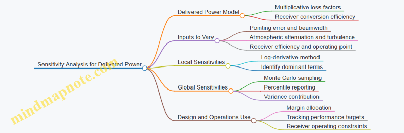
Step 5: Pointing Loss Sensitivity Example
Assume a Gaussian-like coupling where pointing loss depends on angular offset θ relative to effective beamwidth σ. A common approximation is:
L_point ≈ exp(-(θ^2)/(2σ^2))
If the nominal θ is small, the sensitivity to θ grows as σ shrinks. That means narrow beams are efficient but unforgiving: a control system that looks “good” in angular units can still cause large delivered-power swings.
Concrete example: if σ is halved while θ stays the same, the exponent doubles, and delivered power drops more sharply. Sensitivity analysis quantifies this rather than relying on intuition.
Step 6: Atmospheric Loss Sensitivity Example
Atmospheric loss often combines:
- Deterministic attenuation with elevation angle
- Random fading from turbulence (scintillation)
A simple way to separate them is to treat attenuation as a mean loss factor and turbulence as a multiplicative random variable around that mean. Sensitivity then shows whether uncertainty in mean attenuation or the spread from turbulence dominates the low-percentile delivered power.
If turbulence dominates, improving pointing alone won’t fix the tail behavior; if mean attenuation dominates, operational scheduling and elevation constraints matter more.
Step 7: Efficiency Sensitivity Example
Receiver efficiency η_rx can be sensitive to input power level, temperature, and impedance matching. Model η_rx as a function of operating conditions, then vary those conditions in the Monte Carlo.
A useful pattern: if η_rx changes slowly with conditions but pointing and atmospheric losses change quickly, then receiver efficiency is a “second-order” term. If η_rx has a steep operating-point dependence, it becomes a primary driver and you must tighten receiver control.
Step 8: Turn Results into Margins
Sensitivity outputs should map to actions:
- If pointing sensitivity is highest, allocate more margin to tracking residuals and beam steering calibration.
- If atmospheric sensitivity is highest, allocate margin to link availability under elevation and weather bounds.
- If efficiency sensitivity is highest, allocate margin to thermal control and matching stability.
The delivered-power distribution is the final product. Sensitivity analysis is how you decide where the distribution’s tail is coming from—so you don’t waste margin on the wrong place.
Diagram: Sensitivity Analysis Flow
    flowchart TD
  A[Define Delivered Power Model] --> B[Select Inputs and Uncertainty Ranges]
  B --> C[Compute Local Sensitivities]
  C --> D[Identify Dominant Factors]
  D --> E[Run Monte Carlo for Global Sensitivity]
  E --> F[Report Percentiles and Variance Contributions]
  F --> G[Allocate Design and Operational Margins]
10.5 Practical Design Tradeoffs Between Efficiency Mass and Complexity
A space solar power platform is a chain: sunlight becomes DC power, DC becomes RF or optical power, and that becomes delivered watts at the ground receiver. Every link in the chain has a cost in mass, power, and operational complexity. The practical job is to choose where to spend complexity so you do not pay for it twice—once in hardware mass and again in lost delivered energy.
The Efficiency–Mass–Complexity Triangle
Start with a simple rule of thumb: higher efficiency usually requires tighter tolerances, better control, or more elaborate conversion stages. Those improvements often add mass (heavier components, more redundancy, more shielding) and complexity (more control loops, more calibration steps, more failure modes).
A useful way to reason is to treat “complexity” as measurable work: number of subsystems that must be tuned, number of sensors that must stay calibrated, and number of interlocks that must behave correctly during off-nominal events. If you cannot name those items, you cannot budget them.
Where Efficiency Gains Usually Come From
- Conversion efficiency improvements: Better power conditioning, lower-loss RF/optical components, and improved rectification or photovoltaic conversion.
- Link efficiency improvements: Better beam shaping, pointing stability, and receiver coupling.
- Operational efficiency improvements: Using storage and scheduling so the platform delivers closer to the target profile rather than wasting energy during eclipses or misalignment.
Each category tends to push complexity in a different direction. Conversion efficiency often adds electronics and thermal management. Link efficiency often adds control loops and alignment mechanisms. Operational efficiency often adds software logic and ground procedures.
Where Mass and Complexity Tend to Hide
- Thermal control: Higher efficiency can reduce waste heat, but tighter control electronics and higher-power transmitters can increase heat flux density. Radiators, heat pipes, and thermal straps scale with both power and allowable temperature gradients.
- Pointing and beam control: Better pointing stability can require more capable attitude control, star trackers, gyros, and actuators. Even if the transmitter hardware is light, the control stack and calibration procedures can grow.
- Power conditioning and protection: High-power RF or optical chains need robust protection. Adding fast shutdown paths, current limiting, and monitoring increases wiring, harness mass, and validation effort.
- Redundancy: Redundancy improves availability but increases mass and verification workload. A “lightweight” redundancy plan that is hard to test can cost more in commissioning time than the mass it saves.
Mind Map: Efficiency, Mass, Complexity
A Systematic Trade Study Method
- Define the delivered-power requirement: Use an end-to-end metric like delivered watts averaged over an operational cycle, not just peak transmitter power.
- Allocate losses by stage: Separate losses into conversion, link, and operational categories. This prevents “efficiency” from becoming a vague wish.
- Quantify marginal cost: For each design change, estimate how much delivered power improves and what mass and complexity increase. Even rough numbers help you see which lever is worth touching.
- Check the bottleneck: If link losses dominate, improving rectification efficiency by a small percentage may not matter as much as reducing pointing loss or beam divergence.
- Validate with failure-mode realism: A design that is efficient only when everything is perfectly tuned can be less effective than a slightly less efficient design that tolerates drift.
Example: Microwave Versus Receiver Complexity
Suppose you can either (A) increase transmitter effective radiated power by adding RF amplifier mass and thermal capacity, or (B) improve receiver coupling by adding a more capable tracking and combining scheme.
- Option A raises delivered power directly but increases platform thermal load and protection complexity for higher RF power.
- Option B keeps transmitter mass lower but increases ground segment complexity and calibration effort, because receiver gain and phase must be managed across the beam footprint.
A practical decision often comes down to where you can test and maintain performance more reliably. If ground systems are easier to calibrate and monitor than spaceborne high-power electronics, receiver-side complexity can be the cheaper way to recover delivered watts.
Example: Tight Pointing Versus Wider Beam
A tighter beam reduces spreading loss, but it demands more accurate attitude control and faster correction loops. A wider beam relaxes pointing requirements but increases the fraction of power that misses the receiver aperture.
The trade is not just “better pointing costs more.” It is also “better pointing increases the number of things that must stay stable.” If your pointing solution relies on multiple sensors with different drift behaviors, the calibration burden can grow. Sometimes a slightly wider beam with simpler control yields higher delivered energy over time because it spends less time correcting small errors.
Practical Design Rule for This Section
When you compare two designs, compare them on delivered energy and availability over the same operational cycle. Then ask: which one reduces the number of tightly coupled, hard-to-verify assumptions? That question usually points to the most balanced efficiency–mass–complexity choice.
11. Reliability Testing and Verification for Space and Ground Hardware
11.1 Qualification Testing for Solar Arrays and Power Electronics
Qualification testing proves that the hardware can survive the environments it will actually see and still perform within limits after those environments. For space-based solar power, the tricky part is that “survive” and “work” are not the same thing: a solar array can pass a vibration test yet still fail later due to latent damage in interconnects or power electronics.
Qualification Philosophy and Test Flow
A systematic flow reduces surprises and makes failures diagnosable.
- Define acceptance and qualification margins: Start with end-of-life performance requirements and translate them into allowable changes in electrical output, insulation behavior, and control stability. A practical approach is to set limits for array power at standard test conditions and limits for power electronics efficiency and protection thresholds.
- Characterize baseline performance: Measure electrical output, I-V curves, insulation resistance, and control-loop behavior before environmental exposure. Baseline data is what turns a “pass” into a meaningful “pass.”
- Apply environments in a logical order: Typically, start with mechanical and thermal extremes, then radiation, then re-check electrical behavior. This order helps isolate which environment caused a change.
- Re-test after each major environment: After each test block, repeat the most diagnostic electrical checks. If you only test at the end, you may lose the trail.
- Use failure triage rules: Predefine what constitutes a failure versus a “needs investigation.” For example, a small shift in maximum power point might be acceptable if it remains within the allowed range and is repeatable.
Mind Map: Qualification Test Coverage
Solar Array Qualification Testing
Mechanical tests confirm the array structure and interconnects tolerate launch loads. A useful practice is to instrument a small number of representative harness points with strain or temperature sensors during qualification-level vibration. If the array survives but the harness shows abnormal heating, you have a clear suspect.
Thermal vacuum tests verify performance under space-like heat transfer. Arrays often show subtle changes after cycling: connector resistance can drift, and bypass diode behavior can shift due to temperature-dependent characteristics. During thermal vacuum, re-run I-V sweeps at the same setpoints used in baseline testing so the comparison is apples-to-apples.
Radiation tests address both total ionizing dose and displacement damage. For solar arrays, the most informative checks are end-of-life electrical measurements: maximum power point location, fill factor trends, and any increase in leakage or degradation in shunt paths. For power electronics tied to the array, radiation can change control-loop dynamics, so the array and electronics should be evaluated together at least at the functional level.
Power Electronics Qualification Testing
Power electronics qualification focuses on stable regulation and safe behavior under stress. Start with functional verification: confirm startup sequences, regulation modes, and protection actions such as overcurrent limiting and undervoltage lockout. Then test under thermal vacuum to ensure efficiency and control stability remain within limits.
A practical example: suppose a DC-DC converter meets efficiency targets at room temperature but shows oscillation after thermal cycling. The root cause is often not the power stage itself but the control loop’s gain margins shifting with component parameters. The fix is usually design-level compensation or component selection, but qualification testing must catch it by measuring control behavior under representative loads.
Radiation testing for electronics should include checks for latch-up susceptibility and parameter drift in both analog and digital control paths. Even when the device does not fail catastrophically, small threshold shifts can cause protection trips at normal operating conditions.
Electrical Verification and Pass Criteria
Qualification is not just “no smoke.” Define pass criteria that map to mission needs.
- Array electrical: I-V curve shape, maximum power within allowed bounds, and insulation resistance above minimum thresholds.
- Power electronics: regulation accuracy, efficiency range, and correct operation of protection thresholds.
- System-level interface checks: verify that array-to-converter operating points remain stable across expected operating conditions.
A good rule of thumb for test evidence is to require repeatability: if a measurement changes after a test, repeat it under the same setup to confirm it is real and not a measurement artifact.
Example Test Matrix for One Qualification Article
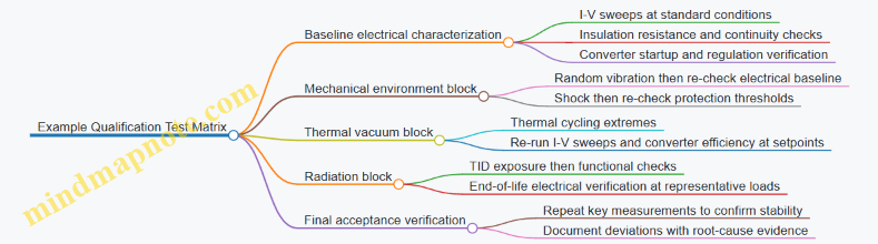
Documentation and Traceability
Qualification reports should connect each test to a specific requirement and show how data reduction supports the conclusion. If a limit is exceeded, the report should state whether the deviation is within measurement uncertainty, whether it is repeatable, and what follow-up checks were performed to isolate the cause.
11.2 Environmental Testing Including Thermal Vacuum Vibration and Radiation
Environmental testing proves that a space solar power platform and its ground receiver chain can survive the trip, operate in vacuum and temperature extremes, and continue functioning after radiation exposure. The goal is not to “stress everything until it breaks,” but to reproduce the dominant failure mechanisms with controlled, measurable conditions.
Foundations of Environmental Test Planning
Start with a failure map: list components by function (power generation, power conditioning, RF/optical transmitters, beam control, receiver rectification, tracking, and protection). For each, identify the most likely stressors—temperature cycling, vacuum-related outgassing, mechanical shock and vibration, and radiation-induced parameter shifts. Then translate those stressors into test requirements: temperature ranges, dwell times, vibration spectra, radiation dose levels, and acceptance criteria.
A practical best practice is to define pass/fail metrics per subsystem before testing. For example, power electronics might be evaluated by output ripple and efficiency drift, while RF hardware is evaluated by S-parameter changes and output power stability. This prevents “it seems fine” outcomes.
Thermal Vacuum Testing for Vacuum and Temperature Cycling
Thermal vacuum testing simulates space conditions by combining vacuum pressure with controlled thermal environments. Vacuum matters because it changes heat transfer: conduction through structure dominates, convection disappears, and outgassing can contaminate optics or RF surfaces.
A systematic thermal vacuum sequence often includes:
- Baseline characterization at room conditions: measure electrical performance, optical alignment references, and any calibration constants.
- Pump-down and stabilization: confirm vacuum level and thermal soak behavior.
- Thermal cycling: alternate hot and cold plateaus with controlled ramp rates.
- Interim checks: at selected cycles, repeat critical measurements to catch early degradation.
- Post-test verification: compare performance drift against acceptance limits.
Concrete example: if a microwave transmitter uses a waveguide feed and a phased array, you can track beam-relevant parameters by measuring phase/amplitude calibration tables before and after cycling. If the calibration shifts beyond tolerance, you adjust the thermal model or redesign thermal coupling.
Vibration Testing for Launch Loads
Vibration testing targets mechanical integrity under launch-induced excitation. The key is matching the test to the expected load spectrum and ensuring the structure responds similarly.
A typical approach:
- Model-based selection: use a structural model to identify modes that matter for the payload.
- Random vibration: apply a power spectral density profile across axes to represent the stochastic nature of launch.
- Sine burst or resonance dwell: optionally excite specific resonances identified as risky.
- Post-vibration inspection: verify connectors, mounts, and alignment-sensitive assemblies.
Concrete example: for a deployable solar array mechanism, vibration can loosen fasteners or degrade hinge friction surfaces. You can include a functional check such as verifying deployment timing and measuring motor current signature before and after vibration.
Radiation Testing for Cumulative Dose and Effects
Radiation testing addresses how components change under ionizing dose and how some parts respond to displacement damage. The testing strategy depends on component technology and mission profile.
A systematic radiation plan includes:
- Dose characterization: determine total ionizing dose and dose rate conditions relevant to the electronics.
- Test article selection: test representative parts, not just the most robust ones.
- Electrical parameter tracking: measure threshold shifts, leakage currents, gain changes, and timing drift.
- Functional verification: confirm that control loops still operate within margins.
Concrete example: power conditioning units may show increased leakage or altered switching behavior after dose. Instead of only checking “it powers on,” evaluate output regulation under representative load steps and confirm protection thresholds still trigger correctly.
Mind Map: Integrated Environmental Testing
Integrated Example: From Measurements to Decisions
Consider a platform subsystem that includes a solar array interface board, a power conditioning unit, and an RF transmitter module. During thermal vacuum, you observe that output ripple increases after cold-to-hot cycling. During vibration, you see no mechanical damage, and post-vibration electrical checks match baseline. During radiation testing, you find that a specific control IC’s gain changes, which reduces loop margin under the same thermal conditions. The integrated conclusion is that the ripple issue is a combined effect of thermal stress and radiation-induced parameter shift, not a single-environment failure.
A final best practice is to document the chain of evidence: which measurement changed, under which environment, and how it maps to a specific design margin. That keeps the test program from turning into a collection of interesting graphs with no engineering decisions attached.
11.3 High Power RF and Optical Testing on Ground Facilities
Ground testing is where you earn the right to trust the numbers. For space-based solar power, the hard part is not generating power; it is proving that the delivered power, beam quality, and safety behavior match the system model under realistic conditions. This section organizes the work from facility foundations to advanced verification steps, with practical examples of what to measure and how to interpret it.
Facility Foundations and Test Readiness
Start with a facility checklist that prevents “mystery failures.” Confirm RF or optical source stability, calibration status, and environmental control. For RF, verify vector network analyzer (VNA) calibration and power sensor traceability. For optical, verify wavelength stability, beam diameter measurement method, and detector linearity range.
A useful practice is to define a test matrix before hardware is touched. Example: for a microwave transmitter, vary output power in three steps (low, nominal, high) and repeat at two temperatures (room and elevated). For an optical transmitter, vary output power and include at least one alignment stress test where the beam is intentionally offset within the expected control bandwidth.
RF High Power Testing Workflow
RF testing typically follows a progression: passive characterization, controlled power ramp, then full chain verification.
- Passive characterization: Measure S-parameters of antennas, waveguides, and matching networks. This tells you where reflections and losses live.
- Controlled power ramp: Increase power slowly while monitoring reflected power, device currents, and temperatures. The goal is to find the onset of nonlinearity.
- Full chain verification: Combine transmitter, beamforming network, and receiver coupling model. Measure delivered effective isotropic radiated power (EIRP) or equivalent metrics.
Example: if reflected power rises sharply at a specific forward power level, you likely hit a mismatch due to thermal drift in a matching network. The fix is not “turn it down,” but to quantify the drift and update the thermal model and control limits.
Optical High Power Testing Workflow
Optical testing focuses on alignment, beam quality, and receiver coupling. The progression mirrors RF: characterize optics and detectors, then test the full optical path.
- Optical path characterization: Measure beam profile, divergence, and pointing repeatability using a camera or beam profiler.
- Receiver coupling tests: Validate that the receiver optics and tracking assumptions produce the expected coupling efficiency.
- Conversion chain tests: For photovoltaic or rectifying receivers, verify electrical conversion efficiency versus incident power and spot size.
Example: if conversion efficiency drops when the spot size increases, you may be seeing mismatch between the receiver active area and the beam footprint. That is a measurable, fixable geometry issue, not a “mystery performance” issue.
Instrumentation, Calibration, and Uncertainty
High power tests are only as good as their uncertainty budget. Build a measurement plan that lists each instrument, its calibration date, its relevant operating range, and the uncertainty contribution.
A practical method is to separate uncertainty into categories:
- Calibration uncertainty (traceability of sensors and standards)
- Repeatability (how much results vary across runs)
- Environmental effects (temperature, humidity, air turbulence for optical)
- Modeling uncertainty (conversion from measured quantities to system-level metrics)
Example: for RF, if power sensors have a known ±1.5% uncertainty and alignment affects coupling by ±2%, your final delivered-power uncertainty cannot be smaller than the combined effect. This prevents overconfidence in a single “good day” measurement.
Safety Interlocks and Facility Controls
Testing high power RF and optical sources requires layered safety. Interlocks should cover access control, beam path verification, emergency shutdown, and monitoring of abnormal operating states.
For RF, include monitoring for reflected power thresholds and device current limits. For optical, include shutter interlocks tied to detector confirmation and beam path sensors. A simple but effective practice is to log every interlock event with the triggering signal and system state so you can distinguish a real fault from a test setup mistake.
Data Reduction and Acceptance Criteria
Define acceptance criteria in terms of measurable quantities tied to system requirements. For RF, typical criteria include gain stability, reflected power limits, spectral purity, and beamforming consistency. For optical, typical criteria include pointing repeatability, spot size stability, and receiver conversion efficiency versus incident power.
Example: if the system model assumes a coupling efficiency of 0.65 at nominal alignment, set an acceptance band that reflects measurement uncertainty and expected alignment jitter. If measured coupling is 0.60 but still within uncertainty, you accept and move on. If it is outside, you investigate alignment, optics cleanliness, or detector saturation.
Mind Map: High Power RF and Optical Testing on Ground Facilities
Example Test Run: RF Transmitter to Receiver Coupling
On 2026-03-16, run a three-step power ramp at two temperatures. At each step, record forward power, reflected power, device current, and antenna temperature. Then compute delivered coupling using the measured antenna pattern and the receiver aperture model.
If delivered coupling stays flat across the ramp but reflected power increases, you have a mismatch that is not yet harming delivered power. If delivered coupling drops while reflected power stays low, the issue is likely in the receiver coupling optics or alignment rather than the transmitter match.
Example Test Run: Optical Alignment and Conversion Efficiency
Perform a baseline alignment, then repeat with controlled pointing offsets within the expected control bandwidth. For each offset, measure beam spot size at the receiver plane and record receiver output power.
If spot size changes but pointing repeatability is good, suspect lens thermal effects or mount compliance. If spot size is stable but receiver output changes, suspect receiver optical alignment, detector linearity, or electrical conversion chain behavior under varying illumination distribution.
11.4 Commissioning Procedures for Receiver Calibration and Alignment
Receiver commissioning is where “it should work” becomes “it does work, consistently.” The goal is to calibrate the receiver’s electrical chain and align its optical or RF coupling so that delivered power matches the modeled link budget within defined tolerances. A good commissioning plan treats calibration and alignment as a single loop: alignment affects calibration inputs, and calibration results guide alignment corrections.
Commissioning Readiness Checks
Start with prerequisites that prevent chasing ghosts. Verify mechanical readiness (mount stability, leveling, cable strain relief), environmental readiness (site temperature range, wind limits for optical tracking), and instrumentation readiness (calibrated power meters, spectrum analyzers, reference attenuators). Confirm that the receiver electronics are in a known safe state: protection circuits armed, interlocks functional, and firmware configuration matching the expected receiver mode.
A practical habit: label every connector and record the exact configuration state before any alignment motion. If you later see a power drop, you’ll know whether it came from optics, RF path changes, or a configuration mismatch.
Electrical Baseline Calibration
Electrical calibration establishes the receiver’s transfer function from incident power to delivered electrical output.
- RF or optical input characterization: For RF, measure insertion loss of waveguides/feeds and confirm matching network behavior using a calibrated source. For optical, verify detector responsivity using a stable optical power reference and check that tracking optics do not vignette the beam.
- Power conversion chain calibration: Measure rectifier or photodetector output versus input power at representative levels, then fit a conversion curve. Include the effect of impedance matching and any automatic gain or bias control.
- Timing and synchronization checks: If the system uses synchronized beam control, confirm that receiver sampling windows align with the expected modulation or gating.
Example: If the conversion curve shows a slope change at a specific input level, treat it as a real nonlinearity, not a measurement error. Then update the commissioning acceptance thresholds so operators aren’t forced to “fix” behavior that is actually expected.
Alignment Strategy for Maximum Coupling
Alignment differs by modality, but the logic is the same: maximize coupling while maintaining stability.
- Coarse alignment: Use survey marks and initial pointing estimates to bring the receiver within the acquisition region. For RF, this means aligning the antenna boresight and feed orientation; for optical, it means setting telescope pointing and focus.
- Fine alignment: Perform a controlled scan around the expected pointing. Use a metric that correlates with delivered power (not just signal strength indicators that may saturate). Apply a small-step search, then refine with a gradient-like approach.
- Stability verification: After alignment, run a short dwell test while logging delivered power and pointing error. If power fluctuates beyond the expected atmospheric or mechanical noise, pause and check mount behavior, cable movement, or tracking loop tuning.
Calibration-to-Alignment Coupling Loop
Treat calibration results as constraints on alignment. If measured delivered power is lower than predicted, first check whether the receiver conversion curve is valid at the current operating point. If conversion is correct, then alignment likely reduced coupling.
A simple workflow:
- Align to maximize coupling metric.
- Re-measure delivered power at one or two known reference levels.
- Compare to the calibrated conversion curve.
- If mismatch persists, adjust alignment and repeat.
This loop prevents the common mistake of “recalibrating” when the real issue is that the beam is slightly off-axis.
Acceptance Criteria and Documentation
Define acceptance criteria before commissioning begins. Typical criteria include:
- delivered power within a specified percentage of predicted value at reference conditions
- conversion curve residual error below a threshold
- pointing error within a defined bound during dwell
- protection and interlock response verified through controlled fault injection (within safe limits)
Document everything: calibration dates, instrument serial numbers, configuration states, scan parameters, and final tuned settings. Use a consistent naming convention for datasets so later troubleshooting doesn’t require detective work.
Example Commissioning Runbook
Example: Microwave receiver commissioning at a ground site.
- Step A: Confirm waveguide/feed path loss using a calibrated source.
- Step B: Measure rectifier output versus input power at two levels (low and mid) to validate the conversion curve.
- Step C: Perform a boresight scan with small angular steps; record delivered power and pointing error.
- Step D: Select the peak that also yields stable power during a 10-minute dwell.
- Step E: Re-check delivered power at the two reference levels to confirm no configuration drift.
If the peak is narrow and stability is poor, prefer a slightly lower peak that maintains coupling under small pointing variations. Stability is often the difference between “works during setup” and “works during operations.”
Mind Map: Receiver Calibration and Alignment
Diagram: Commissioning Workflow
    flowchart TD
  A[Start with readiness checks] --> B[Electrical baseline calibration]
  B --> C[Coarse alignment to acquisition region]
  C --> D[Fine scan using delivered-power metric]
  D --> E[Stability dwell logging]
  E --> F{Power matches calibrated curve?}
  F -- Yes --> G[Finalize acceptance criteria and document]
  F -- No --> H[Determine mismatch source]
  H --> I[Adjust alignment or recalibrate conversion]
  I --> D
  G --> J[Commissioning complete]
Operational Handoff
Before handing control to routine operations, verify that the receiver can return to the tuned state after a controlled restart. Confirm that stored calibration parameters load correctly and that the alignment offsets used during commissioning are applied consistently. A receiver that “remembers” its calibration is a receiver that saves time later—usually the same time you’d rather spend on something else.
11.5 Acceptance Criteria and Documentation for Integrated Systems
Integrated acceptance is where “it works in a lab” becomes “it works as a system.” For space-based solar power with wireless transmission, the integrated system includes the orbital platform, the wireless link, and the ground receiver and power conditioning chain. Acceptance criteria should therefore be written as measurable outcomes tied to specific evidence, not as vague statements like “meets performance.”
Acceptance Criteria Structure
Start with a hierarchy: requirements → acceptance criteria → verification method → evidence. A practical way to keep this from turning into a spreadsheet maze is to group criteria into five buckets.
Functional Performance
Functional criteria confirm that power is delivered to the load as intended.
- Delivered Power at Receiver Output: Specify minimum delivered power at defined link conditions (e.g., elevation/geometry, clear-sky vs. nominal atmospheric loss). Example: “At 10° receiver elevation with nominal atmospheric loss, delivered DC power to the load shall be at least X kW after conversion efficiency is applied.”
- Power Quality: Define allowable ripple, voltage regulation range, and transient behavior when beam power ramps. Example: “During a 1-second ramp, output voltage shall remain within ±Y% and ripple shall remain below Z mV RMS.”
- End-to-End Efficiency: Set a minimum system efficiency for the full chain (generation → conditioning → transmission → conversion → conditioning). Example: “End-to-end efficiency shall be ≥ N% under specified pointing and atmospheric assumptions.”
Link and Pointing Behavior
Wireless links are sensitive to geometry and alignment.
- Pointing Acquisition and Tracking: Define time-to-lock and allowable pointing error. Example: “From command to stable tracking, lock shall occur within 30 seconds; residual pointing error shall be within A arcseconds for at least 95% of the observation window.”
- Beam Steering Stability: Require that steering does not induce unacceptable power oscillations. Example: “Steering control shall limit delivered power modulation to ≤ B% peak-to-peak.”
Safety and Compliance
Safety criteria should be testable and operationally enforceable.
- Exposure Limits and Interlocks: Specify interlock response times and conditions that trigger safe shutdown. Example: “If receiver-side safety monitor flags a violation, transmitter shall reduce output to safe level within T seconds.”
- RF/Optical Emission Control: Define maximum emissions outside the intended beam state. Example: “When in standby, equivalent isotropically radiated power shall not exceed C dBW.”
Reliability and Robustness
Acceptance should include stress that reflects real operational sequences.
- Thermal and Power Cycling Tolerance: Define allowable drift and failure thresholds after repeated cycles. Example: “After 50 thermal cycles between specified limits, array power and conversion efficiency shall degrade no more than D%.”
- Fault Detection and Recovery: Require that faults are detected within a time window and that recovery returns the system to a known safe state. Example: “A rectifier overcurrent event shall be detected within 100 ms and recovery shall follow the documented safe restart procedure.”
Documentation Completeness
Documentation is part of acceptance because it enables repeatable operations.
- Configuration Control: Evidence that all software versions, hardware revisions, and calibration constants are frozen for the acceptance baseline.
- Test Procedures and Results: Traceable test scripts, measured data, and pass/fail criteria.
- As-Built Data Package: Final wiring diagrams, calibration reports, and interface control documents.
Mind Map: Integrated Acceptance Evidence
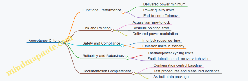
Documentation Package Contents
A clean acceptance package usually contains three layers: what the system is, how it was tested, and how it will be operated.
-
System Definition and Interfaces
- Interface control documents for platform-to-transmitter-to-receiver boundaries.
- A single “system block diagram” showing power flow and signal flow.
-
Verification Records
- Test plans that map each requirement to a verification method.
- Raw and processed data sets, including calibration steps and uncertainty budgets.
- A summary table that lists each criterion, the measured value, the acceptance threshold, and the verdict.
-
Operational Readiness Documentation
- Start/stop procedures that include safe states.
- Beam control and receiver alignment procedures with defined operator actions.
- Fault handling procedures that specify what is automatic vs. what requires human intervention.
Example: Acceptance Checklist Snippet
Acceptance Checklist Snippet
- Delivered Power
- Criterion: Delivered DC power ≥ X kW at nominal conditions
- Evidence: Receiver output measurements with calibration trace
- Verdict: Pass/Fail
- Pointing Acquisition
- Criterion: Time-to-lock ≤ 30 s
- Evidence: Logged control timestamps and pointing telemetry
- Verdict: Pass/Fail
- Safety Interlock
- Criterion: Output reduced to safe level within T s
- Evidence: Interlock test log and oscilloscope capture
- Verdict: Pass/Fail
- Documentation
- Criterion: As-built package complete and configuration frozen
- Evidence: Version-controlled repository manifest and sign-off
- Verdict: Pass/Fail
Practical Sign-Off Flow
Use a staged sign-off that matches how integration actually happens. First, sign off subsystem readiness (platform power conditioning, transmitter chain, receiver conversion). Next, sign off link-level behavior (acquisition, tracking, delivered power under controlled conditions). Finally, sign off end-to-end integrated operation including safety interlocks and documentation completeness. This order prevents the classic problem where everyone agrees the parts are fine—right up until the interfaces disagree.
Evidence Traceability Mindset
Every acceptance criterion should have a named owner, a verification method, and a specific evidence artifact. If a criterion cannot be tied to a measurable outcome or a recorded test result, it is not an acceptance criterion yet—it is a wish. Keep the criteria strict, and the documentation will stay useful instead of decorative.
12. Practical Case Studies of Integrated Energy Delivery
12.1 Case Study: Microwave Rectenna Receiver with Power Conditioning Chain
This case study follows one practical receiver chain for a microwave wireless power link: a rectenna captures incident RF power, converts it to DC, and then conditions that DC into a stable output suitable for a load. The goal is not just “get DC,” but “get usable DC with predictable behavior when conditions change.”
System Setup and Assumptions
Assume a ground receiver site with a fixed antenna pointing strategy and a rectenna array sized to the expected received power. The platform transmits a continuous microwave beam; the receiver experiences variations from pointing error and atmospheric attenuation. The receiver must therefore tolerate a range of incident power while keeping output voltage within the load’s operating window.
A good starting point is to define three targets: (1) delivered power at nominal received RF level, (2) minimum delivered power during worst-case link margin, and (3) output ripple and transient response acceptable to the downstream electronics. These targets drive the rectenna operating point and the power conditioning topology.
Mind Map: Receiver Chain Logic
Rectenna Conversion: From RF to DC
The rectenna’s antenna and rectifier are designed as a coupled system. If the matching network is tuned for the wrong RF level, efficiency drops sharply because the diode sees an unfavorable impedance. A practical best practice is to choose a matching network that provides a relatively broad efficiency “plateau” rather than a single sharp peak.
Example: Suppose the rectenna is optimized around a received power density that yields a diode input power where the rectifier transitions from low-conduction to strong conduction. If the link margin causes the received level to fall by 3 dB, a narrowband match might reduce conversion efficiency by more than 3 dB, effectively double-penalizing the delivered power. A broader match reduces this penalty, even if peak efficiency is slightly lower.
The rectifier output typically includes both DC and residual RF ripple. A simple RC or LC filter can reduce ripple, but the filter also affects transient response. For a receiver that may experience short-term fades, the filter should be strong enough to meet ripple limits yet not so heavy that the output lags during recovery.
Power Conditioning: Making DC Behave
Rectenna output voltage often varies with incident RF power. Power conditioning converts that variable DC into a stable output.
A common approach is a two-layer strategy:
- Energy smoothing with a bulk capacitor and an intermediate stage that limits current spikes.
- Regulation using a converter that can operate across the expected input voltage range.
Example: If the rectenna produces a DC bus that can dip below the load’s minimum supply, a buck converter alone may fail because it requires sufficient headroom. A buck-boost converter can maintain regulation across a wider input range, at the cost of additional complexity and efficiency tradeoffs. The choice should be driven by the measured rectenna output range, not by theoretical convenience.
Protection and Reliability Details
High-power RF can stress rectifier diodes and downstream components through thermal rise and voltage transients. Protection is therefore part of the design, not an afterthought.
Key protections include:
- Overvoltage clamp to protect the regulation stage when incident RF power spikes.
- Current limiting during startup so the converter does not demand more current than the rectenna can supply.
- Soft-start to prevent abrupt load steps that create large ripple and potential diode stress.
Example: During initial beam acquisition, the received power may ramp from near-zero to nominal. Without soft-start, the converter can attempt to regulate immediately, drawing current that the rectenna cannot provide, causing oscillation. A soft-start sequence that waits for the rectenna output to cross a threshold avoids this behavior.
End-to-End Example Calculation
Assume the rectenna conversion efficiency at nominal conditions is 45%, and the incident RF power on the rectenna is 10 W. The rectenna delivers about 4.5 W of DC before conditioning losses. If the power conditioning chain has 90% efficiency at that operating point, the delivered power to the regulated output is about 4.05 W.
Now consider a 3 dB received power drop (incident RF becomes 5 W). If conversion efficiency falls to 35% due to mismatch and diode operating shift, DC becomes 1.75 W. With 88% conditioning efficiency at the lower input, delivered power is about 1.54 W. This example shows why the rectenna efficiency curve matters as much as the link budget’s raw received power.
Monitoring and Acceptance Checks
A receiver chain should be verified with measurements that map directly to the design targets:
- Output voltage ripple under steady incident power.
- Delivered power versus incident power sweep to confirm the efficiency plateau.
- Transient response when incident power steps down and back up.
- Thermal stability by monitoring diode and regulator temperatures during sustained operation.
A practical acceptance rule is to require that delivered power stays within a defined band over the expected received power range, and that ripple and transient overshoot remain below the thresholds that could stress the load or the regulation stage.
12.2 Case Study: Laser Receiver with Tracking and Conversion Electronics
This case study follows one complete receiver chain for a laser-based wireless power link: optical capture, pointing and tracking, power conversion, and electrical conditioning. The goal is to show how each subsystem reduces a specific loss mechanism, using concrete design choices you can reason about.
System Setup and Design Targets
Assume an orbital platform transmits a narrow laser beam to a ground receiver. The receiver must tolerate slow pointing drift from platform motion and faster jitter from atmospheric turbulence. The design targets are:
- Maintain optical coupling despite angular error.
- Convert received optical power to DC with predictable efficiency.
- Provide a stable output for downstream loads.
A practical starting point is to treat the receiver as three coupled loops: an optical alignment loop, a conversion stage, and a power conditioning stage.
Optical Capture and Tracking Loop
Receiver Optics
The receiver begins with a collection optic that focuses incoming light onto a small conversion area. A larger aperture improves collection, but it also narrows the field of view and increases sensitivity to pointing error. A good practice is to size the optical acceptance so that expected tracking error stays within the region where conversion efficiency is near-flat.
Coarse and Fine Pointing
Tracking is typically split into coarse acquisition and fine tracking.
- Coarse acquisition uses a wider field sensor to find the beam. A common approach is a quadrant or wide-area photodiode that can detect direction even when the beam is not yet centered.
- Fine tracking uses a narrower sensor and a fast steering element. The steering element can be a tip-tilt mirror or a fast gimbal stage, depending on bandwidth needs.
Tracking Error Signal
The receiver computes an error signal from the relative illumination of sensor segments. For example, if the beam is to the right of center, the right segment receives more light, and the difference signal becomes positive. That error drives the steering control.
A systematic rule: tune the tracking loop bandwidth to be high enough to correct jitter, but low enough to avoid chasing sensor noise. If the sensor noise dominates at high frequency, the loop will “hunt” and reduce average coupling.
Conversion Electronics
Photovoltaic Conversion
For laser power, a photovoltaic (PV) receiver is often used because it naturally outputs DC. The PV must be matched to the laser wavelength to avoid wasting power in spectral mismatch. A practical check is to compute the expected optical-to-electrical efficiency at the operating irradiance, not just at a nominal datasheet point.
Rectification and Regulation
Even with PV output, the voltage and current can vary with received power and temperature. The conversion electronics therefore include:
- A maximum power point tracking or fixed operating point strategy, depending on how stable the received power is.
- A DC-DC stage to regulate voltage for the load.
- Protection circuits that handle sudden drops in received power without producing unstable control behavior.
A useful example: if the PV output falls quickly due to a brief pointing loss, the DC-DC converter should either ride through using output capacitance or transition to a safe mode. Otherwise, the converter can oscillate during recovery.
End-to-End Example Calculation
Consider a received optical power of 10 W at the PV. Suppose the PV conversion efficiency at that operating point is 45%, yielding 4.5 W electrical. If the DC-DC stage has 92% efficiency under that load, the delivered power becomes:
- Delivered power = 4.5 W × 0.92 = 4.14 W
Now include a coupling loss from tracking error. If the tracking keeps the beam within the receiver’s effective spot size 95% of the time, and the remaining 5% causes a 30% coupling reduction, the average coupling factor is:
- Average coupling = 0.95 × 1.0 + 0.05 × 0.7 = 0.985
So the delivered average power becomes:
- Average delivered power = 4.14 W × 0.985 ≈ 4.08 W
This kind of accounting keeps the design honest: you can see whether tracking improvements are worth the added complexity by comparing their impact to conversion and power-conditioning losses.
Practical Integration Notes
First, treat tracking and conversion as a coupled system: the PV output can be used as a secondary sanity check for alignment, but it should not replace the dedicated tracking sensor because PV response is slower and depends on conversion efficiency.
Second, design the control recovery path for brief losses. A receiver that cleanly returns to regulation after a short pointing dip avoids downstream load instability.
Third, verify the loop behavior with a simple test: inject a known angular offset into the tracking sensor model and confirm that the steering command reduces the offset and increases delivered power in the expected direction. If the sign is wrong, the system will “help” the beam miss the PV—an expensive way to learn the obvious.
12.3 Case Study: Platform Power Budget With Eclipse and Storage Management
This case study walks through a realistic power budget for an orbital solar power platform that must deliver steady wireless power while passing through eclipses. The goal is simple: keep the delivered power within a target band, even when sunlight drops to near zero.
Step 1: Define the Delivered Power Target
Assume the platform drives a transmitter whose required DC input is 120 kW during transmission. The mission requires continuous delivery for a 30-minute window that includes an eclipse segment. The power quality requirement is ±5% at the transmitter input, which translates to an allowable range of 114–126 kW.
A practical design choice is to size the platform so that during sunlight it can run slightly above the nominal transmitter demand, covering conversion losses and charging storage. For this example, set the “sunlight operating point” at 135 kW available from the power conditioning chain.
Step 2: Build the Power Budget Blocks
The budget has four main flows: solar generation, conversion losses, transmitter draw, and storage charging or discharging.
- Solar generation produces DC power at the array output.
- Power conditioning converts array DC to the transmitter bus and manages regulation.
- Transmitter draw is the 120 kW load.
- Storage absorbs surplus during sunlight and supplies deficit during eclipse.
A compact way to keep this coherent is to treat each block as an efficiency factor or a state variable.
Step 3: Choose Efficiencies and Losses
Use conservative, explicit factors so the numbers don’t “mysteriously” work out.
- Array-to-bus efficiency: 0.95 (includes MPPT tracking and conversion losses)
- Bus-to-transmitter efficiency: 0.97 (includes DC/DC conversion and distribution)
- Storage round-trip efficiency: 0.90 (charge and discharge losses)
During sunlight, the transmitter bus needs 120 kW / 0.97 ≈ 123.7 kW from the regulated bus input. With array-to-bus at 0.95, required array output is 123.7 / 0.95 ≈ 130.2 kW.
To allow charging headroom, target array output of 135 kW. That yields a surplus of about 135×0.95×0.97 − 120 ≈ 7.8 kW available for storage charging and regulation margin.
Step 4: Model Eclipse Energy and Depth of Discharge
Assume an eclipse duration of 12 minutes within the 30-minute window. During eclipse, the array contributes ~0 kW, so the storage must supply the transmitter draw.
Energy required from storage at the DC bus level is:
- Transmitter draw: 120 kW for 12 minutes = 120 × 720 s = 86.4 MJ
- Convert to kWh: 120 kW × 0.2 h = 24 kWh
Because storage round-trip efficiency is 0.90, the storage must be charged with more energy than it delivers. For sizing, use delivered energy divided by discharge efficiency. If we treat 0.90 as combined charge/discharge, a simple sizing approach is to divide by 0.90 for delivered capability: 24 / 0.90 ≈ 26.7 kWh of usable storage energy.
Now apply a depth-of-discharge constraint to protect cycle life. Suppose the design allows 80% usable depth of discharge. Then required nominal storage capacity is 26.7 / 0.80 ≈ 33.4 kWh.
Step 5: Check Transition Behavior and Control Strategy
The tricky part is not the average energy; it’s the transitions at eclipse entry and exit.
A stable strategy is:
- Pre-eclipse charge ramp: during the last few minutes of sunlight, increase charging rate so the storage state of charge (SoC) reaches a safe minimum before eclipse begins.
- Eclipse discharge regulation: hold transmitter bus at the target level using storage discharge current control, not by “chasing” the transmitter with the array.
- Post-eclipse recovery: after sunlight returns, resume charging while keeping transmitter power within ±5%.
A simple sanity check: if charging surplus is ~7.8 kW and eclipse deficit is 120 kW, the storage must be sufficiently charged well before eclipse entry. That’s why the pre-eclipse ramp matters.
Mind Map: Platform Power Budget with Eclipse and Storage Management
Example: Numerical Summary for This Case
- Transmitter input requirement: 120 kW
- Eclipse duration: 12 minutes (0.2 h)
- Delivered energy: 24 kWh
- Storage sizing with 0.90 efficiency: 24/0.90 = 26.7 kWh usable
- Usable fraction with 80% DoD: 26.7/0.80 = 33.4 kWh nominal capacity
- Sunlight array target: ~135 kW to cover losses and provide charging headroom
Step 6: Validate Against the Power Quality Band
During eclipse, the storage discharge control must keep the transmitter input between 114 and 126 kW. If storage voltage sag or current limits cause the bus to droop, the platform should reduce transmitter duty cycle or apply a controlled power derate before violating the band. In this case study, the storage capacity margin is chosen so that the discharge current stays within allowable limits for the full 12 minutes.
The result is a coherent budget: the platform charges storage during sunlight using surplus power, then uses that stored energy to maintain transmitter power through eclipse without exceeding the allowed depth of discharge.
12.4 Case Study: Ground Grid Interface with Protection and Metering
This case study follows a single delivered-power chain: a ground receiver produces DC (from a rectenna or optical-to-electric conversion), power conditioning creates a grid-suitable AC output, and the grid interface ensures safe operation, correct metering, and clean power quality. The goal is simple: when the beam is present, the grid sees stable power; when it is not, the system disconnects predictably and records what happened.
System Boundary and Power Flow
Start by drawing a boundary so protection and metering are assigned to the right equipment. In this chain, the boundary typically includes:
- Receiver output (DC or intermediate DC)
- Power conditioning (DC link, inverter, filters)
- Grid interface (transformer, switchgear, protection relays)
- Metering (revenue-grade and operational meters)
A practical rule: protection trips should be based on electrical quantities that exist at the grid interface, not on “beam present” signals alone. Beam presence is useful for control, but protection should still work if the beam signal is wrong.
Protection Philosophy and Coordination
Protection is layered so a single fault does not cause a cascade.
- Local Inverter Protections
- Overcurrent and overvoltage on the inverter output
- DC link undervoltage to prevent unstable switching
- Anti-islanding logic so the inverter cannot energize the grid during outages
- Grid Interface Protections
- Transformer differential or restricted earth fault protection where applicable
- Breaker trip on detected grid faults
- Under/over-frequency and voltage protection aligned with grid codes
- System-Level Interlocks
- A permissive that requires grid voltage and frequency within limits before closing the breaker
- A fast shutdown path that opens the breaker and commands inverter current ramp-down
A small but important best practice: coordinate trip times so the closest device clears first. If the breaker and relay both “decide” to act, you want the relay to command the breaker, not both to race.
Metering Architecture for Delivered Energy
Metering should answer two questions: “How much energy did we deliver?” and “What conditions produced it?”
- Revenue-grade energy meters measure net exported/imported energy at the point of interconnection.
- Operational meters capture DC input, inverter output, and key quality metrics (voltage, current, frequency, harmonics).
- Event logging records protection trips, breaker states, and meter snapshots at the time of change.
To keep accounting consistent, define measurement points and sign conventions. For example, export energy is positive, import energy is negative, and reactive power sign follows the grid standard.
Mind Map: Ground Grid Interface Responsibilities
Example: Protection and Metering Data Flow
Below is a compact data flow showing how protection decisions and metering snapshots connect.
    flowchart TD
  A[Receiver Output] --> B[Power Conditioning Inverter]
  B --> C[Grid Interface Transformer]
  C --> D[Breaker and Protection Relays]
  D --> E[Point of Interconnection]

  D --> F[Protection Event Logger]
  E --> G[Revenue Energy Meter]
  B --> H[Operational Power Quality Meters]

  F --> I[SCADA/Control System]
  G --> I
  H --> I
Example: Start-Up and Trip Behavior
Assume the receiver output rises when the beam is aligned. The inverter should not instantly jump to full current; it should ramp to avoid voltage dips and nuisance trips.
A typical sequence:
- Inverter measures grid voltage and frequency.
- Control checks permissives and confirms no active fault flags.
- Inverter ramps current to a setpoint using a controlled slope.
- Breaker closes only when the inverter output is within limits.
- Metering starts accumulating export energy once the breaker is closed and synchronization is confirmed.
When a grid fault occurs, the protection chain should:
- Detect the fault at the grid interface
- Command inverter current to ramp down
- Open the breaker
- Record a trip cause code and the last meter snapshot
This makes post-event analysis straightforward: you can correlate the energy curve with the exact electrical reason for interruption, rather than guessing whether the beam vanished or the grid faulted.
Practical Checklist for This Case Study
- Define the point of interconnection and place revenue metering there.
- Base protection trips on electrical measurements at the grid interface.
- Use time coordination so the nearest device clears first.
- Log breaker state changes and trip cause codes with timestamps.
- Confirm sign conventions and reactive power polarity before commissioning.
With these pieces in place, the ground grid interface behaves like a well-instrumented boundary: it delivers power when conditions are correct, and it documents why it stopped when they were not.
12.5 Case Study: Operational Runbook for Beam Control and Safety Interlocks
This runbook describes how a ground operator and an automated controller keep a beam aligned, verify it is safe to transmit, and stop transmission quickly when conditions drift. The goal is simple: deliver power to the intended receiver while preventing unintended exposure and avoiding damage to the platform hardware.
Operational Roles and Control Boundaries
The platform controller owns beam generation and interlock enforcement. The ground segment owns receiver tracking commands, site safety status, and operator approvals. A clean boundary prevents “two masters” behavior: the platform refuses to transmit unless the ground segment asserts that the receiver is in a valid state and the safety checks are satisfied.
Example: If the receiver tracking mount reports loss of lock, the ground system marks the receiver as “not ready.” The platform controller then transitions to a safe state even if the operator presses “transmit.”
Pre-Transmission Readiness Checklist
Before any beam is enabled, the controller verifies five categories of conditions.
- Platform health: power conditioning status, RF/optical source temperature within limits, and attitude control mode stable.
- Pointing readiness: predicted beam direction error below a threshold for the current time window.
- Receiver readiness: receiver tracking lock, antenna/optics alignment status, and power conversion chain availability.
- Safety status: emission authorization granted, exclusion zone sensors and procedures satisfied.
- Timing alignment: beam control loop synchronized with the receiver’s expected pointing window.
Example: If the attitude control system reports a transient oscillation, the controller delays enabling the source until the error estimate settles for a defined dwell time.
Mind Map of the Runbook Flow
Interlock Design Principles
Interlocks should be layered so that each failure mode triggers the appropriate response.
- Hard interlocks disable the source immediately when safety-critical conditions occur, such as invalid emission authorization or a pointing condition that could send energy outside the controlled region.
- Soft interlocks reduce power when performance-critical conditions occur, such as receiver lock loss or rising thermal load.
Example: Receiver lock loss triggers a soft stop first, allowing the system to keep the beam in a constrained direction while the ground segment reacquires tracking. If pointing error continues to grow beyond a second threshold, the system escalates to a hard stop.
Beam Enable Sequence with Concrete Steps
A practical sequence reduces surprises.
- Arm: interlock logic becomes active, but the source remains off.
- Verify pointing: compare predicted beam direction to allowable bounds using the latest attitude estimate.
- Low-power trial: enable at a small fraction of target power to validate link behavior and receiver response.
- Ramp: increase power in steps only after link quality and receiver conversion telemetry confirm stable operation.
- Lock-in: once stable, maintain closed-loop control using measured pointing error and receiver feedback.
Example: If the low-power trial shows no receiver conversion activity, the controller does not ramp. It holds at low power and requests ground confirmation of receiver readiness.
Continuous Monitoring and Threshold Logic
Monitoring runs at multiple rates.
- Fast loop: pointing error, source output stability, and immediate safety flags.
- Medium loop: thermal trends, power conditioning health, and receiver lock state.
- Slow loop: periodic recalculation of predicted geometry and exclusion zone status.
Thresholds should include hysteresis to avoid “on-off chatter.”
Example: A pointing error threshold might require three consecutive samples below the “good” limit before re-enabling ramp, and two consecutive samples above the “bad” limit to trigger a soft stop.
Interlock Response Actions
When an interlock triggers, the system records a fault code and executes a deterministic action.
- Soft stop action: reduce source power to a safe minimum, hold beam direction within a constrained region, and notify ground for receiver reacquisition.
- Hard stop action: disable the source, command safe attitude, and require a full precheck rerun before any re-enable.
Example: If emission authorization is revoked, the system performs a hard stop regardless of receiver lock state.
Recovery Procedure Without Guesswork
Recovery is not “press start again.” It is structured.
- Identify the fault category from the recorded code.
- Confirm the underlying condition is cleared (e.g., receiver lock restored, authorization re-granted).
- Re-run prechecks.
- Re-enable with a conservative ramp profile.
- Return to normal monitoring once stability criteria are met.
Example: After a thermal soft stop, the controller waits for source temperature to fall below a lower “resume” threshold, not just the original “trip” threshold.
Operator Communication and Logging
Operators need actionable summaries, not raw telemetry dumps.
- Provide the current state: armed, trial, ramping, stable, soft stop, hard stop.
- Provide the reason: which interlock or which threshold was crossed.
- Provide the next required action: confirm receiver readiness, verify site safety status, or wait for temperature recovery.
This keeps the human in the loop where it matters, while the platform remains the final authority for safety.