Tank and Armored Vehicle Technologies Foundations
1. Mission Requirements and System Engineering Foundations
1.1 Defining Mission Profiles and Performance Requirements
A tank or armored vehicle is not built for “combat” in general; it is built for a specific set of missions, in a specific environment, against a specific threat mix. Mission profiles turn vague intent into measurable outcomes, and performance requirements translate those outcomes into engineering targets that can be tested.
Mission Profiles as Measurable Work
Start by writing mission profiles as sequences of tasks with entry and exit conditions. A useful profile answers: What must the vehicle do, how long does it take, where does it operate, and what does success look like?
A practical way to structure each mission profile is to define:
- Operational context: terrain type, weather, altitude, and expected visibility.
- Engagement pattern: likely standoff distances, frequency of contact, and time spent stationary versus moving.
- Sustainment constraints: resupply intervals, expected maintenance windows, and crew endurance limits.
- Threat set: dominant kinetic threats, shaped-charge threats, indirect fire likelihood, and electronic interference assumptions.
Example: A “river crossing under intermittent fire” profile might specify that the vehicle must traverse a defined route, maintain a minimum speed over soft ground, operate with reduced visibility, and remain combat-ready immediately after exiting the water.
From Tasks to Performance Metrics
Once tasks are listed, convert them into performance metrics that engineering teams can verify. Good metrics are specific, time-bounded, and tied to a failure mode.
Common performance categories include:
- Mobility: maximum grade, trench/obstacle clearance, minimum speed over a defined surface, and turning performance under load.
- Protection: required survivability against specified threat categories, including internal safety measures.
- Firepower: time to acquire, time to first shot, hit probability assumptions, and stabilization limits.
- Command and Control: message latency tolerance, required data rates for situational awareness, and degraded-mode behavior.
- Crew and Systems Availability: maximum allowable downtime for key subsystems and acceptable performance degradation.
Example: If the mission requires firing within 30 seconds of halting after a route interruption, then “time to first shot” becomes a requirement that links sensor readiness, stabilization performance, and crew procedure.
Requirement Levels and Traceability
Performance requirements should be layered so they remain testable and auditable.
- Mission-level outcomes: what “success” means for the profile.
- System-level requirements: measurable targets that support outcomes.
- Subsystem-level requirements: allocations to mobility, protection, power, fire control, and communications.
- Verification evidence: test methods and acceptance criteria.
A simple traceability matrix prevents the classic failure where a mission statement exists but no test can prove the vehicle meets it. For instance, “survive indirect fire” must map to a protection requirement and then to a test plan that uses representative threat conditions.
Defining Operating Envelopes
An operating envelope is the boundary where the vehicle must perform without unacceptable risk or loss of function. Define it using ranges rather than single points.
- Temperature and dust: affects engine derating, cooling margin, and sensor performance.
- Slope and cross-slope: affects traction, braking stability, and suspension load paths.
- Electrical load: affects power availability for sensors, radios, and fire control.
Example: If the vehicle must operate at high ambient temperatures, then mobility requirements should include a minimum sustained speed over a specified duration, not just a short peak speed.
Mind Map: Mission Profiles to Requirements
Example: Turning a Profile Into Requirements
Consider a mission profile dated 2026-04-06 in which a platoon must move to a firing position, conduct a short engagement window, and then displace before the next contact.
- Task: move 8 km on mixed terrain, then halt for engagement.
- Metric: minimum sustained speed for the 8 km segment, plus a maximum time to reach the firing position.
- Task: engage targets immediately after halting.
- Metric: time from halt to first shot, including sensor warm-up and stabilization settling.
- Task: displace after engagement.
- Metric: ability to accelerate from near-standstill within a defined time while maintaining controllability on the expected surface.
This approach keeps the requirements grounded in what the vehicle must actually do, not what it can do in ideal conditions.
Common Pitfalls to Avoid
- Single-number traps: peak performance without sustained performance leads to unrealistic expectations.
- Unspecified success criteria: “survive” without defining threat conditions and acceptable damage states cannot be verified.
- Missing degraded modes: if sensors or communications fail, the mission may still require safe movement and basic engagement capability.
A good mission profile is specific enough to test, flexible enough to account for variation, and consistent enough that every subsystem can be judged by the same mission logic.
1.2 Translating Requirements Into System Level Specifications
Turning mission requirements into system-level specifications is where “what we need” becomes “what we can measure.” The goal is to produce statements that are testable, traceable, and specific enough that different teams can build compatible parts without guessing.
From Mission Outcomes to Measurable System Behaviors
Start with the mission outcomes: what the vehicle must accomplish and under what conditions. Then convert each outcome into a system behavior that can be observed.
A practical pattern is:
- Operational scenario: terrain, weather, threat environment, crew workload constraints.
- Functional need: what the vehicle must do (move, protect, detect, communicate, engage).
- Performance metric: a number or bounded range tied to the functional need.
- Acceptance method: how you will verify the metric.
Example: If the mission says “operate with the infantry during day-night movement,” translate it into a system behavior like “maintain networked situational awareness while moving at specified speeds,” then define metrics such as sustained link availability and sensor update latency.
Building the Specification Hierarchy
System-level specifications sit above subsystem requirements and below mission-level requirements. A clean hierarchy prevents the common failure mode where every subsystem invents its own interpretation.
Use a three-layer structure:
- System performance envelope: ranges for speed, endurance, survivability margins, and communications coverage.
- System interface specifications: timing, data formats, electrical power budgets, and mechanical mounting constraints.
- System verification requirements: test conditions, instrumentation needs, and pass/fail criteria.
This hierarchy also helps when requirements conflict. For instance, increasing cooling capacity may reduce available electrical power for radios; the system-level power budget forces the trade to be explicit rather than accidental.
Defining Metrics That Survive Testing
A metric must be measurable and repeatable. If a requirement uses vague terms like “high” or “adequate,” rewrite it into something you can instrument.
Good metric examples for armored vehicles:
- Mobility: maximum gradeability at a defined vehicle mass, tire/track condition, and ambient temperature.
- Protection: probability of crew survivability for a defined threat set, or energy/overpressure limits for internal components.
- Networking: sustained throughput and latency under specified mobility and radio conditions.
- Fire control: maximum allowable pointing error and time-to-first-shot under defined stabilization and sensor conditions.
When defining metrics, specify:
- Test conditions (terrain type, temperature, vehicle loadout).
- Measurement method (sensor placement, sampling rate, data logging).
- Acceptance tolerance (how close to the target counts as passing).
Allocating Requirements Without Losing the Plot
System-level specifications must allocate to subsystems, but allocation should not become a scavenger hunt. Use allocation rules that preserve meaning.
A typical allocation flow:
- Start with system metrics.
- Allocate to subsystem performance parameters that directly influence the metric.
- Add interface constraints so subsystems remain compatible.
Example: If the system requires “networked track updates every 500 ms,” allocate to:
- radio link throughput and scheduling latency,
- onboard processing time for sensor-to-message conversion,
- bus bandwidth for moving data between compute and radios.
Each allocation should include a trace link back to the system metric, so you can explain why a subsystem number exists.
Managing Assumptions and Operational Constraints
Assumptions are not requirements, but they must be recorded. Otherwise, teams will test under different conditions and argue about results.
Capture assumptions as explicit constraints:
- crew actions allowed or disallowed during tests,
- maintenance state and lubrication assumptions,
- allowable degradation (for example, “acceptable performance after a single sensor fault” only if it is explicitly stated).
A simple rule: if an assumption affects a metric, it belongs in the system specification.
Mind Map: Translating Requirements Into System Specifications
Example: Turning a Single Mission Statement Into System Specs
Mission statement: “Provide continuous command-and-control support while moving with the maneuver element.”
System-level specification set:
- Networking availability: maintain a usable link for at least 90% of a defined route segment under specified radio conditions.
- Update latency: deliver track or status messages to the command interface within 500 ms end-to-end.
- Power constraint: radio and compute loads must remain within the system electrical power budget across the same route segment.
- Verification: route-based test with logged timestamps at radio transmit, onboard processing completion, and command interface receipt.
Notice what’s missing: no hand-waving about “continuous.” The system spec defines continuity as measurable availability and latency.
Example: Resolving a Hidden Conflict Early
Suppose the system spec targets both maximum speed and maximum cooling performance. If the cooling system draws significant power at high speed, you may violate the electrical power budget.
Resolution method:
- quantify the power draw versus speed,
- adjust the cooling control strategy requirements (for example, allowable temperature bands at defined operating points),
- or revise the mobility metric conditions so the system-level envelope remains consistent.
The key is that the conflict is handled at the system level, where tradeoffs are visible and testable.
1.3 Architecture Partitioning for Survivability Mobility and Networking
Architecture partitioning is how you keep a vehicle from becoming one giant “everything depends on everything” system. The goal is simple: survivability, mobility, and networking must share information, but not share failure modes. When a subsystem fails, the vehicle should degrade gracefully—like a well-designed conversation where one person’s microphone dies but the rest of the group can still coordinate.
Foundational Partitioning Principles
Start with three rules.
- Define interfaces before components. If you decide early what data and power each subsystem needs, you can later swap sensors, compute units, or power converters without rewriting the whole vehicle.
- Separate safety-critical from performance-critical paths. Survivability functions such as fire suppression and spall mitigation should not wait on high-rate networking traffic.
- Constrain coupling through physical and logical boundaries. Use separate power rails, distinct network segments, and clear software ownership so that a fault in one area cannot silently corrupt another.
A practical way to think about partitioning is to map each subsystem to three layers: inputs (sensing and operator commands), processing (control logic and computation), and outputs (actuators, alarms, and network messages). If the layers are cleanly separated, you can test them independently.
Survivability Partitioning
Survivability architecture should assume that damage is possible and that some signals will be wrong or missing.
- Localize detection and response. Fire detection, suppression actuation, and emergency shutdown should run on local controllers near the hazard. This reduces latency and avoids reliance on a network that may be degraded.
- Use conservative state machines. For example, if a fire sensor reports a fault, the system should not “guess normal.” It should move to a safe state where suppression readiness and crew alerts remain available.
- Design for internal fragmentation control. Spall mitigation and internal protection are not only materials; they also include how you route wiring, mount sensors, and place line-replaceable units so that damage does not propagate.
Mobility Partitioning
Mobility control must prioritize stable traction and predictable behavior.
- Partition control loops by time scale. Fast loops for torque control and stabilization should not be blocked by slower tasks like logging or network message formatting.
- Stabilize power delivery. Power converters and motor/engine control units should have defined behavior during voltage dips. A common best practice is to specify “what happens next” for each critical signal when power quality degrades.
- Make mechanical and electrical boundaries explicit. Track and suspension health monitoring should be separated from propulsion control so that a sensor fault does not command unsafe actuator outputs.
Networking Partitioning
Networking is a coordination tool, not a control authority for survivability or primary mobility.
- Use a segmented network. Separate operational networks from safety-related networks. If the operational network saturates, survivability and mobility should continue using local control.
- Define message classes. For example, treat crew alerts and suppression status as high-priority and treat nonessential telemetry as best-effort.
- Plan for partial connectivity. A vehicle should operate with degraded communications. That means local autonomy for navigation aids, local recording for later analysis, and clear rules for what data is stale.
Integrated Partitioning Mind Map
Mind Map: Architecture Partitioning for Survivability, Mobility, and Networking
Example: Partitioning a Vehicle Control Stack
Imagine three compute domains: Survivability Compute, Mobility Compute, and Mission Network Compute.
- Survivability Compute receives fire and damage sensor inputs and drives suppression and crew alerts. It publishes a small set of status messages to the network, but it does not subscribe to network commands for suppression.
- Mobility Compute receives operator commands and sensor inputs for traction control. It publishes mobility state to the network and logs events locally.
- Mission Network Compute handles routing, operator displays, and inter-vehicle messaging. It can fail or restart without interrupting suppression or propulsion control.
A simple interface contract makes this concrete:
- Survivability outputs:
FIRE_ACTIVE,SUPPRESSION_ARMED,CREW_ALERT_LEVEL - Mobility outputs:
TRACTIVE_EFFORT,SUSPENSION_HEALTH,CONTROL_MODE - Network inputs:
UNIT_ID,TIME_SYNC,MISSION_TASKS
The key is that survivability and mobility do not depend on mission network inputs to remain safe and controllable.
Verification Through Partition-Aware Testing
Partitioning only helps if you test it.
- Interface tests: verify that each domain can exchange required signals even when other domains are offline.
- Fault injection: simulate a stuck sensor, a network message storm, or a power dip and confirm that only the intended degradation occurs.
- Timing tests: measure that mobility control loops meet deadlines under realistic logging and network loads.
When these tests pass, you get a vehicle architecture where survivability, mobility, and networking cooperate through well-defined boundaries rather than through luck and good intentions.
1.4 Verification and Validation Methods for Vehicle Subsystems
Verification answers, “Did we build it right?” Validation answers, “Did we build the right thing?” For armored vehicle subsystems, the cleanest approach is to treat both as evidence-building activities that start at requirements and end at operationally meaningful demonstrations.
Core Concepts and Evidence Chain
Begin with a requirements baseline that is testable. If a requirement says “high survivability,” it is not testable until it is expressed as measurable outcomes such as allowable spall density, maximum internal temperature rise, or probability of crew injury under defined threat conditions. Then build an evidence chain:
-
Requirement → measurable objective
-
Objective → test method and acceptance criteria
-
Test method → instrumentation plan and data reduction rules
-
Data → pass/fail decision plus documented anomalies
A practical best practice is to keep a single traceability map from each requirement to at least one verification activity and one validation activity. When teams skip this, they often end up with lots of test data and no defensible decisions.
Verification Methods by Subsystem Type
Verification is usually cheaper and faster than full validation, so it should cover as much as possible early.
Protection subsystem verification focuses on material and geometry behavior. Examples include coupon tests for armor materials, component-level blast and fragment tests, and interface checks for modular armor attachment strength. Acceptance criteria should be stated in the same units used in analysis, such as fragment velocity limits or spall area thresholds.
Mobility subsystem verification checks that the vehicle meets mechanical and control performance under controlled conditions. Examples include track tension and wear measurements, suspension load-path checks, brake thermal capacity tests, and controller response tests using repeatable drive cycles.
Weapon and fire control verification confirms that sensors, stabilization, and ballistic computation perform correctly. Examples include calibration routines, sensor-to-gun alignment checks, and software-in-the-loop tests that verify engagement solution outputs for known target scenarios.
Networking and communications verification ensures the system behaves correctly under expected message loads and interface rules. Examples include protocol conformance tests, latency measurements under controlled traffic, and interface robustness tests for message loss and reordering.
Validation Methods That Reflect Real Use
Validation should include the vehicle’s integrated behavior, not just component performance. A common mistake is to validate only at the end with a single full-system test. Instead, validate progressively:
- Subsystem validation: demonstrate the subsystem meets mission-relevant outcomes in a representative environment. For example, validate fire control performance with realistic target motion profiles rather than static targets.
- Integration validation: demonstrate correct behavior across interfaces. For example, validate that sensor data timing aligns with stabilization updates so the computed lead angle remains consistent.
- Operational validation: demonstrate that the overall system supports mission tasks. For example, validate survivability outcomes using threat-representative test setups and crew protection metrics, not just external damage.
A useful rule of thumb: if the validation environment cannot reproduce the key failure modes you care about, the evidence is incomplete.
Test Design, Instrumentation, and Acceptance Criteria
Good verification and validation depend on test design discipline.
- Define stimuli and operating envelopes: specify speed, temperature, terrain, threat geometry, and duty cycle.
- Instrument what matters: measure internal temperatures, spall indicators, brake temperatures, sensor timing, and network latency where decisions depend on them.
- Predefine data reduction: specify how you compute metrics like average latency, peak temperature, or engagement error.
- Set acceptance criteria early: criteria should be tied to requirements and include tolerances for measurement uncertainty.
Example: For a fire control verification test, acceptance criteria might include maximum allowable angular error at a defined range and target motion rate, plus a requirement that stabilization error remains within bounds during recoil events.
Mind Map: Verification and Validation Flow
Example: A Cohesive Plan for One Subsystem Requirement
Suppose a requirement states that the crew compartment must limit internal fragment hazard during a defined blast event.
- Verification: test the armor and internal liners at component level using the same threat representation and measure fragment velocities and spall indicators. Acceptance criteria are set for maximum allowable fragment hazard metrics.
- Validation: test an integrated crew compartment section with representative mounting, seals, and internal layout. Confirm that the measured internal hazard matches the requirement when interfaces are included.
- Decision: if component tests pass but integrated validation fails, the evidence points to interface or installation effects, not the base materials.
This structure prevents the classic “we proved the material, but not the vehicle” problem.
Common Pitfalls and How to Avoid Them
- Non-testable requirements: convert vague language into measurable outcomes before planning tests.
- Unspecified acceptance criteria: define pass/fail thresholds and tolerances up front.
- Missing interface evidence: validate timing, mounting, and data exchange where failures often live.
- Instrumentation that can’t support decisions: measure the variables that directly determine acceptance.
- Traceability gaps: keep requirement-to-evidence links so decisions remain defensible.
When verification and validation are treated as an evidence chain rather than a checklist, subsystem decisions become clearer, faster, and easier to defend.
1.5 Practical Example: Building a Requirements Traceability Matrix
A Requirements Traceability Matrix (RTM) is a structured way to prove that every stated need has a design answer and a test evidence trail. The trick is to keep it simple enough to maintain, while still covering the full chain: mission need → requirement → design element → verification method → evidence.
Step 1: Start with a Small, Realistic Scope
Assume the vehicle mission includes: “Engage targets while moving under threat.” To keep the example concrete, define a narrow slice of requirements for the turret subsystem:
- R1: The fire control system shall provide a stabilized engagement solution while the vehicle is moving.
- R2: The system shall detect and track a target under low-contrast conditions.
- R3: The system shall maintain sensor and computing operation within specified thermal limits.
Best practice: limit the first RTM to one subsystem and one verification level. If you try to cover the whole vehicle at once, the matrix becomes a spreadsheet museum.
Step 2: Define Requirement Attributes That Make Traceability Work
Each requirement row should include fields that answer: what, how measured, where implemented, and what proves it.
Use these columns:
- Req ID
- Requirement Statement
- Rationale or Source (mission need or stakeholder statement)
- Design/Subsystem Owner
- Verification Type (analysis, test, inspection, demonstration)
- Verification Method (test name or analysis model)
- Acceptance Criteria
- Evidence Artifact (test report ID, analysis record ID)
- Status (planned, in progress, complete)
Step 3: Map Requirements to Design Elements
For each requirement, identify the specific design elements that can satisfy it.
Example mapping:
- R1 → Stabilization loop: gyro sensors, control laws, turret drive interface, ballistic computer timing.
- R2 → Sensor chain: thermal/optical processing pipeline, detection thresholds, track management logic.
- R3 → Thermal budget: cooling capacity, heat exchanger sizing, power derating logic, enclosure airflow paths.
Best practice: avoid vague design labels like “improved processing.” Use component-level or function-level items that a test can exercise.
Step 4: Choose Verification Methods and Acceptance Criteria
Verification must be measurable. For each requirement, define acceptance criteria that can be checked without debate.
Example criteria:
- R1 acceptance: engagement solution error remains within a specified angular tolerance during a defined traverse profile.
- R2 acceptance: detection probability exceeds a threshold at defined contrast and range conditions.
- R3 acceptance: compute and sensor temperatures remain below limits for a specified duty cycle.
Step 5: Build the RTM Table
| Req ID | Requirement Statement | Source | Design Element(s) | Verification Type | Verification Method | Acceptance Criteria | Evidence Artifact | Status |
|---|---|---|---|---|---|---|---|---|
| R1 | Stabilized engagement solution while moving | Mission need: engage while moving | Gyro sensors, stabilization control, turret drive interface | Test | Moving traverse firing accuracy test | Angular error ≤ tolerance during profile | TR-FCS-001 | Planned |
| R2 | Detect and track low-contrast targets | Mission need: adverse visibility | Sensor processing, track logic | Test + Analysis | Detection performance test with scenario dataset | Detection ≥ threshold; track continuity ≥ threshold | TR-SENS-014 | Planned |
| R3 | Maintain operation within thermal limits | Mission need: continuous operation | Cooling system, thermal management logic | Analysis + Test | Thermal soak and duty-cycle validation | Temperatures ≤ limits; no throttling beyond allowed | AN-THERM-007, TR-ENV-021 | Planned |
Step 6: Add a Traceability Mind Map
The mind map helps you see whether any requirement lacks a verification path or any verification lacks a requirement target.
RTM Mind Map
Step 7: Perform Integrity Checks Before You Call It Done
Run three quick checks:
- Coverage check: count requirements vs. verification methods. If any requirement has no verification, it’s not finished.
- Uniqueness check: ensure acceptance criteria are not shared across unrelated requirements. Shared criteria often hide missing logic.
- Evidence check: every completed verification must point to a specific evidence artifact ID.
A practical note: if you later change R2’s detection threshold, the RTM should immediately show which test case parameters and which evidence records must be updated. That’s the whole point—traceability that actually reduces rework.
2. Vehicle Protection Fundamentals and Threat Interaction
2.1 Armor Materials and Protection Mechanisms
Armor is the vehicle’s way of saying, “Not today,” to threats that want to transfer energy into the crew compartment. To understand how, start with two ideas: (1) materials behave differently under impact, heat, and blast, and (2) protection is rarely one trick. Most effective designs combine multiple mechanisms so that when one fails, another still limits harm.
Core Material Families and What They Do
Metals are common because they are predictable, manufacturable, and tolerant of damage. Steel and aluminum alloys can provide good baseline protection, especially against fragments and moderate threats. Their limitation is that they can be heavy for the same level of defeat, and their performance depends strongly on heat treatment and thickness.
Ceramics are hard and brittle, which sounds like a bad personality trait until you remember what armor needs: resistance to penetration. Ceramics tend to work by cracking and eroding a penetrator tip, spreading the load, and reducing the penetrator’s ability to stay intact. The tradeoff is sensitivity to backface deformation and spall, so ceramics are usually paired with a ductile backing.
Composites combine fibers and resins (or fiber-reinforced matrices) to tailor stiffness, strength, and energy absorption. They can be effective against fragments and some shaped-charge effects, and they help manage spall by trapping fragments in the backing layers. Their performance depends on bonding quality, moisture exposure, and how the composite is supported.
Polymer and elastomer layers are often used as spall liners, fragment catchers, and blast mitigation layers. They are not usually the primary defeat mechanism against high-energy penetrators, but they can reduce secondary injury by controlling how fragments move after an impact.
Protection Mechanisms That Convert Threat Energy Into Harmless Forms
A threat’s “job” is to deliver energy to a target. Armor’s job is to prevent that energy from becoming the right kind of damage.
Penetration Resistance
For kinetic threats, the main goal is to stop or blunt the penetrator. Materials contribute through:
- Erosion and cracking: Ceramics can fracture the penetrator nose and reduce penetration depth.
- Ductile deformation: Metals and backing layers can deform and absorb energy, increasing the penetrator’s work required to proceed.
- Load spreading: Multi-layer stacks distribute forces so the penetrator does not concentrate stress in one path.
Easy example: Imagine a steel rod hitting a layered wall. If the first layer is hard and brittle, it may chip and force the rod to lose alignment. The backing then deforms and catches fragments, so the rod’s remaining energy is spent on deformation rather than creating a clean hole.
Shaped Charge Interaction
Shaped charges focus energy into a jet. Armor mechanisms include:
- Jet disruption: Certain materials and geometries can disturb the jet formation.
- Jet erosion: Hard layers can reduce jet coherence and penetration capability.
- Backface control: Even if penetration occurs, the backing must limit spall and fragment spread.
Easy example: A jet is like a tightly guided stream. If the armor causes the stream to wobble and break up, it becomes less able to maintain a narrow cutting path. The backing then reduces the chance that broken fragments become lethal inside the compartment.
Blast and Fragmentation Mitigation
Blast protection is about managing pressure waves and secondary fragments. Mechanisms include:
- Standoff and geometry: Spacing can reduce peak pressure at the crew.
- Energy absorption: Deformable layers and controlled flex can reduce impulse.
- Fragment containment: Spall liners and internal barriers keep fragments from traveling into critical spaces.
Easy example: If a panel is rigid, it may transmit shock directly. If it includes a deformable layer, the panel can “give” and reduce the transmitted impulse, while a liner traps fragments.
How Materials Work Together in Real Stacks
Most armor stacks are layered for a reason: one layer handles the threat’s primary interaction, while another handles what happens after the first layer is stressed.
A typical conceptual stack for kinetic threats might be:
- Outer layer: hard face to initiate penetrator damage.
- Middle layer: ceramic or composite to promote erosion and disruption.
- Backing layer: ductile metal or composite to absorb remaining energy and control spall.
- Spall liner: polymer/elastomer to catch fragments and reduce backface injury.
For blast and fragmentation, the outer layer may be less about “defeat” and more about preventing fragments from entering the crew space, while internal liners and attachment methods control how debris moves.
Mind Map: Armor Materials and Protection Mechanisms
Practical Design Checks That Prevent “Right Idea, Wrong Build”
Material choice is only half the story; interfaces and attachment determine whether the stack behaves as intended.
- Backface deformation control: If the backing is too stiff or poorly bonded, spall can form and travel into the crew space.
- Interface quality: Delaminations in composites can create unintended gaps that reduce effectiveness.
- Thickness and coverage: Armor that is correct in a lab but thin at edges and seams often fails where the threat hits first.
Easy example: Two armor panels may use the same materials, but if one has better bonding and continuous coverage around fasteners, it will typically produce fewer internal fragments after impact.
2.2 Kinetic Energy Threat Interaction With Armor
Kinetic energy (KE) threats—typically long-rod penetrators—defeat armor by transferring momentum and concentrating stress at the point of impact. The key idea is simple: the penetrator must keep enough velocity and structural integrity long enough to erode, shear, or plug through the target. The details are less simple, because armor is not one material but a stack of materials, interfaces, and geometry.
Core Physics of Penetration
A penetrator carries kinetic energy proportional to mass and the square of velocity. In practice, what matters is not just energy, but how quickly the penetrator loses velocity due to resistance forces. Those forces come from several mechanisms: material strength resisting plastic flow, friction along the contact surface, and energy spent on deformation and fragmentation.
A useful mental model is the “race” between penetrator erosion and penetration depth. If the penetrator’s nose blunts or the rod fractures early, the contact area grows and resistance rises, slowing penetration. If the armor promotes plugging or spall that increases effective resistance, the penetrator’s remaining velocity drops faster.
Armor Response Mechanisms
KE defeat is often described as a sequence of events at the interface.
- Initial contact and nose shaping: The penetrator nose may be sharp, but the first few millimeters of contact decide whether it stays coherent. Armor hardness and microstructure influence how readily the nose deforms.
- Penetrator erosion and material removal: As the penetrator advances, material is removed from the penetrator and/or the armor. Erosion can be driven by shear, abrasion, and thermal-softening effects from friction.
- Plugging and shear plugging: Many armor systems allow a “plug” of material to form and move with the penetrator. If the plug remains attached and thick, it can increase resistance. If it breaks into fragments, those fragments may still contribute to drag and spall debris.
- Interface effects in layered armor: Interfaces can redirect stress waves, change friction conditions, and create discontinuities that encourage delamination or cracking.
- Spall and back-face failure: Even if the penetrator reaches the back, the internal consequences depend on how the back face fails. A system can be “penetrated” yet still limit hazard by controlling fragment size and velocity.
System-Level Factors That Control Outcome
KE interaction is governed by geometry, materials, and boundary conditions.
- Line-of-sight thickness and impact angle: Oblique impacts increase effective thickness and can cause the penetrator to yaw or slide, changing contact conditions.
- Material strength and ductility: Hardness helps resist indentation, but ductility affects whether the armor forms a stable plug or fractures into debris.
- Layer spacing and support: Spaced armor can allow the penetrator to partially erode before contacting the next layer, but the spacing must be supported so the threat does not simply “bridge” layers.
- Surface roughness and coatings: Small changes in friction and adhesion can alter the balance between shear and abrasion.
- Back-face constraints: If the rear structure is flexible, it may reduce peak stresses but increase fragment motion; if it is rigid, it may increase spall severity.
Mind Map: Kinetic Energy Threat Interaction
Example: Comparing Two Armor Layouts
Consider the same threat striking two armor layouts with equal total mass.
-
Layout A uses a single monolithic plate. The penetrator maintains a relatively stable contact area as it advances. Resistance is dominated by shear strength and friction along the contact surface. If the plate is ductile, a plug may form and remain coherent, which can increase drag.
-
Layout B uses two layers separated by a controlled gap, with a support structure that prevents uncontrolled motion. The penetrator begins to erode in the first layer, then experiences a change in contact conditions before entering the second. If the gap and interface are chosen well, the penetrator’s effective contact area grows and the second layer sees a less favorable alignment. The result is often reduced penetration depth and a different fragment pattern on the back face.
The practical takeaway is that “more thickness” is not the only lever; the way thickness is distributed changes friction, erosion rate, and failure mode.
Example: Impact Angle and Effective Resistance
Assume a plate with line-of-sight thickness of 200 mm at normal impact. At an oblique angle, the effective thickness increases roughly by the cosine relationship, but the real effect is larger because obliquity can induce yaw and sliding. Sliding increases lateral forces and can promote asymmetric erosion of the penetrator nose. That asymmetry increases contact area and accelerates velocity loss, so penetration depth can drop more than thickness alone would suggest.
Practical Modeling Approach for Engineers
A systematic way to reason about KE interaction is to track three quantities through the stack: penetrator integrity, contact area growth, and armor failure mode. Start with initial contact to estimate whether the nose blunts or stays coherent. Then evaluate whether the armor forms a stable plug or fractures into debris. Finally, assess back-face hazard by considering fragment size and velocity rather than only whether the penetrator “made it through.”
2.3 Shaped Charge Threat Interaction With Armor
Shaped charges focus explosive energy into a high-velocity metal jet. When that jet strikes armor, it does not “hit like a bullet” so much as it behaves like a concentrated cutting and penetrating process. The interaction is governed by jet formation quality, jet velocity and coherence, stand-off distance, and the target’s material response.
Core Mechanism and What the Jet Actually Does
A shaped charge uses a liner (often copper or a copper alloy) shaped to collapse inward when detonated. The collapse forms a jet that can be thought of as a stream of metal that is both fast and unusually organized. On impact, the jet’s leading portion erodes and penetrates, while later portions follow with reduced coherence.
A useful mental model is “penetration as a race between jet erosion and jet advance.” The jet advances into the armor while simultaneously breaking down due to heating, plastic deformation, and material removal. If the armor response increases erosion rate or disrupts jet coherence, penetration depth drops.
Stand-Off Distance and Jet Coherence
Stand-off distance is the gap between the charge and the armor surface. Too little stand-off can produce a jet that is still forming, with poor coherence. Too much stand-off can allow the jet to stretch and break up before it reaches the target.
In practice, designers treat stand-off as a controllable variable through vehicle geometry, add-on standoff elements, and spacing between layers. A simple example: if a vehicle has a skirt that increases the effective distance to the main armor, the jet may arrive less coherent, which reduces penetration efficiency.
Jet–Armor Contact and Material Response
When the jet contacts the armor, several things happen at once:
- The jet tip experiences rapid heating and plastic flow.
- The armor surface erodes and forms a crater.
- A mixture of jet and armor material can behave like a hot, flowing plug.
Armor materials respond differently. Softer metals can allow the jet to “work” more easily, while harder or more ductile combinations can increase the energy required for erosion. The key is not hardness alone; it is how the armor manages the jet’s ability to maintain a continuous, penetrating stream.
Layered Armor and Spacing Effects
Layered protection is a practical way to attack multiple parts of the interaction. Spacing can cause the jet to lose coherence before it reaches the main armor. A thin layer can also act as a sacrificial “starter” that disrupts the jet and reduces its effective mass and velocity.
A systematic approach is to separate functions:
- Jet disruption layer: aims to break up or erode the jet early.
- Main armor: aims to resist the remaining penetration energy.
- Back-end protection: aims to manage spall and internal hazards.
Concrete example: a two-layer system where an outer plate is designed to erode and fragment the jet, followed by a thicker inner armor plate that limits crater growth. Even if the outer layer is not “strong” in a simple sense, its job is to change the jet’s condition at the moment it reaches the main armor.
Angle of Attack and Geometry
Shaped charge jets are sensitive to impact angle. At oblique angles, the effective path length through armor increases, and the jet may interact with a different portion of the armor stack. Designers use geometry to increase effective thickness and to avoid creating straight-line “easy paths” through the protection layout.
A practical example: if a side panel is flat, a jet striking at a shallow angle can still travel along a relatively short effective thickness. If that panel is angled or stepped, the jet must traverse more material and may encounter interfaces that promote disruption.
Failure Modes to Watch
Shaped charge defeat is not binary. Common failure modes include:
- Complete perforation through the main armor.
- Partial penetration that still produces hazardous back-face effects.
- Back-face spall that injures crew even when full penetration is avoided.
This is why protection design pairs penetration resistance with internal safety engineering. A system can “stop the jet” yet still fail if fragments and hot material reach the crew compartment.
Mind Map: Shaped Charge Interaction with Armor
Example: Designing a Two-Layer Side Protection Stack
Assume a vehicle side must resist shaped charge threats. A straightforward integrated design goal is to reduce jet coherence at the main armor while limiting back-face hazards.
- Outer disruption element: choose a thin plate or sacrificial layer positioned to increase effective stand-off and to promote jet erosion.
- Air gap or spacing: include a controlled gap so the jet has time to degrade before reaching the main armor.
- Main armor: select a thicker layer to limit crater growth and reduce the chance of full perforation.
- Back-end mitigation: add spall liners or internal barriers to manage fragments if penetration occurs.
If testing shows deeper-than-expected penetration, the first adjustments are usually geometric and interface-related: increase effective stand-off, refine spacing, or adjust layer thickness distribution. If the issue is back-face injury risk, the focus shifts to internal fragment control rather than only improving penetration resistance.
Example: Interpreting Test Outcomes Without Guessing
Suppose a test reports “no full perforation” but significant back-face damage. That outcome indicates the main armor limited jet penetration, but the jet still delivered enough energy to generate hazardous fragments or hot material. The integrated response is to improve back-end mitigation (spall liners, internal barriers, and attachment details) while also checking whether the outer layers are disrupting the jet as intended.
In other words, shaped charge interaction is a chain. If one link prevents perforation but the next link fails to protect the crew, the system still needs redesign.
2.4 Blast and Fragmentation Protection for Crew and Components
Blast protection starts with a simple idea: a crew compartment is not just a box that keeps rounds out; it must also manage pressure waves, flying debris, and internal secondary hazards. The same design choices that improve ballistic protection often help here, but blast and fragmentation add their own physics and failure modes.
Foundational Concepts for Blast and Fragmentation
A blast event produces a rapidly rising pressure front. The crew experiences both the external pressure load and the internal response of the vehicle structure. Two mechanisms dominate outcomes:
- Direct overpressure loading on armor panels and joints.
- Fragmentation and spall that create high-velocity projectiles inside and around the compartment.
A practical way to reason about this is to separate the problem into three layers of protection: structure, containment, and injury mitigation. Structure reduces how much load reaches critical areas. Containment limits how far fragments travel. Injury mitigation reduces the chance that fragments or fragments’ energy reach people.
Structural Load Paths and Panel Response
Blast loads rarely stay neatly on one panel. They travel through welds, fasteners, frames, and bulkheads. Good practice is to treat the compartment like a load-sharing system rather than a collection of plates.
- Joints and seams are common weak points because they can open, slip, or deform in ways that increase fragment ejection.
- Stiffeners and frames help distribute load, but they must be connected well enough to actually carry the load.
- Panel thickness alone is not a guarantee; a thin panel with strong attachments can outperform a thicker panel with poor joint integrity.
Easy example: if a side wall is reinforced only at its center, a blast near the corner can still cause local bending that tears at the corner weld. Reinforcing the corner region and the adjacent frame members often improves performance more than adding material to the middle.
Fragment Sources and How They Behave
Fragments come from multiple places:
- External armor and spall from impacted surfaces.
- Detached components such as covers, brackets, and cable trays.
- Internal debris from equipment mounts and loose items.
Fragment behavior depends on where it originates and how it is constrained. A fragment that is generated but quickly stopped by a barrier is far less harmful than one that remains free to fly.
Best practice is to perform a “debris inventory” of the compartment. List every item that can become a projectile: loose tools, removable panels, stowage doors, and even fasteners. Then evaluate whether it is restrained, shielded, or designed to fail in a controlled way.
Containment Strategies for Crew and Equipment
Containment aims to stop fragments before they reach people or critical systems. Common approaches include:
- Spall liners or internal layers that capture fragments.
- Energy-absorbing mounts that reduce the chance that equipment breaks free.
- Barrier geometry that forces fragments to change direction or lose energy.
A useful rule of thumb: if a barrier is only effective when fragments arrive from one direction, it may still be insufficient for real blast scenarios where debris can spray in multiple angles.
Easy example: a cable tray mounted to the wall with minimal clearance might be protected by an outer cover, but if the cover is thin and can detach, it becomes a fragment source. Securing the cover and using a mount that keeps the tray attached often improves outcomes more than adding another thin cover.
Injury Mitigation and Internal Safety
Even with good containment, blast can injure through pressure effects and fragment impacts. Injury mitigation focuses on reducing the probability and severity of contact.
- Crew seating and restraint design should prevent the body from striking hard surfaces during rapid motion.
- Clearance management reduces the chance that fragments or debris enter the space between seat and hull.
- Internal surface design reduces sharp edges and hard contact points.
A systematic approach is to map “human contact zones” inside the compartment. Mark where the crew’s body can move during a blast-like acceleration event, then ensure those zones have either softening features or are protected by barriers.
Advanced Details That Matter in Practice
Blast and fragmentation performance is strongly influenced by details that are easy to overlook:
- Fastener quality and retention: a design that relies on bolts that can loosen under shock may fail containment.
- Material interfaces: layered systems can delaminate if the interface is weak, turning a liner into a fragment generator.
- Mounting hardware: brackets and standoffs can become projectiles if not designed for retention.
- Vent and pressure relief paths: openings can reduce structural loading, but they must be designed so that they do not create direct fragment channels.
Easy example: adding a pressure relief vent without considering fragment spray can create a “short circuit” path from the blast source to the crew. A vent with a baffle that breaks fragment trajectories can reduce both pressure and debris risk.
Blast and Fragmentation Protection Mind Map
Mind Map: Blast and Fragmentation Protection
Practical Example Workflow for a Compartment
Start with a compartment layout and do three passes.
- Debris inventory pass: identify every removable or breakable item. For each, decide whether it is restrained, shielded, or designed to fail without becoming a projectile.
- Load path pass: check that blast loads can travel into frames and bulkheads without relying on weak seams. Reinforce corners and attachment regions first.
- Containment and injury pass: place liners or barriers so they intercept fragments before they reach crew contact zones. Verify that seating and restraint geometry prevents secondary impacts.
If you can explain, for each critical area, what stops fragments and what keeps them from reaching people, you have a coherent blast and fragmentation protection design rather than a pile of parts that hope for the best.
2.5 Practical Example: Selecting Protection Levels for a Given Threat Set
A practical way to choose protection levels is to start with a threat set, then map each threat to a protection objective, then translate objectives into design targets you can test. The trick is to keep the process traceable: every armor requirement should be explainable as a response to a specific threat mechanism.
Step 1: Define the Threat Set in Usable Terms
List threats as “mechanism + geometry + engagement context,” not just as weapon names. For example:
- Kinetic penetrator: typical impact angle 0–30°, standoff 200–800 m, expected hit location spread across glacis and turret front.
- RPG-class shaped charge: impact angle 0–45°, likely side hits during urban movement, fragment hazard to crew compartment.
- Top-attack blast: uncertain standoff, high likelihood of roof exposure during defilade breaks.
Best practice: include a “hit probability by location” sketch. If you assume equal probability everywhere, you will overbuild the wrong areas.
Step 2: Convert Threats Into Protection Objectives
For each threat mechanism, define what “survive” means. Common objectives are:
- No penetration of the outer armor for the specified threat condition.
- Limited behind-armor effects such as spall and fragment density.
- Crew survivability via internal safety measures like fire suppression and safe ammunition stowage.
Example mapping:
- Kinetic penetrator → primary objective is no penetration at the specified impact conditions; secondary objective is spall control in the crew zone.
- Shaped charge → primary objective is reduced probability of penetration plus internal fragment mitigation.
- Top-attack blast → primary objective is roof integrity and fragment containment for the upper crew space.
Step 3: Choose a Protection Budget by Vehicle Function
Protection is not uniform because the vehicle is not uniform. Allocate protection budget based on mission exposure:
- Front arc often carries higher probability of first contact.
- Side arcs may dominate during maneuver, especially in constrained terrain.
- Roof is critical when threats include top-attack mechanisms.
A simple rule: if the mission profile says the vehicle spends 60% of time exposed to side threats, then side protection targets should not be an afterthought.
Step 4: Translate Objectives Into Design Targets
Turn objectives into measurable targets you can verify.
Example target set for a hypothetical medium tank:
- Glacis and turret front: meet “no penetration” for kinetic and shaped charge threats at defined angles.
- Turret sides: meet “no penetration” for shaped charge threats at typical side angles; require spall mitigation to keep fragment energy below internal limits.
- Roof: meet integrity target for top-attack blast; ensure internal fragment containment and safe stowage behavior.
Best practice: separate outer armor performance from internal safety performance. Outer armor may stop penetration, but internal spall and fire still need explicit targets.
Step 5: Use a Matrix to Keep Tradeoffs Honest
Create a threat-to-area matrix. Each cell states the required objective and the verification method.
| Vehicle Area | Threat Mechanism | Protection Objective | Verification Method |
|---|---|---|---|
| Glacis | Kinetic | No penetration + spall control | Penetration test and behind-armor evaluation |
| Turret Front | Shaped charge | Reduced penetration probability + fragment limits | Shaped charge test with internal instrumentation |
| Turret Side | Shaped charge | No penetration at side angles + spall control | Side-angle test and internal fragment assessment |
| Roof | Top-attack blast | Roof integrity + fragment containment | Blast/fragment test with crew-zone criteria |
Step 6: Check Consistency with Geometry and Coverage
Protection performance depends on where the threat actually hits. Verify:
- Coverage: gaps at hatches, sight mounts, skirts, and seams.
- Angle effects: armor performance changes with impact angle, so your “no penetration” claim must match the assumed angle distribution.
- Field replaceability: modular elements must preserve the intended protection level after maintenance.
A practical example: if the matrix assumes turret front coverage, but a sight mount creates a weak spot, you either redesign the mount area or update the matrix to reflect the real coverage.
Step 7: Validate with a Minimal Test Plan
Before building a full prototype, run a staged verification plan:
- Material and element tests for armor modules and spall liners.
- Subsystem tests for seams, mounts, and interfaces.
- Representative vehicle tests for integrated behavior in the crew zone.
Keep the plan aligned to the matrix cells. If a cell has no verification path, it is not a requirement yet.
Mind Map: Selecting Protection Levels from Threat Set to Targets
Worked Example: A Coherent Outcome
Suppose the threat set includes kinetic and shaped charge as primary, with top-attack blast as secondary but non-negligible. You might end up with:
- Front: highest protection budget to satisfy no-penetration and spall control for both kinetic and shaped charge.
- Sides: moderate-to-high protection for shaped charge with strong spall mitigation, because penetration is less likely to be “first contact” but behind-armor effects still matter.
- Roof: targeted integrity and fragment containment rather than full parity with front armor, because the objective is crew-zone safety under roof exposure.
The result is not “maximum armor everywhere.” It is a protection level that matches the threat mechanisms, the likely hit locations, and the measurable objectives you can actually verify.
3. Armor Design Methods and Protection Layouts
3.1 Multi Layer Armor Concepts and Spacing Effects
Multi-layer armor treats protection as a sequence of events rather than a single wall. Instead of asking “Will the plate stop the threat?”, you ask “What happens to the threat after each layer, and how do the layers cooperate?” A practical way to think about it is: the first layer tries to disrupt or weaken the threat, the middle layer manages energy and fragments, and the last layer prevents dangerous penetration into the crew space.
Core Idea of Layering
A layered system usually includes a combination of materials and functions. For example, a hard outer plate can blunt or erode a kinetic penetrator, while a backing layer captures fragments and limits spall. If the system includes an air gap or standoff, the threat has time to change orientation, shed material, or experience stress growth before it meets the next barrier. The key is that each layer has a job, and the geometry determines whether the jobs happen in the right order.
Spacing Effects and Why Gaps Matter
Spacing is the deliberate separation between layers, such as an outer plate and a backing panel. The gap changes the interaction physics:
- Time for threat evolution: A penetrator or jet may deform, yaw, or partially break before contacting the next layer.
- Fragment and jet dispersion: For shaped-charge jets, spacing can spread the jet and reduce its effective coherence when it reaches the next barrier.
- Reduced direct coupling: The gap can prevent the outer layer’s failure mode from immediately transferring loads to the inner layer.
Spacing is not free protection; it trades mass and volume for interaction benefits. Too little spacing may not change the threat enough, while too much spacing can allow the threat to bypass the intended capture mechanisms.
Mechanisms by Threat Type
Kinetic threats. Hard outer layers can cause erosion and reduce penetrator length, while intermediate layers can encourage yaw or breakage. The backing layer then focuses on stopping remaining fragments and limiting spall. Spacing can help by letting the penetrator lose alignment before it meets the next barrier.
Shaped-charge threats. Layering can reduce jet penetration by forcing the jet to travel through multiple media and by encouraging jet breakup. Spacing can increase the distance over which the jet loses coherence, but the system must still ensure the inner barrier can catch the resulting fragments.
Blast and fragmentation. While “spacing” is often discussed for ballistic threats, it also affects fragment trajectories and spall behavior. A standoff can reduce the chance that a single failure event directly drives fragments into the crew space.
Design Variables That Control Spacing Performance
The most important variables are:
- Gap size: Determines whether the threat has enough time/distance to evolve.
- Layer thickness and material hardness: Controls erosion, deformation, and fragment generation.
- Layer attachment method: Rigid mounts can transmit shock and reduce the benefits of separation; flexible mounts can preserve standoff behavior but must still survive handling and operational loads.
- Angle and curvature: Spacing effects depend on line-of-sight geometry; a gap that works on a flat plate may behave differently on a curved surface.
A useful best practice is to treat spacing as part of the protection “equation,” not an afterthought. If you change gap size, you should re-check the whole chain: threat interaction, fragment capture, and internal safety.
Mind Map: Layering and Spacing
Example: Choosing a Spacing Strategy for a Side Wall
Imagine a side armor bay with three elements: an outer hard plate, a standoff gap, and an inner backing panel. A straightforward approach is to start with a baseline gap that is large enough to allow noticeable threat evolution, then verify that the inner panel still captures fragments.
- Start with a baseline gap: Pick a gap that is known to produce measurable disruption in the threat interaction model you are using.
- Check coupling: Ensure the mounts do not “short-circuit” the gap by creating rigid load paths that force the outer plate to behave like a single monolithic wall.
- Validate fragment capture: Confirm the inner panel’s spall and fragment containment performance under the expected failure mode of the outer layer.
- Adjust thickness before gap if possible: If you need more protection, increasing inner backing thickness often improves fragment capture without risking bypass behavior that can come from excessive standoff.
The practical takeaway: spacing is most effective when it changes the threat before it reaches the layer that must do the hardest job—stopping what remains.
Example: When Spacing Fails to Help
If the gap is too small, the threat may contact the second layer before it has evolved, so the system behaves like a thicker single barrier with less benefit from sequencing. If the gap is too large, the threat may pass through the intended interaction region and arrive at the inner layer with a geometry that the inner layer cannot safely stop. In both cases, the fix is not “more gap,” but rebalancing gap size, layer roles, and attachment behavior so the sequence of events still happens.
Practical Summary
Multi-layer armor works when layers are assigned clear roles and spacing is treated as a controlled interaction parameter. The best results come from aligning gap size, material choices, and mounting methods so that the threat’s failure mode at each stage feeds into the next stage’s job—especially fragment and spall control where crew safety is decided.
3.2 Modular Armor Systems and Field Replaceability
Modular armor systems treat protection as a set of replaceable “tiles” rather than one monolithic casting. The foundational idea is simple: if a panel is damaged, you should be able to restore protection without rebuilding the whole vehicle. That goal drives the design of interfaces, mounting methods, and inspection routines.
Core Concepts That Make Modularity Work
A modular armor system has three layers of structure. First is the protective element, such as a ceramic tile, composite laminate, or metal plate. Second is the backing and support structure that carries loads and maintains alignment. Third is the interface layer that connects the module to the hull while controlling gaps, fastener behavior, and tolerances.
Field replaceability depends on predictable access and repeatable installation. If a crew cannot reach the mounting points quickly, “modular” becomes a fancy word for “hard to replace.” If alignment is sensitive, then a rushed swap can create a protection gap. Good practice is to design modules so that they self-locate during installation and fail safely if a fastener is missing.
Interface Design for Protection Continuity
Protection continuity is where modularity often breaks down. A threat does not care that the armor is in separate pieces; it cares about the line of sight to the backing and the presence of voids. Interface design therefore focuses on three things: gap control, load transfer, and environmental sealing.
Gap control can be achieved with overlapping edges, tongue-and-groove features, or controlled standoff geometry. Load transfer is handled by brackets, rails, or clamping rings that distribute forces into the hull structure rather than concentrating them at a single fastener. Environmental sealing matters because dust and moisture can degrade adhesives, corrosion resistance, and the friction that keeps modules seated.
A practical rule: the interface should be robust to minor installation errors. For example, if a module is slightly rotated, the mounting features should still pull it into the correct position as the fasteners tighten.
Mounting Methods and Their Tradeoffs
Common mounting approaches include bolted panels, clamped modules, and hybrid systems that combine mechanical fasteners with limited bonding. Bolted designs are straightforward for field work, but they require careful torque control and corrosion-resistant hardware. Clamped designs can reduce fastener count and improve alignment, but they may demand access to specific clamp points.
Hybrid systems can improve stiffness and reduce micro-movement, yet they complicate replacement if adhesives are involved. If bonding is used, it should be limited to areas that do not prevent removal with standard tools, and the design should specify whether the adhesive is reusable or must be replaced.
A good “crew reality” check is to map the replacement steps to actual tools. If the procedure assumes a specialized torque wrench that is not carried forward, the system is not truly field replaceable.
Field Replaceability Workflow
Field replacement is not just swapping parts; it is restoring the protection configuration. A systematic workflow usually includes: identify the module, remove it safely, inspect the interface and hull attachment points, install the replacement module, and verify seating.
Inspection should check for deformation, corrosion, stripped threads, and damaged backing structures. If the hull attachment points are compromised, replacing only the armor tile can leave the vehicle with a loose or misaligned module. Seating verification can be as simple as visual alignment checks plus a tactile confirmation of clamp engagement, depending on the design.
To keep the workflow consistent, the system should include clear markings for module location and orientation. If the crew can mix up left and right modules, you get the worst kind of “successful” replacement: the vehicle looks complete but has the wrong geometry.
Mind Map: Modular Armor and Replaceability
Example: Side Skirt Panel Swap with Seating Verification
Consider a vehicle with modular side armor panels mounted to a frame using four fasteners per panel. The panel edges overlap the neighboring modules by a fixed amount, so the gap is controlled by geometry rather than by “eyeballing” during installation.
During replacement, the crew removes the four fasteners and lifts the panel using two lifting points that are accessible even with the vehicle in typical field posture. After removal, they inspect the frame rails for bending and check that the fastener holes are not elongated. The replacement panel is installed with an orientation key so the overlap direction is correct.
Seating verification is done by checking that the panel sits flush along the overlap line and that the fasteners can be tightened to the specified torque without unusual resistance. If a fastener hole is damaged, the correct action is to repair the attachment point before installing the new panel, because a loose module defeats the interface gap control.
Example: Internal Backing Replacement After Interface Damage
Some modular systems separate the outer protective element from the internal backing structure. If the outer tile is cracked but the backing is intact, replacement can be limited to the outer module. If the backing shows deformation near the mounting rails, the system should require backing replacement because the mounting stiffness affects how the module holds its geometry under impact.
This is a key systems lesson: replaceability must be paired with decision rules. A good design includes criteria for when a module-only swap is acceptable and when the backing or attachment structure must be repaired.
3.3 Explosive Reactive Armor Principles and Integration Constraints
Explosive Reactive Armor, or ERA, is built around a simple idea: when a shaped-charge jet or similar threat tries to penetrate, the armor triggers an explosive element that moves a reactive plate into the threat path. The goal is not to “stop everything,” but to change the jet’s geometry, coherence, or effective penetration mechanics so the base armor behind it can do more of the work.
Core Mechanisms That Make ERA Work
ERA elements are typically arranged as tiles with an explosive layer and two metal plates. When the initiation system triggers, the explosive rapidly expands and drives one plate toward the other, or both plates in opposite directions depending on design. That plate motion creates a short-lived interaction window: the reactive plate is moving at the moment the threat jet is most vulnerable.
For shaped charges, the jet’s penetration depends on maintaining a narrow, coherent stream. ERA aims to disturb that stream by forcing the jet to encounter a moving surface, often causing jet breakup, lateral deflection, or increased effective path length through the armor stack. For some kinetic threats, ERA is less effective and can even be counterproductive if the element motion increases spall risk; that’s why ERA is usually treated as a targeted solution tied to a threat set.
Triggering and Timing Constraints
ERA performance is timing-sensitive. The initiation system must detect the threat and fire the explosive so the plate motion overlaps the jet interaction. If initiation is too early, the plate may not be in the right position when the jet arrives. If too late, the jet passes before the reactive motion begins.
In practice, this means integration must preserve the intended standoff and coupling between the threat and the tile. Mounting methods, tile spacing, and the way the tile interfaces with surrounding armor all affect how reliably the initiation sees the threat. A “works on the bench” tile can underperform if the vehicle’s surface geometry changes the threat’s impact angle or the initiation’s sensing conditions.
Integration Constraints That Matter on a Real Vehicle
ERA tiles do not live alone. They must coexist with the vehicle’s base armor, spall liners, wiring harnesses, and external equipment.
- Surface Geometry and Coverage: ERA effectiveness depends on correct placement relative to the threat. Gaps, overlaps, and edges can create weak lines where the jet passes between tiles or interacts with the wrong boundary conditions.
- Mechanical Mounting and Vibration: The tile must survive transport loads, vibration, and thermal cycling without loosening. Even small shifts can change the initiation coupling and the plate motion direction.
- Electrical and Safety Interlocks: Initiation circuits require controlled arming states, fault detection, and safe handling procedures. Integration must prevent unintended firing during maintenance, power transients, or electromagnetic interference.
- Environmental Protection: Tiles need sealing against water, dust, and corrosion. Corrosion can degrade electrical contacts or change the mechanical behavior of the tile stack.
- Interaction With Other Armor Layers: ERA is usually paired with base armor and internal spall mitigation. The combined stack must be designed so that reactive plate motion does not create unacceptable internal fragment levels.
Design Tradeoffs You Can Actually Reason About
ERA adds mass and complexity, and it can change how the vehicle behaves under impact. A useful way to think about tradeoffs is to separate them into three measurable outcomes: external defeat reduction, internal safety, and operational usability.
- External defeat reduction depends on tile coverage, correct orientation, and initiation reliability.
- Internal safety depends on spall liners, crew compartment layout, and fragment containment.
- Operational usability depends on maintainability, wiring access, and the ability to replace tiles without extensive disassembly.
A common best practice is to treat ERA integration as a system-level stack problem rather than a tile-only problem. For example, if you increase ERA coverage on the side but neglect spall liner continuity across tile edges, you may reduce penetration while increasing internal hazard.
Mind Map: Explosive Reactive Armor Integration Logic
Example: Tile Edge Effects and Coverage Planning
Consider a side armor zone protected by ERA tiles arranged in rows. If the vehicle has a curved surface, the tile edges may not remain parallel to the threat’s likely impact direction. A practical integration check is to map likely engagement angles and ensure that tile boundaries do not align with the most probable jet paths.
If two tiles meet with a small gap, the jet can exploit that gap and bypass both the reactive plate and the intended base armor interaction. The fix is not just “add more tiles.” It is to adjust overlap geometry, confirm sealing and mounting tolerances, and verify that the initiation system still triggers consistently at tile boundaries.
Example: Internal Safety When Reactive Motion Changes Fragment Behavior
Suppose the base armor includes a spall liner designed for a certain expected fragment size distribution. If ERA plate motion increases the number of secondary fragments or changes their directionality, the spall liner may see a different load pattern than originally assumed.
A systematic integration approach is to evaluate internal hazard with the full stack: ERA tile, base armor, spall liner, and relevant internal structures. If the internal hazard rises, the response is usually stack-level: adjust liner thickness or attachment method, modify internal standoff, or refine tile placement so the reactive motion does not drive fragments toward crew-critical areas.
Example: Initiation Reliability Under Maintenance Conditions
During maintenance, harnesses may be disconnected and reconnected, and protective covers may be removed. A reliability-focused integration practice is to define and test the arming and fault states so that a disconnected or mis-seated connector cannot leave the system in an ambiguous condition.
For instance, if a connector is reinstalled with a slight misalignment, the system should detect the fault and prevent arming rather than attempting to fire with uncertain timing. This keeps the vehicle safe and ensures that when the system is armed, the initiation timing assumptions remain valid.
3.4 Crew Compartment Layouts and Internal Protection Measures
A tank or armored vehicle’s crew compartment is a “survivability machine” inside the survivability machine. External armor reduces the chance of penetration, but internal layout determines what happens after a hit: where fragments go, how blast pressure travels, whether occupants can reach safe positions, and how quickly the vehicle can be made safe again.
Foundational Layout Principles
Start with the crew’s job flow, not just the geometry. A practical layout supports three concurrent needs: (1) stable operation while the vehicle moves, (2) safe access to controls and emergency exits, and (3) protected separation between crew, ammunition, and energy sources.
A good baseline is to treat the compartment as zones. Crew zones prioritize survivability and ergonomics; hazard zones prioritize containment and isolation. For example, if the commander and gunner share a roof area, their head and torso positions should not line up with the same internal “line of sight” to a likely fragment source.
Next, manage internal blast paths. Blast pressure tends to follow the easiest routes: openings, ducts, and thin panels. That means hatches, cable runs, and ventilation passages must be treated as structural and protective elements, not just convenience features.
Internal Protection Measures That Actually Change Outcomes
Spall and fragment control begins with surfaces. Smooth, continuous inner liners reduce fragment catch points, while controlled energy-absorbing liners reduce the chance that fragments gain momentum toward occupants. A simple example: if a crew member’s torso sits close to a flat wall, a spall liner with a designed thickness and attachment method can prevent the wall from acting like a fragment “catapult.”
Ammunition isolation is the next lever. Ammunition stowage should be separated from crew by barriers designed for both blast and fragment. If the vehicle uses blow-out panels, their placement must align with the likely pressure direction so that the panel vents outward rather than into the crew space. Even without complex modeling, you can sanity-check this by tracing where a pressure wave would go if a panel ruptured and the crew compartment were sealed.
Fire safety depends on more than extinguishers. Fire detection placement should match heat and smoke behavior, and suppression should reach the hazard volume quickly. For instance, if ammunition is the likely source, detectors and nozzles should be positioned so they are not “shielded” by structural ribs or equipment brackets.
Ergonomic survivability matters because people do not operate like CAD models. Controls should be reachable in a constrained posture, and seat mounts should not create hard contact points during sudden deceleration or blast loading. A practical check is to simulate a “brace” posture and verify that the crew can keep hands on controls while minimizing head contact with rigid structures.
Crew Escape and Emergency Access
Escape routes must be usable under stress and with impaired visibility. That means hatch opening direction, handle placement, and clearance around seats and equipment. A useful method is to perform a “reach-and-clear” test: with the crew in their normal operating positions, confirm that the hand can grasp the hatch control and that the body can swing through the opening without snagging on stowage or wiring.
Emergency access also includes internal shutoffs. If power or fuel shutoff controls are buried behind equipment panels, the layout fails when time matters. Place critical controls where they can be reached without removing multiple components.
Integrated Mind Map
Example: Side Hit with Ammunition Near the Hull Wall
Assume a vehicle has ammunition stowage along a hull side and the crew compartment occupies the center. A side hit can generate fragments from the outer armor and spall from the inner wall. The layout response should include:
- A spall liner on the inner hull surface facing the crew zone, with attachment that prevents liner delamination under blast.
- A barrier between the ammunition bay and crew space, designed to resist fragment penetration.
- Vent routing for any blow-out feature so that vented gases and fragments exit outward.
- Cable and duct discipline so that wiring runs do not create a direct “tunnel” for blast pressure into the crew area.
- Seat and control clearance so the crew can brace without striking rigid structures.
If you can walk through these five items and point to where each one is implemented in the compartment, the design is doing more than looking right. It is controlling the internal consequences of a hit in a way the crew can actually survive and operate through.
3.5 Practical Example: Designing a Layered Side and Roof Protection Scheme
A layered side-and-roof protection scheme aims to stop threats from becoming “one-hit problems.” The method below starts with a clear threat picture, then builds layers that each do a specific job: reduce penetration energy, disrupt the threat’s geometry, and protect the crew space from fragments and spall.
Step 1: Define the Threat Set and Coverage Geometry
Start with a threat list that includes at least one kinetic penetrator and one shaped-charge threat, plus a blast/fragment scenario if the operational concept includes it. Then map coverage areas: side hull panels, side skirts, roof over the turret ring, and roof over crew stations. A practical rule is to treat corners and transitions as their own zones because they often have the worst line-of-sight and the most awkward gaps.
Example: If your side armor is 60% of the vehicle’s “exposed” area, but the roof is only 20%, you still design the roof to a higher standard if it is more likely to be engaged from elevated positions.
Step 2: Choose Layer Roles Before Materials
Before picking materials, assign roles to each layer:
- Outer layer role: trigger, erode, or deflect the threat.
- Middle layer role: absorb energy and break up penetration mechanisms.
- Inner layer role: stop residual penetration and control spall.
- Structural role: carry loads without creating thin weak spots.
This prevents a common mistake: stacking layers that all try to do the same job, which wastes mass and still leaves a gap.
Step 3: Build the Side Scheme from the Outside In
A typical side scheme uses an outer element plus a spaced or multi-layer arrangement.
- Outer element: side skirt or applique armor.
- Easy example: a skirt that is replaceable lets you maintain protection after damage without scrapping the whole hull.
- Spacing or standoff: create a gap between outer and main armor.
- Easy example: standoff can reduce the effective performance of some shaped-charge jets by forcing the jet to travel farther before it reaches the main armor.
- Main side armor: multi-layer construction.
- Easy example: combine a hard face to resist initial penetration with a backing layer that supports energy absorption.
- Inner spall control: spall liner or controlled ductile backing.
- Easy example: even if penetration is stopped, fragments can still become the real hazard to crew.
Step 4: Build the Roof Scheme Around Line-of-Sight Reality
Roof protection must handle both direct hits and fragments from above.
- Outer roof layer: hard outer plate or modular tiles.
- Easy example: modular tiles allow you to tailor protection by zone, such as higher protection over the commander’s station.
- Internal spacing: keep wiring, mounts, and equipment from creating unintended “short paths.”
- Easy example: if a cable tray bridges two armor layers, it can become a fragment conduit.
- Main roof armor: layered stop mechanism.
- Easy example: use a combination of face hardness and backing compliance to reduce residual fragment velocity.
- Crew compartment protection: spall liners and controlled attachment points.
- Easy example: ensure fasteners do not create a pattern of weak points.
Step 5: Manage Interfaces and Gaps Like They Matter Because They Do
Most real failures start at interfaces: turret ring edges, side-to-roof transitions, skirt mounts, and access hatches.
- Turret ring interface: treat it as a separate zone with its own layered design.
- Hatch and sight openings: add localized protection rather than relying on the surrounding armor.
- Skirt attachment: avoid creating thin “knife-edge” paths where the skirt meets the hull.
Step 6: Validate with Simple Checks Before Full Simulation
Use quick, structured checks to catch obvious problems.
- Coverage check: confirm no continuous line-of-sight path exists from threat direction to crew space through gaps.
- Mass budget check: verify that the added layers do not force tradeoffs that remove protection elsewhere.
- Maintainability check: confirm that field replacement is feasible for the outer layer.
Mind Map: Layered Side and Roof Protection Scheme
Example: A Concrete Zone-by-Zone Layout
Assume three side zones and two roof zones.
- Side Zone A (front quarter): outer skirt + standoff + main side armor + spall liner.
- Side Zone B (mid hull): slightly reduced outer skirt thickness if engagement angles are lower, but keep inner spall control unchanged.
- Side Zone C (rear quarter): reinforce skirt mounts and transitions because access panels increase gap risk.
- Roof Zone 1 (turret area): highest protection, because it is frequently engaged from above; prioritize spall control and avoid cable bridges.
- Roof Zone 2 (crew stations): moderate protection with localized reinforcement around sight mounts.
The key is that each zone has a protection “story” that matches the expected engagement geometry, rather than copying the same stack everywhere.
Example: Interface Fix That Saves the Design
If a turret ring gap cannot be eliminated, add a localized layered insert that overlaps the side and roof armor by a controlled amount. The overlap reduces the chance that a threat enters one zone and then “walks” through an interface to reach the crew space.
Step 7: Document the Design Rationale for Later Tradeoffs
Write down the layer roles, the zone boundaries, and the interface rules. When you later adjust thickness for weight or packaging, you can preserve the protection story instead of accidentally removing the layer that was doing the critical job.
4. Survivability Systems and Internal Safety Engineering
4.1 Spall Mitigation and Internal Fragment Control
Spall is the shower of high-speed fragments that can peel from armor surfaces after a projectile or shaped charge attack. Even when the outer armor stops the threat, spall can injure crew, jam mechanisms, and ignite stored propellants. Internal fragment control is the broader goal: keeping any fragments that do form from reaching people, critical electronics, fuel lines, and ammunition.
Core Mechanisms and Failure Modes
Spall typically comes from two places: the armor face that is struck, and the internal side that fails in tension or shear. For kinetic threats, the struck face may crack and eject material; for shaped charges, the jet and liner fragments can create both penetration and internal debris. The practical failure modes are consistent: fragments reach the crew compartment, fragments bridge gaps and short wiring, fragments strike sensors or optics, and fragments compromise fire suppression or ventilation paths.
A useful way to reason about mitigation is to treat the problem as three questions. First, can the armor reduce the amount of spall formed? Second, if spall forms, can it be captured before it travels far? Third, can the vehicle layout prevent fragments from becoming a direct line-of-fire to occupants and critical systems?
Spall Mitigation Layers and How They Work
Most designs use a layered approach rather than a single “magic” material. The outer armor manages threat interaction, while internal layers manage what happens after damage.
-
Backface deformation control: Materials and structures that limit how far the armor face moves reduce the energy available to eject fragments. This is often achieved through material selection, thickness distribution, and structural support.
-
Spall catchers: A spall liner is designed to trap fragments. It may be a woven or laminated layer, a polymer composite, or a metal-backed system. The key is that it must remain bonded and mechanically anchored under shock and heat.
-
Fragment barriers and standoff: Spall liners work better when there is controlled standoff between the armor and the crew. If components are mounted directly to the armor, they can become fragment accelerators or create hard points that defeat the liner.
-
Energy absorption in the liner: A liner should not just “hold” fragments; it should slow them. That means the liner must deform and dissipate energy rather than crack into brittle shards.
Internal Fragment Control Beyond the Liner
Even a good spall liner can be undermined by internal details. Fragment control includes how the vehicle is built and assembled.
- Cable and hose routing: Route lines through protected channels and avoid long spans that can be cut by fragments. Use strain relief so a fragment impact does not pull connectors loose.
- Ammunition and propellant protection: Ammunition stowage should include barriers that prevent fragments from reaching rounds and from driving fragments into the stowage walls.
- Equipment mounting strategy: Mount critical boxes on structures that are isolated from the armor where possible. If a device must be near the armor, use protective covers designed to shed fragments.
- Ventilation and fire suppression integrity: Fragment impacts can block nozzles or rupture lines. Protect these elements with physical guards and verify flow paths after representative impacts.
Mind Map: Spall Mitigation and Internal Fragment Control
Example: Designing a Crew Compartment Protection Stack
Imagine a vehicle where the crew sits behind a side armor panel with a spall liner. A systematic approach is to start with the threat-relevant armor region, then design the internal stack.
- Step 1: Define the protected zone: Mark the “no direct line-of-fire” region around seats, optics, and control interfaces.
- Step 2: Choose liner type and attachment: Select a liner system that can deform without brittle failure, then specify attachment points that do not create rigid bridges to the crew.
- Step 3: Manage standoff and mounting: Move equipment off the armor where feasible. If a sensor bracket must be near the armor, add a local fragment shield.
- Step 4: Validate with inspection criteria: After representative impacts, check liner delamination, measure fragment penetration into the protected zone, and verify that fire suppression components still have unobstructed flow.
A practical “gotcha” is assuming that liner coverage alone is enough. If a cable tray runs behind the liner with gaps, fragments can travel along the tray and reach the crew area. The fix is to treat internal routing as part of the protection stack, not as an afterthought.
Example: Failure Review Checklist for Spall Events
Use a checklist that maps observed damage to likely causes.
- Did the liner remain bonded at attachment points?
- Were there delamination seams aligned with the expected fragment paths?
- Did any mounting bracket create a hard point that bypassed the liner?
- Were any cables or hoses cut, exposing conductive paths or fuel lines?
- Did any fire suppression nozzle or line show blockage or rupture?
This turns spall mitigation from a “materials problem” into a vehicle-level integrity problem, where protection is judged by what the crew compartment actually experiences.
4.2 Fire Detection and Fire Suppression System Design
A fire detection and suppression system is a chain: detect early, confirm correctly, suppress effectively, and keep the system safe to operate. In an armored vehicle, the chain must also tolerate vibration, dust, shock, and the fact that crews may be wearing hearing protection and moving under stress.
Detection Goals and Design Constraints
Start with what you must protect. Typical priorities are crew survivability, ammunition cook-off prevention, and limiting fire spread to adjacent compartments. Then set constraints: detection must work in smoke and soot, suppression must not endanger occupants, and the system must remain reliable after long periods of inactivity.
A practical best practice is to define “detection zones” that match compartment boundaries. For example, engine bay, crew fighting compartment, and ammunition stowage each get their own detection logic so a fire in one area doesn’t trigger unnecessary discharge elsewhere.
Detection Technologies and Their Roles
Use multiple sensing principles rather than betting everything on one sensor type.
- Heat detection: Good for fast temperature rise, but it can be late for smoldering fires.
- Flame detection: Can respond quickly to active flames, but it must reject false triggers from muzzle flash, welding, or bright reflections.
- Smoke detection: Sensitive to combustion products, but it can be affected by dust and aerosolized particles.
- Gas detection: Useful for specific combustion signatures, but it requires careful calibration and placement.
A systematic approach is to assign each technology a job. Heat can be the “confirming” signal, while flame or smoke can be the “early warning” signal. That way, the system can be both prompt and less trigger-happy.
Sensor Placement and Coverage Logic
Placement is where good designs separate from “it should work in theory.” Sensors must see the phenomena they are meant to detect.
- Put sensors where hot gases and smoke will travel, not just where flames might appear.
- Avoid dead air pockets behind panels, under shelves, and in cable runs.
- Consider airflow created by fans, forced ventilation, or exhaust routing.
A simple example: in a crew compartment, a smoke sensor mounted high near the ceiling may detect smoke earlier than one mounted low, because smoke stratifies. In contrast, an engine bay with strong convection may require sensors near likely ignition sources and along the path of rising hot gases.
Alarm Logic and False Trigger Control
Detection logic should be explicit and testable. A common pattern is two-stage decisioning:
- Pre-alarm: one sensor indicates a possible fire condition.
- Alarm: additional evidence confirms it, such as a second sensor, a time-above-threshold, or a heat rise rate.
This reduces nuisance discharge. For instance, a flame sensor might briefly see a bright reflection during maintenance; the system should not discharge unless heat detection or smoke confirmation supports the event.
Suppression Agent Selection and Safety
Suppression design starts with the agent and ends with occupant safety.
- Clean agents (where used) aim to reduce residue and protect electronics, but they require sufficient concentration and verified enclosure behavior.
- Aqueous film-forming foam can be effective for certain fuel fires but must be compatible with vehicle materials and electrical systems.
- Inert gas or powder systems can suppress quickly, but they require careful handling of visibility, cleanup, and potential respiratory irritation.
A key best practice is to verify that the agent won’t create unacceptable hazards during and after discharge. That includes checking oxygen displacement effects, residue compatibility with sensors and optics, and whether the agent can interfere with crew breathing equipment.
Nozzle Placement and Agent Distribution
Suppression is not “spray and pray.” Nozzles must deliver agent to the compartment volume and the likely fire location.
- Place nozzles to cover corners and likely flame regions.
- Ensure discharge paths aren’t blocked by structural members, stowed gear, or cable bundles.
- Account for compartment geometry and venting.
Example: if the ammunition stowage compartment has a vented design, suppression nozzles must be positioned to reach the stowage volume before the agent escapes. Otherwise, the system may confirm a fire but fail to suppress it where it matters.
System Integration with Vehicle Functions
Fire systems interact with other vehicle subsystems.
- Ventilation control: On alarm, ventilation may be reduced or shut to limit oxygen supply and keep agent concentration effective.
- Power management: Some systems require controlled power states to avoid spurious activation.
- Crew alerting: Alerts must be clear in noisy conditions and should indicate the compartment involved.
A good integration practice is to define a suppression sequence: detect → confirm → alert → inhibit ventilation → discharge → log event. Each step should be deterministic so testing and troubleshooting are straightforward.
Testing, Validation, and Evidence
Design verification must prove both detection performance and suppression effectiveness.
- Sensor tests: confirm thresholds, response times, and immunity to dust and vibration.
- Logic tests: validate pre-alarm and alarm behavior under controlled stimuli.
- Suppression tests: verify agent distribution, compartment concentration, and suppression outcome.
A systematic acceptance approach is to record evidence for each detection zone and each suppression compartment. For example, you should be able to show that engine-bay sensors trigger pre-alarm within a defined window and that suppression achieves the required effectiveness in the same compartment.
Mind Map: Fire Detection and Fire Suppression System Design
Example: Integrated Detection and Suppression Sequence
In a crew compartment fire scenario, a smoke sensor in the upper zone triggers a pre-alarm. The system then waits for confirmation from either a heat rise rate or a second sensor in the same zone. Once confirmed, the system alerts the crew, reduces ventilation to slow oxygen replenishment, and discharges the agent through nozzles positioned to reach the compartment corners. After discharge, the system logs the event and maintains a safe state so the crew can follow the emergency procedure without guessing what happened.
4.3 Ammunition Stowage and Blow Out Panel Concepts
Ammunition stowage is where “protection” becomes physical reality. The goal is simple to state and hard to execute: keep stored energy where it belongs, prevent sympathetic damage, and give pressure a safe exit path when something goes wrong. Blow out panels are one of the most direct tools for that job.
Core Principles of Ammunition Stowage
Start with the energy chain. If an internal event heats a propellant or detonates a primer, the resulting pressure and fragments can ignite adjacent rounds or damage the crew compartment. Good stowage breaks that chain by controlling three things: heat, mechanical effects, and propagation paths.
Heat control means managing conduction from hot surfaces, limiting airflow that carries heat into stowage, and preventing direct contact between hot components and ammunition. Mechanical control means restraining rounds against vibration and shock so they do not rub, crack, or deform. Propagation control means separating ammunition from ignition sources and from each other, using barriers and spacing.
A practical way to reason about stowage is to treat it like a set of “failure containment zones.” Zone boundaries are not just walls; they include how doors latch, how wiring passes through, how drains route, and how maintenance access is sealed.
Blow Out Panels Purpose and Placement
A blow out panel is designed to fail in a controlled manner so that overpressure vents outward rather than into the crew space. The panel is intentionally weaker than the surrounding structure in the venting direction. When internal pressure rises quickly, the panel opens, reducing peak pressure and fragment energy inside.
Placement follows two rules. First, the vent path must lead away from crew and critical systems. Second, the panel should not create a new hazard by venting into a location where fragments can strike optics, sensors, or external fuel lines.
A useful mental model: the panel is a pressure relief valve with a specific direction and a specific failure mode. If the panel is too strong, it behaves like a normal wall and pressure stays inside. If it is too weak or poorly guided, it can vent fragments unpredictably.
Panel Design Considerations
Panel design is a balancing act between venting effectiveness and structural integrity.
- Opening threshold: The panel must respond to the pressure rise associated with an ammunition event, not to normal vibration or minor impacts.
- Fragment management: The panel should open without producing large, high-velocity fragments that travel back into the compartment.
- Seal strategy: Seals must keep dust and water out during normal operations, yet release reliably when the threshold is reached.
- Mounting and guidance: The panel needs a predictable failure plane. Poor mounting can cause partial tearing that vents inefficiently.
A simple example: imagine two panels on the same stowage wall. Panel A is mounted with a continuous frame and a defined weak section. Panel B is mounted with multiple fasteners and no clear failure plane. Under the same pressure pulse, Panel A tends to vent more consistently, while Panel B can tear irregularly and leave pockets of pressure.
Ammunition Restraint and Separation
Restraint prevents movement that can damage fuzes, primers, and casings. Common restraint approaches include cradles, rails, and individual pockets. The key is to restrain without creating stress points that concentrate loads.
Separation reduces sympathetic ignition. Even when rounds are similar, treat each stowage pocket as its own containment mini-zone. Barriers between pockets can be as important as the outer wall, because they limit flame spread and fragment transfer.
A practical checklist for restraint and separation:
- Rounds should not contact each other under expected vibration.
- Restraint materials should tolerate temperature and not become brittle.
- Barriers should not trap debris that later becomes a heat path.
- Any penetrations through the stowage boundary must be sealed to the same standard as the wall.
Integrated Mind Map
Mind Map: Ammunition Stowage and Blow Out Panel Concepts
Example: Reasoning Through a Stowage Layout
Consider a vehicle with two ammunition pockets on the same side of the hull. Pocket 1 has a blow out panel aligned to vent outward. Pocket 2 has no panel but uses a thicker outer wall.
When an internal event occurs, Pocket 2 may keep pressure inside long enough to damage adjacent systems or ignite nearby rounds. Pocket 1, if the panel threshold and vent direction are correct, reduces peak pressure and limits how far fragments and hot gases travel within the crew-adjacent volume.
Now add restraint and separation. If Pocket 1’s rounds are well restrained and separated, the event is more likely to remain localized. If restraints are loose, a round can shift, increasing contact with hot surfaces or barriers and changing the pressure-time history the panel experiences.
The integrated lesson is that blow out panels are not a standalone solution. They work best when stowage restraint, separation, and boundary integrity are designed to produce a predictable internal pressure pulse and a predictable venting outcome.
4.4 Crew Escape Pathways and Emergency Procedures Integration
Crew escape is not a single event; it is a chain of decisions, motions, and system states that must stay coherent when the vehicle is damaged. Integration means the escape routes, the emergency controls, the alarms, and the crew procedures all agree on what is happening and what to do next.
Foundational Concepts for Escape Integration
Start with three constraints. First, escape must be possible under the worst credible conditions for the crew compartment: reduced visibility, heat, smoke, noise, and limited time. Second, escape actions must not require the crew to perform mutually exclusive tasks at the same moment, such as “fight a fire” and “open a jammed hatch” without a defined priority. Third, the vehicle must provide unambiguous cues about which emergency mode is active.
A practical way to enforce these constraints is to define an “escape scenario matrix.” Each scenario lists the initiating event (penetration, fire, flooding, immobilization), the expected compartment state (smoke level, hatch availability, power availability), and the required crew actions in order. If two scenarios demand different priorities, the procedures must reflect that difference rather than forcing a single generic script.
Escape Pathway Design Principles
Escape pathways include hatches, doors, roof exits, internal handholds, and the route from the crew’s seat to the exit. The best designs treat the route like a path with measurable clearance rather than a vague “get out somehow.”
Key principles:
- Consistent reach envelopes: Controls and latches should be reachable with gloves and in a seated posture, because the crew may not have time to stand.
- Clear obstruction rules: Stowage and equipment must not block the route when the vehicle is in its normal configuration. If a stowage item can shift during impact, define whether it is allowed to block the exit.
- Lighting and marking for low visibility: Mark exits and critical handholds with high-contrast, durable indicators. The goal is to reduce “search time,” not to create a disco.
- Hatch operability under power loss: If an escape hatch uses powered assistance, define the manual fallback and verify the required force.
Emergency Procedures Integration with Vehicle States
Procedures must map to vehicle states, not just to events. For example, a fire alarm should not only say “fire.” It should also imply whether the crew should prioritize suppression, evacuation, or both.
Integrate these elements:
- Alarm logic and escalation: Use distinct cues for “investigate,” “suppress,” and “evacuate.” Escalation should be time-based or condition-based, but never both in a way that confuses the crew.
- Control placement and labeling: Emergency controls should be clustered by function and placed where the crew can reach them while strapped in. Labels must match the procedure wording.
- Interlocks that prevent unsafe actions: If a hatch opening risks feeding oxygen to a compartment fire, define the interlock behavior and the crew override procedure.
- Power and communication assumptions: If the vehicle loses electrical power, procedures must specify what still works, such as manual hatch release and local fire suppression.
Mind Map: Escape and Emergency Integration
Example: Smoke and Fire with Limited Hatch Access
Assume a scenario where a fire starts near a forward equipment bay and smoke reduces visibility. The hatch is not fully blocked, but the crew cannot see the latch clearly.
A coherent integrated procedure might look like this:
- Step 1: Confirm compartment state. The crew identifies smoke and the fire alarm category. The procedure specifies that “investigate” is allowed only if the alarm indicates early-stage conditions.
- Step 2: Suppression priority. The crew initiates suppression using the nearest control cluster while maintaining a defined stance that preserves access to the exit route.
- Step 3: Evacuation trigger. If the alarm escalates or if suppression fails within a defined time window, the procedure switches to evacuation.
- Step 4: Exit execution. The crew uses marked handholds and a tactile latch method if visibility is poor. The procedure includes a “no reattempt” rule if the latch resists beyond a specified effort threshold.
This example works because it ties actions to alarm escalation and defines what “success” and “failure” mean in time and effort terms.
Example: Flooding with Power Loss
For flooding, the integrated procedure should assume that electrical systems may fail. The crew’s actions must rely on manual hatch release and a defined order for removing obstructions.
A simple, consistent sequence:
- Step 1: Stabilize crew position. The crew secures themselves to prevent entanglement.
- Step 2: Identify the exit availability. The procedure instructs how to check whether the primary exit is submerged or blocked.
- Step 3: Choose the alternate exit. If the primary exit is not usable, the crew transitions to the alternate route without attempting to force the blocked hatch.
- Step 4: Post-exit actions. The procedure specifies immediate actions after exiting, such as regrouping and accounting, without requiring radio communication.
Verification Through Integrated Testing
Integration is proven by testing the whole chain, not by checking parts. Run timed drills that include smoke simulation, partial obstruction, and power-off conditions. Capture whether the crew can: recognize the emergency mode, reach the correct control cluster, follow the priority order, and exit using the marked route.
Finally, review failure modes where the procedure could contradict the physical design. If a latch is reachable in normal conditions but blocked after a realistic deformation pattern, the procedure must either include a different exit choice or specify a different action priority. Escape procedures should be boringly consistent with the vehicle’s actual geometry and system behavior.
4.5 Practical Example: Performing a Survivability Failure Modes Review
A survivability Failure Modes Review (FMR) is a structured way to answer one question: when something gets hit or stressed, what fails, how it fails, and what the crew experiences. The goal is not to list every possible breakage; it is to find failure paths that matter for crew safety, mission continuity, and repairability.
Step 1: Define the Review Scope and Ground Rules
Start with a concrete vehicle configuration and a threat set. For this example, assume a light tank variant with:
- Crew compartment with spall liners and fire suppression
- Ammunition in a protected stowage area with blow-out panels
- Electrical power distribution feeding sensors, radios, and fire control
- A standard day/night sensor suite and a basic network gateway
Ground rules:
- Consider both direct hits and indirect effects like spall, fragments, pressure waves, and smoke
- Treat “crew harm” as the top severity driver, then “loss of mission capability,” then “loss of maintainability”
- Use consistent failure language: component failure, functional failure, and system-level consequence
Step 2: Build the System Breakdown Structure
Use a functional breakdown so the review stays connected to what the crew actually needs.
- Protection: armor, spall mitigation, internal bulkheads, seals
- Internal Safety: fire detection, suppression, ventilation, escape aids
- Ammunition Safety: stowage integrity, blow-out panels, fuzing environment
- Power and Control: power distribution, critical controllers, safing logic
- Crew Environment: visibility, alarms, communications, emergency procedures
Step 3: Identify Failure Modes Using a Threat-to-Effect Chain
For each threat interaction, map the likely effects and then the failure modes.
Example threat interactions for this review:
- Kinetic penetrator near side armor
- Shaped charge jet impacting a vulnerable seam
- Fragmentation from a nearby detonation
- Overpressure and smoke ingress through imperfect seals
For each interaction, ask:
- What is the first physical effect? (penetration, spall, fragment strike, pressure wave)
- What is the next internal effect? (spall cloud, ignition source exposure, smoke transport)
- What function fails? (suppression fails to discharge, blow-out panel stuck, alarms not triggered)
- What does the crew experience? (visibility loss, inability to escape, confusion about safe actions)
Step 4: Rate Severity and Prioritize with a Simple Scoring Logic
Use a compact scoring approach to avoid endless debate. Example scales:
- Severity: 1 to 5 (1 minor inconvenience, 5 crew fatality or catastrophic loss)
- Occurrence: 1 to 5 (1 rare, 5 frequent given the threat set)
- Detectability: 1 to 5 (1 easy to detect before harm, 5 hard to detect)
Priority can be Severity × (Occurrence + Detectability). This favors high-consequence, hard-to-detect paths.
Step 5: Capture Mitigations and Verify They Actually Close the Loop
A mitigation must be testable and traceable to a failure mode. Good mitigations include design changes, procedural controls, and verification evidence.
Example failure modes and mitigations:
-
Failure mode: spall liner delamination after a near-penetration
- Consequence: fragments injure crew and disable sensors
- Mitigation: improved bonding process, acceptance tests using representative impact coupons
- Verification: correlate coupon energy absorption to full-scale internal fragment counts
-
Failure mode: fire detection triggers late due to smoke stratification
- Consequence: suppression discharges after ignition spreads
- Mitigation: adjust detector placement and airflow paths; add a procedural “early check” step
- Verification: run smoke transport tests with instrumentation at detector locations
-
Failure mode: blow-out panel fails to open due to mechanical binding
- Consequence: overpressure damages crew compartment and jams controls
- Mitigation: redesign latch geometry and add maintenance inspection intervals
- Verification: thermal and vibration cycling plus functional opening tests
Mind Map: Survivability Failure Modes Review Flow
Step 6: Produce the Review Outputs That Engineers Can Use
The practical deliverables are:
- A failure mode table with threat interaction, failure mode, consequence, severity, and mitigation
- A set of action items tied to design owners
- A verification plan that specifies what evidence will confirm the mitigation works
Example: One Completed Review Entry
Threat interaction: fragment cloud from nearby detonation
Failure mode: ventilation fan control loses command due to power dip
Functional failure: smoke removal slows, increasing detector response time
Crew consequence: reduced visibility and delayed suppression effectiveness
Severity: 4 Occurrence: 3 Detectability: 4
Priority: 4 × (3 + 4) = 28
Mitigation: add ride-through capacity for the fan controller and ensure safing logic keeps ventilation in a safe mode
Verification: instrumented power dip tests plus smoke tests with fan command continuity checks
Step 7: Close the Review with Traceability and Consistency Checks
Before finishing, confirm three things:
- Every high-priority failure mode has at least one mitigation with a verification method
- Mitigations do not conflict with other safety functions, such as escape aids and suppression
- The crew consequence descriptions match the intended training and emergency procedures
When done well, the FMR reads like a chain of cause and effect that ends in measurable evidence. It is less about predicting every hit and more about ensuring the vehicle behaves predictably when the unexpected shows up.
5. Mobility Powertrain and Energy Management
5.1 Engine Types Transmission Types and Gear Train Basics
A tank or armored vehicle is a moving energy conversion machine: chemical energy becomes shaft power, shaft power becomes wheel or track torque, and torque becomes controlled motion. The engine and transmission are the main “conversion steps,” so small design choices show up as big differences in acceleration, gradeability, noise, heat, and fuel use.
Engine Types
Compression Ignition Diesel
Most armored platforms use diesel engines because they balance efficiency, durability, and controllability. Diesel combustion relies on high compression to ignite fuel, which typically supports good fuel economy at steady loads. In practice, the engine is often governed to keep it in a favorable operating band while the transmission handles the torque multiplication needed for starting and climbing.
Example: On a steep ramp, the vehicle needs high tractive effort at low speed. The control system may command a higher engine torque while the transmission selects a lower gear ratio so the track torque rises without forcing the engine to operate at inefficient extremes.
Gas Turbine
Gas turbines can produce high power density and respond quickly to throttle changes. They also tend to be sensitive to inlet conditions and can be less fuel-efficient at low average loads. For armored vehicles, turbine use is usually tied to specific mission profiles and packaging constraints.
Example: If the vehicle frequently stops and idles, the turbine’s efficiency can suffer compared with a diesel that can run efficiently at lower loads.
Hybrid Electric Drive
Hybrid architectures combine an engine with one or more electric machines. The transmission may be simplified because electric torque can provide immediate response and smooth torque transitions. Hybrids also enable energy buffering, which can reduce peak stresses on driveline components.
Example: When crossing rough ground, the electric machine can help maintain traction by modulating torque while the engine speed changes more slowly.
Transmission Types
Mechanical Gearbox
A mechanical gearbox uses gear ratios to match engine speed to driveline speed. Traditional gearboxes provide discrete ratios; modern designs may include automated shifting or multi-speed ranges.
Key idea: Gear ratio is a torque multiplier. If the ratio increases, output torque increases but output speed decreases.
Example: If the engine produces a fixed torque at a given speed, selecting a lower gear ratio increases track torque, helping the vehicle start moving or climb.
Automatic Transmission with Torque Converter or Clutches
Automatic transmissions use torque converters and/or clutches to manage power flow during shifting. Torque converters provide smooth engagement by allowing slip, which can reduce shock loads.
Example: During a hard stop-and-go maneuver, a converter can smooth the transition so the driveline doesn’t experience the same abrupt torque spikes as a purely manual engagement.
Hydrostatic or Hydromechanical Drives
Hydrostatic drives use hydraulic pumps and motors to create variable speed ratios. They can offer fine control of vehicle speed and torque.
Example: When precise low-speed control is needed for obstacle negotiation, hydraulic ratio control can reduce jerk by continuously adjusting the effective ratio.
Electric Transmission or Power Split
In electric drivetrains, the “gear ratio” concept is often replaced by motor control and inverter-driven torque. A reduction gear may still exist, but the main ratio flexibility comes from electrical control.
Example: If traction suddenly drops on loose soil, the controller can reduce motor torque quickly to prevent wheel or track slip.
Gear Train Basics
Gear Ratio and Torque Flow
A gear train consists of gears and shafts that transfer torque while changing speed. The overall ratio is the product of individual stage ratios.
- Higher ratio: more torque at the output, less speed.
- Lower ratio: less torque at the output, more speed.
Example: A two-stage reduction might be chosen so the engine can run near its efficient speed while the tracks receive the torque needed for starting.
Gear Types and Their Practical Effects
- Spur gears: simple, efficient, but typically noisier and less common for high-load angled layouts.
- Helical gears: smoother and quieter due to gradual tooth engagement, often used where packaging allows.
- Planetary sets: compact and can provide multiple ratios with good torque density.
Example: A planetary stage can provide a compact reduction near the final drive, reducing shaft length and potentially improving packaging.
Backlash, Efficiency, and Losses
Every gear mesh has losses from friction and churning. Backlash can create small torque reversals when direction changes, which matters for steering and braking transitions.
Example: When reversing direction on a slope, backlash can cause a brief slack period. Good control logic compensates by timing clutch engagement and torque ramping.
Final Drive and Reduction
The final drive multiplies torque again before it reaches the track or wheel. It also sets the relationship between engine speed and vehicle speed.
Example: If the final drive ratio is increased, the vehicle can climb better at low speed, but top speed may drop unless the engine can run higher.
Mind Map: Engine and Transmission Fundamentals
Integrated Example: Matching Power to Motion
Suppose the vehicle must accelerate from 0 to a moderate speed on level ground, then climb a short grade. On level ground, the control system can select a ratio that keeps the engine near its efficient operating point while providing enough torque for acceleration. When the grade begins, the required tractive effort rises, so the transmission shifts to a lower ratio (or increases effective ratio) to multiply torque. Throughout, the driveline must avoid excessive slip or harsh clutch transitions, because those show up as heat, wear, and reduced controllability.
In short, engine type determines how power is produced and at what efficiency across loads, transmission type determines how that power is converted into usable torque and speed, and the gear train sets the mechanical “math” that links engine behavior to track motion.
5.2 Torque Delivery and Tractive Effort Fundamentals
Torque is the rotational “push” your powertrain produces, while tractive effort is the linear “pull” the vehicle can apply to the ground. The bridge between them is the driveline ratio and the tire or track contact mechanics. If you keep that bridge straight, most mobility problems become solvable with simple cause-and-effect.
Core Relationships That Tie Everything Together
Start with the chain: engine torque → driveline torque → wheel or sprocket torque → track or tire force → vehicle acceleration. Driveline torque is scaled by gear ratios and reduced by losses. A practical way to write it is:
- Output torque at the final drive: \(T_{out} = T_{in} \times i \times \eta\)
- Tractive effort at the contact patch: \(F_{tr} = \frac{T_{out}}{r_{eff}}\)
Here \(i\) is the overall reduction ratio (including transmission and final drive), \(\eta\) is efficiency, and \(r_{eff}\) is the effective rolling radius. For tracks, \(r_{eff}\) is not just a geometric radius; it reflects how the track actually climbs and slips on the ground.
Acceleration then follows from Newton’s second law:
- \(a = \frac{F_{tr} - F_{res}}{m}\)
where \(F_{res}\) includes rolling resistance, grade resistance, and aerodynamic drag. On many armored vehicles, rolling and grade dominate at typical speeds, so you can often ignore drag for first-pass calculations.
Torque Delivery Through the Drivetrain
Torque delivery depends on how the vehicle manages the gap between what the engine can produce and what the traction limit allows.
-
Gear ratio selection: A lower gear (higher ratio) multiplies torque at the sprocket, increasing \(F_{tr}\) but reducing speed for a given engine RPM. This is why starting on a slope uses a lower gear even if the engine could spin faster.
-
Clutch and converter behavior: If the vehicle uses a torque converter or a controlled clutch, the system can smooth torque spikes. The trade is that some energy becomes heat, reducing \(\eta\). In practice, you’ll see this as slower response when the controller is trying to prevent wheel slip.
-
Differential and final drive effects: Differentials split torque between sides. For tracked vehicles, steering systems can bias torque left versus right. That means the “available tractive effort” is not always the same on both sides, which matters for predictable turning on loose ground.
-
Losses that quietly matter: Efficiency drops with load, temperature, and lubrication quality. A simple check is to compare commanded torque to measured acceleration under similar conditions; if acceleration is consistently lower, losses or traction limits are likely the culprit.
Tractive Effort Limits and Slip
Even if the powertrain can deliver huge torque, the ground may not allow it. The maximum usable tractive effort is limited by friction and by how much slip the contact can tolerate.
- \(F_{tr,max} \approx \mu , N\)
where \(\mu\) is the effective friction coefficient and \(N\) is the normal load on the driven contact. For tracks, \(N\) is distributed across multiple road wheels and the track belt, but the total normal load still scales the limit.
Slip is the mismatch between the driven surface speed and the vehicle’s actual speed. Small slip can increase usable force because the contact patch “scrubs” and generates shear. Too much slip reduces effective \(\mu\) and wastes energy.
A useful operational mindset: traction control is not just protection; it is a way to stay near the best \(F_{tr}\) region. If the controller keeps commanding torque beyond the traction limit, you get heat, wear, and slower progress.
From Fundamentals to Practical Computation
To estimate whether a vehicle can climb a grade, use a force balance:
- Grade resistance: \(F_{grade} = m g \sin(\theta)\) (or \(m g \times \text{grade}\) for small angles)
- Rolling resistance: \(F_{roll} = c_r m g\)
Then require \(F_{tr} \ge F_{grade} + F_{roll}\). If your computed \(F_{tr}\) exceeds \(\mu N\), the vehicle will slip before it can meet the demand. That’s the point where torque delivery becomes irrelevant and traction becomes the limiting factor.
Mind Map: Torque to Tractive Effort Chain
Example: Choosing a Gear for a Wet-Surface Start
Assume a vehicle mass of 40,000 kg. On wet ground, take \(\mu = 0.35\). If the driven normal load is essentially the vehicle weight (typical for a tracked vehicle on level ground), then \(N \approx mg = 40{,}000 \times 9.81 \approx 392{,}400,\text{N}\). The traction limit is:
- \(F_{tr,max} \approx 0.35 \times 392{,}400 \approx 137{,}000,\text{N}\)
Now suppose the driveline in a chosen low gear can deliver a sprocket torque that corresponds to \(F_{tr} = 160{,}000,\text{N}\) at the contact patch. The vehicle will not actually achieve that force; it will slip until the effective \(\mu\) drops to a value that matches the available shear. A better gear choice is one that commands torque to stay near \(137{,}000,\text{N}\) so the controller doesn’t spend the start fighting slip.
Example: Why More Torque Can Still Mean Less Progress
Consider two starts on the same slope. In both cases, the powertrain can deliver the same maximum torque, but in one case the driver selects a gear that forces high torque at low speed. The traction controller hits the slip limit quickly, reducing delivered torque and increasing heat. The vehicle ends up with a lower average \(F_{tr}\) over the first few seconds, so it accelerates less even though the maximum torque capability was higher.
The practical takeaway is simple: torque delivery is only useful when it matches the traction-limited tractive effort the ground will accept.
5.3 Suspension and Track or Wheel Kinematics
Suspension and kinematics explain how a vehicle turns bumps into controlled motion. The goal is simple: keep the contact patch working, manage loads inside the hull, and avoid steering surprises when the vehicle is already busy with terrain.
Core Kinematics Concepts
A suspension converts wheel or track-end motion into forces. Those forces then flow through linkages into the chassis. Two ideas keep the math honest.
First, degrees of freedom matter. A track system has fewer “free” motions because the track constrains relative movement, but the suspension still sets how the road wheels move vertically and how the geometry changes under load. A wheeled system has more explicit steering and camber effects because the wheel orientation changes with suspension travel.
Second, geometry controls contact. For tracks, the key is how road wheel positions affect track tension, sag, and the effective ground pressure distribution. For wheels, the key is how suspension travel changes wheel alignment angles and tire slip.
Track Kinematics for Load Sharing
Track kinematics starts with the road wheel path. As the suspension moves, each road wheel describes a curve relative to the hull. That curve changes the track’s wrap angle and the length of track segments between wheels. If the wrap angle increases on one side, the track tends to carry more load there; if it decreases, load shifts.
A practical way to reason about this is to track the “load path story”:
- Terrain pushes up at the contact patch.
- The track transmits that load to the road wheels through tension and wrap.
- Road wheels push through suspension arms into the hull.
Best practice is to design for predictable load sharing across the road wheel set. A common failure mode is uneven wheel loading that accelerates wear on specific wheels and increases vibration. In testing, you can spot this by instrumenting vertical accelerations at multiple road wheels and comparing them during identical obstacle runs.
Suspension Kinematics for Vertical Motion
Vertical motion is not just up and down; it includes how the suspension links rotate and how the chassis moves relative to the ground. For a tracked vehicle, the suspension’s vertical compliance affects track tension and the ability to maintain contact over crests and dips.
For a wheeled vehicle, vertical motion also changes camber and toe. Even if the steering system holds wheel toe at rest, suspension travel can introduce alignment changes that alter tire forces. The result is that the vehicle may “steer itself” slightly over bumps because lateral tire force changes with camber and slip angle.
A simple example: imagine a wheel with negative camber gain as it compresses. On a side slope, the compressed wheel may gain more negative camber, improving contact but increasing scrub if the tire is already near its grip limit. On the other hand, positive camber gain can reduce contact patch effectiveness and raise rolling resistance.
Steering Kinematics and Turning Behavior
Turning behavior depends on how the suspension geometry interacts with steering inputs.
For tracked vehicles, steering often changes track speeds across the vehicle. The suspension then experiences different longitudinal and lateral load distributions because one side may be pulling while the other is braking. If the suspension geometry causes different vertical compliance left versus right, the vehicle can exhibit uneven ride and track tension variation during turns.
For wheeled vehicles, steering kinematics includes Ackermann geometry, kingpin or steering axis inclination, and how these relate to suspension travel. During compression, the steering axis relative to the ground changes, which can alter effective steering angle and scrub radius. A good design keeps scrub radius changes small across the expected travel range.
Advanced Details That Actually Matter
Anti-Roll and Lateral Load Transfer: Suspension roll stiffness affects how much lateral load shifts from one side to the other. Track or wheel contact patch changes with that load transfer, which then changes traction and braking effectiveness.
Damping and Force-Speed Matching: Damping is not just “more is better.” If damping is too low, the vehicle oscillates and loses contact. If it is too high, the suspension resists motion and transfers more impact force into the chassis. A useful practice is to tune damping against measured suspension velocity during representative maneuvers, not against a single static test.
Bump Stops and End Stops: End-of-travel behavior is where kinematics meets reality. Once bump stops engage, the effective stiffness changes abruptly. That changes wheel or track contact and can create steering disturbances. You can reduce surprises by verifying end-stop engagement frequency during obstacle courses and ensuring it aligns with acceptable ride and traction limits.
Mind Map: Suspension and Track or Wheel Kinematics
Example: Comparing Tracked and Wheeled Obstacle Response
Consider a vehicle crossing a low ridge at moderate speed.
A tracked vehicle compresses its suspension as the leading road wheels climb. The track wrap angle increases ahead of the ridge, redistributing load to the forward wheels. If the suspension geometry and damping are well matched, the rear wheels maintain sufficient contact so the vehicle does not “hop” or lose traction.
A wheeled vehicle climbs the ridge with the front wheels first. As the front suspensions compress, camber and toe shift. If camber gain reduces effective contact, the front tires may generate less lateral force, causing a slight yaw correction. If damping is too stiff, the chassis impact increases and the wheel may reach bump stop sooner, making the yaw disturbance more abrupt.
In both cases, the engineering takeaway is the same: kinematics determines how forces arrive at the ground, and damping and end-of-travel rules decide whether those forces stay controlled.
5.4 Fuel Consumption Modeling and Operational Range Planning
Fuel planning for armored vehicles is less about guessing and more about building a model that matches how the vehicle actually behaves. A good workflow starts with energy accounting, then turns that into consumption under specific terrain, speed, and mission patterns, and finally converts the result into an operational range with realistic margins.
Start with Energy Accounting
Fuel is energy stored in chemical form. The vehicle converts that energy into useful work through the powertrain, then loses the rest to heat, rolling resistance, aerodynamic drag, and idling. A practical model begins with a power balance:
- Requested traction power comes from acceleration, grade, and rolling resistance.
- Resistive power includes rolling resistance and aerodynamic drag.
- Auxiliary power covers cooling fans, pumps, hydraulics, electronics, and sometimes turret systems.
- Engine and drivetrain efficiency determine how much fuel energy is needed for the required shaft power.
A simple baseline equation for instantaneous fuel mass flow is:
- Fuel flow ≈ (Total required power) / (Engine efficiency × Fuel lower heating value)
In practice, engine efficiency varies with load and speed, so you either use a map or a piecewise approximation.
Build a Consumption Model from Measurable Inputs
Use mission-relevant inputs rather than generic averages. Typical inputs include:
- Vehicle mass including fuel and mission load.
- Terrain profile expressed as grade, surface type, and roughness.
- Speed profile with dwell times for stops, turns, and slow movement.
- Power demand events such as winching, heavy steering, or sustained high RPM.
- Ambient conditions affecting cooling demand and air density.
A systematic approach is to model the mission as time segments. For each segment, compute resistive forces and power, add auxiliary loads, apply efficiency, and integrate fuel flow over time.
Mind Map: Fuel Modeling Inputs and Outputs
Represent Resistances Without Overcomplicating
Rolling resistance is strongly tied to track condition, tire pressure, and surface. Aerodynamic drag matters more at higher speeds, but armored vehicles often spend much of their time at moderate speeds, so rolling resistance and grade frequently dominate.
A workable method is to use coefficients calibrated from test data:
- Rolling resistance force: Frr = Crr × Normal force
- Grade force: Fgrade = m × g × sin(grade)
- Aerodynamic drag: Fdrag = 0.5 × ρ × CdA × v²
Then traction force must overcome these plus any acceleration demand. If you have limited data, start with conservative coefficients and refine using observed fuel burn from representative runs.
Include Idling and Auxiliary Loads Properly
Idling is not “free.” Cooling systems, electrical generation, and crew comfort loads can keep the engine running at nontrivial power. In a segment model, treat idling as its own time block with a typical engine load and efficiency.
Example: If the vehicle idles for 20 minutes during a halt, and the engine operates near a low but nonzero load, you might see fuel consumption that is surprisingly noticeable compared to a short movement segment. The segment method captures this naturally.
Convert Fuel Use Into Operational Range
Operational range is not simply fuel capacity divided by average consumption. You must account for:
- Usable fuel fraction after unusable reserves.
- Mission reserves for detours, delays, and unexpected slowdowns.
- Consumption growth when the vehicle runs heavier, cooler air changes cooling demand, or track wear increases rolling resistance.
A clean calculation is:
- Range ≈ (Usable fuel mass) / (Average fuel mass per distance)
But the average should come from the mission segment integration, not from a single steady-speed assumption.
Example: Segment-Based Range Planning
Assume a vehicle has 900 L of fuel, 0.84 kg/L density, and 10% unusable reserve, leaving 900 × 0.84 × 0.90 = 680.4 kg usable fuel.
Mission pattern:
- 60 minutes at 20 km/h on mixed terrain with moderate grade
- 20 minutes idling during checks
- 30 minutes at 10 km/h on rougher ground with higher rolling resistance
Compute fuel burn per segment using the power balance method. Suppose the integrated results are:
- Movement at 20 km/h: 240 kg
- Idling: 90 kg
- Movement at 10 km/h: 180 kg
Total used: 510 kg. Remaining fuel: 170.4 kg.
If the next leg repeats the 20 km/h segment, you can estimate additional distance by scaling with the segment’s fuel per distance. If the 20 km/h leg covered 20 km, then fuel per km is 240/20 = 12 kg/km, giving 170.4/12 ≈ 14.2 km additional distance.
This method keeps the logic consistent: you’re not averaging away the idling and rough-ground effects.
Run Sensitivity Checks That Actually Matter
Range planning fails when assumptions drift. Do quick sensitivity checks on the parameters that usually move the needle:
- Average speed during the mission pattern
- Grade distribution and whether the route includes sustained climbs
- Surface/track condition affecting rolling resistance
- Idling duration and whether cooling demand is elevated
A useful practice is to compute a “best estimate” and a “conservative estimate” by adjusting only one or two inputs at a time, then comparing the resulting range spread.
Mind Map: Range Planning Logic
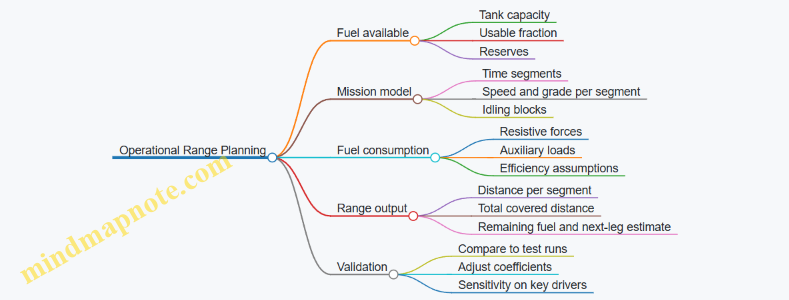
Practical Best Practice Summary
Model fuel use as time segments with explicit idling and auxiliary loads, compute power from resistive forces plus acceleration, apply efficiency in a way that reflects load, and convert to range using usable fuel and mission reserves. If you do those steps, your range estimate becomes explainable and adjustable, not just a number with confidence theater.
5.5 Practical Example: Comparing Mobility Tradeoffs for Different Terrain Profiles
Mobility is not a single number. It is a chain of constraints: power availability, traction at the contact patch, suspension load paths, steering geometry, thermal limits, and driver workload. A good comparison starts with terrain profiles that force different failure modes. Then you score each design against the specific constraints that terrain stresses.
Step 1: Define Terrain Profiles That Stress Different Limits
Use three profiles that are common in training and realistic in operations.
-
Profile A: Soft Loam With Ruts
- Primary stress: traction loss and sinkage.
- Typical symptoms: increasing slip, rising resistance, and track or wheel loading that exceeds ground bearing capacity.
-
Profile B: Rocky Rise With Short Obstacles
- Primary stress: suspension articulation, ground clearance, and impact loads.
- Typical symptoms: loss of contact on one side, high peak forces, and reduced ability to maintain speed without excessive deceleration.
-
Profile C: Wet Grass and Shallow Mud Patches
- Primary stress: variable friction and intermittent bogging.
- Typical symptoms: oscillating traction, frequent throttle changes, and thermal or powertrain strain if the vehicle keeps “hunting” for grip.
Step 2: Choose Metrics That Map to Engineering Reality
Pick metrics that you can measure during test runs.
- Average speed over the profile (not just top speed).
- Distance to recover after a traction event (time and meters).
- Energy per kilometer using fuel or electrical power draw.
- Slip ratio or wheel/track speed difference during steady motion.
- Peak suspension load and articulation margin during obstacles.
- Thermal margin for engine and brakes after repeated passes.
A practical rule: if a metric cannot be observed or instrumented, it will turn into an argument later.
Step 3: Build a Simple Trade Matrix
Assume two candidate platforms.
- Platform 1: Track-Optimized
- Wider contact area, higher traction potential, slower steering response.
- Platform 2: Hybrid Wheel-Track or Wheel-Optimized
- Lower rolling resistance on firm ground, but higher ground pressure and less compliant obstacle handling.
Score each platform from 1 to 5 for each metric on each terrain profile.
- On Soft Loam, Platform 1 typically scores higher for traction and recovery distance because ground pressure is lower and slip can be controlled.
- On Rocky Rise, Platform 2 may score higher for average speed if its suspension geometry maintains contact, but it risks higher peak loads and reduced clearance if articulation is limited.
- On Wet Grass, Platform 2 can be efficient on firm patches, yet it may suffer when friction drops abruptly; Platform 1 usually maintains steadier slip behavior.
Step 4: Use a Mind Map to Keep the Reasoning Connected
Mobility Tradeoff Mind Map
Step 5: Work Through One Profile with Numbers
Pick a representative run length: 1.5 km.
Profile A: Soft Loam With Ruts
- Platform 1 maintains slip around a controlled band and keeps contact pressure low.
- Example outcome: average speed 9 km/h, recovery events rare, energy per km moderate.
- Platform 2 reaches higher slip sooner because ground pressure is higher.
- Example outcome: average speed 6 km/h, more frequent recovery attempts, energy per km higher due to repeated throttle corrections.
Now interpret the results correctly. If Platform 2 is slower but uses less energy, it might be because it avoids deep ruts by taking a different line. That is still a mobility difference, but it is a navigation and control difference, not a pure traction advantage.
Step 6: Add the “Control and Driver” Layer
Mobility comparisons fail when control behavior is ignored. Two vehicles with identical traction capability can behave differently if one has smoother torque delivery or better steering authority.
- In Wet Grass, a vehicle that aggressively commands torque can increase slip oscillations, which raises energy use and heat.
- In Rocky Rise, a vehicle that saturates suspension travel can lose contact, forcing the driver to slow down earlier.
So, during the test, record driver inputs and control states. The goal is to separate “vehicle limitation” from “control strategy limitation.”
Step 7: Convert Scores Into a Decision That Engineers Can Defend
For each terrain profile, identify the dominant constraint.
- Soft Loam: traction and ground pressure dominate.
- Rocky Rise: articulation and clearance dominate.
- Wet Grass: variable friction and control stability dominate.
Then choose the platform that performs best where the mission route spends most of its time, while ensuring the other platform’s dominant constraint does not create unacceptable recovery time or safety risk.
A final sanity check: if the comparison depends on a single metric, it is probably missing the chain of constraints. Mobility is a system, so the evidence should be too.
6. Tracks Suspension Steering and Mobility Control
6.1 Track Design Contact Mechanics and Wear Considerations
Track performance is mostly a contact problem: rubber or steel elements meet terrain, forces flow through the contact patch, and materials gradually change shape. Good track design treats contact mechanics and wear as one system, not two separate checklists.
Contact Mechanics Foundations
A track does not “roll” like a wheel; it drags and lifts in cycles. As a road wheel rotates, the track’s contact patch moves from leading edge to trailing edge, while normal load and shear load vary with vehicle pitch, suspension motion, and terrain compliance.
Key quantities:
- Normal pressure distribution: how load spreads across the contact patch. A narrow, high-pressure patch accelerates surface damage.
- Shear stress: how traction and braking forces act tangentially. High shear promotes abrasion and micro-sliding.
- Slip ratio: the difference between track surface speed and ground speed. Even modest slip increases wear because the contact points repeatedly “scrub.”
A practical way to reason about wear is to track energy per unit distance. If the same vehicle travels farther with lower slip and more even pressure distribution, it usually earns longer track life.
Load Paths and Contact Patch Behavior
For design, it helps to separate where forces come from and where they go.
- From vehicle to track: suspension geometry and track tension set the vertical load level and how it changes over bumps.
- From track to ground: track pad stiffness, grouser geometry, and tread compliance shape the contact patch.
On hard ground, the contact patch tends to be smaller and pressure rises. On soft ground, the patch grows and pressure drops, but the track may sink, increasing the length of time elements spend in deforming soil. Wear mechanisms shift accordingly.
Wear Mechanisms and What Triggers Them
- Abrasion happens when hard particles (sand, grit, crushed rock) cut or plow the surface. It scales with particle hardness, normal pressure, and sliding distance.
- Adhesive wear occurs when surfaces momentarily bond under load and then tear apart. It is more likely when lubrication is poor and temperatures rise.
- Fatigue cracking targets links, pins, and bushings. It is driven by cyclic bending and impact loads, not just average stress.
- Grouser and pad wear reduces traction and changes the pressure distribution, which then feeds back into higher slip and more wear.
A simple example: if a track pad wears unevenly on one side, the vehicle may pull slightly, increasing steering corrections. Those corrections raise slip and shear at the contact patch, which then accelerates the same uneven wear.
Design Levers for Contact and Wear Control
1. Track Tension and Geometry
Proper tension reduces excessive articulation and prevents the contact patch from becoming erratic. Too loose increases impact loads; too tight can raise internal stresses and reduce compliance.
2. Pad and Grouser Geometry
- Wider pads spread normal load and reduce peak pressure.
- Grouser height and spacing influence how traction is generated and how soil is sheared.
- Edge sharpness affects initial bite and early wear; rounding can reduce abrasion but may reduce traction on certain soils.
3. Material Selection and Surface Treatments
Steel and rubber compounds are chosen for a balance of hardness, toughness, and resistance to abrasion. Surface treatments can reduce friction and slow material removal, but they must survive the real temperature and contamination conditions.
4. Suspension and Track System Compliance
Suspension tuning changes how quickly load transfers to the track during bumps. Smoother load transfer reduces peak stresses and slows fatigue growth.
Measurement and Wear Monitoring
Wear is easiest to manage when it is measurable. Common indicators include:
- Pitch and link elongation from pin/bushing wear.
- Grouser height loss or pad thickness reduction.
- Uneven wear patterns that reveal misalignment, track tension issues, or steering-induced slip.
- Track tension drift over time, which often correlates with internal wear.
A useful maintenance habit is to record wear measurements at consistent intervals and locations on the track. If one region consistently wears faster, the cause is usually mechanical alignment or local contact pressure, not “general aging.”
Mind Map: Track Contact Mechanics and Wear Considerations
Example: Diagnosing Uneven Wear on a Steering Turn
A vehicle shows faster wear on the inner side of the track during frequent turns on firm ground.
- Measure slip indicators indirectly by checking how quickly the inner track’s grouser height drops compared to the outer track.
- Inspect track tension and alignment to ensure both tracks share similar effective tension.
- Review steering behavior: tight-radius turns increase lateral shear and scrubbing, raising shear stress and sliding distance.
- Confirm terrain conditions: firm ground increases peak pressure and reduces compliance, which tends to intensify abrasion.
If the wear pattern is repeatable at the same steering geometry, the fix is usually operational technique plus mechanical alignment checks, not simply replacing the track.
Example: Reducing Abrasion Through Pressure Distribution
Two track pad designs are tested on the same abrasive surface.
- Design A has a narrower effective contact area.
- Design B spreads load with a wider pad footprint.
Even if both designs achieve similar mobility, Design B typically shows slower surface material loss because peak pressure and local sliding intensity are lower. The key is that wear rate follows contact intensity, not just total distance traveled.
6.2 Suspension Architectures and Load Path Management
A suspension is not just a set of springs and dampers. It is the vehicle’s load-routing system: it takes forces from the ground, shapes how those forces reach the hull, and keeps critical components from being asked to do jobs they were never designed for. Good load path management is what makes a suspension feel predictable over rough terrain and survive years of vibration, impacts, and maintenance.
Foundational Concepts of Load Paths
A load path is the chain of structural elements that carry forces from an external contact point to the vehicle body. In a tracked vehicle, the chain often runs from track contact forces into the road wheels and suspension arms, then into linkages, torsion bars or springs, dampers, and finally into the hull through mounts and brackets.
Two ideas guide architecture choices:
- Force direction matters. Vertical impacts, longitudinal braking forces, and lateral cornering forces each travel through different members and joints. A design that handles vertical loads well can still suffer if lateral shear concentrates at a single mount.
- Compliance is not free. Every bushing, joint, and bracket flexes. That flex changes wheel alignment, affects track tension behavior, and can amplify stress in nearby welds.
A practical way to think about it is to imagine a “stress spotlight.” When a bump hits, the spotlight should spread through intended members rather than concentrate at one small area like a thin bracket web.
Suspension Architecture Families
Most armored tracked suspensions can be grouped by how they store and transmit energy.
Torsion Bar Suspensions store energy in a bar that twists under load. The load path typically goes from road wheel to torsion bar, then into a pivot and into the hull mount. Best practice is to ensure the bar’s effective lever arm matches the expected wheel travel so that the bar sees manageable stress across the full stroke.
Hydropneumatic or Hydraulic Springs use pressurized chambers and dampers to provide both springing and damping. The load path includes hydraulic cylinders and their mounts, so mount stiffness and seal alignment become part of the structural story. If the cylinder is slightly misaligned, side loads can eat seals and create uneven damping.
Coil Spring and Damper Systems rely on springs and separate dampers. The load path includes spring seats and damper brackets, which must be designed to avoid bending moments that the damper piston was not meant to carry.
Trailing Arm and Linkage Systems use arms and linkages to connect wheel motion to the spring element. These systems can offer favorable wheel-rate characteristics, but they introduce more joints. Each joint adds compliance and potential wear, so load paths must be designed to keep joint forces within bearing and fatigue limits.
Load Path Management Principles
1. Define the primary load cases early. Typical cases include vertical impact, braking and acceleration, lateral cornering, and combined events like turning on uneven ground. If you only design for vertical loads, the suspension may pass a bump test but crack at a mount after repeated side-load cycles.
2. Keep load paths short and direct. Long chains with multiple bends and brackets increase the number of stress concentrations. A direct path also reduces the chance that a component becomes a “load thief,” carrying unintended forces because it is stiffest.
3. Manage stiffness gradients. If one member is much stiffer than its neighbors, it attracts load. For example, a very stiff damper mount can shift bending into the adjacent weld. A balanced stiffness layout spreads stress and reduces fatigue hotspots.
4. Control joint behavior. Bushings and bearings should be selected and preloaded so that they do not allow excessive angular misalignment. Excess misalignment increases friction, changes damping behavior, and accelerates wear.
5. Design mounts for both strength and fatigue. Mounts see repeated stress reversals. Weld toes, bolt holes, and bracket corners are common fatigue initiation sites. Smooth transitions and correct edge distances matter as much as ultimate strength.
Mind Map: Load Path and Architecture
Example: Turning over Uneven Ground
Consider a vehicle turning on a rutted surface. The inside road wheels experience reduced vertical load, while the outside wheels see higher vertical impacts. At the same time, lateral forces push the suspension sideways.
A robust load path handles this by:
- Routing lateral forces through arms and mounts that are designed for shear and bending, not just vertical compression.
- Ensuring bushings allow controlled compliance without letting the wheel shift enough to change track contact pattern.
- Keeping damper mounts from taking significant bending moments. If the damper is forced to carry bending, it will show early seal wear and inconsistent damping.
A simple check during design is to compare expected reaction forces at each mount for the combined case. If one mount’s reaction is an order of magnitude higher than its neighbors, the architecture likely has an unintended stiffness hotspot.
Example: Wheel Travel and Stress Hotspots
Suppose the suspension stroke is increased to improve obstacle clearance. Wheel travel changes the lever arms for torsion bars, linkages, and damper angles. That means the load path changes with position.
Best practice is to evaluate stress and mount reactions at multiple points along the stroke, not only at nominal ride height. If a bracket experiences peak bending near the end of travel, you can often fix it by adjusting geometry, adding a gusset, or changing mount placement so the load path remains direct when the suspension is near its limits.
Practical Summary
Suspension architecture determines how energy is stored and how forces are transmitted. Load path management ensures those forces travel through intended members with controlled compliance and fatigue-friendly details. When the load path is designed with the real combined load cases in mind, the suspension becomes both more predictable to drive and more reliable to maintain.
6.3 Steering Systems and Turning Radius Control
A tank’s turning radius is not just a geometric number; it’s the outcome of how steering inputs change track speeds, how the suspension transfers forces, and how the vehicle’s weight and traction limit what the drivetrain can actually do. Steering systems aim to produce predictable yaw rate while keeping slip, heat, and component stress within acceptable bounds.
Core Steering Concepts
Turning radius definition. For tracked vehicles, the “radius” is often expressed as the path of the vehicle centerline. In practice, you compute it from the instantaneous center of rotation (ICR): the point about which the vehicle effectively rotates at that moment.
Track-speed steering. Most tanks steer by commanding different effective speeds between left and right tracks. If one track slows while the other maintains speed, the ICR shifts toward the slowed track. With both tracks moving but at different speeds, the vehicle follows an arc rather than pivoting in place.
Pivot steering. If one track is commanded near zero forward speed (or reverse) while the other continues forward, the ICR moves close to the stationary track. This yields a tight turn, but it increases shear forces in the contact patch and can raise track and drivetrain loads.
From Inputs to Yaw Rate
Steering input chain. A typical chain is: driver input → steering control law → hydraulic/electric actuators → final drives → sprocket torque and track speed → ground reaction forces → yaw rate and path.
Why control law matters. If the controller simply “sets track speeds,” it may ignore traction limits. A better approach uses feedback such as yaw rate, wheel speed, and sometimes lateral slip estimates, so the commanded differential produces the intended yaw without excessive skidding.
Slip as the hidden variable. Two vehicles with the same commanded track-speed difference can produce different turning radii depending on surface conditions. Soft soil increases sinkage and changes the relationship between torque and effective track speed.
Geometry and Kinematics of Turning
Instantaneous center of rotation. For a vehicle with track separation (effective distance between track contact centroids) of B, and left and right track speeds of vL and vR, the yaw rate r and ICR location can be approximated by:
- r ≈ (vR − vL) / B
- ICR offset from centerline ≈ (B/2) · (vL + vR) / (vR − vL)
These relations assume no major longitudinal slip differences beyond what the speeds represent. In real tests, you validate with measured yaw rate and path tracking.
Neutral steer and symmetry. When vL = vR, yaw rate is near zero and the turning radius is effectively infinite. When vL = −vR (one track forward, the other reverse), the ICR approaches the vehicle centerline, producing a tight rotation.
Traction Limits and Turning Radius Tradeoffs
The “tight turn costs traction” rule. Tight radii require large differential track speeds or near-zero speed on one side. That increases the longitudinal shear demand at the contact patch, which can exceed available friction.
What you observe. Excessive slip shows up as:
- slower-than-expected yaw response,
- longer-than-modeled turn radius,
- increased track wear and heat in driveline components.
Practical best practice. Use a steering schedule that limits differential commands based on measured or estimated traction state. For example, on wet ground you reduce maximum differential for the same steering lever position, so the controller prioritizes predictable radius over maximum agility.
Suspension and Load Transfer Effects
Why the suspension changes steering. During a turn, lateral load transfer alters normal force on each track. Lower normal force reduces available friction, which changes how torque converts to effective speed.
Track contact variability. Uneven terrain can cause one track to have different effective contact length, making the same actuator command produce different ground speeds. Good steering control compensates using feedback rather than assuming identical track-ground conditions.
Control System Design for Turning Radius Control
Feedback signals. Common signals include left/right track speed, yaw rate from a gyro, and sometimes lateral acceleration. With these, you can close the loop on yaw rate and radius rather than only on actuator commands.
Command shaping. Step changes in steering input create transient slip spikes. A simple ramp on differential speed commands reduces peak shear forces and improves repeatability.
Calibration through test data. You map steering input to yaw rate across representative surfaces. Then you adjust control gains so the vehicle reaches the target yaw rate without oscillation.
Mind Map: Steering Systems and Turning Radius Control
Example: Predicting Radius from Track Speeds
Assume track separation B = 3.6 m. At a given moment, the controller commands vL = 1.5 m/s and vR = 3.0 m/s.
- r ≈ (3.0 − 1.5) / 3.6 = 0.417 rad/s
- The ICR offset from the centerline is approximately
- (3.6/2) · (1.5 + 3.0) / (3.0 − 1.5) = 1.8 · 4.5 / 1.5 = 5.4 m
So the vehicle centerline follows an arc with an instantaneous radius near 5.4 m. In a test, if the measured radius is larger, it usually means the left track is slipping more than expected or the right track is traction-limited.
Example: Steering Schedule to Reduce Radius Error
On dry asphalt, you might allow a full steering input to command a large differential. On wet clay, you apply the same steering input but cap the differential speed change so the controller stays within friction limits. The result is a slightly larger radius than the “dry” model predicts, but the radius becomes consistent and the vehicle avoids the long, unpredictable arcs caused by uncontrolled slip.
Example: Pivot Turn Load Management
For a pivot turn, one track is commanded near zero while the other maintains forward motion. A practical approach is to limit the initial differential ramp rate and monitor yaw rate response. If yaw rate lags, the controller reduces differential to prevent excessive shear and track damage, trading a small loss in tightness for a safer, repeatable pivot.
6.4 Braking Systems and Thermal Management
Braking is a job of turning kinetic energy into heat, then making sure the vehicle can do that job repeatedly without losing braking performance or damaging components. On armored platforms, the challenge is not only stopping power, but also heat removal through constrained airflow, protected packaging, and harsh dust and water exposure.
Core Braking Functions and Energy Budget
A useful starting point is the energy balance. If a vehicle slows from speed \(v\) to \(0\), the kinetic energy \(E_k = \frac{1}{2} m v^2\) must be absorbed by friction elements and dissipated to the environment. In practice, some energy goes into drivetrain losses and structural heating, but the majority becomes brake heat. Best practice is to define a braking duty cycle early: number of stops, target decelerations, maximum downhill duration, and allowable temperature limits for pads, discs, calipers, bearings, and nearby seals.
Example: If two vehicles have the same mass but one is heavier by 10% and both brake from the same speed, the heavier vehicle generates about 21% more kinetic energy. That difference often shows up as faster pad wear, higher disc temperature, or reduced braking consistency during repeated stops.
Friction Brakes and Heat Generation Mechanisms
Most armored vehicles use friction brakes with pads or shoes acting on discs or drums. Heat generation depends on brake torque and sliding speed. During a stop, sliding speed is highest at the beginning and decreases as the vehicle slows, so heat rate is not constant. Thermal management must therefore handle both peak temperatures and the time spent near elevated temperatures.
Key design variables include:
- Friction material selection: It must maintain predictable friction across temperature and moisture.
- Contact pressure and area: Higher pressure can reduce stopping distance but increases local heating.
- Brake cooling paths: Airflow, conduction to the housing, and heat transfer to nearby structures.
Example: A brake that meets stopping distance in a single test may fail a downhill requirement because the disc temperature rises over minutes, not seconds. The friction coefficient can drop with temperature, and seals can degrade.
Thermal Paths and Where Heat Actually Goes
Heat flows from the friction interface into the disc or drum, then into the caliper or backing plate, and finally into the vehicle structure and cooling air. In armored layouts, airflow is often intermittent and turbulent, so conduction to a heat-spreading structure can matter as much as direct cooling.
A practical approach is to map thermal resistances:
- Interface resistance between pad and disc
- Material conduction through disc and caliper
- Convection resistance to ambient air
- Radiation as a minor contributor at typical brake temperatures
Best practice is to instrument at least two points: one near the friction surface (disc or rotor) and one in a sensitive neighbor (bearing housing or seal region). Relying on only one temperature can hide overheating in a component that is thermally insulated from the disc.
Braking Control, Fade, and Consistency
Brake fade is the loss of braking effectiveness as temperature rises. It can come from friction coefficient changes, pad glazing, fluid boiling (if hydraulic), or structural distortion that alters contact.
To keep braking consistent:
- Use thermal-aware control logic that limits repeated high-demand braking when temperatures approach thresholds.
- Ensure actuation stiffness so that pedal or controller commands translate into predictable brake torque.
- Maintain clearance management so that thermal expansion does not cause drag or delayed engagement.
Example: If a vehicle is commanded to brake hard every time it reaches a crest, the disc may not cool between events. A control strategy that recognizes temperature rise can reduce peak torque slightly while preserving overall stopping performance across the route.
Cooling Strategies and Packaging Constraints
Cooling methods must survive dust, mud, and water. Common strategies include:
- Ventilated discs to increase surface area and promote internal airflow
- Heat sinks integrated into the caliper or carrier
- Ducted airflow where the vehicle’s motion provides predictable air movement
- Shielding to prevent mud packing that blocks convection
A simple but effective practice is to design for cleaning. If mud can pack into a cooling gap, the thermal path becomes much worse after a few operational cycles.
Testing and Acceptance for Thermal Performance
Thermal validation should include both peak and sustained conditions. A systematic test plan pairs:
- Repeated stop tests to evaluate fade and wear progression
- Downhill or grade tests to evaluate steady-state temperatures
- Environmental tests to check performance after dust and water exposure
Instrumentation should include disc temperature, caliper or bearing housing temperature, and brake torque or deceleration feedback. Acceptance criteria should be expressed as both absolute limits (no component exceeds a safe temperature) and functional limits (stopping distance and deceleration remain within bounds).
Mind Map: Braking Systems and Thermal Management
Example: Building a Thermal-Aware Braking Test Sequence
- Choose a representative mass and tire/track condition for the scenario.
- Define a duty cycle with, for example, ten stops from a specified speed with a fixed time between stops.
- Set a second condition for sustained braking on a grade long enough to reach near steady-state.
- Instrument disc temperature and bearing housing temperature.
- Record deceleration and brake torque for each stop.
- Accept the design only if stopping performance stays within limits and temperatures remain below component thresholds across both conditions.
A good test sequence makes it obvious whether the system fails due to peak temperature, cumulative heating, or environmental effects. That clarity is what turns thermal management from a guess into an engineering decision.
6.5 Practical Example: Building a Mobility Test Plan for Obstacle Traversal
A mobility test plan for obstacle traversal should answer three questions before the first run: what “good” looks like, how you will measure it, and what you will do when the vehicle behaves badly. The plan below is written for a tracked or wheeled armored platform, but the structure stays the same.
Define the Obstacle Set and Success Criteria
Start by listing obstacle types and the exact pass/fail boundaries. Use measurable criteria so the team does not argue about vibes.
Obstacle set (example):
- Step up: 0.3 m, 0.45 m, 0.6 m
- Step down: 0.3 m, 0.45 m
- Trench or gap: 0.5 m, 0.7 m
- Slope: 30°, 35° (up and down)
- Side slope: 20° (left and right)
- Rollover ramp: controlled crest with known geometry
Success criteria (example):
- Traversal completed without immobilization lasting more than 10 seconds
- No track throw or wheel hub damage beyond replaceable limits
- Maximum allowable deceleration spike and peak articulation within defined bounds
- Driver-perceived controllability rating collected after each run using a simple 1–5 scale
Build a Test Matrix That Avoids “One-Off” Runs
A test matrix prevents the classic mistake: changing too many variables at once. Keep the matrix small enough to execute, but complete enough to interpret.
Variables to control:
- Vehicle configuration: normal combat load vs. reduced load
- Tire pressure (wheeled) or track tension (tracked)
- Speed band: crawl (0.5–1.0 m/s) and moderate (1.5–2.0 m/s)
- Operator: primary driver only for baseline, then a second driver for repeatability
- Surface condition: dry firm, wet firm, loose gravel
Example matrix rule:
- For each obstacle and surface, run two speeds at baseline configuration, then repeat one speed after a maintenance check.
Instrumentation and Data Logging Plan
Obstacle traversal produces short, violent events, so instrumentation must capture peaks and time alignment.
Minimum instrumentation (example):
- IMU for pitch/roll/yaw and angular rates
- Wheel/track speed sensors
- Suspension travel sensors or proxy (e.g., encoder-based articulation)
- Engine and transmission parameters (torque, gear, temperatures)
- Brake and steering actuator states
- Optional: strain gauges on critical links for deeper analysis
Logging requirements:
- Sampling rate high enough for impact transients (plan for at least 200 Hz for IMU)
- Timestamp synchronization across all channels
- A run start trigger tied to driver command or throttle rise
Safety, Recovery, and Stop Rules
Define stop rules that protect people and hardware while keeping the test meaningful.
Stop rules (example):
- Immediate stop if smoke, abnormal vibration, or fluid leaks occur
- Stop if immobilization exceeds 10 seconds or if steering cannot be commanded
- Stop if temperatures exceed pre-set limits
Recovery procedure (example):
- Use a standardized recovery method and record the time and method used
- After recovery, inspect only the defined items, then log “recovered” as a separate outcome category
Run Procedure and Repeatability Checks
A run procedure should be consistent enough that differences come from the obstacle, not from the operator’s mood.
Example run steps:
- Pre-run inspection and sensor health check
- Set configuration and confirm speed band using a driver display
- Approach at the commanded speed, hold steering neutral unless the obstacle requires correction
- Execute the traversal, then stop at a marked safe zone
- Post-run inspection and quick data review for sensor dropouts
Repeatability check:
- For the first obstacle of each surface condition, perform two runs back-to-back and compare peak pitch/roll and completion outcome.
Mind Map for the Test Plan Structure
Mobility Obstacle Traversal Test Plan Mind Map
Example: Interpreting One Obstacle Outcome
Suppose the 0.6 m step up on wet firm surface fails to complete.
What to check first:
- Did the vehicle reach the commanded approach speed? If not, treat it as an execution issue.
- Compare peak pitch angle and suspension travel to the matrix baseline. If pitch is higher than expected, the approach angle or obstacle contact point may differ.
- Review torque and gear state. If torque saturates early and speed collapses, the limiting factor is likely traction or power delivery rather than steering control.
- Confirm whether recovery time exceeded the stop rule threshold; if it did, classify outcome as “immobilized” rather than “attempted.”
Data Summary Template for Each Run
Keep the run record compact so it is usable during analysis.
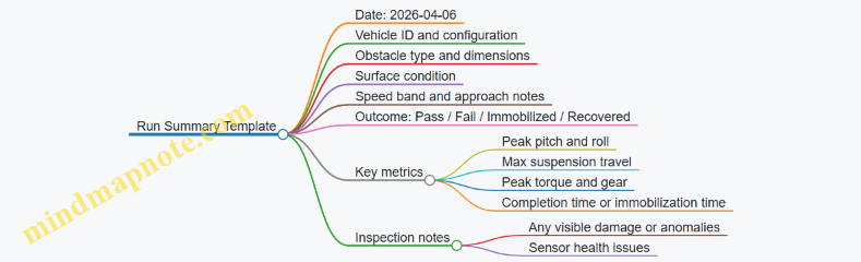
This plan structure scales from a small proving ground session to a full acceptance-style campaign because it separates obstacle definition, controlled variables, measurement, and decision rules. When the vehicle fails, the plan already tells you where to look first, which is the difference between learning and guessing.
7. Thermal Management and Environmental Control
7.1 Heat Sources and Heat Transfer Paths in Armored Platforms
Armored platforms generate heat in several places, and the tricky part is that heat does not respect component boundaries. A powertrain might be “fine” while the crew compartment quietly warms up because heat is traveling through structure, air, and fluids. A systematic approach starts with identifying heat sources, then mapping how heat moves, and finally checking where it ends up.
Heat Sources in the Vehicle
Engine and Aftertreatment Heat. The engine produces heat through combustion and friction, which must be carried away by the cooling system. If the vehicle uses exhaust aftertreatment, additional heat appears near the exhaust manifold and catalyst region. Even when the engine is off, residual heat can continue to warm nearby metal for a while.
Transmission and Drivetrain Losses. Gears, bearings, and clutches convert mechanical work into heat. These losses often concentrate in the transmission housing and near final drives. A common practical observation is that oil temperature rises faster than coolant temperature during sustained low-speed operation.
Hydraulics and Power Electronics. Hydraulic pumps, motors, and actuators generate heat proportional to pressure and flow. Electric drives and inverters also create heat, typically in concentrated hotspots on circuit boards and power modules.
Brakes and Friction Elements. Braking converts kinetic energy into heat at the contact surfaces. Track brakes and service brakes can create sharp temperature spikes, and the heat then spreads into hubs, shafts, and nearby covers.
External Heat Loads. Sun exposure heats outer surfaces, especially dark or matte finishes. Hot ambient air raises the temperature of cooling inlets and reduces radiator effectiveness. Cold conditions matter too because they change air density and viscosity, affecting airflow and convection.
Internal Heat Loads. Crew and onboard equipment add heat to the crew compartment and electronics bays. Even “small” loads matter when ventilation is limited.
Heat Transfer Paths in Armored Platforms
Heat moves through three main mechanisms: conduction, convection, and radiation. In armored vehicles, all three operate at once, and the dominant path changes with operating mode.
Conduction Through Structure. Metal paths connect hot components to cooler ones. For example, an engine block can conduct heat into the engine mounts, then into the hull floor. If the crew compartment shares that structure, the floor can become a slow but persistent heater.
Convection in Fluids and Air. Coolant carries heat from the engine to radiators. Oil carries heat from transmission components to heat exchangers. Airflow over radiators and through ducting drives convection. If a duct leaks or a fan speed control is miscalibrated, the heat rejection rate drops quickly.
Radiation Between Surfaces. Hot exhaust surfaces radiate heat to nearby walls, covers, and wiring bundles. Radiation is often underestimated because it does not require direct contact, so it can warm components even when airflow is minimal.
Mixed Paths and “Heat Bridges.” A heat bridge is a structural or mechanical connection that provides a low-resistance path for heat. Examples include mounting brackets, fasteners, and thick structural ribs. A bracket that looks “small” can still move significant heat because it spans a large temperature difference.
Systematic Mapping Method
Start with a heat source list, then assign each source to a transfer path, then identify the sink.
- Mark heat sources by location and operating condition (steady, transient, or after shutdown).
- Trace conduction paths through mounts, frames, and hull panels.
- Trace convection paths through coolant/oil loops and air ducts.
- Check radiation view factors by identifying nearby hot surfaces and enclosed cavities.
- Identify sinks such as radiators, heat exchangers, coolant reservoirs, and cooled electronics bays.
This mapping is easiest when you use a layered diagram: “hot zone,” “transfer zone,” and “cool zone.”
Mind Map: Heat Sources and Transfer Paths
Example: Why a “Cool Engine” Can Still Mean a Warm Crew Bay
Assume the engine coolant temperature stays within limits during a long drive. Meanwhile, the crew bay floor temperature rises. The likely chain is:
- The engine block conducts heat into engine mounts.
- Mounts conduct heat into the hull floor.
- The floor convects heat to cabin air, especially if ventilation is low.
- Radiation from nearby hot covers adds a smaller but steady contribution.
A practical fix is not only to improve coolant flow, but also to reduce conduction through mounts (insulating standoffs or thermal breaks) and to ensure ducted airflow actually removes heat from the cabin floor region.
Example: Braking Heat That Doesn’t Show Up Where You Measure
If you measure only coolant temperature, you might miss brake-induced overheating. Brake heat first raises hub and brake housing temperatures through conduction. Then it spreads into nearby oil lines and covers. If the oil temperature sensor is located far from the heat source, the sensor may lag or under-report peak conditions. The systematic mapping method prevents this by placing sensors along the expected transfer paths, not just at convenient locations.
Example: External Heat Load During High Sun and Low Airflow
On a clear day with limited airflow through the radiator, sun-heated outer panels can raise the temperature of intake air. That reduces radiator effectiveness, which then increases coolant temperature. Meanwhile, the same sun load can warm wiring bundles through conduction and radiation. The integrated view keeps you from treating “engine overheating” as a purely internal problem.
7.2 Cooling System Components and Flow Management
A tank or armored vehicle cooling system has one job: keep temperatures inside limits while the vehicle does real work—idling, climbing, sprinting, and crawling through dust. The trick is that heat sources change faster than operators can react, so the system must manage both heat transfer and fluid movement with predictable behavior.
Core Cooling Loop Components
Start with the heat source side. The engine produces heat in the cylinder block and oil system, and the transmission and hydraulics often add their own loads. Those loads are connected to a coolant circuit through heat exchangers and jackets.
Next is the coolant path. A typical liquid loop includes:
- Radiator or heat exchanger core: transfers heat from coolant to air.
- Water pump: provides circulation pressure and flow.
- Thermostat or temperature-controlled valve: regulates how much coolant bypasses the radiator.
- Fan drive: moves air through the core when vehicle speed is insufficient.
- Expansion tank and cap: accommodates thermal expansion and maintains pressure for higher boiling margin.
- Hoses, manifolds, and fittings: route coolant while minimizing restrictions.
- Air management features: shrouds, ducting, and louvers that prevent short-circuiting air around the core.
For armored vehicles, oil cooling is usually separate or partially integrated. Engine oil coolers and transmission oil coolers may be plate heat exchangers or finned cores. They often sit in the same airflow envelope as the radiator, but they must be treated as distinct thermal loads because their allowable temperatures and flow rates differ.
Flow Management Principles
Flow management is about controlling three things: flow rate, pressure drop, and mixing behavior.
-
Flow Rate Control
- The pump sets baseline flow, but thermostats and bypass passages decide where that flow goes.
- A simple example: if the thermostat sticks partially closed, the radiator sees less flow, so the engine outlet temperature rises even though the pump is running normally.
-
Pressure Drop Awareness
- Every restriction—radiator core, cooler plates, filters, and tight hose bends—adds pressure drop.
- If pressure drop increases due to fouling, the pump may still run, but actual flow through the core drops. A practical check is to compare coolant temperature rise across the radiator: reduced flow typically increases the temperature difference between inlet and outlet.
-
Mixing and Stratification
- Coolant can stratify in tanks and manifolds if flow enters gently or if dead zones exist.
- Example: a poorly designed expansion tank inlet can create a warm layer that reaches the sensor first, causing the thermostat to open earlier than needed and wasting radiator capacity.
Component-Level Best Practices with Examples
Pump and Cavitation Margin
- Ensure the pump inlet has adequate net positive suction head under all operating attitudes and altitudes.
- Example: during steep climbs, coolant head changes at the pump inlet. If the suction line is too long or has high elevation loss, cavitation bubbles can form, reducing effective flow and causing local hot spots.
Thermostat and Bypass Strategy
- Use thermostats that provide stable modulation rather than abrupt switching.
- Example: a thermostat that oscillates around its set point can cause repeated radiator cycling. That leads to uneven thermal stress in hoses and cooler cores.
Radiator Core Airflow Discipline
- Protect the core from air bypass by using shrouds and sealing edges.
- Example: if the fan pulls air around the sides of the core, the coolant may not receive enough heat transfer even though the fan speed looks correct.
Fan Control Logic
- Fan operation should respond to coolant temperature and, when available, radiator outlet temperature.
- Example: if the fan is controlled only by engine inlet temperature, it may run late when the radiator is already heat-soaked.
Filters and Maintenance Interfaces
- Place strainers or filters where they can be serviced without draining the entire system.
- Example: a clogged inline filter increases pressure drop. The engine may overheat during high-load operation but look fine at idle, because flow demand is lower.
System Behavior from Cold Start to Steady State
A coherent cooling strategy follows a predictable sequence:
- Cold start: thermostat restricts radiator flow to warm the engine quickly while limiting thermal shock.
- Warm-up transition: as coolant reaches the thermostat range, bypass reduces and radiator flow increases.
- Steady operation: fan and thermostat maintain temperatures by balancing heat rejection with airflow and coolant circulation.
- High-load events: increased heat generation raises coolant temperatures; the system responds by increasing radiator engagement and fan airflow.
A useful mental model is to treat the system as a set of controllable valves: the thermostat decides coolant routing, the fan decides airflow, and the pump decides circulation. If any one of those is misbehaving, the temperature pattern across the loop becomes the clue.
Mind Map: Cooling System Components and Flow Management
Example: Diagnosing a Cooling Complaint Using Flow Clues
Suppose an operator reports overheating during sustained climbs but normal temperatures at idle. A systematic check focuses on flow and heat rejection balance:
- Measure coolant temperature at radiator inlet and outlet. If the radiator outlet rises too quickly, flow through the core is likely insufficient.
- Inspect for increased restriction: clogged filter, partially blocked hose, or radiator fouling.
- Confirm thermostat behavior: if it does not fully open under load, radiator engagement is reduced.
- Verify airflow: check fan operation and ensure shrouds prevent air bypass.
This approach keeps the investigation grounded in what the system is physically doing, not what it is supposed to do.
7.3 Intake Exhaust Routing and Dust Ingestion Mitigation
Dust ingestion is a routing problem before it becomes a filtration problem. If dust-laden air reaches the engine intake, it will also find its way into cooling passages, air cleaners, and seals. If exhaust is routed poorly, it can re-entrain dust into intakes and contaminate crew areas. The goal is simple: keep the intake air path away from dust sources, keep the exhaust away from intake inlets, and manage pressure and airflow so the vehicle does not “suck” dust in through unintended leaks.
Foundational Airflow Paths and Pressure Logic
Start with the vehicle’s pressure map. Many armored vehicles run with a slight positive pressure in protected compartments to reduce inward leakage of dust and fumes. That positive pressure must not be created by pulling air through the engine bay. Instead, use a dedicated filtered supply for crew spaces and ensure the engine compartment ventilation does not reverse flow during transient events like fan start, throttle changes, or door opening.
A practical check is to trace where air goes during three conditions: steady travel, engine start-up, and a brief stop with fans running. If the intake ducting and exhaust routing allow any of those conditions to create a low-pressure region near intake openings, dust will be pulled in through gaps, imperfect seals, or even through the air cleaner housing.
Intake Routing Principles That Reduce Dust Exposure
Place intake openings where the dust concentration is lowest. For tracked vehicles, dust is typically highest near the ground and along the sides where tracks throw material. That means intake inlets should be elevated when packaging allows, and angled to reduce direct line-of-sight to dust clouds.
Use duct geometry to avoid “dust traps.” Long, sharp bends can cause particle settling and accumulation, which then becomes a source of re-entrained dust. Smooth transitions and controlled bend radii help. Also, keep intake ducts short and insulated where heat soak could reduce air density and increase the likelihood of condensation, which can make dust clump and stick.
Exhaust Routing Principles That Prevent Re-Entraining
Exhaust should be routed so hot gases do not blow dust toward intake openings. A common failure mode is placing exhaust outlets where crosswinds or vehicle yaw cause exhaust plumes to sweep back into intake inlets. Even without wind, the vehicle’s own motion can create a recirculation zone behind and above the exhaust.
Mitigation is mostly geometric: increase separation distance between exhaust outlet and intake inlet, use outlet orientation that directs flow away from intake, and consider heat shield placement to prevent exhaust-induced convection from drawing dust-laden air upward into intake paths.
Cooling Air Management Without Creating a Dust Vacuum
Cooling fans and radiator airflow can unintentionally become a dust pump. If the cooling air path draws from the same region as the dust cloud, the engine bay becomes a dust concentrator. Route cooling intakes to cleaner zones and use baffles to prevent short-circuiting from exhaust heat and dust-laden air.
A useful rule of thumb is to ensure the engine bay ventilation path has a clear direction: air enters from a controlled location, passes through cooling components, and exits through a defined outlet. If the path is ambiguous, dust will find the easiest leakage route.
Sealing, Interfaces, and the “Small Leak Big Problem” Effect
Dust ingestion often comes from interfaces: duct joints, clamp points, air cleaner seals, and access panels. Use consistent gasket materials and verify compression during assembly. For field maintainability, design joints so technicians can reinstall without twisting ducts or misaligning seals.
A simple example: if an intake duct uses a flexible section to accommodate engine movement, the flexible section can become a dust reservoir if it sags. Keep it supported so it maintains shape under vibration.
Mind Map: Intake Exhaust Routing and Dust Ingestion Mitigation
Example: Routing a Side Intake and Rear Exhaust
Assume a vehicle has a side-mounted engine intake and a rear exhaust outlet. If the intake is at mid-height near the track line, dust concentration will be high during turns. Move the intake upward within the available envelope and angle it so the inlet face is not directly exposed to the track-spray direction.
Then address exhaust. If the exhaust outlet is near the rear deck, dust thrown upward by the tracks can rise into the exhaust plume and be carried forward. Increase separation between exhaust and intake, and rotate the exhaust outlet so the plume exits downward and rearward. Finally, verify that cooling fan intake does not draw from the same rear recirculation zone by checking airflow direction with the vehicle stationary and fans running.
Example: Diagnosing a Dust Ingestion Complaint
If dust is found inside the engine bay air cleaner housing, start with routing and pressure first. Look for a low-pressure region near the intake during fan operation, then inspect duct joints and the air cleaner seal for gaps. Next, check whether exhaust plume recirculation is sweeping dust toward the intake during turns. Only after routing and sealing checks should you increase filtration capacity, because better filters cannot compensate for a system that keeps feeding dust faster than it can be handled.
7.4 Cabin Environmental Control and Crew Comfort Constraints
Cabin environmental control is not a luxury feature; it is a survivability subsystem. Heat, smoke, dust, and oxygen availability all affect crew performance, which then affects aiming quality, reaction time, and safe operation of the vehicle. Comfort constraints are therefore written as measurable limits, not vibes.
Foundational Requirements for Crew Environment
Start with three baseline questions: What must the crew be able to do, how long must they do it, and what conditions will the vehicle face while doing it. From those answers, derive limits for temperature, humidity, airflow, visibility through anti-fog measures, and acceptable contaminant levels.
A practical best practice is to define “task windows.” For example, if the crew must perform navigation and weapon checks for 30 minutes, set tighter limits for that window than for maintenance or transit. This prevents overdesign for short bursts while still protecting the moments that matter.
Air Supply and Pressurization Strategy
Most armored vehicles use filtered air supply to manage dust ingress and protect against smoke. The key design choice is whether the cabin is slightly pressurized relative to the outside. Positive pressure reduces unfiltered leakage paths, but it also increases the consequences of filter saturation and duct leaks.
A simple example: if the cabin is held at a small pressure differential, a torn door seal becomes a “continuous leak” that draws in dust through the leak path. That means the filter system must be sized not only for normal flow, but also for realistic leakage rates.
Filtration and Contaminant Control
Filtration targets particulate dust and, in some designs, smoke aerosols. The system should include staged filtration so that coarse particles do not clog fine media immediately. A good operational practice is to design for filter monitoring using differential pressure sensors, because airflow drop is often the first sign of clogging.
Example: if the differential pressure rises faster than expected, the crew can switch to a reduced flow mode to maintain breathable air longer rather than running the system until it fails.
Thermal Management and Heat Load Budgeting
Cabin temperature is governed by heat sources inside the compartment and heat transfer through hull surfaces. Heat sources include electronics, lighting, battery or power electronics (where applicable), and human metabolism. Heat transfer depends on ambient temperature, solar load, and conduction through walls.
A systematic approach is to build a heat load budget with three columns: internal sensible heat, internal latent heat from moisture, and external heat gain. Then allocate cooling capacity to each column. This avoids the common mistake of sizing the system for “average temperature” while ignoring humidity and peak loads.
Example: during slow movement in cold weather, the engine bay may be cooler, but the crew still adds moisture. If humidity rises, fogging becomes the limiting factor even when temperature is acceptable.
Humidity Control and Anti-Fog Measures
Humidity affects visibility through fogging on optics and windshields. Control can be passive (insulation and airflow distribution) and active (dehumidification or controlled condensation management, depending on architecture).
A practical best practice is to treat anti-fog as a distribution problem. Airflow directed across critical optical surfaces can prevent condensation without overcooling the entire cabin. That reduces thermal gradients that otherwise cause discomfort and uneven sensor performance.
Airflow Distribution and Draft Management
Airflow must be enough to remove heat and contaminants, but not so strong that it causes drafts across faces, eyes, or sensitive controls. Uneven airflow also creates temperature stratification, where one crew member feels cold while another feels hot.
Example: if vents are positioned only near the ceiling, warm air may pool and the lower cabin remains cooler. The crew then compensates by changing clothing or posture, which increases workload. Better practice is to validate airflow with mockups and instrumented airflow mapping.
Noise Vibration and Crew Comfort Constraints
Environmental control hardware introduces noise and vibration through fans, dampers, and duct resonances. These can interfere with radio communication clarity and increase fatigue. Comfort constraints should therefore include allowable sound pressure levels at crew head locations and limits on vibration transmitted to seats or control panels.
A simple example: a fan that meets airflow requirements but produces a narrowband tonal noise can be more fatiguing than a higher broadband noise level. Testing should include both overall level and tonal components.
Operational Modes and Failure Handling
Cabin systems typically operate in modes such as normal filtered ventilation, recirculation, and emergency smoke/contaminant response. Each mode changes airflow rate, filtration usage, and pressurization behavior.
Best practice is to define mode transition rules that are easy for the crew to execute under stress. For instance, emergency mode should prioritize maintaining breathable air and preventing rapid fogging, even if it reduces comfort.
Example: if the system detects a rapid pressure drop indicating a leak, the control logic can reduce total flow to extend filter life while maintaining minimum airflow to critical visibility zones.
Mind Map: Cabin Environmental Control and Crew Comfort Constraints
Example: Turning Requirements Into Testable Limits
Assume a 30-minute task window for navigation and weapon checks. Set a maximum cabin temperature and a maximum humidity level that correlates with acceptable windshield and sight anti-fog performance. Then add airflow minimums for contaminant removal and a noise limit at head height. Finally, require tests that simulate filter loading and a representative leakage scenario so the crew’s “emergency mode” behavior is validated, not guessed.
When these constraints are written this way, the environmental control system becomes predictable. The crew gets breathable air, usable visibility, and fewer distractions—exactly what you want when the vehicle is doing its job.
7.5 Practical Example: Designing a Cooling Capacity Budget for Hot Weather
Start with the idea that “cooling capacity” is not a single number. It is a chain of heat sources, heat paths, and heat sinks that must balance at steady state. In hot weather, the limiting factor is often the radiator’s ability to reject heat to air, which depends on airflow, ambient temperature, and coolant temperature margins.
Step 1: Define Operating Point and Constraints
Assume a tracked armored vehicle operating at a sustained engine load. Pick an operating point that matches how the vehicle is actually used, not a lab maximum.
- Ambient air temperature: 35°C
- Maximum allowable coolant temperature at engine outlet: 105°C
- Minimum radiator inlet air temperature rise margin: 10°C (so the radiator can still reject heat without boiling or derating)
- Target coolant temperature at radiator inlet: 95°C
This gives a coolant-to-air temperature difference budget. If radiator inlet coolant is 95°C and air is 35°C, the average driving temperature is about 60°C before you account for losses and non-uniformities.
Step 2: Build the Heat Source List
Create a heat inventory and keep it specific. Typical sources include:
- Engine heat rejected to coolant (from engine thermal maps or test data)
- Transmission oil heat (from gear and converter losses)
- Hydraulic system heat (from pumps, valves, and return losses)
- Electric motor/inverter heat if applicable
- Fan motor and auxiliary loads
Example values for a hot-weather sustained run (illustrative):
- Engine to coolant: 420 kW
- Transmission oil to cooler: 55 kW
- Hydraulics to cooler: 25 kW
- Electric auxiliaries to cooling loop: 10 kW
Total heat to reject: 510 kW.
Step 3: Separate Cooling Loops and Heat Exchangers
Do not assume one radiator magically handles everything. Many vehicles use multiple loops or staged heat exchangers.
A practical layout might be:
- Loop A: Engine coolant to main radiator
- Loop B: Transmission oil to oil cooler (often air-to-oil)
- Loop C: Hydraulics to separate cooler or shared radiator section
If Loop B and Loop C share the same radiator face area, you must allocate radiator capacity by heat exchanger effectiveness and pressure drop limits.
Step 4: Convert Heat Rejection Into Required Radiator Performance
Radiator heat rejection can be treated as:
- Q = UA × ΔT_lm
Where Q is heat rejected, UA is overall conductance, and ΔT_lm is the log-mean temperature difference between coolant and air. You can approximate ΔT_lm with a conservative average driving temperature.
For a first-pass budget:
- Coolant inlet to radiator: 95°C
- Coolant outlet to radiator: 105°C
- Air temperature: 35°C
- Approximate driving temperature average: (95-35 + 105-35)/2 = 75°C
If you need to reject 510 kW at an effective driving temperature of 75°C, the required UA is roughly:
- UA ≈ Q / ΔT ≈ 510 kW / 75°C ≈ 6.8 kW/°C
Now apply a margin for fouling, aging, and non-ideal airflow. A common budgeting approach is 15% capacity margin reduction.
- Effective UA target ≈ 6.8 × 0.85 ≈ 5.8 kW/°C
That means your radiator core area and fin design must support about 510 kW at the reduced effective conductance.
Step 5: Account for Airflow and Fan/Vehicle Speed
Radiator performance depends on airflow, which depends on vehicle speed and fan duty. Build a simple airflow model:
- At low speed, fan dominates airflow.
- At higher speed, ram air dominates and fan can reduce.
Use test or CFD-derived fan curves to estimate airflow at the operating point. If airflow drops by 20% at the chosen condition, UA often drops similarly (not perfectly, but close enough for budgeting). If UA drops 20%, your effective UA becomes 0.8 × 5.8 = 4.6 kW/°C, which may force derating or higher coolant temperatures.
So the cooling budget must include a “minimum acceptable airflow” check.
Step 6: Check Temperature Margins and Control Logic
Even if the radiator can reject the average heat, control must prevent excursions.
- Thermostat behavior: ensure it does not trap heat in the loop.
- Fan control: verify it reaches the required fan speed before coolant outlet exceeds limits.
- Bypass valves: confirm they do not reduce radiator flow at the wrong time.
A simple sanity check: if coolant outlet approaches 105°C, the system is at the edge. That edge should be reached only under the intended sustained load, not during short transients.
Step 7: Practical Allocation Example for Shared Radiator
Suppose the main radiator face area is shared between Loop A and Loop C. Allocate radiator capacity by heat exchanger effectiveness and measured pressure drop limits.
Example allocation:
- Loop A engine coolant: 420 kW
- Loop C hydraulics: 25 kW
- Remaining capacity for transmission oil cooler air side: 65 kW (if integrated)
If the transmission cooler is actually air-to-oil with its own fin section, treat it as consuming radiator conductance. If you cannot measure conductance directly, use a conservative split: reserve 10–15% of radiator capacity for non-engine loads.
Mind Map: Cooling Capacity Budget Workflow
Step 8: Validation with a Simple Test Plan
Instrument at least:
- Engine coolant inlet and outlet temperatures
- Radiator air temperature upstream and downstream
- Fan speed and electrical power draw
- Transmission oil and hydraulic return temperatures
Run the sustained hot-weather profile and confirm that predicted coolant outlet temperature stays below the limit with the chosen margin. If it doesn’t, adjust the budget in the order that usually fixes it fastest: confirm airflow first (filters, shutters, fan duty), then revisit UA assumptions (core blockage, fin efficiency), and only then revisit heat source estimates.
8. Weapon Integration and Fire Control System Foundations
8.1 Gun System Basics and Recoil Management
A tank gun is a chain of energy conversion steps: chemical energy becomes projectile kinetic energy, and the gun structure must survive the equal-and-opposite reaction. Recoil management is the part that keeps the vehicle stable enough to hit what the crew aimed at, and keeps the gun from beating itself to pieces.
Gun System Components and Their Jobs
A typical tank gun system includes the barrel, recoil mechanism, breech, muzzle device (if fitted), cradle, elevation and traverse drives, fire-control interfaces, and the ammunition handling interface. The barrel provides the bore and rifling or smoothbore geometry, but it is also a precision reference for alignment. The breech seals the chamber, handles pressure containment, and interfaces with the firing mechanism.
The recoil mechanism absorbs rearward energy and returns the gun to battery. It usually combines hydraulic damping with a spring or gas system for energy storage and return. The cradle and trunnions transmit loads into the turret structure, so their stiffness and alignment directly affect how repeatable the gun’s pointing is.
Recoil Physics in Practical Terms
When the projectile accelerates forward, the gun experiences a rearward impulse. Impulse is the integral of force over time, so two guns can have similar peak forces but different recoil durations, which changes how the suspension and turret respond. The recoil force is shaped by chamber pressure rise and fall, projectile mass, propellant burn characteristics, and barrel length.
A useful mental model is to treat recoil as a short “push” that must be absorbed without letting the gun’s aim wander. The recoil stroke length matters because it determines how quickly the energy is dissipated. Longer stroke can reduce peak force but requires space and affects how fast the system can return to a stable firing position.
Recoil Mechanism Operation
Most recoil systems aim for three outcomes: controlled rearward motion, energy dissipation, and consistent return to battery. Hydraulic damping converts kinetic energy into heat through fluid flow restrictions. The return element stores energy during recoil and pushes the gun forward afterward.
Consistency is the quiet hero here. If the damping varies with temperature or if fluid leaks reduce damping, the gun may return to battery at slightly different positions. That shows up as elevation or bore-sight shifts that the fire-control system can compensate only within limits.
Recoil Effects on Accuracy and Stability
Recoil affects accuracy through two pathways. First, the gun’s pointing can change during recoil if the turret structure flexes or if drives allow motion. Second, the vehicle can move if the recoil impulse couples into the hull and suspension.
A simple example: if the turret is allowed to “float” during recoil, the gun may start and end at different angles. Even if the crew sees the same aiming reticle, the projectile leaves the barrel after the system has settled. That makes timing and mechanical stiffness part of accuracy, not just optics.
Elevation and Traverse Drives During Firing
Elevation and traverse drives must handle recoil loads without introducing backlash or oscillation. Many systems use a control strategy that either locks the drives during the firing event or manages motor torque so the gun follows the recoil stroke without fighting it.
Backlash is a common accuracy enemy. If gears or linkages have clearance, the direction reversal during recoil return can cause a small angular error. That error can be repeatable, which is easier to compensate, or variable, which is harder.
Muzzle Devices and Their Influence
Muzzle devices can reduce muzzle blast signature or manage recoil-related effects such as pressure distribution. They also add complexity: added mass at the muzzle changes the barrel’s dynamic response, and gas flow can alter how the barrel vibrates after firing.
A practical check is to observe whether the gun’s settling time changes with the muzzle device configuration. If the barrel takes longer to settle, the fire-control solution must account for that so the shot timing aligns with the stable phase.
Example: Diagnosing a Recoil-Related Accuracy Shift
Assume a crew reports that shots are consistently low by a small amount after a certain number of rounds. The first step is to separate “aiming error” from “mechanical return error.”
- Verify that the fire-control system is using the correct ballistic solution and that range and ammo selection match the load.
- Compare first-round accuracy to subsequent rounds. If the first round is correct and later rounds drift, suspect thermal effects or damping variation.
- Inspect recoil mechanism condition. Low hydraulic fluid, degraded seals, or contaminated fluid can reduce damping.
- Check for turret drive backlash or looseness. If the turret mount shows play, recoil return can shift the gun’s final position.
If the drift correlates with temperature, the recoil mechanism is a prime suspect because damping viscosity changes with temperature. If the drift correlates with rounds fired regardless of temperature, look for wear or fluid aeration.
Mind Map: Gun System Basics and Recoil Management
Key Takeaways
Recoil management is not just about stopping motion; it is about repeatable motion. When the recoil mechanism returns the gun to battery consistently and the drives avoid backlash-induced angle errors, the fire-control solution can do its job with fewer surprises.
8.2 Ammunition Types and Handling Constraints
A tank’s ammunition is more than a list of calibers and weights. It is a tightly managed set of energy sources, mechanical interfaces, and safety rules that must work together under vibration, shock, temperature swings, and tight crew schedules. Handling constraints exist because ammunition is both a weapon and a stored-energy system.
Ammunition Types by Function
Most tank ammunition types can be grouped by what they must do at impact.
- Kinetic energy penetrators rely on projectile mass and velocity to defeat armor. Handling focuses on maintaining projectile integrity, preventing damage to the penetrator tip, and protecting the sabot or driving band surfaces.
- High explosive anti-tank uses shaped effects and explosive energy to create a damaging mechanism. Handling focuses on fuse safety, preventing contamination of fuze components, and avoiding impacts that could compromise arming paths.
- High explosive is optimized for soft targets, structures, and area effects. Handling emphasizes consistent fuze function and safe management of fragmentation hazards.
- Training and inert rounds preserve training realism while reducing hazard. Handling still matters because inert rounds can share the same mechanical interfaces and can still be dangerous if mis-stowed or mis-identified.
A practical way to keep this straight is to treat each type as a “different contract” with the gun: different interfaces, different safety states, and different expected performance.
Ammunition Types by Interface and Packaging
Ammunition is also categorized by how it mates with the gun and how it is packaged for storage.
- Fixed rounds combine projectile and propellant into one unit. Handling constraints center on overall mass, center-of-gravity control, and safe lifting procedures.
- Semi-fixed rounds separate projectile and propellant but still require controlled pairing. Handling constraints center on matching the correct propellant charge to the correct projectile.
- Separate-loading ammunition uses distinct components for projectile and propellant. Handling constraints are stricter because mis-pairing can create incorrect ballistic behavior or unsafe conditions.
Packaging adds another layer: rounds may be stored in bustle racks, hull stowage, or carousel systems, each with different access paths and retention features. The “best” ammunition type is the one that can be reliably loaded in the time available without violating safety rules.
Handling Constraints That Control Safety
Handling constraints fall into four practical categories.
- Fuze and safety device state: Many rounds include safeties that must remain engaged until the correct conditions occur. Handling must prevent accidental arming triggers such as improper seating, damaged safety pins, or contamination.
- Propellant integrity: Propellant is sensitive to heat, moisture, and mechanical damage. Handling constraints include temperature limits, humidity control, and avoiding dents or punctures to propellant containers.
- Mechanical interface cleanliness: Gun breech and loading mechanisms require predictable surfaces. Handling constraints include keeping driving bands, obturating surfaces, and mating interfaces free of debris and corrosion.
- Retention and stowage discipline: Rounds must remain properly secured. Handling constraints include verifying correct stowage location, ensuring locking mechanisms engage, and preventing “temporary” placements that become permanent.
A simple example: if a crew member sets a round on a loading surface “just for a second,” it can end up with a damaged fuze cover or a misread label, and the next loading cycle may proceed with the wrong safety state.
Handling Constraints That Control Performance
Safety is necessary, but performance depends on consistent condition.
- Mass and balance: Damaged projectiles or altered seating can change how the round feeds. Even small feed issues can increase loading time or cause misalignment.
- Surface condition: Scratches on critical surfaces can affect obturation or guidance of the projectile during loading.
- Charge selection and pairing: For systems with variable charges, the correct charge must be paired with the correct projectile and the correct firing mode.
A concrete example is charge selection in separate-loading systems. If the crew loads the correct projectile but the wrong charge, the gun may still fire, but the ballistic solution and impact point will be wrong, and the mismatch can complicate safety margins.
Loading Workflow Constraints for Real Crews
Integrated handling constraints show up in the workflow.
- Identification: Rounds must be positively identified before loading. Labels, markings, and stowage location must agree.
- Condition checks: Crews perform quick inspections for obvious damage, missing covers, or compromised seals.
- Controlled movement: Handling tools and lifting methods prevent drops and impacts.
- Breech and chamber readiness: Loading must occur only when the gun is in the correct state, including safe breech conditions.
A good best practice is to standardize the order of operations so the crew does not rely on memory under stress. For instance, “identify, inspect, move, seat, confirm” reduces the chance of skipping a step.
Mind Map: Ammunition Types and Handling Constraints
Example: Preventing Mis-Pairing in a Separate-Loading System
Imagine a separate-loading setup where the projectile and propellant charges are stored in different compartments. A best practice is to enforce a pairing rule at the moment of retrieval: the loader confirms the projectile type and then selects the matching charge from a stowage location that is physically keyed or clearly marked. If the charge is not the correct one, the round is not moved to the loading area. This single constraint prevents both performance errors and safety complications caused by incorrect component combinations.
Example: Managing Fuze Safety During Handling
Consider a round with a fuze cover that protects sensitive components. Handling constraints require keeping the cover intact until the round is seated in the gun. If a cover is removed early, it can collect dust or be damaged during movement, and it can also lead to confusion about whether the fuze is in the intended safety state. A disciplined workflow treats the fuze cover as part of the safety system, not as packaging.
Summary of Constraints as Practical Rules
Ammunition handling constraints are best remembered as rules that connect safety to performance: keep fuze and propellant in their intended condition, keep interfaces clean, keep stowage disciplined, and keep pairing correct. When those rules are embedded in the workflow, the crew spends less time troubleshooting and more time loading correctly.
8.3 Fire Control Components and Sensor Inputs
Fire control is the vehicle’s way of turning “I see something” into “I can place a hit where it matters.” This section focuses on the components that do that work and the sensor inputs that feed them, with an emphasis on what each part contributes and how errors travel through the chain.
Fire Control Chain from Sensor to Gun
A typical chain has five functional steps: sensing, measurement conditioning, tracking and target state estimation, ballistic computation, and gun/weapon actuation. The key idea is that each step reduces uncertainty in a specific way, but also introduces its own failure modes.
- Sensing provides raw measurements such as bearing, elevation, range, and sometimes target motion cues.
- Conditioning converts sensor outputs into consistent units and timing, filters noise, and aligns coordinate frames.
- Tracking estimates target position and velocity over time, using repeated observations.
- Ballistic computation predicts where the projectile will be at the time the gun fires, accounting for gun geometry, ammunition characteristics, and environmental effects.
- Actuation drives the turret and gun to the computed aim point and manages stabilization during the shot.
A practical best practice is to treat timing as a first-class requirement. If the range measurement and the gun angle are not synchronized, the system can be “accurate” in isolation and still miss in combination. A simple example is a laser rangefinder reading taken a fraction of a second after the turret has moved; the computed lead will be based on stale geometry.
Core Fire Control Components
Fire Control Computer
The computer is the integrator. It stores ballistic tables or models, applies sensor corrections, and outputs commands such as turret traverse rate, gun elevation, and firing solution parameters. It also manages health monitoring so that the system can reject inconsistent inputs.
Stabilization System
Stabilization keeps the line of sight and/or gun aligned despite vehicle motion. It typically uses inertial sensors and feedback loops. If stabilization is degraded, the system may still compute a solution, but the “where the gun actually points” assumption becomes less reliable.
Gun Drive and Control Loops
These include motor drives, encoders, and control electronics. They translate computed aim angles into physical motion. A useful mental model is that the fire control computer computes an angle; the drive system must achieve it quickly and repeatably. Encoder calibration errors are a classic way to create a consistent miss.
Range and Measurement Subsystems
Range can come from laser rangefinding, radar, or other measurement methods depending on the platform. Each method has different uncertainty behavior. For instance, laser range often has strong dependence on reflectivity and atmospheric conditions, while radar range may have different latency and tracking characteristics.
Ammunition and Ballistic Data Inputs
The system needs ammunition identity and parameters such as muzzle velocity model selection, ballistic coefficient usage, and any programmed corrections. A simple example: if the system assumes a standard muzzle velocity but the selected round is a different variant, the computed time of flight shifts and the lead becomes wrong.
Sensor Inputs and Their Roles
Optical and Thermal Imaging Sensors
Imaging sensors provide target detection and bearing information. They also support tracking by producing repeated measurements of target position in the sensor frame. The main practical issue is that image-based measurements can be biased by mounting misalignment and by changes in magnification state.
Inertial Measurement Unit and Gyros
Inertial sensors provide vehicle attitude and angular rates for stabilization and for transforming measurements into a common reference frame. A subtle but important point: gyro bias affects long engagements more than short ones because the attitude estimate drifts over time.
Laser Rangefinder
Laser range provides direct distance to the target or to a point on the target. The system must handle cases where the laser returns are weak or ambiguous. A practical example is a target behind light foliage: the system might lock onto a nearer branch, producing a range that is too small and causing the projectile to fall short.
Environmental Sensors
Wind and temperature inputs may come from onboard sensors or from derived estimates. Even when wind is not directly measured, the system may use assumptions or operator inputs. The best practice is to ensure that environmental values are applied to the correct ballistic model and that units are consistent.
Mind Map: Fire Control Components and Sensor Inputs
Example: Building a Consistent Firing Solution
Assume the system receives: turret bearing from the drive encoders, gun elevation from the elevation encoder, vehicle attitude from the inertial unit, and range from a laser measurement. The computer first transforms the line-of-sight into the vehicle coordinate frame, then into a ballistic reference frame. Next it selects the ammunition model based on the round identity input, computes time of flight using the muzzle velocity model, and applies lead based on the tracked target velocity.
Now introduce a realistic issue: the laser range is taken at a slightly different time than the turret angles. If the vehicle is turning, the bearing changes during that interval. The result is a systematic miss that looks like a “mysterious” lead error. The fix is not changing the ballistic model; it is aligning measurement timestamps and ensuring the conditioning step interpolates turret and attitude states to the range measurement time.
Example: Sensor Input Quality Gates
A robust system does not blindly accept every sensor output. It uses quality checks such as range validity thresholds, track confidence levels, and stabilization status. For instance, if the laser rangefinder reports low confidence, the system can either request a new measurement or fall back to a less precise mode that still maintains safe engagement behavior. This is not about being cautious for its own sake; it prevents the ballistic computation from being driven by measurements that are likely wrong.
8.4 Stabilization and Ballistic Computation Fundamentals
A stabilized fire-control system has two jobs: keep the line of sight steady despite vehicle motion, and compute where the projectile will go given the real conditions at the moment of firing. If either job is sloppy, the gun can be perfectly aimed at the wrong place. The good news is that both jobs are built from straightforward components: sensors, control laws, and a ballistic model.
Stabilization Concepts and Coordinate Frames
Stabilization starts with coordinate frames. The gun has a bore axis, the turret has its own axes, and the vehicle moves in the world frame. The system must know how to convert between them so that “aiming” means “pointing the bore at a computed direction in the world frame.”
A practical way to think about stabilization is to separate two errors:
- Line-of-sight error: the sight or sensor direction differs from the desired direction.
- Bore error: the gun barrel direction differs from the stabilized sight direction.
A typical architecture uses gyros and accelerometers to estimate vehicle angular motion, then drives turret and gun actuators to cancel that motion. The sight may be stabilized directly, or the gun may be stabilized relative to a stabilized sight; either way, the control loop must be consistent with the chosen reference.
Sensor Inputs and State Estimation
The ballistic computer needs more than range. It needs a snapshot of the firing geometry and the platform state. Common inputs include:
- Target direction from the sight system.
- Range from a laser rangefinder or other measurement.
- Vehicle attitude and angular rates from inertial sensors.
- Gun position from elevation and azimuth encoders.
- Environmental parameters such as air temperature and pressure, when available.
State estimation turns noisy sensor signals into usable estimates. For example, gyro rates are integrated to estimate angles, but integration drifts over time. A filter (often a complementary or Kalman-style approach) blends gyro integration with other measurements to keep the estimate stable enough for control.
Stabilization Control Loops
Stabilization control typically uses nested loops:
- Rate control: commands actuator effort to reduce measured angular rate error.
- Position control: commands turret or gun angles to track the desired stabilized angles.
A clean mental model is to treat the gun as a plant with inertia and friction. If you only use position error, the system may lag during sudden motion. If you only use rate error, it may hunt around the target direction. Nested loops let the system respond quickly to motion while still converging to the correct angle.
A simple example: the vehicle hits a bump. The gyro sees a pitch rate spike. The rate loop reacts immediately, preventing the sight line from slewing away. Meanwhile, the position loop slowly corrects the remaining angle error so the gun settles back onto the computed aim point.
Ballistic Computation Fundamentals
Ballistic computation converts a fire-control solution into a gun elevation and, if applicable, lead angles. The core idea is that projectile motion depends on gravity, initial muzzle velocity, drag, and wind. A ballistic model typically uses:
- Time of flight based on range and projectile characteristics.
- Drop due to gravity over that time.
- Lateral displacement due to wind and drag effects.
- Sight-to-bore geometry so the computed direction matches the actual mounting.
The ballistic computer also accounts for muzzle reference and line-of-sight offset. If the sight is above the bore, aiming “at the same point” requires different elevation than a naive geometry calculation.
Example: From Target Data to Gun Elevation
Assume the system measures:
- Range: 2,000 m
- Target direction: straight ahead
- Wind: 3 m/s from the left
- Vehicle pitch rate: small and already compensated by stabilization
The ballistic model estimates time of flight, then computes vertical drop and wind drift. The computer outputs a required gun elevation that includes:
- Gravity drop compensation
- Drag-adjusted trajectory correction
- Sight-to-bore offset correction
If the wind is ignored, the gun elevation might still look correct, but the projectile will land left or right. If stabilization is ignored, the computed elevation may be correct in world coordinates, yet the bore points elsewhere at the firing instant.
Advanced Details Without the Mystery
Lead and motion compensation: If the target moves, the system must use target motion estimates to compute an aim point at the predicted time of impact. Even when the target motion is modest, the time of flight can be long enough that small angular errors become large miss distances.
Muzzle velocity variation: Muzzle velocity can vary with temperature, barrel wear, and ammunition lot. A robust system uses either measured velocity (when available) or correction factors so the ballistic model doesn’t assume a single fixed value.
Uncertainty management: Sensors have error bars. The stabilization loop reduces angular error, but it cannot eliminate it. The ballistic solution should therefore be consistent with the expected measurement quality so that the system doesn’t overreact to noise.
Mind Map: Stabilization and Ballistic Computation
Example: A Consistency Check That Saves Misses
Before firing, the system can perform a sanity check: if the computed gun elevation changes sharply when range changes slightly, the ballistic model may be operating outside its valid assumptions or the range measurement may be noisy. Similarly, if stabilization reports large residual angular error at the moment of command, the system should treat the solution as unreliable because the bore may not be pointing where the ballistic computation assumed it was.
8.5 Practical Example: Tracing From Target Data To Engagement Solution
This practical example shows how a fire control system turns target data into a computed gun laying solution, then into a safe, testable engagement sequence. The goal is traceability: every number used in the final aim point should have a clear origin, a unit, and a reason.
Step 1: Start with Target Data and Measurement Uncertainty
Assume the vehicle has a stabilized sensor that provides a target track in the sensor coordinate frame. The system outputs:
- Line-of-sight angles (azimuth, elevation) with estimated error bounds
- Range estimate or range-from-stereo/laser measurement with uncertainty
- Target track quality flags (for example, stable track vs. tentative track)
Best practice: treat uncertainty as a first-class input. If the range error is large, the system should widen the allowable solution acceptance window or request a new measurement. A simple check prevents “confident aiming at a shaky target.”
Step 2: Convert Coordinates and Apply Time Alignment
Sensor data is time-stamped, but the gun system, turret encoders, and ballistic computer may run on slightly different cycles. The system performs time alignment:
- Interpolate target track to the current fire-control computation time
- Transform target position from sensor frame to turret/gun frame using current boresight calibration
- Apply turret and gun angles from encoders to express the target in a common reference
Easy example: if the turret yaw encoder lags by 30 ms, the computed lead angle will be off for moving targets. Time alignment fixes that by using the turret state at the same instant as the target state.
Step 3: Build the Ballistic Problem Inputs
The ballistic computer needs projectile and environment inputs. Typical inputs include:
- Ammunition ballistic coefficient or drag model selection
- Muzzle reference conditions and barrel wear compensation
- Propellant temperature or charge condition
- Meteorological data such as air temperature and pressure
- Vehicle motion state for line-of-fire stabilization
Best practice: keep a “units sanity check” near the computation. Mixing degrees and mils, or meters and yards, is the kind of mistake that survives reviews because it still produces a number. A quick unit validation step catches it early.
Step 4: Compute Lead, Drop, and Wind Effects
With target position and velocity, the system computes an intercept point in space, then converts it into gun elevation and azimuth commands.
- Lead: uses target motion and projectile time-of-flight
- Drop: uses gravity and projectile time-of-flight
- Wind: applies lateral drift based on wind model and time-of-flight
Concrete example: if the range is 1,500 m and the projectile time-of-flight is 4.0 s, a 2 m/s crosswind produces a lateral drift of roughly 8 m before accounting for drag effects. The ballistic model refines that estimate, but the rough math is useful for plausibility checks.
Step 5: Apply Stabilization and Laying Constraints
The computed solution becomes commands, but the system must respect mechanical and safety constraints:
- Turret and gun slew rate limits
- Maximum elevation limits
- Stabilization mode selection based on vehicle motion
- Cross-checks for sensor-to-gun alignment validity
Best practice: if the required gun motion exceeds limits, the system should flag “solution not achievable” rather than forcing a partial command. That prevents a “looks correct on paper” engagement.
Step 6: Validate Solution Acceptance and Generate Engagement Data
Before firing, the system evaluates whether the solution is acceptable:
- Compare computed aim point error against allowable bounds derived from measurement uncertainty
- Confirm ammunition selection matches the ballistic model
- Verify that safety interlocks are satisfied
The output package should include:
- Gun command angles
- Predicted time-of-flight
- Confidence or acceptance status
- A short trace record for maintenance and training
Step 7: Perform a Traceable Engagement Sequence
A practical sequence might look like this:
- Acquire target track and confirm quality flags
- Update target state at computation time
- Compute ballistic solution using current environment and ammo model
- Check laying constraints and stabilization mode
- Run acceptance tests using uncertainty bounds
- If accepted, present “fire ready” and log the trace record
- If rejected, request updated measurements or adjust sensor mode
Mind Map: Data Flow and Decision Points
Example: A Single Computation Trace Record
A trace record for one engagement attempt should read like a breadcrumb trail:
- Time alignment: target state interpolated to computation time
- Transform: sensor frame to gun frame using current boresight
- Ballistic inputs: ammo model ID, barrel condition index, air temperature and pressure
- Computation: intercept point computed with lead and wind drift
- Constraints: slew rate within limits, elevation within bounds
- Acceptance: predicted aim error within allowable window based on range and angle uncertainty
- Output: gun azimuth and elevation commands plus predicted time-of-flight
When you can point to each line and say where it came from, the system becomes easier to test, easier to debug, and harder to fool with accidental nonsense.
9. Sensors and Targeting for Day Night and Adverse Conditions
9.1 Optical Imaging and Field of View Considerations
Optical imaging for armored vehicles starts with a simple question: what portion of the world can the sensor see at once, and how clearly can it resolve details inside that portion. Field of view (FOV) is the “how much you get in the frame” part, while image quality is the “how much of that you can actually use” part. The two are linked through geometry, optics, and sensor resolution, so good practice is to treat FOV as a design variable, not a fixed spec.
Foundational Geometry of Field of View
For a camera with a horizontal FOV, the scene width covered at range is approximately:
- Scene width ≈ 2 × range × tan(FOV/2)
A practical example: if the horizontal FOV is 10° and the target is 500 m away, the scene width is about 2 × 500 × tan(5°) ≈ 87.5 m. If you widen the FOV to 20°, the scene width doubles to about 175 m. Wider FOV helps acquisition and navigation, but it also spreads the same pixels across a larger area, reducing detail per pixel.
Pixel Resolution and Angular Sampling
To connect FOV to usable detail, use angular resolution per pixel. If the sensor has N pixels across the image and spans an angular width equal to the FOV, then:
- Angular step per pixel ≈ FOV / N
Example: a 1920-pixel-wide sensor with a 10° FOV has about 10° / 1920 ≈ 0.00521° per pixel. At 500 m, 0.00521° corresponds to roughly 500 × tan(0.00521°) ≈ 45.5 mm on the ground plane for small angles. That number is the “smallest feature size you can represent” in a rough sense; real performance is worse due to blur, contrast limits, and atmospheric effects.
Tradeoffs Between Wide and Narrow FOV
A narrow FOV (longer focal length or zoom) increases detail and helps identification, but it makes target acquisition harder because the target occupies fewer degrees of the view. A wide FOV makes it easier to find targets and track them through vehicle motion, but it can force the operator to rely on additional steps such as cueing or digital zoom.
A useful best practice is to define two operational modes:
- Acquisition mode: wider FOV to reduce time-to-first-detection.
- Identification mode: narrower FOV to support confident recognition.
Even if the system uses a single optical channel, you can emulate this behavior by planning how the operator transitions between zoom levels and how the fire control system requests higher magnification.
Stabilization and Motion Effects
Vehicle motion adds a second kind of blur: image smear from angular rate. Stabilization reduces this, but it has limits tied to sensor bandwidth and control loop performance. A simple way to reason about it is to compare expected angular motion during an exposure to the sensor’s angular sampling.
Example: if the vehicle induces 0.02° of angular movement during the effective exposure time, and your pixel step is 0.005°/pixel, the target shifts about 4 pixels. That can be acceptable for detection but problematic for fine identification. The mitigation is not only “better stabilization”; it can also include shorter exposure, higher illumination, or a different optical configuration that tolerates motion.
Atmospheric and Contrast Constraints
Optical imaging is sensitive to contrast loss from haze, dust, and rain. FOV affects how much of the image is dominated by background clutter, which changes the operator’s ability to separate target edges from the environment. A narrow FOV can reduce clutter by focusing on a smaller area, but it also increases the chance that the target leaves the frame during tracking.
Best practice: evaluate performance using metrics tied to tasks, not just resolution. For example, measure the minimum range at which a target feature reaches a usable contrast threshold under representative visibility conditions.
Practical Design Workflow
A systematic workflow keeps the tradeoffs from turning into guesswork:
- Choose the task split between acquisition and identification.
- Select candidate FOV values that cover the expected engagement geometry.
- Compute scene width and angular sampling for each candidate.
- Estimate motion blur impact using stabilization and exposure assumptions.
- Validate with test images that include realistic backgrounds and lighting.
Mind Map: Optical Imaging and Field of View Considerations
Example: Choosing FOV for a Two-Step Engagement
Assume a vehicle must detect a vehicle-sized target at 800 m and then identify it for engagement. If you start with a 12° horizontal FOV, the scene width is about 2 × 800 × tan(6°) ≈ 168 m, which is wide enough to include likely target positions while the vehicle is moving. Once the target is centered, switching to a 4° FOV reduces the scene width to about 56 m, increasing detail and making edge features easier to distinguish. The operator’s job becomes simpler: acquire with context, then refine with detail.
The key is that both FOV settings are justified by task needs and by the geometry-to-pixels relationship, not by a single “best” magnification that ignores acquisition difficulty.
9.2 Thermal Imaging Principles and Detection Performance Metrics
Thermal imaging measures infrared radiation emitted by objects and converts it into a temperature-like signal. In armored vehicle contexts, that signal is rarely “just temperature”; it is shaped by surface emissivity, viewing geometry, atmospheric effects, and the sensor’s own optics and electronics. A useful way to think about thermal imaging is: radiation in, image out, with multiple error sources along the way.
How Thermal Sensors Form Images
A typical uncooled or cooled thermal camera uses an infrared bandpass filter and a detector array to sample radiance across the scene. Optics focus the scene onto the detector, and the camera electronics map detector output to pixel values. If the camera performs radiometric calibration, those pixel values can be converted to an estimated apparent temperature. If not, the image is still meaningful for detection and tracking, but metrics must be defined in terms of contrast and detection probability rather than absolute temperature.
A practical best practice is to treat the camera as two systems: the optics-detector chain (which sets sensitivity and resolution) and the image processing chain (which sets how contrast becomes a usable detection). For example, a vehicle commander may see a target silhouette clearly, yet the algorithmic detector might fail because the processing pipeline suppresses low-contrast edges.
Emissivity and Apparent Temperature
Emissivity describes how efficiently a surface emits infrared radiation compared to an ideal blackbody. Two objects at the same physical temperature can look different if one has a shiny or reflective surface. In the field, dust, paint, and wetness change emissivity, so the same target can appear to “heat up” or “cool down” as conditions change.
A concrete example: a steel track link covered in dust often appears warmer than bare metal at the same ambient temperature because dust behaves closer to a high-emissivity surface. That can improve detectability, but it can also mislead range estimation if you assume a constant emissivity.
Detection Performance Metrics That Matter
Detection performance is usually summarized with metrics that connect sensor physics to operational outcomes.
Signal-to-Noise Ratio (SNR) SNR compares the target’s radiance contrast to sensor noise. Higher SNR means the target stands out more reliably. In practice, SNR is influenced by integration time, detector sensitivity, and scene clutter.
Noise Equivalent Temperature Difference (NETD) NETD is the temperature difference that produces a signal equal to the sensor noise level. Lower NETD indicates better sensitivity. NETD is a convenient spec, but it does not automatically guarantee detection in cluttered scenes; a low-NETD sensor can still struggle if the target contrast is small relative to background variation.
Modulation Transfer and Spatial Resolution
Spatial resolution affects whether a small target occupies enough pixels to be distinguishable from noise and background texture. A target that is only a few pixels wide may be detectable as a blob but not reliably classifiable.
Contrast and Target-Background Separation
Detection depends on contrast, not absolute temperature. A useful metric is the effective contrast-to-noise ratio between target and immediate background. For instance, a vehicle on a uniform sand berm may yield higher contrast than the same vehicle against a rocky slope with similar radiance patterns.
Detection Probability and False Alarm Rate
Operationally, you want a probability of detection (Pd) at an acceptable false alarm rate (Pf). These are often derived from receiver operating characteristics (ROC) curves. A slightly playful but accurate rule: if you tune thresholds to reduce false alarms, you usually pay with reduced Pd, and vice versa.
From Physics to Metrics Without Gaps
Start with radiance contrast: the target’s emitted radiance minus the background’s emitted radiance, adjusted by emissivity and atmospheric transmission. Next, map that contrast through the sensor’s optics and detector response into an expected pixel signal. Then account for noise sources such as detector noise, quantization, and scene-dependent variations. Finally, apply the detection rule, such as thresholding on pixel intensity or using a multi-pixel detector.
A common failure mode is skipping the detection rule. For example, a single-pixel threshold might look good in a lab, but in real scenes the target edges blur due to motion, wind-driven dust, or slight misalignment, reducing the usable contrast across the detector’s spatial support.
Mind Map: Thermal Imaging Metrics Flow
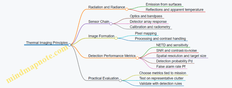
Example: Comparing Two Sensors in One Scenario
Suppose Sensor A has lower NETD than Sensor B, but Sensor A’s processing applies stronger noise suppression. In a scene with a low-contrast target partially occluded by vegetation, Sensor A may produce a smoother image that reduces pixel-level fluctuations, yet it can also attenuate the target edge contrast. The result can be a lower Pd at the same Pf even though NETD is better.
To evaluate properly, you would measure Pd and Pf using the same detection algorithm and thresholding strategy, then report performance at a defined operating point. That keeps the comparison honest: you are comparing detection outcomes, not just sensor specs.
Example: Using Contrast-to-Noise in Vehicle Context
Consider a thermal view of a tank hull against a sun-warmed road. The road’s radiance varies across the frame, creating background texture. Even if the tank is warmer, the local background near the tank may be similar, shrinking effective contrast. A practical metric is to compute contrast in a small neighborhood around the target and divide by the local noise estimate. That directly reflects what the detector sees rather than what the spec sheet promises.
Summary of What to Measure
For thermal imaging detection, measure sensitivity (NETD), spatial adequacy (resolution relative to target size), and scene-dependent separability (contrast-to-noise). Then convert those into operational metrics using detection probability and false alarm rate under representative clutter and viewing geometry. This approach keeps the chain from physics to performance intact, which is exactly what you want when the scene refuses to cooperate.
9.3 Laser Rangefinding and Measurement Uncertainty Handling
Laser rangefinding measures distance by timing a light pulse’s travel or by comparing phase. In armored vehicle contexts, the practical challenge is not the physics of light; it’s the measurement chain: atmospheric effects, target reflectivity, geometry, and the way uncertainty propagates into fire control.
Core Measurement Model
A simple time-of-flight model is:
- Distance \(R = c \cdot t / 2\), where \(c\) is the speed of light and \(t\) is the measured round-trip time.
For phase-based systems, the model is similar but uses phase difference to infer range. Either way, the measured range is not the true range; it is the true range plus error terms.
A useful decomposition is:
- Timing error: jitter in pulse emission and detection, quantization of time bins.
- Propagation error: refractive index variations from temperature, pressure, and humidity.
- Target interaction error: partial return, speckle, motion blur, and reflectivity changes.
- Geometric error: boresight misalignment between laser and sight line, and range-to-point vs range-to-target-surface differences.
Uncertainty Sources and How They Behave
Timing and Quantization
Timing uncertainty often behaves like a random variable. If a system timestamps with resolution \(\Delta t\), a common approximation is \(\sigma_t \approx \Delta t / \sqrt{12}\) for uniform quantization. Detection jitter adds in quadrature.
Example: If \(\Delta t = 0.5,\text{ns}\), then \(\sigma_t \approx 0.14,\text{ns}\). The distance standard deviation is \(\sigma_R \approx c\sigma_t/2 \approx 21,\text{mm}\). That’s small enough that other terms will dominate in most real scenes.
Atmospheric Propagation
The laser travels through air where refractive index \(n\) differs from 1. The effective speed becomes \(c/n\), so the same measured time corresponds to a different range. Atmospheric uncertainty is usually handled by estimating \(n\) from sensors (temperature, pressure, humidity) and applying a correction.
Best practice: Treat atmospheric correction as a measured quantity with its own uncertainty. If temperature is off by 2°C, the refractive index correction shifts range by a small but non-negligible amount at long distances.
Target Reflectivity and Return Quality
Not every pulse returns cleanly. Low reflectivity reduces signal-to-noise, increasing detection time spread and possibly causing missed returns. Speckle can cause the return amplitude to fluctuate even on a static target.
Example: Two consecutive measurements on a matte surface might differ by tens of centimeters because the detector sometimes locks onto a weaker portion of the return. That variability is not “random vibes”; it’s signal-dependent timing error.
Geometry and Boresight
If the laser is not perfectly aligned with the optical line of sight, the measured range corresponds to a different point than the one used for aiming. On sloped armor or irregular terrain, this creates a systematic bias.
Best practice: Calibrate boresight using a known target at multiple ranges and record the residual angular offset. Convert angular offset into range error using \(\Delta R \approx R\cdot \Delta\theta\) for small angles.
Propagating Uncertainty into Fire Control
Fire control uses range to compute ballistic solution. A practical approach is to treat range uncertainty as an input with a standard deviation \(\sigma_R\), then map it to an aiming error.
A simple sensitivity method:
- Compute the ballistic solution at \(R\) and at \(R + \sigma_R\).
- The difference in predicted aim correction approximates the effect of range uncertainty.
Example: If increasing range by 10 m changes the gun elevation by 0.2 mil, then a range standard deviation of 10 m implies about 0.2 mil uncertainty in elevation from range alone. Other uncertainties (velocity, wind, sensor alignment) add similarly.
Handling Uncertainty in the Measurement Process
Multi-Pulse Statistics
Instead of trusting a single measurement, systems typically gather multiple returns and compute a robust estimate.
- Mean works when errors are symmetric and outliers are rare.
- Median or trimmed mean resists occasional bad returns from partial reflections.
Example: With 9 pulses, if 8 are clustered within ±0.5 m and 1 is off by 5 m, the median stays near the cluster while the mean shifts noticeably.
Gating and Quality Metrics
A measurement should be accepted only if return quality meets criteria such as signal amplitude, detector confidence, or consistency across pulses.
Best practice: Use gating before averaging. If a pulse fails a confidence threshold, exclude it rather than letting it drag the average.
Outlier Rejection with Consistency Checks
A simple consistency check compares each new measurement to the running estimate. If it deviates beyond a threshold derived from expected uncertainty, discard it.
Example: If expected \(\sigma_R\) is 2 m, then rejecting points beyond 3\(\sigma\) (6 m) prevents a single glint off a wet surface from corrupting the range.
Laser Rangefinding Uncertainty Handling Mind Map
Practical Example Workflow
- Calibrate geometry: determine residual boresight offset and store it as a correction.
- Measure environment: compute refractive index correction and its uncertainty from sensor tolerances.
- Collect pulses: acquire a small burst (e.g., 5–15) and compute a robust range estimate.
- Gate returns: accept only pulses with adequate confidence and consistent signal behavior.
- Estimate \(\sigma_R\): combine timing spread, observed scatter, and modeled atmospheric uncertainty.
- Map to fire control: convert \(\sigma_R\) into an aiming correction uncertainty using sensitivity.
The result is a range value that is not just “a number,” but a number with an honest uncertainty budget—exactly what fire control needs to decide whether the shot solution is trustworthy.
9.4 Sensor Fusion Concepts for Track and Identification
Sensor fusion for track and identification is the disciplined process of turning multiple imperfect measurements into a single, consistent picture of what is moving and what it likely is. The key idea is simple: each sensor has different strengths, weaknesses, and failure modes, so the fusion logic should reward agreement and penalize contradictions.
Core Inputs and Measurement Types
Start by listing what each sensor actually measures. A radar might provide range, azimuth, and radial velocity; an EO/IR camera might provide pixel coordinates plus a detection confidence; a laser rangefinder might provide distance with a narrow beam footprint. Fusion works best when you treat every measurement as a structured object with a timestamp, a sensor identity, and an uncertainty estimate.
A practical rule: if you cannot explain the uncertainty in plain terms, you cannot fuse it correctly. For example, a thermal detection at dusk might be confident in “there is something,” but uncertain in exact position due to low contrast and motion blur.
Track State and the Estimation Loop
A track is a maintained estimate of an object’s state over time. The state typically includes position and velocity, and sometimes additional attributes such as heading or size. The estimation loop follows a predictable pattern: predict the state forward using a motion model, then update it using new measurements.
A common motion model is constant velocity. It is not “true,” but it is a reasonable baseline for short intervals. If the object accelerates, the filter will lag unless the process noise is set to allow maneuvering.
Data Association and Why It’s the Hard Part
Before you can fuse measurements, you must decide which measurement belongs to which track. This is data association. In cluttered scenes, two sensors may both see the same vehicle, but they may also see different parts of it, reflections, or background objects.
A simple example: a radar track is stable, while the camera sees a moving bright spot that briefly overlaps with a tree line. If you blindly assign every camera detection to the radar track, the track will “jump” toward the tree line. If you never assign camera detections, you lose classification cues.
Good association logic uses gating. Gating checks whether a measurement is physically plausible given the predicted track state and uncertainty. If the predicted position is far from the measurement, you reject the pairing.
Fusion Levels for Track and Identification
Fusion can be organized into levels, each with different complexity.
- Measurement-Level Fusion combines raw measurements into a single estimator. This is powerful but requires consistent calibration and careful uncertainty modeling.
- Feature-Level Fusion fuses extracted features such as bounding boxes, tracklets, or radar cross-section proxies. This reduces dependence on raw sensor details.
- Decision-Level Fusion combines outputs like “vehicle vs. non-vehicle” and “friend vs. unknown” using rules or probabilistic scores.
For track and identification, a common integrated approach is: use measurement-level fusion for track continuity, then use decision-level fusion for identification once the track is stable enough.
Mind Map: Sensor Fusion Concepts for Track and Identification
Integrated Example: One Vehicle, Three Sensors
Imagine a vehicle moving across a field. Radar provides frequent updates with moderate position noise. The camera provides slower detections with higher noise when the vehicle is partially occluded. A laser rangefinder occasionally locks onto the vehicle when the line of sight is clear.
- Initialization: When radar first detects a moving object, create a tentative track with a wide uncertainty. This prevents premature certainty.
- Association: For each camera detection, gate it against the predicted radar track position. If it falls inside the gate, update the track with the camera measurement; if not, treat it as a separate tentative object or ignore it.
- Update with Laser: When the laser provides a distance, convert it into the track coordinate frame and update position with its tighter uncertainty. The track uncertainty should shrink in the direction constrained by the laser geometry.
- Identification: Meanwhile, each sensor produces an identification score. Radar might be weak on type but strong on motion consistency; the camera might be strong on shape but weak during occlusion. Fuse identity scores by accumulating evidence over time for the confirmed track.
The result is a track that stays stable even when one sensor misbehaves, and an identification that becomes more reliable as the track persists.
Common Failure Modes and How to Avoid Them
A frequent mistake is treating confidence as a substitute for uncertainty. Confidence is often a classifier output; uncertainty is about measurement error in physical space. Another mistake is ignoring time alignment. If timestamps drift, the fusion system will “correct” tracks toward where the object was, not where it is.
Finally, do not let identification updates rewrite track geometry. Keep the track estimator focused on kinematics, and let identification influence only the identity likelihoods tied to that track.
9.5 Practical Example: Evaluating Sensor Performance for a Specific Engagement Geometry
You can evaluate a sensor without guessing. Start by fixing the engagement geometry, then compute what the sensor must do, then test whether it actually does it. The geometry matters because detection, ranging, and tracking all degrade differently with range, aspect angle, and background.
Step 1: Define the Engagement Geometry
Assume a vehicle-mounted sensor observing a target vehicle on a road.
- Range to target: 1.8 km
- Target aspect: 30° yaw relative to the sensor line of sight
- Elevation difference: 0 m (flat ground)
- Background: mixed vegetation with road glare
- Engagement window: 20 s of relative motion
This is enough to define the “job” of the sensor: detect the target, measure range, and maintain track quality long enough for fire control to form a stable engagement solution.
Step 2: Convert Geometry Into Required Measurements
For a typical day/night electro-optical system, you can express performance in three layers.
- Detection: Is the target distinguishable from background?
- Ranging: Is the range estimate accurate enough to reduce aiming error?
- Tracking: Does the track stay coherent under motion and sensor noise?
A simple way to avoid hand-waving is to translate geometry into pixel and angular requirements.
- Compute target angular size:
- If the target’s effective width is 2.5 m, angular width ≈ 2.5 / 1800 = 0.00139 rad ≈ 0.079°
- Convert to pixels using instantaneous field-of-view and image resolution.
If the target spans only a few pixels, detection may still work, but tracking stability often becomes the limiting factor.
Step 3: Choose Metrics That Match the Job
Use metrics that correspond to the engagement steps.
- Probability of Detection vs. Range at the given aspect and background
- Range Error Statistics (bias and standard deviation) for the same geometry
- Track Quality such as update consistency, track break rate, or angular-rate residuals
A practical rule: if detection is fine but range error spikes, you will see it as inconsistent ballistic solutions even when the target remains visible.
Step 4: Build a Test Matrix That Mirrors Reality
Create a small matrix around the fixed geometry.
- Range: 1.5 km, 1.8 km, 2.1 km
- Aspect: 0°, 30°, 60°
- Background: vegetation-heavy, road-glare, mixed
- Motion: target speed 0, moderate, fast relative motion
Each combination should be evaluated with the same processing chain used in the vehicle system. Otherwise you end up measuring the pipeline you wish you had.
Step 5: Run the Evaluation with Clear Pass/Fail Criteria
Example criteria for this engagement geometry:
- Detection: target must be detected in at least 9 out of 10 trials at 1.8 km
- Ranging: median range error magnitude ≤ 15 m
- Tracking: track must remain unbroken for ≥ 15 s of the 20 s window
Now connect results to causes.
- If detection fails first: likely contrast-to-noise ratio is too low for the background and aspect.
- If ranging fails first: likely measurement method is sensitive to surface reflectivity or returns are ambiguous.
- If tracking fails first: likely angular motion and image blur exceed the tracker’s gating assumptions.
Mind Map: Sensor Performance Evaluation for Fixed Geometry
Example: Interpreting a Realistic Outcome
Suppose trials at 1.8 km show:
- Detection succeeds 10/10
- Median range error is 22 m with occasional large outliers
- Track breaks occur after 8–10 s
This pattern suggests the sensor can see the target, but ranging is intermittently corrupted, and tracking is not robust to the same corruption. A useful next step is to compare range outlier times with track-break times. If they coincide, the ranging method may be feeding the tracker with inconsistent measurements, or the tracker may be losing the target and then “locking” onto background features.
Step 6: Tie Results Back to Fire Control Inputs
Finally, translate sensor performance into engagement impact.
- If range error is within the criterion, the ballistic solution error stays bounded.
- If tracking breaks, the fire control system may have to reacquire, which changes the effective engagement window.
For this geometry, meeting all three criteria is what ensures the sensor provides stable inputs long enough for the engagement chain to complete without repeated reacquisition.
10. Communications and Networked Vehicle Systems
10.1 Radio Wave Basics and Link Budget Fundamentals
Radio links on armored vehicles are mostly a bookkeeping exercise: you start with how much signal you can radiate, subtract what the channel steals, and check whether the receiver can still make sense of it. The physics matters because every “loss” has a reason, and every reason has a lever you can pull.
Radio Wave Basics for Tactical Links
A radio system sends electromagnetic energy that propagates through space. In free space, power spreads as the wavefront expands, so received power falls with distance. Real channels add extra effects: absorption by air, reflections from terrain and structures, and scattering from dust, foliage, and vehicle surfaces.
Frequency influences how the channel behaves. Higher frequencies generally experience more path loss and are more sensitive to blockage, while lower frequencies tend to diffract around obstacles more effectively. Polarization also matters: if the transmit and receive antennas are misaligned, the receiver sees less power even when the link is otherwise strong.
A useful mental model is that the receiver does not “see the transmitter,” it sees a power level at its antenna terminals plus noise from the environment and the receiver electronics.
Link Budget Fundamentals
A link budget is an accounting chain that estimates received signal strength. A common form is:
- Transmit power (including antenna gain)
- Minus propagation losses (path loss and additional channel losses)
- Plus antenna gains at the receiver
- Minus implementation losses (cables, connectors, filters)
- Compared against the receiver sensitivity requirement
Receiver sensitivity is the minimum received power needed to achieve a target performance, usually expressed as a bit error rate or packet success rate. Sensitivity depends on noise figure, bandwidth, and the modulation and coding scheme.
Noise power grows with bandwidth. If you widen the channel to carry more data, you also widen the noise bucket, which raises the minimum required signal level. That is why “faster” often costs link margin.
Mind Map: Radio Wave and Link Budget Chain
Step-by-Step Link Budget Example
Assume a vehicle-to-vehicle link at 2 km using a 400 MHz band radio. Let the transmitter output power be 10 W (40 dBm). Suppose each antenna provides 6 dBi gain, and feeder and connector losses total 2 dB on each side.
- Start with transmit EIRP: 40 dBm + 6 dBi − 2 dB = 44 dBm.
- Estimate free-space path loss. A standard approximation gives path loss in dB as:
- Path loss ≈ 32.45 + 20·log10(f in MHz) + 20·log10(d in km)
With f = 400 MHz and d = 2 km:
- Path loss ≈ 32.45 + 20·log10(400) + 20·log10(2)
- Path loss ≈ 32.45 + 52.04 + 6.02 ≈ 90.51 dB
- Received power at antenna terminals: 44 dBm − 90.51 dB + 6 dBi = −40.51 dBm.
- Subtract receive feeder loss: −40.51 dBm − 2 dB = −42.51 dBm at the receiver input.
Now check sensitivity. Suppose the receiver sensitivity for the chosen modulation and coding at the required bandwidth is −95 dBm. Then link margin is:
- Margin = −42.51 − (−95) = 52.49 dB
That margin is large, which suggests the example is optimistic or that additional losses (terrain masking, clutter, antenna pattern nulls, and fading) would dominate in real operations. The point is not the exact number; it is the workflow and where uncertainty enters.
Implementation Losses and Antenna Reality
Feeder losses are often underestimated because they look small per component, but a chain of cables, connectors, and filters adds up. Antenna gain is also not “free”: it comes with a pattern, and patterns have nulls. On armored vehicles, mounting location and nearby metal can distort patterns and shift polarization.
A practical best practice is to treat antenna alignment and placement as part of the link budget, not as an afterthought. If you can raise the antenna or reduce blockage by other structures, you effectively reduce the channel losses without touching the radio.
Link Margin and Bandwidth Tradeoffs
If you increase data rate by widening bandwidth, noise power rises by 10·log10(B). For example, doubling bandwidth increases noise by about 3 dB, which typically requires about 3 dB more received signal to maintain the same performance. That is why link budgets should be tied to the actual waveform settings, not just the radio model.
Mind Map: What Changes the Margin

Quick Checklist for Building a Realistic Budget
- Use the actual frequency and distance geometry you expect.
- Include antenna gains and feeder losses on both ends.
- Use receiver sensitivity for the chosen bandwidth and waveform.
- Add a conservative allowance for additional channel losses from clutter and masking.
- Verify that antenna mounting and polarization are consistent with the assumed gains.
When these steps are done carefully, the link budget becomes a clear decision tool: it tells you whether the system is limited by physics, by hardware implementation, or by the chosen waveform settings.
10.2 Network Topologies for Tactical Vehicle Networks
Tactical vehicle networks need to move data reliably under changing conditions: vehicles spread out, radios lose line of sight, and bandwidth is shared among sensors, command links, and vehicle health messages. A topology is the “shape” of connectivity, and it determines who can talk to whom, how routing decisions are made, and what happens when a link drops.
Core Topology Concepts
A topology has three practical dimensions. First is connectivity pattern: whether links are point-to-point, shared, or multi-hop. Second is role structure: whether one node acts as a hub, or every node participates equally. Third is failure behavior: whether losing one node breaks the network or only reduces capacity.
In armored vehicle networks, you also care about latency (time to deliver a command), delivery reliability (probability of successful reception), and resource fairness (preventing one data stream from starving others). These goals often conflict, so the topology must match the mission’s priorities.
Star Topology and Hub-Based Operation
A star topology connects many vehicles to a central node, often a command vehicle or a relay. It is easy to manage because the hub can enforce message scheduling and can maintain a single view of network state.
Best practice: use star when the hub is likely to remain reachable and when you can tolerate a single point of failure. For example, during a convoy halt, the lead vehicle can act as a hub for status broadcasts and short command updates.
Tradeoff: if the hub link degrades, the entire network’s useful connectivity collapses. Mitigation is to provide a backup hub or a fallback mode that switches to a different topology when the hub becomes unreachable.
Mesh Topology and Multi-Path Resilience
A mesh topology allows many inter-vehicle links, enabling multiple paths between nodes. This improves resilience because traffic can reroute when a link fails.
Best practice: use mesh when vehicles operate dispersed or when you expect frequent link changes. For example, in a screen formation, each vehicle can relay sensor reports toward a command node through more than one neighbor.
Tradeoff: mesh increases complexity. More links mean more routing overhead, and radio airtime becomes a shared resource. A practical approach is to limit mesh degree by using only the strongest neighbor links for forwarding.
Line and Chain Topology for Controlled Movements
A chain topology is a mesh with a constrained structure: each vehicle primarily forwards to the next one. It is simple and can be efficient when vehicles move in a predictable corridor.
Best practice: use chain when you can maintain relative spacing and when you want predictable hop counts. For example, along a narrow road, each vehicle can forward to the one behind and ahead, keeping routing stable.
Tradeoff: breaking the chain isolates nodes beyond the break. Mitigation includes adding occasional lateral relays or switching to a mesh when spacing increases.
Hybrid Topologies for Realistic Operations
Most tactical deployments end up hybrid: a star inside a cluster, connected through relays to other clusters. This reduces routing overhead while preserving resilience across the wider area.
Best practice: define cluster boundaries based on radio conditions and mission roles. For example, within a platoon, vehicles can use a star around a local leader for rapid coordination. Between platoons, relay nodes can connect clusters using a limited mesh.
This hybrid approach also supports different data classes. Vehicle health and crew messaging can stay local within a cluster, while higher-priority command messages can traverse inter-cluster links.
Mind Map: Topology Choices and Effects
Example: Choosing a Topology for a Convoy and a Flank
Imagine a convoy of five vehicles moving along a road, with a flank element operating 1–2 km to the side.
- Convoy segment: Use a star with the lead vehicle as hub for short command updates and periodic status. This keeps latency low and makes message handling straightforward.
- Flank segment: Use a small mesh among flank vehicles so they can relay sensor reports even if one radio link fades.
- Inter-segment connection: Use a relay vehicle or a dedicated inter-cluster link. If the relay link degrades, the convoy can continue operating internally while the flank reports queue locally until connectivity improves.
The key is that topology is not a single decision made once. It is a set of connectivity rules that match how vehicles are likely to move and how quickly information must arrive.
Example: Topology-Aware Message Handling
A topology choice should influence how you treat different message types.
- Local periodic telemetry: Prefer star or cluster-local delivery to reduce network load.
- Command and control: Prefer paths with fewer hops and stable links; constrain routing to reduce latency spikes.
- Sensor reports: Prefer mesh or multi-path forwarding so a single weak link does not block delivery.
When you align message handling with topology, you avoid the common failure mode where the network is technically connected but practically unusable because one stream consumes too much airtime.
10.3 Data Interfaces and Message Standards for Vehicle Systems
Modern armored vehicles behave like a small city: sensors, weapons, protection systems, navigation, and radios all need to exchange information fast and reliably. Data interfaces and message standards are the rules that keep that city from turning into a traffic jam with occasional smoke.
Core Interface Concepts
An interface is the combination of electrical or wireless transport, data encoding, timing behavior, and rules for how messages are interpreted. A message standard adds structure: message IDs, field layouts, units, scaling, and error handling. Without these, two subsystems can “talk” yet still disagree on what they heard.
A practical way to reason about interfaces is to separate three layers:
- Transport moves bits (for example, Ethernet, CAN, or a serial link).
- Data model defines what the bits represent (for example, “gun elevation angle” in degrees).
- Message protocol defines how messages are packaged, scheduled, acknowledged, and validated.
Best practice: define the data model first, then map it onto the transport. If you start with wiring and only later decide what a field means, you will eventually pay for it in integration time.
Message Semantics and Field Discipline
Message semantics are the “meaning contract” between sender and receiver. Each field needs:
- Type (integer, fixed-point, floating, bitfield)
- Units (degrees, meters, milliseconds)
- Scaling (for fixed-point values)
- Valid range and resolution
- Status encoding (valid, stale, fault, or unavailable)
A simple example: a sensor reports “range.” If one subsystem sends centimeters as an integer and another expects meters as a scaled fixed-point value, the vehicle will still compile and run—then behave incorrectly at the worst possible moment.
Best practice: include a timestamp or freshness indicator in every time-sensitive message. If the interface cannot guarantee synchronized clocks, freshness flags prevent stale data from being treated as current.
Timing, Scheduling, and Determinism
Vehicle systems often need deterministic behavior for control loops and safety functions. Interfaces therefore must specify timing expectations:
- Update rate for each message class
- Maximum latency from producer to consumer
- Jitter tolerance
- What happens on missed updates
A common pattern is to classify messages by criticality. For example, fire-control inputs and protection triggers are treated differently from operator display updates. The interface standard should state these classes explicitly so integrators do not “optimize” by lowering update rates for everything.
Interface Patterns for Vehicle Subsystems
Three interface patterns show up repeatedly.
Publish Subscribe for State and Events
A producer publishes messages; consumers subscribe. This reduces coupling, but you must define message IDs and ensure consumers can handle missing or out-of-order packets.
Request Response for Diagnostics and Configuration
A controller requests data or configuration and expects a response. Timeouts and retry rules are part of the standard, not an afterthought.
Command and Acknowledgment for Actuation
Commands should be acknowledged when the receiver can confirm execution. If acknowledgment is not possible, the interface must provide an alternative confirmation path, such as a resulting state message.
Best practice: every command should have a corresponding state or event that proves what actually happened.
Data Integrity and Error Handling
Interfaces should define how errors are detected and reported:
- Transport-level checks (CRC, frame checks)
- Application-level validation (range checks, reserved bits)
- Fault reporting (fault codes and severity)
- Degraded-mode behavior (what the system does when data is stale)
A useful example is a navigation message with a freshness flag. If freshness is false, the fire-control system can fall back to a safer mode rather than using old position.
Example Message Layouts
Below is a compact example of a time-sensitive sensor message encoded as fixed-point fields.
Message ID: 0x1203  RangeAndFreshness
Fields:
- timestamp_ms_u16: uint16, ms since boot mod 65536
- range_m_q8_8: uint16, Q8.8 meters (0.0039 m resolution)
- quality_u8: uint8, 0=invalid 1=low 2=good
- freshness_u8: uint8, 0=stale 1=current
- reserved: 8 bits set to 0
Validation:
- if freshness_u8==0 then receiver must not use range_m
- if quality_u8==0 then receiver treats as invalid
This layout forces discipline: units and scaling are explicit, and the receiver has a clear rule for stale data.
Mind Map: Data Interfaces and Message Standards
Example: Interface Contract for a Fire-Control Input
Consider a fire-control computer that needs target bearing and range from a sensor suite. The interface contract should specify:
- Bearing field in degrees with a fixed-point scaling
- Range field in meters with a defined resolution
- Freshness flag and timestamp behavior
- Quality code that indicates whether the sensor is tracking
- Latency budget so the fire-control loop knows when to accept or reject inputs
If the sensor stops tracking, it sends a message with freshness set to stale or quality set to invalid. The fire-control computer then avoids using the data and can switch to a safe engagement posture. That is the point of standards: they turn ambiguity into rules the system can follow.
10.4 Cybersecurity Controls for Embedded and Networked Components
Modern armored platforms mix real-time embedded control with tactical networking. Cybersecurity controls must therefore work under tight constraints: limited compute, strict timing, harsh environments, and safety-critical behavior. The goal is not “perfect security”; it is predictable protection that still lets the vehicle do its job when links are degraded or components are stressed.
Foundational Control Objectives
Start with three control objectives that map cleanly to engineering decisions.
- Prevent unauthorized actions: block unintended command paths and restrict who can change what.
- Detect and contain misuse: identify abnormal behavior early and limit blast radius.
- Maintain safe operation under attack: ensure failures degrade gracefully rather than creating unsafe states.
A practical way to keep these objectives concrete is to write them as acceptance criteria. For example: “A compromised sensor node cannot command turret motion” and “If authentication fails, the system continues local control using last-known safe parameters.”
Asset and Data Classification for Vehicle Components
Before choosing controls, classify assets and data by impact and exposure.
- Assets: firmware images, configuration files, cryptographic keys, control ECUs, gateways, radios, and operator consoles.
- Data: command messages, sensor streams, navigation state, maintenance logs, and identity credentials.
A simple rule helps: if the data can change vehicle motion, weapon behavior, or crew safety, treat it as high impact. If it only supports diagnostics, treat it as lower impact but still protect integrity.
Identity, Authentication, and Authorization
Embedded systems often fail because “who are you?” is answered loosely. Use strong identity and explicit authorization.
- Device identity: each ECU and network endpoint has a unique identity tied to its hardware or secure element.
- Mutual authentication: both sides authenticate before exchanging sensitive messages.
- Authorization rules: define which identities may publish or subscribe to which message classes.
Example: A gateway receives a message labeled “fire enable.” Authorization checks confirm the sender identity belongs to the weapon-control domain and that the message matches the expected session context. If not, the gateway drops the message and logs the event.
Secure Communication and Message Integrity
For networked components, controls should focus on message integrity and replay resistance.
- Integrity protection: use authenticated encryption or message authentication codes so altered messages are rejected.
- Replay protection: include sequence numbers or time windows validated by the receiver.
- Key management: rotate keys on a defined schedule and on rekey events such as component replacement.
Example: If a radio link drops and reconnects, the receiver rejects old sequence numbers even if the packet arrives late. This prevents “stale command” behavior.
Segmentation and Controlled Data Flows
Segmentation reduces the chance that one compromised component can reach everything else.
- Network zones: separate safety-critical control networks from general services networks.
- Gateways with policy: only gateways translate and forward traffic, enforcing allowlists.
- Least privilege routing: avoid broad broadcast domains for command messages.
Example: A maintenance laptop connects to a diagnostics zone. It cannot directly reach the control zone because the gateway only permits read-only diagnostic queries.
Secure Boot, Firmware Integrity, and Update Safety
Embedded controls must assume firmware can be targeted.
- Secure boot: verify firmware signatures before execution.
- Measured or verified runtime: confirm critical components match expected hashes.
- Update integrity: authenticate update packages and verify them before activation.
Example: During an update, the system keeps a known-good firmware slot. If verification fails, it boots the previous slot and reports the failure to the operator console.
Logging, Monitoring, and Incident Containment
Logging is useful only if it is trustworthy and actionable.
- Tamper-resistant logs: protect log integrity so attackers cannot erase evidence.
- Local event triggers: detect anomalies at the edge, not only at a distant console.
- Containment actions: when suspicious behavior is detected, restrict permissions or isolate the endpoint.
Example: If an ECU starts sending malformed messages at a high rate, the gateway throttles that endpoint and switches affected functions to a safe fallback mode.
Safety-Critical Failures and Graceful Degradation
Cybersecurity controls must not create unsafe behavior.
- Fail-safe defaults: if authentication fails, do not accept control commands.
- Defined fallback modes: continue local control using validated parameters.
- Timing-aware design: cryptographic checks must fit real-time deadlines.
Example: If the networked fire-control link is unavailable, the system uses a local engagement mode that requires explicit operator confirmation and validated sensor inputs.
Cybersecurity Controls Mind Map
Mind Map: Cybersecurity Controls for Embedded and Networked Components
Example Control Set for a Typical Vehicle Network
A cohesive baseline looks like this: secure boot on all ECUs, mutual authentication between endpoints, integrity-protected command messages with replay checks, a gateway that enforces allowlists between zones, and tamper-resistant logs that trigger endpoint isolation.
Example: The turret-control ECU accepts only authenticated “aim” and “fire” messages from authorized identities. If the gateway detects repeated authentication failures, it isolates the sender and keeps the turret in a local safe state until the operator confirms a reset procedure.
10.5 Practical Example: Designing a Vehicle-to-Vehicle Data Exchange Workflow
Start with the Message Goal and the Shared Picture
A vehicle-to-vehicle (V2V) workflow should begin with one concrete operational goal: for example, “Vehicle A reports a detected contact so Vehicle B can decide whether to engage, maneuver, or hold fire.” The workflow succeeds when both vehicles interpret the same situation the same way. That means you define a shared picture using a small set of fields: contact identity (if known), location, time of measurement, confidence, and the action constraints (for example, “do not engage” or “engage with gun only”).
Best practice: write the goal as a single sentence, then list the minimum fields needed to support decisions. If you cannot explain why a field exists, it probably does not belong.
Define Roles, Trust Boundaries, and Who Talks When
Assign roles to avoid chatty networks. In the example, Vehicle A is the sensor platform and Vehicle B is the decision platform. Vehicle A transmits updates at a fixed rate until Vehicle B acknowledges receipt or until the contact is lost. Vehicle B sends an acknowledgment that includes what it did with the information: accepted, rejected, or requires clarification.
Best practice: include a “reason code” in acknowledgments. For instance, Vehicle B might reject because the reported location is outside its sensor-referenced coordinate frame or because confidence is below a threshold.
Choose a Coordinate and Time Strategy That Prevents Confusion
Location without time is a rumor. Use a consistent coordinate frame and a time base. A practical approach is to transmit contact position in a vehicle-local frame converted to a common reference at the sender, along with a timestamp from the sender’s clock. Vehicle B then converts into its own frame using its current transform.
Easy example: if Vehicle A reports “contact at (x,y) = (120, 30) meters” but Vehicle B’s transform is 10 meters off due to a different origin, the engagement solution will drift. The workflow should therefore include the sender’s frame identifier and a transform version number.
Build the Workflow as a State Machine
Model the workflow as states so you can test it. A simple set works well:
- Idle: no active contact.
- Track: contact exists and updates are sent.
- Hold: updates pause because Vehicle B requested clarification or because confidence dropped.
- Lost: Vehicle A sends a “lost contact” message.
Best practice: define explicit transitions triggered by message content, not by internal assumptions. For example, transition from Track to Lost only when Vehicle A’s tracking logic declares loss.
Message Types and Field-Level Rules
Use a small message set:
- Contact Update: contact position, velocity (optional), confidence, timestamp, frame id.
- Contact Acknowledgment: accepted/rejected, reason code, optional updated constraints.
- Contact Lost: contact id, timestamp, last known position.
Field rules keep implementations consistent:
- Confidence must be numeric and comparable across vehicles.
- Timestamps must be mandatory.
- Frame id must be mandatory.
- Contact id must persist across updates.
Mind Map of the End-to-End Workflow
V2V Data Exchange Workflow Mind Map
Example Walkthrough with Concrete Numbers
Assume Vehicle A detects a contact and begins Track at time T=0. It sends a Contact Update every 200 ms. The message includes:
- Contact id: 17
- Position: (x,y) = (120, 30) meters in frame id “F3”
- Timestamp: T=0.0 s
- Confidence: 0.78
Vehicle B receives the first update at T=0.06 s. It checks frame id “F3” against its known transform set. If the transform version matches, it converts the position into its frame and compares confidence to its threshold of 0.70. Since 0.78 passes, it accepts and sends an acknowledgment:
- Contact id: 17
- Result: accepted
- Action constraint: engage allowed
If the next update arrives with confidence 0.62, Vehicle B transitions to Hold by sending an acknowledgment reason code “low confidence” and temporarily reduces its decision weight. When Vehicle A later sends Contact Lost with timestamp T=1.4 s, Vehicle B clears the contact and returns to Idle.
Practical Validation Checks
Before field testing, validate three things in simulation or lab benches:
- State correctness: every message type triggers the intended transition.
- Coordinate sanity: frame id mismatches cause rejection with a clear reason.
- Decision consistency: the same input messages produce the same receiver actions.
Best practice: log every received message with the computed converted position and the confidence threshold decision. When something goes wrong, you want the failure to be obvious without guessing.
11. Human Factors and Crew Workload Integration
11.1 Crew Roles and Task Allocation Under Stress
Stress changes what people can do: fine motor skills degrade, attention narrows, and decision-making shifts from “choose the best option” to “choose the fastest safe option.” Good task allocation prevents the crew from competing for the same mental bandwidth at the same time.
Core Roles and Their Stress-Safe Responsibilities
A tank crew’s roles should be defined around what must happen continuously, what can tolerate interruption, and what requires immediate action.
- Commander: Owns the tactical picture and engagement authorization. Under stress, the commander’s job is to keep the team from drifting into conflicting actions by enforcing a single engagement plan and a single set of priorities.
- Gunner: Owns target acquisition, fire control execution, and weapon readiness. Under stress, the gunner must maintain a stable engagement loop even when communications are noisy.
- Driver: Owns vehicle motion, route selection at the moment, and immediate safety around obstacles. Under stress, the driver must prioritize collision avoidance and controllability over “optimal” driving.
- Loader: Owns ammunition handling, weapon feed, and readiness for the next round. Under stress, the loader must avoid rushed handling that creates misfeeds or unsafe stowage behavior.
A practical best practice is to define “stress-safe boundaries” for each role: what they must never stop doing, what they can pause, and what they can delegate.
Task Allocation Logic Under Pressure
When stress rises, tasks should be arranged into three layers.
- Stabilize: Keep the vehicle and weapon system in a safe, predictable state.
- Execute: Perform the current primary task without branching into side tasks.
- Update: Refresh situational awareness and plan changes only when the system is stable.
For example, during a sudden contact, the gunner may need to switch from scanning to engaging. The commander should avoid asking the driver for route changes at the same instant, because the driver’s attention is already committed to motion control. Instead, the commander can authorize a short “hold motion profile” while the gunner completes the first engagement cycle.
Communication Patterns That Reduce Confusion
Stress often turns communication into a flood. Use short, role-targeted messages that map to actions.
- Commander to Gunner: “Engage priority one, target type consistent, hold fire until range verified.”
- Commander to Driver: “Maintain current heading, avoid right-side obstacle, speed moderate.”
- Commander to Loader: “Prepare next round type, confirm feed readiness after engagement.”
- Gunner to Commander: “Range set, solution stable, request authorization.”
- Gunner to Loader: “Round one loaded, standby for round two.”
A simple rule helps: messages should include who acts, what changes, and when. If any of those are missing, the crew will fill the gap with guesswork, which is exactly what stress makes worse.
Mind Map: Stress Roles and Task Allocation
Example: First Engagement Cycle Under Fire
Assume the crew detects a target while moving.
- Driver stabilizes motion by maintaining a controlled speed and avoiding sudden steering inputs.
- Commander sets priorities: “Engage priority one; driver holds heading; no route changes until first shot.”
- Gunner runs the engagement loop: acquire, range, compute, then request authorization.
- Loader prepares the next round only after confirming the current round is correctly fed.
- After the first shot, the commander requests an update: “Gunner, confirm solution status. Loader, report readiness. Driver, obstacle check.”
Notice what is missing: no one is asked to do everything at once. Each role is busy with the task layer that matches its stress-safe boundary.
Example: Communication Degradation Without Losing Control
If radio quality drops, the commander can switch to a pre-agreed minimal call set.
- “Hold” means: driver maintains motion profile.
- “Engage” means: gunner begins the engagement loop.
- “Ready” means: loader confirms feed readiness.
- “Update” means: commander requests status only after stabilization.
This reduces the chance that the crew will interpret partial messages differently. Under stress, consistent meaning beats clever phrasing.
Practical Checklist for Training and Drills
- Define each role’s never-stop tasks.
- Practice the three-layer sequence: stabilize, execute, update.
- Drill role-targeted calls using the who/what/when structure.
- Run scenarios where one communication channel is degraded, and the crew must still complete the first engagement cycle.
When these elements are trained together, the crew doesn’t rely on heroics. They rely on a plan that still works when attention is under pressure.
11.2 Ergonomics for Controls Displays and Visibility
Ergonomics in an armored vehicle is the art of making the right action the easiest action. For controls and displays, that means reducing the number of steps between “I see something” and “I can act,” while keeping the crew safe when the vehicle is loud, hot, vibrating, and occasionally full of smoke.
Foundations of Control Ergonomics
Start with control intent: every switch, lever, or screen should map to a single operational meaning. A practical best practice is to write a one-line “control purpose” for each input, then test whether two different crew members interpret it the same way. If they don’t, the control labeling or placement is doing extra work.
Next is control grouping. Controls that are used together should be physically close and logically clustered on the panel. For example, if the commander and gunner both need to manage the same engagement workflow, keep the shared steps near each other and separate them from unrelated vehicle controls like lighting or ventilation.
Then consider motion and reach. In a moving vehicle, the crew’s body position shifts slightly with every bump. Design for the worst common posture: seated, harnessed, and wearing gloves. A simple check is to mark the “normal reach envelope” on the mockup and verify that the most frequent controls fall inside it without twisting the torso.
Display Ergonomics and Information Prioritization
Displays should answer three questions quickly: What is happening, what changed, and what needs action. A useful method is to define display tiers.
- Tier 1: Immediate safety and system state (fire, overheat, critical faults).
- Tier 2: Mission-critical status (weapon readiness, sensor mode, navigation state).
- Tier 3: Supporting details (diagnostics, maintenance counters).
A best practice is to ensure Tier 1 alerts are visible without hunting through menus. For instance, a fire warning should have a dedicated indicator and a distinct audio pattern, not just a message on a screen.
Color and brightness need restraint. In daylight, overly bright indicators wash out; in darkness, dim indicators can disappear. Use consistent brightness control and avoid relying on color alone. A practical example is to pair every critical color cue with a shape or position cue so the meaning survives if the crew’s night vision is adapting.
Visibility and Line of Sight Design
Visibility is not only about glass and optics; it’s about what the crew can reliably interpret under dust, glare, and vibration. Begin with the “task view” concept: identify where the crew must see to perform a task, then design the viewing path to that point.
For external visibility, prioritize three conditions: bright sun, low sun, and dust. A simple test is to run the vehicle mockup with representative lighting and dust conditions and ask the crew to locate and identify the same reference targets. If they can’t do it consistently, adjust visor angles, wiper placement, and illumination.
For internal visibility, ensure the crew can read controls and displays without moving their head excessively. Head movement costs time and increases the chance of losing the external view. Place the most frequently used displays near the natural head position, and keep the rest within a comfortable glance.
Human-Machine Compatibility for Touch, Switches, and Menus
Controls come in three interaction styles: tactile switches, rotary knobs, and screen-driven menus. Each has a role.
- Tactile switches are best for binary states and safety actions.
- Rotary knobs work well for continuous settings like volume or brightness.
- Menus are acceptable for infrequent configuration, but they must not be the only path to critical functions.
A practical example: if the crew needs to change sensor gain during an engagement, provide a direct control path (knob or dedicated buttons) rather than forcing a multi-step menu navigation.
Mind Map: Controls Displays and Visibility
Example: Commander Station Layout Check
Imagine a commander station where the commander must monitor situational awareness, manage communication, and confirm weapon readiness. A systematic layout check would do the following.
- List the top ten actions by frequency and criticality.
- Assign each action to a control type: safety actions get dedicated switches, frequent toggles get direct buttons, and adjustable settings get knobs.
- Place Tier 1 indicators in the commander’s primary glance zone.
- Verify that the commander can read the weapon readiness state without scrolling.
- Run a short crew test: the commander is asked to identify a fault, confirm readiness, and adjust brightness while the vehicle is stationary and then while it is moving slowly.
If the commander can complete the tasks with consistent timing and without excessive head movement, the ergonomics are doing their job. If not, the fix is usually straightforward: move the control, simplify the mapping, or reduce the number of steps between perception and action.
Validation Mindset for Real-World Use
Ergonomics should be validated with behavior, not just measurements. Ask the crew to perform representative tasks under realistic constraints: gloves on, harnessed posture, noise, and vibration. When the crew can explain what they did and why it worked, the interface is likely to remain usable when conditions get messy.
11.3 Alerting Prioritization and Alarm Management
A vehicle crew can only process so many signals at once, especially while moving, scanning, and operating weapons. Alerting prioritization is the discipline of deciding which alarms get attention first, which ones can wait, and how the system communicates urgency without turning the crew into a blinking-light museum.
Start with the foundational idea: every alert must answer three questions—what is happening, how bad it is, and what the crew should do next. If any of those are missing, the crew will either guess or ignore. The “next action” part is often where designs fail, because engineers describe the fault but not the procedure.
Core Prioritization Concepts
Severity measures potential harm if the condition persists. A minor sensor fault that only reduces accuracy is not the same category as a fire indication or a loss of propulsion control.
Urgency measures time pressure: how quickly the condition can degrade into something more dangerous. A cooling system warning that appears during a long climb has different urgency than the same warning during a short stop.
Operational Context determines what “bad” means right now. A navigation sensor dropout matters more when the vehicle is navigating in low visibility than when it is stationary in a controlled area.
Actionability determines whether the crew can do something effective immediately. If the crew cannot influence the outcome, the alert should still be visible, but it should not compete with alarms that require immediate action.
A practical best practice is to compute a priority score from these factors, then map the score to a small set of alert levels. Keep the number of levels small enough that crews can learn them without a cheat sheet.
Alert Lifecycle Management
Good alarm management treats an alert like a process, not a one-time event.
- Detection: The system identifies a condition using thresholds, logic, or diagnostics.
- Qualification: It confirms the condition is real, not a transient glitch. Qualification prevents alarm storms.
- Presentation: It displays the alert using consistent cues: color, tone, and location.
- Acknowledgment: The crew confirms receipt. Acknowledgment should not silence an alarm that still requires action.
- Escalation or Resolution: If the condition worsens, the alert escalates. If it clears, the alert resolves with a clear “back to normal” message.
A common failure mode is “acknowledge and forget.” For example, a fire warning that is acknowledged but not suppressed by a verified extinguishing status can lead to complacency. The system should require evidence of resolution before downgrading.
Presentation Rules That Reduce Cognitive Load
Use spatial consistency: place the most critical indicators in the same region of the display across vehicle variants. Use temporal consistency: repeat only what matters. For instance, a continuous tone for a non-critical advisory is a great way to teach the crew to ignore tones.
A simple rule set works well:
- One primary alarm at a time gets the loudest cue.
- Secondary alarms are shown visually but do not override the primary cue.
- Advisories are quiet and can be reviewed later.
Mind Map: Alarm Prioritization Logic
Example: Cooling Warning During a Long Climb
Assume the vehicle detects a rising engine coolant temperature. The system qualifies the trend by checking sensor plausibility and confirming it persists for a defined interval. It then evaluates urgency based on current operating mode: during a long climb, the time to overheating is shorter.
Result:
- The alert appears as a Warning with a clear action prompt: reduce load or adjust engine settings per the procedure.
- If temperature continues rising after acknowledgment, the alert escalates to Critical with an instruction to stop or isolate the cooling fault.
- When temperature returns to normal and the system verifies stable readings, it resolves with a brief “condition cleared” message.
This example shows why qualification and escalation matter: the crew gets time to act, but the system still protects against “acknowledge then hope.”
Example: Multiple Faults at Once
Imagine simultaneous alerts: a minor communications fault and a hydraulic pressure warning. The communications fault is likely advisory or warning depending on mission impact, but the hydraulic warning is typically critical because it can affect steering or weapon operation.
Result:
- The hydraulic warning becomes the primary cue.
- The communications fault is displayed as a secondary item without competing tones.
- The crew acknowledges the primary alarm and follows the hydraulic procedure, while the communications item remains available for later troubleshooting.
This approach keeps the crew from splitting attention across problems that do not share the same time pressure.
Practical Checklist for Design and Review
- Every alert has a defined severity, urgency, and required crew action.
- Alerts are qualified to avoid transient alarm storms.
- Only one primary alarm cue competes for attention.
- Acknowledgment does not silence unresolved critical conditions.
- Resolution requires verified evidence, not just sensor recovery.
- Alert levels are limited and consistent across vehicle variants.
When these rules are followed, alarm management becomes less about “more information” and more about the right information at the right moment—an outcome crews can actually use while doing the hard work.
11.4 Training and Procedures for Integrated Systems Operation
Integrated operation means the crew does not “run subsystems,” they run a workflow where protection, mobility, sensing, and weapon control agree on what is happening right now. Training and procedures should therefore be written as repeatable sequences with clear triggers, expected states, and stop conditions.
Foundations of Integrated Workflows
Start with the simplest truth: every action has a system state. A procedure should name the state it expects (for example, “vehicle stabilized,” “gun laid,” “comm link established,” “crew compartment safe”), then list the actions that move the vehicle into the next state.
A good procedure also defines who owns each state. In practice, the commander often owns the engagement decision, while the gunner owns laying and fire control readiness, and the driver owns safe mobility transitions. The loader or assistant typically owns ammunition handling and stowage discipline. Training should make these ownership boundaries explicit so the crew does not “help” by duplicating steps.
Standard Operating Procedures with Built-In Checks
Procedures should include three kinds of checks.
-
Before-Action Checks confirm readiness. Example: before moving to a firing position, verify fire control power, sensor health, and stabilization status, then confirm the driver has clearance for the maneuver.
-
During-Action Checks confirm the workflow is still valid. Example: if the vehicle begins a turn while the gun is laid, the procedure should require re-stabilization and re-laying before the next engagement attempt.
-
After-Action Checks confirm safety and reset. Example: after a shot, verify ammunition status, confirm that any blow-out panel indicators are handled per safety rules, and ensure the vehicle returns to a known defensive posture.
A practical best practice is to write each procedure step with an observable outcome. “Verify stabilization” becomes “confirm stabilization status indicator is in the ready band and the gun control mode is set to stabilized.”
Training Progression from Single-Loop to Integrated Loops
Training should progress in loops.
- Single-Loop Training: one crew task at a time, such as sensor operation or gun laying. The goal is accuracy without coordination pressure.
- Two-Loop Training: pair tasks that naturally interact. Example: sensor acquisition paired with gun laying, where the sensor output must be accepted by the fire control system.
- Integrated-Loop Training: full workflow under time pressure and realistic interruptions.
Interruptions are not a nuisance; they are where integrated systems fail. Train the crew to handle common interruptions such as loss of a data link, a sensor mode change, a mobility control override, or a safety system alert. Each interruption should map to a defined recovery procedure.
Example: Integrated Engagement Procedure
Use a single engagement scenario to train the whole workflow.
Scenario goal: detect a target, prepare the weapon, engage safely, and restore readiness.
- Acquire and Confirm: the sensor operator selects the correct sensor mode and confirms target classification cues are stable for a minimum dwell time.
- Share the Solution: the fire control system receives target data; the gunner confirms the engagement solution is valid and the gun is in the correct control mode.
- Stabilize and Hold: the driver maintains a mobility posture that preserves stabilization. If the vehicle must move, the procedure requires a “pause engagement” state.
- Engage: the commander authorizes; the gunner executes. The procedure requires a post-shot confirmation step that the system recorded the engagement and that ammunition handling status is updated.
- Reset and Defend: return to a defensive posture, re-check sensor health, and confirm the vehicle is ready for the next task.
The key training point is that the crew should not treat “engage” as a single button press. It is a chain of states that must remain consistent.
Mind Map: Integrated Training and Procedures
Recovery Procedures for Real Interruptions
A recovery procedure should be short enough to follow under stress. It should specify what to stop, what to verify, and what to resume.
Example: Data Link Loss
- Stop: pause engagement authorization.
- Verify: confirm sensor output is still valid locally and fire control mode is correct.
- Resume: continue with local targeting workflow or return to a safe posture per the commander’s decision.
Example: Stabilization Degraded
- Stop: prevent firing attempts.
- Verify: check stabilization status and control mode.
- Resume: re-stabilize before re-laying.
Evaluation and Feedback That Improves the Workflow
After each training run, evaluate the workflow as a sequence of state transitions, not as isolated errors. If the crew “missed” a step, identify whether the procedure failed to specify an observable outcome, whether ownership was unclear, or whether the interruption handling lacked a defined recovery path. This keeps improvements grounded in what actually happened, not in what everyone wishes happened.
11.5 Practical Example: Conducting a Crew Station Mockup Evaluation
A crew station mockup evaluation checks whether the vehicle’s protection, mobility, and networking concepts actually work for humans in the real geometry of the hull. The goal is simple: reduce the gap between “it fits on paper” and “it can be used safely and consistently under stress, vibration, and noise.”
Step 1: Define What “Good” Looks Like
Start with measurable usability outcomes tied to mission tasks. For a driver and commander, pick three task types and define success criteria.
- Driver task: reach and operate steering and braking controls while maintaining forward visibility.
- Success: correct control selection within a short time window, no unsafe body positions, and stable sightline.
- Commander task: acquire and confirm a target using sensor displays and fire control cues.
- Success: correct display selection, readable status interpretation, and consistent confirmation behavior.
- Crew task: respond to alarms and system prompts.
- Success: alarms are noticed, the right action is taken, and the crew can recover without confusion.
A practical trick: write each success criterion as a sentence that an observer can verify without guessing intent.
Step 2: Build the Mockup with the Right Fidelity
Use a mockup that matches the real constraints that drive human performance.
- Geometry fidelity: seat height, pedal spacing, hand reach envelopes, and display angles.
- Motion fidelity: vibration and limited movement to mimic vehicle ride and suspension travel.
- Information fidelity: realistic control labels, alarm tones, and display layouts.
If full hardware is unavailable, use representative controls and screens. The evaluation still works as long as the mapping between action and feedback is accurate.
Step 3: Prepare Scenarios That Force Real Decisions
Create scenarios that combine normal operation with one “friction” factor.
- Scenario A: Movement and situational awareness
- Driver navigates a marked path while the commander calls out sensor detections.
- Friction: partial glare on one display and a noisy intercom environment.
- Scenario B: Alarm triage
- A non-critical warning appears first, followed by a higher-priority caution.
- Friction: both alarms occur close together, requiring prioritization.
- Scenario C: Target confirmation under time pressure
- Commander must confirm a target type using a sensor page and then hand off to the gunner.
- Friction: the confirmation button is near another frequently used control.
Keep scenarios short. A 10–15 minute run per crew member often reveals more than a long session where fatigue starts driving the results.
Step 4: Run the Evaluation Using a Simple Observation Method
Use a checklist plus time stamps. Observers should record what happened, not what they think should have happened.
- Reach and posture: note awkward stretches, repeated repositioning, and whether the crew can maintain safe bracing.
- Control selection: record mis-selections and near-misses.
- Display comprehension: capture whether the crew interprets the correct status and understands what action is required.
- Alarm response: log the sequence of actions and whether the crew recovers correctly.
A slightly playful but effective rule: if an observer can’t point to a specific moment in the run where a problem occurred, the problem is probably not specific enough to fix.
Step 5: Convert Findings Into Fixable Design Actions
Group issues into categories so engineering can act.
- Human reach issues: move controls, change spacing, or adjust seat position.
- Visual issues: adjust display placement, brightness, or contrast.
- Mapping issues: revise control-to-function logic or labeling.
- Workflow issues: change task order, alarm grouping, or confirmation steps.
For each issue, write: trigger, observed behavior, risk, and proposed change. That structure prevents “we should improve ergonomics” from turning into a vague wish.
Mind Map: Crew Station Mockup Evaluation Flow
Example: A Concrete Finding and Its Fix
During Scenario B, the commander notices the first warning but delays action because the alarm tone resembles a routine notification. The observer records a 12-second pause before the commander checks the display page, then selects the wrong acknowledgment control once.
A fix is not “make alarms louder.” Instead, update the alarm set so priority levels use distinct tone patterns and require a confirmation step that is spatially separated from routine acknowledgments. Re-run Scenario B to verify that the commander’s action sequence matches the intended priority workflow.
Step 6: Close the Loop with a Re-Test
After changes, run the same scenarios with the same observation method. Success is not that the crew “gets better,” but that the specific failure modes disappear or shrink to an acceptable level.
If you want a date for documentation, use 2026-04-01 as the mockup evaluation record date for the first iteration.
12. Testing Evaluation and Acceptance for Integrated Platforms
12.1 Test Planning for Protection Mobility and Networking
A good integrated test plan starts with one question: what evidence will prove the vehicle meets protection, mobility, and networking requirements together, not in separate silos. The plan should define test objectives, measurable acceptance criteria, instrumentation, scenarios, and the logic that links each result to a requirement.
Start with Integrated Objectives
Begin by grouping requirements into three outcome categories.
- Protection outcomes: crew survivability, internal safety, and maintainable damage behavior.
- Mobility outcomes: ability to traverse terrain and obstacles while maintaining controllability and acceptable thermal margins.
- Networking outcomes: timely sensor-to-shooter data flow, correct system state sharing, and resilient operation under realistic communication conditions.
A practical rule: every test objective must map to at least one protection metric, one mobility metric, or one networking metric, and the mapping must be explicit in the plan.
Define Scenarios That Exercise Coupled Effects
Protection and mobility interact through mass distribution, added armor modules, and altered center of gravity. Networking interacts with mobility through sensor latency, platform motion compensation, and operator workload.
Use scenario templates that combine these effects:
- Urban approach: stop-and-go movement with frequent turns, then a short engagement window requiring networked target handoff.
- Cross-country run: sustained motion to stress thermal and power budgets, followed by a communications check while the vehicle is still in motion.
- Obstacle negotiation: controlled speed over a ditch or ramp to test suspension behavior, then verify that networked navigation and sensor alignment remain stable.
Build the Evidence Chain from Requirements to Acceptance Criteria
For each requirement, write an evidence statement that is testable. For example:
- If a requirement states that spall mitigation must keep injury risk below a threshold, the acceptance criterion should reference measurable proxies such as fragment counts at defined locations, or validated surrogate injury metrics.
- If a requirement states that mobility must support a minimum obstacle traversal performance, the acceptance criterion should include speed, grade, and pass/fail boundaries under specified vehicle load conditions.
- If a requirement states that networked track sharing must meet a latency budget, the acceptance criterion should define end-to-end time and acceptable packet loss.
Keep criteria specific enough that two teams would reach the same pass/fail decision.
Plan Instrumentation and Data Integrity
Instrumentation should answer “what happened” and “why it mattered.” Typical integrated measurements include:
- Protection instrumentation: internal temperature sensors near critical components, fire detection channels, and accelerometers or surrogate spall measurement points where applicable.
- Mobility instrumentation: wheel or track speed, suspension travel, steering angle, brake temperatures, engine load, and power consumption.
- Networking instrumentation: timestamps at message creation and receipt, link quality indicators, and system state logs that show which sensor and which track were used.
Data integrity is not optional. Define time synchronization method, logging rates, and how you will detect dropped samples. If timestamps drift, your latency results become a guessing game.
Choose Test Levels and Environments
Use a layered approach so you don’t discover basic wiring issues during the hardest scenario.
- Component and subsystem level: verify sensors, actuators, and network interfaces with controlled stimuli.
- Integration level: run scenario scripts in a lab or controlled range where you can control communication conditions.
- System level: execute full vehicle scenarios with realistic operator procedures and representative loads.
A simple example is to validate networking message timing in a bench setup first, then repeat the same timing checks during mobility runs to confirm motion compensation doesn’t break the budget.
Define Operator Procedures and Repeatability
Networking performance often depends on operator actions and system mode selection. Mobility performance depends on driving technique and route selection.
Write procedures that specify:
- start conditions and warm-up steps
- mode transitions and when they occur
- driving profiles for repeatability
- how operators confirm networked target acceptance
If you allow “reasonable judgment” without defining it, you will get results that are technically correct but practically unusable.
Manage Risk and Safety Evidence
Protection testing can involve hazardous conditions, and mobility testing can create mechanical risks. Plan safety controls alongside the test steps.
Include:
- pre-test inspections and configuration verification
- interlocks for fire suppression and emergency shutdown
- recovery procedures and criteria for aborting a run
- a checklist that confirms the vehicle is in the intended protection and networking configuration
Example Mind Map for an Integrated Test Plan
Example Test Sequence with Concrete Steps
Use a repeatable sequence that starts easy and ends hard.
- Configuration verification: confirm armor module set, sensor calibration state, and network message routing.
- Static networking check: run a short message exchange script and verify end-to-end latency and packet loss.
- Low-speed mobility run: traverse a short route to validate motion sensors and power stability while logging networking timestamps.
- Obstacle segment: execute the obstacle profile at the defined speed and load, then immediately perform a networked target handoff.
- Post-run inspection: check for damage indicators, verify that protection-related sensors remained functional, and review logs for timing gaps.
A useful detail is to record the exact vehicle configuration and operator mode selections in the same dataset as the measurements, so later analysis can explain failures without reconstructing the run from memory.
Reporting Results in a Way That Supports Decisions
Close the plan with a reporting structure that mirrors the evidence chain.
- For each requirement: list acceptance criteria, measured values, and whether the vehicle passed.
- For each scenario: summarize key events with timestamps, including mode changes and link quality.
- For each failure: identify whether it is a protection, mobility, networking, or integration issue, based on the evidence.
If the report can’t tell you which subsystem caused the problem, the test plan didn’t do its job.
12.2 Instrumentation and Data Collection Methods
Integrated platform testing lives or dies by measurement quality. Good instrumentation turns “it felt rough” into “the suspension peak load was 18% higher at 0.9 m/s over a 0.25 m step.” This section lays out a systematic approach: start with what you must measure, then decide how to measure it, then prove the measurements are trustworthy.
Measurement Objectives and Test Boundaries
Begin by writing measurement objectives in plain language. For example: “Quantify crew compartment blast overpressure and verify fire suppression discharge timing relative to sensor triggers.” Next set test boundaries so the data has meaning. Define the test article configuration, payload mass, ambient conditions, and the exact maneuver or engagement scenario. If you change track tension mid-run, record it; otherwise, your “mobility” data becomes a mystery novel.
A practical habit is to map each objective to a measurable quantity and a time window. Fire timing needs millisecond resolution; thermal soak might tolerate seconds. Protection events often require synchronized high-speed capture.
Sensor Selection and Placement Logic
Choose sensors based on physics, not convenience. For acceleration, decide whether you need structural response (mount near the load path) or human-relevant motion (mount near crew seating). For strain, place gauges where load transfer is expected and avoid areas with complex local bending unless you model it.
Placement should follow a “signal chain” mindset: the sensor must see the phenomenon, the wiring must survive the environment, and the data system must preserve timing. For example, if you measure recoil impulse, mount accelerometers on the gun cradle structure and use a trigger signal from the recoil mechanism so you can align events across runs.
Data Acquisition Architecture and Synchronization
Most integrated tests fail due to time misalignment. Use a single timing reference across subsystems. A common approach is a master clock with distributed triggers so that propulsion, suspension, weapon, and network logs share the same timeline.
Mind the sample rate mismatch. High-speed events like blast or gun firing may require kHz sampling, while CAN or Ethernet messages can be logged at lower rates. Store both, but keep them synchronized.
Mind Map: Instrumentation and Data Collection Flow
Calibration, Verification, and Baseline Runs
Calibration is not a one-time ritual; it’s a chain of evidence. Verify sensors before the test with known inputs. For accelerometers, use a vibration calibrator or a reference shaker. For pressure sensors, apply a controlled pressure source and confirm linearity within expected ranges.
Then run baselines. A baseline run with the vehicle stationary and systems powered can reveal ground loops, sensor drift, and incorrect scaling. For example, if a temperature sensor shows a sudden jump at power-on, you may be measuring connector heating rather than component temperature.
Signal Conditioning and Data Integrity Checks
Signal conditioning choices affect interpretability. Use appropriate filtering to reduce noise, but document it so later analysis can account for phase shifts. Watch for saturation: a clipped accelerometer trace can still look “smooth,” which is exactly how you get wrong conclusions.
Implement integrity checks during acquisition. Examples include monitoring sensor health flags, verifying that expected channels are present, and confirming that trigger events occurred within tolerance. If you log network messages, validate that timestamps are monotonic and that message IDs match the expected schema.
Metadata, Traceability, and File Discipline
Every dataset needs context. Record configuration identifiers, software versions, sensor serial numbers, mounting locations, and calibration dates. Use consistent file naming that encodes test ID, run number, and scenario. If you later need to compare two runs, you should not have to open a dozen spreadsheets to remember which one had the different payload.
A simple rule: if a person could misunderstand the dataset in five minutes, the metadata is not sufficient.
Derived Metrics and Acceptance Mapping
Raw data rarely answers the acceptance question. Define derived metrics with explicit formulas and units. For mobility, derived metrics might include peak vertical acceleration, suspension travel, and track slip ratio. For protection, derived metrics might include overpressure peak, duration above threshold, and spall proxy indicators.
Tie each derived metric to acceptance criteria. For instance: “Overpressure peak must remain below X for Y milliseconds” should map directly to the sensor channel and the processing steps used to compute the peak.
Example: Gun Firing Event Alignment
Suppose you log recoil accelerations and fire control timestamps. Use a trigger from the recoil mechanism to mark the start of recoil, then align the ballistic solution time to that same reference. If the recoil trigger occurs 30 ms after the fire command, you can separate “command latency” from “mechanical response,” which helps diagnose whether the issue is in the control chain or the mechanical system.
Practical Data Collection Checklist
- Objectives translated into quantities and time windows
- Sensor placement tied to expected load paths and phenomena
- Master timing and event triggers across subsystems
- Pre-test calibration and baseline runs
- Saturation and noise monitoring during acquisition
- Metadata completeness and consistent file naming
- Derived metrics defined with units and acceptance mapping
When these steps are followed, the dataset becomes a reliable witness rather than a collection of numbers that merely look convincing.
12.3 Reliability Maintainability and Availability Assessment Basics
Reliability, maintainability, and availability are three different lenses on the same question: how often the vehicle does what it must, how quickly it can be restored, and how much time it is actually ready to operate. Reliability answers “how likely is failure,” maintainability answers “how fast and safely can we repair,” and availability answers “what fraction of time it is mission-capable.” In armored vehicle programs, these are not paperwork exercises; they directly shape spares, maintenance staffing, inspection intervals, and test scope.
Core Definitions and How They Connect
Reliability is typically expressed as a probability of surviving without failure over a time or usage interval. For example, if a sensor module has a reliability target of 0.95 over 1,000 operating hours, then failures are expected to be rare enough that most vehicles can complete a maintenance cycle without replacement.
Maintainability is about the effort required to restore function. It includes access time, diagnostic time, repair time, and the probability of completing the repair correctly. A practical example: if a line-replaceable unit can be swapped in 30 minutes with built-in connectors and clear labeling, maintainability improves even if the underlying failure rate stays the same.
Availability combines both. A simple way to think about it is: availability increases when failures are infrequent (reliability) and when repairs are quick and effective (maintainability). If a component fails once every 500 hours and the average repair time is 6 hours, the vehicle loses time roughly proportional to that repair duration, even if failures are not frequent.
Assessment Inputs and Evidence Strategy
Start with what you can measure and what you can model. Inputs usually include failure data from similar systems, component-level reliability estimates, maintenance procedure times, logistics constraints, and test results from qualification and integration.
A systematic evidence strategy uses three layers:
- Component evidence: failure modes, rates, and wear mechanisms.
- Subsystem evidence: how failures propagate, detectability, and repair actions.
- System evidence: integrated downtime, maintenance workflow, and operational constraints.
A common best practice is to define the “repair boundary” early. For instance, decide whether a failed power distribution board is repaired in the field or replaced with a spare. That decision changes maintainability assumptions and the availability calculation.
Failure Modes, Effects, and Criticality
Reliability assessment begins with failure modes and their effects. A Failure Modes and Effects Analysis (FMEA) or similar method lists what can fail, what it breaks, and how it is detected. Criticality ranking then prioritizes where to spend verification effort.
Example: Suppose a cooling fan controller fails. If the failure is detectable and triggers a safe shutdown, the operational impact may be limited to reduced runtime. If it fails silently and overheats a nearby subsystem, the same failure mode becomes more critical because it can cause secondary failures.
Maintainability Modeling and Time Accounting
Maintainability assessment should be grounded in realistic maintenance actions, not idealized lab swaps. Break down maintenance into measurable steps:
- Access: opening panels, removing covers, ensuring safe conditions.
- Diagnosis: using built-in test, fault codes, or manual checks.
- Repair: replacing parts, reassembling, and verifying.
- Post-repair checks: functional tests and documentation.
Example: A “replace-and-go” approach sounds simple, but if the procedure requires calibration or alignment after replacement, the effective repair time increases. The maintainability model must include those steps.
Availability Calculation Basics
Availability can be computed using reliability and repair time assumptions. A commonly used conceptual form is:
- Operational availability increases with longer mean time between failures and shorter mean time to repair.
In practice, you also account for logistics and administrative delays. If the repair requires a specific spare that is not always on hand, the downtime includes waiting time. That’s why spares strategy and depot capacity are part of the availability story, not an afterthought.
Mind Map: Reliability Maintainability and Availability Assessment
Example: Turning Requirements Into Testable Metrics
Assume a requirement that a vehicle’s communications router must be mission-capable during a 72-hour operational window. You can translate that into:
- Reliability target for the router over the window.
- Maintainability target for field replacement, including access and verification.
- Availability target that includes the expected repair workflow and spare availability.
If the router reliability is high but the replacement procedure takes two hours and requires a specialized tool not routinely issued, availability may still fall short. The fix is not only “make it more reliable,” but also “make it easier to restore,” such as redesigning connectors, standardizing tools, and ensuring fault codes point to the replaceable unit.
Practical Assessment Workflow
A workable workflow is:
- Define mission profile and the operational interval for availability.
- Build a failure mode inventory and rank criticality.
- Estimate reliability using component evidence and test results.
- Measure or model maintainability using procedure step times.
- Compute availability including logistics and administrative delays.
- Use results to set acceptance criteria and maintenance planning assumptions.
When this workflow is done well, the numbers are not just outputs; they become design constraints that guide where to add redundancy, where to improve access, and where to focus verification effort.
12.4 Safety Reviews and Compliance Evidence Packaging
Safety reviews answer a simple question: “If something goes wrong, what stops it from becoming catastrophic?” Compliance evidence packaging answers a different question: “Can an independent reviewer follow the trail from requirement to test result to risk acceptance?” In armored vehicle programs, these two questions must be connected, because safety arguments without traceable evidence are just well-written opinions.
Safety Review Foundations
Start with the safety lifecycle. A practical baseline is to define hazards early, assign safety responsibilities, and decide what evidence is needed before building the first prototype. For example, if the vehicle includes an automatic fire suppression system, the hazard is not “fire exists,” but “fire grows faster than detection and suppression can control it.” That hazard then drives requirements for detection time, suppression coverage, and maintenance constraints.
A good safety review structure typically includes:
- Hazard identification and risk estimation methods
- Review gates tied to design maturity
- Clear criteria for when risk can be accepted, mitigated, or requires redesign
- Evidence expectations for each claim (analysis, test, inspection, or similarity)
Evidence Types and What They Prove
Compliance evidence is strongest when it matches the claim. Use a consistent mapping:
- Requirements evidence proves the design intent exists and is measurable.
- Design evidence proves the architecture implements the intent.
- Verification evidence proves the measurable outcomes were achieved.
- Operational evidence proves procedures and training support safe use.
Concrete example: For ammunition stowage, a claim might be “blow-out panels vent energy away from crew.” Requirements evidence specifies venting performance and placement. Design evidence shows panel geometry and mounting. Verification evidence includes instrumented tests measuring pressure and fragment behavior. Operational evidence includes loading procedures that prevent blocked vent paths.
Safety Review Workflow
A systematic workflow prevents last-minute scrambling. One workable sequence is:
- Hazard register creation with scenario descriptions and initiating events.
- Risk estimation using severity, likelihood, and exposure assumptions.
- Safety requirements derivation with traceability to hazards.
- Design review to confirm requirements are implemented.
- Verification planning to ensure tests can actually measure the safety claims.
- Review of results to confirm evidence satisfies acceptance criteria.
- Residual risk documentation with explicit rationale.
A helpful rule: every hazard must have at least one of the following—an implemented safety requirement, a verification plan, or a documented rationale for why no additional action is needed.
Compliance Evidence Packaging Structure
Package evidence so a reviewer can navigate without guessing. A clean structure looks like this:
- Safety case summary: what hazards exist, what was done, and what remains.
- Traceability matrix: hazards → safety requirements → design elements → verification artifacts.
- Evidence index: each artifact listed with purpose, scope, and acceptance criteria.
- Test reports and data: instrument list, conditions, results, and anomalies.
- Nonconformance handling: how deviations were assessed and dispositioned.
- Configuration control: which design revision the evidence corresponds to.
Example packaging decision: If a test shows a suppression system meets detection-to-actuation timing, include the raw timing data and the calculation method used to derive the final metric. If you only include a one-line pass/fail statement, the reviewer cannot validate whether the metric definition matches the requirement.
Mind Map: Safety Reviews and Evidence Packaging
Example: Packaging a Fire Safety Claim
Claim: “Crew survivability is maintained during internal fire events by detection and suppression within required time windows.”
Evidence package contents:
- Hazard scenario description: ignition source locations and ventilation conditions.
- Safety requirements: detection threshold, actuation latency, suppression coverage, and maximum allowable crew exposure indicators.
- Design evidence: sensor placement, wiring routing, suppression nozzle coverage map, and interlocks preventing unintended discharge.
- Verification evidence: instrumented tests with representative ignition sources, measured detection-to-actuation timing, and post-test inspection results.
- Nonconformance evidence: if one sensor channel underperformed, include the deviation report, the impact assessment on coverage, and the corrective action that restores compliance.
- Configuration evidence: identify the exact vehicle build revision used for the tests.
Evidence Quality Checks
Before release, run a short checklist:
- Traceability is complete for each safety requirement.
- Acceptance criteria are stated where results are presented.
- Assumptions used in analysis are consistent with test conditions.
- Any gaps are either mitigated by additional evidence or explicitly justified.
A date can be included on the evidence cover sheet for version clarity; for example, use 2026-04-01 as the packaging baseline date for the initial review set.
Closing the Loop
Safety reviews produce decisions; evidence packaging preserves the reasoning behind those decisions. When the trail is consistent, reviewers spend their time checking logic and measurements instead of hunting for missing context. That’s the whole point: fewer surprises, more confidence, and a paper trail that behaves like a well-engineered system.
12.5 Practical Example: Running an Integrated Acceptance Test Sequence
An integrated acceptance test sequence checks that protection, mobility, and networked combat functions work together under realistic constraints. The goal is not to prove perfection; it is to confirm that the system meets agreed requirements with evidence you can defend.
Step 1: Lock the Acceptance Scope and Evidence Targets
Start by listing the acceptance requirements in three buckets: protection performance, mobility performance, and networked combat performance. For each requirement, define (1) the measurable outcome, (2) the test method, and (3) the evidence artifact. A simple rule prevents chaos: every test step must produce at least one evidence item that maps to a requirement.
Example evidence artifacts:
- Protection: sensor logs showing hit detection timing, internal temperature rise curves, and post-test inspection photos.
- Mobility: speed and grade profiles, brake temperature traces, and odometry consistency metrics.
- Networking: message latency distributions, dropped-packet counts, and operator display correctness.
Step 2: Build the Integrated Test Matrix
Create a matrix that combines scenarios with subsystem states. Keep it small enough to run, but structured enough to isolate faults.
- Scenario axes: terrain type, target geometry (for sensors), and radio conditions (line-of-sight vs. shadowed).
- Subsystem states: nominal configuration, degraded sensor mode, and degraded communications mode.
A practical best practice is to include “one change at a time” pairs. If you change both radio power and sensor gain, you will not know which one caused the failure.
Step 3: Prepare the Vehicle for Repeatable Results
Repeatability beats heroics. Before the first run, standardize:
- Calibration status for sensors and fire-control inputs.
- Vehicle mass state (fuel, crew load, and any ballast).
- Environmental recording (ambient temperature, wind, dust conditions).
Example: if thermal management is sensitive to ambient temperature, record it every test run and include it as a covariate in your pass/fail interpretation.
Step 4: Execute the Sequence in Logical Layers
Run tests in layers so that early failures do not contaminate later conclusions.
- Baseline health checks: power-up diagnostics, network link establishment, and actuator self-tests.
- Mobility-only motion: short route segments to verify steering response, braking behavior, and odometry stability.
- Protection-only stress: controlled internal checks such as fire system readiness tests and spall/fragment monitoring instrumentation verification.
- Networking-only data exchange: message routing tests between vehicle nodes and operator stations, without engaging weapons.
- Integrated scenario runs: mobility plus sensor tracking plus networked reporting, with engagement logic inhibited unless the acceptance plan allows live firing.
Example: during integrated runs, require that the system timestamps every event with synchronized clocks. If timestamps drift, latency claims become guesswork.
Step 5: Define Pass/Fail Rules That Match the Requirements
Use explicit thresholds and tie them to requirement language.
- Latency: pass if median message latency stays below the requirement and packet loss stays under the allowed limit.
- Mobility: pass if speed/grade performance stays within tolerance and steering response meets the specified bounds.
- Protection: pass if internal temperature and fire suppression performance meet criteria and no unsafe conditions are observed.
When a metric is borderline, record the full context: configuration, environment, and any operator actions that could affect outcomes.
Step 6: Capture Evidence During Every Run
Evidence collection should be boring and complete.
- Log everything: sensor outputs, network traffic, control commands, and subsystem status.
- Photograph and document: pre-test configuration, post-test condition, and any anomalies.
- Maintain a run sheet: start time, route segment identifiers, and deviations.
A helpful practice is to assign a “single source of truth” for each evidence type. For example, network latency comes from the network capture logs, not from a human stopwatch.
Step 7: Perform Integrated Fault Isolation When Something Fails
If a requirement fails, isolate systematically.
- Confirm whether the failure is reproducible by repeating the same scenario state.
- Check whether the failure correlates with a specific subsystem mode (e.g., degraded communications).
- Use the evidence mapping to identify the earliest divergence point in the event timeline.
Example: if the operator display shows a target track late, compare sensor timestamps to network receive timestamps. If sensor timing is correct but network receive is late, the fault is likely in routing or link quality rather than sensing.
Mind Map: Integrated Acceptance Test Sequence
Example: A Single Integrated Run Package
For one acceptance run, define a package with fixed identifiers:
- Route segment: “Segment B” with recorded grade profile.
- Sensor mode: nominal tracking.
- Network condition: controlled shadowed link.
- Safety state: weapon engagement inhibited.
During the run, require three event checkpoints:
- Mobility checkpoint at the end of Segment B.
- Sensor checkpoint when the track is established.
- Networking checkpoint when the track report reaches the operator station.
After the run, compile a one-page summary that lists the measured values against thresholds and includes the evidence artifact names. If you cannot point to the exact log lines that support a pass, you do not have acceptance evidence—you have a story.
Step 8: Close Out with an Acceptance Decision Package
The final package should include:
- A test matrix summary showing which requirements were exercised.
- A results table with pass/fail and measured values.
- A deviation log explaining any departures from the plan and their impact.
- A consolidated anomaly list with disposition (resolved, accepted risk, or requires re-test).
Use a consistent sign-off structure: subsystem leads confirm their metrics, and the system lead confirms the integrated requirement mapping. This prevents the common failure mode where everyone is “right,” but the system still does not meet the acceptance criteria.