Hypersonic Weapons And Defense Systems
1. Hypersonics in Context: What Makes It Different
1.1 Defining hypersonic regimes and operational relevance
“Hypersonic” is not a single magic number; it’s a practical label for a set of flight conditions where the physics changes enough to matter for guidance, survivability, and defense planning. In everyday terms, hypersonics is where the air starts acting less like a simple medium and more like a heat-and-pressure machine that punishes slow thinking.
What “hypersonic” means in practice
Most discussions use two related thresholds:
- Speed threshold: typically Mach 5 and above (about five times the speed of sound). At these speeds, aerodynamic heating and compressibility effects become dominant.
- Flow-regime threshold: high-temperature, high-enthalpy flow where the boundary layer can reach temperatures that affect materials, sensors, and control surfaces.
A useful way to stay grounded is to treat hypersonic as a regime rather than a single point. Two vehicles at the same Mach number can behave differently if their altitude, shape, and trajectory differ. That’s why operational relevance is about conditions, not just speed.
Regime map: speed, altitude, and trajectory
Operational behavior is shaped by how long the system spends in dense air, how it manages heating, and how it trades maneuver for energy. A simple regime map helps connect definitions to what defense systems must handle.
Why the physics changes at hypersonic speeds
At lower speeds, many aerodynamic forces can be approximated with relatively simple models. At hypersonic speeds, several effects become first-order:
- Aerodynamic heating rises sharply. Heating depends strongly on speed and atmospheric density. Even if a vehicle is “only” at Mach 5, spending time in denser air can create severe thermal loads.
- Compressibility dominates. Shock waves form and move with the vehicle’s geometry and angle of attack. Small changes in attitude can produce large changes in drag and heating.
- Control authority becomes constrained. Maneuvering requires forces, but those forces are limited by stability, actuator capability, and the need to avoid excessive heating or structural stress.
- Sensors see a different world. Plasma formation, thermal blooming, and rapidly changing geometry can degrade detection and tracking. Even when a sensor “works,” the track quality can be poor.
A practical takeaway: hypersonic regimes are defined by what breaks—the assumptions that make subsonic and many supersonic problems easier.
Operational relevance: what changes for defense
Defense planning cares about how hypersonic threats affect the chain from detection to intercept. The regime definition matters because it determines which parts of the chain become fragile.
1) Time compression
At hypersonic closing speeds, the time between first useful detection and the moment of intercept can shrink dramatically. That forces defense systems to:
- prioritize fast track initiation,
- reduce latency in sensor-to-shooter data paths,
- and rely on preplanned engagement logic rather than slow, iterative decision-making.
Example (simple timeline): If a target is first detected at a range where the closing speed is extremely high, even a “good” sensor may only provide a handful of measurement updates before the engagement window ends. The defense system then needs to treat early measurements as precious, not as something to refine later.
2) Maneuver and uncertainty
Hypersonic vehicles can maneuver, but their maneuvering is constrained by heating and energy. That means the threat may not follow a smooth, predictable path. Defense systems must handle:
- uncertain future position and velocity,
- changing aerodynamic behavior that alters the trajectory,
- and possible evasive tactics that exploit tracking weaknesses.
Example (tracking reality check): A radar track that looks stable at long range can become noisy near the horizon or during rapid attitude changes. If the defense system assumes a constant-acceleration model, it may overestimate where the target will be.
3) Engagement geometry
Hypersonic trajectories often include phases where the target is near the edge of sensor coverage or where line-of-sight is limited by the Earth’s curvature and terrain. That makes coverage planning as important as raw sensor performance.
Example (coverage edge): Two sensors with identical peak detection range can produce very different results if one has a clearer view during the critical time window. The “best” sensor is the one that sees the target when it matters.
4) Effects on interceptors
Interceptors must meet kinematic and guidance constraints under tight time budgets. Hypersonic regimes influence:
- required endgame energy (speed and altitude at intercept),
- guidance performance under fast-changing target motion,
- and the ability to maintain control authority while managing thermal and structural limits.
Example (endgame constraint): If an interceptor arrives at the predicted intercept point with insufficient energy, it may be unable to correct for target maneuver or for errors in the predicted track.
A practical definition you can use in a design review
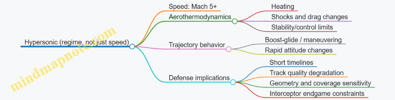
When teams say “hypersonic,” they often mean a combination of conditions. A useful operational definition is:
- Mach regime: typically Mach 5+
- Thermal regime: boundary-layer heating that affects materials and/or sensor performance
- Trajectory regime: maneuvering or gliding phases that reduce predictability
- Engagement regime: short decision and intercept windows that stress latency and tracking
This definition is not about labeling; it’s about ensuring the right engineering problems get attention.
Mind map: from definition to operational consequences
Quick examples that clarify the boundaries
- Example A (speed-only thinking fails): A vehicle at Mach 5 briefly at high altitude may be less thermally stressing than a vehicle at similar Mach that spends longer in denser air. Defense systems should not assume identical signatures or maneuver limits.
- Example B (regime overlap): A system can be “hypersonic-like” in operational effect even if it spends limited time above Mach 5, if the heating and tracking challenges occur during the engagement window.
- Example C (trajectory matters): Two threats with the same speed can present different intercept geometries if one follows a flatter path and the other dives earlier. The sensor-to-shooter chain experiences different constraints.
In short, hypersonic regimes are defined by the conditions that force different physics and different operational constraints. Once you define the regime that matters to the engagement—speed, heating, trajectory behavior, and time pressure—you can reason clearly about what defense systems must do.
1.2 Flight regimes, thermal loads, and aerodynamic constraints
Hypersonic flight is not one uniform experience. The vehicle moves through distinct regimes where the dominant physics changes: how the air compresses, how heat is transferred, and how much control authority remains. A defense system that performs reliably has to be designed around those regime transitions, not just around a single “Mach number.”
Flight regimes: where the physics changes
A practical way to think about regimes is by what the flow does to the vehicle.
- Pre-entry / low-speed approach: Aerodynamic heating is modest, and control is mostly about conventional stability and actuator response.
- High-speed compression: As speed rises, the air ahead of the vehicle compresses strongly. The shock structure forms and moves relative to the vehicle geometry.
- Hypersonic regime: Heat flux and pressure loads become severe. The vehicle may experience strong aerodynamic forces and moments that vary rapidly with angle of attack.
- Terminal / endgame: The vehicle often maneuvers near the boundary of what its guidance and control can sustain. Aerodynamic heating and drag can spike during aggressive maneuvers.
A useful mental model is to track three quantities along the trajectory: dynamic pressure (how hard the flow pushes), heat flux (how fast energy reaches the surface), and control effectiveness (how well the vehicle can generate the moments it needs).
Thermal loads: why heating is more than “hot air”
At hypersonic speeds, heating comes from multiple mechanisms that scale differently with speed, density, and surface conditions.
- Convective heating: Hot, compressed gas transfers energy to the surface. This is often the dominant term on the windward side.
- Radiative heating: At very high temperatures, the gas and surface can emit radiation. It matters when the shock layer is extremely hot.
- Frictional heating: Viscous effects in the boundary layer add heat, especially near stagnation regions and along the surface.
Thermal loads are not uniform. The stagnation region (the point facing the flow) typically sees the highest heat flux. Areas near the shock impingement and along leading edges can also become hot spots.
Concrete example: why a small geometry change matters
Consider two blunt-nosed shapes with the same mass and speed. The one with a slightly larger effective radius of curvature tends to produce a different shock stand-off distance and boundary-layer behavior. Even if peak temperature is not identical, the distribution of heat can shift enough to change where the structure needs insulation or where ablation is expected.
Design implication: thermal protection is not just “how much heat can the material take,” but “where will the heat go, and how will that affect stiffness, mass, and control?”
Aerodynamic constraints: drag, pressure, and control authority
Aerodynamics at hypersonic speeds is dominated by compressible flow. Three constraints show up repeatedly.
- Drag and energy loss: Drag grows with speed and density, and it can change sharply with angle of attack. High drag reduces range and forces the guidance system to manage energy more carefully.
- Pressure loads and structural limits: The vehicle experiences large pressure forces and moments. These loads can exceed what the structure can tolerate, especially during maneuvers.
- Control effectiveness limits: Control surfaces may become less effective as the flow becomes more complex and as the boundary layer thickens or separates.
A simple way to connect these constraints is through the idea of moment budget: the vehicle needs to generate enough aerodynamic moment to follow the commanded trajectory, but the available moment is limited by what the flow will support without causing excessive heating, separation, or structural stress.
Concrete example: angle of attack trade
Suppose a vehicle increases its angle of attack to generate more lift or to tighten a turn. The immediate effect is more aerodynamic force, but the side effects can be costly:
- The stagnation region may shift, changing the heating pattern.
- The shock structure can move, altering pressure distribution.
- Drag can rise, reducing remaining energy for later corrections.
In practice, designers treat angle of attack as a constrained variable, not a free knob. The “best” angle is the one that balances guidance needs against thermal and structural margins.
Regime transitions: the part that breaks assumptions
Many performance models assume a steady flow condition. Real trajectories are not steady: the vehicle changes altitude, speed, and attitude continuously. Regime transitions can cause abrupt changes in heating and aerodynamic forces.
Common transition triggers include:
- Altitude changes: Density changes quickly, affecting both drag and convective heating.
- Maneuver onset: Turning changes the local flow direction relative to the body.
- Attitude trim shifts: Small attitude changes can move the shock and boundary-layer behavior.
Concrete example: “trim” and why it matters
If a vehicle is trimmed for one flight condition, then a maneuver that changes angle of attack or sideslip can move it into a different aerodynamic operating point. The result can be a mismatch between predicted and actual moments, which then forces the guidance loop to work harder—often at the same time heating and drag are increasing.
Mind map: linking regimes, heating, and aerodynamics
Mind map: Flight regimes, thermal loads, aerodynamic constraints
A compact “design reasoning” checklist
When analyzing a hypersonic trajectory, it helps to ask three questions at each segment of the flight profile.
- What regime am I in, and what flow features dominate? (Shock structure, boundary-layer state, and whether heating is convective-dominant.)
- Where are the thermal hot spots, and what do they do to the structure? (Stiffness, mass, and allowable control.)
- What is the moment budget under the expected aerodynamic forces? (Can the vehicle maneuver without triggering separation or exceeding structural limits?)
Answering these in sequence turns “hypersonic” from a single label into a set of constraints that can be engineered, tested, and verified.
1.3 Guidance, control, and navigation challenges at hypersonic speeds
Hypersonic flight compresses the time available for sensing, computing, and acting. Guidance, control, and navigation (GNC) still has to answer the same basic questions—Where am I? Where am I going? How do I get there?—but the answers arrive with less time, more uncertainty, and harsher physical limits.
1) Navigation: “Where am I?” under fast dynamics
The core problem: small errors become big misses
At hypersonic speeds, a navigation error that seems minor in meters can translate into large cross-track or altitude errors before the next control update. The vehicle’s path is also sensitive to atmospheric density and wind, which are hard to measure precisely during the maneuver.
Easy example: Imagine a guidance computer updates guidance commands every 50 ms. If the navigation solution has a 30 m position error, then in the next 50 ms the vehicle can travel roughly 1.5 km at 30 km/s. The controller is effectively steering with a “map” that is already out of date.
Sensor limitations and timing
Common navigation inputs (inertial measurement, satellite navigation when available, radar altimetry, star sensing when geometry allows) each have failure modes:
- Inertial sensors drift over time; bias errors integrate into attitude and position errors.
- Satellite navigation can be degraded by geometry, jamming, or signal blockage.
- Atmospheric sensing (like pressure/temperature) helps infer state but depends on accurate models.
State estimation: filtering with imperfect models
GNC typically uses an estimator (often a Kalman filter or variant) to fuse sensor data into a best estimate of position, velocity, and attitude. The estimator must be tuned for:
- Rapid maneuvers (nonlinear dynamics)
- Changing uncertainty (sensor quality varies)
- Model mismatch (atmosphere and vehicle aerodynamics)
Easy example: If the estimator assumes the vehicle’s lift-to-drag ratio is constant but the actual value changes with angle of attack, the filter may “believe” the wrong aerodynamic response. The result is a consistent bias in estimated flight path angle.
2) Guidance: “Where should I go next?” with limited control authority
Guidance is constrained by what the vehicle can actually do
Hypersonic vehicles often have limited control authority due to:
- Actuator saturation (control surfaces or thrust vectoring reach limits)
- Thermal and structural constraints (certain attitudes or rates may be disallowed)
- Aerodynamic regime changes (control effectiveness varies with Mach number and angle of attack)
Guidance laws must respect these constraints. A guidance command that looks feasible in a simplified model can be impossible in the real vehicle.
Easy example: A guidance algorithm might request a large change in flight path angle to correct a predicted miss. If the vehicle can only generate enough normal acceleration for a smaller turn rate, the controller will saturate, and the vehicle will follow a different trajectory than planned.
The engagement problem: short horizons and late information
Even when the target state is known, the vehicle’s ability to correct depends on how much time remains before the intercept point (or terminal aim point). Guidance often operates with a shrinking “window” where corrections matter.
Easy example: If the guidance system updates every 100 ms and the remaining time to terminal is 1.0 s, there are only about 10 updates. If each update has a delay (sensor processing + computation + actuator lag), the effective correction time is even smaller.
3) Control: turning commands into motion under nonlinear, coupled dynamics
Coupling: guidance, aerodynamics, and attitude are not independent
At hypersonic speeds, aerodynamic forces depend strongly on attitude and velocity. That means:
- A change in commanded flight path angle changes angle of attack.
- Angle of attack affects lift, drag, and heating.
- Heating and structural limits can restrict allowable attitudes.
So the controller is not just “tracking a path”; it is managing a coupled system.
Nonlinearities and gain scheduling
Control design must handle nonlinear relationships between inputs (actuator commands) and outputs (normal acceleration, attitude, rate). Many systems use gain scheduling or nonlinear control strategies to maintain stability across regimes.
Easy example: A controller tuned for moderate dynamic pressure may become underdamped when dynamic pressure increases. The vehicle can overshoot the desired angle of attack, increasing drag and changing the trajectory.
Actuator dynamics and delays
Actuators have their own dynamics: rate limits, dead zones, and response lags. Delays matter more at high speed because the vehicle moves significantly between command issuance and physical response.
Easy example: If the actuator has a 30 ms lag and the vehicle is moving 900 m in that time, the controller may repeatedly “chase” the error, causing oscillations or limit cycles.
4) A practical mental model: the GNC loop at hypersonic speed
A useful way to reason about the problem is to treat GNC as a loop with three time budgets:
- Sense/estimate time (how quickly the state estimate updates)
- Compute time (guidance and control calculations)
- Actuate time (how quickly the vehicle responds)
If the sum of these times is a large fraction of the maneuver time, the loop behaves like it is controlling a moving target with stale information.
Mind map: GNC challenges and where they show up
Mind map: Guidance, Control, Navigation at hypersonic speeds
5) Concrete example scenario: correcting a predicted miss
Consider a vehicle aiming for a terminal point. The estimator provides a state estimate with uncertainty. Guidance computes a maneuver command to reduce the predicted miss distance. The controller then tries to track the commanded flight path angle and/or normal acceleration.
What can go wrong, step by step:
- Navigation error: The estimator’s position error shifts the predicted miss.
- Guidance constraint: The guidance command requires more turn than the vehicle can generate at the current dynamic pressure.
- Control saturation: The controller hits actuator limits, so the actual trajectory deviates.
- Aerodynamic coupling: The deviation changes angle of attack, which changes lift and drag, altering the heating and the remaining control effectiveness.
- Timing effects: By the time the next estimate arrives, the vehicle has already moved along the wrong part of the trajectory.
A well-designed system reduces the damage at each step: it uses uncertainty-aware guidance, respects actuator limits, and tunes the controller for the nonlinear regime so saturation is handled predictably rather than chaotically.
6) Summary: the three bottlenecks
At hypersonic speeds, the biggest practical bottlenecks are:
- Uncertainty growth in navigation and estimation
- Limited correction time for guidance to matter
- Nonlinear control constraints that turn commands into achievable motion
When these are addressed together—through estimator tuning, constraint-aware guidance, and robust control—the system can produce consistent trajectories even when the environment and models are imperfect.
1.4 Mission profiles and typical engagement timelines
Hypersonic threats are not just “fast.” Their mission profiles combine speed, altitude changes, maneuvering, and timing choices that stress every part of defense: detection, tracking, decision-making, and intercept geometry. A useful way to think about this section is to separate (1) what the attacker is trying to accomplish and (2) what the defender must accomplish fast enough to matter.
Mission profile building blocks
Most hypersonic strike concepts can be described with a few repeatable building blocks. Each one changes the timeline in a different way.
-
Boost and separation (early phase)
- The system leaves the launch vehicle and transitions into a trajectory that may include coast, staging, or immediate maneuver.
- For defense, this phase often determines whether you get early track initiation or only a late, short-lived track.
-
Midcourse flight (longer phase, fewer opportunities)
- The vehicle may travel at high speed while changing altitude and lateral position.
- The defender’s job is to keep a stable track through sensor gaps, clutter, and changing geometry.
-
Terminal maneuver (short phase, high stress)
- The vehicle may perform rapid maneuvering near the end of flight.
- The defender’s job is to update the predicted intercept point quickly enough that the interceptor can still arrive with usable energy and guidance authority.
-
Effects timing (what “success” means)
- “Impact time” is the anchor for everything else, but the attacker may choose when to commit to a final approach.
- For defense, the key is not only reaching the target area, but reaching it at the right time with sufficient miss-distance margin.
Mind map: timeline drivers
Typical engagement timelines (defender’s view)
Timelines vary by geography and system design, but the defender’s sequence of actions is usually similar. The difference is how much time each step gets.
Timeline A: Early track, longer decision window
This is the “best case” you plan for, not the case you assume.
-
T0: Threat becomes detectable
- Detection might occur when the threat enters a sensor’s useful field of view or when a boost plume/geometry becomes favorable.
- Example: A radar site with good coverage sees the system early enough to start a track before it reaches the terminal region.
-
T0 + Δ1: Track initiation and confirmation
- The system must confirm that the returns are consistent with a coherent moving target.
- Example: If the first few detections are ambiguous, the tracker may wait for additional measurements, increasing Δ1.
-
T0 + Δ1 + Δ2: State estimation stabilizes
- The defender estimates position, velocity, and uncertainty. Hypersonic maneuvering can cause the uncertainty to grow quickly.
- Example: A filter that assumes smooth motion will struggle if the threat begins aggressive lateral changes early.
-
T0 + Δ1 + Δ2 + Δ3: Engagement decision and resource allocation
- Command and battle management decide whether to commit an interceptor, which one, and where to aim.
- Example: If multiple targets appear, the system may allocate interceptors based on priority and predicted kill probability.
-
T0 + Δ…: Interceptor midcourse updates
- The interceptor may need periodic updates to correct for target maneuver and estimation error.
- Example: A midcourse update every few seconds can reduce miss distance, but only if the data link and processing latency fit the timeline.
-
Terminal: Intercept and kill assessment
- The final geometry window is short. Guidance authority and energy margins must cover the remaining uncertainty.
- Example: If the interceptor arrives with low remaining energy, it may be forced into a shallow approach that is sensitive to target maneuver.
What makes this timeline work: early detection, stable tracking, and enough time for multiple updates before the terminal geometry window.
Timeline B: Late track, compressed decision window
This is common when coverage is limited or geometry is unfavorable.
-
T0: Threat becomes detectable late
- The defender might only see the threat when it is already near the terminal region.
- Example: A sensor horizon or line-of-sight limitation means the first usable track starts just minutes—or even seconds—before terminal.
-
T0 + Δ1: Track initiation under uncertainty
- With fewer measurements, the estimated state has larger uncertainty.
- Example: A tracker may produce a “tentative” track that quickly becomes “confirmed,” but the uncertainty remains large.
-
T0 + Δ1 + Δ2: Rapid state estimation and fusion
- Multisensor fusion helps, but only if other sensors can contribute quickly.
- Example: If a second sensor has a slower revisit rate, fusion may not arrive in time to improve the estimate.
-
T0 + Δ1 + Δ2 + Δ3: Engagement decision with limited options
- The battle manager may have fewer choices: fewer interceptors available, less time to compute aimpoints, and less time for updates.
- Example: The system may choose a “nearest feasible” interceptor rather than the one with the best predicted geometry.
-
Terminal: Guidance and control under tight margins
- The interceptor must handle both target maneuver and its own guidance limitations.
- Example: If the target performs a late maneuver, the interceptor may not have time to re-plan, increasing miss distance risk.
What makes this timeline hard: limited measurement time, larger uncertainty, and fewer opportunities for midcourse corrections.
Concrete example: a simplified timeline with numbers
Consider a notional engagement where the defender’s key steps are measured in seconds. The exact values depend on system design, but the logic is consistent.
-
Early track scenario
- Detection at T0.
- Track initiation and confirmation: Δ1 = 10 s.
- State estimation stabilization: Δ2 = 20 s.
- Decision and allocation: Δ3 = 15 s.
- Interceptor midcourse updates: ~3 updates before terminal.
- Result: the predicted intercept point is updated multiple times, reducing sensitivity to late maneuver.
-
Late track scenario
- Detection at T0.
- Track initiation and confirmation: Δ1 = 5 s (faster confirmation, but fewer measurements).
- State estimation stabilization: Δ2 = 10 s (uncertainty remains higher).
- Decision and allocation: Δ3 = 10 s.
- Interceptor midcourse updates: ~1 update before terminal.
- Result: the interceptor enters terminal with larger uncertainty and less time to correct.
The point isn’t the specific numbers; it’s that each step consumes time, and each step’s output quality affects the next step’s feasibility.
Mind map: what changes the timeline most
Practical takeaways for defense planning
- Track quality is a timeline resource. More time can mean better estimation, but it can also mean more opportunities for the threat to maneuver; planning should treat uncertainty growth as part of the timeline.
- Latency is not just delay—it changes geometry. Even if the system “eventually” gets the right data, the interceptor may already be committed to an aimpoint that no longer fits.
- Engagement doctrine should match the measurement reality. If the defender typically gets late tracks, the doctrine should reflect shorter update opportunities and larger uncertainty, rather than assuming early, clean tracking.
Summary of typical engagement flow
A defender’s engagement timeline can be summarized as: detect → initiate track → estimate state → decide and allocate → update interceptor → execute terminal intercept. Hypersonic mission profiles mainly change how much time each step gets and how quickly uncertainty grows, which then determines whether the interceptor can arrive with enough guidance authority and energy to achieve an acceptable miss distance.
1.5 System-level implications for sensors, C2, and interceptors
Hypersonic defense is less about any single “best” component and more about how sensors, command-and-control (C2), and interceptors behave as one system. At hypersonic speeds, small timing errors become large geometry errors, and small sensing gaps become engagement failures. The system has to manage three hard realities at once: fast dynamics, limited observability, and tight decision windows.
Sensors: from “detect” to “deliver usable track”
Detection is not the same as track quality. A sensor may see a target briefly, but the defense system needs a track that is accurate enough to support an interceptor’s guidance solution. That means the sensor chain must produce not only range and angle, but also uncertainty estimates that C2 can propagate.
Key system implications
- Update rate matters more than peak range. A longer-range sensor that updates slowly can be worse than a closer sensor that updates frequently, because the engagement timeline shrinks.
- Track continuity beats single-frame brilliance. If the target is intermittently lost due to geometry or countermeasures, the system must either maintain the track through prediction or quickly re-acquire it without resetting the engagement.
- Sensor management must consider the engagement plan. If C2 expects an interceptor to be guided by midcourse updates, sensors should prioritize the track quality needed for that update cadence.
Easy example (why update rate wins): Imagine two radars. Radar A detects at 600 km but provides updates every 10 seconds. Radar B detects at 300 km but updates every 1 second. If the target is closing rapidly, the interceptor’s predicted intercept point changes significantly between Radar A updates. Radar B’s more frequent updates keep the predicted geometry aligned with the interceptor’s guidance timeline.
C2: time budgeting and uncertainty-aware decisions
C2 is the “glue” that turns sensor outputs into interceptor commands. In hypersonic defense, the glue must also be honest about uncertainty. A system that treats all tracks as equally reliable will eventually command the wrong intercept geometry.
Key system implications
- Latency budgeting becomes a design requirement. C2 must account for sensor processing time, fusion time, communications delay, and command generation time. The engagement timeline is often so short that “working in the lab” is not enough; the end-to-end pipeline must be measured.
- Data association must handle ambiguity. Multiple objects, clutter, and decoys can create competing track hypotheses. C2 needs logic that can keep the correct hypothesis alive long enough for the interceptor to benefit.
- Engagement decision logic must be uncertainty-aware. Instead of “track exists, fire,” C2 should evaluate whether the predicted miss distance distribution is within acceptable bounds given current uncertainties.
- Resource allocation must anticipate saturation. If multiple threats appear, C2 must decide which interceptors to assign to which tracks, balancing probability of success against the cost of spreading assets too thin.
Easy example (uncertainty-aware decision): Suppose C2 computes an intercept point with a 3-sigma miss-distance bound of 8 meters for one track and 25 meters for another. If the interceptor’s effective kill condition requires the miss distance to be under 10 meters with high confidence, C2 should favor the first track even if the second track has a slightly better raw sensor signal. The system is choosing based on what the interceptor can actually achieve.
Interceptors: guidance depends on what C2 can provide
An interceptor’s performance is not just its own seeker and control laws. It also depends on the quality and timing of the information it receives. If guidance inputs are late or inconsistent with the interceptor’s internal state estimate, the interceptor spends energy correcting errors rather than refining the final approach.
Key system implications
- Guidance mode transitions must match system timing. Many interceptors rely on different guidance phases (for example, externally guided midcourse and autonomous terminal). C2 must trigger these transitions at the right time with the right data.
- Energy management is coupled to track quality. If the predicted target path is uncertain, the interceptor may need larger maneuver margins, which can reduce endgame control authority.
- Seeker performance is constrained by geometry and time. A seeker that can discriminate in ideal conditions may struggle if the target is only visible for a short terminal window or if the interceptor arrives at an unfavorable aspect angle.
- Kill assessment and feedback loops affect subsequent actions. Even if the system is designed for one-shot engagements, C2 benefits from knowing whether an intercept succeeded to avoid wasting remaining assets.
Easy example (late command hurts): Consider an interceptor that can correct its aim using midcourse updates. If the update arrives 2 seconds late, the interceptor’s predicted intercept point can shift enough that it must perform a larger correction maneuver. That maneuver consumes propellant or control authority, leaving less margin for the final approach where the seeker needs stable conditions.
How the system fits together: a practical flow
A useful way to think about the system is as a loop:
- Sensors observe and produce measurements with uncertainties.
- Fusion and C2 convert measurements into tracks and engagement solutions.
- Interceptors execute guidance based on those solutions.
- Results and new sensor data update the track and engagement state.
When any link in the loop is weak—slow updates, optimistic uncertainty handling, or guidance commands that don’t match interceptor state—the loop stops converging.
Mind maps
Mind Map: System-level implications (Sensors → C2 → Interceptors)
Mind Map: Common failure modes and where they originate
Putting best practices into the system (with concrete checks)
Best practice: measure the pipeline, not just component specs. A system requirement should include end-to-end timing from sensor measurement to interceptor command, plus the expected uncertainty growth over that interval.
Concrete check example: Run a test where a simulated target produces a known measurement stream. Verify that C2 outputs an engagement solution within the allowed time budget and that the uncertainty reported to the interceptor matches the observed tracking error.
Best practice: treat uncertainty as a first-class input. C2 should propagate sensor uncertainties into track covariance and then into predicted miss-distance distributions.
Concrete check example: Compare two tracks with the same estimated mean position but different covariance. Confirm that the engagement logic assigns higher priority to the track with lower predicted miss-distance variance, even if both tracks appear “good” by raw signal strength.
Best practice: align sensor tasking with interceptor guidance needs. If the interceptor relies on midcourse updates at a specific cadence, sensors should be scheduled to maintain that cadence during the critical portion of the engagement.
Concrete check example: During exercises, log the number of times the interceptor’s guidance phase waits for an update. If that count rises, the issue is not “interceptor performance”; it’s a system scheduling and timing mismatch.
Together, these implications mean the defense system is only as strong as its slowest link in the loop—and the “slowest link” is often not the sensor range or the interceptor motor, but the timing and uncertainty handling that connect them.
2. Weapon System Architecture and Performance Drivers
2.1 Payload, propulsion, and airframe integration choices
Hypersonic systems are often described as “fast,” but the real engineering story is about fit: the payload must fit the thermal and volume limits, the propulsion must fit the inlet and structural constraints, and the airframe must fit the guidance and control needs. Integration is where small mismatches become big problems—like choosing a payload that needs a stable temperature while the vehicle’s skin is doing its best impression of a hotplate.
Payload integration: mass, volume, interfaces, and survivability
A payload choice starts with the boring-but-decisive constraints: mass properties, center of gravity (CG), volume envelope, and interface standards.
- Mass and CG management. A payload that is heavier than expected shifts CG, which changes control authority and can force larger actuators or different control laws. A practical example: if a seeker electronics bay is moved forward by 10–20 cm to make room for a thermal liner, the resulting CG shift can require retuning the guidance loop and may reduce the available pitch rate near the endgame.
- Thermal environment compatibility. Payloads rarely care about “Mach number”; they care about component temperatures, allowable gradients, and insulation performance. For instance, an infrared sensor may tolerate a certain detector temperature range, so the integration team must allocate space and mass for insulation, heat sinks, or active cooling. Even without active cooling, the design can include a thermal standoff and a controlled heat path so the sensor sees a slower temperature rise than the outer skin.
- Mechanical interfaces and shock loads. Payloads must survive launch vibration and any separation events. A common integration practice is to define a mechanical “interface frame” that isolates the payload from airframe flexure. Example: a modular electronics tray mounted on elastomeric dampers can reduce transmitted vibration, but it also changes stiffness and can affect alignment of optical components.
- Power and data interfaces. Payloads need power rails and timing signals that match the vehicle’s electrical architecture. If the payload draws peak power during a short window (like sensor initialization), the vehicle power system must handle that without causing voltage droop that resets electronics.
Propulsion integration: matching inlet, combustor/rocket, and thermal structure
At hypersonic speeds, propulsion is not just an engine choice; it’s an airframe choice. The inlet geometry, internal ducting, and thermal protection all interact.
- Inlet-airframe compatibility. For air-breathing concepts, the inlet must capture and condition flow across the relevant flight regime. Integration means ensuring the inlet lip, internal ramps, and boundary-layer behavior align with the vehicle’s external shape. A concrete example: if the airframe uses a sharp leading edge for aerodynamic reasons, the inlet may experience different shock placement than predicted, altering mass flow and causing the combustor to run off-design.
- Thermal management of propulsion components. Propulsion hardware often sits in the hottest regions. Materials and cooling paths must be coordinated with the payload thermal strategy. Example: if a propulsion section uses regenerative cooling that warms the structure, that heat can leak into nearby payload compartments unless insulation and thermal breaks are placed deliberately.
- Propulsion-to-structure load paths. Thrust creates bending and torsion loads that the airframe must carry. Integration includes designing structural members so that thrust loads do not distort sensor alignment or create thermal-mechanical stress that cracks liners.
- Energy and mass tradeoffs for rocket-based approaches. Rocket propulsion shifts the integration problem toward propellant volume and tank structure. A practical example: increasing propellant mass to extend range may force a larger tank diameter, which then changes the vehicle’s aerodynamic cross-section and can affect stability margins and control effectiveness.
Airframe integration: geometry, stability, control, and thermal protection
The airframe is the integration “platform,” but it also defines the constraints that payload and propulsion must obey.
- Aerodynamic shape and control authority. Control surfaces and actuators must work within the thermal and structural limits. If the vehicle uses movable fins or control flaps, the hinge line and actuator placement must survive high temperatures and avoid excessive thermal gradients that could seize mechanisms. Example: an actuator mounted too close to a hot skin may require additional insulation, which increases mass and can shift CG.
- Stability and CG envelope. Hypersonic vehicles often operate with limited ability to correct errors quickly. That makes CG placement and mass distribution critical. Integration practice: define a CG envelope across payload configurations (e.g., different payload variants) and verify that the control system can maintain stability without saturating actuators.
- Thermal protection system (TPS) integration. TPS is not a separate layer you can just “add.” It changes external geometry, internal volume, and structural stiffness. Example: a thick TPS panel may reduce heat flux but also reduces internal space for payload cooling hardware, forcing a redesign of the payload thermal path.
- Structural survivability and material compatibility. Materials must handle both mechanical loads and thermal cycling. If propulsion cooling warms one region while the payload compartment remains cooler, differential expansion can stress mounts. Integration includes selecting materials and mount designs that tolerate those gradients.
Integration workflow: how teams avoid last-minute surprises
A useful way to think about integration is to treat it as a constraint satisfaction problem with interfaces.
- Define payload requirements (mass, power, thermal limits, mechanical interfaces).
- Define propulsion requirements (thrust/impulse needs, inlet/duct constraints, cooling approach).
- Define airframe constraints (envelope, stability margins, TPS thickness, structural load paths).
- Iterate with interface checks: CG, power budgets, thermal conduction paths, and mechanical alignment.
- Validate with representative tests: component-level thermal tests and integrated structural/fit checks.
A small but common example: a payload might pass its own thermal test in isolation, but when installed next to a propulsion duct, the local heat soak changes the temperature rise rate. The fix is usually not “make it colder”; it’s adjusting insulation thickness, adding a thermal break, or rerouting the heat path.
Mind map: payload–propulsion–airframe integration
Example integration scenarios (practical, not theoretical)
Scenario A: Payload thermal stability vs. TPS thickness
- Payload needs a narrow detector temperature band.
- TPS thickness increases to reduce skin heat flux.
- Result: internal volume shrinks, leaving less space for insulation around the detector.
- Integration fix: reduce heat leak by improving the detector’s local thermal standoff and adding a low-conductivity standoff bracket, rather than relying on extra global TPS thickness.
Scenario B: Inlet geometry change affects propulsion mass flow
- Airframe shape is adjusted for aerodynamic reasons.
- Inlet shock moves, changing effective capture and mass flow.
- Result: combustor/engine runs off-design, reducing thrust and altering thermal loads.
- Integration fix: update inlet internal geometry (duct contour or ramp angle) and re-check thermal protection placement because the hottest region inside the duct shifts.
Scenario C: Rocket tank sizing changes stability margins
- Range requirement increases propellant mass.
- Tank diameter grows, shifting CG and changing aerodynamic center.
- Result: control authority decreases near the end of the burn.
- Integration fix: redistribute internal components (move payload bay or electronics) to restore CG, and verify actuator capability under the new mass distribution.
Key takeaway
Integration choices are about managing interfaces: payload constraints drive thermal and power needs, propulsion choices drive inlet/duct and cooling requirements, and the airframe must reconcile both while preserving stability and survivability. When those interfaces are treated as first-class design objects, the system behaves like a coherent whole instead of a set of individually impressive parts.
2.2 Propulsion fundamentals: scramjet and rocket-based approaches
Hypersonic vehicles need thrust that survives two hard realities: the air is hot and thin, and the vehicle is moving fast enough that small inefficiencies show up quickly. Propulsion choices mainly trade off how the vehicle uses atmospheric oxygen versus how much onboard propellant it must carry.
Core idea: where the energy comes from
A propulsion system turns stored energy into kinetic energy (speed) and pressure work (pushing the flow). In practice, the system must also manage heat, keep the engine stable across a range of conditions, and deliver thrust at the right time in the flight profile.
A useful way to compare engines is to ask two questions:
- Does the engine carry oxidizer? If yes, it can work without air.
- Does it use atmospheric oxygen? If yes, it can reduce carried mass, but only within an altitude and speed window where the air supply is adequate.
Rocket propulsion: self-contained thrust
Rocket engines carry both fuel and oxidizer, so they can operate from vacuum to dense atmosphere (with appropriate design). The basic thrust comes from accelerating exhaust to high velocity.
Key components and what they do
- Combustion chamber: mixes propellant and ignites it.
- Nozzle: expands hot gas to produce thrust.
- Feed system: regulates flow rates so mixture ratio stays near the target.
Why rockets work well for hypersonics
- They do not require atmospheric oxygen.
- They can provide thrust at high altitudes where air-breathing engines struggle.
Why rockets are expensive in range
- Carrying oxidizer increases mass.
- As the vehicle accelerates, the required thrust to maintain a given acceleration can rise, while propellant mass decreases.
Simple example (range intuition) Imagine two vehicles that must deliver the same total impulse. The rocket must carry all the oxidizer, so its propellant mass fraction is typically higher. If you replace part of that oxidizer with atmospheric oxygen, the vehicle can devote more mass to payload or structure, but only if the engine can ingest and process that air.
Scramjet propulsion: air-breathing thrust at hypersonic speed
A scramjet (supersonic combustion ramjet) relies on the vehicle’s high speed to compress incoming air. The engine ingests air, slows it to a manageable condition, mixes it with fuel, burns it, and then accelerates the flow through the nozzle.
Key flow stages
- Inlet: converts incoming supersonic flow into a slower, higher-pressure stream.
- Fuel injection and mixing: introduces fuel into the compressed air.
- Combustor: sustains supersonic combustion.
- Nozzle/exit: expands the exhaust to produce thrust.
Why scramjets need high speed At lower speeds, the inlet and combustor cannot achieve the pressure and residence time needed for stable combustion. The engine is designed so that the flow remains supersonic through most of the system, which makes ignition and mixing harder than in subsonic engines.
Key constraints that shape design
- Inlet compression limits: shock structures must fit and remain stable.
- Combustion stability: the flame must persist even though the flow is moving quickly.
- Thermal management: the combustor walls see intense heat flux.
Simple example (why mixing matters) Suppose fuel injection creates droplets or jets that do not mix quickly enough. Even if the chemistry is favorable, the mixture may leave the combustor before it burns. The result is lower thrust and higher unburned fuel, which can also affect thermal loads.
Comparing rocket and scramjet: a practical trade study
A common comparison is to look at thrust availability versus altitude and speed.
- Rocket: thrust availability is broad, but propellant mass is the limiting factor.
- Scramjet: thrust availability is strong only where the inlet can compress air effectively and the combustor can sustain supersonic combustion.
This is why many real hypersonic concepts use hybrid propulsion: rockets for portions of the trajectory where air-breathing is inefficient, and scramjets where air supply and inlet performance are suitable.
Mind map: propulsion fundamentals
How thrust is actually produced (with a simple equation)
For a first-order view, thrust can be approximated by the momentum change of the exhaust: \[ F \approx \dot{m} ,(V_e - V_0) + \( p_e - p_0 \)A_e \] where \(\dot{m}\) is mass flow rate, \(V_e\) exhaust velocity, \(V_0\) vehicle speed, and the pressure term accounts for nozzle exit pressure relative to ambient.
What this tells you
- If the vehicle speed \(V_0\) is large, the same exhaust velocity yields less net thrust.
- If ambient pressure \(p_0\) changes with altitude, the pressure term can matter.
Scramjets and rockets differ in how they set \(\dot{m}\) and \(V_e\): rockets control both through propellant flow and chamber pressure, while scramjets depend heavily on how much air the inlet delivers and how effectively the combustor adds energy.
Inlet and combustor: the scramjet “make-or-break” pair
A scramjet’s inlet and combustor are tightly coupled.
- The inlet determines pressure recovery and flow uniformity.
- The combustor depends on that uniformity to achieve stable ignition and sustained burning.
Concrete example: inlet shock behavior If the inlet’s shock system is positioned poorly, the downstream flow can become nonuniform. That can cause some regions to be over-rich or over-lean, leading to incomplete combustion and uneven heating. Even if the average conditions look acceptable, local hot spots can drive material limits.
Rocket engine: mixture ratio and chamber pressure
Rocket performance is sensitive to mixture ratio (fuel-to-oxidizer) and chamber pressure.
- Mixture ratio: affects combustion temperature and exhaust composition.
- Chamber pressure: influences exhaust expansion and thrust.
Concrete example: throttling for control If a vehicle needs to modulate acceleration during a phase of flight, the engine must adjust propellant flow rates. Throttling changes combustion conditions, which can shift flame behavior and heat loads. A control system must therefore manage both thrust and stability.
Integration with the airframe: propulsion is never alone
At hypersonic speeds, propulsion performance is shaped by the vehicle’s geometry.
- The inlet must match the airframe shape and boundary layer behavior.
- The engine’s thermal environment interacts with the structure and any insulation.
- Exhaust expansion and plume effects can influence aerodynamic forces.
Practical example: boundary layer impact on scramjet inlet A thick boundary layer reduces effective capture area. That lowers the mass flow the combustor can process, which reduces thrust. Designers often treat boundary layer management as part of propulsion, not just aerodynamics.
Quick summary
- Rockets provide self-contained thrust across a wide altitude range, but propellant mass is the main constraint.
- Scramjets use atmospheric oxygen and can be efficient at hypersonic speeds, but inlet compression, supersonic mixing, combustion stability, and thermal loads dominate the design.
- The most effective hypersonic propulsion strategies typically match each engine type to the flight regime where it can produce thrust reliably.
2.3 Thermal Protection, Materials, and Structural Survivability
At hypersonic speeds, “thermal protection” is less about one magic coating and more about managing heat flow, keeping structures within allowable temperatures, and preventing small damage from turning into big failures. The key is to treat heat, structure, and materials as a single design problem.
Thermal loads: where the heat actually goes
The dominant heating mechanisms depend on the flight regime, but the design workflow usually starts with a heat-flux estimate and then converts it into temperatures and stresses.
- Aerodynamic heating at the surface: Hot gas transfers energy to the leading edges and any exposed surfaces. Leading edges typically see the highest heat flux because the flow stagnates there.
- Internal conduction: Heat does not stop at the skin. It conducts inward, raising the temperature of the structure and any bonded layers.
- Radiation and re-radiation: Hot surfaces emit thermal radiation. This can reduce net heating, but it also means surface temperature strongly affects heat balance.
- Ablation vs. non-ablative behavior: Some designs intentionally allow material to erode (ablation). Others aim to keep the structure intact using insulation and high-temperature materials.
A practical way to reason about survivability is to track temperature margins: the difference between predicted temperatures and the material’s allowable limits (for strength, creep, oxidation, or bond-line integrity).
Materials selection: matching failure modes to operating conditions
Materials are chosen based on what tends to fail first.
- High-temperature capability (strength and stiffness): At elevated temperatures, many metals lose strength and may creep under load.
- Oxidation and corrosion resistance: Hot air chemistry can degrade surfaces. Materials that survive heat often still need protection against oxidation.
- Thermal conductivity and heat capacity: Low conductivity helps reduce internal heating, while high heat capacity can slow temperature rise during short exposures.
- Thermal expansion compatibility: Bonded layers expand differently. Mismatch can create delamination or cracking.
- Manufacturability and repairability: A material that is perfect on paper but impossible to fabricate reliably becomes a survivability problem of its own.
Example: why “just use a refractory metal” usually fails
Refractory metals can handle high surface temperatures, but they often have high thermal conductivity and can impose large heat flux into the underlying structure. If the goal is to protect a lower-temperature airframe, a high-conductivity skin can move the heat problem inward. In many designs, a high-temperature outer layer is paired with lower-conductivity insulation and a structure that can tolerate the resulting internal temperatures.
Thermal protection system (TPS) architectures
TPS designs typically fall into a few patterns. Real systems often mix them.
- Ablative TPS: The surface erodes in a controlled way, carrying away heat with the removed material. This can be effective when exposure is intense and time is limited.
- Non-ablative TPS: Uses insulation, coatings, and high-temperature materials to keep the structure below critical temperatures.
- Hybrid TPS: Combines ablation at the most stressed regions (like leading edges) with non-ablative protection elsewhere.
A good design question is: Which failure is acceptable? Ablation accepts surface loss but tries to prevent structural failure. Non-ablative TPS accepts no erosion but must prevent oxidation, cracking, and bond failure.
Structural survivability: temperature is only half the story
Even if temperatures stay below a material’s “maximum,” structures can fail due to thermal stress, mechanical loads, and bonding issues.
- Thermal stress and cracking: Temperature gradients create stress. A hot leading edge with a cooler interior can bend or crack the skin.
- Creep and relaxation: Over time, materials can deform under sustained stress, changing alignment and control surfaces.
- Bond-line integrity: Adhesives and brazes can degrade with heat. A TPS that survives surface temperature might still fail at interfaces.
- Stiffness loss: Reduced stiffness can lead to aeroelastic issues, changing how loads distribute.
- Thermal cycling: Repeated heating and cooling can fatigue materials and bonds.
Example: bond-line failure from “safe” skin temperature
Imagine a TPS where the outer surface stays at an allowable temperature, but the bond-line is predicted to exceed the adhesive’s service limit by a small amount. The adhesive may not fail immediately; it can lose strength gradually. During maneuvering, the weakened bond can delaminate, exposing fresh material to direct heating and accelerating damage. Survivability analysis must therefore include interface temperatures, not only the outer skin.
Design workflow: from heat flux to survivability checks
A typical engineering sequence looks like this:
- Compute or bound heat flux on relevant surfaces for the mission profile.
- Model heat transfer through the TPS and into the structure (including conduction and radiation where appropriate).
- Predict temperature fields over time and identify peak temperatures at the skin, interfaces, and critical structural locations.
- Check material limits: strength, creep rate, oxidation tolerance, and allowable strain or stress.
- Assess structural integrity: cracking risk, delamination risk, and stiffness changes.
- Validate with tests that reproduce the thermal environment and measure temperatures and damage.
The “playful but useful” rule of thumb is: if you only validate the outer surface temperature, you are validating the least informative number.
Mind map: Thermal protection and survivability
Mind Map: Thermal Protection, Materials, and Structural Survivability
Concrete examples of design decisions
Example 1: leading-edge protection strategy
Leading edges often face the highest heat flux and the strongest temperature gradients. A common approach is to allocate the most thermally capable protection there, because a small leading-edge failure can expose larger areas to direct heating. If the design uses ablation, the leading edge can be shaped and material-chosen to erode in a predictable way while maintaining aerodynamic shape long enough for the mission.
Example 2: insulation thickness trade
Increasing insulation thickness reduces internal temperatures, but it adds mass and can change structural stiffness. If the insulation is too thin, the structure overheats; if too thick, the structure becomes more flexible and may experience higher stress under aerodynamic loads. Survivability analysis therefore couples thermal and mechanical models rather than treating them as separate tasks.
Example 3: coating vs. substrate
A surface coating may be selected for oxidation resistance, while the substrate is selected for structural strength. The coating can survive surface chemistry, but if it cracks due to thermal stress, oxidation can reach the substrate. That means coating survivability depends on both chemical resistance and mechanical behavior under thermal gradients.
What “survivable” means in practice
Survivability is not a single number. It is a set of constraints that must all hold: temperatures at critical locations, integrity of interfaces, and structural performance under combined thermal and mechanical loads. When those constraints are met with margin, the system can maintain aerodynamic function and structural integrity long enough for the intended mission phase.
In short: thermal protection is the heat-flow plan, materials are the failure-mode match, and structural survivability is the proof that the plan still holds when the loads and gradients show up together.
2.4 Guidance and maneuvering: control authority and stability limits
At hypersonic speeds, “guidance” is less about choosing a clever path and more about staying in control while the airframe fights physics. Control authority is the ability of actuators and aerodynamic surfaces (or thrust vectoring) to produce forces and moments that the guidance law can use. Stability limits are the boundary where the vehicle stops behaving predictably—because the control system can’t generate enough corrective action, or because the vehicle’s dynamics become too nonlinear to manage.
Control authority: what you can actually command
A useful way to think about control authority is to compare what the guidance system demands with what the vehicle can produce.
- Lateral acceleration margin: Guidance often needs a certain lateral acceleration \(a_y\) to bend the trajectory. The vehicle can only generate lateral force \(F_y\) from aerodynamic side force or lift vectoring, so \(a_y \approx F_y/m\). At high dynamic pressure, aerodynamic forces can be large, but control effectiveness can still drop if the vehicle is near a flow regime where surfaces lose effectiveness.
- Moment generation: Turning requires not only force but also moments for pitch, yaw, and roll. If the required moment \(M_{req}\) exceeds what actuators can create \(M_{max}\), the vehicle saturates. Saturation is not just “less control”; it changes the closed-loop behavior and can cause overshoot or loss of track.
- Actuator limits and rate limits: Even if a surface can reach a deflection angle, it may not move fast enough. Rate limits matter more than people expect because guidance updates arrive quickly while the vehicle’s response lags.
Easy example (saturation): Suppose the guidance law requests a pitch moment that would require a canard deflection of \(20^\circ\). If the actuator saturates at \(12^\circ\), the actual moment is smaller than planned. The vehicle then follows a trajectory with a lower curvature than commanded, which can miss the intercept point even if the guidance logic is “correct” on paper.
Stability limits: when the vehicle stops being well-behaved
Stability is about whether small deviations shrink or grow. At hypersonic speeds, stability is influenced by aerodynamic derivatives (how forces change with angle of attack and sideslip), thermal effects, and structural flexibility.
Key stability limit mechanisms include:
- Loss of control effectiveness: Aerodynamic derivatives can change rapidly with angle of attack \(\alpha\) and sideslip \(\beta\). If the derivative that provides restoring behavior flips sign or becomes too small, the vehicle can become weakly stable or unstable.
- Nonlinear aerodynamics: At large angles, the relationship between control input and resulting forces is no longer linear. A controller tuned for small perturbations may overreact.
- Coupled dynamics: Pitch, yaw, and roll can couple through aerodynamic effects and inertial properties. A command intended to correct pitch can inadvertently excite yaw, reducing overall controllability.
- Flexibility and aeroelastic effects: Structural modes can interact with the airflow. Even without “flutter” in the strict sense, flexible response can reduce phase margin and make the control loop harder to stabilize.
Easy example (weak stability): Imagine a vehicle that is normally stable in pitch near \(\alpha=5^\circ\). If the guidance demands a maneuver that pushes it to \(\alpha=18^\circ\), the aerodynamic pitching moment slope \(\frac{dM}{d\alpha}\) might flatten. The controller then has less “natural help” from aerodynamics, so it must rely more heavily on actuators. If actuators are already near their limits, the vehicle may drift away from the desired attitude.
The control authority–stability trade
Control authority and stability limits are linked. When stability is strong, the vehicle corrects itself and the controller can use smaller commands. When stability weakens, the controller must command more corrective moments, which can push actuators into saturation.
A practical way to manage this is to define a maneuver envelope in terms of allowable states and commands:
- State bounds: allowable ranges of \(\alpha\), \(\beta\), and angular rates.
- Command bounds: allowable demanded lateral acceleration and demanded moments.
- Rate and deflection bounds: actuator position and actuator rate limits.
Inside the envelope, the controller can keep the vehicle near a predictable operating point. Outside it, the vehicle may still respond, but the response may not match the guidance model.
Guidance-to-control mapping: from trajectory to actuator
Guidance typically outputs desired motion variables—often a desired line-of-sight rate, desired acceleration, or desired attitude. The control system then converts those into actuator commands.
A common failure mode is mismatch between guidance assumptions and control reality:
- Guidance assumes the vehicle can track a commanded acceleration profile.
- Control saturates or becomes less effective at the required attitude.
- The tracking error grows, and the guidance law keeps “trying,” which can worsen saturation.
Easy example (tracking error): If guidance commands a lateral acceleration step, but the vehicle can only achieve 60% of that step due to actuator limits, the actual trajectory lags. If the guidance law does not account for this lag, it may increase the command further, driving the actuators deeper into saturation.
Mind map: control authority and stability limits
Mind Map: Guidance & Maneuvering Limits
Concrete maneuvering example: building an envelope
Consider a simplified intercept scenario where guidance requires a certain lateral acceleration to align the vehicle with the target line. The vehicle has a maximum achievable lateral acceleration \(a_{y,max}\) that depends on dynamic pressure and control effectiveness.
- Compute demanded acceleration from guidance geometry (conceptually, “how hard must we turn to meet the line-of-sight”). Call it \(a_{y,dem}\).
- Check authority: if \(a_{y,dem} > a_{y,max}\), the controller will saturate. The vehicle curvature will be lower than planned.
- Check stability: if achieving the needed turn requires angles of attack beyond a stability boundary (where restoring moments weaken), even a non-saturated controller may struggle.
- Apply constraints: limit the commanded acceleration to \(a_{y,lim} = \min(a_{y,max}, a_{y,stable})\), where \(a_{y,stable}\) is the acceleration level that keeps \(\alpha\) and \(\beta\) within stable regions.
Easy example (constraint logic): If the guidance demands \(a_{y,dem}=30,g\), but the vehicle can only produce \(a_{y,max}=22,g\) without saturating, and stability is only guaranteed up to \(20,g\), then the safe command is \(a_{y,lim}=20,g\). The intercept solution must be formed with that reality, not with the original demand.
Summary: what to watch during design and test
- Control authority is not just “maximum deflection”; it is the ability to generate the required forces and moments quickly enough, without saturating.
- Stability limits are where the vehicle’s response stops being predictable due to aerodynamic changes, nonlinearities, coupling, or flexibility.
- Guidance and control must be consistent: if guidance assumes tracking that the control system cannot deliver within the stability envelope, performance will degrade in a way that looks like “guidance failure” but is really a control-limit problem.
In short, hypersonic maneuvering is a bookkeeping exercise with physics: you track what you can command, what the vehicle can safely do, and how the two interact when the airframe is working at the edge of its comfort zone.
2.5 Effects characterization: lethality mechanisms and constraints
Effects characterization answers a simple question with a complicated answer: what does the interceptor (or other effector) actually do to the target, and what limits that outcome? At hypersonic closing speeds, “hit” is not the same as “kill,” and “kill” depends on the target’s structure, materials, and mission-critical components.
What “effects” means in practice
For defense planning, effects are usually expressed as a chain:
- Kinematic success (the interceptor reaches the predicted intercept point)
- Proximity or impact (how close it gets, or whether it contacts)
- Energy deposition (how the effector’s energy couples into the target)
- Damage outcome (what fails: structure, control surfaces, propulsion, sensors, or payload)
- Mission impact (whether the target can still execute its mission)
A useful mental model is to separate mechanism (physics) from outcome (system behavior). For example, a fragmentation mechanism may produce severe local damage but still leave enough structural integrity for the target to remain controllable.
Common lethality mechanisms
A) Kinetic impact and fragmentation
Many interceptors use a kinetic kill approach where a hard body or fragments create damage through direct impact and shrapnel.
- Mechanism: fragments travel ballistically; damage depends on fragment mass, velocity, and the target’s exposed geometry.
- Key constraint: at high speed, the relative geometry changes quickly, so the effective “coverage” of fragments over the target is limited by seeker accuracy, navigation errors, and timing.
Concrete example: Suppose an interceptor achieves a miss distance of a few meters. If the target has a slender forebody with limited surface area exposed to the fragment cloud, many fragments may pass without striking critical components. The same miss distance could be far more damaging if the target presents a larger cross-section or if critical components are distributed across the body.
B) Blast and overpressure (where applicable)
Explosive effects can damage structures through overpressure and impulse.
- Mechanism: a detonation produces a pressure wave; the target’s response depends on material strength, thickness, and internal mounting.
- Key constraint: coupling is sensitive to detonation height (or standoff), target orientation, and the presence of shielding.
Concrete example: If an explosive charge detonates too far from the target, the pressure at the surface may drop below the threshold needed to crack or detach structural elements. If it detonates too close, the blast may vent along the body and reduce internal loading.
C) Thermal and heating-related damage
Hypersonic environments already impose intense heating on the target. Interceptor effects that add thermal loading can contribute to failure.
- Mechanism: energy deposition raises local temperatures, weakening materials or causing component degradation.
- Key constraint: thermal effects are often slower than structural fracture or fragmentation damage, and the time available in an engagement is short.
Concrete example: A target’s outer skin might tolerate brief heating spikes without losing structural stiffness. If the interceptor’s effect does not also create mechanical stress (from impact or blast), the target may survive long enough to remain maneuverable.
D) Control and guidance disruption
Some targets can remain “alive” even after partial structural damage if their control systems still function.
- Mechanism: damage to actuators, control surfaces, wiring, or sensor apertures can prevent stable guidance.
- Key constraint: critical components may be shielded or located internally, so external damage must propagate inward to affect control.
Concrete example: A fragmentation cloud may perforate the outer skin but miss actuator linkages. The vehicle could still correct its trajectory, even with increased drag or minor leaks.
The constraint stack: why lethality is hard
Effects at hypersonic speeds are constrained by interacting uncertainties. Think of it as a stack where each layer reduces the probability that energy deposition matches the intended damage pattern.
1) Guidance and navigation uncertainty
Even small errors in predicted relative position translate into large changes in standoff distance and impact geometry.
- Practical effect: a “designed” detonation or proximity point becomes a distribution, not a single value.
2) Timing and synchronization
Detonation timing, fuse behavior, and seeker update rates must align with the rapidly changing geometry.
- Practical effect: a correct geometry at one instant can become incorrect a fraction of a second later.
3) Target aspect and maneuver
Targets may present different surfaces and orientations during the engagement.
- Practical effect: the same interceptor behavior can yield different damage depending on whether the target is tumbling, rolling, or holding a stable attitude.
4) Coupling efficiency
Not all delivered energy becomes useful damage.
- Practical effect: armor, shielding, and internal layout can absorb energy without producing mission-ending failure.
5) Survivability and redundancy in the target
Some systems tolerate damage through redundancy or graceful degradation.
- Practical effect: damage thresholds must be tied to mission requirements, not just visible damage.
Damage thresholds and mission impact
A common planning mistake is to treat “damage” as binary. In reality, damage thresholds are graded and depend on what the target needs to do.
A practical way to characterize lethality is to define:
- Damage metric: e.g., actuator failure probability, structural stiffness loss, sensor aperture blockage rate
- Threshold: the level at which mission performance drops below a required level
- Mapping: how damage metric distributions translate into mission impact
Concrete example: If a target’s mission requires stable attitude control for a terminal maneuver, then lethality is achieved when the probability of control loss exceeds a chosen threshold. Outer-skin perforations alone may not meet that threshold.
Mind map: lethality mechanisms and constraints
Mind Map: Effects Characterization (2.5)
A worked example: from miss distance to mission failure
Consider a kinetic-fragmentation interceptor. The engagement produces a distribution of miss distances and relative orientations. For each outcome in that distribution, you estimate:
- Fragment strikes: probability that fragments intersect critical regions
- Local damage: probability that strikes exceed component failure thresholds
- Control loss: probability that enough critical components fail to destabilize guidance
- Mission impact: probability that guidance failure prevents the target from executing its terminal objective
Even if the interceptor “hits” in the sense of entering the lethal proximity region, the mission impact probability can remain below expectations if critical components are shielded or if the target’s orientation frequently places them out of the fragment cloud.
What to report in an effects characterization
Good characterization is specific enough to be testable and comparable across systems. A clear report typically includes:
- Mechanism type(s): kinetic, blast, thermal, or control-disruption pathways
- Coupling assumptions: how energy becomes damage for representative target geometries
- Uncertainty sources: navigation, timing, target motion, and aspect
- Damage thresholds: which components or functions must fail
- Outcome metric: probability of mission-impact under defined conditions
The goal is not to produce a single number for every scenario. It’s to produce a defensible mapping from engagement conditions to expected mission impact—because at hypersonic speeds, the details are the whole story.
3. Sensing and Tracking: Detecting Fast, Maneuvering Targets
3.1 Radar fundamentals for high-speed, low-observable targets
At hypersonic speeds, the radar problem is less about “seeing farther” and more about “seeing correctly, fast enough, and often enough.” Low-observable targets add another constraint: the radar return is weak and inconsistent, so the system must extract usable information from limited measurements.
The radar equation in plain terms
The received power from a target depends on transmitted power, antenna gain, range, radar cross section (RCS), and propagation losses. A common form is: \[ P_r \propto \frac{P_t G_t G_r \lambda^2 \sigma}{(4\pi)^3 R^4 L} \] Key takeaways for high-speed, low-observable targets:
- Range hurts fast: the \(R^4\) term means doubling range reduces received power by 16×.
- RCS matters directly: low-observable designs reduce \(\sigma\), shrinking the return even at the same range.
- Wavelength helps: \(\lambda^2\) favors longer wavelengths, but those come with resolution tradeoffs.
Example: If a target’s RCS drops by 100× and you keep everything else fixed, the radar must either reduce range, increase gain, increase integration time, or use a more sensitive waveform/processing chain to maintain detection probability.
Resolution: range, Doppler, and angle
Radar “resolution” determines whether you can separate the target from clutter and from other objects.
-
Range resolution depends on waveform bandwidth \(B\): \[ \Delta R \approx \frac{c}{2B} \] Higher bandwidth improves range discrimination, which helps when the target is near other reflectors (terrain, vehicles, structures).
-
Doppler resolution depends on coherent processing interval (CPI) length. Longer CPI improves velocity discrimination, but high-speed motion can cause the target’s signal to change during the integration.
-
Angle resolution depends on antenna aperture and wavelength. Narrow beams improve angular discrimination, but beam steering and dwell time become tight when the target’s track changes quickly.
Example: A radar with fine range resolution can gate out returns that occur at the wrong time delay, even if the target’s RCS is small. But if the angle resolution is poor, clutter may still leak into the same range-Doppler cell.
Coherent processing and the moving target problem
Hypersonic targets produce rapid changes in range and angle. The radar must maintain coherence long enough to measure Doppler and support tracking.
Two practical concepts matter:
- Dwell time: how long the antenna stays on a direction.
- Update rate: how often the system produces a new track estimate.
If the target moves enough during a dwell, the signal energy spreads across multiple range-Doppler bins, reducing peak detectability.
Example: Suppose a radar uses a narrow beam and a short CPI to keep up with fast motion. The CPI may be too short to get strong Doppler discrimination, so the system relies more on range gating and track-based filtering.
Clutter and interference: the enemy of weak returns
Low-observable targets often sit in environments where clutter is strong: ground reflections, sea clutter, rain, chaff-like artifacts, and electronic interference.
Radar processing typically separates the problem into:
- Detection: decide whether a target-like return exists.
- Tracking: estimate target state (position, velocity) over time.
- Discrimination: reduce false alarms by comparing measurements to a predicted track.
Example: If a weak target return is comparable to clutter fluctuations, a simple threshold detector may produce many false alarms. Track-based processing can reject measurements that do not fit the kinematics of a plausible moving object.
Low-observable targets: what “low observable” means to radar
Low observability is not magic invisibility; it’s a reduction in how much energy returns to the radar. For radar, that often shows up as:
- Lower RCS at certain aspect angles.
- RCS variability due to geometry changes during maneuver.
- Spectral dependence: some designs scatter differently across frequency bands.
Example: A target that presents a small RCS when viewed head-on may still produce stronger returns when the aspect changes. A tracking system can exploit this by using multiple looks (different angles or times) rather than assuming a constant return.
Waveforms and measurement types
Different waveforms trade off range resolution, Doppler sensitivity, sidelobe behavior, and processing complexity.
Common measurement types used in practice:
- Pulse compression: improves range resolution without requiring extremely short pulses.
- Frequency agility: helps manage interference and can reduce ambiguity effects.
- MIMO or phased-array beamforming: improves sensitivity and angle estimation.
Example: Pulse compression can increase effective SNR by integrating energy coherently across the compressed pulse, which is helpful when the target return is weak.
Ambiguity functions and why they matter
Ambiguity arises when multiple delays or Doppler shifts produce similar correlations. For fast targets, ambiguity can cause incorrect range or velocity estimates.
A radar system manages ambiguity by:
- Choosing waveform parameters that narrow the ambiguity peaks.
- Using processing that accounts for expected motion.
- Employing track filters that reject inconsistent measurements.
Example: If the radar’s Doppler ambiguity interval is too coarse, a high-speed target may appear at the wrong velocity. The track filter can sometimes correct this, but only if the system has enough measurements and the motion model is reliable.
Practical mind map: radar fundamentals for this problem
Mind Map: Radar fundamentals for high-speed, low-observable targets
Putting it together: a worked scenario
Consider a radar tasked with tracking a fast target near clutter.
- Choose bandwidth to get enough range resolution so clutter at nearby delays can be gated out.
- Select CPI and beam dwell so the target does not smear excessively in range-Doppler bins during coherent integration.
- Use detection logic that accounts for non-homogeneous clutter (thresholds that adapt to local conditions).
- Maintain a track with a motion model that matches expected dynamics; reject measurements that don’t fit.
- Exploit multiple looks: even if RCS is low at one aspect, the target may become more detectable at another angle.
Example: If the target’s return is too weak for standalone detection, the system can still succeed by integrating evidence over time with track-based filtering—provided the radar can keep producing consistent measurements rather than sporadic hits.
Summary of the fundamentals
For high-speed, low-observable targets, radar success depends on the full chain: waveform choice sets resolution, antenna scheduling sets dwell and update rate, the radar equation sets baseline detectability, and clutter/interference determine how much discrimination you need. Low observability mainly reduces RCS and makes returns aspect- and time-dependent, so tracking and measurement consistency become as important as raw sensitivity.
3.2 Sensor coverage, line-of-sight geometry, and horizon limits
Sensor coverage is less about “can we see it?” and more about “can we see it early enough, often enough, and from the right angles to keep a stable track?” At hypersonic speeds, the geometry matters because the target’s apparent motion across the sky can change faster than your update rate, and because the atmosphere limits how far your sensors can look.
Coverage as a geometry problem
Coverage is usually described in terms of azimuth/elevation fields of view, but for tracking you also need:
- Range-dependent detectability: signal strength falls with distance and is affected by clutter and target aspect.
- Update timing: track quality depends on how frequently you can measure the target’s position.
- Angle-to-target constraints: some sensors perform better at certain aspect angles.
A practical way to think about coverage is to imagine a “visibility volume” around the sensor. Inside it, the target is both detectable and trackable with acceptable uncertainty. Outside it, you might still get occasional detections, but the track will be fragile.
Line-of-sight (LOS) geometry: where the target appears
For a sensor at position S and a target at T, the key geometric quantities are:
- Slant range: \(R = |T - S|\)
- Elevation angle: angle above the local horizon
- Azimuth angle: direction in the horizontal plane
- Aspect angle: how the target’s body orientation relates to the sensor line
Even if slant range is within capability, poor geometry can still hurt tracking. For example, if the target is moving almost directly toward or away from the sensor, the measured angles may change slowly while range changes quickly. If your sensor relies heavily on angle measurements, the track can become range-weak. Conversely, if the target crosses the sensor’s line of sight at a steep angle, angles change quickly and you need sufficient update rate to avoid large jumps between measurements.
The horizon limit: why “distance” isn’t the whole story
For ground-based sensors, the radio/optical horizon is a physical limit caused by Earth curvature and, for some sensors, atmospheric refraction. A simple geometric approximation for the distance to the horizon from sensor height \(h\) above the surface is: \[ D \approx \sqrt{2Rh} \] where \(R\) is Earth’s radius. This gives a baseline for how far a line-of-sight path can reach before it skims below the surface.
A useful operational interpretation: if your sensor is low, you can lose the target even when the target is still “in range” by slant distance. The target may be above the horizon at one moment and then drop behind it as it changes its flight path.
Practical example: two sensors, same range rating
Imagine two radars with identical maximum slant range capability, but one is mounted on a hill (higher \(h\)) and the other is near sea level.
- The hill-mounted radar has a larger \(D\), so it can start tracking earlier.
- Earlier tracking means more measurement updates before the target reaches the terminal region.
- More updates generally reduce uncertainty in predicted position, which improves the chance that the next sensor in the chain can reacquire the track.
This is why coverage planning often uses sensor height and placement as first-order variables, not just radar power or processing.
Coverage overlap: the “handoff” problem
In layered defense, multiple sensors may observe the same target at different times. The handoff between sensors depends on overlap in both:
- Time: both sensors can measure during a window.
- Geometry: the new sensor can take over with comparable uncertainty.
A common failure mode is a narrow overlap window where the first sensor’s track quality degrades right as the second sensor begins detecting. The result is a gap in track continuity. To avoid this, planners aim for overlap that supports stable track maintenance, not merely detection.
Elevation constraints and clutter
Low elevation angles often bring more ground clutter and multipath effects. Even if the target is technically above the horizon, the sensor may struggle to separate it from returns caused by terrain, sea state, or atmospheric effects.
A concrete example: a radar tasked to track a fast target near the horizon might detect it intermittently because the target’s apparent elevation is only a few degrees. Each intermittent detection can still be useful, but if the track filter expects consistent measurements, the system may need more time to re-stabilize. That time cost matters when the target’s trajectory is changing quickly.
Coverage maps: what to plot besides range
A coverage map that only shows maximum range is incomplete. Better plots include:
- Minimum elevation angle vs. range (where clutter and horizon effects begin to dominate)
- Expected track quality regions (where geometry supports stable estimation)
- Handoff windows between sensors
One simple visualization is to mark, for each sensor, the region where the target is both:
- above the horizon, and
- within acceptable elevation for detection and tracking.
Then overlay multiple sensors to see where you get continuous coverage.
Mind map: sensor coverage and horizon limits
Worked geometry example (conceptual, not hardware-specific)
Suppose a ground sensor is at height \(h = 100,\text{m}\). Using \(R \approx 6.37\times 10^6,\text{m}\): \[ D \approx \sqrt{2(6.37\times 10^6)(100)} \approx \sqrt{1.274\times 10^9} \approx 3.57\times 10^4,\text{m} \] So the geometric horizon is roughly \(36,\text{km}\). If the target is at low altitude, it may remain below the sensor’s LOS even when its slant range is within radar capability. If the target climbs, it can appear above the horizon earlier, enabling earlier track initiation.
Now compare with a sensor at \(h = 400,\text{m}\): \[ D \approx \sqrt{2(6.37\times 10^6)(400)} \approx \sqrt{5.096\times 10^9} \approx 7.14\times 10^4,\text{m} \] That roughly doubles the horizon distance, which directly increases the time available for track building and handoff.
Key takeaways for tracking performance
- Coverage is a joint condition: detectability + trackability + sufficient update timing.
- LOS geometry affects which state variables you measure well (angles vs range) and how quickly uncertainty grows.
- Horizon limits mean you can lose the target due to line-of-sight, not just because the target is “far.”
- Overlap windows between sensors should support track continuity, not just intermittent detection.
- Elevation constraints and clutter can turn a “technically visible” target into a practically unstable track.
3.3 Track initiation, track maintenance, and data association
At hypersonic speeds, the sensor problem is less about “seeing” and more about deciding what you’re seeing. A track is not a line on a screen; it’s a running estimate with a confidence level, a predicted future state, and a plan for how to update it when new measurements arrive.
Track initiation: turning measurements into a candidate track
Track initiation answers: “Do these measurements belong to the same object, and is it worth tracking?” A practical initiation pipeline usually has three gates.
-
Geometry gate (is it even plausible?)
- Example: A radar reports two detections separated by 2 seconds. If the implied angular motion would require an impossible lateral acceleration given the sensor’s look angle and the platform’s constraints, the detections are rejected early.
-
Kinematic consistency gate (does a simple model fit?)
- Example: Use a constant-velocity or constant-turn-rate seed model to compute whether the detections can be explained by a reasonable trajectory segment. If the residuals are too large, don’t start a track.
-
Probability gate (is it likely to be real?)
- Example: If the sensor has a known false-alarm rate, initiation thresholds are set so that the chance of forming a track from clutter stays under control. In practice, this means requiring multiple detections across time, not just one.
A common initiation pattern is multi-point confirmation: create a candidate track from a small set of detections, propagate it forward, and require subsequent measurements to fall within a predicted “gate.”
Easy-to-understand example (gating):
- Suppose a sensor predicts that the next measurement should land within a 0.2° angular window. If a new detection appears at 0.9° from the prediction, it fails the gate and the candidate track is either not confirmed or is immediately demoted.
Track maintenance: keeping the estimate alive
Once initiated, a track must survive imperfect conditions: missed detections, changing sensor quality, and target maneuvers. Track maintenance is mostly about prediction, gating, and update logic.
-
Prediction step (where should the target be?)
- The filter propagates the track state forward using a motion model. For hypersonics, the model often includes maneuver capability so the predicted region is not unrealistically tight.
-
Measurement gating (what measurements are eligible?)
- Gating uses the predicted state and measurement uncertainty to define an acceptance region. This prevents the filter from “jumping” to a wrong detection.
-
Update step (incorporate the best measurement)
- If exactly one measurement falls in the gate, update the track with it.
- If multiple measurements fall in the gate, the system must decide whether to pick the most likely one, maintain multiple hypotheses, or defer.
-
Track scoring and lifecycle (how long can it survive?)
- Tracks typically move through states: tentative → confirmed → possibly lost.
- Example: A tentative track might require 3 out of 4 updates to become confirmed. If it misses updates, it can be downgraded or dropped.
-
Handling missed detections (the “no news” problem)
- If a sensor misses a target for a short interval, the filter continues to predict. The gate widens as uncertainty grows, which increases the chance of re-acquiring the correct measurement later.
Concrete example (missed detection):
- A track is confirmed at time \( t_0 \). At \( t_0+0.5,s \), the sensor returns nothing for the predicted region. The filter predicts forward anyway. At \( t_0+1.0,s \), a detection appears. If it falls within the expanded gate, the track can be updated; if not, the track may be declared lost.
Data association: deciding which measurement belongs to which track
Data association answers: “Given a set of measurements and a set of tracks, which pairing is correct?” The difficulty grows when clutter is high, multiple objects exist, or the target maneuvers.
A useful way to think about association is as a matching problem under uncertainty.
Mind map: track logic and association flow
Association methods (from simple to robust)
-
Nearest-neighbor association (fast, local)
- Choose the measurement with the smallest residual (difference between predicted and observed) for each track.
- Example: If only one measurement is near each track prediction, nearest-neighbor works well.
- Limitation: It can fail when two tracks compete for the same measurement.
-
Global assignment (reduce conflicts)
- Solve a one-to-one matching problem that minimizes total mismatch across tracks and measurements.
- Example: If two tracks are both close to a single detection, global assignment prevents both from claiming it.
-
Multiple hypothesis tracking (when ambiguity is real)
- Maintain several association possibilities simultaneously, each with a weight.
- Example: At hypersonic speeds, a maneuver can shift the predicted position enough that two different detections are plausible for a short time. Multiple hypotheses can keep both options alive until later measurements disambiguate.
-
Track-to-track and sensor-to-sensor association (fusion-aware)
- When multiple sensors contribute, association must respect that each sensor has different resolution, latency, and uncertainty.
- Example: A coarse radar track might be associated with a more precise optical or IR track by comparing predicted states in a common coordinate frame and using sensor-specific uncertainty.
A concrete association example (two tracks, three measurements)
- Tracks: \( T_1 \) and \( T_2 \)
- Measurements at the next update: \( M_a, M_b, M_c \)
- Gating results:
- \( T_1 \) gates in \( M_a \) and \( M_b \)
- \( T_2 \) gates in \( M_b \) and \( M_c \)
If you use nearest-neighbor:
- \( T_1 \) picks \( M_b \) (smallest residual)
- \( T_2 \) also picks \( M_b \)
That creates a conflict: one measurement can’t update two tracks. A global assignment approach would instead assign \( M_b \) to the track for which it is most likely, and assign the remaining measurement to the other track if available.
Practical association scoring: what “likelihood” usually means
Association scoring typically uses a residual-based metric that accounts for uncertainty. A common form is a normalized squared residual:
\[ \text{score} = (z - \hat{z})^T S^{-1} (z - \hat{z}) \]
- \(z\): measurement
- \(\hat{z}\): predicted measurement from the track
- \(S\): innovation covariance (captures sensor noise and track uncertainty)
Lower score means the measurement is more consistent with the track prediction. Gating is often implemented by comparing this score to a threshold.
Integrated example: from initiation to maintenance to association
Imagine a defense system with a radar that provides frequent detections and a second sensor that provides occasional higher-precision measurements.
-
Initiation
- Radar produces detections at times \( t_1, t_2, t_3 \).
- The system forms a candidate track using the first two detections, predicts the third, and confirms it because the third detection falls within the gate.
-
Maintenance
- Between \( t_3 \) and \( t_4 \), the radar misses the target once.
- The track remains tentative-to-confirmed based on scoring rules and continues predicting.
-
Association with a second sensor
- At \( t_4 \), the second sensor reports two candidate measurements.
- The system compares each candidate to the predicted track state and assigns the one with the better normalized residual score.
- If both are plausible, the system can keep a short-lived ambiguity (multiple hypotheses) until the next radar update resolves it.
The key idea is that initiation, maintenance, and association are not separate chores. Initiation sets the initial uncertainty and confidence. Maintenance controls how uncertainty grows when updates are missed. Association decides which measurement updates which track, using uncertainty-aware gating so the estimate doesn’t “snap” to the wrong object.
3.4 Multisensor fusion for discrimination and uncertainty management
At hypersonic speeds, “seeing” is only half the job. The other half is deciding what you’re seeing and how much you can trust it. Multisensor fusion combines measurements from different sensors—often with different strengths, blind spots, and error patterns—into a single, coherent picture of tracks and identities.
What fusion is trying to fix (and what it can’t)
Sensors fail in different ways. A radar might track a target but struggle with discrimination when the target is close to clutter. An infrared sensor might see a bright object but be confused by hot background or plume-like features. Fusion helps because it can:
- Reduce uncertainty by averaging compatible information rather than trusting one noisy measurement.
- Improve discrimination by using complementary cues (e.g., motion consistency plus thermal signature).
- Prevent “track swapping” by enforcing physical and temporal consistency across sensors.
Fusion cannot magically create information that no sensor provides. If all sensors share the same blind geometry, the fused result will still be wrong—just more confidently wrong.
A practical fusion pipeline
A useful way to think about fusion is as a sequence of gates that each answer a specific question.
-
Time alignment: Convert all sensor reports to a common time basis and coordinate frame.
- Example: A radar report at time \(t\) and an IR report at \(t+\Delta t\) must be propagated to the same epoch before they can be compared.
-
Track management: Decide whether a measurement belongs to an existing track or starts a new one.
- Example: Two objects cross paths in angle. Without track management, the system may swap identities. With it, the system checks whether the measurement’s predicted position and velocity match the track’s expected motion.
-
State estimation: Update the track’s estimated position, velocity, and other parameters using sensor-specific measurement models.
- Example: Radar provides range and angle; IR might provide angle plus a brightness-related cue. Each update uses the measurement’s own noise characteristics.
-
Discrimination logic: Use fused evidence to assign an identity class or likelihood.
- Example: A “maneuvering decoy” might show different motion smoothness than a “coasting payload,” even if both appear similar in brightness.
-
Uncertainty management: Keep and propagate uncertainty so downstream decisions know when to act and when to wait.
- Example: If uncertainty balloons during a sensor outage, the system should widen gating and avoid hard identity commitments.
Mind map: fusion for discrimination and uncertainty management
Discrimination: combining “what it is” clues
Discrimination typically uses multiple evidence streams that are not equally reliable.
-
Kinematic consistency: Does the object’s motion fit the expected dynamics for a payload class?
- Example: A payload might follow a smoother acceleration profile than a decoy that performs frequent small maneuvers.
-
Signature consistency: Do thermal or electromagnetic cues match the class?
- Example: A decoy may have different heating behavior due to geometry or surface properties, producing a different brightness evolution over time.
-
Cross-sensor agreement: Do different sensors imply the same track?
- Example: If IR sees an object at one angle while radar predicts a different angle at the same epoch, the system can down-weight one sensor or treat the association as uncertain.
A common approach is to maintain likelihoods for identity classes and update them as new measurements arrive. Even without naming a specific algorithm, the logic is straightforward: each measurement contributes evidence proportional to how well it matches the class hypothesis.
Uncertainty management: gating, covariance, and “don’t overcommit”
Uncertainty is not a nuisance; it’s the mechanism that prevents bad associations.
Gating uses predicted uncertainty to decide which measurements are plausible for a track.
- Example: Suppose a track prediction says the target’s angle should be \(\theta_0\) with standard deviation \(\sigma_\theta\). A measurement at \(\theta_0 + 4\sigma_\theta\) is unlikely to belong to that track. Tight gating reduces false associations but risks missing true measurements when the model is imperfect.
Covariance propagation matters because hypersonic motion can stress simple motion models.
- Example: If you assume constant velocity but the target actually maneuvers, the filter’s predicted covariance will be too small. The system then becomes overconfident, gating out the correct measurements. A robust design either uses a motion model that can represent maneuvers or inflates uncertainty when residuals grow.
Quality metrics should flow to the engagement decision.
- Example: If discrimination confidence is low, the system can request additional sensor dwell time or adjust engagement timing. If uncertainty is high, it can avoid committing to a narrow intercept solution.
A concrete example: two targets, one clutter patch
Imagine a defense site with radar coverage and an IR sensor co-located but with different noise and clutter behavior.
- At time \(t_1\), radar reports two candidate tracks in the same general region: Track A and Track B.
- At time \(t_2\), IR reports a bright object whose angle aligns better with Track B than Track A.
Without fusion, the system might “pick the brightest” and switch to Track B. With fusion:
- Association: The system checks whether the IR angle measurement is consistent with the radar-predicted angles for both tracks, using each track’s uncertainty.
- Update: The track states are updated with the IR measurement, but the update strength depends on IR measurement noise.
- Discrimination: If Track B’s motion history is consistent with a payload class while Track A’s motion suggests a decoy-like pattern, the identity likelihood for Track B increases.
- Uncertainty-aware decision: If the radar uncertainty is large during a clutter-heavy interval, the system keeps identity probabilities spread rather than forcing a binary choice.
The result is not “certainty,” but a controlled, explainable shift in confidence.
Mind map: uncertainty-aware discrimination mechanics
Key best practices (with simple examples)
-
Use sensor-specific measurement models rather than treating all measurements as equally accurate.
- Example: Radar angle errors might be small but range errors larger; IR might have the opposite pattern. Fusion should respect that.
-
Keep uncertainty explicit and propagate it through every update.
- Example: If a sensor outage occurs, the covariance should widen during prediction so gating becomes less strict.
-
Separate track association from identity assignment.
- Example: A measurement can be correctly associated to a track but still leave identity uncertain; don’t collapse both decisions into one step.
-
Monitor residuals and association statistics to detect when the system’s assumptions stop matching reality.
- Example: If many measurements fall outside gates, the system should treat the situation as degraded rather than forcing associations.
Multisensor fusion is essentially disciplined bookkeeping: align time, associate measurements responsibly, estimate states with uncertainty, and update identity likelihoods using evidence that actually matches. When done carefully, it turns a pile of noisy sensor reports into a track picture that a defense system can act on without pretending the world is perfectly measured.
3.5 Countermeasures and their impact on detection and tracking
Countermeasures affect defense systems in two places: the sensor’s ability to notice something and the tracker’s ability to keep a reliable story about it. The same action can do both, but often it does one more than the other. A useful way to reason about this is to separate countermeasures into what they change (signal, geometry, motion, or timing) and what the defense must estimate (range, angle, velocity, and identity).
Categories of countermeasures (and what they break)
-
Deception (false targets, wrong kinematics)
- What it changes: the apparent position or motion of an object.
- What it breaks: track initiation, track maintenance, and data association.
- Example: A decoy is released so that the radar sees two returns. The tracker must decide whether they are one maneuvering target with multipath, or two separate objects. If the decoy’s apparent acceleration matches the real target’s maneuver, the tracker may “swap” identities.
-
Chaff and aerosols (reduced clarity, clutter-like returns)
- What it changes: the radar scene by adding many scatterers.
- What it breaks: detection probability and false-alarm rates, which then stress the tracker.
- Example: During a terminal approach, a cloud of reflective material creates a dense set of detections. Even if the real target is present, the tracker may struggle to maintain a stable track because the measurement set becomes ambiguous.
-
Electronic attack (jamming, noise, or spoofing in the receiver)
- What it changes: the signal-to-noise ratio or the apparent waveform characteristics.
- What it breaks: detection thresholds and measurement quality (angle/range uncertainty).
- Example: A jammer increases noise in a narrow band. The radar still detects something, but the measurement variance grows, so the tracker’s predicted-to-measured agreement weakens and the track may be dropped or re-initiated.
-
Hardening and maneuvering (making the target harder to model)
- What it changes: the target’s effective signature and its motion relative to assumed dynamics.
- What it breaks: filter consistency and gating logic.
- Example: If a tracker uses a “smooth acceleration” model for expected motion, a sudden lateral maneuver increases innovation (the difference between predicted and observed measurements). If the innovation exceeds gating limits, the system may reject the correct measurements.
-
Thermal and optical countermeasures (for IR/EO sensors)
- What it changes: the apparent temperature distribution and contrast.
- What it breaks: discrimination between target and background, and the reliability of centroid estimates.
- Example: A flare-like source produces a bright region that temporarily dominates the sensor’s image. The tracker may follow the wrong centroid until the target’s motion diverges from the flare’s.
How countermeasures propagate through the detection-to-track pipeline
A defense system typically runs a loop: detection → measurement extraction → association → state estimation → track management. Countermeasures can attack any step, but the most operationally important effects show up as changes in uncertainty and ambiguity.
- Detection stage impact: Countermeasures can lower detection probability \( P_D \) or raise false alarms \( P_{FA} \). Lower \( P_D \) creates gaps; higher \( P_{FA} \) creates clutter that competes for association.
- Measurement quality impact: Even when detections exist, jamming or multipath can increase measurement noise. In tracking, that means larger covariance, wider gates, and more candidate tracks.
- Association stage impact: Deception creates multiple plausible measurement-to-track assignments. Track swaps are often less about “confusion” and more about which hypothesis scores best under the tracker’s assumptions.
- Track management impact: Systems use logic like confirmation thresholds and deletion rules. If countermeasures cause intermittent detections or inconsistent measurements, the track may fail confirmation or be deleted during the most time-critical phase.
A concrete example: suppose a radar tracker uses a gating threshold based on predicted covariance. If jamming increases measurement variance, the gate widens. That can keep the correct measurements inside the gate, but it also admits more wrong measurements. The tracker then needs better discrimination from other sensors or from motion constraints to avoid identity errors.
Mind map: countermeasures and their tracking effects
Defense-side practices that reduce countermeasure damage
These practices are not magic; they are ways to make the tracker less sensitive to the specific failure modes above.
-
Use multiple sensors with different failure characteristics
- Why it helps: a decoy that fools one sensor may not match the motion or signature seen by another.
- Example: If radar measurements are degraded by clutter, fusing with an IR track can keep the identity stable during the clutteriest interval, because the IR centroid may remain consistent even when radar returns multiply.
-
Adaptive gating based on measured conditions
- Why it helps: fixed gates assume stable noise. Jamming breaks that assumption.
- Example: When the system detects elevated noise levels, it can widen gates but also require stronger consistency across time steps. That reduces both missed measurements and identity swaps.
-
Robust estimation and outlier handling
- Why it helps: countermeasures create occasional measurements that are “wrong but plausible.”
- Example: A tracker can down-weight measurements that produce large innovations relative to the predicted state, preventing a single deceptive measurement from pulling the track off course.
-
Track management tuned for time-critical phases
- Why it helps: deletion rules that are too strict can kill the correct track during brief countermeasure-induced gaps.
- Example: During terminal engagement, a system may allow short coasting (predict-only updates) for a confirmed track, rather than deleting it immediately after one missed detection.
-
Discrimination features that target the countermeasure mechanism
- Why it helps: deception often changes apparent kinematics or signature in specific ways.
- Example: If a decoy tends to separate from the main body at a characteristic time, the system can use temporal consistency checks (e.g., relative motion patterns) to reduce the chance of swapping identities.
A worked scenario: how a decoy causes a track swap
Imagine a defense system with a radar tracker and a separate sensor providing coarse confirmation. At first, the radar sees one return and confirms a track. Midway through the approach, a decoy is released.
- The radar now sees two returns with similar angles. One follows the expected acceleration profile; the other follows a slightly different profile.
- The tracker’s association logic evaluates which measurement set best matches the predicted state. If the decoy’s apparent motion happens to align better for a few scans, the tracker may assign the track to the decoy.
- The coarse confirmation sensor then becomes inconsistent with the track’s predicted identity (for example, the confirmation sensor’s signature or motion does not match the swapped track).
- With fusion, the system can detect the mismatch and reassign the track back to the correct return, or at least prevent the fused track from being treated as fully confirmed.
The key point is that countermeasures don’t only “hide” targets; they also create competing explanations for the same measurements. Good tracking is mostly about choosing the explanation that stays consistent over time, not about winning a single scan.
4. Command, Control, and Communications Under Hypersonic Pressure
4.1 C2 Architectures for Time-Critical Engagements
Time-critical engagements are less about having “more information” and more about having the right information at the right moment, in the right format, to the right decision-maker. A good C2 architecture treats time like a budget: every hop, every processing step, and every human action spends it.
Core C2 roles in a hypersonic defense loop
A practical architecture separates responsibilities so that no single node becomes a bottleneck.
- Sense: radars/IR/other sensors produce tracks or track candidates.
- Fuse: a fusion function correlates tracks, estimates uncertainty, and outputs a coherent picture.
- Decide: an engagement manager selects which interceptor(s) to use and when.
- Execute: shooters receive commands and guidance updates.
- Assess: the system checks outcomes (e.g., intercept geometry, kill indications) and updates future decisions.
A time-critical design keeps each role modular so that delays in one role do not silently stall the whole loop.
Architecture patterns (and when they fit)
1) Centralized engagement manager (CEM)
What it looks like: A single engagement manager receives fused tracks and assigns interceptors.
Strength: Consistent decisions and straightforward coordination across multiple sensors.
Weakness: A single point of delay or failure.
Easy example: One control center receives fused tracks for a defended area, then assigns a specific interceptor battery to each predicted intercept opportunity. If the fusion feed is late, the engagement manager can still hold a short “decision window” and either use the last known track state or declare “no-go” for that opportunity.
2) Distributed engagement managers (DEM)
What it looks like: Each region or battery has a local engagement manager, with higher-level coordination for deconfliction.
Strength: Lower latency to shooters and better resilience.
Weakness: More complexity in ensuring consistent track interpretation and resource sharing.
Easy example: A coastal defense has two battery sites. Each site runs its own engagement manager using the best available track feed for its coverage. A coordination layer prevents both sites from committing the same interceptor to the same target.
3) Hybrid: centralized fusion, distributed decision/execution
What it looks like: Fusion is centralized (or at least standardized), while engagement decisions are made closer to the effectors.
Strength: Balances consistent track quality with low-latency shooter commands.
Weakness: Requires careful interface definitions so “fused” data remains usable at the edge.
Easy example: A fusion node outputs track states with uncertainty and time stamps. Each battery’s engagement manager uses those states to compute its own intercept feasibility and sends commands locally.
Mind map: time-critical C2 architecture
The latency budget: define it, then enforce it
A time-critical architecture starts by writing down a latency budget for the engagement loop. The budget is not a single number; it’s a chain.
- Sensor-to-fusion time: how long until tracks arrive.
- Fusion-to-decision time: how long until fused states are ready.
- Decision-to-shooter time: how long until commands are received.
- Command-to-effect time: how long until guidance updates are applied.
Easy example: Suppose the system requires shooter commands within a 200 ms window to keep endgame guidance within acceptable miss distance. If sensor tracks arrive with variable delay, the architecture can use a “last good state” plus uncertainty growth model to avoid waiting indefinitely.
Data products that make decisions possible
Time-critical C2 fails when it sends raw sensor data to decision logic that needs a stable, decision-ready representation.
A decision-ready track state typically includes:
- State: position/velocity (or equivalent)
- Time reference: the epoch the state corresponds to
- Uncertainty: covariance or a simplified uncertainty metric
- Quality indicators: track stability, update rate, or confidence
Easy example: Two sensors report the same target, but one track is “jumpy.” If the engagement manager only sees position without uncertainty, it may assign an interceptor based on an overconfident estimate. If it sees uncertainty, it can choose a different interceptor with a larger feasible intercept region.
Engagement decision logic: feasibility first, then assignment
A common mistake is to decide “which interceptor” before deciding “whether any interceptor can make the geometry work.” A cleaner approach is:
- Compute feasibility for each candidate interceptor using the current track state and uncertainty.
- Select the interceptor(s) that satisfy constraints (kinematics, seeker limits, command update availability).
- Assign resources to avoid conflicts.
- Commit and then send commands.
Easy example: Battery A can intercept only if the target’s predicted path stays within a narrow corridor. Battery B has a wider corridor but requires more time to arm. The engagement manager can compute both feasibility sets and assign based on which corridor is likely given uncertainty.
Deconfliction and commitment control
When multiple interceptors and multiple targets exist, deconfliction prevents wasted shots and contradictory commands.
Key mechanisms:
- Commitment state: each interceptor has a clear status (available, assigned, committed, in-flight update mode).
- Target ownership: each target has an assigned interceptor set or a priority rule.
- Conflict resolution: if two decision processes want the same interceptor, a deterministic rule resolves it.
Easy example: Two engagement managers both see a target. A simple rule—“the one with the earlier feasible intercept time wins”—prevents both from committing the same interceptor. The loser can re-run feasibility with updated track states.
Survivability and graceful degradation
Time-critical systems need defined behavior when parts of the chain degrade.
Common design choices:
- Fallback data paths: if one sensor feed is delayed, use another feed or a reduced fusion mode.
- Local autonomy: if the centralized manager is unavailable, a battery can continue with last-known track states and conservative feasibility.
- Fail-safe commitment: if uncertainty grows beyond thresholds, the system avoids committing to an engagement that would likely fail.
Easy example: If fusion quality drops (e.g., track correlation becomes unstable), the engagement manager can switch from “maximize kill probability” to “minimize wasted commitments,” which means fewer assignments and more waiting for stable track updates.
Human interaction without breaking timing
Humans can be part of C2, but the architecture must prevent human actions from becoming the critical path.
Practical approach:
- Automated execution for time-critical steps (commanding and guidance updates).
- Human oversight for policy decisions (e.g., which engagement priorities are allowed).
- Clear escalation triggers: only when automation cannot meet constraints does the system request human input.
Easy example: If the system cannot determine whether a target is within the defended area due to missing metadata, it can pause at the decision stage and request a policy decision, while still continuing other engagements whose feasibility is clear.
Mind map: decision pipeline and control points
A concrete end-to-end example (one engagement)
- Sensors provide track updates with timestamps; fusion correlates them and outputs a fused state with uncertainty.
- The engagement manager computes feasibility for three interceptors, producing a set of feasible corridors and expected miss-distance margins.
- Deconfliction logic checks interceptor commitment states and assigns one interceptor to the target based on earliest feasible intercept time that still satisfies uncertainty thresholds.
- The system commits and sends commands on a schedule that matches the shooter’s guidance update needs.
- During flight, status updates confirm command receipt; if uncertainty grows too much, the system can either continue with conservative guidance updates or terminate the commitment to avoid wasting remaining resources.
The key point is that each step has a clear input, a clear output, and a defined “stop or proceed” condition tied to time and uncertainty.
4.2 Sensor-to-shooter data pipelines and latency budgets
A sensor-to-shooter pipeline is the chain from “I see something” to “the weapon acts on that information.” At hypersonic-relevant speeds, the chain is short in time but long in steps: detection, tracking, discrimination, message formatting, transmission, decision logic, and finally guidance updates. Latency budgets make these steps measurable so you can see where time is actually going.
What latency budget means in practice
A latency budget is a time allowance assigned to each stage so the total stays within the engagement window. For readability, treat it like a relay race: each runner (stage) has a maximum handoff time, and the baton must arrive before the next runner can do their job.
A simple end-to-end budget can be expressed as: \[ T_{total}=T_{detect}+T_{track}+T_{fuse}+T_{format}+T_{transmit}+T_{decide}+T_{update} \] You don’t need the exact same decomposition everywhere, but you do need a consistent one across tests.
A concrete pipeline example (one engagement loop)
Consider a ground-based layered defense loop where a radar detects a fast target and an interceptor receives guidance updates.
- Detection (sensor processing): The radar signal processing produces candidate detections. This includes clutter suppression and thresholding.
- Track management: The system confirms tracks, updates state estimates, and handles track initiation and maintenance.
- Fusion: If multiple sensors exist, fusion combines tracks and resolves conflicts (for example, two sensors disagree on range).
- Message preparation: The fire-control system packages the track state into a message format the shooter can use.
- Transmission: The message travels over a data link to the shooter or to an intermediate battle manager.
- Decision logic: The system selects which interceptor engages, checks constraints (coverage, kinematics, rules), and computes the engagement plan.
- Guidance update: The shooter’s onboard or near-shooter processor applies the update to its guidance solution.
Each stage has a measured or bounded time. If any stage exceeds its allowance, the engagement may still proceed, but the guidance update may arrive too late to improve the intercept.
Mind map: sensor-to-shooter pipeline and latency
Latency budgets: typical vs worst-case (and why you should care)
A “typical” latency number is useful for day-to-day operations, but defense engagements need worst-case thinking. Worst-case includes:
- Network contention: multiple messages share a link.
- Processing load: fusion or track updates compete for CPU time.
- Scheduling delays: periodic tasks run at fixed rates.
- Serialization overhead: converting internal structures into message formats.
A practical approach is to define two budgets:
- Nominal budget: what you expect under normal load.
- Stress budget: what you must still meet when the system is busy.
If you only budget nominal time, you end up with a system that works in the lab and behaves like a stopwatch with a loose spring in the field.
Jitter: the “latency that changes its mind”
Even if the average latency fits the budget, jitter can break guidance. Guidance updates often assume a known time relationship between the target state and the update application time.
To manage jitter:
- Time-stamp everything: detections, track updates, and messages should carry precise time tags.
- Use consistent time bases: sensor time, system time, and shooter time must be aligned or convertible.
- Bound the variation: define a maximum jitter allowance \(\Delta T_{jitter}\) and test it.
A simple way to express the requirement is: \[ T_{total} \le T_{budget} \quad \text{and} \quad |T_{total}-\bar{T}_{total}| \le \Delta T_{jitter} \]
Data content matters as much as timing
A fast message that contains the wrong state is still wrong. The pipeline should carry not only estimates but also the information needed to interpret them.
Common data fields in a shooter update include:
- Track state: position and velocity in a defined coordinate frame.
- Uncertainty: covariance or a simplified confidence metric.
- Time of validity: when the state estimate is valid.
- Reference frame metadata: so the shooter doesn’t silently mix frames.
A useful practice is to treat the message as a “contract.” The shooter should be able to validate the contract (frame, units, time tags) before using the data.
Example: how a small delay can cause a guidance miss
Suppose the guidance update arrives \(\delta t\) late. If the target continues moving, the predicted position at update time shifts by roughly: \[ \delta \mathbf{r} \approx \mathbf{v}_{t} , \delta t \] If the target speed is \(| \mathbf{v}_{t}| = 2.5,\text{km/s}\) and \(\delta t = 20,\text{ms}\), then \(\delta r \approx 50,\text{m}\). Whether that matters depends on seeker/kill vehicle geometry and the guidance law, but the key point is that “tens of milliseconds” are not small at hypersonic-relevant closing speeds.
Mind map: latency budget components and measurement
Instrumentation: how you prove the budget
To manage latency, you need visibility. A practical instrumentation plan uses trace markers at each stage:
- T0: detection produced (sensor time)
- T1: track state updated (fusion/track time)
- T2: message assembled (fire-control time)
- T3: message received by shooter (link time)
- T4: guidance update applied (shooter time)
Then you compute stage latencies from these markers. If you can’t identify where time is spent, you can’t fix it—you can only hope.
Example: a minimal timing trace table
| Marker | Meaning | Typical source | Used for |
|---|---|---|---|
| T0 | Detection time | Sensor processor | detect latency |
| T1 | Track update time | Track manager | track + fusion latency |
| T2 | Message ready | Fire-control | formatting + decision |
| T3 | Message received | Shooter comms | transmission + queueing |
| T4 | Guidance applied | Shooter processor | end-to-end effectiveness |
Practical best practices (with simple examples)
- Define stage budgets before integration. Example: allocate 5 ms for formatting and 10 ms for decision logic; if formatting later becomes 18 ms, you know exactly what broke.
- Use worst-case measurements in tests. Example: run the pipeline while multiple tracks are active so you capture contention and scheduling delays.
- Carry time-of-validity in every message. Example: if the shooter receives a track state stamped 12 ms earlier, it can propagate the state forward consistently.
- Validate message contracts. Example: reject updates with mismatched coordinate frames rather than letting the shooter “interpret” them incorrectly.
- Measure jitter, not just average latency. Example: if average is fine but jitter spikes during link congestion, guidance updates may land inconsistently.
Putting it together
A good sensor-to-shooter pipeline is not just fast; it is predictable, time-tagged, and self-consistent. Latency budgets turn an abstract “time is critical” requirement into a set of measurable stage constraints, and the message content ensures that the time-critical information is also usable. When both are handled, the system can make guidance updates that are timely enough to matter and structured enough to be trusted.
4.3 Battle management software and engagement decision logic
Battle management software (BMS) is the part of a hypersonic defense system that turns sensor reports into decisions fast enough to matter. In a hypersonic engagement, “fast enough” is not a slogan; it is a set of engineering constraints on latency, data quality, and compute budget.
What the BMS must do in 4.3
A practical BMS for engagement decision logic typically performs five functions in a tight loop:
- Ingest: accept tracks, health status, and timing metadata from sensors and external systems.
- Reconcile: merge duplicate tracks, resolve conflicts, and normalize coordinate frames.
- Assess: estimate threat state (where it is, where it will be, and how uncertain that is).
- Plan: choose which interceptor(s) or effector(s) to use, when, and with what guidance updates.
- Execute: issue commands, monitor outcomes, and decide whether to re-engage or stand down.
A good way to think about engagement decision logic is as a pipeline with explicit gates. Each gate either passes data forward or triggers a fallback behavior.
Mind map: engagement decision logic
The core decision loop: gates, not vibes
A common failure mode in engagement logic is treating every sensor update as equally reliable. The BMS should instead apply gates that reflect uncertainty and timing.
Gate 1: timing sanity
If a sensor report arrives late or with inconsistent timestamps, the BMS should either correct it using known delays or mark it as low confidence. Example: a radar track update says the target was at a certain position at time t, but the message timestamp implies t is 200 ms in the future relative to the BMS clock. The BMS can reject the update for that cycle and keep the previous estimate.
Gate 2: track correlation confidence
When two sensors report similar trajectories, the BMS must decide whether they are the same target. A simple gating approach uses predicted state distance and uncertainty. Example: if Track A and Track B have predicted positions that differ by 3 km, but the combined uncertainty ellipse corresponds to a typical 1 km spread, the BMS might treat them as separate until additional updates reduce ambiguity.
Gate 3: predicted engagement feasibility
Even if a target is real, an interceptor may not be able to reach the geometry in time. The BMS should compute a feasibility window using current state and interceptor constraints.
A minimal feasibility check can be expressed as: \[ \text{Feasible if } t_{launch} \le t_{latest} \text{ and } \Delta v \le \Delta v_{max} \] Here, \(t_{latest}\) comes from kinematic reachability and \(\Delta v_{max}\) from energy limits. Example: if the interceptor’s endgame requires a minimum closing speed that cannot be achieved due to current geometry, the BMS should not waste a launch attempt.
Gate 4: decision under uncertainty
Hypersonic targets can maneuver, and sensors can be noisy. Engagement logic should therefore score options using uncertainty-aware predictions rather than single-point trajectories.
A practical scoring pattern is to estimate a probability of successful intercept (or a proxy such as expected miss distance) and compare it against thresholds that also account for resource cost.
Example: Shooter 1 has a high predicted success probability but is the only one that can cover a second threat later. Shooter 2 has a lower probability but preserves Shooter 1 for a likely follow-on contact. The BMS can encode this as a trade: “use the best shooter now” versus “preserve the best shooter for later,” based on current contact density.
Resource allocation: who shoots, when, and why
Resource allocation is where engagement decision logic becomes concrete. The BMS must handle limited interceptors, limited communication channels, and the fact that multiple threats can overlap in time.
Simple allocation example
Assume two interceptors (I1, I2) and one threat (T). The BMS computes:
- I1: predicted intercept success probability 0.75, launch time 10 s from now.
- I2: predicted success probability 0.55, launch time 6 s from now.
If the ROE requires a minimum success probability of 0.6, the BMS launches I1. If I1 is not ready (e.g., seeker warm-up not complete), the BMS can fall back to I2.
Saturation example
Now assume two threats (T1, T2) arrive close together and only one interceptor is available. The BMS should not “flip a coin.” It can use a priority rule grounded in measurable factors:
- earliest feasible intercept time
- higher predicted success probability
- higher expected threat impact (if such impact metrics are available in the system)
Example: T1 is detected earlier and has a stable track; T2 has high uncertainty and a later feasibility window. The BMS assigns the interceptor to T1 because the decision can be made with less ambiguity and earlier.
Guidance update scheduling: don’t just launch and hope
After launch, the BMS must decide how often to send guidance updates and what to send. Sending every update from every sensor can overwhelm links and compute.
A practical approach is to schedule updates based on:
- how quickly the predicted intercept point is changing
- the uncertainty growth rate
- the interceptor’s guidance update acceptance rate
Example: if the target track is stable and the predicted intercept point moves slowly, the BMS can reduce update frequency. If the track quality degrades (e.g., intermittent sensor returns), the BMS increases update rate to keep the guidance solution aligned.
Kill assessment and re-engagement logic
Kill assessment should be treated as a decision with uncertainty, not a binary truth.
A typical pattern:
- Monitor seeker/effector telemetry and post-intercept sensor returns.
- Compute an assessment score (e.g., evidence of fragmentation, track termination, or characteristic signatures).
- Compare against thresholds for “confirmed,” “probable,” or “insufficient evidence.”
Example: after an intercept, the radar track briefly disappears but reappears with a different trajectory. The BMS can mark “insufficient evidence” and queue another interceptor if feasible, rather than declaring success or failure prematurely.
Fail-safe behaviors: what the BMS does when it can’t decide
Engagement logic must specify what happens when inputs are missing or inconsistent.
Common fail-safe behaviors include:
- Hold: keep current track estimate and wait for the next sensor update.
- Degrade: use a simplified prediction model with larger uncertainty bounds.
- Stand down: if ROE checks fail or feasibility is impossible, prevent launch.
Example: if sensor health indicates one radar channel is miscalibrated and the BMS cannot correct the bias, it can degrade to a conservative uncertainty model and avoid overconfident intercept planning.
Mind map: decision gates and outputs
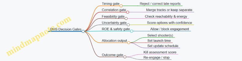
Putting it together: a worked micro-scenario
- A sensor reports a new track with moderate uncertainty and correct timing.
- The BMS correlates it with an existing track and merges them, reducing uncertainty.
- Feasibility checks show I1 can intercept within the engagement window; I2 cannot due to energy limits.
- The uncertainty-aware score for I1 clears the ROE threshold.
- The BMS launches I1 and schedules guidance updates more frequently because the predicted intercept point is moving quickly.
- Post-intercept, evidence is inconclusive, so the BMS holds the option to re-engage if another interceptor is feasible.
This is the essence of battle management software: it is not just computing trajectories, it is making disciplined decisions while the world refuses to be tidy.
4.4 Resilience and survivability of communications and networks
Hypersonic defense is a timing problem as much as a sensing problem. When a track is born, it must survive a chain of handoffs: sensor to fusion, fusion to battle management, battle management to shooter, and shooter back to assessment. Resilience means that chain keeps working when parts of it degrade—because “degrade” is more common than “fail.” Survivability means the system continues to operate (perhaps with reduced performance) under attack, interference, or infrastructure loss.
What “resilient” looks like in practice
Resilience is easiest to understand as a set of graceful behaviors:
- Continuity under partial loss: If one link path is jammed, traffic reroutes over another path.
- Degraded but usable modes: If full-rate data is unavailable, the system switches to lower-rate track updates or compressed messages.
- State preservation: If a node restarts, it recovers the most recent track and engagement context fast enough to avoid “cold start” gaps.
- Controlled uncertainty: If data quality drops, the system reflects that in track confidence and engagement decisions rather than pretending everything is fine.
A simple example: imagine a sensor site sending track updates every 20 ms. If the link can’t sustain that rate, resilience might switch to 100 ms updates while keeping the same message format and time stamps. The shooter may need a different guidance update schedule, but the engagement can still proceed.
Threats to communications (and what they do to the chain)
Communications and networks are stressed by three common categories of disruption:
- Interference and jamming: reduces link capacity, increases packet loss, and can bias timing.
- Cyber compromise: alters data, changes routing, or injects false commands.
- Physical and environmental loss: power interruptions, fiber cuts, antenna damage, or site isolation.
Each category maps to different failure modes:
- Jamming often causes loss and delay.
- Cyber compromise often causes integrity violations.
- Physical loss often causes missing nodes and broken routes.
Resilience design addresses all three, but the emphasis differs by layer.
Network architecture patterns that help
A survivable defense network usually avoids single points of failure and assumes that some links will be unreliable.
1) Multi-path routing with explicit priorities Instead of treating all traffic equally, systems assign priorities such as:
- track updates (high)
- engagement commands (highest)
- health telemetry (medium)
- maintenance logs (low)
If congestion happens, low-priority traffic drops first. A practical example: during a contested period, the network may drop nonessential video feeds while keeping track and command messages flowing.
2) Separation of functions Keeping sensor data, command/control, and administrative traffic on separate logical networks reduces the blast radius of a failure. If an administrative service misbehaves, it shouldn’t stall engagement messages.
3) Local autonomy at the edge Edge nodes (sensor processors, local fusion, or local engagement controllers) can continue operating when they lose the wider network. For instance, a sensor site might maintain local track management and send only the most relevant track summaries when bandwidth is constrained.
4) Time synchronization as a first-class requirement Hypersonic engagements punish timing errors. Systems rely on synchronized clocks so that time stamps mean something across nodes. A concrete example: if two nodes disagree by 50 ms, a fusion algorithm may treat a single target as two different tracks, wasting time on association.
Data integrity and authentication
Survivability isn’t only about keeping messages flowing; it’s also about ensuring they are the right messages.
Key practices:
- Message authentication so receivers can reject forged commands or corrupted track updates.
- Sequence numbers and replay protection to prevent old messages from being resent and misinterpreted.
- Schema validation so malformed packets don’t trigger undefined behavior.
A straightforward example: if a shooter receives an engagement command with an invalid sequence number or a mismatched track identifier, it should refuse the command and request a fresh update rather than acting on stale data.
Latency budgets and “what to do when it’s late”
Resilience includes behavior under delay, not just under loss.
A useful way to reason about this is to define a latency budget for each hop:
- sensor processing time
- network transit time
- fusion update time
- battle management decision time
- command delivery time
- shooter command acceptance time
Then define fallback actions when the budget is exceeded. For example:
- If the full track update arrives late, the system may use the last known track state with increased uncertainty.
- If the command arrives late beyond a safe acceptance window, the shooter may hold fire and request a new command rather than executing a potentially incorrect one.
This is “boring” engineering, which is exactly why it works.
Redundancy that matters (and redundancy that doesn’t)
Not all redundancy improves survivability.
- Useful redundancy: multiple independent communication paths, independent power sources, and independent processing nodes.
- Less useful redundancy: duplicating the same dependency (e.g., two radios that share the same antenna or the same single fiber route).
A practical example: two network links that both traverse the same physical conduit fail together when the conduit is damaged. True survivability requires diversity in routing or physical separation.
Mind map: resilience and survivability of communications
Mind Map: Resilience & Survivability of Communications/Networks
Concrete example: a contested engagement chain
Consider a layered defense system with a sensor site, a regional fusion node, and an engagement controller.
- Normal mode: The sensor sends full track updates at high rate. Fusion produces a track estimate with low uncertainty and forwards it to engagement control.
- Jamming begins: The sensor link experiences packet loss. The network detects rising loss and switches to a lower-rate track summary message. Time stamps remain accurate, so fusion continues updating the same track ID.
- Command delivery under stress: Engagement control prioritizes engagement commands over health telemetry. If a command packet is delayed beyond an acceptance window, the shooter requests a fresh command rather than acting on a stale one.
- Partial node loss: If the fusion node restarts, it loads the most recent track state from local storage and resumes fusion updates. The engagement controller continues using the last valid track estimate until the new estimate arrives.
The key is that each component has a defined response to degraded conditions, so the overall chain doesn’t collapse into “wait for perfect data.”
Practical checklist for designers and operators
- Define latency budgets and explicit late-message rules.
- Implement multi-path routing with traffic priorities.
- Use authentication, sequence numbers, and replay protection for commands and track updates.
- Ensure time synchronization across nodes.
- Provide edge autonomy so local functions continue when the wider network is impaired.
- Validate that redundancy is independent, not just duplicated.
- Test failure modes: packet loss, increased delay, node restart, and link isolation.
Resilience and survivability are not a single feature. They are a set of small, testable behaviors that keep the engagement chain coherent when reality stops cooperating.
4.5 Human-in-the-loop roles and operational procedures
Hypersonic defense is a time-pressured chain: sensors observe, C2 fuses tracks, effectors attempt intercept, and humans decide what to authorize. “Human-in-the-loop” doesn’t mean humans micromanage every calculation; it means humans set boundaries, resolve ambiguity when automation can’t, and verify that the system is operating within approved constraints.
Roles: who does what, and when
1) Watch supervisor (mission-level authority)
- Monitors overall engagement status: track quality, available effectors, and whether the system is operating in the selected engagement mode.
- Approves transitions between modes (e.g., from surveillance posture to active engagement) according to preplanned rules.
- Example: If track confidence drops because of clutter, the supervisor can authorize a “hold and re-acquire” step rather than forcing an immediate shot.
2) Engagement controller (engagement-level authority)
- Reviews the engagement plan produced by C2: which interceptor(s) are assigned, expected intercept geometry, and resource usage.
- Confirms that the plan matches the rules of engagement (ROE) and safety constraints.
- Example: If the plan proposes using a long-range interceptor that would leave a protected asset with no coverage, the controller can request an alternate allocation.
3) Sensor/track analyst (data-quality authority)
- Focuses on track integrity: whether the fused track is stable, whether discrimination is credible, and whether sensor coverage is sufficient.
- Can request specific sensor actions (e.g., adjust search patterns, prioritize certain beams) within approved limits.
- Example: If the fused track is switching between two candidate trajectories, the analyst can flag the ambiguity and ask for additional measurements before authorization.
4) Effector operator (execution authority at the launcher/effector level)
- Ensures the selected effector is in a valid state: power, readiness, safety interlocks, and correct configuration.
- Confirms that the effector’s constraints (field-of-view limits, maintenance status, software version) match the engagement plan.
- Example: If an interceptor is “ready” but its seeker calibration is out of tolerance, the operator can block the shot and request a different effector.
5) Safety and compliance officer (constraint authority)
- Verifies that actions comply with safety rules: geographic constraints, deconfliction zones, and any required authorization gates.
- Example: If an engagement would violate a safety boundary due to a predicted miss distance, the officer can require a replan or a different effector.
6) Automation (decision support, not decision replacement)
- Performs track fusion, generates engagement solutions, and computes predicted outcomes with uncertainty.
- Escalates to humans when confidence thresholds are not met or when ROE constraints require human confirmation.
- Example: If the system cannot discriminate a decoy from a target with acceptable probability, it can recommend “engage with conservative assumptions” or “hold for more data,” but the final choice is human-approved.
Operational procedures: a practical flow
The goal is to reduce surprises. Procedures should specify what information is reviewed, what thresholds trigger human action, and what actions are allowed.
Step 1: Establish engagement posture
- Watch supervisor selects the engagement mode (e.g., passive monitoring, active tracking, or active engagement) based on the operational situation.
- Sensor/track analyst confirms that sensor coverage and data links are healthy.
- Example: If a key sensor is degraded, the supervisor may switch to a mode that expects lower track confidence and uses more conservative authorization gates.
Step 2: Track initiation and stabilization
- C2 initiates tracks from sensor detections and attempts association across time.
- Human involvement is triggered when track stability metrics fail to converge (e.g., repeated track swaps, large covariance growth).
- Example: If the fused track alternates between two trajectories every few seconds, the analyst requests additional sensor dwell on the region of uncertainty.
Step 3: Discrimination and uncertainty handling
- C2 estimates whether the track is consistent with a hypersonic target profile versus clutter or decoys.
- Automation provides uncertainty bounds and a confidence score; humans decide whether the confidence is sufficient for authorization.
- Example: If the confidence is borderline, the engagement controller can authorize a “data-gathering window” that delays authorization by a small, preapproved interval.
Step 4: Engagement planning and authorization gates
- C2 proposes an engagement plan: interceptor assignment, predicted intercept point, and expected miss distance distribution.
- Safety and compliance officer checks geographic and deconfliction constraints.
- Engagement controller authorizes or rejects the plan based on ROE and effector availability.
- Example: If the plan uses the only interceptor capable of terminal intercept, the controller may require a second plan that preserves that asset for a later phase.
Step 5: Effector execution checks
- Effector operator verifies readiness, configuration, and interlocks.
- If any effector constraint conflicts with the plan, the operator blocks execution and requests replanning.
- Example: If the effector’s guidance module reports a calibration flag, the operator prevents launch and triggers a “reassign effector” action.
Step 6: In-flight updates and human override
- During flight, C2 updates guidance commands as new sensor data arrives.
- Humans intervene only when automation flags a constraint violation, a major track discontinuity, or a ROE exception.
- Example: If the fused track suddenly jumps due to a sensor dropout, the system can pause command updates and request human confirmation to resume using the last stable solution.
Step 7: Post-engagement assessment
- After intercept attempt, humans review outcome indicators: whether intercept occurred, whether the effector performed within expected parameters, and whether the system’s confidence estimates were accurate.
- Example: If the system predicted a high probability of kill but the result was a miss, the analyst can tag the event for procedure refinement (e.g., stricter discrimination thresholds for similar sensor geometries).
Mind maps
Mind map: Human-in-the-loop roles
Mind map: Operational procedure flow
Concrete examples of decision points
Example A: “Hold for data” authorization
- Situation: Two candidate tracks exist; fused track confidence is 0.55 (threshold for automatic authorization is 0.70).
- Action: Sensor/track analyst requests additional sensor dwell on the region where the trajectories diverge.
- Human decision: Engagement controller authorizes a short hold window (preapproved) rather than forcing an engagement with high uncertainty.
Example B: Replan due to effector constraint
- Situation: C2 proposes Interceptor 1 for terminal intercept, but effector operator reports a guidance calibration flag.
- Action: Effector operator blocks execution.
- Human decision: Engagement controller authorizes replanning using Interceptor 2, accepting a different intercept geometry but staying within ROE.
Example C: Safety boundary conflict
- Situation: Predicted miss distance distribution indicates a potential violation of a deconfliction zone for the selected engagement.
- Action: Safety/compliance officer rejects the plan.
- Human decision: Engagement controller requests a different effector assignment or a different intercept phase that keeps predicted effects within safe limits.
Design principles for procedures that work under stress
- Make the gate explicit: Humans should know exactly what condition triggers their approval (confidence threshold, constraint violation, or effector readiness mismatch).
- Use small, bounded choices: Procedures should offer limited actions (hold, replan, authorize) rather than open-ended improvisation.
- Separate responsibilities: Role clarity prevents “everyone is responsible” ambiguity; each authority checks a specific class of issues.
- Prefer confirmation over re-computation: Humans should verify inputs and constraints, not redo fusion math.
- Record decisions with reasons: After-action review is only useful if the system logs what was observed and why a gate was passed or rejected.
When these roles and procedures are practiced, the human contribution becomes consistent: not faster calculations, but better judgment about when the system is confident enough to act and when it needs more information or a safer plan.
5. Interceptor Fundamentals: Kinematics, Guidance, and Constraints
5.1 Intercept Geometry and the Engagement Envelope Problem
An interceptor is a moving target chasing a moving target—except the “chase” is constrained by physics, sensing, and guidance authority. The intercept geometry describes how the interceptor’s path, the target’s path, and the relative position evolve over time. The engagement envelope is the set of conditions under which an intercept is feasible with the interceptor’s real-world limits.
The geometry in plain terms
At any moment, define:
- Relative position: where the interceptor is compared to the target.
- Line-of-sight (LOS) direction: the direction from interceptor to target.
- Closing speed: how quickly the distance along the LOS is shrinking.
- Aspect angle: the target’s orientation relative to the interceptor’s LOS (important for sensors and some guidance behaviors).
A useful mental model is to imagine a “cone” of possible interceptor trajectories. The target’s motion sweeps out another curve. An intercept exists when at least one feasible interceptor trajectory intersects the target’s trajectory while staying within guidance and propulsion limits.
Engagement envelope: what it really means
The engagement envelope is not a single shape drawn on a map. It’s a practical boundary defined by multiple constraints:
- Sensor constraints: can the interceptor (or the system) acquire and maintain track long enough to guide?
- Kinematic constraints: can the interceptor reach the required position and velocity at the right time?
- Control constraints: does the interceptor have enough lateral acceleration (or equivalent control authority) to follow the commanded path?
- Energy constraints: does it retain sufficient speed and maneuver capability through the endgame?
- Timing constraints: is there enough time between detection, decision, and endgame to execute the plan?
A common mistake is to treat “range” as the only variable. In reality, two engagements with the same range can have very different feasibility because closing speed, maneuver rate, and sensor geometry differ.
The core problem: time-to-intercept vs. required maneuver
Consider the interceptor’s job in two stages:
- Get to the right place: reach a point in space where the target will be.
- Get there while steering: maintain a trajectory that can still be guided as the target maneuvers.
If the target can change its position faster than the interceptor can adjust its path, the intercept point “moves away.” This is why the envelope often shrinks dramatically when the target’s maneuver capability increases, even if the interceptor’s speed is unchanged.
A simple geometric example (no equations needed)
Suppose the interceptor is launched from a point behind the target’s path. The target is moving away from the interceptor. Early on, the interceptor’s LOS angle changes slowly, so guidance commands are modest. As the interceptor closes, the LOS angle can start changing faster, especially if the target turns. If the interceptor’s control authority is limited, it may be unable to keep the commanded lead angle, causing the miss distance to grow.
Now compare the same interceptor and target speeds, but with the interceptor launched from a position where the target is moving toward it (a head-on or near head-on geometry). The closing speed is higher, and the LOS angle evolution can be more favorable. Even with the same maximum acceleration, the interceptor may have enough time to steer into the intercept point.
This is the engagement envelope problem in one sentence: geometry determines how much time and steering effort the interceptor gets.
A more concrete example with numbers
Assume:
- Target speed: \(V_t = 2,\text{km/s}\)
- Interceptor speed at endgame: \(V_i = 2.5,\text{km/s}\)
- Maximum lateral acceleration available for terminal steering: \(a_{\max} = 20,g\) (where \(g\approx 9.81,\text{m/s}^2\))
If the interceptor approaches in a geometry where the required turn rate is high (because the target is crossing the interceptor’s path or turning hard), the interceptor may need lateral acceleration near \(a_{\max}\) to keep the LOS on the commanded path. If the required acceleration exceeds what is available, the interceptor cannot “stay on the line,” and the miss distance grows.
In a more favorable geometry, the required turn rate is lower. The same interceptor can then keep the LOS error bounded and converge to the intercept point.
The key nuance: the envelope is shaped by required lateral acceleration, not just by whether the interceptor can reach the target’s general area.
LOS rate and the “steering budget”
A practical way to reason about feasibility is to treat guidance as a steering budget problem. The interceptor has:
- limited acceleration (and often limited jerk or rate)
- limited time during which that acceleration is effective (because speed drops, control saturates, or the seeker needs stable geometry)
The target’s motion determines how quickly the LOS direction changes. When LOS rate is high, the interceptor must generate lateral acceleration quickly to keep the trajectory aligned with the guidance solution. If the interceptor saturates, it may still fly toward the target, but it will do so along a path that misses.
Engagement envelope boundaries: typical failure modes
- Too early: the interceptor cannot acquire or maintain track. Even if kinematics would allow an intercept, guidance cannot start.
- Too far: the interceptor runs out of energy or time before it can reduce LOS error enough to converge.
- Too late: the interceptor is already inside the region where it cannot maneuver enough to correct an error.
- Wrong geometry: the interceptor has time, but the required steering is beyond control authority.
These failure modes often overlap. For example, “too far” can also mean “too much LOS rate change before endgame,” which increases steering demand.
Mind map: intercept geometry and envelope
Mind Map: Intercept Geometry and the Engagement Envelope Problem
A practical “envelope check” workflow
When analyzing or designing an engagement concept, a straightforward workflow is:
- Pick a scenario: initial positions, velocities, and target maneuver assumptions.
- Compute or estimate LOS evolution: how LOS direction and LOS rate change over time.
- Estimate required steering: translate LOS evolution into the approximate lateral acceleration demand.
- Compare to interceptor limits: check for saturation and whether guidance can remain stable.
- Verify sensor feasibility: ensure acquisition and track maintenance occur before the guidance solution becomes critical.
- Confirm timing: ensure the interceptor can reach the intercept point before the guidance solution becomes unusable.
This workflow keeps the reasoning grounded: geometry is assessed through LOS evolution, and feasibility is assessed through steering and timing limits.
Another example: same range, different envelope
Imagine two engagements at the same initial separation distance:
- Engagement A: target is moving roughly away; closing speed is modest.
- Engagement B: target is moving across; closing speed is higher and LOS rate changes faster.
Even though the initial range matches, the envelope can differ:
- Engagement A may fail due to insufficient time to complete endgame steering.
- Engagement B may fail due to insufficient control authority because LOS rate forces aggressive steering.
So the envelope is not “distance-limited” in a simple way. It’s “geometry-limited,” because geometry determines both time and steering demand.
Summary
Intercept geometry determines how LOS direction and LOS rate evolve, which in turn determines the steering budget required for convergence. The engagement envelope is the set of initial conditions where sensor feasibility, kinematics, control authority, energy, and timing all line up. When any one of those constraints is stressed—often by unfavorable geometry—the intercept becomes infeasible even if the interceptor is fast enough in a purely straight-line sense.
5.2 Guidance laws and seeker performance at closing speeds
At hypersonic closing speeds, guidance is less about “aiming at a point” and more about managing uncertainty fast enough to matter. The seeker must keep producing usable measurements while the target’s apparent motion changes rapidly, the platform’s own motion is aggressive, and the atmosphere is doing its usual job of making everything harder.
Mind map: guidance laws and what they need from the seeker
Guidance law basics: what changes at hypersonic endgame
Most missile guidance laws start from a geometric idea: reduce the miss distance by steering based on how the line of sight (LOS) evolves. At high closing speeds, two things become dominant.
- Time-to-go shrinks, so guidance has fewer “turning opportunities.” If the seeker update arrives late, the missile may already be past the best correction window.
- LOS dynamics accelerate, so the guidance command must respond to rapid changes without exciting oscillations or saturating actuators.
A useful way to think about it is to separate measurement quality from control authority. Even a perfect guidance law cannot compensate for a seeker that loses lock, produces biased angles, or updates too slowly.
Proportional Navigation (PN): the workhorse and its assumptions
Proportional Navigation commands lateral acceleration proportional to the LOS rate. A common form is
\[ \mathbf{a}_c = N, V_c, \dot{\lambda}, \hat{\mathbf{n}} \]
where \(N\) is the navigation constant, \(V_c\) is closing speed, \(\dot{\lambda}\) is LOS angular rate (in the relevant plane), and \(\hat{\mathbf{n}}\) is the lateral direction.
Why PN works: it implicitly tries to drive the target’s relative motion to zero in the lateral sense by reacting to how the LOS is changing.
What PN needs: reasonably accurate LOS rate estimates and a missile that can generate the commanded acceleration without saturating.
What breaks at high closing speeds:
- LOS rate estimation noise grows when angle measurements are noisy and update intervals are large.
- Navigation constant tuning becomes sensitive because the missile’s ability to turn is limited near endgame.
- Bias in angle measurements can create a consistent steering error that PN will faithfully “correct,” but in the wrong direction.
Example: PN sensitivity to seeker latency
Assume a seeker provides angle \(\theta\) at discrete times with latency \(\tau\). The LOS rate estimate \(\dot{\theta}\) is effectively computed from delayed measurements, so the guidance command is based on \(\dot{\theta}(t-\tau)\) rather than \(\dot{\theta}(t)\).
If \(\tau\) is small, the effect is minor. If \(\tau\) is a meaningful fraction of the remaining time-to-go, the missile turns using stale information. A concrete way to see this: if the missile needs to correct a lateral error of 1 m with only 0.5 s of effective maneuver time, then a 50 ms latency is 10% of the correction window. That doesn’t sound huge until you remember that acceleration saturation and changing LOS geometry can turn that 10% into a noticeable miss-distance increase.
Augmented PN: handling bias and maneuvering targets
To reduce the impact of measurement bias and target maneuvers, augmented PN variants add terms that compensate for known error sources or estimate them online.
Common augmentations include:
- Bias-aware PN: uses an estimated angle bias to correct the LOS measurement before computing LOS rate.
- Acceleration-limited PN: modifies the command when predicted required acceleration exceeds actuator limits.
- Time-to-go aware PN: adjusts \(N\) or command scaling based on an updated time-to-go estimate.
These are not magic; they are bookkeeping. The seeker still must provide enough information to estimate bias and track quality, and the missile still must respect physical limits.
Command-to-line-of-sight (CLOS): simple geometry, strict measurement needs
CLOS guidance commands the missile to steer so that its velocity aligns with the instantaneous LOS. It can be effective when the seeker provides stable, low-noise angles.
At hypersonic closing speeds, CLOS can become fragile if:
- the seeker’s angle noise causes rapid command changes,
- the missile’s turn rate lags behind the commanded LOS alignment,
- the target maneuvers faster than the missile can track.
Practical takeaway: CLOS tends to trade theoretical simplicity for a strong dependence on seeker smoothness and control bandwidth.
Seeker performance: what matters more than raw range
A seeker at hypersonic endgame is judged by how well it supports guidance, not by how far it can “see” in ideal conditions.
Key performance aspects:
- Track continuity (lock maintenance): guidance fails if measurements drop out or jump.
- Angle accuracy and bias stability: a small bias can integrate into a large miss distance over short time.
- Update rate and effective latency: guidance is only as timely as the measurement pipeline.
- Gimbal limits and tracking dynamics: the seeker must keep up with the target’s apparent motion.
- Discrimination quality: confusing the target with clutter or decoys can corrupt the LOS.
Example: gimbal limits and apparent motion
Suppose the target’s apparent angular rate exceeds the seeker’s gimbal tracking capability. The seeker may still “see” the target, but it cannot keep the measurement aligned with the true LOS. The result is a measurement that is delayed, clipped, or biased.
Guidance then receives a LOS that is not the real LOS. Even if the guidance law is correct, it is steering toward the wrong geometry. This is why seeker tracking dynamics are as important as angle noise.
Endgame measurement processing: turning noisy angles into usable LOS rate
LOS rate \(\dot{\lambda}\) is typically derived from angle measurements. Differentiation amplifies noise, so seekers and guidance systems often use filtering.
A typical approach is to estimate angle and rate together using a state estimator (for example, a simple constant-rate model). The filter balances two errors:
- Too much smoothing delays the rate estimate, increasing effective latency.
- Too little smoothing leaves noisy rate estimates, causing command chatter and wasted control effort.
At high closing speeds, the filter must be tuned so that its delay is small compared to the remaining time-to-go.
Putting it together: guidance command feasibility
Even with perfect LOS information, the missile must be able to execute the command. Guidance systems often include a feasibility check:
- compute the commanded lateral acceleration from the guidance law,
- compare it to available acceleration based on current energy state and actuator limits,
- if infeasible, apply saturation handling and adjust the command to avoid integrator windup.
Why this matters: saturation changes the closed-loop behavior. If the guidance law assumes unlimited acceleration, the missile may overshoot, oscillate, or fail to converge.
Example: saturation handling prevents “helpful” mistakes
Imagine PN requests 30 g lateral acceleration, but the missile can only deliver 18 g. If the guidance software keeps integrating the error as if 30 g were possible, it can build up a large internal correction. When the missile finally reaches the limit, the stored correction can drive a delayed overshoot.
A saturation-aware implementation instead clamps the command and updates internal states consistently with the actual applied acceleration. The result is less overshoot and a more predictable miss-distance distribution.
Summary of the guidance–seeker contract
At hypersonic closing speeds, guidance laws succeed when the seeker provides:
- continuous, correctly associated measurements,
- sufficiently accurate angles with stable bias,
- update rates and latency compatible with the remaining time-to-go,
- tracking dynamics that respect gimbal and field-of-view limits.
Guidance laws then use those measurements to generate commands that the missile can physically execute. When either side of the contract fails—measurement quality or command feasibility—the miss distance grows, often quickly and nonlinearly.
5.3 Propulsion and energy management for endgame interception
Endgame interception is where kinematics stop being “nice to have” and become the whole story. At hypersonic closing speeds, the interceptor has only a short window to (1) keep the seeker pointed at the target, (2) generate enough lateral acceleration to correct the miss, and (3) avoid running out of usable energy before the final geometry is achieved.
The endgame energy problem in plain terms
Think of the interceptor’s usable energy as a budget that must cover three costs:
- Kinetic energy you can’t spend twice: If you slow down too early, you reduce closing speed and the time available for terminal corrections.
- Energy for maneuvering: Lateral acceleration requires thrust vectoring and/or control authority, which consumes propellant and can reduce forward speed.
- Energy for staying on the right line: Guidance needs time-to-go and stable pointing; if the interceptor must “fight” its own aerodynamics or control limits, it burns energy without improving aim.
A useful mental model is: miss distance is the result of guidance error integrated over time, and time is limited by how fast you lose speed and how quickly you can turn.
Propulsion modes and what they imply for endgame
Most interceptor concepts use one of two broad propulsion patterns:
- Boost-to-intercept (rocket-dominant): A high-thrust phase raises speed early, then the vehicle coasts or throttles during terminal corrections.
- Sustained propulsion (ramjet/scramjet-like or turbojet-like, depending on concept): Thrust can be maintained longer, but the vehicle must manage inlet/thermal constraints and guidance loads.
Even without committing to a specific design, the endgame lesson is consistent: the propulsion system must provide controllable thrust and predictable thrust-to-mass behavior during the maneuver window.
Example: why “more thrust” isn’t automatically better
Suppose two interceptors have the same mass and guidance law, but one has higher peak thrust. If the higher-thrust interceptor also experiences greater structural or thermal limits that force it to reduce control effectiveness near the endgame, it may end up with less lateral acceleration capability at the exact time it matters. In practice, what matters is effective lateral acceleration over the final time-to-go, not peak thrust in isolation.
Energy management as a guidance constraint
Guidance and propulsion are coupled through constraints like:
- Maximum lateral acceleration \(a_{\max}\) from thrust vector limits, control authority, and aerodynamic limits.
- Minimum and maximum speed constraints to keep the seeker and control surfaces within operating envelopes.
- Propellant mass flow limits that cap how aggressively the vehicle can change its velocity vector.
A common way to express the endgame requirement is to relate required lateral acceleration to the geometry. For small angles, a simplified planar view gives a sense of scaling:
\[ a_{\text{req}} \approx \frac{V}{t_{\text{go}}},\Delta \theta \]
where (V) is interceptor speed, \( t_{\text{go}} \) is time-to-go, and \( \Delta \theta \) is the angular correction needed to reduce miss. The exact form depends on the guidance model, but the takeaway is robust: shorter time-to-go or larger angular correction drives higher required acceleration.
Practical energy management strategies
1) Reserve energy for the last correction window
A straightforward approach is to avoid spending all available impulse early. If you use maximum thrust during midcourse, you may arrive at endgame with the right speed but poor maneuver margin because the remaining propellant can’t support the final turn.
Example (numbers, not magic):
- Interceptor arrives at endgame with \( V=2.5,\text{km/s} \).
- Guidance requires a lateral acceleration of (30,g) for the final \( t_{\text{go}}=2,\text{s} \).
- If the propulsion plan leaves only enough propellant for (15,g) in that window, the miss will grow even if earlier tracking was excellent.
Energy management here is basically: match the thrust schedule to the acceleration demand profile.
2) Throttle and vector to shape the velocity direction, not just the speed
If the interceptor only tries to maximize speed, it may overshoot the desired line-of-sight geometry. Endgame success often depends on arriving with the correct velocity direction so that the remaining turn rate is achievable.
Example: Two interceptors both reach the same speed at the same range, but one arrives with a velocity vector that is \( 5^\circ \) off the desired intercept plane. If the remaining time-to-go is short, that \( 5^\circ \) becomes a large \( \Delta \theta \) term, increasing \( a_{\text{req}} \). The “faster” interceptor can still lose because it has to spend its remaining energy correcting direction rather than closing.
3) Manage drag and thermal limits so they don’t silently steal control authority
At high speed, drag can be a major part of the deceleration budget. More importantly, drag can reduce control effectiveness by changing aerodynamic forces and moments. Thermal constraints can force throttling or limit actuator authority.
Example: An interceptor uses aggressive thrust to maintain speed early. Later, as it enters a denser atmosphere, drag rises and the vehicle must throttle down to stay within thermal limits. The result is not only reduced speed but also reduced ability to generate lateral acceleration. Energy management must therefore include how propulsion interacts with environment-driven limits.
4) Use time-to-go targeting: “arrive when you can still turn”
A useful operational rule is to define a terminal phase start condition based on both geometry and remaining maneuver capability. Instead of starting terminal guidance at a fixed range, start it when the interceptor has enough remaining impulse to meet the acceleration demand for the remaining time-to-go.
Example: If the interceptor’s remaining propellant can support a maximum lateral acceleration \( a_{\max,rem} \), then the guidance system can compute whether the expected \(a_{\text{req}}(t_{\text{go}})\) stays below \( a_{\max,rem} \). If not, the system should adjust earlier thrusting or trajectory shaping so that the terminal phase begins with adequate margin.
A mind map of endgame propulsion and energy management
Mind map: Propulsion & energy management for endgame interception
How to evaluate whether the plan works
A propulsion/energy plan is “good” if it consistently produces the required acceleration profile in the presence of realistic uncertainties (mass properties, actuator response, drag variability, and target maneuver). A practical evaluation checklist:
- Acceleration margin plot: Compare \(a_{\text{req}}(t)\) from guidance against \(a_{\max}(t)\) from propulsion and control limits.
- Time-to-go sensitivity: Small changes in closing speed can shorten the maneuver window; verify the plan still meets acceleration demand.
- Propellant margin at terminal start: Confirm that the remaining impulse supports the final turn without forcing late throttling.
- Seeker/attitude feasibility: Ensure that the attitude rates and pointing constraints required by guidance are achievable while thrusting.
Example: a simple pass/fail logic
- Compute expected \( t_{\text{go}} \) at terminal phase start.
- Estimate \( a_{\text{req}} \) for the expected angular correction.
- If \( a_{\text{req}} \le 0.8,a_{\max,rem} \) (using a margin factor), the plan passes the maneuver feasibility check.
- If not, adjust earlier thrusting or trajectory shaping so the interceptor arrives with more maneuver margin.
Endgame interception is therefore less about “having enough speed” and more about having the right combination of speed, controllable thrust, and remaining maneuver authority at the exact time guidance needs it. When propulsion and energy management are treated as constraints inside the guidance problem, the interceptor stops guessing and starts meeting the geometry.
5.4 Discrimination, miss distance, and kill assessment fundamentals
At hypersonic closing speeds, “did we hit?” is not a single question. It’s a chain of smaller questions: what is it, where will it be when we arrive, and what counts as a successful outcome. This section lays out the core ideas behind discrimination, miss distance, and kill assessment in a way you can map directly to system requirements and test plans.
Discrimination: deciding what you’re tracking (and what you’re not)
Discrimination is the process of separating the target from other objects that look similar to the seeker or sensors. In practice, the seeker sees a stream of measurements (angles, range, Doppler, imaging features, or combinations). The discrimination task is to assign those measurements to the most likely target hypothesis.
Key inputs to discrimination include:
- Kinematics consistency: Does the object’s motion fit the expected dynamics of the target class?
- Measurement consistency: Do successive measurements agree with a coherent track, or do they jump like a different object?
- Feature consistency (when available): Does the object’s radar cross-section pattern, thermal signature, or imaging features match the expected profile?
- Context constraints: Is the object’s location and timing consistent with the predicted threat geometry from earlier sensors?
A simple way to think about discrimination is: you’re not proving identity; you’re reducing confusion. Even a good discriminator can be wrong, so the system design must tolerate residual uncertainty.
Mind map: discrimination fundamentals
Concrete example: track swap under clutter
Imagine a seeker with a narrow field of view. Two objects pass through the same region: the true target and a decoy with similar apparent size. If the system assigns measurements to the wrong track for a few updates, the guidance solution can “chase” the decoy. The miss distance might still be small relative to the wrong track, producing a misleading kill assessment. That’s why discrimination quality is not a side metric; it directly affects the geometry used for interception.
Miss distance: the geometry of “how close”
Miss distance is the spatial separation between the interceptor and the target at the closest approach time (or at a defined intercept point). It’s usually computed from estimated states and relative motion, not from direct measurement of the true 3D separation.
Two practical distinctions matter:
- True miss distance vs. estimated miss distance: The system can only estimate. Estimation error comes from sensor noise, model mismatch, and discrimination uncertainty.
- Deterministic vs. probabilistic miss distance: A single number is rarely enough. A probabilistic view treats miss distance as a distribution.
A common modeling approach is to represent the relative position error at closest approach as a covariance matrix. If the interceptor and target are modeled as points (or with effective radii), then the probability of being within a “success region” can be derived from that distribution.
Mind map: miss distance fundamentals
Concrete example: why “small miss distance” can still fail
Suppose the guidance system predicts a miss distance of 2 meters. If the target state uncertainty is 10 meters (1-sigma) in the direction that matters most for the kill mechanism, then the 2-meter estimate may be optimistic. The interceptor could pass outside the effective success region. In other words, miss distance must be interpreted with its uncertainty, not as a standalone number.
Kill assessment: translating geometry into outcome
Kill assessment is the determination of whether the interceptor’s effects are sufficient to neutralize the target. For many systems, kill assessment is not a direct observation of “destruction.” It’s an inference based on:
- Predicted impact geometry: Did the interceptor pass within the effective success region?
- Effects model: Given the interceptor’s energy, timing, and interaction physics, what outcome is expected?
- Uncertainty propagation: How do estimation errors and discrimination errors affect the predicted outcome?
- Post-event evidence (when available): Some systems use additional sensor returns or telemetry to confirm or refine the assessment.
A useful mental model is: kill assessment is a probability statement about outcome, not a binary switch.
A simple probabilistic formulation
Let the success region be defined by an effective radius \( r_k \) around the target’s critical point. Let the relative position error at closest approach be represented by a distribution. Then the probability of kill can be approximated as:
\[ P_{k} = P\left(|\Delta \mathbf{r}| \le r_k\right) \]
where \(\Delta \mathbf{r}\) is the relative position error at closest approach. In practice, the exact computation depends on how \(\Delta \mathbf{r}\) is modeled (e.g., Gaussian in a local frame) and how \(r_k\) is defined for the specific effects mechanism.
Mind map: kill assessment fundamentals
Putting it together: the discrimination → miss distance → kill chain
A coherent system design treats these as linked stages:
- Discrimination determines which object becomes the target hypothesis. If the wrong object is selected, the state estimate is biased.
- Tracking and navigation propagate that estimate into a predicted intercept geometry. The result is a miss distance estimate with uncertainty.
- Kill assessment converts miss distance and effects physics into an outcome probability. The decision rule should reflect the uncertainty and the defined success criteria.
Concrete example: how a decoy changes the kill assessment
Assume a decoy has similar apparent motion for a short time. Early discrimination assigns it a high probability. The guidance solution is computed to intercept that hypothesis. Even if the interceptor later improves discrimination, the endgame geometry may already be constrained by limited maneuver authority and time-to-go. The miss distance relative to the true target can remain large, which the kill assessment captures as a lower probability of success.
Practical best practices for tests and scoring
- Score discrimination separately from intercept performance. This prevents “credit” for a good intercept while hiding a wrong association.
- Report miss distance with uncertainty metrics. A mean value without spread is hard to interpret and easy to misapply.
- Define the success region using the effects mechanism, not convenience. The kill radius should reflect what the physics and interaction model actually support.
- Use consistent frames and timing definitions. Miss distance depends on the chosen closest approach definition and coordinate frame.
When these pieces are connected correctly, kill assessment becomes a disciplined inference: it uses discrimination to choose the right target, uses miss distance to quantify geometry, and uses an effects model to translate geometry into outcome.
5.5 Testing and evaluation metrics for interceptor effectiveness
Interceptor effectiveness is easiest to misunderstand when metrics are treated like a single number. A good test plan uses a small set of metrics that map to the physics (can you see it?), the geometry (can you get there?), and the decision chain (can you command the shot in time?). The trick is to define each metric so it can be measured without guessing.
Core evaluation questions
Use these questions to drive metric selection:
- Detection & tracking: Did the system obtain a usable track early enough, and did it keep it through the engagement?
- Command & control: Were commands delivered with sufficient timeliness and correctness?
- Guidance & control: Did the interceptor follow a feasible trajectory given the measured target state?
- Endgame discrimination: Did the interceptor select the correct aim point and avoid being fooled by decoys or clutter?
- Effect: Did the interceptor achieve the required miss distance or impact/kill condition?
Each question gets at least one metric and an explicit measurement method.
Metric set: from “can we” to “did it work”
Below is a practical metric stack that teams often use because it separates “system capability” from “engagement outcome.”
A. Engagement timeline metrics
- Track acquisition time (Tₐ): Time from target entering sensor coverage to first stable track.
- Example: If Tₐ is 18 s in a test, but the engagement requires 25 s of guidance time, you already know the shot is at risk even before firing.
- Time-to-go at command (Tₜ): Time between issuing the final guidance command and intercept point.
- Example: If Tₜ is consistently below the guidance law’s effective window, you’ll see systematic miss distances.
B. Guidance and navigation metrics
- Commanded vs. achieved miss distance (MD): The closest approach distance between interceptor and target at closest approach.
- Example: A test might show MD = 12 m on average, but the kill requirement might be 5 m; the system is “working” but not meeting the effect criterion.
- Trajectory adherence error: Difference between predicted and flown interceptor trajectory, often summarized as position/velocity error at key waypoints.
- Example: If adherence error spikes after a maneuver, you can correlate it with actuator limits or model mismatch.
C. Endgame discrimination metrics
- Aim-point correctness rate: Fraction of engagements where the selected aim point matches the intended target component (or correct object among candidates).
- Example: In a clutter scenario, aim-point correctness might be 0.85 even when overall intercept success is 0.70, revealing that discrimination is a major contributor.
- Discrimination latency: Time from candidate presentation to final aim-point selection.
- Example: If latency is too long, the interceptor may commit to a wrong aim point while the target state is still changing rapidly.
D. Effect metrics (the ones people argue about)
- Kill probability (Pk): Probability of meeting the kill condition, typically based on a miss-distance threshold and/or modeled lethality.
- Example: Define a kill condition as MD ≤ 5 m and required energy/impact conditions. Then Pk is computed from test outcomes.
- Confidence bounds on Pk: Uncertainty around Pk due to finite sample size.
- Example: If 8 kills occur out of 20, Pk = 0.40, but the confidence interval is wide; you should not treat 0.40 as a precise truth.
How to compute kill probability without hand-waving
A simple approach is to treat each engagement as a Bernoulli trial (kill or no-kill). If (k) kills occur out of (n) trials, the point estimate is:
\[ \hat{P}_k = \frac{k}{n} \]
To express uncertainty, use a confidence interval. One common method is the Clopper–Pearson interval for a binomial proportion. The key evaluation practice is to report both the estimate and the interval, so decision-makers see whether the test size is adequate.
Separating “intercept” from “kill”
A test can produce an intercept geometry that looks good in kinematics but fails in effect. To prevent confusion:
- Define intercept success using a geometric criterion (e.g., MD within a specified band).
- Define kill success using a lethality criterion (e.g., MD plus modeled effect on the target’s critical components).
Example: Suppose MD ≤ 10 m is achieved in 90% of trials, but kill success is 60% because the target model includes survivable structures or because the aim point is often slightly off. Reporting only “intercept success” would overstate effectiveness.
Test design metrics: coverage and representativeness
Effectiveness numbers are only meaningful if the test set covers the conditions that matter.
A. Scenario coverage metrics
- Engagement geometry coverage: Distribution of aspect angles, ranges, and time-to-go values.
- Example: If all tests use near-identical closing speeds, you might miss guidance failures that occur only at the high end.
- Environmental coverage: Atmospheric conditions, turbulence levels, and sensor clutter states.
- Example: A seeker that performs well in clean air but struggles with heavy clutter will show a lower aim-point correctness rate.
B. Uncertainty and measurement quality
- State estimation quality: Track-quality metrics such as covariance magnitude or track error bounds.
- Example: If the target state error is large, guidance performance may degrade even when the interceptor hardware is fine.
- Instrumentation fidelity: Measurement uncertainty for interceptor and target positions at closest approach.
- Example: If the measurement system has ±2 m uncertainty, then a 5 m kill threshold becomes sensitive to error; you must incorporate that into the evaluation.
A mind map for interceptor effectiveness evaluation
Worked example: turning test data into decisions
Assume 30 engagements. The evaluation team defines:
- Intercept success: MD ≤ 10 m
- Kill success: MD ≤ 5 m and aim-point correctness = true
Results:
- 24/30 have MD ≤ 10 m → intercept success = 0.80
- 14/30 have MD ≤ 5 m → kill candidates = 0.47
- Of those 14, 10 also have correct aim point → kill success = 10/30 = 0.33
Interpretation:
- The system often reaches a good geometry (0.80), so propulsion and basic guidance are not the primary limiter.
- The drop from 0.47 to 0.33 points to discrimination or aim-point control as a major contributor.
- If the confidence interval around 0.33 is wide, you increase sample size or refine scenario coverage before concluding the interceptor is “insufficient.”
Practical reporting checklist
For each test series, report:
- Metric definitions and thresholds (including how uncertainty affects them)
- Sample size (n) and kill count (k)
- Point estimate → \( \hat{P}_k \)
- Confidence interval for \( P_k \)
- Breakdown by metric category (timeline, guidance, discrimination, effect)
- Distributions of MD and aim-point correctness, not only averages
When these are consistent, the evaluation becomes less about arguing over a single number and more about identifying which part of the chain needs improvement. That’s the whole point of metrics: they should tell you what to fix, not just what happened.
6. Ground-Based and Layered Missile Defense Design
6.1 Layering concepts: boost, midcourse, terminal, and beyond
Layering in missile defense means using multiple interception opportunities and multiple sensor-to-effector paths so that no single failure mode decides the outcome. The idea is simple: if the first attempt is late, confused, or out of energy, the system still has another chance with different geometry and different constraints.
Layering by engagement phase
Boost phase (early, fast, and messy)
Boost-phase defense targets the period when a threat is still accelerating and its signature is often strong. The geometry is favorable when defenders can see the launch region early enough, but the challenge is that the target is moving quickly and the time window can be short.
What you design for:
- Early detection and track initiation: enough sensor sensitivity to start a track before the threat becomes hard to discriminate.
- Fast handoff: a short latency path from detection to an interceptor launch decision.
- Energy management: interceptors must reach the threat before it exits the boost-friendly region.
Concrete example: A coastal radar network detects a rising plume and begins tracking within seconds. The battle manager assigns an interceptor to a predicted intercept point that accounts for acceleration. If the track quality degrades due to clutter, the system can still keep the interceptor on a conservative trajectory while a second sensor refines the track.
Midcourse phase (longer time, harder discrimination)
Midcourse defense covers the portion where the threat coasts or follows a ballistic-like path. The engagement window is typically longer than boost, which helps with planning and sensor fusion. The trade is that discrimination can be difficult when decoys or fragmentation are present.
What you design for:
- Track maintenance: keeping consistent tracks through changing viewing angles.
- Discrimination logic: using multiple sensor types or multiple looks to separate likely objects from decoys.
- Resource allocation: deciding how many interceptors to commit to which tracks when the number of plausible objects exceeds inventory.
Concrete example: A defender maintains several candidate tracks. A midcourse interceptor is staged so that it can be retargeted as discrimination improves. If the system later downgrades a candidate, the interceptor can be reassigned to a higher-confidence object without wasting the entire engagement timeline.
Terminal phase (short time, high payoff)
Terminal defense occurs near the target, where the threat may maneuver and where the defender must make a final identification and intercept decision quickly. The time-to-go is small, so the system relies on precise tracking and fast guidance updates.
What you design for:
- High-accuracy sensors: better angular resolution and better measurement stability.
- Endgame guidance: guidance laws that handle late updates and limited control authority.
- Kill assessment and re-engagement: determining whether the threat was neutralized and whether another interceptor is needed.
Concrete example: An interceptor receives a refined track update seconds before intercept. The guidance system uses that update to correct aim point and closing geometry. If the sensor reports uncertainty spikes due to atmospheric effects, the battle manager can schedule a second interceptor for a nearby time window rather than betting everything on one shot.
Beyond (defense beyond the immediate engagement)
“Beyond” is a catch-all for additional layers that extend the defense problem outward in time or space. It can include earlier intercept opportunities, alternate basing modes, or additional sensor/effector paths that are not neatly categorized as boost, midcourse, or terminal.
What you design for:
- Alternate geometry: different sensor viewpoints or different interceptor trajectories.
- Redundancy in the chain: multiple ways to get from detection to engagement.
- Coverage continuity: reducing dead zones caused by terrain, curvature, or platform availability.
Concrete example: If a radar site has a line-of-sight gap over a region, a second sensor network with a different placement can provide continuity. That “beyond” layer doesn’t change the physics of the phases, but it changes whether the defender has enough track quality to support later interceptors.
Mind map: layering concepts
How layers work together (the “chain” view)
Layering is not just four phases; it’s a chain of functions that must survive uncertainty. A useful way to reason about it is to track three quantities through each layer: time-to-go, track quality, and available engagement resources.
- Time-to-go shrinks as you move toward terminal. That forces earlier decisions to be robust to later corrections.
- Track quality often improves with more looks in midcourse, but discrimination can still be uncertain. That’s why the system benefits from staging and retargeting.
- Resources (interceptors, channels, and compute capacity) are finite. Layering helps because it allows the system to spend resources where the probability of success is highest.
Concrete example: Suppose a defender has limited interceptors. In boost, it launches only when track initiation confidence exceeds a threshold. In midcourse, it holds some interceptors in reserve until fusion reduces the number of plausible objects. In terminal, it commits the remaining interceptors to the highest-confidence tracks, with a backup plan if the final measurements degrade.
Practical design principles for phase layering
-
Match interceptor energy to phase geometry Boost intercepts require rapid energy use and quick decisions. Terminal intercepts require precise endgame guidance and stable tracking. Midcourse intercepts benefit from longer planning time.
-
Use different failure modes on purpose If boost fails due to track initiation uncertainty, midcourse can still succeed using longer observation time. If midcourse fails due to discrimination ambiguity, terminal can use tighter geometry and higher-resolution measurements.
-
Plan handoffs, not just launches A layer is only useful if the system can transition from one phase’s sensor picture to the next phase’s engagement plan. That means defining when and how track updates change the interceptor’s aim point or whether it gets reassigned.
-
Keep engagement logic consistent with uncertainty When uncertainty is large, the system should avoid “single-number certainty.” Instead, it should use confidence levels to decide whether to commit, stage, or wait for better measurements.
Summary
Layering by boost, midcourse, terminal, and beyond creates multiple interception opportunities with different strengths: early detection and strong signatures in boost, longer planning and fusion in midcourse, precise endgame execution in terminal, and coverage continuity via additional geometry and paths in beyond. The best systems treat layering as an integrated chain of sensing, decision-making, and engagement management rather than four separate checklists.
6.2 System-of-systems integration across sensors and effectors
A layered defense only works when sensors, decision logic, and effectors agree on the same “story” about the threat. Integration across sensors and effectors is mostly about timing, shared reference frames, and disciplined handling of uncertainty—less about any single component being “smart.”
What “integration” means in practice
Integration is the set of engineering choices that make these three things line up:
- Common track picture: Different sensors produce measurements in different coordinate systems, with different noise and update rates. Integration turns those into consistent tracks.
- Common engagement picture: The engagement planner converts tracks into predicted intercept opportunities, including constraints like seeker field-of-view, interceptor energy, and defended asset geometry.
- Common execution picture: Effectors receive commands that match the predicted geometry and timing, with clear expectations for what happens if the world changes.
A useful mental model is a relay race: sensors hand off “baton” information (measurements and track states), the battle manager passes it forward (engagement solutions), and effectors run their legs (guidance and control). Dropping the baton is usually a data-timing or frame-alignment problem.
Integration architecture: the minimum viable pipeline
A practical pipeline looks like this:
- Sensor layer: Radar, EO/IR, and other sensors provide time-stamped measurements.
- Track layer: A fusion engine estimates target state (position, velocity, and often maneuver parameters) and maintains track confidence.
- Threat assessment layer: Logic evaluates whether a track is credible and relevant to defended assets.
- Engagement layer: An engagement planner computes candidate intercepts and selects which effector(s) to use.
- Effector layer: Interceptors or directed-energy systems execute guidance/pointing commands and report status.
- Feedback layer: Execution reports and late measurements update the track and engagement state.
Each handoff needs explicit contracts: what fields are required, what time reference is used, and how uncertainty is represented.
Mind map: system-of-systems integration
Mind Map: Sensor-to-Interceptor Integration
Key integration practices (with concrete examples)
1) Time synchronization and latency budgeting
Hypersonic engagements compress time. If sensor data arrives late, the track may still be correct, but the engagement solution becomes stale.
Practice: Define a latency budget end-to-end: sensor measurement time → fusion update time → engagement computation time → command generation time → effector command acceptance time.
Example: Suppose a radar reports a measurement at time \( t_m \). The fusion engine updates at \( t_f \), and the engagement planner computes at \( t_e \). If the interceptor needs commands by \( t_c \), then the system must ensure \( t_c - t_m \) exceeds the total processing and communication delay plus a safety margin. If not, the engagement planner should either use predicted states (with larger uncertainty) or decline to launch.
2) Shared reference frames and transformation discipline
Sensors often report in their own coordinate frames (local radar coordinates, Earth-centered coordinates, platform-relative frames). Effectors may require commands in yet another frame.
Practice: Maintain a single authoritative Earth-fixed frame for track states, and perform transformations with explicit metadata (origin, axes definition, and time of transformation).
Example: A radar at a coastal site measures in a local East-North-Up frame. The fusion engine converts to an Earth-centered frame using the sensor’s known position and attitude at the measurement time. If the sensor attitude is updated at 10 Hz but measurements arrive at 100 Hz, the system must either interpolate attitude to each measurement time or accept a known attitude error and inflate uncertainty accordingly.
3) Uncertainty handling that survives the whole pipeline
A track estimate is not just a point; it’s a distribution. Integration fails when uncertainty is treated as an afterthought.
Practice: Carry uncertainty (covariances or equivalent confidence metrics) from fusion into engagement planning and into effector command logic.
Example: Consider two candidate interceptors. Interceptor A has a nominal intercept geometry that looks perfect, but its predicted miss distance distribution has a wide tail due to poor track confidence. Interceptor B has a slightly worse nominal geometry but tighter uncertainty. A robust engagement planner can prefer B because it better meets a probability-of-intercept threshold under uncertainty.
4) Data association rules that prevent “track swapping”
When multiple fast objects are present, fusion must decide which measurements belong to which track. Track swapping can cause the engagement planner to chase the wrong target.
Practice: Use gating and association logic that accounts for expected kinematics at hypersonic speeds, including maneuver likelihood and sensor-specific measurement characteristics.
Example: If two targets cross near the radar line-of-sight, a naive nearest-neighbor association might swap identities. A better approach uses predicted motion from each track’s current state and checks whether the measurement-to-track residual is consistent with both the sensor’s resolution and the track’s maneuver model. If neither association is confident, the system can hold both tracks in a tentative state rather than forcing a decision.
5) Engagement planning with constraint-aware geometry
Effectors have constraints: seeker field-of-view, gimbal limits, minimum range, energy margins, and defended asset geometry.
Practice: Compute engagement solutions using constraint checks early, not after launch.
Example: A terminal-phase interceptor may require a minimum look angle to keep the seeker illuminated. If the engagement planner ignores this and selects a solution that only works at the nominal predicted time, a small timing error can push the look angle outside limits. Constraint-aware planning would reject that solution or request additional sensor updates before committing.
6) Command interfaces with acceptance criteria
Even when the engagement solution is correct, the effector must accept commands that match its internal expectations.
Practice: Define command acceptance criteria and explicit failure modes: what happens if the effector cannot reach the commanded state, if the command is late, or if the effector’s onboard track differs.
Example: An interceptor receives a midcourse command containing a target state and a time-to-go. If the onboard navigation filter estimates a different target state beyond a tolerance, the effector can either re-interrogate the track (if it has a local sensor) or abort and report “solution mismatch.” The battle manager then decides whether to replan using the latest fused track.
7) Feedback loops that update both tracks and engagements
Integration is not a one-way flow. Late sensor updates can change the predicted intercept point.
Practice: Implement feedback that can either (a) update the track and replan before launch, or (b) update guidance/pointing during execution when the effector supports it.
Example: After an engagement is launched, a second sensor provides a refined measurement that shifts the predicted intercept by a few kilometers. If the effector supports midcourse updates, the system sends a corrected command. If not, the battle manager still updates the track confidence and logs the discrepancy to improve future association and planning.
A compact integration checklist
- Are all messages time-stamped and synchronized to a common reference?
- Is there one authoritative track state frame, with documented transformations?
- Does uncertainty propagate into engagement selection and constraint checks?
- Are association rules robust to crossing trajectories and sensor dropouts?
- Do command interfaces include acceptance criteria and clear abort behavior?
- Is there a feedback path for late measurements and execution status?
When these items are handled consistently, the system-of-systems behaves less like a collection of parts and more like a single coordinated process—still imperfect, but predictable in the ways that matter.
6.3 Geographic basing, coverage planning, and redundancy
Geographic basing is where defense plans meet geography’s stubborn realities: terrain masking, radar horizon limits, road access, weather, and the simple fact that not every sensor can see every target. Coverage planning turns those constraints into a deliberate map of who watches what, when, and with what backup.
Coverage planning starts with geometry
A useful first step is to define the “coverage problem” in plain geometry terms:
- What must be detected? (speed range, maneuver level, altitude band)
- From where can sensors see it? (line-of-sight, radar horizon, clutter)
- How quickly must the system respond? (time from first detection to interceptor launch)
A practical way to reason about this is to break the engagement into phases and assign responsibilities. For example, a layered defense might rely on:
- Early detection from higher-elevation sites or long-range sensors
- Track refinement from mid-range sensors with better angles and lower uncertainty
- Terminal support from sites positioned to maintain line-of-sight during the final approach
If you plan only for “maximum range,” you can end up with sensors that see the target early but cannot maintain a stable track long enough to support an intercept. Coverage planning therefore includes track quality, not just detection.
Basing choices: elevation, spacing, and access
Basing decisions usually trade three things against each other: visibility, survivability, and operational practicality.
-
Elevation and terrain masking
- A sensor on a ridge can see farther than one in a valley, even with identical hardware.
- Terrain can also create “blind corridors” where the target’s path stays below the effective horizon.
- Example: Two radar sites 30 km apart on opposite sides of a mountain can cover each other’s blind corridor, while a single site at the valley floor may miss the same corridor entirely.
-
Spacing and overlap
- Overlap is not waste; it is insurance against track loss.
- Spacing should be chosen so that if one sensor’s track quality degrades (clutter, jamming, or geometry), another sensor can take over without a gap.
- Example: If Sensor A can maintain track only for 90 seconds due to geometry, Sensor B should be positioned so that its track begins before A’s track ends, creating a handoff window.
-
Access, mobility, and sustainment
- Fixed sites can be excellent for consistent coverage, but they require robust logistics.
- Mobile elements can reposition to improve coverage, but they need time, roads, and maintenance cycles.
- Example: A defense plan that assumes rapid redeployment must specify how long it takes to move from “stowed” to “ready,” and whether the route remains usable under threat conditions.
Redundancy: what it means in coverage terms
Redundancy is often described as “more sensors,” but coverage redundancy has specific forms:
- Sensor redundancy: multiple sensors can detect and track the same target.
- Path redundancy: multiple routes for data to reach the shooter (so a single link failure does not stop the engagement).
- Geographic redundancy: multiple sites can provide coverage if one site is degraded.
- Functional redundancy: different sensor types (e.g., long-range search plus shorter-range track refinement) can compensate for each other.
A concrete example: If a long-range radar provides early detection but struggles with discrimination during the terminal phase, a shorter-range radar with better angular resolution can provide the refined track needed for endgame guidance. That is redundancy by function, not just by count.
Planning for uncertainty and imperfect information
Coverage planning should assume that tracks will be imperfect. The goal is to ensure that uncertainty stays within usable bounds long enough for the system to act.
Key planning practices include:
- Define acceptable track quality thresholds for handoff between sensors.
- Plan for partial coverage where only some phases are well covered.
- Use conservative geometry assumptions so the plan does not depend on a single ideal line-of-sight.
Example: If the system requires a certain track accuracy to compute an intercept solution, then the coverage plan should ensure that at least one sensor pair can meet that requirement during the time window when the target is most maneuverable.
Mind map: geographic basing, coverage, and redundancy
Example scenarios that show the logic
Scenario A: Mountain blind corridor
- Situation: A valley-based sensor has a horizon limit that hides targets approaching from a specific direction.
- Plan: Place a second sensor on the opposite ridge so that its line-of-sight covers the corridor.
- Redundancy outcome: If the valley sensor’s track degrades, the ridge sensor maintains continuity, enabling a smooth handoff.
Scenario B: Data link fragility
- Situation: A sensor can see the target, but its data path to the shooter depends on a single network segment.
- Plan: Route sensor data through two independent paths and ensure the battle management system can switch sources.
- Redundancy outcome: Coverage is preserved even when one path fails, preventing “seeing without acting.”
Scenario C: Overlap that is too small
- Situation: Two sensors are spaced for maximum coverage radius, but their coverage windows barely touch.
- Plan: Reduce spacing or adjust sensor pointing/altitude so that track handoff occurs before the first sensor’s track quality drops below threshold.
- Redundancy outcome: The system avoids a gap where uncertainty grows too large for intercept computation.
Practical checklist for basing and coverage
- Map line-of-sight for each sensor site against the required altitude bands.
- Identify blind corridors and assign at least one compensating sensor or functional role.
- Specify handoff timing so track continuity is maintained.
- Design redundancy by failure mode (site degradation, link loss, sensor performance drop).
- Validate with representative geometry rather than best-case assumptions.
Geographic basing works best when it is treated like an engineering system: define the geometry, assign responsibilities by engagement phase, and build redundancy that addresses specific ways the plan can fail. When those pieces fit, coverage becomes measurable rather than hopeful.
6.4 Engagement planning and resource allocation under saturation
Saturation happens when the number of incoming threats (or the rate at which they appear) exceeds what the defense system can track, assign, and engage at the same time. Engagement planning under saturation is less about “can we stop everything?” and more about “what can we stop, and what tradeoffs keep the defense coherent?”
Start with a capacity model, not a wish list
A practical plan begins by turning system limits into numbers. Typical constraints include:
- Sensor throughput: how many tracks can be maintained with the required update rate.
- C2 processing: how many engagements can be computed and authorized per unit time.
- Effector availability: how many interceptors (or beams) can be launched/aimed concurrently.
- Engagement timeline: time from track initiation to terminal intercept window.
A simple way to reason about saturation is to compare demand and capacity per time slice. For example, if in a 30-second window you receive 18 targets, but your sensor can only maintain 10 high-quality tracks while your C2 can only authorize 6 simultaneous engagements, then you already know you will not get one-to-one coverage.
A useful planning habit: define what “coverage” means. Coverage might mean “track exists,” “engagement assigned,” or “intercept attempted.” Each has different capacity requirements.
Define priorities that match mission goals
When you cannot engage everything, you need a priority rule that is consistent with the mission. Priorities often combine:
- Expected threat impact: which targets would cause the most operational damage.
- Engagement feasibility: which targets are reachable given geometry and time.
- Uncertainty level: which tracks are stable enough to support a reliable intercept.
- Resource coupling: whether engaging one target consumes resources that would otherwise cover multiple others.
Concrete example: Suppose two targets are detected. Target A is close to the defended asset and has a stable track; Target B is farther away, with intermittent sensor returns. Even if B is “more dangerous” on paper, the plan may prioritize A because B’s track quality would waste limited intercept opportunities.
Use a two-stage allocation: assign first, refine second
A common failure mode is spending all decision effort on the first few targets and then having nothing left when the rest arrive. A two-stage approach helps:
- Coarse allocation (fast): quickly assign limited resources to a subset of threats using approximate feasibility.
- Refinement (continuous): as tracks improve, adjust assignments, reallocate unused resources, or drop low-probability engagements.
Concrete example: If you have 8 interceptors available and 20 tracks appear, you might initially assign interceptors to the 8 highest-priority feasible tracks based on coarse estimates. As sensor updates arrive, you may cancel an engagement if the predicted intercept window collapses, freeing an interceptor for a newly feasible target.
Plan for “drop rules” and “reassignment rules”
Under saturation, the plan must explicitly state when to stop an engagement attempt. Otherwise, the system can get stuck chasing a bad track.
Good drop rules are tied to observable conditions, such as:
- Track stability threshold: if track quality falls below a minimum for a sustained period.
- Time-to-go threshold: if the predicted terminal window becomes too short to execute safely.
- Energy margin threshold: if interceptor energy estimates indicate insufficient capability.
Reassignment rules specify what happens next:
- If an engagement is dropped, the freed effector is reassigned to the next-best candidate that meets feasibility and uncertainty criteria.
- If no candidate meets thresholds, the effector may be held for a later window rather than forced into a low-probability shot.
Concrete example: An interceptor is assigned to a target whose predicted intercept point shifts rapidly as new data arrives. If the guidance solution uncertainty grows beyond a set limit, the plan drops the engagement and reassigns to another target with a stable solution.
Coordinate sensor management with engagement management
Sensor resources are not free. Under saturation, you may need to change how the sensor allocates dwell time or update rates.
A practical strategy is to match sensor effort to engagement intent:
- High-priority candidates: maintain high update rates to support terminal guidance.
- Secondary candidates: maintain lower-rate tracking until they become feasible.
- Low-priority candidates: track only if it helps future allocation (for example, to confirm whether a target will enter a defended region).
Concrete example: If your radar can either maintain 12 tracks at high update rate or 25 tracks at low update rate, you might choose 12 high-update tracks that correspond to the current top engagement candidates, while keeping additional low-rate tracks for situational awareness and potential reassignment.
Mind map: saturation planning logic
Worked example: 20 incoming threats, 6 interceptors
Assume:
- 20 targets appear within 60 seconds.
- You have 6 interceptors ready to engage concurrently.
- Your sensor can maintain 12 high-quality tracks; the rest degrade quickly.
- Your C2 can authorize 6 engagements per 10 seconds.
Step 1: Coarse feasibility sorting
- Select the 6 most feasible targets among those with stable tracks.
- If only 10 targets have stable tracks, you still assign all 6 interceptors to the best feasible set.
Step 2: Sensor allocation
- Maintain high update on the 6 assigned targets plus 6 additional candidates (to keep options open).
- Track the remaining 8 at low rate or with intermittent updates.
Step 3: Drop and reassign
- If one assigned target’s track becomes unstable and fails the stability threshold, cancel that engagement.
- Reassign the freed interceptor to the best candidate among the secondary set whose track has improved and whose predicted time-to-go remains sufficient.
Step 4: Coverage accounting
- Record outcomes as “attempted intercept” for assigned shots, and “maintained track” for others.
- This prevents the common confusion where a maintained track is treated as a defense action.
The key reasoning: the plan is not trying to maximize the number of targets “seen.” It maximizes the number of credible engagement attempts given the bottlenecks.
Practical checklist for the engagement plan
- State the capacity limits explicitly (sensor, C2, effector, timeline).
- Define coverage precisely (track vs attempt vs intercept).
- Use a two-stage allocation to avoid early overcommitment.
- Include drop rules tied to measurable conditions.
- Include reassignment rules so freed resources do not sit idle.
- Couple sensor management to engagement intent.
- Keep a simple accounting log of what was attempted and why.
When saturation arrives, the best plan is the one that stays consistent under pressure: it makes tradeoffs early, updates decisions as data improves, and prevents limited resources from being consumed by low-probability paths.
6.5 Practical constraints: power, mobility, and maintenance cycles
Defense against hypersonic threats is often discussed in terms of sensors and interceptors, but the day-to-day reality is shaped by three constraints: how much power you can generate and move, how quickly you can relocate and reconfigure, and how long you can keep equipment healthy between maintenance windows. These constraints don’t just limit performance; they change what “good coverage” means in practice.
Power: energy is a system design input, not an afterthought
Hypersonic defense systems tend to concentrate demanding loads into short time windows: radar transmit bursts, high-rate processing, cooling for sensitive electronics, and launcher readiness checks. Power planning should therefore be treated like a budgeting exercise with timing.
Key practical considerations
- Peak vs. average power: A site may average within generator limits but still exceed peak capability during simultaneous radar operation and cooling startup. Example: if a radar draws 1.2 MW peak for 30 seconds and the generator is rated for 1.0 MW continuous, you can’t “average your way out” of the problem.
- Power quality and stability: High-power switching can cause voltage dips that reset computers or corrupt data. Example: a maintenance technician swaps a cable run, and the system starts rebooting only when the radar transmits—because the new run has higher resistance.
- Thermal load coupling: Cooling isn’t just comfort; it protects components and preserves calibration. Example: a radar that stays within temperature limits can maintain tracking accuracy, while one that repeatedly overheats may drift and require more frequent recalibration.
- Energy storage for burst operations: Batteries or capacitor banks can smooth peaks. Example: a vehicle-mounted system uses a small energy buffer so the generator doesn’t have to cover the full transmit burst.
Simple best-practice example: the “load timeline”
Create a timeline for a typical engagement cycle: pre-track standby, search, track maintenance, data fusion, interceptor launch preparation, and post-event safe mode. Then map each stage to power draw and thermal state. If the timeline shows repeated thermal stress during routine training, you’ll likely see the same stress during real operations.
Mobility: coverage depends on how fast you can reconfigure
Mobility is often described as “move the system,” but defense effectiveness depends on the time required to go from “parked” to “tracking” and from “tracking” to “ready to engage.” Mobility constraints include road speed, setup time, antenna alignment, network connectivity, and crew workload.
Key practical considerations
- Setup and teardown time: A radar that takes 45 minutes to align and calibrate may be operationally useful only in planned positions. Example: if you relocate every night but need to be tracking within 10 minutes, you’ll either miss the window or operate with reduced calibration confidence.
- Antenna and platform alignment: Hypersonic tracking benefits from precise pointing. Example: after a rough transport, the antenna mount may need a quick boresight check; skipping it can increase track errors.
- Network reach and latency: Mobility changes which communications paths are available. Example: a mobile command post can lose line-of-sight to a relay when it moves 2–3 km, forcing a fallback mode with slower data rates.
- Crew and procedural load: If mobility requires too many manual steps, the system becomes fragile under real schedules. Example: a procedure that works in a training environment may fail during a night move because a two-person task becomes a one-person bottleneck.
Best-practice example: “time-to-track” and “time-to-engage”
Measure two durations for each configuration:
- Time-to-track: from arrival to stable track-quality performance.
- Time-to-engage: from arrival to the point where the system can support an engagement sequence without waiting on additional checks.
A system with excellent raw sensor performance but slow time-to-engage can underperform in practice because it can’t be ready when the engagement opportunity appears.
Maintenance cycles: reliability is a schedule, not a promise
Maintenance is where many theoretical capabilities meet reality. Hypersonic defense systems often operate in harsh conditions: vibration during transport, temperature swings, dust exposure, and long periods of standby. Maintenance planning should therefore focus on wear mechanisms and calibration integrity.
Key practical considerations
- Mean time between maintenance (MTBM) vs. mean time to failure (MTTF): MTBM can look fine until you consider the operational impact of failures that force downtime during critical periods. Example: a component with a low failure rate but a long replacement time can still create unacceptable gaps.
- Calibration intervals: Sensors may require periodic calibration to preserve tracking performance. Example: if calibration is scheduled every 30 days but the unit is deployed for 45, you either extend calibration (risking accuracy) or you accept reduced capability.
- Consumables and wear items: Fans, filters, connectors, and seals can degrade. Example: a clogged air filter increases cooling load, which then accelerates thermal cycling stress on electronics.
- Spares strategy and logistics: Maintenance is limited by what you can replace quickly. Example: if a critical module requires a specialized tool or a factory-level repair, the system may be down longer than the maintenance plan assumes.
- Software and configuration management: Updates can change timing, thresholds, and data handling. Example: a configuration mismatch between sensor and command software can cause track rejection even when the hardware is healthy.
Best-practice example: maintenance “gates” tied to capability
Instead of maintaining on a calendar alone, define maintenance gates tied to measurable capability thresholds. Example gates:
- If tracking error exceeds a set bound during routine checks, schedule calibration.
- If cooling performance drops below a threshold, replace filters and inspect airflow paths.
- If communications throughput falls below a threshold, inspect cabling and relay configuration.
This approach keeps maintenance aligned with what the system must do, not just when it was last serviced.
Mind maps
Mind map: Power constraints

Mind map: Mobility constraints
Mind map: Maintenance cycles
Putting it together: an integrated constraint checklist
When designing or evaluating a layered defense site, treat power, mobility, and maintenance as one constraint chain. A practical checklist for each deployment configuration:
- Power: Can the system sustain required operations without exceeding peak generator limits, and does cooling remain within calibration-safe ranges during the full engagement timeline?
- Mobility: After a move, can the system reach stable tracking and engagement readiness within the operationally relevant time window, including alignment and communications?
- Maintenance: Are calibration and wear-item schedules realistic for the deployment pattern, and do spares/logistics support fast recovery when capability gates are triggered?
A system that passes these checks is not just “capable on paper.” It is capable when the clock is running, the generator is humming, the antenna is settling, and the crew is working from the same checklist every time.
7. Directed Energy and Alternative Defense Effectors
7.1 Beam propagation, atmospheric effects, and pointing requirements
A defense beam—whether radar-like or directed-energy—has to travel through a medium that is not kind to straight lines. The atmosphere changes the beam’s path, spreads its energy, and can scramble the phase information that a tracking system relies on. Pointing requirements are therefore not just “aim it at the target,” but “keep the beam’s energy and phase where the control system expects them to be.”
Beam propagation basics (what changes as the beam travels)
A beam can be treated as a bundle of rays or as a wavefront. In either view, propagation effects show up as:
- Geometric spreading: Even without turbulence, a finite-aperture beam expands with distance. If the beam waist is small, it grows faster; if it’s larger, it stays tighter but starts less concentrated.
- Atmospheric absorption and scattering: Molecules and aerosols remove energy from the beam. This is wavelength-dependent, so the same pointing accuracy can still produce different delivered power.
- Atmospheric refraction: Temperature and humidity gradients bend the beam slightly. Over long paths, small bending becomes a noticeable miss.
- Turbulence: Random refractive-index fluctuations create beam wander, scintillation (rapid intensity changes), and wavefront distortion.
A useful mental model is to separate “slow” effects (like refraction from gradients) from “fast” effects (like turbulence). Pointing systems can often track slow drift with feedback, but fast fluctuations require averaging strategies and robust control.
Atmospheric effects that matter for defense beams
1) Beam wander and jitter
Turbulence can move the beam’s centroid around the target. The result is that the beam may be correctly aimed on average but still miss the high-intensity region.
Example: Suppose a beam spot at the target is about 10 mm in diameter under calm conditions. If turbulence causes the centroid to wander with a standard deviation of 3 mm, then a significant fraction of time the peak intensity lands off-center. Even if the system “tracks,” the delivered heating or damage depends on where the peak goes.
2) Scintillation (intensity flicker)
Scintillation is the rapid variation of intensity at a point. It can be thought of as constructive and destructive interference caused by phase distortions.
Example: Two time windows of the same engagement can deliver different peak intensities. If your effect depends on reaching a threshold intensity, then scintillation can turn a “should work” shot into a “didn’t” shot unless the control and dwell strategy accounts for it.
3) Phase distortion and coherence loss
If the system uses coherent methods (for example, phase-sensitive tracking or focusing), turbulence can reduce the effectiveness of coherent combining. Even when the beam is pointed correctly, the wavefront may not focus where expected.
Example: A focusing optic might be designed to produce a tight spot at a nominal range. If turbulence introduces phase errors, the focal spot can broaden, lowering peak intensity.
4) Absorption and scattering losses
Fog, rain, smoke, and dust increase scattering and absorption. These effects reduce delivered energy and can also change the effective beam profile.
Example: In light haze, the beam may still propagate, but the spot at the target is dimmer and less stable. In heavier conditions, the same pointing accuracy yields less effect because the atmosphere is removing energy along the path.
Pointing requirements: turning physics into tolerances
Pointing requirements are usually expressed as an angular error budget. The key is to connect angular error to spot displacement at the target.
Spot displacement from pointing error
For small angles, the lateral displacement at range (R) is approximately: \[ \Delta x \approx R,\theta \] where \(\theta\) is the pointing error in radians.
Example: If the target is \( R=5,\text{km} \) away and the pointing error is \( \theta=50,\mu\text{rad} \), then: \[ \Delta x \approx 5000\times 50\times 10^{-6} = 0.25,\text{m} \] A quarter-meter miss is enormous if the intended spot is on the order of centimeters. This is why pointing requirements for long-range beams can be extremely tight.
Relating pointing to spot size and effect
Delivered effect often depends on intensity distribution. If the beam spot diameter is \(d\), then a practical requirement is that the beam centroid stays within some fraction of \(d\) so that the peak intensity remains high enough.
Example: If the design assumes a spot diameter of 2 cm and the effect needs the peak to stay within the central 30% of the spot, then the centroid displacement tolerance is roughly 0.3 cm. At 5 km, that corresponds to: \[ \theta \approx \frac{0.003}{5000} = 0.6,\mu\text{rad} \] That’s a demanding requirement, and it immediately tells you that turbulence and tracking errors must be treated as first-class design inputs.
Control loop implications: why pointing is a system property
Pointing is not a single sensor measurement. It’s a closed-loop behavior involving:
- Tracking measurement: how accurately the system knows where the target is.
- Beam steering actuation: how quickly and precisely the beam can be moved.
- Latency and prediction: how the system accounts for time delay between measurement and actuation.
- Disturbances: turbulence-induced beam wander and platform motion.
A simple way to reason about pointing is to separate error sources:
- Static error: calibration offsets, misalignment, and bias.
- Dynamic error: tracking noise, actuator response limits, and time delay.
- Environmental error: turbulence-induced wander and refraction.
Example: If static bias is 2 \(\mu\text{rad}\) and dynamic jitter is 3 \(\mu\text{rad}\), and turbulence adds an RMS wander of 4 \(\mu\text{rad}\), then the combined RMS pointing error is roughly: \[ \theta_{\text{RMS}} \approx \sqrt{2^2 + 3^2 + 4^2} \approx 5.4,\mu\text{rad} \] Even without perfect math rigor, this shows how “small” errors add up.
Mind map: beam propagation and pointing requirements
Mind Map: Beam Propagation, Atmospheric Effects, Pointing
Practical examples that connect the dots
Example A: Clear air vs haze
In clear air, turbulence may still exist, but absorption and scattering are lower. The pointing system can focus on maintaining centroid alignment and managing scintillation. In haze, even perfect pointing delivers less energy because the atmosphere attenuates the beam. The same pointing tolerance can therefore produce different outcomes depending on atmospheric conditions.
Example B: Long range with a small spot
A tightly focused beam at long range has a small spot diameter, which increases sensitivity to pointing error. A modest angular error translates into a large lateral miss. The design must either tighten pointing and tracking or accept a larger spot (lower peak intensity) to reduce sensitivity.
Example C: Fast target motion and latency
If the target moves quickly, the system must predict where it will be when the beam arrives. Latency turns into pointing error. Even if the instantaneous measurement is accurate, the beam can be aimed at the wrong place because the control system is always acting on slightly old information.
Summary
Beam propagation through the atmosphere introduces spreading, attenuation, refraction, and turbulence-driven distortions. Pointing requirements follow directly from how angular error maps to spot displacement at range and how sensitive the desired effect is to where the beam’s peak lands. In practice, pointing is a closed-loop system problem: measurement accuracy, actuation bandwidth, latency, and environmental disturbances all contribute to the final angular error budget.
7.2 Power generation, thermal management, and dwell-time constraints
At hypersonic speeds, “power” is rarely just about having enough watts. It is about delivering usable power while the platform is hot, the airflow is hostile, and the time window for critical functions is short. Thermal management and dwell-time constraints are therefore part of the same engineering problem: heat determines how long components can operate, and time determines how much heat you can afford to store.
Power generation: what counts as “available”
Power generation for hypersonic systems typically includes a mix of sources and loads: propulsion-related power (if any), onboard electrical generation, and energy storage (batteries or capacitors) that smooths peaks. The key is to distinguish between:
- Nameplate power: what the generator can produce under ideal conditions.
- Derated power: what it can produce when temperatures, airflow, and component limits are respected.
- Usable power: what remains after accounting for conversion losses and the power needed to keep thermal control running.
A simple example: suppose a generator can produce 2 kW at room temperature, but its power electronics are limited to a junction temperature that requires active cooling. If cooling consumes 300 W and the generator must be derated to 1.6 kW to stay within thermal limits, the usable power for guidance and actuation might be closer to 1.3 kW. That number matters for control authority and sensor operation.
Thermal management: controlling three heat paths
Thermal management usually has to manage heat flowing through three paths:
- Conduction: heat spreading through structures and heat sinks.
- Convection: heat transfer to the surrounding air, which can be intense at high stagnation temperatures.
- Radiation: heat loss to space or to cooler surfaces, often limited by surface emissivity and temperature.
A practical way to reason about it is to treat the system as a set of thermal “nodes” connected by heat paths. Each node has a maximum allowable temperature. If any node exceeds its limit, the system may fail even if other parts are fine.
Example: thermal bottleneck at the electronics bay
Imagine a sensor package mounted near a structural wall that experiences strong convective heating. The electronics bay is cooled by a heat sink and a thermal interface material. During a short high-heat segment, the electronics may be safe because the heat sink absorbs energy. But if the dwell time is longer than the heat sink can absorb without exceeding its temperature limit, the electronics will cross the threshold.
This is why “thermal capacity” and “time at temperature” are linked. A heat sink is not just a cooler; it is a temporary energy buffer.
Dwell-time constraints: the time window for safe operation
Dwell time is the duration a component can remain within its allowable temperature range while performing required functions. Dwell-time constraints arise from both heat input and heat removal capacity.
A common modeling approach uses an energy balance:
\[ C_{th},\frac{dT}{dt} = Q_{in}(t) - Q_{out}(t) \]
Where:
- \(C_{th}\) is effective thermal capacitance (how much energy raises temperature),
- \(Q_{in}\) is heat input (convection, conduction from hot structures, internal dissipation),
- \(Q_{out}\) is heat removal (conduction to sinks, radiation, any active cooling).
If \(Q_{in}\) exceeds \(Q_{out}\) for long enough, temperature rises until a limit is reached. If \(Q_{out}\) can keep up, temperature may stabilize.
Example: duty cycling a high-power actuator
Suppose an actuator requires 500 W electrical power for 10 seconds during terminal maneuvering, but the thermal limit for the actuator driver electronics allows only 6 seconds at that dissipation level. A straightforward mitigation is duty cycling: run at full power for 6 seconds, then reduce power or switch to a lower-rate control mode for the remaining 4 seconds. The control system must be designed so that the reduced-power mode still meets guidance requirements.
This turns dwell time into a scheduling problem: power usage is planned across the engagement timeline.
Coupling power and thermal management
Thermal control is not free. Active cooling, if used, consumes power and adds complexity. Even “passive” thermal management has power implications because it can require extra mass, which affects thermal conduction paths and sometimes increases internal dissipation due to control effort.
A useful mental model is to treat thermal management as a power sink and a time limiter:
- The more power you draw, the more internal heat you generate.
- The more heat you generate, the sooner a component reaches its temperature limit.
- The sooner a component reaches its limit, the shorter the dwell time for high-performance operation.
Example: sensor operation vs. thermal budget
Consider a seeker that needs high sampling rates to maintain track quality. High sampling increases electrical power and internal heat. If the thermal budget for the seeker electronics is, say, 200 kJ before reaching a safe temperature threshold, then the maximum time at high sampling is constrained by internal dissipation plus absorbed external heat. If the external heating increases during a particular flight segment, the allowable high-sampling time decreases even if the electrical load stays the same.
Mind maps
Mind map: power generation and usable power
Mind map: thermal management and heat paths
Mind map: dwell time as an energy/time budget
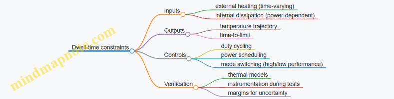
Concrete design practices that follow from these constraints
-
Allocate a thermal budget to functions, not just components. If guidance needs high-rate sensing for 8 seconds, the thermal plan should show that the seeker electronics and driver electronics can support that duty cycle under expected external heating.
-
Use power scheduling tied to thermal state. Instead of fixed “high mode” durations, switch modes based on estimated temperature or measured thermal proxies. This prevents the system from spending its thermal margin early.
-
Design for the worst heat segment, not the average. External heating can spike due to geometry and flight attitude. A thermal plan should identify the segment that drives time-to-limit, then verify that power and cooling choices keep temperatures within bounds.
-
Treat thermal capacitance as a resource with an expiration time. Heat sinks and structural mass can buy time, but only until their temperature rises enough to stop being effective. The dwell-time analysis should explicitly account for that “expiration.”
-
Validate derating assumptions with test data. Electronics often behave differently at elevated temperatures and under airflow. If the power electronics must be derated to survive, the thermal model should be anchored to measured performance.
Summary
Power generation, thermal management, and dwell-time constraints form a coupled system: power determines internal heat, external heating sets the heat input, and thermal capacity and heat removal determine how long components can operate safely. When these relationships are modeled and scheduled correctly, the defense system can maintain required performance during the short, demanding windows where it matters.
7.3 Targeting and tracking for high-speed engagement
High-speed engagement is mostly a timing problem with a geometry problem attached. Targeting means deciding where and when to aim; tracking means estimating what the target is doing well enough that the aim stays correct during the engagement window.
The targeting chain: from track to intercept point
A practical targeting chain has four steps:
- Track state estimation: position, velocity, and uncertainty for the target.
- Trajectory prediction: propagate the target state forward over the relevant time horizon.
- Engagement solution: compute an intercept point and required interceptor commands.
- Execution monitoring: compare expected vs. observed behavior and decide whether to continue, re-task, or terminate.
A simple example: suppose a sensor provides a track update every 100 ms. If the engagement solution assumes the target keeps a constant turn rate, but the target actually changes turn rate after the last update, the intercept point drifts. The system counters this by using uncertainty-aware prediction and by updating the engagement solution when new track data arrives.
Tracking basics that matter at hypersonic speeds
At high closing speeds, small errors become big quickly.
- Time alignment: sensor timestamps must match the fusion time base. If one sensor is consistently late by 20 ms, the predicted intercept point shifts by roughly \(v \times 0.02\), where \(v\) is closing speed.
- Measurement quality: range, angle, and Doppler (if available) have different noise characteristics. A track that looks stable in angle but noisy in range can still produce large miss distances.
- Uncertainty modeling: the filter should carry not just a best estimate but also a covariance that grows when observations are sparse.
A concrete example: a radar track with good angular resolution but poor range resolution can still maintain a tight bearing line. However, the intercept solution depends on range because it sets time-to-go. The system should treat the range uncertainty as a first-class input to the engagement logic.
Data association: deciding which track is the target
High-speed environments often produce multiple plausible tracks due to clutter, decoys, or sensor artifacts. Data association answers: “Which measurement belongs to which track?”
A common approach is gating: only measurements within a predicted region of the target state are considered. The gate size comes from the predicted uncertainty. If the gate is too tight, you drop valid measurements; too loose, you accept wrong ones.
Example: imagine two candidate tracks separated by a small angular distance. If the gate is sized to a covariance that underestimates uncertainty, the filter may “snap” to the wrong track when a measurement arrives. That snap can cause the engagement solution to jump, leading to a miss even if the interceptor guidance is otherwise correct.
Multisensor fusion for stable targeting
Single-sensor tracking can be fragile when the target maneuvers or when the sensor’s geometry degrades. Multisensor fusion improves stability by:
- combining complementary observables (e.g., radar range/angle with another sensor’s different error profile),
- smoothing through intermittent coverage,
- reducing the chance of track swaps.
A practical fusion example: one sensor provides frequent updates but with limited discrimination; another provides less frequent but higher-confidence measurements. The fusion filter can weight the high-confidence measurements more strongly when they arrive, while still maintaining a continuous track between them.
Prediction and maneuver handling without magic
Prediction is where “targeting” becomes “math with assumptions.” The key is to use a model that matches how the target can move during the engagement window.
Two common modeling choices:
- Constant velocity/constant turn models for short horizons.
- Interacting multiple model (IMM) style logic where the filter maintains multiple motion hypotheses and blends them.
Example: if the engagement time-to-go is 10 seconds, a constant turn model may be adequate for the first few seconds but not the last. A model that allows turn-rate changes prevents the filter from becoming overconfident late in the engagement.
A useful rule of thumb for designers: prediction should be consistent with the filter’s uncertainty growth. If the filter says uncertainty is shrinking while the model cannot justify that, the engagement solution will be brittle.
Engagement geometry: line-of-sight, time-to-go, and control authority
Even with perfect tracking, geometry can limit performance.
- Line-of-sight rate affects how quickly the interceptor must steer.
- Time-to-go sets how much the interceptor can correct.
- Control authority limits how sharply the interceptor can maneuver.
Example: if the interceptor must match a rapidly changing line-of-sight near the endgame, the required lateral acceleration might exceed what the interceptor can produce. In that case, the system may need to target an earlier intercept point or rely on a different layer.
This is why targeting logic often includes feasibility checks: “Given current track state and interceptor limits, is an intercept still achievable?” If not, the system should not keep spending compute and bandwidth on an impossible solution.
Uncertainty-aware targeting: aiming with confidence
A robust targeting system treats the intercept point as a distribution, not a single dot.
- Compute the predicted miss distribution from the track covariance and model assumptions.
- Choose an intercept point that maximizes the probability of meeting the interceptor’s kill criteria.
A concrete example: if the predicted miss distance has a mean of 50 m with a standard deviation of 40 m, and the kill threshold corresponds to misses under 30 m, then the system should recognize that the engagement is marginal. It can respond by requesting additional sensor updates, adjusting the intercept point earlier, or reallocating resources.
Execution monitoring: when to update, when to hold
During engagement, the system must decide whether to:
- update the solution with new track data,
- hold the current solution to avoid reacting to noisy measurements,
- re-task if the target behavior changes.
A simple monitoring method is to compare the predicted target state at the next update time against the newly received measurement. If the innovation (measurement minus prediction) is consistently large, the model is wrong or the track is wrong.
Example: if innovations spike right after a sensor handoff, the system may be seeing a track swap. Holding the solution briefly while fusion re-stabilizes can prevent the interceptor from chasing the wrong estimate.
Mind maps
Putting it together: a worked example (conceptual)
Assume:
- A fused track provides target state updates every 100 ms.
- Time-to-go to the candidate intercept is 6 seconds.
- The interceptor can only achieve certain lateral acceleration limits near the end.
Process:
- The system predicts the target state forward 6 seconds using a maneuver-capable model.
- It computes an intercept point that respects interceptor control authority, possibly shifting the intercept earlier if the endgame is infeasible.
- It evaluates miss-distance uncertainty from the track covariance and chooses the aim point that yields the highest probability of meeting the kill criterion.
- As new measurements arrive, it monitors innovations. If innovations remain within expected bounds, it updates the solution. If innovations jump, it pauses aggressive retargeting until fusion stabilizes.
Result: the interceptor doesn’t just “aim at the latest position.” It aims at an intercept point that is feasible, uncertainty-aware, and continuously checked against incoming evidence.
7.4 Effects modeling: heating, structural failure, and uncertainty
Effects modeling answers a practical question: if a hypersonic target is hit (or not hit), what physical changes follow, and how confident are we in that chain of cause and effect? In defense systems, the “effects” portion connects the engagement geometry and tracking quality to whether an interceptor or directed-energy (DE) shot actually produces disabling damage.
Heating as a coupled problem
At hypersonic speeds, heating is not a single number like “temperature.” It is a time history driven by:
- Convective heating from the hot boundary layer.
- Radiative heating from hot gas and surfaces.
- Surface response: the material heats up, changes properties, and may ablate.
A useful modeling approach is to treat heating as a coupled boundary condition problem: the flow model provides heat flux to the surface, and the thermal model updates surface temperature and material state. A simple starting point is a lumped thermal model for each surface patch:
\[ \frac{dT_s}{dt} = \frac{q''(t) - \epsilon\sigma\left(T_s^4 - T_{\infty}^4\right) - h_{\text{cond}}(t)}{\rho c_p L_{\text{eff}}} \]
Where \(q''(t)\) is net heat flux, \(T_s\) is surface temperature, and the denominator represents an effective thermal mass. Even if you later replace the lumped model with a multilayer or ablation model, this equation is valuable because it forces you to track what inputs dominate.
Easy example (convective-only sanity check): Assume constant \(q''=2,\text{MW/m}^2\), \(\rho c_p L_{\text{eff}}=2\times 10^6,\text{J/m}^2\text{-K}\), and ignore radiation and conduction for a short interval. Then \(dT_s/dt \approx 1,\text{K/ms}\). If the engagement window is 50 ms, you expect about 50 K rise from this crude model. That estimate won’t be accurate for real hypersonics, but it quickly tells you whether the model is in the right ballpark.
From temperature to damage: failure modes
Structural failure is rarely “the structure reaches one temperature and breaks.” Models should map thermal and mechanical loads to specific failure modes, such as:
- Thermal stress cracking due to temperature gradients.
- Material property degradation (strength reduction with temperature).
- Ablation-driven geometry change that alters aerodynamics and heating.
- Loss of structural stiffness leading to buckling or control-surface deformation.
A common modeling pattern is:
- Compute surface temperature and heat flux over time.
- Convert to through-thickness temperature (or an approximation).
- Compute stress/strain from thermal expansion mismatch.
- Apply a failure criterion.
Example failure criterion (strength reduction): If the local compressive stress is \(\sigma_c(t)\) and the allowable strength is \(\sigma_{\text{allow}}(T)\), a simple check is: \[ \sigma_c(t) \ge \sigma_{\text{allow}}\big(T(t)\big) \Rightarrow \text{failure likely} \] In practice, \(\sigma_{\text{allow}}(T)\) comes from material tests, and the stress comes from a structural model that may be simplified to a beam/shell approximation for speed.
Uncertainty: where confidence comes from
Uncertainty enters at every link: heating inputs, material properties, geometry, and the failure criterion itself. A good effects model tracks uncertainty in a way that supports decision-making, not just reporting error bars.
Main uncertainty sources
- Flow uncertainty: atmospheric density, wind, and boundary-layer assumptions.
- Heat transfer uncertainty: catalytic efficiency, surface roughness, and radiation modeling.
- Material uncertainty: strength scatter, thermal conductivity variability, ablation rates.
- Model-form uncertainty: the simplified thermal/structural model may miss gradients or coupling.
- Operational uncertainty: target attitude, control surface deflections, and maneuver-induced heating changes.
A practical way to propagate uncertainty
Use a Monte Carlo or sigma-point method on uncertain inputs, but keep the model modular so you can identify which inputs matter most.
Example (uncertainty ranking): Suppose you vary:
- heat flux scale factor \(k\) with \(k\sim\mathcal{N}(1,0.1^2)\)
- allowable strength reduction curve parameter \(a\) with \(a\sim\mathcal{N}(1,0.05^2)\)
- catalytic efficiency \(\gamma\) with \(\gamma\sim\mathcal{U}(0.7,0.9)\) Then you compute failure probability \(P_f\) from the fraction of runs where the failure criterion triggers. If \(P_f\) changes far more with \(k\) than with \(a\), you know which measurement or modeling improvement yields the biggest benefit.
Effects modeling for DE vs kinetic intercept
Effects modeling differs depending on the effector.
Kinetic interceptors: The main question is whether impact and fragmentation produce sufficient damage given the target’s thermal state and structural margins. Heating still matters because it changes material properties and stiffness at the moment of impact.
DE (directed energy): The heating model must include the beam’s energy deposition profile, pointing jitter, and atmospheric attenuation. The “heat flux” input \(q''(t)\) becomes a function of beam power, spot size, and dwell time on the target.
Concrete example (beam spot vs material response): If the beam spot is larger than the characteristic thermal diffusion length over the engagement time, the target heats more uniformly and stresses may be lower. If the spot is small, temperature gradients increase and thermal stress cracking becomes more likely. The model should therefore compute not only peak temperature but also gradient-driven stress.
Mind maps (model structure)
Mind map: heating-to-failure pipeline
Mind map: uncertainty sources and what to measure
Putting it together: an end-to-end example
Consider a simplified DE engagement where the model must estimate whether a target panel fails during a 30 ms dwell.
- Compute heat flux time history \(q''(t)\) from beam power, spot size, and atmospheric attenuation.
- Update surface temperature using a thermal model (lumped or layered) to obtain \(T(t)\).
- Compute stress from thermal expansion and temperature gradients (even a reduced-order gradient model helps).
- Apply failure criterion: for instance, cracking when \(\sigma(t)\) exceeds a temperature-dependent fracture strength.
- Propagate uncertainty in beam pointing, spot size, and fracture strength scatter to obtain \(P_f\).
The output is not just “it fails.” It is “it fails with probability \(P_f\) given the tracked uncertainties,” which is exactly what a defense system needs to decide whether to allocate additional shots, switch layers, or adjust engagement timing.
In short, effects modeling is a disciplined chain: heating drives thermal state, thermal state drives structural response, and uncertainty management turns that chain into a confidence-weighted result.
7.5 Integration with existing C2 and sensor networks
Integrating directed energy (DE) defenses into existing command-and-control (C2) and sensor networks is mostly an engineering problem: getting the right data to the right place fast enough, in the right format, with enough confidence to decide whether to fire. The goal is not to “add a laser,” but to make DE behave like a disciplined participant in the same engagement loop that missiles already use.
What “integration” means in practice
A DE system needs three things from the existing network:
- Track quality: a target state estimate (position, velocity, uncertainty) that is stable enough for pointing.
- Engagement timing: a schedule that accounts for sensor update rates, processing latency, beam dwell time, and any safety interlocks.
- Rules and constraints: the system must receive the same engagement policy inputs as other effectors (priority, authorization, deconfliction, and safety zones).
A useful mental model is a closed loop:
- Sensors produce tracks.
- C2 fuses tracks and selects an engagement.
- The effector requests or receives pointing cues.
- The effector executes within constraints and reports results.
If any link is missing, the DE system either waits (and misses the window) or fires with poor pointing (and wastes dwell time).
Data flow: from sensor to shooter
Most hypersonic-defense C2 architectures already move data in a pipeline. DE integration typically maps onto that pipeline with minimal disruption:
- Track ingestion: DE should subscribe to the same fused track products used by other effectors, not raw sensor returns.
- Pointing cue generation: C2 (or a local DE controller) converts track state into pointing commands using a shared coordinate frame and time reference.
- Authorization and safety checks: C2 issues an “engage authorized” message only after policy checks; the DE controller enforces local safety regardless of C2.
- Execution reporting: DE reports engagement status (attempted, in progress, completed, inhibited) and any measured outcomes that can be used for later decisions.
A concrete example: suppose the network has an air-surveillance radar feeding a track manager, and a separate EO/IR sensor that refines the track during terminal approach. For DE, the track manager provides the fused state and uncertainty. The DE controller uses that uncertainty to choose a conservative pointing strategy (for example, a wider initial dwell pattern) until the track tightens.
Timing and latency budgeting
DE is sensitive to timing because pointing must align with the target’s state at the moment the beam is on target. Integration therefore requires a latency budget that is explicit and testable.
A practical approach is to define time stamps at each stage:
- \( t_0 \): sensor measurement time
- \( t_1 \): fused track time stamp
- \( t_2 \): C2 decision time stamp
- \( t_3 \): effector “beam-on” time stamp
Then the integration requirement becomes: the pointing solution must remain valid over \[ \Delta t = t_3 - t_1. \]
If \(\Delta t\) is too large, the DE controller can compensate only within its own tracking and update loop. That compensation is limited by sensor update rates and by how quickly the effector can retarget.
Concrete example: if the fused track updates at 10 Hz (100 ms intervals) and the DE controller can retarget at 50 Hz (20 ms intervals) but the C2 decision and authorization path adds 250 ms, the effector may spend most of its time correcting stale cues. The integration fix is usually not “faster lasers,” but reducing the time between track update and authorization, or allowing the effector to request updated cues during the engagement window.
Coordinate frames and time standards
Integration failures often come from boring details: mismatched coordinate frames and inconsistent time references.
At minimum, the system must agree on:
- Earth model and local reference (e.g., geodetic vs. local tangent plane)
- Axis conventions (azimuth/elevation definitions, sign conventions)
- Time base (common clock, time synchronization accuracy)
A simple example: if one subsystem defines elevation as positive upward and another uses a different convention, the DE controller may point consistently “off by a little,” which looks like poor performance but is actually a coordinate mismatch. The fix is to enforce a single transformation chain and validate it with calibration shots or simulated tracks.
Engagement deconfliction with other effectors
Existing C2 systems often coordinate multiple effectors to avoid wasted shots and conflicting actions. DE must plug into the same deconfliction logic.
Common deconfliction inputs include:
- Priority rules (which target gets served first)
- Resource limits (number of simultaneous beams or power constraints)
- Safety zones (geographic and line-of-sight restrictions)
- Mutual exclusion (e.g., don’t command two effectors to act on the same target if one would block the other)
Concrete example: if a missile interceptor and a DE unit both receive the same engagement assignment, C2 should decide whether DE is used as a “softening” step (if policy allows) or only as a last-resort effector. Even when policy is simple, the integration must ensure that both effectors share the same engagement state machine so that “target already engaged” is recognized by all.
Mind map: integration responsibilities
Mind map: DE integration with existing C2 and sensor networks
Example: mapping DE into a typical engagement loop
Consider a simplified engagement loop already used for missile defense:
- Track manager maintains a fused track with uncertainty.
- Battle management selects a target based on priority and estimated intercept feasibility.
- Shooter interface sends an engagement command to the selected effector.
- Effector feedback updates the engagement state.
To integrate DE, you keep steps 1–4 but adjust the shooter interface fields:
- Replace “intercept point” with pointing cue and beam window.
- Include uncertainty-aware parameters (e.g., initial dwell pattern width).
- Add inhibit reasons (power limit, safety zone violation, track quality below threshold).
Concrete example: if the track manager reports high uncertainty during early acquisition, C2 can still assign DE, but it should set a policy parameter like “attempt with conservative dwell” rather than “commit to a narrow, high-confidence shot.” That keeps the engagement loop consistent with what the effector can actually do.
Validation: integration tests that catch real issues
Integration should be validated with tests that exercise the full chain rather than isolated components.
Key test categories:
- Latency test: measure \(t_3 - t_1\) under realistic load and confirm pointing performance stays within limits.
- Frame test: verify transformations by feeding known simulated tracks and checking that commanded pointing matches expected geometry.
- Policy test: confirm C2 authorization and local safety interlocks both behave correctly (including inhibited engagements).
- Deconfliction test: run scenarios where multiple effectors are eligible and verify only the intended effector acts.
A practical trick: log every time stamp and every coordinate transform input/output during tests. When performance is poor, you can usually identify whether the issue is stale track data, a transformation mismatch, or a policy timing problem.
Integration checklist (quick but specific)
- DE subscribes to fused track products with uncertainty and time stamps.
- C2 sends authorization plus engagement window constraints.
- Coordinate frames and time standards are explicitly defined and tested.
- DE controller enforces local safety interlocks independent of C2.
- Engagement state machine is shared for deconfliction and reporting.
- Latency budget is measured end-to-end and validated against pointing requirements.
When these items are satisfied, DE becomes a predictable effector in the same engagement system that already coordinates sensors and interceptors—less “new capability,” more “new effector with the same discipline.”
8. Counter-Hypersonic Operations: Practical Defensive Measures
8.1 Defensive countermeasures: deception, hardening, and dispersal
Hypersonic defense is often described as a race against time, but the race is also about information. Countermeasures work best when they target the defender’s assumptions: what the attacker’s sensors can see, what the defender can track reliably, and what the defender can hit with limited shots. Three practical categories—deception, hardening, and dispersal—map cleanly to those assumptions.
Mind map: countermeasures and what they try to break
Deception: make the track wrong, not just the target
Deception aims to degrade the defender’s ability to form a correct, stable track and to assign that track to the right engagement option. The goal is not to “hide everything,” because hypersonic targets are hard to hide at the physics level; the goal is to make the defender’s best estimate less useful.
1) Spoofing with plausible alternatives A common failure mode in tracking is overconfidence: once a filter latches onto a hypothesis, it can take time to recover. Deception tries to create competing hypotheses that are consistent with some measurements. For an easy example, imagine a radar track that expects smooth motion. If the attacker can generate returns that mimic a smooth path for a short interval, the defender may commit resources to that track before the real target’s maneuver becomes evident.
2) Decoys that match the “what the sensor cares about” Sensors don’t measure “a target”; they measure signatures. If a defender relies heavily on a particular band or feature (for instance, a thermal contrast or a radar cross-section pattern), a decoy that reproduces that feature can force extra discrimination steps. A practical example: if a system uses a two-stage process—first track candidates, then classify—then a decoy that triggers candidate formation but fails classification can still consume time and attention.
3) Emission control to reduce predictable patterns Even when the attacker cannot fully conceal, it can reduce regularity. If a system expects certain timing or modulation characteristics, irregular emission behavior can increase uncertainty in data association. A simple analogy: if you’re trying to identify a person by a repeating whistle pattern, changing the pattern makes recognition harder even if the person is still audible.
Best-practice defensive response to deception
- Track quality gates: Require a minimum confidence level before committing an interceptor. If confidence is low, the system should keep collecting data rather than forcing an early decision.
- Multiple hypothesis tracking: Maintain more than one plausible interpretation until measurements justify a single choice.
- Sensor diversity: Use sensors with different measurement mechanisms so that a deception that works against one sensor is less likely to work against all.
Hardening: reduce vulnerability where it matters most
Hardening is about making critical functions survive the engagement timeline. For hypersonic defense, the critical functions are typically: command and control, sensor operation, and the ability to launch or direct effectors.
1) Structural hardening for the “short, intense” problem Hardening is not only about resisting the direct hit; it’s also about surviving near-misses, fragments, and shock effects that can disable electronics or misalign antennas. A concrete example: a radar unit may tolerate a certain level of mechanical shock without losing alignment, but its power supply might fail earlier. In that case, hardening the power path and connectors can be more effective than adding mass to the antenna housing.
2) Thermal and mechanical margins for sensors and effectors Hypersonic environments can impose rapid thermal loads and vibration. Hardening includes protective coatings, improved thermal conduction paths, and mechanical isolation for sensitive components. Example: if a sensor’s protective window experiences thermal gradients, it can warp slightly and degrade calibration. Designing for stable calibration under thermal stress prevents “it still works, but it’s wrong” outcomes.
3) Communications and cyber resilience Hardening also covers the ability to operate when links are degraded or spoofed. A practical example: if a battle management system accepts unauthenticated messages, an attacker can inject false track updates. Authentication, rate limiting, and failover to preplanned procedures reduce the chance that a single compromised link derails the engagement.
Best-practice defensive response to hardening
- Identify single points of failure: If one component can stop the whole chain, harden or duplicate it.
- Test with realistic stressors: Validate that the system remains within calibration and timing tolerances after shock, power dips, or partial sensor loss.
- Design graceful degradation: If one sensor fails, the system should continue with reduced performance rather than freezing.
Dispersal: deny the attacker an easy target set
Dispersal reduces the effectiveness of attacks that rely on concentrating force against a small number of high-value sites. It also helps when deception forces the defender to delay decisions; during that delay, dispersed assets are less likely to all be disabled at once.
1) Geographic dispersal Instead of placing all sensors and shooters in one area, dispersal spreads them so that a single strike cannot cover everything. Example: if two radar sites are separated enough that a single event cannot damage both, the defender can keep tracking even if one site is lost.
2) Dispersal by function, not just by location You can disperse roles: one site focuses on early detection, another on discrimination, and another on engagement. This reduces the chance that a single disruption knocks out the entire process. A simple way to think about it: if you separate “eyes” from “hands,” losing one doesn’t automatically remove the other.
3) Mobility and time-based dispersal Mobility can be a form of dispersal when it changes the attacker’s targeting problem. Example: if a launcher is in a fixed position for hours, it becomes a predictable aim point. Moving on a schedule that matches operational needs reduces predictability.
Best-practice defensive response to dispersal
- Maintain cross-coverage: Dispersal should not create blind spots. Plan so that at least one sensor path remains available for each likely engagement geometry.
- Coordinate with C2: Dispersed units still need a shared picture. If the picture diverges, the system can waste time reconciling.
- Plan for degraded connectivity: Assume some links will fail and ensure local autonomy for safe, limited actions.
Integration: countermeasures work as a system
Deception, hardening, and dispersal are most effective when they reinforce each other. Dispersal reduces the payoff of a deception that aims to force a single engagement plan. Hardening keeps sensors and C2 alive long enough to exploit the uncertainty created by deception. Deception, in turn, is less useful when the defender can maintain track quality through sensor diversity and multiple hypotheses.
A practical integration example: suppose a defense system uses two sensor types and multiple engagement options. If an attacker attempts to create a false track, the system can keep hypotheses alive, avoid early commitment, and route engagement authority to the least disrupted shooter. Even if one site is damaged, hardening and dispersal preserve enough capability to continue tracking and decision-making.
Practical checklist for this section
- Deception: Are track-quality gates and multi-hypothesis tracking in place to resist early commitment?
- Hardening: Are critical electronics, power paths, and calibration stability protected against shock and thermal stress?
- Dispersal: Are sensors and shooters arranged to prevent single-event loss, with cross-coverage and degraded-connectivity procedures?
- Integration: Does C2 coordinate actions so that deception-induced uncertainty does not cascade into paralysis?
8.2 Base and infrastructure protection for hypersonic threat environments
Hypersonic threats compress decision time and reduce the margin for error, so base protection has to focus on what can be controlled locally: hardening, dispersion, rapid recovery, and clear procedures. The goal is not to “stop everything,” but to keep critical functions running long enough to support defense operations.
Start with what must keep working
Protection planning begins by listing mission-critical services and the infrastructure that enables them. Typical categories include:
- Command and control: operations center, secure communications, data links.
- Sensing and processing: radar sites, signal processing rooms, power conditioning.
- Effectors and logistics: interceptor canisters, launchers, fueling, maintenance bays.
- People and continuity: medical support, sheltering, emergency management.
A practical best practice is to assign each category a minimum acceptable capability (MAC). For example, C2 might require only a reduced set of consoles and a single redundant network path to coordinate engagements. If the base can still execute MAC, the defense system remains useful even after partial damage.
Easy example: If the main operations center is hit, the plan should specify that a smaller alternate room can run the same engagement workflow using preloaded track data and a limited set of displays. That is a concrete target for hardening and training.
Reduce vulnerability through dispersion and separation
Hypersonic attacks often aim at fixed, high-value nodes. Dispersion limits the damage from a single strike by ensuring that no one location contains all the pieces needed for a mission.
Key practices:
- Geographic dispersion of launchers, power distribution, and maintenance resources.
- Functional separation so that the failure of one building does not disable the entire workflow.
- Physical separation between power, cooling, and communications paths.
Easy example: Instead of routing all fiber and power through one utility corridor, route them through two corridors with different access points. If one corridor is damaged, the other can still carry essential traffic.
Harden what matters, but harden it intelligently
Hardening includes structural reinforcement, blast/fragment protection, and environmental shielding. The trick is to harden to the right level for the role of the asset.
A useful method is to classify assets by consequence and failure mode:
- Consequence of loss (how much mission capability disappears)
- Repairability (how quickly the asset can be restored)
- Dependency graph (what else fails when this fails)
Then apply layered measures:
- Structural: reinforced shelters for operators and key electronics.
- Environmental: heat and debris protection for sensitive equipment.
- Operational: procedures that keep systems in safe states during and after impact.
Easy example: A radar processing room may not need the same level of structural reinforcement as a shelter for personnel, but it does need protection against power interruption and debris intrusion. That can be achieved with sealed cable runs, protected cooling intakes, and redundant power feeds.
Protect power and communications first
Many base failures after an attack are not “direct hits” but cascading outages: power drops, network segmentation, and loss of timing signals.
Best practices:
- Redundant power with separate feeders and protected switchgear.
- Uninterruptible power supplies for critical control and timing systems.
- Network segmentation so that damage or spoofing does not spread.
- Alternate routing for data paths and secure voice.
Easy example: If the primary network switch is in a single rack, a strike that damages that rack can take down multiple services. Moving critical services to separate racks and VLANs prevents one failure from knocking out everything.
Plan for rapid recovery, not just survival
A base that survives but cannot restart key operations quickly may still fail the mission. Recovery planning should include:
- Pre-staged spares for common components (power modules, connectors, spare cables).
- Clear restoration priorities (power → timing → communications → sensing → C2).
- Damage assessment procedures that distinguish “safe to operate” from “unsafe to enter.”
Easy example: After an incident, teams should know which doors are safe, which rooms require remote inspection, and which systems can be restarted from a checklist without waiting for full site clearance.
Use procedures that match compressed timelines
Hypersonic engagements can create short windows for decision-making. Procedures should be written so they work under stress and limited information.
Practices that help:
- Role-based checklists for operators, maintenance crews, and security.
- Predefined triggers for actions like shutting down nonessential systems, switching to alternate comms, or moving to shelter.
- Drills that include partial information, such as degraded sensor feeds or uncertain track quality.
Easy example: A drill can simulate loss of the main data link. The team practices switching to a backup link and continuing MAC operations using cached track summaries.
Build survivability into the layout
Base layout decisions can reduce exposure and improve response.
Consider:
- Hardened corridors for movement between shelters and critical rooms.
- Protected storage for fuel, munitions, and maintenance supplies to reduce secondary fires.
- Controlled access points to prevent congestion and confusion during emergencies.
Easy example: If fuel storage is adjacent to a critical power substation, a fire can disable both. Separating fuel storage and adding firebreaks can preserve power even when other areas burn.
Mind maps: protection logic and implementation
Mind Map: Base Protection Priorities
Mind Map: What to Protect (Dependency View)
A compact implementation checklist
Use this as a practical sequence for base teams:
- Identify MAC for each critical function.
- Map dependencies (power, timing, data, access) and find single points of failure.
- Apply dispersion and separation to reduce correlated losses.
- Harden key rooms and protect utility routes.
- Implement redundant power and segmented communications.
- Write restoration priorities and pre-stage spares.
- Conduct drills that exercise degraded comms and partial information.
Easy example: If the dependency map shows that both radar processing and C2 share the same UPS, that is a clear, actionable fix: split the UPS feeds and verify failover during routine maintenance.
When these steps are done together, the base becomes harder to disable completely, easier to operate in a degraded mode, and faster to return to full capability—exactly the kind of practical resilience hypersonic threat environments demand.
8.3 Operational procedures for alerting, posture, and readiness
Operational procedures for hypersonic defense need to do three things quickly and consistently: (1) decide whether the situation is real enough to act on, (2) shift the right sensors and effectors into the right modes, and (3) keep humans and systems synchronized despite tight timelines. The goal is not to “go to maximum” every time; it’s to match response intensity to the confidence level and the time available.
Alerting: from cue to action
Alerting is a pipeline, not a switch. A good procedure defines triggers, confidence thresholds, and who gets notified at each step.
A. Trigger categories (example structure)
- Cue-level: A sensor reports a track-like return or a pattern consistent with a fast, maneuvering object.
- Candidate-level: Multiple sensors support a coherent track, but uncertainty remains high (e.g., ambiguous classification).
- Engagement-level: The track is stable enough for an engagement plan, and the system can estimate geometry and time-to-go.
- No-action / hold: Evidence conflicts, or the track cannot be maintained reliably.
B. Confidence thresholds (example, practical and measurable)
- Track stability: Track quality stays above a defined threshold for a minimum duration.
- Cross-sensor agreement: At least two independent sensors agree within tolerance on key parameters (range-rate, bearing-rate, or predicted position).
- Time-to-go feasibility: The engagement timeline remains viable given interceptor kinematics and command latency.
C. Notification rules (who hears what, when)
- Cue-level: Notify the battle management system and the relevant sensor operators; keep higher-level decision-makers informed but not fully committed.
- Candidate-level: Notify the engagement authority and activate pre-planned checklists for data fusion and communications verification.
- Engagement-level: Notify all stakeholders required for terminal actions (C2, interceptor launch authority, and relevant communications nodes).
- Hold/No-action: Log the reason (e.g., track instability, sensor disagreement) and return to the prior posture.
Easy example: If a radar cue appears but only one sensor supports it, the procedure keeps the system in “candidate” mode. Operators run fusion and discrimination steps while the engagement authority waits for cross-sensor agreement. If agreement never arrives, the system returns to normal without consuming interceptor resources.
Posture: selecting the right readiness level
Posture is about configuration. It includes sensor modes, data routing, communications priority, and which effectors are allowed to transition.
A. Define posture levels with explicit differences
- Normal posture: Standard surveillance modes; routine data routing; effectors remain in safe states.
- Elevated posture: High-priority data routing; additional sensor dwell or scanning patterns; pre-checks for communications and timing.
- Engagement posture: Sensors switch to modes optimized for track maintenance; C2 allocates resources for rapid engagement planning; effectors may be authorized to transition to launch-ready states.
- Sustained engagement posture: Used when multiple events occur or when track quality remains high; emphasizes continuity of tracking and repeated engagement planning.
B. Link posture to alert categories
- Cue-level → Elevated posture
- Candidate-level → Engagement posture (if time-to-go remains feasible)
- Engagement-level → Engagement posture with launch authorization rules
- Hold/No-action → return to Normal or Elevated depending on residual uncertainty
Easy example: During candidate-level alerts, you might increase sensor dwell time to improve track stability. You do not authorize launch-ready transitions until engagement-level conditions are met, because those transitions consume maintenance margins and can complicate later decisions.
Readiness: checklists that prevent “small failures” from becoming big ones
Readiness procedures should be written as short checklists with pass/fail criteria. Each item must have a clear owner and a clear time budget.
A. Readiness checklist for C2 and communications (example items)
- Time synchronization: Verify clock alignment for sensor reports and command timestamps.
- Data pipeline health: Confirm that sensor tracks are flowing into the fusion engine without backlog.
- Latency budget check: Ensure end-to-end delay stays within the engagement planning window.
- Fallback routing: Confirm an alternate communications path is available if the primary link degrades.
B. Readiness checklist for sensors (example items)
- Mode verification: Confirm the sensor is in the correct tracking or high-rate mode.
- Calibration status: Check that calibration is current enough for the required measurement accuracy.
- Field-of-view alignment: Confirm the sensor is pointed to maintain coverage for the predicted geometry.
C. Readiness checklist for effectors (example items)
- Safety and arming constraints: Verify that safety interlocks are satisfied according to the approved sequence.
- Energy/propulsion readiness: Confirm that the effector can meet the required energy margin for the planned intercept.
- Command path authorization: Confirm that launch authority and command routing are correct for the specific engagement.
Easy example: If time synchronization is off by more than the allowed tolerance, the procedure forces a hold at candidate-level. The system may still track, but it avoids generating engagement solutions that would be inconsistent with command timing.
Engagement decision flow: a simple logic that scales
A readable procedure uses a decision flow that operators can follow under stress, and systems can implement consistently.
    flowchart TD
  A[Cue-level report] --> B{Track stability OK?}
  B -- No --> H[Hold/No-action; log reason]
  B -- Yes --> C{Cross-sensor agreement OK?}
  C -- No --> D[Run fusion/discrimination; keep Elevated posture]
  D --> B
  C -- Yes --> E{Time-to-go feasible?}
  E -- No --> H
  E -- Yes --> F[Candidate-level]
  F --> G{Engagement-level criteria met?}
  G -- No --> D
  G -- Yes --> I[Engagement posture + launch authorization rules]
  I --> J[Execute engagement plan; monitor kill assessment]
Easy example: If track stability and agreement are good but time-to-go is not feasible, the procedure avoids launch authorization and instead focuses on maintaining track for potential later opportunities or for defensive planning.
Post-engagement actions: learning without second-guessing
After an engagement attempt, procedures should specify what gets updated and what gets reset.
- Kill assessment handling: Record the basis for assessment (sensor confirmation, track termination, or other criteria) and link it to the engagement timeline.
- Resource reset: Return sensors and effectors to the correct posture based on whether the threat is considered resolved.
- After-action logging: Capture checklist outcomes, timing measurements, and any communications anomalies.
- Operator feedback loop: Provide a short summary to the engagement authority so the next event uses the same logic with corrected assumptions.
Easy example: If the engagement plan was executed but the kill assessment is inconclusive, the procedure keeps the system in elevated tracking posture rather than returning immediately to normal, because the uncertainty is about outcome, not about detection.
Mind maps: the procedure in one page
Mind map: Alerting, Posture, Readiness
A compact end-to-end example
- A radar cue appears and enters cue-level. The system switches to elevated posture for higher-priority routing.
- Fusion confirms track stability, but classification remains uncertain. The system stays at candidate-level and runs discrimination steps.
- A second sensor agrees on predicted geometry, and the system estimates time-to-go feasible. The alert advances to engagement-level.
- C2 verifies time synchronization and latency budget, then authorizes effectors to transition according to the approved sequence.
- The engagement executes, and kill assessment is recorded. If inconclusive, the system maintains elevated tracking posture rather than returning to normal.
This procedure keeps actions proportional: it improves tracking quality when uncertainty is high, and it escalates configuration only when the engagement timeline and data quality justify it.
8.4 Rules of engagement and escalation considerations in defense planning
Rules of engagement (ROE) are the written “if this, then that” constraints that turn a defense system from a capability into an action. In hypersonic defense, the timing is short, the uncertainty is real, and the consequences of a wrong call are high. Good ROE planning therefore focuses on decision quality under pressure: what must be known, who decides, what actions are allowed at each confidence level, and how escalation is prevented from happening by accident.
What ROE must specify (beyond “shoot or don’t shoot”)
-
Decision authority and delegation
- ROE should state who can authorize each step: track validation, interceptor launch, and any follow-on actions.
- Example: If the commander is unavailable, a pre-designated duty officer can authorize launch only after a defined minimum track quality threshold is met.
-
Trigger conditions tied to measurable evidence
- “Confirmed hostile” is not a trigger by itself; ROE should reference observable criteria such as track stability, sensor corroboration, and discrimination confidence.
- Example: Launch is permitted when at least two geographically separated sensors maintain a consistent track for a specified time window, and the predicted intercept geometry remains within safe limits.
-
Allowed actions by engagement phase
- ROE should separate phases like detection-to-track, track-to-intercept, and intercept-to-assessment.
- Example: During track validation, the system may request additional sensor dwell or adjust search patterns; during terminal engagement, those options may be restricted to preserve time.
-
Fire control safety constraints
- ROE must include constraints that prevent unsafe or unintended effects: minimum separation from friendly assets, geographic exclusion zones, and interceptor self-destruct or safe-mode rules.
- Example: Even with a valid hostile track, launch is blocked if the predicted miss distance places fragments within a protected area.
-
Communications and authentication requirements
- ROE should define how commands are authenticated and what happens if links degrade.
- Example: If the data link fails after launch authorization, the interceptor continues using onboard guidance; if authorization cannot be authenticated, the system holds fire.
-
Post-action assessment and reporting
- ROE should define what constitutes “engagement complete” and what data must be recorded.
- Example: Engagement is not considered complete until kill assessment is computed from sensor returns and logged with uncertainty bounds.
Escalation considerations: preventing the wrong kind of response
Escalation in defense planning is not only about political messaging; it is also about operational behavior. A defense system can unintentionally escalate by acting on ambiguous tracks, by firing in ways that appear disproportionate, or by failing to communicate internally what it is doing.
Key escalation risks and how ROE can address them:
-
Ambiguity risk (is it a threat or not?)
- Hypersonic targets may be hard to discriminate from decoys or benign objects.
- ROE mitigation: require corroboration and explicitly define “hold fire” thresholds.
- Example: If discrimination confidence drops below a set level after initial track validation, ROE directs the system to continue tracking but suspend launch.
-
Saturation risk (too many targets, too little time)
- When multiple contacts arrive, the system may be tempted to treat all tracks as equally actionable.
- ROE mitigation: prioritize based on threat evaluation and engagement feasibility.
- Example: If two targets are predicted to reach protected assets, ROE may allow engagement of the one with the higher probability of successful intercept, while the other remains under surveillance.
-
Misinterpretation risk (friendly assets and shared airspace)
- Defense actions can be misread if friendly aircraft or satellites are affected.
- ROE mitigation: include positive identification steps for friendly-adjacent regions and require additional safety checks.
- Example: In a corridor with frequent friendly traffic, ROE requires an extra sensor confirmation before terminal engagement.
-
Command-and-control risk (who knows what, when?)
- Delays or inconsistent information can cause different units to act differently.
- ROE mitigation: define a single operational picture source and standardized confidence reporting.
- Example: All units use the same track quality metric; if it is updated, ROE requires synchronized acknowledgement before any new launch authorization.
A practical mind map for ROE design
Example ROE logic: confidence-based engagement
Below is a concrete example of how ROE can be expressed as decision gates. The point is not the exact numbers; it is the structure that makes behavior consistent.
-
Gate A: Track validation
- Condition: Track is maintained by at least two sensors with consistent kinematics.
- Allowed actions: increase sensor dwell, refine track estimate, request additional discrimination data.
- Escalation control: no launch authorization at this stage.
-
Gate B: Hostility likelihood
- Condition: Discrimination confidence exceeds a defined threshold and predicted impact path intersects a protected volume.
- Allowed actions: prepare interceptor, allocate engagement resources.
- Escalation control: preparation is allowed even if launch is not yet authorized.
-
Gate C: Launch authorization
- Condition: Predicted intercept geometry is feasible, safety constraints are satisfied, and command authorization is authenticated.
- Allowed actions: launch interceptor.
- Escalation control: if any safety constraint fails, ROE forces hold fire even if hostility likelihood is high.
-
Gate D: Terminal engagement
- Condition: Interceptor guidance remains within control authority limits and track quality remains above a minimum.
- Allowed actions: continue engagement; no mid-course “re-interpretation” that could cause erratic behavior.
- Escalation control: ROE limits changes that could look like indecision.
-
Gate E: Assessment and reporting
- Condition: Post-intercept sensor returns allow kill assessment with uncertainty bounds.
- Allowed actions: update the operational picture, report results, and record deviations.
- Escalation control: ROE requires consistent reporting so different units do not infer different outcomes.
Example: ROE behavior under a decoy-like scenario
Assume a scenario with a fast-moving object and a secondary track that appears similar in early measurements.
- Gate A: Both tracks are detected, but only one maintains stable track quality across multiple sensors.
- Gate B: Hostility likelihood for the stable track rises; the secondary track’s discrimination confidence remains low.
- ROE outcome: The system prioritizes engagement resources for the stable track and continues tracking the secondary track without launching based on weak discrimination.
This approach reduces the chance of firing at the wrong object while still preserving time to act on the most actionable track.
Example: ROE under saturation
Suppose three targets are predicted to reach protected areas within a short window, but only two interceptors are available.
- ROE prioritization: choose the two targets with the highest intercept feasibility and the greatest expected impact severity.
- Remaining target: keep tracking and update the engagement plan as new sensor data arrives.
The escalation benefit is practical: fewer unnecessary launches, clearer accountability, and less confusion about why some contacts were engaged and others were not.
Writing ROE so it can be executed
ROE should be testable and operationally unambiguous. If a rule cannot be translated into measurable conditions (track quality, geometry feasibility, safety constraints, authentication status), it will be interpreted differently under stress.
A useful checklist for ROE drafts:
- Every “go” decision has a measurable trigger.
- Every “hold” decision has a defined reason and a defined next action.
- Safety constraints override all other conditions.
- Engagement phases restrict actions to what is appropriate for the time available.
- Post-action assessment requirements are explicit.
When ROE is written this way, escalation is less likely to happen because someone filled in missing details during a fast-moving event. The system does what it is told, and the people can explain why.
8.5 Training, drills, and evaluation for time-critical defense
Time-critical defense is less about heroic reactions and more about rehearsed decision speed under uncertainty. Training should therefore focus on three things: (1) getting the right data fast, (2) making consistent engagement decisions, and (3) learning from measured outcomes rather than opinions.
Build training around the engagement timeline
Start every training event by writing a simple timeline with gates. Each gate names the minimum acceptable state of the system.
Example timeline gates (typical layered defense):
- Gate A: Detect/Track Established — tracks are initiated with known uncertainty bounds.
- Gate B: Correlate/Discriminate — tracks are associated to the correct threat type and track quality is stable.
- Gate C: Plan Engagement — an interceptor/effector is selected, with a feasible intercept/engagement window.
- Gate D: Execute — commands are issued with confirmed communications and valid control parameters.
- Gate E: Assess — results are evaluated using consistent scoring rules.
A drill that skips gates teaches people to “feel” readiness. A drill that enforces gates teaches readiness.
Use realistic roles and clear handoffs
Time-critical defense often fails at handoffs: sensor operators, battle managers, and shooter teams may each do their job correctly while the overall process still breaks.
Practice structure:
- Assign one role per function: sensor tasking, track management, engagement planning, shooter execution, and assessment.
- Define who can change what, and when. For instance, track managers can adjust track filters before Gate C, but engagement planners own the final engagement plan.
- Use “handoff cards” that list the current state: track IDs, uncertainty level, recommended engagement window, and any constraints.
Easy example: During a drill, the sensor team reports “track quality improved,” but the handoff card must include the specific quality metric used by the engagement planner. Otherwise, the planner cannot decide whether the improvement matters.
Train with uncertainty, not perfect truth
Hypersonic defense is constrained by limited observation time, clutter, and maneuver uncertainty. Training should therefore include controlled uncertainty so teams learn to act under incomplete information.
How to do it without making training chaotic:
- Inject measurement noise and occasional track swaps in simulation.
- Provide partial truth during exercises only for evaluation, not for decision-making.
- Require teams to state assumptions explicitly at Gate B and Gate C.
Example: If two tracks are plausible, the engagement plan must specify whether it is committing to Track 1, Track 2, or holding until correlation improves. The evaluation then checks whether the choice was consistent with the stated assumptions.
Run drills in three layers: tabletop, simulation, and live
A good training ladder prevents two common problems: tabletop-only exercises that ignore timing, and simulation-only exercises that ignore human workflow.
-
Tabletop drills (process and decision logic):
- Use printed timelines and decision checklists.
- Focus on whether the team reaches Gate A–D in the right order.
- Example: Give a scenario with known sensor coverage gaps; require the team to decide what to do when Gate A cannot be met.
-
Simulation drills (timing and system interactions):
- Use the same interfaces as the operational system.
- Include latency, data dropouts, and resource contention.
- Example: Two simultaneous threats compete for the same interceptor; the team must allocate resources using the defined rules.
-
Live drills (execution and communications):
- Keep the scenario simple but test the real chain: data link, command issuance, and safety interlocks.
- Example: Validate that the shooter team receives the correct engagement window parameters and that the system rejects invalid commands.
Mind maps for drill design and evaluation
Use mind maps to keep training objectives, injects, and scoring aligned.
Mind map: Time-critical drill design
Mind map: Evaluation metrics
Define scoring rules before the drill
Evaluation should measure what the team can control. If scoring rules are invented after the fact, the drill becomes a debate.
Example scoring rubric (simple and usable):
- Gate compliance (0–5 points each gate):
- 5 = met with required uncertainty bounds
- 3 = met but uncertainty exceeded threshold
- 1 = partial or late
- 0 = missed
- Engagement feasibility (0–10 points):
- 10 = feasible window and correct resource allocation
- 5 = feasible window but wrong resource
- 0 = infeasible window or unsafe command
- Outcome (0–10 points):
- 10 = correct assessment and correct engagement result
- 5 = correct engagement but inconsistent assessment
- 0 = incorrect assessment or invalid execution
This rubric forces teams to care about uncertainty thresholds, not just whether an action happened.
Run after-action reviews that produce fixes
After-action reviews should convert observations into specific changes: interface tweaks, checklist updates, or training adjustments.
A practical AAR format:
- What happened (timeline facts): use logs and timestamps.
- Why it happened (root causes): categorize into data quality, decision logic, comms, or execution.
- What changes (action items): each item must name an owner and a measurable target.
Example action item:
- “Update handoff card template to require uncertainty bounds for Gate B; verify in next simulation drill that engagement planners reject plans when bounds are missing.”
Example drill scenario: two threats, one bottleneck
Scenario setup:
- Two incoming threats appear nearly simultaneously.
- Sensor coverage supports Gate A for both, but Gate B correlation is slower for one due to clutter.
- Only one interceptor is available for the earliest engagement window.
Drill objective:
- Ensure the team allocates the interceptor correctly while maintaining consistent assumptions.
Expected behaviors to look for:
- The team reaches Gate A for both tracks quickly.
- At Gate B, the team documents whether it is committing to the correlated track or waiting for improved correlation.
- At Gate C, the engagement plan uses the defined resource allocation rule (e.g., prioritize the threat with higher feasibility or higher confidence, depending on doctrine).
- At Gate E, the assessment matches the scoring rules even if the second threat is not engaged.
Evaluation focus:
- Did the team meet timing gates?
- Did it follow decision rules under uncertainty?
- Did it avoid “fixing” the story after the fact?
Common failure modes to train against
- Checklist theater: teams claim readiness but cannot produce the required state variables at Gate handoff.
- Overconfidence in early tracks: engagement plans proceed without uncertainty bounds meeting thresholds.
- Unowned assumptions: teams make implicit assumptions that never appear in the handoff card.
- Saturation blindness: resource contention is treated as an exception rather than a normal condition.
Training should treat these as expected test conditions, not surprises.
Summary: what “good” looks like
Good time-critical training produces measurable results: consistent gate timing, decision rule adherence under uncertainty, and evaluation outcomes that lead to concrete fixes. The goal is not to make people faster at guessing; it is to make the system and the team faster at making the right decision with the information they actually have.
9. Testing, Modeling, and Verification for Hypersonic Defense
9.1 Modeling and simulation scope: what must be validated
Modeling and simulation for hypersonic defense is not about making pretty trajectories. It is about proving that the model answers the specific questions the program needs answered—under the specific uncertainties the real system will face. A good scope starts by listing the decisions the model must support, then mapping each decision to the physics, algorithms, and data-handling assumptions that must be validated.
1) Start with “model-to-decision” traceability
Validation scope should be driven by decisions, not by components. For each decision, define:
- Input requirements (what the model must ingest: target state, environment, sensor measurements, interceptor constraints).
- Output requirements (what the model must produce: track quality, predicted intercept probability, kill assessment, resource usage).
- Acceptance criteria (how close the model must be to reference behavior, and in what metrics).
Example (engagement planning): If the decision is “which interceptor to assign to which track,” the model must validate that it produces consistent time-to-go, coverage availability, and engagement feasibility under measurement uncertainty. If the decision is “whether the system can maintain track through maneuver,” the model must validate track maintenance and data association behavior, not just kinematics.
2) Define the validation reference: what counts as “truth”
Validation requires a reference that is credible for the question at hand. Common reference types include:
- High-fidelity physics models (used as a reference when they are trusted for the regime).
- Hardware-in-the-loop or closed-loop test data (sensor outputs, command latency, actuator response).
- Instrumented flight or range data (when available, with careful treatment of measurement error).
A model can be “validated” for one purpose and not for another. A kinematic model might match range data for position but still fail validation for seeker behavior if it uses the wrong measurement noise model.
3) Validate the environment model where it matters
Hypersonic engagements are sensitive to atmospheric and propagation effects. Validation scope should include:
- Atmospheric state: density, temperature, winds, and turbulence statistics.
- Propagation effects: radar/EO/IR line-of-sight behavior, clutter assumptions, and attenuation.
- Thermal and aerodynamic coupling (if used): whether the model needs heating and drag changes to predict maneuver response.
Example (radar tracking): If the radar model uses a simplified refractivity profile, track initiation might still look fine, but track maintenance during terminal maneuver can degrade because the predicted measurement uncertainty is wrong. Validation should therefore include metrics tied to tracking performance, not only detection probability.
4) Validate target dynamics and maneuver representation
Target motion is rarely a single smooth curve. Validation scope should cover:
- Dynamics model: equations of motion, mass properties, and actuator limits.
- Maneuver model: how commands translate into acceleration and jerk limits.
- Uncertainty model: variability in maneuver execution and control response.
Example (maneuver uncertainty): Suppose the engagement model assumes a fixed maximum lateral acceleration. If real targets sometimes underperform or overperform due to control authority limits, the model may overestimate intercept opportunities. Validation should test sensitivity by comparing predicted engagement outcomes across a range of maneuver uncertainty parameters.
5) Validate sensor measurement generation and data association
A defense system lives on measurements. Validation scope should include:
- Measurement generation: noise distributions, bias terms, update rates, scan geometry, and field-of-view constraints.
- Detection logic: thresholds, false alarm rates, and gating behavior.
- Data association: track management rules, assignment logic, and how the model handles ambiguous measurements.
Example (track swap risk): If two objects cross near the sensor horizon, a simplified association model may keep tracks stable in simulation while the real system swaps them. Validation should include scenario-based tests that reproduce the ambiguity conditions the system is expected to handle.
6) Validate C2 timing, latency, and resource constraints
Even perfect physics can fail if timing is wrong. Validation scope should cover:
- Latency budgets: sensor-to-processor, processor-to-shooter, and internal computation delays.
- Update synchronization: how different sensors and effectors align in time.
- Resource models: number of channels, processing limits, and scheduling rules.
Example (saturation): In a multi-target scenario, the model must validate that it enforces the same processing limits as the real system. Otherwise, it may show graceful performance that disappears when the system is actually busy.
7) Validate interceptor kinematics, guidance, and energy management
Interceptor modeling should be validated at the level needed for the engagement question:
- Kinematics: state propagation accuracy under realistic constraints.
- Guidance: how commands are computed from estimated target state.
- Energy management: propulsion limits, achievable acceleration profiles, and endgame constraints.
Example (endgame feasibility): A model that matches midcourse intercept geometry might still fail validation if it overestimates achievable terminal acceleration. Validation should therefore include endgame metrics such as miss distance distribution and whether the interceptor can remain within seeker or control limits.
8) Validate kill assessment and discrimination logic
Kill assessment is not a single threshold. Validation scope should include:
- Discrimination assumptions: how the model separates decoys, fragments, or maneuvering components.
- Effect model: what “success” means (e.g., proximity, structural failure likelihood, or sensor-based confirmation).
- Uncertainty propagation: how measurement and model uncertainty affects the final decision.
Example (uncertainty propagation): If the model treats seeker uncertainty as constant, it may underestimate the probability of misclassification during high dynamics. Validation should test how uncertainty changes with geometry and time.
9) Validate the uncertainty and sensitivity framework
Validation is incomplete without uncertainty handling. Scope should define:
- Uncertainty sources: measurement noise, environment errors, target maneuver variability, actuator uncertainty.
- Sampling method: how Monte Carlo or other methods represent these uncertainties.
- Sensitivity checks: which parameters dominate outcome variance.
Example (dominant parameter check): If miss distance variance is mostly driven by one parameter (like drag uncertainty), then validating other parameters to high precision may not improve results. Validation scope should reflect this by focusing effort where it changes decisions.
10) Validate interfaces and data handling
Many failures come from plumbing, not physics. Validation scope should include:
- Coordinate frames: consistent transformations between sensor, platform, and engagement frames.
- Units and conventions: angle definitions, time bases, and sign conventions.
- Data integrity: missing data handling, out-of-order updates, and numerical stability.
Example (frame mismatch): A small sign error in a coordinate transform can look like a guidance bug. Validation should therefore include interface tests with known reference trajectories.
Mind map: what must be validated
Practical validation checklist (scenario-driven)
Use scenarios that stress the exact assumptions you plan to rely on.
- Single-target, nominal environment: validate baseline tracking and engagement feasibility.
- Single-target, maneuver stress: validate target dynamics and interceptor endgame constraints.
- Two-target ambiguity: validate data association and track stability.
- Multi-target saturation: validate C2 resource limits and scheduling.
- Measurement bias test: validate robustness to systematic sensor errors.
- Interface sanity tests: validate coordinate transforms and unit conventions with reference cases.
Example (how to measure success): For each scenario, define metrics such as track quality (e.g., covariance growth or track continuity), engagement feasibility (time-to-go and control authority margin), and outcome (miss distance or kill assessment confidence). Validation is then the comparison of these metrics against reference behavior within stated tolerances.
What “validated” should mean in scope terms
A defensible validation scope states:
- Which components/assumptions are validated (and which are not).
- Against what reference (and under what conditions).
- With what metrics and tolerances (and what failure modes are acceptable).
- For which scenarios the validation claims apply.
If the scope does not specify these items, the model may still be useful for exploration, but it cannot support confident claims about system performance. In defense work, that distinction matters—especially when the model is the only place you can run the scenario 10,000 times without burning a range day.
9.2 Test design: representative targets, environments, and instrumentation
A good test design answers three practical questions: what target behavior you are trying to represent, what environment you are trying to reproduce, and how you will measure the outcome without fooling yourself. The trick is to keep each test case representative enough to be meaningful, while still controlled enough to diagnose what worked and what didn’t.
Representative targets: define behavior, not just hardware
Start by writing a target behavior card for each scenario. Include the motion pattern, maneuver limits, and any distinguishing features relevant to detection and discrimination.
Behavior card fields (example):
- Flight regime: boost-like, glide-like, or terminal-like (use the regime that matches the engagement phase you are testing).
- Trajectory shape: smooth arc vs. segmented path vs. continuous maneuver.
- Maneuver envelope: maximum lateral acceleration (or equivalent turn rate), minimum turn radius, and typical maneuver frequency.
- Thermal/IR signature model: nominal vs. attenuated vs. enhanced (for example, by changing skin emissivity or adding controlled plume-like heating).
- Seeker-relevant features: size, aspect-dependent reflectivity, and any motion-induced blur characteristics.
Easy-to-understand example: If you are testing track maintenance, don’t just use “a fast target.” Use two target cards:
- Stable path card: predictable turns within a known envelope.
- Aggressive card: same average speed but with tighter turn radii and more frequent maneuvers. If the system fails only on the aggressive card, you learn the failure is tied to maneuver-induced tracking uncertainty rather than raw speed.
Representative environments: reproduce the constraints that matter
Hypersonic defense performance is strongly shaped by environment. Your test environment should therefore be built around the limiting factors for the specific sensor and interceptor chain.
Common environment categories:
- Atmosphere: density profile, humidity, aerosol content, and wind shear.
- Clutter and background: terrain returns, sea state, precipitation, and ground reflections.
- Geometry: line-of-sight angles, horizon masking, and platform placement.
- Electromagnetic conditions: interference sources, jamming profiles (if applicable), and propagation effects.
- Thermal environment: for sensors and effectors where thermal drift affects performance.
Easy-to-understand example: For a radar-based track test, create two environment setups:
- Low-clutter setup: open terrain or controlled background to validate baseline detection.
- High-clutter setup: clutter-rich background and multipath conditions to stress track association. You can then separate “can it detect?” from “can it keep the correct track?”
Instrumentation: measure the chain, not just the end result
Instrumentation should cover the full chain: target truth, sensor observations, data products, and interceptor outcomes. If you only measure the final intercept or miss distance, you’ll spend the rest of the program guessing where the error entered.
Minimum instrumentation set (typical):
- Target truth system: high-accuracy tracking (e.g., optical, radar truth, or integrated navigation) to establish the ground-truth trajectory.
- Sensor measurement capture: raw radar/EO/IR data logging, not only processed tracks.
- Time synchronization: a common time reference across all recorders to prevent “latency looks like physics” mistakes.
- C2 and data link logging: messages, timestamps, and system state variables used by the engagement logic.
- Interceptor telemetry: guidance commands, seeker measurements, propulsion state, and control surface or actuator states.
- Environmental sensors: weather stations, atmospheric monitors, and electromagnetic environment monitors.
Easy-to-understand example: Suppose the interceptor misses by 20 meters. Without truth and timing logs, you might blame guidance. With instrumentation, you can check whether the sensor track was biased early, whether the C2 update arrived late, or whether the interceptor’s control authority was reduced by a thermal or actuator constraint.
Test matrix design: cover combinations without exploding the schedule
A test matrix should be structured so that each scenario changes one or two key variables. This keeps results interpretable.
Practical approach:
- Choose baseline scenarios that represent nominal engagement conditions.
- Add stress scenarios that vary one limiting factor at a time (maneuver envelope, clutter level, or sensor geometry).
- Include edge-of-coverage scenarios where the sensor horizon or geometry is near the system’s operational limits.
Example matrix (simplified):
- Target cards: Stable vs. Aggressive maneuver.
- Environments: Low clutter vs. High clutter.
- Geometry: Centerline vs. Near-horizon. This yields 2×2×2 = 8 scenarios, which is often manageable while still revealing interactions.
Instrumentation validation: prove your measurements before you trust them
Before running full engagement tests, validate each measurement path.
Validation checks:
- Timing check: confirm that timestamps align across truth, sensor logs, and C2 logs.
- Calibration check: verify sensor calibration under the same environmental conditions.
- Truth accuracy check: confirm that target truth error is small compared to the performance metric you care about.
- Data integrity check: ensure logs capture the full dynamic range and do not saturate.
Easy-to-understand example: If your tracking metric is based on angular error, but your truth system has a larger angular uncertainty than the metric resolution, you can’t tell whether the system improved or the measurement system did.
Mind maps for test design
Mind map: Representative targets, environments, instrumentation
Concrete scenario example: track maintenance stress test
Goal: determine whether track maintenance fails due to maneuver-induced uncertainty or due to clutter-driven association errors.
Scenario setup:
- Target cards: Stable and Aggressive maneuver envelopes.
- Environments: Low clutter and High clutter.
- Geometry: fixed line-of-sight angles to isolate the effect of target motion and background.
Instrumentation emphasis:
- Log raw sensor returns and processed track outputs.
- Record data association decisions and track quality metrics from the engagement software.
- Use truth tracking to compute the actual target state error relative to the system’s estimated state.
What you look for:
- If track quality degrades mainly on Aggressive targets in both environments, the limiting factor is likely maneuver handling.
- If degradation correlates with High clutter even for Stable targets, association and discrimination are the likely bottlenecks.
- If the interceptor miss correlates with late or inconsistent C2 updates, the issue is likely timing and pipeline behavior rather than sensing.
This kind of scenario is intentionally boring in its structure: controlled geometry, paired target behaviors, and two environment levels. The payoff is that the results can be explained with fewer leaps, which is exactly what you want when you’re trying to improve a defense system rather than just collect numbers.
9.3 Data integrity, uncertainty quantification, and reproducibility
Hypersonic defense testing produces data that is fast, messy, and expensive to repeat. Good results therefore depend on three habits: (1) protecting the data from accidental corruption, (2) measuring uncertainty instead of hiding it, and (3) making the experiment repeatable in principle, not just in spirit.
Data integrity: keep the evidence intact
Data integrity is less about perfection and more about traceability. Every measurement should be tied to a time, a sensor, a processing step, and a versioned configuration.
1) Define the “data contract” before the test A data contract is a short, explicit agreement on what each dataset contains and how it was produced. Include:
- Units and coordinate frames (e.g., meters vs. feet; ECEF vs. local tangent plane).
- Time basis (UTC, TAI, or sensor-local time) and the expected clock drift.
- Missing-data rules (what happens when a track drops, a beam misses, or a channel saturates).
- Processing provenance (which filters, calibration constants, and thresholds were applied).
Example: A radar track file says “range rate in m/s,” but the processing pipeline actually outputs km/s. The contract catches it early because the unit test fails before the first engagement plot is generated.
2) Use checks that fail loudly Integrity checks should be automatic and strict:
- Schema validation: required fields present, correct types, no silent truncation.
- Range checks: physically impossible values flagged (e.g., negative altitude when the sensor model forbids it).
- Monotonic time checks: timestamps should not jump backward beyond a known tolerance.
- Checksum or hash verification: detect file corruption during transfer.
Example: A telemetry stream arrives with a 1% packet loss. A monotonic-time check reveals a repeated timestamp pattern, and the run is quarantined for re-ingestion rather than quietly averaged into results.
3) Separate raw, processed, and derived products Keep three layers:
- Raw: untouched sensor outputs.
- Processed: calibrated and filtered outputs.
- Derived: metrics computed for evaluation (e.g., miss distance, probability of track).
Example: If someone reruns the processing with a different clutter threshold, the derived metrics change, but the raw layer remains the same. That makes comparison meaningful.
4) Version everything that can change Version control should cover:
- Sensor calibration files and ephemeris inputs.
- Track management parameters.
- Fusion logic and gating thresholds.
- Evaluation scripts and plotting templates.
Example: Two teams compute “kill assessment” using the same raw tracks but different gating logic. Without versioning, the disagreement looks like a mystery. With versioning, it becomes a documented parameter difference.
Uncertainty quantification: measure what you don’t know
Uncertainty quantification (UQ) answers: “How much of the result is due to randomness, measurement noise, and modeling limits?” It should be tied to the evaluation metrics, not just to intermediate variables.
1) Identify uncertainty sources by stage A useful approach is to map uncertainty to the pipeline stages: sensing → tracking → fusion → engagement geometry → effect assessment.
Mind map :
2) Propagate uncertainty with covariance where it fits When the system is approximately linear around the operating point, covariance propagation is efficient. For example, if the track state estimate is modeled as a Gaussian with covariance \(\Sigma\), and a derived metric \(m = g(x)\) is computed from state \(x\), then a first-order approximation gives: \[ \Sigma_m \approx J,\Sigma,J^T \] where \(J\) is the Jacobian of \(g\) with respect to \(x\).
Example: If you compute predicted time-to-go from a relative position and velocity estimate, the Jacobian-based covariance gives an uncertainty band for time-to-go. That band can then be used to judge whether the engagement window is robust or fragile.
3) Use Monte Carlo when nonlinearity and discrete events dominate Monte Carlo sampling is appropriate when:
- track initiation depends on thresholds,
- association can flip between candidates,
- guidance and discrimination include nonlinear decision logic.
A practical Monte Carlo plan:
- Sample uncertain parameters (sensor biases, noise levels, calibration offsets) within measured bounds.
- Re-run the pipeline end-to-end for each sample.
- Summarize the metric distribution with confidence intervals.
Example: For probability of intercept, you might sample seeker angular noise and guidance dispersion parameters, then compute intercept outcomes across 1,000 runs. The result is not just a single number; it’s a distribution that shows how often “near misses” become “clean intercepts” under uncertainty.
4) Separate aleatoric and epistemic uncertainty
- Aleatoric: randomness you can’t remove (noise, clutter variability).
- Epistemic: limited knowledge (calibration uncertainty, model mismatch).
Example: If radar angle noise is measured repeatedly, that’s aleatoric. If the calibration constant is estimated from a small dataset, that’s epistemic. Treating both as the same “noise level” can produce misleading confidence intervals.
5) Report uncertainty in the same units as the decision If the decision is based on a threshold (e.g., a kill criterion), report uncertainty as:
- probability of being above threshold,
- expected false-negative/false-positive rates,
- or confidence intervals on those rates.
Example: Instead of saying “miss distance has standard deviation 0.8 m,” report “intercept probability is 0.72 with a 95% interval of [0.66, 0.78] given the measured uncertainty model.” That ties uncertainty directly to evaluation.
Reproducibility: make results re-creatable
Reproducibility means a different analyst can take the same inputs and obtain the same outputs, within defined tolerances.
1) Use deterministic pipelines where possible
- Fix random seeds for any stochastic components.
- Ensure consistent floating-point settings and library versions.
- Avoid hidden state in scripts (e.g., reading from “latest” files).
Example: A track fusion script uses random sampling for association. Without a fixed seed, two runs produce slightly different track sets, and the evaluation metric changes. With a seed, differences become attributable to parameter changes, not randomness.
2) Create a run manifest A run manifest is a single record that lists:
- dataset identifiers (raw file hashes),
- configuration versions,
- calibration and ephemeris versions,
- processing parameters,
- evaluation script version,
- compute environment details.
Example: If a derived metric changes after a software update, the manifest shows exactly which evaluation script produced the earlier number.
3) Validate intermediate products, not only final scores Reproducibility improves when you check intermediate outputs:
- calibrated sensor outputs match expected ranges,
- track counts and gating statistics match within tolerance,
- fusion outputs maintain consistent association rates.
Example: Two teams agree on final probability of intercept but disagree on track initiation timing. Intermediate validation reveals one pipeline uses a different track initiation threshold, which should be corrected even if the final metric happens to match.
4) Define tolerances and acceptance criteria Not every difference is meaningful. Define:
- numeric tolerances for floating-point differences,
- acceptable deviations for intermediate statistics,
- criteria for when a run must be reprocessed.
Example: If time stamps differ by less than 1 ms due to clock alignment, accept it. If they differ by 50 ms, treat it as a data integrity issue.
Mind map :
Putting it together: a concrete mini-workflow
- Start with a data contract specifying units, frames, and time basis.
- Ingest raw data with integrity checks (schema, monotonic time, hashes).
- Process into a calibrated layer using versioned calibration files.
- Quantify uncertainty by propagating covariance for continuous metrics and using Monte Carlo for threshold-driven outcomes.
- Compute evaluation metrics with uncertainty expressed in decision-relevant terms (e.g., probability above kill threshold).
- Record a run manifest and validate intermediate products so another analyst can reproduce the result.
Example: A test run produces a “probability of intercept” estimate. Integrity checks confirm no corrupted packets. UQ shows the estimate’s confidence interval widens when track initiation is near the threshold. Reproducibility checks confirm that track initiation statistics match across reruns with the same manifest, so the uncertainty is attributed to measurement and modeling, not to processing drift.
9.4 Interoperability testing across sensors, C2, and interceptors
Interoperability testing checks whether a sensor network, a command-and-control (C2) system, and one or more interceptors can exchange the right information at the right time, with the right meaning. “Right meaning” is the part people underestimate: two systems can both be correct and still fail if they disagree about coordinate frames, time stamps, units, or what a “track” represents.
What to test (and why)
-
Data contract correctness
- Verify that message fields match: units (meters vs. feet), angles (degrees vs. radians), reference frames (ECI vs. ECEF), and time standards (UTC vs. TAI).
- Example: A radar reports azimuth/elevation in degrees relative to true north, while C2 assumes magnetic north and radians. The track will look “stable” but will drift in a way that only shows up at long range.
-
Time alignment and latency budgets
- Confirm that each message is time-stamped and that C2 can account for propagation and processing delays.
- Example: If sensor-to-C2 latency varies by 200 ms, the same target maneuver can appear as two different trajectories, causing inconsistent intercept solutions.
-
Track semantics and quality indicators
- Ensure that “track” includes the same state definition: position/velocity representation, covariance meaning, and update rate.
- Example: One system provides covariance in a local tangent plane; another interprets it in inertial coordinates. The filter may still output a track, but the uncertainty will be wrong.
-
Engagement handoff integrity
- Test that the engagement plan produced by C2 is correctly translated into interceptor commands.
- Example: C2 outputs a predicted intercept point in a world frame; the interceptor expects a line-of-sight frame. The interceptor will chase the wrong point even if the numbers look reasonable.
-
Failure modes and graceful degradation
- Confirm behavior when a sensor drops out, a track is temporarily lost, or a command is delayed.
- Example: If one sensor goes silent, C2 should either continue with fused tracks using remaining sensors or explicitly declare degraded confidence rather than pretending nothing changed.
Interoperability mind map (test scope)
Test architecture: build a “truth loop”
A practical approach is to create a closed loop where you can replay the same scenario through different system combinations.
- Scenario generator: produces target motion and sensor measurement models.
- Sensor simulators: emit measurement messages exactly as the real sensors would.
- C2 integration: ingests messages, fuses tracks, and generates engagement outputs.
- Interceptor simulator: consumes engagement outputs and simulates guidance/propulsion response.
- Recorder/replayer: captures all messages so you can compare runs.
This structure lets you isolate where the mismatch occurs: sensor-to-C2, C2-to-interceptor, or within C2 fusion.
Concrete test cases (with examples)
-
Schema and unit sanity tests
- Send a known synthetic target state and verify that C2 produces the expected track state.
- Example procedure: Use a target at a fixed inertial position with zero velocity in the simulator. If C2 reports nonzero velocity or the track drifts, you likely have a unit or frame mismatch.
-
Coordinate frame cross-check
- Run the same scenario twice: once with the sensor simulator output in Frame A and once in Frame B, using the correct conversion each time.
- Example: If Frame A is Earth-centered inertial and Frame B is local tangent plane, the track should be identical after C2 converts to its internal representation.
-
Time stamp and interpolation tests
- Introduce controlled latency: constant delay, then jitter, then a step change.
- Example: Apply a 300 ms delay to one sensor only. C2 should either compensate using time stamps or show a predictable degradation in track quality rather than producing erratic intercept commands.
-
Track identity and lifecycle tests
- Verify that track IDs remain consistent across updates and that track deletion/reacquisition rules match.
- Example: Force a track to drop for 2 update cycles and then return. C2 should either re-associate to the same track ID or create a new one according to documented rules.
-
Fusion consistency tests
- Provide two sensors with slightly different measurement noise characteristics.
- Example: Sensor 1 has low noise but a biased range; Sensor 2 has higher noise but unbiased measurements. A correct fusion should reduce bias and reflect increased uncertainty when measurements disagree.
-
Engagement handoff frame tests
- Validate the transformation from C2 engagement outputs to interceptor guidance inputs.
- Example: Use a scenario where the predicted intercept point is directly ahead of the interceptor in its local frame. If the interceptor simulator turns sideways, the guidance frame mapping is wrong.
-
Command timing and rate tests
- Confirm that command update rates and acceptance windows are respected.
- Example: If interceptor commands are expected every 50 ms but C2 sends every 70 ms under load, the interceptor should either reject commands or degrade predictably.
-
Conflicting track resolution tests
- Create two plausible tracks that differ in maneuver estimate.
- Example: One track assumes constant velocity; the other assumes a turn. C2 should select the track that best matches incoming measurements and update the engagement plan accordingly.
Pass/fail metrics that actually help
- Track state error: compare C2 fused track against the scenario truth at defined times.
- Uncertainty calibration: check whether reported covariance matches observed errors (not just whether the track “looks right”).
- Engagement command correctness: compare interceptor-consumed command parameters to expected values after frame/time conversion.
- End-to-end timing: measure sensor-to-C2-to-interceptor command latency and verify it stays within the engagement envelope.
- Robustness outcomes: confirm defined behavior during sensor dropout, delayed messages, and temporary track loss.
Mind map: evidence and artifacts
A simple example run (end-to-end)
Scenario: A target performs a single maneuver at a known time. Sensor A provides measurements with low noise but occasional 150 ms jitter. Sensor B provides higher noise but stable timing.
- Sensor simulators emit measurement messages with explicit time stamps.
- C2 fuses tracks and outputs an engagement plan with a predicted intercept point.
- Interceptor simulator consumes the plan and generates a guidance response.
- The recorder compares: (a) fused track error at maneuver time, (b) whether covariance expands when sensors disagree, and (c) whether the interceptor’s guidance frame conversion produces the expected turn toward the intercept point.
If the interceptor misses, the logs show whether the problem is earlier (wrong track state or uncertainty) or later (handoff frame/time mismatch). That’s the whole point: interoperability testing should tell you where the meaning changed, not just that the outcome was wrong.
9.5 Interpreting results: performance claims and limitations
Test results for hypersonic defense are rarely “pass/fail” in a simple way. Interpreting them well means separating what was measured, what was inferred, and what could change if the test conditions changed. The goal is to translate numbers into operational meaning without pretending the test was the real world.
1) Start with the claim type: what exactly is being asserted?
Performance claims usually fall into a few buckets:
-
Detection claim: “We detected the target at X range under Y conditions.”
- Example: A radar reports track initiation at 120 km for a specific aspect angle and clutter level.
- Limitation to check: Was the target maneuvering? Was the radar operating in a mode that would be available in the intended engagement timeline?
-
Tracking claim: “We maintained track quality (e.g., covariance, track continuity) through Z seconds.”
- Example: Track continuity stayed above a threshold for 40 seconds despite intermittent illumination.
- Limitation to check: Does “continuity” mean the track never broke, or that it was re-acquired quickly? Those are different operational behaviors.
-
Classification/discrimination claim: “We distinguished decoys from the threat.”
- Example: A discrimination algorithm labeled objects with a stated probability of correct classification.
- Limitation to check: Were decoys physically representative, and were they presented with the same kinematics and thermal/radar signatures as in the operational scenario?
-
Engagement claim: “We achieved a kill (or intercept) with miss distance ≤ M.”
- Example: An interceptor reached the terminal region with a measured miss distance of 3 m.
- Limitation to check: Was the kill criterion based on direct hit, proximity fuze logic, or modeled lethality? A “miss” can still be a “kill,” and vice versa.
A useful practice is to write the claim as a single sentence with explicit conditions: what metric, under what environment, with what assumptions. If any of those pieces are missing, the claim is harder to interpret.
2) Read the test conditions like they’re part of the result
Two tests can produce the same headline number while being fundamentally different. Pay attention to:
-
Geometry: aspect angle, elevation, and relative motion determine sensor returns and intercept feasibility.
- Example: A sensor might perform well when the target is in a favorable look angle but degrade when the target crosses near the horizon.
-
Environment: atmospheric conditions affect propagation, clutter, and thermal effects.
- Example: A radar’s detection range can shrink in heavy precipitation even if the target’s radar cross section is unchanged.
-
Target behavior: maneuver profile, timing, and uncertainty bounds.
- Example: If the target maneuver was scripted to be smooth, guidance performance may look better than it would against a more erratic maneuver.
-
System configuration: sensor mode, waveform, processing settings, and data link behavior.
- Example: A test might use a high-power, high-duty-cycle mode that is not available during routine operations.
-
Timeline realism: how much time was available for detection-to-shooter handoff.
- Example: If the test allowed extra processing time, the measured end-to-end performance may not reflect operational latency.
A practical check: list the top five conditions that could plausibly change the metric. If the report doesn’t show those conditions clearly, treat the headline number as incomplete.
3) Separate measurement uncertainty from system uncertainty
Measured performance has uncertainty from instrumentation and data processing. System performance also has uncertainty from modeling, estimation, and unmodeled effects.
-
Measurement uncertainty: sensor calibration error, timing jitter, tracking label uncertainty.
- Example: If range measurements have ±1 km uncertainty, then a “range at detection” threshold may shift.
-
System uncertainty: target state estimation error, seeker tracking error, actuator limits, and model mismatch.
- Example: If the interceptor guidance uses an estimated target acceleration that is biased, miss distance can increase even when the test instrumentation looks precise.
When interpreting results, look for whether the report provides uncertainty bounds or only point estimates. If only point estimates are given, you should assume the true performance could be worse by an amount consistent with the stated uncertainties.
4) Understand thresholds and criteria (the “definition trap”)
Many metrics depend on thresholds that can be chosen differently.
-
Detection threshold: a signal-to-noise or track score cutoff.
- Example: Lowering the threshold can increase detection probability but also increases false tracks, which can overwhelm data association.
-
Track quality threshold: covariance or error bounds used to decide whether the track is “good enough.”
- Example: A track might be “good enough” for midcourse but not for terminal discrimination.
-
Kill criterion: proximity fuze logic, fragmentation effectiveness assumptions, or modeled lethality.
- Example: A proximity fuze might trigger at a certain distance, but the actual effectiveness depends on relative geometry and timing.
A good report makes the criteria explicit and ties them to operational decisions. If the criteria are not stated, the metric may be more about the test design than about the system.
5) Use mind maps to connect metrics to decisions
The trick is to map “what we measured” to “what we decided.” Here’s a compact mind map for interpreting an engagement test.
Mind map: From measurements to operational meaning
6) Example: interpreting a “successful intercept” report
Suppose a report states: “Interceptor achieved miss distance ≤ 5 m in 8 out of 10 trials.”
A careful interpretation asks:
- What was the miss distance definition? Was it 3D miss distance at closest approach, or a projected value at a guidance update?
- What was the fuze/kill logic? If the fuze triggers at 10 m, then 5 m miss distance may be comfortably within kill criteria. If the kill requires near-direct geometry, the same miss distance might not guarantee lethality.
- Were the two failures clustered? If failures occurred only at one aspect angle or only when the track covariance exceeded a threshold, the system may be conditionally effective rather than broadly effective.
- What was the data link behavior? If the test used a stable link but operationally the link could drop during certain phases, the measured success rate may be optimistic.
- How representative were the target signatures? If the target was a surrogate with different thermal or radar properties, seeker performance might not generalize.
This approach turns a success rate into a set of conditional statements tied to observable test factors.
7) Example: interpreting a “high detection range” claim
A radar claims detection at 150 km. The interpretation should check:
- Was that range achieved with the target in a favorable look angle?
- What was the clutter environment and waveform mode?
- Did detection occur early enough to support the engagement timeline, or was it too late to matter?
If detection happens early but tracking quality collapses later, the detection claim alone doesn’t support an engagement claim. Conversely, if tracking is strong but detection is late, the system may still fail operationally due to insufficient time for handoff and guidance.
8) A practical checklist for reading results
Use this checklist when reviewing a test report:
- Metric-to-decision mapping: What operational decision does the metric enable?
- Conditions stated: Are geometry, environment, and system configuration explicit?
- Uncertainty included: Are measurement and estimation uncertainties quantified?
- Thresholds defined: Are acceptance and kill criteria clearly described?
- Failure analysis: Do failures reveal a pattern tied to specific conditions?
- Representativeness: Are target behavior and signatures consistent with the intended scenario?
When these items are satisfied, performance claims become actionable. When they’re missing, the safest interpretation is narrower: the results describe what happened under the tested conditions, not what will happen in every operational case.
10. Strategic and Global Security Implications
10.1 Deterrence dynamics: credibility, survivability, and signaling
Deterrence in hypersonic contexts is less about slogans and more about three practical questions: Can the defender reliably respond? Can the attacker reliably survive the response? Does each side understand what the other side is likely to do next? Hypersonics stress all three because timelines compress, uncertainty grows, and many systems must work together to produce an effect.
Credibility: making “response” more than a plan
Credibility depends on whether a threatened response is both feasible and believable under real constraints.
Feasibility is about physics and engineering: can sensors detect, can command links deliver orders, can interceptors or other effectors reach the target, and can the system do it repeatedly? A threat that assumes perfect detection is not credible when targets maneuver, use countermeasures, or appear late in the engagement.
Believability is about how the other side reasons. If the defender’s posture looks like it cannot execute—because readiness is inconsistent, training is rare, or the system is known to be brittle—then the threat is treated as noise.
A concrete example: imagine a layered defense where the earliest sensor cue comes from a long-range radar with a limited horizon. If the attacker’s flight path keeps the target below that horizon until the last moment, the defender’s “intercept” threat becomes conditional on a short-notice scramble. Credibility then hinges on whether the defender has preplanned engagement geometry, practiced data fusion, and maintained interceptor readiness so the scramble is routine rather than improvisation.
Best-practice lens (easy example): treat credibility like a checklist with measurable gates.
- Gate 1: Can track initiation happen quickly enough to support an engagement?
- Gate 2: Can track maintenance survive countermeasures and maneuvers?
- Gate 3: Can the shooter receive and execute an engagement plan within the time window?
- Gate 4: Can the system handle multiple simultaneous tracks without collapsing? If any gate fails in realistic conditions, the threat should be framed as limited, not absolute.
Survivability: the defender’s ability to keep functioning
Survivability is not just “can we survive an attack,” but “can we keep enough capability to respond.” In hypersonic scenarios, survivability is shaped by how quickly the defender can detect, decide, and act after being hit.
Key survivability mechanisms include:
- Dispersal and redundancy: multiple sensors and effectors reduce single-point failure.
- Hardening and protection: protecting critical nodes (power, communications hubs, command centers) reduces the chance of total paralysis.
- Mobility and reconstitution: if a site is degraded, the system can shift to another location or mode.
- Operational continuity: procedures that allow degraded operations prevent a “blackout equals silence” outcome.
A concrete example: suppose a defense network relies on one central data fusion node. If that node is a high-value target, then even a strong interceptor inventory may not matter, because the network cannot correlate tracks and assign shooters. Survivability improves when fusion is distributed or when there is a fallback mode that can still produce engagement-quality tracks.
Best-practice lens (easy example): design for “graceful degradation.”
- Full mode: all sensors online, full fusion, optimal engagement planning.
- Degraded mode: fewer sensors, reduced fusion complexity, still enough to assign interceptors.
- Emergency mode: minimal sensor set and precomputed engagement rules. The point is to ensure the defender’s response does not require every component to be perfect.
Signaling: communicating intent without relying on wishful thinking
Signaling is about how actions change the other side’s expectations. In hypersonic contexts, signaling often happens through posture, readiness, and the structure of defenses—not through statements.
Effective signaling has three properties:
- Observability: the other side must be able to notice the signal.
- Interpretability: the signal must map to a clear meaning.
- Credible cost: the signal should not be so cheap that it can be faked easily.
A concrete example: if a defender frequently activates a specific sensor network and maintains interceptors in a ready state during tense periods, an attacker can infer that the defender expects a short-notice engagement. If, however, the defender’s readiness changes are inconsistent—sometimes high, sometimes low with no pattern—then the attacker cannot confidently interpret the posture.
Signaling also interacts with uncertainty. If the attacker cannot tell whether a detected hypersonic target is a decoy, a maneuvering payload, or an actual threat, then the attacker’s decision-making may become conservative or erratic. That uncertainty can cut both ways: it can deter by raising perceived risk, or it can reduce deterrence by making outcomes harder to predict.
Best-practice lens (easy example): align signaling with operational routines.
- If you want the other side to understand you can respond quickly, practice the quick response so it is not a one-off.
- If you want to show resilience, demonstrate continuity of operations in exercises that stress communications and sensor fusion.
- If you want to reduce ambiguity, use consistent engagement doctrine so the defender’s behavior is not random.
Mind map: deterrence dynamics for hypersonic scenarios
Putting it together: a simple scenario logic
Consider a defender with a layered system and a clear engagement doctrine.
- Credibility improves when the defender can show (through routine readiness and realistic exercises) that the system can execute within the engagement timeline.
- Survivability improves when the defender can keep fusion and command functions running even if some nodes are degraded.
- Signaling improves when posture changes are observable and consistent, so the attacker can infer that a fast response is likely.
Now swap one element: if the defender’s network depends on a single fragile node, survivability drops, which also damages credibility. The attacker then reasons that even a strong threat might not translate into an actual response, and signaling becomes less effective because the defender’s behavior may not reflect a reliable capability.
Deterrence here is not a single lever. It is the combined effect of execution under time pressure, continuity under damage, and signals that the other side can reliably interpret.
10.2 Crisis stability and decision timelines under hypersonic pressure
Crisis stability is about whether leaders can make careful choices without feeling forced into fast, irreversible actions. Hypersonic pressure affects stability mainly through timing: sensors see less time, communications can be slower than the physics of flight, and decision-makers may feel they must “act now” to avoid losing the chance to respond.
What changes in a hypersonic crisis
- Shorter decision windows: A hypersonic strike can compress the time from first reliable track to potential impact. Even with good sensors, the engagement timeline may be measured in minutes, not tens of minutes.
- More uncertainty early on: Early tracks can be incomplete, and discrimination between decoys, maneuvering objects, and the actual threat can be hard. Uncertainty forces leaders to choose between waiting for better information or acting on imperfect data.
- Latency becomes a strategic factor: If sensor-to-shooter data, battle management processing, or authorization steps take too long, the system may still be “working” but the engagement may already be over.
- Higher perceived irreversibility: Launch authorization, dispersal orders, and escalation-sensitive posture changes can be hard to reverse. When timelines shrink, the cost of hesitation rises.
A useful way to think about this is a simple chain: detect → decide → transmit → execute. Hypersonics mainly shortens the available time for the middle links.
Decision timelines: a concrete breakdown
Consider a notional sequence for a defended region.
- T0: First detection. A sensor begins tracking an object at long range. The track may be noisy.
- T1: Track quality threshold. The track is good enough to maintain a stable estimate of position and velocity.
- T2: Discrimination confidence. The system has enough evidence to classify the object as a likely threat rather than a benign or decoy object.
- T3: Engagement authorization. Command authority approves an action consistent with rules of engagement.
- T4: Shooter cueing. Interceptor or other defensive system receives target data.
- T5: Endgame. The geometry becomes favorable (or not) for interception.
If hypersonic flight compresses the time between T1 and T5, then decision-makers face a trade: raise confidence (wait longer) or preserve time (decide earlier).
Example: “Wait for discrimination” vs “act on track”
Imagine two defense postures:
- Posture A (conservative): Authorization requires high discrimination confidence. This reduces false alarms but risks missing the endgame window if discrimination takes too long.
- Posture B (agile): Authorization can proceed on track quality with lower discrimination confidence, relying on the interceptor’s endgame discrimination and on later updates.
In practice, many systems aim for a hybrid: start with track-based action while keeping the decision logic ready to adjust if later data contradicts the initial assessment.
Crisis stability mechanisms: what helps and what hurts
Stabilizing factors
- Clear thresholds and pre-agreed procedures: If leaders know what “good enough” looks like for action, they spend less time debating definitions.
- Fast, reliable data paths: When the system can share track updates quickly, decision-makers can update their beliefs without waiting for slow manual steps.
- Layered defense and multiple engagement opportunities: If one layer is late or uncertain, another layer may still have a chance, reducing pressure to commit to a single irreversible action.
- Training that rehearses uncertainty: People make better decisions when they have practiced how to act under incomplete information.
Destabilizing factors
- Ambiguous early data: If early tracks look plausible for multiple explanations, leaders may feel forced to choose without enough evidence.
- Communication bottlenecks: If authorization or data relay is slow, the system can become “time-limited,” pushing decision-makers toward premature commitments.
- Saturation and resource scarcity: When many threats arrive, leaders may have to allocate limited interceptors, which can create pressure to prioritize quickly.
- Escalation sensitivity: Defensive actions can be interpreted as offensive preparation, especially if they involve posture changes or visible launches.
Mind map: crisis stability and decision timelines
Practical examples of decision-timeline design
Example 1: Thresholds that prevent “thrash”
Suppose a command system uses two thresholds:
- Action threshold: minimum track quality to begin engagement planning.
- Commit threshold: minimum discrimination confidence to authorize launch.
If the system only had a single threshold, it might oscillate: authorize, then revoke, then authorize again as data improves. That “thrash” wastes precious time and can confuse operators. Two thresholds allow the system to start preparing early while reserving the irreversible step for later confirmation.
Example 2: Latency-aware authorization
If authorization requires a human approval step that takes 60–90 seconds, and the engagement window is only a few minutes, then the approval step becomes a dominant factor. A latency-aware approach can reduce the human burden by:
- using pre-authorized engagement categories for specific threat types,
- requiring human approval only for exceptions,
- and ensuring that the system can continue to update the plan while authorization is being processed.
The key is not “faster humans,” but fewer decisions that must happen at the last possible moment.
Example 3: Allocation under saturation
When multiple hypersonic threats are plausible, leaders may face a resource allocation problem. If interceptors are limited, the system can support stability by making allocation rules explicit, such as:
- prioritize threats with the highest confidence and most favorable engagement geometry,
- reserve a portion of capacity for late-arriving tracks that become clearer,
- and avoid rapid reallocation that causes repeated retargeting.
This reduces the chance that leaders feel compelled to react to every new update with a fresh, irreversible commitment.
Decision timelines as a stability metric
A practical stability metric is the time margin between when the system can act and when it must act.
Let:
- \( t_{min} \) be the earliest time an engagement can be executed given sensor processing and authorization,
- \( t_{end} \) be the latest time that still allows a successful endgame.
Then the margin is:
\[ \text{margin} = t_{end} - t_{min} \]
A small or negative margin means the system is effectively forced into early action with less information. A larger margin supports deliberate decision-making and reduces the incentive to commit on weak evidence.
Bottom line
Hypersonic pressure challenges crisis stability by shrinking the time available for discrimination, authorization, and coordination. Stability improves when decision thresholds are clear, data paths are fast enough to support updates, and engagement planning separates reversible preparation from irreversible commitment. In a hypersonic crisis, the goal is not to “move faster,” but to make fewer last-second choices under uncertainty.
10.3 Arms control considerations grounded in technical verification limits
Arms control lives or dies on verification. For hypersonic systems, verification is constrained less by politics than by physics: short engagement timelines, limited sensor access, and the fact that many relevant signals are indirect. This section frames verification limits as concrete measurement problems, then maps those problems to what agreements can realistically require.
Start with what verification must prove
Most arms control claims reduce to three measurable questions:
- What is deployed? (Type, configuration, and count.)
- What is capable? (Range, speed regime, payload class, and key performance parameters.)
- What is done with it? (Operational status, readiness, and permitted use.)
A verification plan should state which question it answers and which it does not. For example, a site inspection that confirms the presence of a launcher answers “what is deployed,” but it may not answer “what is capable” if the critical performance parameters are inside sealed components.
Why hypersonics strain verification
Hypersonic systems compress time and complicate observation.
- Short windows: A hypersonic flight can traverse relevant sensor geometries quickly, leaving fewer opportunities for independent measurements.
- Ambiguous signatures: Similar flight profiles can arise from different combinations of propulsion, aerodynamics, and guidance behavior. Even when you detect something, you may not uniquely identify the system.
- Sealed or hard-to-access subsystems: Thermal protection, propulsion components, and guidance elements can be difficult to inspect without affecting integrity or safety.
- Dual-use technologies: Many components—materials, control electronics, and test infrastructure—also support non-weapon programs, making attribution harder.
A practical way to think about it: verification is often not “can we measure?” but “can we measure in a way that uniquely maps to the declared item?”
Verification limits: measurement, attribution, and uncertainty
Verification limits can be grouped into three technical categories.
A. Measurement limits (can we observe the signal?)
- Sensor coverage and line-of-sight constraints can prevent consistent observation of test events.
- Atmospheric variability changes radar and optical returns, increasing uncertainty.
B. Attribution limits (can we link the signal to the declared item?)
- Different systems can produce overlapping observable ranges of speed, altitude, and maneuver patterns.
- Payload effects can be masked by the flight environment or by sensor resolution.
C. Uncertainty limits (how confident are we?)
- Even with good data, confidence depends on error bars and model assumptions.
- If the agreement requires a hard yes/no outcome, the verification method must reduce uncertainty enough to support that decision.
A useful rule of thumb for negotiators: if the verification method cannot reduce uncertainty below the threshold that matters for compliance, the agreement will either be unenforceable or become a dispute generator.
Mind map: verification constraints and agreement design choices
Mind map: Arms control verification limits for hypersonics
Concrete example: limiting what can be verified
Consider an agreement that bans “hypersonic-capable” systems above a certain performance threshold. If “hypersonic-capable” is defined by a parameter that is not directly observable—say, internal propulsion performance—then verification must infer it from indirect measurements. That inference can be fragile.
A more verification-friendly approach is to constrain declared configurations and observable markers that correlate with the restricted parameter. For instance, an agreement might:
- Require declared launcher and vehicle configuration at specified sites.
- Use inspection of non-sensitive external features (dimensions, interfaces, and identifiable hardware markers).
- Pair that with process controls for sensitive subsystems (e.g., sealed components that are not opened during routine verification).
This does not magically prove internal performance, but it can reduce the compliance question to something inspectors can actually check.
Concrete example: telemetry and uncertainty management
Telemetry can help, but it introduces its own verification limits.
Suppose two parties agree that, during permitted tests, the launching side will provide telemetry to the observing side. Verification still depends on:
- Data integrity: Are timestamps synchronized? Are data streams complete?
- Calibration: Are sensor calibrations documented and consistent?
- Model assumptions: Does the compliance determination rely on a model that could be tuned?
A practical verification design includes explicit rules for:
- What data fields are mandatory (e.g., time, state estimates, sensor calibration metadata).
- How uncertainty is reported (e.g., confidence intervals rather than single-point values).
- How decisions are made when uncertainty overlaps the threshold.
If the agreement does not define decision rules for overlap cases, the technical uncertainty becomes a political bargaining chip.
Decision rules: when “maybe” must be handled
Verification often produces outcomes like “consistent with” rather than “proves.” Arms control needs a way to treat those outcomes.
A workable structure is to define tiers:
- Tier 1: Evidence strongly supports compliance.
- Tier 2: Evidence is inconclusive but does not contradict compliance.
- Tier 3: Evidence contradicts compliance beyond the agreed uncertainty.
Then the agreement specifies what happens in each tier. For example, Tier 2 might trigger a request for additional observation during a defined window, while Tier 3 triggers a formal compliance concern.
This approach is not about being permissive; it’s about matching the agreement’s enforcement mechanism to the measurement reality.
Avoiding verification traps
Three traps are common when technical limits are ignored:
- Binary compliance with continuous physics: If the verification method cannot sharply separate “allowed” from “not allowed,” then binary rules invite disputes.
- Unverifiable capability claims: Agreements that require proof of internal performance parameters without access to the relevant subsystems tend to fail in practice.
- Ambiguity that can be exploited: If multiple declared configurations can produce indistinguishable observables, a party can remain “within the rules” while still changing what matters operationally.
The antidote is to align the agreement’s compliance criteria with what can be measured and attributed with acceptable uncertainty.
Summary
Hypersonic arms control verification is limited by measurement access, attribution ambiguity, and uncertainty. Agreements can still be meaningful when they constrain what is verifiable, define decision rules for inconclusive cases, and use process-based transparency where direct capability proof is unrealistic. The goal is not perfect certainty; it is a verification system that produces decisions consistent with the physics and the data.
10.4 Regional security impacts: force posture and alliance coordination
Regional security effects from hypersonic threats show up less as a single “new weapon” and more as a set of coordination problems: who sees first, who decides first, who can act in time, and who is allowed to act. Force posture and alliance coordination determine whether defense systems behave like a network or like a collection of separate islands.
Force posture: what changes on the map
1) Forward basing becomes a coverage problem, not a visibility problem. Hypersonic trajectories can compress decision time, so basing choices focus on sensor coverage geometry and engagement windows. A site that is “close” to the threat may still be poor if it sits behind terrain or has a limited view of the relevant flight path.
Example: Two allied radar sites are 200 km apart. Site A has better line-of-sight to the expected approach corridor, while Site B is closer to the coast but frequently blocked by land clutter. In a time-critical engagement, Site A can provide earlier track initiation even though it is not the nearest location.
2) Mobility and survivability shift from “nice to have” to “operational requirement.” If an adversary can plausibly target fixed nodes, alliances plan for redundancy: multiple sensors, alternate communications routes, and reserve interceptor stocks. The goal is not invulnerability; it is maintaining enough capability to complete at least some engagements.
Example: A regional defense plan assumes one command center and one primary data link. After a survivability review, planners add a secondary link path and a backup sensor relay. The change is small on paper, but it prevents a single failure from turning “defense available” into “defense absent.”
3) Posture decisions affect escalation risk through signaling. Deployment choices communicate intent. Even when defensive systems are purely defensive, their placement and readiness levels can be interpreted as preparation for broader operations.
Example: If an alliance moves additional interceptors to a location that had previously been used for training only, the host nation may view it as routine readiness. Neighboring states may interpret it as a shift in operational intent. Coordination mechanisms help align public messaging and internal posture rules.
Alliance coordination: how partners avoid stepping on each other
1) Shared timelines require shared assumptions. Hypersonic engagements are sensitive to latency, track quality, and decision thresholds. Alliances must agree on what “good enough” means for handoff between sensors, command systems, and shooters.
Example: Partner A’s tracking system declares a track when confidence exceeds a threshold of 0.8. Partner B uses 0.7 because its sensor noise is higher. If both thresholds are used without adjustment, the alliance may see inconsistent handoffs: A waits longer, B acts earlier, and the combined picture becomes messy. A joint calibration of thresholds and uncertainty reporting prevents that.
2) Interoperability is more than data formats. Even when systems can exchange tracks, they may interpret them differently: coordinate frames, time stamps, uncertainty ellipses, and target classification labels. Alliances coordinate these details so that a track from one partner is actionable in another partner’s engagement logic.
Example: A track is shared in one system as “probable hypersonic glide phase,” while another system expects “terminal maneuvering.” The data exchange works, but the engagement logic rejects it. A simple mapping agreement—what labels mean operationally—fixes the mismatch.
3) Rules of engagement (ROE) and authorization chains must be explicit. Defense actions often require legal and political authorization. If authorization is too slow or too narrow, the system may be technically capable but operationally blocked.
Example: A host nation requires ministerial approval for any interceptor launch beyond a defined geographic boundary. In a hypersonic scenario, the boundary is crossed quickly. The alliance then needs pre-approved engagement authorities for defined threat corridors, or it risks losing the engagement due to paperwork.
4) Burden-sharing affects trust and sustainability. Partners contribute sensors, interceptors, communications, and personnel. If contributions are uneven or unclear, coordination breaks under stress because each side worries about who will pay the cost of repeated engagements.
Example: During exercises, Partner C provides tracking data but does not commit to interceptor availability for joint engagements. In a real event, Partner C may still provide tracks, but the alliance’s engagement plan becomes conservative. Clear agreements on what is available under which conditions keep the plan coherent.
Practical coordination mechanisms (and what they prevent)
Joint engagement planning: Alliances create a regional engagement plan that links sensor coverage to interceptor allocation. The plan includes fallback modes if a sensor or link fails.
Example: The plan specifies that if Sensor Group 1 is degraded, Sensor Group 2 takes over track initiation and the interceptor group shifts to a different engagement corridor. This avoids improvisation when time is short.
Common uncertainty handling: Partners agree on how uncertainty is represented and propagated. This matters because hypersonic targets can maneuver, and uncertainty grows quickly.
Example: One partner reports uncertainty as a single radius, another as an ellipse. Without agreement, fusion systems may over- or under-estimate risk. A shared representation standard keeps the fusion output consistent.
Exercise design that tests the handoffs: Exercises should measure performance at interfaces: sensor-to-C2, C2-to-shooter, and coalition-to-coalition. Success is not “tracks displayed,” but “engagement executed within defined thresholds.”
Example: In an exercise, the alliance intentionally injects a delay in one partner’s data link. The test checks whether the other partner’s C2 can still meet its decision deadline using alternate timing and uncertainty rules.
Mind map: regional posture and alliance coordination
Mind map: Regional security impacts (Force posture & alliance coordination)
Putting it together: a concrete regional scenario
Consider a three-partner region: Partner A hosts the primary radar, Partner B hosts the command and control node, and Partner C hosts the interceptor batteries. The alliance’s posture problem is to ensure that if Partner A’s radar is degraded, Partner C still receives usable tracks with uncertainty that Partner B’s engagement logic can interpret.
The coordination problem is to ensure that authorization and ROE allow Partner B to task Partner C quickly enough. If Partner B must request approval after a track is declared, the timeline may collapse even if the technical system is ready. The fix is to define pre-approved engagement corridors and thresholds during peacetime, then rehearse the handoffs so the system behaves consistently under stress.
In short, regional security impacts are not only about placing hardware. They are about aligning coverage, decision rules, and authorization so that the alliance can convert sensing into action without losing time—or political clarity—mid-engagement.
10.5 Risk management: misinterpretation, escalation pathways, and safeguards
Hypersonic defense risk management is mostly about timing, uncertainty, and human decision rules. When a system sees something fast and hard to classify, the safest move is rarely “shoot immediately” or “wait for certainty.” It is “reduce the chance that a wrong belief drives the next action.”
Misinterpretation: where the wrong story starts
Misinterpretation usually begins with one of three gaps:
- Sensor-to-track ambiguity: A track may be real but mis-associated (wrong object, wrong time tag, wrong path). A simple example is a radar track that briefly matches a hypersonic glide path, but later the same radar returns are better explained by a decoy or a different vehicle.
- Intent inference from motion: Motion alone rarely proves intent. A maneuvering object can look like an attack profile even when it is a test vehicle or a malfunctioning platform.
- Effects expectation mismatch: Even if the object is correctly tracked, the expected outcome may be wrong. For instance, a defense system might assume a terminal maneuver implies imminent impact, while the actual timeline is longer due to energy state or guidance differences.
A practical best practice is to treat “classification” as a probability distribution, not a label. For example, the battle management system can maintain multiple hypotheses—“attack,” “decoy,” “non-hostile test”—each with a confidence score updated by new sensor data. The key is that the decision logic uses confidence and time-to-impact together.
Escalation pathways: how defensive actions can worsen a crisis
Escalation pathways are the chain reactions that turn uncertainty into irreversible steps. Common pathways include:
- Premature engagement: If a defense unit fires on a low-confidence track, the other side may interpret it as the start of a broader strike.
- Overreaction to partial evidence: A single sensor cue (like a sudden maneuver) can trigger a high-alert posture, even when other sensors disagree.
- Communication breakdown: If units cannot share track quality and intent assessments, each site may act on its own local view.
A concrete example: Suppose Site A detects a fast object and classifies it as “likely hostile” based on limited data. Site B, with different sensor geometry, sees a track that is consistent with a decoy. If Site A cannot quickly communicate track quality metrics, Site A may proceed to an engagement step while Site B holds fire, creating conflicting actions that look coordinated from the outside.
Safeguards: design rules that prevent “bad certainty”
Safeguards work best when they are explicit, testable, and tied to measurable conditions.
A. Engagement gating with confidence and time budgets Define thresholds for each engagement step. For example:
- Step 1 (track confirmation): proceed only when track quality exceeds a minimum (e.g., stable track for a defined number of updates).
- Step 2 (classification refinement): proceed only when hypothesis confidence for “hostile” exceeds a threshold and the system has enough time to complete the engagement without rushing.
- Step 3 (terminal action): proceed only when the expected miss distance and uncertainty bounds are within limits.
This avoids the classic failure mode where the system “runs out of time” and collapses uncertainty into a single label.
B. Uncertainty-aware decision logic Instead of using a single predicted impact point, use an uncertainty region. A simple way to think about it: if the predicted impact point is a dot but the uncertainty is a cloud, the decision should be based on the cloud’s overlap with defended assets.
A practical example: If the uncertainty region intersects a protected area only under one hypothesis, the system can delay terminal action until additional sensors reduce the cloud size or shift it away.
C. Multi-sensor corroboration rules Require corroboration across independent sensor types or geometries. For instance, a radar track should be supported by at least one additional cue such as another radar track, an infrared observation, or a different radar site’s track. The goal is not perfect identification; it is reducing the chance that one sensor artifact drives action.
D. Controlled escalation ladder (not one big switch) Use a ladder of actions that escalate gradually. Example ladder:
- Increase readiness and alerting.
- Request additional sensor tasking.
- Prepare interceptors (but do not launch).
- Launch only after gating conditions are met.
This ladder gives decision-makers time to improve the picture without forcing an immediate irreversible step.
E. Communication safeguards and shared track quality Share not just “hostile/non-hostile,” but also track quality indicators: update rate, track stability, sensor disagreement metrics, and hypothesis confidence. If Site A and Site B exchange these metrics, they can align their escalation ladder rather than each reacting to a local label.
Mind maps
Risk management mind map: misinterpretation → escalation → safeguards
Example decision flow (simple and concrete)
Consider a defended region with two sensor sites and one interceptor battery.
- Initial detection: Site A detects a fast object and starts a track. The system assigns hypothesis probabilities: 0.55 hostile, 0.30 decoy, 0.15 non-hostile test.
- Track confirmation step: After three stable updates, track quality improves. The system updates probabilities to 0.62 hostile, 0.25 decoy, 0.13 test.
- Corroboration step: Site B’s sensor geometry provides a second track that reduces uncertainty. The hostile probability drops to 0.48, while decoy rises to 0.40.
- Gated engagement decision: Because the hostile confidence is below the terminal-action threshold, the battery stays in “prepare” mode. Interceptors are kept ready, but launch is withheld.
- Additional evidence: A new sensor cue resolves the ambiguity, raising hostile confidence to 0.70 with a smaller uncertainty region that overlaps the defended asset.
- Terminal action: Only then does the system proceed to launch, with the decision grounded in both confidence and uncertainty bounds.
The safeguard here is not that the system “never makes mistakes.” It is that mistakes are less likely to become irreversible actions.
Operational safeguards for humans and procedures
Even with good automation, procedures matter. A useful practice is to define who can authorize each ladder step and what information must be present. For example, the authorization for terminal action can require: (1) track stability metrics, (2) corroboration status, and (3) a brief uncertainty summary. This reduces the chance that a decision is made from a single compelling but incomplete cue.
Finally, after-action review should focus on the chain: which sensor cue drove the first hypothesis update, what disagreement existed across sensors, and which gating thresholds were met. That turns “we acted too soon/too late” into a specific, fixable mechanism.
11. Technology Strategies for Defense Programs
11.1 Prioritizing Sensor Performance and Fusion Over Single-Point Solutions
A defense system that relies on one sensor to “get the job done” is like trying to catch a fast ball with one glove and no eyes. It might work sometimes, but the failure modes are predictable: geometry changes, clutter rises, countermeasures appear, and the target’s behavior shifts faster than a single sensor can keep up.
This section focuses on two practical ideas:
- prioritize sensor performance where it matters most for hypersonic defense, and
- fuse multiple sensor views so the system can keep tracking even when any one view degrades.
What “sensor performance” means in hypersonic defense
Sensor performance is not just range. For hypersonic targets, the useful measures are:
- Track quality under maneuver: how quickly the sensor can update a track when the target changes direction.
- Angular accuracy and stability: small pointing errors can translate into large miss-distance errors at long range.
- Update rate and latency: the time from measurement to usable track estimate.
- Discrimination capability: ability to separate the target from decoys, clutter, and atmospheric effects.
- Coverage geometry: whether the sensor can see the target during the engagement window, not just at one favorable moment.
A simple example: a radar with excellent range but slow update rate can lose the track during the target’s endgame maneuver. Another sensor with shorter range but faster updates may maintain a usable track long enough for the interceptor to receive a stable solution.
Why fusion beats single-point solutions
Fusion is not “more data.” It is a controlled way to combine measurements with different strengths and different weaknesses.
A useful mental model is to treat each sensor as answering a different question:
- One sensor may answer “Where is it right now?” with good angular precision.
- Another may answer “How fast is it moving?” with better Doppler stability.
- A third may answer “Is it the real target or a decoy?” using a different measurement type.
When you fuse these answers, the system can:
- maintain tracks through temporary dropouts,
- reduce uncertainty by averaging consistent measurements,
- detect inconsistencies that suggest countermeasures or mis-association,
- and produce a single, time-aligned estimate for C2 and engagement planning.
Mind map: sensor performance and fusion priorities
Mind map: Sensor performance + fusion (hypersonic defense)
Concrete practices for prioritizing sensors
Practice 1: Optimize for track continuity, not peak detection. Peak detection range is easy to advertise and hard to use. Track continuity depends on update rate, processing time, and the ability to keep the track alive through clutter changes.
- Example: If Sensor A can detect at 300 km but updates every 2 seconds, while Sensor B updates every 0.5 seconds at 200 km, the fused system may keep a track during the critical maneuver even if Sensor A’s track quality degrades.
Practice 2: Treat angular accuracy as a first-order requirement. At long range, a small angular error becomes a large position error. That position error then drives guidance and intercept geometry.
- Example: A 0.05° pointing error at 200 km corresponds to about 175 m cross-range error. If the interceptor’s endgame corridor is only a few hundred meters wide, angular stability matters more than raw detection range.
Practice 3: Budget latency like it is part of the physics. Hypersonic engagements compress time. If measurements arrive late, the system may be fusing data that no longer matches the target’s current state.
- Example: Sensor A measures at time (t) but the fused track update reaches C2 at (t+0.8) s. If the target can change direction significantly within that interval, the track estimate will lag. Fusion can help, but only if the system time-aligns measurements and accounts for latency.
Practice 4: Choose sensor modalities that fail differently. If all sensors fail for the same reason, fusion can’t save you.
- Example: Two radars at similar aspect angles may both struggle when the target’s signature drops due to geometry. Adding a sensor with a different aspect or measurement type can keep at least one view informative.
Concrete practices for fusion that actually help
Practice 5: Fuse on a common timeline with explicit uncertainty. Fusion should not just average positions. It should combine measurements using their uncertainties and time stamps.
- Example: Sensor A reports a position with high uncertainty but low latency; Sensor B reports a position with lower uncertainty but higher latency. A good fusion approach time-aligns both to the same reference time and weights them accordingly.
Practice 6: Use data association logic that can survive ambiguity. In clutter and decoy conditions, the system must decide which measurement belongs to which track.
- Example: Suppose three tracks are plausible after initial detection. A consistent set of measurements across multiple sensors reduces the probability that two of them are false. The system can then “lock in” the correct track while keeping alternatives alive briefly to avoid premature commitment.
Practice 7: Maintain multiple hypotheses when the situation is uncertain. When measurements disagree, forcing a single track can cause track swaps.
- Example: If one sensor sees a target-like return and another sees a different kinematic signature, the fusion layer can keep two hypotheses for a short time window. Once additional measurements arrive, it selects the hypothesis that best matches the combined evidence.
Practice 8: Implement track handoffs between sites and sensors. Coverage changes as the target moves. A handoff plan prevents gaps.
- Example: A ground radar site may lose line-of-sight as the target approaches a region with terrain masking. A second site with overlapping coverage can take over before the first site’s track quality collapses.
Example scenario: why fusion matters in the endgame
Imagine an engagement where the target performs a late maneuver.
- Sensor A has excellent angular precision but its update rate drops during heavy clutter.
- Sensor B has slightly worse angular precision but maintains stable updates.
- Sensor C provides a different measurement perspective that helps discriminate decoys.
A single-point design might follow Sensor A until it becomes unreliable, then lose the track. A fusion design keeps Sensor B’s updates active, uses Sensor C to reduce false associations, and continues producing a track estimate with a quantified uncertainty level. Even if the uncertainty grows during the maneuver, C2 can still make a decision because the system knows what it knows—and what it does not.
Practical checklist for design reviews
- Are sensor requirements stated in terms of track quality and update behavior, not only detection range?
- Does the architecture include time alignment and uncertainty-aware fusion?
- Do sensors fail differently (different geometry, modalities, or processing characteristics)?
- Is there a defined plan for track initiation, maintenance, and handoff?
- Are latency budgets explicit from sensor measurement to fused track to shooter decision?
When these items are addressed, fusion becomes a reliability mechanism rather than a data-collection exercise. The system can keep tracking through the messy parts of hypersonic engagements, which is where single-point solutions tend to fall apart.
11.2 Improving latency and resilience in C2 and data links
Latency is the time from “I see something” to “I can act on it.” In hypersonic defense, that chain is short, and every extra step costs geometry, not just milliseconds. Resilience is the ability to keep the chain working when links degrade, nodes fail, or the environment gets noisy.
1) Start with a latency budget that matches reality
A useful budget is not a list of hopes; it’s a measured breakdown of where time goes.
- Define the chain: sensor detection → track update → fusion → engagement decision → shooter cueing → interceptor command.
- Assign budgets per stage using representative conditions (range, clutter, maneuver, and link quality).
- Track worst-case, not averages: a system that averages fine but spikes during stress will fail when it matters.
Example (simple budget exercise):
- Sensor report time: 20 ms
- Network transit: 15 ms (with occasional 40 ms)
- Fusion compute: 10 ms
- Decision logic + formatting: 8 ms
- Shooter cueing + command: 12 ms
If you only budget the “typical” network transit (15 ms), you’ll be surprised by the occasional 40 ms. The fix is either to reduce dependence on that hop or to design the decision so it can proceed with partial information.
2) Reduce “round trips” with one-way or staged workflows
Many C2 designs waste time by waiting for acknowledgements before doing useful work. In time-critical engagements, you often want staged processing.
- One-way sensor-to-fusion updates: accept reports continuously; don’t pause for per-report handshakes.
- Staged decisioning: compute a preliminary engagement plan early, then refine it as better track quality arrives.
- Asynchronous shooter cueing: send cue updates when new track states are ready, not only when a final decision is locked.
Example: If the fusion system can output a “track quality tier” (e.g., high/medium/low confidence) quickly, the C2 can cue an interceptor to an initial aim point for the medium tier, then adjust when the high tier arrives.
3) Make data smaller, earlier, and more useful
Latency often comes from moving more data than you need.
- Send state, not raw history: transmit track state vectors and covariance summaries rather than full sensor waveforms.
- Compress uncertainty: represent uncertainty in a way the fusion system can consume immediately.
- Prioritize fields: if a message must be truncated under bandwidth pressure, ensure the most decision-relevant fields survive.
Example: Instead of sending a full track file, send:
- time stamp
- position/velocity estimate
- covariance (or an uncertainty scalar)
- sensor mode and quality flags This lets fusion update quickly and lets C2 decide whether to wait or proceed.
4) Use time synchronization as a first-class requirement
If time stamps drift, you get “fast” data that is wrong.
- Synchronize clocks across sensors, fusion, and shooters.
- Define allowable time error and test it under realistic conditions.
- Correct for known delays (processing and network) using calibrated offsets.
Example: If one node’s clock is consistently 5 ms late, then at hypersonic closing speeds that can translate into a meaningful miss in predicted intercept geometry. The system might still “work,” but it will work worse than expected.
5) Build resilience with graceful degradation, not binary failure
Resilience means the system keeps producing usable outputs when parts of it degrade.
- Multiple paths: route around failed links or nodes.
- Store-and-forward with limits: buffer briefly to ride out transient outages, but cap the age of data used for decisions.
- Fallback modes: if fusion confidence drops, switch to a conservative engagement strategy that still respects safety and feasibility.
Example: If a primary sensor feed drops, fusion can continue using remaining sensors and output a reduced-confidence track. C2 then chooses an engagement mode that tolerates higher uncertainty (for instance, wider aim-point windows or altered timing constraints).
6) Design for link quality changes and congestion
Data links don’t fail only by going dark; they also fail by slowing down.
- Rate control: prevent one sensor stream from flooding the network.
- Message prioritization: ensure engagement-critical updates outrank non-critical telemetry.
- Admission control: when bandwidth is tight, accept the most decision-relevant updates.
Example: During a saturation event, the system might drop low-priority logs while keeping track updates. The operator sees less detail, but the interceptor still gets the information it needs.
7) Validate with end-to-end tests that measure the chain
Component tests are necessary but insufficient. You need end-to-end measurement.
- Instrument every stage with time stamps and sequence identifiers.
- Measure end-to-end latency distribution (including tails).
- Inject faults: delayed packets, dropped messages, node restarts, and partial sensor loss.
Example test scenario: Start with nominal conditions, then introduce a 30% packet loss on one link for 10 seconds. The pass criterion is not “no errors,” but “track updates continue and engagement decisions remain within acceptable miss-distance margins.”
Mind map: Latency and resilience in C2/data links
Practical checklist for implementers
- Can you state the end-to-end latency distribution (not just a single number)?
- Do you know which hop dominates the tail latency and what you do when it spikes?
- Does the system keep producing usable outputs when a sensor feed or network segment degrades?
- Are time stamps trustworthy across nodes, with calibrated offsets?
- Do you test with realistic message sizes and congestion, including dropped or delayed updates?
When these answers are clear, latency stops being a vague goal and becomes a measurable property of the whole chain. Resilience stops being a slogan and becomes a set of behaviors you can observe during tests.
11.3 Interceptor development tradeoffs: seeker, guidance, and energy margins
Designing an interceptor is mostly choosing what you can afford: time, mass, power, and uncertainty. The seeker, the guidance law, and the energy budget are tightly coupled—tune one, and the others either become easier or suddenly harder.
Seeker tradeoffs: what you can see, and what you can afford to compute
A seeker has three practical limits: field of view, measurement quality, and processing latency.
- Field of view vs. acquisition time: A wider field of view helps you start tracking sooner, which matters when the engagement timeline is short. The tradeoff is that the seeker must discriminate the target from more clutter, which can reduce measurement quality.
- Measurement quality vs. robustness: Higher-resolution sensing can improve angle accuracy, but it may be more sensitive to motion blur, vibration, or atmospheric effects. A “good enough” measurement that stays stable under stress can outperform a theoretically sharper measurement that occasionally fails.
- Processing latency vs. control bandwidth: Guidance needs fresh measurements. If the seeker’s tracking loop updates slowly, the guidance loop must slow down too, which can reduce maneuver performance near the endgame.
Easy example (angle accuracy vs. endgame maneuvering): Imagine two interceptors with the same propulsion. Interceptor A has angle measurements with small noise but updates at 20 Hz. Interceptor B updates at 100 Hz but with noisier angles. If the target is executing a late maneuver, Interceptor B can react earlier because it has more frequent updates, even if each update is less precise. The “better” seeker is the one that supports the guidance loop you can actually run.
Guidance tradeoffs: how you turn measurements into commands
Guidance is where measurement uncertainty becomes geometry and timing.
- Proportional navigation vs. model-based guidance: Simple laws can be robust and fast, but they may rely on assumptions about target motion or measurement behavior. More model-based approaches can reduce miss distance when assumptions hold, but they can degrade when the target’s motion or the measurement errors violate those assumptions.
- Command saturation and control authority: Guidance can compute a command that the vehicle cannot physically execute. If you ignore actuator limits, you get a guidance law that looks great on paper and performs like a brick in tests.
- Endgame strategy: Near the target, small errors matter more because remaining time and distance shrink. Guidance must decide whether to prioritize smooth intercept geometry, aggressive terminal maneuvering, or a balance that avoids control saturation.
Easy example (saturation): Suppose the guidance law demands a lateral acceleration of 40 g at 3 seconds to go, but the interceptor can only provide 25 g. The guidance loop will saturate, and the actual trajectory will deviate from the predicted one. If the seeker also has noisy angles, the guidance loop may “chase” the noise, increasing miss distance. A practical design often limits commanded acceleration earlier so the trajectory remains controllable.
Energy margins: the budget that decides whether guidance can succeed
Energy margins are not just about range; they determine whether the interceptor can maintain the maneuvering capability required by guidance.
- Kinetic energy and available acceleration: Propulsion provides thrust, but the vehicle’s ability to generate lateral acceleration depends on speed, aerodynamic limits, and thrust vectoring (if used). As speed drops, available maneuver authority can drop too.
- Thermal and structural constraints: High-speed flight can impose limits on allowable angles of attack, control surface deflections, or sustained thrust. Guidance may need to respect these constraints to avoid performance collapse.
- Uncertainty in drag and atmospheric conditions: Energy estimates depend on drag coefficients and atmospheric models. If the interceptor’s energy model is optimistic, guidance may plan maneuvers that the vehicle cannot afford.
Easy example (energy shortfall): Two interceptors plan the same terminal maneuver. Interceptor A has a 15% energy margin; Interceptor B has a 5% margin. If drag is 8% higher than expected, Interceptor B may arrive with insufficient speed to execute the planned lateral acceleration. Interceptor A can absorb the error and still meet the maneuver requirement.
The coupled design problem: seeker → guidance → energy
A useful way to think about tradeoffs is to treat the interceptor as a chain of constraints.
- Seeker quality sets the guidance error budget: If angle/range-rate measurements are noisy, the guidance law must tolerate larger uncertainty, which usually requires more maneuvering capability.
- Guidance demands set the energy requirement: If the guidance strategy calls for high lateral acceleration late in the engagement, the propulsion and aerodynamic limits must support it.
- Energy availability sets the feasible guidance envelope: If energy is low, the guidance law must reduce demands (or accept larger miss distance).
Mind map: interceptor tradeoffs
Practical tradeoff patterns (with concrete design choices)
-
Widen the seeker view to buy time, then tighten guidance later If acquisition is the bottleneck, a wider field of view can start tracking earlier. The guidance system can then use a more conservative maneuver profile until the seeker’s track quality improves, reducing the chance of saturating control while measurements are still settling.
-
Use a guidance law that degrades gracefully under measurement dropouts If the seeker occasionally loses lock, a guidance strategy that can coast on the last reliable state (with uncertainty growth) can prevent abrupt command changes. The interceptor still needs energy to survive the uncertainty growth, so the energy margin must cover the worst-case dropout duration.
-
Match guidance aggressiveness to the energy margin you actually have If propulsion margins are tight, the guidance law should avoid late high-demand maneuvers that require sustained acceleration. A common approach is to plan a trajectory that keeps lateral acceleration within a controllable envelope until the final seconds.
A simple quantitative framing (no magic, just bookkeeping)
A common way to connect these pieces is to express the interceptor’s required maneuvering capability in terms of lateral acceleration demand and compare it to what the vehicle can deliver.
Let the guidance require a lateral acceleration command (a_{req}(t)). Let the vehicle’s available lateral acceleration be (a_{avail}(t)), which depends on speed, thrust, and aerodynamic limits. A basic feasibility condition is:
\[ \text{Feasible if } a_{req}(t) \le a_{avail}(t) \text{ for } t \in [t_0, t_f]. \]
Seeker uncertainty affects (a_{req}(t)) because noisier measurements typically increase the commanded maneuver needed to maintain intercept geometry. Energy margin affects (a_{avail}(t)) because lower speed and constrained thrust reduce maneuver authority.
Mind map: what to test and what to measure
Example scenario: choosing between two interceptor concepts
Concept A: a seeker with wider field of view and moderate angle noise, paired with a guidance law that is conservative near endgame.
Concept B: a narrower field-of-view seeker with better angle noise, paired with a guidance law that is more aggressive late.
If the engagement geometry often delays acquisition, Concept A can start tracking earlier and keep the guidance within controllable acceleration limits. If acquisition is usually early and stable, Concept B can reduce miss distance by using higher-quality measurements to justify a more aggressive terminal maneuver. In both cases, the decision hinges on whether the energy margin supports the maneuver demand implied by the guidance strategy.
Bottom line
Seeker design determines measurement timing and uncertainty. Guidance design determines how those uncertainties translate into maneuver commands. Energy margins determine whether those commands are physically achievable under real constraints. The best trade study treats the three as one system, not three separate wish lists.
11.4 Directed energy integration tradeoffs: tracking, power, and effects
Directed energy defense is less about “shooting a beam” and more about running a tight chain: detect and track, point accurately, deliver enough energy to the target, and do it repeatedly while the system stays within thermal and electrical limits. The integration tradeoffs show up in three places: tracking quality, power/energy management, and effects modeling.
Tracking: the pointing problem you can’t ignore
A directed energy system can only be effective if its pointing error stays small compared to the target’s apparent size and maneuver. Tracking tradeoffs typically fall into these categories:
- Update rate vs. measurement quality. Faster updates reduce pointing lag, but may rely on noisier measurements. Slower updates improve signal quality but increase the time the target can move before the next correction.
- Field of view vs. dwell time. A narrow sensor beam can improve angular resolution, but it may require more time to reacquire or maintain lock during target maneuvers.
- Track stability vs. rejection of false tracks. Hypersonic-like targets can produce short-lived or ambiguous returns. The system must decide quickly whether a track is real and worth spending power on.
Practical example: why “good enough” tracking matters
Imagine a system that can correct pointing at 200 Hz (every 5 ms). If the target’s angular rate is high enough that it moves by 0.5 milliradians between updates, then the beam must either be wide enough to cover that motion or the tracking loop must reduce latency. If the beam spot is small, the system will miss even when the sensor is “mostly correct.” Integration means choosing sensor bandwidth, processing latency, and beam spot size together.
Power and energy: the system’s real limiting factor
Directed energy performance is constrained by how quickly the system can generate, store, and deliver energy while keeping components within safe temperatures. Key tradeoffs include:
- Peak power vs. average power. Peak power helps with short dwell shots; average power limits sustained operation. A design that excels at one shot may overheat after a few engagements.
- Energy storage and recharge time. If the system uses capacitors or other storage, the recharge interval sets a practical rate of fire. That rate must align with how often the defense needs to re-point and re-engage.
- Thermal management. Heat removal capacity determines how long the system can run at a given duty cycle. Thermal limits can force the system to reduce dwell time or output power.
- Electrical distribution and safety margins. Power electronics must handle transient loads without tripping protections. Integration requires budgeting for worst-case conditions, not just nominal operation.
Practical example: duty cycle math without the drama
Suppose a defense unit can deliver an effective output of 1 unit for 1 second, then must rest for 9 seconds to cool down. That is a 10% duty cycle. If the engagement timeline requires multiple shots within a 30-second window, the system can only deliver about 3 seconds of effective output total. Integration then becomes a scheduling problem: which targets get the limited “on time,” and how much dwell is needed per attempt.
Effects: translating beam delivery into target damage
Effects modeling is where many systems get stuck, because “beam on target” does not automatically mean “mission kill.” Effects depend on:
- Absorption and reflectivity at the relevant wavelengths. Materials and surface conditions change how much energy turns into heating.
- Thermal response and time constants. A target may need sustained heating to reach a failure threshold, or it may respond quickly but only in certain regions.
- Beam spot size and energy density. A smaller spot increases energy density, but it also increases sensitivity to pointing error and atmospheric turbulence.
- Atmospheric effects. Scattering and absorption in air reduce delivered energy. Even when the system is perfectly pointed, the atmosphere can steal power.
Practical example: why dwell time can beat peak intensity
Consider two engagement strategies:
- Short, intense dwell: high power for a brief time.
- Longer, moderate dwell: lower power but enough time to heat a critical region.
If the target’s failure mechanism depends on reaching a temperature threshold with a thermal time constant of, say, 0.5 seconds, then a 0.2-second pulse may not do enough even if the peak is high. Integration requires matching the beam control strategy to the thermal physics, not just the headline power.
Integration tradeoffs: the three-way coupling
Tracking, power, and effects are coupled. Changing one often forces changes in the others.
1) Beam spot size vs. tracking error
- Smaller spot improves energy density and can reduce required dwell time.
- But it demands tighter pointing control and more stable tracking.
2) Dwell time vs. thermal limits
- Longer dwell can improve effects if the target needs sustained heating.
- But it increases thermal load, reducing the number of engagements the system can support.
3) Reacquisition time vs. energy scheduling
- If tracking is lost during a maneuver, reacquisition consumes time and may require a lower-power search mode.
- That time can be more costly than the energy spent on the shot itself.
Mind map: directed energy integration tradeoffs
A concrete integration workflow (what to decide first)
- Define the required effect in operational terms. For example: “disrupt guidance long enough to prevent intercept” or “cause structural failure of a specific component.” This sets the needed energy deposition profile.
- Translate effect into an energy-and-time requirement. Use an effects model to estimate required delivered energy density and dwell duration, including atmospheric losses.
- Set tracking performance targets that keep the beam on target. Convert pointing error into an allowable spot overlap loss. If the model says you need a certain energy density, then tracking must keep the delivered energy within that margin.
- Budget power and thermal limits to meet the engagement timeline. Determine how many shots (or how much dwell) can be delivered within duty cycle constraints.
- Close the loop with integrated testing. Validate that the end-to-end chain—sensor measurements, pointing control, beam delivery, and damage proxy—matches the assumptions used in the energy-and-time requirement.
Practical example: turning assumptions into acceptance criteria
If the effects model assumes a 20% reduction in delivered energy due to atmospheric losses, then the system’s tracking and pointing must be good enough that the remaining 80% is still sufficient to reach the damage threshold within the planned dwell. That becomes a measurable acceptance criterion: not “the beam is aimed,” but “the combined pointing error and atmospheric loss still yields the required delivered energy density for the chosen dwell.”
Summary of the trade space
Directed energy integration is a balancing act between how well you can keep the beam on a fast-moving target, how much energy you can deliver without overheating, and how that delivered energy translates into a reliable operational effect. The best designs treat tracking, power management, and effects modeling as one coupled system rather than three separate engineering checklists.
11.5 Program execution: requirements, test planning, and sustainment
A defense program succeeds when it can answer three questions with evidence: What exactly is required? How will we prove it? How will it keep working after delivery? This section lays out a practical way to run that loop for hypersonic defense systems.
Requirements that can be tested (and not just admired)
Start by translating operational needs into measurable requirements across the chain: detect → track → decide → engage → assess.
- Define performance in engagement terms. Instead of “better tracking,” specify metrics like probability of track maintenance through a defined maneuver window, or probability of successful intercept given stated geometry and uncertainty.
- Attach conditions to every requirement. A requirement without environment is a wish. Include target kinematics ranges, atmospheric assumptions, sensor geometry, clutter levels, and communications latency bounds.
- Separate “must” from “should.” “Must” requirements drive acceptance tests. “Should” requirements can be improved later without blocking fielding.
- Use requirement traceability. Each requirement should map to a subsystem requirement (sensor, fusion, C2, interceptor, or directed-energy effector) and to specific test events.
Easy example: If the mission needs “timely engagement,” write it as: “For a target crossing a specified corridor, the system shall generate an engagement-quality solution within X seconds after track initiation, for Y% of Monte Carlo runs under defined latency and packet loss.” Then you can test it.
Build a test plan around the decision chain
A good test plan is not a list of shots; it is a structured set of evidence that the whole chain works under realistic uncertainty.
Use a three-layer test strategy:
- Component and subsystem tests (prove physics and interfaces)
- Integrated system tests (prove end-to-end performance)
- Operationally representative exercises (prove procedures, timing, and data handling)
For each layer, define:
- Entry and exit criteria. What must be true to proceed to the next layer?
- Representative uncertainty. Include sensor noise, track uncertainty growth, target maneuver models, and comms delays.
- Instrumentation and logging. You need enough data to reconstruct why a run succeeded or failed, not just whether it did.
Easy example: In an integrated test, you might run the sensor and fusion in real time, but feed the interceptor with a simulated seeker model. That still tests the decision logic and timing, while isolating where uncertainty enters.
Plan test events to cover geometry and saturation
Hypersonic defense performance depends heavily on geometry and resource limits. Test planning should therefore include:
- Engagement envelope coverage. Choose representative bins for altitude, range, aspect angle, and maneuver intensity.
- Latency and bandwidth stress. Run scenarios with worst-case communications conditions that still match the requirement’s stated bounds.
- Multi-target and saturation cases. If the system must handle multiple simultaneous threats, include tests where the scheduler and battle manager allocate limited interceptors or dwell time.
- Countermeasure realism. If the threat includes decoys or jamming, model them in a way that affects tracking uncertainty and decision quality.
Easy example: For a layered defense, test one scenario where the first layer is “on time but uncertain,” and another where it is “certain but late.” The comparison shows whether the system is robust to the trade between early detection and track quality.
Mind map: execution flow from requirements to sustainment
Program execution mind map (requirements → tests → sustainment)
Define acceptance criteria and decision rules
Acceptance is easier when it is explicit. For each test type, specify:
- Pass/fail thresholds tied to requirements.
- Statistical treatment when outcomes are probabilistic (e.g., intercept success under uncertainty).
- Root-cause handling. If a run fails, define whether it is a “system failure” or an “instrumentation failure” that invalidates the result.
Easy example: If a sensor track is lost due to a known calibration drift, the test should be marked as invalid for performance assessment, while still informing maintenance actions.
Sustainment: keep performance stable after fielding
Sustainment is where many systems quietly lose capability. Execution should therefore include engineering controls that prevent “it worked in the lab” from becoming “it works until the first maintenance cycle.”
Key sustainment practices:
- Configuration control for software and models. Hypersonic defense relies on guidance, fusion, and engagement logic that can change. Track versions of algorithms, calibration parameters, and threat libraries.
- Calibration and verification schedules. Sensors and effectors need routine checks that match their operational environment. Verification should include both raw sensor health and end-to-end track quality.
- Spare strategy tied to failure modes. Stock spares based on what actually fails and what blocks mission capability. A spare that fixes a minor nuisance is less useful than one that restores a critical sensor channel.
- Health monitoring with actionable thresholds. Monitoring should trigger maintenance actions when performance indicators drift toward requirement limits.
- Training that mirrors procedures and timing. Operators and maintainers should practice the same data flows and decision timelines used in tests.
Easy example: If a radar’s track quality degrades when a specific component warms beyond a threshold, include that threshold in health monitoring and in the maintenance checklist. Then the system stays within the same performance envelope that the acceptance tests assumed.
Mind map: sustainment details that protect performance
Sustainment mind map
Close the loop: use test outcomes to refine requirements and design
Execution should not treat tests as a one-time hurdle. After each test series, update:
- Requirement interpretation (what the requirement really means in practice)
- Test models (what uncertainty assumptions were wrong)
- Design margins (where performance is fragile)
- Sustainment actions (what maintenance prevents repeat failures)
Easy example: If tests show that track maintenance probability drops sharply when a specific fusion parameter is near its limit, you can either adjust the parameter governance, add calibration steps, or revise the requirement’s conditions—without changing the underlying mission need.
When requirements are testable, tests are designed around the decision chain, and sustainment protects the assumptions those tests relied on, the program becomes measurable. That measurability is the difference between “we built a system” and “we can keep it effective.”
12. Implementation Playbooks: Building Defensible Capability
12.1 Capability gap assessment using measurable engagement metrics
A capability gap assessment answers a simple question: “When the clock is running, what fraction of the right targets do we stop, and why?” The trick is to measure performance in the same way across sensors, C2, and effectors—otherwise you end up comparing apples to the concept of apples.
Step 1: Define the engagement problem in measurable terms
Start by writing an engagement scenario as a set of operational conditions and success criteria.
- Operational conditions: target set (e.g., maneuvering hypersonic glide vehicle), threat behaviors (e.g., evasive maneuvers), environment (e.g., clutter, weather), and geometry (e.g., radar horizon constraints).
- Success criteria: what counts as “stopped.” For example, “target destroyed” may be too strict if effects are probabilistic; “target neutralized” might be defined by acceptable miss distance or structural failure probability.
Example (plain-language metric definition):
- Scenario: 3 incoming targets, each performing lateral maneuvers.
- Success: each target is assigned a track within 2 seconds of first detection, and an interceptor achieves a miss distance ≤ 5 m with probability ≥ 0.6.
Step 2: Choose engagement metrics that map to system functions
Use a small set of metrics that correspond to distinct functions. Keep them measurable, time-stamped, and tied to data products.
Core metric set
-
Detection-to-track timeliness (TTT)
- Definition: time from first sensor detection to stable track.
- Why it matters: hypersonic engagements compress decision windows.
- Example: “TTT ≤ 2 s for ≥ 90% of targets.”
-
Track quality (Q)
- Definition: track uncertainty and consistency (e.g., covariance bounds, gating pass rate).
- Example: “Track uncertainty in cross-range ≤ X meters at terminal handoff.”
-
Assignment and resource sufficiency (A)
- Definition: fraction of targets that receive an interceptor assignment before the engagement becomes infeasible.
- Example: “A ≥ 95% when 3 targets arrive and 2 interceptors are available per sector.”
-
Endgame intercept effectiveness (E)
- Definition: probability of achieving required miss distance or effect threshold.
- Example: “E ≥ 0.6 per assigned target under defined maneuver rates.”
-
System-level mission success (S)
- Definition: probability of meeting the mission outcome across all targets.
- Example: “S ≥ 0.7 for 3-target salvo with defined rules for partial success.”
A useful habit: compute mission success from the chain of functions rather than treating it as a single black-box number.
Step 3: Build a metric chain and compute “where it breaks”
A metric chain turns “we missed” into “we missed because of X.” One practical approach is to model mission success as a product of conditional probabilities.
Let:
- \( P_{TTT} \) = probability track is formed within the timeliness bound
- \( P_{Q} \) = probability track quality meets handoff requirements
- \( P_{A} \) = probability a feasible assignment is made
- \( P_{E} \) = probability of endgame effectiveness given a feasible assignment
A simplified chain for mission success per target can be written as: \[ P_{success} \approx P_{TTT} \cdot P_{Q} \cdot P_{A} \cdot P_{E} \]
Then mission success for multiple targets can be computed using the engagement rules (e.g., independence assumptions only if justified by data; otherwise use empirical outcomes).
Example:
- \( P_{TTT}=0.95 \), \( P_{Q}=0.80 \), \( P_{A}=0.90 \), \( P_{E}=0.70 \)
- \( P_{success}\approx 0.95\times0.80\times0.90\times0.70\approx 0.48 \) If the requirement is 0.60, the gap is not “mysterious”; it’s concentrated in track quality and endgame effectiveness.
Step 4: Define measurable thresholds and acceptance criteria
For each metric, specify:
- Threshold (what value is acceptable)
- Condition (under what scenario and assumptions)
- Measurement method (simulation, live test, or combined)
- Confidence level (how sure you are)
Example thresholds (illustrative):
- TTT: ≤ 2 s, measured from first detection to stable track
- Q: cross-range uncertainty ≤ 50 m at terminal handoff
- A: ≥ 95% of targets receive feasible assignment before endgame
- E: miss distance ≤ 5 m with probability ≥ 0.6
- S: ≥ 0.7 mission success for 3-target salvo
Step 5: Identify candidate gap causes and link them to metrics
Once thresholds exist, list plausible causes that would degrade each metric. Then map each cause to a subsystem and a testable observation.
- TTT causes: sensor revisit rate, detection thresholds, clutter masking, track initiation logic.
- Q causes: measurement noise, poor geometry, insufficient sensor diversity, filtering model mismatch.
- A causes: limited interceptor availability, scheduling conflicts, engagement feasibility logic errors.
- E causes: seeker discrimination limits, guidance control authority, energy margins, endgame timing.
Example observation-to-cause mapping:
- If TTT is late only when targets maneuver hard, the detection-to-track filter may be too conservative, causing delayed confirmation.
- If Q collapses when geometry is unfavorable, you likely need sensor diversity or improved handoff logic rather than “better math” alone.
Mind map: Capability gap assessment workflow
Step 6: Prioritize gaps using impact and evidence strength
A gap list should not be a laundry list. Rank each gap by:
- Impact on mission success: how much (S) would improve if the metric returned to threshold.
- Evidence strength: how directly the data ties the cause to the metric degradation.
- Cost to verify: how expensive it is to confirm the cause with additional tests.
Example prioritization logic (simple):
- Gap A: track quality below threshold in cluttered geometry.
- Impact: high (Q is a major factor in the metric chain)
- Evidence: strong (Q drops consistently in the same conditions)
- Verification cost: moderate (additional sensor diversity tests)
- Gap B: endgame effectiveness slightly below threshold across all conditions.
- Impact: medium
- Evidence: mixed (could be guidance timing or seeker discrimination)
- Verification cost: high (requires endgame-focused instrumentation)
Step 7: Use a concrete assessment artifact
Deliverables should be structured so decision-makers can see the “why” without hunting through spreadsheets.
When this is done well, the assessment becomes actionable: it tells you which metric to fix first, what subsystem is most likely responsible, and what measurement would confirm the fix. That’s the difference between “we need better performance” and “we know what to change and how to prove it.”
12.2 Architecture design for layered defense and redundancy
Layered defense is less about having “more stuff” and more about ensuring that if one part is late, wrong, or unavailable, another part can still produce a usable decision. Redundancy is the practical sibling of layering: it reduces the chance that a single failure mode turns into a single point of defeat.
Layering as a set of decision opportunities
A useful way to design layers is to define decision points, not just physical locations. Each layer should answer a question that the next layer can refine.
- Layer 1 (early detection and track formation): Can we establish a track with enough confidence to start an engagement timeline?
- Layer 2 (midcourse discrimination and refinement): Can we reduce uncertainty about target identity, trajectory, and likely behavior?
- Layer 3 (terminal cueing and intercept attempt): Can we provide an interceptor with the information it needs to guide to a small target window?
- Layer 4 (re-engagement or alternative effectors): If the first attempt fails, can we try again with updated tracks or a different effector type?
A concrete example: if a radar track is temporarily degraded by clutter, Layer 1 might still provide a coarse track that keeps the engagement clock running. Layer 2 can then use additional sensors to refine the track before terminal handoff. Layer 3 should not require perfect information at the start; it should require the right information at the right time.
Redundancy types that actually matter
Redundancy should be mapped to failure modes. Common ones include sensor dropouts, data link latency, software faults, power loss, and physical damage.
1) Sensor redundancy (spatial and functional)
- Spatial redundancy: Multiple sensors with overlapping coverage reduce the chance that a single line-of-sight geometry fails.
- Functional redundancy: Different sensor modalities (for example, radar plus infrared) can compensate when one modality struggles.
Example: if a radar site is down for maintenance, another radar with overlapping coverage can still form tracks, even if the track quality is lower. The architecture should allow that lower quality to trigger a different engagement plan rather than a hard stop.
2) Communications redundancy (paths and protocols)
- Path redundancy: Multiple routes between sensors, fusion, and shooters.
- Protocol redundancy: Ability to fall back to a simpler message format when bandwidth is constrained.
Example: if a high-rate data stream is unavailable, the system can transmit a reduced set of parameters (track state, covariance, and time tags) so the interceptor can still compute a guidance solution.
3) Compute redundancy (processing independence)
- Independent processing chains: Separate compute nodes that can each perform fusion and produce engagement-quality outputs.
- Graceful degradation: If one chain fails, the other chain continues with reduced capability.
Example: one fusion processor might run full multisensor fusion, while a backup processor runs a simpler filter. The backup may not discriminate as well, but it can still support cueing.
4) Effector redundancy (multiple shooters and multiple shots)
- Multiple interceptors: More than one interceptor can be assigned to a target track.
- Multiple attempts: If the first intercept attempt misses due to uncertainty, the system should be able to re-aim using updated tracking.
Example: assign two interceptors with different guidance profiles—one optimized for early terminal cueing, another optimized for later refinement. If the first misses because the target maneuver was underestimated, the second can use the improved estimate.
A layered architecture blueprint
Design the architecture around interfaces and timing. The key artifacts are: sensor outputs, fusion products, engagement messages, and effector response requirements.
Core components
- Sensors: Provide measurements with time tags and uncertainty estimates.
- Track management and fusion: Converts measurements into tracks and track-quality metrics.
- Engagement planning: Chooses which effector(s) to use and when.
- Handoff and guidance support: Delivers the minimum required information to the interceptor.
- Battle management and logging: Coordinates actions and records what happened for later evaluation.
Interface contracts
Each interface should specify:
- Data fields: What parameters are sent (state vectors, covariance, confidence flags).
- Timing: Required update rates and acceptable latency.
- Quality semantics: How uncertainty is represented and interpreted.
- Failure behavior: What the system does when data is missing or stale.
Example: if covariance is missing, the engagement planner should either (a) use a conservative default uncertainty or (b) switch to a different engagement mode that tolerates larger uncertainty.
Mind map: layered defense with redundancy
Example: designing redundancy for a specific engagement timeline
Assume an engagement timeline with three phases: T0–T1 (track formation), T1–T2 (refinement), T2–T3 (terminal). The architecture should specify what each layer must deliver by each time boundary.
-
T0–T1: Track formation layer
- Requirement: at least one track with time-tagged state and uncertainty.
- Redundancy: two sensors with overlapping coverage; one fusion chain active, one in standby.
- Failure behavior: if one sensor drops, the other continues; if fusion fails, standby fusion uses a simpler filter.
-
T1–T2: Refinement layer
- Requirement: updated track quality sufficient for engagement planning.
- Redundancy: alternate communications path for refinement updates; reduced-rate fallback messages.
- Failure behavior: if refinement updates are delayed, engagement planning switches to a more conservative intercept window.
-
T2–T3: Terminal layer
- Requirement: guidance-ready handoff parameters within interceptor tolerances.
- Redundancy: multiple interceptors assigned; handoff can be repeated if the first handoff is invalid.
- Failure behavior: if one interceptor is unavailable, the planner reassigns to the remaining interceptor without requiring a full re-plan.
The point is not that every component must be perfect. The point is that the system has defined “minimum viable outputs” at each phase, and redundancy ensures those outputs still exist when something goes wrong.
Practical checklist for architecture design
- Define decision points (what must be true at T1, T2, T3).
- Specify interface contracts (fields, timing, uncertainty semantics, failure behavior).
- Assign redundancy to failure modes (not to vibes).
- Ensure layers can degrade gracefully (reduced quality triggers different modes, not shutdown).
- Validate with scenarios that stress timing, missing data, and partial outages.
Layered defense works when the architecture is explicit about what information is needed, when it is needed, and what the system does when it isn’t available. Redundancy then becomes a set of engineering choices that preserve those requirements under realistic stress.
12.3 Operational concept development and engagement doctrine
An operational concept answers a practical question: what happens from the first credible detection to the final outcome? Engagement doctrine then turns that concept into repeatable procedures—who does what, in what order, with which thresholds and fallback options.
Step 1: Define the mission in measurable terms
Start with outcomes that can be checked after exercises. For example:
- Primary objective: maximize probability of intercept/defeat for defined threat sets.
- Constraints: limited sensor dwell time, communications latency, and finite interceptor inventories.
- Operating conditions: weather, clutter, platform availability, and rules for when to switch to degraded modes.
Easy example: If your doctrine says “defeat hypersonic threats,” make it specific: “For a defined track quality level, attempt an intercept in terminal geometry; if track quality drops below threshold X for more than Y seconds, transition to a midcourse re-attack plan.” That turns a slogan into a testable behavior.
Step 2: Map the engagement timeline and decision points
Hypersonic engagements are short and information changes quickly. Doctrine should therefore be organized around decision gates rather than a single linear script.
Typical gates (generic):
- Detection credibility gate: does the track meet minimum confidence to proceed?
- Assignment gate: which shooter(s) are tasked, and based on what geometry?
- Update gate: how often guidance updates are required, and what happens if updates are late?
- Re-task gate: can you switch interceptors or sensors without breaking the plan?
- Terminate/continue gate: when to stop an attempt to preserve resources.
Easy example: If the sensor-to-shooter link misses an update window, doctrine can specify: “Use last valid solution for up to 2 guidance cycles; beyond that, either request a new track update or abort to avoid wasting interceptors on an unmaintainable solution.”
Step 3: Specify roles, authorities, and handoffs
Doctrine should state who has authority to:
- declare track credibility,
- assign shooters,
- approve degraded-mode operation,
- authorize termination or re-tasking,
- manage escalation-related constraints.
Handoffs must include what information is transferred (track state, uncertainty bounds, sensor provenance, and time stamps) and what is not (e.g., assumptions that were only valid for the original sensor geometry).
Easy example: During a coalition exercise, one site may generate the track while another runs engagement planning. Doctrine should require that the receiving site also gets the track’s uncertainty estimate, not just the coordinates.
Step 4: Build the engagement logic around uncertainty
Hypersonic defense is not just “fast”; it’s also “uncertain.” Doctrine should therefore treat uncertainty as a first-class input.
Practical practices:
- Use track-quality tiers that map to allowed actions.
- Require uncertainty-aware resource allocation (don’t spend the best interceptor on the worst track unless doctrine says so).
- Define fallback behaviors when uncertainty grows (e.g., switch to a different sensor, change engagement phase, or reduce maneuver expectations).
Easy example: If track quality is Tier 1, allow terminal intercept attempts. If it drops to Tier 2, doctrine might require a midcourse attempt using a different sensor geometry or a different guidance mode.
Step 5: Define sensor-to-shooter procedures and latency budgets
Doctrine should include operational rules for data timeliness:
- acceptable time-of-arrival error for track updates,
- maximum staleness before guidance quality degrades,
- how to handle partial updates (e.g., updated position but stale covariance).
Easy example: If the engagement planner receives an update that is 150 ms late, doctrine can specify whether to accept it, request a new update, or switch to a precomputed solution.
Step 6: Establish engagement doctrine for layered defense
Layering is not just “more interceptors.” Doctrine should specify how layers interact:
- what triggers a layer handoff (e.g., when the target enters a new sensor footprint),
- how to avoid double-counting the same threat across layers,
- how to manage saturation (e.g., allocate terminal shots only after midcourse attempts reduce the threat set).
Easy example: If two layers both plan to fire at the same threat, doctrine should require a coordination rule: “Only one layer may commit a terminal shot per threat track; the other layer can hold fire and switch to a backup plan.”
Step 7: Write the doctrine as procedures, not principles
Principles are useful, but operators need steps. A good doctrine section includes:
- Trigger conditions (what must be true to start an action),
- Action steps (what to do next),
- Stop conditions (when to abort or re-task),
- Data requirements (what inputs are mandatory),
- Degraded-mode rules (what changes when links or sensors fail).
Easy example: A procedure might read: “If track credibility is met and geometry supports endgame, assign one interceptor and request continuous updates. If updates fail for longer than 3 cycles, re-task to a different sensor feed or abort and mark the track as ‘unengageable’ for the current cycle.”
Mind map: Operational concept and engagement doctrine
Worked example: one threat, two sensors, one interceptor
Assume a system with Sensor A (long-range, noisier) and Sensor B (short-range, cleaner), plus one terminal interceptor.
- Detection credibility gate: Sensor A produces a track with Tier 2 quality. Doctrine allows planning but prohibits terminal commitment.
- Assignment gate: Doctrine assigns the interceptor to a “hold” plan that requires an update from Sensor B before final commitment.
- Update gate: When Sensor B enters the footprint, the track improves to Tier 1. The doctrine authorizes terminal commitment.
- Latency handling: If the Sensor B update arrives late beyond the staleness limit, doctrine specifies either to request a fresh update or to abort the terminal attempt and mark the track as unengageable for this cycle.
- Terminate/continue gate: If the track remains Tier 1 through the final decision window, the interceptor proceeds; otherwise, the interceptor is released for the next engagement cycle.
This example shows why doctrine needs thresholds, timing rules, and explicit stop conditions. Without them, the system either wastes interceptors on low-quality solutions or hesitates too long to be useful.
Worked example: saturation and deconfliction
Suppose two threats appear nearly simultaneously, and only one terminal interceptor is available.
Doctrine should include:
- a priority rule (e.g., based on predicted time-to-impact and track quality),
- a deconfliction rule preventing multiple layers from committing the same interceptor,
- a re-task rule if the higher-priority threat becomes unengageable.
Easy example: “If Threat 1 is Tier 1 and Threat 2 is Tier 3, commit to Threat 1. If Threat 1 drops below Tier 2 before the final commitment window, re-task to Threat 2 only if its track quality is Tier 2 or better.”
Quality checks for doctrine readiness
Before doctrine is considered complete, validate it against realistic scenarios:
- Does every decision gate have a clear trigger and measurable input?
- Are degraded-mode behaviors specified for common failure patterns?
- Can operators execute the steps under time pressure without improvising?
- Do layered coordination rules prevent double-commitment and resource waste?
A doctrine that passes these checks reads less like a philosophy and more like a reliable procedure—exactly what you want when the timeline is unforgiving.
12.4 Interoperability and coalition data-sharing requirements
Interoperability in hypersonic defense is less about “sharing everything” and more about sharing the right things, in the right format, at the right time. Coalition data-sharing requirements should therefore be written as engineering constraints: what each partner must provide, what each partner must accept, and how the system behaves when something is missing.
Define the coalition mission threads
Start by describing the end-to-end threads that matter operationally. In practice, most coalition work can be mapped to three threads:
- Track thread: detect → track → maintain track quality → hand off to the next sensor/command node.
- Engagement thread: track quality → generate engagement solution → assign interceptor/effector resources → execute.
- Assessment thread: observe effects (or lack of effects) → update track/kill assessment → feed back to C2.
A good requirement set states which thread each interface supports, and what minimum performance is required for that thread. Example: a partner may contribute early track initiation but not terminal discrimination; the coalition should still function without assuming the partner can do both.
Establish a common data model (and stick to it)
Coalition interoperability breaks when partners disagree on meaning. A common data model prevents “same word, different physics.” Define shared fields for:
- Time: time standard, timestamp precision, and whether times are event-time or receive-time.
- Geometry: coordinate frames, units, and reference ellipsoids.
- State: position/velocity representation (e.g., Cartesian vs. orbital elements), covariance format, and validity intervals.
- Uncertainty: how track quality is expressed (covariance, error bounds, or confidence scores) and how it is interpreted.
- Identity: target track identifiers, sensor identifiers, and how reassociation is handled.
- Intent: engagement status, resource assignment state, and constraints (e.g., “not available for launch”).
Easy example: Partner A reports “range rate” in km/s in a local frame; Partner B expects m/s in an Earth-centered frame. Even if both are “correct,” the fusion engine will produce nonsense. The requirement should explicitly state units and frames, and include a conversion rule test.
Agree on interface contracts: syntax, semantics, and timing
Treat each interface like a contract with three parts.
- Syntax: message structure, field names, encoding, and required vs. optional fields.
- Semantics: meaning of each field, including how to interpret uncertainty and validity.
- Timing: latency budgets, maximum jitter, and what to do when messages arrive late.
A practical timing requirement includes a simple rule: if a message arrives after a specified deadline, the receiver either discards it or uses it only for non-critical functions (like logging). This avoids silent degradation where the system “keeps going” with stale data.
Mind map: coalition interoperability requirements
Define fusion and decision rules that tolerate imperfect inputs
Coalition systems rarely have identical sensor performance. Requirements should therefore specify how fusion and decision logic uses uncertainty.
Key points to require:
- Uncertainty-aware fusion: the fusion layer must weight inputs using covariance or an agreed quality metric.
- Track handoff criteria: define thresholds for when a track is “good enough” to pass onward.
- Resource assignment constraints: if a partner cannot support a certain engagement phase, the coalition C2 must not assign it as if it can.
- Assessment update logic: define how kill assessment is updated when evidence is partial.
Easy example: Partner A provides track state with large covariance during early detection; Partner B provides tighter covariance later. The fusion rule should naturally shift confidence toward B as its data arrives, rather than averaging blindly.
Use “data sharing levels” instead of one-size-fits-all sharing
Coalitions often face classification and operational constraints. Rather than forcing a single data type everywhere, define levels of sharing that preserve usefulness.
A simple three-level approach:
- Level 1: Track-level sharing (e.g., track state, uncertainty, and quality flags) without raw sensor data.
- Level 2: Feature-level sharing (e.g., discrimination features, sensor modality indicators) when allowed.
- Level 3: Raw/near-raw sharing (e.g., raw measurements or detailed logs) only when explicitly authorized.
The requirement should state what each level supports operationally. Example: Level 1 may be sufficient for engagement solution updates, while Level 2 may be required for discrimination improvements.
Specify security governance without breaking operations
Security requirements must be compatible with real-time defense timelines.
Include:
- Provenance: every shared track or decision input should carry enough provenance to support audit and debugging.
- Access control: define who can request which data-sharing level.
- Sanitization rules: if data is reduced (e.g., coarsened uncertainty), define exactly how it is transformed.
- Session management: define how sessions are authenticated and how keys/credentials are rotated.
Easy example: If a partner coarsens covariance for policy reasons, the receiver must know the coarsening method so it can interpret the uncertainty correctly. Otherwise, the fusion system may treat “sanitized” data as overly precise.
Write acceptance criteria that test interoperability, not just message format
Acceptance criteria should include both conformance and operational behavior.
Conformance tests:
- Message schema validation for required fields.
- Unit/frame checks using known test vectors.
- Timestamp precision and deadline behavior.
Operational tests:
- End-to-end track handoff across coalition nodes.
- Engagement solution generation using mixed-quality inputs.
- Failure-mode drills (e.g., missing uncertainty fields, delayed messages, partial sensor coverage).
Easy example: A conformance test might confirm that a “position” field exists. An operational test confirms that the receiver interprets it in the correct frame and uses it to maintain a stable track through a handoff.
Mind map: testing and acceptance
Provide an interface checklist for requirement writers
When drafting coalition data-sharing requirements, use a checklist that forces completeness:
- What is the mission thread supported?
- What is the minimum data required for that thread?
- What is the common data model field list for that interface?
- What are the units, frames, and time standards?
- What is the latency/jitter/deadline requirement?
- What is the behavior on missing or late data?
- What is the security level and sanitization method?
- What are the acceptance tests and pass/fail criteria?
Done well, these requirements let coalition partners plug in without guessing. The system still works when someone contributes less than the ideal case—because the rules for uncertainty, timing, and data levels are already written down.
12.5 Sustainment and lifecycle management for sensors and effectors
Sustainment is what keeps a defense system from becoming a museum piece. For sensors and effectors, it means managing hardware wear, software drift, calibration accuracy, supply risk, and operational readiness—while still meeting performance requirements when it matters.
Define the lifecycle “contract” early
A useful lifecycle plan starts with measurable performance targets and acceptance criteria, not just schedules. For each sensor and effector, document:
- Operational availability targets (how often it must be mission-capable)
- Performance tolerances (what error budget is allowed for detection, tracking, or intercept)
- Maintenance intervals (by hours, cycles, or environmental exposure)
- Software configuration rules (what versions are allowed in which operational modes)
Easy example: if a radar’s track accuracy depends on antenna alignment, the lifecycle contract should specify how alignment error maps to track error, and what maintenance action restores it.
Build a maintenance strategy around failure modes
Treat maintenance as a response to specific failure mechanisms, not a generic “check everything.” Use a failure-mode approach to decide between:
- Preventive maintenance (replace/inspect before predictable wear-out)
- Corrective maintenance (repair after faults appear)
- Condition-based maintenance (act when measurements show degradation)
Easy example: a cooling system for an infrared sensor can be monitored by compressor current draw and coolant temperature stability. If those indicators drift beyond thresholds, maintenance is scheduled before image quality drops.
Calibration and verification: keep measurement trustworthy
Sensors are measurement instruments. Their value depends on calibration staying within tolerance.
Key practices:
- Calibration schedules tied to usage and environment (not just calendar dates)
- Reference standards stored and tracked with calibration certificates
- Verification tests that confirm end-to-end performance, not only component-level checks
Easy example: instead of only calibrating a gyro or accelerometer, verify that the full pointing chain produces the expected boresight accuracy using a known target or test pattern.
Software configuration management (SCM) that operators can live with
Software sustainment fails when changes are hard to reproduce or too risky to deploy.
Practical SCM elements:
- Versioned builds with traceable changes to requirements and test results
- Controlled release trains (which builds are authorized for which operational modes)
- Rollback capability with documented recovery steps
- Data compatibility rules for sensor formats and message schemas
Easy example: if a tracking algorithm update changes output fields, the C2 system should either accept both formats or require a coordinated update. Otherwise, the system can “work” while silently losing track quality.
Supply chain and spares: manage the boring parts like they matter
Sensors and effectors often depend on components with long lead times or specialized manufacturing.
Sustainment should include:
- Spares strategy by criticality and failure likelihood
- Substitution rules (what can be replaced without breaking calibration or performance)
- Lot tracking for components that affect tolerances
- Repair vs replace policies for assemblies
Easy example: if a specific connector type affects RF performance or thermal contact, substitution should be treated as a performance change requiring verification.
Data rights and traceability for test and maintenance
Every maintenance action and test result should be traceable to the configuration that produced it.
Minimum records to keep:
- System configuration ID (hardware and software)
- Test procedure and environment
- Measured results and pass/fail criteria
- Corrective actions taken and their verification
Easy example: if a sensor shows intermittent dropouts, the record should link the dropout timestamps to software build, temperature logs, and any replaced components.
Readiness metrics that reflect real constraints
Availability is not the same as readiness. Readiness includes whether the system can be deployed and sustained under operational conditions.
Use metrics such as:
- Mission-capable rate (with definitions for partial capability)
- Mean time to repair (MTTR) by fault category
- Time-to-calibrate and time-to-verify
- Spares coverage (how many units can be supported with on-hand spares)
Easy example: a system might be “available” but require a two-day calibration to be accurate enough to track. Readiness metrics should capture that time cost.
Training and procedures: make maintenance repeatable
Maintenance quality depends on how well technicians follow procedures.
Include:
- Standard work instructions with clear acceptance checks
- Tool calibration and verification (yes, the tools need their own calibration)
- Competency tracking for critical tasks
- After-action reviews when maintenance causes unexpected behavior
Easy example: if a procedure requires torque values for a thermal interface, the checklist should include a verification step (e.g., thermal resistance measurement) rather than trusting “torque was applied.”
Lifecycle integration across sensors and effectors
Sensors and effectors are coupled through engagement logic, timing, and data formats. Sustainment must coordinate changes across the chain.
Integrated practices:
- Interface control documents (ICDs) treated as living constraints
- Joint regression tests after updates to either side
- End-to-end rehearsal using representative engagement scenarios
Easy example: if a sensor update changes time-stamping precision, the interceptor guidance pipeline might need updated assumptions for latency compensation. Joint testing catches this before it becomes an operational surprise.
Mind maps
Mind map: Sustainment lifecycle for sensors and effectors
Mind map: Example workflow for a sensor update
A concrete sustainment example: “tracking quality drift”
Suppose a radar system begins showing slightly worse track accuracy during routine operations.
A disciplined sustainment response looks like this:
- Confirm the symptom: compare current track error distributions to historical baselines under similar geometry.
- Check configuration changes: verify whether any software build, data format, or timing configuration changed recently.
- Inspect calibration status: review last calibration date, environmental exposure, and reference standard certificates.
- Use condition indicators: examine antenna alignment logs, temperature stability, and power supply ripple.
- Perform targeted verification: run a boresight and pointing verification procedure, then repeat an end-to-end tracking test.
- Record and close the loop: document the root cause, corrective action, and the verification results that restore performance.
This approach prevents the common failure mode of “fixing the wrong thing quickly” and then discovering the real cause later.
Closing principle
Sustainment works best when it is engineered as a system: performance tolerances drive calibration, calibration drives verification, verification drives configuration control, and all of it is recorded so the next maintenance action starts with facts instead of guesses.