Institutional Asset Allocation and Portfolio Construction Essentials
1. Institutional Investing Objectives and Constraints
1.1 Defining Investment Policies, Mandates, and Decision Authority
An investment policy is the institution’s “rules of the road.” A mandate is the specific job description for a portfolio or manager. Decision authority is the governance mechanism that decides who can change what, when, and how. If any of these three are vague, the portfolio will still move—but it will move for reasons you cannot explain.
Investment Policy: Purpose, Scope, and Non-Negotiables
Start with purpose. Is the portfolio meant to meet liabilities, grow purchasing power, or both? Then define scope: which asset pools are covered, which accounts are included, and which decisions the policy governs. Non-negotiables come next: constraints that cannot be violated even when markets are inconvenient.
Common non-negotiables include:
- Liquidity requirements tied to benefit payments or operating needs.
- Legal or regulatory limits (for example, permitted instruments or leverage caps).
- Risk tolerances stated in operational terms, such as maximum drawdown for a sleeve or a tracking error band versus a benchmark.
A practical way to keep the policy usable is to write it as a decision checklist. For each decision type—asset allocation changes, manager changes, hedging changes—state the required inputs, the approval path, and the documentation standard.
Mandates: Translating Policy Into Executable Instructions
A mandate turns policy into constraints and objectives that a portfolio can follow. It should specify:
- Objective and benchmark: what “good” looks like.
- Eligible universe: which securities or strategies are allowed.
- Implementation boundaries: leverage limits, derivatives permissions, and shorting rules.
- Risk controls: concentration limits, factor exposure limits, and liquidity requirements.
- Cash and timing rules: how dividends, coupons, and capital calls are handled.
A mandate that lacks an eligible universe invites inconsistent interpretation. For example, if “global equities” is the mandate but the policy does not define whether ADRs count, two managers may produce portfolios that are not comparable.
Decision Authority: Who Decides, Who Advises, Who Executes
Decision authority should be explicit about roles. A typical structure separates:
- Oversight: the investment committee sets policy and approves major changes.
- Recommendation: staff or an investment office prepares proposals and analysis.
- Execution: the portfolio manager or external manager implements within the mandate.
- Monitoring: risk and operations validate compliance and report exceptions.
To avoid “silent approvals,” define thresholds. For instance, a small rebalancing within a tolerance band might be executed by staff, while a change that alters risk posture or benchmark selection requires committee approval.
Mind Map: Policy, Mandate, and Authority
Example: From Policy to Mandate Without Losing Meaning
Assume the policy states: “The fixed income sleeve must preserve liquidity for benefit payments and limit interest-rate risk.” The mandate then becomes concrete.
- Objective: “Meet cash-flow needs while targeting a benchmark-relative return.”
- Benchmark: a duration-matched aggregate bond index.
- Eligible universe: investment-grade bonds and government securities only.
- Risk controls: maximum duration deviation of ±0.5 years; issuer concentration cap of 5%; minimum portfolio liquidity bucket of 20% in instruments maturing within 12 months.
- Implementation rule: hedging allowed up to the portfolio’s duration exposure; derivatives must be used only to manage interest-rate risk.
Now decision authority can be applied. If duration deviation drifts beyond the band due to market moves, the mandate defines remediation steps and who approves them. If the institution wants to change the duration band itself, that is a policy-level change requiring committee approval.
Example: Decision Authority Thresholds That Prevent Confusion
Consider a private credit sleeve with capital calls. The policy might require that “unfunded commitments do not exceed a liquidity plan.” The mandate specifies the maximum commitment level and the process for funding. Decision authority then clarifies:
- Staff can approve funding calls that remain within the approved liquidity plan.
- Any increase in commitment level beyond the plan requires committee approval.
- Risk monitoring reports breaches within a fixed reporting window, and operations document remediation.
This structure keeps day-to-day execution from turning into governance theater, while still ensuring that meaningful changes are traceable and reviewable.
Practical Output: What a Good Section Produces
By the end of this section, you should be able to answer three questions without guessing: What are the institution’s non-negotiables? What exactly is the mandate asking the portfolio to do? Who can change which rules, and what evidence is required for approval?
1.2 Mapping Stakeholder Objectives to Measurable Targets
Stakeholders rarely disagree about the goal; they disagree about what counts as success. Mapping objectives to measurable targets turns “we want better outcomes” into statements you can monitor, explain, and—when needed—correct. The process starts with clarity about who decides, what can be influenced, and which outcomes matter most given the institution’s constraints.
Step 1: Translate Objectives Into Outcome Statements
Begin by rewriting each stakeholder objective as an outcome statement that answers three questions: What outcome is desired? For whom? Over what evaluation horizon? For example, a pension sponsor might say “improve funded status,” while a treasury function might say “maintain liquidity for benefit payments.” Both are outcomes, but they differ in horizon and controllability.
A useful rule is to separate outcomes from drivers. “Higher return” is an outcome; “increase exposure to credit” is a driver. Drivers can be changed more directly, but outcomes are what ultimately justify the effort.
Step 2: Choose Metrics That Match the Objective
Metrics should be specific, observable, and aligned with the decision level. If the objective is liability protection, the metric should reflect liability behavior rather than only market performance. If the objective is meeting cash needs, the metric should reflect liquidity and timing.
Common objective-to-metric mappings include:
- Liability protection → funded status change, duration-adjusted excess return, or liability-relative tracking error.
- Return generation → expected return vs. a policy benchmark, risk-adjusted return measures, or percentile outcomes over a stated horizon.
- Liquidity management → probability of meeting cash-flow needs without forced sales, time-to-liquidity for required amounts, or drawdown limits on liquid sleeves.
- Risk control → maximum drawdown, volatility bands, stress-test loss thresholds, or concentration limits.
Step 3: Define Targets with Units, Levels, and Tolerances
A measurable target needs three parts: units, a target level, and tolerance bands. “Reduce risk” becomes “keep annualized volatility below X% with a tolerance of Y%,” or “limit drawdown to Z%.” Tolerances matter because real markets do not respect neat lines.
Example: Suppose the investment committee wants to improve funded status over a five-year horizon. A measurable target could be “achieve liability-relative excess return of at least 1.0% per year, with an acceptable range of 0.5% to 1.5% depending on funding status starting point.” The tolerance acknowledges that starting conditions change the feasible set.
Step 4: Link Targets to Decision Levers
Targets should connect to controllable levers: allocation weights, sleeve design, rebalancing policy, manager selection, and hedging rules. If a target cannot be influenced by the institution’s decisions, it will be hard to manage.
Consider a private credit sleeve. A stakeholder objective might be “stable income.” A measurable target could be “cash distributions cover 60% of scheduled benefit payments from the sleeve during normal conditions.” Then you link it to levers like pacing of commitments, expected distribution timing assumptions, and liquidity buffers.
Step 5: Build a Measurement Hierarchy
Use a hierarchy so people can see both the big picture and the reason behind it. A practical structure is:
- Strategic objective (what stakeholders care about)
- Primary metric (how success is judged)
- Supporting metrics (what explains performance)
- Constraints and guardrails (what must not be violated)
This prevents a common failure mode: optimizing one metric while accidentally breaking another.
Mind Map: Objective to Target Mapping
Example: Turning Three Stakeholder Goals Into One Coherent Set
Assume an institution has three stakeholder objectives:
-
Meet benefit payments reliably
-
Reduce funded-status volatility
-
Earn returns above the policy benchmark over five years
A coherent mapping could look like this:
- Primary metric for payments: probability of meeting scheduled cash needs without forced sales, using liquidity-bucket stress scenarios.
- Primary metric for funded status: liability-relative excess return and funded-status volatility band.
- Primary metric for returns: five-year policy benchmark-relative return with risk guardrails.
Supporting metrics explain outcomes: liquidity coverage ratio for the next 12 months, duration gap for liability sensitivity, and active risk vs. benchmark for public sleeves. Guardrails prevent accidental trade-offs: maximum concentration limits, minimum allocation to highly liquid sleeves, and stress-test loss thresholds.
Step 6: Add Decision Triggers and Review Cadence
Targets become useful when they trigger action. Define what happens if a metric breaches a tolerance band: investigate, rebalance, adjust hedges, or revise assumptions. Review cadence should match the metric’s behavior. Liquidity metrics may need more frequent monitoring than long-horizon funded-status measures.
A simple governance pattern is to set quarterly checks for guardrails and supporting metrics, while using semiannual or annual reviews for primary metrics tied to longer horizons. This keeps the committee focused on what can be changed without turning every meeting into a data audit.
1.3 Liquidity, Cash-Flow Needs, and Funding-Status Constraints
Liquidity is not just “how much cash do we have.” For institutional portfolios, it is the ability to meet known and uncertain cash obligations without forcing unwanted sales. Cash-flow needs describe when money leaves and when it returns. Funding-status constraints describe how far the plan or balance sheet can drift before risk limits or governance rules kick in.
Foundational Concepts That Drive Allocation Rules
Start by separating three buckets of liquidity:
- Operating liquidity: near-term cash for expenses, benefit payments, and margin calls.
- Rebalancing liquidity: cash or sale capacity to implement target weights.
- Contingency liquidity: capacity to absorb shocks without breaching policy.
A portfolio can look liquid on paper but still fail in practice if cash flows are mismatched. For example, a plan with steady benefit payments may still face liquidity stress if its liquid assets are tied up in collateral requirements or if private commitments drain cash during the same window.
Mapping Cash-Flow Needs Into Time Buckets
Create a cash-flow calendar that distinguishes:
- Known outflows: benefit payments, administrative costs, scheduled debt service.
- Known inflows: contributions, coupon income, maturities.
- Contingent outflows: margin calls, capital calls, and potential redemption requests.
Then group obligations into time buckets such as 0–3 months, 3–12 months, and 1–5 years. The point is not precision; it is to prevent a portfolio from being designed for a 12-month horizon while the real stress happens in month two.
A simple example: suppose a pension plan expects $40 million of benefit payments in the next quarter and $20 million of administrative costs. If it also expects $30 million of coupon and maturity inflows, the net operating need is $30 million. That $30 million must be covered by assets that can be converted to cash quickly, or by cash already on hand.
Funding Status Constraints as Liquidity Constraints
Funding status affects liquidity because it changes what you are allowed to do. When funding is below a target threshold, governance often restricts risk-taking and may require de-risking actions. Those actions can conflict with private-market illiquidity.
A practical way to integrate funding status is to define liquidity-aware policy bands:
- When funding is comfortably above target, allow a broader range of illiquid commitments.
- When funding approaches a lower band, tighten rebalancing rules and reduce the pace of new commitments.
- When funding breaches a critical band, prioritize liquidity and limit trades that would require selling illiquid positions.
This turns funding status into a constraint that directly shapes allocation decisions, not a report that arrives after the fact.
Liquidity Risk Controls That Actually Matter
Liquidity risk control should cover both asset liquidity and portfolio liquidity behavior.
- Asset liquidity: time to sell, expected price impact, and operational settlement risk.
- Portfolio liquidity behavior: how often you rebalance, how large trades are relative to sleeve size, and whether you rely on a single liquid asset class.
Example: if 80% of your “liquid sleeve” is a single equity index fund, a market drawdown can reduce liquidity in two ways: spreads widen and your risk limits may force selling at the wrong time. Diversifying the sources of liquidity—cash, high-quality short duration bonds, and a modest sleeve of liquid alternatives—reduces the chance that one market condition breaks the plan.
Advanced Details Without the Headaches
- Capital call pacing for private markets: commitments are not paid evenly. Model capital calls by vintage or by manager reporting cadence. If you commit $200 million but expect $120 million of calls in the next 18 months, your liquidity plan must reflect that.
- Cash drag and opportunity cost: holding extra liquidity can reduce returns, but it can also prevent forced selling. Treat liquidity as an insurance premium with a measurable purpose.
- Rebalancing feasibility: define which sleeves are “rebalanceable” in each time bucket. For instance, allow equity and public credit sleeves to rebalance monthly, while private credit and real estate adjust quarterly or semiannually.
Mind Map: Liquidity, Cash-Flow, and Funding Constraints
Example: Turning Constraints Into Allocation Rules
Assume a plan has these policy constraints:
- Maintain at least $25 million of assets that can be liquidated within 10 business days.
- Limit private commitments so that expected capital calls over the next 12 months do not exceed 40% of the projected net inflow.
- If funding falls into the lower band, pause new private commitments and cap monthly rebalancing sales to 2% of the total portfolio.
You can implement this by:
- Building a liquidity reserve from cash and short-duration high-quality instruments.
- Forecasting capital calls by manager and vintage.
- Linking the rebalancing engine to the funding-status band so the system refuses trades that would violate feasibility.
The result is a portfolio that is not only theoretically diversified, but also operationally survivable when cash flows and governance constraints collide.
1.4 Regulatory, Fiduciary, and Governance Requirements for Allocation
Institutional asset allocation is not just a math exercise; it is a legal and governance exercise with real consequences. The goal of this section is to translate regulatory and fiduciary duties into practical allocation rules that an investment committee can apply consistently.
Foundational Duties and Why They Matter
Fiduciary duty generally requires acting in the best interests of beneficiaries and managing conflicts of interest. In practice, that means the allocation process must be documented, repeatable, and focused on risk and return outcomes relevant to the mandate. A common failure mode is treating governance as a one-time checklist. Instead, governance is an ongoing system: decisions, assumptions, monitoring, and corrective actions.
Regulatory requirements vary by jurisdiction and vehicle type, but they often converge on themes: prudent selection of investments, diversification, limits on conflicts, and proper reporting. Even when a specific rule is not explicit, fiduciary expectations usually imply it. For example, if a portfolio concentrates in one manager or one strategy, the committee should be able to explain why that concentration is consistent with the mandate and how risks are monitored.
Governance Architecture from Policy to Execution
A workable governance structure has four layers.
- Investment Policy Statement (IPS): defines objectives, constraints, benchmarks, and decision authority.
- Delegation and Oversight: specifies who can decide what, and how often oversight occurs.
- Operational Controls: covers trade execution, custody, valuation, and data integrity.
- Monitoring and Escalation: defines triggers for review, remediation steps, and reporting cadence.
A helpful rule of thumb: if a requirement cannot be assigned to a responsible party and a review frequency, it is not yet governance—it is wishful thinking.
Conflicts of Interest and How to Control Them
Conflicts show up in several places: manager selection, fee arrangements, cross-trades, side letters, and personal relationships. Governance should require disclosure, assessment, and mitigation. Mitigation can be as simple as independent review, or as strict as prohibiting certain arrangements.
Example: Suppose a committee member’s firm receives a consulting fee from a potential manager. The committee should record the disclosure, evaluate whether the fee could bias the recommendation, and document the mitigation. A practical mitigation is to require that the member abstains from the vote and that an independent subcommittee reviews the manager’s risk controls and performance reporting.
Prudence, Diversification, and Documented Decision-Making
Prudence is demonstrated through process quality. Diversification is not only about number of holdings; it is about exposure to shared risk factors. A portfolio can be “diversified” by count while still being concentrated in one risk driver, such as interest-rate sensitivity.
Example: A pension plan holds many corporate bonds across sectors, but most are concentrated in the same credit rating bucket and similar duration. The committee should document that the diversification assessment considered both issuer-level and risk-factor-level exposures.
Documentation should include the rationale for assumptions, the method used to evaluate alternatives, and the reason constraints were chosen. If the committee later changes course, the earlier decision record helps show consistency rather than randomness.
Delegation, Authority, and Decision Rights
Delegation is essential because committees cannot execute trades or manage daily operations. But delegation must be explicit. Authority should cover: who approves target allocations, who approves manager changes, who can override constraints, and what constitutes an exception.
Example: The IPS sets a maximum allocation to private credit of 10% of total assets. If capital calls cause temporary overshoot, governance should specify whether the overshoot is tolerated within a defined band, and who approves the remediation plan.
Monitoring, Reporting, and Compliance Testing
Monitoring should be tied to the IPS. Typical monitoring categories include:
- Risk: exposures, liquidity, and concentration.
- Performance: benchmark-relative results and attribution.
- Valuation: especially for private assets where appraisal timing and methodology matter.
- Compliance: constraint breaches, mandate adherence, and policy exceptions.
Reporting should be consistent enough that the committee can compare decisions across time. Compliance testing should not wait for an annual review if the IPS defines thresholds that require earlier action.
Integrated Example: Turning Requirements Into Allocation Rules
Assume an IPS requires diversification, sets liquidity constraints, and mandates quarterly reporting. The committee can convert these into allocation rules:
- Diversification rule: limit exposure to a single risk factor (e.g., duration bucket) even if holdings are numerous.
- Liquidity rule: define liquidity buckets and specify how private capital calls affect cash planning.
- Governance rule: require documented rationale for any constraint override, including who approved it and when.
If a constraint breach occurs, escalation should follow a predefined path: identify the cause, quantify impact, propose remediation, and record the decision. This is how governance becomes a system rather than a reaction.
Finally, governance should include a compliance calendar. For example, a quarterly committee meeting on 2026-04-15 can be paired with a monthly compliance test cycle so that issues are surfaced early enough to correct them before they become policy exceptions.
1.5 Translating Constraints Into Portfolio Construction Rules
Constraints are not just “limits”; they are instructions for how the portfolio should behave when markets move, liquidity tightens, or cash flows change. The goal of this section is to convert each constraint into a portfolio construction rule that is testable, repeatable, and consistent across sleeves.
Step 1: Classify Constraints by How They Act
Start by sorting constraints into four buckets:
- Hard constraints: must never be violated (e.g., regulatory limits, legal prohibitions).
- Soft constraints: can be violated but should be penalized (e.g., preferred ranges).
- Path constraints: depend on the sequence of events (e.g., “no more than X trades per quarter”).
- State constraints: depend on the current portfolio state (e.g., “duration must stay within a band”).
Example: If a policy says “equity exposure must be between 35% and 55%,” that is a state constraint. If it says “no more than 10% turnover per year,” that is a path constraint.
Step 2: Translate Each Constraint Into a Mathematical Form
A useful rule has three parts: what to measure, what boundary to enforce, and what to do when the boundary is threatened.
-
Exposure constraints become weight limits:
- Measure: portfolio weight in a sleeve or asset class.
- Boundary: min/max.
- Action: optimization feasibility or penalty.
-
Risk constraints become metric limits:
- Measure: volatility, tracking error, drawdown proxy, or factor exposure.
- Boundary: maximum allowed risk.
- Action: constrain directly or penalize deviations.
-
Liquidity constraints become tradability and cash-flow rules:
- Measure: expected liquidation horizon, bid-ask impact proxy, or cash buffer.
- Boundary: minimum liquidity score or maximum illiquid exposure.
- Action: restrict rebalancing targets when liquidity is stressed.
-
Operational constraints become implementation rules:
- Measure: number of trades, minimum lot sizes, settlement calendars.
- Boundary: trade count, lot size, or scheduling windows.
- Action: add trade-count limits or trade batching.
Step 3: Decide the Enforcement Mechanism
Once constraints are expressed, choose how they will be enforced.
- Feasibility enforcement: the optimizer must find a solution that satisfies all hard constraints.
- Penalty enforcement: violations are allowed but discouraged through a cost term.
- Rule-based overrides: if the optimizer proposes something infeasible, a deterministic override adjusts the portfolio.
Example: Suppose a mandate requires “no single issuer exceeds 5%.” If you treat it as a hard constraint, the optimizer will never propose 6%. If you treat it as a soft constraint, you might see temporary breaches that later get corrected, which can be unacceptable for governance.
Step 4: Add Buffering and Drift Controls
Constraints often fail because of estimation error and drift between rebalancing dates. Buffering converts brittle limits into workable bands.
- If the policy limit is duration between 4 and 6 years, use an internal band like 4.2 to 5.8 for the optimizer, then allow a controlled drift to the policy boundary.
- If the policy limit is illiquid exposure ≤ 20%, require the model to target ≤ 18% so cash calls or valuation changes do not push the portfolio over the limit.
Example: A private credit sleeve might be valued with smoothing. Even if the model targets 18% illiquid exposure, a sudden valuation update can move the reported weight. Buffering reduces the chance of a governance breach.
Step 5: Build a Constraint-to-Rule Map
A constraint-to-rule map makes the portfolio construction process auditable. It also prevents “policy drift,” where different teams interpret the same sentence differently.
Step 6: Use a Worked Example to Validate the Rules
Consider a simplified mandate:
- Equity exposure between 35% and 55%.
- Portfolio duration between 4 and 6 years.
- Illiquid exposure (private assets + restricted instruments) ≤ 20%.
- Turnover ≤ 10% per quarter.
Translate into rules:
- Equity rule: enforce hard state constraint on total equity weight.
- Duration rule: enforce state constraint on duration using the chosen duration measure (e.g., modified duration) and apply an internal buffer (e.g., target 4.2–5.8).
- Illiquidity rule: enforce hard constraint on illiquid weight with a buffer target (e.g., target ≤ 18%).
- Turnover rule: enforce path constraint by limiting the sum of absolute trade weights relative to starting weights over the quarter.
Validation step: run a “constraint stress test” using realistic estimation inputs (not perfect hindsight). If the optimizer frequently lands near boundaries, tighten buffers or revise the feasible set. If it becomes infeasible, the issue is usually conflicting constraints, missing liquidity assumptions, or overly strict operational limits.
The practical takeaway is simple: a constraint becomes useful only when it is measurable, enforceable, and robust to the messy parts of real implementation.
2. Liability-Driven and Return-Seeking Frameworks
2.1 Liability Structures: Duration, Convexity, and Sensitivity
Liability-driven portfolio design starts with a simple question: what does the liability “feel like” over time? Some liabilities behave like a stream of cash payments; others behave like a balance sheet number that changes with interest rates. Duration, convexity, and sensitivity are the three tools that translate that behavior into measurable portfolio construction inputs.
Liability Cash-Flow Shape and Rate Exposure
Begin by representing liabilities as dated cash flows: each payment has a time and an amount. Discounting those cash flows at a chosen yield curve produces a present value. When discount rates move, the present value changes. The magnitude and curvature of that change depend on how far the cash flows sit in the future and how concentrated they are.
A liability with many payments far out tends to be more rate-sensitive than one with near-term payments. A liability with a single large payment behaves differently from one with evenly spaced payments, even if both have the same present value. Duration and convexity capture these differences using the timing of cash flows.
Duration as First-Order Sensitivity
Duration is a weighted average of cash-flow timing, where weights come from present value contributions. In practice, you compute it from the liability’s discounted cash flows. If duration is higher, the liability’s present value typically falls more when yields rise.
A useful interpretation is “percentage change per small yield move.” For small changes in yields, the present value change is approximately proportional to duration. That approximation is why duration is often the first number used in liability matching.
Easy example. Suppose a liability has a single payment of $100 at 5 years. Its present value is $100/(1+r)^5. The duration equals 5 years exactly for a single cash flow. If yields rise slightly, the present value drops roughly in proportion to that 5-year exposure.
Now compare it to a liability with two payments: $50 at year 2 and $50 at year 8, with the same present value. Even if the present value matches, the duration will differ because the present value weights differ by discounting. The liability with more weight on the later payment will have higher duration and greater sensitivity.
Convexity as Second-Order Curvature
Duration alone assumes a straight-line relationship between yield changes and present value changes. Real markets are not linear, so convexity measures the curvature of the price-yield relationship.
Higher convexity generally means the present value falls less when yields rise and rises more when yields fall, relative to the duration-only approximation. This matters for liabilities because rate moves are not infinitesimal, and portfolios are rebalanced over time.
Easy example. Consider two liabilities with the same duration but different cash-flow spacing. One has payments clustered around the middle; the other has payments spread out with more weight at the extremes. The spread-out one typically has higher convexity because the price-yield curve bends more. That extra curvature can reduce mismatch error when yields move beyond “small.”
Sensitivity as Practical Rate-Scenario Mapping
Sensitivity is the operational step: translate duration and convexity into expected present value changes under specific rate shocks. Instead of relying on a single yield change, you apply scenarios to the yield curve (often parallel shifts, but not always).
A common workflow is:
- Choose a base yield curve and compute liability present value.
- Apply a small upward and downward shock to the relevant rates.
- Measure the resulting present value change.
- Compare the observed change to what duration alone would predict.
When the difference is meaningful, convexity is doing its job. When it’s negligible, duration may be sufficient for that shock size.
Mind Map: Liability Rate Sensitivity
From Concepts to Construction Rules
Once you have duration, convexity, and sensitivity for the liability, you can set construction targets for the portfolio. A basic rule is to match duration to reduce first-order mismatch. Then you check convexity and scenario sensitivity to ensure the match holds when rates move more than slightly.
Concrete example. Imagine a pension plan with liabilities concentrated in the next 10 years. You build a bond sleeve whose duration matches the liability duration. Next, you run a +100 bps and -100 bps scenario on the discount curve. If the portfolio’s present value change is consistently smaller in magnitude than the liability’s, you have under-matched sensitivity. If the portfolio overshoots, you have over-matched. Convexity differences often explain why the mismatch is not symmetric across up and down shocks.
The key point is discipline: duration tells you what happens near the base rate; convexity and sensitivity tell you what happens when you move away from it. Together, they turn “liability structure” from a vague idea into numbers you can manage.
2.2 Return-Seeking vs. Liability-Driven Portfolio Design
Institutional portfolios usually have two competing jobs. One job is to earn returns. The other job is to meet obligations whose timing and sensitivity are known with varying precision. Return-seeking design focuses on maximizing expected performance subject to risk limits. Liability-driven design focuses on controlling how the portfolio behaves relative to liabilities, often by matching key risk exposures rather than chasing the highest return.
Core Idea: What You Optimize
Return-seeking portfolios typically optimize an objective like expected return minus a risk penalty, with constraints such as diversification, turnover, and maximum drawdown. Liability-driven portfolios optimize an objective tied to the liability stream, such as minimizing the tracking error to a liability benchmark or minimizing the funded-status volatility.
A useful mental model is to treat the portfolio as a set of exposures. Return-seeking design chooses exposures that are expected to pay off. Liability-driven design chooses exposures that offset liability sensitivities.
Liability-Driven Design: Match the Risks That Matter
Liabilities are not just “a future value.” They have drivers. For pensions, common drivers include interest rates and inflation. For insurers, they can include discount-rate sensitivity and cash-flow timing. The practical step is to identify which risk factors dominate liability changes.
Then you map those factors to investable instruments. For example, if liabilities are sensitive to interest rates, you can use high-quality bonds to control duration and convexity. If liabilities are sensitive to inflation, you can use inflation-linked bonds or inflation-aware cash-flow structures.
A simple example: suppose a pension plan expects benefit payments that are heavily concentrated in the next 10 years. A liability-driven approach would emphasize a bond sleeve with duration near the liability duration and a cash-flow schedule that reduces mismatch in the near term. The goal is not to “beat” a bond index; it is to keep the funded status from swinging wildly when rates move.
Return-Seeking Design: Earn Compensation for Risk
Return-seeking design starts with the idea that different assets earn different risk premia. Equities may compensate for business risk and long-run growth uncertainty. Credit may compensate for default and liquidity risk. Real assets may compensate for inflation and real-economy exposure.
The practical step is to define what “risk” means for the institution. Risk can be volatility, drawdown, tracking error, or downside shortfall. Once risk is defined, the portfolio can be built to target a desired risk level while maintaining diversification and respecting constraints.
A simple example: an endowment with a long horizon might allocate to equities and private investments to target a spending policy. It still needs risk controls, but the controls are framed around portfolio outcomes like expected volatility and drawdown, not around matching a specific liability duration.
The Tradeoff: Matching Liabilities Can Reduce Flexibility
Liability-driven design often concentrates in instruments that hedge the dominant liability risks. That can lower the portfolio’s exposure to return-seeking assets, especially if hedging instruments have lower expected returns than risk premia assets. The tradeoff is manageable when the institution values stability of funded status or solvency metrics.
Return-seeking design often allows broader exposure to risk premia assets. That can improve expected returns, but it can also increase sensitivity to liability-relevant risk factors if those factors are not explicitly hedged.
Integrated Approach: Separate Sleeves, Coordinate Exposures
Most institutions do not choose one extreme. A common integrated structure uses sleeves.
- A liability-hedging sleeve targets the liability risk factors.
- A return-seeking sleeve targets growth and diversification benefits.
- A liquidity and cash sleeve manages timing mismatches and operational needs.
Coordination matters. If the return-seeking sleeve unintentionally adds interest-rate sensitivity, it can undermine the hedging sleeve. If the hedging sleeve is too rigid, it can create cash-flow friction when commitments or rebalancing occur.
Mind Map: Return-Seeking vs. Liability-Driven Design
Example: Choosing the Design for Two Institutions
Consider two plans.
Plan A is a mature pension with near-term benefit payments and a governance mandate to keep funded status stable. A liability-driven design would emphasize duration matching and cash-flow alignment for the next several years, then add a smaller return-seeking sleeve with explicit limits on interest-rate sensitivity.
Plan B is a university endowment with a long horizon and a spending rule. A return-seeking design would prioritize diversified growth assets, but it would still include a liquidity sleeve and a basic hedge for major risk factors that could disrupt spending, such as extreme drawdowns.
In both cases, the key is to align the design with what the institution must protect. Return-seeking design protects performance under risk constraints. Liability-driven design protects obligations under risk factors. The integrated approach protects both by coordinating exposures instead of treating them as separate worlds.
2.3 Measuring Funding Risk and Tracking Error to Liabilities
Funding risk is the chance that the plan’s assets will not keep pace with the liabilities it must pay. Tracking error to liabilities measures how closely the portfolio’s return behavior matches the liability return behavior, not just how “good” the portfolio looks versus a market benchmark. Together, they connect policy choices to the real job: paying obligations on time.
Foundations: From Liabilities to a Liability Return Target
Start by translating liabilities into a liability cash-flow profile. For each payment date, estimate the expected amount and discount it using the plan’s chosen discount framework. Then define a liability “return” series that reflects how the present value changes over time given the discount assumptions.
A practical way to build a liability return target is to compute the liability value each month and take the percentage change. If the liability value is \(L_t\), the liability return is \(r_L,t = (L_t − L_{t-1}) / L_{t-1}\). This is not a guess about future markets; it is a mechanical measure of how the liability present value evolves under your valuation method.
Funding Risk: Measuring the Gap That Matters
Funding risk is often summarized by the funding ratio, but the risk measurement should also reflect volatility and sensitivity.
- Funding ratio level: \(FR_t = Assets_t / Liabilities_t\).
- Funding ratio change: ΔFR over a horizon, such as quarter or year.
- Funding shortfall probability: the chance FR falls below a policy threshold.
- Sensitivity to key drivers: how much the funding ratio moves when discount rates or inflation assumptions shift.
Example: Suppose a plan has Assets = 950 and Liabilities = 1,000, so FR = 95%. If a 50 bps increase in discount rates reduces liabilities by 3% while assets fall by 1%, the funding ratio improves. If the same shock instead raises liabilities (for example, due to inflation-linked components), the funding ratio worsens. Funding risk measurement should capture which direction matters for your liability structure.
Tracking Error to Liabilities: A Return-Based Risk Lens
Tracking error to liabilities focuses on the difference between portfolio returns and liability returns.
Define portfolio return \(r_P,t\) from the actual asset performance series. Then compute the active return versus liabilities: \(a_t = r_P,t − r_L,t\). Tracking error to liabilities over N periods is the standard deviation of \(a_t\):
\(TE_L = \sqrt{ \frac{1}{(N−1)} \times Σ (a_t − mean(a))^2 }\).
This metric answers: “How consistently does the portfolio behave like the liability?” A low \(TE_L\) means the plan’s asset returns and liability return changes move together, even if the absolute returns are not identical.
Decomposing Liability Tracking Error into Drivers
Tracking error is useful, but it becomes actionable when decomposed.
Common decomposition paths:
- Duration and convexity mismatch: fixed income sleeves can match the liability’s interest-rate sensitivity imperfectly.
- Inflation mismatch: inflation-linked liabilities require inflation-linked asset behavior.
- Currency mismatch: foreign-currency liabilities need hedging discipline.
- Credit and spread effects: liabilities may be discount-rate driven, while assets may be spread-driven.
Example: A plan with long-duration liabilities invests in intermediate-duration bonds. Even if the portfolio’s average return is close to the liability return, \(TE_L\) can be high because interest-rate moves cause the liability value to swing more than the asset value.
Choosing the Right Measurement Window and Frequency
Measurement choices affect interpretation.
- Use consistent rebalancing and valuation timing so \(r_P,t\) and \(r_L,t\) align.
- Prefer monthly data for stability, but ensure the liability valuation method is consistent at that frequency.
- Use a window long enough to estimate variability, such as 24–60 months, while still reflecting current policy.
If the plan changed its discount framework on 2026-04-15, recompute the liability return series consistently or treat the change as a break in the measurement history. Otherwise, \(TE_L\) may reflect methodology changes rather than portfolio behavior.
Mind Map: Funding Risk and Liability Tracking Error
Integrated Example: Turning Metrics into Policy Checks
Assume a plan targets a liability-matching strategy with a policy funding ratio floor of 90%. Over the last 36 months, the average active return versus liabilities is +0.2% per month, but \(TE_L\) is 1.8% per month.
- The positive mean suggests the strategy has, on average, kept pace.
- The high \(TE_L\) suggests the plan may experience periods where assets lag liabilities, threatening the 90% floor.
Next, decompose \(TE_L\). If duration mismatch explains most of the variance, the policy check is straightforward: adjust fixed income duration exposure or rebalance rules. If inflation mismatch dominates, the check is to review inflation-linked coverage and hedging effectiveness. The point is not to chase a single number; it is to connect the measured risk to the specific structural lever that can reduce it.
By measuring funding risk through the funding ratio and its sensitivities, and measuring tracking error to liabilities through return consistency, you get a coherent view: whether the plan can pay, and whether the portfolio’s behavior reliably follows the liability’s behavior.
2.4 Choosing Benchmarking Approaches for Public and Private Assets
Benchmarks do two jobs at once: they define what “good” looks like, and they make performance comparisons fair. With public assets, benchmarks are usually straightforward because prices update frequently. With private assets, valuation timing, smoothing, and cash-flow mechanics complicate the story, so the benchmark has to be chosen with the same care you’d use for a map in a foggy city.
Foundational Principles for Benchmark Choice
Start by matching the benchmark to the decision you want to support.
- If the benchmark guides allocation and risk budgeting, it should reflect the economic exposures you intend to hold (duration, credit risk, equity beta, real-asset inflation sensitivity).
- If the benchmark evaluates manager skill, it should be close enough to the manager’s opportunity set that differences in results are not mostly explained by different starting points.
- If the benchmark supports governance and policy compliance, it should be stable, auditable, and consistent across reporting periods.
A practical rule: the benchmark should be “implementable” in the sense that you can explain how it would be constructed and how it would behave under the same constraints as the portfolio.
Public Asset Benchmarking: Simple, but Not Casual
For public equities and bonds, common benchmarks include broad market indices and factor indices. The key is aligning the benchmark’s construction with your portfolio’s implementation.
- Equities: If the portfolio is large-cap growth, a broad total-market index can create misleading comparisons because the manager’s opportunity set is narrower.
- Fixed income: If the mandate is constrained to investment-grade and a specific duration band, the benchmark should share those constraints; otherwise, tracking error becomes a proxy for unintended risk.
A small example: a pension sleeve targets a 5–7 year duration range. If you benchmark it to an all-maturity aggregate bond index, the manager can “beat” the benchmark by simply benefiting from duration drift, not skill.
Private Asset Benchmarking: Match the Economic Exposure, Not the Valuation Timing
Private assets introduce at least three benchmark distortions.
- Valuation lag: reported values update less frequently than underlying economics.
- Smoothing: appraisals can reduce apparent volatility.
- Cash-flow timing: distributions and capital calls change the realized return path.
Because of these distortions, a single “price return” benchmark often fails. Instead, private benchmarking usually combines:
- A public proxy for risk exposure (to explain what the investment is economically doing), and
- A cash-flow aware performance metric (to evaluate results on a comparable basis).
Benchmarking Approaches That Work Together
Use the following hierarchy to keep comparisons coherent.
- Policy benchmark: a long-term target that reflects the intended role of the sleeve (core, diversifier, return-seeking).
- Risk benchmark: a proxy that tracks the sleeve’s economic drivers using public data.
- Performance benchmark: a metric and comparator set that respects private cash flows and valuation mechanics.
Mind Map: Benchmarking Choices for Public and Private Assets
Example: Private Credit Sleeve with a Public Proxy
Assume a private credit sleeve targets floating-rate loans with moderate leverage and a focus on downside protection. A reasonable risk benchmark could be a public floating-rate credit index or a factor-based proxy that captures credit spread and default risk. That proxy helps answer: “Are we being paid for the risk we intended?”
For performance evaluation, you would not rely on a simple time-series of mark-to-market returns. Instead, you evaluate using a cash-flow aware measure such as an internal rate of return or a net multiple, computed from capital calls and distributions. The manager can show a different pattern than the public proxy because the private sleeve’s valuation updates are not synchronized with market prices.
Example: Real Estate Core with a Policy Role
A core real estate allocation often aims for income stability and inflation sensitivity rather than rapid mark-to-market gains. The policy benchmark should reflect that role, which might mean using an income-oriented target and a valuation-consistent comparator approach. The risk benchmark can use public real estate proxies for equity-like risk and interest-rate sensitivity, but the performance benchmark should still respect private cash flows and appraisal timing.
Practical Checklist for Selecting the Right Benchmark Mix
- State the sleeve’s role in plain language: income, growth, diversification, or liability hedging.
- Choose a policy benchmark that matches that role and is stable.
- Add a risk benchmark that explains economic exposure using public data.
- Use a performance metric that matches private cash-flow reality.
- Document return conventions so comparisons are not accidentally apples-to-oranges.
When these pieces are aligned, benchmarking stops being a scoreboard and becomes a decision tool: it clarifies what you intended to buy, what risks you actually took, and how to interpret results without blaming the manager for the calendar.
2.5 Practical Example: Building an IPS for a Multi-Asset Mandate
An Investment Policy Statement (IPS) is the document that turns “we want good outcomes” into rules people can follow when markets get noisy. For a multi-asset mandate, the IPS should connect objectives, constraints, benchmarks, risk limits, and implementation details in one consistent chain.
Step 1: State the Mandate in Plain Language
Start with a short mandate summary that answers three questions: what the portfolio must do, for whom, and under what practical limits.
Example mandate (illustrative):
- Client: Pension plan with a 5-year horizon for major funding decisions.
- Primary goal: Achieve a return target consistent with meeting actuarial assumptions.
- Secondary goal: Preserve liquidity for benefit payments and scheduled capital calls.
- Time horizon: Rebalance quarterly for public assets; review private allocations monthly.
Step 2: Translate Objectives Into Measurable Targets
Objectives should be measurable enough to support decisions, but not so detailed that they become brittle.
Return target and risk framing:
- Target return: 6.0% per year (net of fees for the total portfolio).
- Risk tolerance: Limit annual portfolio drawdown to a level consistent with governance comfort.
- Tracking: For public sleeves, target limited active risk versus the policy benchmark.
A useful trick is to separate what you want (return) from how you can tolerate getting there (risk and liquidity). That prevents the IPS from quietly turning into a wish list.
Step 3: Define the Asset Allocation Policy
Set policy weights by asset class and specify what each sleeve is responsible for.
Example policy weights:
- Public equities: 35%
- Investment-grade fixed income: 30%
- Real assets: 10%
- Private equity: 15%
- Private credit: 10%
Then add sleeve roles:
- Equities: Growth engine.
- Fixed income: Stabilizer and liquidity support.
- Real assets: Inflation and diversification role.
- Private equity: Long-horizon return contribution.
- Private credit: Income and diversification, with explicit liquidity rules.
Step 4: Specify Liquidity and Cash-Flow Rules
Private assets require capital calls, and public assets require rebalancing cash. The IPS should define how cash is handled.
Example liquidity policy:
- Maintain a liquidity buffer of 2%–4% in cash or cash-like instruments.
- Fund private capital calls from the liquidity buffer and scheduled fixed income maturities.
- If liquidity buffer falls below 2%, suspend new commitments and rebalance only to restore liquidity.
This is where many IPS documents become vague. The fix is simple: define thresholds and actions.
Step 5: Choose Benchmarks and Measurement Methods
Benchmarks should match the sleeves and the measurement frequency.
Example benchmark mapping:
- Public equities: broad equity index (net of withholding where relevant).
- Fixed income: aggregate bond index with duration band alignment.
- Real assets: listed real assets proxy plus inflation-linked component where applicable.
- Private equity and private credit: custom blended benchmarks using vintage-aware reporting where available.
Measurement frequency:
- Total portfolio: quarterly performance.
- Public sleeves: monthly performance and active risk.
- Private sleeves: quarterly valuation review with cash-flow reconciliation.
Step 6: Set Risk Limits That Connect to Decisions
Risk limits should be actionable. If a limit is breached, the IPS should say what happens next.
Example risk limits:
- Public sleeves tracking error: cap at 3.0% annualized.
- Concentration: no single issuer exposure above 2% for public credit.
- Duration constraint: fixed income portfolio duration within ±0.75 years of benchmark.
- Liquidity stress: portfolio must remain able to meet capital calls under a defined cash shortfall scenario.
Step 7: Define Rebalancing and Implementation Rules
Implementation rules prevent “policy drift” from becoming a slow-motion governance problem.
Example rebalancing policy:
- Rebalance public sleeves quarterly to policy weights.
- Use a trade band: rebalance only if weight deviates by more than 1.5% absolute for equities and 1.0% for fixed income.
- For private assets, rebalance through commitment pacing rather than secondary trades.
Mind Map: IPS Building Blocks
Example: IPS Breach Response Table
| Trigger | Where It Shows Up | Immediate Action | Follow-Up Review |
|---|---|---|---|
| Liquidity buffer < 2% | Cash dashboard | Suspend new commitments; rebalance to restore buffer | Review capital call forecast and funding plan |
| Public tracking error > 3% | Monthly risk report | Reduce active exposures; check factor tilts | Committee review within 30 days |
| Duration outside ±0.75 years | Fixed income analytics | Adjust duration via futures or swaps | Confirm hedge effectiveness and costs |
Step 8: Put It All Together in One Coherent IPS Narrative
A good IPS reads like a decision system. If someone asks, “What do we do if liquidity tightens?” the answer should be in the IPS without interpretation. If someone asks, “How do we judge success?” the benchmark and measurement method should already be defined.
Example IPS sign-off date: 2026-04-15.
That date anchors the policy versioning so later reports can reference the exact rules in force, which keeps governance tidy and disagreements smaller.
3. Asset Class Characteristics and Role Definitions
3.1 Public Equities, Fixed Income, and Cash: Core Mechanics
Public equities, fixed income, and cash form the “plumbing” of many institutional portfolios. They differ in how they generate returns, how they behave under stress, and how they are implemented in practice. A good allocation starts with understanding these mechanics at a level you can use when building an investment policy, setting risk limits, and explaining results to an investment committee.
Public Equities: Ownership, Expectations, and Market Pricing
Equities represent ownership in a company. Returns come from dividends and changes in the market’s valuation of future cash flows. Because the market price adjusts continuously, equity returns are sensitive to expectations about growth, margins, and risk premia.
Key mechanics to track:
- Earnings and cash-flow drivers: A stock can rise even if current earnings are flat, as long as the market expects better future cash flows.
- Valuation: Multiples (like price-to-earnings) compress or expand as interest rates and risk appetite change.
- Systematic risk: Equity indices move together when macro factors shift, even if individual companies differ.
Implementation basics:
- Index vs. active: Index funds target exposure to a defined market segment; active strategies aim to deviate through security selection or factor tilts.
- Rebalancing: Corporate actions (splits, mergers) and index changes create mechanical turnover that should be anticipated in cost planning.
Example: If a broad equity index rises 8% in a quarter, part of that may be valuation expansion rather than earnings growth. When you later compare performance to a benchmark, you want to know whether the “why” is fundamentals or pricing.
Fixed Income: Contracted Cash Flows and Interest-Rate Sensitivity
Fixed income instruments pay scheduled interest and return principal at maturity (with exceptions for credit risk and structured products). Total return is driven by coupon income and price changes caused by movements in interest rates and credit spreads.
Key mechanics to track:
- Duration: A measure of interest-rate sensitivity. Longer duration generally means larger price moves when yields change.
- Convexity: The curvature of the price-yield relationship. It matters most when rate moves are large.
- Credit spreads: The extra yield demanded for bearing default and downgrade risk. Spread widening can hurt returns even if the risk-free rate is stable.
Implementation basics:
- Yield curve exposure: A portfolio can be positioned to benefit from changes in specific parts of the curve.
- Credit quality and liquidity: Lower-quality bonds may offer higher yield but can experience sharper spread moves and wider bid-ask spreads.
Example: A bond fund with moderate duration may still post a negative month if credit spreads widen. Coupon income helps, but it does not guarantee positive returns.
Cash: Stability, Opportunity Cost, and Operational Role
Cash typically includes bank deposits and money market instruments. It aims for capital stability and liquidity, but it does not eliminate risk entirely. Money market funds can experience price fluctuations in stress scenarios, and cash earns returns that reflect prevailing short-term rates.
Key mechanics to track:
- Yield reset: Cash returns adjust quickly to short-term rate changes.
- Opportunity cost: Holding more cash reduces exposure to assets that may generate higher expected returns.
- Operational constraints: Cash is often needed for subscriptions, redemptions, margin, and capital calls.
Example: If a portfolio has upcoming private market commitments, holding a dedicated liquidity sleeve can prevent forced sales of longer-duration assets.
How the Three Work Together
Equities, fixed income, and cash respond differently to the same macro events. Equities often react strongly to changes in growth expectations and risk premia. Fixed income reacts to interest rates and credit conditions. Cash reacts mainly to short-term rates and liquidity needs.
A practical way to connect mechanics to portfolio design is to map each sleeve to a role:
- Equities for growth and long-horizon risk premia.
- Fixed income for income, ballast, and controlled interest-rate exposure.
- Cash for liquidity, operational stability, and near-term spending.
Mind Map: Core Mechanics Across Asset Classes
Quick Mechanics Checklist for Allocation Decisions
Before setting weights, confirm you can answer these questions:
- For equities, what is the benchmark exposure and what factor or sector risks are you implicitly taking?
- For fixed income, what is your duration and credit spread exposure, and how will you measure them consistently across managers?
- For cash, what liquidity needs must be met without selling other assets, and what is the cost of holding that liquidity?
Example: If an institution targets a stable funding plan, it may keep cash for known near-term outflows, use fixed income for liability-aware interest-rate exposure, and reserve equities for the portion of the plan that can tolerate equity drawdowns.
3.2 Real Assets: Infrastructure, Real Estate, and Commodities
Real assets are investments tied to physical goods and real-world cash flows. They often behave differently from stocks and bonds because their drivers include construction cycles, occupancy, input costs, and supply constraints. In institutional portfolios, they are usually used for diversification, inflation sensitivity, and cash-flow generation—while accepting that liquidity and valuation can be less straightforward.
Foundational Concepts and How Cash Flows Form
Infrastructure typically earns money through regulated tariffs, availability payments, or user fees. Real estate earns through rent, leases, and property-level expenses. Commodities earn through spot price movements and carry (the cost or benefit of holding inventory). These differences matter because they determine what risks dominate: regulatory risk for infrastructure, tenant and lease risk for real estate, and storage and market structure risk for commodities.
A useful way to organize real assets is by the “where the value comes from” question:
- If value comes from operating a facility, you manage operating performance and contracts.
- If value comes from owning space, you manage occupancy, lease terms, and maintenance.
- If value comes from holding a commodity exposure, you manage roll, carry, and market structure.
Infrastructure: Contracts, Regulation, and Project Execution
Infrastructure investments range from transportation and utilities to social infrastructure. Many deals rely on long-term contracts that specify how revenue is calculated. For example, an availability payment model pays a fixed amount if the asset meets performance standards, shifting demand risk away from investors and toward the counterparty.
Key portfolio considerations include:
- Contract structure: user-fee versus availability-based revenue.
- Regulatory regime: how tariffs are set and adjusted.
- Construction and ramp risk: delays can postpone cash flows.
- Concentration: a portfolio can accidentally become “one country, one regulator, one asset type.”
Example: Suppose an investor allocates to a portfolio of toll roads. If one road faces traffic shortfalls while another is availability-based, the cash-flow profile becomes more stable than a single pure toll exposure. The diversification comes from revenue mechanics, not just geography.
Real Estate: Leases, Occupancy, and Property-Level Costs
Real estate returns are driven by net operating income, which equals rental income minus operating expenses and capital expenditures. Lease terms determine how quickly rents adjust to inflation and how much downside is cushioned by tenant protections.
Key portfolio considerations include:
- Lease duration and rent escalation: short leases can reprice quickly; long leases can smooth volatility.
- Occupancy and tenant quality: vacancy rates and credit risk affect cash flows.
- Capex requirements: maintenance and upgrades can be lumpy.
- Property type: offices, industrial, retail, and residential have different demand drivers.
Example: Consider two properties in the same city. One has long-term leases with scheduled rent increases; the other has short leases with market-rate resets. In a rising-cost environment, the first property may show steadier cash flows because rent adjustments are contractually defined, while the second may experience faster repricing but also faster vacancy risk.
Commodities: Spot, Carry, and Roll Mechanics
Commodities are different because there is no “rent” from owning the underlying. Returns come from changes in commodity prices and the economics of holding exposure. For futures-based commodity strategies, carry often matters as much as spot moves.
Key portfolio considerations include:
- Contango and backwardation: whether futures prices are above or below spot.
- Roll yield: the effect of rolling contracts from one maturity to another.
- Storage and convenience: physical constraints can influence pricing.
- Diversification across commodity families: energy, metals, and agriculture respond to different drivers.
Example: If a commodity curve is in contango, rolling futures can systematically reduce returns even when spot is flat. A portfolio that holds multiple commodity families can reduce the chance that one curve structure dominates outcomes.
Mind Map: Real Assets Drivers and Portfolio Implications
Putting It Together: Integrated Allocation Logic
A coherent real-asset allocation starts with matching the investment’s cash-flow source to the portfolio’s needs. If the goal is contract-like cash flows, infrastructure and certain real estate strategies fit better than commodity-only exposure. If the goal is inflation-linked behavior, lease structures and commodity carry can be more relevant than headline correlations.
Finally, real assets require disciplined risk budgeting. Liquidity constraints and valuation lags mean you should treat allocation size and rebalancing policy as part of risk management, not as an afterthought. A portfolio that diversifies across infrastructure revenue mechanics, real estate lease structures, and commodity curve dynamics is more likely to behave consistently with its intended role.
3.3 Private Equity, Private Credit, and Venture Capital: Key Features
Private markets are not just “less liquid public markets.” They are different operating systems: cash moves on schedules, information arrives in installments, and risk shows up through deal structure rather than daily price changes. This section compares private equity, private credit, and venture capital by focusing on what each strategy is trying to get paid for, how it typically gets there, and what can go wrong.
Private Equity
Private equity (PE) buys ownership stakes in companies, aiming to increase value and then sell. The core economic idea is that the investor earns returns from business improvements plus a favorable exit outcome. Because the investor is not trading the stake daily, PE relies on governance rights, active management, and a credible path to an exit.
Key features include:
- Cash flow pattern: Investors commit capital, then fund deals as capital calls occur. Distributions come later, often in waves around refinancing or sale.
- Value creation levers: Operational improvements, strategic repositioning, leverage used to amplify equity returns, and multiple expansion at exit.
- Risk channels: Leverage risk, execution risk in operational plans, and exit timing risk when buyers are scarce.
Example: An institutional investor commits to a PE fund. The fund calls 25% in year one for a buyout, another 25% in year two for add-on acquisitions, and holds the portfolio for several years. The investor’s interim reports show mark-to-model valuations, but the investor only receives cash when the company is sold or refinanced.
Private Credit
Private credit (PC) provides loans or structured debt to borrowers, typically with negotiated terms and fewer public price signals. The investor’s return is primarily driven by interest income and contractual protections, with additional upside or downside depending on how the borrower performs and how the loan is structured.
Key features include:
- Cash flow pattern: More frequent income than PE, but still not “daily.” Interest payments and principal repayments depend on the loan agreement.
- Underwriting focus: Credit quality, collateral, covenants, and recovery expectations in stress.
- Risk channels: Credit risk, liquidity risk if selling is difficult, and model risk when valuations rely on assumptions.
Example: A private credit fund lends to a mid-market firm with a floating-rate coupon and covenants. If the firm’s earnings weaken, the fund may negotiate amendments or enforce protections. The investor’s experience is shaped by how quickly issues are identified and how the loan terms respond to deterioration.
Venture Capital
Venture capital (VC) invests in early-stage companies where cash flows are uncertain and many investments fail. The investor’s return depends on a small number of outcomes that outperform, while the rest provide limited or no cash back.
Key features include:
- Cash flow pattern: Capital is deployed in rounds as milestones are met. Distributions are sporadic and often tied to exits or secondary transactions.
- Decision process: Thesis-driven selection, staged financing, and active involvement through board or advisory roles.
- Risk channels: Technology and execution risk, dilution risk across funding rounds, and valuation risk because marks are based on financing events and comparable transactions.
Example: A VC fund invests in a startup at seed stage. In year two, the company raises a Series A at a higher valuation, increasing the fund’s mark. In year three, another portfolio company misses milestones and raises at a lower valuation, reducing marks. The investor’s realized results depend on which companies achieve scale and exit.
Comparing the Three Strategies
A useful way to compare them is to map “what you get paid for” to “how you experience risk.”
- Private equity pays for ownership value creation and exit outcomes; risk is amplified by leverage and timing.
- Private credit pays for lending terms and recovery prospects; risk is concentrated in borrower credit and liquidity.
- Venture capital pays for rare outsized outcomes; risk is concentrated in failure rates and dilution.
Mind Map: Key Features Across Private Markets
Practical Portfolio Implications
When building an institutional allocation, the key is not to treat these as interchangeable “alternatives.” PE, PC, and VC differ in how quickly cash moves, how valuations are formed, and which risks dominate. A portfolio that combines them can diversify across return drivers—ownership value creation, contractual income, and venture-style outcome dispersion—while still requiring careful attention to liquidity planning, reporting cadence, and underwriting discipline.
Example: An investor sets a liquidity plan that accounts for PE capital calls, expects more regular income from private credit, and treats VC as a long-horizon sleeve with limited interim cash. The allocation review focuses on whether the portfolio’s cash needs align with each strategy’s funding and distribution mechanics, not just on target return assumptions.
3.4 Risk Drivers and Correlation Behavior Across Market Regimes
Correlation is not a personality trait of assets; it’s a temporary agreement between risk sources. In institutional portfolios, the practical question is: when markets shift, which risks move together, and which risks separate? This section builds that answer from first principles—risk drivers first, then how regimes change the correlation map.
Foundational Idea: Correlation Comes from Shared Risk Drivers
Two assets tend to be correlated when they react to the same underlying shocks. Those shocks can be broad (global growth surprises), market-structure (funding stress), or asset-specific (credit selection, liquidity of a particular sector). If two assets load on the same driver, their returns often move in the same direction. If they load on different drivers, correlation can be low or even negative.
A useful way to think is to decompose return into: (1) common factors, (2) idiosyncratic components, and (3) market microstructure effects like liquidity and leverage. Correlation is mostly about the common factor part, but the idiosyncratic part matters when common drivers weaken.
Market Regimes: Why the Same Drivers Behave Differently
A “regime” is a period where the dominant shocks and the market’s ability to absorb them are relatively stable. Regimes change because the market’s constraints change: funding becomes expensive, volatility rises, credit spreads widen, or policy expectations shift. When constraints change, the mapping from drivers to asset returns changes.
Consider three common regime dimensions:
- Growth vs. inflation pressure: affects equities, credit, and real assets differently.
- Risk appetite vs. risk aversion: affects how investors trade liquidity and duration.
- Funding and liquidity conditions: affects correlations through forced selling and bid-ask dynamics.
When liquidity is plentiful, investors can hold positions longer, so idiosyncratic differences matter more. When liquidity is scarce, correlations often rise because many assets are sold for the same reason: cash.
Core Risk Drivers and Their Typical Correlation Signatures
-
Rates and Duration Shocks
- Bonds and rate-sensitive assets often move together because they share exposure to discount-rate changes.
- Equities may correlate with duration differently depending on whether the shock is “growth-friendly” or “inflationary.”
- In a rate-volatility spike, correlations can tighten because many investors rebalance duration risk simultaneously.
-
Credit Risk and Default-Intensity Shocks
- Credit instruments with similar seniority and collateral characteristics often show higher correlation during spread-widening.
- Correlation can be misleading if the market reprices only a subset of issuers; then idiosyncratic credit selection dominates until the repricing broadens.
-
Equity Risk Premium Shocks
- When the equity risk premium changes, broad equity indices and equity beta exposures tend to move together.
- Defensive equity styles may still correlate strongly if the driver is “market-wide de-risking” rather than fundamentals.
-
Liquidity and Funding Stress
- Liquidity stress can create correlation across assets that otherwise would not share fundamental drivers.
- The mechanism is mechanical: margin calls, redemption pressure, and reduced market-making capacity.
-
Volatility and Tail Risk
- Volatility regimes change how investors price convexity and hedging demand.
- Assets with embedded optionality can show correlation shifts because hedging flows become synchronized.
Mind Map: Risk Drivers and Correlation Behavior
Example: Interpreting Correlation Changes Without Guessing
Suppose an institutional portfolio holds: (a) intermediate Treasuries, (b) investment-grade credit, and (c) a global equity index.
- In a growth scare regime, equities may fall while Treasuries rally, producing lower or negative correlation between equities and duration. Credit may also widen, but the magnitude depends on whether the shock is purely growth or includes credit deterioration.
- In an inflationary rate shock regime, Treasuries may sell off, equities may also struggle, and credit spreads can widen due to higher discount rates and weaker refinancing conditions. Correlations can rise because multiple sleeves respond to the same “repricing” event.
A practical diagnostic is to compare correlation changes alongside driver proxies: yield curve moves for rates, spread changes for credit, and volatility or liquidity measures for market stress. If correlation rises while credit spreads widen and liquidity tightens, the likely driver is funding and credit repricing rather than a sudden change in equity fundamentals.
Example: Liquidity Stress Can Override Fundamental Diversification
Imagine two assets: a liquid futures-based commodity exposure and a less liquid private credit sleeve. Under normal conditions, their returns may not correlate much because their drivers differ. During funding stress, both can be affected by investor cash needs: the commodity sleeve may be sold quickly, and the private credit sleeve may be marked down due to wider discount rates and reduced secondary liquidity. Even if the underlying businesses are unrelated, the correlation can rise because the market is trading liquidity, not fundamentals.
Practical Takeaway for Portfolio Construction
Diversification works best when it targets different risk drivers, not just different asset labels. Correlation behavior across regimes is a consequence of which drivers dominate and how market constraints amplify them. When you build portfolios, treat correlation as conditional: it depends on the regime’s dominant shock sources and the market’s ability to absorb them.
3.5 Practical Example: Assigning Roles (Core, Satellite, Diversifier) to Each Sleeve
A common mistake in institutional portfolios is treating every sleeve as if it should do the same job. Instead, assign each sleeve a role that matches what you want it to contribute under normal conditions and under stress. “Core” sleeves stabilize outcomes, “Satellite” sleeves pursue incremental return or targeted exposures, and “Diversifier” sleeves aim to reduce portfolio-level risk when correlations shift.
Step 1: Start with the Portfolio Job Description
Write down three portfolio-level goals before touching weights:
- Stabilize funding or spending needs (liquidity and drawdown control).
- Earn a reasonable return for the risk taken (not just reach for higher expected returns).
- Reduce the chance that one risk factor dominates outcomes (correlation and liquidity diversification).
Example mandate: A pension plan targets a long-run return of 6% with a maximum tolerable drawdown of 20% over a multi-quarter stress period, while maintaining sufficient liquidity for benefit payments and capital calls.
Step 2: Define Sleeve Roles and What “Success” Means
Use role definitions that translate into measurable checks.
- Core sleeve success: maintains exposure to the primary risk premia you accept (e.g., duration for liability sensitivity, broad equity beta for growth), with controlled tracking and liquidity.
- Satellite sleeve success: adds return through narrower tilts (e.g., quality, value, credit spread exposure) while keeping risk budgets explicit.
- Diversifier sleeve success: reduces portfolio volatility or drawdown during correlation spikes, even if it has lower long-run expected return.
Step 3: Map Roles to Asset Classes with Concrete Examples
Below is a practical mapping for a multi-asset portfolio.
Core sleeves
- Core Fixed Income: intermediate-duration government and high-quality credit. Example: target a duration band aligned with liability duration, and rebalance when duration drifts beyond a tolerance.
- Core Public Equity: broad market equity exposure. Example: use a low-cost index or a diversified factor blend that stays close to the equity benchmark.
Satellite sleeves
- Satellite Credit: structured credit or active credit strategies with explicit spread-risk limits. Example: cap exposure to lower-quality issuers and monitor credit migration.
- Satellite Equity Factors: quality and value tilts. Example: set a tracking-error budget versus the equity benchmark so the sleeve cannot dominate outcomes.
Diversifier sleeves
- Diversifier Real Assets: inflation-linked bonds or diversified real assets. Example: include inflation-linked duration as a hedge for unexpected inflation shocks.
- Diversifier Alternatives: market-neutral strategies or defensive diversifiers with liquidity-aware sizing. Example: size so that redemption terms and operational timelines do not break the liquidity plan.
Step 4: Build a Role-Based Weighting Template
A simple template helps avoid “everything is important” portfolios.
- Core: 60–80% of total risk budget.
- Satellite: 10–25% of total risk budget.
- Diversifier: 10–20% of total risk budget.
Example allocation (illustrative):
- Core Fixed Income 45%
- Core Public Equity 25%
- Satellite Credit 10%
- Satellite Equity Factors 10%
- Diversifier Real Assets 7%
- Diversifier Alternatives 3%
The exact percentages matter less than the role logic and the risk budgets you attach to each sleeve.
Step 5: Mind Map of Role Assignment Logic
Mind Map: Assigning Core, Satellite, Diversifier Roles
Step 6: Validate with Role-Specific Diagnostics
Run checks that match the role.
- Core diagnostics: duration drift and equity beta drift. Example: if duration moves outside the band, rebalance fixed income before considering new tilts.
- Satellite diagnostics: tracking error and factor exposure drift. Example: if the value tilt grows too large, reduce the sleeve rather than adding more risk elsewhere.
- Diversifier diagnostics: drawdown contribution during stress periods. Example: if the diversifier sleeve behaves like equity in a stress scenario, downgrade its role from diversifier to satellite or reduce size.
Step 7: Practical Example of Role Adjustment
Suppose the diversifier alternatives sleeve shows weak diversification in a liquidity stress test because its returns are driven by the same funding conditions as credit. The fix is not to “buy more diversification,” but to reassign the role:
- Reduce the sleeve size.
- Increase the diversifier allocation to a sleeve with different drivers, such as inflation-linked exposure.
- Keep the alternatives sleeve as a satellite with a tighter liquidity and risk budget.
This is the core idea: roles are not labels; they are commitments about what each sleeve is supposed to do, how you measure it, and what you change when the evidence disagrees.
4. Data Foundations for Institutional Allocation
4.1 Data Sourcing, Cleaning, and Survivorship Bias Controls
Institutional allocation work lives or dies by data quality. The goal of this section is simple: build a dataset that is consistent, auditable, and resistant to “helpful” distortions like survivorship bias. You want numbers that reflect what you could have known at the time, not what survived long enough to be reported.
Data Sourcing Principles
Start by separating data into three buckets: (1) investable returns, (2) risk and exposure inputs, and (3) metadata that explains how the returns were produced. For public markets, investable returns often come from index providers, pricing vendors, or fund administrators. For private markets, returns may be reported via quarterly valuations, cash-flow statements, and fee schedules.
A practical rule: every return series should have a clear definition of what it includes. Is it gross or net of fees? Is it total return or price return? Does it assume reinvestment of distributions? If you cannot answer these questions consistently across assets, you will end up “cleaning” by accident, which is the most expensive kind.
Data Cleaning Workflow
Cleaning is not a single pass; it is a sequence of checks that progressively reduce ambiguity.
- Standardize identifiers and calendars. Map tickers, fund IDs, and share classes to a canonical identifier. Align frequencies (daily, monthly, quarterly) and decide how to handle non-trading days.
- Validate return construction. Recompute returns from prices when possible. For funds, reconcile reported returns with net asset value changes and distributions.
- Detect outliers and structural breaks. Look for sudden jumps caused by corporate actions, valuation methodology changes, or reporting lags. Outliers are not automatically wrong, but they must be explained.
- Handle missing data deliberately. Prefer methods that preserve the meaning of the series. For example, if a private asset has a valuation gap, you may carry forward the last valuation only if the reporting policy supports it.
- Ensure consistency across sources. When two sources overlap, compare them over the overlap window and document systematic differences.
A useful mindset is to treat each cleaning decision as a “data transformation with a reason.” If you cannot state the reason in one sentence, you probably should not apply the transformation.
Survivorship Bias Controls
Survivorship bias happens when only surviving funds or securities remain in the dataset, making performance look better than it was for investors who faced the full universe.
To control it, you need historical universes, not just current ones. That means sourcing fund lists as-of dates, including funds that later liquidated or merged. If you only have current holdings, you can still reduce damage by using databases that provide dead-fund histories or by applying conservative filters that flag missingness patterns consistent with exits.
Also watch for backfill bias, where performance history is added after a fund becomes successful. A common control is to use the earliest available observation date for each series and avoid treating later-added history as if it were continuously observable.
Mind Map: Data Quality and Bias Controls
Example: Cleaning a Public Equity Index Series
Suppose you ingest an index series and notice that returns are missing on certain holidays. First, align the calendar to the index provider’s trading days. Next, verify that total return includes dividends by comparing the index’s total return series to the price series over a period with known dividend events. If the total return series shows a dividend jump but the price series does not, you have the right structure. If both jump, you likely have double-counting or a mislabeling of series type.
Example: Cleaning a Private Credit Fund Series
You receive quarterly NAVs and cash-flow statements. Compute the quarter’s return from NAV change plus distributions, then compare it to the reported return. If the difference is systematic, check whether the reported return is net of fees while your computed return is not. Once corrected, apply a missing valuation policy: if a quarter is missing but cash-flow data exists, you can still compute a partial return only if the valuation convention supports it; otherwise, mark the quarter as unavailable rather than inventing a number.
Example: Survivorship Bias Control with Dead Funds
Assume you build a dataset for a manager universe. Instead of starting from today’s list, you request the universe as-of each year-end date. You then include funds that later shut down, using their last reported NAV and exit cash flows. When you compute performance, you use each fund’s available history only up to its exit date. The result is less “smooth,” but it reflects the reality of what an investor could have selected at the time.
Practical Output of This Section
By the end of this workflow, each series should have: a consistent return definition, a documented cleaning trail, a clear missing-data policy, and survivorship/backfill controls that prevent overly optimistic performance estimates.
4.2 Benchmark Construction and Index Methodology Alignment
A benchmark is not just a scoreboard; it is the reference system that turns “we performed well” into “we performed well versus a defined opportunity set.” Benchmark construction and index methodology alignment matter because institutional portfolios often mix sleeves, rebalancing rules, and valuation conventions. If the benchmark is built with different assumptions, tracking error becomes a measurement artifact rather than a risk signal.
Benchmark Purpose and Scope
Start by stating what the benchmark must represent. For a public equity sleeve, the benchmark usually represents the investable market segment and the intended risk exposure. For a liability-aware fixed income sleeve, it may represent duration and credit risk targets rather than a pure market index. A useful rule: the benchmark should match the sleeve’s role, not just its asset class label.
Next, define the scope of measurement. Decide whether the benchmark is:
- Total return including income and reinvested distributions.
- Net of fees (rare for market indices) or gross with fees handled separately.
- Currency-adjusted to the portfolio’s reporting currency.
If the portfolio uses multiple currencies, align the benchmark’s FX treatment with the portfolio’s hedging policy. A benchmark that assumes unhedged FX while the portfolio hedges FX will systematically misstate active risk.
Index Methodology Alignment
Index methodology alignment means matching the benchmark’s mechanics to the portfolio’s mechanics. The main mechanics to align are:
-
Constituent selection and eligibility
- If the portfolio excludes certain securities (e.g., sanctions screening, minimum liquidity, ESG exclusions), the benchmark should reflect that investability filter.
- If exclusions are small, you can approximate with a “representative” benchmark; if they are large, you need a custom index or a constrained benchmark.
-
Weighting scheme
- Market-cap weighted, equal weighted, fundamental weighted, and factor-weighted indices behave differently under stress.
- If the portfolio uses a volatility-controlled or risk-parity approach, the benchmark should not be a simple market-cap index unless you explicitly accept that mismatch.
-
Rebalancing and corporate actions
- Indices differ in how they handle dividends, splits, mergers, and rights issues.
- Align the benchmark’s corporate action treatment with the portfolio’s data vendor and accounting conventions. Otherwise, you will see “mysterious” tracking differences around event dates.
-
Reinvestment assumptions
- Total return indices assume reinvestment at specific timing conventions. Portfolio cash management may reinvest at different dates or rates.
- Use a cash proxy that matches the portfolio’s actual reinvestment policy when building a custom benchmark.
Building a Benchmark That Matches the Sleeve
A practical benchmark build process looks like this:
- Start with the closest base index for the sleeve’s investable universe.
- Apply investability constraints (exclusions, liquidity screens, permitted instruments).
- Adjust for portfolio-specific exposures (currency hedging, duration targets, credit quality bands).
- Implement the same rebalancing schedule as the portfolio policy, including drift rules.
- Validate with diagnostics before using it for performance evaluation.
Validation should include checking that the benchmark’s realized return path is consistent with the sleeve’s intended exposure. If the benchmark’s duration or sector weights differ materially from the portfolio’s target ranges, tracking error will be dominated by design mismatch.
Mind Map: Benchmark Construction and Alignment
Example: Equity Benchmark with Currency Hedging
Assume a US-dollar reporting pension invests in a European equity sleeve and hedges FX monthly back to USD. If you benchmark against a standard EUR-based total return index converted to USD using spot FX at month-end, the benchmark will reflect unhedged FX volatility. The portfolio’s hedging reduces FX impact, so the portfolio may appear to “outperform” or “underperform” for reasons unrelated to equity selection.
A better approach is to build a benchmark that applies the same hedging convention: use the same hedging frequency and hedging cost treatment as the portfolio’s policy, then convert the hedged benchmark return into USD. The result is a benchmark whose active risk reflects equity decisions rather than FX mechanics.
Example: Fixed Income Benchmark with Duration Targeting
Consider a fixed income sleeve targeting an average duration of 6 years with a credit quality band of investment grade. If the benchmark is a broad aggregate bond index with duration around 5 years, the portfolio will face a structural mismatch. Even if the portfolio holds the same bonds as the index, duration drift can create persistent tracking error.
To align methodology, construct a constrained benchmark that matches the duration target range and credit band. You can do this by selecting an index subset or by applying a duration-matching overlay to the base index. Then tracking error becomes interpretable: it reflects spread selection, curve positioning within the allowed duration band, and implementation differences.
Practical Checklist for Alignment
Before finalizing a benchmark, confirm that the benchmark and portfolio agree on: total return definition, currency and hedging treatment, investability constraints, weighting logic, rebalancing schedule, and corporate action timing. When those match, tracking error becomes a useful diagnostic rather than a confusing scorekeeping disagreement.
4.3 Handling Missing Data and Smoothing for Estimation Stability
Missing data is not just an inconvenience; it changes what your model thinks is “normal.” In institutional allocation, the goal is to keep estimation stable enough that allocation decisions reflect investment views rather than data artifacts.
Foundational Concepts for Missingness
Start by separating two ideas: missingness is about what you observe, while estimation stability is about how sensitive your inputs are.
-
Types of missingness
- Missing completely at random: the chance of missing does not depend on the value. In practice, this is rare.
- Missing at random: missingness depends on observed variables (like asset class or reporting frequency).
- Missing not at random: missingness depends on the unobserved value (like returns during stress). This is the hardest case because naive filling can bias results.
-
Why it matters for allocation
- Covariances can be distorted when missing periods cluster during volatile markets.
- Expected returns can be biased when missingness correlates with poor performance or stale pricing.
A practical rule: if missingness is concentrated in specific regimes, treat it as a risk factor for estimation, not a nuisance to be erased.
A Systematic Workflow for Missing Data
Use a consistent pipeline so different analysts don’t “solve” the same problem differently.
-
Inventory the gaps
- For each series, compute missing rate, longest consecutive gap, and whether gaps cluster by month.
- Example: if private credit valuations are missing around quarter-end, you may be dealing with reporting lags rather than true absence.
-
Classify the missingness mechanism
- Check whether missingness aligns with known operational events (weekends, holidays, valuation cycles, data vendor changes).
- Example: equity total return series missing on specific days often reflects corporate action timing or trading halts.
-
Choose an imputation strategy by variable type
- Returns and spreads: prefer methods that respect time-series structure.
- Fundamentals: prefer cross-sectional or factor-based approaches when time-series is sparse.
-
Apply smoothing only after imputation decisions
- Smoothing reduces noise, but it can also hide structural breaks. Decide what “noise” means for your data.
Imputation Methods That Behave Well
Imputation should preserve the statistical role of the variable in your model.
-
Forward fill for prices, not for returns
- If a price is missing but the asset didn’t trade, forward filling the price can be reasonable. Converting to returns after the fact avoids inventing return observations.
- Example: if a bond price is missing for one day due to a vendor outage, forward fill the price, then compute daily return; the return becomes zero for that day, which is often more defensible than guessing a return.
-
Linear interpolation for short gaps
- Use for smoothly evolving series where missingness is brief.
- Example: interpolate a monthly risk-free rate series only if gaps are one month and missingness is operational.
-
Model-based imputation for longer gaps
- Use factor models or regression on correlated series.
- Example: for a regional equity index with missing monthly returns, regress it on a global equity factor and a local currency factor using overlapping months, then fill the missing months with predicted values.
-
When to stop imputing
- If a series has too many missing points or gaps that align with market stress, exclude it from covariance estimation or down-weight it.
- Example: if a private asset’s valuation is missing during the same quarter as a known liquidity event, treat the missingness as informative and reduce reliance on that series for short-horizon covariance.
Smoothing for Estimation Stability
Smoothing is about reducing estimation error, especially for covariance and expected return inputs.
-
Moving averages for noisy inputs
- Use when the goal is to stabilize short-term fluctuations.
- Example: compute a 12-month rolling mean of monthly returns for an expected return prior, rather than using a single trailing month.
-
Exponential smoothing for recency control
- Exponential weights respond to recent changes while still using history.
- Example: apply exponential smoothing with a half-life of 6 months to spreads used in expected return models.
-
Shrinkage for covariance matrices
- Instead of trusting sample covariances when data is limited, blend them with a structured target.
- Example: shrink the sample covariance toward a factor-model covariance so that missing-driven instability doesn’t dominate.
-
Smoothing with guardrails
- Keep the smoothing window consistent across assets to avoid giving some series more “effective history” than others.
- Track how many observations contribute to each estimate after missingness handling.
Mind Map: Missing Data and Smoothing
Practical Example: A Cohesive Approach
Suppose you’re building a multi-asset covariance matrix using monthly returns, and one equity sleeve has missing months due to a data vendor change.
- Inventory shows missing months cluster around the vendor transition.
- You treat missingness as operational (missing at random conditional on the transition).
- For one-month gaps, you interpolate returns; for longer gaps, you impute using a regression on a broad equity factor and a currency factor using overlapping months.
- You compute covariances using shrinkage toward a factor structure, and you apply exponential smoothing to reduce month-to-month noise.
- Finally, you verify that the effective sample size for that sleeve is not dramatically lower than peers; if it is, you reduce its influence in the covariance estimate.
This sequence prevents the model from treating “missing” as “zero,” while still producing stable inputs for portfolio construction.
4.4 Building Time Series for Private Market Valuation Inputs
Private market valuation inputs start with a simple question: what exactly is the “time series” you want to feed into allocation and risk models? For public markets, daily prices make the answer easy. For private assets, the answer is usually a mix of appraisal marks, transaction data, and cash-flow events. A usable time series therefore needs a consistent definition of time, a consistent valuation convention, and a consistent way to handle missing observations.
Step 1: Define the Time Grid and Valuation Timestamp
Choose a time grid that matches your downstream model frequency. If your allocation model runs monthly, build monthly series. If it runs quarterly, build quarterly series. Then decide how to treat valuation dates that fall mid-month.
A practical convention is to map each valuation to the month-end (or quarter-end) bucket that contains its valuation timestamp. If a valuation is dated 2026-04-18, it belongs to the April bucket when using month-end. This keeps the series aligned with other sleeves and avoids “phantom” timing differences.
Step 2: Standardize Valuation Units and Currency
Private valuations can arrive as gross asset values, equity values, enterprise values, or net-of-fees figures. Standardize everything to a single unit before building returns. Also normalize currency using the same FX convention across the dataset.
Example: Suppose a fund reports “NAV per unit” in USD, but the underlying property is in EUR. Convert NAV to USD using the FX rate consistent with the valuation timestamp bucket. Then ensure all subsequent cash flows are converted with the same rule.
Step 3: Build a Cash-Flow Aware Value Series
A valuation series is not just marks; it’s marks plus cash flows. For each period, define:
- Beginning value (start of bucket)
- Cash flows during the bucket (calls, distributions)
- Ending value (end of bucket)
If you have beginning and ending marks, you can compute a period return that respects cash flows. One common approach is to treat the ending value as the result of growth plus net cash flows, then derive an implied return.
Example: Beginning value is 100. A capital call of 5 occurs during the month, and the ending value is 107. Net cash flow is -5 (money out to the fund). The implied growth is 107 - (-5) = 112 relative to 100, giving a period return of 12% for that bucket.
Step 4: Handle Missing Marks Without Inventing Returns
Missing valuations are normal in private markets. The goal is to preserve accounting consistency without fabricating performance.
Use one of these approaches, depending on data quality:
- Carry-forward marks: If no new mark exists, carry the last available value into the next bucket and set the period return to zero until a new mark arrives. This avoids fake movement but can understate volatility.
- Interpolate with caution: If you have partial information (e.g., interim estimates), interpolate values, not returns. Interpolating returns can create unrealistic compounding.
- Event-driven updates: If cash flows are known but marks are missing, keep the value series consistent by updating only when a mark arrives, while still recording cash flows in each bucket.
Example: A private credit sleeve has monthly cash flows but quarterly marks. For months without marks, carry the last mark forward, compute returns as zero for those months, and then compute the quarterly return when the next mark arrives.
Step 5: Choose a Smoothing and De-Noise Rule
Appraisal marks can be “sticky,” producing artificially low short-horizon volatility. Smoothing can help, but it must be transparent and consistent.
A conservative rule is to smooth only the derived return series, not the underlying value series. For instance, apply a moving average to returns over a short window (e.g., 3 months) while keeping cash flows and ending marks unchanged.
Example: If monthly implied returns jump because a mark updates, a 3-month moving average reduces the jumpiness for risk models that assume smoother dynamics.
Step 6: Validate the Series Like an Accountant
Validation prevents subtle errors that later look like “risk.” Check:
- Cash-flow reconciliation: Ending value implied from beginning value, cash flows, and derived growth matches reported ending value.
- Monotonicity where expected: For certain structures, equity value should not behave wildly relative to senior debt marks.
- Outlier detection: Flag periods where implied returns exceed a reasonable band given the asset type and recent history.
- Cross-sleeve alignment: Ensure the same time grid and currency conventions are used across all private sleeves.
Mind Map: Building Time Series for Private Market Valuation Inputs
Example: From Raw Fund Reports to a Monthly Series
Assume a fund reports NAV at valuation dates and provides monthly cash calls and distributions. You map each NAV date to the month bucket. For each month:
- Set beginning value to the prior month’s ending value.
- Record net cash flow for the month.
- If a new NAV mark exists, set ending value to that mark; otherwise carry forward the last mark.
- Compute the implied monthly return using the cash-flow aware method.
- Apply optional short-window smoothing to the return series only.
The result is a monthly time series that is consistent with cash-flow timing, aligned to the allocation model’s frequency, and robust to missing marks without inventing performance.
4.5 Practical Example: Creating a Consistent Multi-Asset Return Dataset
A multi-asset dataset is “consistent” when every series answers the same question: what return did the investor earn over the same time interval, measured the same way, with the same treatment of corporate actions, FX, and cash flows. The goal is not perfection; it’s repeatability. If you can re-create the dataset tomorrow and get the same numbers, you’re doing it right.
Step 1: Define the Calendar and Return Interval
Start with a single time grid. For institutional work, a common choice is month-end observations. Pick one convention and stick to it: for example, “use the last available price on each month-end business day.” If a series lacks a month-end price, decide whether to carry forward the last price, drop the month, or use the nearest date within a tolerance window. Document the rule because it affects both sample size and risk estimates.
Example rule: “If the last price is within 3 business days of month-end, use it; otherwise mark the month as missing.”
Step 2: Standardize Each Asset’s Return Definition
Different asset classes naturally produce different cash-flow patterns. To make them comparable, you must align return definitions.
- Public equities: use total return indices or compute returns from adjusted prices that include dividends.
- Government bonds: use total return series (price change plus coupon reinvestment) or compute from clean prices plus accrued interest consistently.
- Cash: use a short-rate index or money-market total return series.
- Commodities: use a total return commodity index that reflects roll mechanics if futures-based.
- Private assets: use appraisal-based net asset value (NAV) changes net of fees, plus any distributions, aligned to the same monthly grid.
Example: If private credit NAV is reported quarterly, you can still build monthly returns by using the NAV change at quarter boundaries and setting intermediate months to zero return only if your modeling explicitly allows it. Otherwise, keep missing months and let the estimation method handle irregularity.
Step 3: Convert Everything to a Single Currency
If your institution reports in USD, convert all non-USD series using consistent FX rates. Use the FX rate that matches the return interval: for month-end returns, use month-end FX for conversion of beginning and ending values.
Example: For a EUR-denominated equity total return index, convert the index level into USD at each month-end using the corresponding EURUSD spot rate, then compute USD total returns from the converted levels.
Step 4: Build a “Return from Levels” Pipeline
Working from levels reduces ambiguity. The pipeline is:
- align dates to the chosen grid,
- convert to base currency,
- compute returns from consecutive levels,
- apply data-quality checks.
A simple return formula for index levels \( L_t \) is:
- Simple return: \((r_t = L_t / L_{t-1} - 1)\)
- Log return (optional): \((\ell_t = \ln(L_t) - \ln(L_{t-1}))\)
Use one consistently. If you later feed returns into covariance estimation, log returns often behave nicely, but the key is consistency.
Step 5: Handle Missing Data Without Breaking the Math
Missingness is inevitable. The dataset should preserve the distinction between “missing because not reported” and “missing because not tradable.”
Practical rules:
- For public series, prefer nearest-date mapping within tolerance.
- For private series, keep missing months rather than inventing returns unless you have a documented cash-flow schedule.
- For FX, ensure the conversion rate exists for both the start and end of the interval.
Example: If a bond series is missing one month-end price but has the next month-end price, you can either drop that month for the bond or interpolate levels. Interpolation changes return dynamics, so only do it if your governance allows it and you apply the same approach across similar series.
Step 6: Apply Corporate Action and Index Methodology Checks
Even with adjusted prices, you should verify that the series behaves like a total return series. Quick checks:
- Compare computed returns against the provider’s stated monthly returns for a sample of months.
- Confirm that dividend events do not create discontinuities inconsistent with total return methodology.
- For bonds, verify that coupon accrual handling matches the provider’s total return definition.
Step 7: Create a Dataset Schema That Supports Later Modeling
Your dataset should include:
date(month-end grid)asset_idasset_classcurrencylevel_base_ccyreturn_simple(orreturn_log)missing_flagmethod_flag(e.g., “mapped within tolerance,” “reported,” “missing”)
This schema makes it easier to filter consistently during optimization and risk estimation.
Mind Map: Consistent Multi-Asset Return Dataset
Mini Example: Putting It Together for Three Sleeves
Assume you track: US equities (USD), a EUR bond index (EUR), and private credit NAV (reported quarterly). You:
- map all series to month-end dates,
- convert the EUR bond index levels into USD at each month-end,
- compute monthly simple returns from consecutive levels for the public series,
- compute private credit returns only in months where NAV changes are reported, leaving other months missing.
The resulting dataset supports covariance estimation on public sleeves using a full monthly history, while private sleeves enter with their observed intervals or with a modeling method that tolerates irregular observations. The dataset stays consistent because every return is computed from the same interval definition and the same currency basis.
5. Risk Measurement and Portfolio Diagnostics
5.1 Volatility, Drawdowns, and Tail Risk Measures
Volatility, drawdowns, and tail risk measures answer three related questions: “How much do returns wiggle?”, “How bad is the peak-to-trough pain?”, and “How ugly are the rare losses?”. In institutional portfolio construction, these metrics are not just descriptive; they guide constraints, stress tests, and how you compare sleeves that trade different instruments and liquidity profiles.
Volatility Foundations
Volatility is typically the standard deviation of returns over a chosen horizon. If you compute daily returns and annualize by multiplying by \(\sqrt{252}\), you are assuming variance scales roughly with time. That assumption is imperfect, but it’s useful when you keep the horizon consistent across assets.
A practical workflow starts with return definitions. Use total return for assets with income (bonds, funds) and consistent currency and hedging treatment for international exposures. Then decide whether you want volatility of arithmetic returns or log returns; for small moves, the difference is minor, but for risk budgeting it’s better to be consistent.
Example: Suppose Asset A has daily return standard deviation 1.0% and Asset B has 1.5%. Over a year, annualized volatility estimates are about 1.0%\(\sqrt{252}\) ≈ 15.9% and 1.5%\(\sqrt{252}\) ≈ 23.9%. If your policy limit is “target 15–20% annualized volatility,” Asset B is already outside the band even before you consider correlations.
Drawdowns and Path Dependence
Drawdown measures how far the portfolio falls from its historical peak. Unlike volatility, drawdowns depend on the path of returns, not just their dispersion. This matters because investors experience losses while still holding the asset, and because many operational decisions (rebalancing, risk limits, liquidity planning) react to drawdown levels.
Common metrics include:
- Maximum drawdown: the worst peak-to-trough decline over the sample.
- Current drawdown: the decline from the most recent peak.
- Drawdown duration: how long it takes to recover to the prior peak.
Example: If a portfolio rises from 100 to 120, then drops to 90, the drawdown is (90/120 − 1) = −25%. Even if the overall volatility is moderate, a large drawdown can trigger governance actions.
Tail Risk Measures
Tail risk focuses on the distribution’s extremes. Two widely used measures are Value at Risk (VaR) and Conditional Value at Risk (CVaR), also called Expected Shortfall.
- VaR at level \(\alpha\) is a threshold loss such that losses worse than that threshold occur with probability \(1-\alpha\).
- CVaR at level \(\alpha\) averages losses conditional on being in the worst \(1-\alpha\) tail.
CVaR is often preferred for portfolio construction because it reflects the severity of tail outcomes rather than only the cutoff.
Example: Using a 95% CVaR on monthly returns, if the worst 5% months average −8%, then CVaR(95%) is −8%. If you compare two portfolios with similar VaR but one has deeper tail losses, CVaR will penalize it more.
Mind Map: How Measures Connect to Portfolio Decisions
From Measures to Integrated Diagnostics
A coherent risk report ties these metrics together rather than listing them separately. Start with volatility to understand baseline variability. Then add drawdowns to capture peak-to-trough experiences. Finally, use tail risk to quantify how bad the worst outcomes can be.
Example: Consider a portfolio with stable volatility but a long drawdown duration due to a slow-recovery asset sleeve. Volatility alone might look fine, but drawdown duration highlights that recovery is operationally slow. Adding CVaR then shows whether the tail is merely prolonged or also severe.
Advanced Details Without the Usual Hand-Waving
-
Rolling windows: Volatility and tail estimates can change over time. Rolling windows (e.g., 1-year monthly or 3-year daily) help you see regime shifts without pretending the future is identical to the past.
-
Distribution assumptions: If you estimate VaR/CVaR from historical returns, you implicitly assume the past tail is a reasonable proxy. If you use parametric methods (e.g., assuming normality), you should recognize that many asset returns have heavier tails than the normal distribution, which can understate tail risk.
-
Liquidity-aware interpretation: For illiquid sleeves, reported returns may be smoothed by valuation practices. That can make volatility look artificially low and drawdowns less visible. The fix is not “ignore the numbers,” but to interpret them alongside liquidity terms and valuation lag assumptions.
Example: A private credit sleeve might show lower measured volatility than public credit, yet drawdown timing can be delayed because valuations update less frequently. When you compute portfolio-level drawdowns, align measurement frequency across sleeves or clearly separate “economic” from “reported” drawdown behavior.
A Small Worked Example for Risk Comparison
Assume two portfolios over the same sample:
- Portfolio X: annualized volatility 12%, max drawdown −18%, 95% CVaR(−6%).
- Portfolio Y: annualized volatility 12.5%, max drawdown −25%, 95% CVaR(−9%).
Even with similar volatility, Portfolio Y has worse peak-to-trough pain and a heavier tail. In an allocation meeting, that combination justifies tighter downside constraints or a smaller allocation to the sleeve driving the tail behavior.
Practical Takeaway for Portfolio Construction
Use volatility to manage baseline variability, drawdowns to manage investor experience and governance triggers, and tail risk to manage rare but consequential losses. When these three disagree, that disagreement is the signal you want—not a nuisance to smooth away.
5.2 Tracking Error, Active Risk, and Benchmark Deviation Metrics
Tracking error measures how much a portfolio’s returns differ from its benchmark over time. Active risk is the risk of that difference, expressed in a way that helps you compare strategies and set limits. Benchmark deviation metrics then translate “difference” into actionable detail: which sleeves, factors, or holdings are driving the gap.
Core Definitions That Keep Everyone Talking About the Same Thing
Start with the return difference, or active return:
- Active return at time t: \(a_t = r_{p,t} - r_{b,t}\)
- Tracking error over a period: the standard deviation of \(a_t\), typically \(TE = \sigma(a_t)\)
If you compute this using monthly returns, the result is “monthly tracking error.” Annualizing is common: \(TE_{ann} \approx TE_{m} \times \sqrt{12}\). The key is consistency: the same frequency and annualization convention must be used across portfolios and across reporting dates.
Active risk is often treated as the same concept as tracking error when the benchmark is the reference and the objective is to control deviations. In practice, teams may also define active risk as the volatility of active returns after accounting for specific risk models. Either way, the goal is to quantify how “off-benchmark” the portfolio tends to be.
Mind Map: Metrics and How They Connect

From Numbers to Meaning
A useful mental model: tracking error is not “how wrong you are,” it is “how much you wander away from the benchmark.” Two portfolios can have the same average active return but different tracking error; the one with higher tracking error typically has more variability in outcomes.
To make this concrete, suppose a portfolio’s monthly active returns over 12 months are: \([0.2%, -0.1%, 0.3%, 0.0%, 0.1%, -0.2%, 0.4%, -0.1%, 0.2%, -0.3%, 0.1%, 0.0%]\). The mean is about 0.05% per month, but the dispersion is what drives tracking error. If the benchmark is stable and the portfolio’s active returns swing widely, tracking error rises even if the average difference is small.
Benchmark Deviation Metrics That Go Beyond One Number
Tracking error summarizes dispersion, but it does not tell you what caused it. Benchmark deviation metrics fill that gap.
-
Weight deviation: absolute or squared differences between portfolio and benchmark weights. For a set of holdings \(i\):
- \(\text{Weight Deviation} = \sum_i |w_{p,i} - w_{b,i}|\)
- Squared versions emphasize large gaps more strongly.
-
Exposure deviation: differences in factor or risk-model exposures, such as duration for bonds, sector tilts for equities, or credit spread sensitivity. This is often more informative than weight deviation because it links to risk.
-
Active share: a measure of how much the portfolio differs from the benchmark in holdings space. It is especially helpful when tracking error is low but the portfolio is still meaningfully different.
-
Benchmark-relative drawdown: compare the portfolio’s peak-to-trough decline versus the benchmark’s. This is not a replacement for tracking error, but it helps interpret whether deviations are “benign” or “painful.”
Active Risk Attribution That Makes Limits Useful
Once you have tracking error, you can break it into components using a risk model. A common approach is to estimate the variance of active returns as the sum of systematic and idiosyncratic contributions.
A practical workflow:
- Compute active returns \(a_t\) and tracking error \(TE\).
- Build a risk model for the benchmark universe.
- Estimate portfolio and benchmark factor exposures.
- Attribute the variance of active returns to factors (e.g., equity style, sector, duration buckets) and to residual terms.
If your tracking error limit is 3% annualized and your attribution shows that 2.2% annualized comes from one factor (say, duration), you can set a tighter duration deviation rule while allowing flexibility elsewhere.
Example: Interpreting a Tracking Error Breach
Assume a mandate targets tracking error below 4% annualized. Over the last quarter, the portfolio’s tracking error rises to 5.2% annualized.
You then check benchmark deviation metrics:
- Weight deviation spikes in a few sectors where the portfolio is overweight.
- Exposure deviation shows a larger-than-usual tilt to a single factor (for equities) or a duration bucket (for fixed income).
- Liquidity checks reveal that trading constraints delayed rebalancing after benchmark changes, increasing drift.
The conclusion is not “the strategy is bad.” It is “the deviation mechanism changed.” That distinction matters because the fix might be operational (rebalancing policy, cash management) rather than strategic (changing the investment thesis).
Common Pitfalls That Distort Tracking Error
- Mixing return frequencies: using daily returns for one portfolio and monthly for another.
- Inconsistent benchmark definitions: total return vs price return, or different currency hedging treatments.
- Ignoring cash and timing effects: especially when private or less liquid sleeves create valuation lags.
- Using too short a history: tracking error becomes noisy and limits become arbitrary.
A good reporting habit is to pair the tracking error number with the sample size, return frequency, and benchmark return convention so the committee can interpret the metric without guessing.
5.3 Scenario Analysis and Stress Testing with Defined Shocks
Scenario analysis and stress testing answer a simple question: “If the world behaves differently than our base case, what breaks first?” The key is to define shocks clearly, map them to portfolio drivers, and then translate the results into decisions the investment committee can use.
Start with Portfolio Drivers and Decision-Relevant Metrics
Begin by identifying the few variables that actually move your portfolio. For a typical institutional mix, these include:
- Rates and curve shape for fixed income and rate-sensitive equities.
- Credit spreads for corporate bonds and private credit proxies.
- Equity risk factors such as market level and volatility.
- FX rates for unhedged exposures.
- Liquidity and funding conditions for both public and private sleeves.
Then choose metrics that match the mandate. Examples include:
- Funding ratio impact for liability-aware portfolios.
- Expected shortfall or tail loss for risk appetite.
- Liquidity coverage using cash-flow timing and redemption assumptions.
- Tracking error to policy for benchmark-relative mandates.
A practical habit: write one sentence per metric explaining what decision it informs. If you cannot, the metric is probably decorative.
Define Shocks as Economic Stories with Quantified Effects
A “defined shock” is not just a number; it is a consistent set of changes across markets. Use a small menu of shock types and specify their magnitude and duration.
Common shock templates:
- Rate shock: parallel shift and optional steepening/flattening.
- Credit shock: spread widening by rating bucket with recovery assumptions.
- Equity shock: drawdown plus volatility increase.
- FX shock: spot move plus basis/hedge cost change.
- Liquidity shock: wider bid-ask spreads, higher haircuts, slower execution.
Example shock set for a multi-asset portfolio:
- Rates: +100 bps parallel up move for 6 months.
- Credit: investment-grade spreads +150 bps, high yield +350 bps.
- Equities: -20% market move with volatility +10 points.
- FX: 10% depreciation of a key currency; hedge costs +50 bps.
- Liquidity: haircut increases on corporate bond collateral by 5%.
Each component should be internally consistent. If you widen credit spreads but assume no default impact, make that assumption explicit and justify it in the model.
Map Shocks to Exposures Using a Driver-Based Approach
Once shocks are defined, translate them into portfolio impacts through exposures.
For public fixed income, map to:
- Duration and convexity for rate effects.
- Spread duration for credit effects.
- Sector and rating buckets for heterogeneous spread moves.
For equities, map to:
- Factor exposures (market, value, quality, size) or sector betas.
- Volatility sensitivity if you hold options or volatility-linked instruments.
For private assets, use a two-step mapping:
- Convert private holdings into public proxy drivers (e.g., private credit to spread and default-rate proxies).
- Apply valuation and liquidity haircuts consistent with appraisal lag and exit assumptions.
This is where many stress tests go wrong: they treat private valuations as if they were daily marks. Instead, model valuation timing and liquidity separately.
Build the Stress Engine with Clear Layers
A robust stress workflow has three layers:
- Market shock layer: apply the defined changes to risk factors.
- Instrument repricing layer: compute P&L or value changes using the chosen sensitivities.
- Portfolio and governance layer: aggregate results, apply constraints, and check liquidity and policy compliance.
Use a simple aggregation rule first, then refine. For example, compute scenario P&L by sleeve, then roll up to total portfolio and compare against risk limits.
Mind Map of Scenario Design and Execution
Mind Map: Scenario Analysis and Stress Testing with Defined Shocks
Example: Liquidity Stress with Cash-Flow Timing and Haircuts
Consider a portfolio with public bonds, a private credit sleeve with quarterly cash distributions, and a policy requiring a minimum cash buffer.
Defined liquidity shock:
- Bid-ask spreads widen by 30%.
- Haircuts on corporate bond collateral rise by 5%.
- Market depth reduces, increasing execution slippage.
- Private distributions are delayed by one quarter.
Execution:
- Reprice public holdings using spread and liquidity assumptions.
- Model cash-flow shortfall from delayed private distributions.
- Recompute liquidity coverage and check whether the cash buffer falls below the policy threshold.
Decision output:
- If the liquidity buffer breaches, the committee can pre-authorize a rebalancing rule such as reducing the most illiquid sleeve or increasing cash within a defined band.
Reporting Results So They Trigger Useful Actions
A scenario report should include:
- Shock definition summary in plain language.
- Top drivers of loss with numeric contributions.
- Constraint and liquidity checks showing pass/fail.
- Sensitivity to assumptions (e.g., recovery rate or valuation lag) using a small set of alternative values.
Keep the narrative tight: the goal is not to explain every detail, but to show what matters and what you would do differently if the shock occurred.
5.4 Liquidity Risk Metrics and Capital-at-Risk Concepts
Liquidity risk is the chance that you cannot meet obligations or rebalance exposures without materially changing prices. In institutional portfolios, it shows up as delayed trades, wider bid-ask spreads, larger market impact, and cash shortfalls during capital calls. The goal of liquidity metrics is not to predict the future; it is to measure how your portfolio behaves when trading conditions deteriorate.
Liquidity Risk Foundations
Start with two distinct liquidity channels. Funding liquidity is the ability to raise cash on time, including meeting margin, collateral, and capital calls. Market liquidity is the ability to trade assets quickly at reasonable cost. A portfolio can have strong market liquidity but weak funding liquidity if cash inflows lag commitments.
A practical way to reason about liquidity is to track three quantities for each asset sleeve: time to trade, cost to trade, and certainty of valuation. Public assets often have short time-to-trade and observable prices, while private assets can have longer time-to-trade and valuation uncertainty.
Liquidity Metrics That Actually Guide Decisions
Use metrics that map directly to actions an investment committee can take.
-
Liquidity Horizon Coverage
Measure the fraction of required cash needs that can be met using assets you can sell within a specified horizon (for example, 5 or 20 business days). Example: if a pension plan expects net outflows of $200 million over 20 days and can liquidate $260 million from highly marketable holdings within that horizon, coverage is 130%. If coverage drops below 100%, you have a funding problem, not a “risk discussion” problem. -
Cash-Flow Stress Gap
Build a simple schedule of expected inflows and outflows, then compute the gap under a stress scenario such as delayed distributions or higher benefit payments. Example: capital calls of $80 million arrive in two months, but distributions are delayed by one month. The stress gap is the cumulative shortfall during the delay window, which you can compare against available cash and credit lines. -
Market Impact and Spread Sensitivity
Track how trading costs scale with trade size. A useful metric is estimated implementation cost per unit traded, combining bid-ask spread and market impact. Example: if selling 1% of a corporate bond index costs 0.20% in total cost, but selling 5% costs 0.90%, then your liquidity is nonlinear. That nonlinearity matters for rebalancing rules. -
Illiquidity Premium Proxy
For assets with stale pricing or appraisal-based valuations, measure the dispersion between valuation changes and observable public proxies. Example: if a private credit sleeve reports stable valuations while a public credit proxy widens materially, the dispersion suggests valuation lag. This does not mean the private asset is “wrong,” but it signals liquidity and pricing uncertainty.
Capital-at-Risk Concepts for Liquidity
Capital-at-Risk (CaR) adapts the idea of Value-at-Risk to the question: how much capital you might lose due to liquidity constraints, not just due to price moves. The key shift is that liquidity risk changes the realizable value of positions under stress.
A clean conceptual decomposition is:
- Price risk: losses from adverse market moves.
- Liquidity realization risk: losses from selling (or funding) under worse trading conditions.
- Valuation risk: losses from uncertainty in marks when you cannot trade.
To operationalize CaR, define a liquidity stress scenario and a liquidation or funding policy. Then compute the difference between starting capital and capital after applying both price changes and liquidity realization assumptions.
A Systematic Example
Assume a portfolio has $1.0 billion in assets and a $50 million monthly net outflow. You define a 20-day liquidity stress with:
- Public equities and government bonds: can be sold with limited impact.
- Corporate credit: can be sold, but with higher market impact.
- Private credit: cannot be sold; only distributions are available.
Step 1: compute the funding need over the horizon (for example, $50 million).
Step 2: determine which public assets are liquid enough to cover the need.
Step 3: apply price shocks to all marked-to-market holdings.
Step 4: apply liquidation cost assumptions to the portion sold.
Step 5: keep private credit at its stressed valuation (or apply a valuation haircut consistent with your uncertainty model).
The resulting CaR is the capital shortfall at the chosen confidence level relative to the baseline. If baseline capital is $1.0 billion and stressed capital after realization is $930 million, then CaR is $70 million for that scenario.
Mind Map: Liquidity Risk Metrics and Capital-at-Risk
Turning Metrics Into Portfolio Rules
Metrics become useful when they trigger actions. A straightforward rule is to set minimum liquidity horizon coverage and maximum cash-flow stress gaps. Another is to cap rebalancing trades in assets where implementation cost rises sharply with trade size. Example: if corporate credit market impact accelerates beyond a 2% portfolio trade threshold, you can require staged execution or alternative hedging instruments to keep realization losses within your CaR budget.
Finally, keep the measurement consistent across sleeves. If public assets use one horizon and private assets use a different horizon, you can accidentally “hide” liquidity risk in the gaps between measurement conventions. Consistency is not glamorous, but it prevents the most common liquidity metric failure: comparing apples to appraisal-based oranges.
5.5 Practical Example: Interpreting Risk Reports for an Investment Committee
An investment committee (IC) receives a monthly risk pack that includes market risk, liquidity risk, and portfolio construction diagnostics. The goal is not to “score” the portfolio, but to answer three questions: What changed? Why did it change? What decision, if any, should follow?
Step 1: Start with the Executive Summary, Then Verify the Drivers
The first page typically shows headline metrics such as expected volatility, tracking error, and a liquidity stress indicator. IC members should treat these as signposts, not conclusions. A simple verification routine works well:
- Compare this month to the prior month and to a rolling average.
- Identify the top three contributors to any increase in risk.
- Check whether the contributors are structural (positioning) or transient (market moves).
Example: Suppose tracking error rose from 2.1% to 2.8%. The report lists contributors: credit spreads (+0.9%), equity factor exposure (+0.6%), and cash drag (-0.2%). The negative cash drag reduces risk, so the committee focuses on the two positive items. Next, the IC checks whether the equity factor exposure change came from deliberate tilts or from benchmark reconstitution.
Step 2: Read Market Risk Through Scenario Lenses
Market risk sections often include stress tests and scenario returns. The IC should map each scenario to a plausible mechanism:
- Rates shock: affects duration and convexity.
- Credit widening: affects spreads and default risk proxies.
- Equity drawdown: affects beta and factor exposures.
- FX move: affects unhedged currency exposures.
Example: A “rates up 100 bps” scenario shows a portfolio loss of 1.2%, while the benchmark loss is 0.7%. The report also provides duration and key-rate duration. If the portfolio’s duration is higher by 0.4 years, the committee can attribute most of the difference to duration rather than to curve shape assumptions. That attribution matters because it points to an actionable lever: reduce duration or adjust key-rate tilts.
Step 3: Interpret Liquidity Risk with Cash-Flow Reality
Liquidity risk is easy to misunderstand because it mixes two different ideas: how quickly you can trade, and how quickly you must pay. A good report separates:
- Market liquidity: bid-ask spreads, depth, and price impact.
- Funding liquidity: cash needs from withdrawals, collateral, or capital calls.
- Portfolio liquidity: how much of the portfolio is in sleeves that can be rebalanced without breaking policy.
Example: The report flags “liquidity stress” as elevated due to a private credit sleeve. The committee should ask: Is the stress metric driven by valuation uncertainty, by expected cash-flow timing, or by the inability to sell? If the stress is mostly about valuation timing, then the committee may focus on reporting and governance rather than on forced selling.
Step 4: Use Portfolio Diagnostics to Connect Risk to Construction Choices
Risk metrics become useful when linked to construction diagnostics such as concentration, factor exposures, and constraint utilization.
- Concentration: top holdings and sector/issuer limits.
- Factor exposures: equity style, credit quality, duration buckets.
- Constraint utilization: how close the portfolio is to policy limits.
Example: The report shows concentration risk increased because a single position moved from 4.8% to 6.2% after price appreciation. The committee checks whether this violates a policy limit (say 6.0%). If it does, the decision is straightforward: schedule a rebalance or approve an exception with documented rationale.
Step 5: Convert Findings Into Decisions Using a Simple Decision Tree
A consistent decision process prevents “metric fatigue.” The committee can use a decision tree:
- If risk increased due to market moves and policy limits are still met, request monitoring and attribution.
- If risk increased due to positioning and limits are breached, rebalance or approve an exception.
- If risk increased due to model or data issues, fix the inputs before acting.
Example: Expected volatility rose, but the report also notes a data update that changed factor returns. The committee should treat the increase as potentially technical until the data change is validated.
Mind Map: Risk Report Interpretation Workflow
Step 6: Present One Clear Recommendation, Not Five Separate Observations
A practical IC recommendation includes: the risk change, the driver, the impact on policy, and the proposed action.
Example recommendation: “Tracking error increased by 0.7% due to an equity factor tilt introduced during rebalancing. Policy tracking error limit remains met, but the factor exposure is now near the internal risk budget. We recommend rebalancing the equity sleeve within two weeks to restore the prior factor mix and keep liquidity stress unchanged.”
This format keeps the committee focused on decisions that are consistent with policy, operational capacity, and the actual sources of risk.
6. Modeling Expected Returns and Uncertainty
6.1 Expected Return Inputs: Fundamentals, Valuation, and Historical Methods
Expected return inputs are the raw material for allocation models. They should be consistent with the asset’s role, the investment horizon, and the risk framework used elsewhere in the book. A practical way to think about expected returns is as three lenses—fundamentals, valuation, and historical methods—each producing an estimate with different strengths and different failure modes.
Fundamentals
Fundamentals start with what drives cash flows and discount rates. For equities, that often means earnings growth, margins, and reinvestment needs. For credit, it means default risk and recovery, plus spread compensation. For real assets, it means income durability and inflation linkage.
A simple fundamentals workflow looks like this:
- Choose the cash-flow driver set relevant to the asset.
- Map drivers to measurable inputs (growth rates, payout ratios, leverage, coverage, term structure of rates).
- Convert drivers into an expected return via a model consistent with the asset type.
Example: Suppose an institutional equity sleeve targets companies with stable free-cash-flow margins. You estimate a long-run revenue growth of 4% and a margin of 12% that is expected to hold. If you also assume a modest reinvestment rate that supports earnings growth of 3.5%, you can translate that into an expected equity return using a valuation-consistent framework (for instance, a dividend-growth style link or a discounted cash-flow approximation). The key is not the exact formula; it’s that the return estimate is anchored to cash-flow logic rather than guesswork.
Valuation
Valuation methods translate today’s price into an implied expected return. They are especially useful when you want the expected return to react to starting conditions, such as whether an asset is expensive or cheap relative to fundamentals.
Common valuation inputs include:
- Equity: earnings yield, dividend yield, and implied growth from price-to-cash-flow.
- Fixed income: yield-to-maturity, forward rates, and credit spreads.
- Real assets: cap rates, rent growth assumptions, and inflation pass-through.
A disciplined valuation approach uses two steps: (1) compute an implied return from current valuation metrics, then (2) adjust for realism by aligning assumptions with the portfolio’s horizon and liquidity constraints.
Example: For investment-grade credit, you observe a current yield of 5.2% and a credit spread component of 1.1%. You estimate expected loss using a default probability and recovery assumption consistent with the rating cohort. If expected loss is 0.6% per year, the remaining spread compensation should cover carry and risk premium for non-default outcomes (like migration and volatility). The resulting expected return is not just “yield minus loss”; it also reflects how you treat spread mean reversion and how you define the horizon.
Historical Methods
Historical methods estimate expected returns from realized data. They are straightforward and transparent, but they inherit all the quirks of the sample: regime shifts, survivorship bias, and changes in market structure.
Three historical approaches are common:
- Arithmetic averages for short-horizon intuition.
- Geometric averages for compounding consistency.
- Factor-based regressions that separate broad drivers from idiosyncratic noise.
Example: For a diversified public equity sleeve, you might compute a geometric average of total returns over 10 years, then blend it with a factor-based estimate using size and value exposures. If the factor model explains a meaningful portion of variation, the blend can reduce the impact of one unusually strong or weak period.
Mind Map: Expected Return Input Pipeline
Integrating the Lenses Into One Input
In practice, you rarely rely on a single lens. A common integrated approach is a blend that weights each method by its expected reliability for that asset class and horizon.
A workable integration rule is:
- Use valuation to anchor starting conditions.
- Use fundamentals to ensure the return is consistent with cash-flow mechanics.
- Use historical methods to stabilize estimates and reflect realized behavior.
Example: For a private credit sleeve, you might start with a valuation-implied carry based on current spreads and expected loss. Then you blend in a historical estimate of realized net returns for similar vintage cohorts, adjusted for differences in underwriting standards. Finally, you sanity-check the result against a fundamentals view of default and recovery drivers. If the three lenses disagree sharply, that’s a signal to revisit assumptions, not to average blindly.
Practical Checks Before You Move to Optimization
Before expected returns enter the allocation optimizer, apply three checks:
- Unit and horizon consistency: returns should match the model’s time step.
- Coherence with constraints: if an asset is illiquid and rebalancing is limited, the return input should not implicitly assume frequent resets.
- Sensitivity awareness: small changes in key inputs (like spreads, growth, or default rates) should not create wildly different allocations without a clear reason.
When these checks are done, expected return inputs become something you can defend in an investment committee meeting: grounded in measurable drivers, consistent across methods, and robust enough to survive normal estimation error.
6.2 Estimation Error, Parameter Uncertainty, and Robustness Checks
Expected returns and risk inputs rarely come with “true” values. They come with estimates, and estimates come with error. In institutional allocation, the practical question is not whether the model is perfect; it’s whether the portfolio remains sensible when inputs move within reasonable bounds.
Estimation Error and Why It Matters
Estimation error shows up when historical data, valuation inputs, or factor exposures produce inputs that differ from the values that would prevail in the future. The impact is uneven: small errors in low-volatility assets can be harmless, while small errors in highly leveraged or illiquid sleeves can distort the whole allocation.
A simple way to see this is to imagine two assets with similar expected returns. If the optimizer is trying to maximize return subject to risk, a tiny upward bias in one asset’s expected return can push its weight higher, especially when constraints are loose. The portfolio then looks “optimal” on paper and fragile in practice.
Parameter Uncertainty as a System of Moving Parts
Parameter uncertainty is broader than estimation error. It includes uncertainty in model structure and in how parameters relate to reality. For example, a factor model might assume stable factor loadings, but loadings can shift when business models change or when market regimes rotate.
Treat parameters as distributions, not single numbers. If you estimate a factor covariance matrix, you are also estimating how factors co-move. If you estimate a credit spread sensitivity, you are also estimating how that sensitivity behaves across rating transitions.
Robustness Checks as Stress Tests for Inputs
Robustness checks answer: “If my inputs are wrong in plausible ways, does the portfolio still meet the mandate?” They are not about finding a single best solution; they are about identifying allocations that are stable under input perturbations.
A good robustness workflow has three layers:
- Input perturbation: vary expected returns, volatilities, and covariances within realistic ranges.
- Re-optimization: re-run the allocation under each perturbed set.
- Decision criteria: measure whether key outcomes stay within tolerances.
Mind Map: Estimation Error to Robustness Outcomes
Practical Examples of Robustness Checks
Example: Expected Return Sensitivity
Suppose you estimate expected returns using a blend of historical averages and valuation signals. Create a perturbation rule: for each asset, add a random shock drawn from a distribution centered at zero with a standard deviation equal to your estimation standard error (or a conservative proxy). Re-optimize 500 times.
Decision criterion: the allocation should not flip from “diversifier-heavy” to “concentrated risk-on” when shocks are small. A useful summary is the weight dispersion for each sleeve: if one sleeve’s weight ranges from 2% to 25% under plausible perturbations, the allocation is not robust.
Example: Covariance Shrinkage and Stress-Consistent Risk
Covariance estimates are notoriously noisy. A robustness check can compare allocations under different covariance constructions: sample covariance, shrinkage covariance, and factor-based covariance. If the portfolio’s risk contributions and top exposures change dramatically across these methods, you have a modeling fragility.
Decision criterion: the portfolio’s risk budget should remain close to targets. For instance, if you aim for fixed-income to contribute roughly 40% of total volatility, it should not collapse to 10% just because you changed the covariance estimator.
Example: Constraint and Liquidity Feasibility
Robustness should include feasibility. If your model allows rebalancing that your operations cannot execute, the “optimal” answer is just a fantasy with spreadsheets.
Create a liquidity-aware perturbation: tighten liquidity limits, increase transaction cost assumptions, or reduce the maximum rebalancing capacity for illiquid sleeves. Re-optimize and check whether the portfolio still respects operational constraints.
Decision criterion: turnover should stay within a pre-set band, and the number of constraint violations should be near zero.
A Simple Robustness Checklist for Allocation Committees
- Are expected returns perturbed using an error scale that matches your estimation process?
- Are covariances tested across at least two reasonable estimators?
- Does the portfolio remain feasible under tighter liquidity and cost assumptions?
- Are stability metrics reported in committee-friendly terms (weight ranges, risk contribution ranges, turnover bands)?
Mind Map: What to Measure When Inputs Move
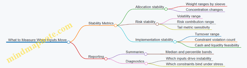
Robustness checks turn estimation error from an abstract worry into measurable behavior. When you can show that allocations remain coherent under plausible input movement, you’re not guaranteeing future accuracy—you’re demonstrating that the process is resilient to the kinds of mistakes that estimation inevitably makes.
6.3 Shrinkage and Blending Techniques for Return Forecasting Inputs
Return forecasting inputs are noisy: small samples, stale fundamentals, and model misspecification all push estimates around. Shrinkage and blending reduce that noise by combining information sources in a controlled way, so the allocation optimizer is less likely to chase random wiggles.
Foundational Idea: Separate Signal from Estimation Error
A practical way to think about expected returns is as an estimate plus error. If you treat the estimate as perfectly precise, optimization will overreact to the loudest (often noisiest) inputs. Shrinkage reduces the impact of uncertain estimates by pulling them toward a baseline that is more stable.
Blending goes one step further: it combines multiple estimators—each with different strengths—into a single input. The key is to blend in a way that respects reliability, not just averages everything.
Shrinkage Toward a Baseline
Choose a baseline that represents “what you would believe with no data.” Common baselines include:
- A historical mean (stable but biased if regimes shift)
- A factor-implied return (more structured, less free-form)
- A cross-sectional prior such as “assets with similar characteristics should have similar expected returns”
Then apply a shrinkage weight. For an asset i, a simple shrinkage form is:
- Shrunk return = w × (estimated return) + (1 − w) × (baseline return)
The weight w should increase when the estimate is reliable and decrease when it is not. Reliability often tracks sample size, data quality, and model fit.
Easy example. Suppose you forecast expected returns for two bonds using 24 months of data. Bond A has clean pricing and stable spreads; Bond B has missing observations and occasional stale quotes. You compute estimated returns: A = 6.0%, B = 9.0%. Your baseline (e.g., a factor-implied return) is 5.0% for both. If you set w_A = 0.8 and w_B = 0.4, then:
- A shrunk = 0.8×6.0% + 0.2×5.0% = 5.8%
- B shrunk = 0.4×9.0% + 0.6×5.0% = 6.6%
Notice what happened: Bond B’s forecast moves closer to the baseline because its estimate is less trustworthy.
Estimating Shrinkage Weights Without Making It Complicated
A common approach is to tie w to an uncertainty measure. For instance, if you have a standard error for each asset’s return estimate, you can set w higher when the standard error is lower. You can also use a “credibility” score based on effective sample size after filtering.
A simple rule of thumb for institutional workflows:
- If the estimate is based on fewer than a threshold number of observations, shrink more.
- If the model residuals are large or unstable, shrink more.
- If the baseline is derived from a robust factor structure, it can serve as a strong anchor.
Blending Multiple Estimators with Reliability Weights
Blending combines estimators such as:
- Historical mean (captures realized behavior)
- Fundamental or valuation-based estimate (captures cross-sectional differences)
- Factor model estimate (captures systematic drivers)
A reliability-weighted blend uses weights that reflect estimator quality. One practical method is to compute each estimator’s out-of-sample error on a rolling window and then assign higher weight to the estimator with lower error.
Easy example. For equities, you produce three expected return inputs for the same universe:
- Historical mean: 7.0%
- Valuation model: 5.5%
- Factor model: 6.2%
Assume recent out-of-sample mean absolute errors are 2.0%, 1.0%, and 1.5% respectively. Convert errors into weights inversely proportional to error (then normalize). The valuation model gets the most weight because it has the smallest error, so the blended return lands closer to 5.5% than a simple average would.
Combining Shrinkage and Blending Into One Coherent Pipeline
In practice, you often do both:
- Build multiple estimators for expected returns.
- Shrink each estimator toward its own baseline or toward a shared baseline.
- Blend the shrunk estimators using reliability weights.
This prevents a common failure mode: a noisy estimator can still dominate if you blend first and shrink later.
Mind Map: Shrinkage and Blending for Return Forecasting Inputs
Diagnostics That Keep the Process Honest
After shrinkage and blending, verify that the inputs behave sensibly:
- Ranking stability: assets shouldn’t flip wildly when you slightly change the estimation window.
- Magnitude control: extreme forecasts should be less extreme, especially for assets with weak data.
- Consistency across sleeves: if you use different models for public vs. private proxies, ensure the resulting expected returns are on comparable scales.
Easy example. You run the pipeline twice: once using 24 months and once using 30 months of data. Without shrinkage/blending, the top decile of expected returns changes membership for 40% of assets. With shrinkage and reliability-weighted blending, it drops to 15%. That’s not magic; it’s reduced sensitivity to sampling noise.
Practical Implementation Notes
Keep the baseline and reliability logic explicit in the investment policy. When someone asks why a forecast moved, the answer should trace back to either (a) changed data quality, (b) changed uncertainty, or (c) changed estimator performance—rather than a black-box recalibration.
A good target is not “perfect forecasts.” It’s forecasts that are stable enough for portfolio construction to express real views, not random estimation artifacts.
6.4 Incorporating Constraints and Model Risk Into Optimization Inputs
Optimization is only as good as the inputs it receives. In institutional allocation, the inputs are rarely “clean”: constraints are real-world rules, and model risk is the gap between what the model assumes and what actually happens. The goal in this section is to make those two issues explicit before the optimizer ever runs.
Constraints as First-Class Inputs
Start by separating constraints into three categories.
-
Feasibility constraints decide what is allowed. Examples include minimum and maximum exposures, leverage limits, or “no shorting” rules for certain sleeves.
-
Policy constraints encode governance decisions. Examples include target ranges for active risk, concentration caps by issuer, or minimum allocations to diversifying sleeves.
-
Implementation constraints reflect how trades and cash flows work. Examples include turnover limits, rebalancing calendars, and liquidity-bucket exposure caps.
A practical way to incorporate them is to translate each rule into either (a) hard bounds that must be satisfied, or (b) soft penalties that discourage violations. Hard bounds are appropriate when breaking the rule is unacceptable. Soft penalties are appropriate when the rule is flexible but costly.
Example: Suppose a pension mandate requires fixed income duration to stay within ±0.5 years of the benchmark. Treat this as a hard constraint if the mandate is strict. If the committee can tolerate small deviations with justification, model it as a soft constraint by adding a penalty proportional to the duration gap.
Model Risk as Uncertainty in Inputs
Model risk shows up when expected returns, covariances, and scenario mappings are wrong. Instead of pretending the estimates are exact, represent uncertainty directly in the optimization inputs.
Common uncertainty sources include:
- Estimation error in expected returns and covariances.
- Structural mismatch where the model’s risk factors do not represent the portfolio’s true drivers.
- Data issues such as stale private valuations or survivorship bias in public histories.
A systematic approach is to convert point estimates into ranges or distributions and then choose an optimization method that respects those ranges.
Robustification Strategies
Robust optimization methods vary, but the principle is consistent: optimize for performance that remains acceptable under adverse input perturbations.
Use three layers of robustness.
-
Parameter uncertainty bounds: Inflate covariance risk and shrink expected returns toward conservative values. This reduces the optimizer’s temptation to chase fragile alpha.
-
Constraint uncertainty: If constraints depend on uncertain inputs (like liquidity classification or duration estimates), widen the effective constraint region. For instance, if duration estimates have error, enforce the duration bound using a conservative buffer.
-
Scenario consistency: When constraints are tied to scenarios (stress liquidity, covenant coverage), ensure the same scenario set drives both risk and feasibility checks.
Example: For a private credit sleeve, suppose cash-flow timing is uncertain and affects liquidity. If the model assumes distributions occur quarterly but actual distributions can lag, incorporate a liquidity buffer by limiting the maximum private credit exposure to a level that remains feasible under a “delayed distributions” scenario.
Turning Constraints and Model Risk Into Optimization Inputs
To keep the pipeline coherent, build an input checklist that the optimizer consumes.
- Decision variables: weights by asset or sleeve.
- Hard constraints: bounds, no-short rules, leverage limits.
- Soft constraints: penalties for deviations from policy targets.
- Risk model inputs: covariance matrix (possibly shrunk), factor exposures, and liquidity mapping.
- Uncertainty settings: covariance inflation factor, expected return shrinkage level, scenario shock magnitudes.
Then run a sensitivity pass where you vary uncertainty settings and confirm that the solution does not hinge on a single fragile assumption.
Mind Map: Constraints and Model Risk Integration
Worked Example: Duration Constraint with Return Uncertainty
Assume a fixed income sleeve must keep duration within ±0.5 years of benchmark (hard constraint). Expected returns for duration-sensitive assets are uncertain, so you shrink them toward a conservative baseline. The optimizer then:
- Enforces the duration band exactly.
- Penalizes allocations that rely heavily on the most optimistic return estimates.
- Uses an inflated covariance to avoid over-concentration in assets that look good only under favorable assumptions.
The result is not necessarily the highest nominal expected return, but it is a portfolio that stays within the mandate even when the model’s inputs wobble. That is the point: constraints and model risk should shape the optimization problem, not appear as after-the-fact explanations.
6.5 Practical Example: Comparing Multiple Return Estimation Approaches for Allocation
A portfolio committee rarely argues about whether expected returns matter; it argues about which expected returns are believable enough to use. This example compares three return estimation approaches for an institutional multi-asset allocation and shows how to compare them systematically.
Step 1: Set the Allocation Problem and the Evaluation Yardstick
Assume an investment policy with three sleeves: Public Equity, Investment-Grade Bonds, and Private Credit. The committee wants a 12-month allocation that targets a volatility budget while keeping liquidity feasible. For each sleeve, we need an expected return input and an uncertainty level.
To compare methods, we use two practical checks:
- Backtest calibration: do the predicted returns line up with realized returns in the recent sample?
- Allocation stability: does the resulting allocation change wildly when inputs shift within reasonable estimation error?
Step 2: Define the Three Estimation Approaches
We compare:
- Historical mean: average realized returns over a lookback window.
- Factor-based model: expected returns driven by exposures to common risk factors (for public assets) and mapped proxies for private credit.
- Blended valuation-and-history: a weighted average of valuation-implied return (or spread-based for credit) and historical performance.
Each approach produces an expected return, but only the blended and factor-based approaches naturally support uncertainty estimates tied to model inputs.
Step 3: Use Consistent Inputs and Avoid Accidental Unfairness
To keep the comparison honest, use the same:
- measurement frequency (monthly)
- currency and total return convention
- rebalancing horizon (12 months)
- risk model for volatility and covariance (so differences come from return estimates, not risk mechanics)
For private credit, use a cash-flow-aware return series: reported marks plus a smoothing rule that reduces timing noise. The committee should document the smoothing rule in the IPS appendix so the method is repeatable.
Step 4: Mind Map of the Comparison Workflow
Return Estimation Comparison Mind Map
Step 5: Compute Example Expected Returns
Suppose the committee uses the last 36 months of monthly data. The estimated 12-month expected returns are:
- Public Equity
- Historical mean: 7.0%
- Factor-based: 6.2%
- Blended: 6.6%
- Investment-Grade Bonds
- Historical mean: 3.2%
- Factor-based: 3.6%
- Blended: 3.4%
- Private Credit
- Historical mean: 8.1%
- Factor-based: 7.3%
- Blended: 7.6%
Uncertainty (standard deviation of the forecast error) is assumed to be:
- Historical mean: higher, because it treats the past as the future without a mechanism.
- Factor-based: moderate, because factor premia and exposures can be estimated.
- Blended: moderate-to-low, because valuation/spread signals anchor the forecast while history tempers noise.
Step 6: Run Three Constrained Allocations and Compare Outcomes
Use the same optimization framework each time: maximize expected return subject to a volatility cap and sleeve-level concentration limits. Keep transaction costs and turnover assumptions identical.
Example results (target weights):
- Using Historical mean
- Equity 55%, Bonds 25%, Private Credit 20%
- Constraint behavior: volatility cap binds frequently
- Using Factor-based model
- Equity 50%, Bonds 30%, Private Credit 20%
- Constraint behavior: fewer binding events
- Using Blended valuation-and-history
- Equity 52%, Bonds 28%, Private Credit 20%
- Constraint behavior: stable across small input perturbations
The committee should not treat these numbers as “the answer.” The point is the pattern: historical mean pushes the portfolio toward the sleeve with the most favorable recent average, while factor-based and blended approaches reduce that overreaction.
Step 7: Interpret Calibration and Stability Together
If backtests show that historical mean errors are both larger and biased toward recent regimes, then its allocation instability is expected. Factor-based models often reduce bias but can underreact if factor exposures are imperfect or if private credit mapping is coarse. Blended methods typically perform well when valuation/spread signals are informative but noisy, because the historical component prevents the model from chasing short-term signal noise.
Step 8: Governance-ready decision rule
A practical rule for the committee:
- Prefer the method with the lowest forecast error in backtests subject to producing allocations that remain within tolerance bands when expected returns shift by one forecast standard deviation.
- If two methods tie, choose the one with clearer documentation of inputs and fewer opaque steps.
In this example, the blended approach wins the stability check without sacrificing calibration, so it becomes the default return input method for allocation—while historical mean remains a diagnostic baseline to catch when the other models are behaving oddly.
7. Covariance Estimation and Correlation Management
7.1 Covariance Estimation Methods and Sample-Size Limitations
Covariance estimation is the quiet engine behind many portfolio optimizations. It turns “how assets move together” into numbers, and those numbers then get treated as if they were truth. In practice, the estimate is noisy, and the noise grows when you have fewer observations than you have assets (or when returns are heavy-tailed). This section builds a practical mental model: what covariance estimators do, why sample size matters, and how to choose methods that behave sensibly.
Core Idea: What You Estimate and What Goes Wrong
For asset returns \(r_t\), the sample covariance is built from deviations from the sample mean. If you have \(N\) assets and \(T\) return observations, the covariance matrix has \(N(N+1)/2\) distinct entries. With small \(T\), many entries are estimated from too little information, so the matrix can become unstable: eigenvalues can be too large or too small, and the optimizer may “see” diversification that isn’t real.
A useful rule of thumb is that you want \(T\) comfortably larger than \(N\). When \(T\) is not much larger than \(N\), you should expect estimation error to dominate the optimization objective.
Mind Map: Covariance Estimation and Sample Size
Sample Covariance and Its Failure Modes
The classic estimator is the sample covariance:
\(\hat\Sigma_{\text{sample}} = \frac{1}{T-1}\sum_{t=1}^{T}(r_t-\bar r)(r_t-\bar r)^\top\).
It is easy to compute and easy to explain, but it has two predictable problems.
-
Noise in off-diagonal terms. Correlations between asset pairs are estimated from limited co-movement observations. With small \(T\), the sign and magnitude can flip just from sampling variation.
-
Instability in optimization. Many optimizers invert \(\hat\Sigma\) or use it in quadratic forms. If \(\hat\Sigma\) is ill-conditioned, small estimation errors can produce large changes in weights.
Example: Suppose you estimate monthly covariances for 40 assets using 24 months of data. The covariance matrix has 820 distinct entries. You are trying to estimate far more parameters than the data can reliably support. Even if the in-sample covariance looks “reasonable,” the resulting portfolio can swing dramatically when you extend the sample by a few months.
Shrinkage Estimators for Stability
Shrinkage addresses the “too many parameters” problem by blending the sample covariance with a structured target \(T\):
\(\hat\Sigma_{\text{shrink}} = \delta T + (1-\delta)\hat\Sigma_{\text{sample}}\).
The target is chosen to be well-behaved, such as:
- Scaled identity: assumes equal variance and zero covariance.
- Constant-correlation model: keeps average correlation but stabilizes pairwise estimates.
- Diagonal plus average correlation: preserves individual variances while regularizing correlations.
The shrinkage intensity \(\delta\) is selected to reduce mean squared error, not to “fit the past better.” That distinction matters: the goal is a covariance estimate that leads to stable decisions.
Example: If your sample covariance implies a few extremely small eigenvalues, shrinkage typically lifts them. That reduces the optimizer’s tendency to allocate extreme weights to directions that look diversifying only because of estimation noise.
Factor Models to Reduce Effective Parameters
Factor models express covariance as:
\(\Sigma \approx BFB^\top + D\),
where \(B\) maps assets to factors, \(F\) is factor covariance, and \(D\) is idiosyncratic risk (often diagonal). Instead of estimating \(N(N+1)/2\) covariances directly, you estimate factor exposures and factor covariances, which can be far fewer.
This helps when assets share common drivers like equity market moves, credit spreads, or interest-rate level changes.
Example: With 60 assets but only 5 meaningful factors, the model estimates a 5×5 factor covariance plus idiosyncratic variances. The covariance structure becomes less sensitive to pairwise sampling noise.
Exponentially Weighted Covariance and Effective Sample Size
Exponentially weighted covariance assigns weights that decay over time. If the decay is too aggressive, the effective sample size becomes small even when \(T\) is large. That can reintroduce instability.
Example: Using daily returns over 2 years but a decay that effectively counts only 60 trading days can produce a covariance estimate that behaves like you only had a couple of months of data.
Practical Diagnostics for Sample-Size Limits
Before using \(\hat\Sigma\) in optimization, check whether it is numerically and economically plausible.
- Eigenvalue spread: very tiny eigenvalues often signal overfitting or near-singularity.
- Condition number: large values indicate inversion instability.
- Out-of-sample portfolio stability: if weights change drastically when you shift the estimation window slightly, the covariance estimate is likely too noisy.
A simple operational approach is to compare three estimators on the same dataset: sample covariance, shrinkage covariance, and a factor-based covariance. The “best” one is the one that produces stable risk estimates and consistent portfolio behavior, not the one that matches in-sample correlations most closely.
Summary of Method Choice
- Use sample covariance when you have ample data and returns are well-behaved.
- Use shrinkage when you need numerical stability and want a controlled bias-variance tradeoff.
- Use factor models when assets share drivers and you want fewer effective parameters.
- Use exponential weighting only when you can justify the time-variation and still maintain a sufficiently large effective sample size.
7.2 Correlation Stability, Regime Effects, and Practical Mitigations
Correlation is often treated like a stable property of assets. In practice, it behaves more like a weather pattern: it changes when markets change, and it can change faster than your rebalancing schedule. This section explains why correlation shifts, how to detect regime effects, and what to do about it in institutional portfolio construction.
Correlation Stability as a Modeling Assumption
Correlation stability means the relationship between two return series does not materially change over the estimation window. The assumption is useful because many allocation methods rely on a covariance matrix that is built from historical correlations. When correlations are unstable, the covariance matrix becomes a shaky input, and optimization can produce weights that look sensible in-sample but behave poorly out-of-sample.
A practical way to think about stability is to separate two components:
- Sampling noise: correlations estimated from limited data vary even if the true relationship is constant.
- Structural change: the true relationship changes because the economic drivers behind the assets change.
You can often tell which is which by checking whether correlation shifts align with identifiable market conditions, such as stress in credit spreads or sharp changes in equity volatility.
Regime Effects and Why Correlations Move
A “regime” is a set of market conditions where the dominant drivers of returns are similar. Correlations move across regimes because the mapping from drivers to asset returns changes.
Common regime drivers include:
- Risk appetite: when investors move from cautious to aggressive, equity and credit often become more synchronized.
- Funding stress: when liquidity dries up, correlations can rise because many assets are sold for cash.
- Inflation and rate shocks: the sensitivity of equities, duration, and real assets can change when the market reprices rates.
- Volatility clustering: when volatility rises, dispersion across assets can shrink, making correlations look higher.
A key nuance is that correlation can rise even if diversification still exists in the underlying exposures. For example, two assets may both react to a common factor like “global risk,” which increases correlation, even though their idiosyncratic risks remain different.
Detecting Regime Changes in Correlation
Detection should be systematic, not based on vibes. Start with a correlation time series computed on rolling windows, then test whether it changes meaningfully.
A simple diagnostic workflow:
- Choose a rolling window length that balances stability and responsiveness.
- Compute rolling correlations for relevant pairs or factor-implied correlations.
- Compare correlation levels across market states using a rule-based state definition.
State definitions can be mechanical. For instance, define “stress” when credit spreads are above a threshold or when equity volatility exceeds a threshold. The point is repeatability.
If you want a more structured approach, use factor models and examine whether the factor loadings or factor covariances change across states. Correlation shifts that are explained by factor covariance changes are easier to manage than unexplained shifts.
Mind Map: Correlation Stability and Mitigations
Practical Mitigations That Work in Real Portfolios
Mitigations should reduce the damage from correlation instability without pretending you can eliminate it.
-
Use covariance estimation that shrinks toward structure
Instead of relying on raw sample correlations, shrink correlations toward a structured target (for example, factor-implied correlations). This reduces sensitivity to noisy estimates.- Example: If you estimate correlations for 30 assets from 2 years of monthly data, the estimation error is large. Shrinkage can prevent the optimizer from treating a random correlation spike as a real diversification signal.
-
Stress-consistent covariance scenarios
Build multiple covariance matrices tied to market states, then evaluate allocations under each. You are not changing the optimizer into a crystal ball; you are checking whether the portfolio remains reasonable when correlations shift.- Example: Construct one covariance matrix for “normal” conditions and one for “stress” conditions defined by credit spreads. If the portfolio’s risk concentration flips dramatically in stress, you need to adjust constraints or exposures.
-
Regime-aware constraints and exposure limits
Constraints can prevent the portfolio from becoming overly dependent on correlations that only hold in one regime.- Example: If a strategy relies on equity and long-duration bonds diversifying each other, impose limits on combined exposure to a common risk factor (such as duration plus equity beta). This reduces the chance that both sleeves move together when the regime changes.
-
Liquidity-aware design for correlation spikes
Correlation spikes often coincide with liquidity stress. If you ignore liquidity, you can end up forced to trade at the worst time, turning correlation risk into implementation risk.- Example: In a stress scenario, assume correlations rise and liquidity worsens. Then test whether your rebalancing policy would require selling illiquid positions to fund margin or capital calls.
A Concrete Example of Regime Effects in Action
Consider a simplified portfolio with two sleeves: equities and investment-grade credit. In calm markets, equities and credit may show moderate correlation because credit spreads are stable and equity drawdowns do not always translate into spread widening. In stress, both sleeves can be driven by the same “risk-off” factor, and credit spreads widen while equities fall, increasing correlation.
If you build a single covariance matrix from a calm period, the optimizer may allocate more to the sleeve that appears to diversify. When stress arrives, the realized diversification benefit shrinks, and the portfolio’s risk target is missed.
A mitigation is to estimate covariances across states and either (a) optimize with robust inputs, or (b) optimize once and then verify that risk and concentration metrics remain within limits under the stress covariance. The portfolio may not be perfect in every regime, but it is less likely to be surprised by correlation behavior.
Practical Takeaways
- Correlation instability is expected, not exceptional.
- Regime effects are often driven by identifiable market conditions like funding stress and volatility clustering.
- Mitigations should focus on robustness: shrinkage, stress-consistent checks, constraints, and liquidity-aware implementation.
- The goal is not to predict correlation perfectly, but to prevent the portfolio from depending on correlation that only exists in one market mood.
7.3 Shrinkage, Factor Models, and Structured Covariance Matrices
Covariance matrices are the engine behind many institutional allocation tools, but they are also fragile. Sample covariance estimates can be noisy when you have limited history, many assets, or shifting market regimes. Shrinkage and factor models reduce that noise by imposing structure that is consistent with how risk actually moves.
Shrinkage: Pulling Estimates Toward Stability
Shrinkage replaces a raw covariance estimate with a weighted average of two matrices: one data-driven and one structured. A common form is
\[ \Sigma_{shrunk} = (1-\lambda),\Sigma_{sample} + \lambda,\Sigma_{target} \]
Here, \(\lambda\) controls how strongly you trust the target. When the sample is unreliable, you increase \(\lambda\). When you have lots of clean data and the market is stable, you decrease it.
A practical target is a constant-correlation model: you keep each asset’s variance from the sample, but you replace pairwise correlations with a single average correlation. Example: suppose 50 assets have only 24 monthly observations. The sample correlations will bounce around. Using constant correlation prevents the optimizer from “seeing” random relationships as real diversification.
How to choose \(\lambda\) without guessing: use a shrinkage estimator that minimizes expected squared error under a statistical criterion (often implemented in standard libraries). Even if you do not compute it manually, the key idea is that \(\lambda\) should rise when the sample is short relative to the number of assets.
Factor Models: Explaining Covariance Through Shared Drivers
A factor model expresses asset returns as
\[ r = Bf + \epsilon \]
where \(B\) are factor loadings, \(f\) are factor returns, and \(\epsilon\) are idiosyncratic residuals. The covariance becomes
\[ \Sigma = B,\Sigma_f,B^T + D \]
with \(D\) as the covariance of residuals, often approximated as diagonal.
This structure matters because many assets move together due to a small set of drivers. For instance, equity sectors share broad market exposure; credit instruments share risk premia and rate sensitivity; real assets often share inflation and growth sensitivities. Instead of estimating every pairwise covariance directly, you estimate factor covariances and loadings.
Concrete example: imagine 30 equity stocks and 10 bond funds. If you estimate a single 40×40 covariance from 36 months of data, you may get unstable cross-asset correlations. With factors, you can use a small set such as “equity market,” “rates,” and “credit spread.” The cross-covariances then come from how each asset loads on those factors.
Structured Covariance Matrices: Combining Both Ideas
Factor models already impose structure, but you can add further constraints to make the matrix more robust.
- Diagonal Residuals: set \(D\) to be diagonal so idiosyncratic risks do not create spurious correlations.
- Shrink Factor Covariances: apply shrinkage to \(\Sigma_f\) so factor relationships are stable.
- Shrink Loadings: if loadings are estimated with error, shrink them toward a simpler pattern (for example, sector-neutral or duration-bucketed structures).
- Positive Semidefinite Enforcement: numerical issues can produce a covariance matrix that is not valid. Projecting to the nearest positive semidefinite matrix prevents optimization failures.
A simple workflow for an institutional setting is: estimate factor loadings from a rolling window, estimate factor covariance, build \(\Sigma\), then shrink either the final \(\Sigma\) or the factor covariance. This keeps the matrix both interpretable and numerically well-behaved.
Mind Map: How Shrinkage and Factors Work Together
Example: From Noisy Sample to Robust Optimization Input
Suppose you have 25 assets and 30 monthly observations. The sample covariance is noisy, and an optimizer may produce extreme weights because it “finds” diversification where none exists.
Step-by-step:
- Choose a factor set that matches the mandate, such as equity market, rates, and credit spread.
- Estimate loadings \(B\) using regressions over the same window.
- Estimate factor covariance \(\Sigma_f\) and apply shrinkage to it.
- Set residual covariance \(D\) to diagonal using regression residual variances.
- Build \(\Sigma = B,\Sigma_f,B^T + D\).
- If needed, apply a final shrinkage toward a target (like constant correlation) to smooth remaining noise.
The resulting covariance matrix typically yields more stable allocations: weights change less when you extend or shorten the window slightly, and the optimizer is less likely to chase random pairwise correlations.
Diagnostic Checks That Keep You Honest
After constructing \(\Sigma\), verify that it behaves sensibly:
- Eigenvalues: confirm the matrix is positive semidefinite.
- Correlation sanity: check that implied correlations are not dominated by estimation noise.
- Sensitivity: rerun with a nearby window length and confirm allocations do not swing wildly.
- Interpretability: ensure factor exposures explain the major co-movements you expect from the mandate.
These checks turn covariance construction from a black box into a controlled, repeatable process—exactly what institutional portfolio construction needs.
7.4 Stress-Consistent Covariance Adjustments for Allocation
Covariance matrices are the quiet engine behind many allocation models: they translate “how assets move together” into portfolio risk. The problem is that covariance is not stable. When markets shift, correlations and volatilities shift too, and a covariance estimate built from calm periods can misprice risk during stress. Stress-consistent covariance adjustments aim to keep the covariance matrix aligned with how risk behaves under specified adverse conditions, while still remaining usable inside an optimizer.
Foundational Idea: Covariance Is a Risk Map, Not a Fact
A covariance matrix Σ implies a variance for any portfolio weight vector w: Var(w)=wᵀΣw. If Σ is wrong in stress regimes, the optimizer can choose weights that look safe in-sample but fail under stress. Stress-consistent adjustments therefore modify Σ so that key risk properties match stress expectations.
Step 1: Define Stress Scenarios with Measurable Targets
Start with scenarios that are operationally specific. For example:
- Equity drawdown with widening credit spreads.
- Rates shock with a simultaneous liquidity squeeze.
- Commodity volatility spike with equity correlation rising.
For each scenario, specify targets you can measure from data or internal assumptions:
- Volatility multipliers by asset class (e.g., equity vol ×1.5, credit vol ×1.2).
- Correlation shifts (e.g., equity–credit correlation increases by +0.20).
- Optional factor shocks (e.g., a 100 bps rate move, a credit spread widening of 150 bps).
A practical way to keep this concrete is to anchor targets to a historical analog. If you use a date like 2026-04-15 as the “stress window anchor,” you can compute realized volatilities and correlations over that window and treat them as scenario-consistent inputs.
Step 2: Choose a Covariance Construction Method That Can Be Adjusted
Two common starting points work well:
- Factor model covariance: Σ = BFBᵀ + D, where F is factor covariance and D is idiosyncratic variance.
- Shrinkage covariance: Σ̂ = αS + (1−α)T, blending sample covariance S with a structured target T.
Stress adjustments are easiest when the method separates “systematic co-movement” from “idiosyncratic noise.” Factor models do this naturally; shrinkage can be adapted by stressing the structured target.
Step 3: Apply Stress Multipliers Consistently
A naive approach multiplies the entire covariance matrix by a scalar. That preserves relative correlations but not correlation changes. Instead, adjust in layers:
- Volatility layer: scale each asset’s variance to match scenario vol targets.
- Correlation layer: adjust off-diagonal covariances to match scenario correlation shifts.
If you have vol targets σᵢ* and correlation targets ρᵢⱼ*, then set covᵢⱼ* = ρᵢⱼ* σᵢ* σⱼ*. This keeps the covariance matrix coherent with the scenario’s intended co-movement.
Step 4: Enforce positive semidefiniteness
Optimizers dislike covariance matrices that are not positive semidefinite (PSD). After adjustments, Σ* may violate PSD due to rounding or inconsistent targets. Fix it by projecting onto the nearest PSD matrix (e.g., eigenvalue clipping):
- Compute eigen-decomposition Σ* = QΛQᵀ.
- Replace negative eigenvalues in Λ with zero (or a small floor).
- Reconstruct Σ_psd = QΛ⁺Qᵀ.
This step is not cosmetic. Without PSD enforcement, risk estimates can become nonsensical for some portfolios.
Step 5: Blend Stressed and Baseline Covariances
A fully stressed covariance can be too pessimistic for normal periods. A common integrated approach is a convex blend:
- Σ_blend = (1−β)Σ_baseline + βΣ_stress
Choose β based on how much the mandate emphasizes robustness versus efficiency. For example, a liquidity-constrained mandate might use a higher β because stress outcomes are more likely to dominate realized risk.
Step 6: Validate with Portfolio-Level Stress Checks
After building Σ_blend, test it with portfolio-level diagnostics:
- Compute scenario portfolio variance using Σ_stress and compare it to your scenario targets.
- Check whether diversification behaves plausibly (e.g., adding a diversifier reduces stress variance rather than increasing it).
- Run a small set of “sanity portfolios” like equal-weight, benchmark-like, and a concentrated tilt.
If stress variance increases for all reasonable portfolios, your correlation targets may be internally inconsistent.
Mind Map: Stress-Consistent Covariance Adjustments
Example: Building a Stress-Adjusted Covariance for a Simple Sleeve
Assume three sleeves: Equity (E), Investment Grade Credit (IG), and Treasury Bonds (T). Baseline volatilities are σ_E=18%, σ_IG=8%, σ_T=6%. Baseline correlations are ρ_E,IG=0.35, ρ_E,T=0.10, ρ_IG,T=0.25.
Scenario targets for a “rates + credit widening” stress are:
- σ_E*=27%, σ_IG*=10%, σ_T*=7%
- Correlation shifts: ρ_E,IG*=0.55, ρ_E,T*=0.05, ρ_IG,T*=0.40
Compute stressed covariances:
- cov_E,IG* = 0.55×0.27×0.10 = 0.01485
- cov_E,T* = 0.05×0.27×0.07 = 0.000945
- cov_IG,T* = 0.40×0.10×0.07 = 0.0028
Set variances on the diagonal using σᵢ*², then assemble Σ_stress. If PSD fails, apply eigenvalue clipping to obtain Σ_psd. Finally, blend with baseline using β=0.6 to get Σ_blend for allocation.
The key outcome is that the optimizer sees higher equity-credit co-movement and higher credit risk in stress, while still retaining some baseline structure so the allocation does not become uniformly defensive.
7.5 Practical Example: Building a Robust Covariance Matrix for Optimization
You are optimizing a multi-asset portfolio with constraints, so the covariance matrix is not just a math input—it’s the difference between a stable allocation and a fragile one. This example builds a covariance matrix that is (1) consistent with your data, (2) robust to estimation noise, and (3) aligned with the risk drivers you actually care about.
Step 1: Start with a Clean Return Panel
Use monthly total returns for public assets and a consistent valuation policy for any sleeve with appraisal-based inputs. Suppose you have 36 months of returns for: US Equity, Developed ex-US Equity, US IG Credit, US High Yield, and 2-year Treasury. Before modeling, check for obvious issues:
- Remove or flag periods with stale pricing or corporate action anomalies.
- Ensure all series are in the same currency and share the same return convention.
- Winsorize extreme outliers only if they are clearly data errors; otherwise keep them and rely on robust estimation.
A quick sanity check: compute pairwise correlations and confirm they are plausible (for example, equities should not be perfectly correlated with short Treasuries).
Step 2: Choose a Covariance Approach That Matches Your Sample Size
With 36 observations and 5 assets, the sample covariance is usable but noisy. A robust approach blends:
- A structured target (factor model or shrinkage-to-diagonal)
- The sample covariance
A practical baseline is shrinkage toward a factor-structured covariance. The goal is to reduce estimation error while preserving the main co-movement patterns.
Step 3: Build a Factor Model Target
Pick a small set of factors that explain most variation. For this example, use three factors:
- Equity market factor (broad equity index)
- Credit spread factor (IG and/or HY spread proxy)
- Rates factor (2-year Treasury return)
Estimate factor exposures via rolling regressions or a single regression using the full sample. Then compute the factor-implied covariance:
- Covariance from factors: \(B \Sigma_f B^T\)
- Idiosyncratic covariance: \(D\) (often diagonal)
This target captures the “why” behind correlations: equities move together because they share equity risk, credit assets share credit risk, and rates assets move with rates.
Step 4: Shrink the Covariance Toward the Target
Let \(S\) be the sample covariance and \(T\) be the factor target. Form the robust covariance: \[ \Sigma = \lambda T + (1-\lambda)S \] Choose \(\lambda\) using a stability criterion such as minimizing out-of-sample portfolio variance over a rolling window, or using a standard shrinkage rule if you prefer a deterministic method.
If you want a concrete workflow, here is a compact pseudo-implementation.
Inputs: returns matrix R (T x N), factor returns F (T x K)
1) Estimate exposures B by regressing each asset on factors
2) Compute factor covariance Σ_f from F
3) Build target T = B*Σ_f*B' + D (diagonal idiosyncratic)
4) Compute sample covariance S from R
5) Select lambda by rolling evaluation of portfolio variance stability
6) Output Σ = λ*T + (1-λ)*S
Step 5: Enforce numerical stability
Optimization routines dislike covariance matrices that are nearly singular. Apply:
- Eigenvalue floor: replace very small eigenvalues with a minimum threshold.
- Symmetrization: \(\Sigma = (\Sigma + \Sigma^T)/2\).
- Check condition number and ensure it is within a reasonable range.
This step prevents “mysterious” optimizer behavior where tiny numerical issues create large weight swings.
Step 6: Validate with Portfolio-Level Diagnostics
Build a few test portfolios and compare risk estimates:
- Minimum-variance portfolio using \(\Sigma\)
- Equal-weight portfolio using \(\Sigma\)
- A constrained portfolio that matches your real mandate
Then compare predicted volatility to realized volatility over a holdout window. You are not trying to predict perfectly; you are checking that the covariance matrix produces reasonable risk magnitudes and relative ordering.
Step 7: Stress the Covariance with Liquidity-Aware Checks
Even though this section is about covariance, your covariance must survive the realities of implementation. If a sleeve is illiquid, you may rebalance less often, so risk should be assessed over longer holding periods. A simple adjustment is to compute covariance using overlapping returns for the holding horizon (for example, 3-month overlapping returns) and then apply the same shrinkage procedure.
Mind Map: Robust Covariance Matrix Workflow
Example Outcome and How to Use It in Optimization
Once \(\Sigma\) is built, feed it into your optimizer with the same constraint set you will use in production. If your optimizer supports it, also compute active risk under the benchmark using the same covariance. A robust covariance should reduce weight churn when you slightly perturb inputs like expected returns or factor exposures.
In practice, the biggest improvement often comes from the combination of (1) a factor-structured target and (2) shrinkage, not from more complex math. The matrix becomes less sensitive to random noise, which makes the portfolio construction behave like it has a spine.
8. Portfolio Optimization for Institutional Asset Allocation
8.1 Objective Functions: Mean-Variance, Risk-Parity, and Utility-Based Forms
Objective functions turn “we want a good portfolio” into something you can compute, constrain, and explain to an investment committee. The trick is choosing an objective that matches how you think risk and return should trade off, then making sure the math respects real-world frictions like turnover and liquidity.
Mind Map: Objective Function Landscape
Mean-Variance Objective
The classic mean-variance objective chooses weights \(w\) to maximize expected return minus a penalty for variance:
\[ \max_w; w^\top \mu - \frac{\lambda}{2} w^\top \Sigma w \]
Here \(\mu\) is the vector of expected returns, \(\Sigma\) is the covariance matrix, and \(\lambda\) controls risk aversion. If you prefer minimization form, it’s equivalent to minimizing \(w^\top \Sigma w\) subject to achieving a target return.
Integrated best practice: keep units consistent. If \(\mu\) is annualized but \(\Sigma\) is monthly, the optimizer will happily produce nonsense with confidence.
Easy example: Suppose two assets have expected returns \(\mu=[6%, 4%]\) and covariance \(\Sigma\) with volatilities 10% and 8% and correlation 0.3. If you set \(\lambda\) high, the solution shifts weight toward the lower-volatility asset even though it has lower expected return. That’s the objective doing exactly what you told it to do.
Advanced detail without gaps: mean-variance is sensitive to estimation error in \(\mu\) and \(\Sigma\). A practical mitigation is to reduce reliance on \(\mu\) by shrinking it toward a benchmark or blending forecasts with historical averages, while still letting \(\Sigma\) drive diversification.
Risk-Parity Objective
Risk-parity aims for balanced risk contributions rather than balanced weights. Define each asset’s marginal contribution to portfolio volatility as \( (\Sigma w)_i / \sqrt{w^\top \Sigma w} \). The risk contribution of asset \(i\) is then:
\[ RC_i = w_i \cdot \frac{(\Sigma w)_i}{\sqrt{w^\top \Sigma w}} \]
A common target is \(RC_i\) equal across assets (or across groups like equities vs. credit). The optimizer minimizes the squared deviation of risk contributions from their target shares.
Integrated best practice: enforce feasibility with constraints early. Risk-parity can demand extreme weights when correlations are high or when an asset’s covariance structure makes its risk contribution hard to adjust.
Easy example: Consider three sleeves: government bonds, investment-grade credit, and equities. If equities are volatile and credit is moderately correlated with equities, risk-parity will typically reduce equity weight and increase bond or credit weight until each sleeve contributes similar volatility to the total portfolio. You get diversification that doesn’t require you to be right about which sleeve will outperform.
Advanced detail: risk-parity implicitly treats expected returns as secondary. That’s not a flaw if your mandate is “control risk and maintain diversification,” but it matters if you also need a specific return profile. In that case, you can combine risk-parity structure with a return-aware overlay or add a mild return term to the objective.
Utility-Based Objective
Utility-based objectives encode preferences directly. A simple mean-variance utility is:
\[ \max_w; \mathbb{E}[R_p] - \frac{A}{2},\mathrm{Var}(R_p) \]
where \(A\) is risk aversion. More general utility forms can incorporate downside preferences. For example, if you model returns as approximately normal, mean-variance utility is already a utility model in disguise.
Integrated best practice: match the utility to the decision context. If the investment committee cares about drawdowns or shortfall, a utility that penalizes downside (rather than variance alone) can be more aligned with how the portfolio will be judged.
Easy example: Suppose two portfolios have the same expected return and variance, but one has a heavier left tail. A downside-aware utility would prefer the portfolio with fewer “bad surprises,” even if variance looks similar.
Putting It Together with Constraints
No objective function lives alone. In practice, you solve:
- Constraints: leverage limits, concentration caps, minimum liquidity buckets, and turnover budgets.
- Implementation penalties: discourage unnecessary trades, especially when private or semi-liquid sleeves are involved.
- Diagnostics: run sensitivity checks by perturbing \(\mu\) and \(\Sigma\) to see whether the solution flips.
Practical rule of thumb: if you trust return forecasts less than you trust risk estimates, risk-parity or utility forms with conservative assumptions often behave better. If you have strong, consistent return signals and robust covariance estimates, mean-variance can be effective and transparent.
Mind Map: Choosing Among Objectives

Example: A Constrained Optimization Sketch
Given:
- Expected returns μ
- Covariance Σ
- Constraints: sum(w)=1, w>=0, max weight per asset
- Turnover limit vs current weights w0
Choose objective:
- Mean-variance: maximize w^T μ - (λ/2) w^T Σ w
- Or risk-parity: minimize deviation of risk contributions
- Or utility: maximize expected utility under chosen return model
Solve with a constrained optimizer
Then check:
- Constraint violations
- Sensitivity to μ and Σ perturbations
- Liquidity feasibility for each sleeve
The objective function is the “engine,” but constraints and diagnostics are the “safety checks.” When those are aligned, the resulting portfolio is not just mathematically optimal—it’s operationally coherent.
8.2 Constraints: Concentration, Turnover, Leverage, and Exposure Limits
Constraints turn an appealing portfolio idea into something you can actually run. They also prevent “optimization theater,” where the math looks great but the real-world implementation quietly breaks. This section builds a practical constraint toolkit, starting with the basics of what each limit controls and ending with how to combine them without creating contradictions.
Concentration Limits
Concentration limits cap how much risk or capital sits in a single name, sector, or factor bucket. The simplest form is a per-issuer weight cap, such as 5% for equities. A more nuanced approach uses groupings: for example, cap the combined weight of banks and insurers if they share similar credit risk drivers.
A useful mental model is: concentration limits control “idiosyncratic fragility.” If one position goes wrong, the portfolio should not go with it.
Example: A pension portfolio targets a 60/40 public allocation. It sets a 6% maximum weight per corporate bond issuer and a 20% maximum weight per credit rating bucket (e.g., BBB). If the optimizer wants 9% in one BBB issuer to improve expected return, the constraint forces it to spread that exposure across other issuers.
Turnover Limits
Turnover limits control trading intensity, which affects transaction costs, market impact, and operational burden. Turnover is usually measured as the sum of absolute changes in weights (or shares) over a period, divided by starting value.
A turnover constraint is not just about costs; it also stabilizes exposures. If you rebalance too aggressively, you can accidentally chase noise.
Example: Suppose a quarterly rebalance policy is planned. The portfolio sets a maximum annualized turnover of 40%. If the model proposes large shifts in the first quarter, the constraint forces smaller trades, letting the portfolio reach targets gradually.
Leverage Limits
Leverage limits restrict borrowed capital or derivative notional exposure relative to portfolio equity. In practice, leverage can appear through margin, futures, total return swaps, or structured notes.
A good leverage constraint specifies both a level and a measurement method. “Gross notional” and “net exposure” can tell different stories, especially when positions offset.
Example: A multi-asset portfolio uses futures for duration and equity beta. It sets a leverage limit of 1.2x on gross notional and requires that net market exposure stays within a defined band. If the optimizer increases futures notional to reduce tracking error, the leverage constraint blocks it.
Exposure Limits
Exposure limits define what you are allowed to be exposed to, regardless of how you get there. They can be expressed as factor exposures (value, momentum), risk-factor sensitivities (duration, credit spread), or thematic exposures (real estate equity vs. real estate debt).
Exposure limits are where public and private integration becomes real. Private assets may have slower valuation updates and different liquidity profiles, so exposure limits help prevent the portfolio from drifting into unintended risk concentrations.
Example: A portfolio includes private credit and public high yield. It sets a combined “credit beta” exposure cap using a proxy such as spread duration or a credit factor model. If public high yield rises due to market moves, the constraint can trigger a rebalance plan that reduces public exposure or adjusts private pacing.
Mind Map: Constraint Types and Their Roles
Combining Constraints Without Contradictions
Constraints can conflict. For instance, a tight concentration limit may force higher turnover when markets move quickly, while a strict turnover cap may prevent concentration from being corrected. The solution is to define a hierarchy and a feasibility strategy.
A common approach is:
- Hard constraints for governance-critical items (e.g., leverage ceiling, regulatory limits, maximum illiquid exposure).
- Soft constraints for optimization stability (e.g., preferred concentration ranges) implemented via penalties.
- Feasibility checks before optimization results are accepted, so the investment committee sees whether the target is achievable.
Example: If the model cannot satisfy both a 5% per-issuer cap and a 20% turnover cap after a large market move, the system should flag infeasibility and propose the smallest relaxation needed, such as allowing turnover to rise to 25% for one rebalance cycle.
Practical Constraint Specification Checklist
A constraint is only useful if it is measurable and operational.
- Unit of measurement: weight, shares, notional, duration, spread duration, factor beta.
- Scope: issuer, sector, region, sleeve, or combined public-private bucket.
- Time window: quarterly, trailing 12 months, or since last rebalance.
- Method: gross vs net leverage, turnover definition, factor model used.
- Action rule: what trade or pacing adjustment follows when the limit is breached.
When these details are explicit, constraints stop being abstract guardrails and become a consistent decision language between the model, the trading desk, and the investment committee.
8.3 Transaction Costs, Rebalancing Frictions, and Implementation Penalties
Transaction costs are not just a line item; they change what “optimal” means once you actually trade. Rebalancing frictions describe the practical reasons you cannot move from today’s portfolio to the target portfolio instantly. Implementation penalties are the gap between the model’s intended outcome and the realized outcome after costs and frictions.
Foundational Cost Components
Start by separating costs into three buckets.
-
Explicit costs are visible and contract-based: commissions, exchange fees, bid-ask spreads, and custody charges tied to trading. For liquid public assets, bid-ask spread often dominates explicit costs.
-
Implicit costs are less visible: market impact from your own trades and opportunity cost from trading at the wrong time. If you rebalance during a volatility spike, your “same trade size” can cost more.
-
Operational costs include internal time, compliance checks, and settlement logistics. These matter most when you rebalance frequently or across many managers and sleeves.
A simple example: a $10 million equity rebalance that the model assumes can be executed at mid-price. If the average effective spread is 8 bps, the spread cost alone is about $80,000. If market impact adds another 5 bps, total trading cost becomes roughly $130,000, which is large enough to move the expected benefit of the rebalance.
Rebalancing Frictions That Break the “Instant Target” Assumption
Most institutional portfolios cannot rebalance continuously to target weights. Common frictions include:
- Liquidity constraints: some assets cannot be traded in size without moving prices.
- Trading windows: certain strategies or mandates restrict when trades can occur.
- Settlement and cash timing: trades settle later than the decision date, so cash flows lag.
- Tax and mandate constraints: realized gains, loss harvesting rules, and restrictions on shorting or leverage.
- Manager and sleeve boundaries: you may be able to trade within a sleeve but not across sleeves.
These frictions create drift. Drift is not a failure; it is the portfolio’s reality. The key is to manage drift with a policy that balances cost versus risk.
Implementation Penalties as the Realized Gap
Implementation penalties combine costs and frictions into a measurable shortfall. A practical way to think about it:
- The model estimates expected return for a target portfolio.
- You trade from current to target.
- The realized portfolio return is reduced by trading costs and by any delay or partial execution.
To quantify this, track expected vs. realized for each rebalance cycle. Even a basic attribution works: compare realized performance over the implementation window to the model’s expected performance net of estimated costs.
Mind Map: Cost and Friction Pathways
Cost-Aware Rebalancing Policies
A cost-aware policy decides when to rebalance and how aggressively to move toward target. The simplest policy uses thresholds: rebalance only when a weight deviates beyond a band. This reduces churn when markets move slightly.
Example: Suppose a policy triggers rebalancing when a sleeve weight deviates by more than 1.0% absolute. If equities drift from 60.0% to 60.7%, you do nothing. If they drift to 61.4%, you rebalance. The model’s benefit must exceed the expected cost of trading plus the cost of any delay.
For execution, use trade sizing and participation limits. If you limit participation to 10% of average daily volume, you reduce market impact but may extend execution time. That trade-off is exactly where implementation penalties come from.
Example: Public Equity Rebalance with Execution Delay
Assume:
- Current equity weight: 60.0%
- Target equity weight: 62.0%
- Portfolio value: $200 million
- Required trade: $4.0 million
- Estimated spread cost: 7 bps
- Estimated market impact: 4 bps
- Execution window: 5 trading days
Estimated total trading cost is (7 + 4) bps on $4.0 million, or 11 bps × $4.0 million = $44,000. Now consider delay risk: if prices move against you during the 5 days, the realized cost increases even if the spread and impact estimates were correct. That is why you should estimate not only cost per share, but also the expected price drift over the execution window using recent realized volatility and your execution schedule.
Practical Implementation Checks
Before approving the rebalance, verify:
- Cost model inputs match the asset’s liquidity regime (tight spreads in calm markets do not stay tight).
- Turnover expectations are consistent with the policy thresholds and rebalancing frequency.
- Cash availability supports the trade schedule without forced liquidation.
- Post-trade reconciliation compares estimated costs to realized costs so future estimates improve.
A good implementation is boring in the best way: it makes the model’s assumptions explicit, then measures where reality differs.
8.4 Robust Optimization and Sensitivity Analysis for Allocation Stability
Robust optimization starts from a simple problem: your inputs are never exact. Expected returns, covariances, liquidity assumptions, and even constraints can be slightly wrong. Sensitivity analysis then answers a practical question: if the inputs move a bit, does the portfolio meaningfully change, or does it stay in the same “neighborhood”? Together, they help you build allocations that are stable enough to survive real-world estimation error.
Foundational Idea of Robustness
A standard optimizer minimizes risk (or maximizes return) using a single “best guess” set of parameters. Robust optimization instead treats key parameters as uncertain within a defined set. The optimizer then chooses weights that perform acceptably across that set.
A useful mental model is “worst reasonable case.” For example, if you estimate the covariance matrix from 36 months of data, you might assume the true covariance could be somewhat higher in certain directions. Robust optimization protects against that by not betting everything on one precise covariance estimate.
Step 1: Identify Which Inputs Matter Most
Not every input deserves robust treatment. Start by ranking sensitivity drivers.
- If your allocation is dominated by a few assets with tight constraints, those assets’ expected returns and volatilities matter.
- If you use a covariance matrix directly, covariance estimation error matters.
- If you include liquidity or turnover constraints, those assumptions matter.
A quick diagnostic is to run a baseline optimization, then perturb one input at a time (small changes) and observe which constraints bind and which weights move the most.
Step 2: Define Uncertainty Sets That Match Your Estimation Process
Uncertainty sets should be grounded in how you estimate.
- Return uncertainty: Use a band around expected returns, such as ±1 standard error from your estimation method.
- Covariance uncertainty: Use shrinkage-based covariance as a center, then allow deviations in a controlled way (for instance, scaling factor ranges for overall risk and structured adjustments for correlations).
- Constraint uncertainty: Treat operational limits (like max position size or turnover budget) as slightly tighter than the nominal value to avoid accidental breaches.
Example: Suppose your private credit sleeve is modeled with a lower volatility than public credit because of smoothing. If your smoothing assumption is uncertain, you can widen the volatility range and slightly reduce the assumed diversification benefit in the robust set.
Step 3: Choose a Robust Objective That Is Implementable
Robust optimization can be implemented in different ways. Two common patterns are:
- Minimize worst-case risk: Optimize for the maximum portfolio variance over the uncertainty set.
- Maximize worst-case utility: Optimize for return minus a risk penalty, where both components are stressed within the uncertainty set.
In practice, you often keep the same portfolio construction framework but replace the single covariance/return input with a stressed version derived from the uncertainty set.
Mind Map: Robust optimization workflow
Step 4: Solve Baseline and Robust Versions Side by Side
Run at least three portfolios:
- Baseline using point estimates.
- Robust using uncertainty sets.
- Conservative baseline using tightened constraints but point estimates.
This comparison separates “robustness from uncertainty” versus “robustness from being cautious.” If robust and conservative baseline look similar, your stability issue is mostly constraint-driven. If robust differs materially, uncertainty in parameters is the key driver.
Step 5: Sensitivity Analysis That Answers Concrete Questions
Use sensitivity analysis to test stability in ways that match decision-making.
- One-way perturbations: Increase covariance for a sector by 10% while holding others fixed; decrease it by 10% as well. Track how weights shift.
- Scenario stress: Apply a small set of coherent stress scenarios, such as “correlations rise” and “credit spreads widen,” while keeping marginal volatilities plausible.
- Parameter sweeps: Vary the robustness level (how wide the uncertainty set is) and observe whether the portfolio changes smoothly or flips.
Example: If your robust level increases slightly and the optimizer suddenly reallocates heavily from public equities to cash, that indicates a knife-edge solution. You can mitigate by adjusting the uncertainty set structure, adding regularization, or revisiting constraints that create discontinuities.
Stability Metrics That Are Easy to Interpret
Track metrics that connect to portfolio behavior:
- Weight stability: Compare baseline and robust weights using an L1 distance or sum of absolute differences.
- Constraint stability: Count how often each constraint binds across perturbations.
- Concentration stability: Monitor Herfindahl-style concentration or top-asset weight changes.
- Risk stability: Check whether portfolio risk stays within a narrow band across stressed inputs.
Example: A Practical Robustness Adjustment
Assume a multi-sleeve portfolio with a liquidity-aware constraint on private credit exposure and a covariance-based risk model for public assets.
- Baseline uses point estimates for public covariance and a single liquidity haircut for private credit.
- Robust version widens public covariance by allowing correlations to increase modestly and tightens the private credit liquidity haircut by a small amount.
If the robust portfolio reduces private credit weight slightly and increases a diversified public sleeve, that’s a coherent response: it trades some expected return for reduced sensitivity to both market correlation and liquidity assumptions.
Implementation Checklist for Allocation Stability
- Confirm which inputs drive binding constraints.
- Use uncertainty sets that reflect estimation error, not arbitrary ranges.
- Compare baseline, robust, and conservative baseline portfolios.
- Run perturbations and scenario stress with coherent changes.
- Require stability metrics to improve, not just objective value.
Robust optimization is not about making the portfolio “safe” in a vague sense. It’s about making the allocation decision resilient to the specific ways your inputs can be wrong, and proving that resilience with sensitivity tests that map to how committees actually review portfolios.
8.5 Practical Example: Solving a Constrained Allocation Problem With Multiple Objectives
You are building a target allocation for a pension-style mandate with both public and private sleeves. The investment committee wants three things at once: (1) expected return above a minimum, (2) risk below a maximum, and (3) liquidity that won’t make cash management miserable. You also have hard constraints: concentration limits, exposure caps, and a turnover budget.
Step 1: Define the Decision Variables and the Investable Universe
Let the decision variables be portfolio weights across five sleeves: Public Equity (Eq), Investment-Grade Bonds (IG), High Yield (HY), Real Assets (RA), and Private Credit (PC). Denote weights as \(w_{Eq}, w_{IG}, w_{HY}, w_{RA}, w_{PC}\). Assume weights sum to 1.
Example starting point (current weights):
- Eq 0.40, IG 0.30, HY 0.10, RA 0.10, PC 0.10
Step 2: Specify the Multiple Objectives in a Way Optimization Can Handle
Instead of trying to “maximize everything,” convert objectives into a single objective with penalties.
Objective components:
- Return objective: maximize expected return \(\mu^T w\).
- Risk objective: minimize portfolio variance \(w^T \Sigma w\) (or a proxy like tracking-error variance).
- Liquidity objective: penalize illiquidity exposure using a liquidity score \(L\) where higher means worse.
A practical combined objective is:
- Maximize \(\mu^T w - \lambda_1 w^T \Sigma w - \lambda_2 (L^T w)\)
Choose \(\lambda_1\) and \(\lambda_2\) to reflect committee tolerance. If the committee is strict on risk, \(\lambda_1\) is larger.
Step 3: Add Hard Constraints That Reflect Policy
Use constraints that are easy to explain and enforce.
Hard constraints example:
- Budget: \(\sum_i w_i = 1\)
- Concentration: \(w_{Eq} \le 0.55\), \(w_{RA} \le 0.20\)
- Credit exposure cap: \(w_{HY} + w_{PC} \le 0.25\)
- Liquidity floor: \(L^T w \le 0.60\)
- Turnover budget: \(\sum_i |w_i - w_i^{old}| \le 0.10\)
To keep the example concrete, set liquidity scores:
- Eq 0.10, IG 0.15, HY 0.45, RA 0.30, PC 0.70
Step 4: Use a Small Numerical Illustration
Assume expected returns (annualized):
- \(\mu_{Eq}=6\%\), \(\mu_{IG}=4\%\), \(\mu_{HY}=7\%\), \(\mu_{RA}=5\%\), \(\mu_{PC}=6.5\%\)
Assume a simplified covariance structure where risk is driven mostly by equity and credit. For illustration, take a diagonal approximation (good for intuition, not for production):
- \(\Sigma\) variances: Eq 0.16, IG 0.04, HY 0.09, RA 0.09, PC 0.12
Now pick \(\lambda_1=0.8\) and \(\lambda_2=0.6\). The optimizer will prefer higher-return sleeves but will pay a cost for variance and illiquidity.
A feasible solution that satisfies the constraints might look like:
- Eq 0.48, IG 0.28, HY 0.08, RA 0.12, PC 0.04
Check the key constraints quickly:
- Budget: 0.48+0.28+0.08+0.12+0.04 = 1.00
- Concentration: Eq 0.48 ≤ 0.55, RA 0.12 ≤ 0.20
- Credit cap: HY+PC = 0.08+0.04 = 0.12 ≤ 0.25
- Liquidity score: \(0.10(0.48)+0.15(0.28)+0.45(0.08)+0.30(0.12)+0.70(0.04)=0.60\) (right at the floor)
- Turnover: \(|0.48-0.40|+|0.28-0.30|+|0.08-0.10|+|0.12-0.10|+|0.04-0.10|=0.08+0.02+0.02+0.02+0.06=0.20\)
Turnover is too high, so the solution must be adjusted. This is the point where multiple objectives and constraints stop being abstract and start being operational.
Step 5: Enforce Turnover Without Breaking the Rest
Tighten turnover by adding a stricter constraint, for example \(\sum |w_i-w_i^{old}| \le 0.10\). A revised feasible allocation could be:
- Eq 0.44, IG 0.29, HY 0.09, RA 0.11, PC 0.07
Now turnover:
 |0.44-0.40|=0.04
 |0.29-0.30|=0.01
 |0.09-0.10|=0.01
 |0.11-0.10|=0.01
 |0.07-0.10|=0.03
 Total = 0.10
Liquidity score becomes: \[ 0.10(0.44)+0.15(0.29)+0.45(0.09)+0.30(0.11)+0.70(0.07)=0.10\cdot0.44+0.15\cdot0.29+0.45\cdot0.09+0.30\cdot0.11+0.70\cdot0.07\approx 0.59 \]
Credit cap: HY+PC = 0.09+0.07 = 0.16 ≤ 0.25.
The committee gets a portfolio that respects implementation reality, not just theory.
Step 6: Interpret the Result in Committee Language
Explain the trade-offs plainly:
- The model reduced Private Credit from 10% to 7% mainly to satisfy turnover and liquidity simultaneously.
- It kept High Yield near 9% because credit cap and risk penalties limited further increases.
- It nudged Equity up to 44% to improve expected return without violating concentration.
Mind Map: Constrained Multi Objective Allocation Workflow
Example: Identifying Binding Constraints
If the revised allocation meets liquidity and credit caps but only barely meets turnover, turnover is likely binding. That means the committee’s implementation policy is the main driver, and the model’s return and risk preferences operate only within that boundary.
9. Public and Private Market Integration
9.1 Liquidity Buckets, Capital Call Schedules, and Distribution Waterfalls
Liquidity buckets are the practical bridge between “we committed capital” and “we can actually fund it when the bill arrives.” The goal is to keep enough liquid resources available for capital calls while still investing the rest in line with the institution’s policy.
Start with the foundational idea: liquidity is not one thing. It is a set of time horizons. A liquidity bucket groups capital by when it must be available, not by what it is invested in today. For private markets, the relevant horizons are driven by capital call timing, distribution timing, and the institution’s cash-flow needs.
A typical bucket design looks like this:
- Bucket 1: Immediate funding for near-term capital calls and operational cash needs. This is where you place cash, T-bills, and other instruments that can be converted quickly with minimal price risk.
- Bucket 2: Short-horizon funding for capital calls that are likely within the next several quarters. This bucket often uses highly liquid fixed income with controlled duration.
- Bucket 3: Medium-horizon funding for capital calls further out, where you can tolerate some mark-to-market movement but still need a plan to meet obligations.
- Bucket 4: Long-horizon capital for committed capital that is not expected to be called soon. This bucket is where private fund exposure can be held without forcing frequent liquidations.
Capital call schedules convert commitments into a funding calendar. They come from fund documents, manager reporting, and historical call patterns. A schedule is not a single forecast number; it is a distribution of possible call amounts by date. The simplest approach is scenario-based: “base,” “low,” and “high” call intensity. The base schedule drives planning, while the low and high schedules stress-test whether the buckets can cover obligations.
To make this concrete, consider an institution with $200 million in private equity commitments across several funds. Suppose the expected call pattern is 20% in year 1, 30% in year 2, 25% in year 3, and 25% thereafter. If the institution targets a liquidity buffer equal to 110% of the next 12 months of expected calls, then Bucket 1 and Bucket 2 must cover 110% of the sum of expected calls due in that window. If expected calls in the next 12 months total $40 million, the funding buffer target becomes $44 million. The remaining committed capital can be allocated according to the institution’s longer-term policy.
Distribution waterfalls explain how money flows back from a fund to investors. In many structures, distributions follow a sequence: return of capital first, then preferred return, then catch-up, and finally profit split between investors and the manager. For liquidity planning, the key is timing and magnitude of distributions, not just the headline internal rate of return.
A useful way to connect waterfalls to buckets is to translate waterfall mechanics into expected cash inflows by year. For example, if a fund is in its early stage, distributions may be small even when the fund’s valuation is rising. Conversely, later-stage funds may distribute regularly even if new calls are still occurring. When you overlay multiple funds, the institution can smooth cash inflows and reduce the risk of a “lumpy” funding gap.
The integrated workflow is straightforward:
- Define liquidity buckets by time horizon and set target coverage levels for near-term obligations.
- Build capital call schedules using base and stress scenarios.
- Map expected distributions from waterfall assumptions into a cash inflow calendar.
- Run a cash-flow feasibility check that ensures each bucket can meet obligations without forced sales.
- Update schedules as manager reports arrive, using actual calls and distributions to recalibrate the next periods.
Mind Map: Liquidity Buckets, Capital Calls, and Distribution Waterfalls
Example: Coverage Gap from Misaligned Buckets
Assume Bucket 1 and Bucket 2 are sized to cover 12-month expected calls at 100% coverage, not 110%. Expected calls are $40 million, so the buckets target $40 million. A stress scenario shows calls of $48 million due to faster deal deployment. If distributions during the same period are only $10 million, the net funding need becomes $38 million after distributions, but the buckets only hold $40 million. That sounds sufficient until you include operational cash needs and settlement timing. A small mismatch can force a sale of liquid holdings at an inconvenient time. The fix is not to “predict perfectly,” but to set coverage targets that reflect timing frictions and scenario uncertainty.
Example: Waterfall Timing Across Multiple Funds
Two funds are both valued at $150 million today, but Fund A is still returning capital while Fund B is in profit distribution. Fund A may have limited distributions for the next two quarters, while Fund B distributes regularly. When the institution overlays both funds’ waterfall-driven cash calendars, it may find that distributions from Fund B offset calls from Fund A, reducing the need to hold extra cash in Bucket 1. The liquidity plan becomes a portfolio-level cash-flow exercise, not a single-fund exercise.
9.2 Valuation Timing, Smoothing, and Cash-Flow Aware Modeling
Private assets rarely trade daily, so valuation timing becomes a design choice, not just an accounting detail. In a portfolio model, you need to decide when cash flows are assumed to occur, when valuations are updated, and how interim values are smoothed so risk and return estimates don’t whipsaw.
Valuation Timing Foundations
Start with three timelines that often get mixed up:
- Economic timing: when value changes because of operations, interest rates, or credit events.
- Reporting timing: when the manager provides an appraisal or NAV update.
- Modeling timing: when your portfolio model updates weights, risk, and performance.
A common failure mode is treating reporting timing as economic timing. For example, if a private credit fund reports quarterly, a default that happens in month two may only appear in your model at month three or four. Your model then understates drawdown speed and overstates stability.
A practical fix is to separate valuation update dates from cash-flow dates. Cash flows (capital calls, distributions, fees) should be placed on the dates they are contractually due or historically observed, while valuations update on the reporting schedule.
Cash-Flow Aware Modeling
Cash-flow aware modeling means your return calculation and risk metrics respect the fact that money moves at specific times. Two portfolios can have the same final NAV but very different investor experiences if one requires capital earlier.
Use a cash-flow ledger with these components:
- Contributions: capital calls and initial investments.
- Distributions: proceeds, income, and return of capital.
- Fees and expenses: management fees, performance fees, and transaction costs.
- Residual value: the latest modeled NAV at the valuation update date.
Then compute performance using a time-consistent approach. A simple internal-rate-of-return style calculation is often used for private assets, but for portfolio construction you also need a time-weighted view so public and private sleeves can be compared on a comparable basis. One workable approach is to convert cash flows into a series of pseudo-returns between valuation dates, using the modeled NAV at each update.
Smoothing Valuation Updates
Valuation smoothing reduces artificial volatility caused by appraisal timing and measurement noise. The goal is not to “make things look better,” but to avoid treating stale or stepwise NAV updates as if they were continuous market moves.
A systematic smoothing workflow:
- Define an update cadence: monthly model updates even if NAV is quarterly.
- Carry forward the last reported NAV for the months until the next report.
- Apply a controlled interpolation between reports using a proxy that reflects economic drivers.
For interpolation, use a driver that matches the asset type:
- Private credit: interpolate using a credit spread or discount-rate proxy.
- Real estate: interpolate using an index proxy for cap rates or property-level appraisal trends.
- Private equity: interpolate using a blended proxy of equity factors and credit conditions, with a conservative weight on the equity component.
Keep the interpolation bounded. If the proxy implies a large move, cap the change rate so you don’t create “model-driven” jumps that the underlying appraisal process cannot support.
Integrated Example
Assume a private credit sleeve reports NAV on 2026-04-30 and 2026-05-31 (monthly in this example), but capital calls occur on 2026-04-15 and 2026-05-10.
- Your ledger places the 2026-04-15 call as a negative cash flow immediately, reducing modeled investor liquidity.
- The NAV update on 2026-04-30 updates the residual value for risk and allocation.
- Between 2026-04-30 and 2026-05-31, you interpolate NAV using a credit spread proxy, but you cap the implied monthly change to a reasonable band.
- The 2026-05-10 call reduces liquidity again, and the model’s pseudo-returns for that period reflect both the cash movement and the interpolated NAV change.
This produces a portfolio time series where liquidity stress shows up when capital is called, while valuation uncertainty is handled through bounded smoothing rather than abrupt step changes.
Mind Map: Valuation Timing, Smoothing, and Cash-Flow Aware Modeling
Practical Diagnostics That Prevent Silent Errors
After implementing timing and smoothing, run three checks:
- Reconciliation: ensure the modeled NAV path plus cash flows explains the reported NAV at each update date.
- Liquidity alignment: confirm that portfolio liquidity metrics react on capital call dates, not on NAV report dates.
- Risk stability: compare risk measures using raw stepwise NAV versus smoothed NAV; smoothing should reduce measurement noise without erasing genuine drawdowns.
When these checks pass, your portfolio model treats private valuations with the respect they deserve: delayed, noisy, and still usable for disciplined allocation decisions.
9.3 Linking Private and Public Risk: Mapping to Public Proxies and Factors
Private assets often report returns on a slower schedule and with valuation smoothing, so their risk signals arrive late and sometimes in softened form. Linking private and public risk means building a bridge: translate private exposures into public, observable drivers using proxies and factor models, then use those drivers to interpret how private portfolios might behave when public markets move.
Start with What “Risk” Means in Each Market
Public risk is usually measured with daily or monthly price changes, so volatility, drawdowns, and correlations are straightforward. Private risk is measured through cash flows and appraised values, so the same concepts require different mechanics. In practice, you map private risk into three buckets:
- Market exposure risk: sensitivity to broad economic and market conditions.
- Cash-flow timing risk: sensitivity to when money is called, distributed, and realized.
- Valuation and liquidity risk: sensitivity to appraisal practices and the ability to transact.
A useful rule of thumb is to treat public factors as a lens for the first bucket, and treat private liquidity and valuation mechanics as adjustments layered on top.
Choose Public Proxies That Match Private Exposure, Not Just Asset Class
A common mistake is to map “private credit” to “high yield” and stop there. Better mapping starts with exposure characteristics.
- For private equity: map to equity factors such as size, value, profitability, and sector/industry risk. Also include broad equity market risk.
- For private credit: map to credit spread factors, duration/interest-rate sensitivity, and equity downside risk (because credit often moves with equity stress).
- For real assets: map to inflation-sensitive factors, rate factors, and relevant equity sector proxies.
Concrete example: Suppose a private credit strategy holds floating-rate loans with modest duration. Instead of using a long-duration bond index proxy, you map interest-rate sensitivity using a short-duration rate factor and map default risk using a credit spread factor. Then you add a liquidity adjustment because private valuations may lag spread widening.
Build a Factor Mapping Framework
A practical framework uses a two-stage mapping.
- Exposure mapping: estimate how the private sleeve’s returns respond to public factors.
- Risk translation: convert those factor sensitivities into portfolio-level risk measures.
For stage one, you can use regression on available private return series against public factor returns, but you must account for smoothing. One approach is to use longer windows and focus on sign and magnitude stability rather than chasing high statistical fit.
For stage two, you compute implied risk by applying factor covariance. If a private sleeve has higher sensitivity to equity downside factors, its implied drawdown risk should rise when those factors historically spike.
Handle Valuation Smoothing and Lag Without Pretending It Doesn’t Exist
Valuation smoothing can make private returns look less volatile than they “should” be given their underlying exposures. To avoid misleading conclusions, incorporate a lag structure.
- Lag mapping: assume private valuations reflect public conditions with a delay.
- Smoothing adjustment: reduce the effective responsiveness of private returns to factor shocks.
Concrete example: If a private real estate fund updates quarterly, you might map it to monthly rate and inflation factors but apply a quarterly lag. Then you compare implied factor-driven risk to observed private volatility; if private volatility is consistently lower, you treat that as evidence of smoothing rather than evidence of low exposure.
Use Liquidity and Cash-Flow Timing as Separate Inputs
Public factor mapping explains how value might move, but it does not explain when cash arrives. Cash-flow timing affects realized risk and portfolio liquidity.
A simple way to separate effects:
- Value risk: driven by factor sensitivities.
- Realization risk: driven by distribution schedules and the probability of delayed exits.
Concrete example: Two private credit sleeves may have similar factor sensitivities, yet one has faster distributions. The faster one can reduce the portfolio’s effective liquidity risk even if both face similar spread widening.
Mind Map: Mapping Private Exposures to Public Drivers
Example: A Private Credit Sleeve with a Factor Lens
Assume a private credit sleeve targets floating-rate senior loans. You map it to:
- a short-duration rate factor (to capture rate resets),
- a credit spread factor (to capture default and risk premium),
- an equity downside factor (to capture stress correlation).
You estimate sensitivities using the longest private return history available, but you apply a quarterly lag to reflect valuation timing. Then you compute implied volatility from factor covariance. If implied volatility is higher than observed private volatility, you do not conclude the sleeve is safer; you treat the gap as smoothing and focus on whether the sleeve’s sensitivity signs remain consistent during public stress periods.
Diagnostics That Keep the Mapping Honest
A mapping is useful only if it survives basic checks:
- Sign stability: credit sensitivity should generally increase when spreads widen; if signs flip frequently, the mapping may be too noisy.
- Regime consistency: factor sensitivities should not contradict known exposure logic.
- Liquidity alignment: if the sleeve’s cash flows are slow, factor-driven value risk may not translate into realized risk immediately, so you must interpret timing separately.
When these checks pass, the mapping becomes a practical tool: it lets you interpret private risk reports using public market behavior without pretending the private data are as clean or as timely as public prices.
9.4 Portfolio Construction Under Illiquidity: Feasible Rebalancing Policies
Illiquidity changes the meaning of “rebalancing.” In a liquid portfolio, you can usually trade to target weights quickly. In a private sleeve, you may not be able to sell at all, or you may only sell through secondary markets with discounts and uncertain timing. So the goal shifts from “reach the target weight today” to “stay within feasible ranges while managing cash calls, distributions, and risk.”
Core Idea: Feasibility First
A feasible rebalancing policy defines what actions are allowed given illiquidity constraints. Start with three building blocks:
- Liquidity schedule: expected cash calls and distributions by month or quarter.
- Tradeability map: which sleeves can be reduced, which can only be increased, and which have limited windows.
- Tolerance bands: acceptable deviations from target weights that trigger actions.
A practical example: suppose a private credit sleeve has a target of 10% of total portfolio value. If the sleeve cannot be reduced for the next two quarters, then the policy should not demand immediate weight correction when the portfolio value rises due to public markets. Instead, it should adjust other sleeves or hold the private sleeve within a wider band until reductions become possible.
Step 1: Define Liquidity Buckets and Cash-Flow Rules
Create liquidity buckets that match how capital moves:
- Available cash for near-term commitments.
- Committed but not called capital.
- Illiquid capital already deployed.
- Distribution pipeline expected from existing positions.
Then set rules such as:
- Only fund new commitments from available cash and committed-but-not-called capital.
- If distributions lag, pause new commitments even if target weights suggest otherwise.
Example: if the policy expects $20M of distributions in Q3 but receives $12M, you reduce or delay new commitments so the portfolio does not rely on forced sales elsewhere.
Step 2: Translate Illiquidity Into Rebalancing Actions
Feasible policies typically use a two-layer approach:
- Public sleeve rebalancing: adjust liquid assets to manage overall risk and keep the portfolio near strategic exposure.
- Private sleeve governance: manage commitments and pacing rather than frequent weight chasing.
Common action types:
- Pacing: vary the rate of new commitments based on liquidity and risk limits.
- Staging: commit in tranches so you can react to realized cash flows.
- Switching: when allowed, shift future commitments among strategies with similar risk profiles.
- Secondary sales: treat as exceptional, with explicit cost assumptions and approval thresholds.
Example: if private equity is above target because public equities rallied, you do not sell the private equity. You instead rebalance public equities down and keep private equity commitments paused until the next staging date.
Step 3: Use Bands Instead of Point Targets
Illiquid sleeves should use tolerance bands that reflect trading frictions. A simple structure:
- Core band where no action is required.
- Review band where you prepare actions.
- Action band where you change pacing, staging, or public hedges.
Example: set a private credit action band of ±3% around target weight. If the sleeve drifts to +4%, you stop new commitments and rebalance public assets to reduce overall portfolio risk, rather than trying to sell the private credit.
Step 4: Control Risk with “Feasible” Hedging
Risk management must respect what can be traded. Use hedges in liquid markets to offset risk exposures that private positions cannot be adjusted quickly.
Example: if private real estate increases exposure to rate-sensitive risk, you can adjust public duration exposure or use liquid rate hedges while private holdings remain fixed.
Mind Map: Feasible Rebalancing Under Illiquidity
Worked Example: A Quarterly Decision
Assume a quarterly review date of 2026-04-15.
- Private equity target: 8% with ±2% bands.
- Current private equity weight: 10.5%.
- Liquidity forecast: distributions expected are 30% lower than planned.
- Public equity is above its target, increasing overall equity beta.
Feasible actions:
- Stop new private equity commitments until weight returns within the review band.
- Rebalance public equities down to reduce equity beta, keeping the portfolio within overall risk limits.
- Adjust pacing for the next two quarters using the revised distribution forecast.
- Document that selling private equity is not feasible under current terms, so the policy relies on public sleeve adjustments and commitment pacing.
This approach keeps the portfolio disciplined without pretending you can trade illiquid assets like liquid ones. The policy is not “perfect”; it is workable, repeatable, and aligned with how capital actually moves.
9.5 Practical Example: Integrating a Private Credit Sleeve Into a Liquidity-Aware Portfolio
Start with a simple portfolio mandate: maintain a target annualized return while meeting liquidity needs for distributions and rebalancing. Suppose the institution has a 60/40 public mix plus a private sleeve, and it must fund quarterly benefit payments and occasional capital calls. The key move is to treat private credit as a sleeve with a cash-flow schedule and a “time-to-cash” profile, not just as an asset with a single expected return.
Foundational Setup
Assume the policy targets:
- 55% public assets, 25% private credit, 20% other diversifiers.
- Liquidity requirement: at least 6% of total portfolio value available within 30 days.
- Private credit structure: quarterly interest payments, semiannual principal distributions only if available, and capital calls that can occur within a 90-day window.
A practical liquidity-aware framework uses three layers:
- Liquidity bucket: cash and near-cash instruments sized to cover known outflows.
- Rebalancing buffer: liquid assets reserved for trading around policy drift.
- Illiquid sleeve: private credit with constrained rebalancing and explicit cash-flow assumptions.
Mind Map: Liquidity-aware integration
Step-by-Step Construction
Step 1: Size the liquidity bucket. Estimate quarterly benefit payments and operating needs. If total portfolio value is $1,000 million and expected net outflows are $18 million per quarter, then 30-day coverage needs roughly $18/3 ≈ $6 million. Add a buffer for timing mismatch, say 2% of portfolio value ($20 million). Target liquidity within 30 days becomes $26 million, or 2.6% of portfolio value. If the policy requires 6%, then the liquidity bucket is $60 million.
Step 2: Translate private credit commitments into cash-flow capacity. Assume the institution has $250 million allocated to private credit commitments, with $150 million already funded and $100 million remaining unfunded. Capital calls may occur within 90 days. To avoid forced sales of public assets, ensure the rebalancing buffer plus liquidity bucket can absorb calls. If expected annual capital calls are 6% of unfunded commitments ($6 million per year), then a conservative quarter estimate is $2 million, but you still plan for a stress call of 10% of unfunded commitments in a quarter ($10 million). Add this to the 30-day bucket requirement, raising the effective liquidity target to $70 million.
Step 3: Build a sleeve-level constraint set. Private credit cannot be rebalanced like a public ETF. Use constraints that reflect feasibility:
- Limit changes in private credit exposure to what can be achieved via new commitments or secondary purchases.
- Cap concentration by vintage year and strategy type.
- Enforce a maximum “unfunded call exposure” relative to liquid assets.
Step 4: Connect risk to liquidity. Liquidity-aware risk is not just volatility. Create a stress scenario where spreads widen and liquidity tightens simultaneously. In practice, you can model two effects:
- Valuation lag: marks update monthly or quarterly, so reported NAV may not reflect immediate stress.
- Cash need shock: outflows increase or capital calls accelerate.
A simple diagnostic: compute whether liquid assets after a stress call remain above the 30-day threshold. If liquid assets drop below the threshold, the allocation is infeasible even if expected return looks attractive.
Worked Example with Numbers
Assume current holdings:
- Liquidity bucket: $55 million
- Rebalancing buffer (public liquid): $120 million
- Private credit funded: $150 million
- Unfunded commitments: $100 million
Policy threshold for 30-day liquidity is $60 million. Under a stress call of $10 million within 90 days, the institution expects to use $10 million from liquidity and buffer. If liquidity bucket is $55 million, it falls short immediately, so you must either:
- Increase liquidity bucket by $5 million (e.g., shift from public equities to cash/short duration), or
- Reduce the pace of new private commitments so unfunded exposure declines.
The clean solution is to rebalance public assets now to raise liquidity to $70 million, then proceed with private credit commitments that keep unfunded call exposure within the liquid capacity.
Monitoring Triggers and Actions
Set triggers that are operational, not theoretical:
- Liquidity trigger: if projected 30-day liquidity falls below 6%, pause new commitments and rebalance public assets.
- Valuation trigger: if private credit marks lag materially behind internal cash-flow indicators, tighten risk limits on the sleeve.
- Concentration trigger: if a vintage becomes a large share of the sleeve, require diversification actions at the next commitment decision.
Mind Map: Implementation workflow
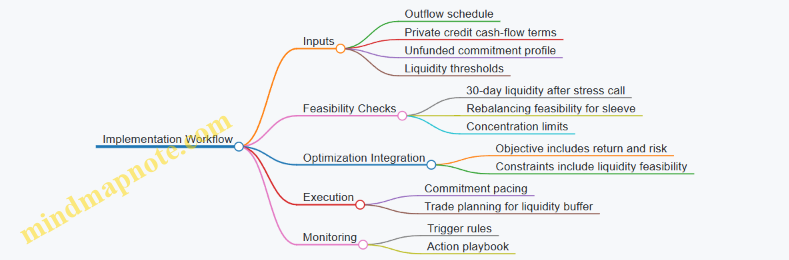
This example shows the practical point: integrating private credit is less about finding a higher expected return and more about ensuring the portfolio can pay its bills without selling the wrong things at the wrong time. Private credit earns its place when liquidity math and sleeve constraints agree with the allocation decision.
10. Implementation Planning and Rebalancing Policies
10.1 From Target Weights to Trade Lists: Practical Implementation Steps
Target weights are a decision; trade lists are an execution plan. The implementation step turns “what we want” into “what we can do today,” while keeping risk, liquidity, and operational constraints from quietly undoing the math.
Translate Targets Into an Execution Inventory
Start by converting each target weight into a dollar amount using the current investable base. Then build an inventory of what you already hold, what is pending settlement, and what is restricted.
A simple checklist:
- Investable base: total portfolio value minus excluded assets (e.g., collateral, restricted holdings).
- Current holdings: include positions that will settle before the trade date.
- Pending orders: subtract shares/dollars already in the pipeline.
- Restrictions: bans on certain issuers, minimum lot sizes, or internal custody limits.
Example: If the investable base is $100m and you target 8% in a bond sleeve, the target is $8.0m. If you already hold $7.3m settled and $0.4m is pending to settle after the trade date, you only adjust the $7.3m portion now. Your immediate buy amount becomes $0.7m, not $1.1m.
Compute Trade Quantities with Rounding Rules
Optimization outputs are continuous; markets trade in discrete units. Apply rounding rules consistently so the portfolio ends up close to target without creating avoidable drift.
Common rounding approaches:
- Shares: round to whole shares for equities; use lot sizes for futures and some fixed income instruments.
- Bonds: round by minimum trade size and consider accrued interest handling.
- Cash and FX: treat as separate sleeves with their own rounding and settlement conventions.
Example: A target requires buying 12,345.6 shares. If your trading system only allows 100-share lots, you round to 12,300 or 12,400 based on whether you prefer under- or over-allocation. Document the choice because it affects tracking error.
Apply Feasibility Filters Before You Touch the Market
Not every desired trade is feasible at the intended time. Feasibility filters prevent “paper trades” that fail compliance, settlement, or liquidity checks.
Filters to run:
- Liquidity: compare intended trade size to average daily volume or dealer capacity.
- Market hours and cutoffs: ensure the order can be placed and settled as expected.
- Instrument eligibility: confirm the security is tradable for your account type.
- Settlement constraints: avoid trades that would create unacceptable settlement mismatches.
Example: If you want to buy $25m of a small-cap equity but your liquidity rule caps single-day participation at 0.5% of ADV, you may need to split the order across multiple days or choose a different implementation vehicle.
Convert “How Much” Into “How to Trade”
Once quantities are feasible, decide the execution method. The goal is to reduce implementation shortfall while respecting risk limits.
A practical structure:
- Execution horizon: same-day, multi-day, or event-driven (e.g., after a corporate action).
- Order type: limit vs. market (or passive vs. aggressive) based on liquidity and urgency.
- Participation rate: cap the fraction of volume you consume.
- Risk controls: stop-loss rules for price movement, and exposure caps during execution.
Example: For a large equity rebalance, you might use a passive limit order with a participation cap. If the price moves sharply against you, you switch to a more aggressive order type only if risk limits still allow it.
Build the Trade List as a Structured Output
A trade list should be machine-readable and audit-friendly. Include fields that let you reconcile outcomes later.
Minimum fields:
- Security identifier
- Side (buy/sell)
- Quantity and unit basis
- Target value and expected proceeds
- Execution window
- Order type and participation settings
- Settlement date
- Internal reference ID
Reconcile Expected vs. Realized Outcomes
After execution, compare realized holdings to targets using a reconciliation workflow.
Key reconciliation components:
- Corporate actions and accruals: adjust for coupon, FX rates, and accrued interest.
- Cash movements: dividends, fees, and settlement differences.
- Partial fills: update remaining quantities and re-run feasibility for the remainder.
Example: If a bond buy partially fills at a different yield, the dollar amount may match but the duration exposure shifts. Your reconciliation should flag the exposure drift so the next rebalance step corrects it.
Mind Map of the Implementation Workflow
Mind Map: From Target Weights to Trade Lists
Mini Example End to End
Assume you target three equity positions and one bond sleeve. You compute deltas from settled holdings, round equity quantities to lot sizes, and cap equity trades by participation. For the bond sleeve, you ensure minimum trade size and account for accrued interest in expected proceeds. You then generate a trade list with settlement dates and execution windows. After execution, you reconcile realized weights and check whether the bond sleeve’s duration drift exceeds your tolerance; if it does, you adjust the next rebalance batch rather than forcing a correction immediately.
This workflow keeps the portfolio’s “target” concept intact while making execution practical, testable, and explainable to the people who have to live with the results.
10.2 Rebalancing Frequency, Thresholds, and Drift Management
Rebalancing is the controlled process of moving from target weights to updated weights as markets, cash flows, and private valuations change. The trick is to rebalance often enough to keep risk and exposures aligned, but not so often that transaction costs and operational effort eat the benefit. Think of it as maintaining a thermostat: you don’t adjust it every time the room temperature wiggles by a fraction.
Core Concepts
Target weights come from the allocation policy and the current liquidity plan. Drift is the gap between target and actual weights caused by relative performance, valuation changes, and cash movements. Rebalancing frequency is how often you check whether drift is large enough to act. Thresholds are the rules that decide whether you trade, and drift management is the overall system that keeps the portfolio within acceptable bounds.
A practical way to frame the decision is: “If the portfolio is still within tolerance, we wait; if it’s outside tolerance, we act.” This avoids the common failure mode of rebalancing on autopilot.
Frequency: Choosing a Check Cycle
Most institutions use a layered cadence:
- Monthly or quarterly review for public holdings where prices are observable and trading is straightforward.
- Quarterly or semiannual review for sleeves with slower valuation updates, where the “data refresh” itself is a constraint.
- Event-driven checks triggered by policy-relevant changes such as a mandate update, a liquidity bucket reclassification, or a material cash flow.
Example: Suppose an allocation policy targets 20% investment-grade credit, 10% high yield, and 5% real estate. If you review monthly, you can catch drift early in credit markets. If real estate is valued quarterly, you still review monthly, but you treat the real estate sleeve as “stale” and avoid making trades based on outdated weights.
Thresholds: Turning Drift Into Decisions
Thresholds translate “how far is too far” into measurable rules. Common threshold types include:
- Absolute weight bands: rebalance if an asset class weight moves more than, say, ±1.0% from target.
- Relative bands: rebalance if the deviation exceeds a percentage of target, such as ±10% of the target weight.
- Risk-based thresholds: rebalance if active risk metrics breach limits, such as tracking error or duration deviation.
A simple example: Target equity is 60%. If it rises to 62.0%, a ±1.0% absolute band would trigger action. If it rises to 60.8%, it would not. This is easy to explain to an investment committee and easy to audit later.
To prevent “thrashing,” pair thresholds with minimum trade size rules. If the required trade is too small to justify costs, you defer and let drift accumulate until it becomes meaningful.
Drift Management: Keeping the System Stable
Drift management is not only about thresholds; it’s also about how you execute trades when you do rebalance.
- Use a drift measurement date that matches valuation timing. If you measure weights on the last business day but execute trades a week later, you introduce avoidable mismatch.
- Separate rebalancing from cash-flow management. If you have net contributions, you can often reduce drift without selling by directing new cash to underweight sleeves.
- Apply liquidity-aware execution. For less liquid assets, you may rebalance by adjusting future commitment schedules or using feasible rebalancing windows rather than forcing immediate trades.
Example: You receive a quarterly contribution of 2% of portfolio value. Equity drift is +1.5% overweight, while private credit is -1.0% underweight. Instead of selling equities immediately, you can allocate the contribution to private credit (within its liquidity constraints) and only trim equities if the drift remains outside tolerance after the cash is invested.
Mind Map: Rebalancing Frequency, Thresholds, and Drift Management
Example: A Complete Decision Workflow
Assume a quarterly review date. You compute drift versus target for each sleeve using the latest available valuations.
- Equity: target 60%, current 61.3% → deviation +1.3% exceeds ±1.0% band → rebalance.
- Investment-grade credit: target 20%, current 20.6% → deviation +0.6% within band → no trade.
- Private real estate: target 5%, current 4.7% → deviation -0.3% within band, but valuation is stale → still no trade.
Execution rule: Use available cash first to reduce underweights, then trade liquid assets to bring overweight sleeves back inside tolerance. If the required equity trim is below the minimum trade size, defer trimming and rely on the next cash-flow allocation.
Practical Governance Notes
A rebalancing policy should specify the measurement date convention, the threshold definitions, and the exception process. When these are explicit, the portfolio’s behavior becomes predictable, and committee discussions focus on decisions rather than on whether the rules were applied consistently.
10.3 Managing Cash, Collateral, and Funding for Ongoing Commitments
Cash management is the part of portfolio construction that shows up in real life: subscriptions, distributions, margin calls, and the occasional “we need this by end of day.” For institutional portfolios spanning public and private markets, the goal is simple—ensure commitments can be funded without forcing unwanted sales, while collateral and cash buffers are sized to match actual risk and operational timing.
Core Concepts and Flows
Start with three cash streams that often get mixed together:
- Operating cash: payroll, fees, and administrative payments.
- Trading cash: settlement for public trades and short-term rebalancing.
- Commitment cash: capital calls for private funds and vehicles.
A practical way to avoid confusion is to maintain a cash waterfall ledger that records expected inflows and outflows by week. For example, if a private credit fund calls $8 million in the first week of the month, that cash should be reserved in the same week bucket, not “somewhere in the quarter.”
Liquidity Buckets and Buffer Logic
Use liquidity buckets aligned to operational reality:
- T+0 to T+2 bucket for settlement and immediate margin needs.
- 1 to 4 week bucket for near-term trading and known capital calls.
- 1 to 12 month bucket for scheduled commitments and planned distributions.
- Beyond 12 months bucket for longer-dated private commitments, funded by a mix of expected distributions and policy-driven reserves.
A buffer is not just “extra cash.” It is cash held because timing uncertainty exists. For private markets, timing uncertainty comes from draw schedules and distribution variability. For public markets, uncertainty comes from volatility-driven margin and settlement frictions.
Collateral Management That Doesn’t Surprise You
Collateral requirements depend on the instruments and the counterparty agreement. Treat collateral as a separate constraint from investment cash because it can be demanded quickly and can be non-redeployable.
Key practices:
- Track collateral eligibility: some collateral types are accepted, others are haircutted or rejected.
- Model margin call timing: margin can be called intraday or on a defined schedule depending on the agreement.
- Separate collateral from investment liquidity: do not assume collateral can be used to fund a private capital call.
Example: Suppose your derivatives book requires daily variation margin. If you hold $5 million in a money market fund but it is pledged as collateral, you may still be “liquid” on paper while being unable to meet a $3 million private equity capital call. The fix is operational: maintain an unencumbered cash reserve for commitment funding.
Funding Sources and Their Tradeoffs
Funding for ongoing commitments typically comes from:
- Unencumbered cash held in eligible settlement accounts.
- Planned distributions from existing private positions.
- Public asset liquidity via pre-approved rebalancing rules.
- Committed credit lines used as a bridge.
Each source has a tradeoff. Credit lines add flexibility but require governance around draw approvals and repayment timing. Selling public assets is straightforward but can create unintended exposure changes if done during stress.
A useful rule is to define a funding priority ladder:
- Use unencumbered cash.
- Use near-term distributions.
- Use pre-approved public liquidity actions within defined risk limits.
- Use credit lines only when the first three steps cannot meet the schedule.
Building the Commitment Calendar
Private commitments are not a single number; they are a schedule of calls. Build a commitment calendar that includes:
- Known capital calls with dates.
- Expected calls with ranges.
- Distribution expectations with ranges.
Then translate ranges into cash reserves using a conservative policy. For example, if a fund historically calls 60% of committed capital over 24 months, you can set a policy reserve that assumes a slower distribution pace than the median case. The point is not pessimism; it is avoiding avoidable liquidity stress.
Operational Controls and Governance
Cash and collateral management needs clear ownership and escalation paths.
- Daily reconciliation: confirm cash balances, collateral postings, and settlement positions.
- Weekly liquidity review: compare the cash waterfall ledger to actuals.
- Exception workflow: if a capital call date shifts, trigger an approval path for funding actions.
Example: A private fund sends a notice on 2026-04-15 that a capital call will be due 2026-04-25. If your weekly review happens on Fridays, you should already have a buffer rule that covers a 10-day notice window without forcing sales.
Example: Putting It Together
Assume a multi-sleeve portfolio has a $10 million private credit capital call due in two weeks, while derivatives require potential variation margin. Your process:
- Reserve $10 million in the 1 to 4 week bucket as unencumbered cash.
- Maintain a separate T+0 to T+2 collateral buffer for margin.
- If the private call is delayed by a week, release the reserved amount back into the next bucket only after confirming no additional near-term calls.
- If the call accelerates, use the funding priority ladder: unencumbered cash first, then pre-approved public liquidity actions, then credit line if needed.
This structure keeps the portfolio investable while ensuring commitments are funded on time, with collateral treated as its own operational constraint.
10.4 Monitoring Implementation Shortfalls and Attribution of Deviations
Implementation shortfalls are the gap between what the portfolio was designed to do and what it actually did after trades, cash movements, and operational frictions. Monitoring them well prevents two common failures: blaming performance on markets when the real cause is execution, and blaming execution when the real cause is a policy mismatch.
Core Concepts and What to Measure
Start with three layers of deviation.
-
Policy deviation: the portfolio manager’s target exposures differ from the approved policy or IPS rules. Example: the policy caps single-country equity at 8%, but the portfolio drifted to 10% because rebalancing thresholds were never triggered.
-
Implementation deviation: the intended trades were not executed as planned. Example: a rebalance required buying illiquid credit, but the trade was partially filled, leaving the sleeve under-allocated.
-
Timing and cash deviation: cash flows and settlement timing changed exposures. Example: a quarterly pension contribution arrived later than expected, so the planned buy orders were delayed and the portfolio held cash longer.
A practical monitoring setup tracks each layer separately so attribution has something solid to stand on.
Building a Deviation Ledger
Create a “deviation ledger” for each rebalance date and each sleeve (public equity, public fixed income, private credit, etc.). The ledger should include:
- Target: the approved target weights or risk exposures.
- Pre-trade: actual holdings just before trading.
- Trade intent: the orders placed, including limit prices and expected fill rates.
- Post-trade: holdings after settlement.
- Cash movements: contributions, distributions, fees, and collateral changes.
From this, compute two key diagnostics.
- Allocation shortfall: how far the post-trade weights are from target, ignoring performance.
- Execution shortfall: how far the realized trade outcomes are from the intended execution assumptions.
Attribution Framework from Holdings to Performance
Attribution should move from mechanical differences to return differences.
-
Exposure effect: return differences caused by being under- or over-exposed versus target. Example: if the portfolio was underweight duration by 0.8 years during a rate selloff, the fixed income sleeve will likely underperform.
-
Execution effect: return differences caused by trade timing and price realization. Example: if equity orders executed at higher prices than the model assumed, the sleeve’s realized return will be lower even if the market moved in your favor.
-
Cash drag and carry: return differences caused by cash held temporarily, collateral posted, or delayed settlement. Example: holding 3% in cash for two weeks during a volatile period can materially change realized results.
-
Valuation and smoothing effects for private assets: differences between valuation timing and the model’s cash-flow schedule. Example: a private credit distribution received earlier than modeled can reduce the period’s effective exposure.
A simple way to keep this systematic is to attribute deviations in this order: policy → allocation → execution → cash/valuation → residual.
Mind Map: Monitoring and Attribution Workflow
Example: One Rebalance, Three Deviations
Assume an end-of-quarter rebalance on 2026-04-15 for a multi-sleeve portfolio.
- Policy target: 60% public equity, 30% investment-grade fixed income, 10% cash.
- Pre-trade: equity 58%, fixed income 31%, cash 11%.
- Trade intent: buy 2% equity and sell 1% fixed income, funded by cash.
- Post-trade (after settlement): equity 59.2%, fixed income 30.4%, cash 10.4%.
Allocation shortfall: equity is 0.8% below target, fixed income is 0.4% above target, cash is 0.4% above target.
Now suppose equity orders were partially filled due to limit constraints, and the average fill price was 0.3% worse than the execution assumption. That creates an execution shortfall.
Finally, settlement for the fixed income sale completed two days later than expected, so cash remained higher for longer, creating cash drag.
In attribution, you would first explain the performance gap by the exposure differences (equity underweight and fixed income overweight), then adjust for execution (worse realized prices), then account for cash drag from delayed settlement. Any remaining difference is recorded as residual and investigated for data timing mismatches.
Turning Monitoring Into Better Decisions
Monitoring should end with actions that are specific and testable.
- If allocation shortfalls repeat at the same sleeve, review rebalancing thresholds and liquidity assumptions.
- If execution shortfalls cluster around certain order types, tighten execution rules or adjust order sizing.
- If cash deviations dominate, align cash forecasting with settlement calendars and fee schedules.
The goal is not to eliminate every deviation, but to ensure deviations are understood, quantified, and consistently managed so the portfolio behaves like the one you approved.
10.5 Practical Example: Designing a Rebalancing Policy for a Multi-Sleeve Portfolio
A multi-sleeve portfolio usually has different “rebalancing personalities.” Public sleeves trade daily and can correct drift quickly. Private sleeves have capital calls, distributions, and valuation lags, so they need policies that respect timing and liquidity. The goal of a rebalancing policy is simple: keep the portfolio close to targets while staying within liquidity, transaction cost, and governance limits.
Step 1: Define the Sleeves and Their Rebalancing Levers
Start by listing each sleeve, its target weight, and the mechanism used to adjust it.
- Public equity: rebalance via trades in liquid markets.
- Public fixed income: rebalance via duration and sector tilts plus trades.
- Real assets: rebalance via listed proxies and periodic adjustments.
- Private credit: rebalance via new commitments, capital calls, and distributions.
- Private equity: rebalance via commitment pacing and secondary sales only if allowed.
A practical rule is to separate “weight drift” from “economic exposure drift.” For example, a fixed-income sleeve might stay near its weight target but drift in duration; you can correct duration without changing total weight.
Step 2: Choose Drift Triggers That Match Liquidity
Use different trigger thresholds by sleeve liquidity.
- Liquid sleeves: rebalance when weight drift exceeds 1.0% absolute (e.g., 10.0% target becomes 11.1%).
- Semi-liquid sleeves: rebalance when drift exceeds 2.0% absolute.
- Illiquid sleeves: rebalance only through commitment pacing and cash-flow management, not frequent “weight chasing.”
To avoid constant trading, add a time gate. For liquid sleeves, evaluate triggers monthly. For semi-liquid sleeves, evaluate quarterly. For illiquid sleeves, evaluate at each capital call/distribution cycle.
Step 3: Add Governance and Cost Controls
Rebalancing should not ignore operational reality.
- Turnover cap: limit total turnover to, say, 20% of liquid sleeve notional per quarter.
- Concentration guardrail: never increase a single issuer or manager exposure beyond pre-set limits.
- Cash buffer: keep a minimum cash percentage to fund near-term commitments and margin needs.
A useful operational detail is to define a “trade budget” for each rebalance date. If the budget is exhausted, you postpone lower-priority trades and document the exception.
Step 4: Build the Policy Logic with a Clear Decision Tree
Below is a mind map that turns the above rules into an implementable workflow.
Mind Map: Rebalancing Policy Logic for Multi-Sleeve Portfolios
Step 5: Work Through an Integrated Example
Assume a portfolio with these target weights:
- Public Equity 40%
- Public Fixed Income 25%
- Real Assets 10%
- Private Credit 15%
- Private Equity 10%
Cash buffer is set at 2% of total portfolio value. Turnover cap is 20% per quarter for liquid sleeves.
On a monthly review date, valuations show:
- Public Equity at 42.0% (drift +2.0%)
- Public Fixed Income at 24.0% (drift -1.0%)
- Real Assets at 10.5% (drift +0.5%)
- Private Credit at 14.2% (drift -0.8%)
- Private Equity at 9.6% (drift -0.4%)
Apply triggers:
- Public Equity is outside the 1.0% drift threshold, so it needs action.
- Public Fixed Income is exactly at the boundary; treat it as within range to reduce churn.
- Real Assets is within range.
- Private sleeves are illiquid; do not rebalance by “trading” weight. Instead, check whether the next private credit capital call can be used to reduce the gap.
Now implement trades:
- Sell public equity to reduce from 42.0% toward 40.0%.
- Buy public fixed income only if it helps keep the overall risk profile aligned with the fixed-income role (for example, maintaining target duration). If duration is already correct, you can route purchases to real assets proxies or cash management instruments, but only if those are defined as eligible.
Assume the required equity reduction implies turnover of 12% for the quarter, which is under the 20% cap. Cash after trades remains above the 2% buffer, so no funding exception is triggered.
For private credit, suppose a capital call is scheduled in two weeks for an amount equal to 0.6% of portfolio value. Since private credit is below target, you fund the call as planned. This is rebalancing through cash-flow alignment rather than forced trades.
Finally, document the outcome:
- Liquid sleeves: rebalanced via trades with turnover 12%.
- Semi-liquid sleeves: no action.
- Private sleeves: no weight trades; capital call funded to support target alignment.
- Exceptions: none.
Step 6: Specify What Happens When Constraints Bind
Constraints are not rare; they are part of the policy. If cash falls below the buffer due to an unexpected call, you prioritize:
- Funding commitments required to avoid default or forced liquidation.
- Trades that reduce the largest risk exposures.
- All other trades postponed until the next review date.
This keeps the policy consistent under stress without inventing new rules midstream.
11. Manager Selection, Due Diligence, and Portfolio Construction with Managers
11.1 Manager Universe Definition and Screening Criteria
A manager universe is not a list of names; it is a controlled set of candidates that you can evaluate consistently. The goal is to reduce avoidable surprises by screening for fit, capacity, and operational reliability before you spend time on deeper analysis.
Step 1: Define the Role and What “Good” Means
Start with the sleeve role you need: core, diversifier, return-seeking, or liability-hedging. Then translate that role into measurable requirements. For example, if the sleeve is meant to dampen equity drawdowns, you screen for downside behavior and factor exposure stability, not just average returns.
Example: A pension fund wants a private credit sleeve to provide steady cash flow. “Good” is defined as predictable distributions, limited covenant-free leverage, and disciplined underwriting standards. That definition drives the screening criteria.
Step 2: Build an Initial Universe with Clear Inclusion Rules
Inclusion rules prevent the universe from drifting into “whoever is available.” Use three filters:
- Strategy match: The manager’s stated mandate must align with the sleeve’s role and allowed instruments.
- Track record relevance: Performance history should cover at least one full market cycle for public strategies, and for private strategies should include multiple vintage years.
- Operational eligibility: The manager must be able to support your reporting, custody, and fee/side-letter requirements.
Example: If your policy requires quarterly reporting, a manager that only provides semiannual updates is excluded even if returns look attractive.
Step 3: Screen for Fit Using a Scorecard
A scorecard makes screening repeatable. Use categories that map to real failure modes: investment process, risk behavior, and operations.
- Investment process clarity: Is the strategy’s decision framework documented and consistent across teams?
- Risk behavior: Does the manager’s realized risk match the intended role?
- Implementation discipline: Are exposures stable enough to avoid unwanted factor bets?
- Operational readiness: Can they meet valuation, audit, and reporting timelines?
A slightly playful rule: if you cannot explain how the manager makes money in plain language, you probably cannot monitor it in plain language either.
Step 4: Use Evidence-Based Filters
Screening should rely on observable data, not vibes.
Quantitative filters (examples):
- Style consistency: Compare factor exposures or sector concentration over time.
- Drawdown profile: Check whether losses are concentrated in a few events or broadly distributed.
- Liquidity alignment: For public strategies, verify turnover and market impact assumptions; for private strategies, verify valuation and distribution patterns.
Qualitative filters (examples):
- Team stability: Assess whether key decision-makers have remained consistent.
- Underwriting and credit discipline: For credit, review covenant usage and loss history.
- Governance: Confirm escalation procedures for breaches and valuation disputes.
Step 5: Apply Exclusion Criteria Early
Early exclusions save time. Common exclusion triggers:
- Mandate drift beyond policy limits.
- Repeated reporting delays.
- Material valuation methodology changes without clear explanation.
- Concentration that conflicts with the sleeve’s diversification goal.
Example: A global equity manager shows strong performance but repeatedly violates concentration limits during volatile periods. Even if the average return is good, the sleeve role is not being delivered.
Step 6: Document the Universe Rationale
Every inclusion and exclusion should be traceable. Record the policy requirement, the evidence used, and the decision outcome. This becomes your audit trail for investment committee discussions.
Step 7: Practical Example of a Screening Workflow
Suppose you are screening managers for a public equity quality strategy.
- Inclusion: Mandate must target quality factors; reporting must be monthly; benchmark must be compatible with your policy.
- Quantitative checks: Verify factor exposure stability and turnover consistency; confirm drawdowns are not driven by hidden leverage.
- Qualitative checks: Confirm the investment committee structure and how the team handles model changes.
- Operations: Test whether they can provide holdings-level data within your required timeframe.
- Outcome: Keep managers that pass all hard filters, then rank the remainder using the scorecard for due diligence interviews.
This approach keeps the universe manageable and ensures that the shortlist reflects both investment intent and operational reality.
11.2 Due Diligence: Process, Risk Controls, and Operational Readiness
Due diligence for private markets and complex public mandates is less about finding “perfect” managers and more about verifying that the manager can consistently do what they say they will do, even when markets get annoying. A good process starts with clarity on what decisions the manager controls, what they can’t control, and how they report both.
Due Diligence Workflow That Matches Real Decision Cycles
Begin with a document-and-interview pass that maps the manager’s workflow to your investment policy. Collect the investment management agreement, fee schedule, side letters, valuation policy, custody arrangements, and reporting templates. Then run structured interviews with the people who actually execute: portfolio managers, risk staff, operations, and the team responsible for valuations and capital calls.
Next, test the workflow with evidence. Ask for trade examples, allocation records, and exception logs from the last 12–24 months. For private strategies, request sample capital call notices, distribution statements, and the manager’s internal valuation memos for a few quarters. The goal is to see whether the process is repeatable, not whether it produced a good outcome.
Finally, convert findings into a decision package: a risk summary, operational readiness assessment, and a list of conditions for approval. If you can’t write conditions in plain language, you probably haven’t identified the real risk.
Risk Controls That Are Specific Enough to Audit
Risk controls should be tied to the manager’s actual exposures. Start with a control inventory: limits, monitoring cadence, escalation paths, and how breaches are handled. Then verify that the controls are used, not merely documented.
Key areas to examine:
- Investment risk: position limits, concentration rules, leverage controls, and factor or sector exposures. Example: if the manager claims diversification, request a month-end holdings snapshot and compare it to their stated concentration limits.
- Liquidity risk: for private credit and real assets, check how the manager estimates liquidity needs, manages redemption or transfer requests, and handles delayed cash receipts. Example: review a period when distributions were slower than expected and see how the manager communicated and managed cash.
- Valuation risk: confirm the valuation methodology, governance, and independence. Example: ask how they treat a single underperforming asset and whether valuation committees review it with documented rationale.
- Model and data risk: for strategies using internal models, verify data lineage, validation steps, and how stale or corrected data is handled. Example: request a case where a pricing input was corrected and trace how it affected reported NAV.
- Operational risk: confirm trade capture, settlement processes, corporate actions handling, and reconciliation. Example: pick one quarter and verify that cash movements reconcile to statements without manual heroics.
Operational Readiness That Covers People, Process, and Systems
Operational readiness is easiest to assess when you treat it like a checklist for “can they run the machine every month.” Evaluate:
- Staffing and coverage: who covers what during vacations, turnover, or system outages. Example: ask who signs off on valuation and whether there is a documented backup.
- Systems: order management, portfolio accounting, valuation workflow, and document management. You don’t need the vendor names; you need to know whether the workflow can be traced.
- Reconciliation and controls: bank reconciliations, custody statements, and variance thresholds. Example: request the last three reconciliation exceptions and how they were resolved.
- Reporting quality: timeliness, completeness, and consistency across public and private sleeves. Example: compare two reporting cycles and check whether the same fields appear with the same definitions.
- Governance: committees, approval authorities, and escalation procedures. Example: ask for the last committee agenda and minutes summary, then verify that actions were tracked.
A practical way to structure this is to score each area against evidence strength: “policy only,” “process demonstrated,” or “process evidenced with records.” Evidence beats confidence.
Mind Map: Due Diligence Inputs, Tests, and Outputs
Example: Turning Findings Into Conditions
Suppose the manager’s valuation policy states that an independent committee reviews hard-to-value assets, but your evidence request shows committee notes are sparse and exceptions are handled informally. A reasonable condition is not “improve valuation,” but “provide committee minutes with documented rationale for all Level 3 assets for the next two quarters, and report exception counts and resolution timelines.”
Similarly, if liquidity monitoring exists but breach escalation is unclear, require a written escalation protocol and a sample of how it was used during a delayed distribution period. These conditions are measurable, so later monitoring is less guesswork and more accounting.
Mind Map: Risk Controls to Verify
Case Study: A Simple Operational Failure Test
Pick one recent month and trace a single asset from trade or acquisition through valuation to reporting. Confirm that:
- The trade was captured correctly and approved per policy.
- Settlement and cash movements reconcile to custody and bank statements.
- Valuation inputs were sourced and approved.
- The reported NAV or mark-to-market reflects the same valuation date and methodology.
- Any exceptions were logged and resolved with documented rationale.
If you can’t complete the trace without relying on informal explanations, that’s an operational readiness gap. It may not break the strategy tomorrow, but it will complicate monitoring when you need clarity quickly.
11.3 Performance Evaluation: Net vs. Gross, Fees, and Benchmark Alignment
Performance evaluation is where the investment story either holds up or quietly falls apart. The goal is simple: compare what the portfolio actually delivered to what the benchmark would have delivered, after accounting for the costs and frictions that make institutions different from backtests.
Net Versus Gross Returns
Gross returns represent the investment manager’s performance before fees. Net returns represent what the investor receives after fees and expenses. In practice, “gross” can still include some costs, depending on reporting conventions, so you should treat gross as “manager-reported before stated fees” rather than “cost-free.”
A practical way to keep this straight is to define three layers in your evaluation workbook:
- Manager gross: performance before management fees (and sometimes before certain fund-level expenses).
- Investor net: performance after management fees and fund-level expenses.
- Policy net: investor net adjusted for any additional institutional costs you control, such as custody, trading, or internal overlays.
Example: Suppose a manager reports 8.0% gross for a year. If the fee schedule is 1.0% and fund expenses are 0.3%, the investor net is roughly 6.7% (ignoring compounding nuances for simplicity). If your policy net includes an extra 0.1% custody cost, your policy net becomes 6.6%. That 0.1% difference matters when you compare managers or evaluate whether a strategy is “worth it.”
Fees That Actually Matter
Fees are not one number; they are a structure. Separate them into categories so you can explain performance differences without hand-waving.
- Management fees: typically tied to assets under management.
- Performance fees: tied to returns, often with hurdles and high-water marks.
- Transaction and financing costs: sometimes embedded in reported returns, sometimes not.
- Fund expenses: administration, audit, legal, and other operating costs.
When performance fees exist, the same gross return can produce different net outcomes depending on prior peaks. That means you should evaluate fees using the manager’s reported fee accruals and the actual net-of-fee series, not just the fee rate.
Benchmark Alignment That Avoids False Comparisons
A benchmark is only useful if it matches the portfolio’s economic exposures and evaluation mechanics. Misalignment creates “free alpha” or “free underperformance” that is not attributable to skill.
Start with four alignment checks:
- Asset class and risk profile: Does the benchmark represent the same opportunity set?
- Currency and hedging: Are returns measured consistently, including FX hedging rules?
- Timing and valuation: Are measurement dates and valuation conventions comparable?
- Cost and implementation: Does the benchmark assume reinvestment and trading costs consistent with the portfolio?
Example: If a manager runs a low-turnover strategy but the benchmark is a high-turnover index, the benchmark’s implied trading friction may be lower than what the manager experiences. If you compare raw index returns to manager net returns, you may penalize the manager for costs the benchmark never pays.
A common fix is to use a benchmark net-of-cost approach. You estimate an implementation cost for the portfolio (or for the benchmark replication) and apply it consistently. Even a simple cost model improves interpretability.
A Systematic Evaluation Workflow
Use the same sequence every time so results are comparable across managers and quarters.
- Normalize return series: ensure the same frequency, currency, and compounding basis.
- Reconcile gross to net: compute the implied fee drag and verify it matches the fee schedule and reported expenses.
- Compute benchmark-relative metrics: use net-of-fee portfolio returns versus an aligned benchmark series.
- Attribute active risk: separate allocation effects from selection effects when holdings are available.
- Check for reporting artifacts: confirm whether cash flows, valuation lags, or smoothing affect the time series.
Performance Evaluation Mind Map
Example: Putting It Together in One Review
Assume a manager reports:
- Manager gross return: 9.2%
- Reported net return: 7.4%
- Fee drag implied: 1.8%
Your aligned benchmark net-of-cost return is 7.1%. The manager’s net alpha is 0.3% (7.4% minus 7.1%). If you instead compared to the benchmark’s raw index return of 7.8%, you would conclude the manager underperformed by 0.4%, even though the difference is mostly benchmark cost and implementation mismatch. The evaluation becomes meaningful only after the net-versus-gross and benchmark-alignment steps are done consistently.
The practical takeaway is that “performance” is not a single number. It is a chain of definitions and comparisons. When each link is explicit—what was gross, what was net, and what the benchmark assumed—the investment committee can focus on decisions rather than accounting mysteries.
11.4 Portfolio Construction with Managers: Diversification and Overlap Analysis
Manager-based investing is a practical way to access skills, but it also creates a new risk: you can accidentally buy the same bet multiple times through different managers. Portfolio construction with managers therefore starts with a clear mapping from manager exposures to the institution’s intended risk sources.
Step 1: Define What Diversification Means for Your Mandate
Diversification is not “own more managers.” It is “own managers whose returns come from different, controllable drivers.” Begin by restating the mandate’s target risk sources, such as duration for fixed income, equity factor exposures for public equity, or credit spread sensitivity for private credit. Then translate those sources into measurable proxy exposures.
Example: If your policy portfolio aims for equity beta around 60% and a low-volatility tilt, two equity managers can both look “diversified” by style label while still holding the same high-beta growth stocks. Your diversification definition should catch that.
Step 2: Build a Manager Exposure Map
Create an exposure map that converts each manager’s holdings or reported characteristics into a common set of risk dimensions. Use what you can reliably obtain: factor models, sector weights, duration buckets, credit quality distributions, and liquidity or leverage measures. Keep the mapping consistent across managers so overlap is measurable rather than vibes-based.
A useful rule: if two managers cannot be compared on the same exposure dimensions, you cannot quantify overlap. That is not a reason to stop; it is a reason to improve the data pipeline.
Step 3: Measure Overlap Using Multiple Lenses
Overlap has at least three forms.
- Holdings overlap: similarity in top positions or sector weights.
- Factor overlap: similarity in factor exposures such as value, momentum, quality, size, or interest-rate sensitivity.
- Risk overlap: similarity in how the manager tends to lose money, captured by drawdown drivers or scenario sensitivities.
Use at least two lenses. Holdings overlap alone can miss shared factor risk. Factor overlap alone can miss concentration in a single sector.
Step 4: Turn Overlap Into Portfolio Constraints
Once overlap is quantified, convert it into constraints that the optimizer or allocation committee can enforce. Common constraints include:
- Maximum similarity thresholds between managers on key factors.
- Limits on combined exposure to a single risk driver, such as duration bands, credit rating buckets, or equity factor tilts.
- Concentration limits at the portfolio level, such as maximum sector weight or maximum single-name exposure for managers that report holdings.
Example: Suppose Manager A and Manager B both show high exposure to the same equity momentum factor. If your policy portfolio already has a momentum tilt from another sleeve, you can cap the portfolio’s net momentum exposure or require that the combined momentum contribution stays within a band.
Step 5: Use a “Diversification Budget” Approach
A diversification budget makes the trade-off explicit: you allocate risk capacity to each sleeve, and overlap consumes that capacity. This prevents the common failure mode where the committee approves multiple managers that each “adds diversification,” but the total portfolio ends up concentrated in one driver.
Example: If your risk budget for credit spread duration is 25% of total risk contribution, then any manager whose credit spread sensitivity is highly correlated with your existing credit sleeve should draw more budget per unit weight.
Step 6: Validate with Scenario-Based Stress Tests
Overlap analysis based on static exposures can miss regime behavior. Add scenario stress tests that apply consistent shocks across managers, then compare how each manager’s expected losses respond. This is especially important when managers use different instruments to express similar views.
Example: Two managers may both hold “investment-grade credit,” but one may be more sensitive to downgrade risk while the other is more sensitive to rate-driven spread changes. Scenario tests separate these.
Step 7: Practical Allocation Workflow
A systematic workflow reduces committee churn.
- Collect manager data and map to common exposures.
- Compute overlap metrics across holdings, factors, and scenarios.
- Translate overlap into constraints and risk budgets.
- Build candidate portfolios and check both expected risk and overlap.
- Document the rationale in terms of risk drivers, not manager narratives.
Case Study: A pension fund has three public equity managers and one private credit manager. Two equity managers show low sector overlap but high factor overlap in quality and value. The committee initially weights them equally. After overlap constraints are added, the optimizer reduces the combined value tilt and increases exposure to a different factor mix from the third equity manager, while keeping total equity beta stable. The result is a portfolio that still uses all managers but avoids paying twice for the same factor bet.
Step 8: Ongoing Re-Checks and Governance
Overlap is not a one-time calculation. Managers change holdings, and the mapping from holdings to factors can drift. Recompute overlap at a fixed cadence and trigger a review when overlap metrics breach thresholds. Governance should specify who can approve exceptions and what evidence is required, so “we’ll fix it later” never becomes a strategy.
11.5 Practical Example: Building a Manager Portfolio With Constraints and Risk Limits
You are building a manager portfolio for an institutional multi-asset mandate. The goal is not just to pick managers, but to combine them so the total portfolio respects constraints and stays inside agreed risk limits.
Step 1: Start with the Mandate in Plain Terms
Assume the investment policy states: target 60% public markets and 40% private markets, with a maximum expected tracking error versus the blended benchmark of 3.0%, a maximum single-manager risk contribution of 2.5% of portfolio volatility, and a liquidity rule that limits near-term cash drag. You also have governance constraints: no more than 25% in any one strategy family and at least 3 independent managers per major sleeve.
A practical way to translate this into inputs is to define each manager’s “role” and “behavior.” For example, a core bond manager should behave like duration exposure with limited credit drift, while a private credit manager should behave like spread risk with cash-flow stability. You will use these behaviors to set constraints that are meaningful, not just numeric.
Step 2: Build a Manager Data Sheet That Supports Constraints
For each manager, collect:
- Net-of-fee return history and benchmark-relative returns
- Risk estimates: volatility, downside measures, and factor exposures (rates, equity beta, credit spread, real assets)
- Liquidity profile: expected capital call and distribution timing for private strategies
- Operational limits: leverage usage, concentration limits, and valuation practices
Example: Manager A (core bonds) has stable duration and low turnover. Manager B (global equity) has higher equity beta and moderate factor tilts. Manager C (private credit) has lower mark-to-model volatility but slower liquidity.
Step 3: Convert Risk Limits Into Portfolio Rules
You need portfolio-level limits that can be checked after optimization.
- Tracking error limit: constrain the active return variance versus the blended benchmark.
- Concentration limit: cap any single manager weight and any single strategy family weight.
- Risk contribution limit: require each manager’s marginal contribution to total volatility to be below the agreed threshold.
- Liquidity limit: enforce a maximum weight in sleeves with capital call timing that would breach cash availability.
A simple numeric example helps. If the portfolio volatility target is 8.0% and the single-manager risk contribution limit is 2.5% of portfolio volatility, then each manager’s contribution should be at or below 0.20% (because 2.5% of 8.0% equals 0.20%).
Step 4: Use a Two-Layer Construction Approach
Layer 1 sets sleeve weights. Layer 2 allocates within each sleeve.
- Sleeve weights: public vs private, plus major asset categories.
- Within-sleeve weights: manager selection and sizing.
This avoids a common failure mode: letting the optimizer “solve” everything at once and producing a portfolio that meets tracking error but violates liquidity or governance rules.
Step 5: Run the Optimization with Hard and Soft Constraints
Use hard constraints for governance and liquidity, and soft constraints for preferences like diversification.
Hard constraints example:
- Total weight equals 100%
- Public/private split equals 60/40
- Each major sleeve has at least 3 managers
- No manager exceeds 10% weight
- Private liquidity rule: capital call schedule must fit cash buffer
Soft constraints example:
- Prefer lower turnover managers
- Prefer balanced factor exposures across sleeves
- Penalize overlap where two managers load heavily on the same factor
Step 6: Check the Results with Diagnostics, Not Just the Objective
After you obtain weights, compute:
- Active risk versus benchmark: confirm tracking error is under 3.0%
- Risk contributions: confirm each manager is under the 0.20% volatility contribution threshold
- Factor exposure totals: verify the portfolio’s rates, equity beta, and credit spread exposures align with the mandate’s intent
- Liquidity stress: confirm that capital calls do not force unwanted sales in public sleeves
If Manager B and Manager D both load strongly on the same equity factor, the optimizer may still meet tracking error while creating hidden concentration. The diagnostic step catches that.
Step 7: Document the Decision Logic for the Investment Committee
Your write-up should connect each constraint to a governance reason and show how the portfolio satisfies it.
Example narrative:
- “We capped single-manager weight at 10% to prevent operational and model risk concentration.”
- “We limited single-manager volatility contribution to 0.20% to keep diversification effective even under stress.”
- “We enforced the 60/40 public/private split and liquidity fit to avoid cash-flow-driven deviations from the policy.”
Mind Map: Manager Portfolio Construction with Constraints and Risk Limits
Example: A Constraint-Driven Outcome
Suppose the optimizer wants to increase Manager C (private credit) because its historical spread returns look attractive. The liquidity constraint blocks that increase because capital calls would exceed the cash buffer during a specific quarter. The final solution therefore reallocates within private credit to a second manager with a slower call profile, keeping the private sleeve weight intact while satisfying the liquidity rule.
That is the point of constraints: they force the portfolio to behave like an institution, not like a spreadsheet with good intentions.
12. Governance, Monitoring, and Reporting for Ongoing Allocation Management
12.1 Investment Committee Materials: Content, Frequency, and Decision Framework
Investment Committee (IC) materials should make decisions easier, not just better informed. The goal is a consistent package that connects objectives to actions, shows what changed since the last meeting, and records why the IC chose one path over another.
Core Purpose and Audience
IC members typically need three things: (1) a clear decision request, (2) the evidence supporting it, and (3) the operational implications. A good packet assumes members will skim first, then ask targeted questions. That means the first page must answer: What are we deciding, what options exist, and what risks are we accepting?
Packet Structure That Works
A reliable order reduces friction and prevents “where is that chart?” meetings.
- Decision Summary: One page with the exact motion (approve, revise, defer), the recommended option, and the effective date (use a fixed example date such as 2026-04-15 when illustrating timelines).
- Context and Policy Alignment: A short section linking the request to the Investment Policy Statement (IPS) and any relevant liquidity or concentration rules.
- What Changed Since Last IC: A concise delta view covering performance, risk, liquidity, and any private-market valuation updates.
- Evidence and Diagnostics: Risk and return metrics, scenario results, and attribution that explain drivers rather than just listing numbers.
- Options Considered: At least two feasible alternatives, including the “do nothing” baseline.
- Implementation and Governance: Trade or commitment steps, manager actions if applicable, and compliance checks.
- Risks, Open Questions, and Mitigations: Specific items with owners and timing.
- Appendix: Detailed tables, model assumptions, and data-quality notes.
Mind Map: IC Packet Logic
Frequency That Matches Decision Types
Frequency should reflect how quickly the information becomes stale.
- Monthly: Performance and risk monitoring, liquidity status, and any manager-level issues that require IC awareness.
- Quarterly: Allocation reviews, rebalancing proposals, and private-market pacing updates with valuation methodology reminders.
- Semiannual or Annual: IPS refresh, benchmark review, policy limit updates, and major methodology changes (such as covariance or liquidity modeling approaches).
A practical rule: if the IC is being asked to approve something that changes exposures, the packet should include the latest data and a clear implementation timeline. If the IC is only monitoring, the packet can be shorter but must still show whether policy limits are being respected.
Decision Framework That Prevents “Good Discussion, No Action”
Each decision request should follow a consistent logic chain.
- Define the Decision: Example motion: “Approve a shift of 1.0% from public equity to high-quality short-duration bonds effective 2026-04-15.”
- State the Constraint Set: Liquidity bucket rules, concentration limits, leverage restrictions, and any mandate-specific requirements.
- Specify the Objective: Reduce funding risk, improve diversification, maintain tracking error within tolerance, or control downside exposure.
- Present Feasible Options: Include at least one alternative that is conservative and one that is more responsive to the objective.
- Quantify Trade-offs: Show how each option changes expected risk, liquidity usage, and implementation complexity.
- Assign Ownership: Name who implements, who monitors, and what triggers escalation.
- Record the Rationale: Capture the key reason the IC chose the recommended option, not every supporting detail.
Integrated Example: Quarterly Allocation Review Packet
Assume the IC meets to review a quarterly rebalancing. The packet’s delta section highlights that public equity volatility rose and that private credit distributions were slower than expected. The evidence section includes a liquidity-aware scenario showing that the proposed rebalancing does not breach near-term cash needs. The options section compares three choices: do nothing, rebalance within existing liquidity buckets, or temporarily reduce a less liquid sleeve. The implementation section lists the trade dates for public assets and the commitment pacing adjustments for private assets. The risks section notes valuation timing uncertainty for private credit and specifies a monitoring cadence and escalation trigger.
Quality Checks Before the Meeting
Materials should be internally consistent and decision-ready.
- Metric Consistency: Use the same benchmark definitions and time windows across sections.
- Limit Checks: Highlight any breaches or near-breaches with proposed remediation.
- Assumption Transparency: Summarize model inputs that materially affect outcomes.
- Actionability: Every recommendation must include what will happen next, by whom, and when.
When these elements are present, the IC can spend time on the few questions that matter: whether the decision fits the policy, whether the trade-offs are acceptable, and whether implementation is realistic.
12.2 Ongoing Monitoring: Risk, Liquidity, Valuation, and Covenant Checks
Ongoing monitoring turns the investment policy from a document into a daily operating system. The goal is simple: detect when reality starts drifting away from the rules, then explain why and what to do next.
Risk Monitoring That Matches How You Actually Take Risk
Start with a risk inventory aligned to the portfolio’s sleeves and instruments. For public holdings, monitor exposures to the intended risk factors (rates, credit spreads, equity beta, FX, and sector tilts) and compare them to policy limits. For private holdings, monitor the risk drivers that show up in cash flows and valuation mechanics, such as leverage at the borrower level, tenant concentration in real estate, or underwriting assumptions in private credit.
A practical workflow uses three layers:
- Position-level checks for breaches (e.g., duration outside a band, single-name credit exposure too large).
- Portfolio-level diagnostics for unintended concentration (e.g., factor exposures that moved because correlations changed).
- Model sanity checks for inputs (e.g., yield curves, credit spreads, discount rates, and assumptions used in valuation).
Example: If a fixed-income sleeve’s duration target is 4–6 years, a duration drift to 7.2 years should trigger both a limit breach and a root-cause question: was it a deliberate hedge change, a benchmark reconstitution, or a data issue?
Liquidity Monitoring That Respects Settlement Reality
Liquidity monitoring should be tied to actual cash needs: distributions, capital calls, margin, and operational cash buffers. Divide liquidity into buckets by time horizon (same week, 1–3 months, 3–12 months, and beyond) and map each holding’s expected cash behavior.
For public assets, track bid-ask spreads, market depth proxies, and historical trading volumes. For private assets, track commitment schedules, expected cash flows, and the time lag between valuation dates and cash events.
A simple but effective check is the liquidity coverage ratio: available liquid resources divided by near-term cash obligations. If the ratio falls below the internal threshold, you don’t need a crisis meeting—you need a plan: reduce new commitments, adjust rebalancing timing, or shift some public exposure toward more liquid instruments.
Valuation Monitoring That Separates Price from Process
Valuation monitoring has two parts: whether the numbers are plausible, and whether the process is consistent.
For public markets, validate that pricing sources and corporate action handling are correct. For private markets, focus on valuation governance: who sets the assumptions, how often they are updated, and whether the valuation method matches the asset type.
Use a valuation variance check to compare valuation changes to what fundamentals would suggest. Example: if a private credit fund’s mark-to-model spread widens sharply while public credit indices are stable, investigate whether the change reflects a real credit deterioration or a model-input update.
Also monitor staleness. A valuation that is technically current but based on old underlying data can still mislead risk reporting.
Covenant Checks That Prevent Quiet Breaches
Covenant monitoring should be instrument-specific and tied to the legal documentation. Build a covenant register that lists: covenant definition, measurement frequency, calculation formula, reporting party, and cure/waiver process.
Then add two operational checks:
- Calculation traceability: the numbers used in the covenant test should be reproducible from stored inputs.
- Event triggers: identify conditions that require immediate escalation, such as missed reporting deadlines, covenant measurement dates approaching, or changes in borrower reporting quality.
Example: A private credit tranche may have a leverage covenant tested quarterly. If the borrower’s latest financials arrive late, the monitoring system should flag the missing inputs and specify the interim action (e.g., hold distributions, increase reserves, or request updated statements).
Mind Map: Ongoing Monitoring Coverage
Integrated Example: One Quarter’s Monitoring Pack
Assume a multi-sleeve portfolio with public bonds, public equities, and a private credit allocation. The monitoring pack should include:
- A risk summary showing factor exposures versus policy bands, plus any limit breaches with root-cause tags.
- A liquidity table by horizon listing cash obligations (including capital calls) and available liquid resources, ending with the liquidity coverage ratio.
- A valuation section comparing valuation changes to expected drivers, highlighting any staleness or process changes.
- A covenant dashboard listing upcoming tests, current status, and any missing inputs.
To keep the workflow coherent, each item should end with one of three outcomes: within policy, requires action, or requires clarification. That last category matters; it prevents “we’ll fix it later” from becoming a permanent lifestyle.
12.3 Performance Attribution Across Public and Private Components
Performance attribution answers a simple question: “Where did the return come from, and which decisions caused it?” For portfolios mixing public and private assets, the main challenge is that the return mechanics differ. Public holdings mark daily; private holdings mark periodically and often reflect cash flows plus valuation changes. A good attribution framework respects those mechanics while still producing one coherent story for the investment committee.
Core Attribution Logic
Start with a decomposition that works for both public and private sleeves:
- Total return is split into income/carry, price/valuation change, and cash-flow effects.
- Active return is split into allocation effects (where you invested) and selection effects (what you chose within a sleeve).
- Risk and liquidity constraints explain why some effects are persistent (for example, private valuation smoothing) and others are temporary (for example, timing of capital calls).
A practical way to unify sleeves is to attribute at two levels:
- Top-down: public vs. private vs. cash, using a policy benchmark that matches each sleeve’s role.
- Bottom-up: within each sleeve, attribute to sub-asset classes and then to managers or strategies.
Public Component Attribution
For public assets, use a benchmark-relative framework with daily or monthly data:
- Allocation effect: difference between your sleeve weight and benchmark sleeve weight, multiplied by the benchmark sleeve return.
- Selection effect: difference between your sleeve return and benchmark sleeve return, holding your sleeve weight constant.
- Within-sleeve manager effect: active return of each manager versus its assigned benchmark.
Example: Suppose the public credit sleeve benchmark returns 6.0% and your sleeve returns 6.6% while your sleeve weight is 30% versus a benchmark weight of 25%. Allocation contributes (0.30−0.25)×6.0% = 0.30% and selection contributes 0.30×(6.6%−6.0%) = 0.18%. The remaining difference is explained by any cash drag or implementation frictions you include in the sleeve return definition.
Private Component Attribution
Private returns require a cash-flow-aware approach. A common pitfall is treating private “period return” like a public mark-to-market return. Instead, treat private performance as:
- Valuation change on existing holdings.
- Income/carry earned during the period.
- Cash-flow timing effects from capital calls and distributions.
A workable method is to compute a time-weighted return for valuation changes and a separate cash-flow contribution for capital calls and distributions. Then you can attribute active effects using the same allocation/selection structure, but with sleeve returns defined consistently.
Example: Your private credit sleeve has a benchmark return of 5.0% for the period, while the sleeve’s valuation change is 5.4%. If you also had net capital calls that increased invested capital during the period, the cash-flow contribution may add or subtract from the realized total return depending on whether the interim cash was held in short-term instruments.
Integrated Attribution Workflow
Use one workflow so the committee sees a single chain of causality.
- Define sleeve benchmarks that match liquidity and valuation mechanics.
- Standardize return definitions: public uses mark-to-market; private uses valuation change plus cash-flow effects.
- Compute active return at the sleeve level.
- Decompose active return into allocation and selection.
- Drill down into manager or strategy effects within each sleeve.
- Reconcile: ensure the sum of components equals total active return after including cash and timing items.
Mind Map: Attribution Building Blocks
Integrated Example with Reconciliation
Assume a portfolio with 60% public and 40% private. The policy benchmark active return is +0.80% for the period.
- Allocation effect (public vs. private): +0.30%
- Selection effect in public sleeve: +0.25%
- Selection effect in private sleeve: +0.20%
- Cash and timing reconciliation (interim cash on private capital calls plus any sleeve-level implementation items): +0.05%
The committee takeaway is not just “we added 0.80%,” but “0.30% came from where we were positioned, 0.45% came from how the sleeves performed versus their benchmarks, and 0.05% came from timing and cash mechanics.” That last piece is often the difference between a clean story and a confusing one.
Common Failure Modes and Fixes
- Mixing return definitions: if private returns include cash-flow effects but public returns do not, allocation and selection comparisons become misleading. Fix by standardizing definitions at the sleeve level.
- Ignoring interim cash: capital calls held in cash can dilute or enhance performance depending on rates. Fix by explicitly including interim cash treatment in the reconciliation.
- Double counting: manager-level active effects plus sleeve-level active effects can overlap if benchmarks are not aligned. Fix by choosing one hierarchy and enforcing it in the calculation.
A strong attribution package ends with a short, factual explanation tied to the computed components. If a driver is not in the decomposition, it should not appear in the narrative.
12.4 Policy Compliance Testing and Exception Management
Policy compliance testing answers one question: “Are we doing what we said we would do?” It is not a paperwork exercise; it is a control system that catches drift, data issues, and process failures before they become investment problems.
Core Concepts and Control Objectives
Compliance testing typically targets four failure modes. First, authorization failures occur when trades or commitments exceed delegated authority. Second, exposure failures occur when portfolio weights, sector limits, credit quality, or liquidity buckets breach policy. Third, valuation and reporting failures occur when inputs used for decisions or monitoring are inconsistent with policy definitions. Fourth, process failures occur when required steps are skipped, such as missing approvals or incomplete documentation.
A good control objective is measurable. For example, “No single issuer exceeds 5% of market value” is testable, while “Keep concentration reasonable” is not.
Designing the Test Plan
Start with a policy-to-test mapping. Each policy clause becomes a testable rule with a data source, a calculation method, a frequency, and an owner. Frequency should match materiality: daily checks for obvious breaches, monthly checks for slower-moving exposures, and event-driven checks for corporate actions or cash-flow changes.
Use three layers of testing. Preventive controls reduce the chance of breach at execution time, such as pre-trade limit checks. Detective controls identify breaches after the fact, such as end-of-day position reviews. Corrective controls ensure breaches are resolved, such as documented remediation steps and follow-up training.
Building the Rules Engine in Plain Language
Most policy rules can be expressed as calculations. Examples include:
- Concentration: issuer exposure as a percentage of total portfolio market value.
- Duration limits: portfolio duration computed using the same methodology as the policy.
- Liquidity buckets: classification based on policy-defined instrument categories.
- Private market commitments: total committed capital versus policy caps, measured against the same commitment definition used in reporting.
The key is consistency. If the policy defines “market value” net of cash, but monitoring uses gross market value, you will get false exceptions and lose trust in the process.
Exception Taxonomy and Severity
Not all exceptions are equal. Classify exceptions so remediation is proportional.
- Type A: Breach of a hard limit (e.g., issuer cap) or a governance violation (e.g., approval missing).
- Type B: Breach of a soft limit or a threshold that is allowed with conditions (e.g., temporary drift with a defined cure period).
- Type C: Data or methodology issues causing incorrect calculations (e.g., stale pricing, wrong factor mapping).
Severity drives response time. Type A requires immediate containment and documented decision-making. Type C requires correction of data or methodology and a re-run of tests.
Mind Map: Policy Compliance Testing and Exception Management
Example: Concentration Breach with a Clear Cure
Assume policy states: “No issuer above 5% of portfolio market value.” On month-end testing, Issuer X is at 5.6% due to a price move after a trade that was within limits.
Step 1: Contain. Confirm whether the breach is real or a calculation artifact by verifying pricing and position data.
Step 2: Classify. If the limit is hard, this is Type A even if the cause is market movement.
Step 3: Cure plan. If policy allows a cure window, propose trades to reduce exposure back to or below 5% by the cure deadline. If no cure window exists, escalate for an exception approval.
Step 4: Document. Record the calculation, the cause, the proposed remediation, approvals, and the re-test result.
This example shows why testing must be paired with a remediation pathway; otherwise, you only learn about the breach, not how it gets fixed.
Example: Data Issue That Would Otherwise Create Noise
Suppose private credit commitments are reported using a “committed capital” definition, but the monitoring system mistakenly uses “funded capital.” The test flags multiple breaches.
Step 1: Classify as Type C because the rule is being applied to the wrong definition.
Step 2: Correct the mapping so the commitment definition matches policy.
Step 3: Re-run tests and update the exception log to show the resolution.
The goal is to prevent repeated false exceptions that train teams to ignore the dashboard.
Exception Workflow That Stays Auditable
A practical workflow has five required artifacts: the exception record, evidence of the calculation, classification (Type A/B/C), containment actions, and final resolution proof.
A minimal exception log should include: portfolio identifier, policy rule reference, measurement date, measured value, limit value, classification, owner, approval status, remediation action, and re-test outcome.
When root-cause analysis is performed, it should focus on the control failure, not blame. If the cause is missing data feeds, the corrective action is a process fix, such as validation checks before month-end.
Reporting for Investment Committee and Operations
Reporting should separate “what happened” from “what changed.” The committee needs a concise summary of Type A exceptions, their remediation status, and whether any governance approvals were required. Operations needs the evidence trail and the corrected definitions so the same mistake does not reappear.
The best compliance reporting makes the next action obvious: either the breach is cured and re-tested, or the exception is approved with a documented cure plan and deadline.
12.5 Practical Example: Creating a Quarterly Allocation Dashboard and Review Workflow
A quarterly allocation dashboard should answer four questions quickly: What changed, why it changed, what risk it created, and what decisions are needed next. The workflow below assumes a multi-sleeve portfolio with both public and private holdings, and it uses a consistent cadence so the Investment Committee (IC) can compare quarters without re-learning the template.
Step 1: Define the Quarter’s “Single Source of Truth”
Start by locking the data cut rules. Use one valuation date for public marks and one for private marks, then record any timing differences as a footnote in the dashboard header. For example, if public prices are pulled as of 2026-04-15 and private valuations are as of 2026-04-30, the dashboard should show both dates and label the private section as “as reported.” This prevents confusion when performance and risk metrics appear slightly out of sync.
Step 2: Build the Dashboard Layout
Use a top-down structure: portfolio summary, sleeve detail, risk and liquidity, and governance checks.
Portfolio Summary
- Target vs. actual weights by sleeve (core, satellite, diversifier).
- Total portfolio return and return attribution split into public vs. private.
- Cash and commitment status for private markets.
Sleeve Detail
For each sleeve, show:
- Benchmark used and active weight.
- Net performance and key drivers (duration for fixed income, factor exposure for equities, credit spread for credit).
- Liquidity bucket classification and any policy breaches.
Risk and Liquidity
- Tracking error vs. policy band.
- Concentration metrics (top holdings, sector, country, and issuer exposure).
- Liquidity metrics by bucket, including “time-to-cash” estimates for public and “capital call exposure” for private.
Governance Checks
- Compliance with allocation policy ranges.
- Rebalancing actions taken vs. planned.
- Exceptions log with owner and resolution date.
Step 3: Add Decision-Ready Commentary
A dashboard without commentary becomes a spreadsheet museum. Keep notes short but specific:
- If weights drifted, state whether drift came from market moves, cash flows, or valuation timing.
- If risk increased, identify the mechanism (e.g., higher duration, wider credit spreads, or correlation shifts).
- If private marks changed, explain whether it was valuation methodology, underlying performance, or reporting timing.
Example: “Private credit weight increased from 6.0% to 6.6% primarily due to valuation marks; liquidity bucket remains Illiquid-2 because distributions are expected quarterly but capital calls remain possible within 60 days.”
Step 4: Run the Review Workflow in Three Meetings
Meeting A: Pre-Read Review (IC staff and portfolio managers)
- Confirm data cut and valuation timing.
- Validate that metrics reconcile: weights, returns, and risk inputs match the same valuation set.
- Identify the top three issues that require IC attention.
Meeting B: IC Review (decision meeting)
- Start with policy compliance and exceptions.
- Review risk and liquidity impacts before discussing return.
- Approve any rebalancing, manager changes, or constraint relaxations.
Meeting C: Implementation Check (operations and PMs)
- Translate decisions into trade and commitment instructions.
- Confirm settlement constraints, cash availability, and expected capital call schedules.
- Record implementation notes so next quarter’s dashboard can explain outcomes.
Step 5: Use a Mind Map to Keep the Workflow Coherent
Quarterly Allocation Dashboard Mind Map
Step 6: Provide a Concrete Example of the “Exceptions Log”
Keep exceptions structured so they can be closed, not debated.
Example exception entry:
- Policy: Single issuer exposure max 5%.
- Status: Breached for 12 days due to corporate action.
- Impact: Active risk increased modestly; tracking error rose from 2.1% to 2.4%.
- Owner: PM team.
- Action: Reduce exposure at next liquidity window; monitor daily until within band.
- Target resolution: Next quarter’s first rebalance date.
When the IC sees a consistent exceptions format each quarter, the discussion shifts from “what happened” to “what we will do,” which is the whole point of the dashboard.