The Inflation Hedging Handbook
1. Understanding Inflation Risk and Asset Value Erosion
1.1 Defining Inflation and Measuring Purchasing Power Loss
Inflation is a sustained rise in the general price level. The key phrase is “general”: it’s not that every item becomes more expensive at once, and it’s not that prices never fall. What matters is that, on average, the money you hold buys less than it used to.
What Inflation Is Measuring
Most inflation measures come from a price index, which tracks the cost of a fixed basket of goods and services over time. If the basket costs 110 units this year and 100 units last year, the index rose by 10%, which is inflation for that period.
A useful mental model: inflation is the “price of the basket,” not the “price of your life.” Your personal experience can differ because your basket differs.
Purchasing Power Loss in Plain Terms
Purchasing power loss is the gap between what your money could buy before and what it can buy now. If your income stays flat while prices rise, you effectively take a pay cut in real terms.
A simple example: suppose a household spends $2,000 per month on a basket that matches the index. If inflation is 5% over a year, the same basket costs about $2,100 a month after one year. Without any income increase, the household must either reduce spending, use savings, or borrow.
Core Measurement Steps
- Choose the basket. Analysts decide which items represent typical consumption.
- Collect prices. Prices are sampled across locations and time.
- Weight items. Items that matter more in spending get higher weights.
- Compute the index. The index summarizes the basket’s cost change.
- Convert to inflation rates. Rates describe how much the index changed over a period.
Each step affects the result. If the basket is outdated, the index may not match how people actually spend. If sampling is uneven, the index may misstate the average.
How to Calculate Inflation and Real Value
Inflation rates are often reported year-over-year or month-over-month. For purchasing power, the most practical measure is the cumulative effect over time.
Example: Cumulative Purchasing Power Loss
If inflation averages 4% per year for 3 years, the purchasing power multiplier is approximately:
- After 3 years: \( (1.04)^3 \approx 1.1249 \)
- That means the basket costs about 12.5% more.
So $100 of purchasing power becomes about $88.90 in real terms, because \( 100 / 1.1249 \approx 88.90 \).
Example: Real Income Change
If your nominal income increases by 3% while inflation is 4%, your real income falls by roughly 1%. The arithmetic is straightforward: prices rise faster than your pay.
Mind Map: Inflation and Purchasing Power
Common Measurement Pitfalls
Basket Mismatch
If your spending is heavy on categories that rise faster than the index, your personal inflation rate is higher than the headline number. For instance, a household with large energy costs can feel inflation even when the index looks moderate.
Timing and Frequency
A monthly index change compounds into a different outcome than a simple average. Two periods with the same average monthly inflation can produce different cumulative effects if the timing differs.
Substitution Effects
People often change behavior when prices rise. A fixed basket assumes you keep buying the same mix, but real consumers substitute toward relatively cheaper options. Some indices adjust for this; others do it less directly.
A Quick Worked Mini-Scenario
Assume you hold $10,000 in cash for one year. If inflation is 6%, the index-implied cost of your basket rises to about $10,600. Your cash still equals $10,000 nominally, but it can buy only about $9,434 worth of the basket in real terms (because \($10,000 / 1.06 \approx 9,433.96\)).
This is the core idea behind inflation hedging: you’re not trying to predict prices, you’re trying to protect the ability of your assets to cover the basket you care about.
1.2 Distinguishing Headline Inflation from Core Inflation and Services Inflation
Headline inflation is the broad headline number reported from a consumer price index basket. It includes everything in the basket, including items whose prices can jump around for reasons that are not tied to ongoing underlying inflation pressure. Core inflation tries to remove some of that noise so the remaining number is more stable and easier to interpret.
Services inflation is a specific slice of the inflation story: it focuses on the prices of services in the basket, which often behave differently from goods because services are less exposed to global shipping costs and commodity price swings. In practice, services inflation can be a useful bridge between “what households feel” and “what policy makers watch,” because services prices are tied to domestic costs like wages and rents.
The Core Idea Behind Headline Versus Core
Headline inflation answers: “How much did the overall basket cost more than last period?” Core inflation answers: “How much did the underlying, more persistent part of inflation change?” The difference matters because headline can be driven by temporary shocks.
A simple example: suppose energy prices rise sharply due to a supply disruption. Headline inflation jumps immediately because energy is in the basket. Core inflation may rise less, because many core measures exclude energy and sometimes food, depending on the index definition. The point is not that energy and food are unimportant; it’s that they can be volatile and may not reflect the persistence you care about when planning hedges.
What Gets Removed in Core Measures
Core inflation typically excludes categories with high short-term volatility. Common exclusions are:
- Energy prices, which can move quickly with global supply and demand.
- Food prices, which can react to weather and agricultural supply constraints.
Some jurisdictions also use alternative “trimmed mean” or “median” approaches that remove the most extreme price changes rather than excluding fixed categories. The practical takeaway is consistent: core measures aim to reduce the influence of one-off price spikes.
Services Inflation as a Distinct Mechanism
Services inflation is not just “inflation excluding goods.” It is tied to how services are produced and priced. Many services are labor-intensive, and their costs adjust through wages, staffing, and contract renewal cycles. That means services inflation can change more slowly than goods inflation.
A concrete example: if shipping costs rise, the prices of imported goods may increase quickly. Services like haircuts or repairs do not depend on shipping the same way, so their prices may lag. If wages rise, services prices can follow later because service providers face higher labor costs.
Mind Map: How the Pieces Fit Together
Example Scenarios That Clarify the Differences
Scenario 1: Headline Jumps, Core Stays Calm
Imagine energy prices rise 15% in a month. Headline inflation rises noticeably. Core inflation rises only slightly because energy is excluded. Services inflation might barely move. For hedging, this pattern suggests the shock is concentrated and may not spread broadly through domestic pricing.
Scenario 2: Core Rises, Services Rises More
Suppose wages increase and rents reprice. Core inflation rises because the persistent categories are moving. Services inflation rises as providers pass through higher labor and occupancy costs. This pattern suggests underlying inflation pressure is more likely to persist, because it is tied to domestic cost dynamics.
Scenario 3: Headline and Core Both Rise, But Services Lags
If goods prices rise broadly due to supply constraints, headline and core can both increase even if services lag. This matters because it indicates the inflation impulse may be concentrated in goods rather than in domestic cost pressure.
Practical Interpretation Without Overcomplication
When headline and core diverge, ask what category is doing the heavy lifting. When services inflation moves in the same direction as core, it often signals that domestic costs are contributing. When services diverge, it suggests the inflation impulse may be concentrated elsewhere in the basket.
A good mental model is to treat headline as the “weather report,” core as the “seasonal-adjusted view,” and services as the “domestic cost temperature.” None of them is perfect alone, but together they help you avoid mistaking a temporary price shock for a sustained change in purchasing power.
1.3 Mapping Inflation Transmission to Wages, Rents, Energy, and Food
Inflation rarely arrives as one uniform number. It travels through the economy via specific channels, and each channel has its own timing, sensitivity, and “stickiness.” Mapping those pathways helps you predict which parts of your budget will erode first, and which hedges or asset choices will actually match the damage.
Inflation Transmission Basics
Start with a simple chain: cost pressures and demand pressures change prices, which then change wages, contract payments, and household behavior. The key is that different categories respond at different speeds.
- Energy and food often react quickly because they are tied to commodity prices, weather, logistics, and supply disruptions.
- Rents respond more slowly because leases and landlord pricing decisions lag behind spot price changes.
- Wages respond with a delay because hiring, bargaining cycles, and labor contracts take time.
This is why two households can face the same headline inflation but experience very different lived inflation.
Mind Map: Inflation Transmission Channels
Energy: The Fast Channel
Energy prices often move first, then spread. When fuel or electricity costs rise, businesses face higher operating expenses. Some of that cost shows up immediately in transportation and manufacturing, and then later in retail prices.
Example: If your commute uses gasoline and electricity, you feel the impact quickly. If you also buy goods shipped from far away, you may see higher prices even if the product itself is not energy-intensive. For budgeting, treat energy as a “high-frequency” risk: it changes before many contracts do.
Practical mapping step: Separate your energy exposure into direct (your bills) and indirect (goods and services that depend on energy). Direct exposure is usually easier to hedge; indirect exposure is often managed through broader portfolio choices.
Food: Supply Shocks and Input Costs
Food inflation can come from two directions: supply shocks (weather, yields, disease) and input costs (fuel, fertilizer, labor in processing). Retail prices adjust when wholesalers and processors reprice inventories.
Example: A bad harvest can raise prices even if demand is unchanged. Meanwhile, a spike in natural gas can raise fertilizer costs, which then affects future harvests. The timing differs, so “food inflation” is not one event; it’s a sequence of cost changes.
Practical mapping step: Break food spending into staples (often more supply-sensitive) and prepared foods (more labor and logistics sensitive). That split helps you understand whether wage pressure or supply pressure is doing the heavy lifting.
Wages: The Delayed Feedback Loop
Wages respond to inflation through bargaining and labor market conditions. When prices rise, workers seek compensation to preserve purchasing power. Employers may accept lower margins temporarily, but persistent cost pressures eventually show up in wage negotiations.
Example: Suppose inflation rises and your employer has annual reviews in March. Even if inflation accelerates in January, your paycheck may not adjust until the review cycle. Your personal inflation experience is therefore “lagged” relative to the market.
Practical mapping step: Compare your income reset frequency to your expense reset frequency. If your income resets annually but rents reset at lease renewal, your real income can fall even if wages eventually catch up.
Rents: Contractual Stickiness
Rents are slow because they are governed by contracts. Lease renewals, landlord pricing, and financing costs determine how quickly rent changes. Vacancy rates matter too: when vacancies rise, landlords have less pricing power.
Example: If your lease renews every 12 months, rent inflation is capped by that schedule. Even if energy and food prices jump immediately, your housing cost may not move for months.
Practical mapping step: Track renewal dates and indexation clauses. Indexation can tie rent to inflation measures, which changes the hedge logic: you may already have partial inflation protection in the contract.
Putting It Together: A Budget Transmission Map
To map your own exposure, create a four-line “channel ledger”:
- Energy: direct bills plus indirect goods sensitivity
- Food: staples vs prepared foods timing
- Wages: income reset schedule and bargaining lag
- Rents: lease renewal timing and indexation
Then align each line with the speed of transmission. Energy and some food are typically first; wages and rents follow. Once you see the timing, you can judge which parts of your finances are vulnerable to near-term inflation versus longer, more persistent rounds.
1.4 Identifying Asset Classes Most Exposed to Inflation and Real Returns
Inflation affects assets through two channels: the cash flows you receive and the discount rate used to value those cash flows. Real returns are what’s left after inflation, so the goal is to identify which assets tend to keep their purchasing power when prices rise.
Start with Two Questions
- Does the asset’s income rise with inflation? If yes, real returns are more stable.
- Does the asset’s valuation fall when real discount rates rise? If yes, nominal gains may not translate into real protection.
A useful way to think about exposure is to separate inflation pass-through (income adjustment) from rate sensitivity (valuation adjustment). Many assets have both, but in different proportions.
Mind Map: Inflation Exposure Map
Fixed Income: Where Inflation Hurts Most
Nominal bonds are the classic inflation exposure. Their coupons are fixed, so inflation reduces purchasing power immediately. The second hit comes from valuation: when inflation expectations rise, yields often rise too, pushing bond prices down.
- Most exposed: long-duration nominal bonds, especially when inflation is unexpected and yields jump.
- Less exposed: short-duration nominal bonds, because cash flows arrive sooner and reinvestment happens faster.
- Best within bonds: inflation-linked bonds, where principal or coupon adjusts with an inflation index. Even then, real returns can vary because the index used may differ from your personal inflation basket.
Example: You hold a 10-year nominal bond paying 5% annually. If inflation averages 8% for the year, your coupon purchasing power drops even if the bond price stays flat. If yields rise during the year, the bond price likely falls, compounding the real loss.
Equities: Inflation Sensitivity Depends on the Business
Equities don’t have a single inflation exposure profile. The key is whether the company can convert higher costs into higher prices.
- More resilient equities: firms with pricing power, strong margins, and manageable input costs. Their earnings can track inflation, supporting real returns.
- More exposed equities: firms with weak pricing power, high cost volatility, or heavy reliance on financing at rising rates.
Valuation matters too. When inflation rises, discount rates often rise, which can compress the value of cash flows far in the future.
Example: Two companies both earn $10 per share today. Company A can raise prices by 6% and keep costs stable; Company B can only raise prices by 1% while wages and materials rise. Even if both have the same current dividend, Company A’s earnings path is more likely to preserve real purchasing power.
Real Assets: Inflation Pass-Through with Real-World Friction
Real assets often provide a partial hedge because their cash flows are tied to goods, services, or replacement costs.
- More exposed: assets with income that doesn’t adjust quickly (for example, fixed rents without escalation).
- More resilient: assets with indexation clauses, short lease terms with renegotiation, or pricing tied to inflation measures.
But real assets can still suffer when financing conditions tighten or when market valuations reprice.
Example: A property with a lease that increases rent by the inflation index each year will usually protect income better than a property with a flat rent schedule. However, if interest rates rise sharply, the property’s market value can drop even while rent grows.
Commodities: Direct Price Link, Plus Roll and Storage Effects
Commodity exposure is often direct: commodity prices tend to rise with inflationary pressure. Yet commodity returns aren’t just spot price changes.
- Key friction: roll yield in futures-based exposure, which depends on whether futures prices are above or below expected spot levels.
- Practical implication: two investors both “own commodities,” but one may experience different real returns due to the structure of exposure.
Example: If oil futures are in backwardation, rolling contracts can add return beyond spot movement. In contango, rolling can subtract return even when spot prices rise modestly.
Currency: Inflation Exposure Can Be Imported or Exported
Currency effects can dominate real outcomes when you hold assets in a different currency.
- Unhedged foreign assets: your real return depends on both inflation in the asset’s country and exchange rate changes.
- Hedged exposure: you reduce currency noise, focusing more on the asset’s local inflation and real discount rate sensitivity.
Example: If a country has higher inflation than yours, its currency often weakens. An unhedged bond position may show nominal yield gains that are offset by currency depreciation, leaving real returns disappointing.
Quick Classification Checklist
Use this to categorize exposure without needing advanced modeling:
- Income linked to inflation? Yes → better real stability.
- Effective duration long? Yes → higher valuation risk when yields rise.
- Credit quality low or leverage high? Yes → greater risk during inflation-driven stress.
- Exposure unhedged in currency? Yes → real return depends on exchange rate moves.
- Liquidity thin? Yes → execution costs can erode real results.
The most “inflation-exposed” assets are usually those with fixed nominal cash flows, long effective duration, weak pricing power, or unhedged currency exposure. The most “real-return-friendly” assets combine inflation pass-through with limited sensitivity to discount rate spikes.
1.5 Building an Inflation Risk Inventory for Households and Businesses
An inflation risk inventory is a structured list of where purchasing power can leak, why it leaks, and what you can do about it. Think of it as a spreadsheet in words: you capture exposures, quantify them as best you can, and connect each exposure to a practical hedge or protection step.
Step 1: Define the “Inflation Unit” you care about
Start by choosing the unit of protection.
- Households: protect the ability to pay monthly essentials in your home currency.
- Businesses: protect the ability to cover operating costs and debt service in the currencies and time buckets you actually face.
Example: If your household spends 60% on rent and utilities, your inventory should treat those as “high-sensitivity” items rather than lumping them into one generic expense category.
Step 2: List Cash Inflows and Outflows by Timing
Inflation bites when costs rise faster than cash arrives. Create two tables in your notes: Inflow Timeline and Outflow Timeline.
- Inflows: salary, bonuses, dividends, business revenue, reimbursements.
- Outflows: rent, payroll, inventory purchases, taxes, loan payments, insurance premiums.
Then bucket each item by when it must be paid: 0–3 months, 3–12 months, 1–3 years, 3+ years.
Step 3: Classify Each Exposure by Inflation Mechanism
Not all inflation exposure works the same way. Use these categories:
- Direct price exposure: you buy goods/services whose prices reset frequently.
- Index-linked exposure: payments move with an index, but the index may not match your lived costs.
- Wage and labor exposure: compensation adjusts with delays and negotiations.
- Debt exposure: fixed-rate debt can be a partial hedge; floating-rate debt can be a direct inflation amplifier.
- Currency exposure: imported inputs or foreign revenue create exchange-rate sensitivity.
Example: A business with fixed-rate debt may see lower real debt burden if inflation rises, but it can still face margin pressure if input costs reprice faster than customer pricing.
Step 4: Identify the “reset frequency” and “lag”
For each cost or revenue line, record:
- Reset frequency: monthly, quarterly, annually, or ad hoc.
- Lag: how long it takes for the new price or wage to show up.
This matters because a hedge that matches the timing can reduce the period where you are “paying higher prices with older cash.”
Step 5: Quantify Exposure with a Simple Scoring Model
You do not need perfect math to be useful. Assign each line item:
- Size score (S): 1 to 5 based on relative importance.
- Sensitivity score (I): 1 to 5 based on how strongly it tends to rise with inflation.
- Timing score (T): 1 to 5 based on how soon it hits cash.
Compute a rough Exposure Priority = S × I × T.
Example: Rent might have S=5, I=4, T=5, giving 100. A long-dated maintenance reserve might have S=2, I=2, T=2, giving 8. The inventory now tells you what to protect first.
Step 6: Map Each Exposure to a Protection Lever
For each high-priority line, write one or more protection levers:
- Match cash flows: align maturities or payment dates with spending needs.
- Use inflation-linked instruments: when available, tie returns to an inflation measure.
- Control rate exposure: manage fixed vs floating interest exposure.
- Reduce currency mismatch: hedge FX when costs and revenues are in different currencies.
- Contract design: indexation clauses, pass-through terms, and renegotiation triggers.
Example: If a household has rent with annual increases, the inventory should flag that the hedge horizon is likely “within 12 months,” not “over decades.”
Mind Map: Inflation Risk Inventory Structure
Step 7: Add a Review Loop That Stays Practical
Inflation risk inventories fail when they become museum pieces. Set a review cadence that matches your reset frequency.
- If major costs reset annually, a quarterly review is usually enough to catch drift.
- If you have frequent repricing, review monthly for the top exposures.
Example: A business with quarterly supplier price changes should update the inventory after each quarter’s pricing cycle, not after a year of “we’ll see.”
Step 8: Produce the Final Inventory Output
Your inventory should end with a one-page summary:
- Top 10 exposure lines with priority scores
- Their reset frequency and lag
- The protection lever(s) you intend to use
- The timing bucket you are targeting
That page becomes the anchor for later hedge selection and implementation, because it already answers the two key questions: what breaks first, and when it breaks.
2. Diagnosing High Volatility Economies and Their Market Mechanics
2.1 Understanding Volatility Drivers Including Currency Regimes and Fiscal Stress
Volatility is not one thing. In high-volatility economies, it often comes from several sources that reinforce each other: exchange-rate swings, shifting inflation expectations, and fiscal decisions that change how investors price risk. The practical goal is to identify which driver is dominant in a given period so your hedges target the right failure mode.
Core Idea: Volatility Is a Price for Uncertainty
When investors are unsure about future inflation, growth, or policy, they demand compensation. That compensation shows up as wider bid-ask spreads, faster repricing of bonds, and larger moves in the currency. For example, if a government’s financing plan becomes less credible, bond yields can jump quickly even if current inflation has not changed.
Currency Regimes and Why They Matter
A currency regime is the rulebook for how the exchange rate is managed. The regime shapes both the size and the pattern of currency moves.
Fixed or Managed Pegs
In a peg, the central bank commits to a rate band. Volatility often looks calm until reserves are strained, then it can shift abruptly. The mechanism is straightforward: maintaining the peg requires selling foreign currency or tightening policy. If those tools become insufficient, the market reprices the probability of devaluation.
Example: A country pegs its currency to the dollar. Importers buy dollars at stable prices for months. Then a fiscal package increases deficits, and investors expect higher money creation. The central bank sells reserves to defend the peg, reserves fall, and the currency starts moving in larger steps.
Floating or Dirty Floating
With a float, the exchange rate adjusts continuously. Volatility can be persistent rather than sudden because the currency reacts to every change in interest-rate differentials, risk appetite, and inflation surprises.
Example: A central bank raises rates to slow inflation. If inflation is still expected to rise faster than abroad, the currency may weaken anyway because the market focuses on real yields, not just nominal rates.
Capital Controls and Market Segmentation
Controls can reduce visible trading in official markets while volatility migrates to parallel markets. That matters for hedging because your “true” exchange-rate risk may be the spread between official and tradable rates.
Example: A firm hedges using an official FX forward. In stress, the firm’s costs clear through a parallel market rate, so the hedge underperforms even if the official forward behaves as expected.
Fiscal Stress as a Volatility Amplifier
Fiscal stress affects volatility through three channels: funding needs, credibility, and the policy reaction function.
Funding Needs and Liquidity Pressure
Large deficits require financing. If investors doubt the government can roll debt smoothly, yields rise and liquidity tightens. That can spill into the currency because investors demand more compensation for holding local assets.
Example: A government faces a large bond maturity wall. If auctions fail or yields spike, the central bank may be pressured to monetize or to support markets, both of which can weaken the currency.
Credibility and Inflation Expectations
Fiscal stress can change expected inflation even before inflation prints. Investors update beliefs about future money growth and tax collection. Those expectation shifts can move real yields and FX immediately.
Example: If budget revisions increase the share of deficit financed via short-term instruments, investors may expect faster inflation later, pushing down real returns and weakening the currency.
Policy Reaction Function and Regime Risk
In some economies, fiscal stress changes how monetary policy behaves. If the central bank prioritizes debt stabilization over inflation control, rate volatility can increase because policy becomes reactive rather than rule-based.
Example: During stress, the central bank alternates between rate hikes and liquidity support. Bond prices then swing because the market cannot forecast the next policy move.
Putting It Together: How Drivers Interact
Currency regime and fiscal stress often combine into a feedback loop. Fiscal stress raises the probability of currency adjustment; currency weakness increases local-currency inflation and raises funding costs; higher funding costs worsen fiscal dynamics.
Example: A depreciation increases the local-currency cost of servicing foreign-currency debt. That can force additional borrowing, which further increases risk premia and exchange-rate pressure.
Mind Map: Volatility Drivers
Practical Diagnostic Checklist for the Moment
To identify the dominant driver, look for patterns rather than single data points.
- FX behavior: Is it smooth (float) or discontinuous (peg stress)?
- Market microstructure: Are spreads widening alongside FX moves, suggesting liquidity stress?
- Rates vs inflation expectations: Are nominal yields rising without matching inflation prints, indicating expectation shifts?
- Fiscal signals: Are there large refinancing needs or repeated auction stress?
- Hedge basis risk: Do official and tradable FX rates diverge, making your hedge instrument incomplete?
When these signals align, volatility is usually not random. It is the market pricing a specific chain of uncertainty—currency mechanics, fiscal financing, and the policy response that connects them.
2.2 How Interest Rate Volatility Affects Bond Prices and Duration Risk
Interest rate volatility matters because bond prices are not linear functions of yields. When yields move around, the “average” price you get over time depends on how price responds to those moves, not just on the size of the move. Duration risk is the practical way to translate yield uncertainty into expected price uncertainty.
Foundational Mechanics of Price Sensitivity
A bond’s price is the present value of future cash flows discounted at the prevailing yield. If yields rise, discount factors shrink, so prices fall; if yields fall, prices rise. The key point is that the relationship between price and yield is curved.
Duration is a first-order approximation of that sensitivity. Modified duration estimates the percentage price change for a small yield change:
- Approximate rule: \(\Delta P/P \approx -D_{mod} \cdot \Delta y\)
This approximation works best when \(\Delta y\) is small. With volatility, you often get a sequence of larger moves, so the approximation error becomes part of the risk.
Why Volatility Creates More Than Linear Damage
Bond price convexity captures the curvature ignored by duration. When yields fluctuate, convexity makes the price response asymmetric: for equal-sized up and down yield moves, the bond typically ends up with a different average price than duration alone would suggest.
A simple way to see it: duration treats price change as a straight line; convexity bends the line. If yields are volatile, you spend more time away from the “center,” so the bending matters.
Duration Risk Under Volatile Yields
Duration risk is not just “how sensitive the bond is.” It is also “how sensitive the bond is across the range of yields you might actually see.” Two bonds can have the same duration but different duration risk if their cash-flow timing and convexity differ.
Consider two bonds with the same modified duration of 6.0, but one has more cash flows concentrated near maturity (higher convexity) and the other has more evenly distributed cash flows (lower convexity). Under volatile yields, the higher-convexity bond tends to lose less on average when yields rise and can gain more when yields fall, because its price-yield curve is more favorable.
Worked Example with Unequal Moves
Assume a bond has modified duration 5.0 and convexity 40 (convexity units vary by convention; here we use the common approximation form). Suppose yields move with volatility such that you experience two scenarios:
- Scenario A: yield increases by 1.0% (0.010)
- Scenario B: yield decreases by 1.0% (−0.010)
Duration-only estimates:
- Scenario A: \(\Delta P/P \approx -5.0 \cdot 0.010 = -5.0\%\)
- Scenario B: \(\Delta P/P \approx -5.0 \cdot (-0.010) = +5.0\%\)
Convexity-adjusted approximation adds a second-order term \(\approx 0.5 \cdot Conv \cdot (\Delta y)^2\). Since \((\Delta y)^2\) is positive in both scenarios, the convexity term improves both outcomes relative to duration-only. That means duration-only understates the average price when volatility is present.
Mind Map: the Causal Chain
Practical Interpretation for Risk Management
Duration risk is best treated as “local sensitivity” around current yields. Volatility tells you how far you might travel from that local point. Higher duration increases the slope magnitude, while higher convexity changes the curvature in a way that can reduce average losses under volatility.
A useful operational check is to compare duration-only estimates to scenario-based repricing for a few yield shocks that match the observed volatility scale. If the differences are material, duration alone is not enough; convexity and cash-flow structure are doing real work.
Case-Style Mini Example for Intuition
Imagine two portfolios, both with modified duration 4.0. Portfolio 1 holds a long-maturity zero-coupon bond; Portfolio 2 holds a ladder of intermediate coupon bonds. When yields swing, Portfolio 1’s price is more sensitive to yield changes across a wider range because its cash flows are concentrated at maturity, which changes how the curve behaves. Portfolio 2 may show a smoother price response because coupons arrive earlier, effectively shortening the timing of discounting. Same duration number, different realized duration risk.
In short: interest rate volatility matters because it forces you to live with duration’s approximation limits. Convexity and cash-flow timing determine whether those limits are mostly harmless or genuinely costly.
2.3 Liquidity Risk in Stress Periods and Its Impact on Execution
Liquidity risk is the risk that you cannot trade when you need to, at a price you can live with, in a size you can actually execute. In calm markets, “liquid” usually means tight bid-ask spreads and reliable settlement. In stress, liquidity often becomes conditional: it depends on who is trading, how large the order is, and whether counterparties believe they can hedge the risk.
What Liquidity Breaks First
Start with the mechanics. Most trading costs in stress come from three sources: wider bid-ask spreads, reduced depth (fewer orders at each price level), and delayed or failed execution (including settlement frictions). Even if the mid-price looks stable, the path to get there can be expensive.
A simple way to think about it: your execution is a pipeline. Stress clogs the pipeline at multiple points—market making, dealer balance sheets, clearing capacity, and operational bandwidth. If any one point clogs, your realized price drifts away from your estimate.
Execution Channels and Their Stress Behavior
Different instruments fail differently. Government bonds may keep trading longer than corporate credit, but they can still gap when dealers step back. FX can become “two-way” until it isn’t, with options markets repricing faster than spot. Exchange-traded funds may trade, but the underlying creation/redemption process can slow, causing tracking error.
Practical implication: you should not assume that liquidity is uniform across venues. A hedge that is “liquid” on paper can be illiquid in the specific venue and time window you need.
Measuring Liquidity Risk Without Guesswork
You can’t manage what you can’t observe. Use a small set of execution-focused metrics:
- Depth at the touch: how much size exists near the bid and ask.
- Spread regime: how spreads behave during volatility spikes.
- Market impact sensitivity: how your order size changes the average fill.
- Time-to-fill: how long it takes to complete a trade at acceptable prices.
- Settlement friction: whether collateral, margin, or operational steps slow down execution.
A useful operational rule: if your plan assumes you can trade at the mid-price, you are already underestimating liquidity risk.
Mind Map: Liquidity Risk to Execution Chain
How Liquidity Risk Changes Your Hedge Implementation
Hedging is not just choosing the right instrument; it is choosing the right execution plan. In stress, the hedge can fail in two ways: you pay too much to enter, or you cannot adjust when the hedge needs rebalancing.
Consider a portfolio that hedges interest rate exposure using bond futures. In normal conditions, you can roll quickly with minimal slippage. In stress, the futures basis may move, and the underlying cash bond market may not support the implied hedge. Your hedge ratio might be correct, but your realized hedge effectiveness drops because execution costs and timing dominate.
Example: Pacing a Large FX Hedge
Suppose you need to hedge the next 30 days of import payments in USD. You estimate that hedging at the mid-rate is acceptable. In stress, spreads widen and depth thins.
A better execution plan:
- Split the hedge into smaller tranches aligned to liquidity windows.
- Use limit orders with price bands tied to observed spread regimes.
- Monitor fill quality after each tranche and adjust pacing.
If the first tranche fills at a tolerable spread but the second tranche widens materially, you stop and reassess rather than completing the full size at a worse regime. This is not “being cautious”; it is preventing a predictable execution cost from turning into a portfolio-level loss.
Example: Bond Portfolio Rebalancing Under Credit Stress
Imagine you hold a diversified bond sleeve and want to reduce duration risk by selling a corporate bond position. In stress, corporate liquidity can evaporate first.
Integrated approach:
- Pre-trade check: compare depth and recent spread widening for the exact ISIN.
- Order type: avoid market orders; use staged limit orders.
- Fallback: if fills are insufficient, reduce exposure via a more liquid proxy (for example, a sector ETF or a government duration hedge) while you work the corporate leg.
The key is to treat the hedge as a process with contingencies, not a single transaction.
A Simple Execution Checklist for Stress Conditions
- Confirm the venue and time window where liquidity is historically best.
- Estimate market impact using recent stress prints, not calm-day averages.
- Set maximum acceptable spread/slippage thresholds per instrument.
- Define minimum fill requirements; if you miss them, switch to the fallback plan.
- Ensure operational steps like margin and settlement won’t delay the hedge.
Liquidity risk is often invisible until you try to trade. The goal of execution planning is to make that invisibility less expensive.
2.4 Credit Spread Widening and Its Relationship to Inflationary Episodes
Credit spreads measure the extra yield investors demand for taking credit risk instead of holding a safer benchmark. When spreads widen, the market is charging more for the same issuer risk—often because default risk feels closer, recovery values feel lower, or liquidity feels thinner. In inflationary episodes, spreads tend to widen for a few connected reasons: higher and more volatile rates raise debt-service burdens, inflation can erode margins, and stress can reduce the willingness of lenders and bond buyers to take risk.
What Credit Spreads Are Really Pricing
Start with the mechanics. A corporate bond’s yield can be thought of as the risk-free rate plus compensation for credit risk and other frictions. The spread is the part above the benchmark. That “above” component is not one thing; it bundles expected losses, changes in expected losses, and the market’s required compensation for bearing uncertainty.
A useful way to interpret spread moves is to ask which component is moving. If the risk-free rate rises but spreads stay stable, the market is saying “rates changed, but credit risk didn’t.” If spreads widen alongside rising rates, the market is saying “credit risk got worse, or at least more expensive to hold.”
Why Inflation Can Widen Spreads
Inflation affects credit through three channels that often reinforce each other.
-
Debt-service pressure: Many firms carry floating-rate debt or refinance frequently. When inflation pushes policy rates higher, interest expense rises. Even if sales keep up, cash flow can lag because costs and wages may adjust faster than revenue.
-
Margin compression: Inflation can raise input costs. If firms cannot pass costs to customers quickly, gross margins shrink. Lower margins reduce the cushion available to absorb shocks, which increases the probability of distress.
-
Balance-sheet and refinancing risk: In high inflation, nominal revenues may rise, but liabilities also reprice. If credit markets tighten, refinancing becomes more expensive or unavailable, turning a liquidity problem into a solvency problem.
A fourth channel is market plumbing. Inflationary periods often coincide with reduced risk appetite and lower market liquidity. When fewer investors are willing to buy, spreads widen even if fundamentals have not yet deteriorated. Think of it as “credit risk plus the cost of finding a buyer.”
How to Tell Which Driver Is Dominant
You can often separate “fundamentals” from “liquidity and uncertainty” by comparing spread behavior across issuers and maturities.
- If spreads widen more for lower-quality issuers while higher-quality spreads move less, fundamentals are likely the main story.
- If spreads widen broadly across quality and the move is abrupt, liquidity and risk appetite are likely playing a larger role.
- If short maturities widen more than long maturities, refinancing risk is likely central.
A practical checklist for an investor or risk manager is to track: (a) spread levels by rating bucket, (b) spread changes over short windows, (c) default-rate proxies, and (d) bid-ask or trading volume measures. The goal is not to predict; it’s to identify what the market is currently charging for.
Mind Map: Spread Widening in Inflationary Episodes
Example: Two Firms, One Inflation Shock
Consider two companies with similar leverage ratios, but different debt structures.
-
Firm A has mostly fixed-rate debt with long maturities. Inflation rises, and policy rates follow. Its interest expense increases slowly, and refinancing is not due for years. In this case, spreads may widen modestly because the market expects less immediate cash-flow strain.
-
Firm B has a large portion of floating-rate debt and near-term maturities. As rates rise, interest expense jumps quickly. If inflation also squeezes margins, cash flow coverage deteriorates. The market then demands a larger spread to compensate for higher distress risk, so spreads widen more for Firm B.
Now add liquidity. If trading volume drops and dealers widen bid-ask spreads, even Firm A can see additional spread widening. That’s why the “same inflation shock” can produce different spread paths across issuers.
Example: How Liquidity Can Mimic Deteriorating Credit
Imagine a corporate bond market where investors suddenly become reluctant to hold risk. Spreads widen across many issuers, including those with strong balance sheets. If you observe that rating dispersion is low and the move is fast, you should treat the widening as partly liquidity-driven. In practice, that means you would not automatically assume fundamentals have worsened everywhere; you would check whether trading conditions and funding stress are also moving.
Practical Takeaway for Risk Management
Credit spread widening during inflationary episodes is usually the market combining cash-flow stress with uncertainty and liquidity costs. The most useful step is to connect spread moves to the specific mechanisms relevant to the issuers you hold: debt structure, margin sensitivity, refinancing schedule, and market liquidity conditions. When you do that, spread changes stop being a mysterious number and start behaving like a set of understandable signals.
2.5 Practical Data Sources and Checklists for Ongoing Monitoring
Ongoing monitoring is less about collecting everything and more about collecting the right signals, on a schedule, with a consistent interpretation. In high-volatility economies, the “what changed?” question matters as much as the “what is the level?” question.
Monitoring Goals and What to Measure
Start by defining three monitoring outputs:
- Inflation pressure: whether price growth is accelerating, decelerating, or shifting across categories.
- Rate and liquidity stress: whether funding conditions and market depth are worsening.
- Transmission to your exposures: whether your specific cash flows, collateral, and hedges are likely to be affected.
A practical rule: each data series you track should map to at least one decision you might make (rebalance, adjust hedge tenors, tighten credit limits, or revise cash buffers).
Data Sources That Actually Move Decisions
Use a layered approach: official macro data for direction, market data for timing, and instrument-specific data for execution.
A. Inflation and inflation expectations
- Headline and core inflation prints: track monthly changes and the gap between headline and core.
- Inflation expectations proxies: use breakeven measures (where available) and survey-based expectations if you can access them reliably.
- Category-level inflation: focus on energy, food, and services because they often drive second-round effects.
Easy example: If headline inflation rises but core is flat, your hedging emphasis may shift toward near-term cash needs rather than broad duration extension.
B. Interest rates and yield curve behavior
- Policy rate and central bank communications: not for predictions, but to interpret policy reaction function changes.
- Government yield curve: monitor level and slope, plus the speed of moves.
- Real yields and inflation-linked spreads: use them to check whether inflation hedges are behaving as expected.
Easy example: If the curve steepens while your bond portfolio is concentrated in the belly, your duration risk may increase even if your average duration looks unchanged.
C. Liquidity and trading conditions
- Bid-ask spreads and market depth (where you can observe them).
- Funding rates and repo haircuts for collateral-intensive strategies.
- Settlement and margin metrics for derivatives positions.
Easy example: A hedge that “works on paper” can fail operationally if margin calls arrive faster than your liquidity buffer.
D. Credit and counterparty risk
- Credit spreads by rating bucket.
- Default and recovery indicators if available.
- Counterparty exposure metrics: current exposure, potential future exposure, and collateral status.
Easy example: If spreads widen while your hedge is with the same counterparty as your main holdings, you may be doubling risk through correlation.
Mind Map: Ongoing Monitoring Signals
Checklists by Frequency
Use three cadences: daily/weekly for market stress, monthly for macro confirmation, and quarterly for governance.
Daily or Weekly Checklist
- Check yield curve moves since last review.
- Observe liquidity proxies: spreads, depth, and any execution slippage.
- Review margin and collateral movements for derivatives.
- Confirm counterparty notices and any collateral eligibility changes.
Monthly Checklist
- Compare headline vs core inflation change and category drivers.
- Review breakeven and real yield behavior versus your hedge assumptions.
- Validate cash flow sensitivity: did your expense basket change?
- Document any policy communication shifts that affect your rate expectations.
Quarterly Checklist
- Re-run scenario tests using the latest observed vol and correlations.
- Check hedge effectiveness: whether gains/losses are offsetting the intended risk.
- Review concentration: issuers, counterparties, and instrument types.
- Update risk limits if volatility regime changes are persistent.
A Simple Monitoring Template You Can Reuse
| Signal | What To Record | Why It Matters | Decision It Can Trigger |
|---|---|---|---|
| Core Inflation Change | Month-over-month and 3-month trend | Distinguishes persistent vs temporary pressure | Shift hedge emphasis between near-term and duration |
| Curve Slope | 2s10s or similar spread | Impacts bond portfolio convexity and roll | Rebalance maturity buckets |
| Bid-Ask Spread | Average and worst-day snapshot | Execution risk during stress | Adjust trade sizing and timing |
| Repo Haircuts | Observed changes | Collateral efficiency and margin needs | Increase liquidity buffer or reduce leverage |
| Credit Spread Widening | Speed and magnitude | Default risk and hedge correlation | Tighten counterparty limits |
Example Walkthrough for One Month
Assume monthly data shows core inflation steady, but energy-driven headline inflation rises. At the same time, bid-ask spreads widen and repo haircuts increase.
- Interpretation: inflation pressure is concentrated, while liquidity stress is broad.
- Action: keep duration hedges stable, but review cash bucket sizing and margin buffer because execution and funding costs are the immediate risk.
- Documentation: record the specific signals that led to the choice so the next month’s review can confirm or correct the logic.
3. Establishing an Inflation Hedging Framework and Governance
3.1 Setting Objectives for Capital Preservation Income and Real Value
A good hedging plan starts with objectives that are measurable, time-bound, and tied to how money actually gets spent. In inflation-heavy, high-volatility economies, the goal is rarely “beat inflation.” It’s usually “avoid losing purchasing power while keeping enough liquidity to live and operate.”
Start with the Real Problem
Capital preservation means more than keeping a nominal balance intact. If your assets fall in real terms, you effectively lost capital even if the account balance looks unchanged. Income objectives should specify whether you need cash for recurring expenses, or whether income can be reinvested to maintain purchasing power. Real value objectives translate inflation risk into a target you can track.
Example: A household expects monthly spending of 4,000 units. If inflation averages 10% and your portfolio return is 6%, your real purchasing power shrinks. Your objective should capture that gap, not just the nominal return.
Define Objectives Using Three Lenses
Use three lenses so you don’t accidentally optimize one thing while breaking another.
- Capital Preservation Objective
- Define a maximum acceptable real drawdown over a chosen horizon.
- Choose a measurement basis: real return versus a specific inflation index.
- Income Objective
- Specify the timing and currency of cash needs.
- Decide whether income must be stable in nominal terms, stable in real terms, or simply sufficient.
- Real Value Objective
- Set a target for maintaining or growing purchasing power.
- Clarify whether “real value” means matching inflation, beating it by a margin, or preventing erosion beyond a threshold.
Example: A business needs 12 months of operating cash in local currency. Its capital preservation objective might limit real drawdown to 5% over that year, while its income objective ensures monthly payments. The real value objective could be “keep the remaining surplus at least at inflation parity.”
Choose Horizons That Match Cash Flow Reality
Hedging works best when the objective horizon matches the time money is needed.
- Near-term horizon (0–6 months): prioritize liquidity and cash certainty. Hedging cost matters, but so does avoiding forced sales.
- Medium horizon (6–24 months): balance stability with cost. You can tolerate some volatility if the plan has rebalancing rules.
- Long horizon (2+ years): focus on maintaining real purchasing power through a mix of inflation-sensitive exposures and disciplined rebalancing.
Example: If you need tuition payments in 9 months, a hedge that only “works” over 3 years is not aligned with the objective.
Convert Objectives into Constraints
Objectives become actionable when you express them as constraints.
- Liquidity constraint: minimum cash buffer and settlement timing.
- Risk constraint: maximum acceptable drawdown in real terms, plus concentration limits.
- Cost constraint: maximum annualized hedge cost or maximum percentage of portfolio value.
- Operational constraint: how often you can rebalance and how quickly trades settle.
Example: If your operational process can only rebalance quarterly, then quarterly triggers must be reflected in the objective design. Otherwise, the plan is “theoretically correct” and practically late.
Mind Map: Objective Design for Inflation Hedging
Worked Example with Clear Targets
Assume a household in a high-volatility economy.
- Spending need: 4,000 units per month for 12 months.
- Inflation index: monthly inflation is tracked.
- Objective horizon: 12 months for spending, 36 months for surplus.
Step A: Capital Preservation Objective
- Set a real drawdown limit of 5% for the portion funding the next 12 months.
Step B: Income Objective
- Ensure monthly cash availability in local currency with settlement before each payment date.
Step C: Real Value Objective
- For the surplus beyond 12 months, target inflation parity with a maximum real erosion of 3% over 36 months.
Step D: Constraints
- Liquidity buffer: keep at least one month of spending fully liquid.
- Cost ceiling: cap hedge-related costs to a fixed percentage of the 12-month funding sleeve.
This structure prevents a common failure mode: choosing instruments that look good on paper but miss the payment calendar, the currency, or the real drawdown limit.
A Simple Objective Checklist
Before selecting instruments, confirm:
- Each objective has a horizon.
- Each objective has a measurement basis.
- Income objectives specify timing and currency.
- Constraints include liquidity, risk, cost, and operational capacity.
- The three lenses don’t conflict (or, if they do, you’ve prioritized explicitly).
When objectives are crisp, the rest of the handbook becomes less about clever hedges and more about disciplined matching: the right protection for the right time, in the right currency, at a cost you can actually tolerate.
3.2 Choosing a Hedging Horizon and Aligning It With Cash Flow Needs
A hedging horizon is the time window you’re trying to protect. Choosing it well prevents two common mistakes: hedging too short (and missing the cash need) or hedging too long (and paying for protection you don’t actually use). The goal is simple: match hedge coverage to when cash must be available, not when you wish it were.
Start with Cash Flow Timing and Certainty
List every cash outflow you care about and sort it by date. Then label each item by certainty:
- Known and scheduled: mortgage payments, payroll, tax installments.
- Known but variable: utilities with seasonal swings, rent with indexation.
- Uncertain: discretionary spending, optional capex.
For each bucket, estimate the “cash need date” as the latest date by which the money must be in hand. If you’re hedging currency, also note the settlement date of the hedge instrument, because it may not align perfectly with your expense date.
Example: A household expects tuition payments on September 1 and January 15. The cash need dates are those exact days. If the tuition provider accepts payment a few days early, you can shift the hedge horizon slightly earlier to reduce timing mismatch.
Define Coverage Depth Instead of Only Duration
Horizon is not just length; it’s also how much of the cash need you want covered. Use three coverage levels:
- Full coverage for essential, scheduled expenses.
- Partial coverage for variable but recurring expenses.
- Catastrophe coverage for uncertain items where you only need protection against extreme outcomes.
This matters because different instruments have different “cost shapes.” Some hedges are cheap near-term but expensive later; others do the opposite. Coverage depth lets you spend where it counts.
Example: If inflation spikes would mainly hurt food and transport, you might fully hedge those near-term cash needs while only partially hedging discretionary spending.
Map Hedge Horizon to Instrument Behavior
Different hedges behave differently across time:
- Interest rate hedges (like swaps or caps) protect against rate moves over a specified period. If your cash need is in six months, a hedge that runs for twelve months may protect more than you need.
- Inflation-linked hedges protect the inflation component tied to an index. Their effectiveness depends on how your expense indexation maps to the chosen reference.
- Currency hedges protect the exchange rate between two currencies over a defined tenor. If your exposure is seasonal, the hedge horizon should follow that seasonality.
A practical rule: choose a horizon that covers the cash need date plus the time required to execute and settle the hedge.
Build a Simple Horizon Ladder
Create a horizon ladder that mirrors your cash flow calendar. Each rung is a time bucket with a distinct hedge objective.
Example: A business has payroll every month, rent quarterly, and a planned equipment purchase in 18 months.
- 0–3 months: full coverage for payroll.
- 3–12 months: partial coverage for rent and variable costs.
- 12–24 months: catastrophe coverage for the equipment purchase, because the exact timing may shift.
Align Rebalancing with the Horizon
A hedge horizon is only useful if you can maintain it. Set a rebalancing cadence that is shorter than the smallest horizon bucket you use.
- If your first bucket is 0–3 months, review at least monthly.
- If your first bucket is 0–6 months, review at least quarterly.
Rebalancing doesn’t mean “change everything.” It often means updating hedge sizes as cash needs move, as exposures change, or as instrument terms become available.
Example: Suppose you hedged the next quarter’s currency exposure using forwards. If sales shift and the expected foreign-currency receipts change, you adjust the notional to keep the hedge aligned with the revised cash need date.
Use a Timing Buffer to Reduce Execution Risk
Even well-designed hedges can fail due to operational timing. Add a buffer for:
- trade confirmation delays,
- settlement cutoffs,
- internal approval cycles,
- collateral posting schedules.
A buffer of a few business days is often enough for liquid markets; for less liquid setups, the buffer should reflect your actual execution process.
Example: If your FX forward settlement requires collateral posting two days before settlement, and your cash need is on a Friday, you should ensure the hedge tenor covers the settlement date earlier than the cash need.
Quick Horizon Checklist
Before finalizing, verify:
- The hedge horizon covers the cash need date plus settlement and execution buffer.
- Coverage depth matches expense importance and certainty.
- The instrument’s reference (rate, inflation index, currency pair) maps to your exposure.
- Rebalancing cadence is frequent enough to keep the hedge aligned.
When these pieces line up, the horizon stops being an abstract number and becomes a practical protection schedule—one that fits your cash flow instead of fighting it.
3.3 Selecting Hedge Instruments Based on Correlation and Cost
Selecting a hedge instrument is a two-part job: (1) confirm it tends to move in the direction you need when inflation and volatility misbehave, and (2) ensure the total cost of carrying that protection fits your budget and time horizon. Correlation is the shortcut people use, but it’s not the whole story—what matters is how the hedge behaves under the specific shocks you’re trying to survive.
Step 1: Define What You’re Hedging
Start by writing the exposure in plain terms: the cash flows you must protect, the currency you need, and the time window. Example: a household wants to protect monthly spending for 18 months against rising local prices and possible currency depreciation. That exposure is mostly “inflation + FX” rather than “equity market risk.”
Then translate exposure into a target payoff. If your goal is to keep purchasing power stable, you want instruments whose value increases when real purchasing power erodes. If your goal is to reduce uncertainty in a known bill, you want instruments that stabilize the relevant rate, index, or exchange rate.
Step 2: Choose the Hedge Universe
Create a short list of instrument types that can plausibly match the target payoff:
- Inflation-linked bonds or index-linked notes for direct index linkage.
- Short-duration bonds and ladders for cash-flow timing when you can’t tolerate mark-to-market swings.
- FX forwards, swaps, or options for currency purchasing power.
- Interest rate swaps or caps when inflation is transmitted through rate volatility.
- Options on rates, FX, or commodities when you need protection with defined downside.
Keep the list small. A hedge that’s “available” but irrelevant to the exposure is just an expensive decoration.
Step 3: Estimate Correlation the Right Way
Correlation should be computed on returns or changes that match the hedge mechanism. For example, if you’re using an FX forward, compare changes in the spot rate (or your local price proxy) with changes in the forward-implied rate or the forward’s mark-to-market. If you’re using an inflation-linked bond, compare its total return to the inflation index you care about.
Use three checks:
- Sign consistency: does the hedge usually move opposite the exposure loss?
- Regime sensitivity: does the relationship weaken when volatility rises?
- Horizon fit: does the relationship hold over the holding period, not just daily noise?
A practical method is to run a small scenario table using historical episodes and compute the hedge effectiveness as “loss reduction” rather than raw correlation.
Step 4: Convert Cost into a Decision Metric
Cost isn’t just the quoted premium or coupon. Use a total-cost view:
- Carry cost: coupon differences, funding spreads, and roll costs.
- Execution cost: bid-ask spreads and settlement frictions.
- Opportunity cost: what you give up by tying capital to margin or collateral.
- Tail cost: how expensive it becomes when volatility is high.
A simple metric is cost per unit of protection: estimate how much the hedge reduces the target loss over your horizon, then divide by the expected total cost. This prevents choosing a “cheap” hedge that barely offsets the loss.
Mind Map: Correlation and Cost Selection Logic
Example: Household Spending Protection with Inflation and FX
Assume a household spends in local currency, but part of income is in foreign currency. You want stability for 12 months.
- Inflation component: If local inflation is the main driver, consider an index-linked bond ladder for the portion of spending due within 3–6 months. This targets the index directly, so the hedge effectiveness is less dependent on correlation assumptions.
- FX component: For the foreign-income-to-local-spending conversion, use FX forwards for the known monthly conversion amounts. For months where income timing is uncertain, use FX options with a strike near the expected conversion rate so you cap downside without forcing you to sell at a bad time.
- Cost control: Compare the forward’s carry and option premium against the expected loss reduction in a small scenario set (e.g., past episodes where inflation and FX moved together). If the option premium is high relative to the loss reduction, reduce the protected fraction and keep the rest as a smaller forward hedge.
Example: Business Input Costs and Rate Volatility
A manufacturer’s costs rise when local rates jump and the currency weakens. A combined hedge can work, but only if you measure correlation correctly:
- Use an interest rate cap to limit the impact of rate spikes on financing costs.
- Pair it with FX forwards for the portion of input purchases denominated in foreign currency.
- Avoid assuming that “rates and inflation are correlated” means “the cap will protect inflation.” The cap protects financing costs, not the price level directly.
Step 5: Lock the Hedge Ratio and Document Assumptions
Once you pick instruments, determine hedge ratios using the same effectiveness metric you used for cost. Then document what you assumed about correlation direction, measurement windows, and cost components. This keeps later rebalancing from becoming guesswork with better spreadsheets.
3.4 Defining Risk Limits Including Drawdown Liquidity and Concentration
Risk limits turn “we want safety” into measurable rules. In an inflation-hedging program, limits should cover three failure modes: (1) the portfolio drops too far, (2) you cannot rebalance when you need to, and (3) one exposure dominates the outcome.
1) Start with What You Can Tolerate
Define limits using plain language first, then translate them into numbers.
- Drawdown limit answers: “How bad can it get before we act?”
- Liquidity limit answers: “How quickly can we raise cash without breaking the hedge?”
- Concentration limit answers: “How much can one risk factor or counterparty matter?”
A useful baseline is a two-layer approach: a warning threshold that triggers review and a hard limit that triggers action. For example, you might set a warning at -6% and a hard limit at -10% over a rolling 30–90 day window, depending on your hedging horizon.
2) Drawdown Limits That Reflect Inflation Hedging Reality
Drawdown is not just “market noise.” In high-volatility economies, hedges can lag while the underlying inflation shock hits.
- Use rolling drawdown rather than calendar drawdown so the limit responds to regime shifts.
- Separate gross drawdown (portfolio value) from hedge effectiveness drawdown (how far the hedge deviates from the target exposure).
Example: A household targets inflation-linked spending for 24 months. You hold a ladder of short-duration bonds plus an inflation-linked sleeve. If the portfolio hits -10% but the inflation-linked sleeve is performing as intended, you may choose to rebalance gradually rather than liquidate the entire hedge. The limit still matters, but the response should match the cause.
3) Liquidity Limits That Prevent Forced Decisions
Liquidity limits should specify both time and cost.
- Time-to-cash limit: how many days you can raise a defined amount.
- Cost limit: maximum acceptable slippage, bid-ask impact, or spread widening.
- Operational limit: whether you can execute under stress, including settlement timing and margin requirements.
A practical method is to classify holdings into three buckets:
- Immediate liquidity: cash and instruments that can be sold same day or next day.
- Near liquidity: instruments that can be sold within 5–10 business days with controlled spreads.
- Staged liquidity: instruments that are not meant to be sold during stress; they fund longer horizons.
Example: You need 30% of next quarter’s spending in 15 days. If your near-liquidity bucket covers only 20%, your liquidity limit is breached even if the portfolio drawdown is still within tolerance. The fix is to adjust maturities or hedge structure, not to “wait and hope.”
4) Concentration Limits That Stop Single-Point Failures
Concentration is about dominance, not just size. In inflation hedging, concentration can appear in:
- Single issuer or counterparty risk (especially for derivatives and structured notes).
- Single index or benchmark risk (if your hedge depends on one inflation measure).
- Single factor exposure (for instance, too much reliance on one currency or one commodity curve).
Set concentration limits using both absolute and relative measures.
- Absolute: “No more than 10% of portfolio value in any one issuer.”
- Relative: “No more than 25% of expected inflation-hedge payoff tied to one index.”
Example: Two hedges both reference the same inflation index. If that index underperforms due to measurement changes, you effectively doubled down. A concentration rule would cap the combined exposure to that index and force diversification across instruments or indices.
5) Turn Limits into a Simple Decision Ladder
A decision ladder makes limit breaches consistent.
- Warning: review hedge ratios, liquidity bucket coverage, and concentration drivers.
- Action: rebalance to restore liquidity and reduce the dominant exposure.
- Stop: suspend new risk-taking until metrics return to range.
Example: If drawdown is -7% (warning) but liquidity coverage is intact, you rebalance only the hedge allocation. If drawdown is -7% and liquidity coverage is short, you prioritize maturity and liquidity fixes first.
6) Mind Map of Risk Limits
Mind Map: Risk Limits for Inflation Hedging
7) A Compact Limit Template You Can Actually Use
Use one page per portfolio with the same structure every time.
- Drawdown: warning at X%, hard at Y%, window Z days.
- Liquidity: minimum coverage of spending in N days; max execution cost.
- Concentration: max per issuer, max per counterparty, max per index, max per factor.
Example: If your spending is quarterly, set liquidity coverage for 45 days. If your derivatives are margin-sensitive, include a counterparty concentration cap that reflects the margin call risk, not just the notional size.
3.5 Documenting Policies for Rebalancing Execution and Review
A rebalancing policy is a written set of rules that answers three practical questions: when to act, what to do, and how to verify the result. In high-volatility economies, the “when” and “how” matter as much as the “what,” because prices move faster than human memory.
Policy Objectives and Scope
Start with a short statement of purpose that ties directly to the hedging framework. For example: “Rebalance to keep inflation-hedge coverage within defined risk limits while preserving liquidity for scheduled spending.” Then define scope: which accounts are included, which instruments qualify, and which constraints are non-negotiable (such as minimum cash buffers or maximum leverage).
Roles and Responsibilities
Assign ownership for each stage. A simple RACI-style split works well:
- Portfolio owner approves policy parameters and exceptions.
- Risk owner maintains limits and validates calculations.
- Execution owner places trades and confirms fills.
- Operations owner handles settlements, documentation, and reconciliations.
This prevents the classic failure mode where everyone assumes someone else will check hedge ratios or confirm that the intended index was used.
Rebalancing Triggers and Decision Rules
Document triggers in a way that can be applied consistently.
- Threshold triggers: act when a metric breaches a band.
- Example: “If inflation-hedge coverage falls below 90% of target for two consecutive valuation dates, rebalance.”
- Time triggers: act on a schedule.
- Example: “Review monthly; rebalance only if thresholds are met.”
- Liquidity triggers: act when cash buffers are at risk.
- Example: “If near-term spending bucket cash falls below 1.5 months of planned expenses, rebalance to restore the buffer.”
- Operational triggers: act when data quality changes.
- Example: “If pricing source changes or becomes stale, pause rebalancing until valuations are validated.”
Include a decision rule for conflicts. For instance: “Liquidity triggers override other triggers; risk limits are restored next.”
Hedge Measurement and Target Definitions
A policy should specify the exact measurement method. Write down:
- The target metrics (coverage ratio, duration band, FX exposure band, credit quality constraints).
- The measurement date convention (trade date vs valuation date).
- The calculation inputs (index used for inflation linkage, FX spot source, yield curve source).
Example: “Inflation-hedge coverage is computed as the present value of inflation-linked cash flows divided by the present value of inflation-sensitive spending cash flows, using the same discount curve across all accounts.”
Execution Procedures and Trade Construction
Document the execution sequence so the same logic is followed under stress.
- Pre-trade checks
- Confirm eligibility of instruments.
- Verify counterparty and collateral status.
- Confirm that the intended notional and tenor match the hedge schedule.
- Trade construction
- Specify how to size trades to move metrics back toward targets.
- Include rounding rules for lot sizes and minimum ticket constraints.
- Order and timing
- Define whether trades are placed at market, limit, or via staged execution.
- State how you handle partial fills.
- Post-trade confirmation
- Reconcile fills to intended notional.
- Recompute hedge metrics using actual execution prices.
Review Cadence and Evidence Standards
A policy should define what “reviewed” means.
- Ongoing review: quick check after execution—did metrics move in the expected direction?
- Periodic review: deeper check monthly or quarterly—did the policy remain consistent with the risk limits?
- Exception review: any deviation requires a written reason and a documented approval.
Evidence standards should be explicit: trade confirmations, valuation snapshots, calculation worksheets, and a one-page summary of metric changes.
Mind Map: Rebalancing Policy Documentation
Integrated Example: Documented Rebalancing for a Two-Bucket Household
Assume a household uses two buckets: near-term spending (0–6 months) and long-term inflation protection (6–36 months). The policy states:
- Liquidity trigger: rebalance if near-term cash drops below 1.5 months of planned expenses.
- Threshold trigger: rebalance long-term hedges if inflation-hedge coverage falls below 90% for two valuation dates.
- Measurement: coverage uses the same inflation index and discount curve each month.
- Execution: restore near-term cash first, then adjust long-term hedges to return coverage to 95%.
- Review: after each rebalance, recompute coverage using execution prices and attach the calculation snapshot to the record.
This turns rebalancing from a “good idea” into a repeatable process with traceable logic—useful when markets move quickly and memories move slowly.
4. Cash Flow Matching Strategies for Inflation-Protected Spending
4.1 Building a Spending Calendar and Categorizing Expenses by Inflation Sensitivity
A spending calendar turns “inflation risk” into something you can actually manage: timing. Inflation doesn’t hit all expenses at the same speed, and it doesn’t hit them with the same intensity. Your first job is to list expenses by when they occur, then label each one by how strongly it tends to move with inflation.
Start with a 12-month view, then expand to a rolling 24-month calendar if your planning horizon is longer. Use a simple rule: every expense item must land on a month (or a specific date if it’s truly fixed). If you have irregular spending, assign it to the most likely month and keep a second line for “true-up” when it happens.
Step 1: Build the Spending Calendar
Create three layers of cash needs:
- Fixed essentials: rent, mortgage, utilities minimums, insurance premiums, loan payments.
- Variable essentials: groceries, transportation fuel, basic healthcare copays.
- Discretionary items: dining out, subscriptions, travel, upgrades.
For each item, record:
- Frequency (monthly, quarterly, annual)
- Typical amount
- Payment timing (early month, end month, mid-quarter)
- Inflation sensitivity label (next section)
A practical example for a household calendar:
- Rent: paid on the 1st, fixed amount but often resets annually.
- Groceries: weekly, variable amount that usually rises with food inflation.
- Car insurance: paid quarterly, often adjusted at renewal.
Step 2: Categorize Expenses by Inflation Sensitivity
Use four categories. The goal is not perfection; it’s consistency.
- Category A: Low sensitivity
Expenses that change slowly or are contractually capped. Examples: fixed-rate debt principal payments, long-term insurance with stable premiums. - Category B: Medium sensitivity
Expenses that adjust occasionally or partially. Examples: utilities with some regulated components, subscriptions with periodic price changes. - Category C: High sensitivity
Expenses that track consumer price movements quickly. Examples: groceries, fuel, many healthcare services. - Category D: Uncertain sensitivity
Expenses that depend on usage, policy, or discretionary choices. Examples: dining out, elective procedures, discretionary travel.
A quick way to label items is to ask: “If inflation rises by 3 percentage points, how likely is this expense to rise within 3–6 months?”
- If the answer is “usually yes,” it’s likely Category C.
- If it’s “only at renewal or with a lag,” it’s likely Category B.
- If it’s “mostly fixed by contract,” it’s likely Category A.
- If it’s “depends,” it’s Category D.
Step 3: Convert Categories into Calendar Buckets
Once labeled, you can group expenses into inflation-aware buckets:
- Bucket 1: Near-term fixed (Category A and the portion of B that won’t reset soon)
- Bucket 2: Near-term inflation-linked (Category C)
- Bucket 3: Reset and renewal (the reset dates for B and any annual items)
- Bucket 4: Variable discretionary (Category D)
This matters because your cash allocation should match the timing of when inflation pressure hits.
Mind Map: Spending Calendar and Inflation Sensitivity
Example: Labeling Expenses for a Household Budget
Assume you start your calendar on 2026-03-15 and you’re planning through the next 12 months.
- Rent: Category B. It’s fixed monthly, but the annual renewal means the calendar should include a “rent reset month” line.
- Groceries: Category C. Weekly purchases make it sensitive to food inflation quickly.
- Electricity: Category B. Rates may change seasonally or via periodic adjustments.
- Car maintenance: Category D. Costs depend on usage and timing of repairs.
- Student loan principal (fixed payment): Category A. The principal portion is stable; only interest rules might change.
Now place each item into its month on the calendar, then map it to a bucket. Groceries go into Bucket 2. Rent goes into Bucket 1 for the months before renewal and into Bucket 3 for the reset month.
Step 4: Sanity Checks That Prevent Budget Drift
- No orphan expenses: every expense must appear on the calendar.
- No double counting: if an annual expense is spread monthly for convenience, record it as a single method and stick to it.
- Renewal visibility: any item that resets at renewal should have a clear month on the calendar.
- Category consistency: if you label groceries as Category C, don’t label similar items differently without a reason.
When you finish, you’ll have a calendar that shows not just what you spend, but when inflation is most likely to matter. That’s the foundation for choosing hedges and structuring cash flows in the next sections.
4.2 Laddering Fixed Income and Using Staggered Maturities
Laddering is a way to reduce “all-at-once” interest-rate risk by spreading maturities across several time buckets. Instead of buying one bond that matures in, say, five years, you buy multiple bonds that mature at different dates. Each maturity date becomes a predictable decision point for reinvestment, which helps you manage both cash-flow needs and rate volatility.
Core Idea and Why It Works
A standard bond price reacts to interest-rate changes, and the reaction depends on maturity and yield. Laddering doesn’t eliminate rate risk, but it smooths the timing of when you are exposed to reinvestment at new yields.
- With a single maturity, reinvestment happens once. If rates are worse at that moment, your future yield takes a hit.
- With a ladder, reinvestment happens repeatedly. Some rungs mature when yields are higher, some when yields are lower, so the average outcome is less dependent on one specific date.
A useful mental model: laddering turns one big “rate bet” into a series of smaller, scheduled bets.
Building Blocks of a Ladder
- Choose the ladder horizon: how far out you want coverage. Example: five years for near-term spending plus a buffer.
- Choose the rung spacing: monthly, quarterly, or yearly maturities. Yearly spacing is simple; quarterly spacing gives finer control.
- Allocate across rungs: equal dollar amounts per rung is the common starting point.
- Select credit quality consistently: mixing very different credit profiles can create return swings that have nothing to do with rates.
Example: You want $12,000 per year of spending support for the next five years. You build a five-rung ladder with yearly maturities and allocate $12,000 to each rung. When the first rung matures, you use it for spending and reinvest the remainder (if any) into a new fifth-year rung.
Ladder Types and When to Use Them
1. Equal-Dollar Ladder
- Each rung has the same face value or market value at purchase.
- Good when spending needs are steady.
2. Cash-Flow-Weighted Ladder
- Larger allocations to earlier rungs if you expect higher near-term expenses.
- Good when your spending profile is front-loaded.
3. Duration-Aware Ladder
- Rung spacing and weights are chosen to target a specific overall interest-rate sensitivity.
- Good when you want a more deliberate balance between stability and yield.
Staggered Maturities for Cash-Flow Matching
Staggered maturities are laddering’s practical cousin: you align maturities with known outflows. The goal is to reduce the chance you must sell bonds at an unfavorable price to fund a bill.
Example: A household has property taxes due in March and insurance due in August. You create two “mini-ladders”:
- A March-focused rung set that matures in late winter.
- An August-focused rung set that matures in early summer.
Even if rates move, you are less likely to be forced into last-minute sales because the cash arrives when you need it.
Reinvestment Rules That Keep the Ladder Honest
A ladder only works well if reinvestment is systematic. Pick rules before you start.
- Roll rule: when a rung matures, reinvest into the far end of the ladder (e.g., the next 5th-year rung) if the credit quality and liquidity match your policy.
- Hold rule: if yields are unattractive relative to your minimum requirements, you may keep proceeds in a short-term vehicle until conditions improve.
- Credit rule: if the issuer’s credit quality deteriorates, you stop rolling into that issuer and replace with a comparable-quality alternative.
Example: You bought five-year rungs from the same issuer family. After a downgrade, you keep the remaining rungs but stop adding new rungs from that issuer. The ladder continues, but the reinvestment target changes.
Mind Map: Laddering and Staggered Maturities
Practical Checklist for a Working Ladder
- Define your cash needs by date and decide which outflows must be funded without selling.
- Pick rung spacing based on how precise your cash timing is.
- Set minimum yield and credit criteria for reinvestment.
- Document the roll and hold rules so decisions are consistent.
- Review the ladder at each maturity rather than only once per year.
Mini Case Example: A Five-Year Household Ladder
You start with $50,000 and want stability plus spending support. You choose yearly rungs: five maturities, $10,000 each. Each year, one rung matures and funds spending. If the reinvestment yield meets your minimum and credit criteria, you roll the proceeds into a new fifth-year rung. If not, you keep proceeds in a short-term, high-liquidity holding until the next maturity decision. The ladder keeps cash arriving on schedule while preventing one single reinvestment date from dominating your results.
4.3 Creating Inflation-Adjusted Buckets for Near Term and Long Term Needs
Inflation-Adjusted Buckets are a practical way to stop treating “inflation protection” as one big, vague goal. Instead, you divide spending into time horizons and match each horizon with assets that can reasonably cover the specific kind of inflation risk you face.
Start with a simple rule: the nearer the spending date, the less you can tolerate price swings in the assets funding it. The farther the spending date, the more you can tolerate volatility if the assets have a better chance of keeping up with rising prices.
Step 1: Classify Spending by Timing and Inflation Sensitivity
Create two buckets—Near Term and Long Term—then refine them by how sensitive each expense is to inflation.
- Near Term Bucket: expenses due within 0–24 months. These are usually rent, utilities, groceries, school fees, and near-term debt payments.
- Long Term Bucket: expenses due beyond 24 months. These often include retirement spending, major healthcare planning, and education beyond the next year.
Inflation sensitivity is not the same as “inflation exposure.” A fixed-rate mortgage payment is inflation-insensitive in the payment amount, even though the household’s overall costs may rise. Conversely, variable expenses like food and energy often rise quickly.
Step 2: Build Buckets Using a Target Coverage Logic
For each bucket, define a target coverage level: how many months of spending you want to be funded without selling assets at a bad time.
A common starting point:
- Near Term: 6–12 months of spending in cash-like instruments and short maturities.
- Long Term: 3–5 years of spending in a mix designed to maintain purchasing power, not just nominal value.
Then decide what “inflation-adjusted” means for that bucket. Near Term often means “minimize real losses,” while Long Term means “aim to track inflation more closely.”
Mind Map: Bucket Design Flow
Step 3: Match Assets to Bucket Job Descriptions
Near Term assets should prioritize certainty of availability. That usually means:
- Cash and money market funds for the first layer
- Short-duration bonds or ladders for the next layer
- Minimal credit risk concentration, because stress periods can shrink liquidity
Long Term assets should prioritize purchasing power. That usually means:
- Inflation-linked bonds or index-linked structures where available
- A real-asset sleeve such as diversified property exposure with lease terms that can adjust
- Equity exposure selected for cost pass-through characteristics, rather than pure growth stories
The key is that Long Term is not “set and forget.” It is “manage the path,” because inflation and rates can move together in ways that temporarily hurt real returns.
Step 4: Use a Simple Example to Make It Concrete
Example: A household expects monthly spending of $6,000.
- Near Term Bucket target: 9 months funded = $54,000
- Long Term Bucket target: next 5 years = $360,000
Near Term construction:
- $30,000 in cash-like instruments
- $24,000 in a 6–12 month bond ladder
Long Term construction:
- $120,000 in inflation-linked instruments
- $120,000 in a diversified real-asset sleeve
- $120,000 in an equity allocation focused on pricing power and balance sheet strength
If inflation spikes, the Near Term bucket is designed to avoid selling at a loss. If inflation persists, the Long Term bucket is designed to keep purchasing power from drifting.
Step 5: Rebalancing Without Guessing
Use rules that don’t require predicting inflation.
- Time-based: review Near Term monthly or quarterly; review Long Term at least semiannually.
- Threshold-based: if a bucket’s liquidity coverage falls below target months, top it up from the Long Term sleeve using a pre-set schedule.
For example, if Near Term coverage drops from 9 months to 7 months due to spending timing, you rebalance back to 9 months using a portion of Long Term assets.
Step 6: Track the Right Metrics
Near Term metric: “months of spending available without selling.”
Long Term metric: “estimated purchasing power coverage,” using a consistent inflation assumption tied to your planning baseline.
If you can explain both metrics in one sentence each, your bucket system is doing its job. If you need a paragraph, it’s probably too complicated to execute under stress.
4.4 Using Real Return Instruments and Inflation Linked Structures
Real return instruments aim to keep the investor’s purchasing power from drifting. The key idea is simple: instead of paying attention only to nominal price changes, you track cash flows in real terms, where inflation has already been accounted for. In practice, “real return” can be achieved directly through inflation-linked securities, or indirectly through structures that convert nominal payments into inflation-referenced outcomes.
Core Concepts You Need Before Choosing Instruments
Start with two building blocks: an inflation measure and a payment mechanism.
-
Inflation measure: Many structures reference a published index (for example, a consumer price index). The index choice matters because it determines what “inflation” means for the contract.
-
Payment mechanism: Real return products typically adjust either the principal, the coupon, or both. If principal is adjusted, the coupon often becomes a percentage of the inflation-adjusted principal.
A practical way to think about it: if your goal is to fund a spending plan, you want the instrument’s payment timing and inflation adjustment to line up with your spending buckets.
Inflation Linked Bonds and Notes
Inflation-linked bonds usually pay a coupon rate on an inflation-adjusted principal. At maturity, you receive the adjusted principal (subject to minimum principal rules in some markets). This structure makes the bond’s real cash flows more stable than a conventional bond.
Example: Suppose you buy an inflation-linked bond with a coupon rate of 3% and an initial principal of 100. If the inflation index rises by 5% over the first year, the principal becomes 105. Your coupon is then 3% of 105, which is 3.15 instead of 3.00. You are not “earning extra” in nominal terms by luck; you are being compensated for inflation according to the contract.
Best practice: Match the index used by the bond to the inflation you actually experience. If your spending is heavy on imported goods, the index may understate your true cost growth, even if it tracks domestic prices.
Real Yield and Breakeven Logic
To compare inflation-linked instruments with nominal bonds, you often use real yields and breakeven inflation.
- Real yield reflects the market’s required return after inflation.
- Breakeven inflation is the inflation rate that would make a nominal bond’s price consistent with an inflation-linked bond’s price, given their cash flow structures.
Example: If an inflation-linked bond implies a real yield of 1% and a nominal bond implies a nominal yield of 6%, the breakeven inflation is roughly 5% over the relevant horizon. You can use this to sanity-check whether the inflation-linked instrument is priced consistently with the nominal market.
Best practice: Don’t treat breakeven as a forecast. Use it as a pricing relationship to understand what you are paying for inflation protection.
Using Real Return Structures When Direct Indexation Is Limited
Sometimes you can’t access inflation-linked bonds in the exact form you want. Real return exposure can still be built using structures that reference inflation indices.
Common approaches include:
- Index-linked notes issued by banks or structured as funds with embedded index exposure.
- Swaps where one side pays inflation index changes and receives a fixed or floating rate.
- Structured products that convert index movements into principal or coupon adjustments.
Example: You need protection for a specific spending bucket over 18 months, but inflation-linked bonds are illiquid. A note that references the same inflation index can provide a cleaner implementation, provided you understand the note’s fee, credit exposure, and how the index is observed.
Best practice: Treat issuer credit and operational terms as part of the hedge cost. A “perfect” inflation adjustment is still imperfect if the counterparty risk is unmanaged.
Mind Map: Real Return Instruments and Inflation Linked Structures
Putting It Together with a Spending Bucket Example
Assume you have two spending buckets: 12 months of essential expenses and 3 years of planned upgrades. You can allocate:
-
Bucket 1 (12 months): Use an inflation-linked bond or note with a maturity close to the spending date. The goal is to reduce uncertainty in near-term purchasing power.
-
Bucket 2 (3 years): Use a ladder of inflation-linked instruments or a swap-based structure that references the same inflation index. The goal is to keep real cash flows aligned with the longer horizon.
Best practice: Rebalance only when your spending plan changes or when the hedge no longer matches the bucket horizon. Otherwise, you risk paying transaction costs to fix a problem you created by moving the target.
Quick Checklist for Selecting the Right Structure
- Confirm the inflation index and its observation rules.
- Identify whether principal, coupon, or both adjust.
- Check maturity or effective dates against your spending calendar.
- Evaluate liquidity and total cost, including spreads and fees.
- Assess credit and counterparty exposure for notes and swaps.
- Verify how index adjustments are treated operationally and, where relevant, tax-wise.
When these items line up, real return instruments do what they promise: they translate inflation into contract terms, so your portfolio decisions can focus on real outcomes rather than nominal noise.
4.5 Case Example: Designing a Household Cash Flow Hedge with Multiple Buckets
A household hedge works best when it’s built around real spending dates and real payment sources. The goal is not to “beat inflation” in general; it’s to keep essential bills from getting squeezed when prices rise and interest rates move.
Step 1: Start with a Spending Map
Assume a household in a high-volatility economy. Monthly essentials are $3,200 (rent, utilities, groceries), and discretionary spending is $1,000. They also expect two irregular costs: $6,000 for a car repair in about 9 months and $8,000 for school fees in about 18 months.
They split spending into three buckets:
- Bucket A Near Term: essentials for the next 3–6 months.
- Bucket B Mid Term: essentials plus the car repair around month 9.
- Bucket C Longer Term: school fees around month 18 and remaining essentials beyond.
This split matters because different instruments behave differently under stress. Cash-like holdings are stable but don’t protect purchasing power well. Longer-dated instruments can help with inflation but can also swing in value.
Step 2: Choose Hedge Tools by Bucket
Bucket A Near Term uses stability first.
- Hold 3–6 months of essentials in a high-liquidity cash or short-term instrument.
- Example: $3,200 × 5 months = $16,000 reserved.
Bucket B Mid Term balances stability and inflation sensitivity.
- Use a short ladder of fixed income with staggered maturities (for liquidity) plus an inflation-linked component (for purchasing power).
- Example structure for $40,000 total in Bucket B:
- $20,000 in a 3–6 month ladder to cover essentials through month 9.
- $20,000 in an inflation-linked note or inflation-linked bond exposure (if available) to reduce the “real value” drop.
Bucket C Longer Term focuses on real value for known future expenses.
- Use longer-dated inflation-linked instruments or a mix of inflation-linked and high-quality fixed income sized to the expected payment date.
- Example: $25,000 earmarked for the $8,000 school fee at month 18, plus additional essentials coverage.
Step 3: Add a Simple Rebalancing Rule
A hedge fails quietly when it’s never adjusted. Here’s a practical rule that doesn’t require constant trading.
- Rebalance every month for Bucket A and every quarter for Buckets B and C.
- Trigger a rebalance if any bucket drifts by more than 10% from its target value or if the instrument’s maturity profile no longer matches the bucket’s spending window.
Example: If inflation-linked holdings in Bucket B have risen sharply and now exceed the target by 12%, trim back to target and move the excess into the short ladder so liquidity stays aligned with the month-9 repair.
Step 4: Mind Map of the Household Multi-Bucket Hedge
Step 5: Walk Through the Numbers
Suppose the household has $100,000 total available for hedging.
- Bucket A: $16,000 (5 months essentials)
- Bucket B: $40,000 (covers month 6–9 essentials and car repair)
- Bucket C: $44,000 (school fee plus longer essentials)
At month 6, Bucket A is partially consumed. The household tops it up from Bucket B’s short ladder maturities as they mature, keeping the next 30–90 days covered.
At month 9, the car repair is paid from Bucket B’s ladder portion. The inflation-linked portion in Bucket B remains invested to support essentials after month 9, rather than being forced to liquidate at the wrong time.
At month 18, the school fee is paid from Bucket C. Any excess in Bucket C after the payment is not automatically “spent”; it is returned to the next bucket’s role based on the same timing logic.
Step 6: What This Example Teaches
- Timing beats guessing: matching maturities to spending dates reduces the need to predict inflation precisely.
- Stability and inflation protection are separate jobs: cash-like holdings handle payment certainty; inflation-linked exposure handles purchasing power.
- Rebalancing is part of the hedge: without drift control, the hedge gradually stops matching the household’s calendar.
5. Fixed Income Hedging with Duration Credit and Inflation Linkages
5.1 Duration Management and Convexity Considerations for Rate Volatility
Duration is the first-order “how much will this bond price move” tool. Convexity is the second-order correction that matters when rate moves are not small. In high-volatility economies, rate changes tend to be large enough that ignoring convexity is like estimating a staircase by counting only the steps you can see.
Duration as a Linear Approximation
Start with the basic relationship: for a small yield change, a bond’s price change is approximately proportional to its modified duration. Modified duration answers: “If yields rise by 1%, how many percent does price fall, roughly?”
Example: Suppose a bond has modified duration of 6.0. If yields rise by 1% (100 bps), the price change estimate is about -6.0%. If yields rise by 0.25%, the estimate scales to about -1.5%. This linear scaling works best when the yield move is modest.
Duration also depends on cash-flow timing and yield level. A bond with earlier cash flows (short maturity, higher coupon, higher yield) typically has lower duration. That’s why two bonds with the same maturity can behave differently: coupons shift the weight of cash flows.
Why Convexity Exists
The price-yield curve is curved, not straight. When yields rise, duration tends to increase or decrease depending on the bond’s structure, so the linear approximation over- or under-shoots. Convexity measures that curvature.
Rule of thumb: higher convexity generally improves the estimate for large yield moves because it accounts for the fact that price declines are not symmetric with price increases.
Example: Consider two bonds with the same modified duration of 6.0, but Bond A has higher convexity than Bond B. If yields jump by 200 bps, Bond A’s price estimate from duration alone will be closer to reality because convexity corrects the curvature over the larger move.
Managing Duration Through Portfolio Design
Duration management is not just about picking a duration number; it’s about controlling how duration changes as yields move.
-
Match duration to your liability timing
If you need to fund a liability in 2 years, you typically target a portfolio duration near 2 years. This reduces sensitivity to yield changes around the funding date. -
Use ladders to reduce timing concentration
A ladder spreads maturities, which smooths duration behavior. Instead of one big duration exposure, you get a blend of shorter and longer cash flows. -
Separate “income” from “rate risk” A higher coupon can lower duration, but it also changes reinvestment timing and cash-flow profile. Treat coupon choice as part of the duration plan, not as an afterthought.
Convexity-Aware Adjustments
When volatility is high, you want to know whether your duration hedge is robust to large yield moves.
-
Prefer structures with more favorable convexity
Plain-vanilla fixed-rate bonds typically have positive convexity. That means for yield increases, price falls less than the linear duration estimate; for yield decreases, price rises more. -
Watch for embedded options
Callable bonds and mortgage-like structures can have negative convexity. In rising-rate scenarios, the issuer is less likely to call, but the effective cash-flow timing can still distort duration and convexity behavior. The key is that the bond’s sensitivity changes in ways duration alone may not capture.
Example: A callable bond may look like it has a certain duration at today’s yields, but as yields move, the call option changes expected cash flows. Your hedge effectiveness can degrade because the instrument’s “duration” is not stable.
Mind Map: Duration and Convexity Controls
A Practical Stress Test Workflow
- Pick a base yield curve and compute each holding’s modified duration and convexity.
- Apply a small shock (e.g., 25 bps) and compare duration-only estimates to actual repricing.
- Apply a larger shock (e.g., 150–200 bps) and observe how the duration-only error grows.
- Rebalance if the error is too large relative to your risk tolerance.
Example: If your duration-only model consistently underestimates losses on large shocks, you likely have insufficient convexity support or you hold instruments with unstable sensitivity.
Putting It Together for Rate Volatility
In volatile environments, the goal is not to eliminate rate risk; it’s to make your risk model match how prices actually move. Duration gives you the first approximation, convexity tells you how that approximation bends under pressure, and portfolio construction determines whether the bend helps you or fights you.
A good practical target is a portfolio whose duration is aligned to your timing needs and whose convexity is consistent with the direction and magnitude of the yield moves you expect to face in your planning horizon.
5.2 Credit Quality Selection and Default Risk Controls
Credit quality selection is the part of fixed income hedging that keeps your “inflation protection” from turning into “inflation plus a surprise loss.” In high-volatility economies, default risk often rises alongside inflation, and spreads can widen faster than your hedges can compensate. The goal here is simple: choose issuers and structures where default risk is measurable, limit the damage if it happens, and keep the portfolio liquid enough to act.
Foundational Concepts for Credit Risk Control
Start with three building blocks: probability of default, loss given default, and exposure at default.
- Probability of Default (PD): how likely the issuer is to miss obligations. You can approximate PD using credit ratings, but ratings are lagging indicators.
- Loss Given Default (LGD): how much you lose if default occurs. Seniority, collateral, and recovery rates matter more than many investors expect.
- Exposure at Default (EAD): how much you owe or hold when the event occurs. For bonds, EAD is usually face value less any structural offsets; for credit derivatives or structured notes, EAD can change with triggers.
A practical way to connect these to inflation hedging is to ask: “If inflation drives rates and spreads up, which holdings are most likely to experience both mark-to-market losses and real default losses?” That question guides selection.
Credit Quality Selection Framework
Use a layered approach rather than a single rating threshold.
- Start with seniority and structure. Prefer senior secured claims when available. A “high yield” bond can be safer than a “higher rated” subordinated note if the claim is structurally stronger.
- Use rating bands as guardrails, not autopilot. Treat ratings as a first screen. Then verify with market signals like spread levels and liquidity.
- Check balance-sheet resilience. Focus on coverage ratios (interest coverage), refinancing needs, and currency mismatch for issuers with foreign debt.
- Assess covenant and documentation strength. Strong covenants can reduce LGD by forcing earlier intervention.
- Stress the issuer under a rate-and-spread shock. If the issuer’s cash flows only work under easy financing conditions, it may fail when inflation tightens credit.
Example: Choosing Between Two “Similar” Bonds
Bond A is rated BBB- and Bond B is rated BB+. Bond A is senior unsecured; Bond B is secured but has weaker coverage. If the secured collateral is liquid and the bond has clear recovery prospects, Bond B can have a lower LGD than Bond A. Your decision should be based on expected loss, not just the letter grade.
Default Risk Controls That Actually Limit Damage
Selection reduces risk, but controls limit the consequences.
Mind Map: Credit Quality and Default Risk Controls
Concentration Limits and Recovery-Aware Sizing
Default risk is rarely evenly distributed. Concentration controls prevent one issuer’s failure from dominating portfolio outcomes.
- Single issuer cap: set a maximum percentage of portfolio market value per issuer.
- Issuer group caps: include affiliates, guarantees, and common ownership.
- Sector and country caps: in inflationary stress, correlated exposures can rise together.
Recovery-aware sizing means you size positions based on expected LGD. If two issuers have similar PD but one has weaker recovery prospects, the weaker one should receive a smaller allocation.
Example: Sizing with Expected Loss
Assume Issuer X and Issuer Y have similar PD. X is senior secured with an estimated recovery of 70%; Y is subordinated with an estimated recovery of 30%. Even with equal PD, Y’s LGD is higher, so you reduce Y’s position size to keep expected loss contribution comparable.
Monitoring Triggers and Action Rules
Monitoring should be operational, not just informational. Define triggers that lead to specific actions.
- Spread widening trigger: if the spread moves beyond a set threshold relative to your baseline, review fundamentals and liquidity.
- Rating change trigger: treat downgrades as a prompt to reassess, not an automatic sell.
- Covenant or event trigger: if there is a covenant breach or payment structure change, reduce exposure according to your liquidity plan.
- Liquidity trigger: if trading becomes too expensive or infrequent, you may need to cut risk even without new fundamentals.
Example: A Simple Decision Rule
If an issuer’s spread widens by a predefined amount and bid-ask spreads widen materially, you reduce the position by a fixed percentage unless you can document that recovery prospects improved. This prevents “hope trading” when the market is signaling both distress and poor exit conditions.
Practical Checklist for Implementation
- Confirm claim seniority and collateral status before buying.
- Use ratings as a screen, then verify with spreads and liquidity.
- Size positions using expected loss logic, not face value comfort.
- Set concentration limits by issuer, sector, and country.
- Define monitoring triggers and pre-agreed actions.
- Ensure you can exit under stress by checking trading costs and settlement mechanics.
Credit quality selection and default risk controls work best when they are connected: structure informs LGD, fundamentals inform PD, and sizing plus monitoring determines how much of the portfolio’s outcome depends on any single failure.
5.3 Using Inflation Linked Bonds and Index Linked Notes Where Available
Inflation-linked bonds and index-linked notes are designed so part of the principal or the coupon adjusts with a published inflation index. That means you are not guessing whether inflation will rise; you are contracting with the issuer to share that inflation risk. The trade-off is that you usually give up some upside versus nominal bonds, and you must understand the index mechanics so the protection matches your spending reality.
Core Concepts You Need First
Start with three building blocks: the inflation index, the adjustment formula, and the payment timing.
- Inflation index: A government or benchmark series (often CPI-based) used to compute the adjustment.
- Adjustment formula: How the bond’s reference amount changes with the index level. Some structures adjust principal, others adjust cash flows directly.
- Payment timing: Coupons are typically paid on a schedule, while the index used for each coupon may be lagged or averaged.
A practical way to think about it: a bond that “links to inflation” is really a contract that converts an inflation index path into a stream of payments. Your job is to confirm that the conversion matches your needs.
Principal-Linked Versus Coupon-Linked Structures
Principal-linked instruments adjust the reference principal upward when inflation rises. Coupons are then calculated on the adjusted principal. This tends to provide stronger protection when inflation persists.
Coupon-linked instruments may keep principal fixed but adjust coupon payments based on the index. These can be useful when you care more about near-term cash flow than long-term principal preservation.
Example: Suppose you hold an instrument with a reference principal of 100. If the index increases by 5% over the relevant period, a principal-linked bond might raise the reference principal to 105, and the next coupon is computed on 105. A coupon-linked note might instead pay a higher coupon without changing the principal.
Index Choice and Index Mismatch Risk
Inflation-linked products are only as good as the index they reference. If your expenses track energy and food more than the index, the hedge may be imperfect.
Best practice: build a simple “expense-to-index” mapping.
- List your major expense categories.
- Estimate which categories move with the bond’s index components.
- Identify the categories that are likely to diverge.
If your spending is heavily concentrated in items not well represented by the index, consider a blended approach: inflation-linked notes for the index-matched portion, plus other hedges for the mismatched portion.
Mechanics That Affect Real Outcomes
Several details determine whether the protection feels smooth or lumpy.
- Index lag: The bond may use an index value from one or more months earlier. That can delay the hedge response.
- Index averaging: Some notes use an average of index levels over a window, which reduces volatility but can soften the hedge during sharp moves.
- Caps and floors: Some structures limit how much the adjustment can rise or fall.
- Deflation handling: If inflation turns negative, the bond may reduce the reference principal or coupon, sometimes with a floor that prevents principal from going below a minimum.
Example: If inflation spikes quickly but the bond uses a lagged index, your first few coupon payments may not reflect the spike. The hedge still works, but the timing differs from what you might expect from headlines.
How to Evaluate Pricing and Risk
Inflation-linked instruments embed multiple risks: real interest rate risk, inflation index risk, and sometimes credit risk.
- Real yield sensitivity: Prices move with changes in real yields, not just inflation.
- Credit quality: The issuer still matters. If credit spreads widen, the bond can fall even if inflation rises.
- Liquidity: Bid-ask spreads can be meaningful, especially in stress.
Best practice: compare the instrument’s implied real yield to your required real return, then stress-test the price under a real-yield move.
Mind Map: What to Check Before Buying
Example: Building a Simple Inflation-Linked Ladder
Assume you need real spending support for three years and you can access index-linked notes tied to a CPI measure.
- Choose maturities that align with your spending dates: one note maturing in 12 months, one in 24 months, one in 36 months.
- Allocate more to the nearer maturity if your spending is front-loaded.
- Confirm the coupon calculation: whether coupons are based on adjusted principal or directly on the index.
- Check the index lag so you know when the first adjustment will show up.
If the CPI-linked notes adjust principal, your near-term coupons benefit from the adjusted reference amount, and your redemption at maturity reflects the cumulative index movement. If the notes adjust coupons only, you may see protection primarily in cash flow rather than redemption value.
Practical Checklist for “Where Available”
When inflation-linked products exist in your market, use them deliberately rather than automatically.
- Confirm the exact index and its component coverage.
- Read the adjustment formula and identify lag or averaging.
- Verify deflation rules and any principal floors.
- Evaluate real yield sensitivity and credit quality.
- Estimate total cost of execution, including liquidity spreads.
- Use ladders or bucketed maturities to match your spending calendar.
Done well, inflation-linked bonds and index-linked notes turn inflation from an uncertain enemy into a measurable input—still not free money, but at least a contract you can understand.
5.4 Structuring Barbell and Core Satellite Fixed Income Portfolios
A barbell and a core-satellite design both aim to balance stability with flexibility. The barbell does it by splitting risk into two distant maturity zones, while core-satellite does it by keeping a stable “engine” and adding targeted “attachments.” In inflation and rate-volatility regimes, the key is to make the structure match how you actually spend and how you actually rebalance.
Core Concepts That Drive the Structure
Start with three inputs: (1) your spending horizon, (2) your tolerance for mark-to-market swings, and (3) your ability to rebalance when prices move. If you need cash soon, you cannot rely on selling longer-duration bonds at the wrong time. If you can rebalance periodically, you can harvest relative value between the core and satellites.
A simple rule of thumb: the core should be the portion you can hold through noise, and the barbell or satellites should be the portion you can adjust without breaking your cash-flow plan.
Barbell Design Foundations
A barbell portfolio holds two maturity buckets: a short end for liquidity and a long end for inflation and real-rate sensitivity. The middle is intentionally lighter to avoid “duration limbo,” where you are neither paid enough carry nor protected enough by short-term stability.
Example: Suppose you want to protect spending for the next 24 months and also maintain long-run purchasing power. You might allocate 50% to short-duration high-quality bonds maturing within 1–2 years, and 50% to longer-duration inflation-aware bonds or high-quality long maturities. The short end reduces forced selling risk; the long end provides a hedge against unfavorable real-rate paths.
Rebalancing logic: when the long end sells off sharply, you can top up the long bucket if your risk limits allow. When the short end matures, you roll it forward rather than chasing yield.
Core Satellite Design Foundations
The core is typically a diversified, high-quality fixed income allocation designed to behave predictably relative to your benchmark. Satellites are smaller allocations that target specific risks or opportunities, such as credit spread exposure, curve positioning, or inflation-linked behavior.
Example: A core of 70% in intermediate high-quality bonds can be paired with 30% satellites: 15% in inflation-linked instruments, 10% in high-quality credit, and 5% in a tactical duration sleeve. Each satellite has a defined purpose and a maximum size so it cannot quietly become the whole portfolio.
Rebalancing logic: satellites are adjusted based on their role, not on whether they “feel cheap.” If the inflation-linked sleeve has drifted beyond its target allocation, you trim it back to the planned weight.
How to Choose Between Barbell and Core Satellite
Use a barbell when your near-term liquidity needs are clear and you want to reduce exposure to the middle of the curve. Use core-satellite when you want a stable baseline plus modular adjustments for specific risks.
In practice, many investors blend them: a core-satellite portfolio where the core itself is barbelled. For instance, the core could be split into short and long maturity zones, while satellites add credit and inflation-linked components.
Mind Map: Portfolio Structure and Decision Flow
Concrete Implementation Example with Numbers
Assume a portfolio of $1,000,000.
Barbell core (60%)
- $300,000 in 1–2 year high-quality bonds
- $300,000 in 7–10 year high-quality bonds or inflation-aware long exposure
Satellites (40%)
- $150,000 in inflation-linked instruments
- $150,000 split between credit and a small tactical duration sleeve, for example $100,000 credit and $50,000 duration adjustment
Define constraints up front: maximum satellite weight per sleeve, maximum total credit exposure, and a duration range for the whole portfolio. Then set a rebalancing rule: review monthly for drift, rebalance when any sleeve exceeds its target by a set percentage, and always roll the short bucket according to the spending calendar.
Common Failure Modes and How the Structure Prevents Them
-
Accidental middle exposure: if the short and long buckets are too small, the portfolio becomes a “middle-duration” blend. The barbell design explicitly avoids that.
-
Satellites growing into the core: without weight caps, satellites can dominate risk. Core-satellite structure with limits keeps the baseline stable.
-
Rebalancing without a plan: if you rebalance only when you feel like it, you will sell when you should hold. The spending calendar and roll schedule turn rebalancing into a routine, not a reaction.
5.5 Case Example Repositioning a Bond Portfolio During Rising Inflation and Spreads
Rising inflation and widening credit spreads usually hit bond portfolios from two directions at once: yields rise (price falls) and credit risk compensation increases (also price falls). The goal in this case is not to “win” every day; it is to reposition the portfolio so the next 6–18 months of cash needs are protected while the rest of the portfolio absorbs volatility in a controlled way.
Starting Point
Assume a €10,000,000 portfolio with three sleeves:
- Liquidity sleeve: €2,000,000 in 3–9 month government bills.
- Core sleeve: €6,500,000 in investment-grade bonds with an average duration of 6.0 years.
- Credit sleeve: €1,500,000 in BBB and BB exposure with an average duration of 4.5 years.
Current conditions: inflation prints are running above target, and credit spreads have widened by 60 bps over the last month. The portfolio’s measured risk is:
- Rate sensitivity: core duration 6.0 implies a rough price impact of about -6% for a 100 bps parallel yield move.
- Spread sensitivity: credit sleeve is more sensitive because a portion of its yield comes from spread compensation.
Step 1: Separate Cash Needs from Market Risk
First, list cash outflows by month for the next year. Suppose €1,200,000 is needed within 6 months, €800,000 within 6–12 months, and the remainder is optional.
Action: keep the liquidity sleeve and extend it slightly.
- Sell or avoid adding to any bond positions that mature after the first 12 months.
- Increase the liquidity sleeve from €2,000,000 to €2,500,000 by reallocating €500,000 from the credit sleeve.
Example: if you sell €500,000 of a BBB bond at a loss of 1.5% due to spread widening, you lock in the loss now to prevent forced selling later when liquidity is scarce.
Step 2: Rebalance Duration Without Pretending You Can Time the Market
Because inflation is pushing yields up, the core sleeve should reduce rate exposure.
Target: reduce core duration from 6.0 to 4.5 years while keeping quality high.
Mechanics:
- Replace part of the core with shorter-duration government or high-quality supranationals.
- Use a barbell inside the core: a portion in 1–3 year bonds and a portion in 7–10 year bonds, but keep the overall duration at 4.5.
Example: selling €1,000,000 of 7-year investment-grade bonds (duration ~6.5) and buying €1,300,000 of 2-year bonds (duration ~2.0) can bring duration down while preserving diversification. The exact amounts depend on current prices, but the principle is consistent: duration reduction comes from shifting toward shorter maturities.
Step 3: Reposition Credit Exposure to Survive Spread Widening
Credit spreads widened, so the credit sleeve should be restructured around two ideas: reduce the probability of default and reduce spread sensitivity.
Actions:
- Downgrade risk control: reduce BBB exposure and increase AA/A exposure.
- Spread sensitivity control: shorten average duration in the credit sleeve from 4.5 to 3.0 years.
- Concentration control: cap any single issuer at a level that allows liquidity under stress.
Example: if the credit sleeve is 70% BBB and 30% BB, cut BBB to 45% and eliminate BB entirely. Fund the change by moving into A-rated bonds with shorter maturities.
Step 4: Use “Hedge First, Then Trade” for the Rate Component
If the portfolio allows derivatives, hedge the rate risk during the transition.
- Enter interest rate futures or swaps to offset the core sleeve’s duration reduction lag.
- Keep hedge notional aligned to the measured duration gap between current and target.
Example: if core duration is 6.0 and target is 4.5, the duration gap is 1.5 years. Hedge notional is set so that the hedge duration exposure roughly equals that gap. This reduces the chance that trading execution timing creates an unintended extra drawdown.
Step 5: Validate with Scenario Checks and a Simple Decision Rule
Run two scenarios using the portfolio’s current holdings:
- Scenario A: yields +100 bps, spreads +40 bps.
- Scenario B: yields +50 bps, spreads +100 bps.
Decision rule: if the repositioning reduces the worst-case loss from Scenario B more than it worsens Scenario A, proceed. In practice, shortening credit duration and upgrading quality usually improves Scenario B materially.
Mind Map: Repositioning Logic During Rising Inflation and Widening Spreads
Outcome Snapshot
After trades, the portfolio might look like this:
- Liquidity sleeve: €2,500,000 (3–9 months)
- Core sleeve: €6,000,000 (duration 4.5, high quality)
- Credit sleeve: €1,500,000 (duration 3.0, upgraded quality)
The repositioning reduces rate sensitivity and spread sensitivity at the same time, which is the key integrated move in this environment. You accept that some losses may already be embedded in current prices, but you prevent those losses from being amplified by liquidity stress and uncontrolled duration exposure.
6. Currency Hedging to Protect Purchasing Power Across Borders
6.1 Measuring Currency Exposure Through Assets Liabilities and Income
Currency exposure is the gap between what you earn and what you owe, measured in the same currency. The goal is not to guess which currency will move most; it’s to quantify which cash flows and balance-sheet items will change value when exchange rates move.
Step 1: Define the Reporting Currency and Time Horizon
Start by choosing the currency you report in (for example, USD). Then set a horizon that matches your decision cycle: near-term for cash-flow hedges (monthly to quarterly) and medium-term for balance-sheet hedges (annual). If you hedge only cash flows but measure only balance-sheet items, you’ll end up with a “hedge” that doesn’t actually hedge.
Step 2: Classify Exposure into Three Buckets
- Transaction exposure: cash flows from contracts, invoices, payroll, and taxes.
- Translation exposure: accounting revaluation of foreign assets and liabilities.
- Economic exposure: the longer-run effect on competitiveness and pricing power.
This section focuses on measuring exposure through assets, liabilities, and income, which primarily captures transaction and translation exposure. Economic exposure is harder to measure precisely, so keep it separate to avoid mixing apples with exchange rates.
Step 3: Measure Assets and Liabilities in Functional Currency Terms
For each foreign currency position, record:
- Amount in foreign currency
- Carrying value in reporting currency
- Maturity or revaluation schedule
- Whether it is hedged already
A simple rule: if you hold foreign-currency assets, a weaker foreign currency reduces their reporting-currency value; if you hold foreign-currency liabilities, a weaker foreign currency reduces the burden in reporting currency.
Example: You report in USD.
- You hold EUR 1,000,000 in a bank account.
- You owe EUR 600,000 to a supplier.
- Net EUR exposure is EUR 400,000. If EUR weakens versus USD, the USD value of the net EUR asset falls. If EUR strengthens, it rises.
Step 4: Convert Exposure into Sensitivity Using Spot Rate Changes
To quantify “how much,” compute a sensitivity measure. A common approach is a first-order estimate:
- Net foreign currency position = Foreign assets − Foreign liabilities
- Sensitivity ≈ Net position × (ΔFX rate)
If EUR/USD moves by +1% (EUR strengthens), the USD value of a net EUR asset increases by about 1% of its USD-equivalent net position. This is an approximation, but it’s useful for comparing exposures across currencies.
Step 5: Add Income and Expense Flows That Hit Cash
Balance-sheet items matter, but income often dominates. Measure expected foreign-currency income and expenses over your horizon.
Create a cash-flow table by currency and period:
- Revenue received in foreign currency
- Costs paid in foreign currency
- Taxes and royalties
- Any scheduled debt service
Then compute net cash-flow exposure per period: foreign inflows − foreign outflows.
Example: Over the next quarter, you expect:
- GBP revenue: GBP 2,000,000
- GBP costs: GBP 1,400,000 Net GBP cash-flow exposure: GBP 600,000. If GBP weakens versus your reporting currency, your translated revenue shrinks more than your translated costs.
Step 6: Netting Rules and Offsetting Reality
Netting is powerful, but only when it’s economically meaningful.
- Natural netting: inflows and outflows in the same currency reduce net exposure.
- Timing netting: only net cash flows that occur in the same period if you can’t fund gaps.
- Accounting netting: don’t assume translation offsets will protect cash.
A practical check: if your net position is small but your cash-flow timing is mismatched, you still need liquidity planning.
Step 7: Separate Revaluation Effects from Hedgeable Cash Flows
Translation exposure can move your reported numbers without changing cash. If your objective is cash preservation, focus on cash-flow exposure and only use translation exposure as context.
Mind Map: Measuring Currency Exposure Through Assets Liabilities and Income
Example: One Currency, Full Stack Measurement
Assume reporting currency is USD and the horizon is one quarter.
- Assets: EUR 1,200,000 bank balance
- Liabilities: EUR 500,000 short-term payables
- Net balance-sheet position: EUR 700,000
- Expected EUR income: EUR 300,000
- Expected EUR expenses: EUR 250,000
- Net cash-flow exposure: EUR 50,000
If you hedge cash flows, you hedge the EUR 50,000 for the quarter. If you hedge translation risk, you consider the EUR 700,000 position. If you hedge both, you avoid double-counting by mapping each hedge to the bucket it targets.
Step 8: Produce a Measurement Output That Supports Decisions
End with a table that lists, for each currency:
- Net assets and liabilities
- Net cash-flow exposure by period
- Sensitivity estimate for each bucket
- Existing hedges and what they cover
When the measurement is structured this way, choosing hedge instruments becomes a straightforward matching exercise: hedge the bucket you actually care about, in the currency you actually have.
6.2 Natural Hedging with Matching Currency Cash Flows
Natural hedging means you reduce currency risk by aligning the currency of your future cash inflows with the currency of your future cash outflows. Instead of paying for hedges to fight every exchange-rate move, you design your operations so that the exchange rate has less room to surprise you. The goal is not to eliminate all risk, but to keep the remaining risk measurable and manageable.
Core Idea and Why It Works
Start with a simple identity: your net exposure over a period is driven by the difference between inflows and outflows in each currency. If you earn in USD and spend in USD, a weaker USD hurts your foreign purchasing power less because your spending currency moves with your income. If you earn in one currency and spend in another, exchange-rate changes hit your net cash flow.
A useful mental model is “currency matching buckets.” Each bucket represents a time window (for example, monthly or quarterly). Within each bucket, you compare expected inflows and outflows by currency. The smaller the gap, the smaller the translation and cash-flow risk.
Step 1: Build a Currency Exposure Map
List your known cash flows for the next 12 months, then group them into buckets. For each bucket and currency, estimate:
- Inflows: revenue, dividends, interest, refunds
- Outflows: payroll, rent, utilities, supplier payments, taxes
- Timing: when cash actually moves, not when invoices are issued
Example: A small manufacturer in Europe sells to US customers (USD revenue) but buys components priced in EUR (EUR costs). If USD revenue is concentrated in Q2 and EUR costs are steady monthly, your exposure is not constant. Your “gap” is largest in the months where USD inflows arrive after EUR outflows.
Step 2: Match What You Can, Then Reduce the Rest
Matching can be direct or engineered.
Direct matching happens when you naturally have both inflows and outflows in the same currency.
Engineered matching uses operational choices to shift cash flows toward the spending currency. Common levers include:
- Contract currency selection for new agreements
- Payment terms adjustments to shift timing
- Supplier renegotiation for partial pricing in your preferred currency
- Revenue mix changes, such as offering local-currency pricing
Example: If you pay suppliers in EUR but invoice customers in USD, you can negotiate a portion of invoices to be payable in EUR. Even a partial match reduces the size of the currency gap that needs financial hedging.
Step 3: Handle Timing Mismatch with a Practical Buffer
Even when currencies match, timing can still create short gaps. A buffer approach keeps the system workable.
- Define a “matching window” (for example, 30–60 days) where you accept small mismatches.
- Hold a short-term liquidity reserve in the spending currency to cover temporary gaps.
- Reassess monthly as actual cash flows replace estimates.
Example: You expect EUR outflows every month, but EUR inflows from a customer arrive at the end of the month. For the first half of the month, you use a EUR liquidity buffer. The exchange rate matters less because you are not forced to convert at the worst moment.
Mind Map: Natural Hedging with Matching Cash Flows
Step 4: Quantify Residual Exposure and Decide What’s Left
Natural hedging is most effective when you can clearly see what remains. After matching and buffer planning, compute the residual gap per currency per bucket. That residual gap is what you would hedge financially if you choose to.
Example: Suppose in a given quarter you have USD inflows of $2.0M and EUR outflows equivalent to €1.6M, with no other USD/EUR matching. If you can renegotiate 25% of revenue to be invoiced in EUR, your residual USD gap shrinks. You may then hedge only the remaining USD gap rather than the full original exposure.
Step 5: Operational Rules That Prevent “Accidental Unhedging”
Natural hedging fails quietly when contracts, invoicing practices, or treasury routines drift.
Use simple rules:
- Currency approval rule for new contracts above a threshold
- Standard invoicing templates that specify currency and settlement terms
- A monthly reconciliation of forecast vs. actual cash flows by currency
- A documented policy for when to top up the liquidity buffer
Example: If your treasury team switches supplier payments from EUR to USD “for convenience,” your natural hedge disappears. A rule that requires currency-change approvals keeps the system aligned with the exposure map.
Quick Worked Example
A business expects the following next month:
- EUR inflows: €400,000 on the 25th
- EUR outflows: €60,000 per week (4 weeks) totaling €240,000
- USD inflows: $300,000 with no USD outflows
Natural hedging outcome:
- EUR: timing mismatch exists early in the month, but the EUR outflows are covered by the EUR buffer until the 25th inflow.
- USD: there is no USD spending, so USD exposure remains a residual gap. Natural hedging reduces nothing here unless you create USD outflows or shift part of revenue to EUR.
The practical takeaway is straightforward: matching works best when you can align both currency and timing, and it becomes a planning tool rather than a hope.
6.3 Using FX Forwards and Swaps with Defined Notional and Tenor
FX forwards and swaps let you lock a future exchange rate (forwards) or exchange currencies now and later (swaps). The key discipline is defining notional and tenor so the hedge matches the timing and size of the exposure. If you get those two inputs wrong, the rest of the math becomes a very expensive hobby.
Foundational Concepts for Defined Notional and Tenor
Notional is the currency amount used to calculate payments. It is not the “investment amount”; it is the reference size for the contract.
Tenor is the contract length from trade date to maturity (or to the relevant payment dates). Tenor should align with when you actually need the foreign currency (or when you will receive it).
A practical way to start: write down your exposure schedule as a list of cash-flow dates and amounts. Then choose a hedge instrument whose payment dates can be mapped to those dates with minimal mismatch.
FX Forwards for One-Off or Bucketed Exposures
An FX forward agrees to exchange two currencies at a fixed rate on a future date. It is commonly used for a known, single payment such as an import invoice due on a specific day.
Example: A company expects to pay EUR 2,000,000 in 90 days and its functional currency is USD. It enters a EURUSD forward with:
- Notional: EUR 2,000,000
- Tenor: 90 days
- Settlement: one exchange at maturity
If the forward rate is 1.0850 USD per EUR, the company will effectively pay 2,000,000 × 1.0850 = USD 2,170,000 at maturity, regardless of the spot rate then.
Best practice: hedge in “buckets” when invoices are spread across weeks. For example, if you have EUR 500,000 due each week for four weeks, you can use four forwards with tenors of 7, 14, 21, and 28 days rather than one forward with a vague average date.
FX Swaps for Rolling Needs and Funding Alignment
An FX swap typically combines a spot exchange and a forward re-exchange. It is useful when you need foreign currency funding now and repayment later, or when you want to roll exposure without repeatedly negotiating new spot trades.
Example: A firm needs JPY funding for six months and will repay USD at maturity. It structures an FX swap where it receives JPY today and delivers USD at the six-month forward date.
How defined notional and tenor matter:
- The notional sets the size of the currency legs.
- The tenor sets the repayment date and therefore the interest and FX rate components embedded in the swap pricing.
Mind Map: Choosing Notional and Tenor
Mapping Exposure to Contracts Without Gaps
Start with a simple mapping table in your head: each exposure date should map to either a forward maturity or a swap forward leg date. If you cannot match dates exactly, decide whether to:
- accept a small mismatch (and quantify it), or
- split the exposure into multiple hedges to reduce timing error.
Example: You have USD receivables from a customer on the 15th of each month for three months, but your internal hedge process runs at month-end. You can hedge with tenors that mature on or just after the 15th, or you can hedge the expected receipt using two forwards per month (one for the portion received early, one for the portion received later). The goal is not perfection; it is controlled mismatch.
Practical Contract Details That Affect Outcomes
Even with defined notional and tenor, outcomes depend on contract mechanics:
- Settlement convention: some contracts settle on the maturity date, others on a value date.
- Delivery vs cash settlement: physical delivery changes operational steps; cash settlement changes how P&L is realized.
- Day count and business day adjustments: these affect the exact tenor used in pricing and settlement.
Mini Case Study: Importer Hedge Using Forwards
A trader imports goods and pays EUR invoices in 60, 75, and 90 days. It hedges with three forwards:
- 60-day forward: EUR 1,200,000
- 75-day forward: EUR 800,000
- 90-day forward: EUR 1,000,000
If the EUR strengthens, the spot cost in USD rises, but the forward locks the USD cost for each invoice date. If the importer later learns that one invoice will be paid early, it can adjust by closing or replacing the relevant forward rather than leaving a hedge that no longer matches the exposure schedule.
Summary of the Discipline
Defined notional and tenor turn FX hedging from “we think this will help” into “we matched the hedge to the cash-flow reality.” Notional anchors size; tenor anchors timing. Together they determine whether the hedge reduces volatility for the right reasons, instead of creating a new mismatch problem with a nicer spreadsheet.
6.4 Managing FX Options for Asymmetric Protection and Cost Control
FX options help when you want protection against an adverse currency move without paying for full linear hedging. The key idea is asymmetric payoff: you cap your worst-case loss while keeping some upside. The second key idea is cost control: options are not free, so you structure them to match the risk you actually care about.
Start with the Payoff You Want
Begin by writing the currency exposure in plain terms: what you will pay or receive, in what currency, and when. Then decide what “bad” looks like. For example, an importer may fear the domestic currency weakening beyond a threshold, while an exporter may fear it strengthening too much.
Options translate that fear into payoff shapes:
- Protective put: you buy the right to sell foreign currency (or buy domestic) at a fixed rate. Loss is limited if the foreign currency strengthens against you.
- Protective call: you buy the right to buy foreign currency at a fixed rate. Loss is limited if the foreign currency weakens.
- Collar: you buy a put and finance part (or all) of it by selling a call (or vice versa). You trade some upside for a lower premium.
A practical way to choose: decide whether you need protection for a specific date (single payment) or a window (rolling receipts/payments). Single-date exposures fit vanilla options well; windows often use multiple expiries or average-rate structures, but the cost tradeoffs must be explicit.
Choose Strike Levels Using Realistic Thresholds
Strike selection is where “asymmetric” becomes concrete. Suppose you expect USD/LOCAL to average around 5.00 over the next quarter. You might set:
- A put strike at 5.20 if that level would materially hurt your budget.
- A call strike at 4.80 if you can tolerate some benefit from a stronger LOCAL.
This creates a corridor: you pay to insure the bad region, and you give up some upside in the good region. The corridor width determines both protection and premium.
Control Premium with Moneyness and Tenor
Premium depends on time to expiry and how “in the money” the option is. Two rules of thumb keep you from paying for protection you don’t need:
- Match tenor to cash flow: if the payment is on the 15th, don’t buy a 6-month option unless you truly need coverage for that whole period.
- Use near-the-money strikes for budgeted risk: deep out-of-the-money options are cheaper but may not trigger when you need them.
Example: An importer owes USD 1,000,000 in 60 days. If the budget breaks at 5.15 LOCAL per USD, a put strike near 5.15 with 60–65 day expiry is often more sensible than a far lower strike that only pays in extreme moves.
Use Collars to Finance Cost Without Losing the Plot
A collar is a structured compromise. You buy protection and sell a capped upside. The mechanics are straightforward, but the risk is not: selling options introduces exposure if the currency moves strongly in the direction that benefits you.
Collar example (importer hedging USD payments):
- Buy a put with strike 5.15 to protect against USD/LOCAL rising above 5.15.
- Sell a call with strike 4.85 to reduce premium.
If USD/LOCAL ends at 5.30, the put pays and offsets the loss. If USD/LOCAL ends at 4.60, the call you sold limits the benefit you would otherwise get from LOCAL strengthening.
Mind Map: Option Structure Decisions
Example: Turning a Budget into an Option Trade
Assume:
- You pay USD 2,000,000 in 90 days.
- Your budget rate is 5.10 LOCAL per USD.
- You can tolerate some benefit if LOCAL strengthens, but you want to avoid paying above 5.10.
A clean starting structure is a put with strike 5.10 and expiry aligned to the payment date. If the premium is too high, you convert it into a collar:
- Buy the 5.10 put.
- Sell a call at 4.90.
Now your cost is lower, but you accept that if USD/LOCAL falls below 4.90, the call sale reduces your gain. The trade is not “free insurance”; it’s insurance with a deductible-like corridor defined by strikes.
Operational Details That Prevent Costly Mistakes
Before you place the trade, confirm settlement conventions and documentation:
- Settlement date and valuation time: ensure the option payoff references the correct fixing.
- Notional and currency: verify which currency is delivered/received.
- Exercise style: European vs American affects payoff timing.
Finally, run a simple payoff table for three scenarios: one adverse, one near budget, and one favorable. If the table doesn’t match your budgeting logic, adjust strikes or structure before you pay premium.
Quick Decision Checklist
- Do I know the cash flow date and the budget threshold?
- Is the option direction correct for my exposure?
- Are strikes chosen to match the budget tradeoff, not just market quotes?
- Is tenor aligned to the cash flow?
- If using a collar, do I understand the upside cap in numbers?
- Have I confirmed settlement and fixing details?
When these boxes are checked, FX options become a controlled tool rather than a premium surprise.
6.5 Case Example: Hedging Import Costs and Foreign Revenue with FX Instruments
A mid-sized importer buys components priced in EUR but reports expenses in USD. It also sells finished goods to customers in EUR, receiving EUR revenue. The company’s problem is not “FX risk exists,” but “which cash flows matter, when, and how to hedge without paying for protection it doesn’t need.”
Step 1: Identify Exposures by Timing and Currency
Create an exposure table for the next 6 months.
- Import payments: EUR outflows on the 15th of each month.
- Foreign revenue: EUR inflows on the 25th of each month.
- Netting rule: If both occur in the same month, net the expected EUR inflows against EUR outflows to reduce hedge size.
Example (monthly EUR amounts):
- Month 1: Imports €2.0m, Revenue €1.2m → Net outflow €0.8m
- Month 2: Imports €2.0m, Revenue €1.6m → Net outflow €0.4m
- Month 3: Imports €2.0m, Revenue €2.2m → Net inflow €0.2m
This matters because a hedge is only needed for the net exposure. If you hedge gross flows, you may pay twice for the same currency movement.
Step 2: Choose Instruments That Match the Cash Flow Shape
Use two instrument types:
- FX forwards for known or highly probable payment dates. They lock the USD/EUR rate for a specific tenor.
- FX options when timing or volume is uncertain, because options cap the worst-case cost while allowing benefit if rates move favorably.
Here, import payments are contractually scheduled, so forwards fit. Revenue is subject to customer payment timing, so options cover the uncertain portion.
Step 3: Build a Hedge Plan with Clear Objectives
Objective A: Stabilize USD cost of imports.
Objective B: Reduce USD revenue volatility from EUR receipts.
Objective C: Keep hedge accounting and operational steps manageable.
A practical plan is:
- Hedge 80% of the expected net EUR outflow each month with EURUSD forwards.
- Hedge 50% of the uncertain EUR revenue with EURUSD put options (protecting USD value of EUR receipts).
Step 4: Example Numbers for Forwards and Options
Assume spot is 1 EUR = 1.0800 USD. Forward rates for monthly tenors are slightly different; for illustration, use these forward rates:
- 1-month forward: 1.0820
- 2-month forward: 1.0830
- 3-month forward: 1.0840
Month 1 net outflow €0.8m. Hedge 80% → €0.64m.
- Forward contract: Sell EUR, buy USD for €0.64m at 1.0820.
- Locked USD amount ≈ €0.64m × 1.0820 = $0.6925m.
Month 2 net outflow €0.4m. Hedge 80% → €0.32m.
- Forward contract at 1.0830.
- Locked USD amount ≈ $0.3466m.
Month 3 net inflow €0.2m. No import hedge needed; instead, consider a revenue hedge.
- If the company wants USD certainty, it can buy a forward to sell EUR later (or use options). In this case, revenue timing is uncertain, so options are used rather than a forward.
For options, suppose the company expects EUR receipts around Month 3 but with variability. It buys EURUSD put options on €0.10m (50% of €0.2m net inflow uncertainty).
- A put gives the right to sell EUR for USD at a strike (say 1.0825), limiting USD downside if EUR weakens.
- If EUR strengthens, the company can let the option expire and sell at the better market rate.
Step 5: Mind Map of the Integrated Process
Mind Map: Hedging Import Costs and Foreign Revenue with FX Instruments
Step 6: Execution Notes That Prevent Common Mistakes
- Align tenors to settlement dates, not trade dates. A one-month forward should match the payment/receipt window.
- Recalculate net exposure monthly using updated forecasts. The hedge is only as good as the forecast it’s built on.
- Avoid hedging both sides of the same net position. If net EUR is an outflow, hedging EUR inflows separately can create unnecessary offsetting positions.
- Track hedge effectiveness in plain terms: compare the USD outcome of hedged cash flows versus an unhedged baseline for the same period.
Step 7: What the Result Looks Like in Practice
After execution, the company can compute a “hedged USD cash flow” for each month:
- Imports: USD locked via forwards for the hedged portion.
- Revenue: USD protected via options for the uncertain portion; remaining revenue follows spot.
- Netting: the combined effect reduces the range of USD outcomes without forcing the company to lock everything it cannot forecast.
That’s the point of the integrated approach: forwards handle what is known, options handle what is not, and netting keeps the hedge size honest.
7. Real Assets and Inflation Resilient Ownership Structures
7.1 Understanding Real Asset Cash Flows and Inflation Pass Through
Real assets generate value through cash flows tied to real-world usage: rent from property, production and storage economics for commodities, tolls and leases for infrastructure, and service fees for certain real-asset businesses. Inflation matters because it changes both the level of costs and the ability to pass those costs to customers. The key is to understand which cash flows move with inflation, which lag behind, and which get squeezed.
Core Cash Flow Mechanics
Start with a simple chain: revenue → operating costs → maintenance and capex → financing costs → net cash flow. Inflation can affect each link differently.
- Revenue sensitivity depends on pricing power and contract terms. A lease with indexation can raise rent automatically; a lease without indexation may require renegotiation.
- Cost sensitivity depends on what you buy and how quickly prices change. Energy, labor, and repairs often reprice faster than long-term revenue.
- Capex and maintenance can be inflation-linked through replacement costs, even when revenue is slow to adjust.
- Financing costs depend on whether debt is fixed-rate or floating-rate and how quickly rates reprice.
A practical way to avoid vague thinking is to label each cash flow component as fixed, step-adjusting, or variable.
Inflation Pass Through Defined
Inflation pass through is the fraction of inflation that ultimately shows up in the asset’s net cash flows. It is not the same as inflation showing up in headline rent or prices. Net cash flow pass through is reduced by costs that rise faster than revenue, by taxes and fees that do not adjust, and by timing mismatches.
To quantify pass through, use this working identity:
- Net cash flow pass through ≈ (Revenue inflation sensitivity − Cost inflation sensitivity − Timing drag − Financing drag)
You do not need perfect numbers to use the framework. You need consistent assumptions and a way to test them.
Timing Matters More Than People Expect
Even when contracts include inflation clauses, the timing can create a temporary squeeze.
- Lag: Rent may adjust annually while costs adjust monthly.
- Floor and cap: Some indexation formulas include limits that cap increases.
- Repricing friction: If indexation requires documentation or disputes, adjustments can be delayed.
A useful mental model is to separate gross pass through (revenue) from net pass through (after costs and financing). Many assets show decent gross pass through but weaker net pass through.
Contract Features That Drive Pass Through
Real assets often sit inside contracts. The contract terms determine how inflation flows through.
- Indexation type: CPI-linked, wage-linked, or commodity-linked formulas behave differently.
- Coverage: Some clauses apply to base rent only; others include recoveries and service charges.
- Scope of pass through: Tenants may reimburse only certain expenses.
- Termination and vacancy risk: If inflation makes tenants struggle, vacancy can reduce revenue even if rent is indexed.
When you review a lease or concession agreement, focus on three questions: What adjusts? What is the adjustment formula? What happens if the tenant can’t pay?
Example Property Cash Flows Under Inflation
Consider a small commercial property with these annual figures at baseline:
- Rent: 1,000,000 per year
- Operating costs: 600,000 per year
- Maintenance and capex: 120,000 per year
- Debt: 300,000 per year interest, fixed-rate
Now assume inflation rises by 5%.
Scenario A: Lease is CPI-indexed with annual adjustment.
- Revenue increases roughly with CPI after the adjustment date.
- Costs rise with inflation immediately.
- Net effect: revenue catches up over time, but the first year shows a lag squeeze.
Scenario B: Lease has fixed rent for two years.
- Revenue stays flat.
- Costs rise with inflation.
- Net effect: net cash flow declines immediately, and the decline persists until renegotiation.
The difference between A and B is not just “indexed vs not indexed.” It is the combination of timing, coverage, and cost behavior.
Mind Map: Real Asset Cash Flows and Pass Through
A Simple Diagnostic Workflow
- Break cash flows into revenue, costs, capex, and financing.
- For each component, assign a sensitivity label: fixed, step-adjusting, or variable.
- Identify contract adjustment rules and note lag, floors, caps, and reimbursement scope.
- Estimate net pass through qualitatively by comparing revenue sensitivity to cost sensitivity and adding timing drag.
- Stress the lag year because that is where many assets show the most visible cash flow damage.
This approach keeps the analysis grounded: you are not guessing whether inflation is “good” or “bad” for real assets; you are tracing how each cash flow line item responds and when it responds.
7.2 Property Strategies Including Lease Indexation and Tenant Quality
Property can hedge inflation when its cash flows adjust with prices and when the tenant base holds up under stress. The trick is to separate two jobs: (1) keeping rent aligned with inflation, and (2) keeping occupancy and collections stable when the economy gets noisy.
Foundational Concepts for Inflation-Resilient Property
Start with the rent equation: Net operating income (NOI) ≈ Rent collected − Operating costs − Vacancy/collection losses. Inflation affects each term differently. Rent may rise with indexation or market repricing; operating costs often rise too; vacancy can rise if tenants struggle.
A useful baseline is to classify leases by how rent responds:
- Fixed rent: inflation hits you twice—rent lags while costs rise.
- Market rent reviews: protection depends on timing and negotiation power.
- Index-linked rent: protection is mechanical, but you must understand the index, caps, and floors.
Then classify tenants by how they respond to inflation:
- Pricing power: can pass through higher costs.
- Balance sheet strength: can survive margin compression.
- Contract structure: whether the lease shifts costs to the tenant.
Lease Indexation Mechanics That Matter
Indexation is not one thing; it is a set of design choices. Focus on five elements.
-
Index choice
Pick an index that tracks your cost reality. For example, a retail landlord might prefer an index tied to consumer prices, while a logistics landlord might prefer a broader measure that correlates with wage and fuel costs. The key is correlation, not brand-name indices. -
Timing and frequency
Annual adjustments are common. Quarterly adjustments can reduce the “lag” period when inflation spikes. If adjustments are infrequent, you can model a gap where costs rise faster than rent. -
Caps and floors
Caps limit upside protection; floors can help in deflationary periods. A cap that is too tight can turn “index-linked” into “mostly fixed.” A floor that is too high can create disputes if the index falls. -
Base date and reset rules
Clarify what the index is measured against. A base date that is stale can understate rent growth during a new inflation regime. -
Scope of indexation
Some leases index only base rent; others index additional rent components. If operating expenses are passed through, indexation of base rent may be less critical.
Tenant Quality as a Cash-Flow Stabilizer
Tenant quality is about probability of paying and ability to stay. Use a structured checklist rather than vibes.
- Industry resilience: tenants in essential categories often handle cost pressure better.
- Financial buffers: look at leverage, interest coverage, and cash conversion.
- Lease incentives and renewal history: frequent renegotiations can signal future payment stress.
- Operational footprint: tenants with multiple locations may shift demand internally rather than default.
A practical approach is to score tenants on two axes: payment reliability and lease flexibility. High payment reliability with low flexibility can still be risky if the lease is hard to enforce or if the tenant has strong bargaining power.
Mind Map: Property Strategies with Indexation and Tenant Quality
Example: Comparing Two Retail Leases
Lease A: Base rent is fixed for three years, then market review. Operating expenses are passed through with annual caps.
- Inflation impact: rent lags; costs rise; tenant may push back on pass-throughs.
- Tenant quality matters more because rent cannot self-correct.
Lease B: Base rent is indexed annually to a consumer price measure with a modest cap, and operating expenses are passed through without a cap but with strict audit rights.
- Inflation impact: rent adjusts mechanically; audit rights reduce disputes.
- Tenant quality still matters, but the lease structure reduces the landlord’s exposure to inflation-driven payment strain.
If you model both leases under a scenario where inflation rises for two years, Lease B typically shows less NOI volatility because the rent catch-up is built in.
Example: Tenant Selection for a Logistics Facility
Suppose two potential tenants offer similar rent. Tenant 1 has strong margins but uses a single customer; Tenant 2 has weaker margins but diversified customers and a history of meeting obligations.
Even if Tenant 1 looks better on current profitability, Tenant 2 may be the better inflation hedge because diversified revenue reduces the chance of sudden payment interruptions during cost spikes. Pair that with a lease that includes indexation on base rent and clear rules for reimbursable expenses, and you reduce both “rent lag” and “collection risk.”
Practical Checklist for Underwriting
When reviewing a property, abstract the lease into three buckets: rent mechanics, expense mechanics, and tenant risk. Then run a simple scenario: inflation rises, costs rise, and collections face mild stress. If the lease structure and tenant profile can keep NOI relatively stable under that scenario, you have the core ingredients of an inflation-aware property strategy.
7.3 Commodities Exposure Through Physical Storage or Financial Instruments
Commodities can hedge inflation because many of their prices respond to supply constraints and demand shifts that also affect consumer prices. The trick is choosing how you hold commodities so the hedge behaves the way you expect. Physical storage and financial instruments both work, but they differ in costs, timing, and what risks you actually take.
Core Concepts for Commodities as an Inflation Hedge
Start with what you’re hedging: not “inflation” as a single number, but purchasing power. Commodities often rise when real-world constraints tighten—energy shortages, crop failures, shipping bottlenecks, or industrial demand surges. A hedge is more useful when the commodity you hold has a plausible link to your spending basket.
Next, separate three layers of return:
- Spot price movement: the immediate commodity price.
- Carry and storage: costs (or benefits) of holding inventory.
- Roll effects: when futures positions are rolled from one contract to another.
Physical storage mainly exposes you to spot plus storage and logistics. Financial instruments expose you to spot plus roll and financing effects, even if you never touch the commodity.
Physical Storage Approach and Its Practical Tradeoffs
Physical storage means owning inventory or holding it through a structure that actually stores it. The main advantage is conceptual simplicity: you’re closer to spot exposure, and you can align inventory with real consumption or business needs.
Key tradeoffs are straightforward:
- Storage and handling: warehouses, insurance, pest control, and quality degradation.
- Quality and grade risk: the stored commodity may not match the grade you priced against.
- Liquidity and conversion: turning inventory into cash can take time and paperwork.
A concrete example: a small manufacturer that uses industrial metal can hedge by building a buffer inventory when prices are favorable. If prices rise, the inventory reduces the need to buy at higher prices. If prices fall, the manufacturer still has usable metal, but the opportunity cost shows up as tied-up cash and storage expenses.
To keep this from becoming a “storage hobby,” set rules:
- Define the inventory horizon (how long you can store without quality issues).
- Estimate all-in holding cost per unit per month.
- Decide whether the goal is cost smoothing (near-term) or balance-sheet protection (longer-term).
Financial Instruments Approach and How Returns Are Built
Financial instruments include commodity futures, commodity-linked notes, ETFs, and swaps. They’re convenient, but the return path depends on contract mechanics.
The most important concept is roll yield. Futures contracts have different prices across maturities. When you roll from a nearer contract to a farther one, you may buy higher or lower than you sold. In backwardation, rolling can help; in contango, it can hurt. You don’t need to predict which regime you’ll get; you do need to measure the historical roll behavior of the specific instrument.
A concrete example: suppose you buy a broad commodity futures ETF. Each month it sells the expiring futures and buys the next set. If the curve is in contango, the ETF tends to sell low and buy high during rolls, which can drag performance even when spot is stable.
To manage this, treat the instrument like a strategy, not a commodity proxy. Compare:
- Tracking vs spot over a full cycle.
- Expense ratio and financing assumptions.
- Rebalancing frequency and roll schedule.
Choosing Between Physical and Financial Exposure
Use physical when you have a real consumption or operational link and can manage storage quality and costs. Use financial instruments when you need flexibility, faster liquidity, or exposure to a commodity you cannot store.
A simple decision checklist:
- Do you need the commodity for operations within the storage horizon?
- Can you quantify storage, insurance, and spoilage risk?
- Do you require quick reallocation if your budget changes?
- Are you comfortable with roll effects and instrument-specific tracking behavior?
Mind Map: Commodities Exposure Pathways
Example: Two Ways to Hedge Energy Cost Volatility
Assume a business expects electricity and fuel costs over the next quarter.
-
Physical-style hedge: If the business can store fuel safely and economically, it buys a buffer inventory before a known procurement window. The hedge reduces exposure to near-term price spikes, and the cost is visible as storage, insurance, and handling.
-
Financial hedge: If storage is impractical, the business uses a commodity-linked instrument tied to relevant energy benchmarks. The hedge reduces procurement uncertainty, but performance depends on the instrument’s roll schedule and tracking versus the benchmark.
In both cases, the “best” choice is the one where you can quantify the non-spot costs—storage for physical, roll and tracking for financial—and where the commodity exposure matches the part of your cost structure that actually moves with commodity prices.
7.4 Infrastructure and Real Asset Funds with Fee and Liquidity Due Diligence
Infrastructure and real asset funds can be excellent inflation hedges, but only if you understand what you’re paying for and how quickly you can exit when life happens. This section gives you a practical due diligence path that starts with basics and ends with decision-ready checklists.
Foundational Concepts for Fund-Level Due Diligence
Start by separating three layers that often get mixed in investor conversations:
- Asset cash flows: rent, tolls, regulated returns, contracted power sales, or service fees.
- Fund cash flows: how those asset cash flows are collected, timed, and distributed.
- Investor access: subscription terms, redemption windows, gates, and side pockets.
A fund can own high-quality assets and still fail your needs if distributions are delayed, fees are front-loaded, or liquidity is constrained.
Fee Architecture You Must Understand Before You Compare Performance
Fees are not just “expense ratios.” In real asset funds, they often include multiple components:
- Management fee: typically calculated on committed capital, invested capital, or net asset value. The base matters because it changes when the fee stops.
- Performance fee: may be based on internal rate of return, net profit, or realized gains. Pay attention to whether it is measured on gross or net of certain costs.
- Acquisition and transaction fees: can be charged when assets are bought or refinanced.
- Financing and hedging costs: sometimes embedded in fund expenses, sometimes passed through.
- Reimbursement of expenses: legal, audit, travel, and monitoring costs.
Easy example: Two funds both claim “2% management fee.” Fund A charges 2% on committed capital for five years; Fund B charges 2% only on invested capital. If Fund A invests slowly, you pay longer even if assets are not yet producing cash.
Liquidity Terms That Determine Whether You Can Use the Hedge
Liquidity is a contract feature, not a market feature. Review:
- Redemption frequency: monthly, quarterly, semiannual, or annual.
- Notice period: how long you must request redemption before the window.
- Redemption limits: percentage caps per period.
- Gates: rules that delay redemptions when too many investors request exits.
- Side pockets: assets carved out when they are illiquid or under dispute.
- Valuation methodology: how NAV is calculated and how often it is updated.
Easy example: You need cash in 60 days. A fund with quarterly redemptions and a 90-day notice period effectively turns “liquid” into “not now,” even if NAV is marked monthly.
Due Diligence Mind Map for Fees and Liquidity
Mind Map: Infrastructure and Real Asset Fund Due Diligence
Systematic Workflow for Decision-Ready Analysis
- Build an all-in fee timeline: list each fee component and map when it is charged. Don’t stop at annual totals; timing affects your real cost.
- Translate liquidity terms into a “cash availability” calendar: combine redemption frequency, notice period, and expected settlement timing.
- Stress test the exit path: assume you request redemption at the worst point in the cycle. If the fund has gates, model a partial redemption.
- Check alignment with your objective: if you’re hedging near-term spending, prioritize funds with redemption terms that match your calendar. If you’re hedging long-term wealth, focus more on fee drag and distribution reliability.
- Validate reporting quality: confirm how often you receive asset-level updates, debt terms, and valuation explanations.
Example: Comparing Two Infrastructure Funds with Different Liquidity Profiles
- Fund A: 1.75% management fee on invested capital, quarterly redemptions, 30-day notice, no gates mentioned.
- Fund B: 2.0% management fee on committed capital, semiannual redemptions, 90-day notice, gates possible.
If you invest for a five-year horizon, Fund B’s committed-capital fee may be a meaningful drag early on, while Fund A’s redemption terms better match a scenario where you need to rebalance due to life events. The “better hedge” is the one you can actually use without being trapped.
Practical Checklist for Fees and Liquidity
- Fee base and duration are explicitly stated.
- Performance fee is defined with net/gross clarity and hurdle mechanics.
- Transaction fees and financing costs are itemized.
- Expense reimbursements are capped or clearly described.
- Redemption frequency, notice period, and settlement timing are concrete.
- Gates, side pockets, and suspension clauses are reviewed.
- NAV valuation method is consistent with the redemption process.
- You can produce a cash-availability calendar for your own needs.
When you finish this due diligence, you should be able to answer two questions without hand-waving: What will it cost me, and when will I be able to get money back if I need it?
7.5 Case Example: Building a Diversified Real Asset Sleeve with Risk Controls
A diversified real asset sleeve aims to protect purchasing power by owning assets whose cash flows or replacement costs tend to rise with inflation. The trick is not just picking “real” assets; it’s controlling concentration, liquidity, and operational risks so the sleeve can be funded and rebalanced when markets get weird.
Step 1: Define the Sleeve’s Job and Boundaries
Start with a clear mandate: cover a portion of inflation-sensitive spending while limiting drawdowns from valuation swings and forced sales. For a household, that might mean matching near-term spending needs; for a business, it might mean stabilizing input costs and maintaining collateral quality.
Set boundaries that prevent accidental overreach:
- Target share of total portfolio (for example, 15–30%) so real assets don’t dominate risk.
- Liquidity tiering so you can meet obligations without selling the least liquid holdings.
- Currency alignment so real assets priced in one currency don’t silently create FX exposure.
Step 2: Choose a Diversified Mix by Cash Flow Type
Real assets typically fall into three cash-flow patterns:
- Lease-linked income (property with indexation clauses)
- Usage-linked or commodity-linked income (infrastructure contracts, certain commodity exposures)
- Replacement-cost exposure (assets whose value tracks the cost to rebuild or replace)
A practical sleeve might combine:
- A property component for steady income and inflation pass-through.
- A commodity or commodity-adjacent component for inflation spikes.
- An infrastructure or real-economy component for long-lived cash flows.
Example allocation (illustrative): 50% property, 25% infrastructure, 25% commodity exposure. The exact split depends on your liquidity needs and how much of your spending is tied to housing versus energy versus general goods.
Step 3: Apply Risk Controls That Actually Matter
Real assets can be “real” and still behave badly under stress. Use controls that map to specific failure modes.
-
Concentration limits
- Cap any single property, sector, or geography.
- Cap any single commodity exposure by contract type and maturity.
-
Liquidity controls
- Separate holdings into liquid, semi-liquid, and illiquid buckets.
- Ensure the illiquid bucket is sized so you can wait out valuation lags.
-
Indexation and contract quality checks
- For lease-linked income, verify the index used, caps/floors, reset frequency, and tenant credit.
- For infrastructure-like cash flows, check contract duration, escalation terms, and termination clauses.
-
Valuation and appraisal discipline
- Property and many fund vehicles rely on appraisals. Require a consistent valuation policy and understand appraisal lag.
-
Counterparty and custody controls
- For commodity derivatives or structured exposures, track margining, collateral terms, and counterparty risk.
Step 4: Build the Mind Map for Ongoing Management
Mind Map: Real Asset Sleeve with Risk Controls
Step 5: Use a Concrete Example with Simple Numbers
Assume the sleeve targets inflation protection for a household with a three-year spending horizon. The household keeps a separate emergency fund, so the sleeve can tolerate valuation noise but not liquidity shocks.
- Liquid bucket (20%): commodity exposure via a rules-based, short-dated approach to reduce roll stress.
- Semi-liquid bucket (30%): infrastructure fund exposure with quarterly valuation.
- Illiquid bucket (50%): diversified property holdings with staggered lease expiries.
Risk controls applied:
- No single property exceeds 8% of the sleeve.
- No single geography exceeds 25%.
- Commodity exposure is capped by notional and contract tenor to avoid being stuck in a single roll window.
- Rebalancing is allowed only when liquidity is sufficient; otherwise, you rebalance using cash flows (rent, distributions) rather than selling illiquid assets.
Step 6: Define Rebalancing Triggers and Execution Rules
Rebalancing should be rule-based, not mood-based.
- Weight drift trigger: rebalance if an allocation moves more than 5 percentage points from target.
- Liquidity trigger: if the liquid bucket falls below a minimum coverage level, pause sales of semi-liquid and illiquid holdings.
- Contract trigger: if lease indexation terms change materially or tenant credit deteriorates, adjust exposure rather than waiting for the next appraisal.
This case example shows the sleeve as a system: diversification by cash-flow type, sizing by liquidity, and controls tied to the ways real assets can fail. When those pieces fit, the sleeve can do its job without turning “real” into “unmanageable.”
8. Equity Hedging Through Inflation Sensitive Business Models
8.1 Identifying Companies with Pricing Power and Cost Pass Through
Pricing power means a company can raise prices without losing too much volume. Cost pass through means it can convert higher input costs—labor, materials, freight, energy—into higher selling prices, usually with a lag. In high-volatility economies, these two traits often decide whether margins hold up or get squeezed.
Start with the Basics of Margin Mechanics
A useful first step is to separate three margin drivers: gross margin (product pricing vs. direct costs), operating margin (gross margin minus operating expenses), and net margin (after interest and taxes). Pricing power mainly protects gross margin; cost pass through can protect both gross and operating margins if the company can reprice quickly enough to offset cost inflation.
Example: A packaged-food producer sees wheat and packaging costs rise 15%. If it can raise shelf prices and keep unit sales stable, gross margin stays steadier. If it cannot, gross margin drops and the company may try to cut operating costs, which rarely fully offsets direct cost increases.
Use a Simple Evidence Ladder
Move from observable outcomes to deeper causes.
- Outcome evidence: stable or rising gross margin during periods when input costs rise.
- Process evidence: pricing policies, contract terms, and sales channels that support timely repricing.
- Structural evidence: differentiation, switching costs, and demand that doesn’t collapse when prices move.
- Constraint evidence: where the company is forced to absorb costs due to regulation, customer bargaining, or competitive intensity.
If you only look at outcome evidence, you can be fooled by temporary factors like one-off cost declines. If you only look at structural evidence, you can miss operational delays.
Mind Map: What to Check
Identify Pricing Power Using Demand Behavior
Pricing power shows up in how volume reacts to price changes. You can’t observe demand curves directly, but you can infer them.
- Look for price-led growth: revenue growth that comes from higher prices rather than only from higher volumes.
- Check unit economics: if revenue per unit rises while unit volumes fall only modestly, pricing power is likely.
- Compare to peers: if competitors’ margins compress while this company’s margins hold, the company probably has better pricing leverage.
Example: Two logistics providers face higher fuel costs. Provider A keeps gross margin stable and reports that it adjusted surcharges quickly. Provider B reports margin compression and slower pass through. The difference is often not “efficiency” alone; it’s repricing ability.
Identify Cost Pass Through Using Lag and Coverage
Cost pass through is rarely instant. The key is the lag between cost increases and price adjustments, and whether the company has enough coverage to survive that lag.
Practical approach:
- Estimate the cost shock (what inputs rose and by how much).
- Estimate the repricing lag (how long before selling prices reflect new costs).
- Assess whether the company has buffering (inventory timing, hedges, or flexible procurement).
Example: A retailer buys inventory months ahead. If it sells through inventory before repricing, gross margin can look stable for a quarter even without true pass through. Later, when the new higher-cost inventory arrives, margins may drop. That pattern helps you distinguish temporary effects from genuine pricing power.
Separate Pricing Power from Cost Cutting
A company can protect margins by cutting costs, but that’s not the same as pass through. Cost cutting often shows up as declining headcount, reduced service levels, or lower capex. Those actions may help temporarily, yet they can also weaken the company’s ability to maintain quality and differentiation.
What to look for:
- If gross margin holds while operating expenses rise normally, pricing power is more likely.
- If gross margin falls but operating expenses fall sharply, the company may be offsetting cost inflation through internal reductions rather than repricing.
Stress-Test with a “Two-Scenario” Lens
Use two scenarios to avoid one-sided thinking.
- Scenario 1: Costs rise, prices can rise. The company should show stable gross margin and manageable volume declines.
- Scenario 2: Costs rise, prices cannot rise. The company should show margin compression, and management may describe absorbing costs or losing share.
Example: A building materials firm with long-term contracts indexed to input costs should behave more like Scenario 1. A firm selling mostly spot-market contracts with short notice periods may behave more like Scenario 2.
Red Flags That Reduce Confidence
- High customer concentration: if a few large buyers can negotiate hard, pass through becomes harder.
- Commoditized products: if buyers see little differentiation, price increases trigger substitution.
- Regulated or politically constrained pricing: even strong companies may be forced to absorb costs.
- Frequent margin swings without clear cost explanations: could indicate accounting noise or inconsistent pricing discipline.
Quick Practical Checklist
- Gross margin stability during cost inflation periods
- Evidence of price increases with limited volume loss
- Contract terms that support indexation or repricing
- Clear segmentation of customers and channels
- Management explanations that tie pricing actions to margin outcomes
When these pieces align, you’re not just guessing. You’re building a coherent picture of how the company converts cost pressure into pricing outcomes—exactly what matters in a high-volatility economy.
8.2 Evaluating Balance Sheet Strength Under Inflation and Rate Shocks
Balance sheet strength is what keeps a plan from turning into a scavenger hunt when inflation and rates move at the same time. The goal here is practical: determine whether the balance sheet can absorb higher funding costs, maintain liquidity, and keep assets from losing value faster than liabilities can be managed.
Core Concepts That Drive Resilience
Start with three linked ideas.
- Liquidity is time-based: can you meet obligations as they come due, even if asset values wobble?
- Solvency is value-based: if asset values fall and funding costs rise, does net worth stay intact?
- Interest-rate sensitivity is path-based: does the balance sheet reprice quickly, slowly, or not at all?
A useful mental model is to treat inflation and rate shocks as two simultaneous stressors: inflation pressures operating cash flows and working capital, while rate shocks pressure both asset prices (especially fixed income) and the cost of new or rolled funding.
Step 1: Inventory Assets and Liabilities by Repricing Speed
Classify each major line item into buckets by how quickly it changes value or cash flows when rates move.
- Assets: cash, receivables, inventory, fixed-rate bonds, floating-rate loans, real assets.
- Liabilities: deposits, short-term borrowings, long-term debt, leases, trade payables, hedges.
Then label each bucket as fast repricing, slow repricing, or non-repricing.
Example: A firm holds a $10M portfolio of fixed-rate bonds with an average duration of 6 years (slow repricing in the sense that market value changes immediately when yields move). It funds itself with $6M of floating-rate debt that resets quarterly (fast repricing). If rates jump, bond market value drops quickly while interest expense rises quickly. That mismatch is a red flag even if the firm is profitable today.
Step 2: Stress Liquidity Using a Cash-Flow Waterfall
Liquidity analysis should be done with a simple waterfall, not vibes.
- Cash on hand
2. Near-term inflows (collections, maturing assets) - Near-term outflows (debt maturities, interest, payroll, taxes, margin calls)
- Contingent outflows (credit lines drawn, collateral posting)
- Net liquidity gap
Use two scenarios: one for inflation-driven working capital strain and one for rate-driven funding strain. Combine them for the integrated stress.
Example: A household has $80k in cash, $200k in a mortgage with monthly payments, and $60k in credit card balances. Inflation raises food and utilities, increasing monthly spending by $600. If rates also rise, the credit card interest cost increases by $250 per month. The liquidity gap is not just about the mortgage; it’s about the compounding effect on revolving debt.
Step 3: Measure Solvency with Net Worth Under Mark-to-Market
Solvency is tested by whether equity can absorb losses.
- For fixed-rate assets, estimate price impact using duration and convexity approximations.
- For credit-sensitive assets, estimate expected losses and spread widening effects.
- For liabilities, consider whether they are fixed (less repricing) or floating (higher interest expense) and whether any are callable or subject to covenants.
Example: An investor holds $1M of bonds. A 200 bps yield increase can reduce value meaningfully. If equity is $120k, a $90k mark-to-market loss leaves a thin buffer. Even if the investor plans to hold to maturity, the balance sheet still matters because liquidity needs and covenant triggers often react to market values.
Step 4: Evaluate Capital Structure and Covenant Risk
Balance sheet strength isn’t only about ratios; it’s about constraints.
- Leverage: debt-to-equity and debt-to-cash-flow.
- Coverage: interest coverage and fixed-charge coverage.
- Covenants: thresholds tied to leverage, liquidity, or asset values.
- Maturity profile: concentration of maturities in the next 12–24 months.
Example: Two firms both have similar leverage. Firm A has maturities spread out; Firm B has 40% of debt due within 18 months. Under a rate shock, Firm B faces refinancing at higher costs and may breach liquidity covenants sooner.
Step 5: Check Inflation Pass-Through and Cost Stickiness
Inflation affects operating cash flows through pricing power and cost structure.
- Pass-through: can revenues adjust with inflation?
- Cost stickiness: are major costs fixed by contracts or labor agreements?
- Working capital: do receivables lengthen or inventory rise?
Example: A retailer with short inventory cycles and frequent price updates may handle inflation better than a manufacturer with long production lead times and delayed pricing adjustments. The balance sheet shows it through faster inventory turnover and steadier cash conversion.
Mind Map: Balance Sheet Strength Under Inflation and Rate Shocks
Step 6: Integrate the Findings into a Single Decision Rule
After the analysis, convert it into a decision rule that can be applied consistently.
- If the liquidity gap is manageable and solvency buffer remains positive under the combined stress, the balance sheet is resilient.
- If liquidity fails first, focus on funding stability and collateral/margin planning.
- If solvency fails first, focus on asset risk, credit exposure, and leverage reduction.
Example: A portfolio manager finds that a bond sleeve creates mark-to-market losses that are survivable, but a margin policy forces additional cash during stress. The balance sheet is not “strong” in practice because liquidity is the binding constraint.
Quick Self-Check
Ask four questions: Does the balance sheet reprice in a balanced way? Can obligations be paid on time under stress? Is equity thick enough to absorb asset value declines? Are covenants and maturities likely to force action at the worst time?
8.3 Sector and Factor Selection Using Valuation and Quality Filters
Inflation changes how investors should think about sectors and factors because it affects both costs and pricing power. Valuation tells you what you’re paying today; quality tells you whether the business can keep earning through messy price and rate changes. The goal is not to find “the best” sector, but to build a repeatable filter that selects companies whose cash flows are more likely to survive inflation shocks.
Step 1: Start with the Factor Logic Behind Inflation
Use two core ideas.
-
Inflation tends to pressure margins when costs rise faster than prices. So you want quality traits that support margin stability: strong gross margins, disciplined operating expenses, and balance sheet resilience.
-
Inflation and rate volatility can reprice growth expectations. So you want valuation discipline: avoid paying too much for uncertain future cash flows.
A simple way to connect this to factors is:
- Quality factors: profitability, balance sheet strength, and earnings durability.
- Valuation factors: price-to-earnings, enterprise value to cash flow, and price-to-book where accounting is reliable.
- Sector lens: choose sectors where the business model naturally supports pricing power or cost pass-through.
Step 2: Apply Sector Filters Before Company Filters
Sector selection reduces noise. If a sector’s economics make pricing power hard, quality at the company level may not be enough.
Use a three-part sector screen:
- Cost structure fit: Does the sector have input costs that can be passed through (contracts, pricing mechanisms, or customer demand elasticity)?
- Demand stability: Are revenues tied to discretionary spending or to recurring needs?
- Balance sheet sensitivity: Are capital needs high enough that rising rates can squeeze equity returns?
Example: In many markets, consumer staples and utilities often show more stable demand than highly cyclical discretionary categories. That doesn’t guarantee outperformance, but it makes margin survival more plausible.
Step 3: Use Valuation Filters That Match the Cash Flow Reality
Valuation metrics behave differently across sectors.
- For mature, cash-generative sectors, enterprise value to operating cash flow can be more informative than earnings multiples.
- For sectors with heavy intangible investment or accounting quirks, price-to-book can mislead; prefer cash-flow-based measures.
- For sectors with cyclicality, valuation alone can be a trap if you buy “cheap” during a downturn that hasn’t ended.
Practical rule: require valuation to be “reasonable relative to quality,” not just low.
Example: Two companies trade at the same earnings multiple. The one with higher free cash flow conversion and lower leverage is the better candidate because inflation stress usually shows up first in cash generation.
Step 4: Use Quality Filters That Survive Margin Pressure
Quality filters should be measurable and comparable.
Common quality checks:
- Profitability: stable or improving gross margin and return on invested capital.
- Earnings durability: consistent operating income across multiple periods.
- Balance sheet strength: manageable net debt, strong interest coverage, and limited reliance on short-term funding.
- Cash conversion: free cash flow that tracks earnings rather than diverging.
Example: A company with strong reported earnings but weak cash conversion often faces working-capital strain. In inflationary periods, receivables can stretch and inventory can become expensive, turning “paper profit” into cash headaches.
Step 5: Combine Sector and Factor Scores into a Ranking
A coherent approach is to score each company using both valuation and quality, then apply a sector cap so one theme doesn’t dominate.
- Compute a valuation score (lower is better for EV/OCF or P/E, depending on sector norms).
- Compute a quality score (profitability stability, leverage, and cash conversion).
- Rank within each sector, then select a fixed number of names per sector.
This avoids the classic mistake of buying the cheapest stocks in the market without checking whether they can keep paying bills.
Mind Map: Sector and Factor Selection Workflow
Example: A Simple Two-Stage Screen for a Hypothetical Portfolio
Assume you invest across five sectors. You first keep only sectors with pass-through potential and recurring demand. Then within each remaining sector, you apply:
- Valuation: EV/OCF in the bottom half of the sector’s range over the last year.
- Quality: net debt to EBITDA below a threshold and free cash flow conversion above a threshold.
Result: you avoid “cheap but fragile” firms and “expensive but unproven” firms. The portfolio ends up with companies that are not just low-priced, but also capable of turning earnings into cash when inflation squeezes margins.
Step 6: Validate the Filters with Basic Consistency Checks
Before committing capital, verify that your filters behave as intended.
- Check that the selected names have not only low valuation but also stable profitability.
- Confirm that cash conversion is not driven by one-off working-capital swings.
- Ensure sector weights reflect the sector screen rather than random factor clustering.
If the selected group looks cheap but has deteriorating margins and rising leverage, the issue is not “the market is wrong.” The issue is that the quality filter is too weak or the valuation metric is mismatched to the sector’s cash flow profile.
8.4 Using Equity Indexes and Hedged Equity Strategies for Broad Exposure
Equity indexes help you get broad exposure without picking individual stocks, which matters when inflation and volatility make company-specific outcomes harder to forecast. The key is to treat an index as a building block, not a guarantee: you still need to decide what you’re hedging, how you’ll measure success, and what you’re willing to pay in carry and transaction costs.
Foundational Idea: What an Index Hedge Can and Cannot Do
An equity index hedge typically targets one of three risks:
- Price risk: the index level falls.
- Inflation sensitivity: the index underperforms when inflation rises.
- Currency risk: the index exposure is in a different currency than your spending or liabilities.
A common mistake is assuming that “hedged equity” automatically protects purchasing power. In practice, you can hedge market moves, but inflation pass-through depends on the index’s sector mix, pricing power, and balance-sheet structure.
Choosing the Right Index Exposure
Start by matching the index to your underlying economic exposure. If your costs are mostly local and wages are tied to local inflation, a broad local equity index is a closer match than a global index with a different currency and sector profile.
Then check two practical items:
- Sector composition: inflation often changes relative performance across sectors. If the index is heavy in sectors that benefit from inflation, it may need less hedging for inflation sensitivity.
- Dividend policy: dividends can cushion drawdowns, but dividend yields vary across regimes. When volatility rises, dividend stability becomes more important than headline yield.
Hedged Equity Strategies for Broad Exposure
Hedged equity strategies typically combine an equity index position with derivatives that reduce downside or reduce sensitivity to specific risk factors.
1) Equity Index Protective Puts
You hold the index and buy put options. This caps downside over the option horizon while keeping upside.
Example: Suppose you want 12 months of exposure to an equity index currently at 1,000. You buy a 1,000 strike put expiring in 12 months. If the index drops to 850, the put offsets part of the loss, and you still participate in any recovery above the strike minus the option premium.
Best practice: Choose strike and maturity based on your cash-flow needs. If you need liquidity in six months, a 6-month hedge is more relevant than a 12-month hedge.
2) Covered Calls to Reduce Carry Risk
You hold the index and sell call options. This generates premium that can offset some drawdowns, but it limits upside.
Example: If the index is 1,000, you sell a call with strike 1,050 expiring in three months. If the index stays below 1,050, the premium helps reduce net volatility. If the index rallies above 1,050, gains are capped.
Best practice: Use covered calls when your goal is smoother returns rather than maximum upside. In inflation spikes, upside can be sharp, so set strikes with care.
3) Put Spreads for Cost Control
You buy puts and sell lower-strike puts. This reduces premium cost versus a full protective put, but leaves some tail risk.
Example: Buy a 1,000 put and sell a 900 put with the same maturity. If the index falls to 850, the hedge helps between 1,000 and 900, but losses below 900 remain.
Best practice: Put spreads are useful when you want protection but have a strict budget for option premium.
4) Dynamic Hedging with Volatility Targeting
Some strategies adjust exposure based on realized volatility or option-implied measures. The goal is to keep risk within a band.
Example: If realized volatility rises above your target, the strategy reduces index exposure or increases hedging intensity. If volatility falls, it increases exposure back toward target.
Best practice: Track how the strategy behaves during sustained volatility, not just short spikes. The “reduction” phase can last longer than expected.
Mind Map: Hedged Equity Building Blocks
Measurement and Decision Rules That Keep You Honest
To evaluate whether a hedged equity approach is working, focus on outcomes that matter for asset protection:
- Net return after hedge costs: option premium and roll costs can dominate results.
- Drawdown depth and time-to-recovery: inflation volatility often creates prolonged stress, not just quick dips.
- Correlation stability: if the hedge instrument’s relationship to the index breaks during stress, effectiveness drops.
Example: If a protective put reduces the worst drawdown but the premium is so high that returns lag in calmer periods, you may still end up with worse long-run purchasing power. The fix is not “more hedging,” but better alignment of hedge horizon, strike, and cost.
Practical Integration with an Inflation-Hedging Portfolio
Use hedged equity as one sleeve among others such as inflation-linked fixed income, real assets, and currency hedges. The equity sleeve should primarily address equity market risk, while other sleeves address inflation transmission and currency purchasing power.
Example: If your fixed income sleeve already targets inflation-linked cash flows, your hedged equity sleeve can be designed with a narrower goal: limit equity drawdowns during inflation-driven volatility while keeping enough upside participation to avoid the portfolio feeling like a bond-only strategy.
8.5 Case Example: Constructing an Equity Sleeve With Inflation Resilience Criteria
Step 1: Start with the Job the Sleeve Must Do
Assume an investor already has a bond and cash plan for near-term spending. The equity sleeve’s job is to protect long-term purchasing power while avoiding the classic inflation trap: owning companies whose costs rise faster than their prices. The sleeve should also tolerate volatility without forcing sales at the worst time.
A practical target is a portfolio that (1) holds businesses likely to pass through costs, (2) avoids heavy reliance on cheap financing, and (3) keeps valuation risk from dominating results.
Step 2: Translate Criteria into Measurable Filters
Use a small set of inflation resilience criteria that can be checked each quarter.
Core filters
- Pricing power proxy: stable or improving gross margins during inflationary periods.
- Cost pass-through ability: revenue mix with recurring or contract-linked pricing.
- Balance sheet durability: manageable net debt and interest coverage.
- Earnings quality: cash flow that supports reported earnings.
- Valuation discipline: avoid extreme multiples relative to the company’s own history.
Example scoring rule
Score each company 0 to 2 on each filter, then require a minimum total score of 8 out of 10. This prevents “one good metric” selections.
Step 3: Build the Sleeve Around Two Buckets
Instead of one undifferentiated equity pool, split into a Pricing Power Bucket and a Financial Strength Bucket.
- Pricing Power Bucket (60%): companies with evidence of margin stability and recurring demand.
- Financial Strength Bucket (40%): companies with conservative leverage and strong cash generation.
This split matters because inflation resilience is not one trait. Some firms protect margins but carry leverage; others have balance sheet strength but limited pricing power.
Step 4: Apply the Filters to a Concrete Shortlist
Suppose the investor screens 30 large-cap stocks and narrows to 12. Pick 8 for the sleeve.
Illustrative picks and why they pass
- Consumer staples with contract-like pricing: higher score on pricing power proxy.
- Industrial firms with backlog visibility: better cost pass-through ability.
- Healthcare services with recurring volumes: steadier earnings quality.
- Utilities with regulated return mechanisms: margin stability, but check leverage.
- Software-like services with strong renewal economics: cost control and cash flow.
- Selected distributors: only if gross margin is resilient, not merely high.
For each chosen company, record three numbers: gross margin trend, net debt to EBITDA, and operating cash flow margin. The sleeve becomes a spreadsheet exercise, not a vibes exercise.
Step 5: Mind Map of the Decision Logic
Mind Map: Inflation-Resilient Equity Sleeve
Step 6: Position Sizing and Rebalance Rules
Use simple rules that prevent the sleeve from becoming a concentration bet.
- Single-name cap: 8% maximum weight.
- Sector cap: 25% maximum per sector to avoid “inflation winners” clustering.
- Rebalance trigger: if a company’s total score drops by 2 points or weight drifts beyond 2 percentage points from target.
Example: If a pricing power company’s gross margin trend deteriorates for two consecutive quarters and its score falls from 9 to 7, reduce it to the minimum weight band and reallocate to a higher-scoring substitute.
Step 7: Quick Walkthrough with Numbers
Assume the sleeve is $200,000.
- Pricing Power Bucket: $120,000 across 5 names → $24,000 each before caps.
- Financial Strength Bucket: $80,000 across 3 names → about $26,667 each before caps.
If one name hits the 8% cap, redistribute its excess to the other names within the same bucket, then re-check sector caps.
Step 8: What “Resilience” Looks Like in Practice
Resilience here means the sleeve’s earnings can keep up with inflationary cost pressure without relying on new debt. When inflation raises input costs, pricing power should stabilize margins, and financial strength should prevent earnings from being squeezed by interest expense.
That’s the whole point of the criteria: they connect business mechanics to portfolio behavior, so the equity sleeve earns its keep even when the macro environment is noisy.
9. Derivatives for Hedging Inflation and Volatility Without Overexposure
9.1 Using Interest Rate Swaps and Caps for Rate Volatility Control
Rate volatility control is about reducing how much your portfolio’s value or cash flows swing when rates move unpredictably. Interest rate swaps and caps are two practical tools for that job: swaps help you exchange one stream of interest payments for another, while caps limit the maximum rate you effectively pay or receive.
Foundations: What You Are Actually Hedging
Start by naming the risk you want to reduce.
- Cash-flow risk: your payments change as floating rates reset. Example: a loan tied to 3M SOFR.
- Market-value risk: the present value of fixed-rate assets or liabilities changes with yield levels.
A swap can target either, depending on whether you receive or pay fixed versus floating. A cap targets cash-flow risk by putting a ceiling on the floating rate component.
Interest Rate Swaps in Plain Terms
An interest rate swap is a contract where two parties exchange interest payments on the same notional amount.
- Pay-fixed receive-floating: you pay a fixed rate and receive a floating rate.
- Receive-fixed pay-floating: you receive fixed and pay floating.
Key mechanics that matter for hedging:
- Notional is usually exchanged only conceptually; it typically does not change hands.
- Payment frequency and day count conventions must match your underlying exposure.
- Reset schedule for the floating leg drives when the hedge updates.
When a Swap Is the Right Tool
Use a swap when you want to convert exposure type.
- If you have floating-rate liabilities and want more certainty, you often use receive-fixed pay-floating to offset rising payments.
- If you have fixed-rate assets and want to reduce sensitivity to falling rates, you may use pay-fixed receive-floating.
A quick example: Suppose you owe interest on a floating-rate note. If rates rise, your interest expense rises. If you enter a receive-fixed pay-floating swap, you receive fixed (stable) and pay floating (rising). That sounds like it would worsen things, but the swap is paired with your liability so the net effect can stabilize total payments. The direction depends on whether your liability is paying floating or receiving floating.
The Swap Hedge Ratio Without Hand-Waving
A hedge ratio aligns the swap’s interest sensitivity with your exposure.
- For market-value risk, you often think in terms of duration and convexity.
- For cash-flow risk, you align notional and reset/payment schedules.
A practical approach for many users is to match the notional to the exposure amount and match the floating index and tenor. Then you test effectiveness with scenarios rather than assuming it will be perfect.
Caps: Rate Ceilings with Defined Cost
An interest rate cap is a bundle of caplets. Each caplet covers one reset period.
- If the floating reference rate stays below the strike, the caplet pays nothing.
- If the floating rate rises above the strike, the caplet pays the excess.
This creates a clear risk profile: you pay a premium upfront (or periodically, depending on structure), and you limit the worst-case cash-flow impact.
Choosing Between Swaps and Caps
Use a swap when you want to exchange exposure type and accept that you are committing to a fixed rate outcome. Use a cap when you want protection against rate spikes but are willing to keep some upside or downside.
A common integrated strategy is:
- Swap for baseline stabilization
- Cap for tail protection
That way, you reduce volatility broadly and still cap the maximum payment impact.
Mind Map: Swap and Cap Mechanics for Rate Volatility Control
Example: Stabilizing a Floating Loan with a Swap and Cap
Assume a company has a $10 million floating-rate loan indexed to a 3-month benchmark. Payments reset every quarter for 2 years.
- Baseline stabilization with a swap
- Enter a receive-fixed pay-floating swap with:
- Notional: $10 million
- Maturity: 2 years
- Floating leg: same index and reset frequency as the loan
- Net effect: the swap offsets changes in the floating leg so total interest expense becomes closer to a fixed level.
- Tail protection with a cap
- Buy a cap with:
- Same index and tenor
- Strike chosen to reflect your acceptable maximum effective rate
- Maturity: 2 years
- Net effect: if the benchmark jumps above the strike, the cap pays the excess, limiting the worst-case quarterly payment impact.
- Why this combination works
- The swap reduces day-to-day variability by converting the exposure type.
- The cap prevents the remaining variability from becoming extreme.
Advanced Details That Prevent Common Mistakes
- Index mismatch: using a different benchmark tenor than your loan can create imperfect offsets.
- Schedule mismatch: if reset dates differ, the hedge updates at different times.
- Strike selection: a cap with a strike too low becomes expensive; too high becomes mostly decorative.
- Premium and cash management: cap premiums affect liquidity, so include them in your cash-flow plan.
Practical Checklist for Execution
- Confirm the exposure’s index, tenor, reset dates, and payment frequency.
- Choose swap direction based on whether you want to stabilize payments or values.
- Align notional and conventions; document them.
- Select cap strike and maturity to match the periods where volatility hurts most.
- Run scenario tests across rate paths to verify the hedge behaves as intended.
When swaps and caps are set up with matching conventions and tested with realistic scenarios, they stop being “financial instruments” and start behaving like tools: one for converting exposure, one for limiting the maximum pain.
9.2 Inflation Swaps and Their Mechanics for Index Linked Protection
Inflation swaps let one party exchange payments tied to an inflation index for payments tied to a fixed rate. The goal is straightforward: if inflation rises, the inflation-linked leg pays more, offsetting the purchasing-power damage. If inflation falls, the fixed-rate leg does the opposite. Think of it as a contract that turns an uncertain inflation outcome into a more predictable cash-flow pattern.
Core Contract Anatomy
An inflation swap has four practical ingredients: the inflation index, the observation dates, the payment dates, and the settlement convention.
-
Inflation index: Usually a consumer price index (CPI) or a closely related measure. The index level at the start and end of each accrual period determines the inflation factor.
-
Observation dates: The index is sampled on specific dates, not continuously. This matters because inflation can move sharply within a month, and the contract only “sees” the sampled values.
-
Accrual periods and payment dates: Payments occur at scheduled dates. The accrual period defines which index observations map to which payment.
-
Settlement convention: Many swaps settle on a net basis, meaning only the difference between the two legs is exchanged.
How the Inflation Leg Is Calculated
Most inflation swaps use a ratio of index levels. For a given period, the inflation factor is typically:
- Inflation factor = (Index_end / Index_start) − 1
That factor is then multiplied by a notional and scaled by a day-count convention. Some contracts include caps, floors, or index-specific adjustments; you should read the schedule because these details change the economics.
Easy example: Suppose a swap has a notional of $1,000,000 and an accrual period where the CPI goes from 250 to 265.
- Inflation factor = (265 / 250) − 1 = 0.06
- Inflation leg payment (before netting) ≈ $1,000,000 × 0.06 = $60,000
If the CPI had instead fallen to 255, the inflation factor would be 2%, producing about $20,000. The direction is consistent: higher inflation yields a larger inflation-leg payment.
How the Fixed Leg Works
The fixed leg is usually a predetermined rate applied to the same notional and accrual period. It is paid regardless of realized inflation.
Easy example: If the fixed rate is 4% for the same period and notional is $1,000,000, the fixed leg payment is about $40,000.
Net Settlement and Protection Logic
In a net-settled swap, the payment is the difference between the inflation leg and the fixed leg.
- If inflation leg is $60,000 and fixed leg is $40,000, the inflation leg wins by $20,000.
- If inflation leg is $20,000 and fixed leg is $40,000, the fixed leg wins by $20,000.
This is the mechanical reason inflation swaps can protect index-linked liabilities: when inflation rises, the inflation leg increases and offsets higher real costs.
Index-Linked Protection with Practical Constraints
Inflation swaps are not magic; they protect against the inflation measure specified in the contract.
- Index mismatch: Your expenses might track a different CPI basket than the swap. Even if both are “inflation,” the correlation can be imperfect.
- Timing mismatch: Your costs may reset monthly, while the swap accrues over quarterly periods.
- Notional and amortization: Some swaps use a constant notional; others amortize. Your hedge should match the liability profile.
Mind Map: Inflation Swap Mechanics
Example: Matching a Liability Profile
Assume a business has a contract that increases quarterly operating costs based on CPI, with a quarterly reset. It wants protection for the next two quarters.
- Notional: $2,000,000
- Accrual: quarterly
- Fixed rate: 3.5% per quarter (set at trade inception)
Quarter 1 outcome: CPI rises enough that the inflation factor for the quarter is 4.2%.
- Inflation leg ≈ $2,000,000 × 4.2% = $84,000
- Fixed leg ≈ $2,000,000 × 3.5% = $70,000
- Net payment ≈ +$14,000
Quarter 2 outcome: CPI rises less, with inflation factor 2.8%.
- Inflation leg ≈ $2,000,000 × 2.8% = $56,000
- Fixed leg ≈ $70,000
- Net payment ≈ −$14,000
The hedge doesn’t guarantee profit; it stabilizes the real cost path relative to the fixed rate embedded in the contract. If your liability resets similarly, the net swap cash flows tend to offset the liability’s inflation-driven changes.
Advanced Detail: Why Observation Dates Matter
Suppose CPI is volatile around month-end. If the swap uses index observations on the 15th and the last day of the month, a sharp move on the 16th won’t be captured until the next observation window. That timing can create a temporary hedge gap even when the overall trend is in your favor.
A practical best practice is to align your internal “cost reset” calendar with the swap’s observation schedule. When they differ, you can still hedge, but you should expect basis risk from timing rather than from index composition.
Summary of Mechanics in One Sentence
An inflation swap pays the difference between realized index-linked inflation and a fixed rate on a notional, with the contract’s observation and settlement rules determining exactly how that protection shows up in cash flows.
9.3 Commodity Futures and Roll Yield Considerations in Hedging Programs
Commodity futures can hedge inflation-linked spending, input costs, or revenue exposure, but the “hedge” is not just about price direction. The futures curve and the mechanics of rolling contracts can quietly add or subtract value. Roll yield is the main reason two hedges with the same commodity can behave differently.
What Roll Yield Means in Practice
A futures position is usually maintained by closing the expiring contract and opening a later-dated one. If the futures curve is in contango (later contracts priced higher than near contracts), rolling typically sells the cheaper contract and buys the more expensive one, creating negative roll yield. If the curve is in backwardation (later contracts priced lower), the roll tends to be positive.
A simple example: suppose crude oil futures are 80 for the near contract and 82 for the next contract. If you roll as the near contract approaches expiry, you effectively pay 2 per barrel to move to the next contract. Over repeated rolls, that cost accumulates even if the spot price stays flat.
Building the Hedging Logic Before Choosing Contracts
Start with the exposure you’re hedging:
- Timing match: align the hedge horizon with when cash flows occur.
- Commodity specification: ensure the contract matches the physical exposure (grade, delivery location, quality).
- Liquidity: prefer the most actively traded contracts to reduce execution slippage.
Then decide how you will maintain exposure. A common approach is a laddered roll (splitting across several maturities) to reduce the “all-at-once” jump in hedge value when you roll.
The Futures Curve as Your Hidden Variable
Roll yield depends on the curve shape, which is driven by storage costs, convenience yield, supply disruptions, and financing conditions. You don’t need a full macro model to use this idea; you need a repeatable check:
- Observe whether the curve is mostly contango or backwardation over the relevant maturities.
- Compare the implied roll cost across the maturities you plan to use.
- Track how quickly the curve shape changes during stress.
A practical rule: if your hedge horizon spans multiple roll dates, evaluate roll yield using the average curve shape across those dates, not just the current snapshot.
Roll Method Choices and Their Effects
Two roll methods are common:
- Calendar roll: roll on a fixed schedule (for example, the first week of each month). This is operationally simple but can be sensitive to sudden curve changes.
- Volume or open-interest roll: roll when the next contract becomes more liquid. This often reduces trading friction but can shift the effective hedge timing.
A third option is threshold roll: roll when the spread between contracts exceeds a set band. This can reduce repeated small losses in contango, but it requires careful monitoring and clear rules.
Example: Hedging Input Costs with a Controlled Roll
Assume a manufacturer expects to buy a commodity-linked input over the next six months. They choose a three-month futures ladder with monthly rolls.
- Month 1: near contract 100, next contract 102 (contango). Rolling costs about 2.
- Month 2: near contract 101, next contract 101 (flat curve). Roll cost near zero.
- Month 3: near contract 99, next contract 98 (backwardation). Rolling benefit about 1.
If the spot price is unchanged at 100 throughout, the hedge P&L is still driven by the roll sequence: roughly -2 + 0 + 1 = -1 per unit before transaction costs. That’s the key lesson: direction hedges spot; roll yield hedges the curve.
Mind Map: Commodity Futures and Roll Yield Considerations
Practical Controls That Keep the Hedge Honest
To prevent roll yield from becoming a surprise expense, implement three controls:
- Isolate roll effects: run a scenario where spot is flat and only the curve changes according to your assumptions.
- Budget transaction costs: rolling creates repeated trading; include spreads and fees in the hedge evaluation.
- Document roll rules: define roll timing, ladder weights, and what happens if liquidity drops.
If you do these steps, commodity futures stop being a black box. You still hedge price risk, but you also account for the curve risk you’re implicitly taking—because futures always come with a roll, whether you notice it or not.
9.4 Options Strategies Including Collars and Protective Puts with Defined Risk
Options can hedge inflation-linked and volatility-linked risks without forcing you to sell assets at the wrong time. The trick is to choose strategies where the worst-case outcome is known in advance, and where the hedge cost is either capped or financed by giving up a specific upside.
Core Building Blocks for Defined-Risk Hedging
A protective put is the simplest defined-risk hedge: you hold the asset (or an index exposure) and buy a put with a strike near the level you want to defend. If the market drops, the put offsets losses down to the strike; if the market rises, you still participate, but you pay the premium.
A collar is a “pay for protection with a trade” approach. You buy a put for downside protection and sell a call to finance part of the premium. Defined risk comes from the fact that the call sale caps upside beyond the call strike, while the put limits downside beyond the put strike.
Both strategies depend on three practical choices: strike selection, expiration matching, and premium budgeting. If you mismatch expiration to your cash-flow need, the hedge may expire right when you need it. If you pick strikes without considering how much loss you can tolerate, you may end up paying for protection you don’t actually use.
Protective Puts with Defined Risk
A protective put is best when you want a clear floor on portfolio value over a specific period. Example: suppose you own shares worth $100,000. You buy a 3-month put with a strike at $95,000. If the shares fall to $90,000, the put can pay roughly $5,000 (ignoring option pricing details), reducing the effective loss to about $5,000 plus the premium you paid. If the shares rise to $110,000, the put expires worthless and you keep the $10,000 gain, less the premium.
Premium budgeting matters. If the put premium is too expensive, you can choose a lower strike (a wider floor) or a shorter duration (a hedge aligned to the risk window). The goal is not to eliminate all downside; it’s to prevent the downside that would break your plan.
Collars with Defined Risk
A collar typically uses three strikes: the put strike sets the downside floor, and the call strike sets the upside cap. Example: you own the same $100,000 position and want protection for 3 months. You buy a $95,000 put and sell a $110,000 call. If the shares drop to $90,000, the put offsets about $5,000, and the call expires worthless. If the shares rise to $120,000, the put expires worthless, but the call sale offsets gains above $110,000, effectively capping the upside.
The collar is often attractive in high-volatility regimes because call premiums can be meaningful. But you must accept the trade: you are choosing to cap upside in exchange for reduced or even zero net premium.
Mind Map: Strategy Choices and Tradeoffs
Selecting Strikes Without Guesswork
Strike selection should reflect two numbers: the level you want to defend and the level you can afford to lose. For protective puts, a strike near your defense level creates a tighter floor but costs more. For collars, the put strike sets the floor, while the call strike determines how much upside you’re willing to give up.
A useful method is to translate your tolerance into a target hedge payoff. If you can tolerate a 5% drawdown over the hedge window, you can set the put strike around 95% of the current value. Then you choose the call strike to bring the net premium to your budget. This keeps the strategy anchored to decisions you already understand.
Expiration Matching and Hedge Window Discipline
Options are time-limited contracts. If your risk is tied to a specific event—such as a known spending date, a debt service date, or a period when liquidity is constrained—choose an expiration that covers that window with a buffer. If you hedge too short, you may be unprotected at the moment the risk materializes. If you hedge too long, you pay for time you don’t need.
Position Sizing and Avoiding Over-Hedging
Over-hedging happens when the option notional exceeds the exposure you’re trying to protect. If you hedge a $100,000 position with options that effectively cover $150,000, you may lock in a loss from the hedge even when the underlying behaves normally. A clean approach is to hedge the portion of the portfolio that would cause the most damage if it fell, while leaving the rest to do what it’s meant to do.
Example: Choosing Between a Put and a Collar
Assume a $100,000 equity exposure for a 3-month window.
- Protective put plan: buy a put at $95,000. You pay a premium, but you keep all upside.
- Collar plan: buy the same $95,000 put and sell a call at $110,000. You reduce net premium, but you cap gains above $110,000.
If your plan depends on preserving capital more than capturing upside, the protective put fits. If your plan can tolerate giving up some upside in exchange for lower hedge cost, the collar fits.
Mind Map: Decision Checklist Before Entering
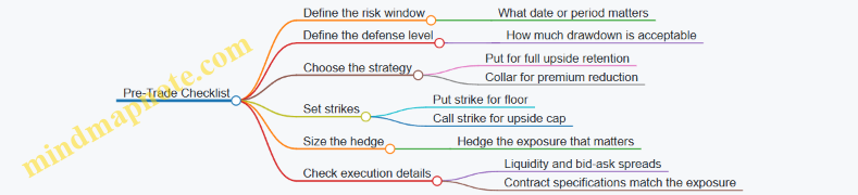
Defined Risk in Practice
Defined risk doesn’t mean “no risk.” It means the payoff structure is known: protective puts cap losses beyond the strike at the cost of the premium; collars cap losses beyond the put strike and cap gains beyond the call strike. When you align expiration to the risk window and size the hedge to the exposure that would actually harm your plan, these strategies become straightforward tools rather than complicated bets.
9.5 Technical Spec: Hedge Ratio Selection and Scenario Testing Methodology
Hedge ratio selection answers one practical question: “How much protection do we buy for the risk we actually have?” Scenario testing answers the second: “Does the protection behave the way we think it does when the world gets weird?” Together, they turn hedging from a guess into a repeatable process.
Hedge Ratio Selection Foundations
Start by defining the exposure you are hedging in the same units as your hedge instrument.
- Exposure metric: choose a measurable driver such as bond duration (DV01), FX notional, commodity price level, or an equity index return.
- Hedge instrument metric: identify the instrument’s sensitivity to the same driver (e.g., swap DV01 per unit notional, option delta per strike, futures contract price per tick).
- Target alignment: decide whether you want to match level (same dollar exposure) or sensitivity (same first-order risk). In high-volatility economies, sensitivity matching is usually more stable than level matching.
A baseline hedge ratio uses a sensitivity ratio:
- Hedge ratio (β) ≈ (Exposure sensitivity) / (Hedge sensitivity)
Easy example: You hold a bond portfolio with DV01 = $12 per $1 million notional. You plan to hedge with a futures contract whose DV01-equivalent is $3 per contract. Then β ≈ 12/3 = 4 contracts. If you later rebalance the bond notional, you recompute β using the updated DV01.
Choosing Between Static and Dynamic Hedge Ratios
A static hedge ratio keeps β fixed over a hedge horizon. It’s simple and reduces trading friction, but it assumes sensitivities don’t drift much.
A dynamic hedge ratio recalculates β at set intervals or when thresholds are breached. It’s more responsive, but it requires operational discipline and transaction cost awareness.
Practical rule: Use dynamic hedging when the exposure driver is volatile (rates, FX, commodity spot) and static hedging when the exposure driver is comparatively stable (long-term real income streams with infrequent cash flow changes).
Scenario Testing Methodology
Scenario testing should cover both market moves and hedge mechanics. Market moves include changes in rates, inflation indices, FX levels, credit spreads, and volatilities. Hedge mechanics include roll effects, option time decay, and basis differences between instruments.
A systematic workflow:
- Build scenario set: include (a) a small move near current conditions, (b) a moderate move, and (c) a stress move that reflects plausible extremes.
- Map scenario variables: translate each scenario into the risk drivers your hedge depends on (e.g., real yields for inflation-linked instruments, implied vol for options, FX spot for forwards).
- Revalue exposure and hedge: compute P&L for both legs under each scenario.
- Measure hedge effectiveness: evaluate both hedge ratio error and residual risk.
Effectiveness metrics that stay interpretable:
- Residual risk: P&L(exposure) + P&L(hedge)
- Hedge error: difference between predicted and realized hedge P&L using the sensitivity model
- Cost-adjusted effectiveness: residual risk after hedge costs (premiums, roll costs, bid-ask)
Easy example: You hedge inflation risk with an inflation-linked instrument. Your sensitivity model predicts that a +2% inflation shock reduces net loss by $50. In the stress scenario, the actual reduction is $35 because the inflation index basis differs between your instrument and the cash flow index. The $15 gap becomes a documented model limitation, not a surprise.
Mind Map: Hedge Ratio Selection and Scenario Testing
Worked Mini-Scenario with Options
Suppose you hedge a floating-rate liability using an interest rate cap. Your hedge ratio is based on matching expected payoff sensitivity, often via delta or vega depending on the goal.
- If the cap’s delta is 0.35 to your rate driver and your liability’s rate sensitivity implies you need protection of $100 per 1% rate move, you target a cap notional such that the cap’s delta-equivalent equals $100.
- Then test scenarios where rates jump and implied vol changes. If the stress scenario includes higher vol, the cap may outperform the sensitivity prediction; if vol collapses, it may underperform. The scenario test quantifies both outcomes.
Implementation Checks
Before you lock the hedge ratio, verify three things for each scenario:
- Unit consistency: sensitivities and P&L are in the same currency and scale.
- Timing consistency: cash flow dates and option expiries align with the scenario horizon.
- Mechanics consistency: futures roll, index lag, and day-count conventions are applied the same way to exposure and hedge.
If these checks pass, the hedge ratio becomes a parameter you can defend, and scenario testing becomes a repeatable audit trail rather than a one-off spreadsheet exercise.
10. Portfolio Construction and Rebalancing Under Inflation Regimes
10.1 Correlation Breakdown and How It Changes Diversification Assumptions
Diversification works when different holdings respond differently to the same stress. Correlation breakdown is what happens when those responses start looking similar—often because the same underlying driver is forcing prices to move together. In high-volatility economies, the usual assumption that “assets are not perfectly linked” becomes fragile, not because the math is wrong, but because the economic regime changes.
What Correlation Assumptions Usually Mean
Most diversification plans implicitly assume:
- Stable relationships: correlations estimated from the past remain roughly useful.
- Common shocks are limited: one shock does not dominate every asset’s return.
- Liquidity is not the main character: you can trade without severe price impact.
When these assumptions fail, correlation estimates become less like “forecasts” and more like “postcards.” They describe what happened, not what will happen.
Why Correlations Break in Inflation and Volatility Regimes
Correlation is not a property of assets alone; it’s a property of assets under a particular set of conditions. In inflation-heavy, high-volatility environments, several mechanisms commonly push correlations toward the same direction.
-
Discount-rate dominance: When inflation expectations and policy rates move sharply, many assets reprice through the same discount-rate channel. Long-duration bonds, growth equities, and even some real assets can start behaving similarly.
-
Currency and funding stress: If investors need cash in one currency, they sell whatever is liquid, regardless of fundamentals. That creates “liquidity correlation,” where assets fall together because they are the easiest to sell.
-
Risk-premium compression or expansion: Credit spreads, equity risk premia, and commodity risk premia can widen or tighten together when investors change how they price uncertainty.
-
Volatility targeting and forced rebalancing: Strategies that reduce exposure when volatility rises can sell multiple holdings at once, mechanically increasing co-movement.
A Simple Example of Correlation Breakdown
Imagine a portfolio with two sleeves:
- Sleeve A: short-term bonds
- Sleeve B: equities
In calmer periods, bonds might have a low or even negative correlation with equities because bonds respond more to rate expectations while equities respond more to earnings expectations.
Now consider a stress episode where inflation surprises cause rapid rate repricing and a funding squeeze. Both sleeves can drop: bonds because yields jump, equities because discount rates rise and risk appetite falls. The correlation you estimated during normal times may have been near zero; during stress it can become strongly positive.
How to Detect Breakdown Without Overcomplicating It
Start with a disciplined workflow:
- Use rolling windows: compute correlations over multiple window lengths (for example, 20, 60, and 120 trading days) to see whether relationships are stable.
- Separate regimes: compare correlations during “normal” periods versus periods with large inflation surprises or large policy moves.
- Check liquidity proxies: if bid-ask spreads widen or trading volumes drop, correlation changes may be driven by trading constraints rather than fundamentals.
- Inspect drivers: estimate whether returns are moving together because of rates, FX, credit spreads, or commodity inputs.
A practical rule: if correlation changes coincide with measurable shifts in rates, FX, or spreads, treat the breakdown as structural for that regime, not as random noise.
Mind Map: Correlation Breakdown Logic
Turning Diagnosis into Portfolio Decisions
Correlation breakdown changes what “diversification” should mean. Instead of relying on historical correlation, you can diversify by payoff drivers and tradeability.
- Diversify payoff drivers: pair assets that respond differently to inflation shocks. For example, some hedges are designed to respond to real-rate moves or inflation-indexed changes rather than general risk appetite.
- Diversify liquidity profiles: include instruments you can actually trade during stress. If an asset becomes illiquid, its correlation during stress is often determined by who needs to sell.
- Use scenario risk budgeting: allocate risk to the drivers you expect to dominate (rates, FX, credit spreads, commodity inputs) rather than to asset labels.
Case Example: Two “Diversifiers” That Fail Together
Suppose a portfolio holds:
- A nominal bond fund
- A commodity-linked fund
During a commodity-specific period, they may move differently. But in a regime where inflation is driven by broad currency depreciation and policy tightening, both can be pulled by the same macro forces: nominal yields rise and risk premia widen. The commodity fund might still hedge some inflation components, but if its returns are dominated by funding stress and risk appetite, it can correlate more with bonds than expected.
The takeaway is simple: diversification is not “owning different things.” It’s owning things whose returns are driven by different mechanisms under the conditions that matter.
10.2 Risk Budgeting Across Inflation Rate FX Credit and Liquidity Risks
Risk budgeting is how you decide what “bad outcomes” you can tolerate, then translate that tolerance into limits for each risk type. In inflation-heavy, high-volatility environments, the tricky part is that risks don’t stay in their own lanes: rate moves can change credit spreads, FX swings can stress liquidity, and liquidity stress can force you to sell at the worst time. A good budget makes those interactions explicit.
Foundational Inputs You Need Before Setting Limits
Start with three inputs, because limits without inputs are just vibes.
- Time horizon and cash needs. Separate near-term spending from longer-term goals. Liquidity risk matters most where you cannot wait.
- Loss tolerance. Define what “too much” means in your context: a maximum drawdown, a minimum probability of meeting obligations, or a maximum acceptable shortfall.
- Hedge objective. Decide whether hedges are for stabilizing cash flows, protecting purchasing power, or reducing volatility. Each objective implies different risk budgets.
A practical rule: set liquidity limits first, then rate and FX, then credit. If you can’t fund margin calls or roll hedges, the “best” hedge strategy is just a paper plan.
The Risk Budgeting Map
Use a budget that allocates capacity across four buckets: inflation-rate risk, FX risk, credit risk, and liquidity risk. Each bucket has a limit and a measurement method.
Mind Map: Risk Budgeting Structure
Translating Limits into Numbers
A budget becomes useful when it is measurable.
Inflation Rate Risk Budget
Measure the rate sensitivity of your portfolio relative to your obligations. For example, if your spending is due in 12 months and your assets have a much longer average duration, you are effectively borrowing duration risk from the future.
Example: You hold a bond portfolio with a duration of 6 years, but your next 12 months of spending is covered by only 20% of that portfolio. If rates jump sharply, the mark-to-market loss can be large even if you plan to hold. Your limit should reflect whether you can tolerate that mark-to-market while still meeting cash needs.
A simple budgeting approach:
- Set a near-term liquidity-first limit: the portion of assets needed within 12 months must be in instruments with stable pricing and minimal duration.
- Set a rate shock limit for the remaining portion: compute estimated PnL under a defined rate move and cap it.
FX Risk Budget
FX risk is not just “currency exposure”; it’s exposure to your ability to pay. Convert all obligations into a base currency and compute net exposure by currency.
Example: A business has monthly import costs in EUR and revenue in local currency. If you hedge only the next month, you may still face a liquidity crunch when the hedge rolls. Your FX budget should include both:
- a hedge ratio limit for the obligation horizon, and
- a roll and collateral capacity limit so hedges don’t become a funding problem.
Credit Risk Budget
Credit risk in inflation regimes often shows up as spread widening rather than immediate defaults. Budget credit risk using spread sensitivity and concentration.
Example: Two portfolios have the same duration, but one holds mostly high-yield issuers. In a rate shock, the high-yield portfolio can lose more because spreads widen. Your credit budget should cap the estimated loss under a spread widening scenario, and also cap issuer concentration so one downgrade doesn’t dominate.
Liquidity Risk Budget
Liquidity risk is about whether you can execute without selling at punitive prices or failing margin requirements.
Example: You use FX options and interest rate derivatives. Even if the expected hedge outcome is fine, a volatility spike can increase margin calls. Your liquidity budget should specify:
- a minimum cash buffer after hedging setup,
- maximum acceptable margin usage under stress, and
- which instruments are allowed for near-term funding.
Handling Interactions Without Double-Counting
Interactions are where budgets can fail. If you cap rate risk and credit risk separately, you might still exceed your true loss capacity because rate shocks can drive credit spreads.
A clean method is to run joint scenario checks:
- Apply a rate shock.
- Apply a correlated spread widening response.
- Apply an FX move if your obligations are currency-mismatched.
- Apply a liquidity stress that increases transaction costs or reduces executable size.
If the combined scenario breaches your loss tolerance, reduce exposure in the bucket that contributes most to the breach, then re-check.
Governance and Monitoring Metrics
Set monitoring metrics that match your limits.
- Rate: duration gap and scenario PnL versus limit.
- FX: net exposure by currency and hedge coverage by obligation horizon.
- Credit: spread duration and concentration measures.
- Liquidity: cash buffer coverage, margin usage, and estimated execution impact.
Finally, define rebalancing triggers that respect liquidity. If a hedge becomes too expensive or coverage drifts, adjust within the liquidity budget rather than treating rebalancing as an optional hobby.
10.3 Rebalancing Rules Including Threshold and Time Based Triggers
Rebalancing is the discipline of bringing a portfolio back toward its target risk and cash-flow plan. In inflation and volatility regimes, the “drift” can be fast, and the cost of acting can also be fast. So the goal is not to rebalance often; it is to rebalance when the drift meaningfully changes outcomes.
Foundational Idea: What Drift Means
Start with two targets: (1) allocation targets across risk drivers (rates, inflation, currency, credit, real assets), and (2) hedge coverage targets for specific liabilities or spending buckets. Drift happens when market moves change weights, hedge notionals, or effective exposures.
A practical way to measure drift is to track each sleeve’s contribution to the portfolio’s intended risk. For example, if your “rate sleeve” is meant to offset real spending volatility, you monitor both its weight and its interest-rate sensitivity (duration or swap delta). If your “currency sleeve” is meant to cover import costs, you monitor notional coverage versus expected spend in the relevant currency.
Threshold Triggers: When Drift Becomes Material
A threshold rule says: rebalance only if drift exceeds a pre-set limit. Use two thresholds: one for allocation and one for hedge effectiveness.
Allocation threshold. Example: target 30% for a rate sleeve. If it rises to 34% or falls to 26%, you rebalance. This creates a deadband so small fluctuations don’t generate trading costs.
Hedge effectiveness threshold. Example: you hedge 80% of next-quarter import costs with FX forwards. If the hedge ratio falls below 70% due to changes in expected spend or contract roll timing, you rebalance even if the overall portfolio weight hasn’t moved much.
Why two thresholds. Allocation drift can be misleading when the hedge instrument’s sensitivity changes. Hedge effectiveness drift is the “real” signal for whether the protection is still doing its job.
Time-Based Triggers: When You Must Check Even if Drift Looks Small
Time triggers prevent the portfolio from quietly drifting due to operational realities: cash flows, coupon payments, roll schedules, and index changes. A time rule also helps you avoid decision fatigue by making reviews routine.
A common structure is:
- Monthly review for hedge coverage and cash-flow alignment.
- Quarterly rebalance for allocation drift, but only execute trades if thresholds are breached.
- Event-based review for changes in liabilities, major policy changes, or material liquidity constraints.
Time triggers are not “automatic trading.” They are “decision checkpoints.” If thresholds are not breached, you document why you did nothing and move on.
Combined Logic: The Decision Tree
Use a simple decision process so the rule is consistent across sleeves.
Example: Multi-Sleeve Portfolio with Clear Rules
Assume a portfolio with three sleeves: rate (target 30%), real assets (target 25%), and currency hedge for import costs (target 80% coverage for the next quarter).
-
On Month 1, rate sleeve rises to 33% (within a 26%–34% band). Currency hedge coverage drops to 68% because expected import volumes increased. Threshold breach occurs on hedge effectiveness, so you rebalance the FX hedge to restore coverage to 80%. You do not trade the rate sleeve.
-
On Month 2, rate sleeve falls to 27% (still within band). Hedge coverage is 79%. No thresholds breached. You still perform the monthly review, but you execute no trades.
-
On Quarter End, rate sleeve is 35% (breach). You execute trades to return it to 30%, using the quarter’s liquidity window and netting where possible. You also confirm that the FX hedge is still aligned with the next quarter’s import forecast.
This example shows the key point: time triggers decide when you look; thresholds decide whether you act.
Execution Guardrails That Prevent Rule-Driven Mistakes
Even good rules can fail if execution is sloppy. Add guardrails:
- Minimum trade size. If the required adjustment is too small relative to spreads and fees, you may defer until the next checkpoint.
- Liquidity check. If the market is temporarily illiquid, you may rebalance partially to reach the most important hedge coverage first.
- Netting and sequencing. When multiple trades offset each other (for example, reducing one exposure while increasing another), sequence them to reduce unnecessary turnover.
Documentation Standard for Consistency
For every checkpoint, record: measured drift, whether thresholds were breached, the specific actions taken, and the operational constraints considered. This turns rebalancing from a gut-feel habit into a repeatable process—less exciting, more reliable, and much easier to audit.
10.4 Stress Testing Portfolios With Historical And Hypothetical Shocks
Stress testing answers a practical question: “If inflation, rates, FX, or credit behave badly, what breaks first, and how do we respond?” The goal is not to predict outcomes; it’s to map vulnerabilities to specific drivers and to verify that your hedges and liquidity plan actually work when correlations stop behaving.
What Stress Tests Should Cover
Start with three layers of risk, each with a different purpose.
- Market price risk: losses from moves in yields, spreads, FX rates, and commodity prices.
- Liquidity and execution risk: losses from wider bid-ask spreads, delayed trades, or forced selling.
- Model and hedge risk: losses when hedge instruments don’t offset the exposures you assumed.
A useful rule: every stress test should produce (a) a loss estimate, (b) a driver breakdown, and (c) an action check. If you can’t link losses to drivers, you can’t improve anything.
Historical Shocks with Driver Attribution
Historical testing uses real episodes to ground your assumptions. The key is to avoid “copy the calendar, ignore the portfolio.” Instead, reprice your current holdings under the historical path of risk factors.
Workflow
- Choose episodes that resemble your current regime: high inflation, rapid rate repricing, FX instability, or credit widening.
- Build a mapping from portfolio positions to risk factors (e.g., bond duration to yield curve nodes, credit exposure to spread buckets, FX exposure to currency pairs).
- Reprice using consistent conventions: same day count, same compounding, same index methodology.
- Attribute results to drivers: “How much came from rates vs spreads vs FX?”
Example:
Suppose a portfolio holds a mix of nominal bonds and an FX-hedged cash reserve. In a historical episode where yields rose and the domestic currency depreciated, you might find:
- Nominal bond losses: driven mainly by duration.
- FX hedge effectiveness: partial offset, but not complete, because hedge tenors didn’t match the cash outflow dates.
- Net result: the biggest gap is timing mismatch, not direction.
That’s actionable: adjust hedge tenor or rebalance rules rather than changing everything at once.
Hypothetical Shocks with Clear Assumptions
Hypothetical shocks are scenario designs. They’re most valuable when historical episodes don’t match your current exposures or when you need to test specific failure modes.
Design shocks using three components:
- Magnitude: how far each risk factor moves.
- Shape: whether the move is parallel, steepening, or curve twist.
- Co-movement: how rates, spreads, and FX move together.
Avoid vague scenarios like “inflation spikes.” Use concrete moves such as “front-end yields +250 bps, 5–10y +120 bps, credit spreads +300 bps, FX -8%.”
Example:
You test a “rates up, spreads up, FX down” shock. Your bond sleeve may lose from duration, and your credit sleeve may lose from spread widening. If your inflation-linked holdings are small, the test will show a gap in inflation pass-through. That tells you whether the hedge set is incomplete.
Liquidity Stress and Margin Effects
Price losses are only half the story. In stress, liquidity can turn into a cost center.
Include at least:
- Haircuts and margin: higher collateral requirements can force cash outflows.
- Trading frictions: wider bid-ask spreads and reduced depth.
- Redemption or funding constraints: limits on how quickly you can rebalance.
Example:
If you rely on selling a less-liquid asset to fund margin, a stress test should model the sale at a discount and include the time delay. Otherwise, your “hedge works” conclusion may fail in practice.
Mind Map of Stress Testing Logic
Mind Map: Stress Testing Portfolios
Interpreting Results and Turning Them into Rules
A stress test is useful only if it changes decisions.
Convert results into bucketed metrics:
- Rate sensitivity bucket: losses from yield curve moves.
- Spread sensitivity bucket: losses from credit widening.
- FX sensitivity bucket: losses from currency moves.
- Liquidity bucket: losses from friction and forced selling.
Then define action triggers. For example:
- If liquidity bucket exceeds a threshold, reduce reliance on illiquid hedges.
- If hedge effectiveness drops due to tenor mismatch, rebalance hedge schedules.
- If spread losses dominate, tighten credit quality constraints or reduce concentration.
Example:
In one stress run, the total loss is moderate, but the liquidity bucket is large because margin timing concentrates cash outflows in the first two weeks. The action isn’t “buy more hedges.” It’s “pre-fund the margin buffer and stagger maturities so cash arrives before the outflow window.”
A Practical Mini-Template for Your Next Run
Use a consistent structure so results are comparable across iterations.
- Scenario definition: list risk factor moves and co-movement.
- Repricing: compute P&L by risk bucket.
- Hedge check: compare exposure vs hedge offset by tenor.
- Liquidity check: model margin, haircuts, and execution delay.
- Decision: specify one change you will make if the scenario breaches limits.
If you can’t write the decision in one sentence, the test is still too abstract. Stress testing should end with a lever you can pull, not a report you can admire.
10.5 Case Example: Implementing a Rebalancing Policy for a Multi Asset Portfolio
You manage a multi-asset portfolio designed to protect purchasing power during inflation and volatility spikes. The policy goal is simple: keep the portfolio’s risk exposures near targets, even when prices move quickly and correlations shift.
Portfolio Setup and Targets
Assume a monthly review cadence with a small set of risk targets:
- Inflation sensitivity: target 40% real-return exposure via inflation-linked bonds and real assets.
- Rate risk: target moderate duration exposure using a bond sleeve.
- Currency risk: target partial hedging of foreign-currency spending needs.
- Credit risk: target limited spread exposure through high-quality credit.
- Liquidity: ensure at least 20% of the portfolio can be liquidated within 5 business days.
Example starting weights (illustrative):
- 30% inflation-linked bonds
- 25% short-duration government bonds
- 15% high-quality credit
- 15% real assets (property or real-asset funds)
- 10% diversified equities with inflation-aware tilt
- 5% cash and near-cash
You also define a “risk budget” using measurable proxies:
- Duration band for the bond sleeve
- Credit quality band for the credit sleeve
- FX hedge ratio band for foreign exposure
- Equity factor tilt limits (e.g., quality and pricing-power screens)
Rebalancing Rules That Don’t Fight Reality
A good policy uses triggers and constraints. Triggers decide when to act; constraints decide how to act.
Triggers
Use two layers:
- Weight deviation triggers (fast, intuitive)
- Rebalance if any sleeve weight moves more than ±5 percentage points from target.
- Risk deviation triggers (more robust)
- Rebalance if duration leaves its band by more than 0.75 years.
- Rebalance if FX hedge ratio drifts by more than 10% of the intended hedge coverage.
Constraints
- Liquidity constraint: do not sell assets that would push liquid holdings below 20%.
- Transaction cost constraint: avoid trading if the expected benefit is smaller than a pre-set cost estimate.
- Hedge integrity constraint: keep derivatives notionals aligned with the underlying exposure they are meant to hedge.
Step-by-Step Implementation Example
On a review date, prices move sharply after a volatility burst. Your monitoring shows:
- Inflation-linked bonds rose, pushing their sleeve from 30% to 37%.
- Short-duration government bonds fell from 25% to 19%.
- Credit spreads widened, but the credit sleeve is still near target at 15%.
- Foreign-currency exposure increased, and the FX hedge ratio fell from 70% to 55%.
- Real assets and equities are within weight bands.
Decision Logic
-
Check weight triggers
- Inflation-linked bonds: +7 pp → exceeds ±5 → action required.
- Short-duration bonds: −6 pp → exceeds ±5 → action required.
-
Check risk triggers
- Duration band: still within tolerance because the bond sleeve mix changed in a way that roughly offsets duration.
- FX hedge ratio: 55% vs 70% → drift of 15% → action required.
-
Apply constraints
- Liquidity is currently 24% → selling is allowed.
- Expected benefit from restoring target weights exceeds estimated costs.
Trade Plan
-
Rebalance bond sleeves
- Sell part of inflation-linked bonds to bring that sleeve back toward 30%.
- Buy short-duration government bonds to restore that sleeve toward 25%.
- Keep the bond sleeve duration within the band by using the duration estimate of each bond sleeve.
-
Restore FX hedge coverage
- Increase FX hedges to return hedge ratio to 70%.
- Use the same tenor structure as the underlying spending/income timing so the hedge “expires” when the exposure does.
-
Leave credit and equities unchanged
- Credit is within weight band and you already have spread risk exposure; you avoid unnecessary churn.
- Equities and real assets are within bands and liquidity remains adequate.
Mind Map: Rebalancing Policy Workflow
Verification and Recordkeeping
After trades, you re-run the same checks:
- Inflation-linked bonds back near 30% and short-duration near 25%.
- Duration remains inside the band.
- FX hedge ratio returns to 70%.
- Liquidity stays at or above 20%.
Finally, you document the trigger(s) that caused action and the constraint(s) that shaped trade sizing. This prevents “policy drift,” where the process slowly turns into discretionary trading with a spreadsheet costume.
Mini Example Summary
In this case, rebalancing required two coordinated fixes: bond sleeve weight restoration and FX hedge coverage restoration. Credit and equity sleeves stayed put because they did not breach triggers and trading them would mainly add cost, not protection.
11. Asset Protection for Households and Businesses in Stress Periods
11.1 Protecting Emergency Funds and Operational Liquidity
Emergency funds are not just “extra cash.” In high-volatility economies, they’re a system that keeps you solvent when prices jump, payments bunch up, and normal funding channels get moody. Operational liquidity is the same idea, but tied to payroll, taxes, utilities, and vendor terms—money that must move on schedule.
Core Principle: Separate Safety from Convenience
Start by splitting liquidity into two buckets: (1) emergency funds for unexpected shocks and (2) operational liquidity for planned-but-nonnegotiable expenses. Mixing them creates a slow leak: you spend emergency money to cover operational gaps, then you rebuild at the worst time—often when spreads are wide and cash is expensive.
A practical rule: emergency funds should be hard to touch and easy to access, while operational liquidity should be easy to touch and hard to misallocate. That sounds contradictory until you define access rules and accounting categories.
Mind Map: Liquidity Protection System
Build the Emergency Fund Like a Ladder, Not a Pile
A ladder reduces the chance you need to sell something at the wrong moment. For households, a simple structure can be: a first rung for immediate access (for example, rent and utilities), a second rung for near-term needs (for example, groceries and insurance premiums), and a third rung for longer emergencies (for example, medical deductibles).
Example: Suppose monthly essential spending is $2,500. You set a 6-month emergency target of $15,000. You allocate $5,000 to immediate access, $5,000 to same-week access, and $5,000 to a low-volatility vehicle that can be converted within a defined window. If prices rise, you still have time to adjust without panic selling.
Key best practice: define “essential spending” precisely. If you include discretionary items, the emergency fund becomes a disguised budget and will be spent the moment life gets inconvenient.
Operational Liquidity: Match Money to Payment Timing
Operational liquidity is about timing certainty. Create a payment calendar that lists payroll dates, tax deadlines, rent, utilities, and vendor payment terms. Then map each payment to a funding source that can be accessed with the same settlement timing.
Example: A small business pays payroll every 15th and 30th, taxes on the 10th, and a key supplier on net-30 terms. If you hold all cash in a single instrument that settles in three days, you can still be fine—until a holiday, a bank delay, or a market disruption stretches settlement. The fix is to hold a near-term operational buffer in instruments with predictable settlement.
Choose Instruments with Operational Friction in Mind
In volatile economies, the “risk” of a cash-like instrument is often operational, not theoretical. Consider:
- Settlement certainty: Can you convert and receive funds on the day you need them?
- Counterparty reliability: Are you exposed to a bank or broker that might restrict withdrawals?
- Fee and spread behavior: Do costs widen when everyone else is rushing?
- Currency usability: If expenses are in one currency, holding emergency funds in another can create a timing mismatch.
Best practice: keep emergency funds in instruments that you can access without negotiating, waiting, or submitting extra paperwork during stress.
Add Currency Discipline Without Overcomplicating
If your expenses are mostly in one currency, your emergency fund should be primarily in that currency. If you have unavoidable exposure to another currency (for example, imported inputs), create a smaller “operational FX sleeve” sized to the portion of costs that truly require it.
Example: A household earning locally but paying for a medication subscription in USD can split the emergency fund: most in local currency for essentials, and a smaller USD reserve sized to cover the subscription for a defined period.
Stress Test the Liquidity Plan with Realistic Friction
Stress testing should include delays and constraints, not just price moves. Run scenarios such as:
- A one-week delay in access to funds.
- A temporary increase in conversion costs.
- A partial loss of expected income.
- A sudden need to pay a clustered set of bills.
Then check whether your emergency ladder still covers essentials and whether operational liquidity still covers the next payroll and tax dates.
Mind the Human Part: Access Rules and Accountability
Liquidity fails when decisions are slow or chaotic. Set withdrawal and approval rules in advance. For households, that might mean one person has access credentials and another has the authority to approve spending above a threshold. For businesses, it might mean a defined process for moving funds between accounts and documenting the reason.
Example: If a business needs to cover a vendor invoice early, the policy should specify who can authorize the transfer, what documentation is required, and how the cash calendar is updated afterward.
Monitoring Metrics That Actually Matter
Track a few metrics consistently:
- Runway: weeks of operational expenses covered by near-term liquidity.
- Buffer ratio: emergency fund coverage relative to essential spending.
- Settlement readiness: whether conversion windows match your payment calendar.
- Concentration: how much of your liquidity depends on one institution or one currency.
When these metrics drift, act early. Liquidity problems are easier to fix before you need them.
11.2 Securing Collateral and Managing Counterparty Exposure
Collateral is the practical “seatbelt” for hedging and lending relationships: it reduces the amount you can lose if the other party fails to perform. Counterparty exposure is the amount at risk at any moment, which changes as market prices move. The goal is to control both the size of exposure and the speed and certainty of recovery.
Core Concepts That Drive Collateral Design
Start with three building blocks.
-
Exposure measurement: For derivatives, exposure is not just the current mark-to-market; it also depends on how prices could move before the next settlement. This is why collateral terms often reference “variation margin” for current value and “initial margin” for potential future exposure.
-
Legal enforceability: Collateral only works if you can legally call it, net it, and seize it when needed. Two agreements matter most: the master agreement that governs the trade and the collateral agreement that governs posting and rehypanding.
-
Operational reliability: Even with good legal terms, collateral can fail if calls are missed, thresholds are wrong, or transfers settle late.
A simple example: you enter a swap with a counterparty. If the swap moves against you by $200,000, variation margin should be called quickly so you don’t wait for a default to recover value.
Collateral Types and What They Actually Do
Cash is usually the cleanest collateral because it is easy to value and transfer. Securities can be efficient but require valuation haircuts, eligibility rules, and custody arrangements.
- Variation margin: exchanged frequently to keep exposure close to zero for current valuation.
- Initial margin: posted to cover potential future exposure over a defined risk horizon.
- Haircuts: reductions applied to non-cash collateral to reflect volatility and liquidity risk.
Example: If you accept corporate bonds as collateral, a haircut might be applied so that a bond that drops 10% in value does not fully translate into a 10% loss for you.
The Collateral Workflow That Prevents Surprises
A robust workflow has four checkpoints: trade confirmation, valuation, margin call, and transfer.
- Trade confirmation ensures the correct terms and identifiers are in place.
- Valuation uses agreed pricing sources and conventions.
- Margin call follows thresholds, minimum transfer amounts, and dispute windows.
- Transfer and reconciliation confirm settlement and update balances.
If you want a practical rule: treat margin calls like payroll. If the timing is inconsistent or the inputs are unclear, you will eventually pay for it.
Netting and Set-Off for Exposure Reduction
Netting reduces exposure by allowing you to offset amounts owed under multiple trades. Without netting, you might have to collect on one trade while paying on another, even if both are with the same counterparty.
Example: You have two derivatives with the same counterparty. One is +$150,000 to you and the other is -$120,000. With netting, your exposure is closer to $30,000 rather than requiring separate settlement of both positions.
Eligibility, Concentration, and Liquidity Controls
Collateral is not just “what you accept,” but “what you can safely use when you need it.”
- Eligibility: define which instruments qualify and under what conditions.
- Concentration limits: prevent overreliance on a single issuer or asset class.
- Liquidity and custody: ensure you can liquidate collateral quickly and that custody arrangements support timely access.
Example: If a counterparty posts only one illiquid bond, you may face a valuation haircut that is too optimistic or a liquidation process that is slower than your operational timeline.
Dispute Management and Timing
Disputes happen when valuation inputs differ or pricing sources are contested. The key is to limit the damage by controlling timing.
- Dispute windows: time-limited periods for challenging a margin call.
- Undisputed amounts: require transfer of amounts that are not in dispute.
- Fallback valuation: specify what happens if a pricing source fails.
A practical approach: require that even during disputes, the undisputed portion is transferred so exposure does not quietly grow.
Mind Map: Collateral and Counterparty Exposure Controls
Example: A Clean Margin Setup for a Derivatives Counterparty
Assume you trade a monthly-settled interest rate swap.
- You negotiate netting so all swaps with the same counterparty settle on a net basis.
- You require variation margin with a low threshold so that when the swap moves, collateral is posted quickly.
- You accept only highly liquid government securities as non-cash collateral and apply haircuts.
- You define a dispute window and require undisputed amounts to transfer.
Result: if the swap moves against you by $200,000, you receive collateral promptly, and your exposure is reduced to the remaining timing and dispute risk.
Case-Style Checklist for Implementation
Use this checklist to verify the system is coherent end to end.
- Legal: netting works, collateral can be called, and rehypothecation rules are clear.
- Valuation: pricing conventions are documented and consistently applied.
- Margin terms: thresholds, minimum transfer amounts, and frequency match the risk.
- Collateral rules: eligibility, haircuts, concentration, and custody are defined.
- Operations: margin calls are monitored, transfers reconcile, and disputes are time-bounded.
When these pieces align, collateral becomes more than paperwork. It becomes a predictable mechanism that reduces losses and shortens the time between “something changed” and “we adjusted.”
11.3 Legal and Contract Review for Indexation and Payment Terms
Indexation and payment terms are where inflation hedges either work cleanly or quietly fail. A good legal review treats the contract like a machine: you verify inputs (indices, dates, definitions), the mechanism (calculation and payment), and the outputs (timing, currency, remedies).
Core Concepts That Drive Contract Outcomes
Start with three foundational questions.
-
What exactly is being indexed? The contract must specify the reference index (and version), the measurement unit, and the scope of items included. For example, “CPI” is not enough if the contract doesn’t state the country, basket definition, and whether it uses headline or core.
-
When is the index observed? Indexation often depends on observation dates, publication lags, and whether the contract uses the latest available value. If the contract says “use the CPI for March,” you still need the rule for what happens if March’s value is published after the payment date.
-
How does the index translate into money? The formula should be explicit: base value, index ratio, rounding rules, caps or floors, and whether adjustments compound or apply once. A contract that says “adjusted by CPI” without a calculation method is like a hedge without a payoff diagram.
Indexation Clauses to Check Line by Line
Reference index definition. Confirm the exact index name, provider, and geography. If the index is discontinued or replaced, the contract should define a fallback mechanism (for example, a successor index) and a method to preserve continuity.
Base period and base value. The base period anchors the ratio. If the base period is ambiguous, two parties can compute different adjustment factors from the same index.
Observation date and effective date. Separate the date the index is measured from the date the adjustment becomes effective. This matters when payments are monthly but index values are quarterly.
Rounding and settlement precision. Specify rounding to cents, basis points, or whole units. Small rounding differences can compound across many payments.
Caps, floors, and exclusions. If the contract limits adjustments, verify the limit interacts correctly with the payment schedule. Also confirm whether certain components of the index are excluded.
Audit and evidence. The contract should state what documentation is acceptable to support calculations, such as official index publications and calculation worksheets.
Payment Terms That Prevent Operational Failure
Indexation is only useful if payment mechanics are reliable.
Payment currency and conversion rules. If payments are in one currency but indexed to another, the contract must specify the FX rate source, rate type (spot vs. fixing), and timing. Without this, the “hedge” becomes a dispute about which rate to use.
Due dates and grace periods. Define when payment is due, whether there is a grace period, and what constitutes late payment.
Interest on late payments. Specify the interest rate, compounding method, and whether interest is calculated on the indexed amount or the original amount.
Set-off and netting. If parties can net amounts, confirm the order of operations: do you net before or after indexation? The difference can change the final cash flow.
Dispute resolution for calculations. A practical clause defines a calculation agent or an agreed process for resolving calculation disputes quickly, including timelines.
Remedies and Risk Allocation
A contract should clearly allocate who bears the risk of index errors, publication delays, and calculation mistakes.
- Index publication delay: confirm whether the contract uses the last published value until the new value is available, or whether it requires retroactive true-up.
- Calculation error: specify correction procedures and whether corrected payments include interest for the delay.
- Termination triggers: if the index becomes unavailable, confirm whether the contract terminates, switches indices, or freezes adjustments.
Mind Map: Legal Review Checklist for Indexation and Payment Terms
Example: Lease Indexation with Publication Lag
A commercial lease states: “Rent shall be adjusted annually based on the CPI published for the prior year.” The tenant pays on January 1, but the CPI for the prior year is published in February.
A robust clause specifies: (1) the observation uses the CPI value published for the prior year, (2) if not yet published by the payment date, the contract uses the most recent available CPI and performs a retroactive true-up within 10 business days after publication, and (3) the true-up is paid with no additional interest if paid within the true-up window.
Without these details, the parties may disagree on whether the January payment should be provisional, whether the adjustment should be retroactive, and whether interest applies to the difference.
Example: Cross-Currency Indexed Loan Payment
A borrower repays monthly in USD, but the principal adjustment is tied to a local inflation index. The contract must state the FX rate source (for example, a specific exchange fixing), the rate date (payment date vs observation date), and whether the indexed principal is converted first or converted then adjusted.
If the contract is silent, two parties can compute different USD amounts from the same inflation index because FX rates move. A clean clause removes that ambiguity by defining the exact order of operations and the exact FX reference.
Practical Review Output
Conclude the review by producing a short “terms map” that lists each indexed variable, each relevant date, the calculation formula, and the payment timing and remedies. When the contract is later used to compute payments, this map becomes the reference point for both accounting and dispute handling—less guesswork, fewer surprises, and a hedge that behaves like one.
11.4 Insurance Structures Including Inflation Sensitive Coverage Review
Insurance is often treated as a single purchase, but in inflation-prone environments it behaves more like a set of contracts with different “indexing” behaviors. A good review checks whether each policy pays in real terms when you need it, whether the payment timing matches your cash-flow reality, and whether the policy’s definitions line up with how your losses actually occur.
Foundational Concepts for Inflation Sensitive Coverage
Start with three building blocks: the insured value, the benefit trigger, and the claim settlement method.
- Insured value is what the policy agrees to protect. If it is fixed while costs rise, the policy can become underinsured.
- Benefit trigger is the event that starts payment. Inflation can change the likelihood and timing of triggers, especially for property damage and business interruption.
- Settlement method determines how the insurer calculates payment. Some policies pay replacement cost, others pay actual cash value, and some apply caps or depreciation.
A practical rule: if the policy pays only after repairs begin, you may still face a funding gap even when the final payout is “correct.” That gap is often the real inflation problem.
Coverage Types That Commonly Need Inflation Review
Property and casualty policies should be checked for replacement cost wording, valuation clauses, and any sublimits for building systems, contents, and temporary relocation.
Business interruption coverage is where inflation can quietly do damage. Review whether the policy uses “gross profit” or “actual loss sustained,” whether it includes extra expense, and how it defines the indemnity period. If the indemnity period is shorter than the time it takes to rebuild under higher construction costs, the policy may pay less than the real duration of disruption.
Liability policies matter too, because legal costs and settlements can rise with inflation. Confirm whether defense costs are within limits or outside limits, and whether there are aggregate caps that could compress payments.
Mind Map: Inflation Sensitive Insurance Review
Systematic Review Workflow with Concrete Checks
-
Inventory what each policy promises: create a one-page matrix listing each coverage, limit, deductible, sublimit, waiting period, and settlement basis. If you can’t summarize it in one page, you can’t reliably manage it.
-
Test insured value against replacement reality: compare the policy’s insured value to a recent rebuild estimate. For example, if a warehouse replacement estimate is $5.0 million but the policy limit is $4.0 million, a 20% shortfall can translate into a proportional reduction depending on the policy’s underinsurance rules.
-
Check business interruption for duration mismatch: suppose your indemnity period is 6 months. If rebuilding typically takes 9 months when materials are scarce, you may receive payments for only part of the disruption. The fix is often extending the indemnity period or ensuring extra expense coverage is robust.
-
Validate settlement method for real value: consider a policy that pays actual cash value. If a roof is 5 years old and depreciation is applied, the payout may reflect age rather than replacement cost. In inflationary periods, the replacement cost can rise faster than depreciation reduces the payout, creating a double squeeze.
-
Review deductibles and sublimits for inflation sensitivity: a deductible that is fixed in nominal terms becomes more painful when repair costs rise. Sublimits for specific items, like electrical systems or temporary housing, can also cap the portion that inflation affects most.
Example: Property and Business Interruption Together
A small manufacturer insures its facility for $2.5 million replacement cost and has business interruption with a 6-month indemnity period. After a fire, rebuilding costs rise due to labor and material pricing. The insurer pays property replacement cost, but business interruption covers only 6 months. Even if the property claim is settled fairly, the company still faces a cash crunch because it must fund operations during the final 3 months of rebuilding. The integrated fix is to extend the indemnity period and confirm extra expense coverage, not just to raise the property limit.
Example: Liability Defense Costs Within Limits
A service firm has a liability policy with defense costs inside the aggregate limit. If inflation increases legal billing rates, defense can consume the limit faster, leaving less for settlements. A coverage review would confirm whether defense costs are outside limits or whether the aggregate limit is sufficiently high relative to expected claim size and defense duration.
Practical Output of the Review
Conclude with three deliverables: a gap list, a prioritized set of endorsements or limit adjustments, and a claim-readiness checklist. Claim readiness includes knowing what documents the insurer requires and who is responsible for producing them quickly. In inflation environments, speed and completeness are part of the coverage, even when the policy wording is unchanged.
11.5 Case Example: Protecting Business Cash Flows with Contract and Financial Hedges
A mid-sized manufacturer, Northbridge Components, faces two inflation-linked risks: (1) input costs that rise faster than customer payments, and (2) a currency mismatch because 40% of raw materials are priced in USD while most sales are in local currency. The goal is not to “beat inflation,” but to keep operating cash flow stable enough to pay suppliers, payroll, and debt service.
Step 1: Map Cash Flows to Risk Drivers
Northbridge starts with a simple cash-flow map for the next 12 months.
- Inflation-sensitive outflows: USD-denominated raw materials, energy surcharges, and maintenance contracts with annual indexation.
- Inflation-sensitive inflows: customer invoices with partial indexation and a lag of 30–60 days.
- Fixed obligations: loan principal and interest payments in local currency.
A practical rule: if a payment is both timed and indexed (explicitly or implicitly), it can be hedged with a contract term or a financial instrument. If it is neither, it usually needs operational controls first.
Step 2: Use Contract Terms as the First Line of Defense
Northbridge renegotiates two supplier agreements and one customer agreement.
Supplier contract change A: indexation alignment
- Old: supplier invoices index to a broad inflation measure with a 90-day lag.
- New: invoices index to the same measure used in customer pricing, with a 30-day lag.
Supplier contract change B: cost-sharing caps
- Old: full pass-through of cost increases.
- New: pass-through applies above a threshold, with a cap on monthly increases.
Customer contract change C: payment timing and partial indexation
- Old: net 60 days, indexation only at renewal.
- New: net 30 days, monthly surcharge tied to the same index, plus a clause allowing suspension of production commitments if the surcharge is disputed.
Why this works: contract terms reduce the “timing gap” between when costs rise and when cash arrives. Financial hedges then cover the remaining gap.
Step 3: Hedge the Remaining Mismatch with Financial Instruments
After contract changes, Northbridge estimates the residual exposure as a monthly net cash-flow shortfall in local currency.
- Currency hedge: hedge 70% of expected USD purchases for the next 6 months using FX forwards with monthly settlement.
- Rate and inflation interaction: because local borrowing costs are tied to a floating benchmark, Northbridge uses an interest rate cap on a portion of forecast borrowing to limit payment spikes during volatile periods.
- Optional commodity hedge: if energy is a major driver and contracts are not indexed, hedge a portion of expected energy consumption with futures or swaps, sized to the portion that is not already covered by supplier pass-through.
Sizing is conservative: hedges cover the portion of exposure that is both measurable and time-bound. Anything uncertain gets handled through contract terms and working-capital controls.
Step 4: Mind Map of the Integrated Hedge Plan
Mind Map: Protecting Business Cash Flows
Step 5: A Concrete Monthly Example
Assume the following for one month:
- USD purchases: $10,000,000
- Expected FX rate at invoice: 1.10 local/USD
- Actual FX rate at settlement: 1.18 local/USD
- Northbridge hedges 70% of USD purchases with FX forwards
Without hedging, the local-currency cost rises by 0.08 per USD, adding $10,000,000 × 0.08 = 800,000 local units.
With a 70% hedge, the forward covers $7,000,000, reducing the effective increase by $7,000,000 × 0.08 = 560,000 local units. The remaining 240,000 local units becomes the “budgeted residual” that contract caps and working-capital buffers are designed to absorb.
Now add contract alignment: if customer surcharges adjust monthly using the same index, the timing gap shrinks, so the cash shortfall is smaller even when FX moves.
Step 6: Governance That Prevents Hedge Drift
Northbridge sets three rules:
- Hedge ratio bands: FX hedge stays between 60% and 80% of measurable USD purchases.
- Rebalancing trigger: if forecast USD purchases change by more than 10% for two consecutive weeks, hedge notional is adjusted.
- Effectiveness review: each month compares actual net cash-flow versus the hedged exposure model, focusing on timing and index alignment rather than pretending every dollar is perfectly predictable.
The result is a layered system: contracts reduce the mismatch at the source, financial hedges cover the measurable remainder, and governance keeps the plan from quietly drifting into “hedging the wrong thing.”
12. Implementation Checklists Due Diligence and Cost Controls
12.1 Selecting Providers Custodians Brokers and Fund Structures
Selecting the right providers is less about finding the “best” firm and more about matching responsibilities to the job you actually need done. In inflation hedging, the job list is specific: execute trades reliably, hold assets safely, price instruments accurately, report performance clearly, and handle operational details when markets are moving fast.
Provider Roles and What They Must Get Right
Start by separating four roles that are often bundled together.
-
Custodian: holds assets, settles trades, and provides account-level records. If you cannot reconcile holdings to statements quickly, hedging becomes guesswork.
-
Broker: executes trades and manages trading logistics such as order routing, confirmations, and corporate actions processing. Execution quality matters most when spreads widen.
-
Fund structure manager: if you use a fund or managed account, this entity handles portfolio construction, subscriptions/redemptions, and compliance. The structure determines liquidity and how quickly you can adjust hedges.
-
Administrator and transfer agent: produces valuations, calculates NAV, and manages investor records. For inflation-linked products, consistent valuation methodology is essential.
A practical rule: write down the exact deliverables you need—statements, trade confirmations, NAV timing, corporate action handling—and verify each provider can produce them on your schedule.
Due Diligence Checklist That Maps to Real Risks
Use a checklist that ties each risk to a provider.
- Operational reliability: confirm settlement timelines, cut-off times, and how exceptions are handled. Example: if a trade fails due to missing documentation, ask who fixes it and how quickly.
- Counterparty and collateral handling: for derivatives, confirm margining processes, segregation of collateral, and dispute resolution steps. Example: if you post collateral in a stress week, you need to know where it sits and how it is tracked.
- Valuation discipline: ask how prices are sourced for inflation-linked instruments and how stale pricing is treated. Example: if an index level is published late, what valuation convention is used?
- Reporting clarity: require holdings-level reporting that distinguishes instrument type, index reference, and currency. Example: if you hedge with an index-linked note, you should be able to see the index and not just a generic “bond” label.
- Fees and cost transparency: request a fee schedule that separates custody fees, trading commissions, fund expenses, and derivative costs. Example: compare total cost of hedging for the same notional and horizon across two structures.
Choosing Custody and Settlement Setup
Custody choices affect speed and reconciliation.
- Segregated vs. commingled custody: segregated custody generally improves clarity for asset ownership. Example: if you have multiple portfolios, segregated accounts reduce the chance of mixing holdings during reconciliation.
- Account structure: determine whether you need multiple accounts by currency or strategy bucket. Example: a cash-flow bucket in one account and a derivatives hedge in another can simplify monitoring.
- Reconciliation workflow: define who reconciles—your team, the broker, or the custodian—and the frequency. Example: daily reconciliation during volatile weeks prevents surprises like missing corporate action adjustments.
Selecting Brokers for Execution and Trade Lifecycle
Brokers differ in how they handle the trade lifecycle.
- Order handling: confirm how orders are confirmed, amended, and cancelled. Example: if you place a hedge with a specific expiry, you need confirmation that the expiry matches your documentation.
- Corporate actions and index-linked events: ask how they process events that affect pricing or cash flows. Example: inflation-linked instruments may have indexation adjustments; you want them reflected consistently.
- Stress execution: request examples of how they behaved when spreads widened. Example: compare fills and confirmation times for similar trades during a volatile period.
Fund Structures and Their Practical Consequences
Fund structures change liquidity, transparency, and operational timing.
- Open-ended funds: typically offer daily or periodic subscriptions/redemptions, but liquidity can be affected by underlying instruments. Example: if the fund holds less liquid derivatives, redemption timing may not match your hedge horizon.
- Closed-ended structures: can provide stability in portfolio management but may limit exit flexibility. Example: if you need to rebalance quickly after inflation data surprises, exit constraints matter.
- Managed accounts: often provide more control over hedge implementation and reporting granularity. Example: you can align hedge tenors to your spending calendar more precisely than in a pooled vehicle.
A good selection process tests whether the structure supports your rebalancing rules, not just whether it looks efficient on paper.
Mind Map: Provider Selection Logic
Example: Matching Providers to a Two-Bucket Hedge
Assume you hedge inflation-sensitive spending using two buckets: a near-term cash-flow bucket and a longer-term inflation-linked bucket.
- Custodian: holds both buckets in separate accounts by currency so you can reconcile index-linked cash flows and derivative collateral independently.
- Broker: executes the near-term trades with strict confirmation checks for expiry and settlement dates, because you rebalance monthly.
- Fund structure: use a pooled vehicle for the longer-term bucket if it provides consistent NAV timing and transparent valuation for index-linked exposure; otherwise, use a managed account to align tenors to your multi-year spending plan.
The key is that each provider choice supports the operational rhythm you already decided: how often you rebalance, how quickly you need cash-flow visibility, and how precisely you must track index and currency exposure.
12.2 Evaluating Fees Spreads Commissions and Total Cost of Hedging
Total cost of hedging is not just “the fee.” It’s the sum of explicit charges (commissions, custody, structuring) plus implicit costs (bid-ask spreads, financing, option time value, and any friction from rolling or rebalancing). A good cost review starts with a simple question: if the hedge works, what portion of the gain gets eaten before you ever see it?
Foundational Cost Components
Explicit costs are easy to list and hard to argue about: brokerage commissions, platform fees, custody charges, legal or documentation fees, and structuring fees for notes or swaps. These are usually stable per trade or per period.
Implicit costs are where surprises hide: bid-ask spreads, market impact from execution, FX conversion costs, and financing embedded in derivatives (for example, swap funding legs). These vary with volatility and liquidity—exactly when hedges are most needed.
Hedge effectiveness drag is the third bucket: even if you pay little, the hedge may underperform because the instrument doesn’t match the risk you’re hedging (tenor mismatch, index mismatch, or wrong delta). That mismatch can be treated as a cost because it reduces the realized protection.
A Systematic Cost-Calculation Workflow
- List the hedge instruments and their cash-flow schedule. Write down every payment and receipt: premium, coupon, margin interest, settlement cash, and roll costs. If the hedge is rolled, include the roll frequency.
- Separate one-time from recurring costs. Commissions and setup fees are one-time; custody and monitoring are recurring; spreads and financing are per execution or per period.
- Compute an all-in cost per unit of protection. Choose a unit that matches your objective: cost per month of coverage, cost per $1 of notional, or cost per unit of expected loss reduction.
- Use scenario pricing for spreads and financing. In high-volatility economies, bid-ask spreads widen. Use the spread you actually expect at execution time, not the tightest quote you can find.
- Compare against a no-hedge baseline. The point is not to minimize fees; it’s to maximize net protection after costs.
Mind Map: Total Cost of Hedging
Example: Comparing Two Inflation Hedges
Assume you want 12 months of protection for a known spending bucket. You compare:
- Instrument A: an inflation-linked note with an annual fee of 0.60% and a small bid-ask spread at purchase.
- Instrument B: an option-based hedge with lower upfront fees but wider spreads and higher time value.
A practical way to compare is to estimate expected net payoff under a few inflation outcomes and then subtract costs:
- For Instrument A, the dominant costs are the annual fee and any spread at entry and exit.
- For Instrument B, the dominant costs are option premium (time value) plus bid-ask spreads at entry and any later adjustment.
If inflation ends up near the hedge’s strike region, options can look expensive because time value decays even when the hedge doesn’t “pay big.” If inflation overshoots, options may outperform despite higher costs. The comparison becomes a net-protection problem, not a “cheapest fee wins” contest.
Example: Spotting Hidden Spread Costs in FX Hedging
Suppose you hedge import costs in a foreign currency using FX forwards. The quoted forward rate is not the full story. Your realized cost includes:
- the bid-ask spread on the forward quote,
- any roll if you extend the hedge beyond the original tenor,
- and settlement friction if the hedge is net-settled versus physically settled.
A simple check: compute the implied cost of carry from the forward points you actually receive, then compare it to the financing you expected. If the difference is consistent, it’s a pricing assumption mismatch; if it jumps around, it’s likely liquidity and spread.
Advanced Details That Matter in Practice
Margin and funding effects: For derivatives, margin requirements can create an opportunity cost. Even if margin is “returned,” the cash tied up may earn less than your alternative use.
Rebalancing frequency: If your hedge requires frequent adjustments, spreads and commissions compound. A hedge that is “perfectly matched” on paper can still be costly if it needs constant re-entry.
Cost reconciliation: After execution, reconcile expected vs realized costs. Track the realized spread (execution price vs mid-quote) and financing components. This turns cost evaluation from a one-off spreadsheet into a repeatable control.
Mind Map: What to Measure After Every Trade
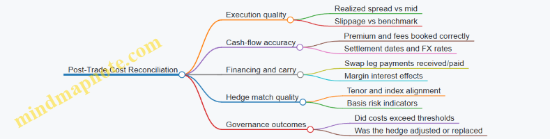
Practical Cost Checklist
- Do you have a complete cash-flow map for the hedge life?
- Are bid-ask spreads and financing estimated for the volatility regime you’re actually in?
- Did you convert costs into a common unit of protection?
- Did you include effectiveness drag from mismatch, not just fees?
- Can you reconcile expected vs realized costs after execution?
When these answers are “yes,” you’re not just measuring cost—you’re measuring whether the hedge delivered protection after the bill arrived.
12.3 Operational Readiness Including Settlement Netting and Documentation
Operational readiness is what turns a hedging plan into actual protection. It covers how trades get placed, how cash and collateral move, how confirmations match, and how records prove what happened. If you can’t explain the workflow in plain language, the workflow will eventually explain itself—usually at the worst time.
Foundational Workflow from Trade Capture to Settlement
Start with a single, end-to-end path for each hedge type. A practical way is to define the “system of record” for each step:
- Trade capture: where the hedge decision becomes an executable order.
- Execution: where the order is matched or sent to a counterparty.
- Confirmation: where terms are verified against the intended trade.
- Settlement: where cash, securities, and margin actually move.
- Recordkeeping: where the final evidence is stored.
Example: A portfolio manager decides to hedge three months of import costs with an FX forward. The operational team must know which document records the forward’s notional, rate, value date, and settlement currency, and where the confirmation will be stored for later reconciliation.
Settlement Netting That Reduces Friction Without Reducing Clarity
Netting is about reducing the number of cash movements by offsetting obligations. It can lower operational load and settlement risk, but only if you can prove the netted amounts.
Key concepts to operationalize:
- Legal basis: netting depends on enforceable agreements.
- Economic basis: netting depends on matching counterparties, currencies, and settlement dates.
- Operational basis: netting depends on systems that can calculate and report netted amounts.
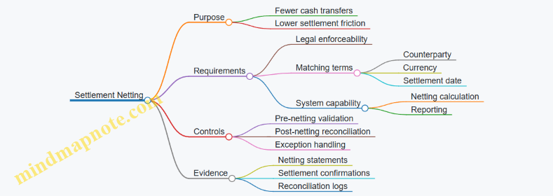
Example: You have two FX forwards with the same counterparty, both settling on the same date in the same currency. Without netting, you might receive on one and pay on the other. With netting, you pay or receive only the net amount. The control is to verify that the netting statement matches the sum of the underlying legs.
Documentation That Survives Reconciliation
Documentation is not paperwork for its own sake. It is the bridge between what you intended and what actually settled.
Create a documentation set that answers five questions for every hedge:
- What was hedged? (exposure description and hedge objective)
- What instrument was used? (terms and identifiers)
- When did it start and end? (trade date, effective date, maturity)
- How will settlement happen? (value dates, settlement method, currencies)
- How will performance be measured? (hedge effectiveness method and tolerance)
A clean approach is to separate documents by function:
- Trade documents: executed terms and confirmations.
- Operational documents: settlement instructions, standing settlement details, margin/collateral instructions.
- Governance documents: approvals, risk limits, and rebalancing decisions.
- Reconciliation documents: netting statements, matching reports, and exception tickets.
Controls for Matching, Exceptions, and Audit Trails
Operational readiness includes knowing what happens when things don’t match.
Core controls:
- Pre-confirmation checks: verify notional, currency, dates, and settlement instructions before accepting confirmations.
- Matching rules: define what fields must match exactly and what fields can differ due to standard conventions.
- Exception workflow: specify who investigates, how long they have, and what escalation path applies.
- Audit trail: ensure every change is timestamped and linked to a reason.
Example: A confirmation arrives with a value date one business day later than expected due to a holiday calendar mismatch. The exception workflow should catch it before settlement, route it to the person who can adjust instructions or renegotiate terms, and record the resolution.
Practical Example Workflow with Integrated Netting and Documentation
Assume a hedge executed on 2026-03-15 for settlement on 2026-06-15.
- Trade capture records the hedge objective and exposure window.
- Execution produces a trade identifier.
- Confirmation is matched against the intended terms, including settlement currency and value date.
- Settlement instructions are validated for the receiving and paying accounts.
- If netting applies, the system generates a netting statement for 2026-06-15.
- Post-settlement reconciliation compares:
- netted cash movement vs. netting statement
- underlying trade confirmations vs. settlement report
- The final record package is stored with a reconciliation summary and any exceptions.
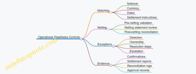
Documentation Templates That Keep Teams Aligned
Use consistent naming and structure so the right person can find the right proof quickly. A simple rule: every file name should include counterparty, instrument type, settlement date, and unique trade identifier.
Example template fields for a hedge record:
- Hedge Objective
- Exposure Reference
- Instrument Terms
- Settlement Method
- Netting Eligibility Flag
- Confirmation Storage Location
- Settlement Report Storage Location
- Reconciliation Summary
When these elements are present and consistently stored, settlement netting becomes a controlled optimization rather than a mystery box. Documentation then functions as a working tool, not a last-minute scavenger hunt.
12.4 Monitoring Metrics Including Breakevens Real Yields and Hedge Effectiveness
Monitoring is where hedging stops being a one-time decision and becomes a controlled process. You’re trying to answer three practical questions: Did inflation expectations move? Did the hedge behave as intended? And did the hedge cost more than the protection it delivered?
Breakevens as Inflation Expectation Proxies
Breakeven inflation is the difference between a nominal bond yield and the yield on an inflation-linked bond tied to the same index and maturity. It’s not “expected inflation” in a pure sense; it’s a market-implied spread that mixes expectations, risk premia, and liquidity.
A simple way to use breakevens is to treat them as a directional signal with a confidence level. If breakevens rise sharply, inflation-linked instruments may reprice favorably, while nominal bonds may face headwinds. If breakevens fall, the opposite can happen.
Example: Suppose a 5-year breakeven rises from 3.0% to 3.6% after you initiate an inflation-linked hedge. You should expect the inflation-linked leg to show improved mark-to-market, but you still need to check whether the hedge’s payoff matches your actual inflation exposure (index choice and timing matter).
Real Yields and What They Actually Tell You
Real yield is the yield level on inflation-linked instruments, often interpreted as the market’s compensation for time value and real risk. Real yields move with both inflation expectations and real interest rate conditions.
To avoid confusion, separate two effects:
- Expectation effect: breakevens move.
- Real rate effect: real yields move.
Example: If breakevens rise but real yields fall, the market may be pricing higher inflation expectations while simultaneously expecting lower real rates. Your hedge effectiveness can differ depending on which component dominates.
Hedge Effectiveness as a Measurement, Not a Feeling
Hedge effectiveness is the degree to which changes in the hedge offset changes in the hedged item. In practice, you measure it with a small set of repeatable metrics.
Use a two-layer approach:
- Economic effectiveness: Does the hedge reduce the variability of the target outcome (real purchasing power, cash flow, or liability value)?
- Accounting or contractual effectiveness: Does the hedge meet the documentation and indexation terms you set at implementation?
Example: You hedge a 12-month expense stream with an inflation-linked instrument. If inflation prints higher than expected, the hedge should increase in value or cash flows in a way that offsets the expense increase. If the index used in the hedge doesn’t match your expense index, the offset can be partial even when the hedge is “working” mechanically.
Metrics That Tie Everything Together
Track metrics on a consistent schedule (for example, weekly for liquid instruments and monthly for less liquid positions). Use the same measurement window each time.
Core metrics
- Breakeven change: ΔBE for the relevant maturity.
- Real yield change: ΔRY for the relevant maturity.
- Hedge P&L attribution: Separate P&L into index movement, rate movement, and carry/roll components.
- Offset ratio: Hedged-item change divided by hedge change, using consistent sign conventions.
- Tracking error: Volatility of the residual after offset.
- Cost of carry: Total hedge cost including financing, roll, and bid-ask impacts.
Example: If your hedge shows strong P&L but the offset ratio is low, the issue may be mismatch in maturity, index, or timing rather than hedge “failure.”
Mind Map of Monitoring Workflow
Monitoring Metrics Mind Map
A Practical Monitoring Example with Numbers
Assume you hedge a monthly expense bucket using a 1-year inflation-linked instrument.
- You record baseline values at setup: breakeven 3.2%, real yield 1.1%.
- After one month, breakeven is 3.5% and real yield is 0.9%.
- You compute hedge P&L and the hedged expense change using the same index and timing convention.
If the hedge P&L offsets 80% of the expense increase (offset ratio 0.8) but tracking error is rising, you likely have a mismatch in index timing or maturity bucket. If offset ratio is near 1.0 but cost of carry is high, the hedge may be “effective” but inefficient, which you should address by adjusting hedge horizon or instrument selection.
Common Failure Modes and How Metrics Expose Them
- Index mismatch: breakevens move but offset ratio stays low; P&L attribution shows index component not aligning.
- Timing mismatch: hedge P&L occurs earlier or later than the expense change; tracking error increases even when breakevens behave.
- Liquidity and pricing drift: breakeven and real yield changes look small, but hedge P&L attribution shows large bid-ask or valuation adjustments.
Monitoring is successful when your metrics consistently explain outcomes. If the numbers can’t tell you why the hedge worked or didn’t, the next step is usually not “hedge harder,” but “measure more precisely.”
12.5 Technical Spec: End-to-End Hedging Workflow from Setup to Review
Workflow Overview
A hedging program only works if it can be executed, measured, and corrected under real constraints like settlement timing, liquidity, and documentation. This workflow moves from setup to review in a way that keeps decisions traceable and results measurable.
Step 1: Define Hedge Purpose and Boundaries
Start by writing a one-page hedge charter: what risk is being hedged (inflation, rates, FX, or credit), what exposures are in scope, and what is explicitly out of scope. Example: a household may hedge monthly spending inflation risk for 12 months, but not long-term discretionary spending.
Create an exposure inventory with three columns: exposure amount, measurement basis (index, currency, or cash-flow schedule), and hedge objective (stabilize nominal cash flows, protect real purchasing power, or reduce drawdowns). This prevents “hedging everything” and then wondering why nothing is consistent.
Step 2: Choose Instruments and Map Payoffs
Select instruments based on payoff structure, not just headline labels.
- For inflation-linked spending, prefer index-linked cash flows or instruments whose payoff references the relevant inflation index.
- For rate volatility, use duration-aware instruments and consider convexity effects when rates move sharply.
- For FX exposure, match currency cash flows and tenor to reduce basis risk.
Example: if rent is indexed to a local CPI series, a hedge that references a different CPI variant may still help, but you should record the expected mismatch as basis risk.
Step 3: Determine Hedge Ratio and Notional
Compute a hedge ratio using a simple mapping: hedge notional × instrument sensitivity ≈ exposure sensitivity.
Use scenario testing to avoid a “works in calm markets” trap. Example: if your bond portfolio has a duration of 6 and your rate hedge is designed for duration 5, adjust notional so the effective duration aligns under the scenario you care about.
Step 4: Validate Trade Feasibility and Operational Constraints
Before placing trades, confirm:
- Settlement dates align with cash-flow needs.
- Counterparty terms match your documentation standards.
- Liquidity is sufficient for the intended size without unacceptable slippage.
- Margin or collateral requirements are understood.
A practical check: build a settlement calendar that includes trade date, valuation date, payment date, and any index observation dates for inflation-linked instruments.
Step 5: Execute with Controls and Evidence
Execution should be repeatable.
- Use approved venues and counterparties.
- Record pricing, quotes, and any deviations from the intended terms.
- Capture confirmations and legal documents immediately.
Example: for an FX forward, store the forward rate, notional, trade date, maturity, and any netting agreement details so later reconciliation can explain differences between expected and realized P&L.
Step 6: Set Up Measurement and Reconciliation
Define how hedge effectiveness will be measured. Use two layers:
- Economic effectiveness: does the hedge reduce the targeted risk metric?
- Accounting/valuation effectiveness: does the valuation method produce consistent results?
Reconcile daily or at least weekly:
- Market data inputs (rates, FX, index levels)
- Position valuations
- Cash flows received/paid
- Corporate actions or index publication timing
Example: if an inflation index updates with a lag, your valuation model must reflect the last known observation and the expected next observation window.
Step 7: Monitor Risk Limits and Trigger Rules
Monitoring is not just watching numbers; it’s enforcing pre-set boundaries.
- Hedge coverage ratio limits (minimum and maximum)
- Concentration limits by issuer, index, or counterparty
- Liquidity limits based on bid-ask spreads and expected market depth
- Counterparty exposure limits including collateral thresholds
Trigger rules should be explicit. Example: rebalance if coverage drops below 80% due to exposure changes or if basis risk widens beyond a tolerance band.
Step 8: Rebalance and Manage Costs
Rebalancing should be planned, not improvised.
- Rebalance when exposures change materially or when hedge effectiveness deteriorates.
- Track total cost of hedging: spreads, commissions, option premiums, roll costs, and financing.
Example: if you use a rolling hedge for a 12-month horizon, compare the cost of rolling monthly versus quarterly and record the decision rationale tied to liquidity and cost.
Step 9: Review Outcomes and Update the Program
At review time, compare planned versus realized outcomes:
- Risk reduction achieved versus target metric
- Sources of mismatch (basis risk, timing differences, model assumptions)
- Operational issues (late confirmations, missing data, settlement errors)
Then update the hedge charter: adjust instrument selection, hedge ratio methodology, or trigger thresholds based on what actually happened.
Mind Map: End-to-End Hedging Workflow
Example: One-Month Setup to Review Timeline
Assume a hedge is initiated on 2026-03-15 for a 12-month spending horizon.
- Week 1: charter, exposure inventory, instrument mapping, hedge ratio calculation.
- Week 2: feasibility checks, settlement calendar, trade execution with evidence capture.
- Week 3: valuation model inputs, reconciliation rules, risk limits and triggers.
- Week 4: first effectiveness measurement, cost review, and documentation cleanup.
The point of the timeline is simple: by the time the first measurement happens, you already know what “good” looks like and where mismatches are expected to come from.