Hedge Fund Strategies and Absolute Return Investing Essentials
1. Foundations of Absolute Return Investing
1.1 Defining Absolute Return and Risk Adjusted Performance
Absolute return means the portfolio aims to produce a positive result over a defined period regardless of whether the overall market is up or down. Risk adjusted performance means you do not just ask, “Did we make money?” You also ask, “How hard did we work for it, and what did it cost in risk?” A strategy can look great on raw returns and still be a poor fit if it required extreme drawdowns or relied on fragile assumptions.
Absolute Return: What It Really Measures
Absolute return is usually expressed as a percentage change in net asset value over a measurement window. The key detail is that it is portfolio-level, not a single trade-level outcome. For example, if a fund’s net value rises from 100 to 103 over a quarter, the absolute return is +3% for that quarter.
However, absolute return alone can mislead. A portfolio that earns +3% with a 20% peak-to-trough drawdown may be less attractive than one that earns +3% with a 6% drawdown. That is why risk adjusted performance matters.
Risk Adjusted Performance: The “Cost of Getting There”
Risk adjusted performance converts return into a score that accounts for volatility, drawdowns, or downside behavior. The most common inputs are:
- Volatility: how variable returns are over time.
- Downside risk: how bad losses can be, not just how often they happen.
- Drawdown: the size of the worst decline from a prior peak.
A simple example: Strategy A averages +8% annual return with 16% volatility, while Strategy B averages +8% with 8% volatility. Even if both have the same average return, Strategy B is typically preferred because its outcomes are more stable.
The Core Metrics You Will Use
Absolute return and risk adjusted performance are often summarized with a small set of metrics that complement each other.
1) Sharpe Ratio
Sharpe ratio compares excess return to volatility. If a strategy earns 10% and the risk-free rate is 4%, the excess return is 6%. If volatility is 12%, Sharpe is 6% / 12% = 0.5.
2) Sortino Ratio
Sortino replaces total volatility with downside deviation. This helps when upside swings are large but losses are the real concern.
3) Maximum Drawdown
Maximum drawdown measures the worst peak-to-trough decline. It is not a “forecast,” it is a historical stress snapshot of how the strategy behaved.
4) Calmar Ratio
Calmar ratio is annual return divided by maximum drawdown. If a strategy returns +12% and its maximum drawdown is -6%, Calmar is 12% / 6% = 2.
These metrics work best together. Sharpe can look fine even when drawdowns are uncomfortable; drawdown alone can ignore how quickly recovery happens.
A Practical Example with Integrated Reasoning
Consider two hypothetical quarterly outcomes:
- Portfolio X: +2% return, 5% volatility, -4% max drawdown.
- Portfolio Y: +2% return, 10% volatility, -12% max drawdown.
Both have the same absolute return, so the decision hinges on risk. Portfolio X shows tighter variability and a smaller worst decline, which usually improves investor experience and reduces the chance that risk limits force premature de-risking.
Now add one more nuance: if Portfolio Y’s drawdown occurs early in the quarter and recovery is slow, the strategy may trigger operational or mandate constraints even if the quarter ends positive. Absolute return can be positive while the path is still problematic.
Mind Map: Absolute Return and Risk Adjusted Performance
Putting It Into a Simple Working Definition
For practical use, treat absolute return as the outcome target and risk adjusted performance as the quality control. A strategy is “absolute return oriented” when it is designed to produce positive net results across varying market conditions, and it is “risk adjusted” when its evaluation explicitly penalizes volatility and drawdowns rather than pretending they do not exist.
1.2 Hedge Fund Role in Portfolio Construction and Diversification
Hedge funds are often used to improve a portfolio’s risk-adjusted performance, not by chasing the highest return, but by changing how risk is delivered. In portfolio construction, “diversification” means more than holding many positions; it means combining exposures that do not move together in the same way, at the same time, for the same reasons.
What Hedge Funds Add to a Portfolio
A typical hedge fund strategy can contribute one or more of these building blocks:
- Return sources that are not tied to a single market beta, such as relative value trades or event-driven spreads.
- Downside behavior that differs from equities, for example through hedging, market neutrality, or defined-risk structures.
- Diversified risk factors like volatility, credit spreads, or cross-asset relationships rather than only equity direction.
A useful mental model is to treat a hedge fund as an “exposure engine.” You want to know which exposures it runs (explicitly or implicitly), how those exposures respond under stress, and how they interact with the rest of your portfolio.
Diversification Beyond Correlation
Correlation is a starting point, but it can mislead when relationships change. Hedge fund diversification is better evaluated with three lenses:
- Sensitivity: How does the strategy’s P&L respond to equity moves, rates, credit spreads, and volatility?
- Path dependence: Does the strategy lose money during drawdowns even if the long-run average looks fine?
- Tail behavior: Are losses clustered in specific scenarios, such as liquidity gaps or funding stress?
For example, two strategies can both have low average correlation to equities, yet one may suffer large losses during equity selloffs while the other holds up due to hedged exposures.
Portfolio Construction Workflow
A systematic approach keeps the process from becoming a collection of opinions.
- Start with the portfolio’s current exposures
- Estimate factor exposures (equity beta, duration, credit sensitivity, volatility exposure) for your existing holdings.
- Translate the hedge fund into exposures
- Use historical returns, holdings data when available, and strategy mechanics to infer sensitivities.
- Set objectives and constraints
- Decide what “better” means: lower drawdown, steadier returns, reduced volatility, or improved performance net of fees.
- Run a risk-aware allocation
- Allocate based on marginal risk contribution, not just expected return.
- Stress test the combination
- Evaluate performance under scenarios that matter for the strategy’s failure modes.
A practical rule: if you cannot explain what the hedge fund is likely to be doing during a market shock, you are not ready to size it.
Mind Map: Hedge Fund Diversification in Practice
Example: Using a Market-Neutral Strategy
Suppose your portfolio is equity-heavy and has a high equity beta. You consider a market-neutral long-short equity strategy.
- What you want to confirm: the strategy’s equity beta is near zero, and its main exposures are stock-specific and sector-relative.
- What you test: performance during equity selloffs. If the strategy’s losses spike when volatility rises, you may be buying “equity neutrality” that breaks under stress.
- How you size: you allocate based on marginal contribution to portfolio drawdown, not on average correlation.
If the strategy reduces drawdowns but increases volatility modestly, it can still be a net improvement because the objective is risk-adjusted performance.
Example: Adding Relative Value to a Credit-Sensitive Portfolio
If your portfolio already has meaningful credit spread exposure, a relative value fixed income hedge fund may help by targeting spread mispricings rather than taking outright credit beta.
- What you want to confirm: the strategy’s duration and credit sensitivity are controlled, and the P&L is driven by spread relationships.
- What you test: whether the strategy hedges well when correlations between credit instruments rise.
In this case, diversification comes from changing the “where the risk lives” question: you want credit risk that is more selective and less directionally tied to the overall credit cycle.
Key Takeaway
Hedge funds earn their place in portfolio construction when they provide identifiable, testable exposure differences. Diversification is not a label; it is a measurable change in how risk is generated, experienced over time, and realized under stress.
1.3 Core Performance Metrics and Their Practical Interpretation
Absolute return sounds simple until you try to measure it. Metrics turn “it felt good” into numbers you can compare across strategies, time periods, and risk levels. The trick is to interpret each metric in context: what it rewards, what it hides, and what it assumes.
Performance Metrics Mind Map
Return Metrics That Set the Baseline
Total return answers a straightforward question: what did the strategy make over the measurement window? For example, if a portfolio grows from 100 to 112 over a year, total return is 12%. This metric is useful, but it ignores how bumpy the ride was.
Annualized return converts different time spans into a comparable rate. If the same 12% happened over 6 months, the annualized return is roughly 1.12² − 1 ≈ 25.4%. The practical point: annualization can make short, lucky periods look more impressive than they are.
Rolling return helps you see whether performance is stable or clustered. Suppose a strategy posts +2% per month for 10 months, then −15% in month 11, then +2% in month 12. Total return might still be positive, but rolling results reveal the “lumpiness” that risk metrics should capture.
Risk Metrics That Explain the Ride
Volatility measures dispersion of returns. If monthly returns average 1% with a standard deviation of 4%, volatility is 4% per month (convert to annual by multiplying by √12 for a rough estimate). Volatility is easy to compute, but it treats upside and downside symmetrically, which can be misleading for strategies that aim to avoid large losses.
Maximum drawdown captures the worst peak-to-trough decline. Example: equity peaks at 120, then falls to 96 before recovering. Drawdown is (96/120 − 1) = −20%. Two strategies can share similar volatility but have very different drawdowns; investors usually feel drawdowns more than they feel volatility.
Tail risk focuses on extreme outcomes. A simple practical proxy is the worst 5% monthly loss (a quantile). If Strategy A’s worst 5% month is −8% and Strategy B’s is −15%, A has a better downside profile even if both have similar average returns.
Risk-Adjusted Metrics That Compare Apples to Apples
Sharpe ratio is the classic: (average excess return) / (return volatility). If monthly excess return averages 0.5% and monthly volatility is 3%, Sharpe ≈ 0.5/3 = 0.167 per month. Annualizing Sharpe is often done by multiplying by √12, giving about 0.58. Interpretation: higher Sharpe means more return per unit of total variability. Limitation: it penalizes upside volatility too.
Sortino ratio replaces total volatility with downside deviation. If average return is 0.5% monthly, but only months below 0% contribute to downside deviation, Sortino can reward strategies that generate upside without frequent deep negatives. Example: two strategies both have 3% volatility, but one has many small negative months and the other has occasional large losses; Sortino typically distinguishes them.
Calmar ratio uses annualized return divided by maximum drawdown magnitude. If annualized return is 10% and max drawdown is −25%, Calmar = 10/25 = 0.40. This metric is practical for absolute return because it directly links reward to the pain investors actually experience.
Information ratio compares active return versus a benchmark divided by tracking error. Even for “absolute return” strategies, you still need an opportunity-cost benchmark. Example: if a strategy earns 6% while a cash-like alternative earns 4%, the active return is 2%. If tracking error is 3%, information ratio ≈ 0.67. Interpretation: it measures consistency of outperformance, not just level.
Practical Interpretation Rules That Prevent Misreads
- Match frequency and compounding. If you compute Sharpe on daily returns but report annualized return from monthly compounding, you can create inconsistencies.
- Use net returns when fees matter. A strategy with strong gross metrics can look mediocre net if turnover is high. Example: if gross Sharpe is 1.2 but fees reduce average return by 0.3% per month, the net Sharpe can drop sharply.
- Beware small samples. A few months can inflate ratios. Rolling windows and confidence intervals (even simple ones) help you judge stability.
- Check for leverage effects. If leverage increases, volatility and drawdowns often rise nonlinearly. A metric that looks “better” might simply be taking more risk in disguise.
- Separate performance from risk timing. A strategy might have a good Sharpe but still fail during specific regimes. Drawdown and tail metrics catch that mismatch.
A Worked Example with Integrated Metrics
Assume a strategy over one year has: total return +8%, annualized return +8% (same window), monthly volatility 4%, maximum drawdown −12%, and average monthly excess return over cash +0.3%.
- Sharpe ≈ 0.3/4 = 0.075 per month; annualized Sharpe ≈ 0.075√12 ≈ 0.26.
- Calmar = 8/12 ≈ 0.67.
- If downside deviation is 2.5% (because losses are less frequent than gains), Sortino ≈ 0.3/2.5 = 0.12 per month; annualized Sortino ≈ 0.12√12 ≈ 0.42.
Interpretation: the strategy’s drawdowns are moderate relative to its return (Calmar is decent), but its total variability is still high enough that Sharpe remains modest. That combination often points to a strategy that produces gains but with enough volatility to dilute risk-adjusted performance.
Summary of Metric Roles
Return metrics tell you what happened. Risk metrics tell you how it happened. Risk-adjusted metrics tell you whether the outcome was worth the risk, given the measure’s assumptions. When you read them together—especially Sharpe with drawdown and tail—you get a coherent picture instead of a single number that can be gamed by luck.
1.4 Constraints and Objectives That Shape Strategy Design
Strategy design starts with a simple question: what must be true for the strategy to work in the real world? Objectives tell you what “work” means, while constraints tell you what you are not allowed to do. When these two are aligned, the rest of the design becomes a sequence of choices that are easier to justify and easier to test.
Objectives That Define Success
An objective is not just a target return. It is a statement about the shape of outcomes.
- Absolute return goal: You want positive performance over a defined horizon, even if markets are flat or choppy. Example: a strategy that targets +6% annually with monthly volatility around 4%.
- Risk-adjusted goal: You care about drawdowns, not only average returns. Example: “Keep maximum drawdown under 10%” forces the strategy to avoid fragile exposures.
- Liquidity and capacity goal: You need returns that survive trading at realistic sizes. Example: if your average position turnover implies $50 million of daily trading, you must ensure spreads and slippage stay within a cost budget.
- Implementation goal: You need operational feasibility. Example: if the strategy requires frequent corporate action handling, you must set a constraint on how complex the security universe can be.
A practical way to write objectives is to pair each one with a measurable metric and a review cadence. If you cannot measure it monthly, you probably cannot manage it monthly.
Constraints That Limit Feasible Designs
Constraints are the guardrails that prevent “paper strategies” from becoming “paper losses.” They come from markets, portfolios, and operations.
- Capital and leverage constraints: Margin rules, internal risk limits, and funding costs cap how much exposure you can take. Example: if leverage is capped at 2x, a strategy that needs 3x to reach its return target must be redesigned.
- Shorting and borrow constraints: Availability and borrow rates limit short positions. Example: a pair strategy that assumes unlimited borrow will fail during stress when borrow becomes scarce.
- Trading cost constraints: Spreads, commissions, and slippage reduce expected returns. Example: if the expected edge is 0.20% per trade and average round-trip costs are 0.18%, you have almost no room for execution slippage.
- Market impact constraints: Large orders move prices. Example: a momentum strategy that rebalances daily may breach impact limits when volatility spikes.
- Model and data constraints: Missing data, stale corporate actions, and regime shifts limit what signals can reliably do. Example: a factor model built on stale fundamentals may look stable in backtests and drift in live trading.
- Operational and compliance constraints: Trading restrictions, approval workflows, and settlement rules affect what you can trade and when. Example: if certain instruments require pre-trade approvals, you cannot assume instantaneous execution.
Turning Objectives and Constraints Into Design Choices
Once objectives and constraints are explicit, you can translate them into design parameters.
- Choose the risk budget first. If maximum drawdown is capped, you set position sizing and exposure limits accordingly.
- Select the strategy family that matches the constraints. If shorting is constrained, long-only or market-neutral-with-borrow-management may be more feasible than pure long-short.
- Define the execution policy that fits the cost budget. If turnover is high, you must use tighter cost controls or lower turnover.
- Set monitoring rules that trigger de-risking. Constraints are not only for initial construction; they must be enforced continuously.
Mind Map: Objectives and Constraints to Strategy Parameters
Example: A Momentum Strategy with a Cost Budget
Suppose your objective is +8% annual absolute return with a maximum drawdown of 12%. Your constraints include a cost budget of 0.30% per round trip and a leverage cap of 1.5x.
- If you rebalance daily, turnover is high and average round-trip costs might reach 0.35%, exceeding the budget. The design choice is not “try harder,” it is to change the rebalance frequency or reduce trading intensity.
- If you switch to weekly signals, turnover drops and costs might fall to 0.25% per round trip, leaving room for the expected edge.
- If drawdown still threatens the 12% limit, you adjust volatility scaling and stop rules so that position sizes shrink during high-volatility regimes.
The key is that each constraint forces a specific parameter change: frequency for cost, sizing for drawdown, and leverage for funding feasibility.
Example: Pair Trading Under Borrow Constraints
A market-neutral pair strategy aims for stable returns by hedging beta and holding a spread position. The objective is low drawdown, but the constraint is borrow availability.
- In backtests, the short leg is always available, so the strategy looks consistent.
- In live trading, borrow becomes expensive or unavailable for certain names, causing missed entries and forced exits.
Design fixes are concrete: restrict the universe to names with reliable borrow, cap borrow rates, and add a fallback rule such as holding the long leg only when the short leg cannot be established within a defined cost threshold.
When objectives and constraints are written down early, the strategy stops being a collection of clever ideas and becomes a set of enforceable rules that can be tested, monitored, and improved without surprises.
1.5 Practical Example: Mapping Objectives to Strategy Choices
You can’t pick a hedge fund strategy by vibes. You start with objectives, translate them into constraints, and then match those constraints to what each strategy can realistically deliver. Here’s a systematic example that moves from foundational choices to implementation details.
Step 1: Write the Objective in Measurable Terms
Assume an investor wants:
- Target return: 6% annualized
- Risk tolerance: maximum 8% peak-to-trough drawdown
- Liquidity need: monthly subscriptions and redemptions
- Capital stability: avoid strategies that require frequent large leverage changes
A practical best practice is to convert “risk” into something you can monitor daily or weekly. For instance, you can translate drawdown tolerance into a volatility budget and a de-risking rule (for example, reduce gross exposure when portfolio volatility breaches a threshold).
Step 2: Translate Objectives Into Constraints
From the objective set, you derive constraints that will later eliminate unsuitable strategies.
- Drawdown constraint implies you need either (a) naturally defensive exposures, (b) hedges that respond quickly, or (c) position sizing that scales down during stress.
- Monthly liquidity implies you should avoid strategies with settlement or execution cycles that make pricing stale or trading too slow.
- Leverage stability implies you prefer strategies where risk can be managed through sizing and hedging rather than constant leverage rebalancing.
Step 3: Map Constraints to Strategy Families
Different strategy families “solve” different parts of the problem. The mapping below is intentionally blunt: it helps you decide what to test first.
Mind Map: Objective to Strategy Mapping
Step 4: Choose a Shortlist Using a Simple Scoring Rubric
A quick rubric prevents endless debate. Score each strategy family from 1 to 5 on each criterion, then sum.
Example criteria aligned to the constraints:
- Drawdown control (can the strategy reduce risk quickly?)
- Liquidity and pricing timeliness (can you trade and value consistently?)
- Leverage stability (can risk be managed without constant leverage swings?)
- Cost realism (can you model trading and hedging costs without hand-waving?)
Suppose you score:
- Market Neutral Equity: 5 (drawdown control), 4 (liquidity), 4 (leverage stability), 3 (cost realism) → 16
- Long Short Equity: 4, 4, 3, 3 → 14
- Fixed Income Relative Value: 4, 5, 4, 4 → 17
- Volatility Options: 3, 3, 4, 2 → 12
The top two are Fixed Income Relative Value and Market Neutral Equity. That doesn’t mean they’re “best,” only that they match the objective constraints more closely.
Step 5: Turn the Choice Into an Implementation Plan
Now you define the rules that make the strategy behave like the objective.
Example A: Market Neutral Equity sleeve
- Risk budget: target portfolio volatility of 6% with a hard cap at 8%.
- Sizing rule: scale gross exposure inversely with estimated idiosyncratic volatility.
- Hedge rule: maintain factor neutrality using a small set of liquid factors (for example, sector and style) and rebalance when exposures drift beyond thresholds.
- De-risking: if realized volatility breaches the cap for two consecutive weeks, cut gross exposure by 25% and tighten stop conditions.
Concrete example: if a pair trade’s spread z-score suggests entry but the factor exposure drift exceeds the threshold, you skip the trade or reduce size. This is how you prevent “good signals” from breaking the risk budget.
Example B: Fixed Income Relative Value sleeve
- Risk budget: limit key rate duration and spread risk so the sleeve contributes a controlled fraction of total portfolio drawdown.
- Scenario stress: run historical spread widening and rate shock scenarios, then set position limits so losses stay within the sleeve’s drawdown budget.
- Execution rule: trade in liquid tenors first, and cap turnover to keep transaction costs predictable.
Concrete example: if a curve trade looks attractive on carry but the scenario set shows that spread widening dominates, you reduce position size or choose a different maturity pair with better stress behavior.
Step 6: Validate the Mapping with Backtests That Respect Constraints
Finally, you test whether the strategy choices actually honor the constraints when costs and timing are included.
- Use realistic bid-ask and slippage assumptions.
- Include delays for signal formation and rebalancing.
- Apply the same de-risking rules used in the plan.
If the backtest shows drawdowns exceeding the 8% target even after de-risking, the mapping is wrong. The fix is not “try harder,” it’s to adjust the strategy choice, the risk budget, or the hedging and sizing rules.
Step 7: Produce the Decision Artifact
You end with a one-page mapping summary:
- Objective metrics
- Derived constraints
- Shortlisted strategy families
- Scoring rubric results
- Implementation rules for sizing, hedging, and de-risking
That artifact is what keeps the strategy selection coherent when real trading starts behaving like real trading.
2. Market Microstructure and Trading Mechanics
2.1 Order Types Execution Paths and Cost Implications
Order execution is where “strategy” meets “reality.” The order type you choose determines how your intent is routed through the market, how quickly it can be filled, and what costs you’ll likely pay. Those costs show up as explicit fees and implicit frictions like spread, slippage, and market impact.
Execution Path Basics
An order typically moves through three stages: submission, matching, and post-trade processing. Submission includes routing to a venue and choosing how the order behaves while it waits. Matching is where the order interacts with the limit order book or with auction mechanisms. Post-trade processing covers settlement and reporting, which affects operational cost but not trading P&L directly.
The key idea: different order types change your “interaction style” with liquidity. A market order aggressively seeks immediate execution, while a limit order offers a price and waits for counterparties who like that price.
Market Orders
A market order is executed against the best available prices until the order quantity is filled or liquidity runs out. The execution path is straightforward: it consumes liquidity at the top of the book and then walks the book if needed.
Cost implication: you pay the spread in expectation because you cross it immediately. If the order is large relative to visible depth, you also pay additional levels of the book, which shows up as slippage.
Example: Suppose the best bid is 100.00 and best ask is 100.01. A buy market order for 10 shares likely fills at 100.01 first. If the ask depth at 100.01 is only 4 shares, the remaining 6 shares fill at the next ask level, say 100.02. Your average fill becomes 100.014, not 100.01.
Limit Orders
A limit order specifies the worst acceptable price. A buy limit at 100.00 will only execute at 100.00 or lower. The execution path depends on whether the market reaches your price and whether your order becomes the best available offer or bid.
Cost implication: you avoid crossing the spread, so you typically reduce immediate slippage. The trade-off is fill probability. If price moves away, you may get partial fills or none.
Example: You place a buy limit at 100.00 for 10 shares. If the market trades down to 100.00 for a moment, you might get a partial fill at 100.00 and then stop. If it never returns, you pay no trading cost but also achieve no position.
Limit vs Market Under Volatility
Volatility changes the balance between speed and price. In fast markets, market orders tend to fill quickly but with worse average prices due to book walking. Limit orders can protect price but may miss the move entirely.
A practical best practice is to align order aggressiveness with your signal horizon. If your edge depends on being in quickly, you accept higher expected costs. If your edge tolerates waiting, you can use limit orders to control price.
Time-in-Force and Queue Position
Time-in-force (TIF) controls how long the order stays active. Common choices include Day (expires at end of session) and Good-Til-Cancelled (remains until canceled). Queue position matters: earlier orders at the same price generally get matched first.
Cost implication: a longer-lived limit order can improve fill probability, but it also increases exposure to adverse selection if the market moves against you while you wait.
Example: Two traders submit buy limits at 100.00 for 10 shares. Trader A submits at 10:00:01, Trader B at 10:00:05. If the price touches 100.00 for 3 seconds with enough sell liquidity, Trader A is more likely to get filled first, reducing the chance of partial fills.
Routing and Venue Selection
Routing determines where your order is sent and how it’s exposed to liquidity. Some venues may have tighter spreads or deeper books for a given instrument, while others may have different fee schedules.
Cost implication: the same order type can produce different results across venues because of fee differences and available depth.
Example: A limit order routed to a venue with a narrower spread may execute at a better price, even if the maker fee is slightly higher. Conversely, a venue with deeper depth can reduce slippage for market orders.
Partial Fills and Average Price
Partial fills are not a failure; they’re a cost profile. Your realized execution quality depends on the sequence of fills and the evolving book.
Best practice: track average execution price versus the prevailing mid at submission time. If average price deteriorates quickly, your order type may be too aggressive for the current liquidity.
Mind Map: Order Types and Cost Drivers
Practical Example: Choosing an Order Type
Assume you want to buy 1,000 shares and the instrument’s top-of-book depth at the best ask is 300 shares. If you use a market order, you will likely consume multiple price levels, increasing slippage. If you use a limit order at the best ask, you may get only the 300 shares initially, then wait for additional sellers to appear at your price.
A systematic approach is to estimate visible depth and decide whether you prefer predictable price with uncertain timing (limit) or predictable timing with uncertain price (market). Then set TIF to match your tolerance for waiting, and route to venues that offer the best combination of depth and fees for that order type.
2.2 Liquidity Measurement and Trading Venue Selection
Liquidity is not one number; it’s a set of frictions that show up as spreads, depth, and the way prices move when you trade. Venue selection is the practical step where those frictions become real costs.
Liquidity Components That Actually Matter
Start with three observable pieces:
- Bid-ask spread: the immediate cost of crossing from one side to the other. If you buy at the ask and later sell at the bid, the spread is your first hurdle.
- Order book depth: how much size is available near the top of book. Thin depth means your order walks the book, widening your effective spread.
- Price impact: how much the midprice shifts due to your trade. Impact depends on size relative to typical order flow and on how quickly liquidity replenishes.
A useful mental model: spread is the “cover charge,” depth is the “how many seats are left,” and impact is the “how much the room changes when you sit down.”
Measuring Liquidity with Practical Metrics
Use metrics that connect to execution, not just market snapshots.
- Effective spread: compare execution price to mid at the time of trade. For a buy, effective spread is roughly \(2 \times (\text{exec price} - \text{mid})\). This captures both spread and microstructure noise.
- Depth at distance: measure cumulative size within a few basis points from mid (for example, within 1 bp and 5 bp). This helps estimate how far your order will travel if you join the book.
- Volume at price and replenishment: track how quickly the book refills after trades. A venue with similar depth can still be worse if replenishment is slow.
- Realized slippage vs. size: bucket trades by participation rate (your order size divided by venue volume over the interval) and compute average slippage. This turns “liquidity” into a size-dependent cost curve.
Venue Selection Framework
Venue choice should be driven by the execution objective.
- If you need immediacy: prioritize venues with lower effective spread and lower short-horizon impact for your typical order size.
- If you can wait: prioritize venues with strong replenishment and sufficient depth near mid, since you’ll often trade via passive orders.
- If you trade across venues: compare not only prices but also how quickly your order can be filled without moving the market.
A simple decision rule is to estimate expected total execution cost for each venue:
\(\text{Expected cost} = \text{Expected spread component} + \text{Expected impact component} + \text{Expected adverse selection component}\)
Adverse selection is the risk that your trade hits informed flow; it shows up as worse-than-expected execution relative to mid.
Mind Map: Liquidity Measurement and Venue Selection
Example: Choosing Between Two Venues
Assume you trade 200,000 shares of a liquid equity.
- Venue A shows a quoted spread of 1.0 bp, but depth within 1 bp is only 50,000 shares. Your order likely walks the book.
- Venue B shows a quoted spread of 1.3 bp, but depth within 1 bp is 250,000 shares and replenishment is fast.
If you place a passive order, Venue B can yield a lower effective spread because your order fills without moving far from mid. If you must cross immediately, Venue A might win because the smaller quoted spread reduces the crossing cost, even if depth is thin.
To make this concrete, compute for each venue:
- expected fill price using depth buckets,
- expected impact using slippage vs participation from recent executions,
- and compare the sum.
Example: Participation Rate as the Bridge Between Liquidity and Impact
Suppose your typical interval volume on Venue A is 10 million shares, and your order is 200,000 shares. Participation is 2%. If historical data shows that at 2% participation, average slippage is 2.5 bp on Venue A and 1.8 bp on Venue B, then Venue B is cheaper for your usual urgency level.
If you later change order size to 600,000 shares (6% participation), the impact curve may steepen. Venue selection should follow the new participation regime rather than the old one.
Operational Checks That Prevent “Good Theory, Bad Fills”
Before routing decisions become policy, verify:
- Time-of-day effects: liquidity often changes across the session, so compute metrics by time buckets.
- Instrument-specific behavior: depth and impact can differ even for similar tick sizes.
- Consistency of midprice reference: ensure you use the same mid definition when computing effective spread.
A venue that looks best on a random snapshot can lose once you account for how your order size interacts with depth and replenishment.
2.3 Slippage Modeling and Transaction Cost Estimation
Slippage is the difference between the price you intended and the price you actually get. Transaction costs are broader: they include explicit fees and implicit costs like spread and market impact. Modeling both matters because a strategy that looks profitable on mid-price can quietly lose money once you pay the bill.
Core Concepts and What They Mean in Practice
Start with three price references:
- Mid-price: average of best bid and best ask. It’s a convenient “fair” reference.
- Execution price: where your order actually fills.
- Realized cost: execution price minus the reference, adjusted for direction (buy vs sell).
A simple way to think about costs for a buy order is:
- Half-spread cost: if you cross the spread, you effectively pay the ask; relative to mid, that’s about half the spread.
- Adverse selection: if you trade when the market is about to move against you, you pay more than the spread alone.
- Market impact: your order changes prices, especially when size is large relative to liquidity.
A good model separates these components so you can test which lever actually improves results.
Building a Slippage Model from Observable Inputs
A practical slippage model uses observable market data and a few strategy parameters:
- Order aggressiveness: market order vs limit order, and how quickly you cancel.
- Trade size: shares/contracts relative to typical volume.
- Liquidity: spread width and depth near the best quotes.
- Volatility: faster markets tend to widen realized costs.
- Time of day: liquidity and volatility vary across the session.
Mind Map: Slippage Modeling Components
Estimating Spread and Fees First
Before impact modeling, compute the easy parts.
- Spread cost: estimate using historical average bid-ask spread at the time you would trade. If you use mid-price in backtests, you can convert to a more realistic reference by subtracting half the spread for buys and adding half the spread for sells.
- Fees: use your venue schedule. Even if fees are small, leaving them out can distort comparisons between strategies with different turnover.
Example: Suppose the average spread at your execution times is 10 bps (0.10%). If your backtest assumes mid-price, a market buy will typically cost about 5 bps relative to mid, before impact.
Modeling Market Impact with a Size-to-Liquidity Lens
Market impact grows with order size and with how quickly you trade. A common approach is to relate impact to participation rate:
- Participation rate = your order size / typical volume over the order’s time window.
Then estimate impact as a function of participation and volatility. A simple, robust form is:
- Impact ≈ k × (participation rate)^α × volatility
Where:
- k scales the level for your instrument and venue,
- α controls curvature (often between 0.3 and 1.0 in practice),
- volatility can be measured as short-horizon realized volatility.
You don’t need a perfect formula to be useful. You need a model that responds correctly when liquidity worsens.
Example: Impact Sensitivity with Two Trade Sizes
Assume:
- short-horizon volatility proxy = 1.0% per day,
- α = 0.6,
- k chosen so that a 10% participation trade costs 0.20%.
If you double participation to 20%, impact scales by (2^0.6) ≈ 1.52, so cost becomes about 0.30%. That’s the key behavior you want: bigger trades cost disproportionately more.
Adverse Selection and Timing Effects
Adverse selection captures the idea that your order may execute when the market is already moving against you. A workable method is to estimate slippage conditional on short-term price movement:
- Compute the return over a short window around execution (for example, from 1 minute before to 1 minute after).
- Regress realized execution price vs that movement, separately for buys and sells.
If buys tend to fill after upward moves, you’ll see negative adverse selection for buys (you paid more than expected). If the sign flips, your model should reflect it rather than assuming a constant bias.
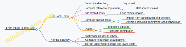
Putting It Together for Total Transaction Cost Estimation
For each simulated trade, estimate:
-
Reference adjustment from spread
-
Fees
-
Impact from participation and volatility
-
Adverse selection from timing-conditioned bias
Then sum across trades, including rebalancing and any hedges. A strategy with frequent small trades may have low impact but still lose to spread and fees. A low-turnover strategy may look great until you model impact on the occasional large rebalance.
Mind Map: From Inputs to Total Cost
Validation That Doesn’t Lie
Validate the model against historical executions or realistic proxy fills. Check three things:
- Level: does predicted average slippage match observed averages?
- Shape: does slippage increase with size and worsen in low-liquidity periods?
- Direction: do buy and sell costs behave differently when the market moves?
If the model matches level but not shape, your backtest may still be misleading. If it matches shape but not level, your assumptions about fees, spread, or scaling are off. Either way, fixing it improves the strategy’s cost realism without changing the core trading logic.
2.4 Market Impact and Turnover Management
Market impact is the price change caused by your own trading. Turnover is how often you trade, usually measured as traded value divided by average portfolio value. Together, they determine whether a strategy’s expected edge survives real trading costs—or gets quietly eaten by the market.
Why Market Impact Matters
Even if your signal is correct, execution can shift your realized entry and exit prices. Impact tends to rise when liquidity is thin, when orders are large relative to typical volume, and when urgency is high. A useful mental model is: you trade, the order book adjusts, and the adjustment becomes part of your cost.
A simple decomposition helps: total trading cost is roughly (i) explicit costs like commissions and fees, (ii) implicit costs like bid-ask spread, and (iii) impact costs from moving the price. Turnover management mainly targets the third component, but it also changes how often you pay spread and fees.
Foundational Building Blocks
- Order size vs. liquidity: If your order is a noticeable fraction of the average volume over your execution window, impact is more likely to be meaningful.
- Execution speed: Faster execution usually increases impact because you consume liquidity quickly.
- Participation rate: A common control variable is the fraction of market volume you intend to trade during a time slice.
- Order type and aggressiveness: Market orders typically pay more impact than passive limit orders, but passive orders can face adverse selection and fill uncertainty.
Impact Models in Practice
You don’t need a PhD-level model to manage impact. A practical approach is to estimate a cost-per-share (or cost-per-dollar) that increases with size and urgency.
A common structure is:
- Temporary impact: cost that depends on how quickly you execute.
- Permanent impact: longer-lasting price effects that may persist after your trade.
For day-to-day execution planning, temporary impact is often the main driver. You can approximate it by scaling observed slippage with participation rate and volatility.
Turnover Management as a Cost Control System
Turnover management is not “trade less” as a slogan. It is choosing a trading frequency that matches signal decay and rebalancing needs.
- If a signal changes slowly, frequent rebalancing just adds spread and impact without improving outcomes.
- If a signal changes quickly, delaying trades can reduce edge, but executing too aggressively can also destroy it.
A systematic workflow:
- Define a target rebalance rule: e.g., rebalance when weight deviates by a threshold or on a schedule.
- Estimate incremental cost per rebalance: include expected spread and impact.
- Compare incremental benefit to incremental cost: if the expected improvement is smaller than the cost, the rebalance rule is too sensitive.
Concrete Example: Rebalance Threshold vs. Execution Cost
Suppose you run a strategy that targets a 5% position in a liquid stock. Your average daily volume is $200 million, and your typical portfolio value is $50 million.
- Aggressive schedule: rebalance daily back to target. If you trade $2.5 million per day (5% of $50m), your participation rate is about 1.25% of daily volume.
- Threshold schedule: rebalance only when the position drifts by more than 0.5 percentage points. If drift is usually small, you might trade only 2–3 times per week.
Even if the stock is liquid, the threshold approach reduces the number of times you cross the spread and reduces how often you create short-term price pressure. The key is that you’re not changing the signal; you’re changing how often you convert it into trades.
Mind Map: Market Impact and Turnover Management
Advanced Details Without the Confusion
Participation rate targeting: Instead of “execute quickly,” set a participation rate cap. If you cap participation, you implicitly slow down execution when liquidity is low.
Slice and schedule: Break a large order into smaller slices and distribute them across time windows with better liquidity. This reduces peak pressure.
Avoiding adverse selection: Passive orders can be filled by counterparties who know something you don’t. A balanced approach uses limit orders when spreads are stable and switches to more aggressive execution when fill risk becomes too high.
Turnover-aware portfolio rules: Weight-based thresholds, banded rebalancing, and volatility-scaled position updates all reduce unnecessary trading. The best rules are the ones that are measurable: you can compute expected drift, expected trade size, and expected cost.
Practical Checklist for Execution Planning
- Estimate expected trade size and participation rate.
- Choose order type based on liquidity and urgency.
- Use slicing to reduce peak impact.
- Apply rebalance thresholds to avoid churn.
- Validate with realized slippage and cost attribution by trade bucket.
When impact and turnover are treated as first-class design constraints, execution stops being a post-trade surprise and becomes part of the strategy’s cost-aware logic.
2.5 Practical Example: Building a Trade Cost Budget
A trade cost budget is a simple, disciplined way to decide whether a strategy’s expected edge can survive real-world frictions. The goal is not to predict the future perfectly; it’s to set a cost ceiling that your execution must beat, and to quantify what “beat” means.
Step 1: List Cost Components in Plain Categories
Start with costs you can estimate before trading:
- Explicit costs: commissions, exchange fees, clearing fees.
- Implicit costs: bid-ask spread, slippage from price movement during execution.
- Market impact: price pressure caused by your own orders, especially for larger trades.
- Operational costs: failed orders, late cancels, re-quotes, and any systematic delays.
A useful rule: if a cost is small but frequent, include it; if it’s rare but huge, include it too. Either way, your budget should reflect the strategy’s trading pattern.
Step 2: Choose a Unit of Measurement
Pick one consistent unit so comparisons are meaningful. Common choices:
- Cost per share (good for single-name equity trades)
- Cost per notional dollar (good for cross-asset)
- Cost per trade (good for event-driven)
For this example, use basis points (bps) of notional so it scales cleanly.
Step 3: Build a Numeric Example for One Trade
Assume a strategy trades $1,000,000 notional of a liquid stock.
Inputs (illustrative, but realistic in structure):
- Commission and fees: $2,500 per trade
- Average bid-ask spread: $0.02 per share
- Average price: $50
- Shares traded: $1,000,000 / $50 = 20,000 shares
- Slippage from execution timing: 0.8 bps
- Market impact allowance: 1.2 bps
Convert the spread into bps. If you cross the spread once on average, the spread cost is roughly half-spread to full-spread depending on execution. Use a conservative midpoint assumption: 0.75 of the spread.
- Spread dollars per share: $0.02
- Spread cost per share: 0.75 × 0.02 = $0.015
- Spread cost total: 20,000 × 0.015 = $300
- Spread cost in bps of notional: ($300 / $1,000,000) × 10,000 = 3.0 bps
Commission and fees in bps: ($2,500 / $1,000,000) × 10,000 = 25 bps
Now sum the budget components:
- Fees: 25.0 bps
- Spread: 3.0 bps
- Slippage: 0.8 bps
- Market impact: 1.2 bps
Total trade cost budget = 30.0 bps.
If your strategy’s expected gross alpha per trade is, say, 35 bps, then the net edge is 5 bps before taxes, financing, and any model error. If expected gross alpha is 25 bps, the trade is structurally unprofitable under this cost ceiling.
Step 4: Translate the Budget Into Execution Requirements
A budget is only useful if it becomes actionable. Turn the total into constraints:
- If fees are fixed, the remaining “execution allowance” is 30.0 − 25.0 = 5.0 bps.
- That 5.0 bps must cover spread, slippage, and impact.
- If your historical slippage is trending toward 2.5 bps, you must reduce impact via smaller slices, better timing, or more selective liquidity.
Step 5: Add a Simple Stress Check
Costs are not constant. Add a stress scenario that increases slippage and impact while leaving fees unchanged.
- Base: slippage 0.8 bps, impact 1.2 bps
- Stress: slippage 1.6 bps, impact 2.4 bps
Recompute: fees 25.0 + spread 3.0 + slippage 1.6 + impact 2.4 = 32.0 bps.
Your strategy must still clear the threshold under stress, or you need to adjust position sizing, execution style, or signal selectivity.
Mind Map: Trade Cost Budget Workflow
Example: Budgeting for a Different Execution Style
If instead of crossing you use passive orders and achieve a better fill, the spread component can drop. Suppose spread cost falls from 3.0 bps to 1.5 bps, but slippage rises from 0.8 bps to 1.4 bps due to waiting.
New total: fees 25.0 + spread 1.5 + slippage 1.4 + impact 1.2 = 28.1 bps.
The budget tells you whether passive execution is actually improving net cost. If it doesn’t, you don’t “try harder”; you change the assumptions or the execution approach.
Step 6: Record the Budget and Compare to Realized Costs
For each trade, store:
- Notional
- Realized effective spread (or proxy)
- Realized slippage vs decision price
- Any impact proxy you track
- Total realized cost in bps
Then compare realized costs to the budget ceiling. If realized costs are consistently above budget, the issue is usually one of three things: the spread proxy is wrong, slippage is underestimated, or impact is larger than assumed for your trade size and venue.
A good trade cost budget is boring in the best way: it turns “execution matters” into numbers you can manage.
3. Portfolio Construction for Hedge Fund Style Returns
3.1 Risk Factor Decomposition and Exposure Management
Risk factor decomposition turns “the portfolio is risky” into a map of what is actually driving returns and losses. In practice, you start with a factor model, estimate exposures, and then manage those exposures so the portfolio behaves the way you intend under different market conditions.
Core Idea: Separate Return Drivers from Random Noise
A factor model expresses portfolio returns as a combination of systematic components plus idiosyncratic noise. The systematic components are the ones you can manage; the noise is the part you can only reduce by diversification and better estimation.
A simple linear form is:
- Portfolio return ≈ sum of (factor exposure × factor return) + residual
If your residual is large, your strategy is relying on things you cannot reliably forecast. If your factor exposures are unstable, your risk control will be inconsistent even if your backtest looks fine.
Step 1: Choose a Factor Set That Matches Your Strategy
Factor sets should be practical, not encyclopedic. For equity long-short, common categories include:
- Market beta (broad equity direction)
- Style factors (value, growth, size, momentum)
- Sector or industry factors
- Quality or profitability proxies
- Volatility or liquidity proxies
For absolute return goals, you typically want to control broad direction and style drift while allowing controlled idiosyncratic selection.
Example: If your long-short book is meant to be market neutral, you still need to decide whether “neutral” means beta-neutral only, or also neutral across size and sector. Beta-neutral alone can still leave you exposed to sector swings.
Step 2: Estimate Exposures Using Holdings and Factor Loadings
Exposure estimation links what you hold to how those holdings behave. You can estimate factor exposures using:
- Factor loadings per security (from a regression or vendor model)
- Portfolio weights (including long and short positions)
- Optional adjustments for corporate actions, borrow costs, and liquidity constraints
A practical workflow:
- Compute net weights by factor-relevant dimensions (e.g., sector, style).
- Convert those into factor exposures using the chosen factor loadings.
- Validate exposures by checking whether predicted factor PnL explains realized PnL during recent windows.
Example: Suppose you hold 60% long and 60% short with equal gross exposure. If your factor model shows a +0.20 market beta exposure, the book is not neutral; it is directionally tilted even if the gross is balanced.
Step 3: Manage Exposures with Explicit Targets and Limits
Exposure management is not “minimize risk” in the abstract. It is “keep exposures within ranges that match your mandate.” Typical controls include:
- Target exposures (e.g., beta = 0, sector net = 0)
- Hard limits (e.g., |value factor exposure| ≤ 0.05)
- Soft penalties (e.g., discourage concentration in a single sector)
- Turnover-aware constraints (to avoid rebalancing that breaks cost assumptions)
Example: You run a market-neutral strategy. You set:
- Market beta target: 0
- Sector exposure limits: ±0.02 per sector
- Momentum exposure limit: ±0.03
If a new trade candidate increases momentum exposure beyond the limit, you either reduce its size, pair it with an offsetting position, or reject it.
Step 4: Account for Estimation Error and Model Risk
Factor models are approximations. Two common failure modes are:
- Factor loadings drift over time
- Correlations among factors change, making exposures harder to interpret
Mitigations that fit naturally into the workflow:
- Use rolling windows for loadings and exposures
- Monitor factor exposure stability (not just level)
- Stress-test exposure changes under plausible shocks to factor returns
Example: If your value factor exposure is near zero today but has been swinging between -0.10 and +0.10, you should treat it as unstable and tighten limits or improve the estimation method.
Step 5: Translate Factor Exposures Into Risk Budgeting
Risk budgeting connects exposures to expected volatility and drawdown behavior. A common approach is to use a factor covariance matrix:
- Factor risk ≈ exposure vector × factor covariance × exposure vector
- Add residual risk from idiosyncratic variance
Then you allocate risk budgets across sleeves or strategies.
Example: If your total risk budget is 8% annualized volatility and your equity sleeve consumes 6%, you can cap its factor-driven risk while allowing controlled residual risk from stock selection.
Mind Map: Risk Factor Decomposition and Exposure Management
Worked Example: From Holdings to Controlled Exposure
Assume a long-short equity book with net market beta target 0.
- Current portfolio market beta exposure: +0.12
- Target: 0
- Allowed band: ±0.03
You identify a candidate trade that would add +0.04 beta exposure if added alone. Instead of rejecting immediately, you check whether pairing it with an offsetting position reduces net beta to within the band. If the pair brings beta to +0.02 while keeping sector exposure within limits, the trade is acceptable. If it fixes beta but pushes sector exposure beyond its limit, you adjust the pair or reduce size.
The key is that every decision is evaluated against the same exposure framework, so risk control stays consistent as the portfolio evolves.
3.2 Position Sizing Methods for Volatility and Drawdown Control
Position sizing is where “good ideas” meet “survivable reality.” The goal is simple: scale exposure so losses stay within a drawdown budget while still allowing enough size to matter when signals work. This section builds from volatility basics to drawdown-aware sizing, then turns it into implementable rules.
Core Concepts That Drive Sizing
Volatility sizing starts with the idea that risk is not constant. If a strategy’s returns swing more, the same notional position can produce larger losses. Drawdown control adds a second layer: even if average risk looks fine, clustering of losses can push the portfolio into unacceptable territory.
A practical way to connect these ideas is to treat sizing as a mapping from forecasted risk to allowed loss. You can do this with either (1) volatility targeting, (2) drawdown budgeting, or (3) a hybrid that uses both.
Volatility Targeting with a Clear Loss Budget
Volatility targeting chooses position size so the expected contribution to portfolio volatility matches a target. A common starting point uses realized volatility over a recent window.
Example: Suppose you trade an equity long/short sleeve and estimate the sleeve’s 20-day annualized volatility at 25%. Your portfolio volatility target for this sleeve is 10% annualized. If the sleeve’s return stream is roughly proportional to position size, scale by:
- Size multiplier ≈ target_vol / current_vol = 10% / 25% = 0.4
If you would normally allocate $1,000,000 notional, you allocate $400,000 instead. The “why” is straightforward: when volatility rises, the multiplier shrinks, reducing the chance that a normal signal produces an outsized loss.
Best practice: use a volatility estimate that is stable enough to avoid whipsaw. A shorter window reacts faster but can overreact to noise; a longer window is steadier but slower to respond.
Volatility Targeting with Correlation-Aware Scaling
Portfolio risk is not just the sleeve’s own volatility; it’s also how it moves with the rest. If your sleeve is correlated with existing exposures, the same notional can increase portfolio volatility more than you expect.
Example: You already hold a factor-tilted book. Your new sleeve has 25% standalone volatility, but its correlation with your factor book is 0.6. If you ignore correlation, you may size too large. A correlation-aware approach estimates the incremental portfolio variance contribution and scales to keep the incremental contribution near the target.
A simple approximation uses covariance:
- Incremental variance ≈ w_new^2 * var_new + 2 * w_new * w_existing * cov(new, existing)
Then solve for w_new that yields the desired incremental variance. Even a rough covariance estimate improves sizing discipline.
Drawdown-Aware Sizing That Reacts to Loss Clustering
Volatility targeting controls typical risk, but drawdowns are about the path of returns. Drawdown-aware sizing reduces exposure after losses accumulate, even if volatility is unchanged.
A workable method is to define a drawdown budget and scale down when the portfolio drawdown breaches thresholds.
Example: Let your maximum tolerable drawdown for the sleeve be 8% from its recent peak. Create two bands:
- Band A: drawdown 0%–4% → 100% size
- Band B: drawdown 4%–8% → linearly scale from 100% to 50%
If the sleeve drawdown reaches 6%, the scale factor is 75%. A $1,000,000 notional becomes $750,000. This prevents “normal” sizing from turning a temporary slump into a portfolio-level problem.
Best practice: use a rolling peak definition (e.g., peak over the last N trading days) so the drawdown measure resets in a controlled way.
Hybrid Approach Combining Volatility and Drawdown
The most robust practical sizing rules often combine both controls: volatility targeting sets the baseline size, and drawdown control applies a risk-off multiplier.
Example: Baseline volatility targeting gives a multiplier of 0.4. The drawdown band multiplier at the moment is 0.75. Final multiplier = 0.4 * 0.75 = 0.3. If you would allocate $1,000,000 notional, you allocate $300,000.
This hybrid avoids two common failure modes: volatility-only sizing that ignores loss streaks, and drawdown-only sizing that ignores changing market regimes.
Implementation Mind Map
Mind Map: Position Sizing for Volatility and Drawdown Control
Practical Guardrails That Prevent Accidental Overconfidence
- Cap leverage and notional changes: Even with correct formulas, sudden sizing jumps can create execution stress.
- Use consistent units: Volatility estimates, targets, and multipliers must align (annualized vs daily).
- Separate signal strength from sizing: If your signal is weak, sizing should not compensate by increasing risk.
- Validate with backtests that include transaction costs: Sizing changes alter turnover, which changes net returns.
Mini Example with All Steps Together
Assume:
- Baseline notional: $1,000,000
- Volatility estimate: 30% annualized
- Sleeve volatility target: 12% annualized
- Current drawdown band multiplier: 0.7
Step 1: volatility multiplier = 12% / 30% = 0.4
Step 2: final multiplier = 0.4 * 0.7 = 0.28
Final notional = $280,000
That’s the whole point: the position size is a computed response to measurable risk conditions, not a guess.
3.3 Correlation Estimation and Regime Aware Risk Controls
Correlation is a relationship, not a law of physics. In hedge fund portfolios, the practical question is: “When correlation changes, do our risk controls still behave the way we intended?” This section builds a workflow that estimates correlation carefully, then uses regime awareness to keep risk limits meaningful.
Start with What Correlation Actually Measures
Correlation between two return series is a standardized co-movement over a chosen window. If you estimate it on the wrong horizon, you can get a “high correlation” that only exists during a specific market behavior. For risk controls, you typically need correlation that is stable enough to guide sizing, but responsive enough to avoid being blindsided.
A useful mental model is to separate three layers:
- Sampling layer: window length, missing data, and outliers.
- Model layer: how you estimate correlation and whether you adjust for noise.
- Control layer: how you translate correlation into limits and de-risking actions.
Mind Map: Correlation Estimation and Regime Aware Controls
Estimate Correlation Without Fooling Yourself
Begin with clean, aligned returns. If one series has stale prices or different trading calendars, correlation can look “real” while actually reflecting data artifacts.
Next, choose an estimation method. The raw sample correlation matrix can be noisy, especially with short windows or many assets. A common best practice is shrinkage: blend the sample covariance with a structured target (like equal correlations or factor-implied covariance). This reduces estimation error and makes risk limits less jumpy.
A simple example: suppose you estimate correlation between two equity sectors using 20 trading days. If one sector has a single idiosyncratic shock, the 20-day correlation can swing dramatically. Shrinkage dampens that swing by pulling the estimate toward a more stable structure.
Finally, run diagnostics. Compute correlation stability by rolling the window and tracking how often correlations change sign or exceed thresholds. If your correlation estimate is wildly unstable, your risk control will be too.
Regime Awareness That Actually Helps
Regimes are not mystical states; they are operational buckets that correspond to different market behavior. For correlation, regimes often relate to volatility and stress.
A practical regime definition uses observable variables:
- Volatility level: e.g., rolling realized volatility above a threshold.
- Market stress: e.g., credit spreads widening beyond a level.
- Broad risk-on or risk-off: e.g., index trend strength.
Then decide how to apply regimes:
- Hard switching: use one correlation matrix per regime.
- Soft weighting: blend matrices using probabilities of being in each regime.
Soft weighting is usually smoother. Hard switching is simpler and can be effective when regimes are clearly separated.
Example: Regime-Specific Correlation for a Long Short Portfolio
Imagine a portfolio holding long positions in Quality stocks and short positions in Value stocks. In calm markets, these sleeves might have modest correlation because idiosyncratic selection dominates. During stress, both sleeves can move together as liquidity and risk appetite dominate.
Workflow:
- Estimate two correlation matrices using different windows:
- Calm regime: 60-day window when volatility is below threshold.
- Stress regime: 60-day window when volatility is above threshold.
- Compute portfolio risk using the appropriate matrix.
- Add a control rule: if the portfolio’s estimated risk under the stress matrix exceeds a limit, reduce gross exposure or tighten position caps.
Concrete control logic: if the stress-matrix risk is 12% annualized and your limit is 10%, cut gross by 15% and re-check. This is not prediction; it is conditional risk budgeting.
Mind Map: Regime Mapping to Risk Controls
Advanced Details That Prevent Common Failure Modes
Two failure modes show up often.
First: regime leakage. If your regime signal is computed using the same data window as the correlation estimate, you can create circularity. Use a signal window that is earlier than the correlation estimation window, or compute the regime signal from a separate set of observations.
Second: mismatched horizons. If your correlation matrix is estimated on daily returns but your rebalancing is weekly, the correlation used for risk might not match the holding period. Align estimation horizon, rebalancing frequency, and the risk metric horizon.
Operationalizing the Control Loop
A clean implementation loop looks like this:
- Recompute regime classification on a schedule.
- Update correlation estimates per regime using shrinkage.
- Recalculate portfolio risk and factor exposures.
- Apply limits and de-risking rules consistently.
- Monitor correlation drift and limit breach frequency to ensure the system is behaving as designed.
When done well, regime-aware correlation controls turn “correlation changed” from an uncomfortable surprise into a structured input for risk decisions. And yes, it’s still correlation—just with better manners.
3.4 Leverage Use and Margin Constraints in Practice
Leverage turns small equity into larger exposure, but margin rules decide how much leverage you can actually use. In practice, “allowed leverage” is not a single number; it’s the result of margin requirements, haircuts, liquidity terms, and how your broker or prime broker treats your positions. The goal is to size leverage so the portfolio can survive normal volatility and still meet margin calls without forced liquidation.
Leverage Basics That Matter for Margin
Start with the simplest mapping: equity is what you post, exposure is what you control. If you hold $1 of equity and borrow $4, your gross exposure is $5, and your leverage is 5x on a gross basis. Margin constraints then cap borrowing by requiring collateral coverage. Two portfolios with the same leverage can behave very differently if one uses instruments with higher haircuts or less favorable margin treatment.
A practical way to think about margin is as a buffer equation:
Margin buffer = Equity − Required Margin
Required margin rises when prices move against you, when volatility increases, or when the broker applies larger haircuts to certain assets. If the buffer goes negative, you get a margin call and must add collateral or reduce positions.
Margin Types and Why They Change
Margin requirements typically depend on:
- Initial margin: posted at trade entry.
- Variation margin: posted as mark-to-market P&L changes.
- Haircuts: reductions applied to collateral value, often higher for less liquid or more volatile assets.
- Concentration and liquidity adjustments: extra margin for large positions or hard-to-fund instruments.
Even if your strategy is “market neutral,” margin can still bite. A long-short equity book may have low net market exposure, but if both legs are volatile or correlated in stress, the broker may increase margin requirements for the gross positions.
A Systematic Sizing Workflow
Use a repeatable process that connects strategy risk to margin capacity.
- Choose a target risk level: for example, a maximum expected drawdown over a holding period.
- Convert risk into position volatility: estimate how much P&L moves per unit of exposure.
- Translate exposure into required margin: apply instrument-specific margin rates and haircuts.
- Add a buffer: require that equity covers required margin under a stress move, not just under today’s prices.
- Set a leverage cap: the cap should be the minimum of (a) strategy-driven leverage and (b) margin-driven leverage.
Here’s a concrete example. Suppose you manage $10,000,000 equity. Your broker requires initial margin of 8% of gross exposure for liquid equities, and you plan a gross exposure of $120,000,000. Required margin is 0.08 × 120,000,000 = $9,600,000. Your margin buffer is $10,000,000 − $9,600,000 = $400,000.
Now assume a stress move reduces your equity by $600,000 before you can rebalance. Your buffer would be negative, triggering a margin call. To avoid that, you either reduce gross exposure or increase equity buffer. If you want at least a $1,000,000 buffer after a $600,000 drawdown, you need required margin ≤ 10,000,000 − 1,000,000 + 600,000 = $9,600,000. In this setup, you can’t increase gross exposure beyond $120,000,000; in fact, you may need to lower it if margin rates rise during stress.
Margin Stress Testing That Doesn’t Lie
Margin stress tests should include both P&L moves and margin-rate changes. A common mistake is to test only price moves while keeping margin requirements fixed. Instead, run scenarios where:
- prices move against your positions,
- volatility increases,
- haircuts widen,
- and concentration penalties apply.
Then compute whether the margin buffer stays positive through the rebalancing window. If your rebalancing window is two business days, you need the buffer to survive two days of mark-to-market and operational delays.
Mind Map: Leverage and Margin Constraints
Operational Controls in Practice
Sizing is not enough; you need controls that prevent accidental over-leverage.
- Pre-trade margin checks: block trades that would reduce the margin buffer below a minimum threshold.
- Gross exposure limits: cap gross and per-instrument exposure, not just net exposure.
- De-risking triggers: define actions when buffer falls, such as reducing the largest gross leg first.
- Collateral planning: keep a dedicated liquidity reserve so variation margin can be met without selling at the worst time.
Example: De-Risking Rule for a Long-Short Book
Assume the same $10,000,000 equity and $120,000,000 gross exposure setup. Set a buffer warning at $300,000 and a hard limit at $100,000. If mark-to-market pushes the buffer to $250,000, you reduce gross exposure by 10% by trimming the leg with the highest marginal contribution to required margin. If the buffer hits $90,000, you cut another 10% and pause new trades until the buffer recovers.
This rule works because it ties action to the margin buffer, not to a subjective “feels risky” moment. It also respects the fact that margin requirements often increase when volatility rises, so the safest time to reduce exposure is before the hard limit.
3.5 Practical Example Constructing a Risk Balanced Portfolio
A risk-balanced portfolio aims to keep the risk contribution of each sleeve (or factor bucket) aligned with a target, rather than forcing equal dollar weights. The easiest way to see why this matters is to compare two sleeves: one that is volatile but uncorrelated, and another that is stable but highly correlated with the rest. Equal weights can still produce uneven risk.
Step 1: Define the Sleeves and the Risk Model
Assume you want an absolute return portfolio with three sleeves:
- Equity Long Short (LS): expected to be moderately volatile and equity-factor sensitive.
- Statistical Arbitrage (SA): lower volatility, designed to be market-neutral.
- Fixed Income Relative Value (RV): typically smoother returns but can react to rate shocks.
For each sleeve, you need a volatility estimate and a correlation matrix. Use a rolling window (for example, 60 trading days) to estimate:
- \(\sigma_{LS}\), \(\sigma_{SA}\), \(\sigma_{RV}\)
- Correlations \(\rho_{ij}\) between sleeve returns.
A simple covariance matrix is \(\Sigma_{ij} = \rho_{ij}\sigma_i\sigma_j\). This is the engine for risk budgeting.
Step 2: Choose a Risk Budget Target
Pick target risk contributions that reflect your intent. A common starting point is equal risk contribution across sleeves:
- Target risk shares: \(b = [1/3, 1/3, 1/3]\)
Risk contribution for sleeve \(i\) is computed from weights \(w\):
- Portfolio variance: \(\sigma_p^2 = w^T\Sigma w\)
- Marginal contribution: \(m_i = (\Sigma w)_i\)
- Risk contribution: \(RC_i = w_i m_i\)
Then normalize: \(RC_i / \sum_j RC_j\) should match \(b_i\).
Step 3: Solve for Weights with a Practical Constraint Set
In real portfolios you rarely allow unconstrained weights. Add constraints such as:
- Long-only for RV sleeve: \(w_{RV} \ge 0\)
- Gross exposure cap: \(\sum |w_i| \le 1.5\)
- Minimum allocation to avoid “zombie” sleeves: \(w_i \ge 0.05\) for SA and RV
If you allow shorting in LS, you might set \(w_{LS}\) to be positive or negative depending on your implementation, but for this example assume \(w_{LS} \ge 0\) and the sleeve itself handles its internal hedging.
Step 4: Work a Concrete Numeric Example
Suppose estimated volatilities and correlations are:
- \(\sigma_{LS}=12\%\), \(\sigma_{SA}=6\%\), \(\sigma_{RV}=4\%\)
- \(\rho_{LS,SA}=0.20\), \(\rho_{LS,RV}=0.10\), \(\rho_{SA,RV}=0.30\)
Then the covariance matrix (in decimal units) is:
- \(\Sigma_{LS,LS}=0.12^2=0.0144\)
- \(\Sigma_{SA,SA}=0.06^2=0.0036\)
- \(\Sigma_{RV,RV}=0.04^2=0.0016\)
- \(\Sigma_{LS,SA}=0.20\cdot0.12\cdot0.06=0.00144\)
- \(\Sigma_{LS,RV}=0.10\cdot0.12\cdot0.04=0.00048\)
- \(\Sigma_{SA,RV}=0.30\cdot0.06\cdot0.04=0.00072\)
Now choose weights \(w=[w_{LS},w_{SA},w_{RV}]\) to target equal risk contributions. A reasonable solution under these assumptions is approximately:
- \(w_{LS}=0.45\), \(w_{SA}=0.35\), \(w_{RV}=0.20\)
Why these numbers make sense: LS is the most volatile, so it gets less weight than SA would under equal-dollar logic. RV is the least volatile, so it gets the smallest weight, but not zero, because its correlation with SA is not negligible.
Step 5: Validate with Realized Behavior and Stress Checks
Before trusting the weights, sanity-check them:
- Risk contribution check: compute \(RC_i\) using \(\Sigma\) and confirm each sleeve contributes close to one-third of total variance.
- Scenario check: apply a simple shock by increasing correlations (for example, multiply off-diagonal correlations by 1.2) and re-evaluate risk shares. If one sleeve suddenly dominates, your diversification assumption is fragile.
- Turnover check: if weights change sharply from the prior rebalance, add a smoothing rule such as limiting weight changes to 20% per rebalance.
A portfolio that passes these checks is not “perfect,” but it is coherent: the risk budget is consistent with the covariance model, and the constraints prevent accidental concentration.
Mind Map: Risk Balanced Portfolio Construction
Example: Interpreting the Result
If after rebalancing you observe that LS contributes more than half the portfolio variance, the issue is usually one of three things: the volatility estimate for LS is too high, correlations are higher than expected, or constraints forced the optimizer to violate the risk budget. The fix is not to “guess harder,” but to update \(\Sigma\) with a more stable estimation window or adjust constraints so the risk budget can actually be achieved.
This example shows the core workflow: define sleeves, estimate covariance, set a risk budget, solve under constraints, then validate with both contribution math and simple stress logic.
4. Statistical Tools for Signal Generation and Backtesting
4.1 Data Preparation Cleaning Corporate Actions and Survivorship Bias
Good backtests fail for boring reasons: the data is inconsistent, the universe changes without telling you, and corporate actions quietly rewrite history. Data preparation is where you make the past behave like a real trading environment.
Data Foundations That Prevent Hidden Errors
Start by defining what each row means. For example, decide whether your dataset is “end-of-day prices,” “adjusted close,” or “intraday bars.” Mixing definitions creates phantom returns. Next, standardize identifiers: map tickers to a stable security ID so that splits, renames, and symbol changes don’t look like new assets.
A practical check is to verify monotonic time ordering per security and to confirm there are no duplicate timestamps. If you see duplicates, you need a rule: keep the last observation, average them, or drop them—just don’t let the rule vary across securities.
Corporate Actions Cleaning That Keeps Returns Honest
Corporate actions include splits, dividends, spin-offs, mergers, and symbol changes. The key idea is simple: raw prices are not comparable across time unless you adjust them consistently.
Splits: A 2-for-1 split halves the price and doubles the shares. If you use unadjusted prices, your backtest will show a sudden price drop that is not a market move. Use split-adjusted prices or adjust historical prices by the cumulative split factor.
Dividends: Dividends reduce the stock price on the ex-dividend date. Adjusted prices incorporate this effect so that total return is consistent. If your strategy uses price-based signals (like moving averages), you must decide whether the signal should reflect total return or price-only behavior. Most absolute return equity strategies prefer total-return consistency for comparability.
Spin-offs and mergers: These are trickier because the “same” security may no longer exist. A clean approach is to define a continuity rule: either roll into the successor security using a mapping table, or stop trading the old security at the effective date and start trading the new one with its own history. Either way, be explicit in your dataset.
Example: Suppose ABC trades at $100 on 2026-04-01 and undergoes a 2-for-1 split effective 2026-04-15. If you compute a 20-day return using raw closes, you’ll see a large negative return around the split. With split-adjusted prices, the return reflects actual trading.
Survivorship Bias That Stops You from Trading the Dead
Survivorship bias happens when your dataset only includes securities that still exist today. Your backtest then benefits from information that was never available to the strategy at the time.
To prevent it, build your universe using historical membership. For index-based universes, store the constituents at each date. For fundamental universes, store the security list as-of each rebalancing date, including delisted names.
Also handle delistings and missing data deliberately. If a security disappears because it went bankrupt, your backtest should reflect that outcome. A common mistake is to drop missing observations and pretend the security was never there.
Example: If you screen for “top 50 liquidity” using today’s constituents, you’ll exclude names that were liquid in the past but later disappeared. Your backtest will look smoother than reality because the worst cases are missing.
Integrated Workflow from Raw Data to Backtest-Ready Series
Use a repeatable pipeline so the same logic applies to every security.
- Ingest and normalize: map tickers to security IDs; standardize time zones and trading calendars.
- Apply corporate action adjustments: use split and dividend factors; ensure factors are cumulative and correctly aligned to effective dates.
- Resolve identity events: handle renames, mergers, and spin-offs with explicit continuity rules.
- Build the historical universe: generate the investable set as-of each decision date.
- Impute or exclude missing values: define rules for gaps; do not silently fill with future information.
- Validate outcomes: compare summary statistics before and after cleaning; check return distributions around known corporate action dates.
Mind Map: Data Preparation Cleaning and Bias Control
Validation Checks That Catch Problems Early
After cleaning, run targeted diagnostics. Plot adjusted vs unadjusted returns around major corporate action dates. If the adjustment is correct, the “event-day” return should not show a mechanical jump. Next, compute the fraction of missing observations by security and by date; spikes often indicate mapping failures or calendar mismatches.
Finally, verify that your investable universe at each rebalance date matches your intended rules. If your universe shrinks unexpectedly, it may be a survivorship bias leak wearing a data-quality trench coat.
4.2 Feature Engineering and Robustness Checks
Feature engineering turns raw market and fundamentals data into inputs that a model can use without pretending the past is a different planet. Robustness checks then test whether those inputs still behave when assumptions change, data quality varies, or the market does something rude.
Feature Engineering Principles
Start with a clear target definition: for example, predict next-week return, next-day volatility, or probability of a drawdown. Every feature should be traceable to that target. If you cannot explain why a feature should help, it probably won’t survive testing.
Use consistent time alignment. A common mistake is “future leakage,” where a feature accidentally includes information that would not have been known at decision time. A practical rule: compute features using only data available up to the prediction timestamp, and shift labels accordingly.
Prefer features that are stable under scaling. For instance, use log prices or returns rather than raw price levels when comparing across stocks. For fundamentals, use ratios like debt-to-equity instead of absolute values.
Feature Families That Work in Practice
- Price and return features: log returns over multiple horizons (1d, 5d, 20d), rolling volatility, and drawdown measures.
- Volume and liquidity features: volume z-scores, bid-ask spread proxies, and turnover (traded value divided by shares).
- Cross-sectional context: rank of a metric within the universe, percentile of momentum, and relative valuation versus peers.
- Fundamental features: earnings surprise proxies, valuation ratios, and growth rates computed from reported statements.
- Technical state features: moving average distances, breakout flags, and regime indicators derived from volatility or trend strength.
A simple example: suppose the target is next-day return. You might create a 5-day momentum feature as the cumulative log return from t-5 to t-1, then standardize it by subtracting the rolling mean and dividing by rolling standard deviation over the last 252 trading days. That standardization helps when the stock’s typical volatility changes.
Robustness Checks That Prevent “Looks Great” Failures
Robustness is not one test; it’s a set of stressors that try to break your pipeline in controlled ways.
Data Quality Checks
- Missing data handling: verify whether imputation changes results materially. For example, compare forward-fill versus dropping rows for a small set of features.
- Outlier treatment: winsorize extreme values (e.g., at the 1st and 99th percentiles) and confirm performance does not collapse.
- Corporate action consistency: ensure splits and dividends are adjusted so returns remain continuous.
Leakage and Alignment Checks
- Time shift audit: intentionally shift features forward by one day and confirm performance drops to near noise. If it doesn’t, you likely have leakage.
- Universe membership audit: ensure features are computed only when the asset is tradable and present in the dataset.
Stability Across Time
Use rolling evaluation windows. If a model performs well only in one period, it’s probably learning quirks.
Example workflow:
- Train on 2019–2020.
- Validate on 2021.
- Test on 2022.
- Repeat with different splits.
If feature importance flips wildly across splits, investigate whether the features are capturing transient artifacts.
Sensitivity to Hyperparameters and Preprocessing
Robustness includes preprocessing choices.
- Compare standardization windows: 60 vs 252 days.
- Compare winsorization thresholds: 0.5% vs 1%.
- Compare label horizon: next-day vs next-two-days.
A feature that only works for one narrow setting is fragile.
Cross-Section and Regime Stress
Test whether the model behaves similarly across market conditions.
- Volatility regimes: evaluate separately when market volatility is high versus low.
- Size buckets: check performance for large-cap versus small-cap universes.
- Liquidity buckets: compare results for high versus low turnover names.
If performance is concentrated only in the most liquid bucket, you may be building a strategy that cannot be executed broadly.
Mind Map: Feature Engineering and Robustness Checks
Example: Building a Momentum Feature with Checks
Suppose you build a 20-day momentum feature for each stock.
- Compute cumulative log return from t-20 to t-1.
- Standardize using rolling mean and standard deviation over the last 252 days ending at t-1.
- Winsorize the standardized value at ±3.
- Run leakage audit by shifting the feature forward one day and re-evaluating.
- Evaluate performance in high-volatility and low-volatility market slices.
If the shifted-feature model still performs similarly, you stop and fix alignment. If performance collapses only in low-liquidity buckets, you adjust the feature set or add liquidity-aware controls.
Practical Output: A Feature Readiness Checklist
Before backtesting a strategy, confirm:
- Features are computed with correct timestamp alignment.
- Labels and features do not overlap in time.
- Missing data and outliers are handled consistently.
- Results are stable across rolling windows.
- Performance holds across at least a few meaningful slices (time, volatility, liquidity).
This is the unglamorous part that keeps your “signal” from being a well-dressed coincidence.
4.3 Backtesting Methodology Walk Forward Validation and Overfitting Control
Backtesting is where good ideas go to be tested, and where bad ideas go to look convincing. Walk-forward validation helps you separate the two by repeatedly training on the past and evaluating on the next slice, like a coach who keeps changing the drill after each practice.
Core Idea of Walk Forward Validation
Walk-forward validation splits time into sequential windows. For each iteration, you:
- Fit parameters using an in-sample period.
- Run the strategy on the immediately following out-of-sample period.
- Record performance and risk metrics.
- Move forward and repeat.
This design matters because it respects time ordering. Random shuffles leak future information into the training set, which can make a strategy look smarter than it is.
Mind Map: Walk Forward Validation Flow
Choosing Windows and Step Sizes
A common mistake is using windows that are too short to estimate parameters reliably, or too long so the model never adapts. A practical approach is to tie window lengths to the strategy’s holding period and signal decay.
- Training window length: long enough to estimate parameters with reasonable variance.
- Test window length: long enough to observe meaningful outcomes, not just noise.
- Step size: how often you refit. Smaller steps test adaptability but increase computation and the chance of accidental overfitting.
Example: Suppose your strategy holds positions for 10 trading days. A training window of 6 months and a test window of 1 month often gives enough observations to estimate signal behavior while still testing forward performance.
Overfitting Control Through Design Constraints
Overfitting happens when parameter choices start matching quirks of the historical sample rather than repeatable structure. Walk-forward validation reduces this risk, but it doesn’t eliminate it—especially if you tune aggressively using the same evaluation windows.
Mind Map: Overfitting Control Mechanisms
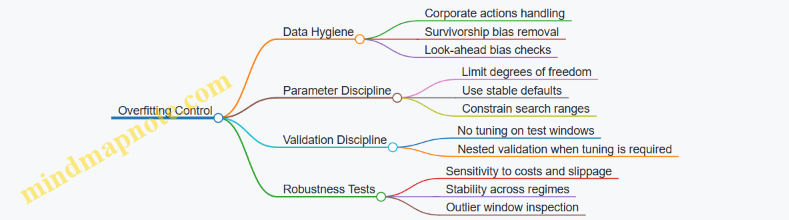
Nested Validation for Parameter Tuning
If you tune parameters, you need a separation between “choose” and “judge.” Nested validation provides that separation.
- Outer loop: walk-forward splits used to judge final performance.
- Inner loop: within each outer training window, you tune parameters using an additional split (or smaller walk-forward) and then lock them.
This prevents the common trap: optimizing parameters because they look good in the same windows you later report.
Example: Simple Nested Walk-Forward
Assume you test a moving-average crossover with parameters (fast length, slow length).
- Outer iteration 1:
- Train: Jan–Jun
- Test: Jul
- Inner tuning inside Jan–Jun:
- Train subwindow: Jan–Apr
- Validate subwindow: May–Jun
- Choose parameters that maximize a risk-adjusted metric on the inner validation.
- Evaluate chosen parameters on July.
Repeat for subsequent outer iterations. If the chosen parameters change wildly from one outer iteration to the next, that’s a red flag that the strategy may be chasing noise.
Metrics That Reveal Fragility
Overfitting often hides in “average looks fine” results. Use metrics that expose instability:
- Distribution of window returns: not just the mean.
- Maximum drawdown across windows: a strategy can be profitable on average yet unacceptable in practice.
- Turnover and cost sensitivity: if performance collapses when you slightly increase costs, the edge is likely thin.
- Exposure stability: track factor or beta exposure over time; large swings can indicate the model is reacting to transient patterns.
Example: If two parameter sets both produce similar average Sharpe ratios, but one has consistently lower turnover and smaller drawdowns across most windows, the more stable one is usually the better candidate.
Practical Implementation Checklist
Before trusting results, verify these items for each walk-forward iteration:
- Parameter selection uses only in-sample data.
- Trading rules are fully specified before running evaluation.
- Transaction costs and slippage assumptions are applied consistently.
- No features rely on information unavailable at decision time.
- You record parameters chosen each iteration to assess stability.
Mind Map: Iteration-Level Checklist

Walk-forward validation is not a magic filter, but it forces a disciplined separation between learning and judging. When combined with nested tuning, constrained parameter searches, and stability-focused metrics, it turns backtesting from a confidence game into a measurement process you can defend.
4.4 Performance Attribution and Benchmarking Frameworks
Absolute return investing is only half the job; the other half is explaining where the returns came from. Performance attribution and benchmarking frameworks turn a single return number into a structured story you can audit, replicate, and defend.
Core Concepts and Goals
Attribution answers three questions: what drove returns, how much each driver contributed, and whether the drivers were intentional exposures or accidental side effects. Benchmarking answers a different question: how your realized risk and return compare to a reference set of assumptions.
A useful mental model is: attribution decomposes performance; benchmarking contextualizes it. If you skip either, you risk blaming the wrong thing. For example, a strategy can outperform a benchmark while still taking unintended factor risk that later hurts drawdowns.
Choosing Benchmarks That Match the Strategy
Start with benchmark alignment, not convenience. A benchmark should reflect the investable opportunity set and the strategy’s intended risk profile.
- Return benchmark: a target return or hurdle rate used for absolute return goals.
- Risk benchmark: a reference portfolio with comparable volatility, leverage, or factor exposures.
- Style benchmark: a proxy for the strategy’s typical exposures, such as market-neutral equity risk factors.
A practical best practice is to maintain two benchmarks: one for investor communication (hurdle or policy benchmark) and one for internal risk control (exposure-matched benchmark). If they disagree, that disagreement is information, not a problem.
Example: Two Benchmarks with Different Messages
Suppose a long-short equity strategy returns +6% over a quarter.
- Against a policy hurdle of +4%, it looks successful.
- Against an exposure-matched benchmark that reflects unintended beta drift, it may show that +2% came from factor exposure rather than alpha.
The second view tells you what to fix, not just what to celebrate.
Attribution Models from Simple to Advanced
Attribution models differ in how they treat exposures and how they handle interactions.
1) Brinson-Style Allocation and Selection
This approach is common when you can define holdings relative to a benchmark portfolio. It separates:
- Allocation effect: returns due to overweighting or underweighting sectors or sleeves.
- Selection effect: returns due to security-level choices within those sleeves.
It works best when the benchmark is a meaningful portfolio and the strategy’s structure resembles the benchmark’s grouping.
2) Factor Attribution with Risk Premia
Factor models explain returns using systematic drivers such as market, size, value, momentum, quality, or volatility. The decomposition typically includes:
- Factor contribution: exposure times factor return.
- Idiosyncratic contribution: residual return not explained by factors.
- Interaction terms: effects from changing exposures during the period.
A key best practice is to compute factor exposures using a consistent method (e.g., end-of-day weights, average weights, or risk-model exposures) and document it. Otherwise, you can “explain” returns differently each time.
3) Transaction-Level Attribution
For trading-heavy strategies, attribution should account for timing and implementation. This separates:
- Signal P&L: what the intended positions would have earned.
- Execution and cost P&L: slippage, commissions, and spread capture/loss.
- Rebalancing effects: gains or losses from changing weights.
This is where many absolute return strategies find the real reasons returns differ from backtests.
Attribution Mechanics and Data Integrity
Attribution is only as good as the inputs.
- Corporate actions and dividends: ensure price series and total return series are consistent.
- Cash and financing: include financing costs and borrow fees explicitly, especially for short books.
- Corporate events: treat deal-related cash flows consistently with your valuation rules.
A simple audit check is to reconcile: total portfolio return = sum of attribution components within a small tolerance. If it doesn’t reconcile, you have a bookkeeping problem, not a theory problem.
Mind Map: Attribution and Benchmarking
Integrated Example: From Holdings to Attribution Report
Consider a quarter where a market-neutral strategy holds two sleeves: Long and Short.
- Compute portfolio total return including financing and borrow fees.
- Estimate factor exposures using the same risk model used for risk limits.
- Attribute returns into:
- Market factor contribution (should be near zero if neutral)
- Other factor contributions (size, value, momentum)
- Idiosyncratic residual (alpha-like component)
- Add transaction-level attribution to separate:
- Signal P&L from intended position changes
- Execution and cost P&L from trading frictions
If the market factor contribution is not near zero, you can trace whether it came from:
- position sizing drift,
- factor-model mismatch,
- or execution timing.
That traceability is the point: attribution becomes a control loop, not a post-mortem.
4.5 Practical Example: Evaluating a Candidate Signal with Controls
You have a candidate signal built from cleaned price and fundamentals. The goal is not to prove it will work forever; it’s to test whether it behaves sensibly under realistic constraints and whether the results survive basic ways of fooling yourself.
Step 1: Specify the Signal and the Trade Rule
Start with a precise mapping from data to actions.
- Signal:
S_tcomputed daily from features (e.g., earnings surprise score and a short-term momentum filter). - Direction: long when
S_t > 0, short whenS_t < 0. - Holding period: 5 trading days.
- Rebalance: every day, but positions are held for 5 days with overlapping trades.
A common mistake is to test “signal performance” without defining the trade rule. If you can’t state entry, exit, and sizing, you’re not evaluating a tradable strategy.
Step 2: Add the First Control Layer
Controls prevent you from mistaking noise for skill.
- Lookahead control: ensure every feature used at time
tis only available at or beforet. If you use quarterly fundamentals, assume they become tradable after a realistic publication lag. - Survivorship control: use constituents from the historical universe, not today’s list.
- Transaction cost control: include a conservative estimate of spread plus slippage. If your backtest assumes zero costs, it’s basically running a fantasy market.
Step 3: Build a Backtest That Matches Execution
Use a backtest structure that respects how trades would actually be placed.
- Universe: top 500 liquid stocks by average dollar volume.
- Sizing: volatility targeting to a fixed annualized target (e.g., 10%), capped at a maximum gross exposure (e.g., 1.5x).
- Constraints: limit single-name exposure (e.g., 5% of gross) and enforce factor neutrality (e.g., market beta near zero using a rolling regression).
Here’s a compact pseudo-implementation of the evaluation loop.
for each day t in test_period:
  X_t = features_available_at(t)
  S_t = signal(X_t)
  w_raw = position_weights(S_t)          # long/short weights
  w_neutral = factor_neutralize(w_raw)  # beta or style neutrality
  w_scaled = volatility_target(w_neutral, target=10%)
  w_capped = apply_position_caps(w_scaled)
  trades = w_capped - w_prev
  pnl_t = portfolio_pnl(trades, costs, returns[t:t+H])
  record(metrics, pnl_t)
Step 4: Evaluate Performance with Risk-Adjusted and Robust Metrics
Use metrics that answer different questions.
- Center: annualized return and median daily return.
- Efficiency: Sharpe ratio and information ratio versus a relevant benchmark (e.g., market-neutral peer set).
- Tail behavior: maximum drawdown and worst 5% daily loss.
- Stability: performance by subperiods (e.g., split the test into 4 quarters).
A signal that looks great only in one quarter is usually a sign of overfitting or regime dependence.
Step 5: Stress the Strategy with Control Variants
Now you test whether the edge is fragile.
- Cost stress: increase estimated costs by 25–50%.
- Delay stress: shift the signal by 1 day to mimic slower data or execution.
- Parameter stress: vary holding period (e.g., 4–7 days) and threshold (e.g.,
S_tcutoffs).
If performance collapses under small, realistic changes, treat the signal as unproven.
Step 6: Check for Implementation Red Flags
These are practical issues that often explain “good backtests.”
- Turnover: compute average daily turnover. If it’s extremely high, costs and market impact likely dominate.
- Liquidity: verify that trades concentrate in names with adequate liquidity at the time of trading.
- Borrow and short constraints: for short legs, ensure borrow availability assumptions are consistent with the universe.
Mind Map: Candidate Signal Evaluation with Controls
Step 7: A Concrete Example Outcome and Decision
Assume the candidate signal produces the following in the test period (ending around 2024-04-15):
- Net annualized return: 8%
- Sharpe ratio: 0.9
- Max drawdown: -10%
- Worst 5% daily loss: -2.2%
- Quarterly results: all quarters positive, with the smallest quarter still above zero
After controls:
- Cost stress (+40%): net annualized return drops to 3%, Sharpe to 0.4
- Delay stress (1-day shift): net annualized return becomes -1%
- Parameter stress (holding 4–7 days): performance stays positive but varies widely
Decision: the signal shows some promise in the baseline, but the sharp deterioration under a 1-day delay suggests the edge depends on timely information or execution. You would either tighten the data pipeline and execution assumptions, or treat the signal as a candidate for further work rather than a deployable strategy.
Step 8: Document the Evaluation So It’s Repeatable
Close with a checklist that can be rerun.
- Signal definition and data availability rules
- Backtest assumptions for costs, slippage, and neutrality
- Metric set and subperiod split
- Stress tests and thresholds for pass/fail
- Implementation red flags and what you changed to address them
Repeatability is the control that keeps you honest when the next candidate signal arrives.
5. Long Short Equity Strategies with Absolute Return Focus
5.1 Equity Selection Frameworks and Fundamental Screening
Equity selection for long short strategies starts with a simple question: which stocks are most likely to outperform on a risk-adjusted basis, and which are most likely to underperform? The trick is to answer that question in a way that survives contact with reality—trading costs, changing accounting, and the fact that “cheap” can stay cheap.
Core Idea: Separate Business Quality from Price
A practical framework treats fundamentals as two layers.
- Business quality: evidence that the company can generate cash, defend margins, and fund growth.
- Valuation and expectations: evidence that the market is pricing in too much bad news or too little good news.
A stock can score well on one layer and poorly on the other. For example, a company with improving margins may still be overpriced if expectations are already high. Conversely, a temporarily weak company can look “cheap” but fail the business-quality checks.
Step 1: Define the Universe and Screening Rules
Start with a universe that matches your execution constraints. If you trade liquid names, screen out low-float or thinly traded stocks early. Then apply basic filters that prevent obvious accounting traps.
- Liquidity filter: minimum average daily value traded.
- Data completeness: consistent filings for the last 8–12 quarters.
- Corporate action sanity: adjust for splits and mergers so per-share metrics remain comparable.
- Balance sheet guardrails: exclude firms with persistent negative equity unless your strategy explicitly targets distressed recoveries.
Example: If you require quarterly financials for the last two years, you avoid “newly listed” noise where ratios can be distorted by one-time events.
Step 2: Build a Fundamental Scorecard
Use a scorecard that is interpretable and testable. A common approach is to score each category from 0 to 5, then combine with weights.
Business Quality
- Profitability: operating margin trend and stability.
- Cash conversion: operating cash flow relative to earnings.
- Balance sheet strength: net debt to EBITDA or interest coverage.
Earnings Power
- Revenue durability: growth consistency rather than one-off spikes.
- Unit economics proxy: gross margin trend and operating leverage.
Valuation and Expectations
- Earnings multiple: EV/EBIT or P/E with normalization.
- Cash multiple: EV/FCF when cash flows are reliable.
- Relative valuation: compare to peers with similar business models.
Example: A retailer with volatile margins might still rank well if cash conversion is consistently strong and leverage is manageable. A software firm might rank poorly if revenue growth is supported by aggressive capitalization or weakening cash conversion.
Step 3: Normalize Accounting and Handle One-Offs
Fundamental screening fails when ratios are built on inconsistent accounting. Normalize by:
- Using trailing twelve months for cash flow and earnings.
- Adjusting for major restructuring or asset sales when they distort operating income.
- Checking whether “earnings” are supported by cash rather than only accruals.
A simple rule: if operating cash flow repeatedly lags net income by a large margin, treat profitability scores as less reliable.
Step 4: Add a Quality-At-A-Reasonable-Price Constraint
For long positions, you want quality without paying an unlimited premium. For shorts, you want weak quality without a “too-good-to-be-true” valuation.
One integrated method is to require both:
- A minimum business-quality score.
- A valuation score that is not extreme versus peers.
Example: You might exclude the top 10% most expensive names even if their quality score is high, because your edge can shrink once spreads and execution costs are included.
Step 5: Convert Scores Into Trade Candidates
Turn the scorecard into a ranking and then into portfolios.
- Long candidates: top decile by quality-adjusted valuation.
- Short candidates: bottom decile by quality-adjusted valuation.
- Neutralization: optionally control for sector and market beta so the trade reflects selection rather than broad exposure.
Example: If you short only the worst names across all sectors, you can end up betting on sector underperformance. Sector-neutral grouping reduces that risk.
Mind Map: Fundamental Screening Workflow
Step 6: Sanity Checks Before You Commit Capital
Before turning candidates into positions, run three quick checks.
- Consistency check: does the story implied by ratios match the trend? If margins improved but cash conversion worsened, investigate.
- Peer comparability: are you comparing firms with similar revenue models and accounting practices? If not, valuation signals can mislead.
- Crowding risk proxy: if many names share the same “obvious” metric, selection can become crowded. A practical mitigation is to diversify across sub-industries and to avoid overconcentrating on a single factor.
Example: Two banks may both show low P/B, but one might have higher credit risk and weaker coverage. Peer-relative checks help prevent “cheapness” from becoming a trap.
Practical Example: From Screen to Short List
Suppose you screen 2,000 stocks and apply liquidity and data filters, leaving 1,200. You compute a scorecard and normalize cash flows.
- Long list: top 120 by quality-adjusted valuation, then remove names with extreme leverage or persistent cash shortfalls.
- Short list: bottom 120, then remove names where valuation is already distressed but quality is stabilizing.
The result is a smaller set where fundamentals and valuation agree more often than they disagree, which is exactly what you want when you later add execution and risk controls.
5.2 Pair Construction and Market Neutral Implementation
Pair construction aims to isolate a relative value relationship while neutralizing broad market exposure. Market neutral does not mean “no risk”; it means the portfolio is designed so that common risk factors—especially the market beta—have limited impact on returns.
Core Idea and What You Are Actually Neutralizing
A pair trade typically holds a long position in one asset and a short position in another. The goal is that the spread between them mean-reverts or at least behaves more predictably than either leg alone. Neutralization targets two things:
- Market exposure: the portfolio’s sensitivity to the overall market should be close to zero.
- Common factor exposure: sector and style effects should be reduced so the spread is driven by relative fundamentals or microstructure effects.
A useful mental model is: you are trading the difference between two price processes, not betting on their absolute levels.
Step 1: Choose a Candidate Universe
Start with a universe where relative relationships are plausible and tradable. Practical filters include:
- Liquidity: both legs must support your intended turnover without excessive slippage.
- Shareability and borrow: shorting requires reliable borrow availability.
- Economic similarity: same industry, similar business model, or shared drivers.
Example: For a long-short equity pair, you might restrict to large-cap stocks within the same sector and with comparable trading hours and corporate action histories.
Step 2: Measure Relationship Strength
You need evidence that the two assets move together in a way that supports a spread model.
Common tools:
- Correlation: quick screen, but it can be misleading during regime shifts.
- Cointegration tests: support for a mean-reverting spread under a linear model.
- Regression-based hedge ratio: estimates how much of asset B is needed to hedge asset A.
Example: If you regress A on B over a training window and get a hedge ratio of 0.8, a first pass spread is Spread = A - 0.8*B. If the spread’s volatility is stable and it tends to revert, the pair is a candidate.
Step 3: Build the Hedge Ratio and Spread
A hedge ratio can be estimated with ordinary least squares, but you should be consistent about assumptions and scaling.
Best practice: use the same data window for both hedge ratio estimation and spread standardization, and update on a schedule that matches how quickly relationships change.
Example: Suppose you estimate A ≈ 1.2*B (so hedge ratio is 1.2). If the current spread is A - 1.2*B = +0.05 and the spread’s rolling standard deviation is 0.02, then the z-score is +2.5. A positive z-score suggests A is “rich” versus B under the model.
Step 4: Define Entry, Exit, and Risk Limits
A standard approach uses z-scores.
- Entry: go long the undervalued leg and short the overvalued leg when
|z|exceeds a threshold. - Exit: close when z-score returns toward zero or when a time stop triggers.
- Risk limits: cap maximum loss per pair and limit exposure to extreme spread moves.
Example: Enter when |z| > 2.0, exit when |z| < 0.5, and stop out if |z| > 3.5 or if the position has not mean-reverted after 20 trading days.
Step 5: Convert Hedge Ratio Into Position Sizes
Market neutral requires careful mapping from hedge ratio to dollar exposure.
A practical method is to target a fixed gross exposure and then allocate dollars using the hedge ratio.
Example: Target $1,000,000 gross exposure per pair. If the hedge ratio implies you want 1.2 units of B per 1 unit of A, you can set dollar weights so that the net market beta is minimized and the gross exposure stays near target. You then scale the pair size based on estimated spread volatility so that each pair contributes comparable risk.
Step 6: Implement Market Neutral Controls
Market neutral is enforced through factor-aware sizing and monitoring.
- Beta neutrality: estimate each leg’s beta to a market index and size so the portfolio beta is near zero.
- Factor neutrality: optionally neutralize sector or style factors using a factor model.
- Rebalancing policy: update hedge ratios and weights on a schedule or when drift exceeds a threshold.
Example: If A has beta +1.1 and B has beta +0.9, and your initial hedge ratio produces a net beta of +0.15, you adjust weights slightly so net beta approaches 0.
Mind Map: Pair Construction Workflow
Example: A Complete Pair Trade in Numbers
Assume you estimate a hedge ratio of 1.2 and compute z-scores from a rolling window.
- Current z-score:
+2.3 - Rule: enter when
|z| > 2.0 - Action: short A and long B (because A is rich vs B)
- Exit: close when
|z| < 0.5 - Stop: close if
|z| > 3.5
Sizing: target gross exposure of $2,000,000 and scale by spread volatility so that the expected daily loss at the entry z-score stays within your per-pair limit. Before sending orders, verify beta neutrality with current betas and adjust weights if the net beta is meaningfully away from zero.
Implementation Notes That Prevent Common Failures
- Corporate actions can distort prices and spreads; adjust consistently before modeling.
- Borrow constraints can force partial execution; treat missing short capacity as a sizing constraint.
- Model drift shows up as widening spread volatility or persistent z-score excursions; hedge ratio updates and re-standardization reduce stale signals.
A well-built pair trade is mostly boring engineering: consistent data handling, disciplined sizing, and rules that translate a statistical relationship into controlled exposures.
5.3 Factor Neutrality and Style Exposure Management
Factor neutrality means your portfolio’s returns are not driven by unintended exposures to common risk factors. Style exposure management means you control how much of your P&L comes from broad “style” tilts like value, growth, momentum, quality, or low volatility. In long-short equity, these controls are the difference between “market neutral-ish” and “actually neutral where it matters.”
Core Idea: What You Are Neutralizing
Start with a factor model that maps each stock’s expected return to factor exposures. A simple form is:
- Expected return ≈ factor exposures × factor premia
- Portfolio exposure ≈ weighted sum of stock exposures
If your portfolio’s net exposure to a factor is near zero, then changes in that factor should not systematically move your portfolio. That does not guarantee zero risk—idiosyncratic moves still exist—but it prevents the most common accidental sources of drift.
Step 1: Choose a Factor Set That Matches Your Strategy
Use factors that are relevant to your holding universe and holding period. For example, a market-neutral long-short book trading liquid large caps may use:
- Market beta (or market return)
- Size and value-growth
- Momentum
- Quality or profitability
- Volatility or low-volatility
A practical best practice is to keep the factor set stable across the strategy lifecycle. If you change the factor definitions frequently, your “neutrality” becomes a moving target.
Step 2: Define Neutrality Targets and Tolerances
Neutrality is rarely exact in practice. Set targets like:
- Net market beta = 0
- Net value-minus-growth = 0
- Net momentum = 0
- Net quality = 0
Then add tolerances, such as “within ±0.05 factor units” or “within ±X% of gross exposure.” This avoids over-trading when the model is noisy.
Step 3: Build a Neutral Portfolio with Constraints
A common approach is constrained optimization or iterative reweighting. The goal is to keep your intended alpha exposures while forcing factor exposures toward targets.
A simple iterative method works well for intuition:
- Start with your raw long and short weights from your stock selection.
- Compute current factor exposures using the factor loadings.
- Adjust weights to reduce the largest factor deviations.
- Re-check exposures and stop when within tolerances.
Here’s a compact example using three factors and a single adjustment pass.
Example: Suppose your current book has net exposures of:
- Market = +0.12
- Value = -0.08
- Momentum = +0.03
If your tolerance is ±0.05, you must fix Market and Value. You can reduce Market exposure by slightly trimming longs and increasing shorts in stocks with negative market loadings (or vice versa). For Value, you rebalance within the long side and short side to offset the value tilt without changing gross leverage too much.
Step 4: Manage Style Drift from Rebalancing and Selection
Even if you neutralize at construction, style drift can reappear after:
- Universe changes (new names enter, old names leave)
- Signal updates (winners and losers shift)
- Corporate actions and liquidity changes
A best practice is to monitor factor exposures at the same cadence you rebalance, not only at inception. If you rebalance weekly, check exposures weekly. If you rebalance daily, check daily. Consistency matters.
Step 5: Handle Practical Friction
Neutrality is constrained by trading realities:
- Transaction costs: frequent factor rebalancing can erase alpha
- Borrow and liquidity: shorts may be limited, forcing unintended tilts
- Model error: factor loadings are estimates, not truths
So you should neutralize the factors that most strongly explain your observed drift. If momentum exposure is stable but market beta swings, focus on market beta first.
Mind Map: Factor Neutrality Workflow
Step 6: Use Sleeves to Keep Neutrality Local
If your book has multiple sleeves—say, a pair-trading sleeve and a fundamental long-short sleeve—neutralize at the sleeve level when possible. This prevents one sleeve’s style tilt from being “hidden” by another sleeve’s opposite tilt.
Example: If the pair sleeve is designed to be market neutral, but the fundamental sleeve is allowed to carry mild value exposure, then report both exposures separately. Investors and risk teams can then see whether the overall neutrality is structural or accidental.
Step 7: Validate Neutrality with Simple Diagnostics
Before trusting the model, run diagnostics:
- Regression of portfolio returns on factor returns to estimate realized exposure
- Tracking error decomposition by factor
- Exposure time series to confirm drift is controlled
If realized exposure remains large even when modeled exposure is near zero, the factor loadings may be stale or the factor set may be missing the relevant drivers.
Summary: What “Good” Looks Like
Good factor neutrality is not “zero everywhere.” It is “controlled where it counts,” with explicit targets, tolerances, and monitoring. Style exposure management is the operational discipline that keeps your portfolio from quietly turning into a different strategy every time you rebalance.
5.4 Risk Controls for Crowding and Liquidity Stress
Crowding happens when many positions share the same trade logic, factor exposure, or hedging behavior. Liquidity stress happens when the market can’t absorb normal trading sizes without large price moves. Together, they create a nasty feedback loop: crowded trades lose money, forced selling increases, bid-ask spreads widen, and execution costs rise.
Start with What You Can Measure
Begin with two measurable inputs: (1) how similar your portfolio is to other market participants, and (2) how costly it is to trade your intended size.
For crowding, use proxy measures that are practical for a hedge fund workflow:
- Position similarity: overlap of holdings or exposures with a peer universe (internal or vendor-based). If you can’t get peer holdings, use factor exposure overlap.
- Strategy similarity: overlap in signals, holding periods, and hedging rules. Two strategies can look different in holdings but behave similarly in risk.
- Crowdedness by instrument: concentration in the same stocks, futures, or options strikes that are known to be heavily used for hedging.
For liquidity stress, measure both static and dynamic liquidity:
- Static liquidity: average spread, average depth, and typical market impact at your usual size.
- Dynamic liquidity: how spreads and impact change during volatility spikes, earnings windows, macro releases, or index rebalances.
A simple best practice is to maintain a trade cost budget per instrument: expected spread + estimated impact + expected slippage from your execution model. If the budget is exceeded under stress scenarios, you reduce size or change execution.
Mind Map: Controls
Integrated Limits That Don’t Contradict Each Other
Use a limit system that forces consistency between crowding and liquidity. A common failure mode is having a tight liquidity limit but allowing large positions that are highly crowded, or vice versa.
A practical structure:
- Crowding score limit per sleeve or instrument group.
- Liquidity score limit per instrument based on stress-adjusted trade cost.
- Combined de-risk trigger when both are elevated.
Example: Suppose you trade a long-short equity sleeve. You compute a crowding score for each stock based on factor overlap with a peer universe and your own concentration. Separately, you compute a liquidity score using stress-adjusted impact for a target order size.
- If crowding score is high but liquidity score is normal, you reduce turnover and tighten entry thresholds.
- If liquidity score is high but crowding score is normal, you reduce size and switch to more passive execution.
- If both are high, you cut exposure and slow rebalancing until trade cost returns within budget.
Position Sizing That Accounts for Execution Cost
Volatility scaling alone ignores the fact that liquidity can worsen exactly when you need to trade. Add an impact-aware sizing cap.
A simple approach:
- Estimate impact cost per unit traded for each instrument under a stress scenario.
- Convert that into a maximum position size such that the expected cost of rebalancing stays within a fraction of expected risk budget.
Example: You target a sleeve volatility of 8%. For a mid-cap stock, your stress impact model says that trading 1% of average daily volume (ADV) costs 0.35% of notional in adverse slippage. If your risk budget allows only 0.10% expected cost per rebalance cycle, you cap the position so that the rebalance trade size is about 0.29% of ADV (because 0.29% × 0.35% ≈ 0.10%). This turns “liquidity” into a concrete sizing rule.
Execution Policies for Crowded, Illiquid Moments
When crowding is high, many participants try to trade the same way at the same time. Execution controls should reduce urgency and avoid signaling.
Best practices that are straightforward to implement:
- Slice sizing: trade smaller chunks sized to a fraction of visible depth, not just ADV.
- Passive-first with guardrails: use passive orders when spreads are stable; switch to more active execution only if fills lag beyond a time limit.
- Cancel and re-quote rules: if the order book thins, cancel rather than keep stale orders that worsen effective execution.
- Venue diversification: if one venue’s depth collapses, route to venues with better stress liquidity.
Example: You want to reduce a crowded long position. Instead of placing one large market order, you place limit orders at the best bid/ask with a slice size tied to stress depth. If the bid retreats and your order sits too long, you cancel and re-place closer to the new mid, but only up to a predefined maximum slippage.
Monitoring That Catches Problems Early
Monitoring should focus on leading indicators:
- Realized trade cost drift: compare realized slippage and spread to your budget.
- Turnover pressure: track whether your rebalance cadence is forcing trades during stress.
- Exposure drift: if liquidity worsens, your positions may become harder to unwind; track how far you are from target.
Example: After a volatility spike, your realized slippage rises from 5 bps to 18 bps while your liquidity score also deteriorates. You immediately reduce rebalance frequency and tighten entry criteria for new trades, rather than waiting for the next scheduled risk review.
A Compact Control Checklist
- Compute crowding and liquidity scores per instrument or sleeve.
- Set separate limits and a combined de-risk trigger.
- Size positions using impact-aware caps, not only volatility.
- Use slice sizing, passive-first execution, and cancel rules.
- Monitor realized trade cost drift and turnover pressure daily.
5.5 Practical Example: Building a Long Short Equity Sleeve
A long short equity sleeve aims to deliver equity-like opportunity while targeting absolute return behavior through controlled exposures. The example below uses a simple, repeatable workflow: define the sleeve goal, build a candidate universe, construct a market-neutral core, add controlled factor tilts, and finish with risk and execution rules.
Sleeve Goal and Constraints
Assume the sleeve objective is to target low net market exposure while seeking positive alpha from stock selection. Set three constraints up front:
- Net beta near zero: keep the portfolio’s estimated market beta between -0.05 and +0.05.
- Gross exposure: start with 200% gross (100% long, 100% short) to allow meaningful selection while keeping leverage moderate.
- Position limits: cap any single name at 3% of gross and cap sector exposure drift to avoid accidental concentration.
A practical habit: write these constraints as numbers, not vibes. When the model disagrees, the numbers win.
Candidate Universe and Data Hygiene
Start with a liquid equity universe (e.g., top 1500 by average daily value). Apply filters that prevent common backtest-to-reality failures:
- Exclude stocks with persistent trading halts or extremely low liquidity.
- Remove corporate actions effects by using adjusted prices consistently.
- Use a survivorship-free universe snapshot for historical membership.
Example: if a stock disappears because it was acquired, it should still have been tradable during its historical period. Otherwise, your “alpha” is just a memory upgrade.
Signal Construction and Ranking
Use a two-stage approach: a fundamental or quantitative score for expected relative return, then a risk-aware ranking.
- Alpha score: combine a value metric and a quality metric into a single z-scored signal.
- Risk penalty: subtract a term proportional to estimated idiosyncratic volatility so that noisy names don’t dominate.
Example scoring rule:
- Alpha score = 0.6 * ValueZ + 0.4 * QualityZ
- Adjusted score = Alpha score - 0.5 * IdioVolZ
Then rank by adjusted score. Long candidates are the top decile; short candidates are the bottom decile.
Market-Neutral Core Construction
Build a market-neutral book using a factor model with at least one market factor and one style factor.
- Estimate exposures for each stock: beta to market and beta to a style factor (e.g., momentum or value).
- Solve for weights that satisfy:
- Sum of long weights = 1
- Sum of short weights = -1
- Portfolio market beta ≈ 0
- Optional: portfolio style beta ≈ 0
Example implementation logic:
- Start with equal-weight longs and equal-weight shorts within each decile.
- Compute current portfolio factor exposures.
- Iteratively scale weights to reduce market beta toward zero while respecting position caps.
Controlled Factor Tilts
If the sleeve allows modest tilts, add them after neutrality is achieved. For instance, allow a small value tilt while keeping market beta neutral.
- Target style beta to +0.10 for value.
- Re-run the factor exposure adjustment while keeping net market beta within the -0.05 to +0.05 band.
This order matters: neutrality first, tilt second. Otherwise, you end up “neutral” on paper but not in practice.
Position Sizing and Rebalancing
Use volatility targeting at the sleeve level and position caps at the name level.
- Estimate each stock’s idiosyncratic volatility.
- Allocate weights proportional to adjusted score divided by idio volatility.
- Apply caps: max 3% gross per name.
Rebalance schedule example:
- Rebalance weekly for signal updates.
- Rebalance factor hedges daily or at least twice weekly if your factor exposures drift quickly.
Risk Checks Before Trading
Run a pre-trade checklist:
- Concentration: top 10 positions should not exceed a set gross threshold (e.g., 35%).
- Liquidity: expected daily volume coverage for each trade should exceed a minimum (e.g., 0.25% of ADV per side).
- Crowding proxy: avoid pairs where both legs are in the same high-ownership bucket.
Example: if a short candidate is illiquid, replace it with the next ranked name that meets liquidity coverage.
Mind Map: Long Short Equity Sleeve Build
Example Trade List and Cost-Aware Execution
Suppose after optimization you need to hold 20 longs and 20 shorts. For each rebalance:
- Compute target weights.
- Translate to share quantities using the latest close.
- Apply a trade cost budget by limiting turnover.
Example turnover rule:
- If estimated one-way cost exceeds a threshold, reduce turnover by blending old and new weights (e.g., 70% new, 30% old).
This prevents the sleeve from “earning” alpha while spending it on friction. The portfolio should survive its own trading.
What “Good” Looks Like in the Sleeve
After implementation, verify that the sleeve behaves consistently with the design:
- Net market beta stays within the band.
- Long and short books have similar liquidity profiles.
- Factor exposures match the intended neutrality and tilt.
- Drawdowns are driven by selection and risk events, not by accidental leverage creep.
If any check fails, fix the construction inputs or constraints before blaming the market. The sleeve is a system, not a wish.
6. Equity Market Neutral and Statistical Arbitrage Techniques
6.1 Cointegration and Spread Modeling for Mean Reversion
Mean reversion strategies often start with a simple question: if two related price series drift apart, do they tend to come back together? Cointegration gives a precise statistical answer for pairs (or small baskets) of assets whose individual prices may wander, yet some linear combination of them behaves more calmly.
Core Idea of Cointegration
Consider two price series, \(X_t\) and \(Y_t\). If each series is non-stationary, you cannot safely model their raw levels with standard mean-reversion tools. Cointegration says there exists a coefficient \(\beta\) such that the spread
\[ S_t = X_t - \beta Y_t \]
is stationary. “Stationary” here means the spread’s distribution does not keep changing over time: its mean is stable and its fluctuations are bounded in a statistical sense. That stability is what makes mean-reversion rules meaningful.
A practical way to think about it: \(X_t\) and \(Y_t\) can both trend, but their relative relationship is anchored. When the spread deviates, the deviation is not just noise; it is a temporary mismatch.
Step 1: Testing for Cointegration
Before modeling the spread, you need to confirm cointegration rather than assume it. A common workflow is:
- Test each series for unit roots (often with an Augmented Dickey-Fuller style test).
- If both look non-stationary, test whether a cointegrating relationship exists.
- Estimate \(\beta\) from the cointegrating regression.
If the cointegration test fails, you can still trade mean reversion in some cases, but you should treat it as a different problem (for example, short-horizon stationarity or regime-specific behavior). For a cointegration-based approach, the spread should be stationary by construction.
Step 2: Estimating the Hedge Ratio
The hedge ratio \(\beta\) determines how you translate the relationship between assets into a spread. A simple estimation approach is an ordinary least squares regression of \(X_t\) on \(Y_t\):
\[ X_t = \alpha + \beta Y_t + \epsilon_t \]
Then define the spread as \(S_t = X_t - \alpha - \beta Y_t\). Including \(\alpha\) matters because it centers the spread around its long-run mean. If you omit \(\alpha\), your spread can show a persistent bias that looks like “mean reversion” but is actually just mis-centering.
Step 3: Modeling the Spread Dynamics
Once you have \(S_t\), you need a rule for how it reverts. A standard model is an error-correction form, which is closely related to an AR(1) model for the spread:
\[ S_t = \mu + \phi (S_{t-1} - \mu) + u_t \]
If \(|\phi|<1\), deviations shrink over time toward \(\mu\). The half-life of a deviation is a useful intuition: it tells you how quickly the spread tends to move back halfway to the mean.
In practice, you estimate \(\mu\) and \(\phi\) on a training window, then use the spread’s recent volatility to scale entry thresholds.
Step 4: Turning the Spread Into Trades
A common trading signal uses a standardized spread (a z-score):
\[ Z_t = \frac{S_t - \bar{S}}{\sigma_S} \]
where \(\bar{S}\) and \(\sigma_S\) are computed over a rolling window. Mean reversion rules then become mechanical:
- If \(Z_t\) is high, \(X\) is “too expensive” relative to \(Y\); short \(X\), long \(Y\).
- If \(Z_t\) is low, do the opposite.
- Exit when \(Z_t\) returns toward 0 (or toward a smaller band around 0).
This is where cointegration earns its keep: the spread’s stationarity supports the idea that “back toward 0” is statistically grounded.
Mind Map: Cointegration to Trading Flow
Example: A Simple Pair Spread and Signal
Suppose you estimate a cointegrating regression on daily closes and get \(\alpha=1.20\) and \(\beta=0.85\). Your spread is
\[ S_t = X_t - 1.20 - 0.85Y_t. \]
Over the last 60 trading days, the rolling mean of \(S_t\) is \(\bar{S}=0.02\) and rolling standard deviation is \(\sigma_S=0.10\). On a new day, you compute \(S_t=0.32\), so
\[ Z_t = (0.32-0.02)/0.10 = 3.0. \]
If your entry rule is \(|Z_t|\ge 2.5\), you enter a trade: short \(X\) and long \(Y\) in the hedge ratio implied by \(\beta\). You then monitor \(Z_t\) daily and exit when \(|Z_t|\le 0.5\), meaning the spread has moved back close to its long-run center.
The mechanics are simple, but the logic is not: cointegration justifies treating the spread’s center as stable, while the z-score standardizes how “far” the current deviation is relative to recent variability.
6.2 Z Score Thresholds Position Entry and Exit Rules
Z Score Thresholds for Position Entry and Exit Rules
Z-score trading turns a messy price series into a simple question: “How far is the spread from its typical level, in standard deviation units?” Entry and exit rules then become threshold crossings plus risk controls, which is exactly what you want when you’re trying to be systematic rather than emotional.
Foundational Setup for Z Scores
Start with a spread series, typically defined from two legs (or more) so that the spread is mean-reverting. Let the spread be \(S_t\). Estimate a rolling mean \(\mu_t\) and rolling standard deviation \(\sigma_t\) over a lookback window (for example, 60 trading days). Then compute:
\[ Z_t = (S_t - \mu_t) / \sigma_t \]
Interpretation is straightforward: \(Z_t = 0\) means the spread is at its estimated typical level; \(Z_t = +2\) means it is two standard deviations above typical; \(Z_t = -2\) means two standard deviations below.
A practical best practice is to standardize the sign convention early. For instance, define that “positive Z means spread is rich” and “negative Z means spread is cheap.” Then your long/short mapping stays consistent across backtests and live trading.
Entry Rules Using Threshold Crossings
Use two entry thresholds: \(Z_{entry}\) for initiating a trade and \(Z_{exit}\) for closing it. A common starting point is \(Z_{entry}=2.0\) and \(Z_{exit}=0.5\), but the key is to choose them based on your spread’s behavior and transaction costs.
Long entry (mean reversion from cheap):
- If \(Z_t \le -Z_{entry}\) , open a long position in the spread (buy the cheap leg, sell the rich leg).
Short entry (mean reversion from rich):
- If \(Z_t \ge +Z_{entry}\) , open a short position in the spread.
To avoid “chasing” noise, prefer crossing logic over level logic. For example, enter only when \(Z_t\) crosses below \(-Z_{entry}\) from above, or crosses above \(+Z_{entry}\) from below. This reduces repeated entries when Z hovers around the threshold.
Exit Rules for Mean Reversion and Noise Control
Exit rules should reflect the fact that mean reversion is not a guarantee of hitting exactly zero. A robust approach uses a band around zero.
Primary exit:
- For a long spread position, close when \(Z_t \ge -Z_{exit}\).
- For a short spread position, close when \(Z_t \le +Z_{exit}\).
This creates a “reversion band” between \(-Z_{exit}\) and \(+Z_{exit}\) . If \(Z_{exit}\) is too small, you’ll churn and pay costs; if it’s too large, you’ll leave money on the table.
Secondary exit: add a time stop and a risk stop.
- Time stop: close after \(N\) trading days regardless of Z, such as 20 days.
- Risk stop: close if \(|Z_t|\) exceeds a larger threshold \(Z_{stop}\) , such as 3.5.
These are not “panic buttons.” They enforce that your strategy has a defined holding horizon and a defined maximum adverse excursion.
Position Management and Scaling
Most Z-score mean reversion systems use one of two sizing styles:
- Binary sizing: enter with a fixed notional or fixed volatility target when the threshold triggers.
- Scaled sizing: size increases with distance from the mean, for example proportional to \(|Z_t|\) capped at a maximum.
Scaled sizing can improve efficiency, but it requires careful cost modeling because larger Z often coincides with wider spreads and worse liquidity.
A simple compromise is binary entry with a capped add-on: add only if Z moves further in your favor by an additional step (for example, from 2.0 to 2.5), and only once.
Mind Map: Threshold Logic
Example: Turning Numbers Into Trades
Assume \(Z_{entry}=2.0\), \(Z_{exit}=0.5\), \(Z_{stop}=3.5\), and \(N=20\) trading days.
Scenario A: Long spread
- Day 1: \(Z=-2.3\) crosses below \(-2.0\) → open long spread.
- Day 6: \(Z=-0.4\) reaches \(\ge -0.5\) → close long spread.
- Result: spread reverted toward typical level before the time stop.
Scenario B: Short spread with risk stop
- Day 1: \(Z=+2.1\) crosses above \(+2.0\) → open short spread.
- Day 9: \(Z=+3.7\) exceeds \(+3.5\) → close due to risk stop.
- Result: the spread moved away from mean, so the trade ends with a controlled loss.
Scenario C: Time stop
- Day 1: \(Z=-2.2\) triggers long.
- Days 10–20: \(Z\) stays around \(-1.2\) to \(-0.8\), never reaching \(-0.5\).
- Day 20: close due to time stop.
- Result: you avoid paying costs indefinitely for a slow or broken mean reversion.
Practical Parameter Selection Without Guessing
Choose \(Z_{entry}\) and \(Z_{exit}\) together. If you increase \(Z_{entry}\) but keep \(Z_{exit}\) fixed, you’ll trade less often and typically hold trades longer. If you decrease \(Z_{exit}\) , you’ll exit closer to zero, which can increase turnover and cost drag.
A clean workflow is to backtest a small grid of \(Z_{entry}\) and \(Z_{exit}\) values while keeping \(Z_{stop}\) and \(N\) constant, then verify that the strategy remains stable when you slightly change the rolling window used for \(\mu_t\) and \(\sigma_t\) . Stability is the difference between a rule that works because it’s clever and a rule that works because it’s consistent.
6.3 Hedging with Beta and Factor Models
Hedging with beta and factor models is about separating what you want from what you accidentally get. In practice, you start with a position’s exposures, estimate how those exposures move with risk drivers, and then trade instruments that offset the unwanted parts. The goal is not to eliminate all volatility; it’s to reduce the specific risks that would otherwise dominate your absolute return.
Core Idea Beta Hedging
A beta hedge treats your portfolio like it has one dominant driver: the market. If your portfolio has beta \(\beta_p\) versus a benchmark index, you can offset that exposure by shorting or buying the benchmark (or a liquid proxy).
- If \(\beta_p = 1.2\), your portfolio tends to move 20% more than the index. A hedge ratio of \(-1.2\) in index exposure targets zero market beta.
- If you hedge with a futures contract, you translate the desired index exposure into contract notional using contract multiplier and current price.
Example: Suppose a long-short equity book has estimated market beta \(\beta_p = 0.8\) and you want to neutralize market exposure. If you can trade an index future that represents one unit of index beta, you short 0.8 units of that future. If the index drops, the hedge tends to rise, offsetting the book’s market component.
Beta hedging is simple, but it assumes one driver and stable relationships. That’s where factor models help.
Factor Model Foundations
A factor model expresses returns as a combination of systematic drivers plus idiosyncratic noise:
\[ R = Bf + \epsilon \]
- \(B\) is the exposure matrix linking assets to factors.
- \(f\) is the factor return vector.
- \(\epsilon\) is residual return not explained by the factors.
For a portfolio, you compute portfolio exposures \(b_p\) by weighting asset exposures. Then you hedge by taking positions in instruments whose exposures offset \(b_p\).
Example: If your long-short book has positive exposure to a value factor and negative exposure to a momentum factor, you may not want either. You can hedge by trading factor-mimicking portfolios (or liquid proxies) that carry the opposite exposures.
Estimating Exposures and Factor Returns
You typically estimate:
- Factor loadings \(B\): from historical regressions or model-based characteristics (e.g., size, value, quality).
- Factor returns \(f\): from the factor construction itself, such as long-short factor portfolios.
- Residual risk \(\epsilon\): to understand what remains after hedging.
A practical best practice is to use a rolling window and check stability. If factor loadings swing wildly, your hedge will be a moving target.
Choosing Hedge Instruments
You rarely trade “factors” directly. Instead, you trade instruments that approximate factor exposures:
- Index futures for market beta.
- Sector ETFs or baskets for sector tilts.
- Style factor baskets for value, growth, momentum, or quality.
- Credit or duration hedges for fixed income factor exposures.
The key is matching exposures, not matching names. A hedge that neutralizes factor exposure is usually better than one that matches the most obvious benchmark.
Hedge Ratio Construction
To hedge multiple factors, you solve for hedge weights \(w_h\) that offset portfolio exposures:
\[ b_p + B_h w_h \approx 0 \]
Where \(B_h\) maps hedge instruments to factor exposures. In practice, you may also include constraints:
- Limit leverage or notional.
- Avoid instruments with poor liquidity.
- Keep residual risk within a target band.
A common approach is a constrained least-squares solve that minimizes hedging error while respecting trading limits.
Mind Map: Beta and Factor Hedging Workflow
Example Multi Factor Hedge with Constraints
Assume your portfolio has estimated exposures to three factors: market (M), value (V), and momentum (U). Your exposures are:
- \(b_p = [0.9, 0.4, -0.2]\)
You can trade two hedge instruments:
- Instrument A approximates \([1, 0, 0]\) (market)
- Instrument B approximates \([0, 1, 1]\) (value plus momentum)
You want to neutralize all three factors as closely as possible, but you cap total hedge notional to avoid liquidity stress. You solve for hedge weights \(w_A\) and \(w_B\) that minimize \(|b_p + B_h w|\) subject to the notional cap. The result won’t perfectly zero every factor because you have fewer instruments than factors, but it can still reduce the dominant systematic moves.
Common Failure Modes and How to Avoid Them
- Exposure drift: Recompute exposures on a schedule and when large trades occur.
- Overfitting factor loadings: Use conservative windows and sanity-check sign consistency.
- Liquidity mismatch: A hedge that is theoretically correct but expensive to rebalance can worsen risk-adjusted returns.
- Ignoring residual risk: Even perfect factor hedges leave \(\epsilon\). Monitor residual PnL to confirm you’re not accidentally hedging away your edge.
Factor hedging works best when you treat it as a controlled process: measure exposures, map instruments, solve for constrained hedge weights, and monitor hedge error like it matters—because it does.
6.4 Execution Timing and Rebalancing Policies
Execution timing and rebalancing policies decide when you trade, how often you adjust, and how you avoid paying the market’s “tax” for being too eager. In equity market neutral and statistical arbitrage, the goal is simple: keep exposures aligned with the model while minimizing turnover, slippage, and borrow or financing frictions.
Execution Timing Foundations
Start with two clocks: the signal clock and the execution clock. The signal clock is when your model updates its estimates of spread, hedge ratios, and risk. The execution clock is when orders actually hit the market. If these clocks drift, you can end up trading on stale information.
A practical rule is to separate “decision time” from “order time.” For example, compute z-scores and hedge ratios at the close, then place orders for the next session’s opening window. This reduces intraday noise in estimates while still reacting quickly enough to capture mean reversion.
Execution timing also depends on liquidity and microstructure. If the pair is thinly traded, you may prefer fewer, larger rebalances during the most liquid hours. If both legs are liquid, you can rebalance more frequently without the cost dominating.
Rebalancing Frequency and Thresholds
Rebalancing is not a calendar event; it’s a control system. Use thresholds so you only trade when the deviation matters.
Define three quantities:
- Target hedge ratio from your spread model.
- Target position size from your risk budget.
- Current position from your portfolio holdings.
Then rebalance when at least one threshold is breached:
- Hedge ratio drift threshold: rebalance if the hedge ratio changes enough that the spread’s effective sensitivity meaningfully changes.
- Position drift threshold: rebalance if your dollar exposure deviates beyond a set band.
- Risk drift threshold: rebalance if estimated volatility or factor exposure changes beyond a band.
A concrete example: suppose you run a pair strategy with a target market-neutral notional of $10 million per sleeve. If your hedge ratio moves by 5% and your current net exposure rises above $200,000, you rebalance. If hedge ratio moves by 2% but net exposure stays within $200,000, you wait.
Order Execution Policies
Execution policies specify order type, timing within the session, and how you handle partial fills.
- Use limit orders when spreads are tight and you can tolerate small execution delays.
- Use time-sliced execution when you need to reduce market impact, especially during volatile opens.
- Cap participation rate to avoid becoming the liquidity you’re trying to consume.
For market neutral pairs, you must also coordinate both legs. If one leg fills and the other doesn’t, you temporarily lose neutrality. A common mitigation is to submit both legs simultaneously and allow a short “grace window.” If the second leg fails to fill within that window, you either cancel the first leg or reduce it to a smaller interim exposure.
Rebalancing Mechanics for Pair and Spread Trades
In spread trading, rebalancing often means updating hedge ratios and adjusting entry/exit levels.
A systematic approach:
- Recompute spread and z-score at decision time.
- Update hedge ratio using your chosen estimation method.
- Check thresholds for whether hedge ratio and position drift require action.
- Apply risk scaling so the portfolio stays within volatility and drawdown limits.
- Execute both legs with coordinated order logic.
When you change hedge ratios, keep exit logic consistent. If you redefine the spread too aggressively, you can “move the goalposts” and exit later than intended. A simple safeguard is to only update hedge ratios when thresholds are met, not every time the model ticks.
Mind Map: Execution Timing and Rebalancing Policies
Example: Coordinated Rebalance with Thresholds
Assume you hold a long-short pair with target net exposure near zero. Your model updates at 4:00 PM and you trade between 9:30 AM and 10:00 AM.
- At the close, the hedge ratio changes from 0.80 to 0.84.
- Your current position implies a net exposure of $150,000.
- Your hedge ratio drift threshold is 5% and your net exposure threshold is $200,000.
Because the hedge ratio change is exactly 5% and the net exposure is below $200,000, you do not rebalance immediately. If the next update shows the hedge ratio at 0.86, the drift exceeds the threshold and you rebalance. You submit both legs as limit orders, time-sliced into small clips, and you cancel the first leg if the second leg does not fill within a short grace window.
This policy reduces churn: you avoid trading when the model wiggles but the portfolio remains effectively neutral. It also prevents neutrality from breaking due to one-leg execution gaps.
Example: Risk-Aware Rebalance During Volatility Spikes
Suppose your spread volatility estimate rises, which would normally increase position size risk if you keep notional constant. Instead of rebalancing purely on z-score crossings, you also check a risk drift threshold.
If estimated spread volatility increases by 20% and your risk drift threshold is 15%, you rebalance by scaling down both legs to keep the expected spread variance within your budget. You still respect entry and exit rules, but you adjust size so the strategy’s behavior stays consistent even when the market gets noisier.
6.5 Practical Example: Designing a Spread Trading Playbook
A spread trading playbook is a written set of rules that turns a statistical idea into repeatable execution. The goal is not to predict the next move; it is to define what you do when the spread looks cheap or expensive, how you size the trade, and how you stop when reality disagrees.
Step 1: Choose the Spread and Define the Economic Link
Start with two instruments that share a driver. For a concrete example, use a pair of equity ETFs: one focused on large-cap value and one focused on large-cap growth. You are not betting on “value beats growth”; you are betting that the relative pricing of the two baskets mean-reverts.
Define the spread as:
- Spread = Price(Value ETF) − beta × Price(Growth ETF)
- Beta is estimated from a rolling regression over a fixed window (for example, 252 trading days).
Best practice: keep the spread definition stable. If you change the beta window or the transformation midstream, your backtest and live behavior won’t match.
Step 2: Build the Signal with Clear Entry and Exit Rules
Compute a standardized spread:
- Z = (Spread − Mean) / Std
Use simple thresholds:
- Enter long spread when Z < −1.5
- Enter short spread when Z > +1.5
- Exit when Z crosses 0
Add a time stop so you don’t wait forever:
- If the position is still open after 20 trading days, exit at market.
Example: If Z falls to −1.7 on day 10, you open a long spread. If Z returns to +0.2 on day 18, you exit when it crosses 0 on day 16, not day 18.
Step 3: Risk Budgeting and Position Sizing
Absolute return needs consistent risk. Convert your spread trade into a portfolio risk unit.
One practical approach:
- Estimate 1-day volatility of the spread, sigma_spread
- Choose a target daily risk, R_target (for example, 0.25% of portfolio value)
- Set notional so that expected daily PnL volatility matches R_target
Then enforce leverage and concentration limits:
- Max gross exposure per sleeve
- Max single-instrument exposure across all strategies
Best practice: size using the spread volatility, not the individual legs. The legs can be volatile while the spread is stable, and vice versa.
Step 4: Execution Rules That Respect Costs
Execution is where many “good” signals quietly die.
Use a cost-aware entry:
- Place limit orders at the mid price adjusted by half the bid-ask spread
- If not filled within 30 minutes, cancel and reprice
Rebalancing rule:
- Recompute beta and Z daily, but only rebalance positions when Z moves by at least 0.5 units or when beta changes materially.
Step 5: Backtest with the Same Playbook You Will Trade
Your backtest must include:
- Rolling beta estimation
- Rolling mean and standard deviation for Z
- Transaction costs and slippage assumptions
- The time stop and exit-on-zero crossing
Mind the “look-ahead” trap: compute rolling statistics using only information available at each timestamp.
Step 6: Monitoring and De-Risking Triggers
Define what “off the rails” means.
Use triggers such as:
- Z stays beyond the entry threshold for 10 consecutive days
- Spread volatility doubles versus its rolling median
- One leg becomes illiquid relative to its recent average volume
When triggered:
- Reduce position size by 50%
- Or exit immediately if liquidity deteriorates sharply
Mind Map: Spread Trading Playbook
Example: One Trade Walkthrough
Assume portfolio value is $10,000,000 and target daily risk is 0.25% ($25,000). On day 0, beta is 1.10 and the spread Z is +1.6, so you short the spread.
On day 7, Z is +0.8, so you hold. On day 12, Z crosses 0.1 and then crosses 0 at the close; you exit at the next tradable price using your limit logic. If the position hasn’t exited by day 20, you exit regardless.
This playbook keeps the decision logic simple: signal defines direction, Z crossing defines timing, and risk rules define how big the bet is. The result is a repeatable process rather than a one-off guess.
7. Event Driven Strategies with Risk Managed Execution
7.1 Merger Arbitrage Mechanics and Cash Flow Modeling
Merger arbitrage aims to profit from the price gap between a target company and the announced acquisition terms. The core idea is simple: if a deal is likely to close, the target’s stock should drift toward the offer price; if it’s likely to fail, the stock may fall back toward a pre-deal level. The job is to model both outcomes and the timing of cash flows, then size the position so the risk is paid for, not hoped for.
Deal Mechanics That Drive the Spread
Most announced deals specify a consideration structure. Common forms include cash, stock, or a mix. Cash deals usually create a cleaner cash-flow path: the target’s shareholders receive a fixed amount per share at closing. Stock deals introduce additional moving parts because the value depends on the acquirer’s stock price at closing.
Key deal terms affect the spread’s behavior:
- Payment timing: closing can take months, so the spread embeds a time value component.
- Regulatory approvals: antitrust review can delay or block the transaction.
- Financing conditions: for leveraged or complex deals, the acquirer must satisfy funding requirements.
- Shareholder votes and conditions: some deals include thresholds or specific approvals.
- Termination fees: these can partially cushion losses in a failed deal, but they rarely eliminate them.
A practical way to think about the spread is as a bundle of probabilities and timing. The market is pricing “close vs. fail” and “how long it takes.”
Cash Flow Modeling Foundations
Start with the target’s current price and the deal’s economics at closing.
For a cash deal, define:
- Offer price per share (O)
- Current target price (P0)
- Expected time to close in years (T)
- Probability of closing (p)
- Recovery in failure (R), often approximated by a fraction of P0 or an estimate of post-failure value
- Risk-free discount rate (r) for time value
A basic expected value model for the target position is:
- Expected closing payoff: p × O
- Expected failure payoff: (1 − p) × R
- Discounted expected payoff: (p × O + (1 − p) × R) / (1 + r)^T
The implied “fair” price is that discounted expected payoff. The difference between the market price P0 and the fair price is the mispricing you’re trying to capture.
For a stock deal, replace O with a function of the acquirer’s closing price. A simple approximation is to model the acquirer’s return distribution over T and translate it into an expected value for the target’s received shares. Even a rough model helps because it clarifies whether the spread is mostly about deal risk or about market risk in the acquirer.
Probability Inputs Without Hand-Waving
Probability estimates should be tied to observable deal features rather than vibes. A systematic approach uses a checklist:
- Deal structure: cash vs. stock, and whether there are financing contingencies
- Regulatory posture: whether approvals are already obtained or still pending
- Timeline: whether the deal is within expected review windows
- Precedent: how similar deals with comparable conditions have resolved
- Legal constraints: whether termination rights exist and how fees are applied
You don’t need perfect probabilities; you need probabilities that are consistent with the terms and the current state of the process.
Timing and Discounting That Actually Matter
Two deals can have the same spread but different expected returns because one closes in 60 days and the other in 12 months. Discounting converts “offer minus price” into a time-adjusted return.
A common simplification is to compute an annualized return using the expected payoff and the time to close. For a cash deal with recovery R ≈ P0 in failure, the expected payoff becomes close-weighted toward O. The annualized figure helps compare deals with different durations.
Risk Controls for Deal-Specific Failure
Merger arbitrage risk is not just “deal fails.” It’s also how much the target price moves in failure and how quickly that happens. Termination fees can raise recovery, but they are not guaranteed to fully offset equity losses.
Practical controls include:
- Limit position size by spread width and implied downside
- Use scenario ranges for p and R rather than a single point estimate
- Avoid concentration in the same regulatory bottleneck or acquirer financing channel
- Track deal milestones and update T and p when the process changes
Mind Map: Cash Flow Logic for Merger Arbitrage
Example: Cash Deal with Two Outcome Scenarios
Assume a cash offer of O = $50 for a target trading at P0 = $46. The expected time to close is T = 0.33 years (about four months). Use r = 5%. Suppose your base-case probability of closing is p = 70%. For failure recovery, assume R = $44 because the market typically reverts toward a pre-deal range.
Expected payoff: 0.70 × 50 + 0.30 × 44 = 35 + 13.2 = $48.2.
Discounted fair value: 48.2 / (1.05)^0.33 ≈ 48.2 / 1.016 ≈ $47.4.
Market price is $46, so the model suggests a positive expected value of about $1.4 per share before considering transaction costs and execution timing.
Now stress the inputs: if closing probability drops to p = 55% while recovery stays R = $44, expected payoff becomes 0.55×50 + 0.45×44 = 27.5 + 19.8 = $47.3. Discounted fair value is 47.3 / 1.016 ≈ $46.6, leaving little margin versus the market. That’s the practical takeaway: the spread is often more sensitive to deal probability than to small changes in discount rate.
Example: Stock Deal Adds Market Risk
If the offer is 0.80 shares of the acquirer per target share, then the closing payoff is 0.80 × Acquirer Price at Close. If the acquirer trades at $60 today, the “today’s implied offer value” is $48, but the realized value depends on the acquirer’s path over T. In modeling, you treat the received shares as a contingent claim: deal risk affects whether you get the shares at all, and market risk affects what those shares are worth.
Case Study: Building a Deal Model Checklist
Use a repeatable workflow:
- Extract offer terms and compute the closing payoff definition (cash O or stock conversion).
- Estimate T from the current stage and expected review timeline.
- Set p using deal conditions and milestone status.
- Set R using plausible failure outcomes consistent with the deal structure.
- Discount the expected payoff to get a fair value.
- Compare fair value to P0 and translate the gap into an annualized expectation.
- Run a small scenario grid for p and R and size the position so the downside is tolerable.
This approach keeps the spread from becoming a mystery. It turns “spread is wide” into a measurable statement about probabilities, timing, and cash flows.
7.2 Corporate Action Handling and Deal Probability Inputs
Corporate actions are the boring parts of deal math—until they aren’t. In merger arbitrage, they change the cash you expect, the timing of payments, and sometimes the number of shares you hold. Deal probability inputs then translate those mechanics into a probability-weighted expected value.
Corporate Action Types That Matter in Deal Spreads
Start with the actions that directly affect the spread’s payoff.
- Cash dividends and special dividends: If the acquirer pays a dividend before closing, the target’s shareholders may receive cash that reduces the effective purchase price. In practice, you adjust the expected cash legs so the spread reflects the net consideration.
- Stock dividends and splits: These change share counts and strike prices. If your model assumes a fixed share quantity, you’ll misstate the conversion ratio and hedge ratios.
- Rights offerings and subscription mechanics: They can dilute the target or require additional capital. Even when the deal terms compensate for dilution, the timing of capital flows matters for financing and margin.
- Spin-offs and asset transfers: Some deals include carve-outs or require distributing a subsidiary to target holders. You need to map what portion of the consideration is cash versus distributed equity.
- Tender offer amendments and exchange ratio changes: These are the “deal-level” corporate actions. They often arrive as amendments that alter the exchange ratio, proration rules, or the treatment of fractional shares.
A practical rule: if the action changes either (1) the number of shares you own, (2) the cash you receive at closing, or (3) the timing of those cash flows, it belongs in the deal spread model.
Building a Corporate Action Adjustment Workflow
Treat corporate actions as a pipeline with explicit inputs and outputs.
- Event ingestion: Capture the announcement date, effective date, record date, and payment date. For merger arbitrage, the effective date is usually what matters for your position and hedge.
- Position mapping: Convert your current holdings into “economic units” that survive the action. For example, a 2-for-1 split doubles shares but leaves economic value unchanged; your model should scale share counts and any conversion ratios accordingly.
- Consideration mapping: Translate deal terms into cash legs. If the merger consideration is a mix of cash and stock, represent each leg separately so later actions can adjust the correct component.
- Timing mapping: Update the expected settlement window. A dividend paid before closing can shift cash earlier; a later record date can delay when the adjustment becomes realized.
- Reconciliation: Compare model-implied cash and share counts to broker statements after the event. If they differ, the model’s event mapping is wrong, not the market.
Mind Map: Corporate Action Handling and Probability Inputs
From Corporate Actions to Deal Probability
Corporate actions rarely change the “chance of closing” directly, but they change the payoff conditional on closing. That matters because probability-weighted expected value is payoff times probability. If your payoff is off by even a few percent, the probability calibration becomes misleading.
A clean approach is to separate two layers:
- Probability layer: estimates the likelihood of closing given deal conditions.
- Payoff layer: computes what “closing” pays after all corporate actions and deal mechanics.
Then you combine them: expected value equals probability of closing times adjusted closing payoff minus probability of failure times adjusted failure payoff.
Example: Dividend Before Closing and Probability-Weighted Payoff
Assume you hold target shares in a cash-and-stock deal.
- Current target price: $50.00
- Expected closing consideration: $52.00 cash plus 0.10 acquirer shares
- Expected acquirer share price at closing: $200.00
- Probability of closing: 60%
- A $1.50 special dividend is expected to be paid to target holders before closing.
First compute the closing payoff per target share.
- Stock leg value: 0.10 × $200.00 = $20.00
- Total gross closing payoff: $52.00 + $20.00 = $72.00
- Adjust for special dividend received before closing: $72.00 − $1.50 = $70.50
If the deal fails, suppose you assume a failure payoff equal to the current target price $50.00 (you can refine this with a failure scenario model).
Expected value per share:
- EV = 0.60 × $70.50 + 0.40 × $50.00
- EV = $42.30 + $20.00 = $62.30
The spread you trade is driven by the difference between EV and the current price. Here, EV − current price = $62.30 − $50.00 = $12.30. Notice what happened: the dividend reduced the closing payoff you should model, without changing the closing probability. That’s the separation doing its job.
Example: Exchange Ratio Change After an Amendment
Suppose the deal originally offered 0.50 acquirer shares per target share, but an amendment changes it to 0.48.
If you don’t update the payoff layer, your model will overstate the stock leg by 0.02 acquirer shares per target share. With an acquirer price of $200, that’s 0.02 × $200 = $4.00 per target share of payoff error. That error can easily dominate the spread’s size, making probability inputs look “wrong” when the real issue is the corporate action mapping.
Practical Checks That Prevent Silent Errors
- Date sanity: ensure record and effective dates align with when your position is actually entitled to the action.
- Share count reconciliation: after splits, verify your broker-reported share count matches the model’s scaling.
- Leg-level accounting: keep cash and stock legs separate so amendments and dividends adjust the correct component.
- Probability calibration discipline: only adjust probability inputs after payoff inputs have been reconciled; otherwise you’re fitting the model to its own mistakes.
7.3 Hedging Considerations Across Capital Structure
Hedging across the capital structure means you treat each security as a different claim on the same underlying company outcomes. A merger spread, for example, is not just “deal risk”; it is also “who gets paid first, who gets paid last, and what happens if the deal price changes.” The practical goal is to hedge the parts of the payoff you can hedge, while accepting the parts you cannot.
Foundational Mapping of Claims to Risks
Start by mapping the capital stack: senior secured debt, senior unsecured debt, mezzanine, preferred equity, and common equity. Each layer has a different sensitivity to deal probability, deal price, timing, and recovery in adverse scenarios.
- Deal probability risk affects all layers, but the magnitude differs. If the deal fails, equity usually absorbs the largest loss; senior debt often has a smaller loss but can still suffer via covenant breaches or liquidity stress.
- Deal price risk matters most for equity and junior claims. If the offer price is revised downward, the equity payoff changes sharply, while senior debt may be less sensitive if it is near par.
- Timing risk impacts discounting and funding costs. Longer deal timelines increase carry costs and the chance of interim events.
- Recovery risk is central for debt. In a failure scenario, the recovery rate depends on asset values, seniority, and restructuring terms.
A clean way to think about hedging is: hedge the drivers you can model (probability, price, timing, recovery), not the ticker symbols.
Hedge Instruments and What They Actually Hedge
Common hedges include equity index futures, single-name equity, credit default swaps (CDS), and interest rate hedges. The key is to match the hedge instrument to the driver.
- Equity hedge (single-name or index) primarily hedges deal probability and market-wide risk. It is less effective for recovery-driven debt outcomes.
- Credit hedge (CDS or bond-to-CDS basis trades) targets credit spread widening, which often correlates with deal failure risk and restructuring expectations.
- Rate hedge (Treasury futures or swaps) addresses discounting and carry effects, especially when the deal horizon is long.
- Cross-claim hedges (e.g., long senior debt, short equity) can reduce net exposure to deal probability while leaving price sensitivity partially intact.
If you hedge the wrong driver, you can end up with a “hedge” that looks good in one scenario and fails in another. That’s not a moral failing; it’s a mismatch.
Practical Example Across the Stack
Suppose you are long a merger spread in the target’s common equity. You also want to reduce deal failure risk.
- Identify the dominant loss mode: for common equity, failure usually means a large drawdown tied to recovery and restructuring.
- Choose a hedge that tracks that mode: a CDS on the target (or a senior unsecured bond spread) often tracks credit deterioration better than an equity index.
- Set hedge ratios using scenario deltas: estimate how the common spread and CDS spread move under a “deal fails” scenario versus a “deal succeeds” scenario.
A simple starting point is to compute a hedge ratio using historical co-movements during deal-related stress windows. Then refine with scenario-based sensitivities from your deal model.
Advanced Details That Prevent Common Mistakes
1. Basis risk across instruments: CDS and bonds can diverge due to liquidity, technicals, and restructuring clauses. If your hedge uses CDS but your position is a bond, you must monitor basis and adjust.
2. Seniority and recovery nonlinearity: recovery is not linear in credit spreads. In distressed regimes, small changes in probability can cause large changes in expected recovery for junior claims.
3. Optionality embedded in terms: preferred shares and certain debt instruments may have call features, conversion terms, or make-whole provisions. These create payoff shapes that standard linear hedges won’t capture.
4. Funding and settlement mechanics: hedges can introduce margin and funding costs that change the net carry. A hedge that reduces price risk but increases funding drag can still worsen absolute return.
Mind Map: Hedging Across Capital Structure
A Simple Workflow for Building the Hedge
- Classify the position by which driver dominates its payoff.
- Select hedge instruments that track those drivers, not just the same company.
- Estimate scenario sensitivities for both position and hedge under at least two regimes: deal success and deal failure.
- Compute hedge ratios and include funding/carry costs in the net expected outcome.
- Stress test basis and liquidity by checking how the hedge behaves when spreads widen and volumes change.
Done well, this approach turns “hedging the deal” into “hedging the payoff drivers,” which is exactly what you want when capital structure layers behave like different species sharing the same habitat.
7.4 Financing Risk and Borrow Availability Constraints
Financing risk in event-driven strategies is the risk that you cannot fund positions as expected, or that the cost and availability of funding changes in ways that break your plan. In merger arbitrage, the “funding” problem is often less about cash and more about borrow availability for hedges, margin requirements, and the timing of settlement. A strategy that looks clean on paper can still fail if the market refuses to lend, or if collateral demands rise faster than your liquidity buffer.
Core Concepts That Drive Borrow Constraints
Borrow availability constraints show up when you need to short a security to hedge deal exposure. The key variables are (1) whether shares exist to borrow, (2) the borrow fee (often quoted as an annualized rate), and (3) the operational path to place and maintain the short. If any of these variables move against you, your hedge can become expensive or impossible.
Start with a simple mapping: you hold a long position in the target (or a spread instrument) and short the acquirer or a related hedge instrument. The hedge is meant to reduce market beta and sector drift. If the short becomes unavailable, your hedge ratio effectively collapses, and your risk profile changes even if your deal spread thesis remains correct.
Financing Mechanics in Practice
Most event-driven portfolios rely on margin and collateral. When you short, your broker requires collateral and may adjust it as volatility or concentration changes. When you go long, you still tie up capital, and you may face haircuts on collateral if you use securities as margin.
A practical way to think about it is to separate three cash flows:
- Initial funding: cash needed to establish longs and meet margin for shorts.
- Ongoing carry: borrow fees, dividends in lieu, and interest on margin balances.
- Settlement timing: cash released or required when deals close, fail, or are partially settled.
Borrow fees are the most visible carry cost, but settlement timing is often the hidden one. If the deal closes on a date that differs from your expectation, you may remain in the position longer than planned, paying borrow fees and margin costs for extra days.
Borrow Availability Failure Modes
Borrow constraints tend to fail in predictable ways:
- Hard-to-borrow: shares exist but are scarce, so the borrow fee spikes.
- Recall risk: lenders can demand shares back, forcing you to cover or find replacement borrow.
- Operational friction: the hedge is delayed because the borrow is not confirmed before you need to rebalance.
- Collateral tightening: margin requirements increase, reducing your ability to maintain the hedge.
Each failure mode changes the economics differently. A fee spike reduces expected return; a recall can force a loss at an unfavorable price; operational delays can leave you temporarily unhedged.
Building a Borrow-Aware Risk Budget
A robust approach is to treat borrow as a risk factor with limits, not as a background detail.
Step 1: Pre-trade borrow checks. For each hedge leg, record expected borrow fee range and the probability of “no borrow” based on recent availability. Even a basic history helps.
Step 2: Translate borrow into a cost limit. Convert an annualized borrow fee into an expected daily cost and compare it to the spread you are targeting.
Step 3: Set hedge maintenance rules. Define what happens if borrow fee exceeds a threshold or if borrow becomes unavailable. Options include reducing hedge size, switching hedge instruments, or pausing new exposure.
Step 4: Reserve liquidity for margin changes. Keep a buffer that covers plausible margin increases during deal volatility spikes.
Example: When the Hedge Becomes Too Expensive
Assume you target a merger spread of 6% annualized over the expected holding period. You hedge with a short that currently has a borrow fee of 10% annualized, but it can jump to 60% annualized.
If the deal is expected to close in 90 days, the borrow cost at 10% is roughly:
- 10% × (90/365) ≈ 2.47% of notional
At 60% it becomes:
- 60% × (90/365) ≈ 14.8% of notional
If your expected spread return is only 6% annualized, then over 90 days that’s about:
- 6% × (90/365) ≈ 1.48%
In the high-fee scenario, the hedge carry can overwhelm the spread economics. The correct response is not “hope fees stay low,” but to enforce a borrow-aware limit that either reduces hedge size or changes the hedge instrument when fees cross your threshold.
Mind Map: Financing Risk and Borrow Availability Constraints
Example: Hedge Maintenance Rule That Prevents Surprise Exposure
Suppose your hedge is sized to neutralize market beta. You set a rule: if the borrow fee exceeds 40% annualized for two consecutive checks, you cut the hedge by half and cap the remaining unhedged beta exposure. If borrow becomes unavailable, you stop adding new deal exposure until borrow is restored or an alternative hedge is available.
This keeps the portfolio’s risk profile aligned with the original intent: you may accept a less perfect hedge, but you avoid a silent shift into a fully directional position.
Practical Checklist for Borrow-Constrained Event Trades
- Confirm borrow availability before initiating the hedge leg.
- Record the fee and the operational lead time to establish the short.
- Convert borrow fees into expected cost over the planned holding window.
- Define explicit actions for fee spikes, recall events, and “no borrow” outcomes.
- Maintain a liquidity buffer sized for margin changes, not just normal trading.
Financing risk is manageable when it is treated as part of the strategy design. Borrow constraints are not a footnote; they are a constraint on what hedges you can actually run, for how long, and at what cost.
7.5 Practical Example: Valuing and Risking a Deal Spread
This example walks through a merger-arbitrage style deal spread using a simple valuation and a disciplined risk process. Imagine a target stock trading at $48.50 while the announced deal offers $50.00 in cash per share. The spread is the market’s implied probability-weighted path from “deal announced” to “deal closes.”
Deal Setup and Core Valuation
Assume:
- Offer price: $50.00
- Current target price: $48.50
- Time to expected close: 120 calendar days
- Risk-free rate: 5% annualized
- Deal closing probability: 70%
- Recovery if deal fails: 0.60 of current price (i.e., $48.50 × 0.60)
A clean starting point is an expected value model discounted to today:
Expected payoff = P(close) × Offer + (1 − P(close)) × Recovery
Recovery = $48.50 × 0.60 = $29.10
Expected payoff = 0.70 × $50.00 + 0.30 × $29.10 = $35.00 + $8.73 = $43.73
Discount factor for 120 days at 5%:
- DF = 1 / (1 + 0.05 × 120/365) ≈ 0.9836
The model-implied fair value ≈ $43.73 × 0.9836 = $43.60.
Because the market price is $48.50, the spread is not “cheap” under these assumptions. That’s useful: it forces you to check whether your probability, recovery, or timing assumptions are off.
Converting Valuation Into Deal Spread Logic
The deal spread is often expressed as an annualized return on the target price. Here, the “cash-like” payoff is the offer minus the current price, but the probability of failure matters.
If the deal closes, profit per share = $50.00 − $48.50 = $1.50.
If it fails, the loss depends on recovery. Loss per share on failure = $48.50 − $29.10 = $19.40.
So the spread is a compact way of packaging two very different outcomes. The trick is to risk it explicitly rather than relying on the spread size alone.
Mind Map: Valuing and Risking the Deal Spread
Scenario Table with Concrete PnL
Keep the mechanics constant and vary the probability and recovery. Use the same 120-day discount factor (0.9836).
| Scenario | P(Close) | Recovery Multiple | Recovery Value | Fair Value | PnL vs $48.50 |
|---|---|---|---|---|---|
| Base | 0.70 | 0.60 | 29.10 | 43.60 | -4.90 |
| Optimistic | 0.80 | 0.70 | 33.95 | 46.90 | -1.60 |
| Conservative | 0.60 | 0.50 | 24.25 | 37.90 | -10.60 |
Fair value is computed as DF × [P(close) × 50 + (1 − P(close)) × Recovery]. The table shows why deal spreads can look stable while still being fragile: small probability shifts can move the fair value meaningfully.
Risk Controls That Actually Map to the Model
- Probability bands: Instead of one probability, maintain a range and revalue daily. If your fair value stays far from market, you either reduce size or revisit assumptions.
- Recovery sensitivity: Recovery is where equity markets and legal outcomes collide. Use a conservative recovery multiple for risk sizing even if your base case is higher.
- Timing stress: If the close drifts from 120 to 180 days, discounting and carry change. Even with a small rate, longer time increases exposure to probability and market moves.
- Market beta overlay: Treat the target’s equity factor exposure as a separate risk. If the broader market drops, the target can fall even when the deal outcome is unchanged.
Practical Position Sizing Example
Suppose you cap single-deal loss at 1% of portfolio value under a conservative scenario. If the conservative PnL is −$10.60 per share versus $48.50, then the maximum shares are:
- Max shares = (0.01 × Portfolio Value) / 10.60
If the portfolio is $10,000,000, max shares ≈ $100,000 / 10.60 ≈ 9,434 shares.
That sizing rule is boring in the best way: it ties risk limits to the same valuation assumptions you used to decide whether the spread is attractive.
Execution Notes That Prevent “Model Meets Reality” Failures
- Entry discipline: Enter when your model-implied fair value is within a tolerable gap to market, given your probability and recovery bands.
- Revaluation cadence: Revalue after major deal milestones and after meaningful market moves that affect the target’s equity component.
- Liquidity awareness: If spreads widen due to liquidity, your realized entry price can differ from the quote. Use conservative fills in back-of-the-envelope PnL.
In this example, the key takeaway is simple: deal spreads are not just “offer minus price.” They are a probability-weighted payoff with explicit recovery and timing risk, plus ordinary equity market exposure. When you risk it that way, the spread becomes a measurable bet rather than a vague hope.
8. Fixed Income Relative Value and Absolute Return Methods
8.1 Yield Curve Construction and Term Structure Concepts
A yield curve is a map from time to maturity to the yield you’d earn on a bond-like instrument, assuming you can invest and reinvest consistently. In absolute return investing, the curve matters because many positions are really bets on how rates move across maturities, not just on the level of rates.
Term Structure Basics
The term structure is the relationship between interest rates and maturities. If you plot yields for instruments with different maturities on the same date, you get the yield curve. A key nuance: yields are not directly comparable across instruments unless you standardize the underlying cash-flow conventions and credit assumptions.
Two practical distinctions drive most curve work:
- Risk-free curve vs. market curve: A “risk-free” curve is typically built from instruments treated as having negligible credit risk (e.g., government securities or collateralized rates). A “market” curve may embed additional spread.
- Spot rates vs. forward rates: Spot rates describe the yield from today to a future date. Forward rates describe the implied rate for a future period starting at a later date.
A simple example: if the 1-year spot rate is 4% and the 2-year spot rate is 5%, the implied 1-year forward rate for the second year is higher than 4%. That forward rate is what matters for pricing cash flows that occur in year two.
From Bond Prices to Zero Rates
Curve construction often starts from observed prices or yields of liquid instruments. The goal is to infer a set of zero-coupon rates (or discount factors) that reproduce those market quotes.
A clean mental model uses discount factors. If a discount factor for maturity \(t\) is \(DF(t)\), then the present value of a cash flow \(CF\) at time \(t\) is \(CF \times DF(t)\). Once you have discount factors, you can compute spot rates and forward rates.
Bootstrapping is the standard approach: solve for the earliest maturity discount factor first, then use it to solve for the next maturity, and so on. This works because each new instrument adds one new unknown discount factor.
Instruments and Conventions
You must align instruments to a common framework. Common choices include:
- Government bonds for a government curve
- Swap rates for a collateralized curve
- Money market instruments for short maturities
Each instrument has its own day count, compounding, and payment schedule. If you ignore these, you can fit the curve “perfectly” to quotes while still producing wrong forward rates and wrong pricing for other cash flows.
Bootstrapping with a Concrete Example
Suppose you have two instruments on the same valuation date:
- A 1-year zero-coupon bond priced at 96.00. Then \(DF(1)=0.96\).
- A 2-year par bond with annual coupons and price 100, paying 5% of face value each year.
Let \(DF(2)\) be unknown. The present value equation is:
\(100 = 5\times DF(1) + 105\times DF(2)\)
Plug in \(DF(1)=0.96\):
\(100 = 5\times 0.96 + 105\times DF(2)\)
\(100 = 4.8 + 105\times DF(2)\Rightarrow DF(2)=0.910476\)
From \(DF(2)\), you can compute the 2-year spot rate. The important point is that the curve is not guessed; it is solved to match market quotes under consistent conventions.
Smoothing and Interpolation
Bootstrapping gives discount factors at specific maturities, but you often need rates at intermediate tenors. Interpolation methods matter because they affect forward rates, which are sensitive to curvature.
A practical approach is to interpolate discount factors or zero rates using a smooth method (for example, a spline). The goal is to avoid unrealistic kinks that can create trading signals that are artifacts of the interpolation.
Mind Map: Yield Curve Construction and Term Structure Concepts
Using the Curve in Relative Value Thinking
Once you have a curve, you can price any cash-flow stream by discounting each payment date. In relative value trades, you compare how two instruments would be priced under the same curve framework. If the market price implies a different set of discount factors, the difference becomes the basis for a spread trade.
A quick example: if a 5-year bond is “too expensive” relative to the curve, its implied discount factors will be higher than the curve’s. A relative value strategy can then target the spread between market-implied and curve-implied pricing, while keeping the rest of the curve consistent.
8.2 Duration Convexity and Key Rate Hedging
Duration and convexity explain how bond prices react to interest-rate changes. Duration gives the first-order move; convexity corrects the curvature. Key rate hedging goes one step further by hedging specific points on the yield curve rather than the curve’s average shift.
Duration as a First-Order Approximation
Macaulay duration measures the weighted average timing of cash flows, while modified duration converts that timing into a sensitivity to yield changes. For a small yield change \(\Delta y\), price change is approximated by: \[ \Delta P \approx -D_{mod} \cdot P \cdot \Delta y \] A practical way to internalize this: if a bond has modified duration 6 and price is 100, a +10 bps move implies roughly \(-6 \times 100 \times 0.001 = -0.60\) price points. The approximation works best for small moves and smooth yield changes.
Convexity as the Second-Order Correction
Convexity captures how the duration itself changes as yields move. A common approximation is: \[ \Delta P \approx -D_{mod} P\Delta y + \tfrac{1}{2} C P(\Delta y)^2 \] where \(C\) is convexity. Two bonds can share the same duration but differ in convexity, leading to different outcomes for larger rate moves. Higher convexity generally means the bond loses less when yields rise and gains more when yields fall, all else equal. The “all else equal” part matters: coupon, maturity, and embedded options all influence convexity.
Why Convexity Matters in Hedging
A hedge built only on duration matches the first-order effect. When rates move enough to make curvature relevant, the hedge can drift. Convexity-aware hedging reduces that drift by aligning the portfolio’s curvature profile with the liability or target exposure.
Key Rate Hedging as Curve-Point Sensitivity
Key rate hedging treats the yield curve as a set of points. Instead of assuming a parallel shift, it estimates how the portfolio value changes when a specific maturity bucket moves while others stay fixed.
Define key rates at maturities \(t_1, t_2, \dots\). For each key rate \(t_i\), compute a sensitivity \(KR_i\) using a bump-and-reprice approach: bump the zero rate at \(t_i\) by a small amount, reprice the portfolio, and record the change. The result is a vector of sensitivities.
A hedging portfolio is then chosen so that its key rate sensitivity vector matches the target’s vector. If the target is a liability stream, the goal is often to neutralize the liability’s key rate exposures with the hedge assets.
Mind Map: Duration, Convexity, and Key Rates
Example: Duration and Convexity in Action
Assume a bond portfolio priced at 100 has modified duration 5.2 and convexity 45 (convexity units consistent with the approximation). Consider a +50 bps move \(\Delta y = 0.005\).
First-order estimate: \(\Delta P_1 \approx -5.2 \times 100 \times 0.005 = -2.60\).
Second-order correction: \(\Delta P_2 \approx \tfrac{1}{2} \times 45 \times 100 \times (0.005)^2 = 0.05625\).
Total estimate: \(\Delta P \approx -2.60 + 0.056 = -2.54\). The correction is small here, but it’s systematic. If you hedge only duration, you’re effectively ignoring that curvature benefit or cost.
Example: Key Rate Hedging with Two Curve Buckets
Suppose a liability has key rate sensitivities \(KR_{2y} = -3.0\) and \(KR_{10y} = -1.5\) in price points per 1% bump (sign indicates the liability loses value when rates rise). You can use two hedging instruments: a 2-year note and a 10-year note with sensitivities:
- 2-year note: \(k_{2y}=+2.4\), \(k_{10y}=+0.2\)
- 10-year note: \(k_{2y}=+0.3\), \(k_{10y}=+1.8\)
Let hedge weights be \(w_1\) for the 2-year note and \(w_2\) for the 10-year note. Solve: \[ 2.4w_1 + 0.3w_2 = 3.0 \] \[ 0.2w_1 + 1.8w_2 = 1.5 \] This yields a hedge that neutralizes both curve points. The payoff is that if the curve twists—2-year moves but 10-year barely moves—the hedge still behaves as intended.
Validation Through Scenario Repricing
After matching duration, convexity, or key rates, validate by repricing under a small set of rate scenarios. The goal is not to prove perfection; it’s to confirm that the approximation errors are controlled and that the hedge doesn’t rely on a single “parallel shift” assumption.
8.3 Spread Trades and Curve Relative Value Selection
Spread trades aim to earn from the difference between two related rates rather than their absolute level. In fixed income, “related” usually means instruments that share a common driver (same issuer, same curve, same sector) but differ in maturity, seniority, or embedded optionality. The curve relative value (RV) version focuses on how the yield curve’s shape should behave across tenors, then trades the mispricing in that shape.
Core Idea of Spread Trades
A spread trade starts with a spread definition, such as:
- Inter-tenor spread: yield(10Y) − yield(5Y)
- Swap spread: swap rate − Treasury yield at the same maturity
- Curve RV spread: a weighted combination of multiple tenors designed to isolate a specific curvature component
The key is that the spread should be more stable than the individual legs. If both legs move together for most macro reasons, the spread can move for more specific reasons like supply, hedging pressure, or technical imbalances.
Curve Relative Value Selection Logic
Curve RV selection is a disciplined process: define the RV target, choose instruments that map cleanly to that target, then verify that the spread is tradable with manageable costs.
Step 1: Choose the RV Dimension
Common RV dimensions include:
- Level: overall rates move up or down together
- Slope: short vs long tenors diverge
- Curvature: belly vs wings behave differently
A practical way to decide is to ask which component you want to be right about. If you expect the curve to “flatten” because the belly is rich, you target a slope or curvature spread rather than a single maturity.
Step 2: Build a Weighted Spread
To isolate curvature, you can use a three-point “butterfly” style construction. For example, define a curvature RV spread as:
- Curvature spread = 2×Y(7Y) − Y(5Y) − Y(10Y)
If the belly yield is too high relative to the wings, the curvature spread is positive. A mean-reversion style trade would then be: short the rich belly exposure and long the cheaper wings exposure, implemented through the corresponding instruments.
Step 3: Map to Tradable Instruments
Yields are not directly traded; you trade instruments that approximate the curve points. For curve RV, typical legs are:
- Treasury futures or cash Treasuries for Treasury curve exposure
- Interest rate swaps for swap curve exposure
- Options-adjusted instruments when optionality matters (but then hedging becomes more complex)
A clean mapping reduces “basis risk,” meaning the trade’s P&L doesn’t track the intended RV spread.
Step 4: Check Sensitivities Before You Commit
Even if the spread looks attractive, you must verify that the legs hedge the unwanted exposures. Two checks are usually enough to start:
- DV01 balance: the trade should have near-zero net DV01 if the goal is curvature rather than level
- Key rate balance: the trade should load on the intended tenors and minimize loading on others
If you skip this, you can accidentally build a “curve RV” trade that is really a directional bet.
Step 5: Estimate Costs and Execution Friction
Spread trades often require multiple legs, so costs add up. You need a simple cost budget:
- bid-ask and expected slippage per leg
- financing or margin effects if using swaps
- rebalancing frequency if the spread is actively managed
A spread with a small expected move can be untradeable if costs exceed the plausible spread change.
Mind Map: Curve RV Selection
Worked Example: A Curvature Butterfly
Assume you observe that the 7Y point is rich relative to the 5Y and 10Y points. You define:
- Curvature spread = 2×Y(7Y) − Y(5Y) − Y(10Y)
If the curvature spread is high, you expect it to compress. Implementation example:
- Leg A: short an instrument that tracks the 7Y curve point
- Leg B: long an instrument that tracks the 5Y point
- Leg C: long an instrument that tracks the 10Y point
To avoid a hidden level bet, you adjust notionals so the net DV01 is close to zero. Then you monitor the curvature spread itself, not just the individual yields.
Practical Example: Avoiding a Common Mistake
A frequent error is using instruments that look similar on paper but behave differently in practice. For instance, if one leg is a swap and another is a Treasury, the spread can be dominated by swap-specific factors rather than the intended curve shape. The fix is to keep the curve RV “like with like” when possible, or explicitly include the basis component in the spread definition.
Summary of Selection Criteria
A good curve RV spread has four traits:
- The spread definition isolates the intended curve component.
- The instrument mapping tracks the curve points with limited basis risk.
- Sensitivities are balanced so the trade is not accidentally directional.
- Costs are small relative to the spread move you are targeting.
When these hold, spread trades become less about predicting the market and more about trading a measurable relationship with controlled exposures.
8.4 Interest Rate Volatility and Scenario Based Risk Limits
Interest rate volatility shows up in two places: the prices you trade and the hedges you rely on. Scenario based risk limits turn that volatility into concrete, testable rules. The goal is simple: if rates move in ways that matter for your book, your losses should stay within a pre-agreed envelope.
Core Concepts for Volatility Aware Limits
Start with what “volatility” means in practice. For rates, it is not one number. It varies by maturity (2Y vs 10Y), by curve segment (front end vs long end), and by direction (rates can jump up or down). Options make this visible through implied volatility surfaces, but you can also model it with historical measures and regime splits.
A useful mental model is: volatility drives distribution of future yield changes, and yield changes drive P&L through sensitivities. Those sensitivities are the bridge between market movement and portfolio outcome.
From Sensitivities to Scenario Losses
Scenario based limits require a mapping from “what happens to the curve” to “what happens to the portfolio.” The mapping can be linear or nonlinear.
- Linear approximation uses risk measures like DV01 or key rate durations. It is fast and works well for small moves.
- Nonlinear repricing revalues instruments under shocked curves. It is slower but handles convexity, caps/floors, and option-like payoffs.
A practical best practice is to use linear measures for limit prechecks and nonlinear repricing for the actual limit breach test. That keeps the workflow efficient without pretending convexity doesn’t exist.
Building Scenario Sets That Actually Stress the Book
Scenarios should be designed around curve dynamics, not generic “rates go up” statements. A scenario set typically includes:
- Parallel shifts: all maturities move together.
- Twist moves: short end and long end move in opposite directions.
- Bumps by tenor: targeted shocks to key maturities where your exposures concentrate.
- Volatility shocks: implied vol changes that affect option premia and hedging costs.
To keep scenarios coherent, define them using a consistent curve representation. For example, shocks can be applied to zero rates, discount factors, or a parametric curve. Mixing representations is a common way to get “limits” that don’t match reality.
Mind Map: Scenario Based Risk Limits for Interest Rate Volatility
Example: Turning a Volatility Shock Into a Limit
Suppose a portfolio holds a 5Y receiver swaption and hedges with 5Y and 10Y swaps. You want a limit for a scenario where the curve twists and implied volatility rises.
- Define the curve shock: apply a twist such that 2Y–5Y rates move up by 30 bps while 7Y–10Y move down by 20 bps, with intermediate tenors interpolated smoothly.
- Define the volatility shock: increase implied vol by 10% for the 5Y expiry bucket, and adjust skew by shifting the smile so out-of-the-money receivers become relatively more expensive.
- Compute P&L:
- Linear precheck: estimate swaption P&L using key rate durations and vega.
- Nonlinear repricing: revalue the swaption under the shocked curve and shocked vol surface, and revalue hedges under the shocked curve.
- Apply the limit: compare the scenario loss to an absolute threshold, say 0.75% of NAV for that scenario bucket.
If the nonlinear repricing loss exceeds the threshold while the linear precheck looks safe, that is a signal to refine the sensitivity model or tighten the precheck buffer. Limits should be consistent with the valuation method that actually matters.
Example: Multi-Day Scenario Limits Without Guessing
For multi-day horizons, avoid naive scaling of single-day losses. Instead, either:
- Re-simulate scenarios over the horizon using a consistent volatility and correlation model, or
- Use a conservative multiplier derived from historical multi-day move distributions for the specific curve segments you trade.
A simple governance rule helps: if your instruments are option-heavy, prefer repricing over scaling. If your book is mostly linear swaps and futures, scaling can be acceptable with a documented error check.
Operationalizing Limits with Clear Triggers
Finally, scenario based limits need a workflow. A clean approach is:
- Pre-trade: run linear prechecks for all relevant scenario buckets.
- Post-trade: run nonlinear repricing for the same buckets.
- Breach handling: if a scenario loss exceeds the limit, trigger a de-risking action defined in advance, such as reducing exposure to the affected tenor or reducing option vega.
When the trigger is explicit, the limit becomes a tool rather than a surprise. That’s the whole point: volatility is uncertain, but your risk process shouldn’t be.
8.5 Practical Example: Building a Treasury Spread Portfolio
A treasury spread portfolio aims to earn returns from relative value between two points on the yield curve, rather than from a single directional bet on rates. The basic idea: if the spread between two yields or prices is mispriced, the portfolio is structured so that the “wrong” part cancels out and the “spread” part remains.
Step 1: Choose the Spread Pair and Define the Hedge
Start with a pair that is economically linked and liquid. A common choice is a 2-year versus 10-year spread, or a 5-year versus 30-year spread. Suppose we choose the 2s10s spread.
You need a hedge ratio so the portfolio is approximately neutral to overall rate moves. Use duration as a first pass.
- Let D2 be the modified duration of the 2-year leg.
- Let D10 be the modified duration of the 10-year leg.
- Choose notionals N2 and N10 so that N2·D2 ≈ N10·D10.
Example setup (illustrative):
- D2 = 1.9, D10 = 8.6.
- Target duration neutrality: N10 = N2·(D2/D10) ≈ N2·(1.9/8.6) ≈ 0.221·N2.
Interpretation: if the curve shifts up or down broadly, the duration-neutral structure reduces the impact. The remaining driver is the relative movement of the 2-year and 10-year yields.
Step 2: Convert the Trade Into a Tradable Instrument Mix
In practice, you rarely trade “pure” maturities. You trade specific Treasury issues or futures.
A practical approach is:
- Use Treasury futures for the main legs to reduce roll complexity.
- Use a small amount of on-the-run notes for precision if needed.
If you use futures, replace modified duration with DV01 (dollar value of a 1 bp move). Hedge using DV01 neutrality:
- Choose position sizes so DV01(2-year leg) + DV01(10-year leg) ≈ 0.
This is more robust than duration when convexity and cheapest-to-deliver effects matter.
Step 3: Define the Spread Signal and Entry Rules
Define the spread as either:
- Yield spread: (Y10 − Y2), or
- Price spread: the difference in normalized prices, or
- Futures-implied spread.
A simple, testable rule is mean reversion using a z-score.
- Compute the historical mean and standard deviation of the spread over a lookback window.
- Enter when the z-score exceeds a threshold.
Example rules:
- Enter long the spread when z-score < −1.5.
- Enter short the spread when z-score > +1.5.
- Exit when z-score returns to 0 or when it crosses back through ±0.25.
To keep the trade from turning into a “hope position,” add a time stop. For instance, exit if the z-score has not mean-reverted after 20 trading days.
Step 4: Add Risk Controls That Match the Payoff
Spread trades can still lose money if the relationship breaks or if volatility spikes.
Use three layers:
- DV01 limit: cap total DV01 exposure per strategy.
- Convexity check: ensure the hedge ratio doesn’t drift too far when rates move.
- Stop-loss on spread: stop when the spread moves further against you by a fixed bp amount.
Example risk limits:
- Max loss: 0.50% of strategy notional.
- Spread stop: 25 bp adverse move.
- Re-hedge frequency: daily, or when DV01 drift exceeds 10%.
Step 5: Build the Portfolio Workflow
A workable workflow is mechanical and repeatable.
Mind Map: Treasury Spread Portfolio Build
Step 6: Put Numbers on a Single Trade
Assume you allocate a strategy notional of $10,000,000 to the combined legs.
- Choose N2 and N10 for DV01 neutrality.
- Apply signal direction:
- If z-score is +1.8, short the spread: short the 10-year leg and long the 2-year leg (so you benefit if Y10 − Y2 mean-reverts downward).
- Set exit conditions:
- Primary exit: z-score returns to 0.
- Secondary exit: time stop at 20 trading days.
- Set risk exits:
- Stop if spread widens by 25 bp.
- Stop if P&L hits −0.50% of notional.
Finally, record the trade’s “why” in plain terms: the expected driver is spread mean reversion, while the hedge is designed to reduce sensitivity to parallel shifts.
Step 7: Validate the Hedge Effectiveness Before Scaling
Before increasing size, check two practical diagnostics:
- Hedge P&L attribution: how much of daily P&L comes from spread movement versus residual rate moves.
- DV01 drift: whether your hedge ratio stays close enough as yields change.
If residual rate exposure is large, tighten the hedge using updated DV01 and consider a different pair or a more precise instrument mapping.
9. Volatility Strategies and Options Based Risk Premia
9.1 Volatility Surface Inputs and Option Pricing Basics
A volatility surface is a map from two inputs—strike and time to maturity—to a third quantity: implied volatility. Implied volatility is the volatility level that makes an option’s theoretical price match its market price. Once you can read that map, you can price options consistently and estimate how option values change when markets move.
What the Surface Represents
Start with a single option quote: strike \(K\), maturity \(T\), and market price \(P_{mkt}\). Using an option pricing model (commonly Black–Scholes for a first pass), you solve for \(\sigma_{imp}\) such that \(P_{model}(S_0,K,T,r,q,\sigma_{imp})=P_{mkt}\). Doing this for many strikes and maturities produces a surface \(\sigma_{imp}(K,T)\).
A practical detail: the surface is usually built on implied volatility, not on raw historical volatility. That’s because option prices embed forward-looking expectations and risk premia, and implied volatility is the common language between the market and the model.
Core Inputs You Must Specify
To build and use a volatility surface, you need:
- Spot price \(S_0\): current underlying level.
- Risk-free rate \(r\): often term-structured, used per maturity.
- Dividend yield \(q\): for equities, or analogous carry for other underlyings.
- Option type: call or put.
- Strike and maturity grid: the set of \(K\) and \(T\) where you have quotes.
- Bid and ask handling: you typically use mid prices, but you must be consistent.
Then you compute implied volatilities for each quoted \((K,T)\). If the model can’t match a quote cleanly (for example, due to stale quotes or deep in-the-money numerical issues), you flag or smooth those points.
From Quotes to Implied Volatility
A common workflow is:
- Choose a pricing model and conventions (day count, compounding, dividend treatment).
- For each market quote, solve for \(\sigma_{imp}\).
- Clean the resulting volatility points by removing obvious outliers.
- Interpolate across strikes and maturities to get a continuous surface.
Here’s a tiny numerical example to make the idea concrete. Suppose you observe a call with \(S_0=100\), \(K=105\), \(T=0.5\), \(r=0.03\), \(q=0\), and market price \(P_{mkt}=2.20\). You solve for \(\sigma_{imp}\) that reproduces 2.20. If the solution is \(\sigma_{imp}=0.22\), then the surface at \((105,0.5)\) is 22%.
Mind Map: Volatility Surface and Pricing Flow
Interpolation and Smoothing Without Making Things Worse
Interpolation is where many surfaces quietly break. If you interpolate implied volatilities directly with a naive method, you can create kinks that cause unstable Greeks.
A more robust approach is to:
- Interpolate within each maturity slice across strikes using a method that respects the typical shape (often a smile).
- Interpolate across maturities using a method that avoids oscillations.
- Apply light smoothing only where needed, and keep an eye on how the surface behaves near the edges of your strike grid.
A useful sanity check: if implied volatilities jump sharply between adjacent strikes for the same maturity, your interpolation is probably amplifying noise rather than representing market structure.
Option Pricing Basics with Implied Volatility
Once you have \(\sigma_{imp}(K,T)\), pricing is straightforward: plug it into the model.
For a call under Black–Scholes with continuous dividend yield \(q\):
- \(d_1=\frac{\ln(S_0/K)+(r-q+\sigma^2/2)T}{\sigma\sqrt{T}}\)
- \(d_2=d_1-\sigma\sqrt{T}\)
- \(C=S_0e^{-qT}N(d_1)-Ke^{-rT}N(d_2)\)
If you price a new option at strike \(K=100\) and maturity \(T=0.5\) using the surface-implied \(\sigma_{imp}(100,0.5)\), you should get a value close to the market mid for that option, assuming the surface was built from similar quotes.
Greeks Depend on the Surface, Not Just the Model
Greeks like vega and delta depend on how \(\sigma_{imp}\) changes with strike and maturity. If your surface interpolation is rough, your computed Greeks will be rough too.
A practical rule: when you compute sensitivities, verify that small changes in \(K\) or \(T\) produce small, reasonable changes in implied volatility. If they don’t, fix the interpolation or smoothing before trusting risk numbers.
Mind Map: Pricing with a Volatility Surface

Example: Pricing Consistency Check
Assume your surface gives \(\sigma_{imp}(K=105,T=0.5)=0.22\). Using Black–Scholes with the same \(S_0\), \(r\), and \(q\) as the quote, you compute a model price \(C_{model}\). If \(|C_{model}-P_{mkt}|\) is large for a nearby strike and maturity, the issue is usually one of these: wrong conventions, inconsistent rates/dividends, or a surface construction problem (bad implied vol extraction or interpolation artifacts).
9.2 Delta Hedging Mechanics and Rebalancing Costs
Delta hedging aims to reduce the sensitivity of an options position to small moves in the underlying. The core idea is simple: if a portfolio has net delta \(\Delta_{P}\), you hold \(-\Delta_{P}\) units of the underlying so that first-order price changes roughly cancel out.
Delta as a Local Sensitivity
Delta is defined as the derivative of option value with respect to the underlying price. In practice, you compute delta from a pricing model or from market-implied parameters. For a long call, delta is positive; for a long put, delta is negative; for a spread, deltas add algebraically.
A useful mental model is “local slope.” If the underlying moves by a small amount \(dS\), the option value changes by approximately \(\Delta, dS\). Hedging sets the portfolio’s net slope near zero.
Building the Hedge Ratio
Suppose you hold one call with delta \(\Delta_{call}=0.60\). Your option position has net delta \(+0.60\). To neutralize it, you short 0.60 shares (or the equivalent notional) of the underlying. If the underlying is $100 and you hedge with shares, the hedge notional is $60 per option contract’s share-equivalent.
If you hold multiple options, compute net delta:
- \(\Delta_{P} = \sum_i w_i \Delta_i\), where \(w_i\) are position sizes in contract units.
- Hedge by trading the underlying so that \(\Delta_{P} + \Delta_{hedge} \approx 0\).
Rebalancing Frequency and Why It Costs Money
Delta changes as the underlying price moves and as time passes. Rebalancing means updating the hedge to match the new delta. The cost has two parts:
- Explicit transaction costs: commissions, bid-ask spread, and fees.
- Implicit costs: market impact and slippage, which grow with trade size and urgency.
Even if you rebalance perfectly, you cannot eliminate second-order effects. Gamma causes the delta to drift between rebalances, so you trade more often to reduce drift, but trading more often increases costs. That trade-off is the whole game.
A Systematic Rebalancing Workflow
A practical workflow keeps the hedge disciplined and measurable.
- Choose a hedging horizon: e.g., rebalance every 1 hour, or when delta moves by a threshold.
- Compute current net delta: use updated implied inputs and contract multipliers.
- Compare to target hedge: target is net delta near zero.
- Trade the difference: \(\text{trade} = -\Delta_{P}^{new} - (-\Delta_{P}^{old})\) in underlying units.
- Record costs and realized PnL: separate hedge PnL from option PnL and from trading costs.
Threshold Hedging to Reduce Unnecessary Trades
Instead of rebalancing at a fixed time interval, you can rebalance only when the delta error exceeds a tolerance \(\varepsilon\). For example, if your net delta is within \(\pm 0.02\), you do nothing. This reduces churn when delta changes are small relative to transaction costs.
A concrete example: you hold an option with delta around 0.50. If the underlying wiggles by tiny amounts, delta might move from 0.50 to 0.512. If your hedge tolerance is 0.02, you skip the rebalance. When delta eventually reaches 0.53, you trade once to restore neutrality.
Quantifying Rebalancing Costs in a Simple Example
Assume:
- Underlying price: $100
- Option contract multiplier: 1 share-equivalent
- You rebalance from delta 0.50 to 0.55, so you increase the short underlying by 0.05 shares.
- Bid-ask spread cost approximation: 0.10% of traded notional.
Trade notional is $0.05 \(\times\) $100 = $5. Spread cost is about 0.10% \(\times\) $5 = $0.005 per rebalance (ignoring impact). If you rebalance 200 times, spread-only cost is about $1.00. Add impact and costs can rise quickly.
This is why “more frequent hedging” can underperform even if it reduces delta drift: the hedge improves one error term while increasing another.
Mind Map: Delta Hedging Mechanics and Rebalancing Costs
Practical Example: Time vs Threshold Hedging
Consider a short-dated option with relatively high gamma. Time-based hedging every 30 minutes keeps delta closer to zero but may trigger many small trades during noisy price action. Threshold hedging might wait until delta moves enough to justify the transaction cost. If the underlying oscillates within a narrow band, threshold hedging can materially reduce trading costs while keeping the delta error small enough that the resulting PnL degradation is limited.
The key is to evaluate both versions using the same cost model and the same underlying path assumptions, then compare total realized PnL net of trading costs. The “best” policy is the one that minimizes the combined effect of delta drift and rebalancing costs, not the one that looks most precise on paper.
9.3 Volatility Targeting and Risk Budgeting for Options
Volatility targeting is the practice of scaling an options strategy so its realized risk matches a chosen budget. Risk budgeting is the broader discipline: you decide how much of your total risk budget goes to each strategy and how that budget changes when volatility, correlations, or liquidity conditions shift.
Core Idea Volatility Targeting Without Magic
Options PnL is driven by multiple channels: directional moves, volatility changes, carry, and hedging costs. A practical way to keep risk stable is to scale position size using an estimate of the strategy’s expected volatility of returns.
Start with a simple target: “I want this sleeve to have about 10% annualized volatility of returns.” If your current estimate says the sleeve would produce 15% annualized volatility at the current size, you scale down by roughly 10/15. If the estimate drops to 7%, you scale up by 10/7, subject to leverage and liquidity constraints.
A key nuance: the scaling factor should be based on the volatility of the strategy’s returns, not the implied volatility of the options. Implied volatility is an input; realized strategy volatility is the outcome you are trying to control.
Risk Budgeting from Portfolio Level to Option Sleeve
Risk budgeting answers two questions.
-
How much risk does each sleeve get?
-
How do you measure and compare risk across sleeves?
For options, a common approach is to allocate based on expected volatility contribution. Suppose your total portfolio risk budget is 12% annualized. You might allocate 4% to a volatility-controlled long options sleeve, 5% to a market-neutral equity sleeve, and 3% to a tail-hedge sleeve. The numbers are not sacred; the method is what matters.
To compare risk across sleeves, you need a consistent measurement window and a consistent definition of returns. If one sleeve is measured on daily mark-to-market and another on less frequent pricing, your risk budget will be internally inconsistent.
Estimating Strategy Volatility for Scaling
You can estimate strategy volatility using rolling realized returns of the strategy at a baseline size. The workflow is:
- Choose a baseline position size.
- Compute daily (or weekly) returns from marks.
- Estimate annualized volatility from a rolling window.
- Compute the scaling factor: target_vol / estimated_vol.
To avoid unstable scaling, apply guardrails:
- Use a minimum history length before trading.
- Cap the scaling factor changes per rebalance.
- Use a volatility floor and ceiling so you don’t scale into illiquid extremes.
A small example: baseline sleeve returns show 18% annualized volatility. Target is 12%. Scaling factor is 12/18 = 0.667. If the sleeve is currently holding 1,000 option-equivalent units, you reduce to about 667 units.
Options-Specific Risk Budgeting Channels
Volatility targeting works best when you understand which channel dominates.
- Vega exposure: If the strategy is long volatility, it tends to benefit when realized volatility rises relative to implied. Scaling controls how much vega you carry.
- Delta and gamma effects: Hedging frequency and execution costs affect realized PnL volatility. If hedging is expensive, the “risk” you measure includes those costs.
- Carry and roll effects: Selling options can have lower realized volatility in calm markets but can spike during stress. Risk budgeting should reflect that tail behavior, not just calm-period volatility.
A practical best practice is to compute volatility estimates separately for calm and stressed regimes, then blend them. That keeps scaling from being overly reactive to a single noisy window.
Rebalancing Policy That Doesn’t Create Its Own Problem
Rebalancing too frequently can increase transaction costs and hedging churn. Rebalancing too rarely can let risk drift.
A workable policy is:
- Rebalance on a fixed schedule (for example, weekly) and also when volatility estimate moves beyond a threshold.
- Use bands: only trade if the scaling factor differs by more than, say, 10% from the current applied scale.
This turns risk control into a controlled process rather than a constant trading impulse.
Mind Map: Volatility Targeting and Risk Budgeting for Options
Example Risk Budgeting with a Two Sleeve Portfolio
Assume a portfolio risk budget of 12% annualized.
- Sleeve A: long options with volatility targeting.
- Sleeve B: directional equity sleeve with its own risk controls.
You allocate 5% to Sleeve A and 7% to Sleeve B. For Sleeve A, you set a target of 5% annualized volatility for its returns. If Sleeve A’s estimated volatility rises to 10% at baseline size, scaling factor becomes 0.5. If it later falls to 4%, scaling factor becomes 1.25, but you cap it at 1.15 to avoid sudden size jumps.
The result is that Sleeve A’s contribution to portfolio risk stays closer to its budget, while Sleeve B can be managed independently. The portfolio-level check is whether the combined realized volatility matches the 12% budget; if not, you adjust allocations or measurement consistency.
Practical Checklist for Implementation
- Measure volatility on strategy returns, not implied volatility.
- Use rolling estimates with guardrails to prevent unstable scaling.
- Apply rebalance bands to reduce cost-driven noise.
- Allocate risk at the portfolio level using consistent return definitions.
- Monitor hedging and execution costs because they change realized volatility.
When these pieces are in place, volatility targeting becomes a disciplined scaling rule, and risk budgeting becomes a coherent allocation system rather than a collection of separate controls.
9.4 Skew and Term Structure Considerations in Trade Design
Skew and term structure are two different “shapes” of the options market, and good trade design treats them as separate inputs. Skew describes how implied volatility changes across strikes for a fixed maturity. Term structure describes how implied volatility changes across maturities for a fixed strike. When you ignore either one, you can end up paying for volatility you don’t actually need—or selling volatility at a price that assumes a move you never planned to benefit from.
Skew: What It Means for Your Payoff
Start with a simple mental model: implied volatility is the market’s price for uncertainty. If implied volatility is higher for out-of-the-money puts than calls, the market is charging more for downside insurance. That pattern is common because downside moves tend to be more expensive to hedge.
In trade design, skew matters because many strategies are strike-sensitive. A put spread, a call spread, and a variance swap replication all respond differently to changes in the volatility smile.
Practical example: choosing between two put structures
Assume the same maturity and the same notional exposure, but different strikes.
- Buying a single put: You benefit if the market moves down enough. If skew is steep, the put you buy is expensive, so your break-even move must be larger.
- Buying a put spread: You cap your upside in the payoff profile. If the short strike sits in a region where implied volatility is lower, the spread can reduce the “skew premium” you pay.
The key design step is to compare the strategy’s payoff region to the smile region you’re trading. If your payoff concentrates where implied volatility is already high, you’re paying a higher “uncertainty tax.”
Term Structure: How Time Changes the Trade
Term structure affects strategies that hold positions across time or that are sensitive to volatility at specific maturities. Even if the smile shape stays constant, implied volatility can still vary by maturity due to supply and demand for hedging at different horizons.
Practical example: calendar spread intuition
Consider a strategy that is long options in one maturity and short options in another. If the near-term implied volatility is higher than the longer-term implied volatility, the trade is effectively betting on convergence. But convergence is not guaranteed; it depends on how realized volatility evolves and how the market reprices implied volatility.
To design the trade, you need a consistent mapping from your view to the term structure you’re trading:
- If you expect a short-lived shock, you typically want exposure concentrated in the near-term maturity.
- If you expect persistent volatility, you may prefer longer maturities or a structure that benefits from sustained variance.
Joint Effects: Skew Meets Term Structure
Skew and term structure interact because the smile can change with maturity. A common pattern is that downside skew is steeper for shorter maturities, reflecting near-term fear. That means a strategy’s sensitivity is not just “delta to volatility,” but “delta to volatility at specific strikes and maturities.”
A useful design approach is to treat your position as a set of local exposures. For each option leg, identify:
- The strike region it targets (where skew is steep or flat).
- The maturity bucket it targets (where term structure is high or low).
- The direction of your exposure to changes in implied volatility for that bucket.
Mind Map: Skew and Term Structure Considerations in Trade Design
A Concrete Trade-Design Checklist
- Locate your payoff’s “center of gravity.” If most of your profit requires a move into a region with high implied volatility, your entry price will be demanding.
- Check maturity alignment. If your payoff needs volatility at a specific horizon, ensure the term structure you’re trading actually provides that exposure.
- Stress both dimensions separately. First shift implied volatility across maturities while holding the smile shape fixed. Then rotate or steepen the smile while holding the term structure level fixed. If the trade only survives one stress but not the other, your design is too fragile.
- Confirm break-even logic. Use a simple scenario: estimate the move size required for your payoff to overcome the premium paid or received, then compare it to the implied move implied by the options you traded.
Skew and term structure don’t just “explain” option prices; they determine which parts of the market you are actually buying or selling. Good trade design makes that mapping explicit, so the strategy’s assumptions match the market’s shape.
9.5 Practical Example: Implementing a Defined Risk Options Strategy
Defined-risk options strategies aim to cap the worst-case outcome up front. That cap is not magic; it comes from choosing a structure where the maximum loss is known at trade inception, then enforcing position sizing so the portfolio can survive the full loss scenario.
Step 1: Pick the Objective and the Risk Cap
Assume the objective is to generate positive carry-like returns with limited downside over a short horizon, while avoiding unlimited loss. A common defined-risk structure is a bull put spread: sell a put at strike K1 and buy a put at strike K2 below it. Maximum loss is limited to the net premium paid/received and the spread width.
Example assumptions:
- Underlying: a liquid index ETF
- Horizon: 30–45 trading days
- Volatility: implied volatility is near the middle of its recent range
- Target: small positive expected return with capped drawdown
You choose strikes so that K1 is near a level where you would be comfortable owning the asset, and K2 is far enough to keep the spread width reasonable.
Step 2: Translate Quotes Into Payoff and Maximum Loss
Suppose the option chain shows:
- Sell 1 put at K1 = 100 for a premium of 2.10
- Buy 1 put at K2 = 95 for a premium of 0.80
- Net credit = 2.10 − 0.80 = 1.30 per share
- Spread width = 100 − 95 = 5
At expiration:
- If price ≥ 100: both puts expire worthless; profit = 1.30
- If price ≤ 95: the long put offsets the short put; loss = spread width − net credit = 5 − 1.30 = 3.70
- If price is between 95 and 100: profit declines linearly from +1.30 to −3.70
Maximum loss per spread is therefore 3.70 × contract multiplier (typically 100). If you sell 10 spreads, maximum loss is 3.70 × 100 × 10 = 3,700.
Step 3: Enforce Portfolio-Level Risk Limits
A defined-risk trade can still be too large for the portfolio. Use a simple rule: allocate capital so that the maximum loss from the position is a fixed fraction of portfolio equity.
Example:
- Portfolio equity: 1,000,000
- Risk budget per trade: 0.25% = 2,500
- Max loss per spread: 3.70 × 100 = 370
- Max spreads allowed: floor(2,500 / 370) = 6
You would size to 6 spreads, not 10, even though the structure is defined-risk.
Step 4: Choose Entry Timing with Cost Awareness
For options, “entry timing” is mostly about pricing and liquidity, not chart vibes.
Best-practice checks:
- Use mid prices to estimate fair value, then apply a conservative execution slippage assumption.
- Avoid strikes with wide bid-ask spreads; the spread is your hidden tax.
- Confirm that the credit is large enough to compensate for transaction costs and expected assignment/hedging frictions.
A practical rule: if the bid-ask spread on either leg is large relative to the net credit, the realized outcome can drift away from the theoretical payoff.
Step 5: Define Management Rules Before You Trade
Management rules should specify what triggers action and what action you take. For a bull put spread, two common triggers are:
- Profit taking: close when a target fraction of max profit is reached.
- Risk control: close or roll when the underlying breaches a level that makes the remaining credit unattractive.
Example rules:
- Close at 50% of max profit (profit target = 0.65 per share).
- If underlying closes below 97 for two consecutive closes, close the spread to avoid letting time decay turn into a slow bleed.
- If implied volatility collapses early, consider closing because the credit may compress even if price is stable.
These rules reduce decision fatigue and keep outcomes consistent.
Step 6: Track Greeks and Scenario Losses
You don’t need to obsess over Greeks, but you do need to understand what changes the P&L.
Key sensitivities for a put spread:
- Delta: changes as the underlying moves; the spread becomes more negative as price falls toward K2.
- Theta: typically positive for credit spreads; time decay helps if price stays above K1.
- Vega: credit spreads often benefit when implied volatility falls, but the relationship can vary by strike.
Scenario check (at entry):
- Base case: underlying drifts sideways; implied volatility stable.
- Stress case: underlying drops to 96; compute approximate mark-to-market using a pricing model or scenario grid.
- Liquidity stress: assume wider spreads and less favorable fills; verify the risk budget still holds.
Mind Map: Defined Risk Options Strategy Workflow
Example: Putting It Together with Numbers
You size to 6 spreads. You enter at a net credit of 1.30 using mid-based estimates and assume a small execution slippage of 0.05 per share, so realized net credit is closer to 1.25.
- Max profit becomes 1.25 per share.
- Max loss becomes 5 − 1.25 = 3.75 per share.
- Max loss for 6 spreads is 3.75 × 100 × 6 = 2,250, which stays under the 2,500 budget.
If the underlying closes above 100 early and the spread value has decayed, you close at 50% of max profit. If the underlying closes below 97 twice, you exit even if the position is not at maximum loss yet.
This is the core idea: defined risk controls the shape of outcomes, and explicit sizing and management rules control the size of the outcomes.
10. Systematic Trend and Momentum Strategies
10.1 Trend Definitions Time Horizons and Signal Construction
A “trend” in systematic trading is not a feeling; it’s a rule for how price is allowed to move. Your job is to define (1) what counts as trend, (2) which time horizon you care about, and (3) how you turn that definition into a tradable signal with explicit entry and exit logic.
Trend Definitions That Don’t Contradict Themselves
Start with a direction rule and a persistence rule.
- Direction rule: what feature must be above or below something. Common choices are moving averages, linear regression slope, or the sign of returns over a window.
- Persistence rule: how long the direction must hold before you act. This prevents reacting to one-off noise.
A simple, consistent definition for a long-only trend signal is:
- Compute a moving average of price over a window.
- Consider the market “in trend up” when price is above the moving average.
- Require the condition to hold for k consecutive bars before entering.
This definition is coherent because it uses the same horizon for both direction and persistence.
Time Horizons That Match the Strategy’s Job
Different horizons answer different questions:
- Short horizon (minutes to days): captures microstructure effects and fast momentum, but costs and slippage matter more.
- Medium horizon (days to weeks): often balances responsiveness with noise reduction.
- Long horizon (weeks to months): smooths more, but you accept slower reaction to reversals.
Pick one primary horizon for signal generation, then treat other horizons as risk context rather than the main trigger. For example, you might enter based on a 20-day trend filter, but reduce size when a 100-day filter disagrees.
Signal Construction from Definitions
A robust signal pipeline has four steps: compute, normalize, threshold, and schedule.
- Compute: choose the trend feature.
- Example feature: moving average of close, or regression slope of log price.
- Normalize: make the signal comparable across regimes.
- Example: use the distance between price and moving average divided by recent volatility.
- Threshold: decide when the signal is strong enough.
- Example: enter when normalized distance exceeds a value like 0.5 standard deviations.
- Schedule: decide how often you update and how you hold.
- Example: evaluate daily, rebalance daily, but only change positions when the signal crosses thresholds.
Here’s a concrete long/short example using a volatility-normalized moving-average distance.
Example:
- Let \(MA_t\) be the 20-day moving average of close.
- Let \(\sigma_t\) be the 20-day rolling standard deviation of daily returns.
- Define \(x_t = (\text{Close}_t - MA_t) / (\sigma_t \cdot \text{Close}_t)\).
- Enter long when \(x_t > 0.5\) for 2 consecutive days.
- Enter short when \(x_t < -0.5\) for 2 consecutive days.
- Exit to flat when \(|x_t| < 0.2\).
Notice the asymmetry: entry needs stronger evidence than exit. That reduces churn when the market hovers near the boundary.
Mind Map: Trend Horizons and Signal Building Blocks
Advanced Details Without the Confusion
1) Avoid look-ahead by construction. If you use a 20-day moving average, ensure it uses only data up to the decision time. In backtests, this usually means shifting the signal by one bar so trades occur after the information is known.
2) Use consistent units. If your trend feature is a slope, normalize it by an estimate of typical slope variability. If your feature is a distance, normalize by volatility. Otherwise, thresholds become accidental and unstable.
3) Separate signal horizon from risk horizon. A common mistake is using the same window everywhere. Instead, let the signal horizon define entries, and let a longer horizon control exposure. Example: enter on 20-day trend, but cap leverage when the 100-day trend filter is neutral.
4) Define what “flat” means. Many systems only define long and short. A third state prevents overtrading. Use a dead zone around zero signal, like the \(|x_t| < 0.2\) exit rule above.
Practical Checklist for Building Your First Trend Signal
- Choose one primary horizon for entries.
- Define direction and persistence rules that use the same horizon.
- Normalize the feature so thresholds mean something.
- Use separate entry and exit thresholds.
- Add a dead zone to reduce churn.
- Confirm implementation timing so backtests don’t cheat.
With these pieces in place, “trend” becomes a set of rules you can test, stress, and refine—without changing the meaning of the signal every time you tweak a parameter.
10.2 Risk Managed Positioning With Volatility Scaling
Volatility scaling is a practical way to keep risk steadier when market conditions change. The core idea is simple: size positions so that expected portfolio volatility stays near a target, rather than letting exposure drift with the market’s mood.
Foundational Concepts That Make Scaling Work
Start with three quantities:
- Signal strength: how strongly your model wants to be long or short. Call it \(s_t\). It might be a z-score, a momentum score, or a normalized forecast.
- Instrument volatility estimate: how much the instrument typically moves. Call it \(\hat{\sigma}_t\). Use a rolling window and keep it consistent across backtests and live trading.
- Risk target: the portfolio volatility you want to maintain. Call it \(\sigma^*\).
A basic single-asset scaling rule is:
\[ \text{position}_t = \frac{\sigma^*}{\hat{\sigma}_t} \cdot s_t \]
If volatility rises, \(\hat{\sigma}_t\) increases and the position shrinks. If volatility falls, the position grows. That’s the whole mechanism—everything else is about making it behave.
From Single Assets to Portfolios
In a portfolio, volatility depends on correlations. If you ignore correlations, you can end up with a portfolio that looks “scaled” per instrument but still swings too much overall.
A workable approach is to scale by marginal risk using a covariance estimate \(\hat{\Sigma}_t\). For weights \(w\), portfolio variance is \(w^\top \hat{\Sigma}_t w\). A practical workflow is:
- Compute raw desired weights from signals.
- Estimate covariance from recent returns.
- Apply a scaling factor \(k_t\) so that \(\sqrt{w^\top \hat{\Sigma}_t w} \approx \sigma^*\).
This keeps the portfolio near the target volatility without requiring perfect forecasts.
Mind Map: Risk Managed Positioning with Volatility Scaling
Volatility Scaling with Guardrails
Volatility estimates can misbehave. Two common failure modes are division by tiny volatility and overreacting to noisy estimates.
Use guardrails:
- Volatility floor: \(\hat{\sigma}_t \leftarrow \max(\hat{\sigma}*t, \sigma*{\min})\). This prevents giant positions when returns are unusually quiet.
- Volatility ceiling: \(\hat{\sigma}_t \leftarrow \min(\hat{\sigma}*t, \sigma*{\max})\). This prevents positions from collapsing to near zero during brief spikes.
- Signal clipping: \(s_t \leftarrow \text{clip}(s_t, -s_{\max}, s_{\max})\). This stops extreme signals from dominating risk.
These are not “nice to have” tweaks. They keep the sizing rule stable when the inputs are imperfect.
Example: Volatility Scaling for a Trend Sleeve
Assume a trend signal \(s_t\) ranges from -1 to +1. You target annualized volatility \(\sigma^* = 10\%\). For simplicity, use daily volatility estimates and convert consistently.
- Day A: \(\hat{\sigma}_t = 5\%\) annualized. Then \(\sigma^*/\hat{\sigma}_t = 2\). If \(s_t = 0.6\), position multiplier is \(2 \times 0.6 = 1.2\).
- Day B: \(\hat{\sigma}_t = 20\%\) annualized. Then \(\sigma^*/\hat{\sigma}_t = 0.5\). If \(s_t = 0.6\), position multiplier is \(0.5 \times 0.6 = 0.3\).
The signal didn’t change, but the risk budget did. That’s the point: the strategy’s exposure adapts to market variability.
Turnover and Transaction Cost Awareness
Scaling can increase turnover if volatility estimates change frequently. If you rebalance daily, you may trade more than you think.
A simple control is to rebalance only when the target position changes enough to justify costs. For instance, rebalance when the new position differs by more than 25% of the current notional, or on a fixed schedule like weekly. Pair this with a transaction cost estimate so the risk target is not secretly a trading-cost target.
Monitoring What Matters
After implementation, check:
- Realized volatility vs target over rolling windows.
- Exposure concentration across correlated instruments.
- Drawdown shape: scaling should reduce volatility spikes, but it won’t prevent losses when signals are wrong.
- Exception frequency: how often guardrails activate. If they trigger constantly, your volatility estimate window or signal scaling is likely miscalibrated.
Volatility scaling is a disciplined way to keep risk from wandering. With guardrails, correlation-aware portfolio scaling, and cost-aware rebalancing, it becomes a reliable positioning layer rather than a source of surprises.
10.3 Stop Loss Take Profit and Drawdown Constraints
Stop loss, take profit, and drawdown constraints are the three knobs that keep a strategy from turning “a bad trade” into “a bad month.” The key is to define them in a way that matches how your positions are sized, how you exit, and how you measure risk.
Foundational Concepts That Make Exits Coherent
A stop loss is an exit rule triggered by adverse movement relative to your entry and your risk budget. A take profit is an exit rule triggered by favorable movement, but it should not be treated as a guarantee of good outcomes; it’s a way to harvest when the edge is likely to be exhausted.
Drawdown constraints are portfolio-level guardrails. They prevent a cluster of losing trades from compounding into a drawdown that exceeds what your process can tolerate. Think of them as “circuit breakers” that override trade-level logic.
Stop Loss Design from First Principles
Start with the distance from entry that corresponds to your intended loss. If you size positions so that a 1R move equals a fixed fraction of portfolio equity, then your stop loss should be placed at approximately 1R away in the dimension that matters for your signal.
Example: Suppose your system targets 0.50% portfolio risk per trade (0.50% of equity at stop). If a stock’s typical daily volatility implies that a 2% adverse move corresponds to 1R for your model, then a stop around -2% from entry is consistent with your sizing. If you instead place the stop at -5% while keeping the same sizing, your realized risk per trade becomes larger than planned.
Use stop types that match execution reality:
- Fixed price stop: simple, but can be sensitive to noise.
- Volatility stop: stop distance scales with recent volatility, keeping risk more stable across regimes.
- Structure stop: stop sits beyond a technical level (e.g., below a recent swing low), which often reduces whipsaws but may increase average loss size.
To avoid accidental “stop slippage,” model the stop as a range, not a point. If your backtest assumes you exit at the stop price but live execution fills worse, your effective loss will drift.
Take Profit Rules That Don’t Fight Your Stop
A take profit should be consistent with your expected payoff distribution and your exit horizon. A common mistake is setting take profit far away while keeping a tight stop; that can reduce hit rate but also increase the chance that the stop dominates outcomes.
A practical approach is to define take profit in terms of R multiples:
- If your stop is 1R, set take profit at 1.5R or 2R depending on how quickly the signal tends to mean-revert or trend.
- If you use trailing stops, take profit can be a “soft target” rather than a hard cap.
Example: In a mean-reversion strategy, you might enter when the z-score reaches -2.0 and set a stop at -1R in z-score terms (e.g., back toward -1.0), while taking profit when z-score returns to -0.2. This ties exits to the same statistical scale that generated the signal.
Drawdown Constraints That Override Trade-Level Logic
Drawdown constraints should be defined at least at two levels:
- Daily or intraday loss limit: prevents a single session from draining capital.
- Rolling drawdown limit: prevents slow bleed across multiple days.
Define the measurement precisely. For example, use peak-to-trough drawdown on mark-to-market equity. If you only measure realized P&L, you can breach risk limits while positions are still open.
A clean workflow is:
- Compute current drawdown.
- If drawdown exceeds a threshold, reduce exposure or halt new entries.
- If drawdown recovers below a lower “resume” threshold, allow trading again.
This hysteresis avoids flip-flopping.
Mind Map: Stop Loss, Take Profit, and Drawdown Constraints
Integrated Example with Numbers
Assume a systematic trend strategy that sizes each position so that a stop at 1R corresponds to 0.50% portfolio risk. You set:
- Stop loss at 1R using volatility scaling.
- Take profit at 1.5R.
- A daily loss limit of 1.5% portfolio equity.
- A rolling 10-trading-day drawdown limit of 5% peak-to-trough.
If two trades hit their stops early in the day, you may still be within the daily limit, so you continue but with reduced position size if your drawdown is above a warning threshold. If the daily limit is breached, you stop new entries for the remainder of the day even if trade-level signals still trigger. If the rolling drawdown limit is breached, you halt trading until drawdown recovers below the resume threshold.
The result is a system where trade exits are internally consistent, and portfolio exits are decisive when the environment stops cooperating.
10.4 Cross Asset Diversification and Correlation Control
Cross-asset diversification aims to reduce portfolio volatility and drawdowns by combining exposures that do not move together. Correlation control is the practical side: you measure relationships, translate them into risk limits, and adjust positions when relationships change.
The Core Idea Correlation Is Not a Constant
Correlation is a summary of co-movement over a chosen window. It depends on the horizon, the market regime, and the way you measure returns. Two assets can have low average correlation yet still hurt you during stress if their correlation rises when liquidity dries up.
A useful starting point is to separate three layers:
- Return comovement (correlation),
- Risk drivers (factors like rates, credit spreads, equity volatility),
- Trading frictions (costs and liquidity that can amplify losses).
If you only manage correlation, you may miss that both assets are reacting to the same underlying driver.
Measuring Correlation with Enough Structure
Use correlation estimates that match your holding period. For example, if you rebalance weekly, compute correlations on weekly returns, not daily returns. Then add two checks:
- Stability check: compare correlation in recent windows (e.g., last 3 months vs last 12 months).
- Tail check: look at co-movement during large market moves by conditioning on volatility or drawdown days.
A simple workflow:
- Compute rolling correlations for candidate asset pairs.
- Identify pairs with unstable correlation.
- Prefer combinations where the correlation is not only low on average, but also less likely to spike together.
From Correlation to Portfolio Constraints
Correlation control becomes actionable when you convert it into constraints. Common approaches:
- Pairwise limits: cap the contribution of a pair to total variance.
- Factor limits: cap exposure to shared drivers (rates, credit, equity beta, volatility).
- Risk parity style scaling: size positions so each sleeve contributes similarly to portfolio risk.
Pairwise limits are intuitive but can be incomplete when many assets share a driver. Factor limits are more robust because they explain why correlation exists.
Mind Map: Correlation Control Workflow
Example: Building a Two Sleeve Portfolio
Suppose you combine:
- Equity long-short sleeve (sensitive to equity risk and volatility),
- Treasury relative value sleeve (sensitive to rates and curve shape).
If you only look at correlation between total returns, you might see a low number and assume diversification. Instead, estimate factor exposures:
- Equity sleeve exposure to an equity beta proxy and a volatility proxy.
- Treasury sleeve exposure to duration and curve slope proxies.
If both sleeves show sensitivity to a common “risk-off” factor (for instance, volatility spikes that also move rates), correlation can rise during stress. Correlation control then means:
- Cap equity sleeve size so its volatility-proxy exposure stays within a limit.
- Size the treasury sleeve so its duration exposure does not concentrate risk in the same stress scenario.
A concrete rule: set a maximum allowed contribution to portfolio variance from the equity sleeve’s volatility proxy. When the proxy exposure rises (often during market stress), scale down the equity sleeve even if its standalone correlation looks acceptable.
Example: Correlation Break and How to Respond
Imagine correlation between two sleeves drifts from 0.2 to 0.6 over a month. A correlation-only system might keep positions unchanged until a hard threshold triggers, then react late.
A better response uses two triggers:
- Early warning: correlation stability deteriorates (e.g., rolling correlation variance increases).
- Action trigger: factor exposure caps are breached.
When the early warning appears, reduce turnover by tightening rebalancing bands. When the action trigger appears, scale positions to bring factor exposures back under limits. This keeps the portfolio aligned with the risk model rather than chasing noisy correlation estimates.
Practical Correlation Control Checklist
- Use returns aligned to your rebalance horizon.
- Check correlation stability, not just the average.
- Attribute correlation to shared drivers using factor exposures or proxies.
- Convert correlation insights into constraints that affect sizing.
- Scale positions with cost-aware turnover limits.
- Monitor limit breaches and variance contribution after each rebalance.
Correlation control is less about finding “uncorrelated” assets and more about ensuring your portfolio does not accidentally concentrate the same risk driver in multiple places. When you manage that driver exposure directly, correlation becomes a diagnostic rather than a crutch.
10.5 Practical Example: Backtesting a Multi Asset Trend System
A multi-asset trend system tries to answer one question: when price is moving persistently in one direction, can we capture enough of that movement after costs and risk controls? We’ll build a backtest that is systematic, cost-aware, and resistant to the classic failure modes: look-ahead bias, overfitting, and pretending liquidity is free.
Step 1: Define the Universe and Data Rules
Pick liquid instruments with continuous histories, such as equity index futures, major currency futures, and government bond futures. Use daily closes for simplicity. Apply corporate action adjustments for any cash instruments, and ensure the backtest uses only information available at the decision time (e.g., today’s close cannot be used to trade at today’s open unless you explicitly model that).
Example rule set:
- Rebalance frequency: weekly (trade on next day’s open after the weekly signal is computed from the prior week’s close).
- Lookback windows: 20, 60, 120 trading days.
- Volatility estimate: 60-day rolling standard deviation of daily returns.
- Trading costs: a fixed basis-point spread plus a slippage term proportional to volatility.
Step 2: Construct the Trend Signal
For each asset, compute a simple momentum score from log prices:
- Trend score = average of three standardized returns over 20/60/120 days.
- Standardize each window by its rolling volatility so assets with different noise levels don’t dominate.
Position direction is the sign of the trend score. Position size is determined by a target risk budget.
Step 3: Risk Targeting and Portfolio Aggregation
We want each asset to contribute roughly the same risk, then cap total exposure. A practical approach:
- Target volatility per asset: e.g., 8% annualized.
- Convert to daily target using the volatility estimate.
- Cap leverage: e.g., total absolute notional exposure cannot exceed 3x baseline.
To avoid the “everything moves together” trap, include a correlation-aware scaling step:
- Estimate a rolling correlation matrix over 120 days.
- Compute a simple portfolio risk proxy from the asset volatilities and correlations.
- Scale all positions down if the proxy exceeds a portfolio risk limit.
Step 4: Add Realistic Execution Assumptions
Trend systems can trade frequently, so costs matter. Use:
- Transaction cost per trade = spread_cost + slippage_cost.
- Slippage_cost = k × (asset_volatility × traded_notional).
- Turnover control: only rebalance if the desired position changes by more than a threshold (e.g., 25% of the current position size).
This threshold is small enough to keep the strategy responsive, but large enough to avoid death-by-a-thousand-rebalances.
Step 5: Backtest Loop and Validation Checks
Run the backtest with walk-forward validation to reduce overfitting. For example, calibrate parameters on 2019–2020, test on 2021, then recalibrate on 2019–2021 and test on 2022. Use the same cost model across all periods.
Key validation checks:
- No look-ahead: signals computed only from past data.
- Survivorship bias: ensure the futures roll schedule is handled consistently.
- Stability: verify performance doesn’t collapse when you slightly shift windows (e.g., 60→55 days).
Mind Map: Multi Asset Trend Backtest Flow
Example: Minimal Pseudocode for the Core Loop
for each rebalance_date t:
  for each asset i:
    hist = prices[i] up to t-1
    score = avg( ret20/vol20, ret60/vol60, ret120/vol120 )
    dir = sign(score)
    vol = rolling_vol60(hist)
    target_notional[i] = dir * risk_target / vol

  portfolio_scale = risk_limit / portfolio_risk_proxy(target_notional)
  target_notional *= min(1, portfolio_scale)
  target_notional = cap_leverage(target_notional)

  for each asset i:
    if abs(target_notional[i]-current_notional[i]) > threshold:
      trade = target_notional[i]-current_notional[i]
      cost = spread_cost(i) + k * vol(i) * abs(trade)
      execute trade at next_open
      pnl -= cost

  update current_notional
Step 6: Interpret Results with Cost and Risk in Mind
After the run, examine three things together:
- Cost drag: if net returns are much lower than gross, your execution assumptions are doing real work.
- Drawdown behavior: trend systems often survive by staying mostly on the right side of reversals; check whether drawdowns coincide with volatility spikes.
- Turnover: high turnover with modest signal strength usually indicates the threshold or window choices are too aggressive.
A good backtest doesn’t just produce a high Sharpe; it produces a coherent story: signals align with persistent moves, risk targeting keeps volatility stable, and costs explain the gap between theoretical and realized performance.
Example: A Concrete Parameter Set to Start With
Use these baseline choices for the first iteration:
- Windows: 20/60/120 days
- Rebalance: weekly
- Volatility targeting: 8% annualized per asset
- Portfolio risk limit: 12% annualized proxy
- Leverage cap: 3x
- Turnover threshold: 25% position change
- Costs: spread_cost = 0.5 bps per notional unit, slippage k = 0.2
Then run walk-forward validation and perform small window perturbations. If results are fragile, the system is probably learning noise rather than trend persistence.
Step 7: Practical Reporting for Decision-Making
Report, for each test segment:
- Net and gross performance
- Max drawdown and time under water
- Average turnover and total transaction costs
- Exposure distribution across assets
This keeps the backtest honest: you can see whether the strategy earns its returns through trend capture or through cost-insensitive assumptions.
11. Risk Management Frameworks for Absolute Return Portfolios
11.1 Risk Taxonomy Market Credit Liquidity and Operational Risk
A risk taxonomy is a map of “what can go wrong” that stays consistent across strategy, portfolio construction, and operations. For absolute return portfolios, the goal is not to list risks endlessly; it is to classify them so you can measure them, limit them, and respond when reality deviates from assumptions.
Market Risk
Market risk is the loss from broad price moves and factor shifts. It includes directional exposure (beta-like behavior), volatility exposure, and cross-asset correlation changes.
A practical way to start is to separate risk drivers:
- Factor moves: equity indices, rates, FX, commodities.
- Volatility moves: option implied volatility and realized volatility.
- Liquidity-sensitive moves: price gaps that happen when spreads widen.
Example: A long-short equity book that looks market-neutral by construction can still lose money if both legs load on the same growth factor during a selloff. The taxonomy forces you to check factor neutrality, not just net market exposure.
Credit Risk
Credit risk is the loss from a counterparty or issuer failing to meet obligations, or from credit spreads widening beyond what your model expects.
Split credit risk into two buckets:
- Default and recovery uncertainty: the probability of default and the recovery rate.
- Spread and downgrade risk: mark-to-market losses from spread widening even without default.
Example: You hold a corporate bond as a “carry” position. If spreads widen 150 bps due to a sector shock, the bond can drop more than the coupon you expected to earn. Your taxonomy should treat this as spread risk, not as “normal volatility.”
Liquidity Risk
Liquidity risk is the loss from trading and holding under conditions where you cannot transact at expected prices. It shows up as slippage, wider bid-ask spreads, and forced position reduction.
A useful taxonomy splits liquidity into:
- Execution liquidity: how costly it is to enter or exit.
- Funding liquidity: whether margin and collateral requirements can be met.
- Market depth liquidity: how quickly price moves when size increases.
Example: A strategy that rebalances weekly may be fine in calm markets, but if the book requires large trades during a stress day, the realized execution cost can dominate the signal. Liquidity risk is not a footnote; it is a core driver of realized returns.
Operational Risk
Operational risk is the loss from people, processes, systems, or external events. It includes trade capture errors, incorrect corporate action handling, model implementation mistakes, and settlement failures.
Operational risk is easiest to manage when you classify it by failure mode:
- Process failures: missing approvals, broken workflows.
- System failures: data feed issues, incorrect mappings.
- Control failures: limits not enforced, reconciliations not performed.
- Human errors: wrong instrument, wrong quantity, wrong account.
Example: A corporate action changes share counts, but the position is not adjusted correctly. The next rebalance trades based on the wrong holdings, creating unintended exposure. The taxonomy makes this a measurable control gap rather than a “one-off mistake.”
Mind Map: Risk Taxonomy for Absolute Return Portfolios
Integrated Measurement and Limits
A taxonomy becomes useful when each category has a measurement and a limit workflow.
- Market risk limits often use factor exposures, scenario P&L, and volatility-adjusted position sizing.
- Credit risk limits use issuer concentration, rating buckets, and spread-sensitivity measures.
- Liquidity risk limits use estimated execution cost, stress-day turnover assumptions, and funding/margin headroom.
- Operational risk limits use control coverage metrics such as reconciliation completion rate, exception counts, and model change approval logs.
Example: Suppose your credit sleeve uses a spread-based valuation. You can set a limit on maximum spread widening tolerated before de-risking, and separately set a liquidity limit on maximum expected slippage for the planned rebalance size. If spreads widen and liquidity worsens together, both limits trigger, and you have a clear de-risking rule rather than a subjective decision.
Case Example: One Day, Four Risk Types
On a stress day, an absolute return book can lose for four different reasons:
- Market: factor selloff moves both legs against you.
- Credit: spreads widen on your weakest issuers.
- Liquidity: execution costs rise as spreads widen.
- Operational: a late price update causes stale marks for a subset of positions.
The taxonomy helps you diagnose which loss drivers are dominant and which controls to improve. That diagnosis is the difference between “we lost money” and “we can reduce the chance of repeating the same failure mode.”
Practical Best Practices That Keep the Taxonomy Honest
- Use the same categories across strategy and operations so risk reports match reality.
- Require each limit to map to a taxonomy node to prevent vague “risk is high” reporting.
- Track exceptions for operational controls the same way you track breaches for market limits.
- Test combined scenarios where market moves and liquidity deterioration occur together, because that is where many surprises hide.
A good taxonomy is boring in the best way: it makes risk measurable, limits enforceable, and post-trade reviews specific enough to fix the actual problem.
11.2 Stress Testing and Scenario Analysis with Historical and Synthetic Shocks
Stress testing answers a practical question: “If the world misbehaves in specific ways, what breaks first, and how much does it cost?” Scenario analysis adds structure by defining the misbehavior, then mapping it to portfolio exposures, liquidity, and execution realities. The goal is not to predict; it is to quantify vulnerability with enough clarity to drive limits, hedges, and contingency actions.
Core Concepts and Modeling Choices
Start with three building blocks.
-
Risk factors: rates, credit spreads, equity levels, FX, vol, and liquidity proxies. Use the same factor set across stress runs so results are comparable.
-
Transmission: how factor moves affect positions. For liquid instruments, factor-to-PnL can be approximated with sensitivities (duration, delta, beta). For less liquid or nonlinear instruments, use scenario repricing with pricing models.
-
Constraints: what you assume you can do during stress. Include margin calls, borrow limits, and the fact that trading costs widen when liquidity thins. A stress test that ignores execution is like a fire drill that assumes the sprinklers work instantly.
Mind Map: Stress Testing Workflow
Historical Shocks with Clear Mapping
Historical shocks use real episodes to anchor magnitudes and co-movements. Pick episodes that resemble plausible stress for your strategy, not just the biggest headlines. For example, a market-neutral equity strategy may care more about correlation spikes and borrow availability than about a single-day index drop.
A systematic approach:
- Select episodes: choose windows like 10 trading days around a crisis date (for example, 2024-04-12 to 2024-04-26 for a mid-spring volatility episode). Keep the window consistent across runs.
- Compute factor moves: convert raw market changes into your factor set. If your model uses rates and spreads, translate equity drawdowns into implied vol and credit spread proxies when needed.
- Reprice the portfolio: apply factor changes to positions. For linear instruments, sensitivities often suffice; for options, reprice with the scenario-implied vol and skew.
- Add execution realism: widen bid-ask spreads and increase slippage based on liquidity proxies observed during the episode.
Example: Suppose your portfolio holds a basket of long-short equities with a factor-neutral constraint. During a historical episode, correlations between “long” and “short” names rise. Your stress test should show whether the factor-neutral hedge still neutralizes the intended exposures after transaction costs and whether borrow constraints force you to unwind.
Synthetic Shocks with Controlled Assumptions
Synthetic shocks let you test “what if” combinations that history may not contain. The key is to define them in a controlled, auditable way.
Use three layers:
-
Shock magnitudes: specify moves for each factor, such as “rates +120 bps, equity vol +35 points, credit spreads +250 bps.”
-
Correlation structure: decide whether factors move together or diverge. A simple method is to start from historical correlation estimates, then apply a stress multiplier to correlations that matter most for your strategy.
-
Nonlinearities: include effects like option convexity, funding haircuts, and liquidity-driven price impact. If you ignore nonlinearities, you often understate tail losses.
Example: For a volatility strategy, define a synthetic shock where implied volatility rises sharply while realized volatility lags. Then apply a repricing model that reflects how option prices respond to both level and term structure changes. Finally, incorporate hedging costs by assuming re-hedging frequency increases when vol is unstable.
Scenario Execution Rules and Time Horizons
Stress tests must specify a time horizon and what you do during it.
- Static horizon: assume no trading; useful for measuring pure exposure.
- Dynamic horizon: allow hedging and rebalancing under rules. For instance, “rebalance to target factor exposures daily unless a limit would be breached.”
Dynamic tests should include a simple execution model: if turnover rises, transaction costs rise. This is where many “paper” stress tests become optimistic.
Outputs That Drive Decisions
A stress test is useful only if it produces actionable outputs.
- Scenario PnL and drawdown: report worst-case and percentile outcomes across scenarios.
- Limit breach map: show which limits fail first, such as leverage, factor exposure, or liquidity capacity.
- Risk driver attribution: identify the top contributors by factor. If credit spreads dominate a portfolio you thought was equity-driven, that’s a useful correction.
Example: In a synthetic scenario, you might see that a small FX exposure becomes large because funding costs widen and force leverage reduction. The driver attribution should flag funding and liquidity assumptions as the reason, not just the raw FX move.
Practical Checklist for Sound Stress Runs
- Use the same factor mapping across historical and synthetic scenarios.
- Keep scenario definitions and assumptions documented so results are reproducible.
- Include transaction costs and financing effects, not just mark-to-market.
- Separate exposure-only results from results that include hedging and rebalancing.
- Review which limits breach first and adjust sizing, hedges, or rules accordingly.
11.3 Limit Systems for Concentration Leverage and Factor Exposures
A limit system is a set of rules that turns risk thinking into enforceable behavior. The goal is not to stop trading; it is to prevent a portfolio from drifting into a state where a normal market move becomes a portfolio event. Concentration, leverage, and factor exposure are three common failure modes, so they deserve dedicated limits with clear measurement, triggers, and actions.
Concentration Limits That Match How Losses Actually Happen
Concentration risk shows up when a small number of positions dominate P&L. Start with a measurement hierarchy:
- Position-level concentration: each position’s notional or risk contribution relative to portfolio totals.
- Group concentration: positions that share a common driver, such as issuer, sector, or liquidity bucket.
- Tail concentration: concentration measured under stressed volatility or wider spreads.
A practical rule is to set both a hard limit and a soft limit. Soft limits trigger review and gradual de-risking; hard limits block new orders or force immediate reduction.
Example: Suppose a portfolio has a 20% hard limit on any single issuer notional and a 12% soft limit. If a new trade would take the issuer from 11% to 13%, the system flags it for review and requires either smaller size or an offsetting reduction in another issuer within the same group.
Leverage Limits That Separate Accounting from Economic Risk
Leverage can be measured in multiple ways, and the limit system should use the measure that matches the portfolio’s risk behavior.
- Gross leverage: total exposure relative to equity.
- Net leverage: net exposure relative to equity.
- Margin and financing leverage: constraints from prime brokerage and funding.
Use at least two layers: one for economic leverage (how much exposure the portfolio carries) and one for operational leverage (whether you can fund it through margin calls). The system should also specify whether derivatives are converted using delta-equivalent, notional, or scenario-based exposure.
Example: A strategy uses options to express views. If you only cap gross notional, you might still create large scenario losses when implied volatility rises. A scenario-based leverage limit can cap the estimated loss at a defined confidence level, using the same shock assumptions as your stress tests.
Factor Exposure Limits That Control Hidden Bets
Factor exposure limits prevent the portfolio from accidentally becoming a disguised single-factor bet. Define factors consistently with your risk model and ensure the limits are expressed in the same units.
A clean approach is to separate limits into:
- Core factor limits: market beta, size, value, momentum, quality, or your chosen set.
- Style and sector interaction limits: constraints that stop multiple factors from stacking in the same direction.
- Residual and idiosyncratic limits: caps on what the model cannot explain.
Example: A long-short equity book aims to be market neutral. You set a beta soft limit of ±0.05 and a hard limit of ±0.10. If the model estimates beta at 0.08 after a rebalance, new trades are restricted until beta is brought back under the soft threshold. If beta exceeds 0.10, the system forces a reduction in the offending sleeve.
The Limit Workflow That Makes Rules Actionable
A limit system needs a lifecycle: measurement, evaluation, decision, and audit.
- Measurement cadence: intraday for leverage and concentration breaches that can trigger margin issues; end-of-day for factor exposures.
- Order-time checks: before sending orders, estimate the post-trade metrics.
- Rebalance-time checks: after fills, recompute exposures and apply de-risking if limits are breached.
- Exception handling: define who can override and what documentation is required.
Example: If a trade would breach a factor hard limit, the system can automatically reduce size to the maximum allowed quantity while keeping the trade’s direction. If that is not possible, it blocks the order and routes it to a pre-defined review path.
Mind Map: Concentration, Leverage, Factor Limits
A Compact Example: Putting It Together in One Trade Decision
Imagine a new long-short pair trade. The order-time engine estimates:
- issuer concentration would move from 10% to 13% (soft breach)
- scenario-based leverage would remain within the economic cap
- factor beta would rise from 0.04 to 0.06 (still within soft)
The system can allow the trade but requires a size reduction so issuer concentration stays under 12%. If the reduced size also keeps beta under 0.05, the trade proceeds without manual intervention. If not, the system blocks and requests a different pair or a different hedge ratio.
A good limit system is consistent: every limit has a metric, a threshold, a measurement method, and a clear action. When those pieces line up, risk control becomes a routine part of execution rather than a last-minute argument.
11.4 Monitoring Drawdowns and Implementing De-Risking Procedures
Drawdowns are not just a statistic; they are a signal about how your risk controls are behaving under stress. Monitoring works best when it answers three questions: How bad is it right now? How fast is it getting worse? What action would reduce risk without breaking the strategy’s logic?
Drawdown Monitoring Foundations
Start with a clear drawdown definition and stick to it. A common choice is peak-to-trough drawdown on net asset value (NAV): the largest percentage drop from the highest historical NAV to the current NAV. Track both magnitude and duration, because a 5% drop that lasts two days is different from a 5% drop that lasts two months.
Next, monitor drawdown drivers, not just the outcome. For each sleeve or factor exposure, track contribution to portfolio volatility and correlation shifts. A simple approach is to compute rolling risk metrics (for example, 20-day volatility and factor exposures) and compare them to the levels seen when the portfolio was healthy. If drawdown accelerates while volatility rises and factor exposures drift, your de-risking should target the exposure drift rather than only cutting positions.
Finally, separate realized drawdown from mark-to-model noise. If your strategy includes illiquid instruments or complex pricing, track a “valuation stress” indicator such as bid-ask widening or pricing dispersion across sources. When valuation stress rises, drawdown may look worse even if trading risk is stable, so de-risking should be calibrated.
A Practical Drawdown Dashboard
Use a dashboard that can be read in under a minute. Include:
- Current drawdown and max drawdown over multiple windows (for example, 1 month and 3 months).
- Drawdown slope using a short rolling window, such as the change in drawdown over the last 5 trading days.
- Risk budget utilization for leverage, gross exposure, and factor limits.
- Concentration flags for single-name and sector exposure.
- Liquidity stress using average daily volume coverage and estimated transaction cost.
Here is a compact example of how thresholds can be organized.
| Level | Trigger | Typical Response | Goal |
|---|---|---|---|
| Green | Drawdown below 5% and slope flat | Normal sizing | Maintain edge |
| Yellow | Drawdown 5–8% or slope rising | Reduce gross and tighten stops | Slow deterioration |
| Red | Drawdown above 8% or risk limits breached | Cut exposure and hedge | Protect capital |
De-Risking Procedures That Preserve Strategy Logic
De-risking should be rule-based and reversible when conditions improve. The key is to reduce risk in the same direction that caused the drawdown.
- Reduce exposure first, then tighten trading behavior. Cutting position sizes lowers risk immediately. Tightening entry/exit rules can help, but it may also reduce opportunity and increase churn.
- Prefer hedges that match the risk driver. If drawdown is driven by market beta, add a hedge to reduce beta rather than cutting everything indiscriminately.
- Use staged actions. A single “panic switch” often overshoots. Staging lets you respond proportionally.
- Respect liquidity and execution constraints. If you cut positions too quickly in illiquid names, you may lock in losses through slippage.
Example: Equity Long Short Sleeve
Suppose a long-short equity sleeve experiences a drawdown from 0% to -7% over two weeks. Your dashboard shows rising market factor exposure and widening spreads in the short leg.
- Yellow action: Reduce gross exposure by 20% and rebalance the pair to restore factor neutrality. Keep the same entry thresholds but reduce position size.
- Red action: Add a market hedge to bring beta back to target and cut the most concentrated positions by 50%. For the short leg, replace the least liquid names with more liquid equivalents to reduce transaction cost.
This sequence targets the drift in factor exposure and the liquidity stress, rather than simply shrinking everything.
Mind Map: Monitoring and De-Risking Workflow
Implementation Details That Prevent “Rule Theater”
Write procedures so they can be executed without interpretation. Define who can trigger actions, how often the dashboard is reviewed, and what data quality checks must pass before decisions. For example, if factor exposures are computed from stale data, you should delay de-risking or switch to a conservative fallback rule.
After an action, verify that the intended risk metric moved. If you reduced gross exposure but drawdown slope does not improve, the driver likely changed. In that case, the next step should be based on the updated diagnostics, not on repeating the same action.
Finally, document the rationale in plain language: which trigger fired, which driver was identified, what action was taken, and what metric you expected to improve. This makes the process consistent across time and across teams, which is the boring part that actually works.
11.5 Practical Example: Building a Risk Dashboard and Limit Workflow
A risk dashboard is only useful if it drives decisions. The workflow below turns risk data into clear actions: measure exposures, compare them to limits, explain breaches, and trigger a defined response. The example assumes a multi-strategy absolute return fund with equities, rates, and options sleeves.
Step 1: Define What You Measure
Start with a small set of metrics that map directly to how the portfolio can lose money.
- Market risk: factor exposures, DV01 or duration buckets, beta to equity indices, and volatility sensitivity.
- Credit risk: spread duration, issuer concentration, and downgrade exposure buckets.
- Liquidity risk: average daily volume coverage, bid-ask spread bands, and stress liquidity scores.
- Leverage and margin: gross notional, net notional, margin usage, and collateral haircuts.
- Model risk: key assumptions flags, scenario coverage, and stale pricing indicators.
Example: If the equity sleeve uses long-short pairs, the dashboard should show both pair spread risk (mean reversion failure) and residual market factor exposure (beta drift). A strategy can be “market neutral” in theory and still leak risk in practice.
Step 2: Choose Limits That Match the Failure Mode
Limits should be specific enough to guide action, not just to satisfy reporting.
- Hard limits: cannot exceed without immediate de-risking (e.g., margin usage, single-issuer concentration).
- Soft limits: require review and potential throttling (e.g., factor exposure bands).
- Time-based limits: breaches that persist for N days trigger escalation (e.g., liquidity stress score).
Example: Set a liquidity stress limit for each sleeve based on the worst historical spread widening over a defined window. If the score crosses the threshold, new orders are paused and existing positions are reviewed for reduction.
Step 3: Build the Dashboard Layout
Use a consistent structure so the team can scan it quickly.
- Top row: today’s status summary (pass/soft breach/hard breach) for each risk category.
- Middle: metric cards with limit lines and current values.
- Bottom: breach details with the “why” and the “what to do next.”
Example: A metric card for “Rates DV01 bucket 5–10Y” includes current DV01, limit, and the top contributors by position. If the bucket breaches, the contributors list tells you whether it’s a single trade, a hedge mismatch, or a valuation shift.
Step 4: Create a Limit Workflow with Clear Triggers
A workflow prevents debates during stress. It defines who acts, how fast, and what actions are allowed.
- Trigger: metric crosses soft or hard limit.
- Triage: risk team validates inputs, pricing, and factor mapping.
- Action: apply pre-approved responses based on breach type.
- Documentation: record the reason, actions taken, and expected recovery path.
Example: If margin usage hits a hard limit, the allowed actions might be “reduce gross notional by X%,” “close the most liquid positions first,” and “recompute margin after execution.” No improvisation, no mystery.
Step 5: Use Scenarios to Explain Breaches
When a limit breaches, the dashboard should show whether it’s a one-off pricing issue or a genuine risk shift.
- Historical scenario: replay a past stress window relevant to the sleeve.
- Sensitivity scenario: apply small shocks to key inputs (rates up/down, vol up/down, spread widening).
- Cross-factor scenario: test whether multiple exposures move together.
Example: A volatility sleeve breaches a “vol sensitivity” limit. Sensitivity scenarios reveal whether the breach is driven by a single option chain repricing or by a broader implied vol regime shift. That determines whether to adjust hedges or reduce exposure.
Mind Map: Risk Dashboard and Limit Workflow
Step 6: Concrete Example Workflow for One Day
Assume the dashboard runs daily and also after major rebalances.
- Detection: “Equity beta exposure” shows a soft breach at +0.18 vs limit +0.15.
- Triage: risk validates factor mapping and confirms no stale prices.
- Scenario check: sensitivity scenario shows the breach is driven by a small number of long positions whose hedges were not updated.
- Action: throttle new longs, rebalance hedges, and reduce the top three contributing positions by a pre-set percentage.
- Re-measurement: after execution, beta returns to +0.14.
- Documentation: record the root cause as “hedge lag” and note the operational control to prevent recurrence.
This is the key idea: the dashboard isn’t a scoreboard; it’s a decision system with metrics, limits, and actions that connect cleanly.
12. Operations Compliance and Performance Reporting Essentials
12.1 Trade Lifecycle Controls From Order Capture to Settlement
A hedge fund’s returns are only as reliable as the plumbing behind them. Trade lifecycle controls are the set of checks that keep orders, executions, allocations, valuations, and settlements consistent with each other. When controls are designed well, errors get caught early—before they turn into broken P&L, failed reconciliations, or late-night emails.
Order Capture Controls
Order capture is where intent becomes a record. The first control is identity: every order must be tied to a strategy, account, and mandate with a unique reference. Next comes completeness: required fields such as symbol, side, quantity, order type, time-in-force, and limit price must be validated before the order is sent.
A practical best practice is “schema validation plus business rules.” Schema validation checks formats (e.g., numeric fields are numeric). Business rules check meaning (e.g., a short sale order must be eligible for the account and instrument). For example, if a strategy is configured for market-neutral equity pairs, a “buy” order for a non-eligible universe should be rejected or flagged for review.
Execution Capture Controls
Execution capture turns fills into accounting-ready facts. Controls here focus on matching: the system should reconcile each fill to the originating order reference and confirm that the executed quantity and price are consistent with the venue’s report.
Two common failure modes are partial fills and late reports. Controls should handle both by allowing multiple execution records per order while maintaining an audit trail of what arrived when. A simple example: you place a limit order for 1,000 shares, receive 400 at 10.05, then 600 at 10.07. The control ensures the combined fills equal the intended total and that each fill is timestamped and stored without overwriting.
Allocation and Trade Ticket Controls
After execution, trades often need allocation across accounts or sub-portfolios. Allocation controls ensure that the sum of allocated quantities equals the executed quantity, and that allocations follow the strategy’s rules.
A useful example is a multi-account sleeve. If the execution is 1,000 shares and the allocation plan is 60% to Account A and 40% to Account B, the system should compute 600 and 400 shares and block any allocation that totals 999 or 1,001. Allocation also needs a consistent mapping to broker confirmations and internal trade tickets so that later reconciliation does not require guesswork.
Confirmation and Corporate Action Controls
Broker confirmations and corporate actions can change the meaning of a trade. Confirmation controls verify that the broker’s report matches internal execution facts within defined tolerances. Corporate action controls ensure that splits, dividends, and mergers update positions and cost bases correctly.
Example: if a stock splits 2-for-1 after you trade, your position quantity should double, and your historical cost basis should adjust accordingly. The control is not just updating positions; it’s ensuring the trade history remains internally consistent so that realized and unrealized P&L calculations do not drift.
Settlement Controls
Settlement is where cash and securities actually move. Controls should track settlement instructions, including counterparty, account identifiers, and settlement dates. A strong practice is to run a “pre-settlement check” that compares expected settlement amounts from the trade record against the broker’s expected settlement statement.
Example: you buy 10,000 shares at $25.00 with a $0.01 fee per share. The expected cash outflow is 10,000 × 25.00 plus fees, adjusted for currency and any taxes. The settlement control ensures the broker’s statement matches this expectation within tolerance, and it flags mismatches before settlement deadlines.
Reconciliation and Exception Handling
Reconciliation connects the dots between systems: order management, execution logs, accounting, position keeping, and broker statements. Controls should define reconciliation frequency and ownership, plus clear exception categories.
A practical exception workflow:
- Break detected: quantities, prices, or identifiers don’t match.
- Triage: determine whether the issue is data entry, broker reporting, corporate action, or instruction mismatch.
- Resolution: correct the underlying record with an audit trail, not silent edits.
- Closure: confirm that downstream systems now reconcile.
Mind Map: Trade Lifecycle Controls
Mini Example: End-to-End Control Walkthrough
On 2026-04-01, a strategy submits a limit order for 500 shares. Order capture validates fields and attaches the strategy reference. Execution capture records two fills: 200 shares at $18.40 and 300 shares at $18.42, both matched to the order reference. Allocation assigns 250 shares to Account A and 250 to Account B, and the system blocks any allocation that doesn’t total 500.
When the broker confirmation arrives, the system compares executed quantities and prices within tolerance. Later, a dividend adjustment updates the position without altering the trade’s identity. Finally, settlement pre-check computes the expected cash movement including fees and verifies it against the broker’s expected settlement statement. If anything doesn’t match, the exception workflow routes it to the right owner with enough detail to fix it without guesswork.
12.2 Valuation Methodologies and Pricing Governance
Valuation turns trades and positions into numbers you can report, risk-manage, and reconcile. Pricing governance ensures those numbers are consistent across systems, defensible to auditors, and stable enough for decision-making. The goal is simple: the same instrument should produce the same value for the same inputs, even when different teams touch it.
Core Valuation Concepts
Start with the valuation date and the valuation hierarchy. The valuation date is the “as of” point for marks; intraday marks are a separate operational choice. The hierarchy typically ranks inputs by observability: Level 1 uses quoted prices in active markets, Level 2 uses observable inputs such as yields or spreads derived from market data, and Level 3 relies on unobservable inputs like model parameters calibrated internally.
Next, separate valuation from pricing. Pricing is what you paid or would pay in a transaction; valuation is the mark-to-market or mark-to-model used for reporting. A position can be valued conservatively even if it was executed at a different price, as long as the governance rules explain why.
Valuation Methodologies
Discounted cash flow for fixed income. Cash flows are projected from coupon schedules and principal, then discounted using a curve. A practical governance check is to confirm the curve source, day count convention, compounding convention, and whether the curve is built from the same currency and settlement conventions as the instrument.
Option pricing for derivatives. Options often use an implied volatility surface and an interest rate curve. Governance focuses on surface construction: interpolation method, extrapolation rules, dividend assumptions, and whether the surface is updated from the same market data vendor and timestamp policy.
Equities and credit instruments. For equities, valuation often uses last close or a specified benchmark price with corporate action adjustments. For credit, valuation may use hazard rates or spread curves; governance ensures the spread curve is consistent with the instrument’s seniority, recovery assumptions, and reference entity mapping.
Structured and illiquid instruments. When observable inputs are limited, models dominate. Governance must document calibration methodology, parameter constraints, and how model outputs are stress-tested against observable proxies.
Pricing Governance Operating Model
Governance is not a single policy document; it’s a workflow with controls.
- Data intake control. Define approved market data sources, required fields, and timestamp cutoffs. If a curve arrives late, the system should either hold the prior curve or flag the valuation as stale.
- Model and methodology control. Maintain a library of valuation models with versioning. A model change should trigger validation and a change log entry.
- Independent price verification. A second team or system recomputes marks using the same inputs or a controlled subset of inputs. The purpose is not to “win” but to detect mismatches.
- Exceptions and thresholds. Establish tolerances by instrument type and liquidity. For example, a small move in a liquid bond might be acceptable, while the same move in a Level 3 instrument could require investigation.
- Reconciliation and audit trail. Every valuation should be traceable to instrument identifiers, corporate action adjustments, curve versions, model versions, and input snapshots.
Mind Map: Valuation and Governance Flow
Example: Fixed Income Curve Governance
Suppose a portfolio holds a 5-year USD corporate bond. The valuation model discounts projected cash flows using a credit curve plus a risk-free curve. Governance requires that the curve used for discounting matches the bond’s settlement conventions and that the credit spread curve is mapped to the correct rating bucket or index methodology.
A common failure mode is mixing day count conventions. If one system uses ACT/360 and another uses 30E/360, the discount factors differ slightly, producing a mark difference that looks like “market movement.” A reconciliation rule should compare key intermediate outputs, such as discount factors at standard tenors, not only the final price.
Example: Options Surface Consistency
Consider an equity option valued from an implied volatility surface. Governance defines how the surface is built: which strikes are included, how missing quotes are handled, and how dividends are incorporated. If one desk uses dividend yield from the last close and another uses a forward dividend estimate, the option vega-weighted impact can be large even when the underlying price is unchanged.
A practical control is to store the surface inputs used for each valuation run and to require independent verification to use the same surface snapshot. If the independent price differs beyond tolerance, the exception report should list the specific surface parameters that drove the mismatch.
Example: Level 3 Documentation and Checks
For a structured note with limited market quotes, valuation may rely on a model with calibrated parameters. Governance should record: calibration dates, calibration instruments, parameter constraints, and the mapping from model state to instrument payoff. Then it should run sensitivity checks, such as varying the key parameter within a defined band and confirming the resulting price change is consistent with the instrument’s payoff structure.
Practical Governance Outputs
At the end of the process, you want three artifacts. First, the official marks with valuation hierarchy tags. Second, a reconciliation summary showing differences between primary and independent valuations and whether exceptions were resolved. Third, an audit trail that ties each mark to input snapshots and model versions. When these artifacts are complete, valuation becomes a controlled measurement system rather than a recurring argument.
Summary of What “Good” Looks Like
Good valuation methodology is consistent with the instrument’s economics and the available inputs. Good pricing governance is consistent with the organization’s ability to reproduce marks, explain deviations, and correct errors quickly. Together, they keep absolute return reporting grounded in numbers that hold up under scrutiny.
12.3 Compliance Controls for Trading Restrictions and Reporting
Compliance controls for trading restrictions and reporting are easiest to understand when you treat them like a pipeline: inputs arrive, rules are applied, decisions are logged, and outputs are produced in a form that can be audited. The goal is not to stop trading; it is to stop trading that violates constraints, while keeping a clear paper trail.
Core Concepts for Trading Restrictions
Trading restrictions usually come from four sources: (1) legal or regulatory limits, (2) internal policy limits, (3) instrument-specific constraints, and (4) operational constraints like settlement or borrow availability. A practical best practice is to represent each restriction as a rule with a scope, a trigger, and an action.
- Scope answers what it applies to: account, desk, strategy, instrument, or time window.
- Trigger answers when it applies: order submission, modification, execution, or post-trade processing.
- Action answers what happens: block, allow with conditions, require approval, or flag for review.
A simple example: a policy may restrict trading in certain securities for specific accounts during a blackout window. The trigger is “order submission,” the scope is “restricted accounts and restricted instruments,” and the action is “block and log.”
Restriction Rule Design and Governance
Rules should be written so they can be executed by systems, not just interpreted by humans. That means clear identifiers for instruments, consistent time zones, and deterministic logic for edge cases.
Best practice: maintain a restriction registry that maps each rule to its owner, effective dates, and test cases. When a rule changes, you want to know what it affects before it affects it. For example, if a restriction list is updated on 2026-04-10, you should be able to replay the last day’s orders against the new list in a test environment.
Pre-Trade Controls
Pre-trade controls run before an order reaches the market. They typically include:
- Instrument eligibility checks: verify the security is allowed for the account and strategy.
- Time window checks: enforce blackouts and restricted periods.
- Quantity and leverage constraints: ensure orders do not exceed policy limits.
- Approval routing: if a rule requires human sign-off, route the order to the correct approver.
Concrete example: an order to buy a restricted security is submitted at 10:03. The system checks the instrument against the restriction list, sees it is blocked for that account during the blackout window, and rejects the order with a reason code. The order is not sent to the broker, and the rejection is recorded for later reporting.
Post-Trade Controls
Post-trade controls verify that what happened matches what was allowed. They include:
- Execution reasonableness checks: confirm the executed instrument and side match the approved order.
- Corporate action and identifier mapping: ensure the trade is attributed to the correct security after identifier changes.
- Borrow and settlement checks: for short sales, confirm borrow availability and correct settlement instructions.
Example: a short sale executes, but the borrow record is missing or insufficient. The system flags the trade for operational review and prevents it from being treated as compliant in downstream reporting until resolved.
Reporting Controls and Audit Trail
Reporting is where many programs fail quietly. A compliant reporting workflow needs consistent data lineage and reconciliation.
Key elements:
- Event capture: store timestamps for order submission, modification, execution, and cancellation.
- Reason codes: every block, approval, or exception should have a structured reason.
- Reconciliation: compare internal trade records to broker confirmations and corporate action feeds.
- Versioning: record which restriction rule set was active at the time of the decision.
Example: if an order is approved manually, the approval record should include approver identity, decision timestamp, and the specific rule that required approval. Later, when an investor report is produced, the compliance system can show that the trade was eligible under the rule set active at that time.
Mind Map: Compliance Controls for Trading Restrictions and Reporting
Example Workflow for a Restricted Security Order
- An order is submitted for a restricted instrument.
- The pre-trade engine checks eligibility and time window.
- The order is blocked and assigned a reason code.
- The system logs the rule ID, rule version, and timestamps.
- Post-trade reconciliation confirms no execution occurred.
- The reporting layer includes the blocked event in compliance exception summaries.
This workflow keeps the system honest: it prevents the violation, and it leaves a trail that explains exactly why the system acted as it did.
12.4 Performance Reporting Net Returns Fees and Attribution Standards
Performance reporting turns trading results into something investors can audit. The goal is simple: show net returns after fees, explain what drove the returns, and make the methodology consistent enough that two analysts can reproduce the same numbers.
Net Returns Foundations
Net return is the investor’s experience, not the manager’s wish list. Start with a clear definition of the reporting period, the valuation time convention, and the fee schedule.
A practical workflow:
- Collect valuations at the start and end of the period, plus any interim valuation points used for time-weighting.
- Record cash flows such as subscriptions and redemptions.
- Apply fees using the contract’s rules, including whether fees are charged on net asset value, on profits, or both.
- Compute net performance using a time-weighted approach so contributions and withdrawals don’t distort results.
Time-Weighted Return with Fees
If an investor adds money mid-month, a money-weighted return can look great or terrible for reasons unrelated to skill. Time-weighted return avoids that by measuring growth in each sub-period.
Example:
- Beginning NAV: 100
- Investor adds 20 on day 10
- End NAV: 135
- Management fee charged during the month: 1.5
Step 1: adjust end NAV for fees to get net ending NAV: 135 − 1.5 = 133.5.
Step 2: compute sub-period growth. From day 0 to day 10, NAV grows from 100 to the pre-contribution NAV level implied by the cash flow convention. Then from day 10 to month-end, growth is measured on the post-contribution base. The exact sub-period math depends on the cash-flow timing convention, but the principle stays: fees reduce the NAV used in the growth calculation, and cash flows are treated as external.
Fee Reporting That Doesn’t Surprise Anyone
Fees should be reported with enough detail to reconcile net to gross performance.
Minimum items to include:
- Management fee rate and calculation base.
- Performance fee rules, including hurdle or high-water mark mechanics.
- Accrual vs. crystallization policy for performance fees.
- Any rebates, waivers, or fee offsets.
Example: If a performance fee accrues monthly but crystallizes annually, the report should state both the accrual amount included in net returns and the crystallization basis, so the investor can reconcile the fee line item to the contract.
Attribution Standards for Explaining Returns
Attribution answers: which exposures and decisions caused the return, and how much of the result is explainable versus residual.
A robust attribution structure has three layers:
- Benchmark and allocation effects: what the portfolio held relative to the benchmark.
- Selection effects: how the chosen securities or positions performed versus what would be expected from their weights.
- Interaction and residuals: effects from rebalancing timing, model approximations, and instruments that don’t map cleanly.
Choosing an Attribution Model
Common choices include:
- Brinson-style for equity and factor allocation where benchmark weights are meaningful.
- Factor model attribution for multi-asset portfolios where exposures drive returns.
- Trade-level attribution for systematic strategies where position-level P&L can be traced.
The standard is not “pick the fanciest model.” The standard is “pick the model that matches how the portfolio earns returns, then document the assumptions so the residual is understandable.”
Mind Map: Performance Reporting and Attribution
Example: Reconciling Gross to Net and Explaining Drivers
Assume a portfolio has gross return of 6.0% for the month. Fees total 0.8%, so net return is 5.2%.
Attribution then breaks the 6.0% gross into:
- Allocation effect: +1.2% (overweight to a sector that outperformed)
- Selection effect: +2.0% (security selection within sectors)
- Interaction and residual: +2.8% (timing, hedging frictions, and model approximation)
The report should present net attribution as well, or clearly state whether attribution is computed on gross P&L and then adjusted for fees. Either approach is acceptable if it is consistent and reconciles to the net return figure.
Governance and Reproducibility Checks
Standards are only useful if they survive scrutiny. Include internal checks such as:
- Recalculation test: rerun the return and fee calculation from raw inputs.
- Attribution sum check: components should sum to the total explainable return, with residual explicitly labeled.
- Version control: document model versions used for factor exposures or benchmark mappings.
A good report makes the investor feel like the numbers are not a magic trick. They are a chain of calculations with clear links, and every link can be inspected without guesswork.
12.5 Practical Example: Producing an Investor Ready Performance Package
You have a hedge fund portfolio with monthly reporting. The goal of an investor ready performance package is simple: someone who was not in the room when trades were placed should still be able to reconcile returns, understand risk, and see what changed.
Step 1: Lock the Reporting Inputs
Start by freezing the data sources used for valuation and PnL. Use the same pricing timestamps for positions and for trades, and document any corporate action adjustments. A practical check is to reconcile end-of-month position market values from the portfolio system against the valuation engine output. If the difference is more than a small tolerance, fix it before touching performance numbers.
Example: If the portfolio holds 1,000 shares of a stock and the valuation engine uses a different close price than the position system, you might see a small but persistent return drift. Catching it early prevents “mystery” attribution later.
Step 2: Produce Net Returns with Fee and Expense Clarity
Investors care about net returns, but net returns must be computed consistently. Define the fee model used for the period (management fee, performance fee, and any hurdle or catch-up rules). Then compute:
- Gross PnL from validated valuations
- Net PnL after fees and expenses
- Net return using the investor’s capital base and any cash flows
Example: If an investor contributed mid-month, you should not treat the contribution as if it were present for the entire month. Use a time-weighted approach so the return reflects performance rather than timing of capital.
Step 3: Reconcile Performance to the Trade Lifecycle
A performance package should reconcile from trades to positions to returns. Build a bridge table that links:
- Beginning positions
- Trades during the period
- Corporate actions
- Ending positions Then connect that bridge to total return components: income, realized gains/losses, unrealized gains/losses, and FX effects if applicable.
Example: In a long short equity sleeve, realized PnL might look correct while unrealized PnL is off due to a stale price on a short leg. The reconciliation bridge highlights which component is mispriced.
Step 4: Add Risk Context Without Turning It Into a Textbook
Include risk metrics that match the strategy’s claims. For an absolute return mandate, show drawdown behavior and volatility, plus exposure summaries that explain why returns happened.
Minimum set for a monthly package:
- Monthly and year-to-date net return
- Volatility estimate and downside volatility
- Maximum drawdown and current drawdown
- Gross and net exposure by sleeve or factor
- Leverage and concentration snapshots
Example: If returns were positive but drawdown worsened, the risk section should explain whether leverage increased, liquidity tightened, or exposures shifted toward a correlated factor.
Step 5: Provide Attribution That Is Specific and Checkable
Attribution should answer “what drove the return” in a way that can be audited. Use a consistent decomposition such as:
- Strategy sleeve attribution (equity long short, event driven, fixed income relative value)
- Factor or risk model attribution (market beta, size, value, rates duration)
- Trading attribution (selection vs execution) if your data supports it
Example: If the long short sleeve contributed +2.0% net, split it into long book and short book contributions, then further split by sector or factor. If the sum does not match the sleeve total within tolerance, stop and fix the mapping.
Step 6: Present a Clean Narrative Tied to Numbers
Keep the narrative short and factual. Use a “what changed” structure:
- Market conditions that mattered for your exposures
- Portfolio changes that affected risk or PnL
- Any operational notes that explain deviations (pricing source changes, model updates)
Example: “Duration increased from 2.1 to 2.6 due to adding a curve position; spread contribution was the largest driver of gross PnL.” This is specific enough to verify.
Mind Map: Investor Ready Performance Package Workflow
Step 7: Quality Checks That Prevent Embarrassing Inconsistencies
Before sending, run three checks:
- Sum checks: sleeve attribution sums to total return within tolerance.
- Bridge checks: ending positions implied by trades and actions match the portfolio system.
- Fee checks: fee accruals reconcile to the fee ledger for the period.
Example: If net return is correct but attribution is off, investors will notice. They may not know the math, but they will see that the story doesn’t add up.
Step 8: Assemble the Final Package Layout
A practical layout for a monthly investor packet:
- Cover page with period end date and net return summary
- Performance table with monthly and year-to-date net returns
- Risk dashboard with drawdown and volatility
- Attribution section with sleeve and factor breakdown
- Reconciliation appendix with bridge tables
- Notes section for exceptions and operational changes
Example: If you include an appendix, keep the main body readable. The appendix is where the reconciliation bridges live, so the investor can verify without hunting through the narrative.
Example: One Page Summary Content
- Net return: +0.85% for the month
- Drawdown: current drawdown -1.20%, max drawdown -2.10% since inception
- Volatility: 1.9% monthlyized estimate
- Sleeve drivers: Long short equity +0.60%, Event driven +0.15%, Fixed income relative value +0.10%
- Risk notes: Net exposure reduced from 0.30 to 0.20; leverage decreased due to lower gross positions
- Operational notes: Pricing source unchanged; corporate action adjustments applied consistently
This structure keeps the package auditable: every headline number has a path back to valuation, trades, and risk calculations.