Scenario Planning for Volatile Markets
1. Foundations for Scenario Planning in Volatile Markets
1.1 Define Scenario Planning and Its Role in Strategic Decision Making
Scenario planning is a structured way to test decisions against multiple plausible versions of how the world can behave. Instead of betting on one forecast, you build a small set of scenarios that differ in the key uncertainties that matter for your choices. The goal is not to predict; it is to reduce decision regret by revealing where your plan is fragile.
A useful mental model is: decisions produce outcomes through mechanisms. A scenario changes the mechanisms, not just the numbers. For example, inflation can raise input costs, but it can also change customer price sensitivity and supplier behavior. Supply chain disruption can lengthen lead times, but it can also force different allocation rules and alter which products can be produced at all. Uncertain global demand can shift volumes, but it can also change mix, order timing, and service expectations.
What Scenario Planning Is For
Scenario planning supports decisions that have long lead times, high cost of error, or irreversible commitments. If a decision can be easily reversed next quarter, you can usually rely on rolling forecasts. If it involves tooling, contracts, network changes, or inventory positioning that will be expensive to unwind, scenario planning earns its keep.
Consider a mid-sized consumer goods company deciding whether to lock in packaging capacity for the next six months. A single forecast might show stable demand, but scenarios can expose different realities:
- Inflation scenario: higher resin and freight costs compress margins unless pricing and sourcing actions adjust.
- Disruption scenario: longer lead times increase stockouts risk, forcing different safety stock and allocation.
- Demand scenario: demand drops in one region while rising in another, changing mix and production scheduling.
Scenario Planning Versus Forecasts and Stress Tests
Forecasts answer, “What is likely?” Scenario planning asks, “What would make our plan fail?” Stress tests push variables to extremes to see if the system breaks. Scenarios sit in between: they are coherent stories with internally consistent drivers, so you can see how multiple uncertainties interact.
A practical distinction: forecasts often treat uncertainty as noise around one path; scenarios treat uncertainty as alternative paths with different cause-and-effect chains. That is why scenario planning is especially relevant for volatile markets.
The Core Components
Scenario planning typically includes four elements:
- Uncertainties: the variables you cannot control, such as inflation rate, supplier reliability, or regional demand.
- Mechanisms: how uncertainties affect costs, capacity, lead times, service levels, and customer behavior.
- Scenarios: a small set of coherent combinations of uncertainties and mechanisms.
- Decision tests: evaluating options under each scenario using the same decision model.
If you skip mechanisms, you end up with “number-only” scenarios that are hard to act on. If you skip decision tests, you end up with a report that looks smart but does not change choices.
Mind Map: Scenario Planning and Strategic Decision Making
A Simple Example That Shows the Logic
Imagine a company with two suppliers and one distribution center. The decision is how much inventory to hold and how to allocate orders when one supplier slows.
- Forecast-only approach: assumes supplier reliability stays within historical bounds. Inventory is set to a single expected lead time.
- Scenario planning approach: creates three scenarios.
- Scenario A: moderate inflation, normal lead times.
- Scenario B: high inflation, partial supplier slowdown.
- Scenario C: normal costs, demand spikes in one region, causing allocation pressure.
Now the decision test reveals something concrete: the “best” inventory level depends on whether the slowdown also changes supplier yield. If yield drops, you need more safety stock than lead time alone would suggest. That insight is the point of scenario planning: it connects uncertainty to the mechanism that drives outcomes.
The Role in Strategic Decision Making
Strategic decisions are often made under time pressure and incomplete information. Scenario planning gives a disciplined way to ask the right questions before committing. It also creates a shared language across finance, operations, and commercial teams: everyone can see which assumptions matter, which mechanisms connect them, and which options remain sensible across different realities.
In short, scenario planning is a decision tool that trades one confident story for several coherent ones—so your strategy survives more than one version of the market.
1.2 Distinguish Scenarios from Forecasts and Stress Tests
Scenario planning, forecasting, and stress testing all use numbers and assumptions, but they answer different questions. Forecasts aim to estimate what is most likely. Stress tests ask what happens under extreme conditions. Scenarios explore how different plausible worlds could unfold and how decisions should adapt.
Forecasts: Most Likely Path with Quantified Uncertainty
A forecast is a single baseline trajectory for a variable like demand, costs, or exchange rates. It typically includes a central estimate plus a confidence range. The model is tuned to predict the near future using historical patterns and current signals.
Example: A consumer goods firm forecasts monthly demand for the next six months. It uses last year’s seasonality, current retailer orders, and a regression on price and promotions. The output is “expected units” per month, with an error band.
Best practice: Keep the forecast anchored to measurable drivers and update it on a fixed cadence. If the forecast changes because assumptions changed, record the reason. That record becomes input to scenario planning later.
Stress Tests: Extreme Conditions to Check Vulnerability
A stress test applies a small set of severe shocks to a model to see whether the system breaks. It is often one-variable-at-a-time or a few combinations, chosen to represent worst-case plausibility. The emphasis is on resilience and thresholds.
Example: The same firm runs a stress test where freight costs rise 60% and supplier lead times double. It checks whether inventory policies still meet service targets and whether cash flow stays above a minimum.
Best practice: Define what “break” means before running the test. For instance, “service level below 95% for more than two consecutive weeks” or “cash balance below $10M.” Without explicit failure criteria, stress tests become expensive guessing.
Scenarios: Plausible Worlds with Decision-Relevant Mechanisms
A scenario is a coherent set of assumptions that describes a plausible future state and the mechanisms connecting variables. The goal is not to pick the most likely outcome, but to test whether strategies hold up when the world behaves differently.
Example: Instead of “freight costs up,” a scenario might describe “regional port congestion plus higher fuel taxes plus retailer demand shifting to in-stock substitutes.” That scenario changes lead times, substitution effects, and pricing power at the same time.
Best practice: Build scenarios around decision-relevant uncertainties, not around every interesting variable. If your key decision is sourcing allocation, then scenarios should vary supplier reliability, capacity availability, and contract terms in ways that affect allocation.
How They Differ in Purpose, Structure, and Outputs
Forecasts produce trajectories. Stress tests produce failure checks. Scenarios produce comparative decision insights.
- Forecast output: expected demand and cost paths, often with confidence intervals.
- Stress test output: performance under extreme shocks and identification of weak links.
- Scenario output: option performance across multiple coherent worlds, plus guidance on what to do when indicators point to a scenario.
Mind Map: Scenarios Versus Forecasts Versus Stress Tests
Practical Integration: Use Each Tool in Its Lane
A common workflow is to start with forecasts for baseline planning, then use stress tests to identify where the model is fragile, and finally use scenarios to decide what to do.
Example workflow for a supply chain and pricing decision:
- Forecast baseline demand and unit costs to set initial targets.
- Stress test cash and service thresholds under extreme freight and lead-time shocks to find the most sensitive constraints.
- Create scenarios that combine inflation dynamics, disruption patterns, and demand shifts in coherent ways, then evaluate sourcing and pricing options across them.
A Simple Decision Check to Avoid Category Confusion
Ask one question: “If I only had this output, could I choose an action that depends on how the world behaves?”
- If the answer is yes, you likely have scenarios.
- If the answer is “I can only judge risk under extremes,” you likely have stress tests.
- If the answer is “I can only plan around the most likely path,” you likely have forecasts.
When teams label everything as “scenario planning,” they often end up with either a forecast with extra charts or a stress test with more scenarios. Clear definitions prevent that. The payoff is simple: decisions get tested against the right kind of uncertainty, and the model’s results stay interpretable.
1.3 Identify Decision Types and Map Them to Planning Horizons
Scenario planning works best when you stop treating “the future” as one blob. Different decisions need different time horizons, different levels of detail, and different tolerance for uncertainty. The goal here is to classify decisions by how they behave over time, then map each class to a planning horizon that matches its real-world timing.
Decision Types That Behave Differently over Time
Start with four practical decision types. You can use them even if your organization uses different labels.
-
Strategic choices set direction and capacity shape. They are hard to reverse quickly.
- Examples: choosing a manufacturing footprint, signing a multi-year logistics contract, approving a new product platform.
-
Tactical choices allocate resources within the chosen direction. They can be adjusted, but with lead times.
- Examples: setting production schedules, selecting suppliers for the next quarter, deciding inventory safety stock targets.
-
Operational choices manage day-to-day execution under constraints.
- Examples: expediting shipments, reallocating scarce components, changing order promising rules.
-
Commercial choices govern revenue and customer experience.
- Examples: pricing, promotions, allocation policies, and service-level commitments.
A quick sanity check: if reversing the decision takes months, it’s probably strategic or tactical. If it can be changed within days, it’s operational or commercial.
Planning Horizons That Match Decision Reversibility
Map each decision type to a horizon based on three timing realities: lead time, contracting cycles, and execution cadence.
-
0–4 weeks: Execution horizon
- Best for operational and near-term commercial decisions.
- Inputs should be current and specific: actual orders, current inventory, confirmed carrier capacity.
-
1–3 months: Tactical horizon
- Best for tactical allocation and scheduling.
- Inputs can be scenario-driven but should still reflect near-term constraints like supplier lead times and production changeover.
-
3–18 months: Strategic horizon
- Best for strategic capacity, footprint, and multi-year sourcing decisions.
- Inputs should emphasize structural uncertainty: cost inflation mechanisms, disruption likelihood patterns, and demand regime shifts.
-
18+ months: Directional horizon
- Use sparingly. Only for decisions where you must commit early and can tolerate coarse modeling.
- Keep outputs decision-ready, not overly precise.
Mind Map: Decision Types to Horizons
Example: Mapping Decisions in a Disrupted Supply Chain
Assume a manufacturer faces potential port congestion and energy price volatility. Here’s how decisions map cleanly.
-
Strategic: Decide whether to dual-source a critical component.
- Horizon: 3–18 months.
- Scenario variables: supplier qualification time, unit cost inflation mechanism, disruption persistence.
-
Tactical: Set safety stock and reorder points for the next quarter.
- Horizon: 1–3 months.
- Scenario variables: expected lead time distribution, service-level targets, working-capital limits.
-
Operational: When a shipment misses the cutoff, decide whether to expedite via air or reallocate inventory.
- Horizon: 0–4 weeks.
- Scenario variables: current backlog, available carrier slots, real-time inventory positions.
-
Commercial: Adjust allocation rules for high-demand SKUs.
- Horizon: 0–4 weeks for execution, 1–3 months for policy changes.
- Scenario variables: demand segment behavior and service impact on customer churn risk.
Notice the pattern: the same disruption event appears in all horizons, but the model inputs change from structural assumptions to operational facts.
Example: A Simple Decision Inventory Table
Use a table to prevent “one model fits all” thinking.
| Decision | Type | Horizon | Primary Inputs | Output Used For |
|---|---|---|---|---|
| Dual-source component | Strategic | 3–18 months | qualification time, cost drivers, disruption persistence | commitment and budget approval |
| Safety stock target | Tactical | 1–3 months | lead time distribution, service target, cash limit | inventory policy and procurement plan |
| Expedited shipment choice | Operational | 0–4 weeks | current backlog, carrier availability, inventory | action selection and service recovery |
| Allocation rule update | Commercial | 0–4 weeks to 1–3 months | demand segment response, service impact | customer promise and revenue protection |
Practical Integration Step
Once you map decisions to horizons, you can define which scenario variables belong where. Strategic scenarios should carry the “why it changes” mechanisms. Tactical scenarios should carry the “how it affects constraints” details. Execution scenarios should carry the “what we can do today” facts. This keeps scenario planning coherent instead of just busy.
1.4 Establish Governance, Ownership, and Documentation Standards
Scenario planning fails quietly when no one owns the model, when assumptions live in spreadsheets with no lineage, or when decisions can’t be explained later. Governance fixes that by making responsibilities explicit and documentation usable.
Governance: Who Decides What
Start with a simple decision-rights model. Assign roles for (1) scenario design, (2) model maintenance, (3) data stewardship, and (4) decision approval. Keep the number of roles small so people actually follow them.
A practical rule: every scenario variable must have a single “source of truth” owner. If inflation pass-through is estimated from contracts, the contracts owner owns that parameter. If disruption lead times come from logistics history, the logistics owner owns that parameter. If a variable is derived, document the derivation inputs and the person who approved the method.
Ownership: Make Accountability Concrete
Ownership works best when it includes three deliverables: a defined scope, a change process, and a sign-off checkpoint.
- Scope: what the owner is responsible for, and what they are not. For example, the data steward owns data quality checks, not the business decision criteria.
- Change process: how updates happen. Require a short change note that states what changed, why it changed, and which scenarios it affects.
- Sign-off checkpoint: when the owner confirms the parameter is ready for scenario runs.
Example: A pricing parameter called “energy cost index multiplier” is updated after a contract review. The contracts owner submits a change note, the data steward verifies the underlying index series and outliers, and the model owner confirms the parameter mapping into the pricing logic.
Documentation: Enough Detail to Reproduce Results
Documentation should support three questions: What did we assume? Where did it come from? What did it change in the model?
Use a consistent structure for every scenario and every parameter:
- Assumption statement: one sentence, measurable.
- Mechanism description: how the assumption affects the model (e.g., lead time increases reduce fill rate).
- Data source and time window: include the period used and the owner.
- Transformation steps: how raw data becomes model inputs.
- Approval record: who signed off and when.
For approvals, use a standard date format and a fixed cadence. For instance, sign-offs for the quarterly planning pack can be recorded with a date like 2026-03-01.
Mind Map: Governance and Documentation Flow
Integrated Example: From Assumption to Audit Trail
Imagine a scenario variable: “supplier disruption reduces yield by 6% for 8 weeks.”
- The scenario designer writes the assumption statement and links it to the disruption narrative.
- The supplier operations owner confirms the mechanism: lower yield reduces available units.
- The data steward checks historical yield distributions and verifies the 6% figure against comparable events.
- The model owner ensures the yield parameter is mapped to the correct production stage and time bucket.
- The approval record captures who signed off, using the standard date format, and the change note lists which scenarios include the variable.
When results are reviewed, stakeholders can trace a service-level shortfall back to the yield assumption, then forward to the exact model input and output metric. That traceability reduces debate about “what we meant” and increases debate about “what we should do.”
Practical Controls That Keep Standards Lightweight
To avoid bureaucracy, add three controls that are quick to execute:
- Pre-run checklist: verify every scenario variable has an owner, a source, and an approval.
- Versioning rule: store model version and data snapshot identifiers together with the scenario run outputs.
- Result review protocol: require a short explanation of any unexpected output shift, tied to documented changes.
These controls make governance feel less like paperwork and more like a map. People can navigate it under time pressure, which is exactly when volatile markets demand clarity.
1.5 Set Scope Boundaries for Markets, Products, and Regions
Scope boundaries prevent scenario planning from turning into a “model everything everywhere” project. The goal is to decide what is inside the decision model, what is summarized, and what is ignored—on purpose.
Start with Decision-Driven Scope
Begin by listing the decisions the model must support: for example, pricing actions, sourcing shifts, inventory policy changes, and allocation rules during shortages. Then work backward to determine which markets, products, and regions can materially change those decisions.
A practical rule: include any market-product combination that can move at least one decision lever beyond a threshold. If a product’s price change cannot affect demand enough to alter order quantities, it can be grouped with similar products.
Example: A consumer goods firm models two product lines. Line A has high price sensitivity and short replenishment cycles; Line B is contract-driven with stable volumes. Even if both are sold globally, the scenario model may treat Line B as “fixed volume with cost pass-through,” while Line A gets full demand and supply modeling.
Define Market Boundaries Using Demand and Channel Mechanics
Markets are not just geographies. A market boundary should reflect how customers buy and how orders translate into revenue and service outcomes.
Use three lenses:
- Demand behavior: similar elasticity, seasonality, and substitution patterns.
- Channel structure: direct vs distributor vs retailer, and how allocation affects each.
- Operational linkage: whether the same supply constraints and lead times apply.
Example: Two countries may share the same language and marketing calendar, but if one is served through a distributor with backorder tolerance and the other is direct-to-retail with strict fill-rate targets, they belong in different market scopes.
Define Product Boundaries Using Cost Structure and Substitutability
Product scope should reflect what changes under inflation and disruption.
Group products when:
- Cost drivers match: similar material shares, energy exposure, freight sensitivity, and labor intensity.
- Substitution is plausible: customers switch between SKUs when availability or price changes.
- Operational routing is shared: the same plants, lanes, and packaging constraints apply.
Keep products separate when:
- Bottlenecks differ: one SKU depends on a constrained component or specialized packaging.
- Service requirements differ: one SKU must maintain a high fill rate to avoid penalties.
Example: A manufacturer groups three SKUs that use the same resin and packaging line. A fourth SKU uses a different resin with a distinct supplier lead time. The first three can be modeled together for disruption impacts; the fourth needs separate lead-time and cost assumptions.
Define Regional Boundaries Using Supply Network and Contract Terms
Regions should align with how supply is sourced and how contracts behave under inflation.
Regional boundaries should capture:
- Sourcing lanes: which plants supply which regions and through which transport modes.
- Customs and compliance friction: delays and documentation requirements.
- Contract escalation rules: whether costs are passed through, partially absorbed, or capped.
Example: Region North is supplied from one plant with predictable lead times and contracts that allow index-based price adjustments. Region South is supplied from multiple plants with longer customs delays and contracts that cap price increases. Even if both regions are “Europe,” they require different regional scope because the same inflation shock will not produce the same margin outcome.
Choose the Level of Detail and Summarization Strategy
Scope boundaries include a detail strategy: what gets modeled explicitly versus summarized.
A common approach:
- Explicit: top revenue products, products with high service risk, and markets where allocation rules matter.
- Summarized: long-tail products with stable demand, or markets with minimal operational constraints.
- Excluded: items with no meaningful impact on decision levers.
Example: If a firm has 200 SKUs but only 25 drive 80% of revenue and all 25 share the same disruption-sensitive component, it can model those 25 explicitly and roll the rest into a “remainder bucket” with conservative service assumptions.
Document Scope Decisions with Traceable Rules
Write scope boundaries as rules, not opinions. Each rule should reference a decision lever and a measurable criterion.
Example scope rule set:
- Include market-product pairs where expected revenue impact exceeds a defined threshold.
- Separate products when they have different constrained components or different service penalty structures.
- Separate regions when contract escalation differs or when supply lanes change lead-time distributions.
Mind Map: Scope Boundaries for Markets, Products, and Regions
Quick Scope Check Before Moving On
Before building scenarios, run a sanity check:
- Can every scenario variable change at least one included decision lever?
- Are there any included items that never affect outputs beyond noise?
- Are any excluded items actually linked to constraints that could spill over into included items?
If the answers are messy, adjust scope now. It is cheaper than fixing a bloated model later.
2. Build the Decision Model Before Building the Scenarios
2.1 Select the Core Decisions to Model and the Key Performance Measures
Scenario planning works best when you model decisions, not just conditions. Inflation, disruption, and demand uncertainty matter because they force choices: what to price, what to source, what to stock, and how to allocate limited supply. This section helps you pick the smallest set of decisions that still explains most of the business outcomes.
Start with Decision Ownership and Timing
List decisions that have a clear owner and a deadline. If nobody can say who approves the choice, the model will become a polite spreadsheet with no consequences. Also note when the decision must be made relative to operational lead times.
Example: A consumer goods company decides weekly on promotional pricing, but supplier lead times are 10–14 weeks. Pricing decisions can be updated frequently; sourcing and production capacity decisions cannot. That difference determines which decisions belong in the scenario model and which belong in a faster “rolling” model.
Choose Decisions That Change Actions, Not Just Numbers
A good core decision changes at least one of these levers:
- Price and promotion intensity
- Sourcing mix and supplier selection
- Production or capacity allocation
- Inventory policy and safety stock levels
- Order acceptance rules and allocation priorities
Avoid decisions that only re-label outcomes. If a “decision” is merely a reporting view—like “track margin”—it belongs as a performance measure, not a modeled choice.
Build a Decision Inventory Map
Create a simple inventory of decision candidates, then score them. Use three criteria: impact, controllability, and timing.
| Candidate Decision | Impact on Outcomes | Controllability | Timing Fit | Score (1-5) |
|---|---|---|---|---|
| Adjust pricing by region | 5 | 5 | 4 | 14 |
| Switch suppliers for key inputs | 4 | 3 | 3 | 10 |
| Increase safety stock | 4 | 4 | 2 | 10 |
| Change order acceptance rules | 3 | 4 | 4 | 11 |
Keep the top-scoring items. If you end up with more than 6–8 core decisions, the model will struggle to stay consistent across scenarios.
Mind Map: Decision Levers to Model
Define Key Performance Measures That Match the Decisions
Pick measures that answer: “Did the decision work?” and “Was it worth the tradeoff?” Use a small set across three categories.
- Financial measures
- Contribution margin or gross margin: captures pricing and cost effects.
- Working capital or cash conversion: captures inventory and payment timing.
- Service and operational measures
- Fill rate or order fulfillment rate: reflects availability under disruption.
- On-time delivery: reflects lead time and logistics friction.
- Backorder days or backlog size: shows how long customers wait.
- Constraint and risk measures
- Constraint violations: e.g., capacity exceeded, minimum service level breached.
- Margin shortfall in the worst scenario: helps avoid “looks good on average” traps.
Example: If you model pricing and sourcing together, margin alone can mislead. A price increase that boosts margin but causes a service drop can increase returns, expedite costs, and churn. Add fill rate and expedited logistics cost so the model can represent that tradeoff.
Use a Measure Hierarchy to Prevent Metric Confusion
Create a hierarchy:
- Primary measures: the ones you optimize or compare across options.
- Secondary measures: the ones you monitor for side effects.
- Guardrail measures: the ones that must not break.
Guardrail example: “Fill rate must stay above 92% for priority customers.” If a scenario makes that impossible, the model should show the failure clearly rather than pretending the target is achievable.
Example: Turning Decisions into Model Inputs and Outputs
Suppose the core decisions are:
- Choose regional pricing strategy (base price and discount depth)
- Choose supplier allocation for a constrained component
- Choose safety stock level for finished goods
Primary measures:
- Contribution margin by region
- Working capital tied to inventory
Secondary measures:
- Fill rate and on-time delivery
- Backorder days
Guardrail measures:
- Maximum capacity utilization for each supplier
- Minimum service level for top accounts
Now each scenario run produces a decision outcome that is comparable and actionable, not just a pile of simulated numbers.
Practical Checklist for Selecting the Core Set
- Each core decision has an owner and a deadline.
- Each core decision changes at least one lever in the model.
- Measures include at least one financial, one service/operational, and one guardrail or risk metric.
- The measure hierarchy is explicit: primary, secondary, guardrail.
- The final list fits in one page so stakeholders can review it without a meeting marathon.
When this is done, later steps—scenario construction and option evaluation—stop being abstract. You are modeling choices that can actually be made, and you are measuring results in a way that respects the tradeoffs those choices create.
2.2 Choose Modeling Granularity for Pricing, Cost, and Capacity
Granularity is the level of detail you model. Too coarse, and the model misses the levers that actually move profit. Too fine, and you spend time maintaining assumptions instead of making decisions. The goal is not “most detail,” it is “enough detail to represent the decision mechanics.”
Start with Decision Mechanics
Pricing, cost, and capacity are connected through constraints and customer behavior. A practical way to choose granularity is to ask: which variables change the outcome of the decision?
- If the decision is about pricing by customer segment, then segment-level demand and segment-level price response must be modeled.
- If the decision is about sourcing under disruption, then capacity constraints by lane or supplier must be represented.
- If the decision is about margin under inflation, then cost drivers that change with inflation must be separated from costs that do not.
A useful rule: model at the resolution where you can justify the direction and magnitude of change when a scenario variable shifts.
Granularity for Pricing
Pricing granularity should match how customers buy.
- Customer segment level: Model price by segment when segments differ in willingness to pay or switching behavior.
- Channel level: Model price by channel when distributor terms, rebates, or retail markups change the effective price.
- Product level: Model by product when costs and demand elasticity differ materially.
Example: A consumer goods firm sells the same SKU through direct and distributors. Direct customers respond to list price changes quickly, while distributors negotiate rebates quarterly. If you model only one blended price, you will misestimate both volume and margin during an inflation shock.
A simple starting structure is a three-layer price table: Segment × Channel × Product. If that is too heavy, collapse the product dimension first, but keep segment and channel separate.
Granularity for Cost
Cost granularity should reflect how costs are incurred and how they react to inflation.
Split costs into categories that behave differently:
- Material and components: Often indexed or exposed to commodity inflation.
- Energy and logistics: Often move with fuel and freight indices.
- Labor: May lag inflation due to contracts and wage cycles.
- Overhead: Often fixed or semi-fixed over the planning horizon.
Then decide the level of detail per category.
- Use driver-level costs when inflation passes through via indices or contracts.
- Use aggregate costs when the cost behavior is stable and not decision-relevant.
Example: If packaging costs are contract-indexed monthly but labor is fixed for 6 months, you need monthly packaging granularity and can keep labor at a quarterly or horizon-level granularity.
Granularity for Capacity
Capacity granularity determines whether constraints bind.
Choose the smallest unit where capacity constraints matter:
- Production line or plant when bottlenecks are local.
- Shift or week when lead times and scheduling decisions are time-sensitive.
- Supplier or lane when disruption changes availability or transit time.
A common mistake is modeling capacity only at the plant level while pricing decisions depend on product mix. If one product uses a constrained line, plant-level capacity will hide the real limitation.
Example: A manufacturer can produce two product families on the same line but family A requires a longer setup. If you model capacity as total units per week, you will overstate feasible output during disruption. Modeling capacity as “setup-adjusted capacity” per family per week fixes the issue without modeling every minute of the schedule.
Mind Map: Granularity Choices
A Systematic Workflow
- List decision levers: price, sourcing, inventory policy, allocation, and any contract actions.
- Identify binding constraints: capacity, service level, cash, minimum order quantities.
- Map scenario variables to model parameters: inflation affects cost drivers; disruption affects lead time and availability; demand uncertainty affects segment volumes.
- Pick resolution per parameter: monthly vs quarterly, segment vs product, plant vs line.
- Run a “granularity sanity check”: change one scenario input and verify the output moves in the expected direction.
Granularity Sanity Check Example
Suppose inflation increases material costs by 8%.
- If your cost model aggregates materials with overhead, margin may drop by only 2–3%, which is likely wrong.
- If you separate materials and apply the 8% to that driver, margin drops roughly in proportion to the materials share, and the model behaves plausibly.
This check is not about precision; it is about whether the model’s internal cause-and-effect matches how the business actually works.
Practical Default and Escalation
Start with a “minimum viable resolution” that preserves the decision mechanics:
- Pricing: Segment × Channel × (collapsed product groups if needed)
- Cost: Driver categories with inflation-sensitive components separated
- Capacity: Bottleneck unit × weekly time buckets
Escalate granularity only when the sanity check fails or when a constraint binds in a way the coarse model cannot represent.
2.3 Define Constraints for Supply, Inventory, Labor, and Cash
Constraints are the guardrails that keep scenario-based plans from becoming wishful thinking. In a decision model, you translate “what we can realistically do” into explicit limits on flow, timing, capacity, and money. The goal is not to model every detail; it’s to represent the bottlenecks that actually bind outcomes.
Supply Constraints
Start with the supply network as a set of capacity and availability limits.
- Source capacity: Each supplier or plant has a maximum output per period. If a disruption reduces throughput, you lower that capacity rather than inventing new behavior.
- Lead time: Orders placed now arrive later. Lead time is a constraint on when inventory becomes usable, not just a delay in the narrative.
- Routing and allocation: If materials can only travel through certain lanes or require approvals, model those as feasible routes and route-specific capacity.
- Quality and yield: If only a fraction of incoming lots pass inspection, represent it as yield loss that reduces usable supply.
Example: A component supplier normally ships 10,000 units/week with a 2-week lead time. Under disruption, you set capacity to 6,000/week and lead time to 4 weeks. If yield drops from 98% to 90%, usable receipts become 0.90 × shipped units. The model will automatically show how service levels suffer even if demand stays unchanged.
Inventory Constraints
Inventory constraints govern what can be stored, how it ages, and how much you can hold without breaking policy.
- Storage capacity: Warehouses and tanks have maximum volumes or units. If exceeded, you must either reject inbound or incur overflow handling costs.
- Safety stock rules: Safety stock is a minimum inventory position to protect service. In scenarios, safety stock can be fixed or policy-driven based on variability.
- Reorder logic: If you use (s, S) or periodic review, encode it as decision rules that determine order quantities and timing.
- Shelf life and obsolescence: For perishable or time-sensitive items, include a disposal or write-off mechanism once items exceed age limits.
Example: You cap finished-goods storage at 50,000 units. In a high-inflation scenario, demand falls but production continues, causing inventory to hit the cap. The model then forces either production reduction, slower replenishment, or costly overflow handling—each with different cash impact.
Labor Constraints
Labor constraints connect operational capacity to staffing reality.
- Work hours and shift structure: Convert labor availability into effective production hours per period.
- Skill mix: Some tasks require specific certifications. Represent this as separate labor pools or task-specific capacity.
- Learning and ramp limits: If you can’t instantly scale up, impose ramp rates on production or staffing.
- Overtime rules: Overtime increases capacity but at a cost and with a maximum limit.
Example: A plant has 3,000 regular labor hours/week. Normal output uses 2 hours per unit. Under disruption, absenteeism reduces regular hours by 20%. You allow overtime up to 15% of regular hours. The model will show whether the company can meet demand without triggering overtime costs that erode margins.
Cash Constraints
Cash constraints prevent the plan from assuming unlimited financing.
- Working capital mechanics: Cash ties to inventory investment, receivables, payables, and production costs.
- Payment timing: Encode supplier payment terms and customer collection lags so cash flows reflect reality.
- Credit limits: If there is a maximum borrowing capacity, treat it as a hard constraint on negative cash.
- Minimum cash balance: Many organizations require a floor to avoid operational interruptions.
Example: If suppliers require payment 30 days after receipt and customers pay 60 days after shipment, cash can dip even when profit is positive. In an inflation scenario, higher input costs increase inventory value, which increases the cash tied up before collections arrive.
Integrated Constraint Mind Map
Mind Map: Constraints for Supply, Inventory, Labor, and Cash
Practical Modeling Steps
- List each constraint as a measurable limit (capacity, minimum, maximum, timing, or policy rule). If you can’t measure it, you can’t constrain it.
- Decide which constraints are hard vs soft. Hard constraints must never be violated; soft constraints can be violated with penalties (for example, overflow storage costs).
- Connect constraints through time. Lead times, review periods, and payment lags are what make constraints interact.
- Check for binding constraints by running a baseline scenario. If outcomes barely change when you loosen one constraint, it likely isn’t binding.
Example: If loosening storage capacity doesn’t improve service, then the bottleneck is likely supply lead time or labor capacity. That insight helps you focus scenario effort where it matters.
Quick Constraint Checklist
- Supply: capacity, lead time, routes, yield
- Inventory: storage cap, safety stock, reorder policy, shelf life
- Labor: hours, skill mix, ramp limits, overtime caps
- Cash: payment/collection timing, credit limit, minimum cash floor
When these constraints are explicit, scenario planning becomes a controlled experiment: you change one uncertainty at a time, and the model shows how the real-world limits shape decisions.
2.4 Specify Uncertainty Inputs and Their Allowed Ranges
Uncertainty inputs are the knobs in your decision model that you cannot set with confidence. Specifying them well means three things: (1) each input has a clear meaning in the real world, (2) the allowed range reflects what could plausibly happen, and (3) the model’s behavior is consistent when inputs move within that range.
Start with Uncertainty That Actually Moves Decisions
List candidate uncertainties by asking, “If this changes, what decision would we reconsider?” For inflation shocks, examples include input prices for key materials and energy, wage rates, and logistics costs. For supply disruption, examples include supplier lead time, yield (usable output rate), and service reliability. For uncertain global demand, examples include segment-level demand volume and the fraction of demand that can be captured at different price and availability levels.
A practical filter: if changing an input does not change any modeled constraint (capacity, inventory, cash) or any objective (profit, service level, working capital), it probably doesn’t deserve a range.
Define Each Uncertainty Input with a Single Real-World Quantity
For each uncertainty input, write a one-sentence definition that a planner could repeat without referencing the model. Then specify the unit and where it enters the model.
Example: “Logistics cost per shipment in USD” is a single quantity. It enters as a per-unit cost or per-order cost depending on your structure. Avoid definitions like “transport conditions,” which are too vague to map to a parameter.
Choose Range Type That Matches How You Will Use Scenarios
Allowed ranges can be expressed as:
- Discrete values for scenario sets (e.g., lead time: 2, 4, 7 weeks).
- Continuous intervals for sensitivity analysis (e.g., energy index: 0.9× to 1.3× baseline).
- Percent changes when the model is built on baseline assumptions (e.g., material price multiplier).
If you plan to run a scenario matrix, discrete values keep the combinations manageable. If you plan to test robustness, continuous intervals help you see where the model flips from “fine” to “not fine.”
Set Allowed Ranges Using Mechanisms, Not Vibes
Ranges should be grounded in mechanisms that explain why values move.
Inflation mechanism example: If a contract includes an escalation clause tied to an index, the uncertainty is not “inflation in general.” It is the index movement over the contract period. Your range should reflect observed index volatility and the contract’s pass-through rules.
Supply disruption mechanism example: If a port closure affects lead time and yield, the uncertainty inputs should be lead time and yield, not “disruption severity” as a single number. Lead time range can be derived from historical recovery times; yield range can be derived from quality loss rates observed during similar events.
Demand mechanism example: If demand depends on price and availability, the uncertainty is not only “demand is high or low.” It is the demand response curve parameters and the availability constraint that limits fulfillment. Your range should cover plausible shifts in both.
Keep Ranges Coherent Across Time Phases
Many models use time buckets. Allowed ranges must specify whether uncertainty is constant across the horizon or changes by period.
Example: For inflation, you might model a one-time jump in month 1 and then a slower drift. That means the allowed range for the month-1 multiplier differs from later months. For supply disruption, lead time might spike immediately and then gradually normalize; represent that with a phased range rather than one flat number.
Control Correlations So Scenarios Don’t Contradict Themselves
Uncertainty inputs often move together. If you ignore correlation, you can create scenarios that no one recognizes as realistic.
Example: Higher energy prices often coincide with higher logistics costs. If you allow energy and logistics to vary independently, you might generate a case where energy is high but logistics is unchanged, which can be internally inconsistent.
A simple approach: define correlation rules at the scenario-construction stage. For instance, “When energy index is in the high band, logistics cost is also in the high band.” You don’t need a full statistical model to avoid obvious contradictions.
Validate Ranges with Model Behavior Checks
Once ranges are set, run quick checks:
- Constraint sanity: Does any scenario violate hard constraints due to parameter extremes that should never occur?
- Sensitivity sanity: Do small parameter moves cause huge discontinuities? If yes, identify whether the model has a threshold artifact or whether the range is too wide.
- Unit sanity: Confirm that multipliers, percentages, and absolute values are not mixed.
A good sign: when you widen a range slightly, outcomes change smoothly until you hit a meaningful operational boundary like capacity or safety stock depletion.
Mind Map: Uncertainty Inputs and Range Design
Example: Turning Three Uncertainties into Usable Ranges
Assume a 12-week planning horizon with weekly buckets. You define three uncertainty inputs:
- Energy index multiplier: allowed range 0.95× to 1.25× baseline, with month 1 using 0.95× to 1.30× and weeks 5–12 using 0.98× to 1.18×.
- Supplier lead time: discrete values 2, 4, 7 weeks, where 7 weeks only occurs when the disruption scenario is active.
- Demand volume for a region: continuous interval -15% to +25% versus baseline, paired with an availability capture fraction range of 70% to 95% when service levels are constrained.
Notice the structure: each range is tied to a specific model parameter, time phasing is explicit, and demand uncertainty is split into volume and capture so you can represent both “people want more” and “we can’t fulfill it.”
Example: A Range That Is Too Vague
“Inflation severity: low/medium/high” is not an uncertainty input by itself. It becomes usable only after mapping to specific parameters like material price multipliers and logistics cost multipliers, with allowed ranges for each. Otherwise, the model cannot translate scenario narratives into numbers, and you end up debating definitions instead of decisions.
2.5 Validate the Model Structure With Stakeholders and Subject Matter Experts
Validation is where the model earns trust. You are not trying to prove it is “right” in every detail; you are checking that it is coherent, usable, and aligned with how decisions are actually made. A good validation session ends with a short list of confirmed behaviors, a short list of known gaps, and a clear plan for fixes.
Start with Shared Expectations
Begin by aligning on what the model is for: pricing decisions, sourcing tradeoffs, inventory policy, or allocation rules. Then agree on what “good” looks like for this use case. For example, if the model will support scenario-based planning, stakeholders should expect outputs like contribution margin, service level, and working capital to move in the right direction when uncertainty changes.
A practical way to set expectations is to define three validation questions:
- Does the model represent the decision levers we plan to change?
- Does it produce outputs that respond logically to those levers?
- Does it respect constraints that would make the plan infeasible?
Use a Structured Walkthrough
Run a guided walkthrough that follows the model’s logic from inputs to outputs. Keep it systematic: each step should answer “what goes in,” “what happens,” and “what comes out.”
A useful sequence:
- Inputs: inflation drivers, disruption parameters, demand segments.
- Mechanisms: cost build-up, lead time effects, inventory replenishment, demand response.
- Constraints: capacity limits, contract terms, service level targets, cash or budget caps.
- Outputs: margins, fill rates, backlog, inventory turns, and any decision-specific KPIs.
If a stakeholder cannot explain what a variable represents after the walkthrough, the model needs clearer definitions, not more meetings.
Validate with Stakeholder-Specific Lenses
Different experts see different failure modes.
- Finance checks whether cash timing, margin composition, and cost escalation are consistent with accounting reality.
- Operations checks whether lead times, yields, and inventory policies behave like the real system.
- Sales and Marketing checks whether demand segments and price/availability effects reflect how customers actually respond.
- Procurement and Logistics check whether supplier constraints, routing options, and customs friction are represented in a decision-relevant way.
To keep this efficient, assign each group a small set of “model questions” tied to their domain. Example: operations might ask, “If lead time doubles, does service level drop before inventory rises?” Finance might ask, “Does escalation apply to the correct cost components and time periods?”
Mind Map: Validation Activities and Evidence
Run Three Types of Tests
Validation becomes concrete when you test behavior, not just definitions.
- Unit Checks: Verify each component produces sensible results in isolation. Example: if the model calculates landed cost, confirm that currency conversion and fees apply to the correct shipment types.
- Boundary Tests: Push variables to extremes that should still behave logically. Example: set disruption severity to zero and confirm the model reproduces the baseline lead time and service behavior.
- Directional Tests: Change one driver at a time and confirm outputs move in the expected direction. Example: increase safety stock policy and confirm service level improves while working capital increases.
These tests are fast, and they catch most structural errors before deeper calibration.
Example: A Stakeholder Validation Session
Suppose the model includes a demand response function that reduces demand when price rises and availability falls. During validation, sales asks for a simple sanity check: “If availability is perfect and price stays constant, does demand stay stable across scenarios?”
You run a directional test:
- Hold price constant.
- Set availability to baseline.
- Compare demand outputs across inflation and disruption scenarios.
If demand still changes, the team identifies the cause: demand is accidentally linked to cost or lead time variables. The fix is structural—relink demand drivers to the correct inputs—rather than a parameter tweak.
Capture Decisions and Traceability
End the session with a validation log that records:
- The exact behavior confirmed (e.g., “Lead time increase reduces fill rate before backlog grows”).
- The evidence used (test type and scenario settings).
- The owner for any change.
- The remaining open questions.
Traceability matters because later you will need to explain why a result happened. A model that cannot be traced is a model that will be questioned every time.
Close with a Fix Plan and a Re-Validation Trigger
Agree on what triggers re-validation. For example, if a stakeholder requests a change to constraint logic or demand mechanism, rerun the three test types and confirm that previously validated behaviors still hold. A lightweight re-check prevents “fixes” from breaking other parts of the model.
A validation process that is structured, test-driven, and traceable keeps everyone focused on the same thing: whether the model’s structure matches the decision reality it is supposed to represent.
3. Data Preparation for Inflation Shocks and Cost Volatility
3.1 Inventory and Normalize Historical Data for Comparable Periods
Inventory planning starts with a simple question: “What did we actually have, when, and at what cost?” Historical data answers that—if it’s cleaned and made comparable. The goal of normalization is to remove differences caused by calendar quirks, product mix shifts, and accounting changes, so scenario inputs reflect mechanisms rather than artifacts.
Inventory Data You Need Before Normalization
Start with a consistent grain. Most teams use weekly or monthly snapshots for on-hand and a daily or weekly view for movements. At minimum, capture:
- On-hand inventory by SKU and location (beginning and ending balances)
- Receipts, shipments, and adjustments (so you can reconcile balances)
- Lead times and order cycles used by planning
- Unit costs and cost components (purchase price, freight, duties, handling)
- Service outcomes tied to inventory (fill rate, backorders, stockouts)
A quick sanity check: beginning on-hand + receipts + adjustments − shipments should equal ending on-hand. If it doesn’t, fix the data before modeling; otherwise you’ll normalize errors with confidence.
Normalize Time: Make Periods Comparable
Comparable periods mean the same “kind” of time. If you compare a holiday-heavy month to a quiet month, you’ll attribute demand seasonality to inventory policy.
Use three normalization steps:
- Align calendar structure: convert to weekly buckets or adjust for different numbers of days.
- Handle partial periods: if a month starts mid-week, either exclude it or prorate movements to a consistent week basis.
- Separate seasonality from policy: tag periods with known events (major promotions, strikes, weather disruptions) so you can exclude or treat them explicitly.
Example: If you have 2026-03-15 to 2026-04-14 as a “month,” but the next period is a full calendar month, convert both to weeks. Then compute average on-hand and total movements per week.
Normalize Product Mix: Convert Inventory to Like-for-Like
Inventory levels are affected by assortment changes. If you added SKUs, your “total inventory” will rise even if policy didn’t change.
Use one of these approaches:
- Common-SKU normalization: restrict analysis to SKUs present in all periods.
- Weighted normalization: express inventory in a comparable unit like “standard cost dollars” or “days of supply” using a consistent costing basis.
- Category mapping: group SKUs into families with similar demand patterns and replenishment rules.
Example: Suppose SKU A was discontinued after one quarter. If you keep it, you’ll see inventory decay that looks like improved policy. If you drop it, you can measure policy effects on the remaining assortment.
Normalize Cost: Remove Accounting Noise
Cost volatility can come from inflation, but also from accounting mechanics. Normalize unit costs so they represent the same concept across periods.
Common normalization choices:
- Use standard cost for planning comparisons, and store actual cost separately.
- If you must use actual cost, decompose it into components (material, freight, duties) and normalize each component to a consistent index or baseline.
- Ensure currency consistency for multi-region data.
Example: Freight may be recorded at receipt time, while duties may be recorded later. If you compare total landed cost across periods without timing alignment, you’ll misread inventory cost trends.
Reconcile Inventory Flows: Validate Before You Trust
After time, mix, and cost normalization, reconcile flows again. This catches issues like double-counted adjustments or missing receipts.
A simple reconciliation rule per SKU-location-period:
- Balance check: beginning + receipts + adjustments − shipments = ending
- Movement check: shipments should correlate with demand signals used elsewhere in the model
- Outlier check: flag periods where on-hand changes exceed plausible bounds given lead time and order quantities
Mind Map: Normalization Workflow
Example: From Raw Snapshots to Comparable Inputs
Imagine weekly snapshots for SKU B at DC1 across four weeks. Week 2 includes a partial week due to a system cutover. Normalize by:
- Converting movements to weekly totals (not daily averages).
- Using standard cost for unit cost comparisons.
- Restricting analysis to weeks with full snapshot coverage.
- Recomputing ending on-hand from flows and replacing the snapshot value if reconciliation shows a data error.
The resulting dataset supports scenario modeling because it reflects inventory behavior under consistent measurement rules, not under inconsistent bookkeeping.
3.2 Decompose Costs into Drivers for Materials, Energy, Labor, and Logistics
Cost volatility during inflation shocks is rarely random. It usually comes from a handful of drivers that move together in predictable ways. Decomposing costs into those drivers makes scenarios easier to build, easier to explain, and easier to audit when results look surprising.
Start with Cost Categories and Decision-Relevant Definitions
Create a cost tree that matches how decisions change costs. A practical starting point is four buckets: Materials, Energy, Labor, and Logistics. For each bucket, define what “cost” means in your model: cash outflow, standard cost, or fully loaded cost including overhead allocations. Pick one definition and keep it consistent across scenarios.
Example: If you model manufacturing, “Labor” might mean direct wages plus employer payroll taxes and shift premiums, but not corporate HR overhead. If you model distribution, “Logistics” might include freight, warehousing handling, and customs duties, but not marketing spend.
Build a Driver Layer Under Each Category
For each bucket, break costs into drivers that can be varied by scenario inputs.
- Materials drivers: unit material price, input mix, yield/scrap rate, and minimum order quantities.
- Energy drivers: energy price per unit, consumption per production unit, and downtime losses that increase consumption per good unit.
- Labor drivers: wage rate, productivity (units per labor hour), overtime fraction, and staffing levels.
- Logistics drivers: transport rate, distance or lane, shipment size, lead time, and service level penalties (expedite fees, demurrage, chargebacks).
A useful rule: every driver should connect to a scenario variable you can justify. If you cannot explain why a driver changes under inflation or disruption, it probably belongs in a separate “fixed” bucket.
Translate Drivers into Cost Equations
Once drivers are defined, express each bucket as a small set of equations. Keep them simple enough that stakeholders can follow them without a spreadsheet séance.
Materials
- Material cost per unit = \( Σ material_i_qty_per_unit × material_i_price \) ÷ yield_factor
- Yield factor captures scrap and rework. If yield drops, the same demand consumes more input.
Energy
- Energy cost per unit = energy_price × energy_consumption_per_unit × (1 + downtime_loss_rate)
- Downtime loss rate can be scenario-dependent when disruption increases stoppages.
Labor
- Labor cost per unit = wage_rate × labor_hours_per_unit × (1 + overtime_fraction)
- Productivity changes labor_hours_per_unit. Overtime changes the effective wage.
Logistics
- Logistics cost per unit = (freight_cost_per_shipment ÷ units_per_shipment) + warehousing_handling_per_unit + penalties_per_unit
- Penalties_per_unit can represent expedite fees or service failures when lead times slip.
Use a Mind Map to Keep the Structure Tight
Cost Decomposition Mind Map
Connect Drivers to Scenario Mechanisms
Now map each driver to a mechanism that your scenario narrative implies.
- Inflation shocks often change material prices, energy prices, and wage rates. They may also change working capital needs if you pay earlier or hold more inventory.
- Supply chain disruption often changes yield, downtime, overtime, and logistics penalties. Even if unit prices stay the same, the cost per good unit can rise.
Example: Suppose a component shortage forces you to run at lower yield due to substitutions. Even without higher material prices, the materials driver increases through yield_factor.
Add Practical Guardrails for Data and Consistency
To prevent “driver drift” across scenarios, implement three checks.
- Unit consistency: ensure every driver uses the same unit basis (per good unit, per shipped unit, per labor hour).
- Non-negativity and bounds: yield_factor should not exceed realistic limits; overtime_fraction should be capped.
- Reconciliation: compare modeled total costs for a baseline scenario against actuals within a tolerance. If the gap is large, fix the driver definitions before tuning scenario multipliers.
Example: If baseline modeled logistics cost is 25% higher than actual, check whether you double-count warehousing handling or include penalties that are already embedded in freight charges.
Example Driver Set for a Simple Manufacturing Case
Assume one product with these baseline parameters:
- Materials: 2.0 kg input at $4/kg, yield 95% (scrap 5%)
- Energy: $0.12/kWh, 18 kWh per good unit, downtime loss 3%
- Labor: $28/hour, 0.6 labor hours per unit, overtime 10%
- Logistics: $1.80 per shipped unit freight, $0.40 handling, $0.10 penalties
Compute per-unit costs using the equations above, then vary scenario inputs: inflation increases material and energy prices; disruption increases downtime loss and overtime fraction; demand changes shipment size, which can alter logistics cost per unit if freight is shipment-based.
This driver-first approach keeps scenario planning grounded: you can point to exactly which mechanism caused which cost change, instead of treating the whole cost line as a single blob.
3.3 Build Inflation and Indexing Assumptions From Observed Mechanisms
Inflation assumptions work best when they describe mechanisms, not just percentages. A mechanism is the “how” behind price movement: which costs change, how quickly they change, and whether the change is absorbed or passed through. Start by separating three layers: (1) observed inflation signals, (2) contract and pricing rules that translate signals into your costs and revenues, and (3) timing rules that determine when the translation hits the P&L.
Identify Observed Inflation Signals That Matter
Use observed data to anchor assumptions, but choose signals that map to your cost structure. For example, if freight is a major cost, a general CPI number is less useful than a freight index or fuel component. If labor is a major cost, wage growth and overtime premiums matter more than broad consumer inflation.
A practical way to keep this systematic is to list cost categories and assign each one a candidate inflation signal. Then add a “reason code” for the choice, such as “index-linked contract,” “historical correlation,” or “dominant driver.” This prevents the common failure mode where the model uses the most available index rather than the most relevant one.
Translate Signals into Cost Changes Using Contract Rules
Observed inflation becomes actionable only after you apply contract terms. Many contracts include escalation clauses, pass-through language, or caps and floors. Even when contracts are not explicit, internal pricing policies often behave like rules.
Example: A supplier contract states that monthly unit price adjusts by 80% of an input index change, with a 2-month lag. If the index rises 3% in March, the supplier price for May increases by 0.8 × 3% = 2.4%. Your model should reflect both the partial pass-through and the lag.
To build this consistently, define for each cost driver:
- Index mapping: which observed signal drives it.
- Participation rate: how much of the index change flows through.
- Lag: how many periods between index movement and cost impact.
- Limits: caps, floors, or maximum adjustment per period.
- Reset frequency: monthly, quarterly, or annual.
Convert Cost Inflation into Revenue Pricing Behavior
Revenue inflation is not automatic. Your pricing may lag costs, move faster than costs, or partially offset them. Model pricing behavior as a rule set tied to your commercial strategy and constraints.
Example: You update list prices quarterly, but you offer discounts based on competitor pricing. If costs rise sharply, you may protect margin by reducing discount depth rather than raising list price immediately. In the model, represent this as two levers: list price adjustment frequency and discount policy response.
A simple but effective approach is to define a “pass-through ratio” for revenue pricing: the fraction of cost inflation you attempt to recover in the same period. Then apply timing: same-period, one-quarter lag, or blended recovery.
Build Timing and Phasing Rules Without Contradictions
Timing errors are the silent killer of scenario models. Ensure that the lag structure for costs and the lag structure for pricing do not accidentally imply impossible behavior.
Example: If supplier costs reprice monthly with a 1-month lag, but your revenue repricing is quarterly with no interim adjustments, then margin compression can occur within a quarter. That is fine, but it must be represented intentionally.
Use a phasing table that shows, for each period, which index movements affect which cost and revenue lines. If the same index movement is applied to multiple periods without a clear rule, you will double-count.
Use Mechanism-Based Assumption Ranges
Instead of one inflation path, define ranges for mechanism parameters. Keep the ranges tied to evidence: historical variability, contract language, or observed policy behavior.
Example parameter ranges:
- Participation rate: 0.6–0.9 for a partially indexed input.
- Lag: 1–3 months depending on contract renewal cycles.
- Cap: maximum 4% per quarter for certain commodities.
Then run scenario logic by sampling or selecting parameter combinations that are internally consistent. This yields results that are explainable: “margin drops because participation is low and lag is long,” not “margin drops because inflation was high.”
Mind Map of Inflation and Indexing Mechanisms
Mind Map: Inflation and Indexing Assumptions
Validation with a Concrete Walkthrough
Pick one historical episode (for example, a period around 2024-03) where inflation moved and contracts mattered. Apply your mechanism rules to see whether the model reproduces the direction and approximate magnitude of cost changes.
Example walkthrough:
- Index change in March: +3%
- Participation rate: 0.8
- Lag: 2 months
- Cap: 5% per quarter
Result: cost impact begins in May at +2.4% per unit, and the cap does not bind. If the model shows a different pattern, the issue is usually mapping (wrong index), translation (wrong participation), or timing (wrong lag), not the inflation level itself.
When validation passes, document the mechanism parameters in plain language so later scenario work stays consistent. The goal is not perfect realism; it is a model that behaves predictably when the inputs change.
3.4 Capture Contract Terms Including Escalation Clauses and Pass Through
Inflation shocks and cost volatility rarely show up as a single number. They arrive as contract mechanics: who bears the risk, how costs are measured, when adjustments happen, and what proof is required. Capturing those mechanics in your decision model prevents a common failure mode: the model assumes costs move freely, but the contract only allows certain moves, on certain dates, with certain documentation.
Start by separating contract terms into three layers.
Layer 1: Price and Cost Linkage
- Escalation clause: a rule that increases a contract price when an index or cost metric changes.
- Pass-through clause: a rule that reimburses specific cost categories (often with caps, exclusions, or documentation).
Layer 2: Measurement and Timing
- Index definition: which index, which region, which currency, and which publication lag.
- Measurement window: monthly average, spot rate, or cumulative change.
- Effective date: when the adjustment applies to invoices and shipments.
Layer 3: Risk Boundaries
- Caps and floors: limits on how much can be adjusted.
- Exclusions: costs not eligible for pass-through.
- Audit rights and evidence: what documents are required and how disputes are handled.
Mind Map: Contract Mechanics to Model Inputs
Escalation Clauses as Deterministic Rules with Uncertain Inputs
In the model, treat escalation as a function that converts an observed index path into an adjusted unit price. The key is to represent the clause exactly, not approximately.
Example: Index-Based Escalation for a Component A supplier contract states: “Unit price adjusts monthly based on the Producer Price Index for Industrial Components. Adjustment equals the percentage change in the index from the prior month, applied to the base unit price. Adjustments are capped at 3% per month.”
To implement this, you need three inputs per month: the index level (or percent change), the cap rule, and the base price. If your scenario includes an inflation shock, you can model the index path directly. If you only have an inflation rate assumption, you still need a mapping to the index change rule.
Best practice: store the clause as a parameterized formula in your model documentation. When someone changes the scenario inflation assumption, the model should automatically update the escalation outputs without manual edits.
Pass-Through Clauses as Category-Level Reimbursement
Pass-through clauses are usually more granular than escalation. They reimburse specific cost categories, often with evidence requirements and sometimes with administrative delays.
Example: Freight and Customs Pass Through With Proof A logistics contract says: “Carrier will invoice a base freight rate plus a fuel surcharge equal to actual fuel cost per mile, subject to a maximum of 8% of base freight. Customs duties are reimbursed at actual cost with supporting declarations.”
In your decision model, represent this as:
- Base freight cost: affected by your scenario’s baseline transportation rates.
- Fuel surcharge: computed from scenario fuel cost per mile, capped at 8% of base freight.
- Customs duties: computed from scenario duty rates and shipment values, reimbursed at actual with a documentation delay.
Best practice: include a timing lag for pass-through reimbursement. Even if the cost is reimbursed, cash flow can still be strained until invoices are processed. In a scenario model, that lag can be the difference between “profitable on paper” and “cash-constrained in practice.”
Capturing Evidence Requirements Without Overcomplicating the Model
Evidence requirements can be modeled at two levels.
- Operational level: whether documentation is available to claim reimbursement.
- Financial level: the fraction of eligible costs that successfully pass through.
Example: Documentation Success Rate Suppose disruptions increase missing paperwork. The contract requires bills of lading to claim customs reimbursement. In a disruption scenario, you might model a “claim success rate” of 95% for normal operations and 80% under severe disruption. This keeps the model realistic without simulating every document.
Interaction with Pricing and Margin Strategy
Contract terms affect not only costs but also how you set selling prices and manage margins.
Example: Customer Pricing With Back-to-Back Terms You sell to customers under a contract that allows you to pass through certain surcharges, but only if you can demonstrate your supplier’s eligible costs. If your supplier contract has a cap on escalation, your ability to pass through may be capped too. Your model should therefore link supplier clause outputs to customer clause eligibility.
Implementation Checklist for Modelers
- Extract clause text into structured fields: index name, formula, cap/floor, measurement window, effective date.
- Define eligible cost categories for pass-through and map each category to scenario cost drivers.
- Add timing mechanics: invoice effective dates and reimbursement lags.
- Model risk boundaries: caps, exclusions, and claim success rates.
- Validate with a worked example: pick one month and one shipment batch, compute adjusted prices and reimbursed costs by hand, then confirm the model matches.
Example: One-Month Sanity Check Choose a month with a known index change and a known fuel cost increase. Compute escalation-adjusted unit price with the cap, then compute capped fuel surcharge and reimbursed customs duties. If the model’s outputs differ, the mismatch is usually in timing (which month’s index applies) or in cap application (cap on surcharge vs cap on total freight).
When these contract mechanics are captured precisely, scenario planning becomes less about guessing how inflation “might” behave and more about understanding how your contracts actually allocate the bill.
3.5 Create Data Quality Checks for Missing, Outlier, and One Off Events
Good scenario inputs depend on boring things: consistent units, complete records, and data that behaves like the story you’re telling with the model. This section builds a practical quality-check sequence you can run before any scenario math.
Start with Data Contracts and Field Rules
Define a “data contract” for every variable you plan to use in cost and demand scenarios. For each field, specify: expected unit, allowed range, required granularity (daily, weekly, monthly), and whether missing values are acceptable.
Example: For “freight cost per shipment,” require currency, shipment date, origin-destination pair, and weight band. If weight is missing, you can’t safely impute freight because carriers price by weight.
Detect Missing Values with Meaning, Not Just Nulls
Missingness has types. Treat them differently.
- Structural missing: the event cannot exist (e.g., no shipments in a closed lane). Missing here is fine.
- Operational missing: the event should exist (e.g., shipments recorded but cost missing). This needs action.
- Measurement missing: the value exists but is not captured (e.g., cost recorded without fuel surcharge).
A simple rule set:
- Flag required fields missing for any record that will enter the model.
- For optional fields, decide whether you can compute a substitute (e.g., derive total cost from components).
- Track missingness rate by segment, lane, product, and time bucket.
Example: If 12% of invoices for one supplier lack escalation clause fields, don’t average them with complete records. Either exclude those invoices from escalation calibration or impute using contract templates—explicitly.
Use Outlier Checks That Respect Business Mechanisms
Outliers often reveal either data errors or real but rare mechanisms. Your job is to classify which.
Use layered checks:
- Range checks: hard limits based on physics and policy.
- Freight per kg should not be negative.
- Lead time should not be zero when shipments are known to be in transit.
- Distribution checks: identify points far from typical behavior.
- Use median and median absolute deviation (MAD) for robustness.
- Context checks: confirm whether the outlier aligns with known events.
- A spike in energy cost during a specific month may be real; a spike in unit conversion factor is likely wrong.
Example: If “material cost per unit” jumps 4× for one SKU only, verify whether the unit changed (kg vs lb) or whether the SKU mapping is wrong. If the jump aligns with a known contract renegotiation month, keep it but label it as event-driven.
Handle One-Off Events with Controlled Inclusion
One-off events are records that reflect exceptional circumstances: a one-time expedited shipment, a temporary tariff change, or a bulk purchase that doesn’t represent normal purchasing cadence.
Create a “one-off flag” and decide one of three treatments:
- Exclude from baseline calibration but keep for scenario-specific branches.
- Include with down-weighting so it doesn’t dominate parameter estimates.
- Replace with a modeled proxy (e.g., use standard lead time plus an added expedite cost) when the one-off is better represented as a mechanism.
Example: A single month with unusually high scrap rate might be a plant incident. If your model uses scrap as a stable cost driver, exclude that month from scrap calibration and represent the incident as a scenario variable that increases scrap for that period only.
Build a Repeatable Quality Pipeline
Run checks in a fixed order so later steps don’t hide earlier problems.
- Schema and unit validation: required columns, data types, unit consistency.
- Missingness audit: by field and by segment.
- Outlier detection: range, then robust distribution, then context verification.
- One-off classification: rule-based flags plus a short review queue.
- Imputation policy application: only after you know what kind of missingness you have.
- Final acceptance report: counts of excluded records, imputed fields, and flagged events.
Mind Map: Data Quality Checks for Missing, Outlier, and One-Off Events
Example: A Concrete Check Workflow for Cost Inputs
Suppose you’re preparing monthly “landed cost per unit” for scenario calibration.
- Schema: confirm every record has month, product, supplier, and landed cost components.
- Missingness: if fuel surcharge is missing for 30% of records in one supplier, treat it as operational missing and either reconstruct from surcharge rules or exclude those records from calibration.
- Outliers: run range checks first. Then compute median and MAD by product. Flag points beyond a chosen threshold and review whether they coincide with known contract changes.
- One-off: if a flagged point corresponds to a single expedited shipment, mark it as one-off and exclude it from baseline landed cost estimation while keeping it available for an “expedite” scenario branch.
The result is a dataset that’s not just clean, but explainable: every exclusion, imputation, and retained anomaly has a reason you can trace back to a check.
4. Model Supply Chain Disruption with Operational Detail
4.1 Represent Supply Network Structure and Routing Options
A supply network is more than a list of suppliers and warehouses. For scenario planning, you need a structure that can be stressed: where goods can physically move, what constraints bind each move, and how routing choices affect cost, service level, and cash.
Core Network Elements
Start by defining the nodes and edges your model will use.
- Nodes represent locations or decision points: suppliers, plants, distribution centers, cross-docks, and customer regions.
- Edges represent feasible flows between nodes: lanes with lead times, costs, capacities, and any special handling requirements.
- Attributes on nodes and edges capture what scenarios change: disruption reduces capacity, inflation changes lane cost, and demand uncertainty changes how much you need to push through the network.
A practical rule: if a scenario can change the outcome through a specific mechanism, that mechanism must appear somewhere in the network representation.
Routing Options as First-Class Decisions
Routing options are not just “which lane.” They include how you split volume across lanes, how you prioritize inventory sources, and how you handle service commitments.
Represent routing at two levels:
- Source selection for each demand segment and time period (which plant or DC supplies the order).
- Lane selection for each shipment (which edge carries the flow).
Even if your model uses a single optimization step, you still need to encode routing choices explicitly so that disruption can force different paths.
Minimal Data Model That Still Works
You can keep the representation lean without losing realism.
- Lane lead time: base transit time plus handling time.
- Lane cost: variable transportation cost per unit and any fixed per-shipment charges.
- Lane capacity: maximum units per period, optionally by mode.
- Quality or yield constraints: if a lane or facility affects defect rates.
- Service rules: whether partial shipments are allowed and whether backorders are permitted.
Example: If a DC can ship to two regions, you model two lanes. If disruption hits one lane, capacity drops on that edge, and the model must reroute to the other lane or use a different source.
Mind Map: Network Structure and Routing
From Structure to Constraints
Once you have nodes and edges, convert them into constraints that the model can enforce.
- Flow conservation: what leaves a node must come from somewhere (inventory, inbound shipments, or production).
- Inventory balance: beginning inventory plus receipts minus shipments equals ending inventory.
- Capacity constraints: shipments on each lane cannot exceed lane capacity per period.
- Lead time logic: shipments placed in period t arrive in period t + L.
- Facility throughput: if plants have production capacity, treat it as a node constraint rather than a lane constraint.
This is where routing becomes meaningful. If you only track total shipments, you can’t capture the effect of a blocked lane. If you track lane-level flows, you can.
Example: Two Plants, One DC, Two Regions
Assume:
- Plants P1 and P2 supply DC D.
- DC D supplies regions R1 and R2.
- Lane capacities are per week.
Base case:
- P1→D: 10,000 units/week, 2-week lead time, cost $1.20/unit.
- P2→D: 8,000 units/week, 3-week lead time, cost $1.00/unit.
- D→R1: 9,000 units/week, 1-week lead time, cost $2.00/unit.
- D→R2: 7,000 units/week, 1-week lead time, cost $2.40/unit.
Disruption scenario:
- D→R2 capacity drops to 3,000 units/week and lead time increases by 1 week.
Routing impact:
- The model can still fulfill R2, but it must either (a) reduce service commitments, (b) rely on earlier shipments that arrive despite the delay, or (c) shift fulfillment to any alternative source if your network includes one (for example, a second DC or direct-to-region lane).
If your network representation lacks lane-level capacity and lead time, the disruption becomes a vague “service problem” instead of a solvable routing constraint.
Advanced Detail Without Getting Lost
When you need more realism, add these layers in a controlled way:
- Mode splits: represent lanes by mode (truck, rail, air) with different lead times and capacities.
- Transshipment nodes: cross-docks can consolidate flows, changing both lead time and cost.
- Shipment sizing: if fixed charges exist, model shipment decisions at the lane level rather than assuming continuous flow.
- Priority rules: if contracts require certain customers to be served first, encode allocation logic so routing respects commitments.
A good check: if you can point to a specific scenario mechanism and show where it changes a lane, node, or constraint, your network representation is doing its job.
Mind Map: Routing Decision Mechanics
Quick Implementation Checklist
Before moving to scenario construction, verify:
- Every lane that can be disrupted exists as an edge with capacity and lead time.
- Every routing choice that can change outcomes is represented as a decision variable or an explicit allocation rule.
- Costs and service metrics are tied to the flows that routing controls.
With that in place, later scenario inputs can change the network behavior in a way the model can actually respond to.
4.2 Translate Disruption Events Into Lead Time, Yield, and Service Level Impacts
A disruption event rarely shows up in a model as a single number. It usually arrives as a chain of effects: parts arrive later, some units fail quality checks, and customers experience lower availability. This section shows a systematic way to translate event descriptions into three model-ready levers—lead time, yield, and service level—so scenario inputs stay consistent and decision outputs remain interpretable.
Start with an Event-to-Mechanism Inventory
Write each disruption as a short statement of what changed operationally. Then attach it to mechanisms your model can represent.
Mechanisms you can model directly
- Lead time: time from order release to usable inventory.
- Yield: fraction of received units that become sellable or usable.
- Service level: probability that demand is fulfilled without stockout, or the fraction of demand satisfied within the promised window.
Example: “Port congestion increases waiting time for inbound containers.”
- Mechanism: lead time increases.
- Secondary effects: longer lead time can increase safety stock needs, which indirectly affects service level.
Convert Lead Time Changes into Time-Phased Distributions
Lead time in scenario models is often represented as a distribution rather than a constant. Use a baseline lead time and then apply the disruption as an additive or multiplicative shift.
- Baseline: capture typical lead time by lane or supplier (e.g., 18 days average, 6 days standard deviation).
- Disruption shift: define how the event changes the distribution.
- Additive: “+7 days average waiting.”
- Multiplicative: “1.4× transit time.”
- Time phasing: specify when the shift starts and ends within the planning periods.
Example: If congestion begins in week 3 and clears after week 8, apply the shift only to orders released during those weeks.
Mind Map: Lead Time Translation
Translate Yield Loss into Quality and Rework Flows
Yield loss is not just “some units are bad.” In models, you need to decide whether bad units are scrapped, reworked, or returned to inventory after processing.
- Define yield scope: is yield applied at receipt, after inspection, or after a production step?
- Choose yield representation:
- Single yield factor: sellable fraction of received units.
- Two-stage yield: inspection pass rate and then production yield.
- Add processing time if rework consumes capacity: rework can increase effective lead time for the reworked portion.
Example: “New supplier batches have higher defect rates.”
- Baseline yield: 97% pass.
- Disruption yield: 90% pass.
- If rework is possible, model 7% reworkable with an extra 3 days processing time.
Mind Map: Yield Translation
Convert Service Level Effects into Fulfillment Logic
Service level can be modeled in multiple ways. The key is to align it with how your demand is satisfied.
Common approaches:
- Fill rate: fraction of demand met from available inventory within the period.
- Stockout probability: probability that inventory hits zero before replenishment.
- Backorder policy: whether unmet demand becomes backlog and is satisfied later.
Example: If customers accept backorders, a lead time increase may reduce fill rate now but improve it later. If customers cancel orders when promised dates slip, service level drops more sharply.
To translate an event into service level, connect it to the mechanisms you already modeled:
- Longer lead time reduces replenishment frequency.
- Lower yield reduces usable receipts.
- Together they change inventory trajectories, which then drive fill rate or stockout events.
Mind Map: Service Level Translation
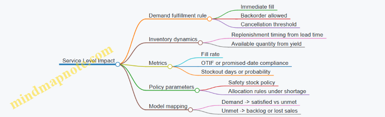
Keep the Three Levers Consistent with One Another
A common modeling mistake is to adjust service level directly while also changing lead time and yield. That double-counts the same operational reality.
Use this rule of thumb:
- Lead time and yield are physical/operational translations.
- Service level is the outcome of the fulfillment logic given those physical changes.
If you must incorporate a service-level-specific mechanism (e.g., “customers refuse substitutions”), represent it as a policy constraint in the fulfillment logic, not as an independent service-level multiplier.
Worked Mini-Example with Time Phasing
Assume a product uses Supplier X.
- Baseline lead time: 20 days.
- Baseline yield: 95% usable.
- Disruption window: 2026-03-01 to 2026-03-31.
- Event: “Transit delay adds 8 days; inspection backlog reduces pass rate.”
Translation:
- Orders released during the window use lead time shifted to 28 days.
- Received units during the window use yield reduced to 90%.
- Inventory simulation then computes fill rate and backlog outcomes under the chosen demand policy.
The result is a scenario input set that is traceable: every service-level change can be explained by the modeled lead time shift, yield reduction, and the fulfillment rules—no mystery multipliers required.
4.3 Model Inventory Policies Including Safety Stock and Reorder Logic
Inventory policy is where disruption narratives turn into numbers you can simulate. The goal is not to guess the future; it’s to represent how your operations behave when lead times stretch, yields drop, and demand keeps showing up (or doesn’t).
Inventory Policy Basics That Drive the Model
Start by choosing the policy style your business actually uses. Two common patterns are:
- Periodic review: you check inventory every fixed interval (e.g., weekly) and place orders.
- Continuous review: you monitor continuously and reorder when inventory hits a threshold.
In a scenario model, both patterns reduce to the same mechanics: compute an order quantity and an order timing rule, then translate those into inventory position and service outcomes.
A practical modeling choice is to represent inventory with three linked quantities:
- On-hand inventory: what you can ship now.
- Inventory position: on-hand plus on-order minus backorders.
- Backorders or lost sales: decide whether unmet demand waits or disappears.
Example: If you treat unmet demand as backorders, a longer lead time increases backlog, which can later be filled when shipments arrive. If you treat unmet demand as lost sales, the same disruption reduces revenue immediately.
Safety Stock as Protection Against Lead Time and Demand Variability
Safety stock is the buffer that reduces the chance of stockouts during the time you’re waiting for replenishment. In most models, safety stock depends on two uncertainties:
- Lead time variability: orders arrive later than expected.
- Demand variability: demand during the lead time is higher than expected.
A simple starting formula for continuous review is:
- Safety Stock = Z × σ(LT demand)
Where Z is a service level factor and σ(LT demand) is the standard deviation of demand over the lead time.
To keep the model grounded, compute σ(LT demand) from scenario inputs rather than from vibes. If demand per period has standard deviation σd and lead time has variability, you can approximate σ(LT demand) by combining demand variance across periods and lead time variance. If that feels heavy, use a scenario-level “effective lead time demand standard deviation” parameter derived from historical lead time and demand behavior.
Example: Suppose your average weekly demand is 10 units with moderate variability, and your lead time averages 3 weeks. Under disruption scenarios, lead time might stretch to 5 weeks and become more erratic. Your model should increase safety stock accordingly, not just by multiplying by the lead time mean, but by reflecting higher uncertainty.
Reorder Point Logic for Continuous Review
Continuous review uses a reorder point (ROP). The core rule is:
- Reorder when inventory position ≤ ROP
- ROP = Expected demand during lead time + Safety stock
Expected demand during lead time is the mean demand over the lead time distribution. Safety stock covers the tail risk.
Example: If expected demand during lead time is 120 units and safety stock is 30 units, then ROP is 150. If a disruption increases lead time variability, safety stock rises, pushing ROP upward. That means you reorder earlier, which is exactly what you want when arrivals are less reliable.
Order Quantity Logic and Lot Sizing
Once the reorder trigger fires, you need an order quantity rule. Common options:
- Order-up-to (S) policy: order enough so inventory position reaches a target level.
- Fixed order quantity (Q): order a constant amount each time.
Order-up-to is often easier for scenario simulation because it naturally accounts for current inventory position.
Example: With an order-up-to target S, when inventory position drops to ROP, you order S − inventory position. If you choose S based on desired coverage (e.g., lead time plus review period), you can keep policy behavior consistent across scenarios.
Periodic Review Logic for Weekly Ordering
Periodic review checks inventory every review interval R. The reorder rule typically uses:
- Order when inventory position ≤ target
- Target = Expected demand during lead time + Expected demand during review interval + Safety stock
This prevents a subtle modeling error: if you only cover lead time but ignore the time until the next review, you’ll under-protect the system.
Example: If you review weekly and lead time is 3 weeks, then demand can accumulate for 4 weeks between the moment you place an order and the moment you can react again. Safety stock should cover uncertainty across that combined horizon.
Translating Policy into Scenario Inputs
To make the policy scenario-aware, link these inputs to your scenario variables:
- Lead time distribution: mean and variability change under disruption.
- Demand distribution: mean and variability change under demand uncertainty.
- Service mode: backorder vs lost sales stays fixed unless policy changes.
- Supplier yield and fill rate: affects effective supply quantity.
Example: If supplier yield drops from 98% to 90%, then an order of 100 units effectively delivers 90 units. Your model should reduce the quantity received (and possibly increase lead time if rework or partial shipments occur).
Mind Map: Inventory Policies
Inventory Policies Mind Map
Worked Example Policy in One Pass
Assume continuous review with backorders. In a baseline scenario, expected demand during lead time is 120 units and safety stock is 30, so ROP = 150. In an inflation-and-disruption scenario, lead time variability increases and demand volatility rises, so safety stock becomes 55 while expected demand during lead time becomes 130. Now ROP = 185.
If inventory position is 170 at the time of evaluation, the baseline policy would not reorder (170 > 150), but the disruption scenario would reorder (170 ≤ 185). With an order-up-to target S of 220, the baseline order would be 0, while the disruption scenario orders 220 − 170 = 50 units.
This is the kind of cause-and-effect your scenario model should preserve: disruption changes the uncertainty, uncertainty changes safety stock, safety stock changes reorder timing, and reorder timing changes service and cash outcomes.
4.4 Incorporate Supplier Qualification Constraints and Dual Sourcing Limits
Supplier qualification is where “we can buy it” meets “we are allowed to buy it.” Dual sourcing is where “we have options” meets “options are limited by reality.” In a scenario-based supply chain model, these constraints must be explicit, measurable, and time-phased so they affect service levels, costs, and allocation decisions.
Define Qualification Status as Model State
Start by representing each supplier as having a qualification state that can change by scenario and over time. Common states include:
- Qualified for the product and site
- Qualified for a subset of materials or grades
- Conditionally qualified pending documentation
- Not qualified
Example: A packaging supplier is qualified for standard film but not for a new barrier layer. In an inflation shock scenario, demand for the barrier layer rises, but the supplier can only fulfill the standard film portion. Your model should reflect that split rather than assuming full capability.
Model Qualification as Constraints, Not Narrative
Qualification should constrain feasible flows. Use constraints that limit:
- Which SKUs or material grades each supplier can ship
- Which plants or lanes each supplier can serve
- Which lead-time distributions apply when qualification is conditional
Practical rule: if a supplier is “conditionally qualified,” allow shipments only if the scenario includes “documentation accepted” and reduce the effective capacity or increase lead time.
Represent Dual Sourcing Limits with Clear Policy Logic
Dual sourcing limits typically come from policy and operational capacity, not just preference. Capture them with two layers:
- Minimum diversification: e.g., at least two suppliers must be used when feasible.
- Maximum concentration: e.g., no more than 70% of a SKU’s volume from a single supplier.
Example: A medical device component must be sourced from two qualified suppliers when both are available. If one supplier is disrupted, the model can relax diversification, but only up to a concentration cap and only if an internal waiver is “active” in that scenario.
Time-Phase Qualification and Waivers
Qualification often changes slowly. Model it with time-phased availability:
- Qualification effective date
- Qualification expiration date
- Waiver duration and renewal rules
Use a concrete timeline. For instance, a supplier’s requalification completes on 2026-03-01. Before that date, shipments are allowed only for limited grades. After that date, full grade coverage becomes feasible.
Build the Constraint Set in the Decision Model
Include these elements in your formulation:
- Supplier-SKU eligibility matrix
- Supplier-plant eligibility matrix
- Capacity by supplier and period
- Qualification state by supplier and period
- Dual sourcing concentration constraints by SKU and period
- Optional waiver binary variables if you need strict on/off behavior
A simple way to keep it understandable is to separate feasibility from optimization: first filter eligible routes by qualification, then optimize flows within remaining capacity and dual sourcing caps.
Mind Map: Qualification and Dual Sourcing Constraints
Example: Allocation Under Disruption and Conditional Qualification
Assume SKU A has demand 1,000 units in a month. Two suppliers exist:
- Supplier 1: qualified for SKU A, capacity 600
- Supplier 2: conditionally qualified for SKU A, capacity 500, but only if “inspection passed” is true in the scenario Dual sourcing policy: at least two suppliers if both are feasible; max 70% from one supplier.
Scenario outcome:
- Disruption reduces Supplier 1 capacity to 500.
- Inspection passed is false. Result: Supplier 2 cannot ship, so only Supplier 1 is feasible. The model must allow a service shortfall rather than forcing dual sourcing. If inspection passed were true, the model would allocate up to 500 from Supplier 1 and up to 500 from Supplier 2, while also checking the 70% concentration cap.
Validation Checks That Prevent Silent Modeling Errors
Before running scenarios, verify:
- No flow exists on ineligible supplier-SKU routes
- Dual sourcing caps are applied per SKU and period, not globally
- Waivers only relax constraints when the scenario includes the required trigger
- Qualification state changes are consistent with the time-phased calendar
If your model passes these checks, the optimization will behave like a planner: it will try to use the best suppliers, but it will not pretend unqualified supply is available.
4.5 Quantify Transportation and Customs Friction Under Disruption Conditions
Transportation and customs friction is the part of disruption that shows up as time, money, and uncertainty before goods even reach your dock. Quantifying it well means you can compare options (reroute, expedite, buffer inventory, change Incoterms) using the same model logic as cost and service level.
Core Concepts and What to Measure
Start by separating three friction components:
- Transit time inflation: longer routes, slower modes, reduced capacity, and border delays.
- Direct friction cost: demurrage, storage, handling, expediting fees, and additional freight charges.
- Compliance friction: paperwork rework, inspection probability, tariff classification disputes, and documentation lead time.
A practical measurement set for the decision model is:
- Expected lead time (days) and lead time variance (days)
- Expected landed cost uplift (currency per unit)
- Service impact via fill rate or backorder cost
Example: If a shipment normally takes 12 days and disruption adds an average of 5 days with high variance, your inventory policy must cover both the mean and the tail, not just the average.
Build a Friction Calculator from First Principles
Use a simple structure that can be parameterized by lane, mode, and scenario.
Step 1: Define lanes and routing choices
- Lane = origin region → destination region
- Mode = air, ocean, truck, rail
- Route option = specific carrier/service or border crossing pattern
Step 2: Represent time components Let total lead time be:
- T = T_transport + T_handling + T_border + T_docs
Under disruption, each component gets an additive uplift and sometimes a probability of extra delay.
Step 3: Represent cost components Let landed cost uplift be:
- C = C_freight_uplift + C_handling + C_storage_demurrage + C_expedite + C_compliance_rework
Step 4: Represent uncertainty explicitly For border and documentation, use a probability of “extra delay” rather than a single inflated average.
Example: Border inspection might be 10% normally and 30% during disruption. If inspection adds 2–4 days, model it as a distribution or a two-state mixture.
Quantify Transportation Friction by Lane and Mode
For each lane and mode, estimate disruption multipliers using operational signals.
- Capacity reduction increases transit time and may increase freight rates.
- Routing changes increase distance and handling stops.
- Carrier performance degradation increases variability.
A workable approach:
- Baseline: use historical median transit time and typical freight cost.
- Disruption: apply scenario-specific uplift factors to median and separate factors to variability.
Example: Truck lanes might see a 1.3× median transit time uplift and a 1.6× standard deviation uplift. Ocean lanes might have smaller median uplift but larger tail risk due to port congestion.
Quantify Customs Friction with a Two-Layer Model
Customs friction is often the most annoying because it mixes time and money with compliance uncertainty.
Use two layers:
-
Documentation lead time
- Add days for document preparation, corrections, and approvals.
- Probability of rework depends on disruption severity and documentation quality.
-
Border delay and inspection
- Model inspection as a probability event.
- Add storage/demurrage costs when dwell time exceeds a free period.
Example: If free dwell time is 3 days and disruption increases average dwell to 6 days, demurrage may kick in. You can compute expected demurrage as:
- Expected demurrage = P(dwell > free) × (expected dwell − free) × daily rate
Mind Map: Transportation and Customs Friction
Worked Example with Numbers
Assume a lane ships 1,000 units per week.
Baseline:
- Transport time: 10 days
- Border delay: 1 day
- Docs lead time: 2 days
- Freight cost: $1.20/unit
- Demurrage: $250/day after free dwell of 3 days
Disruption scenario:
- Transport time uplift: +3 days (median)
- Border delay becomes a two-state event: 70% at +1 day, 30% at +4 days
- Docs lead time uplift: +1 day with 20% chance of rework adding +2 more days
- Freight cost uplift: +18%
Compute expected lead time:
- Expected transport+handling: 10 + 3 = 13 days
- Expected border: 1 + (0.7×1 + 0.3×4) = 1 + 2. - Wait: border delay baseline already included as 1 day; treat uplift as extra. So total border = 1 + (0.7×1 + 0.3×4) = 1 + 2. - That equals 3 days.
- Expected docs: 2 + 1 + (0.2×2) = 3.4 days
- Total expected lead time = 13 + 3 + 3.4 = 19.4 days
Compute expected landed cost uplift (simplified):
- Freight uplift: $1.20×1.18 − $1.20 = $0.216/unit
- Demurrage: approximate dwell as border+handling time. Baseline dwell 1 day + handling not modeled separately here; use border total as dwell proxy.
- Free dwell 3 days, expected dwell 3 days means demurrage is mostly driven by the tail.
- Tail dwell occurs when border uplift is +4 (30%): dwell ≈ 1 + 4 = 5 days → 2 days demurrage.
- Expected demurrage per unit = (0.30×2×$250) / 1,000 = $0.15/unit
Total expected uplift ≈ $0.216 + $0.15 = $0.366/unit.
This gives the model a consistent way to translate disruption assumptions into both inventory timing pressure and cost pressure.
Practical Integration into the Supply Model
Once you have expected lead time and cost uplift per lane and route option, integrate them into:
- Inventory policy: use lead time distribution (or conservative quantiles) to set safety stock.
- Capacity and allocation: route options with higher friction may still be chosen if they preserve service.
- Cash and working capital: higher lead time increases inventory in transit, which ties directly to cash constraints.
Example: If expedited air reduces lead time by 6 days but adds $0.80/unit in freight and compliance handling, the decision model can compare it against holding extra safety stock for ocean shipments.
Validation Checks That Prevent Silent Errors
Before trusting results, run three checks:
- Unit consistency: days per shipment, currency per unit, rates per day.
- Probability sanity: two-state events must sum to 1 and should not produce negative delays.
- Cross-check with observed behavior: compare predicted lead time against recent disruption-like shipments from 2026-03-01 to 2026-03-31 for at least one lane.
When these checks pass, transportation and customs friction becomes a controllable part of the scenario model rather than a vague “it’s worse” note.
5. Represent Uncertain Global Demand in a Decision Model
5.1 Define Demand Segments and Their Distinct Drivers
Demand segmentation is the step where you stop treating “demand” as one number and start treating it as a set of behaviors. In scenario planning, this matters because inflation, supply disruption, and service changes rarely affect every customer the same way. A good segment definition makes those differences show up in your model outputs instead of getting averaged away.
Start with What You Can Actually Act On
A demand segment should be something you can influence through decisions like pricing, allocation, lead-time promises, packaging, or channel strategy. If you cannot tie a segment to at least one controllable lever, it usually becomes a reporting label rather than a modeling input.
Example: A consumer electronics firm might be tempted to segment by “age group.” If pricing and availability are the only levers, “age group” may not map cleanly. A more actionable segmentation could be “online direct buyers” versus “retail partners,” because each channel has different ordering cadence, tolerance for backorders, and willingness to switch brands.
Use a Simple Segmentation Logic
Work from three layers: who buys, what they buy, and how they buy.
- Who buys: customer type, geography, industry, or contract type.
- What they buy: product family, feature tier, or substitute set.
- How they buy: channel, ordering process, service expectations, and payment terms.
You can create segments by combining one choice from each layer. Keep the number of segments manageable; 6–12 is often enough for scenario modeling, because each segment adds parameters and validation work.
Identify Distinct Drivers per Segment
Drivers are the variables that move demand within a segment. The goal is not to list everything you can measure; it is to identify a small set of drivers that explain demand changes under your scenario dimensions.
Common driver categories include:
- Price sensitivity: how demand shifts when your effective price changes.
- Availability sensitivity: how demand shifts when lead time or fill rate changes.
- Income or cost pressure: how customer budgets respond to inflation.
- Substitution behavior: whether customers switch to alternatives when your product is constrained.
- Ordering cadence: how often orders are placed and how that cadence changes with service.
- Contract structure: fixed commitments versus flexible orders.
Example: For a food manufacturer, “grocery retail” might be availability-sensitive because shelves must be replenished quickly. “Food service distributors” might be more price-sensitive because they can adjust menu pricing and pass costs through with some delay.
Build Driver Statements That Can Be Modeled
Turn each driver into a statement with direction and mechanism. A mechanism is the “why,” not a story—something you can translate into equations or rules.
Example driver statement for availability sensitivity:
- “When fill rate drops, orders shift from immediate replenishment to later waves, reducing near-term demand but increasing backlog conversion later.”
This statement implies time-phased demand effects rather than a single multiplier.
Mind Map: Demand Segments and Drivers
Example Segmentation with Integrated Drivers
Consider a company selling industrial components.
-
Segment A: Contracted buyers
- Drivers: contract structure, substitution limits, availability sensitivity.
- Mechanism: demand is relatively stable until service breaches trigger penalties or renegotiation.
-
Segment B: Project-based buyers
- Drivers: ordering cadence, lead-time sensitivity, price sensitivity.
- Mechanism: demand spikes when projects start, but delays reduce the start window and shift orders.
-
Segment C: Maintenance buyers
- Drivers: availability sensitivity, substitution behavior, budget pressure.
- Mechanism: when your part is unavailable, customers switch to approved substitutes, causing immediate lost sales but possible later reversion.
Notice how each segment’s drivers map to scenario themes: inflation changes budget pressure and effective price; disruption changes lead time and fill rate; uncertain global demand changes ordering cadence and project timing.
Validate Segments with a Quick Consistency Check
Before you lock segments, test whether they produce different demand responses under the same scenario variable. If two segments behave identically for price and availability in your model, they probably should be merged. If they behave differently, you have a defensible segmentation.
A practical check: pick one historical disruption event and compare segment-level outcomes. If you cannot approximate the observed differences with your chosen drivers, refine the segmentation or revise the driver mechanisms.
By the end of this section, each segment should have a clear definition and a short list of drivers with mechanisms that your model can represent. That is what makes scenario planning more than a set of narratives—it becomes a structured way to compute how demand actually changes.
5.2 Build Demand Response Functions for Price and Availability
Demand response functions translate two levers—price and availability—into expected demand behavior. The goal is not to predict perfectly; it’s to represent how customers react so your scenario model can produce consistent, decision-relevant outcomes.
Start with Customer Behavior Building Blocks
A useful demand response function separates three ideas:
- Baseline demand: what you’d sell if price and availability were “normal.”
- Price effect: how demand changes when your effective price changes.
- Availability effect: how demand changes when you can’t fulfill orders on time or in full.
A simple structure is:
- Demand = Baseline × Price Multiplier × Availability Multiplier
Example: A regional beverage brand expects 10,000 units per week under normal pricing and 95% on-time in-full (OTIF). If a scenario raises effective price by 8% and OTIF drops to 80%, the multipliers reduce demand accordingly.
Define Effective Price and Availability
“Price” in models should reflect what customers actually pay, not just list price. Use an effective price that includes:
- discounts and promotions
- freight or surcharges that are passed through
- contract tiering (e.g., volume rebates)
“Availability” should reflect fulfillment reality. Common choices:
- OTIF for service reliability
- fill rate for in-stock completeness
- lead time for how long customers wait
Example: If you can ship 90% of orders within the promised window, you can treat availability as 90% OTIF for the week, even if inventory exists but routing delays prevent timely delivery.
Choose Functional Forms That Behave Well
Demand response functions must be monotonic and stable. Two practical forms work well.
1. Price multiplier using elasticity
Let elasticity be ε (negative for typical goods). If effective price changes from P0 to P1:
- Price Multiplier = (P1 / P0)^ε
Example: If ε = -1.2 and price rises 10%, then (1.1)^-1.2 ≈ 0.88, meaning demand drops about 12% before availability effects.
2. Availability multiplier using a service curve
A service curve converts OTIF or fill rate into demand capture. One straightforward approach is a piecewise linear rule:
- At OTIF ≥ 95%, multiplier = 1.00
- At OTIF = 80%, multiplier = 0.85
- At OTIF ≤ 60%, multiplier = 0.60
Example: If OTIF falls from 95% to 80%, you assume customers still buy, but some switch to alternatives or delay purchases.
Model Substitution, Backlogging, and Lost Sales
Availability effects depend on what customers do when you can’t deliver.
- Lost sales: demand disappears if not fulfilled quickly.
- Backlogging: demand shifts to later periods.
- Substitution: customers switch to other products or suppliers.
A clean way to represent this is to split demand into two streams:
- Captured demand: demand you fulfill in the period
- Uncaptured demand: demand you don’t fulfill, which either becomes backlog or lost sales
Example: For a spare-parts SKU, customers may tolerate a 2-week delay, so uncaptured demand becomes backlog. For a seasonal product, uncaptured demand is mostly lost sales.
Mind Map: Demand Response Function Design
Calibrate with Segment-Level Evidence
Calibration is where many models go wrong: they use one elasticity for everything. Instead, calibrate by segment that shares behavior.
Segment examples:
- customer type (retail vs industrial)
- geography with different logistics reliability
- product tier (commodity vs premium)
Example: A premium skincare line may have lower price sensitivity than a mass-market cleanser. If you apply the same ε across both, your model will misattribute demand drops to price when the real driver is availability or vice versa.
Implement Time Phasing Without Contradictions
Availability effects should be applied consistently across periods. If you use backlogging, then:
- uncaptured demand in week t becomes backlog
- backlog is attempted fulfillment in week t+1 based on capacity and lead times
Example: Suppose OTIF drops in week 3 due to a disruption. Your demand function should reduce captured demand in week 3, then increase captured demand in week 4 if capacity recovers.
Add Consistency Checks That Save You Later
Before trusting outputs, verify:
- Demand decreases when price increases (for the chosen ε sign)
- Demand increases when availability improves (service curve monotonicity)
- Backlog never grows without a reason (capacity constraints and fulfillment logic)
- Revenue doesn’t behave impossibly under extreme inputs
Example: If a scenario sets OTIF to 100% and price to P0, your model should return baseline demand exactly. If it doesn’t, you likely have mismatched units or inconsistent multipliers.
Worked Example in One Pass
Assume:
- Baseline demand = 10,000 units
- Effective price increases 8% (P1/P0 = 1.08)
- Price elasticity ε = -1.0 → Price Multiplier = 1.08^-1 ≈ 0.93
- OTIF drops to 80% → Availability Multiplier = 0.85
Captured demand in the period = 10,000 × 0.93 × 0.85 ≈ 7,905 units.
If 30% of uncaptured demand becomes backlog for this segment, then backlog added ≈ (10,000 − 7,905) × 0.30 ≈ 628 units, which your fulfillment logic will attempt to clear later.
This approach keeps the model interpretable: each lever has a measurable effect, and the customer response is explicit rather than hidden in a black-box curve.
5.3 Incorporate Channel Effects Including Distributor and Retail Behavior
Channel effects matter because the same end-customer demand can produce very different orders, inventory levels, and service outcomes once it passes through distributors and retailers. In a scenario model, you want to represent how channel partners react to price, availability, promotions, and service failures—without turning the model into a soap opera.
Start with a Clear Channel Map
A practical approach is to separate the channel into three layers: end demand, channel ordering, and channel fulfillment. End demand is what customers want. Channel ordering is what distributors and retailers decide to buy. Channel fulfillment is what the supply chain can actually deliver.
A simple baseline mapping looks like this:
- End demand by segment drives sell-through.
- Retailers translate sell-through into replenishment orders.
- Distributors translate retailer orders into replenishment orders to you.
- Your ability to ship determines fill rates, backlogs, and lead-time variability.
This separation prevents a common modeling mistake: using one demand number to represent both customer demand and ordering behavior.
Model Distributor Behavior with Two Levers
Distributors typically react through (1) order-up-to targets and (2) service-driven adjustments.
-
Order-Up-To Target
Represent distributor inventory policy as a target coverage in weeks. When coverage falls below target, orders rise. When coverage exceeds target, orders slow. Example: if the target is 6 weeks of supply and shipments arrive late, coverage drops, triggering larger replenishment orders. -
Service-Driven Adjustment
When your fill rate drops, distributors may either wait for better availability or place larger orders to protect their own shelves. Use a parameter that captures the direction and strength of this response.
Concrete example for a scenario:
- Scenario A: inflation increases your unit costs, so you raise list prices slightly.
- Retailers slow purchases, but distributors may still order to maintain coverage.
- If your fill rate remains high, distributor orders track demand changes smoothly.
- If disruption reduces fill rate, distributors may over-order to avoid stockouts, increasing your backlog and working capital needs.
Model Retailer Behavior with Promotion and Substitution
Retailers often manage inventory with a mix of baseline replenishment and promotional cycles. Two behaviors are especially useful.
- Promotion Elasticity Through Ordering Promotions increase sell-through. Retailers respond by increasing orders, but not always proportionally. Use a promotion uplift factor applied to sell-through, then convert it to orders using a retailer order responsiveness parameter.
Example: a promotion lifts sell-through by 20%, but retailer orders rise only 12% because they expect partial demand cannibalization and want to avoid excess inventory.
- Substitution When Availability Is Low If your product is out of stock, retailers may substitute with alternatives, or they may backorder and wait. Represent this with an availability-to-fulfillment rule.
Example: when your in-stock rate falls below a threshold, 30% of lost sales shift to substitutes and never return; the remaining 70% become backorders that reappear when supply improves.
Connect Channel Behavior to Your Model Outputs
To keep the model coherent, channel effects must feed into measurable outputs: shipments, fill rate, backlog, and inventory.
A workable linkage is:
- Sell-through drives retailer demand for replenishment.
- Retailer ordering determines distributor orders.
- Distributor orders determine your inbound demand.
- Your fill rate determines how much of inbound demand becomes shipments versus backlog.
This linkage also helps you interpret scenario results. If a scenario shows higher orders but lower sales, it likely reflects channel over-ordering under poor availability.
Mind Map: Channel Effects Logic
Example Walkthrough for a Single Scenario
Assume a two-month planning period with weekly steps.
- Week 1: baseline demand is stable.
- Week 2: disruption reduces your fill rate from 95% to 75%.
- Week 3: you raise prices due to inflation.
Model behavior:
- Retailers see lower in-stock availability, so lost sales split into substitution and backorders.
- Backorders increase retailer orders in later weeks.
- Distributors, using a 6-week coverage target, increase orders when their coverage drops.
- If your fill rate stays low, backlog grows faster than shipments, and inventory at retailers and distributors may still rise even while end sales fall.
The result is not just “demand went down.” It is “channel ordering changed because availability and pricing changed,” which is exactly what scenario planning should capture.
Practical Guardrails
- Calibrate ordering responsiveness so that orders do not move more than sell-through without a clear availability reason.
- Ensure substitution and backorder rates sum to the fraction of demand that is not permanently lost.
- Keep channel parameters scenario-consistent: price affects ordering through retailer and distributor rules, while disruption affects ordering primarily through service and availability.
When these guardrails are in place, channel effects become a controlled mechanism rather than a mysterious multiplier—useful for comparing options and explaining why the same end demand can produce different operational outcomes.
5.4 Model Order Timing and Backlog Dynamics Under Service Changes
Order timing is where “we can deliver” turns into “we did deliver.” In a volatile environment, service changes—like longer lead times, reduced capacity, or lower fill rates—shift when customers place orders, how much they order, and whether they accept backlog. A good model treats timing as a first-class variable, not an afterthought.
Core Concepts for Timing and Backlog
Start with three quantities per period: orders received, units shipped, and backlog carried. Backlog is not just “unfilled demand”; it is demand that has been promised but not yet satisfied, and it can be cleared only by future shipments.
A simple flow for each period t:
- Available supply = beginning inventory + arrivals at t
- Shipments = min(available supply, demand that is eligible to ship at t)
- Backlog update = backlog from prior period + new demand not shipped
Service changes affect two things at once: (1) the probability that an order is accepted immediately, and (2) the customer’s willingness to wait.
Representing Service Changes in the Model
Service changes typically show up as one or more of these levers:
- Lead time shifts: arrivals move later.
- Capacity reductions: fewer units can be shipped per period.
- Fill rate changes: partial shipments become more common.
- Promise policy changes: customers are quoted later dates or offered alternatives.
Model each lever as a mechanism that changes either arrivals, shipments, or backlog acceptance. For example, if lead time increases by two weeks, arrivals move to later periods, which increases backlog even if demand is unchanged.
Order Timing Mechanisms That Affect Backlog
Customers rarely behave like perfectly patient robots. In models, you can represent timing effects with practical mechanisms that are easy to explain and calibrate.
-
Order deferral under poor service
- When promised dates slip, some customers delay ordering.
- Example: If service level drops below a threshold, 20% of orders that would have arrived this week move to next week.
-
Order escalation under high urgency
- Some customers place orders earlier to avoid missing future availability.
- Example: During a disruption, a segment increases ordering frequency, raising near-term demand while later demand normalizes.
-
Backlog acceptance and cancellation
- Customers may accept backlog, cancel, or switch suppliers.
- Example: If backlog exceeds a limit, 10% of backlog demand cancels each period until backlog falls.
These mechanisms can be implemented as fractions that reallocate demand across periods, or as rules that determine how much demand becomes backlog versus lost sales.
A Systematic Step-by-Step Modeling Approach
-
Choose the period grain
- Use a period length that matches operational decisions, such as weekly for shipping and replenishment.
-
Define demand timing inputs
- For each segment, specify a base demand per period and a timing response to service.
-
Define service metrics used by the timing rules
- Common choices: fill rate, on-time promise rate, or backlog level.
-
Translate service into customer behavior
- Use simple piecewise rules. Example: if fill rate < 85%, defer 20% of orders; if backlog > 4 weeks, cancel 10%.
-
Update backlog and shipments in a consistent order
- Apply arrivals first, then shipments, then backlog updates, then cancellations/lost sales.
-
Check conservation of units
- Ensure that every unit of demand is either shipped, becomes backlog, or is lost/canceled.
Mind Map: Order Timing and Backlog Dynamics
Example: Weekly Model with Deferral and Cancellation
Assume weekly periods. Beginning inventory is 500 units, backlog is 200 units, and inbound arrivals are 300 units this week. Total demand for the week is 1,200 units.
- Compute available supply: 500 + 300 = 800.
- Apply service-driven order deferral: if fill rate is expected to be low, defer 20% of this week’s new demand to next week.
- New demand this week becomes 1,200 × 0.8 = 960.
- Determine shipments: shipments are limited by supply and backlog eligibility.
- Ship 800 units this week.
- Update backlog:
- Total demand needing satisfaction = prior backlog 200 + new demand 960 = 1,160.
- Backlog carried = 1,160 − 800 = 360.
- Apply backlog cancellation: if backlog duration exceeds a threshold, cancel 10% of backlog.
- Backlog after cancellation = 360 × 0.9 = 324.
This example shows why timing rules must be applied before backlog updates: deferral changes the demand that competes with backlog for limited supply.
Example: Promise Policy That Changes Acceptance
If the company switches from “ship as soon as possible” to “quoted date only,” some customers stop accepting backlog and instead treat late fulfillment as lost sales.
In the model, represent this as a change in the backlog acceptance fraction. Example: under the old policy, 90% of unshipped demand becomes backlog; under the new policy, only 60% becomes backlog and the rest is lost sales. The same supply and demand inputs will then produce a different backlog trajectory and different revenue outcomes.
Practical Guardrails for Credible Timing Dynamics
- Keep rules monotonic where possible: worse service should not reduce backlog without an explicit mechanism like cancellation.
- Calibrate fractions with operational evidence: deferral and cancellation rates should be consistent with observed order behavior.
- Avoid double counting: if you model lost sales via cancellation, do not also reduce demand separately for the same effect.
When these pieces fit together, backlog becomes a measurable consequence of service changes and customer timing behavior, not a mysterious number that appears after the fact.
5.5 Establish Demand Data Reconciliation Across Regions and Currencies
Demand reconciliation is the step where you stop treating regional demand numbers as if they were already comparable. You take messy inputs—different currencies, different reporting cutoffs, different product mappings, and different definitions of “order” or “shipment”—and convert them into a single, decision-ready view.
Start with a Shared Definition of Demand
Before touching spreadsheets, align on what “demand” means for the model. In practice, teams mix at least four concepts: customer orders, distributor orders, shipments to customers, and sell-through at retail. Pick one as the modeling target and document it as a rule.
Example: A consumer electronics firm models demand as “sell-through units” because pricing decisions are tied to shelf movement. In one region, the data feed reports sell-through weekly; in another, it reports shipments monthly. Reconciliation begins by converting both into the chosen unit definition, not by averaging them.
Normalize Currency and Price Basis
If demand is measured in revenue, reconcile currency and price basis first. Use a consistent exchange-rate convention and a consistent price basis (gross vs net, list vs realized, including or excluding rebates).
Best practice: Convert all revenue to a single currency using the same rate type across regions—either average for the period or end-of-period—then reconcile realized price components separately.
Example: Region A reports “net sales” after rebates; Region B reports “gross sales” before rebates. If you convert currencies and then directly compare revenue, you’ll confuse rebate timing with demand. Instead, reconcile units and realized price separately: units from orders/sell-through, realized price from net-to-gross adjustments.
Reconcile Product Mapping and Packaging Units
Demand data often disagrees on what a “unit” is. One region may sell by SKU; another may report by bundle. Even when SKUs match, packaging can differ (case size, weight, or configuration).
Best practice: Create a mapping table from source product identifiers to model product identifiers, including conversion factors for pack sizes.
Example: A pharmaceutical company receives demand for “bottles” in one country and “blister packs” in another. The model uses “treatment courses.” Reconciliation uses conversion factors (bottles per course, packs per course) so the demand curve is driven by comparable consumption.
Align Time Buckets and Reporting Cutoffs
Time misalignment is a silent error source. Regions may report by local calendar, fiscal weeks, or shipment dates. Reconciliation requires a consistent time axis.
Best practice: Use a single planning calendar for the model and map each region’s timestamps into it. If you only have month-level data, decide whether to allocate uniformly across weeks or to use a known seasonality profile from historical patterns.
Example: Region C reports orders by “order entry date,” while Region D reports by “invoice date.” If you aggregate both into monthly buckets without adjustment, you’ll see artificial spikes that are really billing delays.
Build a Reconciliation Pipeline with Checks
A practical pipeline has four stages: standardize, map, convert, and validate.
- Standardize fields: currency, units, time bucket, and demand definition.
- Map identifiers: product and channel mapping to model segments.
- Convert measures: currency conversion and unit conversions.
- Validate: sanity checks and reconciliation residuals.
Validation checks should be explicit and repeatable:
- Totals check: sum of reconciled demand equals sum of standardized inputs after conversion.
- Price consistency check: implied realized price stays within a plausible band.
- Movement check: week-over-week or month-over-month changes do not violate known operational constraints.
Example: If a region’s reconciled realized price jumps 30% while units remain flat, you likely have a rebate timing mismatch or a currency-rate convention mismatch.
Use a Reconciliation Mind Map
Mind Map: Demand Data Reconciliation Across Regions and Currencies
Handle Missingness and Conflicting Signals
When data is missing or contradictory, reconciliation should produce a decision-ready output with confidence flags, not a silent guess.
Best practice: Use a hierarchy of sources. For example, prefer sell-through where available; otherwise use shipments; if both exist but disagree, reconcile using known lag patterns (e.g., shipments lead sell-through by 2–4 weeks).
Example: Region E has sell-through for two months and shipments for the rest. Reconciliation uses the overlap period to estimate a lag and scaling factor, then applies it to convert shipments into an estimated sell-through series for the missing months. The model receives the series plus a flag indicating it is derived.
Keep an Audit Trail That Explains the “Why”
Reconciliation is not just math; it’s a chain of decisions. Store transformation rules and the reason each rule exists. When stakeholders ask why Region B’s demand looks lower, you should be able to point to the exact step: currency convention, rebate basis, pack conversion, or time mapping.
Example: A reconciliation log states: “Region B net sales converted using average monthly FX; rebates removed using contract schedule; units converted using case-to-SKU factor.” That’s enough to resolve disagreements without re-running everything from scratch.
Practical Output Format for the Model
The reconciled dataset should be segment-level and model-ready, with these fields: time bucket, model product/segment, demand units (or revenue if that’s the target), realized price (if applicable), and confidence flags. Confidence flags let your scenario model treat uncertain segments differently instead of pretending all numbers are equally reliable.
6. Construct Scenario Sets Using a Structured Logic
6.1 Select Scenario Dimensions and Determine Their Independence or Coupling
Scenario dimensions are the variables you let move in your planning model. The trick is choosing enough dimensions to represent real decision tradeoffs, without creating a combinatorial mess that no one can reason about. Independence versus coupling is how you decide whether dimensions can be varied separately or must move together because they share a mechanism.
Start with Decision-Relevant Mechanisms
A dimension should trace to a mechanism that changes outcomes your organization actually cares about: margin, service level, working capital, capacity utilization, or cash timing. For example, “inflation” is too broad by itself. “Input price inflation for steel” is closer to a mechanism that affects unit cost, procurement timing, and potentially pricing power.
A practical way to begin is to list the top 5–10 decisions you modeled in earlier steps, then ask: “What must be different for this decision to change?” If the answer is “lead times,” that suggests a dimension around supply disruption severity. If the answer is “customers switch to substitutes when availability drops,” that suggests a coupling between supply constraints and demand.
Define Candidate Dimensions Using a Consistent Template
For each candidate dimension, write three items:
- What changes (the variable), 2) Where it enters the model (cost, capacity, demand, logistics, contract terms), and 3) What evidence would justify it (historical patterns, contract structure, operational constraints).
Example candidate dimensions:
- Inflation shock intensity for key inputs (affects unit cost and sometimes supplier lead times).
- Disruption severity (affects lead time distribution, yield, and service level).
- Global demand uncertainty (affects order volumes by segment and timing).
- Exchange rate movement (affects landed cost and pricing in local currency).
If a dimension cannot be mapped to model inputs, it will usually become a narrative-only variable that doesn’t help decisions.
Independence: When Dimensions Can Move Separately
Two dimensions are approximately independent when changing one does not systematically change the other through a shared mechanism. Independence is not “true in the universe”; it’s “independent enough for planning.”
Example of near-independence:
- Demand uncertainty and warehouse automation capacity. If automation capacity is fixed by capex and lead time, and demand uncertainty doesn’t change the automation schedule, you can vary them separately.
Independence is also useful when you have limited data. If you cannot justify a coupling with evidence, treat them as independent and keep scenario count manageable.
Coupling: When Shared Mechanisms Force Joint Movement
Coupling exists when one dimension changes the conditions that determine the other. Coupling should be based on mechanisms you can explain in one or two sentences.
Example of coupling:
- Disruption severity and effective demand. If disruption reduces availability, customers may delay orders, cancel, or switch channels. That means demand outcomes depend on disruption.
Another coupling example:
- Input inflation and supplier lead time. Some suppliers prioritize higher-margin contracts during cost spikes, which can shift allocation and lead times. Even if the relationship is imperfect, you can represent it as a rule: “higher inflation scenario implies longer lead times for constrained suppliers.”
Use a Mind Map to Keep the Logic Visible
Mind Map: Scenario Dimensions and Coupling Logic
Convert Coupling into Modeling Rules
Once you decide coupling, you need a rule that turns it into model inputs. A coupling rule should specify direction and scope.
Example coupling rule for availability-demand:
- If disruption severity is “high,” then service level drops for affected regions, and demand realization shifts from “fulfilled immediately” to “delayed or canceled.” In the model, that means the demand distribution is conditioned on the service outcome.
Example coupling rule for inflation-allocation:
- If input inflation is “high,” then constrained suppliers allocate more to contracts with escalation clauses, increasing lead times for contracts without pass-through. In the model, that means lead time parameters depend on the inflation scenario.
Choose a Minimal Set of Dimensions That Still Covers Tradeoffs
A common failure mode is including every uncertain variable. Instead, select dimensions that create distinct outcomes for options you might choose.
A simple selection checklist:
- Does this dimension change at least one decision outcome metric?
- Does it change feasibility (capacity, lead time, constraints), not just the story?
- Is it independent or coupled in a way you can model explicitly?
- Can you justify the scenario levels with operational or contractual logic?
If a dimension fails the checklist, either remove it or merge it into a broader dimension with a clear mechanism.
Example: A Small Scenario Set with Explicit Coupling
Suppose you plan for three dimensions: inflation intensity (low/medium/high), disruption severity (none/moderate/high), and demand uncertainty (weak/base/strong). If you treat all as independent, you get 3×3×3 = 27 combinations.
If you identify coupling between disruption and demand realization, you can reduce combinations by conditioning demand levels on disruption severity. For instance:
- With “high disruption,” demand realization uses only “weak” and “base” effective fulfillment because cancellations and delays dominate.
- With “no disruption,” all three demand levels remain possible.
This keeps the scenario set smaller while preserving the mechanism that actually changes outcomes.
Independence and Coupling Summary
Independence helps you vary dimensions without exploding scenario count. Coupling ensures you don’t create unrealistic combinations that your model would never produce. The goal is a scenario set where every dimension either (1) changes decision-relevant model inputs directly or (2) changes them through a mechanism you can state and encode.
6.2 Use Scenario Archetypes to Cover Inflation, Disruption, and Demand Variability
Scenario archetypes are reusable “shapes” of uncertainty. Instead of inventing dozens of unrelated stories, you define a small set of archetypes that systematically cover the main ways inflation, supply disruption, and demand variability can interact with your decisions.
Start with Three Archetype Axes
Treat each axis as a controllable modeling dimension.
- Inflation pressure: how fast costs rise and whether pricing can keep up.
- Supply disruption: how lead times, yields, and service levels degrade.
- Demand variability: how order volumes shift and how customers react to price and availability.
A practical rule: each archetype should change at least one decision-relevant mechanism (cost, capacity, service, or demand response), not just a single number.
Define Archetypes as Mechanism Bundles
An archetype is more than a label like “high inflation.” It bundles mechanisms that your model can represent.
- Mechanism: “Input costs rise faster than contract pass-through.”
- Model lever: escalation clause effectiveness, timing of cost updates, and pricing lag.
- Decision impact: margin erosion, working capital needs, and option feasibility.
Repeat this pattern for disruption and demand.
Mind Map: Archetype Coverage
Choose a Small Set of Archetypes That Cover Combinations
A common mistake is using one archetype per axis. That covers “what if inflation is high,” but not “what if inflation is high and supply is late.” Use a coverage matrix approach: pick archetypes that represent meaningful combinations of mechanisms.
A compact set that works for many planning cycles:
- Inflation-Only Archetype: severe cost pressure with normal supply performance.
- Disruption-Only Archetype: supply degradation with stable cost behavior.
- Demand-Only Archetype: demand shifts with normal costs and supply.
- Inflation + Disruption Archetype: cost spikes plus service degradation.
- Inflation + Demand Archetype: cost spikes plus price-sensitive demand response.
- Disruption + Demand Archetype: service failures plus availability-driven demand loss.
- All-Three Archetype: simultaneous pressure across cost, service, and demand.
You can reduce or expand this set depending on how many decision levers your model includes. If your model has no pricing lag or no backlog logic, don’t include archetypes that rely on those mechanisms.
Example Archetype Translation into Model Inputs
Assume a manufacturer with monthly planning, two regions, and a pricing policy that updates every quarter.
Archetype: Inflation + Disruption
- Inflation mechanism: input costs rise 6% per month; pass-through effective only after the next contract update.
- Disruption mechanism: lead time increases from 4 weeks to 10 weeks; supplier yield drops by 8%.
- Demand mechanism: availability-driven demand loss; when fill rate falls below 90%, customers shift orders.
Model inputs you would set
- Cost escalation rate and timing of cost updates.
- Pass-through effectiveness and pricing update lag.
- Lead time distribution parameters and yield reduction.
- Service level thresholds that trigger demand switching.
Easy-to-check outputs
- Margin trend: does it fall immediately or only after pricing updates?
- Service level: does the model show backlog growth or cancellations?
- Cash: does working capital spike due to inventory build or due to lost sales?
If the outputs don’t change in the expected direction, the archetype mechanisms are not wired correctly to the model levers.
Keep Archetypes Distinct with “What Changes” Tests
Before finalizing, run a simple test for each archetype: list the three mechanisms that change. If two archetypes share the same mechanism set, merge them.
Example of distinctness:
- Inflation-only changes cost timing and pricing lag.
- Disruption-only changes lead time, yield, and service.
- Demand-only changes demand response to price and availability.
This keeps your scenario set small, interpretable, and directly connected to decisions.
Document Archetypes with Decision-Relevant Variables
For each archetype, record:
- The mechanism statements (one sentence each).
- The exact model parameters they map to.
- The decision levers they stress (pricing, sourcing, inventory, allocation).
A good archetype reads like a checklist for model wiring. If it can’t be translated into parameters, it’s not ready for scenario modeling.
6.3 Define Scenario Narratives Using Measurable Variables and Mechanisms
Scenario narratives are the story you tell the model, but the model only listens to numbers and cause-and-effect. A good narrative states what changes, when it changes, and why the change propagates through costs, capacity, service levels, and demand behavior. The trick is to write the narrative so it can be translated into inputs without hand-waving.
Start with Measurable Variables
Begin by listing the variables that will actually move in your decision model. Keep the list small enough to manage, but complete enough to explain outcomes.
Common variable types for volatile markets
- Inflation and cost variables: commodity index level, energy price multiplier, freight rate index, labor wage growth.
- Supply chain disruption variables: supplier lead time, yield loss, capacity reduction, port congestion delay, customs clearance time.
- Demand variables: segment demand level, price elasticity, availability-driven substitution, order timing shift.
Example variable set for one scenario
- Inflation: materials index +18% over 3 months; freight index +25%.
- Disruption: average lead time +40%; yield -3%; service level cap at 92%.
- Demand: demand for in-stock items +6% (availability effect); demand for backordered items -10% (substitution away).
Each variable should have a unit, a time phasing rule, and a plausible range. If you cannot state the unit, you probably cannot model it.
Add Mechanisms That Explain Propagation
A mechanism is the causal chain that turns a variable change into operational and commercial effects. Mechanisms prevent the narrative from becoming a list of disconnected facts.
Mechanism templates
- Cost pass-through mechanism: higher input costs flow into unit cost first, then into price if contracts allow.
- Capacity and service mechanism: longer lead times and lower yield reduce available inventory, which lowers service level.
- Demand substitution mechanism: when availability drops, customers shift to alternatives, changing segment mix.
Example mechanism for supply disruption
- Lead time increases → fewer replenishment cycles → lower on-hand inventory → higher backorders → customers substitute away → segment demand declines and mix shifts.
Write mechanisms in terms of model components: inventory, backlog, pricing, allocation, and demand response. If your model does not include a component, either add the minimum needed representation or keep the mechanism at the level the model can express.
Define Scenario Time Phasing
Narratives fail when timing is vague. Use a consistent planning calendar and specify when each variable changes.
A practical approach is to define three phases:
- Onset: the first period where the change becomes visible in operations.
- Sustained period: the interval where the mechanism dominates.
- Normalization: the period where variables revert or stabilize.
Example phasing
- Month 1: freight index jumps; lead time begins increasing.
- Months 2–3: yield loss persists; service level constraints bind.
- Month 4: lead time stabilizes; demand substitution effect peaks.
This structure helps you avoid accidental double counting, like applying both “onset” and “sustained” effects to the same inventory cycle.
Specify Boundaries and Assumptions
Scenario narratives should include explicit boundaries so readers know what is held constant. Boundaries reduce debate later.
Boundary examples
- Pricing policy: “Prices can change only for spot contracts; long-term contracts use a fixed escalation rule.”
- Sourcing policy: “Dual sourcing exists, but only one alternate supplier can be qualified within the horizon.”
- Demand policy: “Marketing spend is unchanged; only availability and price affect demand.”
Assumptions should be testable against your model structure. If the model cannot represent a boundary, translate it into a variable constraint.
Use a Narrative-to-Input Mapping
To keep the narrative operational, include a mapping table that links each story element to model inputs.
| Narrative element | Variable | Model input type | Time phasing |
|---|---|---|---|
| Freight spikes due to congestion | Freight rate index | Cost multiplier | Month 1 onward |
| Supplier yield drops from process issues | Yield factor | Capacity/production parameter | Months 2–3 |
| Customers switch when backorders rise | Substitution rate | Demand response parameter | Months 2–4 |
This mapping is where “story” becomes “model.” It also makes review meetings faster because people can point to a specific row.
Mind Map: Scenario Narrative Construction
Integrated Example Narrative
Scenario name: Inflation plus disruption with availability-driven demand shift.
Narrative (what changes):
- Materials and freight costs rise quickly, while a key supplier experiences yield loss and longer lead times.
- As service level falls, customers substitute toward in-stock alternatives, increasing demand for available products while reducing demand for backordered items.
Measurable variables:
- Materials index: +18% over Month 1–3.
- Freight index: +25% starting Month 1.
- Lead time: +40% starting Month 1.
- Yield: -3% during Months 2–3.
- Service level cap: 92% during Months 2–3.
- Substitution away: -10% demand for backordered items during Months 2–4.
Mechanisms (why it propagates):
- Higher costs increase unit cost first; price changes follow contract rules, so margin compresses before any recovery.
- Longer lead times and lower yield reduce replenishment, increasing backlog and lowering service.
- Lower availability triggers substitution, shifting demand toward in-stock SKUs and away from backordered ones.
Boundaries:
- Long-term contracts use a fixed escalation clause; spot pricing can adjust monthly.
- No new suppliers are added within the horizon.
Time phasing:
- Onset in Month 1 for cost and lead time.
- Sustained operational impact in Months 2–3.
- Demand substitution effect peaks and fades by Month 4.
This narrative is specific enough to translate into model inputs, yet structured enough that reviewers can verify each causal link without guessing what you meant.
6.4 Create Scenario Matrices and Ensure Coverage of Decision Relevant Combinations
A scenario matrix is a practical way to ensure you have not accidentally planned for only the “usual” combinations. The goal is coverage: every decision-relevant interaction among key uncertainties should appear in at least one scenario, and the scenarios should be distinct enough to change outcomes.
Step 1: Choose the Matrix Axes That Actually Move Decisions
Start with the uncertainties that can change your decision variables or constraints. For inflation shocks, supply chain disruption, and global demand uncertainty, a common set of axes is:
- Inflation pressure (e.g., moderate vs. severe)
- Supply reliability (e.g., stable vs. disrupted)
- Demand strength (e.g., strong vs. weak)
If you have more than three uncertainties, do not cram them into one giant grid. Instead, pick the two or three that most directly affect the modeled decisions (pricing, sourcing, inventory, capacity, allocation). Then treat the remaining uncertainties as “within-scenario” variations.
Step 2: Define Decision-Relevant Combinations Using Mechanisms
Coverage is not about listing all combinations; it is about covering the mechanisms that drive different results. A simple test: if two combinations produce the same direction and magnitude of impact on your key KPIs, they may not need separate scenarios.
Example mechanism links:
- High inflation + stable supply changes margin via cost and pricing power.
- High inflation + disrupted supply changes both margin and service level, because you may not be able to fulfill even if customers are willing to pay.
- Weak demand + stable supply changes inventory risk and working capital.
- Weak demand + disrupted supply can create the worst operational mix: you hold inventory you cannot sell while also missing orders you could have fulfilled earlier.
Step 3: Build the Matrix and Assign Scenario Labels
Use a matrix that is small enough to reason about, but structured enough to prevent blind spots. Below is a 2×2×2 example. You can later collapse cells if they are redundant.
Mind Map: Scenario Matrix Coverage Logic
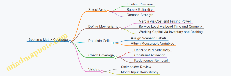
Example: 2×2×2 Scenario Matrix
| Inflation Pressure | Supply Reliability | Demand Strength | Scenario Label | What Changes First |
|---|---|---|---|---|
| Moderate | Stable | Strong | S1 | Pricing and volume drive revenue |
| Moderate | Stable | Weak | S2 | Inventory and discounting pressure |
| Moderate | Disrupted | Strong | S3 | Service level limits revenue |
| Moderate | Disrupted | Weak | S4 | Backlog churn and cash strain |
| Severe | Stable | Strong | S5 | Cost escalation tests margin |
| Severe | Stable | Weak | S6 | Margin + inventory risk |
| Severe | Disrupted | Strong | S7 | Service + margin both under stress |
| Severe | Disrupted | Weak | S8 | Worst-case constraint stacking |
Step 4: Ensure Coverage by Checking Constraint Activation
A scenario is “covered” when it triggers different constraint behavior in your model. Typical constraint activation checks:
- Capacity constraint: does production or sourcing capacity bind?
- Inventory constraint: does safety stock policy cause excess or stockouts?
- Service constraint: does lead time push service level below target?
- Cash constraint: does working capital exceed limits?
If two matrix cells never activate any new constraints and produce similar KPI patterns, you can merge them. If a cell activates a unique constraint, keep it even if it feels extreme.
Step 5: Add Within-Scenario Variations Without Exploding the Matrix
Once the matrix covers the main combinations, you can represent uncertainty inside each scenario using controlled variation. For example, within “S7 Severe + Disrupted + Strong,” you might vary:
- disruption duration (short vs. long)
- supplier yield (normal vs. reduced)
- demand timing (early vs. delayed orders)
This keeps the scenario set manageable while still reflecting realistic uncertainty.
Step 6: Validate Coverage with a Decision Walkthrough
Pick one decision (e.g., allocation between two regions) and walk through how each scenario changes the recommended action. If the recommendation is identical across multiple scenarios, that is a signal either the decision is not sensitive to the chosen axes, or the model is missing a mechanism.
A practical checklist:
- For each scenario, list the top two KPI drivers.
- Confirm at least one scenario changes the sign or binding status of a key constraint.
- Confirm each scenario has a distinct narrative tied to measurable inputs.
When this holds, your matrix becomes a coverage tool, not a decorative grid. It helps you see which combinations matter for decisions, and it keeps your scenario set honest about why outcomes differ.
6.5 Document Assumptions and Trace Each Assumption to Model Inputs
Scenario planning fails quietly when assumptions are undocumented or loosely connected to model inputs. This section builds a practical habit: write assumptions so they can be checked, then trace each one to the exact parameter, formula, or dataset field it drives.
Start with an Assumption Ledger
Create an “assumption ledger” that treats every uncertain statement as a record with a purpose. For each assumption, capture: (1) the scenario variable it belongs to, (2) the modeling element it affects, (3) the numeric value or distribution, (4) the source of the value, and (5) the confidence level.
Example: “Inflation passes through to supplier costs.” If you model supplier unit cost as base_cost * (1 + inflation_rate), then the assumption is not just the inflation rate; it is the pass-through mechanism. The ledger should explicitly state whether pass-through is 100%, partial, or delayed.
Use a Consistent Assumption Taxonomy
A taxonomy prevents “miscellaneous” entries that nobody can interpret later. A simple set works well:
- Level assumptions: fixed values like safety stock days or initial lead time.
- Rate assumptions: growth or change like monthly inflation or demand volatility.
- Behavior assumptions: how decisions respond, like allocation rules or pricing elasticity.
- Constraint assumptions: hard limits like maximum supplier capacity or customs clearance time.
- Mechanism assumptions: the causal story, like how disruption affects yield or service level.
Example: “Dual sourcing reduces risk.” That is a mechanism assumption. It must map to how you split orders and how supplier availability changes.
Trace Assumptions to Model Inputs with a Mapping Table
For each ledger entry, create a trace record that answers: “Where does this assumption land in the model?” Use a mapping table with four columns: Assumption ID, Model Input Name, Input Type, Transformation Rule.
| Assumption ID | Model Input Name | Input Type | Transformation Rule |
|---|---|---|---|
| INF-PT-01 | supplier_cost_multiplier | parameter | 1 + pass_through * inflation_rate |
| DIS-LEAD-02 | lead_time_days | parameter | base_lead + disruption_additional_days |
| DEM-ELAS-03 | price_elasticity | parameter | demand_multiplier = (price/base_price) ^ elasticity |
This table is the backbone for audits and for debugging when results look odd.
Mind Map of Assumption Traceability
Use the mind map to ensure you cover the full chain from narrative to number to output.
Mind Map: Assumption Documentation and Traceability
Document Units, Time Phasing, and Conversions
Most “mystery errors” come from unit mismatches. Record units for every input and every intermediate conversion. Also specify time phasing: does an inflation shock apply immediately, ramp over three months, or only after contract renewal?
Example: If lead time is modeled in days but your disruption narrative is “two weeks,” the ledger should state the conversion rule: 14 days (or a distribution around it). If you phase it, specify the month buckets used by the model.
Add Validation Checks That Prove the Trace Works
Documentation should come with tests. Add checks that fail fast:
- Unit checks: lead time days vs hours, currency per unit vs per order.
- Boundary checks: service level between 0 and 1, elasticity within a plausible range.
- Consistency checks: if capacity is reduced, ensure inventory and backlog logic can still produce feasible flows.
- Cross-scenario checks: assumptions that should not change across scenarios (like a fixed tax rate) must remain constant.
Example: If a scenario assumes “supplier availability drops by 30%,” verify that the model’s effective capacity reduction matches that 30% and that it propagates into both fulfillment and backlog.
Trace from Assumptions to Outputs and Decisions
Tracing is not complete until you can answer: “Which KPIs and options are affected by this assumption?” Add an “output trace” field to the ledger or maintain a companion table.
Example: The assumption pass_through = 0.6 likely affects gross margin, pricing decisions, and order volumes via demand response. If your option evaluation ranks choices by cash impact, then pass_through should be linked to cash KPIs and the option set that uses pricing.
Keep the Documentation Usable, Not Just Complete
A good ledger supports quick review. Limit narrative length, but make the mechanism explicit. If two assumptions interact, record the interaction rule once, then reference it from both ledger entries.
Example: If inflation affects both supplier costs and your ability to raise prices (because of contract caps), document the contract cap as a separate constraint assumption and specify how it limits the pricing transformation rule.
Mini Case Walkthrough for One Assumption
Assumption: “Customs delays increase effective lead time by 10–20 days during disruption.”
- Ledger entry: DIS-CT-01, scenario variable disruption severity.
- Value: distribution Uniform(10, 20) days.
- Model input: lead_time_days.
- Transformation rule:
lead_time_days = base_lead_time + customs_delay_days. - Time phasing: apply to months where disruption is active.
- Validation: ensure lead_time_days remains nonnegative and that capacity planning uses the updated lead time.
- Output trace: affects service level, backlog, and inventory carrying cost.
When you can follow this chain in minutes, you’ve turned assumptions from “notes” into model-ready, reviewable inputs.
7. Translate Scenario Narratives into Model Inputs
7.1 Map Scenario Variables to Cost and Pricing Parameters
Scenario variables only become useful when they change something measurable in your model. This section shows a systematic path from scenario narratives to the exact cost and pricing parameters your decision model needs, with examples that stay grounded in typical operations.
Start with a Parameter Inventory
Before mapping, list every cost and pricing parameter the model can touch. Group them into three buckets:
- Pricing parameters: base price, price by segment, discounts, surcharges, contract terms (e.g., escalation), and channel-specific markups.
- Cost parameters: materials, labor, energy, logistics, duties, warehousing, scrap/yield loss, and overhead allocations.
- Operational parameters that indirectly affect cost: lead time, service level targets, inventory policy, production rate limits, and capacity utilization.
Example: If your scenario narrative says “inflation accelerates,” you should not jump straight to “higher costs.” Instead, decide whether inflation affects materials only, or also freight contracts, warehousing, and labor rates.
Translate Scenario Variables into Mechanisms
A scenario variable is a knob; a mechanism is how that knob moves your parameters. For each variable, write a short mechanism statement in plain language.
- Inflation shock variable → “Index-linked costs reprice monthly; non-indexed costs lag by one quarter; labor moves via wage bands.”
- Supply disruption variable → “Longer lead times increase expedite freight and safety stock; yield drops due to alternate inputs.”
- Demand uncertainty variable → “Lower availability reduces realized sales; higher discounts increase conversion but also compress margin.”
This mechanism statement becomes the mapping rule from scenario inputs to model parameters.
Use a Mapping Table with Explicit Equations
Create a mapping table that links each scenario variable to one or more parameters and specifies the equation or rule. Keep it deterministic at first; add distributions later.
Example mapping for inflation
-
Scenario variable: Materials inflation rate (e.g., 6% vs 12%)
-
Parameter: Unit material cost
-
Rule:
UnitMaterialCost_t = UnitMaterialCost_base * (1 + InflationRate) ^ t -
Scenario variable: Freight contract indexation
-
Parameter: Unit freight cost
-
Rule:
UnitFreightCost_t = UnitFreightCost_base * (1 + FreightIndexRate) ^ t -
Scenario variable: Wage band movement
-
Parameter: Hourly labor cost
-
Rule:
HourlyLaborCost_t = HourlyLaborCost_base * (1 + WageBandRate)
If a scenario variable affects only part of the cost stack, reflect that explicitly. Otherwise you’ll accidentally inflate everything and wonder why margins collapse in every scenario.
Mind Map: From Scenario Variables to Pricing and Cost Parameters
Map Pricing Parameters Using Contract Logic
Pricing often changes because contracts allow it, not because you feel like it. Map scenario variables to pricing through contract terms and customer behavior.
Example: pass-through clause
- Scenario variable: Materials inflation
- Contract term: “Customers pay base price plus 80% of verified material index changes.”
- Parameter mapping:
Price_t = BasePrice + 0.8 * (MaterialIndex_t - MaterialIndex_base)
Example: discount behavior under availability
- Scenario variable: Service level deterioration
- Customer rule: “Discounts apply only when fill rate exceeds 95%.”
- Parameter mapping:
- If fill rate < 95%, set discount rate to 0 for that segment in that period.
This prevents a common modeling error: applying discounts in scenarios where customers can’t actually buy, which would overstate volume and understate margin.
Handle Time Phasing and Lags
Most cost and pricing effects do not hit instantly. Add time phasing rules so scenario variables affect the correct periods.
- Indexing lag: non-indexed costs reprice after a delay.
- Contract renewal timing: price changes only at renewal months.
- Operational lag: yield degradation affects unit cost immediately, but capacity recovery takes time.
Example: If inflation spikes in Month 2, but contracts renew in Month 4, then pricing parameters change in Month 4 while costs may change in Month 2.
Validate Mappings with Unit Consistency Checks
After mapping, run quick sanity checks:
- Unit check: costs per unit remain costs per unit after applying inflation and yield.
- Sign check: higher disruption should not reduce lead time in the model.
- Magnitude check: a 10% inflation variable should not produce a 60% unit cost increase unless your mechanism includes compounding across multiple cost layers.
Example: If yield drops from 98% to 95%, effective unit cost rises by roughly 1 / 0.95 relative to the yield-adjusted denominator. If your model shows a much larger jump, you likely double-counted scrap.
Produce a Final Mapping Output for Model Inputs
End by outputting a clean list of scenario-specific parameter values (or parameter rules) for each planning period. Your model should be able to run without re-reading the scenario narrative.
A good mapping output includes:
- parameter name
- scenario variable source
- equation or rule
- time phasing
- any caps/floors (e.g., discount caps, pass-through limits)
When this is done, the scenario narrative becomes a source of parameter changes, not a separate story your model can’t execute.
7.2 Convert Disruption Descriptions Into Lead Time and Capacity Constraints
A disruption narrative becomes useful only after you translate it into two model-ready quantities: lead time and available capacity. Lead time controls when orders can be fulfilled; capacity controls how much can be fulfilled once the material or service is available. Treat them as separate levers, because a port closure can delay shipments without reducing the factory’s ability to produce, while a power outage can reduce production without changing shipping routes.
Start with a Mechanism, Not a Label
Use the disruption description to identify the mechanism that affects flow. For each mechanism, decide whether it changes:
- Transit time (shipping duration)
- Handling time (loading, customs, inspections)
- Processing time (manufacturing or service execution)
- Throughput limits (maximum units per day or per shift)
Example: “Supplier A cannot ship for two weeks” is a processing/availability mechanism. “Vessel delays at the port” is a transit/handling mechanism.
Convert Lead Time into Time-Phased Constraints
Lead time in a planning model is rarely a single number. Use a time-phased representation so the model can react as the disruption starts, persists, and recovers.
Step-by-step mapping
- Choose your planning buckets, such as weeks or days.
- For each disruption, define a lead time multiplier or lead time add-on per bucket.
- If the disruption is intermittent, represent it as a pattern rather than an average.
- Separate order-to-ship and ship-to-receive if your model distinguishes them.
Example: If normal ship-to-receive is 10 days, and customs inspection increases by 6 days during weeks 2–4, then weeks 2–4 use 16 days, while week 1 and week 5 revert to 10.
Convert Capacity into Available Production or Fulfillment
Capacity constraints should reflect what the network can actually do during each bucket.
Common capacity effects
- Reduced throughput due to labor shortages or equipment downtime
- Reduced yield due to quality holds or rework
- Reduced availability due to supplier stoppage
- Reduced routing capacity due to carrier limits or warehouse congestion
Represent capacity as either:
- A maximum units per bucket for each node or route, or
- A capacity factor applied to baseline capacity.
Example: A plant normally produces 8,000 units per week. During a disruption it runs at 60% capacity for three weeks, so capacity becomes 4,800 units per week for those buckets.
Handle Partial Recovery and Bottlenecking
Disruptions often recover unevenly. Model recovery as a bucket-by-bucket change in capacity and lead time.
Also check bottlenecks. If upstream capacity is reduced but downstream capacity is not, the downstream node will idle. If downstream capacity is reduced but upstream is not, inventory may pile up upstream.
Example: Supplier capacity drops to 50% but distribution centers remain at 100%. Your model should show lower shipments from the supplier, not artificially reduced distribution capacity.
Use a Mind Map to Keep the Mapping Consistent
Mind Map: Disruption to Lead Time and Capacity
Practical Example: One Narrative, Two Constraints
Disruption narrative: “During weeks 2–3, Supplier B’s machining line is down; during weeks 3–4, shipments from the region face port delays.”
Lead time mapping
- Weeks 2–3: ship-to-receive unchanged, because nothing ships.
- Weeks 3–4: ship-to-receive add-on of 5 days due to port delays.
Capacity mapping
- Weeks 2–3: supplier node capacity factor 0% (no output from that line).
- Weeks 4 onward: capacity returns to baseline.
This separation prevents a common modeling mistake: increasing lead time during a period when shipments are impossible anyway.
Validation Rules That Prevent Contradictions
Before running the model, apply three checks:
- No input, no output: if capacity is zero at a node, downstream shipments must also be zero regardless of lead time.
- Lead time changes must be mechanism-linked: transit delays should not change processing capacity.
- Time phasing must be aligned: the disruption start bucket for capacity should match the narrative’s downtime start.
A model that passes these checks is usually easier to explain, easier to audit, and less likely to produce “results” that are really just internal inconsistencies wearing a spreadsheet costume.
7.3 Convert Demand Narratives Into Segment Level Demand Distributions
Demand narratives describe what might happen, but decision models need numbers that behave consistently. This section turns narrative statements into segment-level demand distributions—probability-weighted demand values by customer segment, region, and time bucket.
Start with Segment Definitions That Match the Narrative
A demand narrative is only useful if it can be mapped to segments the model already understands. Begin by listing each segment’s decision-relevant attributes: customer type, buying channel, product family, and geography. Then attach narrative drivers to those attributes.
Example: A narrative says “inflation reduces discretionary purchases in Europe while essential categories hold up.” Your segments might be:
- Europe, essential category, direct channel
- Europe, discretionary category, distributor channel
- Rest of world, essential category, distributor channel
If the narrative mentions “distributor behavior,” it must land on segments that include distributor-led ordering, not on direct-only segments.
Choose a Distribution Shape That Reflects Real Ordering Behavior
Segment demand is rarely normal. Order quantities are often skewed because of stock availability, promotions, and lead-time effects. A practical approach is to use one of three distribution families per segment:
- Lognormal for positive quantities with right skew (most common for unit demand)
- Triangular when you have a low, likely, and high value but limited evidence
- Discrete scenario-weighted values when the narrative is categorical (e.g., “tight availability” vs “normal availability”)
Example: For discretionary Europe distributor segments, you might use a triangular distribution with low = 70% of baseline, likely = 85%, high = 100% of baseline, because distributors can reduce orders quickly but may still place near-normal orders when inventory is available.
Convert Narrative Mechanisms into Quantitative Drivers
Narratives usually describe mechanisms, not distributions. Translate each mechanism into a driver that the model can apply.
Common mechanisms and driver translations:
- Price pressure → demand elasticity or price-to-demand multiplier
- Availability constraints → demand-to-fulfilled conversion using service level or fill rate
- Consumer substitution → cross-segment reallocation ratios
- Channel shifts → mix changes across direct vs distributor segments
Example: “Consumers trade down to smaller pack sizes.” If your model tracks product families, represent this as a mix shift: total category demand stays similar, but units move from premium family to value family using a reallocation ratio.
Build Segment-Level Distributions Using Baseline Scaling
A reliable workflow is baseline scaling plus driver adjustments.
- Establish a baseline demand level per segment and time bucket (units or revenue).
- Apply narrative multipliers derived from drivers.
- Apply availability effects if the narrative implies constrained supply.
- Ensure the resulting distribution respects segment constraints (e.g., minimum order quantities, capacity-driven caps).
Example: Baseline for Europe discretionary distributor in month 2 is 10,000 units. Narrative drivers imply a price multiplier of 0.85 and a substitution multiplier of 0.95. Availability is “tight,” so fulfilled demand is capped by expected fill rate. The distribution is built on demand before fulfillment (10,000 × 0.85 × 0.95) and then transformed into fulfilled demand using the service model output.
Use a Time Phasing Rule So the Distribution Doesn’t Jump
Narratives often describe gradual effects. Represent that by phasing multipliers across time buckets rather than applying the full effect instantly.
Example: If inflation impact “emerges over two months,” define multipliers as:
- Month 1: 0.95 of the full inflation effect
- Month 2: 1.00 of the full inflation effect
- Month 3: maintain or revert based on the narrative mechanism
This prevents unrealistic month-to-month discontinuities that can distort inventory and cash outcomes.
Mind Map: The Conversion Workflow
Validate the Distribution with Three Consistency Checks
- Total consistency: Sum segment distributions to ensure they match narrative-level expectations (e.g., “Europe discretionary down overall”).
- Variability realism: Confirm the spread is plausible. If the narrative says “mostly stable,” a wide distribution is a mismatch.
- Model interaction consistency: If supply constraints are modeled elsewhere, ensure demand-to-fulfilled transformation doesn’t double-count constraints.
Example: If your supply model already caps fulfilled units via capacity and lead times, do not also impose a tight demand cap at the distribution stage. Instead, let demand represent customer intent and let fulfillment reflect constraints.
Example: Turning a Short Narrative into a Distribution Set
Narrative: “In North America, essential demand stays steady, while discretionary demand drops when availability is tight. Distributor orders react faster than direct orders.”
Segment outputs:
- North America essential, direct: lognormal around 100% baseline with low variance
- North America essential, distributor: lognormal around 100% baseline with slightly higher variance
- North America discretionary, direct: triangular 85%–95% baseline, likely 90%
- North America discretionary, distributor: discrete two-state demand
- Normal availability: 95% baseline
- Tight availability: 75% baseline
Then apply time phasing: distributor reaction occurs in the next time bucket; direct reaction lags by one bucket.
The result is a set of segment-level demand distributions that are traceable to narrative mechanisms, consistent across time, and compatible with the rest of the decision model.
7.4 Specify Time Phasing for Each Scenario Variable Across Planning Periods
Time phasing turns a scenario narrative into a usable model. Without it, you end up with the right assumptions but the wrong timing—like ordering inventory for a disruption that already passed. The goal is to define, for every scenario variable, when it starts, how long it lasts, and how it ramps or decays across the planning periods.
Start with a Planning Calendar and Period Logic
Define the planning periods first: for example, weekly for the next 8 weeks and monthly thereafter. Then decide what each period represents in the model. If lead times are measured in days, convert them into period offsets. A practical rule: align all timing to the same “decision cycle” boundary (e.g., orders placed at the start of each week).
Example: If you place purchase orders on Mondays and shipments arrive after a 14-day lead time, then a disruption that begins on a Wednesday affects the next two order cycles differently than a disruption that begins on Monday.
Break Each Scenario Variable into a Time Profile
For each variable (inflation rate, supplier capacity reduction, port congestion, demand shift), create a time profile with three components:
- Onset: the first period where the variable differs from baseline.
- Magnitude: the level in each affected period.
- Duration and Shape: how it changes over time (step, ramp, plateau, decay).
Keep the shapes simple at first. A step change is often enough to capture decision impact; ramps matter when timing drives cash or service.
Example: Supplier capacity drops by 30% starting in Week 3, stays through Week 6, then recovers linearly to baseline by Week 8.
Map Time Profiles to Model Mechanics
Time phasing must connect to how the model uses variables.
- Pricing and cost: apply time-phased unit costs and escalation factors to the periods when units are produced, shipped, or invoiced (choose one and be consistent).
- Supply constraints: apply capacity reductions to production or inbound shipment windows.
- Demand: apply demand changes to order intake periods, not to production periods.
- Inventory and service: ensure that service-level calculations use the same period boundaries as demand and supply.
Example: If demand spikes in Month 2 but production constraints begin in Month 3, the model should show backlog growth in Month 2, then fulfillment catch-up later.
Use a Baseline and Define Deviations
Represent scenario variables as deviations from baseline. This reduces confusion when multiple scenarios share common elements.
Example: Baseline inflation is 3% annualized. In the “High Inflation” scenario, you might apply +2% annualized in Months 1–3, then +1% in Months 4–6, then return to baseline. In the model, unit costs become baseline cost multiplied by a time-phased inflation index.
Enforce Consistency Across Coupled Variables
Some variables must move together because they describe the same mechanism.
- Disruption that increases lead time should also reduce effective throughput in the same periods.
- Demand that increases order volume should also increase backlog sensitivity if service levels constrain fulfillment.
- Inflation that raises freight costs should align with the periods when freight is incurred.
If you allow independent timing, you can accidentally create impossible states (e.g., freight costs rising after shipments have already cleared).
Create a Time-Phased Variable Template
Use a repeatable template so each scenario variable is specified the same way.
Mind Map: Time Phasing Template
Example: Three Variables in One Scenario
Assume monthly periods for Months 1–6.
Scenario: Inflation Shock + Port Disruption + Demand Uncertainty
- Inflation index: +4% annualized in Months 1–2, +2% in Months 3–4, 0% in Months 5–6.
- Port disruption: lead time increases by 10 days starting Month 2, capacity throughput reduced by 20% in Months 2–3, then returns to baseline in Month 4.
- Demand: base demand plus a segment-specific uplift that peaks in Month 3, then normalizes by Month 5.
In the model, you apply inflation to unit costs in the periods when production is booked (or when invoices are issued—pick one). You apply port capacity reduction to inbound supply availability in Months 2–3. You apply demand uplift to order intake in Months 1–6.
Add Practical Validation Checks
Before running the scenario, verify timing with three quick checks:
- First-impact check: confirm the earliest period where outputs change matches the earliest onset among variables.
- Last-impact check: confirm the model returns to baseline behavior after the last duration period.
- Causality check: ensure that service shortfalls occur only after supply constraints and demand changes overlap in time.
Document Time Phasing in a Way People Can Audit
For each scenario variable, store: onset period, duration, shape, and the exact mapping to model timing (production, shipment, invoicing, or order intake). This prevents “it looked right” debates later, and it makes scenario comparisons meaningful.
Example documentation line (plain language): “Port disruption increases effective lead time starting Month 2; inbound capacity is reduced by 20% in Months 2–3; no capacity reduction in Months 4–6.”
7.5 Run Input Consistency Checks to Prevent Contradictory Assumptions
A scenario model fails quietly when inputs contradict each other. The goal of consistency checks is not to “make everything true,” but to ensure every assumption can coexist with the model’s mechanics. Think of it as a set of guardrails: if two inputs cannot both be correct under the same scenario, the model should flag the conflict before you trust the outputs.
Start with an Input Inventory and Ownership
Create a simple inventory of every input that can vary by scenario: prices, costs, lead times, yields, service levels, demand distributions, exchange rates, and policy rules (like safety stock and allocation priorities). For each input, record:
- Source (system, spreadsheet, contract, expert estimate)
- Scenario scope (global, region-specific, product-specific)
- Time phasing (which months/weeks it applies to)
- Owner (who can approve changes)
Example: If “freight cost per unit” is scenario-specific, but “landed cost” is also scenario-specific, you must decide whether freight is included twice. The inventory makes that decision explicit.
Define Consistency Rules by Model Mechanism
Consistency checks should mirror how the model calculates outcomes. Use mechanism-based rules so you catch contradictions where they matter.
Core rule categories:
- Accounting identity rules: ensure cost components sum correctly and are not double-counted.
- Capacity and feasibility rules: ensure supply, capacity, and lead times can produce the planned shipments.
- Policy logic rules: ensure inventory and allocation policies respond to the same service assumptions.
- Demand and fulfillment rules: ensure demand distributions align with order timing and backlog behavior.
- Unit and currency rules: ensure conversions happen once, with consistent units.
Use a Three-Pass Checking Workflow
Pass 1: Static checks (before running the model)
- Units: verify every input has a unit label and conversion path.
- Bounds: prices and costs must be non-negative; service levels must be between 0 and 1.
- Completeness: every scenario variable has a value for every product-region-time combination it claims to cover.
Pass 2: Cross-input checks (still before running)
- Double counting: if landed cost already includes freight, freight should not be added again.
- Coupling: if disruption increases lead time, the model should also reflect reduced effective capacity or higher backlog risk, depending on your mechanism.
Pass 3: Dynamic checks (after running, but with targeted diagnostics)
- Conservation: inventory cannot go negative unless backorders are explicitly modeled.
- Feasibility: if shipments exceed available supply given lead times, the model should report the violated constraint.
- Sensitivity sanity: small input changes should not cause discontinuous output jumps unless the model has intentional thresholds.
Mind Map of Consistency Checks
Mind Map: Input Consistency Checks
Concrete Examples of Contradictions and Fixes
Example A: Freight Double Counting
- Assumption: “Freight per unit” increases under disruption.
- Contradiction: “Landed cost” is also increased by the same disruption factor.
- Check: Compare landed cost decomposition to cost components.
- Fix: Choose one representation. Either compute landed cost from base cost + freight + duties, or treat landed cost as the single scenario-driven input.
Example B: Lead Time Increase Without Capacity Impact
- Assumption: Disruption raises lead time from 4 to 8 weeks.
- Contradiction: Supplier capacity remains unchanged and the model still ships the same volume in the next month.
- Check: Run a feasibility diagnostic for the first impacted period.
- Fix: If the model mechanism ties lead time to effective supply availability, reduce near-term available supply or increase backlog. If not, document why (for instance, you reroute inventory from another node).
Example C: Service Level vs Backlog Logic Mismatch
- Assumption: Service level target is 95% and backlog is allowed.
- Contradiction: The policy logic forces all demand to be filled immediately, making backlog impossible.
- Check: Verify the fulfillment rule that translates service level into acceptance or allocation behavior.
- Fix: Align the service level interpretation with the backlog mechanism, such as defining whether service level limits backlog growth or limits lost sales.
Record Results as “Verified,” “Blocked,” or “Needs Review”
Consistency checks should produce an auditable outcome per rule. Use three statuses:
- Verified: rule passes for all scenario-product-time combinations.
- Blocked: rule fails and the scenario cannot be trusted.
- Needs Review: rule passes but is close to a boundary (for example, inventory hits zero frequently).
Example: If a scenario repeatedly violates feasibility in the first two periods, you may still want it for comparison, but you should label it as “blocked” until the mechanism is corrected or the scenario narrative is adjusted.
Keep the Check Set Small Enough to Use Every Time
A long checklist gets ignored. Keep the rules focused on contradictions that change decisions: cost composition, feasibility under lead times, and fulfillment logic. When you add a new input, add one or two targeted consistency rules that protect the mechanism it influences. That way, the model stays coherent without turning every run into a full audit.
8. Evaluate Strategic Options Under Each Scenario
8.1 Define Option Catalogs Including Pricing, Sourcing, and Inventory Actions
An option catalog is a structured list of strategic moves you can actually execute, each tied to the decisions your model can evaluate. The goal is not to brainstorm everything; it’s to define a manageable set of options that cover the main levers: pricing, sourcing, and inventory. A good catalog makes scenario results usable in meetings, because people can see what would change and why.
Start with Decision Levers and Action Types
Create three buckets and keep them consistent across scenarios.
- Pricing actions: price changes, discount rules, contract terms, and allocation-based pricing (for example, “priority customers get a fixed discount; others get a volume-based discount”).
- Sourcing actions: switch suppliers, change lanes, use dual sourcing, adjust minimum order quantities, and re-route shipments.
- Inventory actions: safety stock policy changes, expedite orders, reorder point adjustments, and allocation of limited inventory.
A practical rule: each option should change at least one model input (price, lead time, cost, capacity, service level, or cash tied up in inventory).
Define Option Templates with Clear Parameters
Write each option as a template with parameters you can vary by scenario. This prevents “one-off” options that don’t map cleanly to model inputs.
Pricing template
- Price level or discount schedule by customer segment
- Contract escalation or pass-through rule for inflation
- Allocation rule when supply is constrained
Sourcing template
- Supplier selection by component or finished good
- Lane selection and expected lead time distribution
- Supplier capacity limits and qualification constraints
- Transportation mode and customs handling assumptions
Inventory template
- Safety stock multiplier
- Reorder point and order quantity logic
- Expediting policy (when and at what cost)
- Allocation priority rules
Mind Map: Option Catalog Structure
Add Feasibility and Transition Costs So Options Don’t Cheat
Options should include constraints and transition costs, even if they are simple. Otherwise, the model may select an option that looks profitable but is impossible.
- Feasibility constraints: supplier qualification status, contract notice periods, minimum order quantities, and maximum expedite capacity.
- Transition costs: one-time reconfiguration costs, tooling or documentation updates, and administrative costs for changing pricing terms.
Example: If you propose “switch 100% of a component to Supplier B,” you also need a constraint like “Supplier B can ramp to 60% in month 1 and 90% by month 3.” That ramp can be represented as capacity limits in the sourcing template.
Keep Options Small Enough to Compare
A catalog with 150 options becomes a spreadsheet hobby. Aim for 10–25 options per major decision area, then combine them into bundles only when the interactions matter.
A useful approach is to define atomic options (single-lever moves) and bundles (multi-lever moves). Bundles should be few and intentional.
Example Options That Map Cleanly to Model Inputs
Pricing option example
- Option P2: Segment price adjustment with inflation pass-through
- Inputs changed: segment price, pass-through rate
- Rule: if scenario inflation exceeds 6%, apply 70% of the excess to list price for 60 days
- Constraint: contract terms allow changes only for two segments
Sourcing option example
- Option S1: Dual source with lane rerouting under disruption
- Inputs changed: supplier choice, lead time distribution, logistics cost
- Rule: keep Supplier A for 40% capacity; route remaining demand via Supplier C with a longer lead time and higher customs friction
- Constraint: Supplier C has a maximum monthly capacity and requires a minimum order quantity
Inventory option example
- Option I3: Safety stock increase with limited expediting
- Inputs changed: safety stock multiplier, reorder point, expedite cost and capacity
- Rule: raise safety stock by 25% and allow expediting only for orders above a service-critical threshold
- Constraint: expedite capacity cap per week
Bundle Options into Decision-Ready Packages
When you bundle, specify the interaction explicitly.
Example bundle: Bundle B4: Protect service for priority customers
- Pricing: allocate priority customers first and reduce discounts for non-priority segments
- Sourcing: dual source with a slower lane for non-priority demand
- Inventory: increase safety stock but expedite only for priority orders
This bundle changes multiple model inputs in a coordinated way, so scenario comparisons reflect real tradeoffs rather than random combinations.
Mind Map: Option Parameters and Outputs
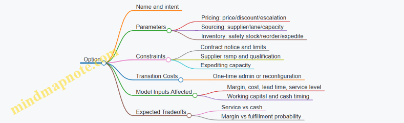
Quick Catalog Quality Checklist
Before you run scenarios, verify each option:
- Changes at least one model input.
- Includes feasibility constraints.
- Has transition costs or a clear statement that it is “no-cost within horizon.”
- Uses parameters that can be set per scenario.
- Can be explained in one minute to a finance and operations audience.
Once the catalog passes this checklist, scenario evaluation becomes straightforward: the model can compute outcomes, and decision-makers can choose among options without guessing what the model assumed.
8.2 Model Tradeoffs Between Service Level and Working Capital
Service level and working capital are linked by a simple mechanism: higher service targets usually require more inventory and faster replenishment, which ties up cash. Lower service targets can free cash but increase stockouts, backorders, and sometimes lost sales. A good model treats this as a measurable tradeoff, not a slogan.
Core Concepts That Connect the Two
Service level is the probability you can satisfy demand without delay during a lead time window. Common proxies include fill rate (percent of demand shipped immediately) and service level (percent of demand met without stockout). Working capital is cash tied in inventory and receivables minus payables; in this section, inventory is the main lever.
A practical modeling stance is to separate two costs:
- Inventory carrying cost: cost of capital plus storage, handling, shrink, and obsolescence. Even if you estimate these crudely, keep them explicit.
- Service failure cost: costs from stockouts such as expedited freight, production disruption, customer penalties, and lost contribution margin.
When you model both, the “best” option becomes the one with the best net outcome under each scenario.
A Modeling Pattern That Keeps the Tradeoff Honest
- Choose a service metric that matches how your business feels pain. If customers tolerate backorders but not delays, fill rate may matter more than “no stockout.”
- Represent inventory policy with parameters you can change: safety stock, reorder point, order quantity, and review period.
- Translate service into inventory using the lead time and demand variability you already modeled for inflation and disruption.
- Translate inventory into working capital using average inventory and carrying cost.
- Translate stockouts into service failure costs using backorder rules and penalty/expedite assumptions.
A tiny example: Suppose a product has average weekly demand of 1,000 units with lead time variability. If you increase safety stock by 200 units, you might raise fill rate from 95% to 97%, but you also increase average inventory and carrying cost. The model should compute both sides.
Mind Map: Service Level Versus Working Capital
Example: One SKU, Two Policies, One Clear Decision
Assume one SKU with:
- Unit contribution margin: $10
- Unit cost: $60
- Carrying cost rate: 20% per year
- Planning horizon: 1 year
- Average demand: 1,000 units per week (52,000 units/year)
- Lead time and variability are already embedded in your simulation or analytical service model.
Policy A targets fill rate 95%.
- Expected shipped quantity: 95% × 52,000 = 49,400 units
- Expected stockout/backorder quantity: 2,600 units
- Average inventory (from your policy math): 8,000 units
- Carrying cost: 8,000 × $60 × 0.20 = $96,000
- Service failure cost: assume backorders incur $2 per unit in penalties/extra handling = 2,600 × $2 = $5,200
- Contribution profit: 49,400 × $10 = $494,000
- Net (simplified): $494,000 − $96,000 − $5,200 = $392,800
Policy B targets fill rate 97%.
- Shipped quantity: 97% × 52,000 = 50,440 units
- Stockout quantity: 1,560 units
- Average inventory: 10,000 units
- Carrying cost: 10,000 × $60 × 0.20 = $120,000
- Service failure cost: 1,560 × $2 = $3,120
- Contribution profit: 50,440 × $10 = $504,400
- Net (simplified): $504,400 − $120,000 − $3,120 = $381,280
Even though Policy B ships more, it ties up extra cash in inventory and loses money in this simplified setup. The model’s job is to show that outcome without hand-waving.
Advanced Details That Prevent Common Modeling Mistakes
1) Use average inventory, not end-of-period inventory. Working capital is driven by time in inventory. If you only track ending inventory, you’ll systematically bias toward policies that look good at the snapshot.
2) Separate pipeline inventory from safety stock. Pipeline inventory changes with lead time and ordering cadence; safety stock changes with variability. Mixing them makes it hard to interpret why a policy wins.
3) Model backorder behavior explicitly. If backorders convert into lost sales after a cutoff, service failure cost becomes nonlinear. A linear “penalty per unit” can still work, but only if your business truly behaves linearly.
4) Keep cash constraints as constraints, not just another cost. If you have a hard cash limit, treat it as a feasibility rule: discard policies that exceed it even if they look profitable.
How to Compare Options Across Scenarios
For each scenario (inflation shock, disruption, demand uncertainty), compute:
- Expected net profit (or contribution) after carrying and failure costs
- Expected average inventory and peak cash impact
- Service metric outcomes (fill rate, backorder rate)
Then compare options using a decision rule such as:
- Best expected net subject to a minimum service threshold and a cash ceiling, or
- Best robust option that avoids large downside when lead times stretch.
This keeps the tradeoff consistent: service targets are not “free,” and cash is not “just a number.”
8.3 Compare Options Using Scenario Outcomes and Decision Criteria
Comparing options is where scenario planning stops being a story and starts being a decision. The key is to use the same decision criteria across all scenarios, so you can tell whether an option is good because it truly fits the business logic or just because it happens to match one narrative.
Step 1: Lock the Decision Criteria and Make Them Measurable
Start with a short list of criteria that reflect what “better” means for the business. Typical criteria for volatile markets include:
- Expected service level (fill rate, on-time delivery, or backlog tolerance)
- Working capital impact (inventory turns, cash tied up in stock)
- Profitability under cost shocks (gross margin after inflation and logistics)
- Operational feasibility (ability to execute within lead times and capacity)
- Risk of severe outcomes (worst-case drawdown beyond a threshold)
Example: A manufacturer chooses between two sourcing strategies. Criteria might be: maintain at least 95% fill rate, keep inventory cash within a limit, and avoid margin falling below a floor in any scenario.
Step 2: Define How Each Criterion Is Scored
Criteria need a scoring rule so comparisons are consistent.
- Threshold criteria: pass/fail (e.g., fill rate ≥ 95%).
- Ordinal criteria: rank options (e.g., best, acceptable, unacceptable).
- Numeric criteria: compute values (e.g., projected cash at risk).
Example: If Option A meets the fill-rate threshold in all scenarios but Option B fails in one, Option A automatically wins on that criterion even if B has slightly higher average margin.
Step 3: Build a Scenario Outcome Table That Shows Tradeoffs
Create a matrix where rows are options and columns are scenarios. Each cell contains the outcome values needed for scoring.
| Option | Inflation Shock | Supply Disruption | Demand Weakness | Service Level | Margin | Cash Impact | Worst-Case Breach |
|---|---|---|---|---|---|---|---|
| A: Dual sourcing | High costs | Moderate delays | Lower volumes | 96% | 18% | -$12M | No |
| B: Single sourcing | Higher costs | Severe delays | Lower volumes | 88% | 20% | -$9M | Yes |
In this example, Option B looks better on average margin, but it triggers a worst-case breach due to service failure. That’s the kind of insight you only get when you compare across scenarios, not when you average them away.
Step 4: Apply Decision Rules That Match the Business’s Risk Appetite
Use one or more decision rules, depending on how the organization makes tradeoffs.
Common rules:
- Satisficing: choose options that meet all thresholds, then pick the best on the remaining criteria.
- Lexicographic: prioritize criteria in order (e.g., service level first, then cash).
- Expected value with guardrails: maximize expected profit but reject options that violate critical limits.
- Minimax: minimize the worst-case loss when survival matters.
Example: If service level is non-negotiable, use satisficing. If cash shortfalls are unacceptable beyond a limit, use expected value with guardrails.
Step 5: Use a Mind Map to Keep the Logic Straight
A mind map helps teams avoid the classic mistake: mixing criteria types (thresholds, rankings, and averages) without a clear rule.
Mind Map: Comparing Options Across Scenarios
Step 6: Walk Through One Concrete Comparison
Assume three scenarios:
- Inflation shock with partial cost pass-through
- Supply disruption with longer lead times
- Demand weakness with slower sell-through
Option A (dual sourcing) and Option B (single sourcing) produce these outcomes:
- Service level: A = 96% across all scenarios; B = 88% in the disruption scenario.
- Margin: A averages 18%; B averages 20%.
- Cash impact: A = -$12M; B = -$9M.
- Worst-case breach: A = none; B = margin breach due to expedited logistics and stockouts.
Decision rule: service level is a threshold at 95%.
- Option B fails the threshold, so it is rejected.
- Between remaining options (only A in this simplified example), select A because it satisfies both service and worst-case constraints, even though it has slightly lower average margin.
This is the point: the comparison is not about finding the “best” number. It’s about finding the option that survives the criteria logic when the world behaves differently.
Step 7: Document the Rationale in a Way That Survives Scrutiny
For each selected option, record:
- Which criteria it met in each scenario
- Which tradeoffs it accepted (e.g., lower cash efficiency for higher service)
- Which assumptions drove the result (e.g., lead time ranges, escalation clauses)
A short rationale prevents later debates from turning into re-litigating the entire model. It also makes it easier to update the comparison when inputs change, without changing the decision rules.
8.4 Incorporate Operational Feasibility Including Lead Times and Transition Costs
Operational feasibility answers a simple question: “Can we actually do the option we modeled?” Scenario planning often produces attractive financial outcomes that fail when lead times, capacity constraints, and transition costs collide. This section shows how to bake feasibility into the decision model so results reflect reality, not wishful spreadsheets.
Feasibility as a Constraint, Not a Footnote
Start by treating feasibility as a set of model constraints and time-dependent effects.
- Lead times determine when inventory, production, or shipments become available.
- Capacity and routing limits determine whether the option can be executed at the required volume.
- Transition costs capture the one-time and recurring expenses to change the operating state.
- Transition lags capture the delay before the option reaches full effectiveness.
A practical rule: if an option changes sourcing, production, pricing policy, or allocation logic, it should also change at least one feasibility element.
Lead Times as Time-Phased Availability
Represent lead time explicitly rather than as a single “average delay.” Use a time-phased availability approach.
- Define the lead time components: order processing, production, inspection/quality, transport, customs, and receiving.
- Map each component to scenario variables: disruption increases transport time; inflation may increase supplier production time if energy costs rise.
- Convert lead time into a delivery schedule: each planned order placed in period t arrives in period t + L.
Example: A manufacturer modeled a switch from Supplier A to Supplier B to reduce unit cost under an inflation shock. Feasibility modeling reveals Supplier B has a 6-week production lead time and 2-week receiving/inspection time, while Supplier A averages 2 weeks total. Even if Supplier B is cheaper, the switch creates a service gap in weeks 1–8 unless the model also changes inventory policy or allocation.
Capacity and Routing Limits That Actually Bite
Feasibility constraints should be enforced where decisions are made.
- Production capacity: maximum units per period by plant and line.
- Labor or shift constraints: overtime limits, staffing ramp-up limits.
- Logistics capacity: lane capacity, container availability, warehouse throughput.
- Routing rules: if a lane is disrupted, rerouting may be possible but slower and more expensive.
Example: Under supply chain disruption, the model allows rerouting to an alternate port. Feasibility adds a lane capacity cap and a longer transit time. The option remains feasible but only for part of the volume; the rest must be allocated to other customers or deferred.
Transition Costs and Transition Lags
Transition costs are not just “implementation expenses.” They include operational friction that shows up in cash and margins.
Common transition cost categories:
- Qualification and validation: supplier onboarding, material testing, regulatory documentation.
- Tooling and setup: line changeovers, new packaging formats, calibration.
- Contract and commercial changes: penalties, minimum order commitments, expediting fees.
- Inventory repositioning: write-down risk, safety stock adjustments, stranded stock.
Transition lags specify when the option becomes effective.
Example: Switching packaging suppliers under uncertain demand. The model includes a qualification cost of $120k and a 3-month ramp where only 40% of required volume can be produced initially. Without the ramp, the option looks profitable because it assumes full supply immediately.
Mind Map: Operational Feasibility Inputs and Model Mechanics
A Systematic Modeling Workflow
Use a repeatable workflow so feasibility is consistent across scenarios.
- List each option’s operational changes: sourcing, production, logistics, allocation, pricing execution.
- For each change, identify feasibility elements: lead time, capacity, routing, transition cost, transition lag.
- Parameterize with scenario logic: specify what changes under inflation and disruption.
- Implement time phasing: ensure costs and availability land in the correct periods.
- Run feasibility checks: confirm the model does not “deliver” quantities before they could exist.
- Report feasibility-aware results: show service shortfalls and cash impacts alongside margin.
Feasibility-Aware Decision Example
Suppose the option is “allocate limited supply to high-margin customers and switch part of demand to a new supplier.” Feasibility modeling does three things:
- It delays new-supplier deliveries using time-phased lead times.
- It limits total shipped volume using capacity and lane constraints.
- It subtracts transition costs in the periods when qualification and setup occur, while ramping effectiveness over time.
The outcome may still be better than the baseline, but the model will reveal when the benefit arrives and what it costs to get there. That timing is often the difference between a plan that survives the first month and one that collapses quietly in month two.
8.5 Use Example Decision Walkthroughs for Pricing and Supply Allocation
Pricing and supply allocation are tightly coupled decisions: price affects demand and order timing, while supply constraints affect service levels and the ability to fulfill those orders. The walkthroughs below show how to use the scenario-based decision model without skipping the “boring” parts that usually break in real life.
Mind Map: Pricing and Supply Allocation Decision Flow
Example: Pricing Walkthrough Under Inflation and Disruption
Setup. A manufacturer sells two product segments: A (price sensitive) and B (less price sensitive). The model uses a planning horizon of 12 weeks. Costs include materials and logistics, both affected by inflation. Disruption increases lead time and reduces effective yield at one key supplier.
Scenario variables.
- Inflation: low, medium, high (drives unit cost)
- Disruption: mild vs severe (drives lead time, yield, and service level)
- Demand: stable vs volatile (drives demand distribution)
Option catalog. Create three pricing options, each with explicit rules:
- Static price: keep base price fixed; no escalation.
- Cost-indexed price: adjust price weekly using a cost index; cap changes at ±3% per week.
- Availability-aware price: same as cost-indexed, but apply a smaller increase when predicted fill rate drops below 92% to reduce order spikes that the supply system cannot satisfy.
Model mapping.
- Inflation scenario updates unit cost drivers.
- Disruption scenario updates lead time and yield, which changes inventory availability.
- Pricing option feeds demand response: segment A demand shifts more with price; both segments shift with availability (modeled via service-level effect).
Run and interpret. Suppose in the “high inflation + severe disruption + volatile demand” scenario:
- Static price yields higher volume early, but service level falls and backlog grows; margin erodes because costs rise faster than price.
- Cost-indexed price improves margin, but the weekly cap still leaves a gap; service level remains constrained, so lost sales appear when customers switch away.
- Availability-aware price slightly reduces price increases during low fill-rate weeks, which smooths demand and improves fill rate; margin improves because fewer orders are lost and fewer expedited shipments are needed.
The key modeling discipline: the option is not “a number,” it is a rule that changes demand and fulfillment outcomes through the model’s causal links.
Example: Supply Allocation Walkthrough with Customer Priorities
Setup. The firm can ship 1,000 units per week from the constrained node. Customer segments are:
- Tier 1: strategic accounts with contractual service targets
- Tier 2: standard accounts
- Tier 3: spot orders
Allocation policy options.
- Proportional allocation: distribute available units by forecasted share.
- Service-first allocation: satisfy Tier 1 up to contract targets, then allocate remaining to Tier 2.
- Margin-aware allocation: allocate to maximize expected contribution margin, using predicted willingness-to-pay and penalty costs for late fulfillment.
Mind the mechanics. Allocation must specify what happens when demand exceeds supply:
- Is backlog allowed or are orders rejected?
- Are partial fills allowed?
- Can substitution occur (e.g., alternate SKU) and at what yield penalty?
Run and interpret. In the “medium inflation + severe disruption + stable demand” scenario:
- Proportional allocation keeps everyone somewhat happy, but Tier 1 misses targets, triggering penalties and damaging future order timing in the model.
- Service-first allocation meets Tier 1 targets, reducing penalties and stabilizing future demand behavior; Tier 2 experiences more backlog, but the model’s backlog dynamics show fewer cancellations than expected.
- Margin-aware allocation shifts units toward Tier 1 and Tier 2 orders with higher expected contribution, but it can increase backlog for Tier 2 in a way that later reduces repeat orders. The model captures this because demand timing depends on service experience.
Decision Criteria and Governance Checks
After running all scenario combinations, select options using criteria that match decision intent:
- Primary: expected contribution margin under constraints.
- Constraint checks: minimum fill rate for Tier 1 and maximum cash tied in inventory.
- Robustness: prefer options with smaller performance swings across scenarios.
A practical governance rule: if an option violates a hard constraint in any scenario where leadership has declared “must not fail” conditions, it is excluded even if its average looks good. That keeps the model from becoming a fancy way to justify wishful thinking.
9. Assess Robustness and Sensitivity Without Overfitting
9.1 Conduct Sensitivity Analysis on Key Drivers and Thresholds
Sensitivity analysis answers a simple question: if one assumption moves, how much does the decision outcome move? In scenario planning, it prevents a common failure mode—choosing an option that only works because a few inputs were quietly “just right.” The goal is not to find the single true future; it’s to identify which drivers and thresholds actually control the decision.
Step 1: Pick the Right Inputs to Test
Start with inputs that (a) are uncertain, (b) are decision-relevant, and (c) can plausibly move within your scenario ranges. Typical candidates include unit costs under inflation, supplier lead times under disruption, service-level targets, and demand elasticity under price or availability changes.
A practical way to choose: rank drivers by their modeled impact on the objective (for example, contribution margin, service level, or cash-to-cash cycle time) and then keep the top 5–10. If you test everything, you’ll learn nothing except that your spreadsheet is tired.
Step 2: Define Thresholds, Not Just Ranges
Many decisions hinge on thresholds—points where behavior changes. Examples:
- Inventory policy threshold: when safety stock drops below a minimum, service level falls sharply.
- Allocation threshold: when available supply falls below committed demand, the model switches from full-fill to partial-fill.
- Pricing threshold: when price increases beyond a customer-acceptance band, demand elasticity changes.
For each threshold, define two bands: a “safe” region and a “crossing” region. Then test values just below, at, and just above the threshold.
Step 3: Choose a Sensitivity Method That Matches the Model
Use one of these methods depending on model complexity:
- One-at-a-time (OAT): vary one driver while holding others fixed. Good for quick diagnosis.
- Local sensitivity: vary a driver in small steps around the scenario’s baseline. Good for identifying steep regions.
- Scenario-aware sensitivity: run the same driver perturbations across multiple scenarios. Good for checking whether the driver matters only in one narrative.
If your model includes nonlinearities (piecewise costs, service-level caps, allocation rules), local sensitivity is usually more informative than wide OAT swings.
Step 4: Run Perturbations Consistently
For each selected driver, apply a structured perturbation plan:
- Linear drivers: test ±5%, ±10%, and the scenario min/max.
- Rate drivers (lead time, defect rate): test absolute changes (for example, +2 days, +5 days) because percentage changes can mislead.
- Threshold drivers: test three points (below, at, above) plus one extra point if the curve looks steep.
Keep the perturbations consistent across options so differences reflect the decision, not the testing style.
Step 5: Measure Sensitivity in Decision Terms
Report results using decision-relevant metrics, not just raw output changes. For example:
- Margin impact: change in contribution margin per unit and total.
- Service impact: change in fill rate and backorder days.
- Cash impact: change in working capital and financing needs.
A useful summary is a “sensitivity score” per driver: the maximum absolute change in the primary objective across tested values, normalized by the baseline. This makes it easier to compare drivers with different units.
Mind Map: Sensitivity Analysis Workflow
Example: Pricing Threshold Under Inflation
Suppose you model demand as a function of price and availability, and you have a pricing acceptance threshold where demand drops faster after a certain price premium. You test three price points: 4% below the threshold, at the threshold, and 4% above.
If the option’s margin is stable below the threshold but collapses above it, you’ve learned the decision is fragile to that threshold. The next move is to check whether the same fragility appears in other scenarios (for example, when supply is constrained). If it only fails in constrained supply scenarios, you can focus mitigation on the intersection of high price and low availability.
Example: Lead Time Threshold and Service Level Collapse
Consider a supply disruption where lead time increases. Your inventory policy might hold safety stock until a reorder point, after which service level drops quickly. You test lead time at baseline, baseline +2 days, and baseline +5 days.
If the fill rate barely changes at +2 days but drops sharply at +5 days, the threshold is real and operational. That result supports targeted actions like adjusting safety stock or changing allocation rules, rather than making broad changes that don’t address the actual tipping point.
Step 6: Interpret Results Without Overreacting
Sensitivity results should answer three questions:
- Which drivers dominate the objective?
- Which thresholds cause discontinuous behavior?
- Does the preferred option stay preferred across tested perturbations?
If option rankings flip with small changes, treat the decision as fragile and revisit the option set or constraints. If rankings stay stable, you can be confident the decision doesn’t depend on a single lucky assumption.
Step 7: Document Assumptions and Testing Logic
Record: driver definitions, perturbation values, method choice, and the exact metrics used. This makes later reviews faster and prevents “we tested it somehow” from becoming a tradition.
9.2 Perform Scenario Impact Analysis to Identify Dominant Uncertainties
Scenario impact analysis answers a practical question: which uncertainties actually move the decision outcome the most, given the way your model translates inputs into cash, service, and constraints? The goal is not to rank everything in sight; it is to find the few uncertainties that deserve attention in monitoring, option design, and data collection.
Start with a Clear Outcome Lens
Pick one primary outcome metric and one secondary metric. For example, primary could be expected profit or net present value; secondary could be service level or ending inventory. Then define what “dominant” means in your context. A common, easy rule is: an uncertainty is dominant if changing it within its allowed range shifts the primary metric by more than a chosen threshold (say, 5% of the metric’s baseline magnitude) in at least one scenario.
Example: A consumer goods manufacturer models inflation-driven cost changes and supply disruption. The primary metric is contribution margin; the secondary metric is fill rate. If inflation assumptions move margin by 12% while disruption assumptions move fill rate by 3% but margin by only 2%, inflation is dominant for the profit decision, while disruption is dominant for the service decision.
Map Uncertainties to Model Pathways
Dominance depends on pathways, not just volatility. Start by listing uncertainties as model inputs: inflation rate, supplier lead time, yield loss, demand elasticity, payment terms, and so on. Next, trace each input to the outputs through the model logic.
A simple pathway sketch helps. For instance:
- Inflation → unit material cost → pricing decision → demand response → order volume → production schedule → margin.
- Lead time increase → available supply → fill rate → lost sales/backlog → revenue → margin.
If an uncertainty affects an output only through a weak link, it may be non-dominant even if it looks scary in isolation.
Use Scenario-Level Contribution Before Fine-Grained Sensitivity
Begin with scenario impact analysis at the scenario set level. For each scenario, compute the outcome metric and compare it to a baseline scenario. Then ask: which uncertainty differences between scenarios explain the gap?
A practical method is “scenario decomposition by variable changes.” Create a table where each scenario is represented by a vector of uncertainty settings. Then compute the outcome difference from baseline and attribute it to the variables that differ. When multiple variables change together, attribution is approximate, but it still highlights which variables frequently appear in the biggest outcome gaps.
Example: You have four scenarios:
- S1: moderate inflation, normal lead time, stable demand.
- S2: high inflation, normal lead time, stable demand.
- S3: moderate inflation, long lead time, stable demand.
- S4: high inflation, long lead time, demand down. If the largest margin drop occurs in S4 and S2, inflation is likely dominant for margin. If fill rate collapses mainly in S3 and S4, lead time is dominant for service.
Apply Targeted Sensitivity to Confirm Dominance
Scenario-level findings can be misleading when variables interact. Confirm dominance with targeted sensitivity on the top candidates.
Use one-at-a-time sensitivity first, but only for the shortlisted uncertainties. Hold other inputs at the scenario’s settings, then vary one uncertainty across its allowed range. Record the change in the primary metric.
Example: In the high-inflation scenario, vary supplier lead time by ±20% while keeping inflation fixed. If margin barely changes but fill rate does, lead time is not dominant for the profit decision. Then vary inflation by ±2 percentage points and observe margin movement.
To handle interactions without exploding effort, run a small grid for the top two or three dominant candidates. For instance, test inflation at three levels and lead time at three levels within the same scenario structure. The interaction pattern tells you whether dominance is additive (each factor independently matters) or coupled (one factor amplifies the other).
Mind Map: Dominant Uncertainty Identification
Scenario Impact Analysis Mind Map
Mind Map: What to Record for Each Uncertainty
Evidence Capture Mind Map
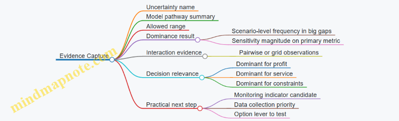
A Worked Example with Clear Logic
Assume three uncertainties: inflation (I), lead time (L), and demand elasticity (E). You run a scenario set and compute primary metric changes versus baseline:
- S2 (high I): margin -10%
- S3 (long L): margin -2%
- S4 (high I + long L + lower demand via E): margin -14% Scenario-level evidence suggests inflation dominates margin because it appears in the largest drops.
Next, targeted sensitivity within the high-inflation scenario:
- Vary L by ±20%: margin changes from -10% to -11% (about 1% swing).
- Vary I by ±2 points: margin changes from -10% to -16% (about 6% swing). This confirms inflation dominance for margin.
Finally, interaction check with a 3×3 grid for I and L:
- When I is high, L increases fill rate losses but margin remains mostly driven by cost.
- When I is moderate, L still causes service issues, but margin impact stays small. You conclude: inflation is dominant for profit; lead time is dominant for service. That split is useful because it prevents one monitoring plan from trying to solve two different problems.
Close the Loop with Decision Criteria
Dominant uncertainties should connect back to decisions. If an uncertainty is dominant for the primary metric, it should influence which options you prioritize and which triggers you set. If it is dominant only for a secondary metric, treat it as a constraint or a service lever rather than a profit driver. The analysis is complete when each dominant uncertainty has a clear pathway explanation and a specific decision implication.
9.3 Use Robustness Metrics for Option Selection Across Scenarios
Use Robustness Metrics for Option Selection Across Scenarios
Robustness metrics answer a practical question: “If the world looks different than expected, which option still performs well enough?” In scenario planning, you already have multiple plausible futures; robustness metrics help you compare options without pretending you know which future will happen.
Start with What “Robust” Means
A good robustness metric has three properties. First, it rewards performance, not just survival. Second, it penalizes unacceptable outcomes, such as service failures or cash shortfalls. Third, it behaves consistently when scenarios change slightly, so you don’t chase noise.
A simple mental model: each option produces a performance score per scenario. Robustness is about how that score behaves across the set.
Define Option Outcomes and Score Direction
Before metrics, standardize the score direction. For example, higher is better for margin, but lower is better for stockouts. Convert everything into a common “higher is better” score, or keep separate metrics but compare them with clear rules.
Example: Suppose you track two KPIs per scenario for a sourcing option: gross margin and service level. You can compute a composite score:
- Margin score: (margin − target) / target, capped at a reasonable range.
- Service score: service level as a fraction of required minimum. Then combine them with weights that reflect decision priorities.
Use Three Core Robustness Metrics
-
Worst-Case Performance
- Metric: minimum composite score across scenarios.
- Why it helps: it blocks options that look good on average but fail badly.
- Example: Option A averages high margin but has one scenario with severe service drops. Its minimum score flags the risk.
-
Lower-Quantile Performance
- Metric: 10th or 20th percentile of composite score.
- Why it helps: it reduces sensitivity to a single outlier scenario while still focusing on bad outcomes.
- Example: If Option B has two weak scenarios but no catastrophic one, its 20th percentile may outperform Option A.
-
Regret Relative to Best in Each Scenario
- Metric: for each scenario, regret = (best score in that scenario − option score). Then summarize regret using mean or upper-quantile.
- Why it helps: it measures how much you lose when you don’t pick the scenario-specific best.
- Example: If Option C is never the best, but it stays close to the best across all scenarios, it can win on regret even if its average is not top.
Add a Feasibility Gate Before Ranking
Robustness metrics should not rank options that violate hard constraints. Use a feasibility gate first:
- If service level falls below the minimum in any scenario, mark the option as infeasible.
- If cash constraints break beyond an allowed buffer, mark it as infeasible.
Example: A pricing option might increase margin in many scenarios but causes inventory liquidation in one scenario that breaches a cash covenant. The gate prevents it from winning on robustness metrics.
Mind Map: Robustness Metrics and How They Connect
A Worked Example with Clear Ranking Rules
Assume three scenarios: Inflation High, Disruption Severe, Demand Weak. You compute a composite score (higher is better) for three options:
- Option A: [0.70, 0.20, 0.60]
- Option B: [0.55, 0.45, 0.50]
- Option C: [0.60, 0.35, 0.10]
Feasibility gate: all three pass hard constraints.
Compute metrics:
- Worst-case (min): A = 0.20, B = 0.45, C = 0.10 → B leads.
- 20th percentile (approx): A is near 0.20, B near 0.45, C near 0.10 → B leads.
- Regret: for each scenario, compare to best score.
- Scenario 1 best = 0.70 (A), regrets: A 0, B 0.15, C 0.10
- Scenario 2 best = 0.45 (B), regrets: A 0.25, B 0, C 0.10
- Scenario 3 best = 0.60 (A), regrets: A 0, B 0.10, C 0.50
- Average regret: A ≈ 0.083, B ≈ 0.083, C ≈ 0.233 → A and B tie, C loses.
Decision logic: choose the primary robustness metric as worst-case or lower-quantile. That yields Option B. If you use regret as a tie-breaker, B remains competitive because it avoids large regret in the worst scenario.
Interpretation and Sensitivity Without Overfitting
Robustness metrics can still mislead if the scenario set is too small or unbalanced. A quick integrity check is to confirm that the ranking doesn’t flip when you slightly adjust scenario weights or when you remove a scenario that is clearly redundant.
Finally, keep the decision rule explicit: “We select the option with the best lower-quantile score among feasible options; if tied, we use regret.” That single sentence prevents the team from quietly changing the goalposts mid-discussion.
9.4 Apply Stress Testing to Validate Model Behavior at Extremes
Stress testing checks whether your decision model behaves sensibly when inputs hit the edges of what you consider plausible. It is not about finding the “worst possible” world; it is about verifying that the model’s logic, constraints, and unit economics do not break when conditions are extreme.
Stress Testing Foundations
Start with three questions. First, what does “extreme” mean for each uncertainty driver? For inflation, it might be a high indexation rate plus delayed pass-through. For disruption, it might be a lead-time jump that exceeds your normal safety stock coverage. For demand, it might be a sharp drop in order rate combined with higher cancellation or lower conversion.
Second, what should remain true under extremes? Examples: inventory cannot go negative; service level cannot exceed what supply can physically deliver; cash constraints must still bind; and pricing rules must still apply even when volumes collapse.
Third, what failure modes are you guarding against? Common ones include sign errors (costs becoming revenues), constraint bypass (capacity limits ignored), and discontinuities (a tiny input change causing a huge output jump).
Define Extreme Scenarios with Guardrails
Pick a small set of stress cases that target model mechanics rather than just outcomes. A practical set is:
- Single-driver extremes: one uncertainty at an extreme while others stay at baseline.
- Coupled extremes: two drivers at extremes that are known to interact (e.g., high inflation plus delayed pass-through).
- Constraint-saturation extremes: inputs pushed until a key constraint becomes binding (e.g., capacity or cash).
Use guardrails to keep extremes interpretable. For instance, if you stress lead time, keep the disruption mechanism consistent: the model should reflect fewer usable shipments, not magically increase yield.
Stress Test Execution Steps
- Lock the model structure: run a baseline to confirm outputs match expectations and that no parameters are accidentally changed.
- Select stress inputs: choose values at the edge of your allowed ranges, not outside them.
- Run option sets: evaluate the same strategic options you would under normal scenarios, such as pricing changes, sourcing shifts, and inventory policy adjustments.
- Check invariants: verify non-negativity, conservation of flow, and correct application of constraints.
- Inspect sensitivity around the edge: move the extreme input slightly inward and confirm outputs change smoothly.
What to Validate at Extremes
Stress testing is only useful if you validate specific behaviors. Use a checklist tied to your model components.
- Cost and margin logic: Under high inflation, costs should rise according to your indexing rules. If you model pass-through, revenue should respond only through the pricing mechanism you defined.
- Supply and service logic: Under long lead times, service level should fall unless you increase inventory or reallocate supply. If service stays constant, your model likely has an unrealistic buffering assumption.
- Demand and order logic: Under low demand, backlog should shrink or cancellations should rise depending on your demand-to-orders mapping. If backlog grows while demand drops, the mapping is inconsistent.
- Cash and working capital: Under extreme volumes or costs, cash constraints should bind and restrict actions. If the model continues to recommend actions that require more cash than available, the cash constraint is not enforced.
Mind Map: Stress Testing Coverage
Example: Stress Testing a Pricing and Allocation Model
Assume a model that recommends between two sourcing options: A (lower cost, longer lead time) and B (higher cost, shorter lead time). You stress inflation to a high index rate and also delay pass-through by one period.
- Stress case: inflation index at the upper bound; pass-through delay active; demand held at baseline.
- Expected behavior: margins should compress in the delayed period, then partially recover once pricing catches up. If the model shows margins improving immediately, pass-through is being applied too early.
- Constraint check: if cash is limited, the model may need to reduce expensive sourcing B. If it still allocates mostly to B despite cash constraints, the cash constraint is not connected to the allocation decision.
- Smoothness check: reduce inflation slightly (still high) and confirm the margin changes gradually. If margin jumps sharply, there may be a discontinuity in how pricing or allocation thresholds are coded.
Example: Stress Testing Supply Disruption with Inventory Policy
Now stress lead time so it exceeds the maximum reorder cycle. Keep demand constant.
- Expected behavior: service level should drop unless safety stock is sufficiently high. Backlog should increase if demand cannot be met.
- Invariant check: inventory should not go negative; shipments should be limited by usable lead time.
- Mechanism consistency: if the model “recovers” service level without any change in inventory or sourcing, it likely treats lead time as a cosmetic label rather than a binding constraint.
Interpreting Results Without Overreacting
When a stress test fails, classify the issue. If outputs violate invariants, fix model logic first. If outputs are invariant but unstable near the edge, review threshold rules and rounding. If outputs are stable but counterintuitive, confirm that the stress inputs match the mechanisms you encoded.
A good stress test produces evidence: which constraints bind, which invariants hold, and where behavior becomes inconsistent. That evidence is what makes the model trustworthy when the world gets messy—without pretending you can predict the mess perfectly.
9.5 Interpret Results With Clear Decision Rules and Evidence Standards
Scenario results are only useful if they tell you what to do. Interpretation turns model outputs into decisions by pairing (1) decision rules that specify when an option is acceptable and (2) evidence standards that specify what you trust and what you must verify.
Decision Rules That Prevent “Best Guess” Choices
Start by writing decision rules in plain language, then translate them into measurable criteria.
-
Define the decision threshold for each objective. If service level is critical, set a minimum acceptable value (for example, “no scenario may drop below 95% on-time delivery”). If cash is constrained, set a maximum drawdown (for example, “ending cash must stay above $10M”).
-
Use a hierarchy of objectives. Many teams try to optimize everything at once and end up with no clear winner. A hierarchy avoids that. Example: first filter options that violate hard constraints, then choose among the remaining options using the primary objective (for example, maximize contribution margin) and only then consider secondary objectives (for example, minimize working capital).
-
Specify tie-breakers that are stable across scenarios. If two options perform similarly, pick the one with lower sensitivity to the most uncertain drivers. Example tie-breaker: “prefer the option with the smaller worst-case margin loss when disruption lead time increases by 20%.”
-
Require coverage of decision-relevant scenarios. Not every scenario deserves equal weight. If your decision is about a specific region, ensure the rule references scenarios that include that region’s demand and supply conditions.
Evidence Standards That Make Results Defensible
Evidence standards answer a simple question: “What must be true for this result to count?”
-
Model validity checks. Confirm that outputs behave consistently with the model logic. Example: if the scenario increases lead time, the model should not simultaneously show higher service without any compensating inventory or capacity changes.
-
Input plausibility checks. Evidence includes whether scenario inputs are internally consistent. Example: if a scenario assumes higher demand but also assumes lower available inventory due to disruption, the model should reflect both effects rather than smoothing them away.
-
Uncertainty handling transparency. If you use distributions, state what they represent (for example, demand variability around a mean) and what they do not (for example, not capturing every possible supplier failure mode).
-
Data traceability. For each key driver, record where it came from and how it was transformed. Example: inflation assumptions should trace to the cost components they affect (materials, energy, logistics) and the timing of those costs.
-
Decision evidence completeness. A rule should specify what evidence is required: scenario outcomes only, or also sensitivity results, feasibility checks, and constraint violations.
Mind Map: Interpreting Scenario Outputs into Decisions
Example: Turning Outputs into a Concrete Choice
Assume you are choosing between Option A (expedite shipments, higher logistics cost) and Option B (standard shipping, lower logistics cost). Your hard constraints are: ending cash must be at least $10M and service must be at least 95%.
- In the Inflation + Mild Disruption scenario, Option A yields service 97% and ending cash $12M; Option B yields service 94% and ending cash $13M.
- In the Inflation + Severe Disruption scenario, Option A yields service 96% and ending cash $9M; Option B yields service 93% and ending cash $11M.
Interpretation using decision rules:
- Apply hard constraints first. Option B fails service in both scenarios. Option A fails cash in the severe disruption scenario.
- Because no option satisfies all hard constraints across all decision-relevant scenarios, the decision rule triggers an escalation: either relax a constraint with explicit tradeoff approval or revise the option set (for example, add a third option that combines partial expediting with inventory pre-positioning).
Evidence standards applied:
- Validate that service changes align with lead time and inventory policy changes.
- Check that cash differences align with logistics cost timing and working capital effects, not just revenue shifts.
Example: Evidence-Based Tie-Breaking
If two options both meet constraints in all scenarios, choose the one with better robustness. Example tie-breaker: Option A and Option C both keep service above 95% everywhere, but Option A’s worst-case margin drops by 8% while Option C’s drops by 5%. Evidence standard: confirm the margin difference is driven by identifiable cost components (for example, logistics and expediting) rather than a modeling artifact like an inconsistent demand allocation.
Practical Interpretation Checklist
- Are hard constraints explicitly stated and applied before ranking?
- Is the objective hierarchy clear and consistent with leadership priorities?
- Do tie-breakers reference the most uncertain drivers with measurable metrics?
- Do you have validity checks that confirm outputs match scenario mechanisms?
- Can each key driver be traced from scenario narrative to model input to output impact?
When these rules and standards are written down, interpretation becomes repeatable. The model stops being a report generator and becomes a decision tool that can survive scrutiny from finance, operations, and the people who will actually run the plan.
10. Build Early Warning Indicators and Triggered Responses
10.1 Define Indicator Sets Linked to Scenario Variables and Mechanisms
Indicator sets are the bridge between “what we assumed in the scenario” and “what we observe in the real world.” The goal is not to watch everything; it’s to watch the few things that move the model’s mechanisms.
Start with Mechanisms, Not Metrics
A scenario variable is a number you set in the model (for example, inflation rate, supplier lead time, or regional demand). A mechanism is the causal path that turns that variable into outcomes (for example, higher input prices flow into margin erosion; longer lead times force inventory policy changes; lower availability shifts demand to competitors).
For each scenario mechanism, define:
- Indicator: a measurable signal.
- Direction: whether the signal increasing makes the scenario more likely.
- Link: which model component it affects.
- Action: what decision you will revisit when the indicator crosses a threshold.
Easy example: If your disruption mechanism is “lead time increases reduce fill rate and trigger expediting,” then your indicator set should include a lead-time proxy (like carrier transit time or supplier confirmed ship dates) and a service proxy (like order fill rate or backorder aging). Watching only one of them often produces false comfort.
Build an Indicator Inventory by Scenario Dimension
Use a simple inventory table in your head, then formalize it in your planning notes.
Inflation and Cost Volatility
- Input price indices (direction: up increases scenario likelihood)
- Freight rate indices (direction: up increases landed cost)
- Contract pass-through status (direction: faster pass-through reduces margin damage)
- Working-capital strain (direction: up increases cash pressure)
Supply Chain Disruption
- Supplier on-time confirmation rate (direction: down increases likelihood)
- Actual-to-quoted lead time ratio (direction: up increases likelihood)
- Port or lane congestion metrics (direction: up increases likelihood)
- Quality yield or defect rates (direction: down increases rework and capacity loss)
Uncertain Global Demand
- Order intake by segment (direction: down increases likelihood of weak demand)
- Backlog conversion speed (direction: slower conversion can indicate demand softness)
- Channel availability signals (direction: stockouts can mask demand)
- Price realization vs list (direction: lower realization can indicate competitive pressure)
Define Indicator Granularity and Timing
Indicators must match the time phasing in the model. If your scenario assumes a step-change in costs in month 2, then a monthly indicator may be enough. If your model reacts weekly to service levels, then weekly indicators are required.
A practical rule: choose the coarsest frequency that still catches the mechanism before it forces irreversible decisions. For inventory and expediting, “monthly” is often too slow; for contract escalation clauses, “quarterly” may be fine.
Mind Map: Indicator Sets Linked to Variables and Mechanisms
Example: One Scenario Mechanism to a Complete Trigger Set
Scenario mechanism: Lead time increases reduce fill rate, causing backlog growth and forcing expediting.
Indicator set:
- Actual-to-quoted lead time ratio (weekly). If it rises above 1.3 for two consecutive weeks, treat the disruption as “active.”
- Supplier on-time confirmation rate (weekly). If it drops below 85%, expect continued lead-time pressure.
- Fill rate (weekly). If fill rate drops below the model’s service threshold (for example, 92%), backlog dynamics will likely diverge.
- Expedite spend rate (weekly). If expedite spend rises faster than the model’s assumed cost curve, you may be in a worse-than-modeled disruption.
Threshold logic should be consistent with the model’s structure. If your model assumes expediting is available but limited, then expedite spend is both an indicator and a constraint check.
Example: Avoiding a Common Indicator Trap
Trap: using inventory on hand as the primary disruption indicator.
Why it fails: inventory is an outcome of decisions, not a direct measure of the mechanism. A company can hold high inventory because it anticipated disruption, even if the disruption is not currently worsening. Better indicators are those that measure the mechanism inputs (lead time, confirmation rate, congestion) and the service outputs (fill rate, backlog aging).
Operationalize Ownership and Evidence
Each indicator needs an owner and a short evidence note describing what data source and calculation are used. This prevents “it looks high” debates during trigger meetings.
A clean indicator set is small, mechanism-linked, time-aligned, and decision-connected. When the signal changes, the team should know which scenario variable it corresponds to, which model component it affects, and which option set will be reconsidered.
10.2 Specify Trigger Thresholds and Decision Rights for Actioning
Trigger thresholds turn scenario monitoring into action. Decision rights ensure the right people can act quickly without a committee meeting every time a metric wiggles. Together, they prevent two common failure modes: “nothing happens until it’s too late” and “everything happens too often.”
Foundational Concepts for Thresholds and Rights
A trigger threshold is a rule that maps observed signals to an action category. The threshold must be measurable, time-bound, and tied to a specific operational lever. For example, “If landed cost rises” is too vague; “If spot freight index increases by 20% for 5 consecutive business days, activate expedited shipping option A” is actionable.
Decision rights define who can approve which action, under what conditions, and with what constraints. Rights should be tiered by impact and reversibility. Pricing changes and supplier switching are higher impact than adjusting safety stock within a pre-approved band.
Designing Trigger Thresholds That Don’t Lie
Start with a signal-to-mechanism mapping. Each signal should correspond to a mechanism in your model.
- Inflation shock: cost index → margin compression → pricing or sourcing response
- Supply chain disruption: lead time variance → service level risk → allocation or inventory policy response
- Demand uncertainty: order backlog or sell-through deviation → production or inventory rebalancing
Use three threshold types:
- Warning thresholds detect early drift. They should be easier to hit and trigger analysis, not irreversible moves.
- Action thresholds authorize operational changes. They should include a minimum duration to avoid reacting to one-off noise.
- Escalation thresholds require senior approval because they may affect customers, contracts, or cash.
A practical rule set looks like this:
- Warning: metric crosses level for 2 days
- Action: metric crosses level for 5 days
- Escalation: metric crosses level for 10 days or breaches a hard limit
Example: If lead time variance for a critical component exceeds 30% for 5 days, activate alternate routing and increase safety stock by the pre-approved increment. If it exceeds 45% for 10 days, escalate to procurement leadership for supplier qualification and contract renegotiation steps.
Decision Rights as a Simple Ladder
Create a decision ladder with clear authority boundaries. Assign rights to roles, not job titles that change every quarter.
- Level 1: Operations Manager approves reversible actions within bands (e.g., reorder points, allocation priorities).
- Level 2: Supply Chain Director approves moderate-impact actions (e.g., switching to secondary suppliers, changing production schedules).
- Level 3: Finance and Commercial Leads approve high-impact actions (e.g., price changes, contract terms, customer allocation exceptions).
Each action should list constraints that cannot be violated without escalation. Constraints include service commitments, minimum cash balance, regulatory limits, and contract clauses.
Mind Map: Triggers and Rights
Example: A Trigger-to-Action Playbook
Assume you monitor three signals weekly and daily for critical items.
Signal A: Landed Cost Index
- Warning: +10% vs baseline for 2 days → run margin impact report and check contract pass-through clauses.
- Action: +20% for 5 days → approve temporary surcharge within a pre-approved range.
- Escalation: +30% for 10 days → Finance and Commercial approve renegotiation or longer-term pricing reset.
Signal B: Lead Time Variance for Critical SKU
- Warning: variance > 25% for 2 days → review supplier reliability and confirm inventory coverage.
- Action: variance > 30% for 5 days → switch to alternate routing and adjust safety stock by +X units.
- Escalation: variance > 45% for 10 days → procurement leadership initiates supplier qualification steps.
Signal C: Demand Deviation
- Warning: sell-through down 8% for 2 days → pause incremental production increases.
- Action: down 12% for 5 days → reallocate inventory from low-turn regions to higher-turn channels.
- Escalation: down 18% for 10 days → Commercial approves customer-facing changes such as revised order caps.
Each action includes evidence requirements: the metric value, the time window, and the impacted SKUs or regions. That keeps decisions consistent and auditable.
Operationalizing Thresholds Without Creating Chaos
Define a single owner for the trigger log. Every time a threshold is crossed, record: timestamp, metric, scenario context, action taken, and who approved it. If multiple thresholds trigger simultaneously, prioritize by customer impact and cash impact, using a pre-defined ordering rule.
Finally, test the system with historical episodes. Use a known disruption period from around two months ago to validate that the thresholds would have triggered the intended actions, not just produced a lot of red dashboards.
10.3 Design Monitoring Dashboards with Data Refresh and Ownership
A monitoring dashboard is only useful if it answers two questions quickly: “What changed?” and “What should we do next?” The design starts with the decision triggers you defined earlier, then works backward to the data refresh schedule, ownership, and the exact visual signals that prompt action.
Start with Decision Triggers and Metrics
List each indicator you will monitor and link it to a specific decision right. For example, if your pricing playbook triggers when input costs jump, the dashboard must show the cost index, the rate of change, and the threshold status. Keep the metric set small enough that every number has a job.
A practical metric trio for inflation shocks looks like this:
- Level: current input cost index (e.g., “steel index = 128”).
- Velocity: week-over-week change (e.g., “+6.2%”).
- Trigger status: whether it crosses the decision threshold (e.g., “trigger ON”).
For supply chain disruption, pair service outcomes with operational causes:
- Service: fill rate, on-time-in-full, or backorder days.
- Cause: lead time variance, supplier reliability score, or customs clearance delays.
For uncertain demand, monitor both demand signals and operational symptoms:
- Demand: order intake by segment and region.
- Symptom: backlog growth and inventory stockout risk.
Choose a Dashboard Layout That Matches How People Work
Use a consistent layout so users don’t hunt for meaning.
- Top row: trigger cards for the decisions that matter today.
- Middle: trend charts for each indicator with threshold lines.
- Bottom: diagnostic breakdowns that explain why the indicator moved.
Example: If fill rate drops, the diagnostic section should immediately show whether it’s driven by lead time variance, allocation constraints, or demand spikes. Otherwise, the dashboard becomes a “report,” not a “monitor.”
Data Refresh Cadence That Fits Operational Reality
Refresh frequency should match the decision lead time. A simple rule: refresh at least as often as the fastest decision you might trigger.
Common cadences that work well:
- Hourly or daily: order intake, backlog, shipment status, inventory availability.
- Daily or weekly: supplier lead time statistics, cost indices, freight rates.
- Weekly or monthly: contract-level reconciliation, margin rollups, regional demand normalization.
If you refresh too slowly, triggers arrive late. If you refresh too often, teams drown in noise. Add a “last updated” timestamp on every indicator so people can trust the numbers.
Ownership and Accountability That Prevents Dashboard Drift
Assign ownership at two levels:
- Metric owner: accountable for correctness of the calculation and data lineage.
- Action owner: accountable for what happens when the trigger is ON.
A dashboard without action ownership turns into a passive scoreboard. Make ownership explicit in the UI by showing the responsible team or role next to each trigger card.
Mind Map: Monitoring Dashboards with Refresh and Ownership
Example Dashboard Specification for One Trigger
Consider a trigger for inflation-driven pricing changes.
Indicator card: “Input Cost Trigger”
- Metric owner: Procurement Analytics
- Action owner: Pricing Committee
- Refresh: daily
- Display:
- Current index value
- 7-day change percentage
- Threshold status badge
- Link to the driver breakdown (materials vs energy vs logistics)
Diagnostic panel:
- Materials index trend
- Energy index trend
- Freight rate trend
- Contract pass-through coverage (percentage of spend with escalation clauses)
This structure prevents the common failure mode where teams see the trigger but cannot tell whether it’s broad-based inflation or a narrow logistics spike.
Data Quality Checks That Keep Trust Intact
Add simple, visible safeguards:
- Missing data flag: show “data stale” when refresh fails.
- Outlier guardrails: highlight sudden jumps that exceed plausible bounds.
- Cross-source consistency: compare order intake totals from the order system and the planning system.
When quality issues appear, the dashboard should explain the limitation, not silently substitute numbers.
Operationalizing Refresh and Ownership in Practice
Set a recurring review meeting cadence, such as weekly for operational indicators and monthly for reconciliations. Use a change log for threshold edits and formula updates, and require metric owners to confirm that the dashboard still matches the decision logic. If the dashboard changes without governance, the triggers become less reliable than the market itself.
10.4 Create Playbooks for Triggered Actions Including Pricing and Allocation
Triggered playbooks turn monitoring signals into specific actions, with clear ownership and decision rules. The goal is not to guess faster; it is to act consistently when the model’s assumptions start breaking.
Start with Trigger Logic That Matches How Decisions Actually Happen
A playbook needs three layers: a trigger, a decision, and an action. A trigger is a measurable condition tied to a scenario mechanism, such as “supplier lead time exceeds the modeled 95th percentile” or “gross margin drops below the minimum acceptable band.” A decision is the choice you must make, like “adjust list price” or “reallocate limited inventory.” An action is the concrete step, such as “apply a 3% price increase to Segment A and pause promotional discounts.”
Example: If inflation shocks raise input costs, your monitoring might track “spot-to-contract cost ratio.” When it crosses 1.15 for two consecutive weeks, the playbook triggers a pricing decision. If it falls back below 1.10, the playbook triggers a reversal rule.
Define Pricing Actions as a Small Set of Reversible Levers
Pricing playbooks work best when they use a limited menu of levers, each with a clear scope and rollback. Common levers include:
- Price increases by segment or region
- Discount suspension or discount caps
- Surcharges for expedited shipping or higher input costs
- Contract terms changes, such as shorter payment terms or revised escalation handling
Example: During supply disruption, you may see service levels drop. A playbook can respond by suspending discounts for orders that would worsen backlog, while enabling a surcharge for customers willing to accept longer lead times. The rollback rule can be tied to “fill rate returns above 97% for 10 business days.”
Define Allocation Actions as Rules over Scarce Supply
Allocation playbooks should specify how to distribute constrained inventory across demand segments. Use rules that are explainable to sales, operations, and finance.
A practical allocation rule set often includes:
- Priority tiers (e.g., strategic accounts, contract-critical orders, standard orders)
- Allocation basis (e.g., forecasted demand, historical share, order date)
- Service policy (e.g., fill-or-partial, minimum order size)
- Backlog handling (e.g., cap backlog growth per tier)
Example: If inbound shipments arrive 30% below plan, allocate first to contract-critical orders to protect renewal risk, then allocate remaining units by “proportional to last 60 days demand” with a cap that prevents one region from consuming all available stock.
Build a Mind Map of the Playbook Components
Mind Map: Triggered Actions Playbooks
Use a Trigger-to-Action Table for Fast Execution
A playbook becomes usable when it is operationally specific. Keep it short, but include the fields teams need during a busy week.
| Trigger condition | Decision | Action | Evidence | Rollback rule |
|---|---|---|---|---|
| Lead time P95 exceeds plan by 20% | Allocation | Re-tier orders and cap backlog growth at 8% per tier | Carrier ETAs + ERP lead time report | Fill rate > 97% for 10 business days |
| Spot-to-contract ratio > 1.15 for 2 weeks | Pricing | Increase list price 3% for affected segments; suspend discounts | Cost dashboard + contract index | Ratio < 1.10 for 2 weeks |
| Demand intake > 120% of baseline | Allocation | Allocate by proportional share; prioritize contract-critical | Order intake vs baseline | Intake < 110% for 2 weeks |
Add Guardrails So Actions Don’t Create New Problems
Guardrails prevent “correct” actions from causing avoidable damage. Include constraints such as:
- Maximum price change per cycle to avoid channel churn
- Minimum discount floor for strategic accounts
- Allocation caps to prevent stockouts in critical regions
- Communication timing rules so customers receive consistent lead-time expectations
Example: If pricing increases are capped at 5% per month, the playbook can still respond to cost shocks by using surcharges for expedited shipping rather than pushing list prices too far.
Run a Short Tabletop Exercise with Real Numbers
A tabletop exercise tests whether the trigger thresholds, decision rights, and action parameters are coherent. Use a single week of historical data and simulate the trigger.
Example exercise steps:
- Pick a week where lead time worsened and margin tightened.
- Apply the trigger thresholds exactly as written.
- Execute the pricing and allocation actions using the table.
- Record what would have been communicated and who approved it.
If the exercise reveals ambiguity, revise the playbook until the action is unambiguous for a new operator. Consistency beats cleverness; the playbook should be boring in the best possible way.
10.5 Document Indicator Limitations and Avoid Misinterpretation
Indicators are only useful when people trust what they measure and understand what they do not. This section focuses on documenting limitations in a way that prevents common misreads, such as treating a lagging metric as a leading signal or assuming an indicator implies a single cause.
Start with What the Indicator Actually Measures
Begin each indicator entry with a plain-language definition: the numerator, denominator, data source, and refresh cadence. Then state the intended interpretation in one sentence. For example, “Service Level Indicator measures the percentage of orders shipped on or before the promised date, updated daily.” That sentence should be followed by what it cannot tell you: whether the delay was caused by inbound shortages, production constraints, or carrier issues.
A useful rule: if you cannot explain the metric to a new analyst in under a minute, the documentation is not ready.
Map Limitations to Specific Failure Modes
Document limitations as a set of failure modes linked to the indicator. This turns “limitations” from a vague warning into actionable guidance.
- Lag and smoothing: A daily average can hide sudden deterioration. If the indicator is smoothed, note the window.
- Coverage gaps: If data excludes certain regions, product lines, or channels, specify what is missing.
- Revisions and backfills: Some systems correct historical records. State whether the indicator can change after publication.
- Proxy behavior: If the indicator is a proxy (e.g., “freight cost index” standing in for “transport disruption”), list the conditions where the proxy breaks.
- Threshold brittleness: A fixed trigger may not behave consistently across seasons or promotions.
Mind Map: Indicator Limitations and Misinterpretation Traps
Add Evidence Rules So People Know When to Act
A trigger should not be a single number with a dramatic interpretation. Document evidence rules that specify what must be true before action is justified.
Example: “Freight Lead Time Triggered” might be defined as: (1) lead time exceeds the threshold for two consecutive days, (2) data quality flags show no missing lanes, and (3) the carrier exception log indicates congestion rather than billing delays. Without these rules, teams may act on a data glitch or on a non-operational issue.
Use Concrete Examples That Show Misinterpretation
Include short “do not assume” examples in the indicator record.
Example 1: Service Level Drop
- Indicator: On-time shipment rate falls from 96% to 90%.
- Common misinterpretation: “Demand increased, so we are behind.”
- Documented limitation: The indicator reflects fulfillment timing, not demand volume.
- Required corroboration: Check backlog growth and production completion status.
Example 2: Cost Index Spike
- Indicator: Input cost index rises 8% week over week.
- Common misinterpretation: “Margins will collapse immediately.”
- Documented limitation: Contracts may include pass-through clauses and inventory may buffer costs.
- Required corroboration: Review contract terms and inventory age profile.
Example 3: Order Intake Volatility
- Indicator: Order intake variance increases.
- Common misinterpretation: “Demand is unpredictable everywhere.”
- Documented limitation: Variance may be driven by one region’s channel reporting changes.
- Required corroboration: Compare by region and channel; confirm reporting stability.
Specify Data Quality Flags and Their Meaning
Indicators should carry data quality flags that are documented like safety labels. For instance: “Missing lane coverage: yes/no,” “Outlier filtering applied: yes/no,” and “Backfill pending: yes/no.”
Then define what each flag changes. A flag might downgrade the indicator from “trigger eligible” to “monitor only.” This prevents teams from treating a compromised metric as operational truth.
Keep Documentation Auditable and Consistent
Use a standard template for every indicator so limitations are comparable across the dashboard. Include:
- Definition and intended use
- Known limitations and failure modes
- Evidence rules for triggers
- Corroboration checks
- Owner and last review date
If a review date is needed, use a date like 2026-03-05. Consistency matters more than recency because it supports governance and reduces the chance that someone reads an outdated limitation as current behavior.
Close the Loop with Trigger Communication
Finally, document how the indicator limitation affects the trigger message. If the indicator is lagging, the trigger should be framed as “confirming” rather than “predicting.” If coverage is partial, the trigger should specify the scope. When people see the boundaries in the same place as the trigger, misinterpretation drops—usually faster than you’d expect, and with fewer meetings than you’d fear.
11. Implementation Planning for Scenario Based Decision Modeling
11.1 Establish a Planning Cadence and Integration With Budgeting
A scenario-based decision model only helps if it runs on a schedule that matches how decisions actually get made. The planning cadence should connect three rhythms: (1) scenario updates, (2) model runs and option evaluation, and (3) budgeting and approvals. When these rhythms drift, teams end up arguing about numbers that were produced for a different purpose.
Cadence Design Principles
Start with decision dates, not model dates. Budgeting typically has fixed milestones: target setting, draft budget, review cycles, and final approval. Work backward to define when inputs must be frozen for each milestone. A practical rule is to separate “learning” from “locking”: learning cycles can change assumptions, but budgeting cycles require stable inputs.
Next, define the minimum viable cadence. Many organizations can run a monthly monitoring cycle and a quarterly scenario refresh cycle. Monthly monitoring checks whether the world is still consistent with the scenario set; quarterly refresh updates scenario variables, constraints, and option catalogs.
Finally, assign ownership for each cadence step. If nobody owns the transition from monitoring to refresh, the process becomes a series of meetings with no decision outputs.
Integration with Budgeting Workflow
Budgeting integration means the model must produce artifacts that finance can use without translation. That usually includes: (a) a baseline plan, (b) scenario-adjusted plans, and (c) a mapping from scenario outcomes to budget line items.
A common approach is to treat the baseline as the “budget anchor” and scenarios as “budget stress overlays.” For example, inflation shocks may change material cost assumptions and working capital needs; supply chain disruption may change lead times and safety stock; uncertain demand may change volume and pricing mix. The budget then reflects the baseline, while scenario overlays quantify how much the baseline could miss.
Mind Map: Planning Cadence and Budget Integration
Example: A Simple Cadence That Fits Budget Season
Assume budgeting decisions happen at three points: target setting in early March, draft budget in mid-April, and final approval in late May. Use a learning cadence in January and February, then lock inputs before each milestone.
- Late January: monthly monitoring run. Output is a short “assumption health” report: which indicators moved, which scenario variables should be reconsidered, and whether the current scenario set still covers the decision space.
- Early February: quarterly refresh run. Update inflation drivers (e.g., energy index linkage), disruption constraints (e.g., supplier lead time ranges), and demand segment behavior (e.g., price sensitivity bands).
- Mid-March: lock baseline inputs for target setting. The model runs baseline and scenario overlays, but only baseline assumptions feed the budget target numbers.
- Early April: lock inputs again for draft budget. Scenario overlays are recalculated using the locked baseline, so finance can compare “what changed” without reinterpreting the baseline.
- Late May: approval package. Include a decision memo that states which options were recommended under which scenario outcomes and what assumptions were locked.
This structure prevents a common failure mode: updating scenario variables after finance has already built the budget, then asking finance to rebuild everything.
Practical Mechanics for Integration
To keep the cadence systematic, use three documents that travel with each cycle.
-
Assumption register: every scenario variable and model parameter with source, owner, and lock date. If a parameter changes, the register records what changed and why.
-
Run checklist: a short list that confirms data reconciliation, constraint consistency, and option catalog completeness before results are shared.
-
Variance explanation template: a standardized way to explain differences between baseline and scenario overlays, such as “cost increase came from energy-linked materials” or “service shortfall came from lead time expansion.”
Example: Locking Inputs Without Freezing Learning
Suppose monthly monitoring shows a supplier’s quoted lead time range has widened. During the learning window, you update the disruption constraint distribution and rerun the model. During the locking window for draft budget, you keep the baseline inputs fixed but still report the monitoring update as an overlay delta. That way, the budget remains stable while leadership still sees the operational reality.
Output Definition for Each Cadence Step
Each cadence step should end with a decision-ready output, not just a report. Monthly monitoring ends with a go/no-go on whether a scenario refresh is needed. Quarterly refresh ends with an updated scenario set and option catalog. Budget milestones end with baseline numbers plus scenario overlay impacts mapped to budget line items, along with the assumption register and lock dates.
When these outputs are consistent, stakeholders stop asking, “Which version of the model are we using?” and start asking, “Which assumptions matter most for the decision we’re making?”
11.2 Build Workflow for Scenario Updates and Model Version Control
A scenario-based decision model is only useful if people can reproduce results. That means updates must be controlled, changes must be explainable, and outputs must be traceable to inputs. The workflow below treats scenario updates and model version control as one system, not two separate chores.
Core Principles for Change Control
Start with three rules. First, every run must be tied to a specific model version and a specific scenario definition. Second, changes must be reviewed by someone who understands both the model logic and the business meaning of the assumptions. Third, the system must separate “what changed” from “why it changed,” so reviewers can focus on correctness rather than detective work.
A practical way to enforce this is to define three layers: model code, model data, and scenario parameters. Code changes affect equations, constraints, and logic. Data changes affect inputs like costs, lead times, and demand distributions. Scenario parameter changes affect only the scenario’s chosen values, such as an inflation rate range or a disruption duration.
Workflow Overview
Use a repeatable sequence: propose, validate, review, publish, and monitor. Each step has clear artifacts.
- Propose: A change request describes the intent, the affected layer (code, data, or scenario parameters), and the expected impact on key metrics.
- Validate: Automated checks confirm schema compatibility, unit consistency, and internal consistency of assumptions.
- Review: A reviewer checks logic correctness and business plausibility, then signs off.
- Publish: The new version is locked, tagged, and made available to scenario runners.
- Monitor: After publishing, you compare a small set of “golden scenarios” against prior outputs to catch unintended shifts.
Versioning Scheme That People Can Follow
Adopt a version format that encodes meaning. For example: MAJOR.MINOR.PATCH.
- MAJOR: changes to model logic that alter interpretation of outputs.
- MINOR: additions or refinements that preserve prior interpretation.
- PATCH: bug fixes or data corrections that should not change the model’s conceptual meaning.
Scenario definitions also need identifiers. Use a scenario ID that includes a stable name and a revision number, such as SCN-INFL-02-r3. This prevents the common failure mode where “the scenario” quietly morphs over time.
Artifacts and Traceability
Every published run should store: model version, scenario revision, input hashes (or checksums), run parameters, and output summaries. If you cannot answer “which exact inputs produced this table,” you do not have version control—you have vibes.
A lightweight checklist for traceability:
- Scenario narrative text matches the parameter set.
- Units are consistent across inputs (currency, time buckets, lead time units).
- Constraints are unchanged unless explicitly modified.
- Output metrics are computed from the same definitions across versions.
Mind Map: the Update and Control Loop
Example Workflow in Practice
Imagine a team updating disruption assumptions for a logistics bottleneck. The change request states: “Supplier lead time increases from 12–18 days to 18–26 days for Region A for the next two quarters.”
- Propose: The request targets scenario parameters only, not model code.
- Validate: Checks confirm the lead time distribution format is unchanged and time buckets align with the planning horizon.
- Review: A supply chain owner confirms the range matches operational reality and that service-level constraints still make sense.
- Publish: The scenario revision increments from
SCN-DSR-01-r2toSCN-DSR-01-r3, while the model version remains1.4.2. - Monitor: Golden scenarios run and show expected service-level and working-capital movement. If results shift in unrelated regions, the team investigates whether unintended data edits occurred.
Advanced Details That Prevent Quiet Failures
Two failure modes deserve special attention.
First, “mixed provenance” runs happen when scenario parameters are updated but data inputs are pulled from a newer dataset. Prevent this by snapshotting data at publish time and binding scenario runs to those snapshots.
Second, “definition drift” happens when metric formulas change without a version bump. Prevent this by versioning metric definitions alongside model logic, and by requiring reviewers to confirm that output labels and calculation logic match the prior contract.
Minimal Governance Without Bureaucracy
You do not need a committee for every change, but you do need role clarity. Assign one owner for model logic, one for data definitions, and one for scenario semantics. For small PATCH updates, a single reviewer may be enough; for MAJOR changes, require at least two reviewers—one technical and one business.
A final practical touch: include a short change log entry in plain language, dated with a stable reference point like “2026-03-05,” describing what changed and what did not. That single line often saves hours during review meetings.
11.3 Train Teams on Model Use, Assumption Handling, and Reporting
Training is what turns a scenario model from “a spreadsheet with opinions” into a shared decision tool. The goal is not to teach everyone to be a modeler; it’s to teach them how to use the model safely, interpret outputs consistently, and update assumptions without breaking the logic.
Training Objectives and Audience Fit
Start with three outcomes and tailor sessions by role.
- Decision owners learn how to select options, read scenario comparisons, and approve assumption changes.
- Model users learn how to run scenarios, interpret KPIs, and spot input errors.
- Data and operations contributors learn how to provide inputs, document sources, and flag data limitations.
A practical way to align expectations is a one-page “model contract” that states: what the model does, what it does not do, which inputs are editable, and which outputs are decision-grade.
Core Concepts Teams Must Share
Before hands-on work, ensure everyone agrees on five foundational ideas.
- Scenarios are input bundles, not predictions. Example: “High inflation + tight shipping” is a scenario package; it does not claim the future will match it.
- Assumptions drive causality. Example: if lead time increases, service level and backlog should change through the model’s logic, not through manual spreadsheet edits.
- KPIs have definitions. Example: “Fill rate” must specify whether it is order-line, unit-based, or time-window based.
- Constraints are binding when they matter. Example: if capacity is capped, the model should allocate or delay rather than silently “creating” supply.
- Traceability is part of correctness. Example: if a cost escalation assumption changes, the training should require updating the linked cost driver and noting the reason.
Mind Map: Training Scope and Flow
Hands-On Practice That Builds Muscle Memory
Use short exercises that mirror real work.
Exercise A: Run a scenario and verify outputs.
- Step 1: Select a scenario set.
- Step 2: Confirm the model version and planning horizon.
- Step 3: Check three sanity KPIs: total demand served, total cost, and ending inventory.
- Step 4: Compare against a baseline scenario.
Example: If a “tight shipping” scenario shows higher service level than baseline, the user should investigate whether lead time inputs were applied correctly or whether the scenario accidentally used baseline parameters.
Exercise B: Change one assumption and observe the causal chain.
- Change only one driver, such as material cost inflation rate.
- Require users to record: what changed, where it changed, and which outputs moved.
Example: Increasing unit material cost should raise total cost and may reduce margin, but it should not automatically change demand unless the model explicitly links price to demand.
Exercise C: Report results using a standard template.
- Include: scenario name, key assumptions, top three KPI impacts, and the decision implication.
- Require a “what would change our mind” section that lists which assumptions are most sensitive.
Example: If the best option depends on whether customers accept higher prices, the report should name the demand elasticity assumption rather than saying “demand might change.”
Assumption Handling Workflow
Train teams to treat assumptions like controlled inputs, not casual edits.
- Request: describe the assumption change in plain language.
- Evidence: attach the data source or rationale (even if it’s expert judgment).
- Impact check: run a minimal scenario set to confirm outputs respond as expected.
- Approval: decision owners approve changes that affect customer-facing or financial KPIs.
- Documentation: update the assumption log with date, owner, and reason.
Use a date such as 2026-03-01 for the assumption log example so teams see consistent formatting.
Reporting Standards That Prevent Misinterpretation
Reporting training should focus on clarity and consistency.
- Scenario naming rules: inflation level, disruption severity, and demand regime must appear in the name.
- KPI presentation: show units and time window.
- Comparison discipline: always state what the baseline is.
- Uncertainty communication: report ranges only when the model produces them; otherwise report point results with the assumption set.
Quality Gates and Review Sessions
End training with a review gate that catches common errors.
- Input completeness check: required fields filled.
- Consistency check: no contradictory assumptions (e.g., “no capacity constraints” with “capacity capped” in the same scenario).
- Output plausibility check: service level and inventory move in the expected direction.
A short peer review works well: each trainee explains one scenario run, one assumption change, and one reporting decision. If they can’t explain it, the model isn’t ready for broader use.
11.4 Create Standard Templates for Scenario Documentation and Results
Standard templates keep scenario work usable months later, not just presentable next week. The goal is simple: every scenario document should let a reader answer, in order, what decision was modeled, what assumptions were used, what outputs were produced, and why those outputs are credible enough to act on.
Template Principles
Start with a consistent structure across all scenarios and options. Use the same section order, the same naming rules, and the same level of detail. When teams disagree, templates reduce debate to facts: which assumption changed, which constraint bound, and which metric moved.
A good template also separates “what happened in the model” from “what we believe.” Model behavior belongs in outputs and diagnostics; belief belongs in assumptions and evidence notes. This separation prevents the common failure mode where a narrative substitutes for a calculation.
Mind Map: Scenario Documentation and Results
Scenario Documentation Template
Use a one-page header block at the top of every scenario document.
Header block fields
- Scenario ID and name (e.g., INF-2_DIS-1_DEM-3)
- Decision under analysis (e.g., “Q3 pricing and allocation plan”)
- Model version and run timestamp (use a fixed format like 2026-03-01)
- Owner and approver
- Planning horizon and granularity (weekly, monthly, etc.)
Scenario definition section Write a short narrative that states the mechanism, not just the outcome. Example: “Inflation rises faster than contract pass-through, so effective unit cost increases for 8 weeks before indexing catches up.” Then list the key variables with numeric values and time phasing.
Assumptions register For each assumption, include: parameter name, value or distribution, unit, time window, and evidence note. Evidence notes should be brief and factual, such as “derived from supplier invoice samples for the last 6 months” or “based on contract escalation clause.” If an assumption is a placeholder, label it as such and specify the impact metric it most affects.
Model inputs snapshot This is where you freeze the exact inputs used for the run. Include a compact parameter table and a constraint list. Add data quality flags like “missing freight rate for week 5, imputed using week 4” so readers can judge reliability without hunting through spreadsheets.
Results Template
Results should be structured so a reader can compare scenarios without reinterpreting the model.
KPI table Include the same KPIs for every scenario and option. A typical set:
- Contribution margin or profit
- Service level (fill rate or OTIF)
- Backlog and lost sales (if modeled)
- Working capital and inventory turns
- Cash flow timing (if relevant)
Scenario comparison section Show deltas relative to a baseline scenario. Example: “Compared to BASE, INF-2_DIS-1_DEM-3 reduces margin by 6% but improves service by 2 points due to higher safety stock.” This links metric movement to model behavior.
Diagnostics and audit trail List the binding constraints and the top drivers of change. Example diagnostics entries:
- “Constraint binding: supplier capacity at Port A weeks 3–6”
- “Cost driver: energy index increases effective unit cost by $0.18”
- “Demand driver: availability reduction shifts orders to backlog rather than lost sales”
Integrated Example Template Snippets
Example: Assumption row format
- Parameter: Energy index multiplier
- Value: 1.00 baseline; 1.08 weeks 1–4; 1.05 weeks 5–12
- Unit: multiplier
- Evidence: “monthly index series; interpolated to weekly”
- Confidence: medium
- Primary KPI impact: margin
Example: Results delta statement format
- “Scenario INF-2_DIS-1_DEM-3: margin -6%, service +2 points, working capital +$12M. Binding constraint was supplier lead time; inventory policy increased safety stock to maintain fill rate.”
Practical Consistency Rules
- Use stable IDs for scenarios, options, and runs.
- Keep narrative length short and mechanism-focused.
- Ensure every KPI has a defined calculation source inside the model.
- Require an assumptions register entry for every nontrivial input.
- Include diagnostics so readers can see what actually constrained outcomes.
With these templates, scenario work becomes repeatable: the next team can reproduce the run, understand the logic, and decide whether the outputs are actionable for the current planning cycle.
11.5 Manage Change Control for Model Parameters and Data Sources
Scenario-based decision modeling only works if people trust what changed, why it changed, and how it affects outputs. Change control is the discipline that keeps that trust intact when parameters, datasets, and assumptions evolve during planning cycles.
Change Control Goals and Scope
Start by stating what is in scope: model parameters (prices, costs, lead times, service levels), data sources (ERP extracts, supplier lead-time logs, demand history), and transformation logic (currency conversion, inflation indexing, outlier handling). Then define what is out of scope: one-off analyst notes, exploratory scratch files, and ad hoc spreadsheet edits that never touch the controlled model.
A practical rule: if a change can alter a decision recommendation, it needs a controlled path. For example, updating a freight rate table from “average last quarter” to “contracted rates” can flip which sourcing option is optimal, so it must be governed.
Roles, Responsibilities, and Approval Paths
Assign three roles with clear boundaries.
- Model Owner: accountable for model integrity and final approval.
- Data Steward: accountable for data source definitions, refresh cadence, and data quality checks.
- Change Request Approver: accountable for whether the change is adopted in the current planning run.
Use an approval path that matches risk. Low-risk changes might be adding a missing field that does not affect calculations. High-risk changes include modifying transformation logic, changing unit conventions, or altering the definition of a KPI.
Versioning Strategy That People Can Follow
Use two version numbers: one for the model logic and one for the data snapshot.
- Model Version: increments when formulas, mappings, or scenario-to-input rules change.
- Data Snapshot Version: increments when source extracts or transformation inputs change.
Example: If the model logic stays the same but the demand history refreshes, only the data snapshot version increments. If you change how demand is segmented, increment the model version.
Keep a changelog that records: request ID, date, owner, affected components, rationale, and expected impact. A date like 2026-03-05 is fine for internal records.
Change Request Lifecycle
A change request should move through a consistent sequence.
- Intake: describe the problem and the proposed fix in plain language.
- Impact Assessment: identify affected parameters, scenarios, and KPIs.
- Validation Plan: specify tests and acceptance criteria.
- Implementation: apply changes in a controlled branch or staging environment.
- Testing and Sign-off: run comparisons against baseline outputs.
- Release: publish the new model/data snapshot for the next planning run.
A helpful acceptance criterion is “no silent drift.” For instance, if a cost driver update changes total unit cost by more than a threshold (say, 2%), require explicit sign-off and a written explanation.
Testing That Catches the Usual Mistakes
Testing should cover both correctness and consistency.
- Schema and Unit Checks: confirm currency, units, and time granularity match expectations.
- Transformation Regression: verify indexing and conversions reproduce known sample results.
- Scenario Output Comparison: compare key outputs across scenarios before and after the change.
- Boundary Behavior: ensure constraints still bind correctly when lead times or service levels shift.
Example: If lead time is stored in days but a new dataset provides hours, unit checks prevent a tenfold error that would otherwise look like “better performance” due to accidental constraint relaxation.
Data Source Governance
Treat each data source as a contract.
- Define the source of truth (system and table/view).
- Document the refresh cadence and extraction filters.
- Record field definitions (what “shipped quantity” means, whether returns are included).
- Maintain data lineage from raw fields to model inputs.
When a source changes, capture it as a change request even if the new data “looks similar.” Similar-looking demand curves can still differ in seasonality or segmentation rules.
Mind Map: Change Control for Model Parameters and Data Sources
Example: Controlled Update of Freight Rates
Suppose the team updates freight rates from a historical average to a contract-based table.
- Request: “Replace freight rate input source for region X.”
- Impact Assessment: affects logistics cost driver, working capital KPI, and sourcing option comparisons.
- Validation: run a regression on three sample lanes to confirm currency and unit consistency; compare baseline vs updated outputs for all scenarios.
- Acceptance: if total logistics cost changes exceed the threshold, require a written rationale and confirm the change aligns with contract terms.
After sign-off, record the model version and data snapshot version used for the planning run so stakeholders can reproduce the results.
Example: Controlled Fix to Demand Segmentation
If demand segmentation rules change, treat it as a model logic change.
- Increment model version.
- Keep the same data snapshot version for the first test run to isolate the effect of segmentation.
- Only after confirming the segmentation change behaves as intended should you refresh data and increment the data snapshot version.
This sequencing prevents confusion like “the model changed and the data changed, so we can’t tell what caused the output shift.”
Practical Controls That Keep the System Honest
Finally, enforce two operational habits.
- No direct edits in the release branch: changes must flow through the request lifecycle.
- Baseline retention: keep the previous approved model/data snapshot so comparisons are always possible.
With these controls, change becomes a traceable, testable event rather than a mystery that shows up after the planning meeting.
12. Reporting, Communication, and Auditability of Scenario Results
12.1 Present Scenario Results with Decision Focused Narratives
Scenario results are only useful if they answer a decision question. A decision-focused narrative starts by restating the choice, then shows how each scenario changes the modeled outcomes, and ends with a clear recommendation tied to decision criteria. The goal is not to summarize everything the model can do; it is to explain why the chosen option wins under the scenarios that matter.
Start with the Decision, Not the Data
Open with three items in plain language:
- Decision being made: e.g., “Select sourcing and pricing actions for Q3.”
- What success means: e.g., service level target, margin floor, and cash constraint.
- Time horizon and scope: e.g., 12-week horizon for fulfillment, regional scope for demand segments.
Example: If the decision is whether to dual-source a key component, the narrative should immediately state the tradeoff: dual sourcing may raise unit cost but reduces stockout risk when lead times stretch.
Use a Consistent Story Arc Across Scenarios
For each scenario, follow the same sequence so readers can compare without mental gymnastics:
- Scenario mechanism in one sentence (what changed and why it matters).
- Key model inputs that moved (the few variables that drive the outcome).
- Outcome highlights (the metrics that map to the decision criteria).
- Operational implications (what the numbers mean for execution).
- Option performance ranking (which options do well and which fail, with reasons).
This structure prevents the common failure mode where Scenario A gets a full explanation and Scenario B gets a shrug.
Translate Metrics into Decision Language
Most models output numbers that need translation. Convert metrics into decision-relevant statements:
- Margin becomes “profit after cost inflation and logistics effects.”
- Service level becomes “probability of meeting requested delivery dates.”
- Working capital becomes “cash tied up in inventory and receivables under each policy.”
Example: A scenario may show higher revenue but lower margin because price increases are partially offset by expedited freight and higher component scrap. The narrative should explicitly connect those mechanisms.
Show Comparisons That Matter
After presenting scenarios individually, add a comparison layer:
- Decision matrix: options on one axis, decision criteria on the other.
- Dominance checks: identify options that are worse on every criterion in every scenario.
- Tradeoff explanation: when no option dominates, explain the specific criterion tradeoff.
Example: Option 1 might dominate on service level, while Option 2 dominates on cash. The narrative should state the decision rule used to choose between them, such as “cash constraint is non-negotiable, so Option 2 is preferred unless service level falls below X.”
Include a Minimal Assumption Trace
Readers trust results when they can see what assumptions were pivotal. Keep it short and targeted:
- List the top three assumptions that most influenced the outcome (e.g., lead time distribution, pass-through effectiveness, demand elasticity).
- For each, state whether the model treated it as fixed, ranged, or scenario-specific.
Example: If demand elasticity is the top driver, the narrative should note whether elasticity was applied uniformly across regions or adjusted by segment.
Mind Map: Decision-Focused Narrative Flow
Worked Example: Two Scenarios, One Choice
Decision: choose between single sourcing and dual sourcing for a component.
-
Scenario 1: Inflation Shock With Stable Supply
- Mechanism: input prices rise, but lead times remain predictable.
- Key inputs: cost inflation rate, contract pass-through.
- Outcome: dual sourcing slightly reduces margin due to higher base unit cost, while service level stays near target for both options.
- Implication: the extra sourcing flexibility is not needed for service, so cash efficiency favors single sourcing.
-
Scenario 2: Supply Disruption With Demand Volatility
- Mechanism: lead times stretch and availability drops; customers reorder based on availability.
- Key inputs: lead time distribution, safety stock policy, demand response to service.
- Outcome: single sourcing violates service level and creates backlog-driven revenue timing; dual sourcing maintains service and stabilizes margin despite higher costs.
- Implication: dual sourcing reduces the operational chaos that turns “lost sales” into “delayed sales with added costs.”
Cross-scenario comparison: if the decision criteria treat service level as a hard constraint, dual sourcing is recommended. If service is soft and cash is strict, single sourcing may be acceptable only when the inflation shock is present without disruption.
Close with a Recommendation That Can Be Executed
End the narrative with:
- the selected option,
- the criteria it satisfies,
- the specific conditions under which the recommendation would change (expressed as thresholds, not vibes),
- and the immediate operational actions that follow from the choice.
A good narrative reads like a decision memo: it explains what happened in the model, why it happened, and what to do next—without making the reader hunt for the point.
12.2 Use Comparative Tables and Decision Matrices for Stakeholder Alignment
Stakeholder alignment fails when people compare different things. Comparative tables and decision matrices fix that by forcing a shared structure: the same options, the same criteria, and the same scoring logic. The goal is not to produce a perfect number; it’s to make disagreements visible and actionable.
Comparative Tables That Everyone Can Read
Start with a table that compares options across a small set of outcomes and constraints. Keep it “decision-sized”: enough detail to choose, not so much that nobody finishes reading.
Example comparative table for inflation and disruption
| Option | Price Action | Supply Risk Handling | Expected Service Level | Working Capital Impact | Key Constraint | Stakeholder Concern To Resolve |
|---|---|---|---|---|---|---|
| A | Pass-through with caps | Dual sourcing for top SKUs | 92% | High | Cash limits | Finance asks if caps reduce margin too much |
| B | Absorb costs on essentials | Prioritize allocation to profitable regions | 88% | Medium | Brand tolerance | Sales worries about customer backlash |
| C | Delay price moves | Use expedited lanes selectively | 90% | Low | Lead time | Ops asks if expedited volume is feasible |
How to use it in a meeting: ask each stakeholder to point to one row and one column. If they can’t, the table is missing the language they use.
Decision Matrices That Make Tradeoffs Explicit
A decision matrix turns criteria into a consistent evaluation. It works best when criteria map to the decision’s purpose and are limited to what the organization can influence.
Step-by-step matrix design
- List criteria that reflect outcomes and constraints (e.g., service level, margin stability, cash usage, operational feasibility).
- Define scoring rules so “5” means the same thing to everyone (e.g., service level ≥ 95% = 5, 90–94% = 4, etc.).
- Assign weights only after stakeholders agree the criteria matter. If weights are contentious, run the matrix unweighted first.
- Score each option under each scenario or score against scenario-robust criteria (depending on how the rest of the model is set up).
- Check for scoring artifacts like one criterion dominating due to a weight error.
Example decision matrix for three scenarios
| Criteria | Weight | Option A | Option B | Option C |
|---|---|---|---|---|
| Service Level | 0.35 | 4 | 3 | 4 |
| Margin Stability | 0.25 | 4 | 2 | 3 |
| Working Capital | 0.20 | 2 | 3 | 4 |
| Operational Feasibility | 0.20 | 3 | 4 | 2 |
| Weighted Score | 1.00 | 3.55 | 2.95 | 3.15 |
In practice, you’ll often see Option A win on service and lose on cash. That’s not a problem; it’s the point. The matrix becomes a structured conversation about which tradeoff the organization can live with.
Mind Map: Stakeholder Alignment Workflow
Practical Example: Aligning Finance, Ops, and Sales
Use a single scenario to keep the first alignment session focused. Suppose the scenario is “high inflation with partial port disruption.”
- Finance wants to know whether caps on pass-through reduce margin more than the model’s cost inflation increases it.
- Ops wants to know whether dual sourcing is realistic given supplier qualification limits and lead time variability.
- Sales wants to know whether allocation rules will create customer churn risk.
The comparative table captures these concerns as columns, not as side conversations. The decision matrix then forces each group to agree on scoring thresholds. For instance, if Sales argues that service level below 90% triggers churn, that becomes a scoring rule rather than a vague warning.
Common Failure Modes and Fixes
- Too many criteria: reduce to what can change the decision.
- Unclear scoring scale: publish the thresholds before scoring.
- Weights decided too early: start unweighted, then weight after criteria are understood.
- Options not comparable: ensure each option is evaluated with the same scenario inputs and constraints.
When these tools are used together, the meeting output becomes durable: a documented rationale tied to criteria, not to who spoke last.
12.3 Provide Traceability from Assumptions to Outputs and Metrics
Traceability answers one practical question: if someone challenges a result, can you show exactly which assumptions produced it, through which model steps, into which metrics. In scenario planning, this matters because the model is only as trustworthy as its links between narrative and numbers.
Start with a Traceability Map
Begin by listing every scenario input that can change outcomes. Then connect each input to the model parameters it feeds and the metrics it influences. A good traceability map is not a diagram for decoration; it is a checklist you can audit.
Mind Map: Traceability Chain
Define Assumptions as Structured Objects
Treat each assumption like a record, not a sentence. For each one, capture: (1) scenario scope, (2) variable name in the model, (3) numeric value or distribution, (4) rationale source, and (5) owner. For example, “Freight cost increases 18% in Disruption High” becomes a structured item with a model variable such as freight_index and a defined mapping to cost per unit.
A simple rule prevents confusion: every assumption must have exactly one “home” variable in the model. If two assumptions both modify the same parameter, you will eventually get double counting or silent overrides.
Map Assumptions to Parameters with Explicit Links
Create a mapping table that states how each assumption changes parameters. Keep it mechanical. If the assumption is narrative, the mapping should still be concrete.
Example: Inflation Assumption to Cost and Margin Metrics
- Assumption: “Steel input prices follow an inflation index; contracts pass through 60% with a 30-day lag.”
- Parameter links:
steel_price_indexdrives unit material cost.pass_through_ratescales revenue-side or cost-side adjustments depending on contract terms.lag_daysshifts the timing of the adjustment.
- Logic impact:
- Material cost updates in the time-phased cost module.
- Revenue adjustment updates in the pricing/contract module.
- Metrics impacted:
- Gross margin by month.
- Working capital via inventory valuation timing.
This is where traceability becomes useful: if gross margin drops in a scenario, you can point to whether the lag hit costs before revenue, or whether pass-through was partial.
Trace Through Model Logic, Not Just Inputs
Inputs rarely affect outputs directly. They pass through rules: allocation, service level enforcement, inventory replenishment, and cash constraints. Document the logic path using step identifiers.
Mind Map: Logic Path Granularity
If your model has a “service level” rule, trace it to the exact metric definition. For instance, “service level” might be defined as fill rate, or as percent of orders shipped within a promised window. Those are different metrics, and they should not be treated as interchangeable.
Lock Metric Definitions to the Same Traceability Standard
Metrics need their own traceability: definition, formula, time window, and aggregation method. A metric that changes definition between scenarios breaks auditability.
Example: Service Level Metric Definition
- Metric:
fill_rate - Formula: shipped units divided by ordered units per segment
- Time window: monthly
- Aggregation: weighted by ordered units
- Threshold: decision trigger at 95%
Now you can trace: which assumptions changed shipped quantities, which logic steps determined shipped quantities, and how that translated into fill_rate.
Use Versioned Evidence and Approval
Attach evidence to assumptions and to any parameter transformations. Record who approved the assumption and which model version produced the outputs. A lightweight approach works: a single “assumption register” plus a “run manifest” that records scenario ID, model version, and parameter snapshot.
For example, an assumption approved on 2026-03-01 should be traceable to the exact parameter values used in the run manifest. If someone reruns the scenario later, the manifest tells you whether you changed inputs or only reran the same ones.
Validate Traceability with a Challenge Test
Run a short internal exercise: pick one output metric and ask, “What is the smallest set of assumptions that could change this metric materially?” If the answer requires guessing, the traceability chain is incomplete. If the answer is crisp—assumptions A, B, and C map to parameters X, Y, and Z, which feed steps 2 and 4—then you have a traceable model.
When traceability is done well, scenario planning stops being a black box. It becomes a chain of accountable decisions, where every narrative statement has a numeric consequence you can point to, and every metric has a clear path back to the assumptions that shaped it.
12.4 Conduct Model Review Sessions and Capture Actionable Feedback
A model review session should answer one question: “What will we change, and how will we know it improved the decision?” The goal is not to admire the spreadsheet; it’s to reduce avoidable errors in assumptions, logic, and outputs.
Prepare the Session with Clear Inputs
Start by collecting the artifacts the team will judge: the decision model definition, scenario input tables, option catalog, and the output metrics used for selection. Assign a single “model owner” who can explain intent, and separate “reviewers” who focus on correctness rather than ownership. If the model owner cannot point to where each scenario variable enters the model, that’s a review finding, not a minor inconvenience.
Use a short pre-read checklist so reviewers arrive ready. For example, ask them to verify: (a) units are consistent across cost, volume, and time; (b) constraints are enforced (no negative inventory, no impossible lead times); (c) scenario narratives map to specific inputs; and (d) output metrics match the decision criteria defined earlier.
Run a Structured Walkthrough from Assumptions to Outputs
Begin with assumptions, not formulas. Walk through the chain: scenario narrative → input parameters → model logic → outputs → decision interpretation. This order prevents the common failure mode where people debate a formula while the real issue is an incorrect assumption.
A practical technique is to pick one scenario and one option and trace it end-to-end. For instance, choose an “inflation high, disruption medium, demand uncertain” scenario and an option like “dual-source with higher safety stock.” Reviewers should confirm that the model increases unit costs, adjusts lead times, changes service levels, and reflects the working capital impact. If any link is missing, capture it as a specific gap.
Capture Feedback as Actionable Items
Feedback should be recorded as items with four fields: finding, evidence, impact, and proposed fix. Evidence can be a screenshot of an input table, a mismatch between two metrics, or a calculation inconsistency. Impact should state what decision could change. Proposed fix can be a suggested formula change, a data correction, or a clarification of scope.
Example finding:
- Finding: “Safety stock increases in the model, but service level does not improve in the output.”
- Evidence: “In scenario 3, safety stock rises from 40 to 60 units, yet fill rate remains 92%.”
- Impact: “Option ranking may incorrectly favor low-inventory strategies.”
- Proposed fix: “Check whether service level is computed from available-to-promise after lead time adjustments.”
Keep a “won’t fix” log too. If something is intentional—like a simplified approximation—record the rationale so future reviewers don’t treat it as a defect.
Use Mind Maps to Keep the Review Focused
Mind maps help the group see coverage gaps and avoid random discussion.
Model Review Coverage Mind Map
Run a “Red Team” Pass for Failure Modes
After the walkthrough, do a short red team pass. Each reviewer selects one failure mode category and checks for it quickly. Common categories include: silent unit errors, constraint bypasses, scenario-variable miswiring, and metric definition drift.
Example failure mode check:
- Category: constraint bypass
- Test: “Set disruption lead time to an extreme value and confirm the model still prevents negative available inventory.”
- Expected: “Service level should drop, backlog should rise, and feasibility should remain intact.”
Close with Decisions, Not Just Notes
End the session with a decision list. For each actionable item, assign an owner and a due date, and decide whether it changes model logic, data, documentation, or interpretation. If an item affects decision outputs, require a re-run of the affected scenarios.
Use a simple acceptance rule: the fix must change the output in the direction implied by the evidence. For example, if a cost escalation clause was missing, the corrected scenario should increase total cost and reduce profitability metrics for the same option.
Example Review Agenda and Output
A 90-minute session can follow this flow:
- 10 minutes: scope, artifacts, and scenario/option trace selection
- 35 minutes: end-to-end walkthrough from assumptions to outputs
- 25 minutes: red team failure mode checks
- 20 minutes: compile findings, assign owners, confirm re-run needs
Capture the final output as a single table in the session notes:
- Item ID
- Finding
- Evidence
- Impact on decision
- Proposed fix
- Owner
- Re-run required
- Status
A good review ends with fewer debates and more clarity: what changes, why it matters, and how the team will verify improvement.
12.5 Prepare Audit Ready Documentation for Governance and Compliance
Audit-ready documentation is what lets someone else reproduce your scenario results without guessing. The goal is simple: every number in a scenario outcome should trace back to an owner, a source, and a modeling rule.
Governance Artifacts That Auditors Expect
Start with a document set that answers four questions: who approved the work, what was decided, how the model produced outputs, and how changes were controlled.
- Scenario governance charter: states scope, decision owners, approval workflow, and the planning cadence. Include a single page that lists the decisions the scenarios support (for example, pricing actions, sourcing shifts, inventory policy changes).
- Model inventory: a catalog of model components, including inputs, transformations, constraints, and outputs. Auditors do not need your entire spreadsheet; they need a map of what exists.
- Assumption register: a table of scenario variables with definitions, units, allowed ranges, and evidence links to internal data or contract terms. For example, “Energy cost index multiplier” should specify whether it is applied to variable logistics cost only or also to manufacturing overhead.
- Decision rationale memo: explains why the scenario set is sufficient for the decisions. A good memo references coverage logic, such as “inflation high/medium/low crossed with disruption severity and demand volatility.”
- Change control log: records every parameter update, model logic change, and data refresh, including who made the change and why.
Traceability from Inputs to Outputs
Traceability is built in layers.
- Input layer: each input has an owner, a source, a timestamp, and a version label. If you normalize historical data, document the exact normalization rule.
- Transformation layer: document how raw inputs become model parameters. Example: if lead time is derived from historical supplier performance, specify the percentile used and the treatment of outliers.
- Constraint layer: list constraints that can cap or redirect results, such as service level targets, supplier capacity limits, or cash availability.
- Output layer: define each output metric and its calculation path. For instance, “working capital” should state whether it includes inventory only or also receivables and payables.
A practical check is the “one-number test.” Pick a single output like “expected gross margin under Scenario C.” Trace it back to the exact pricing rule, cost drivers, and demand allocation logic used for that scenario.
Evidence Standards for Common Scenario Inputs
Inflation shocks, supply chain disruption, and demand uncertainty each generate different evidence.
- Inflation: keep copies or extracts of index sources used internally, plus the mapping from index movement to cost categories. If you apply pass-through clauses, record the contract clause text or a summary approved by legal.
- Disruption: store the event-to-parameter mapping. Example: “port congestion severity 3” might translate to a lead time increase of 10–18 days and a yield reduction of 1–3%. The mapping should be consistent across scenarios.
- Demand: document how demand distributions were built from historical segments and how service levels affect order timing. If you model backlog, record the backlog carryover rule.
Versioning, Approvals, and Audit Trail
Use a consistent naming convention for scenario sets and model versions. Include an approval record that captures the meeting date and approvers. For example, record approvals dated 2026-03-01 for the scenario set used in the latest planning cycle.
Also define what is “frozen.” Auditors want to know whether results were produced from a locked dataset and locked model logic, or whether late edits were allowed.
Mind Map: Audit Ready Documentation Flow
Example: Assumption Register Row
Use a consistent row structure so auditors can scan quickly.
- Scenario variable: “Logistics cost multiplier for disruption severity 2”
- Definition: applies to inbound freight and customs handling only
- Units: multiplier (1.00 = baseline)
- Allowed range: 1.10 to 1.25
- Evidence: internal carrier rate review dated 2026-02-15
- Owner: Supply Planning Lead
- Model mapping: multiplier multiplies base freight cost before any volume discounts
- Notes: excludes outbound distribution costs
Example: Change Control Entry
A good entry answers what changed, where, and why.
- Date: 2026-03-01
- Change ID: CC-014
- Component: Demand response function
- What changed: price elasticity parameter updated from -1.2 to -1.15
- Why: revised segment-level reconciliation after data refresh
- Impact: reran scenarios; margin changed by less than 0.3% in all cases
- Approvals: Model Owner and Finance Controller
Final Audit Checklist
Before submission, confirm these items exist and are consistent across documents: scenario set name, model version, dataset version, assumption register completeness, traceability for each output metric, and a change control log that covers every deviation from the frozen baseline.