Mineral Beneficiation and Ore Processing Explained
1. Scope, Terminology, and Process Overview
1.1 Definitions: Ore, Gangue, Liberation, Concentrate, Tailings
A beneficiation process is basically a controlled argument between particles: which ones should stay together, which ones should separate, and how much energy and water you can spend to make that happen. The key terms below keep that argument precise.
Ore
Ore is the rock or material that contains valuable minerals in enough quantity and form that processing is technically feasible and economically sensible. “Valuable” is not just chemistry; it includes how the mineral behaves during crushing, grinding, and separation.
Example: A copper-bearing rock might contain chalcopyrite at 0.5% Cu. If the mineral is locked in hard silicates, you may need finer grinding and more reagent. The ore is still the same rock, but the processing cost changes because the mineral is harder to liberate.
Gangue
Gangue is the non-valuable portion of the ore. It can be inert, but it often matters because it affects particle size, hardness, surface chemistry, and how well separation methods work.
Example: In a gold ore, quartz is common gangue. Quartz is hard and tends to generate slimes during grinding. Those slimes can consume reagent and reduce flotation selectivity, even though quartz has no gold.
Liberation
Liberation means separating valuable minerals from gangue so that each valuable grain can be recovered by the chosen separation method. Liberation is not binary; it is a distribution. Some valuable grains are free, others are still trapped inside gangue.
Example: Suppose you grind until 70% of the valuable mineral grains are liberated at the target size. If you grind further, liberation may rise to 80%, but overgrinding can also create more ultra-fine particles that are harder to separate and can lower concentrate grade.
Liberation depends on two things: the mineral texture (how grains are intergrown) and the particle size you produce. That is why mineralogy and grind size are always discussed together.
Concentrate
A concentrate is the product enriched in the valuable mineral(s) relative to the feed. Concentrate grade is usually reported as an assay (e.g., % Cu, g/t Au) and is tied to recovery and mass balance.
Example: If 100 tonnes of ore contain 1% Cu, that is 1 tonne of copper in the feed. If you produce 20 tonnes of concentrate at 5% Cu, that concentrate contains 1 tonne of copper total, implying high recovery with strong enrichment.
Concentrate quality is not only grade. Moisture, particle size, and impurities (like iron in a copper concentrate) can determine whether the product meets handling and specification requirements.
Tailings
Tailings are the waste product leaving the process, typically depleted in valuable minerals. Tailings are not “nothing”; they are where losses happen. The goal is to minimize valuable mineral in tailings without making the process inefficient.
Example: In flotation, some valuable mineral may report to tailings because it is too finely disseminated, coated by gangue, or not sufficiently hydrophobic. Measuring tailings grade tells you where the separation is failing.
How the Terms Fit Together
Think of the process as moving material through five states: ore contains valuable minerals plus gangue; grinding aims to increase liberation; separation sends liberated valuable minerals into concentrate; everything else exits as tailings.
Mind Map: Core Definitions and Relationships
Practical Example: One Pass Through the Definitions
Imagine a lead-zinc ore where sphalerite (valuable) is intergrown with dolomite (gangue). Crushing reduces size, but liberation requires grinding to a fineness where sphalerite grains are exposed. A separation step then collects liberated sphalerite into a zinc concentrate. Any sphalerite still locked with dolomite, or too fine to separate cleanly, ends up in tailings. The ore is the starting rock; gangue is the dolomite; liberation is the fraction of exposed sphalerite; concentrate is the zinc-rich product; tailings are the depleted residue.
When you keep these definitions straight, you can interpret test results without confusion: liberation tells you whether separation has a chance, concentrate and tailings assays tell you how well it worked.
1.2 Typical Beneficiation Flowsheets: From Run-of-Mine to Concentrate
A beneficiation flowsheet is the ordered set of unit operations that turns run-of-mine (ROM) rock into a saleable product. The key idea is simple: you first make the valuable minerals accessible by size reduction, then you separate them from gangue using differences in physical or surface properties, and finally you manage water and solids so the plant can run steadily. A “typical” flowsheet varies by ore type, but the logic stays consistent.
From ROM to Feed Preparation
ROM arrives with wide size variation and mixed moisture. The first job is to standardize the feed so downstream equipment sees predictable particle sizes and slurry conditions.
- Primary crushing reduces ROM to a manageable size for grinding. If the ore is already coarse and hard, crushing may be the main energy consumer, so the target is usually “big enough for grinding,” not “as small as possible.”
- Screening removes undersize material early. This prevents overloading mills with fines that would otherwise consume power without improving liberation.
- Stockpiling and reclaiming buffer grade variability. A common practice is blending multiple stockpiles to reduce swings in mineralogy and hardness.
Example: A plant processing a copper ore with variable hardness may blend ROM from two faces before crushing. Without blending, the mill feed can alternate between “grinds easily” and “grinds slowly,” causing unstable cyclone performance and inconsistent concentrate grade.
Comminution for Liberation
Liberation is the point where valuable minerals are separated from gangue at the particle scale. Achieving it usually requires crushing plus grinding, followed by classification.
- Grinding produces the size range where mineral boundaries become exposed.
- Classification (screens or cyclones) returns oversized particles to the mill and sends the right-size fraction onward.
Example: If a gold-bearing sulfide occurs as thin rims around quartz, the ore may need finer grinding than a gold-bearing free-milling ore. The flowsheet changes not because the separation method changes, but because the liberation requirement changes.
Separation Stage Logic
Once particles are in the right size range, separation methods take over. Most plants use one main separation route, sometimes with a pre-concentration step.
- Gravity concentration is often used when valuable minerals have a strong density contrast. It can also reduce the mass sent to flotation or magnetic separation.
- Magnetic separation targets minerals with strong magnetic susceptibility, such as magnetite.
- Electrostatic separation can separate particles based on conductivity or surface charging behavior.
- Flotation is common for sulfides and many fine-grained ores where density-based methods struggle.
Example: An iron ore with both magnetite and hematite might use magnetic separation first to pull magnetite-rich material, then use additional processing for the remaining fraction. This reduces the load on later steps and improves overall efficiency.
Concentrate Cleanup and Product Handling
Separation rarely produces a perfect product on the first pass. Plants use staged cleaning and scavenging.
- Rougher concentrates the valuable minerals from the bulk feed.
- Cleaner upgrades the rougher concentrate by removing misplaced gangue.
- Scavenger recovers valuable minerals lost to tailings.
Dewatering follows because concentrates are typically sold as solids with controlled moisture.
- Thickening and filtration remove water from concentrate and tailings.
- Moisture control matters for transport and for meeting customer specifications.
Example: A zinc concentrate may be filtered to a consistent cake moisture so that smelter handling remains stable. If moisture drifts, the effective metal content per shipment can appear to change even when dry mass is correct.
Water and Solids Circulation
Most beneficiation plants recycle process water. This reduces fresh water demand and stabilizes slurry chemistry.
- Thickener underflow returns to the process circuit.
- Overflow typically becomes process water.
- Slime management is crucial because very fine particles can consume reagents in flotation and reduce separation sharpness in gravity methods.
Mind Map: Typical Beneficiation Flowsheet
A Cohesive Example Flowsheet
Consider a mixed sulfide ore where flotation is the main separation method.
- ROM is crushed and screened to protect the mill from excess fines.
- Grinding produces a target size range that liberates sulfide grains from silicate gangue.
- Cyclones return oversize to the mill and send the correct fraction to flotation.
- Rougher flotation produces a sulfide-rich concentrate and tailings.
- Cleaner flotation upgrades the rougher concentrate; scavenger flotation recovers missed sulfides.
- Concentrate is thickened and filtered for shipment; tailings are thickened and routed to storage.
In this example, each step supports the next: crushing and screening stabilize feed, grinding and classification create liberation, flotation separates by surface behavior, and dewatering makes the product manageable. The flowsheet is not a list of machines; it’s a chain of constraints that must all be satisfied at once.
1.3 Material Balances and Sampling: What Must Be Measured and Why
Material balance is the discipline of accounting for every kilogram that enters and leaves a process. In ore processing, it is also a reality check: if your measured grades and flows don’t reconcile, the problem is usually in sampling, not in physics.
Why Material Balances Matter
A beneficiation circuit has multiple streams—feed, intermediate products, concentrates, and tailings. Each stream carries both mass and valuable components. A correct balance lets you:
- Verify that measured recoveries are consistent with stream assays.
- Identify where losses occur: poor liberation, misclassification, reagent mismatch, or simply sampling error.
- Compare operating conditions using the same accounting rules.
A simple mental model helps. Imagine a “budget” where the valuable mineral is the currency. You can’t spend more currency than you received, and you can’t claim you spent it if you never counted it.
The Core Quantities You Must Measure
To build a balance, you need measurements that connect physical flow to chemical composition.
-
Stream Mass Flow Rate
Measure each stream’s mass flow (typically wet mass, then convert to dry basis using moisture). If you only measure tonnage once, you’ll miss drift from feed variability or water addition. -
Moisture Content
Moisture affects dry mass and therefore grade on a consistent basis. Two samples with the same metal content can show different “% grade” if one is wetter. -
Assay Grade of the Valuable Component
Assay the relevant component(s): element assays (e.g., Cu, Fe) or mineral assays (e.g., magnetite, chalcopyrite). Use the same basis across all streams. -
Particle Size and Solids Concentration Where Relevant
For comminution and classification, size distributions explain why a stream behaves differently even if grades look similar. For slurry circuits, solids % affects residence time and separation efficiency. -
Sampling Mass and Sampling Frequency
Sampling is not a single act; it is a controlled procedure. You need enough mass to represent the stream and enough frequency to capture variability.
Sampling Principles That Make Balances Work
Sampling errors are the most common reason balances “don’t close.” The goal is representativeness.
- Take samples from the right location. A splitter at the wrong point can bias results toward coarse or fine fractions.
- Use consistent sampling intervals. If you sample feed every hour but products every ten minutes, your balance mixes mismatched conditions.
- Control segregation. Coarse particles settle; fines float. Agitation and correct sampling timing reduce this.
- Track the sampling chain. From primary collection to lab prep, record masses and subsampling steps so you can spot where bias enters.
A Systematic Balance Workflow
Follow a repeatable sequence so the logic stays intact.
- Choose the basis. Decide whether grades are on a dry basis and whether you balance by element or mineral.
- Collect stream data. For each stream, record dry mass flow and assay grade.
- Compute component mass. Multiply dry mass by grade (converted to consistent units).
- Check closure. The sum of component mass in products should match component mass in feed within measurement uncertainty.
- Investigate discrepancies. If closure fails, first audit sampling and moisture, then audit assays, then audit flow measurements.
Mind Map: Measurements and Logic
Example: Two-Stream Balance with Moisture Correction
Suppose a circuit feed is 1,000 kg/h wet with 8% moisture. The dry mass is 1,000 × (1 − 0.08) = 920 kg/h. The assay shows 0.50% Cu on a dry basis.
So Cu in feed = 920 × 0.005 = 4.60 kg/h.
Now consider products:
- Concentrate: 120 kg/h wet at 10% moisture, Cu grade 3.2% dry
- Dry mass = 120 × 0.90 = 108 kg/h
- Cu = 108 × 0.032 = 3.46 kg/h
- Tailings: 880 kg/h wet at 6% moisture, Cu grade 0.13% dry
- Dry mass = 880 × 0.94 = 827.2 kg/h
- Cu = 827.2 × 0.0013 = 1.08 kg/h
Total Cu in products = 3.46 + 1.08 = 4.54 kg/h. The difference from feed (4.60 − 4.54 = 0.06 kg/h) is small and can be explained by measurement uncertainty. If the difference were 0.6 kg/h, you would suspect sampling mismatch, moisture inconsistency, or assay bias.
Example: When Closure Fails for the Right Reason
Imagine the same circuit, but moisture was measured only on the feed and assumed constant. If tailings moisture actually drifted from 6% to 10%, the dry mass would be overstated or understated, and the computed tailings Cu would shift even if the lab assay were correct. In other words, the balance would “fail” while the chemistry was fine.
Material balances are only as trustworthy as the sampling and moisture accounting behind them. Measure consistently, compute on a consistent basis, and treat closure as a diagnostic tool rather than a scorecard.
1.4 Ore Characterization Inputs: Mineralogy, Chemistry, and Physical Properties
A good flowsheet starts with a boring truth: you cannot separate what you cannot describe. Ore characterization inputs translate a rock into numbers and observations that guide crushing targets, grinding size, reagent choices, and separation methods. This section organizes the inputs into three pillars—mineralogy, chemistry, and physical properties—then shows how they connect to practical decisions.
Mineralogy Inputs
Mineralogy answers “what minerals are present, and how are they locked together?” It is not just a list; it includes texture and association.
Key outputs include:
- Mineral species and proportions from XRD and microscopy.
- Liberation characteristics such as grain size of valuable minerals and how often they are intergrown with gangue.
- Occurrence mode: coatings, inclusions, solid solution, and grain boundary phases.
Why it matters: if valuable mineral is mostly locked inside hard gangue, you need finer grinding and tighter classification. If it occurs as coatings on gangue, flotation or leaching may behave differently than when it is free grains.
Example: A copper sulfide ore shows chalcopyrite as the main copper mineral, but microscopy reveals it is frequently locked with pyrite. That combination typically pushes you toward a grind size that liberates chalcopyrite without producing excessive slimes that can consume reagents.
Chemistry Inputs
Chemistry answers “what elements and compounds are present, and how do they behave in processing?” It includes bulk assays and targeted tests.
Key outputs include:
- Elemental assays (e.g., Cu, Fe, S, SiO2, CaO, Al2O3) to estimate mass balance and concentrate feasibility.
- Mineral-forming chemistry such as sulfide vs oxide proportions.
- Acid-base and solubility behavior using leach tests or dissolution checks when relevant.
- Impurity chemistry that can limit product specs, like deleterious elements or gangue-forming oxides.
Why it matters: chemistry can dominate reagent consumption and selectivity. Even if mineralogy looks favorable, high levels of interfering ions can suppress flotation or increase scaling risk.
Example: Two ores both contain magnetite, but one has higher silica and alumina in the gangue. The second ore often yields a lower magnetite concentrate grade unless desliming and cleaning steps are tuned.
Physical Properties Inputs
Physical properties answer “how does the ore behave as a material?” This includes size distribution, hardness, density, wettability-related behavior, and flow characteristics.
Key outputs include:
- Hardness and grindability from lab tests or correlations tied to energy use.
- Particle size distribution of the run-of-mine and expected comminution response.
- Density and specific gravity for gravity separation and slurry design.
- Surface and wetting behavior that influences flotation conditioning and desliming effectiveness.
Why it matters: physical properties determine equipment settings and operating stability. For instance, slurry density and cyclone feed pressure depend on density and particle size distribution.
Example: If the ore contains a high fraction of very fine clay-sized material, desliming becomes essential before gravity or magnetic separation; otherwise, fine slimes can carry valuable minerals away with tailings.
How Inputs Connect to Decisions
Treat characterization as a decision map rather than a report. Mineralogy guides liberation targets; chemistry flags reagent and spec constraints; physical properties set the operating window.
A practical way to think: mineralogy tells you what to separate, chemistry tells you what might interfere, and physical properties tell you how the ore will move through the circuit.
Mind Map: Ore Characterization Inputs
Practical Integration Example
Suppose a lead-zinc ore shows sphalerite and galena in microscopy, with sphalerite often locked in silicate gangue. Bulk chemistry confirms high silica and moderate iron. Physical tests show the ore is relatively hard and produces significant fines during grinding.
A systematic response follows: choose a grind size that improves sphalerite liberation while controlling slimes, plan desliming to protect separation efficiency, and account for silica-driven reagent consumption and concentrate cleanliness. The characterization inputs do not replace test work; they make test work smaller, faster, and more targeted.
1.5 Practical Example: Building a Baseline Flowsheet from Assay and Mineral Data
A baseline flowsheet is the first “working sketch” that turns lab results into a mass-flow story. It does not need to be perfect; it needs to be consistent with the ore’s mineral makeup and the measured size and chemistry. The goal is to choose a logical sequence of comminution and concentration steps, then set initial targets (like grind size and cut points) that you can test.
Step 1: Convert Assay and Mineral Data Into What You Can Separate
Start with two lists: (1) valuable minerals and (2) gangue minerals. From mineralogy, note which valuable minerals are liberated at coarse sizes and which are locked inside gangue. From assays, record head grade and the main impurities that will report to the concentrate or tailings.
Example ore dataset (illustrative):
- Head assay: Cu 1.2%, Fe 18%, S 0.9%
- Mineralogy: chalcopyrite (locked with quartz), bornite (partly liberated), pyrite (liberated at finer sizes), quartz as main gangue
- Key observation: chalcopyrite is mostly locked; bornite is more accessible
This immediately suggests that gravity alone is unlikely to capture chalcopyrite, while flotation has a clear path for sulfides.
Step 2: Translate Liberation Into a Grind Target
Liberation data tells you whether you should aim for “enough” grinding or “very fine” grinding. If the target valuable mineral is locked, the baseline must include grinding plus a classification loop to control overgrinding.
A practical way to set an initial target is to use the measured liberation curve: pick the size where the majority of valuable mineral grains become liberated, then add a margin to account for variability in ore feed.
Example decision:
- Bornite liberation reaches a useful level around 75 µm
- Chalcopyrite liberation requires closer to 45–60 µm
- Baseline choice: target a P80 near 55 µm, with classification to keep most particles near that range
Step 3: Choose a Concentration Route That Matches Mineral Behavior
Use mineral type to pick separation physics:
- Sulfides with surface chemistry suited to reagents → flotation
- Heavy minerals with density contrast → gravity
- Magnetite/iron oxides → magnetic separation
- Conductivity or surface charge differences → electrostatic (only if data supports it)
Example decision logic:
- Main valuable minerals are chalcopyrite and bornite (sulfides) → flotation
- Pyrite is present and may float with copper minerals → reagent scheme and selectivity control are required
- Quartz gangue is non-magnetic and low density contrast → no gravity step in the baseline
Step 4: Build the Flowsheet Skeleton
A baseline flowsheet usually includes: crushing, grinding, classification, conditioning, separation, and dewatering. Add only what the data supports.
Example baseline skeleton:
- Crushing: reduce ROM to a mill feed size that avoids excessive fines
- Grinding: ball mill with hydrocyclone classification
- Flotation: rougher–cleaner stages for copper sulfides
- Tailings: discard stream after flotation
- Concentrate handling: thickening and filtration
Step 5: Set Initial Operating Targets and Where They Come From
Tie each target to a measured or inferred constraint.
- Mill feed size: based on crusher product and desired mill duty
- Cyclone cut size: aligned with liberation target (e.g., 55 µm P80)
- Solids % in flotation feed: chosen to match reagent performance and stable froth
- pH: set from mineral chemistry to control collector ionization and surface charge
- Reagent order: set so depressants act before collectors where selectivity is needed
Example starting points (not final designs):
- Cyclone cut size to support P80 ≈ 55 µm
- Conditioning time long enough for reagent adsorption (then refined by tests)
- pH adjusted to reduce pyrite activation and improve copper selectivity
Step 6: Check Mass Balance Consistency with a Simple “Sanity Model”
Before running detailed simulation, do a quick check: if you float copper sulfides, the copper grade in concentrate should be higher than head, and the tailings copper should drop. If the predicted mass pull is wildly inconsistent with the assay, the route or targets need revision.
A simple approach:
- Assume a concentrate grade based on typical recoveries from similar mineral types
- Compute approximate mass pull from grade ratio
- Verify that the implied recovery matches what liberation suggests (coarser lock-up means lower recovery unless grinding is sufficient)
Mind Map: Baseline Flowsheet Construction from Ore Data
Example: Putting It Together Into One Coherent Baseline
For the illustrative Cu–Fe–S ore:
- Include grinding and classification because chalcopyrite is locked and needs liberation.
- Use flotation as the primary concentration step because the valuable minerals are sulfides.
- Add selectivity controls because pyrite is present and can float.
- Keep the baseline simple: no gravity or magnetic step unless mineralogy shows a meaningful fraction that responds to those mechanisms.
The baseline is now a testable plan: you can run bench flotation at the chosen grind target, then adjust cyclone cut size and reagent scheme based on measured recovery, grade, and impurity behavior.
2. Ore Characterization and Test Work Planning
2.1 Sampling Strategies: Representativeness, Compositing, and QA/QC
Sampling is the quiet part of ore processing that decides whether the rest of the work is trustworthy. If the sample does not represent the lot, every downstream decision—test work, circuit design, reagent selection—starts from a shaky foundation. The goal is simple: collect enough material, from the right places, in the right way, and then prove that the result is consistent.
Representativeness: What “Good” Looks Like
Representativeness means the sample’s composition and particle characteristics match the material being evaluated. In practice, ore varies by location (bench, stockpile zone, conveyor belt position), by time (shift changes, feed blending), and by physical state (moisture, segregation, particle size). A sampling plan should therefore specify:
- Sampling unit: the smallest portion you treat as a meaningful piece of the lot (for example, one belt segment over a fixed time).
- Number of increments: how many separate grabs or cuts you take.
- Sampling locations: where on the belt or in the stockpile you take increments.
- Increment mass and size: enough mass to capture variability in coarse and fine fractions.
A useful mental check is to ask whether the sample would still look “about right” if you repeated the same plan on another day with similar operating conditions. If not, the plan is probably under-sampling or biased.
Compositing: Turning Many Increments Into One Test Sample
Compositing combines increments into a single bulk sample for analysis or test work. It reduces noise from random variation, but it can also hide systematic bias if increments are not collected fairly.
A practical approach is equal-mass compositing when the stream is stable and time-weighted compositing when the stream fluctuates. For belt sampling, you can take increments across the belt width and over time, then combine them proportionally.
Example: Conveyor Belt Sampling for a Mixed Sulfide Ore
Imagine a belt carrying ore with visible size segregation: larger lumps tend to ride near one edge, fines concentrate elsewhere. If you only sample the center, your composite will over-represent the fines. Instead, you take increments from multiple belt positions and over multiple time intervals, then blend them into a composite. The composite should then be split into subsamples for mineralogical work and flotation tests.
QA/QC: Proving the Sample Is Reliable
QA/QC is not paperwork for its own sake; it is how you detect sampling errors early. The core QA/QC elements are controls, traceability, and repeatability.
Traceability and Chain of Custody
Every sample should have a unique identifier, clear origin (lot, location, time), and documented handling steps. Even a correct sampling plan can fail if material is swapped during bagging, drying, or splitting.
Field Controls
Field QA/QC typically includes:
- Duplicate composites: split the composite stream into two independent bulk samples to check repeatability.
- Blanks or rinses: used when equipment is cleaned between lots to detect carryover.
- Moisture checks: because moisture affects mass, particle behavior, and sometimes assay results.
Laboratory Controls
In the lab, QA/QC focuses on whether the sample is handled consistently after collection:
- Split verification: confirm that the splitting method (riffle, rotary splitter) produces the intended mass fractions.
- Assay repeatability: run duplicates or standards to quantify analytical variability.
- Top-size management: ensure oversized particles are treated consistently so they do not bias splits.
Mind Map: Sampling Workflow and Error Checks
Systematic Example: From Plan to Verified Composite
Suppose you need a composite for grindability and flotation testing. You start with a sampling plan that specifies increments across the belt width and across several time windows within the shift. You then composite increments into a bulk sample, record mass and moisture, and create a duplicate composite for repeatability.
Next, you split the bulk sample into subsamples using a method appropriate for the top size. You verify split mass balance and run duplicate assays on key components. If the duplicate composite results agree within expected variability, you treat the composite as representative. If not, you investigate whether the discrepancy is due to sampling location coverage, moisture differences, or splitting errors.
Common Failure Modes and How to Avoid Them
- Under-sampling: too few increments makes the composite sensitive to random segregation.
- Location bias: sampling only one belt position or one stockpile zone.
- Moisture inconsistency: comparing wet and dry masses without correction.
- Splitting bias: poor handling of coarse particles during reduction.
- Documentation gaps: losing the link between sample ID and lot/time.
A good sampling strategy is the one you can defend with evidence: the plan explains how representativeness was achieved, compositing explains how variability was averaged, and QA/QC explains how errors were detected.
2.2 Mineralogical Characterization: Optical Microscopy, SEM-EDS, and XRD
Mineralogical characterization answers a practical question: which minerals are present, how they are locked together, and how their chemistry relates to processing behavior. For beneficiation, that means you need both “what” (mineral identity) and “where” (texture, grain boundaries, and association). Optical microscopy gives fast, texture-focused evidence; SEM-EDS adds spot-level chemistry and microtextures; XRD provides bulk mineral identification that helps reconcile what microscopy sees in limited fields.
Optical Microscopy
Optical microscopy starts with sample preparation because mineral appearance is sensitive to section thickness, polishing quality, and mounting medium. In reflected light, opaque minerals show color, reflectance, and internal features; in transmitted light, transparent minerals show birefringence and extinction angles. A useful workflow is to begin with low magnification to map major phases, then move to higher magnification to observe grain boundaries, inclusions, and alteration rims.
A concrete example: suppose you suspect a copper sulfide ore contains both chalcopyrite and bornite. Under reflected light, chalcopyrite often appears yellowish with characteristic reflectance behavior, while bornite can show a more reddish tint and may display distinct tarnish or alteration products. You still confirm identity because similar-looking sulfides can occur together. The “best practice” is to record observations as measurable descriptors—grain size ranges, degree of intergrowth, and whether sulfides are rimmed by oxides—then connect those descriptors to later steps like grind size targets and reagent selection.
Optical microscopy also helps with liberation thinking. If sulfides occur as coarse grains with gangue films between them, you may need less aggressive grinding than if sulfides are finely intergrown with silicates. Texture observations become hypotheses you test with SEM and XRD.
SEM-EDS
Scanning electron microscopy with energy-dispersive X-ray spectroscopy (SEM-EDS) provides higher resolution and localized chemistry. SEM imaging shows surface morphology and microtextures that optical microscopy can miss, especially when grains are small or boundaries are irregular. EDS then estimates elemental composition at a spot or over a small area.
Best practice is to treat EDS as “composition evidence,” not final mineral identity. Many minerals share overlapping elemental signatures, and beam conditions can affect results. Use standards or at least consistent calibration, and interpret spectra with attention to peak overlaps and matrix effects. For sulfides, you typically look for element ratios that distinguish mineral families: for example, Cu-Fe-S patterns help separate chalcopyrite-like compositions from bornite-like ones, while the presence of additional elements can indicate substitutions or alteration.
A concrete example: during SEM-EDS, you might find that grains labeled as “sulfide” by optical microscopy actually split into two populations. One population shows Cu and Fe with S dominance consistent with chalcopyrite-like chemistry; the other shows higher Cu relative to Fe, consistent with a bornite-like composition. That microchemical split explains why flotation tests may show two different response behaviors, even if bulk assays look similar.
SEM also clarifies locking mechanisms. If you observe sulfide grains enclosed in gangue with thin reaction layers, you can anticipate that overgrinding may increase slime generation and reduce selectivity. If sulfides occur as discrete grains, you can focus on achieving liberation without excessive fines.
XRD
X-ray diffraction (XRD) identifies crystalline phases from bulk samples. It is especially valuable when microscopy fields are limited or when minerals are too fine, too intergrown, or too similar in appearance. XRD reports phase presence and often estimates relative abundance, but it depends on sample preparation and detection limits.
A key best practice is to match XRD sample preparation to the question. If you need bulk mineralogy for mass balance, use representative bulk composites. If you need mineralogy of a specific size fraction, you must prepare that fraction consistently. Grinding for XRD should be controlled to avoid preferential breakage of soft phases and to ensure adequate randomization of grains.
A concrete example: optical microscopy may suggest abundant carbonates due to visible effervescence during acid tests, but XRD might show that the carbonate is actually dolomite with a smaller calcite fraction. That matters because carbonate minerals can consume acid or affect pH conditioning and reagent performance. XRD also helps confirm whether “alteration products” seen in microscopy are truly crystalline phases or amorphous materials that XRD may not detect.
Integrating the Three Methods
Integration is where the characterization becomes useful. Optical microscopy provides texture and association; SEM-EDS provides microchemistry and confirms ambiguous grains; XRD provides bulk phase identity and checks whether microscopy is missing phases.
A practical integration logic is:
- Use optical microscopy to list candidate minerals and describe textures.
- Use SEM-EDS to verify ambiguous candidates and map microchemical variations.
- Use XRD to confirm bulk phase presence and reconcile any missing or low-abundance phases.
- Convert observations into processing-relevant statements such as likely liberation behavior, expected reagent sensitivity, and the risk of slime-forming constituents.
Example: Mixed Sulfide Ore Characterization
Imagine a composite where optical microscopy shows yellow opaque grains with gangue intergrowth and occasional dark rims. SEM-EDS reveals two sulfide chemistries: one Cu-Fe-S pattern consistent with chalcopyrite-like material and another with higher Cu relative to Fe consistent with bornite-like material. XRD confirms the presence of both sulfides and also detects a crystalline alteration phase associated with the rims. With that integrated picture, you can rationalize why a single flotation reagent scheme may underperform: the two sulfide populations can respond differently, and the alteration phase can influence surface chemistry and froth behavior.
2.3 Chemical Characterization: Assays, Leach Tests, and Solubility Considerations
Chemical characterization answers a simple question with serious consequences: what elements are present, in what chemical forms, and how readily they move into solution under realistic processing conditions? Assays tell you what’s there; leach tests tell you how it behaves; solubility considerations explain why the same ore can act differently across circuits.
Assays and What They Actually Measure
Assays quantify elemental content, typically reported as oxides (for example, Fe2O3) or elements (for example, Cu). The key is recognizing that “total” assays reflect digestion of the whole sample, not the mineral-specific forms. For beneficiation design, you usually need three layers of information:
- Bulk composition for mass balance and target grades.
- Phase-sensitive composition to understand which minerals host valuable and unwanted elements.
- Soluble vs insoluble fractions to anticipate reagent consumption and water chemistry effects.
A practical approach is to pair routine assay work with mineralogical observations. If mineralogy suggests sulfides dominate copper, but total copper is high while soluble copper is low, you can expect flotation to be more effective than direct leaching for copper recovery—at least under mild conditions.
Leach Tests and Their Role in Process Design
Leach tests simulate how valuable or troublesome species dissolve under controlled chemistry. They are not “one test fits all”; the chemistry must match the process intent.
Common leach test types include:
- Acid leach for oxides and many carbonates, and for assessing acid consumption.
- Alkaline leach for certain silicates and some oxide systems.
- Oxidative leach when sulfides or refractory phases require oxidation.
- Selective leach to remove impurities while leaving valuable minerals mostly intact.
A systematic leach test plan includes: fixed solids %, controlled temperature, defined reagent concentration, agitation rate, and a sampling schedule. Results are typically reported as fraction dissolved vs time and element dissolved vs pH (or vs reagent dose). The most useful output is not just “how much dissolved,” but the rate and plateau behavior, because slow dissolution can bottleneck downstream steps.
Example: Acid Leach for Acid Consumption
Suppose you have an ore with high CaCO₃. A bottle test with dilute sulfuric acid might show rapid initial dissolution of carbonate, followed by a slower phase once carbonate is depleted. If you only look at final dissolved copper, you might miss that acid was largely consumed neutralizing gangue. Reporting acid consumption alongside dissolved valuable species prevents designing a circuit that “works” on paper but fails on reagent economics.
Solubility Considerations That Control Real Behavior
Solubility is governed by equilibrium chemistry, but in practice it’s shaped by pH, redox conditions, ionic strength, temperature, and competing ions. Three considerations repeatedly matter in mineral processing.
- pH control and speciation: Many metals change form with pH, shifting between soluble ions and precipitated hydroxides or basic salts.
- Redox state: Oxidation state affects solubility of elements like iron and sulfur species, which can indirectly influence reagent stability and downstream separation.
- Complexation and competing ions: Chlorides, sulfates, and dissolved silica can form complexes that keep metals in solution longer than expected.
A useful way to interpret solubility is to treat it as a “behavior map” rather than a single number. Two ores with the same total metal content can show different dissolution because their gangue controls pH drift and buffering capacity.
Mind Map: Chemical Characterization Logic
Case Study: Linking Leach Results to Concentration Strategy
Imagine a mixed ore where assays show moderate copper and high iron. Mineralogy indicates copper is mostly in sulfides, while iron is partly in oxides. A short acid leach might dissolve iron quickly but leave most copper undissolved, suggesting copper is not readily soluble under those conditions. That outcome supports a flotation-first approach for copper, while iron removal may be better handled through pH conditioning, desliming, or selective separation steps rather than relying on direct dissolution.
Practical Checklist for Reliable Chemical Data
- Ensure sample representativeness and consistent preparation across assays and leach tests.
- Match leach chemistry to the intended circuit chemistry, not just to “common practice.”
- Track both dissolved metal and reagent consumption to avoid misleading success metrics.
- Interpret solubility results alongside mineralogical evidence to separate “not present” from “present but not soluble.”
When chemical characterization is done this way, it becomes a decision tool rather than a pile of numbers. You stop guessing whether the chemistry supports the separation route, and you start designing around what the ore actually does in solution.
2.4 Physical Property Characterization: Density, Hardness, and Grain Size Distribution
Physical property characterization answers a practical question: how will the ore behave when you try to crush, grind, classify, and separate it? Density, hardness, and grain size distribution (GSD) are the three anchors. They connect lab measurements to equipment settings, energy demand, and separation efficiency.
Density: From “How Heavy” to “How It Separates”
Density is not one number; it has multiple meanings. Bulk density reflects how much mass fits in a container, while particle density reflects the mass of solid mineral grains. True density is measured for the solid material itself, often using pycnometry or displacement methods.
For beneficiation, the key is relative density between valuable minerals and gangue. Gravity separation relies on settling behavior, which depends on density contrast and particle size. A simple example: if a heavy mineral is 4.5 g/cm³ and the gangue is 2.7 g/cm³, the heavy mineral tends to settle faster at the same particle size, improving recovery in jigs or spirals. If the density contrast is small, gravity separation becomes sensitive to small changes in particle size and slurry conditions.
Density measurement also feeds into mass balance and slurry preparation. If you know particle density and target solids percentage, you can calculate how much water and solids to add to achieve a consistent pulp density. Consistency matters because viscosity and hindered settling change with solids concentration.
Hardness: Predicting Energy and Wear
Hardness describes resistance to breakage. In practice, you want a measure that correlates with energy consumption and wear rate in crushers and mills. Common approaches include scratch hardness tests, indentation methods, and grindability indices derived from test work.
A useful way to think about hardness is as a control knob for comminution. Harder ore generally requires more energy to reach the same product size, and it accelerates wear on liners and grinding media. But hardness alone is not enough; mineral texture and association affect how energy is spent. For instance, a rock with hard quartz grains may still grind efficiently if the grains are already liberated and fracture along weak boundaries.
To connect hardness to operations, you typically compare measured hardness with observed mill power draw and product size distributions from short test runs. If the ore is harder than expected, you often see slower size reduction, higher circulating load, and a shift toward coarser product.
Grain Size Distribution: The Map of What You Actually Have
GSD tells you how much material lies in each size range. It is usually reported as cumulative or differential curves, summarized by metrics like D10, D50, and D80, and by the spread between them. Two ores can have the same D50 but different spreads; the one with more fines behaves differently in classification and flotation.
GSD affects three major things:
- Liberation progress: finer grinding increases the chance that valuable minerals become free particles.
- Classification behavior: hydrocyclones and screens respond to size and density, so the feed curve shape changes the cut size.
- Surface and slime effects: very fine particles can consume reagents in flotation and increase slurry viscosity.
A concrete example: suppose you target a cyclone cut size that should send liberated particles to the overflow. If the feed has an unusually steep size distribution, a small change in cyclone pressure can cause a large shift in the fraction reporting to overflow. If the feed has a broad distribution, the same pressure change produces a more gradual shift.
How Measurements Fit Together in a Single Workflow
Start with density to set slurry preparation and to interpret separation potential. Next, use hardness to anticipate energy demand and wear risk. Then measure GSD to understand how much grinding and classification effort is required to reach the liberation size.
A systematic workflow looks like this:
- Step 1: Measure density for solids and, if relevant, bulk density for handling and transport.
- Step 2: Measure hardness or grindability using appropriate tests and confirm with small-scale comminution observations.
- Step 3: Measure GSD on representative samples, ensuring consistent drying and dispersion so the curve is not biased.
- Step 4: Link to circuit targets by comparing measured GSD to the desired product size and by using density and hardness to interpret deviations.
Mind Map: Physical Property Characterization Inputs and Uses
Example: Interpreting a Mismatch Between Target and Results
Imagine a circuit designed for a target product P80. After commissioning, the mill product is coarser than expected and the cyclone overflow contains more middlings than planned. The first check is GSD: confirm whether the feed curve shifted or whether sampling/dispersion changed the measured distribution. Next, review hardness: if the ore is harder than the test sample, the mill may not achieve the same breakage. Finally, check density: if slurry density was off, classification behavior in the cyclone can change, altering the cut size even if the mill product size is correct.
When these three measurements are treated as a linked system rather than separate lab tasks, troubleshooting becomes faster and less guessy. You stop arguing about “what went wrong” and start asking which physical property measurement best explains the observed shift in size and performance.
2.5 Practical Example: Designing a Test Program for a Mixed Sulfide Ore
A mixed sulfide ore typically contains more than one valuable mineral family (for example, chalcopyrite plus sphalerite, or galena plus pyrite) and a gangue that may be silicates, carbonates, or quartz. The goal of the test program is simple to state and annoyingly hard to execute: generate reliable liberation, grind, and separation data that can be turned into a flowsheet with defensible mass balance.
Step 1: Lock the Decision Questions
Start by writing the decisions the test work must support. For a mixed sulfide ore, common decision questions are:
- What grind size is needed to liberate each target mineral without creating excessive slimes?
- Which separation method(s) work best for each mineral family: flotation, gravity, magnetic, or combinations?
- What reagent scheme and pH windows produce acceptable selectivity and stable operation?
- What concentrate grades and recoveries are realistic given the ore’s mineral associations and surface chemistry?
A practical way to keep the work focused is to define acceptance criteria before testing. For example: copper concentrate grade must exceed a set threshold, zinc concentrate must meet its own grade, and tailings losses must stay below a specified limit.
Step 2: Build a Sampling and QA Plan
Mixed sulfides punish sloppy sampling. Use representative composites from multiple locations and depths, then split each composite into test portions with traceable IDs. Include duplicates for key tests (such as flotation) and retain archive samples for re-tests. A simple QA habit that saves time: run the same mineralogical sample through both microscopy and size analysis so you can connect “what you see” to “what you measured.”
Step 3: Characterize the Ore Like You Mean It
Run a mineralogical program that answers three questions: which sulfides are present, how they are locked together, and how much of each mineral is already liberated at relevant sizes. Pair that with bulk chemistry and size distribution.
A useful output is a liberation-by-size table. For each size fraction, estimate the fraction of each valuable mineral that is liberated versus locked in gangue or other sulfides. This table becomes the bridge between comminution targets and flotation expectations.
Step 4: Determine the Grind Target Systematically
Do a staged comminution test to relate grind size to liberation and slimes generation. The key is to test a range of P80 values rather than betting on one number. For each grind condition, measure:
- P80 and size distribution
- liberation fractions for each target mineral
- slimes content (fine particles that can consume reagents and reduce selectivity)
Example logic: if one valuable mineral remains mostly locked at coarse sizes, you increase grinding. If slimes rise sharply and liberation gains flatten, you stop increasing grind and instead adjust flotation selectivity.
Step 5: Choose a Separation Strategy Before Reagents
Before touching reagent chemistry, decide the separation sequence. In many mixed sulfide ores, a staged flotation approach is used: rougher stages to recover most of the sulfides, then cleaner stages to upgrade, sometimes with selective depression to separate mineral families.
A practical strategy is to map mineral families to expected floatability behavior. If one mineral family is naturally more responsive under a certain pH, you may float it first, then depress it while floating the next.
Step 6: Design Bench Flotation Tests with a Controlled Matrix
Use a structured test matrix rather than one-off trials. A typical matrix includes:
- pH levels (covering the likely activation/depression windows)
- collector type and dosage range
- frother dosage range
- depressant presence or absence for each competing mineral family
- conditioning time and order of reagent addition
Keep variables limited per test series. For instance, first identify a workable pH window using a fixed collector dosage, then refine collector dosage within that window.
Step 7: Convert Results Into Flowsheet Inputs
For each test condition, compute mass pull, recovery, and grade for each concentrate stream. Then connect outcomes to the grind target and liberation data. If a condition gives high recovery but poor grade, check whether the liberation data shows insufficient liberation or whether selectivity is failing due to reagent interactions.
A simple sanity check: compare the “expected” mineral recovery from liberation fractions to the “observed” recovery from flotation. Large gaps usually indicate reagent or conditioning issues, not just particle size.
Mind Map: Test Program for Mixed Sulfide Ore
Example: A Practical Mini-Plan for One Composite
Take one composite and split it into three grind conditions (coarse, mid, fine). For each grind, run a pH sweep with a fixed collector dosage to find a workable window, then run a smaller dosage sweep for the best pH. Finally, run a cleaner-focused test at the best condition to estimate upgrade potential.
If the fine grind improves liberation but slimes spike, you’ll likely see recovery rise while grade drops. That pattern tells you to keep the grind moderate and improve selectivity through reagent order, depressant strength, or conditioning time rather than grinding harder.
Example: Interpreting a Confusing Result
Suppose zinc recovery is high but copper concentrate grade is low. First check liberation data at that grind: if copper minerals are still locked with zinc-bearing material, grade will suffer even with perfect reagents. If liberation looks adequate, then the issue is likely reagent selectivity, such as insufficient depression of the competing mineral family or poor conditioning order.
A good test program makes these diagnoses possible without guesswork. The trick is not doing more tests; it’s designing tests so each result has a clear explanation path.
3. Comminution Fundamentals: Crushing and Grinding
3.1 Comminution Objectives: Size Reduction for Liberation and Classification
Comminution is the step where you reduce particle size so valuable minerals can be separated from waste. Two objectives drive the design: liberation and classification. Liberation means breaking mineral associations so each valuable grain can be recovered by the chosen separation method. Classification means producing a controlled size distribution so downstream equipment can work efficiently and consistently.
Liberation starts with the mineral texture. If valuable grains are locked inside gangue, no amount of clever separation chemistry will help until the grains are exposed. Size reduction creates exposure by creating new surfaces and fractures. The practical question is not “How small can we grind?” but “How small must we grind to expose enough valuable area while avoiding unnecessary damage?”
A useful way to think about liberation is in terms of association. Consider a composite particle where a copper sulfide grain is attached to silicate gangue. If the particle remains intact, flotation may report mostly to the gangue stream. Once the sulfide is broken out, flotation can attach bubbles to the sulfide surface and recover it. The same logic applies to gravity separation: heavy minerals need to be free enough to move differently from lighter gangue during settling.
Classification is the second objective because separation equipment has size windows. For example, gravity devices often require a relatively narrow size range to maintain stable settling behavior. Flotation can tolerate a wider range, but very fine slimes can consume reagents and increase entrainment. Classification also supports stable circuit operation by controlling recirculating loads and preventing overloading of screens, cyclones, or classifiers.
A mind map helps connect these ideas to measurable targets.
Mind Map: Comminution Objectives
Liberation is not a binary switch. As you reduce size, the fraction of liberated particles increases gradually. At coarse sizes, most valuable grains remain locked. As size decreases, more grains break free, and recovery rises. Eventually, you reach a point where additional size reduction yields diminishing returns because most valuable grains that can be liberated are already liberated. Past that point, you mainly create extra fines, which can reduce concentrate grade through entrainment and increase reagent consumption.
Classification ties directly to those fines. When grinding produces too many particles below the effective separation size, you can see a drop in concentrate grade even if overall recovery stays flat. The circuit may also become harder to control because classifiers struggle with very fine slimes, leading to unstable recirculating loads.
To connect objectives to practical design, you choose a target size distribution based on liberation requirements and separation constraints. A common workflow is:
- Determine the mineralogical locking and estimate the grind size needed for acceptable liberation.
- Identify the downstream separation method’s effective size range.
- Select a circuit that can reliably produce the required size distribution at acceptable energy cost.
Example: Liberation-Driven Size Target
Imagine an ore where valuable mineral occurs as 50–200 µm grains locked in gangue. If your separation method is flotation, you might find that liberation becomes acceptable when the majority of particles are reduced enough that the locked grains can separate. In practice, you would run test work at several grind sizes and measure both liberation statistics (free vs locked) and flotation performance. Suppose recovery improves sharply from one grind size to the next, then levels off. The leveling point indicates that further grinding is mostly generating fines rather than additional liberation.
Example: Classification-Driven Size Constraint
Now consider the same ore, but with a downstream gravity step. If grinding produces a large fraction of very fine particles, the gravity step may lose selectivity because fine gangue can remain suspended and report to the concentrate. In test work, you would observe that recovery might not change much, but concentrate grade drops as the feed becomes too fine. The classification objective then sets an upper limit on fines generation, even if liberation could still improve slightly.
A practical design principle follows: liberation objectives set the minimum effective grind, while classification objectives set the maximum acceptable fines. The “best” comminution target is the size distribution that achieves sufficient liberation without pushing the circuit into a fines-dominated regime.
Finally, remember that liberation and classification interact with equipment selection. Crushers primarily reduce size by creating macroscopic fractures, while mills create finer particles and more surface area. If you need liberation, you must ensure the circuit reaches the required size range. If you need classification stability, you must ensure the circuit can control the distribution rather than just the average size.
In short, comminution is successful when it produces the right mix of liberated particles and manageable size distribution for the chosen separation method. That mix is measurable, testable, and—unfortunately for anyone hoping for a single magic number—specific to each ore and circuit.
3.2 Crushing Stages and Equipment: Jaw, Gyratory, Cone, and Impact Crushers
Crushing is usually the first major size-reduction step after sampling and feed preparation. The goal is not just “smaller particles,” but a controlled product size that supports downstream grinding and classification. A practical way to think about crushing stages is by function: primary crushing breaks large rock to a manageable size, secondary and tertiary crushing shape the product and improve uniformity, and sometimes a fourth stage polishes the size distribution for specific liberation needs.
Stage Logic from Feed Size to Product Size
Primary crushers handle the widest feed size range and the toughest lumps. They typically accept run-of-mine material and produce a coarse product that can be screened to remove undersize. Secondary crushing reduces the coarse product further and often uses closed-circuit operation with screens to control the top size. Tertiary crushing tightens the size distribution and can reduce the amount of overgrinding later. Impact crushers are often used when a more cubical product is desired or when the rock is suitable for breakage by high-velocity impacts.
A useful rule of thumb is to match crusher type to feed hardness and desired product shape. Hard, abrasive ores tend to favor compression crushers (jaw, gyratory, cone) because they rely on pressure and have predictable wear patterns. Softer or more friable materials can benefit from impact crushers, which can generate a sharper size cut with less reliance on liner wear.
Jaw Crushers: Robust Primary Breakers
Jaw crushers use two plates that move toward each other to compress rock until it fractures. The motion is typically a toggle mechanism that drives the movable jaw. Jaw crushers are popular for primary crushing because they tolerate irregular feed and can accept large lumps.
Key operating variables include the closed side setting (CSS), feed rate, and the presence of tramp material. If CSS is too large, the product top size increases and downstream circuits see a wider feed distribution. If CSS is too small, the crusher can choke, power draw rises, and wear accelerates.
Easy example: Suppose your feed is 600 mm and you need a primary product with a maximum of about 150 mm. A jaw crusher with an appropriate CSS and a stable feed rate can achieve that reduction while keeping the crusher from cycling between empty and overloaded conditions.
Gyratory Crushers: High Throughput Primary Compression
Gyratory crushers are also compression machines, but with a continuous crushing chamber and a gyrating mantle. They are common in large plants because they can handle high throughput and maintain a steady product flow.
Compared with jaw crushers, gyratories generally offer smoother feed acceptance and more consistent product gradation when operated correctly. The mantle and concave wear surfaces define the effective crushing geometry, so liner selection and maintenance scheduling matter.
Easy example: If your plant struggles with fluctuating feed rate, a gyratory’s more continuous action can reduce product variability, which helps screens and conveyors downstream run more steadily.
Cone Crushers: Secondary and Tertiary Shaping
Cone crushers compress rock between a mantle and a concave, but with a rotating mantle that provides a more uniform crushing action than jaws. They are widely used for secondary and tertiary stages because they can produce a controlled product size and support closed-circuit operation.
Cone crushers are often described by their chamber type and reduction ratio. A tighter chamber and smaller CSS reduce the top size but increase power draw and liner wear. Closed-circuit operation with screens helps prevent excessive fines generation by returning oversize material to the crusher.
Easy example: If you target a P80 of 25 mm for feed to grinding, you can use a cone crusher with a screen to recycle the oversize fraction. When the screen efficiency drops, more oversize passes through, and mill feed becomes coarser than intended.
Impact Crushers: Breakage by High-Velocity Impacts
Impact crushers accelerate rock into a breaking path using rotors and blow bars. The rock fractures due to impact forces and repeated collisions with the breaker surfaces. Impact crushing can produce a more cubical product, which can be helpful when you want better packing in grinding and more predictable classification.
Impact crushers are sensitive to feed moisture, particle size distribution, and the presence of oversize. Too much oversize can overload the rotor and increase wear. Too much fines in the feed can reduce impact efficiency because particles cushion each other.
Easy example: If your secondary product contains a lot of fines, feeding it directly to an impact crusher may yield limited additional size reduction. A screen can remove fines first, improving the effectiveness of the impact stage.
Crusher Selection and Stage Responsibilities
Mind Map: Crushing Stages
Mind Map: Operating Levers
Putting It Together with a Simple Flowsheet Example
Consider a plant that receives 500 mm run-of-mine material and needs a controlled product for grinding. A common approach is: jaw crusher for primary reduction, screen to remove undersize, cone crusher in closed circuit for secondary/tertiary control, and an impact crusher only if product shape or a tighter size distribution requires it. The “integrated” part is that each stage sets up the next one: the screen after primary prevents overloading the cone, and the cone’s closed circuit stabilizes mill feed so grinding can be tuned with less guesswork.
3.3 Grinding Mechanisms: Attrition, Impact, and Abrasion
Grinding is not one single event; it is a set of particle-scale interactions that happen repeatedly as solids move through a crusher or mill. The three main mechanisms—attrition, impact, and abrasion—describe how energy is transferred to particles and how cracks form and grow until particles break.
Attrition: Surface Shearing and Microcrack Growth
Attrition dominates when particles are pressed together and sheared by relative motion. In a mill, this often occurs between grinding media and the ore, or between ore particles themselves in dense slurries.
A useful mental model is “scratching and peeling.” Hard asperities on one surface drag across another surface, creating small chips. Those chips expose fresh surfaces, and repeated shearing gradually reduces particle size.
Attrition tends to produce more fine particles than impact at similar energy input because it can keep breaking already small fragments. It also tends to be more sensitive to slurry conditions: if the slurry is too thin, particles may not maintain close contact; if it is too thick, motion can be restricted and the effective shear rate drops.
Practical example: Suppose you are grinding a brittle gangue mineral that contains thin clay films. If water addition is increased slightly, the slurry becomes more mobile and particles experience more consistent shearing. You may see a faster reduction in the mid-size range (for example, around the mill’s target P80 window) without a dramatic jump in the coarsest fraction.
Impact: Crack Initiation from High Local Stress
Impact is the mechanism where particles experience a rapid, high stress event. In mills, impact is associated with media lifting and falling, or with collisions in high-velocity zones. The key is the stress spike: cracks initiate at flaws, then propagate when the local tensile stress exceeds the material’s strength.
Impact is efficient at breaking larger particles because big pieces need a strong event to create a critical crack. As particles become smaller, the probability that a collision produces a fully developed fracture decreases, and impact shifts toward generating fines rather than reducing the coarse fraction.
Practical example: Consider a feed with a wide size distribution. If you increase mill speed within safe limits, you increase the number and severity of collisions. You typically reduce the coarse tail faster, but you may also increase the proportion of very fine material, which can raise downstream classification load and sometimes reduce flotation performance if slimes increase.
Abrasion: Progressive Wear and Particle-to-Particle Grinding
Abrasion is wear-driven grinding. It occurs when particles are trapped between moving surfaces and are gradually worn down by repeated rubbing and micro-cutting. Unlike impact, abrasion is usually less about a single decisive fracture and more about cumulative material removal.
Abrasion is strongly influenced by hardness contrast. If the ore contains very hard inclusions, those inclusions can act like embedded grinding tools, accelerating wear and also changing the ore breakage pattern. Media wear also matters: worn media surfaces can change contact mechanics and shift the balance between attrition and abrasion.
Practical example: If you switch from a softer ore to one containing hard quartz-rich bands, you may notice higher liner and media wear rates. Even if the mill power stays similar, the product size distribution can shift because the hard bands are abraded into smaller fragments more readily, increasing the fraction of intermediate sizes.
How Mechanisms Coexist Inside a Mill
In real circuits, attrition, impact, and abrasion overlap. Their relative contribution depends on media size, mill speed, slurry density, filling level, and the presence of slimes.
- Higher collision intensity increases impact contribution.
- Dense, well-contacting slurries increase attrition and abrasion opportunities.
- Hard, angular particles increase abrasion and can raise wear.
A simple way to connect mechanism to operating variables is to think in terms of contact mode: sliding and rubbing favor attrition and abrasion; collisions and rapid stress spikes favor impact.
Mind Map: Grinding Mechanisms and What Controls Them
Example: Reading a Size Distribution Like a Mechanism Clue
Imagine a mill that is producing too many fines. If the coarse fraction is also dropping quickly, impact may be dominating. If the coarse fraction changes slowly but the mid-size range shrinks steadily, attrition and abrasion are likely stronger. If wear rates rise at the same time, abrasion and hard inclusions are probably contributing.
A targeted operating adjustment follows the mechanism diagnosis. For impact-heavy behavior, reducing collision intensity (for example, by lowering mill speed or adjusting feed rate) can curb excessive fines. For attrition-heavy behavior, improving slurry contact without over-shearing (for example, tuning water addition and solids concentration) can stabilize the product size distribution.
The point is not to force one mechanism to “win,” but to align the mechanism balance with the liberation requirement and the downstream classification limits.
3.4 Grinding Circuit Components: Feeders, Mills, Liners, and Media Selection
A grinding circuit is a chain of small decisions that must agree with each other: how solids enter, how energy is applied, how the mill surface behaves, and what the grinding media can realistically do. When one link is off, the circuit usually compensates by wasting power, producing the wrong size distribution, or both.
Feeders That Deliver the Right Solids Load
Feeders control two things that matter immediately: mass flow rate and consistency of slurry concentration. In practice, a mill cannot grind “dry ore dust” and “perfectly mixed slurry” at the same time; it needs a stable feed.
Common feeder types include gravimetric belt feeders and loss-in-weight feeders for steady throughput. For slurry feeds, the key is controlling solids % and preventing stratification in the feed line. A simple operational check is to compare the mill feed density trend with the mill power trend. If power rises while feed density falls, the mill is likely receiving less solids than expected and will grind less efficiently per ton.
A practical best practice is to include a feed surge bin or buffer tank when upstream crushing or screening is variable. That buffer turns short-term fluctuations into smoother mill loading, which helps maintain stable residence time and classification performance.
Mills That Match the Duty
The mill is the energy converter. Ball mills, rod mills, SAG mills, and AG mills differ mainly in how they use the available energy and what size range they handle.
A ball mill is typically used when the circuit target is finer grinding and the feed is already reasonably sized. A rod mill is often used for coarser reduction because rods maintain a more effective impact-and-shear environment at larger particle sizes. SAG mills combine crushing and grinding in one vessel, which can reduce equipment count but increases sensitivity to feed size distribution and rock hardness.
Mill selection is not only about “can it reach the target P80,” but also about whether the mill can do it without excessive circulating load. If the mill is oversized for the duty, it may run at low load and produce a broad product size distribution. If it is undersized, it may run near choke conditions and generate fines that classification cannot separate cleanly.
Liners That Control Wear and Grinding Efficiency
Mill liners are not just protection. They shape the motion of the grinding media and the slurry, which changes how often particles are struck and how effectively energy is transferred.
Common liner styles include lifter bars and wave liners. Lifter bars raise media and promote cascading, which is useful for impact-dominant grinding. Wave liners increase turbulence and can improve grinding efficiency for certain ore types by enhancing media motion and slurry mixing.
A best practice is to align liner design with the media size and mill diameter. If the liner profile is mismatched, media may not lift to the intended height, reducing impact energy. Liner wear also changes the effective internal volume and can shift the mill’s operating point. Operators often track liner wear by measuring mill charge height or by scheduled inspections tied to throughput and power draw.
Media Selection That Sets the Grinding “Rules”
Media selection determines the dominant breakage mechanism. Larger media tends to produce more impact events and can handle coarser feeds, while smaller media increases the number of contact points and supports finer grinding.
Key media variables include media size distribution, media density, and charge filling level. Charge filling level is the fraction of mill volume occupied by media. Too low, and media motion becomes inefficient; too high, and the mill can become energy-limited by excessive bed depth and reduced slurry movement.
A practical example: suppose a circuit is producing a product that is too coarse, with poor liberation downstream. The first suspects are often classification cut size and mill feed size, but media size can also be the culprit. If the mill is running with media that is too large for the current feed, the mill may not generate enough fine breakage events. Switching to a smaller media size distribution can increase the frequency of finer grinding contacts, improving the proportion of particles near the desired size.
Integrated Example: Stabilizing Product Size by Coordinated Changes
Consider a plant that reports stable throughput but fluctuating mill power and inconsistent product P80. The feed system shows occasional density dips during upstream changes. The mill power follows those dips, indicating the mill is underfed in solids for short periods. Meanwhile, liner wear has progressed enough that media motion is slightly different than during the last maintenance window.
A coordinated fix looks like this: first, correct feed density control by tightening feeder setpoints and improving slurry mixing before the feeder. Second, verify liner condition and confirm that the current charge height matches the expected operating window. Third, review media size distribution against the current feed size distribution. After these adjustments, the mill power trend becomes smoother, and the product size distribution stabilizes because the circuit is no longer “chasing” variable feed conditions.
Mind Map: Grinding Circuit Components
Quick Reference: What to Check First
If product size is off, start with the feed stability. If power is unstable, confirm slurry density and mixing. If power is stable but size is wrong, check liner condition and media size distribution relative to the current feed size distribution.
3.5 Practical Example: Selecting a Crushing and Grinding Train for Target P80
Suppose you’re designing a comminution circuit for a copper sulfide ore. Lab work shows the valuable minerals are mostly locked in a narrow size band, and liberation improves sharply once the product reaches a target grind. Your process requirement is a target P80 of 150 µm in the final mill discharge (or mill product to the classification system). The job is to choose a crushing and grinding train that reaches that P80 reliably, without wasting energy on unnecessary size reduction.
Step 1: Translate the P80 Target Into a Circuit Goal
P80 is the size where 80% of the mass is finer. If your classification system is a hydrocyclone, the mill discharge P80 is usually coarser than the cyclone overflow P80. So you set a mill discharge target that accounts for classification efficiency.
A practical rule is to start with a mill discharge P80 about 1.2–1.6× the cyclone overflow target, then refine using pilot or historical data. For 150 µm overflow, a reasonable starting point is 200 µm mill discharge P80.
Step 2: Estimate Feed Size to the Grinding Stage
You need a feed size distribution to the mill. Crushing typically provides a top size and a workable F80 (80% passing) to the mill.
Assume run-of-mine (ROM) has a top size around 600 mm and a typical F80 around 250 mm. You choose a primary crusher to reduce to a manageable secondary feed, then a secondary crusher to produce a mill feed that won’t choke screens or overload the mill.
A common design target is mill feed F80 between 10 and 25 mm for many ball mill and SAG/ball combinations, depending on ore hardness and mill type. For this example, choose F80 = 15 mm.
Step 3: Pick a Crushing Train That Matches the Reduction Ratio
Reduction ratio is the ratio of top size (or characteristic size) before and after a stage. For a two-stage crushing train:
- Primary crusher: reduce ROM to an intermediate size
- Secondary crusher: reduce intermediate size to mill feed
If ROM F80 is 250 mm and you want mill feed F80 of 15 mm, the overall reduction is about 16.7×. Splitting across two stages might look like:
- Primary: ~4× reduction (250 → ~60 mm)
- Secondary: ~3× reduction (60 → ~20 mm)
That lands close to the 10–25 mm mill feed window. In practice, you also check product gradation and the amount of oversize that bypasses screening.
Step 4: Choose Equipment Types and Operating Setpoints
For sulfide ores with moderate abrasiveness, a typical choice is:
- Primary: jaw or gyratory crusher
- Secondary: cone crusher with closed-circuit screening
Closed-circuit secondary crushing matters because it controls the fraction of particles that are too large for the mill feed. If you allow too much oversize, the mill sees spikes in power draw and the grind becomes less stable.
Setpoints to define:
- Secondary crusher closed-side setting (CSS)
- Screen cut size (e.g., 20 mm)
- Target recirculating load (enough to stabilize product size, not so high that you create excess fines)
Example operating logic:
- Use a screen cut size near the desired mill feed top size.
- If the mill feed is too fine (too many <5 mm), you may increase the risk of slimes and reduce classification efficiency.
- If the mill feed is too coarse, you’ll likely miss the target P80 or spend extra energy to catch up.
Step 5: Select the Grinding Circuit Configuration
To reach 150 µm overflow P80, a ball mill with hydrocyclone classification is a straightforward baseline when the ore is not extremely competent.
A typical configuration:
- Ball mill
- Hydrocyclone cluster
- Cyclone overflow to flotation (or next stage)
- Cyclone underflow returned to the mill
Key design variables:
- Mill diameter and length
- Ball size distribution
- Solids % in the mill
- Water addition to control slurry density
- Cyclone feed pressure and cut size
You’re aiming for mill discharge P80 ~200 µm and cyclone overflow P80 ~150 µm.
Step 6: Use a Simple Mass-And-Size Check
Before finalizing, do a sanity check using expected size splits.
If cyclone overflow is 150 µm P80 and underflow is coarser, the underflow recirculation ratio affects how quickly the mill reaches the steady-state size distribution. Higher recirculation generally increases the residence time of coarse particles in the mill, improving the chance of hitting the target P80.
A practical approach is to set a starting recirculation ratio based on classification cut size and then adjust with operating data:
- If overflow is too coarse, reduce cyclone cut size or increase recirculation.
- If overflow is too fine, increase cut size or reduce recirculation.
Mind Map: Crushing and Grinding Train Selection for Target P80
Step 7: Put It Together as a Concrete Train
For this example, a coherent starting design is:
- Primary crusher: jaw or gyratory, reduce ROM F80 ~250 mm to ~60 mm
- Secondary crusher: cone crusher in closed circuit with screening, target screen cut ~20 mm to deliver mill feed F80 ~15 mm
- Grinding: ball mill with hydrocyclones
- Aim for mill discharge P80 ~200 µm
- Tune cyclone cut size and pressure to achieve overflow P80 ~150 µm
The “best practice” embedded here is not just picking equipment, but matching size control at each boundary: ROM to mill feed, mill feed to mill discharge, and mill discharge to classified product. When each boundary is controlled, the final P80 becomes a target you can hit repeatedly rather than a number you hope for.
4. Crushing Circuit Design and Operating Practice
4.1 Closed vs. Open Circuit Crushing: When and How to Choose
Crushing circuits exist to deliver a controlled product size to the next stage. The key difference is whether the circuit returns oversized material for re-crushing (closed circuit) or sends everything forward after one pass (open circuit). That choice affects product size distribution, wear, energy use, and how stable the downstream grinding feed will be.
Foundations: What “Circuit” Changes in the Rock
In an open circuit, each particle gets one opportunity to break. If the feed contains a wide range of sizes, the product will also be wide, because the larger fragments that survive the first pass simply move on.
In a closed circuit, screens separate the “small enough” fraction from the “still too big” fraction. Oversize material returns to the crusher, so the final product is tighter in size and less variable.
A practical way to think about it: open circuit is like sorting once; closed circuit is like sorting repeatedly until the size requirement is met.
Decision Drivers: When Open Circuit Works
Open circuit is often a good fit when:
- You can tolerate a broad product size distribution. If downstream equipment can handle variability (for example, a primary grinding stage with robust classification), the extra spread may not hurt much.
- The feed is already fairly uniform. When the run-of-mine or stockpile feed has a narrow size range, one pass can produce a predictable product.
- You need maximum throughput with simpler control. Fewer moving parts and less recirculating load can mean easier operation.
- You are targeting a coarse product. For example, producing a feed where the next stage will do most of the size reduction.
Example: Open Circuit for a Coarse Feed
Suppose you need a crusher product with a target top size of 80 mm, but the next stage is a gyratory crusher that will further reduce material. If the downstream crusher is designed to accept a range of sizes, an open circuit can be acceptable. You’ll still monitor product gradation, but you won’t be chasing a narrow distribution at this step.
Decision Drivers: When Closed Circuit Is Necessary
Closed circuit becomes the better choice when:
- Downstream performance depends on tight size control. Grinding efficiency and flotation or leach performance often suffer when the mill feed swings between too coarse and too fine.
- You must reduce the amount of oversize. A closed circuit directly limits the fraction above the screen cut size.
- You want steadier mill feed density and classification behavior. Less variability in particle size reduces fluctuations in cyclone performance and mill load.
- You face high wear from recirculating oversize in the next stage. If oversize particles reach the mill, they can increase liner wear and power draw.
Example: Closed Circuit for Stable Mill Feed
Imagine a plant feeding a ball mill that relies on a cyclone to return oversize. If the crusher product is too variable, the cyclone cut size shifts, changing the circulating load. That can cause mill power to drift and reduce grinding selectivity. A closed circuit with a properly sized screen can keep the mill feed closer to the intended distribution, making cyclone control more stable.
How to Choose: A Systematic Selection Method
- Define the product size requirement in terms of distribution, not just a single number. Use a target like “P80” and also specify how much material is allowed above the top size.
- Check downstream sensitivity. If the next stage includes classification that expects a consistent feed, closed circuit usually wins.
- Evaluate feed variability. Wide feed size ranges push you toward closed circuit because the screen can correct the survivors.
- Estimate recirculating load impact. Closed circuit increases crusher utilization of the oversize fraction. You must confirm the crusher can handle the recirculation without choking.
- Confirm screen capability. A closed circuit is only as good as the screening system. If the screen blinding risk is high due to sticky fines, you may need desliming, feed conditioning, or a different approach.
Operating Reality: How Each Circuit Behaves
Open Circuit Behavior
- Product size distribution reflects crusher settings and feed variability.
- Oversize fraction can be significant when feed contains large lumps.
- Control is simpler, but you may see larger swings in downstream mill load.
Closed Circuit Behavior
- Product size distribution tightens around the screen cut size.
- Recirculating load increases crusher duty, so feed control and crusher choke management matter.
- Screen performance becomes a primary control lever.
Mind Map: Closed vs. Open Circuit Crushing
Quick Example: Choosing Between Them
If your crusher is producing feed for a mill that uses cyclones, and you observe cyclone cut size drifting during normal operation, that’s a strong sign the crusher product distribution is too variable. Switching from open to closed circuit (or improving screening efficiency within a closed circuit) typically reduces that variability by removing oversize before it reaches the mill.
If, instead, the next stage is another coarse crusher and the process can tolerate a wider distribution, open circuit can reduce complexity while still meeting the required top size after the next reduction step.
4.2 Screen Sizing and Recirculating Loads: Controlling Product Size
Controlling product size in crushing and grinding circuits is mostly about two things: (1) how efficiently the screen separates “already small enough” from “still too big,” and (2) how much oversized material you keep feeding back until it finally makes it through. If either part is off, you’ll see it quickly in the product gradation and in the circuit’s power and tonnage.
Foundational Idea: Cut Size and What the Screen Really Does
A screen does not have a single perfect cut size. Instead, it has a cut range where some particles pass and others don’t. The practical cut size depends on aperture geometry, particle shape, feed distribution, and how the bed of solids behaves on the screen. A useful mental model is: the screen is trying to “sort by size,” but it also sorts by how particles move, tumble, and stack.
A good sizing starts with the target product distribution (often described by P80 or a desired top size) and the expected feed size distribution. Then you choose a screen area and operating conditions so that the screen can handle the solids load without blinding (apertures plugging) or flooding (too much bed depth).
Screen Sizing Inputs That Matter in Practice
- Aperture size and opening type: Woven wire, punched plate, and polyurethane panels behave differently with slimes and sticky surfaces. Smaller apertures are more sensitive to blinding.
- Screen area: More area reduces the chance of flooding and improves separation efficiency at a given throughput.
- Feed rate and solids concentration: Higher solids load increases bed depth and reduces the probability that borderline particles get a clean chance to pass.
- Feed gradation: If the feed is already mostly fine, the screen can look “too good” and hide a sizing problem. If the feed is heavy in oversize, the screen is stressed and the cut range widens.
- Inclination and stroke or vibration: These affect particle movement and the residence time on the screen.
Recirculating Load: The Circuit’s “Second Chance” Mechanism
Recirculating load is the fraction of material returned to the screen feed because it didn’t pass. In a closed circuit, recirculation is not a flaw; it’s the control knob. Too little recirculation means oversize escapes to the next stage. Too much recirculation means you keep reprocessing material that was already close to the cut, wasting energy and often generating extra fines.
A simple way to reason about it:
- If the screen cut is too coarse (oversize passing), you need more recirculation or a finer effective cut.
- If the screen cut is too fine (too much material rejected), you’ll see higher recirculation and a product that may be too fine, with higher wear and power.
How to Connect Screen Sizing to Recirculation Targets
Start with a target product top size and an acceptable oversize fraction. Then choose a screen area and operating setpoints that achieve the required separation efficiency at the expected feed rate. After that, tune recirculation by adjusting:
- Feed rate to the screen (changing bed depth and residence time)
- Water addition (for wet screening) to reduce blinding and control slime effects
- Screen speed or amplitude (to improve particle stratification and passage)
- Cut-point behavior via aperture selection (when operational tuning isn’t enough)
Mind Map: Screen Sizing and Recirculating Loads
Example: Choosing a Screen Area for a Target Top Size
Assume a closed crushing circuit where the next stage requires a product with a top size around 25 mm. The feed to the screen has a wide distribution with a significant fraction between 20 and 35 mm. If you select a screen with insufficient area, the bed becomes thick, and particles that should pass get trapped in the solids layer.
What you’ll observe:
- Product gradation shifts upward (more 25–35 mm material passes)
- Oversize reports to the next stage, increasing its load
- Recirculation may initially look “high” because the screen is rejecting, but the cut range is poor, so the rejected fraction is not the right fraction
A properly sized screen improves the separation efficiency so that the rejected fraction is concentrated in the truly oversized range. Then recirculation becomes a controlled loop rather than a noisy reprocessing cycle.
Example: Tuning Recirculation to Reduce Fines Without Losing Top Size Control
Suppose the product meets the top size requirement, but the circuit is generating more fines than expected. This often happens when recirculation is too aggressive: the screen rejects too much near-cut material, sending it back for additional breakage.
A practical adjustment sequence:
- Reduce feed rate to the screen slightly to lower bed depth.
- If wet screening, adjust water addition to improve aperture cleaning.
- Recheck the product gradation and the oversize fraction.
If the screen cut tightens, you’ll see less recirculating load and a reduction in fines, while maintaining the required top size.
Quick Checklist for Stable Product Size
- Screen area supports the expected throughput at the planned solids concentration.
- Bed depth stays in a workable range to prevent blinding and flooding.
- Recirculating load matches the separation efficiency, not just the tonnage.
- Product gradation trends are monitored alongside power and wear indicators.
When screen sizing and recirculation are treated as one system, the circuit stops “fighting itself” and starts producing a predictable product size distribution.
4.3 Crusher Performance Metrics: Throughput, Power Draw, and Product Gradation
Crusher performance is best understood as three linked outcomes: how much material you process (throughput), how much energy you spend (power draw), and what size distribution you produce (product gradation). If you track only one, the others will quietly punish you later.
Throughput: Measuring What the Circuit Actually Feeds
Throughput is usually reported as mass per hour (t/h) at a defined feed condition. The key is to measure it consistently: weigh belt loads, use calibrated weigh feeders, or compute from belt speed and belt scale data. Throughput is not just “how fast the crusher runs”; it is the system’s ability to keep the crusher supplied without starving or flooding.
A practical way to interpret throughput is to compare three rates:
- Feed rate to crusher (t/h)
- Discharge rate (t/h)
- Recirculating or bypassed material (t/h)
Example: If a cone crusher is set to 200 t/h but the upstream screen is undersized, fines may build up in the crusher feed. The crusher may still run at the same RPM, yet effective throughput drops because the crusher spends more time handling sticky, fine-rich feed.
Operational checks that often explain throughput changes:
- Feed size distribution: larger top size increases crushing time.
- Feed moisture and stickiness: wet feed can form build-ups.
- Closed-side setting stability: drift increases product size and can change load behavior.
Power Draw: Energy Use Tied to Load and Settings
Power draw is typically measured as motor kW or specific power (kWh per tonne). For crushers, power draw is strongly tied to how much material is in the crushing chamber and how resistant it is.
Use power draw as a load indicator, not a standalone “efficiency” score. A high power draw with poor gradation often means the crusher is working hard but not producing the intended size reduction. A low power draw with coarse product often means the crusher is under-loaded or the feed is not reaching the crushing zone effectively.
Common causes of power draw shifts:
- Higher hardness or abrasion in the ore (more energy per tonne).
- Higher feed rate (more material in the chamber).
- Worn liners or incorrect mantle/concave alignment (less effective crushing contact).
- Incorrect choke behavior in cone crushers (either too little or too much material in the chamber).
Example: A jaw crusher shows rising kW while discharge size also increases. That combination can indicate that the crusher is “bridging” with oversized lumps or that the feed is too variable, causing inefficient crushing cycles.
Product Gradation: The Size Distribution That Determines Downstream Success
Product gradation is usually summarized by percent passing at key sieve sizes (or screen apertures), plus parameters like P80. For crushers, gradation is the bridge to grinding and concentration. If the crusher produces too many fines, grinding energy rises and slimes can interfere with separation steps. If it produces too much coarse material, downstream mills may be overloaded and liberation may be delayed.
To make gradation actionable, define targets that match the next unit operation. For example, if the grinding circuit expects a feed with a stable P80, you should monitor the crusher discharge at a consistent sampling point and time window.
A simple interpretation framework:
- Too fine: check screen performance (if present), closed-side setting, and feed moisture.
- Too coarse: check closed-side setting, liner wear, and feed top size.
- Wide distribution: check feed variability and whether the crusher is being fed uniformly.
Example: In a closed-circuit cone system, if the screen cut size drifts larger, more coarse material returns to the crusher. You may see higher power draw and a gradation that looks “coarser than expected,” even if the crusher settings are unchanged.
Integrated View: Linking Metrics to Diagnose the Real Cause
The most useful practice is to read throughput, power draw, and gradation together. The same throughput can be achieved with different energy and different product quality, so you need a combined diagnosis.
Mind Map: Crusher Metrics and Their Connections
Quick Diagnostic Examples
- High throughput, high power, too fine product: likely feed is fine-rich or settings are effectively tighter than intended; check moisture, screen performance, and closed-side setting control.
- Low throughput, high power, coarse product: often indicates inefficient crushing contact or feed bridging; verify liner condition and feed top size control.
- Stable throughput, gradation drift only: suggests a setting or wear change rather than a feed-rate issue; confirm closed-side setting and liner wear measurements.
The point of these metrics is not to collect numbers; it is to connect each number to a physical cause you can act on. When you do that, “performance” stops being a vague word and becomes a set of controllable levers.
4.4 Wear and Maintenance: Liner Profiles, Feed Control, and Risk Mitigation
Wear is not a single event; it is a chain reaction. The liner shape controls how the charge moves, the feed control controls how much energy the charge receives, and maintenance timing controls whether small losses stay small. When these three are managed together, you get steadier product size and fewer surprises in power draw.
Liner Profiles and What They Actually Do
Liner profiles shape the “path” of the ore and grinding media. In crushers and mills, the same idea applies: a good profile turns energy into useful breakage rather than wasted rubbing.
- In mills, lifter height and face angle influence how high the charge lifts and how it falls. Higher lifters increase impact energy but can raise power and wear if the feed is too fine or too wet.
- In crushers, tooth or mantle geometry sets the effective bite and the residence time in the crushing zone. Worn profiles reduce bite, which often increases fines because particles spend more time sliding than breaking.
- In both, wear changes the profile. A liner that starts as “aggressive” can become “polishing” as the sharp edges round off, shifting the circuit toward overgrinding or excess fines.
A practical way to think about profile performance is to link it to two observable outcomes: product size stability and power draw stability. If both drift together, the liner is usually the culprit. If only size drifts, feed preparation or classification is more likely.
Feed Control as the Wear Multiplier
Even a perfect liner cannot compensate for inconsistent feed. Wear accelerates when the circuit receives the wrong combination of particle size, moisture, and feed rate.
- Feed rate: Too high can overload the crushing zone or mill, increasing liner stress and causing more bypass of effective breakage. Too low can lead to inefficient charge motion and uneven wear.
- Feed size distribution: A coarser feed increases impact events and can raise wear on the most exposed surfaces. A finer feed can increase abrasion and fines generation.
- Moisture and slimes: Wet feed can promote sticking and uneven charge distribution. Slimes can change slurry rheology, affecting how the charge moves and how evenly it contacts the liner.
A simple example: suppose a cone crusher is producing too many fines. If the screen is unchanged and the crusher power is stable, check feed size distribution first. If the feed has shifted finer, the same mantle profile will now spend more time rubbing, which increases fines and accelerates mantle wear.
Maintenance Planning That Prevents “Small Wear, Big Cost”
Maintenance is a decision about timing and method. The goal is to replace or reprofile liners when the circuit can still tolerate the change.
- Measure wear, don’t guess: Use consistent checks such as liner thickness readings, tooth height measurements, or wear-plate profiles at defined intervals.
- Track wear against operating conditions: Record feed rate, product size, and power draw during each inspection. Wear that progresses faster under one condition points to a controllable root cause.
- Plan changeovers around stability: If you must stop, do it when the circuit is already operating consistently. A liner swap during unstable operation makes it harder to interpret what changed.
A concrete maintenance workflow:
- Inspect liners at scheduled intervals.
- Compare current measurements to baseline “as-new” or “last replacement” values.
- Confirm whether product size and power draw have drifted in the same direction.
- Decide between reprofile, partial replacement, or full replacement based on the measured wear pattern.
Risk Mitigation for Mechanical and Operational Safety
Risk mitigation is about preventing both mechanical failures and operational instability.
- Avoid uneven loading: Misaligned feed chutes or poor distribution can create localized wear. Local wear then changes the profile locally, which can destabilize product size.
- Control tramp material and oversize: In crushers, tramp metal can damage liners and also distort the crushing zone. In mills, oversize can cause abnormal impacts that crack liners.
- Protect against feed surges: Buffering and stable feed control reduce peak stresses. Peak stress is where cracks start.
- Use clear inspection triggers: Define thresholds such as abnormal vibration, sudden power spikes, or rapid wear-rate changes. When thresholds are crossed, inspect immediately rather than waiting for the next routine window.
Mind Map: Wear and Maintenance Controls
Example: Diagnosing Wear from Power and Product Changes
A mill shows rising power draw over two weeks while the cyclone overflow becomes slightly finer. Liner thickness readings confirm accelerated wear on the leading lifter face. The feed rate logs show a higher solids feed during the same period, and moisture readings are unchanged. The most direct fix is to return feed rate to the prior operating window and verify slurry density control. After stabilization, the wear rate slows, and product size returns toward baseline.
This example highlights the core logic: liner wear reflects both contact conditions and energy input. When you connect measurements to operating logs, maintenance becomes targeted rather than reactive.
4.5 Practical Example: Troubleshooting Excess Fines and Poor Throughput in a Cone Circuit
A cone circuit can misbehave in two common ways: it makes too many fines (often from over-crushing or poor feed control), and it runs slowly (often from choking, mis-sized screens, or unstable recirculating loads). This example walks through a systematic diagnosis using measurements you can take during normal operation.
Step 1: Confirm the Symptom Pattern
Start by separating “excess fines” from “poor throughput.” Collect three snapshots over 1–2 hours:
- Feed rate to the cone (t/h) and crusher motor load (% or kW).
- Product size distribution from the screen oversize and undersize (at least P80 and % passing a fines threshold, e.g., 75 µm or 150 µm depending on your plant).
- Recirculating load: how much material returns from the screen undersize to the cone.
If throughput is low and fines are high, suspect a choking or over-crushing loop. If throughput is low and fines are normal, suspect screen capacity limits or feed instability.
Step 2: Use a Quick Cause Map
Step 3: Diagnose using two “tells”
Tell A: Motor load behavior.
- High motor load with low throughput often means the cone is working against a thick bed (choking) or receiving too much material that should have been screened out.
- Low motor load with low throughput often means the cone is underfed or the screen is restricting flow upstream.
Tell B: Screen undersize behavior.
- If screen undersize increases while cone throughput drops, the screen may be over-cutting (too fine a cut size) or blinding, causing poor separation.
- If screen undersize decreases but fines still rise, the cone is likely over-crushing (clearance too tight, choke too high, or excessive minus feed).
Step 4: Apply Targeted Fixes with Examples
Fix 1: Stabilize feed rate and reduce minus feed to the cone. Example: Suppose the cone feed is 500 t/h target, but it oscillates between 350 and 600 t/h. During low-feed periods, the cone may “bite” differently and during high-feed periods it may choke, both increasing fines.
- Install or tune feed control so the cone sees a steadier mass flow.
- If your feed contains a high fraction of already-fine material (e.g., from upstream crushing), divert or re-screen that portion before the cone.
Fix 2: Re-tune the screen cut and check for blinding. Example: Your screen cut size is intended to send most -25 mm to recirculation, but you observe a sudden jump in undersize. Check:
- Screen speed and amplitude against setpoints.
- Water addition and slurry content if applicable.
- Screen deck condition and plugging. If blinding is present, reduce wetting, adjust feed distribution, and clean the deck. Then re-run the size distribution test to confirm the cut size moved back toward target.
Fix 3: Adjust closed-side setting and choke behavior. Example: After a liner change, the circuit produces 12% more -150 µm fines and throughput drops 15%. Worn or newly installed liners can shift the effective crushing geometry.
- Verify mantle/concave condition and hydraulic settings.
- Adjust closed-side setting in small increments while monitoring both P80 and motor load.
- Aim for the smallest setting that meets product size without creating a persistent high recirculating load.
Fix 4: Reduce recirculating load if it is excessive. Example: If recirculating load rises from 20% to 35%, the cone receives more material that should be passing the screen, increasing bed thickness and fines.
- Confirm screen capacity is adequate for the current feed.
- If the screen is near its limit, correct the screen operation first; then re-balance the circuit.
Step 5: Validate with a Short “Before-After” Test
Run a controlled 30–60 minute window after each adjustment. For each window, record:
- Cone throughput (t/h)
- Motor load
- Screen undersize %
- Product P80 and fines % passing your chosen threshold
If motor load decreases and fines drop while P80 remains stable, the fix worked. If throughput improves but P80 becomes too coarse, you likely loosened the crushing too much; return toward the prior setting while keeping the screen cut stable.
Step 6: A Compact Troubleshooting Checklist
- Is motor load high or low when throughput is low?
- Did screen undersize change at the same time as fines?
- Is feed stable, and is minus feed to the cone excessive?
- Are liners and hydraulic settings consistent with the intended geometry?
- Is recirculating load within the tuned range?
When you treat the cone and screen as one coupled system, the symptoms usually stop being mysterious. Excess fines and poor throughput are rarely independent; they are usually two expressions of the same control problem—feed, separation, or crushing geometry.
5. Grinding Circuit Design: Classification and Control
5.1 Classification Principles: Hydrocyclones and Screening for Closed Circuits
Closed circuits exist to do one job well: send the “not-yet-right” particles back for more size reduction while keeping the “already-right” fraction moving forward. In practice, the circuit needs a classifier that separates by size (and sometimes by density or shape), plus a control strategy that keeps the classifier output stable as feed conditions change.
What Closed-Circuit Classification Must Achieve
A classifier in a closed circuit must maintain a consistent cut size, meaning the particle size where the probability of reporting to the oversize or undersize streams is balanced. It also must handle variations in feed solids, slurry density, and the amount of slimes (very fine material). If the classifier cut size drifts, the mill either overgrinds (extra energy for no benefit) or undergrinds (insufficient liberation and lower recovery).
A useful mental model is to treat the classifier as a “probability filter.” Instead of pretending every particle is perfectly sorted, we accept that each size fraction has a distribution of outcomes. That is why performance is described with metrics like efficiency curves and split functions rather than a single sharp boundary.
Screening in Closed Circuits
Screening uses mechanical sieving to separate particles above and below a mesh opening. It works best when the feed has limited slimes and the target product size is not extremely fine. Key operating variables include:
- Feed rate and bed depth: Too much solids can blind the screen and reduce separation.
- Vibration amplitude and frequency: These control the transport of material across the deck.
- Screen opening condition: Wear changes the effective opening and shifts the cut size.
A simple example: suppose you want a product with most particles below 150 µm. If the screen deck is partially blinded by fines, the “oversize” stream will contain more fines than expected, increasing recirculating load and mill power draw.
Hydrocyclones in Closed Circuits
Hydrocyclones classify by centrifugal forces. Slurry enters tangentially, spins, and exits as two streams: underflow (coarser) and overflow (finer). The cut size depends mainly on pressure drop, cyclone geometry, feed solids, and slurry viscosity.
Hydrocyclones are often preferred for finer cut sizes where screens struggle with blinding. However, they are sensitive to feed conditions. Three practical realities matter:
- Solids concentration: Higher solids can increase viscosity and change the effective cut size.
- Pressure drop: Higher pressure generally reduces cut size, but only if feed conditions are stable.
- Feed pressure and density control: If density swings, the cyclone response becomes inconsistent.
A concrete example: if cyclone pressure is increased to tighten the cut size, but water addition is not adjusted, the slurry density rises. The cyclone may then send more mid-size particles to overflow than intended, increasing fines in the product and potentially hurting flotation or leaching performance.
How Cut Size Is Controlled in Practice
Closed-circuit performance is usually managed by adjusting the classifier feed and operating parameters to keep the circuit “in balance.” The mill output and classifier output must match the target grind.
Common control loops include:
- Cyclone pressure control to stabilize cut size.
- Cyclone feed density control to stabilize slurry behavior.
- Water addition control to manage viscosity and transport.
- Screen feed rate control to prevent blinding and maintain deck motion.
When control is working, the recirculating load stays within a predictable range. When it is not, you often see symptoms like rising mill power with little improvement in product size, or a product that is too fine with higher reagent demand.
Mind Map: Classification Principles for Closed Circuits
Example: Choosing Between Screening and Hydrocyclones
Imagine two circuits targeting a similar product size range, but one feed contains significant slimes. In the slimes-rich case, screening tends to blind, causing the effective opening to shrink and the cut size to drift. Hydrocyclones can still separate because the classification relies on fluid dynamics and centrifugal forces rather than a clean sieve surface. In the low-slimes case, screening may be simpler and energy-efficient, especially when the cut size is not extremely fine.
Practical Takeaway
A closed circuit is only as good as its classifier’s ability to deliver a stable cut size under real feed variability. Screening and hydrocyclones can both do the job, but they demand different kinds of discipline: screens need clean, controlled feed beds; cyclones need stable density and pressure. When those conditions are met, the mill spends its energy on useful size reduction instead of chasing a moving target.
5.2 Mill Types and Operating Variables: Ball, Rod, SAG, and AG Mills
Mill choice is really a choice about how you want the ore to be treated before it reaches the classifier. Ball, rod, SAG, and AG mills differ in what they contain, how they break particles, and how they respond to operating variables like feed size, mill speed, and slurry density. The goal is consistent: produce the right size distribution with the right energy use, while avoiding excessive slimes that make downstream separation harder.
Mill Types and What They Break
A ball mill uses steel balls as the grinding media. It’s typically used for finer grinding because balls can create a lot of surface area through repeated impacts and abrasion. A rod mill uses long steel rods and is often used as a primary grinding step for coarser feeds; rods tend to “slice” and break larger particles more efficiently than balls.
A SAG mill (semi-autogenous grinding) uses a mix of ore and steel media. Large ore particles contribute to grinding by tumbling and impacting other particles, while added steel balls fill in where ore alone can’t provide enough contact. An AG mill (autogenous grinding) uses only ore as the grinding medium, relying entirely on particle-to-particle impacts.
A simple way to remember the trade: rod and ball mills are more controllable because the media is engineered; SAG and AG mills are more flexible with feed but more sensitive to feed hardness, size distribution, and the presence of sticky or very fine material.
Operating Variables That Actually Matter
1) Mill Speed
Mill speed controls the motion regime. Too slow and the charge doesn’t lift enough to create effective impacts. Too fast and the charge rides up and falls less effectively, reducing grinding efficiency. Operators often target a speed that keeps the charge in a tumbling regime where impacts and abrasion both contribute.
2) Charge Level and Filling
Filling degree affects how many collisions occur and how much energy is absorbed per pass. Higher filling can increase power draw and grinding rate, but it can also raise wear and reduce throughput if the charge becomes too thick to move.
3) Feed Size and Feed Rate
Feed size determines how much of the breakage happens immediately versus after the particles have been reduced and re-circulated. Feed rate changes residence time and can shift the balance between impact-dominated breakage and abrasion-dominated breakage.
4) Slurry Density and Water Addition
Slurry density influences how the charge behaves and how efficiently energy transfers into particle breakage. Higher density can increase collision frequency but may also increase viscosity effects and reduce effective transport of fines. Water addition also affects classification performance downstream because it changes cyclone feed conditions.
5) Media Size and Media Loading
In ball and rod mills, media size and loading are central. Larger media can improve throughput for coarse feeds but may underperform for liberation targets that require finer grinding. Media loading affects both grinding rate and power consumption.
6) Liner Design and Wear State
Liners shape the charge motion. Worn liners can reduce lift and change the impact pattern, leading to a shift in product size distribution even if operating variables look unchanged.
How Variables Interact in Practice
Consider a ball mill in a closed circuit. If you increase feed rate without adjusting water, slurry density rises, which can increase power draw but also increase the production of very fine particles. Those fines may bypass classification or report to tailings, lowering overall recovery. If you instead reduce mill speed slightly while keeping density stable, you may preserve the size distribution while maintaining throughput.
In SAG/AG mills, feed size distribution is especially important. A feed that is too fine can reduce the amount of “autogenous” grinding action because there are fewer large particles to create effective impacts. A feed that is too coarse can overload the mill, increasing power draw and causing poor classification performance downstream.
Mind Map: Mill Types and Operating Variables
Example: Choosing Media and Variables for a Target Grind
Suppose a plant needs a product P80 that supports flotation liberation. If the ore is relatively hard and the feed is coarse, starting with a rod mill can reduce the load on the ball mill by doing the first stage of size reduction. As the material becomes finer, switching to a ball mill helps achieve the required surface area.
If the ore is hard and the plant wants to reduce steel consumption, a SAG mill may be used. In that case, operators typically focus on maintaining a stable feed size distribution and controlling slurry density so the mill charge behaves predictably. If the mill starts producing too many fines, the first checks are feed moisture and density, then liner condition, and only then major changes to speed.
Example: Diagnosing a Shift in Product Size Distribution
A closed-circuit ball mill suddenly produces a finer-than-usual product. The classifier cut size hasn’t changed. The most likely causes are increased slurry density, higher effective mill speed, or a change in liner wear that increases impact intensity. A quick operational check is to compare power draw and cyclone feed density to the baseline. If power is higher and density is higher, the mill is likely generating more fines through more frequent collisions rather than through a classification upset.
A coarser-than-usual product can come from the opposite direction: lower mill speed, reduced charge level, or insufficient media loading. In rod mills, a worn liner or reduced feed size can also shift the breakage pattern toward less effective cutting, raising the product size.
Summary of Systematic Control
Ball and rod mills offer direct control through media and charge behavior, while SAG and AG mills add sensitivity to feed size distribution and ore hardness. In all cases, operating variables should be adjusted in a way that keeps slurry density and classification conditions consistent, because the mill is only half the story; the other half is how the classifier responds to what the mill produces.
5.3 Control Strategies: Feed Rate, Water Addition, and Recirculating Load
Grinding circuits behave like a three-variable balancing act: how much solids you feed, how much water you add, and how much you send around again. If any one of these drifts, the mill may still run, but classification and liberation targets quietly miss.
Foundational Idea: Control the Slurry, Not Just the Mill
A mill’s job is to create the right particle size distribution, but the downstream classifier decides what “right” means. Hydrocyclones (or screens) split the stream by size using slurry density, viscosity, and pressure. So control must stabilize the slurry conditions entering classification.
Feed Rate Control: Keep the Solids Load Aligned with Classification Capacity
Feed rate affects:
- Residence time in the mill (more feed usually means less time per ton).
- Mill power draw and grinding intensity.
- Classifier load (too much solids can overload the cyclone, increasing the coarse fraction).
A practical approach is to control feed rate using a target mill power band and a target cyclone feed flow. For example, if cyclone overflow becomes coarser while mill power stays constant, the issue is often classifier overload rather than grinding intensity.
Easy example: Suppose you run at 100 t/h solids feed with a cyclone designed for that load. If you increase feed to 120 t/h without changing cyclone pressure, the cyclone may cut at a larger size. The circuit then returns more coarse material, and you get a “grind more but still not finer” loop.
Water Addition Control: Stabilize Slurry Density and Viscosity
Water addition sets slurry density, which strongly influences cyclone separation. Higher density generally increases the chance of coarse particles reporting to overflow because the hydraulic forces used for separation become less effective.
Control water by measuring cyclone feed density (or a reliable proxy such as mass flow of solids and water). Use a feedback loop that adjusts dilution water to keep density near target.
Easy example: If your cyclone feed density rises from 1.25 to 1.35 t/m³, the cyclone cut size often shifts upward. The overflow may still look “wet and fine,” but the size distribution can drift coarse enough to hurt flotation or gravity recovery.
Recirculating Load Control: Manage the Internal “Grind Loop”
Recirculating load is the fraction of material returned from classification to the mill. It determines how many times particles experience grinding before leaving the circuit.
Key effects:
- Higher recirculation increases effective residence time and can improve liberation, but it also increases circulating solids, wear, and energy.
- Lower recirculation reduces grinding opportunities and can leave locked particles intact.
Recirculation is controlled indirectly through cyclone pressure, feed flow, and density, and sometimes directly by adjusting the cyclone apex/underflow handling or the mill discharge flow path.
Easy example: If you reduce cyclone pressure, the cyclone may send more material to underflow. That raises recirculating load, which can make the mill “busy” grinding the same material longer. Recovery might improve initially, then stall as overgrinding creates more slimes that complicate downstream separation.
Integrated Control Logic: One Loop for Feed, One for Density, One for Classification
Use three coordinated targets:
- Mill feed rate to keep power and throughput stable.
- Cyclone feed density via dilution water.
- Cyclone pressure (or equivalent classifier driving force) to keep cut size consistent.
A simple control structure is:
- Feed controller adjusts solids feed to maintain mill power.
- Density controller adjusts dilution water to maintain cyclone feed density.
- Pressure controller adjusts pump speed or valve position to maintain cyclone pressure and underflow/overflow split.
Mind Map: Control Strategies for Grinding Circuit Stability
Practical Operating Checks: What to Look at When Results Drift
When product size shifts, don’t start by blaming the mill. Check the chain in order:
- Cyclone feed density: if it drifted, separation behavior likely changed.
- Cyclone pressure: if it drifted, cut size likely shifted.
- Mill power vs feed rate: if power rose with feed, grinding intensity increased; if power stayed flat, you may be under-grinding.
- Recirculating load indicators: rising underflow solids with stable density often points to a separation imbalance.
Example scenario: Overflow becomes coarser. If mill power is unchanged and cyclone feed density is higher than target, the likely cause is water shortage. Correcting dilution water often restores cut size without changing mill operation.
Worked Mini-Example: Adjusting Three Knobs Safely
Assume targets:
- Solids feed: 100 t/h
- Cyclone feed density: 1.25 t/m³
- Cyclone pressure: 3.0 bar
You observe overflow P80 increasing. First verify density and pressure. If density is 1.32 t/m³, add dilution water to return to 1.25 t/m³. If pressure is also low (e.g., 2.6 bar), increase pump speed to return to 3.0 bar. Only after these checks adjust feed rate, because changing feed without fixing density and pressure often just moves the problem around.
This sequence keeps the circuit’s internal logic consistent: solids load, slurry conditions, and classification driving force are aligned, so the circuit can correct itself rather than compensate blindly.
5.4 Efficiency and Energy Considerations: Specific Energy and Grindability
Energy use in grinding is mostly about how much work you spend to create new surface area and how much of that work turns into heat, wear, and unhelpful size reduction. The key idea is simple: if you know how “grindable” your ore is, you can estimate the specific energy needed to reach a target product size and then design the circuit to spend that energy efficiently.
Specific Energy as a Design and Operating Signal
Specific energy is the energy consumed per unit mass of product (often kWh/t). In practice, you’ll see it reported for the mill as a whole, or inferred from power draw and throughput. A useful way to interpret it is to compare it against what you expected from test work and against what you achieved at similar feed conditions.
A quick example: if a ball mill draws 1,200 kW and processes 200 t/h, the specific energy is 1,200/200 = 6 kWh/t. If the next day throughput drops to 160 t/h while power stays near 1,200 kW, specific energy rises to 7.5 kWh/t. That’s not “mystical ore behavior”; it’s often feed rate, slurry density, ball charge, or classification control changing the mill’s effective load.
Grindability and Why It Isn’t One Number
Grindability describes how readily an ore breaks under comminution. It depends on mineral hardness, texture, liberation state, and the presence of soft gangue that can cushion impacts. Two ores with the same average hardness can behave differently because one may be brittle and fracture cleanly while the other may smear, deform, or generate more slimes.
A practical way to think about grindability is to separate it into two effects:
- Breakage tendency: how easily particles fracture.
- Breakage efficiency: how much of the energy actually produces the desired size reduction rather than extra fines or ineffective grinding.
Linking Energy to Size Reduction
Grinding performance is often summarized by relationships between feed and product size and the energy required to achieve that reduction. The most common operational takeaway is that smaller targets require disproportionately more energy, especially once you approach liberation sizes where overgrinding starts to create extra slimes.
Consider a target shift in a flotation feed. If you reduce P80 from 150 µm to 100 µm, you may not get a linear increase in energy. The mill may need more residence time, finer classification cut, and tighter control to avoid bypassing coarse particles. The result is often higher specific energy plus a higher fraction of -10 µm material, which can affect reagent consumption and concentrate grade.
Measuring and Interpreting Power Draw
Mill power draw is influenced by more than just ore hardness. Key drivers include:
- Ball charge level: too low reduces impact and abrasion; too high increases power and can choke throughput.
- Slurry density and viscosity: higher density can increase load but also change hydrodynamics and effective grinding.
- Mill speed: affects the motion regime and the balance between cascading and cataracting.
- Feed size distribution: a coarser feed can increase breakage demand and change the mill load profile.
A systematic operating check is to track specific energy alongside mill discharge size and circulating load. If specific energy rises while discharge size becomes coarser, you likely have a classification or feed control issue. If specific energy rises and discharge size becomes finer, you may be grinding harder than necessary, which can be a sign of overgrinding or excessive recirculation.
Grindability Testing for Practical Circuit Decisions
Test work typically uses batch or pilot grinding to generate size reduction curves and to estimate energy requirements for a given product size. The goal is not to memorize a model; it’s to translate test results into operating targets such as mill residence time, classification cut size, and expected circulating load.
A concrete example: suppose batch tests show that reaching 120 µm P80 requires 10 kWh/t for your ore. In the plant, you initially run at 12 kWh/t and achieve 110 µm P80. That suggests you are overshooting the target size. The fix is usually not “use less power” in a vague sense; instead, adjust classification cut size, reduce recirculating load, and verify that the feed rate and slurry density match the test conditions.
Mind Map: Specific Energy and Grindability
Example: Diagnosing a Specific Energy Spike
Assume a closed-circuit mill with hydrocyclones. Over a week, specific energy increases from 6.0 to 7.2 kWh/t. Discharge P80 shifts from 140 µm to 135 µm, slightly finer than before.
A likely explanation is that the circuit is recirculating more material than intended, often due to cyclone feed pressure changes, underflow density shifts, or a cut size that is too fine. Since the product is already slightly finer, the extra energy is probably not improving liberation enough to justify the cost. The corrective action is to re-balance the cyclone operating point to restore the intended cut size and to confirm that feed rate and slurry density match the conditions under which the original energy target was validated.
Example: Using Grindability to Set a Target Without Overgrinding
If liberation tests indicate that the valuable mineral becomes sufficiently liberated at 160 µm, you can set the grinding target around that value rather than chasing a much finer P80. In many ores, pushing from 160 µm to 120 µm increases slimes and can reduce concentrate grade even if recovery improves slightly. The energy model helps you choose a target that meets liberation needs while keeping specific energy and fines generation within a controlled band.
In short, efficiency comes from matching energy input to the actual size reduction required for liberation and separation. Specific energy tells you whether the mill is spending work effectively, while grindability helps you predict how much work you should expect to spend for a given target size under real operating conditions.
5.5 Practical Example: Improving Recovery by Adjusting Cyclone Cut Size and Density
You can often improve flotation or gravity recovery without changing the chemistry—just by getting the right particle size and the right classification behavior out of the cyclone. In a typical closed grinding circuit, the cyclone decides what returns to the mill (coarse, not yet liberated) and what leaves as product (fine enough to be useful, but not so fine that it becomes mostly slimes).
Start with the Two Levers
Cyclone performance is mainly governed by:
- Cut size (d50): the particle size at which 50% reports to the overflow.
- Slurry density and flow conditions: which affect viscosity, particle settling behavior, and the cyclone’s effective separation sharpness.
A helpful mental model is: cut size controls “how much” you send forward, while density controls “how the cyclone behaves” while doing it.
Baseline Situation
Assume a grinding circuit producing a flotation feed. The plant reports:
- Recovery is lower than expected.
- Product grade is inconsistent.
- Cyclone overflow contains a noticeable fraction of very fine material (high slimes), and the mill discharge has a broad size distribution.
A common root cause is that the cyclone is either:
- Too “coarse” in its cut (sending too much coarse material to overflow), reducing liberation and lowering recovery, or
- Too “fine” in its cut (over-reporting slimes), which can depress flotation by increasing surface area and consuming reagents.
Step 1: Measure What Matters
Before turning knobs, confirm the baseline with three checks:
- Cyclone overflow and underflow size distributions (at least P80 or a few sieve/laser fractions).
- Cyclone feed density and overflow/underflow densities.
- Mass split (how much returns to the mill versus leaves).
Example baseline numbers (illustrative but realistic):
- Cyclone feed density: 35% solids by weight
- Estimated cut size: ~75 µm
- Mass split: 60% overflow / 40% underflow
- Overflow slimes fraction: high (e.g., <10 µm is elevated)
Step 2: Adjust Cyclone Cut Size
To shift cut size, operators typically change cyclone feed pressure/flow and vortex finder dimensions (or, in some plants, operating flow splits). In practice, you start with controllable operating changes.
Goal: reduce slimes in overflow while ensuring enough liberated particles reach flotation feed.
If overflow slimes are high, you generally want a slightly coarser cut (so fewer ultra-fines escape to overflow) or a sharper separation.
A practical adjustment sequence:
- Reduce cyclone feed flow slightly (or increase pressure in a controlled way depending on the circuit design) to move the operating point toward a higher effective separation efficiency.
- Re-check overflow PSD after one steady-state period.
Suppose after adjustment:
- Estimated cut size increases to ~85 µm
- Overflow slimes fraction drops by 10–20%
- Coarse leakage to overflow decreases (fewer particles above the target liberation size)
Step 3: Adjust Cyclone Density
Density affects how particles behave inside the cyclone. Higher density can increase particle–particle interactions and change the effective separation behavior, often leading to poorer sharpness if pushed too far.
If you observe that overflow still carries too many fines or the size distribution remains broad, test a density change.
A controlled approach:
- Change cyclone feed density by 1–2% solids by weight (not 10%—that’s how you end up chasing your tail).
- Keep water addition stable elsewhere so you don’t accidentally change mill residence time and grind size at the same time.
Example density test:
- Baseline: 35% solids
- Adjustment: 34% solids
- Result: overflow PSD becomes narrower, and the mass split shifts to 62% overflow / 38% underflow
Step 4: Link Classification Changes to Recovery
Now connect the cyclone outputs to flotation feed behavior.
- Less coarse leakage improves recovery because more valuable mineral is properly liberated and not “half-baked” in the flotation tank.
- Less slimes improves recovery because there’s less reagent demand and fewer fine particles that tend to report to tailings or consume collector.
In the example, flotation tests show:
- Recovery increases from 78% to 84%
- Grade improves modestly because the overflow is more representative of the intended size range
Step 5: Validate with a Simple Mass Balance
A quick sanity check prevents “it worked” from becoming “it worked for the wrong reason.”
If overflow mass fraction increases while recovery improves, you should confirm that the valuable mineral distribution is shifting in the right direction.
A practical check is to compare:
- Assay of cyclone overflow (valuable mineral content)
- Assay of cyclone underflow (what you’re sending back)
- Overall circuit feed assay
If overflow assay rises and underflow assay falls, the classification change is doing useful work.
Mind Map: Cyclone Cut Size and Density Tuning
Example: A One-Shift Optimization Plan
- Hour 0–2: verify cyclone feed density, pressure, and take PSD samples.
- Hour 2–4: adjust operating flow/pressure to move cut size toward a slightly coarser effective separation.
- Hour 4–6: adjust water addition to change feed density by ~1–2% solids.
- Hour 6–8: sample overflow/underflow PSD again and run flotation performance checks.
The best part is that the logic stays the same even when the ore changes: you’re always trying to make the cyclone send the right particle sizes forward and return the rest for further grinding—without flooding overflow with slimes or leaking coarse, insufficiently liberated particles.
6. Liberation, Particle Size, and Liberation Modeling
6.1 Liberation Concepts: Degree of Liberation and Mineral Association
Liberation is the point where a valuable mineral becomes physically separated from unwanted material so that downstream separation methods can act on it. In practice, “liberated” does not mean “perfectly pure grains everywhere.” It means the valuable mineral is exposed on particle surfaces or occurs as sufficiently independent fragments that a chosen separation process can distinguish it from gangue.
Degree of Liberation
Degree of liberation describes how much of the valuable mineral exists as separate particles at a given size range. Two particles can have the same overall mineral content but different liberation degrees. For example, if copper minerals occur as thin films along quartz grain boundaries, crushing may increase surface area but still leave copper attached to quartz. Liberation improves only when copper breaks into independent fragments.
A useful way to think about liberation is to separate three ideas:
- Association: which minerals are physically connected.
- Liberation state: whether the valuable mineral is free, partially exposed, or locked.
- Size dependence: liberation is measured at a specific particle size distribution, because grinding changes both association and exposure.
Mineral Association
Mineral association is the pattern of how minerals occur together in the ore. Association can be “grain-to-grain” (distinct mineral boundaries), “intergrown” (fine-scale mixing), or “coating” (one mineral forms a shell or film around another). These patterns determine how easily liberation can be achieved.
Consider a simplified ore where hematite is the valuable mineral and silica is gangue. If hematite occurs as large grains with clean boundaries, liberation may be achieved with moderate size reduction. If hematite is intergrown with silica at a scale smaller than the target grind size, liberation may remain incomplete even after extensive grinding. In that case, the process may rely more on selectivity at the surface level (for example, flotation) rather than full physical separation.
Measuring Liberation in a Practical Way
Liberation is usually quantified by examining representative particles and counting how much of the valuable mineral is found in different liberation states. A common approach is to classify each observed particle into categories such as:
- Fully liberated: the particle contains only the valuable mineral (plus negligible gangue).
- Partly liberated: the particle contains valuable mineral plus gangue, but the valuable mineral is present as exposed fragments.
- Locked: the valuable mineral is enclosed or intimately intergrown with gangue such that separation is unlikely.
The key is that the “degree” is not a single number for the whole ore. It is tied to a specific size fraction and measurement definition. If you change the size cut, the measured liberation degree changes too.
From Concepts to Decision Making
Liberation concepts guide circuit design because they connect ore texture to achievable separation performance. If liberation is low at the planned grind size, you should expect either lower recovery, lower grade, or higher reagent/energy demand. If liberation is high, the circuit can often be simpler and more stable.
A concrete example: suppose you target a product where gangue must be below a threshold. If valuable mineral is mostly locked, you may grind finer to break associations, but finer grinding also creates more slimes that can carry gangue into concentrates. Liberation improvement and downstream losses can move in opposite directions, so the “best” grind size is the one that balances liberation gains against these penalties.
Mind Map: Liberation Concepts and Mineral Association
Example: Quartz Locked with a Valuable Sulfide
Imagine a sulfide ore where the valuable mineral is finely disseminated within quartz. After primary crushing, particles are large and mostly locked. As grinding proceeds, sulfide fragments break out, but only once the grind size becomes small enough to fracture the intergrowth scale.
If you examine two size fractions—say, a coarser fraction and a finer fraction—you will typically see:
- The coarser fraction has more locked particles and lower liberation degree.
- The finer fraction has more partly liberated and fully liberated particles.
However, the finer fraction may also contain more very fine quartz that behaves like a “surface contaminant,” reducing concentrate quality. Liberation improves, but separation becomes harder to control. That is why liberation concepts must be evaluated alongside size-dependent behavior, not in isolation.
Example: Coated Grains and Partial Exposure
Now consider a case where the valuable mineral forms a thin coating on gangue grains. Full liberation might be difficult because the coating is continuous. Instead, the practical goal becomes creating conditions where coated grains break so that coating fragments become independent particles. In this scenario, “partly liberated” can still be useful: exposed coating fragments can respond to surface-based separation, even when the original grain was never fully separated at the micro-scale.
Liberation concepts therefore connect what you see in the ore to what your process can actually separate. Degree of liberation tells you how much separation potential you have at a given size, while mineral association tells you why that potential is easy or stubborn to achieve.
6.2 Liberation vs. Overgrinding: Balancing Recovery and Selectivity
Liberation is the goal: you want valuable minerals to become exposed enough that the chosen separation method can act on them. Overgrinding is the cost: you grind past the point where additional exposure helps, and you start creating new problems—more slimes, more surface area, and more “wrong” particles reporting to the wrong product. The balancing act is easiest when you treat liberation as a measurable target and overgrinding as a set of measurable penalties.
Liberation as a Size-Dependent Target
Start with the practical definition: a mineral is “liberated enough” when a separation step can distinguish it from gangue with acceptable grade and recovery. In comminution terms, liberation improves as particle size decreases, but not uniformly. Two minerals in the same rock can liberate at different sizes because of grain boundaries, cementing phases, and how minerals are intergrown.
A useful way to think about this is the “cut size for liberation” idea. If you know (from microscopy or liberation analysis) the fraction of valuable mineral that is exposed at each size class, you can estimate how much valuable mineral will be available to float, concentrate by gravity, or respond to magnetic separation. That fraction rises with finer grinding until it plateaus.
What Overgrinding Actually Breaks
Overgrinding doesn’t just “waste energy.” It changes the particle population and surfaces in ways that directly affect separation.
- More slimes and fines: Extra ultrafines increase water demand and reduce the effectiveness of classification. In flotation, slimes can consume reagents and create poor bubble–particle attachment.
- Surface area growth: More surface means more adsorption sites. If your chemistry is tuned for a certain particle surface, overgrinding shifts the required reagent dosage and can reduce selectivity.
- Re-association and entrainment: Finer particles are harder to separate cleanly. They can report to concentrate by entrainment rather than true mineral liberation.
- Breakage into gangue-rich particles: If valuable minerals are already liberated, further breakage mainly increases the number of gangue particles and mixed particles that behave like gangue in the separation step.
The Balance: Recovery vs. Selectivity
Recovery asks, “How much of the valuable mineral ends up in the concentrate?” Selectivity asks, “How much gangue rides along?” Overgrinding often increases recovery slightly at first (because some remaining locked grains finally break), then selectivity drops faster than recovery improves.
A systematic approach is to evaluate performance at multiple grind sizes using the same separation chemistry and operating conditions. Plot grade and recovery against a size metric such as P80 or the cyclone cut size. The “best” operating point is where grade is not collapsing while recovery is still meaningfully improving.
Mind Map: Liberation and Overgrinding Controls
Example: Locked vs. Already-Liberated Mineral
Imagine a copper sulfide ore where chalcopyrite is locked in silicate gangue. Liberation analysis shows that at P80 = 75 µm, about 70% of chalcopyrite is exposed. At P80 = 45 µm, exposure rises to 88%. Going further to P80 = 30 µm only increases exposure to 90%.
If you grind to 45 µm, flotation recovery improves because the remaining locked grains break. If you grind to 30 µm, the extra 2% exposure is small, but slimes increase and reagent demand rises. The result is often a concentrate that looks “better” in recovery but “worse” in grade because more gangue and fine particles report to the concentrate.
A practical operating lesson: when the liberation curve is flattening, classification and chemistry control become more important than pushing the mill harder.
Example: How Classification Changes the Outcome
Suppose two circuits both target the same mill discharge size, but one has poorer cyclone control. The poor circuit sends more fines to the flotation feed. Even if liberation is similar, the separation step sees a different size distribution: more slimes, more entrainment, and more reagent consumption. The “overgrinding” symptom can appear even when the mill isn’t grinding excessively—because the circuit is failing to keep the fine fraction under control.
Practical Checklist for the Balance
- Use liberation data to identify where improvement starts to plateau.
- Test or model grade–recovery at a few size points rather than assuming “finer is better.”
- Watch for signs of slimes growth: higher reagent dosage needs, poorer concentrate grade, and unstable classification.
- Treat classification as part of the liberation system, not a downstream afterthought.
When you balance liberation against overgrinding, you’re really balancing two particle populations: the fraction that becomes separable because it is exposed, and the fraction that becomes troublesome because it is too fine and too surface-rich. The best operating point is where the separable fraction is still increasing, but the troublesome fraction is not yet taking over.
6.3 Particle Size Distribution Metrics: P80, D50, and Tailings Fines Effects
Particle size distribution (PSD) is the common language between comminution and separation. If you know how much material sits in each size band, you can predict how fast it will classify, how likely it is to liberate, and how much slime will sneak into your concentrate losses. Three metrics show up repeatedly: P80, D50, and the practical “fines” fraction that often behaves like an extra process stream.
P80 and D50 as Classification Anchors
P80 means 80% of the cumulative mass (or volume, depending on your measurement basis) is finer than that size. D50 is the median size where 50% is finer. In a closed grinding circuit, these metrics are most useful because classifiers (screens or cyclones) effectively impose a cut size. A smaller P80 usually indicates a finer product, but the key is how the distribution shape changes, not just the average.
A simple way to interpret them: imagine a pile of particles sorted by size. D50 tells you the “middle of the pile.” P80 tells you how far the tail of fine material extends. Two PSDs can share the same D50 but differ in P80, which matters because the coarse fraction controls throughput and the fine fraction controls slime losses.
Measuring PSD Without Fooling Yourself
PSD is typically measured by sieve analysis for coarser ranges and laser diffraction or sedimentation methods for finer ranges. The measurement method must match the expected size range and the slurry chemistry. For example, if particles flocculate in water due to high ionic strength, laser diffraction may report larger “effective” sizes than the true primary particles. That can make D50 look coarser and P80 look less fine than reality.
A practical best practice is to report PSD with the measurement basis (mass vs volume) and the dispersant or water chemistry used. Even small differences can shift the cumulative curve enough to change your operating decisions.
Tailings Fines Effects as a Mass and Surface Problem
“Tailings fines” usually refers to the very fine fraction that ends up in tailings and can also report to the feed of downstream steps. These fines matter for two reasons.
First, fines increase surface area. In flotation, that can consume reagents and increase non-selective attachment, which lowers concentrate grade. In gravity and magnetic separation, fines can carry valuable minerals away by entrainment or prevent proper stratification.
Second, fines change hydrodynamics. In cyclones, a high fines fraction can alter the underflow density and the cyclone’s effective cut behavior, leading to a loop where the circuit keeps producing more slime-like material.
A concrete example: suppose you target a cyclone overflow that is mostly liberated mineral. If your cyclone feed has a high fraction below the desliming cut, the overflow may look “fine enough,” but the fines can be mineral-poor gangue that drags valuable particles into tailings by adsorption and poor separation efficiency.
Mind Map: PSD Metrics and Their Process Meaning
Example: Reading PSD Curves to Diagnose a Circuit
Imagine two grinding products with the same D50 of 75 µm.
- Case A: P80 is 110 µm.
- Case B: P80 is 140 µm.
Both have the same median, but Case B has a heavier coarse tail. In a flotation plant, that often means less liberation for some particles, so recovery may drop even if the fines fraction is similar. If instead Case B had a lower P80 (say 95 µm), you would expect more fines, which can increase reagent consumption and reduce grade.
Now add tailings fines: if the tailings stream shows a larger fraction below a desliming threshold (for instance, 10–20 µm depending on mineral and equipment), you should expect more slime-related losses. The PSD metrics tell you where the distribution sits; the tailings fines tell you what the distribution is doing to separation.
Practical Checklist for Using P80, D50, and Fines Together
- Use D50 to track the “typical” grind level.
- Use P80 to monitor the fine tail that drives slime and classification behavior.
- Quantify fines as a fraction below a chosen size threshold relevant to your circuit.
- Interpret changes as a combined effect: a shift in D50 without a change in P80 may be less risky than a shift that increases fines.
- Always connect PSD to separation outcomes using mass balance: if fines rise, check whether valuable minerals are leaving with tailings or whether reagents are being consumed.
When these three pieces are read together, PSD stops being a set of numbers and becomes a control signal: D50 tells you where the grind is, P80 tells you how much fine tail you created, and tailings fines tell you what that tail is costing you.
6.4 Liberation Measurement Methods: QEMSCAN/SEM Statistics and Microscopy
Liberation measurement answers a simple question with messy reality: how much of each valuable mineral is exposed on particle surfaces, and how much is locked inside other minerals. Microscopy gives you the “what you can see,” while QEMSCAN and SEM-based statistics give you the “how often you see it” across many particles. Together, they support decisions on grind size, reagent schemes, and expected recovery.
Foundations: What “Liberation” Means in Measurements
Liberation is usually reported as a relationship between a particle and a mineral of interest. A practical measurement workflow defines:
- Particle basis: liberation is assessed per particle, not per mass slice.
- Mineral basis: you measure whether the target mineral is present as a single phase or mixed with others.
- Cut size and imaging rules: you must specify the size range and the minimum detectable grain size, or comparisons become apples-to-porcupines.
A key nuance: “liberated” does not mean “pure.” A particle can be liberated for one mineral but still contain gangue on the same particle surface. That’s why liberation is often paired with association categories (e.g., valuable mineral with gangue A, gangue B, or no gangue).
Microscopy: Direct Observation with Controlled Bias
Optical microscopy and reflected-light microscopy are fast for screening. You mount a representative sample, polish it, and count particles in defined fields. To keep the counts meaningful:
- Use a consistent mounting and polishing approach so cracks and pull-outs don’t masquerade as liberation.
- Apply a grid-based counting rule (e.g., count every particle intersecting a grid line) to reduce selection bias.
- Record detection limits: if grains below a threshold are missed, “locked” can be overestimated.
Example: Suppose you’re evaluating a gold-bearing sulfide. Under the microscope, you might find that many visible gold grains sit inside pyrite. If polishing removes soft gangue, you could falsely increase the “liberated” fraction. The fix is to compare multiple mounts from the same composite and to document the grain-size visibility limit.
Microscopy is excellent for building intuition: you can see whether liberation is controlled by mineral texture (intergrowths) or by grain boundary geometry (coarse inclusions). But it’s labor-intensive for large datasets.
QEMSCAN and SEM Statistics: Counting Many Particles, Measuring Many Phases
QEMSCAN (Quantitative Evaluation of Minerals by Scanning Electron Microscopy) and SEM-based automated mineralogy aim to classify minerals across thousands of particles. The workflow typically includes:
- Sample preparation: polished blocks with a stable surface.
- Imaging and classification: the instrument collects signals and assigns mineral identities.
- Segmentation and particle reconstruction: particles are delineated, then mineral phases are mapped.
- Liberation statistics: for each particle, the system assigns liberation and association categories.
The statistical strength comes from scale. Instead of counting a few hundred particles, you can classify tens of thousands, which makes the liberation curve smoother and more reliable for process design.
A practical detail: automated mineralogy depends on classification confidence. If two minerals have similar signals at your operating conditions, the system may misclassify them, which shifts association counts. Good practice is to validate mineral assignments with targeted manual checks on representative fields.
Example: In a magnetite–silicate ore, SEM classification might confuse fine hematite with magnetite if the grain size is near the detection limit. If you see inconsistent phase boundaries during manual verification, you adjust the classification settings or refine the preparation to improve surface quality.
Turning Maps Into Liberation Curves
Once you have mineral maps, you compute liberation metrics such as:
- Single-mineral fraction for the target mineral (particle contains only that mineral phase).
- Liberation degree (target mineral present and not associated with specified gangue phases).
- Association matrix (target mineral paired with each gangue phase).
To connect liberation to grinding, you measure these metrics across size fractions. A typical output is a liberation curve versus particle size (often using P80 or a defined sieve fraction). The curve helps you choose a grind target that balances recovery and energy.
Mind Map: Liberation Measurement Workflow
Systematic Example: From Maps to a Grind Decision
Imagine you test three size fractions after crushing and grinding. For each fraction, you generate an association matrix for the valuable mineral.
- Coarse fraction: high “locked” category; target mineral mostly paired with gangue.
- Intermediate fraction: target mineral increasingly appears as single-mineral particles, but gangue still dominates at grain boundaries.
- Fine fraction: single-mineral fraction rises, yet the total number of particles with detectable boundaries may drop if grains become too small for reliable classification.
You then interpret the liberation curve with two checks: (1) whether the increase in liberation is consistent with microscopy texture observations, and (2) whether automated classification confidence remains stable across fractions. If liberation improves but classification confidence degrades, you treat the fine-fraction results cautiously and rely more on the intermediate fraction for process targeting.
Practical Quality Controls That Prevent Misleading Liberation Numbers
- Replicate mounts from the same composite to detect preparation artifacts.
- Consistent imaging parameters across fractions so differences reflect ore behavior, not instrument settings.
- Manual verification of mineral assignments in each key association category.
- Clear reporting of detection limits so readers know what “locked” means at your resolution.
When these controls are in place, QEMSCAN/SEM statistics and microscopy stop being two competing methods and become a single measurement story: microscopy explains the “why,” while automated statistics quantify the “how much.”
6.5 Practical Example: Determining the Required Grind Size for a Locked Mineral
Suppose you have a copper sulfide ore where chalcopyrite is the valuable mineral, but it is often locked inside a hard gangue (quartz + silicates). Your goal is to choose a target grind size that liberates chalcopyrite enough for flotation, without wasting energy on overgrinding that creates slimes and lowers selectivity.
Step 1: Define the “Locked Mineral” Problem in Measurable Terms
Start with two measurements from ore characterization and test work:
- Liberation requirement: the fraction of chalcopyrite that must be exposed to achieve acceptable flotation recovery at a given grade.
- Overgrinding penalty: how recovery and grade change when the product becomes finer than necessary.
A practical way to express the liberation requirement is through a liberation curve: recovery (or flotation response) versus grind size, often represented by P80 or d80.
Step 2: Build a Liberation–Size Relationship Using Locked-Particle Logic
Locked minerals behave like “trapped inclusions.” If the inclusion is smaller than the gangue grain boundary thickness, it stays locked until the gangue breaks down enough to separate surfaces.
A simple working model is:
- Coarse product: many locked particles remain, so chalcopyrite stays unavailable to collectors.
- Intermediate product: liberation increases quickly as gangue fractures reach inclusion boundaries.
- Too fine product: liberation may increase only slightly, while slimes increase and bubble attachment becomes less selective.
This is why the best target grind size is usually where the liberation curve starts to flatten but before the selectivity losses dominate.
Step 3: Run a Small Grind-Size Test Set
Choose 4–6 grind sizes around your expected range. For each size, keep flotation conditions constant (same reagent scheme, pH, solids %, aeration, and residence time). Only the grind size should change.
Example test set (lab scale):
- P80 120 µm
- P80 90 µm
- P80 70 µm
- P80 55 µm
- P80 40 µm
For each test, record:
- Chalcopyrite recovery (or copper recovery as a proxy)
- Concentrate grade
- Mass pull
- Slimes fraction (for example, % passing 10 µm)
Step 4: Convert Test Results Into a Decision Rule
Pick a decision rule that matches your plant constraints. A common rule is:
- Choose the smallest grind size that achieves the required recovery while keeping grade above a threshold and slimes within limits.
Assume your results look like this (illustrative but consistent):
- 120 µm: recovery 78%, grade 25% Cu, slimes 8%
- 90 µm: recovery 86%, grade 24% Cu, slimes 10%
- 70 µm: recovery 90%, grade 23.5% Cu, slimes 13%
- 55 µm: recovery 91%, grade 22.8% Cu, slimes 16%
- 40 µm: recovery 91.5%, grade 21.5% Cu, slimes 22%
Here, the recovery gain from 70 to 55 µm is only 1 percentage point, while grade drops and slimes rise noticeably. That suggests the liberation benefit is nearly saturated at P80 ≈ 70 µm.
Step 5: Check the “Locked Mineral” Mechanism with Microscopy Statistics
Use mineral liberation analysis to confirm that the chosen grind size actually increases exposure of chalcopyrite rather than merely creating more fines.
You want to see:
- The fraction of chalcopyrite in liberated or near-liberated particles increases sharply from 120 → 90 → 70 µm.
- The fraction of locked chalcopyrite decreases meaningfully by 70 µm.
- From 70 → 55 → 40 µm, locked fraction changes little, but the proportion of very fine particles rises.
Step 6: Translate Lab P80 Into Circuit Targets
Plant circuits often use cyclone cut size and mill operating conditions to achieve a product P80. The translation is not one-to-one, so you apply a practical calibration:
- Determine the relationship between cyclone cut size and measured product P80 from prior campaigns.
- Set the circuit to target a product P80 near the lab optimum (here, ~70 µm), then verify with product size analysis.
If your plant typically overshoots fineness by ~10–15% relative to lab expectation, you might target a slightly coarser product setting to land at 70 µm in practice.
Mind Map: Grind Size Selection for Locked Minerals
Example: Applying the Decision Rule Cleanly
Using the illustrative results above, the decision rule selects P80 = 70 µm because it meets the recovery requirement (≈90%) while avoiding the steep grade loss and slimes increase seen at 55 µm and finer.
Finally, you document the rationale in one sentence for operators: “Target product P80 near 70 µm because liberation saturates there; finer grinding adds fines without meaningful additional exposure.”
7. Gravity Concentration and Density-Based Separation
7.1 Principles of Gravity Separation: Settling, Stratification, and Concentration
Gravity separation works because particles do not all behave the same way in a fluid. The core idea is simple: when a slurry flows through a separation device, particles with different densities and sizes settle at different rates, then form layers. Those layers can be harvested as concentrate and tailings.
Settling: Why Particles Separate by Rate
Settling is the motion of particles under the combined influence of gravity and fluid drag. In a quiescent liquid, a particle accelerates briefly, then reaches a terminal settling velocity when drag balances the effective weight. That terminal velocity depends on particle size, density difference relative to the fluid, and shape.
A practical way to think about it is to imagine two grains of sand in water: a heavy mineral grain and a light gangue grain of similar size. The heavy grain has a larger effective driving force, so it reaches a higher terminal velocity. If the slurry is given enough time and the flow is calm enough, the heavy grains move downward while the light grains lag behind.
In real ore slurries, particles are not perfect spheres and they can be irregular. Shape affects drag, so two minerals with the same density can settle differently. That is why gravity circuits often use a controlled size range and avoid excessive slimes, which behave like a fog rather than like discrete particles.
Stratification: How Layers Form in Flow
Stratification is the formation of distinct bands of different particle types. It happens because settling competes with upward and lateral transport caused by fluid motion. In a settling tank or gravity concentrator, the fluid velocity is chosen so that heavier particles can move downward relative to lighter ones, but not so aggressively that everything is mixed.
A useful mental model is “relative settling.” If the device provides a stable environment, particles with higher settling velocity drift downward faster. Over time, this creates a vertical concentration gradient. In many gravity units, the gradient is then translated into a horizontal separation by the geometry of the flow and the presence of a bed or riffles.
Stratification is sensitive to feed conditions. If the slurry is too dilute, the fluid can carry particles without allowing stable banding. If the slurry is too concentrated, hindered settling and particle crowding can blur the layers. Even small changes in water addition can shift the cut point between concentrate and tailings.
Concentration: Turning Layers into Products
Concentration is the step where the stratified bands are collected. The device design determines how the layers are positioned and how they are removed.
In a jig, a pulsating flow encourages repeated settling and release. Heavy particles tend to move downward during the settling portion and remain in the lower region, while lighter particles are more likely to be carried upward during the release portion. The result is a bed with a sharper separation than simple settling alone.
In a spiral concentrator, the slurry travels down a helical channel. Centrifugal effects and gravity create a radial stratification: heavier particles migrate toward the outer wall, while lighter particles stay closer to the inner region. Adjustable water and feed distribution control the position of the bands, and the machine’s discharge points collect the concentrate and middlings.
In a shaking table, the combination of deck slope, shaking motion, and wash water creates a thin flowing film where particles stratify by both density and size. The table’s riffle pattern and motion help maintain separation while the wash water removes lighter material.
Key Operating Levers and Their Effects
- Particle size range: Coarse particles settle quickly but may not fully liberate; very fine slimes stay suspended and reduce selectivity.
- Slurry density and water addition: These control fluid viscosity effects and hindered settling.
- Flow rate and residence time: Too fast means mixing; too slow can increase throughput penalties and allow re-entrainment.
- Bed behavior or channel geometry: Riffles, pulsation, and channel curvature determine how stratification is maintained.
- Feed preparation: Desliming and consistent sizing improve separation by reducing the “fog” fraction.
Mind Map: Settling, Stratification, Concentration
Example: Heavy Mineral Recovery from a Mixed Sand
Suppose a feed contains heavy mineral (density ~4.5) mixed with quartz sand (density ~2.65). After screening and desliming, the target size range is narrowed so that particles behave more like discrete grains.
If the slurry is sent to a jig with a controlled water flow, the heavy mineral grains settle into the bed during each settling pulse. Quartz grains, settling more slowly, are more likely to be washed upward and rejected. The concentrate discharge is taken from the lower region where the heavy fraction accumulates.
If the same feed is processed without desliming, fine particles remain suspended. They increase slurry viscosity and blur the bed, so some quartz fines report to the concentrate, lowering grade and making the separation less repeatable.
The takeaway is practical: gravity separation is not just “density in, concentrate out.” It is density plus time, plus controlled flow, plus particle size behavior, all working together to create layers that can be collected.
7.2 Equipment Overview: Jigs, Tables, Spirals, and Dense-Medium Systems
Gravity concentration works because particles separate by differences in settling behavior, drag, and density. The equipment below all aim to create a controlled “sorting environment” where those differences show up as measurable splits in grade and recovery. The key is not the brand of machine; it’s how the device manages water flow, bed behavior, and particle size.
Jigs
A jig is essentially a tank with a bed of solids and a pulsating water flow. The pulsation alternates between lifting particles and letting them settle, which encourages stratification by density. Lighter particles tend to rise and wash out of the bed during the lift portion, while heavier particles remain and accumulate.
Where jigs fit best: relatively coarse, well-sized feeds where liberation is adequate and slimes are limited. If the feed is too fine, the bed behaves like a suspension and separation becomes fuzzy.
Practical operating levers:
- Pulsation frequency and stroke control the intensity of bed expansion. Too gentle gives poor stratification; too aggressive can remix the bed.
- Water flow rate affects the cut-point density. A simple way to think about it: higher flow tends to carry more middlings away.
- Bed depth and feed rate determine how long particles interact with the stratifying environment.
Example: Suppose a heavy mineral concentrate is needed from a coarse sand. If the jig feed contains excess -75 µm material, the bed will not form a stable stratification layer. Reducing fines via screening or desliming typically improves both concentrate grade and recovery.
Tables
Concentration tables use a thin film of slurry spread over a deck that is inclined and vibrated. A combination of vibration and water flow creates differential movement: heavier particles travel differently across the deck than lighter ones. The deck’s riffle pattern helps guide flow paths and stabilizes separation.
Where tables fit best: feeds that are already in a manageable size range and where you want sharper separation than many simple gravity devices can deliver.
Practical operating levers:
- Deck slope influences how quickly material moves downslope.
- Vibration amplitude and frequency affect how particles settle and re-entrain.
- Feed rate and water addition control the film thickness; too thick reduces resolution.
Example: A mixed heavy mineral stream can be split into a high-grade fraction and a middling fraction by adjusting water rate to thin the slurry film. If the film is too thick, the riffles become less effective and the middlings smear into the concentrate.
Spirals
Spiral concentrators create separation using a helical channel where slurry flows downward. Centrifugal effects and the channel’s geometry cause particles to migrate toward different positions based on density and size. Heavier particles tend to move toward the outer wall and are collected in one set of outlets.
Where spirals fit best: medium-size feeds with relatively consistent particle size distribution. Spirals are forgiving compared with some devices, but they still dislike wide size spreads and excessive slimes.
Practical operating levers:
- Feed solids concentration changes slurry viscosity and particle settling behavior.
- Feed distribution matters; uneven feed can create outlet bias.
- Spiral diameter and number of starts affect capacity and cut-point behavior.
Example: If a spiral circuit shows low recovery of heavy minerals, check whether the feed has shifted to a finer fraction. Fines can follow the water more readily, reducing the density-driven migration and increasing losses to tailings.
Dense-Medium Systems
Dense-medium separation (DMS) uses a medium with a controlled density (commonly magnetite-based) to make separation depend on relative density. Particles denser than the medium sink; lighter particles float. The medium is circulated, and the separation is followed by medium recovery and product washing.
Where DMS fits best: coarse, relatively clean feeds where density differences are strong and where you can manage medium recovery efficiently.
Practical operating levers:
- Medium density set-point defines the effective cut density.
- Medium viscosity and temperature influence settling and separation sharpness.
- Magnetite recovery and washing determine how much medium reports to products.
Example: For a coal/rock mixture, setting the medium density slightly below the target mineral’s density can improve yield of the desired fraction. If washing is inadequate, residual medium can contaminate the product and raise ash or impurity levels.
Mind Map: Equipment Roles and Control Levers
Integrated Selection Logic
A practical way to choose among these devices is to start with feed condition. If the feed is coarse and you can remove slimes, jigs and DMS often give strong density-based splits. If the feed is in a narrower size range and you want higher resolution, tables can sharpen the separation. If you need continuous throughput on medium-sized material with manageable size distribution, spirals are a common fit.
Finally, remember that “equipment” includes the feed preparation steps. Screening, desliming, and consistent slurry density often determine whether the machine can express the physics it was designed for.
7.3 Feed Preparation for Gravity: Desliming, Conditioning, and Size Ranges
Gravity separation works best when particles arrive at the separator in a predictable size range, with minimal slimes, and with slurry conditions that let dense particles move differently from lighter ones. Feed preparation is where you trade “messy reality” for “repeatable behavior.”
Desliming: Removing the Fine Stuff That Causes Trouble
Slimes are typically the particles finer than the separator’s effective cut size. In gravity circuits, they matter because they increase water demand, reduce bed permeability, and blur density differences by keeping everything suspended. A simple way to think about it: if fines behave like a thick fog, the bed can’t form a clear stratification.
Common desliming approaches include:
- Hydrocyclones: Use pressure to split the feed into an overflow (fines) and underflow (coarser fraction). The underflow is what you send to jigs, spirals, or tables.
- Screens: Mechanical removal of oversize slimes agglomerates or liberation-rich fines when the size distribution is favorable.
- Settling and classification tanks: Useful when you need a gentle cut and can tolerate larger equipment footprints.
A practical rule is to target the size range where the gravity device can build and maintain a stable bed. If you see poor stratification, high entrainment, or fluctuating concentrate grade, desliming performance is often the first suspect.
Example: Suppose a heavy-mineral feed contains 30% material below 20 µm. If you feed it directly to a spiral, the spiral’s lighter fraction may “ride along” because the slurry stays too mobile. After hydrocyclone desliming, the underflow might drop to 10% below 20 µm, and the spiral bed becomes more stable, improving both recovery and concentrate grade.
Conditioning: Getting the Slurry to Behave
Conditioning is about controlling how particles interact with water and with each other. Gravity circuits usually don’t rely on chemical collectors, but they still need consistent slurry properties.
Key conditioning controls:
- Slurry density: Too high can cause poor mixing and uneven bed formation; too low can reduce separation sharpness.
- Water quality and chemistry: High dissolved solids or unusual ionic conditions can change viscosity and particle surface behavior, affecting settling and stratification.
- Dispersing or flocculating behavior: Some ores form sticky slimes that trap valuable minerals. Conditioning can reduce this by improving dispersion or by breaking weak flocs.
- Residence time: Overmixing can keep fine particles suspended; undermixing can create density gradients.
A useful operating mindset is to treat conditioning like “slurry calibration.” You want the same solids concentration and similar particle dispersion every time you run.
Example: In a jig circuit, operators notice that concentrate grade improves when slurry density is reduced slightly and water addition is stabilized. The change doesn’t magically make minerals heavier; it improves bed formation by letting the bed drain and stratify consistently between pulsations.
Size Ranges: Matching the Feed to the Separator
Gravity devices have effective size windows. Outside those windows, you lose either differential settling or bed control.
Typical tendencies:
- Jigs: Better for coarser particles where pulsation can separate by settling velocity. Too fine, and fines follow the water rather than the bed.
- Spirals: Often used for a mid-size range where stratification can develop along the spiral channel. Excess fines reduce cut sharpness.
- Tables: Prefer a narrow, controlled size distribution so that particle trajectories and bed flow remain predictable.
To choose a size range, you combine:
- Mineral liberation and association: If valuable minerals are locked in gangue, you may need more comminution before gravity.
- Particle size distribution: Use classification data to estimate how much of the feed falls inside each device’s effective window.
- Cut-point behavior: Run small tests to see how recovery and grade change as you shift the classification cut.
Example: If your heavy mineral is mostly 150–300 µm but the feed includes a large fraction at 50–100 µm, you can expect “leakage” of valuable material into tailings (because fines don’t stratify well). A hydrocyclone cut that removes most below 100 µm can raise recovery even if the overall head assay stays the same.
Mind Map: Feed Preparation Logic for Gravity
Putting It Together: A Coherent Workflow
Start with classification to remove the slimes that prevent bed formation. Then condition the slurry so density and dispersion are consistent. Finally, set the size range so the gravity device receives particles that can separate by settling velocity and bed behavior. When these three pieces align, gravity separation becomes less about “hoping for the best” and more about controlling the physics you already understand.
7.4 Performance Evaluation: Recovery, Grade, and Cut-Point Behavior
Performance evaluation in gravity, magnetic, and flotation circuits often comes down to three linked outcomes: how much valuable mineral you keep (recovery), how much value you concentrate into the product (grade), and where the separation boundary sits (cut-point behavior). The tricky part is that these are not independent knobs. Change one, and the others usually move.
Start with the basics of mass flow and assays. For any stream, you can compute recovery of a target component (e.g., metal, mineral, or element) by comparing how much of that component reports to the product versus the feed. Grade is simply the component concentration in that product. Cut-point behavior describes how the separation outcome changes as you vary the operating condition that shifts the boundary between “reports to product” and “reports to tails.” In practice, the cut-point is not a single magic number; it’s a distribution.
A useful mental model is to treat separation as a probability. For a given particle size, density, magnetic susceptibility, or flotation response, some fraction will go to concentrate and the rest to tails. When you plot recovery versus a variable that controls the boundary (often particle size, density, or classifier cut), you get a curve. When you plot grade versus the same variable, you see the tradeoff: pushing the boundary to be more selective usually raises grade but can lower recovery.
Recovery and Grade Tradeoffs
Consider a gravity concentration step separating a heavy mineral from lighter gangue. If you tighten the bed or increase the settling selectivity, more gangue stays in tails, so concentrate grade rises. But the heavy mineral that is slower to settle (often because it is finer, coated, or locked with gangue) may also be lost, reducing recovery.
This is why “best” performance is usually defined by a criterion, not by a single metric. Common criteria include maximizing metal contained in concentrate at a required grade, or maximizing overall recovery at an acceptable grade. In both cases, you are choosing a point on the recovery–grade surface.
Cut-Point Behavior and Why It Matters
Cut-point behavior is easiest to see in classification-controlled circuits. Suppose you have a classifier that sends “coarse” particles to one path and “fine” particles to another. The classifier does not separate perfectly; it produces a split that depends on particle size distribution and hydrodynamics. As you adjust the classifier setting, the cut-point shifts, and the split changes.
To evaluate cut-point behavior systematically, you need data that links operating setting to stream splits and assays. A practical approach is to run a series of steady tests at different settings, then compute recovery and grade for each. If the target mineral is mostly liberated at a certain size range, you’ll often see a recovery peak near that range. If the mineral is locked, recovery may keep dropping as you move to finer sizes.
Building the Evaluation Dataset
For each test condition, record:
- Feed mass flow and feed assay for the target component.
- Concentrate and tails mass flow and assays.
- The operating setting that defines the cut-point (e.g., cyclone overflow pressure, screen aperture, bed depth, magnetic field strength, or flotation residence time).
- Key particle property distributions if available (size distribution is usually the minimum).
Then compute:
- Recovery: target in concentrate divided by target in feed.
- Grade: target concentration in concentrate.
- Mass pull: concentrate mass flow divided by feed mass flow.
Mass pull helps interpret why grade changes. If grade rises while mass pull drops, you’re likely becoming more selective. If grade rises without much mass pull change, you may be improving selectivity within the same reporting fraction.
Mind Map: Recovery, Grade, and Cut-Point
Example: Classifier Cut-Point in a Grinding Circuit
Imagine a circuit where cyclone overflow is sent to flotation and underflow to further grinding. You vary the cyclone apex size or operating pressure, which shifts the effective cut-point. For each setting, you measure assays.
At a coarse cut-point (more particles report to underflow), concentrate grade might be high because the overflow is enriched in liberated target. Recovery could be moderate because some liberated particles are still trapped in underflow. As you move to a finer cut-point, more liberated particles reach overflow, so recovery rises. Eventually, the overflow includes more gangue slimes that dilute grade, and recovery may plateau or even decline if the additional particles are not truly valuable or are too fine to separate well.
The key observation is that the “best” setting is where the liberation-driven recovery gain is balanced against the dilution-driven grade loss. Without cut-point behavior data, you might pick a setting that looks good on grade alone but quietly sacrifices contained metal.
Example: Gravity Separation Bed Selectivity
In a jig, increasing bed depth can improve recovery for coarse heavy particles because the bed has more time to stratify. But if the bed becomes too deep, some gangue may also stratify into the concentrate zone, lowering grade. If you instead reduce bed depth, grade may improve, but fine heavy particles may not settle fast enough and will report to tails.
Plotting recovery and grade versus bed depth reveals the cut-point behavior: the boundary shifts from “heavy particles mostly report to concentrate” to “only the fastest-settling heavy particles report.” The operating point is chosen based on whether the process goal is to maximize contained metal or to meet a strict concentrate specification.
In all cases, performance evaluation is about mapping operating settings to outcomes and then selecting a boundary that matches the circuit’s purpose. Recovery, grade, and cut-point behavior are three views of the same separation reality, and the data should be treated as a linked system rather than three separate scorecards.
7.5 Practical Example: Recovering Heavy Minerals Using a Jig and Spiral Combination
This example shows a gravity route that uses a jig first, then a spiral to polish the concentrate. The goal is to recover heavy minerals (for instance, ilmenite or magnetite) from a sand-sized feed while keeping gangue in the tailings. The logic is simple: the jig does coarse separation where density differences are strong, and the spiral improves recovery by handling intermediate-size particles that still contain mixed density.
Step 1: Start with Feed Targets and Why They Matter
Assume a run-of-mine sand is screened to a workable size range, then delivered as slurry. You set targets for three things: (1) particle size distribution, (2) solids concentration, and (3) the “cut” behavior you want between heavy and light minerals.
A practical starting point is a feed where most particles are between about 0.5 and 2.0 mm. If the feed is too coarse, the jig bed can stratify poorly and the spiral may overload. If it is too fine, slimes reduce density contrast and increase short-circuiting.
Step 2: Prepare the Feed for Gravity Separation
Gravity equipment is picky about water and fines.
- Deslime: If the feed contains significant <0.1 mm material, remove it using a simple classifying step so the jig bed is not “muddy.”
- Condition slurry density: Use a consistent solids % so the jig bed height and water flux stay stable.
- Control feed rate: Keep the feed steady; density separation is sensitive to hydraulic disturbances.
Example numbers: Suppose the slurry is adjusted to a solids concentration that gives a stable jig bed (often in the mid-range used by the plant). If the bed height fluctuates, you’ll see it immediately as grade swings in the jig concentrate.
Step 3: Jig Separation as the First Cut
The jig works by pulsing water upward through a bed. Heavy particles tend to settle faster and concentrate in the lower part of the bed.
Key operating variables:
- Pulse intensity and frequency: Too weak gives poor stratification; too strong can lift heavy particles and lower grade.
- Bed depth: A deeper bed can improve capacity but may reduce sharpness if the feed is not well sized.
- Overflow and underflow split: The concentrate is typically the underflow or a controlled discharge from the bed.
Example outcome: After tuning pulses, you might observe that the jig concentrate grade rises quickly while recovery increases more slowly. That’s your sign that you’ve found a reasonable cut point.
Step 4: Split the Jig Products for a Spiral Polishing Step
Instead of sending all jig tailings to disposal, route the jig tailings (or a fraction of them) to the spiral. The spiral is better at handling intermediate size particles where the jig may have left a mixed fraction.
A common approach is:
- Collect jig concentrate as the primary heavy product.
- Send jig tailings to a spiral circuit.
- Combine spiral concentrate with jig concentrate if specs allow.
Step 5: Spiral Operation and the “Cut Point” Behavior
Spirals separate by a combination of settling velocity and lateral transport along the spiral grooves. The feed enters near the top; particles move down while stratifying by density.
Key operating variables:
- Feed solids % and water addition: A stable slurry is essential for consistent stratification.
- Feed distribution: Uneven feed causes channeling and grade variability.
- Groove loading: Overloading reduces separation sharpness.
Example outcome: If the spiral concentrate grade improves but recovery drops, you likely need to adjust the feed rate or water addition to reduce short-circuiting.
Step 6: Mass Balance Check with Simple Accounting
You verify performance using a basic mass balance.
- Let F be feed mass flow.
- Let C be combined heavy concentrate flow.
- Let T be tailings flow.
- Use assays (heavy-mineral content) to compute recovery and grade.
Example: If the jig removes most heavy minerals but leaves a “residual heavy” fraction in tailings, the spiral should recover part of that residual without pulling too much gangue.
Mind Map: Jig Plus Spiral Heavy Mineral Recovery
Step 7: Practical Troubleshooting with Clear Signals
- Low jig grade: Often caused by pulses too strong or feed too fine; reduce pulse intensity and confirm desliming.
- Low jig recovery: Often caused by pulses too weak or bed too shallow; increase pulse intensity slightly or adjust bed depth.
- Spiral grade drops after combining: Spiral may be pulling too much light material; reduce feed rate or increase water to improve stratification.
- Spiral recovery stagnates: Likely overloading or uneven feed; check distribution and slurry consistency.
Example Summary in One Flow
Screen and deslime the feed, run a tuned jig to make a first heavy cut, then polish jig tailings in a spiral. Combine jig concentrate with spiral concentrate, and confirm performance with recovery and grade from assays. The route works because each unit targets a different part of the particle-size and density story: jig for the first separation, spiral for the remaining mixed fraction.
8. Magnetic Separation and Electromagnetic Methods
8.1 Magnetic Susceptibility and Mineral Response: What Drives Separation
Magnetic separation starts with a simple question: how strongly does a mineral respond to a magnetic field? That response is captured by magnetic susceptibility, usually written as χ. In practical beneficiation, χ is not just a number on a datasheet; it governs how minerals behave in a slurry as the field strength changes, how particles move relative to the carrier water, and what ends up in the magnetic product versus the non-magnetic tail.
Magnetic Susceptibility as the Core Driver
Magnetic susceptibility describes how much a material becomes magnetized when exposed to a magnetic field. For many ores, the key minerals fall into three broad behaviors:
- Diamagnetic minerals have weak negative susceptibility and are slightly repelled. Quartz and calcite often behave this way, so they tend to stay with the tail.
- Paramagnetic minerals have weak positive susceptibility and are attracted, but only modestly. Many silicates and some iron-bearing phases fall here.
- Ferromagnetic minerals have strong positive susceptibility and are strongly attracted. Magnetite is the classic example, and it usually dominates magnetic separation performance.
A useful mental model is that the magnetic force grows with both field strength and susceptibility. If you double the field strength, the magnetic pull generally increases enough to change where particles report, especially for minerals near the “borderline” between paramagnetic and effectively non-responsive under a given operating condition.
What Controls Susceptibility in Real Ores
Ore minerals rarely behave like perfectly pure lab samples. Several factors shift effective susceptibility and therefore separation behavior.
1. Mineral chemistry and composition
Small compositional changes can alter susceptibility. For instance, magnetite can vary in oxidation state and stoichiometry, changing how strongly it responds. Hematite is much less responsive than magnetite, so an ore with partial oxidation can show weaker magnetic recovery than expected.
2. Grain size and liberation
Magnetic separation is sensitive to particle size because smaller particles experience different hydrodynamic drag and may not be captured even if they are magnetic. Liberation matters too: if magnetite is locked inside non-magnetic gangue, the whole particle may behave as “mostly gangue” in terms of motion and capture.
3. Particle shape and surface effects
Irregular shapes can increase drag and reduce capture efficiency. Surface coatings from oxidation or slime films can also reduce effective magnetic interaction by changing how the particle couples to the field.
4. Slurry chemistry and magnetite oxidation
In wet circuits, water chemistry affects surface condition and can promote oxidation of iron minerals over time. Oxidation reduces the fraction of strongly magnetic material, shifting recovery downward.
Field Strength, Equipment, and the “Cut Point” Idea
Magnetic separators are designed so that particles experience a magnetic force that competes with drag and gravity. As field strength increases, the separator captures progressively less magnetic material. This creates a practical “cut point”: minerals above a certain effective susceptibility (and favorable particle conditions) report to the magnetic product.
Equipment design shapes the cut point. High-intensity systems typically generate stronger fields and can capture weaker paramagnetic minerals. Low-intensity systems often excel at recovering strongly magnetic minerals like magnetite, while leaving most gangue in the tail.
Mind Map: Magnetic Response Drivers
Example: Why Two “Magnetite” Samples Separate Differently
Imagine two ore samples both assaying 20% total iron. Sample A contains mostly magnetite with minimal oxidation; Sample B contains a similar iron grade but a larger fraction of oxidized iron minerals and fine locked magnetite.
In a low-intensity magnetic separator, Sample A produces a strong magnetic concentrate because magnetite grains respond strongly and are sufficiently liberated to be captured. Sample B yields a weaker magnetic product: oxidized phases contribute less susceptibility, and locked magnetite inside gangue may not move as a magnetic particle. Even if the bulk chemistry looks similar, the effective magnetic susceptibility of the particles that actually travel through the separator is lower for Sample B.
Example: Borderline Paramagnetic Minerals
Consider an ore where the target is a weakly paramagnetic iron silicate. If the circuit uses a field strength suited for magnetite recovery, the iron silicate may remain in the tail because its susceptibility is too low to overcome drag at the chosen flow rate. Increasing field strength or improving feed conditions (finer grind for liberation, reduced slimes, and stable slurry density) can shift the cut point enough to recover more of that mineral.
In short, magnetic susceptibility sets the physics, but separation performance is determined by how that susceptibility is expressed through mineralogy, particle characteristics, and operating conditions.
8.2 Wet vs. Dry Magnetic Separation: Equipment and Operating Differences
Magnetic separation can run with either a wet slurry or dry feed, and the choice changes nearly everything: how particles move, how they contact the magnetic field, how the equipment is fed, and how the product is cleaned. Wet systems usually aim for stable slurry flow and controlled particle size, while dry systems prioritize simpler water handling and faster turnaround for certain ores.
Foundational Differences That Drive Equipment Choice
In wet separation, ore is dispersed in water, so particles travel as a slurry through pumps, cyclones, and magnetic separators. This helps prevent dusting and can keep fine particles from re-agglomerating. In dry separation, particles move through air or on a moving bed, so the system must manage dust, static charge, and particle cohesion. Dry feed also tends to be more sensitive to moisture, because a small amount of water can cause clumping that ruins separation sharpness.
A practical rule of thumb: if your ore naturally forms a stable slurry at the required solids concentration, wet separation is often easier to control. If water removal is expensive or the ore is already dry and free-flowing, dry separation can be more straightforward.
Wet Magnetic Separation Equipment and Operating Practice
Wet magnetic separators typically include:
- Slurry feed system with pumps and flow control
- Conditioning and desliming steps when slimes interfere with separation
- Magnetic separator (often drum or induced-roll types) with controlled slurry residence time
- Rinse water and wash sections to reduce entrained gangue
- Thickening and dewatering to produce saleable concentrate
Operating variables are usually expressed as slurry density, magnetic field strength, and feed rate. For example, if the slurry is too dilute, the separator may lose effective contact time and produce a lower-grade concentrate. If it is too dense, the slurry can overload the magnetic matrix, increasing carryover of non-magnetic particles.
A simple example: suppose magnetite is liberated at a target size, but the feed contains fine clay. In a wet circuit, desliming removes the clay fraction so the magnetic separator sees particles that can actually reach the magnetic collection surface. Without desliming, the clay can act like a “sticky passenger,” dragging non-magnetic material into the concentrate.
Dry Magnetic Separation Equipment and Operating Practice
Dry magnetic systems commonly use:
- Drying or moisture conditioning to keep feed free-flowing
- Magnetic separators such as drum separators, roll separators, or belt systems
- Air handling for dust control and to transport fines
- Screening/classification to control particle size before separation
- Product collection with minimal water-based dewatering
Key operating variables include feed moisture, particle size distribution, and the uniformity of bed thickness. If moisture is slightly high, particles can form bridges on the drum surface, which reduces the effective separation cut point. If the feed is too fine, it may behave like a powder cloud and bypass the intended contact with the magnetic field.
Concrete example: consider a hematite ore that is already dry from upstream crushing. If you screen it to remove the ultra-fines and keep moisture below a level that prevents clumping, the magnetic drum can produce a cleaner magnetic fraction. If you skip screening and feed everything, the fines can increase non-magnetic carryover because they do not settle into a stable layer.
How Separation Performance Differs
Wet separation often provides better control over fine particles because slurry flow can keep particles separated and reduce dust losses. It also enables washing stages that improve concentrate cleanliness. Dry separation can be efficient for coarser, dry feeds, but it struggles when fines are abundant or when moisture causes agglomeration.
In both cases, the “physics bottleneck” is the same: non-magnetic particles must be prevented from reaching the magnetic collection zone. Wet systems do this through slurry flow patterns and wash water, while dry systems do it through bed formation, air management, and moisture control.
Mind Map: Equipment and Operating Differences
Example: Choosing Between Wet and Dry for the Same Ore
Imagine the same magnetite-bearing ore is available in two forms: (1) as a wet slurry from a grinding circuit, and (2) as a dry crushed product. If the ore contains significant slimes, the wet route can include desliming so the magnetic separator sees particles that behave predictably. If the ore is relatively clean and coarser, the dry route can avoid thickening and filtration, provided moisture is controlled and fines are screened.
In both scenarios, the best practice is to match the separator’s strengths to the feed’s behavior: wet systems manage fine particles through slurry control and washing, while dry systems manage particle motion through moisture control and stable bed formation.
8.3 Low-Intensity and High-Intensity Systems: Selection Criteria
Magnetic separation splits particles based on how strongly they respond to a magnetic field and how easily they move through the separator. In practice, the “low-intensity vs high-intensity” choice is mostly about two things: the magnetic susceptibility of the target mineral and the presence of competing weakly magnetic material. A good selection starts with a simple question: can the mineral be pulled out at the field strength you can apply, without dragging too much gangue along?
Foundational Selection Logic
Step 1: Identify the magnetic behavior you need. If your feed contains strongly magnetic minerals (for example, magnetite), they often respond well to lower field strengths, especially when particle size is not too fine. If the valuable mineral is weakly magnetic (for example, some iron silicates or fine paramagnetic species), you typically need higher field intensity to get meaningful recovery.
Step 2: Check particle size and slurry conditions. Fine slimes reduce separation efficiency because particles have less mass to overcome drag forces and because they can form stable suspensions. If the target mineral is present mainly in the -10 to -20 µm range, you will usually struggle with low-intensity systems unless you also manage desliming and slurry chemistry.
Step 3: Consider feed rate and residence time. Low-intensity separators often rely on a balance between magnetic attraction and the hydrodynamic flow. If you push too much feed, weakly magnetic material can ride the flow past the capture zone. High-intensity systems can tolerate higher capture demands, but they still need controlled slurry density and consistent feed distribution.
Low-Intensity Systems: When They Win
Low-intensity separators (commonly used in wet magnetic separation) are a practical choice when the valuable mineral is strongly magnetic and the liberation is adequate. They are also easier to operate when you want robust performance across moderate variations in feed.
Typical fit conditions
- Target mineral is strongly magnetic.
- Feed contains limited fine slimes, or you can remove them upstream.
- You can accept a concentrate that may not be extremely selective, as long as grade meets spec.
Easy example
Suppose you have a magnetite-bearing iron ore where the magnetite grains are mostly liberated at your grinding size. A low-intensity wet drum can often produce a usable magnetite concentrate because the magnetic force is strong enough to pull magnetite toward the matrix while nonmagnetic gangue continues with the slurry.
Operational tell
If you see that increasing field strength in testing improves recovery only slightly, it often means the limiting factor is not magnetic force but liberation or particle size. In that case, low-intensity may already be “good enough,” and the next improvement should be upstream classification or desliming.
High-Intensity Systems: When They Earn Their Keep
High-intensity systems are used when the valuable mineral is weakly magnetic or when you need higher selectivity to reduce losses to tailings. They create a stronger magnetic field gradient, increasing the chance that weakly magnetic particles are captured.
Typical fit conditions
- Target mineral is weakly magnetic.
- Feed has more fine particles, and you need stronger capture to compensate.
- You require higher grade and lower contamination from weakly magnetic gangue.
Easy example
Consider an ore where hematite is present but largely locked with silicates, and the valuable fraction is not strongly magnetic. A high-intensity separator can capture more of the weakly responsive particles than a low-intensity unit, improving recovery of the valuable mineral fraction—provided your feed preparation keeps slimes under control.
Operational tell
If low-intensity tests show high tailings losses that correlate with weak magnetic response, high-intensity is the logical next step. If high-intensity improves recovery but grade drops, the issue may be that weakly magnetic gangue is also being captured, so you may need better size control or improved desliming.
Selection Criteria Checklist
Use this checklist to make the decision systematically.
- Magnetic susceptibility class: strong vs weak response.
- Liberation quality: whether valuable minerals are exposed enough to be captured.
- Particle size distribution: especially the fraction of fines and slimes.
- Slurry density and water chemistry: stable flow and consistent behavior.
- Target metrics: prioritize recovery, grade, or both, depending on your downstream constraints.
- Mass pull and split efficiency: whether the separator is capturing too much unwanted material.
Mind Map: Low-Intensity and High-Intensity Selection
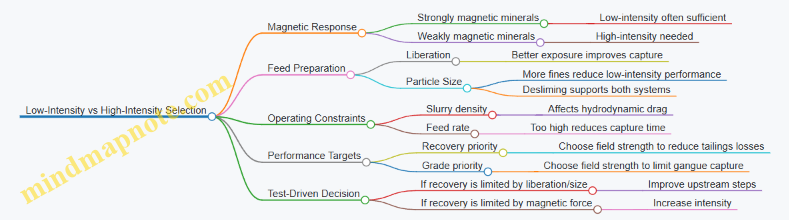
Practical Decision Workflow
- Run a bench comparison at the same feed preparation level (same size range, same desliming state).
- If low-intensity recovery is already close to your target and grade is acceptable, stop there and focus on upstream improvements.
- If recovery is poor and tailings contain the valuable mineral fraction, move to high-intensity.
- If high-intensity increases recovery but also increases contamination, adjust feed size control and slurry preparation before assuming the field strength is the only lever.
This approach keeps the decision grounded: field intensity is powerful, but it cannot fix poor liberation or excessive slimes. When you match the system to the mineral response and the feed condition, the separator behaves like a predictable tool rather than a guessing game.
8.4 Matrix and Drum/Separator Design: Feed Rate, Slurry Density, and Field Strength
Matrix and drum/separator performance comes down to three knobs that interact: how much material you feed, how thick the slurry is, and how strong the magnetic field (or equivalent separation field) is. Get one wrong and the others can’t compensate—so the design process should treat them as a coupled system.
Foundational Idea: What the Field Must Do
In a magnetic separator, particles experience a force that depends on field strength and particle magnetic response. But the force only helps if particles have enough time and the right path to reach a collection zone. That “time and path” is controlled by feed rate and slurry density, which together set the slurry velocity, turbulence, and residence time near the separation gap.
A simple way to think about it: the field provides the push, while the slurry flow decides whether the pushed particles actually get to where you want them.
Feed Rate: Controlling Residence Time and Bed Behavior
Feed rate determines how quickly solids enter the separation zone. If you increase feed rate without changing anything else, the slurry velocity rises, particles spend less time in the effective field, and the separation sharpness typically worsens. In matrix designs, high feed can also overload the matrix surface, causing a “wetting” or bypass effect where particles ride through without being captured.
Practical example: Suppose you’re treating 1000 kg/h of dry solids in a drum separator. If you raise feed to 1300 kg/h while keeping the same drum speed and gap, the slurry layer becomes thicker and the effective capture zone shrinks. The concentrate grade often drops because more target particles fail to reach the collection region.
Design practice: choose a target solids throughput based on required residence time, then verify it with pilot or plant data using two metrics: (1) concentrate grade and (2) recovery. If grade falls and recovery stays similar, you’re likely under-collecting; if both fall, you may be overloading the separation zone.
Slurry Density: Thickness, Viscosity, and Particle Crowding
Slurry density affects separation in three ways.
- Hydrodynamics: Higher solids concentration increases slurry viscosity and changes flow patterns, often increasing turbulence near the matrix or gap.
- Particle crowding: When particles are too crowded, the matrix surface can become coated, and magnetic particles can be physically blocked by non-magnetic solids.
- Effective field exposure: A thicker slurry layer means particles deeper in the layer experience a weaker effective field gradient at the collection surface.
Practical example: If you run at 30% solids by weight and then increase to 40% solids, you may see the concentrate grade drop even if the magnetic field is unchanged. The likely cause is that the matrix surface is no longer “seeing” a clean stream of particles; instead, it’s dealing with a dense, competing population.
Design practice: treat slurry density as a controlled variable. Measure it frequently, because small changes can shift the separation from “clean capture” to “surface crowding.” Use water addition control and verify with periodic density checks.
Field Strength: Matching Force to Particle Response
Field strength sets the magnitude of magnetic attraction. But stronger is not automatically better. Excess field can increase capture of weakly magnetic gangue, raising concentrate contamination. The goal is to apply enough field to capture the target particles at your actual flow conditions.
In matrix separators, field strength interacts with matrix geometry and permeability. The matrix acts like a collection scaffold, so the field must be strong enough to magnetize the matrix and pull target particles into the capture sites. In drum separators, field strength is tied to magnet design and the gap between the drum surface and the slurry.
Practical example: Consider a magnetite ore where some particles have lower magnetic susceptibility due to grain size or surface alteration. If you keep feed rate high and increase field strength, you might recover more of those weaker particles, but you can also pull more fine non-magnetic material into the concentrate, reducing selectivity.
Design practice: adjust field strength while holding feed rate and slurry density constant, then map the grade–recovery tradeoff. Use the “best separation point” where recovery is acceptable and contamination is minimized.
Coupled Design Logic: How to Set the Three Knobs Together
A systematic approach is to start with a baseline field strength from equipment capability, then set feed rate and slurry density to achieve stable hydrodynamics. After that, fine-tune field strength for selectivity.
- Fix slurry density to establish a predictable slurry layer thickness.
- Set feed rate to achieve the desired residence time and avoid matrix overload.
- Tune field strength to match particle response under those flow conditions.
- Confirm with performance checks using recovery and concentrate grade, plus observation of concentrate discharge behavior.
Mind Map: Matrix and Drum/Separator Design Parameters
Example: Choosing Operating Setpoints for a Magnetite Stream
Assume you have a magnetite-bearing slurry and you want stable concentrate discharge.
- Start with a moderate slurry density (e.g., 30% solids by weight) to avoid excessive crowding.
- Choose a feed rate that keeps the separation zone from visibly “flooding” the matrix or gap.
- Run at a baseline field strength and measure concentrate grade and recovery.
If grade is low but recovery is acceptable, reduce feed rate slightly or lower slurry density to improve capture selectivity. If recovery is low, increase field strength modestly or improve feed distribution (so particles reach the effective field region). If both grade and recovery are poor, the separation zone is likely overloaded—reduce feed rate and density before changing field strength.
This sequence works because it respects causality: flow conditions determine whether particles can reach the field’s effective capture region, and field strength determines what gets captured once they do.
8.5 Practical Example Producing a Magnetite Concentrate from a Mixed Iron Ore
A mixed iron ore often contains magnetite (Fe3O4), hematite (Fe2O3), and silicate gangue such as quartz and clays. The goal is to produce a magnetite-rich concentrate while keeping silica and slimes under control. The workflow below shows how to move from fundamentals to practical operating decisions without skipping the parts that usually cause trouble.
Step 1: Define the Separation Targets
Start with assay and mineralogical data. Suppose the feed averages 30% Fe, 8% SiO2, and contains magnetite plus some hematite. A reasonable target might be 55–60% Fe with low silica, plus a tailings stream that removes most gangue. Because magnetite is magnetic and hematite is weakly magnetic, magnetic separation can work well if the magnetite is sufficiently liberated and not locked inside silicate grains.
A quick sanity check: if the ore is very fine-grained and heavily intergrown, magnetic separation alone may struggle. In that case, the magnetic circuit still helps, but it should be paired with controlled grinding and possibly a downstream flotation or gravity step. For this example, assume grinding and desliming are sufficient to make magnetite respond cleanly.
Step 2: Prepare the Feed for Magnetic Separation
Magnetic separation is sensitive to particle size and slurry chemistry. Begin with crushing to a manageable feed size, then grind to a target where magnetite grains are mostly liberated. In practice, you choose a grind size based on liberation data, but a common operational approach is to run a few test conditions and pick the one that improves Fe grade without exploding silica or magnetite losses.
Next, deslime. Clays and ultrafines increase viscosity and can carry gangue into the magnetic product through entrainment. A practical method is to classify the slurry so that the magnetic stage sees a controlled size fraction. If you cannot fully remove slimes, you compensate by tightening water addition and improving wash steps.
Step 3: Choose the Magnetic Separation Mode
For magnetite, wet high-intensity magnetic separation (WHIMS) is often effective when magnetite is not coarse. Low-intensity systems can work for coarse, strongly magnetic particles, but WHIMS gives more control over recovery versus grade.
A useful operating principle is to treat the magnetic separator as a “cut-point” device: stronger field and better particle exposure increase recovery but can also pull more weakly magnetic material and fine gangue. Therefore, you tune field strength, feed rate, and slurry density to hit the desired grade.
Step 4: Run a Controlled WHIMS Circuit
A typical WHIMS circuit includes conditioning, feed dilution, magnetic separation, and product washing. Use these practical levers:
- Slurry density: Too high reduces particle mobility and increases uneven flow; too low wastes capacity and can reduce effective contact time.
- Feed rate: Higher feed rate increases throughput but can reduce separation sharpness.
- Wash water: Washing removes non-magnetic entrainment from the magnetic product bed.
- Magnetic field strength: Increase field to recover more magnetite, but watch silica and hematite contamination.
Example operating targets for this case study: set slurry density to a mid-range value that maintains stable flow, choose a feed rate that keeps the matrix bed from flooding, and use wash water to reduce gangue carryover. Then collect magnetic concentrate and non-magnetic tailings for mass balance and assay.
Step 5: Evaluate Performance with Mass Balance and Cut-Point Logic
After each run, calculate:
- Magnetite recovery: how much of the magnetite-bearing Fe reports to concentrate.
- Concentrate grade: Fe% and SiO2% in the magnetic product.
- Iron distribution: Fe in concentrate versus tailings.
If concentrate grade is low, common causes are insufficient liberation (grind too coarse), too aggressive recovery settings (field too high or wash too low), or poor desliming. If recovery is low, causes include overgrinding that creates too many ultrafines, insufficient field strength, or feed that is too dilute or too fast for the matrix to capture magnetite.
Step 6: Integrate a Simple Decision Loop
Use a repeatable loop rather than guessing. Change one variable at a time and keep the rest constant.
Step 7: A Concrete Example Outcome
Assume three WHIMS runs on the same ore fraction:
- Run A (conservative recovery): moderate field, strong wash. Result: concentrate ~58% Fe but SiO2 ~4.5%, recovery 70%.
- Run B (balanced): slightly higher field, slightly reduced feed rate, optimized wash. Result: concentrate ~60% Fe, SiO2 ~3.8%, recovery 78%.
- Run C (aggressive recovery): highest field, high feed rate, minimal wash. Result: concentrate ~57% Fe, SiO2 ~6.0%, recovery 86%.
Run B is the practical choice because it improves grade without sacrificing recovery. Run C shows the classic trade: pushing recovery too hard pulls more gangue and weakly magnetic material, which raises silica and lowers overall product quality.
Step 8: Document the Operating Recipe
For stable production, record the final recipe as a set of operating conditions tied to measurable outcomes: grind target, classification cut, slurry density, field strength, feed rate, wash water rate, and expected concentrate grade and recovery. This turns “we tuned it” into something that can be repeated on the next batch of ore with similar behavior.
9. Electrostatic Separation and Surface-Property Effects
9.1 Electrostatic Principles: Charging, Conductivity, and Particle Behavior
Electrostatic separation starts with a simple idea: particles can be made to carry different electrical charges, and then those charges can be used to steer particles into different product streams. The steering does not require particles to be perfect insulators or perfect conductors; it requires predictable differences in how they charge and how they move through an electric field.
Core Concepts: Charge, Field, and Force
A particle’s motion in an electrostatic separator is driven by the electric force on its charge. If a particle has charge \(q\) and experiences an electric field \(E\), the force scales roughly with \(qE\). In practice, the field is created between electrodes, and the particle’s charge depends on how it interacts with the charging mechanism and with its own material properties.
Two material properties matter most. Conductivity controls how quickly charge can move within the particle. Permittivity influences how the particle polarizes in the field. For separation, conductivity is usually the practical lever because it strongly affects whether charge stays on the surface or redistributes and leaks away.
Charging Mechanisms: How Particles Get Their Charge
Charging is typically done by contact with a charged surface or by induction in a field. In many mineral systems, the most common approach is triboelectric charging, where particles rub against a material that becomes positively or negatively charged. The sign and magnitude of the charge depend on the pair of materials and on surface conditions.
A useful way to think about triboelectric charging is as a balance between charge transfer and charge loss. Charge transfer increases with adequate contact and surface roughness, while charge loss increases with moisture and ionic contamination. That is why “same ore, different water” can produce noticeably different separator behavior.
Conductivity Effects: Why Some Particles Hold Charge
Consider two particles placed in the same charging environment. A low-conductivity particle tends to retain surface charge longer, so it experiences a stronger net force in the separator field. A higher-conductivity particle can allow charge to redistribute or leak, reducing the effective charge that drives separation.
This leads to a practical rule: electrostatic separation works best when the charging step creates a meaningful charge difference that is not immediately erased by conductivity-driven leakage. If both minerals have similar conductivity and similar surface chemistry, they may charge similarly and separate poorly.
Moisture is the usual culprit for “why did the separation get worse?” Water can form thin conductive films on particle surfaces. Even small amounts can raise effective conductivity and increase charge dissipation, which reduces the difference in particle trajectories.
Particle Behavior in the Separator Field
Once charged, particles enter a region with an electric field. Their paths depend on the balance between electric force and other influences like gravity, drag, and particle–particle collisions.
- Charge magnitude sets how strongly a particle responds to the field.
- Charge sign determines which electrode direction it moves toward.
- Particle size and mass affect how easily the electric force can overcome gravity.
- Surface condition affects how stable the charge remains during flight.
A practical observation: if the feed contains a wide size distribution, fine particles may follow the field more closely while coarse particles may not deflect enough to reach the intended collection zone. That is why feed preparation and sizing are not “optional extras”; they are part of the physics.
Electrostatic Separation Mind Map
Mind Map: Charging, Conductivity, and Behavior
Example: Two Minerals with Different Surface Conductivity
Imagine a feed containing mineral A and mineral B. During triboelectric charging, both minerals pick up charge, but mineral A is more insulating and holds its charge longer. Mineral B has higher effective conductivity due to surface impurities.
In the separator, mineral A experiences a larger net electric force and bends toward the collection electrode. Mineral B loses charge faster, so its trajectory is closer to the gravity-driven path. The result is a higher grade of mineral A in the electrode-associated product and more mineral B in the opposite stream.
If you add water during conditioning, mineral B’s surface film becomes more conductive. The charge difference shrinks, and the split becomes less distinct. The same separator settings now produce more mixed products, even though the field strength and electrode geometry did not change.
Example: Feed Size Distribution and Cut-Point Behavior
Suppose the target is to separate a conductive gangue from a less conductive valuable mineral. If the feed includes many very fine particles, those fines may follow the field strongly regardless of mineral type, increasing entrainment into the “wrong” product. If the feed is too coarse, the electric force may not overcome gravity for either mineral, and both may land in similar zones.
A practical fix is to control the size range so that the electric force can create a consistent trajectory difference between minerals. That makes the cut-point behavior sharper and reduces the need for guesswork during operation.
9.2 Equipment Types: Triboelectric and Corona/High-Voltage Systems
Electrostatic separation depends on how particles respond to an electric field. In practice, two families of equipment dominate: triboelectric systems, where particles gain charge by contact and friction, and corona or high-voltage systems, where a strong electric field charges particles through ion bombardment. Both can separate minerals with different surface conductivity, dielectric behavior, and moisture sensitivity, but they do it with different charging routes.
Triboelectric Systems
Triboelectric separators charge particles by rubbing them against a material with a different tendency to hold electrons. The key idea is that the charge is created during particle–surface contact, so the equipment must control contact intensity, residence time, and particle surface condition.
A typical triboelectric setup includes a charging section, a conditioning or feed preparation section, and a separation section with an electric field that deflects charged particles. Feed preparation matters because moisture can short-circuit charge. For example, if you run a dry silica-rich tailings stream with a small amount of clay, the clay can hold water films and reduce charge stability, which lowers separation sharpness.
Operationally, triboelectric performance is often constrained by three practical variables:
- Charge generation: controlled by the tribo-material type and the mechanical action that creates contact.
- Charge retention: affected by humidity, temperature, and surface contamination.
- Particle size distribution: fine particles charge differently and can behave like “field fog,” reducing cut-point clarity.
A concrete example: suppose you want to separate a conductive graphite-like mineral from a nonconductive gangue. In a triboelectric system, the conductive particles may lose charge quickly to the environment, while the nonconductive particles retain charge longer. The separation field then sends the retained-charge fraction toward one electrode and the low-charge fraction toward the other.
Corona and High-Voltage Systems
Corona systems charge particles using ionized gas produced near a high-voltage electrode. The ions attach to particles, creating a charge without requiring direct particle-to-tribo-material contact. This can be advantageous when you cannot tolerate abrasion, or when the feed is abrasive and would rapidly wear tribo surfaces.
A corona separator typically includes a charging zone with a corona electrode, a transport path through an electric field, and collection electrodes or bins. The charging zone must be designed so that particles spend enough time in the ion cloud to reach a useful charge level, but not so long that they agglomerate or overcharge.
Corona charging is sensitive to gas conditions and geometry. Airflow affects ion availability and particle residence time. If the feed contains significant moisture, water can change surface conductivity and lead to charge leakage. In a high-voltage system, the separation field strength and electrode spacing determine how strongly trajectories diverge.
A concrete example: consider a dry stream of feldspar and quartz where one mineral surface becomes more conductive after slight contamination. In a corona system, the more conductive particles may acquire less stable charge or discharge faster, so their deflection is smaller. The result is a split that correlates with surface conductivity differences rather than bulk composition.
Comparing Equipment Types in Real Terms
Triboelectric systems emphasize contact-driven charging, so they reward good control of feed dryness and surface condition. Corona systems emphasize field-driven charging, so they reward stable gas conditions and careful electrode geometry.
A simple way to decide which equipment type fits a mineral stream is to ask: does the process tolerate particle rubbing and wear, and is the feed dry enough to keep charge from leaking? If the answer is “no” on dryness or abrasion tolerance, corona/high-voltage charging often becomes the more straightforward choice.
Equipment Logic for Triboelectric and Corona Systems
Mind Map: Equipment Types for Electrostatic Separation
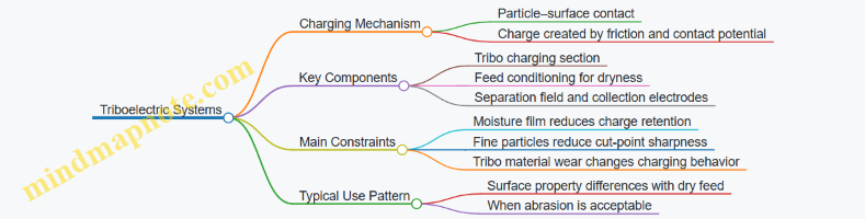
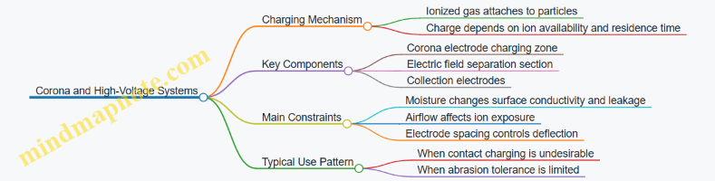
Example: Choosing Settings for a Dry Mineral Stream
Imagine a plant running a dry separation step on a mixed mineral feed with a target cut between a conductive mineral fraction and a nonconductive fraction. Start by ensuring consistent feed moisture, because both triboelectric and corona systems lose effectiveness when charge leaks.
For a triboelectric unit, you would then adjust the charging intensity to reach stable deflection without excessive fines carryover. For a corona unit, you would adjust the corona intensity and airflow so particles receive a consistent charge before entering the separation field. In both cases, you validate the outcome by checking how the product split changes with small, controlled shifts in feed rate and moisture, since those shifts reveal whether the separator is charge-limited or field-limited.
Example: Diagnosing Poor Separation Without Guesswork
If both products show similar grades, the separator may be failing to create a meaningful charge difference or the particles may not be spending the right time in the charging zone. In a triboelectric system, the first suspect is moisture or surface contamination that prevents charge retention. In a corona system, the first suspect is ion exposure, often tied to airflow or electrode geometry. Once you identify which limitation dominates, the corrective action is usually direct: improve dryness and contact control for triboelectric, or stabilize airflow and charging-zone residence for corona.
9.3 Conditioning Requirements: Moisture Control, Particle Size, and Surface Cleanliness
Conditioning is the quiet part of ore processing where the feed is made “separable.” In flotation and other surface-driven steps, the goal is simple: put particles into a consistent physical and chemical state so the separation mechanism can do its job. In practice, that means controlling moisture, particle size distribution, and surface cleanliness so you don’t accidentally change what the mineral “looks like” to the reagents.
Moisture Control
Moisture control starts with slurry behavior. Too much water dilutes reagent concentration and slows collision rates; too little water increases viscosity, reduces mixing quality, and can trap air or reagents in pockets. A useful way to think about it is that conditioning is a mixing problem with a chemistry overlay.
A practical example: suppose you’re conditioning a copper sulfide ore for flotation. If the solids % drifts upward, the same impeller speed produces poorer dispersion. You may still add the correct reagent mass, but the effective dose per wetted surface changes because mixing is uneven. The result is often a “mottled” response: some particles get enough collector to float, while others remain indifferent.
Operationally, moisture control is handled by:
- Consistent feed solids using weigh feeders and controlled water addition.
- Stable residence time in conditioners so reagent adsorption can approach a repeatable equilibrium.
- Temperature and water chemistry awareness because dissolved ions affect wetting and surface charge.
Particle Size
Particle size affects both liberation and surface area. Smaller particles provide more surface area per unit mass, which can increase reagent demand. At the same time, very fine particles often behave like stubborn freeloaders: they increase slimes, consume reagents, and can reduce selectivity by carrying gangue into the concentrate.
A concrete example: in flotation of a mixed oxide-sulfide ore, if grinding produces a larger fraction of fines than planned, you may see higher froth stability but lower concentrate grade. The froth may look “busy,” yet the valuable mineral recovery can stagnate because the collector is being spent on fine gangue and slime-coated surfaces.
Particle size control during conditioning is therefore about matching the feed to the separation target:
- Use classification upstream (screens or cyclones) to keep the conditioning feed within a predictable size range.
- Avoid over-conditioning when fines are present; extra time can increase adsorption on unwanted surfaces.
- Track P80 and fines fraction as routine indicators, not one-time lab curiosities.
Surface Cleanliness
Surface cleanliness is the difference between “reagent meets mineral” and “reagent meets a coating.” Coatings include natural hydrophobic films, oxidation products, clays, and residual process water chemistry. Even when the mineral is the same, surface condition can change how strongly it wets, how it charges, and how readily it attaches to bubbles.
A practical example: consider a sulfide mineral that has partially oxidized. Oxidation can create surface species that either consume collector or reduce its effectiveness. If you condition with the same reagent scheme as for fresh ore, you may observe lower recovery and higher reagent consumption. The fix is not just “add more collector”; it’s to adjust conditioning steps that improve surface readiness, such as:
- Desliming or clay removal upstream to reduce slime coatings.
- Controlled pH conditioning to manage surface charge and reagent speciation.
- Conditioning order so activators and collectors contact the right surfaces under the right conditions.
Surface cleanliness also includes mechanical cleanliness: poor feed handling can introduce tramp oils, excessive dust carryover, or inconsistent water quality. These contaminants can create false hydrophobicity and destabilize the separation.
Integrated Mind Map
Mind Map: Conditioning Requirements
Putting It Together with a Simple Workflow
- Set solids % to a target that your mixing system can handle consistently.
- Confirm size distribution from upstream classification so fines are within the expected band.
- Prepare the surface by managing pH and removing or reducing coatings that interfere with reagent contact.
- Condition in stages when needed, because activator and collector do not behave the same way on every surface.
When these three controls move together, the separation step becomes more predictable: reagent consumption stabilizes, concentrate grade improves, and the circuit stops reacting to every small change in feed like it’s guessing the rules.
9.4 Interpreting Results: Cut Size, Split Efficiency, and Contamination Control
When you run a separation test, you’re really answering three questions: What size range reports to each stream, how much of the target mineral ends up where you want it, and how much unwanted material sneaks along for the ride. The trick is to interpret results in a way that connects particle size behavior to mass balance and contamination.
Cut Size: What “Reports To” Means
Cut size is the particle size at which a given fraction has a 50/50 chance of going to the product versus the reject (or vice versa, depending on convention). In practice, you estimate it from split data across size fractions.
Start with a size-by-size mass split. For each sieve or class, compute the fraction of feed mass that reports to the product stream. Plot cumulative product mass fraction versus size (often using a log size axis). The curve’s midpoint is your cut size. If the curve is steep, the separation is sharp; if it’s flat, the system is mixing sizes.
A concrete example: suppose a cyclone overflow product is intended to be the “fines” stream. If the 20–30 µm class shows 80% reporting to overflow while the 10–20 µm class shows 95%, your cut size is somewhere between those classes, and the slope tells you how cleanly the boundary is defined.
Split Efficiency: Turning Splits Into Performance
Split efficiency describes how effectively the separation sends the target mineral to the intended stream relative to what the size split alone would predict. Use it to avoid a common trap: a size boundary can look good while mineral selectivity is poor.
Compute split efficiency using mineral or assay data per size fraction. A simple approach is to compare the recovery of the valuable mineral in the product to the mass fraction of that size class in the feed. For each size class i:
- Valuable recovery in product: Ri
- Feed mass fraction in class: Mi
- Ideal reporting would send all valuable from that class to product, so the “efficiency” is how close Ri is to the valuable content available in that class.
If you don’t have mineral assays by size, you can still use grade–recovery logic, but the interpretation becomes less precise. With assays, you can see whether losses are due to mis-sizing (cut size mismatch) or due to true selectivity issues (e.g., similar surface properties, poor reagent performance, or hydrodynamic entrainment).
Contamination Control: Where the Unwanted Comes From
Contamination is usually not random. It comes from three mechanisms: (1) true co-reporting of gangue that shares the same size range, (2) entrainment of fine particles that bypass the intended separation mechanism, and (3) liberation limits where valuable and gangue are locked together.
To interpret contamination, compare two curves: the size distribution of the product mass and the size distribution of the valuable mineral within that product. If the product mass is dominated by a size range but the valuable mineral peaks at a different range, contamination is likely high in the “wrong” sizes.
Also check the tails of the size distribution. Many separations perform best near the cut size and worst at the extremes. For example, very fine slimes may behave like a suspension and follow the fluid path, increasing gangue carryover. Coarser particles may not fully respond to the separation mechanism, increasing locked contamination.
Mind Map: Interpreting Results for Cut Size, Split Efficiency, and Contamination
Example: Reading a Flotation or Classification Split Without Guesswork
Imagine you have a feed that contains valuable mineral mostly in 20–60 µm particles, while gangue is broadly distributed. After classification, you test two streams: product A (intended to be cleaner) and reject B.
- From mass splits, you estimate the cut size is around 35 µm, with a moderate slope.
- From mineral assays, you find valuable recovery to A is 70%, but grade in A is only slightly higher than feed.
- From size-resolved assays, you observe that A contains a large fraction of gangue from the 10–20 µm class.
This combination points to contamination driven by fines entrainment rather than a poor cut size alone. The cut size is “in the right neighborhood,” but the boundary is not preventing gangue from the fine end from reporting to A.
Practical Checklist for Interpreting Test Data
- Confirm the cut size using size-by-size reporting, not just overall recovery.
- Use split efficiency to distinguish mis-sizing from selectivity or mechanism failure.
- Quantify contamination by linking gangue grade to specific size classes.
- Inspect the smallest and largest size classes first; they often explain most of the contamination.
- Close the loop with mass balance so you know whether losses are going to the intended stream or disappearing into the wrong one.
9.5 Practical Example: Separating Conductive and Nonconductive Fractions from a Tailings Stream
This example shows how to use electrostatic separation to split a tailings stream into conductive and nonconductive fractions. The goal is simple: particles that behave differently electrically should end up in different product streams, even when they look similar under a quick glance.
Step 1: Start with the Right Feed Condition
Electrostatic separation is picky about feed. Begin by targeting a narrow size range, because charging and flight behavior vary with particle size. A practical target is often a few hundred micrometers down to tens of micrometers, depending on the separator design.
Next, control moisture. If the tailings are too wet, water forms conductive paths and reduces charge retention. If they are too dry, dusting can cause losses and unstable feed. A common approach is to condition the slurry, then dewater to a consistent moisture level before dry separation.
Finally, remove sticky fines when needed. If the tailings contain a lot of ultrafines, they can coat larger particles and blur the electrical contrast. A simple desliming step or classification cut can improve separation without changing the chemistry.
Step 2: Establish the Electrical Contrast Mechanism
Conductive particles tend to lose charge quickly or redistribute it, while nonconductive particles can hold charge longer. The separator then uses an electric field to deflect charged particles differently.
To confirm the mechanism, run a small bench test with representative samples. Measure mass split and grade of a marker component in each fraction. For instance, if conductive particles are associated with magnetite-bearing gangue and nonconductive particles are associated with silicates, track iron content in each product.
Step 3: Choose the Separator Mode and Electrode Setup
Select a separator configuration that matches the expected charging behavior. In practice, you tune three things: charging method, field strength, and residence time.
- Charging method: triboelectric charging can work well when particles can rub and exchange charge.
- Field strength: higher field increases deflection but can also increase misplacement if particles are poorly charged.
- Residence time: too short gives weak separation; too long can cause re-entrainment and mixing.
A useful operational rule is to start with conservative settings, then adjust one variable at a time while watching both product mass split and marker grade.
Step 4: Run a Controlled Separation and Track Performance
Assume the tailings feed is 1000 kg/h dry equivalent. After conditioning and size selection, feed enters the separator.
You collect two products:
- Conductive fraction: expected to land closer to the grounded or less-deflected side.
- Nonconductive fraction: expected to deflect farther.
Track:
- Mass pull: how much of the feed ends up in each fraction.
- Recovery of the marker: how much of the marker component is captured in the intended product.
- Purity: marker grade in each product.
Example target outcomes (illustrative):
- Conductive fraction mass pull: 45% with 80% of the marker captured.
- Nonconductive fraction mass pull: 55% with 85% of the complementary marker captured.
If the conductive fraction is too contaminated, it usually means conductive particles are not behaving as expected electrically. That can happen when moisture is high, fines are coating particles, or the size distribution is too broad.
Step 5: Troubleshoot Using Cause-and-Effect Logic
Common issues and what they imply:
- Poor separation with both fractions similar in grade: feed moisture too high or particle size too broad.
- Conductive fraction mass pull too large: field strength too low or charging ineffective.
- Nonconductive fraction grade drops: re-entrainment from excessive feed rate or dust losses.
Fixes should be targeted. Reduce moisture first, then narrow the size range, then adjust field strength and feed rate.
Mind Map: Conductive Versus Nonconductive Separation Workflow
Step 6: Close the Loop with a Simple Mass Balance Check
After you have stable splits, do a quick mass balance using marker assays. If the marker recovery sums to much less than 100% (allowing for sampling error), you likely have losses in dust, carryover, or miscollection. If the marker recovery sums correctly but purity is low, the separation is happening but the electrical contrast is weaker than assumed, so feed conditioning and size control become the main lever.
This example works because each step supports the next: conditioning preserves charge behavior, size control improves trajectory predictability, and performance metrics confirm that the electrical contrast is actually translating into physical separation.
10. Flotation Fundamentals and Reagent Chemistry
10.1 Flotation Mechanisms: Bubble–Particle Attachment and Selectivity
Flotation separates minerals by making some particles prefer the air side of a slurry. That preference is not magic; it comes from a chain of physical events: particles must collide with bubbles, attach strongly enough to resist detachment, and then stay attached long enough to rise and report to the froth.
Mind Map: Bubble–Particle Attachment and Selectivity
Bubble–Particle Collision
The first hurdle is getting close enough for attachment to matter. In a stirred cell, bubbles and particles move with different velocities, so collisions occur when their paths intersect. Higher agitation increases collision frequency, but it can also increase shear that later promotes detachment. Bubble size matters too: smaller bubbles provide more surface area per unit volume and often increase the probability of collision, yet they can also rise faster and spend less time in the collection zone.
A simple way to picture collision is to imagine marbles in a bowl with a steady stream of soap bubbles. If the marbles are too far apart (low solids, poor mixing), bubbles pass without meeting them. If the bowl is shaken violently, collisions happen, but the attached “stickiness” has to survive the shaking.
Film Drainage and Contact Formation
Even after collision, attachment is not guaranteed. Between a bubble and a particle there is usually a thin liquid film. For attachment to occur, that film must thin and drain so the surfaces can come into direct contact at a microscopic level.
Collectors create the key chemical condition for this step. On hydrophobic mineral surfaces, collector molecules adsorb and present nonpolar groups toward the water. This reduces the energetic penalty of replacing water–mineral contact with water–bubble and mineral–bubble contact. As the film drains, the system reaches a stable three-phase contact line where the particle sits on the bubble surface.
Hydrophobicity is often summarized by contact angle, but in real slurries it is better treated as a practical outcome: particles that form a stable three-phase contact resist re-separation when the hydrodynamic forces change.
Selectivity Through Surface Chemistry
Selectivity means only certain minerals attach under the same operating conditions. That selectivity is created by differences in surface chemistry, not by differences in “importance.”
- Collector adsorption: Sulfide minerals often respond strongly to xanthate or similar collectors, while many silicates do not without activation or special reagents. If a collector does not adsorb, the particle remains water-wet and attachment fails.
- pH and ionic environment: pH controls collector speciation and mineral surface charge. For example, a collector may be ineffective at one pH because it cannot form the right surface complex, even if the mineral is present.
- Surface charge and repulsion: Particles and bubbles can carry charges that either promote or hinder approach. If electrostatic repulsion keeps the film from thinning, you can get many collisions but few attachments.
Detachment and Why “Good Attachment” Still Fails
Once attached, particles must survive the journey upward. Detachment can happen when shear forces exceed the adhesive strength at the three-phase contact. Bubble bursting in the froth can also release particles. This is why flotation performance is not determined only by chemistry; hydrodynamics and froth stability matter.
A practical example: if you increase air rate, you may increase bubble numbers and collision frequency, but you can also create a froth that is too turbulent. The result can be higher recovery of coarse valuable particles while fine particles detach more easily, lowering concentrate grade.
Example: Why Collector Dose Changes Recovery and Grade
Consider a copper sulfide ore with a gangue of quartz. At low collector dosage, copper sulfide surfaces are only partially covered, so attachment is weak and recovery is low. As dosage increases, more copper sulfide particles form stable three-phase contacts, so recovery rises. Push the dosage too far and you often increase unintended hydrophobicity on some gangue surfaces or create excessive frothiness that entrains non-target particles. Grade then drops because the system collects more than it should.
The key mechanism is that selectivity depends on whether collector adsorption and surface conditions create stable attachment only on the target mineral. The best operating point is where attachment is strong for the target and weak for the rest, while detachment losses remain manageable.
10.2 Reagent Roles: Collectors, Frothers, Depressants, Activators, and pH Modifiers
Flotation reagents work as a coordinated set of “surface instructions” for mineral particles. The goal is simple: make the target mineral attach to bubbles while unwanted minerals stay in the water. Each reagent class changes a different part of that surface story—chemistry, wettability, and bubble behavior—so the sequence and dosage matter.
Collectors
Collectors create hydrophobic character on specific mineral surfaces. They typically adsorb through chemical bonding or strong surface interactions, turning the mineral from water-wet to bubble-friendly.
A practical way to think about collectors is by their “fit” to the mineral surface. For example, a sulfide ore often responds to xanthates or dithiophosphates because sulfur-bearing surfaces can form surface complexes. If you dose too little collector, the mineral remains mostly hydrophilic and recovery drops. If you dose too much, collector can start coating gangue minerals too, lowering concentrate grade.
Example: In a lab flotation test on a copper sulfide sample, start with a moderate collector dose and observe the rougher concentrate grade. If grade is high but recovery is low, increase collector slightly. If recovery rises but grade falls sharply, you are likely over-coating and should reduce collector or improve selectivity with depressants.
Frothers
Frothers control bubble size and froth stability. Smaller bubbles increase the number of attachment opportunities, while froth stability helps maintain a workable froth layer for skimming.
Frothers do not “select” minerals directly; they shape the bubble environment. Too little frother can produce coarse bubbles that separate poorly. Too much frother can create overly stable froth that traps water and fine gangue, hurting both grade and drainage.
Example: If a rougher produces a thick, persistent froth with muddy appearance and the concentrate grade is low, reduce frother and check whether the froth collapses faster and releases entrained fines.
Depressants
Depressants reduce flotation of unwanted minerals by making their surfaces more hydrophilic or by blocking collector adsorption sites.
Depressants are often the difference between “it floats” and “it floats selectively.” They can target specific gangue minerals such as clays, carbonates, or oxides. Their effectiveness depends on surface chemistry and particle size, because fine slimes have more surface area and can consume depressant quickly.
Example: If clay-rich gangue is reporting to the concentrate, a depressant that disperses or coats clay surfaces can improve selectivity. In practice, you may need to adjust both depressant dosage and conditioning time, because clays can adsorb reagents slowly.
Activators
Activators increase the floatability of minerals that otherwise do not respond well to collectors. They do this by modifying surface chemistry so that collector adsorption becomes favorable.
Activators are especially relevant when the target mineral surface is covered by an oxide film or has low affinity for the collector. A common pattern is: activator first to prepare the surface, then collector to attach.
Example: Suppose a zinc-bearing oxide mineral shows weak response to a collector. Adding an activator before collector can increase recovery. If grade also improves, the activator is likely enabling selective adsorption rather than broadly activating gangue.
pH Modifiers
pH modifiers set the chemical environment that governs adsorption, ion speciation, and mineral surface charge. Many collectors and depressants only work in certain pH ranges because their active forms change with acidity.
A useful mental model is that pH controls “who is available” in solution. For instance, some collector species are more effective at certain pH values, and depressants may only bind strongly when the surface charge supports adsorption.
Example: If you keep collector dosage constant and adjust pH, you may see a recovery peak at a specific pH. That peak indicates a balance where collector adsorption is strong on the target mineral but weaker on gangue.
Integrated Reagent Sequencing
A typical conditioning logic is: prepare surfaces, set pH, manage selectivity, then promote bubble attachment.
- pH modifier establishes the baseline chemistry.
- Activator (if needed) prepares the target surface for collector adsorption.
- Depressants protect gangue from collector attachment.
- Collectors provide hydrophobicity to the target.
- Frother sets bubble size and froth behavior.
Systematic Conditioning Checklist
Before changing dosages, verify that the conditioning order matches the chemistry you expect. Then adjust one variable at a time:
- Confirm pH is stable during conditioning.
- If the target responds weakly, test activator need before increasing collector.
- If grade is poor, reduce collector or strengthen depressant action.
- If froth behavior is off, tune frother rather than chasing mineral selectivity.
This approach keeps the cause-and-effect chain intact, so you can interpret results without guessing.
10.3 Water Chemistry and Conditioning: Hardness, Slimes, and Ionic Effects
Water chemistry is not background noise in flotation; it is part of the reagent system. Collectors, frothers, and depressants all behave differently depending on hardness, fine slimes, and the ions already dissolved in the water. Conditioning is where you decide whether those ions help your separation or quietly sabotage it.
Hardness and Alkalinity
Hardness mainly comes from dissolved calcium and magnesium. In flotation, these ions can change mineral surface charge and also interact with reagents. A simple way to see the effect: if you run the same ore slurry in two waters—one soft, one hard—you often observe different froth stability and different reagent consumption even when pH is held constant.
Alkalinity, often expressed through pH and buffering species, affects how collectors ionize and how mineral surfaces protonate or deprotonate. For many sulfide systems, pH control is used to keep the collector in the right form and to manage the surface charge so bubbles attach selectively. For oxide and silicate gangues, pH also influences whether the surface becomes more hydrophilic or more receptive to adsorption.
A practical conditioning rule: treat pH and hardness as coupled variables. If you adjust pH using lime or soda, you are also changing ionic strength and calcium availability. That means a “successful” pH target from one water source may not reproduce in another.
Slimes and Surface Area Control
Slimes are the fine particles that pass through screens and often remain suspended. They matter because they provide enormous surface area per unit mass, which increases reagent demand and can physically block mineral-bubble contact.
Slimes also change slurry rheology, making it harder to maintain consistent air dispersion and mixing. In flotation tests, this shows up as inconsistent recovery at the same reagent dosage, especially when the feed has variable fines content.
Conditioning approaches focus on two goals: reduce slime interference and manage how much slime is allowed to participate. Desliming by classification is one lever. Another is controlling grinding and water addition so the slimes fraction entering flotation stays within a predictable range. If you cannot remove slimes, you compensate by using depressants or dispersants to reduce slime attachment to bubbles and to keep the mineral surfaces more selective.
Easy example: imagine two samples of the same ore. Sample A has 5% slimes; Sample B has 20% slimes. If you dose collector based on Sample A, Sample B will often consume collector on slimes first, leaving less collector for the target mineral. The result is lower grade and sometimes lower recovery because the froth carries more gangue.
Ionic Effects and Water Chemistry
Beyond hardness, other ions—sulfates, chlorides, bicarbonates, and dissolved metals—affect flotation through ionic strength and specific ion effects. Ionic strength influences the electrical double layer around particles, which changes how close particles and bubbles can approach before repulsion dominates. Specific ions can also adsorb onto surfaces, altering wettability.
A useful mental model: flotation is a competition between adsorption and repulsion. Reagents must adsorb strongly enough to change surface hydrophobicity, while unwanted species must not adsorb in a way that makes the gangue equally hydrophobic.
Common conditioning consequences include:
- High ionic strength can reduce the effectiveness of some dispersants, leading to flocculation and uneven reagent distribution.
- Certain ions can promote slime aggregation, which may either help by reducing surface area or hurt by trapping gangue in flocs.
- Dissolved metals can interact with collectors or modifiers, changing reagent availability.
Conditioning Workflow for Real Slurry
A systematic conditioning sequence reduces surprises.
- Measure baseline water properties: pH, hardness (Ca/Mg), and conductivity as a proxy for ionic strength.
- Characterize the slurry fines level: estimate slimes fraction or at least track feed size distribution.
- Precondition with water first: mix the slurry without reagents briefly to reach a stable temperature and dispersion state.
- Add pH modifiers next: adjust alkalinity while recognizing that lime and soda also introduce ions.
- Add dispersants or slime control agents if slimes are high: aim to keep slimes from attaching to bubbles.
- Add collectors and frothers last: minimize time for nonselective adsorption and keep reagent action focused.
- Verify with a quick mass pull and grade check: if froth is carrying more gangue than expected, revisit slimes control before increasing collector.
Mind Map: Water Chemistry and Conditioning
Example: Hard Water with High Slimes
Suppose a plant switches to a harder water source and simultaneously sees more fines from a change in feed preparation. In flotation tests, the same collector dosage yields lower concentrate grade and a higher tailings loss of the target mineral.
A likely chain is: hardness increases ionic strength and calcium availability, which shifts surface behavior and can increase nonselective adsorption. Higher slimes then consume additional collector and can attach to bubbles or change froth carryover. The fix is not simply “add more collector.” Instead, reduce slimes entering flotation (or improve desliming), confirm pH targets under the new water, and adjust slime control so the collector has a cleaner surface to adsorb on.
When water chemistry, fines, and conditioning order are treated as one system, flotation becomes more predictable—and the lab results start matching the plant reality.
10.4 Flotation Variables: Air Rate, Agitation, Residence Time, and Solids %
Flotation performance is usually decided by how often particles meet bubbles, how long they stay in the froth zone, and whether the slurry conditions let collectors and frothers do their job. Air rate, agitation, residence time, and solids % are the four knobs that control those interactions.
Air Rate
Air rate sets the number of bubbles and their size distribution. More air generally increases bubble–particle collision frequency, but it can also create smaller bubbles that rise faster and may reduce attachment time. In practice, operators watch for two symptoms: (1) froth that is too wet and collapses easily, and (2) a pulp that looks overly aerated with little improvement in concentrate grade.
A simple way to think about it: if you double air rate without changing anything else, you may increase the number of chances for attachment, but you also change froth structure and hydrodynamics. The “right” air rate is the one that improves recovery without dragging too much gangue into the froth.
Agitation
Agitation controls mixing intensity, bubble dispersion, and particle suspension. Too little agitation leads to poor bubble distribution and localized “dead zones” where bubbles and particles don’t meet. Too much agitation can break fragile froth structures and strip attached particles from bubbles.
Agitation also affects how quickly the slurry reaches uniform reagent concentration. If you add collector and frother, the first minutes matter because surface chemistry must stabilize before you rely on bubble attachment. In a well-run cell, agitation is high enough to keep solids suspended and distribute bubbles, but not so high that it constantly re-suspends froth and undermines selectivity.
Residence Time
Residence time is the time particles spend in the flotation cell. It is not just a function of cell volume; it depends on slurry flow rate and how stable the froth and pulp zones are. Short residence time can limit recovery because attachment and froth transport may not complete. Excess residence time can increase entrainment, especially when slimes and fine particles are present.
A practical rule: if concentrate grade drops while recovery rises, you may be “overstaying” particles that should have been rejected. If recovery is low and grade is stable, you may be under-delivering collisions or attachment time.
Solids %
Solids % changes slurry viscosity, bubble rise behavior, and the probability of collisions. Higher solids can increase collision frequency because particles are closer together, but it also increases the chance of bubble crowding and reduces effective froth drainage control. Lower solids can improve froth stability and reduce entrainment, but it may lower collision frequency.
Solids % also affects how much water is available for froth drainage. If the slurry is too thick, froth may become unstable and carry more gangue. If it is too dilute, the cell may not achieve the particle concentration needed for efficient attachment.
Mind Map: Flotation Variables and Their Effects
Integrated Example: Adjusting a Copper Sulfide Rougher
Assume a rougher is producing low recovery and the concentrate grade is acceptable. The froth looks thin and the pulp appears under-aerated.
- Increase air rate gradually while keeping agitation constant. If recovery improves without grade loss, you likely corrected collision frequency.
- If recovery improves but froth becomes overly wet, reduce agitation slightly to stabilize froth and reduce bubble–particle detachment.
- If recovery still lags, increase residence time by reducing feed rate or adjusting cell duty so particles have more time to attach and rise.
- If grade begins to slip as recovery rises, lower solids % modestly to reduce entrainment and froth carryover.
This sequence matters because each variable has a different failure mode. Air rate first addresses contact; agitation then addresses stability; residence time addresses kinetics; solids % addresses hydrodynamics and entrainment.
Quick Operating Checks
- If froth is wet and concentrate grade drops, suspect excessive air, excessive agitation, or too high solids %.
- If froth is stable but recovery is low, suspect insufficient air, insufficient agitation for dispersion, or too short residence time.
- If both recovery and grade are poor, revisit reagent conditioning and slurry preparation, because the variables can’t compensate for weak surface chemistry.
10.5 Practical Example: Designing a Collector and pH Scheme for a Copper Sulfide Ore
A typical copper sulfide ore contains chalcopyrite with some chalcocite and bornite, plus gangue like quartz and calcite. The goal of the collector and pH scheme is simple: make copper sulfide surfaces more willing to attach to bubbles, while keeping common gangue minerals from doing the same. In practice, that means choosing a collector family, setting pH to control surface chemistry, and using conditioning steps that keep the slurry stable.
Step 1: Start with What the Surface Wants
Copper sulfides respond strongly to pH because it changes the balance between metal ions, surface oxidation, and the availability of reactive sites. At low pH, many sulfide surfaces oxidize quickly, which can either help (by creating active sites) or hurt (by forming films that block attachment). At higher pH, oxidation slows, but you may lose some activation benefits.
A practical starting point for chalcopyrite is mildly acidic conditions. For example, set pH around 9.0 for many sulfide flotation practices, then adjust based on test results. The key is to avoid guessing blindly: run a short pH sweep with a fixed collector dose and measure copper recovery and concentrate grade.
Step 2: Choose a Collector Family and Set a Baseline Dose
For copper sulfides, common collector families include xanthates and dithiophosphates. Xanthates often work well when the ore is not overly oxidized and when you can maintain consistent pulp chemistry. Dithiophosphates can be more forgiving in some cases because they form strong surface complexes.
Baseline example:
- Collector: sodium isopropyl xanthate (SIPX)
- Initial dose: 20 g/t
- Target pH: 9.0
- Conditioning time for collector: 2–4 minutes
If you see low copper recovery at this baseline, increase collector dose gradually (for example, 20 → 30 → 40 g/t) while keeping pH constant. If grade drops as dose increases, that usually signals increased gangue collection or poor selectivity.
Step 3: Add Activation and Depression Logic
Copper sulfides sometimes need activation to improve collector adsorption, especially when surfaces are coated or when iron minerals dominate. A typical approach is to use a copper activator or adjust redox conditions, but the exact reagent depends on what the ore is doing.
A common depression target is pyrite or other iron sulfides that can consume collector and float undesirably. For gangue, you may use depressants like starch for certain silicates, but in this example we focus on collector and pH.
Integrated example scheme:
- pH adjuster: lime to reach pH 9.0
- Collector: SIPX
- Optional depressant: small starch addition if silicate slimes are high (only if tests show gangue response)
Step 4: Build the Conditioning Sequence
Conditioning order matters because reagents compete for time on the particle surface.
Example conditioning sequence for a rougher:
- Add water and slurry to target solids (often 30–35% solids by weight).
- Add lime to reach pH 9.0.
- Condition 3–5 minutes to stabilize pH and slurry chemistry.
- Add collector (SIPX) and condition 2–4 minutes.
- Add frother and proceed to flotation.
If you add collector before pH adjustment, you can create inconsistent surface states and get erratic results from test to test.
Step 5: Interpret Results Using Simple Diagnostics
During pH and collector testing, track three signals:
- Copper recovery: tells you whether copper sulfide surfaces are attaching to bubbles.
- Copper grade: tells you whether you are also collecting unwanted minerals.
- Mass pull: tells you whether the froth is carrying too much gangue.
Concrete example outcome:
- At pH 8.0 with 20 g/t SIPX: copper recovery is moderate, but grade is low.
- At pH 9.0 with 20 g/t SIPX: recovery improves and grade increases.
- At pH 10.0 with 20 g/t SIPX: recovery drops, suggesting insufficient active surface chemistry.
This pattern supports the choice of pH near 9.0 as a practical operating point.
Step 6: Lock in a Working Setpoint with a Small Matrix Test
Instead of a single trial, run a compact matrix:
- pH: 8.5, 9.0, 9.5
- Collector dose: 20, 30 g/t
- Keep everything else constant
Pick the combination that gives the best balance of recovery and grade, then confirm with a repeat test.
Mind Map: Collector and pH Scheme for Copper Sulfide Flotation
Example: Putting It Together as a Rougher Setpoint
A workable setpoint for a chalcopyrite-rich ore might be:
- pH: 9.0 (lime adjusted)
- Collector: SIPX at 30 g/t
- Collector conditioning: 3 minutes
- Frother: set to achieve stable froth without excessive carryover
If the concentrate grade is too low, reduce collector dose or tighten pH toward the best-performing point from the pH sweep. If recovery is too low, increase collector dose slightly while staying near the chosen pH, because shifting pH too far can change surface chemistry faster than collector dose can compensate.
11. Flotation Circuit Design, Testing, and Scale-Up
11.1 Bench-Scale Testing: Batch Flotation, Kinetic Tests, and Reproducibility
Bench-scale flotation testing answers three practical questions: what floats, how fast it floats, and whether your results hold up when you repeat them. A good program starts simple—one ore, one target product, one set of operating conditions—then adds complexity only when the data justify it.
Batch Flotation Testing: What You Measure and How
Batch flotation is a controlled “snapshot” where you mix conditioned slurry with air and reagents, then collect froth at set times or after a fixed duration. The core outputs are cumulative mass pull, concentrate grade, and recovery for the target mineral (or element). To make those outputs meaningful, you need consistent solids concentration, pH, reagent dosages, and water chemistry.
A systematic batch workflow looks like this:
- Prepare slurry consistently: Use the same solids % and the same water source each run. If you change water, you change ionic strength and sometimes surface behavior.
- Condition in the right order: Add pH modifiers first, then activators or depressants, then collectors, and finally frother. Conditioning time matters because reagents adsorb at different rates.
- Control aeration and agitation: Keep impeller speed and air rate constant. If you vary them, you change bubble size distribution and collision frequency.
- Collect froth on a schedule: Either collect at fixed times (e.g., 1, 3, 5, 8 minutes) or collect once after a set duration. Time-scheduled collection is what enables kinetic interpretation.
- Analyze products with a mass balance mindset: Measure head grade, concentrate grade, and tailings grade. If mass balance is off, the test is telling you something—often sampling or measurement error.
Example: Suppose you are testing a copper sulfide ore where chalcopyrite is the target. You run a batch at pH 10.2 with a collector dose of 150 g/t and frother at 30 g/t. After 5 minutes, you collect concentrate and find 60% recovery at 18% Cu. If you repeat the same run and get 60% recovery again but with concentrate grade fluctuating by a few percent, you likely have stable flotation behavior but variable froth entrainment or sampling variability.
Kinetic Tests: Turning Time Into Mechanism
Kinetic tests treat flotation as a time-dependent process. Practically, you collect concentrate fractions at multiple time intervals and compute cumulative recovery versus time. This gives you a curve you can compare across reagent schemes.
A useful way to interpret kinetics is to separate “fast” and “slow” behavior:
- Fast floaters: minerals that attach quickly to bubbles, often due to favorable surface chemistry and adequate liberation.
- Slow floaters: minerals that require more time for reagent adsorption, surface conditioning, or bubble attachment.
You can quantify this with simple models, but the model is less important than the consistency of the curve shape. For example, if increasing collector dose shifts the curve left (higher early recovery) without changing the final plateau much, you improved attachment speed rather than creating new floatable material.
Example: In a batch test, cumulative recovery reaches 40% at 2 minutes and 70% at 8 minutes. When you increase collector dose, the 2-minute recovery rises to 55% while the 8-minute recovery stays near 72%. That pattern suggests faster attachment for the same overall floatable fraction.
Reproducibility: Proving the Test Is Trustworthy
Reproducibility is not a formality; it is how you avoid chasing noise. A reproducible test shows similar recovery and grade trends when repeated under the same conditions.
Key practices for reproducibility:
- Run duplicates or triplicates for at least the baseline condition. If the baseline is unstable, everything built on it will be unstable.
- Use the same ore preparation: consistent crushing, splitting, and mixing reduces variability in liberation and surface area.
- Standardize reagent preparation: make solutions at fixed concentration and mix them thoroughly before dosing.
- Track pH and temperature: pH drift during conditioning can happen, especially with slimes or carbonate content.
- Keep froth handling consistent: the same collection vessel, same scraping method, and same timing reduce operator effects.
Example: You test two collector schemes, A and B. Scheme A gives 65% recovery at 5 minutes, scheme B gives 62%. If duplicates for scheme A vary between 60% and 70%, the difference is not reliable. If duplicates for both schemes cluster tightly (e.g., A: 64–66%, B: 61–63%), then the difference is meaningful.
Mind Map: Bench-Scale Batch Flotation Logic
Practical Mini-Plan for a First Kinetic Run
Start with one baseline scheme and collect concentrate at multiple times. Use duplicates to confirm stability. Then change only one variable at a time—typically collector dose, conditioning time, or pH—so the kinetic curve differences can be attributed to a specific cause rather than a pile of small uncontrolled changes.
11.2 Circuit Layouts: Rougher–Cleaner–Scavenger and Recleaning Strategies
A rougher–cleaner–scavenger (RCS) flotation circuit is built around one idea: you don’t try to get perfect separation in the first pass. The rougher makes a “first cut” by collecting the valuable mineral into a froth product, while the scavenger recovers additional value that escaped the rougher. Cleaners then upgrade the rougher concentrate by removing remaining gangue.
Rougher–Cleaner–Scavenger Layout Logic
Start with the rougher because it tolerates imperfect selectivity. You typically run it with enough reagent strength and air–agitation conditions to keep valuable particles attached to bubbles, even if some gangue also reports to froth. The rougher concentrate becomes the feed to cleaners, where conditions are tightened to reduce gangue carryover.
The scavenger is not a “second rougher” in spirit; it is a targeted recovery step. It treats the rougher tailings (and sometimes intermediate streams) under conditions that improve the chance that missed valuable particles will attach. In practice, scavenger performance depends on two things: how much valuable mineral remains in the tailings and whether the particle size and surface chemistry are still suitable for flotation.
A common integrated flow is:
- Rougher feed → Rougher → Rougher concentrate to cleaners; Rougher tailings to scavenger
- Scavenger concentrate to cleaners (or to a recleaner stage)
- Cleaner tailings back to rougher or to scavenger, depending on where you want to spend reagent and residence time
Mind Map: RCS Circuit Components and Decisions
Cleaner Stages and Recleaning Strategies
Cleaners come in stages because each pass can remove a portion of the remaining gangue. The first cleaner often removes the bulk of the easily detached impurities. If the final concentrate grade is still not acceptable, recleaning becomes a practical lever.
Recleaning means taking cleaner concentrate (or a portion of it) and running it through an additional cleaning step. This is usually justified when the impurity minerals are present as fine locked or partially liberated particles that survive the first cleaning. Recleaning can also help when the rougher concentrate contains “sticky” gangue that attaches under rougher conditions but can be discouraged under cleaner conditions.
A systematic way to decide whether to reclean is to track where the valuable mineral and gangue are going. If the valuable mineral is already mostly in the cleaner concentrate, then recleaning can improve grade with limited recovery loss. If the valuable mineral is still widely distributed, recleaning may just throw away recovery while only slightly improving grade.
Example: Copper Sulfide with Gangue Silicates
Imagine a copper sulfide ore where chalcopyrite is the target and silicate gangue reports to froth during roughing. A typical RCS approach might be:
- Rougher: strong collector dosage and moderate pH to promote chalcopyrite collection; produce rougher concentrate with acceptable copper recovery but elevated silica.
- Scavenger: treat rougher tailings with slightly adjusted conditioning to improve attachment of missed chalcopyrite; send scavenger concentrate to the cleaner feed.
- Cleaner: reduce gangue by using a more selective reagent scheme and tighter control of froth conditions; produce a cleaner concentrate meeting most of the copper grade requirement.
- Recleaner: if silica remains high, run a second cleaning pass on the cleaner concentrate using the same pH but reduced collector strength and careful water addition to manage slime effects.
The key operational nuance is that recleaning should not be a “repeat everything” step. The second pass is usually where you change one or two variables that most strongly influence selectivity, such as collector dosage, depressant strength, or froth depth.
Practical Operating Checks That Keep the Circuit Honest
- Mass pull balance: If the rougher mass pull rises without a corresponding improvement in copper grade, you are likely collecting more gangue, and the cleaner load will increase.
- Stream assays by stage: Compare assays for rougher concentrate, cleaner feed, cleaner concentrate, and tailings. This reveals whether losses are happening in the rougher, during cleaning, or in the scavenger.
- Conditioning discipline: Cleaner feed conditioning time and reagent order matter because surface chemistry can shift quickly. Small changes can alter which minerals attach to bubbles.
- Tailings routing: Cleaner tailings can be recycled to rougher or sent to scavenger. The best choice depends on whether the cleaner tailings contain recoverable valuable mineral or mostly gangue.
When these checks are used together, the RCS layout becomes a controlled sequence rather than a collection of tanks. Rougher sets the recovery baseline, scavenger captures what the rougher missed, cleaners tighten selectivity, and recleaning is applied only when the data show grade is being limited by residual gangue in the concentrate.
11.3 Conditioning And Timing: Order of Reagent Addition and Conditioning Duration
Conditioning is where flotation chemistry becomes flotation performance. In practice, it means giving each reagent the right contact time with the right slurry conditions—before bubbles start doing the separating. If you add reagents in the wrong order, or you rush conditioning, you often get “almost works” results: middling grades, unstable froth, and recovery that refuses to match bench tests.
Core Idea: Conditioning Is Controlled Contact
Conditioning has three levers: reagent order, conditioning duration, and slurry state. Slurry state includes pH, temperature, solids %, and the presence of slimes or surface-active contaminants. Order matters because many reagents compete for the same mineral surface sites. Duration matters because adsorption and surface reactions have kinetics; some reagents act quickly, others need time to build a stable surface layer.
A Practical Order-Of-Addition Logic
A reliable starting sequence is:
- pH adjustment first using pH modifiers (often lime or acid) to set the surface charge environment.
- depressants or dispersants next to reduce unwanted activation or to keep gangue from reporting to the froth.
- activators (when used) to create or expose sites that collectors can bind to.
- collectors last, so they adsorb onto the intended mineral surfaces rather than onto gangue or previously conditioned layers.
- frother near the end, because it mainly affects bubble size and stability rather than mineral surface chemistry.
This order is not universal, but it matches the typical roles of reagents: charge control, selectivity control, surface activation, hydrophobicity creation, then froth control.
Conditioning Duration as a “Surface Time Budget”
Think of conditioning time as a budget allocated to adsorption and reaction steps. Short conditioning can leave collectors partially unadsorbed, producing weak hydrophobicity and poor attachment. Overlong conditioning can be just as harmful when it allows unwanted reactions, such as collector adsorption on gangue or reagent consumption by fine slimes.
A useful way to structure timing is to treat each reagent addition as a step with its own target window. For example, pH conditioning is often fast because it changes bulk chemistry. Collector adsorption may require longer, especially on less reactive surfaces or when particle surfaces are coated with oxidation products.
Example: Copper Sulfide Flotation Timing
Suppose you are floating chalcopyrite with pyrite present. A common goal is to depress pyrite while collecting chalcopyrite.
- Step 1: pH adjustment: Add lime to reach the target pH range and condition for a short, consistent time so the slurry reaches equilibrium.
- Step 2: depressant: Add a pyrite depressant and condition long enough to cover pyrite surfaces and reduce collector affinity.
- Step 3: activator (if required by your chemistry): Add activator and condition briefly to prepare chalcopyrite surfaces.
- Step 4: collector: Add collector and condition for the main adsorption period.
- Step 5: frother: Add frother shortly before flotation to stabilize bubble formation.
If you swap collector and depressant, you may see pyrite float early, because the collector finds hydrophobic sites before the depressant can block them. If you shorten collector conditioning, you may see lower grade because attachment becomes inconsistent across particle sizes.
Example: Iron Ore Reverse Flotation Timing
In reverse flotation of silicates from iron-bearing minerals, you typically want silicates to become hydrophobic while iron minerals stay depressed.
- Condition pH to the regime where silicate surfaces respond to the chosen collector.
- Add depressant for iron minerals and condition enough to keep them hydrophilic.
- Add collector for silicates and condition as the primary adsorption step.
- Add frother near the end to control bubble behavior without disturbing surface chemistry.
A frequent timing mistake is giving the collector too little contact time. Silicates then remain partly hydrophilic, so they report to tailings even if the froth looks “active.”
Conditioning and Timing Mind Map
Mind Map: Order and Timing Control
Verification in the Plant: Timing Is Measurable
After you set an order and duration, verify with two checks. First, confirm that pulp pH stays within the intended range during conditioning and early flotation. Second, compare grade and recovery trends across rougher stages: if timing is off, you often see the “wrong mineral” appear early or the “right mineral” fade quickly.
A simple operational discipline helps: keep the sequence fixed, then adjust one timing window at a time. That way, when performance changes, you know whether you improved adsorption, reduced competition, or merely shifted reagent consumption. Conditioning is not a mystery; it’s controlled contact, and the slurry will tell you when the contact time is right.
11.4 Performance Metrics: Recovery Curves, Grade–Recovery Tradeoffs, and Mass Pull
Performance metrics turn flotation results from “it improved” into “it improved for a reason.” Three metrics do most of the work: recovery, grade, and mass pull. Together they explain how much valuable mineral you captured, how concentrated it became, and how much material you moved into the concentrate.
Recovery Curves
A recovery curve shows how recovery changes as you vary a controllable decision, most commonly the flotation time or the number of stages. In a batch test, you can plot cumulative recovery versus time. In a circuit, you can approximate the same idea by plotting cumulative recovery versus residence time or stage number.
A practical way to build the curve is to compute cumulative recovery at each sampling point:
- Recovery of valuable mineral = (mass of valuable mineral in concentrate) / (mass of valuable mineral in feed)
Example: Suppose a batch feed contains 10.0 kg of copper mineral. At 6 minutes, the concentrate contains 4.2 kg of copper mineral. The cumulative recovery is 4.2/10.0 = 42%. If at 10 minutes it rises to 6.1 kg, recovery becomes 61%. The curve is rarely linear: it often rises quickly early on, then slows as remaining particles become harder to float or as entrainment increases.
Grade–Recovery Tradeoffs
Grade and recovery usually fight each other. Pushing for more recovery often means collecting more middlings and entrained gangue, which lowers grade. The grade–recovery plot makes that tradeoff visible.
Grade is typically expressed as mass fraction of valuable component in the concentrate. For copper, grade might be %Cu in the concentrate. A grade–recovery plot places recovery on the x-axis and concentrate grade on the y-axis, using data from different sampling times or different circuit settings.
Example: At 6 minutes, you might get 42% recovery at 25% Cu grade. At 10 minutes, recovery increases to 61%, but grade drops to 18% Cu. The “best” point depends on constraints such as concentrate specification, downstream smelting tolerance, and how much penalty exists for low grade.
A useful rule of thumb is to choose the operating point near the “knee” of the curve, where additional recovery costs a relatively large grade drop. The knee is not a universal location; it shifts with reagent scheme, particle size, and how much slime is present.
Mass Pull
Mass pull answers a different question: how much feed material ended up in the concentrate. It is defined as:
- Mass pull = (mass of concentrate) / (mass of feed)
Mass pull matters because grade alone can be misleading. A concentrate can have decent grade but come from a large mass pull, which may overload downstream thickening, filtration, or smelting limits. Conversely, a small mass pull can yield high grade but poor recovery.
Example: If 1000 kg of flotation feed produces 120 kg of concentrate, mass pull is 12%. If that concentrate contains 18% Cu, then copper in concentrate is 21.6 kg. If the feed contained 35 kg Cu, recovery is 21.6/35 = 62%. Notice how mass pull helps you reconcile grade and recovery into a consistent mass balance.
Connecting the Three Metrics
To avoid “metric whiplash,” compute all three for each sampling point. When recovery rises but grade falls, check whether mass pull is increasing faster than the valuable mineral content. If mass pull jumps sharply, you are likely collecting more gangue by entrainment or by insufficient selectivity.
A systematic workflow for each sampling point is:
- Measure concentrate mass and assay to compute concentrate grade.
- Use feed assay to compute valuable mineral in feed.
- Compute valuable mineral in concentrate to get recovery.
- Compute mass pull from concentrate mass over feed mass.
- Interpret the direction of change across time or stages.
Mind Map: Metrics Interpretation
Example: Reading a Batch Flotation Dataset
Assume a batch feed of 1000 kg with 3.5% Cu, so copper in feed is 35 kg. Consider three sampling times:
- 6 minutes: concentrate mass 110 kg, grade 25% Cu
- Cu in concentrate = 27.5 kg
- Recovery = 27.5/35 = 79%
- Mass pull = 110/1000 = 11%
- 10 minutes: concentrate mass 160 kg, grade 18% Cu
- Cu in concentrate = 28.8 kg
- Recovery = 28.8/35 = 82.3%
- Mass pull = 160/1000 = 16%
- 14 minutes: concentrate mass 220 kg, grade 14% Cu
- Cu in concentrate = 30.8 kg
- Recovery = 30.8/35 = 88%
- Mass pull = 220/1000 = 22%
Recovery improves with time, but grade drops and mass pull rises. The incremental recovery from 10 to 14 minutes is 5.7 percentage points, while mass pull increases by 6 points. That pattern suggests diminishing returns: the later material is contributing more gangue than copper, even if some additional copper is still being recovered.
The key takeaway is that good flotation performance is not a single number. Recovery curves show capture behavior, grade–recovery plots show selectivity, and mass pull reveals how much material you are moving. When all three agree, the operating point is not just “better,” it is explainable.
11.5 Practical Example: Converting Bench Results Into a Multi-Stage Flotation Flowsheet
A good bench test gives you more than a single recovery number. It gives you a shape: how recovery changes with time, how grade responds to mass pull, and how sensitive the system is to pH and reagent dosage. The conversion to a multi-stage flowsheet is basically controlled arithmetic plus disciplined observation.
Example Setup and Bench Outputs
Assume a copper sulfide ore where the target is to float chalcopyrite while keeping pyrite and silicates from reporting. Bench tests are run at three pH values and two collector dosages. For each condition, you record rougher kinetics (grade and recovery vs. time) and a cleaner response (how much of the rougher concentrate can be upgraded).
From the bench work you extract:
- Rougher kinetic curve: recovery rises quickly at first, then slows.
- Mass pull behavior: as you extend flotation time, concentrate grade drops because more gangue enters.
- Cleaner window: cleaner feed grade vs. final concentrate grade shows where you stop gaining grade and start losing recovery.
A practical way to summarize the bench results is to choose one “operating point” for roughing and one for cleaning. For example, you might pick rougher conditions that achieve ~70% recovery at a concentrate grade that is acceptable for cleaning, then use cleaner tests to decide the number of stages.
Mind Map: From Bench Curves to Circuit Stages
Step 1: Convert Bench Residence Time Into Rougher Design
Bench flotation time is not the same as plant residence time, but it correlates through bubble-particle contact and mixing. You convert by matching effective residence time using the bench’s solids %, impeller speed class, and froth behavior.
A simple method:
- Pick the rougher “stop” from the bench where incremental recovery per additional time becomes small.
- Use that stop to set rougher residence time in the plant.
- If the bench shows a long tail of slow recovery, add a scavenger rather than extending the rougher indefinitely. That keeps the rougher concentrate cleaner and reduces gangue carryover.
Step 2: Decide Cleaner Stages Using Grade Gain per Stage
Cleaner tests tell you how much grade improvement you get when you float the rougher concentrate again. If the first cleaner boosts grade a lot but the second cleaner adds only a little, you stop at one cleaner. If the second cleaner still provides meaningful grade improvement without collapsing recovery, you add a second cleaner.
To avoid guessing, use the bench cleaner mass pull. If cleaner mass pull is low and grade gain is high, the stage is doing useful work. If mass pull is high and grade gain is modest, that stage is mostly moving water and fine gangue around.
Step 3: Build the Multi-Stage Flowsheet Logic
A typical layout for this example is:
- Rougher: primary flotation to create a concentrate suitable for cleaning.
- Scavenger: treats rougher tails to recover remaining valuable mineral.
- Cleaner: upgrades rougher concentrate.
- Recleaner (optional): if cleaner concentrate still contains too much unwanted mineral.
The key integrated practice is stream discipline: do not “average” everything into one tank. Each stage should have a clear job, and the job should match the bench behavior you observed.
Step 4: Do a Mass Balance Check with Bench Mass Pull
Use bench mass pull to estimate plant stream splits. If rougher concentrate mass pull is 10% of feed and cleaner mass pull is 40% of rougher concentrate, you can estimate final concentrate mass as 4% of feed. Then compare predicted final grade to the spec.
If the predicted grade is too low, you have three levers that usually map cleanly to bench observations:
- shorten rougher residence time (reduce gangue entrainment)
- increase cleaner intensity by adding a stage or adjusting pH within the bench window
- reduce scavenger aggressiveness so it doesn’t overload the cleaner feed
Step 5: Translate Reagent Scheme Into Conditioning Blocks
Bench tests often show that pH and collector dosage interact. In the plant, you implement this as separate conditioning steps:
- condition pH first (stabilize surface chemistry)
- add collector with controlled mixing time
- add frother near flotation to avoid foaming issues in conditioning
This ordering matters because the bench kinetics reflect how quickly surfaces become floatable. If you mix everything at once, you blur that timing and the circuit behaves like a compromise.
Example Outcome Summary
Using the selected rougher stop and one cleaner stage, the predicted final concentrate meets grade but recovery is slightly low. The bench kinetics show slow recovery after the rougher stop, so you add a scavenger with the same chemistry but a shorter residence time and a stricter concentrate grade target. The cleaner feed becomes less contaminated, and the final concentrate grade remains stable while total recovery improves.
The conversion is successful when the circuit reproduces the bench’s relationships—not just its single-point numbers: rougher should create a clean-enough product for cleaning, scavenger should recover what rougher leaves behind, and cleaner stages should match the grade gain you measured on the bench.
12. Concentration Flowsheets, Dewatering, and Product Handling
12.1 Combining Methods: Gravity–Magnetic–Flotation Hybrids and Sequencing Logic
Hybrid beneficiation uses more than one separation principle so each mineral gets treated by the method that matches its behavior. Gravity is fast and low reagent, magnetic separation is selective for magnetic susceptibility, and flotation is the workhorse for fine particles and surface chemistry. The trick is sequencing: you want to reduce the burden on the next step, avoid contaminating it, and keep the mass balance predictable.
Foundational Logic for Sequencing
Start with three questions:
- Where is the valuable mineral in size and liberation? Gravity helps when particles are coarse enough to settle and stratify. Magnetic separation can work across a range of sizes if the magnetic mineral is sufficiently liberated. Flotation is most reliable when particles are fine, locked, or require surface selectivity.
- What is the main gangue that will cause trouble later? Slimes and clays can consume reagents and foul flotation. Silica-rich gangue can reduce magnetic selectivity by diluting the magnetic component. Heavy minerals can report to flotation froth if they are not removed earlier.
- What is the cost of “handling” a stream? Every additional unit operation adds pumping, conditioning, and sampling complexity. A good sequence minimizes the number of times you move the full tonnage through expensive steps.
A practical rule: remove what you can cheaply first, then concentrate the remaining problem for the more selective method.
Typical Hybrid Flows and Why They Work
A common starting point is gravity pre-concentration on the coarser fraction. This reduces the mass entering magnetic and flotation circuits and often removes dense gangue that would otherwise increase slurry viscosity and hinder classification.
Next, apply magnetic separation to capture magnetite or other magnetic minerals. If you send the entire feed to flotation first, magnetic minerals can consume reagents indirectly by altering pulp chemistry and by carrying unwanted gangue into the froth.
Finally, use flotation for the remaining fine fraction and for minerals that require surface chemistry. Flotation also benefits from earlier steps because the feed becomes cleaner: less clay means less reagent demand and more stable froth behavior.
Mind Map: Sequencing Decisions
Example: Mixed Iron Ore with Dense Gangue and Fine Silicates
Assume a feed where magnetite is present, some valuable iron is locked in fine silicates, and there is dense gangue that increases settling problems.
- Classification and desliming: Split the feed so that very fine slimes are removed early. This protects gravity and reduces reagent consumption later.
- Gravity pre-concentration: Treat the coarser fraction to recover dense magnetite-rich particles and to reject some heavy gangue. The gravity concentrate becomes a smaller, richer stream.
- Magnetic separation on remaining slurry: Send the gravity tailings (or the non-gravity fraction) to magnetic separation. This captures magnetite that was too fine for gravity or not liberated enough to settle well.
- Flotation on the final fine fraction: Use flotation to recover iron-bearing minerals associated with fine silicates. Because slimes were reduced earlier, the froth is less prone to carrying clay and the reagent scheme can be tuned with fewer “mystery” losses.
The integrated benefit is mass reduction: flotation sees less tonnage and less clay, magnetic separation sees a cleaner slurry, and gravity is not forced to handle slimes.
Mind Map: Stream Splits and Control Points
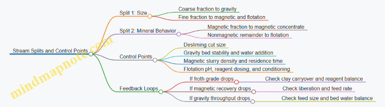
Sequencing Logic Checklist for Stable Performance
- Do a mass balance by stream, not just by final products; hybrid circuits can hide losses in intermediate recycles.
- Match cut sizes to equipment limits: gravity needs a workable settling range, magnetic separation needs stable slurry flow, flotation needs manageable slimes.
- Prevent cross-contamination: if dense gangue or magnetic minerals are likely to report to flotation, remove them earlier.
- Tune each step to the next step’s feed: the goal is not maximum recovery in the first unit, but the best overall recovery at acceptable grade.
When these pieces align, the hybrid circuit behaves like a set of coordinated filters: gravity reduces bulk and dense interference, magnetic separation captures the obvious magnetic fraction, and flotation finishes the job on the fine, chemistry-sensitive remainder.
12.2 Dewatering Technologies: Thickening, Filtration, and Drying Basics
Dewatering is the step that turns a slurry—solid particles suspended in water—into a transportable product and a manageable water stream. The key idea is simple: you separate water from solids, but you must do it without losing too much valuable mineral to the water and without creating a cake that is impossible to handle.
Thickening Basics
Thickening concentrates solids by gravity settling, usually in a tank with a rotating rake. The feed enters near the center, and clarified overflow exits at the top. Underflow is the concentrated slurry sent to filtration or further processing.
Two practical concepts govern thickener performance: settling behavior and slurry rheology. Settling behavior depends on particle size, shape, and how strongly particles stick together. Slurry rheology matters because as solids increase, the mixture can become resistant to flow, which affects how well the underflow can be raked and pumped.
A useful way to think about thickening is the “traffic jam” effect. At low solids, particles have room to settle. As solids rise, particles interfere with each other, and the settling rate drops. That is why thickener control often focuses on maintaining a stable underflow density rather than chasing maximum concentration.
Example: Suppose a flotation tailings stream has 20% solids by weight and needs to reach about 50–60% solids before filtration. If the feed contains more slimes than expected, the settling rate slows and the overflow becomes cloudy. Operators respond by adjusting flocculant dosage, changing feed dilution, or revising the target underflow density to avoid unstable operation.
Filtration Basics
Filtration removes water by forcing slurry through a porous medium or by using a pressure differential. The result is a filter cake with much higher solids content and a filtrate that can often be recycled.
Common filtration types include vacuum filters, pressure filters, and belt filters. The choice depends on particle size distribution, cake permeability, and how much water must be removed.
Cake formation is the make-or-break step. If the cake is too fine or compressible, water removal slows and the filter can clog. If the cake is too coarse, you may get poor cake strength and higher moisture in the cake.
Example: A concentrate slurry with fine silica gangue may form a tight cake on a vacuum filter. Adding a conditioning step—such as controlled flocculation before filtration—can improve cake permeability and reduce specific filtration time. The goal is not “more flocculant,” but flocculant that creates stable, filterable aggregates.
Drying Basics
Drying is the final moisture reduction step, typically used when product specifications require low water content for storage or transport. Drying can be done with thermal methods such as rotary dryers or indirect dryers.
Drying is energy-intensive, so it is usually applied after filtration has already removed most free water. The remaining water is often bound within pores or held by surface forces, so drying conditions must be controlled to avoid excessive heat that can change material properties.
Example: If a concentrate specification requires low moisture, filtration may reduce moisture from, say, 30% to 10–15%. Drying then targets the last portion. Operators monitor exhaust temperature and residence time to prevent overheating that could affect downstream handling.
Integrated Mind Map
Dewatering Technologies Mind Map
Practical System Logic
A coherent dewatering system matches the equipment to the slurry’s behavior. Thickening is best at removing free water efficiently when particles settle reasonably well. Filtration is best when you need a strong cake and a clear filtrate, especially after thickening has reduced the water load. Drying is reserved for the moisture that filtration cannot remove economically.
Example: If a plant sees rising filter cake moisture, the issue may start upstream in thickener overflow clarity or underflow density. Fixing the thickener feed solids and flocculant addition can improve cake formation, which then reduces filtration time and lowers the drying requirement. In other words, dewatering is not three separate machines; it is one connected water-removal chain.
12.3 Tailings Management: Thickener Underflow Handling and Slime Control
Thickener underflow is where “separation” turns into “transport.” Gravity has already done its job in the thickener, so the underflow must be handled so it stays pumpable, settles predictably in downstream units, and does not create new problems like excessive viscosity, plugging, or poor water recovery.
Foundational Goals for Underflow Handling
A thickener underflow should meet three practical targets: (1) consistent solids concentration, (2) stable rheology so pumps and pipelines behave, and (3) controlled slime behavior so fine particles do not migrate into the wrong streams. The underflow concentration is not just a number; it determines slurry viscosity, which controls pressure drop, wear, and the ability to dewater further.
A helpful mental model is to treat the underflow as a “moving sediment.” If the sediment is too dilute, you waste pumping energy and reduce thickener efficiency. If it is too concentrated without proper conditioning, the slurry becomes hard to move and can form deposits.
Slime Control: What “Slimes” Do in Practice
Slimes are very fine particles that tend to remain suspended, increase water demand, and reduce settling rates. In tailings systems, slimes can also carry over into clarified water, raising turbidity and increasing the load on return-water clarification.
Slime control starts with recognizing that fine particles behave differently from sand-sized solids. They have higher surface area, so they adsorb reagents and water, and they can form flocs that either settle well or break apart depending on chemistry and shear.
Thickener Underflow Handling Workflow
- Choose the target underflow density based on downstream needs. If the underflow feeds a filter, you want a relatively high solids content to reduce filter load. If it feeds a tailings pipeline, you want a concentration that stays pumpable at expected line velocities.
- Stabilize the feed to the thickener. Variations in feed solids, particle size, and flocculant dosage show up as underflow density swings. Those swings then cause pipeline pressure fluctuations.
- Manage flocculation and shear. Flocculated aggregates settle faster, but they can be damaged by excessive shear in transfer lines. Underflow lines should be designed and operated to minimize unnecessary turbulence.
- Control underflow withdrawal rate. Over-withdrawing can thin the underflow and reduce settling efficiency. Under-withdrawing can thicken the underflow and raise viscosity beyond what pumps can handle.
- Monitor and correct using underflow density, torque/current on drives, and pressure at key points. When you see rising pressure with stable density, it often indicates increasing viscosity from slime behavior or poor dispersion.
Practical Examples of Slime Control Decisions
Example: High turbidity in return water. If clarified overflow turbidity rises, check whether slimes are escaping due to insufficient settling time or flocculation. A common fix is adjusting flocculant dosage and ensuring adequate mixing time before the thickener. If dosage increases but turbidity worsens, it can mean over-flocculation that creates fragile flocs that break under shear.
Example: Underflow becomes difficult to pump. Suppose underflow density is near target, but pipeline pressure rises and flow rate drops. This can happen when slime content increases or when flocs are breaking, turning a structured slurry into a more viscous one. The operational response is to reduce shear in transfer, verify flocculant addition points, and confirm that the thickener is not being operated at an underflow withdrawal rate that forces the sediment to compact too aggressively.
Advanced Details That Prevent Recurring Issues
- Sediment bed behavior: The bed should compact in a controlled way. If the bed compacts too quickly, it can lead to higher underflow viscosity and potential underflow line plugging. If it compacts too slowly, you get dilute underflow and poor water recovery.
- Desliming upstream: When feasible, removing a portion of the finest fraction before the thickener reduces the slime load. This can be done by classification steps that separate coarse and fine fractions, so the thickener sees a more settling-friendly feed.
- Rheology-aware pumping: Slurry viscosity depends on solids concentration and particle interactions. Pump selection and operating points should match the expected underflow rheology, not just the average density.
Mind Map: Thickener Underflow Handling and Slime Control
Quick Checklist for Day-to-Day Operation
If underflow density drifts, first verify feed consistency. If overflow turbidity rises, focus on flocculation quality and settling time. If pumping pressure rises without density change, suspect slime-driven viscosity changes or floc damage from shear. In all cases, correct the cause upstream of the thickener rather than compensating downstream with brute-force changes.
12.4 Quality Assurance for Products: Assay Verification, Moisture Control, and Sampling
Quality assurance for concentrates is mostly about making sure the number on the report matches what the customer actually receives. That means controlling sampling representativeness, verifying assay results with repeatable procedures, and tracking moisture so grade and payment calculations stay consistent.
Assay Verification Fundamentals
Start with the idea that an assay is a chain: sample collection → sample preparation → analytical measurement → calculation. Break any link and the final grade becomes a story with missing chapters.
Verification by mass balance checks. If you have a flowsheet, compare expected product grade from circuit performance (mass pull and feed grade) with the lab result. For example, if a rougher–cleaner circuit typically yields a 30% mass pull and the feed assay is 1.2% Cu, a product around 3–4% Cu is plausible. A result of 0.8% Cu would trigger a review of sampling or preparation, not a shrug.
Verification by method repeatability. Run duplicates from the same prepared sample. If two determinations of, say, Fe in a magnetite concentrate differ beyond your lab’s control limits, investigate before issuing final numbers. A simple rule of thumb: if the lab can’t reproduce its own prepared sample, the plant data won’t help.
Verification by reference materials. Use certified reference materials or internal standards to confirm the instrument and chemistry are behaving. For instance, if a reference material for Au shows a consistent bias low by 5%, you correct or re-run the batch rather than silently accepting the drift.
Moisture Control for Payment-Grade Consistency
Moisture matters because many contracts price on a dry basis. If moisture changes but the dry-basis conversion is wrong, the customer pays for water—or you do.
Define the basis clearly. Decide whether the reported grade is on a wet basis, dry basis, or both. Then apply the same basis to every shipment.
Measure moisture with a controlled procedure. Moisture tests should use consistent drying conditions and timing. For a concentrate that contains easily oxidized sulfides, drying too aggressively can alter chemistry and indirectly affect assay. A practical approach is to use a standardized drying method that your lab has validated for the specific product.
Use moisture as a control variable. Track moisture trends by shift or by batch. Example: if a thickener underflow becomes more dilute during a pump change, moisture in the filter cake rises. If you only measure moisture once per day, you’ll miss the window where the product grade on a dry basis is miscalculated.
Sampling That Actually Represents the Product
Sampling is where most “mystery grade” problems begin. The goal is not to collect more material; it’s to collect the right material.
Choose the sampling point based on flow behavior. If the product is conveyed, take samples from a location with stable flow and minimal segregation. If the product is bagged, sample across bags rather than grabbing the first and last.
Use incremental sampling and compositing. For a shipment, collect multiple increments over time or across the stream, then composite them. Example: instead of one grab sample from a 10-hour loading period, take 10 increments evenly spaced. This reduces the impact of short-term fluctuations.
Control particle size and segregation. Fine particles can segregate in chutes and bins. If your concentrate contains a wide size distribution, ensure the sampling device doesn’t preferentially pull fines or oversize grains.
Document chain of custody. Labeling errors are common and boring, which is exactly why they’re dangerous. Record sample ID, time, location, operator, and any deviations.
Integrated QA Workflow
A systematic workflow keeps the process from becoming a checklist that nobody trusts.
- Plan the sampling event: define product, basis, sampling frequency, and increment count.
- Collect and composite: use the same sampling method each time.
- Prepare consistently: crushing, splitting, and grinding steps must be standardized.
- Run verification assays: duplicates plus reference materials.
- Measure moisture: apply the moisture basis conversion to assay.
- Perform reasonableness checks: compare with expected mass pull and circuit behavior.
- Release with traceability: store sample IDs and results so you can reproduce the decision.
Mind Map: Product Quality Assurance
Example: Concentrate Shipment with QA Flags
A plant ships a zinc concentrate. The lab reports 52.0% Zn on a dry basis, but the moisture test shows 8.0% water. The contract expects dry-basis pricing, so the wet-basis equivalent is 47.8% Zn (52.0 × (1 − 0.08)). During QA, duplicates differ by 0.6% Zn, within control limits, and the reference material matches the expected range. However, the reasonableness check compares the measured mass pull to the circuit’s typical performance and finds the product mass pull is unusually low. The QA team re-checks the sampling increments and discovers that one increment came from a different belt section during a short belt speed change. After re-compositing with the corrected increment set, the final Zn grade is updated and the moisture basis remains valid.
This is the point of QA: not to produce perfect numbers, but to ensure the numbers are defensible and traceable to the material that left the plant.
12.5 Practical Example: Producing and Handling Concentrates for Shipment with Spec Constraints
A spec-constrained concentrate is basically a contract in solids form: you must hit grade, recovery-linked impurities, and physical limits (moisture, size, and sometimes chemistry like chloride or silica). The practical goal is to turn a lab-validated flowsheet into a stable product stream that survives sampling, transport, and customer testing.
Step 1: Translate Spec Into Measurable Targets
Start by converting each customer requirement into a measurable internal target.
- Grade targets: e.g., Cu in concentrate, Fe in magnetite concentrate.
- Impurity limits: e.g., silica, phosphorus, arsenic, or MgO.
- Physical limits: moisture %, particle size (if relevant), and density.
- Process-linked constraints: reagent residues or water chemistry can affect downstream acceptance.
Example: A copper concentrate spec might require 28–30% Cu, max 2% SiO₂, and moisture below 10%. Your internal targets could be set slightly tighter (for instance, 29% Cu average with a 95% confidence margin) because sampling and test variability are real.
Step 2: Lock the Product Stream at the Source
Concentrate quality is usually decided by what happens right before thickening and filtration.
- Control the circuit feed: stable cyclone cut size (for grinding circuits feeding flotation) reduces variability in liberation.
- Control flotation residence and reagent dosing: small shifts in pH or collector dosage can change both grade and impurity entrainment.
- Separate “grade” from “water”: thickener and filter performance can change moisture and apparent assay.
Example: If silica rises, check whether it’s coming from gangue entrainment (flotation) or from poor desliming (feed preparation). Fixing the wrong unit operation wastes time and keeps the spec problem alive.
Step 3: Use a Sampling Plan That Matches the Product Reality
Sampling is where good plants go to lose points.
- Choose the right sampling point: ideally after dewatering, where moisture is stable.
- Use composite sampling for bulk variability: a single grab sample can misrepresent the lot.
- Match customer test method: if the customer uses a specific digestion or drying protocol, your internal lab should mirror it.
Example: A concentrate lot shipped with 9.5% moisture might test at 11% if the customer dries differently. Align methods so the spec comparison is apples-to-apples.
Step 4: Dewater to Spec, Not to “Good Enough”
Moisture affects handling, storage stability, and sometimes assay.
- Thickener underflow density influences filtration efficiency.
- Filter cake moisture depends on vacuum/pressure, cloth condition, and slurry solids.
- Avoid over-washing: it can lower moisture but also remove fine valuable minerals or increase impurity ratios.
Example: If moisture is drifting upward, first check filter cloth blinding and vacuum stability. If moisture is stable but grade drifts, the issue is upstream separation, not dewatering.
Step 5: Build a Lot-Control Routine for Shipment
A “lot” is a defined time window or mass batch with documented quality.
- Define lot boundaries: start/stop based on stable operating conditions.
- Track key control variables: feed rate, reagent rates, cyclone cut, thickener underflow density, filter vacuum/pressure.
- Hold-and-release logic: if assay or moisture is out of tolerance, stop the lot from mixing with good material.
Example: Suppose the plant produces 200 tons per day. If assays show Cu grade trending low during a 2-hour window, you can isolate that window as a separate lot rather than blending it into the next shipment.
Step 6: Handle Concentrate So It Stays the Same Concentrate
Physical handling can change what the customer receives.
- Minimize segregation: avoid long drop heights that can separate fines and coarser particles.
- Control dust and spillage: losses can shift grade and create safety issues.
- Use consistent packaging and labeling: moisture and test results must match the lot ID.
Example: If you load into bulk bags, ensure the discharge rate doesn’t cause fines to preferentially flow out first. A simple operational change—like adjusting discharge speed—can reduce lot-to-lot variability.
Mind Map: Concentrate Shipment with Spec Constraints
Worked Example: Closing the Gap to Spec
Assume a magnetite concentrate spec requires Fe 66–68%, SiO₂ max 3%, and moisture 8–10%.
- Moisture is on target but Fe is low: focus on separation efficiency (e.g., magnetic intensity and feed size distribution), not filtration.
- SiO₂ spikes during certain shifts: check whether desliming performance or cyclone overflow carryover changed.
- Lot variability is high: tighten lot boundaries and increase composite sampling frequency during transitions.
The key is that each symptom points to a specific control layer: upstream separation for grade/impurities, dewatering for moisture, and sampling/lot logic for variability. When those layers are managed together, spec compliance becomes a routine outcome rather than a last-minute scramble.