Financial Statement Analysis and Corporate Finance Principles for Investment Professionals
1. Introduction to Financial Statement Analysis
1.1 Overview of Financial Statements: Balance Sheet, Income Statement, and Cash Flow Statement
Financial statements are the backbone of corporate financial analysis, providing a structured and standardized way to understand a company’s financial health, performance, and cash movements. For investment professionals, mastering these statements is essential for making informed decisions.
The Three Core Financial Statements
- Balance Sheet
- Income Statement
- Cash Flow Statement
Each statement serves a unique purpose and collectively offers a comprehensive picture of a company’s financial condition.
Mind Map: Core Financial Statements Overview
Balance Sheet: Snapshot of Financial Position
The balance sheet provides a snapshot of a company’s financial position at a specific point in time. It follows the fundamental accounting equation:
Assets = Liabilities + Equity
- Assets represent resources owned by the company.
- Liabilities are obligations owed to outsiders.
- Equity represents the owners’ residual interest.
Example:
Consider a company with:
- Cash and equivalents: $100,000
- Accounts receivable: $50,000
- Property, plant & equipment: $200,000
- Accounts payable: $40,000
- Long-term debt: $150,000
- Shareholders’ equity: $160,000
The balance sheet would confirm that $350,000 (assets) = $190,000 (liabilities) + $160,000 (equity).
Income Statement: Performance Over Time
The income statement summarizes revenues and expenses over a period, showing profitability.
Key components include:
- Revenue: Income from sales or services.
- Cost of Goods Sold (COGS): Direct costs of producing goods.
- Operating Expenses: Selling, general & administrative expenses.
- Net Income: Bottom-line profit after all expenses.
Example:
A company reports:
- Revenue: $500,000
- COGS: $300,000
- Operating expenses: $120,000
- Interest expense: $10,000
- Tax expense: $14,000
Net Income = $500,000 - $300,000 - $120,000 - $10,000 - $14,000 = $56,000
Cash Flow Statement: Cash Movement Insights
The cash flow statement explains changes in cash during a period, divided into three sections:
- Operating Activities: Cash from core business operations.
- Investing Activities: Cash used for or generated from investments in assets.
- Financing Activities: Cash flows from borrowing, repaying debt, or equity transactions.
Example:
- Cash from operations: $70,000
- Cash used in investing: -$30,000 (purchase of equipment)
- Cash from financing: $20,000 (new debt raised)
Net increase in cash = $70,000 - $30,000 + $20,000 = $60,000
Mind Map: Relationship Between Financial Statements
Integrated Example: Understanding a Company’s Financial Health
Imagine analyzing Company ABC:
- The balance sheet shows strong assets but high short-term liabilities.
- The income statement reveals growing revenues but shrinking profit margins.
- The cash flow statement indicates positive operating cash flow but heavy investing outflows.
Interpretation:
- The company is expanding (investing heavily), which may pressure short-term liquidity.
- Profit margin decline signals cost management issues.
- Positive operating cash flow is a good sign of core business strength.
Best Practices for Investment Professionals
- Always analyze the three statements together to get a holistic view.
- Pay attention to the timing differences between income recognition and cash flows.
- Use the balance sheet to assess financial stability and capital structure.
- Track trends over multiple periods rather than relying on a single snapshot.
- Validate data consistency across statements (e.g., net income should reconcile with cash flow from operations).
Mastering these fundamentals sets the foundation for deeper financial analysis and corporate finance decision-making.
1.2 Importance of Financial Statement Analysis in Investment Banking and Financial Analysis
Financial statement analysis is a cornerstone skill for investment bankers and financial analysts. It enables professionals to make informed decisions by interpreting the financial health, performance, and prospects of companies. This section explores why financial statement analysis is critical in these roles, supported by mind maps and practical examples.
Why Financial Statement Analysis Matters
- Investment Decision-Making: Helps determine the viability and risk of investments.
- Valuation Accuracy: Provides the quantitative foundation for company valuation.
- Credit Assessment: Assesses a company’s ability to meet debt obligations.
- Strategic Advisory: Supports M&A, restructuring, and capital raising decisions.
- Performance Monitoring: Tracks financial trends and operational efficiency.
Mind Map: Core Purposes of Financial Statement Analysis
Example 1: Investment Banking – Evaluating an M&A Target
An investment banker analyzing a potential acquisition target reviews the target’s financial statements to:
- Understand revenue growth and profit margins.
- Assess debt levels and liquidity to gauge financial risk.
- Identify any unusual accounting items that may distort earnings.
- Forecast future cash flows to estimate valuation.
Best Practice: Use common-size financial statements and ratio analysis to compare the target against industry peers, ensuring a relative perspective.
Mind Map: Financial Statement Analysis in M&A
Example 2: Financial Analyst – Credit Risk Assessment
A financial analyst at a credit rating agency examines a company’s financial statements to determine creditworthiness:
- Calculates interest coverage ratio to evaluate the ability to pay interest expenses.
- Analyzes cash flow from operations to ensure sufficient liquidity.
- Reviews maturity schedules of debt to anticipate refinancing needs.
Best Practice: Combine quantitative ratio analysis with qualitative factors such as industry outlook and management quality.
Mind Map: Financial Statement Analysis for Credit Risk
Summary
Financial statement analysis is indispensable for investment professionals. It provides a structured approach to decode complex financial data, enabling better investment decisions, accurate valuations, effective credit assessments, and strategic advisory services. Mastery of this skill, combined with best practices such as comparative analysis and integration of qualitative insights, equips professionals to add significant value in their roles.
1.3 Key Users of Financial Statements and Their Analytical Needs
Financial statements serve as a critical source of information for various stakeholders who rely on them to make informed decisions. Understanding who these key users are and what their specific analytical needs entail is fundamental for investment professionals such as investment bankers and financial analysts. This section explores the primary users of financial statements, their objectives, and the best practices for tailoring analysis to meet their requirements.
Mind Map: Key Users of Financial Statements
Investors
Equity Investors focus on the company’s ability to generate profits and grow shareholder value. They analyze earnings trends, dividend policies, and return ratios such as Return on Equity (ROE). For example, an equity investor reviewing a tech startup might prioritize revenue growth and R&D expenses to gauge future potential rather than just current profits.
Debt Investors (bondholders, banks) prioritize the company’s ability to meet interest and principal payments. They focus on liquidity ratios (current ratio, quick ratio), leverage ratios (debt-to-equity), and cash flow adequacy. For instance, a bank considering a loan to a manufacturing firm will analyze the firm’s operating cash flow and interest coverage ratio to assess repayment capacity.
Management
Management uses financial statements to evaluate operational efficiency and guide strategic decisions. They analyze cost structures, profitability by segment, and capital expenditure needs. For example, a CFO might use segment reporting to decide whether to expand or divest a business unit based on its profit margin and cash flow contribution.
Creditors and Lenders
Creditors assess the risk of lending by analyzing solvency and liquidity. They often require detailed covenant compliance reports and monitor financial ratios regularly. For example, a lender may impose a covenant requiring the company to maintain a minimum interest coverage ratio of 3.0x to reduce default risk.
Regulators
Regulatory bodies ensure companies comply with accounting standards and financial disclosure requirements. They analyze financial statements to detect irregularities or potential fraud. For example, the SEC reviews public companies’ filings to ensure transparency and protect investors.
Employees
Employees may use financial statements to assess job security and negotiate compensation. Profitability and cash flow trends can influence bonus schemes or profit-sharing plans. For example, union representatives might analyze the company’s earnings before negotiating wage increases.
Customers and Suppliers
Long-term customers and suppliers evaluate a company’s financial health to ensure continuity of business relationships. A supplier might review a retailer’s liquidity to decide on credit terms.
Analysts and Advisors
Financial analysts and advisors synthesize financial data to provide investment recommendations. They require comprehensive, accurate data and often perform ratio analysis, trend analysis, and valuation modeling.
Example: Tailoring Financial Analysis for Different Users
Consider a publicly traded consumer goods company:
- Equity Investor: Focuses on earnings growth, dividend payout ratio, and market valuation multiples like P/E ratio.
- Debt Investor: Concentrates on debt-to-equity ratio, interest coverage, and free cash flow to service debt.
- Management: Reviews segment profitability, operating margins, and capital expenditure efficiency.
- Lender: Monitors liquidity ratios and covenant compliance.
By understanding these distinct needs, investment professionals can customize their analysis and reporting to provide relevant insights.
Best Practice
- Identify the primary user(s) before conducting analysis. This ensures the focus is aligned with their decision-making criteria.
- Use appropriate financial metrics and ratios tailored to each user’s needs. For example, prioritize cash flow metrics for creditors and growth metrics for equity investors.
- Communicate findings in a clear, concise manner emphasizing the aspects most relevant to the user.
This user-centric approach enhances the value of financial statement analysis and supports more effective corporate finance decisions.
1.4 Best Practices for Initial Financial Data Gathering and Validation
Financial data gathering and validation form the foundation of any robust financial statement analysis. For investment professionals, ensuring accuracy and completeness at this stage is critical to making informed decisions. This section outlines best practices, supported by clear examples and mind maps, to streamline the process.
Key Steps in Financial Data Gathering and Validation
Best Practice #1: Use Multiple Reliable Data Sources
Relying on a single source can lead to incomplete or biased data. Cross-checking financial statements from company filings (e.g., 10-K) with independent databases like Bloomberg or Capital IQ helps verify accuracy.
Example:
When analyzing Company ABC, an investment analyst first downloads the latest 10-K from the SEC EDGAR database. They then compare key figures such as total assets and net income with Bloomberg terminal data. Minor discrepancies prompt a review of the notes section, revealing a recent asset revaluation not yet reflected in Bloomberg.
Best Practice #2: Validate Data Consistency Across Statements
The balance sheet, income statement, and cash flow statement should reconcile logically. For instance, net income from the income statement should align with the change in retained earnings on the balance sheet.
Example:
An analyst notices that Company XYZ’s net income is $5 million, but retained earnings increased by only $3 million. Upon reviewing the notes, they discover a $2 million dividend payout, explaining the difference. This validation prevents misinterpretation of profitability.
Best Practice #3: Perform Ratio and Trend Analysis Early
Applying preliminary ratio analysis (e.g., current ratio, debt-to-equity) and trend analysis over multiple periods helps identify outliers or data entry errors.
Example:
While reviewing historical data for Company DEF, an analyst observes an unusual spike in the debt-to-equity ratio in the latest quarter. This triggers a deeper dive, revealing a recent debt issuance that was not clearly documented in the initial data set.
Best Practice #4: Document Data Sources and Maintain Version Control
Maintaining a clear audit trail of where data was sourced and tracking versions of datasets ensures transparency and facilitates updates.
Example:
An analyst creates a spreadsheet with tabs for raw data, cleaned data, and analysis. Each tab includes notes on data origin and date accessed. When new quarterly data arrives, the analyst updates the raw data tab and saves a new version, preserving prior work.
Mind Map: Validation Techniques
Summary
Initial financial data gathering and validation require a disciplined approach combining multiple data sources, consistency checks, and thorough documentation. By embedding these best practices into the workflow, investment professionals can build a reliable foundation for deeper financial analysis and corporate finance decision-making.
1.5 Example: Analyzing a Sample Company’s Financial Statements for the First Time
When approaching a company’s financial statements for the first time, it is crucial to have a structured framework to guide your analysis. This example will walk you through the initial steps of analyzing a hypothetical company, “TechNova Inc.”, using its Balance Sheet, Income Statement, and Cash Flow Statement.
Step 1: Understand the Company and Its Industry
- Gather background information about TechNova Inc.: sector, business model, competitors.
- Understand industry-specific financial characteristics (e.g., capital intensity, typical margins).
Step 2: Review the Financial Statements Overview
- Identify the reporting period.
- Note any accounting policies or changes disclosed in the notes.
Step 3: Analyze the Balance Sheet
Mind Map: Balance Sheet Analysis
Example:
- TechNova’s current assets are $150M, with cash of $40M, receivables of $60M, and inventory of $50M.
- Current liabilities total $100M, including $30M in accounts payable and $20M in short-term debt.
Initial Observations:
- Current Ratio = Current Assets / Current Liabilities = 150M / 100M = 1.5 (indicates reasonable liquidity).
Step 4: Analyze the Income Statement
Mind Map: Income Statement Analysis
Example:
- TechNova reports revenue of $500M.
- COGS is $300M, resulting in a gross profit of $200M.
- Operating expenses total $120M.
- Operating income is $80M.
- Interest expense is $10M, taxes are $15M.
- Net income is $55M.
Initial Observations:
- Gross Margin = 200M / 500M = 40%.
- Operating Margin = 80M / 500M = 16%.
- Net Profit Margin = 55M / 500M = 11%.
Step 5: Analyze the Cash Flow Statement
Mind Map: Cash Flow Statement Analysis
Example:
- Operating cash flow is $70M.
- Capital expenditures are $30M.
- Financing activities show $20M debt repayment and $5M dividends paid.
Initial Observations:
- Free Cash Flow = Operating Cash Flow - Capital Expenditures = 70M - 30M = $40M.
- Positive free cash flow indicates capacity to invest or return capital to shareholders.
Step 6: Synthesize Findings
Mind Map: Initial Financial Analysis Summary
Example:
- TechNova appears profitable with healthy margins.
- Liquidity is sufficient to cover short-term obligations.
- Generates positive free cash flow, supporting growth or shareholder returns.
Step 7: Next Steps and Best Practices
- Compare these metrics to industry peers for benchmarking.
- Review notes for off-balance sheet items or contingent liabilities.
- Look for trends by analyzing prior periods.
- Use ratio analysis to deepen insights.
Summary
This example demonstrates a systematic approach to analyzing a company’s financial statements for the first time. By breaking down each statement, calculating key metrics, and synthesizing insights, investment professionals can form a solid foundation for more advanced analysis and decision-making.
Remember: Always complement quantitative analysis with qualitative understanding of the company’s strategy, market position, and risks.
2. Understanding the Balance Sheet
2.1 Components of the Balance Sheet: Assets, Liabilities, and Equity
The balance sheet is a fundamental financial statement that provides a snapshot of a company’s financial position at a specific point in time. It is structured around the fundamental accounting equation:
Assets = Liabilities + Equity
Understanding each component is essential for investment professionals to analyze a company’s financial health, liquidity, and capital structure.
Assets
Assets represent the resources owned or controlled by a company that are expected to generate future economic benefits. They are typically classified into two categories:
- Current Assets: Assets expected to be converted into cash or used up within one year or the operating cycle, whichever is longer.
- Non-Current (Long-Term) Assets: Assets held for use over multiple years.
Common Current Assets:
- Cash and Cash Equivalents
- Accounts Receivable
- Inventory
- Prepaid Expenses
Common Non-Current Assets:
- Property, Plant, and Equipment (PP&E)
- Intangible Assets (e.g., patents, trademarks)
- Long-term Investments
Mind Map: Assets
Example:
Consider a manufacturing company with the following assets:
- Cash: $200,000
- Accounts Receivable: $150,000
- Inventory: $300,000
- PP&E: $1,200,000
- Patents: $100,000
Total Assets = $200,000 + $150,000 + $300,000 + $1,200,000 + $100,000 = $1,950,000
Liabilities
Liabilities are the company’s obligations or debts that it must settle in the future, usually through the transfer of assets or services. Like assets, liabilities are classified as:
- Current Liabilities: Obligations due within one year or the operating cycle.
- Non-Current (Long-Term) Liabilities: Obligations due beyond one year.
Common Current Liabilities:
- Accounts Payable
- Short-term Debt
- Accrued Expenses
- Current Portion of Long-Term Debt
Common Non-Current Liabilities:
- Long-Term Debt (e.g., bonds, bank loans)
- Deferred Tax Liabilities
- Pension Obligations
Mind Map: Liabilities
Example:
Using the same manufacturing company:
- Accounts Payable: $180,000
- Short-term Debt: $100,000
- Long-Term Debt: $700,000
Total Liabilities = $180,000 + $100,000 + $700,000 = $980,000
Equity
Equity represents the residual interest in the assets of the company after deducting liabilities. It reflects the owners’ claims and includes:
- Common Stock: Par value of shares issued.
- Additional Paid-In Capital: Amount paid by investors above par value.
- Retained Earnings: Accumulated net income not distributed as dividends.
- Treasury Stock: Shares repurchased by the company (contra equity account).
Mind Map: Equity
Example:
Continuing with the manufacturing company:
- Common Stock: $500,000
- Additional Paid-In Capital: $200,000
- Retained Earnings: $270,000
Total Equity = $500,000 + $200,000 + $270,000 = $970,000
Putting It All Together
| Component | Amount ($) |
|---|---|
| Assets | 1,950,000 |
| Liabilities | 980,000 |
| Equity | 970,000 |
Check: Assets = Liabilities + Equity
$1,950,000 = $980,000 + $970,000
This confirms the balance sheet equation holds true.
Best Practice: Analyzing Balance Sheet Components
- Assess Asset Quality: Understand the liquidity and valuation methods of assets. For example, inventory valuation methods (FIFO, LIFO) can affect asset values.
- Evaluate Liability Maturity: Distinguish between short-term and long-term obligations to assess liquidity risk.
- Examine Equity Composition: Review retained earnings trends and share issuances or buybacks.
Example: Quick Analysis of a Balance Sheet Snapshot
Imagine you are analyzing Company XYZ’s balance sheet:
- Current Assets: $500,000
- Non-Current Assets: $1,000,000
- Current Liabilities: $300,000
- Long-Term Liabilities: $400,000
- Equity: $800,000
Step 1: Calculate total assets = $500,000 + $1,000,000 = $1,500,000
Step 2: Calculate total liabilities = $300,000 + $400,000 = $700,000
Step 3: Verify equity = Assets - Liabilities = $1,500,000 - $700,000 = $800,000
This confirms the balance sheet is balanced and provides a clear picture of Company XYZ’s financial position.
Summary Mind Map: Balance Sheet Components
Understanding these components deeply enables investment professionals to perform thorough financial analysis, identify risks, and make informed decisions.
2.2 Asset Classification and Valuation Techniques
Understanding asset classification and valuation is fundamental for investment professionals analyzing a company’s financial health. Assets represent resources controlled by a company expected to generate future economic benefits. Proper classification and valuation ensure accurate financial reporting and sound investment decisions.
Asset Classification
Assets are broadly classified into two main categories:
- Current Assets
- Non-Current (Long-Term) Assets
Mind Map: Asset Classification
Current Assets
Current assets are expected to be converted into cash or used up within one operating cycle or one year, whichever is longer. Examples include:
- Cash and Cash Equivalents: Highly liquid assets like cash on hand and short-term investments.
- Accounts Receivable: Money owed by customers.
- Inventory: Raw materials, work-in-progress, and finished goods.
Non-Current Assets
Non-current assets provide long-term value and are not expected to be liquidated within a year. Examples include:
- Property, Plant, and Equipment (PP&E): Tangible fixed assets like buildings, machinery.
- Intangible Assets: Non-physical assets such as patents and goodwill.
Valuation Techniques
Accurate valuation of assets is critical for assessing company worth and making investment decisions. The valuation method depends on asset type and accounting standards.
Historical Cost Method
Assets are recorded at their original purchase price, less accumulated depreciation or amortization.
- Best Practice: Useful for PP&E where market value is stable.
Example: A machine purchased for $100,000 with a useful life of 10 years is recorded at $100,000 and depreciated annually.
Fair Value Method
Assets are recorded at their current market value.
- Best Practice: Used for marketable securities and investment properties.
Example: A portfolio of stocks purchased at $50,000 is reported at $60,000 if the market value increases.
Net Realizable Value (NRV)
Used primarily for inventory valuation, NRV is the estimated selling price minus costs to complete and sell.
- Best Practice: Ensures inventory is not overstated.
Example: Inventory costing $30,000 has an NRV of $25,000 due to obsolescence; it should be written down to $25,000.
Present Value Method
Used for long-term receivables or assets with future cash flows, discounting expected cash flows to present value.
- Best Practice: Important for valuing financial assets and intangible assets with measurable cash flows.
Example: A patent expected to generate $10,000 annually for 5 years is valued by discounting those cash flows to present value.
Mind Map: Asset Valuation Techniques
Integrated Example: Asset Classification and Valuation
Scenario: Company ABC’s balance sheet includes:
- Cash: $20,000
- Accounts Receivable: $50,000
- Inventory: $40,000 (NRV estimated at $35,000)
- Machinery (PP&E): Purchased for $200,000, accumulated depreciation $50,000
- Patent: Expected future cash flows discounted to $30,000
Analysis:
- Cash and Accounts Receivable: Classified as current assets, valued at face value.
- Inventory: Classified as current asset, valued at NRV ($35,000) due to obsolescence.
- Machinery: Non-current asset, valued at historical cost less depreciation ($150,000).
- Patent: Non-current intangible asset, valued using present value method ($30,000).
This classification and valuation provide a realistic picture of the company’s asset base for investment analysis.
Best Practices Summary
- Always classify assets based on liquidity and usage.
- Use valuation methods appropriate to asset type and industry standards.
- Regularly review asset values for impairment or obsolescence.
- Cross-check valuation with market data when available.
- Document assumptions used in valuation for transparency.
By mastering asset classification and valuation techniques, investment professionals can better assess a company’s financial position, identify risks, and make informed recommendations.
2.3 Liability Structures and Their Implications for Financial Health
Liabilities represent a company’s financial obligations and debts that it must settle in the future. Understanding the structure of liabilities is crucial for investment professionals because it directly impacts a firm’s liquidity, solvency, and overall financial health.
Types of Liabilities
Liabilities are generally classified into two main categories:
- Current Liabilities: Obligations due within one year.
- Non-Current Liabilities (Long-Term Liabilities): Obligations due beyond one year.
Mind Map: Liability Classification
Current Liabilities: Key Components and Implications
- Accounts Payable: Money owed to suppliers; reflects operational efficiency.
- Short-term Debt: Loans or borrowings due within a year; affects liquidity.
- Accrued Expenses: Expenses recognized but not yet paid; indicates timing of cash outflows.
- Current Portion of Long-term Debt: Portion of long-term debt due in the next year; important for cash flow planning.
Implications:
- High current liabilities relative to current assets may signal liquidity risk.
- Efficient management of payables and accruals can improve working capital.
Example:
Company A has current assets of $500,000 and current liabilities of $600,000. This results in a current ratio of 0.83, indicating potential liquidity issues since the company may struggle to cover short-term obligations.
Non-Current Liabilities: Key Components and Implications
- Long-term Debt: Loans and bonds payable beyond one year; affects leverage and interest expenses.
- Bonds Payable: Debt securities issued to investors; may have fixed or variable interest rates.
- Deferred Tax Liabilities: Taxes owed but deferred to future periods; impacts future cash outflows.
- Lease Obligations: Long-term lease commitments; recognized under accounting standards like IFRS 16.
Implications:
- Long-term liabilities influence the company’s capital structure and financial risk.
- Excessive long-term debt can increase bankruptcy risk but may also provide leverage benefits.
Example:
Company B has $2 million in long-term debt with an interest rate of 6%. If earnings before interest and taxes (EBIT) are $300,000, the interest coverage ratio is:
\[ \text{Interest Coverage Ratio} = \frac{EBIT}{Interest Expense} = \frac{300,000}{2,000,000 \times 0.06} = 2.5 \]
A ratio of 2.5 indicates moderate ability to cover interest payments but may be a warning sign if it declines.
Liability Structure and Financial Health
The composition and maturity profile of liabilities affect several key financial health indicators:
- Liquidity: Ability to meet short-term obligations.
- Solvency: Ability to meet long-term obligations.
- Financial Flexibility: Capacity to raise funds or restructure debt.
Mind Map: Liability Structure Impact on Financial Health
Best Practices for Analyzing Liability Structures
- Assess Maturity Profiles: Understand when liabilities come due to anticipate refinancing needs.
- Evaluate Interest Rates and Covenants: Fixed vs. variable rates affect risk; covenants may restrict operations.
- Compare to Industry Benchmarks: Contextualize leverage and liquidity ratios.
- Analyze Trends Over Time: Increasing liabilities without asset growth may indicate risk.
- Incorporate Off-Balance Sheet Liabilities: Such as operating leases or guarantees.
Integrated Example: Liability Structure Analysis of Company C
Company C’s balance sheet shows:
- Current Liabilities: $800,000
- Current Assets: $1,200,000
- Long-term Debt: $3,000,000 at 5% interest
- EBIT: $400,000
- Equity: $4,000,000
Step 1: Liquidity Analysis
- Current Ratio = $1,200,000 / $800,000 = 1.5 (healthy liquidity)
Step 2: Leverage Analysis
- Debt-to-Equity = ($800,000 + $3,000,000) / $4,000,000 = 0.95 (moderate leverage)
Step 3: Interest Coverage
- Interest Expense = $3,000,000 * 5% = $150,000
- Interest Coverage Ratio = $400,000 / $150,000 = 2.67 (adequate coverage)
Step 4: Interpretation
- Company C maintains a balanced liability structure with sufficient liquidity and manageable leverage.
- The interest coverage ratio suggests the company can comfortably meet interest payments.
Summary
Understanding liability structures enables investment professionals to:
- Evaluate short-term liquidity risks and long-term solvency.
- Assess financial flexibility and risk exposure.
- Make informed recommendations on capital structure optimization.
By integrating detailed liability analysis with other financial statement components, professionals can form a comprehensive view of a company’s financial health.
2.4 Equity Analysis: Shareholder’s Equity and Retained Earnings
Overview
Shareholder’s equity represents the residual interest in the assets of a company after deducting liabilities. It is a critical component of the balance sheet and provides insight into the company’s net worth from the shareholders’ perspective. Understanding equity and retained earnings helps investment professionals assess the company’s financial stability, growth potential, and dividend capacity.
Components of Shareholder’s Equity
- Common Stock: Par value of shares issued to shareholders.
- Additional Paid-In Capital (APIC): Amount paid by investors above the par value.
- Retained Earnings: Cumulative net income retained in the business after dividends.
- Treasury Stock: Shares repurchased by the company, reducing equity.
- Other Comprehensive Income: Gains/losses excluded from net income but affecting equity.
Mind Map: Components of Shareholder’s Equity
Understanding Retained Earnings
Retained earnings reflect the accumulated profits that have been reinvested in the company rather than distributed as dividends. It is calculated as:
\[ \text{Retained Earnings}_{end} = \text{Retained Earnings}_{beginning} + \text{Net Income} - \text{Dividends Paid} \]
This figure is crucial for evaluating how much profit a company has reinvested to fuel growth.
Mind Map: Retained Earnings Calculation
Best Practice: Analyzing Changes in Equity
Investment professionals should analyze changes in shareholder’s equity over time to understand capital raising activities, dividend policies, and profitability retention. Key steps include:
- Review Equity Statement: Examine the statement of changes in equity for detailed movements.
- Identify Capital Issuances or Buybacks: Note any new share issuances or treasury stock transactions.
- Analyze Dividend Trends: Understand how dividends impact retained earnings.
- Assess Profitability Impact: Correlate net income trends with retained earnings growth.
Example 1: Interpreting Shareholder’s Equity Movements
Company ABC’s equity section (in $ millions):
| Item | Year 1 | Year 2 |
|---|---|---|
| Common Stock | 100 | 100 |
| Additional Paid-In Capital | 200 | 250 |
| Retained Earnings | 300 | 350 |
| Treasury Stock | (50) | (50) |
| Total Shareholder’s Equity | 550 | 650 |
Analysis:
- APIC increased by $50 million, indicating new capital raised.
- Retained earnings grew by $50 million, reflecting net income retention.
- Treasury stock remained constant.
- Overall equity increased by $100 million, signaling strengthening financial position.
Example 2: Calculating Retained Earnings
Given:
- Beginning retained earnings: $500 million
- Net income for the year: $120 million
- Dividends paid: $40 million
Calculation:
\[ 500 + 120 - 40 = 580 \text{ million} \]
Interpretation: Retained earnings increased to $580 million, indicating the company retained a significant portion of its earnings for reinvestment.
Equity Analysis in Decision-Making
- Dividend Policy: A high retained earnings balance may indicate capacity to pay dividends or reinvest.
- Financial Health: Increasing equity generally signals financial strength.
- Capital Structure: Changes in equity affect leverage ratios and cost of capital.
Mind Map: Equity Analysis for Investment Professionals
Summary
Equity analysis, particularly understanding shareholder’s equity and retained earnings, is vital for investment professionals to evaluate a company’s financial foundation and growth trajectory. By combining quantitative calculations with qualitative insights, professionals can make informed recommendations on investments, capital structure, and dividend policies.
2.5 Best Practice: Assessing Liquidity and Solvency Using Balance Sheet Data
Assessing a company’s liquidity and solvency is fundamental for investment professionals to understand its short-term financial health and long-term viability. The balance sheet provides critical data to perform these assessments effectively.
Understanding Liquidity and Solvency
- Liquidity refers to a company’s ability to meet its short-term obligations using its most liquid assets.
- Solvency refers to the company’s capacity to meet long-term obligations and sustain operations over time.
Key Metrics for Liquidity Assessment
- Current Ratio = Current Assets / Current Liabilities
- Quick Ratio (Acid-Test Ratio) = (Current Assets - Inventories) / Current Liabilities
- Cash Ratio = Cash and Cash Equivalents / Current Liabilities
Key Metrics for Solvency Assessment
- Debt to Equity Ratio = Total Debt / Total Equity
- Interest Coverage Ratio = EBIT / Interest Expense
- Debt Ratio = Total Debt / Total Assets
Mind Map: Liquidity Assessment
Mind Map: Solvency Assessment
Step-by-Step Best Practice Approach
-
Gather Balance Sheet Data
- Extract current assets, inventories, cash, current liabilities, total debt, total equity, EBIT, and interest expense.
-
Calculate Liquidity Ratios
- Compute current, quick, and cash ratios.
- Compare against industry benchmarks.
-
Calculate Solvency Ratios
- Compute debt to equity, interest coverage, and debt ratios.
- Analyze trends over multiple periods.
-
Interpret Results
- Identify potential liquidity crunches or solvency risks.
- Consider qualitative factors such as industry cyclicality.
-
Integrate with Broader Financial Analysis
- Combine with cash flow and income statement insights for a holistic view.
Example: Assessing Liquidity and Solvency for XYZ Corp
Balance Sheet Extract (in $ millions):
| Item | Amount |
|---|---|
| Current Assets | 500 |
| Inventories | 150 |
| Cash and Equivalents | 100 |
| Current Liabilities | 400 |
| Total Debt | 700 |
| Total Equity | 800 |
Income Statement Extract:
| Item | Amount |
|---|---|
| EBIT | 200 |
| Interest Expense | 40 |
Calculations:
- Current Ratio = 500 / 400 = 1.25 (Healthy liquidity)
- Quick Ratio = (500 - 150) / 400 = 350 / 400 = 0.875 (Acceptable liquidity)
- Cash Ratio = 100 / 400 = 0.25 (Moderate cash buffer)
- Debt to Equity Ratio = 700 / 800 = 0.875 (Moderate leverage)
- Interest Coverage Ratio = 200 / 40 = 5 (Strong ability to cover interest)
- Debt Ratio = 700 / (700 + 800) = 700 / 1500 = 0.467 (Less than 50% assets financed by debt)
Interpretation:
- XYZ Corp shows solid liquidity with current and quick ratios above typical thresholds.
- Cash ratio is lower, suggesting limited immediate cash but acceptable given other liquid assets.
- Solvency ratios indicate moderate leverage and strong interest coverage, implying manageable long-term debt risk.
Summary
- Use multiple ratios to get a comprehensive picture.
- Always benchmark against industry standards.
- Analyze trends over time, not just single-period data.
- Combine quantitative analysis with qualitative insights for robust conclusions.
This best practice approach enables investment professionals to confidently assess a company’s financial health and make informed decisions.
2.6 Example: Interpreting a Real-World Balance Sheet to Identify Financial Strengths and Weaknesses
In this section, we will walk through a practical example of analyzing a real-world balance sheet to uncover a company’s financial strengths and weaknesses. This exercise is essential for investment bankers and financial analysts who need to make informed decisions based on a company’s financial health.
Step 1: Overview of the Balance Sheet
Let’s consider the simplified balance sheet of XYZ Corporation (all figures in millions):
| Assets | Amount | Liabilities & Equity | Amount |
|---|---|---|---|
| Current Assets | 500 | Current Liabilities | 300 |
| - Cash and Equivalents | 150 | - Accounts Payable | 120 |
| - Accounts Receivable | 200 | - Short-term Debt | 180 |
| - Inventory | 150 | Long-term Debt | 400 |
| Non-Current Assets | 1000 | Shareholders’ Equity | 800 |
| - Property, Plant & Equip | 700 | - Common Stock | 300 |
| - Intangible Assets | 300 | - Retained Earnings | 500 |
| Total Assets | 1500 | Total Liabilities & Equity | 1500 |
Step 2: Mind Map - Key Areas to Analyze
Step 3: Analyze Liquidity
Liquidity measures the company’s ability to meet short-term obligations.
-
Current Ratio = Current Assets / Current Liabilities = 500 / 300 = 1.67
- Interpretation: A current ratio above 1 indicates the company can cover its short-term liabilities with current assets, which is a positive sign.
-
Quick Ratio = (Current Assets - Inventory) / Current Liabilities = (500 - 150) / 300 = 350 / 300 = 1.17
- Interpretation: Excluding inventory, the company still has more than enough liquid assets to cover current liabilities.
Mind Map - Liquidity Analysis
Step 4: Analyze Solvency
Solvency assesses the company’s long-term financial stability.
-
Debt-to-Equity Ratio = Total Debt / Shareholders’ Equity = (300 + 400) / 800 = 700 / 800 = 0.875
- Interpretation: Less than 1, indicating the company uses less debt than equity to finance assets, which is generally conservative.
-
Interest Coverage Ratio (Assuming EBIT of 150 million and interest expense of 50 million):
- EBIT / Interest Expense = 150 / 50 = 3
- Interpretation: The company earns 3 times its interest expense, which is acceptable but could be improved.
Mind Map - Solvency Analysis
Step 5: Asset Quality and Composition
-
Intangible Assets represent 300 million out of 1000 million non-current assets (30%).
- High intangible assets may indicate strong brand value or intellectual property but can be less liquid and harder to value.
-
Inventory at 150 million is 30% of current assets.
- Inventory management efficiency should be monitored to avoid obsolescence.
Mind Map - Asset Quality
Step 6: Equity Position
- Retained Earnings of 500 million indicate accumulated profits reinvested in the company.
- Common Stock of 300 million reflects shareholder capital.
A strong equity base supports financial stability and growth potential.
Step 7: Summary of Financial Strengths and Weaknesses
| Strengths | Weaknesses |
|---|---|
| Healthy liquidity ratios (Current and Quick) | Moderate interest coverage ratio (3x) |
| Conservative debt-to-equity ratio (0.875) | Significant intangible assets (valuation risk) |
| Strong cash reserves (150 million) | Inventory concentration (risk of obsolescence) |
| Solid retained earnings supporting equity | Reliance on short-term debt (180 million) |
Step 8: Final Mind Map - Holistic View
Conclusion
By carefully interpreting the balance sheet of XYZ Corporation, investment professionals can identify that the company demonstrates solid liquidity and a conservative capital structure, which are financial strengths. However, attention should be paid to the moderate interest coverage ratio and the relatively high proportion of intangible assets and inventory, which pose potential risks.
This comprehensive approach, combining ratio analysis, asset composition review, and equity evaluation, equips investment bankers and financial analysts with actionable insights to support investment decisions, credit assessments, or corporate finance strategies.
3. Income Statement Analysis
3.1 Revenue Recognition and Its Impact on Financial Results
Revenue recognition is a fundamental accounting principle that determines the specific conditions under which income becomes realized as revenue. For investment professionals, understanding revenue recognition is critical because it directly affects the reported earnings, valuation, and financial health of a company.
What is Revenue Recognition?
Revenue recognition refers to the process and timing by which a company records revenue in its financial statements. The key principle is to recognize revenue when it is earned and realizable, not necessarily when cash is received.
Why It Matters for Financial Analysis
- Earnings Quality: Proper revenue recognition ensures earnings reflect the true economic activity.
- Comparability: Consistent revenue recognition policies allow for meaningful comparisons across companies and periods.
- Valuation Impact: Revenue drives profitability and cash flow forecasts, influencing valuation models.
Core Principles of Revenue Recognition (IFRS 15 / ASC 606)
- Identify the contract(s) with a customer
- Identify the performance obligations in the contract
- Determine the transaction price
- Allocate the transaction price to the performance obligations
- Recognize revenue when (or as) the entity satisfies a performance obligation
Mind Map: Revenue Recognition Process
Common Revenue Recognition Methods
| Method | Description | Example |
|---|---|---|
| Point in Time | Revenue recognized when control transfers | Retail sale when customer takes possession |
| Over Time | Revenue recognized over contract duration | Construction project progress billing |
| Completed Contract | Revenue recognized at contract completion | Custom software development |
Example 1: Software Company with Subscription Model
Scenario: A SaaS company sells annual subscriptions for $1,200.
- Cash received upfront: $1,200
- Revenue recognized monthly: $100
Impact: Although cash is received upfront, revenue is recognized ratably over the subscription period to match service delivery.
Financial Statement Effect:
- Income Statement: $100 revenue per month
- Balance Sheet: Deferred revenue liability of $1,100 initially, decreasing monthly
Mind Map: Impact of Revenue Recognition on Financial Statements
Example 2: Construction Company Using Percentage-of-Completion Method
Scenario: A construction firm enters a $10 million contract expected to last 2 years.
- Year 1: 40% complete
- Revenue recognized in Year 1: $4 million
Impact: Revenue and profit are recognized based on progress, providing a more accurate reflection of economic activity.
Financial Statement Effect:
- Income Statement: $4 million revenue in Year 1
- Balance Sheet: Construction in progress asset and billings on account
Best Practices for Investment Professionals
- Review Revenue Recognition Policies: Always examine the notes to financial statements for the company’s revenue recognition methods.
- Analyze Deferred Revenue: Large deferred revenue balances may indicate future revenue streams but also potential risks.
- Watch for Changes in Policy: Changes can signal aggressive accounting or shifts in business model.
- Compare Across Peers: Ensure consistency in revenue recognition to make valid comparisons.
Summary
Revenue recognition is a cornerstone of financial reporting that directly influences a company’s reported earnings and financial position. Investment professionals must understand the timing and methods of revenue recognition to accurately interpret financial results, assess earnings quality, and make informed investment decisions.
3.2 Cost of Goods Sold, Operating Expenses, and Profit Margins
Understanding the components of the income statement is crucial for investment professionals analyzing a company’s profitability and operational efficiency. This section delves into Cost of Goods Sold (COGS), Operating Expenses (OPEX), and Profit Margins, explaining their definitions, relationships, and implications with practical examples and mind maps.
What is Cost of Goods Sold (COGS)?
COGS represents the direct costs attributable to the production of the goods sold by a company. This includes raw materials, direct labor, and manufacturing overhead directly tied to production.
- Direct Materials: Raw materials used in production.
- Direct Labor: Wages of employees directly involved in manufacturing.
- Manufacturing Overhead: Indirect costs like factory utilities and depreciation of production equipment.
Example: A furniture manufacturer buys wood and fabric for $50,000 and pays $20,000 in wages to factory workers in a quarter. The factory electricity bill is $5,000. The COGS for that quarter would be $75,000.
What are Operating Expenses (OPEX)?
Operating expenses are costs required to run the business that are not directly tied to production. They include selling, general, and administrative expenses (SG&A).
- Selling Expenses: Marketing, sales commissions, distribution costs.
- General & Administrative Expenses: Salaries of office staff, rent, utilities, office supplies.
Example: The same furniture company spends $15,000 on marketing, $10,000 on administrative salaries, and $3,000 on office rent in the same quarter. These total $28,000 in operating expenses.
Profit Margins Explained
Profit margins measure the percentage of revenue that remains after certain costs are deducted. They help assess profitability at different stages.
- Gross Profit Margin: (Revenue - COGS) / Revenue
- Operating Profit Margin: (Operating Income) / Revenue
- Net Profit Margin: (Net Income) / Revenue
Example: If the furniture company has revenue of $150,000 in the quarter:
-
Gross Profit = $150,000 - $75,000 = $75,000
-
Gross Margin = $75,000 / $150,000 = 50%
-
Operating Income = Gross Profit - Operating Expenses = $75,000 - $28,000 = $47,000
-
Operating Margin = $47,000 / $150,000 ≈ 31.3%
-
Assuming interest and taxes total $7,000, Net Income = $40,000
-
Net Margin = $40,000 / $150,000 ≈ 26.7%
Mind Maps
Mind Map 1: Components of Income Statement Costs
Mind Map 2: Profit Margin Types
Best Practices for Analysis
- Analyze COGS Trends: Rising COGS as a percentage of sales may indicate increasing production costs or inefficiencies.
- Evaluate Operating Expenses: Compare OPEX to industry benchmarks to identify cost control effectiveness.
- Use Common-Size Statements: Express COGS and OPEX as a percentage of sales for easier comparison across periods or companies.
- Assess Profit Margins Over Time: Look for consistent or improving margins as a sign of operational strength.
Example: Analyzing a Retail Company’s Income Statement
Company ABC Retail reports the following for the fiscal year:
| Item | Amount ($) |
|---|---|
| Revenue | 2,000,000 |
| Cost of Goods Sold | 1,200,000 |
| Operating Expenses | 400,000 |
| Interest Expense | 50,000 |
| Taxes | 70,000 |
Calculations:
-
Gross Profit = $2,000,000 - $1,200,000 = $800,000
-
Gross Margin = 800,000 / 2,000,000 = 40%
-
Operating Income = $800,000 - $400,000 = $400,000
-
Operating Margin = 400,000 / 2,000,000 = 20%
-
Net Income = $400,000 - $50,000 - $70,000 = $280,000
-
Net Margin = 280,000 / 2,000,000 = 14%
Interpretation:
- The company retains 40% of revenue after direct costs, which is healthy for retail.
- Operating expenses consume 20% of revenue, indicating moderate overhead.
- Net margin of 14% suggests solid profitability after all costs.
Investment professionals can use these insights to compare ABC Retail with peers, evaluate operational efficiency, and assess potential investment risks or opportunities.
Summary
- COGS directly impacts gross profit and reflects production efficiency.
- Operating Expenses affect operating income and indicate management’s cost control.
- Profit Margins provide layered insights into profitability at different stages.
- Using mind maps and examples helps clarify these concepts and supports robust financial analysis for investment decisions.
3.3 Non-Operating Items and Their Effects on Earnings
Non-operating items are revenues, expenses, gains, or losses that are not related to a core business operations of a company. Understanding these items is crucial for investment professionals because they can significantly distort the true operating performance and profitability of a company if not analyzed properly.
What Are Non-Operating Items?
- Definition: Items that arise from activities outside the primary business operations.
- Common Types:
- Interest income and expense
- Gains or losses on asset sales
- Restructuring charges
- Impairment losses
- Foreign exchange gains or losses
- Litigation settlements
Why Are Non-Operating Items Important?
- They can inflate or deflate earnings temporarily.
- They affect comparability across periods and companies.
- Analysts need to adjust earnings to reflect sustainable operating performance.
Mind Map: Classification of Non-Operating Items
Effects of Non-Operating Items on Earnings
| Effect Type | Description | Example |
|---|---|---|
| Earnings Volatility | Sudden spikes or drops due to one-time items | Gain from sale of a subsidiary |
| Misleading Profitability | Operating profit appears higher or lower than actual core business results | Large restructuring charge in a quarter |
| Impact on Valuation | Distorts metrics like EPS, P/E ratio | Foreign exchange gain boosting net income |
Example 1: Impact of Asset Sale Gain on Earnings
Scenario:
Company ABC sells a piece of machinery for $1 million. The book value of the machinery was $700,000.
- Gain on sale = $1,000,000 - $700,000 = $300,000
- This gain is recorded as a non-operating income item.
Effect:
- The net income will increase by $300,000 in the period.
- Operating income remains unaffected.
- Analysts should exclude this gain when assessing ongoing profitability.
Mind Map: Adjusting Earnings for Non-Operating Items
Example 2: Restructuring Charges and Their Impact
Scenario:
Company XYZ incurs a $5 million restructuring charge to close an underperforming division.
- This charge is recorded as a non-operating expense.
- It reduces net income significantly in the current period.
Effect:
- Operating income excludes this charge, so it better reflects ongoing operations.
- Analysts may adjust earnings by adding back the restructuring charge (net of tax) to evaluate normalized earnings.
Best Practices for Analysts
- Identify Non-Operating Items: Carefully review income statement and notes.
- Adjust Earnings: Calculate adjusted earnings excluding non-operating items for better comparability.
- Consider Tax Impact: Adjustments should reflect after-tax amounts.
- Evaluate Recurrence: Determine if items are truly one-time or recurring.
- Use Segment Reporting: Helps isolate operating vs. non-operating results.
Summary
Non-operating items can significantly affect reported earnings, often masking the true operating performance of a company. Investment professionals must identify, analyze, and adjust for these items to make informed decisions about profitability, valuation, and financial health.
Additional Example: Foreign Exchange Gain Impact
Scenario:
A multinational company reports a $2 million foreign exchange gain due to currency fluctuations.
- This gain is non-operating and can vary widely from period to period.
- Including it in earnings may overstate profitability.
Analyst Action:
- Exclude the $2 million gain when calculating adjusted net income.
- Focus on operating income and cash flows for sustainable performance analysis.
3.4 Earnings Quality and Sustainable Profitability Assessment
Earnings quality refers to the degree to which reported income reflects the company’s true economic performance and is free from distortion or manipulation. Sustainable profitability assesses whether a company can maintain its earnings over the long term without relying on one-time gains or accounting gimmicks.
Understanding earnings quality and sustainable profitability is crucial for investment professionals because it helps distinguish between companies with genuine operational strength and those with potentially misleading financial results.
Key Factors Affecting Earnings Quality
Components of Sustainable Profitability
Best Practices to Assess Earnings Quality
-
Analyze the Composition of Earnings:
- Separate recurring operating income from non-recurring items such as gains on asset sales or restructuring charges.
- Example: A company reports a 20% increase in net income, but 5% is from selling a subsidiary. Adjusted earnings growth is 15%, reflecting core operations.
-
Evaluate Cash Flow vs. Net Income:
- High-quality earnings typically correlate with strong operating cash flows.
- Example: Company A reports net income of $10 million but operating cash flow is only $2 million, signaling potential earnings quality issues.
-
Review Changes in Accounting Policies:
- Identify if changes in revenue recognition or expense capitalization inflate earnings.
- Example: A firm switches from cash to accrual accounting, increasing reported revenue without actual cash inflow.
-
Detect Earnings Management:
- Look for unusual accruals, reserves, or timing of expenses.
- Example: A company defers maintenance expenses to inflate current period profits.
-
Use Financial Ratios:
- Accruals ratio, cash conversion ratio, and quality of earnings ratio help quantify earnings quality.
Example: Assessing Earnings Quality of XYZ Corp
XYZ Corp reported the following for fiscal year 2023:
| Metric | Amount (in $ millions) |
|---|---|
| Net Income | 50 |
| Operating Cash Flow | 45 |
| Non-Recurring Gains | 5 |
| Revenue Growth | 10% |
| Change in Accounting Policy | None |
- Step 1: Adjust net income by removing non-recurring gains: $50M - $5M = $45M
- Step 2: Compare adjusted net income ($45M) to operating cash flow ($45M) — strong alignment indicates high earnings quality.
- Step 3: No accounting policy changes reported.
Conclusion: XYZ Corp demonstrates high earnings quality with sustainable profitability driven by core operations.
Mind Map: Steps to Evaluate Earnings Quality and Sustainable Profitability
Summary
For investment bankers and financial analysts, distinguishing between high and low-quality earnings is essential to making informed investment decisions. Sustainable profitability ensures that earnings are not only strong today but can be maintained or grown in the future. Combining quantitative analysis with qualitative insights provides a comprehensive view of a company’s financial health.
3.5 Best Practice: Using Common-Size Income Statements for Comparative Analysis
What is a Common-Size Income Statement?
A common-size income statement expresses each line item as a percentage of total revenue (sales). This standardization allows investment professionals to compare companies of different sizes or analyze a single company’s performance over time, eliminating the distortion caused by absolute dollar amounts.
Why Use Common-Size Income Statements?
- Comparability: Enables apples-to-apples comparison between companies regardless of scale.
- Trend Analysis: Highlights changes in cost structure and profitability over time.
- Benchmarking: Helps identify operational efficiencies or inefficiencies relative to peers.
How to Prepare a Common-Size Income Statement
- Take each line item from the income statement.
- Divide the line item by total revenue (net sales).
- Express the result as a percentage.
Example:
| Income Statement Item | Amount ($) | % of Revenue |
|---|---|---|
| Revenue | 1,000,000 | 100% |
| Cost of Goods Sold | 600,000 | 60% |
| Gross Profit | 400,000 | 40% |
| Operating Expenses | 200,000 | 20% |
| Operating Income | 200,000 | 20% |
| Interest Expense | 20,000 | 2% |
| Net Income | 150,000 | 15% |
Mind Map: Common-Size Income Statement Analysis
Example: Comparative Analysis Using Common-Size Income Statements
Consider two companies in the retail sector:
| Item | Company A ($) | % of Revenue A | Company B ($) | % of Revenue B |
|---|---|---|---|---|
| Revenue | 2,000,000 | 100% | 5,000,000 | 100% |
| Cost of Goods Sold | 1,200,000 | 60% | 3,750,000 | 75% |
| Gross Profit | 800,000 | 40% | 1,250,000 | 25% |
| Operating Expenses | 400,000 | 20% | 750,000 | 15% |
| Operating Income | 400,000 | 20% | 500,000 | 10% |
| Net Income | 300,000 | 15% | 350,000 | 7% |
Insights:
- Company A has a lower cost of goods sold percentage (60% vs. 75%), indicating better cost control or supplier terms.
- Company A’s operating income margin is double that of Company B (20% vs. 10%), suggesting more efficient operations.
- Despite Company B’s higher absolute revenue, Company A is more profitable relative to sales.
Mind Map: Interpreting Comparative Common-Size Income Statements
Tips for Investment Professionals
- Always pair common-size analysis with absolute figures to understand scale.
- Use industry averages as benchmarks to contextualize percentages.
- Track common-size percentages over multiple periods to identify trends.
- Combine with ratio analysis (e.g., gross margin, operating margin) for deeper insights.
Summary
Using common-size income statements is a best practice that allows investment bankers and financial analysts to perform meaningful comparative analysis across companies and time periods. By converting income statement line items into percentages of revenue, professionals can uncover insights about cost structures, profitability, and operational efficiency that raw numbers alone might obscure.
3.6 Example: Evaluating Profitability Trends in a Competitive Industry
In this section, we will walk through a detailed example of evaluating profitability trends for a company operating in a highly competitive industry — the consumer electronics sector. This example will demonstrate how investment professionals can analyze income statements, apply best practices, and interpret profitability metrics to make informed decisions.
Step 1: Understanding the Industry Context
Competitive industries often experience pressure on pricing, margins, and innovation cycles. Profitability analysis must consider these factors alongside raw financial data.
Mind Map: Industry Context and Profitability Factors
Step 2: Collecting and Reviewing Income Statement Data
Consider Company A, a mid-sized consumer electronics manufacturer. Below is a simplified income statement for the last three years (in millions):
| Year | Revenue | Cost of Goods Sold (COGS) | Operating Expenses | Operating Income | Net Income |
|---|---|---|---|---|---|
| 2021 | 1,000 | 700 | 200 | 100 | 70 |
| 2022 | 1,100 | 770 | 220 | 110 | 77 |
| 2023 | 1,200 | 840 | 260 | 100 | 65 |
Step 3: Calculating Profitability Metrics
Key profitability metrics include:
- Gross Profit Margin = (Revenue - COGS) / Revenue
- Operating Profit Margin = Operating Income / Revenue
- Net Profit Margin = Net Income / Revenue
| Year | Gross Profit Margin | Operating Profit Margin | Net Profit Margin |
|---|---|---|---|
| 2021 | (1000-700)/1000 = 30% | 100/1000 = 10% | 70/1000 = 7% |
| 2022 | (1100-770)/1100 = 30% | 110/1100 = 10% | 77/1100 = 7% |
| 2023 | (1200-840)/1200 = 30% | 100/1200 = 8.33% | 65/1200 = 5.42% |
Step 4: Analyzing Trends and Identifying Drivers
- Gross Profit Margin remains stable at 30%, indicating consistent cost control on production.
- Operating Profit Margin declines from 10% to 8.33%, suggesting rising operating expenses.
- Net Profit Margin declines more sharply, from 7% to 5.42%, possibly due to increased interest, taxes, or other non-operating expenses.
Mind Map: Profitability Trend Analysis
Step 5: Benchmarking Against Competitors
Compare Company A’s margins with Industry Averages:
| Metric | Company A (2023) | Industry Average (2023) |
|---|---|---|
| Gross Profit Margin | 30% | 32% |
| Operating Profit Margin | 8.33% | 9.5% |
| Net Profit Margin | 5.42% | 6.5% |
Company A is slightly below industry averages, indicating potential operational inefficiencies or higher costs.
Step 6: Applying Best Practices
- Use Common-Size Income Statements: Express all line items as a percentage of revenue to facilitate comparison.
- Analyze Expense Breakdown: Drill down into operating expenses to identify areas of cost increase.
- Consider Non-Recurring Items: Adjust net income for one-time expenses or gains.
- Review Notes and Disclosures: Look for explanations about margin changes.
Step 7: Example Conclusion and Recommendations
- Company A maintains stable gross margins, showing effective production cost control.
- Operating expenses are rising faster than revenue growth, pressuring operating margins.
- Net margins are declining, possibly due to increased financial costs or non-operating expenses.
Recommendations:
- Conduct a detailed expense audit to identify controllable costs.
- Evaluate pricing strategies to improve revenue growth without sacrificing market share.
- Explore refinancing options to reduce interest expenses.
- Monitor competitor moves and market trends to anticipate further margin pressures.
This example illustrates how investment professionals can systematically evaluate profitability trends by combining quantitative analysis with qualitative insights, enabling better investment decisions in competitive industries.
4. Cash Flow Statement and Its Strategic Importance
4.1 Structure of the Cash Flow Statement: Operating, Investing, and Financing Activities
The cash flow statement is a crucial financial document that provides insights into a company’s cash inflows and outflows over a specific period. Unlike the income statement, which shows profitability, the cash flow statement reveals the actual liquidity position by categorizing cash movements into three main activities: Operating, Investing, and Financing. Understanding these categories helps investment professionals assess the company’s cash generation ability, investment strategy, and financing decisions.
Mind Map: Overview of Cash Flow Statement Structure
Operating Activities
Operating activities reflect the core business operations that generate cash. This section adjusts net income for non-cash items and changes in working capital to arrive at cash generated or used by operations.
Key Components:
- Cash received from customers
- Cash paid to suppliers and employees
- Interest paid
- Income taxes paid
- Adjustments for non-cash expenses (depreciation, amortization)
- Changes in working capital (accounts receivable, inventory, accounts payable)
Best Practice: When analyzing operating cash flow, focus on the consistency and quality of cash generated relative to net income. A company with strong operating cash flow is generally more financially stable.
Example: Consider a retail company with a net income of $500,000. It reports depreciation expense of $50,000 (non-cash), an increase in accounts receivable of $30,000, and an increase in accounts payable of $20,000.
Operating cash flow calculation:
- Start with net income: $500,000
- Add back depreciation: +$50,000
- Subtract increase in accounts receivable: -$30,000
- Add increase in accounts payable: +$20,000
Operating Cash Flow = $500,000 + $50,000 - $30,000 + $20,000 = $540,000
This indicates the company generated $540,000 in cash from its core operations.
Investing Activities
Investing activities capture cash flows related to the acquisition and disposal of long-term assets and investments.
Key Components:
- Purchase of fixed assets (capital expenditures)
- Sale of fixed assets
- Purchase or sale of investments (e.g., securities, subsidiaries)
Best Practice: Analyze investing cash flows to understand the company’s growth strategy. Negative cash flow here often indicates investment in future growth, while positive cash flow may indicate asset sales.
Example: A manufacturing firm purchases new machinery for $200,000 and sells an old vehicle for $30,000 during the period.
Investing cash flow calculation:
- Cash outflow for machinery: -$200,000
- Cash inflow from vehicle sale: +$30,000
Net Investing Cash Flow = -$170,000
This suggests the company is investing heavily in its production capacity.
Financing Activities
Financing activities reflect cash flows related to changes in the company’s capital structure.
Key Components:
- Proceeds from issuing shares or debt
- Repayment of debt
- Payment of dividends
- Share repurchases
Best Practice: Evaluate financing cash flows to understand how the company funds its operations and growth, and how it returns value to shareholders.
Example: A company issues $100,000 in new debt, repays $40,000 of existing loans, and pays dividends of $10,000.
Financing cash flow calculation:
- Debt issuance: +$100,000
- Debt repayment: -$40,000
- Dividends paid: -$10,000
Net Financing Cash Flow = $50,000
This indicates the company raised more capital than it repaid and paid out dividends.
Mind Map: Detailed Cash Flow Activities
Summary
The cash flow statement’s tripartite structure provides a comprehensive view of how a company generates and uses cash. For investment professionals, dissecting each section with an eye on best practices and real examples enables a deeper understanding of liquidity, operational efficiency, investment strategy, and financing decisions.
By mastering the cash flow statement structure, analysts and bankers can better forecast future cash flows, assess financial health, and make informed investment or financing recommendations.
4.2 Free Cash Flow Calculation and Interpretation
Free Cash Flow (FCF) is a critical financial metric that investment professionals use to assess a company’s ability to generate cash after accounting for capital expenditures necessary to maintain or expand its asset base. Understanding and accurately calculating FCF helps in valuation, credit analysis, and strategic decision-making.
What is Free Cash Flow?
Free Cash Flow represents the cash a company generates from its operations minus the capital expenditures (CapEx) required to maintain or grow its asset base. It reflects the cash available to all capital providers, including debt and equity holders.
Formula:
\[ \text{Free Cash Flow} = \text{Operating Cash Flow} - \text{Capital Expenditures} \]
Alternatively, starting from Net Income:
\[ \text{FCF} = \text{Net Income} + \text{Non-Cash Charges} + \text{Changes in Working Capital} - \text{Capital Expenditures} \]
Why is Free Cash Flow Important?
- Valuation: FCF is the foundation for Discounted Cash Flow (DCF) valuation models.
- Financial Health: Indicates the company’s ability to generate cash to pay dividends, repay debt, or reinvest.
- Investment Decisions: Helps assess whether a company can sustain growth or requires external financing.
Mind Map: Components of Free Cash Flow
Step-by-Step Calculation Example
Company ABC’s Financial Data (in $ millions):
| Item | Amount |
|---|---|
| Net Income | 120 |
| Depreciation & Amortization | 30 |
| Increase in Accounts Receivable | (10) |
| Increase in Inventory | (5) |
| Increase in Accounts Payable | 8 |
| Capital Expenditures | 40 |
Step 1: Calculate Changes in Working Capital
\[ \text{Changes in Working Capital} = (\Delta \text{Accounts Receivable}) + (\Delta \text{Inventory}) - (\Delta \text{Accounts Payable}) \]
\[ = (-10) + (-5) - 8 = -10 - 5 - 8 = -23 \]
Note: Since Accounts Payable increase is a source of cash, it is subtracted here because of the sign convention; alternatively, some analysts add increases in payables.
Step 2: Calculate Operating Cash Flow (OCF)
\[ \text{OCF} = \text{Net Income} + \text{Depreciation} + \text{Changes in Working Capital} \]
\[ = 120 + 30 + (-23) = 127 \]
Step 3: Calculate Free Cash Flow (FCF)
\[ \text{FCF} = \text{OCF} - \text{Capital Expenditures} = 127 - 40 = 87 \]
Interpretation:
Company ABC generated $87 million in free cash flow, indicating strong cash generation after reinvesting in its assets.
Mind Map: Interpreting Free Cash Flow
Best Practices for FCF Calculation and Analysis
- Use Consistent Definitions: Different firms may report CapEx differently; verify what is included.
- Adjust for Non-Recurring Items: Remove one-time gains or losses to get normalized FCF.
- Analyze Over Multiple Periods: Look for trends rather than single-period snapshots.
- Compare with Net Income and Earnings: Large discrepancies may indicate accounting differences or cash flow issues.
- Consider Industry Norms: Capital intensity varies; benchmark against peers.
Example: Comparing Two Companies Using FCF
| Metric | Company X ($M) | Company Y ($M) |
|---|---|---|
| Net Income | 200 | 150 |
| Operating Cash Flow | 250 | 180 |
| Capital Expenditures | 100 | 90 |
| Free Cash Flow | 150 | 90 |
Analysis:
- Company X has higher net income and FCF, indicating more cash available after investments.
- Company Y’s lower FCF relative to net income suggests either higher reinvestment or less efficient cash conversion.
- Investment bankers might view Company X as having greater financial flexibility.
Summary
Free Cash Flow is a vital metric that bridges accounting profits and actual cash generation. For investment professionals, mastering FCF calculation and interpretation enables more accurate valuation, risk assessment, and strategic financial decisions.
4.3 Cash Flow vs. Earnings: Identifying Discrepancies
Understanding the differences between cash flow and earnings is critical for investment professionals. While earnings (net income) reflect profitability under accrual accounting, cash flow shows the actual liquidity generated or consumed by the business. Discrepancies between these two can reveal important insights about a company’s financial health, quality of earnings, and potential risks.
Key Concepts
- Earnings (Net Income): Profit reported on the income statement, calculated using accrual accounting principles. Includes non-cash items like depreciation, amortization, and accruals.
- Operating Cash Flow (OCF): Cash generated from core business operations, reported on the cash flow statement.
- Discrepancies: Differences between net income and operating cash flow that can indicate earnings quality issues, aggressive revenue recognition, or working capital management.
Mind Map: Cash Flow vs. Earnings Discrepancies
Why Discrepancies Matter
- Quality of Earnings: A company reporting strong net income but weak or negative operating cash flow may be inflating earnings through aggressive accounting or facing collection issues.
- Liquidity Insight: Cash flow reveals the actual cash available to meet obligations, pay dividends, or invest in growth.
- Risk Identification: Persistent negative cash flow despite reported profits can signal financial distress.
Example 1: Identifying Earnings Quality Issues
Scenario:
- Company A reports net income of $10 million.
- Operating cash flow is only $2 million.
Analysis:
- Investigate working capital changes: large increase in accounts receivable (+$8 million) suggests sales booked but cash not collected.
- Check for non-cash expenses: depreciation is $3 million, which reduces net income but doesn’t affect cash.
Conclusion: Earnings may be overstated due to aggressive revenue recognition or collection delays.
Mind Map: Analytical Approach to Discrepancies
Example 2: Positive Earnings but Negative Cash Flow
Scenario:
- Company B reports net income of $5 million.
- Operating cash flow is negative $3 million.
Investigation:
- Large inventory build-up of $7 million indicates cash tied up in unsold goods.
- Accounts payable decreased by $2 million, meaning the company paid off suppliers faster.
Implication:
- Despite profitability, cash is being consumed, which may affect the company’s ability to fund operations or service debt.
Best Practices for Investment Professionals
- Always analyze operating cash flow alongside net income to assess earnings quality.
- Use cash flow to net income ratio as a quick check (ideal ratio is close to or above 1).
- Investigate significant changes in working capital accounts for cash flow impacts.
- Adjust earnings for non-cash items to get a clearer picture of cash-generating ability.
- Be cautious of companies with persistent divergence between earnings and cash flow.
Summary Table: Common Causes of Discrepancies
| Cause | Effect on Earnings | Effect on Cash Flow | Notes |
|---|---|---|---|
| Depreciation & Amortization | Decreases earnings (non-cash) | No cash impact | Normal accounting adjustment |
| Increase in Accounts Receivable | Increases earnings (revenue recognized) | Decreases cash | Cash not yet collected |
| Increase in Inventory | No immediate earnings impact | Decreases cash | Cash tied up in stock |
| Decrease in Accounts Payable | No immediate earnings impact | Decreases cash | Paying suppliers faster |
| One-time Gains (Asset Sales) | Increases earnings | Increases cash | May distort ongoing earnings |
By mastering the analysis of cash flow versus earnings discrepancies, investment professionals can better evaluate the true financial performance and sustainability of a company, leading to more informed investment decisions.
4.4 Best Practice: Forecasting Cash Flows for Valuation and Credit Analysis
Forecasting cash flows is a cornerstone of both valuation and credit analysis. Accurate cash flow projections enable investment professionals to assess a company’s future financial health, determine intrinsic value, and evaluate creditworthiness. This section will cover best practices in forecasting cash flows, supported by mind maps and practical examples.
Key Steps in Forecasting Cash Flows
Step 1: Collect and Analyze Historical Data
- Gather at least 3-5 years of historical financial statements.
- Identify trends in cash flows from operating, investing, and financing activities.
- Understand seasonality or cyclicality in cash flows.
Example: A manufacturing company shows consistent positive operating cash flows but fluctuating investing cash flows due to irregular capital expenditures.
Step 2: Understand Business Drivers and External Factors
- Identify key revenue drivers, cost structures, and capital expenditure plans.
- Consider macroeconomic factors such as interest rates, inflation, and market demand.
Example: An energy company’s cash flows are sensitive to commodity prices; forecast models incorporate expected oil price trends.
Step 3: Forecast Operating Cash Flows
- Start with projected revenues.
- Estimate operating expenses and changes in working capital.
- Adjust for non-cash items like depreciation.
Example: Using a bottom-up approach, a retail firm forecasts a 5% annual revenue growth, expects inventory turnover to improve, and models working capital accordingly to project operating cash flows.
Step 4: Forecast Investing and Financing Cash Flows
- Investing activities include capital expenditures (CapEx), asset sales, and acquisitions.
- Financing activities include debt issuance/repayment, equity issuance, and dividend payments.
Example: A tech company plans a $50 million CapEx next year and intends to repay $20 million in debt, which must be reflected in cash flow forecasts.
Step 5: Apply Scenario and Sensitivity Analysis
- Develop base, optimistic, and pessimistic scenarios.
- Test key assumptions such as sales growth, margins, and CapEx.
Example: In a credit analysis, a lender tests the impact of a 10% decline in sales on the company’s ability to meet debt covenants.
Step 6: Validate Forecasts
- Cross-check cash flow forecasts with earnings projections.
- Compare with industry peers’ cash flow patterns.
- Use financial ratios (e.g., free cash flow to debt) to assess plausibility.
Example: If forecasted free cash flow is significantly higher than net income, investigate assumptions to ensure no over-optimism.
Practical Example: Forecasting Free Cash Flow for Valuation
Company: ABC Manufacturing
- Historical revenue growth: 4% annually
- Operating margin: 12%
- Depreciation: 5% of revenue
- CapEx: $10 million per year
- Change in working capital: 2% of revenue increase
Forecast for Year 1:
- Revenue: $200 million * 1.04 = $208 million
- Operating Income: $208 million * 12% = $24.96 million
- Depreciation: $208 million * 5% = $10.4 million
- Change in Working Capital: ($208M - $200M) * 2% = $0.16 million
- CapEx: $10 million
Free Cash Flow Calculation:
Free Cash Flow = Operating Income + Depreciation - Change in Working Capital - CapEx
= $24.96M + $10.4M - $0.16M - $10M = $25.2 million
This free cash flow forecast can be used in a discounted cash flow (DCF) valuation or to analyze the company’s ability to service debt.
Summary of Best Practices
- Use multiple years of historical data to identify trends.
- Incorporate business drivers and macroeconomic factors.
- Separate forecasting of operating, investing, and financing cash flows.
- Apply scenario and sensitivity analyses to capture uncertainty.
- Validate forecasts with earnings and peer comparisons.
- Document assumptions clearly for transparency and review.
By following these best practices, investment professionals can produce robust cash flow forecasts that enhance valuation accuracy and credit risk assessment.
4.5 Example: Analyzing Cash Flow Patterns to Assess Financial Flexibility
Financial flexibility refers to a company’s ability to generate sufficient cash to meet its obligations, invest in opportunities, and withstand financial distress. Analyzing cash flow patterns is critical for investment professionals to assess this flexibility.
Step 1: Understand the Components of the Cash Flow Statement
- Operating Activities: Cash generated or used in core business operations.
- Investing Activities: Cash used for or generated from investments in assets like property, equipment, or securities.
- Financing Activities: Cash flows from borrowing, repaying debt, issuing equity, or paying dividends.
Mind Map: Components of Cash Flow Statement
Step 2: Analyze Historical Cash Flow Patterns
Evaluate trends over multiple periods to identify consistency, growth, or volatility.
Example:
| Year | Operating CF (M) | Investing CF (M) | Financing CF (M) | Free Cash Flow (M) |
|---|---|---|---|---|
| 2020 | 150 | (80) | (40) | 70 |
| 2021 | 170 | (90) | (50) | 80 |
| 2022 | 160 | (100) | (30) | 60 |
- Operating cash flow is positive and relatively stable, indicating strong core business cash generation.
- Investing cash flow is negative, reflecting ongoing capital expenditures.
- Financing cash flow is negative, suggesting debt repayments or dividend payments.
- Free cash flow remains positive, showing capacity to fund investments and obligations.
Step 3: Calculate Free Cash Flow (FCF)
Formula:
Free Cash Flow = Operating Cash Flow - Capital Expenditures
Why FCF Matters:
- Indicates cash available after maintaining or expanding asset base.
- Positive FCF signals financial flexibility to invest, pay dividends, or reduce debt.
Mind Map: Cash Flow Analysis for Financial Flexibility
Step 4: Assess Cash Reserves and Access to External Financing
- Review cash and cash equivalents on the balance sheet.
- Evaluate existing credit facilities and borrowing capacity.
Example:
Company XYZ has $50 million in cash reserves and an unused revolving credit facility of $100 million, providing ample liquidity to manage unexpected cash needs.
Step 5: Identify Cash Flow Volatility and Risks
- Look for fluctuations in operating cash flow that may signal earnings quality issues.
- Large swings in investing or financing cash flows may indicate aggressive expansion or restructuring.
Example:
If a company shows erratic operating cash flows, it may face challenges meeting short-term obligations, reducing financial flexibility.
Step 6: Integrate Cash Flow Analysis with Other Financial Metrics
- Combine cash flow insights with liquidity ratios (e.g., current ratio, quick ratio).
- Use debt coverage ratios (e.g., interest coverage, debt service coverage) to understand repayment capacity.
Summary Example: Company ABC
| Metric | Value | Interpretation |
|---|---|---|
| Operating Cash Flow | $120M | Strong and stable cash generation |
| Capital Expenditures | $40M | Moderate investment in assets |
| Free Cash Flow | $80M | Positive, supports growth and obligations |
| Cash Reserves | $30M | Adequate liquidity buffer |
| Revolving Credit Facility | $70M unused | Access to external funds if needed |
Conclusion: Company ABC demonstrates strong financial flexibility, with consistent operating cash flows, positive free cash flow, sufficient cash reserves, and access to external financing.
Final Best Practice Tips:
- Always analyze cash flow trends over multiple periods.
- Calculate and monitor free cash flow as a key indicator.
- Consider cash reserves and credit facilities as part of liquidity assessment.
- Watch for volatility and unusual cash flow patterns.
- Integrate cash flow analysis with other financial metrics for a holistic view.
This comprehensive approach enables investment professionals to assess a company’s ability to adapt to financial challenges and capitalize on growth opportunities effectively.
5. Financial Ratios and Metrics for Investment Professionals
5.1 Liquidity Ratios: Current Ratio, Quick Ratio, and Cash Ratio
Liquidity ratios are critical tools for investment professionals to assess a company’s ability to meet its short-term obligations. These ratios provide insight into the firm’s financial health, operational efficiency, and risk profile. Understanding and applying liquidity ratios effectively can guide investment decisions, credit evaluations, and corporate finance strategies.
Overview of Key Liquidity Ratios
| Ratio | Formula | Purpose |
|---|---|---|
| Current Ratio | Current Assets / Current Liabilities | Measures ability to cover short-term debts with short-term assets |
| Quick Ratio | (Current Assets - Inventories) / Current Liabilities | Measures ability to cover short-term debts excluding less liquid inventories |
| Cash Ratio | (Cash + Cash Equivalents) / Current Liabilities | Measures ability to cover short-term debts with the most liquid assets |
Mind Map: Liquidity Ratios Breakdown
Detailed Explanation and Best Practices
Current Ratio
- Definition: Indicates whether the company has enough current assets to pay off its current liabilities.
- Interpretation: A ratio above 1 suggests the company can cover its short-term obligations; however, an excessively high ratio might indicate inefficient asset use.
- Best Practice: Compare the current ratio against industry benchmarks and historical company data to understand context.
Quick Ratio
- Definition: Also known as the acid-test ratio, it excludes inventory from current assets because inventory may not be quickly convertible to cash.
- Interpretation: A ratio above 1 is generally considered good, indicating strong liquidity without relying on inventory sales.
- Best Practice: Use this ratio when inventory turnover is slow or inventory is less liquid.
Cash Ratio
- Definition: The most conservative liquidity measure, focusing only on cash and cash equivalents.
- Interpretation: A ratio below 1 is common, but a very low ratio may signal liquidity risk.
- Best Practice: Use in stress testing and scenarios where immediate liquidity is critical.
Example: Liquidity Ratios Calculation for XYZ Corporation
XYZ Corporation’s financial data (in $ millions):
- Cash and Cash Equivalents: 50
- Accounts Receivable: 120
- Inventory: 80
- Prepaid Expenses: 10
- Current Assets Total: 260 (50 + 120 + 80 + 10)
- Current Liabilities: 150
Calculations:
- Current Ratio = 260 / 150 = 1.73
- Quick Ratio = (260 - 80) / 150 = 180 / 150 = 1.20
- Cash Ratio = 50 / 150 = 0.33
Interpretation:
- The current ratio of 1.73 suggests XYZ Corporation has sufficient current assets to cover its liabilities.
- The quick ratio of 1.20 indicates good liquidity even when excluding inventory.
- The cash ratio of 0.33 shows that immediate cash covers only a third of current liabilities, which is typical but should be monitored.
Mind Map: Example Walkthrough
Practical Tips for Investment Professionals
- Contextualize Ratios: Always benchmark liquidity ratios against industry peers and historical trends.
- Analyze Components: Dive into the composition of current assets to understand liquidity quality.
- Monitor Trends: Declining liquidity ratios over time can signal emerging financial distress.
- Use in Combination: Combine liquidity ratios with profitability and leverage ratios for a holistic financial view.
- Scenario Analysis: Stress test liquidity under adverse conditions, such as delayed receivables or inventory write-downs.
Summary
Liquidity ratios are foundational metrics for assessing a company’s short-term financial health. By mastering the current ratio, quick ratio, and cash ratio, investment bankers and financial analysts can make informed decisions about credit risk, investment viability, and corporate finance strategies. Integrating these ratios with qualitative insights and broader financial analysis enhances their practical value.
5.2 Profitability Ratios: ROA, ROE, and Net Profit Margin
Profitability ratios are critical metrics that help investment professionals evaluate a company’s ability to generate earnings relative to its revenue, assets, and equity. Understanding these ratios enables analysts and bankers to assess operational efficiency, management effectiveness, and overall financial health.
Return on Assets (ROA)
Definition: ROA measures how efficiently a company uses its assets to generate profit.
\[ \text{ROA} = \frac{\text{Net Income}}{\text{Average Total Assets}} \times 100\% \]
- Interpretation: A higher ROA indicates more effective asset utilization.
- Best Practice: Use average total assets (beginning + ending assets / 2) to smooth out fluctuations.
Example:
Company A reports a net income of $5 million. Its total assets at the beginning and end of the year are $50 million and $60 million, respectively.
\[ \text{Average Assets} = \frac{50 + 60}{2} = 55 \text{ million} \]
\[ \text{ROA} = \frac{5}{55} \times 100 = 9.09\% \]
This means Company A generates approximately 9.09 cents of profit for every dollar of assets.
Mind Map: Return on Assets (ROA)
Return on Equity (ROE)
Definition: ROE measures the profitability generated on shareholders’ equity.
\[ \text{ROE} = \frac{\text{Net Income}}{\text{Average Shareholders’ Equity}} \times 100\% \]
- Interpretation: Indicates how well the company uses equity financing to generate profits.
- Best Practice: Compare ROE to cost of equity and industry peers.
Example:
Company B has net income of $8 million. Shareholders’ equity was $40 million at the start and $50 million at year-end.
\[ \text{Average Equity} = \frac{40 + 50}{2} = 45 \text{ million} \]
\[ \text{ROE} = \frac{8}{45} \times 100 = 17.78\% \]
This means Company B generates 17.78 cents of profit for every dollar of equity invested.
Mind Map: Return on Equity (ROE)
Net Profit Margin
Definition: Net Profit Margin shows the percentage of revenue that remains as net income after all expenses.
\[ \text{Net Profit Margin} = \frac{\text{Net Income}}{\text{Revenue}} \times 100\% \]
- Interpretation: Indicates overall profitability and cost control.
- Best Practice: Analyze trends over time and compare with competitors.
Example:
Company C reports revenue of $100 million and net income of $12 million.
\[ \text{Net Profit Margin} = \frac{12}{100} \times 100 = 12\% \]
This means Company C retains 12 cents as profit for every dollar of sales.
Mind Map: Net Profit Margin
Integrating Profitability Ratios
These ratios complement each other:
- ROA focuses on asset efficiency.
- ROE highlights returns to shareholders.
- Net Profit Margin reflects operational profitability.
Best Practice: Use all three to get a holistic view of profitability.
Combined Mind Map: Profitability Ratios Overview
Practical Example: Using Profitability Ratios for Investment Decisions
Imagine you are evaluating two companies in the retail sector:
| Metric | Company X | Company Y |
|---|---|---|
| Net Income | $10M | $15M |
| Revenue | $200M | $300M |
| Average Assets | $150M | $250M |
| Average Equity | $100M | $120M |
Calculate:
-
Company X:
- ROA = 10 / 150 = 6.67%
- ROE = 10 / 100 = 10%
- Net Profit Margin = 10 / 200 = 5%
-
Company Y:
- ROA = 15 / 250 = 6%
- ROE = 15 / 120 = 12.5%
- Net Profit Margin = 15 / 300 = 5%
Interpretation:
- Company X has a slightly higher ROA, indicating better asset utilization.
- Company Y has a higher ROE, suggesting better returns to shareholders.
- Both have the same net profit margin, showing similar profitability per sales dollar.
Decision Insight: Depending on your investment focus (asset efficiency vs. shareholder returns), you might prefer one company over the other. This illustrates the importance of analyzing multiple profitability ratios in tandem.
Summary
- Profitability ratios are essential tools for investment professionals.
- ROA, ROE, and Net Profit Margin each provide unique insights.
- Best practices include using averages, benchmarking, and trend analysis.
- Combining these ratios with qualitative factors leads to better investment decisions.
5.3 Leverage Ratios: Debt-to-Equity, Interest Coverage, and Debt Ratios
Leverage ratios are critical tools for investment professionals to assess a company’s financial structure and risk profile. They provide insight into how much debt a company is using to finance its assets and operations relative to equity, and how comfortably it can meet its debt obligations.
Key Leverage Ratios Overview
Leverage Ratios Mind Map
Debt-to-Equity Ratio (D/E)
Definition: Measures the relative proportion of shareholders’ equity and debt used to finance a company’s assets.
Formula:
\[ \text{Debt-to-Equity Ratio} = \frac{\text{Total Debt}}{\text{Shareholders’ Equity}} \]
Interpretation:
- A higher D/E ratio indicates more leverage and potentially higher financial risk.
- A lower D/E ratio suggests a more conservative capital structure.
Best Practices:
- Always benchmark against industry averages since capital structure norms vary.
- Analyze the trend over multiple periods to detect increasing leverage.
Example:
Company ABC has total debt of $500 million and shareholders’ equity of $1 billion.
\[ D/E = \frac{500,000,000}{1,000,000,000} = 0.5 \]
This means ABC uses $0.50 of debt for every $1 of equity, indicating moderate leverage.
Interest Coverage Ratio
Definition: Measures how easily a company can pay interest on outstanding debt with its operating earnings.
Formula:
\[ \text{Interest Coverage Ratio} = \frac{\text{EBIT}}{\text{Interest Expense}} \]
Where EBIT = Earnings Before Interest and Taxes.
Interpretation:
- A ratio above 3 is generally considered safe.
- A ratio below 1 indicates the company is not generating enough earnings to cover interest expenses.
Best Practices:
- Use EBIT rather than net income to exclude tax effects.
- Monitor changes over time for signs of deteriorating debt service ability.
Example:
Company XYZ reports EBIT of $120 million and interest expense of $30 million.
\[ \text{Interest Coverage} = \frac{120,000,000}{30,000,000} = 4.0 \]
XYZ can cover its interest payments 4 times over, indicating strong debt servicing capacity.
Debt Ratio
Definition: Indicates the proportion of a company’s assets financed through debt.
Formula:
\[ \text{Debt Ratio} = \frac{\text{Total Debt}}{\text{Total Assets}} \]
Interpretation:
- A higher debt ratio means more assets are financed by debt, implying higher financial risk.
- A lower ratio indicates a more asset-financed company.
Best Practices:
- Compare against industry peers and historical company data.
- Use in conjunction with other leverage ratios for comprehensive analysis.
Example:
Company DEF has total debt of $400 million and total assets of $1 billion.
\[ \text{Debt Ratio} = \frac{400,000,000}{1,000,000,000} = 0.4 \]
This means 40% of DEF’s assets are financed by debt.
Integrated Example: Applying Leverage Ratios in Analysis
Consider Company LMN with the following data:
- Total Debt: $600 million
- Shareholders’ Equity: $900 million
- EBIT: $150 million
- Interest Expense: $50 million
- Total Assets: $1.5 billion
Calculate and interpret each leverage ratio:
- Debt-to-Equity:
\[ \frac{600,000,000}{900,000,000} = 0.67 \]
Moderate leverage; company uses $0.67 debt per $1 equity.
- Interest Coverage:
\[ \frac{150,000,000}{50,000,000} = 3.0 \]
Adequate ability to cover interest payments.
- Debt Ratio:
\[ \frac{600,000,000}{1,500,000,000} = 0.4 \]
40% of assets financed by debt, which is reasonable.
Conclusion: LMN maintains a balanced leverage profile with sufficient earnings to cover interest, but continuous monitoring is advised.
Summary Best Practices for Leverage Ratios
- Always analyze leverage ratios in the context of industry norms and economic conditions.
- Use multiple leverage ratios together for a comprehensive risk assessment.
- Monitor trends over time to detect early signs of financial distress.
- Combine leverage analysis with cash flow and profitability metrics for deeper insights.
Additional Mind Map: Leverage Ratios Analysis Workflow
By mastering leverage ratios and their interpretation, investment bankers and financial analysts can make informed decisions regarding credit risk, capital structure, and investment viability.
5.4 Efficiency Ratios: Asset Turnover and Inventory Turnover
Efficiency ratios are critical tools for investment professionals to evaluate how effectively a company utilizes its assets to generate sales and manage inventory. These ratios provide insight into operational performance, helping analysts identify strengths and potential inefficiencies.
Asset Turnover Ratio
Definition: Asset Turnover Ratio measures how efficiently a company uses its total assets to generate revenue.
Formula:
Asset Turnover = Net Sales / Average Total Assets
- Net Sales refers to total revenue from sales minus returns, allowances, and discounts.
- Average Total Assets is usually calculated as (Beginning Assets + Ending Assets) / 2.
Interpretation:
- A higher asset turnover ratio indicates better utilization of assets to generate sales.
- Industries with low asset intensity (like retail) tend to have higher ratios, while capital-intensive industries (like utilities) have lower ratios.
Best Practice: Always compare asset turnover ratios within the same industry to account for asset intensity differences.
Mind Map: Asset Turnover Ratio
Example: Asset Turnover Calculation
Company XYZ reported net sales of $1,200,000 for the year. The total assets at the beginning and end of the year were $600,000 and $800,000 respectively.
- Average Total Assets = ($600,000 + $800,000) / 2 = $700,000
- Asset Turnover = $1,200,000 / $700,000 = 1.71
This means Company XYZ generates $1.71 in sales for every dollar invested in assets.
Inventory Turnover Ratio
Definition: Inventory Turnover Ratio measures how many times a company’s inventory is sold and replaced over a period.
Formula:
Inventory Turnover = Cost of Goods Sold (COGS) / Average Inventory
- COGS represents the direct costs attributable to the production of goods sold.
- Average Inventory is calculated as (Beginning Inventory + Ending Inventory) / 2.
Interpretation:
- A higher inventory turnover indicates efficient inventory management and strong sales.
- A very high ratio might suggest insufficient inventory levels, risking stockouts.
- A low ratio may indicate overstocking, obsolescence, or weak sales.
Best Practice: Analyze alongside days inventory outstanding (DIO) for a fuller picture.
Mind Map: Inventory Turnover Ratio
Example: Inventory Turnover Calculation
Company ABC has a COGS of $900,000. The inventory at the beginning and end of the year was $150,000 and $250,000 respectively.
- Average Inventory = ($150,000 + $250,000) / 2 = $200,000
- Inventory Turnover = $900,000 / $200,000 = 4.5
This means Company ABC sells and replaces its inventory 4.5 times per year.
Integrated Example: Comparing Two Companies
| Metric | Company Alpha | Company Beta |
|---|---|---|
| Net Sales | $2,000,000 | $2,000,000 |
| Average Total Assets | $1,000,000 | $2,000,000 |
| COGS | $1,200,000 | $1,200,000 |
| Average Inventory | $300,000 | $600,000 |
-
Asset Turnover:
- Alpha: 2,000,000 / 1,000,000 = 2.0
- Beta: 2,000,000 / 2,000,000 = 1.0
-
Inventory Turnover:
- Alpha: 1,200,000 / 300,000 = 4.0
- Beta: 1,200,000 / 600,000 = 2.0
Analysis: Company Alpha is more efficient in using its assets and managing inventory compared to Company Beta, despite both having the same sales and COGS. This suggests Alpha operates with leaner asset and inventory bases, potentially resulting in better profitability and cash flow.
Summary and Best Practices
- Always contextualize efficiency ratios within the industry and company size.
- Use average balances to smooth out seasonal fluctuations.
- Combine efficiency ratios with profitability and liquidity metrics for comprehensive analysis.
- Monitor trends over multiple periods to identify improvements or deteriorations.
- Use visual tools like mind maps to organize and communicate findings effectively.
This section equips investment professionals with practical understanding and tools to analyze asset and inventory efficiency, enabling better operational and investment decisions.
5.5 Market Valuation Ratios: P/E, EV/EBITDA, and Price-to-Book
Market valuation ratios are essential tools for investment professionals to assess how the market values a company relative to key financial metrics. These ratios help compare companies within the same industry, evaluate investment attractiveness, and guide decision-making in mergers, acquisitions, and portfolio management.
Price-to-Earnings (P/E) Ratio
-
Definition: The P/E ratio measures the price investors are willing to pay per dollar of earnings.
-
Formula: \[ \text{P/E Ratio} = \frac{\text{Market Price per Share}}{\text{Earnings per Share (EPS)}} \]
-
Interpretation:
- High P/E may indicate high growth expectations or overvaluation.
- Low P/E may suggest undervaluation or potential issues.
-
Best Practice: Always consider industry norms and growth prospects when interpreting P/E.
Example:
- Company A stock price: $50
- EPS: $5
- P/E = 50 / 5 = 10
- If industry average P/E is 15, Company A might be undervalued or facing challenges.
Enterprise Value to EBITDA (EV/EBITDA)
-
Definition: EV/EBITDA compares the total value of the company (including debt and equity) to its earnings before interest, taxes, depreciation, and amortization.
-
Formula: \[ \text{EV/EBITDA} = \frac{\text{Enterprise Value}}{\text{EBITDA}} \]
-
Enterprise Value (EV): Market capitalization + total debt - cash and cash equivalents.
-
Interpretation:
- Lower EV/EBITDA suggests a potentially undervalued company.
- Useful for comparing companies with different capital structures.
-
Best Practice: Use EV/EBITDA when capital structure varies significantly across peers.
Example:
- Market Cap: $500 million
- Debt: $200 million
- Cash: $50 million
- EBITDA: $100 million
- EV = 500 + 200 - 50 = $650 million
- EV/EBITDA = 650 / 100 = 6.5
- Compared to industry average EV/EBITDA of 8, this indicates potential undervaluation.
Price-to-Book (P/B) Ratio
-
Definition: P/B ratio compares the market price of a stock to its book value per share.
-
Formula: \[ \text{P/B Ratio} = \frac{\text{Market Price per Share}}{\text{Book Value per Share}} \]
-
Interpretation:
- P/B < 1 may indicate undervaluation or asset quality concerns.
- P/B > 1 often reflects expected earnings power beyond book value.
-
Best Practice: Particularly useful for asset-heavy industries like banking and manufacturing.
Example:
- Market Price: $30
- Book Value per Share: $25
- P/B = 30 / 25 = 1.2
- Indicates market values the company slightly above its net asset value.
Mind Maps
Mind Map 1: Overview of Market Valuation Ratios
Mind Map 2: Interpreting P/E Ratio
Mind Map 3: EV/EBITDA Calculation and Use
Mind Map 4: Price-to-Book Ratio Insights
Integrated Example: Comparing Three Companies Using Market Valuation Ratios
| Metric | Company X | Company Y | Company Z |
|---|---|---|---|
| Stock Price ($) | 40 | 60 | 25 |
| EPS ($) | 4 | 6 | 2 |
| Market Cap ($M) | 400 | 600 | 250 |
| Debt ($M) | 100 | 50 | 150 |
| Cash ($M) | 20 | 30 | 10 |
| EBITDA ($M) | 80 | 90 | 60 |
| Book Value/Share ($) | 15 | 20 | 18 |
-
P/E Ratios:
- Company X: 40 / 4 = 10
- Company Y: 60 / 6 = 10
- Company Z: 25 / 2 = 12.5
-
EV/EBITDA:
- Company X EV = 400 + 100 - 20 = 480; EV/EBITDA = 480 / 80 = 6.0
- Company Y EV = 600 + 50 - 30 = 620; EV/EBITDA = 620 / 90 ≈ 6.89
- Company Z EV = 250 + 150 - 10 = 390; EV/EBITDA = 390 / 60 = 6.5
-
P/B Ratios:
- Company X: 40 / 15 ≈ 2.67
- Company Y: 60 / 20 = 3.0
- Company Z: 25 / 18 ≈ 1.39
Interpretation:
- Company X and Y have similar P/E but Company X has a lower EV/EBITDA, suggesting it might be a better value considering capital structure.
- Company Z has the highest P/E but lowest P/B, indicating the market expects higher earnings growth despite lower asset valuation.
Summary
Market valuation ratios like P/E, EV/EBITDA, and P/B provide complementary perspectives on company valuation. Investment professionals should use them together, contextualizing results within industry norms, company fundamentals, and capital structure to make informed investment decisions.
5.6 Best Practice: Integrating Ratio Analysis into Comprehensive Financial Models
Financial ratio analysis is a cornerstone of financial statement analysis, providing key insights into a company’s liquidity, profitability, leverage, efficiency, and market valuation. However, to maximize its value, ratio analysis should not be performed in isolation but integrated seamlessly into comprehensive financial models. This integration enables investment professionals to perform dynamic scenario analysis, forecast future performance, and make informed decisions.
Why Integrate Ratio Analysis into Financial Models?
- Holistic View: Ratios contextualize raw financial data, helping to interpret trends and relationships.
- Forecasting: Ratios can be projected based on historical trends or industry benchmarks to forecast future financial statements.
- Scenario Analysis: Changing assumptions in the model dynamically updates ratios, revealing impacts on financial health.
- Decision Support: Ratios embedded in models support valuation, credit analysis, and strategic planning.
Key Steps to Integrate Ratio Analysis into Financial Models
- Select Relevant Ratios: Choose ratios that align with the company’s industry, business model, and analysis objectives.
- Calculate Historical Ratios: Compute ratios from historical financial statements to identify trends and benchmark performance.
- Incorporate Ratios into Model Structure: Embed ratio calculations within the model’s worksheet, linking them to underlying financial statement line items.
- Use Ratios for Forecasting: Develop assumptions for future ratios based on historical trends, management guidance, or peer analysis.
- Link Ratios to Financial Statements: Use forecasted ratios to drive or validate projected financial statement line items.
- Perform Sensitivity and Scenario Analysis: Adjust key assumptions to observe ratio fluctuations and assess risk.
- Visualize Ratios: Include dashboards or charts for quick interpretation and communication.
Mind Map: Integrating Ratio Analysis into Financial Models
Example: Integrating ROE and Debt-to-Equity Ratios into a Financial Model
Context: An investment analyst is building a 5-year financial projection model for a manufacturing company. The goal is to forecast the company’s financial statements and evaluate its capital structure and profitability.
Step 1: Calculate Historical ROE and Debt-to-Equity Ratios
| Year | Net Income ($M) | Shareholders’ Equity ($M) | Total Debt ($M) | Debt-to-Equity Ratio |
|---|---|---|---|---|
| 2020 | 50 | 250 | 150 | 0.6 |
| 2021 | 55 | 270 | 160 | 0.59 |
| 2022 | 60 | 290 | 180 | 0.62 |
- ROE = Net Income / Shareholders’ Equity
- Debt-to-Equity = Total Debt / Shareholders’ Equity
Step 2: Embed Ratio Calculations in the Model
- Create formula cells calculating ROE and Debt-to-Equity based on linked financial statement line items.
Step 3: Forecast Ratios
- Assume ROE stabilizes at 20.5% based on historical average.
- Debt-to-Equity ratio targeted at 0.6 to maintain financial leverage.
Step 4: Use Ratios to Drive Projections
- Project Net Income = Forecasted Shareholders’ Equity * Forecasted ROE
- Project Total Debt = Forecasted Shareholders’ Equity * Debt-to-Equity Ratio
Step 5: Link Back to Financial Statements
- Use projected Net Income to update Retained Earnings.
- Use projected Total Debt to update liabilities section.
Step 6: Perform Scenario Analysis
- Vary ROE between 18% and 23% to assess impact on profitability.
- Adjust Debt-to-Equity between 0.5 and 0.7 to evaluate leverage risk.
Step 7: Visualize Results
- Create charts showing ROE and Debt-to-Equity trends under different scenarios.
Mind Map: Example Workflow for ROE and Debt-to-Equity Integration
Additional Tips for Best Practice
- Automate Ratio Calculations: Use Excel formulas or financial modeling software to automate ratio updates as inputs change.
- Use Rolling Averages: Smooth out volatility in ratios by using rolling averages for forecasting.
- Benchmark Against Peers: Integrate peer ratio data to set realistic forecast assumptions.
- Document Assumptions Clearly: Maintain transparency in ratio assumptions within the model.
- Validate Model Outputs: Cross-check ratio-driven projections with qualitative insights and external data.
By embedding ratio analysis into comprehensive financial models, investment professionals can create dynamic, insightful tools that enhance decision-making, risk assessment, and valuation accuracy.
5.7 Example: Using Ratio Analysis to Compare Peer Companies in an M&A Scenario
In the context of mergers and acquisitions (M&A), ratio analysis is a vital tool for investment professionals to evaluate and compare potential target companies against their peers. This helps in identifying the most financially sound and strategically suitable candidate for acquisition.
Step 1: Define the Peer Group
Before performing ratio analysis, identify a relevant peer group. For example, if the target company operates in the technology sector specializing in cloud computing, select companies with similar business models, size, and market focus.
Step 2: Select Key Financial Ratios
Focus on ratios that reveal liquidity, profitability, leverage, efficiency, and valuation. Commonly used ratios include:
- Liquidity Ratios: Current Ratio, Quick Ratio
- Profitability Ratios: Return on Equity (ROE), Net Profit Margin
- Leverage Ratios: Debt-to-Equity Ratio, Interest Coverage Ratio
- Efficiency Ratios: Asset Turnover, Inventory Turnover
- Valuation Ratios: Price-to-Earnings (P/E), EV/EBITDA
Step 3: Collect Financial Data
Gather the latest financial statements of the target and peer companies. Normalize data if necessary to ensure comparability.
Step 4: Calculate Ratios
Calculate the selected ratios for each company. Below is an example table:
| Company | Current Ratio | ROE (%) | Debt-to-Equity | Asset Turnover | P/E Ratio |
|---|---|---|---|---|---|
| Target Co. | 1.8 | 15 | 0.6 | 1.2 | 18 |
| Peer A | 1.5 | 12 | 0.8 | 1.0 | 20 |
| Peer B | 2.0 | 18 | 0.4 | 1.3 | 22 |
| Peer C | 1.6 | 14 | 0.7 | 1.1 | 19 |
Step 5: Analyze and Interpret
- Liquidity: Target Co.’s current ratio of 1.8 indicates a solid liquidity position, better than Peer A and Peer C but slightly below Peer B.
- Profitability: ROE of 15% is competitive, suggesting efficient use of equity capital.
- Leverage: Debt-to-equity of 0.6 shows moderate leverage, balancing risk and growth potential.
- Efficiency: Asset turnover of 1.2 implies effective asset utilization.
- Valuation: P/E ratio of 18 is reasonable compared to peers, indicating fair market valuation.
Step 6: Visualize with Mind Maps
M&A Ratio Analysis Mind Map
Step 7: Make Informed M&A Decisions
Using the ratio analysis, investment professionals can:
- Identify financially strong targets with sustainable profitability.
- Assess risk levels through leverage and liquidity ratios.
- Evaluate valuation attractiveness to negotiate deal terms.
- Compare operational efficiency to anticipate integration challenges.
Additional Example: Scenario Analysis
Suppose Peer B has a higher ROE and asset turnover but a higher P/E ratio, indicating the market expects strong future growth. If the acquirer prioritizes growth potential, Peer B might be preferred despite a higher valuation.
Conversely, if the acquirer seeks stability and moderate risk, Target Co. or Peer C with balanced ratios might be more suitable.
Summary
Ratio analysis in M&A scenarios provides a structured, quantitative approach to compare peer companies. By integrating best practices such as selecting relevant peers, focusing on key ratios, and visualizing insights with mind maps, investment professionals can make well-informed decisions that align with strategic objectives.
6. Corporate Finance Fundamentals for Investment Professionals
6.1 Time Value of Money and Discounted Cash Flow Concepts
Introduction
The Time Value of Money (TVM) is a foundational principle in corporate finance and investment analysis. It asserts that a dollar today is worth more than a dollar in the future due to its potential earning capacity. Understanding TVM is critical for investment professionals when evaluating projects, valuing companies, or making financing decisions.
Key Concepts of Time Value of Money
- Present Value (PV): The current worth of a future sum of money discounted at a specific rate.
- Future Value (FV): The value of a current asset at a future date based on an assumed rate of growth.
- Discount Rate: The interest rate used to discount future cash flows to their present value.
- Compounding: The process of earning interest on both the initial principal and the accumulated interest.
- Discounting: The process of determining the present value of a payment or a stream of payments that is to be received in the future.
Mind Map: Time Value of Money Core Components
Formulas
-
Future Value (FV): \[ FV = PV \times (1 + r)^n \] where:
- \(PV\) = Present Value
- \(r\) = interest rate per period
- \(n\) = number of periods
-
Present Value (PV): \[ PV = \frac{FV}{(1 + r)^n} \]
-
Net Present Value (NPV): \[ NPV = \sum_{t=1}^n \frac{CF_t}{(1 + r)^t} - Initial Investment \] where \(CF_t\) is the cash flow at time \(t\)
Example 1: Calculating Future Value
Scenario: You invest $10,000 today in a savings account that earns 5% annual interest compounded yearly. What will be the value after 3 years?
Calculation:
\[ FV = 10,000 \times (1 + 0.05)^3 = 10,000 \times 1.157625 = 11,576.25 \]
Interpretation: After 3 years, your investment will grow to $11,576.25.
Example 2: Calculating Present Value
Scenario: You expect to receive $15,000 three years from now. If the discount rate is 6%, what is the present value of this future amount?
Calculation:
\[ PV = \frac{15,000}{(1 + 0.06)^3} = \frac{15,000}{1.191016} = 12,594.25 \]
Interpretation: The $15,000 expected in 3 years is worth $12,594.25 today.
Discounted Cash Flow (DCF) Concept
DCF is a valuation method used to estimate the value of an investment based on its expected future cash flows, which are discounted back to their present value.
Steps to perform DCF analysis:
- Forecast the expected future cash flows.
- Determine the appropriate discount rate (often WACC).
- Calculate the present value of each future cash flow.
- Sum the present values to get the total value of the investment.
Mind Map: Discounted Cash Flow Analysis
Example 3: Simple DCF Valuation
Scenario: A project is expected to generate cash flows of $5,000, $6,000, and $7,000 over the next three years. The discount rate is 8%. What is the present value of these cash flows?
Calculation:
\[ \begin{aligned} PV &= \frac{5,000}{(1 + 0.08)^1} + \frac{6,000}{(1 + 0.08)^2} + \frac{7,000}{(1 + 0.08)^3} \\ &= \frac{5,000}{1.08} + \frac{6,000}{1.1664} + \frac{7,000}{1.2597} \\ &= 4,629.63 + 5,144.03 + 5,555.67 = 15,329.33 \end{aligned} \]
Interpretation: The present value of the expected cash flows is $15,329.33. If the initial investment is less than this, the project may be considered financially viable.
Best Practices for TVM and DCF Application
- Always use a discount rate that reflects the risk profile of the cash flows.
- Be consistent with compounding periods when calculating PV and FV.
- Incorporate realistic assumptions in forecasting cash flows.
- Use sensitivity analysis to understand how changes in discount rate or cash flows affect valuation.
Summary
Understanding the Time Value of Money and Discounted Cash Flow concepts equips investment professionals with the tools to evaluate investment opportunities rigorously. Mastery of these concepts ensures sound decision-making aligned with maximizing shareholder value.
6.2 Capital Budgeting Techniques: NPV, IRR, and Payback Period
Capital budgeting is a critical process in corporate finance that helps investment professionals evaluate and decide on long-term investment projects. The goal is to determine whether a project will generate sufficient returns to justify the initial investment. Three widely used techniques are Net Present Value (NPV), Internal Rate of Return (IRR), and Payback Period. Below, we explore each method with detailed explanations, mind maps, and practical examples.
Net Present Value (NPV)
Definition: NPV is the difference between the present value of cash inflows and outflows over a project’s lifetime. It accounts for the time value of money by discounting future cash flows to their present value using a discount rate (usually the cost of capital).
Formula:
\[ NPV = \sum_{t=0}^{N} \frac{CF_t}{(1 + r)^t} \]
Where:
- \(CF_t\) = Cash flow at time t
- \(r\) = Discount rate
- \(N\) = Project duration in periods
Decision Rule:
- If NPV > 0, accept the project (it adds value).
- If NPV < 0, reject the project.
Mind Map: NPV
Example:
A company is considering a project requiring an initial investment of $100,000. The project is expected to generate cash inflows of $30,000 annually for 5 years. The company’s cost of capital is 8%.
Calculate the NPV.
Calculation:
| Year | Cash Flow | Discount Factor (8%) | Present Value |
|---|---|---|---|
| 0 | -100,000 | 1.000 | -100,000 |
| 1 | 30,000 | 0.926 | 27,780 |
| 2 | 30,000 | 0.857 | 25,710 |
| 3 | 30,000 | 0.794 | 23,820 |
| 4 | 30,000 | 0.735 | 22,050 |
| 5 | 30,000 | 0.681 | 20,430 |
NPV = Sum of PVs = -100,000 + 27,780 + 25,710 + 23,820 + 22,050 + 20,430 = $19,790
Since NPV > 0, the project is financially viable.
Internal Rate of Return (IRR)
Definition: IRR is the discount rate that makes the NPV of all cash flows equal to zero. It represents the expected annualized rate of return of the project.
Decision Rule:
- If IRR > cost of capital, accept the project.
- If IRR < cost of capital, reject the project.
Mind Map: IRR
Example:
Using the same project cash flows from the NPV example, calculate the IRR.
Calculation:
We solve for r in:
\[ 0 = -100,000 + \frac{30,000}{(1 + r)^1} + \frac{30,000}{(1 + r)^2} + \frac{30,000}{(1 + r)^3} + \frac{30,000}{(1 + r)^4} + \frac{30,000}{(1 + r)^5} \]
Using financial calculator or Excel’s IRR function, IRR ≈ 14.5%.
Since 14.5% > 8% cost of capital, accept the project.
Payback Period
Definition: The payback period is the time it takes for the project to recover its initial investment from its cash inflows.
Decision Rule:
- Accept projects with payback periods less than a predetermined cutoff.
Note: Payback period ignores the time value of money and cash flows beyond the cutoff.
Mind Map: Payback Period
Example:
Using the same project:
| Year | Cash Flow | Cumulative Cash Flow |
|---|---|---|
| 0 | -100,000 | -100,000 |
| 1 | 30,000 | -70,000 |
| 2 | 30,000 | -40,000 |
| 3 | 30,000 | -10,000 |
| 4 | 30,000 | 20,000 |
Payback period is between year 3 and 4.
Exact payback period = 3 + (10,000 / 30,000) = 3.33 years.
If the company’s cutoff is 4 years, the project is acceptable.
Integrating the Techniques
| Technique | Considers Time Value of Money? | Measures Absolute Value? | Ease of Use | Best For |
|---|---|---|---|---|
| NPV | Yes | Yes | Moderate | Value creation and profitability |
| IRR | Yes | No | Moderate | Rate of return comparison |
| Payback Period | No | No | Easy | Liquidity and risk assessment |
Best Practice
Investment professionals should use these techniques in combination:
- Use NPV as the primary decision metric.
- Use IRR to understand the project’s rate of return relative to the cost of capital.
- Use Payback Period to assess liquidity risk and how quickly the investment is recovered.
Summary Mind Map
By mastering these capital budgeting techniques, investment bankers and financial analysts can make informed, data-driven decisions that align with corporate finance principles and maximize shareholder value.
6.3 Cost of Capital: Calculating WACC and Its Components
The Weighted Average Cost of Capital (WACC) is a fundamental concept in corporate finance, representing the average rate of return a company is expected to pay to its security holders to finance its assets. It serves as a critical discount rate in valuation models and investment decisions.
What is WACC?
WACC is the weighted average of the costs of all sources of capital, including debt, equity, and any preferred stock. Each component is weighted by its proportion in the company’s capital structure.
Formula:
\[ \text{WACC} = \left( \frac{E}{V} \times R_e \right) + \left( \frac{D}{V} \times R_d \times (1 - T_c) \right) + \left( \frac{P}{V} \times R_p \right) \]
Where:
- \(E\) = Market value of equity
- \(D\) = Market value of debt
- \(P\) = Market value of preferred stock (if any)
- \(V = E + D + P\) = Total market value of the firm’s financing (equity + debt + preferred stock)
- \(R_e\) = Cost of equity
- \(R_d\) = Cost of debt
- \(R_p\) = Cost of preferred stock
- \(T_c\) = Corporate tax rate
Components of WACC Mind Map
Cost of Equity (Re)
The cost of equity is the return required by equity investors given the risk of the investment in the company.
Common Methods to Calculate Cost of Equity:
-
Capital Asset Pricing Model (CAPM): \[ R_e = R_f + \beta (R_m - R_f) \]
- Risk-Free Rate (Rf): Typically the yield on long-term government bonds.
- Beta (β): Measures the stock’s volatility relative to the market.
- Market Risk Premium (Rm - Rf): Expected return of the market above the risk-free rate.
-
Dividend Discount Model (DDM): \[ R_e = \frac{D_1}{P_0} + g \]
- D1: Expected dividend next year
- P0: Current stock price
- g: Growth rate of dividends
Example:
Suppose:
- Risk-free rate (Rf) = 3%
- Beta (β) = 1.2
- Market risk premium = 6%
Then, \[ R_e = 3\% + 1.2 \times 6\% = 3\% + 7.2\% = 10.2\% \]
Cost of Debt (Rd)
The cost of debt is the effective rate a company pays on its borrowed funds.
- It can be estimated by the yield to maturity (YTM) on existing debt or the interest rate on new borrowing.
- Interest expense is tax-deductible, so cost of debt is adjusted for tax savings.
After-Tax Cost of Debt: \[ R_d (1 - T_c) \]
Example:
- Yield to maturity on bonds = 5%
- Corporate tax rate = 30%
After-tax cost of debt: \[ 5\% \times (1 - 0.30) = 3.5\% \]
Cost of Preferred Stock (Rp)
Preferred stock dividends are generally fixed and must be paid before common stock dividends.
\[ R_p = \frac{D_p}{P_p} \]
Where:
- \(D_p\) = Annual preferred dividend
- \(P_p\) = Market price of preferred stock
Example:
- Preferred dividend = $5
- Preferred stock price = $100
\[ R_p = \frac{5}{100} = 5\% \]
Capital Structure Weights
Weights are based on the market value of each component, not book value.
Example:
- Market value of equity (E) = $600 million
- Market value of debt (D) = $400 million
- No preferred stock
Total value (V) = $600M + $400M = $1,000M
Weights:
- Equity weight = 600/1000 = 0.6
- Debt weight = 400/1000 = 0.4
Putting It All Together: WACC Calculation Example
Given:
- Cost of equity (Re) = 10.2%
- Cost of debt before tax (Rd) = 5%
- Corporate tax rate (Tc) = 30%
- Market value of equity (E) = $600M
- Market value of debt (D) = $400M
Calculate WACC:
\[ \begin{aligned} WACC &= \left( \frac{600}{1000} \times 10.2\% \right) + \left( \frac{400}{1000} \times 5\% \times (1 - 0.3) \right) \\ &= 0.6 \times 10.2\% + 0.4 \times 5\% \times 0.7 \\ &= 6.12\% + 1.4\% \\ &= 7.52\% \end{aligned} \]
The company’s WACC is 7.52%, which means it must earn at least this return on its investments to satisfy its investors and creditors.
Mind Map: Step-by-Step WACC Calculation Process
Best Practices for Calculating WACC
- Use Market Values, Not Book Values: Market values better reflect current investor expectations.
- Update Inputs Regularly: Risk-free rates, beta, and market risk premiums fluctuate over time.
- Consider Company-Specific Risks: Adjust beta or risk premiums if the company operates in unique or volatile industries.
- Tax Rate Accuracy: Use the marginal corporate tax rate relevant to the company’s jurisdiction.
- Check for Preferred Stock: Include if significant in capital structure.
Summary
WACC is a cornerstone metric in corporate finance, blending the costs of equity, debt, and preferred stock into a single hurdle rate. Understanding each component and how to calculate them accurately empowers investment professionals to make informed valuation and capital budgeting decisions.
Additional Example: WACC with Preferred Stock
Given:
- Equity = $500M, Re = 11%
- Debt = $300M, Rd = 6%, Tax rate = 25%
- Preferred Stock = $200M, Dividend = $8, Price = $100
Calculate Rp: \[ R_p = \frac{8}{100} = 8\% \]
Total value (V) = 500 + 300 + 200 = $1,000M
Weights:
- Equity weight = 0.5
- Debt weight = 0.3
- Preferred weight = 0.2
WACC: \[ = (0.5 \times 11\%) + (0.3 \times 6\% \times (1 - 0.25)) + (0.2 \times 8\%) = 5.5\% + 1.35\% + 1.6\% = 8.45\% \]
This example illustrates how preferred stock influences the overall cost of capital.
This detailed understanding of WACC and its components equips investment bankers and financial analysts to assess financing costs accurately and make sound corporate finance decisions.
6.4 Capital Structure Theories and Practical Implications
Capital structure refers to the mix of debt and equity that a company uses to finance its operations and growth. Understanding capital structure theories helps investment professionals evaluate how companies optimize their financing to maximize value and minimize costs.
Key Capital Structure Theories
-
Modigliani-Miller Theorem (Without Taxes)
- Proposition: In a perfect market, the value of a firm is unaffected by its capital structure.
- Implication: Debt or equity financing does not change firm value.
-
Modigliani-Miller Theorem (With Corporate Taxes)
- Proposition: Because interest payments are tax-deductible, debt financing provides a tax shield, increasing firm value.
- Implication: Firms benefit from debt up to a point due to tax advantages.
-
Trade-Off Theory
- Balances the tax benefits of debt with bankruptcy costs and financial distress.
- Firms aim for an optimal capital structure where marginal benefit of debt equals marginal cost.
-
Pecking Order Theory
- Firms prefer internal financing first, then debt, and issue equity as a last resort.
- Based on asymmetric information and costs of issuing new securities.
-
Agency Costs Theory
- Debt can reduce agency costs by limiting free cash flow and disciplining management.
- However, excessive debt can lead to conflicts between debt holders and equity holders.
Mind Map: Overview of Capital Structure Theories
Practical Implications for Investment Professionals
-
Assessing Optimal Capital Structure
- Evaluate the balance between debt tax shields and bankruptcy risk.
- Example: A manufacturing firm with stable cash flows may sustain higher debt levels than a tech startup.
-
Analyzing Industry Norms
- Capital structure varies by industry; compare target company’s leverage with peers.
- Example: Utility companies typically have higher debt ratios due to stable revenues.
-
Impact on Cost of Capital
- Changes in capital structure affect Weighted Average Cost of Capital (WACC).
- Example: Increasing debt may lower WACC initially but raise financial distress costs if excessive.
-
Signaling Effects
- Issuing equity might signal overvaluation; issuing debt may signal confidence.
- Example: A company issuing new equity during a downturn may be perceived as weak.
-
Agency Considerations
- Debt can mitigate managerial overinvestment but may increase risk-taking.
- Example: Highly leveraged firms may cut R&D spending to meet debt obligations.
Mind Map: Practical Considerations in Capital Structure
Example 1: Evaluating Capital Structure for a Retail Company
Scenario: A retail company is considering increasing its debt from 20% to 50% of total capital.
Analysis:
- The company has stable cash flows but operates in a competitive market.
- Using Trade-Off Theory, the tax shield benefit of additional debt is attractive.
- However, higher debt increases bankruptcy risk if sales decline.
- Peer analysis shows competitors have debt ratios around 40-45%.
Conclusion: A moderate increase to 40-45% debt may optimize value without excessive risk.
Example 2: Pecking Order Theory in Practice
Scenario: A tech startup with limited retained earnings needs financing for expansion.
Analysis:
- Internal funds are insufficient.
- Due to high uncertainty, debt financing is costly and risky.
- The company opts for equity issuance despite dilution.
Conclusion: Pecking Order Theory explains preference for internal funds, but external equity is necessary when internal funds and debt are constrained.
Summary
Understanding capital structure theories equips investment professionals to:
- Analyze financing decisions critically.
- Assess risk-return trade-offs.
- Provide strategic recommendations aligned with company context.
By integrating theory with practical examples and industry insights, professionals can better evaluate corporate financing strategies and their implications on firm value.
6.5 Dividend Policy and Its Impact on Firm Valuation
Dividend policy refers to the strategy a company uses to decide how much it will pay out to shareholders in dividends versus how much it will retain for reinvestment in the business. For investment professionals, understanding dividend policy is crucial because it directly affects firm valuation, investor perception, and capital allocation.
Key Concepts of Dividend Policy
-
Dividend Types:
- Cash Dividends
- Stock Dividends
- Special Dividends
-
Dividend Payout Ratio: The proportion of earnings paid out as dividends.
-
Retention Ratio: The proportion of earnings retained in the company.
-
Dividend Stability: Consistency and predictability of dividend payments.
-
Residual Dividend Policy: Dividends are paid from leftover equity after all acceptable investment opportunities are funded.
-
Clientele Effect: Different groups of investors prefer different dividend policies based on their tax situations and income needs.
Mind Map: Dividend Policy Overview
Dividend Policy Theories and Their Valuation Implications
-
Dividend Irrelevance Theory (Modigliani-Miller):
- Assumes perfect capital markets.
- Dividend policy does not affect firm value.
- Investors are indifferent between dividends and capital gains.
-
Bird-in-the-Hand Theory:
- Investors prefer certain dividends over potential future capital gains.
- Higher dividends can increase firm value.
-
Tax Preference Theory:
- Investors prefer capital gains over dividends due to tax advantages.
- Firms might retain earnings to maximize shareholder value.
-
Signaling Theory:
- Dividends convey information about management’s confidence in future earnings.
- Changes in dividend policy can impact stock price.
Mind Map: Dividend Theories and Valuation
Impact of Dividend Policy on Firm Valuation
- Cash Flow to Shareholders: Dividends represent immediate cash returns.
- Reinvestment Opportunities: Retained earnings can fund growth projects.
- Cost of Capital: Dividend policy can influence perceived risk and thus WACC.
- Market Perception: Stable or increasing dividends often signal financial health.
Example 1: Dividend Policy Impact on Valuation
Scenario: Company A earns $10 million annually and has two options:
- Pay out 60% of earnings as dividends.
- Retain all earnings for reinvestment.
Assumptions:
- Cost of equity: 10%
- Expected return on reinvested earnings: 12%
Analysis:
- Paying dividends provides immediate cash but less reinvestment.
- Retaining earnings at a higher return than cost of equity should increase firm value.
Valuation:
- Dividend payout: $6 million
- Retained earnings: $4 million
- Value from dividends: $6 million / 0.10 = $60 million
- Value from reinvestment: $4 million * (12% - 10%) / 0.10 = $0.8 million
- Total firm value = $60 million + $0.8 million = $60.8 million
If the company pays no dividends, the value is based on reinvestment returns, potentially higher if reinvestment is efficient.
Best Practice: Align Dividend Policy with Corporate Strategy
- Evaluate growth opportunities and capital needs before setting dividend payouts.
- Communicate dividend policy clearly to manage investor expectations.
- Use dividend stability to build investor confidence.
- Consider tax implications for shareholders.
Example 2: Real-World Case - Apple Inc.
Apple historically retained earnings to fund innovation but began paying dividends in 2012 to return cash to shareholders.
- This shift signaled maturity and strong cash flow.
- Dividend payments and share buybacks positively impacted stock valuation.
- Demonstrates how dividend policy evolves with corporate lifecycle.
Mind Map: Best Practices for Dividend Policy
Summary
Dividend policy is a vital lever in corporate finance that impacts firm valuation, investor relations, and capital allocation. Investment professionals must analyze dividend strategies in the context of firm growth prospects, investor preferences, and market conditions to make informed valuation and advisory decisions.
6.6 Best Practice: Aligning Corporate Finance Decisions with Strategic Objectives
Aligning corporate finance decisions with a company’s strategic objectives is critical for sustainable growth and long-term value creation. Investment professionals must ensure that financing, investment, and dividend decisions support the broader goals of the organization rather than focusing solely on short-term financial metrics.
Why Alignment Matters
- Ensures resource allocation supports strategic priorities.
- Enhances stakeholder confidence by demonstrating coherent decision-making.
- Reduces risk of conflicting objectives between finance and operations.
- Improves ability to measure performance against strategic goals.
Key Steps to Achieve Alignment
-
Understand the Strategic Objectives
- Growth targets (e.g., market expansion, product development)
- Profitability goals
- Risk appetite
- Sustainability and ESG commitments
-
Translate Strategy into Financial Metrics
- Revenue growth rates
- Return on invested capital (ROIC)
- Capital expenditure budgets
- Debt capacity and leverage ratios
-
Evaluate Corporate Finance Decisions Against Metrics
- Capital budgeting decisions (NPV, IRR) aligned with growth or efficiency goals
- Capital structure choices reflecting risk tolerance and cost of capital
- Dividend policies balancing reinvestment needs and shareholder returns
-
Continuous Monitoring and Feedback
- Regularly review financial outcomes vs. strategic KPIs
- Adjust financing or investment plans as market conditions and strategy evolve
Mind Map: Aligning Corporate Finance with Strategy
Practical Example: Aligning Financing with Growth Strategy
Scenario: A technology firm aims to double its market share in 5 years by investing heavily in R&D and international expansion.
Strategic Objectives:
- Accelerate product innovation
- Expand into new geographic markets
- Maintain moderate financial risk
Corporate Finance Alignment:
- Capital Budgeting: Approve large R&D and market entry projects with positive NPV reflecting expected long-term growth.
- Capital Structure: Opt for a balanced mix of equity and long-term debt to fund expansion without overleveraging.
- Dividend Policy: Temporarily reduce dividends to conserve cash for reinvestment.
Outcome:
- Financial decisions directly support strategic growth, enabling the firm to invest aggressively while maintaining financial stability.
Mind Map: Example Case - Growth Strategy Alignment
Additional Tips for Investment Professionals
- Engage with strategy teams early to understand evolving priorities.
- Use scenario analysis to test how finance decisions perform under different strategic outcomes.
- Communicate clearly how financial choices support or impact strategic goals in reports and presentations.
- Incorporate non-financial strategic metrics (e.g., customer acquisition, ESG scores) into financial models.
By embedding strategic alignment into corporate finance decisions, investment professionals can drive value creation that is both financially sound and strategically coherent, ultimately benefiting shareholders and stakeholders alike.
6.7 Example: Evaluating a Capital Investment Decision Using DCF and WACC
In this section, we will walk through a detailed example of evaluating a capital investment decision using the Discounted Cash Flow (DCF) method and the Weighted Average Cost of Capital (WACC). This example is designed to help investment professionals understand how to apply these fundamental corporate finance principles in practice.
Step 1: Define the Investment Project
Imagine a company, TechNova Inc., is considering investing in a new manufacturing facility. The initial cost of the project is $10 million. The project is expected to generate additional cash flows over the next 5 years.
Step 2: Forecast Free Cash Flows (FCF)
Free Cash Flow is the cash generated by the project after accounting for operating expenses and capital expenditures, available to all capital providers.
| Year | Projected Revenue ($M) | Operating Expenses ($M) | Depreciation ($M) | EBIT ($M) | Taxes (30%) ($M) | NOPAT ($M) | CapEx ($M) | Change in Working Capital ($M) | Free Cash Flow ($M) |
|---|---|---|---|---|---|---|---|---|---|
| 0 | 0 | 0 | 0 | 0 | 0 | 0 | 10 | 0 | -10 |
| 1 | 5 | 2 | 1 | 2 | 0.6 | 1.4 | 1 | 0.2 | 0.2 |
| 2 | 6 | 2.5 | 1 | 2.5 | 0.75 | 1.75 | 1 | 0.1 | 0.65 |
| 3 | 7 | 3 | 1 | 3 | 0.9 | 2.1 | 1 | 0 | 1.1 |
| 4 | 8 | 3.5 | 1 | 3.5 | 1.05 | 2.45 | 0.5 | -0.1 | 2.05 |
| 5 | 9 | 4 | 1 | 4 | 1.2 | 2.8 | 0.5 | -0.1 | 2.2 |
Note: Free Cash Flow = NOPAT + Depreciation - CapEx - Change in Working Capital
Step 3: Calculate WACC
WACC represents the average rate TechNova Inc. must pay to finance its assets, weighted by the proportion of debt and equity.
- Cost of Equity (Re): 12%
- Cost of Debt (Rd): 6%
- Debt-to-Equity Ratio: 1:1
- Corporate Tax Rate: 30%
WACC Calculation:
\[ WACC = \left( \frac{E}{V} \times Re \right) + \left( \frac{D}{V} \times Rd \times (1 - Tax) \right) \]
Where:
- E = Market value of equity
- D = Market value of debt
- V = E + D
Given Debt-to-Equity = 1:1, E = D = 50%
\[ WACC = 0.5 \times 12\% + 0.5 \times 6\% \times (1 - 0.3) = 6\% + 2.1\% = 8.1\% \]
Step 4: Discount Free Cash Flows to Present Value
Using the WACC as the discount rate, calculate the present value (PV) of each year’s free cash flow.
| Year | Free Cash Flow ($M) | Discount Factor (8.1%) | Present Value ($M) |
|---|---|---|---|
| 0 | -10 | 1.000 | -10.00 |
| 1 | 0.2 | 0.925 | 0.185 |
| 2 | 0.65 | 0.857 | 0.557 |
| 3 | 1.1 | 0.793 | 0.872 |
| 4 | 2.05 | 0.734 | 1.505 |
| 5 | 2.2 | 0.680 | 1.496 |
Net Present Value (NPV) = Sum of PVs = -10 + 0.185 + 0.557 + 0.872 + 1.505 + 1.496 = -5.385 million
Step 5: Interpretation and Decision
- Since the NPV is negative (-$5.385M), the project is expected to reduce shareholder value and should be rejected based on this analysis.
- However, sensitivity analysis could be performed to test assumptions such as revenue growth, cost savings, or WACC changes.
Mind Map: Capital Investment Evaluation Process
Mind Map: Components of WACC
Additional Example: Sensitivity Analysis on WACC
If TechNova Inc. believes the cost of equity might be lower due to improved market conditions, say 10%, recalculate WACC:
\[ WACC = 0.5 \times 10\% + 0.5 \times 6\% \times (1 - 0.3) = 5\% + 2.1\% = 7.1\% \]
Recalculate the NPV with 7.1% discount rate:
| Year | Free Cash Flow ($M) | Discount Factor (7.1%) | Present Value ($M) |
|---|---|---|---|
| 0 | -10 | 1.000 | -10.00 |
| 1 | 0.2 | 0.935 | 0.187 |
| 2 | 0.65 | 0.873 | 0.567 |
| 3 | 1.1 | 0.815 | 0.897 |
| 4 | 2.05 | 0.761 | 1.560 |
| 5 | 2.2 | 0.711 | 1.564 |
New NPV = -10 + 0.187 + 0.567 + 0.897 + 1.560 + 1.564 = -4.225 million
The NPV improves but remains negative, indicating the project is still not financially viable under these assumptions.
Summary
This example demonstrates how investment professionals can use DCF analysis combined with WACC to evaluate capital investment decisions. Key takeaways include:
- Accurate forecasting of free cash flows is critical.
- WACC reflects the company’s cost of financing and is used as the discount rate.
- NPV provides a clear metric for decision-making: accept projects with positive NPV.
- Sensitivity analysis helps assess the robustness of the investment decision.
By mastering these techniques, investment bankers and financial analysts can make informed, data-driven recommendations that align with corporate finance best practices.
7. Advanced Financial Statement Analysis Techniques
7.1 Trend Analysis and Horizontal/Vertical Analysis
Financial statement analysis is incomplete without understanding how financial figures evolve over time and how they relate proportionally within a single period. Trend analysis along with horizontal and vertical analysis are foundational techniques that investment professionals use to glean insights about a company’s performance, financial health, and operational efficiency.
What is Trend Analysis?
Trend analysis involves examining financial statement data over multiple periods to identify patterns, growth rates, or declines. This longitudinal view helps investment bankers and financial analysts forecast future performance and detect early warning signs.
Key Benefits:
- Identifies growth or contraction trends
- Highlights cyclical or seasonal patterns
- Assists in benchmarking against industry or peers
Horizontal Analysis (Comparative Analysis)
Horizontal analysis compares line items in financial statements over a series of periods. It calculates the dollar and percentage changes from one period to the next.
Formula: \[ \text{Percentage Change} = \frac{\text{Current Period Amount} - \text{Base Period Amount}}{\text{Base Period Amount}} \times 100 \]
Purpose:
- Measures growth or decline
- Detects unusual fluctuations
Vertical Analysis (Common-Size Analysis)
Vertical analysis expresses each item in a financial statement as a percentage of a base figure within the same period.
- For the Income Statement, each line item is typically expressed as a percentage of total sales/revenue.
- For the Balance Sheet, each item is expressed as a percentage of total assets.
Purpose:
- Facilitates comparison between companies of different sizes
- Reveals cost structure and profitability ratios
Mind Maps
Mind Map 1: Overview of Trend Analysis
Mind Map 2: Horizontal Analysis Process
Mind Map 3: Vertical Analysis Process
Example 1: Horizontal Analysis on Income Statement
| Income Statement Item | Year 1 ($) | Year 2 ($) | Dollar Change ($) | % Change |
|---|---|---|---|---|
| Revenue | 1,000,000 | 1,200,000 | 200,000 | 20% |
| Cost of Goods Sold | 600,000 | 720,000 | 120,000 | 20% |
| Operating Expenses | 200,000 | 230,000 | 30,000 | 15% |
| Net Income | 100,000 | 150,000 | 50,000 | 50% |
Interpretation:
- Revenue and COGS increased by 20%, indicating proportional cost increase.
- Operating expenses grew slower at 15%, showing some operational efficiency.
- Net income grew by 50%, suggesting improved profitability possibly from better expense control or other income.
Example 2: Vertical Analysis on Balance Sheet (Year 2)
| Balance Sheet Item | Amount ($) | % of Total Assets |
|---|---|---|
| Cash | 150,000 | 15% |
| Accounts Receivable | 100,000 | 10% |
| Inventory | 250,000 | 25% |
| Property, Plant & Equipment | 400,000 | 40% |
| Total Assets | 1,000,000 | 100% |
|---|---|---|
| Accounts Payable | 120,000 | 12% |
| Long-term Debt | 300,000 | 30% |
| Shareholders’ Equity | 580,000 | 58% |
| Total Liabilities & Equity | 1,000,000 | 100% |
Interpretation:
- Inventory constitutes 25% of assets, which may indicate working capital intensity.
- Equity is 58%, suggesting a relatively strong capital base.
Best Practices for Trend, Horizontal, and Vertical Analysis
- Use multiple periods: Analyze at least 3-5 years to identify meaningful trends.
- Normalize data: Adjust for one-time events or accounting changes.
- Compare with peers and industry averages: Contextualize findings.
- Combine analyses: Use horizontal and vertical analyses together for richer insights.
- Visualize data: Use charts and graphs to spot trends quickly.
Summary
Trend analysis, through horizontal and vertical methods, is a powerful toolset for investment professionals to understand financial dynamics over time and within a period. By applying these techniques with best practices and real-world examples, analysts can make informed decisions, identify risks, and uncover opportunities.
7.2 Common-Size Financial Statements for Cross-Company Comparisons
Common-size financial statements are a powerful analytical tool that allow investment professionals to compare companies of different sizes and across industries by expressing each line item as a percentage of a base figure. This standardization facilitates clearer insights into operational efficiency, cost structure, and financial health.
What Are Common-Size Financial Statements?
- Definition: Financial statements where each line item is presented as a percentage of a key total.
- For the Income Statement, each item is expressed as a percentage of total sales/revenue.
- For the Balance Sheet, each item is expressed as a percentage of total assets.
Why Use Common-Size Statements?
- Enables cross-company comparisons regardless of size.
- Highlights structural differences in financials.
- Helps identify trends and anomalies.
- Useful in benchmarking and industry analysis.
How to Prepare Common-Size Financial Statements
- Select the financial statement (Income Statement or Balance Sheet).
- Identify the base figure:
- Income Statement: Total Revenue/Sales
- Balance Sheet: Total Assets
- Divide each line item by the base figure and multiply by 100 to get a percentage.
Mind Map: Common-Size Financial Statements Overview
Example 1: Income Statement Common-Size Analysis
| Income Statement Item | Company A ($) | % of Revenue | Company B ($) | % of Revenue |
|---|---|---|---|---|
| Revenue | 1,000,000 | 100% | 5,000,000 | 100% |
| Cost of Goods Sold (COGS) | 600,000 | 60% | 3,200,000 | 64% |
| Operating Expenses | 200,000 | 20% | 800,000 | 16% |
| Interest Expense | 50,000 | 5% | 150,000 | 3% |
| Net Income | 100,000 | 10% | 450,000 | 9% |
Analysis:
- Company A has a lower COGS percentage (60% vs. 64%), indicating better cost control or pricing power.
- Company B has lower operating expenses as a percentage of revenue, possibly due to economies of scale.
- Interest expense is higher proportionally in Company A, indicating higher leverage or cost of debt.
Example 2: Balance Sheet Common-Size Analysis
| Balance Sheet Item | Company A ($) | % of Total Assets | Company B ($) | % of Total Assets |
|---|---|---|---|---|
| Total Assets | 2,000,000 | 100% | 10,000,000 | 100% |
| Cash and Cash Equivalents | 200,000 | 10% | 500,000 | 5% |
| Accounts Receivable | 300,000 | 15% | 1,200,000 | 12% |
| Inventory | 400,000 | 20% | 2,500,000 | 25% |
| Property, Plant & Equipment | 900,000 | 45% | 5,000,000 | 50% |
| Total Liabilities | 1,200,000 | 60% | 6,000,000 | 60% |
| Shareholders’ Equity | 800,000 | 40% | 4,000,000 | 40% |
Analysis:
- Company B holds a larger proportion of inventory (25% vs. 20%), which might indicate different inventory management or industry norms.
- Both companies have the same leverage ratio (60% liabilities), but Company A has a higher cash percentage, indicating better liquidity.
Best Practices for Using Common-Size Statements
- Always compare companies within the same industry or sector for meaningful insights.
- Use common-size analysis in conjunction with ratio analysis and trend analysis.
- Review notes to financial statements to understand accounting policies that may affect comparability.
- Combine with qualitative factors such as management quality and market conditions.
Mind Map: Best Practices for Common-Size Analysis
Summary
Common-size financial statements are essential for investment professionals to normalize financial data, enabling apples-to-apples comparisons across companies of different sizes. By expressing line items as percentages of key totals, analysts can uncover operational efficiencies, cost structures, and financial strategies that raw dollar values might obscure. Integrating common-size analysis with other financial tools enhances decision-making in investment banking and financial analysis contexts.
7.3 Quality of Earnings and Earnings Manipulation Detection
Understanding Quality of Earnings (QoE)
Quality of Earnings refers to the degree to which reported earnings reflect the company’s true economic performance and are sustainable over time. High-quality earnings are:
- Repeatable and sustainable
- Derived from core operations
- Free from significant accounting distortions or one-time items
Low-quality earnings might be inflated by aggressive accounting, one-off gains, or non-operating income.
Why Quality of Earnings Matters
- Provides a clearer picture of the company’s ongoing profitability
- Helps investment professionals assess the reliability of earnings for valuation and forecasting
- Detects potential red flags for earnings manipulation or aggressive accounting
Common Indicators of Earnings Manipulation
- Unusual revenue recognition patterns
- Frequent one-time gains or losses
- Significant changes in accounting policies or estimates
- Discrepancies between net income and cash flows
- Large or increasing accruals
Mind Map: Components Influencing Quality of Earnings
Detecting Earnings Manipulation: Key Techniques
-
Compare Net Income to Operating Cash Flow
- Persistent divergence may indicate aggressive accrual accounting.
-
Analyze Revenue Recognition Practices
- Look for premature revenue recognition or unusual spikes near period-end.
-
Examine One-Time Items
- Frequent or large one-time gains may mask poor operational performance.
-
Review Changes in Accounting Policies
- Sudden changes can impact comparability and inflate earnings.
-
Calculate and Analyze Accruals
- Use the formula: Accruals = Net Income - Operating Cash Flow
- Large positive accruals may indicate earnings manipulation.
-
Use Beneish M-Score Model
- A statistical model to detect earnings manipulation based on financial ratios.
Mind Map: Earnings Manipulation Detection Workflow
Example 1: Comparing Net Income and Operating Cash Flow
Company A reports net income of $10 million but operating cash flow of only $2 million consistently over several quarters. This large gap suggests earnings may be supported by accruals rather than cash generation.
Interpretation: The low cash flow relative to net income could indicate revenue recognition before cash collection or underreported expenses.
Example 2: Identifying One-Time Gains Masking Poor Performance
Company B shows a 30% increase in net income driven by a $5 million gain from the sale of a subsidiary, while core operating income declined by 5%.
Interpretation: The reported earnings growth is not sustainable and does not reflect operational health.
Example 3: Using the Beneish M-Score
The Beneish M-Score uses eight financial ratios to identify earnings manipulation risk. For example, a score above -1.78 suggests a higher likelihood of manipulation.
- Inputs include: Days Sales in Receivables Index, Gross Margin Index, Asset Quality Index, etc.
Application: Investment analysts can calculate the M-Score to flag companies for further investigation.
Best Practices for Investment Professionals
- Always cross-verify earnings with cash flows.
- Scrutinize notes to financial statements for accounting policy changes.
- Use multiple analytical tools and ratios rather than relying on a single metric.
- Consider industry norms and economic context.
- Maintain skepticism when earnings growth is driven by non-operating items.
Summary
Quality of Earnings analysis is a critical skill for investment professionals to ensure that reported profits reflect genuine business performance. Detecting earnings manipulation requires a combination of ratio analysis, cash flow examination, and qualitative assessment of accounting policies and disclosures. By integrating these approaches, professionals can make more informed investment decisions and mitigate risks associated with misleading financial reports.
7.4 Segment Reporting and Its Analytical Value
Segment reporting is a critical aspect of financial statement analysis that provides detailed insights into the different business units or geographic areas within a company. This granularity allows investment professionals to better understand the sources of revenue, profitability, risks, and growth opportunities.
What is Segment Reporting?
Segment reporting involves disclosing financial information separately for different parts of a business, typically by product line, service type, or geographic region. It is mandated by accounting standards such as IFRS 8 and ASC 280 to enhance transparency.
Why Segment Reporting Matters for Investment Professionals
- Enhanced Visibility: Understand which segments drive revenue and profit.
- Risk Assessment: Identify segments with higher volatility or risk.
- Resource Allocation: Evaluate capital deployment efficiency across segments.
- Valuation Accuracy: Apply segment-specific multiples or growth assumptions.
Key Components of Segment Reporting
- Revenue
- Operating Profit or Loss
- Assets and Liabilities
- Capital Expenditures
- Depreciation & Amortization
Mind Map: Segment Reporting Overview
Analytical Value of Segment Reporting
- Performance Comparison: Enables benchmarking of segments internally and against competitors.
- Trend Analysis: Tracks growth or decline trends at the segment level.
- Profitability Drivers: Identifies which segments contribute most to margins.
- Capital Efficiency: Measures returns on invested capital per segment.
Mind Map: Analytical Uses of Segment Reporting
Example: Segment Reporting Analysis of a Diversified Conglomerate
Company: GlobalTech Inc.
Segments:
- Consumer Electronics
- Industrial Solutions
- Renewable Energy
Key Data (in $ millions):
| Segment | Revenue | Operating Income | Assets | CapEx |
|---|---|---|---|---|
| Consumer Electronics | 5,000 | 700 | 3,500 | 250 |
| Industrial Solutions | 3,200 | 400 | 2,800 | 300 |
| Renewable Energy | 1,800 | 150 | 1,200 | 500 |
Analysis:
- Consumer Electronics is the largest revenue and profit contributor with strong margins.
- Renewable Energy has the highest capital expenditure, indicating growth investment but lower current profitability.
- Industrial Solutions shows moderate profitability and asset base.
Investment Insight:
- The company’s growth strategy appears focused on Renewable Energy, which may imply higher future returns but also higher risk.
- Valuation multiples might differ by segment; applying a higher growth multiple to Renewable Energy and a stable multiple to Consumer Electronics is prudent.
Mind Map: Example Analysis Breakdown
Best Practices for Using Segment Reporting in Analysis
- Always review the company’s segment definitions and accounting policies.
- Compare segment data over multiple periods to identify trends.
- Use segment asset and CapEx data to assess capital intensity.
- Cross-reference segment disclosures with management discussion and analysis (MD&A) for qualitative insights.
- Apply segment-specific risk assessments when building financial models.
By integrating segment reporting analysis, investment professionals can derive a nuanced understanding of a company’s operational dynamics, enabling more informed valuation, risk assessment, and strategic decision-making.
7.5 Best Practice: Using Financial Statement Notes to Uncover Hidden Risks
Financial statement notes, often overlooked, are a goldmine of information for investment professionals. These notes provide detailed disclosures that complement the primary financial statements, offering insights into accounting policies, contingent liabilities, off-balance-sheet items, and other critical factors that may not be immediately apparent.
Why Focus on Financial Statement Notes?
- They reveal assumptions and judgments management uses in preparing financials.
- They disclose risks such as litigation, guarantees, and commitments.
- They clarify accounting treatments that impact comparability and valuation.
Mind Map: Key Areas to Analyze in Financial Statement Notes
Practical Examples
Example 1: Detecting Hidden Debt Through Lease Disclosures
A company’s balance sheet shows low debt levels, but the notes reveal significant operating lease commitments classified as off-balance-sheet items. These leases represent future payment obligations that increase the company’s financial leverage.
Key Insight: Adjust leverage ratios by capitalizing operating leases to get a true picture of debt.
Example 2: Understanding Revenue Recognition Policies
The notes disclose that a company recognizes revenue upon shipment rather than delivery, which may accelerate revenue recognition and inflate current period sales.
Key Insight: Assess the sustainability of revenue and potential risks of revenue reversal.
Example 3: Contingent Liabilities from Litigation
Notes reveal ongoing lawsuits with potential material financial impact. Although no liability is recorded, the risk could affect future cash flows.
Key Insight: Incorporate potential contingent liabilities into risk assessment and valuation models.
Step-by-Step Approach to Using Notes Effectively
- Read the Notes Thoroughly: Don’t skim; read all notes related to significant line items.
- Identify Areas of Judgment: Focus on estimates and assumptions that affect financial outcomes.
- Quantify Risks: Where possible, quantify the financial impact of contingencies or off-balance-sheet items.
- Compare with Industry Peers: Check if disclosures align with industry norms or indicate unusual risk.
- Incorporate Findings into Analysis: Adjust financial ratios, forecasts, and valuation models accordingly.
Mind Map: Workflow for Integrating Notes into Financial Analysis
Summary
Financial statement notes are indispensable for uncovering hidden risks that can materially affect investment decisions. By systematically analyzing these disclosures, investment bankers and financial analysts can enhance the accuracy of their financial assessments, improve risk management, and make more informed corporate finance decisions.
7.6 Example: Detecting Earnings Management in a Publicly Listed Company
Earnings management refers to the deliberate manipulation of financial statements by company management to present a desired picture of financial performance. Detecting such practices is crucial for investment professionals to avoid misleading valuations and investment decisions.
Understanding Earnings Management
Earnings management can take many forms, including:
- Revenue Recognition Manipulation: Accelerating or delaying revenue recognition.
- Expense Manipulation: Deferring expenses or capitalizing costs improperly.
- Cookie Jar Reserves: Using excessive provisions in good years to smooth earnings in bad years.
- One-time Items: Classifying recurring expenses as non-recurring to inflate earnings.
Mind Map: Key Indicators of Earnings Management
Step-by-Step Example: Detecting Earnings Management in Company XYZ
Background: Company XYZ is a publicly listed manufacturing firm. Over the past three years, it has reported steadily increasing net income, but investment analysts suspect earnings management.
Step 1: Analyze Revenue Trends
- Revenue grew 15% annually, but the industry average was 5%.
- Check for unusual seasonality or one-time sales spikes.
Step 2: Examine Expense Patterns
- Operating expenses decreased as a percentage of sales, which is unusual for a growing manufacturing company.
- Investigate if costs are being capitalized instead of expensed.
Step 3: Compare Net Income and Operating Cash Flow
- Net income increased by 20%, but operating cash flow only grew by 5%.
- Calculate Quality of Earnings Ratio:
- Year 3: CFO / Net Income = $50M / $100M = 0.5 (Low quality)
Step 4: Review Financial Ratios
- Days Sales Outstanding (DSO) increased from 30 to 60 days, indicating potential aggressive revenue recognition.
- Inventory turnover slowed, suggesting possible inventory buildup.
Step 5: Scrutinize Notes and Disclosures
- Management changed depreciation method in Year 2, extending asset life.
- Significant related party transactions disclosed.
Step 6: External Signals
- Auditor changed in Year 3.
- Regulatory inquiry announced regarding revenue recognition.
Mind Map: Analytical Workflow for Earnings Management Detection
Practical Tips for Investment Professionals
- Always cross-verify earnings growth with cash flow trends.
- Look for inconsistencies between operational metrics and reported profits.
- Pay close attention to changes in accounting policies and estimates.
- Use multiple ratios and analyses to build a comprehensive picture.
- Stay updated on industry norms to spot outliers.
Summary
Detecting earnings management requires a holistic approach combining quantitative analysis, qualitative assessment, and external intelligence. By applying these best practices and analytical frameworks, investment professionals can better identify red flags and make informed decisions.
References and Further Reading
- Healy, P. M., & Wahlen, J. M. (1999). A Review of the Earnings Management Literature and Its Implications for Standard Setting. Accounting Horizons, 13(4), 365-383.
- Dechow, P. M., Sloan, R. G., & Sweeney, A. P. (1995). Detecting Earnings Management. The Accounting Review, 70(2), 193-225.
- Investopedia: Earnings Management [https://www.investopedia.com/terms/e/earningsmanagement.asp]
8. Integrating Financial Statement Analysis with Corporate Finance Decisions
8.1 Linking Financial Analysis to Capital Raising Strategies
Financial analysis plays a pivotal role in shaping a company’s capital raising strategies. Investment professionals must leverage insights from financial statements to determine the optimal mix of debt and equity financing, assess the timing and scale of capital raises, and align funding decisions with the company’s strategic goals.
Key Objectives of Linking Financial Analysis to Capital Raising
- Assess Financial Health: Understand liquidity, solvency, and profitability to gauge the company’s capacity to raise capital.
- Determine Capital Needs: Quantify funding requirements based on growth plans, working capital needs, and refinancing obligations.
- Select Financing Instruments: Decide between debt, equity, or hybrid instruments based on cost, risk, and control considerations.
- Optimize Capital Structure: Balance debt and equity to minimize cost of capital and maximize shareholder value.
- Timing and Market Conditions: Use financial metrics to decide the best timing for capital raising in relation to market sentiment.
Mind Map: Linking Financial Analysis to Capital Raising Strategies
Step-by-Step Process to Link Financial Analysis with Capital Raising
-
Analyze Current Financial Position:
- Review liquidity ratios (e.g., current ratio, quick ratio) to ensure short-term obligations can be met.
- Examine solvency ratios (e.g., debt-to-equity, interest coverage) to understand long-term financial risk.
- Evaluate profitability and cash flow to determine internal funding capacity.
-
Identify Capital Requirements:
- Use financial forecasts and strategic plans to estimate the amount and timing of capital needed.
- Consider upcoming debt maturities or refinancing needs.
-
Evaluate Financing Alternatives:
- Assess the cost and impact of debt versus equity financing.
- Consider hybrid instruments if appropriate.
-
Optimize Capital Structure:
- Calculate weighted average cost of capital (WACC) under different financing scenarios.
- Analyze trade-offs between financial risk and cost savings.
-
Plan Capital Raising Execution:
- Align timing with favorable market conditions.
- Prepare investor communications based on financial analysis insights.
Example: Capital Raising Decision for TechCo
Background: TechCo, a growing technology firm, plans to raise $50 million to fund product development and expand sales operations.
Financial Analysis Highlights:
- Current Ratio: 1.8 (healthy liquidity)
- Debt-to-Equity Ratio: 0.4 (low leverage)
- Interest Coverage Ratio: 8x (strong ability to service debt)
- Operating Cash Flow: $15 million annually
- Free Cash Flow: $8 million annually
Capital Needs:
- $50 million required over the next 12 months.
Financing Options Considered:
- Debt Financing: Issue bonds at 6% interest.
- Equity Financing: Issue new shares, diluting existing ownership.
Analysis:
- Adding $50 million debt would increase debt-to-equity to approximately 0.9, still within manageable levels.
- Interest expense would increase by $3 million annually, reducing net income but preserving ownership.
- Equity issuance would dilute current shareholders but avoid interest costs.
Decision:
- TechCo opts for a hybrid approach: $30 million in debt and $20 million equity.
- This balances cost of capital, maintains financial flexibility, and limits dilution.
Mind Map: TechCo Capital Raising Decision
Best Practices for Investment Professionals
- Integrate Multi-Dimensional Financial Metrics: Use liquidity, solvency, profitability, and cash flow metrics collectively rather than in isolation.
- Scenario Analysis: Model different capital raising scenarios to understand impacts on financial ratios and shareholder value.
- Market Intelligence: Combine financial analysis with market conditions and investor appetite to time capital raises effectively.
- Clear Communication: Translate complex financial insights into clear recommendations for management and investors.
By systematically linking financial statement analysis to capital raising strategies, investment professionals can craft financing plans that support sustainable growth, optimize capital costs, and align with shareholder interests.
8.2 Using Financial Metrics to Guide Mergers and Acquisitions
Mergers and Acquisitions (M&A) are complex transactions that require thorough financial analysis to ensure value creation and strategic fit. Financial metrics serve as critical tools for investment professionals to assess target companies, structure deals, and forecast post-merger performance.
Key Financial Metrics in M&A
- Valuation Multiples (e.g., EV/EBITDA, P/E, Price-to-Book)
- Profitability Ratios (e.g., ROE, ROIC)
- Leverage Ratios (e.g., Debt/Equity, Interest Coverage)
- Liquidity Ratios (e.g., Current Ratio, Quick Ratio)
- Cash Flow Metrics (e.g., Free Cash Flow, Operating Cash Flow)
- Growth Metrics (e.g., Revenue Growth, EBITDA Growth)
Mind Map: Financial Metrics in M&A Analysis
How Financial Metrics Guide M&A Decisions
-
Valuation Assessment:
- Multiples such as EV/EBITDA and P/E help determine if the target is fairly priced compared to peers.
- Example: If a target trades at an EV/EBITDA of 8x while industry average is 10x, it may indicate undervaluation or operational issues.
-
Profitability Evaluation:
- ROE and ROIC indicate how efficiently the target uses capital to generate returns.
- Example: A target with ROIC significantly below the acquirer’s may require operational improvements post-acquisition.
-
Leverage and Financial Health:
- Debt/Equity and Interest Coverage ratios reveal the target’s financial risk.
- Example: A highly leveraged target (Debt/Equity > 3) might increase the acquirer’s financial risk unless deleveraging strategies are planned.
-
Liquidity Check:
- Current and Quick Ratios assess the target’s ability to meet short-term obligations.
- Example: A low current ratio (<1) may signal liquidity issues that need to be addressed.
-
Cash Flow Analysis:
- Free Cash Flow (FCF) is critical for understanding the target’s ability to generate cash for debt repayment and reinvestment.
- Example: Negative FCF over several periods could indicate cash constraints.
-
Growth Potential:
- Revenue and EBITDA growth rates help forecast future performance and synergies.
- Example: A target with consistent double-digit EBITDA growth may justify a premium valuation.
Mind Map: Using Financial Metrics to Guide M&A Decisions
Practical Example: Evaluating a Target Company for Acquisition
Scenario: An investment banker is analyzing Company X as a potential acquisition target.
| Metric | Company X | Industry Average | Interpretation |
|---|---|---|---|
| EV/EBITDA | 9x | 11x | Slightly undervalued |
| P/E Ratio | 15x | 18x | Below industry average, potential value |
| ROIC | 8% | 12% | Lower operational efficiency |
| Debt/Equity | 2.5 | 1.8 | Higher leverage risk |
| Interest Coverage | 4x | 6x | Adequate but lower than peers |
| Current Ratio | 1.2 | 1.5 | Acceptable liquidity |
| Free Cash Flow Margin | 5% | 7% | Slightly below average |
| Revenue Growth (3yr) | 6% | 8% | Moderate growth potential |
Analysis:
- Company X appears undervalued based on valuation multiples.
- Profitability and growth metrics are below industry averages, indicating room for operational improvements.
- Leverage is higher than peers, which may increase financial risk.
- Liquidity and cash flow metrics are acceptable but warrant monitoring.
Decision:
- The investment banker recommends pursuing the acquisition with a focus on post-merger operational enhancements and deleveraging strategies.
Best Practices
- Combine multiple metrics: Avoid relying on a single ratio; use a holistic approach.
- Benchmark against industry peers: Contextualize metrics to understand relative performance.
- Analyze trends over time: Look for improving or deteriorating financial health.
- Incorporate qualitative factors: Consider strategic fit, market position, and management quality alongside financial metrics.
- Perform scenario and sensitivity analysis: Assess how changes in assumptions affect deal viability.
Summary
Financial metrics are indispensable in guiding M&A decisions. They provide quantitative insights into valuation, profitability, risk, liquidity, cash flow, and growth potential. By integrating these metrics with strategic considerations, investment professionals can make informed decisions that maximize value creation in mergers and acquisitions.
8.3 Debt Financing vs. Equity Financing: Analytical Considerations
When making corporate finance decisions, choosing between debt and equity financing is a critical analytical step. Each financing method has distinct implications for a company’s capital structure, cost of capital, risk profile, and shareholder value.
Key Analytical Considerations
-
Cost of Capital
- Debt typically has a lower cost due to tax deductibility of interest.
- Equity is more expensive but does not require fixed payments.
-
Impact on Financial Risk
- Debt increases financial leverage, raising default risk.
- Equity dilutes ownership but reduces insolvency risk.
-
Control and Ownership
- Debt does not dilute ownership or voting rights.
- Equity issuance dilutes existing shareholders’ control.
-
Cash Flow Implications
- Debt requires regular interest and principal repayments.
- Equity dividends are discretionary and depend on profitability.
-
Market Conditions and Investor Sentiment
- Favorable debt market conditions may encourage borrowing.
- Strong equity markets may favor issuing new shares.
-
Company Lifecycle Stage
- Mature firms with stable cash flows often prefer debt.
- Growth companies may prefer equity to avoid fixed obligations.
Mind Map: Debt vs. Equity Financing Analytical Framework
Example 1: Analyzing a Company’s Decision to Raise $50 Million
Scenario: A mid-sized manufacturing company needs $50 million to expand production capacity. The CFO must decide whether to raise this amount through debt or equity.
Debt Financing Analysis:
- Interest rate: 6%
- Tax rate: 25%
- Annual interest expense: $3 million
- Tax shield: $3 million * 25% = $0.75 million
- Net cost of debt: $3 million - $0.75 million = $2.25 million
- Impact: Increases leverage, fixed obligations, but cheaper after tax.
Equity Financing Analysis:
- Current shares outstanding: 10 million
- Current share price: $20
- New shares issued: $50 million / $20 = 2.5 million shares
- Ownership dilution: 20%
- No fixed payments, but earnings per share (EPS) dilution expected.
Decision Factors:
- The company has stable cash flows and can service debt comfortably.
- Management wants to avoid ownership dilution.
- Debt financing is preferable given the lower after-tax cost and control retention.
Mind Map: Cost Comparison of Debt vs. Equity
Example 2: Startup Considering Equity Financing
Scenario: A technology startup with uncertain cash flows requires $10 million for R&D.
Debt Financing Risks:
- Uncertain cash flows make fixed interest payments risky.
- High interest rates due to perceived risk.
Equity Financing Benefits:
- No mandatory payments, preserving cash.
- Investors share risk and reward.
Decision:
- Equity financing is more suitable despite dilution because it aligns with the company’s risk profile and cash flow uncertainty.
Summary Table: Debt vs. Equity Financing
| Aspect | Debt Financing | Equity Financing |
|---|---|---|
| Cost | Lower after-tax cost | Higher cost of capital |
| Risk | Increased financial risk | Dilution of ownership |
| Cash Flow Impact | Fixed interest and principal payments | Dividends discretionary |
| Control | No dilution | Dilution of voting rights |
| Suitability | Mature, stable cash flow companies | Growth, high-risk companies |
Best Practice Tips
- Always assess the company’s cash flow stability before choosing debt.
- Consider the impact of ownership dilution on shareholder relations.
- Use scenario and sensitivity analysis to understand how changes in interest rates or earnings affect financing costs.
- Factor in market conditions and investor appetite.
- Align financing decisions with long-term strategic goals.
This integrated analytical approach ensures investment professionals can make informed recommendations balancing cost, risk, control, and strategic fit when advising on debt versus equity financing.
8.4 Impact of Financial Statement Trends on Dividend and Share Repurchase Policies
Financial statement trends provide critical insights that influence a company’s decisions regarding dividend distributions and share repurchase programs. For investment professionals, understanding these trends is essential to evaluate the sustainability and strategic rationale behind such corporate finance policies.
Key Financial Statement Trends Affecting Dividend and Share Repurchase Decisions
Liquidity Trends
- Why it matters: Adequate liquidity ensures the company can meet dividend payments or fund share repurchases without jeopardizing operations.
- Example: A company with a declining current ratio from 2.5 to 1.2 over three years may face liquidity constraints, signaling caution in increasing dividends.
Profitability Trends
- Why it matters: Consistent profitability supports sustainable dividends and share buybacks.
- Example: A firm showing steady EPS growth from $1.50 to $2.10 over five years indicates strong earnings capacity to support dividend hikes.
Cash Flow Trends
- Why it matters: Positive and growing free cash flow (FCF) is critical since dividends and buybacks are cash outflows.
- Example: A company with increasing operating cash flow but negative free cash flow due to heavy capital expenditures might prioritize reinvestment over dividends.
Leverage Trends
- Why it matters: High or rising debt levels may limit the ability to distribute cash to shareholders.
- Example: A rising debt-to-equity ratio from 0.4 to 1.2 suggests increased financial risk, often leading to dividend freezes.
Growth Metrics
- Why it matters: Companies in growth phases may retain earnings to fund expansion rather than pay dividends.
- Example: A tech firm with 20% annual revenue growth and increasing capital expenditures may opt for share repurchases instead of dividends to maintain flexibility.
Integrated Example: Analyzing ABC Corp’s Dividend and Share Repurchase Policy
| Year | Current Ratio | Net Income ($M) | Operating CF ($M) | Free CF ($M) | Debt/Equity | Dividend per Share ($) | Shares Repurchased (M) |
|---|---|---|---|---|---|---|---|
| 2019 | 2.3 | 150 | 180 | 120 | 0.5 | 1.00 | 5 |
| 2020 | 1.8 | 140 | 160 | 90 | 0.7 | 1.05 | 3 |
| 2021 | 1.4 | 130 | 140 | 60 | 1.0 | 1.05 | 1 |
| 2022 | 1.1 | 110 | 120 | 30 | 1.3 | 0.90 | 0 |
Analysis:
- Declining liquidity and free cash flow over four years.
- Increasing leverage ratio indicating higher financial risk.
- Dividend per share remained stable initially but cut in 2022.
- Share repurchases tapered off and stopped by 2022.
Conclusion: ABC Corp’s financial trends suggest tightening cash availability and rising risk, prompting conservative dividend policy and suspension of buybacks.
Best Practices for Investment Professionals
- Monitor multi-year trends: Single-year data can be misleading; focus on 3-5 year trends.
- Cross-analyze liquidity, profitability, and cash flow: Dividend sustainability depends on a combination of these factors.
- Consider industry norms: Some sectors traditionally pay higher dividends; others prefer buybacks or reinvestment.
- Evaluate management’s communication: Look for guidance on dividend policy in earnings calls and reports.
- Use scenario analysis: Model impacts of different financial trends on dividend and buyback capacity.
Additional Mind Map: Decision Factors for Dividend vs. Share Repurchase
Summary
Financial statement trends serve as a compass guiding corporate decisions on dividends and share repurchases. Investment professionals must integrate liquidity, profitability, cash flow, leverage, and growth metrics to assess the sustainability and strategic intent behind these policies. Using real-world examples and mind maps enhances clarity and supports informed investment recommendations.
8.5 Best Practice: Scenario and Sensitivity Analysis in Corporate Finance Planning
Scenario and sensitivity analysis are essential tools in corporate finance planning, enabling investment professionals to evaluate how different assumptions and variables impact financial outcomes. These analyses help in risk assessment, decision-making, and strategic planning by providing a structured approach to understanding uncertainties.
What is Scenario Analysis?
Scenario analysis involves creating multiple plausible future states (scenarios) by varying key assumptions or inputs simultaneously to assess their combined impact on financial metrics.
- Purpose: To explore best-case, base-case, and worst-case outcomes.
- Use Cases: Capital budgeting, valuation, risk management, strategic planning.
What is Sensitivity Analysis?
Sensitivity analysis examines how changes in a single input variable affect a particular financial outcome, holding other variables constant.
- Purpose: To identify the most influential variables.
- Use Cases: Testing robustness of valuation, understanding key drivers of profitability.
Mind Map: Scenario Analysis Overview
Mind Map: Sensitivity Analysis Overview
Step-by-Step Guide to Conduct Scenario and Sensitivity Analysis
-
Identify Key Variables: Select variables that significantly impact financial outcomes, e.g., sales growth, cost of capital, operating margins.
-
Define Ranges and Scenarios: For scenario analysis, define realistic ranges for each variable and construct scenarios (e.g., optimistic, pessimistic).
-
Build Financial Model: Develop a dynamic financial model (e.g., in Excel) that links inputs to outputs such as NPV, IRR, or cash flow.
-
Run Sensitivity Tests: Change one variable at a time across its range to observe effects on outputs.
-
Run Scenario Tests: Simultaneously change multiple variables according to defined scenarios.
-
Analyze Results: Identify variables with the highest impact and assess the range of possible outcomes.
-
Make Informed Decisions: Use insights to guide investment, financing, or strategic choices.
Example 1: Sensitivity Analysis on Discount Rate Impacting NPV
Context: An investment banker is evaluating a project with a base-case NPV calculated at a 10% discount rate.
- Variables:
- Discount Rate: 8%, 10%, 12%, 14%
- Project Cash Flows: Fixed
Process:
- Calculate NPV at each discount rate.
Results:
| Discount Rate | NPV (in $ million) |
|---|---|
| 8% | 15.2 |
| 10% | 12.5 |
| 12% | 10.1 |
| 14% | 7.8 |
Insight: NPV is highly sensitive to the discount rate; a 4% increase reduces NPV by almost 50%. This highlights the importance of accurately estimating WACC.
Example 2: Scenario Analysis for Revenue Growth and Operating Margin
Context: A financial analyst is assessing a company’s valuation under three scenarios:
| Scenario | Revenue Growth | Operating Margin |
|---|---|---|
| Best Case | 12% | 25% |
| Base Case | 8% | 20% |
| Worst Case | 4% | 15% |
Process:
- Adjust revenue and margin assumptions in the financial model.
- Calculate resulting EBITDA and net income.
Results:
| Scenario | EBITDA (in $ million) | Net Income (in $ million) |
|---|---|---|
| Best Case | 120 | 70 |
| Base Case | 95 | 55 |
| Worst Case | 70 | 35 |
Insight: The combined effect of lower revenue growth and margin compression in the worst case significantly reduces profitability, guiding cautious investment decisions.
Mind Map: Integrating Scenario and Sensitivity Analysis in Corporate Finance Planning
Tips and Best Practices
- Use Dynamic Models: Build flexible models that allow easy input changes.
- Focus on Material Variables: Prioritize variables that materially affect outcomes.
- Document Assumptions: Clearly record assumptions for transparency.
- Use Visual Tools: Tornado diagrams, spider charts, and scenario tables enhance understanding.
- Combine Both Analyses: Use sensitivity analysis to identify key variables, then develop scenarios around those.
- Regular Updates: Update analyses with new data or changing market conditions.
Example Visualization: Tornado Diagram for Sensitivity Analysis
| Variable | Impact on NPV ($ million) |
|---|---|
| Revenue Growth | +20 / -15 |
| Operating Margin | +18 / -12 |
| Discount Rate | +15 / -20 |
| Capital Expenditure | +10 / -8 |
This diagram ranks variables by their impact, helping prioritize focus areas.
Conclusion
Scenario and sensitivity analyses are indispensable in corporate finance planning. They provide investment professionals with a structured approach to anticipate risks, understand key drivers, and make informed, resilient financial decisions. Integrating these analyses into regular financial modeling enhances strategic agility and supports robust investment recommendations.
8.6 Example: Structuring an Optimal Capital Mix for a Growth-Oriented Firm
Investment professionals often face the challenge of determining the optimal capital structure for firms aiming for aggressive growth. This example demonstrates how to analyze and structure a capital mix that balances risk, cost, and flexibility.
Step 1: Understand the Firm’s Growth Objectives and Financial Profile
- The firm is a technology startup with high growth potential.
- Requires significant capital for R&D, marketing, and scaling operations.
- Current financials show moderate revenues but negative net income due to reinvestment.
- Limited tangible assets but strong intellectual property.
Step 2: Identify Financing Options
- Equity Financing: Venture capital, private equity, or public offerings.
- Debt Financing: Bank loans, bonds, convertible debt.
- Hybrid Instruments: Mezzanine financing, preferred stock.
Step 3: Evaluate Cost of Capital and Risk
- Equity is more expensive but does not require fixed payments.
- Debt is cheaper but increases financial risk and requires collateral or covenants.
- Hybrid instruments provide flexibility but may dilute control or increase complexity.
Step 4: Construct Mind Map of Capital Mix Considerations
Step 5: Quantitative Example
Assume the following:
| Financing Type | Amount ($M) | Cost (%) | Notes |
|---|---|---|---|
| Equity | 40 | 15 | Venture capital round |
| Debt (Bank Loan) | 30 | 6 | Secured loan with covenants |
| Convertible Debt | 10 | 8 | Convertible to equity in 3 yrs |
Calculate Weighted Average Cost of Capital (WACC):
-
Total Capital = $40M + $30M + $10M = $80M
-
Weight Equity = 40/80 = 0.5
-
Weight Debt = 30/80 = 0.375
-
Weight Convertible Debt = 10/80 = 0.125
-
WACC = (0.5 * 15%) + (0.375 * 6% * (1 - Tax Rate)) + (0.125 * 8%)
Assuming a tax rate of 25%:
-
After-tax cost of debt = 6% * (1 - 0.25) = 4.5%
-
WACC = (0.5 * 15%) + (0.375 * 4.5%) + (0.125 * 8%)
-
WACC = 7.5% + 1.6875% + 1.0% = 10.1875%
This WACC is reasonable for a high-growth firm, balancing the expensive equity with cheaper debt.
Step 6: Analyze Financial Flexibility and Control
- Equity financing dilutes ownership but provides no mandatory payments.
- Debt increases risk but is limited to 37.5% of capital, maintaining flexibility.
- Convertible debt offers a bridge with potential equity conversion, aligning incentives.
Step 7: Final Recommendations
- Maintain equity at around 50% to support growth and absorb volatility.
- Use moderate debt to leverage tax benefits without overburdening cash flows.
- Employ convertible debt to attract investors with upside potential.
- Regularly review capital structure as firm matures and cash flows stabilize.
Summary Mind Map
This example illustrates how investment professionals can integrate financial analysis, cost of capital calculations, and strategic considerations to structure an optimal capital mix tailored to a growth-oriented firm’s unique profile and objectives.
9. Valuation Techniques for Investment Professionals
9.1 Intrinsic Valuation: Discounted Cash Flow (DCF) Method
Overview
The Discounted Cash Flow (DCF) method is a fundamental intrinsic valuation technique used by investment professionals to estimate the value of an asset, company, or project based on its expected future cash flows. The core principle is that the value of an investment is the present value of its future cash flows, discounted back at a rate that reflects the riskiness of those cash flows.
Key Components of DCF Valuation
Step 1: Forecasting Free Cash Flows (FCF)
Free Cash Flow represents the cash generated by the company that is available to all capital providers (debt and equity holders). It is typically calculated as:
\[ FCF = EBIT(1 - Tax Rate) + Depreciation \text{&} Amortization - Change in Net Working Capital - Capital Expenditures \]
Best Practice: Use detailed historical financial statements to identify trends and drivers of cash flow, then build a forecast model for 5-10 years.
Example:
Company ABC has the following forecast for Year 1:
- EBIT: $100 million
- Tax Rate: 25%
- Depreciation & Amortization: $10 million
- Change in Net Working Capital: $5 million (increase)
- Capital Expenditures: $15 million
Calculate Year 1 FCF:
\[ FCF = 100 \times (1 - 0.25) + 10 - 5 - 15 = 75 + 10 - 5 - 15 = 65 \ million \]
Step 2: Determining the Discount Rate
The discount rate reflects the opportunity cost of capital and risk associated with the cash flows. The most common discount rate used is the Weighted Average Cost of Capital (WACC):
\[ WACC = \frac{E}{V} \times Re + \frac{D}{V} \times Rd \times (1 - Tc) \]
Where:
- \(E\) = Market value of equity
- \(D\) = Market value of debt
- \(V = E + D\)
- \(Re\) = Cost of equity
- \(Rd\) = Cost of debt
- \(Tc\) = Corporate tax rate
Best Practice: Calculate WACC using market values, not book values, and adjust for company-specific risks.
Example:
- Market value of equity (E): $600 million
- Market value of debt (D): $400 million
- Cost of equity (Re): 10%
- Cost of debt (Rd): 6%
- Tax rate (Tc): 25%
Calculate WACC:
\[ WACC = \frac{600}{1000} \times 0.10 + \frac{400}{1000} \times 0.06 \times (1 - 0.25) = 0.06 + 0.018 = 0.078 \ or \ 7.8\% \]
Step 3: Calculating Terminal Value
Since it is impractical to forecast cash flows indefinitely, a terminal value estimates the value beyond the forecast period.
Two common methods:
- Perpetuity Growth Model:
\[ TV = \frac{FCF_{n} \times (1 + g)}{WACC - g} \]
Where \(g\) is the perpetual growth rate (usually aligned with inflation or GDP growth).
- Exit Multiple Method:
\[ TV = Financial Metric_{n} \times Exit Multiple \]
Where the exit multiple is derived from comparable company analysis.
Example:
Assuming Year 5 FCF = $80 million, perpetual growth rate = 3%, and WACC = 7.8%:
\[ TV = \frac{80 \times (1 + 0.03)}{0.078 - 0.03} = \frac{82.4}{0.048} = 1716.67 \ million \]
Step 4: Discounting Cash Flows to Present Value
Each forecasted FCF and terminal value is discounted back to present value using the discount rate:
\[ PV = \sum_{t=1}^{n} \frac{FCF_t}{(1 + WACC)^t} + \frac{TV}{(1 + WACC)^n} \]
Example:
Assuming 5 years of forecasted FCFs: $65M, $70M, $75M, $78M, $80M and terminal value as above.
Calculate present values:
| Year | FCF ($M) | PV Factor (7.8%) | PV of FCF ($M) |
|---|---|---|---|
| 1 | 65 | 0.928 | 60.32 |
| 2 | 70 | 0.861 | 60.27 |
| 3 | 75 | 0.798 | 59.85 |
| 4 | 78 | 0.739 | 57.64 |
| 5 | 80 | 0.685 | 54.80 |
PV of Terminal Value:
\[ 1716.67 \times 0.685 = 1176.94 \ million \]
Total Enterprise Value:
\[ 60.32 + 60.27 + 59.85 + 57.64 + 54.80 + 1176.94 = 1469.82 \ million \]
Step 5: Interpreting the DCF Valuation
The resulting Enterprise Value (EV) represents the intrinsic value of the company based on its cash flow generating ability.
To find Equity Value:
\[ Equity\ Value = Enterprise\ Value - Net\ Debt \]
Where Net Debt = Total Debt - Cash & Cash Equivalents.
Example:
If Company ABC has $400 million in debt and $100 million in cash:
\[ Equity\ Value = 1469.82 - (400 - 100) = 1469.82 - 300 = 1169.82 \ million \]
Dividing by shares outstanding gives the intrinsic share price.
Mind Map: DCF Valuation Process
Common Pitfalls and Best Practices
- Overly optimistic cash flow projections: Use conservative assumptions and scenario analysis.
- Incorrect discount rate: Ensure WACC reflects current market conditions and company risk.
- Ignoring changes in working capital: Accurately forecast changes to avoid valuation distortions.
- Terminal value dominates valuation: Try to extend forecast period or justify growth assumptions.
Summary
The DCF method is a powerful tool for intrinsic valuation, providing a detailed and forward-looking estimate of value based on fundamentals. By carefully forecasting cash flows, selecting an appropriate discount rate, and calculating terminal value, investment professionals can derive meaningful valuations that support informed decision-making.
9.2 Relative Valuation: Comparable Company and Precedent Transaction Analysis
Relative valuation is a fundamental technique used by investment professionals to estimate the value of a company by comparing it to similar businesses or transactions. This approach is widely used because it leverages market data and provides a market-based perspective on valuation.
Key Concepts in Relative Valuation
- Comparable Company Analysis (Comps): Valuing a company based on valuation multiples derived from similar publicly traded companies.
- Precedent Transaction Analysis (Precedents): Valuing a company based on multiples paid in recent M&A transactions involving similar companies.
Mind Map: Overview of Relative Valuation
Step 1: Comparable Company Analysis (Comps)
1.1 Selecting the Peer Group
- Identify companies in the same industry, with similar size, growth rates, and business models.
- Use industry classifications (e.g., GICS, NAICS) and financial screening.
Example: For valuing a mid-sized software company, select publicly traded software firms with revenues between $200M and $1B, similar growth rates, and business focus.
1.2 Choosing Valuation Multiples
- Common multiples include:
- EV/EBITDA (Enterprise Value to Earnings Before Interest, Taxes, Depreciation, and Amortization)
- P/E (Price to Earnings)
- EV/Sales
- Price/Book
Best Practice: Use multiples that reflect the company’s profitability and capital structure.
1.3 Normalizing Financials
- Adjust for non-recurring items, differences in accounting policies, and one-time expenses.
1.4 Calculating Multiples and Deriving Valuation Range
- Calculate multiples for each comparable company.
- Determine median or mean multiples.
- Apply multiples to the target company’s corresponding financial metric.
Example: If median EV/EBITDA of peers is 8x and target EBITDA is $50M, estimated enterprise value = 8 x $50M = $400M.
Mind Map: Comparable Company Analysis Process
Step 2: Precedent Transaction Analysis (Precedents)
2.1 Identifying Relevant Transactions
- Find recent M&A deals involving companies similar to the target.
- Consider deal size, timing, and industry.
2.2 Adjusting for Control Premium
- Precedent transactions often include a control premium (premium paid to acquire controlling interest).
- This premium typically makes precedent multiples higher than comparable company multiples.
2.3 Calculating Transaction Multiples
- Calculate multiples such as EV/EBITDA, EV/Sales based on deal enterprise value and target financials at transaction time.
2.4 Applying Multiples to Target
- Use the range of multiples to estimate the target’s value.
Example: A recent acquisition of a competitor at an EV/EBITDA multiple of 10x suggests a valuation range higher than the 8x from comps, reflecting control premium and strategic value.
Mind Map: Precedent Transaction Analysis Process
Best Practices for Relative Valuation
- Use Multiple Methods: Combine comps and precedents to triangulate valuation.
- Adjust for Differences: Normalize financials and adjust for size, growth, and profitability differences.
- Consider Market Conditions: Be aware of market cycles and sentiment that affect multiples.
- Document Assumptions: Clearly state peer selection criteria and adjustments.
Integrated Example: Valuing “TechNova” Using Relative Valuation
Scenario: TechNova is a software company with $60M EBITDA, operating in cloud-based solutions.
Step 1: Comparable Company Analysis
- Peer group: 5 publicly traded cloud software companies.
- Median EV/EBITDA multiple: 9x.
- Valuation: 9 x $60M = $540M enterprise value.
Step 2: Precedent Transaction Analysis
- Recent acquisition of a similar company at 11x EV/EBITDA.
- Adjust for slightly higher growth in TechNova; apply 10.5x multiple.
- Valuation: 10.5 x $60M = $630M enterprise value.
Conclusion: Relative valuation suggests TechNova’s enterprise value lies between $540M and $630M.
Summary
Relative valuation techniques provide investment professionals with market-driven benchmarks to value companies efficiently. By carefully selecting peers, normalizing data, and understanding control premiums, professionals can derive meaningful valuation ranges that support investment decisions.
Additional Resources
- Damodaran, Aswath. Investment Valuation: Tools and Techniques for Determining the Value of Any Asset.
- Pratt, Shannon P. Valuing a Business: The Analysis and Appraisal of Closely Held Companies.
- Online databases: Capital IQ, Bloomberg, PitchBook for peer and transaction data.
9.3 Asset-Based Valuation Approaches
Asset-based valuation is a fundamental approach that focuses on the value of a company’s underlying assets to determine its worth. This method is particularly useful for companies with significant tangible assets or in liquidation scenarios. It contrasts with income-based or market-based valuation methods by emphasizing the balance sheet rather than future earnings or market comparables.
Key Concepts in Asset-Based Valuation
- Book Value: The value of assets recorded on the balance sheet minus liabilities.
- Liquidation Value: The net cash that could be realized if assets were sold off quickly.
- Replacement Cost: The cost to replace the company’s assets at current market prices.
- Adjusted Net Asset Value (ANAV): Book value adjusted for asset revaluations, hidden assets, or liabilities.
Mind Map: Asset-Based Valuation Approaches
Step-by-Step Process for Asset-Based Valuation
-
Identify and List All Assets and Liabilities
- Extract from the latest balance sheet.
- Include tangible assets (property, plant, equipment) and intangible assets if applicable.
-
Adjust Asset Values
- Revalue assets to reflect current market or replacement costs.
- Write down obsolete or impaired assets.
-
Adjust Liabilities
- Include all known liabilities, including contingent liabilities.
-
Calculate Net Asset Value (NAV)
- NAV = Adjusted Assets - Adjusted Liabilities.
-
Consider Additional Adjustments
- Add value for intangible assets not recorded on the balance sheet (e.g., brand value).
- Subtract off-balance sheet liabilities.
-
Interpret the Result
- Compare NAV to market capitalization or transaction prices.
Example 1: Asset-Based Valuation for a Manufacturing Company
Scenario: A manufacturing firm has the following balance sheet data (in $ millions):
| Item | Book Value |
|---|---|
| Property, Plant & Equipment (PP&E) | 150 |
| Inventory | 50 |
| Accounts Receivable | 40 |
| Cash and Equivalents | 10 |
| Intangible Assets (not recorded) | N/A |
| Total Assets | 250 |
| Total Liabilities | 100 |
Adjustments:
- PP&E market value is estimated at $180 million (replacement cost).
- Inventory is written down by 10% due to obsolescence.
- Accounts receivable are fully collectible.
- Intangible assets such as patents and brand value are estimated at $20 million.
Calculation:
- Adjusted PP&E = $180 million
- Adjusted Inventory = $50 million * 90% = $45 million
- Accounts Receivable = $40 million
- Cash = $10 million
- Total Adjusted Assets = 180 + 45 + 40 + 10 + 20 (intangibles) = $295 million
- Total Liabilities = $100 million
Net Asset Value (NAV) = $295 million - $100 million = $195 million
Interpretation: The asset-based valuation suggests the company is worth $195 million based on its adjusted net assets. This can be compared to market valuation or used as a floor value in negotiations.
Example 2: Liquidation Value Estimation
Scenario: A retail company is facing bankruptcy. The forced sale values are estimated as follows (in $ millions):
| Asset | Book Value | Forced Sale Value |
|---|---|---|
| Store Fixtures | 30 | 15 |
| Inventory | 20 | 10 |
| Accounts Receivable | 10 | 8 |
| Cash | 5 | 5 |
| Total Assets | 65 | 38 |
| Total Liabilities | 50 | N/A |
Calculation:
- Liquidation Value = Total Forced Sale Value of Assets - Liabilities
- = $38 million - $50 million = -$12 million
Interpretation: The negative liquidation value indicates liabilities exceed realizable asset value, highlighting financial distress and potential insolvency.
Best Practices for Asset-Based Valuation
- Always adjust asset values to reflect current market conditions rather than relying solely on book values.
- Include intangible assets where possible, especially for companies with significant intellectual property.
- Consider the purpose of valuation: liquidation, going concern, or investment analysis.
- Use multiple valuation approaches to triangulate a more accurate estimate.
- Document all assumptions and adjustments clearly for transparency.
Summary Mind Map: Asset-Based Valuation Workflow
Asset-based valuation is a powerful tool in the investment professional’s toolkit, especially when earnings are volatile or difficult to forecast. By understanding and applying these approaches with real-world adjustments and examples, analysts can derive meaningful insights into a company’s intrinsic value based on its asset base.
9.4 Incorporating Financial Statement Analysis into Valuation Models
Valuation models are only as reliable as the financial data and assumptions that underpin them. Incorporating thorough financial statement analysis ensures that valuation inputs reflect the true economic reality of the business, improving accuracy and credibility.
Key Steps to Incorporate Financial Statement Analysis into Valuation Models
Analyze Historical Financial Statements
Start by deeply analyzing the historical financial statements to understand the company’s financial health, profitability, cash flow generation, and capital structure.
- Balance Sheet: Identify asset quality, debt levels, and working capital trends.
- Income Statement: Examine revenue growth, margin stability, and unusual items.
- Cash Flow Statement: Assess operating cash flow consistency and capital expenditure patterns.
Example:
A technology firm shows increasing revenue but declining operating cash flow over three years. This discrepancy signals potential issues with receivables collection or capitalizing expenses, which must be reflected in valuation assumptions.
Use Ratio and Trend Analysis to Validate Assumptions
Ratios and trends help validate the reasonableness of forecast assumptions.
Example:
If historical ROE is 15% and stable, projecting a sudden drop to 5% without clear rationale would be inconsistent. Similarly, if the current ratio has been above 2.0, a forecast showing a ratio below 1.0 should be justified by planned changes.
Normalize Earnings and Adjust for Non-Recurring Items
Financial statements often include one-time gains/losses, restructuring costs, or extraordinary items that distort ongoing earnings.
- Remove these items to estimate sustainable earnings.
- Adjust depreciation and amortization if capital expenditure policies have changed.
Example:
A company recorded a $10 million gain from asset sales last year. For valuation, this gain should be excluded from operating cash flow forecasts to avoid overestimating future cash generation.
Adjust Working Capital and Capital Expenditures
Working capital and capex assumptions directly impact free cash flow calculations.
- Analyze historical working capital as a percentage of sales.
- Adjust for seasonality or growth plans.
- Review capex trends and planned investments.
Example:
If a retailer historically maintains working capital at 15% of sales, but plans to expand rapidly, increasing inventory levels to 25%, the forecast model should incorporate this change to avoid overstating free cash flow.
Forecast Financial Statements Based on Analysis
Use insights from financial statement analysis to build realistic forecasts:
- Revenue growth rates aligned with historical trends and market conditions.
- Margin assumptions reflecting cost structure and competitive environment.
- Capex and working capital changes consistent with growth strategy.
Example:
A manufacturing company with stable 5% revenue growth and 10% EBITDA margin historically should not have a forecast showing 20% revenue growth and 25% EBITDA margin without strong justification.
Derive Valuation Inputs from Forecasted Financials
- Calculate Free Cash Flow to Firm (FCFF) or Free Cash Flow to Equity (FCFE) from forecasted statements.
- Estimate the Weighted Average Cost of Capital (WACC) using capital structure and market data.
- Determine terminal value using perpetuity growth or exit multiples.
Example:
Using forecasted EBIT, subtract taxes, add back non-cash charges, adjust for working capital and capex to get FCFF. This becomes the core input for DCF valuation.
Integrated Example: Valuing a Retail Company
- Historical Analysis: Revenue grew 8% annually; net margin stable at 6%. Operating cash flow closely tracks net income.
- Ratio Check: Current ratio steady at 1.8; debt/equity ratio at 0.5.
- Adjustments: Last year included a $5M restructuring charge; normalize earnings by excluding this.
- Working Capital: Historically 12% of sales; management plans to increase to 15% due to expansion.
- Forecast: Revenue growth projected at 7%, margins stable at 6.5% due to efficiency gains.
- Valuation Inputs: Calculate FCFF from forecasted data, apply WACC of 8%, terminal growth of 2%.
This integrated approach ensures the valuation model is grounded in realistic financial assumptions derived from rigorous statement analysis.
Summary
Incorporating financial statement analysis into valuation models involves:
- Thoroughly understanding historical financials.
- Using ratio and trend analysis to validate assumptions.
- Normalizing earnings and adjusting for one-time items.
- Carefully forecasting working capital and capex.
- Deriving accurate cash flow projections and cost of capital.
This process leads to more credible and defensible valuations that investment professionals can confidently use for decision-making.
9.5 Best Practice: Reconciling Valuation Outcomes from Multiple Approaches
Valuation is both an art and a science, and investment professionals often rely on multiple valuation methods to triangulate a company’s true worth. Reconciling valuation outcomes from different approaches is critical to ensure a robust, defendable, and comprehensive valuation conclusion.
Why Reconcile Multiple Valuation Approaches?
- Mitigate Method-Specific Biases: Each valuation method has inherent assumptions and limitations.
- Cross-Validate Results: Confirm consistency or identify discrepancies.
- Enhance Credibility: Provides a well-rounded perspective for stakeholders.
- Adapt to Context: Different methods may be more relevant depending on industry, company lifecycle, or data availability.
Common Valuation Approaches
- Discounted Cash Flow (DCF): Intrinsic valuation based on projected free cash flows discounted at the weighted average cost of capital (WACC).
- Comparable Company Analysis (Comps): Relative valuation using valuation multiples from similar publicly traded companies.
- Precedent Transactions: Analysis of multiples paid in recent M&A transactions involving similar companies.
- Asset-Based Valuation: Sum of the company’s net asset values, often used for asset-heavy or distressed companies.
Mind Map: Reconciling Valuation Outcomes
Step-by-Step Process to Reconcile Valuation Outcomes
-
Gather and Validate Inputs: Ensure all data used in each valuation approach is accurate and consistent.
-
Perform Each Valuation Method Independently: Generate valuation ranges or point estimates from DCF, Comps, Precedents, and Asset-Based methods.
-
Analyze the Range and Spread: Identify if valuations are clustered or widely dispersed.
-
Investigate Discrepancies: Understand why certain methods yield higher or lower values. For example, DCF may be sensitive to growth assumptions, while Comps depend on market sentiment.
-
Apply Weighting Based on Context: Assign weights to each method reflecting their relevance and reliability for the specific company or industry.
-
Conduct Sensitivity and Scenario Analysis: Test how changes in key assumptions affect valuation outcomes.
-
Make Qualitative Adjustments: Consider non-quantifiable factors such as management quality, market conditions, or regulatory environment.
-
Document and Present the Final Valuation Range: Clearly communicate the rationale behind the selected valuation and its components.
Example: Reconciling Valuation for TechCo
Background: TechCo is a mid-stage technology firm undergoing valuation for a potential acquisition.
| Method | Valuation Outcome (USD millions) |
|---|---|
| DCF | 450 |
| Comparable Companies | 400 |
| Precedent Transactions | 480 |
| Asset-Based | 350 |
Step 1: Note the Asset-Based valuation is lower, reflecting TechCo’s intangible-heavy assets.
Step 2: DCF and Precedent Transactions suggest higher valuations due to growth potential and recent market deals.
Step 3: Assign weights based on relevance:
- DCF: 40% (strong focus on cash flow projections)
- Comparable Companies: 30% (industry peers are relevant)
- Precedent Transactions: 20% (market conditions slightly different)
- Asset-Based: 10% (less relevant for tech firm)
Step 4: Calculate weighted average:
= (450 * 0.4) + (400 * 0.3) + (480 * 0.2) + (350 * 0.1)
= 180 + 120 + 96 + 35 = 431 million USD
Step 5: Conduct sensitivity analysis on DCF assumptions (e.g., growth rate ±1%) to check valuation robustness.
Step 6: Final valuation range presented as $410M - $450M with a midpoint of $431M, justified by combined approaches.
Additional Mind Map: Weighting and Sensitivity Analysis
Key Takeaways
- Always use multiple valuation approaches to capture different perspectives.
- Understand the assumptions and limitations behind each method.
- Use weighting and sensitivity analysis to reconcile differences.
- Document the rationale clearly to support investment decisions.
- Incorporate qualitative factors alongside quantitative results.
By following these best practices, investment professionals can present a balanced and credible valuation that withstands scrutiny and supports strategic decision-making.
9.6 Example: Valuing a Technology Company Using DCF and Market Multiples
Valuing a technology company requires a nuanced approach due to the sector’s rapid growth, innovation cycles, and often intangible assets. In this example, we will walk through the valuation of a hypothetical technology firm, TechNova Inc., using both the Discounted Cash Flow (DCF) method and Market Multiples approach.
Step 1: Understanding the Business and Gathering Data
- Company: TechNova Inc.
- Industry: Cloud-based software solutions
- Historical Financials: Last 3 years revenue, EBITDA, net income, capital expenditures, working capital changes
- Projections: Management provides 5-year financial projections
Step 2: Discounted Cash Flow (DCF) Valuation
Forecast Free Cash Flows (FCF)
Free Cash Flow is calculated as:
\[ \text{FCF} = \text{EBIT} \times (1 - \text{Tax Rate}) + \text{Depreciation} - \text{Capital Expenditures} - \text{Change in Working Capital} \]
Example Data (in $ millions):
| Year | Revenue | EBIT | Tax Rate | Depreciation | CapEx | Change in WC | FCF |
|---|---|---|---|---|---|---|---|
| 1 | 150 | 30 | 25% | 5 | 10 | 3 | ? |
| 2 | 180 | 36 | 25% | 6 | 12 | 4 | ? |
| 3 | 210 | 42 | 25% | 7 | 14 | 5 | ? |
| 4 | 240 | 48 | 25% | 8 | 16 | 6 | ? |
| 5 | 270 | 54 | 25% | 9 | 18 | 7 | ? |
Calculations for Year 1:
- EBIT after tax = 30 * (1 - 0.25) = 22.5
- FCF = 22.5 + 5 - 10 - 3 = 14.5
Similarly, calculate for other years:
| Year | FCF ($M) |
|---|---|
| 1 | 14.5 |
| 2 | 18 |
| 3 | 21.5 |
| 4 | 25 |
| 5 | 28.5 |
Calculate Terminal Value
Assuming a perpetual growth rate (g) of 3% and a Weighted Average Cost of Capital (WACC) of 10%:
\[ \text{Terminal Value} = \frac{\text{FCF}_5 \times (1 + g)}{WACC - g} = \frac{28.5 \times 1.03}{0.10 - 0.03} = \frac{29.355}{0.07} = 419.36 \text{ million} \]
Discount FCF and Terminal Value to Present Value
Using WACC = 10%, discount factors for years 1 to 5:
| Year | Discount Factor = 1/(1+0.10)^Year |
|---|---|
| 1 | 0.909 |
| 2 | 0.826 |
| 3 | 0.751 |
| 4 | 0.683 |
| 5 | 0.621 |
Calculate Present Value (PV) of FCF:
| Year | FCF ($M) | PV of FCF ($M) = FCF * Discount Factor |
|---|---|---|
| 1 | 14.5 | 13.18 |
| 2 | 18 | 14.87 |
| 3 | 21.5 | 16.14 |
| 4 | 25 | 17.08 |
| 5 | 28.5 | 17.70 |
PV of Terminal Value:
\[ 419.36 \times 0.621 = 260.46 \text{ million} \]
Calculate Enterprise Value (EV)
Sum of PV of FCF + PV of Terminal Value:
\[ EV = (13.18 + 14.87 + 16.14 + 17.08 + 17.70) + 260.46 = 339.43 \text{ million} \]
Step 3: Market Multiples Valuation
Select Comparable Companies
- Identify 3-5 publicly traded technology companies with similar business models and growth profiles.
Gather Market Multiples
| Company | EV/EBITDA | P/E |
|---|---|---|
| Comp A | 15x | 30x |
| Comp B | 18x | 35x |
| Comp C | 16x | 32x |
Average EV/EBITDA = (15 + 18 + 16) / 3 = 16.33x
Average P/E = (30 + 35 + 32) / 3 = 32.33x
Apply Multiples to TechNova
- Latest EBITDA = $40 million
- Latest Net Income = $25 million
Valuation based on EV/EBITDA:
\[ EV = 40 \times 16.33 = 653.2 \text{ million} \]
Valuation based on P/E:
\[ Equity Value = 25 \times 32.33 = 808.25 \text{ million} \]
Reconcile Differences
- DCF EV = $339.43 million
- Market EV (from EV/EBITDA) = $653.2 million
- Market Equity Value (from P/E) = $808.25 million
The market multiples suggest a significantly higher valuation, possibly reflecting higher growth expectations or market optimism.
Step 4: Mind Maps
Mind Map 1: DCF Valuation Process
Mind Map 2: Market Multiples Valuation
Mind Map 3: Reconciliation and Interpretation
Step 5: Best Practices Highlighted
- Use multiple valuation methods to triangulate a reasonable value.
- Validate assumptions with industry benchmarks and management guidance.
- Perform sensitivity analysis on key variables such as growth rate, WACC, and multiples.
- Understand the limitations of each method, especially in high-growth technology sectors.
- Document all assumptions and rationale clearly for transparency.
Summary
This example illustrates how investment professionals can combine DCF and market multiples to value a technology company. While the DCF provides an intrinsic value based on cash flow projections and risk-adjusted discounting, market multiples offer a relative valuation based on comparable firms. Together, they provide a comprehensive view that supports informed investment decisions.
10. Risk Assessment and Management Using Financial Data
10.1 Identifying Financial Risks Through Statement Analysis
Financial statement analysis is a critical tool for investment professionals to identify and assess the financial risks a company faces. By carefully examining the balance sheet, income statement, and cash flow statement, analysts can uncover potential vulnerabilities that may impact the company’s financial health and investment attractiveness.
Key Types of Financial Risks Identified Through Statement Analysis
- Liquidity Risk: The risk that a company cannot meet its short-term obligations.
- Solvency Risk: The risk that a company cannot meet its long-term obligations.
- Credit Risk: The risk of default on debt obligations.
- Market Risk: Exposure to market fluctuations affecting revenues or costs.
- Operational Risk: Risks arising from internal processes, which may be reflected indirectly in financials.
Mind Map: Overview of Financial Risks from Statement Analysis
Liquidity Risk Identification
Definition: Liquidity risk arises when a company struggles to convert assets into cash quickly enough to meet short-term liabilities.
Key Financial Statement Indicators:
- Current Ratio = Current Assets / Current Liabilities
- Quick Ratio = (Current Assets - Inventory) / Current Liabilities
- Cash and Cash Equivalents levels
Best Practice: Analyze trends over multiple periods and compare against industry benchmarks.
Example:
A company with a current ratio declining from 1.8 to 1.1 over three years signals deteriorating liquidity. Further, if the quick ratio is below 1, it indicates reliance on inventory liquidation, which may not be timely.
Mind Map: Liquidity Risk Analysis
Solvency Risk Identification
Definition: Solvency risk concerns the company’s ability to meet long-term debt and financial obligations.
Key Financial Statement Indicators:
- Debt-to-Equity Ratio = Total Debt / Total Equity
- Interest Coverage Ratio = EBIT / Interest Expense
- Long-term Debt Levels
Best Practice: Evaluate the sustainability of debt levels relative to earnings and equity.
Example:
A company with a debt-to-equity ratio of 3.5 compared to an industry average of 1.2 and an interest coverage ratio below 2 may face solvency challenges, indicating high leverage and difficulty covering interest payments.
Mind Map: Solvency Risk Analysis
Credit Risk Identification
Definition: Credit risk is the risk that a company will default on its debt obligations.
Key Financial Statement Indicators:
- Debt maturity schedules (from notes to financial statements)
- Cash flow from operations
- Credit rating changes (if disclosed)
Best Practice: Analyze cash flow adequacy to cover upcoming debt maturities.
Example:
If a company has $100 million in debt maturing within the next year but only $50 million in cash flow from operations, it may face credit risk unless it can refinance or raise capital.
Mind Map: Credit Risk Analysis
Market Risk Identification
Definition: Market risk involves exposure to changes in market conditions affecting revenues or costs.
Key Financial Statement Indicators:
- Revenue volatility over periods
- Gross margin fluctuations
- Sensitivity of earnings to commodity prices or foreign exchange (disclosed in notes)
Best Practice: Use horizontal analysis to detect unusual revenue or margin swings.
Example:
A commodity-based company showing large swings in gross margin percentage year-over-year may be highly exposed to market price risk.
Mind Map: Market Risk Analysis
Operational Risk Identification
Definition: Operational risk arises from failures in internal processes, people, or systems.
Key Financial Statement Indicators:
- Unusual or non-recurring expenses
- Asset impairments or write-downs
- Increasing SG&A expenses disproportionate to revenue
Best Practice: Review notes to financial statements for explanations of unusual items.
Example:
A company reporting a large asset impairment charge may be facing operational challenges or poor investment decisions.
Mind Map: Operational Risk Analysis
Integrated Example: Identifying Risks in a Sample Company
Company ABC presents the following simplified financial data:
| Metric | Year 1 | Year 2 | Year 3 |
|---|---|---|---|
| Current Ratio | 1.5 | 1.2 | 0.9 |
| Quick Ratio | 1.1 | 0.9 | 0.7 |
| Debt-to-Equity Ratio | 1.0 | 1.8 | 2.5 |
| Interest Coverage Ratio | 5.0 | 3.0 | 1.5 |
| Cash Flow from Operations | $50M | $45M | $30M |
| Debt Maturing Next Year | $20M | $40M | $60M |
| Gross Margin % | 40% | 35% | 25% |
| Asset Impairment Charges | $0 | $0 | $10M |
Risk Identification:
- Liquidity risk is increasing as current and quick ratios fall below 1 in Year 3.
- Solvency risk is rising with debt-to-equity increasing and interest coverage falling dangerously close to 1.
- Credit risk is notable as debt maturing next year doubles while cash flow from operations declines.
- Market risk is evident from the sharp drop in gross margin.
- Operational risk is flagged by the $10M asset impairment charge in Year 3.
Conclusion: The company is facing multiple financial risks that require careful monitoring and possibly corrective actions.
Summary
Identifying financial risks through statement analysis involves a systematic review of key ratios, trends, and disclosures across all financial statements. Investment professionals should integrate these insights to form a comprehensive risk profile, enabling informed decision-making and proactive risk management.
10.2 Credit Risk Evaluation Using Financial Ratios and Cash Flows
Credit risk evaluation is a critical component for investment professionals, especially when assessing the likelihood that a borrower or counterparty will default on their obligations. This section explores how financial ratios and cash flow analysis can be leveraged to evaluate credit risk effectively.
Understanding Credit Risk
Credit risk refers to the possibility that a borrower will fail to meet their debt obligations, leading to financial loss for the lender or investor. Accurate evaluation helps in pricing risk, structuring debt, and making informed investment decisions.
Key Financial Ratios for Credit Risk Evaluation
Financial ratios provide quantitative measures of a company’s ability to meet its short-term and long-term obligations. Below is a mind map summarizing the primary ratios used:
Liquidity Ratios
- Current Ratio = Current Assets / Current Liabilities
- Measures the ability to cover short-term obligations with short-term assets.
- Quick Ratio = (Current Assets - Inventories) / Current Liabilities
- More conservative, excludes less liquid inventory.
- Cash Ratio = Cash and Cash Equivalents / Current Liabilities
- Most stringent liquidity measure.
Example:
Company A has:
- Current Assets = $500,000
- Inventories = $150,000
- Current Liabilities = $400,000
- Cash = $100,000
Calculations:
- Current Ratio = 500,000 / 400,000 = 1.25
- Quick Ratio = (500,000 - 150,000) / 400,000 = 0.875
- Cash Ratio = 100,000 / 400,000 = 0.25
Interpretation: Company A has adequate liquidity but a low cash ratio, indicating limited immediate cash availability.
Leverage Ratios
- Debt-to-Equity Ratio = Total Debt / Shareholders’ Equity
- Indicates the proportion of debt financing relative to equity.
- Debt-to-Assets Ratio = Total Debt / Total Assets
- Shows the percentage of assets financed by debt.
- Interest Coverage Ratio = EBIT / Interest Expense
- Measures ability to cover interest payments from operating earnings.
Example:
Company B has:
- Total Debt = $1,200,000
- Shareholders’ Equity = $800,000
- EBIT = $300,000
- Interest Expense = $100,000
Calculations:
- Debt-to-Equity = 1,200,000 / 800,000 = 1.5
- Interest Coverage = 300,000 / 100,000 = 3.0
Interpretation: Company B is moderately leveraged but can cover interest payments 3 times over, which is acceptable but warrants monitoring.
Cash Flow Analysis in Credit Risk
Cash flow analysis complements ratio analysis by assessing the actual cash generated and available to service debt.
Key Metrics:
- Operating Cash Flow (OCF): Cash generated from core operations.
- Free Cash Flow (FCF): OCF minus capital expenditures, indicating cash available after reinvestment.
- Cash Flow to Debt Ratio = Operating Cash Flow / Total Debt
Example:
Company C’s financials:
- Operating Cash Flow = $500,000
- Capital Expenditures = $150,000
- Total Debt = $1,000,000
Calculations:
- Free Cash Flow = 500,000 - 150,000 = $350,000
- Cash Flow to Debt = 500,000 / 1,000,000 = 0.5
Interpretation: Company C generates half of its debt amount in operating cash flow annually, which is a positive sign for debt servicing capacity.
Mind Map: Integrating Ratios and Cash Flow for Credit Risk Evaluation
Best Practices for Credit Risk Evaluation
- Use Multiple Ratios: No single ratio tells the full story; combine liquidity, leverage, and coverage ratios.
- Analyze Trends: Look at ratios over multiple periods to identify improving or deteriorating creditworthiness.
- Incorporate Cash Flow: Ratios based on accrual accounting can be misleading; cash flow provides a reality check.
- Benchmark Against Peers: Compare ratios to industry averages to contextualize risk.
- Consider Qualitative Factors: Financial metrics should be supplemented with qualitative analysis.
Real-World Example: Credit Risk Evaluation of XYZ Corp
XYZ Corp is a manufacturing firm with the following data:
- Current Assets: $2,000,000
- Inventories: $600,000
- Current Liabilities: $1,500,000
- Total Debt: $4,000,000
- Shareholders’ Equity: $3,000,000
- EBIT: $700,000
- Interest Expense: $350,000
- Operating Cash Flow: $900,000
- Capital Expenditures: $200,000
Step 1: Calculate Liquidity Ratios
- Current Ratio = 2,000,000 / 1,500,000 = 1.33
- Quick Ratio = (2,000,000 - 600,000) / 1,500,000 = 0.93
Step 2: Calculate Leverage and Coverage Ratios
- Debt-to-Equity = 4,000,000 / 3,000,000 = 1.33
- Interest Coverage = 700,000 / 350,000 = 2.0
Step 3: Analyze Cash Flows
- Free Cash Flow = 900,000 - 200,000 = 700,000
- Cash Flow to Debt = 900,000 / 4,000,000 = 0.225
Interpretation:
- Liquidity ratios indicate moderate ability to cover short-term liabilities.
- Leverage is moderate but interest coverage is low (2x), suggesting tight coverage of interest payments.
- Cash flow to debt ratio is relatively low, indicating limited cushion for debt repayment.
Conclusion: XYZ Corp presents a moderate credit risk profile. While liquidity is adequate, the low interest coverage and cash flow to debt ratio suggest the need for close monitoring and possibly structuring debt with covenants.
Summary
Credit risk evaluation using financial ratios and cash flow analysis provides a robust framework for investment professionals to assess the likelihood of default. By combining liquidity, leverage, coverage ratios, and cash flow metrics, professionals can form a comprehensive view of a company’s creditworthiness, enabling better risk management and investment decisions.
10.3 Market and Operational Risks Impacting Financial Performance
Investment professionals must thoroughly understand how market and operational risks influence a company’s financial performance. These risks can significantly affect revenue, costs, cash flows, and ultimately valuation.
Market Risks
Market risks arise from external economic factors that affect the entire market or specific sectors. Key market risks include:
- Interest Rate Risk: Changes in interest rates can increase borrowing costs or affect investment income.
- Foreign Exchange Risk: Fluctuations in currency rates impact companies with international operations.
- Commodity Price Risk: Volatility in raw material prices affects cost structures, especially in manufacturing and energy sectors.
- Equity Price Risk: Changes in stock prices influence companies with marketable securities or equity-based compensation.
- Economic Cycles: Recessions or booms affect demand and pricing power.
Mind Map: Market Risks
Example: Foreign Exchange Risk Impact
Consider a U.S.-based multinational company generating 40% of its revenue in Europe. A sudden 10% depreciation of the Euro against the U.S. Dollar reduces the reported revenue in USD terms, negatively impacting the income statement and potentially the stock price. To mitigate this, the company might use currency hedging instruments.
Operational Risks
Operational risks stem from internal processes, people, systems, or external events that disrupt business operations. Key operational risks include:
- Supply Chain Disruptions: Delays or shortages increase costs and reduce sales.
- Technology Failures: System outages can halt operations or cause data loss.
- Regulatory Compliance: Non-compliance can lead to fines and reputational damage.
- Human Error and Fraud: Mistakes or unethical behavior can cause financial losses.
- Natural Disasters: Events like floods or earthquakes can damage assets and interrupt operations.
Mind Map: Operational Risks
Example: Supply Chain Disruption
A consumer electronics company relies on a single supplier for a critical component. A factory fire halts production for two months, causing inventory shortages and lost sales. This operational risk impacts revenue and increases costs due to expedited shipping from alternative suppliers.
Integrating Market and Operational Risks into Financial Analysis
Investment professionals should incorporate these risks into financial models and forecasts by:
- Stress testing cash flows under adverse market conditions (e.g., interest rate spikes, currency depreciation).
- Adjusting cost assumptions to reflect potential operational disruptions.
- Evaluating the company’s risk management and mitigation strategies.
Mind Map: Risk Integration in Financial Analysis
Example: Stress Testing Interest Rate Risk
A company with $500 million in variable-rate debt faces a potential 2% increase in interest rates. Analysts model the impact on interest expense and net income, helping lenders and investors understand the company’s vulnerability and capital structure resilience.
Summary
Market and operational risks are critical factors that can materially affect a company’s financial performance. Investment professionals must identify, quantify, and integrate these risks into their analysis to make informed decisions and provide accurate valuations.
10.4 Best Practice: Stress Testing Financial Models Under Different Risk Scenarios
Stress testing financial models is a critical best practice for investment professionals seeking to understand how adverse conditions can impact a company’s financial health and valuation. This process involves simulating extreme but plausible scenarios to evaluate the resilience of financial forecasts and corporate strategies.
What is Stress Testing?
Stress testing is a risk management technique used to evaluate how a financial model performs under unfavorable conditions. It helps identify vulnerabilities and potential points of failure in the financial structure.
Why Stress Test?
- Risk Identification: Detect hidden risks that may not be evident under base-case assumptions.
- Decision Support: Inform strategic decisions such as capital allocation, financing, and contingency planning.
- Regulatory Compliance: Meet requirements from regulators and stakeholders for robust risk assessment.
Key Steps in Stress Testing Financial Models
Common Stress Scenarios for Investment Professionals
| Scenario Type | Description | Example Inputs to Adjust |
|---|---|---|
| Macroeconomic Shock | Economic downturn, recession, inflation spikes | GDP growth rate, interest rates, inflation |
| Industry-Specific Risk | Regulatory changes, commodity price swings | Raw material costs, sales volume |
| Company-Specific Event | Loss of major customer, litigation, operational disruption | Revenue decline, increased legal expenses |
Example: Stress Testing a Financial Model for a Manufacturing Company
Base Case Assumptions:
- Revenue growth: 5% annually
- Gross margin: 30%
- Interest rate on debt: 4%
- Capital expenditures: $10 million per year
Stress Scenario: Severe economic downturn with:
- Revenue decline of 15%
- Gross margin compression to 20%
- Interest rate increase to 7%
- Capital expenditures cut by 30%
Process:
- Adjust revenue growth from +5% to -15%.
- Reduce gross margin from 30% to 20%.
- Increase interest expense by recalculating debt cost at 7%.
- Reduce capital expenditures accordingly.
- Recalculate cash flows, net income, and key financial ratios.
Outcome:
- Free cash flow declines by 40%.
- Debt service coverage ratio falls below 1.2x, indicating liquidity risk.
- Net income turns negative, signaling potential covenant breaches.
This stress test highlights the need for contingency plans such as refinancing or cost-cutting measures.
Mind Map: Stress Testing Workflow Example
Best Practices for Effective Stress Testing
- Use Multiple Scenarios: Cover a range of adverse conditions to capture different risk dimensions.
- Incorporate Correlations: Reflect how variables move together under stress (e.g., revenue and cost changes).
- Update Regularly: Refresh stress tests as market conditions and company operations evolve.
- Document Assumptions: Maintain transparency on scenario rationale and input changes.
- Integrate with Decision-Making: Use stress test results to guide capital structure, liquidity management, and strategic planning.
Additional Example: Stress Testing in an LBO Model
In a leveraged buyout (LBO) model, stress testing might involve:
- Increasing interest rates to simulate rising debt costs.
- Reducing EBITDA margins to reflect operational challenges.
- Delaying exit timing to test impact on IRR (Internal Rate of Return).
Example Result: IRR drops from 25% base case to 12% under stress, signaling the deal’s sensitivity to operational and financing risks.
By systematically stress testing financial models under different risk scenarios, investment professionals can better anticipate challenges, enhance risk mitigation strategies, and make more informed investment decisions.
10.5 Example: Assessing the Risk Profile of a Leveraged Buyout Target
When evaluating a leveraged buyout (LBO) target, investment professionals must conduct a thorough risk assessment to ensure the deal’s viability and to anticipate potential pitfalls. This example will walk through the key steps and considerations, supported by mind maps and practical illustrations.
Step 1: Understand the Business and Industry Risks
- Industry Cyclicality: Is the target in a cyclical industry prone to downturns?
- Competitive Position: Does the company have a sustainable competitive advantage?
- Regulatory Environment: Are there regulatory risks that could affect operations?
Mind Map: Business and Industry Risks
Example: A manufacturing company in the automotive supply chain may face cyclical demand tied to vehicle production cycles, exposing it to revenue volatility.
Step 2: Analyze Financial Statement Risks
- Leverage Levels: Examine existing debt and the capacity for additional leverage.
- Cash Flow Stability: Assess operating cash flows and free cash flow consistency.
- Earnings Quality: Identify non-recurring items or aggressive accounting practices.
Mind Map: Financial Statement Risks
Example: The target company shows a Debt-to-Equity ratio of 3.5x and an interest coverage ratio of 1.8x, indicating high leverage and potential difficulty meeting interest obligations if cash flows decline.
Step 3: Evaluate Operational Risks
- Customer Concentration: Is revenue dependent on a few large customers?
- Supply Chain Vulnerabilities: Are there risks related to suppliers or logistics?
- Management Team Strength: Does the company have experienced leadership?
Mind Map: Operational Risks
Example: 60% of revenue comes from two customers, increasing risk if either reduces orders or switches suppliers.
Step 4: Assess Market and Macroeconomic Risks
- Interest Rate Sensitivity: Impact of rising rates on debt servicing costs.
- Economic Downturn Exposure: How would a recession affect revenues and margins?
- Currency Risks: For companies with international operations.
Mind Map: Market and Macroeconomic Risks
Example: The target has $200 million in variable-rate debt, which could increase interest expenses significantly if rates rise.
Step 5: Perform Stress Testing and Scenario Analysis
- Model cash flows under adverse scenarios (e.g., 20% revenue decline, 100bps interest rate increase).
- Evaluate covenant compliance under stress.
- Identify the breakeven points for debt servicing.
Mind Map: Stress Testing and Scenario Analysis
Example: Under a scenario of 20% revenue decline and 1% interest rate increase, the interest coverage ratio falls below 1.2x, breaching debt covenants and triggering default risk.
Step 6: Summarize Risk Profile and Mitigation Strategies
- Key Risks Identified: High leverage, customer concentration, interest rate exposure.
- Mitigation Approaches: Negotiating fixed-rate debt, diversifying customer base, building liquidity reserves.
Mind Map: Risk Summary and Mitigation
Example: The investment team proposes a debt refinancing plan to fix interest rates and a strategic initiative to onboard new customers within 12 months.
Conclusion
Assessing the risk profile of an LBO target requires a multi-dimensional approach combining financial, operational, market, and strategic analyses. Using mind maps helps organize complex risk factors, while scenario modeling provides insight into potential vulnerabilities. This comprehensive assessment enables investment professionals to make informed decisions and structure deals that balance risk and return effectively.
11. Practical Applications and Case Studies
11.1 Comprehensive Financial Analysis of a Publicly Traded Company
Performing a comprehensive financial analysis of a publicly traded company is a critical skill for investment professionals. This process involves a deep dive into the company’s financial statements, ratios, market position, and qualitative factors to form a holistic view of its financial health and investment potential.
Step 1: Gathering and Understanding Financial Statements
- Obtain the latest annual (10-K) and quarterly (10-Q) reports.
- Focus on the three core financial statements: Balance Sheet, Income Statement, and Cash Flow Statement.
- Review the notes to financial statements for additional context and disclosures.
Example: Consider analyzing Company ABC, a technology firm listed on NASDAQ. Download its latest 10-K report from the SEC EDGAR database.
Step 2: Conducting Vertical and Horizontal Analysis
- Vertical Analysis: Express each line item as a percentage of a base figure (e.g., total assets or sales) to understand structure.
- Horizontal Analysis: Compare financial statement items over multiple periods to identify trends.
Mind Map: Vertical and Horizontal Analysis
Example:
- Vertical: Calculate cost of goods sold as a % of revenue for ABC over the last 3 years.
- Horizontal: Track revenue growth year-over-year to spot acceleration or deceleration.
Step 3: Ratio Analysis
- Liquidity Ratios: Current Ratio, Quick Ratio
- Profitability Ratios: ROA, ROE, Net Profit Margin
- Leverage Ratios: Debt-to-Equity, Interest Coverage
- Efficiency Ratios: Asset Turnover, Inventory Turnover
- Market Ratios: P/E, EV/EBITDA
Mind Map: Key Financial Ratios
Example: Calculate ABC’s ROE for the past 3 years and compare it to industry averages to assess relative profitability.
Step 4: Cash Flow Analysis
- Analyze operating cash flow to assess core business cash generation.
- Calculate free cash flow (FCF) to understand cash available after capital expenditures.
- Compare cash flow trends to net income to detect quality of earnings.
Example: ABC shows consistent positive operating cash flow but declining free cash flow due to increased capital expenditures for R&D expansion.
Step 5: Assessing Financial Health and Risk
- Evaluate solvency via debt ratios and interest coverage.
- Assess liquidity to ensure short-term obligations can be met.
- Review off-balance sheet liabilities and contingent risks from notes.
Example: ABC’s debt-to-equity ratio is 0.8, indicating moderate leverage; interest coverage ratio is 6x, suggesting comfortable ability to service debt.
Step 6: Qualitative Analysis
- Review management discussion and analysis (MD&A) for strategic initiatives.
- Analyze competitive positioning, market trends, and regulatory environment.
- Consider ESG factors impacting long-term sustainability.
Example: ABC is investing heavily in AI technology, positioning itself ahead of competitors but increasing short-term expenses.
Step 7: Summarizing Findings and Investment Thesis
- Combine quantitative and qualitative insights.
- Highlight strengths such as strong cash flow and innovation pipeline.
- Identify risks like rising debt or market competition.
- Formulate buy, hold, or sell recommendation.
Mind Map: Comprehensive Financial Analysis Summary
Example: Based on ABC’s strong profitability, positive cash flow, and strategic investments, but noting increased leverage, the recommendation is a “Hold” with a watch on debt levels.
Summary
Comprehensive financial analysis integrates multiple dimensions of a company’s financial data and business context. For investment professionals, mastering this approach enables informed decision-making and effective communication with stakeholders.
Additional Example: Quick Financial Snapshot of Company ABC
| Metric | Year 1 | Year 2 | Year 3 | Industry Avg |
|---|---|---|---|---|
| Revenue Growth (%) | 10% | 12% | 8% | 9% |
| Net Profit Margin (%) | 15% | 16% | 14% | 13% |
| ROE (%) | 18% | 20% | 19% | 17% |
| Debt-to-Equity | 0.7 | 0.75 | 0.8 | 0.6 |
| Current Ratio | 1.8 | 1.7 | 1.6 | 1.5 |
This snapshot helps quickly identify trends and relative performance.
Tools to Aid Analysis
- Excel for financial modeling and ratio calculations.
- Financial databases like Bloomberg, Capital IQ for peer comparisons.
- Visualization tools (e.g., Power BI) to create dashboards.
By following these structured steps and leveraging examples and mind maps, investment professionals can perform thorough and insightful financial analyses of publicly traded companies.
11.2 Corporate Finance Decision-Making in a Real Acquisition Deal
Acquisition deals are complex transactions that require a deep understanding of corporate finance principles, financial statement analysis, and strategic decision-making. This section explores the step-by-step process investment professionals follow when evaluating and executing an acquisition, supported by practical examples and mind maps to visualize key concepts.
Step 1: Strategic Rationale and Target Identification
Before diving into numbers, investment professionals assess the strategic fit of the target company. This involves understanding how the acquisition aligns with the buyer’s long-term goals such as market expansion, product diversification, or cost synergies.
Mind Map: Strategic Rationale
Example: A technology firm aims to acquire a smaller AI startup to enhance its product offerings and gain a competitive edge in machine learning capabilities.
Step 2: Preliminary Financial Analysis of the Target
Analyze the target’s financial statements to understand its profitability, liquidity, leverage, and cash flow generation.
Key Focus Areas:
- Revenue and earnings trends
- EBITDA margins
- Debt levels and interest coverage
- Free cash flow generation
Mind Map: Preliminary Financial Analysis
Example: The AI startup shows consistent revenue growth of 20% annually, EBITDA margins of 25%, and low debt, indicating a healthy financial position.
Step 3: Valuation of the Target
Valuation is critical to determine a fair acquisition price. Common methods include Discounted Cash Flow (DCF), Comparable Company Analysis, and Precedent Transactions.
Mind Map: Valuation Techniques
Example:
- DCF valuation estimates the target’s enterprise value at $150 million based on projected cash flows and a WACC of 10%.
- Comparable companies trade at an average EV/EBITDA multiple of 12x, implying a valuation of $144 million.
- Precedent transactions suggest a premium of 15% over market price.
Step 4: Financing the Acquisition
Deciding on the optimal capital structure for the acquisition involves balancing debt and equity to minimize cost of capital and maintain financial flexibility.
Mind Map: Financing Options
Example: The acquiring firm plans to finance 60% of the deal with debt at an interest rate of 6% and 40% with equity issuance to preserve cash reserves.
Step 5: Synergy Estimation and Integration Planning
Quantifying expected synergies (cost savings, revenue enhancements) is essential to justify the acquisition premium.
Mind Map: Synergy Types
Example: The acquiring firm estimates annual cost synergies of $10 million from consolidating R&D and administrative functions.
Step 6: Due Diligence and Risk Assessment
Comprehensive due diligence uncovers potential risks including legal issues, financial misstatements, or operational challenges.
Mind Map: Due Diligence Focus Areas
Example: Due diligence reveals a pending patent litigation that could impact the target’s product roadmap.
Step 7: Deal Structuring and Negotiation
Structuring the deal involves deciding on purchase price adjustments, earn-outs, representations and warranties, and closing conditions.
Mind Map: Deal Structuring Elements
Example: The buyer negotiates an earn-out clause where the seller receives additional payments if the target achieves certain revenue milestones post-acquisition.
Step 8: Post-Acquisition Integration and Performance Monitoring
Successful acquisitions require effective integration and ongoing monitoring to realize projected benefits.
Mind Map: Post-Acquisition Integration
Example: The acquiring firm establishes a dedicated integration team to oversee the merger of IT systems and track synergy realization quarterly.
Summary Table: Acquisition Deal Decision-Making Process
| Step | Key Activities | Example Highlight |
|---|---|---|
| 1 | Define strategic rationale | Acquire AI startup for product enhancement |
| 2 | Analyze target’s financials | 20% revenue growth, 25% EBITDA margin |
| 3 | Perform valuation | DCF valuation at $150M |
| 4 | Plan financing | 60% debt, 40% equity |
| 5 | Estimate synergies | $10M annual cost savings |
| 6 | Conduct due diligence | Identify patent litigation risk |
| 7 | Structure deal | Earn-out based on revenue milestones |
| 8 | Integrate and monitor | Dedicated integration team established |
By following this structured approach, investment professionals can make informed corporate finance decisions that maximize value creation and mitigate risks in acquisition deals.
11.3 Turnaround Analysis: Identifying Red Flags and Recovery Strategies
Turnaround analysis is a critical skill for investment professionals tasked with evaluating distressed companies or those experiencing operational or financial difficulties. The goal is to identify early warning signs (red flags), understand the root causes of underperformance, and recommend actionable recovery strategies to restore financial health and operational efficiency.
Key Objectives of Turnaround Analysis
- Detect financial and operational distress early
- Diagnose underlying problems causing performance decline
- Develop realistic and effective recovery plans
- Support decision-making for investment, restructuring, or divestiture
Mind Map: Turnaround Analysis Framework
Identifying Red Flags
Investment professionals should systematically review financial statements and operational data to spot signs of distress. Some common red flags include:
- Declining Revenues: Persistent revenue drops may indicate loss of market share or product relevance.
- Negative Operating Cash Flow: Indicates the company is not generating sufficient cash from core operations.
- Rising Debt Levels: Excessive leverage can strain liquidity and increase bankruptcy risk.
- Shrinking Profit Margins: May result from cost pressures or pricing challenges.
- Inventory Build-up or Slow Receivables: Suggests demand issues or collection problems.
- Frequent Management Changes: Can signal internal instability.
- Auditor’s Going Concern Warnings: A formal red flag on financial viability.
Example:
Consider Company ABC, which reported a 15% revenue decline over two consecutive years, operating cash flow turned negative, and its debt-to-equity ratio increased from 1.2 to 2.5. These indicators collectively signal financial distress warranting a turnaround analysis.
Root Cause Analysis
Once red flags are identified, the next step is to diagnose the underlying causes. This involves both quantitative and qualitative assessments:
- Market Conditions: Has the industry contracted? Are competitors gaining ground?
- Operational Inefficiencies: Are production costs too high? Is there wastage?
- Cost Control Issues: Are expenses growing faster than revenues?
- Product/Service Problems: Is the company’s offering outdated or low quality?
- Governance and Leadership: Is management capable and aligned with turnaround goals?
Example:
For Company ABC, further analysis revealed that a new competitor introduced a disruptive product, eroding ABC’s market share. Additionally, ABC’s manufacturing costs were 20% higher than industry average due to outdated equipment.
Recovery Strategies
Based on the root causes, tailored recovery strategies can be developed:
Cost Reduction Initiatives
- Streamline operations
- Reduce discretionary spending
- Optimize supply chain
Asset Divestitures
- Sell non-core or underperforming assets
- Generate cash to reduce debt
Debt Restructuring
- Renegotiate terms with creditors
- Extend maturities or reduce interest rates
Operational Restructuring
- Improve production efficiency
- Implement new technologies
Strategic Pivot or Repositioning
- Enter new markets
- Innovate product lines
Leadership Changes
- Bring in turnaround specialists
- Strengthen governance
Example:
Company ABC implemented a cost reduction program that cut manufacturing expenses by 15%, divested a non-core subsidiary to raise cash, and negotiated with lenders to extend debt maturities by 3 years. Additionally, they hired a new COO with experience in operational turnarounds.
Mind Map: Recovery Strategy Implementation
Monitoring and Reporting
Continuous monitoring is essential to ensure the turnaround plan is effective. Key performance indicators (KPIs) should be established, such as:
- Revenue growth rates
- Operating cash flow
- Debt service coverage
- Inventory turnover
- Customer retention
Regular reporting to stakeholders (management, board, creditors) helps maintain transparency and support.
Example:
Post-turnaround, Company ABC tracked monthly cash flows and margin improvements, reporting quarterly progress to creditors, which helped maintain lender confidence and facilitated further financing.
Summary
Turnaround analysis combines rigorous financial statement review with strategic corporate finance principles. Investment professionals must identify red flags early, diagnose root causes accurately, and recommend practical recovery strategies. Real-world examples, like Company ABC, illustrate how integrated analysis and decisive action can restore a company’s financial health and create value.
Additional Resources
- “Corporate Turnaround: How Managers Turn Losers Into Winners!” by Donald B. Bibeault
- Harvard Business Review articles on turnaround management
- Financial modeling templates for distressed companies
This section equips investment bankers and financial analysts with a structured approach to turnaround analysis, blending best practices with practical examples and visual mind maps for clarity and application.
11.4 Best Practice: Documenting and Presenting Financial Analysis Findings to Stakeholders
Effective documentation and presentation of financial analysis findings are critical skills for investment professionals. Clear communication ensures that stakeholders—from executives and board members to investors and clients—understand the insights and can make informed decisions. This section covers best practices for structuring your documentation, using visual aids like mind maps, and delivering compelling presentations.
Key Elements of Financial Analysis Documentation
- Executive Summary: Concise overview of key findings and recommendations.
- Methodology: Explanation of analytical techniques and data sources.
- Detailed Analysis: In-depth review of financial statements, ratios, trends, and valuation.
- Supporting Data: Appendices with raw data, models, and assumptions.
- Conclusions and Recommendations: Clear, actionable insights.
Mind Map: Structuring Financial Analysis Documentation
Best Practices for Presentation to Stakeholders
- Know Your Audience: Tailor the depth and technicality of your presentation to the stakeholders’ expertise.
- Use Visual Aids: Charts, graphs, and mind maps help convey complex data simply.
- Tell a Story: Frame your analysis as a narrative that highlights challenges, opportunities, and solutions.
- Highlight Key Metrics: Focus on the most impactful financial ratios and trends.
- Be Transparent: Clearly state assumptions, limitations, and risks.
- Engage and Invite Questions: Encourage dialogue to ensure understanding and buy-in.
Mind Map: Effective Presentation Techniques
Example: Documenting and Presenting a Financial Analysis for a Mid-Sized Manufacturing Company
Scenario: You have completed a comprehensive financial analysis for “ABC Manufacturing,” focusing on liquidity challenges and growth opportunities.
Documentation Excerpt:
-
Executive Summary:
- ABC Manufacturing faces liquidity constraints due to rising short-term liabilities.
- Profit margins have declined over the past three years, primarily due to increased raw material costs.
- Recommendations include renegotiating supplier terms and exploring short-term financing options.
-
Methodology:
- Analysis based on audited financial statements from the past five years.
- Ratio analysis, trend analysis, and discounted cash flow valuation applied.
-
Detailed Analysis:
- Balance Sheet shows a current ratio decline from 1.8 to 1.2.
- Income Statement reveals a drop in gross margin from 35% to 28%.
- Cash Flow Statement indicates negative free cash flow in the last two years.
-
Supporting Data:
- Excel financial model with scenario analysis.
- Assumptions on raw material price trends and sales growth.
-
Conclusions and Recommendations:
- Immediate focus on working capital management.
- Consider strategic partnerships to stabilize supply chain costs.
Presentation Approach:
- Start with a high-level summary slide highlighting liquidity risks.
- Use a line chart to illustrate declining current ratio over five years.
- Present a bar graph comparing gross margins across competitors.
- Deploy a mind map to show the interrelation between liquidity, profitability, and operational efficiency.
- Conclude with a slide outlining recommended actions and expected impact.
Mind Map: Example Presentation Flow for ABC Manufacturing
Additional Tips
- Use consistent formatting and professional templates.
- Summarize complex tables into digestible charts.
- Provide handouts or digital copies for stakeholders to review post-presentation.
- Practice delivering your presentation to ensure clarity and confidence.
By following these best practices, investment professionals can ensure their financial analysis is not only accurate but also impactful and actionable for stakeholders.
11.5 Example: Preparing an Investment Memorandum Based on Financial and Corporate Finance Analysis
An investment memorandum (IM) is a critical document used by investment professionals to present a comprehensive overview of an investment opportunity. It synthesizes financial statement analysis, corporate finance principles, and strategic insights to inform decision-making by stakeholders such as investors, lenders, or board members.
Key Components of an Investment Memorandum
Investment Memorandum Mind Map
Step-by-Step Preparation Process
-
Executive Summary
- Provide a concise overview of the investment opportunity.
- Highlight key financial metrics such as revenue growth, EBITDA margins, and valuation multiples.
-
Company Overview
- Describe the company’s business model, products/services, and market position.
- Include insights from competitive analysis and industry trends.
-
Financial Analysis
- Present historical financial statements with trend and ratio analysis.
- Use common-size statements to facilitate comparability.
- Example: “The company’s ROE improved from 12% to 18% over three years, driven by margin expansion and efficient asset utilization.”
-
Corporate Finance Considerations
- Analyze the current capital structure and cost of capital.
- Summarize valuation results using DCF and comparable multiples.
- Detail the funding requirements and proposed use of proceeds.
-
Investment Risks and Mitigation
- Identify key risks supported by financial data (e.g., high leverage ratio indicating credit risk).
- Propose mitigation strategies such as refinancing or operational improvements.
-
Appendices
- Attach detailed financial statements, valuation models, and any relevant legal or market documents.
Mind Map: Financial Analysis Section Breakdown
Financial Analysis Mind Map
Practical Example: Financial Highlights Section
Financial Highlights:
- Revenue increased from $150M in 2020 to $210M in 2023, representing a CAGR of 12.7%.
- EBITDA margin improved from 18% to 22%, reflecting operational efficiencies.
- Free cash flow averaged $25M annually, supporting debt repayment and dividend payments.
- Debt-to-equity ratio stands at 1.2x, slightly above industry average of 1.0x, indicating moderate leverage.
Mind Map: Corporate Finance Considerations
Corporate Finance Mind Map
Practical Example: Corporate Finance Summary
Capital Structure and Valuation:
The company’s weighted average cost of capital (WACC) is estimated at 8.5%, reflecting a cost of equity of 11% and after-tax cost of debt of 4%. Using a DCF model with conservative growth assumptions, the enterprise value is estimated at $350M. Comparable company multiples suggest an EV/EBITDA range of 10x to 12x, consistent with the DCF valuation.
Funding Requirements:
The transaction requires $50M in new equity to finance expansion projects and reduce short-term debt. The proposed capital raise will maintain a balanced leverage profile and support sustainable growth.
Tips for Writing an Effective Investment Memorandum
- Use clear, concise language avoiding jargon.
- Support all claims with data and analysis.
- Include visual aids such as charts, graphs, and tables for clarity.
- Tailor the memorandum to the audience’s knowledge level and interests.
- Maintain transparency about risks and assumptions.
Summary
Preparing an investment memorandum is an integrative exercise that combines rigorous financial statement analysis with corporate finance principles. By systematically organizing the content and supporting it with clear examples and visual mind maps, investment professionals can create compelling documents that facilitate informed investment decisions.
12. Tools and Technologies for Financial Analysis and Corporate Finance
12.1 Excel Modeling Best Practices for Financial Analysts
Financial analysts rely heavily on Excel models to analyze data, forecast financial performance, and support decision-making. Adhering to best practices in Excel modeling not only improves accuracy and efficiency but also enhances model transparency and ease of use for stakeholders.
Key Best Practices
Excel Modeling Best Practices Mind Map
Detailed Explanation with Examples
Structure & Organization
- Separate Inputs, Calculations, and Outputs:
- Create separate sheets named “Inputs”, “Calculations”, and “Outputs”.
- This makes it easier to locate and update assumptions without disturbing calculations.
Example:
'Inputs'!B2: Revenue Growth Rate
'Calculations'!C10: = 'Inputs'!B2 * Previous Year Revenue
'Outputs'!D5: Displayed Revenue Forecast
Naming & Documentation
- Use Named Ranges:
- Instead of referencing cells like
B2, name the cellRevenueGrowthRate. - This improves formula readability.
- Instead of referencing cells like
Example:
= RevenueGrowthRate * PreviousYearRevenue
- Add Comments:
- Right-click a cell and add a comment explaining the logic.
Formula Design
-
Avoid Hardcoding:
- Instead of
=B2 * 1.05, use=B2 * (1 + GrowthRate)whereGrowthRateis a named input.
- Instead of
-
Break Complex Formulas:
- Instead of one long formula, use helper columns or rows.
Example:
Step 1: Calculate EBITDA = Revenue - COGS - Operating Expenses
Step 2: Calculate EBIT = EBITDA - Depreciation
Step 3: Calculate Net Income = EBIT - Taxes
Data Validation & Error Checking
- Data Validation:
- Restrict inputs to valid ranges, e.g., growth rate between 0% and 20%.
Example:
Data > Data Validation > Settings > Allow: Decimal > Data: between > Minimum: 0 > Maximum: 0.2
-
Error Flags:
- Use formulas like
=IF(Revenue < 0, "Error: Negative Revenue", "")
- Use formulas like
-
Conditional Formatting:
- Highlight negative values in red.
Model Flexibility & Scalability
- Dynamic Ranges:
- Use Excel Tables or OFFSET formulas to automatically adjust ranges when data expands.
Example:
=SUM(OFFSET(Inputs!$B$2,0,0,COUNTA(Inputs!$B:$B)-1,1))
- Modular Design:
- Build reusable modules for common calculations.
Presentation & Usability
-
Color Coding:
- Blue font for input cells
- Black font for formulas
- Green font for links to other sheets/files
-
Cover Sheet:
- Include model purpose, version, author, and instructions.
-
Sheet Protection:
- Lock formula cells to prevent accidental edits.
Performance Optimization
-
Limit Volatile Functions:
- Functions like
NOW(),RAND(),OFFSET()recalculate frequently and slow down the model.
- Functions like
-
Audit Model:
- Use Excel’s formula auditing tools to trace precedents and dependents.
Mind Map: Excel Modeling Workflow
Practical Example: Building a Simple Revenue Forecast Model
- Inputs Sheet:
| Parameter | Value |
|---|---|
| Base Year Revenue | 1000 |
| Annual Growth Rate | 5% |
- Calculations Sheet:
| Year | Revenue Calculation | Revenue |
|---|---|---|
| 2023 | = Inputs!B2 | 1000 |
| 2024 | = Previous Year Revenue * (1 + GrowthRate) | 1050 |
| 2025 | = Previous Year Revenue * (1 + GrowthRate) | 1102.5 |
- Outputs Sheet:
- Display the forecasted revenues in a clean table.
- Use charts to visualize growth.
Formula Example:
= 'Calculations'!C3 * (1 + Inputs!B3)
Data Validation:
- Restrict growth rate input to between 0% and 20%.
Color Coding:
- Inputs in blue
- Calculations in black
- Outputs formatted for presentation
By following these best practices, financial analysts can create robust, transparent, and efficient Excel models that facilitate better decision-making and communication with investment professionals.
12.2 Leveraging Financial Databases and Software Platforms
In the fast-paced world of investment banking and financial analysis, access to reliable, comprehensive, and timely financial data is critical. Leveraging financial databases and software platforms effectively can significantly enhance the quality and speed of financial statement analysis and corporate finance decision-making.
Why Use Financial Databases and Software Platforms?
- Data Accuracy & Reliability: These platforms aggregate data from verified sources, reducing errors.
- Comprehensive Coverage: Access to global markets, historical data, and various financial instruments.
- Time Efficiency: Automated data retrieval and analysis save hours of manual work.
- Advanced Analytical Tools: Built-in functions for ratio analysis, valuation, and scenario modeling.
Popular Financial Databases and Platforms
| Platform | Key Features | Use Case Example |
|---|---|---|
| Bloomberg | Real-time market data, news, analytics, terminals | Equity research, M&A analysis, risk management |
| Capital IQ | Company financials, market data, screening tools | Peer comparison, credit analysis |
| FactSet | Integrated data and analytics, portfolio management | Portfolio analytics, financial modeling |
| Thomson Reuters | News, financial data, analytics | Market monitoring, regulatory compliance |
| PitchBook | Private market data, valuations, deal tracking | Private equity and venture capital analysis |
Mind Map: Key Functionalities of Financial Databases
Best Practices for Leveraging Financial Databases
- Define Your Data Needs Clearly: Before accessing a platform, identify the exact data points and frequency required.
- Use Screening Tools to Narrow Down Universe: Utilize built-in filters to focus on relevant companies or securities.
- Validate Data with Multiple Sources: Cross-check critical data points across platforms to ensure accuracy.
- Leverage Excel Plugins and APIs: Automate data import to reduce manual errors and increase efficiency.
- Stay Updated on Platform Enhancements: Regularly learn about new features or datasets added.
Example 1: Using Capital IQ to Perform Peer Group Analysis
Scenario: An analyst needs to compare the financial performance of a mid-cap technology company against its peers.
Steps:
- Log into Capital IQ.
- Use the screening tool to select companies in the technology sector with similar market capitalization.
- Extract key financial metrics: revenue growth, EBITDA margin, ROE, debt-to-equity ratio.
- Export data to Excel using the Capital IQ plugin.
- Create a comparative dashboard highlighting strengths and weaknesses.
Outcome: The analyst quickly identifies that the target company has a higher EBITDA margin but slightly higher leverage, informing the investment recommendation.
Mind Map: Workflow for Peer Group Analysis Using Financial Databases
Example 2: Automating Financial Data Retrieval with Bloomberg Excel Add-In
Scenario: A financial analyst needs to update a valuation model weekly with the latest market prices and financial ratios.
Steps:
- Open Excel and enable Bloomberg Add-In.
- Use Bloomberg formulas (e.g., =BDP(), =BDH()) to pull real-time stock prices and historical financial data.
- Set up dynamic ranges to refresh data automatically.
- Link data to valuation model inputs.
Outcome: The analyst saves time on manual data entry and ensures the model always reflects the most current information.
Mind Map: Automation of Data Retrieval
Challenges and Mitigation
| Challenge | Mitigation Strategy |
|---|---|
| Data Overload | Define clear objectives and filter data |
| Platform Learning Curve | Invest in training and use vendor resources |
| Cost of Subscriptions | Prioritize platforms based on critical needs |
| Data Integration Issues | Use APIs and standardized formats |
Summary
Leveraging financial databases and software platforms is indispensable for investment professionals aiming to perform efficient, accurate, and insightful financial statement analysis and corporate finance evaluations. By understanding the functionalities, adopting best practices, and utilizing automation tools, analysts and bankers can significantly enhance their analytical capabilities and decision-making processes.
12.3 Automation and AI in Financial Statement Analysis
Automation and Artificial Intelligence (AI) are revolutionizing how investment professionals approach financial statement analysis. These technologies enable faster data processing, improved accuracy, and deeper insights, empowering analysts and bankers to make more informed decisions.
Key Benefits of Automation and AI in Financial Statement Analysis
- Speed: Automated tools can process large volumes of financial data in seconds, compared to manual analysis which can take hours or days.
- Accuracy: AI algorithms reduce human errors by standardizing data extraction and calculations.
- Consistency: Automation ensures uniform application of analytical methods across different companies and time periods.
- Insight Generation: AI can identify patterns, anomalies, and trends that might be missed by human analysts.
- Scalability: Enables analysis of multiple companies or portfolios simultaneously.
Mind Map: Automation and AI Components in Financial Statement Analysis
Automation Techniques
-
Optical Character Recognition (OCR):
- Converts scanned financial statements or PDFs into machine-readable data.
- Example: An investment analyst receives quarterly reports in PDF form; OCR tools extract balance sheet and income statement data automatically, eliminating manual data entry.
-
Natural Language Processing (NLP):
- Analyzes textual data such as footnotes, management discussion & analysis (MD&A), and earnings call transcripts.
- Example: NLP algorithms scan MD&A sections to detect sentiment changes or risk disclosures that impact valuation.
-
API Integrations:
- Connects financial databases (e.g., Bloomberg, FactSet) directly with analysis platforms.
- Example: Automated retrieval of up-to-date financial ratios and stock prices for peer comparison.
AI Applications in Financial Statement Analysis
-
Automated Ratio and Trend Analysis: AI models calculate and interpret key financial ratios, highlighting deviations from historical trends or industry benchmarks.
-
Anomaly Detection: Machine learning algorithms flag unusual transactions or accounting entries that may indicate errors or manipulation.
-
Predictive Modeling: AI forecasts future earnings, cash flows, or credit risk based on historical financial data and external factors.
-
Sentiment Analysis: AI evaluates qualitative disclosures to assess management’s tone and confidence.
Mind Map: AI Workflow in Financial Statement Analysis
Example 1: Automating Ratio Analysis with AI
Scenario: A financial analyst needs to evaluate the liquidity and profitability of 50 companies quarterly.
Traditional Approach: Manually input data into spreadsheets, calculate ratios, and compare results.
With Automation & AI:
- Data is automatically extracted from financial statements using OCR and APIs.
- AI algorithms compute ratios like Current Ratio, ROE, and Debt-to-Equity.
- The system highlights companies with ratios outside normal ranges.
- A dashboard provides real-time updates and peer comparisons.
Outcome: Time spent on routine calculations reduces from days to minutes, allowing the analyst to focus on interpretation and strategy.
Example 2: AI-Powered Anomaly Detection
Scenario: An investment banker is performing due diligence on a potential acquisition target.
Challenge: Detect any signs of earnings manipulation or accounting irregularities.
Solution:
- AI models trained on historical financial data flag unusual revenue recognition patterns and expense spikes.
- NLP scans footnotes for inconsistent disclosures.
- The system generates a risk score indicating potential financial statement issues.
Outcome: Early identification of red flags enables the banker to negotiate better terms or reconsider the deal.
Best Practices for Implementing Automation and AI
- Data Quality: Ensure input data is clean and standardized to maximize AI effectiveness.
- Human Oversight: Use AI as a decision-support tool, not a replacement for professional judgment.
- Continuous Training: Regularly update AI models with new data to maintain accuracy.
- Integration: Seamlessly integrate AI tools with existing financial analysis workflows.
- Transparency: Understand AI model assumptions and limitations to interpret results correctly.
Summary
Automation and AI are powerful enablers for financial statement analysis, offering speed, accuracy, and deeper insights. By combining these technologies with professional expertise, investment professionals can enhance their analytical capabilities and make more informed corporate finance decisions.
12.4 Best Practice: Ensuring Data Integrity and Version Control in Financial Models
Maintaining data integrity and effective version control in financial models is critical for investment professionals. Errors or inconsistencies can lead to flawed analysis, poor decision-making, and loss of credibility. This section outlines best practices, supported by mind maps and practical examples, to help you build robust, reliable financial models.
Why Data Integrity and Version Control Matter
- Accuracy: Ensures that inputs, calculations, and outputs are correct.
- Consistency: Prevents conflicting data across different model versions.
- Auditability: Enables tracing changes and understanding model evolution.
- Collaboration: Facilitates teamwork without overwriting or losing work.
Key Components of Data Integrity in Financial Models
Explanation:
- Inputs: Validate all data inputs using data validation tools (e.g., Excel’s Data Validation feature) and verify sources (e.g., audited financial statements).
- Calculations: Use consistent formulas and audit them regularly with Excel’s formula auditing tools.
- Outputs: Reconcile outputs with source data and perform sensitivity analysis to understand impact of input changes.
- Documentation: Clearly document assumptions and changes to maintain transparency.
Best Practices for Ensuring Data Integrity
-
Use Data Validation Rules:
- Restrict input types (e.g., dates, numbers within ranges).
- Example: Limit revenue input cells to positive numbers only.
-
Link to Trusted Data Sources:
- Avoid manual data entry where possible.
- Example: Use Excel’s Power Query to import financial data directly from databases or APIs.
-
Implement Error Checks and Flags:
- Add conditional formatting or error flags for outliers or inconsistencies.
- Example: Highlight negative cash flow values in red.
-
Protect Critical Cells:
- Lock formula cells to prevent accidental overwriting.
-
Regular Reconciliation:
- Cross-check model outputs with source documents periodically.
Version Control Mind Map
Explanation:
- Naming Conventions: Use clear, consistent file names, e.g., “ModelName_YYYYMMDD_v1.xlsx”.
- Change Tracking: Maintain a change log sheet inside the workbook or use Excel’s Track Changes feature.
- Backup Strategies: Store backups in multiple locations, including cloud services like OneDrive or SharePoint.
- Collaboration: Use shared drives or version control platforms (e.g., Git with Excel plugins) to manage teamwork.
Practical Example: Applying Data Integrity and Version Control
Scenario: You are building a discounted cash flow (DCF) model for a client.
-
Data Input Validation:
- Set revenue growth input cells to accept only percentages between -10% and +50%.
- Use dropdown lists for selecting scenarios (e.g., Base, Optimistic, Pessimistic).
-
Linking Data:
- Import historical financials directly from a financial database using Power Query.
-
Error Checks:
- Add a “Model Health Check” sheet that flags if net income is negative for three consecutive years.
-
Protecting Formulas:
- Lock all calculation cells, allowing only input cells to be edited.
-
Version Control:
- Save the initial model as “ClientX_DCF_20240601_v1.xlsx”.
- Maintain a “Change Log” sheet documenting every update, e.g., “2024-06-05: Updated WACC to 8.5%.”
- Store the file on a SharePoint folder with version history enabled.
Additional Tips
- Use Comments Liberally: Annotate complex formulas or assumptions to aid future reviewers.
- Automate Backups: Use scripts or software to create automatic backups at regular intervals.
- Test Model Changes: Before finalizing, run scenario and sensitivity analyses to ensure model stability.
Summary
Ensuring data integrity and version control in financial models is a cornerstone of professional financial analysis. By applying structured validation, protecting key elements, documenting changes, and managing versions systematically, investment professionals can enhance model reliability and stakeholder confidence.
For further reading, consider exploring Excel’s advanced auditing tools and version control software tailored for finance teams.
12.5 Example: Building a Dynamic Financial Dashboard for Real-Time Analysis
In today’s fast-paced investment environment, having a dynamic financial dashboard that updates in real-time is essential for investment bankers and financial analysts. Such dashboards enable quick decision-making by providing instant insights into key financial metrics, trends, and anomalies.
Step 1: Define Objectives and Key Metrics
Before building the dashboard, clarify what you want to monitor. Common objectives include tracking liquidity, profitability, leverage, and operational efficiency.
Key Metrics to Include:
- Revenue and Revenue Growth
- EBITDA and EBITDA Margin
- Net Income
- Free Cash Flow
- Current Ratio
- Debt-to-Equity Ratio
- Return on Equity (ROE)
- Earnings Per Share (EPS)
Mind Map: Defining Dashboard Objectives and Metrics
Step 2: Data Sources and Integration
Identify reliable data sources such as ERP systems, accounting software, or financial databases like Bloomberg or Capital IQ. Use APIs or data connectors to automate data import.
Example: Using Excel’s Power Query to connect to a SQL database that stores the company’s financial statements.
Step 3: Designing the Dashboard Layout
Organize the dashboard into logical sections:
- Summary Section: High-level KPIs with traffic light indicators (green/yellow/red) for quick status checks.
- Trend Analysis: Line charts showing revenue, EBITDA, and net income over multiple periods.
- Ratio Analysis: Gauge charts or bar charts for liquidity and leverage ratios.
- Cash Flow Overview: Waterfall chart displaying cash inflows and outflows.
Mind Map: Dashboard Layout

Step 4: Building Interactive Elements
Add slicers or dropdowns to filter data by:
- Time Period (Quarterly, Yearly)
- Business Unit or Segment
- Geographic Region
This interactivity allows users to drill down into specific areas of interest.
Example: A dropdown to select fiscal years updates all charts and KPIs dynamically.
Step 5: Implementing Real-Time Data Refresh
Set up automatic refresh schedules or real-time data streaming where possible. For Excel dashboards connected via Power Query, configure refresh every hour or upon opening the file.
For more advanced setups, use Power BI or Tableau with live connections to data warehouses.
Step 6: Example Walkthrough
Imagine you are analyzing a mid-sized manufacturing company. Your dashboard shows:
- Revenue: $120M this quarter, up 8% QoQ (green indicator).
- EBITDA Margin: 18%, slightly down from 20% last quarter (yellow indicator).
- Current Ratio: 1.5, indicating good liquidity (green indicator).
- Debt-to-Equity: 1.8, higher than industry average (red indicator).
Using the dropdown, you filter to the “North America” segment and notice revenue growth is 12%, but EBITDA margin dropped to 15%. This prompts a deeper dive into segment-level expenses.
Step 7: Best Practices
- Keep the dashboard uncluttered; focus on actionable metrics.
- Use consistent color codes for status indicators.
- Validate data regularly to avoid misleading conclusions.
- Document data sources and refresh schedules.
- Incorporate user feedback to improve usability.
Summary Mind Map
Mind Map: Building a Dynamic Financial Dashboard
By following these steps, investment professionals can build powerful financial dashboards that provide real-time insights, enabling faster, data-driven decisions that enhance corporate finance strategies and investment outcomes.
13. Ethical Considerations in Financial Statement Analysis and Corporate Finance
13.1 Understanding Ethical Standards and Regulatory Requirements
Ethical standards and regulatory requirements form the backbone of trustworthy financial statement analysis and corporate finance practices. For investment professionals such as investment bankers and financial analysts, adherence to these standards ensures credibility, protects investors, and maintains market integrity.
What Are Ethical Standards?
Ethical standards are principles that guide professionals to act with honesty, integrity, transparency, and fairness. In financial analysis and corporate finance, these standards prevent misleading information, conflicts of interest, and manipulation.
What Are Regulatory Requirements?
Regulatory requirements are legally mandated rules and guidelines established by governing bodies to ensure accurate financial reporting, protect investors, and promote fair markets. Examples include the Sarbanes-Oxley Act (SOX), Securities Exchange Commission (SEC) regulations, and International Financial Reporting Standards (IFRS).
Mind Map: Ethical Standards and Regulatory Requirements
Key Ethical Principles for Investment Professionals
-
Integrity: Always present financial data truthfully without distortion or omission.
Example: An analyst discovers a material misstatement in a company’s earnings report. Ethical integrity requires reporting this issue rather than ignoring or concealing it.
-
Objectivity: Avoid bias or conflicts of interest when analyzing financial statements or advising clients.
Example: An investment banker should disclose if they hold shares in a company they are advising on to prevent biased recommendations.
-
Confidentiality: Protect sensitive client and company information from unauthorized disclosure.
Example: A financial analyst working on a merger deal must not share non-public information with outside parties.
-
Professional Competence and Due Care: Maintain up-to-date knowledge and perform duties diligently.
Example: Keeping abreast of new accounting standards to accurately interpret financial statements.
Regulatory Frameworks Impacting Financial Professionals
| Regulation/Standard | Description | Example Application |
|---|---|---|
| Sarbanes-Oxley Act (SOX) | U.S. law enhancing corporate governance and financial disclosures | Ensuring internal controls are in place to prevent financial misstatements |
| Securities Exchange Commission (SEC) | U.S. regulatory body overseeing securities markets and filings | Filing accurate 10-K and 10-Q reports with no material omissions |
| International Financial Reporting Standards (IFRS) | Global accounting standards for transparent reporting | Applying IFRS rules for revenue recognition in multinational companies |
| Generally Accepted Accounting Principles (GAAP) | U.S. accounting standards governing financial reporting | Using GAAP to prepare income statements and balance sheets |
Mind Map: Regulatory Bodies and Their Roles
Example Scenario: Ethical Dilemma in Financial Reporting
Situation: A financial analyst at an investment bank notices that a client company has delayed recognizing certain expenses to inflate quarterly earnings.
Ethical Response:
- The analyst raises concerns internally and requests clarification.
- Refuses to endorse or promote the misleading financials.
- Advises management on the risks of non-compliance with accounting standards and regulatory scrutiny.
Regulatory Implication: If the misstatement is material and intentional, it may violate SEC rules and SOX provisions, leading to penalties.
Best Practices for Compliance
- Stay current with evolving regulations and ethical guidelines.
- Implement rigorous internal controls and review processes.
- Foster a culture of transparency and accountability.
- Document all analyses and decisions thoroughly.
- Engage in continuous professional education.
Summary
Understanding and applying ethical standards and regulatory requirements is essential for investment professionals to maintain trust, avoid legal consequences, and contribute to efficient capital markets. Integrating these principles into daily financial statement analysis and corporate finance decisions safeguards both the professional and their clients.
13.2 Detecting and Avoiding Conflicts of Interest
Conflicts of interest (COI) pose significant risks in financial statement analysis and corporate finance, especially for investment professionals such as investment bankers and financial analysts. Detecting and avoiding COIs is crucial to maintain professional integrity, ensure unbiased decision-making, and uphold regulatory compliance.
What is a Conflict of Interest?
A conflict of interest occurs when an individual’s personal interests, relationships, or financial considerations have the potential to influence or appear to influence their professional judgment or actions.
Why Detecting and Avoiding COI Matters
- Maintains Credibility: Ensures trustworthiness of financial analysis and recommendations.
- Regulatory Compliance: Avoids legal penalties and sanctions.
- Protects Stakeholders: Safeguards investors, clients, and the firm from biased decisions.
Common Sources of Conflicts of Interest in Investment Banking and Financial Analysis

Detecting Conflicts of Interest
- Self-Assessment and Disclosure: Regularly evaluate personal and professional relationships and financial holdings.
- Review of Financial Holdings: Check if analysts or bankers hold positions in companies they cover.
- Monitoring Advisory Roles: Ensure roles do not overlap in a way that biases analysis.
- Audit Trails: Maintain documentation of decision-making processes.
- Whistleblower Mechanisms: Encourage reporting of suspected conflicts.
Avoiding Conflicts of Interest: Best Practices
Example 1: Detecting a Conflict of Interest
Scenario: Jane, a financial analyst, owns a significant number of shares in Company X. She is assigned to analyze Company X for a potential investment.
Detection: Through mandatory disclosure forms and portfolio reviews, Jane’s holdings are identified.
Action: Jane discloses her holdings to her compliance department and recuses herself from the analysis to avoid bias.
Example 2: Avoiding Conflict of Interest in Advisory Roles
Scenario: An investment bank is advising Company Y on a merger while its analysts are preparing valuation reports on Company Y.
Risk: Analysts may be pressured to produce favorable valuations to support the advisory mandate.
Best Practice: The bank separates the advisory team from the valuation analysts and establishes an independent review committee to ensure unbiased analysis.
Summary
Detecting and avoiding conflicts of interest requires vigilance, transparency, and strong internal controls. Investment professionals must proactively disclose potential conflicts, adhere to firm policies, and maintain ethical standards to protect the integrity of financial analysis and corporate finance decisions.
Additional Resources
- CFA Institute Code of Ethics and Standards of Professional Conduct
- SEC Guidelines on Conflicts of Interest
- Firm-specific COI Policies and Training Modules
13.3 Transparency and Disclosure Best Practices
Transparency and disclosure are foundational pillars in financial statement analysis and corporate finance, ensuring that all stakeholders—investors, creditors, regulators, and management—have access to accurate, timely, and comprehensive information. For investment professionals, mastering these best practices is critical to maintaining trust, making informed decisions, and complying with regulatory frameworks.
Why Transparency and Disclosure Matter
- Builds investor confidence and supports fair valuation.
- Mitigates risks of legal penalties and reputational damage.
- Enhances comparability across companies and industries.
- Facilitates better corporate governance and accountability.
Best Practices for Transparency and Disclosure
Full and Fair Presentation
- Ensure financial statements reflect the true financial position and performance.
- Avoid selective disclosure or omission of material information.
Timeliness
- Disclose financial information promptly to reduce information asymmetry.
- Align disclosures with regulatory deadlines and market expectations.
Clarity and Understandability
- Use plain language and avoid jargon where possible.
- Provide explanations for complex transactions or accounting policies.
Consistency
- Apply accounting policies consistently across periods.
- Clearly disclose any changes in accounting methods and their impact.
Materiality
- Focus disclosures on information that could influence decision-making.
- Avoid overloading reports with immaterial details.
Use of Financial Statement Notes
- Provide detailed breakdowns and explanations beyond headline figures.
- Disclose contingencies, commitments, and off-balance sheet items.
Segment Reporting
- Break down financial results by business units or geographic areas.
- Highlight performance drivers and risks specific to segments.
Mind Map: Transparency and Disclosure Best Practices
Example 1: Clear Disclosure of Revenue Recognition Policy
Scenario: A technology company adopts a new revenue recognition standard (e.g., IFRS 15 / ASC 606).
Best Practice Application:
- The company discloses the new policy in the notes, explaining how revenue is recognized over time or at a point in time.
- It quantifies the impact of the change on prior periods and current earnings.
- Provides examples of typical contracts to illustrate application.
Outcome: Investors understand how revenue figures are derived and can adjust their valuation models accordingly.
Example 2: Disclosure of Off-Balance Sheet Arrangements
Scenario: A manufacturing firm uses operating leases extensively.
Best Practice Application:
- The firm discloses the nature and terms of lease commitments in the notes.
- It quantifies future minimum lease payments.
- Explains the impact on liquidity and financial ratios.
Outcome: Analysts can better assess the company’s leverage and cash flow obligations.
Mind Map: Example - Off-Balance Sheet Disclosure
Example 3: Segment Reporting for a Diversified Conglomerate
Scenario: A conglomerate operates in consumer goods, energy, and financial services.
Best Practice Application:
- The company reports revenue, operating profit, assets, and liabilities by segment.
- Discloses key performance indicators and risks specific to each segment.
- Explains inter-segment transactions and eliminations.
Outcome: Investment professionals can evaluate segment-level profitability and growth prospects, aiding in targeted investment decisions.
Summary
Transparency and disclosure are not just regulatory obligations but strategic tools that empower investment professionals to make sound decisions. By adhering to these best practices, companies foster trust and enable a clearer understanding of their financial realities.
Additional Resources
- IFRS and US GAAP disclosure requirements
- SEC Regulation S-K for public companies
- COSO framework on internal control and disclosure
13.4 Case Study: Ethical Dilemmas in Financial Reporting and Corporate Finance
Introduction
Ethical dilemmas in financial reporting and corporate finance arise when professionals face conflicts between their duties to stakeholders, regulatory requirements, and personal or organizational pressures. These dilemmas can lead to misstatements, loss of trust, legal consequences, and damage to reputations.
This case study explores common ethical challenges, illustrates them with real-world examples, and provides frameworks to navigate such situations responsibly.
Mind Map: Ethical Dilemmas in Financial Reporting and Corporate Finance
Real-World Example 1: Earnings Management Pressure
Scenario: A publicly traded company faces pressure from its board and investors to meet quarterly earnings expectations. The CFO considers accelerating revenue recognition on long-term contracts to inflate current period earnings.
Ethical Dilemma: Recognizing revenue prematurely violates accounting standards and misleads stakeholders but may satisfy short-term market expectations.
Best Practice: Adhere strictly to revenue recognition principles (e.g., ASC 606 or IFRS 15). Communicate transparently with stakeholders about performance challenges.
Outcome: Companies that manipulate earnings often face restatements, loss of investor confidence, and regulatory penalties.
Mind Map: Revenue Recognition Ethical Dilemma
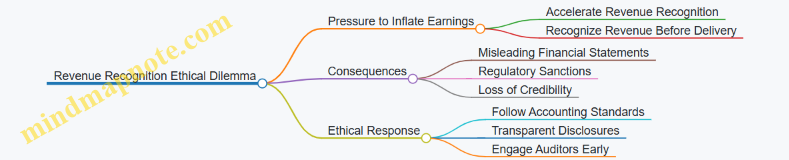
Real-World Example 2: Conflict of Interest in M&A Valuation
Scenario: An investment banker advising a client on an acquisition also holds a financial interest in the target company. This conflict may bias valuation and deal recommendations.
Ethical Dilemma: The banker’s personal gain conflicts with the duty to provide objective advice to the client.
Best Practice: Disclose conflicts of interest immediately. Recuse oneself from decision-making if impartiality is compromised.
Outcome: Failure to manage conflicts can lead to legal actions, loss of licenses, and reputational harm.
Mind Map: Conflict of Interest in Corporate Finance
Framework for Ethical Decision-Making
- Identify the Ethical Issue: Clearly define the dilemma and involved parties.
- Gather Relevant Information: Understand facts, regulations, and company policies.
- Evaluate Alternatives: Consider consequences for all stakeholders.
- Consult Professional Codes: Refer to CFA Institute, AICPA, or company ethics guidelines.
- Make a Decision: Choose the option that upholds integrity and transparency.
- Implement and Communicate: Act responsibly and document decisions.
Example Application of Framework
Situation: A financial analyst discovers that management is omitting a significant contingent liability from disclosures.
- Identify: Omission impacts investor decisions.
- Gather: Review contracts, legal opinions.
- Evaluate: Reporting liability vs. company pressure to hide it.
- Consult: Accounting standards and ethical codes.
- Decide: Recommend disclosure despite pressure.
- Implement: Report findings to audit committee and document communications.
Summary
Ethical dilemmas in financial reporting and corporate finance require vigilance, transparency, and adherence to professional standards. Investment professionals must balance pressures with their fiduciary duties to maintain trust and market integrity.
By applying structured ethical frameworks and learning from real-world cases, professionals can navigate complex situations effectively.
Additional Resources
- CFA Institute Code of Ethics and Standards of Professional Conduct
- AICPA Code of Professional Conduct
- SEC Guidance on Revenue Recognition and Disclosure
- “Financial Shenanigans” by Howard Schilit (for detecting earnings manipulation)
13.5 Best Practice: Maintaining Professional Integrity in Investment Decisions
Maintaining professional integrity is paramount for investment professionals who analyze financial statements and make corporate finance decisions. Integrity ensures trustworthiness, credibility, and long-term success in the investment field. This section explores best practices to uphold integrity, supported by practical examples and mind maps to visualize key concepts.
Why Professional Integrity Matters
- Builds investor and client trust
- Enhances reputation and career longevity
- Ensures compliance with laws and regulations
- Prevents financial scandals and legal consequences
Key Principles of Professional Integrity
Mind Map: Principles of Professional Integrity
Best Practices to Maintain Integrity
-
Adhere to Ethical Codes and Standards
- Follow CFA Institute Code of Ethics, GAAP, IFRS, and SEC regulations.
- Example: An analyst refuses to manipulate earnings forecasts despite pressure from management.
-
Ensure Transparency in Financial Analysis
- Disclose assumptions, limitations, and potential conflicts.
- Example: Clearly stating the sources and assumptions behind a DCF valuation model.
-
Avoid Conflicts of Interest
- Identify and disclose any personal or financial interests that may bias decisions.
- Example: Recusing oneself from evaluating a company where one holds shares.
-
Maintain Objectivity and Independence
- Base recommendations solely on factual data and rigorous analysis.
- Example: Recommending a sell rating on a favored client’s stock due to deteriorating fundamentals.
-
Protect Confidential Information
- Do not share non-public information that could unfairly influence markets.
- Example: An investment banker refrains from disclosing an upcoming merger before public announcement.
-
Continuous Education and Self-Reflection
- Stay updated on ethical guidelines and reflect on personal biases.
- Example: Attending ethics workshops and reviewing past decisions for improvement.
Mind Map: Best Practices to Maintain Integrity
Example Scenario: Upholding Integrity in an Investment Decision
Situation: A financial analyst is evaluating a company that is a potential acquisition target for their firm’s client. The company’s management requests the analyst to downplay certain liabilities to present a healthier balance sheet.
Integrity in Action:
- The analyst refuses to alter or omit any financial information.
- They document all findings transparently, including liabilities.
- The analyst discloses the management’s request to senior compliance officers.
- The final recommendation reflects the true financial position, enabling informed decision-making.
Outcome: The client makes a well-informed decision, avoiding potential post-acquisition surprises and legal risks.
Tools and Techniques to Support Integrity
- Audit Trails: Maintain detailed records of data sources and analytical steps.
- Peer Reviews: Have analyses reviewed by colleagues to catch errors or biases.
- Ethics Checklists: Use checklists before finalizing reports to ensure compliance with ethical standards.
Maintaining professional integrity is not just a regulatory requirement but a cornerstone of effective and responsible investment decision-making. By embedding these best practices into daily workflows, investment bankers and financial analysts can safeguard their reputations and contribute to a fair and transparent financial market.
14. Future Trends and Continuing Education for Investment Professionals
14.1 Emerging Trends in Financial Reporting and Corporate Finance
The landscape of financial reporting and corporate finance is evolving rapidly, driven by technological advancements, regulatory changes, and shifting investor expectations. Staying abreast of these emerging trends is critical for investment bankers and financial analysts to maintain a competitive edge and make informed decisions.
Key Emerging Trends
Detailed Exploration of Selected Trends
Digital Transformation and Automation
Automation is revolutionizing financial reporting by reducing manual errors and accelerating data processing. AI-powered tools can analyze vast datasets to identify anomalies or forecast financial outcomes.
Example: A financial analyst uses an AI-driven platform to automatically extract and consolidate financial data from multiple subsidiaries, reducing the monthly close process from 10 days to 3 days.
Mind Map: Digital Transformation in Financial Reporting
Integrated and Real-Time Reporting
Traditional quarterly or annual reports are giving way to continuous reporting models, enabling investment professionals to make timely decisions based on up-to-date financial data.
Example: A hedge fund uses a real-time dashboard connected to a company’s ERP system to monitor liquidity ratios daily, allowing rapid response to any liquidity stress.
Mind Map: Real-Time Reporting
ESG Integration
ESG factors are increasingly influencing corporate finance decisions and valuations. Companies are required to disclose sustainability metrics alongside traditional financials.
Example: An investment banker evaluates two companies in the renewable energy sector; the one with superior ESG scores secures a lower cost of capital due to investor preference.
Mind Map: ESG in Financial Reporting

Advanced Analytics and Big Data
Big data analytics enables deeper insights into financial trends and risk factors by combining structured financial data with unstructured data sources.
Example: A financial analyst employs sentiment analysis on social media and news feeds to anticipate market reactions ahead of earnings releases.
Mind Map: Advanced Analytics in Corporate Finance
Summary
Investment professionals must adapt to these emerging trends by embracing new technologies, understanding evolving regulatory requirements, and integrating broader non-financial factors like ESG into their analyses. Doing so enhances the accuracy, timeliness, and relevance of financial statement analysis and corporate finance decision-making.
Additional Example: Applying Emerging Trends
A financial analyst at an investment bank is tasked with evaluating a potential acquisition target. By leveraging real-time reporting dashboards, ESG data integration, and AI-powered forecasting tools, the analyst produces a comprehensive valuation that accounts for sustainability risks and market sentiment. This holistic approach leads to a well-informed bid strategy that aligns with the bank’s risk appetite and client objectives.
14.2 The Role of ESG (Environmental, Social, Governance) Factors in Financial Analysis
Environmental, Social, and Governance (ESG) factors have become increasingly critical in the evaluation of companies by investment professionals. ESG analysis complements traditional financial statement analysis by providing insights into risks and opportunities that may not be immediately apparent through conventional metrics.
What is ESG?
- Environmental (E): Concerns related to a company’s impact on the natural environment, including carbon footprint, resource usage, waste management, and climate change initiatives.
- Social (S): Focuses on relationships with employees, suppliers, customers, and communities, including labor practices, diversity, human rights, and community engagement.
- Governance (G): Encompasses corporate policies and practices related to leadership, executive pay, audits, internal controls, and shareholder rights.
Why ESG Matters in Financial Analysis
- Risk Identification: ESG factors can signal potential regulatory, reputational, or operational risks.
- Value Creation: Companies with strong ESG practices often demonstrate better long-term financial performance.
- Investor Demand: Increasingly, investors integrate ESG criteria into their decision-making processes.
- Regulatory Compliance: Growing regulations require transparent ESG disclosures.
Mind Map: ESG Integration in Financial Analysis
How to Incorporate ESG into Financial Analysis
-
Data Collection: Gather ESG data from company reports, third-party ESG rating agencies (e.g., MSCI, Sustainalytics), and regulatory filings.
-
Materiality Assessment: Identify which ESG factors are most relevant to the industry and company.
-
Quantitative Analysis: Incorporate ESG metrics into financial models, such as adjusting discount rates for ESG risk or forecasting revenue impacts from sustainable product lines.
-
Qualitative Analysis: Evaluate governance structures, management quality, and social initiatives through qualitative research.
-
Scenario Analysis: Model potential outcomes under different ESG-related scenarios (e.g., carbon tax implementation).
Example: ESG Impact on a Manufacturing Company
Company: ABC Manufacturing
- Environmental: ABC has invested in energy-efficient machinery reducing carbon emissions by 20% over 3 years.
- Social: Implements strong labor safety programs and has a diverse workforce.
- Governance: Board includes independent directors with ESG expertise.
Financial Analysis Integration:
- Adjusted WACC downward by 0.5% due to lower regulatory and reputational risk.
- Projected revenue growth of 3% annually from new eco-friendly product lines.
- Included potential cost savings from energy efficiency in operating expense forecasts.
Outcome: The ESG integration led to a higher intrinsic valuation compared to a traditional DCF analysis.
Mind Map: ESG Risks and Opportunities
Best Practices for ESG Integration
- Use standardized ESG frameworks such as SASB (Sustainability Accounting Standards Board) or GRI (Global Reporting Initiative) for consistent data.
- Combine ESG scores with traditional financial ratios for a holistic view.
- Engage with company management to clarify ESG disclosures and initiatives.
- Continuously monitor ESG developments and update models accordingly.
Summary
Incorporating ESG factors into financial analysis enables investment professionals to better assess long-term risks and value creation potential. By systematically integrating ESG data with traditional financial metrics, analysts can enhance decision-making, align with investor expectations, and contribute to sustainable investment practices.
14.3 Continuous Learning: Certifications and Resources for Investment Professionals
In the fast-evolving fields of corporate finance and financial analysis, continuous learning is essential for investment professionals to maintain their competitive edge, deepen expertise, and adapt to new market realities. This section explores key certifications, educational resources, and practical strategies to foster ongoing professional development.
Why Continuous Learning Matters
- Keeps skills current with regulatory changes and market innovations.
- Enhances credibility and career advancement opportunities.
- Facilitates mastery of emerging tools, techniques, and frameworks.
Key Certifications for Investment Professionals
| Certification | Focus Area | Ideal For | Example Use Case |
|---|---|---|---|
| CFA (Chartered Financial Analyst) | Investment analysis, portfolio management, ethics | Financial analysts, portfolio managers, investment bankers | Applying advanced valuation techniques in equity research |
| CPA (Certified Public Accountant) | Accounting, auditing, financial reporting | Analysts focused on financial statement integrity and audit | Evaluating financial statement quality and detecting earnings manipulation |
| CMA (Certified Management Accountant) | Management accounting, financial strategy | Corporate finance professionals, financial controllers | Designing budgeting and forecasting models for corporate planning |
| FRM (Financial Risk Manager) | Risk management, quantitative analysis | Risk analysts, portfolio managers | Assessing credit and market risk in leveraged buyouts |
| CAIA (Chartered Alternative Investment Analyst) | Alternative investments, hedge funds, private equity | Professionals focused on alternative asset classes | Analyzing private equity deals and alternative investment structures |
Mind Map: Certifications Overview
Essential Learning Resources
-
Online Courses & Platforms
- Coursera, edX, and LinkedIn Learning offer courses on financial modeling, valuation, and corporate finance.
- Example: “Financial Modeling and Valuation” course by Wharton on Coursera.
-
Professional Associations & Networks
- CFA Institute, AICPA, and GARP provide webinars, publications, and conferences.
- Example: Attending CFA Institute’s annual conference to gain insights on market trends.
-
Industry Publications & Journals
- The Journal of Finance, Harvard Business Review, and Financial Analysts Journal.
- Example: Reading case studies on mergers and acquisitions to understand practical applications.
-
Books & Reference Materials
- “Investment Valuation” by Aswath Damodaran
- “Corporate Finance” by Jonathan Berk and Peter DeMarzo
-
Financial Modeling Software Tutorials
- Excel advanced modeling, VBA programming, and tools like FactSet or Bloomberg Terminal.
- Example: Creating dynamic dashboards using Excel VBA to automate financial analysis.
Mind Map: Learning Resources
Practical Strategies for Continuous Learning
- Set Learning Goals: Define specific skills or certifications to pursue annually.
- Schedule Regular Study Time: Dedicate weekly hours to courses, reading, or practice.
- Engage in Peer Learning: Join study groups or professional forums to exchange knowledge.
- Apply Learning on the Job: Use new techniques in live projects to reinforce concepts.
- Seek Mentorship: Connect with senior professionals for guidance and feedback.
Example: Applying Continuous Learning in Practice
Jane, a financial analyst at an investment bank, decided to pursue the CFA charter to deepen her valuation skills. She allocated 10 hours per week for study, joined a local CFA study group, and applied valuation models learned in her weekly pitch presentations. Over two years, Jane not only passed all CFA levels but also improved her analytical rigor, resulting in more accurate investment recommendations and recognition from senior management.
Summary
Continuous learning through certifications and diverse resources empowers investment professionals to excel in financial statement analysis and corporate finance. By integrating structured education with practical application and networking, professionals can sustain growth and adapt to the evolving financial landscape.
14.4 Best Practice: Staying Ahead with Industry Developments and Networking
In the fast-evolving fields of corporate finance and financial analysis, staying current with industry developments and actively networking are critical for investment professionals. These practices not only enhance your knowledge base but also open doors to new opportunities, insights, and collaborations.
Why Staying Ahead Matters
- Rapid Market Changes: Financial markets and corporate finance strategies evolve quickly due to regulatory changes, technological advancements, and macroeconomic shifts.
- Competitive Edge: Being informed allows you to anticipate trends and make better investment decisions.
- Professional Growth: Networking connects you with experts, mentors, and potential clients or employers.
Key Strategies to Stay Ahead
Practical Examples
Example 1: Leveraging Financial News and Reports
Sarah, a financial analyst, dedicates 30 minutes daily to reading market updates from sources like Bloomberg and the Financial Times. She subscribes to sector-specific newsletters and regulatory bulletins, which help her anticipate changes impacting her portfolio companies.
Example 2: Participating in Industry Conferences
John, an investment banker, attends the annual Global Corporate Finance Summit. There, he learns about emerging valuation techniques and meets peers who share insights on deal structuring. Post-event, he follows up with contacts on LinkedIn, expanding his professional network.
Example 3: Engaging in Online Learning and Certifications
Emily enrolls in a specialized course on ESG investing to incorporate sustainability factors into her financial analysis. She also pursues the CFA certification, which keeps her updated on best practices and ethical standards.
Example 4: Building a Mentorship Relationship
Michael connects with a senior analyst through a professional association’s mentorship program. Regular discussions help him navigate complex financial models and gain career advice.
Tips for Effective Networking
- Be Genuine: Focus on building meaningful relationships rather than just collecting contacts.
- Prepare Your Elevator Pitch: Clearly articulate your expertise and interests.
- Follow Up: After meetings or events, send personalized messages to maintain connections.
- Offer Value: Share relevant articles, insights, or introductions to help others.
Summary
Staying ahead in corporate finance and financial analysis requires a proactive approach to learning and relationship-building. By integrating regular industry updates, continuous education, and strategic networking into your routine, you position yourself as a knowledgeable and connected investment professional.
Additional Resources
- CFA Institute Events and Webinars
- Investopedia Financial News
- LinkedIn Groups for Financial Analysts
- Coursera Corporate Finance Courses
Mind Map Visualization
14.5 Example: Incorporating ESG Metrics into Traditional Financial Analysis
Incorporating Environmental, Social, and Governance (ESG) metrics into traditional financial analysis is becoming essential for investment professionals seeking a holistic view of a company’s long-term value and risk profile. This section provides a detailed example of how ESG factors can be integrated into standard financial analysis frameworks, supported by mind maps and practical illustrations.
Understanding ESG Integration
ESG integration involves evaluating non-financial factors alongside traditional financial metrics to assess a company’s sustainability, ethical impact, and governance quality. These factors can influence financial performance, risk, and ultimately valuation.
Mind Map: ESG Integration Framework
Step 1: Selecting Relevant ESG Metrics
For a technology company, relevant ESG metrics might include:
- Environmental: Energy consumption of data centers, e-waste recycling programs
- Social: Employee diversity ratios, data privacy policies
- Governance: Board independence, anti-bribery policies
Step 2: Quantifying ESG Metrics
Assign quantitative scores or ratings to ESG factors, for example:
| ESG Factor | Metric | Score (1-10) |
|---|---|---|
| Energy Efficiency | kWh per user | 7 |
| E-Waste Recycling | % of e-waste recycled | 8 |
| Employee Diversity | % of underrepresented groups | 6 |
| Data Privacy Compliance | Number of breaches last year | 9 |
| Board Independence | % independent directors | 8 |
Step 3: Linking ESG Scores to Financial Analysis
- Risk Adjustment: Lower ESG scores may indicate higher operational or regulatory risks, warranting a higher discount rate.
- Revenue Impact: Strong social responsibility can enhance brand loyalty, potentially increasing revenue growth.
- Cost Implications: Environmental inefficiencies may increase operating costs.
Mind Map: ESG Impact on Financial Metrics
Step 4: Practical Example
Company: TechCo, a mid-sized cloud services provider.
Traditional Financials:
- Revenue Growth: 12% YoY
- Operating Margin: 18%
- WACC: 8%
ESG Scores:
- Environmental: 6/10 (moderate energy efficiency, room for improvement)
- Social: 7/10 (good diversity, strong privacy policies)
- Governance: 8/10 (solid board structure)
Integration:
- Increase WACC by 0.5% due to moderate environmental risks.
- Adjust revenue growth down by 1% to reflect potential regulatory headwinds.
Revised Financial Inputs:
- Revenue Growth: 11%
- WACC: 8.5%
Valuation Impact: Using a discounted cash flow (DCF) model, the revised inputs lower the enterprise value by approximately 5%, reflecting ESG-related risks.
Step 5: Scenario Analysis
Perform sensitivity analysis on ESG factors:
| Scenario | WACC | Revenue Growth | Valuation Impact |
|---|---|---|---|
| Base Case | 8% | 12% | Baseline |
| ESG Improvement | 7.5% | 13% | +7% valuation |
| ESG Deterioration | 9% | 10% | -10% valuation |
Summary
Integrating ESG metrics into traditional financial analysis enables investment professionals to:
- Identify hidden risks and opportunities
- Adjust valuation models to reflect sustainability factors
- Communicate a more comprehensive investment thesis
This approach aligns financial analysis with evolving investor expectations and regulatory frameworks.
For further reading and tools, consider exploring ESG rating agencies (e.g., MSCI, Sustainalytics) and software platforms that facilitate ESG data integration into financial models.