Leveraged Buyouts and Acquisition Financing Internals
1. Overview of Buyout Transactions and Financing Objectives
1.1 Deal Anatomy from Purchase Price to Closing Mechanics
A leveraged buyout (LBO) looks simple on a term sheet: buy the company, finance the purchase with debt and equity, then repay lenders from cash flow. The mechanics are less simple because money moves through multiple documents, multiple accounts, and multiple timing gates. This section maps the path from purchase price to closing so you can see where cash is committed, where it is released, and where errors tend to hide.
Purchase Price Components and What They Really Mean
The purchase price is rarely one number that lands cleanly on the seller’s bank account. It is usually a bundle:
- Base purchase price: the headline amount for the equity interest or assets.
- Working capital adjustment: an amount that true-ups based on a target level at closing.
- Net debt adjustment: adjusts for the difference between actual debt and a defined “net debt” concept.
- Transaction expenses: some are paid by the buyer, some are netted from proceeds, and some are reimbursed.
- Earn-outs or contingent consideration: paid later if performance metrics are met.
A practical way to avoid confusion is to write the purchase price as a “sources-and-uses friendly” equation: what the buyer must fund at closing versus what will settle later through adjustments.
Sources and Uses: The Closing Funding Blueprint
At closing, the buyer must show that sources (equity, debt proceeds, and other funding) equal uses (purchase price, fees, refinancing payoffs, and transaction costs). If sources exceed uses, the excess typically goes to a cash sweep, a reserve, or reduces the amount drawn.
Example: Suppose the base purchase price is $500m, with $20m expected working capital adjustment and $10m expected transaction expenses. If the agreement defines net debt such that the buyer assumes $60m of net debt at closing, the buyer’s immediate funding need is not just $500m. It becomes a negotiated combination of base price plus/minus adjustments, plus fees, minus any seller-paid items.
The Financing Stack and Funding Timing
Debt proceeds are not all released at once. A typical stack includes:
- Senior secured term loan: often funded at closing, sometimes with a portion held back for conditions.
- Revolver: may be undrawn at closing but can fund fees or interim needs.
- Second lien or mezzanine: frequently funded at closing but subject to additional deliverables.
- Equity: sponsor equity is usually wired at or shortly before closing to satisfy conditions precedent.
Each layer has its own conditions, but the closing date is the same. That means the sponsor and lenders must coordinate deliverables so the last missing document does not delay the whole party.
Conditions Precedent and Deliverables
Closing mechanics are driven by conditions precedent, which are checklists of what must be true before funds move. Common categories include:
- Legal and regulatory: approvals, consents, and absence of injunctions.
- Accuracy of representations: bring-down of key reps in the acquisition agreement.
- No material adverse change: defined thresholds for adverse events.
- Debt documentation effectiveness: credit agreement execution and collateral steps.
- Security perfection: filings, control agreements, and lien priority steps.
Deliverables are the concrete items that prove conditions are met: executed agreements, payoff letters, lien search results, officer certificates, and evidence of collateral filings.
Closing Accounts and Payment Mechanics
Most LBOs use closing accounts to prevent “cash surprises.” Two common ones are:
- Closing cash / cash sweep: defines how much cash stays with the company versus is paid out or credited.
- Working capital target: sets the baseline for later true-up.
Payment mechanics also matter. Funds may be wired to escrow, used to pay seller notes, or applied to retire existing credit facilities. Payoff letters are critical because they define the exact amount required to release liens and avoid residual claims.
Mind Map: Deal Anatomy from Purchase Price to Closing
Integrated Example: A Clean Closing Flow
Assume a buyer signs an equity purchase agreement and a financing package on 2026-04-06. At closing, the buyer wires sponsor equity first to satisfy equity funding conditions. Lenders fund the senior term loan next, subject to credit agreement effectiveness and collateral deliverables. If the deal includes a second lien tranche, its proceeds fund after additional intercreditor and collateral steps are confirmed. Finally, the buyer pays the seller using the purchase price calculation net of defined adjustments and transaction expenses, while escrow holds amounts needed for working capital and other post-closing true-ups.
The key takeaway is that closing is a choreography of definitions and deliverables. If you can trace each dollar from “sources” to “uses,” and each condition to a specific document or filing, the mechanics stop feeling like paperwork and start behaving like a system.
1.2 Roles of Sponsors Lenders and Target Stakeholders
A leveraged buyout is a coordination problem with money attached. The sponsor, the lenders, and the target stakeholders each optimize for different constraints, and the deal documents exist to make those constraints compatible.
Sponsor Role: Ownership, Control, and Risk Allocation
Sponsors typically originate the transaction, negotiate the purchase price, and assemble the equity needed to fund the acquisition. Their practical job is to decide how much risk to take directly versus how much to push into debt. That decision shows up in equity sizing, the choice of debt layers, and the willingness to accept tighter covenants in exchange for lower interest costs.
Sponsors also manage the “governance plumbing.” They appoint or influence management, set reporting cadence, and define how decisions are approved under shareholder agreements. In many deals, sponsor control is not just voting power; it is the ability to enforce budgets, approve major capex, and control distributions.
A simple example: if a sponsor contributes 30% equity instead of 20%, the same operating cash flow can support higher debt service with less pressure on covenants. The sponsor’s return profile changes because equity is larger, but the probability of covenant stress often drops.
Lender Role: Cash Flow Protection and Contract Enforcement
Lenders provide the acquisition financing and care about two things: repayment and the ability to stop the borrower from taking actions that reduce repayment capacity. That is why lenders focus on collateral, covenants, and intercreditor arrangements.
Senior lenders usually prioritize predictable cash flows. They set leverage and coverage tests, require compliance certificates, and restrict asset sales and additional debt. They also negotiate remedies such as acceleration or foreclosure if covenants are breached and not cured.
Subordinated lenders and mezzanine providers accept higher risk in exchange for higher yield or equity-like features. Their protections often include tighter consent rights for certain actions, call protection, and specific payment terms.
A practical example: a term loan may require a quarterly leverage test. If EBITDA declines due to margin compression, the borrower may need to use an equity cure or adjust distributions to avoid breaching the test. Lenders design the covenant package so that cash flow stress triggers predictable responses.
Target Stakeholder Role: Continuity, Incentives, and Deal Feasibility
Target stakeholders include existing shareholders, management, employees, and sometimes key customers or suppliers. Their role is less about financing mechanics and more about whether the business can keep operating while the capital structure changes.
Management is central because lenders and sponsors underwrite the plan through forecasts and operating assumptions. Management incentives matter: if bonuses and equity awards are misaligned, the post-close behavior can drift away from the model.
Existing shareholders care about price, timing, and certainty of proceeds. They also care about whether rollover equity is required to keep them invested in the new structure.
A concrete example: if management is asked to rollover equity but the vesting schedule is too aggressive relative to the company’s cash generation, management may resist or negotiate for additional protections. That negotiation affects both sponsor equity economics and lender comfort because it influences retention and execution.
How Roles Interlock Through Documentation
The sponsor proposes the structure, lenders validate the repayment logic, and target stakeholders validate operational continuity. The documents translate those validations into enforceable rules.
- Equity documents define distributions, governance, and rollover mechanics.
- Credit agreements define covenants, reporting, collateral, and remedies.
- Intercreditor agreements define how different debt classes share recoveries and consent rights.
- Shareholder agreements define sponsor control and how management decisions are approved.
Mind Map: Who Does What and Why It Matters
Example: A Small Deal Walkthrough
Assume a sponsor buys a company for $100 million enterprise value. The sponsor contributes $30 million equity and arranges $70 million of debt. Senior lenders require a leverage covenant tested quarterly and a restricted payments basket. Management must rollover part of their equity to stay aligned, and the sponsor agrees to a budget approval process that prevents management from approving capex that would strain covenant headroom.
If EBITDA drops in the first year, the covenant test becomes the focal point. The lenders do not need to guess what happens next; the agreement specifies whether an equity cure is available, whether distributions are restricted, and what approvals are required for actions that could worsen repayment capacity. That is the core reason these roles are separate but coordinated: each party optimizes its constraints, and the contract makes the constraints work together.
1.3 Financing Objectives and Constraints in Acquisition Structures
Financing objectives describe what the deal must achieve in cash, control, and risk. Constraints describe what the structure must respect so the financing can actually be documented, funded, and serviced. In a leveraged acquisition, these two lists should be written side by side; otherwise, the model will look neat while the credit agreement quietly refuses to cooperate.
Financing Objectives
Objective 1: Fund the purchase price and transaction costs on closing. The structure must cover sources and uses, including equity contribution, debt proceeds, fees, and any required reserves. A common best practice is to separate “closing funding” from “ongoing liquidity,” because a facility that funds the deal may still leave the company short of cash for working capital swings.
Objective 2: Match debt service to cash flow timing. Debt payments are scheduled, but cash flow is seasonal and operational. If the target has uneven EBITDA through the year, the sponsor often prefers amortization profiles that avoid forcing principal payments during weak quarters.
Objective 3: Preserve flexibility for operations and refinancing. Flexibility shows up as permitted payments, covenant headroom, and amendment pathways. For example, a structure with tight restricted payments limits may block management bonuses or dividends even when leverage temporarily improves.
Objective 4: Achieve an acceptable equity return with controlled downside. Sponsors typically optimize for IRR and MOIC, but the financing must also survive downside cases. That means the debt stack should not rely on optimistic EBITDA adjustments to meet covenants.
Financing Constraints
Constraint 1: Covenant math and testing mechanics. Covenants are not just ratios; they include definitions, measurement periods, and cure rights. A leverage covenant tested quarterly can behave very differently from an annual test, especially when EBITDA is volatile.
Constraint 2: Intercreditor and payment waterfall rules. Even if the borrower generates cash, the waterfall can restrict where that cash goes. Subordinated lenders may receive payments only after senior obligations are satisfied, and “excess cash flow” calculations can delay distributions.
Constraint 3: Collateral and security package limitations. Lenders require enforceable collateral. Constraints arise from asset types, jurisdictional perfection, and whether certain assets are excluded. This affects both borrowing capacity and recovery expectations.
Constraint 4: Legal and structural limits on restricted payments. Equity distributions, management fees, and certain affiliate transactions may be capped by baskets or require compliance with leverage thresholds.
Constraint 5: Pricing, fees, and hedging realities. The effective cost of debt includes upfront fees, OID-like economics, and hedging costs if floating rates are swapped. A structure that “looks cheap” on headline margin can become expensive after modeling all-in interest.
How Objectives and Constraints Interlock
A useful way to think about the structure is as a set of “gates.” Each gate is a constraint that must be passed for the objective to be met.
- Gate A: Closing funding gate checks sources and uses, including fees and any required reserves.
- Gate B: Covenant gate checks whether the borrower can remain compliant under realistic operating paths.
- Gate C: Cash availability gate checks whether cash can flow through the waterfall to equity.
- Gate D: Legal gate checks whether documentation permits the intended payments and amendments.
If any gate fails, the sponsor may still close, but the economics shift immediately: equity distributions slow, refinancing becomes harder, or amendments become necessary.
Mind Map: Financing Objectives and Constraints
Example: Choosing Between Amortizing Term Loan and Bullet-Heavy Structure
Assume the target has EBITDA of $100m in a strong year and $85m in a weaker year, with quarterly seasonality. The sponsor wants to minimize equity dilution and keep distributions possible.
- Option 1: Amortizing term loan reduces principal over time. This can improve leverage optics, but it increases cash outflow in every period. If the covenant is leverage-based and tested quarterly, the borrower may breach during weak quarters even if annual EBITDA looks fine.
- Option 2: Bullet-heavy structure keeps principal payments lower early. This can protect covenant compliance and preserve cash for working capital. However, it increases refinancing risk at maturity and may require tighter restricted payments or higher pricing.
A practical best practice is to run the same operating downside through both options and compare: (1) covenant headroom each test date, (2) cash available for restricted payments, and (3) total all-in debt cost including fees.
Example: Restricted Payments Versus Equity Return
Suppose the sponsor expects to distribute $20m to equity in year one. The credit agreement permits restricted payments only if leverage is below a threshold and if baskets remain.
If the model shows leverage compliance only in the last two quarters, the structure may still be viable, but the timing changes. The sponsor can either (a) reduce the planned distribution, (b) rely on a permitted basket, or (c) use an equity cure if available. The key is to treat the distribution plan as a constraint-driven schedule, not a single number.
Example: Intercreditor Waterfall Blocking an “Available Cash” Assumption
A borrower may generate $30m of excess cash flow in a year, but the waterfall can require that senior lenders receive payments first, and subordinated lenders only later. If the model assumes excess cash flows directly to equity, equity IRR will be overstated.
The fix is straightforward: model the waterfall explicitly by debt class and payment trigger. When the numbers stop matching, the structure is telling you where the constraints actually live.
1.4 Key Documentation Map for Credit Agreements and Equity Side Letters
A leveraged buyout is a stack of promises. The credit agreement is the main contract for the debt, but the equity side letters are where sponsors and management often negotiate the “how” of governance, economics, and information. A good documentation map helps you trace each promise to the document that controls it, then to the clause that enforces it.
Foundational Map of Who Controls What
Start with three layers:
- Debt layer: The credit agreement (and any intercreditor agreement) controls payment priority, covenants, events of default, and remedies.
- Equity layer: The equity purchase agreement, shareholders agreement, and side letters control voting, transfer restrictions, management participation, and sponsor protections.
- Operational layer: The security documents and guarantees control collateral and credit support, while disclosure schedules and officer certificates control what was promised about the target.
A practical way to avoid confusion is to label every key term with three tags: who benefits, who must do something, and what document contains the enforcement mechanism.
Core Debt Documents and Their “Job Descriptions”
In most deals, the credit agreement is the hub. It typically includes:
- Definitions and financial calculations: EBITDA adjustments, leverage ratios, and covenant measurement mechanics.
- Borrowing and repayment mechanics: draw conditions, amortization schedules, mandatory prepayment triggers, and permitted payments.
- Covenants: affirmative covenants (reporting, maintenance of existence), negative covenants (limitations on liens, investments), and financial covenants (leverage or fixed charge tests).
- Events of default: non-payment, covenant breaches, misrepresentations, and cross-defaults.
- Remedies: acceleration, enforcement of collateral, and voting rights through agent actions.
Security documents then answer: what collateral is pledged, who holds it, and how it is perfected. Guarantees answer: which entities back the obligations.
If there are multiple debt classes, the intercreditor agreement answers: how proceeds are shared and how enforcement is coordinated. Without this document, the credit agreement’s payment priority can be incomplete in practice.
Equity Side Letters and Why They Exist
Side letters are not “extra paperwork”; they are where the equity layer gets operational. Common topics include:
- Information rights: who receives financials, budgets, and covenant compliance reports, and on what timeline.
- Management participation: vesting, employment-related triggers, and how management equity is treated during transfers.
- Sponsor protections: consent rights, standstill arrangements, and how certain actions require sponsor approval.
- Economic alignment: how fees, expense reimbursements, or preferred returns are handled relative to debt covenants.
A key integration point is that equity actions can be constrained by the debt agreement. For example, equity distributions may be permitted only if a restricted payments test is satisfied. Side letters can specify the sponsor’s internal waterfall, but the credit agreement decides whether distributions are legally allowed.
Integrated Clause Tracing Example
Suppose the sponsor wants management to receive an annual bonus funded from the company. Trace it like this:
- Step 1: Identify whether the bonus is treated as an operating expense or a restricted payment.
- Step 2: Check the credit agreement’s definition of restricted payments and permitted payments baskets.
- Step 3: Confirm whether the bonus depends on a covenant test (often leverage or fixed charge) and whether the company can meet it.
- Step 4: Use the side letter to confirm who is entitled, when it vests, and what approvals are required.
If the credit agreement restricts distributions, the side letter should not promise a payment that the company cannot legally make. The best deals align the side letter’s payment timing with the debt agreement’s compliance calendar.
Mind Map: Documentation Ownership
Practical Checklist for Building the Map
- Create a term inventory: list every economic and control term you care about (distributions, bonuses, consent rights, reporting).
- Assign a controlling document: credit agreement, intercreditor, security documents, or side letter.
- Verify definitions: if “EBITDA” or “restricted payments” is defined differently, you have a modeling and compliance mismatch.
- Confirm timing: covenant tests often run quarterly; side letter payment dates should not assume a test result that is not yet measured.
- Check enforcement paths: a right without a remedy is a suggestion; a remedy without the right document is a dead end.
When you can trace each sponsor or management promise to a specific clause and enforcement mechanism, the rest of the modeling work becomes less guessy and more mechanical.
1.5 Practical Example: Building a Transaction Stack from Sources and Uses
A transaction stack is the clean, arithmetic view of how money moves at closing: what the deal needs (Uses) and where it comes from (Sources). The goal is not just to balance a spreadsheet; it’s to ensure the financing terms you modeled earlier can actually fund the purchase price, fees, and required cash buffers.
Step 1: Define the Uses with Timing and Purpose
Start with a “closing uses” list that separates cash that leaves the buyer from cash that stays behind as a buffer.
Example Uses (USD, millions):
- Purchase price to sellers: 500
- Transaction fees and expenses (financing + legal + advisory): 18
- Funded debt payoff at closing: 120
- Required cash at close (minimum cash covenant): 12
- Working capital true-up reserve: 10
Total Uses = 500 + 18 + 120 + 12 + 10 = 660.
A practical check: if your model later assumes a certain level of cash available for debt service, the “required cash at close” belongs here, not in some later fantasy reconciliation.
Step 2: Build Sources that match the Uses
Sources should include equity and each debt layer, plus any seller rollover or other credits that reduce cash needed.
Example Sources (USD, millions):
- Sponsor equity contribution: 90
- New senior secured term loan A: 260
- New senior secured revolver (draw at close): 40
- Second lien notes: 120
- Mezzanine instrument (cash pay): 50
- Seller rollover equity credit: 0 (assume none)
Total Sources = 90 + 260 + 40 + 120 + 50 = 560.
We’re short by 100. That’s not a failure; it’s the spreadsheet telling you the deal needs either more financing or fewer uses.
Step 3: Reconcile the Gap with Realistic Adjustments
Common adjustments are (a) increase a debt layer, (b) reduce a reserve, or (c) change the structure of the equity contribution. In a real credit agreement, some of these are constrained by leverage limits, collateral availability, or minimum liquidity requirements.
Adjustment option used in this example: Increase term loan A by 100.
- Revised term loan A: 360
Revised Total Sources = 90 + 360 + 40 + 120 + 50 = 660.
Now Sources = Uses = 660, and the stack is fundable.
Step 4: Translate the Stack Into a Closing Cash Flow Narrative
Once balanced, map each source to what it actually pays.
Example closing allocation (USD, millions):
- Term loan A and revolver draw pay purchase price and fee items.
- Second lien and mezzanine fund the remaining purchase price and refinance payoff.
- Required cash at close is funded last so it doesn’t get accidentally “spent” in the allocation.
A simple way to keep this consistent is to enforce the rule: every dollar of Uses is either paid out immediately or parked as required cash/reserve.
Step 5: Mind the Debt Structure Implications for Later Modeling
Even though the stack is a closing view, it sets the starting balances for your cash flow and covenant calculations.
- Revolver draw at close becomes part of the initial funded debt base and affects interest expense immediately.
- Mezzanine cash pay versus PIK changes the first-year cash burden even if the closing proceeds are the same.
- Any required cash at close reduces the cash available for early debt service, which can matter for fixed charge coverage.
Mind Map: Transaction Stack from Sources and Uses
Example: Quick Stack Summary Table
| Item | Amount (USDm) |
|---|---|
| Uses | |
| Purchase price | 500 |
| Fees and expenses | 18 |
| Existing debt payoff | 120 |
| Required cash at close | 12 |
| Working capital reserve | 10 |
| Total Uses | 660 |
| Sources | |
| Sponsor equity | 90 |
| Term loan A | 360 |
| Revolver draw at close | 40 |
| Second lien notes | 120 |
| Mezzanine cash pay | 50 |
| Total Sources | 660 |
Step 6: Sanity Checks That Prevent Downstream Errors
Before moving on to interest and covenants, run three checks:
- No double counting: required cash at close should not also appear as “available cash” in your early-period cash flow.
- Debt payoff consistency: the “existing debt payoff” must match the starting funded debt you remove from the target’s balance sheet.
- Fee treatment alignment: if fees are financed or paid from proceeds, the stack should reflect the same cash timing your model uses.
With a balanced stack and consistent mapping, the rest of the model can focus on economics—interest, coverage, and equity returns—without fighting basic arithmetic.
2. Capital Structure Design for Leveraged Acquisitions
2.1 Equity Contributions and Sponsor Control Considerations
Equity contributions are the sponsor’s “skin in the game,” but they also determine who gets to steer the deal when things get messy. In a leveraged acquisition, lenders care about equity because it absorbs losses first and funds the transaction when debt markets are tight. Sponsors care about equity because it shapes governance, consent rights, and the practical ability to manage through covenant pressure.
Equity Contribution Basics and Why They Matter
Equity in a buyout usually includes sponsor common equity, management equity, and sometimes preferred equity or equity-like instruments. The key modeling point is that equity is not just a funding source; it is the first layer of cash flow that can be reduced without triggering a default. That is why lenders often require a minimum equity contribution at closing and may restrict additional equity withdrawals.
A simple way to see the difference: if the business generates $10 million of annual free cash flow and debt service is $8 million, the remaining $2 million can go to equity. If free cash flow drops to $6 million, debt service still must be paid, and equity distributions shrink to zero before any lender is at risk.
Sponsor Control Through Governance and Consent
Sponsor control is not only about ownership percentage. It is about which decisions require consent from equity holders versus which decisions can be made by management under the credit agreement.
Common control levers include:
- Board composition and voting: Sponsors often negotiate board seats proportional to their equity and may require certain board approvals for major actions.
- Management appointment rights: Sponsors typically control hiring and replacement of key executives, subject to employment agreements.
- Reserved matters: Equity holders may have veto rights over actions like asset sales, additional debt, or changes to business lines.
- Credit agreement restrictions: Even if sponsors control the board, the debt documents can limit actions through covenants and restricted payments rules.
A practical example: a sponsor wants to sell a non-core division to fund a working capital need. The board can approve the sale, but the credit agreement may require that proceeds be applied to debt prepayment or be subject to a permitted investment basket. Control exists, but it operates within the lender-defined boundaries.
Equity Sizing and Its Link to Leverage
Equity size determines leverage, and leverage determines covenant tightness and refinancing flexibility. Higher equity reduces leverage ratios, which can widen covenant headroom and reduce the probability of needing an equity cure.
Consider two otherwise identical deals:
- Deal A: Purchase price $200 million, equity $60 million, debt $140 million.
- Deal B: Purchase price $200 million, equity $40 million, debt $160 million.
If EBITDA is $40 million, Deal A starts at 3.5x leverage while Deal B starts at 4.0x. That 0.5x gap can matter when covenants step down over time. Sponsors often trade off lower equity return in Deal A against a smoother path to distributions.
Equity Contribution Mechanics at Closing
Equity contributions can be funded through cash at closing, capital calls, or staged funding tied to milestones. Lenders typically want certainty that equity is actually funded before or at closing, because staged contributions can create a funding gap.
A clean closing flow looks like this:
- Sources include debt proceeds and sponsor equity.
- Uses include purchase price, transaction fees, and refinancing costs.
- Equity is wired so that the transaction closes without relying on post-closing equity injections.
If equity is staged, sponsors may need to provide additional documentation or guarantees to satisfy lender conditions.
Mind Map: Equity Contributions and Control
Example: Equity Cure and Practical Control
Suppose a covenant test fails because EBITDA is temporarily lower. Sponsors may have an equity cure right, but the cure typically requires equity to be contributed to the issuer and applied in a defined way. Control shows up here: sponsors must be prepared to fund quickly, and they must coordinate with management on the timing and documentation.
A workable approach is to model a “cure budget” alongside the base case. If the sponsor expects the business to be tight in year two, the sponsor can size equity and negotiate cure mechanics so that a cure is feasible without forcing a distressed restructuring.
Key Takeaways for Sponsors and Lenders
Equity contribution is both a financial input and a control mechanism. Sponsors should treat equity sizing as a covenant and governance design choice, not just a funding number. Lenders should treat equity as the buffer that determines how much flexibility the deal has when cash flow is uneven.
In short: ownership percentage matters, but the real control story is how equity, governance rights, and credit agreement limits interact when the model stops behaving nicely.
2.2 Debt Layers and Their Intended Economic Roles
A leveraged buyout stacks multiple debt instruments so each layer can do a specific job: fund the purchase, absorb risk in a controlled way, and create a predictable path for cash to move from operations to lenders and finally to equity. The “intended economic role” of a layer is not just legal priority; it’s the combination of (1) who gets paid first, (2) how much cash they expect to receive, and (3) what happens when performance is weaker than planned.
Foundational Idea: Priority, Risk, and Cash Flow Expectations
Start with a simple mapping: seniority determines payment order, while instrument design determines the timing and form of payment.
- Priority of payments answers: “Who gets paid before whom?”
- Payment form answers: “Is it mostly cash interest, cash principal, or deferred/PIK components?”
- Performance sensitivity answers: “How does the layer behave when EBITDA drops or leverage rises?”
In practice, a sponsor chooses layers to match the target company’s cash generation profile. A stable cash business can support more cash-pay amortization. A volatile cash business often needs structures that reduce near-term cash outflows.
Layer 1: Senior Secured Debt as the Funding Backbone
Senior secured debt typically provides the largest portion of acquisition financing. Its economic role is to be the “anchor” layer: lenders receive first claim on collateral and first access to cash flows after required expenses.
Key design features usually include:
- Security and collateral: lenders expect recovery in downside scenarios.
- Covenants: leverage or coverage tests constrain borrower behavior.
- Cash interest focus: payments are typically current, not deferred.
Example: Suppose a company generates $120 million of annual EBITDA and the model assumes $90 million of cash available after operating costs and maintenance capex. Senior lenders might be structured to receive interest and scheduled amortization from that cash, with covenants designed to keep leverage within a band. If EBITDA falls to $100 million, the covenant headroom becomes the early warning system.
Layer 2: Second Lien or Similar “Step-Down” Debt as Risk Absorber
Second lien debt sits below senior secured in priority. Its economic role is to provide additional funding while accepting lower collateral priority and, often, tighter recovery assumptions.
Design features commonly include:
- Reduced collateral priority: recovery is less certain than senior.
- Higher yield: pricing compensates for the extra risk.
- Intercreditor terms: payment and enforcement rights are coordinated with senior.
Example: If senior secured debt is $400 million and second lien is $150 million, the second lien layer might receive interest and limited principal payments only after senior obligations are satisfied. In a stressed year, the second lien may still be paid interest, but principal may be delayed or reduced depending on the waterfall.
Layer 3: Mezzanine Debt as a Bridge Between Cash and Equity Risk
Mezzanine debt often behaves like a hybrid: it provides capital with equity-like risk characteristics while still being contractually debt. Its economic role is to fill the gap between what senior lenders will fund and what equity investors are willing to contribute.
Common economic traits include:
- Higher spread: compensation for subordination.
- PIK or cash/PIK mix: part of the return may be deferred.
- Call protection: lenders may receive protections against early repayment.
Example: A mezzanine instrument might require 8% cash interest plus 6% PIK interest. If the company has temporary cash pressure, PIK interest can reduce immediate cash outflow, but it increases the eventual payoff burden. That trade-off is intentional: the layer is designed to survive cash troughs while preserving the sponsor’s ability to fund the acquisition.
Layer 4: Unitranche as a Blended Role with Internal Economics
Unitranche debt combines multiple economic layers into a single facility. Its economic role is practical: simplify documentation and administration while still reflecting different risk appetites inside the blended structure.
Even when presented as one facility, unitranche economics often split into:
- A senior-like tranche with tighter protections and priority within the facility.
- A junior-like tranche with higher yield and more subordination.
Example: A $550 million unitranche might be priced as a blended rate, but internally allocated so that the “senior-like” portion receives priority in payment and enforcement, while the “junior-like” portion absorbs more downside.
Mind Map: Debt Layers and Their Economic Roles
Putting It Together: How Layers Work as a System
A useful way to think about the stack is as a cash-flow routing system. Senior debt typically captures the “must-pay” portion of cash interest and scheduled principal. Subordinate layers capture the “pay-when-available” portion, with their designs tuned to the company’s expected cash generation and downside tolerance.
Example: In a base case, senior receives full interest and amortization, second lien receives interest, and mezzanine receives its cash/PIK mix. In a weaker case, covenants may tighten behavior, senior payments remain protected by priority, and subordinate layers experience reduced principal payments or increased PIK accrual. The sponsor’s job is to ensure the system can operate across those scenarios without forcing equity to absorb every cash shock immediately.
2.3 Common Equity Instruments and Preferred Equity Variants
In leveraged buyouts, “equity” is not one thing. It’s a bundle of rights that determine who gets paid first, who bears losses, and how control is exercised. Common equity is the baseline: it absorbs residual risk and typically carries voting power. Preferred equity is the customization layer: it can add payment preferences, fixed or semi-fixed economics, and sometimes protective provisions that sit between debt and common.
Common Equity Foundations
Common equity usually receives distributions only after all debt obligations and any preferred obligations are satisfied. That residual position is why common investors care about downside protection mechanisms like subordination, restricted payments, and the timing of cash sweeps.
Voting rights typically attach to common shares. In practice, sponsors use common equity to secure governance influence—board seats, consent rights, and approval thresholds—while lenders focus on covenants and collateral rather than day-to-day control.
A practical example: if a company generates $10 million of operating cash flow in a year, and the debt stack requires $8 million of interest and scheduled payments, only the remaining $2 million is available for equity distributions. If there is no preferred equity, common gets the $2 million subject to any restricted payments limits. If there is preferred equity with a required dividend, common may receive less or nothing even when cash exists.
Preferred Equity Variants and Their Economic Role
Preferred equity is equity legally, but it often behaves like a hybrid. The key design choices are (1) payment priority, (2) dividend or return mechanics, (3) maturity or redemption features, and (4) conversion or participation rights.
A useful way to think about preferred equity is as a “bridge” between debt-like certainty and common-like residual upside.
Preferred Equity Payment Mechanics
Preferred dividends can be:
- Cash pay: dividends are paid in cash when permitted.
- PIK: dividends accrue and are added to the preferred balance, increasing the eventual claim.
- Step-up: dividends increase after certain triggers, often tied to time or performance.
Example: Suppose preferred equity has a 10% cash-pay dividend on a $50 million preferred balance. If the company can pay, it owes $5 million. If covenants restrict distributions, the preferred may still accrue (if PIK) or may be unpaid (if cash-pay only), changing both cash needs and the eventual equity stack.
Preferred Equity Redemption and Call Features
Preferred instruments may include redemption rights that let the company buy back the preferred at a defined price, sometimes after a lock-up period. Sponsors often negotiate call protection for the preferred holders, such as a premium or limited redemption windows.
Example: A preferred class might be redeemable at 102% of par after year three. If the company refinances at year four, redemption becomes a cash planning event: the refinancing proceeds must cover the redemption premium before common sees meaningful distributions.
Preferred Equity Conversion and Participation
Some preferred equity converts into common under specified conditions. Conversion ratios determine how much common the preferred holder receives, which can be set to reflect a target ownership outcome.
Participation rights can also matter. A participating preferred may receive its preferred return and then share additional upside with common, while a non-participating preferred stops after its preference.
Example: If preferred is non-participating, once it receives its required dividends and any redemption amount, remaining value goes to common. If it participates, the preferred holder may also share in residual value, reducing the common’s upside.
How Preferred Equity Interacts with Debt and Covenants
Preferred equity sits below debt in payment priority, but it can still be constrained by debt covenants. Many credit agreements restrict “restricted payments,” which can include dividends to preferred and common. The practical outcome is that preferred economics may be contractually defined, but cash timing depends on covenant baskets and compliance.
A concrete scenario: assume the company has a leverage covenant tested quarterly. In a weak quarter, leverage tightens and restricted payments are limited. Even if preferred dividends are “required” on paper, the company may be unable to pay without breaching covenants. If the preferred is PIK, the claim grows; if it is cash-pay only, the unpaid amount may accumulate or may be forfeited depending on the instrument.
Mind Map: Equity Instruments and Design Choices
Example: Comparing Two Preferred Structures
Consider two $50 million preferred classes in the same deal.
- Structure A: 10% cash-pay, non-participating, no PIK.
- Structure B: 10% PIK, participating, with a redemption at 101% after year three.
If the company has strong cash flow and covenant headroom, Structure A pays $5 million annually in cash, and common receives distributions sooner. If cash flow is constrained, Structure A may skip dividends entirely (depending on terms), while Structure B accrues dividends, increasing the preferred claim and potentially sharing upside later due to participation.
The sponsor’s job in structuring is to align these mechanics with the company’s expected cash generation pattern and the lender’s covenant framework, so the model’s “required” payments match what the company can actually do without tripping restrictions.
2.4 Intercreditor Relationships and Priority of Payments Setup
Intercreditor relationships are the rules of the road between different lenders. They answer two practical questions: who gets paid first when cash is limited, and what each lender is allowed to do when the borrower misses payments. Priority of payments setup is where those rules become operational—translated into a payment waterfall, enforcement permissions, and consent rights.
Foundational Concepts That Drive the Waterfall
Start with the capital stack and the “payment intent” of each debt class. Senior secured lenders typically expect first claim on cash flows and collateral proceeds. Second lien and mezzanine lenders accept a later position in exchange for higher yield or different risk. Equity sits at the bottom, so its distributions depend on whether debt has been fully serviced and whether restricted payments baskets allow more.
Next, distinguish between two kinds of priority:
- Payment priority: the order in which cash is applied under the waterfall.
- Enforcement priority: the order and permissions for actions like acceleration, foreclosure, or initiating insolvency proceedings.
A common mistake is to model only payment priority while ignoring enforcement priority. In practice, enforcement rights can determine whether a lender can force an early event that changes the economics for everyone.
Core Intercreditor Building Blocks
Most intercreditor agreements revolve around a few recurring mechanics.
-
Payment Waterfall Terms
The agreement defines what counts as “available proceeds” and how they are applied. It also specifies whether payments are made on a pro rata basis within a class, and whether certain items (like fees or expenses) are paid before principal and interest. -
Standstill and Non-Interference
Junior creditors often agree not to take enforcement actions while senior creditors are pursuing remedies. The standstill is usually triggered by a senior enforcement notice or a defined default state. -
Consent Rights and Amendments
Intercreditor terms typically require senior consent for changes that would impair senior collateral, payment priority, or core economic terms. Junior consent may be required for changes that affect junior rights. -
Collateral and Proceeds Allocation
If collateral is shared, the agreement clarifies how collateral proceeds are distributed. If collateral is structurally separated, the agreement still defines how proceeds from each pool interact with the waterfall. -
Release and Substitution Rules
When collateral is released or replaced, the agreement defines whether junior lenders must be compensated through additional collateral, a release fee, or a consent right.
Priority of Payments Setup in Practice
Priority of payments is usually implemented through a waterfall that runs at key times: scheduled interest dates, payment dates after an event of default, and application of excess cash flow. The waterfall typically includes:
- First: fees, expenses, and amounts required to keep the facility running.
- Second: interest and other regularly accruing obligations for the senior class.
- Third: principal amortization or mandatory prepayments for senior.
- Then: interest and principal for junior classes in their agreed order.
- Finally: permitted payments to equity, often constrained by restricted payments baskets.
To make this concrete, consider a simplified stack:
- Senior secured term loan
- Second lien notes
- Mezzanine debt
- Equity
Assume the borrower has $10 million of “available cash” on a payment date. If the waterfall requires $6.5 million for senior interest and fees, the remaining $3.5 million goes to senior principal (if mandatory) or to the next allowed senior bucket. Only after senior obligations are satisfied do second lien and mezzanine receive payments, and equity receives nothing unless the agreement’s restricted payments conditions are met.
Mind Map: Intercreditor and Waterfall Logic
Example: How Standstill Changes the Outcome
Imagine the borrower misses a payment. Senior lenders decide to pursue a remedy under the credit agreement. Junior lenders are subject to a standstill, so they cannot accelerate or initiate foreclosure immediately. This matters because the waterfall during the enforcement period may differ from the regular period, and the timing of enforcement can change how much cash is available before collateral proceeds are realized.
In modeling terms, you treat the enforcement path as a defined scenario with specific waterfall rules, not as a free-form sequence of lender actions. That keeps the analysis consistent and prevents accidental “double counting” of cash applications.
Example: Consent Rights Prevent Priority Drift
Suppose the borrower requests an amendment that would extend senior maturity and reduce senior scheduled principal payments. Even if the borrower can still pay interest, junior lenders may object because the amendment changes the timing of when junior gets paid under the waterfall. Intercreditor consent rights are designed to stop that kind of priority drift.
A practical modeling check is to confirm that any scenario involving amendments also updates the waterfall timing assumptions for each class. If the senior schedule changes, the cash flow timing for junior classes changes too, even if the total enterprise value is unchanged.
Practical Checklist for Building the Setup
- Identify each debt class and its payment order.
- Define the waterfall buckets and what is paid first.
- Specify triggers for regular payments versus default-period payments.
- Map enforcement permissions and standstill triggers.
- Confirm consent rights for amendments that affect priority or collateral.
- Ensure restricted payments rules are applied before any equity distributions.
When these elements line up, the priority of payments becomes a deterministic mechanism rather than a negotiation outcome. That’s the whole point: lenders can disagree on strategy, but the agreement should still produce a clear cash allocation.
2.5 Practical Example: Designing a Target Capital Structure for a Modeled Case
A modeled case starts with a simple question: what mix of equity and debt lets the company meet its obligations while still producing a credible equity return. The trick is to design the target capital structure so that (1) the debt is financeable under reasonable covenant tests, (2) the cash flow waterfall is workable in both normal and stressed operating periods, and (3) the equity economics are consistent with the sponsor’s risk tolerance.
Step 1: Establish the Operating Baseline and Cash Flow Capacity
Assume a target company with modeled EBITDA of $120 million in Year 1, growing to $132 million by Year 3. Revenue is stable enough that the forecast focuses on cost discipline and working capital. For cash flow modeling, define three drivers that will later map into debt service:
- EBITDA as the starting point for cash generation.
- Cash taxes based on an effective rate applied to taxable income approximations.
- Working capital and capex to convert EBITDA into free cash flow.
A practical approach is to compute Year 1 free cash flow (FCF) before financing as:
- EBITDA: $120m
- Less cash taxes: $18m
- Less capex: $10m
- Less working capital change: -$2m (a use)
That yields FCF before financing of $90m. This number is not yet “available for debt,” because interest and required amortization come next.
Step 2: Translate FCF Into Debt Service Requirements
Decide the debt stack first at a high level, then check whether the stack can be serviced. A common target is to use a senior secured layer for stability and a higher-yield layer for leverage capacity.
For the modeled case, propose:
- Senior secured term loan: $300m
- Revolver: $50m (assume average drawn $20m)
- Second lien: $150m
- Mezzanine: $100m
- Equity: $250m
Total enterprise value purchase price is not required yet, but the sources must later match uses. For now, focus on whether the debt stack can be paid.
Assume blended interest rates of:
- Senior secured: 8.0% on term loan and 8.5% on revolver draws
- Second lien: 11.5%
- Mezzanine: 13.0% with 50% cash interest and 50% PIK
Year 1 interest expense becomes:
- Senior: $300m * 8.0% = $24m
- Revolver: $20m * 8.5% = $1.7m
- Second lien: $150m * 11.5% = $17.25m
- Mezzanine cash interest: $100m * 13.0% * 50% = $6.5m
Total cash interest is $49.45m. If the senior term loan amortizes at 1% per year, required principal is $3m. Cash available for mandatory payments is therefore roughly:
- FCF before financing: $90m
- Less cash interest: $49.45m
- Less required amortization: $3m
That leaves about $37.55m before considering any additional mandatory items like fees or restricted payments constraints.
Step 3: Check Covenant Headroom with a Simple Test
Covenants usually test leverage and/or fixed charge coverage. Use a conservative Year 1 stress by reducing EBITDA by 10% to $108m while keeping cash taxes and capex roughly proportional.
If EBITDA drops to $108m, cash interest stays similar because rates and debt balances do not instantly change. Fixed charge coverage is then:
- Cash available for fixed charges ≈ (EBITDA - cash taxes - capex - working capital)
- Less cash interest and required amortization
Even without perfect precision, the goal is to ensure the structure does not rely on “perfect” EBITDA to avoid covenant failure. If the modeled leverage test is too tight, reduce leverage by increasing equity or lowering the higher-yield layers.
Step 4: Align the Waterfall with the Capital Structure
A target capital structure should match how cash is expected to flow. In this stack, the waterfall typically prioritizes:
- Cash interest on senior secured
- Cash interest on second lien
- Cash interest on mezzanine (only the cash portion)
- Required amortization
- Then excess cash sweep or optional prepayments depending on triggers
- Restricted payments only after baskets and tests are satisfied
To keep the model coherent, define one “excess cash” concept and apply it consistently. For example, if excess cash sweep applies at 50% of excess cash above a threshold, you can estimate how quickly the senior balance declines and how that affects future interest expense.
Step 5: Ensure Equity Economics Are Consistent with the Stack
Equity return depends on purchase price allocation, debt paydown path, and exit value. With equity at $250m, distributions depend on whether the waterfall permits dividends or other restricted payments.
A simple sanity check is to compute Year 1 equity cash flow as:
- Cash available after mandatory debt payments
- Minus any excess cash sweep
- Minus any required reserves
If the model shows that equity distributions are near zero in Year 1 but become meaningful by Year 3, that is often acceptable if the sponsor’s return target is driven by multiple expansion or debt paydown. If distributions are negative, the structure is likely too aggressive for the operating baseline.
Mind Map: Target Capital Structure Design Logic
Example: Adjusting the Stack When Headroom Is Tight
Suppose the stressed fixed charge coverage fails because cash interest is too high. A straightforward fix is to reduce the mezzanine size from $100m to $70m and increase equity by $30m, keeping senior and second lien unchanged. This lowers cash interest by $100m * 13% * 50% - $70m * 13% * 50% = $1.95m of cash interest in Year 1, which can be enough to restore covenant headroom without changing the entire model.
The key is that every adjustment should be traceable: changing mezzanine affects interest, which affects coverage, which affects covenant compliance, which affects whether restricted payments are allowed, which ultimately affects equity returns.
3. Senior Secured Term Loans and Revolving Credit Facilities
3.1 Term Loan Mechanics Amortization and Maturity Profiles
A term loan is the “payback” engine of many leveraged buyouts. It typically funds a large portion of the purchase price at closing, then returns principal over time through scheduled amortization and optional prepayments. The mechanics matter because they determine (1) how quickly leverage falls, (2) how much cash is available for interest, fees, and equity distributions, and (3) how covenant headroom behaves as the model moves forward.
Core Components of a Term Loan
A term loan usually has a principal amount, an interest rate formula, a maturity date, and an amortization schedule. Amortization can be expressed as a fixed percentage of original principal, a declining balance, or a set of scheduled payments. Even when the loan is “mostly bullet,” there is often some amortization, because lenders prefer predictable principal reduction.
Interest is typically calculated on outstanding principal. That means amortization reduces interest expense mechanically, not just economically. If your model amortizes principal faster, interest expense drops earlier, which can improve coverage ratios and reduce the chance of covenant stress.
Amortization Patterns and What They Imply
- Straight-Line Amortization
Principal is reduced by the same amount each period. This creates a smooth decline in interest expense and a steady improvement in leverage.
Example: A $100 million term loan with 5% annual amortization pays $5 million per year. After year 1, outstanding principal is $95 million; after year 2, $90 million. If interest is 9% all-in, interest falls from $9.0 million to $8.55 million after the first payment.
- Percentage of Original Principal
Payments are based on the original principal amount, even as the balance declines. This is common when the loan is designed to keep early amortization consistent.
Example: $100 million original principal with 1% quarterly amortization means $1 million per quarter regardless of the remaining balance. The interest reduction accelerates over time because the same payment size hits a smaller base.
- Declining Balance Amortization
Payments are tied to the remaining principal. This front-loads less principal reduction early and more later, or vice versa depending on the formula.
Example: If amortization is 2% of beginning-of-quarter principal, the quarterly payment shrinks as the balance shrinks. Interest declines too, but the path is less “even” than straight-line.
- Bullet Maturity with Minimal Amortization
A bullet loan pays most principal at maturity, with small scheduled amortization along the way. This can keep early cash flow available for interest and optional prepayments, but it concentrates refinancing risk into the final period.
Example: $100 million with 0.25% quarterly amortization pays $0.25 million per quarter and $97.5 million at maturity. Interest stays high for longer, so coverage ratios rely more heavily on operating performance.
Maturity Profiles and Payment Timing
The maturity date is the deadline for the remaining principal balance. Between closing and maturity, the loan’s amortization schedule defines the “principal curve.” In models, the timing of payments matters: payments made at the end of each quarter reduce the average outstanding principal for that quarter only if you model interest on an average balance. If you model interest on period-end balances, interest will step down only after the payment date.
A practical modeling approach is to align interest calculation with the payment convention used in the credit agreement. If the agreement specifies interest accrues daily and payments occur quarterly, using a daily accrual method is more accurate than a simple end-of-period approximation.
Prepayments and Their Interaction with Amortization
Term loans often allow optional prepayment, sometimes with a premium or fee in early periods. Mandatory prepayments can also occur from asset sales, excess cash flow, or refinancing proceeds. These prepayments reduce outstanding principal immediately, which then reduces future interest.
Example: Suppose a loan has $95 million outstanding after year 1 with 5% annual amortization. If an asset sale triggers a $10 million mandatory prepayment at the start of year 2, the remaining principal becomes $85 million. Year 2 amortization then applies to the reduced base, so the interest path improves more than it would under amortization alone.
Mind Map: Term Loan Amortization and Maturity
Practical Example: Building a Simple Principal Curve
Assume a $100 million term loan with 5% annual amortization, paid quarterly, and a maturity at year 5. Quarterly amortization is $100 million × 5% ÷ 4 = $1.25 million per quarter. After 16 quarters (4 years), principal is $100 million − 16 × $1.25 million = $80 million. After 20 quarters (5 years), principal is $100 million − 20 × $1.25 million = $75 million, which would not reach zero—so the agreement must include either a higher amortization rate, a final catch-up payment, or a bullet component.
That mismatch is exactly why maturity profiles must be checked against amortization schedules. In a real deal, the credit agreement ensures the amortization and maturity structure fully extinguish the loan by the maturity date, either through a final payment or a different amortization pattern.
Modeling Checklist for Amortization and Maturity
- Confirm the amortization basis: original principal, beginning balance, or fixed payment.
- Match payment timing to interest accrual convention.
- Ensure the principal curve reaches zero by maturity, accounting for any bullet or final payment.
- Apply mandatory prepayments immediately to the outstanding balance before the next interest and amortization calculations.
- Track how the principal curve affects leverage and coverage through time, not just at closing.
When these pieces line up, the term loan becomes predictable in the model: principal declines for the right reasons, interest follows the balance, and covenant calculations reflect the actual cash reality.
3.2 Revolving Credit Facilities Draws Letters of Credit and Swinglines
A revolving credit facility (RCF) is designed for flexibility: the borrower can draw, repay, and redraw while staying within a borrowing base or leverage limits defined in the credit agreement. Two common “uses” of an RCF are (1) direct cash draws and (2) non-cash obligations like letters of credit (LCs). A third feature, the swingline, is a short-term cash advance meant to bridge timing gaps.
Core Mechanics of Revoling Draws
An RCF typically has a maximum commitment amount. When the borrower draws cash, the lender advances funds and the borrower incurs interest based on the agreement’s rate definition (often a base index plus a margin). Repayment reduces outstanding principal and restores availability.
A practical way to think about availability is: Availability = Total Commitment − Outstanding Loans − LC Exposure − Swingline Exposure (exact formulas vary by agreement). This matters because LCs and swinglines consume capacity even when no cash is received.
Letters of Credit and Why They Exist
A letter of credit is a bank’s promise to pay a beneficiary if the borrower fails to meet the underlying obligation. In buyout financing, LCs are often used for things like customs, insurance, or performance guarantees. The borrower does not receive cash when the LC is issued, but the borrower must still support the bank’s exposure.
Most credit agreements treat LC issuance as a draw on the RCF for capacity purposes. When an LC is outstanding, the borrower’s available borrowing capacity is reduced by the LC face amount (or an agreed percentage). If the LC is drawn upon by the beneficiary, the bank pays the beneficiary and then seeks reimbursement from the borrower. That reimbursement is usually structured as a cash draw under the RCF, turning a non-cash obligation into an actual loan.
Swinglines as Timing Bridges
A swingline is a short-term borrowing sub-facility within the RCF. It exists to cover short-term liquidity needs without waiting for the full draw process of the main facility. Swingline advances are typically repaid quickly, often within a few business days, and may have a higher interest rate than standard RCF loans.
Swingline usage is usually limited by a separate sub-limit. Like LCs, swinglines reduce availability while outstanding, because they are still obligations under the RCF structure.
Step-by-Step Operational Flow
- Request: The borrower requests an LC issuance or swingline advance through the notice procedures in the agreement.
- Eligibility checks: The agent verifies compliance with conditions such as no event of default and required availability.
- Issuance or advance: The bank issues the LC or funds the swingline.
- Ongoing exposure management: The borrower tracks LC expiry dates, face amounts, and any collateral or cash cover requirements.
- Reimbursement or repayment: If an LC is honored by the beneficiary, reimbursement becomes a cash draw; swinglines are repaid on the required schedule.
Mind Map: RCF Uses and Capacity Consumption
Example: LC Issuance and Capacity Impact
Assume an RCF commitment of $100 million. At signing, the borrower has $20 million of cash loans outstanding. Availability is therefore $80 million before considering LCs.
The borrower requests an LC for $15 million. Once issued, LC exposure consumes capacity. Availability becomes $65 million ($100m − $20m − $15m). If the LC is later drawn upon and the bank pays the beneficiary, the borrower must reimburse. That reimbursement is typically processed as a cash draw, increasing outstanding loans and reducing availability further until repaid.
Example: Swingline Bridge During a Payoff Timing Gap
Suppose the borrower must pay a vendor $8 million on Friday, but a customer payment arrives Monday. The borrower uses a swingline for $8 million on Friday.
While the swingline is outstanding, availability is reduced by $8 million. The borrower repays the swingline on Monday (or per the agreement’s required timing). After repayment, availability returns, and the borrower resumes normal RCF borrowing capacity.
Key Agreement Terms to Watch
Even when the mechanics are straightforward, the credit agreement details determine how the facility behaves in practice. Pay attention to: LC reimbursement timing, whether LC fees are charged to the borrower, swingline interest rate and repayment deadlines, notice procedures, and how the agent calculates availability when multiple items are outstanding at once. These details are where “it should work” becomes “it works,” especially during busy weeks when LCs, swinglines, and cash draws overlap.
3.3 Covenants and Compliance Testing Frameworks
Covenants are the contract’s “if-then” rules for staying solvent and predictable. They translate lender comfort into measurable tests, and they force management to run the business with numbers that can be checked—not just argued. A good compliance framework makes testing routine, reduces surprises, and clarifies what happens when a test is close to failing.
Covenant Types and What They Measure
Start with the two big buckets: incurrence covenants and maintenance covenants.
- Incurrence covenants restrict actions unless a condition is met. Example: you can’t take on additional debt unless leverage is below a threshold.
- Maintenance covenants require ongoing compliance each test date. Example: quarterly leverage must stay under a limit.
Within those buckets, the most common measurements are:
- Leverage ratios based on debt and EBITDA.
- Coverage ratios based on cash flow or earnings versus interest and sometimes fixed charges.
- Liquidity and cash management tests that focus on minimum cash or unrestricted cash.
- Restricted payments and asset sale rules that indirectly protect lenders by limiting value leakage.
A practical way to think about it: leverage covenants police the balance sheet; coverage covenants police the ability to pay; liquidity covenants police the timing of cash.
The Compliance Testing Calendar
Covenants only matter when they are tested. Most deals define:
- Test dates (often quarterly, sometimes semiannual).
- Measurement periods (trailing twelve months for EBITDA-based tests is common).
- Reporting deadlines for delivery of financial statements and compliance certificates.
- Cure and grace mechanics that specify what can be fixed and when.
Example: if leverage is tested quarterly using trailing twelve months EBITDA, then the quarter’s results affect the next test even if the quarter itself looks fine. That’s why forecasting should be aligned to the testing period, not just to the next reporting date.
Building the Calculation Stack
Most covenant disputes come from calculation differences, not from bad faith. A compliance framework should standardize the “calculation stack”:
- Start with the financial statements used by the agreement.
- Apply permitted adjustments to EBITDA or other metrics.
- Define the numerator (debt) precisely, including how to treat cash, letters of credit, and certain funded obligations.
- Apply the denominator rules, including add-backs, exclusions, and consistency requirements.
- Confirm accounting consistency with prior periods unless the agreement allows changes.
Example: EBITDA may permit adding back non-recurring expenses, but the agreement often requires they be “reasonably detailed” and not recurring in nature. If the finance team labels something as non-recurring without meeting the definition, the test can fail even if the underlying economics are unchanged.
Mind Map: Covenant Testing Workflow
Example: Leverage Test with Step-Downs
Assume a borrower has a leverage covenant tested quarterly with a step-down schedule:
- Q1 threshold: 6.50x
- Q2 threshold: 6.25x
The borrower’s debt definition includes term loan principal plus certain funded obligations, but excludes cash above a defined minimum. EBITDA is calculated using trailing twelve months results with permitted add-backs for restructuring costs.
A systematic approach:
- Compute debt using the debt schedule as of the test date.
- Compute EBITDA using the trailing twelve months, ensuring adjustments are supported.
- Apply cash exclusions exactly as written.
- Compare ratio to the threshold for that quarter.
If the borrower is at 6.30x in Q1, it passes. But if Q2’s threshold drops to 6.25x, the same business performance can fail due to the step-down alone. That’s why headroom should be tracked by quarter thresholds, not just by a single “current” ratio.
Example: Fixed Charge Coverage with Interest Nuances
Fixed charge coverage often includes interest expense and sometimes lease payments or other fixed obligations. The tricky part is timing and classification:
- Interest may be based on accruals or actual cash paid depending on the agreement.
- Hedging can change the effective interest rate, but the covenant may specify whether hedge gains/losses affect the calculation.
- Capitalized interest and fees may be treated differently.
Example: if a swap converts floating to fixed, the finance team should confirm whether the covenant uses “interest expense” from the income statement or a covenant-specific interest calculation. Using the wrong basis can create a mismatch between internal reporting and the compliance certificate.
Governance and Documentation That Prevents Surprises
A compliance framework should assign clear ownership:
- Finance owns EBITDA and adjustments support.
- Treasury owns debt balances and cash definitions.
- Legal or credit operations owns covenant interpretation and certificate language.
Then implement a review cadence before the reporting deadline. A simple internal checklist helps:
- Every adjustment has a support file and a definition match.
- Debt balances reconcile to the lender reporting system.
- Cash exclusions are applied consistently.
- The certificate numbers tie to the model and the statements.
When these steps are routine, covenant compliance becomes a controlled process rather than a last-minute scramble. That’s the boring part lenders like, and it’s usually the part that keeps everyone out of trouble.
3.4 Collateral Packages and Security Perfection Concepts
A collateral package is the set of assets a lender can claim if a borrower defaults. Security perfection is the process of making that claim enforceable against the borrower and, crucially, against third parties like other creditors and buyers of the assets. In leveraged acquisitions, the collateral package is usually negotiated early, but perfection details determine whether the negotiated rights actually work when things get messy.
Core Collateral Categories and Why They Matter
Most buyout deals focus on a few asset buckets because they are both valuable and legally “attachable.”
- Real property: Mortgages or deeds of trust create a lien on land and buildings. Perfection typically requires recording in the local land records.
- Tangible personal property: Equipment, vehicles, and inventory are often covered by a security interest under Article 9 of the Uniform Commercial Code (UCC). Perfection commonly happens by filing a UCC-1 financing statement.
- Intellectual property: Patents, trademarks, and copyrights can be collateral, but perfection may require specific filings with the relevant registries in addition to UCC filings.
- Deposit accounts and cash: These are high-priority targets because they are liquid. Perfection often requires a “control” mechanism, not just a UCC filing.
- Receivables and contract rights: Accounts receivable and payment streams are usually perfected via UCC filings, sometimes paired with notices to account debtors depending on the structure.
- Equity interests in subsidiaries: Parent-level pledges can be powerful, but perfection depends on the form of the equity (certificated vs. uncertificated) and the governing law.
A practical way to think about the package is to map each asset to the enforcement path: if the lender can’t perfect quickly, the asset may be less useful even if it is “listed” in the documents.
Security Agreement Scope and Attachment
The security agreement is the contract that grants the lien. For the lien to attach, three things generally must be true: the borrower has rights in the collateral, the lender gives value, and the borrower signs a security agreement describing the collateral. The description should be broad enough to cover after-acquired property if that is intended, and specific enough to avoid disputes about what was actually granted.
A common best practice is to align the collateral description across documents: the credit agreement, security agreement, schedules, and perfection filings should all point to the same legal entities and asset categories. If the borrower’s name is slightly off in a filing, the lien can become harder to enforce.
Perfection Methods and Their Tradeoffs
Perfection methods vary by asset type. The main idea is that some assets require filings, others require control, and some require both.
- UCC-1 financing statements: Often the workhorse for tangible assets, receivables, and general intangibles. They must be filed in the correct jurisdiction and identify the debtor accurately.
- Mortgage recording: For real property, recording is the perfection step. Timing matters because priority can turn on recording dates.
- Control for deposit accounts: A UCC filing may not be enough. Control arrangements with the bank can establish priority and reduce the risk of competing claims.
- Intellectual property filings: Trademarks and patents may require registry steps. UCC filings alone may not fully protect the lender.
- Equity pledges: Perfection can depend on whether shares are certificated and whether the lender receives control through possession or control agreements.
A useful example: if a lender relies on a UCC filing for deposit accounts, but the account is perfected only by filing and not by control, another creditor who obtains control could gain priority. The collateral package may look complete on paper, yet the cash collateral behaves differently in practice.
Priority, Intercreditor Terms, and the “Who Wins First” Question
Even with a perfected lien, priority matters. Priority can be affected by filing dates, recording dates, and whether another creditor has a superior perfected position. Intercreditor agreements coordinate payment and enforcement rights across debt classes, but they do not replace the need for correct perfection.
A systematic approach is to pair each collateral category with: (1) the perfection method, (2) the expected priority rule, and (3) the enforcement trigger. That prevents the common mismatch where documents say “first lien,” but the filings or control steps do not support that outcome.
Mind Map: Collateral and Perfection Logic
Practical Example: Building a Clean Perfection Checklist
Assume a borrower owns equipment, has accounts receivable, holds cash in a main operating account, and owns 100% of a subsidiary’s equity.
- Equipment and receivables: File UCC-1 statements naming the correct legal debtor and covering the intended collateral classes.
- Operating cash: Put in place a control arrangement with the bank for the deposit account so the lender’s priority is not dependent on filing alone.
- Subsidiary equity: Execute the pledge and perfect it based on the equity form and applicable control or possession requirements.
- Cross-check: Confirm that the collateral schedules in the security agreement match what was actually filed and that any after-acquired property language is consistent.
If the operating account is not perfected by control, the lender might still have a security interest, but the cash could be less effective as a recovery source compared to other creditors who perfected by control. The checklist approach prevents that kind of “paper perfection” problem.
Advanced Detail Without the Headaches
Advanced deals often add complexity through multiple borrowers, multiple jurisdictions, and collateral held by different entities. The key discipline is entity-by-entity perfection: each debtor requires its own filings and control steps. Also, perfection can be time-sensitive around closing, so the process should be designed to avoid last-minute errors like incorrect debtor names, missing signatures, or incomplete collateral descriptions.
A final sanity check is to test the package against a default scenario: if the lender had to enforce against each collateral category, what exact legal mechanism would be used, and is it perfected in the right place? If the answer is “it’s in the agreement,” that’s not enough. The agreement creates the lien; perfection makes it enforceable in the real world.
3.5 Practical Example: Modeling Interest Expense and Covenant Headroom
Start with a simple but realistic capital structure: one senior secured term loan plus a revolving credit facility (RCF). The goal is to compute interest expense each period and then test covenant headroom using the same EBITDA and leverage definitions that appear in the credit agreement.
Step 1: Define the Debt Schedule and Interest Components
Assume a quarterly model. On 1-Apr-2026 (use any consistent start date in your model), the company has:
- Term Loan B: $100.0m outstanding, amortization $2.5m per quarter.
- RCF: $30.0m drawn at quarter start, with no amortization; assume it stays drawn for the year.
- Interest rate: SOFR + 3.50% for both facilities.
- SOFR assumption: 5.25% for the year.
- Interest payment: quarterly, based on average outstanding during the quarter (for simplicity, use beginning balance).
Compute quarterly interest:
- Term loan interest rate = 5.25% + 3.50% = 8.75%
- RCF interest rate = 8.75%
Quarter 1 (beginning balances):
- Term loan: $100.0m × 8.75% ÷ 4 = $2.1875m
- RCF: $30.0m × 8.75% ÷ 4 = $0.6563m
- Total interest = $2.8438m
Quarter 2:
- Term loan beginning balance = $97.5m
- Term loan interest = $97.5m × 8.75% ÷ 4 = $2.1403m
- RCF interest unchanged at $0.6563m
- Total interest = $2.7966m
Step 2: Build Covenant Calculations That Match the Agreement
Use two common covenant tests:
- Leverage covenant: Total Net Debt / EBITDA.
- Fixed Charge Coverage: (EBITDA − Cash Taxes − Capex) / (Interest + Lease Payments).
Assume the agreement uses:
- EBITDA as modeled.
- Net Debt = Total Debt − Cash.
- Cash is $5.0m constant for the year (a modeling simplification that still shows mechanics).
- Lease payments are $0.20m per quarter.
- Cash taxes are 20% of EBITDA, paid in cash each quarter.
- Capex is $1.0m per quarter.
Example EBITDA path (in $m): Q1 25.0, Q2 26.0, Q3 26.5, Q4 27.0.
For Q1:
- Total debt beginning = Term loan 100.0 + RCF 30.0 = 130.0
- Net Debt = 130.0 − 5.0 = 125.0
- Leverage = 125.0 / 25.0 = 5.00x
For Q2:
- Term loan beginning = 97.5; RCF = 30.0; total debt = 127.5
- Net Debt = 127.5 − 5.0 = 122.5
- Leverage = 122.5 / 26.0 = 4.71x
Now fixed charge coverage for Q1:
- Cash taxes = 20% × 25.0 = 5.0
- Numerator = EBITDA − Cash Taxes − Capex = 25.0 − 5.0 − 1.0 = 19.0
- Denominator = Interest + Lease = 2.8438 + 0.20 = 3.0438
- Coverage = 19.0 / 3.0438 = 6.24x
Step 3: Compute Headroom Versus Covenant Thresholds
Assume covenant thresholds:
- Maximum leverage: 5.25x
- Minimum fixed charge coverage: 2.50x
Headroom in Q1:
- Leverage headroom = 5.25 − 5.00 = 0.25x
- Coverage headroom = 6.24 − 2.50 = 3.74x
Headroom in Q2:
- Leverage headroom = 5.25 − 4.71 = 0.54x
- Coverage headroom improves further because amortization reduces interest and leverage.
Mind Map: Modeling Interest Expense and Covenant Headroom
Step 4: Practical Checks That Prevent Model Mistakes
- Consistency check: Use the same EBITDA line for both interest and covenant tests; if EBITDA is adjusted for covenant purposes, mirror those adjustments everywhere.
- Timing check: If your agreement uses average daily balance, replace the beginning-balance shortcut with an average of beginning and ending balances.
- Sign check: Ensure taxes and capex reduce the numerator in fixed charge coverage; it’s easy to accidentally add them back.
- Unit check: Keep everything in $m and ratios in x; mixing $ and $m silently breaks headroom.
Example: One-Line Sensitivity That Shows What Matters
If SOFR rises by 50 bps (0.50%), the interest rate becomes 9.25% instead of 8.75%. Q1 incremental interest is approximately:
- Increment = (Term loan 100.0 + RCF 30.0) × 0.50% ÷ 4 = 130.0 × 0.005 ÷ 4 = $0.1625m This increases the fixed charge denominator, reducing coverage, while leverage changes only through EBITDA and net debt definitions. That separation helps you see whether the covenant risk is driven by operating performance or by financing cost.
4. Second Lien and Mezzanine Debt Structures
4.1 Second Lien Positioning and Typical Recovery Expectations
Second lien debt sits behind senior secured loans but ahead of mezzanine and equity. That single sentence drives most of the modeling work: who gets paid first, what collateral is available, and how much cash flow must survive before the second lien sees anything.
Foundational Positioning Concepts
Second lien facilities are usually secured by a defined collateral pool that is either (a) a distinct set of assets from the senior lien package or (b) a shared pool with a contractual lien priority structure. In practice, the intercreditor agreement governs priority of payment and enforcement rights, while the security documents govern what is actually pledged.
A useful way to think about positioning is in two layers:
- Legal priority: who can foreclose and when, and how proceeds are allocated.
- Economic priority: how much value is realistically left after senior debt is satisfied.
If senior debt is large relative to enterprise value, second lien recovery can be thin even when the second lien is “secured.” Security helps, but it does not create value out of thin air.
Collateral and Enforcement Mechanics
Second lien recovery depends on whether the collateral is likely to be sold for more than the senior secured claim plus enforcement costs. Typical drivers include:
- Collateral coverage: the ratio of collateral value to total secured debt.
- Asset quality and liquidity: cash-generating assets often sell with less discount than specialized equipment.
- Enforcement friction: legal costs, time to sell, and operational disruption.
Intercreditor terms often include standstill provisions and voting or consent rights. For modeling, the key is not the legal text itself but the practical effect: whether second lien holders can act independently or must wait for senior to trigger enforcement.
Typical Recovery Expectations
Recovery is usually expressed as a percentage of par, but the range is what matters. Second lien recovery tends to be most sensitive to the gap between:
- Enterprise value (or liquidation value)
- Senior secured debt plus accrued interest and fees
A simple recovery logic works well for intuition:
- If enterprise value is below senior debt, second lien recovery is often near zero.
- If enterprise value covers senior debt and leaves a modest remainder, second lien recovery can be partial.
- If enterprise value comfortably exceeds senior debt, second lien recovery can approach full par, subject to collateral costs.
Mind Map: Second Lien Recovery Drivers
Practical Example: Translating Value Into Recovery
Assume a simplified capital stack at a distressed point in time:
- Senior secured debt: $500 million (including accrued interest)
- Second lien debt: $200 million at par
- Estimated enterprise value available for creditors: $620 million
- Estimated enforcement and sale costs: $20 million
Step 1: Compute value after costs.
- $620m − $20m = $600m available
Step 2: Allocate to senior first.
- Senior gets $500m
- Remaining for second lien: $600m − $500m = $100m
Step 3: Convert to recovery.
- Second lien recovery = $100m / $200m = 50%
This example shows why second lien recovery is often described as “residual.” The second lien’s fate is mostly determined by how much value survives after senior is made whole.
Practical Example: Why Collateral Scope Matters
Now suppose the same numbers, but the second lien collateral is narrower and more specialized, leading to higher liquidation discounts. If the enforcement process yields only $580 million of value after costs instead of $600 million, then:
- Remaining after senior: $580m − $500m = $80m
- Recovery: $80m / $200m = 40%
The debt did not change; the collateral’s realizable value did. That is the practical reason collateral scope and asset liquidity show up in every recovery model.
Modeling Checklist for Second Lien Recovery
When you build a recovery estimate, keep the workflow consistent:
- Start with value available after enforcement costs.
- Subtract senior secured claim including accrued interest and relevant fees.
- Allocate the remainder to second lien up to par, then confirm whether any contractual caps or priority nuances apply.
- Validate assumptions by checking whether the implied collateral coverage is plausible given asset liquidity.
Second lien debt is often marketed as “secured,” but the recovery math is still about the residual. Once you treat it that way, the modeling becomes straightforward and the results become easier to explain to someone who is not reading the intercreditor agreement for fun.
4.2 Mezzanine Instruments Payment Terms and Equity Like Features
Mezzanine debt sits between senior secured loans and equity, so its payment terms usually trade cash certainty for higher yield. The core idea is simple: mezzanine lenders accept more credit risk and, in return, receive either (a) higher cash interest, (b) payment deferral via PIK, (c) equity-like upside through warrants or conversion, or (d) some combination.
Payment Term Building Blocks
Start with the cash interest pattern. A common structure is a cash-pay coupon with periodic interest payments, paired with a maturity that is later than the senior tranche. For example, if senior amortizes modestly and matures in year 6, mezzanine might mature in year 8 with a coupon that is partly cash-pay and partly PIK.
Next comes PIK interest, which accrues rather than pays in cash. Suppose a mezzanine note has a 12% stated rate split into 8% cash-pay and 4% PIK. If the borrower has a quarter with tight liquidity, the 4% PIK increases the principal balance (or creates a separate PIK balance that is repaid at maturity). This matters for modeling because the “interest expense” shows up even when cash does not leave the bank account.
Finally, consider amortization and maturity. Many mezzanine instruments are “bullet” at maturity, meaning principal repayment is concentrated at the end. That concentration is not just a legal feature; it drives the borrower’s free cash flow planning. If the business cannot generate enough cash by the end date, the structure often relies on refinancing, asset sales, or equity contributions—none of which you should assume in a base case.
Equity-Like Features That Change the Incentives
Mezzanine often includes features that resemble equity returns. The most direct is an equity warrant. Warrants give the lender the right to buy equity at a fixed price or formula, so the lender benefits if the sponsor’s equity value rises. In practice, warrants are priced so that the lender’s expected return matches the risk of being structurally subordinated.
Another equity-like feature is conversion. Some mezzanine notes can convert into preferred equity or common equity upon certain triggers. Conversion terms typically specify a conversion ratio or valuation formula. For modeling, treat conversion as an alternative payoff path: either the borrower repays the note in cash, or the lender receives equity.
A third feature is payment flexibility. Some mezzanine agreements allow interest to be paid in cash up to a threshold, with the remainder accruing as PIK. This can be framed as a liquidity management tool, but it also increases the eventual payoff amount. The borrower’s choice is constrained by covenants and by the intercreditor waterfall, so you cannot treat it as unlimited discretion.
Interactions with the Payment Waterfall
Mezzanine payment terms only make sense when placed into the priority of payments. Senior lenders usually receive interest first, then mezzanine, then equity distributions. If a borrower has a period of weak cash generation, senior interest may be covered while mezzanine interest is partially deferred or paid via PIK. That deferral changes the principal balance, which then increases the amount mezzanine must receive later.
A practical example helps. Assume annual EBITDA stays flat, but working capital consumes cash in year 3. Senior interest is paid from available cash. Mezzanine has a 10% coupon with 6% cash-pay and 4% PIK. In year 3, the borrower pays the 6% cash portion and accrues the 4% PIK, increasing the mezzanine balance. In year 4, even if EBITDA recovers, the borrower is now servicing a larger mezzanine principal, so the cash-pay portion may be tighter again.
Mind Map: Mezzanine Payment Terms and Equity Like Features
Example: Modeling a Mixed Cash Pay and PIK Note
Consider a mezzanine note with a $50 million principal, 12% stated rate, and quarterly accrual. It pays 7% cash-pay and 5% PIK. In a quarter where cash is available, the borrower pays $0.875 million in cash interest (7% annualized on $50 million, divided by 4). The remaining $0.3125 million accrues as PIK, increasing the principal balance to $50.3125 million by quarter end. Over time, the compounding effect means the effective yield is higher than the cash coupon suggests, which is why mezzanine returns can look “equity-like” even without conversion.
Example: Equity Warrant as a Second Payoff Channel
Assume the mezzanine lender receives warrants to buy 1.0 million shares at a fixed strike. If the sponsor’s equity value rises, the warrants can be exercised for intrinsic value, supplementing the lender’s recovery beyond the cash and PIK repayment. In a model, you represent this as a contingent payoff at exit, not as a periodic cash flow. That separation keeps the cash flow statement honest while still capturing the lender’s upside.
Practical Modeling Checklist
When you implement mezzanine terms, verify four items: (1) whether PIK increases principal or sits as a separate balance, (2) whether interest accrues quarterly or annually, (3) whether conversion or warrants are triggered by specific events or are optional, and (4) how the intercreditor waterfall limits cash available for mezzanine payments. If those are consistent, the rest of the structure usually behaves predictably—like a well-labeled gearbox.
4.3 Call Protection and Prepayment Mechanics
Call protection is the set of contractual limits that control when and how a borrower may repay debt early. In leveraged acquisitions, it matters because early repayment changes lender economics: interest stops, fees may be lost, and reinvestment risk rises. Prepayment mechanics translate that economic reality into precise rules—notice periods, permitted amounts, premium calculations, and exceptions.
Core Concepts and Why They Exist
Call protection usually appears as a “no-call” window followed by restricted prepayment terms. A typical structure is:
- Non-call period: the borrower cannot prepay (or can only prepay in limited ways) for a defined number of months.
- Restricted prepayment period: prepayment is allowed but may require a premium or is limited to certain sources.
- Open prepayment: after the call protection ends, the borrower can prepay without premium, subject to notice and minimum amounts.
A simple way to remember the logic: lenders price the risk that the borrower might refinance quickly. The contract compensates them if that happens.
Prepayment Types and Their Contractual Treatment
Prepayments are not all treated the same. Contracts often distinguish between:
- Voluntary prepayments: borrower-initiated, usually subject to premiums and notice.
- Mandatory prepayments: triggered by events like asset sales, casualty proceeds, or excess cash flow.
- Refinancing prepayments: repayment using proceeds from a new debt issuance; sometimes allowed with different premium rules.
- Debt purchase prepayments: buying back debt in the market; may be governed by separate provisions.
Best practice is to map each prepayment source to the exact clause that governs it, because the premium and timing can differ even when the end result is “debt goes down.”
Notice, Timing, and Amount Mechanics
Most prepayment provisions require:
- Notice: often 3–10 business days before the payment date.
- Payment date alignment: for floating-rate loans, prepayment may be tied to interest payment dates or allow payment on any business day with accrued interest.
- Minimum amounts: some deals require prepaying at least a threshold (for example, $1 million or 5% of the facility).
Example: A borrower wants to prepay $3 million of a $100 million term loan. If the contract requires a minimum of 5% of the outstanding principal, the borrower must prepay at least $5 million (unless an exception applies). This is why “we can prepay” is not the same as “we can prepay in the amount we want.”
Premiums and How They Are Calculated
Premiums compensate lenders for early repayment. Two common approaches are:
- Make-whole premium: the borrower pays a present value of lost interest based on a benchmark rate and discounting.
- Declining call premium: a simpler schedule that steps down over time, such as 3% in year one, 2% in year two, 1% in year three.
Example: Suppose a declining premium schedule applies to voluntary prepayment. If the borrower prepays $20 million during the restricted period when the premium is 2%, the premium payment is $0.40 million (2% × $20 million), plus accrued interest to the prepayment date.
A practical modeling best practice is to compute premiums on the principal actually prepaid, not on the original facility size, and to include accrued interest separately so the premium logic stays clean.
Exceptions That Let Borrowers Prepay Without the Usual Premium
Contracts often include carve-outs that reduce or eliminate premiums, such as:
- Mandatory prepayments: premiums may not apply because the borrower did not choose the event.
- Debt purchase mechanics: open-market purchases may avoid the premium, but can be limited by volume caps.
- Refinancing with proceeds: sometimes allowed with a reduced premium if the new financing meets specific criteria.
Example: If casualty proceeds trigger a mandatory prepayment, the borrower may repay principal using those proceeds without paying a voluntary call premium. The contract treats this as lender compensation already addressed through the mandatory nature of the event.
Interplay with Covenants and Restricted Payments
Prepayment mechanics connect to covenant compliance because debt reduction can improve leverage ratios, but premiums and timing can affect cash availability. A common workflow is:
- Identify the prepayment trigger or borrower intent.
- Determine whether the premium applies.
- Confirm the notice window and the permitted amount.
- Re-run covenant calculations after the prepayment date.
This avoids a classic modeling mismatch: the borrower reduces debt in the model, but forgets that the premium and timing reduce cash before the covenant test date.
Mind Map: Call Protection and Prepayment Mechanics
Worked Example: Putting It Together
Assume a term loan has a 12-month non-call period, then a declining premium schedule for voluntary prepayments. A borrower receives excess cash in month 14 and wants to prepay $10 million.
- The non-call period is over, so voluntary prepayment is allowed.
- The premium at month 14 is 2%.
- The contract requires 5 business days’ notice and a minimum prepayment of $5 million.
Result: the borrower prepays $10 million plus accrued interest, and pays a $0.20 million premium (2% × $10 million). After the prepayment date, the borrower updates leverage and coverage calculations using the reduced principal balance.
This is the practical point of call protection: it turns “early repayment” into a set of measurable cash flows with clear rules, so both sides know what happens when the borrower’s plans change.
4.4 Subordination and Intercreditor Payment Waterfalls
A payment waterfall is the rulebook for who gets paid first when cash is limited. In leveraged buyouts, multiple debt classes coexist, and intercreditor agreements translate “priority” into specific payment instructions. The goal is not just legal order; it is predictable cash allocation that supports pricing, covenants, and expected recoveries.
Foundational Concepts That Drive the Waterfall
Start with three building blocks.
-
Payment priority: Each debt class has a contractual rank. Senior secured typically sits at the top, followed by second lien, then mezzanine, then equity. “Secured” affects collateral proceeds, while “rank” affects cash flow payments.
-
Payment sources: Cash can come from ordinary operations, asset sales, insurance proceeds, or refinancing. Many waterfalls separate these sources because collateral and enforcement rights differ.
-
Payment permissions: Even if a class is senior, it may be restricted by baskets, covenant tests, or “blocked payments” during default. Intercreditor terms often define what happens when a junior class is ready to be paid but the senior class is not.
A practical way to remember it: priority tells you who is eligible; permissions tell you whether they are allowed; sources tell you which bucket you are in.
Typical Waterfall Flow from Cash in to Cash Out
Most intercreditor waterfalls follow a consistent logic.
-
Identify the cash bucket: For example, “available cash” from excess cash flow or “proceeds” from a sale of assets.
-
Apply mandatory senior payments first: Interest, fees, and required principal payments for the highest-ranking class are paid before anything else.
-
Apply cure and default mechanics: If a default exists, the agreement may require that certain payments be redirected to cure or to preserve collateral value.
-
Pay junior classes only after senior obligations are satisfied: This includes both scheduled amounts and permitted optional payments.
-
Handle collateral proceeds separately: In enforcement scenarios, collateral proceeds follow lien priority, which may differ from the cash-flow waterfall.
-
Allow restricted payments only after debt is current: Equity distributions usually sit behind the debt payment ladder and behind restricted payment baskets.
Mind Map: Intercreditor Payment Waterfalls
Concrete Example with Numbers
Assume a buyout with three debt classes and one equity holder.
- Senior secured term loan: $100m outstanding, 10% cash interest.
- Second lien: $60m outstanding, 14% cash interest.
- Mezzanine: $40m outstanding, 12% cash interest plus 2% PIK.
- Equity distributions are permitted only after debt is current and a restricted payments test is satisfied.
In a given quarter, the company generates $18m of available cash for the waterfall.
-
Senior interest first: Senior interest due is $100m × 10% ÷ 4 = $2.5m. Pay $2.5m.
-
Senior mandatory principal or prepayment: Suppose there is a required amortization/prepayment of $1.0m. Pay $1.0m.
Remaining cash: $18m − $3.5m = $14.5m.
-
Second lien interest: Second lien interest due is $60m × 14% ÷ 4 = $2.1m. Pay $2.1m.
-
Second lien permitted prepayment: Suppose the intercreditor agreement allows optional prepayment of second lien up to a threshold, and the company elects to pay $3.0m.
Remaining cash: $14.5m − $5.1m = $9.4m.
-
Mezzanine interest: Mezzanine cash interest due is $40m × 12% ÷ 4 = $1.2m. Pay $1.2m.
-
Equity: If the restricted payments test is satisfied and no other mandatory payments remain, equity may receive distributions. Suppose the test allows up to $2.0m; pay $2.0m.
Remaining cash: $9.4m − $3.2m = $6.2m. That residual may be retained for liquidity, future capex, or additional permitted prepayments depending on the agreement.
The key point: the waterfall is not “whoever has the highest interest rate gets paid first.” It is “who is contractually next in line, subject to permissions.”
Advanced Details That Prevent Common Misreads
-
Blocked payments during default: If a senior class is in default, junior classes may be prohibited from receiving payments even if they are otherwise “due.” This protects senior recovery and avoids value leakage.
-
Different waterfalls for different sources: Cash-flow waterfalls often govern recurring payments, while proceeds waterfalls govern enforcement and asset sale proceeds. A payment that is permitted from operating cash might be restricted from collateral proceeds.
-
Optional prepayment elections: Intercreditor terms may require pro rata offers, minimum notice periods, or “no harm” provisions. These rules can change the economics even when the company has excess cash.
-
PIK and payment timing: Mezzanine PIK increases principal without cash outflow, but it still affects future waterfall outcomes because it can raise the amount due later.
Mind Map: Priority Layers and Permissions
A Quick Consistency Check You Can Apply
When reviewing a term sheet or model, verify three items match across documents: (1) the rank order of debt classes, (2) the definition of “available cash” or “proceeds,” and (3) the conditions that block or permit payments. If any of those three disagree between the credit agreement and the intercreditor agreement, the waterfall will not behave as expected—usually to someone’s surprise, and rarely to the junior’s advantage.
4.5 Practical Example: Comparing Debt Pricing and Cash Pay Versus PIK Profiles
Start with the simplest question: what does the lender actually get each period—cash interest, or interest added to principal via PIK? The answer controls both the borrower’s near-term liquidity and the lender’s effective yield. In a buyout model, you compare these profiles by translating each structure into the same unit: cash flows over time and the resulting internal rate of return.
Core Mechanics in Plain Terms
A cash-pay instrument pays interest in cash each period. A PIK instrument accrues interest and increases the outstanding balance; the borrower pays later, typically at maturity or upon a refinancing event. Many deals mix the two: a cash-pay period followed by PIK toggles, or a mezzanine tranche with cash interest plus PIK on the margin.
The lender’s pricing is usually quoted as a stated rate, but the effective economics depend on compounding and timing. A 12% PIK rate does not behave like 12% cash-pay if the borrower never pays cash until the end.
Mind Map: What You Must Compare
Example Setup
Assume a $100.0 million second-lien style tranche with annual compounding, tested over a 3-year hold. Ignore amortization for clarity. Compare two profiles:
- Cash Pay: 12.0% paid annually in cash.
- PIK: 12.0% accrued annually and added to principal.
Assume the company exits at the end of year 3 with enterprise value sufficient to repay the tranche in full. To keep the comparison clean, use the same exit repayment for both profiles.
Step 1: Compute Debt Balances and Cash Flows
Cash Pay
- Year 1 interest cash: $12.0m
- Year 2 interest cash: $12.0m
- Year 3 interest cash: $12.0m
- Principal repaid at exit: $100.0m
PIK
- Year 1 accrual: $12.0m, ending balance $112.0m
- Year 2 accrual: $13.44m, ending balance $125.44m
- Year 3 accrual: $15.0528m, ending balance $140.4928m
- Principal repaid at exit: $140.4928m
Notice what changed: the lender receives less cash during the holding period under PIK, but receives more at exit because interest compounded into principal.
Step 2: Translate to Lender Yield Using IRR
If the lender funds $100.0m at time 0, then:
- Cash Pay lender cash flows: +$12.0m at years 1–3, and +$112.0m at year 3.
- PIK lender cash flows: +$140.4928m at year 3 only.
The IRR for the PIK profile will be close to the stated 12% when compounding assumptions match the model. The cash-pay profile also yields roughly 12% under the same timing conventions. The practical difference is not the nominal rate; it is the borrower’s liquidity and how that liquidity affects the rest of the capital stack.
Step 3: Add the Borrower Liquidity Effect
Now assume the borrower uses the saved cash-pay interest to reduce leverage or fund working capital. A simple way to model this is to apply the cash savings to EBITDA or to reduce required cash sweeps. For a concrete illustration, suppose the company can convert the $12.0m per year cash-pay interest into a $6.0m per year improvement in free cash flow available for debt service or reinvestment, and that improvement persists through year 3.
Under cash pay, the borrower has less free cash flow because it must pay $12.0m interest. Under PIK, it retains that $12.0m each year, and the model credits the retained cash to improved operating outcomes worth $6.0m per year.
Step 4: Show the Impact on Equity Distributions
Let total enterprise value at exit be fixed for the comparison, but allow the retained cash to reduce the probability of a covenant breach that would otherwise force a restricted payment or trigger a costly amendment. In modeling terms, you can represent this as a reduction in mandatory cash sweeps or as a one-time cost avoided.
Example: under cash pay, a covenant breach forces a $3.0m one-time fee at year 2 and reduces year-3 distributable cash by $2.0m. Under PIK, no breach occurs, so those cash outflows do not happen.
Even with the same exit enterprise value, equity IRR can differ because equity distributions depend on interim cash availability and on whether the deal incurs avoidable costs.
Step 5: Practical Modeling Checklist
- Use consistent compounding and timing for PIK accrual.
- Ensure the ending debt balance from PIK feeds into the payoff waterfall.
- Model fees and OID separately from interest so you do not double-count yield.
- Tie covenant outcomes to cash-pay versus PIK liquidity, not just to the stated rate.
- Compare lender IRR and equity IRR side by side to see whether the borrower’s liquidity benefit outweighs the higher ending principal.
Quick Summary of the Trade
Cash pay shifts value to the lender through periodic cash receipts and pressures borrower liquidity early. PIK shifts value to the lender through compounded principal and gives the borrower breathing room, which can matter if that breathing room prevents covenant friction or funds cash needs that keep operations stable. The model’s job is to quantify both effects using the same timeline and the same payoff logic.
5. Unitranche and Multi Tranche Debt Implementation
5.1 Unitranche Architecture and Blended Pricing Concepts
A unitranche facility is a single debt instrument that behaves like a blended stack. Instead of negotiating separate senior and mezzanine loans with different covenants and payment priorities, the deal packages them into one “tranche” with one borrower-facing agreement and one lender group. Internally, however, the lenders often split economics across risk layers, so the borrower gets simplicity without losing the lender’s ability to price different risk components.
Core Architecture
Start with the borrower’s perspective: there is one facility, one draw schedule, one set of reporting, and one payment waterfall for the debt service. The facility typically includes a term component for amortization and may include a revolving component for liquidity. The key architectural choice is how the unitranche is structured to fund the acquisition and how it is repaid over time.
From the lender group’s perspective, the unitranche is usually modeled as a blended rate that reflects multiple underlying risk buckets. Those buckets might correspond to senior-like collateral coverage, junior-like cash flow sensitivity, and any structural protections such as call protection or payment flexibility. The borrower does not need to track each bucket, but the blended pricing is computed from them.
Blended Pricing Mechanics
Blended pricing is the weighted average of the economics the lender group expects to earn. The borrower sees one interest rate and one fee schedule. Under the hood, the blended rate is often built from:
- A base margin that reflects credit risk and collateral quality.
- An additional component that compensates for structural subordination-like risk within the unitranche.
- A component for expected losses and recovery timing.
- Sometimes, an “all-in” fee effect that is economically similar to additional yield.
A practical way to think about it: if the lender group expects two different return profiles—one closer to senior and one closer to mezzanine—the blended rate is the average return required to make both profiles work given their internal allocation.
Payment Structure and Cash Flow Fit
Unitranche facilities commonly use a single interest payment stream with a single set of cash interest rules. Amortization may be scheduled (for example, quarterly or semiannual) and can be paired with a bullet maturity at the end. The borrower’s model should treat the unitranche as one debt class for covenant testing and waterfall purposes, even if the internal lender economics differ.
A simple example helps anchor the mechanics. Suppose a unitranche facility is $100 million with a blended cash interest rate of 10.5% and scheduled amortization of 2% per year. In year one, interest is $10.5 million on the opening balance, and principal repayment is $2.0 million. Year two interest is computed on the reduced balance, so it becomes $10.5% × $98.0 million = $10.29 million. The borrower’s cash flow forecast should reflect that the debt service declines as principal amortizes.
Intercreditor and Internal Allocation
Even with one borrower-facing tranche, internal allocation matters for how lenders share risk. The facility agreement may define payment priority among lender groups, but the borrower typically experiences one waterfall. If the deal includes multiple lender classes, the internal split can affect how prepayments, call protection, and enforcement proceeds are allocated.
For modeling, the borrower should focus on the borrower-facing waterfall and covenant definitions. Internal lender allocation is relevant when you interpret fees, prepayment economics, or the effective yield, but it should not change the borrower’s cash outflows unless the agreement explicitly does.
Mind Map: Unitranche Architecture and Blended Pricing
Example: Building a Blended Rate from Two Internal Profiles
Assume the lender group internally allocates economics as follows: 60% of the unitranche amount is priced like a “senior-like” component at 9.0%, and 40% is priced like a “junior-like” component at 13.0%. The blended cash interest rate is the weighted average:
- 0.60 × 9.0% = 5.4%
- 0.40 × 13.0% = 5.2%
- Blended rate = 10.6%
If the facility is $100 million, the expected annual cash interest is $10.6 million on the opening balance, subject to any amortization schedule and any rate index changes.
Practical Modeling Checklist
When you model a unitranche, treat it as one debt class for cash flow and covenants, then sanity-check that the blended rate is consistent with the facility’s stated all-in economics. Confirm whether interest is calculated on opening balance, daily balance, or average balance, and verify how amortization reduces the base over time. Finally, ensure that any prepayment provisions are applied in the same way the agreement defines, because call protection can change the economics even when the borrower-facing waterfall looks simple.
5.2 Internal Tranche Splits and Economic Allocation Methods
Large leveraged facilities often look like one loan on the term sheet, but internally they behave like multiple “mini-debts” with different economics. Sponsors and lenders split the facility into internal tranches so they can price risk, allocate fees, and control how cash flows are shared—without changing the external legal structure.
Foundational Concepts for Internal Splits
An internal tranche split typically defines three things: (1) which cash flows belong to which tranche, (2) how interest and fees are calculated, and (3) how principal is allocated when repayments occur. The external agreement may still reference a single class, but the internal waterfall determines who gets paid first, how much, and when.
Start with the simplest split: a “senior” internal tranche that receives scheduled interest and principal before a “junior” internal tranche that receives residuals. Even if both tranches are within the same legal class, the internal allocation can mimic a multi-tranche capital structure.
Economic Allocation Methods
Internal allocation methods usually fall into three buckets: interest allocation, principal allocation, and fee allocation. Each method should be consistent with the facility’s intended risk profile.
Interest allocation. If the facility has a blended coupon, internal tranches can still receive different effective interest rates by applying tranche-specific margins, floors, or participation factors. A common approach is to compute total facility interest, then allocate it by a tranche’s “economic share,” which is often tied to principal outstanding or a notional amount.
Principal allocation. When there is a repayment event—mandatory prepayment, optional prepayment, or excess cash sweep—principal must be assigned to internal tranches. The most common method is sequential allocation: senior internal tranche principal is reduced first, then junior. Another method is pro rata allocation based on current internal tranche balances.
Fee allocation. Upfront fees, OID, and ongoing fees can be allocated using either a time-based method (fees amortize across the facility life) or an event-based method (fees are allocated when cash is received or when a tranche is funded). The goal is to avoid mismatches where one tranche bears costs while another receives the cash.
Mind Map: Internal Tranche Mechanics
Example: Sequential Principal with Blended Interest
Assume a single legal term loan of $100 million is internally split into two tranches: Senior Internal A at $70 million and Junior Internal B at $30 million. The facility pays total interest of 10.0% annually on the full $100 million, so total cash interest is $10.0 million.
Interest allocation: Allocate interest by economic share based on current internal principal. Initially, A gets 70% of interest ($7.0 million) and B gets 30% ($3.0 million).
Principal allocation: Suppose a $20 million mandatory prepayment occurs. Under sequential allocation, A principal reduces first: A goes from $70 million to $50 million, and B remains at $30 million. After the prepayment, the internal balances are A $50 million and B $30 million, totaling $80 million outstanding.
Reallocation after the event: In the next interest period, interest is allocated again by economic share. A now receives 50/80 = 62.5% of interest, and B receives 37.5%. This is the key reason internal splits matter: the economics shift as principal moves.
Example: Pro Rata Principal with Tranche-Specific Fees
Now assume the same $100 million facility, but principal repayments are allocated pro rata. A $10 million optional prepayment reduces both internal tranches proportionally.
If A starts at $70 million and B at $30 million, after a $10 million pro rata repayment, A becomes $63 million and B becomes $27 million. Interest allocation remains proportional, so the internal interest shares stay constant.
For fees, suppose there is an annual monitoring fee of $0.8 million. If the fee is allocated by notional outstanding, then after the repayment event the monitoring fee allocation follows the new balances: A receives 70% of $0.8 million before the repayment, then 63/90 = 70% again after the repayment because pro rata keeps the ratio unchanged. If instead the fee were allocated by tranche-specific funding dates, the allocation could differ even when principal ratios match—so the model must follow the defined method.
Practical Modeling Checks
To keep internal splits from becoming a spreadsheet maze, reconcile three totals every period: (1) sum of tranche interest equals total facility interest, (2) sum of tranche principal equals total outstanding principal, and (3) sum of tranche fees equals total facility fees. If any of these fail, the allocation method is inconsistent, or the model is applying the wrong timing rule for an event.
Finally, document the allocation logic in plain terms inside the model: “Interest allocated by economic share on tranche principal,” “Principal allocated sequentially on mandatory prepayments,” and “Fees allocated by time-based amortization.” When those sentences match the waterfall, the internal split becomes a reliable tool rather than a source of surprises.
5.3 Covenant Design for Unitranche Facilities
Unitranche facilities blend what would otherwise be multiple debt tranches into one “single” credit package. That simplicity is convenient for administration, but it changes covenant design: you still need lender protections, yet you must avoid creating internal inconsistencies that would make enforcement messy.
Foundational Covenant Goals for Unitranche
Start with three practical goals.
First, protect the ability to service cash interest. In a unitranche, interest is typically paid from operating cash flow, so the covenant set should detect deterioration early enough to give the borrower time to respond.
Second, protect the collateral and the priority of payments. Even if the facility is one tranche, the credit agreement still needs rules for liens, asset sales, and restricted payments so that the lender’s recovery path does not quietly erode.
Third, preserve flexibility for ordinary operations. A covenant that is technically correct but operationally unworkable just leads to constant waivers, which defeats the point.
A useful mental model is: covenants should be “tight where it matters, loose where it doesn’t.” For unitranche, “where it matters” usually means leverage and cash flow coverage, and “where it doesn’t” often means small timing differences in working capital.
Covenant Architecture That Works in Practice
Most unitranche agreements use a small set of recurring tests plus a few event-driven restrictions.
-
Financial maintenance tests: leverage and/or fixed charge coverage tested quarterly.
-
Incurrence tests: allow additional debt, liens, or restricted payments only if the borrower meets defined thresholds.
-
Negative covenants: limit actions that impair collateral or cash flow, such as asset sales, mergers, or certain affiliate transactions.
-
Cure rights: allow temporary breaches to be corrected without immediate default.
The key design choice is whether the facility is “maintenance” heavy or “incurrence” heavy. Maintenance tests are more protective but require careful definition of EBITDA and permitted adjustments. Incurrence tests are more flexible but can be less informative about gradual deterioration.
Leverage Covenants and Their Definitions
Leverage covenants typically measure net debt relative to EBITDA. For unitranche, the definition of net debt is where many modeling surprises hide.
Include these elements explicitly:
- Cash and cash equivalents: decide whether excess cash is deducted from net debt.
- Debt-like items: treat leases, letters of credit, and certain preferred instruments consistently.
- Unfunded pension liabilities: either include or exclude with a clear rule.
Example: Suppose a borrower has $100m of total debt, $12m of unrestricted cash, and $3m of letters of credit. If net debt is defined as debt minus cash plus letters of credit, net debt becomes $91m. If EBITDA is $30m, leverage is 3.03x. A small change in cash treatment can move leverage by 0.1x to 0.3x, which matters when the covenant headroom is thin.
Coverage Covenants and Cash Flow Reality
Fixed charge coverage is often used as a second line of defense. It measures the borrower’s ability to cover interest, scheduled principal, and other fixed charges.
To keep it workable, coverage definitions should align with actual cash timing:
- Use interest expense based on the agreement’s interest calculation method.
- Include mandatory principal payments if they are contractually scheduled.
- Be cautious with add-backs that are not cash-like. If an adjustment does not change cash, it should not inflate coverage.
Example: A borrower has EBITDA of $40m, interest expense of $8m, and scheduled principal of $2m. Fixed charges are $10m, so coverage is 4.0x. If the agreement includes a one-time “transaction fee amortization” add-back that does not affect cash, the borrower may appear safer on paper while cash remains tight. That mismatch is exactly what lenders try to prevent.
Interplay Between Tests and Headroom
Unitranche covenants often include step-downs, where leverage becomes stricter over time. The design should reflect the expected debt paydown schedule and the operating plan.
A clean approach is to test the covenant definitions under multiple scenarios of EBITDA and working capital, then verify that headroom is not accidentally created by overly optimistic adjustments.
Example: If EBITDA is $30m in year one and expected to fall to $28m, but the covenant EBITDA definition includes a large discretionary adjustment, leverage may still look compliant. If that adjustment is later removed or disputed, the borrower could breach unexpectedly. Good covenant design reduces that “definition risk” by limiting adjustments to those with clear documentation and repeatability.
Negative Covenants That Protect the Credit Without Overreach
Negative covenants should be targeted.
- Liens: allow liens only under a permitted liens basket, with clear exceptions for ordinary-course security.
- Asset sales: require proceeds to be reinvested or used to repay debt, with a defined reinvestment period.
- Restricted payments: tie dividends and equity distributions to covenant compliance and available baskets.
- Affiliate transactions: require arm’s-length terms or board approval with a fairness standard.
Example: If the borrower sells a non-core asset for $5m and the agreement allows reinvestment within 12 months, the covenant should specify whether the reinvestment must be in the same business line and how to treat partial reinvestment. Ambiguity here is where disputes start.
Cure Rights and Practical Enforcement
Cure rights are not just legal comfort; they are operational design. A typical structure allows a borrower to cure a covenant breach by using equity contributions or cash payments.
For unitranche, ensure the cure mechanism is consistent with the payment waterfall and restricted payment rules. If the borrower can cure leverage using equity, the agreement should specify whether that equity can be introduced via management rollover, sponsor contribution, or third-party capital.
Example: A borrower breaches leverage by 0.2x in Q2. The agreement allows a cure using a sponsor equity contribution equal to the “cure amount.” If the cure amount is calculated using a formula based on net debt reduction, the sponsor can compute the required contribution precisely rather than negotiating after the fact.
Mind Map: Covenant Design for Unitranche Facilities
Example: Building a Covenant Set for a Modeled Unitranche
Assume a unitranche with quarterly testing.
- Leverage maintenance: tested quarterly with a step-down from 5.50x to 4.75x over 12 quarters.
- Fixed charge coverage: tested quarterly with a minimum of 1.75x.
- Restricted payments: permitted only if the borrower is compliant and within a basket.
- Asset sales: proceeds must repay debt or be reinvested within a defined period.
- Cure: sponsor equity contribution allowed to cure leverage within a specified window.
The design is coherent when the borrower’s modeled cash flow can support interest and mandatory payments, while the covenant definitions do not rely on discretionary adjustments that are hard to document. That coherence is what keeps the unitranche from becoming a “single tranche” in name only and a multi-tranche negotiation in practice.
5.4 Refinancing and Amendment Mechanics in Practice
Refinancing and amendments are the two main ways a buyout capital structure changes after closing. Refinancing replaces existing debt with new debt, usually to lower cost, extend maturities, or change covenants. Amendments modify the existing credit agreement, often to cure a covenant breach, adjust pricing, or permit a transaction without fully refinancing. In both cases, the mechanics matter because they determine who gets paid, what gets tested, and how quickly the deal can move.
Foundational Concepts That Drive the Process
A credit agreement typically defines three things that govern change: (1) what approvals are required, (2) what fees and consent payments are owed, and (3) what “restricted actions” need lender permission. The approval threshold is usually tied to the voting power of affected lenders, measured by outstanding principal. Consent mechanics also define whether the change is “amendment” versus “waiver,” and whether the change is “non-material” or “material,” which affects both approvals and documentation.
Two practical distinctions prevent confusion. First, a refinancing can be a full paydown of the old facility or a partial replacement where some tranches remain. Second, an amendment can be temporary (a waiver for a specific test date) or structural (a permanent covenant reset). The cash impact differs: waivers often come with one-time fees, while structural amendments can include recurring pricing steps.
Mind Map: Refinancing Versus Amendment Workflow
Amendment Mechanics in Practice
Start with the covenant test date. Suppose the borrower expects leverage to breach the quarterly maximum because EBITDA is temporarily lower. A common approach is a waiver for the specific test date combined with a short-term covenant relief package. The waiver agreement will specify the exact calculation period, the permitted EBITDA adjustment approach (if any), and the revised compliance requirement for that date.
Next comes pricing and fees. Many amendments include a consent fee paid to consenting lenders, plus an amendment fee paid to the administrative agent or as a class fee. If the amendment changes the covenant permanently, it often also changes the interest margin or adds a pricing step-up after a certain date. A simple example: a facility priced at SOFR + 4.50% might become SOFR + 5.00% after the amendment effective date, while also adding a tighter leverage covenant in later quarters.
Finally, confirm the “affected class” concept. If the amendment changes terms only for the senior secured term loan, then only that class votes. If it changes payment priority or collateral coverage, it can require broader consent across classes, which increases negotiation complexity.
Refinancing Mechanics in Practice
A refinancing begins with a sources-and-uses view. New debt proceeds fund (a) repayment of existing debt, (b) transaction fees, and (c) any required paydown of revolver borrowings. The agreement will also specify whether repayment is mandatory on closing or can be staged. Staging can matter when collateral releases and perfection updates must be completed.
Consider a partial refinancing example. A borrower has a $300m term loan due in 2027 and wants to extend maturities by replacing $150m with a new tranche due in 2029. The new tranche may be structured as an incremental facility or a replacement facility. If it is incremental, the borrower must ensure it does not violate leverage or other incurrence limits. If it is a replacement, the documentation will address whether the new tranche shares the same collateral package and whether the old tranche is fully or partially extinguished.
Prepayment economics are the practical landmine. Some loans have call protection, such as declining premiums or make-whole provisions. Even when a refinancing is “permitted,” the borrower may still owe a premium that reduces the net benefit of lower interest rates. A quick numeric example: if the old debt has a 2.0% prepayment premium on $150m, that premium is $3.0m. If the refinancing saves 150 bps per year on $150m, the annual interest savings are about $2.25m. The premium alone implies roughly 16 months to break even, before considering fees.
Closing Conditions and Operational Details
Both amendments and refinancings require conditions precedent. Typical items include updated representations, solvency or similar certifications, and compliance with any borrowing base or collateral requirements. Collateral mechanics can be surprisingly detailed: if the refinancing adds a new lender group or new tranche, the security documents may need updates to reflect the new administrative agent or security trustee, and filings may need to be refreshed.
Intercreditor arrangements also need alignment. If the refinancing changes the relative priority of debt classes, the intercreditor agreement must reflect the new payment waterfall and any changes to permitted payments.
Example: Covenant Relief with a Targeted Amendment
Assume a borrower has a leverage covenant tested at 6.0x. EBITDA is expected to be 5.8x after a one-time adjustment, but the agreement’s definition does not permit that adjustment. The borrower negotiates an amendment that (1) permits a specific adjustment for the upcoming quarter only, (2) waives the breach for that test date, and (3) adds a consent fee of 0.25% of principal to consenting lenders. The amendment also tightens the leverage covenant to 5.75x for the next two quarters to prevent “fix it now, ignore it later.”
The borrower’s internal checklist should confirm that the waiver is limited to the stated period and that the covenant definition changes are precisely reflected in the compliance certificate format used by the finance team.
Example: Refinancing with a Replacement Tranche
A borrower replaces $100m of existing term loan with a new $100m tranche at a lower margin. The closing uses proceeds to repay the old tranche immediately, pays transaction fees, and settles any prepayment premium. After closing, the borrower recalculates the covenant schedule based on the new debt terms, verifies that the payment waterfall routes mandatory payments correctly, and updates reporting so lenders receive consistent information.
The key takeaway is that refinancing is not just “new interest rate, same structure.” It is a full re-anchoring of economics, approvals, and compliance mechanics, with cash costs that must be modeled alongside the interest savings.
5.5 Practical Example: Building a Unitranche Model With Fees and Ongoing Costs
A unitranche model is easiest when you treat the facility as one blended debt instrument but still track the cash mechanics that lenders care about: interest, fees, amortization, and any required cash sweeps. The goal is not to mimic every clause, but to produce a cash flow timeline that is internally consistent with the waterfall and covenant logic.
Step 1: Define the Unitranche Inputs
Start with a clean input block. For a worked example, assume:
- Purchase date: 2024-04-15
- Unitranche principal: $100,000,000
- Closing fees: 3.50% of principal, paid at closing
- Ongoing fees: 0.50% per year on undrawn revolver is not relevant here, so assume 0.75% per year on the unitranche principal as an annual administrative fee
- Interest rate: SOFR + 6.00% with a 1.00% floor on SOFR
- Interest payment frequency: quarterly
- Amortization: 1.00% per year scheduled, paid quarterly
- Prepayment: allowed without penalty after year 2, but model it as “optional” via excess cash sweep
A practical modeling habit: separate “cash interest” from “accrued interest.” If you only compute cash, you can still be correct, but you’ll struggle when you later add hedges or day-count conventions.
Step 2: Build the Timeline and Interest Engine
Assume SOFR averages 5.20% in year 1, 5.00% in year 2, and 4.80% in year 3. With a 1.00% floor, the effective SOFR is the average (all above the floor). The blended cash interest rate becomes:
- Year 1: 5.20% + 6.00% = 11.20%
- Year 2: 5.00% + 6.00% = 11.00%
- Year 3: 4.80% + 6.00% = 10.80%
Quarterly interest is computed on the beginning-of-quarter principal balance. That means amortization and any sweep-driven paydowns must be applied before the next quarter’s interest.
Step 3: Model Closing Fees and Their Cash Impact
Closing fees of 3.50% on $100,000,000 equal $3,500,000. In a unitranche deal model, these fees typically reduce cash at closing (a source/uses effect) and may also create an accounting amortization schedule. For cash flow modeling, you usually only need the cash timing.
Example cash flow at closing:
- Uses include purchase price, transaction costs, and $3,500,000 closing fees
- Sources include equity, unitranche proceeds, and any other debt
If you later want a more complete debt schedule, you can track “fee amortization” separately, but keep it from contaminating the cash waterfall.
Step 4: Add Ongoing Costs and Keep Them Out of Interest
The annual administrative fee of 0.75% on principal equals $750,000 per year initially. Pay it quarterly for modeling simplicity: $187,500 per quarter, adjusted for principal if the fee base is principal outstanding.
To avoid double counting, treat ongoing fees as a separate line in the cash waterfall (often under “interest and fees” or “other financing costs”), not inside the interest rate.
Step 5: Create the Debt Schedule with Amortization and Sweeps
Assume scheduled amortization is 1.00% per year, paid quarterly. That is $1,000,000 per year total, or $250,000 per quarter, subject to availability rules if your deal restricts amortization.
Now add an excess cash sweep concept. Suppose the model calculates excess cash each quarter and applies it to the unitranche after mandatory payments. For a simple example, apply 100% of excess cash to principal.
Mind map of the unitranche mechanics:
Step 6: Worked Mini-Quarter Example
Take Q1 of year 1 with beginning principal $100,000,000.
- Scheduled amortization: $250,000
- Excess cash sweep: assume $0 in Q1 (so no extra paydown)
- Ending principal: $99,750,000
Cash interest for Q1 at 11.20% annual rate:
- Quarterly interest = $100,000,000 × 11.20% ÷ 4 = $2,800,000
Ongoing admin fee for Q1 (0.75% annual on principal, quarterly):
- Quarterly admin fee = $100,000,000 × 0.75% ÷ 4 = $187,500
So total cash outflow for unitranche debt service in Q1 is:
- $2,800,000 (interest) + $187,500 (admin fee) + $250,000 (scheduled principal) = $3,237,500
This is the number you feed into the waterfall as the mandatory unitranche payment bucket.
Step 7: Sanity Checks That Prevent Model Faceplants
- Principal balance must reconcile: beginning principal minus scheduled amortization minus sweeps equals ending principal.
- Interest must use the correct base: beginning-of-quarter principal, not ending.
- Fees must not be embedded in the interest rate: admin fees should appear as their own cash line.
- Closing fees must reduce cash at closing but should not recur in later quarters.
Step 8: Integrate Into the Waterfall Cleanly
In the waterfall, treat unitranche as one debt class with two cash components (interest and fees) plus principal. If your model has a “restricted payments” basket, ensure that excess cash is computed after mandatory unitranche cash interest and fees, then applied to principal.
That structure keeps the model coherent: cash interest and fees explain why coverage ratios move, while principal paydowns explain why future interest declines.
6. Equity Instruments and Sponsor Return Engineering
6.1 Common Equity Versus Preferred Equity And Their Payment Rights
In buyouts, “equity” is not one thing. Common equity is the residual owner: it gets whatever cash remains after all debt and preferred obligations are satisfied. Preferred equity is a contractually defined class that can receive specified payments before common, often with additional terms that shape timing and risk.
Payment Rights: What Gets Paid First
Start with the payment waterfall logic. If the company generates cash, lenders are paid according to the credit agreement. Then preferred equity, if any, receives its contractual distributions. Only after those obligations are met does common equity receive distributions.
A practical way to remember it: common equity is the “last call” at the bar; preferred equity is the “reserved seat” with a ticket stub that says what you’re entitled to.
Common Equity: Residual Cash and Control
Common equity typically has:
- Residual distributions: dividends are discretionary and paid only if the company has surplus cash and any restricted payment tests are satisfied.
- Voting rights: common usually controls governance, including board elections and major approvals.
- Loss absorption: in downside scenarios, common is the first to be wiped out because it sits at the bottom of the capital stack.
Example: Suppose the company has $10 million of distributable cash after debt service and required reserves. If there is no preferred equity, the entire $10 million can flow to common (subject to any equity distribution restrictions). If preferred exists, common might receive $0 even when the company is profitable.
Preferred Equity: Contracted Distributions and Priority
Preferred equity often includes one or more of these payment rights:
- Stated dividend or interest-like coupon: a fixed percentage paid periodically, commonly quarterly or semiannually.
- Cumulative dividends: if unpaid in a period, the amount accrues and must be paid later before common receives distributions.
- Non-cumulative dividends: unpaid amounts do not accumulate; the preferred holder simply misses that period.
- Payment-in-kind (PIK) features: dividends may be added to the preferred balance rather than paid in cash, increasing the future claim.
- Liquidation preference: on exit or liquidation, preferred receives a specified amount before common.
Example: Preferred has a 10% cumulative dividend on a $20 million issue. If the company skips the first year due to cash constraints, the preferred accrues $2 million. In year two, if the company can pay $3 million of preferred dividends, it typically pays the accrued $2 million first, then the current-year $2 million if available; any remaining cash can go to common.
How Terms Change Cash Flow Timing
Preferred equity can shift the timing of equity cash flows without changing the total enterprise value. Two structures can produce the same exit value but different equity IRRs because the preferred changes when cash becomes available.
Key timing levers:
- Cumulative versus non-cumulative: cumulative increases the chance that common is “blocked” for longer.
- Cash versus PIK: PIK preserves cash but increases the future preferred claim.
- Participation rights: some preferred participates with common after a threshold; others are capped.
Mind Map: Common Versus Preferred Payment Rights
Integrated Example: Same Company, Different Equity Outcomes
Assume annual distributable cash after debt service is $6 million.
- Case A: Only Common
- Common receives $6 million (subject to restricted payment rules).
- Case B: Preferred First
- Preferred has a 12% cumulative dividend on $30 million, so annual preferred dividends are $3.6 million.
- If paid in cash, preferred receives $3.6 million and common receives $2.4 million.
- If dividends were skipped in the prior year and are cumulative, common could receive less or nothing until the accrued preferred amount is satisfied.
The modeling takeaway is straightforward: when you compare equity returns across structures, you must map each equity class to its exact payment trigger, accrual behavior, and exit priority. Otherwise, you end up comparing “equity” that behaves like different instruments.
Practical Modeling Checklist for Payment Rights
When building the equity section of a buyout model, confirm:
- Whether preferred dividends are cumulative.
- Whether preferred dividends are cash or PIK.
- Whether preferred has a liquidation preference and how it is calculated.
- Whether preferred has participation after preference is satisfied.
- How restricted payment tests interact with equity distributions.
Do these five items correctly, and the rest of the equity story usually follows with minimal surprises.
6.2 Management Incentives and Equity Participation Structures
Management incentives in a leveraged buyout are not just “motivation.” They are a design problem: align decision-making with the debt structure, protect downside through downside-aware terms, and avoid perverse incentives that accidentally optimize for covenant optics instead of business performance.
Foundations of Incentive Alignment
Start with what management can actually control. In most buyouts, the biggest levers are pricing, cost discipline, working capital habits, and capex prioritization. Incentives should map to those levers and to the timing of cash flows that service debt.
A practical rule: if an incentive pays only at exit, it can ignore near-term behaviors that affect covenant compliance. If it pays only quarterly, it can encourage short-term cash extraction that harms long-term value. The cleanest structures blend both, using a mix of equity participation and performance-based vesting.
Equity Participation Mechanics
Equity participation means management holds an ownership stake that benefits from enterprise value growth and from debt paydown that increases equity value. The key is how that stake is granted, when it vests, and what happens if management leaves.
Common approaches include:
- Direct common equity: simple and transparent, but management bears full downside and dilution risk.
- Preferred equity or preferred-like instruments: can introduce a preferred return or liquidation preference, changing the risk profile.
- Equity-linked awards: options, profits interests, or restricted units that convert into equity upon vesting.
A useful modeling lens is to treat management equity as a claim on the same cash waterfall as other equity, but with different timing and forfeiture rules. That timing matters because debt holders often care about cash flows before exit.
Vesting, Forfeiture, and Continuity
Vesting schedules should reflect both retention and performance. A typical structure might vest over three to five years, with a portion tied to operational milestones.
Forfeiture rules prevent “drive-by ownership.” If management exits early, unvested awards are forfeited or repurchased. Repurchase terms should be clear about valuation method and payment timing.
Example: Suppose a manager receives 1% of equity subject to four-year vesting. If they leave after year two, only 50% vests. The remaining 50% is forfeited or repurchased at a pre-agreed formula price, which reduces the chance that management can monetize the deal without staying to execute.
Performance Conditions That Don’t Fight the Debt
Performance conditions should be compatible with the credit agreement. If the company must maintain leverage or fixed charge coverage, management incentives should not reward actions that temporarily boost EBITDA while harming cash.
A common best practice is to use metrics that connect to cash flow quality, such as:
- Free cash flow or cash conversion targets
- Working capital discipline measures
- Capex efficiency gates
Example: If management is rewarded for “EBITDA growth” alone, they might delay maintenance capex to hit targets. A better design adds a capex compliance condition or uses cash conversion so that EBITDA improvements must translate into cash.
Mind Map: Management Incentives and Equity Participation
Example Structures You Can Model
Example 1: Blended vesting with cash conversion gate
- 60% of the award vests over four years based on continued employment.
- 40% vests based on a cumulative cash conversion target.
- If cash conversion misses, the award still time-vests but is reduced by a percentage.
Why it works: time vesting retains management, while the cash gate discourages “accounting wins” that don’t show up in cash.
Example 2: Equity participation with downside-aware repurchase
- Management receives restricted units that convert to common equity after vesting.
- If management leaves early, the company repurchases unvested units at a formula price tied to the original grant value minus a discount.
Why it works: it reduces moral hazard while keeping the structure administratively manageable.
Documentation Details That Prevent Future Confusion
Even well-designed incentives fail if definitions are sloppy. The agreement should specify:
- how metrics are calculated and adjusted
- whether incentives use GAAP, credit-agreement definitions, or a hybrid
- how disputes are resolved
- what happens on change of control, termination for cause, or resignation
A practical approach is to align incentive metric definitions with the company’s budgeting and reporting cadence, so management can manage toward the numbers without guessing which adjustments will be allowed.
Integrated Takeaway
Management incentives should be engineered as part of the overall capital structure. Equity participation provides upside alignment, vesting and forfeiture protect retention and fairness, and performance conditions should be chosen so that the behaviors that improve equity value also support the cash flows required by the debt stack.
6.3 Fees Carried Interest and Waterfall Mechanics
In buyout equity structures, “fees” and “carried interest” are often the difference between a model that looks tidy and one that matches how cash actually moves. The key is to separate (1) what gets paid to the sponsor and its affiliates, (2) what gets paid to equity investors, and (3) what gets paid first when cash is limited. A waterfall is the rulebook for that ordering.
Foundational Terms and Why They Matter
Fees are payments tied to the financing and ownership process. They may be paid at closing, during the holding period, or at exit. Common examples include arrangement fees, monitoring fees, and transaction fees charged by sponsor-controlled entities.
Carried interest is the sponsor’s performance-based share of equity profits. It is typically calculated after returning investor capital and meeting a preferred return or hurdle, depending on the deal.
Waterfall is the sequence of distributions from available cash to different equity classes and sponsor economics. If your waterfall is wrong, your IRR is wrong—even if your debt model is perfect.
Mind Map: Fee and Carry Building Blocks
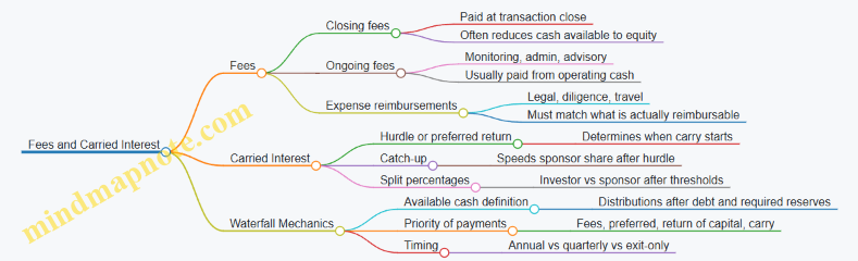
Fees: Where They Sit in the Cash Flow
Start by defining available cash for equity distributions. In most models, this is after:
- interest and principal payments on debt,
- required reserves (often for taxes, maintenance capex, or liquidity), and
- any mandatory payments to other equity classes.
Fees then determine whether equity investors receive distributions immediately or only after sponsor-related payments.
Example: Closing Fees That Reduce Equity Cash
Assume a $100 million purchase price. Sources include $40 million equity and $60 million debt. If sponsor-controlled entities charge $2 million in transaction fees paid at closing, the equity check effectively becomes $42 million worth of economic funding unless the fee is paid from debt proceeds or another source. In a model, you should reflect the fee in uses or as a reduction to cash available to equity, not as a random line item later.
Example: Ongoing Monitoring Fees That Reduce Distributable Cash
Suppose the fund charges $0.5 million per year in monitoring fees. If the business generates $10 million of distributable cash before fees, and the waterfall applies fees first, then only $9.5 million is available for preferred return and capital return. This matters for the timing of when carry begins.
Carried Interest: The Hurdle, Catch-Up, and Split
A typical carry structure has three stages:
- Return of capital to investors.
- Preferred return to investors, often calculated on invested capital.
- Carry participation to the sponsor once thresholds are met.
Catch-up is the mechanism that prevents the sponsor from waiting too long. Without catch-up, the sponsor might receive carry only after investors have already received most of the economics, which defeats the purpose of performance alignment.
Example: Simple Hurdle With Catch-Up
Assume:
- Investor capital: $40 million
- Preferred return: 8% annually
- Carry split after hurdle: 20% sponsor / 80% investors
- Catch-up: sponsor receives 100% of distributions until it has “caught up” to the target split.
If exit proceeds after debt are $60 million and fees are already accounted for, the waterfall first returns $40 million to investors. Next, investors receive preferred return on $40 million. Only after the preferred return is satisfied does the catch-up start, accelerating sponsor receipts until the sponsor reaches the 20% share of the remaining profit pool.
Waterfall Mechanics: Ordering Rules and Edge Cases
A practical waterfall should specify:
- Priority: which payments occur first (fees, preferred, capital return, carry).
- Measurement period: annual, semiannual, or exit-only.
- Compounding: whether preferred return compounds or is simple.
- Treatment of losses: whether carry is clawed back or only earned on net gains.
Example: Fees Paid Before Preferred Return
If the waterfall states that sponsor fees are paid before preferred return, then fees reduce the base that earns preferred return. That shifts the timing of when the hurdle is met and can delay carry.
Example: Fees Paid From Exit Proceeds
Some fees are exit-only. If they are deducted from proceeds before the preferred return calculation, the sponsor effectively reduces the profit pool available for carry. In a model, this should be explicit: treat exit fees as a reduction in distributable proceeds, not as a separate distribution class.
Mind Map: Waterfall Ordering Logic
Practical Modeling Checklist
- Put every fee into the correct timing bucket: closing, periodic, or exit.
- Ensure fees reduce the correct distribution base before preferred return if the documents say so.
- Implement carry with explicit threshold logic: return of capital, then preferred, then catch-up, then split.
- Reconcile the sponsor’s total receipts to the carry formula using the same profit pool definition used in the waterfall.
When these pieces align, the model becomes explainable: you can point to a specific cash source, a specific priority step, and a specific threshold that determines whether carry starts this year or waits until exit.
6.4 Tax Considerations in Equity Cash Flow Modeling
Equity cash flow models translate operating performance into what investors actually receive. Taxes are the bridge, but they are also where models quietly go wrong: mixing entity-level and investor-level taxes, using the wrong timing, or applying deductions that the structure cannot support. A clean approach is to model taxes at the level where cash is paid, then carry the after-tax results into the equity distribution waterfall.
Core Tax Layers in a Buyout
Start by separating three layers:
- Entity taxes: taxes paid by the operating company on its taxable income.
- Financing-related tax effects: how interest, amortization, and other deductions reduce taxable income.
- Investor-level taxes: taxes on dividends, interest-like returns, or capital gains depending on the investor’s jurisdiction and vehicle.
In most buyout models, the first two layers are the most material and are modeled explicitly. Investor-level taxes are often approximated or parameterized because they depend on investor type and local rules.
Modeling Entity-Level Taxes Systematically
A practical workflow:
- Compute taxable income from forecasted earnings.
- Apply deductions allowed by the tax regime, especially interest expense and depreciation or amortization.
- Apply tax rate(s) to arrive at current tax expense.
- Track timing differences if your model includes them, otherwise use a simplified effective tax rate.
A common simplification is to use an effective tax rate on earnings before tax after interest. This works when the operating profile is stable and the structure does not create large one-off tax items. If the deal includes unusual deductions, tax attributes, or significant changes in capital spending, you’ll need more granular logic.
Interest Deductibility and Debt Tax Shields
Interest is usually deductible, creating a tax shield that reduces entity taxes. The key is to ensure the model deducts interest in the same way the tax rules allow.
Two modeling checks keep you honest:
- Deduction limits: some regimes restrict interest deductibility based on earnings or leverage. If the structure is highly levered, you may need a cap or a carryforward mechanism.
- Timing: interest accrues and is paid on a schedule; tax deductions may follow accrual or payment rules depending on the jurisdiction.
Example: Suppose the operating company has $100 of EBITDA, $60 of interest expense, and $10 of depreciation. If taxable income is computed as EBITDA minus interest minus depreciation, taxable income is $30. With a 25% tax rate, current tax is $7.5. If interest deductibility is limited so only $50 is deductible, taxable income becomes $40 and tax becomes $10. The $2.5 difference flows directly into equity cash flow.
Depreciation, Amortization, and Basis Effects
Capital spending affects taxes through depreciation or amortization. In buyouts, purchase accounting can also create differences between book and tax bases.
Model depreciation as a driver of taxable income, not as an afterthought. If you use a simplified effective tax rate, you still need to ensure your earnings measure already reflects depreciation consistent with the tax logic.
Example: If maintenance capex is $20 per year and the tax system allows faster depreciation than book, taxable income will be lower early in the hold period. That reduces taxes now and increases equity distributions later, even if enterprise cash flow is unchanged.
Losses, Tax Attributes, and Utilization
Loss carryforwards and other tax attributes can materially change equity outcomes. The model should include:
- Availability of losses at acquisition.
- Utilization rules that limit how much can offset taxable income.
- Expiration or limitation schedules if applicable.
If you ignore loss utilization, you may overstate taxes in early years and understate equity returns.
Example: Assume the company has $50 of tax losses available and expects taxable income of $30 in year 1 and $30 in year 2. If losses can fully offset taxable income, taxes are $0 in year 1 and $0 in year 2 until losses are exhausted. If utilization is limited to 50% of taxable income, year 1 taxes apply on the remaining $15 taxable income.
Investor-Level Taxes and Distribution Timing
Equity distributions can be taxed differently from capital gains. Many models handle this by applying a distribution tax rate to cash distributions, or by using a simplified assumption that investor taxes are proportional to distributions.
Timing matters: taxes are often triggered when cash is distributed, not when accounting income is earned. Therefore, the equity waterfall should apply investor-level tax after determining distributable cash.
Example: If distributable cash before investor tax is $40 and the investor-level tax rate is 15%, investor tax is $6 and the net cash received is $34. If the model instead taxes $40 at the operating level, it will mis-time cash and distort IRR.
Mind Map: Tax Considerations in Equity Cash Flow Modeling
Integrated Example: From Taxable Income to Equity Distributions
Assume forecasted EBITDA is $120, interest is $55, depreciation is $15, and the entity tax rate is 25%. Taxable income is $50, so current tax is $12.5. After-tax operating cash available for distribution is reduced by $12.5 (plus any other non-tax cash items already modeled in your free cash flow definition). If the equity waterfall distributes $60 before investor tax and investor tax is 15%, investor tax is $9 and net equity cash received is $51. The model should keep the entity tax reduction in the operating-to-distributable step, and the investor tax reduction in the distribution-to-equity step.
Practical Consistency Rules
- Use the same earnings base for both interest and tax calculations.
- Apply investor taxes only when distributions occur.
- Keep tax timing aligned with cash timing in the waterfall.
- When simplifying, document the assumption in-model so it is traceable during sensitivity testing.
6.5 Practical Example: Constructing an Equity Waterfall With Multiple Tranches
An equity waterfall turns a pile of exit proceeds into a sequence of payments that match the legal economics of each equity tranche. The trick is to keep the order, the measurement base, and the “catch-up” logic consistent across the whole model. Below is a systematic build that starts with the minimum concepts and ends with a worked example.
Foundational Setup
Step 1: Define the equity tranches and their economic terms. A common buyout stack includes:
- Tranche A: Preferred equity with a fixed preferred return and a liquidation preference.
- Tranche B: Common equity held by the sponsor and management.
- Tranche C: Carried interest that participates after a hurdle, often with a catch-up.
Step 2: Choose the measurement base. In practice, waterfalls usually measure against Sale Proceeds (enterprise value translated to equity) after paying debt and transaction expenses. For modeling, use a single line item called Available Equity Proceeds.
Step 3: Lock the payment order. A typical order is:
- Return of preferred principal
- Preferred return
- Catch-up to the sponsor (if applicable)
- Split of remaining proceeds between sponsor and carry
Mind Map: Equity Waterfall Components
Worked Example with Clear Numbers
Assume the deal exits after one year.
Equity capital structure
- Preferred equity (Tranche A): $40.0m principal, 10% preferred return, paid at exit.
- Common equity (Tranche B): $20.0m.
- Carried interest (Tranche C): 20% of profits after a 12% preferred hurdle, with a 100% catch-up until the sponsor reaches the hurdle.
Exit proceeds to equity
- Enterprise value at exit: $120.0m
- Less: net debt and transaction costs paid from enterprise value: $60.0m
- Available Equity Proceeds: $60.0m
Compute the preferred entitlement
- Preferred principal: $40.0m
- Preferred return: $40.0m × 10% = $4.0m
- Total paid to Tranche A before any profit split: $44.0m
Remaining proceeds after preferred:
- $60.0m − $44.0m = $16.0m
Catch-Up and Profit Split Logic
Now apply the sponsor economics. The hurdle and catch-up are easiest to model if you treat them as allocations of the remaining $16.0m.
Assumption for this example: the hurdle is measured on the sponsor’s invested equity, and the catch-up is designed so the sponsor receives an additional amount that brings total sponsor receipts up to what the hurdle implies. In many models, this is implemented as a two-stage allocation:
- Catch-up stage: allocate proceeds so sponsor effectively receives 100% of the remaining amount until the sponsor’s total return reaches the hurdle.
- Residual stage: after catch-up, split remaining proceeds between sponsor and carry.
To keep the example concrete, set the catch-up target as follows:
- Sponsor’s hurdle target receipts on invested common: assume the sponsor needs $18.0m total receipts to meet the 12% hurdle on its $15.0m invested portion (common allocation assumed for illustration).
- Sponsor already receives its share of common before carry; in this simplified example, treat the sponsor’s “base” share as $6.0m, so the catch-up needs $12.0m of additional sponsor receipts.
Since the remaining proceeds are only $16.0m, the catch-up can be fully satisfied.
Stage 1: Catch-up allocation
- Sponsor receives $12.0m
- Carry receives $0.0m
- Proceeds left after catch-up: $16.0m − $12.0m = $4.0m
Stage 2: Residual split
- Carry is 20% of profits; sponsor is 80%
- Sponsor receives 80% × $4.0m = $3.2m
- Carry receives 20% × $4.0m = $0.8m
Final Waterfall Table
| Allocation Step | Amount (m) | Paid To |
|---|---|---|
| Preferred principal | 40.0 | Tranche A |
| Preferred return | 4.0 | Tranche A |
| Remaining proceeds | 16.0 | Profit allocation |
| Catch-up stage | 12.0 | Sponsor (via Tranche B economics) |
| Residual split | 3.2 | Sponsor |
| Residual split | 0.8 | Carry (Tranche C) |
| Total | 60.0 | All equity |
Modeling Checks That Prevent Common Errors
- Sum check: $44.0m + 12.0m + 3.2m + 0.8m = $60.0m.
- No overpayment: Tranche A receives exactly principal plus stated preferred return.
- Catch-up isolation: carry receives nothing during catch-up in this example, so the residual split only applies to the leftover $4.0m.
Mind Map: Allocation Flow

This structure gives you a repeatable template: change the tranche terms, recompute the preferred entitlement, then apply the same two-stage allocation framework to the remaining proceeds.
7. Cash Flow Modeling Foundations for Buyout Transactions
7.1 From Historical Financials to Forecast Assumptions
Historical financials are the starting point, but they are not the forecast. The job is to translate what happened into a set of assumptions that explain why it happened, then adjust for what will change. A clean workflow prevents two common modeling failures: copying last year’s numbers without understanding drivers, and building forecasts that match the past but fail basic logic.
Step 1: Normalize the Historical Baseline
Start by converting the target company’s reported statements into a consistent baseline.
- Pick a consistent period set. Use at least 3 years plus trailing twelve months if available. If seasonality exists, keep monthly or quarterly detail for working-capital lines.
- Normalize one-time items. Remove restructuring charges, litigation settlements, gains on asset sales, and unusual tax effects. Example: if EBITDA includes a one-time insurance recovery of $2.0m, subtract it to get “run-rate” operating performance.
- Reconcile accounting quirks. Align revenue recognition, capitalization policies, and lease treatment. Example: if maintenance capex was capitalized inconsistently, restate it so future capex assumptions reflect the true cash spending pattern.
A practical check: your normalized EBITDA should be explainable by operating drivers (volume, pricing, utilization, churn, headcount) rather than by accounting artifacts.
Step 2: Identify the Operating Drivers Behind Each Line
Forecasts should be built from drivers, not from percentages.
- Revenue drivers. Break revenue into components such as units sold, average selling price, customer count, and retention. Example: if revenue grew 8% last year, determine whether it was 3% from price and 5% from volume, because those behave differently under stress.
- Cost drivers. Map cost of goods sold and operating expenses to variables like labor hours, material costs, energy usage, or service tickets. Example: if gross margin improved due to lower input costs, you need an assumption for input cost pass-through rather than assuming margin stays constant.
- Working capital drivers. Model receivables days, inventory days, and payables days. Example: if DSO fell from 55 to 45, confirm whether it came from improved collections, a one-time billing change, or a customer mix shift.
Step 3: Convert Drivers into Forecast Assumptions
Turn each driver into a measurable assumption with a clear method.
- Pricing assumptions. Use a pricing rule tied to contract terms or historical renegotiation cycles. Example: assume average selling price increases 2.5% annually, but only 1.0% in the first year if contracts reset mid-year.
- Volume assumptions. Use capacity constraints, demand indicators, or customer pipeline conversion rates only if they are supported by historical conversion. Example: if new customer adds averaged 120 per quarter with a 20% churn, forecast net adds rather than gross adds.
- Cost inflation and productivity. Separate pure inflation from productivity. Example: labor costs rise 4% due to wage inflation, while productivity reduces labor hours per unit by 1.5%.
- Capex assumptions. Split maintenance capex from growth capex. Example: maintenance capex equals 3% of revenue based on the last two years, while growth capex scales with incremental capacity additions.
Step 4: Build a Forecast Bridge from Normalized History
A bridge shows how you move from normalized historical results to forecast year assumptions.
- Start with the last normalized year. Then apply driver changes: revenue growth, margin shifts, working-capital timing, and capex.
- Reconcile to the income statement and cash flow. If EBITDA rises but operating cash flow falls, the bridge should explain why (often working capital or capex timing).
Step 5: Validate Assumptions with Consistency Tests
Use simple tests that catch errors early.
- Margin sanity. If gross margin is stable historically, don’t forecast a sudden step change without a driver.
- Cash conversion sanity. Compare historical free cash flow conversion (FCF/EBITDA) to the forecast. Example: if conversion averaged 70% and your forecast implies 95% without a working-capital improvement driver, re-check receivables and payables assumptions.
- Covenant-relevant definitions. Ensure forecast EBITDA and free cash flow align with the definitions used in the credit agreement. Example: if add-backs are capped or require documentation, reflect that constraint in the forecast.
Mind Map: From Historical Financials to Forecast Assumptions
Example: Turning a Revenue Trend into Forecast Logic
Suppose normalized revenue grew from $100m to $108m. A naive approach would assume 8% growth again. A driver-based approach might show:
- Average selling price increased 3% (from contract renewals).
- Volume increased 5% (from higher utilization).
- No meaningful change in customer count.
If the next year’s contracts reset later, you might forecast price growth of 1.5% in year one, then 2.5% thereafter, while volume growth slows to 2% due to utilization nearing capacity. The forecast then explains both the level and the shape of revenue, which matters for working capital and debt service coverage.
Example: Working Capital Assumptions That Don’t Contradict Cash
If DSO improved last year, you need to know why. If it was driven by a one-time collections push, you might forecast DSO reverting from 45 back toward 52. That single change can reduce operating cash flow even when EBITDA looks strong, which is exactly the kind of mismatch that can break a leveraged buyout model.
When historicals are normalized, drivers are mapped, assumptions are quantified, and validation checks are applied, the forecast becomes a coherent explanation of cash flow—not just a spreadsheet that happens to look plausible.
7.2 Revenue Cost and Working Capital Drivers
Revenue, costs, and working capital move together in buyout models because cash is the constraint. A clean way to structure the section is to start with how revenue is generated, then how costs respond, and finally how timing differences between cash receipts and cash payments create working capital needs.
Revenue Drivers That Create Cash
Revenue in a buyout model is usually built from volume and price. Volume can be units sold, customers served, or usage measured by contracts. Price can be list price, realized price after discounts, or effective rate after rebates. The practical modeling habit is to separate “what you sell” from “what you get paid,” because discounts often change faster than volumes.
Example: A distributor sells 10,000 units per month at $50 list price. If average discount is 8%, realized price is $46. The model should compute revenue as volume × realized price, not as a single blended number, so you can test whether a discount change is the real driver.
For recurring revenue businesses, revenue may be driven by customer count and churn, plus expansion. For project-based businesses, revenue may be driven by backlog conversion and billing schedules. In both cases, the key is to align revenue recognition with cash collection timing later in the working capital section.
Cost Drivers That Determine Margin and Flexibility
Costs should be split into variable and fixed components. Variable costs scale with volume and often include direct materials, direct labor, and transaction-based costs. Fixed costs include rent, salaried headcount, and baseline overhead. This split matters because buyouts often rely on margin improvement, and margin improvement is only as good as the model’s cost flexibility.
Example: If variable cost is 60% of revenue, then a 1% revenue increase increases variable cost by 0.6% of revenue, while fixed costs stay flat. If instead you model costs as a single percentage of revenue, you lose the ability to represent step-changes like hiring or overtime.
Operating expenses also have internal drivers. Sales and marketing may scale with revenue, but customer support may scale with customer count. Maintenance may scale with asset base or usage. The model should map each cost line to a driver so that changes in volume or customer count propagate logically.
Working Capital Drivers That Create Timing Gaps
Working capital is the difference between cash tied up in operations and cash generated by operations. In most buyout models, the main components are accounts receivable (AR), inventory, and accounts payable (AP).
AR is driven by revenue and collection speed. A common approach is to model AR days: AR = (Revenue per day) × AR days. If collection terms tighten from 45 to 30 days, AR falls even if revenue stays the same, improving cash.
Inventory is driven by cost of goods sold (COGS) and inventory days. Inventory = (COGS per day) × Inventory days. If supply chain improves and inventory days drop, cash is released because less cash is stuck in stock.
AP is driven by purchases and payment speed. AP = (COGS per day) × AP days, or sometimes purchases per day depending on how the business buys. Extending payment terms increases cash in the short run, but it can strain supplier relationships, so the model should treat AP days as a controllable assumption rather than a magic lever.
Mind Map: Revenue, Cost, and Working Capital Links
Integrated Example from Revenue to Cash
Assume a company has monthly revenue of $10.0m, COGS of 65% of revenue ($6.5m), and stable fixed operating expenses. Collection terms are 45 days, inventory days are 30, and AP days are 25.
- AR: Revenue per day is $10.0m / 30 = $0.333m. AR ≈ $0.333m × 45 = $15.0m.
- Inventory: COGS per day is $6.5m / 30 = $0.217m. Inventory ≈ $0.217m × 30 = $6.5m.
- AP: AP ≈ $0.217m × 25 = $5.4m.
Net working capital ≈ AR + Inventory − AP = $15.0m + $6.5m − $5.4m = $16.1m.
Now suppose realized price improves by 2% while volume is unchanged, and COGS stays at 65% of revenue. Revenue rises to $10.2m and COGS to $6.63m. If AR days, inventory days, and AP days remain constant, AR and inventory increase proportionally, and net working capital increases too. That’s the modeling point: margin improvement can still consume cash if timing assumptions don’t move.
Practical Modeling Checks That Prevent Silent Errors
First, confirm that working capital assumptions are consistent with the revenue and cost bases used in the formulas. If AR is calculated from revenue, don’t accidentally use recognized revenue when the business bills later.
Second, test sensitivity in small steps. Change AR days by 5 days and observe the cash impact; if the effect is wildly inconsistent with the business size, the days-to-dollar conversion is likely wrong.
Third, ensure that working capital changes flow into free cash flow through the correct sign convention. An increase in net working capital is a cash use; a decrease is a cash source. This is one of those rules that feels obvious until a sign flips and the model starts paying you for holding inventory.
7.3 Capital Expenditures and Maintenance Versus Growth Capex Modeling
Capital expenditures (capex) modeling is where “cash flow” stops being a concept and starts being a spreadsheet habit. In buyout models, capex affects free cash flow directly, and it also shapes how much cash is available for interest, principal, and equity distributions. A clean approach separates maintenance capex from growth capex, then ties both to operational drivers so the forecast behaves like the business rather than like a guess.
Core Definitions and Modeling Goal
Maintenance capex is spending required to keep existing assets producing at the forecasted level. Growth capex is spending intended to expand capacity, add locations, improve throughput, or otherwise increase future operating performance.
Modeling goal: forecast capex by driver, not by percentage alone. Percent-of-revenue rules can work as a starting point, but they often hide the real cause of cash outflows—asset age, utilization, backlog, or planned expansions.
Step 1: Build the Capex Bridge from Financials
Start with historical capex from the cash flow statement, then reconcile it to the model’s capex line items.
- If the company reports “capital expenditures” net of asset sales, decide whether your model uses net or gross. Keep it consistent with how you treat proceeds from asset disposals.
- If capex includes software capitalization, separate it if your operating model treats software as a cost driver rather than a balance sheet asset.
Practical example: A manufacturer shows $12m capex last year. You review notes and find $3m was required maintenance for aging equipment and $2m was compliance-related upgrades. The remaining $7m is capacity expansion. Your model should reflect that split, even if the income statement only sees depreciation later.
Step 2: Separate Maintenance Versus Growth Capex
A useful rule: maintenance capex should correlate with keeping revenue and margins stable, while growth capex correlates with changes in scale.
Common ways to classify spending:
- Maintenance indicators: replacement cycles, asset condition assessments, recurring turnaround costs, and “keep the lights on” projects.
- Growth indicators: new production lines, additional warehouses, new stores, major automation intended to increase throughput.
Easy-to-understand example: A retailer plans 10 new stores in year 1. The capex for store build-outs is growth capex. The annual roof repairs for existing stores are maintenance capex. Even if both are “projects,” their cash-flow purpose differs.
Step 3: Choose Driver-Based Forecast Methods
Use one of these methods for each capex bucket.
- Percent of Revenue with Guardrails
- Maintenance capex = base percent × revenue, adjusted for asset intensity.
- Growth capex = separate schedule tied to expansion milestones.
- Per-Unit or Per-Asset Spending
- Maintenance capex = units serviced × cost per unit.
- Growth capex = new assets × cost per asset.
- Capex as a Function of Utilization or Throughput
- Maintenance capex increases when utilization rises beyond normal ranges.
- Growth capex triggers when capacity constraints appear.
Practical example: A logistics firm has maintenance capex of $2,000 per truck per year. If the fleet grows from 800 to 900 trucks, maintenance capex rises with the fleet size, while growth capex is only the purchase of the additional 100 trucks.
Step 4: Model Timing and the Cash Reality
Capex is paid when projects progress, not when the model “decides” to spend. Timing matters for covenant testing periods.
- Use a simple timing assumption: 50% of growth capex paid in year 1 and 50% in year 2, or align payments to project start dates.
- For maintenance, assume smoother spending unless the company has known shutdown periods.
Example: If expansion capex is $20m starting mid-year, you might model $10m in year 1 and $10m in year 2. This prevents an artificial year-1 cash crunch.
Step 5: Connect Capex to Depreciation Without Mixing Cash and Non-Cash
Depreciation affects EBITDA and therefore leverage and coverage tests, while capex affects free cash flow. They are related but not identical.
- Depreciation schedule: use existing asset base and expected useful lives.
- Capex schedule: use cash payment timing and project completion.
If you add growth capex, depreciation should increase later, not immediately. That lag is often the difference between a model that looks “tight” and one that behaves realistically.
Step 6: Include Working Capital Interactions Carefully
Some projects are funded through working capital changes (for example, long-lead inventory for expansions). Keep capex and working capital separate, but ensure the operational model reflects the same project.
Example: A food producer buys long-lead ingredients for a new line. Inventory build is working capital. The equipment purchase is capex. Mixing them leads to double counting cash usage.
Mind Map: Capex Modeling Workflow
Example: A Simple Integrated Capex Build
Assume a business has $30m revenue in year 1 and plans a capacity expansion.
- Maintenance capex: 4% of revenue, so $1.2m in year 1.
- Growth capex: $10m total for a new line, paid 60% in year 1 and 40% in year 2.
- Year 1 growth capex cash: $6.0m
- Year 2 growth capex cash: $4.0m
Total capex cash outflow:
- Year 1: $1.2m + $6.0m = $7.2m
- Year 2: $1.2m (if revenue stays flat) + $4.0m = $5.2m
Then depreciation increases based on the completed asset base and useful life, not on the capex cash payment. This keeps EBITDA and free cash flow moving for the right reasons.
Validation Practices That Prevent Common Errors
- Reconcile capex totals to historical patterns before splitting into maintenance and growth.
- Ensure maintenance capex does not quietly drift upward without an asset-intensity reason.
- Check that growth capex schedules align with operational drivers in the revenue and margin model.
- Confirm that capex timing aligns with covenant testing periods so coverage doesn’t fail due to accounting timing mismatches.
When these pieces fit together, capex becomes a controlled driver of cash flow rather than a late-stage adjustment that surprises the equity return model.
7.4 Free Cash Flow Definitions and Reconciliation to Debt Service
Free Cash Flow (FCF) is the cash a business generates after paying for the things it must pay for to keep operating and investing at a basic level. In leveraged buyouts, the definition matters because lenders and equity investors care about different slices of cash, and the model must translate accounting numbers into cash available for debt service.
Core Definitions That Drive Consistent Modeling
Start with a forecast that produces an operating cash base. A practical modeling approach is to compute:
- EBITDA from the operating forecast.
- Less cash taxes based on taxable income assumptions.
- Less capital expenditures to reflect maintenance and required growth capex.
- Less changes in working capital to capture cash tied up in receivables, inventory, and payables.
A common buyout-friendly definition is FCF to Firm:
- FCF to Firm = EBITDA − Cash Taxes − Capex − Change in Working Capital
This is “to the firm” because it is before interest and principal payments. That separation is what makes reconciliation clean: you can then allocate the cash to debt service and equity distributions using an explicit waterfall.
Reconciling FCF to Debt Service Without Mixing Concepts
Debt service is not just interest. It includes interest payments and scheduled principal repayments, plus any required fees that behave like cash outflows. The reconciliation step converts FCF into the cash that can be applied to each debt class.
A systematic reconciliation uses three layers:
- Operating cash generation (FCF to Firm).
- Cash required for debt (interest + mandatory principal + required fees).
- Residual cash (available for voluntary prepayments, restricted payments, or cash sweeps depending on the credit agreement).
A simple reconciliation line item set looks like this:
- Cash Available for Debt Service = FCF to Firm
- Debt Service = Interest Paid + Mandatory Principal + Required Fees
- Residual Cash After Debt Service = Cash Available for Debt Service − Debt Service
If your model includes cash interest hedges, keep them consistent: treat hedge settlements as cash flows in the interest line (or a dedicated hedge line) so the “interest paid” number matches what actually hits the bank account.
Mind Map: From Operating Forecast to Debt Service
Practical Example: One Year, One Debt Stack
Assume a company forecasts:
- EBITDA: 120
- Cash taxes: 18
- Capex: 20
- Change in working capital: +6 (a use of cash)
Then:
- FCF to Firm = 120 − 18 − 20 − 6 = 76
Now assume debt terms require:
- Interest paid on senior secured: 14
- Interest paid on mezzanine: 6
- Mandatory principal repayments: 10 total
- Required fees that are cash outflows: 2
Then:
- Debt Service = 14 + 6 + 10 + 2 = 32
- Residual Cash After Debt Service = 76 − 32 = 44
That residual cash is what your waterfall logic will allocate. If the agreement includes an excess cash flow sweep, you would compute the sweep base separately and then apply it to the residual cash, ensuring you do not double-count the same cash.
Advanced Details That Prevent Common Reconciliation Errors
-
Cash taxes vs. accounting taxes: If you use an effective tax rate on earnings, you still need a cash timing assumption. Otherwise, your FCF-to-debt-service bridge will drift.
-
Capex classification: Maintenance capex should be treated as required for operations. Growth capex can be modeled explicitly, but it must still be cash outflow in the FCF definition you use for debt service.
-
Working capital sign discipline: Define whether “Change in Working Capital” is positive when it consumes cash. Pick one convention and stick to it across the model.
-
Principal schedule alignment: Mandatory principal should come from the amortization schedule, not from a generic “debt reduction” plug.
-
Fees and OID-like effects: Some financing items affect interest expense but not cash in the same period. If the model uses cash interest, ensure the reconciliation uses cash outflows, not accrual-only expense.
Reconciliation Checklist You Can Run Every Time
- FCF to Firm is computed from operating drivers and cash-based assumptions.
- Interest paid equals the cash payment schedule for each debt class.
- Mandatory principal equals scheduled amortization or required repayments.
- Required fees are included where they are cash outflows.
- Residual cash is the single source for sweeps and distributions logic.
When these pieces line up, the model becomes easier to audit: if residual cash is negative, you know debt service exceeded operating cash; if it is positive, you can trace exactly where the cash goes next.
7.5 Practical Example: Building an Integrated Model From Income Statement to Cash Flow
Start with one simple goal: every cash movement in the debt section must trace back to an operating cash driver or a balance sheet change. If you can’t trace it, the model is just a spreadsheet with opinions.
Step 1: Set Up the Operating Core
Build the income statement first because it determines EBITDA and taxes, which then drive cash taxes and working capital needs.
Example assumptions for a single forecast year
- Revenue: $100.0m
- EBITDA margin: 25% → EBITDA $25.0m
- D&A: $6.0m
- EBIT: $19.0m
- Cash interest: modeled later from debt schedule
- Taxes: 25% on EBT (after interest)
Practice tip: keep D&A separate from capex. D&A affects taxes; capex affects cash.
Step 2: Convert EBITDA to Free Cash Flow
Define Free Cash Flow (FCF) consistently. A common buyout-friendly definition is:
- FCF = EBITDA − Cash Taxes − Capex − Change in Net Working Capital
To compute cash taxes, use:
- EBT = EBIT − Cash Interest
- Cash Taxes = Tax Rate × EBT
Example:
- EBIT $19.0m
- Assume average cash interest $4.0m (from Step 4 later)
- EBT $15.0m
- Cash taxes $3.75m
Now working capital and capex:
- Change in NWC: assume NWC increases by $1.5m → cash outflow (−1.5m)
- Capex: $5.0m
So:
- FCF = 25.0 − 3.75 − 5.0 − 1.5 = $10.75m
Step 3: Reconcile to the Balance Sheet
An integrated model should reconcile cash and debt movements. Use a cash bridge:
- Beginning Cash
- + Operating Cash Flow
- − Capex
- − Debt Service
- − Equity Distributions
- = Ending Cash
Operating Cash Flow can be expressed as:
- Operating Cash Flow = EBITDA − Cash Taxes − Change in NWC
This keeps the income statement and cash flow aligned without double-counting.
Step 4: Build the Debt Schedule That Feeds Interest
Create a debt schedule with beginning balance, draws, repayments, and ending balance. Then compute interest from the average balance.
Example debt layer
- Senior secured term loan: $60.0m beginning
- Interest rate: 9.0% (floating plus margin already reflected)
- No repayments during the year yet
Interest:
- Average balance ≈ $60.0m
- Cash interest = 60.0 × 9.0% = $5.4m
Now update taxes from Step 2 using the correct interest. This is where integration matters: if you change interest, taxes must change.
Step 5: Link FCF to Debt Paydown and Equity Distributions
Use an application waterfall logic to decide how FCF becomes repayments.
Example simplified rule
- First, mandatory debt amortization: $2.0m
- Then, excess cash after a cash minimum of $1.0m goes to optional prepayment
- Remaining cash can be distributed to equity
If FCF is $10.75m and mandatory amortization is $2.0m, then available for optional uses is $8.75m, subject to the cash minimum and any restricted payments limits.
Step 6: Mind Map of the Integration Logic
Mind Map: Integrated Model Flow
Step 7: Mini Worked Example with One Consistent Loop
Use this loop: interest → taxes → FCF → paydown → ending debt → next period interest.
Example for Year 1
- Beginning term loan: $60.0m
- Cash interest: $5.4m
- EBIT: $19.0m
- EBT: 19.0 − 5.4 = $13.6m
- Cash taxes: 25% × 13.6 = $3.4m
- Change in NWC: +$1.5m outflow
- Capex: $5.0m
- FCF: 25.0 − 3.4 − 5.0 − 1.5 = $11.1m
- Mandatory amortization: $2.0m
- Optional prepayment: $9.1m (subject to cash minimum and restrictions)
- Ending debt: 60.0 − 2.0 − 9.1 = $48.9m
That ending debt becomes the input for Year 2 interest. If your Year 2 interest doesn’t reflect Year 1 paydown, your model is not integrated—it’s just connected by hope.
8. Debt Service Coverage and Covenant Calculations
8.1 Covenant Types and Testing Frequencies
Covenants are the contract’s way of saying, “We’ll keep an eye on the business, and if it drifts too far, we pause or renegotiate.” In leveraged buyouts, the practical question is not just which covenant, but how often it is tested and what numbers are allowed to move.
Foundational Covenant Categories
Most credit agreements group covenants into a few buckets.
- Financial maintenance covenants require the borrower to meet a metric at each test date. If the metric fails, it’s usually a default unless a cure or waiver applies.
- Incurrence covenants restrict actions unless a condition is satisfied at the time of the action. For example, “You may incur additional debt only if leverage is below X.”
- Reporting covenants require timely delivery of financial statements and compliance certificates. These don’t usually trigger a default based on the metric itself, but they can trigger default if missed.
- Negative covenants restrict specific behaviors such as liens, asset sales, restricted payments, or affiliate transactions.
A useful mental model: maintenance covenants are like seatbelts checked while driving; incurrence covenants are like rules for changing lanes.
Testing Frequencies and Their Meaning
Testing frequency determines how quickly covenant breaches can be detected and how much flexibility management has.
- Quarterly testing is common for leverage and coverage metrics. It reduces the “surprise factor,” because the lender sees deterioration sooner.
- Semiannual or annual testing appears in some structures, often where the borrower’s reporting cadence is slower or the lender is comfortable with less frequent checks.
- Event-driven testing occurs when a covenant is tied to an action, such as issuing equity, making a restricted payment, or incurring new debt.
If you’re modeling, testing frequency affects the number of covenant measurement points and therefore the number of opportunities for headroom to shrink.
The Core Financial Metrics
Two metric families dominate maintenance covenants.
-
Leverage covenants compare debt to a cash-earnings proxy (often EBITDA, sometimes adjusted EBITDA).
- Example: “Total Net Leverage Ratio must be ≤ 5.50x.”
- Practical nuance: definitions of “net” (cash netting, permitted cash, and debt exclusions) can change the ratio materially.
-
Coverage covenants compare earnings to fixed obligations.
- Example: “Fixed Charge Coverage Ratio must be ≥ 1.50x.”
- Practical nuance: fixed charges may include interest, scheduled principal, leases, and sometimes certain cash taxes depending on the definition.
How Testing Works in Practice
Testing is usually performed on a trailing basis.
- Quarterly maintenance tests often use the last twelve months (LTM) or last four quarters.
- Annual tests may use the fiscal year results, sometimes still expressed as LTM but aligned to year-end.
This matters because a one-quarter dip may not immediately break a leverage covenant if the trailing window still includes stronger quarters.
Mind Map: Covenant Types and Testing Frequencies
Example: Quarterly Leverage Test with Headroom
Assume a borrower has a leverage covenant tested quarterly using LTM EBITDA.
- Covenant: Net Leverage ≤ 5.50x
- Current quarter results imply LTM EBITDA of $120m
- Net debt definition yields $660m
- Ratio: $660m / $120m = 5.50x
Now suppose the next quarter EBITDA drops to $105m on an LTM basis while net debt stays $660m.
- New ratio: $660m / $105m ≈ 6.29x
If the agreement has no cure or waiver, this quarter’s test date becomes the breach point. If there is an equity cure, management can inject cash to reduce net debt or increase the numerator/denominator depending on the cure mechanics—so the exact wording of “cure” is not a footnote; it’s a lever.
Example: Incurrence Covenant Tested at Action Time
Consider a restricted payment covenant that allows dividends only if leverage is below a threshold.
- Rule: “Restricted payments permitted if Net Leverage ≤ 4.75x.”
- At the time of the proposed dividend, the borrower’s LTM leverage is 4.80x.
Even if the borrower expects leverage to improve next quarter, the action is still not permitted under a strict incurrence covenant. That’s why lenders like incurrence tests: they tie permission to the moment of risk.
Advanced Detail: Why Definitions Control Outcomes
Two agreements can both say “Net Leverage” and still produce different results.
- Cash netting: permitted cash may be excluded, or only certain cash accounts count.
- Debt exclusions: some debt may be treated as non-recourse or excluded if it’s subject to specific conditions.
- EBITDA adjustments: add-backs for restructuring, one-time expenses, or management fees can change the numerator.
A disciplined approach is to treat covenant compliance as a calculation pipeline: inputs, adjustments, exclusions, and then the ratio. If you can’t trace each component to a line item, you don’t yet have covenant certainty.
Practical Checklist for Testing Frequency
- Identify whether the covenant is maintenance or incurrence.
- Confirm the test date cadence and whether it uses LTM.
- Map the exact metric definitions for net debt, EBITDA, and fixed charges.
- Check for cure rights and what they can actually fix.
- Ensure your model updates the covenant window consistently each quarter.
When these pieces line up, covenant compliance becomes less of a mystery and more of a repeatable process—like balancing a checkbook, except the checkbook has interest rate risk.
8.2 Leverage Ratios and EBITDA Adjustments
Leverage ratios answer one simple question: how much debt the business can support with its operating earnings. In buyout credit agreements, the most common leverage test is Total Debt to EBITDA or Senior Secured Debt to EBITDA. The “EBITDA” part is where the real work happens, because it is not always the same as the EBITDA you see in a financial statement.
Foundational Concepts for Leverage Testing
Start with the two ingredients.
Debt numerator. “Total Debt” typically includes term loans, revolvers drawn amounts, and other funded obligations. Some agreements exclude certain items (for example, letters of credit that are not drawn, or specific intercompany debt). “Senior Secured Debt” is narrower and usually tracks only debt secured by the first-priority collateral package.
EBITDA denominator. EBITDA is built from earnings, then adjusted for items the agreement treats as non-recurring, non-cash, or otherwise outside the test’s intent. The agreement also defines whether EBITDA is calculated on a trailing basis (TTM) or forward-looking basis (often quarterly with a rolling twelve-month view).
A practical way to keep your footing: treat the leverage test as a translation exercise. You translate accounting results into “agreement EBITDA,” then compare it to “agreement debt.” If you translate consistently, the ratio becomes meaningful.
EBITDA Adjustments Framework
Most EBITDA adjustment schedules follow a pattern: start with a base, then add permitted add-backs, subtract permitted deductions, and apply caps or limits.
Common adjustment categories include:
- Non-cash charges. Depreciation and amortization are usually included in EBITDA by definition, but other non-cash items may be added back if they are excluded elsewhere.
- Cash interest and taxes. These are not part of EBITDA, but they matter indirectly because the base earnings line can vary by agreement.
- Non-recurring items. Restructuring costs, transaction expenses, and one-time legal settlements may be added back if they meet the agreement’s definition.
- Pro forma adjustments. If the company acquired a business, the agreement may allow pro forma EBITDA for a period, subject to documentation.
- Run-rate adjustments. Some agreements permit adjustments for cost savings or revenue changes that are expected to occur, but only if the agreement’s conditions are satisfied.
The agreement’s wording matters because it controls three things: what qualifies, how it is measured, and whether it is capped.
Mind Map: Leverage Ratio Mechanics
Example: Adjustments That Change the Ratio
Assume a company reports the following for the trailing twelve months:
- Reported EBITDA: $120.0 million
- Non-recurring restructuring costs: $6.0 million
- One-time transaction expenses: $3.0 million
- Stock-based compensation: $4.0 million (agreement allows add-back)
- Cap on non-recurring add-backs: 10% of EBITDA
First compute the cap. Ten percent of reported EBITDA is $12.0 million. The non-recurring items total $9.0 million ($6.0m + $3.0m), which is within the cap, so both are eligible.
Then build agreement EBITDA:
- Agreement EBITDA = 120.0 + 6.0 + 3.0 + 4.0 = $133.0 million
Now assume debt:
- Total Debt = $560.0 million
Leverage ratio = 560.0 / 133.0 = 4.21x.
If you instead used reported EBITDA without adjustments, leverage would be 560.0 / 120.0 = 4.67x. That difference is not magic; it is the direct effect of permitted add-backs.
Example: When Adjustments Are Not Fully Usable
Now change one fact: suppose restructuring costs rise to $15.0 million while transaction expenses remain $3.0 million. Non-recurring total becomes $18.0 million. The cap is still $12.0 million, so only $12.0 million of non-recurring add-backs are allowed.
Agreement EBITDA = 120.0 + 12.0 + 3.0? Careful: the $3.0m is already included in the $18.0m non-recurring total. The cap limits the entire non-recurring pool to $12.0m, so agreement EBITDA becomes:
- Agreement EBITDA = 120.0 + 12.0 + 4.0 = $136.0 million
Leverage = 560.0 / 136.0 = 4.12x.
Notice what happened: the extra $6.0 million of non-recurring costs did not help the covenant because the agreement’s limit prevented it from flowing into EBITDA.
Practical Checklist for Accurate Calculations
- Confirm the debt definition used in the covenant (Total Debt vs Senior Secured Debt).
- Identify the EBITDA base line the agreement starts from.
- List each add-back and verify it meets the definition.
- Apply caps and thresholds before summing.
- Match the measurement period to the testing date and ensure the same period is used for both numerator and denominator.
If you do these steps in order, leverage testing becomes a controlled arithmetic exercise rather than a debate about interpretation.
8.3 Fixed Charge Coverage and Interest Coverage Mechanics
Fixed charge coverage and interest coverage are the two most common “can we pay without borrowing more?” checks in leveraged buyouts. The first focuses on a broader set of cash obligations; the second focuses narrowly on interest. Both are usually tested on a quarterly or semiannual basis, using a defined EBITDA measure and a defined cash charge measure. The trick is that the definitions matter as much as the arithmetic.
Core Definitions and Why They Differ
Interest Coverage typically measures whether operating cash earnings cover net interest expense. A common form is:
- Interest Coverage = EBITDA / Net Interest Expense
Fixed Charge Coverage typically measures whether EBITDA covers interest plus other fixed cash charges such as scheduled principal amortization and lease payments (depending on the credit agreement). A common form is:
- Fixed Charge Coverage = EBITDA / Fixed Charges
Fixed charges often include items that interest coverage ignores, so fixed charge coverage is usually tighter, especially when amortization steps up or when leases are material.
Step 1: Build EBITDA the Way the Agreement Says
Start with the EBITDA definition in the credit agreement, not your spreadsheet’s default. Typical components include:
- Starting from operating results (often consolidated)
- Adding back depreciation and amortization
- Adjusting for certain non-cash or non-recurring items
- Applying permitted adjustments and limits
Easy example: Suppose EBITDA per the agreement is $120. Your income statement might show $110, but the agreement allows $10 of permitted add-backs. If you use $110, you will understate coverage and may fail a test that would otherwise pass.
Step 2: Compute Net Interest Expense
Net interest expense is usually:
- Cash interest on funded debt
- Plus or minus interest related to hedges, depending on how the agreement treats them
- Minus interest income if permitted
Easy example: If gross cash interest is $18 and the agreement permits netting $2 of interest income, then net interest expense is $16.
Step 3: Compute Fixed Charges
Fixed charges commonly include:
- Net interest expense
- Scheduled principal amortization (not optional prepayments)
- Required lease payments (if included)
- Other mandatory fixed payments specified in the agreement
Easy example: If net interest is $16 and scheduled principal is $6, fixed charges are $22. If leases are included and total required lease payments are $3, fixed charges become $25.
Step 4: Apply the Ratio and Interpret the Result
If the covenant requires:
- Interest Coverage ≥ 2.5x
- Fixed Charge Coverage ≥ 1.5x
Then with EBITDA $120:
- Interest coverage = 120 / 16 = 7.5x (comfortably passes)
- Fixed charge coverage = 120 / 25 = 4.8x (also passes)
A ratio passing is not the same as “safe forever.” But for covenant testing, you only need to pass the tested period using the defined inputs.
Mind Map: Coverage Mechanics
Advanced Details That Commonly Break Models
-
Measurement period mismatch. Covenants often test using trailing twelve months or a quarterly run-rate. If your EBITDA is forecast for a single quarter but the covenant uses TTM, your ratios will be wrong.
-
Principal amortization timing. Scheduled principal may be quarterly, semiannual, or annual. Use the exact schedule and ensure you include only what is “required” under the agreement, not what you plan to prepay.
-
Lease treatment. Some agreements include lease payments in fixed charges; others exclude them or include only certain leases. If your model uses lease expense but the covenant uses lease payments, you may need to convert.
-
Hedge accounting effects. Even when hedges are economically real, the covenant may define how hedge gains or losses affect net interest. Model the covenant definition, not the accounting presentation.
Example: One Covenant Passes While the Other Fails
Assume:
- EBITDA per agreement = $90
- Net interest expense = $30
- Scheduled principal amortization = $40
- Lease payments included in fixed charges = $0
Interest coverage = 90 / 30 = 3.0x. If the covenant requires ≥ 2.5x, it passes.
Fixed charges = 30 + 40 = 70. Fixed charge coverage = 90 / 70 = 1.29x. If the covenant requires ≥ 1.5x, it fails.
This is the practical reason fixed charge coverage exists: it forces attention to principal and other fixed cash obligations, not just interest.
Example: Sensitivity Through a Single Driver
If EBITDA is $120 and net interest is $20, interest coverage is 6.0x. Now increase scheduled principal amortization from $5 to $10 while fixed charges become 20 + 10 = 30. Fixed charge coverage drops from 120 / 25 = 4.8x to 120 / 30 = 4.0x. The ratio changes because fixed charges move directly with amortization, even when interest stays constant.
Practical Checklist for Covenant-Ready Calculations
- Confirm the EBITDA definition and whether it is TTM or run-rate.
- Confirm whether net interest includes interest income and how hedges are treated.
- Confirm which items are included in fixed charges, especially principal amortization and leases.
- Use the debt schedule for required principal, not planned prepayments.
- Reconcile every input to the credit agreement language before trusting the ratio.
8.4 Cure Rights and Equity Cure Provisions
Covenants are enforced through testing and remedies, but the real question is what happens when a test fails. Cure rights and equity cure provisions are the structured “second chance” mechanisms that let a borrower fix the covenant breach without triggering immediate default. They are not magic; they are carefully bounded tools that trade cash or equity for compliance.
Foundational Concepts of Covenant Failure
A covenant breach typically occurs when a measurement date arrives and the borrower’s calculation shows a ratio or coverage level outside the permitted range. The credit agreement then specifies whether the breach is an event of default, a default that can be cured, or a breach that triggers a remedy like increased pricing or restricted actions.
Cure rights usually fall into two buckets:
- Borrower cure rights: the borrower can take an action that changes the covenant calculation (often by adding cash, reducing debt, or increasing EBITDA adjustments within defined limits).
- Equity cure provisions: the borrower can contribute equity (or cash treated as equity) to improve the covenant metric, usually by reducing leverage or improving coverage.
What Cure Rights Actually Do
Cure rights are designed to preserve deal continuity when the breach is temporary or caused by timing. The agreement typically defines:
- Cure amount: how much cash or equity can be used.
- Cure timing: the window after the breach notice or test date.
- Cure frequency: limits such as “no more than once per fiscal year” or “aggregate cap over the term.”
- Cure mechanics: whether the cure must be applied to reduce debt, fund a restricted cash account, or be treated as an equity contribution.
A practical way to see the logic: if leverage is too high because net debt is temporarily elevated, a cure can reduce net debt immediately. If coverage is too low because earnings are temporarily depressed, a cure can still help by lowering interest burden or leverage, depending on the covenant definition.
Equity Cure Provisions and Their Economic Purpose
Equity cure provisions exist because sponsors often prefer not to force a default for a solvable accounting or timing issue. The sponsor’s equity contribution effectively replaces borrower cash that would otherwise be used to meet the covenant.
The key economic constraint is that the cure must be real and documented. The agreement usually requires:
- The contribution is made by equity holders or affiliates, not by the borrower indirectly.
- The contribution is treated as equity for accounting and covenant purposes.
- The cure does not create circularity, such as borrowing the same money back from lenders.
Mind Map: Cure Rights and Equity Cure Provisions
Example: Leverage Covenant Breach with an Equity Cure
Assume a borrower has a leverage covenant tested quarterly: Net Total Leverage must be ≤ 6.0x. At the test date, the borrower calculates 6.4x, failing by 0.4x.
If the credit agreement allows an equity cure up to a cap and within a cure window, the sponsor can contribute equity cash that is used to reduce net debt or otherwise changes the net leverage calculation as permitted. Suppose the agreement’s mechanics treat the contribution as reducing net debt dollar-for-dollar for covenant purposes.
If net debt is $200 million at 6.4x and EBITDA is $31.25 million (since 200 / 31.25 = 6.4), then to reach 6.0x the borrower needs net debt of 6.0 × 31.25 = $187.5 million. The required reduction is $12.5 million. The sponsor contributes $12.5 million as equity, and the borrower re-tests under the agreement’s cure mechanics.
The subtle point: the cure amount is not “whatever fixes the ratio in your spreadsheet.” It must follow the agreement’s defined treatment of the contribution.
Example: Cure Timing and Notice Mechanics
Consider a scenario where the borrower discovers the breach during preparation of the compliance certificate. If the agreement requires notice within a specific period and allows a cure only after notice, the borrower must act quickly. A cure that is technically available but submitted after the cure window can fail, even if the amount is correct.
This is why compliance certificate preparation is operationally important: the cure process depends on the paperwork trail, not just the math.
Advanced Details That Prevent Common Mistakes
- Cure does not automatically erase the breach for all purposes: some agreements treat the breach as cured for default purposes but still require disclosures or may affect other baskets.
- Cure frequency limits matter: if the sponsor uses a cure early in the year, later breaches may be uncureable under the same provision.
- Documentation must match the covenant definition: the contribution must be structured and evidenced so it qualifies as equity for the specific covenant calculation.
- Intercreditor and waterfall interactions: if the cure involves debt reduction, the agreement may specify which debt is reduced and how that interacts with payment priorities.
Practical Checklist for Equity Cure Execution
- Confirm the covenant type and the exact cure mechanics allowed.
- Verify the cure window and the required notice steps.
- Calculate the minimum equity contribution using the agreement’s covenant definitions.
- Ensure the contribution is made by eligible equity holders and is treated as equity.
- Provide documentation that supports the covenant re-test and cure completion.
When done correctly, cure rights and equity cure provisions convert a covenant failure from an immediate enforcement event into a controlled compliance reset. The borrower keeps the deal alive, and the sponsor pays for the privilege—within the boundaries the agreement sets.
8.5 Practical Example: Testing Covenants Across Multiple Periods With Step Downs
Covenants usually start “tight” and then loosen via step-downs, so the same leverage ratio can be compliant early and noncompliant later. The practical skill is to test the covenant the way the credit agreement defines it, at each test date, using the correct EBITDA adjustments and the correct debt measure.
Foundational Setup
Assume a buyout with a single borrower and one consolidated covenant package tested quarterly. The agreement defines:
- Leverage covenant: Total Debt / EBITDA must be ≤ 5.50x for the first two quarters, then ≤ 5.25x for the next two quarters, then ≤ 5.00x thereafter.
- EBITDA definition: Starting from GAAP EBITDA, add permitted adjustments (e.g., one-time restructuring) and subtract required items (e.g., management fees above a cap). For simplicity, assume adjustments are already reflected in the forecast EBITDA below.
- Total Debt measure: Includes drawn term loans and revolver borrowings; excludes cash. Assume no capitalized leases.
Mind Map: Covenant Testing Logic
Example Data Across Four Quarters
Assume the borrower forecasts the following (in $ millions):
- Q1: EBITDA 120; Total Debt 660
- Q2: EBITDA 125; Total Debt 660
- Q3: EBITDA 118; Total Debt 660
- Q4: EBITDA 130; Total Debt 650
Step-down thresholds:
- Q1–Q2: 5.50x
- Q3–Q4: 5.25x
Now test each quarter.
Quarter-by-Quarter Testing
Q1
- Leverage = 660 / 120 = 5.50x
- Threshold = 5.50x
- Result: Compliant (exactly at the limit is still compliant if the agreement uses “not greater than”).
Q2
- Leverage = 660 / 125 = 5.28x
- Threshold = 5.50x
- Result: Compliant with headroom of 0.22x.
Q3
- Leverage = 660 / 118 = 5.59x
- Threshold = 5.25x
- Result: Noncompliant.
This is the key learning: even with stable debt, a modest EBITDA dip can break compliance once the threshold steps down.
Q4
- Leverage = 650 / 130 = 5.00x
- Threshold = 5.25x
- Result: Compliant.
So the borrower is compliant in Q1 and Q2, fails in Q3, then passes again in Q4. Whether that matters depends on the agreement’s remedies and cure mechanics.
Practical Covenant Dashboard Checks
To avoid “model says compliant, agreement says otherwise” problems, use these checks each period:
- Debt roll-forward: Confirm whether any revolver draws, repayments, or mandatory repayments occurred before the test date. In this example, debt is flat from Q1 to Q3, then drops in Q4.
- EBITDA bridge discipline: Ensure the same EBITDA definition is used for each quarter. If Q3 includes a one-time adjustment, confirm it meets the agreement’s eligibility criteria.
- Rounding and precision: Many agreements specify calculation conventions. If the agreement requires rounding to two decimals, 5.59x might round differently than 5.585x.
- Test date timing: Confirm whether the covenant is tested on the last day of the quarter using trailing twelve months or quarterly EBITDA. Here we used quarterly EBITDA for clarity.
Mind Map: What to Do When You Fail
Concrete “Fix” Illustration for Q3
Suppose the borrower has an equity cure right that can effectively reduce leverage by increasing EBITDA-equivalent amounts for the test. To pass Q3 under a 5.25x threshold, required EBITDA is:
- Required EBITDA = Total Debt / 5.25 = 660 / 5.25 = 125.71
Current EBITDA is 118, so the borrower needs an additional 7.71 (in $ millions) of EBITDA-equivalent benefit for the covenant test. If the cure mechanism converts an equity contribution into an EBITDA adjustment for covenant purposes, the model should show that contribution explicitly and tie it to the agreement’s permitted cure language.
Summary of the Example’s Takeaway
Step-downs turn small operating changes into covenant outcomes. The systematic approach is simple: compute leverage using the agreement’s definitions, apply the correct threshold for the period, document the inputs, and run the same test logic every quarter so the “surprise” is replaced by a spreadsheet you can defend.
9. Payment Waterfalls and Priority of Payments Mechanics
9.1 Standard Waterfall Components and Permitted Payments
A payment waterfall is the rules engine that turns operating cash into creditor and equity payments in a leveraged buyout. The “standard” version is not one universal template; it is a consistent pattern across many credit agreements: define what cash is available, then apply it in a fixed priority order, while carving out “permitted payments” that can be made even if the waterfall would otherwise block them.
Core Inputs and Definitions
Start with three building blocks.
- Cash Available: usually cash on hand plus collections from receivables, less required reserves. Many deals also separate Excess Cash Flow from ordinary cash, because the waterfall can treat them differently.
- Payment Classes: each debt and equity class belongs to a priority bucket, such as senior secured, second lien, mezzanine, and equity.
- Restricted vs. Permitted: restricted payments are blocked unless baskets or specific waterfall steps allow them. Permitted payments are explicitly allowed at certain steps.
A practical way to think about it: the waterfall answers “who gets paid first” and “what cash is allowed to move” without breaking the credit agreement’s constraints.
Waterfall Components in Priority Order
Most waterfalls follow a sequence like this.
-
Fees and Expenses
- Administrative and trustee fees.
- Interest and principal on the most senior debt, depending on the step.
- Example: If the company pays a quarterly agent fee, it typically happens before any debt service distribution to ensure the agreement stays operational.
-
Interest Payments
- Interest on each debt class is paid according to its terms.
- If a class has a payment-in-kind (PIK) feature, the waterfall may allow cash interest to be paid first, with PIK accruing when cash is insufficient.
- Example: A mezzanine note might allow cash interest up to a cap, with the remainder accruing as PIK. The waterfall step must specify whether accrued PIK counts as “paid” or “added.”
-
Mandatory Principal Payments
- Scheduled amortization for term loans.
- Mandatory prepayments triggered by events like asset sales or excess cash flow.
- Example: If a term loan has 1% quarterly amortization, the waterfall usually forces that principal payment before any optional prepayment.
-
Permitted Optional Prepayments
- Optional prepayments may be allowed only after meeting mandatory steps.
- Some deals require pro rata prepayment across lenders; others allow targeted prepayment if the agreement permits.
- Example: If the company has extra cash, it may be allowed to prepay the senior revolver first to reduce interest, but it cannot distribute to equity until the permitted prepayment step is satisfied.
-
Restricted Payments With Baskets
- Dividends, equity redemptions, and management fees are usually restricted.
- They can be permitted only when specific baskets are available and the company meets conditions such as leverage or liquidity thresholds.
- Example: A “permitted tax distribution” basket might allow a cash payment to equity to cover shareholder taxes, even when equity distributions are otherwise blocked.
-
Equity Distributions
- Distributions to common and preferred equity typically occur only after all debt service and permitted payments are satisfied.
- Example: If preferred equity has a liquidation preference and a fixed dividend, the waterfall may require those payments before common distributions.
Permitted Payments Categories
Permitted payments are not a single bucket; they are a set of carve-outs that keep the company running and prevent technical defaults.
- Operating and Maintenance Payments: payments required to keep the business functioning, including taxes, payroll, and ordinary course vendor obligations.
- Debt-Related Payments: interest, scheduled amortization, and required fees.
- Tax and Regulatory Payments: payments needed to satisfy tax obligations and compliance costs.
- Equity-Specific Permitted Payments: tax distributions, certain management compensation, and sometimes limited equity contributions.
A key nuance: permitted payments still usually require that the company meets liquidity and covenant conditions, so “permitted” does not mean “unlimited.”
Mind Map: Waterfall Logic and Permitted Payments
Worked Example: One Quarter of Cash Application
Assume the company has $10.0 million of cash available.
- Step 1 Fees and expenses: $0.2 million.
- Step 2 Interest: $2.8 million total, split as $2.0 million senior secured and $0.8 million mezzanine.
- Step 3 Mandatory principal: $1.0 million senior amortization.
- Step 4 Optional prepayment: agreement permits optional prepayment of senior debt up to $3.0 million after mandatory steps. The company uses $2.0 million.
- Remaining cash: $10.0 - 0.2 - 2.8 - 1.0 - 2.0 = $4.0 million.
- Step 5 Restricted payments with baskets: tax distribution basket allows $0.6 million.
- Step 6 Equity distributions: remaining $3.4 million goes to equity, subject to any leverage or liquidity conditions already satisfied.
Notice what did not happen: equity did not receive anything until debt interest, mandatory principal, and the permitted optional prepayment step were completed. That ordering is the whole point of the waterfall.
Practical Checks to Avoid Waterfall Mistakes
- Confirm the cash source: is it ordinary cash, excess cash flow, or event-driven proceeds?
- Match each payment to its step: interest vs. principal vs. fees are not interchangeable.
- Respect class rules: pro rata and permitted prepayment limitations can block “simple” allocations.
- Treat PIK correctly: accrued amounts may increase balances without consuming cash, but they still affect future priority.
When these checks are done, the waterfall becomes predictable: cash moves in a controlled order, and permitted payments explain exactly which exceptions are allowed and why.
9.2 Mandatory Versus Optional Prepayments and Their Triggers
Prepayments are the credit agreement’s way of turning “extra cash” into “less debt.” The key distinction is whether the borrower must apply cash to repay principal (mandatory) or may choose to do so (optional). Both paths usually reduce interest expense, but only mandatory prepayments can force a change in the payment waterfall.
Foundational Concepts for Prepayment Triggers
Most leveraged facilities define three building blocks:
- What cash counts: often “excess cash flow,” “asset sale proceeds,” or “insurance/condemnation proceeds.”
- What debt is eligible: typically the senior secured term loan first, then other classes depending on the intercreditor agreement.
- What form of repayment is required: usually principal-only, sometimes with “make-whole” or “breakage” if the loan is prepaid during a protected period.
A practical way to read the agreement is to map each trigger to a specific clause: the trigger definition, the calculation mechanics, and the application order. If any of those are missing, the model will quietly drift.
Mandatory Prepayments and Their Triggers
Mandatory prepayments are triggered by events or calculations that the borrower cannot ignore. Common mandatory categories include:
- Excess Cash Flow: After the borrower meets permitted payments and reserves, remaining cash is applied to reduce principal. The agreement typically specifies a percentage (for example, 50% or 75%) and a testing period.
- Asset Sale Proceeds: When the borrower sells non-ordinary-course assets, proceeds above permitted reinvestment thresholds must be used to repay debt.
- Casualty and Condemnation Proceeds: Insurance proceeds tied to destroyed or condemned assets often require repayment unless the borrower reinvests.
- Debt Incurrence Proceeds: Some structures require that certain new borrowings be used to repay existing debt, especially if the new debt is used to refinance.
Example: A borrower has $10 million of excess cash flow for the year. The credit agreement requires 50% to be applied to the term loan. If permitted payments and reserves are already satisfied, the mandatory prepayment is $5 million of principal. Interest expense drops immediately in the model if the repayment is assumed to occur at period end; if the agreement allows quarterly application, timing matters.
Optional Prepayments and Their Triggers
Optional prepayments are borrower-controlled. They are often allowed:
- At Any Time with a premium or make-whole during a call-protection window.
- After a Specified Date with no premium.
- Using Voluntary Prepayment Baskets that may require notice periods.
Optional prepayments typically require notice (for example, 3–10 business days) and specify whether the borrower can prepay a portion or must prepay in minimum amounts. Many agreements also allow optional prepayment to be applied to specific tranches, but the intercreditor agreement may still force a priority order.
Example: The borrower receives a one-time $3 million cash inflow from a customer settlement. If the loan is within a 12-month call-protection period with a 2% prepayment premium, the borrower may decide whether the interest savings outweigh the premium. In a simple model, compare the premium cost to the present value of reduced interest over the remaining protected period.
Mind Map: Prepayment Logic and Application Order
Advanced Details That Prevent Modeling Mistakes
- Timing conventions: Mandatory prepayments tied to annual excess cash flow may be applied after the fiscal year-end, while optional prepayments can occur mid-period. Your interest schedule should reflect the assumed repayment date.
- Proceeds classification: The agreement may distinguish between “ordinary course” asset sales and “non-ordinary” dispositions. Misclassifying a transaction changes whether repayment is mandatory.
- Premium and make-whole: Optional prepayments during call protection can include a premium that is not interest. Treat it as a separate cash outflow so equity return calculations remain accurate.
- Waterfall interaction: Mandatory prepayments often occur after restricted payments and after certain reserves. If your model applies prepayment before permitted payments, you may incorrectly block distributions.
Case-Style Example: One Year with Both Types
Assume a borrower has:
- $10 million excess cash flow, requiring 50% mandatory prepayment.
- A $6 million asset sale with $2 million reinvested, leaving $4 million proceeds to repay.
- An optional $1 million voluntary prepayment during call protection with a 2% premium.
Total mandatory principal reduction is $5 million + $4 million = $9 million. The optional principal reduction is $1 million plus a $20,000 premium cash outflow. The model should show: (a) principal decreases for both mandatory and optional amounts, (b) interest decreases based on repayment timing, and (c) the premium reduces cash available to equity in the period it is paid.
Mind Map: Trigger to Cash Flow Mapping

Mandatory prepayments are about compliance with defined events and calculations; optional prepayments are about borrower choice within contractual limits. When you model both, the agreement’s order of operations becomes the difference between a clean credit story and a spreadsheet that quietly lies.
9.3 Excess Cash Flow Calculations and Application
Excess Cash Flow (ECF) is the portion of cash generated after required operating needs and scheduled obligations that must be applied to debt, typically through mandatory prepayment. The exact definition lives in the credit agreement, but the calculation pattern is consistent: start with a cash flow measure, subtract permitted uses and required reserves, then apply a “sweep” rule.
Step 1: Identify the Agreement’s Starting Point
Most deals begin with either:
- Cash Flow From Operations (or a similar operating cash measure), or
- EBITDA-based proxy converted into a cash figure using adjustments.
Practical best practice: treat the starting point as a “measurement contract.” If the agreement says “cash receipts minus cash disbursements,” do not substitute an accrual metric. A model that swaps definitions will still balance, but it will balance the wrong story.
Step 2: Apply Required Adjustments
ECF definitions usually include adjustments for items that are real cash but not available for debt sweeps, such as:
- Maintenance capital expenditures (often required to keep the business running),
- Working capital changes (sometimes with a target or permitted range),
- Taxes and interest paid or payable during the period,
- Reserves for contingencies, insurance, or compliance.
Easy example: Suppose a company generates $20.0m of operating cash. The agreement requires $3.5m maintenance capex and permits $1.0m for working capital increases above a target. If taxes and interest are already reflected in the operating cash figure, you subtract only the capex and the permitted working capital need. ECF becomes $20.0m − $3.5m − $1.0m = $15.5m.
Step 3: Subtract Permitted Uses and Restricted Payments
Many agreements allow certain uses before the sweep applies, such as:
- Permitted investments within baskets,
- Restricted payments up to a specified limit,
- Payments to affiliates under permitted terms,
- Debt service already scheduled for the period.
Best practice: keep a “use-of-cash ledger” in the model. It prevents double counting, like subtracting debt service once in the ECF definition and again in the waterfall. A clean approach is to calculate ECF as a standalone number, then apply it once in the application section.
Step 4: Determine the Mandatory Application Amount
After adjustments, the agreement typically requires applying ECF to:
- Prepay the term loan (often first),
- Optionally prepay other tranches if permitted,
- Pay down revolver if the deal uses a revolving sweep.
The application can be constrained by mechanics like minimum thresholds, pro rata rules, or “no prepayment of certain classes” language.
Step 5: Model the Sweep Timing
ECF is usually tested quarterly or annually, with payment due shortly after the measurement date. In modeling, timing matters because prepayments reduce interest expense in subsequent periods.
Simple timing example: If ECF is measured for Year 1 and paid in early Year 2, then Year 1 interest stays unchanged, while Year 2 interest drops due to lower principal. This is one of the easiest places to accidentally shift cash flows between years.
Mind Map: Excess Cash Flow Calculation and Application
Worked Example: From Cash to Prepayment
Assume the agreement defines ECF as: operating cash flow minus maintenance capex minus required working capital needs, then subtracts permitted restricted payments.
- Operating cash flow: $18.0m
- Maintenance capex: $4.0m
- Required working capital need: $1.5m
- Permitted restricted payments: $2.0m
ECF = 18.0 − 4.0 − 1.5 − 2.0 = $10.5m.
If the sweep requires applying 100% of ECF to the term loan, the model records a $10.5m principal reduction. If the agreement instead applies ECF only after a $1.0m threshold, then prepayment becomes max(0, 10.5 − 1.0) = $9.5m.
Common Modeling Pitfalls and How to Avoid Them
- Double counting debt service: decide whether scheduled payments are excluded from ECF or only handled in the application.
- Mixing definitions across periods: keep the same measurement logic for every test date.
- Ignoring class priority: if the agreement specifies term loan first, do not reduce mezzanine before senior.
- Forgetting timing: prepayment reduces future interest, not the interest already accrued.
Practical Application in the Waterfall Context
ECF is one input into the broader priority of payments. In practice, you treat it as a “mandatory cash use” that sits above optional distributions. That placement is what turns a calculation into a real constraint: it limits how much cash equity can receive without first satisfying the sweep requirement.
9.4 Restricted Payments Baskets and Debt Incurrence Capacity
Restricted payments are the “no, not yet” rules in a leveraged credit agreement. They limit when the borrower can pay dividends, make equity redemptions, or transfer value to equity holders. The agreement then gives the borrower specific ways to do those payments anyway, usually by using baskets and by proving that additional debt capacity exists.
Core Concepts and Why They Exist
Most restricted payment covenants are built around two ideas: (1) preserve cash for debt service, and (2) prevent value leakage that would weaken the lenders’ position. In practice, the borrower can’t simply pay a dividend because it has cash; it must show that the payment fits within an allowed category or within a quantified basket.
A typical structure includes:
- A baseline “restricted” rule that blocks most payments.
- A set of permitted payments that are carved out from the restriction.
- A basket system that measures how much capacity remains.
- A debt incurrence test that can indirectly fund restricted payments by allowing the borrower to incur new debt under defined conditions.
Mind Map: Restricted Payments Logic
Basket Mechanics from First Principles
Baskets are usually tracked in a “starting amount plus growth minus usage” format. The starting amount might be a fixed dollar figure, and the growth might be tied to retained excess cash flow or EBITDA. The agreement often defines a measurement period and a calculation method, which matters because small differences in definitions can swing the available capacity.
Example: General Basket With Cumulative Growth
Assume the agreement provides a general restricted payment basket of $10 million, plus annual growth of 50% of cumulative excess cash flow since closing. If excess cash flow over two years totals $12 million, the growth is $6 million. Total basket capacity becomes $16 million.
- Year 1: borrower uses $6 million for a tax distribution. Remaining basket: $10 million.
- Year 2: borrower wants to pay a $9 million dividend. It can, because $9 million is within the remaining $10 million.
Notice the practical point: the borrower’s ability to pay is not just about current cash; it’s about how much basket capacity has accumulated and how much has already been spent.
Debt Incurrence Capacity as a Back Door with Rules
Many agreements allow restricted payments if the borrower can incur additional debt under an incurrence test. This is not a free pass; the borrower must meet conditions such as:
- No default or event of default at the time of incurrence.
- Compliance with leverage limits on a pro forma basis.
- Sufficient collateral or structural protections, depending on the debt class.
Example: Using New Debt Capacity to Fund a Restricted Payment
Suppose the borrower wants to pay $8 million to equity holders. The restricted payments basket is exhausted. The agreement allows restricted payments up to the amount of net proceeds from permitted debt incurrence, provided the borrower meets a leverage test.
- Current leverage is 5.0x.
- The incurrence test allows up to 6.0x pro forma.
- The borrower issues new debt of $20 million at closing.
- Pro forma leverage becomes 5.8x, so the test is satisfied.
- If the net proceeds after fees and transaction costs are $18 million, the borrower can fund the $8 million restricted payment from those net proceeds (subject to any additional limits in the covenant).
The key nuance is that the covenant ties the payment to a credit-quality gate. If the leverage test fails, the borrower can’t “buy” restricted payment capacity with debt.
Common Basket Categories and How They Behave
-
Tax Distributions Basket: Often permitted to cover equity holders’ tax liabilities. The agreement usually limits the amount to the tax actually owed and may require a calculation based on the borrower’s taxable income.
-
Net Proceeds From Equity or Debt: Some baskets allow restricted payments using net proceeds from certain issuances. This prevents the borrower from converting restricted payment capacity into a circular funding scheme.
-
Asset Sale Proceeds and Reinvestment Mechanics: If the borrower sells an asset, proceeds may be used for debt repayment, reinvestment, or restricted payments depending on how the agreement defines “excess proceeds.”
Example: Asset Sale Proceeds With Excess Amount
The borrower sells a non-core asset for $30 million. After paying transaction costs and reinvesting $20 million into permitted uses, the remaining $8 million is “excess proceeds.” If the agreement allows restricted payments from excess proceeds up to that amount, the borrower can pay dividends up to $8 million, assuming no other restrictions block it.
Practical Calculation Workflow
When modeling or reviewing a covenant package, use a repeatable sequence:
- Identify the payment type and confirm whether it is blocked or permitted.
- If blocked, determine which basket category applies.
- Compute basket remaining using the agreement’s definitions and measurement dates.
- If the basket is insufficient, check whether debt incurrence capacity can fund the payment.
- Run the pro forma leverage and confirm no default conditions are triggered.
- Update basket usage and carryforward balances for subsequent periods.
This workflow keeps the logic consistent across quarters, which is exactly what lenders and borrowers want when the spreadsheet starts asking uncomfortable questions.
9.5 Practical Example: Implementing a Waterfall With Multiple Debt Classes
A payment waterfall is the rulebook for where cash goes after the business pays operating expenses and taxes. In a leveraged buyout, the waterfall must coordinate multiple debt classes with different priorities, triggers, and permitted payments. The goal is simple: apply cash in the contractually correct order, then stop when the cash runs out.
Foundational Setup
Assume a buyout with three debt classes:
- Senior Secured Term Loan (TLA): first-priority lien, cash interest paid quarterly, mandatory principal amortization.
- Second Lien Notes (SLN): second-priority, cash interest paid quarterly, no scheduled amortization.
- Mezzanine (MEZ): subordinated, interest is partly cash and partly PIK (paid-in-kind) depending on the period.
Also assume the equity holder can receive restricted payments only if tests are satisfied and baskets are available. In practice, those tests are often tied to leverage or excess cash flow definitions.
Mind Map: Waterfall Logic
Example: One Quarter with Cash Shortfall
Let’s model a quarter where the company generates $12.0 million of cash available for distribution after operating costs, taxes, and required maintenance capex.
Contractual requirements for the quarter:
- TLA cash interest: $3.6m
- TLA mandatory principal: $1.4m
- SLN cash interest: $2.2m
- MEZ cash interest: $1.0m cash portion; remaining interest accrues as PIK if not paid
- Equity restricted payments: only allowed if excess cash flow is positive and baskets remain; assume tests fail this quarter
Now apply the waterfall in order.
- Senior Secured Interest: pay $3.6m. Remaining cash: $12.0m − $3.6m = $8.4m.
- Senior Secured Mandatory Principal: pay $1.4m. Remaining cash: $8.4m − $1.4m = $7.0m.
- Second Lien Interest: pay $2.2m. Remaining cash: $7.0m − $2.2m = $4.8m.
- Mezzanine Cash Interest: pay $1.0m. Remaining cash: $4.8m − $1.0m = $3.8m.
- Equity Restricted Payments: tests fail, so pay $0 even though cash remains.
What happens to the remaining $3.8m? In many agreements, excess cash after required payments is either used for optional prepayments (subject to call protection and permitted prepayment rules) or retained as cash for future periods. For this example, assume the documents permit optional prepayment of Second Lien but require that Senior Secured be fully paid first (it is) and that prepayment is allowed only up to a permitted amount. Suppose the permitted optional prepayment is $2.5m.
- Optional Second Lien Prepayment: pay $2.5m. Remaining cash: $3.8m − $2.5m = $1.3m.
- Residual Cash: remaining $1.3m is retained (no further mandatory payments; equity still restricted).
Waterfall Output Table
| Step | Payment Type | Debt Class | Amount (USD m) | Cash Remaining (USD m) |
|---|---|---|---|---|
| 1 | Interest | TLA | 3.6 | 8.4 |
| 2 | Mandatory Principal | TLA | 1.4 | 7.0 |
| 3 | Interest | SLN | 2.2 | 4.8 |
| 4 | Cash Interest Portion | MEZ | 1.0 | 3.8 |
| 5 | Restricted Payments | Equity | 0.0 | 3.8 |
| 6 | Optional Prepayment | SLN | 2.5 | 1.3 |
| 7 | Residual Cash Retained | Company | 0.0 | 1.3 |
Advanced Detail: Where Mistakes Usually Happen
- Priority drift: If someone pays mezzanine before senior interest, the model may look “reasonable” but it violates the contractual order.
- Equity leakage: Cash remaining after debt payments does not automatically mean dividends are allowed; restricted payment tests control that.
- PIK accounting: If mezzanine interest is partly PIK, the unpaid portion increases the mezzanine balance. In this example, only the cash portion is paid; the rest accrues as PIK per the instrument terms.
Quick Check Mind Map

This quarter ends with senior and second lien current obligations satisfied, mezzanine cash interest paid, equity distributions blocked, and optional prepayment applied within limits. The remaining cash is retained because the waterfall has no further permitted mandatory destinations.
10. Interest Rate Structures and Hedging Impacts
10.1 Floating Rate Indexes and Margin Components
Floating-rate debt usually pays interest as:
Interest Rate = Index Rate + Margin
The index is the market reference (for example, SOFR), and the margin is the lender’s spread over that reference. In practice, the margin is the part that stays put; the index moves with short-term funding conditions. That simple split is what makes modeling manageable: you can treat margin as a fixed parameter and drive the index from your rate assumptions.
Floating Rate Indexes: What They Reference
SOFR (Secured Overnight Financing Rate) is common in U.S. leveraged loans. It reflects overnight secured borrowing in the repo market. Because it’s overnight, lenders typically apply a lookback and use a compounded or averaged method over an interest period.
EURIBOR is common in euro markets and references unsecured interbank term rates. It is typically available for multiple tenors (1M, 3M, etc.), which makes it easier to align with quarterly interest periods.
Prime Rate appears in some facilities and is usually tied to a bank’s published prime rate. It can be less transparent than SOFR-based benchmarks, but the modeling logic is the same: index plus margin.
The key modeling nuance is that the index you use in a given period may not equal the “current” index. Lookbacks and compounding mean the interest rate for period t can depend on index observations from earlier dates.
Margin Components: The Spread That Does the Heavy Lifting
The margin is quoted in basis points (bps) per year. A margin of 500 bps means 5.00% added to the index. Margins can differ by:
- Facility type: term loan vs revolver
- Pricing level: step-ups tied to leverage or covenant compliance
- Borrower status: first-lien vs second-lien, or different tranches
Even when the margin is “fixed,” it may still change through pricing grids. A pricing grid is not an index; it’s a rule that maps your leverage ratio to a margin level. So your model needs both: (1) leverage-driven margin selection and (2) index-driven rate movement.
How Index and Margin Combine in Real Interest Calculations
Most buyout models compute interest in two layers:
- Determine the applicable rate for the period: index method output + margin
- Apply it to the average outstanding principal: interest = rate × principal × day fraction
If the facility uses quarterly interest periods, you’ll typically use a day-count convention such as Actual/360 or Actual/365 depending on the credit agreement. This affects the interest amount even if the annual rate is the same.
Lookback, Compounding, and the “Same Period” Trap
A common mistake is to assume the index used for a quarter equals the index observed at the start of that quarter. For SOFR-based loans, the agreement often specifies a lookback window and a compounding method. That means your quarter’s interest rate can be driven by index prints from the prior month.
A practical way to avoid errors is to model the index series at the daily level (or at least at the observation frequency required) and then compute the compounded index for each interest period.
Example: Margin Selection Meets Index Lookback
Assume a term loan uses SOFR compounded in arrears with a 5-business-day lookback, and the credit agreement has a pricing grid:
- Leverage ≤ 4.0x: margin 4.50%
- Leverage > 4.0x: margin 5.50%
Now consider two quarters.
- Quarter A: leverage stays at 3.8x, so margin = 4.50%
- Quarter B: leverage rises to 4.3x, so margin = 5.50%
Suppose the compounded SOFR for Quarter A’s interest period evaluates to 5.20% and for Quarter B evaluates to 5.10% (because the index path differs due to lookback and compounding). Then:
- Quarter A rate = 5.20% + 4.50% = 9.70%
- Quarter B rate = 5.10% + 5.50% = 10.60%
Even though the index is slightly lower in Quarter B, the margin step-up makes the total rate higher.
Mind Map: Floating Rate Indexes and Margin Components
Practical Modeling Checklist
- Confirm the index type and the index calculation method (compounded vs averaged).
- Implement the lookback so the period’s rate uses the correct index observations.
- Encode the margin as either fixed or grid-driven based on your leverage measure.
- Apply the correct day-count convention and use average principal for the period.
- Validate with a sanity check: if margin steps up by 100 bps, interest should move by roughly 1.00% of principal per year, scaled by the day fraction.
10.2 Interest Rate Floors and Their Modeling Implications
Interest rate floors are contractual minimum interest rates that apply to floating-rate loans. They matter because they cap the benefit of falling benchmark rates: even if the index drops, the borrower still pays at least the floor level. In a leveraged buyout model, floors can quietly change interest expense, covenant headroom, and the timing of cash flows.
Foundational Mechanics of Floors
Most floors are written as a minimum for the benchmark component (for example, “3-month SOFR shall not be less than 2.00%”). The all-in rate typically looks like:
- Base rate component = max(index, floor)
- Total interest rate = base rate component + margin
A practical way to model this is to compute the base rate first, then add the margin. If you skip the max step, your model will overstate interest savings when rates fall.
Mind Map: Where Floors Show Up in the Model
Step-by-Step Modeling Approach
- Forecast the benchmark index for each interest period (monthly, quarterly, or per the contract).
- Apply the floor to the benchmark component using a max function.
- Add the margin to get the total rate.
- Compute interest using the contract day count convention (often 30/360 or actual/360).
- Multiply by the outstanding principal for that period, accounting for amortization, prepayments, or revolver draws.
Here’s a compact example for a term loan with a 3-month SOFR index, a 2.00% floor, and a 5.50% margin.
- Index forecast: 1.20%
- Floor: 2.00%
- Base rate component: max(1.20%, 2.00%) = 2.00%
- Total rate: 2.00% + 5.50% = 7.50%
If your model instead used 1.20% directly, it would produce a total rate of 6.70%, understating interest by 0.80 percentage points. That difference can be large enough to flip a covenant test from “pass” to “tight.”
Example: The “Kink” in Sensitivity Analysis
Floors create a kink: below the floor threshold, changes in the index no longer change the interest rate. This is why sensitivity tables should be designed to show behavior both above and below the floor.
Suppose you run a sensitivity on the index from 1.0% to 3.0% with the same margin and floor.
- For index = 1.0% or 1.5%, base rate component stays at 2.00%, so total rate stays at 7.50%.
- For index = 2.5% or 3.0%, base rate component equals the index, so total rate becomes 8.00% and 8.50%.
A good sanity check is to confirm that your interest expense curve is flat until the index reaches the floor.
Advanced Details That Commonly Trip Models
1. Floors by tranche. Senior secured, second lien, and mezzanine facilities may each have different floors. Treat them as separate inputs, not a single global assumption.
2. Floors on the base rate only. Some documents specify the floor applies only to the benchmark component, not to the margin. Your formula should reflect that structure.
3. Reset timing. Floors typically apply at each interest period reset. If your model uses average index assumptions, ensure the floor is applied consistently with the contract’s reset method.
4. Interaction with hedges. If an interest rate swap references the floating index, the swap may offset some of the floor-driven cost. However, the floor still affects the underlying loan cash interest, which then interacts with swap cash flows in the model’s net interest calculation.
Validation Checks You Can Run Immediately
- Floor-implied minimum rate: For each tranche, compute total rate using the floor and margin, then verify the model never produces a lower total rate for periods where the index is below the floor.
- Period-by-period audit: Pick one quarter where the index is below the floor and reconcile the model’s interest expense to principal × total rate × day count.
- Covenant sensitivity: If your covenant uses interest expense or fixed charges, re-run the covenant test under an index scenario below the floor to confirm the “flat” behavior.
Floors are simple in definition but not always simple in implementation. Once you treat them as a max operation on the benchmark component and validate the kink in sensitivity, the rest of the model tends to behave.
10.3 Hedging Instruments Swaps Caps and Collars
Floating-rate debt in buyouts often uses an index like SOFR plus a margin. That means interest expense moves when the index moves, even if the company’s operating cash flow is stable. Hedging instruments aim to separate “business performance” from “interest-rate noise” by converting some variable-rate exposure into a more predictable cash cost.
Foundations of Hedging Instruments
A hedge starts with three choices: the exposure, the hedge instrument, and the hedge horizon.
- Exposure is usually the forecasted interest payments on floating-rate borrowings. In practice, teams hedge the portion of debt that is expected to remain outstanding through the hedge term.
- Hedge instrument determines how payments are exchanged. The most common tools are interest rate swaps, caps, and collars.
- Horizon is the period over which the hedge is expected to offset variability. Many deals hedge in “blocks” aligned to covenant testing and budgeting cycles.
Interest Rate Swaps
An interest rate swap exchanges payments based on a notional amount. The typical structure for a borrower is:
- The borrower pays fixed rate to the counterparty.
- The borrower receives floating rate from the counterparty.
Net effect: the borrower’s variable interest cost is effectively converted into a fixed rate, ignoring basis differences and fees.
Example: Suppose a company has $100 million of floating-rate debt at SOFR + 4.00%. If SOFR averages 5.00% over a quarter, the gross interest is 9.00% annualized. If the swap is set so the fixed rate equals 9.00% (plus or minus any spread conventions), then when SOFR rises, the floating received from the swap rises too, offsetting the higher interest paid on the debt.
Swaps require attention to notional, payment dates, and day count conventions. Also, the swap’s fixed rate is not “free”; it reflects current market expectations and the counterparty’s pricing.
Interest Rate Caps
A cap is an insurance-like instrument. The borrower pays a premium upfront (or periodically), and the counterparty pays the borrower when the floating rate exceeds a strike.
Mechanically, the cap payoff is based on the difference between the floating rate and the strike, multiplied by the notional and the accrual period.
Example: If the company buys a cap with a strike of 6.00% on a $50 million notional, and SOFR averages 7.50% during a quarter, then the cap pays for the 1.50% excess (again, adjusted for accrual and conventions). If SOFR averages 4.00%, the cap pays nothing.
Caps are often used when the company wants protection against high rates but does not want to pay for full fixed-rate conversion.
Interest Rate Collars
A collar combines a cap and a floor. Typically:
- The borrower buys a cap at a higher strike.
- The borrower sells a floor at a lower strike.
- The premium is reduced or eliminated because the floor offsets part of the cap cost.
This creates a band: the borrower’s effective floating rate is limited on the upside by the cap and supported on the downside by the floor.
Example: A collar might cap SOFR at 7.00% and floor it at 4.00% on a $60 million notional. If SOFR averages 8.00%, the cap pays the excess over 7.00%. If SOFR averages 3.50%, the floor payments compensate the borrower, reducing the benefit of falling rates.
Collars are useful when management wants cost control for hedging premiums while still limiting worst-case interest expense.
Mind Map: Hedging Instruments
Advanced Details That Matter in Buyout Models
- Notional alignment: If the debt amortizes or is repaid early, the hedge notional may no longer match. Models should reflect whether the hedge is static, stepped, or reset.
- Basis risk: Even when both debt and hedge reference the same index, differences in conventions can create residual mismatch. This shows up as “hedge effectiveness” gaps in cash forecasting.
- Collateral and credit support: Many derivatives include collateral posting triggers. That can create cash outflows during stress even if the hedge payoff is positive.
- Accounting classification: Hedge accounting can affect how gains and losses flow through financial statements. Cash flow modeling should still use contractual payment timing, not accounting presentation.
Example: Choosing Between Swap, Cap, and Collar
Assume $80 million of floating-rate debt and a budget that can tolerate moderate rate increases but not spikes.
- A swap gives the most certainty. It is best when the company wants a stable interest budget and is comfortable with the opportunity cost of locking in a fixed rate.
- A cap is best when the company wants protection only above a threshold and expects rates to be uncertain but not necessarily persistently high.
- A collar fits when the company wants cap-like protection but needs to manage premium cost, accepting that falling rates may not fully benefit the company.
In all cases, the model should compute the hedge’s net cash impact each period: debt interest paid plus or minus swap net settlements, and cap or collar payoffs net of any premium timing.
10.4 Hedge Accounting Versus Cash Flow Accounting Considerations
Hedging changes how interest expense and hedge gains or losses appear in financial statements. The key choice is whether the hedge is accounted for under hedge accounting rules (often called “fair value” or “cash flow” hedge accounting) or treated as an ordinary derivative with gains and losses recognized in profit or loss as they occur. Both approaches can reduce economic volatility, but they differ in timing and presentation.
Foundational Concepts for How Accounting Shows Up
Start with what the derivative is doing economically: a swap (or cap/collar) exchanges floating-rate exposure for a more stable cash cost. Accounting then decides when the swap’s value changes hit earnings.
In cash flow hedge accounting, the effective portion of the hedge is deferred in equity and later reclassified to profit or loss when the hedged interest affects earnings. The goal is to match hedge results with the underlying interest expense pattern.
In non-hedge accounting (often called “cash flow accounting” in practice, meaning no hedge designation), the derivative’s fair value changes generally flow straight through profit or loss. That can create visible earnings swings even if the actual cash interest paid is stable.
A practical way to remember it: hedge accounting tries to align the accounting “story” with the cash “story,” while non-designated accounting tells the fair value story as it happens.
Mind Map: Hedge Accounting Versus Non-Designated Treatment
Systematic Comparison of Timing and Where Numbers Land
Under cash flow hedge accounting, you typically see three layers of impact:
- Derivative fair value movement: part is treated as effective and deferred.
- Ineffectiveness: the portion that does not perfectly offset the hedged item hits profit or loss.
- Reclassification: when the hedged interest expense is recognized, deferred amounts move from equity to profit or loss.
Under non-designated accounting, the derivative fair value movement bypasses equity and lands in profit or loss immediately. If rates move, earnings move too, even if the swap is doing its job on cash interest.
This matters for buyout modeling because lenders and investors often focus on different lines: some covenant calculations use EBITDA and may exclude derivative fair value effects, while other internal return models use cash interest. The accounting choice can therefore affect reported earnings without changing cash coverage.
Example: Same Cash, Different Earnings
Assume a company has $500 million of floating-rate debt and enters a pay-fixed receive-floating interest rate swap to reduce variability. The swap is designated as a cash flow hedge.
-
Scenario 1: Rates rise during the quarter
- Cash interest paid on debt increases.
- The swap’s fair value becomes more favorable to the company.
- Under hedge accounting, the effective portion of the swap’s gain is deferred in equity (OCI), while the hedged interest expense increases in profit or loss.
- Later, when the hedged interest is recognized, deferred amounts are reclassified to profit or loss to offset the interest pattern.
-
Scenario 2: Rates fall during the quarter
- Cash interest paid decreases.
- The swap’s fair value becomes less favorable.
- The effective portion is again deferred, but the direction reverses.
- The reclassification later offsets the interest expense pattern.
Now compare that to a non-designated derivative treatment. In the same rate-rise scenario, the swap’s fair value gain would hit profit or loss immediately. Reported earnings would swing more than cash interest, because the accounting does not wait for the hedged interest to be recognized.
Advanced Details That Affect Whether Hedge Accounting Works Cleanly
Hedge accounting is not “set and forget.” Effectiveness depends on how closely the hedge terms match the hedged exposure.
- Hedge ratio: If the notional of the swap does not match the debt exposure being hedged, ineffectiveness increases.
- Term alignment: Mismatched reset dates or maturity differences can create timing differences.
- Documentation: Designation and documentation must be in place at inception, and the hedge relationship must be tracked.
- Ineffectiveness measurement: Even with good alignment, small differences in valuation inputs can produce a portion that must go to profit or loss.
A modeling implication is straightforward: your forecast should separate (a) cash interest effects, (b) derivative fair value movements, and (c) any deferred OCI and reclassification mechanics if hedge accounting is expected to apply.
Practical Modeling Checklist for This Section
- Identify the hedged item: which debt tranche, which interest periods, and which index.
- Identify the hedge instrument: swap, cap, collar, and notional schedule.
- Decide the accounting presentation: cash flow hedge with OCI deferral and reclassification, or non-designated fair value through profit or loss.
- Track ineffectiveness: expect it to appear in profit or loss even when the hedge is mostly effective.
- Reconcile to covenant metrics: confirm whether derivative accounting lines are included or excluded in the specific covenant definitions used in the deal.
When these pieces are aligned, the accounting presentation becomes predictable. When they are not, you may still stabilize cash interest, but the financial statements will tell a messier story—just one that is easier to interpret once you know where each number is supposed to go.
10.5 Practical Example: Modeling Interest Expense With Hedging and Fees
This example shows how to model interest expense when a leveraged buyout uses floating-rate debt, an interest rate swap, and both upfront and ongoing fees. The goal is to produce a clean bridge from debt terms to monthly interest expense and then to equity-relevant cash flows.
Step 1: Set Up the Debt and Hedge Inputs
Assume a $100,000,000 acquisition financed with:
- $70,000,000 Senior Secured Term Loan B (floating rate)
- $20,000,000 Revolving Credit Facility (unused, so $0 drawn)
- $10,000,000 Mezzanine (fixed, ignored here to keep focus on hedging)
Loan pricing (for the term loan):
- Base index: 3M SOFR
- Margin: 5.50%
- Interest is paid quarterly in cash
- No principal amortization in the first year (interest-only)
Hedge:
- Pay-fixed/receive-floating swap notional: $70,000,000
- Fixed rate on swap: 6.00%
- Swap matches the term loan’s floating reset dates
- Hedge is treated as an economic hedge for cash flow modeling
Fees:
- Upfront financing fee on the term loan: 2.0% of principal, paid at closing
- Amortization method: straight-line over 5 years for modeling simplicity
- Ongoing administrative fee on the term loan: 0.25% per year on outstanding principal, paid quarterly
Step 2: Build a Monthly Rate Timeline
Create a monthly table for the index and compute the floating interest rate. Example index path (3M SOFR):
- Months 1–3: 5.00%
- Months 4–6: 5.20%
- Months 7–9: 5.10%
- Months 10–12: 4.90%
Because the loan uses a 3M index, each quarter’s cash interest uses the index observed at the start of that quarter. For a quarterly payment schedule, you can model cash interest by quarter while still tracking monthly for forecasting consistency.
Step 3: Compute Unhedged Cash Interest
For each quarter:
- Floating cash interest rate = 3M SOFR + 5.50%
- Quarterly cash interest = principal × rate × (days/360)
Using a 90-day quarter approximation (90/360 = 0.25):
- If 3M SOFR = 5.00%, rate = 10.50%, quarterly interest = 70,000,000 × 10.50% × 0.25 = $1,837,500
Do the same for each quarter’s SOFR level.
Step 4: Add Swap Cash Flows to Get Net Interest
A pay-fixed/receive-floating swap offsets the floating component. Economic net cash interest becomes:
- Net rate = (swap fixed rate) + (loan margin) + (index effect cancels)
In practice, for cash modeling you can compute swap net settlement each quarter as:
- Swap settlement = receive-floating leg − pay-fixed leg
- Receive-floating leg uses the same floating index as the loan
- Pay-fixed leg = notional × fixed rate × 0.25
Then:
- Net interest expense cash = loan floating cash interest + swap settlement + (admin fees)
If the swap perfectly matches the loan’s floating index and notional, the net interest rate stabilizes at:
- Net rate ≈ swap fixed rate + loan margin = 6.00% + 5.50% = 11.50%
So quarterly net interest ≈ 70,000,000 × 11.50% × 0.25 = $2,012,500.
Step 5: Model Fees Separately from Interest
Upfront fee amortization affects accounting interest expense, not cash at closing. For cash flow, it’s usually excluded from interest cash paid, but included in total interest expense in an income statement.
- Upfront fee cash outflow at closing: 70,000,000 × 2.0% = $1,400,000
- Annual amortization: $1,400,000 / 5 = $280,000
- Quarterly amortization: $70,000
Administrative fee cash:
- Annual admin fee = 70,000,000 × 0.25% = $175,000
- Quarterly admin fee cash = $43,750
Accounting interest expense per quarter typically equals:
- Net cash interest (from Step 4) + amortization of upfront fee
Cash interest per quarter equals:
- Net cash interest (from Step 4) + admin fee cash
Mind Map: Modeling Flow for Interest Expense with Hedging and Fees
Example: One Quarter Worked Through
Assume Quarter 1 index = 5.00%.
- Loan floating cash interest:
- Rate = 5.00% + 5.50% = 10.50%
- Cash = 70,000,000 × 10.50% × 0.25 = $1,837,500
- Swap settlement (economic net):
- Net rate target = 11.50%
- Net cash interest = 70,000,000 × 11.50% × 0.25 = $2,012,500
- Admin fee cash:
- $43,750
- Cash interest paid:
- $2,012,500 + $43,750 = $2,056,250
- Accounting interest expense:
- Cash interest paid + upfront fee amortization
- $2,056,250 + $70,000 = $2,126,250
Step 6: Sanity Checks That Prevent Spreadsheet Faceplants
- If SOFR changes but the hedge matches notional and reset dates, net cash interest should stay near the fixed net rate (here, ~11.50%).
- Upfront fee amortization should sum to the upfront fee over the amortization period.
- Admin fees should scale with outstanding principal; if principal amortizes later, update the base.
This structure keeps interest modeling consistent across cash flow, income statement, and equity return calculations without mixing accounting amortization into cash paid.
11. Fees Expenses and Transaction Cost Modeling
11.1 Financing Fees Upfront Versus Amortized Treatment Concepts
Financing fees are the price of getting capital in the door. The tricky part is that they can be accounted for in different ways, and that changes how they show up in your model and, indirectly, how they affect covenant calculations and return metrics. The two most common modeling treatments are (1) expensing upfront and (2) amortizing over the life of the debt. Both can be defensible; your job is to be consistent with the way the fee is economically tied to the borrowing.
Foundational Distinction: What the Fee Is Really Paying For
Upfront fees typically include underwriting, arrangement, and certain closing costs. They are usually incurred at or near closing, but they often relate to the availability of the facility over time. Amortized treatment reflects that “time spread” idea: the fee is treated like a reduction of proceeds or an effective interest component, then recognized systematically.
A quick mental model: if the fee is essentially a one-time transaction cost with no ongoing benefit, expensing upfront is reasonable. If the fee is tied to the facility’s existence and you expect to benefit over multiple periods, amortizing is often more faithful.
Upfront Treatment: Cash Out Now, Expense Now
In an upfront expense approach, the fee hits the income statement immediately (or is reflected as a direct reduction of equity in some modeling conventions). In cash terms, you still record the cash payment at closing. In P&L terms, you reduce earnings in the first period, which can reduce EBITDA only if your model defines EBITDA to include those fees.
Practical modeling implication: upfront fees can create an early-period “dip” in coverage ratios if your covenant definitions use net income or if your model routes fees through operating expense rather than interest expense.
Example: A $100 million term loan has a 2.0% arrangement fee paid at closing ($2.0 million). If you expense it upfront in Year 1, Year 1 operating profit drops by $2.0 million. If your covenant uses EBITDA excluding financing fees, the dip may not affect leverage, but it will affect interest coverage if the fee is treated as interest-like expense.
Amortized Treatment: Spread the Cost Like Interest
Amortized treatment recognizes the fee over time, typically using a straight-line approximation in models or an effective interest method in more detailed accounting. In a simplified buyout model, you often treat the fee as an “interest-like” expense that reduces earnings each period.
Cash still goes out at closing, but the income statement impact is smoother. That smoothing matters for covenant testing periods and for return calculations that depend on timing of expenses.
Example: Using the same $2.0 million fee on a 5-year term loan, a straight-line amortization would recognize about $0.4 million per year ($2.0 million ÷ 5). Year 1 earnings are higher than in the upfront approach, and later years are lower.
The Modeling Choice That Prevents Confusion
To avoid inconsistent results, decide where the amortization lands in your model:
- Interest expense bucket: Common when you want the fee to behave like an effective interest cost.
- Other expense bucket: Used when your model separates transaction costs from interest.
- Balance sheet netting approach: Fee reduces the carrying amount of debt, and amortization flows through interest expense.
If your covenant definitions treat interest expense consistently, placing amortization in interest expense usually reduces surprises.
Mind Map: Upfront Versus Amortized Fee Treatment
Advanced Details Without the Accounting Fog
-
Fee base matters. Some fees are calculated on total commitments, others on drawn amounts. If your facility is partially drawn at closing, amortizing based on the wrong base can distort annual expense.
-
Amortization period matters. Use the expected duration of the borrowing, not just the contractual maturity if the facility is likely to be refinanced immediately. In a model, “expected” should be replaced with the scenario’s actual assumptions.
-
Prepayment and refinancing. If the debt is repaid early, amortization may stop and any remaining unamortized balance may be accelerated depending on the treatment convention you adopt. Your model should specify what happens to the remaining fee balance at the prepayment date.
Integrated Example: Two Treatments, Same Cash, Different Timing
Assume a $100 million term loan, 2.0% fee ($2.0 million), 5-year maturity, straight-line amortization, and no prepayment.
- Upfront treatment: Year 1 expense = $2.0 million; Years 2–5 expense = $0.
- Amortized treatment: Year 1–5 expense = $0.4 million per year.
Both models use the same cash at closing, but they produce different earnings timing. If your equity return model uses distributions based on free cash flow, the difference may be limited because cash interest and principal drive most cash outcomes. If your model uses earnings-based metrics for covenants or management incentives, the timing difference can be material.
The practical takeaway is simple: choose a fee treatment that matches how your model defines interest, EBITDA, and covenant inputs, then apply it consistently across all debt tranches in the deal.
11.2 Ongoing Costs Administrative Fees and Monitoring Fees
Ongoing costs are the quiet line items that keep showing up after closing, even when the deal is performing exactly as modeled. In leveraged buyouts, they matter because they reduce distributable cash and can tighten covenant headroom. The goal of this section is to map the typical administrative and monitoring fees to their cash timing, payment triggers, and modeling treatment so your cash flow stays consistent with the credit agreement.
Foundational Concepts for Ongoing Fees
Most ongoing fees fall into two buckets:
- Administrative fees: recurring charges tied to operating the facility, maintaining accounts, and providing notices.
- Monitoring fees: charges tied to lender oversight, reporting packages, and compliance administration.
A practical way to think about them is to separate who charges from what they charge for. Facility agents and trustees often handle administrative work, while lenders or their representatives may charge monitoring for ongoing diligence.
Where Fees Live in the Documents
In credit agreements, fees are usually defined in a fee schedule and then referenced in the main body. You typically find:
- Fee amounts and frequency (monthly, quarterly, annually)
- Payment dates (e.g., first business day after quarter end)
- Who pays (borrower, guarantor, or restricted payment allocation)
- Whether fees scale with outstanding debt
- What happens on default (some fees increase, some are accelerated, some are simply still owed)
A common best practice is to build a “fee calendar” in the model that mirrors the agreement’s payment cadence. If the agreement says quarterly, don’t sneak in monthly equivalents unless the agreement explicitly allows it.
Administrative Fees Common in Practice
Administrative fees often include facility agent fees, collateral administration, and document processing. Even when the amounts are small relative to interest, they can be meaningful when you’re modeling multiple debt tranches.
Example: Suppose the facility agent fee is $25,000 per quarter and is payable on the first day of each quarter. If your model uses monthly periods, you can allocate the quarterly amount across the three months in a straight-line way, but only if you also ensure the cash payment lands in the correct month. Otherwise, you’ll distort cash balances and downstream coverage ratios.
Monitoring Fees and Reporting Costs
Monitoring fees are tied to lender oversight and the administrative burden of compliance. They can be fixed or depend on the number of reporting events.
Example: A monitoring fee might be $10,000 per quarter plus $2,500 per compliance certificate delivered. If the borrower must deliver quarterly financials and an additional certificate after an amendment, your model should reflect the extra delivery event rather than assuming a flat quarterly cost.
A useful modeling habit is to link monitoring fees to the same logic that drives covenant testing and reporting. If your model already calculates covenant compliance each quarter, you can trigger monitoring fees off that same schedule.
Scaling, Triggers, and Default Behavior
Some fees scale with outstanding principal, while others remain fixed. Scaling is usually tied to the facility size or the average outstanding balance.
Example: If a monitoring fee is 0.10% per annum on average drawn amount, then a partial draw reduces the fee compared with a fully drawn scenario. Your model should compute average drawn balances for the period, not just end-of-period balances.
Default behavior is another key area. Some agreements increase fees or add additional administrative charges after a default notice. Even if you don’t model defaults in the base case, you should still code the fee logic so the model doesn’t break when you run downside scenarios.
Modeling Treatment in Cash Flow Statements
Ongoing fees are typically treated as operating cash outflows or financing-related cash outflows depending on your model’s structure. The important part is internal consistency:
- If you subtract fees in the cash flow available for debt service, you must also ensure the same cash flow definition is used for covenant calculations.
- If your interest expense is modeled net of hedging costs, keep fee treatment separate so you don’t accidentally double-count.
Example: If your free cash flow definition is:
- EBITDA
- minus cash taxes
- minus capex
- minus working capital changes
- minus cash interest
- minus cash fees
then administrative and monitoring fees must be included in the “cash fees” line every period they are payable.
Mind Map: Ongoing Costs Structure
Practical Example: Building a Fee Calendar
Assume a deal has two facilities: a term loan and a revolver. The agreement states:
- Facility agent fee: $25,000 quarterly per facility
- Monitoring fee: $10,000 quarterly per facility plus $2,500 per compliance certificate
- Compliance certificates delivered quarterly only
If both facilities exist for the full year, you can compute annual fees as:
- Administrative: 2 facilities × $25,000 × 4 quarters = $200,000
- Monitoring: 2 facilities × $10,000 × 4 quarters = $80,000
- Certificates: 2 facilities × $2,500 × 4 quarters = $20,000
Total ongoing fees: $300,000 per year, with cash payments landing on the specified quarter dates. This is the kind of arithmetic that prevents “mystery differences” between the model’s fee totals and the agreement’s fee schedule.
11.3 Equity Side Fees and Their Cash Versus Non Cash Effects
Equity side fees are payments and economic benefits that sit outside the main debt fee schedule, typically negotiated between sponsors, equity holders, and the target or its owners. They matter because they can change the timing and character of cash flows available to the equity waterfall, even when the headline purchase price and debt terms look unchanged.
What Counts as an Equity Side Fee
Equity side fees usually fall into four buckets:
- Sponsor or management fees paid to an equity affiliate for services such as advisory, sourcing, or transition support.
- Equity financing fees paid to equity holders or their affiliates for providing equity capital or structuring the deal.
- Deferred or contingent fees that accrue over time and are settled later, sometimes at exit.
- Fees embedded in instruments where the economics resemble a fee but are paid through preferred returns, PIK-like accruals, or redemption premiums.
A practical way to classify them is to ask two questions: Who receives the payment? and When does the company actually pay cash?
Cash Versus Non Cash Effects in the Waterfall
The cash impact is straightforward: if the fee is paid in cash during the holding period, it reduces cash available for debt service and restricted payments. The non-cash impact is subtler: if the fee accrues but is not paid immediately, it can still reduce equity value through dilution of distributable amounts or by increasing the claim that must be satisfied at exit.
To keep modeling consistent, treat each side fee as having three attributes:
- Accrual basis: fixed amount, percentage of equity, or percentage of enterprise value.
- Payment timing: upfront, quarterly, annually, deferred, or exit-only.
- Settlement form: cash, additional units, preferred return compounding, or redemption premium.
If a fee accrues but is settled at exit, it may not reduce annual cash, but it will reduce the equity proceeds at the end. That’s why two deals can show similar annual free cash flow yet produce different equity IRRs.
Example: Upfront Equity Affiliate Fee
Assume a sponsor negotiates a $5.0 million upfront equity affiliate fee paid at closing from the equity contribution. The company does not pay cash; the sponsor pays it out of its own funds.
- Cash effect on the company: none at closing.
- Cash effect on sponsor economics: sponsor’s net equity invested increases by $5.0 million.
- Waterfall effect: distributions to the sponsor are computed on the reduced net investment base.
In a model, this is often handled as a reduction to sponsor net proceeds at time zero rather than as an operating expense.
Example: Annual Management Fee Paid by the Company
Now assume the company pays a $1.0 million annual management fee to an affiliate, starting year one.
- Cash effect on the company: reduces cash available for debt service and any excess cash flow application.
- Non-cash effect: none, because it is paid in cash.
- Covenant interaction: depending on definitions, it may reduce EBITDA if it is treated as an operating expense, or it may be added back if the credit agreement allows adjustments.
The modeling takeaway is to align the fee’s treatment with the EBITDA definition used for covenants, not with the fee’s label.
Example: Deferred Equity Fee Accruing to Exit
Consider a deferred fee of $3.0 million that accrues annually at 8% and is paid at exit.
- Cash effect during the holding period: none.
- Non-cash effect: the claim grows, so equity distributions at exit must satisfy the larger deferred amount.
- Equity IRR impact: IRR can drop even if annual cash flows look healthy, because the exit distribution is smaller.
In practice, you model this as an equity obligation that increases over time and is deducted from distributable proceeds at the relevant settlement date.
Mind Map: Equity Side Fees and Their Effects
Modeling Checklist That Prevents Common Mistakes
First, map each fee to the correct “bucket” in the model: operating expense, financing expense, equity obligation, or time-zero net investment. Second, ensure the waterfall deducts deferred amounts at the same time they are contractually settled. Third, confirm that covenant calculations use the same earnings definition that the credit agreement specifies, because a fee can be cash-paid yet still be treated differently for EBITDA.
A good model makes the fee’s story consistent: who gets paid, when cash leaves (or doesn’t), and how the equity waterfall reflects the final settlement. When those three align, the equity return math stops being a guessing game and starts being a clean accounting exercise.
11.4 Transaction Expenses and Their Timing in Models
Transaction expenses are the costs you pay to make the deal happen, plus the costs you pay to keep it running long enough to matter. In a buyout model, the main risk is not the total amount—it’s the timing. A fee paid at closing hits equity returns immediately, while a fee paid later can be absorbed by operating cash flow and may change covenant headroom in the interim.
Core Expense Buckets
Start by separating expenses into buckets that behave differently in the model:
- Financing fees: upfront lender fees (origination, structuring, commitment fees at close) and later amortized fees.
- Legal and advisory: legal counsel, diligence, documentation, and negotiation support.
- Financing-related third parties: appraisal, collateral valuation, rating agency fees (if any), and trustee/agent costs.
- Equity-side costs: sponsor fees payable at close, management fees, and any equity issuance costs.
- Ongoing administration: monitoring fees, audit fees, and compliance costs that recur.
A practical modeling rule: if the expense is tied to a specific closing event, treat it as a closing cash use; if it supports ongoing compliance or reporting, treat it as operating or administrative expense over time.
Timing Mechanics That Drive Cash Flow
Transaction expenses typically appear in three places in a model: Sources and Uses, Income Statement, and Cash Flow.
-
Sources and Uses at Closing
- Upfront fees reduce cash available to equity.
- Example: If the deal uses $100.0m of debt and $30.0m of equity, but $2.0m of financing fees are paid at close, equity must fund the gap unless the fee is netted from proceeds.
-
Income Statement and Interest Expense
- Some fees are amortized and flow through interest expense over the life of the debt.
- Example: A $1.5m upfront fee amortized over 6 years increases annual interest expense by roughly $0.25m, assuming straight-line for modeling simplicity.
-
Cash Flow Statement and Debt Service Coverage
- Amortization is non-cash in the period it’s recognized, but the cash was already paid at close.
- Example: In year 1, EBITDA may be unchanged, but free cash flow is lower due to the initial cash outflow at close; covenant calculations may still reflect interest expense including amortization.
A Simple Closing Example
Assume:
- Purchase price: $200.0m
- Debt proceeds at close: $120.0m
- Equity contribution at close: $80.0m
- Transaction fees paid at close: $6.0m (legal + upfront financing fees)
If the $6.0m is paid from cash at closing, then equity must effectively cover it. The model should show:
- Uses include purchase price plus fees.
- Sources include debt plus equity.
- Equity contribution becomes $86.0m unless the debt proceeds are modeled net of fees.
This is why you should decide early whether your model nets fees from debt proceeds or treats them as separate uses. Pick one approach and keep it consistent.
Ongoing Versus One-Time Costs
Ongoing costs should not be lumped into closing uses. A clean approach is:
- One-time costs: charged at close and reflected in the opening cash balance.
- Recurring costs: modeled as annual administrative expense (or included in operating expenses) starting in the first full forecast period.
Example: If monitoring fees are $0.3m per year and the first forecast year starts immediately after closing, include $0.3m in that year’s expenses. If the forecast begins mid-year, prorate based on the number of months.
Modeling the “Double Count” Trap
Double counting happens when a fee is both:
- included in closing uses, and
- also added to interest expense as if it were still being paid in cash.
To avoid this, use a two-layer representation:
- Cash outflow at close for the actual payment.
- Non-cash amortization for the accounting impact, if your model includes it.
If your model is cash-based only, skip amortization and keep the fee entirely in closing uses.
Mind Map: Transaction Expenses and Timing
Practical Implementation Checklist
- Define whether fees are netted from debt proceeds or treated as separate uses.
- For each fee, record: amount, payment timing (close vs recurring), and accounting treatment (cash-only vs amortized).
- Ensure the model’s opening cash balance reflects all close-paid expenses.
- Confirm covenant calculations use the intended interest expense definition for the chosen fee treatment.
If you keep those decisions consistent, transaction expenses stop being a mysterious line item and start behaving like a predictable set of cash movements—exactly what a model needs.
11.5 Practical Example: Reconciling Sources and Uses with Fee Waterfalls
A sources-and-uses schedule lists where the money comes from (sources) and where it goes (uses) at closing. A fee waterfall then explains how specific fees are paid from specific cash pools, which is where models often go wrong: the sources-and-uses view can look balanced while the fee waterfall quietly double-counts or mis-times a payment.
Foundational Setup
Assume a buyout closing on 2025-04-15 with these simplified inputs:
- Purchase price (enterprise value): $500.0m
- Net working capital adjustment: +$5.0m to be settled at closing
- Transaction fees and expenses: $12.0m total
- Financing structure: $350.0m senior secured term loan, $50.0m revolver drawn at close, $100.0m sponsor equity
- Debt issuance fees: 3.0% of drawn debt, paid upfront from proceeds
- Original issue discount (OID): 1.0% of term loan principal, reducing net proceeds
Key modeling rule: treat “gross proceeds” and “net proceeds” separately. Gross proceeds are what lenders commit; net proceeds are what the borrower actually receives after fees and OID.
Mind Map: Fee Waterfall Reconciliation
Step 1: Compute Gross and Net Debt Proceeds
Gross proceeds
- Term loan: $350.0m
- Revolver draw: $50.0m
- Total gross debt: $400.0m
Debt issuance fees (3.0% of drawn debt)
- Fees = 3.0% × $400.0m = $12.0m
OID (1.0% of term loan principal)
- OID = 1.0% × $350.0m = $3.5m
Net debt proceeds
- Net = $400.0m − $12.0m − $3.5m = $384.5m
Step 2: Determine Equity Needed to Balance Uses
Uses at closing
- Purchase price: $500.0m
- Working capital adjustment: $5.0m
- Total uses before fees: $505.0m
Now include borrower transaction fees and expenses. To keep the example consistent, assume the $12.0m transaction fees and expenses are the same $12.0m already computed as debt issuance fees. In practice, these are often separate line items, but the reconciliation method is identical.
So total uses = $505.0m + $0.0m additional (because the $12.0m is already embedded in the net proceeds calculation).
Equity required
- Sources = net debt proceeds + equity = $384.5m + equity
- Set sources = uses: $384.5m + equity = $505.0m
- Equity = $120.5m
Notice what happened: if you instead used gross debt proceeds ($400.0m) and also added $12.0m fees as a separate use, you would overstate sources by $12.0m and end up with a “balanced” schedule that is wrong in cash terms.
Step 3: Build the Fee Waterfall Logic
A fee waterfall is easiest to implement as a cash allocation from net proceeds.
Cash pool: net debt proceeds of $384.5m.
Payments from the pool at closing
1. Debt issuance fees to lenders: $12.0m
2. OID is not a cash payment; it reduces proceeds. In the waterfall, represent it as a “proceeds reduction” line so the cash allocation still sums correctly.
3. Remaining cash funds purchase price and working capital.
Reconciliation check:
- Cash available for uses from net proceeds = $384.5m
- Equity funds the remainder = $120.5m
- Total = $505.0m
Step 4: Practical Example Table
Use this mental checklist while modeling:
- If a fee is paid in cash at closing, it should reduce the cash available for purchase price.
- If a fee is an accounting construct (like OID), it should reduce net proceeds, not appear as an extra cash use.
Example reconciliation summary
- Gross debt: $400.0m
- Less issuance fees (cash): $12.0m
- Less OID (proceeds reduction): $3.5m
- Net debt proceeds: $384.5m
- Equity: $120.5m
- Total sources: $505.0m
- Total uses: $505.0m
Step 5: Common Failure Modes and How to Avoid Them
- Double counting fees: If you reduce net proceeds for issuance fees and also add the same fees to uses, the model still “balances” but cash is overstated.
- Mixing gross and net: Any line labeled “proceeds” must specify whether it is gross commitment or net received.
- Ignoring timing: Fees paid at closing must be in the closing waterfall; fees amortized later belong in the debt accounting schedule, not the closing uses.
When sources-and-uses and the fee waterfall agree on net proceeds, the rest of the model (interest, amortization, and equity distributions) becomes much harder to break accidentally.
12. Equity Returns and Sensitivity Analysis Using Internal Rate of Return
12.1 Return Metrics IRR MOIC and Cash Multiple Definitions
Return metrics translate a messy set of cash flows into a small set of numbers you can compare across deals, debt structures, and exit outcomes. In buyouts, the cash flows are usually driven by distributions to equity, debt paydowns, and the timing of fees and interest. The three most common metrics—IRR, MOIC, and cash multiple—answer different questions, so using all of them together prevents “one number to rule them all” mistakes.
Core Cash Flow Inputs for Equity Returns
Equity return metrics start with equity cash flows, not enterprise cash flows. At minimum, you need:
- Initial equity outflow at closing (including any equity-funded fees and capital contributions).
- Periodic equity inflows from distributions, dividends, or equity-funded debt paydowns that result in equity receiving cash.
- Final equity inflow at exit (sale proceeds after repaying debt and transaction costs, plus any cash retained if it is distributed).
A practical rule: if a cash movement changes the equity holder’s bank account, it belongs in the equity cash flow series.
IRR Definition and Interpretation
IRR is the single discount rate that makes the net present value of equity cash flows equal to zero.
- If IRR is 25%, it means the equity cash flows behave as if the equity earned 25% per year on average, accounting for timing.
- IRR is sensitive to when cash arrives. Early distributions can lift IRR even if the final MOIC is unchanged.
Example: Suppose equity invests $10.0 million at closing. It receives $2.0 million after one year, $3.0 million after two years, and $6.0 million at exit after three years. IRR will be higher than a deal with the same total $11.0 million received but delayed later, because the earlier $2.0 million and $3.0 million reduce the time equity is “waiting.”
MOIC Definition and Interpretation
MOIC (Multiple on Invested Capital) is the ratio of total equity proceeds to total equity invested.
- MOIC = Total Equity Inflows ÷ Total Equity Outflows.
- MOIC ignores timing. Two deals can have the same MOIC but very different IRRs.
Example: If equity invests $10.0 million and receives $15.0 million total, MOIC is 1.50x. Whether that $15.0 million arrives in 2 years or 6 years does not change MOIC, but it changes IRR.
Cash Multiple Definition and When It Differs from MOIC
“Cash multiple” is often used informally to mean the same thing as MOIC, but in modeling contexts it can be defined more narrowly as cash returned to equity divided by cash invested, excluding non-cash items.
Common modeling distinction:
- MOIC may include proceeds that are effectively non-cash at the time of measurement (for example, if a distribution is treated differently in the model).
- Cash multiple focuses on actual cash received.
Example: If an exit includes a rollover equity component where part of the consideration is reinvested rather than paid out as cash, a cash multiple definition may treat the rollover differently than a MOIC definition. The key is consistency: define it once and apply it across scenarios.
How Debt Structure Affects These Metrics
Debt structure changes both the amount and timing of equity cash flows.
- Senior amortization and mandatory prepayments can increase equity distributions earlier, improving IRR.
- PIK interest and payment-in-kind features can delay cash interest, reducing early equity cash and potentially lowering IRR even if final MOIC is similar.
- Excess cash flow sweeps can force cash away from equity until covenants are satisfied, again affecting timing.
Mind Map: Return Metrics and Their Inputs
Practical Example: Same MOIC, Different IRR
Deal A: Equity invests $10.0 million and receives $15.0 million at year 5. MOIC is 1.50x.
Deal B: Equity invests $10.0 million and receives $5.0 million at year 1, $5.0 million at year 3, and $5.0 million at year 5. Total inflows are still $15.0 million, so MOIC is 1.50x, but IRR is higher because more cash arrives earlier.
Using IRR and MOIC together answers two questions: “How much did equity get back?” and “How quickly did equity get it back?”
12.2 Building Equity Cash Flows from Distributions and Paydowns
Equity cash flows in a buyout are the story of when value leaves the company and reaches the sponsor’s ownership. In practice, that story is built from two sources: (1) distributions paid to equity and (2) equity paydowns created by debt principal repayments that reduce the amount of leverage supporting the equity. The second source matters because many models treat equity as receiving value indirectly through lower debt at exit or through recurring excess cash sweeps.
Core Building Blocks
Start with a simple timeline: the deal closes on a specific date, debt is drawn, and the company generates operating cash flow. From there, cash flows follow a sequence: cash is used for interest, then principal (if required), then any permitted or mandatory sweeps, and finally distributions to equity. If you model only distributions, you miss the fact that principal repayments change the equity’s balance sheet position even when no cash is paid out.
A clean modeling approach uses three layers:
- Debt cash flows: interest expense, scheduled principal, and any optional prepayments.
- Equity cash flows: distributions, equity contributions, and fees paid by equity.
- Equity balance evolution: how debt paydowns and retained cash affect net debt and therefore equity value.
Distributions: What to Include and What to Exclude
Distributions are usually driven by a waterfall. Your equity cash flow line should include only cash actually paid to equity holders. Exclude non-cash items like PIK interest from “distribution cash,” even if they increase debt and later affect equity value.
A practical rule: if the model shows a cash outflow from the company to equity, include it in equity cash flows. If the model shows a balance sheet movement without cash leaving the company, treat it as balance-sheet value change, not a distribution.
Paydowns: How They Translate Into Equity Cash Flows
Debt paydowns reduce net debt. That reduction increases equity value at exit and can also increase the amount of cash available for distributions in later periods if covenants or excess cash tests are sensitive to leverage.
There are two common ways to reflect paydowns in equity returns:
- Exit-based method: compute equity value at exit as enterprise value minus net debt, where net debt includes cumulative principal paid. In this method, paydowns affect IRR through the terminal value.
- Cash-flow method: treat principal repayments as indirectly benefiting equity by reducing the claim of lenders. You still do not record principal repayments as “equity distributions” in the period they occur; instead, you reflect their effect through the changing net debt used for terminal value or through excess cash availability.
Mind Map: Equity Cash Flow Components
Example: A Two-Year Simplified Cash Flow Build
Assume equity contributes $100 at close. The company generates operating cash flow of $60 in Year 1 and $60 in Year 2. Interest is $20 each year, and scheduled principal is $10 in Year 1 and $10 in Year 2. After debt service, the company has $30 in Year 1 and $30 in Year 2 available for distributions, but the waterfall permits only $20 in Year 1 and $25 in Year 2.
- Year 1: cash after interest and principal is $60 − $20 − $10 = $30. Distribute $20 to equity. The remaining $10 stays in the company.
- Year 2: cash after interest and principal is $60 − $20 − $10 = $30. Distribute $25 to equity. The remaining $5 stays in the company.
Now compute terminal equity value at exit. Suppose enterprise value at exit is $220. Net debt at exit equals original debt minus cumulative principal paid. If original debt was $120 and cumulative principal paid is $20, net debt is $100. Terminal equity value is $220 − $100 = $120.
Equity cash flows for IRR become:
- Time 0: −100 (equity contribution)
- Year 1: +20 (distribution)
- Year 2: +25 (distribution)
- Exit: +120 (terminal equity value)
Notice what happened to the $10 and $5 retained in the company. They increase enterprise value (or reduce the need for additional funding) in the way your exit valuation captures, rather than appearing as “distributions” in those years.
Advanced Detail: Aligning Paydowns with the Terminal Value Bridge
To avoid inconsistencies, build a terminal value bridge that uses the same net debt definition everywhere. If your exit enterprise value is based on an EBITDA multiple, ensure that net debt uses the modeled ending balances after principal payments and any optional prepayments. If you include cash on hand as part of net debt, make sure the cash balance reflects retained cash after distributions.
A small but common mistake is to compute terminal equity value using a net debt figure that ignores optional prepayments or uses the wrong timing convention for principal. When that happens, equity IRR can look “reasonable” while being mathematically inconsistent with the cash waterfall.
Practical Checklist for Equity Cash Flow Construction
- Record equity contributions and equity-paid fees as equity cash outflows at close.
- Record only actual cash distributions as equity inflows in each period.
- Model principal paydowns to update net debt for terminal equity value.
- Use one net debt definition across the waterfall, balance sheet, and terminal value bridge.
- Validate that equity cash flows reconcile to the equity value bridge at exit.
12.3 Exit Value Mechanics and How to Translate Enterprise Value to Equity
Exit value starts life as an enterprise number and ends up as an equity number. The translation is mostly arithmetic, but the arithmetic depends on which claims sit where in the capital structure and which cash items are included at exit.
Enterprise Value at Exit
Enterprise value (EV) represents the value of the operating business before financing claims. In practice, EV is typically derived from an exit multiple applied to an operating metric (often EBITDA) or from a purchase price less cash plus debt adjustments. The key modeling choice is consistency: if you use an EV multiple, you should not also add financing cash flows into the EV.
A simple EV build looks like this conceptually:
- EV from operations: multiple × EBITDA (or another operating base)
- Less: transaction costs that reduce proceeds to the buyer/seller (depending on convention)
- Plus or minus: items that are treated as non-operating or working-capital-like adjustments
From EV to Equity Proceeds
To translate EV to equity, you subtract the net value of debt-like claims and add back equity-like cash items, using the same definitions you used when modeling sources and uses.
A practical rule of thumb:
- Equity proceeds at exit = EV − (Debt principal and accrued interest claims net of exit cash) + (cash-like items that belong to equity)
The “net of exit cash” part is where many models quietly drift. If your EV convention assumes cash is included in the business value, then you must remove cash when moving to equity. If your EV convention already excludes cash, then you should not subtract it again.
Capital Structure Claim Mapping
Exit translation requires a claim map: which instruments are senior, which are subordinated, and which are paid in cash versus in kind (PIK). Even if you are not modeling recoveries in detail, you still need to know what gets paid first.
In a typical leveraged buyout stack, the order is:
- Senior secured debt (term loans and revolver draws)
- Second lien debt
- Mezzanine debt
- Preferred equity (if any)
- Common equity
Each layer can have different payoff mechanics:
- Revolver: paid down to the target cash level or left outstanding if the buyer assumes it
- Term loans: repaid at par plus accrued interest, subject to prepayment premiums if modeled
- Mezzanine: often includes PIK interest that increases the claim size
Mind Map: EV to Equity Translation
Worked Example with Clear Conventions
Assume a modeled exit EV of $500 million. Your model also tracks exit cash of $40 million and gross debt claims as follows at the exit date:
- Senior secured term loans: $300 million
- Revolver draws: $20 million
- Second lien: $60 million
- Mezzanine: $50 million (includes $5 million of PIK interest accrued)
- Accrued interest across all debt: $10 million
Assume your EV convention includes cash (so you must subtract cash to get to equity proceeds).
-
Compute total debt-like claims to subtract:
- Gross debt principal: 300 + 20 + 60 + 50 = $430 million
- Accrued interest: $10 million
- Total claims: $440 million
-
Subtract net cash:
- Equity proceeds = EV − total claims + cash
- Equity proceeds = 500 − 440 + 40 = $100 million
If instead your EV convention already excludes cash, the cash term should not be added back. The same numbers would produce $60 million instead of $100 million, which is why convention discipline matters.
Advanced Detail Without Overcomplication
Two refinements improve accuracy without turning the model into a spreadsheet monster.
1. Prepayment premiums and fees
If the exit triggers mandatory prepayment at a premium, include it as an incremental cost that reduces equity proceeds. Model it as part of the debt payoff amount, not as a separate “mystery expense,” so it flows through the same claim logic.
2. Working Capital True-Up
Some deals adjust purchase price based on working capital at closing. If your EV already reflects an assumed working-capital level, then the true-up should be treated as a transfer between buyer and seller rather than as a change in enterprise value. In modeling terms, it affects the cash available to equity at exit.
Consistency Checks That Save Time Later
Before you trust the equity proceeds, run three quick checks:
- Debt payoff equals the sum of principal plus modeled accrued/PIK amounts for each layer.
- Cash treatment matches the EV convention used to compute EV.
- The residual logic holds: if EV is below senior claims, equity proceeds should be zero (or only reflect any equity-like instruments that are contractually senior).
When these checks pass, your IRR and MOIC outputs stop being “numbers you hope are right” and become “numbers you can explain in one minute to a skeptical colleague.”
12.4 Sensitivity Analysis Design for Leverage Interest and Operating Drivers
Sensitivity analysis answers a practical question: which assumptions move equity returns the most, and how do those moves propagate through debt service and distributions. The goal is not to produce a wall of numbers; it’s to build a small set of controlled experiments that map drivers to outcomes.
Start with the Return Engine
Equity IRR and MOIC come from a timeline of equity cash flows: initial equity outlay, interim distributions (if permitted), and the terminal equity value. In a typical buyout model, distributions depend on (1) operating cash flow, (2) working capital and capex, (3) interest and fees, (4) mandatory debt payments, and (5) restricted payments and excess cash flow mechanics. That means a sensitivity must be designed around the cash flow engine, not just around EBITDA.
A clean workflow is:
- Lock the model structure and waterfall rules.
- Choose a small set of drivers that plausibly vary.
- Change one driver at a time across a range.
- Record the resulting IRR, MOIC, and key intermediate metrics like DSCR and excess cash flow.
Choose Drivers That Actually Flow Through the Waterfall
Leverage and interest are tightly linked, but they enter the model through different channels.
- Leverage driver: usually the starting net leverage or the debt amount relative to EBITDA. This changes interest expense (directly via principal) and also changes covenant headroom and mandatory paydown capacity.
- Interest driver: usually the all-in rate on floating debt (index plus margin), plus any assumed hedging effect. This changes interest expense without necessarily changing principal.
- Operating drivers: EBITDA margin, revenue growth, cost inflation, and working capital intensity. These change cash available for debt service and distributions.
To keep experiments interpretable, avoid mixing drivers in the same run. If you want to test “bad operations plus higher rates,” do it as a separate scenario after the one-at-a-time sensitivities.
Define Ranges Using Model-Specific Plausibility
Ranges should reflect how the model is built. For example, if your debt is floating with a quarterly reset, a reasonable range might be expressed as basis-point shifts to the all-in rate. If your operating model uses annual EBITDA margin, vary margin in percentage points rather than in raw EBITDA dollars.
A practical set of ranges for a base case might be:
- Interest rate: -100 bps, -50 bps, base, +50 bps, +100 bps
- Leverage: base debt amount, then ±0.5x net leverage equivalent
- EBITDA margin: base margin, then ±2 percentage points
- Working capital: base days, then ±10% on net working capital requirement
Measure More Than the Final IRR
Two sensitivities can produce the same IRR but for different reasons. Track intermediate outputs so you can explain the result.
Recommended outputs to capture for each run:
- Interest expense and total debt service
- Minimum DSCR or covenant ratio
- Excess cash flow available for optional prepayments or distributions
- Whether restricted payments are triggered or blocked
This turns the sensitivity from a scorecard into a diagnostic.
Mind Map: Driver-to-Outcome Mapping
Build a Two-Layer Sensitivity Plan
Layer 1 is one-at-a-time sweeps to rank drivers. Layer 2 is two-factor overlays to capture interaction.
Layer 1 example: Run five interest-rate cases and five leverage cases while holding operating drivers constant. If interest-rate changes move IRR more than leverage changes, your equity return is more sensitive to debt cost than to principal size. If leverage dominates, your model likely has tight covenant headroom or strong mandatory paydown effects.
Layer 2 example: Combine +100 bps interest with -2 percentage point EBITDA margin. This tests whether higher interest expense reduces excess cash flow enough to block distributions, even if EBITDA is still positive.
Example: Interpreting a Results Pattern
Suppose the base case IRR is 18%. After a +100 bps interest shock, IRR drops to 15%, and the minimum DSCR falls from 1.35x to 1.10x, but still stays above the covenant threshold. After a -2 point EBITDA margin shock, IRR drops to 12%, and the model shows restricted payments blocked in two periods because excess cash flow is insufficient to cover mandatory debt service plus permitted distributions.
The interpretation is straightforward: interest rate stress reduces cushion but doesn’t fully change the distribution regime, while operating margin stress changes the regime by constraining excess cash flow. That’s why capturing DSCR and restricted payments status matters.
Practical Output Format for Decision Use
Present results in a compact table where each driver has a clear direction and magnitude. Include the ranking logic: “largest IRR swing” and “largest regime change likelihood” (based on whether distributions are blocked or covenants approach breach).
| Driver | Range Tested | IRR Swing | Key Intermediate Shift | Regime Change |
|---|---|---|---|---|
| Interest rate | -100 to +100 bps | -3% to +2% | DSCR minimum moves | No |
| Leverage | ±0.5x net leverage | -4% to +3% | Mandatory paydown capacity | Yes |
| EBITDA margin | ±2 pts | -6% to +4% | Excess cash flow drops | Yes |
| Working capital | ±10% WC need | -2% to +2% | Timing of DSCR | Mild |
Keep the Experiments Consistent
Use the same compounding conventions, same day-count for interest, and the same covenant testing frequency across runs. If your model uses quarterly interest accrual but annual covenant tests, ensure the sensitivity changes feed the same accrual logic. Consistency prevents “model artifacts” from masquerading as economic effects.
Finally, document the driver definitions in plain language inside the model assumptions section: what exactly changed, what stayed fixed, and which outputs were recorded. That small discipline makes the sensitivity results usable for both underwriting and internal review.
12.5 Practical Example: Calculating IRR Under Multiple Debt Paydown Paths
Start with a simple but complete equity cash flow build. Assume a buyout where the sponsor funds the equity at closing, the company generates operating cash flows, and those cash flows are applied to debt service and optional prepayments according to a modeled waterfall. The only thing that changes across scenarios is the timing and amount of debt paydown.
Step 1: Define the Capital Stack and Entry Equity
Assume closing on 2026-04-06. Enterprise value is $200.0m, and net debt at close is $120.0m, so equity value at close is $80.0m. The sponsor contributes $60.0m of common equity and $20.0m of preferred equity.
Debt at close:
- Senior secured term loan: $70.0m
- Second lien: $30.0m
- Mezzanine: $20.0m Total debt: $120.0m
Assume all debt is interest-only for simplicity in early years, with principal amortization and prepayments handled by the paydown paths below. Fees are ignored here to keep the mechanics readable; in a full model, they would shift equity IRR slightly.
Step 2: Set Operating Cash Flow and Debt Service Logic
Assume annual unlevered free cash flow (UFCF) of $30.0m for Years 1–5. Each year, cash is applied to:
- Interest on all debt
- Required amortization (if any)
- Optional prepayment of the most senior debt allowed by the scenario rules
- Remaining cash to equity distributions
For interest, assume blended rates:
- Senior secured: 9.0% on $70.0m = $6.3m
- Second lien: 11.0% on $30.0m = $3.3m
- Mezzanine: 13.0% on $20.0m = $2.6m Total annual interest: $12.2m
Required amortization is $2.0m per year on the senior term loan in all scenarios. That reduces senior principal regardless of paydown path.
Step 3: Create Three Debt Paydown Paths
All scenarios share the same UFCF and interest rates; they differ only in optional prepayment behavior.
Path A: No optional prepayment
- Equity receives all remaining cash after interest and required amortization.
Path B: Moderate optional prepayment
- Each year, after interest and required amortization, 50% of remaining cash pre-pays senior debt.
Path C: Aggressive optional prepayment
- Each year, after interest and required amortization, 80% of remaining cash pre-pays senior debt.
To keep arithmetic explicit, compute Year 1 equity distribution.
- UFCF: $30.0m
- Less interest: $12.2m
- Less required amortization: $2.0m Remaining cash before optional prepay: $15.8m
Path A: optional prepay 0% → equity gets $15.8m
Path B: optional prepay 50% → prepay $7.9m, equity gets $7.9m
Path C: optional prepay 80% → prepay $12.64m, equity gets $3.16m
As senior principal declines in Paths B and C, future interest expense falls, which increases later equity distributions even though early distributions are smaller.
Step 4: Build Equity Cash Flows and Compute IRR
Assume exit at end of Year 5 with enterprise value of $260.0m. Net debt at exit equals remaining senior plus other debt (assume second lien and mezzanine principal never changes in this simplified example). Equity at exit is EV minus net debt.
Equity cash flows for IRR:
- t=0: -$80.0m (equity invested)
- t=1..5: equity distributions from the waterfall
- t=5: equity proceeds from exit (after any remaining debt)
Below is a compact Year 1–5 illustration using the mechanics above. For brevity, distributions are shown as totals to common+preferred.
| Scenario | Year 1 Dist. | Year 2 Dist. | Year 3 Dist. | Year 4 Dist. | Year 5 Dist. | Exit Equity Proceeds (t=5) |
|---|---|---|---|---|---|---|
| A No Optional | 15.80 | 15.80 | 15.80 | 15.80 | 15.80 | 140.0 |
| B Moderate | 7.90 | 10.60 | 12.20 | 13.30 | 14.00 | 152.0 |
| C Aggressive | 3.16 | 7.10 | 10.10 | 12.00 | 13.10 | 160.0 |
Interpretation: Path A pays more early but leaves more debt outstanding, so exit equity is lower. Paths B and C reduce senior interest drag, so later distributions rise and exit equity increases.
Compute IRR by solving the discount rate r that satisfies: \[-80.0 + \sum_{t=1}^{5} \frac{D_t}{(1+r)^t} + \frac{E_{exit}}{(1+r)^5} = 0\]
Using the table values, the approximate IRRs are:
- Path A: ~21%
- Path B: ~23%
- Path C: ~24%
The exact numbers depend on how you model interest reduction timing and whether required amortization continues to stack with optional prepay. The key point is structural: prepaying senior debt trades early cash for lower future interest and higher exit equity.
Mind Map: IRR Sensitivity to Debt Paydown Timing
Step 5: Practical modeling checks that prevent IRR “mysteries”
- Update principal before computing next period interest; otherwise, Path B and C won’t show the intended interest relief.
- Keep the waterfall order identical across scenarios; only the optional prepayment percentage should change.
- Confirm exit equity uses the same remaining debt balances produced by the paydown path, not a static net debt assumption.
With those checks in place, IRR differences become explainable rather than magical: they come from the timing of equity distributions and the way paydown changes interest expense and exit net debt.