Industrial Water Desalination and Membrane Plant Engineering
1. Scope and System Boundaries for Industrial Desalination Projects
1.1 Defining Project Objectives, Product Water Targets, and Site Constraints
A desalination project starts with three decisions that quietly control everything else: what the plant must deliver, what the site can physically support, and what the project must comply with. If those are fuzzy, later calculations for membrane sizing, energy recovery, and brine handling will be based on guesses—expensive guesses.
Product Water Targets That Drive Membrane Design
Product water targets should be stated as measurable requirements, not aspirations. A practical target set includes:
- Average production rate (e.g., 10,000 m³/day)
- Minimum production during worst-case conditions (e.g., winter temperature, high feed salinity)
- Maximum allowable permeate salinity or conductivity (e.g., < 500 mg/L TDS or < 800 µS/cm)
- Quality stability requirements (e.g., allowable variation over a day)
- Operational mode (continuous, seasonal, or intermittent)
Example: Suppose the contract requires 10,000 m³/day average permeate, but the site experiences feed salinity spikes that reduce RO rejection. The design must still meet the permeate limit during those spikes, which typically means either more membrane area, a different recovery strategy, or tighter pretreatment to reduce fouling.
Defining Objectives with Clear Performance Boundaries
Objectives translate into engineering boundaries. Common objective categories include:
- Water quantity: how much permeate must be produced
- Water quality: how clean the permeate must be
- Reliability: how much downtime is acceptable
- Operational flexibility: how the plant handles feed variability
- Compliance: what discharge and chemical limits apply
A useful way to write objectives is to include a “must” and a “how measured.” For instance, “Must meet permeate conductivity < 800 µS/cm, measured at permeate outlet every hour.” This prevents later disputes about sampling points and averaging periods.
Site Constraints That Shape the Entire Plant
Site constraints are not just obstacles; they are design inputs. Treat them like parameters in a calculation.
Key site constraints to capture early:
- Intake and outfall hydraulics: available elevation head, allowable intake velocity, and outfall mixing conditions
- Feedwater variability: seasonal salinity, temperature range, turbidity patterns, and organic load
- Space and layout: footprint limits for pretreatment, RO skids, chemical storage, and cleaning systems
- Utilities: power availability and voltage stability, instrument air, cooling water, and potable water for cleaning
- Chemical handling: storage volume limits, bunding requirements, and delivery logistics
- Permitting constraints: maximum chemical dosing rates, discharge limits, and monitoring requirements
Example: If the site has limited space for pretreatment, you may still achieve the required RO performance, but the pretreatment train might need a different configuration (for example, fewer stages with tighter control). That choice affects membrane fouling rate and cleaning frequency, which then feeds back into availability and spare capacity.
Turning Objectives and Constraints into Design Basis
A design basis document should convert requirements into engineering-ready statements. Include:
- Design feed conditions: minimum and maximum expected salinity and temperature
- Design recovery: target recovery and maximum recovery under constraints
- Design permeate quality: limits at specified operating points
- Availability target: uptime expectation and planned maintenance approach
- Sampling and monitoring plan: where measurements occur and how often
A simple checklist helps avoid missing assumptions:
- What is the worst-case feedwater condition for quality compliance?
- What is the minimum acceptable production rate during that condition?
- What utilities are guaranteed, and what are the fallback options?
- What discharge limits constrain brine concentration and chemical use?
Mind Map: Objectives, Targets, and Constraints
Example: Writing Requirements That Engineers Can Build
Consider a requirement set written as:
- “Produce 10,000 m³/day permeate on average.”
- “Maintain permeate conductivity below 800 µS/cm at the permeate outlet during the highest expected feed salinity period.”
- “Operate with no more than 8 hours of unplanned downtime per month.”
- “Use chemical dosing within permitted maximums and monitor dosing rates continuously.”
This style forces clarity on measurement points, worst-case conditions, and compliance boundaries. It also gives the engineering team a concrete operating envelope to use when sizing membranes, selecting energy recovery, and planning brine handling.
Practical Takeaway
Define targets as numbers with measurement rules, then list site constraints as parameters that limit those numbers. When both are explicit, later design steps become calculations rather than negotiations.
1.2 Mapping Process Boundaries From Intake to Brine Discharge
Process boundaries are the lines that tell everyone—designers, operators, and permit writers—what equipment belongs to the RO scope, what inputs and outputs are counted, and where responsibilities shift. A good boundary map prevents the classic “it was in the scope yesterday” problem and makes mass and energy balances add up without interpretive dance.
Start with the Intake Envelope
Begin by defining the intake envelope: the point where raw water enters your plant boundary and the point where it leaves the intake system and becomes feed to pretreatment. For seawater, the intake envelope often includes intake pumps, strainers, and coarse screening; for brackish groundwater, it may include well pumps and pressure boosting. The boundary should specify:
- Physical point: a pipe flange, valve tag, or skid interface.
- Quality basis: which water quality measurements represent “raw intake” (turbidity, temperature, salinity, organics proxies).
- Operational basis: whether intake flow is constant or variable and how that variability affects downstream design.
Example: If intake pumps deliver water to a pretreatment feed header, the boundary is typically the pretreatment feed header inlet valve. Turbidity readings used for pretreatment sizing should be taken at the same location.
Define Pretreatment as a Boundary Layer
Pretreatment is not just “everything before membranes.” It is a boundary layer with its own performance targets and failure modes. Map pretreatment boundaries by identifying the last pretreatment step that protects membranes and the point where pretreatment effluent becomes RO feed.
Common boundary decisions include:
- Whether antiscalant dosing is considered part of pretreatment or part of RO skid operation.
- Whether cartridge filtration is included in the pretreatment scope or treated as a membrane-protection add-on.
- How backwash and rinse water are handled—internal recycle versus discharge.
Example: If antiscalant is injected after media filtration but before RO feed, the injection skid is inside the pretreatment boundary. The RO feed header outlet is the boundary into the RO section.
Establish the RO Train Boundary
The RO train boundary should include all components that directly affect membrane hydraulics and performance: high-pressure pumps, pressure vessels, energy recovery devices, permeate and concentrate control valves, and the membrane cleaning interfaces.
To map this cleanly, define three interface points:
- RO feed inlet to the first pressure vessel stage.
- Permeate outlet from the last stage to permeate post-treatment.
- Concentrate outlet from the last stage to brine handling.
Also specify whether the boundary includes:
- Energy recovery piping and bypass logic.
- Stage-to-stage interconnections and pressure sensing locations.
- Sampling points used for performance verification.
Example: If permeate conductivity monitoring is installed on a permeate header after the last vessel, that monitoring is outside the RO train boundary but inside the plant boundary.
Map Brine Discharge and Its Accounting Rules
Brine discharge boundaries must be unambiguous because they drive compliance calculations and disposal system sizing. The brine boundary typically starts at the concentrate outlet from the last RO stage and ends at the discharge structure or mixing point.
Your boundary map should include:
- Brine flow basis: design recovery and resulting concentrate flow.
- Brine composition basis: how salinity and scaling species are represented at discharge.
- Disposal path: pipeline, outfall, evaporation pond, or deep well injection.
- Blowdown and purge inclusion: whether cleaning waste and filter backwash are routed to the same disposal system.
Example: If RO concentrate and filter backwash are combined before discharge, the brine boundary must include the mixing tank and the combined discharge line, otherwise mass balances will not match permit limits.
Use a Single Source of Truth for Interfaces
Create a boundary table that ties each interface to a tag, a measurement location, and a responsibility owner. This prevents “same pipe, different definition” issues.
| Interface | Typical Tag Location | What Is Measured There | Scope Owner |
|---|---|---|---|
| Intake to Pretreatment | Intake outlet valve | Raw turbidity, temperature, salinity | Intake/Pre-treatment |
| Pretreatment to RO Feed | RO feed header inlet | Pretreatment effluent quality | Pre-treatment |
| RO Feed to Stage 1 | Stage 1 inlet | Feed pressure and flow | RO Train |
| Permeate to Post-Treatment | Permeate header outlet | Permeate conductivity and flow | RO Train/Permeate |
| Concentrate to Brine Handling | Last stage concentrate outlet | Concentrate flow and conductivity | RO Train/Brine |
| Brine to Discharge | Discharge structure inlet | Final brine composition basis | Brine Handling |
Mind Map of Boundary Mapping
Mind Map: Intake to Brine Discharge Boundaries
Quick Consistency Checks Before You Move On
Before finalizing the boundary map, verify that:
- Every major flow has a defined start and end point.
- Every quality measurement used for design is taken at the same defined location.
- Cleaning waste, backwash, and purge streams are either included in a boundary or explicitly excluded with a routing statement.
- The brine discharge boundary matches the compliance calculation boundary.
Example: If your design recovery assumes a certain concentrate flow, but your brine boundary excludes purge streams that actually enter the discharge line, the calculated salt load will be off even if the RO train itself is correct.
1.3 Selecting Plant Configuration Types for Industrial RO Facilities
Industrial RO plants come in a few repeatable configuration patterns. The “right” choice is usually the one that matches your feed variability, recovery target, pretreatment limits, and how much operational flexibility you need. Think of configuration as the plumbing and sequencing of membranes, not just the number of stages.
Start with the Decision Inputs
Begin by listing constraints that directly affect configuration:
- Feed type and variability: seawater vs brackish water, seasonal turbidity swings, and temperature range.
- Target recovery and product flow: higher recovery increases scaling risk and concentrate handling complexity.
- Pretreatment performance limits: if pretreatment can’t reliably control turbidity and organics, you’ll want more conservative RO staging.
- Energy recovery availability: some layouts pair naturally with energy recovery devices; others require extra bypass logic.
- Operational philosophy: do you need to run at partial load frequently, or can you operate near a steady point?
A simple rule: if feed quality is stable and pretreatment is strong, you can push recovery with fewer stages. If feed quality is variable, staging and redundancy become your safety rails.
Configuration Families and What They Solve
Single Stage with One Pass
A single stage treats the feed once through the membrane train. It’s straightforward and often used for brackish water where scaling risk is manageable.
Easy example: A plant producing 500 m³/day from groundwater with moderate salinity might use one stage because the concentrate salinity stays within a predictable range, and cleaning can be scheduled without frequent surprises.
When it struggles: if you need very high recovery, the concentrate becomes harsh quickly, and scaling control becomes a constant battle.
Two Stage with Interstage Blending or Re-Pressurization
Two stage configurations split the RO into two sequential steps. The first stage produces permeate and a concentrate that becomes the feed to the second stage.
Easy example: If your first stage concentrate reaches a scaling-prone saturation index, sending it to a second stage reduces the effective driving conditions per stage and can improve overall salt rejection while keeping each stage within a safer operating window.
Key design nuance: interstage pressure and flow distribution determine whether you gain stability or just add complexity. You also need to decide how permeate and concentrate streams are routed to maintain consistent hydraulics.
Multi Stage RO Trains
Multi stage trains extend the same idea: each stage reduces the remaining salt load and controls concentrate severity. They are common when recovery targets are high or when brine management constraints are strict.
Easy example: A seawater RO plant aiming for high recovery might use multiple stages so that the final stage handles the most concentrated stream with carefully controlled flux and pressure.
Tradeoff: more stages mean more vessels, more valves, and more places where instrumentation must be correct. The benefit is operational control over scaling and cleaning frequency.
Parallel Trains with Duty and Standby
Parallel trains split total capacity into multiple independent RO lines. This is less about membrane chemistry and more about reliability and maintainability.
Easy example: If the plant must keep producing during membrane cleaning, two parallel trains allow one train to be cleaned while the other maintains product flow.
Design nuance: parallel trains require careful matching of permeate quality and pressure control so that blending of permeate streams doesn’t create unexpected conductivity swings.
Hybrid Configurations with Staging and Parallelism
Many industrial plants combine staging (to manage concentration) with parallelism (to manage availability). This is often the practical answer when both recovery and uptime matter.
Easy example: Four parallel trains, each with two stages, can meet a high production target while still allowing one train to be taken offline for cleaning.
Mind Map: Configuration Selection Logic
Practical Selection Workflow
- Set the recovery target and product flow. This determines how quickly concentrate salinity rises and how many stages you likely need.
- Estimate scaling and fouling severity per stage using your pretreatment quality and expected feed chemistry. If severity spikes early, single stage is usually a bad fit.
- Choose staging depth to keep each stage within an operating window that supports predictable cleaning intervals.
- Add parallelism based on uptime needs. If downtime for cleaning is unacceptable, parallel trains are not optional.
- Verify hydraulics and controls. A configuration that looks good on paper can still fail if pressure control and flow balancing are under-specified.
A Concrete Mini-Scenario
Suppose you need 1,000 m³/day of product from brackish water with moderate variability. Pretreatment can reliably keep turbidity low, but organics fluctuate. You target 70% recovery.
- Single stage: concentrate becomes too harsh quickly, and cleaning would likely be frequent.
- Two stage: reduces concentrate severity in the second stage, improving stability.
- Two parallel trains: lets you clean one train without dropping product output.
That combination—two stages for concentration control and parallel trains for availability—matches the inputs without forcing the plant to “work harder than it should.”
1.4 Establishing Design Basis Documents for Permitting and Engineering Handover
A Design Basis Document (DBD) is the plant’s “single source of truth” for what the facility must do, under what conditions it must do it, and how the engineering team will prove it. For industrial RO, the DBD prevents the classic mismatch where permitting assumes one operating envelope and engineering builds another. The goal is not to write a novel; it is to lock down decisions early enough that later documents can be consistent.
Core Inputs and Assumptions
Start with a short list of inputs that everything else depends on. Include source water basis, target product water quality, recovery range, and maximum allowable brine discharge characteristics. Add site constraints such as available footprint, intake/outfall interfaces, power supply limits, and chemical storage restrictions. If you use a design date, use one like 2024-03-15 for traceability.
Example: If the intake salinity is reported as 45,000 mg/L TDS with seasonal variation, the DBD should state the design minimum and maximum TDS used for membrane selection, pump sizing, and chemical dosing. Pretreatment requirements then follow from those extremes, not from the “average day.”
Regulatory and Permitting Requirements
Translate permitting requirements into engineering requirements. Capture discharge limits, mixing zone assumptions, noise limits, air emissions for chemical handling, and any monitoring frequency requirements. Convert qualitative statements into measurable targets.
Example: If a permit requires “no visible oil sheen” and “stable pH,” the DBD should specify the monitoring points and the operational controls that keep pH within a defined band during upset conditions, such as during cleaning or concentrate purge.
Performance Targets and Verification Plan
Define performance in terms of what operators can measure: permeate flow, permeate conductivity or TDS, recovery, salt rejection, specific energy, and availability. Then define how each metric will be verified during commissioning and acceptance testing.
Example: If the target is 99.2% salt rejection at a specified temperature and feed salinity, the DBD should state the test conditions and the acceptance criteria for permeate conductivity measurement uncertainty.
Process Design Basis and Interfaces
Document the RO train configuration basis, including stage count, membrane element type, and expected operating flux range. Specify interface requirements between disciplines: intake pretreatment skid to RO feed header, chemical dosing to pretreatment, energy recovery device to high-pressure piping, and brine handling to outfall.
A practical trick is to include an interface matrix that lists each interface, the controlling parameter, and the handover deliverable. This reduces “who owns the valve setting?” arguments later.
Safety, Reliability, and Operability Requirements
Include design requirements for high-pressure hazards, chemical handling, and interlocks. Reliability requirements should cover redundancy philosophy, maintenance access, and acceptable downtime for planned cleaning.
Example: If the plant must continue producing during a single cartridge filter change, the DBD should specify the bypass logic and the allowable pressure drop so pretreatment does not starve the RO.
Data Management and Document Control
Define what data is authoritative, how revisions are tracked, and what constitutes a controlled change. The DBD should name the revision owner and the approval workflow. Engineering handover packages should reference the DBD revision number so the EPC and owner operator teams are aligned.
Mind Map: Design Basis Document Structure
Example: DBD Requirement Statements That Engineers Can Build
Use requirement language that is testable and unambiguous.
- Product water quality: “Permeate TDS shall be ≤ 500 mg/L under design feed TDS of 45,000–55,000 mg/L at 25°C, with temperature correction applied as defined in the acceptance test procedure.”
- Recovery: “Overall recovery shall be 40% ± 2% during steady-state operation; deviations during cleaning shall follow the cleaning mode definition.”
- Brine handling: “Concentrate shall be conveyed to the outfall system with a maximum brine temperature of 35°C and a pH maintained within 6.5–8.5 during normal operation.”
Handover Deliverables and Traceability
Finally, specify what the DBD must feed into: process flow diagrams, mass balance, hydraulic calculations, membrane selection basis, energy recovery sizing basis, chemical dosing philosophy, and instrumentation/control narratives. Each downstream document should cite the DBD section it depends on.
When the DBD is written this way, permitting reviewers see measurable commitments, and engineers see buildable constraints. Operators also get fewer surprises, because the plant’s “rules of the road” were defined before steel and software were asked to behave.
1.5 Organizing Engineering Deliverables for EPC and Owner Operator Teams
A desalination project lives or dies by how well engineering outputs are organized. The goal is simple: the Owner Operator should be able to operate, maintain, and troubleshoot the plant using the same logic the EPC used to design it. That means deliverables must be complete, traceable, and arranged so people can find the right detail at the right time.
Deliverable Philosophy and Ownership
Start by defining who owns what. The EPC typically owns design intent and construction-ready documentation; the Owner Operator owns operational decisions and long-term asset stewardship. In practice, this becomes a deliverable map with three layers:
- Design intent: why a choice was made (basis, assumptions, calculations).
- Buildable instructions: what to install and how to connect it (drawings, specs, datasheets).
- Operational usability: how to run and maintain it safely (procedures, setpoints logic, maintenance plans).
A useful rule of thumb is that every operational requirement should point back to a design basis statement. If it cannot, the requirement is probably floating.
Core Deliverable Sets and Their Contents
Design Basis and Performance Verification
Provide a Design Basis Document that includes feedwater assumptions, target recovery, product quality, pretreatment philosophy, membrane cleaning approach, and brine handling constraints. Include a performance verification package that shows how the RO train meets flux, recovery, and salt rejection targets under the stated operating envelope.
Example: If the Owner Operator needs to justify why recovery is limited to a specific percentage, the deliverable should include the stage-by-stage salt passage logic and the scaling risk screening that drove the limit.
Process and Mechanical Documentation
Deliverables should include PFDs, P&IDs, equipment datasheets, line lists, and hydraulic summaries. The key is consistency: equipment tags, stream numbers, and instrument tags must match across documents.
Example: When a control valve is tuned for concentrate flow stability, the same valve tag must appear in the P&ID, the instrument list, the control narrative, and the commissioning test sheet.
Electrical, Instrumentation, and Control Packages
The EPC should deliver control narratives, cause-and-effect matrices, loop diagrams, and alarm philosophies. For RO plants, the Owner Operator needs clarity on interlocks that protect membranes and high-pressure equipment.
Example: A “high differential pressure across pretreatment filter” alarm should have a defined operator action and an automatic response path. The deliverable set should show both.
Membrane-Specific Operating and Maintenance Documentation
Membrane deliverables must include element selection rationale, cleaning compatibility, recommended operating limits, and a cleaning schedule framework. Include spare part lists tied to element types and pressure vessel configurations.
Example: If the cleaning program uses a specific temperature range and chemical sequence, the Owner Operator should receive a step-by-step procedure with acceptance criteria and waste handling instructions.
Commissioning, Testing, and Handover
Commissioning deliverables should include test procedures, acceptance criteria, and performance test data sheets. Handover should include as-built drawings, updated setpoints, and a training record that maps topics to responsible personnel.
Example: During performance testing, the Owner Operator should be able to compare measured permeate flow and salt rejection against the design verification targets using the same calculation method.
Traceability and Document Control
Traceability prevents “orphan documents.” Implement a simple structure:
- Requirement ID → Design Basis section → Calculation → Drawing/spec → Control logic → Test procedure → O&M procedure.
Use a document control index that lists each deliverable, its revision, and the requirement IDs it supports. This index becomes the Owner Operator’s map during troubleshooting.
Mind Map: Deliverable Organization
Example: A Single Requirement Walkthrough
Consider the requirement: “Maintain product conductivity below a specified limit during normal operation.”
- Design basis states the target salt rejection and allowable operating envelope.
- Membrane optimization calculations show how stage recovery and flux affect rejection.
- P&ID and instrument list identify conductivity measurement location and sampling method.
- Control narrative defines how the plant responds to deviations, including any recovery throttling logic.
- Commissioning test specifies how conductivity is measured, averaged, and compared to acceptance criteria.
- O&M procedure instructs operators on corrective actions and when to initiate cleaning.
If any step is missing, the requirement becomes hard to enforce in real life.
Practical Formatting and Handover Checklist
Deliverables should be packaged so the Owner Operator can navigate them without hunting through folders. Include a one-page “how to use this package” cover for each major deliverable set, and ensure every drawing references the latest revision.
Example: A control narrative should include a table listing each loop, its purpose, normal operating range, and the interlocks that can override it. That single table often saves hours during commissioning and later during upset conditions.
Finally, align training with documentation. If operators are trained on a procedure that does not match the final revision, the plant will eventually run on the wrong instructions. The deliverables should be the source of truth, not a suggestion.
2. Feedwater Characterization and Pretreatment Engineering
2.1 Sampling Plans and Analytical Methods for Seawater and Brackish Sources
A good sampling plan starts with one question: what decision will the data support? In RO pretreatment design, the decisions usually involve pretreatment type, chemical dosing points, cleaning frequency, and membrane operating limits. If the sampling plan doesn’t match those decisions, the lab results become expensive trivia.
Step 1: Define Sampling Objectives and Decision Criteria
Start by listing the parameters that drive design and operation. For seawater and brackish sources, typical decision-driving parameters include:
- Scaling drivers: calcium, magnesium, alkalinity, sulfate, silica
- Fouling drivers: turbidity, suspended solids, dissolved organic carbon (DOC), biological indicators
- Operational constraints: temperature, pH, conductivity, salinity
Example: If the pretreatment design includes antiscalant dosing, you need reliable alkalinity and hardness data, not just “total hardness.” If you plan to manage biofouling, you need a sampling approach that doesn’t accidentally kill or bias the biological signal.
Step 2: Choose Sampling Locations and Depths
Sampling locations should represent the water that actually enters the pretreatment train. For seawater, that often means sampling near the intake but after any mixing zones that affect temperature and salinity. For brackish sources, it often means sampling at the point where upstream variability is already mixed.
Depth matters because stratification is real. A simple rule: sample at the depth that matches the intake screen or intake pipe draw. If the intake draws from multiple depths, take composite samples over those depths.
Example: A coastal intake drawing from near-surface water may show lower temperature and different carbonate chemistry than deeper water. If you sample only at one depth, you can end up designing for the wrong scaling risk.
Step 3: Set Sampling Frequency and Timing
Frequency depends on variability. Use more frequent sampling during conditions that change water quality quickly, such as tidal cycles for seawater or pumping schedule changes for brackish wells.
Timing also affects results. Temperature and dissolved gases shift quickly, and some parameters can change between collection and analysis.
Example: If you measure DOC, plan for rapid handling and consistent preservation so the “time between bottle and instrument” doesn’t become a hidden variable.
Step 4: Define Sample Handling, Preservation, and Holding Times
A sampling plan is incomplete without handling rules. Define:
- Container type (plastic vs glass)
- Preservation method (acidification, cooling, or none)
- Holding time (how long before analysis)
- Mixing method (gentle inversion vs shaking)
Example: For metals like iron and manganese, acidification may be required to prevent adsorption onto container walls. For alkalinity, the sample can be sensitive to CO₂ exchange, so the preservation approach must be consistent.
Step 5: Use Analytical Methods That Match the Water Matrix
Analytical methods should be chosen for the matrix and expected concentration range.
- Turbidity and suspended solids: use methods that handle high salinity without bias. Confirm instrument calibration with appropriate standards.
- Major ions: ion chromatography or titration methods are common, but verify that interferences are controlled.
- Alkalinity: titration is often used, but endpoint selection and CO₂ handling matter.
- DOC: use oxidation and detection methods appropriate for saline samples, and ensure blanks are treated consistently.
Example: A method that works well for freshwater may show systematic error in seawater because of matrix effects. The fix is not “try harder,” it’s selecting a method validated for saline conditions.
Step 6: Quality Assurance and Quality Control
Quality control is how you avoid trusting the wrong number.
Include:
- Field blanks to detect contamination during sampling
- Duplicates to measure sampling and lab repeatability
- Calibration checks for instruments
- Reference standards for ion and chemical analyses
- Mass balance sanity checks where possible
Example: If measured cations and anions don’t roughly balance, investigate before using the data for scaling calculations. Sometimes the issue is sampling preservation; sometimes it’s a lab method mismatch.
Mind Map: Sampling Plan to Analytical Results
Example: Turning Raw Sampling into RO Design Inputs
Suppose you sample a brackish source and find:
- High alkalinity with moderate calcium
- Elevated sulfate
- DOC that correlates with turbidity spikes
A coherent interpretation is to treat scaling risk as carbonate-driven and sulfate-involved, while fouling risk is linked to episodic solids and organics. That leads to a pretreatment train that targets turbidity and organics, plus a dosing strategy that uses alkalinity and hardness data to set antiscalant requirements. The key is that each analytical result maps to a specific design decision, not a general “water quality report.”
Step 7: Document Everything So Results Are Reproducible
Record the sampling plan details in a way that another team could repeat it:
- sampling date and time (use consistent local time)
- weather or operational context
- exact location and depth
- container and preservation steps
- chain-of-custody and lab receipt time
- method IDs and calibration status
Example: If two sampling campaigns disagree, you should be able to trace whether the difference came from the source, the sampling depth, or the holding time. That traceability is what makes the data usable for engineering decisions.
2.2 Interpreting Key Water Quality Parameters for RO Performance
Reverse osmosis behaves like a careful bouncer: it lets water through, but it does not enjoy certain guests. The “guests” are ions and organics that affect flux, scaling risk, membrane life, and pretreatment requirements. Interpreting water quality parameters means translating lab numbers into design and operating decisions.
Foundational Parameters and What They Control
Start with the parameters that most directly determine whether RO runs smoothly.
-
TDS and Conductivity: TDS (or conductivity as a proxy) sets the baseline osmotic pressure. Higher osmotic pressure requires higher applied pressure to achieve the same permeate flow. Example: if two feeds have similar temperature and pretreatment quality, the higher TDS feed will typically demand more pressure or accept lower recovery.
-
Temperature: Membrane permeability increases with temperature, so flux rises and required pressure can drop slightly for the same rejection. Example: a plant designed for 25°C may see reduced permeate rate during winter at 10°C unless operating pressure and recovery are adjusted.
-
pH and Alkalinity: pH and alkalinity influence carbonate scaling and the effectiveness of acid dosing. Example: two waters with the same calcium and bicarbonate can behave differently if one has higher alkalinity, because more carbonate species are available to precipitate.
-
Hardness and Key Cations: Calcium and magnesium drive scaling potential, especially with carbonate, sulfate, and silicate. Example: if calcium is high but sulfate is low, calcium carbonate risk may dominate; if sulfate is high, calcium sulfate becomes the main concern.
-
Anions and Scaling Partners: Sulfate, chloride, bicarbonate, and sometimes nitrate affect both scaling and rejection. Chloride is usually not a scaling driver but contributes to salinity and osmotic pressure.
-
Silica: Silica scaling is sensitive to pH and concentration. Example: silica that looks manageable at low recovery can become problematic when concentration increases in later stages.
-
Organics and Oxidation Demand: TOC and related measures indicate fouling risk and cleaning frequency. Example: a feed with moderate TDS but high TOC may require stronger pretreatment and more frequent cleaning even if scaling calculations look fine.
Turning Lab Numbers into Design-Relevant Metrics
Design work needs more than a list of parameters. It needs derived metrics that connect chemistry to RO behavior.
-
Saturation and Scaling Indices: Use ion activity or simplified saturation approaches to estimate whether a salt is likely to precipitate under expected concentrate conditions.
- Example: if the saturation index for calcium carbonate exceeds a threshold at the planned concentrate pH, you either reduce recovery, adjust pH, add antiscalant, or change stage recovery.
-
Concentration Factor and Recovery Link: Recovery determines how much the feed is concentrated before it reaches the membrane.
- Example: at 50% recovery, the concentrate TDS is roughly doubled (ignoring small permeate salinity). That doubling can push scaling risk from “unlikely” to “routine nuisance.”
-
Membrane Compatibility Checks: Some water chemistries require careful selection of cleaning chemicals and operating pH windows.
- Example: if the feed contains high hardness and alkalinity, cleaning plans must account for scale removal rather than only organic cleaning.
Practical Interpretation Workflow
Use a systematic sequence so decisions are traceable.
- Confirm the feed is representative: Compare multiple sampling days and seasons. A single grab sample can mislead scaling risk.
- Normalize for temperature: Convert expected operating temperature into flux and pressure expectations.
- Screen scaling drivers: Identify the likely limiting salts using hardness, alkalinity, sulfate, and silica.
- Estimate concentrate chemistry: Apply the planned recovery and stage configuration to approximate concentrate ion concentrations.
- Check fouling risk: Review TOC, turbidity, and biological indicators to assess pretreatment adequacy.
- Translate to operating constraints: Set pressure, recovery, and dosing strategy boundaries that keep scaling risk controlled.
Mind Map: Key Water Quality Parameters for RO Performance
Example: From Numbers to a Decision
Assume a brackish feed with the following lab results: TDS 3,000 mg/L, temperature 20°C, pH 7.8, alkalinity 180 mg/L as CaCO3, calcium 120 mg/L, magnesium 20 mg/L, sulfate 80 mg/L, silica 12 mg/L, and TOC 6 mg/L.
- Scaling screening: Calcium plus alkalinity points to carbonate scaling risk; calcium plus sulfate points to sulfate scaling risk; silica adds a concentration-sensitive risk.
- Recovery implication: If the design recovery is 60%, the concentrate TDS is roughly 7,500 mg/L, and the calcium and alkalinity species scale similarly, increasing saturation likelihood.
- Decision: The plant design should include antiscalant dosing and a pH control strategy, and it may favor staged recovery to keep later-stage concentrate chemistry from crossing scaling thresholds.
- Fouling check: TOC at 6 mg/L suggests organic fouling is not negligible; pretreatment should be sized to reduce organics and protect membranes from frequent cleaning.
Example: When Two Feeds Look Similar
Two feeds can share the same TDS but behave differently. If Feed A has higher alkalinity and Feed B has lower alkalinity, Feed A will typically require more attention to carbonate scaling control because carbonate species are more available to precipitate as concentration increases. The same RO train can run with different dosing and recovery limits even when conductivity readings match.
Key Takeaways for Interpreting Parameters
- Treat TDS and temperature as performance levers, not just “quality numbers.”
- Treat pH, alkalinity, hardness, sulfate, and silica as scaling drivers that must be evaluated at concentrate conditions.
- Treat TOC and turbidity as fouling risk indicators that determine pretreatment intensity and cleaning workload.
- Convert lab data into derived metrics tied to recovery and stage design so decisions are consistent across the plant.
2.3 Pretreatment Process Selection for Turbidity, Organics, and Biofouling Control
Pretreatment is the part of an RO plant that tries to keep membranes boring. Membranes dislike three things in particular: suspended solids (turbidity), dissolved organics that can foul surfaces, and biological growth that turns “cleaning later” into “cleaning often.” Selection starts with what the feed actually contains, then matches each pretreatment step to a specific failure mode.
Step 1: Translate Water Quality into Fouling Risks
Start with a short list of measured indicators and what they typically cause.
- Turbidity and particle counts correlate with rapid plugging of filters and with cake formation on membranes.
- TOC and UV254 are practical indicators for organic fouling and for the likelihood of biofilm formation.
- BOD/COD and assimilable organic carbon help estimate how quickly microbes can grow.
- Temperature, pH, and salinity affect scaling chemistry and also influence biological activity.
A useful rule of thumb: if turbidity swings daily, your pretreatment must tolerate variability; if TOC is consistently high, you need a plan for organics even when turbidity is low.
Step 2: Choose Pretreatment Trains by Targeted Removal
Most industrial RO plants use a staged approach. Each stage has a job, and the job should be measurable.
Turbidity Control
Turbidity control usually begins with coagulation and clarification (for higher turbidity) or direct filtration (for lower turbidity).
- Coagulation plus clarification reduces fine particles by aggregating them into settleable flocs.
- Media filtration (sand or multimedia) captures remaining suspended solids.
- Cartridge filtration provides a final polishing step to protect membranes.
Concrete example: If raw water turbidity averages 20 NTU with spikes to 80 NTU, a clarification train plus media filtration can handle the spikes by removing bulk solids before polishing. If turbidity is steady at 1–3 NTU, clarification may be unnecessary and cartridge filters can be sized for the expected particle load.
Organics Control
Organics removal is about reducing the fraction that contributes to membrane surface fouling.
Common options include:
- Activated carbon for adsorbing hydrophobic organics and reducing oxidant demand.
- Coagulation to remove some organics bound to particles.
- Oxidation (often with controlled dosing) to break down certain organics, but it must be paired with downstream filtration and careful monitoring.
Concrete example: If TOC is moderate but UV254 is high, that often points to aromatic or UV-absorbing organics. Activated carbon can be effective because it targets adsorption rather than relying only on particle removal.
Biofouling Control
Biofouling is controlled by preventing growth and by limiting nutrients and attachment surfaces.
- Biocide dosing can be used to control planktonic microbes.
- Dechlorination is required when oxidants are used, to avoid damaging membranes.
- Operational hygiene matters: minimizing stagnant zones and ensuring effective cleaning water distribution.
Concrete example: If the plant uses an oxidant for bio control, the dechlorination stage must be sized for the maximum oxidant residual, not the average. Otherwise, membranes become the “final filter,” and that’s expensive.
Step 3: Match Chemical Dosing to Pretreatment Hardware
Chemical dosing is not a standalone decision; it must align with mixing, contact time, and filtration.
- Antiscalant is typically not a turbidity solution, but it can influence cleaning chemistry and scaling behavior.
- Coagulant dosing requires rapid mixing followed by slower flocculation before clarification or filtration.
- Antifoam and pH adjustment may be needed to keep dosing stable and prevent process upsets.
Concrete example: If coagulation is dosed without adequate mixing, flocs can be fragile and break during filtration, increasing headloss and pushing more solids to cartridge filters.
Step 4: Build a Selection Matrix with Measurable Targets
A practical selection matrix links each pretreatment step to a performance target.
| Fouling Driver | Pretreatment Step | Typical Design Target | Example Verification |
|---|---|---|---|
| Suspended solids | Clarification + media filtration | Low turbidity and stable headloss | Filter run time and differential pressure trend |
| Fine particles | Cartridge filtration | Consistent particle counts | Integrity checks and pressure drop |
| Dissolved organics | Activated carbon or coagulation | Reduced TOC/UV254 | TOC trend after carbon |
| Biofouling risk | Biocide + dechlorination | Controlled residuals | Residual measurement before RO |
Mind Map: Pretreatment Selection Logic
Example: Two Pretreatment Trains for Different Feeds
Case A: Brackish feed with low turbidity, moderate TOC
- Direct media filtration to remove occasional solids.
- Activated carbon to reduce organics that drive fouling.
- Biocide dosing with dechlorination if oxidants are used.
Case B: Surface water with high turbidity swings, higher bio risk
- Coagulation and clarification to handle spikes.
- Media filtration sized for run length and backwash recovery.
- Cartridge polishing for final protection.
- Stronger bio control with careful oxidant management and residual monitoring.
In both cases, the “best” train is the one that keeps RO feed conditions within the membrane’s tolerance envelope while producing data you can act on. When pretreatment is selected this way, membrane cleaning becomes a planned activity rather than a recurring surprise.
2.4 Designing Coagulation Clarification and Media Filtration Trains
Purpose and Design Logic
Coagulation clarification and media filtration exist to remove the particles that membranes hate: suspended solids, colloids, and organics that can form a sticky cake or accelerate scaling. The design logic is simple: destabilize particles with coagulant, separate the floc in clarification, polish remaining turbidity in filtration, and verify performance with clear operating targets.
A good train design starts with feed characterization from earlier sections. If your feed has high turbidity and visible seasonal swings, you design for variability. If it has low turbidity but high dissolved organic matter, you design for floc formation that reduces fouling potential even when turbidity looks calm.
Mind Map: the Clarification and Filtration Train
Coagulation System Design
Rapid mix is where chemistry meets physics. You want fast dispersion of coagulant so particles see the same dose quickly. A practical approach is to set a target velocity gradient range and confirm it with jar testing, then verify mixing performance with tracer checks during commissioning.
Coagulant selection depends on water chemistry and desired floc behavior. For many brackish and seawater pretreatment trains, metal salts are common because they neutralize charges and form hydroxide flocs that capture colloids. Dose control should be tied to measurable signals such as raw water turbidity and color, not just a fixed number. A simple control strategy is to run a baseline dose from jar test results, then adjust in small steps based on real-time turbidity trends.
pH and alkalinity matter because coagulant hydrolysis is pH-sensitive. If pH is too low, floc formation can be weak; if it is too high, you may reduce effectiveness and increase residuals. The design should include a pH adjustment point upstream of rapid mix and a clear plan for how alkalinity changes affect dosing.
Flocculation uses gentler mixing to grow particles without breaking them. You design flocculation detention time and mixing intensity so that flocs are strong enough to settle but not so large that they shear during transfer. A useful check is to observe floc size and settleability during jar testing and then confirm that the clarifier effluent turbidity stays within target during steady operation.
Clarification Train Design
Clarification separates floc from water before filtration, reducing filter load and extending run length. You select clarifier type based on site constraints and expected solids loading. The two key design parameters are surface overflow rate and settling time. Higher solids loading requires either more settling area or improved floc strength.
Sludge management is not an afterthought. Clarifier sludge has to be thickened or dewatered, and the system needs a predictable solids concentration. Design the sludge withdrawal rate so that the clarifier does not become a “slow blender” where floc breaks and returns to the water side.
A practical performance target is clarifier effluent turbidity that supports stable filtration. If clarifier effluent is inconsistent, filtration becomes a band-aid and you will see frequent backwashing and higher chemical consumption.
Media Filtration Train Design
Media filtration provides the final particle removal and protects membranes from the fine stuff that slips through clarification. Choose filter type based on operational preference and water quality variability. Common choices include dual-media filters or multimedia filters, where graded media captures particles by size and depth.
Design bed depth and media grading to balance capture efficiency and headloss. Too shallow a bed leads to early breakthrough; too deep increases pressure drop and backwash water demand. Backwash design is equally important: it must expand the bed enough to clean media without losing it or damaging the grading.
Control should be based on headloss and/or effluent turbidity. A straightforward operating rule is to backwash when headloss reaches a setpoint that correlates with turbidity rise, then confirm that post-backwash turbidity returns to baseline within a defined time window.
Integrated Example: From Jar Test to Train Setpoints
Assume jar testing indicates that a metal coagulant dose of 18 mg/L at pH 6.8 produces strong floc settleability for a brackish feed with raw turbidity around 60 NTU. You set rapid mix to achieve uniform dispersion, flocculation detention to allow floc growth, and clarifier overflow rate to match the expected solids loading.
For filtration, you select a dual-media bed with sufficient depth to handle the clarifier effluent turbidity. During operation, you monitor clarifier effluent turbidity and filter headloss. If raw turbidity jumps to 90 NTU, you increase coagulant dose in small increments while keeping pH within the jar-tested window. You then expect clarifier effluent turbidity to remain within the filtration design basis, preventing rapid filter breakthrough.
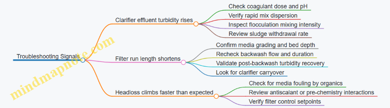
Example Mind Map for Troubleshooting
Acceptance Criteria and Handover to RO
The clarification and filtration train should deliver water quality that supports stable RO operation. Define acceptance criteria such as maximum filtered water turbidity and a fouling proxy used by your plant. Also define sampling locations: raw feed, clarifier effluent, filter effluent, and any intermediate points where chemical dosing changes occur. When these criteria are met consistently, membrane cleaning frequency becomes a predictable maintenance activity rather than a recurring surprise.
2.5 Designing Cartridge Filtration and Antiscalant Dosing Points
Cartridge filtration and antiscalant dosing are the two “small but strict” design steps that often decide whether an RO pretreatment train behaves predictably or turns into a maintenance hobby. The goal is simple: remove particles that would plug membranes and deliver antiscalant where it can actually prevent scale.
Cartridge Filtration Design Foundations
Start with the feedwater reality. Cartridge filters are typically used for polishing after clarification and media filtration, or as a final barrier before RO. Design begins with three inputs: target differential pressure (ΔP) limit, required particle removal rating, and expected solids loading.
A practical way to set the cartridge rating is to tie it to the RO risk. If the upstream pretreatment already achieves low turbidity and low suspended solids, you can select a finer cartridge rating to protect membranes. If upstream performance is variable, choose a rating that balances protection with manageable pressure drop.
Housing and Flow Arrangement
Cartridge housings should be sized for the maximum expected flow at the minimum operating temperature. Cold water increases viscosity and raises ΔP, so “rated flow” at room temperature is not the same as “design flow” at site conditions.
Use a configuration that supports stable operation during cartridge changeout. A common best practice is to provide duplex housings with isolation valves so one side can be swapped while the other side maintains flow. Even if you do not plan frequent changes, duplex design prevents a single plugged housing from forcing a full RO shutdown.
Differential Pressure and Changeout Logic
Design ΔP instrumentation across each housing. Set alarm and action thresholds based on the cartridge manufacturer’s recommended limits and your cleaning or replacement plan. For example, if you expect gradual loading, you can trigger an alarm at a conservative ΔP and schedule replacement at a higher ΔP before RO performance is affected.
A simple example: suppose the RO train requires 200 m³/h feed. You select two parallel cartridge housings, each rated for 110 m³/h at design conditions. If one housing reaches the action ΔP threshold, you can isolate it and keep the other running at 100 m³/h, which stays within its operating envelope.
Antiscalant Dosing Point Design
Antiscalant works only if it mixes with the feed stream before the RO membranes enter the scaling-prone zone. That means the dosing point must provide adequate residence time and mixing intensity, without creating dead zones where chemical concentration becomes uneven.
Where to Dose
Dose after the final filtration step and before the RO high-pressure pump suction or the first pressure vessel inlet manifold, depending on your skid layout. The key is to avoid dosing into a location where cartridges will capture the chemical and reduce its effectiveness.
If you dose upstream of filtration, you risk adsorption onto filter media and cartridges. If you dose too far downstream, you may not achieve uniform distribution before scale risk begins.
How to Dose
Use a metering pump sized for the maximum antiscalant dose rate and the full range of RO operating conditions. Dose control should follow a measured or calculated basis such as feed conductivity, recovery, or a scaling index proxy. If you only dose on a fixed schedule, you will eventually meet a day where the feed is different and the membranes pay the price.
A straightforward control strategy is proportional dosing to a conductivity-based signal with limits. For instance, if conductivity rises by 20%, the antiscalant dose increases by 20% within a defined minimum and maximum. This keeps chemical delivery aligned with the salt load that drives scaling.
Mixing and Residence Time
Provide a static mixer or ensure turbulent flow in a short, straight section. The objective is uniform concentration across the cross-section, not a long pipe that wastes space and time.
Example: if your design requires 30 seconds of mixing before the RO inlet, you can calculate the required pipe volume using the design flow. At 200 m³/h (55.6 L/s), 30 seconds corresponds to about 1.67 m³ of volume. You can then size a mixing section and verify that it fits the skid layout.
Integrated Design Checks
Cartridge filtration and antiscalant dosing must be checked together as a system.
- Chemical compatibility with filtration: confirm the antiscalant does not cause excessive cartridge plugging or interfere with differential pressure behavior.
- Hydraulic stability: ensure dosing does not change viscosity or create localized concentration gradients that affect pressure drop.
- Sampling access: place sampling points so you can verify antiscalant concentration and feed quality without pulling samples from a dead zone.
- Interlocks: link dosing enable/disable to filtration status and RO operating state. If filtration is bypassed or cartridges are isolated, dosing should not continue blindly.
Mind Map: Cartridge Filtration and Antiscalant Dosing Points
Example: Putting It Together on a Typical RO Skid
Assume a RO feed train with clarification and media filtration upstream, followed by cartridge polishing and antiscalant dosing.
- Two duplex cartridge housings are installed in parallel, each sized for half the design flow at the minimum expected temperature.
- Differential pressure transmitters are installed across each housing, with alarms set below the manufacturer’s recommended cartridge limit.
- Antiscalant is dosed downstream of the cartridge housings into a short section containing a static mixer.
- The metering pump is controlled by a conductivity-based signal with defined minimum and maximum dose limits.
- Interlocks prevent antiscalant dosing if a housing is isolated or if the filtration train is not in its normal operating configuration.
This arrangement keeps particles from reaching the membranes and ensures the chemical arrives at the right place, in the right concentration, at the right time—without relying on heroic operator memory.
3. Membrane Materials and Reverse Osmosis Module Selection
3.1 Membrane Chemistry and Structural Considerations for Industrial RO
Industrial reverse osmosis (RO) is a chemistry-and-structure problem wearing a hydraulics outfit. Membrane performance depends on the polymer’s surface chemistry, the way it’s formed into a thin-film composite, and how the module’s mechanical design handles pressure, flow, and cleaning.
Membrane Chemistry Fundamentals
Most industrial RO membranes are thin-film composites: a very thin selective layer supported by a thicker porous substrate. The selective layer controls salt rejection and water permeability, while the support layer provides mechanical strength and pathways for permeate flow.
Key chemistry choices include:
- Polyamide selective layer: Common for seawater and brackish RO because it balances rejection and permeability. Its performance is sensitive to pH and oxidants, so pretreatment and cleaning chemistry matter.
- Functional groups and charge behavior: The membrane surface can attract or repel ions depending on pH and ionic strength. This affects both rejection and scaling tendency near the surface.
- Oxidant tolerance: If residual chlorine or other oxidants reach the membrane, they can damage the selective layer. That’s why pretreatment often includes dechlorination for polyamide systems.
A practical way to think about chemistry is to treat the membrane surface like a “selective gate.” If the gate chemistry is stable under your operating pH and cleaning agents, the gate stays aligned with your design rejection. If not, the gate changes shape, and rejection drifts.
Structural Considerations in Thin-Film Composite Membranes
Even when chemistry is correct, structure can limit performance.
- Active layer thickness: Thinner selective layers can increase flux, but they can also be more vulnerable to compaction and chemical attack.
- Porous support and permeate spacer: These layers determine how permeate is collected and how pressure is distributed. Poor support integrity can lead to localized flow paths and reduced rejection.
- Compaction resistance: Under sustained pressure, polymers can compress slightly, reducing permeability. Membranes with better compaction resistance maintain flux longer at the same operating pressure.
A simple example: two membranes with similar salt rejection can behave differently over months. The one with better compaction resistance may require less pressure to maintain the same permeate flow, which reduces energy and slows fouling progression.
Module Structure and Mechanical Design
Spiral-wound modules dominate industrial RO because they pack membrane area efficiently. Their structure includes membrane elements, permeate collection tubes, feed spacers, and pressure vessel interfaces.
Important structural factors:
- Feed spacer geometry: Spacer thickness and channel design influence crossflow velocity and concentration polarization. Higher crossflow can reduce scaling risk, but it also increases pressure drop.
- Element sealing and end caps: Leaks or seal degradation can bypass the selective layer. Even small bypassing can noticeably reduce rejection.
- Pressure vessel compatibility: The vessel must withstand operating pressure and resist corrosion. Material selection also affects long-term integrity.
- Flow distribution: Uneven distribution can create “hot spots” where scaling or biofouling starts earlier.
A concrete example: if an element experiences poor flow distribution, one section may reach higher local concentration. That section becomes the first to scale, and cleaning becomes more frequent even if the average water quality looks acceptable.
Chemistry-Structure Interactions That Affect Performance
Membrane chemistry and structure interact through the boundary layer at the membrane surface.
- pH and scaling: pH shifts can change carbonate and sulfate solubility, altering scale formation on the surface. The membrane’s surface charge can also influence how ions arrange near the film.
- Cleaning chemistry and structural stress: Cleaning agents must remove foulants without damaging the selective layer or swelling the support. Overly aggressive cleaning can increase permeability but reduce rejection.
- Temperature effects: Higher temperature can increase flux but also accelerates chemical reactions and may change viscosity, affecting pressure drop and spacer shear.
A useful mental model: structure sets how the boundary layer behaves, while chemistry sets how the boundary layer chemistry reacts. Together they determine whether the membrane stays clean and stable.
Mind Map: Membrane Chemistry and Structural Considerations
Example: Selecting Chemistry and Structure for a Brackish RO Train
Assume a brackish RO system with variable feed salinity and occasional high turbidity events.
- Pretreatment goal: Keep oxidants away from the membrane. If the source includes chlorinated water, dechlorination is not optional; it’s a membrane protection step.
- Chemistry fit: Choose a polyamide membrane rated for the expected operating pH range and cleaning program. If cleaning requires a pH outside the membrane’s tolerance, plan a compatible cleaning strategy.
- Structural fit: Select a module with feed spacers that support adequate crossflow at your design recovery. If recovery is pushed high, concentration polarization rises, and spacer design becomes a scaling-control lever.
- Verification: During performance testing, track both permeate flow and salt rejection. A membrane that shows rising flux but falling rejection is often telling you that chemistry or structure is being compromised.
This approach keeps the membrane’s selective gate stable while ensuring the module’s mechanical design supports the boundary-layer conditions you need for reliable operation.
3.2 Spiral Wound Module Selection for Flow, Pressure, and Cleaning Compatibility
Spiral wound RO modules are the “plumbing inside the plumbing.” Choosing the right one is mostly about matching three things: how water moves through the element, how pressure is applied and contained, and how the element survives cleaning without losing performance. The goal is simple: stable permeate output with predictable cleaning behavior.
Foundational Geometry and Flow Paths
A spiral wound element stacks membrane leaves around a permeate collection tube. Feed flows along the membrane surface in a thin channel, while permeate passes through the membrane into the spacer and then toward the permeate tube. The concentrate exits at the end of the element after traveling the length of the spiral.
Start selection by identifying the required permeate flow per pressure vessel and the target recovery. For example, if you need 100 m³/day permeate at a given operating pressure, you can estimate the number of elements by dividing the required permeate by the element’s manufacturer-rated permeate at your expected temperature and salinity. Then verify that the element’s channel design supports the required crossflow velocity to limit concentration polarization.
Flow Compatibility and Hydraulics
Flow compatibility is about more than “element size.” It includes spacer channel height, effective membrane area, and how concentrate flow distribution behaves across the pressure vessel.
A practical way to reason about it:
- Higher crossflow velocity generally reduces scaling risk by lowering the thickness of the boundary layer.
- But higher velocity increases pressure drop, which can force pump energy up and reduce available pressure for permeation.
Example: Suppose two candidate elements have similar membrane area, but one uses a tighter spacer. The tighter spacer may raise pressure drop and reduce the net pressure available for permeation. If your system pressure budget is tight, you might prefer the element with lower pressure drop even if its spacer is slightly less aggressive on fouling control.
Pressure Ratings and Mechanical Fit
Spiral wound modules must match the pressure vessel’s design pressure and the operating pressure range. Verify:
- Maximum allowable operating pressure for the element
- Maximum allowable differential pressure across the element during operation and cleaning
- Temperature limits for both operation and cleaning
A common engineering mistake is selecting elements based on operating pressure only, then ignoring cleaning conditions. Cleaning can involve higher flow rates, different temperatures, and sometimes chemical concentrations that affect material behavior. If the element’s pressure rating is marginal, you may see early performance drift or seal issues.
Cleaning Compatibility and Cleaning Envelope
Cleaning compatibility is the element’s ability to tolerate the cleaning method used in your plant. Cleaning typically includes flushing, chemical cleaning, and sometimes hot water or warm alkaline/acid steps depending on fouling type.
Key selection checks:
- Maximum cleaning temperature
- Permitted pH range and chemical exposure limits for membrane and adhesives
- Maximum cleaning flow rate through the element
- Whether the element is designed for the cleaning frequency implied by your pretreatment quality
Example: If your pretreatment is strong and you expect mostly mild organic fouling, you might use shorter, lower-temperature cleanings. If pretreatment is weaker and you anticipate more frequent scaling events, you need an element that tolerates repeated chemical exposure and maintains rejection after cleaning.
Seal, End Cap, and Permeate Side Considerations
Spiral wound elements rely on end seals and permeate-side structures to prevent mixing of feed and permeate. Selection should consider:
- Seal material compatibility with cleaning chemicals
- Resistance to osmotic shock during start-up and shutdown
- Tolerance to permeate pressure and backpressure during cleaning
A simple operational example: During start-up, if permeate is initially throttled or if permeate pressure rises slowly, the element experiences changing osmotic conditions. Elements with robust seal design and appropriate start-up procedures reduce the chance of early leakage.
Integrated Selection Workflow
Use a structured workflow so decisions don’t contradict each other later.
- Define operating targets: permeate flow, recovery, feed salinity, and temperature.
- Confirm system pressure budget: available pressure at the vessel inlet after accounting for pretreatment and piping losses.
- Choose element type and membrane area to meet permeate capacity.
- Verify flow hydraulics: pressure drop across elements and expected crossflow behavior.
- Validate cleaning envelope: chemicals, temperature, flow rate, and frequency.
- Check mechanical and seal compatibility with both operation and cleaning.
- Confirm that the chosen element fits the pressure vessel configuration and distribution design.
Mind Map: Spiral Wound Module Selection
Example: Comparing Two Candidate Elements
Assume both candidates meet permeate capacity at your design pressure. Candidate A has lower pressure drop but slightly lower crossflow effectiveness. Candidate B has higher pressure drop but better scaling resistance.
If your plant’s pretreatment already keeps turbidity and organics low, scaling risk may be dominated by brine chemistry rather than solids. In that case, Candidate A can be attractive because it preserves pressure for permeation and reduces pump load. If your pretreatment is less consistent and you expect more frequent scaling, Candidate B’s crossflow advantage can reduce the severity of concentration polarization, making cleaning less aggressive and less frequent.
The “right” choice is the one that stays consistent with your pressure budget and your cleaning program. If you pick an element that requires cleaning conditions outside its envelope, you’ll eventually pay for the mismatch—usually as declining rejection, higher cleaning frequency, or seal-related issues.
3.3 Module Layout and Pressure Vessel Sizing for High Reliability Operation
A reliable RO train starts with layout decisions that make the plant easy to operate, clean, and troubleshoot. Module layout and pressure vessel sizing are where “design intent” meets real hardware behavior: pressure losses, flow distribution, cleaning access, and how consistently membranes experience the same conditions.
Foundational Layout Principles
1) Keep pressure and flow distribution predictable. Each membrane element should see similar crossflow and similar feed conditions. Uneven distribution increases local scaling risk and creates “mystery fouling” that looks like random performance drift.
2) Design for cleaning without guesswork. Cleaning requires controlled permeate-side and concentrate-side flow paths, plus enough space for hoses, valves, and safe chemical handling. If the layout makes cleaning awkward, operators will shorten or skip steps.
3) Budget pressure losses early. Vessel inlet/outlet headers, element end caps, and concentrate spacers all contribute to pressure drop. If you size vessels only for average pressure, you can end up with elements that operate at different net driving pressures.
Pressure Vessel Sizing Logic
Pressure vessel sizing is primarily about matching required membrane area to the available pressure rating and maintaining acceptable pressure drop across the element string.
1) Determine membrane area from performance targets. Use the required permeate flow and the design flux to estimate total active area. Then convert active area to number of elements per vessel based on element active length and element type.
2) Check net driving pressure across the vessel. The feed pressure decreases along the train due to friction and fittings. The vessel must be sized so the minimum pressure at the far end still supports the target permeate production.
3) Verify pressure rating and safety margins. Vessel pressure rating must exceed maximum operating pressure including transients such as start-up ramping and valve operations. A practical margin also accounts for measurement uncertainty and pressure control behavior.
4) Ensure hydraulic stability at the element level. Crossflow is influenced by spacer design and element packing. If crossflow is too low, concentration polarization worsens and scaling accelerates. If crossflow is too high, you waste energy and can increase cleaning water demand.
Module Layout for High Reliability
A typical spiral-wound RO train uses multiple vessels in series, often arranged as stages. Within each stage, vessels are connected so that feed pressure and concentrate flow are controlled and distribution is consistent.
1) Choose series versus parallel vessel grouping. Series increases recovery per pass but also increases concentration along the stage. Parallel grouping can improve hydraulic uniformity and redundancy, but it requires careful manifold design to avoid one branch starving.
2) Design inlet and outlet headers. Manifolds should minimize dead zones and avoid sharp flow restrictions. A simple rule: if you can’t explain the flow path to an operator in one minute, the manifold likely needs redesign.
3) Place sampling and instrumentation where they represent reality. Sampling ports should be located to reflect the stream conditions membranes actually see. For example, a sample taken after a mixing tee may hide branch imbalance.
4) Plan for element replacement. Layout should allow safe element extraction and reinstallation without disassembling major piping. This reduces downtime and helps keep cleaning and performance verification consistent.
Mind Map: Module Layout and Vessel Sizing
Example: Sizing a Vessel String for Consistent Net Pressure
Assume a stage must deliver a target permeate flow using a design flux that implies 1200 m² of active membrane area for that stage. If each element provides 40 m² active area, you need 30 elements total.
If you choose 6 elements per vessel, you get 5 vessels in series. Now check pressure drop: suppose the feed pressure at the stage inlet is 70 bar and the total pressure loss across a vessel string is 6 bar. If the minimum acceptable feed pressure at the far end is 62 bar to maintain the required net driving pressure, then 70 − 6 = 64 bar passes the check with a 2 bar buffer.
Next, verify cleaning circulation. If cleaning requires a minimum crossflow equivalent to a certain flow rate through each element, confirm that the recirculation pump and piping can deliver that flow uniformly across all vessels in the stage. If the manifold causes one vessel to receive less flow, that vessel will likely show earlier performance decline.
Example: Manifold Imbalance and How Layout Prevents It
Consider a parallel arrangement where two branches feed two vessel groups. If one branch has a slightly smaller pressure drop, it will carry more flow, leaving the other branch under-crossflow. The under-crossflow branch then experiences higher concentration polarization and earlier scaling.
A reliable layout addresses this by designing manifolds so both branches have matched hydraulic resistance. A practical verification step is to compare expected branch pressure drops at design flow and ensure they are within a tight tolerance. Operators then see similar differential pressures across branches, which makes troubleshooting straightforward.
Reliability Verification Checklist
- Confirm membrane area and elements per vessel match permeate targets.
- Verify minimum feed pressure at the far end supports required net driving pressure.
- Check pressure vessel rating against maximum operating and transient conditions.
- Validate crossflow distribution through manifold and header design.
- Ensure cleaning circulation paths provide uniform flow across vessels.
- Place sampling and instrumentation to represent membrane-side conditions.
- Confirm maintenance access allows element replacement without major disassembly.
3.4 Permeate and Concentrate Flow Path Design for Hydraulics and Recovery
A good RO flow path design makes three things happen at once: the membrane elements see the right crossflow velocity, the pressure losses stay predictable, and the recovery target is achieved without forcing the system into unstable operation. The permeate and concentrate paths are not just “pipes around membranes”; they are part of the hydraulic performance equation.
Foundational Goals for Flow Path Design
Start by defining the hydraulic intent for each stream.
- Permeate path intent: keep permeate pressure low and stable at the element outlet so permeate flux is not unintentionally throttled. In practice, this means minimizing unnecessary pressure drops in permeate headers and ensuring consistent manifold backpressure.
- Concentrate path intent: maintain sufficient crossflow across the membrane surface to reduce concentration polarization and limit scaling risk. This is achieved by controlling element-level pressure drop, distributing flow evenly across pressure vessels, and avoiding dead zones.
- Recovery intent: ensure the concentrate flow rate and stage pressure profile match the recovery strategy. If the concentrate path is too restrictive, the system may reach the desired permeate flow only by raising pressure, which can worsen scaling.
A simple way to remember it: permeate path design protects flux consistency; concentrate path design protects membrane surface conditions.
Permeate Manifold and Header Layout
Permeate leaves each element through the permeate channel and collects into a permeate header. Design choices here affect both hydraulics and operational behavior.
- Equalization across elements: use a manifold geometry that reduces sensitivity to small differences in element resistance. For example, if one vessel has slightly higher permeate resistance, a poorly balanced header can cause that vessel to produce less permeate, shifting load to other vessels.
- Minimize header pressure drop: keep permeate header losses small relative to the element permeate-side driving pressure. If header losses are large, the effective permeate backpressure rises, reducing net flux.
- Air and venting strategy: include vents at high points and ensure drains are available. Trapped air can create local flow resistance and cause uneven permeate production.
Easy example: Suppose two pressure vessels are connected to a common permeate header. If one branch has an extra elbow and longer run, its pressure drop increases. Without balancing, the system may still meet total permeate flow, but one vessel will operate at a different effective permeate backpressure, leading to uneven flux and earlier cleaning triggers.
Concentrate Channel, Vessel, and Stage Hydraulics
Concentrate flow is where crossflow discipline matters most.
- Crossflow distribution: within a pressure vessel, concentrate must distribute across the membrane elements. Uneven distribution can create “fast lanes” with higher local velocity and “slow lanes” where concentration polarization is worse.
- Stage pressure profile: in multi-stage RO, the concentrate from stage 1 becomes the feed to stage 2. The stage-to-stage pressure drop must be accounted for so the second stage sees the intended feed pressure.
- Pressure drop budgeting: treat each component—feed piping, vessel inlet/outlet, concentrate valves, and energy recovery device connections—as a line item. The goal is to keep the total concentrate-side loss within the design basis so the pump pressure setpoint translates into the expected element inlet pressure.
Easy example: If you target 45% recovery in a two-stage train but underestimate concentrate-side pressure losses by 0.5 bar, the second stage may receive lower pressure than planned. The plant might still hit permeate flow by increasing pump pressure, but that raises concentrate salinity and scaling risk in the first stage.
Recovery-Driven Flow Path Interactions
Recovery is not only a function of membrane area and feed salinity; it is also a function of how the flow path shapes pressure and flow rates.
- Concentrate flow rate control: recovery increases when permeate production rises relative to feed. If concentrate flow is throttled too aggressively to chase recovery, crossflow velocity may drop, increasing scaling tendency.
- Valve placement and control stability: place control valves so they do not create large, rapidly varying pressure drops across the membrane elements. A valve that sits upstream of a vessel can cause element inlet pressure oscillations if control tuning is poor.
- Energy recovery coupling: when energy recovery devices are used, their pressure exchange performance depends on matching flow rates and pressure levels. Poorly designed concentrate routing can reduce the effective energy recovery and indirectly push operating pressures higher.
Advanced Details That Prevent “Small” Problems from Becoming Big Ones
- Avoiding bypass leakage paths: ensure seals, gaskets, and blind flanges do not create unintended bypasses that short-circuit crossflow.
- Consistent vessel orientation and support: mechanical alignment affects how concentrate distributes through inlet manifolds and how permeate drains.
- Cleaning compatibility: flow paths should allow cleaning solution to reach all elements with the intended flow distribution. If the permeate side is not properly valved and isolated, cleaning may be uneven.
Mind Map: Permeate and Concentrate Flow Path Design
Integrated Example Walkthrough
Consider a two-stage RO train aiming for 40% overall recovery. You design permeate headers to keep permeate-side pressure drop under a small fraction of the element driving pressure, and you include vents to prevent air pockets. On the concentrate side, you budget pressure losses across inlet piping, vessel manifolds, and stage transfer piping so stage 2 feed pressure matches the design basis. During operation, you control concentrate flow to maintain crossflow velocity rather than only chasing recovery. The result is that permeate flux remains consistent across vessels, and concentrate salinity rises as expected by the recovery model rather than being distorted by unplanned pressure losses.
This is the core idea: permeate path design stabilizes the “how much water passes,” while concentrate path design stabilizes the “how the membrane surface behaves” so recovery is achieved without surprise.
3.5 Selecting Membrane Elements for Temperature and Salinity Ranges
Selecting RO membrane elements is mostly about matching the element’s operating limits to the plant’s actual temperature and salinity profile. Do it carefully, and you get stable flux, predictable rejection, and cleaning that doesn’t feel like a recurring surprise.
Temperature Range Fundamentals
Temperature affects both permeate production and the risk of scaling. Higher temperature lowers viscosity and increases water permeability, so flux tends to rise at the same pressure. That sounds great until higher flux also concentrates foulants faster and can push scaling indices closer to saturation.
Start with a temperature map of the feedwater across seasons and operating modes. For seawater, temperature can swing enough to change the required operating pressure and the frequency of chemical cleaning. For brackish sources, temperature swings often show up as changes in permeate flow more than in rejection, because rejection is driven more strongly by membrane chemistry and salt passage.
Then check element specifications for:
- Maximum operating temperature and allowable cleaning temperature.
- Temperature limits for pressure vessel materials and seals.
- Performance curves or correction factors for permeability and rejection versus temperature.
A practical example: if your design feed temperature is 25°C but summer peaks at 32°C, you may need to reduce recovery or adjust pressure so the element doesn’t run at an unintended flux. Otherwise, you may see higher differential pressure and faster scaling even if the plant “still meets” permeate flow.
Salinity Range Fundamentals
Salinity determines osmotic pressure, which directly influences the net driving pressure. As salinity increases, the same applied pressure yields less effective driving force, so permeate flow drops unless you increase pressure or reduce recovery.
Build a salinity profile that includes:
- Average and worst-case TDS or conductivity.
- Seasonal variation and any upstream process effects.
- Stage-wise salinity after each pass, because multi-stage trains expose later stages to higher concentrate levels.
A useful rule of thumb is to design around the highest osmotic pressure you expect during stable operation, not just during upset conditions. If you only size for average salinity, the membranes may operate at lower net driving pressure during high-salinity periods, which can reduce production and increase the chance that operators compensate with higher pressure.
Matching Membrane Chemistry to Water Chemistry
Temperature and salinity are only half the story. Membrane chemistry determines how well the element resists scaling and how consistently it rejects salts under your specific ionic mix.
When selecting elements, verify compatibility with:
- Target pH range during operation and cleaning.
- Antiscalant and cleaning chemical types.
- Presence of multivalent ions that drive scaling (for example, calcium and barium).
Example: two elements may both be rated for the same temperature, but one may tolerate your cleaning pH range better. If your pretreatment leaves residual hardness, the element that tolerates your cleaning regimen without performance drift will usually reduce downtime.
Selecting Elements by Operating Envelope
Treat the element as a system component with an operating envelope. The envelope is defined by maximum feed pressure, maximum permeate backpressure, maximum differential pressure, and allowable flux.
Use these steps:
- Convert your design temperature and salinity into expected osmotic pressure and net driving pressure.
- Choose a target permeate flux that stays within the element’s recommended flux range for your fouling risk.
- Verify that the required pressure and recovery fit the element’s performance and pressure limits.
- Confirm cleaning compatibility for the highest temperature you might use during CIP.
If your plant uses a staged RO train, repeat the check for each stage. Stage 1 often sees lower salinity but higher flow; later stages see higher salinity and can be more sensitive to salt passage and scaling.
Mind Map: Temperature and Salinity Selection Logic
Example: Two Candidate Elements Under Summer Conditions
Assume summer feed temperature rises from 25°C to 32°C and salinity increases by 10%. Candidate A has higher permeability at warm temperatures but a narrower recommended flux range. Candidate B has slightly lower permeability but a wider flux tolerance.
If you keep the same pressure and recovery, Candidate A will produce more permeate initially, but the higher flux can accelerate scaling and increase the frequency of chemical cleaning. Candidate B may produce less permeate at first, yet it can maintain a steadier operating point within its recommended flux range, reducing the chance that operators need to chase production by raising pressure.
The selection outcome is not “which element gives more flow on day one.” It’s which element keeps the plant within its intended operating envelope across the temperature and salinity range you actually see.
Example: Stage-Wise Element Choice for Multi-Stage Trains
In a two-stage train, Stage 1 concentrate salinity is lower than Stage 2 feed salinity. If you choose elements for Stage 2 using only the overall feed salinity, you may underestimate osmotic pressure and scaling risk at the higher concentrate level.
A systematic approach is to:
- Estimate Stage 2 feed salinity from the recovery and Stage 1 performance.
- Check Stage 2 element flux and pressure limits at the worst-case temperature.
- Confirm that cleaning chemistry and temperature remain within the element’s allowable CIP envelope.
This prevents a common mismatch: Stage 1 looks fine, while Stage 2 becomes the bottleneck because it experiences the most challenging combination of salinity and concentration polarization.
Quick Validation Checklist
- Temperature: element max operating and max cleaning temperature verified against plant extremes.
- Salinity: osmotic pressure and net driving pressure checked for worst-case and stage-wise conditions.
- Flux: chosen flux stays within recommended range for fouling risk.
- Chemistry: antiscalant and cleaning pH compatibility confirmed.
- Hydraulics: pressure, differential pressure, and backpressure limits validated for the selected module layout.
When these checks align, membrane selection becomes a controlled engineering decision rather than a “we’ll see how it behaves” exercise.
4. Membrane Optimization for Flux, Recovery, and Fouling Control
4.1 Establishing Flux Targets and Operating Pressure Windows
Flux is the membrane’s “work rate”: how much permeate passes per unit membrane area per unit time. In industrial RO, you don’t pick a flux number because it sounds good; you pick it because it fits your feed quality, pretreatment reliability, and cleaning plan. The operating pressure window is the practical range where the plant can hit the flux target while staying inside limits for scaling, compaction, and mechanical stress.
Foundational Inputs for Flux Targets
Start with the design basis that ties together water quality, recovery, and membrane area.
- Feed salinity and temperature set the osmotic pressure and therefore the pressure needed to achieve a given permeate flow.
- Pretreatment performance controls fouling rate. If turbidity or organics slip through, the same pressure will produce a lower stable flux because the membrane surface “gets busy.”
- Recovery strategy determines concentrate composition along the train. Higher recovery increases scaling risk and reduces the safe flux.
- Membrane type and element geometry affect how flux translates to pressure and how quickly performance declines.
A practical way to set a flux target is to define three numbers: initial clean flux, target stable flux, and end-of-run flux. The stable flux is what you expect between cleanings; the end-of-run flux is what you can tolerate without violating product quality or operational constraints.
Example: Translating a Flux Target into Area
Suppose you need 500 m³/day of permeate. If the chosen stable flux is 18 L/m²·h, then required membrane area is:
- Convert permeate flow: 500 m³/day = 20.83 m³/h = 20,830 L/h
- Area = 20,830 L/h ÷ 18 L/m²·h = 1,157 m²
Now you can check whether that area is consistent with your pressure window and expected fouling rate. If not, you adjust flux target, recovery, or pretreatment scope.
Pressure Window Logic
The pressure window is bounded by two realities: you need enough pressure to overcome osmotic pressure and you must avoid conditions that accelerate scaling or damage membranes.
- Lower bound: minimum pressure to meet permeate flow at the stable flux. This depends on temperature, salinity, and expected performance decline.
- Upper bound: maximum pressure limited by scaling risk, compaction, and mechanical constraints of vessels and seals.
A good design pressure window is not a single number; it’s a range that supports normal operation and still leaves room for feed variability.
Example: Why “More Pressure” Is Not Free
If feed temperature drops by 2–3°C, viscosity increases and permeate flux tends to fall. Operators often respond by raising pressure. That can restore flow, but it also increases the driving force for scaling because the concentrate reaches higher saturation faster. The pressure window exists so the plant can compensate for temperature without turning scaling control into a full-time job.
Step-by-Step Method to Set Flux and Pressure
- Choose the design permeate specification (flow and product quality) and define the acceptable cleaning interval.
- Estimate osmotic pressure using feed salinity and temperature, then compute the required net driving pressure for the chosen flux.
- Screen for scaling risk at the concentrate conditions corresponding to your recovery and operating pressure. If scaling risk is high, reduce target flux, lower recovery, or strengthen antiscalant and pretreatment.
- Account for performance decline using a fouling allowance. This is where pretreatment quality matters: better pretreatment reduces the decline rate, allowing a higher stable flux without shrinking the cleaning interval.
- Set the operating pressure window by combining the minimum pressure needed for stable flux with the maximum pressure allowed by scaling and mechanical limits.
- Validate with hydraulics and element performance so that the pressure you plan at the skid actually reaches the membrane elements with the expected distribution.
Mind Map: Flux Targets and Pressure Windows
Advanced Details That Prevent Design Surprises
Flux Allocation Across Stages
In multi-stage RO, each stage sees different salinity and recovery. A common mistake is to apply the same flux logic to every stage without adjusting for concentrate strength. Stage-specific flux targets keep scaling risk balanced and reduce the chance that one stage becomes the bottleneck.
Cleaning Interval as a Design Variable
If you set a high stable flux but plan infrequent cleaning, the membrane may reach unacceptable performance before the next scheduled cleaning. Instead of treating cleaning as an afterthought, tie the flux target to the cleaning interval so the plant can operate predictably.
Pressure Control Strategy and Measurement Points
Pressure readings are only useful if they represent the pressure at the membrane inlet. Pressure drops in headers and skids can mislead operators into thinking the membrane is receiving a certain pressure when it isn’t. Design the measurement points and control loops so the pressure window is enforced where it matters.
Quick Reference Example: Choosing a Safe Window
Assume you target 18 L/m²·h stable flux and you expect performance decline that requires a pressure increase over time. You might set:
- Minimum operating pressure: the pressure that achieves 18 L/m²·h at the coldest expected temperature and best-case pretreatment.
- Maximum operating pressure: the pressure that keeps scaling indices within limits at the highest expected concentrate conditions.
If the calculated minimum exceeds the calculated maximum, the design must change: reduce flux target, adjust recovery, improve pretreatment, or increase membrane area so the same permeate flow is achieved at lower flux and safer pressure.
4.2 Recovery Strategy Design for Multi Stage RO Trains
Recovery is the fraction of feed converted to permeate. In multi stage RO, recovery is split across stages so each stage runs within its membrane flux and fouling risk limits. The trick is to treat recovery as a design variable that couples hydraulics, membrane performance, and brine chemistry—rather than a single “setpoint” you hope will behave.
Foundational Concepts That Drive Recovery Splits
Start with two practical relationships. First, stage recovery determines how concentrated the brine becomes before it enters the next stage. Second, concentration affects scaling tendency and osmotic pressure, which in turn changes the net driving pressure and the required operating pressure.
A useful way to think about a two stage train is:
- Stage 1: permeate flow reduces the feed to Stage 2.
- Stage 2: permeate flow reduces the remaining brine to final concentrate.
If Stage 1 recovery is too high, Stage 1 brine becomes harsh for Stage 2, pushing osmotic pressure up and increasing the likelihood of scaling. If Stage 1 recovery is too low, you may waste capacity and end up forcing Stage 2 to work harder than it should.
Designing Recovery Targets by Stage
Set recovery targets stage-by-stage using a simple workflow.
- Choose a maximum allowable flux or pressure window per stage. This is where membrane optimization meets reality: you pick a conservative operating envelope that matches your cleaning plan and pretreatment quality.
- Estimate permeate and concentrate flow rates per stage. Use mass balance to compute how much brine each stage passes forward.
- Check concentration dependent risks. Scaling indices and salt passage expectations should be evaluated for the brine concentration entering each stage.
- Iterate with pressure and flow constraints. Pumps, energy recovery devices, and pressure drops limit what you can physically achieve.
A concrete example: suppose you have 100 m³/h of seawater feed. If you target 40% recovery in Stage 1, you produce 40 m³/h permeate and send 60 m³/h brine to Stage 2. If Stage 2 targets 30% recovery relative to its feed, it produces 18 m³/h permeate and leaves 42 m³/h final concentrate. Overall recovery is 58% (40 + 18 out of 100). Now compare two alternatives: 50% in Stage 1 and 20% in Stage 2 gives the same overall recovery (58%), but Stage 2 sees a higher concentration because it starts with less brine volume and more dissolved salts. That difference matters for scaling and required pressure.
Multi Stage Recovery Strategies That Actually Work
Multi stage trains typically use one of these recovery strategies.
- Front-loaded recovery. Higher recovery in early stages. This can reduce the volume handled by later stages, but it increases the concentration burden on downstream membranes.
- Back-loaded recovery. Lower recovery early, higher recovery later. This often improves scaling control in Stage 1, but it may require more pressure and careful hydraulic design in Stage 2.
- Balanced recovery with staged constraints. Recovery is tuned so each stage hits its own “comfort zone” for flux, pressure, and scaling risk.
In practice, balanced recovery is common because it respects both membrane performance and brine chemistry. It also makes control easier: if Stage 1 is stable, Stage 2 can be adjusted without constantly fighting scaling.
Hydraulics and Energy Recovery Coupling
Recovery design is not just chemistry. It changes flow rates, which changes pressure drops and the operating point of pumps and energy recovery devices. In a pressure exchanger system, the concentrate and permeate flow rates must be matched closely enough to maintain efficiency.
If you increase Stage 1 recovery, Stage 1 concentrate flow decreases. That can shift the exchanger operating point and reduce energy recovery efficiency unless the design includes appropriate bypass and control logic. Therefore, recovery targets should be checked against:
- pressure drop budgets across skids and vessels
- exchanger flow matching ranges
- pump efficiency curves at the new duty points
Control Logic for Stable Recovery During Operation
Design recovery so the plant can hold it without constant operator intervention. A typical control approach is to regulate permeate flow or permeate conductivity while using pressure control to maintain membrane flux within limits.
A simple control philosophy:
- Stage 1: pressure control maintains flux and rejection.
- Stage 2: pressure control compensates for changes in feed salinity and temperature.
- Concentrate throttling or bypass is used to keep exchanger and pump conditions within stable ranges.
This matters because recovery changes with feed conditions. The plant should respond by adjusting pressure and flow distribution, not by letting scaling risk silently creep upward.
Mind Map: Recovery Strategy Design for Multi Stage RO Trains
Example: Choosing a Recovery Split for Scaling Control
Assume both stages have similar membrane area. You want overall recovery near 60%, but scaling risk rises sharply with concentration. If Stage 1 recovery is set to 45%, Stage 2 receives brine that is more concentrated than in a 35% Stage 1 case. Even if Stage 2 is operated at the same flux, the higher inlet concentration increases the likelihood of scale formation in Stage 2.
A practical decision rule is to cap Stage 1 recovery based on the maximum acceptable scaling index at Stage 2 inlet, then use the remaining recovery budget in Stage 2. This keeps the “most sensitive” stage from being fed a brine concentration that forces aggressive pressure or chemical dosing.
Diagram: Two Stage Recovery Flow and Concentration Progression
    flowchart LR
  A[Feed 100 m3/h] --> B[Stage 1]
  B --> C[Permeate 40 m3/h]
  B --> D[Brine 60 m3/h]
  D --> E[Stage 2]
  E --> F[Permeate 18 m3/h]
  E --> G[Final Concentrate 42 m3/h]
  D -. Concentration increases .-> E
Summary of the Recovery Split Logic
Design recovery splits so each stage stays within its membrane operating envelope and so brine concentration entering later stages does not exceed scaling and hydraulic limits. Then verify that the chosen split remains compatible with energy recovery matching and stable control behavior.
4.3 Salt Passage and Rejection Calculations for Performance Verification
Salt passage and rejection calculations turn “the membranes feel fine” into measurable proof. In RO, you verify performance by comparing how much salt leaves with the permeate versus how much salt enters with the feed. The core idea is simple: rejection is high when permeate salinity is low, and salt passage is the fraction that sneaks through.
Foundational Definitions and What You Actually Measure
Start with measurable quantities:
- Feed TDS (or conductivity): \(C_f\)
- Permeate TDS (or conductivity): \(C_p\)
- Concentrate TDS: \(C_c\)
- Feed flow: \(Q_f\)
- Permeate flow: \(Q_p\)
- Concentrate flow: \(Q_c\)
- Recovery: \(R = Q_p / Q_f\)
For performance verification, you typically use TDS or conductivity as a proxy for salt concentration. If you use conductivity, keep the same temperature basis and conversion method across all measurements.
Salt passage fraction is:
\[ \text{Salt Passage} = \frac{\text{Salt in Permeate}}{\text{Salt in Feed}} = \frac{Q_p C_p}{Q_f C_f} \]
Using \(Q_p = R Q_f\), this becomes:
\[ \text{Salt Passage} = R \cdot \frac{C_p}{C_f} \]
Salt rejection is:
\[ \text{Rejection} = 1 - \frac{C_p}{C_f} \]
Notice the difference: rejection depends on concentration ratio, while salt passage also depends on recovery. That’s why a system can show high rejection but still pass more total salt at higher recovery.
Single-Stage Verification Workflow
A practical verification workflow keeps the math honest and the data consistent.
- Measure flows: \(Q_f\), \(Q_p\), \(Q_c\). Confirm \(Q_f \approx Q_p + Q_c\).
- Measure concentrations: \(C_f\) and \(C_p\) at the same operating condition.
- Compute rejection: \(1 - C_p/C_f\).
- Compute salt passage: \(R \cdot C_p/C_f\).
- Cross-check salt balance: salt in feed should equal salt in permeate plus salt in concentrate within measurement uncertainty.
A quick cross-check uses salt mass rates:
- Salt in feed: \(S_f = Q_f C_f\)
- Salt in permeate: \(S_p = Q_p C_p\)
- Salt in concentrate: \(S_c = Q_c C_c\)
If you don’t measure \(C_c\), you can still estimate it from mass balance:
\[ C_c \approx \frac{S_f - S_p}{Q_c} \]
Example Calculation with Realistic Numbers
Assume a single-stage RO train operates at:
- \(Q_f = 100,\text{m}^3/\text{h}\)
- Recovery \(R = 0.45\Rightarrow Q_p = 45,\text{m}^3/\text{h}\), \(Q_c = 55,\text{m}^3/\text{h}\)
- Feed TDS \(C_f = 35{,}000,\text{mg/L}\)
- Permeate TDS \(C_p = 350,\text{mg/L}\)
Rejection:
\[ 1 - \frac{350}{35{,}000} = 1 - 0.01 = 0.99 = 99\% \]
Salt passage:
\[ R \cdot \frac{C_p}{C_f} = 0.45 \cdot 0.01 = 0.0045 = 0.45\% \]
Salt mass rates:
- \(S_f = 100 \times 35{,}000 = 3{,}500{,}000\) (mg/L·m³/h units consistent)
- \(S_p = 45 \times 350 = 15{,}750\)
So about 0.45% of the feed salt ends up in permeate, even though the permeate concentration is only 1% of feed concentration. The recovery factor is doing its job.
Multi-Stage Trains and How Rejection Compounds
In multi-stage RO, each stage sees a different feed salinity. You verify stage-by-stage performance using the same definitions, but you must use the correct stage feed concentration.
For two stages:
- Stage 1: feed concentration: \( C_{f1} \)
- Stage 1: permeate becomes Stage 2 feed: \(C_{f2} = C_{p1}\)
- Stage 2: permeate: \(C_{p2}\)
Overall rejection from feed to final permeate is:
\[ \text{Rejection}_{\text{overall}} = 1 - \frac{C_{p2}}{C_{f1}} \]
Overall salt passage is:
\[ \text{Salt Passage}_{\text{overall}} = R_{\text{overall}} \cdot \frac{C_{p2}}{C_{f1}} \]
If you want a stage-wise view, compute each stage’s rejection using its own feed and permeate concentrations, then confirm the overall result matches the final measured \( C_{p2} \). If it doesn’t, the likely culprit is measurement mismatch (temperature basis, sampling location, or time alignment).
Mind Map: Salt Passage and Rejection Calculations
Advanced Details That Prevent “Math That Looks Right”
1) Temperature and conductivity basis. If you measure conductivity and convert to TDS, ensure the conversion uses the same temperature correction method for both feed and permeate. A small temperature mismatch can shift \( C_p/C_f \) enough to move rejection by noticeable points.
2) Sampling alignment. Flows can change faster than chemistry. Use synchronized sampling or average over a defined steady window so \( Q_p \) and \(C_p\) represent the same operating period.
3) Units consistency. Whether you use mg/L, g/L, or conductivity-derived TDS, keep the ratio \( C_p/C_f \) consistent. The rejection equation only needs concentration ratio; salt passage needs recovery too.
4) Uncertainty budgeting. Treat measurement uncertainty as part of verification. If rejection is near a contractual threshold, a 5–10% uncertainty in permeate TDS can matter more than small differences in recovery.
Quick Summary for Performance Verification
- Rejection tells you how concentrated the permeate is relative to feed: \( 1 - C_p/C_f \).
- Salt passage tells you how much salt mass actually leaves with permeate: \(R \cdot C_p/C_f\).
- Multi-stage verification uses stage-specific feed concentrations and confirms overall performance against final permeate measurements.
When the numbers are consistent, you can confidently say the membranes are doing what the design basis expected—no guesswork required.
4.4 Fouling Mechanism Mapping for Scaling, Biofouling, and Organic Fouling
Fouling is not one problem with one cause. In industrial RO, it is usually a stack of mechanisms that start differently, grow at different rates, and respond to different controls. A fouling mechanism map turns “the membranes are getting worse” into “which process condition is driving which deposit, and where to intervene first.”
Foundational Signals You Can Measure Without Guessing
Start with the three signals that consistently separate scaling, biofouling, and organic fouling.
- Pressure and flux behavior: Scaling often shows a relatively fast rise in pressure drop at stable feed conditions, while organic fouling can show a slower drift as organics accumulate and compress. Biofouling often shows a stronger link to temperature, residence time, and pretreatment performance.
- Cleaning response: If a cleaning step restores flux quickly, the deposit is often more reversible (commonly scaling or loosely attached organics). If flux recovery is partial and requires multiple chemistries, the foulant layer is likely more complex or biologically conditioned.
- Permeate quality and differential pressure pattern: Scaling can increase salt passage slightly as the surface becomes rough and permeation pathways change. Biofouling can correlate with changes in permeate conductivity stability and with pretreatment upset events.
A practical mapping workflow uses these signals to assign a “dominant mechanism” and a “secondary mechanism” rather than forcing a single label.
Mechanism Map Logic from Chemistry to Biology
Scaling is primarily a supersaturation and precipitation story. Organic fouling is a surface adsorption and pore blockage story. Biofouling is a growth and attachment story that depends on nutrients, time, and surface conditioning.
- Scaling drivers: high recovery, high temperature, high hardness, high alkalinity, and inadequate antiscalant performance. The key is whether the local concentrate stream crosses saturation limits.
- Organic drivers: natural organic matter, surfactants, and degradation products that adsorb to the membrane surface and can form a gel-like layer. The key is whether pretreatment removes them or whether they remain and accumulate.
- Biofouling drivers: viable microorganisms and biofilm formation supported by residual organics and insufficient biocide control. The key is whether cells can survive pretreatment and establish attachment.
Mind Map: Fouling Mechanism Mapping
Example: Mapping a “Pressure Drop Problem”
Assume an RO train shows a steady flux decline over two weeks, with differential pressure rising faster after a recovery increase.
- Check scaling likelihood: If feed temperature also rose and hardness/alkalinity stayed steady, scaling becomes the leading candidate. A quick test is to compare the timing of the recovery change with the onset of DP acceleration.
- Check organic contribution: If pretreatment turbidity remained stable but UV254 increased, organic fouling likely contributes. Organic layers can make scaling more likely by changing surface conditions.
- Check bio contribution: If there was a shutdown longer than normal or biocide dosing was interrupted, biofouling moves up the list. Biofouling often shows stubborn residual pressure after a standard cleaning.
A useful decision rule is: scaling correlates with supersaturation changes; organic fouling correlates with organic carryover; biofouling correlates with time, temperature, and pretreatment upset.
Example: Cleaning Response as a Mechanism Fingerprint
During a routine clean, suppose flux recovery is 80% after a scale-focused chemical, but only 50% after an organic-focused step. That pattern strongly suggests scaling is dominant. If the reverse happens—good recovery with an organic-targeted chemistry and poor recovery with scale chemistry—organic fouling is dominant.
When both chemistries recover only partially, the deposit is often mixed: organics can act as a scaffold for biofilm, and biofilms can trap scale-forming ions. In that case, the map should record a mixed mechanism and the corrective action should address both the chemical driver (supersaturation control) and the biological driver (pretreatment and disinfection discipline).
Turning the Map into Actionable Checks
A mechanism map is only useful if it links to controls. For each dominant mechanism, record one immediate verification and one corrective lever.
- Scaling: verify antiscalant dosing control and concentrate recovery profile; adjust dosing/mixing or recovery staging.
- Organic fouling: verify filter integrity and TOC/UV254 trends; tighten coagulation/filtration and cartridge performance.
- Biofouling: verify microbial indicators and biocide contact time; correct dosing continuity and shutdown disinfection.
This approach keeps the team from treating symptoms. It also prevents the classic mistake of increasing chemical dose without confirming whether the deposit is actually scaling, organic, or biological in nature.
4.5 Cleaning Compatibility and Operational Envelope for Membrane Longevity
Membrane cleaning is not just “washing.” It is controlled chemistry plus controlled hydraulics, performed within a window where the membrane can tolerate the stress. Staying inside that window is what turns cleaning from a necessary evil into a predictable maintenance routine.
Foundational Compatibility Rules
Start with three compatibility questions. First, does the cleaning chemistry match the dominant foulant? If you use the wrong chemistry, you may remove a little surface gunk while leaving the real problem to keep growing.
Second, does the chemistry stay within the membrane’s tolerance for pH, temperature, and oxidant exposure? For example, many RO membranes tolerate moderate pH swings, but repeated harsh conditions can thin the active layer or weaken the polymer support.
Third, does the cleaning method respect the membrane’s mechanical limits? High crossflow, aggressive pressure cycling, or excessive backpressure can deform elements or damage seals.
A practical way to remember this: chemistry controls what you dissolve; hydraulics controls what you shear off; mechanical stress controls whether the membrane survives the process.
Defining the Operational Envelope
The operational envelope is the set of cleaning parameters that are both effective and membrane-safe. Treat it like a checklist with measurable boundaries:
- pH envelope: Keep cleaning solutions within the manufacturer’s allowed range for the membrane type. If you need to reach a target pH, do it gradually with controlled dosing rather than “dump and hope.”
- Temperature envelope: Higher temperature can speed reactions, but it also increases polymer stress and can accelerate degradation. Use the lowest temperature that achieves cleaning goals.
- Oxidant envelope: If oxidants are used for biofouling, limit concentration and exposure time. Oxidants are effective, but they are also unforgiving.
- Flow and crossflow envelope: Maintain sufficient crossflow to prevent redeposition, but avoid exceeding the element’s recommended hydraulic limits.
- Pressure and backpressure envelope: Keep pressures within the RO skid’s safe operating range and avoid sudden pressure spikes during circulation.
Matching Cleaning Type to Fouling Mechanism
Cleaning compatibility improves when you first classify the fouling. A simple decision logic works well in practice:
- Scaling-dominant: Look for hardness-related precipitation behavior. Use scale-removal chemistry and ensure pH is controlled to dissolve the scale without overexposing the membrane.
- Organic fouling-dominant: Use cleaning chemistry designed to remove organics and confirm that the solution does not push pH or temperature outside the envelope.
- Biofouling-dominant: Use biocide/oxidant steps only when needed, followed by thorough rinsing. The envelope matters most here because oxidants can degrade membranes if misapplied.
Cleaning Cycle Structure That Protects Longevity
A robust cleaning cycle typically includes preparation, circulation, dwell, and rinse. Each phase has a compatibility purpose.
- Preparation: Verify solution concentration, pH, and temperature before circulation. Calibrate dosing pumps and confirm mixing so the membrane does not see localized extremes.
- Circulation: Circulate at a controlled flow rate to scour the surface. If pressure rises unexpectedly, treat it as a sign of poor flow distribution or excessive fouling rather than forcing the system.
- Dwell: Hold for the minimum time that achieves reaction. Longer dwell can increase cleaning effectiveness but also increases chemical exposure risk.
- Rinse: Rinse until conductivity and pH return toward baseline. Skipping or shortening rinses can leave residues that later accelerate scaling.
Mind Map: Compatibility and Envelope
Example: Scale Cleaning Without Overexposure
Assume an RO train shows increasing differential pressure and a gradual decline in permeate flow, consistent with scaling. A scale-focused cleaning is selected.
Operationally, the team prepares a cleaning solution with a target pH that dissolves the expected scale. Instead of jumping directly to the final pH, they dose in steps while mixing is verified. During circulation, they keep crossflow within the element’s recommended range and watch for pressure rise. If pressure climbs faster than expected, they stop and reassess rather than extending time.
After circulation and a short dwell, they rinse until conductivity and pH stabilize near baseline. This prevents leftover cleaning chemistry from becoming a future scaling trigger.
Example: Biofouling Cleaning with Controlled Oxidant Use
For biofouling, the cleaning plan includes an oxidant step only after confirming that the symptoms align with biological growth rather than scaling alone. The oxidant concentration and exposure time are set to the minimum that achieves the cleaning goal.
During the cycle, the team maintains stable circulation conditions and avoids aggressive pressure cycling. After the oxidant step, they perform extended rinsing to remove residual oxidant. This is where compatibility pays off: membranes last longer when oxidant residues do not linger.
Operational Discipline That Prevents “Accidental Damage”
Longevity comes from small habits. Record actual pH, temperature, flow, and pressure during each cleaning. If a cleaning parameter drifts, you learn whether the drift was harmless or damaging.
Also, treat cleaning frequency as a symptom response, not a schedule. If performance declines faster than expected, the fix is usually earlier pretreatment adjustment or operating condition correction, not simply more aggressive cleaning.
5. High Pressure Pumping Systems and Hydraulic Design
5.1 Pump Selection Criteria for RO Duty Cycles and Efficiency
Selecting the right high-pressure pump for an RO plant is mostly about matching hydraulic reality to operating intent. A pump that looks efficient on a datasheet can still waste energy if its duty point, control method, and suction conditions are off. The goal is to choose a pump that hits the required pressure and flow across the plant’s duty cycle while staying within acceptable efficiency, NPSH margin, and mechanical limits.
Duty Cycle Foundations
Start by defining the duty cycle as a set of operating points, not a single “design” point. For each point, specify required permeate flow, recovery, and the corresponding concentrate flow and pressure. Then translate those into pump requirements: flow rate at the pump, discharge pressure, and allowable variation.
A practical way to build this is to create a small table of operating modes, such as normal production, partial production, and cleaning circulation. For each mode, compute the total dynamic head (TDH) the pump must overcome: static lift (if any), friction losses in piping and skids, pressure losses across filters and RO trains, and any pressure setpoints required for stable permeate production.
Efficiency at the Real Duty Point
Pump efficiency depends on where the pump runs relative to its best efficiency point (BEP). If your duty cycle spends most of its time far from BEP, the “peak efficiency” number becomes a consolation prize.
Use the pump curve to estimate efficiency at each duty point. Then compute a weighted average efficiency using time fractions from the duty cycle. This is more informative than comparing pumps by BEP alone.
Example: Suppose Pump A has BEP efficiency of 86% but operates around 78% for most of the day, while Pump B runs around 82% for the same duty points. Even if Pump A is slightly better at one condition, Pump B can win on daily energy.
Control Method and Its Energy Impact
RO plants rarely run at one fixed speed. Common control approaches include variable frequency drive (VFD) speed control, discharge pressure control, and sometimes throttling. Throttling usually costs energy because it creates extra head loss without improving system pressure needs.
When using a VFD, check that the pump curve and system curve intersect at stable points across the duty cycle. Also verify that the control strategy does not push the pump into unstable regions such as very low flow where efficiency drops and vibration risk rises.
Suction Conditions and NPSH Margin
High-pressure pumps are sensitive to cavitation. Cavitation is not just a noise issue; it damages impellers and seals and can cause performance drift.
Compute available NPSH (NPSHa) from the suction pressure, temperature, and vapor pressure, then compare it to required NPSH (NPSHr) from the pump curve at each duty point. A typical design practice is to keep a comfortable margin so that minor changes in feed temperature, fouling in suction strainers, or level variations do not erase your safety buffer.
Example: If NPSHa is only slightly above NPSHr at partial production, a modest increase in feed temperature or a small suction pressure drop can trigger cavitation. In that case, improving suction piping, reducing suction losses, or adjusting intake conditions can be more effective than changing the pump.
Hydraulic Matching and Pressure Loss Budgeting
Pump selection depends on the system’s pressure loss budget. If the friction losses in piping, valves, and RO train headers are underestimated, the pump will run at higher head than expected, reducing efficiency and increasing motor load.
Build a pressure loss budget that includes:
- Intake and suction piping losses
- Strainer and filter losses
- RO train inlet header losses
- Energy recovery device losses (if present in the high-pressure loop)
- Instrumentation and control valve losses
Then confirm that the pump has sufficient head margin at the maximum expected operating condition, including fouling allowance where appropriate.
Mechanical and Operating Limits
Check that the pump can handle:
- Maximum operating pressure and surge conditions
- Maximum and minimum flow limits under control
- Motor power limits at the duty points
- Vibration and bearing life requirements
Also verify seal compatibility with the RO feed and cleaning chemicals. A pump that survives hydraulics but fails seals will not survive the plant’s maintenance schedule.
Mind Map: Pump Selection Criteria
Example: Comparing Two Pumps with a Duty Cycle
Assume two candidate pumps meet the same TDH at design flow. Pump A is slightly more efficient near BEP, but its efficiency drops sharply at partial flow. Pump B has a flatter efficiency profile.
If the plant runs 70% of the time at partial production and 30% near design, the weighted efficiency favors Pump B. The final check is motor power at each duty point to ensure neither pump exceeds electrical limits when the system pressure loss rises.
Selection Checklist
- Confirm duty points and time fractions
- Build a TDH pressure loss budget
- Compare pump efficiency at each duty point, not just BEP
- Validate control stability across the operating range
- Compute NPSHa and verify margin versus NPSHr
- Check motor power, vibration, and seal compatibility
When these pieces line up, the pump selection stops being a single-number decision and becomes a controlled match between the plant’s real operating behavior and the pump’s real performance.
5.2 Suction Conditions, NPSH, and Cavitation Risk Mitigation
Cavitation is what happens when local pressure drops below the liquid’s vapor pressure, forming vapor bubbles that later collapse. In RO high-pressure pumping, that collapse can pit impellers, erode seals, and cause performance drift that looks like “mysterious” loss of flow or pressure. The goal of this section is to keep suction conditions comfortably above the minimum pressure needed for stable liquid flow.
Foundational Concepts That Drive Suction Design
Start with the pump’s net positive suction head available (NPSHa). It represents the head margin between the actual suction pressure and the vapor pressure at the pump inlet, accounting for losses in the suction piping and fittings.
NPSHa must exceed the pump’s required NPSH (NPSHr) at the duty point. NPSHr is provided by the pump manufacturer and is typically tied to a specified performance drop (often 3% head drop). If NPSHa approaches NPSHr, bubbles form more easily, and the pump may still “run” while quietly damaging itself.
A practical way to think about it: NPSHa is your real-world pressure margin; NPSHr is the margin the pump needs to stay calm.
Building NPSHa from Real Suction Conditions
Compute NPSHa using the measured or designed suction pressure, the liquid’s vapor pressure at the operating temperature, and suction-side losses. The key inputs are:
- Suction pressure at the pump inlet: influenced by tank level, suction line elevation, and any suction control valves.
- Liquid temperature: higher temperature increases vapor pressure, shrinking the margin.
- Suction piping losses: friction losses rise with flow velocity; elbows, strainers, and filters add extra loss.
- Static head: if the source is a tank, the vertical distance to the pump inlet matters.
Easy example: Suppose the suction line is long and has a strainer. As the strainer loads with solids, pressure drop increases. Even if the tank level stays constant, NPSHa decreases. That’s why suction strainers are not just “maintenance items”; they are part of the cavitation safety system.
Suction Conditions That Commonly Trigger Cavitation
Cavitation risk rises when any of the following occurs:
- Low suction pressure from insufficient tank level or excessive suction valve throttling.
- High suction temperature from warm feedwater or heat tracing that raises inlet temperature.
- High suction line losses from undersized piping, dirty strainers, or high flow velocities.
- Air entrainment from vortexing at the intake, poor venting, or leaks on the suction side.
Air entrainment is sneaky: it can reduce effective liquid density and create vapor-like behavior even when calculated NPSHa looks acceptable. A quick check is to inspect suction piping for bubbles and verify the suction line is fully flooded under all operating modes.
Mitigation Measures with Clear Engineering Logic
Mitigation is about increasing NPSHa, reducing NPSHr exposure, or both.
-
Raise suction pressure margin
- Maintain adequate tank level and avoid suction starvation during start/stop.
- Use suction piping layouts that minimize elevation losses.
-
Reduce suction losses
- Size suction piping to keep velocity reasonable.
- Select strainers with appropriate mesh and design for predictable pressure drop.
- Keep suction elbows and fittings to a minimum where possible.
-
Control temperature at the pump inlet
- Insulate suction lines and avoid unnecessary heating that increases inlet temperature.
- If the feed source varies, measure inlet temperature and treat it as a design input, not an afterthought.
-
Prevent air ingestion
- Ensure intake submergence is sufficient to avoid vortex formation.
- Seal suction-side joints and confirm no negative pressure exists that would pull air.
-
Operational safeguards
- Interlock pump start or ramp-up logic to avoid operating at low NPSHa conditions.
- Monitor suction pressure and strainer differential pressure so the plant can respond before cavitation damage begins.
Mind Map of Suction, NPSH, and Cavitation Controls
Mind Map: Suction Conditions, NPSH, and Cavitation Risk Mitigation
Example: Strainer Loading and the Hidden NPSHa Drop
Assume a suction strainer adds 0.5 bar pressure drop when clean and 1.5 bar when loaded. If the pump inlet pressure is otherwise fixed, NPSHa drops by 1.0 bar (about 10 m of water head). If your NPSHa margin above NPSHr was only a few meters, the pump may cross into cavitation territory during periods of high solids loading.
The mitigation is straightforward and practical: set a differential pressure threshold for the strainer, and tie it to operator alarms or automatic actions that reduce flow, switch trains, or schedule cleaning. This turns cavitation risk from a “surprise event” into a managed operating condition.
Example: Suction Temperature Changes from Start-Up
If the feedwater warms during a shutdown period, inlet temperature at restart can be higher than the value used for initial calculations. Higher temperature increases vapor pressure, shrinking NPSHa even if suction pressure and flow are unchanged. The mitigation is to measure inlet temperature and ensure the NPSHa check covers the highest expected operating temperature, not just the average.
When suction conditions are treated as dynamic—pressure, temperature, and losses—you stop relying on a single static NPSHa number and start engineering for the actual operating envelope.
5.3 Piping Layout, Valves, and Pressure Drop Budgeting
A good RO piping layout does two jobs at once: it keeps hydraulics predictable and it makes maintenance sane. If you treat piping as “just connect the skids,” you’ll eventually pay for it in unstable pressures, hard-to-clean dead legs, and valves that never quite do what the control logic expects.
Foundational Layout Principles
Start with the flow direction and the pressure hierarchy. High-pressure RO piping should be laid out so the pump discharge feeds the pressure control valve and then the membrane train with minimal fittings and consistent pipe sizes. Concentrate and permeate headers should be routed to avoid unnecessary crossovers that create pressure gradients across the train.
Next, plan for cleaning and sampling. RO systems need controlled flow paths for CIP, plus safe access for pressure taps and conductivity/flow measurement. A practical rule: every major stream gets at least one place where you can measure pressure without removing hardware.
Finally, design for stable operation under changing conditions. Feed flow, recovery, and fouling state shift over time, so the piping should not amplify those changes. That means pressure drop should be “budgeted,” not left to chance.
Pressure Drop Budgeting Method
Pressure drop budgeting is the accounting system for hydraulics. You assign allowable losses to each segment so the membrane elements see the pressure you designed for.
- Define the design point: feed temperature, target recovery, and expected operating pressures.
- List segments: intake piping to pretreatment outlet, pretreatment outlet to high-pressure pump, pump discharge to energy recovery device, concentrate and permeate headers, and each train inlet/outlet.
- Estimate losses: use friction factors for straight pipe and include fittings, valves, strainers, and energy recovery internals.
- Allocate margins: include uncertainty for fouling and manufacturing tolerances.
- Check control valve authority: ensure the pressure control valve can overcome the downstream losses at the worst case.
A simple example helps. Suppose the design requires 65 bar at the membrane inlet. You might allocate 2 bar for pump discharge piping, 1 bar for strainers, 3 bar for the pressure control valve and associated fittings, and 4 bar for the membrane train inlet header. That totals 10 bar, leaving 55 bar after the upstream components. If your energy recovery device adds 6 bar of effective loss at the operating point, you immediately see the mismatch before steel is ordered.
Valves That Behave Like Valves
Valves are not interchangeable. Choose them based on function and how they affect pressure drop and control stability.
- Isolation valves: full-port where possible to reduce unnecessary loss and to keep maintenance straightforward.
- Control valves: size for adequate authority. If the valve’s pressure drop is too small compared to the rest of the line, the controller will chase noise.
- Check valves: placed to prevent backflow during pump trips, but avoid excessive cracking pressure that steals operating pressure.
- Air release and drain valves: positioned at high points and low points to prevent trapped air and to enable complete draining.
A practical layout detail: put pressure taps upstream and downstream of major valves and strainers. It turns “mystery pressure changes” into measurable causes.
Layout Details That Prevent Operational Headaches
Dead Legs and Cleaning Effectiveness
Dead legs create stagnant zones where scale and biofouling can start. Keep branch lengths short, and where branches are unavoidable, ensure they are included in CIP flow paths or have purge capability.
Header Balancing Across Trains
If you have multiple membrane trains, header geometry and valve placement matter. Unequal pressure drop to each train inlet can cause uneven flux, which then accelerates fouling in the “unlucky” train. Use symmetric routing and consider balancing orifice plates where needed.
Pressure Taps and Measurement Reliability
Pressure taps should be located where flow is reasonably uniform. Avoid placing taps immediately after elbows or control valves without straight run. Use isolation valves for instruments so you can service gauges and transmitters without shutting down the plant.
Mind Map: Piping Layout, Valves, and Pressure Drop Budgeting
Example: Budgeting and Layout Check for a Two-Train RO Skid
Assume two identical trains fed from a common header. You budget 6 bar from pump discharge to the pressure control valve, 2 bar through the valve and immediate fittings, and 3 bar through the common header to the train split. That leaves the remaining pressure for train inlet headers and membrane elements.
Now check train symmetry. If Train A has an extra elbow and a longer branch that adds 0.8 bar, Train A will run at lower effective pressure unless the control system compensates. Even if the controller adjusts, the compensation can change flow split and concentrate pressure, which then affects scaling risk. The fix is usually mechanical: shorten the branch, reorder fittings, or add a balancing restriction so both trains see the same pressure drop.
Quick Validation Checklist
- Membrane inlet pressure target is met at the design point after subtracting the full pressure drop budget.
- Control valve has sufficient authority at the worst-case downstream losses.
- Pressure taps are placed for reliable readings and maintainable isolation.
- Branch lengths minimize dead legs or ensure CIP coverage.
- Multi-train headers are symmetric or balanced to prevent uneven flux.
5.4 Pressure Control Strategies for Stable Permeate Production
Stable permeate production in industrial RO is mostly a pressure story: the permeate flow depends on effective membrane driving pressure, and the plant’s ability to hold that pressure steady depends on how you control high-pressure pumping, concentrate throttling, and energy recovery devices. A good strategy starts with the physics, then chooses control loops that match the plant’s time scales.
Foundational Concepts for Pressure Control
Effective driving pressure is the net pressure difference across the membrane after accounting for osmotic pressure. In practice, you control the applied pressure and manage concentration polarization and fouling indirectly through operating windows.
Time scales matter. Pump speed changes can respond quickly, while pretreatment and membrane fouling evolve slowly. Control loops should be tuned so fast loops don’t fight slow process changes.
Recovery changes the hydraulics. When recovery increases, concentrate flow drops and concentrate pressure behavior changes, which can shift permeate flow even if the pump setpoint stays constant.
Control Objectives and Key Measurements
A pressure control strategy typically aims to:
- Hold permeate flow within a target band.
- Maintain stable permeate pressure at the permeate outlet (or permeate header).
- Prevent excessive concentrate pressure that accelerates scaling.
- Keep energy recovery devices operating within their efficiency and stability range.
Core measurements include high-pressure header pressure, concentrate pressure at the RO skid boundary, permeate flow, permeate pressure, and conductivity or salinity proxies for performance verification.
Hierarchical Control Architecture
Use a layered approach so each loop has a clear job:
- Primary pressure regulation: keeps high-pressure header pressure at a setpoint.
- Permeate flow regulation: adjusts feed pressure or concentrate throttling to maintain permeate flow.
- Stage and train balancing: ensures parallel trains share load without one train doing all the work.
- Safety and protection: trips or overrides for high pressure, low flow, chemical dosing interlocks, and energy recovery bypass conditions.
A practical rule: the permeate flow loop should not directly fight the pump pressure loop at the same time. Instead, it should adjust a slower actuator (like concentrate valve position or pump setpoint with rate limits).
Actuator Options and When to Use Them
Variable-speed high-pressure pump (VFD)
- Best for maintaining header pressure and responding to load changes.
- Use ramp-rate limits to avoid pressure oscillations.
- Pair with feed flow control so the pump doesn’t chase pressure while starving the membranes.
Concentrate throttling valve
- Useful for fine control of concentrate pressure and for stabilizing permeate flow when energy recovery is sensitive.
- Avoid excessive throttling that wastes energy and increases local pressure gradients.
Energy recovery device bypass and staging valves
- Used during start-up, shutdown, and upset conditions.
- When bypassing, expect a temporary change in pressure distribution; control setpoints should shift accordingly.
Pressure Control Mind Map
Pressure Control Strategies Mind Map
Example: Holding Permeate Flow During Feed Conductivity Changes
Imagine a plant producing 10,000 m³/day permeate with a target permeate flow of 1,000 m³/h per train. A sudden rise in feed conductivity increases osmotic pressure, reducing permeate flow for the same applied pressure.
A robust approach:
- Keep the primary header pressure loop on a fixed setpoint initially.
- Let the permeate flow loop adjust the pump setpoint slowly (with a ramp limit), not the concentrate valve.
- If the required pump pressure approaches the maximum allowable membrane pressure, the controller should reduce recovery by adjusting stage recovery or concentrate flow distribution, rather than forcing pressure.
This prevents the system from “winning” on flow while losing on membrane stress.
Example: Preventing Pressure Oscillations at Start-Up
During start-up, permeate flow is low and the system is filling and stabilizing. If the permeate flow loop is tuned aggressively, it can cause the pump speed to overshoot, then undershoot, creating oscillations.
A simple prevention method:
- Use a start-up mode where the permeate flow loop is disabled or heavily damped.
- Rely on header pressure control and gradual ramping of pump speed.
- Enable permeate flow regulation only after permeate flow reaches a defined fraction of steady-state.
This keeps the controller from reacting to measurement noise and transient hydraulics.
Advanced Details for Multi-Stage and Multi-Train RO
Multi-stage trains
- Control pressure at the stage boundary so each stage sees a consistent driving pressure window.
- If you adjust recovery, do it by shifting stage recovery targets rather than only changing the first-stage pressure.
Parallel trains
- Balance by using permeate flow as the shared variable and pressure as the constraint.
- Ensure each train has its own pressure feedback, but use a common recovery target so one train doesn’t become the “pressure hog.”
Practical Checklist for Stable Operation
- Confirm sensor placement: header pressure should reflect the membrane inlet conditions, not a distant pipe.
- Apply rate limits to pump speed and valve moves.
- Keep loop tuning consistent with process time scales.
- Define operating windows for maximum pressure and minimum concentrate flow.
- Ensure energy recovery bypass logic changes setpoints in a controlled sequence.
When these pieces fit together, the plant behaves like a well-tuned instrument: permeate flow stays steady, pressure stays within limits, and the control system doesn’t waste effort correcting for predictable process changes.
5.5 Instrumentation and Control Points for High Pressure Skid Integration
High pressure RO skids live or die by what they measure and how quickly they respond. The goal is simple: keep membrane feed conditions stable, protect equipment, and make operator actions predictable. This section walks from the basics of signals and loops to the practical control points you’ll wire into a skid.
Foundational Instrumentation Concepts for Skid Integration
Start with signal types and what they can realistically do.
- Analog inputs carry continuous values like pressure, flow, and conductivity. Use them for control loops, not just display.
- Digital inputs capture states like valve position feedback, pump run permissive, or high-pressure trip status.
- Analog outputs drive actuators such as control valves, variable frequency drives (VFDs), and dosing pumps.
- Discrete outputs handle permissives and interlocks like “allow high pressure start” or “enable chemical dosing.”
A useful rule of thumb: if a signal affects safety or prevents damage, it should participate in an interlock path, not only a control loop.
Core Measurement Points on the High Pressure Skid
Feed and Concentrate Pressures
Measure pressure where it matters for both hydraulics and protection.
- High pressure pump discharge pressure: primary variable for pressure control and pump protection.
- RO feed header pressure: confirms the skid actually delivers what the membranes see.
- Concentrate line pressure: helps detect abnormal backpressure or valve misposition.
Example: If discharge pressure is stable but feed header pressure drops, a partially closed valve or fouled strainer may be the culprit. Operators get a clear diagnosis instead of guessing.
Flow Measurements
Flow signals prevent “looks fine” situations.
- Feed flow: supports recovery control and mass balance checks.
- Permeate flow: supports permeate production stability and rejection verification.
- Concentrate flow: supports energy recovery matching and detects throttling issues.
Example: During start-up, permeate flow rises slowly. If permeate flow jumps while feed flow is low, a bypass or valve position error may be present.
Conductivity and Temperature
These measurements connect hydraulics to membrane performance.
- Permeate conductivity: indicates salt passage and membrane integrity.
- Feed conductivity: supports rejection calculations and scaling risk context.
- Feed temperature: affects viscosity, pump load, and membrane flux.
Example: A colder feed increases viscosity, raising pump power. If the control loop only targets pressure without considering temperature, the skid may hit flow limits sooner.
Control Loops and Their Integration Points
Pressure Control Loop
A typical approach is to regulate pump speed (VFD) or high pressure control valve to hold target feed pressure.
- Use pump discharge pressure as the loop PV.
- Apply rate limits to avoid sudden pressure swings that stress membranes.
- Include valve position feedback for any throttling valve.
Example: If the operator changes setpoint from 55 to 60 bar, the loop ramps the VFD frequency over a controlled time window, preventing water hammer and reducing operator “whiplash.”
Recovery and Flow Balancing
Recovery is usually managed by balancing concentrate throttling and/or stage feed distribution.
- Use feed and permeate flow to compute instantaneous recovery.
- Adjust concentrate valve position or stage bypass to maintain target recovery.
Example: If recovery drifts upward, concentrate flow may be falling. The control system can respond by opening the concentrate control valve slightly to restore the balance.
Start-Up and Shut-Down Sequencing
Sequencing is where many integration failures hide.
- Permissives: pretreatment running, filters in service, chemical dosing ready, and energy recovery device ready.
- Ramp logic: build pressure gradually while monitoring permeate conductivity and flows.
- Stop logic: on trips, move to a safe state by closing high pressure valves and stopping pumps in a controlled manner.
Example: If permeate conductivity spikes during ramp, the logic can pause the pressure increase and require operator confirmation before proceeding.
Interlocks and Safety Instrumentation
Interlocks should be decisive and simple.
- High pressure trip: based on discharge pressure exceeding a hard limit.
- Low flow trip: protects membranes and prevents dry running of components.
- Chemical dosing permissive: blocks dosing unless pretreatment and mixing conditions are satisfied.
- VFD fault and motor overload: immediate stop with defined restart conditions.
Example: A low flow trip prevents membrane damage during a valve misposition. The skid stops before the operator notices the trend on a screen.
Practical Mind Map for Skid Instrumentation and Control
Mind Map: High Pressure Skid Instrumentation and Control Points
Example Signal List for Integration
A clean integration package typically includes:
- Analog Inputs: discharge pressure, feed header pressure, concentrate pressure, feed flow, permeate flow, concentrate flow, permeate conductivity, feed conductivity, feed temperature.
- Digital Inputs: pump run permissive, pretreatment running, valve position feedbacks, energy recovery ready, VFD fault.
- Analog Outputs: VFD speed command, concentrate control valve position command, dosing pump speed command (if dosing is skid-controlled).
- Discrete Outputs: trip relay status, permissive “allow high pressure,” chemical dosing enable, pump start command.
Example: If the skid controller receives “pretreatment running = false,” it should block high pressure start even if pressure setpoint and valves look correct. That single permissive prevents a whole class of start-up failures.
6. Energy Recovery Engineering for Cost Efficient RO Operation
6.1 Energy Recovery Device Types and Selection Basis
Energy recovery in RO is the art of taking pressure energy from the brine and reusing it to pressurize incoming feed. The goal is simple: reduce net pumping power without making the hydraulics, controls, or maintenance harder than they need to be.
Foundational Concepts for Device Selection
Start with three quantities that drive almost every choice:
- Pressure level and pressure ratio: Higher brine pressure relative to feed pressure increases the value of recovery.
- Flow split and recovery target: Devices behave differently when concentrate flow is large or when recovery must be limited.
- Feed and concentrate quality: Pretreatment quality affects fouling risk, which affects how often you clean or replace parts.
A practical way to think about selection is to match the device to the RO train’s hydraulic “shape.” If your train uses multi-stage pressure vessels, the brine pressure available for recovery may differ by stage, which can change the best device placement.
Main Energy Recovery Device Types
Pressure Exchangers
Pressure exchangers transfer pressure between incoming feed and outgoing brine through a semipermeable barrier or internal flow paths. The key benefit is that they can be efficient when the brine and feed flows are well matched.
Easy example: Suppose you run a single-stage RO where the brine exits at roughly the same pressure level you need for the feed. A pressure exchanger can route brine pressure to the feed side so the high-pressure pump does less work. If your recovery is pushed too high and brine flow drops, the pressure exchanger may still work, but the hydraulic matching becomes less favorable.
Selection basis:
- Best fit when brine and feed flow rates are predictable and pretreatment keeps fouling manageable.
- Requires careful attention to differential pressure control and sealing performance.
Turbine-Based Energy Recovery
Turbines expand the brine to generate shaft power, which can drive a pump or generator. The recovered power is then used to reduce external electrical demand.
Easy example: If brine exits at high pressure and you can tolerate mechanical complexity, a turbine converts that pressure drop into usable work. The RO plant still needs a high-pressure pump, but the pump’s electrical draw can be reduced because the turbine supplies part of the required energy.
Selection basis:
- Works well when you can maintain stable brine flow and pressure.
- More sensitive to solids and scaling because rotating equipment does not enjoy being coated.
Hydraulic Turbine and Pump-Driven Variants
Some systems use a turbine coupled to a pump arrangement that improves integration with the RO train. The selection logic is similar to turbines, but the mechanical coupling can change how you handle start-up, bypass, and partial-load operation.
Easy example: During start-up, you may not want to send full brine flow through the turbine. A coupled arrangement can allow controlled ramping so the turbine sees conditions it can handle.
Selection basis:
- Choose when you need tight integration with plant control and when you can manage mechanical maintenance.
Selection Criteria That Actually Matter
Use a weighted checklist rather than a single “best efficiency” number.
-
Hydraulic matching
- Compare brine flow and pressure to feed requirements across operating points.
- If your RO recovery changes frequently, devices that depend on tight matching may lose advantage.
-
Pretreatment robustness
- If you expect variable raw water quality, prioritize devices that tolerate some fouling without rapid performance collapse.
- For any device, verify that your pretreatment design supports the required cleanliness.
-
Control and bypass strategy
- The device must behave safely during start-up, shutdown, and upset conditions.
- Confirm that bypass lines, check valves, and pressure relief paths are consistent with the device’s operating envelope.
-
Maintenance practicality
- Consider access for inspection, cleaning, and seal replacement.
- Ask how the device will be isolated without disrupting the entire RO train.
-
Integration with pump and piping design
- Energy recovery changes effective pressure requirements for the high-pressure pump.
- Ensure the pump curve, control valve authority, and piping pressure drops are consistent with the device’s expected pressure transfer.
Mind Map: Energy Recovery Device Types and Selection Basis
Worked Example for a Rational Choice
Assume two RO trains have the same product flow and similar pretreatment. Train A runs at moderate recovery with stable brine flow. Train B runs at higher recovery with more frequent operating changes.
- For Train A, a pressure exchanger often performs well because brine and feed conditions stay close to design matching.
- For Train B, turbine-based systems can still be efficient, but the plant must control brine flow and pressure tightly to avoid performance swings and mechanical stress.
The selection conclusion is not “turbine is better” or “exchanger is better.” It is that each device type has a comfort zone defined by hydraulic stability, cleanliness, and how much control effort you can reasonably allocate.
Practical Selection Output
A good selection basis ends with a clear decision package:
- Device type and placement in the RO train
- Expected pressure ratio and flow matching range
- Required pretreatment performance to protect the device
- Control and bypass logic for start-up and upset conditions
- Maintenance and isolation plan that fits the plant’s shutdown philosophy
When these items are consistent, the energy recovery system tends to deliver predictable savings instead of surprises.
6.2 Pressure Exchanger Sizing for Concentrate and Permeate Streams
Pressure exchangers recover energy by transferring pressure from the high-pressure concentrate to the lower-pressure permeate (or vice versa, depending on the configuration). Sizing is not just a mechanical exercise; it determines how much energy you actually recover, how stable the RO train runs, and how much head you must provide from the high-pressure pump.
Foundational Concepts That Drive Sizing
Start with the mass and energy picture. In an RO train, permeate flow is typically a fraction of feed flow, and concentrate flow is the remainder. The pressure exchanger sits between these streams and is designed to create a pressure drop on the concentrate side while raising pressure on the permeate side, with losses due to friction and heat transfer.
A practical sizing workflow uses three inputs:
- Flow rates: permeate flow and concentrate flow at design recovery and operating temperature.
- Pressure levels: concentrate inlet pressure, permeate inlet pressure, and the target permeate outlet pressure.
- Allowable losses: maximum pressure drop across the exchanger and acceptable approach temperature if thermal effects are considered.
Step 1: Define Design Operating Points
Pick a design case that matches how the plant will actually run. Use the design recovery (for example, 45%) and the design feed salinity and temperature (for example, 25°C). Then compute:
- Permeate flow = Feed flow × Recovery
- Concentrate flow = Feed flow × (1 − Recovery)
Example: If the RO train treats 100 m³/h of feed at 45% recovery, permeate is 45 m³/h and concentrate is 55 m³/h. These are the exchanger-side flow rates you must use for sizing, not the nominal permeate product rate after any post-treatment adjustments.
Step 2: Establish Pressure Targets and Loss Budget
Pressure exchanger performance is usually expressed as a recovery factor or effectiveness, but sizing still needs explicit pressure targets. Define:
- Concentrate inlet pressure (from pump discharge after pretreatment and RO staging)
- Concentrate outlet pressure (after the exchanger)
- Permeate inlet pressure (after permeate throttling or after the RO membrane stage)
- Permeate outlet pressure (before permeate goes to the next stage or to post-treatment)
Then allocate a loss budget. A common engineering approach is to set a maximum allowable pressure drop on each side so the RO membrane stage can maintain its required operating pressure. If the exchanger causes too much drop on the concentrate side, the membrane stage may underperform; if it causes too much drop on the permeate side, you lose energy recovery.
Step 3: Convert Flow and Pressure Requirements into Heat and Hydraulic Constraints
Even though pressure exchangers are often treated as “hydraulic devices,” they still have internal flow paths that create friction losses. The exchanger must be sized so that velocities stay within the manufacturer’s recommended range to avoid excessive pressure drop and to maintain stable operation.
Key sizing checks include:
- Velocity limits on both sides to control friction losses
- Pressure drop across the exchanger at design flow
- Fouling tolerance assumptions based on pretreatment quality and expected solids carryover
If pretreatment is weak, the exchanger becomes the first place where problems show up as rising pressure drop. That’s why exchanger sizing should be paired with pretreatment performance assumptions, not treated as a standalone calculation.
Step 4: Select Exchanger Type and Determine Required Surface Area
Two common industrial approaches are plate-and-frame or shell-and-plate designs (exact naming varies by vendor). The sizing logic is similar: the exchanger must provide enough heat-transfer and flow area to achieve the desired pressure recovery while keeping pressure drops within limits.
In practice, you use the manufacturer’s performance curves or sizing equations to map your required pressure recovery and flow rates to a required exchanger size (often expressed as number of plates, channels, or effective area).
Example: Suppose your design requires permeate outlet pressure to be 10 bar higher than permeate inlet, but your pressure drop budget allows only 0.5 bar total additional loss on the permeate side. If the chosen exchanger size yields 1.2 bar drop at 45 m³/h, it will not meet the RO stage pressure requirement even if the theoretical pressure recovery looks good.
Step 5: Verify Multi-Stage Train Integration
In multi-stage RO, each stage has its own pressure levels and flow splits. The exchanger may be placed between stages or arranged per stage depending on the train design. Sizing must respect:
- Stage-to-stage pressure compatibility
- Flow changes as recovery increases across stages
- Control valve behavior during start-up and steady operation
A useful check is to simulate the train at design recovery and at a lower recovery case (for example, 35%) to ensure the exchanger does not push the system into unstable throttling.
Mind Map: Pressure Exchanger Sizing Logic
Example: Quick Sizing Sanity Check with Numbers
Assume the RO stage needs concentrate pressure at the membrane inlet of 60 bar. The pump provides 62 bar at the exchanger inlet. If the exchanger is selected such that concentrate-side pressure drop at design flow is 1.0 bar, the membrane inlet becomes 61 bar, which may be acceptable. But if the exchanger drop is 3.0 bar due to undersizing, the membrane inlet becomes 59 bar, and permeate flux may fall because the effective driving pressure is lower.
On the permeate side, if permeate inlet is 5 bar and the exchanger adds 8 bar of pressure recovery, you get 13 bar. If the exchanger also causes 2 bar extra permeate-side loss, the net becomes 11 bar, which may force additional throttling elsewhere and reduce the net energy benefit.
The point of the sanity check is simple: confirm that both sides’ pressure drops stay within the budget so the RO membrane stage sees the pressures it was designed for.
6.3 Efficiency Loss Accounting for Fouling and Hydraulic Mismatch
Efficiency in RO energy recovery is rarely lost in one dramatic event. It leaks away through small mismatches between what the design assumed and what the plant actually experiences: membrane fouling changes pressure requirements, and hydraulic mismatch changes how much of the available pressure energy is transferred to the energy recovery device.
Foundational Definitions for Loss Accounting
Start with a clear accounting chain. For a given operating point, define:
- Specific energy to permeate: total electrical energy divided by permeate production rate.
- High-pressure pump hydraulic power: based on pump flow and discharge pressure.
- Energy recovery effectiveness: how much concentrate pressure energy is transferred to the feed side (or reduced in the pump work).
- Net recovery loss: the difference between ideal recovery and actual recovery.
A practical approach is to separate losses into two buckets:
- Fouling-driven losses: increased feed pressure and reduced permeate flux at the same recovery.
- Hydraulic mismatch losses: reduced energy recovery due to flow/pressure non-idealities in piping, control valves, and device internal hydraulics.
Fouling Loss Pathway from Flux Decline to Pump Work
Fouling increases the effective resistance of the membrane. In design terms, that shows up as higher required pressure to maintain permeate flow, or lower permeate flow at the same pressure.
A simple way to quantify it is to track transmembrane pressure (TMP) and flux over time.
- If flux drops while permeate salinity stays stable, the membrane is likely adding resistance rather than changing rejection chemistry.
- If the operator compensates by raising pressure, the pump power rises roughly with pressure, while permeate gain may be partial.
Concrete example: Suppose a train is designed for 40 bar average feed pressure and 25 L/h·m² flux. After fouling, the same flux requires 46 bar. Pump hydraulic power scales with pressure, so the pump work increases by about 46/40 = 1.15, or 15%. If energy recovery effectiveness also drops slightly due to altered concentrate conditions, the net specific energy rises more than 15%.
To avoid double counting, treat fouling as changing the operating pressure and flow conditions, then compute the resulting pump power and energy recovery performance at the new operating point.
Hydraulic Mismatch Loss Pathway from Flow and Pressure Non-Idealities
Energy recovery devices depend on matching concentrate and permeate-side flow and pressure behavior. Mismatch comes from:
- Valve throttling that changes pressure ratios without transferring useful energy.
- Piping pressure drops that reduce the concentrate pressure available to the device.
- Control logic that prioritizes permeate flow stability, sometimes at the expense of concentrate-side pressure profile.
- Temperature and viscosity changes that alter internal device hydraulics.
Concrete example: A pressure exchanger is designed assuming concentrate pressure at the inlet is 55 bar and permeate-side backpressure is 20 bar. If piping losses reduce concentrate inlet to 52 bar, the available pressure differential drops by 3 bar. Even if the device is mechanically healthy, the transferred energy decreases because the driving pressure is smaller.
A second mismatch example is flow ratio. If the concentrate flow is lower than expected at the exchanger inlet, the device may not operate in its best efficiency region. The result is lower recovery effectiveness and higher net pump work.
Systematic Accounting Method Using Measured Operating Data
Use a repeatable workflow:
- Pick a baseline operating point: clean membrane or commissioning reference.
- Record measured pressures and flows: feed flow, permeate flow, concentrate flow, pump discharge pressure, and energy recovery device inlet/outlet pressures.
- Compute pump hydraulic power: \( P_{pump} = Q_{feed} \times \Delta P_{pump} \) adjusted for pump efficiency if you have it.
- Compute energy recovery effectiveness: from measured pressure changes across the exchanger or from device performance curves used with measured conditions.
- Compute net specific energy: electrical energy per permeate volume.
- Attribute losses:
- Fouling loss is the change in required pressure/flux relationship between baseline and current state.
- Hydraulic mismatch loss is the difference between measured device performance and what it would be under baseline-like hydraulic conditions.
This attribution works best when you can hold recovery strategy constant (same target recovery and stage configuration) while comparing time-separated data.
Mind Map: Efficiency Loss Accounting
Integrated Example with Numbers
Assume baseline: 40 bar pump discharge, energy recovery effectiveness of 0.80, and permeate production rate \( Q_p \).
After fouling: required pressure rises to 46 bar to maintain flux. Pump hydraulic power rises by ~15%.
Now include hydraulic mismatch: piping and control changes reduce concentrate inlet pressure to the exchanger by 3 bar, dropping effective recovery effectiveness from 0.80 to 0.76.
Net result: the pump must supply more work because less concentrate energy is recovered, and the pump is already working at higher pressure. Even without recalculating every term, the direction is clear: fouling increases the pressure requirement, and hydraulic mismatch reduces the fraction of that pressure energy that can be offset by the recovery device.
Practical Checks That Keep Accounting Honest
- Consistency check: if permeate flow is stable but pump pressure rises, fouling is the likely driver.
- Device sanity check: if pump pressure is stable but recovery effectiveness drops, suspect hydraulic mismatch (valves, piping losses, flow ratio).
- Mass balance check: if concentrate flow measurements don’t close, the mismatch attribution will be wrong even if the math is perfect.
When you separate fouling-driven operating changes from hydraulic-driven device performance changes, the efficiency loss story becomes measurable instead of mysterious. And yes, it’s still a bit like detective work, just with fewer dramatic monologues and more pressure gauges.
6.4 Bypass and Start Up Arrangements for Energy Recovery Systems
Energy recovery devices (ERDs) work by transferring pressure from the high-pressure concentrate stream to the lower-pressure feed stream. During start-up, that pressure transfer can’t be assumed to exist yet, so bypass and staged start-up logic are essential. The goal is simple: protect membranes and pumps, stabilize pressures, and only engage ERDs when flow and pressure conditions are within the device’s operating envelope.
Foundational Concepts for Safe Engagement
Start-up has three phases: (1) establish pretreatment and RO feed flow, (2) bring high-pressure pumping and RO train pressures to a controlled baseline, and (3) engage ERDs once concentrate and permeate-side flows are synchronized.
A bypass arrangement typically includes a parallel path that routes concentrate around the ERD during early operation. This prevents the ERD from seeing low or unstable flow, which can cause poor efficiency and, in some designs, mechanical stress. The bypass also supports maintenance and troubleshooting without shutting down the entire RO train.
Bypass Layout and Valve Logic
A practical bypass design includes:
- Concentrate bypass valve upstream and downstream of the ERD.
- ERD isolation valves to allow safe maintenance.
- Check valves to prevent backflow when pumps stop.
- Pressure transmitters on both sides of the ERD to confirm differential pressure.
Valve sequencing matters. A common approach is to keep the bypass open until the ERD inlet pressure and concentrate flow reach minimum thresholds. Then the bypass is gradually throttled while the ERD is brought into service. Once stable, the bypass is fully closed or left cracked depending on the control philosophy.
Start Up Sequence for Multi Stage RO Trains
A systematic start-up sequence reduces surprises:
- Pretreatment stabilization: confirm filtered feed quality and antiscalant dosing interlocks.
- Low-pressure circulation: start RO feed and permeate circulation paths so the train is hydraulically “alive.”
- High-pressure pump ramp: increase pump speed slowly while monitoring permeate flow, concentrate flow, and pressure stability.
- Concentrate flow confirmation: verify concentrate flow is within the ERD’s minimum operating range.
- ERD engagement: open ERD inlet control and begin bypass throttling.
- Stabilization: hold permeate production at a controlled setpoint until pressures and flows settle.
- Bypass closure: close bypass once ERD differential pressure and flow are stable.
If the RO train is multi stage, engage ERDs stage by stage. This avoids forcing the downstream stage to compensate for upstream pressure transients.
Control Strategy for Smooth Pressure Transfer
ERDs are sensitive to mismatched flows. Use control loops that reference measurable signals:
- Pressure-based enable: engage ERD only when concentrate pressure exceeds a minimum and permeate-side pressure is within a target band.
- Flow-based enable: require concentrate flow above a minimum before bypass throttling begins.
- Ramp rate limits: limit how quickly ERD inlet pressure setpoints change.
A useful operational rule is to treat bypass throttling as a controlled ramp, not a switch. Even if the ERD could technically handle a sudden change, the RO train likely cannot.
Mind Map: Bypass and Start Up Logic
Example: Single Stage RO with Pressure Exchanger
Assume a pressure exchanger ERD on the concentrate line. During start-up, the bypass remains open while the high-pressure pump ramps to a baseline permeate flux target. When concentrate flow reaches the ERD minimum (for example, 60% of design concentrate flow) and the concentrate inlet pressure is within the exchanger’s operating band, the control system begins throttling the bypass from 100% open to 0% open over a fixed ramp time.
During this ramp, permeate flow is monitored. If permeate flow drops sharply, it indicates the RO train is not yet stable, so bypass throttling is paused and then reversed to prevent pressure oscillations. Once pressures and flows settle, the bypass is fully closed.
Example: What Happens When Sensors Disagree
If the ERD inlet pressure transmitter reports a value above the enable threshold while the downstream pressure transmitter reports an implausibly low differential, the logic should not engage the ERD. Instead, it should keep bypass open and raise an alarm. This prevents the system from “believing” a bad sensor and engaging under conditions that could reduce efficiency or stress components.
Practical Start Up Checklist for Operators
- Bypass valve position confirmed and tagged for the current phase.
- ERD isolation valves confirmed open/closed per sequence.
- Minimum concentrate flow and pressure thresholds met.
- Ramp time and ramp rate limits active.
- Differential pressure across ERD within expected range.
- Alarms configured for unstable permeate flow during engagement.
When bypass and start-up logic are treated as part of the engineering design—not an afterthought—the ERD delivers its intended pressure recovery without turning start-up into a guessing game.
6.5 Practical Example Energy Balance for Single Stage and Multi Stage Trains
Energy recovery in RO is easiest to understand when you write down what must happen to pressure energy as water moves through the train. The goal of this section is to show a practical, numbers-based energy balance for both a single-stage and a multi-stage configuration, then connect the results to membrane operation and hydraulics.
Foundational Energy Balance Terms
For RO, the main energy inputs and outputs are:
- High-pressure pump power: raises feed pressure to overcome osmotic pressure and provide the driving force for permeation.
- Energy recovery device power: transfers pressure from concentrate back to incoming feed (or to another stream), reducing net pump work.
- Hydraulic losses: pressure drops in piping, vessels, valves, and energy recovery internals. These losses increase required pump pressure.
- Thermal effects: usually small for short calculations; treat temperature as affecting osmotic pressure and viscosity, not as a direct energy term.
A simple way to compare designs is to compute specific energy (kWh per m³ permeate):
- Specific energy = (Net electrical power to RO skid) / (Permeate flow)
Net electrical power is approximated by:
- Net pump power = (Pump hydraulic power) / (Pump efficiency)
- Net electrical power = Net pump power − (Any net electrical reduction from energy recovery, if modeled explicitly)
In practice, energy recovery is modeled as reducing the required pump discharge pressure, not as generating electricity.
Example Assumptions for Both Trains
Use the same baseline so the comparison is fair.
- Permeate flow: 100 m³/h
- Recovery ratio: 40% (so feed flow = 100 / 0.40 = 250 m³/h; concentrate flow = 150 m³/h)
- Feed density: 1030 kg/m³
- Gravity constant: 9.81 m/s²
- Pump efficiency: 0.85
- Concentrate and feed pressure drops inside vessels and piping: 2.0 bar per pass for the relevant stream path (lumped)
- Energy recovery device efficiency: 0.90 (represents how much of concentrate pressure is usefully transferred)
Convert pressure to hydraulic power using:
- Hydraulic power (kW) ≈ (Flow in m³/s) × (Pressure in Pa) / 1000
Single-Stage Train Energy Balance
Assume a single high-pressure pump raises feed to a required net operating pressure at the membrane inlet. Let:
- Required membrane inlet pressure: 70 bar
- Total hydraulic losses before membrane inlet: 2 bar
- Therefore pump discharge pressure ≈ 72 bar
Compute pump hydraulic power:
- Feed flow = 250 m³/h = 0.06944 m³/s
- Pressure = 72 bar = 7.2×10⁶ Pa
- Hydraulic power ≈ 0.06944 × 7.2×10⁶ / 1000 ≈ 500 kW
- Electrical pump power ≈ 500 / 0.85 ≈ 588 kW
Now apply energy recovery. In a single-stage train, a pressure exchanger typically reduces the effective pressure the pump must supply by transferring concentrate pressure to the incoming feed. Approximate the reduction as:
- Effective pressure reduction ≈ (Concentrate pressure × ER efficiency) × (fraction of transferred pressure usable)
For a practical estimate, assume the concentrate pressure available for transfer is close to the concentrate pressure at the exchanger inlet, say 60 bar, and that the exchanger can transfer most of it to the feed. Then:
- Usable transferred pressure ≈ 60 bar × 0.90 = 54 bar
But the pump still must overcome the required membrane pressure and losses. So the pump discharge pressure becomes:
- Pump discharge ≈ (Membrane inlet requirement + losses) − transferred contribution
- Pump discharge ≈ 72 bar − (54 bar × 0.75)
The factor 0.75 accounts for imperfect matching between streams and that not all transferred pressure directly replaces pump work. That gives:
- Pump discharge ≈ 72 − 40.5 = 31.5 bar
Recompute pump power:
- Hydraulic power ≈ 0.06944 × 3.15×10⁶ / 1000 ≈ 219 kW
- Electrical pump power ≈ 219 / 0.85 ≈ 258 kW
Specific energy for the single-stage train:
- Permeate flow = 100 m³/h = 0.02778 m³/s
- Electrical power = 258 kW = 258 kJ/s
- Specific energy ≈ (258 kWh/h) / (100 m³/h) = 2.58 kWh/m³
Multi-Stage Train Energy Balance
A multi-stage train splits the overall pressure requirement across stages, typically reducing fouling risk and improving flux stability. It also changes how much pressure is available for recovery at each exchanger.
Assume two stages with equal permeate production:
- Stage 1: permeate: 50 m³/h; Stage 2 permeate: 50 m³/h
- Stage 1: feed: 125 m³/h; Stage 1 concentrate: 75 m³/h
- Stage 2: feed: 75 m³/h; Stage 2 concentrate: 45 m³/h
Let membrane inlet pressures be:
- Stage 1: membrane inlet pressure: 45 bar
- Stage 2: membrane inlet pressure: 55 bar
- Losses per stage path: 2 bar
Without energy recovery, pump discharge pressures would be about 47 bar and 57 bar. With energy recovery, each stage’s concentrate pressure is partially transferred.
Approximate exchanger inlet concentrate pressures as:
- Stage 1: concentrate pressure: 40 bar
- Stage 2: concentrate pressure: 50 bar
Usable transferred pressures:
- Stage 1: 40 × 0.90 = 36 bar
- Stage 2: 50 × 0.90 = 45 bar
Apply the same matching factor 0.75:
- Stage 1: pump discharge ≈ (45 + 2) − 36×0.75 = 47 − 27 = 20 bar
- Stage 2: pump discharge ≈ (55 + 2) − 45×0.75 = 57 − 33.75 = 23.25 bar
Compute pump powers separately.
Stage 1:
- Flow = 125 m³/h = 0.03472 m³/s
- Pressure = 20 bar = 2.0×10⁶ Pa
- Hydraulic power ≈ 0.03472×2.0×10⁶/1000 ≈ 69.4 kW
- Electrical ≈ 69.4/0.85 ≈ 81.6 kW
Stage 2:
- Flow = 75 m³/h = 0.02083 m³/s
- Pressure = 23.25 bar = 2.325×10⁶ Pa
- Hydraulic power ≈ 0.02083×2.325×10⁶/1000 ≈ 48.4 kW
- Electrical ≈ 48.4/0.85 ≈ 57.0 kW
Total electrical power ≈ 81.6 + 57.0 = 138.6 kW
Specific energy for the multi-stage train:
- Permeate flow = 100 m³/h
- Specific energy ≈ 138.6/100 = 1.39 kWh/m³
Mind Map: Energy Balance Logic
Integrated Interpretation and Design Checks
The multi-stage example shows lower specific energy because each stage operates at a pressure level that better matches the pressure exchanger’s available concentrate pressure, so the pump does less “catch-up work.” In real designs, the biggest reasons the calculated advantage shrinks are usually mundane: underestimated pressure drops, mismatched flow splits between stages, and energy recovery devices not operating at their best efficiency across the full operating range.
A practical way to sanity-check the numbers is to compare pump discharge pressure against membrane inlet pressure plus losses. If the exchanger model implies a pump discharge pressure that is unrealistically low relative to what the membrane must see, then the assumed transferred-pressure fraction is too optimistic for the actual hydraulics.
Example Summary Table
| Item | Single Stage | Multi Stage |
|---|---|---|
| Permeate flow (m³/h) | 100 | 100 |
| Total electrical power (kW) | 258 | 139 |
| Specific energy (kWh/m³) | 2.58 | 1.39 |
| Key driver | One exchanger transfer | Better pressure matching across stages |
7. Brine Management System Design and Concentrate Handling
7.1 Brine Characterization and Concentration Targets for Compliance
Brine management starts with a simple question: what exactly leaves the plant, and what limits must it meet? Compliance targets are not just regulatory numbers; they define the design envelope for concentration, scaling risk, and downstream handling. A good approach is to treat brine characterization as a chain of measurements that supports mass balance, permits, and operating decisions.
Foundational Inputs for Brine Characterization
Begin with the brine’s composition drivers. For RO, the dominant contributors are the feed salinity profile, recovery strategy, and any pretreatment chemicals that end up in the concentrate. Even if the RO membranes reject most ions, the concentrate becomes more concentrated, so small changes in feed quality can noticeably shift brine chemistry.
Key inputs to establish in the design basis include:
- Feedwater salinity and major ion breakdown (at least conductivity, TDS, and major ions such as chloride, sulfate, sodium, calcium, magnesium).
- Temperature and pH ranges across operating conditions.
- Pretreatment chemical dosing points and expected residuals in concentrate (antiscalant, coagulant residuals, biocide carryover if used).
- Recovery ratio and stage configuration, because concentration targets depend on how much water is removed.
A practical example: if the feed TDS is 35,000 mg/L and the plant targets 45% overall recovery, the concentrate TDS is roughly 35,000 / (1 − 0.45) ≈ 63,600 mg/L, before accounting for any dilution or chemical effects. That estimate is a starting point; the compliance target must be verified with measured brine samples and mass balance.
Defining Concentration Targets That Match Compliance
Compliance limits typically fall into categories: salinity-related measures, specific ion or constituent limits, and operational constraints that affect discharge behavior. The most common salinity-related metric is TDS or conductivity. Some permits use chloride, while others use site-specific mixing-zone criteria.
To translate permit language into engineering targets, define three layers:
- Design target: the concentration assumed for equipment sizing and brine handling design.
- Operating target: the concentration the plant aims to maintain during normal operation.
- Compliance verification target: the concentration basis used for sampling, reporting, and demonstrating compliance.
These layers differ because sampling is not continuous and because operating conditions vary. For instance, if the permit limit is expressed as a maximum chloride concentration at the outfall, the plant may set an internal operating target lower than the permit limit to account for variability in feed quality and recovery.
Measurement Strategy and Sampling Logic
Brine characterization must be measurable in a way that supports decisions. Sampling should capture the range of operating states: start-up, steady operation, and any periods when recovery is adjusted.
A systematic sampling plan includes:
- Sampling locations at the RO concentrate header and, if relevant, after any brine treatment or dilution steps.
- Time-weighted sampling aligned with how compliance is assessed (for example, composite sampling over a defined period).
- Analytical methods that match the constituents of concern, such as ion chromatography for major ions and appropriate methods for residual chemicals.
Example: if compliance is based on a daily composite, then grab samples taken only during stable operation can misrepresent the daily average. A simple fix is to collect proportional samples over the day and combine them into a composite for analysis.
Mass Balance Link Between Recovery and Brine Concentration
Concentration targets should be tied to recovery with a mass balance that includes any dilution or recycle streams. The basic relationship for a conservative ion is:
- Concentrate concentration ≈ Feed concentration / (1 − Recovery)
For ions affected by pretreatment chemistry, adjust the mass balance to include residuals and any reactions that change speciation. Even when reactions are minor, the adjustment matters for constituents with tight limits.
Example: if antiscalant is dosed into the feed and a fraction passes through to concentrate, the brine may meet salinity limits but fail a residual chemical limit. In that case, the concentration target must be paired with a dosing and removal strategy, not treated as a standalone number.
Mind Map: Brine Characterization and Concentration Targets
Integrated Example Workflow for Compliance Readiness
Suppose a permit limits chloride at the outfall. The engineering team first establishes feed chloride variability and the planned recovery range. Next, they compute a design chloride concentration for the concentrate header using the recovery relationship, then apply any dilution factor from the discharge system. They set an operating chloride target below the design value to cover variability.
Finally, they align sampling and analysis with the compliance method. If the permit uses daily averages, they use composite sampling and verify that the measured concentrate chemistry supports the mass balance used in design. The result is a compliance-ready chain: permit limit → internal targets → sampling and analysis → verified mass balance.
7.2 Concentrate Conveyance Design Including Pumps and Pipelines
Concentrate conveyance is the part of an RO plant that turns “what the membranes reject” into “a controlled stream you can handle safely.” The design goal is simple: deliver concentrate to the next process step (energy recovery, brine treatment, or disposal) at the required flow, pressure, and quality, while keeping scaling risk, corrosion risk, and operating headaches under control.
Start with Stream Conditions and Design Basis
Before sizing any pipe, define the concentrate envelope: expected flow rate range, temperature range, salinity or conductivity range, pH range, and any chemical additions from upstream (antiscalant, acid, biocide). Even if pretreatment is stable, concentrate conditions shift with recovery, membrane fouling state, and stage configuration.
A practical way to avoid surprises is to build a “conveyance mass and energy snapshot” for minimum and maximum operating points. For example, if the plant runs at 40% and 50% recovery, concentrate flow changes by roughly 1.67× between those points, and pressure losses in pipes scale with flow squared. That scaling matters when you want stable energy recovery performance.
Hydraulic Design from First Principles
Pipeline sizing is not just about diameter; it’s about pressure loss budgeting. Allocate head losses across:
- Suction piping and fittings to the concentrate pump
- Pump suction and discharge nozzles
- Straight pipe friction losses
- Valves, strainers, flow meters, and energy recovery device interfaces
- Any pressure control components (e.g., control valves or bypass loops)
Use a consistent friction model and include the actual fittings count from the P&ID. A common mistake is to size the pipe from a “clean” estimate and then discover that the valve lineup adds more loss than the pipe itself.
For concentrate, keep velocities in a range that reduces settling and minimizes deposition. If your concentrate contains any suspended solids (even low levels), higher velocity can help prevent deposition, but excessive velocity increases erosion and noise. The compromise is usually guided by material limits and the expected solids profile.
Pump Selection and Duty Strategy
Concentrate pumps must handle high salinity, chemical exposure, and variable duty. Select based on required flow, discharge pressure, NPSH margin, and efficiency at the duty points.
Key design checks:
- NPSH availability: concentrate pumps often sit downstream of pressure letdowns or energy recovery devices, so suction pressure can be tight. Ensure NPSH margin at minimum operating level and maximum temperature.
- Materials and seals: choose corrosion-resistant wetted parts and seals compatible with antiscalant and any pH adjustment chemicals.
- Operating map fit: verify that the pump stays in a stable region across the expected flow range. If the plant frequently changes recovery, consider variable-speed control or a duty arrangement that avoids long periods near shutoff.
A simple example: if the concentrate line requires 6 bar at design flow and friction losses rise by 30% when flow increases, the pump curve must still cover the new head without pushing into low-efficiency or unstable operation.
Layout Choices That Reduce Fouling and Operational Friction
Pipeline layout should support both normal operation and maintenance.
- Minimize dead legs: stagnant concentrate pockets can become scale “hot spots.”
- Provide drain and vent points: trapped air and trapped concentrate complicate start-up and cleaning.
- Use strainers where needed: if upstream pretreatment can occasionally pass debris, a strainer protects pumps and energy recovery internals.
- Plan for bypasses: a bypass around a strainer or a control valve can keep the plant running during minor maintenance.
Also consider thermal effects. Temperature changes alter viscosity and can shift pressure losses. If the plant has seasonal temperature swings, include them in the hydraulic basis rather than treating them as a footnote.
Pressure Control and Stability
Concentrate lines often feed energy recovery devices or brine management systems that prefer stable inlet pressure. Use pressure control logic that avoids hunting.
Common approach:
- Use a pressure transmitter on the concentrate discharge (or at the energy recovery inlet).
- Control pump speed or discharge valve position to maintain setpoint.
- Coordinate with upstream RO pressure control so the system doesn’t fight itself.
A workable rule: if the RO high-pressure pump changes permeate production, the concentrate pump control should respond smoothly without creating rapid oscillations in concentrate pressure.
Materials, Corrosion, and Compatibility
Concentrate is chemically aggressive because it combines high ionic strength with any residual chemicals. Material selection should address:
- Corrosion resistance under the expected chloride and pH conditions
- Erosion resistance at valves and elbows
- Compatibility with antiscalant and cleaning residues
Even when the main pipe material is robust, pay attention to elastomers, gaskets, and seals. A plant can run for months and then develop leaks after a cleaning cycle if elastomer compatibility wasn’t verified.
Mind Map
Mind Map: Concentrate Conveyance Design
Example: Sizing a Concentrate Pump and Line for Two Recovery Points
Assume a plant produces 10,000 m³/day permeate at 40% recovery. Feed is 16,667 m³/day, so concentrate is 6,667 m³/day. At 50% recovery, feed is 20,000 m³/day and concentrate becomes 10,000 m³/day.
If the concentrate line pressure loss at 6,667 m³/day is 3.0 bar, then at 10,000 m³/day the loss scales approximately with flow squared: (10,000/6,667)² ≈ 2.25, giving about 6.75 bar. Add static head and any required inlet pressure to the next unit. The pump must cover the higher head at the higher flow while maintaining NPSH margin and staying in a stable operating region. This is why conveyance design is tied to membrane operating strategy, not treated as a standalone piping exercise.
7.3 Brine Treatment Options for Scaling Control and Solids Management
Brine from RO is not just “more salty water.” It is a concentrated mix where scaling risk rises, dissolved organics and suspended solids can concentrate, and chemical additives from pretreatment and antiscaling can accumulate. A good brine treatment design starts by separating two jobs: (1) keep scale from forming inside equipment, and (2) manage any solids that do form or that arrive with the feed.
Foundational Logic for Treatment Selection
First, determine what “solids” means in your case. Some plants see mostly dissolved salts that precipitate only when conditions change (temperature, pH, recovery). Others also receive particulate matter from upstream pretreatment failures or from biofilm sloughing. Next, identify the dominant scale type using the same saturation logic used for membrane scaling control, but applied to brine conditions. Finally, map where solids would cause trouble: inside energy recovery devices, high-pressure piping, heat exchangers, filters, or disposal diffusers.
A practical rule: if you can prevent precipitation, you can often avoid mechanical solids handling. If you cannot, you design for capture and removal with predictable maintenance.
Scaling Control Options
Antiscalant Strategy in Brine
Antiscalant dosing can be extended into brine treatment, but the dosing point matters. Injecting antiscalant upstream of the equipment at risk (for example, before a heat exchanger or before any concentration step) improves coverage. A simple example: if brine temperature rises in a heat recovery unit, dose antiscalant before the temperature increase so the inhibitor is present when solubility drops.
Because brine is concentrated, antiscalant demand can be higher than in feed. Use jar testing or pilot data to estimate effective dose at brine salinity, then confirm with operational monitoring such as differential pressure trends across any downstream filters.
pH and Alkalinity Adjustment
Some scale types depend strongly on carbonate chemistry. Adjusting pH or alkalinity can shift species away from sparingly soluble forms. For example, lowering pH can reduce carbonate scaling tendency, but it may increase corrosion risk and can change how antiscalant performs. In design, treat pH control as a system-level decision: chemical storage, metering, mixing, and corrosion allowance all need to match the chosen approach.
Thermal and Concentration Steps with Scale Management
If brine is further concentrated (for example, via evaporation or crystallization), scaling control becomes more demanding. Heat transfer surfaces are unforgiving: even brief supersaturation can create hard deposits. The engineering response is usually a combination of tighter chemical control, better mixing, and surface protection strategies such as controlled supersaturation and periodic cleaning.
Solids Management Options
Filtration and Straining
When brine contains suspended solids, filtration is the most direct defense. A typical design uses strainers or cartridge filters sized for expected particle size distribution and flow rate, with backwash or cartridge change intervals based on differential pressure. Example: if pretreatment turbidity occasionally spikes, a brine strainer prevents those particles from reaching energy recovery components where they can cause wear or plugging.
Filtration also helps with “soft solids” such as precipitated flocs formed by chemical dosing. If you dose coagulants upstream, include a solids capture step before any sensitive equipment.
Coagulation and Flocculation for Precipitation Capture
If scaling cannot be fully prevented chemically, you can encourage controlled precipitation in a tank and then remove the solids. The idea is to make crystals large and settleable rather than fine and adhesive. Example: if calcium carbonate scaling is unavoidable, you can adjust conditions to form larger particles in a controlled reactor, then separate them via clarification or filtration.
This approach requires careful mixing and residence time control. Poor mixing creates uneven supersaturation, which can produce both fine scale and hard deposits.
Clarification and Settling
For brine streams with settleable solids, clarification reduces solids load before disposal. Design includes flocculation (if used), settling basin sizing, sludge handling, and a plan for periodic sludge removal. Example: if brine treatment produces a predictable carbonate-rich sludge, you can route sludge to a dewatering step and keep the clarified brine consistent for downstream discharge.
Sludge Dewatering and Handling
Once solids are captured, the plant needs a stable handling path. Dewatering options include filter presses, centrifuges, or belt presses depending on sludge characteristics. Example: carbonate-rich sludge often dewaters well, but if organics are present, dewatering performance can change and may require polymer optimization.
Integrated Treatment Train Examples
Example 1: Scaling-Dominant Brine with Minimal Suspended Solids
- Maintain antiscalant dosing into the brine line before any heat or concentration step.
- Use a strainer to protect energy recovery and piping.
- Avoid aggressive pH changes unless corrosion and chemical compatibility are already managed.
Outcome: fewer solids events, lower maintenance, and predictable antiscalant consumption.
Example 2: Mixed Dissolved and Particulate Risk
- Add a brine filtration stage sized for worst-case turbidity.
- If scale precipitation occurs, use a controlled precipitation reactor with clarification.
- Dewater sludge and manage it as a routine waste stream.
Outcome: you trade higher operational steps for reduced risk of hard deposits.
Mind Map: Brine Treatment Options for Scaling Control and Solids Management
Design Checkpoints That Keep the System Honest
Confirm dosing effectiveness at brine concentration, not just at feed conditions. Place injection and mixing where the chemistry actually meets the risk zone. Size filtration for the worst-case solids event, then set maintenance triggers using differential pressure rather than calendar dates. Finally, ensure sludge handling capacity matches the solids capture strategy, because “solids removed” must become “solids managed,” not “solids stored somewhere inconvenient.”
7.4 Outfall and Disposal System Engineering for Diffusion and Mixing Performance
A brine outfall is not just a pipe that ends somewhere. It is a controlled release system designed to meet mixing and concentration limits at the point of compliance. Engineering starts with the receiving environment and works backward to the discharge geometry, hydraulics, and operating envelope.
Foundational Requirements for Outfall Performance
First, define the compliance boundary and the concentration metric. For RO brine, the metric is often a conservative proxy such as salinity or a specific ion concentration, evaluated at a specified distance or time-averaged condition. Next, establish the discharge conditions that drive mixing: flow rate, discharge temperature, density relative to seawater, and momentum (jet velocity). If the brine is denser than the receiving water, it tends to sink and spread as a gravity-driven plume; if it is lighter, it rises and spreads differently. Either way, the outfall must be designed so the plume dilutes quickly enough to meet the boundary requirement.
A practical way to keep the design grounded is to build a “release envelope” table. Include normal operation, maximum brine flow, minimum brine flow, and worst-case temperature. Then add the expected range of brine density based on salinity and temperature. This envelope becomes the input to hydraulic checks and mixing calculations.
Outfall Geometry and Discharge Mechanics
Outfall design choices strongly affect diffusion and mixing:
- Discharge orientation: Horizontal diffusers promote lateral spreading; vertical or angled discharges can reduce near-field stagnation.
- Jet momentum: Higher exit velocity increases initial entrainment, but it can also increase near-field shear and require careful structural design.
- Diffuser port configuration: Multiport diffusers distribute momentum and reduce the risk of a single high-concentration jet dominating the near field.
- Submergence depth: The distance from the discharge to the free surface or seabed changes plume behavior and interaction with stratification.
A simple example: if you discharge through a single port at a high velocity, the plume may remain concentrated longer in the centerline. Switching to a multiport diffuser with the same total flow can spread momentum across a larger area, improving dilution at the same compliance boundary.
Hydraulics and Operating Envelope Checks
Before mixing modeling, confirm the discharge hydraulics. The outfall must deliver the required flow without excessive friction losses or cavitation risk in upstream pumps. Engineers typically verify:
- Pressure and velocity at the diffuser under each operating point.
- Jet exit conditions including temperature and density.
- Thrust and structural loads on diffuser supports due to momentum.
- Backpressure and air entrainment risk for submerged lines.
If the plant uses energy recovery and variable recovery rates, the brine flow can vary. That means the outfall should either be sized for the maximum flow case or include an operating strategy that keeps discharge conditions within the modeled envelope.
Mixing Modeling Workflow
A systematic workflow prevents “black box” results:
- Characterize the receiving water: density stratification, baseline salinity, typical current speeds, and turbulence assumptions.
- Select a mixing approach: near-field jet/plume models for the diffuser region, and far-field dispersion for the compliance boundary.
- Input discharge parameters: flow rate, jet velocity, port layout, and brine density.
- Run scenarios: use the release envelope and include conservative current and stratification cases.
- Check sensitivity: identify which parameter most affects compliance, such as current speed or discharge submergence.
A common engineering pitfall is using a single “design current” without checking sensitivity. If compliance is highly sensitive to current speed, the outfall may need operational constraints (for example, limiting discharge rate during low-current periods) or a diffuser design that improves entrainment.
Diffuser and Outfall Design Example
Assume a plant discharges brine at 500 m³/h through a diffuser with 8 ports. The total flow splits evenly, so each port carries about 62.5 m³/h. If the modeled compliance boundary requires faster dilution, you can increase port exit velocity by reducing port diameter or by using a diffuser manifold that maintains pressure. The key is to keep the jet momentum consistent with structural limits and to ensure the manifold can handle the pressure drop across all ports.
Engineers often validate the port distribution with a near-field check: confirm that port jets do not merge too quickly into a single concentrated plume. If they do, the diffuser may need a different port spacing or angle.
Mind Map: Outfall and Disposal System Engineering
Verification, Monitoring, and Acceptance Criteria
Even with good modeling, acceptance should be measurable. Define verification steps that connect model inputs to field reality:
- As-built discharge parameters: port dimensions, diffuser elevation, and manifold pressure at commissioning.
- Operational monitoring: flow rate, brine density proxy (from conductivity and temperature), and discharge temperature.
- Sampling plan: where feasible, collect concentration data near the compliance boundary to confirm dilution behavior.
A useful acceptance mindset is to treat the outfall as a system with controllable inputs. If the plant can measure flow and brine density reliably, then the outfall can be operated within the modeled envelope rather than relying on “set and forget.”
Example: Diffuser Choice Under Density-Driven Plume Risk
If brine density is significantly higher than seawater, the plume may sink and hug the seabed. In that case, a diffuser that increases entrainment near the exit can reduce seabed contact and improve dilution. Engineers may also adjust diffuser elevation to keep the plume from immediately interacting with bottom sediments, which can otherwise increase localized concentration and complicate compliance.
The engineering logic stays consistent: identify the dominant plume behavior (gravity-driven sinking versus jet-driven mixing), then choose geometry and operating constraints that produce the required dilution at the compliance boundary.
7.5 Practical Example Mass Balance for Brine Volume and Salt Load
Mass balance is where RO design stops being a set of equations and starts being a set of numbers you can check. The goal here is to compute (1) brine volume flow and (2) salt load carried in the brine, using a simple but realistic RO train snapshot.
Foundational Setup
Assume a single RO stage with steady operation and negligible salt in the permeate compared to the feed. In practice, permeate carries some salt, so we include it.
Define:
- Feed flow, \(Q_f\) (m³/h)
- Permeate flow, \(Q_p\) (m³/h)
- Concentrate or brine flow, \(Q_b\) (m³/h)
- Feed salinity, \(C_f\) (kg/m³)
- Permeate salinity, \(C_p\) (kg/m³)
- Brine salinity, \(C_b\) (kg/m³)
- Recovery, \(R = Q_p/Q_f\)
Two core balances:
- Water balance: \(Q_f = Q_p + Q_b\)
- Salt balance: \(Q_f C_f = Q_p C_p + Q_b C_b\)
Mind Map: What You Calculate and Why
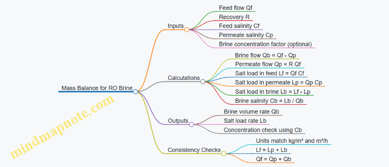
Example: Single Stage with Given Recovery and Salinities
Let:
- \(Q_f = 1,000\) m³/h
- Recovery \(R = 0.45\)
- Feed salinity \(C_f = 35\) kg/m³ (about 35 g/L)
- Permeate salinity \(C_p = 0.5\) kg/m³ (about 0.5 g/L)
Step 1: Compute permeate and brine flows
- \(Q_p = R Q_f = 0.45 \times 1,000 = 450\) m³/h
- \(Q_b = Q_f - Q_p = 1,000 - 450 = 550\) m³/h
Step 2: Compute salt loads
- Feed salt load: \(L_f = Q_f C_f = 1,000 \times 35 = 35,000\) kg/h
- Permeate salt load: \(L_p = Q_p C_p = 450 \times 0.5 = 225\) kg/h
- Brine salt load: \(L_b = L_f - L_p = 35,000 - 225 = 34,775\) kg/h
Step 3: Compute brine salinity
- \(C_b = L_b / Q_b = 34,775 / 550 \approx 63.23\) kg/m³
Quick sanity check: brine salinity should be higher than feed salinity. Here, 63.23 kg/m³ is about 1.81× the feed salinity, which is consistent with a recovery of 45% (concentration factor is roughly \(1/(1-R) = 1/0.55 \approx 1.82\), with small adjustment because permeate still contains salt).
Example: Using a Concentration Factor Instead of Permeate Salinity
Sometimes you know the brine concentration factor \(K\) where \(C_b = K C_f\). Then you can solve for brine salt load without explicitly using \(C_p\).
Let:
- \(Q_f = 1,000\) m³/h
- Recovery \(R = 0.45\) so \(Q_b = 550\) m³/h
- \(C_f = 35\) kg/m³
- \(K = 1.80\) so \(C_b = 1.80 \times 35 = 63\) kg/m³
Then:
- \(L_b = Q_b C_b = 550 \times 63 = 34,650\) kg/h
If you want \(C_p\) from the salt balance:
- \(L_f = 35,000\) kg/h
- \(L_p = L_f - L_b = 35,000 - 34,650 = 350\) kg/h
- \(C_p = L_p / Q_p = 350 / 450 \approx 0.78\) kg/m³
This is useful when you have brine concentration from stage calculations but still need permeate salinity for downstream checks.
Practical Design Checks That Prevent Costly Mistakes
- Unit discipline: \(Q\) in m³/h and \(C\) in kg/m³ gives \(L\) in kg/h. Mixing g/L with kg/m³ is a classic way to get a “perfectly wrong” answer.
- Mass balance closure: ensure \(Q_f = Q_p + Q_b\) and \(L_f = L_p + L_b\). If either fails, revisit inputs or rounding.
- Brine salinity reasonableness: for a first-pass estimate, \(C_b \approx C_f/(1-R)\). If your computed \(C_b\) is wildly different, permeate salinity or recovery assumptions likely need correction.
Summary of the Example Results
For the base case:
- Brine flow \(Q_b = 550\) m³/h
- Brine salt load \(L_b \approx 34,775\) kg/h
- Brine salinity \(C_b \approx 63.23\) kg/m³
These outputs feed directly into brine handling sizing and compliance calculations, because both volume rate and salt load determine how aggressive the brine is for scaling risk and disposal constraints.
8. Scaling Control and Chemical Dosing System Engineering
8.1 Scaling Indices and Saturation Calculations for Design Screening
Scaling is the membrane’s version of “slow and steady”: small deposits reduce permeate flux, increase pressure demand, and can trigger irreversible damage. Design screening aims to answer one practical question early: will the feed and operating conditions push the system toward scale formation faster than pretreatment and chemical control can manage.
Foundational Concepts for Saturation Screening
Start with saturation state, not guesses. For a given scale-forming salt, saturation index compares the ion activity product to the solubility product. In practice, you compute a dimensionless indicator using estimated ion activities, temperature, pH, and ionic strength.
Key inputs:
- Temperature: solubility and equilibrium shift with temperature.
- pH: controls carbonate and hydroxide speciation.
- Ionic strength: affects activity coefficients.
- Recovery and concentration: concentrate ions as water is removed.
- Antiscalant and pretreatment: reduce effective scaling tendency by changing free ion availability or crystal growth behavior.
A useful mental model is “where the chemistry wants to go.” If the operating point drives the system beyond equilibrium for a salt, scaling risk rises. If it stays comfortably below equilibrium, the job becomes managing variability rather than fighting a losing battle.
Scaling Indices You Will Actually Use
Most RO design screening focuses on three common families:
- Calcium carbonate scale: sensitive to pH, alkalinity, and carbonate speciation.
- Calcium sulfate scale: sensitive to calcium and sulfate concentrations and ionic strength.
- Barium/strontium sulfate scale: often lower concentration but can be stubborn.
You typically evaluate an index for each salt and then apply a conservative margin for uncertainty in feed analysis, temperature, and recovery.
Systematic Calculation Workflow
-
Collect representative feed data Use measured alkalinity, calcium, magnesium, sulfate, chloride, sodium, silica, and temperature. If you only have partial data, you still screen, but document assumptions because missing ions can shift ionic strength and speciation.
-
Convert to design concentrations at target recovery Concentrate ions approximately with the recovery ratio, adjusted for any known removal in pretreatment. Example: if recovery is 45%, the concentrate factor is about 1/(1−0.45)=1.82.
-
Compute speciation and ion activities For carbonate systems, pH determines whether carbon exists as CO2(aq), HCO3−, or CO3^2−. For sulfate and calcium, activity coefficients matter because ions interact in concentrated brine.
-
Calculate saturation index for each scale Use the equilibrium relationship for the salt at the design temperature and pH. The result is a screening indicator that increases as the system becomes more supersaturated.
-
Apply design margins and interpret risk Treat the index as a “risk ranking,” not a guarantee. Use conservative margins for measurement uncertainty and operational excursions.
Example: Quick Screening for Calcium Carbonate
Assume a brackish feed at 25°C with:
- Alkalinity expressed as CaCO3: 120 mg/L
- Calcium: 80 mg/L
- pH: 7.8
- Target recovery: 45%
Step A: Concentrate factor ≈ 1.82, so calcium becomes ~146 mg/L and alkalinity becomes ~218 mg/L as CaCO3.
Step B: At pH 7.8, carbonate fraction is limited, but it increases if pH rises due to operational conditions or chemical dosing changes. If the calculated saturation index for CaCO3 at the concentrate point exceeds the chosen threshold, you plan for antiscalant dosing and pH control strategy.
Step C: If you later confirm that antiscalant reduces effective scaling tendency, you still keep the saturation calculation as the baseline for dosing setpoints and monitoring triggers.
Mind Map: From Feed Data to Scale Risk
Practical Interpretation for Design Decisions
A good screening output is a scale risk matrix: each salt family gets an index value at the design point and a risk category. That matrix then directly informs where you place chemical dosing (often at the start of the RO train or before the most concentrated stage) and what you monitor (pH, conductivity/TDS proxy, and key hardness/alkalinity indicators).
Finally, remember that saturation calculations are only as reliable as the input chemistry. If alkalinity or calcium is off by a lot, the computed saturation index will be off too, and the “best” design will still be wrong—just confidently wrong. The fix is disciplined sampling and consistent basis for concentration and speciation assumptions.
8.2 Antiscalant Selection and Dosage Control Strategy
Antiscalant performance depends on two things: the chemistry must match the likely scale, and the dosing system must deliver the right amount at the right moment. In industrial RO, the “right amount” is not a single number; it changes with feed temperature, recovery, pH adjustment, and pretreatment variability.
Foundational Inputs for Selection
Start with a short list of what the plant actually sees. Use the pretreatment outlet water quality (not raw feed) and the design operating envelope.
- Scaling risk profile: Identify dominant scale types using saturation calculations (typically calcium carbonate, calcium sulfate, barium sulfate, strontium sulfate, and silica). If silica is present, note that it often behaves differently from salts.
- Operating conditions: Record pH after any acid dosing, temperature, and expected concentrate concentration factor across stages.
- Hydraulic and recovery plan: Higher recovery increases ion concentration and shifts the risk toward the most insoluble salts.
- Cleaning and compatibility constraints: The antiscalant must not interfere with cleaning chemistry and should be compatible with membrane material and typical cleaning pH ranges.
A practical way to avoid “chemistry guessing” is to run jar tests or pilot checks for the specific antiscalant candidates against the plant’s pretreatment water, using the same pH and temperature conditions you plan to operate.
Choosing an Antiscalant Chemistry
Antiscalants generally work by one or more mechanisms: threshold inhibition (preventing crystal growth), dispersion (keeping particles from aggregating), and complexation (binding scale-forming ions). Selection should map to the scale you expect.
- Carbonate scale focus: If calcium carbonate is dominant, you want strong threshold inhibition and good performance across the pH range created by your acid dosing.
- Sulfate scale focus: For calcium sulfate or mixed sulfate systems, complexation and inhibition strength at higher ionic strength matter more than low-salinity behavior.
- Barium and strontium: These can be low in concentration but high in impact. Ensure the antiscalant candidate shows control at the plant’s barium/strontium levels and concentrate conditions.
- Silica: Silica control is often more sensitive to pH and temperature. Confirm that the candidate’s performance is validated for silica under your actual operating pH.
Dosage Control Strategy That Actually Works
A dosing strategy should be built around measurable signals and a control philosophy that respects process delays.
Control Objective
Maintain scale inhibition across the operating envelope while minimizing excess chemical. Excess antiscalant can increase organic load and complicate cleaning, so “more” is not automatically “better.”
Recommended Control Layers
- Base dose from design: Start with a design-based dose tied to recovery and saturation risk.
- Feed-forward adjustment: Adjust dose when conditions change in ways that directly affect scaling, such as temperature and conductivity (as a proxy for ionic strength).
- Feedback trim using scaling indicators: Use practical indicators like differential pressure trends, permeate flux decline patterns, and periodic scaling checks from concentrate samples. These are slower signals, so they should trim the base dose rather than override it.
Example: Temperature and Conductivity Shift
Suppose the plant runs at 25°C during commissioning, then later operates at 18°C due to seasonal conditions. Lower temperature often changes solubility behavior and can shift scaling risk. If conductivity rises at the same time (higher salinity), the antiscalant dose should increase.
A simple control approach is:
- Base dose: 5 mg/L (as delivered to the dosing point)
- Temperature correction: +10% when temperature drops from 25°C to 18°C
- Conductivity correction: +15% when conductivity rises by 20%
Resulting dose = 5 × 1.10 × 1.15 = 6.3 mg/L. The exact factors should come from your jar tests or pilot data, but the logic is the same: scale risk moves with both solubility conditions and ionic strength.
Dosing Point and Mixing
Where you inject matters as much as how much you inject.
- Injection location: Dose upstream of the membrane where mixing is reliable but after pretreatment steps that would remove or react with the antiscalant.
- Mixing time and turbulence: Poor mixing can cause local over-concentration, leading to uneven inhibition and potential membrane surface effects.
- Hydraulic residence time: Ensure the time between injection and RO feed is consistent across operating modes.
Practical Dosage Calculation Workflow
Use a repeatable workflow so operators and engineers are not relying on memory.
- Convert the target dose to mass per volume at the dosing point.
- Convert to pump flow rate using the antiscalant concentration.
- Apply control multipliers from temperature and conductivity signals.
- Verify with sampling: check concentrate scaling tendency and monitor membrane performance.
Mind Map: Antiscalant Selection and Dosage Control
Example: Building a Simple Control Loop
If your plant has limited instrumentation, you can still implement a robust loop using two signals.
- Signal 1: RO feed conductivity (proxy for ionic strength)
- Signal 2: Feed temperature
Then:
- Compute a multiplier from each signal using values derived from tests.
- Multiply the base dose by the combined multiplier.
- Keep the pump interlocked with chemical tank level and minimum flow to prevent underdosing.
This approach avoids overreacting to noisy measurements while still responding to the two most common drivers of scaling risk.
Dosage Verification and Tuning
After implementation, tune using evidence rather than assumptions. Compare expected scaling control (from jar tests and saturation calculations) with observed membrane behavior and concentrate sample results. If scaling indicators worsen, first check dosing accuracy (pump calibration, dilution, and injection flow), then revisit the chemistry match to the dominant scale type.
A good antiscalant program is boring in the best way: stable dosing, predictable membrane performance, and clear links between water quality changes and dose adjustments.
8.3 Acid and pH Adjustment Design for Scale Prevention
Acid and pH adjustment is the “steering wheel” for preventing carbonate and hydroxide scale in RO. The goal is not to make the water acidic for its own sake; it is to shift carbonate chemistry and control precipitation risk at the membrane surface.
Foundational Chemistry and Why pH Matters
In seawater and many brackish feeds, scaling often starts with carbonate species. When pH is high, bicarbonate and carbonate shift toward carbonate ions, which readily combine with calcium and magnesium to form solids. Lowering pH converts carbonate toward bicarbonate and carbon dioxide, reducing the concentration of carbonate ions available to precipitate.
A practical design mindset is to treat pH as a lever that changes saturation indices. You set a target pH range based on the dominant scale type, the feed alkalinity, and the expected recovery. Then you verify that the pH shift survives mixing, dosing dynamics, and any buffering in the pretreatment effluent.
Design Inputs and Data You Actually Need
Start with these inputs from feed characterization and pretreatment performance:
- Alkalinity and hardness: total alkalinity (or alkalinity species) and calcium/magnesium concentrations.
- Temperature and pressure: affects equilibrium and solubility.
- Feed pH and expected post-pretreatment pH: including any changes from filtration and antiscalant dosing.
- RO recovery and stage layout: pH effects can be stronger in later stages where concentration increases.
- Antiscalant strategy: acid dosing and antiscalant dosing interact; antiscalant can be less effective if pH is pushed outside its intended operating window.
A simple example: if alkalinity is high, the same acid dose produces a smaller pH change than in low-alkalinity water. That means your control system must be sized for buffering, not just for a one-time adjustment.
Acid Selection and Compatibility
Common acids include sulfuric and hydrochloric, chosen based on availability, handling, and downstream compatibility. Sulfuric acid adds sulfate; hydrochloric acid adds chloride. Either can be acceptable, but you must check:
- Corrosion allowance and materials: acid storage, piping, and injection lances must match the acid strength and concentration.
- Sulfate or chloride impact on scaling: sulfate can influence gypsum-type scaling risk; chloride generally does not form sparingly soluble salts like carbonate scales.
- Interaction with cleaning and neutralization: if cleaning chemicals are planned, ensure the acid system does not create unexpected neutralization burdens.
A concrete rule of thumb: choose the acid that your plant can handle safely with the least material stress, while still meeting the chemistry target for scale prevention.
Injection Point Engineering
Where you inject acid matters as much as how much you inject.
Best practice is to inject acid upstream of the membrane feed but after any pretreatment steps that would consume acid unnecessarily (for example, where alkalinity is already stabilized). Injection should be followed by rapid mixing and sufficient residence time so the pH at the membrane inlet matches the control objective.
Design elements include:
- Injection lance location: near a turbulent mixing zone to reduce pH gradients.
- Static mixer or mixing section: sized for flow and viscosity.
- Short, controlled piping runs: minimize dead legs where pH can drift.
- pH measurement location: placed where it represents membrane inlet conditions, not just the injection header.
Example: if pH is measured right at the injection skid outlet but the membrane feed has long, poorly mixed piping, the controller may “chase” a pH that is not actually what the membranes see.
Control Strategy and Stability
pH control should be stable and conservative. A typical approach is a PID loop using a pH analyzer with temperature compensation, controlling acid dosing pump speed.
Key design features:
- Setpoint selection by scale risk: choose a pH that reduces carbonate scale risk without pushing the system into conditions that increase other issues (like excessive corrosion or destabilizing pretreatment).
- Dose rate limits: prevent overshoot during analyzer noise or flow transients.
- Feedforward from flow: dosing proportional to permeate production or concentrate flow can reduce lag.
- Interlocks: stop acid dosing if pH probe signals are invalid, if flow is out of range, or if mixing conditions are not met.
A simple example of stability: during start-up, flow may ramp slowly while pH probes stabilize later. Without dose limits, the controller can dump acid while the probe is still reading the previous condition.
Mass Balance Example for Acid Dose Sizing
Assume you need to shift alkalinity-related carbonate chemistry by lowering pH from 8.2 to 7.2 at the membrane inlet. The required acid dose depends on alkalinity buffering, not just the pH change.
A practical sizing workflow:
- Convert alkalinity to an equivalent acid requirement using the alkalinity species and target pH.
- Apply a safety factor for measurement uncertainty and pretreatment variability.
- Convert equivalent acid to dosing concentration and pump flow rate.
- Validate with a jar test or pilot data where possible.
Example: if alkalinity is high, the calculated acid requirement may be several times larger than what you’d estimate from pH alone. That’s why alkalinity data is non-negotiable.
Mind Map: Acid and pH Adjustment Design
Common Design Pitfalls and How to Avoid Them
- Measuring pH in the wrong place: the analyzer must reflect membrane inlet conditions.
- Ignoring alkalinity buffering: pH change is not proportional to acid dose when alkalinity is high.
- Overdosing during transients: dose limits and interlocks prevent overshoot.
- Forgetting mixing time: without residence time, the controller can be correct on paper and wrong at the membrane.
Example: Coordinating Acid and Antiscalant
If antiscalant is used to manage scaling, acid dosing should not be treated as independent. Lowering pH can change antiscalant performance by altering the chemistry it is designed to inhibit. A workable approach is to set the antiscalant dosage based on baseline conditions, then adjust acid setpoints while checking that scaling indicators remain controlled and that the antiscalant is not being “undone” by chemistry shifts.
The end result is a controlled pH at the membrane inlet that reduces carbonate scale formation while keeping the rest of the pretreatment and dosing strategy consistent.
8.4 Coagulant and Biocide Dosing Integration With Pretreatment
Pretreatment dosing is where pretreatment stops being “supporting cast” and starts doing real work. Coagulants and biocides must be integrated so they target the right problem at the right point, with dosing rates that match the water’s variability. A practical way to keep the system coherent is to treat dosing as a chain: feedwater quality measurement → chemical selection → injection point hydraulics → mixing and contact time → filtration response → RO feed verification.
Foundational Integration Logic
Coagulants primarily help remove colloids and natural organic matter fractions that contribute to fouling and pressure loss. Biocides primarily control biological growth that can form biofilms in filters and on RO feed surfaces. These goals interact: if you dose coagulant without controlling biology, you can create a “food source” for microbes trapped in filter media. If you dose biocide without adequate coagulation, you may reduce bioactivity but still deliver colloids that foul membranes.
A clean integration approach uses two rules. First, inject coagulant upstream of clarification or media filtration so destabilized particles can be captured. Second, inject biocide where it can reach the biological population without interfering with coagulation chemistry or damaging downstream equipment.
Coagulant Dosing Integration
Start with jar testing or equivalent bench screening to determine the coagulant type, approximate dose range, and pH sensitivity. Then translate that into a dosing control strategy.
Injection point and mixing: Coagulant needs rapid dispersion followed by a short flocculation window. In practice, that means injection into a fast-mixing section (static mixer or well-designed turbulent zone) and then a controlled residence time before the clarification step. If the plant uses cartridge filtration after coagulation, the flocculation time must be long enough to form removable flocs but short enough to avoid floc breakage from excessive shear.
Control variables: Use at least one real-time proxy for coagulation demand, such as turbidity, UV254, or dissolved organic carbon surrogate signals. When the proxy changes, adjust coagulant dose proportionally within a safe band. Keep the control “bounded” so a sensor glitch does not cause a chemical overfeed.
Example: Suppose raw water turbidity rises from 2 NTU to 8 NTU after a storm. A bounded control might increase coagulant dose by 30–50% while maintaining pH setpoints. After clarification, the target is stable filtrate turbidity and reduced UV254, indicating that the colloidal load is actually being removed rather than merely destabilized.
Biocide Dosing Integration
Biocide selection depends on whether you need oxidizing control (often for biofilm suppression) or non-oxidizing control (often for compatibility with downstream chemistry). Integration focuses on contact time and compatibility.
Injection point: For media filters, biocide injection is typically placed so it can reach the filter bed and associated piping where bioactivity develops. If you dose too close to the RO feed, you may not control growth in the filter system. If you dose too far upstream, you may waste chemical and increase the burden on dechlorination or residual management.
Compatibility with coagulant: Some biocides can affect floc formation or interfere with residual chemistry. The integration step is to verify that the chosen biocide does not destabilize the coagulated flocs or change filtrate quality. If compatibility is uncertain, separate dosing locations and validate with pilot or staged testing.
Example: If a plant uses an oxidizing biocide and observes higher filtrate turbidity after biocide changes, the issue may be floc disruption or increased fine particle release. The fix is usually to adjust injection location, mixing intensity, or dose timing so the biocide acts on biological surfaces without breaking the particle capture mechanism.
Residual Management and RO Feed Verification
Even when dosing is correct, residuals can cause downstream problems. For oxidizing biocides, residual control often requires dechlorination or equivalent reduction steps before RO. For non-oxidizing biocides, residual limits are still important because they can affect membrane performance and cleaning chemistry.
RO feed verification closes the loop. Track filtrate turbidity, particle counts, and key organic indicators. If RO feed pressure rises or flux declines, dosing may be “technically active” but not achieving the intended removal.
Example: A plant maintains low RO feed turbidity but sees gradual flux loss. That can indicate that dosing is controlling particles but not the dissolved fraction that drives membrane fouling. In that case, coagulant dose may need adjustment or the pretreatment train may need a different capture mechanism.
Mind Map: Coagulant and Biocide Dosing Integration
Practical Integration Checklist
- Confirm coagulant type, dose range, and pH sensitivity with bench testing.
- Confirm biocide type and residual handling requirements with compatibility checks.
- Place coagulant injection upstream of the capture step with adequate mixing and flocculation time.
- Place biocide injection where biological activity occurs, with sufficient contact time.
- Use bounded feedback control tied to measurable proxies, not uncontrolled manual tweaks.
- Verify RO feed quality indicators and residual limits so dosing success is measured downstream, not just in chemical tanks.
A well-integrated dosing system behaves like a coordinated team: coagulant captures what fouls, biocide prevents biological buildup, and residual management keeps RO membranes out of the chemical crossfire.
8.5 Chemical Storage, Metering, and Interlock Design for Safety
Chemical systems in RO plants are small in footprint but big in consequences. A safe design starts with knowing what each chemical can do to people, equipment, and the process—then it turns that knowledge into storage choices, metering accuracy, and interlocks that prevent the wrong thing from happening at the wrong time.
Foundational Safety Concepts for Chemical Systems
Begin with a simple hazard map: identify chemical identity, concentration, primary exposure routes (inhalation, skin contact, ingestion), and the most likely failure modes (leak, overfeed, underfeed, wrong chemical, blocked discharge, loss of ventilation). For RO antiscalant, acid, and biocide systems, the “wrong chemical” scenario is often the most preventable and most damaging.
A practical best practice is to define a “chemical intent” for each dosing point: what the chemical is supposed to correct (scaling, pH control, biofouling), what operating conditions must exist for it to work, and what conditions make it harmful. For example, acid dosing intended to reduce pH should be interlocked with a confirmed pH measurement and a minimum flow through the dosing location; otherwise, acid can pool and create localized corrosion.
Chemical Storage Design
Storage design should match the chemical’s physical behavior and compatibility. Use secondary containment sized for the largest single tank volume, plus precipitation allowance where relevant. Keep incompatible chemicals separated by design, not by hope—acid and oxidizing biocides should not share containment or adjacent spill paths.
Ventilation and detection matter because many dosing rooms are quiet until they are not. Provide mechanical ventilation sized for worst-case release scenarios, and place gas or vapor detection where it can actually reach sensors (near likely leak points, not only near the ceiling). For corrosive liquids, ensure ventilation materials and ducting are compatible with the chemical.
Labeling and access control should be operational, not decorative. Use color-coded piping tags and lockable cabinet access for concentrated chemicals. A simple operational check that works: require a “tank-to-skid” verification before enabling dosing, using both tank identification and a permissive signal from the control system.
Metering System Engineering
Metering accuracy is safety. Overdosing antiscalant can increase organic load and worsen fouling; overdosing acid can drive pH too low and accelerate corrosion. Underfeeding can cause scaling that plugs membranes and forces aggressive cleaning.
Select metering equipment based on chemical viscosity, required dose range, and acceptable response time. Common choices include diaphragm metering pumps for many RO chemicals and peristaltic pumps for certain low-viscosity or sensitive solutions. Design the suction side with proper strainers and check valves to prevent backflow through the pump.
A good metering layout includes:
- A day tank or bulk tank with level indication and low-level alarm.
- A dosing pump with stroke feedback or flow verification.
- A static mixer or injection quill sized for the expected flow velocity.
- A flush line that can purge the injection line when dosing stops.
Example: If acid is injected into a recirculation line, the injection quill should be positioned so the chemical is immediately dispersed. If the quill is installed where flow is turbulent only intermittently, the system can create pH “hot spots” that damage downstream components.
Interlock Design for Safety
Interlocks should prevent three categories of unsafe events: dosing without the correct process conditions, dosing when measurement is unreliable, and dosing when containment or discharge paths are compromised.
Core Interlock Set
-
Process Flow Permissive Dosing enable should require a confirmed minimum flow at the dosing location. If flow drops below threshold, stop dosing and initiate line flush if configured.
-
Instrumentation Health Permissive For pH-based acid control, require pH sensor signal validity and calibration status. If pH measurement is out of range or flagged invalid, freeze dosing at a safe default or stop dosing depending on the chemical’s risk profile.
-
Tank Level and Pump Status Permissive Low tank level should alarm and inhibit dosing to avoid running pumps dry. Pump fault interlocks should include loss of prime, motor overload, and stroke failure.
-
Containment and Ventilation Permissive If secondary containment monitoring or ventilation failure detection is available, use it to inhibit dosing. For corrosive systems, a ventilation failure should not be treated as a “warning only.”
-
Backflow and Isolation Interlocks Check valves and normally closed isolation valves should be monitored. If an isolation valve fails to prove closed or open as required, inhibit dosing.
Interlock Logic Example
The following logic is intentionally conservative: it stops dosing when any safety-critical condition is not met.
IF (ProcessFlow >= MinFlow)
AND (pHValid = TRUE)
AND (TankLevel >= MinLevel)
AND (PumpFault = FALSE)
AND (VentilationOK = TRUE)
AND (InjectionValveProvedOpen = TRUE)
THEN Enable AcidDosing
ELSE Stop AcidDosing and FlushInjectionLine
A key nuance: “Stop” should be defined. For many systems, stopping dosing without flushing can leave chemical in the injection line, which later mixes into the process when flow resumes. Flushing is not glamorous, but it prevents the classic “why did the pH jump during restart?” question.
Integrated Example for Antiscalant and Acid
Consider a two-chemical setup: antiscalant is dosed upstream of the RO feed, while acid is dosed to maintain pH in the pretreatment outlet. The integrated safety approach is to separate permissives by chemical intent.
- Antiscalant dosing permissive: pretreatment filter differential pressure within limits and RO feed flow above minimum.
- Acid dosing permissive: pH sensor validity and stable pretreatment outlet flow.
If pretreatment filters plug, RO feed flow may still exist briefly due to buffer volumes. Antiscalant dosing should inhibit when differential pressure exceeds the limit, even if flow is temporarily present. That prevents dosing into a condition where mixing and control are unreliable.
Mind Map: Chemical Storage, Metering, and Interlock Design
Practical Design Checklist for Commissioning Readiness
Before handover, verify that every interlock has a defined alarm, a defined inhibit action, and a defined recovery action. Also verify that the “stop and flush” behavior is tested under controlled conditions, because that is where many safety designs quietly fail during real operations.
9. Plant Wide Process Design for RO Trains and Auxiliary Systems
9.1 RO Train Configuration Design Including Staging and Train Redundancy
Designing an RO train is mostly about controlling where pressure, recovery, and fouling risk land. A good configuration makes the plant easier to operate, easier to clean, and easier to keep within brine and product quality limits.
Foundational Concepts That Drive Configuration
Start with three inputs: feedwater quality, target recovery, and required product salinity. Feedwater quality sets pretreatment strictness and cleaning frequency. Target recovery determines how many stages you need to keep membrane performance stable. Product salinity and flow rate determine how many elements and trains you must run.
A simple mental model helps: each stage increases concentration in the remaining brine. That concentration raises osmotic pressure, which increases required pressure and accelerates scaling risk. Staging spreads that burden across multiple passes so each membrane sees a manageable operating envelope.
Staging Strategy for Reverse Osmosis Trains
Most industrial RO plants use either single-pass staging (one stage) or multi-stage staging (two or three stages). Two-stage designs are common because they balance complexity and performance.
In a two-stage train, the first stage produces permeate while sending a more concentrated brine to the second stage. The second stage typically runs at higher salinity and may require tighter control of antiscalant dosing and pH. The key design decision is how to split recovery between stages.
A practical example: if the plant target is 45% overall recovery, you might allocate 25% recovery in stage 1 and 20% in stage 2. This keeps stage 1 membranes from seeing excessive concentration early, while stage 2 still achieves the remaining recovery without forcing stage 1 to operate at a pressure that would be inefficient or unstable.
Staging also affects cleaning. If fouling is expected to be dominated by scaling, you want the stage with the highest saturation risk to be the one you can isolate and clean without taking the entire train offline. That pushes you toward designs where each stage has clear isolation valves and predictable flow paths.
Train Redundancy for Reliability and Maintenance
Redundancy is not just “more equipment.” It is the ability to keep producing product when one portion of the system is unavailable. In RO plants, redundancy usually appears at the train level: multiple RO trains run in parallel, each with its own high-pressure pump(s), membrane pressure vessels, and energy recovery device.
A typical arrangement is N trains with one train capable of being offline for maintenance while the remaining trains cover the required production rate. For example, if the plant needs 10,000 m³/day, you might design four trains of 2,500 m³/day each. If one train is down, the other three provide 7,500 m³/day, so you would only accept that reduced output if the site can tolerate it. If full output must be maintained, you increase the number of trains or oversize the remaining trains.
Redundancy also influences how you handle feed and concentrate manifolds. Parallel trains reduce the need for complex valve gymnastics during maintenance, but they require careful hydraulic balancing so each train receives the intended feed flow and concentration.
Configuration Patterns and How to Choose Them
Single-stage configurations are simpler and can work well for lower recovery targets and more stable feedwater. Multi-stage configurations are preferred when you need higher recovery or when feed salinity and temperature variations would otherwise push the membranes outside a comfortable operating window.
Within a stage, element arrangement matters. You size pressure vessels and elements so that permeate flow is balanced across the train. If one vessel group produces significantly more permeate than another, the train can drift into uneven flux conditions, which increases the chance of localized scaling.
A concrete example: suppose you have a stage designed for 2,000 m³/day permeate. If you distribute elements unevenly so that one pressure vessel group carries 35% of the stage flow instead of 25%, that group will experience higher local flux. Even if the average design looks fine, the high-flux group can foul faster, forcing earlier cleaning and reducing overall availability.
Isolation, Bypass, and Operational Flexibility
Configuration quality shows up during abnormal events: a pump trips, a pressure exchanger needs bypass, or a membrane section requires cleaning. Your design should allow isolation of a stage or train without breaking the overall mass balance.
At minimum, plan for:
- Feed isolation to a train so pretreatment and high-pressure systems can remain stable.
- Concentrate isolation so brine routing stays within permitted limits.
- Energy recovery bypass so the plant can still run safely during energy recovery maintenance.
A small but important detail: isolation valves should be placed so that dead legs are minimized. Dead legs can become chemical traps during cleaning and can later release diluted residues that affect scaling control.
Mind Map: RO Train Configuration Design
Example: Two-Stage, Four-Train Layout
Assume a plant requires 10,000 m³/day permeate at a fixed salinity target. You choose four parallel trains, each designed for 2,500 m³/day. Each train uses two RO stages.
Stage 1 is configured for 25% recovery within the train, producing the majority of permeate at lower brine concentration. Stage 2 provides the remaining 20% recovery, where antiscalant control and pH management are tightened because saturation risk is higher.
During maintenance, one train can be isolated while the other three continue operating. The plant output drops to 7,500 m³/day, which is acceptable if the site has storage or demand flexibility. If full output is required, the design basis would instead allocate more trains or increase element count so the remaining trains can cover the full demand.
This example shows the core logic: staging manages concentration and fouling risk inside a train, while redundancy manages availability across trains. Both decisions are made from the same inputs—quality, recovery, and required output—so the configuration stays coherent from design basis to commissioning checks.
9.2 Permeate Post Treatment and Stabilization System Design
Permeate from an RO train is typically low in hardness and alkalinity, with reduced dissolved salts but not necessarily reduced dissolved gases or residual organics. Post treatment exists to make permeate safe for its intended use and stable during storage and distribution. The design goal is simple: deliver water that meets quality targets at the point of use, while avoiding corrosion, scaling in downstream equipment, and microbial growth.
Foundational Quality Targets and Design Basis
Start by translating the end-use requirement into measurable permeate properties. Common targets include conductivity, total organic carbon, dissolved oxygen, pH, alkalinity, hardness, and silica. For example, a boiler feed system often cares about silica and hardness, while a process rinse line may care more about conductivity and TOC.
A practical design basis also defines operating conditions that affect stability: permeate temperature range, storage duration, and whether the water will be recirculated. If permeate sits in a tank for 24 hours, the system must manage oxygen ingress and microbial risk. If it is used immediately, the stabilization requirements can be lighter.
Process Sequence and Core Treatment Functions
A typical permeate post treatment train includes:
- Degassing or air stripping to reduce dissolved gases such as CO₂, which otherwise drives pH downward.
- pH and alkalinity adjustment to protect downstream metals and prevent corrosion.
- Mineral stabilization such as remineralization to set a controlled hardness and alkalinity level.
- Disinfection to control microbial growth, especially when storage or recirculation is present.
- Filtration and polishing when TOC or suspended solids must be reduced further.
An easy way to keep the design coherent is to map each function to a failure mode. Low alkalinity leads to corrosion; dissolved CO₂ leads to low pH; storage without disinfection leads to biofilm; insufficient polishing leads to filter fouling in later steps.
Degassing and PH Control
RO permeate often has low alkalinity, so even small CO₂ levels can push pH into a corrosive range. Degassing can be done with packed towers or membrane contactors. Packed towers are straightforward: air is introduced counter-currently, and CO₂ transfers from water to air.
Example: If permeate pH is measured at 5.2 after RO, and the target is 7.0–8.0 for corrosion control, the design can include degassing followed by chemical alkalinity adjustment. Degassing reduces CO₂ load, so the chemical dose required for pH correction is smaller and more stable.
pH adjustment is commonly achieved with lime, caustic soda, or sodium bicarbonate. Lime adds calcium and alkalinity but requires careful handling of solids and settling. Caustic soda raises pH quickly but adds no alkalinity by itself, so it may be paired with bicarbonate for buffering.
Remineralization and Corrosion Management
Stabilization is not just about hitting a pH number; it is about providing buffering capacity and controlling aggressiveness. Remineralization sets hardness and alkalinity to reduce corrosion rates in carbon steel and to limit leaching from piping.
Example: For a distribution loop made of carbon steel, the system may target a modest alkalinity and hardness to maintain a stable carbonate system. If the loop is made of stainless steel, the target can be different, but the principle remains: avoid water that is too “hungry” for minerals.
Disinfection and Microbial Control
When permeate is stored or recirculated, disinfection becomes part of the stabilization strategy. Chlorination, chloramination, or UV can be used depending on residual requirements and downstream constraints.
Example: If the plant uses a recirculating tank and piping, maintaining a small disinfectant residual helps prevent biofilm formation. If the process cannot tolerate chlorinated byproducts, UV with careful filtration and tight operational controls may be selected.
Design details that matter include contact time, mixing, and monitoring points. A common mistake is placing sampling taps where disinfectant has not mixed uniformly, leading to misleading readings.
Filtration and Polishing Options
Even after RO, small amounts of suspended solids and trace organics can remain. Polishing filters (often cartridge or multimedia depending on load) protect downstream equipment and reduce TOC when required.
Example: If TOC must be reduced for a sensitive process, a granular media filter followed by activated carbon can be used to capture residual organics. The filter sizing should reflect expected turbidity and backwash capability, not just average values.
Instrumentation, Sampling, and Control Logic
A stable post treatment system needs measurements that reflect the water state after each function. Typical instrumentation includes:
- pH and conductivity after stabilization
- disinfectant residual at the tank outlet and return line
- turbidity after polishing filtration
- temperature for dose correction
Sampling should be placed to represent the actual point of use. If the system includes a tank, sample from the distribution loop, not only from the tank inlet.
Mind Map: Permeate Post Treatment and Stabilization
Example Integrated Design Flow
- Measure permeate pH, alkalinity, conductivity, TOC, and dissolved gases.
- If pH is low due to CO₂, install degassing before chemical adjustment.
- Add alkalinity and hardness to reach buffering targets for the distribution materials.
- If storage or recirculation exists, add disinfection with residual monitoring at the loop.
- Add polishing filtration if turbidity or TOC targets require it.
- Verify sampling points and control loops reflect the point of use.
This sequence keeps each subsystem from compensating for another’s shortcomings, which is how post treatment designs stay predictable during real operation.
9.3 Concentrate Stream Handling Including Blowdown and Purge Logic
Concentrate handling starts with one simple goal: keep the RO train operating inside its scaling and hydraulics limits while meeting brine discharge requirements. The concentrate stream is not “waste”; it is a controlled side stream whose salt load, temperature, and solids content must be managed so the membranes stay clean enough to produce permeate consistently.
Foundational Concepts for Blowdown and Purge
Blowdown is a controlled discharge from a loop or concentration stage to prevent salt and scaling species from building up. Purge is similar in intent but usually refers to removing a smaller portion to maintain a target concentration in a recirculating or staged system.
A practical way to think about it is with two balances:
- Salt mass balance: how much salt enters the loop versus how much leaves with blowdown/purge.
- Water balance: how much water is removed with blowdown/purge versus how much is recovered as permeate.
Example: If your RO train produces permeate at 50 m³/h and the concentrate flow is 10 m³/h, then the overall recovery is 50/(50+10)=83.3%. If scaling risk rises at higher concentrate salinity, you may reduce effective recovery by increasing blowdown so the concentrate salinity stays within the design envelope.
Concentrate Path Design Before Any Discharge
Before blowdown logic is written, the piping and instrumentation must make the discharge controllable:
- Define concentrate control points: typically after each stage or after the final stage, depending on where salinity and scaling risk are highest.
- Provide flow measurement: at least one reliable concentrate flow meter and one discharge flow meter (or a validated mass balance approach).
- Ensure mixing and residence control: blowdown should not create dead zones where solids settle.
- Budget pressure drops: discharge valves and pipelines must not starve the RO train of required backpressure.
Example: If a blowdown valve is placed upstream of a pressure control loop, the valve can fight the pressure controller. The result is oscillating concentrate pressure, which changes membrane flux and can worsen fouling.
Blowdown Logic Using Concentration Targets
Most plants implement blowdown based on a concentration proxy. The most common proxy is conductivity (converted to TDS using site-specific calibration). The logic typically uses a setpoint, a deadband, and a ramp rate.
A systematic approach:
- Choose a maximum allowable concentrate conductivity that corresponds to acceptable scaling index and cleaning frequency.
- Set a deadband to avoid rapid cycling.
- Use a ramp limit so valve movements do not cause hydraulic shocks.
Example: If the maximum allowable conductivity corresponds to 70,000 µS/cm, you might start blowdown at 68,000 µS/cm, stop at 66,000 µS/cm, and limit valve opening changes to 5% per minute.
Purge Logic for Solids and Operational Stability
Purge is often used when the concentrate loop includes components that can accumulate solids or when there are intermittent operating conditions such as start-up, shutdown, or cleaning cycles.
Common purge triggers:
- High differential pressure across filters or strainers in the concentrate pretreatment line.
- Elevated turbidity or suspended solids in the concentrate feed to the RO train.
- Cleaning cycle transitions where residual cleaning solution must be removed from a loop.
Example: During a cleaning cycle, the concentrate line may contain diluted cleaning chemicals and loosened scale fragments. A short purge after the rinse can prevent those fragments from being carried back into the RO pressure vessels.
Integrating Blowdown and Purge with Stage Recovery
In multi-stage RO, blowdown can be applied at different locations. The key is to keep the stage concentrate salinity within its scaling limits while maintaining overall recovery.
- Stage blowdown reduces salt load entering downstream stages.
- Final-stage blowdown is simpler but may allow higher salinity in earlier stages.
Example: If Stage 1 has robust scaling control but Stage 2 is more sensitive, you can place blowdown between stages so Stage 2 sees a lower conductivity without sacrificing Stage 1 performance.
Mass Balance Example for Valve Sizing
Assume:
- Feed to RO train: 60 m³/h
- Permeate: 45 m³/h
- Concentrate leaving RO: 15 m³/h
- You add a blowdown stream from the final concentrate loop: 2 m³/h
Then the remaining concentrate to discharge or further handling is 13 m³/h, and the blowdown fraction is 2/15=13.3% of the final concentrate flow. Valve sizing should be based on the maximum blowdown rate needed to keep conductivity below the setpoint under worst-case feed salinity.
Mind Map: Concentrate Handling Logic
Operational Interlocks That Keep Logic from Becoming Chaos
Blowdown and purge valves should be interlocked with safe operating conditions. Typical interlocks include:
- Minimum RO operating pressure before allowing blowdown to avoid destabilizing permeate production.
- Minimum concentrate flow so the valve does not open against near-zero flow.
- Chemical system status so purge does not mix incompatible streams.
Example: If the RO train is in a low-flow mode during start-up, conductivity may spike due to reduced dilution. A minimum flow interlock prevents blowdown from reacting to that transient.
Practical Implementation Checklist
- Confirm conductivity-to-TDS calibration for your temperature range.
- Set blowdown thresholds using design scaling limits, not operator preference.
- Add deadband and ramp limits to the control strategy.
- Place purge triggers on measurable solids or cleaning transitions.
- Validate mass balance so discharge flow aligns with the intended recovery reduction.
When these pieces are connected, blowdown and purge become predictable tools: they reduce scaling risk and protect membrane performance without turning the RO train into a control-system experiment.
9.4 Backwash, Rinse, and Cleaning Water System Design
A backwash, rinse, and cleaning water system has one job: provide the right water quality, at the right flow and pressure, at the right time, without contaminating the rest of the plant. In RO pretreatment trains, this system also protects membranes indirectly by keeping filters and media clean enough to reduce fouling load.
Foundational Requirements
Start with three design inputs: pretreatment equipment list, cleaning method, and water quality boundaries. Backwash is typically for media filters (sand, multimedia, or dual media), while cartridge filters and some polishing steps may use rinse-only or chemical cleaning. Cleaning water quality should be consistent with the worst-case requirement of the equipment being cleaned. If the system uses RO permeate or softened water, specify the maximum allowable TDS, turbidity, and SDI so the cleaning does not reintroduce scale-formers or fine solids.
Next define hydraulic targets. Backwash flow is usually expressed as a bed expansion percentage or superficial velocity. Rinse flow is lower and aims to return the bed to its operating state and remove residual loosened solids. Cleaning water for chemical cleaning (if used) must support required contact time and mixing, which means you design for stable flow and temperature.
Finally, define operational boundaries. Backwash and rinse should be isolated from product water pathways. Use dedicated piping, check valves, and air gaps where backflow risk exists. A simple rule: if the cleaning water could ever contact a membrane feed or permeate line, treat it as contaminated and prevent cross-connection.
System Architecture
A practical architecture uses four subsystems: water source, storage and conditioning, distribution headers, and drainage/collection.
-
Water source: Options include raw water, filtered water, softened water, or RO permeate. Choose based on what you must avoid. For example, if you are cleaning filters that are prone to scaling, using softened or RO permeate reduces the chance of leaving scale residues.
-
Storage and conditioning: Provide a buffer tank or surge tank sized for the longest single cleaning event plus start-up losses. Add pressure control so the backwash flow does not sag when a pump starts. If temperature matters for cleaning chemistry, include a controlled heating or heat-trace strategy.
-
Distribution headers: Design headers with minimal dead legs and clear labeling. Include flow meters on each branch so operators can verify that the bed expansion and rinse rates are actually achieved.
-
Drainage and collection: Backwash water is typically high in suspended solids and may contain antiscalant or coagulant residues. Route it to the brine management or wastewater handling system. Provide a sampling point before discharge so you can confirm compliance and troubleshoot dosing issues.
Backwash and Rinse Hydraulic Design
Backwash design should include a bed expansion check and a pressure loss budget. A common mistake is sizing pumps for nominal flow while ignoring filter headloss at the start of backwash. Use the maximum expected headloss during the first minutes, when the bed is most resistant.
Rinse design focuses on clearing fines without over-expanding the bed. Use a staged rinse: a short high-flow rinse to remove loose particles, then a lower-flow rinse to stabilize. This reduces water use while still achieving a consistent filter performance after cleaning.
Cleaning Water Quality Control
Treat cleaning water quality as a controllable variable. Install turbidity monitoring on the cleaning water feed when the source is not RO permeate. If you use softened water, monitor hardness to ensure the softener is actually working; otherwise, you may trade filter fouling for scale deposition.
For chemical cleaning, ensure compatibility between cleaning chemicals and the water source. For instance, if you use acid cleaning, avoid water with high alkalinity that will consume acid before it reaches the membrane surface (or the media surface in pretreatment).
Controls, Interlocks, and Verification
Backwash and rinse should be automatic but not mysterious. Interlock the cleaning sequence with filter isolation valves so you cannot backwash while the filter is in service. Use timers and flow feedback together: timers alone can fail when valves stick or pump performance drifts.
Verification should include post-cleaning checks. After backwash and rinse, confirm that the filter returns to its target differential pressure range before resuming normal operation. If the differential pressure does not recover as expected, you likely have incomplete bed settling or residual fines.
Mind Map: Backwash, Rinse, and Cleaning Water System Design
Example: Sizing and Sequencing a Backwash and Rinse Event
Assume a multimedia filter requires a backwash flow that corresponds to 40% bed expansion. You calculate the required superficial velocity and convert it to a total flow rate for the filter area. Then you size the backwash pump using the maximum headloss at the start of backwash plus piping losses to the filter inlet.
For sequencing, you run:
- Backwash at the target flow until the differential pressure drops to a set fraction of its pre-backwash value.
- High-flow rinse for a short fixed time to remove loosened fines.
- Low-flow rinse until turbidity in the rinse discharge falls below a chosen threshold.
Finally, you hold the filter out of service until the bed settles and the differential pressure returns to the normal operating band. This prevents “cleaning success” from being declared early, when the bed is still rearranging itself.
Example: Preventing Cross-Connection During Cleaning
If the cleaning water source is filtered water, you still treat it as non-product water. Install check valves on the cleaning water inlet and ensure the drain line cannot siphon back into the header. Use an air gap or break tank arrangement where the cleaning water could otherwise reach a RO feed line through a failed valve. The goal is simple: even if a valve fails, the plant should fail safely.
9.5 Instrumentation and Sampling System Layout for Process Verification
Process verification is where design assumptions meet reality. In an RO plant, “verification” means you can measure what matters, compare it to expected ranges, and trace deviations to a specific subsystem—feedwater quality, pretreatment performance, membrane behavior, hydraulics, or energy recovery. A good instrumentation and sampling layout is systematic: it starts with foundational measurements, then adds targeted sampling points, and finally ties everything together with data handling rules.
Foundational Measurements That Prove the Plant Is Behaving
Begin with measurements that indicate mass balance and operating stability.
- Flow measurements: Install permeate flow, concentrate flow, and feed flow (or feed pump discharge flow with a validated correction). Use flowmeters with appropriate turndown so you can measure during start-up and cleaning.
- Pressure measurements: Provide pressure transmitters at key RO train locations: feed to pretreatment outlet, RO feed inlet, each stage inlet and outlet if multi-stage, and concentrate discharge. Pressure is the quickest way to spot hydraulic mismatch or fouling drift.
- Temperature measurements: Measure feed temperature entering RO and permeate temperature leaving RO. Temperature affects viscosity, permeate flux, and rejection behavior.
- Conductivity measurements: Measure permeate conductivity and concentrate conductivity. Permeate conductivity is your primary rejection indicator; concentrate conductivity helps confirm recovery and salt passage trends.
A practical rule: every “performance claim” needs at least one direct measurement and one supporting measurement. For example, if you expect stable permeate conductivity, you also track permeate flow and feed pressure to ensure the stability isn’t accidental.
Sampling Point Strategy That Matches Failure Modes
Sampling should be placed where it answers a specific question. Avoid “sampling everywhere” because it creates maintenance burden and inconsistent results.
- Feedwater sampling: Take samples after pretreatment to represent what membranes actually see. If you also sample raw intake, use it only for troubleshooting and trend context.
- Post-pretreatment sampling: Include turbidity and organics proxies (such as UV absorbance if used on-site). This helps explain membrane fouling changes without guessing.
- RO stage sampling: For multi-stage trains, sample at stage inlets and outlets when feasible. Stage-to-stage salt passage differences reveal whether rejection loss is localized.
- Cleaning sampling: During chemical cleaning, sample cleaning loop conductivity and pH at the skid level. This confirms chemical strength and mixing rather than relying on tank readings alone.
- Brine sampling: For brine management verification, sample concentrate conductivity and temperature at the point where brine enters the disposal or treatment system.
Instrumentation Layout Logic from Skid to Panel
Design the physical layout so operators can correlate readings without hunting.
- On-skid transmitters: Mount pressure, temperature, and conductivity transmitters close to the process lines to reduce signal noise and avoid long impulse lines that drift.
- Sampling manifolds: Use a sampling manifold per train with labeled ports for each sampling location. Each port should have a dedicated valve and a short, drainable sample line.
- Panel grouping: Group signals by function: pretreatment, RO hydraulics, membrane performance, energy recovery, and brine handling. This reduces cognitive load during upset conditions.
Example: Verifying a Recovery Change
Suppose permeate flow rises while permeate conductivity stays similar. That can be a true recovery shift or a measurement artifact. Verification steps:
- Check feed pressure and concentrate flow to confirm the hydraulic operating point.
- Compare concentrate conductivity to expected recovery-based salt concentration.
- Confirm feed temperature hasn’t changed enough to explain the flux increase.
- If pretreatment turbidity increased, fouling could be changing in a way that still preserves conductivity—so check pretreatment performance trends.
Data Handling Rules That Make Measurements Comparable
Instrumentation is only useful if data is consistent.
- Calibration intervals: Define calibration and verification schedules for conductivity cells, pressure transmitters, and flowmeters. Record calibration factors in the historian.
- Signal validation: Implement plausibility checks such as “pressure must be within operating envelope” and “conductivity must correlate with flow regime.”
- Sampling-to-measurement alignment: When you take grab samples, note the exact time and operating conditions. If grab samples are used to validate online conductivity, ensure the sample handling procedure preserves temperature and avoids dilution.
Mind Map: Process Verification Instrumentation and Sampling
Example: Fouling Drift Diagnosis with Minimal Sampling
If permeate conductivity gradually increases while permeate flow slowly declines, you likely have rising salt passage due to membrane performance loss. A minimal, targeted approach:
- Use online permeate conductivity and permeate flow trends.
- Check RO feed pressure and temperature trends to separate fouling from hydraulic changes.
- Sample only the post-pretreatment water for turbidity and conductivity to confirm whether pretreatment performance is degrading.
- If stage sampling is available, compare stage outlet conductivity to locate whether the issue is concentrated in one stage.
This approach keeps sampling focused on the most informative points, while instrumentation provides continuous context.
10. Membrane Cleaning and Maintenance Engineering
10.1 Cleaning Program Development for Preventive and Corrective Cleaning
A cleaning program is a decision system, not a calendar. It defines when to clean, what to clean with, how to run the cleaning hydraulics, and how to confirm the membranes are back to expected performance. The goal is to remove foulants without damaging the membrane surface or upsetting the chemistry balance that pretreatment is trying to maintain.
Foundations for Building a Cleaning Program
Start with three inputs: (1) feed and pretreatment behavior, (2) membrane performance trends, and (3) operational constraints. Pretreatment tells you what foulants are likely to show up; performance trends tell you whether they are actually showing up. Operational constraints include maximum allowable pressure, temperature limits for cleaning, and limits on chemical handling and drain disposal.
A practical baseline is to set a “normal operating envelope” for each RO train: typical permeate flow, typical pressure, typical differential pressure across filters, and typical normalized permeate flux. For example, if normalized flux drops 10–15% while feed temperature and recovery remain steady, you treat that as a signal to investigate rather than immediately cleaning.
Preventive Cleaning Strategy
Preventive cleaning is scheduled based on risk and observed fouling rate, not just elapsed time. The program should specify a trigger ladder:
- Early warning trigger: gradual flux decline, rising differential pressure, or increasing cleaning frequency from prior months.
- Operational trigger: flux falls below a defined threshold or salt rejection trends show signs of membrane stress.
- Cleaning trigger: confirmatory checks indicate foulant accumulation that pretreatment alone is not removing.
Easy example: A brackish plant sees normalized flux decline by about 1% per week during summer. Instead of waiting for a large drop, the team schedules a mild cleaning every 4–6 weeks, then compares post-clean normalized flux to the pre-clean baseline. If the post-clean recovery is consistently high, the preventive interval is working.
Corrective Cleaning Strategy
Corrective cleaning responds to abnormal events or rapid fouling. The program should define “what changed” so the cleaning doesn’t become a bandage. Common causes include pretreatment media exhaustion, antiscalant dosing interruptions, unexpected turbidity spikes, or temperature changes.
A corrective workflow looks like this:
- Stop and stabilize: keep operating within safe pressure limits while you investigate.
- Confirm the symptom: verify whether the issue is scaling, biofouling, or organic fouling using available indicators such as cleaning history, feed conditions, and post-clean performance.
- Select the cleaning chemistry and sequence: scaling control often needs different chemistry than biofouling.
- Run a controlled clean: maintain target crossflow and temperature within the membrane manufacturer limits.
- Verify: compare post-clean flux and rejection to the expected range.
Example: After a dosing pump failure, the plant notices rapid flux loss within days. The corrective program first checks scaling risk indicators from water chemistry and then uses a scale-focused cleaning sequence rather than a generic cleaner.
Cleaning Chemistry Selection Logic
Choose chemistry based on the dominant foulant type. The program should include a decision table that maps observable indicators to likely foulants and recommended cleaning approach.
- Scaling: often linked to saturation conditions and antiscalant performance; cleaning focuses on dissolving inorganic scale.
- Biofouling: often linked to inadequate biocide control or warm stagnant conditions; cleaning includes bio-control steps compatible with the membrane.
- Organic fouling: often linked to natural organic matter and pretreatment performance; cleaning emphasizes removing organics and restoring surface permeability.
A key best practice is to avoid “chemistry roulette.” If you don’t know the foulant, start with the least aggressive compatible approach and use the response as evidence for the next step.
Cleaning Hydraulics and Operating Parameters
Membranes don’t care only about chemistry; they care about contact and shear. The program must specify:
- Flow rate or crossflow during cleaning to reduce boundary layer resistance.
- Temperature within allowed limits to improve reaction rates without accelerating damage.
- pH and concentration targets with tolerances.
- Recirculation time based on cleaning response, not a single fixed duration.
Example: Two plants use the same cleaner, but one runs at higher recirculation flow. The higher-flow plant typically achieves faster flux recovery because the foulant layer is less protected by stagnant zones.
Verification and Acceptance Criteria
Cleaning is successful only if performance returns to an agreed benchmark. The program should define acceptance criteria such as:
- Normalized flux recovery compared to the pre-fouling baseline.
- Salt rejection stability after cleaning.
- Pressure and differential pressure behavior returning toward normal.
If flux recovery is partial, the program should require a structured review: check pretreatment logs, chemical dosing records, and whether cleaning parameters matched the plan.
Mind Map: Cleaning Program Development
Example Cleaning Trigger Ladder with Numbers
Assume a plant tracks normalized permeate flux (NPF). The program defines:
- Early warning: NPF drops 5% from the 30-day average.
- Operational trigger: NPF drops 10% while recovery and temperature are within ±2%.
- Cleaning trigger: NPF drops 12% and differential pressure across pretreatment rises above its normal band.
When the early warning hits, the team inspects pretreatment media differential pressure and antiscalant dosing verification. If the operational trigger hits, they schedule a mild preventive clean. If the cleaning trigger hits due to a dosing interruption, they switch to a corrective sequence tailored to the likely foulant.
Documentation That Makes Cleaning Repeatable
A good program includes templates for:
- cleaning plan parameters (chemistry, concentration, temperature, flow, time)
- pre-clean and post-clean measurements (flux, rejection, pressures)
- chemical batch and dosing verification records
- deviation notes and outcomes
This turns cleaning from a “try again” exercise into a traceable engineering process, where each cleaning teaches the next one.
10.2 Cleaning Chemistry Selection and Compatibility Checks
Cleaning works only when the chemistry matches what is on the membrane and when it won’t attack the membrane, the brine-side hardware, or the cleaning skid. A good selection process starts with identifying the fouling type, then choosing a chemistry that dissolves or loosens it at realistic temperatures and contact times, and finally verifying compatibility with membranes, seals, and materials of construction.
Foundational Inputs for Chemistry Selection
Begin with three inputs from the plant’s operating history and water quality logs:
- Fouling signature: scaling tendency from saturation indices, biofouling indicators from differential pressure trends, and organic loading from feed TOC and pretreatment performance.
- Observed cleaning behavior: whether prior cleanings reduced flux decline, how quickly pressure stabilized, and whether permeate conductivity rebounded after cleaning.
- Operational constraints: maximum allowable cleaning temperature, limits on chemical handling, and required wastewater neutralization capacity.
A practical example: if differential pressure rises slowly while salt rejection stays stable, scaling or inorganic deposition is likely. If pressure spikes after warm periods and flux recovers only partially, biofouling or mixed fouling is more probable.
Chemistry Families and What They Target
Select chemistry based on the dominant deposit mechanism:
- Acidic cleaners target carbonate and metal hydroxide scales by dissolving them into soluble salts. They are typically used when scaling indices indicate calcium carbonate or similar hardness-driven deposits.
- Chelants bind metal ions and help remove scale that resists simple acid dissolution, especially when deposits include mixed metals.
- Alkaline cleaners remove organic foulants and some biofilms by saponifying fats and disrupting weakly attached layers.
- Surfactant-assisted alkaline solutions improve wetting and penetration, which matters when deposits are patchy or when cleaning does not reach the full membrane surface.
- Oxidizing biocides are used carefully for biofouling control, but they require strict compatibility checks because they can damage some membrane chemistries and degrade certain polymers.
A simple decision rule: if the deposit is mostly inorganic and conductivity rises during cleaning, start with an acid or chelant approach; if the deposit is mostly organic and cleaning effluent shows higher TOC, an alkaline approach with good wetting usually performs better.
Compatibility Checks That Prevent Expensive Mistakes
Compatibility is not a single yes/no gate; it’s a set of checks across membrane chemistry, element materials, and the cleaning system.
Membrane and Element Compatibility
Verify the following against the membrane manufacturer’s chemical resistance guidance:
- pH limits for the chosen cleaner and any required pre/post rinse steps.
- Maximum temperature during circulation.
- Exposure time including soak time and recirculation time.
- Oxidant compatibility if any oxidizing agent is used.
Example: if the cleaning plan requires an oxidizing step after an alkaline step, confirm that the membrane and element materials tolerate the full sequence, not just the individual step.
Seal, Spacer, and Housing Compatibility
Even when the membrane polymer is compatible, seals and spacers may not be. Check:
- O-ring elastomer compatibility with pH and oxidants.
- Adhesives and potting materials for swelling or embrittlement.
- Compatibility with antiscalants and residual dosing that may remain on the membrane surface.
A common failure mode is “chemistry works, seals suffer.” The cleaning effluent looks great, but the plant later sees leaks or rising permeate flow variability.
Cleaning Skid and Downstream System Compatibility
Chemistry must also work with the skid and wastewater handling:
- Material compatibility for tanks, pumps, hoses, and heat exchangers.
- Corrosion allowance for acidic or chelant solutions.
- Neutralization and precipitation behavior in the wastewater system.
Example: a chelant-based cleaner may keep metals soluble in the tank, but after neutralization it can form precipitates that clog strainers or foul neutralizers. Plan filtration and neutralization sequencing accordingly.
Systematic Selection Workflow
Use a repeatable workflow so the team can explain decisions during troubleshooting.
- Classify fouling using operating trends and pretreatment performance.
- Choose a primary chemistry that targets the dominant foulant mechanism.
- Define a chemistry envelope: target concentration, temperature, and contact time.
- Run compatibility checks for membrane, seals, and skid materials.
- Plan rinses to remove residual chemicals and avoid reactions with subsequent steps.
- Set acceptance criteria: flux recovery percentage, pressure stabilization time, and permeate conductivity behavior.
Mind Map: Cleaning Chemistry Selection and Compatibility Checks
Example: Two-Step Cleaning Plan with Checks
Assume mixed fouling: scaling indicators are high, and biofilm is suspected from warm-period pressure rise.
- Step 1: circulate a mild acidic solution to dissolve inorganic scale. Keep pH within the membrane’s allowed range and limit temperature to the maximum approved for the element.
- Step 2: follow with an alkaline surfactant solution to remove loosened organics and residual biofilm. Confirm that the alkaline step does not exceed seal elastomer pH tolerance.
- Rinse strategy: perform thorough rinsing between steps to prevent acid–alkali neutralization products from depositing and to avoid chemical reactions that could stress materials.
Acceptance criteria might include stable differential pressure within a defined time window and a measurable flux recovery compared to the pre-clean baseline.
Example: Compatibility Failure to Avoid
A plant uses a strong oxidizing cleaner because the deposit “looks biological.” The cleaning effluent improves, but months later permeate flow becomes erratic and rejection drifts. The root cause is often oxidant incompatibility with element materials or seals, even if the membrane polymer survives short exposure. The fix is to select an oxidant-compatible approach only after confirming material resistance and to use non-oxidizing chemistry where possible.
10.3 Cleaning Skid Design Including Flow Control and Temperature Management
A membrane cleaning skid is basically a controlled way to push the right liquid through the right flow paths at the right temperature, while measuring enough to prove it happened. Flow control and temperature management are the two knobs that most directly affect cleaning effectiveness and membrane safety.
Cleaning Skid Functional Blocks
Start with the minimum set of blocks that make the skid controllable and verifiable: chemical storage and metering, cleaning feed preparation, circulation loop piping, heat management, filtration or straining where needed, and instrumentation. A practical skid also includes a drain and neutralization path so you can end a run cleanly instead of “hoping for the best.”
Flow Control Foundations
Flow control has two jobs: deliver sufficient shear to remove foul layers and avoid excessive pressure or bypassing that leaves parts of the element under-cleaned.
Use a circulation loop design that keeps the element inlet and outlet hydraulics predictable. In practice, that means:
- Use a variable-speed pump or a control valve with a stable pressure control strategy.
- Include a flow meter sized for the expected cleaning flow range, not the RO production range.
- Add a pressure gauge pair across the element loop to detect blockages or air binding.
Example: If the target cleaning flow is 1.5 m³/h through a vessel loop, set the pump curve and valve authority so the control system can hold that flow within ±10% while chemical concentration is adjusted. If flow drifts when you change dosing, you likely have valve interaction or unstable suction conditions.
Temperature Management Foundations
Temperature affects reaction rates for many cleaning chemistries and also changes viscosity, which changes flow distribution. Temperature control should therefore be treated as part of the flow control system, not a separate “nice-to-have.”
Key design choices:
- Heat source selection and heat exchanger placement so the loop reaches temperature without overshoot.
- Temperature sensor location in the loop where it reflects the bulk fluid temperature, not the wall temperature.
- A mixing strategy if you blend hot and cold streams to avoid local hot spots.
Example: For a caustic cleaning step, if you aim for 35°C, use a control loop that ramps to setpoint and holds it. If you only use a simple on/off heater, you may overshoot to 45°C during start-up, increasing risk of membrane damage and accelerating unwanted side reactions.
Integrated Control Logic for Flow and Temperature
A robust skid control sequence coordinates flow and temperature so the system reaches temperature at the intended circulation rate.
- Interlock flow before enabling heating so you do not heat stagnant liquid.
- Use a temperature controller that modulates a valve or heater output based on loop temperature.
- Include alarms for high pressure, low flow, and out-of-range temperature.
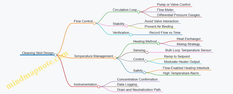
Instrumentation That Actually Helps
For flow and temperature, instrument selection should support three checks: the skid delivered the intended conditions, the conditions stayed stable, and the run ended safely.
Include:
- Flow meter with calibration traceability.
- Temperature sensor with a defined measurement range and response time.
- Pressure sensors to confirm the loop is not blocked.
- A data logger that records at a consistent interval so you can reconstruct the run.
Example: During a cleaning run, if temperature holds but differential pressure rises steadily, you may be forming a scale-like deposit that is restricting flow. The skid should allow you to stop and adjust rather than continuing to “cook” the problem.
Practical Layout Considerations
Keep the heat exchanger and temperature sensor in a location that minimizes dead legs and stratification. Provide isolation valves so you can service the heater or exchanger without draining the entire skid. Ensure the drain system is sized for the maximum purge and rinse volumes so the operator can complete the cycle without manual improvisation.
Diagram: Typical Cleaning Loop with Flow and Temperature Control
    flowchart LR
  A[Cleaning Chemical Storage] --> B[Metering Pumps]
  B --> C[Mixing Manifold]
  C --> D[Circulation Pump]
  D --> E[Heat Exchanger]
  E --> F[Element Loop]
  F --> G[Return Line]
  G --> H[Flow Meter]
  H --> I[Temperature Sensor]
  I --> J[Temperature Controller]
  H --> K[Flow Controller]
  J --> E
  K --> D
  F --> L[Drain and Neutralization]
Case Example Flow and Temperature Setpoints
For a two-step cleaning sequence, you might use a lower-temperature step for organic removal and a higher-temperature step for scale-prone deposits. The skid should support different setpoints per step while keeping the same control structure.
Example: Step 1 at 25°C with moderate circulation flow to avoid excessive swelling; Step 2 at 35°C with the same flow target but tighter temperature tolerance. The key is that the control system enforces the flow first, then temperature, and logs both so the next operator can repeat the conditions without guesswork.
10.4 Wastewater Handling for Cleaning Effluent and Neutralization
RO cleaning produces a small volume of wastewater, but it can be chemically “loud”: it may contain antiscalant, biocide residues, dissolved scale, surfactants, and high pH or low pH depending on the cleaning chemistry. Wastewater handling is therefore an engineering task, not just a drain decision.
Define Waste Streams and Acceptance Criteria
Start by listing every cleaning mode that generates effluent: acid cleaning, caustic cleaning, enzymatic or surfactant cleaning, and any pre-rinse or post-rinse discharges. Then define what the receiving system can tolerate. Typical acceptance criteria include pH range, conductivity or TDS limits, suspended solids limits, and restrictions on specific chemicals (for example, oxidants or chelants). A practical approach is to set two targets: a “process target” for safe neutralization and a “site target” for final discharge or treatment.
Example: If the plant’s drain allows pH between 6 and 9, you still need an internal neutralization target that prevents overshoot. A common internal target is to neutralize to pH 7.0–7.5, then verify with a final sample before discharge.
Characterize Effluent Composition Using Simple Measurements
You do not need a full lab for every batch, but you do need consistent indicators. Measure at minimum: pH, temperature, conductivity (as a proxy for dissolved salts), and visual solids. If your cleaning chemicals include antiscalant or chelants, conductivity can rise even when solids are low. If scale dissolves, you may see increased turbidity and settleable solids.
Operationally, take samples from the collection tank after mixing, not from the first hose connection. Early flow can be more concentrated because it carries the highest chemical strength.
Collection Tank Design for Mixing and Containment
A dedicated collection tank prevents accidental mixing of incompatible chemistries and provides time for neutralization. Size it for the largest expected cleaning batch plus a margin for rinses. Include:
- A mixing system sized to homogenize pH and conductivity within a short time.
- Secondary containment and leak detection.
- Venting sized for safe pressure relief.
- A way to isolate and drain the tank for maintenance.
Example: If a cleaning cycle generates 6 m³ of effluent and you expect an additional 2 m³ from rinsing, design for at least 10 m³ usable volume to avoid frequent overflow or rushed neutralization.
Neutralization Strategy and Control Logic
Neutralization is usually the core step. Choose between batch neutralization in the collection tank or staged neutralization using a small dosing tank. Batch neutralization is simpler when effluent volume is predictable.
Control logic should be based on measured pH, but dosing should also respect conductivity and temperature because reaction rates change. Use a two-step approach:
- Bulk dosing to bring pH close to the target.
- Fine dosing with slower addition near the setpoint.
Example: For acid cleaning effluent, add alkali in pulses while monitoring pH every few minutes. When pH approaches 7.5, switch to smaller pulses to avoid overshoot. Overshoot is not just a pH problem; it can change solubility and increase the chance of precipitating dissolved scale components.
Solids Handling and Settling Behavior
Some cleaning effluents carry dissolved scale that later re-precipitates during neutralization. Provide a settling step or a filtration step if turbidity is expected. If you settle, design for sludge removal and disposal. If you filter, select a filter that can handle the expected particle size and chemical environment.
Example: After neutralizing an acid cleaning batch, check turbidity and settleability. If the effluent clears after a short hold, a simple clarifier or lamella separator may be enough. If it stays cloudy, filtration becomes the safer choice.
Chemical Compatibility and Safety Interlocks
Neutralization chemicals must be compatible with the cleaning residues. Ensure the dosing system has:
- Separate chemical lines for acid and alkali.
- Interlocks that prevent simultaneous dosing.
- Overfill protection for the collection tank.
- Spill containment and eyewash/shower provisions near dosing areas.
A good rule: treat the neutralization system like a mini process plant. If the pH probe fails, the system should default to a safe mode (for example, stop dosing and hold the batch for manual verification).
Verification Sampling and Discharge Readiness
Before discharge, verify that the effluent meets acceptance criteria. Use a defined sampling point (well-mixed tank outlet) and a defined sampling frequency (for example, after neutralization stabilization). Record batch data: cleaning type, initial pH, dosing volumes, final pH, conductivity, and any solids observations.
Example: If conductivity is high but pH is within limits, you may still need to blend with permeate or rinse water to meet site conductivity limits. Blending should be controlled and documented, not done by guesswork.
Mind Map: Wastewater Handling for Cleaning Effluent and Neutralization
Example Batch Sequence for Acid Cleaning
- Collect acid cleaning effluent and associated rinse water into the neutralization tank.
- Mix until pH and conductivity stabilize.
- Dose alkali in pulses to reach pH 7.5.
- Hold for a short mixing period to allow any re-precipitation to occur.
- Check turbidity and settleability; settle or filter if needed.
- Verify final pH and conductivity against acceptance criteria.
- Discharge or blend as required, then document the batch.
This sequence keeps the chemistry controlled, prevents incompatible mixing, and makes the final discharge decision based on measurements rather than hope.
10.5 Maintenance Planning for Membrane Elements and Pressure Vessels
Maintenance planning is easiest when you treat membranes and pressure vessels as two interacting systems: membranes control performance, while vessels control containment, alignment, and pressure integrity. A good plan starts with what you can observe, then ties those observations to actions, spares, and documentation.
Foundational Inputs for a Maintenance Plan
Begin with the design basis and operating reality. Collect the membrane type, element configuration, target recovery, design flux, cleaning limits, and maximum allowable pressure and temperature. Then add the operating record: feed quality trends, normalized permeate flow, differential pressure across pretreatment, and cleaning frequency. If you track only “how often you clean,” you’ll miss why you clean.
A practical baseline is to define three performance indicators for each RO train: (1) normalized permeate flow, (2) salt rejection or conductivity-based rejection proxy, and (3) pressure drop behavior across the element string. When these drift together, you likely have a feed or pretreatment issue; when only one drifts, the cause is narrower.
Maintenance Objectives and Priorities
Your objectives should be explicit and measurable. Prioritize safety and containment first: pressure vessel integrity, gasket condition, and high-pressure piping isolation. Next prioritize membrane performance: preventing irreversible fouling and minimizing chemical exposure outside the cleaning envelope. Finally prioritize uptime: planning shutdown windows, cleaning labor, and spare element availability.
A simple rule of thumb helps: if normalized permeate flow drops while pressure drop rises, investigate fouling or scaling before you increase cleaning intensity. If salt rejection drops without a corresponding flow change, suspect membrane damage, improper sealing, or bypassing.
Inspection and Condition Monitoring
Plan inspections in layers.
-
Daily/Shift checks: permeate flow and conductivity trends, high-pressure pump discharge pressure stability, and pretreatment differential pressure. If pretreatment pressure climbs, membrane fouling risk rises even if permeate flow looks stable for a few days.
-
Weekly checks: verify dosing system status and chemical tank levels, confirm antiscalant and biocide interlocks, and review any alarms related to valves or energy recovery bypass.
-
Monthly checks: compare element differential pressure trends to historical baselines and review cleaning logs for chemical concentration, temperature, and contact time.
-
Shutdown inspections: during element change-outs or major cleanings, inspect end caps, brine seals, and pressure vessel internals for corrosion, scaling deposits, and gasket deformation.
Cleaning Planning as a Maintenance Backbone
Cleaning is not just an event; it is a controlled maintenance cycle. For each cleaning, record feed conditions, operating parameters, cleaning chemistry, and the resulting post-clean normalized flow. Use those results to decide whether the next cleaning should be the same chemistry, a different sequence, or a membrane inspection.
A useful decision structure is: start with the least aggressive effective method, then escalate only when evidence supports it. If a cleaning restores flow but not rejection, you may be removing foulants while leaving membrane damage or channeling unaddressed.
Pressure Vessel Maintenance and Integrity Checks
Pressure vessels require attention to sealing and mechanical condition. Plan gasket and seal inspections at element change-outs, and verify torque and seating practices match the manufacturer’s requirements. Inspect for signs of leakage at end connections, corrosion under deposits, and abnormal vessel pressure drop patterns.
Also plan for hydraulic maintenance: ensure flush and drain valves operate correctly, confirm that brine recirculation lines are not blocked, and verify that pressure relief devices are tested per your site safety procedure.
Spares, Work Packs, and Documentation
Maintenance planning should include what you will do when you find problems. Maintain a spares list for membrane elements by size and configuration, plus critical seals, O-rings, and end-cap components. Keep a work pack template that includes: element identification, vessel ID, cleaning history summary, required tools, torque specs, and acceptance criteria for post-install performance.
Document every intervention with enough detail that another engineer could reproduce the reasoning. A good log includes the “before” and “after” normalized flow and rejection, not just the date.
Mind Map: Maintenance Planning Flow
Example: Turning Data into an Action
Assume a train shows normalized permeate flow down 15% over two weeks, while salt rejection proxy stays steady and pretreatment differential pressure rises. The maintenance plan should prioritize pretreatment correction first: inspect filter media loading, verify coagulant and cartridge integrity, and confirm antiscalant dosing is within range. Schedule a cleaning only after pretreatment performance stabilizes, then compare post-clean normalized flow to the baseline.
If instead normalized flow drops 10% and rejection proxy drops sharply, plan a shutdown inspection sooner. Check for bypassing at seals, verify element seating, and inspect for membrane damage during the last cleaning. Replace affected elements and re-establish baselines.
Example: Work Pack for Element Change-Out
A work pack should specify: element IDs and positions, vessel ID, required seals, torque procedure, flushing steps, and acceptance tests. After installation, run a controlled start-up, record permeate flow and conductivity, and confirm that pressure drop across the element string returns to the expected range. If it does not, treat it as a mechanical or hydraulic issue rather than immediately repeating chemical cleaning.
Maintenance Schedule Structure
Use a schedule that matches how failures actually show up. Daily checks catch operational drift; weekly checks prevent dosing and valve surprises; monthly reviews refine baselines; shutdown work handles seals, internals, and element replacement. When you connect each schedule item to a measurable trigger, maintenance becomes predictable rather than reactive.
11. Electrical, Instrumentation, and Control Engineering for RO Plants
11.1 Control Philosophy for RO Production, Recovery, and Pressure Regulation
A reverse osmosis plant is a set of interacting loops: feedwater quality affects fouling, fouling changes membrane resistance, and resistance shifts the pressure needed to hit permeate flow and quality targets. A good control philosophy treats those interactions as design inputs, not surprises.
Foundational Control Objectives
Start with three measurable targets.
- Permeate production rate: keep permeate flow near setpoint so downstream users get consistent water.
- Permeate quality: maintain conductivity and/or salt rejection within limits by controlling operating conditions that influence rejection.
- System pressure regulation: hold high-pressure conditions stable enough to prevent oscillations that accelerate fouling and stress equipment.
A practical rule: pressure control is the “fast” lever, chemical dosing and pretreatment are “slower” levers, and recovery staging is a “structural” lever.
Control Architecture from Fast to Slow
Fast loop: high-pressure regulation. Use a pressure transmitter on the high-pressure header and control a valve or pump speed to maintain target pressure at the membrane inlet. The setpoint should be derived from the required permeate flow and expected membrane resistance, not from a fixed guess.
Medium loop: permeate flow and recovery management. Control permeate flow using permeate valve position or feed pressure trim. Recovery is managed by stage bypasses, concentrate throttling, or stage feed distribution so the plant can hold a stable operating point even as fouling increases resistance.
Slow loop: feed conditioning and fouling response. Pretreatment performance (turbidity, SDI, disinfectant residual) and antiscalant dosing are monitored continuously. When pretreatment drifts, the control system should adjust dosing and alert operators rather than blindly pushing higher pressure.
Pressure Setpoint Strategy That Doesn’t Fight Reality
Pressure setpoint logic should account for two realities: membrane resistance rises over time, and energy recovery devices can change hydraulic behavior. A robust approach uses a feed-forward term plus feedback correction.
- Feed-forward: estimate required pressure from current permeate flow demand, temperature, and measured conductivity trend.
- Feedback: correct pressure based on deviation between actual and target permeate flow.
Example: If permeate flow drops by 5% while feed temperature is stable, the controller increases pressure gradually until flow returns, but it also checks whether pretreatment turbidity rose. If turbidity rose, the system prioritizes pretreatment correction and limits pressure increase to protect membranes.
Recovery Control Without Surprise Oscillations
Recovery affects concentrate concentration, which affects scaling risk and rejection. To avoid oscillations, recovery changes should be rate-limited and synchronized with stage hydraulics.
- Change recovery in small steps (for example, adjusting concentrate throttling by a limited percentage per control interval).
- Require settling time before accepting new operating conditions.
- Use interlocks tied to scaling indicators such as antiscalant dosing status and conductivity trends.
Example: During a demand increase, the plant raises permeate flow setpoint. Instead of immediately maximizing recovery, it first stabilizes pressure and permeate flow, then increases recovery in steps while monitoring concentrate conductivity and pressure stability.
Safety and Protection Layers
Pressure regulation must include hard limits and permissive conditions.
- High-pressure trips: prevent exceeding design pressure for vessels, seals, and energy recovery devices.
- Chemical dosing permissives: block operation at high pressure if antiscalant dosing is not confirmed.
- Flow plausibility checks: if permeate flow sensor readings are inconsistent with pump speed and valve positions, the system should hold pressure steady and alert operators.
A slightly playful but useful mindset: the controller should never “win” by ignoring bad sensors. It should fail safe.
Mind Map: Control Philosophy for RO
Example Control Sequence During Normal Operation
- Start-up to stable pressure: ramp pressure to a conservative target while verifying pretreatment quality and dosing permissives.
- Lock permeate flow: once pressure is stable, switch permeate flow control to maintain the production setpoint.
- Maintain recovery: hold recovery at the selected value; if permeate flow drifts, adjust pressure first, then recovery if needed.
- Respond to fouling indicators: if pressure required to hold flow rises beyond a threshold, trigger a cleaning recommendation and reduce recovery to lower scaling pressure.
Example Interlock Logic for Pressure Regulation
- If antiscalant dosing confirmation is lost, then:
- freeze pressure setpoint at the current safe value,
- prevent recovery increases,
- alarm and require operator action.
This prevents the common failure mode where the plant tries to compensate for missing chemistry by pushing harder—harder is exactly what scaling likes.
Operator-Facing Control Philosophy
Operators need fewer knobs, not more. Present setpoints in a hierarchy: pressure is controlled automatically within limits, permeate flow is the primary production target, and recovery is a controlled variable with constraints. Alarms should indicate which lever is blocked and why, so troubleshooting is about process conditions rather than guessing what the controller is doing.
11.2 PLC and SCADA Integration for Skid Level and Plant Level Control
A good RO plant control system is less about “more screens” and more about clean responsibilities. The PLC runs the skid in real time; SCADA coordinates the plant, records what happened, and helps operators make decisions without guessing.
Foundational Roles and Data Flow
At the skid level, the PLC executes deterministic logic: start/stop sequences, interlocks, valve states, pump permissives, and chemical dosing safety. At the plant level, SCADA provides supervisory control: operator commands, trend visualization, alarms, batch-like logging for cleaning events, and performance summaries.
A practical rule: if a decision must happen within seconds to protect equipment, it belongs in the PLC. If it can wait for operator review or reporting, it belongs in SCADA.
Data flow should be designed as a one-way pipeline for critical signals and a two-way channel for setpoints. Typical patterns:
- PLC to SCADA: measured values, device states, alarm bits, and event logs.
- SCADA to PLC: operator setpoints, mode selections, and recipe parameters for cleaning cycles.
Tag Strategy and Naming That Prevents Confusion
Use a consistent tag structure so engineers and operators don’t need a decoder ring. A common approach is to encode area, skid, subsystem, and signal type.
Example tag naming:
RO1-HP-PUMP1_SpeedCmdRO1-ERX-PEX1_PressureInRO1-CHEM-ACID_DoseRateRO1-VALVE-FeedThrottle_PositionRO1-ALM-HighPressureTrip
Keep units in the tag metadata (or a companion tag) rather than in the tag name. That reduces mistakes when units change during commissioning.
Modes, Interlocks, and Safe State Logic
Define modes explicitly in the PLC and expose them to SCADA. For instance:
Auto: sequences enabled, setpoints accepted.Manual: individual devices controlled with strict permissives.Local: operator controls at the skid panel.Stop: all pumps commanded off, valves placed in a defined safe configuration.
Interlocks should be implemented as boolean conditions that gate actions. For example, a high-pressure pump start permissive might require:
- pretreatment filters differential pressure within limit
- antiscalant dosing enabled and confirmed
- emergency shutdown not active
- minimum suction pressure and NPSH margin satisfied
SCADA should not “recreate” interlock logic. It should display the reason codes coming from the PLC so operators understand what blocked the action.
Alarm Philosophy and Operator Usability
Alarms should be actionable. A useful hierarchy is:
- Trips: require immediate equipment response; PLC sets them.
- Warnings: indicate conditions that may lead to trips; PLC sets them.
- Informational: state changes like “Cleaning Cycle Started.”
Each alarm needs at least:
- alarm text that matches the field device
- severity
- cause category (process, utility, chemical, instrumentation)
- operator response guidance in plain language
A small but effective example: if permeate conductivity rises above limit, the alarm should indicate whether the cause is likely “membrane performance drift” (trend shows gradual rise) or “process upset” (sudden rise coincides with a valve change). The PLC can tag the likely cause using event timing and state transitions.
Skid Level Control Blocks and Plant Level Coordination
At skid level, organize logic into blocks:
- Start/Stop sequence controller
- Pump control with pressure regulation
- Valve position control and sequencing
- Chemical dosing controller with feedback
- Cleaning cycle controller
- Safety and shutdown controller
At plant level, SCADA coordinates across skids:
- selects which train is active
- manages shared utilities like cleaning water supply
- schedules cleaning windows and logs results
- provides a unified view of recovery, flux, and salt rejection proxies
To avoid conflicts, SCADA should write setpoints only when the PLC is in the correct mode. Otherwise, SCADA can display “setpoint locked by PLC mode” rather than silently failing.
PLC and SCADA Integration Mind Map
Example: Cleaning Cycle Coordination Without Surprises
Consider a CIP/cleaning cycle for a single RO train. The PLC runs the step logic: pre-rinse, chemical circulation, soak, rinse, and return to production. SCADA provides the recipe parameters (target temperature, circulation flow setpoint, and duration) and logs each step completion.
A clean integration behavior looks like this:
- Operator selects “Clean Train 1” in SCADA.
- SCADA writes
CleaningRecipeIDand setpoints to the PLC. - PLC checks permissives: production valves closed, brine handling available, chemical tanks not empty.
- PLC starts the cycle and sets
CleaningStepandStepStatustags. - SCADA displays step progress and records timestamps for each step transition.
If a permissive fails, the PLC sets a reason code tag like PermissiveBlock=NoAntiscalantFlow and SCADA shows it directly. Operators fix the cause once, rather than trying random restarts.
Commissioning Checks That Confirm Integration Quality
During commissioning, verify integration with tests that cover both logic and usability:
- Confirm SCADA mode changes actually switch PLC behavior.
- Confirm alarm text matches the field device and severity.
- Confirm trends align with event timestamps from the PLC.
- Confirm setpoint writes are rejected when PLC is not in Auto.
When these checks pass, the plant behaves like a system instead of a collection of gadgets. The PLC keeps the skid safe; SCADA helps people run it correctly.
11.3 Safety Instrumented Functions for High Pressure and Chemical Systems
High-pressure RO skids and chemical dosing systems share a common theme: small control errors can become big mechanical or safety events. Safety Instrumented Functions (SIFs) are the engineered layer that prevents or mitigates those events when normal control does not do the job.
Foundational Concepts for SIF Design
A SIF is a specific safety action triggered by defined conditions, implemented with independent sensors, logic, and final elements. The goal is not to “stop everything,” but to reach a safe state that limits harm and equipment damage.
Start with a clear hazard statement for each subsystem:
- High pressure pumping and piping: risk of overpressure, rupture, or uncontrolled discharge.
- Chemical dosing: risk of incorrect dosing, wrong chemical routing, or unsafe mixing.
- Cleaning and flushing: risk of exposing personnel to concentrated chemicals or creating uncontrolled waste streams.
Then define the safe state. For RO high pressure, a typical safe state is “pump stop and safe depressurization path open.” For chemical systems, it is “stop dosing, isolate chemical supply, and maintain containment with controlled flushing.”
Hazard to Function Mapping
A practical approach is to map hazards to protection layers:
- Prevention: normal control limits, interlocks, and operator procedures.
- Detection: sensors that can reliably identify abnormal conditions.
- Mitigation: SIF actions that bring the plant to a safe state.
SIFs should be independent of the normal control loop. If the normal controller fails, the SIF still needs to act.
High Pressure SIFs
Common SIF triggers for RO high pressure include:
- Discharge pressure high-high: trips the high pressure pump(s) and opens a depressurization valve.
- Low suction pressure: prevents cavitation damage by stopping the pump when suction pressure drops below a safe threshold.
- Motor overload or drive fault: stops the pump to avoid overheating and mechanical stress.
- Emergency stop: immediately halts hazardous motion and initiates safe shutdown logic.
A concrete example: if discharge pressure exceeds the high-high setpoint for longer than a short confirmation time (to avoid nuisance trips), the SIF closes the feed control valve, stops the pump, and routes concentrate to a safe bypass or storage tank while maintaining membrane protection flow.
Chemical System SIFs
Chemical dosing SIFs focus on preventing unsafe dosing and unsafe mixing. Typical triggers:
- Dosing pump run without flow confirmation: stops dosing if the chemical flow meter does not indicate flow.
- Tank level low or empty: prevents dosing pump dry-run and avoids drawing air into lines.
- Wrong chemical valve position: uses interlocked valve permissives so only the selected chemical path can open.
- Mixing tank agitation failure: stops dosing if agitation is not confirmed, preventing localized high concentration.
- Secondary containment level high: triggers isolation and alarms to prevent overflow.
Concrete example: antiscalant dosing is enabled only when the RO train is in a state that can accept it. If the RO feed flow drops below a minimum, the SIF stops dosing and flushes the chemical line with water to reduce residual chemical in the line.
Independence, Reliability, and Proof Testing
Independence means the SIF should not share the same failure-prone components as the normal control. Reliability comes from sensor selection, signal diagnostics, and logic voting where appropriate.
Proof testing is the scheduled verification that the SIF still works. For instance, a pressure transmitter used for high-high overpressure trips should be periodically tested for correct signal response and alarm behavior.
Mind Map: SIF Architecture for RO High Pressure and Chemicals
Example: Integrated SIF Sequence for a High Pressure Trip
- Condition: discharge pressure reaches high-high.
- Logic: SIF confirms the condition for a short time window.
- Actions:
- Stop high pressure pump(s).
- Close feed control valve to reduce driving force.
- Open depressurization valve to bring pressure down safely.
- Maintain a controlled flow path to protect membranes from stagnant concentrate.
- Post-trip: alarm indicates “High-high discharge pressure SIF,” and the system requires a manual reset after the pressure is in a safe range.
Example: Integrated SIF Sequence for Chemical Dosing Without Flow
- Condition: dosing pump is commanded on, but chemical flow meter reads below minimum.
- Logic: SIF detects mismatch and confirms for a defined duration.
- Actions:
- Stop dosing pump.
- Close chemical isolation valve.
- Start a short flush to clear the line.
- Post-trip: alarm indicates “Dosing flow confirmation failed,” and the operator must verify the chemical line and meter before restart.
Practical Engineering Details That Prevent Nuisance and Misuse
Setpoints should be coordinated with mechanical design limits and normal operating ranges. Confirmation timers should be long enough to ignore transient spikes, but short enough to protect equipment. Bypass modes must be controlled and logged because bypassing a SIF is effectively removing a safety layer.
Finally, ensure the operator-facing alarm text matches the actual cause and the actual action taken. A good alarm tells you what happened, what the system did, and what condition must be corrected before reset. That’s the difference between “something tripped” and “we can fix this quickly and safely.”
11.4 Metering, Flow Measurement, and Data Logging for Performance Assurance
Performance assurance starts with measurement that is both accurate and usable. A flow number that looks precise but is biased by installation effects will happily produce the wrong operating decisions. The goal here is to connect metering hardware, calibration discipline, and data logging into one chain that supports mass balance checks, membrane performance tracking, and troubleshooting.
Foundational Measurement Concepts for RO Performance
In industrial RO, the most useful measurements are the ones that let you compute what you care about: permeate flow, concentrate flow, recovery, and specific permeate flux. Permeate flow is typically measured directly; concentrate flow is often derived from mass balance if direct measurement is impractical.
Recovery is computed as:
- Recovery = Permeate Flow / Feed Flow
Specific permeate flux is computed as:
- Flux = Permeate Flow / Membrane Area
These calculations require consistent units and stable reference conditions. Temperature affects viscosity and membrane transport, so logging feed and permeate temperatures alongside flows prevents “mystery drift” when conditions change.
Flow Measurement Selection and Installation Discipline
Choose measurement types based on expected flow range, fouling risk, and required accuracy. Common choices include:
- Turbine or insertion meters for clean-ish streams with manageable pressure drop.
- Electromagnetic meters for conductive liquids where available.
- Ultrasonic meters where installation constraints allow.
Installation matters as much as the sensor. A meter placed too close to elbows, valves, or reducers can see distorted velocity profiles. A practical rule is to provide straight pipe runs upstream and downstream according to the manufacturer’s guidance, then verify with commissioning checks.
A simple commissioning sanity check is to compare measured permeate flow against expected permeate flow from pump curves and operating pressure, using a rough but consistent model. If the difference is consistently large, you likely have a calibration or installation issue rather than a process issue.
Metering Points That Actually Help Operators
A metering plan should cover the streams that define mass balance and performance:
- Feed flow to the RO train or to each train stage.
- Permeate flow from each train or stage.
- Concentrate flow either directly or derived.
- Cleaning and rinse flows for maintenance verification.
- Chemical dosing flows for correlating performance changes with antiscalant and pH control.
For multi-train plants, log per-train values separately. Aggregated totals hide which train is drifting, and troubleshooting becomes guesswork.
Data Logging Architecture for Traceable Performance
Data logging should capture enough context to interpret flow changes without requiring operator memory. A good logging set includes:
- Time-stamped flows (feed, permeate, concentrate or derived)
- Pressures at key points (pump discharge, permeate header, concentrate header)
- Temperatures (feed and permeate at minimum)
- Conductivity or salinity proxies for rejection checks
- Key chemical dosing signals (setpoint and actual where available)
- RO operating mode flags (normal operation, cleaning, standby)
Sampling interval should match the dynamics you need. Flows and pressures can change quickly during valve actions, but membrane performance trends are slower. A practical approach is to log raw signals frequently enough to capture transitions, then compute performance metrics on a rolling basis.
Calibration, Drift, and Data Quality Checks
Calibration is not a one-time event. Establish a schedule and a method for verifying meter accuracy. Drift shows up as systematic bias in mass balance.
Use automated data quality checks:
- Range checks for impossible values (negative flow, conductivity spikes beyond sensor limits)
- Rate-of-change checks to catch sensor glitches during steady operation
- Mass balance checks comparing feed = permeate + concentrate within an acceptable tolerance
When a check fails, log a reason code so the performance dashboard can exclude bad data rather than silently mixing it with good data.
Mind Map: Metering, Flow Measurement, and Data Logging
Example: Building a Simple Performance Metric Pipeline
Assume you log feed flow (F), permeate flow (P), feed temperature (Tf), and permeate temperature (Tp). You compute recovery and flux every 5 minutes using the latest stable window.
Example workflow:
- Filter out data points where operating mode is not “normal.”
- Exclude points failing range checks for P and F.
- Compute recovery = P / F.
- Compute flux = P / membrane area.
- Store both raw inputs and computed outputs with the same timestamp.
This avoids the common failure mode where the dashboard shows a smooth recovery curve that is actually built from mixed cleaning and normal-operation data.
Example: Mass Balance Check for Concentrate Derivation
If concentrate flow is derived, use a tolerance band tied to measurement uncertainty. For instance, if permeate and feed meters each have ±1% uncertainty, a practical tolerance for mass balance might be around ±2% to ±3%.
Example logic:
- If |F - (P + C_derived)| / F > 0.03, flag the dataset.
- If the flag persists for a day, schedule a meter verification.
This turns “something seems off” into a measurable rule, and it keeps the plant’s performance assurance grounded in physics rather than vibes.
Practical Logging Rules for RO Operators
Keep the computed metrics consistent with the logged raw signals. If you compute recovery from feed and permeate, log the exact formula version used. If you change the membrane area basis after a retrofit, record the change date and element configuration so historical comparisons remain meaningful.
Finally, ensure that every logged performance number can be traced back to inputs. When an operator asks why recovery dropped, the answer should be visible in the logged pressures, temperatures, and flow measurements—no detective work required.
11.5 Alarm Management and Operator Procedures for Stable RO Operation
Stable RO operation depends on two things that sound simple but are easy to mess up: alarms must be meaningful, and operator actions must be repeatable. This section ties alarm design to practical procedures so operators can respond quickly without guessing.
Foundations for Alarm Meaning
Start by defining what “stable” means for the plant: permeate flow within target band, recovery consistent with membrane limits, and pressure/flow conditions that keep fouling and scaling under control. Alarms should map to those stability variables.
Use a layered approach:
- Process alarms indicate a deviation in a measured variable (pressure, differential pressure, conductivity, flow).
- Performance alarms indicate a deviation in calculated outcomes (salt rejection trend, flux decline rate, energy recovery efficiency).
- Safety alarms indicate conditions that require immediate protective action (high pressure, chemical dosing interlocks, low flow to membranes).
A useful rule of thumb: if an alarm can be cleared without any operator action and the process returns to normal, it likely belongs as an event log, not an alarm.
Alarm Prioritization and Setpoint Strategy
Operators need fewer alarms, but the right ones. Prioritize by consequence and time-to-impact.
- High priority: protects membranes and pressure boundaries. Examples include high differential pressure across pretreatment filters, low crossflow, or high feed pressure beyond design limits.
- Medium priority: protects performance and prevents escalation. Examples include gradual permeate conductivity rise, antiscalant dosing pump fault, or energy recovery bypass valve not in the intended position.
- Low priority: supports troubleshooting. Examples include minor deviations in temperature or small flow imbalances.
Setpoints should include hysteresis and time delays. For instance, a pretreatment differential pressure alarm should trigger after a sustained rise (not a single spike) because short surges often occur during normal backwash transitions.
Operator Procedure Logic for Alarm Response
Procedures should follow a consistent sequence so operators do not reinvent the process under stress.
-
Confirm the alarm and its category
- Check whether it is safety, process, or performance.
- Verify the measurement quality using transmitter status and recent trends.
-
Stabilize the system
- If the alarm threatens membranes or pressure boundaries, move to a protective operating mode (for example, reduce recovery or initiate controlled shutdown of the affected train).
-
Diagnose with minimal data
- Use a short checklist: pretreatment status, dosing status, pump status, valve positions, and key flows.
- Look for “root-cause clusters” rather than single-variable blame.
-
Correct and verify
- Apply the correction (adjust setpoint, switch standby equipment, restart dosing after interlock clearance).
- Confirm that the stability variables return to target bands.
-
Document and close
- Record what happened, what was changed, and the time-to-recovery. This turns alarms into learning without requiring guesswork.
Mind Map: Alarm Management Workflow
Examples of Integrated Alarm and Procedure Use
Example: Pretreatment Differential Pressure High
- Alarm meaning: filters are loading, which can starve RO and accelerate fouling.
- Immediate operator action: confirm DP trend and filter run status; check whether backwash is complete and valves are in correct positions.
- Procedure outcome:
- If backwash is incomplete, correct valve alignment and allow stabilization time.
- If DP remains high, switch to standby filter train and reduce RO feed flow until pretreatment DP returns to normal.
Example: Permeate Conductivity Rise
- Alarm meaning: salt passage is increasing, often due to membrane integrity issues or operating conditions that promote scaling.
- Immediate operator action: verify conductivity measurement health, then check feed pressure, recovery, and antiscalant dosing.
- Procedure outcome:
- If conductivity rise coincides with higher recovery or reduced crossflow, adjust operating parameters to restore the flux target.
- If conductivity rise persists after stabilization and dosing is correct, isolate the affected train and initiate membrane integrity checks per plant protocol.
Example: Energy Recovery Bypass Not In Intended Position
- Alarm meaning: hydraulic mismatch can increase energy use and may affect concentrate conditions.
- Immediate operator action: confirm ERD valve position feedback and pump operating mode.
- Procedure outcome:
- If the bypass is stuck, switch to the correct ERD configuration and monitor concentrate pressure and permeate flow for stability.
Practical Operator Checklists That Prevent Escalation
A good checklist is short enough to use during an alarm and structured enough to avoid missed steps.
- Pretreatment: filter DP, turbidity trend, backwash status, chemical dosing upstream.
- Membranes: feed pressure, permeate flow, crossflow, recovery setting, temperature.
- Chemicals: antiscalant pump run status, dosing rate, interlock alarms.
- Hydraulics: valve positions, ERD mode, pressure gauge sanity checks.
When operators follow the same order every time, alarms become a tool instead of a test.
12. Commissioning, Performance Testing, and Operational Acceptance
12.1 Pre Commissioning Checks for Mechanical, Electrical, and Instrumentation
Pre-commissioning is where you prove the plant can start safely and measure what it claims to measure. The goal is not to run membranes yet; it’s to confirm that every mechanical connection, electrical path, and instrument signal behaves as designed under dry, low-risk conditions.
Mind Map: Pre Commissioning Checks
Mechanical Checks
Start with the mechanical “can it physically survive” questions. Verify skid alignment, anchor bolts, and vibration isolation so the high-pressure equipment isn’t fighting misalignment from day one. Then inspect piping routing and supports: RO skids dislike sagging lines because they trap air and complicate priming.
Perform pressure integrity tests on the relevant loops according to the project test plan. A practical example: if the concentrate line has a blind flange installed for testing, confirm it is removed before commissioning and that the gasket material matches the service temperature and chemical exposure.
Check valve operation before energizing anything. For each motorized or pneumatically actuated valve, move it through full stroke and confirm end-position feedback signals match the expected state. A common failure mode is a limit switch wired correctly but mechanically misadjusted, which later shows up as “valve closed” while the valve is actually open.
For pumps, confirm correct rotation direction using a brief, no-load test. Verify seal flush and any bearing lubrication systems are connected and clean. If a pump has a mechanical seal with a flush line, ensure the flush line is not capped and that the flush flow path is unobstructed.
Inspect pressure vessels and housings for cleanliness and correct installation. Even without elements, confirm that end caps, O-rings, and port connections are seated properly and that no debris remains inside. For chemical dosing lines, verify they are flushed and dry where required, because residue can interfere with antiscalant dosing accuracy.
Electrical Checks
Electrical readiness is about preventing the plant from doing the wrong thing quickly. Verify grounding continuity and check that cable shields and terminations are intact. Confirm motor wiring and phase sequence before any pump run; a reversed phase can cause a pump to run backward, which is not a “minor inconvenience.”
For VFDs, load the correct parameter set and verify key settings like motor rated current, ramp times, and control mode. A simple example: if the VFD is configured for speed control but the PLC expects pressure control, the plant may start but will not regulate pressure as intended.
Check control cabinets for correct labeling, terminal tightness, and absence of loose jumpers. Validate that E-stops and safety interlocks are wired to the correct safety devices and that a trip actually prevents the associated start command. Don’t just press the button; confirm the logic state changes in the PLC and that the alarm text matches the intended cause.
Instrumentation Checks
Instrumentation checks ensure the plant measures reality. Start with loop checks: verify 4–20 mA signals, verify scaling, and confirm that the PLC tag mapping matches the instrument identity. A practical example: if conductivity is scaled as µS/cm but the instrument is configured for mS/cm, your RO control will “think” water is far saltier or far cleaner than it is.
Calibrate or verify calibration status for critical sensors: feed and permeate conductivity, pressure transmitters, flow meters, and temperature sensors. Confirm sensor ranges cover the expected operating span with margin. Check that temperature sensors are installed in the correct flow direction and that thermowells are fully seated.
Verify level switches and level transmitters by simulating levels according to the commissioning procedure. For sampling systems, confirm purge logic and check for leaks at sample valves and tubing connections; a slow leak can bias measurements and create chemical exposure risks.
Integrated Readiness Checks
Once mechanical, electrical, and instrumentation are individually acceptable, rehearse the safe start sequence. Confirm cause-and-effect logic: when a permissive is lost, the correct actions occur, such as stopping pumps, closing valves, and raising the right alarm.
Perform alarm and trend sanity checks. Ensure alarms are not stuck in an active state and that trends show meaningful variation when signals are simulated. A good test is to temporarily simulate a pressure input and confirm the trend updates and the control logic responds without latching into a fault.
Finally, complete documentation and sign-offs for each discipline. The sign-off should reference the specific test results, not just the fact that “checks were done,” so the next team member can trace what was verified and what was not.
12.2 Membrane Element Installation Verification and Leak Testing
Installation verification is the part where “it looks installed” becomes “it will operate without surprises.” The goal is simple: confirm correct element placement, confirm seals and fittings are intact, and confirm the system is leak-tight at pressures and conditions that matter.
Foundational Checks Before Any Pressure
Start with the physical basics. Verify the element type and size match the pressure vessel and RO train design basis. Confirm the element orientation marks are consistent with the flow direction. Check that end caps, brine seals, and permeate tube connections are clean and undamaged; a single nick on an O-ring can turn into a slow leak that only shows up after hours of operation.
Next, confirm the pressure vessel internals. Ensure the feed spacer stack is correctly seated and that permeate collection components are aligned. If the vessel has multiple elements, confirm the element-to-element spacing and that permeate tubes are properly connected without kinks. A kinked permeate tube can cause localized flow restriction that later looks like “fouling,” even when the membrane is fine.
Finally, verify the manifold and piping connections. Confirm torque values for flange bolts and that fittings are assembled with the correct gasket type and seating. If the plant uses quick-connect fittings, confirm the locking mechanism is fully engaged and that any protective caps were removed before commissioning.
Seal Integrity Verification Using Low-Risk Methods
Before high-pressure testing, perform low-risk checks that catch common assembly errors.
-
Visual and tactile inspection: Look for displaced O-rings, twisted seals, or gaps at end caps. A seal that “looks fine” but feels uneven is not fine.
-
Permeate-side integrity check: If the design allows, isolate permeate headers and confirm there is no cross-connection to concentrate lines. A simple continuity check at the manifold level can prevent confusing results later.
-
Dry run of flow paths: With membranes removed or bypassed where permitted, confirm that valves open and close correctly and that there are no trapped air pockets in critical headers.
Hydrostatic Leak Testing at Test Pressure
Leak testing should be systematic: pressurize, hold, observe, and document. Use clean water for hydrostatic tests unless the project specifies otherwise.
Step-by-step approach
- Isolate the test boundary: Close valves to define what is being tested. Include the pressure vessel end connections, element seals, and relevant manifolds.
- Fill and vent thoroughly: Air trapped in the system can mask leaks or create false alarms. Vent until flow is steady and free of bubbles.
- Pressurize gradually: Increase pressure in controlled increments. Watch for sudden pressure drops, abnormal noises, or visible seepage.
- Hold at test pressure: Maintain the specified hold time and record pressure at the start and end of the hold.
- Inspect during the hold: Check end caps, permeate tube connections, flange joints, and any sampling ports.
Acceptance logic Leak testing acceptance is usually based on allowable pressure decay and/or allowable seepage rate. If your project uses a pressure-decay criterion, ensure the pressure gauge is calibrated and that temperature changes are accounted for, because water temperature drift can mimic a pressure change.
Example Leak Scenarios and What They Look Like
Example: O-Ring Pinch at End Cap
- Symptom: Slow pressure decay during hold, sometimes with a faint wetness at the end cap seam.
- Likely cause: O-ring twisted during element insertion or displaced during end cap tightening.
- Corrective action: Depressurize, open the vessel, inspect the O-ring for deformation, replace if required, and re-seat the element carefully.
Example: Permeate Tube Connection Leak
- Symptom: Permeate header shows unexpected flow or moisture while concentrate side remains stable.
- Likely cause: Loose connection at permeate tube coupler or misalignment causing a poor seal.
- Corrective action: Verify tube alignment, reassemble with correct gasket and seating, and repeat the permeate-side portion of the test.
Example: Flange Gasket Mis-Seating
- Symptom: Visible seepage at a flange joint, often worse at higher pressure.
- Likely cause: Gasket not centered, uneven bolt torque, or gasket damage during assembly.
- Corrective action: Depressurize, re-seat the gasket, torque in a cross pattern, and retest.
Mind Map: Installation Verification and Leak Testing
Documentation That Prevents Rework
Record the membrane batch or element serial identifiers, vessel numbers, test boundary valves, fill/vent procedure notes, pressure gauge ID, and the pressure readings at each stage. If a leak is found, document the location and the assembly step that most likely contributed. This turns troubleshooting from guesswork into a repeatable process—no mystery, just evidence.
12.3 Performance Test Protocols for Recovery, Flux, and Salt Rejection
A good performance test protocol answers three questions with numbers: How much water is produced (recovery), how hard the membranes are working (flux), and how well salts are rejected (salt rejection). The protocol below is written to produce comparable results across days, trains, and operating modes.
Test Objectives and Acceptance Criteria
Start by defining what “pass” means before you start the pumps. Typical objectives include:
- Recovery: target range based on design recovery and allowable concentrate conditions.
- Flux: stable permeate production at a defined feed temperature and pressure window.
- Salt Rejection: minimum salt rejection based on conductivity or ion-specific measurements.
Example acceptance logic: if permeate flow is within ±5% of the test baseline, feed pressure is within the specified band, and salt rejection meets the minimum threshold, then the train is considered performance-acceptable for commissioning.
Test Readiness Checks
Before collecting data, verify the system is in a state where measurements mean something.
- Instrumentation calibration: conductivity meters, flow meters, pressure transmitters, temperature sensors.
- Sampling points: ensure permeate and feed/concentrate samples are representative and not affected by dead legs.
- Chemical dosing stability: antiscalant and pH control should be at steady setpoints; cleaning chemicals must be fully flushed.
- Hydraulic stability: confirm no rapid valve hunting, no air entrainment, and stable pump speeds.
A practical rule: if you cannot hold feed pressure within the allowed band for 15 minutes, you cannot claim a meaningful flux or rejection result.
Baseline Operating Conditions
Define a baseline operating point and keep it steady during the test window.
- Feed temperature: record continuously; RO performance is temperature-sensitive.
- Feed pressure: set and maintain within a narrow range.
- Crossflow and recovery mode: specify whether you test at constant permeate flow, constant pressure, or constant recovery.
Example baseline: 25 °C feed, target feed pressure at the design operating point, and a recovery level that keeps concentrate within the specified scaling control envelope.
Measurement Plan for Recovery
Recovery is computed from measured flows:
- Permeate flow: Qp from permeate flow meter.
- Feed flow: Qf from feed flow meter.
- Recovery: R = Qp / Qf.
To reduce error, use a steady-state window (commonly 30–60 minutes) and compute recovery from averaged flow readings. If the plant uses multiple trains, test each train independently or ensure flow splits are stable and documented.
Measurement Plan for Flux
Flux is permeate flow normalized by membrane area:
- Flux: J = Qp / A.
Key details that prevent “mystery flux”:
- Use the correct active membrane area for the installed elements.
- Confirm permeate flow meter units and scaling.
- Record temperature so flux can be interpreted consistently.
Example: if permeate flow is stable but flux drifts, the active area used in calculations may not match the installed element count or configuration.
Measurement Plan for Salt Rejection
Salt rejection is typically derived from conductivity measurements:
- Rejection: Rj = 1 − (Cp / Cf), where Cp is permeate conductivity and Cf is feed conductivity.
To keep conductivity-based rejection honest:
- Use the same temperature compensation mode for both Cp and Cf.
- Ensure permeate conductivity is above the meter’s reliable detection range.
- Sample long enough to flush the sampling line and reach representative readings.
Example: if Cf is stable but Cp fluctuates, check for sampling line mixing, air bubbles, or delayed stabilization in the permeate sample stream.
Data Logging and Steady-State Definition
Log at a consistent interval (e.g., every 1–5 seconds) and compute test results from the steady-state portion.
Steady-state definition can be operationalized as:
- Feed pressure variation within the allowed band.
- Permeate flow variation within a small tolerance.
- Conductivity readings stable within a defined range.
If these conditions are not met, shorten the test window or adjust the control strategy until stability is achieved.
Mind Map: Performance Test Inputs to Outputs
Example Test Run Structure
Use a repeatable sequence:
- Stabilization: reach baseline pressure and recovery; wait until flows and conductivities stop drifting.
- Steady-State Collection: record data for the defined window.
- Verification Checks: confirm no sampling interruptions and that conductivity temperature compensation is consistent.
- Result Computation: compute recovery, flux, and rejection from averaged steady-state values.
Example outcome reporting: “At 25 °C feed temperature and 62 bar average feed pressure, recovery averaged 45.2%, flux averaged 18.6 LMH, and conductivity-based salt rejection averaged 99.2%.”
Common Failure Modes and How the Protocol Prevents Them
- Unstable feed pressure leads to misleading flux and rejection; the steady-state definition blocks this.
- Incorrect active area makes flux wrong; the protocol requires installed element verification.
- Sampling delays distort permeate conductivity; the protocol requires line flushing and stabilization.
- Conductivity meter mismatch causes rejection errors; the protocol requires consistent temperature compensation.
A performance test should feel a bit like baking: measure ingredients carefully, keep the oven temperature steady, and then record the result. The protocol above is designed to make the numbers reproducible, not just impressive.
12.4 Energy Recovery Verification and Pump Efficiency Validation
Energy recovery devices (ERDs) and high-pressure pumps are the two places where “design intent” meets “real electricity.” This section provides a systematic way to verify ERD performance and validate pump efficiency using measurable plant data, not guesswork.
Foundational Concepts for Verification
Start by separating what you can measure directly from what you must compute.
- Direct measurements: ERD inlet and outlet pressures, concentrate and permeate flow rates, pump discharge pressure, motor power, and temperatures.
- Computed values: hydraulic power transferred, specific energy consumption, and overall efficiency.
A practical reminder: ERDs shift energy between streams, but they do not create energy. If the ERD is working, you should see reduced net pressure demand at the high-pressure pump for the same permeate production, after accounting for fouling and control actions.
Mind Map: Verification Logic
ERD Performance Verification Method
-
Select a steady operating window: Choose a period where permeate flow and feed temperature are stable, and control valves are not hunting. A 30–60 minute window is often enough if the plant is well tuned.
-
Confirm correct flow paths: Verify that the ERD is not inadvertently bypassed. A common “gotcha” is a bypass valve position that looks correct in the control room but is not aligned with the physical valve feedback.
-
Compute hydraulic power transfer: Use measured flows and pressure differences.
- Concentrate-side hydraulic power change is estimated from ERD inlet and outlet pressures and the concentrate flow.
- Permeate-side pressure rise or flow-side effects are included through the device’s net pressure recovery.
-
Account for pressure losses: The ERD does not operate in isolation. Include upstream and downstream piping losses by comparing measured pressures at consistent points (same tags used during design basis modeling).
-
Compare to the baseline model: Use the design model’s expected pressure recovery at the measured flows and temperatures. If the ERD underperforms, the likely causes are mismatched flow distribution, fouling in the ERD passages, or incorrect valve settings.
Example: Interpreting a Pressure Recovery Shortfall
Assume measured ERD inlet pressure is 70 bar and outlet pressure is 55 bar, giving 15 bar recovery. The baseline model at the same flow and temperature predicts 18 bar. The 3 bar gap can be traced by checking:
- ERD inlet flow distribution (does one channel dominate?)
- Concentrate temperature and density used in calculations
- Pressure sensor calibration or tag mismatch
If sensors are verified and flow distribution is correct, the remaining gap points to hydraulic losses within the ERD, often due to partial fouling or internal leakage paths.
Pump Efficiency Validation Method
Pump efficiency is validated by comparing hydraulic power delivered to electrical power consumed.
-
Measure electrical input: Record motor power from the VFD or power meter. Use the same measurement source consistently.
-
Compute hydraulic power: Hydraulic power is estimated from pump discharge pressure, suction pressure, and flow. Use fluid density based on measured temperature.
-
Correct for operating point: Pump efficiency varies with speed and duty. If the plant uses VFDs, record VFD frequency and map the operating point to the pump curve.
-
Check for cavitation and abnormal hydraulics: Cavitation can reduce efficiency and cause vibration. Look for:
- Unusual suction pressure drops
- Increased discharge pressure oscillation
- Motor current spikes at steady setpoints
- Validate with multiple points: Repeat the calculation at two or three permeate flux levels. A single point can be misleading if a control valve is compensating for another loss.
Example: Efficiency Calculation at a Representative Duty
Suppose:
- Pump discharge pressure: 65 bar
- Suction pressure: 5 bar
- Flow: 120 m³/h
- Temperature: 25°C (use corresponding density)
- Motor electrical power: 1.8 MW
Compute hydraulic power from pressure rise and flow, then divide by electrical power to get efficiency. If the result is consistently lower than the expected curve by a similar margin across operating points, investigate suction conditions, internal wear, or measurement bias.
Acceptance Criteria and Uncertainty Handling
Define acceptance using both model agreement and measurement uncertainty.
- ERD acceptance: Pressure recovery within a defined band of the baseline model after accounting for temperature and flow deviations.
- Pump efficiency acceptance: Efficiency within a band of the pump curve at the measured speed and duty.
Measurement uncertainty matters. Pressure sensors, flow meters, and temperature probes each contribute error. If the discrepancy is smaller than the combined uncertainty, treat it as “informational,” not a failure.
Mind Map: What to Check First
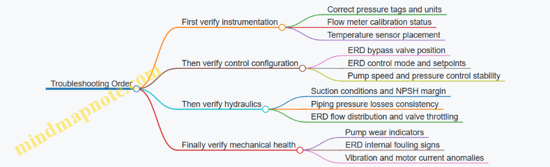
Output Deliverables for the Commissioning Record
Document the verified ERD pressure recovery, the validated specific energy consumption, and the pump efficiency at each tested operating point. Include the exact measurement tags used, the steady-state window definition, and the calculation assumptions for density and pressure losses so the results can be reproduced without interpretive gymnastics.
12.5 Operational Handover Documentation Including As Built and Test Records
A good handover package answers three questions: what was built, how it performed during testing, and how to operate it without guessing. The documents should be organized so an operator can find the right procedure in minutes, not hours.
As Built Documentation That Matches Reality
As built drawings and data must reflect the installed plant, not the design intent. Start with a document index that links each drawing to a tag list, equipment IDs, and the commissioning test that verifies it.
Include:
- Process and Piping As Built: RO train piping, valve lineups, chemical dosing injection points, sampling locations, and drain routing. A simple check is to trace every sample line back to its analyzer or manual sample point.
- Instrumentation As Built: loop diagrams, instrument tags, calibration certificates, and final setpoints for controllers. If a pressure transmitter was moved during construction, the loop diagram must match the final location.
- Electrical and Power As Built: motor nameplates, VFD settings, MCC feeder IDs, and interlock wiring diagrams for high-pressure and chemical systems.
- Skid and Module Layout: element arrangement, vessel numbers, permeate/concentrate headers, and cleaning connections. Operators should be able to identify “vessel 3” without opening a spreadsheet.
Example: If the antiscalant injection point is installed upstream of a filter, the as built must show the exact tie-in location and the line size. During operation, dosing flow verification depends on that geometry.
Commissioning Test Records That Prove Performance
Test records should be written like a checklist with evidence attached. Each test entry should include the objective, acceptance criteria, actual results, and any deviations with their resolution.
Include:
- Mechanical Completion Tests: pressure tests, leak checks, torque records where applicable, and verification of relief valve settings.
- Instrument Calibration and Loop Checks: zero/span results, sensor serial numbers, and loop response tests.
- Hydraulic and Flow Verification: permeate flow, concentrate flow, recovery confirmation, and pressure drop across pretreatment and RO trains.
- Membrane Performance Tests: baseline flux and salt rejection (or conductivity-based proxies), plus temperature and feed salinity conditions used for normalization.
- Energy Recovery Verification: pressure exchanger performance and pump efficiency checks under representative operating points.
- Chemical System Verification: dosing accuracy, interlock behavior, and safe shutdown sequences.
Example: During a performance test, record feed temperature and pressure, then compute normalized permeate flow. If the normalized value meets criteria but raw flow is low, the record should explain the temperature effect rather than leaving operators to interpret it.
Operational Documentation That Turns Records into Actions
Operators need procedures that align with the test records and as built configuration.
Include:
- Start Up and Shutdown Procedures: step order, required permissives, expected pressure ramps, and what “normal” looks like at each stage.
- Operating Setpoints and Ranges: permeate pressure targets, recovery limits, antiscalant dosing ranges, and cleaning triggers.
- Sampling and Data Logging Instructions: where to sample, how often, and which fields to record for troubleshooting.
- Alarm Response Guides: what to check first, which interlocks block operation, and how to return to stable production.
A practical approach is to cross-reference each procedure step to the relevant drawing and test record ID.
Document Control and Traceability
Use a controlled numbering scheme and revision history. Every document should show:
- revision number and effective date (for example, 2026-03-15),
- author and reviewer,
- linked equipment tags,
- and the commissioning test IDs that support it.
If a deviation occurred, the record should state the impact on operation and the compensating control (for example, adjusted dosing range or modified operating pressure limit).
Mind Map: Operational Handover Package Structure
Example: Traceability from Procedure to Evidence
When the start-up procedure says “confirm antiscalant dosing flow before RO feed,” the package should link:
- the procedure step to the dosing skid flow meter tag,
- the as built drawing showing the injection point,
- the commissioning test record proving dosing accuracy,
- and the alarm response guide for low dosing flow.
This keeps the operator from relying on memory, and it keeps troubleshooting grounded in measured facts.