Mastering Fermented Systems
1. Foundations of Fermentation as a Biological Process
1.1 Defining Fermentation and Distinguishing It from Respiration
Fermentation is a microbial process where cells generate energy by converting substrates into simpler products, without using oxygen as the terminal electron acceptor. In practical terms, fermentation is what you get when microbes keep producing ATP even when oxygen is absent or limited. Respiration is also energy generation, but it uses oxygen (or another external electron acceptor) to complete electron transfer.
Core Energy Logic
Both fermentation and respiration start with the same basic problem: cells need a steady way to move electrons from nutrients to a final acceptor. The difference is the identity of that acceptor.
- Respiration: electrons end up on oxygen, forming water in aerobic respiration. This allows a larger energy yield.
- Fermentation: electrons end up on internal molecules derived from the original substrate. This typically yields less energy, but it works when oxygen is missing.
A helpful way to picture it is to imagine a delivery route. Respiration has a well-marked final drop-off (oxygen). Fermentation uses a local drop-off inside the neighborhood (internal products), so it can still function, just with a shorter route and less total payoff.
What Fermentation Produces
Fermentation is defined not by the organism alone, but by the end products and the electron-acceptor pathway. Common fermentation product families include:
- Lactic acid from lactic acid bacteria
- Ethanol and carbon dioxide from yeast
- Acetic acid from acetic acid bacteria, often under conditions where oxygen is involved in the oxidation step
- Mixed acids from many anaerobic bacteria
In food and industrial settings, these products are the reason fermentation matters: they change flavor, texture, acidity, and stability.
Distinguishing Fermentation from Respiration
The cleanest distinction is operational: does oxygen function as the terminal electron acceptor?
- If oxygen is present and the microbes use it to finish electron transfer, the process is respiration.
- If oxygen is absent or the microbes do not use it for electron transfer, the process is fermentation.
In real systems, oxygen can be partially present, and microbes may switch strategies. That is why you will sometimes see “mixed metabolism” during early growth or in poorly mixed vessels.
Oxygen Limitation and Microbial Switching
Even when you intend to run an anaerobic fermentation, oxygen can enter from air trapped in liquid, headspace, or leaks in seals. Microbes often respond quickly:
- When oxygen is available, many organisms grow efficiently and may suppress fermentation pathways.
- As oxygen becomes limited, fermentation pathways turn on to keep ATP production going.
This switching explains why the same recipe can behave differently across batches if headspace, agitation, or loading volume changes.
Mind Map: Fermentation Versus Respiration
Concrete Examples
Example: Sourdough Starter
A sourdough starter contains lactic acid bacteria and yeasts. Early on, oxygen in the dough and headspace can support some aerobic respiration. As oxygen decreases, yeasts and bacteria increasingly rely on fermentation pathways, producing acids and carbon dioxide. The result is a tangy flavor and gas-driven rise.
Example: Beer Brewing
Brewing yeast ferments wort primarily to ethanol and carbon dioxide. If oxygen is limited, fermentation proceeds to completion. If oxygen is excessive during the wrong stage, yeast may shift toward respiration, changing the balance of byproducts and slowing the expected fermentation profile.
Example: Yogurt Making
Lactic acid bacteria convert sugars into lactic acid. The process is designed to keep oxygen from dominating, so fermentation pathways remain the main route for energy generation. The acidity increase also helps set the gel by affecting proteins.
A Simple Operational Checklist
When you need to decide whether you are looking at fermentation or respiration, use three practical signals:
- Oxygen role: Is oxygen being used as the terminal acceptor?
- Product profile: Are you seeing fermentation end products like lactic acid or ethanol?
- Process behavior: Does activity continue under oxygen limitation, with a shift in metabolism as oxygen drops?
With those signals aligned, “fermentation” stops being a vague label and becomes a specific, testable description of how microbes extract energy.
1.2 Microbial Diversity in Fermented Foods and Industrial Media
Fermented foods and industrial media host communities of microbes that are not random guests. Diversity emerges because each fermentation environment creates a set of “rules” for survival: available sugars, salt level, oxygen exposure, acidity, temperature, and the presence of competing organisms. The result is a predictable cast of characters, even when the exact lineup varies by recipe, raw material, and handling.
Core Microbial Groups You Commonly Meet
In many food fermentations, lactic acid bacteria (LAB) dominate because they tolerate acid and convert carbohydrates into lactic acid and other metabolites. Yeasts often appear alongside LAB, especially when oxygen is limited but sugars remain. In alcoholic fermentations, Saccharomyces yeasts are common, while in some mixed fermentations other yeasts and non-Saccharomyces species contribute aroma compounds.
Industrial media can support a broader range of organisms depending on the target product. For example, aerobic bacteria and fungi may be used when oxygen demand is high or when the process relies on enzymes secreted into the broth. Even when a process is “single-organism,” trace contaminants can still matter because they may consume nutrients, alter pH, or produce off-metabolites.
Why Diversity Changes over Time
Microbial communities shift because the environment changes as fermentation proceeds. Early on, microbes that can quickly use the available nutrients gain an advantage. As sugars drop and acids accumulate, the conditions favor organisms that tolerate lower pH or can metabolize remaining substrates.
A practical way to see this is to imagine two microbes with different pH comfort zones. When fermentation starts near neutral pH, both can grow. As acid builds, the one that prefers higher pH slows down, while the acid-tolerant one keeps going. This is succession driven by selection, not magic.
Fermented Foods as Ecological Niches
Consider three common food contexts:
- Brined vegetables: Salt reduces many competitors and selects for salt-tolerant LAB. If oxygen is present at the surface, yeasts and aerobic microbes may contribute to surface films, while deeper zones become more LAB-driven.
- Sourdough: Flour brings a mixed community. LAB and yeasts cooperate and compete depending on hydration, temperature, and refresh frequency. Frequent feeding resets the community toward fast growers.
- Fermented beverages: Sugar availability and ethanol accumulation shape the community. Yeasts typically dominate once ethanol rises, while LAB may contribute acidity and flavor depending on conditions.
Industrial Media as Controlled Ecosystems
Industrial fermentations aim for consistency, but “consistency” is achieved by controlling the ecosystem’s rules. Sterility reduces unwanted entrants, while defined media limits nutrient variability. Still, diversity can appear within the intended organism group. For instance, different strains of the same species can vary in growth rate, stress tolerance, and byproduct formation.
A useful operational concept is that diversity affects performance through measurable outcomes: growth rate, product yield, byproduct profile, and process stability. Two cultures that both “work” can behave differently under the same operating window.
Mind Map: Microbial Diversity Drivers
Example: Interpreting a Simple Community Shift
Suppose a brined fermentation starts with a mixed community. During the first day, gas production and rapid acidification suggest active fermentation. If acidification slows while pH stops dropping, it often indicates that the dominant acid producers have been suppressed by rising acidity or nutrient depletion. A second symptom can be surface film formation, which hints at oxygen exposure and yeast activity near the top.
The best response is not guesswork. Measure pH, titratable acidity, and sugar levels at consistent time points. If pH is already low but sugars remain, the issue may be nutrient limitation or mixing problems. If sugars are low but acid is not increasing, the community may have shifted away from acid producers, possibly due to temperature drift or salt imbalance.
Example: Industrial Media Diversity Without Changing the Species
Imagine an industrial run using a single yeast strain for ethanol production. Even with the same strain, variability can occur if inoculum viability differs or if the medium’s nitrogen content varies. Lower viability can extend the lag phase, giving contaminants time to establish. Nitrogen imbalance can change the yeast’s metabolism, shifting byproduct formation and affecting downstream recovery.
In both food and industrial settings, microbial diversity is best understood as a system property: who is present, why they can grow, and how the environment changes their roles.
1.3 Growth Kinetics and Metabolic Pathways in Fermenting Systems
Fermentation performance depends on two linked stories: how cells grow and how they route carbon and energy into products. Growth kinetics describe the pace of biomass change, while metabolic pathways explain where substrates go and why products appear when they do. In practice, you treat them as one system: the same conditions that speed growth also shift pathway usage.
Core Growth Kinetics Concepts
A common starting point is the specific growth rate, μ, which is the fractional increase in biomass per unit time. In a simple batch system with abundant substrate, biomass often follows exponential growth: biomass rises quickly at first, then slows as nutrients or space run out. The “slowing” is not a mood swing; it follows substrate depletion, waste buildup, and changes in cell physiology.
For many fermentations, the growth rate is limited by more than one factor. A useful mental model is that cells have an intrinsic capacity to grow, but real conditions impose limits. Temperature, pH, and oxygen availability can reduce the effective μ even when substrate remains. That’s why two batches with the same recipe can behave differently if mixing or sensor calibration differs.
Substrate Limitation and Product Formation
As substrate concentration drops, growth rate declines. Meanwhile, product formation can track growth, lag behind it, or switch on later depending on the pathway. For example, some lactic fermentations produce acid strongly during active growth, while others show a shift where acid production continues after growth slows. This separation matters for process control: “more growth” does not always mean “more product.”
A practical example: in a vegetable brine fermentation, early days often show rapid acidification as lactic acid bacteria establish dominance. Later, acid production may continue even as visible bubbling slows. The kinetics changed because the limiting factor changed—first available sugars, later the ability to maintain metabolism under lower pH.
Metabolic Pathways and Carbon Routing
Metabolic pathways are the cell’s decision tree for converting substrate into energy (ATP) and building blocks (biomass). The key idea is that cells balance ATP generation with biosynthesis and with redox needs.
In aerobic metabolism, cells can fully oxidize substrates to generate lots of ATP efficiently. In oxygen-limited conditions, cells often rely on fermentation pathways that regenerate NAD+ by converting intermediates into reduced products such as organic acids or ethanol. That redox balancing is why oxygen availability can dramatically change product profiles.
A concrete example is yeast fermentation. With sufficient oxygen, yeast tends to prioritize biomass and respiration. With limited oxygen, it shifts toward ethanol production even if sugar remains. If you’ve ever seen a “stuck” fermentation, it often isn’t stuck sugar—it’s a mismatch between yeast health, oxygen/sterol needs, and the metabolic state.
Energetics and Yield Thinking
Two quantities help connect kinetics to metabolism: yield and maintenance. Yield describes how much product or biomass you get per unit substrate consumed. Maintenance describes substrate use that doesn’t directly build biomass, such as repairing damage and maintaining ion gradients.
When substrate becomes scarce, maintenance costs become a larger fraction of total consumption. That can reduce apparent yields and change the ratio of product to biomass. In industrial terms, this is why late-stage samples can look “worse” even if the process is still running.
Oxygen, Redox, and Pathway Switching
Oxygen affects both energy generation and redox balance. In aerobic conditions, cells can use oxygen as a terminal electron acceptor, reducing the need for fermentation pathways. Under microaerobic or anaerobic conditions, cells must regenerate redox cofactors internally, often producing organic acids, ethanol, or other reduced end products.
A simple way to reason about pathway switching is to track the limiting factor over time. Early in a batch, substrate is abundant and oxygen transfer may be sufficient, so growth dominates. Later, substrate drops and oxygen transfer may become limiting due to higher biomass density and altered viscosity. The pathway shift then follows the new constraints.
Mind Map: Growth Kinetics to Metabolic Pathways
Example: Interpreting a Batch Curve
Imagine a batch where biomass rises for the first half, then plateaus, while product continues increasing. That pattern suggests growth and product formation are not perfectly coupled. If product rises after biomass stops, the pathway likely remains active due to ongoing substrate uptake for maintenance and redox balancing. If both biomass and product stop together, substrate depletion or inhibition is probably the dominant constraint.
To make this actionable, you would pair time-series measurements of substrate, product, and a growth indicator. When substrate drops but product rises, metabolism is still converting carbon. When substrate drops but product stalls, inhibition or cofactor imbalance is likely interfering with the pathway.
Example: Oxygen Management in a Mixed Culture
In mixed fermentations, oxygen can reshape community behavior. Suppose a system contains both aerobic and facultative organisms. Early oxygen availability may favor fast-growing aerobic members. As oxygen becomes limited, facultative organisms can take over and produce different end products. The “community shift” is not magic; it’s the same kinetics and pathway logic applied to multiple species with different oxygen needs.
In summary, growth kinetics tell you how fast biomass changes under constraints, and metabolic pathways tell you how cells allocate substrate and electrons under those same constraints. When you connect the two, you can interpret fermentation behavior without guessing—just by asking which limitation is currently steering the cell’s decisions.
1.4 Mass Transfer and Mixing Effects on Substrate Utilization
Fermentation performance often looks like a “microbes problem,” but a lot of the time it’s a “delivery problem.” Microorganisms can only use what reaches them, and mixing determines how quickly fresh substrate arrives and how efficiently waste products are removed near the cells.
The Core Idea of Transport Limits
Substrate utilization depends on two coupled steps. First, substrate must move from the bulk liquid to the cell surface or the biofilm boundary. Second, the cell must take it up and convert it to biomass and product. When transport is slow, cells behave as if substrate is scarce even when the tank contains plenty.
A useful mental model is a concentration gradient. In a well-mixed system, the bulk concentration is fairly uniform, so the gradient is small. In poorly mixed regions, the bulk concentration may be high, but near the cells it drops, and uptake slows.
Mixing Regimes and What They Change
Mixing affects three practical outcomes: (1) how fast concentration gradients form and relax, (2) how oxygen and carbon dioxide distribute, and (3) how easily cells encounter nutrients.
In batch fermentations, mixing is often tuned to keep the system uniform enough that sampling reflects the true bulk. In fed-batch and continuous systems, mixing also prevents local overfeeding, which can cause rapid acidification or osmotic stress near the feed inlet.
A simple example: imagine feeding glucose into a tank without adequate agitation. The inlet region can briefly reach very high glucose, driving fast acid production locally. That local drop in pH can inhibit the microbes there, and the inhibition can spread as the region mixes.
Mass Transfer in Aerobic and Microaerobic Systems
Oxygen is the most common limiting substrate in aerobic fermentations. Oxygen transfer has two steps: gas-to-liquid transfer and liquid-to-cell transfer. Agitation and aeration primarily increase the first step by raising the interfacial area and reducing bubble size.
Even when oxygen is supplied, cells can still face a local oxygen deficit if mixing is weak. In that case, oxygen gradients form around aggregates or biofilms. The result is mixed metabolic behavior: outer regions run more aerobically while inner regions shift toward less efficient pathways.
A concrete example is yeast in a flocculated state. If flocs are large and mixing is insufficient, the outer layer consumes oxygen while the interior becomes oxygen-limited. You may see slower overall productivity and a higher fraction of unwanted byproducts.
Biofilm, Aggregates, and Boundary Layers
For immobilized cells or systems with flocs, the relevant transport distance is not the tank scale; it’s the thickness of the boundary layer around cells. Boundary layers act like tiny diffusion barriers. Higher mixing reduces boundary layer thickness, improving substrate delivery.
In vegetable fermentations, the “cells” are often in a matrix rather than a perfectly suspended culture. Brine movement and headspace conditions influence how quickly sugars and acids distribute. If the surface layer is not well managed, you can get uneven fermentation where some zones acidify faster than others.
Practical Levers for Better Utilization
- Agitation intensity and pattern: Increase mixing to reduce concentration gradients, but avoid excessive shear that can damage fragile cells or break desired aggregates.
- Aeration rate and sparging strategy: For aerobic processes, adjust airflow and sparger design to improve oxygen transfer without flooding or excessive foaming.
- Impeller placement and geometry: Poorly chosen impeller configurations can create dead zones where substrate and oxygen distribution lag.
- Feed strategy: Add feeds in a way that prevents local spikes. A common best practice is to distribute feed through a location that promotes rapid dispersion.
- Viscosity and solids loading: As viscosity rises, mixing becomes less effective and diffusion dominates more. That’s why thick broths often need different agitation settings.
How to Diagnose Transport Limitations
Transport limitation shows up as patterns, not single measurements. If increasing agitation or aeration improves yield rate, you likely had a delivery constraint. If pH and substrate concentration profiles show large spatial variability, mixing is probably insufficient.
A straightforward diagnostic workflow for a lab-scale batch is: run a baseline agitation condition, then increase agitation stepwise while keeping temperature and feed constant. Track substrate consumption rate and product formation rate. If both improve together, transport was limiting. If product improves but substrate consumption doesn’t, the bottleneck may be uptake or metabolism rather than delivery.
Mind Map: Mass Transfer and Mixing Effects on Substrate Utilization
Worked Example: Preventing Local Substrate Spikes
Suppose a fed-batch process uses a concentrated sugar feed. At low agitation, the feed inlet creates a short-lived high-sugar zone. Microbes there consume sugar quickly, producing organic acids and lowering pH locally. When the tank mixes, the bulk pH drops more than expected, and the overall fermentation slows.
When agitation is increased and feed is dispersed more effectively, the local sugar peak is reduced. Acid production becomes more evenly distributed, bulk pH stays closer to the target, and substrate consumption proceeds at a steadier rate. The key change is not that microbes suddenly became better at eating; it’s that the substrate arrived at the right places at the right times.
1.5 Environmental Controls Including Temperature pH and Redox
Fermentation is a controlled conversation between microbes and their environment. Temperature, pH, and redox potential set the rules of that conversation: they affect enzyme speed, membrane transport, nutrient availability, and which metabolic routes are even possible. The goal is not to “optimize everything,” but to keep the system inside a workable window long enough to produce the desired product.
Temperature Control and Its Practical Effects
Temperature primarily changes reaction rates. Enzymes that build acids, alcohols, or biomass generally speed up as temperature rises, up to a point where proteins lose structure. In practice, temperature also affects viscosity and gas behavior, which can change mixing and oxygen transfer.
A useful way to think about temperature control is in three layers:
- Target range: choose a setpoint that matches the organism and process goal.
- Stability: limit swings; microbes experience temperature change as stress.
- Uniformity: ensure the bulk liquid matches the sensor reading.
Example: In a lactic fermentation, holding 30°C instead of 35°C may slow acid formation, but it can improve consistency if the strain is sensitive to heat. If you see faster acidification but more variability between batches, check whether temperature gradients exist (for instance, poor mixing or a sensor mounted in a dead zone).
Best practice: Use a temperature map during commissioning. Move a calibrated probe through representative locations and compare to the installed sensor. If the difference is more than a few tenths of a degree, your “setpoint” may be a local rumor.
pH Control and Buffering Reality
pH affects ionization of acids and bases, enzyme activity, and transport across cell membranes. Many fermentations also generate acids or consume them, so pH often drifts even when nothing else changes.
pH control has two common failure modes:
- Overcorrection: adding too much base or acid causes oscillations.
- Hidden buffering: the medium’s buffering capacity makes control sluggish or forces large dosing.
Example: Suppose a vegetable brine fermentation drops from pH 5.2 to 4.0 over 24 hours. If you add base to “hold pH at 4.0” without measuring buffering capacity, you may end up with a brine that tastes off and supports slower acidification later. Better is to decide whether the process needs a pH trajectory (fast drop for safety) or a stable endpoint (for flavor consistency).
Best practice: Track pH alongside titratable acidity. pH alone can look stable while the system’s acid load is still changing.
Redox Control and Oxygen Availability
Redox potential (often reported as ORP) is a proxy for the balance between oxidizing and reducing conditions. It matters because oxygen and other electron acceptors determine which pathways microbes use.
Redox control is tricky because ORP is influenced by many factors: dissolved oxygen, mixing, substrate composition, and the presence of reducing compounds. Still, you can use redox as a practical indicator.
Example: In an aerobic yeast process, increasing aeration raises dissolved oxygen and typically shifts ORP upward. If ORP rises but product formation stalls, the issue may be nutrient limitation or oxygen transfer inefficiency caused by foaming or poor sparging.
Best practice: Treat ORP as a trend tool. Pair it with dissolved oxygen (DO) when possible, and interpret it in the context of aeration rate and agitation.
Integrated Control Strategy
Temperature, pH, and redox interact. For instance, temperature affects CO₂ stripping and can indirectly influence pH measurements. pH affects the speciation of many compounds, which can change redox behavior. Oxygen transfer depends on viscosity, which temperature influences.
A systematic approach is to control in this order:
- Temperature to set baseline kinetics.
- pH to keep the chemistry and enzyme environment within the desired window.
- Redox and oxygen to steer metabolic routes.
Then validate with mass balance and product formation trends, not just sensor readings.
Mind Map: Environmental Controls
Example Workflow for a Stable Setpoint Window
- Set temperature to the organism’s operating range and confirm uniformity with a mapping check.
- Start pH monitoring early and record the natural drift before adding any dosing.
- Choose a pH strategy: hold a setpoint only if the process needs it; otherwise allow a controlled trajectory.
- Manage oxygen and redox using aeration and agitation, then interpret ORP alongside DO.
- Confirm outcomes by comparing product rate and final composition across runs, not just by “hitting numbers.”
When these controls are integrated, the fermentation becomes less of a guessing game and more of a measurable system: sensors guide decisions, and the product tells you whether the decisions were correct.
2. Microbial Ecology and Community Management
2.1 Starter Cultures and Their Functional Roles in Fermentation
Starter cultures are the intentional microbial “crew” you add to a fermentation system so the process follows a predictable path. In practice, they do three jobs: they establish dominance early, they convert the right substrates into desired products, and they keep the environment within a workable range for the target microbes. Without starters, fermentation can still happen, but the outcome depends heavily on whatever microbes arrive from the air, equipment, and ingredients—like rolling dice with your dinner.
What Starter Cultures Actually Provide
A starter culture is not just “more microbes.” It is a defined mix (or a single strain) with known behavior under specific conditions. When you inoculate, you’re setting initial conditions for:
- Population size and timing: faster establishment reduces the window where unwanted microbes can gain a foothold.
- Metabolic direction: the starter determines which pathways dominate, such as lactic acid production in many vegetable ferments.
- Environmental shaping: starters often acidify, consume oxygen, or produce compounds that suppress competitors.
Functional Roles in Fermentation
Rapid Establishment and Competitive Exclusion
Early growth matters because many contaminants grow too, but not all at the same speed. Starters can outcompete others by:
- consuming available sugars quickly,
- lowering pH through organic acid production,
- producing inhibitory metabolites.
Easy example: In a cabbage brine, a lactic acid starter helps the pH drop sooner. If the pH drops quickly, spoilage organisms that prefer higher pH have less room to operate.
Product Formation and Consistency
Different microbes produce different end results. Starters help you get repeatable product profiles by steering metabolism toward:
- acids (tang and preservation),
- alcohol and aroma compounds (fermented beverages),
- exopolysaccharides (texture and mouthfeel in some foods),
- enzymatic transformations (flavor development and substrate breakdown).
Easy example: In sourdough, the starter’s lactic acid bacteria and yeasts work together. Yeasts generate CO₂ for lift, while bacteria contribute acidity that affects flavor and stability.
Environmental Control Through Metabolic Byproducts
Starters modify the fermentation environment in ways that support their own survival and the process goals:
- pH reduction from lactic or acetic acid,
- redox changes by consuming oxygen,
- nutrient scavenging that limits competitors.
Easy example: In many aerobic-to-microaerobic processes, oxygen availability changes which microbes thrive. A starter that tolerates low oxygen can keep the process moving when oxygen transfer is limited.
Robustness Under Real-World Variability
Ingredients and conditions vary: salt concentration drifts, flour batches differ, and temperatures fluctuate. A good starter tolerates normal variation while still producing the target outcome.
Easy example: If your kitchen is cooler than usual, a starter that grows reliably at lower temperatures will still acidify the batch, just more slowly.
Choosing a Starter: Matching Microbes to Your System
Starter selection is a fit problem. You match the starter’s strengths to your fermentation constraints.
- If you need acidification: choose microbes known for acid production under your salt and temperature range.
- If you need gas production: include yeasts or yeast-like organisms that ferment your available sugars.
- If you need specific flavors: consider starter composition and how it metabolizes your substrate.
A practical rule: start with a starter that already performs under conditions close to your target. Then adjust temperature, salt, and inoculation rate to fine-tune.
Mind Map: Starter Cultures and Their Functional Roles
Practical Example: Building a Simple Starter Plan
Suppose you want a consistent lactic fermentation of vegetables.
- Pick a starter known for lactic acid production.
- Set salt to the range where the starter thrives and competitors struggle.
- Inoculate at a reasonable rate so the starter reaches dominance quickly.
- Monitor pH and taste early, because the first day often determines the trajectory.
If pH drops too slowly, you don’t just “wait harder.” You check temperature, salt accuracy, and whether the starter is active.
Common Pitfalls and How Starters Help Avoid Them
- Inactive starter: old or improperly stored cultures may not establish quickly, extending the risky early window.
- Wrong conditions: a starter that expects lower oxygen or different salt may underperform.
- Overconfidence: even with a starter, sanitation and correct handling still matter; starters reduce risk, they don’t erase it.
Summary
Starter cultures function as controlled microbial inputs that shape growth timing, steer metabolism toward desired products, and modify the fermentation environment. When you choose a starter that matches your substrate and operating conditions, you turn fermentation from a lucky event into a repeatable process—still alive, but at least not random.
2.2 Competitive Exclusion and Cross Inhibition Mechanisms
Competitive exclusion happens when one microbial group occupies the same “real estate” as another—nutrients, space, attachment sites, or environmental conditions—so the newcomer cannot establish. Cross inhibition is the related idea that one group actively suppresses another using chemical or physical effects. In real fermentations, these processes usually show up together: exclusion sets the stage, and inhibition tightens the lock.
Core Foundations of Microbial Competition
Start with the simplest question: what limits growth in your system? In many fermentations, the limiting factors are not mysterious; they are concrete and measurable.
- Nutrient availability: If a resident consumes sugars or amino acids faster than the invader can access them, the invader’s growth rate collapses.
- Environmental fit: pH, salt level, temperature, and oxygen availability define which organisms can grow at all.
- Space and attachment: Biofilms and surfaces matter. A resident that forms a stable layer can block access for others.
- Redox and metabolic byproducts: Oxygen gradients and fermentation products can shift conditions away from what the invader needs.
A practical way to think about this is “who gets there first” and “who stays.” Early establishment often matters because it changes the chemistry of the medium before competitors arrive.
Mechanisms of Competitive Exclusion
1. Resource preemption
A dominant lactic acid bacterium (LAB) can rapidly take up available carbohydrates. As it produces organic acids, it also changes pH, which further reduces the growth of less acid-tolerant organisms.
Easy example: In a vegetable brine, if the LAB population rises quickly, the pH drops early. A later contamination event may still be present, but it struggles to multiply because the environment is already “set.”
2. Niche occupation and metabolic specialization
Some microbes specialize in using specific substrates or operating under specific oxygen levels. If the resident is well-matched to the niche, it outcompetes newcomers even when total nutrients seem sufficient.
Easy example: In a mixed grain fermentation, one group may preferentially use maltose while another targets more complex carbohydrates. If the maltose is consumed quickly, the second group loses its advantage.
3. Physical exclusion via biofilms and aggregation
Biofilms can be protective. They trap nutrients, slow diffusion of inhibitors, and create microenvironments. A resident biofilm can reduce the effective access of invaders.
Easy example: On equipment surfaces, a biofilm of a desired organism can make later sanitization less effective at removing the resident community entirely. That resident community then competes with any incoming microbes.
Mechanisms of Cross Inhibition
Cross inhibition is often chemical, but not always.
1. Acidification and pH depression
Many fermentations rely on acid production. Lower pH can inhibit pathogens and spoilage organisms by disrupting membrane function and enzyme activity.
Easy example: If a sourdough culture is healthy, its acidity discourages many unwanted bacteria. If the culture weakens, pH may rise and off-odors become more likely.
2. Production of antimicrobial compounds
Some microbes produce substances that directly inhibit others, such as bacteriocins, hydrogen peroxide, or other inhibitory metabolites.
Easy example: In certain dairy fermentations, LAB can produce bacteriocins that suppress closely related bacteria. The result is a cleaner flavor profile and fewer late-stage spoilage symptoms.
3. Redox shifts and oxygen limitation
In aerobic or microaerobic systems, oxygen availability can determine which organisms dominate. In anaerobic systems, redox-active metabolites can suppress invaders that require different electron acceptors.
Easy example: In a brined fermentation, maintaining the right oxygen exposure can favor LAB activity while discouraging organisms that prefer higher oxygen conditions.
4. Competition for micronutrients
Iron and other trace elements can be limiting. Some microbes bind these tightly, leaving little for others.
Easy example: If a resident efficiently scavenges trace nutrients, an invader may fail even when bulk nutrients appear adequate.
How Exclusion and Inhibition Work Together
Exclusion reduces the invader’s growth rate; inhibition reduces its survival and reproduction. Together they create a “gap” between arrival and establishment.
- Early dominance: The resident changes pH and consumes key substrates.
- Sustained suppression: Antimicrobials and redox effects keep conditions unfavorable.
- Reduced recovery: Even if the invader survives briefly, it cannot rebound because the environment keeps shifting.
Mind Map: Competitive Exclusion and Cross Inhibition
Integrated Example Workflow for Diagnosis
When you suspect competition or inhibition, look for patterns rather than single measurements.
- Track pH and substrate consumption early: A fast pH drop and steady substrate decline suggest resident dominance.
- Observe timing of symptoms: If off-notes appear late, the resident likely established first, and inhibition weakened later.
- Compare batches with different inoculation strength: Stronger early inoculation often increases exclusion effectiveness.
- Check for oxygen and mixing consistency: Uneven conditions can create micro-niches where invaders gain a foothold.
If you see a fermentation that starts well but later loses control, the likely story is not “no competition,” but “competition changed.” The resident may have run out of its preferred substrate, its inhibitory chemistry may have weakened, or the environment may have drifted into a range where the invader can grow.
2.3 Contamination Pathways and Practical Prevention Measures
Contamination in fermentation is rarely a single “bad actor.” It’s usually a chain: a contaminant arrives, survives the early conditions, finds nutrients, and then multiplies faster than the intended microbes. The practical goal is to break that chain at multiple points, using controls that are easy to verify.
Contamination Pathways That Actually Matter
1) Raw material introduction
Contaminants hitchhike on ingredients, packaging, and even the air above open vessels. For example, a vegetable lot with high background microbes can overwhelm a lactic fermentation if salt levels or temperature don’t quickly favor lactic acid bacteria.
2) Water and rinse water
Water used for dilution, brine preparation, or equipment rinsing can carry spores and biofilm fragments. A common failure mode is “it was clean, then it got rinsed,” where rinse water re-seeds surfaces.
3) Equipment and biofilm reservoirs
Biofilms form in gaskets, valves, hose ends, and drain lines where flow is slow and residues accumulate. Even after cleaning, biofilm can release cells back into the next batch.
4) Personnel and workflow transfer
Hands, gloves, aprons, and clothing move microbes between zones. A typical pathway is moving from dirty prep to clean fermentation without a clear handoff routine.
5) Airborne contamination and aerosols
Open transfers, venting, and splashing can move microbes into the headspace. In small-scale setups, a simple lid discipline and gentle transfers often outperform complicated “air filtration” fantasies.
6) Process conditions that fail to suppress invaders
If pH drops too slowly, oxygen stays too high for the intended organism, or temperature is off-target, contaminants gain time to establish. The early hours are where prevention pays the most.
A Mind Map of Prevention Controls
Mind Map: Contamination Pathways and Prevention
Practical Prevention Measures with Concrete Examples
Raw material controls
Use consistent sourcing and basic checks. For fermented vegetables, keep salt concentration within a tight range and avoid mixing new and old brine. If a batch starts with unusually high background load, the same recipe can behave differently—so treat ingredient variability as a real input, not a surprise.
Water and rinse discipline
If you rinse equipment, rinse with water that matches the sanitation intent. For instance, after sanitizing a small fermenter valve, draining and then refilling with non-sanitized rinse water can negate the sanitizer’s effect. A simple rule helps: once sanitized, avoid wetting with untreated water.
Cleaning that removes residues before sanitizing
Sanitizers don’t reliably work through leftover organic material. In practice, clean-in-place should include a step that removes biofilm-prone residues, followed by a sanitizer contact time you can actually measure. If you can’t time it, you can’t control it.
Target the “biofilm corners” Gaskets, hose ends, and drain lines are where contamination hides. A practical approach is to inspect and disassemble where feasible, and to include periodic deeper cleaning for parts that can’t be fully reached during routine cycles.
Workflow and personnel hygiene
Define a clear direction of movement: from clean to dirty, not the other way around. For example, if you prepare starter or handle raw ingredients, do it in a prep area, then sanitize hands and tools before touching fermentation vessels. Gloves are not magic; they are just washable carriers.
Reduce aerosols and open-time
Minimize splashing during transfers and keep vessels covered except when necessary. If you must open a vessel, plan the steps so the lid is off for seconds, not minutes.
Make early conditions suppress contaminants
The intended microbes need a head start. In lactic fermentations, ensure temperature and salt support rapid acidification so pH drops before invaders gain traction. In aerobic processes, ensure oxygen delivery matches the organism’s needs; under-aeration can slow the target and give contaminants an opening.
Verification That Prevents “Clean-Looking” Failures
Prevention without verification is just hope with extra steps. Use simple checks: visual inspection for residues, swab tests on high-risk surfaces, and review of batch deviations like temperature drift or delayed inoculation. When a contamination event happens, trace it by pathway: was the ingredient unusual, was rinse water untreated, did cleaning contact time get shortened, or did early conditions drift?
Example: Diagnosing a Contaminated Batch
A batch of fermented grain turns cloudy and develops off odors after a slow start. The recipe is correct on paper, but the first inoculation was delayed by 45 minutes, and the fermenter was rinsed with untreated water after a prior cleaning cycle. The most likely pathway is re-seeding from rinse water combined with a slow early establishment of the intended microbes. Fixing both—sanitized rinse discipline and tighter inoculation timing—prevents the same failure from recurring.
2.4 Managing Microbial Succession During Batch and Continuous Runs
Microbial succession is the predictable shift in which organisms dominate over time as conditions change. In fermentation, the “conditions” are not just temperature and pH; they also include nutrient depletion, metabolite buildup, oxygen availability, and the physical environment created by mixing and mass transfer. Managing succession means shaping those conditions so the community stays on the path you want, whether that path is a clean single-species process or a stable mixed culture.
Core Idea: Succession Follows Changing Constraints
At the start of a run, many microbes can grow because nutrients are abundant and inhibitory byproducts are low. As the run proceeds, constraints tighten: sugars drop, organic acids accumulate, ethanol or other solvents may rise, and redox conditions can shift. The organisms that tolerate the new constraints outcompete the rest. In batch systems, constraints change continuously with time. In continuous systems, constraints can be held nearly steady, so succession becomes a matter of which organisms can persist under steady inflow and outflow.
Batch Runs: Time-Driven Community Shifts
In batch fermentation, you can think of succession as a timeline with phases.
Early phase: fast growers often dominate because they capture available substrate quickly. If you start with a mixed inoculum, early dominance may not match your desired end state.
Mid phase: substrate limitation begins. Growth slows, and organisms that can use alternative substrates or tolerate accumulating acids gain ground.
Late phase: inhibitory metabolites and stress responses become decisive. Some organisms survive but stop producing the target product, while others may produce secondary metabolites that cause off-notes.
A practical best practice is to define a “target window” for product formation and stop or harvest when the community is still producing efficiently. For example, in a lactic fermentation of vegetables, the community often transitions from fast acidifiers to organisms that tolerate lower pH. If you keep fermenting long after the desired sourness is reached, you may see texture softening or flavor drift as the dominant group changes.
Continuous Runs: Steady Constraints and Washout
Continuous systems add a second driver: dilution. Cells that cannot grow fast enough under the imposed conditions are washed out. This creates a selection pressure that differs from batch.
Key concept: the dilution rate competes with effective growth rate. If dilution is too high, even good performers can’t maintain their population. If dilution is too low, metabolites may accumulate toward levels that favor slower, more tolerant organisms.
A simple way to manage succession in continuous culture is to treat the process like a controlled ecosystem: you set inflow composition, temperature, aeration, and dilution so that the desired functional group has both the growth advantage and the tolerance to the prevailing metabolite environment.
Mind Map: Succession Drivers in Batch and Continuous Runs
Managing Succession with Concrete Controls
1) Inoculum strategy. A larger, well-characterized inoculum can reduce the time window where unwanted early dominators take over. In craft sourdough, for instance, maintaining a consistent starter refresh schedule helps keep the community dominated by lactic acid bacteria and yeast that match your flavor profile.
2) Nutrient shaping. If you feed all nutrients at once, succession may swing quickly from fast growers to stress-tolerant survivors. With fed-batch or controlled feeding, you can slow the transition by keeping substrate levels in a range that supports the desired metabolism.
3) pH and acid control. pH is both a direct constraint and an indirect signal. In batch, letting pH drift naturally can be fine when you want a classic acidification curve. In continuous, pH control can stabilize the community, but it also changes which organisms can compete, so the setpoint should match the target product pathway.
4) Oxygen and redox management. Oxygen availability can flip which metabolic routes dominate. In aerobic fermentations, insufficient oxygen can cause a shift toward organisms that tolerate low redox conditions, often changing product yield and byproduct patterns.
5) Mixing and gradients. Poor mixing creates microenvironments where different organisms thrive. Even if the bulk pH and temperature look correct, local substrate pockets can support unwanted growth. A simple check is to compare early and mid-run samples from different sampling locations; large differences suggest gradients.
Example: Batch vs Continuous Decision Logic
In a batch run, you monitor product formation and key indicators like pH and acidity. When the product rate drops and indicators suggest the community has shifted into a less productive phase, you harvest. In a continuous run, you monitor steady-state product concentration and cell activity. If product drops while indicators show metabolite buildup, you adjust dilution or feed composition to restore the community’s functional balance.
Example: Detecting Succession Shifts Without Overcomplication
You do not need full community sequencing to manage succession. A workable approach is to combine:
- Process signals: pH, temperature, gas flow (if applicable), and substrate consumption.
- Simple microbiology: periodic plate counts on selective media that distinguish functional groups.
- Product-linked chemistry: titratable acidity, ethanol, organic acids, or target compound concentration.
When these signals change together—such as rising acidity rate slowing while a different microbial group increases—you have evidence that succession is moving into a new functional regime. The control action then follows the system type: in batch, harvest or adjust the remaining run conditions; in continuous, correct the operating point so the desired group remains competitive.
2.5 Designing Selective Conditions Using Salt Sugar Oxygen and Nutrients
Selective fermentation is the art of choosing conditions that favor the microbes you want and make life harder for the ones you don’t. In practice, you tune four knobs—salt, sugar, oxygen, and nutrients—so the desired organisms win early, then keep winning as conditions shift.
Core Idea: Selection Happens in Time
Selection is not a single decision; it plays out across hours or days. Early conditions determine who establishes first, while later conditions determine who survives the middle and end of the run. A common mistake is to set conditions for the “average” day and ignore the first 6–12 hours, when the microbial community is most sensitive.
Salt: Osmotic Pressure and Competitive Advantage
Salt controls water activity and changes how quickly microbes can import nutrients. Higher salt generally favors salt-tolerant lactic acid bacteria (LAB) and can suppress many spoilage organisms.
Easy example: For a simple vegetable brine fermentation, start with a salt level that keeps the mix salty but not harsh—then watch for steady acidification. If acid production is slow, salt may be too high for your chosen starter; if you see surface film or off odors, salt may be too low or oxygen exposure may be excessive.
Practical rule: Salt selection should match the organism’s tolerance, not just the recipe tradition. If you switch from a wild community to a defined starter, re-check salt suitability.
Sugar: Substrate Availability and Acid Production Pace
Sugar is the fuel that drives growth and product formation. Too little sugar leads to weak acidification and poor flavor development; too much can cause overly rapid fermentation, excessive acid, or unwanted byproducts depending on the microbe.
Easy example: In a fruit mash, adding sugar can speed fermentation, but if you overshoot, you may get a sharp taste and faster oxygen consumption that later stresses the culture. A better approach is to measure initial sugar (or estimate it from fruit) and adjust to a target fermentation speed.
Practical rule: Sugar selection should consider how quickly it becomes available. If sugar is locked in complex forms, you may need enzymatic conditioning or a process that allows gradual release.
Oxygen: Redox Control and Metabolic Pathways
Oxygen determines whether microbes rely on aerobic respiration or switch to fermentative metabolism. Even when oxygen is not “allowed,” small amounts can matter because they affect redox potential and stress responses.
Easy example: For LAB fermentations, you typically want low oxygen exposure to reduce the risk of aerobic spoilage and to support lactic acid pathways. For yeast fermentations, controlled aeration can improve yeast health early, but excess oxygen later can shift flavor outcomes.
Practical rule: Oxygen management is about consistency. If headspace and mixing change from batch to batch, selection becomes unpredictable.
Nutrients: Growth Support Without Overfeeding Spoilers
Nutrients include nitrogen sources, minerals, vitamins, and buffering capacity. Many fermentations work with “natural” nutrients from the substrate, but selection improves when you understand what’s limiting.
Easy example: If a fermentation stalls, it may not be because salt is wrong; it may be because the culture lacks assimilable nitrogen. Adding a small, controlled nutrient source can restore growth and stabilize acid production.
Practical rule: Nutrients should be sufficient for the desired microbes, not a free buffet for contaminants. If contamination risk is high, avoid large nutrient additions that can feed unwanted organisms.
Integrated Design Workflow
- Choose the target microbe and its tolerance profile. Salt and oxygen preferences come first.
- Set sugar to achieve the desired acid or product trajectory. Aim for steady progression rather than a single fast burst.
- Confirm nutrient sufficiency for growth and product formation. Identify likely limiting nutrients from the substrate type.
- Lock in oxygen exposure strategy. Decide whether you want low-oxygen conditions or early controlled aeration.
- Run a small validation batch and observe early indicators. Early acidification rate, aroma profile, and surface behavior reveal whether selection is working.
Mind Map: Selective Conditions Using Salt Sugar Oxygen and Nutrients
Example: Designing a Vegetable Brine
Start with a salt level that your starter tolerates, then set sugar indirectly by choosing vegetables with typical fermentable sugars. Keep oxygen exposure low by submerging solids and minimizing headspace disturbance. If acidification is sluggish, check whether the substrate is low in assimilable nitrogen and adjust carefully rather than reducing salt.
Example: Designing a Yeast-Driven Beverage
Use sugar to control fermentation intensity and flavor development. Provide a modest oxygen window early to support yeast establishment, then limit oxygen afterward to keep metabolism on track. Ensure nutrients are adequate for yeast growth, but avoid excessive additions that can encourage off-flavor microbes if sanitation is imperfect.
What to Measure to Confirm Selection
Track at least three signals: acidification rate (or equivalent product formation), surface behavior (film, bubbles, discoloration), and aroma direction (clean fermentation notes versus stale or solvent-like cues). If these signals disagree with your intended selection, adjust one knob at a time so you can interpret the outcome.
3. Substrates Media Preparation and Process Inputs
3.1 Selecting Substrates and Characterizing Composition for Consistency
Consistency starts before inoculation. If the substrate varies, the microbes will “solve” the process differently each run—sometimes by producing the right product, sometimes by producing the wrong one with impressive confidence. This section focuses on how to choose substrates and measure their composition so fermentation behavior stays predictable.
Core Idea: Substrate Composition Drives Microbial Decisions
Microbes convert what you give them into biomass and products. The same organism can behave differently when carbon source type, available nitrogen, mineral content, or inhibitory compounds change. Therefore, substrate selection is not only about cost or availability; it’s about controlling the inputs that shape growth rate, product yield, and byproduct formation.
Step 1: Define the Target Fermentation Outcome
Start with what you want to optimize: acidification, ethanol production, biomass growth, or specific metabolites. Then translate that goal into substrate requirements.
- If you need rapid acidification, you typically want a readily fermentable carbon source and sufficient buffering capacity.
- If you need high ethanol, you want fermentable sugars in a predictable ratio and low levels of inhibitors.
- If you need consistent biomass, you must ensure nitrogen and minerals are not limiting or wildly fluctuating.
A practical example: when making lactic acid from grain-derived slurry, two batches can have the same total solids but different sugar availability after enzymatic conversion. The microbes respond to the sugars they can actually use, not the solids you can weigh.
Step 2: Select Substrate Sources with Stable Variability
Choose suppliers and raw material lots that show consistent composition. Even within the same ingredient name, composition can shift due to harvest conditions, storage, and processing.
- For fruit juices, sugar concentration and organic acid profile can change with ripeness.
- For molasses, mineral content and viscosity can vary, affecting mixing and oxygen transfer in aerobic steps.
- For dairy whey, protein and lactose fractions can shift with processing history.
A simple best practice is to treat each new lot as a “mini experiment”: run a small characterization and compare against your acceptance ranges before committing to a full batch.
Step 3: Characterize Composition Using a Practical Measurement Set
You do not need every possible assay. You need the measurements that explain performance differences.
Minimum useful set for many fermentations
- Total solids and moisture: tells you how concentrated the substrate is.
- Carbohydrate profile: total sugars and, when relevant, reducing sugar content or sugar fractionation.
- Nitrogen availability: total nitrogen, amino nitrogen, or a proxy such as protein content.
- Minerals and ions: key cations and salts that affect osmotic stress and enzyme activity.
- pH and buffering capacity: predicts how quickly pH will move during fermentation.
- Inhibitors and off-components: compounds that slow growth or change product pathways.
Example: Vegetable brine vs. vegetable slurry
- In brined fermentations, salt concentration and initial pH are dominant.
- In slurry fermentations, particle size and soluble sugar fraction can matter more than total solids.
Step 4: Standardize Pre-Treatment So “Same Recipe” Means Same Chemistry
Substrate characterization must match how you prepare the feed.
- Milling changes surface area and affects enzymatic hydrolysis rate.
- Heating can release sugars but also create degradation products.
- Enzymatic conditioning should be controlled by enzyme dose, time, and temperature so the resulting sugar profile is repeatable.
A concrete example: if you hydrolyze starch to fermentable sugars, two batches with identical starting solids can yield different reducing sugar levels if mixing during heating differs. Measuring only total solids misses that difference.
Step 5: Convert Measurements into Operating Inputs
Once you know composition, you can set feed targets.
- Adjust dilution to hit a consistent fermentable sugar concentration.
- Supplement nitrogen or minerals only when measurements show a gap.
- Use buffering or controlled acidification when initial pH varies.
A helpful rule: if you can’t connect a measurement to a control action, it may not belong in your routine set.
Mind Map: Substrate Selection and Characterization Workflow
Example: Building Acceptance Ranges for a Sugar-Based Feed
Suppose you ferment a sugar solution derived from hydrolyzed grain. You measure reducing sugars, total nitrogen proxy, and initial pH for several lots. You then set acceptance ranges that reflect what your process can tolerate.
- If reducing sugars fall below the lower limit, fermentation rate drops and residual sugar increases.
- If nitrogen is too low, product yield decreases and biomass formation becomes inefficient.
- If initial pH is too high, lag time increases because the culture must adjust its internal chemistry.
Your acceptance ranges should be tied to observed performance, not just “typical” values. That’s how characterization becomes a control tool rather than a report.
Practical Checklist for Consistent Substrate Inputs
- Confirm the substrate identity and lot number.
- Measure the minimum set aligned to your outcome.
- Match characterization to your pre-treatment steps.
- Compare results to acceptance ranges.
- Adjust feed targets using measured values, not assumptions.
When these steps are consistent, fermentation becomes less of a guessing game and more of a controlled conversion—still biological, still variable, but no longer mysterious.
3.2 Water Quality and Its Impact on Fermentation Performance
Water is not a passive ingredient. In fermentation, it sets the stage for microbial growth, controls ionic strength, and influences how fast acids and gases build up. Even when the recipe is identical, small differences in water can change fermentation speed, flavor profile, and defect rates.
Core Water Properties That Matter
Mineral content and hardness. Hard water contains calcium and magnesium ions. These ions can stabilize cell membranes and affect enzyme activity, but they can also shift pH behavior by interacting with buffering systems. For example, if you dissolve the same amount of salt in soft versus hard water, the measured pH may start similar, yet the pH drift during fermentation can differ because the buffering response is not the same.
Alkalinity and buffering capacity. Alkalinity reflects how much acid the water can neutralize before pH drops. High alkalinity slows acidification, which can delay lactic acid production in vegetable fermentations. Practical example: when making sauerkraut, high-alkalinity water may require either more salt or a longer fermentation to reach the same tang, because the microbes must “spend” extra acid to overcome the water’s resistance.
pH and temperature at mixing. Water pH affects the starting point for fermentation, while water temperature affects how quickly the system reaches the target operating range. If you mix warm water into a cold batch, you may see an early burst of activity followed by a slowdown when the temperature equalizes.
Dissolved oxygen and redox conditions. Oxygen availability matters most for aerobic or microaerobic processes. Water that has been stored or handled in ways that trap air can raise dissolved oxygen, which can change yeast behavior in beer-like fermentations or alter oxidative byproducts in some mixed cultures.
Chlorine and chloramine. Municipal disinfectants can inhibit microbes even at low concentrations. A simple check is to let treated water stand with aeration; if the disinfectant is present, microbial activity in a test inoculation will lag. For craft workflows, using filtered or dechlorinated water often reduces “mysterious” slow starts.
How Water Quality Changes Fermentation Outcomes
Growth rate and lag time. Inoculated microbes need a workable ionic environment. Excess salts or unusual ion ratios can increase osmotic stress, extending lag time. Example: if you prepare a starter with water high in sodium relative to potassium, you may observe slower yeast rise and a less predictable fermentation finish.
Acidification and flavor balance. Acid production depends on both microbial metabolism and the system’s ability to hold pH. High alkalinity can flatten the pH curve, leading to milder acidity and different organic acid proportions. In sourdough, this can shift the balance between lactic and acetic notes because the ecosystem experiences different pH and substrate availability.
Texture and stability in foods. Calcium ions can strengthen pectin networks in some vegetable systems, affecting firmness. Too much calcium can also make brines taste “mineral,” while too little may yield softer texture. If you’ve ever seen inconsistent crunch in the same recipe, water hardness is a common suspect.
Foaming and gas behavior. Water chemistry influences surfactant-like compounds and protein interactions. In aerobic fermentations, this can affect foam formation and the efficiency of gas-liquid contact.
Practical Measurement and Control
Start with a water profile. Measure at least: pH, alkalinity (or bicarbonate), hardness (calcium and magnesium), and disinfectant presence. If you cannot measure disinfectants directly, run a small inoculation test and compare lag time to a known-good water source.
Use a simple bench test. Prepare two small fermentations with identical inoculum and substrate, differing only in water. Track pH over time and note sensory markers like aroma intensity and off-notes. If one batch acidifies slower and smells “flat,” alkalinity is likely the driver.
Adjust the water intentionally. When alkalinity is high, acidification of the water before mixing can bring the starting pH into a consistent range. When hardness is low, controlled addition of calcium can improve texture and fermentation consistency. The key is to adjust based on measured properties, not guesswork.
Sanitize the workflow, not just the water. Even good water can be undermined by dirty hoses, unclean tanks, or residual sanitizer. If you change water chemistry and still see defects, check contact surfaces and mixing equipment.
Mind Map: Water Quality to Fermentation Performance
Example: Troubleshooting a Slow Vegetable Fermentation
A batch of brined vegetables takes twice as long to reach the expected tang. The recipe and salt level are unchanged. The water report shows higher alkalinity than usual. The brine pH drops slowly during the first 24 hours, and the aroma is less sharp. The fix is to adjust the water’s starting pH to match prior successful batches and confirm that disinfectant is absent. After correction, the pH curve aligns with the earlier batch, and texture returns to the expected firmness.
Example: Preventing Inhibition in a Starter Culture
A sourdough starter begins reliably, but the first refresh after a water change shows a longer lag and weaker rise. The new water source is chlorinated. A small test compares untreated versus dechlorinated water for two refresh cycles. The dechlorinated water produces faster acidification and more consistent activity, confirming that the disinfectant was suppressing early microbial growth.
3.3 Nutrient Requirements Including Nitrogen Phosphorus and Trace Elements
Microbes turn sugar and other carbon sources into biomass and products, but they need more than carbon. Nitrogen builds proteins and nucleic acids, phosphorus supports energy transfer and membrane chemistry, and trace elements act like enzyme “hardware.” If any of these are missing or imbalanced, fermentation can stall even when sugar is plentiful.
Nutrient Roles and What They Control
Nitrogen is usually the limiting nutrient in many food and industrial fermentations. Too little nitrogen reduces growth rate and slows product formation; too much can increase biomass without improving yield, and it can also raise off-flavor risk in some systems.
Phosphorus is required for ATP-related reactions and for nucleic acids. In practice, phosphorus can also influence pH behavior because phosphate systems buffer around useful ranges, which affects enzyme activity and transport.
Trace elements are required in small amounts but have outsized effects. Many enzymes need metal cofactors such as Mg, Mn, Fe, Zn, Cu, or Mo. If trace elements are low, cells may grow slowly and produce less product per unit sugar.
Nitrogen Forms and Practical Selection
Nitrogen can enter as ammonium salts, nitrate, urea, amino acids, or peptides. Microbes differ in what they can use efficiently.
- Ammonium nitrogen is fast and commonly used because it supports rapid protein synthesis.
- Nitrate requires reduction steps, which can increase oxygen demand and change redox balance.
- Organic nitrogen from yeast extract, peptone, or corn steep liquor often improves performance because it supplies amino acids and growth factors, but it can complicate downstream purification.
A practical best practice is to match nitrogen form to oxygen availability. Aerobic systems often handle nitrate well; oxygen-limited systems may perform better with ammonium or readily assimilable organic nitrogen.
Phosphorus Levels and Buffering Effects
Phosphate is typically supplied as salts such as potassium phosphate or ammonium phosphate. Besides being a nutrient, phosphate can stabilize pH, reducing swings that otherwise stress cells.
However, excess phosphate can contribute to precipitation with cations and can increase downstream filtration load. A simple check is to monitor turbidity and filterability during early runs, not just at the end.
Trace Elements and Cofactor Logic
Trace element supplementation is most useful when you know your base medium is low in metals or when you see consistent performance limits.
Common roles include:
- Mg for ATP-dependent reactions and enzyme stability.
- Mn for redox enzymes and some carbohydrate-processing enzymes.
- Fe for electron transport and enzymes involved in oxidative metabolism.
- Zn and Cu for specific catalytic proteins.
- Mo for enzymes that handle specific redox chemistry.
Because trace metals can also catalyze unwanted reactions, the goal is not “more is better.” Use targeted supplementation and keep water and salts consistent.
Mind Map: Nutrient Requirements
Example: Building a Balanced Medium for a Simple Lactic Fermentation
Suppose you ferment a carbohydrate-rich substrate into lactic acid using lactic acid bacteria. If fermentation slows after an initial drop in sugar, nitrogen may be insufficient or poorly available.
A practical approach is to start with a known nitrogen source such as a small amount of yeast extract or peptone, then add phosphate for buffering. If performance remains inconsistent across batches, trace elements may be the missing piece, especially if water quality varies.
Easy-to-understand diagnostic: compare three small trials that differ only in one nutrient class: one with standard nitrogen, one with reduced nitrogen, and one with standard nitrogen plus a modest trace element mix. If the reduced-nitrogen trial shows earlier slowing, nitrogen is limiting. If the trace-enhanced trial improves rate without changing pH behavior, trace elements likely matter.
Example: Oxygen-Limited Yeast Fermentation and Nitrogen Choice
In a low-aeration alcoholic fermentation, yeast can struggle with nitrate because nitrate reduction increases metabolic burden and can shift redox requirements. If you switch from nitrate to ammonium or a readily assimilable organic nitrogen source, you often see smoother fermentation curves and fewer stalls.
A practical best practice is to keep total nitrogen constant while changing only the nitrogen form. That way, you can attribute differences to form rather than concentration.
How to Confirm Nutrient Limitation Without Guessing
Instead of changing everything at once, use a structured plan:
- Keep carbon and temperature constant.
- Vary one nutrient class at a time.
- Track sugar consumption rate, biomass increase, and product formation.
When nitrogen is limiting, you typically see reduced biomass formation and slower product accumulation. When phosphorus is limiting, pH control may worsen and growth can become inefficient. When trace elements are limiting, growth may be sluggish even when nitrogen and phosphorus are adequate, and product formation per unit sugar can drop.
The integrated takeaway is simple: nitrogen sets the pace of biosynthesis, phosphorus supports energy and cellular structure, and trace elements ensure enzymes can do their jobs. Treat them as a system, not three separate checkboxes.
3.4 Pre Treatment Methods Such As Milling Heating and Enzymatic Conditioning
Pre-treatment is what you do to raw inputs before the main fermentation step. The goal is simple: make the substrate easier for the microbes to use, and make the process less sensitive to day-to-day variation. If fermentation is the conversation, pre-treatment is the way you tune the microphone and reduce background noise.
Foundational Logic of Pre Treatment
Most fermentation substrates are complex mixtures: starches, proteins, fibers, lipids, minerals, and water. Microbes cannot “eat” the whole mixture at once; they need accessible forms. Pre-treatment targets three bottlenecks:
- Accessibility: breaking down particle size or cell walls so enzymes and transporters can work.
- Solubility: converting solids into dissolved or swellable fractions.
- Inhibitor control: reducing compounds that slow growth or interfere with desired pathways.
A practical rule: choose pre-treatment based on what the microbes need, not on what equipment you happen to have.
Milling Methods for Particle Size Control
Milling reduces particle size and increases surface area. That speeds up hydration and enzyme contact, especially for grains and fibrous plant materials.
Key considerations:
- Too coarse leads to slow starts because enzymes must diffuse into large particles.
- Too fine can create viscous slurries that hinder mixing and oxygen transfer, and can complicate downstream separation.
- Moisture matters: milling dry material can generate heat and dust; milling wet or conditioned material can reduce heat but may smear and reduce effective surface.
Easy example: If you ferment cracked wheat into a lactic acid beverage, compare coarse cracked wheat versus medium-ground flour. The finer material typically reaches measurable acidity faster because water penetrates and enzymes act sooner.
Heating for Sterilization and Substrate Conditioning
Heating can serve two different purposes depending on temperature and time:
- Microbial reduction: lowering background flora so the intended culture dominates.
- Substrate conditioning: gelatinizing starches, denaturing proteins, and improving solubility.
For starch-rich inputs, moderate heating can gelatinize starch granules, making them more susceptible to amylases during fermentation. For protein-rich inputs, heating can unfold proteins, which can improve enzymatic hydrolysis and reduce clumping.
Practical cautions:
- Excessive heating can create darkened products and reduce available nutrients through reactions like browning.
- Heating can release minerals and change buffering capacity, shifting pH behavior during fermentation.
Easy example: When preparing a mash for alcoholic fermentation, a brief heat step that gelatinizes starch can reduce the lag phase. Without it, yeast may start slowly because sugars are not readily available.
Enzymatic Conditioning for Controlled Hydrolysis
Enzymatic conditioning uses specific enzymes to convert polymers into fermentable building blocks. This is especially useful when you want consistent performance without relying on microbes to produce enough of the right enzymes early.
Common targets:
- Amylases for starch to sugars.
- Proteases for proteins to peptides and amino acids.
- Cellulases or hemicellulases for plant fibers to improve access.
How to think about it: enzymes work best when pH, temperature, and mixing match their activity window. If you add enzymes but keep the substrate too cold or too acidic, you get partial hydrolysis and uneven results.
Easy example: For grain-based lactic fermentations, adding an amylase step before inoculation can raise the initial sugar availability. That often improves acidification speed and reduces variability between batches.
Integrating Methods into a Coherent Workflow
Pre-treatment is rarely one step. A typical integrated workflow is:
- Size reduction to improve contact.
- Conditioning by heating to change physical state.
- Enzymatic hydrolysis to generate fermentable fractions.
- Cooling and pH adjustment to align with the fermentation culture.
- Inoculation once the substrate is in the right operating window.
The “right window” is not a slogan; it is the practical alignment of substrate chemistry with microbial preferences.
Mind Map of Pre Treatment Decisions
Mind Map: Pre Treatment Methods
Quick Example Scenarios
- Starch-heavy grain mash: mill to medium size, apply a short heat step to gelatinize, then add amylase conditioning before inoculation. Expect faster sugar availability and shorter fermentation lag.
- Vegetable brine fermentation: use size control (slicing or coarse chopping) to standardize surface area. Heating is usually limited because it can soften texture and change water release; enzymatic conditioning is optional and depends on desired acidification speed.
- Protein-rich substrates: mild heating can reduce clumping, followed by protease conditioning to increase amino nitrogen. This supports robust microbial growth without forcing the culture to wait for slow protein breakdown.
Pre-treatment is not about making the substrate “perfect.” It is about making it predictable enough that the fermentation step can do its job with minimal surprises.
3.5 Sterilization and Sanitization Strategies for Media and Ingredients
Sterilization and sanitization are not the same job. Sterilization aims for complete elimination of viable microorganisms, while sanitization reduces them to a level that will not interfere with fermentation goals. In practice, you choose based on how sensitive your process is to contamination and what you can physically treat without ruining the media.
Core Concepts and Decision Logic
Start with three questions. First, what is the contamination risk at the point of addition? Ingredients added late in the process often bypass earlier controls. Second, what is the consequence of survivors? If your culture is slow-growing or oxygen-limited, even a small contaminant can gain an advantage. Third, what is the media’s tolerance to heat, chemicals, and filtration? Sugars, proteins, and vitamins can degrade when overheated, so “sterilize everything the same way” is rarely correct.
A useful rule of thumb: if the ingredient can be sterilized without quality loss, do it. If not, sterilize what you can (base media) and use sanitization or aseptic handling for the rest (heat-sensitive additives).
Sterilization Methods for Media
Heat sterilization is the workhorse because it is reliable and easy to validate. For aqueous media, steam sterilization in a pressure vessel is common. The key is not just reaching a target temperature, but holding it long enough for the slowest-heating point. Stirring, fill volume, and container geometry affect heat penetration, so “same cycle, different bottle” can change outcomes.
Filtration sterilization is the go-to for heat-sensitive components such as certain vitamins, amino acid solutions, and enzyme preparations. Use a filter with an appropriate pore size and confirm compatibility with your liquid (viscosity, adsorption, and fouling). Fouling is not a minor inconvenience; it can reduce flow so much that you stop early, leaving viable organisms behind.
Chemical sterilization is less common for fermentation media because residues can inhibit microbes or interfere with downstream analysis. When used, it must be followed by thorough removal or neutralization, and the neutralization step must be validated so you do not trade contamination risk for chemical stress.
Sanitization Strategies for Ingredients and Surfaces
Sanitization is often the right choice for dry ingredients, packaging, and equipment surfaces. The goal is to reduce microbial load before contact with sterile media. For surfaces, apply a sanitizing agent that matches your material compatibility and contact time requirements. For example, stainless steel tolerates many agents better than plastics, and residues can accumulate in crevices.
For ingredients that cannot be sterilized in their final form, consider a layered approach: sanitize the outer packaging, use aseptic transfer, and minimize the time the ingredient spends exposed. The “time exposed” part matters because many contaminants are introduced after sterilization, not before.
Practical Workflow for Mixed Media
A systematic workflow prevents the common failure mode: sterilizing the base, then adding heat-sensitive components in a way that reintroduces contamination.
- Prepare base media with all heat-stable components.
- Sterilize base media using steam sterilization.
- Cool to addition temperature appropriate for the heat-sensitive components.
- Sterilize heat-sensitive additives by filtration.
- Aseptically combine under conditions that limit exposure.
- Record lot and cycle parameters so you can trace problems to a step.
This workflow also helps you troubleshoot. If contamination appears, you can compare which step introduced the risk by checking records and sampling points.
Mind Map: Sterilization and Sanitization Decision Framework
Example: Heat-Sensitive Additive in a Fermentation Batch
Suppose you have a standard carbohydrate-mineral base that tolerates heat, plus a vitamin mix that degrades with prolonged heating. You steam-sterilize the base in a pressure vessel, cool it, and then filter-sterilize the vitamin mix through a membrane filter sized for microbial removal. You then combine them aseptically. If you skip filtration and add the vitamin mix directly after cooling, you may not notice contamination immediately—until the culture enters a phase where the contaminant’s growth rate becomes competitive.
Example: Sanitizing Dry Ingredients and Preventing Recontamination
Dry salts and powders are often “clean enough” to proceed with sanitization rather than sterilization. Sanitize the outer packaging, transfer quickly into a closed container, and avoid leaving powders open near airflow that also carries dust from other processes. If you use a shared prep area, contamination can hitchhike on gloves, scoops, and benches, so cleaning those contact points is part of the strategy, not an afterthought.
Validation and Verification Without Overcomplication
You do not need elaborate lab theatrics to verify your approach. Use routine indicators appropriate to your method: cycle records for heat sterilization, filter integrity checks for filtration, and simple microbial checks on representative samples when your process changes. The point is to confirm that your chosen method actually matches the step you are performing, not just that it worked once in the past.
4. Traditional Craft Workflows and Their Underlying Principles
4.1 Fermentation in Brines and Salted Matrices Practical Handling
Brine and salted matrices are fermentation systems where salt does two jobs at once: it shapes which microbes can grow, and it controls how fast water moves in and out of the food. In practice, “good handling” means you keep salt concentration stable, prevent oxygen and contamination from getting a free pass, and give the microbes a predictable environment.
Core Concepts That Drive Practical Handling
Salt concentration is the main steering wheel. Too little salt invites unwanted microbes; too much slows the desired fermenters and can leave texture dull. A simple rule of thumb is to measure salt as a percentage of total liquid in brine systems, and as a percentage of total mass in salted solids. If you salt by “pinch and hope,” you’ll get inconsistent results even when the recipe looks the same.
Water activity and osmosis explain why brined foods often release liquid. Salt draws water out of the food surface, creating brine around it. That brine then becomes the habitat for lactic acid bacteria (LAB) and, depending on conditions, other organisms. The practical implication is straightforward: you want enough salt to start selective fermentation, and enough time for the food to equilibrate.
Oxygen exposure matters because many spoilage pathways are aerobic. In brine fermentations, you reduce oxygen by keeping the food submerged and using covers that limit air contact. In salted matrices, you reduce oxygen by packing tightly and using a weight or lid system that prevents floating.
Practical Workflow from Setup to Stabilization
-
Prepare and verify salt strength
- For brines, dissolve measured salt in water, then confirm concentration with a salinity meter or by mass calculation. If you can’t measure, at least weigh everything. “Approximate” is fine for cooking; fermentation is less forgiving.
- For salted solids, weigh the food and salt, then mix thoroughly so salt distribution is even.
-
Load the vessel and manage submersion
- Use clean, food-grade containers. Add food so it sits below the brine level. If the food floats, use a weight that won’t react with salt.
- Avoid leaving large air pockets. They create local oxygen zones where off odors and softening can start.
-
Control temperature during the active phase
- LAB generally work faster at warmer temperatures, but faster is not always better. Warmer conditions can also accelerate unwanted microbes if salt is borderline.
- Keep temperature stable rather than chasing a target every day.
-
Monitor fermentation progress with simple indicators
- Track pH or titratable acidity if you have tools. If not, use sensory checks plus time. The key is consistency: same vessel size, same temperature range, same salt strength.
- Watch for surface film, excessive bubbling, or persistent foul odors. Small changes early are easier to correct than major failures later.
-
Stabilize and store
- Once acidity and flavor reach your target, reduce temperature to slow further changes. Keep food submerged during storage.
- If you remove food frequently, expect oxygen exposure. Use clean utensils and minimize time the surface is uncovered.
Handling Details That Prevent Common Failures
Uneven salt distribution leads to patchy fermentation and soft spots. Mix salted solids thoroughly and pack brined foods so the brine contacts all surfaces.
Floating food increases oxygen exposure. Weights and tight packing are not optional; they’re part of the recipe.
Dirty surfaces and utensils introduce competing microbes. Clean containers, rinse with potable water if needed, and avoid touching the food with unclean hands.
Brine dilution happens when liquid is lost or when foods are rinsed after salting. Keep the system closed and avoid draining unless your method calls for it.
Mind Map: Brine and Salted Matrix Practical Handling
Example: Cucumber Brine with Submersion Discipline
Youigh cucumbers and prepare brine at a measured salt strength. Dissolve salt fully, then pour enough brine to cover the cucumbers by a few centimeters. Add a weight so nothing floats. Keep the vessel in a stable temperature range for the first few days, then check acidity and smell. If the surface develops a persistent film, skim only if you can do it cleanly; otherwise, focus on preventing oxygen exposure next time by improving submersion and packing.
Example: Sauerkraut-Style Salted Solid with Even Mixing
Weigh shredded cabbage and salt by mass. Mix until the cabbage looks evenly coated and begins to release liquid. Pack tightly into a container, pressing down to remove air pockets. Use a weight so the cabbage stays under its own brine. During fermentation, avoid opening the container repeatedly; each opening increases oxygen exposure and can slow the acidification you’re aiming for.
Practical Checklist for This Section
- Salt strength measured by mass or salinity
- Food fully submerged or tightly packed under brine
- Vessel and tools clean and dedicated to the process
- Temperature kept stable during the active phase
- Monitoring based on acidity and sensory cues
- Storage keeps oxygen exposure low and brine contact maintained
4.2 Dough Fermentation and Sourdough Starter Maintenance
Dough fermentation is the controlled work of microbes turning flour’s carbohydrates into acids, alcohol, and flavor compounds. In sourdough, you maintain a starter culture that reliably produces the right balance of acidity and gas. The goal is not “more fermentation,” but fermentation that is predictable enough to shape, proof, and bake with consistent results.
Starter Basics and What You Are Actually Maintaining
A sourdough starter is a mixed culture of lactic acid bacteria and wild yeasts living in a flour-and-water environment. The bacteria produce lactic and acetic acids; the yeasts produce carbon dioxide and small amounts of alcohol. Together they create two practical outcomes: flavor and leavening.
Think of starter maintenance as keeping three variables stable: food availability, temperature, and oxygen exposure. If any of these drift, the starter’s activity changes, and your dough’s fermentation schedule stops matching reality.
Feeding Ratios and Timing
Feeding ratio describes how much fresh flour and water you add relative to existing starter. A higher ratio (more new food) generally speeds recovery after feeding because microbes have more substrate. A lower ratio keeps the starter more “tight,” often producing stronger acidity relative to gas.
Example: If your starter is at peak activity and you feed 1:5:5 (starter:water:flour by weight), it will usually rise again faster than a 1:2:2 feed at the same temperature. Use this to match your baking rhythm.
Timing matters because starters are not uniform throughout the cycle. Early after feeding, microbes are adapting; later, they are consuming available sugars and acids accumulate. Baking works best when you use the starter at a known stage, commonly near peak activity.
Temperature Control and Its Effects
Temperature is the fastest lever you have. Warmer conditions increase metabolic rate, shortening the time to peak. Cooler conditions slow fermentation, which can increase acid development and improve flavor complexity.
Practical rule: choose a temperature you can repeat. If you feed at room temperature one day and refrigerate the next without adjusting schedules, you’ll get inconsistent dough behavior.
Hydration and Flour Choice
Starter hydration affects viscosity and diffusion of nutrients. Higher hydration tends to make the starter more fluid and can change how quickly it rises. Flour choice affects available carbohydrates and minerals. Whole grain flours often start faster because they contain more nutrients and enzymes, but they can also make acidity rise quickly.
Example: If your starter seems sluggish, switching temporarily to a portion of whole rye or whole wheat for a few feeds can help re-establish activity. Once stable, you can return to your preferred flour.
Oxygen, Mixing, and Surface Behavior
Stirring after feeding distributes microbes and nutrients, reducing local depletion. Oxygen also influences yeast activity and can affect acid balance. You do not need to aerate aggressively; you need consistent mixing.
Example: If you always stir thoroughly but sometimes skip it, you may notice uneven rise or a “stuck” middle stage where gas production lags.
Mind Map: Starter Maintenance Workflow
Using Starter in Dough Without Guesswork
A common mistake is treating starter as a “mystery ingredient.” Instead, treat it as a measured fermenting agent. If your starter peaks in 4 hours at your chosen temperature, then your dough fermentation plan should reflect that baseline.
Example workflow: Mix dough with starter that is at peak. Keep dough temperature consistent by using cool or warm water as needed. Then monitor dough expansion rather than relying only on the clock. When dough rises faster than expected, reduce starter amount next time or lower dough temperature.
Troubleshooting with Clear Signals
If your starter smells sharply solvent-like or shows minimal rise after feeding, it often indicates starvation, temperature mismatch, or insufficient mixing. If it rises well but dough tastes overly sour, the starter may be too “tight” or used too late in its cycle.
Example adjustments:
- Slow rise: feed at a higher ratio and keep it warmer for a few cycles.
- Weak leavening: use starter closer to peak and ensure thorough mixing after feeding.
- Excess acidity: feed with a higher ratio or use a cooler maintenance temperature, then use starter earlier.
A Simple Maintenance Routine You Can Repeat
Choose a schedule you can follow. For instance, feed once daily at a consistent temperature, and use starter at peak for baking. If you bake less often, you can maintain a slower cycle in the refrigerator, but you must bring it back to active conditions with a couple of feeds before using it in dough.
Example: If you plan to bake on 2026-03-25, feed normally the day before and again earlier that day so the starter is active when mixed into dough. Consistency beats cleverness every time.
4.3 Lactic Fermentation in Vegetables and Grains Practical Examples
Lactic fermentation is a controlled souring process where lactic acid bacteria convert sugars into lactic acid (and sometimes other acids). The practical goal is simple: create conditions where desirable microbes win early, then keep them comfortable long enough to produce stable flavor and preservation.
Core Concepts You Use Every Time
Start with three levers: sugar availability, acidity, and oxygen exposure. Vegetables often have enough surface sugars to begin fermentation, but salting changes what microbes can access. Grains usually need added water and time for enzymes to release fermentable sugars. As lactic acid accumulates, pH drops, which suppresses many spoilage organisms. Oxygen matters because many lactic fermentations are best when the bulk liquid is low in oxygen; that’s why brine and tight packing show up in almost every reliable method.
Example: Sauerkraut with Brine and Tight Packing
What you do:
- Shred cabbage and weigh it.
- Add salt at about 2% by weight (for example, 20 g salt per 1 kg cabbage).
- Massage until liquid pools, then pack firmly into a jar.
- Keep cabbage submerged under its own brine.
Why it works:
- Salt selects for salt-tolerant lactic acid bacteria.
- Submergence limits oxygen exposure, reducing the chance of surface spoilage.
- As fermentation proceeds, the brine becomes more acidic, which stabilizes the product.
What to watch:
- If cabbage rises above brine, oxygen exposure increases and you may see film or off odors.
- If fermentation is very slow, temperature may be low or salt may be too high for the starting microbial population.
Example: Quick Pickles with a Starter Culture
If you want more predictability, you can use a small amount of active fermented brine as a starter.
What you do:
- Prepare a brine with salt around 2–3%.
- Add sliced cucumbers or other vegetables.
- Add 1–5% of active starter brine from a previous successful batch.
- Keep vegetables submerged.
Why it works:
- The starter reduces the “waiting period” where random microbes compete.
- The new batch still follows the same logic: acidification and salt selection.
Practical note: Starter brine should smell pleasantly sour, not rotten. If it’s questionable, don’t use it.
Example: Lactic Fermentation of Whole Grains for a Tangy Mash
Grain fermentations rely on converting starch into sugars first, then fermenting those sugars.
What you do:
- Rinse grains and soak in water until softened.
- Maintain a warm temperature that supports enzymatic activity.
- Stir occasionally during the early phase to distribute microbes and sugars.
- Once it tastes tangy, reduce stirring and keep it covered.
Why it works:
- Enzymes break down starch, creating fermentable material.
- Lactic acid bacteria then produce acid, lowering pH and improving keeping quality.
What to watch:
- If the mash smells strongly putrid, something went wrong early. Sour is normal; rotten is not.
- If it never turns sour, the temperature may be too low or the system may be too oxygen-rich for the microbes you want.
Mind Map: Lactic Fermentation in Vegetables and Grains
Systematic Troubleshooting That Matches the Levers
If the fermentation is too mild, check temperature first, then salt level. If it’s too salty, reduce salt next time; if it’s not sour enough, the microbes may not have had enough time or the system may be too cold.
If you see surface film, the most common cause is oxygen exposure. Fix it by repacking and ensuring submergence. For grains, excessive aeration early can shift the microbial balance; cover more consistently once sourness begins.
If you get unexpected odors, treat it as a process hygiene issue. Clean vessels, use fresh ingredients, and avoid reusing questionable starter brine.
Quick Reference Workflow
For vegetables, the workflow is: shred or slice → salt → pack → submerge → wait until sour. For grains, it’s: soak → warm for enzymatic activity → ferment until tangy → cover and maintain conditions that keep the sour culture dominant.
4.4 Alcoholic Fermentation in Beverages Practical Examples
Alcoholic fermentation turns sugars into ethanol and carbon dioxide using yeast. In beverage practice, the goal is not just “make alcohol,” but make alcohol with predictable flavor, stable finish, and manageable byproducts. The same core biology shows up in beer, wine, cider, and many traditional drinks, but the operating details differ because the starting sugar, oxygen exposure, and yeast handling differ.
Foundational Setup for Beverage Fermentation
Start with three inputs: fermentable sugars, yeast, and conditions. Sugars come from wort, grape must, apple juice, or added sugar. Yeast converts sugars through glycolysis and alcoholic fermentation, producing ethanol and CO₂. Conditions determine how much yeast grows versus how much it ferments.
A practical rule: early on, yeast needs enough oxygen to build cell membranes and synthesize sterols. Later, oxygen is reduced because it shifts metabolism toward biomass and away from ethanol. That’s why many beverage processes include a brief oxygenation step at inoculation, then avoid aeration.
Example Mind Map: Beer Style Fermentation Workflow
Practical Example: Managing Yeast Health in Beer
Imagine a 12°P wort (about 12% extract by mass). You pitch enough yeast to avoid a long lag phase. If pitching is too low, yeast spends extra time growing, which can increase ester formation and leave more residual sugars. A simple operational check is to watch the start time and the vigor of CO₂ release. Slow start plus a weak finish often points to underpitching or poor yeast viability.
Oxygenation at pitching helps yeast build membranes. In practice, you can oxygenate briefly and then stop. If you keep oxygen high throughout, you may get less ethanol for the same sugar and more biomass, which can also affect attenuation and flavor.
Temperature scheduling is where flavor and byproducts get controlled. Many ales ferment warmer to encourage yeast activity, while lagers ferment cooler for a cleaner profile. If you ferment too cold, yeast may stall before reaching the target final gravity. If you ferment too warm without control, you may push ester levels higher than intended.
Practical Example: Wine Fermentation with Nutrient and Temperature Control
Wine fermentation often starts with grape must that already contains some nutrients, but the balance varies widely. Yeast needs nitrogen for amino acid synthesis. If nitrogen is low, fermentation can slow and produce harsher flavors or stuck fermentation.
A systematic approach is to monitor fermentation rate and pH. As fermentation proceeds, pH typically drops because organic acids and CO₂ dissolution equilibria shift. If the pH drop is unusually slow or the fermentation rate slows early, check yeast health and nutrient status rather than only increasing temperature.
Temperature control in wine is also about managing aroma compounds. Cooler fermentations can preserve more delicate volatiles, while warmer fermentations can increase extraction from skins and seeds. The key is consistency: sudden temperature swings can stress yeast and lead to uneven fermentation.
Practical Example: Cider Fermentation and Sugar-to-Finish Reasoning
Cider often uses apple juice with variable sugar composition and sometimes higher levels of pectin and haze-forming compounds. Yeast converts fermentable sugars to ethanol, but the “finish” depends on how much of the sugar is actually fermentable and how well yeast tolerates the environment.
A practical mass-balance mindset helps. If you know the initial sugar concentration and measure final gravity, you can estimate how much sugar was consumed. Large gaps between expected and measured consumption suggest issues such as nutrient limitation, yeast stress, or measurement errors.
CO₂ evolution is useful but not perfect. Some fermentations slow down because sugars become less accessible or because ethanol concentration rises. That’s normal. What’s not normal is a long plateau well before the target final gravity.
Mind Map: Flavor and Process Levers
Example: Troubleshooting a Stuck Fermentation
Suppose fermentation stops at a higher-than-expected final gravity. First confirm measurement: hydrometers and refractometers can be biased by alcohol, so verify with appropriate correction or an alternate method. Next check temperature stability and yeast condition. If the temperature is too low, yeast may be alive but sluggish. If it’s too high, yeast may be stressed and produce more off-notes.
If the process is nutrient-limited, adding yeast-available nitrogen can restart activity, but only after confirming that oxygen and temperature are reasonable. Adding sugar without addressing yeast limitation can simply increase osmotic stress and worsen the situation.
Example: A Simple Batch Checklist
- Record starting sugar and expected final gravity.
- Pitch with adequate yeast and brief oxygen at inoculation.
- Use a temperature schedule appropriate to the beverage style.
- Track gravity and pH trends, not just time.
- Confirm completion with final gravity and sensory checks.
This is the practical heart of alcoholic fermentation in beverages: consistent inputs, controlled conditions, and measurements that connect biology to the numbers you care about.
4.5 Quality Defects in Craft Fermentation and Root Cause Diagnosis
Craft fermentation quality defects usually come from a small set of controllable variables: the microbes you invited, the environment you provided, and the handling you performed between steps. The trick is to diagnose in a way that narrows the cause quickly, rather than collecting symptoms like souvenirs.
A Practical Defect Diagnosis Mindset
Start with three questions.
- What changed since the last good batch? Even a “same recipe” can hide differences in water source, salt level, temperature, or timing.
- Does the defect look like a microbial imbalance or a process handling issue? Microbial issues often show strong odor and rapid pH or texture shifts; handling issues often show unevenness across the batch.
- Which stage is most likely responsible? Early-stage problems often affect growth and acidification; late-stage problems often affect flavor development, gas retention, or spoilage.
Mind Map of Defects and Likely Causes
Mind Map: Quality Defects and Root Cause Diagnosis
Root Cause Diagnosis Workflow
Use a short sequence so you don’t chase ghosts.
- Confirm the baseline measurements. Check salt concentration, initial pH if available, and fermentation temperature history. If you only have “it felt warm,” treat that as a suspect, not evidence.
- Inspect spatial patterns. Defects limited to the surface suggest oxygen exposure or incomplete submersion. Defects throughout the jar suggest starter or substrate issues.
- Compare timing. If acidification lagged, focus on starter viability, salt level, and temperature. If acidification was normal but flavor later went wrong, focus on contamination and handling after the main fermentation.
- Perform a simple sensory-to-physical mapping. Odor plus texture tells you more than odor alone. For example, sliminess with haze often points to microbial community shifts rather than just “too long.”
Common Defects with Concrete Examples
Example: Soft Cabbage with Mild Sourness
Symptoms: cabbage becomes soft, brine tastes only lightly sour, and the jar smells “flat.”
Likely causes: salt too low, temperature too high for too long, or insufficient sugar availability.
Diagnosis steps: verify salt by measuring brine density or weighing salt-to-produce ratio. Check whether the cabbage was fully submerged. Review whether the batch sat warm during the first 24–48 hours.
Best practice fix: keep salt within your target range, ensure full submersion, and avoid long warm holds after the main souring phase.
Example: Slimy Brine with Cloudiness
Symptoms: brine looks hazy and feels slightly viscous; texture turns slippery.
Likely causes: microbial community imbalance, extended fermentation time, or contamination from reused tools.
Diagnosis steps: compare jar-to-jar outcomes when using the same starter and substrate. If only one vessel shows sliminess, suspect tool sanitation or cross-contact.
Best practice fix: use clean, dedicated utensils; avoid reintroducing brine from one batch into another; shorten fermentation time to your sensory endpoint.
Example: Mold on the Surface
Symptoms: fuzzy growth at the top, sometimes with a musty odor.
Likely causes: oxygen exposure from floating pieces, inadequate weights, or a cover that allowed drying and cracking.
Diagnosis steps: check whether any pieces rose above the brine line. Look for gaps around the jar rim where air could enter.
Best practice fix: maintain submersion with proper weights, keep the rim clean, and ensure the cover system prevents drying while limiting oxygen access.
Example: Sulfur Smell in a Fermented Grain
Symptoms: “rotten egg” or sharp sulfur notes, sometimes with a bitter aftertaste.
Likely causes: oxygen stress, temperature too warm early, or an imbalance between yeast and bacteria.
Diagnosis steps: recall whether the process was warmer than usual at the start. If sulfur appears quickly, focus on early-stage conditions rather than late handling.
Best practice fix: stabilize temperature during the initial growth window and ensure your starter is active and consistent.
A Simple Decision Table
| Observation | Most Likely Category | First Checks |
|---|---|---|
| Surface mold or dry patches | Oxygen exposure | Submersion, rim cleanliness, cover fit |
| Soft texture with weak sourness | Salt or temperature mismatch | Salt level, early temperature, sugar availability |
| Slimy haze across the jar | Community shift or contamination | Tool sanitation, fermentation time, cross-contact |
| Off odor with normal acidity | Late contamination or imbalance | Handling after acidification, starter source |
| Uneven defects in one jar | Local handling issue | Utensils, weights, jar sealing |
Root Cause Notes You Should Actually Write Down
Record: salt level, temperature range, starter source and age, batch time to first sourness, and whether pieces stayed submerged. When a defect repeats, these notes usually point to the same variable within two or three batches. That’s the goal: fewer mysteries, more controlled outcomes.
5. Bioreactor Fundamentals and Equipment Selection
5.1 Reactor Types Including Batch Fed Batch and Continuous Systems
Fermentation reactors come in a few standard operating patterns. The pattern you choose determines how you handle inputs, how you control conditions, and how you recover product. Think of it as a scheduling problem with biology attached.
Batch Systems
A batch reactor is charged once, runs until the process ends, and is then cleaned before the next run. Inputs typically include a prepared medium, an inoculum, and a defined headspace. Control is usually “set and hold” for temperature and pH, while aeration and agitation may be ramped to match oxygen demand.
A practical example is lactic fermentation in a small stirred tank for a single production lot. You prepare medium, inoculate, run until the target acidity is reached, then stop and transfer for downstream steps. The main advantage is simplicity: fewer moving parts and straightforward recordkeeping. The main limitation is that conditions drift as substrates are consumed and byproducts accumulate, so the process window is often narrower.
Fed Batch Systems
Fed batch starts like batch, but adds substrate (or another limiting input) during the run. This prevents early substrate excess, which can cause osmotic stress, overflow metabolism, or unwanted byproduct formation. The reactor still ends with a stop-and-clean cycle, but the run length and metabolic state are more controllable.
A concrete example is ethanol or yeast biomass production where you want steady growth without a sugar spike. You begin with a modest sugar concentration, then feed additional sugar at a rate that keeps growth active while avoiding oxygen starvation or excessive ethanol formation. In practice, the feed rate is often adjusted using measurements such as off-gas trends, dissolved oxygen behavior, or periodic substrate assays.
Fed batch is also where you see “control by constraint.” If oxygen is limiting, you can feed more slowly to keep oxygen demand within what the aeration system can supply. If nitrogen is limiting, you can feed carbon while holding nitrogen constant to steer toward the desired product profile.
Continuous Systems
Continuous reactors run while fresh medium enters and spent broth exits at matching rates. The system reaches a steady state where concentrations fluctuate around stable values. This is common in processes that benefit from constant product quality and high utilization of equipment.
A simple example is continuous lactic acid production where you maintain a constant dilution rate and monitor pH and temperature. The key idea is residence time: the average time cells spend in the reactor equals the reactor volume divided by the flow rate. If the dilution rate is too high, cells wash out because they cannot reproduce fast enough to replace those leaving the vessel.
Continuous operation also changes how you think about contamination. A small contamination event can persist because the system never fully stops. That means the process design must include reliable sterilization, tight aseptic connections, and robust monitoring.
Choosing the Right Operating Pattern
Selection is mostly about how you want concentrations to behave over time.
- If you want straightforward execution and lot-based quality control, batch fits well.
- If you need to avoid substrate shocks or manage limiting nutrients, fed batch is often the practical middle ground.
- If you require steady output and can support tight monitoring and aseptic discipline, continuous can be efficient.
Mind Map: Reactor Types and Their Operating Logic
Example: Mapping Process Goals to Reactor Choice
Suppose your goal is consistent acid production with minimal variability between lots. If you run a small facility and can tolerate some time-dependent drift, batch is workable, but you may need tighter endpoint criteria and frequent calibration of pH and titratable acidity. If variability comes from substrate depletion timing, fed batch helps by smoothing the substrate curve. If variability comes from day-to-day equipment differences and you want constant operating conditions, continuous can reduce that source—provided you can maintain stable residence time and prevent washout.
Practical Integration Notes
Regardless of reactor type, the same fundamentals apply: mixing affects gradients, aeration affects oxygen availability, and sampling affects decisions. The difference is when those effects matter. In batch, they accumulate until the run ends. In fed batch, they influence how you choose feed. In continuous, they determine whether the system stays at steady state or drifts into washout or runaway byproduct formation.
5.2 Mixing Configurations and Their Effects on Oxygen Transfer
Oxygen transfer is where mixing stops being a “stirring” problem and becomes a mass-transfer problem. In most aerobic fermentations, oxygen must move from the gas phase into bubbles, through the liquid film around bubbles, and finally across the boundary layer near cells. Mixing changes the thickness and renewal rate of those liquid layers, which changes the overall volumetric oxygen transfer capacity, often summarized as kLa.
Core Concepts for Oxygen Transfer
Start with three linked ideas.
First, oxygen transfer depends on the driving force between dissolved oxygen (DO) and the saturation DO at the current conditions. If DO is low, the driving force is high.
Second, the liquid-side resistance matters. Even when the gas contains plenty of oxygen, a stagnant liquid near bubbles or near cells slows transfer.
Third, mixing affects both bubble behavior and boundary layers. Better mixing can increase bubble dispersion, reduce bubble size, and renew liquid near the interface.
A useful mental model is that mixing controls how often “fresh” liquid contacts oxygen-bearing bubbles and how quickly oxygen-depleted liquid is replaced.
Mixing Configurations and What They Change
Axial Flow Impellers
Axial impellers push fluid along the tank axis. They are common because they move large volumes efficiently.
Effect on oxygen transfer: axial flow tends to create strong bulk circulation, which helps distribute oxygen throughout the vessel. However, oxygen transfer near the gas-liquid interface still depends on local turbulence and bubble breakup, so DO can be uneven if gas distribution is poor.
Easy example: In a small pilot tank, axial flow with moderate aeration often gives stable DO if the sparger distributes gas evenly. If the sparger is off-center, you may see a DO gradient despite vigorous stirring.
Radial Flow Impellers
Radial impellers fling liquid outward, generating high local shear and turbulence.
Effect on oxygen transfer: radial flow can increase bubble breakup and reduce the thickness of the liquid film around bubbles, which raises kLa. The tradeoff is that high shear can stress sensitive cells or affect foaming.
Easy example: For yeast or bacteria that tolerate shear, a radial impeller often improves oxygen transfer at the same aeration rate. For shear-sensitive systems, you may need to lower impeller speed and compensate with better gas distribution.
Combination Impellers
Many industrial designs use more than one impeller type or place them at different heights.
Effect on oxygen transfer: combinations can target both bulk circulation and interfacial renewal. A common pattern is an upper impeller to manage gas dispersion and a lower impeller to maintain overall circulation.
Easy example: If DO drops when you increase feed rate, a two-impeller setup can restore oxygen transfer by improving mixing in the region where bubbles accumulate.
Baffles and Their Role
Baffles prevent vortex formation and improve mixing efficiency.
Effect on oxygen transfer: without baffles, gas can form large channels and bubbles can rise quickly with less contact time. Baffles increase turbulence and help keep bubbles suspended longer.
Easy example: In a baffled tank, you can often achieve the same DO at lower impeller speed. In an unbaffled tank, increasing speed may not help much because the flow pattern remains organized rather than chaotic.
Gas Distribution and Sparger Placement
Mixing is not only about impellers; it includes how gas enters.
A sparger that produces smaller, more uniformly distributed bubbles increases interfacial area and improves transfer. Placement matters because bubbles rise and coalesce; if they enter where liquid is poorly circulated, they can create local oxygen-starved zones.
Easy example: Two tanks with identical impellers can behave differently if one sparger is centered and the other is near a wall. The wall tank may show higher DO near the center and lower DO near the wall.
Practical Design Logic for kLa Improvement
Use a systematic approach.
- Check DO behavior versus agitation and aeration. If DO responds strongly to aeration, oxygen transfer is gas-limited. If it responds strongly to agitation, it is liquid-side or dispersion-limited.
- Improve gas dispersion before pushing shear. Better sparging and moderate agitation often raise kLa with less stress.
- Use impeller type to match the limitation. Radial flow helps when bubble breakup and interfacial renewal are limiting. Axial flow helps when bulk circulation is limiting.
- Confirm that mixing is uniform. DO probes can lie; a single probe may miss gradients. Look for consistent off-gas behavior and stable DO across operating changes.
Mind Map: Oxygen Transfer Through Mixing
Example: Choosing a Configuration for a DO Drop
A batch run starts with stable DO at a given agitation rate. As substrate feed begins, DO begins to fall.
A common first diagnosis is that oxygen demand increased faster than oxygen transfer capacity. If DO improves significantly when you increase aeration, the system is likely limited by gas-liquid contact and dispersion. If DO barely changes with aeration but responds to agitation, the limitation is often liquid-side renewal.
If the tank is unbaffled, adding baffles or correcting flow pattern can raise kLa without extreme shear. If the tank is baffled but gas distribution is uneven, adjusting sparger placement or improving sparger performance can reduce local oxygen starvation. If the cells tolerate shear, switching to a more radial or mixed impeller strategy can increase turbulence and bubble breakup, raising kLa at the same aeration.
The goal is not “more mixing,” but mixing that specifically reduces the resistances that are currently limiting oxygen transfer.
5.3 Aeration and Sparging Strategies for Aerobic and Microaerobic Runs
Aeration and sparging are the practical levers that control how much oxygen reaches microbes. The goal is not “more bubbles,” but the right oxygen transfer rate at the right time, with minimal side effects like foaming, shear stress, or unwanted stripping of volatile compounds.
Core Concepts That Drive Oxygen Transfer
Oxygen transfer depends on three linked ideas: (1) how much oxygen is available in the gas phase, (2) how efficiently it moves into the liquid, and (3) how quickly microbes consume it. In aerobic runs, consumption can be fast enough that dissolved oxygen (DO) drops unless transfer keeps up. In microaerobic runs, DO is intentionally kept low, so the strategy shifts from “supply enough oxygen” to “avoid oversupplying.”
A useful mental model is a balance: oxygen transfer must match oxygen uptake. If transfer exceeds uptake, DO rises and you may waste gas or strip aroma compounds. If uptake exceeds transfer, DO falls and metabolism shifts toward oxygen-limited pathways.
Gas Choice and Its Consequences
Air is the default gas because it is cheap and predictable, but it caps oxygen availability. Enriching with oxygen increases the driving force for transfer, which can reduce the required gas flow. That matters when foaming or shear limits gas rates. However, oxygen enrichment can also accelerate oxidative stress if the organism is sensitive, so DO control still matters.
For microaerobic processes, using air with tight flow control often works better than oxygen enrichment, because it is easier to stay near low DO without sudden jumps.
Sparger Types and When They Fit
Spargers shape bubble size and distribution, which strongly affects mass transfer. Smaller bubbles increase interfacial area and can improve transfer efficiency, but they may also increase pressure drop and clogging risk.
- Porous spargers create many small bubbles and are efficient for aerobic work, but they require clean gas and good maintenance.
- Ring spargers provide moderate bubble sizes and are robust, often used when clogging risk is higher.
- Nozzles and jet spargers can create strong mixing and larger bubbles; they may be useful when you need agitation more than fine dispersion.
A practical rule: choose the sparger that matches your constraints. If foaming is a recurring issue, prioritize strategies that achieve transfer without excessive gas volume.
Aeration Control Strategies for Aerobic Runs
Aerobic runs usually aim to maintain DO above a setpoint. The most common control loop adjusts gas flow and, if available, oxygen enrichment.
- Start with agitation and sparger wetting: ensure the liquid is fully engaged with the sparger before ramping gas. Dry or partially wetted spargers underperform and cause unstable DO.
- Ramp gas flow gradually: DO often responds nonlinearly at low flow rates. A slow ramp helps avoid overshoot and reduces foam spikes.
- Use DO feedback to fine-tune: if DO drops, increase transfer by raising gas flow first, then oxygen enrichment if gas flow is already near your limit.
- Watch for oxygen-limited byproducts: if DO is stable but product formation changes, the issue may be metabolic regulation rather than oxygen availability.
Aeration Control Strategies for Microaerobic Runs
Microaerobic runs require restraint. The control objective is to keep DO low but not chaotic.
- Prefer small, controlled gas additions: instead of continuous high flow, use low flow with careful ramping or intermittent dosing when the system supports it.
- Avoid aggressive oxygen enrichment: it can push the system from microaerobic to aerobic faster than your control loop can react.
- Stabilize mixing first: poor mixing makes DO readings misleading because oxygen may be locally high near bubbles and low elsewhere.
A helpful operational check is to compare DO behavior with off-gas trends. If DO oscillates while off-gas oxygen remains steady, the sensor may be influenced by bubbles or calibration drift.
Foam, Volatile Loss, and Other Side Effects
Gas rates and bubble size affect foaming. Foam can block probes, reduce effective volume, and cause contamination risks if it overflows. If foaming appears, reduce gas flow before adding antifoam; antifoam can also change oxygen transfer by altering bubble behavior.
Aeration can strip volatile compounds, which matters for flavor-active products and some intermediates. If product quality depends on volatiles, keep gas flow as low as possible while meeting DO requirements.
Mind Map: Aeration and Sparging Strategies
Example: Choosing a Strategy for an Aerobic Batch
Suppose a batch culture targets DO at 30% air saturation. Agitation is set to achieve good bulk mixing. Gas flow is increased in small steps while monitoring DO response. If DO reaches setpoint quickly and stays steady, you stop. If DO cannot reach setpoint without exceeding your gas-flow limit, you switch to oxygen enrichment while keeping total gas flow lower to reduce foaming risk.
Example: Running Microaerobic Conditions Without DO Whiplash
A microaerobic process targets DO around 5% air saturation. You start with low air flow and confirm that DO is stable after mixing equilibrates. If DO repeatedly spikes, reduce flow and check whether the sparger is producing intermittent bubble bursts. If spikes persist, verify sensor calibration and ensure the probe is not being affected by local bubble clouds.
Practical Checklist for Reliable Aeration
- Confirm sparger wetting and distribution before DO control ramps.
- Ramp gas slowly to prevent DO overshoot and foam spikes.
- Use DO feedback, but interpret it alongside mixing quality.
- Prefer flow adjustments before oxygen enrichment when possible.
- Manage foam early to protect probe function and oxygen transfer.
- Watch for volatile loss when gas rates rise.
5.4 Instrumentation Including Sensors Probes and Data Logging
Fermentation instrumentation is the difference between “it seemed fine” and “we can explain what happened.” The goal is simple: measure the variables that control microbial metabolism, verify the measurements are trustworthy, and record them in a way that supports decisions during the run and diagnosis afterward.
Core Measurement Philosophy
Start with a control question for each variable. If you can’t state what action the measurement will trigger, the sensor is just expensive decoration.
- pH answers whether acid production and buffering behavior match the target.
- Temperature answers whether heat transfer and cooling capacity keep the culture in its operating window.
- Dissolved Oxygen answers whether aerobic or microaerobic metabolism is oxygen-limited.
- Off-gas composition answers whether oxygen demand and carbon dioxide evolution align with expected metabolic activity.
- Flow and mass answer whether feed additions are accurate and whether dilution or substrate limitation is occurring.
A practical rule: measure fewer variables well rather than many variables vaguely.
Sensor Types and What They Actually Measure
pH probes typically use a glass membrane and reference electrode. In fermentation, the main failure modes are drift (slow changes in reading), junction fouling (salt and proteins clog the reference), and temperature mismatch (pH is temperature-dependent). Best practice is to calibrate with buffers that bracket the expected pH range and to verify slope and offset, not just “it reads correctly.”
Temperature probes are usually RTDs. Their accuracy depends on correct placement and good thermal contact with the liquid. If the probe sits in a stagnant zone, it can lag behind the bulk temperature, especially during mixing changes.
Dissolved oxygen probes come in optical or electrochemical forms. Optical probes are often easier to maintain because they don’t consume oxygen at the sensor surface, but they still require correct calibration and periodic checks. Electrochemical probes can be sensitive to flow conditions and membrane aging.
Conductivity and ORP are sometimes used as supporting indicators. Conductivity can track salt and feed changes; ORP can reflect redox shifts, but it’s less directly tied to a single control action than pH or DO.
Probe Placement and Mixing Reality
Sensors measure the local environment. In a stirred tank, local conditions can differ from the bulk if mixing is weak or if there are gradients near baffles, spargers, or feed ports.
- Place probes where they represent the bulk: away from direct jet impingement.
- Ensure the probe tip is fully wetted and not shadowed by hardware.
- Confirm that changes in agitation or aeration produce consistent sensor response times.
A quick sanity check is to compare sensor trends during controlled step changes. If the DO signal jumps instantly when aeration starts but pH changes lag unrealistically, you likely have a placement or calibration issue.
Data Logging That Supports Decisions
Data logging is not only about storage; it’s about time alignment and data integrity.
- Use a consistent sampling interval for each channel, and record the timestamp source.
- Log both process variables and control actions (valve positions, pump speeds, heater/cooler output, agitation setpoint).
- Store raw data when possible, not only processed values.
When you later troubleshoot, you want to answer: “Did the controller command a change, and did the measured variable respond?” Without control-action logs, that question becomes guesswork.
Calibration, Verification, and Maintenance
Treat calibration as a routine, not an emergency ritual.
- Before the run: calibrate pH and DO, verify temperature probe readings against a reference, and check sensor response time.
- During the run: watch for drift indicators such as slow pH creep without corresponding process changes.
- After the run: record calibration results and maintenance actions so the next run starts with context.
Keep a simple sensor health record: last calibration date, buffer used, DO calibration points, membrane or cap status, and any cleaning performed.
Mind Map: Instrumentation Workflow
Example: Diagnosing a “Slow Fermentation” Signal
Assume a batch shows slower-than-expected acidification.
- Check pH trend vs. control actions: If the temperature and agitation followed setpoints, temperature is likely fine.
- Check DO trend: If DO stayed high while pH fell slowly, the culture may not be consuming substrate as expected, or the inoculum may be weak.
- Check feed timing and flow logs: If a feed pump under-delivered, substrate limitation could explain the slow pH drop.
- Check sensor health: If pH calibration slope was off before the run, the pH reading may be biased.
The key is that each sensor reading is interpreted using the logged context, not in isolation.
Example: Building a Minimal Yet Complete Logging Set
For many fermentation setups, a practical baseline log includes:
- pH, temperature, DO
- agitation setpoint and actual speed
- aeration rate or sparger flow
- feed pump rate and cumulative feed mass
- timestamps for any manual interventions
This set is small enough to manage, but it covers the main causes of “why did the culture behave differently today?”
5.5 Cleaning and Sanitization of Fermentation Hardware
Cleaning and sanitization are two different jobs. Cleaning removes soil and residues that protect microbes and foul sensors; sanitization reduces the remaining microbial load to a level that won’t interfere with the next run. Treat them as a sequence, not a menu.
Core Principles for Reliable Results
Start by defining what “clean” means for your system: no visible film, no sticky biofilm, stable sensor readings, and no carryover of product or nutrients. Then match the chemistry and conditions to the soil type.
- Protein and biomass residues respond well to alkaline cleaning and mechanical action.
- Mineral scale responds to controlled acid cleaning and thorough rinsing.
- Sugars and organic acids often require detergents plus time and temperature to prevent redeposition.
A practical rule: if you can’t remove the soil, sanitization is just paying for a smaller microbial problem.
Stepwise Workflow from Dirty to Ready
Pre-Rinse and Drain
Pre-rinse with water to remove bulk liquid. Drain completely to avoid diluting the cleaning solution and to reduce the chance of “floating” residues that later reattach.
Example: After a lactic fermentation, a quick warm water rinse helps remove spent broth before the alkaline step. Skipping this can leave a thin film that later turns into stubborn biofilm.
Clean-In-Place Using Correct Chemistry
Choose a cleaning agent based on residue.
- Alkaline detergent for general organic soil and biofilm.
- Enzymatic cleaners for stubborn proteinaceous layers when compatible with your materials.
- Acid descaling for scale around heat exchangers, sight glasses, and spargers.
Control three variables: concentration, temperature, and contact time. Higher temperature usually speeds cleaning, but it can also increase corrosion risk for certain alloys and gaskets.
Best practice: Use a conductivity or titration check for detergent strength when possible, rather than trusting dilution by eye.
Mechanical Action Where It Matters
Flow patterns decide whether soil is lifted or merely softened. Ensure adequate turbulence and velocity in critical zones like spray balls, impellers, and dead legs.
Example: In a jacketed tank, the top recirculation line may have lower velocity. If you observe recurring residue there, increase circulation or redesign the spray pattern.
Intermediate Rinse to Prevent Chemical Carryover
Rinse until detergent and loosened soil are removed. Chemical carryover can neutralize sanitizers or create off-notes in the next batch.
Example: If you sanitize with an oxidizer, residual detergent can reduce effectiveness. A thorough rinse protects both the sanitizer and the next fermentation.
Sanitization with Verified Contact Time
Sanitization methods include hot water, steam, and chemical sanitizers. The key is contact time at the right concentration and coverage of all wetted surfaces.
- Hot water or steam works well for heat-tolerant systems and reduces chemical residues.
- Chemical sanitizers require correct concentration and time, plus a rinse decision based on product contact rules.
Best practice: Measure sanitizer concentration using a test method appropriate to the chemical. “Smells right” is not a measurement.
Final Rinse or Direct Inoculation Decision
Some sanitizers require a rinse to meet product contact requirements; others allow direct inoculation if validated. Follow your internal acceptance criteria and material compatibility.
Example: If your process uses a sanitizer that leaves residues, you may need a final sterile or sanitized rinse. If you skip it, you can see delayed fermentation due to residual inhibition.
Equipment-Specific Attention Points
- Gaskets and seals: Clean under compression surfaces; replace if they trap residue.
- Sight glasses and valves: These are residue magnets. Disassemble when required by your cleaning validation.
- Spargers and filters: Biofilm can form inside pores. Use the cleaning method validated for those components.
- Sampling lines: Treat them as part of the system. If they’re not cleaned, they become a microbial shortcut.
Mind Map: Cleaning and Sanitization
Verification and Documentation That Actually Help
Verification should be tied to your process risk. Use a combination of in-process checks (concentration, temperature, time) and post-clean verification (visual checks, swab or rinse sampling where appropriate).
Example: If a batch shows slow start, review whether the sanitizer concentration and contact time were within limits, then check whether the rinse step removed detergent carryover.
Finally, document what you did in a way that supports troubleshooting: cleaning agent, measured concentration, temperatures, times, flow conditions, and any deviations. When the next run behaves differently, you’ll know where to look without guessing.
6. Process Control for Reliable Fermentation Performance
6.1 Control Objectives Including Yield Rate Purity and Consistency
Control objectives translate “we want good fermentation” into measurable targets and decision rules. In practice, you manage three linked outcomes: how fast you make product (yield rate), what fraction of the output is the intended product (purity), and how repeatable the whole run is (consistency). When these are defined together, operators can adjust inputs without accidentally trading one objective for another.
Yield Rate
Yield rate is the speed of product formation per unit time and per unit working volume. For aerobic processes it often tracks with substrate consumption and oxygen availability; for anaerobic processes it tracks with sugar uptake and metabolic overflow. A simple way to make it operational is to define a target slope from time-series data.
Example: In a lactic acid batch, you measure lactic acid concentration every 2 hours. If the concentration rises from 5 g/L at hour 2 to 15 g/L at hour 6, the average formation rate over that window is (15−5)/(6−2)=2.5 g/L·h. Your control objective might be to keep the rate within 2.3–2.7 g/L·h during the active production phase.
To control yield rate, you typically adjust one or two levers that most directly affect the limiting factor: feed rate for substrate availability, aeration and agitation for oxygen transfer, or temperature for enzyme activity. The key is to define the “active phase” so you don’t chase noise during lag.
Purity
Purity is the proportion of product in the final mixture that matches your intended chemical identity and functional spec. In fermentation, “impurities” can be other acids, alcohols, pigments, residual substrates, or unwanted byproducts formed when conditions push metabolism off the desired route.
Example: Suppose your target is ethanol. If off-gassing and CO₂ evolution look normal but gas chromatography shows higher-than-expected acetaldehyde and higher fusel alcohols, purity is low even if yield rate looked fine. That happens because yeast can produce different byproducts depending on nitrogen availability, temperature, and oxygen exposure.
Purity control is usually indirect during the run. You set constraints on conditions that influence byproduct pathways, then confirm with analytics on samples or end-point testing. A practical objective is to define acceptable ranges for key impurity markers, not just a single purity number.
Consistency
Consistency means the process produces the same outcomes across batches: similar yield rate profiles, similar purity, and similar final quality attributes. Consistency is not only about average performance; it’s about variability. Two batches can both meet the mean yield rate but differ in how long they take and how much byproduct they generate.
Example: If Batch A reaches the target product concentration in 18 hours and Batch B takes 26 hours with the same final concentration, you have a consistency problem. The longer run may also increase contamination risk and downstream processing load.
Consistency objectives are best expressed as variability limits: acceptable standard deviation for rate metrics, acceptable range for time-to-endpoint, and acceptable limits for impurity markers.
Integrated Control Logic
These objectives must be coordinated. Increasing feed can raise yield rate but may reduce purity by causing metabolic overflow. Raising temperature can speed kinetics but can also shift byproduct formation and reduce viability, harming both purity and consistency.
A workable approach is to define a hierarchy:
- Safety and containment constraints (never trade these for performance).
- Primary control objective (often yield rate during the active phase).
- Secondary constraints (purity-related limits enforced by condition windows).
- Variability targets (consistency limits that trigger process review).
Mind Map: Control Objectives and How They Connect
Practical Example: Setting Objectives for a Batch Run
Define three measurable targets before you start:
- Yield rate target: product formation rate within a specified band during the active phase.
- Purity constraints: impurity markers must remain within defined ranges at sampling points and at endpoint.
- Consistency limits: acceptable variability in rate profile and time-to-endpoint across batches.
Then link each target to a control action. For instance, if yield rate drops below the band while purity markers remain acceptable, you adjust the most likely limiting factor (often substrate availability or mixing). If yield rate is acceptable but impurity markers drift, you adjust conditions that influence byproduct pathways (often oxygen exposure, nutrient balance, or temperature). If both drift, you stop optimizing and investigate root causes such as inoculum differences, media composition, or sensor calibration.
When these objectives are written as numbers and decision rules, the process becomes easier to run and easier to troubleshoot. The goal is not to “control everything,” but to control the few things that determine whether yield rate, purity, and consistency move together in the right direction.
6.2 pH Control Strategies and Buffering Considerations
pH is the fermentation system’s “thermostat for chemistry”: it steers enzyme activity, nutrient transport, and the balance between organic acid production and consumption. Because pH can drift quickly—especially in high-sugar or high-acid runs—control works best when you treat it as a coupled problem with buffering, feed composition, and microbial metabolism.
Core pH Concepts That Matter in Control
Start with what pH actually measures: the activity of hydrogen ions, not just the concentration. In practice, that means two broths with the same measured pH can behave differently if their ionic strength and buffering differ.
Buffering capacity is the system’s resistance to pH change. It comes from weak acids and their conjugate bases, dissolved salts, proteins, and phosphate systems. A buffered broth may look stable on the meter while still shifting internally in acid/base speciation, which can affect growth and product formation.
Measurement First, Control Second
pH control begins with reliable measurement. Calibrate the probe with at least two standards bracketing the expected range, and verify temperature compensation is active. During fermentation, matrix effects can cause drift: proteins and CO₂ can foul junctions, and high solids can slow response time. A practical habit is to record the probe slope and response time during routine runs, then schedule cleaning when performance degrades.
A simple control loop assumes the measured pH represents the bulk. If mixing is weak, you can chase a local pH pocket that disappears when you sample. That’s why pH control and mixing validation should be treated as a pair.
Buffering Considerations for Strategy Selection
Buffering determines how aggressive your control must be.
- Low buffering systems: small acid additions cause large pH swings. Use tighter control intervals, smaller dosing increments, and consider pre-conditioning feeds to reduce sudden acid loads.
- High buffering systems: pH changes slowly, so you may need larger cumulative dosing to correct drift. In these cases, focus on preventing overshoot by using conservative controller settings and checking whether the buffer is being consumed or overwhelmed.
A useful mental model is “acid load versus neutralization capacity.” If the culture is producing acid faster than you can neutralize, pH will fall regardless of dosing. Conversely, if you neutralize too much, you can suppress acid-producing pathways and shift product profiles.
Control Actions and Their Tradeoffs
There are two main ways to influence pH: adding base/acid or changing the process inputs.
-
Direct acid or base dosing
- Choose titrants that are compatible with downstream processing and microbial tolerance.
- Add slowly and allow mixing time before the next decision.
- Watch conductivity and osmolarity; neutralization changes ionic strength, which can affect growth.
-
Feed and formulation adjustments
- Adjust the pH of feeds when feasible so the system starts closer to target.
- Modify feed concentration to reduce sudden acid or substrate spikes.
- Use nutrient forms that do not create strong pH shocks upon uptake.
In both approaches, the best practice is to control pH with a goal of maintaining metabolic conditions, not just hitting a number.
Practical Control Logic That Avoids Overshoot
Use a controller that respects process delay. pH changes lag behind dosing because of mixing and probe response. A conservative approach is to combine:
- a deadband around the setpoint to prevent constant micro-dosing,
- a minimum dosing interval to let the broth equilibrate,
- and rate limits on dosing to avoid sudden ionic jumps.
Mind Map: pH Control and Buffering
Example: Two Fermentations with the Same Target pH
Example 1: Low buffering lactic fermentation
A broth with limited buffering drops from pH 5.5 to 5.0 within 30 minutes after a high-sugar feed. If you dose base in large steps, pH overshoots to 6.0, and acid production slows. The fix is to pre-adjust the feed pH slightly upward and dose base in smaller increments with longer intervals, so the controller corrects the trend rather than reacting to noise.
Example 2: High buffering yeast fermentation
A buffered medium holds pH near 5.0 for hours, then begins drifting downward as acids accumulate. Here, frequent small dosing does little until the buffer is partially consumed. The practical approach is to tune the controller to allow gradual correction, and to verify that the probe is not lagging behind the true bulk pH.
Example: Buffering Capacity Check Using a Mini Titration
Before a full run, you can estimate buffering behavior by taking a representative sample and titrating with a small amount of base or acid while recording the pH response. If pH changes sharply per unit titrant, the system is low buffering and needs tighter dosing control. If pH changes slowly, you can use a wider deadband and slower dosing rate, but you still must ensure the culture’s acid production rate is not outpacing your neutralization.
Common Failure Modes and How to Prevent Them
- Probe drift mistaken for process drift: confirm with a secondary measurement or frequent calibration checks.
- Controller chatter: reduce dosing frequency with a deadband and rate limits.
- Overshoot from delayed mixing: validate mixing before enabling aggressive control.
- Neutralization changing product chemistry: track product profile alongside pH to ensure the correction supports the intended pathway.
6.3 Temperature Control and Heat Transfer Limitations
Temperature control is where fermentation plans meet physics. Microbes respond quickly to temperature changes, but heat does not move instantly through a tank, a jacket, or a batch of viscous broth. Good control means you understand both the biology and the heat-transfer bottlenecks.
Temperature as a Process Variable
Temperature affects growth rate, enzyme activity, and product formation pathways. In practice, you treat temperature as a controlled variable with a measurable effect on fermentation rate. A useful mental model is: if temperature changes, the reaction rates change; if reaction rates change, heat generation and gas production can also change. That feedback is why temperature control should be designed with the system’s thermal inertia in mind.
Heat Transfer Basics for Fermentation Tanks
Most fermentation vessels rely on a jacket, internal coils, or plate heat exchangers. The heat-transfer chain typically looks like this: heating/cooling medium temperature → heat transfer through the jacket wall → heat transfer into the liquid → mixing homogenizes the tank. Any weak link limits how fast the bulk temperature can follow the setpoint.
Two practical quantities matter. First is the overall heat-transfer coefficient, often summarized as UA, which captures surface area and resistance to heat flow. Second is the effective thermal mass of the broth, which determines how much energy is needed to change temperature by 1°C. Even with a strong UA, a large thermal mass slows response.
Mixing Determines Whether You Control the Bulk
If mixing is weak, the tank can have temperature gradients even when the jacket is doing its job. The jacket may be cooling the wall region while the center remains warmer. This creates sampling confusion: your probe reads one location, your product forms based on the local environment, and your control loop reacts to the probe rather than the whole tank.
A simple check is to compare temperature probe readings at different locations during a controlled step change. If the difference grows, you have a mixing limitation. In that case, improving agitation or adjusting impeller placement can be more effective than increasing cooling capacity.
Control Loop Behavior Under Thermal Lag
Temperature controllers often use proportional-integral logic. Thermal lag means the tank temperature responds slowly to actuator changes, so the controller can overshoot if it “pushes” too hard early. Overshoot is not just a comfort issue; it can shift metabolic pathways and alter product profiles.
A practical approach is to tune for the system’s time constant. If you see oscillations after a setpoint change, reduce aggressiveness or increase measurement filtering. If you see a slow drift that never reaches setpoint, you may need more cooling/heating capacity or better UA through fouling control and correct jacket flow.
Heat Generation and Cooling Capacity Limits
Fermentation can generate heat through metabolism. Even if the heat generation is modest, it adds a load that the cooling system must remove. The limitation shows up as a steady-state error: the controller runs at high duty cycle but the temperature plateaus below the setpoint.
To diagnose this, compare the maximum available cooling power to the estimated heat load. If the cooling medium is already near its practical minimum temperature, you cannot “control harder.” The solution is usually operational: reduce batch size, improve UA, increase jacket flow within safe limits, or adjust the process schedule so peak heat generation occurs when cooling capacity is available.
Fouling and Jacket Flow Effects
Heat-transfer performance degrades when surfaces foul. In food and industrial systems, biofilm, scaling, or precipitation can reduce UA. Fouling also changes the effective flow regime in jackets and coils, lowering the heat-transfer coefficient on the liquid side.
A good operational habit is to track temperature control effort over time. If the same setpoint requires increasingly aggressive actuator output, suspect UA loss. Cleaning frequency and cleaning effectiveness should be treated as part of temperature control, not as a separate chore.
Mind Map: Temperature Control and Heat Transfer Limitations
Example: Step Change with Mixing Constraint
Suppose you increase the setpoint from 30°C to 33°C. The jacket temperature follows quickly, but the center probe rises slowly and lags by 1.5°C for 20 minutes. Meanwhile, the wall-adjacent probe reaches 33°C almost immediately. The controller believes the tank is warm enough because it reads the wall probe, so it reduces heating early. The result is a bulk temperature that never fully reaches the target during the critical early phase.
Best practice here is to place the primary temperature sensor where it represents the bulk, or to validate mixing by comparing multiple probes during commissioning. If gradients persist, adjust agitation before retuning the controller.
Example: Cooling Capacity Limit at Steady State
A lactic fermentation run targets 37°C. After several hours, the controller output remains near maximum cooling, yet temperature stabilizes at 35.8°C. The jacket outlet temperature is already near its minimum allowable value. This indicates a capacity limit rather than a tuning issue.
You can confirm by estimating the required heat removal rate from the temperature trend and broth thermal mass, then comparing it to available cooling power. If the load is real, the fix is to reduce peak heat generation (for example by adjusting feed timing) or increase UA through improved heat-exchanger performance and verified jacket flow.
Example: Fouling Revealed by Control Effort Drift
Over multiple batches, the same setpoint and the same controller settings lead to longer times to reach temperature and higher actuator duty cycle. The broth composition is consistent, but the heating/cooling response worsens. That pattern points to reduced UA, commonly from fouling on the heat-transfer surfaces.
The integrated action is to correlate control effort with cleaning intervals and verify cleaning effectiveness using post-clean inspection and, where available, heat-transfer performance checks. Temperature control quality improves when thermal hardware performance is treated as a controlled variable too.
6.4 Dissolved Oxygen Control and Oxygen Limitation Management
Dissolved oxygen (DO) is the oxygen actually available to microbes in the liquid phase, not the oxygen you hoped to supply. In aerobic fermentations, DO is often the tightest constraint on productivity because oxygen transfer from gas to liquid can lag behind microbial oxygen demand. In microaerobic or oxygen-limited processes, DO is still important, but the goal shifts from “keep it high” to “keep it low and stable in the right range.”
Core Concepts That Drive Control
DO is governed by two linked processes: oxygen transfer and oxygen consumption. Oxygen transfer depends on gas flow, agitation, sparger design, and liquid properties; oxygen consumption depends on biomass, substrate availability, and metabolic state. A useful mental model is a balance: when consumption rises faster than transfer, DO drops; when transfer rises faster than consumption, DO rises.
In practice, you control DO indirectly by manipulating aeration and mixing. You also manage oxygen limitation by shaping the process so that oxygen demand never overwhelms transfer, or by intentionally restricting oxygen supply.
Measuring DO Without Getting Fooled
Most DO probes measure oxygen concentration via electrochemical or optical methods. Calibration matters because drift turns a “control” system into a “suggestion” system. Use a two-point approach: a zero point (oxygen-free conditions) and an air-saturated point at the operating temperature. Also remember that DO readings depend on temperature and salinity; if your broth changes composition, the same probe reading can represent different true oxygen availability.
A practical habit: log DO together with agitation speed, aeration rate, and off-gas behavior (if available). If DO changes while inputs stay constant, you likely have a measurement or mixing issue.
Control Strategy for Aerobic Fermentations
For aerobic runs, the typical objective is to maintain DO above a setpoint that supports the desired metabolic pathway. A common approach is feedback control using a DO setpoint with actuators such as:
- Agitation speed to increase kLa (mass transfer capacity)
- Aeration rate to increase oxygen availability
- Oxygen enrichment in the gas stream when air is insufficient
- Backpressure to improve gas dissolution in some systems
Start simple: tune agitation first because it usually improves mixing and transfer with predictable effects. Then adjust aeration. Oxygen enrichment is powerful but can increase costs and stress cells if it causes sudden DO overshoot.
A simple control logic that works in many setups is staged control: keep agitation within a safe mechanical range, then increase aeration, and only then enrich oxygen. This prevents the controller from oscillating between extremes.
Oxygen Limitation Management for Microaerobic and Oxygen-Limited Runs
Oxygen limitation is not “failure”; it is a controlled condition that changes metabolism. When DO falls, cells may shift from fully aerobic respiration toward pathways that produce different byproducts or yield profiles. The key is to manage the limitation so it is reproducible across batches.
Instead of chasing a single DO setpoint, many oxygen-limited processes use a controlled DO band. The band approach reduces controller hunting when oxygen demand fluctuates with feeding.
To hold a DO band, you must coordinate feeding with oxygen transfer capacity. If you feed too aggressively, oxygen demand spikes and DO collapses. If you feed too conservatively, DO stays high and the process behaves more aerobic than intended.
A practical example: suppose you run a fed-batch where substrate feeding increases oxygen demand over time. You can reduce feed rate when DO approaches the lower edge of the band, rather than waiting for DO to crash. This is feed-forward behavior implemented with feedback signals.
Mass Transfer Capacity and kLa Thinking
DO control is often limited by kLa, the volumetric mass transfer coefficient. If kLa is too low, no amount of controller action can maintain DO at the setpoint without pushing agitation or aeration beyond feasible limits. That’s why DO control tuning should be paired with a quick check of transfer capacity.
A straightforward diagnostic: perform a short “step test” where you change agitation or aeration and observe the DO response. If DO responds slowly or not at all, you have a transfer bottleneck. If DO responds quickly but still drifts downward, oxygen consumption is rising faster than transfer.
Integrated Example: Choosing Actuators and Setpoints
Consider two scenarios.
Scenario A: Aerobic production
- Goal: keep DO at 30% air saturation.
- Actuators: agitation first, then aeration.
- Best practice: set a DO setpoint slightly above the minimum needed for stable growth, then verify that product formation correlates with DO stability.
Scenario B: Oxygen-limited flavor formation
- Goal: keep DO between 5% and 10% air saturation.
- Actuators: agitation and aeration to maintain the band, feed rate to prevent demand spikes.
- Best practice: use a DO band and adjust feed when DO trends downward, not only when it crosses the threshold.
In both scenarios, the controller should be tuned to avoid oscillations. Oscillations waste oxygen and can create alternating metabolic states that complicate downstream consistency.
Mind Map: Dissolved Oxygen Control and Oxygen Limitation
Quick Practical Checklist
- Calibrate DO probes at the operating temperature.
- Tune agitation and aeration in a staged order before using oxygen enrichment.
- For oxygen-limited processes, control a DO band and coordinate feeding to prevent demand spikes.
- Use step tests to distinguish transfer limitations from consumption-driven DO drops.
When DO control is treated as a system—measurement, transfer capacity, and metabolic demand—the controller becomes a reliable tool instead of a noisy referee.
6.5 Feed Control Using Mass Balance and Stoichiometric Reasoning
Feed control is the art of adding the right amount of substrate at the right time, so the microbes get what they need without wasting it or starving them. Mass balance gives you the accounting; stoichiometry tells you the rules of conversion. Together, they turn “more feed” into “feed that matches the chemistry and biology.”
Core Idea of Mass Balance in a Fermenter
Start with a simple batch balance on a key substrate S (for example, glucose):
- What goes in minus what leaves equals what gets consumed plus what remains.
- In a batch tank with no inflow or outflow, the balance is just: initial amount equals consumed plus remaining.
For a fed-batch system, the balance becomes:
- Accumulation in the tank = (feed in) − (outflow if any) − (consumption by cells).
A practical control move is to estimate consumption rate from measured concentrations and known volumes, then choose a feed rate that keeps the substrate near a target window.
Stoichiometry as the Conversion Map
Stoichiometry links substrate to products and biomass. A common form is:
- Substrate → biomass + product + byproducts + CO₂ + water (depending on the pathway).
You don’t need a full metabolic model to use stoichiometry. You can use an overall yield relationship, such as:
- Biomass yield on substrate: Yx/s = dX/dS
- Product yield on substrate: Yp/s = dP/dS
These yields let you translate a planned substrate consumption into expected biomass and product formation. If your measured product is low, either yields are off (wrong assumptions) or conditions changed (oxygen, pH, inhibition).
Translating Balances into a Feed Rate Equation
In fed-batch, a typical control goal is to maintain a low, nonzero substrate concentration to avoid overflow metabolism or substrate inhibition. Let:
- F = feed flow rate
- Sin = substrate concentration in the feed
- X = biomass concentration
- S = substrate concentration in the broth
- V = broth volume
A workable reasoning chain is:
- Estimate the specific substrate consumption rate qS from recent concentration changes.
- Convert qS into a total consumption rate: rS = qS · X.
- Choose F so that the net substrate input matches consumption plus any desired change in S.
If you aim to hold S approximately constant (dS/dt ≈ 0), then:
- F · Sin ≈ rS · V
So the feed rate becomes a function of biomass and estimated qS. That’s the “mass balance + stoichiometry” bridge: mass balance sets the accounting, stoichiometry and yields help estimate qS and expected product outcomes.
Mind Map: Feed Control Logic
Example: Glucose-Limited Fed-Batch with Yield Checks
Assume you run a fed-batch with glucose feed Sin = 500 g/L. You measure at time t1:
- V = 5.0 L
- X = 2.0 g/L
- S = 0.5 g/L
After a short interval Δt, you measure:
- X = 2.2 g/L
- S = 0.3 g/L
Approximate substrate consumed over Δt:
- ΔS ≈ (0.5 − 0.3) g/L = 0.2 g/L
- Total consumed ≈ ΔS · V = 0.2 · 5.0 = 1.0 g
If Δt = 1.0 h, then rS ≈ 1.0 g/h. To keep S roughly constant, you want net input ≈ consumption, so:
- F ≈ rS / Sin = 1.0 g/h ÷ 500 g/L = 0.002 L/h = 2 mL/h
Now use stoichiometry to sanity-check product formation. Suppose you expect Yp/s = 0.5 g product per g glucose. Then the same 1.0 g glucose consumed should yield about 0.5 g product over that hour. If your measured product increase is far lower, either:
- the effective yield dropped due to oxygen limitation or stress, or
- some substrate went to byproducts not tracked in your product measurement, or
- sampling/measurement timing missed the true consumption window.
This is why feed control is not just “keep S low.” It’s “keep S low in a way consistent with observed conversion.”
Example: When Stoichiometry Says Your Assumptions Are Wrong
Imagine you keep S near 0.2 g/L using the mass-balance feed rule, but product P stalls while biomass keeps rising. That pattern often means substrate is being diverted to maintenance or alternative pathways, changing the effective yields. A practical response is to:
- re-estimate qS and yields from the latest concentration and product data,
- tighten the substrate window if overflow or stress is suspected, or
- verify that oxygen transfer and mixing are adequate, since stoichiometry is conditional on the metabolic regime.
The key point is that stoichiometry provides a consistency check. If the accounting works but the conversion doesn’t, the system is telling you your yield assumptions no longer match reality.
Practical Implementation Notes
- Use frequent measurements of S and X early in the run to stabilize your qS estimate.
- Apply feed rate limits to prevent sudden jumps when sensor readings lag.
- Prefer control logic that updates with new data rather than relying on a single initial calibration.
- Always do a mass balance closure check at least periodically: if the numbers don’t add up, the control law is feeding on a bookkeeping error.
When mass balance and stoichiometry agree with measurements, feed control becomes predictable. When they disagree, the mismatch points to where the model assumptions stopped being true—usually a measurement timing issue, a yield shift, or a change in metabolic regime.
7. Kinetics Modeling and Scale Up Using Practical Methods
7.1 Building Simple Kinetic Models From Batch Data
A simple kinetic model turns batch measurements into a usable story: how fast biomass grows, how fast product forms, and what limits the process. The goal here is not to fit every wiggle in the data; it is to capture the dominant behavior with parameters you can reuse.
Core Batch Data You Need
Start with time series from a single batch run:
- Biomass proxy (e.g., OD, cell dry weight, or viable counts)
- Substrate concentration (e.g., glucose)
- Product concentration (e.g., lactic acid or ethanol)
- Optional: dissolved oxygen, off-gas CO₂/O₂, pH, temperature
Best practice: align sampling times with mixing and measurement delays. If your probe reads late, your model will “learn” the delay as biology.
Choose a Modeling Level
A practical approach is to begin with one of these levels, in order of increasing realism.
Level 1: Empirical Rate Form
Assume a rate law for product formation:
- dP/dt = k · Sⁿ where P is product, S is substrate, k is a rate constant, and n is an exponent.
This works when product tracks substrate availability and other factors are relatively stable.
Level 2: Monod-Type Growth with Product Coupling
Assume biomass growth depends on substrate:
- dX/dt = μ(S) · X
- μ(S) = μmax · S/(Ks + S) Then couple product formation to growth or to substrate consumption:
- dP/dt = α · dX/dt (growth-associated)
- or dP/dt = β · X · S/(Ks + S) (mixed association)
This is the workhorse for many fermentation problems because it separates “how cells grow” from “how they make product.”
Level 3: Two-Phase or Inhibition Extensions
If you see substrate depletion followed by product slowdown, or if product accumulation suppresses rates, add an inhibition term. Keep it simple: one extra parameter is usually enough to explain the shape.
Mind Map: From Data to Parameters
Step-by-Step Parameter Estimation That Doesn’t Collapse
- Inspect early-time behavior. If X grows exponentially early, estimate μmax from the slope of ln(X) vs time.
- Estimate substrate dependence. As S declines, growth slows. The curvature helps estimate Ks in Monod models.
- Fit product coupling. Use P(t) to estimate α or β. If P rises mainly during growth, α is often more stable than β.
- Use substrate as a consistency check. If you have S(t), verify that the implied substrate consumption matches the observed decline. If it doesn’t, your coupling choice is likely wrong.
A small but important practice: fit fewer parameters than you think you need. If you fit μmax, Ks, α, and β from one batch with noisy measurements, you may get a “perfect” curve that fails on the next run.
Example: Empirical Product Kinetics from Substrate Decline
Suppose you measure S(t) and P(t) and notice that product formation slows as substrate drops. Use:
- dP/dt = k · S
Compute an approximate rate from finite differences:
- dP/dt ≈ (Pᵢ₊₁ − Pᵢ)/(tᵢ₊₁ − tᵢ)
- Pair each rate with the average substrate S̄ᵢ
Then fit k by linear regression of dP/dt vs S̄. If the plot is curved, try dP/dt = k · Sⁿ and fit n, but only if you have enough points across the substrate range.
Example: Monod Growth with Growth-Associated Product
Assume:
- dX/dt = μmax · S/(Ks + S) · X
- dP/dt = α · dX/dt
Procedure:
- Use X(t) to estimate μmax and Ks.
- Use P(t) to estimate α.
- Simulate the coupled ODEs and compare predicted P(t) and X(t) to data.
If P(t) rises while X(t) is flat, growth-associated coupling (α · dX/dt) will underpredict. In that case, switch to a substrate-associated term for dP/dt.
Practical Validation Checks
- Residual pattern: random scatter is good; systematic underprediction at mid-run suggests missing inhibition or a wrong coupling form.
- Nonnegativity: concentrations should never go negative in simulation; if they do, time step or parameter bounds need adjustment.
- Identifiability: if two parameters trade off without changing the fit much, report them as a combined effect or simplify the model.
A good simple kinetic model is the one that explains the batch shape with a small set of parameters you can defend with the data you actually measured.
7.2 Interpreting Biomass Growth and Product Formation Trends
Biomass growth and product formation are linked, but not always in a simple one-to-one way. The same culture can show fast cell growth with modest product, or slow growth with strong product formation. Interpreting trends means reading the timing, slopes, and shapes of curves together, then checking whether the underlying biology and process constraints agree.
Core Signals in Growth and Product Curves
Start with the most informative pair: biomass (often measured as OD, dry cell weight, or cell counts) and product (concentration, titer, or specific activity). Plot them against time and look for three features.
- Lag-to-log transition: When biomass starts rising, the culture is switching from adaptation to active growth. If product appears before biomass rises, it often points to constitutive expression, carryover enzymes, or early substrate conversion.
- Log-phase slope: The steepness of biomass increase reflects growth rate. A decreasing slope can indicate substrate limitation, oxygen limitation, or inhibitory byproducts.
- Product curve shape: Product can be growth-associated (rising with biomass), partially growth-associated (rising during log then continuing), or non-growth-associated (rising mainly after growth slows).
A practical rule: if product formation rate peaks when biomass growth rate is highest, suspect growth association. If product formation rate peaks after biomass growth slows, suspect non-growth association or a switch in metabolism.
Specific Rates and Why They Matter
Concentration trends can mislead because they mix two effects: how fast cells are making product and how much biomass is present. To separate them, interpret specific product formation rate (qP) and specific growth rate (µ).
- µ is derived from biomass increase during log phase.
- qP is derived from product increase normalized by biomass.
If qP stays roughly constant while µ changes, the process is likely limited by something that affects growth but not the per-cell production machinery. If qP changes strongly, the culture’s metabolic state is shifting.
Reading Common Pattern Sets
Pattern a Growth-Associated Product
Biomass and product both rise steeply during log phase. qP is relatively stable early, then may drop when substrate becomes limiting. A common example is many enzyme productions where expression is tied to active metabolism.
Example: In a batch run, OD increases rapidly from hour 6 to 18. Product concentration rises in the same window. Later, OD growth slows and product continues to increase but at a lower slope. Interpretation: cells were the main production engine during log phase; later, limitation reduced both growth and per-cell output.
Pattern B Non-Growth-Associated Product
Biomass rises first, then levels off. Product keeps increasing after biomass plateaus. qP often increases or stays high after µ drops.
Example: In a lactic acid fermentation, biomass may reach a stationary phase while acid continues accumulating. Interpretation: product formation is driven by metabolic activity that persists under nutrient stress, or by a shift toward maintenance and fermentation pathways.
Pattern C Mixed Association with a Metabolic Switch
Biomass grows, product rises, then product formation accelerates or decelerates again. This often reflects a change in oxygen availability, carbon source composition, or pH stress.
Example: In an aerobic process, dissolved oxygen might fall during early growth, then recover after a feed adjustment. Product formation can track the oxygen regime rather than biomass alone.
Connecting Trends to Process Constraints
Trends become useful when you map them to constraints.
- Substrate limitation: Biomass slope decreases first; product may continue if cells can still convert remaining substrate.
- Oxygen limitation: In aerobic systems, biomass growth rate often drops and product may shift toward overflow metabolites or reduced yields.
- Inhibition: If product or byproducts inhibit growth, you’ll see µ decline earlier than expected and qP may either drop (if the machinery is inhibited) or rise (if cells redirect metabolism).
- pH effects: pH drift can change enzyme activity and transport. A product curve that bends while biomass remains stable can indicate pH-sensitive production steps.
A Mind Map for Trend Interpretation
Mind Map: Interpreting Biomass Growth and Product Formation Trends
A Simple Workflow for Turning Curves into Decisions
- Identify the log phase and estimate µ.
- Compare product slope during log phase to product slope after log phase.
- Compute or approximate qP trends by normalizing product increase to biomass.
- Match the timing pattern to likely constraints: growth-associated suggests active metabolism; delayed production suggests a switch or maintenance-driven pathway.
- Validate with process logs: aeration rate, agitation, feed additions, and pH adjustments should align with the curve changes.
When these steps agree, you can interpret trends confidently. When they don’t, the mismatch itself is information: it usually means the measurement timing, sampling frequency, or an untracked constraint is distorting the apparent relationship between growth and product.
7.3 Scale Up Using Similarity Concepts for Mixing and Oxygen Transfer
Scaling fermentation is mostly about preserving the relevant physics rather than copying the recipe. Two knobs dominate aerobic and microaerobic performance: how quickly the liquid mixes, and how quickly oxygen moves from gas to cells. Similarity concepts give a disciplined way to choose operating conditions so the new tank behaves like the old one.
Core Similarity Targets
Start by deciding what you must match for your organism and product.
- Mixing similarity: ensure the same time scale for homogenizing nutrients and temperature. If mixing is too slow, you get local substrate spikes, pH gradients, and oxygen pockets.
- Oxygen transfer similarity: ensure the same oxygen delivery capacity. In many fermentations, the key metric is the volumetric oxygen transfer rate, often summarized as kLa.
- Gas-liquid flow similarity: ensure bubbles behave similarly enough that oxygen transfer mechanisms stay comparable.
A practical rule: if your process is oxygen-limited, matching oxygen transfer matters more than matching growth kinetics directly. If it’s mixing-limited, matching mixing time matters more.
Mixing Similarity from Time Scales
A common mixing measure is mixing time (how long until the tank is uniform after a perturbation). In scale-up, you can relate mixing time to impeller power and geometry.
- Keep geometry similar: same impeller-to-tank ratios, same baffle configuration, and similar impeller types.
- Match power per volume: higher power per volume generally reduces mixing time.
- Check Reynolds regime: mixing behavior changes when flow transitions from laminar to turbulent.
Example: A 5 L lab fermenter uses a 45 mm impeller at 600 rpm with baffles. When moving to a 200 L tank, you keep the same impeller-to-tank ratio and choose rpm so the Reynolds number stays in the turbulent range. Then you verify mixing time by a tracer step test (for instance, conductivity or pH jump) and adjust rpm or impeller configuration if the mixing time grows.
Oxygen Transfer Similarity Through kLa
Oxygen transfer is often summarized as:
- kLa: how fast oxygen transfers per unit driving force.
- OTR: oxygen transfer rate, which depends on kLa and the oxygen concentration difference between saturation and bulk liquid.
To scale kLa, you typically rely on correlations that connect kLa to gas flow, agitation, and physical properties. The key is to use correlations consistently and validate with at least one oxygen transfer test at the pilot scale.
Example: In the lab, you measure kLa using a dynamic method (e.g., sulfite oxidation or DO-off approach). Suppose kLa is 120 h⁻¹ at 30% air saturation and 800 rpm. At pilot scale, you adjust agitation and aeration to reach a similar kLa, but you also watch for foam and increased gas holdup that can distort DO readings. If kLa matches but DO control becomes unstable, the issue is often sensor placement, mixing around the probe, or gas distribution rather than oxygen transfer chemistry.
Gas-Liquid Similarity with Superficial Velocity
Gas distribution changes with scale. Two tanks can have the same kLa yet different bubble size distributions, which affects mixing and local oxygen availability.
A useful way to keep gas behavior comparable is to match superficial gas velocity (gas flow normalized by cross-sectional area) and maintain similar sparger design.
- Keep sparger type and location similar.
- Match superficial gas velocity as a starting point.
- Adjust aeration to hit the target kLa after accounting for differences in gas holdup.
Mind Map: Similarity Levers for Mixing and Oxygen Transfer
A Systematic Scale-Up Workflow That Doesn’t Skip Steps
- Determine the limiting regime: run a short characterization at lab scale to see whether DO drops quickly (oxygen-limited) or whether pH/substrate gradients appear (mixing-limited).
- Lock geometry: choose a scale-up that preserves impeller and sparger proportions.
- Set initial mixing conditions: match power per volume or mixing time targets using tracer tests.
- Set initial oxygen transfer conditions: match kLa by adjusting agitation and aeration, using the same kLa measurement approach.
- Check gas distribution and control: confirm that DO probes read representative bulk values and that aeration/agitator control loops behave similarly.
- Reconcile differences with targeted adjustments: if kLa is correct but performance differs, investigate mixing around cells, foam behavior, or sensor artifacts.
Example: A process that worked at 10 L suddenly shows slower growth at 500 L even though kLa matches. A tracer test reveals longer mixing time near the probe location. After repositioning the probe and slightly increasing agitation, the growth rate returns to expected behavior without changing the oxygen transfer target.
Key Takeaways
Similarity scale-up is not about matching everything; it’s about matching the right time scales and transfer capacities. Mixing time and kLa are the two most common anchors. Measure them, keep geometry consistent, and use controlled adjustments so the new tank’s limitations are the same ones you already understand.
7.4 Translating Laboratory Recipes into Pilot Scale Operating Parameters
Laboratory fermentation recipes often look like a list of ingredients and a single temperature. Pilot scale needs something more specific: the same biology, but with different heat transfer, mixing, oxygen transfer, and measurement delays. The goal is to translate the lab’s “what” into pilot’s “how,” while keeping the key constraints that make the process work.
Start with What Actually Matters in the Lab
Begin by identifying the lab recipe’s controlling variables. In most fermentations, these fall into four buckets: (1) initial conditions (inoculum level, starting pH, substrate concentration), (2) environmental setpoints (temperature, pH, agitation, aeration), (3) feed strategy (batch vs fed-batch, feed rate profile), and (4) operational limits (maximum viscosity, maximum foaming, oxygen availability). If the lab recipe only states “add X g/L and incubate,” you still need to infer the hidden variables: how quickly the substrate becomes available, how oxygen is supplied, and how pH is maintained.
A practical way to do this is to compute lab “effective conditions” from observations. For example, if the lab run shows a rapid pH drop during the first hour, that implies a high early acid production rate and therefore a strong need for buffering or tighter pH control at pilot scale.
Convert Volumetric Quantities into Pilot-Compatible Targets
Lab recipes usually use concentrations (g/L) and sometimes total amounts. Pilot scale must also respect mixing and mass transfer. Keep concentrations as your first translation layer: set the same initial substrate concentration (or the same initial sugar-to-biomass ratio) in the pilot tank. Then adjust the timing and delivery so the pilot does not experience a sudden local excess.
Example: A lab fed-batch might add 50 g/L glucose over 6 hours. If the pilot tank has slower mixing or different feed line dead volume, the same feed profile can create short-lived glucose spikes near the inlet. Those spikes can shift byproduct formation. The fix is not changing the total glucose, but shaping the feed to reduce peak local concentration—often by lowering instantaneous feed rate and extending the feed duration while keeping the same total carbon.
Use Similarity Thinking Without Pretending It’s Perfect
Scale-up is not a single equation; it’s a set of approximations. Two common similarity anchors are oxygen transfer and mixing intensity.
- Oxygen transfer anchor: If the process is oxygen-limited, match the pilot’s oxygen transfer capacity rather than just agitation speed. In practice, you translate lab agitation and aeration into a target dissolved oxygen control behavior (for example, maintain DO above a set threshold during the growth phase).
- Mixing anchor: If the process is sensitive to gradients (pH, substrate, or foam), match mixing time or use a conservative agitation strategy until you can measure homogeneity.
A useful operational compromise is to start with conservative mixing and aeration, then tighten based on pilot measurements. Biology usually tolerates “more mixing” better than “less mixing,” but foaming and shear can be limiting.
Translate Control Loops into Pilot Hardware Reality
Lab control often uses frequent sampling and direct titration. Pilot scale uses sensors with response time and control valves with lag. Translate the control intent, not just the setpoint.
- pH control: Lab might maintain pH by adding base when pH falls. Pilot should use the same control direction and similar deadband, but you must account for sensor lag and mixing delay. If the lab shows pH oscillations of ±0.1, aim for similar oscillation amplitude rather than forcing a tighter band that the pilot cannot physically achieve.
- Temperature control: Lab incubators are stable; pilot jackets have thermal inertia. Use a ramp or step strategy that avoids overshoot, especially during start-up when metabolic heat is rising.
- DO control: If DO is controlled by agitation and aeration, confirm that the pilot can reach the DO setpoint at the highest expected oxygen demand. If not, you must revisit the feed rate profile.
Build a Pilot Operating Window from Lab Phase Behavior
Treat the lab run as a phase map. Identify when growth dominates, when product formation dominates, and when substrate limitation begins. Then assign pilot operating windows for each phase.
Example: A lab lactic fermentation might show three phases: early growth with rapid acidification, mid-phase steady production, and late-phase slowdown as substrate depletes. In pilot, you can implement phase-based feed control: maintain a higher feed rate during early growth to avoid starvation, then reduce feed rate to prevent excessive acid accumulation, and finally stop feeding when analytics indicate substrate depletion.
Mind Map: Translation Logic from Lab to Pilot
Example: A Simple Fed-Batch Translation Workflow
- Lab summary: Record initial glucose (e.g., 10 g/L), total feed glucose (e.g., 40 g/L), temperature (e.g., 30°C), pH target (e.g., 5.5), and the time when growth slows.
- Pilot targets: Set initial glucose to 10 g/L in the pilot. Keep total feed glucose at 40 g/L.
- Feed shaping: If pilot mixing is slower, reduce the maximum feed rate by 20–30% and extend feed duration so total glucose matches.
- Control tuning: Set pH control direction and approximate deadband from lab oscillation behavior. Verify that pH corrections do not overshoot during the first hour.
- Oxygen check: If DO drops in lab during peak growth, ensure pilot DO control can maintain the lab’s effective oxygen availability. If it cannot, reduce feed rate during peak growth.
- Phase-based adjustment: Use pilot analytics to confirm phase timing. If product formation starts earlier than lab, adjust feed timing rather than changing the final totals.
A Quick Checklist for “No Surprises” Translation
- Do the pilot initial conditions match lab concentrations, not just totals?
- Does the pilot feed profile prevent local substrate spikes?
- Can the pilot maintain DO and pH control behavior during peak demand?
- Are sensor response times and mixing delays accounted for in control tuning?
- Do phase transitions in pilot analytics align with lab phase timing?
When these questions are answered, the lab recipe becomes a pilot operating parameter set that is specific enough to run, yet flexible enough to correct based on measured behavior.
7.5 Mass Balance Checks for Substrate Carbon and Byproduct Accounting
Mass balance is the sanity check that keeps fermentation from becoming a “trust me” exercise. In practice, you track how much carbon enters with the feed and how much carbon leaves in biomass, product, and other measurable byproducts. If the accounting doesn’t close within a reasonable tolerance, you either missed something in the measurements or the process is doing chemistry you didn’t model.
Core Carbon Accounting Idea
Start with a simple carbon ledger for a batch or fed-batch run. Carbon enters mainly with the substrate feed (and any carbon-containing nutrients). Carbon leaves in:
- Biomass (cell material)
- Main product (e.g., lactic acid, ethanol, organic acids, enzymes with carbon skeletons)
- Byproducts (e.g., acetate, glycerol, CO₂, residual sugars)
- Off-gas CO₂ and dissolved gases
- Unreacted substrate remaining in the broth
A practical approach uses measured concentrations and stoichiometric relationships rather than trying to measure every molecule. The goal is closure, not perfection.
Step 1: Define the Carbon Basis
Pick a consistent carbon basis before calculating anything. Common choices:
- Carbon mass as grams of carbon (g C)
- Carbon equivalents based on substrate molecular formula
For each relevant species, define its carbon content. For example, glucose (C₆H₁₂O₆) has 6 carbons per mole, so 1 mol glucose contains 6 mol C. If you measure glucose as g/L, convert to g C/L using molecular weight and carbon count.
Step 2: Write the Batch Balance
For a batch with no feed after time zero, the carbon balance can be expressed as:
Carbon in = Carbon in biomass + Carbon in products + Carbon in byproducts + Carbon remaining + Carbon in off-gas
Carbon in biomass is estimated from biomass concentration and an assumed biomass elemental composition. A typical simplification uses a biomass carbon fraction (often around 0.45–0.55 g C per g dry biomass, depending on organism and conditions). Use the same fraction consistently across runs.
Carbon in off-gas is often the hardest part. If you have CO₂ measurements from an off-gas analyzer, convert CO₂ mass to carbon mass directly (CO₂ contains one carbon per molecule). If you don’t measure CO₂, you can still do a partial closure and treat “missing carbon” as an unknown sink.
Step 3: Convert Measurements into Carbon Terms
Turn your analytical results into carbon accounting terms:
- Substrate: convert residual sugar concentration to g C remaining
- Main product and byproducts: convert their measured concentrations to g C
- Biomass: convert dry cell weight to g C using the biomass carbon fraction
- CO₂: convert measured CO₂ flow or cumulative CO₂ to g C
A small but important detail: if you measure product as titratable acidity or as an ion (e.g., lactate), ensure you convert to the correct molecular form used in your carbon conversion.
Step 4: Compute Closure and Interpret the Residual
Define closure error as:
Residual = Carbon in − (Carbon in biomass + products + byproducts + remaining + off-gas)
Then express it as a percent of carbon in. Typical tolerances depend on measurement quality, but a residual within a few percent is often achievable when CO₂ and major species are measured well.
Interpretation rules of thumb:
- Positive residual (unaccounted carbon): likely missing product species, under-measured substrate consumption, or CO₂ not captured.
- Negative residual (too much accounted carbon): likely overestimated concentrations, incorrect carbon fractions, or sampling/analytical bias.
This is where you stop blaming “biology being biology” and start checking the numbers.
Mind Map: Carbon Ledger for Fermentation
Example: Batch with Glucose and Lactic Acid
Assume a 1.0 L batch started with 50 g/L glucose. At the end you measure:
- Residual glucose: 10 g/L
- Lactic acid: 40 g/L
- Biomass dry weight: 5 g/L
- CO₂: measured cumulative 0.0 g (e.g., anaerobic)
- No other byproducts measured
Carbon in glucose at start: glucose MW is 180.16 g/mol and has 6 carbons, so g C per g glucose is (6×12.01)/180.16 ≈ 0.400. Thus carbon in = 50×0.400 = 20.0 g C.
Carbon remaining in glucose = 10×0.400 = 4.0 g C.
Lactic acid (C₃H₆O₃) has 3 carbons; MW is 90.08 g/mol, so g C per g lactic acid is (3×12.01)/90.08 ≈ 0.400. Carbon in lactic acid = 40×0.400 = 16.0 g C.
Biomass carbon: if biomass carbon fraction is 0.50, carbon in biomass = 5×0.50 = 2.5 g C.
Now sum accounted carbon: biomass 2.5 + lactic acid 16.0 + residual glucose 4.0 = 22.5 g C.
Residual = 20.0 − 22.5 = −2.5 g C, or −12.5% closure error. That negative residual suggests one of these: the biomass carbon fraction is too high for this run, lactic acid concentration is overestimated (common with conversion from titration), or residual glucose measurement is biased low.
A useful next action is to re-check conversions and units first, then revisit whether any unmeasured byproducts exist that would shift the carbon distribution. In this anaerobic example, CO₂ being zero is plausible, so the mismatch likely comes from measurement conversion or biomass carbon fraction.
Advanced Detail: Fed-Batch and Time-Resolved Checks
For fed-batch, you can do the same ledger but with carbon in from each feed addition. A time-resolved version improves diagnosis: compute closure at multiple sampling times using cumulative feed carbon and cumulative measured outputs. If closure drifts early, it often points to sampling timing issues or incorrect feed concentration assumptions.
Mind Map: Common Failure Points
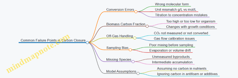
Practical Checklist for Reliable Closure
- Use one carbon basis and one conversion method across the run.
- Convert every measured species into g C, not just g/L.
- Treat biomass carbon fraction as a parameter to verify, not a sacred constant.
- Include CO₂ if you can; if you can’t, report partial closure and track the missing carbon explicitly.
- Interpret residual sign before you start changing the chemistry in your head.
When you do this consistently, mass balance becomes less of a calculation and more of a process instrument: it tells you whether your measurements and assumptions agree with the laws of conservation. Fermentation is messy; carbon accounting doesn’t have to be.
8. Downstream Processing and Product Recovery
8.1 Clarification Filtration and Centrifugation Options
Clarification is the step where you reduce suspended solids so the next operation—concentration, purification, or packaging—stays predictable. In fermentation, “solids” can mean intact cells, cell debris, precipitated proteins, yeast flocs, or fine particulates from media. The right choice depends on particle size, how easily the solids compress, and whether you need to keep product in the liquid phase.
Clarification Goals and What They Mean in Practice
A good clarification plan hits three targets at once: (1) remove particles to meet turbidity or clarity requirements, (2) minimize product loss to the cake or filter medium, and (3) avoid changing product chemistry through heat, shear, or long residence times. For example, if you’re producing an organic acid, you usually want to keep the acid in the filtrate while removing cells. If you’re producing a protein, you also care about adsorption losses and fouling caused by protein aggregates.
Particle Behavior That Drives Method Selection
Particles behave differently under pressure and flow. Centrifugation separates based on density and size; larger or denser particles settle faster. Filtration separates by a combination of size exclusion and depth capture, but fine particles often create a cake that changes resistance over time.
A practical rule: if your solids are mostly large and settle readily, centrifugation often gives fast, consistent clarification. If solids are fine and you can tolerate a controlled pressure drop, filtration can be efficient—especially when you can form a stable, low-resistance cake.
Centrifugation Options and How to Choose
Batch vs Continuous Centrifugation
Batch centrifugation is straightforward for small runs and quick troubleshooting. Continuous centrifugation suits steady production and reduces downtime. In both cases, the key operating variables are rotational speed, feed rate, and temperature.
Decanter, Disc Stack, and Tubular Designs
- Decanter centrifuges handle higher solids and can discharge continuously. They’re common when you expect a thick slurry.
- Disc stack centrifuges are efficient for clearer separation and can produce a cleaner clarified stream, but they require careful feed consistency.
- Tubular centrifuges are often used for specific separation tasks where geometry and flow control matter.
Example: Yeast Removal for Beverage Clarification
Suppose you ferment a beverage with yeast cells that you want to remove before flavor adjustment. If the yeast forms flocs, centrifugation can quickly produce a clarified supernatant. You still monitor turbidity because floc strength can vary with pH and nutrient balance from the fermentation step.
Filtration Options and How They Work
Depth Filtration
Depth filters capture particles throughout a porous medium. They’re forgiving for moderately dirty feeds and can handle a range of particle sizes. The tradeoff is that fine particles can increase fouling gradually, so you track pressure drop and throughput.
Surface Filtration with Membranes
Membrane filtration uses defined pore sizes. Microfiltration can remove cells and fine debris; ultrafiltration can retain larger solutes like proteins. The advantage is sharper separation, but fouling can be faster when the feed contains sticky proteins or colloids.
Crossflow vs Dead-End Filtration
Dead-end filtration pushes all feed through the medium, building a cake that eventually limits flow. Crossflow filtration sweeps some material along the membrane surface, slowing cake growth. Crossflow is common when you need stable flux and when product is sensitive to residence time.
Example: Clarifying a Cell-Free Enzyme Solution
If you have an enzyme in the liquid phase and want to remove cells without losing enzyme to the filter, you choose a filtration strategy that minimizes adsorption. You can reduce adsorption by selecting compatible filter materials and by controlling pH and ionic strength so the enzyme stays soluble and less prone to aggregation.
Mind Map: Clarification Decision Path
Integrated Workflow for a Typical Clarification Step
Start by measuring or estimating solids and turbidity in the fermentation broth. If you see large flocs or fast settling, centrifugation can be your first pass to reduce bulk solids. If turbidity remains high due to fine particles, follow with filtration to polish the clarified stream.
A common integrated approach is centrifuge first, filter second. The centrifuge removes most cells and debris, which lowers filter fouling and extends filter life. The filter then captures the remaining fine haze so downstream operations behave consistently.
Practical Best Practices That Prevent Common Failures
- Control temperature: viscosity changes can swing both centrifuge separation and filtration resistance.
- Avoid overloading: pushing too much solids into a filter accelerates cake formation and increases product loss.
- Monitor pressure drop or flux: a stable trend means you’re operating in a predictable regime; a sudden change signals fouling or feed inconsistency.
- Plan for product adsorption: if product is prone to sticking, test small-scale filter compatibility and consider preconditioning the feed.
- Use clear acceptance criteria: define turbidity and recovery targets so operators can stop at the right point rather than “just keep going.”
Example: Choosing a Two-Step Clarification Plan
Imagine a fermentation broth with moderate cell density and a persistent haze after settling. You run a small centrifuge trial to remove the bulk solids and measure turbidity in the supernatant. If the supernatant is still cloudy, you add a polishing filtration step sized to remove the remaining fine particles. You track product recovery by comparing product concentration before and after clarification, so you can adjust filter type or operating conditions without guessing.
8.2 Cell Removal and Biomass Handling for Food and Industrial Products
Cell removal is the step where you separate living or once-living biomass from the liquid phase so the product can be clarified, purified, or stabilized. In food fermentations, the goal is often to keep flavors and acids while removing cells that can keep metabolizing. In industrial fermentations, the goal is usually to recover product and protect downstream steps from fouling, viscosity spikes, and unwanted biochemistry.
What You Are Removing and Why It Matters
Biomass can be intact cells, cell fragments, or flocs. The “why” is practical: cells consume remaining sugars, produce off-odors, and can release enzymes that keep changing the product after fermentation ends. Even if the cells are not actively growing, they may still metabolize residual substrates. That’s why cell removal is not just physical separation; it’s also a control lever for product consistency.
A useful way to think about it is by product sensitivity. If your product is a small molecule like lactic acid, ethanol, or organic acids, you can often tolerate some fine particles but must manage color and turbidity. If your product is a protein or enzyme, you must consider whether cells are protecting the product or contaminating it with proteases and nucleases.
Clarification Options and How to Choose
Start with the properties of the broth: solids concentration, particle size distribution, viscosity, and whether cells form flocs. These properties determine which separation method behaves well.
- Centrifugation works when you need fast separation and can handle higher operating costs. It’s common for yeast removal in beverage fermentations and for biomass harvesting in many industrial processes.
- Filtration is attractive when you need consistent clarification and can manage fouling. Microfiltration and depth filtration are typical when particle sizes are small or when you want to reduce turbidity without harsh conditions.
- Flocculation and settling can be effective for floc-forming organisms. It’s cheaper but less precise, and it may leave more residual solids.
A simple decision rule: if the broth is thick or has stubborn fine particles, filtration may foul quickly and centrifugation may be more reliable. If the broth is dilute and floc-forming, settling can reduce the load on downstream filters.
Centrifugation Fundamentals for Biomass Handling
Centrifuges separate based on density differences and particle size. For biomass removal, you typically aim for a clarified supernatant and a concentrated pellet or slurry.
Key operating variables include rotor speed, residence time, and feed rate. Higher speed increases separation force but can compact pellets, making them harder to resuspend for certain workflows. Feed rate affects how well the separator maintains a stable flow regime.
Practical best practice: monitor turbidity or suspended solids in the clarified stream, not just the visual appearance. A broth that looks clear can still carry enough fine cells to keep consuming residual sugars.
Filtration Fundamentals and Fouling Control
Filtration separates by size exclusion or by depth capture. Fouling happens when particles block pores or form a cake layer.
Common strategies include:
- Pre-treatment such as coarse filtration or settling to reduce solids load.
- Operating pressure and flux management to avoid rapid cake formation.
- Backflushing or periodic cleaning when equipment allows.
For food systems, you also need to consider whether cleaning chemicals and residues are compatible with your sanitation requirements. For industrial systems, you need to manage cleaning cycles so you don’t lose throughput.
Biomass Handling After Separation
Once removed, biomass becomes a material stream with its own handling requirements.
- Storage: Biomass can continue to change composition if stored warm. Cooling and time control reduce ongoing metabolism and odor formation.
- Washing: Washing can remove residual product and salts. For example, yeast harvested from beer or bioethanol processes is often washed to reduce carryover compounds that would interfere with downstream recovery.
- Deactivation: Some processes require inactivation to stop enzymatic activity. Heat or chemical deactivation must be chosen based on what the biomass will be used for.
- Utilization or disposal: Food-grade biomass may be directed to animal feed or ingredient streams, while industrial biomass may be routed to energy recovery or waste treatment. The separation step affects how easy that routing becomes.
A practical example: in a lactic fermentation where the product is lactic acid, you may centrifuge to remove cells, then polish the supernatant by filtration to reduce turbidity. The biomass slurry can be dewatered, and washing can reduce residual acid so the waste stream is less corrosive.
Mind Map: Cell Removal and Biomass Handling
Example: Yeast Removal for a Clearer Beverage
A beverage fermentation often ends with a broth that contains yeast cells and fine particulates. If you bottle without removing cells, residual sugars can drive continued fermentation and create unwanted carbonation.
A typical workflow is:
- Centrifuge to remove most yeast and large flocs.
- Polish filter to reduce remaining turbidity.
- Verify suspended solids and turbidity in the clarified stream.
- Handle biomass by dewatering and storing cold to limit off-odors and compositional drift.
The key is that each step reduces a different problem: centrifugation handles the bulk biomass, while filtration handles the fine particles that would otherwise slip through.
Example: Biomass Removal in Industrial Organic Acid Production
For organic acid broths, the supernatant is the product-rich phase. Cells and fragments can contribute color and enzymes that keep reacting with residual substrates.
A practical approach is:
- Harvest biomass by centrifugation to reduce solids quickly.
- Filter to remove fine particles and improve clarity.
- Minimize product loss by optimizing washing so the acid stays in the liquid phase.
- Manage biomass so residual acid does not create excessive load in waste handling.
This keeps downstream purification steps stable because the feed entering them is less variable in solids and enzymatic activity.
Quality Checks That Close the Loop
After cell removal, confirm three things: clarity, residual substrate risk, and product loss. Clarity is measured by turbidity or suspended solids. Residual substrate risk is assessed indirectly through indicators like residual sugar or fermentation activity in a small hold test. Product loss is checked by measuring product concentration in both the clarified stream and the biomass stream.
When these checks are consistent, the rest of downstream processing becomes less of a guessing game and more of a controlled sequence.
8.3 Product Separation Techniques Including Distillation Extraction and Adsorption
Separation is where fermentation turns into a product you can ship, bottle, or package. The core idea is simple: different components leave the system in different ways because they differ in volatility, solubility, charge, or affinity. The trick is choosing a method that matches the product’s physical chemistry and the process constraints you already have, like broth viscosity, solids content, and allowable solvent residues.
Foundational Concepts for Choosing a Separation Method
Start by classifying what you’re separating.
- Volatile product: distillation often works well when the product can vaporize without decomposing.
- Nonvolatile but soluble product: extraction is a strong fit when you can move the product between two immiscible liquid phases.
- Low concentration product or product with strong affinity: adsorption can polish dilute streams using a solid that selectively holds the target.
Before any separation step, treat the broth so the method can do its job. For example, distillation dislikes suspended solids because they foul heat surfaces; extraction dislikes emulsions because they slow phase separation; adsorption dislikes fine particulates that block pores. That’s why clarification and filtration are frequently upstream of 8.3.
Distillation: Separating by Volatility and Boiling Behavior
Distillation separates components based on differences in vapor–liquid equilibrium. In a basic sense, the more volatile component prefers the vapor phase, leaving the less volatile component behind.
Key Operating Levers
- Pressure: lowering pressure reduces boiling temperatures, which helps protect heat-sensitive products.
- Reflux and column design: higher reflux improves separation sharpness but increases energy use.
- Feed condition: a clear feed improves performance and reduces fouling.
Practical Example
Imagine fermenting to produce an ethanol-containing broth. After removing solids, you can distill to concentrate ethanol. If the broth is still warm and contains residual sugars, they can contribute to viscosity and boiling behavior; careful clarification and controlled feed rates reduce bumping and stabilize operation.
Common Failure Modes
- Fouling and scaling from nonvolatile salts or proteins.
- Overheating leading to product degradation.
- Poor separation when components have close boiling points, requiring more stages or a different method.
Extraction: Moving Product Between Two Liquid Phases
Liquid–liquid extraction transfers a solute from one solvent phase to another based on partitioning. The partition coefficient tells you how much product prefers the extractant compared with the original phase.
Key Operating Levers
- Solvent selection: choose an extractant that dissolves the product well but stays immiscible with the aqueous phase.
- pH and ionic form: many products change solubility when protonation state changes.
- Mixing intensity and residence time: enough mixing improves mass transfer; too much can create stubborn emulsions.
Practical Example
Suppose you’re producing an organic acid from fermentation. By adjusting pH, you can shift the acid between ionized and non-ionized forms. The non-ionized form often partitions better into an organic phase. After extraction, you back-extract or neutralize to recover the acid in a usable form.
Common Failure Modes
- Emulsion formation that traps product in the interface.
- Solvent losses due to entrainment.
- Insufficient driving force when the partition coefficient is unfavorable.
Adsorption: Capturing Product on a Solid Surface
Adsorption separates by molecular affinity to a solid. Unlike extraction, it doesn’t require two liquid phases to exchange the product; instead, the product sticks to the adsorbent until you regenerate or elute it.
Key Operating Levers
- Adsorbent type: activated carbon, resins, or specialized media depending on polarity and functional groups.
- Bed conditions: flow rate affects contact time and breakthrough.
- Regeneration strategy: choose conditions that release the product without destroying the adsorbent.
Practical Example
Consider a dilute fermentation broth where the target product is present at low concentration. After clarification, pass the broth through an adsorption bed. The product binds while many impurities pass through. Then elute the product using a solvent or pH shift, producing a concentrated stream suitable for final polishing or formulation.
Common Failure Modes
- Early breakthrough from too-high flow rate or insufficient bed height.
- Pore blockage by residual solids.
- Strong binding without clean regeneration, leaving product behind.
Mind Map: Product Separation Logic for Distillation Extraction and Adsorption
Integrated Workflow Example: Choosing and Sequencing Methods
A common integrated approach is to clarify first, then select the separation step that matches the product’s behavior. If the product is volatile, distillation can concentrate it after solids removal. If it’s nonvolatile, extraction can transfer it into an organic phase, followed by back-extraction or neutralization. If the product is dilute or needs selectivity, adsorption can polish the clarified stream, producing a concentrated eluate.
In practice, sequencing matters because each method changes the stream composition. Distillation concentrates volatiles but can leave nonvolatile impurities behind. Extraction can remove the target while carrying some co-extracted compounds that later require cleanup. Adsorption can concentrate the target but may also co-bind strongly interacting impurities, so upstream clarification and controlled conditions are not optional.
Quick Decision Checklist
- Is the product volatile enough to vaporize cleanly? Distillation.
- Is the product nonvolatile but can partition into a second liquid phase? Extraction.
- Is the product dilute and selective capture is needed? Adsorption.
- Are solids present that will foul, emulsify, or block? Clarify before separation.
The best separation plan is the one that respects these constraints while keeping the stream conditions aligned with the method’s assumptions. When those assumptions hold, the math and the hardware both behave.
8.4 Concentration and Drying Methods Including Spray Drying and Freeze Drying
Concentration and drying turn a wet fermentation broth into a stable ingredient, but they also change the product. Water removal can shift pH, concentrate salts, and stress proteins or cells. The goal is to remove enough water to meet a specific stability target while keeping the product’s functional properties where they matter.
Core Concepts of Concentration Before Drying
Concentration reduces the drying load and can improve energy efficiency. It also lets you adjust composition before drying, such as lowering bulk sugars that would otherwise caramelize. Common concentration steps include:
- Evaporation: Useful when the product tolerates heat. It concentrates by boiling under controlled conditions, often with reduced pressure to lower temperature.
- Membrane concentration: Useful when heat sensitivity is high. Ultrafiltration concentrates proteins or enzymes, while nanofiltration can retain larger solutes and pass smaller ones.
A practical rule: choose concentration based on what you cannot afford to lose. If enzymes are fragile, membrane concentration is often gentler than evaporation.
Drying Targets and What “Stable” Means
Drying is not just “make it dry.” Stability depends on residual moisture and water activity. Lower water activity slows microbial growth and many chemical reactions. For many fermented ingredients, you also care about:
- Reconstitution behavior: powders that dissolve quickly reduce process headaches later.
- Color and flavor retention: excessive heat can darken products and drive off volatiles.
- Functional performance: foaming, emulsification, or enzymatic activity may drop if drying conditions are too harsh.
Spray Drying Fundamentals and Process Logic
Spray drying converts a liquid feed into fine droplets, then dries them rapidly with hot gas. The short residence time is the main advantage: the product experiences heat briefly, which helps when the feed is not extremely heat sensitive.
How it works in steps
1. Feed preparation: adjust solids content and viscosity so droplets form consistently.
2. Atomization: use a nozzle or rotary atomizer to create droplets.
3. Drying chamber: hot air evaporates water; droplets shrink into particles.
4. Separation and collection: cyclones or filters recover powder.
Key operating variables
- Inlet air temperature and outlet air temperature: outlet temperature is a practical proxy for how much water remains.
- Feed solids: too low wastes energy; too high can cause stickiness and wall deposition.
- Atomization quality: poor droplet formation yields broad particle sizes and uneven drying.
Easy example
A lactic acid or enzyme-containing broth is concentrated to a workable solids level, then spray dried. If the powder comes out sticky, the usual suspects are high feed solids, high inlet temperature, or insufficient drying gas flow. Lowering feed solids or reducing inlet temperature often fixes the issue without changing the chemistry.
Freeze Drying Fundamentals and Process Logic
Freeze drying removes water by sublimation: first freeze the product, then apply vacuum so ice turns directly to vapor. This typically preserves heat-sensitive components better than spray drying.
How it works in steps
1. Freezing: forms ice crystals and concentrates solutes in the remaining unfrozen phase.
2. Primary drying: sublimates ice under vacuum.
3. Secondary drying: removes bound water to reach target moisture.
Key operating variables
- Freezing profile: affects ice crystal size and the structure of the dried cake.
- Shelf temperature during primary drying: must stay below conditions that cause collapse.
- Vacuum level: controls sublimation rate.
Easy example
A probiotic powder needs high viability. Freeze drying can better protect cells because it avoids hot air exposure. If the dried cake collapses, the freezing step may have produced an unfavorable structure or the shelf temperature during primary drying was too high.
Mind Map: Concentration and Drying Decision Path
Practical Comparison and Selection Guide
Spray drying is usually faster and more scalable for products that tolerate brief heat exposure and can be formulated to suitable viscosity and solids. Freeze drying is slower and more energy intensive, but it often better preserves fragile biological activity and sensitive flavors.
A simple selection approach:
- If the product must keep activity high and is heat sensitive, lean toward freeze drying.
- If the product is robust and you want efficient bulk production, lean toward spray drying.
- If you are unsure, start with a concentration step that matches sensitivity, then compare drying outcomes using moisture, reconstitution time, and a functional assay relevant to the product.
Example Workflow: From Broth to Powder
- Measure feed properties: solids, viscosity, and heat sensitivity indicators.
- Concentrate appropriately: membrane for fragile enzymes; evaporation for heat-tolerant acids.
- Choose drying method: spray drying for rapid conversion; freeze drying for maximum preservation.
- Set targets: moisture and water activity, plus a quality check like enzymatic activity or reconstitution time.
- Troubleshoot systematically: if performance drops, adjust concentration solids first, then drying temperatures, then atomization or freezing profile.
Concentration and drying are a coupled system. When you treat them as one process—rather than separate chores—you get powders that behave predictably in the next step, whether that step is mixing, dosing, or reconstitution.
8.5 Stabilization Packaging and Shelf Life Considerations for Fermented Products
Stabilization starts with a simple goal: slow down the changes you want to keep, and stop the changes you do not. For fermented products, those changes include ongoing microbial activity, chemical reactions like oxidation and pigment shifts, and physical effects such as gas retention or texture softening. Packaging is the control surface that connects your fermentation outcome to what the customer experiences later.
Core Stabilization Principles
1) Match packaging to the product’s dominant change. If the product is still biologically active, temperature and oxygen exposure matter most. If the product is microbiologically stable but chemically fragile, oxygen and light exposure dominate. For example, a fresh lactic-fermented vegetable often continues slow acidification and texture change, while a fermented oil-based product may be more sensitive to oxidation.
2) Control oxygen and water activity. Oxygen drives oxidation of lipids and some flavor compounds. Water activity influences whether microbes can grow. Packaging choices should reduce oxygen ingress and, when appropriate, limit moisture migration.
3) Use a barrier strategy, not a single trick. A lid alone rarely solves everything. A good approach combines headspace management, barrier films, seals, and storage temperature.
Packaging Formats and What They Do
Glass jars. Excellent oxygen barrier when properly sealed and handled. They also tolerate pasteurization or hot-fill processes when used. A practical example: fermented pickles in glass with a tight seal typically maintain color and crunch better than flexible packaging stored warm.
Flexible pouches and films. Often good for cost and logistics, but barrier performance varies widely. Choose films based on oxygen transmission rate and moisture permeability. Example: a pouch for fermented grains can work well if it uses a low-oxygen barrier and is sealed without wrinkles.
Cans and metal containers. Strong physical protection and good barrier properties. They are common when thermal steps are used. Example: canned fermented sauces rely on a validated heat process to stop microbial activity, so packaging mainly preserves quality after processing.
Vacuum and modified atmosphere packaging. These reduce oxygen in the headspace. Vacuum can collapse some products, affecting texture. Modified atmospheres can be effective for oxygen-sensitive products, but the gas composition must be compatible with the product’s chemistry.
Headspace, Seals, and Oxygen Management
Headspace is not just empty space; it is where oxygen and carbon dioxide live. For carbon dioxide–producing fermentations, too much headspace can lead to pressure swings and seal stress. Too little headspace can cause overflow or excessive foaming during filling.
Seal integrity is the quiet hero. A micro-leak can turn a stable product into a slow oxygen-driven oxidation experiment. Practical checks include visual seal inspection, periodic seal strength testing, and pressure or dye-based leak tests where appropriate.
Stabilization Steps That Pair with Packaging
Packaging alone may not be enough. Common stabilization steps include:
- Temperature reduction. Rapid cooling after filling slows microbial and chemical reactions. Example: cooling fermented beverages quickly reduces continued ethanol and off-flavor formation.
- Pasteurization or mild heat treatment. Used when you need to stop or reduce microbial activity. Example: some fermented drinks are heat-treated to extend shelf life while keeping acidity-driven flavor.
- Filtration or centrifugation. Removes cells when the product can tolerate it. Example: clarifying a fermented broth can reduce ongoing metabolism, but it may also change mouthfeel.
- Adjustment of formulation. Salt, sugar, and acidity can be tuned so the remaining microbes are less active. Example: increasing acidity slightly can reduce post-pack microbial drift in certain vegetable ferments.
Shelf Life Determination and Testing Logic
Shelf life is not a guess; it is a measured boundary. A systematic approach uses real storage conditions and tracks the specific failure modes.
1) Define quality attributes and failure points. Typical attributes include pH, titratable acidity, microbial counts, sensory changes, gas production, and texture. Failure points should be measurable, not just “tastes off.”
2) Run storage studies at relevant temperatures. Use at least two temperatures that reflect normal storage and a higher stress condition. Example: test a fermented sauce at refrigerated and room-temperature conditions to understand how quickly flavor and microbial stability change.
3) Sample on a schedule that captures early and late changes. Early sampling catches fast reactions; later sampling confirms the long tail. For products with active fermentation, frequent early sampling is especially important.
4) Use packaging-specific comparisons. The same product in two packages can behave differently because oxygen ingress and seal performance differ. Example: compare glass jars versus low-barrier films under identical storage.
Mind Map: Stabilization and Shelf Life Workflow
Example: Choosing Packaging for a Fermented Vegetable
A crunchy, lactic-fermented vegetable typically has ongoing low-level activity and sensitivity to oxygen. A practical stabilization plan might include: fill into glass jars with minimal headspace, ensure a consistent seal, cool promptly, and store refrigerated. Shelf life testing should track pH drift, texture (firmness), and microbial counts over time. If oxygen exposure is the main driver of flavor dulling, switching to a lower-oxygen film or improving jar sealing performance can extend shelf life without changing the fermentation.
Practical Checklist for Packaging Release
Before release, verify that packaging performance matches your stabilization assumptions: seals are intact, headspace is within target range, containers are clean and properly filled, and the product meets defined microbial and chemical criteria. When those boxes are checked, shelf life becomes a controlled outcome rather than a hopeful timeline.
9. Analytical Methods for Monitoring and Quality Assurance
9.1 Sampling Plans and Handling to Avoid Measurement Bias
Sampling bias is what happens when the sample you test is not the same as the material you meant to measure. In fermentation, that mismatch can come from where you sample, when you sample, how you mix, and how you handle the sample before testing. The goal is simple: make the measurement reflect the batch, not the sampling process.
Core Sampling Logic
Start by defining the decision you need the data for. If you need to confirm a pH setpoint was met, you sample differently than if you need to estimate average lactic acid concentration across the tank. Then translate the decision into measurable targets: mean value, trend over time, or detection of outliers.
A practical sampling plan includes five elements: sampling location, sampling frequency, sample size, sample handling steps, and acceptance criteria for sample quality. Each element should connect to a known source of variation such as gradients, settling, or rapid metabolism.
Where to Sample Without Creating a “Local” Answer
Tanks often have gradients in temperature, dissolved oxygen, and substrate concentration. Even in mixed systems, gradients can persist near inlets, baffles, or dead zones. Choose locations that represent the bulk. For example, if you have a stirred tank with a top sparger, sampling near the sparger can overrepresent gas-liquid mass transfer effects. Instead, sample from a port positioned to reflect the well-mixed region.
For brines and viscous matrices, stratification is common. A simple rule is to sample after a defined mixing interval. If you cannot mix the whole tank, take multiple samples from different heights and combine them into a composite sample, then treat the composite as your “bulk” measurement.
When to Sample to Capture the Real State
Measurement bias also appears when the process changes between sampling and measurement. Some analytes shift quickly after withdrawal because cells keep metabolizing. To reduce this, define a maximum time from sampling to quenching or measurement. For pH and conductivity, the drift may be small; for sugars, organic acids, and ethanol, drift can be significant.
A systematic approach is to sample at times that match process events: start-up, mid-run, near expected endpoint, and any time you adjust feeds or aeration. If you are tracking a trend, sample more frequently during fast-changing phases and less frequently during stable phases.
How Many Samples and How Big a Sample
If you take one small grab, you risk measuring a pocket rather than the batch. Sample size should be large enough to represent heterogeneity, especially for solids or uneven distribution of nutrients. For liquid systems, the “small grab” problem shows up when there are suspended cells or particulates.
Use replication when you need confidence, not just a number. For example, if you are verifying that a batch meets an acid specification, run duplicate analyses from the same collected sample. If duplicates disagree beyond your method tolerance, the bias is in handling or measurement, not in the fermentation.
Handling Steps That Prevent Post-Sampling Changes
Once collected, samples should be protected from the processes you are trying to measure. Common safeguards include:
- Temperature control: Keep samples cool when analytes degrade or reactions continue.
- Quenching: For metabolite measurements, stop biological activity promptly using an appropriate quench method consistent with your analytical method.
- Mixing before subsampling: If the sample contains cells or precipitates, mix gently and consistently before taking aliquots.
- Container choice: Use containers that do not adsorb analytes or leach interfering substances.
- Labeling and chain of custody: Record time, location, operator, and any deviations so you can trace anomalies.
A small but effective practice is to standardize the handling workflow with a checklist. If two operators handle samples differently, you can end up measuring operator technique.
Mind Map: Sampling Plan and Bias Controls
Example: Composite Sampling for a Stratified Brine
Suppose you measure titratable acidity in a vegetable brine where solids settle. If you sample only from the bottom port, you may overestimate acidity because fermentation products accumulate where solids sit. A better plan is to take equal-volume samples from top, middle, and bottom after a brief mixing interval, then combine them into one composite. Analyze the composite as your batch-average estimate. If the composite result is within spec but individual layers differ widely, you also learn that mixing or brine circulation needs attention.
Example: Timing Bias in Organic Acid Measurements
Imagine you withdraw a sample at 10:00, but quenching and centrifugation happen at 10:20. Cells can continue converting sugars to acids during those 20 minutes, shifting the measured concentrations upward. The fix is to set a hard target such as quench within a defined window, then record the actual time for each sample. If you later see an unexpected spike, you can check whether the handling window was exceeded.
Example: Duplicate Analysis to Separate Sampling from Testing
If two lab runs from the same quenched aliquot disagree, the bias is likely analytical or handling-related, not fermentation-related. For instance, incomplete mixing before aliquoting can cause one duplicate to contain more precipitated material than the other. Duplicate analysis is not just a formality; it tells you whether your measurement system is stable.
Practical Checklist for a Bias-Resistant Sampling Plan
Define the decision, choose representative locations, set timing around process events, standardize sample size and replication, and enforce handling controls with recorded times. When results look odd, use the logs to determine whether the fermentation changed or the sample did.
9.2 pH Titratable Acidity and Buffer Capacity Measurements
pH and titratable acidity answer different questions. pH tells you the hydrogen ion activity at the moment you measure it. Titratable acidity tells you how much base you can add before the sample reaches a chosen endpoint, which is a proxy for the total amount of acid species that can be neutralized under your conditions. Buffer capacity describes how resistant the system is to pH change as you add acid or base—basically, how “stubborn” the sample is.
Mind Map: What You Measure and Why
Foundational Concepts That Keep You Honest
A titration is only as meaningful as its endpoint. For food and fermentation matrices, endpoints are often selected to match product specifications or to represent a practical “neutralization” level. Common endpoints include pH 8.1 for many lactic and acetic acid–containing products, but the key is consistency with your method and reference standard.
Titratable acidity is typically reported as an equivalent amount of a specific acid, such as lactic acid for dairy fermentations or acetic acid for vinegar-like products. This conversion is not magic; it’s stoichiometry. If your titrant is sodium hydroxide, each mole of OH⁻ neutralizes one mole of monoprotic acid. For diprotic acids, the stoichiometry changes, which is why method selection matters.
Buffer capacity is derived from how pH changes as you add a small amount of titrant. Two samples can have the same pH but different buffer capacities: one may change pH quickly because it has little buffering species, while the other resists change due to higher concentrations of conjugate acid/base pairs.
Practical Measurement Workflow
Sample Preparation and Temperature Control
Measure pH and titrate at a controlled temperature because both electrode response and acid dissociation shift with temperature. Homogenize thoroughly to avoid sampling bias, especially in products with suspended solids. If the sample is viscous, ensure consistent stirring during titration so the pH electrode sees a representative mixture.
Instrument Calibration and Electrode Handling
Calibrate the pH meter using at least two standards that bracket your expected pH range. Rinse the electrode with deionized water, blot gently (don’t wipe aggressively), and keep the electrode hydrated according to the manufacturer’s guidance. A drifting electrode can turn a careful titration into a slow-motion guessing game.
Performing the Titration
- Record the initial pH of the sample.
- Add titrant in small increments while stirring steadily.
- Record pH after each increment once it stabilizes.
- Continue until the chosen endpoint pH is reached.
- Run a blank titration using the same diluent and reagents to correct for any background acidity or alkalinity.
A good practice is to capture the full pH-versus-volume curve. Even if you only need the endpoint for TA, the curve helps you compute buffer capacity and spot anomalies like poor mixing or electrode lag.
Calculations with Clear Units
Titratable Acidity as Equivalent Acid
Compute moles of titrant used:
- \(n_{OH^-} = C_{base} \times (V_{sample} - V_{blank})\)
- Convert to moles of the reference acid using stoichiometry.
Then convert to a mass basis using the reference acid molecular weight and normalize to sample volume or mass as required by your reporting format.
Buffer Capacity from the Titration Curve
Buffer capacity around a pH region is often expressed as the amount of strong acid or base needed to change pH by one unit, normalized to sample volume or concentration. Practically, you can estimate it by selecting two points on the curve near the pH of interest and using the slope:
- \(\beta \approx \frac{\Delta C_{titrant}}{\Delta pH} \)
Choose the pH region where the curve is smooth and not dominated by the endpoint approach. If the curve flattens, buffer capacity is higher; if it steepens, buffering is weaker.
Example: Comparing Two Fermented Samples
Sample A and Sample B both start at pH 3.60. During titration to pH 8.10, Sample A requires 12.0 mL of 0.100 mol/L NaOH, while Sample B requires 8.0 mL.
- Sample A has higher titratable acidity because it consumes more base to reach the same endpoint.
- If Sample A’s pH changes slowly during the mid-portion of the titration curve, it also likely has higher buffer capacity, meaning more conjugate species are present to resist pH change.
If instead Sample B consumed less base but still showed a relatively gentle pH slope, it could indicate that its buffering species are effective only over a narrow pH range. That’s why curve shape matters, not just the endpoint volume.
Common Pitfalls and How to Avoid Them
- Endpoint drift: If pH takes a long time to stabilize, record after stabilization or use a consistent time criterion.
- Electrode lag in viscous samples: Increase stirring consistency and allow equilibration after each increment.
- Ignoring blanks: Background titration consumption can bias TA, especially for low-acid samples.
- Inconsistent dilution: If you dilute samples before titration, apply the dilution factor in the final normalization.
Mind Map: Quality Checks During the Run

What the Results Mean Together
pH tells you the current acidity level. Titratable acidity tells you how much neutralization capacity the sample has under your endpoint definition. Buffer capacity tells you how that acidity system behaves as you move away from the starting pH. When you report all three, you can distinguish “same pH, different acid load” from “same acid load, different buffering behavior,” which is exactly what you need for reliable fermentation and product quality control.
9.3 Microbiological Testing Including Plate Counts and Selective Media
Microbiological testing answers two practical questions: “How many?” and “Which ones?” Plate counts estimate the number of viable microorganisms, while selective media bias recovery toward specific groups. Together, they turn fermentation quality from a gut feeling into measurable evidence.
Core Concepts That Drive Good Testing
Viable counts depend on three links in the chain: sampling, dilution, and plating. If any link is sloppy, the math becomes confident but wrong. Selective media add another layer: they suppress unwanted organisms and encourage the target group, but they never guarantee exclusivity. Think of selectivity as a filter, not a magic spotlight.
Plate Counts with Dilution Logic
A typical workflow starts with a representative sample, then serial dilution to land colonies in a countable range (often a few dozen to a few hundred colonies per plate). You then spread or pour a known volume onto agar, incubate under defined conditions, and count colonies.
Key best practices:
- Use consistent dilution steps so colony numbers translate cleanly into CFU per mL or CFU per g.
- Mix each dilution thoroughly before transferring to the next tube; otherwise, you count clumps.
- Plate duplicates to detect pipetting errors and uneven spreading.
- Record incubation parameters because colony appearance and growth rates are condition-dependent.
Interpreting Colony Counts Without Overconfidence
Countable plates are not just “not too many.” If colonies merge, you undercount; if colonies are too sparse, random variation dominates. When plates fall outside the target range, choose the closest acceptable plate and document why. Also watch for morphology drift across dilutions; a sudden shift can indicate contamination or selective effects.
Selective Media as Targeted Recovery
Selective media use one or more of the following strategies:
- Selective inhibitors that slow or stop non-target organisms.
- Differential indicators that help distinguish target colonies from others.
- Nutrient preferences that favor the target group’s metabolism.
Selective media are especially useful when fermentation samples contain mixed populations, such as lactic acid bacteria plus yeasts, or when you need to monitor hygiene indicators in a process environment.
Choosing Media Based on the Question
Match the medium to the decision you must make:
- If you need total viable counts, use a general medium and count colonies.
- If you need group-specific monitoring, use a selective medium aligned with that group.
- If you need confirmation, follow up with a confirmatory method after initial recovery.
Mind Map: Plate Counts and Selective Media
Example: Total Viable Counts During Fermentation
Suppose you test a fermented vegetable brine. You prepare serial dilutions and plate 0.1 mL onto a general agar. After incubation, one dilution yields 86 colonies on one plate and 90 on the duplicate. Another dilution yields 12 and 15 colonies.
You would typically calculate CFU using the dilution that lands in the countable range. Averaging duplicates reduces random error. The lower-count plates are more sensitive to chance events, so they contribute less to the final estimate unless the higher-count plates are invalid due to merging or contamination.
A practical check: if the two countable plates differ by a lot, revisit plating technique and dilution mixing. A small difference is normal; a large one often points to a handling issue.
Example: Selective Media for Hygiene Monitoring
Imagine you swab a contact surface after cleaning. You plate the swab eluate on a selective medium designed to recover a hygiene indicator group. After incubation, you observe colonies with the expected morphology on the selective plates, but none on the general medium.
That outcome can happen when the selective medium suppresses most background organisms and the target group is present at low levels. It can also happen if the general medium conditions were not optimal for that group. The disciplined response is to compare results across media and confirm the target morphology rather than declaring victory or failure based on a single plate type.
Quality Controls That Keep Results Honest
Even the best technique benefits from controls:
- Media sterility control verifies the agar wasn’t contaminated.
- Negative control checks that diluent or sampling handling didn’t introduce organisms.
- Positive control confirms the selective medium can recover the target under the chosen incubation conditions.
- Replicate consistency acts like a built-in sanity check for pipetting and spreading.
Practical Calculation and Documentation
When you report results, include the sample basis (per mL or per g), the dilution used, the plated volume, and the incubation conditions. Clear documentation prevents “mystery numbers” that cannot be traced back to a plate. If you ever need to compare batches, this record is what makes the comparison fair.
In short: plate counts quantify viable load, selective media steer recovery toward specific groups, and controls plus careful interpretation keep the whole system from lying politely.
9.4 Chemical Analytics for Sugars Organic Acids Ethanol and Volatiles
Chemical analytics turns fermentation from “it smells right” into measurable reality. In this section, the goal is to connect what you measure to what it means for fermentation performance, product quality, and downstream processing.
What You Measure and Why It Matters
Sugars track substrate consumption and help distinguish underfeeding from stalled metabolism. Organic acids often drive flavor and safety characteristics, and they can also signal metabolic shifts. Ethanol quantifies alcoholic fermentation progress and supports mass balance checks. Volatiles explain aroma and can reveal off-notes caused by oxygen exposure, nutrient imbalance, or contamination.
A practical mindset: each analyte should answer one operational question. If the data cannot guide a decision—adjust feed, change temperature, alter aeration, or investigate a defect—then the measurement is not pulling its weight.
Sample Handling That Prevents False Results
Most measurement errors come from sampling, not instruments. Use consistent sampling points and times relative to mixing. For fast-changing systems, quench reactions immediately (for example, by cooling and/or rapid acidification depending on the method). Filter or centrifuge when solids interfere with chromatography or colorimetric assays.
Keep a simple chain-of-custody: label, record time, note temperature, and document any dilution. If you dilute, record the dilution factor so results can be reported in the original matrix.
Sugars Analysis for Substrate Accounting
Common targets include glucose, fructose, sucrose, and sometimes maltose or other saccharides depending on the feedstock. Colorimetric methods can be fast but may lack specificity if multiple sugars are present. Enzymatic assays improve specificity by using selective enzymes that convert one sugar into a measurable product.
For complex sugar mixtures, chromatography is the workhorse. Ion chromatography or HPLC separates sugars before detection, reducing cross-talk. When you interpret results, compare sugar disappearance to expected stoichiometry. If sugars drop but acids do not rise as expected, you may be seeing diversion to biomass or unmeasured byproducts.
Organic Acids Analysis for Flavor and Metabolic Signals
Organic acids such as lactic, acetic, citric, malic, and succinic are typically quantified by HPLC with UV or refractive index detection, or by ion chromatography for certain acid profiles. The key is matrix compatibility: high salt brines can affect detector response and column performance.
Report acids as concentrations in the original broth, not just in the diluted sample. Also track pH alongside acids, because pH alone can mislead: buffering can mask acid changes until later. A useful check is to compare total titratable acidity trends with individual acid concentrations; agreement suggests the method is capturing the dominant acids.
Ethanol Analysis for Fermentation Progress and Balance
Ethanol can be measured by gas chromatography, enzymatic assays, or distillation-based approaches depending on the lab setup. GC is often preferred for specificity and for separating ethanol from other alcohols. Enzymatic methods are convenient but can be sensitive to interfering compounds.
Interpret ethanol alongside residual sugars and biomass indicators. If ethanol rises while sugars remain high, you may have incomplete conversion or measurement issues. If ethanol is low but acids are high, the process may be shifting toward acidogenesis rather than alcoholic pathways.
A mass balance habit helps: estimate carbon distribution among ethanol, acids, and biomass. Large imbalances usually point to sampling errors, unmeasured substrates, or losses during handling.
Volatile Compounds Analysis for Aroma and Defect Detection
Volatiles include aldehydes, esters, higher alcohols, and sulfur compounds. They are present at low concentrations, so sample preparation matters. Headspace sampling is common because it reduces matrix effects and improves repeatability.
For separation and identification, GC with appropriate detectors is standard. Quantification can be done with calibration curves using representative standards. When full identification is not required, targeted quantification of known key volatiles can still be operationally useful.
Interpretation should be tied to process conditions. For example, oxygen exposure can increase certain oxidation products, while nutrient limitation can shift ester and higher alcohol formation. Instead of treating volatile profiles as “mystery fingerprints,” map them to plausible causes using your process log.
Mind Map: Analytical Workflow
Example Integrated Interpretation
Imagine a batch where residual sugars fall from 40 g/L to 10 g/L, lactic acid rises from 2 g/L to 18 g/L, and ethanol stays near zero. That combination supports lactic fermentation rather than alcoholic conversion, so downstream planning should prioritize acid removal or neutralization rather than ethanol recovery.
Now consider a second batch with similar sugar decline, but ethanol reaches 6 g/L while lactic acid remains low. That indicates a pathway shift or different microbial dominance. If volatile analysis shows elevated esters alongside higher alcohols, it aligns with active fermentation and can explain a stronger aroma profile.
Finally, if sugars decline but neither acids nor ethanol increase as expected, treat it as a measurement and accounting problem first: check sampling, dilution, and method suitability for the matrix before changing the process.
Practical Quality Checks for Every Run
Run blanks and calibration standards appropriate to each method. Include at least one quality control sample that matches the expected concentration range. Confirm that replicate injections or replicates of the assay agree within your lab’s acceptance limits.
When results look odd, do not immediately blame biology. Verify the basics: sample labeling, dilution factors, instrument calibration status, and whether the method was validated for the broth matrix you actually used.
9.5 Instrument Calibration Validation And Routine Quality Checks
Fermentation measurements are only as trustworthy as the instruments behind them. Calibration sets the instrument’s scale to reality, validation checks that the whole measurement chain behaves as expected, and routine quality checks catch drift before it turns into a batch problem. The goal is simple: when you read pH, temperature, dissolved oxygen, or conductivity, you should know what that number means and how confident you can be.
Calibration Foundations and Measurement Chain
Calibration is not just “adjusting a probe.” It is aligning the instrument, sensor, and measurement method. A measurement chain typically includes sensor, signal conditioning, calibration standards, temperature compensation, and data logging. If any link is off, the number can look precise while being wrong.
A practical example: a pH probe can be calibrated with fresh buffers, yet still read incorrectly if the temperature compensation is wrong or the probe is coated with fermentation residues. That’s why calibration and validation must be treated as a pair.
Choosing Calibration Standards and Acceptance Logic
Standards should match the expected operating range. For pH, use at least two buffers that bracket your process setpoints. For temperature, use a reference thermometer with an accuracy appropriate to your control tolerance. For dissolved oxygen, use either air-saturation and zero-point approaches or a certified oxygen standard, depending on your system design.
Acceptance logic should be explicit. Instead of “it seems fine,” define allowable error and allowable drift. For example, you might require pH readings in calibration buffers to fall within a specified tolerance, and you might require that repeated checks after cleaning show no meaningful shift.
Stepwise Calibration Procedure with Built-In Sanity Checks
- Inspect and clean the sensor before calibration. A dirty probe can cause stable but biased readings.
- Condition the sensor if the manufacturer specifies hydration or stabilization time.
- Calibrate using fresh standards at a controlled temperature.
- Record calibration data including buffer lot, temperature, and instrument settings.
- Perform a post-calibration check by re-reading one standard after a short interval.
A small but important sanity check: after calibration, rinse and gently blot the sensor, then measure a buffer you did not use for calibration. If that “third point” is far off, the probe may be behaving nonlinearly or the sensor may be damaged.
Validation Beyond Calibration
Validation asks whether the instrument chain produces correct results in the context you actually use it. For fermentation, that context includes sample matrix effects, fouling, and mixing conditions.
Example for pH: calibrate the probe in buffers, then validate in a fermentation-like solution (same ionic strength and similar solids content). If readings drift or show slow stabilization, you may need a different probe type, improved cleaning frequency, or a revised sampling approach.
Example for dissolved oxygen: validate that the probe responds correctly under your expected aeration and mixing conditions. A probe that reads correctly in clean water can under-report in viscous broths because oxygen transfer to the sensor surface is limited.
Routine Quality Checks That Catch Drift Early
Routine checks are scheduled, lightweight, and designed to detect drift without interrupting production more than necessary.
- Frequency: daily for critical sensors, and after any cleaning, maintenance, or sensor replacement.
- Method: measure one or more control points that represent your process region.
- Trend review: track readings over time to distinguish random noise from systematic drift.
A simple routine for pH: measure a single mid-range buffer and compare to the last verified value. If the reading shifts beyond your tolerance, investigate probe condition, buffer freshness, and temperature compensation before trusting process control.
Mind Map: Calibration, Validation, and Checks
Example: A Weekly DO Probe Check Workflow
Use a consistent routine so results are comparable.
- Verify probe is clean and membrane is intact.
- Check zero response using an established zero condition.
- Check air-saturation response at a known temperature.
- Compare to the last verified values and acceptance limits.
- If out of tolerance, clean, replace membrane if needed, and repeat the check.
This workflow prevents the common failure mode where the probe “works” but slowly loses sensitivity due to membrane aging or biofilm buildup.
Documentation That Makes Troubleshooting Possible
Routine checks should be recorded in a way that supports root-cause analysis. Include sensor ID, calibration/verification results, standard identifiers, temperatures, and operator notes. When a batch result looks odd, the instrument record often explains whether the issue started with measurement bias or with process behavior.
A good record answers three questions quickly: What was measured? How was it verified? Did it stay within limits over time?
10. Case Study Workflows for Food and Industrial Fermentations
10.1 Case Study: Fermented Vegetables with Brine Management and Defect Control
Fermented vegetables live or die by brine behavior. The goal is simple: keep the right microbes active, keep oxygen away from the brine surface, and prevent conditions that favor spoilage organisms. This case study follows a practical workflow for cabbage, carrots, and similar vegetables using salt-brine fermentation.
Core Setup and Foundational Choices
Start with consistent inputs. Use fresh vegetables, remove damaged outer leaves, and cut to similar sizes so salt penetration and acid production happen at a predictable pace. For cabbage, shredding to a uniform thickness reduces pockets of under-salted material.
Choose a salt level that supports lactic acid bacteria while discouraging unwanted microbes. A common starting point is 2% to 2.5% salt by weight of water plus vegetable mass. If you use a jar with no added water, salt is still measured against the total expected liquid mass; the practical workaround is to weigh vegetables, add salt to reach the target percentage, and rely on vegetable release to form brine.
Brine Management That Prevents Defects
Brine management is mostly about two things: concentration and coverage.
-
Concentration control: Salt must be high enough to slow competitors but low enough to allow steady acidification. If brine looks unusually cloudy early on, it can be normal microbial activity, but if it later becomes slimy or smells putrid, suspect under-salting or contamination.
-
Coverage control: Vegetables must remain submerged. Oxygen exposure at the surface encourages yeast and molds and can create off-odors. Use a weight that fits the vessel and a brine level that stays above the solids. If brine drops, top up with pre-mixed salt solution at the same concentration.
A simple rule for jar work: check coverage daily during the first week, then every other day once acidification is clearly underway.
Step-by-Step Process with Integrated Checks
Day 0 to 2: Mix vegetables with measured salt. Pack tightly to reduce trapped air. Press down until liquid begins to pool. If using a container, leave headspace for foam.
Day 2 to 7: Watch for steady acidification. You should see bubbles and a mild sour smell rather than a sharp, rotten, or sulfur-like odor. If you see surface film, remove it promptly and ensure submersion. Surface film can be a thin yeast layer; it is not the same as a fully compromised batch.
Week 2 onward: Texture should become pleasantly crisp-tender. Flavor should shift from raw vegetable to sour and savory. At this stage, brine should taste clearly salty-sour, not flat.
Defect Map and Root Cause Reasoning
Defects are rarely random. Each one points to a specific failure mode in brine concentration, oxygen exposure, or hygiene.
Mind Map: Brine Management and Defect Control
Concrete Examples for Easy-to-Use Decisions
Example 1: Brine is low after two days
- Symptom: Vegetables start to peek above brine.
- Action: Make a matching salt solution (same concentration as the original) and top up until fully submerged.
- Reasoning: Oxygen exposure at the surface is the fastest route to surface yeast and mold.
Example 2: Slow fermentation with bland flavor
- Symptom: Few bubbles after several days; taste is still mostly vegetable.
- Action: Confirm salt percentage next batch; for the current batch, check that brine is not diluted by excess added water and that temperature is within a typical room range.
- Reasoning: Under-salting or inconsistent mixing delays lactic acid production.
Example 3: Surface film appears but brine smells normal
- Symptom: Thin, pale film; sour smell remains.
- Action: Remove film, skim any floating debris, and ensure full submersion.
- Reasoning: Early yeast films can form when oxygen reaches the surface, even if the bulk fermentation is healthy.
Practical Quality Targets for This Case
Aim for a batch that becomes sour in a predictable window, maintains crispness, and stays free of mold growth. If you can’t keep coverage and salt concentration consistent, you’ll see the same defects repeatedly, which is useful information. Fermentation is forgiving, but brine management is not optional; it’s the steering wheel.
10.2 Case Study: Sourdough Fermentation with Starter Maintenance and Consistency
Sourdough is a living system you can’t fully control, but you can manage. The goal in this case study is repeatable flavor and predictable rise by treating starter maintenance as part of the process, not a separate chore.
Starter Foundations for Consistent Fermentation
A sourdough starter is a mixed culture of lactic acid bacteria and yeasts. Their balance depends on feed timing, flour type, hydration, and temperature. Consistency starts with two practical rules: keep the starter at a known hydration and feed it on a schedule you can reproduce.
Example practice: Use a 100% hydration starter (equal weights flour and water). Feed it at the same time each day. If you feed at 9:00 a.m., always feed at 9:00 a.m. Even small timing shifts change how much acid and gas are present when you mix dough.
Maintenance Workflow That Prevents Drift
Starter drift shows up as slow rise, overly sharp acidity, or weak fermentation. The fix is usually not “more yeast,” because the starter already contains yeast. The fix is to restore the culture’s activity by adjusting feed strength and temperature.
Step-by-step maintenance approach:
- Assess activity: After feeding, note when the starter peaks and whether it shows bubbles and expansion.
- Choose a feed ratio: If it peaks quickly, use a larger inoculation (higher carryover). If it peaks slowly or smells overly sour, reduce carryover.
- Keep temperature stable: Room temperature swings are a common hidden variable.
Example practice: If your starter peaks in 3–4 hours at 24°C, but you need it ready in 6–7 hours, increase the feed ratio (less carryover) so it takes longer to reach peak.
Case Setup for a Repeatable Bake
This case uses a single starter and a consistent dough formula. The key is to define “ready starter” as a measurable state, not a feeling.
Operational definition of ready starter: Use starter at peak or shortly after peak, when gas production is strong and acidity is within your target range.
Example practice: If your starter peaks at 6 hours after feeding, mix dough at 6.5 hours. If you mix at 3 hours, you’ll often get underproofing because fermentation hasn’t built enough structure.
Feeding and Timing Logic for the Day of Mixing
Sourdough schedules fail when the starter’s peak time doesn’t match the dough’s fermentation needs. Build the schedule backward from your desired mix time.
Example schedule logic:
- Desired dough mix: 10:00 a.m.
- Starter peak target: 9:30–10:00 a.m.
- Starter feed time: 3.5–4.0 hours earlier if your starter peaks in that window.
If your starter peaks earlier than expected, increase carryover next time. If it peaks later, reduce carryover or warm the starter.
Dough Fermentation and Consistency Controls
Once dough is mixed, starter activity becomes one input among others: dough hydration, salt level, flour strength, and bulk fermentation time. Salt slows fermentation, so changing salt without adjusting timing shifts the outcome.
Example practice: Keep salt constant across bakes. If you change flour (whole grain vs. white), expect different water absorption and fermentation speed, and adjust hydration or bulk time accordingly.
Troubleshooting with Cause-Effect Reasoning
Use symptoms to narrow the likely cause.
- Weak rise, dense crumb: Starter may be underfed or mixed before peak. Also check flour strength and bulk time.
- Overly sour flavor: Starter may be overfermented before mixing or maintained at too warm a temperature with high carryover.
- Slow fermentation despite bubbles in starter: Dough may be too cool, too salty, or too dry.
Example practice: If the starter looks bubbly but dough rises slowly, try mixing at a later starter time (closer to peak) and verify dough temperature. Bubbles in starter don’t guarantee enough fermentation power at the moment you need it.
Mind Map: Starter Maintenance and Consistency
Example: A Simple Consistency Checklist
Before mixing dough, confirm:
- Starter was fed on schedule.
- Starter is at peak or shortly after peak.
- Starter hydration matches your usual baseline.
- Dough temperature is within your normal range.
- Salt level and flour type match the planned formula.
This checklist turns sourdough from a guessing game into a controlled process with a few well-chosen variables. The starter stays alive, and your results stay repeatable.
10.3 Case Study: Alcoholic Fermentation with Yeast Health and Fermentation Finish
Alcoholic fermentation is a controlled yeast-driven conversion of sugars into ethanol and carbon dioxide. The case goal is consistent finish: the fermentation stops when it should, not when it feels like it. We’ll build from yeast health basics to finish criteria, then connect both to practical checks and decisions.
Case Setup and Target Outcomes
Start with a defined must or wort (grape juice, apple juice, or a sugar-water blend). Record initial sugar (°Brix or g/L), initial pH, and temperature. Choose a yeast strain appropriate for the expected alcohol and flavor profile. Define finish targets before inoculation: residual sugar threshold, stable gravity over time, and acceptable ethanol and acidity ranges.
A simple example target for a 12% v/v beer-like fermentation might be: stable specific gravity for 2 consecutive days, residual sugar below a chosen limit, and no off-aroma indicators such as excessive sulfur notes.
Yeast Health Foundations
Yeast health is not a single variable; it’s a bundle of conditions that determine whether cells can reproduce, ferment efficiently, and then stop cleanly.
Inoculum preparation: Rehydrate yeast in clean, non-chlorinated water at a moderate temperature. Avoid adding yeast directly into very cold or very hot must. If using dry yeast, follow the rehydration approach that prevents osmotic shock.
Nutrient reality check: Many musts have enough nitrogen for healthy fermentation, but not always. Yeast needs assimilable nitrogen and micronutrients to build enzymes for sugar uptake and fermentation. If nitrogen is low, fermentation can stall even when sugar is present.
Oxygen management: Yeast needs a limited oxygen exposure early to synthesize sterols and unsaturated fatty acids. After the initial phase, oxygen becomes a risk for oxidation and off-flavor formation. A practical approach is to aerate gently at inoculation, then avoid further aeration.
Temperature control: Temperature influences both rate and byproduct formation. A typical workflow is to start at a temperature that supports active fermentation, then hold steady or slightly adjust to reduce unwanted compounds.
Fermentation Finish Criteria
“Finish” means fermentation has reached a stable endpoint. In practice, you confirm it with measurements, not vibes.
Primary finish indicator: Specific gravity (or °Brix) should stabilize. For example, if gravity drops from 1.050 to 1.010 in the first few days, you keep monitoring until it stays within a narrow range, such as ±0.001, over 48 hours.
Residual sugar check: If you have access to a sugar assay, confirm residual sugar is below your threshold. Without assays, gravity stability is still useful, but it’s less precise.
Aroma and taste sanity check: Off-notes can indicate stuck fermentation, stressed yeast, or nutrient issues. A clean finish often includes a consistent profile without sharp solvent-like aromas.
Mind Map: Yeast Health to Fermentation Finish
Monitoring Plan and Decision Points
Create a schedule that matches fermentation speed. For many alcoholic fermentations, daily measurements are enough early on, then more frequent checks near the endpoint.
Example monitoring sequence
- Day 0: Record initial sugar, pH, temperature. Inoculate.
- Day 1: Measure gravity and temperature. Confirm active fermentation signs.
- Days 2–4: Measure gravity every 24 hours. Note any slowdown.
- Near endpoint: Measure gravity every 12–24 hours until stable.
Decision point 1: Slow start
If gravity barely changes by day 1, check temperature, mixing, and inoculum viability. If nitrogen is likely low, consider nutrient supplementation consistent with your process rules.
Decision point 2: Mid-fermentation slowdown
If gravity drops early then stalls, suspect nutrient depletion, temperature drift, or inhibitory compounds. A practical first step is to verify temperature and pH, then confirm whether yeast is still active by observing CO₂ production and, if available, yeast viability.
Decision point 3: Finish confirmation
When gravity stabilizes, allow a short settling period if your process uses it, then confirm stability again before packaging or transferring.
Practical Example: A Clean Finish Workflow
Suppose a must starts at 22 °Brix and ferments at 18–20°C. You aerate gently at inoculation, keep temperature steady, and measure gravity daily. By day 4, gravity has fallen to 1.020. By day 6, it reaches 1.010 and stays there on day 7. You confirm residual sugar is below your threshold (or accept gravity stability if no assay is available). The result is a fermentation that ends predictably, with yeast that has completed its job rather than lingering in stress.
Troubleshooting Map for Common Finish Failures
Mind Map: Finish Failures and Root Causes
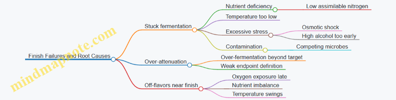
Wrap-Up: What “Good” Looks Like
A good alcoholic fermentation case is defined by measurable finish and yeast health that supports a smooth trajectory. Yeast must start strong, ferment without unnecessary stress, and then reach a stable endpoint confirmed by gravity trends and, when possible, residual sugar. The process is less about forcing an outcome and more about removing the conditions that make yeast hesitate.
10.4 Case Study: Lactic Acid Production with Substrate Feeding and Purification
Case Setup and Goal
This case study targets lactic acid production using a lactic acid bacterium (LAB) in a fed-batch fermentation. The core goal is consistent acid formation while preventing substrate oversupply, which can cause rapid pH drops, stress responses, and messy downstream purification.
A practical target is a fermentation broth that reaches high lactic acid concentration while maintaining manageable viscosity and minimal co-produced impurities such as acetic acid, ethanol, or excessive biomass.
Foundational Concepts That Drive the Plan
Lactic acid production is a metabolic outcome, not a switch. LAB convert carbohydrates into lactic acid, and the process performance depends on three linked constraints:
- Carbon availability: Too little substrate slows production; too much can shift metabolism and increase byproducts.
- Acid stress: As lactic acid accumulates, pH drops. Many LAB slow down when pH becomes too low.
- Mass transfer and mixing: In fed-batch, feeding changes viscosity and local concentrations. Good mixing reduces “hot spots” of sugar.
Mind Map: Process Logic
Substrate Feeding Strategy
Choosing a Feeding Approach
For fed-batch lactic acid production, the simplest reliable approach is controlled feeding based on residual sugar. You feed when residual sugar falls below a setpoint, which keeps cells in a productive regime.
Easy example: Suppose you measure residual glucose every hour. If it drops below 0.5 g/L, you start feeding at a moderate rate. If it rises above 1.0 g/L, you pause. This creates a “sawtooth” pattern that avoids long periods of excess sugar.
Why Feeding Works
LAB often perform best when carbon is available but not overwhelming. Excess sugar can increase osmotic stress and can push metabolism toward byproducts depending on strain and conditions. Controlled feeding also stabilizes the rate of acid formation, which makes pH control less chaotic.
Practical Feeding Window
A typical operational window is:
- Early phase: lower feed to build biomass and enzyme capacity.
- Production phase: higher feed rate to sustain lactic acid formation.
- Late phase: reduce feed as residual sugar rises or as acid concentration approaches the limit where activity slows.
Easy example: If lactic acid concentration rises quickly and residual sugar begins to climb, you reduce feed before pH control becomes a constant battle.
pH Control as the Hidden Co-Process
Lactic acid accumulation lowers pH. Many processes use base addition to keep pH in a workable range. The base choice matters because it influences downstream purification load.
Easy example: If you use calcium hydroxide, you form calcium lactate and later must convert it back to lactic acid, often requiring additional steps. If you use sodium hydroxide, you may simplify conversion but increase sodium salt handling.
A systematic approach is to:
- Set a pH window that supports production.
- Add base gradually rather than in large jumps.
- Track how base addition correlates with lactic acid rate.
Monitoring and Decision Rules
You need measurements that connect to actions.
- Residual sugar: drives feeding on/off.
- Lactic acid concentration: confirms production rate.
- pH trend: indicates whether acid formation is outpacing neutralization.
- Turbidity or biomass estimate: helps anticipate filtration difficulty.
Easy example: If lactic acid rises but residual sugar stays high, you likely have inefficient conversion or mixing issues. If lactic acid rises and residual sugar stays low, feeding is probably well matched.
Downstream Purification Workflow
Step 1: Cell Removal
Remove biomass first to prevent fouling in later steps. Centrifugation or filtration reduces solids and improves clarity.
Easy example: If you skip cell removal and go straight to concentration, you risk membrane fouling and higher cleaning frequency.
Step 2: Clarification
Clarification reduces suspended particles and color. This improves ion exchange performance and reduces the chance of precipitates.
Easy example: A simple polish filtration after centrifugation can noticeably reduce turbidity entering the purification stage.
Step 3: Concentration
Concentrate the clarified broth to reduce volume. Options include evaporation or membrane concentration.
Easy example: If you concentrate too aggressively, you may increase salt concentration and promote unwanted precipitation. Moderate concentration with controlled temperature helps.
Step 4: Purification by Ion Exchange or Conversion
Two common routes are:
- Ion exchange to remove salts and impurities.
- Conversion and re-acidification if you produced a lactate salt during fermentation.
Easy example: If your fermentation used calcium-based neutralization, you convert calcium lactate to lactic acid by removing calcium via a controlled conversion step, then polish.
Step 5: Final Polishing and Quality Checks
Polish to meet purity targets by removing residual salts, color, and trace impurities. Quality checks typically include lactic acid concentration, residual sugars, and impurity profiling.
Mind Map: Purification Decision Points
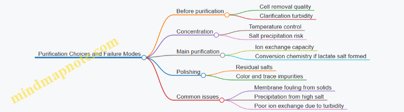
Integrated Example Run Summary
A coherent run looks like this: start with a low feed to establish biomass, maintain pH in a production-friendly window using gradual base addition, and feed based on residual sugar to prevent spikes. After fermentation, remove cells, clarify, concentrate under controlled conditions, and purify using the route consistent with your neutralization chemistry. The result is a broth that is both chemically concentrated and physically manageable, so purification steps stay stable rather than turning into a long series of “fix it later” interventions.
10.5 Case Study: Enzyme or Bioproduct Production with Monitoring and Recovery
This case study follows a typical workflow for producing an extracellular enzyme using a microbial culture, then recovering it with a sequence of steps that protect activity and remove unwanted material. The same logic applies to many bioproducts: you monitor the system while it is still changing, then you recover the target while the product is still stable.
System Setup and Target Definition
Start by defining what “success” means in measurable terms. For an extracellular enzyme, you usually track three signals: growth or biomass proxy, product activity in the broth, and product concentration or purity in the recovered fraction. A practical target might be “increase specific activity in the final concentrate” rather than only “maximize total activity,” because purification steps can concentrate impurities faster than they concentrate the enzyme.
A simple baseline plan uses a small set of sampling points: early growth, mid-production, and end of run. If you only sample at the end, you cannot tell whether the process failed due to poor production, poor recovery, or both.
Monitoring Strategy During Production
Monitoring should connect cause to effect. For extracellular enzymes, the broth is a mixture of cells, medium components, and secreted product. That means you need at least one measurement that reflects secretion and one that reflects broth clarity.
Key measurements and what they tell you:
- pH and temperature: enzyme activity is often sensitive to both, and microbial metabolism shifts pH during production.
- Dissolved oxygen or aeration rate: oxygen limitation can reduce secretion or change byproduct formation.
- Substrate consumption: if the carbon source drops early, production may stall; if it stays high, you may be feeding too aggressively.
- Broth activity assay: measure enzyme activity directly in clarified samples so you don’t confuse cell-associated activity with secreted activity.
- Turbidity or centrifuged supernatant volume: a quick proxy for how much material you must remove later.
A concrete example: suppose activity in the broth rises from 6 to 20 U/mL between mid and late sampling, but turbidity also increases sharply. That combination often means you will spend more time on clarification and may lose activity if filtration clogs. The fix is not only “filter better,” but also “reduce conditions that drive excessive biomass” such as overly strong agitation or feed that triggers rapid growth.
Process Control Decisions
When monitoring reveals a mismatch, you adjust the process using the smallest change that addresses the root cause.
- If pH drifts downward and activity later drops, you likely need stronger buffering or tighter pH control.
- If substrate remains high and activity plateaus early, you may be accumulating inhibitory metabolites or simply not reaching the secretion phase.
- If oxygen demand spikes and activity stalls, you may need to increase aeration or mixing, but only if the enzyme is stable under those conditions.
A useful habit is to record each adjustment alongside the next sampling results. That turns troubleshooting from guesswork into a short chain of evidence.
Recovery Workflow and Activity Protection
Recovery aims to separate the enzyme from cells and medium components while preserving activity. The order matters because each step changes the composition of the mixture.
A typical sequence:
- Clarification: remove cells by centrifugation or depth filtration. Keep samples cold and minimize hold times.
- Concentration: use ultrafiltration to reduce volume while retaining the enzyme. This step can also remove small inhibitors.
- Polishing: apply an additional separation such as ion exchange or affinity capture, depending on the enzyme’s properties.
- Buffer exchange and formulation: adjust to a storage-compatible buffer and stabilize the enzyme.
Concrete example of activity loss: if you concentrate at too high a temperature, the enzyme may denature even if the assay later looks “fine” at first. You can catch this by running a quick post-concentration stability check: measure activity immediately and again after a short hold under the intended storage conditions.
Mind Map: Monitoring to Recovery Logic
Mass Balance Example and What It Means
To connect monitoring to recovery, track activity through the workflow. For instance, if you start with 5,000 mL broth at 20 U/mL, total activity is 100,000 U. After clarification you might recover 85,000 U in supernatant, indicating 15% loss due to adsorption or handling. After concentration you might have 30,000 U in a smaller volume, suggesting additional loss from shear, temperature, or membrane effects. That pattern tells you where to focus improvements: clarification conditions if the first drop is large, membrane and temperature control if the second drop dominates.
Example: A Practical Sampling and Recovery Plan
- Sample at early growth, mid-production, and end.
- For each sample, clarify quickly and measure activity, pH, and turbidity.
- During recovery, measure activity after clarification, after concentration, and after polishing.
- Keep a simple log of volumes and activity so you can compute recovery yield and specific activity changes.
This structure prevents the common failure mode where the culture looks “okay” but the final product is weak because the recovery steps quietly removed activity. When monitoring and recovery are linked by mass balance, you can fix the right step instead of repeating the whole run and hoping for better luck.
11. Risk Management Sanitation and Regulatory Quality Practices
11.1 Hazard Analysis for Fermentation Operations and Process Steps
Hazard analysis in fermentation is about mapping what can go wrong, where it can go wrong, and how you will notice and prevent it. The goal is not to list every possible failure; it is to focus on hazards that can reasonably affect safety, legality, and product quality. A practical approach starts with process steps, then connects each step to credible hazards, and finally assigns controls that are measurable.
Process Step Mapping and Scope
Begin by writing a step-by-step flow from receiving inputs to final release. Include cleaning and sanitation steps, because they are part of the process, not background chores. Define the scope clearly: for example, whether you are analyzing food-grade lactic fermentations, industrial enzyme production, or both. Also decide what “hazard” means in your context: biological hazards (pathogens, spoilage organisms), chemical hazards (cleaning residues, allergens from ingredients), and physical hazards (foreign material, broken equipment parts).
A simple rule helps: if a step changes the environment for microbes, changes chemical composition, or changes exposure to people and equipment, it belongs in the map.
Hazard Identification by Step
For each step, ask three questions: What could introduce a hazard? What could allow it to survive or multiply? What could prevent detection until it is too late?
Common fermentation hazards include:
- Biological: contamination from raw materials, air, water, or equipment; cross-contamination between batches; survival of unwanted organisms through inadequate sanitation.
- Chemical: incomplete removal of sanitizers; carryover of cleaning agents; incorrect dosing of nutrients or antifoams.
- Physical: fragments from gaskets, seals, filters, or packaging; metal from wear; glass from sampling tools.
Example: In a vegetable brine process, the hazard at “ingredient loading” is contamination from produce surfaces and brine handling. The hazard at “fermentation” is survival and growth of unwanted microbes if salt concentration or temperature is off. The hazard at “packaging” is recontamination if seals or filling practices allow it.
Control Measures and Their Logic
Controls should be specific to the hazard and the step. Use a layered mindset: preventive controls reduce the chance of hazard introduction or growth, and detection controls catch problems before release.
Typical controls include:
- Sanitation controls: validated cleaning procedures, correct chemical concentration and contact time, and verification by swab or visual checks.
- Process controls: temperature and pH targets, salt concentration, oxygen management, and time-at-condition limits.
- Input controls: supplier specifications, incoming water testing, and ingredient screening.
- Engineering controls: filtration for air where relevant, closed transfers, strainers, and proper valve and gasket maintenance.
- Operational controls: batch segregation, controlled access, and defined sampling practices.
A control is stronger when it has a measurable criterion. “Clean” is not measurable; “sanitizer concentration within target range for the required contact time” is.
Detection, Verification, and Corrective Actions
Detection methods should match the hazard. For biological hazards, rely on microbiological testing where it is meaningful, but also use process indicators that correlate with microbial risk. For chemical hazards, verify cleaning effectiveness through residue checks and confirm dosing records. For physical hazards, use strainers, magnets where appropriate, and inspection routines.
Corrective actions should be pre-written for common deviations. For instance, if sanitizer concentration is out of range, you do not just “continue carefully.” You stop, re-clean, document the deviation, and assess whether any product contacted the affected surfaces.
Mind Map: Hazard Analysis Flow
Example: Brine Fermentation Hazard Analysis Snapshot
Consider a brine fermentation line.
- Step: Ingredient loading
- Hazard: unwanted microbes from produce surfaces
- Controls: rinse/trim standards, controlled handling time, closed transfer to brine tank
- Detection: incoming and in-process microbiological checks where applicable
- Step: Fermentation conditions
- Hazard: insufficient acidification leading to spoilage growth
- Controls: salt and temperature targets, pH monitoring frequency, defined hold times
- Detection: pH and titratable acidity trends; escalation when trajectories drift
- Step: Packaging
- Hazard: recontamination during filling
- Controls: hygienic design, validated sanitation of fillers, operator access control
- Detection: environmental monitoring and release testing aligned to your risk
Practical Output: What You Should End Up With
A complete hazard analysis results in a usable set of decisions: a process map, a hazard list tied to steps, control measures with criteria, verification methods, and corrective actions. When the document is good, a new operator can trace why a parameter matters and what to do when it is out of range—without guessing, improvising, or hoping for the best.
11.2 Cleaning Validation Including Swab Rinse and Visual Verification
Cleaning validation answers one practical question: after cleaning, can you prove the surface is acceptably free of residues and microbes, not just “looks clean”? The approach below combines swab sampling, rinse sampling, and visual verification so each method covers what the others might miss.
Core Concepts and Acceptance Logic
Start by defining what “clean” means for the specific surface and product. Residues can be chemical (acids, salts, sugars, proteins), biological (cells, spores), or both. Validation then sets acceptance criteria for each residue type and for microbial indicators when required. A good rule is to align sampling with the risk: high-touch areas, gasket grooves, weld seams, and dead legs get more attention than flat, freely draining surfaces.
A validation plan typically includes: (1) worst-case soil selection, (2) worst-case cleaning parameters, (3) sampling locations and number of replicates, (4) analytical methods and detection limits, and (5) documentation of deviations. If you only validate “easy” runs, you will eventually meet a “not-so-easy” run and be surprised.
Swab Sampling Foundations
Swabbing is best for irregular surfaces where rinsing may not recover residues well: valves, clamps, threads, and corners. The key is consistency.
- Define the swab area using a template (for example, 10 cm × 10 cm). Without a known area, results cannot be compared across runs.
- Use a validated swab and extraction method. The swab must release the target residue into the extraction liquid. If the extraction is weak, you will get false “clean” results.
- Swab with a repeatable pattern. A common approach is horizontal strokes, then vertical strokes, then diagonal strokes, rotating the swab tip to use fresh material.
- Include controls:
- Blank swabs handled like samples to check background.
- Positive recovery controls by spiking known residue on a similar surface and confirming you can recover it.
- Process blanks to ensure the cleaning chemicals or water do not interfere with analysis.
Example: Suppose you clean a stainless-steel transfer line used for a protein-containing broth. You swab the inner surface near a valve seat where flow slows. If your recovery control shows only 50% extraction efficiency, you adjust interpretation so a measured low value doesn’t automatically mean “no residue.”
Rinse Sampling Foundations
Rinse sampling is useful for smooth, drainable surfaces and for systems where you can collect a defined volume of rinse water or cleaning solution. It measures what comes off during the rinse step.
- Choose a defined rinse volume and collection method. For a tank, collect the final rinse fraction after a standardized drain time.
- Standardize flow and contact time for CIP systems. If the rinse is too short, residues remain; too long can dilute and complicate detection.
- Use appropriate containers and handling to prevent adsorption or degradation of target residues.
- Consider the “last rinse” concept. The final rinse is often the most informative because it represents the end state after cleaning.
Example: For a fermenter jacketed tank, you collect the final rinse from the bottom drain into a clean container, then test for conductivity or specific residue markers. If conductivity stays high but swabs on the top manway are clean, you likely have residue in the drain path rather than on the main wall.
Visual Verification as a Structured Layer
Visual verification is not a standalone proof, but it is excellent for catching gross failures and for guiding where swabbing should focus.
A structured approach uses a checklist and consistent lighting and viewing distance. Train personnel to look for specific indicators tied to residue types:
- Water break behavior on stainless steel can suggest oily residues.
- Discoloration or film can indicate incomplete removal of soils.
- Dry spots can point to poor wetting or inadequate rinse coverage.
Example: After cleaning a brine tank, you observe a faint ring stain near a gasket. Swabs taken only from the flat wall show low residue, but swabs around the gasket groove show elevated target marker levels. The visual cue correctly directed sampling.
Integrating Swab, Rinse, and Visual Results
Integration means you interpret results together, not in isolation.
- If rinse is positive but swabs are negative, suspect residues in drain lines, low-flow zones, or sampling mismatch.
- If swabs are positive but rinse is negative, suspect localized buildup on crevices that do not release during the rinse.
- If both are negative but visual shows residue, re-check sampling coverage and cleaning step execution; visual can reveal residue that your analytical method misses.
Mind Map: Cleaning Validation Workflow
Practical Validation Example with Reasoned Decisions
Imagine validating cleaning for a small pilot fermenter used for a sugar-rich medium.
- You select a worst-case run where the medium is allowed to dry slightly on a gasket during a delayed drain.
- You swab the gasket groove and a nearby weld seam using a 10 cm × 10 cm template for each location.
- You collect the final rinse fraction from the bottom drain after a standardized drain time.
- Visual verification flags a thin film near the gasket.
- Results show low residue in rinse but elevated residue in gasket swabs. The conclusion is not “cleaning failed” in general; it is “gasket groove cleaning coverage is insufficient under this worst-case condition,” prompting adjustment of spray pattern or contact time for that zone.
Documentation That Makes Results Defensible
Validation records should include the sampling plan, templates used, swab lot and extraction details, rinse collection volume and timing, visual checklist outcomes, raw analytical results, and calculations tied to acceptance criteria. If a deviation occurs, document what changed and whether it affects comparability. Clean data is useful; defensible data is usable.
11.3 Cross Contamination Control in Shared Facilities and Lines
Shared facilities are where good intentions meet real-world plumbing, traffic patterns, and “just one quick run” behavior. Cross contamination control is therefore less about one magic step and more about designing the whole system so the wrong microbes, allergens, or residues have fewer chances to hitch a ride.
Foundational Concepts for Shared Environments
Cross contamination happens through three main pathways: (1) direct contact, like splashes or shared tools; (2) indirect transfer, like aerosols, condensate, or dust; and (3) process carryover, like residues in hoses, valves, or drains. In shared lines, the biggest risk is often not the active fermentation itself but the transitions: changeovers, cleaning gaps, and sampling moments.
A practical way to think is “separation of time, space, and people.” If you can’t separate all three, you compensate with stronger cleaning verification, tighter scheduling, and controlled movement.
Facility Zoning and Flow Control
Start with physical and operational zoning. Define clean and dirty zones based on where contamination risk is highest. For example, ingredient receiving and waste handling belong in the dirty zone, while sterile connections and open product handling belong in the clean zone.
Then control flow:
- Use one-direction movement for personnel during changeovers.
- Keep carts, hoses, and utensils dedicated to a zone or clearly labeled for transfer.
- Prevent condensate from dripping across open product areas by managing overhead piping and using drip trays.
A simple rule helps: if something can move, it must be either controlled or cleaned between uses.
Shared Equipment and Line Changeover Strategy
Shared equipment is where “same tank, different batch” becomes “same tank, different problem.” Build changeover steps around the equipment’s contamination hotspots: gaskets, dead legs, valve seats, sight glasses, and hose connections.
Use a structured changeover sequence:
- Drain and remove bulk residues so cleaning starts with less material.
- Pre-rinse to reduce soil load.
- Clean with the validated detergent or cleaning agent at the required temperature and contact time.
- Rinse until conductivity or residue criteria are met.
- Sanitize or sterilize when the process requires it.
- Verify with swabs, visual inspection, and any line-specific checks.
Verification is not optional because visual cleanliness can miss biofilm in low-flow areas.
Mind Map: Cross Contamination Control System
Sampling and Handling Discipline
Sampling is a common “small action, big consequence” event. If you sample from multiple products on a shared line, you need a clear order of operations and tool control.
Best practice example: when switching from a high-risk organism process to a lower-risk one, sample the lower-risk product first. Use disposable sampling tools where feasible, or sanitize sampling ports and tools between products. Keep sample containers closed and labeled immediately to avoid mix-ups that cleaning can’t fix.
Example: Changeover Between Two Fermentation Products
Imagine a shared line used for Product A (high microbial load risk) and Product B (lower risk but strict quality specs). The control plan should include:
- Scheduling so Product B does not start until the full verification package for Product A is complete.
- Dedicated hoses or a documented hose swap with cleaning verification.
- A changeover record that lists the exact cleaning cycle parameters used.
- Swab sites that include valve manifolds and hose connection points.
If the swab results for a hotspot fail acceptance criteria, the line should remain on hold until re-cleaning and re-verification are completed. This prevents “we’ll just run and see” behavior.
Example: Preventing Condensate and Aerosol Transfer
Condensate can carry residues and microbes from overhead piping. A straightforward control is to inspect overhead lines for leaks and ensure drip trays are in place above open product areas. For aerosol risk, keep compressed air and venting systems routed away from open handling zones and ensure any vent filters are maintained according to the facility’s documented schedule.
Response Planning for Deviations
Even with good controls, deviations happen. Define what triggers an investigation: unexpected microbial results, failed swab sites, abnormal cleaning verification metrics, or evidence of cross-contact like a mislabeled container.
When a deviation occurs, the response should be systematic:
- Stop affected operations.
- Isolate the line or equipment section involved.
- Re-clean and re-verify the specific hotspots.
- Review the changeover record for missed steps or incorrect parameters.
The goal is to fix the mechanism, not just the symptom.
Practical Checklist for Shared Lines
- Zoning and one-direction flow are enforced.
- Changeovers follow a fixed sequence with validated parameters.
- Hotspots are included in swab verification.
- Sampling tools and order of sampling are controlled.
- Labels and traceability are immediate and consistent.
- Deviations trigger hold, isolation, re-cleaning, and re-verification.
11.4 Documentation Practices Including Batch Records and Deviation Handling
Good documentation turns fermentation from “it seemed fine” into “we can explain why it was fine.” Batch records capture what happened, when it happened, and what decisions were made. Deviation handling captures what went wrong, how it was assessed, and what was done to prevent the same mistake from reappearing in the next run.
Batch Records as the Source of Truth
A batch record is not a diary; it is a structured record that supports traceability, reproducibility, and release decisions. Start with identifiers: product name, batch number, equipment ID, strain or culture ID, and the planned process version. Then record the actual inputs: substrate lot numbers, water quality notes, inoculum preparation details, and any ingredient substitutions.
Next, document the operating timeline. For each critical step, record setpoints and actual values at defined intervals. Examples include:
- Inoculation time and inoculum volume or target cell density.
- Temperature profile and any hold times.
- pH setpoint, measured pH, and additions made to correct pH.
- Aeration or agitation settings, including any changes due to foaming or sensor issues.
- Feed additions with amounts, times, and calculated rationale.
Finally, record outcomes and checks. Include measurements that support acceptance criteria: final product attributes, yield or conversion calculations, and microbiological results. If a measurement is missing, document why and how the gap was handled.
Mind Map: Batch Record Content Flow
Deviation Handling as a Controlled Response
A deviation is any departure from the approved plan, including missing steps, unexpected results, or equipment behavior that could affect product quality. The key is to respond quickly enough to protect the batch, but systematically enough to avoid guessing.
Begin with classification. Not every deviation needs the same level of effort. A minor transcription error that does not affect process conditions may be corrected with documentation. A sensor failure that could change pH or temperature requires a deeper assessment because it can affect microbial performance and product formation.
Then perform immediate containment. If the deviation occurs during the run, decide whether to pause, continue, or adjust based on safety and quality risk. Document the decision and the reasoning, including what data supported it.
After the run, conduct an investigation. The goal is to determine impact, not to assign blame. Compare planned versus actual conditions, review calibration records, check whether similar issues occurred in prior batches, and evaluate whether the deviation could have altered critical quality attributes.
Mind Map: Deviation Handling Workflow
Example: Batch Record Entry That Prevents Confusion
Suppose pH control required additions. A strong entry looks like this: “At 10:40, measured pH 5.2 vs setpoint 5.8; added 0.8 L of 10% lactic acid solution; pH returned to 5.8 by 10:55.” This includes time, measurement, action, and outcome. A weak entry would only say “pH corrected,” which makes later review harder and increases the chance of repeating the same correction pattern blindly.
Example: Deviation Handling with Clear Impact Logic
During a vegetable brine fermentation, the temperature probe reading drifts by 2°C for 30 minutes. The deviation report should state what was observed, when it started, and what the operator did in response. Investigation then checks: whether the jacket control maintained temperature, whether the probe was recently calibrated, and whether the drift aligns with any change in acidification rate. If analytics show normal acid levels and microbial counts within acceptance criteria, the batch may be released with a documented rationale. If acidification is slow or off-profile, the batch may be rejected or subjected to defined disposition steps.
Practical Controls That Make Documentation Work
Use consistent terminology for measurements and actions so reviewers can scan quickly. Require contemporaneous entries so the record reflects reality rather than memory. Control amendments: if a correction is needed, record what changed and why, and ensure the correction is traceable to evidence.
Finally, link documentation to decisions. Batch records should feed directly into review sign-off, and deviation reports should feed directly into disposition. When the paperwork ends up disconnected from the decision, the system becomes a filing exercise instead of a quality tool.
11.5 Quality Specifications Including Acceptance Criteria and Release Testing
Quality specifications turn “it looks good” into measurable statements. They define what must be true for a batch to be released, how those truths are checked, and what happens when results land near the edge.
Quality Specifications as a System
A complete specification set usually includes:
- Identity: the product type and key characteristics that confirm you made the intended thing.
- Purity and Safety: limits for contaminants and hazards relevant to the process and product.
- Composition and Performance: targets or ranges for key nutrients, acids, alcohol, salt, or other functional components.
- Physical Properties: clarity, viscosity, particle size, or texture indicators when they matter.
- Microbiological Status: counts or absence criteria aligned to the product’s intended use.
- Packaging and Label Integrity: correct lot traceability and packaging configuration.
A practical rule: every specification should map to a test method and a decision rule. If you cannot state how you will measure it, it does not belong in the release specification.
Acceptance Criteria That Match the Test
Acceptance criteria are the “pass or fail” thresholds. They should reflect both analytical uncertainty and process variability.
Example: For fermented vegetables, you might set:
- pH: 3.6 to 4.2
- Titratable acidity: minimum value based on historical performance
- Yeast and mold: maximum count
- Enteric indicators: absence criteria
If your pH meter has a known repeatability, you set the acceptance limits with enough margin so normal measurement noise does not cause unnecessary holds.
Release Testing Workflow
Release testing is typically staged so you do not waste time on batches that fail early checks.
-
Pre-Release Review
- Confirm batch record completion, critical parameter logs, and deviations disposition.
- Verify that sampling was performed at the correct time and location.
-
Core Release Tests
- Microbiological results that define safety status.
- Chemical composition checks that confirm fermentation outcome.
- Physical checks when they affect usability or stability.
-
Lot Disposition Decision
- Pass: release.
- Hold: retest only when the deviation is clearly tied to sampling or instrument performance.
- Reject: when results exceed limits or safety criteria are not met.
A useful mindset: release testing is not just measurement; it is a controlled decision.
Mind Map: Quality Specifications to Release Decisions
Concrete Examples of Acceptance Criteria
Example: Lactic Fermentation Beverage
- pH: 3.2 to 3.8
- Lactic acid: minimum concentration
- Residual sugar: maximum to control sweetness and stability
- Yeast and mold: maximum count to reduce spoilage risk
- Pathogen indicators: absence criteria
- Label match: correct batch code and declared alcohol content if applicable
Example: Alcoholic Fermentation Intermediate
- Ethanol: within a defined range
- Residual sugars: maximum to prevent unintended secondary fermentation
- Volatile acidity: maximum to control off-notes
- Microbial counts: limits aligned to downstream processing tolerance
Release Testing Records and Traceability
Release testing must be traceable to the batch and to the method. Each result should link to:
- sample ID and sampling time
- method ID and instrument calibration status
- analyst or approved reviewer
- raw data summary and final calculated value
When a result is near a limit, the record should show whether the decision was based on the primary result, an approved retest, or a predefined exception rule.
Decision Rules That Prevent Confusion
Acceptance criteria should include explicit retest and hold rules. For instance:
- Retest is allowed only if the initial result is within a defined “investigation band” and there is a documented sampling or analytical issue.
- Safety-related criteria typically do not allow discretionary retesting after confirmatory failure.
This keeps release decisions consistent across batches and people, which is the whole point of writing specifications in the first place.
12. Practical Protocols from Bench to Pilot Scale
12.1 Designing Bench Experiments With Controls Replicates And Sampling
Bench experiments are where you earn the right to trust your results. The goal is not to “see what happens,” but to measure what changes when you change one thing at a time, while keeping the rest boringly consistent.
Core Experiment Logic
Start by writing a one-sentence question that can be answered with data. Example: “Does lowering fermentation temperature from 30°C to 26°C reduce lactic acid production rate in 24 hours?” Then list the controllable factors (temperature, inoculum level, substrate concentration, aeration) and the response variables (pH trajectory, product concentration, biomass proxy, defect indicators).
Next, define the experimental unit. In fermentation, the unit is usually one vessel with its own sampling and measurements. If you prepare one inoculum batch and split it into multiple vessels, the inoculum preparation becomes a separate source of variation, so you should treat it as a factor or randomize it across conditions.
Controls That Actually Control
Use controls to separate “process effect” from “setup effect.” A typical set:
- Negative control: no inoculation, to detect background acidification or contamination.
- Positive control: a condition you already know works (your baseline recipe).
- Process blank: all steps except the substrate, if relevant, to catch sensor drift or media carryover.
A practical example: if you’re testing a new salt level in vegetable brine, your negative control can be sterile brine with the same salt but no starter. Your positive control is the standard salt level with starter.
Replicates That Separate Noise from Signal
Replicates are not decoration; they let you estimate variability. Use:
- Biological replicates: independent fermentations started separately, ideally on different days or with different inoculum aliquots.
- Technical replicates: repeated measurements from the same sample, like duplicate pH readings or duplicate assay runs.
A good bench plan often uses 3 biological replicates per condition. If you only have resources for 2, increase sampling frequency to improve confidence in trends, and be explicit about uncertainty.
Sampling Plan with Timing and Handling
Sampling is where many experiments quietly go off the rails. Decide sampling times based on expected kinetics, not convenience. For fast fermentations, include early points (for example 0, 2, 4, 8, 12, 24 hours). For slower processes, space points wider.
Define how you handle samples:
- Volume: ensure you don’t remove enough liquid to change the system meaningfully.
- Mixing before sampling: stir or swirl consistently so you sample the same distribution.
- Temperature during handling: keep samples at a consistent condition before measurement.
- Filtration or centrifugation: decide whether you measure soluble products directly or after removing cells.
Example: for sugar and organic acid measurements, you might centrifuge samples at a fixed speed and time, then analyze the supernatant. If you do this, apply it identically across all conditions.
Factorial Thinking Without Overcomplication
If you test multiple factors, avoid random combinations that make interpretation impossible. Start with a one-factor-at-a-time approach for early screening. Once you know which factors matter, move to a small factorial design.
Example screening set for lactic fermentation:
- Temperature: 26°C vs 30°C
- Inoculum level: 1% vs 5%
- Salt: 1.5% vs 3.0%
Instead of testing all eight combinations immediately, run a 2×2 for temperature and inoculum first, keeping salt fixed at the baseline. Then add salt as a second stage.
Data Recording That Makes Analysis Straightforward
Use a template that captures:
- Batch identifiers and start time
- Exact recipe and measured starting values (not just targets)
- Environmental conditions (room temperature, incubator settings)
- Sampling times and any deviations
When you record pH, also record titration method or instrument calibration status. When you record product concentration, record assay conditions and dilution factors.
Mind Map: Bench Experiment Design Flow
Example: A Simple Bench Plan
Baseline: lactic fermentation in brine with a starter.
- Conditions: 26°C, 30°C
- Replicates: 3 biological replicates each
- Controls: one negative control at 30°C (no starter) and one positive baseline at 30°C
- Sampling: 0, 4, 8, 12, 24 hours
- Measurements: pH, titratable acidity, lactic acid concentration from clarified supernatant
If the 26°C condition shows a slower pH drop and lower lactic acid at 24 hours, you can quantify the difference in slope between 4–12 hours rather than relying on a single endpoint.
Common Failure Points to Prevent
- Changing more than one factor between conditions without noting it.
- Sampling inconsistently, like different mixing intensity or different centrifuge times.
- Treating technical replicates as a substitute for biological replicates.
- Forgetting that controls need the same handling steps as the test conditions.
A well-designed bench experiment makes the next step easier: you can interpret results without guessing which part of the setup caused the outcome.
12.2 Preparing Inoculum Including Propagation and Viability Checks
Inoculum preparation is where “the process” starts behaving like a system. If you begin with inconsistent cells, everything downstream—growth rate, acid production, ethanol yield, off-flavors—gets harder to control. The goal is simple: use a culture that is active, correctly adapted to the medium, and present in the right physiological state.
Core Concepts for Inoculum Readiness
Start by separating three ideas: identity, physiology, and quantity. Identity means the right organism or strain. Physiology means the cells are in a usable state for the intended fermentation conditions. Quantity means you can estimate how many active cells you are adding.
A practical way to think about physiology is “what the cells were doing right before you asked them to ferment.” Cells taken from an old plate may be stressed or entering stationary phase. Cells propagated in a medium similar to your process feed are more likely to resume growth quickly.
Propagation Workflow from Starter to Working Inoculum
Propagation is a controlled chain of transfers that moves cells from a source culture to a working inoculum volume. Keep transfers limited and purposeful.
-
Choose the propagation path
- For food fermentations with mixed cultures, propagation often means maintaining a starter under the same salt, temperature, and substrate profile used in production.
- For single-strain industrial fermentations, propagation typically uses defined media and controlled growth conditions.
-
Set the adaptation target
Match key environmental variables between propagation and production: temperature, pH range, oxygen availability, and major nutrients. You do not need identical conditions, but you do need the cells to recognize the “shape” of the environment. -
Use a staged scale-up
Transfer in steps that prevent overgrowth and excessive stress. Each step should reach a predictable growth phase rather than simply “as much volume as possible.” -
Plan the timing
Inoculum should be ready when the production vessel is ready. A common failure is adding inoculum that has sat too long after reaching the desired phase.
Viability Checks That Actually Help
Viability is not just “alive.” For fermentation performance, you care about whether cells can resume metabolism under your process conditions.
What to Measure
- Viable cell count: estimates the number of living cells.
- Metabolic activity: indicates whether cells are ready to consume substrate.
- Purity: confirms you did not accidentally propagate contaminants.
How to Interpret Results
- If viable counts are high but fermentation starts slowly, the issue is often physiological stress or mismatch in medium composition.
- If fermentation starts normally but later deviates, you may have a purity problem or an inoculum that was not adapted to the process feed.
Example Propagation and Viability Plan
Example: Single-strain lactic fermentation
- Propagate the strain in a medium with similar sugar type and buffering capacity to the production medium.
- Transfer to a working inoculum when cultures show active growth rather than deep stationary phase.
- Perform a viability estimate and a purity check before inoculation.
- In production, use a consistent inoculation ratio by volume or by estimated viable cells.
Example: Sourdough-style starter
- Maintain the starter with the same flour type, hydration level, and refresh schedule used for your process.
- Use a “refresh before production” step so the microbial community is active and producing acids and CO₂ at the expected pace.
- Check for obvious contamination signs and confirm that fermentation kinetics match your historical baseline.
Mind Map: Inoculum Preparation Logic
Practical Quality Controls and Documentation
Document the inoculum chain like you would document a recipe: source, media composition, transfer volumes, incubation conditions, and the moment you decided the culture was ready. A simple record prevents “mystery variability” when two batches behave differently.
Also, treat inoculum as a time-sensitive input. If you must hold it, define a maximum holding window and a temperature range, and verify that performance remains consistent within that window.
Quick Checklist Before Inoculation
- Correct organism or starter identity
- Propagation conditions matched to the production environment
- Culture reached the intended growth phase
- Viability and purity checks meet your acceptance criteria
- Inoculum is added promptly after readiness is confirmed
When these steps are consistent, inoculum becomes a predictable lever rather than a source of surprises. That predictability is what makes later control strategies work.
12.3 Running Batch and Fed Batch Trials with Defined Operating Windows
A batch or fed batch trial is a controlled experiment where you decide, in advance, what “good” looks like and what you will do when reality disagrees. The goal is not just to produce data, but to produce data you can interpret without guessing.
Define the Operating Windows First
Start by writing a one-page “operating window” that lists targets and allowable ranges for the variables that actually move the outcome.
- Biology-facing variables: temperature, pH, dissolved oxygen (DO) or oxygen limitation mode, agitation, and inoculum state.
- Chemistry-facing variables: substrate concentration (or feed rate), nitrogen source level, and key ratios such as carbon-to-nitrogen.
- Process-facing variables: mixing time, aeration rate, backpressure (if used), sampling frequency, and hold times.
Example: If you are running a lactic fermentation, you might set pH at 5.5 with an allowable band of 5.3–5.7, because small drift changes acid production rate and can shift the microbial community. For a yeast alcoholic run, you might instead prioritize temperature and sugar feed timing, because yeast performance can drop when osmotic stress spikes.
Build a Trial Plan That Matches the Kinetics
Batch trials are best for learning the shape of the curve: how quickly growth starts, when substrate becomes limiting, and when product formation accelerates or slows. Fed batch trials are best for learning how the system behaves when you prevent substrate from overshooting.
A practical way to structure the plan:
- Choose one baseline condition (your best guess from craft practice or lab history).
- Run one stress condition within safe bounds (slightly higher temperature, slightly lower DO, or a different feed concentration).
- Run one control condition (lower agitation, reduced aeration, or a conservative feed rate) to confirm the system is sensitive to the variable you think it is.
Mind Map: Trial Design Logic
Run Batch Trials with Defined Start-Up Rules
Batch execution often fails at the beginning, not the middle. Define start-up rules so you don’t “fix” the run in ways that blur interpretation.
- Inoculum rule: record inoculum source, time since preparation, and any preconditioning. A fresh inoculum can shorten lag time; an aged one can make the same recipe look ineffective.
- Start-up sampling rule: sample more frequently during the first third of the run, when pH and DO can swing quickly.
- Action rule for drift: if pH control is used, specify the maximum correction rate and the acceptable overshoot. For example, if pH rises above 5.7, you might reduce base addition rather than aggressively forcing it back.
Example: In a vegetable brine fermentation, you might not use active pH control, but you still define an operating window for temperature and salt concentration. If temperature rises, you expect faster acidification; if it rises too much, you may see off-odors due to unwanted metabolic routes. Your trial notes should capture which window you crossed.
Run Fed Batch Trials with Feed Logic and Delay Awareness
Fed batch is where “defined windows” matter most, because feed changes can take time to show up in measurements.
- Feed trigger rule: decide whether feed is based on time, DO, residual substrate, or an indirect proxy. Time-based feeding is simple but can miss unexpected delays.
- Feed concentration rule: keep feed concentration consistent so you can interpret rate changes as biology, not dilution artifacts.
- Feed-to-response delay rule: estimate how long it takes for a feed change to affect DO, pH, or product formation. Then sample at a cadence that captures that delay.
Example: Suppose you feed a sugar solution to a yeast culture. If you increase feed rate, DO may drop first (oxygen demand rises), then ethanol production may shift later. If you sample only once per hour, you might miss the DO-driven transition and misattribute the later behavior.
Use a Simple Decision Checklist During the Run
When something goes out of range, don’t improvise. Use a checklist that separates measurement issues from real process changes.
- Sensor sanity: confirm probe calibration status and check for obvious fouling or air bubbles.
- Mixing sanity: verify agitation and aeration are within setpoints; poor mixing can create local substrate pockets.
- Control sanity: confirm valves and pumps responded correctly to commands.
- Biology sanity: if the system is truly out of range, document the exact time and magnitude of deviation.
Interpret Results with Rate and Balance Checks
After the run, compute at least two things: a rate estimate and a mass balance sanity check.
- Rate estimate: use time-series data to estimate specific growth or specific product formation over the window where conditions were stable.
- Mass balance check: compare substrate consumed (or feed added) with product formed. If the numbers don’t reconcile, the issue is often sampling timing, measurement bias, or untracked byproducts.
Example: If you fed more substrate but product yield per substrate drops sharply, check whether pH drift or oxygen limitation changed the metabolic route. If yield stays consistent but total titer is lower, check whether the system spent time in a longer lag phase due to inoculum state or start-up conditions.
Record Everything That Affects Interpretation
A trial log should include: operating window values, actual setpoints, measured values, sampling times, and any deviations with timestamps. The log is the difference between “we ran it” and “we learned something.”
12.4 Troubleshooting Common Failures Including Slow Start Stuck Fermentation and Off Notes
When fermentation goes wrong, the fastest path to a fix is to separate symptoms from causes. A slow start usually points to inoculum or early environmental conditions. A stuck fermentation points to a later-stage limitation such as oxygen, pH drift, nutrient depletion, or inhibitory byproducts. “Off notes” can come from the same root causes, but the sensory clues help you narrow which metabolic route went sideways.
Mind Map: Failure Modes and First Checks
Slow Start Fermentation
A slow start is when activity begins later than expected, even though the batch is otherwise “healthy.” Start with a timeline: record inoculation time, first temperature stabilization, and the first measurable change (CO₂ evolution, pH drop, or product formation). If nothing moves after the expected lag, check inoculum first.
Inoculum viability and readiness. If you propagate starter cultures, viability can drop quietly. A simple example: a sourdough batch uses a starter that was refrigerated for weeks and fed only once. The dough may rise sluggishly because the starter contains many cells that are alive but not metabolically ready. Fix by using a fresh, actively fermenting starter and confirm it shows consistent activity in a small test before scaling.
Inoculum size. Under-inoculation can look like “mysterious failure.” Example: a small lactic fermentation uses too little culture to overcome initial stress from salt and temperature. The culture may survive but not dominate quickly. Increase inoculum within your process limits or adjust early conditions to help it establish.
Temperature and pH at the moment of inoculation. Many fermentations are sensitive to early conditions. Example: fermenting at 20°C when your target is 30°C can extend the lag so much that competitors gain ground. Verify that the bulk temperature is at target before adding inoculum, and confirm pH is within the organism’s working window.
Oxygen level and mixing. Aerobic or microaerobic organisms can stall if oxygen is too low or too high. Example: an aerobic yeast process with poor sparging may show delayed CO₂ production because oxygen transfer is insufficient. Conversely, excessive aeration can push metabolism toward unwanted byproducts. Improve mixing and confirm aeration delivery rather than only adjusting setpoints.
Stuck Fermentation
A stuck fermentation often shows a plateau: pH stops changing, CO₂ evolution slows, and product formation flattens. Treat it like a balance problem: what is left to consume, and what is limiting growth or metabolism.
Substrate or nutrient depletion. If sugar is depleted, the system will stop even if cells are fine. Example: a fed-batch plan that under-feeds carbon can lead to early exhaustion and a plateau long before the intended endpoint. If nitrogen is limiting, cells may remain present but stop producing the desired product. Check residual substrate and nutrient levels rather than guessing.
pH drift and acid accumulation. Many fermentations slow when acids accumulate and pH moves out of range. Example: lactic fermentation in a brine can stall if buffering capacity is low and acid production drops the pH faster than expected. Use your measured titratable acidity and pH trend to decide whether to adjust buffering or revise feed rate.
Inhibitors and residues. Cleaning residues can inhibit cells even when sanitation looks “clean.” Example: a line rinsed quickly after CIP may leave traces that suppress yeast activity, causing a plateau. Confirm rinse effectiveness and verify that the first samples after cleaning show normal growth behavior.
Mixing and mass transfer. Poor mixing can create local zones with high substrate or low oxygen. Example: in a larger tank, the top layer may be oxygen-rich while the bottom becomes oxygen-poor, leading to uneven metabolism and early stalling. Improve mixing intensity or adjust impeller placement and verify with simple tracer tests.
Off Notes
Off notes are not just sensory complaints; they are diagnostic signals. The key is to link the note to a likely metabolic pathway and then to a controllable variable.
Acid profile imbalance. If a fermentation intended to be lactic becomes more acetic, you may be seeing oxygen exposure or competition. Example: a vegetable brine that was repeatedly opened for tasting can introduce oxygen and favor acetic pathways. Reduce headspace oxygen exposure and minimize unnecessary agitation.
Sulfur-like aromas. Sulfur compounds often correlate with nitrogen form and redox conditions. Example: an alcoholic fermentation with inadequate assimilable nitrogen can produce harsh sulfur notes. Measure available nitrogen indicators and adjust nutrient strategy within your formulation.
Contamination signatures. Off notes that appear suddenly after a period of normal activity often indicate contamination or a process interruption. Example: a batch that was stable until a temperature dip then develops unexpected flavors may have allowed a contaminant to outcompete the intended culture. Compare microbial counts from early and late timepoints to confirm.
Sampling and measurement errors. Sometimes the “off note” is real, but the data is misleading. Example: pH probes calibrated incorrectly can make you think the fermentation is acidifying too fast, leading to unnecessary interventions. Recalibrate and verify probe performance with fresh standards before changing the process.
Example: A Systematic Troubleshooting Workflow
- Confirm the symptom pattern using a time series of temperature, pH, and a product proxy.
- Check inoculum history for viability, storage time, and whether it was actively fermenting before use.
- Verify early conditions at inoculation: temperature, pH, and oxygen delivery.
- Measure what is left in the system: residual substrate and key nutrients.
- Inspect process hygiene and residues if the failure follows cleaning or line changes.
- Assess mixing and mass transfer using operational observations and simple tracer checks.
- Link sensory notes to likely pathways and adjust only the variable that matches the suspected mechanism.
A good troubleshooting habit is to change one lever at a time and document the outcome. That turns “mystery fermentation” into a repeatable diagnosis, even when the batch is already behaving badly.
12.5 Building Standard Operating Procedures for Repeatable Fermentation
Repeatable fermentation comes from repeatable decisions. A Standard Operating Procedure (SOP) should therefore describe not only what to do, but also what to check, what to record, and what to do when reality disagrees with the plan. The goal is simple: two operators following the same SOP should produce the same outcome, within defined limits.
SOP Purpose and Scope
Start with a short statement of purpose and a clear scope: product type, organism or culture source, vessel size range, and whether the SOP covers upstream, fermentation, and/or downstream handoff. Include a “non-goals” line to prevent accidental use for tasks it doesn’t cover, such as media formulation or packaging.
Roles, Responsibilities, and Handoffs
Define who performs each step and who verifies it. For example, the operator might prepare inoculum and start the run, while a second person verifies calibration status and approves the batch record before fermentation begins. Handoffs should specify what must be true at transfer time: temperature within tolerance, pH sensor reading valid, and inoculum added at the stated time window.
Materials, Equipment, and Calibration Requirements
List equipment by function, not brand: jacketed tank, pH probe, DO probe, balance, thermometer, and sampling tools. For each measurement device, state calibration frequency and acceptance criteria. A practical SOP includes a quick pre-run checklist: probe cleanliness, cable integrity, calibration date, and whether the probe passes a short verification step.
Process Steps with Decision Points
Write the SOP as a sequence of actions with explicit decision points. Each step should include: objective, method, target range, sampling frequency, and what to do if results drift.
A useful pattern is:
- Prepare
- Verify readiness
- Execute
- Monitor
- Record
- Release or stop
For instance, during fermentation monitoring, the SOP should specify what “pH out of range” means (e.g., below 4.2 or above 4.6 for a lactic process) and the corrective action order: confirm probe reading, check mixing, then adjust dosing. If the corrective action fails, the SOP should require escalation and a deviation record.
Sampling Plan and Data Integrity
Sampling is where good intentions go to die. Define sample volume, container type, labeling rules, and mixing before sampling. Specify how samples are handled to avoid bias: time to analysis, temperature control, and whether samples are filtered or preserved. Record the exact time of sampling and the operator initials.
Include a rule for data integrity: if a measurement is invalid, record the reason and the replacement method. Never silently overwrite values.
Batch Record Structure
A batch record should mirror the SOP steps. Use fields that force completeness: lot numbers for ingredients, inoculum ID, vessel ID, start time, setpoints, actual readings, and any deviations. Add a section for “observations” that are factual, such as foam level category or odor description, without interpretation.
Deviation Handling and Corrective Actions
Define what triggers a deviation: missed sterilization hold time, temperature excursion beyond tolerance, unexpected contamination signal, or sensor failure. The SOP should require immediate containment actions (e.g., stop addition, isolate vessel, increase sampling frequency) and a structured follow-up: root cause hypothesis, corrective action, and effectiveness check.
Example: SOP Template for Fermentation Monitoring
Example: Monitoring and Correction Logic
- Objective: Maintain pH and temperature within target ranges.
- Targets: pH 4.3–4.5; temperature 30–32°C.
- Frequency: pH and temperature every 30 minutes; DO every 15 minutes for aerobic runs.
- If pH < 4.3:
- Verify probe reading with a secondary check.
- Confirm mixing is active.
- Adjust dosing per dosing table.
- Recheck within 10 minutes.
- If pH remains low after two corrections: stop corrective dosing, escalate, and start deviation record.
Mind Map: SOP Components and Flow
Completion and Release Criteria
End criteria should be measurable: time-based, product-based (e.g., acid concentration), or growth-based (e.g., cell density). Specify final sampling, acceptance thresholds, and what must be true before transfer. If the run ends early, the SOP should state whether the batch is released, reworked, or discarded.
Practical Example: A Repeatable Start-Up Section
A start-up SOP section should include a “readiness gate” checklist: calibrated sensors installed, mixing confirmed, media temperature at target, and inoculum ID verified. Then it should specify the exact start event definition, such as “start time recorded when inoculum addition begins,” so later calculations and comparisons stay consistent.
A good SOP reads like a reliable conversation between the process and the people running it. When followed, it turns fermentation from a craft that depends on memory into a craft that depends on method.