Practical Machine Learning Engineering with End to End Model Development and Deployment
1. Introduction to Machine Learning Engineering
1.1 Overview of Machine Learning Engineering
Machine Learning Engineering (MLE) is a discipline that combines software engineering principles with machine learning (ML) techniques to design, build, deploy, and maintain ML systems that deliver real-world value. Unlike traditional data science, which often focuses on model development and experimentation, MLE emphasizes the operationalization and scalability of ML models in production environments.
What is Machine Learning Engineering?
- Definition: The practice of applying engineering principles to the end-to-end lifecycle of machine learning models, from data ingestion and model training to deployment and monitoring.
- Goal: To create reliable, scalable, maintainable, and efficient ML systems that integrate seamlessly with existing software infrastructure.
Key Components of Machine Learning Engineering
Why is Machine Learning Engineering Important?
- Bridging the Gap: Translates ML research and prototypes into production-ready systems.
- Reliability: Ensures models perform consistently and robustly in real-world scenarios.
- Scalability: Designs systems that handle large volumes of data and requests.
- Maintainability: Facilitates easy updates, retraining, and debugging.
Example: From Prototype to Production
Imagine a data scientist builds a model to predict customer churn using Jupyter notebooks. The model achieves 85% accuracy on test data. However, deploying this model directly to production without engineering can cause issues:
- Lack of automated data validation might lead to poor input data causing failures.
- No version control can cause confusion about which model is live.
- Absence of monitoring means model degradation goes unnoticed.
Machine Learning Engineering addresses these by:
- Building automated data pipelines that validate and preprocess incoming data.
- Packaging the model with dependencies and versioning it using tools like MLflow.
- Deploying the model behind a REST API with logging and monitoring to track performance.
Mind Map: Roles and Responsibilities of an ML Engineer
Practical Example: Simple ML Engineering Workflow
- Data Ingestion: Collect customer data from a database.
- Data Validation: Check for missing or anomalous values.
- Feature Engineering: Create features like “days since last purchase.”
- Model Training: Train a logistic regression model.
- Model Evaluation: Use cross-validation to assess accuracy.
- Model Packaging: Serialize the model using
pickle. - Deployment: Serve the model via a Flask API.
- Monitoring: Log prediction requests and track accuracy over time.
# Example: Packaging and serving a simple model
import pickle
from flask import Flask, request, jsonify

# Load trained model
with open('model.pkl', 'rb') as f:
    model = pickle.load(f)

app = Flask(__name__)

@app.route('/predict', methods=['POST'])
def predict():
    data = request.json['features']
    prediction = model.predict([data])
    return jsonify({'prediction': prediction[0]})

if __name__ == '__main__':
    app.run(debug=True)
Summary
Machine Learning Engineering is a critical discipline that ensures ML models are not just accurate in theory but also effective, reliable, and maintainable in production. It encompasses data management, model development, deployment, monitoring, and continuous improvement, all supported by automation and best practices.
By mastering MLE, engineers and data scientists can deliver impactful ML solutions that drive business value at scale.
1.2 Differences Between Data Science and ML Engineering
Machine Learning Engineering and Data Science are closely related fields but have distinct roles, responsibilities, and skill sets. Understanding these differences is crucial for professionals aiming to excel in either domain or collaborate effectively across teams.
Overview
| Aspect | Data Science | Machine Learning Engineering |
|---|---|---|
| Primary Goal | Extract insights and knowledge from data | Build, deploy, and maintain ML models at scale |
| Focus Area | Data exploration, statistical analysis | Model productionization, scalability, reliability |
| Typical Outputs | Reports, visualizations, prototypes | Production-ready ML systems, APIs, pipelines |
| Tools & Skills | Python, R, SQL, visualization tools | Python, Java, Docker, Kubernetes, CI/CD tools |
| Collaboration | Works closely with business stakeholders | Works closely with software engineers and DevOps |
Mind Map: Core Focus Areas
Detailed Comparison
Data Handling and Preparation
- Data Scientist: Focuses on understanding data distributions, cleaning data, and feature engineering primarily to improve model accuracy and insights.
- ML Engineer: Builds robust, automated data pipelines that ensure data consistency and availability in production environments.
Example:
- A data scientist might manually clean and transform a dataset using Jupyter notebooks to explore correlations.
- An ML engineer implements an automated ETL pipeline using Apache Airflow to feed real-time data into the model serving system.
Model Development vs. Productionization
- Data Scientist: Develops and experiments with various models to find the best performing one using frameworks like scikit-learn or TensorFlow.
- ML Engineer: Focuses on converting these models into scalable, reliable services that can handle production workloads.
Example:
- Data scientist prototypes a fraud detection model with XGBoost.
- ML engineer packages the model into a Docker container, sets up REST APIs, and integrates it with the transaction processing system.
Performance and Scalability
- Data Scientist: Concerned with model accuracy, precision, recall, and other evaluation metrics.
- ML Engineer: Ensures low latency, high throughput, fault tolerance, and resource optimization in production.
Example:
- Data scientist optimizes hyperparameters to improve F1-score.
- ML engineer optimizes model inference by quantizing the model and deploying it on GPU-enabled servers.
Monitoring and Maintenance
- Data Scientist: May be involved in periodic model evaluation and retraining based on new data.
- ML Engineer: Implements continuous monitoring for data drift, model degradation, and automates retraining pipelines.
Example:
- Data scientist analyzes model performance monthly.
- ML engineer sets up dashboards and alerting systems using Prometheus and Grafana to detect anomalies in real-time.
Mind Map: Skill Sets Comparison
Integrated Example: Building a Spam Detection System
| Role | Responsibilities | Example Tasks |
|---|---|---|
| Data Scientist | Analyze email datasets, build initial models | Exploratory data analysis, feature extraction, model prototyping with logistic regression |
| ML Engineer | Deploy model to production, maintain system | Containerize model, build REST API, set up monitoring, automate retraining pipeline |
Scenario:
- The data scientist uses a sample dataset to create a spam classifier prototype.
- The ML engineer takes the prototype, packages it into a scalable microservice, and integrates it with the email platform.
Summary
While data scientists excel at extracting insights and building models, ML engineers specialize in operationalizing these models to deliver reliable, scalable, and maintainable ML-powered applications. Both roles are complementary and critical for successful machine learning projects.
Further Reading
- Machine Learning Engineering vs Data Science: What’s the Difference?
- MLOps: Continuous Delivery and Automation Pipelines in ML
This section has provided a comprehensive understanding of the differences between Data Science and Machine Learning Engineering, enriched with mind maps and practical examples to clarify their distinct yet interconnected roles.
1.3 Key Challenges in ML Engineering
Machine Learning Engineering is a multidisciplinary field that combines software engineering, data science, and domain expertise to build scalable, reliable, and maintainable ML systems. Despite its promise, ML engineering faces several unique challenges that can impact the success of projects. In this section, we will explore these key challenges with practical examples and mind maps to help you visualize and address them effectively.
Challenge 1: Data Quality and Availability
Poor data quality or insufficient data can severely limit model performance. Issues include missing values, noisy data, biased samples, and inconsistent formats.
Example: Imagine building a customer churn prediction model where the dataset has missing customer interaction logs or outdated demographic information. The model might learn incorrect patterns or fail to generalize.
Mind Map:
Challenge 2: Feature Engineering Complexity
Creating meaningful features that capture domain knowledge is often time-consuming and requires iterative experimentation.
Example: In a credit scoring model, transforming raw transaction data into features like “average monthly spend” or “number of late payments” can significantly improve model accuracy.
Mind Map:
Challenge 3: Model Selection and Training
Choosing the right algorithm and tuning hyperparameters can be challenging, especially with limited computational resources.
Example: Selecting between a Random Forest and a Gradient Boosting model for a classification task requires understanding trade-offs in interpretability, training time, and performance.
Mind Map:
Challenge 4: Deployment and Scalability
Deploying ML models into production environments requires integration with existing systems, scalability, and low latency.
Example: Deploying a recommendation engine that serves millions of users per day demands efficient model serving and load balancing.
Mind Map:
Challenge 5: Monitoring and Maintenance
Models can degrade over time due to data drift or concept drift. Continuous monitoring and retraining are essential.
Example: A spam detection model may become less effective as spammers change tactics, requiring retraining with new data.
Mind Map:
Challenge 6: Reproducibility and Collaboration
Ensuring that experiments can be reproduced and that teams can collaborate efficiently is critical for scaling ML efforts.
Example: Two data scientists working on the same project need to share code, data versions, and model checkpoints to avoid duplicated efforts.
Mind Map:
Challenge 7: Security, Privacy, and Compliance
Handling sensitive data and complying with regulations like GDPR or HIPAA adds complexity to ML engineering.
Example: Training a healthcare model requires anonymizing patient data and ensuring secure data storage.
Mind Map:
Summary
| Challenge | Key Considerations | Example Use Case |
|---|---|---|
| Data Quality and Availability | Handling missing, noisy, biased data | Customer churn prediction |
| Feature Engineering Complexity | Domain knowledge, automation | Credit scoring features |
| Model Selection and Training | Algorithm choice, hyperparameter tuning | Random Forest vs Gradient Boosting |
| Deployment and Scalability | Serving, latency, infrastructure | Recommendation engine at scale |
| Monitoring and Maintenance | Drift detection, retraining | Spam detection model maintenance |
| Reproducibility and Collaboration | Experiment tracking, version control | Team collaboration on ML projects |
| Security, Privacy, Compliance | Data anonymization, regulatory adherence | Healthcare predictive models |
Understanding and addressing these challenges early in the ML lifecycle will improve your chances of building robust, scalable, and maintainable machine learning systems.
1.4 Importance of End-to-End Model Lifecycle
Machine Learning (ML) engineering is not just about building a model that performs well on a dataset; it encompasses the entire journey from problem conception to deploying and maintaining models in production. Understanding the end-to-end model lifecycle is crucial for delivering reliable, scalable, and maintainable ML solutions.
What is the End-to-End Model Lifecycle?
The end-to-end model lifecycle refers to all stages involved in developing, deploying, and maintaining a machine learning model. It ensures that models are not only accurate but also robust, reproducible, and aligned with business objectives.
Why is it Important?
- Holistic View: Enables engineers and data scientists to see the bigger picture beyond just model accuracy.
- Reproducibility: Ensures experiments and results can be replicated, which is vital for debugging and compliance.
- Scalability: Facilitates smooth scaling from prototype to production.
- Maintenance: Allows continuous monitoring and updating to keep models relevant.
- Collaboration: Bridges gaps between data scientists, engineers, and business stakeholders.
Mind Map: End-to-End Model Lifecycle Overview
Detailed Breakdown with Examples
Problem Definition
- Define the business problem clearly.
- Example: Predict customer churn to reduce attrition rate.
Data Collection & Understanding
- Gather relevant data and perform exploratory data analysis.
- Example: Collect customer interaction logs, demographics, and transaction history.
Data Preparation & Feature Engineering
- Clean data, handle missing values, and create meaningful features.
- Example: Create features like “days since last purchase” or “average monthly spend.”
Model Training & Selection
- Train multiple models and select the best performing one.
- Example: Compare Random Forest, Gradient Boosting, and Logistic Regression.
Model Validation & Testing
- Use cross-validation and test on unseen data.
- Example: Evaluate using ROC-AUC and confusion matrix.
Model Packaging & Serialization
- Serialize the model with dependencies for deployment.
- Example: Save a Scikit-learn model using
joblib.
Model Deployment
- Deploy the model as an API or batch job.
- Example: Serve the model using Flask REST API.
Monitoring & Maintenance
- Track model performance and data drift.
- Example: Monitor prediction accuracy and input feature distributions.
Model Retraining & Updating
- Retrain models periodically or when performance degrades.
- Example: Schedule monthly retraining with fresh data.
Documentation & Governance
- Document experiments, decisions, and compliance requirements.
- Example: Maintain an ML model registry with metadata.
Mind Map: Benefits of Managing the Full Lifecycle
Practical Example: End-to-End Lifecycle in Action
Imagine a retail company wants to implement a demand forecasting model:
- Problem Definition: Forecast weekly sales for inventory optimization.
- Data Collection: Gather historical sales, promotions, holidays, and weather data.
- Data Preparation: Clean missing sales data, engineer features like “week of year” and “promotion flag.”
- Model Training: Train an XGBoost regression model.
- Validation: Use time-series cross-validation to avoid lookahead bias.
- Packaging: Serialize the model and dependencies using Docker.
- Deployment: Deploy on AWS Lambda for serverless inference.
- Monitoring: Track forecast accuracy and input feature distributions.
- Retraining: Retrain monthly with new sales data.
- Documentation: Log all experiments and deployment details in MLflow.
This approach ensures the model remains accurate, scalable, and aligned with business needs.
Summary
The end-to-end model lifecycle is the backbone of practical machine learning engineering. By embracing this full lifecycle approach, ML engineers and data scientists can build models that are not only performant but also reliable, maintainable, and impactful in real-world applications.
1.5 Setting Up Your Development Environment: Tools and Frameworks
Setting up a robust and efficient development environment is a foundational step for any machine learning engineer. This section guides you through selecting the right tools and frameworks, configuring your workspace, and ensuring reproducibility and scalability.
Why is Environment Setup Important?
- Ensures consistency across development, testing, and production.
- Facilitates collaboration among team members.
- Simplifies debugging and maintenance.
- Enables scalability and deployment readiness.
Mind Map: Development Environment Setup
Step 1: Choose Your Hardware
Example: For deep learning projects, a GPU-enabled machine significantly speeds up training. If you don’t have access to local GPUs, consider cloud platforms like Google Colab or AWS EC2 instances with GPU support.
# Example: Check if GPU is available in PyTorch
import torch

gpu_available = torch.cuda.is_available()
print(f"GPU Available: {gpu_available}")
Step 2: Select and Configure Your Operating System
Linux (Ubuntu) is often preferred for ML development due to better support for ML libraries and tools.
Best Practice: Use WSL2 on Windows to run a Linux environment if you are on Windows.
Step 3: Setup Package Management and Virtual Environments
Use virtual environments to isolate project dependencies.
Example: Using conda to create and activate an environment.
conda create -n ml_env python=3.9 -y
conda activate ml_env
Install essential packages:
pip install numpy pandas scikit-learn jupyter matplotlib seaborn
Step 4: Choose Your IDE or Editor
- Jupyter Notebook: Great for exploratory data analysis and prototyping.
- VS Code: Lightweight, extensible, supports debugging and Git integration.
- PyCharm: Full-featured IDE with advanced debugging and refactoring.
Example: Launch Jupyter Notebook
jupyter notebook
Step 5: Install Core ML Frameworks
- Scikit-learn: For classical ML algorithms.
- TensorFlow / Keras: For deep learning.
- PyTorch: Flexible deep learning framework.
Example: Installing PyTorch with GPU support
pip install torch torchvision torchaudio --extra-index-url https://download.pytorch.org/whl/cu117
Step 6: Data Handling and Version Control
- Use Pandas and NumPy for data manipulation.
- Use DVC (Data Version Control) to version datasets and track changes.
Example: Initialize DVC in your project
git init

dvc init
Add a dataset to DVC tracking:
dvc add data/dataset.csv
Step 7: Experiment Tracking and Logging
Track experiments to compare model versions and hyperparameters.
Tools: MLflow, Weights & Biases
Example: Logging parameters and metrics with MLflow
import mlflow

mlflow.start_run()
mlflow.log_param("learning_rate", 0.01)
mlflow.log_metric("accuracy", 0.95)
mlflow.end_run()
Step 8: Containerization with Docker
Containerize your environment to ensure portability and consistency.
Example: Basic Dockerfile for a Python ML project
FROM python:3.9-slim
WORKDIR /app
COPY requirements.txt ./
RUN pip install --no-cache-dir -r requirements.txt
COPY . ./
CMD ["python", "train.py"]
Build and run:
docker build -t ml-project .
docker run -it ml-project
Step 9: Version Control with Git
Maintain code versions and collaborate effectively.
Best Practice: Commit often with clear messages.
git add .
git commit -m "Initial environment setup"
git push origin main
Summary Table of Recommended Tools
| Category | Tool/Framework | Purpose |
|---|---|---|
| Hardware | GPU-enabled machines | Accelerated training |
| OS | Ubuntu/Linux | Stable ML environment |
| Package Manager | conda, pip | Dependency management |
| Virtual Env | venv, conda env | Isolate dependencies |
| IDE | Jupyter, VS Code, PyCharm | Development and debugging |
| ML Frameworks | Scikit-learn, TensorFlow, PyTorch | Model building |
| Data Handling | Pandas, NumPy | Data manipulation |
| Data Version Control | DVC | Dataset versioning |
| Experiment Tracking | MLflow, Weights & Biases | Track experiments |
| Containerization | Docker | Environment portability |
| Version Control | Git | Code versioning and collaboration |
By carefully setting up your development environment with these tools and best practices, you lay a strong foundation for efficient, reproducible, and scalable machine learning projects.
2. Problem Definition and Data Understanding
2.1 Defining the Business Problem and Success Metrics
Defining the business problem clearly is the foundational step in any successful machine learning project. Without a well-articulated problem statement and measurable success criteria, the project risks misalignment with business goals, wasted resources, and ultimately, failure to deliver value.
Why Defining the Business Problem Matters
- Alignment: Ensures ML efforts target real business needs.
- Focus: Narrows down the scope to manageable, impactful tasks.
- Communication: Provides a common language between stakeholders and engineers.
- Measurement: Enables objective evaluation of model success.
Steps to Define the Business Problem
- Engage Stakeholders: Understand their pain points, goals, and constraints.
- Contextualize the Problem: Frame the problem within the business domain.
- Specify the Objective: What exactly do we want to predict, classify, or optimize?
- Identify Constraints: Data availability, latency, cost, compliance.
- Define Success Metrics: Quantitative measures to evaluate outcomes.
Mind Map: Defining the Business Problem
Example 1: Predicting Customer Churn for a Telecom Company
Business Context: A telecom company wants to reduce customer churn to improve revenue retention.
Defined Problem: Predict which customers are likely to cancel their subscription in the next 30 days.
Constraints: Limited historical data for churn, real-time prediction needed for targeted marketing.
Success Metrics:
- Business Metric: Reduce churn rate by 5% within 6 months.
- Model Metric: Achieve at least 85% recall on churned customers.
Mind Map: Customer Churn Problem
Example 2: Fraud Detection in Online Transactions
Business Context: An e-commerce platform wants to detect fraudulent transactions to minimize financial losses.
Defined Problem: Classify transactions as fraudulent or legitimate in near real-time.
Constraints: Highly imbalanced data, low tolerance for false negatives.
Success Metrics:
- Business Metric: Reduce fraud losses by 20%.
- Model Metric: Precision >= 90%, Recall >= 80% on fraud class.
Mind Map: Fraud Detection Problem
Defining Success Metrics: Best Practices
- Align Metrics with Business Impact: Choose metrics that reflect the business value, not just model accuracy.
- Use Multiple Metrics: Combine precision, recall, F1-score, or business KPIs for a balanced view.
- Consider Cost of Errors: Differentiate between false positives and false negatives in terms of business cost.
- Set Realistic Targets: Base targets on historical data and stakeholder expectations.
Example: Calculating Business Impact from Model Metrics
Suppose a fraud detection model flags 100 transactions as fraudulent:
- True Positives (TP): 80
- False Positives (FP): 20
- False Negatives (FN): 10
If each fraudulent transaction costs $1000 and investigating a false positive costs $50:
- Savings from TP: 80 * $1000 = $80,000
- Cost from FP: 20 * $50 = $1,000
- Loss from FN: 10 * $1000 = $10,000
Net Benefit: $80,000 - $1,000 - $10,000 = $69,000
This calculation helps justify model deployment and guides metric prioritization.
Summary
Defining the business problem and success metrics is a critical first step that shapes the entire ML project. Using mind maps helps visualize components and relationships, while concrete examples ground abstract concepts in reality. Always ensure metrics reflect business priorities and are measurable.
Actionable Checklist
- Conduct stakeholder interviews to gather problem context.
- Write a clear problem statement.
- Identify constraints and assumptions.
- Define measurable success metrics aligned with business goals.
- Validate problem and metrics with stakeholders.
By investing time upfront to define the problem and success metrics properly, ML engineers and data scientists set the stage for effective, impactful model development and deployment.
2.2 Understanding Data Sources and Data Collection
Understanding your data sources and the methods of data collection is foundational to building effective machine learning models. This section dives deep into the types of data sources, how to evaluate them, and practical examples to help you navigate real-world scenarios.
What Are Data Sources?
Data sources are origins from which data is obtained. They can be internal or external, structured or unstructured, static or streaming.
Types of Data Sources
- Internal Data Sources: Data generated within your organization.
- Databases (SQL, NoSQL)
- Logs and event data
- CRM systems
- External Data Sources: Data obtained from outside your organization.
- Public datasets
- APIs
- Web scraping
- Purchased datasets
Mind Map: Types of Data Sources
Data Collection Methods
- Manual Collection: Data entry, surveys, interviews.
- Automated Collection: Sensors, logs, web scraping, APIs.
- Streaming Data: Real-time data from IoT devices, social media feeds.
Mind Map: Data Collection Methods
Evaluating Data Sources
When selecting data sources, consider:
- Relevance: Does the data align with the problem?
- Quality: Completeness, accuracy, consistency.
- Volume: Is there enough data to train your model?
- Accessibility: Can you legally and technically access the data?
- Latency: How fresh or real-time does the data need to be?
Example: Choosing Data Sources for a Customer Churn Model
Suppose you want to build a model to predict customer churn for a telecom company.
- Internal Data: Customer demographics, call logs, billing history.
- External Data: Social media sentiment, competitor pricing data.
You might prioritize internal data for accuracy and accessibility, and supplement with external social media data for sentiment analysis.
Practical Example: Collecting Data via APIs
Let’s say you want to collect weather data to enhance a sales forecasting model.
- Use a public API like OpenWeatherMap.
- Example Python snippet to fetch data:
import requests

api_key = 'your_api_key'
city = 'San Francisco'
url = f'http://api.openweathermap.org/data/2.5/weather?q={city}&appid={api_key}'

response = requests.get(url)
if response.status_code == 200:
    weather_data = response.json()
    print(weather_data)
else:
    print('Failed to retrieve data')
Mind Map: Practical Data Collection Example
Best Practices for Data Collection
- Automate Where Possible: Use scripts and APIs to reduce manual errors.
- Document Data Sources: Keep metadata about origin, collection date, and method.
- Ensure Compliance: Respect privacy laws and licensing agreements.
- Version Your Data: Use tools like DVC or Git LFS to track data changes.
Summary
Understanding your data sources and collection methods is critical for building reliable ML models. By carefully selecting, evaluating, and documenting your data, you lay a strong foundation for all subsequent stages in the ML pipeline.
2.3 Exploratory Data Analysis with Practical Examples
Exploratory Data Analysis (EDA) is a crucial step in the machine learning pipeline that helps you understand the underlying patterns, spot anomalies, test hypotheses, and check assumptions with the help of summary statistics and graphical representations. This section will guide you through practical EDA techniques with easy-to-understand examples and mind maps to visualize the process.
What is EDA?
EDA is the process of analyzing datasets to summarize their main characteristics, often with visual methods. It helps you gain insights about the data before applying machine learning models.
Mind Map: Overview of EDA
Step 1: Loading the Data
Let’s use the popular Titanic dataset as an example.
import pandas as pd
# Load dataset
data = pd.read_csv('https://raw.githubusercontent.com/datasciencedojo/datasets/master/titanic.csv')
# Display first 5 rows
data.head()
Step 2: Understanding Data Types and Structure
# Check data types and null counts
data.info()
This tells us which columns are numeric, categorical, and how many missing values exist.
Step 3: Summary Statistics
# Summary statistics for numeric columns
data.describe()

# Summary for categorical columns
data.describe(include=['O'])
Mind Map: Data Cleaning and Handling Missing Values
Step 4: Visualizing Missing Data
import seaborn as sns
import matplotlib.pyplot as plt

sns.heatmap(data.isnull(), cbar=False, yticklabels=False, cmap='viridis')
plt.title('Missing Data Heatmap')
plt.show()
Step 5: Univariate Analysis
Univariate analysis focuses on one variable at a time.
- Numerical Variable Example: Age
sns.histplot(data['Age'].dropna(), bins=30, kde=True)
plt.title('Age Distribution')
plt.show()
- Categorical Variable Example: Embarked
sns.countplot(x='Embarked', data=data)
plt.title('Embarked Counts')
plt.show()
Step 6: Bivariate Analysis
Explore relationships between two variables.
- Categorical vs. Numerical: Survival vs Age
sns.boxplot(x='Survived', y='Age', data=data)
plt.title('Age Distribution by Survival')
plt.show()
- Categorical vs. Categorical: Survival vs Sex
sns.countplot(x='Survived', hue='Sex', data=data)
plt.title('Survival Counts by Sex')
plt.show()
Mind Map: Feature Relationships and Correlation
Step 7: Correlation Matrix
corr = data.corr()
sns.heatmap(corr, annot=True, cmap='coolwarm')
plt.title('Correlation Matrix')
plt.show()
This helps identify which numeric features are strongly correlated.
Step 8: Multivariate Analysis with Pairplot
sns.pairplot(data[['Age', 'Fare', 'Pclass', 'Survived']], hue='Survived')
plt.suptitle('Pairplot of Key Features', y=1.02)
plt.show()
Step 9: Outlier Detection
Using boxplots to detect outliers in Fare:
sns.boxplot(x=data['Fare'])
plt.title('Fare Boxplot')
plt.show()
Step 10: Documenting Insights
- Age has some missing values; consider imputation.
- Fare shows some extreme values (outliers).
- Survival rate differs significantly by Sex and Pclass.
- Embarked has few missing values; check if imputing mode is appropriate.
Summary
EDA is iterative and exploratory. The examples above provide a foundation for understanding your dataset deeply before model building. Always combine visualizations with statistical summaries and document your findings.
Additional Resources
- Pandas Profiling for automated EDA reports.
- Seaborn Documentation for advanced visualizations.
- Data Cleaning Techniques tutorial.
By integrating these practical examples and mind maps into your workflow, you can perform effective exploratory data analysis that sets a strong foundation for successful machine learning projects.
2.4 Data Quality Assessment and Handling Missing Data
Ensuring high data quality is a foundational step in any machine learning project. Poor data quality can lead to misleading insights, suboptimal models, and ultimately, failed deployments. In this section, we will explore how to assess data quality effectively and handle missing data with practical examples and mind maps to guide you.
What is Data Quality?
Data quality refers to the condition of data based on factors such as accuracy, completeness, consistency, timeliness, and validity. High-quality data is essential for building reliable machine learning models.
Key Dimensions of Data Quality
Mind Map: Data Quality Dimensions
Assessing Data Quality
-
Summary Statistics
- Use descriptive statistics (mean, median, mode, standard deviation) to understand data distribution.
-
Visual Inspection
- Histograms, boxplots, and scatter plots reveal outliers and anomalies.
-
Missing Data Analysis
- Identify missing values and patterns.
-
Data Consistency Checks
- Verify if data adheres to expected formats and ranges.
-
Duplicate Detection
- Find and handle duplicate records.
Practical Example: Data Quality Assessment in Python
import pandas as pd
import matplotlib.pyplot as plt
import seaborn as sns

# Load sample dataset
data = pd.read_csv('customer_data.csv')

# 1. Summary statistics
print(data.describe())

# 2. Missing data overview
print(data.isnull().sum())

# 3. Visualize missing data
sns.heatmap(data.isnull(), cbar=False)
plt.title('Missing Data Heatmap')
plt.show()

# 4. Check for duplicates
duplicates = data.duplicated().sum()
print(f'Duplicate records: {duplicates}')

# 5. Boxplot to detect outliers
sns.boxplot(x=data['age'])
plt.title('Age Distribution')
plt.show()
Handling Missing Data
Missing data can arise due to various reasons such as data entry errors, sensor failures, or privacy restrictions. Proper handling is crucial to avoid bias and maintain model performance.
Types of Missing Data
Mind Map: Types of Missing Data
Strategies for Handling Missing Data
-
Remove Missing Data
- Drop rows or columns with missing values.
- Use when missingness is minimal.
-
Imputation
- Fill missing values using various techniques:
- Mean/Median/Mode Imputation
- Forward/Backward Fill
- Interpolation
- Model-based Imputation (e.g., KNN, Regression)
- Fill missing values using various techniques:
-
Flag Missingness
- Create indicator variables to mark missing values.
-
Use Algorithms That Handle Missing Data
- Some models (e.g., XGBoost) can handle missing values natively.
Practical Example: Handling Missing Data in Python
import pandas as pd
from sklearn.impute import SimpleImputer

# Sample data
sample_data = pd.DataFrame({
    'age': [25, 30, None, 22, None, 28],
    'salary': [50000, 60000, 55000, None, 52000, 58000]
})

print('Original Data:')
print(sample_data)

# 1. Drop rows with missing values
cleaned_data = sample_data.dropna()
print('\nAfter Dropping Missing Rows:')
print(cleaned_data)

# 2. Mean Imputation
imputer = SimpleImputer(strategy='mean')
imputed_data = pd.DataFrame(imputer.fit_transform(sample_data), columns=sample_data.columns)
print('\nAfter Mean Imputation:')
print(imputed_data)

# 3. Flag missing values
sample_data['age_missing'] = sample_data['age'].isnull().astype(int)
print('\nWith Missing Value Flag:')
print(sample_data)
Best Practices for Handling Missing Data
- Understand the cause of missingness before choosing a strategy.
- Visualize missing data patterns to detect systematic issues.
- Avoid dropping data blindly; consider impact on dataset size and bias.
- Use domain knowledge to inform imputation methods.
- Test multiple imputation strategies and validate model performance.
- Document your approach to missing data handling for reproducibility.
Summary Mind Map: Data Quality Assessment & Missing Data Handling
Mind Map: Data Quality & Missing Data Handling
By following these guidelines and examples, you can ensure your dataset is robust and ready for the next steps in the machine learning pipeline, ultimately leading to better model performance and reliability.
2.5 Best Practices for Data Documentation and Versioning
Effective data documentation and versioning are critical components of a robust machine learning engineering workflow. They ensure data transparency, reproducibility, and collaboration across teams. In this section, we’ll explore best practices, illustrated with practical examples and mind maps to help you implement these strategies seamlessly.
Why Data Documentation and Versioning Matter
- Reproducibility: Enables recreating experiments and models reliably.
- Collaboration: Facilitates clear communication among data scientists, engineers, and stakeholders.
- Auditability: Helps track data lineage and understand data transformations.
- Error Tracking: Simplifies identifying when and where data issues were introduced.
Best Practices Overview
Data Documentation
a) Data Dictionary
Create a comprehensive data dictionary that describes each feature, its type, allowed values, and meaning.
Example:
| Feature Name | Data Type | Description | Example Values |
|---|---|---|---|
| age | Integer | Age of the customer in years | 25, 40, 60 |
| gender | Categorical | Gender of the customer | Male, Female, Other |
| purchase_amt | Float | Amount spent in last transaction | 12.50, 99.99 |
b) Metadata
Maintain metadata about data source, collection date, update frequency, and data owner.
Example:
source: "CRM Database"
collection_date: "2024-05-15"
update_frequency: "Daily"
data_owner: "Marketing Team"
c) Data Provenance and Transformation Logs
Track the origin of data and all transformations applied.
Example:
- Raw data imported from
sales_2024_05.csv - Applied missing value imputation on
purchase_amtusing median - Filtered out records with
age< 18
d) Schema Definitions
Use schema validation tools (e.g., Great Expectations, Cerberus) to define and enforce data schemas.
Example:
from cerberus import Validator

schema = {
  'age': {'type': 'integer', 'min': 0, 'max': 120},
  'gender': {'type': 'string', 'allowed': ['Male', 'Female', 'Other']},
  'purchase_amt': {'type': 'float', 'min': 0.0}
}

v = Validator(schema)
record = {'age': 30, 'gender': 'Male', 'purchase_amt': 45.50}
print(v.validate(record))  # True
Data Versioning
a) Dataset Snapshots
Save immutable snapshots of datasets used for training and evaluation.
Example:
# Using DVC to version data
$ dvc add data/train.csv
$ git add data/train.csv.dvc .gitignore
$ git commit -m "Add training dataset snapshot"
b) Incremental Changes and Branching
Track incremental changes and use branching strategies to experiment with different data versions.
Example:
$ dvc checkout feature/new-feature-engineering
$ # Work on new features with separate data version
c) Storage Solutions
Use scalable storage solutions compatible with version control, such as:
- Cloud storage (AWS S3, GCP Storage) integrated with DVC
- Delta Lake for versioned data lakes
- Git Large File Storage (Git-LFS) for medium-sized datasets
d) Integration with Pipelines
Automate data versioning by integrating with ML pipelines (e.g., MLflow, Kubeflow) to track dataset versions alongside models.
Example:
import mlflow

with mlflow.start_run():
    mlflow.log_param("data_version", "v1.2")
    mlflow.log_metric("accuracy", 0.92)
Mind Map: Data Versioning Workflow
Practical Example: Versioning a Dataset with DVC
- Initialize DVC in your project:
$ dvc init
- Add your dataset:
$ dvc add data/raw/customers.csv
- Commit changes to Git:
$ git add data/raw/customers.csv.dvc .gitignore
$ git commit -m "Add raw customer data"
- Push data to remote storage:
$ dvc remote add -d myremote s3://mybucket/dvcstore
$ dvc push
- Track dataset version in ML experiments:
import mlflow

mlflow.log_param("dataset_version", "customers_v1")
Collaboration and Governance
- Define clear guidelines for data documentation and versioning within your team.
- Implement access controls to protect sensitive data.
- Conduct regular reviews of data documentation and version histories.
Summary
| Practice | Description | Example Tool/Method |
|---|---|---|
| Data Dictionary | Define features clearly | tables, YAML files |
| Metadata Documentation | Track data source and ownership | YAML, JSON |
| Schema Validation | Enforce data quality | Cerberus, Great Expectations |
| Dataset Versioning | Save immutable data snapshots | DVC, Git-LFS, Delta Lake |
| Integration with Pipelines | Link data versions to experiments and models | MLflow, Kubeflow |
| Collaboration Guidelines | Ensure team alignment and data governance | Documentation, Access Controls |
By following these best practices, machine learning engineers and data scientists can ensure their data assets are reliable, traceable, and ready for scalable production workflows.
3. Data Preparation and Feature Engineering
3.1 Data Cleaning Techniques with Code Examples
Data cleaning is a crucial step in the machine learning pipeline. It ensures that the data fed into models is accurate, consistent, and free from errors or inconsistencies that could negatively impact model performance. In this section, we will explore common data cleaning techniques, illustrated with easy-to-understand Python examples using pandas.
Mind Map: Data Cleaning Techniques
Handling Missing Data
Missing data can arise due to various reasons such as data entry errors, sensor failures, or incomplete data collection. Handling missing data properly is essential.
Example Dataset:
import pandas as pd
import numpy as np

data = {'Name': ['Alice', 'Bob', 'Charlie', 'David', 'Eva'],
        'Age': [25, np.nan, 30, 22, np.nan],
        'City': ['New York', 'Los Angeles', np.nan, 'Chicago', 'New York'],
        'Salary': [70000, 80000, 65000, np.nan, 72000]}
df = pd.DataFrame(data)
print(df)
Output:
      Name   Age         City   Salary
0    Alice  25.0     New York  70000.0
1      Bob   NaN  Los Angeles  80000.0
2  Charlie  30.0          NaN  65000.0
3    David  22.0      Chicago      NaN
4      Eva   NaN     New York  72000.0
a) Removing Rows with Missing Values:
df_dropped = df.dropna()
print(df_dropped)
This removes any row with at least one missing value.
b) Imputing Missing Values:
- Using Mean for Numerical Columns
df['Age'].fillna(df['Age'].mean(), inplace=True)
print(df['Age'])
- Using Mode for Categorical Columns
df['City'].fillna(df['City'].mode()[0], inplace=True)
print(df['City'])
- Forward Fill (propagates last valid observation forward)
df['Salary'].fillna(method='ffill', inplace=True)
print(df['Salary'])
Handling Duplicates
Duplicates can skew analysis and model training.
Example:
df_duplicates = pd.DataFrame({'Name': ['Alice', 'Bob', 'Alice'], 'Age': [25, 30, 25]})
print(df_duplicates)
Remove duplicates:
df_no_duplicates = df_duplicates.drop_duplicates()
print(df_no_duplicates)
Handling Outliers
Outliers can distort model training. Detecting and handling them is important.
Example: Using Z-score to detect outliers
from scipy import stats

ages = df['Age']
z_scores = stats.zscore(ages)
print(z_scores)

# Filter out outliers (e.g., |z| > 3)
filtered_df = df[(np.abs(z_scores) < 3)]
print(filtered_df)
Example: Using IQR method
Q1 = df['Salary'].quantile(0.25)
Q3 = df['Salary'].quantile(0.75)
IQR = Q3 - Q1

filtered_salary = df[(df['Salary'] >= (Q1 - 1.5 * IQR)) & (df['Salary'] <= (Q3 + 1.5 * IQR))]
print(filtered_salary)
Data Type Correction
Correct data types ensure proper processing.
Example: Parsing dates
df_dates = pd.DataFrame({'date_str': ['2023-01-01', '2023/02/15', 'March 3, 2023']})
df_dates['date'] = pd.to_datetime(df_dates['date_str'])
print(df_dates)
Example: Converting data types
df['Age'] = df['Age'].astype(int)
print(df.dtypes)
Handling Inconsistent Data
Standardizing categorical variables and fixing typos improves data quality.
Example: Standardizing categories
df_cats = pd.DataFrame({'City': ['new york', 'New York', 'NEW YORK', 'Los Angeles', 'los angeles']})
df_cats['City'] = df_cats['City'].str.lower()
print(df_cats)
Example: Fixing typos manually
df_cats['City'] = df_cats['City'].replace({'new york': 'new york', 'los angeles': 'los angeles'})
print(df_cats)
Noise Reduction
Smoothing noisy data can improve model stability.
Example: Rolling mean smoothing
import matplotlib.pyplot as plt

series = pd.Series([1, 2, 2, 3, 100, 2, 3, 2, 1])
rolling_mean = series.rolling(window=3).mean()

plt.plot(series, label='Original')
plt.plot(rolling_mean, label='Smoothed')
plt.legend()
plt.show()
Summary
Data cleaning is iterative and context-dependent. The techniques above form a foundation for preparing clean, reliable datasets. Always combine domain knowledge with automated methods to achieve the best results.
Additional Resources
- Pandas Documentation on Missing Data
- Scipy Stats Module
- Data Cleaning Best Practices
3.2 Feature Selection and Dimensionality Reduction
Feature selection and dimensionality reduction are critical steps in the machine learning pipeline that help improve model performance, reduce overfitting, and decrease computational cost. This section covers practical techniques, best practices, and easy-to-understand examples.
What is Feature Selection?
Feature selection is the process of identifying and selecting a subset of relevant features (variables, predictors) for use in model construction. It helps eliminate redundant or irrelevant features.
What is Dimensionality Reduction?
Dimensionality reduction transforms the feature space into a lower-dimensional space while preserving important information. Unlike feature selection, it creates new features (combinations or projections) instead of selecting existing ones.
Why Are They Important?
- Improved Model Performance: Reduces noise and irrelevant data.
- Reduced Overfitting: Less complex models generalize better.
- Faster Training: Fewer features mean quicker computations.
- Better Interpretability: Simpler models are easier to understand.
Mind Map: Overview of Feature Selection and Dimensionality Reduction
Feature Selection Techniques
a) Filter Methods
These methods select features based on statistical measures.
Example: Correlation Coefficient
- Calculate Pearson correlation between each feature and the target.
- Select features with high absolute correlation.
import pandas as pd
import numpy as np
from sklearn.datasets import load_boston

# Load dataset
boston = load_boston()
df = pd.DataFrame(boston.data, columns=boston.feature_names)
df['PRICE'] = boston.target

# Calculate correlation
correlations = df.corr()['PRICE'].abs().sort_values(ascending=False)
selected_features = correlations[correlations > 0.5].index.tolist()
print("Selected Features based on correlation > 0.5:", selected_features)
b) Wrapper Methods
Use a predictive model to evaluate feature subsets.
Example: Recursive Feature Elimination (RFE) with Logistic Regression
from sklearn.datasets import load_breast_cancer
from sklearn.feature_selection import RFE
from sklearn.linear_model import LogisticRegression

# Load dataset
cancer = load_breast_cancer()
X = cancer.data
y = cancer.target

# Initialize model
model = LogisticRegression(max_iter=1000)
rfe = RFE(model, n_features_to_select=5)
rfe.fit(X, y)

print("Selected features:", cancer.feature_names[rfe.support_])
c) Embedded Methods
Feature selection occurs during model training.
Example: Lasso Regression for Feature Selection
from sklearn.linear_model import Lasso
from sklearn.datasets import load_boston

boston = load_boston()
X = boston.data
y = boston.target

lasso = Lasso(alpha=0.1)
lasso.fit(X, y)

selected_features = [boston.feature_names[i] for i, coef in enumerate(lasso.coef_) if abs(coef) > 1e-4]
print("Selected features by Lasso:", selected_features)
Dimensionality Reduction Techniques
a) Principal Component Analysis (PCA)
Transforms features into orthogonal components that capture maximum variance.
Example: PCA on Iris Dataset
from sklearn.datasets import load_iris
from sklearn.decomposition import PCA
import matplotlib.pyplot as plt

iris = load_iris()
X = iris.data

pca = PCA(n_components=2)
X_pca = pca.fit_transform(X)

plt.scatter(X_pca[:, 0], X_pca[:, 1], c=iris.target)
plt.xlabel('PC1')
plt.ylabel('PC2')
plt.title('PCA on Iris Dataset')
plt.show()
b) Linear Discriminant Analysis (LDA)
Supervised dimensionality reduction maximizing class separability.
c) t-SNE (t-distributed Stochastic Neighbor Embedding)
Non-linear technique useful for visualization of high-dimensional data.
d) Autoencoders
Neural network-based non-linear dimensionality reduction.
Mind Map: Practical Workflow for Feature Selection and Dimensionality Reduction
Best Practices
- Always start with domain knowledge to guide feature selection.
- Use filter methods for quick elimination of irrelevant features.
- Combine multiple methods for robust selection.
- Scale features before applying PCA or LDA.
- Visualize results to understand the impact of dimensionality reduction.
- Beware of information loss when reducing dimensions.
Summary
Feature selection and dimensionality reduction are complementary techniques that help build efficient, interpretable, and high-performing machine learning models. By combining statistical methods, model-based approaches, and dimensionality reduction techniques, ML engineers can optimize their feature sets effectively.
3.3 Creating New Features: Domain Knowledge Integration
Feature engineering is a critical step in the machine learning pipeline, and integrating domain knowledge can significantly enhance model performance by creating meaningful, context-aware features. This section explores practical approaches to creating new features using domain expertise, supported by mind maps and examples.
Why Integrate Domain Knowledge?
- Helps uncover hidden relationships in data
- Improves feature relevance and interpretability
- Reduces noise by focusing on meaningful transformations
- Enables creation of features that raw data alone cannot provide
Mind Map: Domain Knowledge Integration in Feature Engineering
Step 1: Understand the Business Context
Before creating features, deeply understand the problem domain. For example, in a retail sales prediction task, knowing that holidays and promotions affect sales is crucial.
Example:
# Raw data: sales, date, store_id
# Domain knowledge: holidays impact sales
import pandas as pd

sales_df['date'] = pd.to_datetime(sales_df['date'])
holidays = ['2023-12-25', '2023-11-24']
sales_df['is_holiday'] = sales_df['date'].isin(pd.to_datetime(holidays)).astype(int)
Step 2: Identify Key Variables and Relationships
Use domain knowledge to select variables that interact meaningfully.
Example:
- In credit scoring, debt-to-income ratio is more informative than raw debt or income alone.
Example:
# Assuming df has 'debt' and 'income' columns

df['debt_to_income_ratio'] = df['debt'] / (df['income'] + 1e-5)  # Avoid division by zero
Step 3: Create Aggregated and Interaction Features
Aggregations like sums, means, counts, or interactions between variables can capture complex patterns.
Mind Map: Aggregation & Interaction Features
Example:
# E-commerce example: average order value per customer

orders = pd.DataFrame({
    'customer_id': [1,1,2,2,2],
    'order_value': [100, 150, 200, 50, 75]
})

avg_order_value = orders.groupby('customer_id')['order_value'].mean().reset_index()
avg_order_value.rename(columns={'order_value': 'avg_order_value'}, inplace=True)

# Merge back to main df
customers = pd.DataFrame({'customer_id': [1,2]})
customers = customers.merge(avg_order_value, on='customer_id')
Step 4: Temporal Features Using Domain Insights
Time-based features often benefit from domain knowledge, such as business hours, seasonality, or event cycles.
Example:
# For a website traffic prediction model
traffic_df['hour'] = traffic_df['timestamp'].dt.hour
traffic_df['is_weekend'] = traffic_df['timestamp'].dt.weekday >= 5

# Domain knowledge: traffic peaks during business hours (9am-5pm)
traffic_df['is_business_hours'] = traffic_df['hour'].between(9, 17).astype(int)
Step 5: Text and Categorical Transformations
Domain knowledge can guide the grouping or encoding of categorical variables.
Example:
- Grouping rare categories into ‘Other’
- Creating sentiment scores from customer reviews
Example:
# Grouping rare categories
category_counts = df['product_category'].value_counts()
rare_categories = category_counts[category_counts < 50].index

df['product_category_grouped'] = df['product_category'].apply(lambda x: 'Other' if x in rare_categories else x)

# Sentiment score example (using TextBlob)
from textblob import TextBlob

df['review_sentiment'] = df['customer_review'].apply(lambda x: TextBlob(x).sentiment.polarity)
Step 6: Validate New Features
Use correlation analysis, feature importance from models, or ablation studies to confirm the value of new features.
Example:
import seaborn as sns
import matplotlib.pyplot as plt

corr = df.corr()
sns.heatmap(corr, annot=True)
plt.show()

# Using feature importance from a Random Forest
from sklearn.ensemble import RandomForestClassifier

X = df.drop('target', axis=1)
y = df['target']
model = RandomForestClassifier()
model.fit(X, y)

importances = model.feature_importances_
feature_names = X.columns

for name, importance in zip(feature_names, importances):
    print(f'{name}: {importance:.4f}')
Summary
Integrating domain knowledge into feature engineering involves understanding the problem context, identifying meaningful variables, creating aggregated and interaction features, leveraging temporal and categorical transformations, and validating the impact of these features. This approach leads to more robust, interpretable, and performant machine learning models.
3.4 Handling Imbalanced Datasets: Practical Approaches
Imbalanced datasets are a common challenge in machine learning, especially in classification problems where one class significantly outnumbers the other(s). This imbalance can cause models to be biased toward the majority class, leading to poor predictive performance on the minority class, which is often the class of interest (e.g., fraud detection, rare disease diagnosis).
Why Imbalanced Data is a Problem
- Models tend to predict the majority class more often.
- Accuracy can be misleadingly high.
- Minority class detection suffers, leading to high false negatives.
Mind Map: Understanding Imbalanced Datasets
Practical Approaches with Examples
Resampling Techniques
a) Random Oversampling
Duplicates minority class examples to balance the dataset.
from imblearn.over_sampling import RandomOverSampler
from collections import Counter

X = [[i] for i in range(10)]
y = [0]*9 + [1]  # Imbalanced: 9 zeros, 1 one

print('Original dataset shape:', Counter(y))

ros = RandomOverSampler(random_state=42)
X_resampled, y_resampled = ros.fit_resample(X, y)

print('Resampled dataset shape:', Counter(y_resampled))
b) SMOTE (Synthetic Minority Over-sampling Technique)
Generates synthetic samples for the minority class by interpolating between existing minority samples.
from imblearn.over_sampling import SMOTE

smote = SMOTE(random_state=42)
X_smote, y_smote = smote.fit_resample(X, y)
print('SMOTE dataset shape:', Counter(y_smote))
c) Random Undersampling
Reduces the majority class by randomly removing samples.
from imblearn.under_sampling import RandomUnderSampler

rus = RandomUnderSampler(random_state=42)
X_rus, y_rus = rus.fit_resample(X, y)
print('Undersampled dataset shape:', Counter(y_rus))
d) Combining Over- and Under-sampling
Using pipelines to balance data more effectively.
from imblearn.pipeline import Pipeline

steps = [('over', SMOTE(random_state=42)), ('under', RandomUnderSampler(random_state=42))]
pipeline = Pipeline(steps=steps)
X_balanced, y_balanced = pipeline.fit_resample(X, y)
print('Combined resampling shape:', Counter(y_balanced))
Algorithm-Level Approaches
a) Using Class Weights
Many ML algorithms accept class weights to penalize misclassification of minority class more heavily.
Example with Logistic Regression:
from sklearn.linear_model import LogisticRegression

model = LogisticRegression(class_weight='balanced', random_state=42)
model.fit(X_train, y_train)
b) Cost-Sensitive Learning
Custom loss functions or weighted losses in deep learning frameworks.
Example with TensorFlow:
import tensorflow as tf

loss = tf.keras.losses.BinaryCrossentropy(from_logits=True)

# Sample weights can be provided during training to emphasize minority class
model.fit(X_train, y_train, sample_weight=class_weights)
c) Ensemble Methods
- Balanced Random Forest: modifies random forest to balance classes in bootstrap samples.
- EasyEnsemble: trains multiple classifiers on balanced subsets.
Example with Balanced Random Forest:
from imblearn.ensemble import BalancedRandomForestClassifier

brf = BalancedRandomForestClassifier(random_state=42)
brf.fit(X_train, y_train)
Evaluation Metrics for Imbalanced Data
Accuracy is often misleading. Use metrics that better reflect minority class performance:
- Precision: TP / (TP + FP)
- Recall (Sensitivity): TP / (TP + FN)
- F1-score: Harmonic mean of precision and recall
- ROC-AUC: Area under ROC curve
- PR-AUC: Area under Precision-Recall curve (more informative for imbalanced data)
Example:
from sklearn.metrics import classification_report

y_pred = model.predict(X_test)
print(classification_report(y_test, y_pred))
Cross-Validation Strategies
Use stratified cross-validation to preserve class distribution in train/test splits.
from sklearn.model_selection import StratifiedKFold

skf = StratifiedKFold(n_splits=5)
for train_index, test_index in skf.split(X, y):
    X_train_fold, X_test_fold = X[train_index], X[test_index]
    y_train_fold, y_test_fold = y[train_index], y[test_index]
    # Train and evaluate model
Summary
Handling imbalanced datasets requires a combination of data-level and algorithm-level strategies. Resampling techniques like SMOTE and undersampling help balance the data, while class weighting and ensemble methods improve model sensitivity to minority classes. Always evaluate models using appropriate metrics and use stratified splits to ensure reliable performance estimates.
Additional Resources
- Imbalanced-learn documentation
- Scikit-learn User Guide on Imbalanced Data
- SMOTE Paper by Chawla et al., 2002
3.5 Automating Feature Engineering Pipelines
Automating feature engineering pipelines is a critical step in scaling machine learning workflows and ensuring reproducibility, efficiency, and consistency. Manual feature engineering can be time-consuming and error-prone, especially when dealing with large datasets or complex feature transformations. Automation helps streamline this process, enabling faster iteration and deployment.
Why Automate Feature Engineering?
- Consistency: Automated pipelines reduce human errors and ensure the same transformations are applied across training and inference.
- Reproducibility: Pipelines can be versioned and reused, making experiments easier to reproduce.
- Scalability: Automation allows handling large datasets and complex workflows efficiently.
- Maintainability: Modular pipelines are easier to update and debug.
Key Components of an Automated Feature Engineering Pipeline
- Data Ingestion: Loading raw data from various sources.
- Data Cleaning: Handling missing values, outliers, and inconsistencies.
- Feature Transformation: Scaling, encoding categorical variables, creating interaction features.
- Feature Selection: Removing redundant or irrelevant features.
- Feature Extraction: Deriving new features from raw data.
- Pipeline Orchestration: Managing the sequence and dependencies of transformations.
Mind Map: Automating Feature Engineering Pipeline
Example 1: Using Scikit-learn Pipelines for Automation
Scikit-learn provides a powerful Pipeline class that allows chaining multiple feature engineering steps with model training. This ensures transformations are applied consistently during training and inference.
from sklearn.pipeline import Pipeline
from sklearn.impute import SimpleImputer
from sklearn.preprocessing import StandardScaler, OneHotEncoder
from sklearn.compose import ColumnTransformer
from sklearn.linear_model import LogisticRegression

# Sample feature groups
numeric_features = ['age', 'income']
categorical_features = ['gender', 'occupation']

# Numeric pipeline
numeric_transformer = Pipeline(steps=[
    ('imputer', SimpleImputer(strategy='median')),
    ('scaler', StandardScaler())
])

# Categorical pipeline
categorical_transformer = Pipeline(steps=[
    ('imputer', SimpleImputer(strategy='constant', fill_value='missing')),
    ('onehot', OneHotEncoder(handle_unknown='ignore'))
])

# Combine pipelines
preprocessor = ColumnTransformer(
    transformers=[
        ('num', numeric_transformer, numeric_features),
        ('cat', categorical_transformer, categorical_features)
    ])

# Full pipeline with model
clf = Pipeline(steps=[('preprocessor', preprocessor),
                      ('classifier', LogisticRegression())])

# Fit pipeline
clf.fit(X_train, y_train)

# Predict
preds = clf.predict(X_test)
Best Practices Highlighted:
- Modular pipelines for numeric and categorical features.
- Imputation and scaling/encoding automated.
- Single pipeline object for training and inference.
Example 2: Featuretools for Automated Feature Extraction
Featuretools is a Python library for automated feature engineering, especially useful for relational and time-series data.
import featuretools as ft
import pandas as pd

# Sample data
customers_df = pd.DataFrame({
    'customer_id': [1, 2],
    'join_date': ['2020-01-01', '2020-06-15']
})

transactions_df = pd.DataFrame({
    'transaction_id': [1, 2, 3],
    'customer_id': [1, 1, 2],
    'amount': [100, 200, 300],
    'transaction_date': ['2020-01-10', '2020-02-15', '2020-07-01']
})

# Create an entity set
es = ft.EntitySet(id='CustomerData')
es = es.entity_from_dataframe(entity_id='customers', dataframe=customers_df, index='customer_id', time_index='join_date')
es = es.entity_from_dataframe(entity_id='transactions', dataframe=transactions_df, index='transaction_id', time_index='transaction_date')
es = es.add_relationship(ft.Relationship(es['customers']['customer_id'], es['transactions']['customer_id']))

# Run Deep Feature Synthesis
feature_matrix, feature_defs = ft.dfs(entityset=es, target_entity='customers')

print(feature_matrix.head())
Best Practices Highlighted:
- Automates creation of aggregation and transformation features.
- Handles relational data naturally.
- Easily integrates into ML pipelines.
Mind Map: Example Pipeline with Featuretools
Example 3: Using Apache Airflow for Orchestration
For complex pipelines involving multiple data sources and steps, orchestration tools like Apache Airflow help automate and schedule feature engineering workflows.
from airflow import DAG
from airflow.operators.python_operator import PythonOperator
from datetime import datetime

# Define feature engineering tasks

def extract_data(**kwargs):
    # Code to extract data
    pass

def transform_features(**kwargs):
    # Code to transform features
    pass

def load_features(**kwargs):
    # Code to save features
    pass

# Define DAG
with DAG('feature_engineering_pipeline', start_date=datetime(2024, 1, 1), schedule_interval='@daily') as dag:
    t1 = PythonOperator(task_id='extract_data', python_callable=extract_data)
    t2 = PythonOperator(task_id='transform_features', python_callable=transform_features)
    t3 = PythonOperator(task_id='load_features', python_callable=load_features)

    t1 >> t2 >> t3
Best Practices Highlighted:
- Clear task separation.
- Scheduling and monitoring capabilities.
- Scalable and maintainable pipeline orchestration.
Summary
Automating feature engineering pipelines is essential for robust, scalable machine learning systems. Leveraging tools like scikit-learn Pipelines, Featuretools, and orchestration frameworks such as Airflow can drastically improve workflow efficiency and model quality. Always aim for modular, reproducible, and well-documented pipelines to facilitate collaboration and maintenance.
4. Model Selection and Training
4.1 Choosing the Right Algorithm for Your Problem
Selecting the appropriate machine learning algorithm is a foundational step in building an effective model. The choice depends on several factors including the type of problem (classification, regression, clustering, etc.), data characteristics, interpretability requirements, and computational resources.
Key Considerations When Choosing an Algorithm
- Problem Type: Is it supervised (classification, regression) or unsupervised (clustering, dimensionality reduction)?
- Data Size and Dimensionality: Large datasets may favor scalable algorithms.
- Feature Types: Numerical, categorical, text, images, or mixed.
- Model Interpretability: Is explainability critical?
- Training Time and Resources: Real-time constraints or batch processing?
- Performance Requirements: Accuracy, precision, recall, or other metrics.
Mind Map: Algorithm Selection Based on Problem Type
Example 1: Choosing an Algorithm for a Binary Classification Problem
Scenario: Predict whether a customer will churn (Yes/No) based on customer demographics and usage data.
Step 1: Understand the data - mostly structured, tabular data with numerical and categorical features.
Step 2: Consider interpretability - business stakeholders want to understand why a customer is predicted to churn.
Step 3: Candidate algorithms:
- Logistic Regression (high interpretability)
- Decision Trees (interpretable and handles non-linearities)
- Random Forest (better accuracy but less interpretable)
Step 4: Start with Logistic Regression as a baseline, then try Decision Trees and Random Forest to improve performance.
Best Practice: Use SHAP or LIME to explain complex models like Random Forest.
Example 2: Choosing an Algorithm for Image Classification
Scenario: Classify images of handwritten digits (0-9).
Step 1: Data is image-based, high-dimensional.
Step 2: Accuracy is critical; interpretability is less important.
Step 3: Candidate algorithms:
- Support Vector Machines with image features (e.g., pixel intensities or extracted features)
- Convolutional Neural Networks (CNNs)
Step 4: CNNs are the state-of-the-art for image data due to their ability to capture spatial hierarchies.
Best Practice: Use transfer learning with pre-trained CNN models to reduce training time and improve accuracy.
Mind Map: Factors Influencing Algorithm Choice
Practical Tips
- Start Simple: Begin with simple models to establish a baseline.
- Iterate: Experiment with more complex models if simple ones underperform.
- Cross-Validate: Use cross-validation to compare algorithms fairly.
- Leverage Domain Knowledge: Use domain insights to guide feature engineering and algorithm choice.
- Automate Selection: Consider AutoML tools for initial algorithm screening.
Summary
Choosing the right algorithm is a balance between problem type, data characteristics, and business needs. By systematically evaluating these factors and iterating with practical experiments, you can identify the best algorithm for your machine learning project.
4.2 Setting Up Training Pipelines with Reproducibility
Reproducibility is a cornerstone of robust machine learning engineering. It ensures that your model training process can be reliably repeated, audited, and improved upon. Setting up training pipelines with reproducibility in mind not only helps in debugging and collaboration but also accelerates experimentation and deployment.
Why Reproducibility Matters
- Consistency: Ensures that the same input data and code produce the same model.
- Debugging: Easier to trace and fix issues when results can be replicated.
- Collaboration: Team members can reproduce experiments and build upon each other’s work.
- Compliance: Auditable pipelines help meet regulatory requirements.
Key Components of a Reproducible Training Pipeline
Example: Building a Simple Reproducible Training Pipeline in Python
Step 1: Environment Setup
python -m venv ml_env
source ml_env/bin/activate
pip install numpy scikit-learn mlflow
Step 2: Code Structure
project/
├── data/
│   └── dataset.csv
├── configs/
│   └── config.yaml
├── train.py
├── requirements.txt
└── README.md
Step 3: Configuration File (configs/config.yaml)
random_seed: 42
model:
  type: RandomForestClassifier
  n_estimators: 100
  max_depth: 5
training:
  test_size: 0.2
  stratify: true
Step 4: Training Script (train.py)
import yaml
import numpy as np
import pandas as pd
from sklearn.model_selection import train_test_split
from sklearn.ensemble import RandomForestClassifier
from sklearn.metrics import accuracy_score
import mlflow
import mlflow.sklearn
import random
import os

# Load config
with open('configs/config.yaml') as f:
    config = yaml.safe_load(f)

# Set random seeds
seed = config['random_seed']
np.random.seed(seed)
random.seed(seed)

# Load data
data = pd.read_csv('data/dataset.csv')
X = data.drop('target', axis=1)
y = data['target']

# Split data
X_train, X_test, y_train, y_test = train_test_split(
    X, y,
    test_size=config['training']['test_size'],
    stratify=y if config['training']['stratify'] else None,
    random_state=seed
)

# Initialize model
model_params = config['model']
model_type = model_params.pop('type')

if model_type == 'RandomForestClassifier':
    model = RandomForestClassifier(random_state=seed, **model_params)
else:
    raise ValueError(f"Unsupported model type: {model_type}")
# Start MLflow run
with mlflow.start_run():
    # Train
    model.fit(X_train, y_train)

    # Predict
    preds = model.predict(X_test)

    # Evaluate
    acc = accuracy_score(y_test, preds)

    # Log parameters and metrics
    mlflow.log_params(model_params)
    mlflow.log_metric('accuracy', acc)

    # Log model
    mlflow.sklearn.log_model(model, 'model')

    print(f"Test Accuracy: {acc:.4f}")
Mind Map: Reproducible Training Pipeline Example
Best Practices
- Use Configuration Files: Avoid hardcoding parameters; use YAML/JSON to enable easy changes and tracking.
- Pin Random Seeds: Set seeds for all libraries that use randomness.
- Version Data and Code: Use tools like DVC for data and Git for code.
- Track Experiments: Use MLflow, Weights & Biases, or similar tools to log runs.
- Automate Pipelines: Use orchestration tools to automate and schedule training.
- Containerize Environments: Use Docker to capture environment dependencies.
Summary
Setting up training pipelines with reproducibility involves managing data, code, configuration, randomness, and experiment tracking systematically. By following these practices and leveraging tools, ML engineers can ensure their models are reliable, auditable, and easier to maintain.
4.3 Hyperparameter Tuning Strategies with Examples
Hyperparameter tuning is a crucial step in building effective machine learning models. Unlike model parameters learned during training, hyperparameters are set before the training process and control the learning process itself. Proper tuning can significantly improve model performance.
What are Hyperparameters?
- Learning rate
- Number of trees in a Random Forest
- Number of hidden layers in a neural network
- Regularization strength
Why Tune Hyperparameters?
- Optimize model accuracy
- Prevent overfitting or underfitting
- Improve training speed and convergence
Common Hyperparameter Tuning Strategies
Grid Search
Grid Search tries every combination of hyperparameters from a predefined set.
Example: Tuning a Random Forest classifier hyperparameters using scikit-learn.
from sklearn.ensemble import RandomForestClassifier
from sklearn.model_selection import GridSearchCV

param_grid = {
    'n_estimators': [50, 100, 200],
    'max_depth': [None, 10, 20],
    'min_samples_split': [2, 5]
}

rf = RandomForestClassifier(random_state=42)
grid_search = GridSearchCV(estimator=rf, param_grid=param_grid, cv=3, n_jobs=-1, verbose=2)
grid_search.fit(X_train, y_train)

print(f"Best parameters: {grid_search.best_params_}")
print(f"Best score: {grid_search.best_score_}")
Best Practices:
- Use when search space is small
- Combine with cross-validation
- Beware of computational cost
Random Search
Random Search samples hyperparameters randomly from specified distributions.
Example: Using RandomizedSearchCV for an SVM classifier.
from sklearn.svm import SVC
from sklearn.model_selection import RandomizedSearchCV
from scipy.stats import uniform, randint

param_dist = {
    'C': uniform(0.1, 10),
    'kernel': ['linear', 'rbf'],
    'gamma': ['scale', 'auto']
}

svm = SVC(random_state=42)
random_search = RandomizedSearchCV(svm, param_distributions=param_dist, n_iter=20, cv=3, verbose=2, random_state=42, n_jobs=-1)
random_search.fit(X_train, y_train)

print(f"Best parameters: {random_search.best_params_}")
print(f"Best score: {random_search.best_score_}")
Best Practices:
- More efficient than grid search for large spaces
- Set reasonable distributions for sampling
Bayesian Optimization
Bayesian Optimization builds a probabilistic model of the objective function and uses it to select promising hyperparameters.
Example: Using scikit-optimize (skopt) for tuning a Gradient Boosting classifier.
from skopt import BayesSearchCV
from sklearn.ensemble import GradientBoostingClassifier

param_space = {
    'n_estimators': (50, 300),
    'learning_rate': (0.01, 0.3, 'log-uniform'),
    'max_depth': (3, 10),
    'subsample': (0.5, 1.0)
}

gbc = GradientBoostingClassifier(random_state=42)
bayes_search = BayesSearchCV(gbc, param_space, n_iter=30, cv=3, n_jobs=-1, verbose=2, random_state=42)
bayes_search.fit(X_train, y_train)

print(f"Best parameters: {bayes_search.best_params_}")
print(f"Best score: {bayes_search.best_score_}")
Best Practices:
- Efficient for expensive-to-train models
- Requires fewer evaluations than grid/random search
Hyperband
Hyperband uses adaptive resource allocation and early-stopping to quickly discard poor hyperparameter configurations.
Example: Using ray[tune] for Hyperband tuning.
from ray import tune
from ray.tune.schedulers import HyperBandScheduler
from sklearn.datasets import load_iris
from sklearn.model_selection import train_test_split
from sklearn.ensemble import RandomForestClassifier
from sklearn.metrics import accuracy_score

# Define training function

def train_rf(config):
    clf = RandomForestClassifier(
        n_estimators=int(config['n_estimators']),
        max_depth=int(config['max_depth']),
        random_state=42
    )
    clf.fit(X_train, y_train)
    preds = clf.predict(X_val)
    acc = accuracy_score(y_val, preds)
    tune.report(mean_accuracy=acc)

# Load data
X, y = load_iris(return_X_y=True)
X_train, X_val, y_train, y_val = train_test_split(X, y, test_size=0.2, random_state=42)

# Define search space
search_space = {
    'n_estimators': tune.randint(10, 200),
    'max_depth': tune.randint(1, 20)
}

# Scheduler
scheduler = HyperBandScheduler()

# Run tuning
analysis = tune.run(
    train_rf,
    config=search_space,
    num_samples=50,
    scheduler=scheduler
)

print("Best config: ", analysis.get_best_config(metric="mean_accuracy", mode="max"))
Best Practices:
- Use when training time varies significantly
- Combine with early stopping for efficiency
Summary Table of Strategies
| Strategy | Pros | Cons | When to Use |
|---|---|---|---|
| Grid Search | Simple, exhaustive | Computationally expensive | Small search spaces |
| Random Search | More efficient, easy to implement | May miss optimal regions | Large or high-dimensional spaces |
| Bayesian Optimization | Efficient, fewer evaluations | More complex to implement | Expensive training, moderate spaces |
| Hyperband | Fast, early stopping | Requires variable training time | Large search spaces with variable costs |
Final Tips for Effective Hyperparameter Tuning
- Always use cross-validation to evaluate performance.
- Start with a coarse search, then refine.
- Monitor training time and resource usage.
- Log all experiments and results for reproducibility.
- Use domain knowledge to limit search space.
Hyperparameter tuning is an iterative and experimental process. Combining these strategies with practical examples will help you build robust and high-performing machine learning models.
4.4 Cross-Validation and Model Evaluation Metrics
Cross-validation and model evaluation metrics are fundamental to building robust machine learning models. They help ensure that your model generalizes well to unseen data and provide quantitative measures to compare different models and configurations.
What is Cross-Validation?
Cross-validation is a technique to assess how the results of a statistical analysis will generalize to an independent dataset. It is mainly used to prevent overfitting and to get a reliable estimate of model performance.
Common Cross-Validation Techniques:
- Holdout Validation: Splitting data into training and testing sets once.
- K-Fold Cross-Validation: Dividing data into k subsets (folds), training on k-1 folds, and testing on the remaining fold, repeated k times.
- Stratified K-Fold: Ensures each fold has the same class distribution as the full dataset (important for classification).
- Leave-One-Out (LOO): Extreme case of K-Fold where k = n (number of samples).
Mind Map: Cross-Validation Techniques
Practical Example: Implementing K-Fold Cross-Validation in Python
from sklearn.datasets import load_iris
from sklearn.model_selection import KFold, cross_val_score
from sklearn.ensemble import RandomForestClassifier

# Load dataset
iris = load_iris()
X, y = iris.data, iris.target

# Define model
model = RandomForestClassifier(random_state=42)

# Define K-Fold cross-validator
kf = KFold(n_splits=5, shuffle=True, random_state=42)

# Evaluate model using cross-validation
scores = cross_val_score(model, X, y, cv=kf, scoring='accuracy')

print(f"Cross-validation accuracy scores: {scores}")
print(f"Mean accuracy: {scores.mean():.4f}")
This example demonstrates how to use 5-fold cross-validation to evaluate a Random Forest classifier on the Iris dataset.
Model Evaluation Metrics
Choosing the right evaluation metric depends on the problem type (classification, regression, ranking, etc.) and business goals.
Classification Metrics
- Accuracy: Fraction of correct predictions.
- Precision: True Positives / (True Positives + False Positives) — useful when false positives are costly.
- Recall (Sensitivity): True Positives / (True Positives + False Negatives) — important when missing positives is costly.
- F1 Score: Harmonic mean of precision and recall.
- ROC-AUC: Area under the Receiver Operating Characteristic curve, measures trade-off between true positive rate and false positive rate.
- Confusion Matrix: Tabular summary of prediction results.
Regression Metrics
- Mean Absolute Error (MAE): Average absolute difference between predicted and actual values.
- Mean Squared Error (MSE): Average squared difference, penalizes larger errors.
- Root Mean Squared Error (RMSE): Square root of MSE, interpretable in original units.
- R-squared (R²): Proportion of variance explained by the model.
Mind Map: Model Evaluation Metrics
Practical Example: Evaluating Classification Metrics
from sklearn.metrics import accuracy_score, precision_score, recall_score, f1_score, roc_auc_score, confusion_matrix
from sklearn.model_selection import train_test_split
from sklearn.ensemble import RandomForestClassifier

# Load dataset
X, y = iris.data, iris.target

# For binary classification example, filter two classes
X_binary = X[y != 2]
y_binary = y[y != 2]

# Split data
X_train, X_test, y_train, y_test = train_test_split(X_binary, y_binary, test_size=0.3, random_state=42)

# Train model
model = RandomForestClassifier(random_state=42)
model.fit(X_train, y_train)

# Predict
y_pred = model.predict(X_test)

# Probabilities for ROC-AUC
y_proba = model.predict_proba(X_test)[:, 1]

# Calculate metrics
acc = accuracy_score(y_test, y_pred)
prec = precision_score(y_test, y_pred)
rec = recall_score(y_test, y_pred)
f1 = f1_score(y_test, y_pred)
roc_auc = roc_auc_score(y_test, y_proba)
cm = confusion_matrix(y_test, y_pred)

print(f"Accuracy: {acc:.4f}")
print(f"Precision: {prec:.4f}")
print(f"Recall: {rec:.4f}")
print(f"F1 Score: {f1:.4f}")
print(f"ROC-AUC: {roc_auc:.4f}")
print(f"Confusion Matrix:\n{cm}")
Practical Example: Evaluating Regression Metrics
from sklearn.datasets import load_boston
from sklearn.model_selection import train_test_split
from sklearn.linear_model import LinearRegression
from sklearn.metrics import mean_absolute_error, mean_squared_error, r2_score
import numpy as np

# Load dataset
boston = load_boston()
X, y = boston.data, boston.target

# Split data
X_train, X_test, y_train, y_test = train_test_split(X, y, test_size=0.3, random_state=42)

# Train model
model = LinearRegression()
model.fit(X_train, y_train)

# Predict
predictions = model.predict(X_test)

# Calculate metrics
mae = mean_absolute_error(y_test, predictions)
mse = mean_squared_error(y_test, predictions)
rmse = np.sqrt(mse)
r2 = r2_score(y_test, predictions)

print(f"MAE: {mae:.4f}")
print(f"MSE: {mse:.4f}")
print(f"RMSE: {rmse:.4f}")
print(f"R-squared: {r2:.4f}")
Best Practices for Cross-Validation and Evaluation
- Use stratified folds for classification to maintain class distribution.
- Choose metrics aligned with business objectives (e.g., prioritize recall for fraud detection).
- Avoid data leakage by ensuring no information from test folds leaks into training.
- Report multiple metrics to get a holistic view of model performance.
- Visualize results using confusion matrices, ROC curves, and residual plots.
By integrating cross-validation with appropriate evaluation metrics, you can build more reliable and effective machine learning models that perform well in real-world scenarios.
4.5 Avoiding Overfitting and Underfitting: Practical Tips
Overfitting and underfitting are two common pitfalls in machine learning model development that can severely impact model performance and generalization. Understanding these concepts and applying practical strategies to mitigate them is essential for building robust models.
What is Overfitting?
Overfitting occurs when a model learns the training data too well, including its noise and outliers, resulting in excellent performance on training data but poor generalization to unseen data.
What is Underfitting?
Underfitting happens when a model is too simple to capture the underlying patterns in the data, leading to poor performance on both training and test datasets.
Mind Map: Overfitting vs Underfitting
Practical Tips to Avoid Overfitting
Use Cross-Validation
- Employ k-fold cross-validation to ensure your model generalizes well across different subsets of data.
- Example: Using scikit-learn’s
cross_val_scoreto evaluate model stability.
from sklearn.model_selection import cross_val_score
from sklearn.ensemble import RandomForestClassifier

model = RandomForestClassifier()
scores = cross_val_score(model, X_train, y_train, cv=5)
print(f"Cross-validation scores: {scores}")
print(f"Average score: {scores.mean():.3f}")
Regularization Techniques
- Apply L1 (Lasso) or L2 (Ridge) regularization to penalize overly complex models.
- Example: Adding L2 regularization to a logistic regression model.
from sklearn.linear_model import LogisticRegression

model = LogisticRegression(penalty='l2', C=1.0)
model.fit(X_train, y_train)
Early Stopping
- Monitor validation loss during training and stop when performance degrades.
- Example: Using early stopping in TensorFlow/Keras.
from tensorflow.keras.callbacks import EarlyStopping

early_stop = EarlyStopping(monitor='val_loss', patience=3)
model.fit(X_train, y_train, validation_split=0.2, epochs=100, callbacks=[early_stop])
Simplify the Model
- Reduce model complexity by limiting depth in decision trees or number of layers in neural networks.
Data Augmentation
- Increase training data diversity to reduce overfitting, especially in image or text data.
Practical Tips to Avoid Underfitting
Increase Model Complexity
- Use more complex algorithms or add layers/nodes in neural networks.
Feature Engineering
- Create new features or use feature extraction techniques to provide more informative inputs.
Train Longer
- Increase the number of training epochs or iterations.
Reduce Regularization
- If regularization is too strong, it may cause underfitting; adjust hyperparameters accordingly.
Hyperparameter Tuning
- Use grid search or random search to find optimal model parameters.
Mind Map: Practical Strategies to Balance Bias and Variance
Example: Diagnosing Overfitting and Underfitting with Learning Curves
Learning curves plot training and validation error as a function of training set size or epochs to diagnose model behavior.
import matplotlib.pyplot as plt
from sklearn.model_selection import learning_curve
from sklearn.svm import SVC
import numpy as np

train_sizes, train_scores, val_scores = learning_curve(
    SVC(kernel='rbf', C=1), X, y, cv=5, scoring='accuracy',
    train_sizes=np.linspace(0.1, 1.0, 10))

train_mean = np.mean(train_scores, axis=1)
val_mean = np.mean(val_scores, axis=1)

plt.plot(train_sizes, train_mean, label='Training accuracy')
plt.plot(train_sizes, val_mean, label='Validation accuracy')
plt.xlabel('Training Set Size')
plt.ylabel('Accuracy')
plt.title('Learning Curves')
plt.legend()
plt.show()
- Interpretation:
- If training and validation accuracy are both low and close, model is underfitting.
- If training accuracy is high but validation accuracy is low, model is overfitting.
Summary
| Issue | Cause | Symptoms | Remedies |
|---|---|---|---|
| Overfitting | Complex model, small data | High train accuracy, low test | Regularization, early stopping, simplify model, cross-validation |
| Underfitting | Simple model, insufficient training | Low train & test accuracy | Increase complexity, feature engineering, train longer, reduce regularization |
By systematically applying these tips and continuously monitoring model performance, machine learning engineers can effectively avoid overfitting and underfitting, leading to models that generalize well and deliver reliable predictions.
5. Model Validation and Testing
5.1 Creating Robust Validation Sets
Creating robust validation sets is a critical step in the machine learning model development lifecycle. A well-constructed validation set helps ensure that the model’s performance metrics reflect its true generalization ability on unseen data, preventing overfitting and underfitting.
Why Are Robust Validation Sets Important?
- Reliable Performance Estimation: They provide an unbiased estimate of model performance.
- Hyperparameter Tuning: Help in selecting the best model configuration.
- Model Selection: Assist in comparing different algorithms fairly.
- Detecting Overfitting: Reveal if the model is too closely fitted to the training data.
Key Principles for Creating Robust Validation Sets
- Representativeness: The validation set should reflect the distribution of the real-world data the model will encounter.
- Independence: Validation data must not leak information from the training set.
- Sufficient Size: Large enough to provide statistically meaningful evaluation.
- Stratification: For classification problems, maintain class proportions.
- Temporal Considerations: For time-series data, respect chronological order.
Mind Map: Components of a Robust Validation Set
Common Validation Strategies with Examples
Hold-Out Validation
Split the dataset into training and validation sets once.
from sklearn.model_selection import train_test_split

X_train, X_val, y_train, y_val = train_test_split(
    X, y, test_size=0.2, random_state=42, stratify=y)
- Best practice: Use stratification for classification to maintain class balance.
K-Fold Cross-Validation
Split data into k subsets; train on k-1 and validate on the remaining one, rotating through all folds.
from sklearn.model_selection import StratifiedKFold

skf = StratifiedKFold(n_splits=5, shuffle=True, random_state=42)
for train_index, val_index in skf.split(X, y):
    X_train, X_val = X[train_index], X[val_index]
    y_train, y_val = y[train_index], y[val_index]
    # Train and validate model
- Best practice: Shuffle data before splitting unless temporal order matters.
Time Series Split
For time-dependent data, split respecting temporal order.
from sklearn.model_selection import TimeSeriesSplit

tscv = TimeSeriesSplit(n_splits=5)
for train_index, val_index in tscv.split(X):
    X_train, X_val = X[train_index], X[val_index]
    y_train, y_val = y[train_index], y[val_index]
    # Train and validate model
- Best practice: Never shuffle time series data.
Example: Creating a Robust Validation Set for an Imbalanced Classification Problem
Suppose you have a dataset with 90% negative and 10% positive samples.
from sklearn.model_selection import train_test_split

# Stratified split to maintain class proportions
X_train, X_val, y_train, y_val = train_test_split(
    X, y, test_size=0.2, random_state=42, stratify=y)

print('Training class distribution:', np.bincount(y_train))
print('Validation class distribution:', np.bincount(y_val))
This ensures the validation set has a similar imbalance ratio, preventing misleading performance metrics.
Avoiding Data Leakage in Validation Sets
- Feature Leakage: Ensure features derived from future information are not included.
- Duplicate Data: Remove duplicates that appear in both training and validation sets.
- Preprocessing Leakage: Fit preprocessing steps (e.g., scaling) only on training data, then apply to validation.
Example:
from sklearn.preprocessing import StandardScaler

scaler = StandardScaler()
X_train_scaled = scaler.fit_transform(X_train)
X_val_scaled = scaler.transform(X_val)  # Use the same scaler
Mind Map: Data Leakage Prevention
Summary Checklist for Creating Robust Validation Sets
- Understand your data distribution and problem type
- Choose appropriate splitting strategy (hold-out, k-fold, time series)
- Use stratification for classification problems
- Ensure no data leakage occurs
- Maintain independence between training and validation sets
- Validate the size and representativeness of the validation set
By following these best practices and examples, you can create robust validation sets that provide reliable insights into your model’s true performance, guiding better model development and deployment decisions.
5.2 Performance Metrics for Classification and Regression
Understanding and selecting the right performance metrics is crucial for evaluating machine learning models effectively. This section covers the most commonly used metrics for classification and regression tasks, along with intuitive explanations, practical examples, and mind maps to help visualize the concepts.
Classification Metrics
Classification problems involve predicting discrete labels or categories. The performance metrics focus on how well the model distinguishes between classes.
Key Metrics Overview
Accuracy
- Definition: The ratio of correctly predicted observations to the total observations.
- Formula: \[ \text{Accuracy} = \frac{TP + TN}{TP + TN + FP + FN} \]
- Use Case: Good when classes are balanced.
Example: Suppose a binary classification model predicts 90 true positives (TP), 5 false positives (FP), 3 false negatives (FN), and 102 true negatives (TN).
\[ \text{Accuracy} = \frac{90 + 102}{90 + 102 + 5 + 3} = \frac{192}{200} = 0.96 \]
Precision
- Definition: The ratio of correctly predicted positive observations to the total predicted positives.
- Formula: \[ \text{Precision} = \frac{TP}{TP + FP} \]
- Use Case: Important when the cost of false positives is high.
Example: Using the same confusion matrix,
\[ \text{Precision} = \frac{90}{90 + 5} = \frac{90}{95} \approx 0.947 \]
Recall (Sensitivity)
- Definition: The ratio of correctly predicted positive observations to all actual positives.
- Formula: \[ \text{Recall} = \frac{TP}{TP + FN} \]
- Use Case: Important when the cost of false negatives is high.
Example:
\[ \text{Recall} = \frac{90}{90 + 3} = \frac{90}{93} \approx 0.968 \]
F1 Score
- Definition: The harmonic mean of precision and recall.
- Formula: \[ F1 = 2 \times \frac{Precision \times Recall}{Precision + Recall} \]
- Use Case: Useful when you want a balance between precision and recall.
Example:
\[ F1 = 2 \times \frac{0.947 \times 0.968}{0.947 + 0.968} \approx 0.957 \]
Confusion Matrix
A table that summarizes the performance of a classification model by showing the counts of TP, FP, FN, and TN.
| Predicted Positive | Predicted Negative | |
|---|---|---|
| Actual Positive | TP | FN |
| Actual Negative | FP | TN |
ROC Curve and AUC
- ROC Curve: Plots True Positive Rate (Recall) vs False Positive Rate.
- AUC (Area Under Curve): Measures the entire two-dimensional area underneath the ROC curve.
- Use Case: Useful for evaluating models across all classification thresholds.
Log Loss (Cross-Entropy Loss)
- Definition: Measures the uncertainty of your predictions based on how much they diverge from the actual labels.
- Use Case: Useful for probabilistic classification models.
Regression Metrics
Regression problems involve predicting continuous numerical values. Metrics focus on measuring the difference between predicted and actual values.
Key Metrics Overview
Mean Absolute Error (MAE)
- Definition: Average of absolute differences between predicted and actual values.
- Formula: \[ MAE = \frac{1}{n} \sum_{i=1}^n |y_i - \hat{y}_i| \]
- Use Case: Easy to interpret, treats all errors equally.
Example:
Actual values: [3, -0.5, 2, 7]
Predicted values: [2.5, 0.0, 2, 8]
\[ MAE = \frac{|3-2.5| + |-0.5-0| + |2-2| + |7-8|}{4} = \frac{0.5 + 0.5 + 0 + 1}{4} = 0.5 \]
Mean Squared Error (MSE)
- Definition: Average of squared differences between predicted and actual values.
- Formula: \[ MSE = \frac{1}{n} \sum_{i=1}^n (y_i - \hat{y}_i)^2 \]
- Use Case: Penalizes larger errors more than MAE.
Example:
\[ MSE = \frac{(3-2.5)^2 + (-0.5-0)^2 + (2-2)^2 + (7-8)^2}{4} = \frac{0.25 + 0.25 + 0 + 1}{4} = 0.375 \]
Root Mean Squared Error (RMSE)
- Definition: Square root of MSE.
- Formula: \[ RMSE = \sqrt{MSE} \]
- Use Case: Same units as target variable, sensitive to outliers.
Example:
\[ RMSE = \sqrt{0.375} \approx 0.612 \]
R-Squared (Coefficient of Determination)
- Definition: Proportion of variance in the dependent variable predictable from the independent variables.
- Formula: \[ R^2 = 1 - \frac{SS_{res}}{SS_{tot}} \] where \(SS_{res} = \sum (y_i - \hat{y}*i)^2\) and \(SS*{tot} = \sum (y_i - \bar{y})^2\)
- Use Case: Indicates goodness of fit; ranges from 0 to 1.
Example:
If \(SS_{res} = 10\) and \(SS_{tot} = 50\), then
\[ R^2 = 1 - \frac{10}{50} = 0.8 \]
Adjusted R-Squared
- Definition: Adjusts R-squared for the number of predictors in the model.
- Use Case: Useful when comparing models with different numbers of features.
Summary Mind Map
Practical Tips
- Choose metrics aligned with business goals: For example, in medical diagnosis, recall might be more important than accuracy.
- Use multiple metrics: Relying on a single metric can be misleading.
- Visualize results: Confusion matrices and ROC curves provide intuitive insights.
- Consider data imbalance: Accuracy can be misleading if classes are imbalanced.
Code Example: Calculating Classification Metrics with Scikit-learn
from sklearn.metrics import accuracy_score, precision_score, recall_score, f1_score, confusion_matrix, roc_auc_score

y_true = [0, 1, 1, 0, 1, 0, 1, 1]
y_pred = [0, 1, 0, 0, 1, 0, 1, 0]

print("Accuracy:", accuracy_score(y_true, y_pred))
print("Precision:", precision_score(y_true, y_pred))
print("Recall:", recall_score(y_true, y_pred))
print("F1 Score:", f1_score(y_true, y_pred))
print("Confusion Matrix:\n", confusion_matrix(y_true, y_pred))

# For ROC-AUC, need predicted probabilities
from sklearn.linear_model import LogisticRegression
import numpy as np

X = np.random.rand(8, 2)
model = LogisticRegression().fit(X, y_true)
y_proba = model.predict_proba(X)[:, 1]
print("ROC AUC:", roc_auc_score(y_true, y_proba))
Code Example: Calculating Regression Metrics with Scikit-learn
from sklearn.metrics import mean_absolute_error, mean_squared_error, r2_score

y_true = [3, -0.5, 2, 7]
y_pred = [2.5, 0.0, 2, 8]

print("MAE:", mean_absolute_error(y_true, y_pred))
print("MSE:", mean_squared_error(y_true, y_pred))
print("RMSE:", mean_squared_error(y_true, y_pred, squared=False))
print("R2 Score:", r2_score(y_true, y_pred))
By mastering these performance metrics and understanding when and how to apply them, machine learning engineers and data scientists can better evaluate models, communicate results, and make informed decisions throughout the model development lifecycle.
5.3 Stress Testing Models Against Edge Cases
Stress testing machine learning models against edge cases is a critical step to ensure robustness, reliability, and generalization beyond typical scenarios. Edge cases are rare, unusual, or extreme inputs that can cause models to behave unpredictably or fail. Properly identifying and testing these cases helps uncover vulnerabilities and improve model resilience.
What is Stress Testing in ML?
Stress testing involves deliberately feeding a model with challenging, atypical, or boundary inputs to evaluate its behavior under extreme conditions. Unlike standard validation, which focuses on average or expected data distributions, stress testing probes the limits of model performance.
Why Stress Test Against Edge Cases?
- Identify failure modes: Detect where the model breaks or produces unreliable predictions.
- Improve robustness: Guide improvements in data preprocessing, feature engineering, or model architecture.
- Ensure safety: Especially important in high-stakes domains like healthcare, finance, or autonomous systems.
- Build trust: Demonstrate to stakeholders that the model can handle unexpected inputs gracefully.
Types of Edge Cases to Consider
Practical Steps to Stress Test Models
- Identify potential edge cases: Analyze domain knowledge, data distribution, and historical failure points.
- Create or collect edge case data: Use synthetic data generation, data augmentation, or targeted sampling.
- Evaluate model predictions: Measure performance metrics and inspect outputs qualitatively.
- Analyze failure patterns: Understand why the model fails and which features or processes contribute.
- Iterate improvements: Adjust data preprocessing, retrain with augmented data, or refine model architecture.
Example 1: Stress Testing a Credit Scoring Model with Missing and Extreme Values
Suppose you have a credit scoring model trained on customer financial data. Stress testing can include:
- Inputting records with missing income or employment length.
- Feeding extremely high or low credit utilization ratios.
- Testing with zero or negative balances.
import numpy as np
import pandas as pd

# Example edge case inputs
edge_cases = pd.DataFrame({
    'income': [50000, np.nan, 1e9, 0],
    'employment_length': [10, 0, np.nan, -1],
    'credit_utilization': [0.3, 1.5, -0.1, 0],
    'balance': [1000, -500, 0, 1e7]
})

# Assuming model is a trained sklearn model
predictions = model.predict(edge_cases.fillna(0))
print(predictions)
Observe if the model outputs reasonable predictions or if it produces errors or nonsensical results. This helps identify preprocessing gaps (e.g., handling negative values) or model brittleness.
Example 2: Stress Testing an Image Classification Model with Adversarial and Noisy Inputs
For an image classifier, edge cases might include:
- Images with heavy noise or blur.
- Adversarial perturbations designed to fool the model.
- Unusual lighting or occlusions.
Using libraries like torchvision.transforms or imgaug, you can generate these edge cases and evaluate model confidence and accuracy.
Example 3: Stress Testing NLP Models with Out-of-Vocabulary and Ambiguous Inputs
In natural language processing, edge cases include:
- Sentences with rare or misspelled words.
- Ambiguous phrases or sarcasm.
- Extremely long or short inputs.
edge_texts = [
    "Ths is a smple txt with mispelled wrds.",  # misspellings
    "Can you believe it?",  # ambiguous
    "".join(["word "] * 1000),  # very long input
    "Ok."  # very short input
]

for text in edge_texts:
    prediction = nlp_model.predict(text)
    print(f"Input: {text}\nPrediction: {prediction}\n")
Check if the model gracefully handles these inputs or outputs low-confidence or erroneous predictions.
Best Practices for Stress Testing
- Integrate stress tests into your continuous integration pipelines to catch regressions early.
- Document edge cases and model responses for transparency.
- Use stress testing results to prioritize model improvements and data collection.
Summary
Stress testing models against edge cases is essential to build resilient machine learning systems. By systematically identifying, generating, and evaluating edge cases, ML engineers can uncover hidden weaknesses and improve model robustness. Combining domain expertise with automated testing and continuous monitoring ensures models perform reliably even under challenging conditions.
5.4 Bias and Fairness Evaluation in Models
Machine learning models can inadvertently perpetuate or even amplify biases present in training data, leading to unfair or discriminatory outcomes. Evaluating bias and fairness is critical to ensure ethical, responsible, and legally compliant AI systems.
Understanding Bias and Fairness
- Bias: Systematic error or prejudice in data or model predictions that leads to unfair treatment of certain groups.
- Fairness: The principle that model outcomes should not be unjustly influenced by sensitive attributes such as race, gender, age, or other protected characteristics.
Types of Bias in Machine Learning
Mind Map: Types of Bias
Example:
- Sampling bias occurs if a facial recognition dataset contains mostly lighter-skinned individuals, causing poor performance on darker-skinned faces.
Common Fairness Metrics
Mind Map: Fairness Metrics
Example:
- Demographic Parity: The probability of a positive prediction should be equal across groups (e.g., male vs. female).
- Equal Opportunity: True positive rates should be equal across groups.
Step-by-Step Bias and Fairness Evaluation Process
-
Identify Sensitive Attributes
- Attributes like race, gender, age, disability status.
-
Analyze Data Distribution
- Check representation of groups.
- Visualize feature distributions.
-
Evaluate Model Performance by Group
- Calculate accuracy, precision, recall per group.
-
Compute Fairness Metrics
- Use libraries like
AIF360,Fairlearn.
- Use libraries like
-
Interpret Results and Identify Bias Sources
-
Mitigate Bias
- Pre-processing: Rebalancing, data augmentation.
- In-processing: Fairness-aware algorithms.
- Post-processing: Adjusting decision thresholds.
Practical Example: Evaluating Bias in a Loan Approval Model
import pandas as pd
from sklearn.metrics import accuracy_score, recall_score
from fairlearn.metrics import MetricFrame, selection_rate, true_positive_rate

# Sample dataset with sensitive attribute 'gender'
data = pd.DataFrame({
    'gender': ['male', 'female', 'female', 'male', 'female', 'male'],
    'y_true': [1, 0, 1, 1, 0, 0],
    'y_pred': [1, 0, 0, 1, 1, 0]
})

# Define sensitive feature
sensitive_feature = data['gender']

# Calculate overall accuracy
overall_accuracy = accuracy_score(data['y_true'], data['y_pred'])

# Calculate group-wise metrics using MetricFrame
metric_frame = MetricFrame(
    metrics={'accuracy': accuracy_score, 'true_positive_rate': true_positive_rate, 'selection_rate': selection_rate},
    y_true=data['y_true'],
    y_pred=data['y_pred'],
    sensitive_features=sensitive_feature
)

print("Overall Accuracy:", overall_accuracy)
print("Accuracy by Gender:\n", metric_frame.by_group['accuracy'])
print("True Positive Rate by Gender:\n", metric_frame.by_group['true_positive_rate'])
print("Selection Rate by Gender:\n", metric_frame.by_group['selection_rate'])
Interpretation:
- If females have significantly lower true positive rates or selection rates, the model may be biased against them.
Mitigation Strategies
Mind Map: Bias Mitigation Techniques
Example:
- Using
Fairlearn’sExponentiatedGradientto impose fairness constraints during training.
Tools and Libraries for Bias and Fairness Evaluation
- IBM AI Fairness 360 (AIF360): Comprehensive toolkit for bias detection and mitigation.
- Fairlearn: Microsoft’s toolkit focused on fairness assessment and mitigation.
- What-If Tool: Interactive visual interface for model fairness analysis.
Summary
Evaluating bias and fairness is an iterative process that requires:
- Careful identification of sensitive attributes.
- Use of appropriate fairness metrics.
- Thorough analysis of model performance across groups.
- Application of mitigation techniques.
Embedding fairness evaluation into your ML pipeline ensures responsible AI that aligns with ethical standards and regulatory requirements.
5.5 Documenting Model Validation Results
Effective documentation of model validation results is a crucial step in the machine learning lifecycle. It ensures transparency, reproducibility, and facilitates communication among stakeholders such as data scientists, ML engineers, product managers, and compliance teams. This section covers best practices, examples, and mind maps to help you document validation results comprehensively.
Why Document Model Validation Results?
- Traceability: Track how a model was evaluated and the rationale behind model selection.
- Reproducibility: Allow others to reproduce results and verify model performance.
- Communication: Provide clear insights to non-technical stakeholders.
- Compliance: Meet regulatory requirements and audit trails.
Key Components to Document
Mind Map: Components of Model Validation Documentation
Example: Documenting Validation for a Classification Model
Model Validation Report: Customer Churn Prediction
Dataset Description
- Training Set: 8,000 samples, 20 features
- Validation Set: 2,000 samples
- Test Set: 2,000 samples
Validation Strategy
- Stratified 5-fold cross-validation
Evaluation Metrics
| Metric | Score |
|---|---|
| Accuracy | 0.85 |
| Precision | 0.82 |
| Recall | 0.78 |
| F1-Score | 0.80 |
| ROC-AUC | 0.88 |
Confusion Matrix (Validation Set)
| Predicted No | Predicted Yes | |
|---|---|---|
| Actual No | 1300 | 150 |
| Actual Yes | 180 | 370 |
Error Analysis
- Most false negatives occur in customers with less than 6 months tenure.
- Model struggles with customers in the “Business” segment.
Bias and Fairness
- Checked demographic parity across age groups; no significant disparity found.
Limitations
- Model performance drops for new customers with limited history.
Next Steps
- Collect more data for new customers.
- Experiment with feature engineering targeting tenure and segment.
Example: Documenting Validation for a Regression Model
Model Validation Report: House Price Prediction
Dataset Description
- Training Set: 10,000 samples
- Validation Set: 2,500 samples
Validation Strategy
- 80/20 train-validation split
Evaluation Metrics
| Metric | Score |
|---|---|
| RMSE | 35,000 |
| MAE | 25,000 |
| R2 Score | 0.75 |
Residual Analysis
- Residuals mostly centered around zero.
- Slight underestimation for houses priced above $500,000.
Limitations
- Model less accurate for luxury homes due to limited data.
Next Steps
- Collect more data on high-value properties.
- Explore non-linear models or ensemble methods.
Tools and Formats for Documentation
- : Lightweight and easy to share.
- Jupyter Notebooks: Combine code, results, and narrative.
- Model Cards: Standardized format for model reporting.
- MLflow: Track experiments and validation metrics.
- Confluence / Wiki: Centralized documentation for teams.
Mind Map: Best Practices for Documenting Validation Results
Summary
Documenting model validation results is not just about recording numbers; it’s about telling the story of your model’s performance, strengths, weaknesses, and readiness for deployment. By following structured documentation practices and including clear examples and visualizations, you improve collaboration, trust, and the overall quality of your ML projects.
6. Model Packaging and Serialization
6.1 Best Practices for Model Serialization Formats
Model serialization is a critical step in the machine learning engineering workflow. It involves saving a trained model to disk so it can be loaded later for inference, sharing, or deployment. Choosing the right serialization format and following best practices ensures model portability, reproducibility, and efficient deployment.
Why Model Serialization Matters
- Portability: Share models across different environments and teams.
- Reproducibility: Ensure the same model can be loaded and produce consistent predictions.
- Deployment: Enable smooth integration with production systems.
- Versioning: Track different iterations of models.
Common Model Serialization Formats
Mind Map: Model Serialization Formats
Best Practices for Model Serialization
Choose the Right Format for Your Use Case
- Use Pickle or Joblib for quick prototyping and Python-centric workflows.
- Use ONNX for interoperability between frameworks (e.g., PyTorch to TensorFlow or deployment on different platforms).
- Use framework-native formats (e.g., TensorFlow SavedModel, TorchScript) for production-grade deployments.
Avoid Security Risks
- Never unpickle models from untrusted sources as it can lead to arbitrary code execution.
- Prefer safer formats like ONNX or PMML when sharing models externally.
Include Model Metadata
- Save model hyperparameters, training configuration, and preprocessing steps alongside the model.
- Use JSON or YAML files or embed metadata within the serialization format if supported.
Version Your Models
- Use semantic versioning to track changes.
- Store models in artifact repositories or model registries (e.g., MLflow, DVC).
Test Deserialization
- Always test loading the serialized model in the target environment before deployment.
Optimize for Size and Speed
- Compress serialized files if needed (e.g., gzip).
- Use formats optimized for large arrays (Joblib) to reduce load time.
Practical Examples
Example 1: Serializing a Scikit-learn Model with Joblib
from sklearn.ensemble import RandomForestClassifier
from sklearn.datasets import load_iris
import joblib

# Train a simple model
iris = load_iris()
X, y = iris.data, iris.target
model = RandomForestClassifier(n_estimators=10)
model.fit(X, y)

# Serialize model
joblib.dump(model, 'rf_model.joblib')

# Deserialize model
loaded_model = joblib.load('rf_model.joblib')
print(loaded_model.predict(X[:5]))
Example 2: Exporting a PyTorch Model to TorchScript
import torch
import torch.nn as nn

class SimpleModel(nn.Module):
    def __init__(self):
        super(SimpleModel, self).__init__()
        self.linear = nn.Linear(10, 2)

    def forward(self, x):
        return self.linear(x)

model = SimpleModel()
model.eval()

# Example input
example_input = torch.randn(1, 10)

# Trace the model
traced_model = torch.jit.trace(model, example_input)

# Save the traced model
traced_model.save('simple_model.pt')

# Load the model
loaded_model = torch.jit.load('simple_model.pt')
output = loaded_model(example_input)
print(output)
Example 3: Exporting a Model to ONNX
import torch
import torchvision.models as models

model = models.resnet18(pretrained=True)
model.eval()

# Dummy input for the model
dummy_input = torch.randn(1, 3, 224, 224)

# Export to ONNX
torch.onnx.export(model, dummy_input, 'resnet18.onnx',
                  input_names=['input'], output_names=['output'],
                  opset_version=11)

print("Model exported to ONNX format")
Summary Mind Map
Mind Map: Best Practices for Model Serialization
By following these best practices and choosing the right serialization format, machine learning engineers can ensure their models are robust, portable, and ready for deployment in diverse environments.
6.2 Packaging Models with Dependencies
Packaging machine learning models with their dependencies is a critical step to ensure that your model runs consistently across different environments—from development to production. This section covers best practices, tools, and examples to help you package your models effectively.
Why Package Models with Dependencies?
- Reproducibility: Ensures the model behaves the same way regardless of where it is deployed.
- Portability: Simplifies moving models between environments (local, cloud, edge).
- Maintainability: Easier to update and manage models and their environments.
Key Components to Package
- Model Artifacts: Serialized model files (e.g.,
.pkl,.joblib,.onnx). - Code: Preprocessing, postprocessing, and inference scripts.
- Dependencies: Python packages, system libraries, environment variables.
- Configuration: Model parameters, environment configs.
Mind Map: Packaging Models with Dependencies
Best Practices for Packaging Models with Dependencies
-
Use Environment Management Tools:
- Use
virtualenv,conda,pipenv, orpoetryto isolate dependencies. - Example: Create a
requirements.txtorenvironment.ymlfile.
- Use
-
Pin Dependency Versions:
- Avoid version conflicts by specifying exact versions.
- Example:
scikit-learn==1.0.2
-
Include All Runtime Dependencies:
- Include system-level dependencies if needed (e.g.,
libgomp1for some ML libraries).
- Include system-level dependencies if needed (e.g.,
-
Automate Packaging:
- Use Docker to containerize the model and its environment.
- Automate builds with scripts or CI/CD pipelines.
-
Separate Model from Code:
- Keep model artifacts separate from inference code for modularity.
-
Document the Environment:
- Provide clear README or metadata files describing the environment.
Example 1: Packaging a Scikit-learn Model with requirements.txt
Step 1: Train and serialize the model
from sklearn.datasets import load_iris
from sklearn.ensemble import RandomForestClassifier
import joblib

# Load data
iris = load_iris()
X, y = iris.data, iris.target

# Train model
model = RandomForestClassifier(n_estimators=100, random_state=42)
model.fit(X, y)

# Serialize model
joblib.dump(model, 'rf_model.joblib')
Step 2: Create requirements.txt
scikit-learn==1.0.2
joblib==1.1.0
numpy==1.21.2
Step 3: Write inference script predict.py
import joblib
import numpy as np

# Load model
model = joblib.load('rf_model.joblib')

def predict(input_features):
    input_array = np.array(input_features).reshape(1, -1)
    prediction = model.predict(input_array)
    return prediction[0]

if __name__ == '__main__':
    sample = [5.1, 3.5, 1.4, 0.2]
    print(f'Prediction: {predict(sample)}')
Step 4: Package everything in a folder
my_model_package/
├── rf_model.joblib
├── predict.py
└── requirements.txt
Step 5: Install dependencies and run
pip install -r requirements.txt
python predict.py
Example 2: Using Docker to Package Model and Dependencies
Dockerfile:
# Use official Python image
FROM python:3.9-slim

# Set working directory
WORKDIR /app

# Copy requirements and install
COPY requirements.txt ./
RUN pip install --no-cache-dir -r requirements.txt

# Copy model and code
COPY rf_model.joblib ./
COPY predict.py ./

# Define entrypoint
ENTRYPOINT ["python", "predict.py"]
Build and Run:
docker build -t sklearn-model:latest .
docker run --rm sklearn-model
This ensures the model and its dependencies run identically on any machine with Docker.
Example 3: Using Conda Environment
Step 1: Create environment.yml
name: ml_model_env
channels:
  - defaults
dependencies:
  - python=3.9
  - scikit-learn=1.0.2
  - joblib=1.1.0
  - numpy=1.21.2
Step 2: Create environment and activate
conda env create -f environment.yml
conda activate ml_model_env
python predict.py
Mind Map: Docker-Based Packaging Workflow
Summary
Packaging models with dependencies is essential for reproducibility and smooth deployment. Using environment management tools like pip, conda, or containerization with Docker ensures your model runs reliably in any environment. Always pin dependency versions, include all necessary files, and automate the packaging process for best results.
6.3 Versioning Models for Production Readiness
Model versioning is a critical best practice in machine learning engineering that ensures reproducibility, traceability, and smooth deployment workflows. Proper versioning allows teams to manage multiple iterations of models, roll back to previous versions if needed, and maintain consistency between training and production environments.
Why Version Models?
- Track changes and improvements over time
- Facilitate collaboration among data scientists and engineers
- Enable rollback in case of performance degradation
- Support A/B testing and canary deployments
- Ensure reproducibility of results
Key Concepts in Model Versioning
- Model Artifact: The serialized model file (e.g.,
.pkl,.onnx,.pt) - Metadata: Information about the model such as training data version, hyperparameters, evaluation metrics, and environment details
- Model Registry: Centralized storage and management system for model versions
Mind Map: Core Components of Model Versioning
Practical Example: Versioning a Scikit-learn Model Using MLflow
MLflow is a popular open-source platform for managing the ML lifecycle, including model versioning.
import mlflow
import mlflow.sklearn
from sklearn.ensemble import RandomForestClassifier
from sklearn.datasets import load_iris
from sklearn.model_selection import train_test_split
from sklearn.metrics import accuracy_score

# Load data
iris = load_iris()
X_train, X_test, y_train, y_test = train_test_split(iris.data, iris.target, test_size=0.2, random_state=42)

# Train model
model = RandomForestClassifier(n_estimators=100, random_state=42)
model.fit(X_train, y_train)

# Predict and evaluate
preds = model.predict(X_test)
acc = accuracy_score(y_test, preds)

# Start MLflow run
with mlflow.start_run():
    # Log parameters
    mlflow.log_param("n_estimators", 100)
    mlflow.log_param("random_state", 42)

    # Log metric
    mlflow.log_metric("accuracy", acc)

    # Log model
    mlflow.sklearn.log_model(model, "random_forest_model")

    print(f"Model version logged with accuracy: {acc}")
This code snippet trains a model, logs parameters, metrics, and the model artifact to MLflow. Each run is automatically versioned.
Mind Map: MLflow Model Versioning Workflow
Best Practices for Model Versioning
- Use a Model Registry: Tools like MLflow, DVC, or SageMaker Model Registry provide centralized version control.
- Version Training Data: Model versions should be linked to specific versions of training data.
- Include Environment Details: Log software dependencies and environment configurations.
- Automate Versioning: Integrate versioning into your CI/CD pipelines.
- Document Changes: Maintain clear documentation for each version describing changes and improvements.
Example: Versioning with Git and DVC
DVC extends Git to handle large data and model files.
# Initialize Git and DVC
git init
dvc init

# Add data and model files
dvc add data/train.csv

dvc add models/random_forest.pkl

# Commit changes
git add data/train.csv.dvc models/random_forest.pkl.dvc .gitignore
git commit -m "Add training data and initial model"

# Push data and model to remote storage
dvc remote add -d storage s3://mybucket/dvcstore
dvc push
This approach versions both data and models alongside code, enabling full reproducibility.
Mind Map: Git + DVC Model Versioning
Summary
Model versioning is indispensable for production readiness. By combining model artifact management, metadata tracking, and integration with version control systems, ML engineers can ensure robust, reproducible, and maintainable ML workflows. Tools like MLflow and DVC simplify these processes and enable seamless collaboration and deployment.
Additional Resources
- MLflow Model Registry Documentation
- DVC Documentation
- Best Practices for Machine Learning Model Versioning
6.4 Containerizing Models Using Docker
Containerization is a fundamental practice in modern Machine Learning Engineering that ensures your model runs consistently across different environments. Docker is the most popular containerization platform, enabling you to package your ML model, dependencies, and runtime environment into a portable container.
Why Containerize ML Models?
- Environment Consistency: Avoid “works on my machine” problems by packaging everything your model needs.
- Scalability: Easily deploy containers on cloud or on-prem infrastructure.
- Isolation: Containers isolate your model and dependencies from other applications.
- Portability: Run containers on any system with Docker installed.
Mind Map: Containerizing ML Models with Docker
Step 1: Prepare Your Model and Code
Before containerizing, ensure your model is serialized (e.g., using pickle, joblib, or torch.save) and your inference code is ready. For example, a simple Flask app serving a Scikit-learn model:
# app.py
from flask import Flask, request, jsonify
import joblib

app = Flask(__name__)
model = joblib.load('model.joblib')

@app.route('/predict', methods=['POST'])
def predict():
    data = request.json['data']
    prediction = model.predict([data])
    return jsonify({'prediction': prediction.tolist()})

if __name__ == '__main__':
    app.run(host='0.0.0.0', port=5000)
Step 2: Write a Dockerfile
A Dockerfile defines how to build your Docker image. Here’s an example Dockerfile for the Flask app above:
# Use official Python runtime as a parent image
FROM python:3.9-slim

# Set working directory
WORKDIR /app

# Copy requirements file and install dependencies
COPY requirements.txt ./
RUN pip install --no-cache-dir -r requirements.txt

# Copy the rest of the application code
COPY . ./

# Expose port 5000 for the Flask app
EXPOSE 5000

# Define environment variable
ENV FLASK_ENV=production

# Run the application
CMD ["python", "app.py"]
requirements.txt example:
flask
scikit-learn
joblib
Step 3: Build the Docker Image
Run the following command in the directory containing the Dockerfile:
docker build -t ml-model-flask:latest .
This command creates a Docker image named ml-model-flask.
Step 4: Run the Docker Container
Start a container from the image:
docker run -p 5000:5000 ml-model-flask:latest
The Flask app is now accessible at http://localhost:5000.
Step 5: Test the Model API
Use curl or any HTTP client to send a prediction request:
curl -X POST -H "Content-Type: application/json" -d '{"data": [5.1, 3.5, 1.4, 0.2]}' http://localhost:5000/predict
Expected response:
{"prediction": [0]}
Best Practices for Dockerizing ML Models
- Use slim base images: Minimize image size for faster deployment.
- Pin dependency versions: Avoid unexpected version upgrades.
- Multi-stage builds: Separate build environment from runtime to reduce image size.
- Health checks: Add Docker HEALTHCHECK to monitor container health.
- Logging: Ensure logs are accessible and properly managed.
- Security: Avoid running containers as root; scan images for vulnerabilities.
Mind Map: Best Practices
Advanced Example: Multi-Stage Dockerfile for a PyTorch Model
# Stage 1: Build stage
FROM python:3.9-slim as builder
WORKDIR /app
COPY requirements.txt ./
RUN pip install --user -r requirements.txt
COPY . ./

# Stage 2: Runtime stage
FROM python:3.9-slim
WORKDIR /app
COPY --from=builder /root/.local /root/.local
COPY --from=builder /app ./
ENV PATH=/root/.local/bin:$PATH
EXPOSE 5000
CMD ["python", "app.py"]
This approach installs dependencies in the builder stage and copies only the necessary files to the runtime stage, reducing the final image size.
Summary
Containerizing ML models with Docker streamlines deployment by packaging code, model, and dependencies into a portable unit. This section covered:
- Why containerization matters
- Writing Dockerfiles
- Building and running containers
- Best practices to follow
By integrating Docker into your ML engineering workflow, you enhance reproducibility, scalability, and maintainability of your models in production.
6.5 Example: Packaging a Scikit-learn Model for Deployment
Packaging a machine learning model is a crucial step in transitioning from development to production. This section walks through a practical example of packaging a Scikit-learn model, covering serialization, dependency management, and containerization to prepare the model for deployment.
Step 1: Train and Serialize the Scikit-learn Model
Let’s start by training a simple classification model using the Iris dataset and then serialize it using joblib.
from sklearn.datasets import load_iris
from sklearn.model_selection import train_test_split
from sklearn.ensemble import RandomForestClassifier
import joblib

# Load data
iris = load_iris()
X, y = iris.data, iris.target

# Split data
X_train, X_test, y_train, y_test = train_test_split(X, y, test_size=0.2, random_state=42)

# Train model
model = RandomForestClassifier(n_estimators=100, random_state=42)
model.fit(X_train, y_train)

# Serialize model
joblib.dump(model, 'rf_iris_model.joblib')
Best Practice: Use joblib for efficient serialization of Scikit-learn models. Always include the training code in your repository for reproducibility.
Step 2: Create a Model Inference Script
Create a Python script (predict.py) that loads the serialized model and exposes a prediction function.
import joblib
import numpy as np

# Load the model
model = joblib.load('rf_iris_model.joblib')

def predict(input_features):
    """
    input_features: list or numpy array of shape (n_features,)
    returns: predicted class label
    """
    input_array = np.array(input_features).reshape(1, -1)
    prediction = model.predict(input_array)
    return int(prediction[0])

# Example usage
if __name__ == '__main__':
    sample = [5.1, 3.5, 1.4, 0.2]
    print(f'Predicted class: {predict(sample)}')
Best Practice: Keep the inference logic separated and simple to facilitate testing and deployment.
Step 3: Define Dependencies in requirements.txt
List all Python dependencies to ensure consistent environments.
scikit-learn==1.2.2
numpy==1.24.3
joblib==1.2.0
Best Practice: Pin dependency versions to avoid unexpected breaking changes.
Step 4: Containerize the Model with Docker
Create a Dockerfile to containerize the model and inference script.
# Use official Python runtime as a parent image
FROM python:3.9-slim

# Set working directory
WORKDIR /app

# Copy requirements and install
COPY requirements.txt ./
RUN pip install --no-cache-dir -r requirements.txt

# Copy model and inference script
COPY rf_iris_model.joblib ./
COPY predict.py ./

# Define default command
CMD ["python", "predict.py"]
Build and run the Docker container:
docker build -t sklearn-iris-model:latest .
docker run --rm sklearn-iris-model
Best Practice: Use lightweight base images and multi-stage builds for smaller image sizes.
Mind Map: Packaging a Scikit-learn Model
Step 5: Testing the Packaged Model
Test the inference script locally before deployment.
python predict.py
Expected output:
Predicted class: 0
You can also test the Docker container prediction by overriding the command to run a custom input script or by extending the container to expose an API (covered in later sections).
Additional Tips:
- Model Versioning: Store models with version identifiers, e.g.,
rf_iris_model_v1.joblib. - Metadata: Save metadata such as training date, parameters, and performance metrics alongside the model.
- Security: Avoid including sensitive data in the container.
Summary
Packaging a Scikit-learn model involves:
- Training and serializing the model.
- Writing a clean inference script.
- Managing dependencies explicitly.
- Containerizing the model for consistent deployment environments.
This process ensures your model is production-ready, reproducible, and easy to deploy across different platforms.
7. Deployment Strategies and Infrastructure
7.1 Overview of Deployment Options: Batch, Online, Edge
Deploying machine learning models effectively is a critical step in turning insights into actionable outcomes. Understanding the various deployment options helps ML engineers and data scientists choose the right approach based on latency requirements, infrastructure, and use case constraints.
Deployment Options Mind Map
Batch Deployment
Batch deployment involves running inference jobs on large datasets at scheduled intervals. This approach is suitable when real-time predictions are not necessary, and latency can be tolerated.
Example:
Imagine a retail company wants to update customer segments every night to tailor marketing campaigns. The ML engineer sets up a batch job that processes all customer data and generates updated segments.
Best Practices:
- Use distributed processing frameworks like Apache Spark for scalability.
- Automate batch jobs with schedulers like Apache Airflow.
- Store batch outputs in databases or data warehouses for downstream use.
Code Snippet (PySpark example):
from pyspark.sql import SparkSession

spark = SparkSession.builder.appName("BatchInference").getOrCreate()

# Load customer data
customer_df = spark.read.parquet("s3://data/customers/")

# Load pre-trained model (example: MLlib pipeline model)
from pyspark.ml.pipeline import PipelineModel
model = PipelineModel.load("s3://models/customer_segmentation")

# Run batch predictions
predictions = model.transform(customer_df)

# Save results
predictions.select("customer_id", "prediction").write.mode("overwrite").parquet("s3://predictions/customer_segments/")
Online Deployment (Real-time Serving)
Online deployment serves predictions in real-time, responding to individual requests with low latency. This is essential for applications like fraud detection, chatbots, or personalized recommendations.
Example:
A financial institution requires real-time fraud detection for credit card transactions. Each transaction triggers a prediction API call to decide if it is fraudulent.
Best Practices:
- Containerize models for easy deployment and scaling.
- Use REST or gRPC APIs for serving predictions.
- Implement caching and load balancing to handle traffic spikes.
- Monitor latency and throughput continuously.
Code Snippet (FastAPI example):
from fastapi import FastAPI
import joblib
import pydantic

app = FastAPI()

# Load model
model = joblib.load("fraud_detection_model.pkl")

class Transaction(pydantic.BaseModel):
    amount: float
    merchant_id: int
    user_id: int
    timestamp: str

@app.post("/predict")
def predict(transaction: Transaction):
    features = [transaction.amount, transaction.merchant_id, transaction.user_id]
    prediction = model.predict([features])[0]
    return {"fraud": bool(prediction)}
Edge Deployment
Edge deployment runs models on devices close to the data source, reducing latency and dependency on network connectivity. This is ideal for IoT devices, mobile phones, or embedded systems.
Example:
A smart camera uses an on-device model to detect unusual activities locally without sending video streams to the cloud, preserving privacy and reducing bandwidth.
Best Practices:
- Optimize models for size and inference speed (quantization, pruning).
- Use frameworks designed for edge devices (TensorFlow Lite, ONNX Runtime).
- Test models on target hardware to ensure performance.
Example Workflow:
- Train a model in the cloud.
- Convert the model to TensorFlow Lite format.
- Deploy the TFLite model to the mobile or embedded device.
Code Snippet (TensorFlow Lite conversion):
import tensorflow as tf

# Load Keras model
model = tf.keras.models.load_model('my_model.h5')

# Convert to TFLite
converter = tf.lite.TFLiteConverter.from_keras_model(model)
converter.optimizations = [tf.lite.Optimize.DEFAULT]
tflite_model = converter.convert()

# Save the TFLite model
with open('model.tflite', 'wb') as f:
    f.write(tflite_model)
Summary Table
| Deployment Type | Latency | Throughput | Infrastructure | Use Cases |
|---|---|---|---|---|
| Batch | High (minutes to hours) | High (bulk data) | Distributed clusters (Spark, Hadoop) | Periodic reporting, segmentation |
| Online | Low (milliseconds) | Moderate (per request) | REST/gRPC APIs, Kubernetes, Cloud | Fraud detection, recommendations |
| Edge | Very low (milliseconds) | Limited by device | On-device hardware, IoT devices | Mobile apps, IoT anomaly detection |
By understanding these deployment options, ML engineers can design systems that meet business requirements, optimize resource usage, and deliver value effectively.
7.2 Setting Up REST APIs for Model Serving
Introduction
Serving machine learning models via REST APIs is a common and effective way to integrate models into production environments. REST APIs provide a standardized interface for clients to send data and receive predictions, enabling scalable and language-agnostic communication.
Why Use REST APIs for Model Serving?
- Interoperability: REST APIs use HTTP protocols, making them accessible from virtually any programming language or platform.
- Scalability: Easily deployable on cloud platforms and container orchestration systems.
- Decoupling: Separates model inference logic from client applications.
- Monitoring & Logging: Easier to track requests, latency, and errors.
Key Components of a REST API for Model Serving
Step-by-Step Guide to Setting Up a REST API for Model Serving
Choose a Framework
Popular Python frameworks for building REST APIs include:
- Flask: Lightweight, easy to get started.
- FastAPI: Modern, fast, supports async, automatic docs.
- Django REST Framework: More heavyweight, for complex apps.
For this example, we’ll use FastAPI due to its speed and simplicity.
Prepare the Model
Assuming you have a trained and serialized model (e.g., a scikit-learn model saved as model.pkl).
Create the API
# app.py
from fastapi import FastAPI, HTTPException
from pydantic import BaseModel
import pickle
import numpy as np

# Load the trained model
with open('model.pkl', 'rb') as f:
    model = pickle.load(f)

app = FastAPI()

# Define the input data schema
class ModelInput(BaseModel):
    features: list[float]

@app.post('/predict')
async def predict(input_data: ModelInput):
    try:
        # Convert input features to numpy array
        data = np.array(input_data.features).reshape(1, -1)
        # Model inference
        prediction = model.predict(data)
        # Return the prediction
        return {'prediction': prediction[0].tolist()}
    except Exception as e:
        raise HTTPException(status_code=400, detail=str(e))
Run the API
uvicorn app:app --reload
Test the API
Using curl or any HTTP client:
curl -X POST "http://127.0.0.1:8000/predict" -H "Content-Type: application/json" -d '{"features": [5.1, 3.5, 1.4, 0.2]}'
Expected response:
{"prediction": "setosa"}
Mind Map: Typical REST API Request Flow for Model Serving
Best Practices for REST API Model Serving
- Input Validation: Use schema validation (e.g., Pydantic) to ensure data integrity.
- Error Handling: Return meaningful HTTP status codes and error messages.
- Logging: Log requests, responses, and errors for debugging and monitoring.
- Security: Implement authentication and authorization if exposing APIs publicly.
- Versioning: Use URL versioning (e.g.,
/v1/predict) to manage API changes. - Asynchronous Processing: For heavy models, consider async endpoints or background jobs.
- Documentation: Use OpenAPI/Swagger (FastAPI auto-generates this) for easy client integration.
Example: Adding Input Validation and Response Model
from pydantic import BaseModel, conlist

class ModelInput(BaseModel):
    features: conlist(float, min_items=4, max_items=4)  # Expecting exactly 4 features

class ModelOutput(BaseModel):
    prediction: str

@app.post('/predict', response_model=ModelOutput)
async def predict(input_data: ModelInput):
    try:
        data = np.array(input_data.features).reshape(1, -1)
        prediction = model.predict(data)
        return ModelOutput(prediction=prediction[0])
    except Exception as e:
        raise HTTPException(status_code=400, detail=str(e))
Example: Deploying Multiple Models with Different Endpoints
@app.post('/predict/modelA')
async def predict_model_a(input_data: ModelInput):
    # Inference logic for model A
    pass

@app.post('/predict/modelB')
async def predict_model_b(input_data: ModelInput):
    # Inference logic for model B
    pass
This allows serving different models under the same API server.
Summary
Setting up REST APIs for model serving involves:
- Selecting an appropriate web framework.
- Loading and preparing your trained model.
- Defining input and output data schemas.
- Implementing inference logic with error handling.
- Running and testing the API.
By following best practices and using modern frameworks like FastAPI, ML engineers can efficiently deploy models in production-ready APIs that are scalable, maintainable, and easy to integrate.
Additional Resources
- FastAPI Documentation
- Building Machine Learning APIs with Flask
- ML Model Deployment Best Practices
7.3 Using Cloud Platforms for Scalable Deployment
Deploying machine learning models on cloud platforms offers scalability, flexibility, and ease of management. Cloud providers such as AWS, Google Cloud Platform (GCP), and Microsoft Azure provide managed services tailored for ML deployment, enabling engineers to focus on model performance rather than infrastructure.
Why Use Cloud Platforms for ML Deployment?
- Scalability: Automatically handle varying loads without manual intervention.
- Managed Infrastructure: Reduce operational overhead with managed services.
- Integration: Seamlessly connect with data storage, monitoring, and CI/CD pipelines.
- Global Availability: Deploy models closer to end-users for reduced latency.
Key Cloud Services for ML Deployment
| Cloud Provider | Service Name | Description |
|---|---|---|
| AWS | SageMaker Endpoint | Fully managed real-time model hosting |
| GCP | AI Platform Prediction | Scalable model serving with versioning |
| Azure | Azure Machine Learning | End-to-end ML lifecycle and deployment |
| AWS | Lambda + API Gateway | Serverless deployment for lightweight models |
| GCP | Cloud Run | Container-based serverless deployment |
Mind Map: Cloud Deployment Options
Example 1: Deploying a Scikit-learn Model on AWS SageMaker
- Prepare the Model: Train and serialize your model (e.g., using joblib).
import joblib
from sklearn.ensemble import RandomForestClassifier

# Train model
model = RandomForestClassifier()
model.fit(X_train, y_train)

# Save model
joblib.dump(model, 'model.joblib')
-
Create a Docker Container (optional): Package your inference code and model.
-
Upload Model to S3:
aws s3 cp model.joblib s3://your-bucket-name/models/model.joblib
- Create a SageMaker Model and Endpoint: Use SageMaker SDK or AWS Console.
import sagemaker
from sagemaker.sklearn.model import SKLearnModel

sagemaker_session = sagemaker.Session()
role = 'arn:aws:iam::your-account-id:role/your-sagemaker-role'

model = SKLearnModel(model_data='s3://your-bucket-name/models/model.joblib',
                     role=role,
                     entry_point='inference.py')

predictor = model.deploy(instance_type='ml.m5.large', initial_instance_count=1)
- Invoke Endpoint:
response = predictor.predict(X_test)
Example 2: Deploying a TensorFlow Model on Google Cloud AI Platform
- Export the SavedModel:
model.save('saved_model/')
- Upload to Google Cloud Storage:
gsutil cp -r saved_model gs://your-bucket-name/models/saved_model/
- Create a Model and Version on AI Platform:
gcloud ai-platform models create my_model

gcloud ai-platform versions create v1 --model my_model --origin gs://your-bucket-name/models/saved_model/ --runtime-version 2.5 --python-version 3.7
- Make Predictions:
gcloud ai-platform predict --model my_model --version v1 --json-instances input.json
Best Practices for Cloud Deployment
- Automate Deployment: Use Infrastructure as Code (IaC) tools like Terraform or CloudFormation.
- Use Versioning: Maintain multiple model versions for rollback and A/B testing.
- Secure Endpoints: Apply authentication and encryption.
- Monitor Performance: Track latency, error rates, and resource utilization.
- Optimize Costs: Choose appropriate instance types and scale dynamically.
Summary
Cloud platforms provide powerful tools to deploy ML models at scale with minimal infrastructure management. By leveraging managed services, containerization, and serverless options, ML engineers can deliver robust, scalable, and maintainable model deployments.
For further reading, explore the official documentation of AWS SageMaker, Google AI Platform, and Azure Machine Learning.
7.4 Deploying Models with Kubernetes and Serverless Architectures
Deploying machine learning models in production requires scalable, reliable, and maintainable infrastructure. Kubernetes and serverless architectures have emerged as powerful paradigms to meet these requirements. This section explores how to deploy ML models using Kubernetes and serverless platforms, highlighting best practices and providing practical examples.
Why Use Kubernetes and Serverless for ML Deployment?
- Kubernetes offers container orchestration, enabling easy scaling, rolling updates, and self-healing of model services.
- Serverless architectures abstract infrastructure management, allowing you to focus on code and pay only for actual usage.
Both approaches help address challenges like scalability, availability, and operational complexity.
Mind Map: Key Concepts in Kubernetes-based ML Deployment
Mind Map: Serverless ML Deployment Overview
Deploying a Model with Kubernetes: A Step-by-Step Example
Containerize Your Model
Create a Dockerfile to package your model and serving code.
# Use an official Python runtime as a parent image
FROM python:3.9-slim

# Set working directory
WORKDIR /app

# Copy requirements and install
COPY requirements.txt ./
RUN pip install --no-cache-dir -r requirements.txt

# Copy model and serving script
COPY model.pkl ./
COPY app.py ./

# Expose port
EXPOSE 5000

# Command to run the app
CMD ["python", "app.py"]
Build and Push Docker Image
docker build -t your-dockerhub-username/ml-model:latest .
docker push your-dockerhub-username/ml-model:latest
Define Kubernetes Deployment and Service
Create a deployment.yaml file:
apiVersion: apps/v1
kind: Deployment
metadata:
  name: ml-model-deployment
spec:
  replicas: 3
  selector:
    matchLabels:
      app: ml-model
  template:
    metadata:
      labels:
        app: ml-model
    spec:
      containers:
      - name: ml-model-container
        image: your-dockerhub-username/ml-model:latest
        ports:
        - containerPort: 5000
        resources:
          requests:
            cpu: "250m"
            memory: "512Mi"
          limits:
            cpu: "500m"
            memory: "1Gi"

apiVersion: v1
kind: Service
metadata:
  name: ml-model-service
spec:
  type: LoadBalancer
  selector:
    app: ml-model
  ports:
  - protocol: TCP
    port: 80
    targetPort: 5000
Deploy to Kubernetes Cluster
kubectl apply -f deployment.yaml
Scale and Monitor
- Scale replicas manually or use Horizontal Pod Autoscaler:
kubectl autoscale deployment ml-model-deployment --min=3 --max=10 --cpu-percent=70
- Monitor pods:
kubectl get pods -l app=ml-model
Deploying a Model Using Serverless Architecture: AWS Lambda Example
Prepare Your Model and Code
- Use a lightweight model or compress it.
- Write a handler function that loads the model and responds to events.
Example lambda_function.py:
import json
import pickle
import boto3
import os

# Load model from S3 on cold start
s3 = boto3.client('s3')
model_path = '/tmp/model.pkl'

if not os.path.exists(model_path):
    s3.download_file('your-bucket-name', 'model.pkl', model_path)

with open(model_path, 'rb') as f:
    model = pickle.load(f)


def lambda_handler(event, context):
    data = json.loads(event['body'])
    features = data['features']
    prediction = model.predict([features])
    return {
        'statusCode': 200,
        'body': json.dumps({'prediction': prediction[0]})
    }
Package and Deploy
- Zip your code and dependencies.
- Upload to AWS Lambda via console or CLI.
Configure API Gateway
- Create an API Gateway to expose your Lambda function as an HTTP endpoint.
Test Your Endpoint
curl -X POST https://your-api-id.execute-api.region.amazonaws.com/prod/predict \
-H "Content-Type: application/json" \
-d '{"features": [5.1, 3.5, 1.4, 0.2]}'
Best Practices for Kubernetes and Serverless ML Deployments
- Containerization: Keep images lightweight; use multi-stage builds.
- Resource Management: Set CPU/memory requests and limits to optimize cluster utilization.
- Security: Use secrets management for credentials; restrict container permissions.
- Monitoring: Integrate Prometheus and Grafana for Kubernetes; use CloudWatch for serverless.
- CI/CD: Automate build, test, and deployment pipelines.
- Cold Start Mitigation: For serverless, keep functions warm or use provisioned concurrency.
- Model Size: Optimize model size for serverless constraints.
Summary
Deploying ML models with Kubernetes provides robust orchestration and scalability for production workloads, while serverless architectures offer simplicity and cost efficiency for lightweight or event-driven use cases. Understanding the trade-offs and applying best practices ensures reliable, maintainable ML services.
7.5 Monitoring Model Performance in Production
Monitoring model performance in production is a critical step to ensure that your machine learning system continues to deliver accurate and reliable predictions over time. Without proper monitoring, models can degrade silently due to changes in data distribution, concept drift, or infrastructure issues.
Why Monitor Model Performance?
- Detect model drift and degradation early
- Ensure business metrics and SLAs are met
- Identify data quality issues impacting predictions
- Facilitate timely retraining and updates
- Maintain trust and compliance
Key Metrics to Monitor
- Prediction Accuracy Metrics: Accuracy, Precision, Recall, F1-score (for classification), RMSE, MAE (for regression)
- Data Drift Metrics: Distribution changes in input features
- Prediction Distribution: Changes in output probabilities or predicted values
- Latency and Throughput: Response time and request volume
- Resource Utilization: CPU, memory, GPU usage
Mind Map: Components of Model Monitoring
Practical Example: Monitoring a Classification Model
Suppose you have deployed a binary classification model for fraud detection. Here’s how you can monitor it:
-
Collect Ground Truth Labels: Periodically collect true labels for a sample of predictions.
-
Calculate Metrics: Compute precision, recall, and F1-score on recent predictions.
-
Monitor Feature Distributions: Use statistical tests like the Kolmogorov-Smirnov test to detect shifts in key features such as transaction amount or location.
-
Track Prediction Confidence: Monitor the distribution of predicted probabilities to detect unusual confidence patterns.
-
Set Alerts: Trigger alerts if F1-score drops below a threshold or if feature distributions shift significantly.
-
Visualize with Dashboards: Use tools like Grafana or Kibana to visualize metrics and trends.
Code Snippet: Simple Data Drift Detection with Python
import numpy as np
from scipy.stats import ks_2samp

# Reference feature distribution (training data)
reference = np.random.normal(loc=0, scale=1, size=1000)

# Incoming batch feature distribution (production data)
current = np.random.normal(loc=0.2, scale=1.1, size=1000)

# Kolmogorov-Smirnov test
stat, p_value = ks_2samp(reference, current)

print(f"KS Statistic: {stat:.4f}, p-value: {p_value:.4f}")

if p_value < 0.05:
    print("Alert: Significant data drift detected!")
else:
    print("No significant data drift detected.")
Mind Map: Monitoring Workflow
Best Practices
- Automate Monitoring: Integrate monitoring into your ML pipeline to run continuously.
- Use Baselines: Compare current metrics against baseline performance.
- Monitor Both Data and Predictions: Data drift can cause performance degradation.
- Incorporate Business Metrics: Align monitoring with business KPIs.
- Set Meaningful Alerts: Avoid alert fatigue by tuning thresholds carefully.
- Document and Log Everything: Maintain logs for auditing and troubleshooting.
Tools and Frameworks
- Prometheus & Grafana: For infrastructure and custom metric monitoring.
- Evidently AI: Open-source tool for data and model monitoring.
- WhyLabs: ML observability platform.
- Seldon Core: Model deployment with monitoring capabilities.
- MLflow: Experiment tracking with some monitoring features.
Summary
Monitoring model performance in production is essential to maintain model reliability and business value. By tracking key metrics, detecting drift, and setting up alerting and visualization, ML engineers can proactively manage their deployed models and ensure continuous improvement.
8. Continuous Integration and Continuous Deployment (CI/CD) for ML
8.1 Introduction to CI/CD in Machine Learning
Continuous Integration and Continuous Deployment (CI/CD) are foundational practices in modern software engineering that enable teams to deliver code changes more frequently and reliably. In the context of Machine Learning (ML), CI/CD extends beyond traditional software to include data, models, and infrastructure, making it a critical component of robust ML engineering.
What is CI/CD in Machine Learning?
- Continuous Integration (CI): The process of automatically integrating code changes, running tests, and validating models and data to ensure quality and consistency.
- Continuous Deployment (CD): The automated release of validated ML models and associated components into production environments.
Unlike traditional software, ML pipelines involve additional complexities such as data versioning, model training, validation, and monitoring, which CI/CD must accommodate.
Why is CI/CD Important for ML?
- Reproducibility: Ensures that model training and evaluation can be repeated with the same results.
- Automation: Reduces manual errors and accelerates delivery.
- Collaboration: Facilitates teamwork by integrating changes frequently.
- Quality Assurance: Automated testing of data, code, and models improves reliability.
- Rapid Iteration: Enables faster experimentation and deployment of improved models.
Key Components of ML CI/CD Pipelines
Example: Simple ML CI/CD Workflow
- Code Commit: Data scientist pushes feature engineering and model training code to a Git repository.
- Automated Build & Test: CI server runs unit tests on code, validates data schema, and triggers model training on a sample dataset.
- Model Validation: Evaluates model performance against predefined metrics.
- Model Packaging: If validation passes, the model is serialized and packaged.
- Deployment: The packaged model is deployed to a staging environment via automated scripts.
- Monitoring: Post-deployment monitoring collects metrics and triggers alerts if anomalies occur.
Practical Example: GitHub Actions for ML CI
name: ML CI Pipeline

on:
  push:
    branches: [ main ]

jobs:
  build-and-test:
    runs-on: ubuntu-latest
    steps:
      - uses: actions/checkout@v2
      - name: Set up Python
        uses: actions/setup-python@v2
        with:
          python-version: '3.8'
      - name: Install dependencies
        run: |
          pip install -r requirements.txt
      - name: Run unit tests
        run: |
          pytest tests/
      - name: Validate data schema
        run: |
          python scripts/validate_data.py
      - name: Train model
        run: |
          python scripts/train_model.py --sample
      - name: Evaluate model
        run: |
          python scripts/evaluate_model.py
This workflow automates testing, data validation, training, and evaluation whenever code is pushed to the main branch.
Best Practices for ML CI/CD
- Version Control Everything: Code, data schemas, model artifacts, and configuration.
- Automate Data Validation: Catch schema changes or data quality issues early.
- Use Modular Pipelines: Separate data processing, training, validation, and deployment stages.
- Implement Automated Testing: Unit tests for code, integration tests for pipelines, and validation tests for models.
- Monitor Pipeline Health: Track pipeline execution times, failures, and resource usage.
Summary
CI/CD in ML engineering is a vital practice that ensures the reliability, reproducibility, and rapid delivery of ML models. By integrating automated testing, validation, and deployment into your ML workflows, you can build scalable and maintainable ML systems that adapt quickly to changing data and business needs.
8.2 Automating Data and Model Validation in Pipelines
Automating data and model validation is a critical step in building robust, reliable, and maintainable machine learning pipelines. It ensures that the data feeding your models is clean, consistent, and meets quality standards, and that the models themselves perform as expected before deployment. Automation reduces human error, accelerates development cycles, and supports continuous integration and delivery.
Why Automate Validation?
- Consistency: Automated checks run the same way every time, reducing variability.
- Early Detection: Catch data quality issues or model performance degradation early.
- Scalability: Handle large datasets and frequent model updates without manual intervention.
- Reproducibility: Validation steps are codified and version-controlled.
Key Components of Automated Validation
Automating Data Validation
a) Schema Validation
- Ensure incoming data matches expected schema (types, columns, ranges).
- Example: Using
panderaorgreat_expectationsto define and enforce schemas.
import pandera as pa
from pandera import Column, DataFrameSchema, Check

schema = DataFrameSchema({
    "age": Column(int, Check.ge(0), nullable=False),
    "income": Column(float, Check.ge(0)),
    "gender": Column(str, Check.isin(["male", "female", "other"]))
})

# Validate a DataFrame
validated_df = schema.validate(raw_df)
b) Missing Value Checks
- Automatically flag columns or rows with excessive missing data.
- Example: Threshold-based alerts in pipeline.
c) Outlier Detection
- Use statistical methods (e.g., z-score) or ML-based detectors to identify anomalies.
d) Data Drift Detection
- Monitor distribution changes over time.
- Example: Use
evidentlyoralibi-detectfor drift detection.
from evidently.dashboard import Dashboard
from evidently.tabs import DataDriftTab

drift_dashboard = Dashboard(tabs=[DataDriftTab()])
drift_dashboard.calculate(reference_data, current_data)
drift_dashboard.save('drift_report.html')
e) Duplicate Record Detection
- Identify and remove duplicates automatically.
Automating Model Validation
a) Performance Metrics Automation
- Automatically compute metrics like accuracy, precision, recall, F1, RMSE.
- Example: Integrate metric computation in pipeline with
scikit-learn.
from sklearn.metrics import accuracy_score, f1_score

def evaluate_model(y_true, y_pred):
    return {
        "accuracy": accuracy_score(y_true, y_pred),
        "f1_score": f1_score(y_true, y_pred, average='weighted')
    }
b) Cross-Validation Automation
- Automate k-fold cross-validation to assess model stability.
c) Bias and Fairness Checks
- Automate fairness metrics like demographic parity, equal opportunity.
- Example: Use
fairlearnto evaluate and mitigate bias.
from fairlearn.metrics import MetricFrame, selection_rate

metric_frame = MetricFrame(metrics=selection_rate, y_true=y_true, y_pred=y_pred, sensitive_features=sensitive_features)
print(metric_frame.by_group)
d) Stress Testing
- Automatically test model on edge cases or adversarial examples.
e) Regression Testing
- Compare new model performance against baseline to avoid degradation.
Integrating Validation into Pipelines
Example: Automating Validation with Great Expectations and MLflow
Step 1: Define Expectations for Data
import great_expectations as ge

gdf = ge.from_pandas(raw_df)
gdf.expect_column_values_to_not_be_null('age')
gdf.expect_column_values_to_be_between('income', min_value=0)
result = gdf.validate()
if not result['success']:
    raise ValueError("Data validation failed")
Step 2: Log Model Metrics with MLflow
import mlflow

with mlflow.start_run():
    mlflow.log_param("model", "RandomForest")
    mlflow.log_metric("accuracy", accuracy)
    mlflow.log_metric("f1_score", f1)
    mlflow.sklearn.log_model(model, "model")
Step 3: Integrate into CI/CD Pipeline
- Use Jenkins or GitHub Actions to run data validation and model evaluation scripts on every commit.
name: ML Pipeline Validation
on: [push]
jobs:
  validate:
    runs-on: ubuntu-latest
    steps:
      - uses: actions/checkout@v2
      - name: Set up Python
        uses: actions/setup-python@v2
        with:
          python-version: '3.8'
      - name: Install dependencies
        run: pip install -r requirements.txt
      - name: Run Data Validation
        run: python validate_data.py
      - name: Run Model Evaluation
        run: python evaluate_model.py
Summary
Automating data and model validation within ML pipelines is essential for maintaining high-quality, reliable machine learning systems. Leveraging tools like Great Expectations, MLflow, and fairness libraries, combined with CI/CD integration, enables teams to catch issues early, ensure compliance with standards, and accelerate deployment cycles.
By embedding validation as a continuous, automated process, ML engineers and data scientists can focus on innovation while maintaining trust in their models and data.
8.3 Integrating Testing for ML Models
Testing machine learning models is a critical step in ensuring reliability, robustness, and correctness before deploying them into production. Unlike traditional software testing, ML model testing involves validating not only the code but also the data, model behavior, and performance metrics.
Why Testing ML Models is Different
- Models learn from data, so tests must consider data variability.
- Outputs are probabilistic, not deterministic.
- Model performance can degrade over time due to data drift.
Types of Testing in ML Engineering
Unit Testing
Unit tests focus on small, isolated components of the ML pipeline.
Examples:
- Data Validation: Check if input data schema matches expectations.
import pandas as pd
import pytest

def test_data_schema(df: pd.DataFrame):
    expected_columns = {'age', 'income', 'gender', 'target'}
    assert set(df.columns) == expected_columns

# Example usage
# test_data_schema(training_data)
- Feature Engineering: Verify transformations produce expected outputs.
def test_feature_scaling():
    from sklearn.preprocessing import StandardScaler
    import numpy as np

    scaler = StandardScaler()
    data = np.array([[1, 2], [3, 4], [5, 6]])
    scaled = scaler.fit_transform(data)
    # Mean should be approx 0
    assert abs(scaled.mean()) < 1e-6
- Model Code: Test custom model functions or wrappers.
def test_custom_loss_function():
    import numpy as np
    from my_ml_module import custom_loss

    y_true = np.array([1, 0, 1])
    y_pred = np.array([0.9, 0.1, 0.8])
    loss = custom_loss(y_true, y_pred)
    assert loss >= 0
Integration Testing
Integration tests ensure that different components of the ML pipeline work together correctly.
Example: Testing the end-to-end data flow from raw data ingestion to model prediction.
from my_pipeline import ingest_data, preprocess, predict

def test_pipeline_integration():
    raw_data = ingest_data('sample_input.csv')
    processed_data = preprocess(raw_data)
    predictions = predict(processed_data)
    assert len(predictions) == len(processed_data)
Performance Testing
Evaluate model accuracy, latency, and throughput to ensure it meets requirements.
Example: Check if model accuracy exceeds a threshold.
def test_model_accuracy(model, X_test, y_test):
    from sklearn.metrics import accuracy_score
    y_pred = model.predict(X_test)
    acc = accuracy_score(y_test, y_pred)
    assert acc > 0.8, f"Accuracy too low: {acc}"
Example: Measure prediction latency.
import time

def test_prediction_latency(model, sample_input):
    start = time.time()
    model.predict(sample_input)
    latency = time.time() - start
    assert latency < 0.1, f"Latency too high: {latency}s"
Regression Testing
Ensure that new model versions do not degrade performance or change outputs unexpectedly.
Example: Compare new model predictions with baseline.
def test_regression(new_model, baseline_model, X_test):
    new_preds = new_model.predict(X_test)
    baseline_preds = baseline_model.predict(X_test)
    difference = (new_preds != baseline_preds).mean()
    assert difference < 0.05, f"Prediction difference too high: {difference}"
Stress Testing
Test model behavior on edge cases and adversarial inputs.
Example: Input data with missing or extreme values.
def test_model_with_missing_values(model):
    import numpy as np
    import pandas as pd

    test_data = pd.DataFrame({
        'feature1': [1, np.nan, 3],
        'feature2': [4, 5, np.nan]
    })
    try:
        preds = model.predict(test_data)
    except Exception as e:
        assert False, f"Model failed on missing values: {e}"
Fairness and Bias Testing
Evaluate if model predictions are fair across different demographic groups.
Example: Using Fairlearn to check demographic parity.
from fairlearn.metrics import MetricFrame, selection_rate
import pandas as pd

def test_demographic_parity(y_true, y_pred, sensitive_feature):
    metric_frame = MetricFrame(metrics=selection_rate,
                               y_true=y_true,
                               y_pred=y_pred,
                               sensitive_features=sensitive_feature)
    disparity = metric_frame.difference()
    assert disparity < 0.1, f"Demographic parity disparity too high: {disparity}"
Summary
Integrating testing into your ML workflow helps catch issues early, ensures model robustness, and builds trust in your deployed models. Combining unit, integration, performance, regression, stress, and fairness testing creates a comprehensive safety net.
Recommended Tools for ML Testing
- pytest: For unit and integration tests.
- Great Expectations: Data validation.
- MLflow: Experiment tracking and model versioning.
- AIF360 / Fairlearn: Fairness evaluation.
- Locust / JMeter: Performance testing.
By embedding these tests into your CI/CD pipelines, you can automate quality assurance and accelerate safe deployment cycles.
8.4 Example: Building a CI/CD Pipeline with Jenkins and MLflow
In this section, we will walk through a practical example of building a Continuous Integration and Continuous Deployment (CI/CD) pipeline for a machine learning project using Jenkins and MLflow. This pipeline automates the process of training, validating, packaging, and deploying ML models, ensuring reproducibility, scalability, and faster iteration.
Overview of the CI/CD Pipeline
Step 1: Setting Up the Environment
- Jenkins Server: Install Jenkins on a server or use a cloud-hosted Jenkins.
- MLflow Server: Set up MLflow tracking server and model registry (can be local or remote).
- Code Repository: Use GitHub/GitLab to store your ML code, data processing scripts, and Jenkinsfile.
Step 2: Structuring the ML Project
Example project structure:
ml-project/
├── data/
│   └── raw_data.csv
├── src/
│   ├── data_preprocessing.py
│   ├── train.py
│   ├── evaluate.py
│   └── deploy.py
├── Jenkinsfile
├── requirements.txt
└── README.md
train.py: Contains training logic and logs metrics to MLflow.evaluate.py: Evaluates model performance and registers the model if it meets criteria.deploy.py: Deploys the model to the target environment.
Step 3: Writing the Jenkins Pipeline (Jenkinsfile)
pipeline {
    agent any
    environment {
        MLFLOW_TRACKING_URI = 'http://mlflow-server:5000'
        MODEL_NAME = 'example-ml-model'
    }
    stages {
        stage('Checkout') {
            steps {
                git 'https://github.com/your-repo/ml-project.git'
            }
        }
        stage('Install Dependencies') {
            steps {
                sh 'pip install -r requirements.txt'
            }
        }
        stage('Data Validation') {
            steps {
                sh 'python src/data_preprocessing.py'
            }
        }
        stage('Train Model') {
            steps {
                sh 'python src/train.py'
            }
        }
        stage('Evaluate Model') {
            steps {
                script {
                    def evalStatus = sh(script: 'python src/evaluate.py', returnStatus: true)
                    if (evalStatus != 0) {
                        error('Model evaluation failed or did not meet criteria')
                    }
                }
            }
        }
        stage('Deploy Model') {
            steps {
                sh 'python src/deploy.py'
            }
        }
    }
    post {
        success {
            echo 'Pipeline completed successfully!'
        }
        failure {
            mail to: '[email protected]',
                 subject: "Build Failed: ${env.JOB_NAME} #${env.BUILD_NUMBER}",
                 body: "Check Jenkins logs for details."
        }
    }
}
Step 4: MLflow Integration in Training and Evaluation
Example: train.py
import mlflow
import mlflow.sklearn
from sklearn.ensemble import RandomForestClassifier
from sklearn.model_selection import train_test_split
from sklearn.metrics import accuracy_score
import pandas as pd

# Load data
data = pd.read_csv('data/raw_data.csv')
X = data.drop('target', axis=1)
y = data['target']

# Split data
X_train, X_test, y_train, y_test = train_test_split(X, y, test_size=0.2, random_state=42)

with mlflow.start_run():
    # Train model
    clf = RandomForestClassifier(n_estimators=100)
    clf.fit(X_train, y_train)

    # Predict and evaluate
    preds = clf.predict(X_test)
    acc = accuracy_score(y_test, preds)

    # Log parameters and metrics
    mlflow.log_param('n_estimators', 100)
    mlflow.log_metric('accuracy', acc)

    # Log model
    mlflow.sklearn.log_model(clf, 'model')

    print(f'Model trained with accuracy: {acc}')
Example: evaluate.py
import mlflow
from mlflow.tracking import MlflowClient

MODEL_NAME = 'example-ml-model'

client = MlflowClient()

# Get latest run
runs = client.search_runs(experiment_ids=['0'], order_by=['attributes.start_time DESC'], max_results=1)

if not runs:
    print('No runs found')
    exit(1)

latest_run = runs[0]
accuracy = latest_run.data.metrics.get('accuracy', 0)

# Define threshold
threshold = 0.8

if accuracy >= threshold:
    # Register model
    model_uri = f'runs:/{latest_run.info.run_id}/model'
    client.create_registered_model(MODEL_NAME)
    client.create_model_version(MODEL_NAME, model_uri, latest_run.info.run_id)
    print(f'Model registered with accuracy: {accuracy}')
    exit(0)
else:
    print(f'Model accuracy {accuracy} below threshold {threshold}')
    exit(1)
Step 5: Deployment Script Example (deploy.py)
import mlflow
from mlflow.tracking import MlflowClient
import subprocess

MODEL_NAME = 'example-ml-model'

client = MlflowClient()

# Get latest model version
latest_versions = client.get_latest_versions(MODEL_NAME, stages=['None'])

if not latest_versions:
    print('No registered model versions found')
    exit(1)

model_version = latest_versions[0].version
model_uri = f'models:/{MODEL_NAME}/{model_version}'

# Example: Deploy model by loading and saving to a specific directory or pushing to a model server
model = mlflow.sklearn.load_model(model_uri)

# For demonstration, save model locally
model_path = f'deployed_models/{MODEL_NAME}_v{model_version}'
mlflow.sklearn.save_model(model, model_path)
print(f'Model deployed at {model_path}')
Mindmap: Jenkins Pipeline Flow
Best Practices Highlighted
- Reproducibility: Using MLflow to track experiments and models.
- Automation: Jenkins automates the entire pipeline from code checkout to deployment.
- Validation Gate: Model evaluation stage acts as a gate to prevent bad models from deploying.
- Versioning: MLflow model registry handles versioning and lifecycle.
- Notifications: Jenkins sends alerts on failure to keep the team informed.
Summary
This example demonstrates how Jenkins and MLflow can be combined to build a robust CI/CD pipeline for ML projects. By automating training, evaluation, and deployment, teams can accelerate delivery while maintaining quality and traceability.
Feel free to customize the pipeline stages, add unit tests, or integrate with other tools like Docker and Kubernetes for production-grade deployments.
8.5 Rollback Strategies and Canary Deployments
In machine learning engineering, deploying models to production is a critical step that requires careful planning to minimize risks. Two essential practices to ensure safe and reliable deployments are rollback strategies and canary deployments. This section explores these concepts in detail, providing practical examples and mind maps to help you implement them effectively.
What is a Rollback Strategy?
A rollback strategy is a predefined plan to revert a deployed model or system to a previous stable state if the new deployment causes issues such as degraded performance, increased errors, or unexpected behavior.
Key reasons for rollback:
- Model performance degradation
- Unexpected bugs or crashes
- Data pipeline failures
- User experience issues
Mind Map: Rollback Strategy Components
What is a Canary Deployment?
Canary deployment is a technique where a new model version is gradually rolled out to a small subset of users or traffic before full deployment. This allows monitoring the new model’s behavior in production with minimal risk.
Benefits:
- Early detection of issues
- Reduced impact of failures
- Data-driven decision making for rollout
Mind Map: Canary Deployment Workflow
Practical Example: Implementing Rollback and Canary Deployment with MLflow and Kubernetes
Scenario: You have a fraud detection model deployed as a REST API on Kubernetes. You want to deploy a new model version safely.
Step 1: Version Control and Packaging
- Package your model using MLflow, which tracks model versions.
- Each model version is tagged and stored in the MLflow Model Registry.
Step 2: Canary Deployment Setup
- Deploy the new model version to a separate Kubernetes deployment (canary deployment).
- Use a Kubernetes service to route 10% of traffic to the canary deployment and 90% to the stable deployment.
Step 3: Monitoring
- Monitor key metrics such as prediction latency, error rates, and business KPIs (e.g., fraud detection accuracy).
- Use Prometheus and Grafana for real-time monitoring.
Step 4: Decision Making
- If the canary model performs well for a predefined period, gradually increase traffic to 100%.
- If issues arise, trigger rollback.
Step 5: Rollback Execution
- Rollback involves switching traffic back to the stable deployment.
- Use Kubernetes commands or service mesh tools (e.g., Istio) to redirect traffic.
- Optionally, redeploy the stable model version if the canary deployment replaced it.
Code snippet: Traffic splitting with Istio (YAML example)
apiVersion: networking.istio.io/v1alpha3
kind: VirtualService
metadata:
  name: fraud-detection
spec:
  hosts:
  - fraud.example.com
  http:
  - route:
    - destination:
        host: fraud-detection-stable
      weight: 90
    - destination:
        host: fraud-detection-canary
      weight: 10
Rollback command example:
kubectl patch virtualservice fraud-detection -p '{"spec":{"http":[{"route":[{"destination":{"host":"fraud-detection-stable"},"weight":100}]}}]}'
Best Practices for Rollback and Canary Deployments
- Automate monitoring and alerting: Use tools to detect anomalies automatically.
- Define clear rollback criteria: Set thresholds for metrics that trigger rollback.
- Test rollback procedures: Regularly practice rollback to ensure smooth execution.
- Use feature flags: Control model activation dynamically without redeployment.
- Document deployment versions: Keep detailed logs for traceability.
Summary Mind Map: Integrating Rollback and Canary Deployment
By incorporating rollback strategies and canary deployments into your ML engineering workflow, you significantly reduce the risks associated with model updates, ensuring a more reliable and maintainable production environment.
9. Monitoring, Maintenance, and Model Retraining
9.1 Setting Up Monitoring for Data Drift and Model Drift
Monitoring data drift and model drift is a critical aspect of maintaining the performance and reliability of machine learning systems in production. Drift occurs when the statistical properties of input data or the relationship between inputs and outputs change over time, potentially degrading model accuracy.
What is Data Drift and Model Drift?
- Data Drift: Changes in the input data distribution compared to the training data.
- Model Drift (Concept Drift): Changes in the relationship between input features and target variables, causing model predictions to become less accurate.
Why Monitor Drift?
- Detect performance degradation early.
- Trigger retraining or alert stakeholders.
- Ensure compliance and fairness.
Key Components of Drift Monitoring
Step-by-Step Guide to Setting Up Drift Monitoring
Define Baseline Distributions and Metrics
- Collect and store statistical summaries of training data features.
- Record baseline model performance metrics.
Select Drift Detection Methods
- Statistical Tests:
- Kolmogorov-Smirnov (KS) Test: Measures if two samples differ significantly.
- Population Stability Index (PSI): Quantifies distribution changes.
- Chi-Square Test: For categorical features.
Implement Data Monitoring Pipelines
- Periodically sample incoming data.
- Compute feature distributions and compare with baseline.
- Example: Calculate PSI for a numeric feature.
import numpy as np

def calculate_psi(expected, actual, buckets=10):
    def scale_range(input, min, max):
        input += -(np.min(input))
        input /= np.max(input) / (max - min)
        input += min
        return input

    expected_percents, bins = np.histogram(expected, bins=buckets)
    actual_percents, _ = np.histogram(actual, bins=bins)

    expected_percents = expected_percents / len(expected)
    actual_percents = actual_percents / len(actual)

    psi_value = np.sum((expected_percents - actual_percents) * np.log(expected_percents / actual_percents))
    return psi_value

# Example usage
train_data = np.random.normal(0, 1, 1000)
new_data = np.random.normal(0.5, 1, 1000)  # Shifted mean
psi = calculate_psi(train_data, new_data)
print(f"PSI: {psi:.4f}")
Monitor Model Performance Metrics
- Continuously evaluate model predictions against ground truth when available.
- Track metrics like accuracy, precision, recall, F1-score.
Set Thresholds and Alerts
- Define thresholds for acceptable drift (e.g., PSI > 0.2 indicates moderate drift).
- Configure alerting systems (Slack, email, dashboards).
Automate Retraining or Human Review
- Use drift detection as a trigger for retraining pipelines.
- Alternatively, flag data for human review.
Example: Monitoring Data Drift in a Credit Scoring Model
- Baseline: Training data feature distributions stored as histograms.
- Monitoring: Daily batch jobs compute KS test p-values for each feature.
- Alert: If p-value < 0.05 for any feature, alert the data science team.
- Action: Investigate data source changes or retrain model.
Practical Tips and Best Practices
- Monitor both individual features and multivariate distributions.
- Combine multiple drift detection methods for robustness.
- Incorporate domain knowledge to interpret drift signals.
- Use visualization dashboards (e.g., Grafana, Kibana) for real-time monitoring.
- Maintain logs and version metadata for auditability.
Mindmap: Drift Monitoring Workflow
Summary
Setting up monitoring for data and model drift involves understanding the types of drift, selecting appropriate detection methods, implementing automated pipelines to track changes, and establishing alerting and retraining mechanisms. This proactive approach helps maintain model accuracy and trustworthiness in dynamic production environments.
9.2 Alerting and Incident Management
Effective alerting and incident management are critical components of maintaining reliable machine learning systems in production. As models operate in dynamic environments, unexpected behaviors, data drift, or infrastructure issues can arise, impacting model performance or availability. This section covers best practices, practical examples, and mind maps to help ML engineers implement robust alerting and incident management strategies.
Why Alerting and Incident Management Matter in ML
- Early Detection: Quickly identify model degradation, data drift, or system failures.
- Minimize Downtime: Reduce the impact on end-users by addressing issues promptly.
- Maintain Trust: Ensure stakeholders have confidence in ML-driven decisions.
- Continuous Improvement: Use incidents as learning opportunities to improve models and pipelines.
Key Components of Alerting and Incident Management
Monitoring for Alerting
Monitoring is the foundation of alerting. Key metrics to monitor include:
- Data Drift Metrics: Changes in feature distributions, population stability index (PSI), or KL divergence.
- Model Performance Metrics: Accuracy, precision, recall, F1-score, AUC, or regression error metrics.
- Infrastructure Metrics: CPU, memory usage, latency, error rates, and throughput.
Example: Using Prometheus and Grafana to monitor model latency and error rates.
Designing Effective Alerts
Best Practices:
- Set meaningful thresholds based on historical data and business impact.
- Use anomaly detection to catch subtle or unexpected changes.
- Avoid alert fatigue by tuning sensitivity and grouping related alerts.
- Implement multi-channel notifications (email, Slack, PagerDuty).
Example:
# Example: Simple threshold alert for model accuracy drop
model_accuracy = 0.82
alert_threshold = 0.85

if model_accuracy < alert_threshold:
    send_alert("Model accuracy dropped below threshold: {:.2f}".format(model_accuracy))
Incident Response Workflow
A well-defined incident response process ensures timely and effective resolution.
Example:
- Incident: Sudden drop in model precision detected via alert.
- Triage: Severity classified as high; ML engineer assigned.
- Investigation: Found recent data pipeline change introduced noisy data.
- Resolution: Rolled back pipeline change; retrained model with clean data.
- Communication: Updated team and stakeholders.
- Postmortem: Documented root cause and preventive measures.
Tools for Alerting and Incident Management
- Monitoring: Prometheus, Grafana, Datadog, New Relic
- Alerting: PagerDuty, Opsgenie, VictorOps
- Collaboration: Slack, Microsoft Teams
- Incident Tracking: Jira, ServiceNow
- ML-Specific: Evidently AI (data drift monitoring), WhyLabs
Practical Example: Implementing Alerting for Data Drift Using Evidently AI
from evidently.dashboard import Dashboard
from evidently.dashboard.tabs import DataDriftTab
import pandas as pd

# Reference data (training)
reference_data = pd.read_csv("training_data.csv")

# Current data (production)
current_data = pd.read_csv("production_data.csv")

# Create a data drift dashboard
dashboard = Dashboard(tabs=[DataDriftTab()])
dashboard.calculate(reference_data, current_data)

# Save report as HTML
dashboard.save("data_drift_report.html")

# Example alert logic based on drift score
drift_score = dashboard.get_metrics().data.drift_score
alert_threshold = 0.3

if drift_score > alert_threshold:
    send_alert(f"Data drift detected with score {drift_score:.2f}")
Summary
- Implement monitoring for data, model, and infrastructure metrics.
- Design alerts carefully to balance sensitivity and noise.
- Establish a clear incident response workflow.
- Use appropriate tools to automate alerting and incident management.
- Document and learn from incidents to improve system resilience.
By integrating these practices into your ML engineering workflow, you can ensure your models remain reliable, performant, and trustworthy in production environments.
9.3 Strategies for Model Retraining and Updating
Model retraining and updating are critical components in maintaining the performance and relevance of machine learning models in production. Over time, data distributions can shift, new patterns may emerge, and the model’s predictive power can degrade. This section explores practical strategies to effectively retrain and update models, ensuring sustained accuracy and robustness.
Why Retrain Models?
- Data Drift: Changes in the input data distribution.
- Concept Drift: Changes in the relationship between input features and target variable.
- Model Degradation: Performance decay due to outdated patterns.
- New Data Availability: Incorporating fresh data to improve model generalization.
Key Strategies for Model Retraining and Updating
Scheduled Retraining
Description: Retrain models at fixed time intervals regardless of performance.
Best Practices:
- Choose interval based on data volatility.
- Automate retraining pipelines.
- Validate model performance before deployment.
Example:
from sklearn.linear_model import LogisticRegression
from sklearn.model_selection import train_test_split
import joblib

# Load new data
X_new, y_new = load_new_data()

# Scheduled retraining
X_train, X_val, y_train, y_val = train_test_split(X_new, y_new, test_size=0.2)
model = LogisticRegression()
model.fit(X_train, y_train)

# Evaluate
score = model.score(X_val, y_val)
print(f"Validation accuracy: {score}")

# Save updated model
joblib.dump(model, 'model_v2.pkl')
Trigger-Based Retraining
Description: Retrain triggered by performance degradation or data drift alerts.
Best Practices:
- Monitor key metrics continuously.
- Define thresholds for retraining triggers.
- Use automated alerting systems.
Example:
# Pseudocode for trigger-based retraining
if current_auc < baseline_auc - 0.05:
    retrain_model()
Incremental Learning
Description: Update model incrementally with new data without full retraining.
Best Practices:
- Use algorithms that support partial_fit (e.g., SGD, Perceptron).
- Monitor cumulative performance.
Example:
from sklearn.linear_model import SGDClassifier

model = SGDClassifier()

for batch_X, batch_y in data_stream():
    model.partial_fit(batch_X, batch_y, classes=[0,1])
Ensemble Updating
Description: Update ensemble models by adding or removing base learners.
Best Practices:
- Maintain diversity among base models.
- Remove stale models that degrade ensemble performance.
Example:
# Adding a new weak learner to an ensemble
ensemble.add(new_weak_learner)
ensemble.remove(old_weak_learner)
Transfer Learning
Description: Fine-tune pre-trained models on new or updated datasets.
Best Practices:
- Freeze layers as needed.
- Use smaller learning rates.
Example:
from tensorflow.keras.applications import MobileNetV2
from tensorflow.keras.layers import Dense, GlobalAveragePooling2D
from tensorflow.keras.models import Model

base_model = MobileNetV2(weights='imagenet', include_top=False)

x = base_model.output
x = GlobalAveragePooling2D()(x)
predictions = Dense(num_classes, activation='softmax')(x)
model = Model(inputs=base_model.input, outputs=predictions)

# Freeze base layers
for layer in base_model.layers:
    layer.trainable = False

# Compile and train on new data
model.compile(optimizer='adam', loss='categorical_crossentropy')
model.fit(new_data, epochs=5)
Hybrid Approaches
Description: Combine multiple retraining strategies for robustness.
Example Mindmap:
Summary Table of Strategies
| Strategy | When to Use | Pros | Cons |
|---|---|---|---|
| Scheduled | Stable data, predictable changes | Simple, automated | May retrain unnecessarily |
| Trigger-Based | Unstable data, sudden shifts | Efficient, responsive | Requires monitoring setup |
| Incremental | Streaming data, real-time updates | Fast updates, low compute | Limited to specific algorithms |
| Ensemble Updating | Complex models, diverse data | Improves robustness | More complex management |
| Transfer Learning | Domain adaptation, limited data | Saves training time | Requires pre-trained models |
| Hybrid | Complex environments | Flexible, balanced | More complex to implement |
By integrating these strategies with automated pipelines, monitoring, and validation, ML engineers can ensure their models remain performant and relevant in dynamic production environments.
9.4 Managing Model Lifecycle with ML Metadata Stores
Managing the lifecycle of machine learning models is a critical aspect of ML engineering that ensures models remain performant, reproducible, and auditable throughout their deployment. ML Metadata Stores provide a structured way to track and manage all artifacts, parameters, metrics, and lineage associated with models and experiments.
What is an ML Metadata Store?
An ML Metadata Store is a centralized repository designed to store metadata related to ML workflows, including datasets, features, model versions, training parameters, evaluation metrics, and deployment details. It enables teams to track the evolution of models, reproduce experiments, and manage model governance.
Why Manage Model Lifecycle?
- Reproducibility: Easily reproduce past experiments by tracking parameters and data versions.
- Traceability: Understand the lineage of a model, including data sources and transformations.
- Collaboration: Share metadata across teams for better coordination.
- Governance & Compliance: Maintain audit trails for regulatory requirements.
- Automation: Facilitate automated retraining and deployment pipelines.
Core Components Tracked in Metadata Stores
Popular ML Metadata Store Tools
- MLflow Tracking: Lightweight, easy to integrate with Python.
- TensorBoard: Primarily for TensorFlow but supports metadata visualization.
- Kubeflow Metadata: Kubernetes-native metadata management.
- Weights & Biases: Cloud-based experiment tracking and metadata.
- Neptune.ai: Collaboration-focused metadata store.
Mind Map: Managing Model Lifecycle with Metadata Stores
Practical Example: Using MLflow Tracking Server
MLflow is a popular open-source platform to manage the ML lifecycle, including experiment tracking.
import mlflow
from sklearn.ensemble import RandomForestClassifier
from sklearn.datasets import load_iris
from sklearn.model_selection import train_test_split
from sklearn.metrics import accuracy_score

# Load data
iris = load_iris()
X_train, X_test, y_train, y_test = train_test_split(iris.data, iris.target, test_size=0.2, random_state=42)

# Start MLflow run
with mlflow.start_run(run_name="RandomForest_Iris"):
    # Log parameters
    n_estimators = 100
    max_depth = 3
    mlflow.log_param("n_estimators", n_estimators)
    mlflow.log_param("max_depth", max_depth)

    # Train model
    clf = RandomForestClassifier(n_estimators=n_estimators, max_depth=max_depth, random_state=42)
    clf.fit(X_train, y_train)

    # Predict and evaluate
    preds = clf.predict(X_test)
    acc = accuracy_score(y_test, preds)
    mlflow.log_metric("accuracy", acc)

    # Log model
    mlflow.sklearn.log_model(clf, "random_forest_model")

    print(f"Logged run with accuracy: {acc}")
This example demonstrates how MLflow tracks parameters, metrics, and model artifacts automatically, making it easy to compare runs and reproduce results.
Mind Map: MLflow Tracking Workflow
Best Practices for Using Metadata Stores
- Consistent Naming Conventions: Use clear and consistent names for experiments, runs, and artifacts.
- Version Control Integration: Link metadata with code repositories (e.g., Git commit hashes).
- Automate Logging: Integrate metadata logging into training pipelines to avoid manual errors.
- Secure Access: Control permissions to metadata stores to protect sensitive information.
- Regular Audits: Periodically review metadata for completeness and accuracy.
Summary
Managing the model lifecycle with ML metadata stores is essential for robust, scalable, and maintainable ML systems. By capturing detailed metadata throughout the ML workflow, teams can ensure reproducibility, facilitate collaboration, and maintain compliance. Tools like MLflow provide practical, easy-to-use solutions to implement metadata tracking seamlessly.
Further Reading and Resources
- MLflow Documentation
- Kubeflow Metadata
- Weights & Biases
- Neptune.ai
- Best Practices for ML Metadata Management
9.5 Case Study: Maintaining a Fraud Detection Model in Production
Maintaining a fraud detection model in production is a critical task that involves continuous monitoring, retraining, and adaptation to evolving fraud patterns. This case study walks through the practical steps and best practices to ensure the model remains effective and reliable over time.
Overview
Fraud detection models are typically deployed in financial institutions or e-commerce platforms to identify suspicious transactions in real-time or batch mode. Due to the adversarial nature of fraud, patterns constantly evolve, making maintenance essential.
Key Challenges in Maintaining Fraud Detection Models
- Data Drift: Changes in transaction patterns or user behavior over time.
- Concept Drift: Fraudsters adapt, causing the underlying relationship between features and fraud label to change.
- Imbalanced Data: Fraud cases are rare, making model updates sensitive.
- Latency Requirements: Real-time detection demands low-latency inference.
- Regulatory Compliance: Ensuring model updates comply with legal standards.
Mind Map: Maintaining Fraud Detection Model
Step 1: Monitoring Data and Model Performance
Example: Using Python and scikit-multiflow for data drift detection.
from skmultiflow.drift_detection import ADWIN
import numpy as np

# Simulated feature stream
feature_stream = np.random.normal(loc=0, scale=1, size=1000)

adwin = ADWIN()

for i, value in enumerate(feature_stream):
    adwin.add_element(value)
    if adwin.detected_change():
        print(f"Data drift detected at index {i}")
Best Practice: Set up dashboards with key metrics such as precision, recall, false positive rate, and data distribution histograms. Use automated alerts to notify the team when metrics degrade beyond thresholds.
Step 2: Handling Data Drift and Concept Drift
- Data Drift Detection: Monitor feature distributions using statistical tests (e.g., KS-test) or drift detectors like ADWIN.
- Concept Drift Detection: Monitor model prediction distributions and performance metrics over time.
Example: Using Kolmogorov-Smirnov test to detect feature distribution changes.
from scipy.stats import ks_2samp

# baseline_feature and new_feature are numpy arrays
stat, p_value = ks_2samp(baseline_feature, new_feature)
if p_value < 0.05:
    print("Significant data drift detected")
Step 3: Retraining the Model
Triggering Retraining:
- Performance metrics fall below a threshold.
- Scheduled retraining intervals (e.g., weekly, monthly).
- Significant data or concept drift detected.
Example: Retraining pipeline snippet using scikit-learn.
from sklearn.ensemble import RandomForestClassifier
from sklearn.metrics import precision_score

# Assume X_train, y_train, X_val, y_val are prepared
model = RandomForestClassifier()
model.fit(X_train, y_train)
predictions = model.predict(X_val)
precision = precision_score(y_val, predictions)

if precision < 0.8:
    print("Retrain model with updated data")
    # Retraining code here
Best Practice: Use automated pipelines (e.g., with MLflow or Kubeflow) to retrain, validate, and deploy models.
Step 4: Deployment and Rollback Strategies
- Use canary deployments to release the new model to a small subset of traffic.
- Monitor performance closely before full rollout.
- Implement rollback mechanisms to revert to the previous stable model if issues arise.
Example: Kubernetes deployment snippet for canary release (YAML):
apiVersion: apps/v1
kind: Deployment
metadata:
  name: fraud-model-canary
spec:
  replicas: 1
  selector:
    matchLabels:
      app: fraud-model
      version: canary
  template:
    metadata:
      labels:
        app: fraud-model
        version: canary
    spec:
      containers:
      - name: fraud-model
        image: fraud-model:latest
Step 5: Documentation, Compliance, and Explainability
- Maintain detailed model cards documenting training data, performance, limitations, and version.
- Log all model versions and deployment events for auditability.
- Use explainability tools (e.g., SHAP, LIME) to interpret model decisions.
Example: Generating SHAP explanations for a fraud prediction.
import shap

explainer = shap.TreeExplainer(model)
shap_values = explainer.shap_values(X_val)
shap.summary_plot(shap_values, X_val)
Summary Mind Map: End-to-End Maintenance Workflow
Final Thoughts
Maintaining a fraud detection model is an ongoing process that requires vigilance and automation. By implementing robust monitoring, retraining pipelines, and deployment best practices, ML engineers can ensure their models remain effective against evolving fraud tactics while complying with regulatory requirements.
This case study highlights practical examples and tools that can be adapted to your own fraud detection systems for sustained success.
10. Security, Privacy, and Compliance in ML Engineering
10.1 Securing ML Models and Data Pipelines
Machine Learning (ML) models and data pipelines are critical components of modern AI systems. Securing them is essential to protect sensitive data, maintain model integrity, and ensure reliable operation. This section covers best practices, common vulnerabilities, and practical examples to help ML engineers safeguard their systems.
Why Security Matters in ML Engineering
- Data Sensitivity: Training data often contains personal or proprietary information.
- Model Integrity: Models can be tampered with, leading to incorrect or malicious outputs.
- Operational Reliability: Attacks can disrupt pipelines causing downtime or degraded performance.
Key Areas to Secure
Data Security
a) Encryption
- Encrypt data at rest and in transit using protocols like TLS and AES.
- Example: Use AWS S3 server-side encryption for storing datasets.
import boto3
s3 = boto3.client('s3')
s3.put_object(Bucket='my-bucket', Key='data.csv', Body=data, ServerSideEncryption='AES256')
b) Access Control
- Implement Role-Based Access Control (RBAC) to restrict data access.
- Example: Use IAM policies in cloud environments to limit data access to authorized users.
c) Data Validation
- Validate incoming data to prevent injection attacks or corrupted inputs.
- Example: Use schema validation libraries like
panderaorcerberus.
import pandera as pa

schema = pa.DataFrameSchema({
    "age": pa.Column(pa.Int, checks=pa.Check.greater_than_or_equal_to(0)),
    "income": pa.Column(pa.Float, nullable=True)
})
schema.validate(input_dataframe)
Model Security
a) Model Integrity Checks
- Use cryptographic hashes to verify model files have not been altered.
- Example: Generate and verify SHA-256 hashes.
import hashlib

def hash_model(file_path):
    sha256_hash = hashlib.sha256()
    with open(file_path,"rb") as f:
        for byte_block in iter(lambda: f.read(4096),b""):
            sha256_hash.update(byte_block)
    return sha256_hash.hexdigest()

model_hash = hash_model('model.pkl')
print(f"Model SHA-256: {model_hash}")
b) Adversarial Attack Mitigation
- Incorporate adversarial training or input sanitization.
- Example: Use libraries like
Adversarial Robustness Toolbox (ART)to test and harden models.
c) Model Access Control
- Restrict who can deploy or query models.
- Example: Use API keys or OAuth tokens for model endpoints.
Pipeline Security
a) Secure CI/CD Pipelines
- Use signed commits and verify dependencies.
- Example: Integrate automated security scans (e.g., Snyk, Dependabot) in your pipeline.
b) Dependency Management
- Pin package versions and monitor for vulnerabilities.
- Example: Use
pip freezeand vulnerability scanners.
c) Audit Logging
- Maintain logs of data access, model training, and deployment events.
- Example: Use ELK stack or cloud-native logging services.
Infrastructure Security
a) Network Security
- Use firewalls, VPNs, and private subnets to isolate ML infrastructure.
b) Container Security
- Scan Docker images for vulnerabilities.
- Example: Use tools like
ClairorTrivy.
c) Cloud Security
- Follow cloud provider best practices for identity and access management.
Practical Example: Securing a Model Deployment Pipeline
- Data Ingestion: Validate and encrypt incoming data.
- Model Training: Use hashed model artifacts and store in secure artifact repositories.
- CI/CD: Automate security scans on code and dependencies.
- Deployment: Serve models behind authenticated APIs with rate limiting.
- Monitoring: Log all access and monitor for anomalies.
Summary
Securing ML models and data pipelines requires a multi-layered approach covering data, models, pipelines, and infrastructure. By applying encryption, access controls, validation, integrity checks, and monitoring, ML engineers can build robust and trustworthy systems.
Further Reading and Tools
- Adversarial Robustness Toolbox (ART)
- OWASP Machine Learning Security
- ML Model Security Best Practices (Google)
- Trivy Container Scanner
10.2 Privacy-Preserving Machine Learning Techniques
Privacy-preserving machine learning (PPML) refers to a set of methods and practices designed to enable machine learning on sensitive data while protecting individuals’ privacy. As ML models increasingly rely on personal and confidential data, ensuring privacy becomes critical to comply with regulations and maintain user trust.
Key Privacy-Preserving Techniques
Mind Map: Privacy-Preserving Machine Learning Techniques
Data Anonymization
Data anonymization techniques modify data to prevent identification of individuals. Common approaches include:
- Masking: Replacing sensitive fields with random or hashed values.
- Generalization: Reducing data precision (e.g., replacing exact ages with age ranges).
- Suppression: Removing sensitive attributes entirely.
Example:
Suppose a dataset contains user ages: [23, 27, 31, 45]. Generalization might convert these to [20-30, 20-30, 30-40, 40-50] to reduce identifiability.
Best Practice: Always assess the risk of re-identification after anonymization.
Differential Privacy (DP)
Differential privacy provides a mathematical guarantee that the output of a computation does not reveal much about any single individual’s data.
- Core Idea: Add calibrated noise to data or model outputs.
- Privacy Budget (ε): Controls the tradeoff between privacy and accuracy.
Example:
Consider a query that counts how many users have a certain attribute. Instead of returning the exact count, return count + Laplace(1/ε) noise.
Mind Map:
Practical Example:
Using TensorFlow Privacy, you can train a model with DP-SGD (Differentially Private Stochastic Gradient Descent) to limit privacy leakage.
import tensorflow_privacy
# Setup DP optimizer with noise multiplier and clipping norm
Federated Learning (FL)
Federated learning trains models across multiple decentralized devices or servers holding local data samples, without exchanging them.
- Process:
- Initialize a global model.
- Send model to clients.
- Clients train locally.
- Clients send model updates (not raw data) back.
- Server aggregates updates.
Mind Map:
Example:
Google’s Gboard uses federated learning to improve text prediction without uploading users’ typing data.
Best Practice: Combine FL with Differential Privacy and Secure Aggregation for stronger privacy guarantees.
Homomorphic Encryption (HE)
HE allows computations to be performed directly on encrypted data, producing encrypted results that, when decrypted, match the result of operations performed on plaintext.
- Types:
- Partial HE (supports limited operations)
- Fully Homomorphic Encryption (FHE) (supports arbitrary computations)
Mind Map:
Example:
A hospital encrypts patient data and sends it to a cloud service that performs encrypted inference on a cancer detection model without decrypting data.
Secure Multi-Party Computation (SMPC)
SMPC enables multiple parties to jointly compute a function over their inputs while keeping those inputs private.
- Techniques: Secret sharing, garbled circuits.
Example:
Multiple banks collaboratively compute fraud detection models without sharing their customer data.
Trusted Execution Environments (TEE)
Hardware-based secure enclaves that isolate code and data to protect against unauthorized access.
Example:
Intel SGX allows running ML inference inside a secure enclave, protecting model and data confidentiality.
Synthetic Data Generation
Generating artificial data that mimics real data distributions to train models without exposing sensitive information.
- GANs (Generative Adversarial Networks) are often used.
Example:
Create synthetic patient records for research that preserve statistical properties but do not correspond to real individuals.
Summary Table
| Technique | Privacy Guarantee | Example Use Case | Pros | Cons |
|---|---|---|---|---|
| Data Anonymization | Reduces identifiability | Public datasets | Simple to implement | Risk of re-identification |
| Differential Privacy | Mathematical privacy guarantee | Private query release | Strong privacy, quantifiable | Accuracy tradeoff |
| Federated Learning | Data never leaves client devices | Mobile keyboard prediction | Data locality, scalable | Communication overhead |
| Homomorphic Encryption | Compute on encrypted data | Secure cloud inference | Strong security | High computational cost |
| Secure Multi-Party Computation | Joint computation without data sharing | Collaborative model training | Strong privacy | Complex protocols |
| Trusted Execution Environments | Hardware isolation | Secure model inference | High security | Hardware dependency |
| Synthetic Data Generation | No real data exposure | Research datasets | Useful for sharing | May lose data fidelity |
Final Best Practices
- Combine multiple techniques (e.g., federated learning + differential privacy) for layered privacy.
- Always quantify privacy guarantees using formal metrics.
- Evaluate the tradeoff between privacy and model utility.
- Keep abreast of evolving privacy regulations.
By integrating these privacy-preserving techniques into your ML engineering workflow, you can build models that respect user privacy while maintaining performance and compliance.
10.3 Regulatory Compliance: GDPR, HIPAA, and Beyond
Regulatory compliance is a critical aspect of machine learning engineering, especially when dealing with sensitive data such as personal information, healthcare records, or financial data. Understanding and adhering to regulations like GDPR (General Data Protection Regulation), HIPAA (Health Insurance Portability and Accountability Act), and other regional or industry-specific laws is essential to avoid legal risks and build trust with users.
Overview of Key Regulations
- GDPR (General Data Protection Regulation): Applies primarily to organizations processing personal data of EU citizens. It emphasizes data privacy, user consent, data minimization, and the right to be forgotten.
- HIPAA (Health Insurance Portability and Accountability Act): U.S. regulation focused on protecting sensitive patient health information (PHI) in healthcare.
- Other Regulations: CCPA (California Consumer Privacy Act), PIPEDA (Canada), and sector-specific rules.
Mind Map: Regulatory Compliance in ML Engineering
GDPR in Machine Learning
Key Concepts:
- Lawful Basis for Processing: ML engineers must ensure data is collected and processed under a lawful basis (e.g., consent, legitimate interest).
- Data Minimization: Use only the data necessary for the ML task.
- Right to Access & Erasure: Users can request their data or ask for deletion; models must account for this.
- Data Protection Impact Assessment (DPIA): Required for high-risk processing activities.
Example:
Imagine building a customer churn prediction model for an EU-based telecom company.
- Best Practice: Before training, anonymize or pseudonymize personal identifiers.
- Consent: Ensure customers have consented to their data being used for analytics.
- Right to Erasure: Implement a process to remove a customer’s data from the training dataset and consider retraining or updating the model to reflect this.
Code snippet for pseudonymization:
import hashlib

def pseudonymize(identifier: str) -> str:
    return hashlib.sha256(identifier.encode()).hexdigest()

# Example usage
user_id = '[email protected]'
pseudo_id = pseudonymize(user_id)
print(pseudo_id)
HIPAA Compliance in ML
Key Concepts:
- Protected Health Information (PHI): Any individually identifiable health information.
- Privacy Rule: Governs the use and disclosure of PHI.
- Security Rule: Requires safeguards to ensure confidentiality, integrity, and availability.
- Breach Notification: Obligates reporting of data breaches.
Example:
Developing a model to predict patient readmission risks using electronic health records (EHR).
- Best Practice: Use de-identified datasets where possible.
- Access Controls: Limit access to PHI only to authorized personnel and systems.
- Audit Logging: Maintain logs of who accessed data and when.
Example Audit Log Entry (JSON):
{
  "timestamp": "2024-06-01T14:23:45Z",
  "user": "data_scientist_01",
  "action": "accessed",
  "resource": "patient_record_12345",
  "reason": "model training"
}
Practical Considerations for ML Engineers
- Data Encryption: Encrypt data at rest and in transit.
- Access Management: Use role-based access control (RBAC).
- Model Explainability: Provide explanations to comply with transparency requirements.
- Data Subject Rights: Implement mechanisms to fulfill data subject requests (access, correction, deletion).
- Documentation: Maintain detailed records of data provenance, processing activities, and compliance measures.
Mind Map: ML Engineering Compliance Workflow
Example Scenario: Handling a Data Deletion Request Under GDPR
- Request Received: A user requests deletion of their personal data.
- Data Identification: Locate all instances of the user’s data in datasets and logs.
- Data Removal: Remove the user’s data from storage.
- Model Impact: Assess if the model needs retraining to remove influence of deleted data.
- Documentation: Log the deletion request and actions taken.
Code snippet to filter out user data from dataset:
import pandas as pd

def remove_user_data(df: pd.DataFrame, user_id: str, user_column: str) -> pd.DataFrame:
    return df[df[user_column] != user_id]

# Example usage
original_df = pd.DataFrame({
    'user_id': ['user1', 'user2', 'user3'],
    'feature': [10, 20, 30]
})

cleaned_df = remove_user_data(original_df, 'user2', 'user_id')
print(cleaned_df)
Summary
Regulatory compliance in machine learning engineering is not just a legal obligation but a foundational element for ethical and trustworthy AI. By integrating compliance considerations into every stage of the ML lifecycle—from data collection to deployment and monitoring—engineers can build models that respect user privacy, ensure data security, and align with global regulations.
Further Reading:
- EU GDPR Portal
- HIPAA Overview
- NIST Privacy Framework
10.4 Ethical Considerations and Responsible AI Practices
Ethics in AI and machine learning is a critical area that ensures the technology we build respects human values, promotes fairness, and minimizes harm. Responsible AI practices help engineers and data scientists create systems that are transparent, accountable, and aligned with societal norms.
Key Ethical Principles in AI
Fairness and Bias Mitigation
Machine learning models can inadvertently perpetuate or amplify biases present in training data, leading to unfair outcomes.
Example: A hiring algorithm trained on historical data may discriminate against certain demographic groups if the data reflects past biases.
Best Practices:
- Analyze datasets for representation gaps.
- Use fairness-aware algorithms (e.g., reweighing, adversarial debiasing).
- Regularly audit models for disparate impact.
Transparency and Explainability
Transparent AI systems allow stakeholders to understand how decisions are made.
Example: In credit scoring, providing explanations for loan approval or rejection builds trust with customers.
Best Practices:
- Use interpretable models where possible.
- Apply post-hoc explainability tools (e.g., SHAP, LIME).
- Document model decisions and limitations clearly.
Accountability
Assigning clear responsibility for AI system outcomes is essential to address errors or harms.
Example: If an autonomous vehicle causes an accident, understanding who is accountable (developer, operator, manufacturer) is crucial.
Best Practices:
- Maintain audit logs of data, model versions, and decisions.
- Define roles and responsibilities within teams.
- Establish governance frameworks for AI projects.
Privacy
Protecting user data and respecting consent are foundational to ethical AI.
Example: Using anonymized data or federated learning to train models without exposing sensitive user information.
Best Practices:
- Implement data minimization and anonymization.
- Obtain informed consent for data usage.
- Use privacy-preserving techniques like differential privacy.
Safety and Robustness
AI systems must be resilient to adversarial inputs and unexpected scenarios.
Example: A spam detection model should not be easily fooled by slight changes in email text.
Best Practices:
- Test models against adversarial attacks.
- Implement fallback mechanisms.
- Continuously monitor model performance in production.
Practical Example: Ethical AI in Loan Approval
Imagine building a loan approval model:
- Fairness: Analyze historical loan data for bias against minority groups; apply reweighing to balance training data.
- Transparency: Use SHAP values to explain why a loan was rejected to the applicant.
- Accountability: Log all model versions and decisions; assign team members to monitor outcomes.
- Privacy: Anonymize applicant data and ensure compliance with data protection laws.
- Safety: Test the model for edge cases, such as applicants with unusual financial histories.
Summary
Ethical considerations are not an afterthought but an integral part of the ML engineering lifecycle. Embedding responsible AI practices ensures that models serve society positively and sustainably.
For further reading, explore frameworks like the AI Ethics Guidelines by IEEE and Google’s Responsible AI Practices.
10.5 Practical Example: Implementing Differential Privacy in Model Training
Differential Privacy (DP) is a mathematically rigorous framework designed to provide strong privacy guarantees when analyzing and sharing data. In machine learning, DP ensures that the inclusion or exclusion of a single data point does not significantly affect the model’s output, protecting individual data privacy.
What is Differential Privacy?
- Goal: Protect individual data points from being inferred by adversaries.
- Mechanism: Add calibrated noise to data or model parameters.
- Privacy Budget (ε): Controls the trade-off between privacy and utility.
Mind Map: Core Concepts of Differential Privacy

Why Use Differential Privacy in ML Training?
- Protect sensitive training data (e.g., medical records, financial data).
- Comply with privacy regulations (GDPR, HIPAA).
- Build trust with users and stakeholders.
Approaches to Implement DP in Model Training
- Output Perturbation: Add noise to the final model parameters.
- Objective Perturbation: Add noise to the loss function.
- Gradient Perturbation (DP-SGD): Add noise to gradients during training.
Among these, DP-SGD is the most widely used in deep learning.
Mind Map: DP-SGD Workflow
Step-by-Step Example: Implementing DP-SGD with TensorFlow Privacy
Setup
import tensorflow as tf
import tensorflow_datasets as tfds
import tensorflow_privacy
from tensorflow_privacy.privacy.optimizers.dp_optimizer_keras import DPKerasSGDOptimizer

# Load dataset
(train_data, test_data), info = tfds.load('mnist', split=['train', 'test'], as_supervised=True, with_info=True)

# Preprocessing function
def preprocess(image, label):
    image = tf.cast(image, tf.float32) / 255.0
    return image, label

train_data = train_data.map(preprocess).batch(256)
test_data = test_data.map(preprocess).batch(256)
Define Model
model = tf.keras.Sequential([
    tf.keras.layers.Flatten(input_shape=(28, 28)),
    tf.keras.layers.Dense(128, activation='relu'),
    tf.keras.layers.Dense(10)
])
Configure DP Optimizer
noise_multiplier = 1.1  # Controls noise scale
l2_norm_clip = 1.0     # Gradient clipping norm
num_microbatches = 256  # Usually equal to batch size
learning_rate = 0.15

optimizer = DPKerasSGDOptimizer(
    l2_norm_clip=l2_norm_clip,
    noise_multiplier=noise_multiplier,
    num_microbatches=num_microbatches,
    learning_rate=learning_rate
)
Compile Model
loss = tf.keras.losses.SparseCategoricalCrossentropy(from_logits=True, reduction=tf.losses.Reduction.NONE)
model.compile(optimizer=optimizer, loss=loss, metrics=['accuracy'])
Train Model
model.fit(train_data, epochs=15, validation_data=test_data)
Privacy Accounting
from tensorflow_privacy.privacy.analysis import compute_dp_sgd_privacy

# Parameters
num_samples = 60000  # Size of training set
batch_size = 256
epochs = 15

# Compute privacy budget (epsilon)
epsilon, _ = compute_dp_sgd_privacy.compute_dp_sgd_privacy(
    n=num_samples,
    batch_size=batch_size,
    noise_multiplier=noise_multiplier,
    epochs=epochs,
    delta=1e-5
)
print(f"Achieved privacy budget: ε = {epsilon:.2f}, δ = 1e-5")
Explanation of Key Steps
- Gradient Clipping: Limits the influence of any single data point by bounding the gradient norm.
- Noise Addition: Gaussian noise is added to the clipped gradients to mask individual contributions.
- Privacy Budget Calculation: Quantifies the privacy loss over training iterations.
Mind Map: Best Practices for DP in Model Training
Practical Tips
- Higher noise_multiplier → stronger privacy but lower accuracy.
- Smaller clipping norm → tighter privacy but can hurt training.
- Use pre-trained models with DP fine-tuning to improve accuracy.
- Consider hybrid approaches combining DP with other privacy techniques.
Summary
Implementing differential privacy in model training is essential for protecting sensitive data. Using frameworks like TensorFlow Privacy, ML engineers can integrate DP-SGD into their workflows with relative ease. Balancing privacy and model performance requires careful tuning and monitoring of privacy budgets.
Additional Resources
- TensorFlow Privacy GitHub
- Google’s Differential Privacy Project
- DP-SGD Paper
This practical example demonstrates how to incorporate differential privacy into your machine learning pipeline, ensuring ethical and compliant AI development.
11. Advanced Topics and Emerging Trends
11.1 MLOps: Bridging DevOps and ML Engineering
Introduction
MLOps (Machine Learning Operations) is an emerging discipline that combines principles from DevOps and machine learning engineering to streamline the development, deployment, and maintenance of ML models in production. It aims to bring automation, monitoring, and collaboration to the ML lifecycle, ensuring reliability, scalability, and faster iteration.
Why MLOps?
Traditional software engineering benefits greatly from DevOps practices such as continuous integration, continuous deployment (CI/CD), and infrastructure as code. However, ML systems introduce unique challenges:
- Data dependencies and versioning
- Model training and retraining
- Model validation and monitoring for drift
- Complex deployment pipelines involving data and models
MLOps addresses these challenges by extending DevOps principles specifically for ML workflows.
Core Components of MLOps
Key Phases in MLOps Lifecycle
Example: Implementing a Simple MLOps Pipeline
Let’s consider a practical example where we build a CI/CD pipeline for a classification model using GitHub Actions and MLflow.
Step 1: Version Control
- Store code, data schema, and model training scripts in Git.
Step 2: Experiment Tracking with MLflow
- Log parameters, metrics, and artifacts during training.
import mlflow
from sklearn.ensemble import RandomForestClassifier
from sklearn.datasets import load_iris
from sklearn.model_selection import train_test_split
from sklearn.metrics import accuracy_score

# Load data
iris = load_iris()
X_train, X_test, y_train, y_test = train_test_split(iris.data, iris.target, test_size=0.2, random_state=42)

with mlflow.start_run():
    clf = RandomForestClassifier(n_estimators=100, random_state=42)
    clf.fit(X_train, y_train)
    preds = clf.predict(X_test)
    acc = accuracy_score(y_test, preds)
    mlflow.log_param("n_estimators", 100)
    mlflow.log_metric("accuracy", acc)
    mlflow.sklearn.log_model(clf, "model")
    print(f"Logged model with accuracy: {acc}")
Step 3: CI Pipeline with GitHub Actions
- Automate linting, testing, and model training on every push.
name: ML Pipeline
on: [push]
jobs:
  build:
    runs-on: ubuntu-latest
    steps:
      - uses: actions/checkout@v2
      - name: Set up Python
        uses: actions/setup-python@v2
        with:
          python-version: '3.8'
      - name: Install dependencies
        run: |
          pip install -r requirements.txt
      - name: Run tests
        run: pytest tests/
      - name: Train and log model
        run: python train.py
Step 4: Deployment
- Package the model with Docker and deploy to a cloud service or Kubernetes cluster.
Best Practices in MLOps
- Data and Model Versioning: Use tools like DVC or MLflow to track datasets and models.
- Automated Testing: Include unit tests for data validation, model performance, and integration.
- Reproducibility: Ensure training runs are reproducible by fixing random seeds and documenting dependencies.
- Monitoring: Continuously monitor model predictions and data inputs for drift.
- Collaboration: Use shared experiment tracking and model registries for team transparency.
Summary
MLOps is essential for operationalizing machine learning at scale. By bridging DevOps practices with ML-specific needs, MLOps enables teams to deliver reliable, maintainable, and scalable ML systems. Incorporating automation, monitoring, and collaboration tools ensures that ML models continue to perform well long after deployment.
Further Reading & Tools
- MLflow
- Kubeflow
- DVC (Data Version Control)
- TensorFlow Extended (TFX)
- Seldon Core
11.2 Explainable AI and Model Interpretability Techniques
Introduction
Explainable AI (XAI) and model interpretability have become crucial components in modern machine learning engineering. As models grow more complex, especially with deep learning and ensemble methods, understanding how and why a model makes certain predictions is essential for trust, debugging, compliance, and improving model performance.
This section explores key concepts, techniques, and practical examples to help ML engineers and data scientists build interpretable models and explain their predictions effectively.
Why Explainability Matters
- Trust & Adoption: Stakeholders need to trust model outputs before deploying them in critical domains like healthcare, finance, and legal.
- Debugging Models: Interpretability helps identify data issues, model biases, or unexpected behavior.
- Regulatory Compliance: Laws like GDPR require explanations for automated decisions.
- Ethical AI: Ensures fairness and transparency.
Mind Map: Explainable AI Overview
Types of Interpretability
- Intrinsic Interpretability: Models that are inherently understandable (e.g., linear regression, decision trees).
- Post-hoc Interpretability: Techniques applied after training complex models (e.g., neural networks, random forests) to explain predictions.
Common Explainability Techniques
Feature Importance
Measures how much each feature contributes to the model’s predictions.
Example: Using a Random Forest classifier on the Iris dataset, calculate feature importances.
from sklearn.ensemble import RandomForestClassifier
from sklearn.datasets import load_iris
import pandas as pd

# Load data
iris = load_iris()
X = pd.DataFrame(iris.data, columns=iris.feature_names)
y = iris.target

# Train model
rf = RandomForestClassifier(random_state=42)
rf.fit(X, y)

# Feature importances
importances = pd.Series(rf.feature_importances_, index=X.columns)
print(importances.sort_values(ascending=False))
Partial Dependence Plots (PDP)
Show the marginal effect of a feature on the predicted outcome.
Example: Plot PDP for petal length in the Iris dataset.
from sklearn.inspection import plot_partial_dependence
import matplotlib.pyplot as plt

plot_partial_dependence(rf, X, ['petal length (cm)'])
plt.show()
SHAP (SHapley Additive exPlanations)
A unified approach to explain individual predictions based on game theory.
Example: Explain prediction for a single instance.
import shap

explainer = shap.TreeExplainer(rf)
shap_values = explainer.shap_values(X)

# Plot SHAP summary
shap.summary_plot(shap_values, X)

# Explain single prediction
shap.force_plot(explainer.expected_value[0], shap_values[0][0,:], X.iloc[0,:])
Mind Map: Post-hoc Explanation Techniques
LIME (Local Interpretable Model-agnostic Explanations)
Explains individual predictions by approximating the model locally with an interpretable model.
Example: Explain a prediction on the Iris dataset.
import lime
import lime.lime_tabular

explainer = lime.lime_tabular.LimeTabularExplainer(
    training_data=X.values,
    feature_names=X.columns,
    class_names=iris.target_names,
    mode='classification'
)

exp = explainer.explain_instance(X.values[0], rf.predict_proba, num_features=3)
exp.show_in_notebook(show_table=True)
Intrinsic Interpretable Models
- Linear Models: Coefficients directly indicate feature impact.
- Decision Trees: Path from root to leaf explains prediction.
Example: Train and visualize a decision tree.
from sklearn.tree import DecisionTreeClassifier, plot_tree

clf = DecisionTreeClassifier(max_depth=3, random_state=42)
clf.fit(X, y)

plt.figure(figsize=(12,8))
plot_tree(clf, feature_names=X.columns, class_names=iris.target_names, filled=True)
plt.show()
Best Practices for Explainability
- Choose interpretable models when possible.
- Use multiple explanation techniques for complementary insights.
- Validate explanations with domain experts.
- Document explanations alongside model artifacts.
- Be aware of limitations: explanations approximate complex model behavior.
Summary
Explainable AI techniques empower ML engineers and data scientists to build transparent, trustworthy models. By combining intrinsic interpretability with post-hoc methods like SHAP and LIME, you can effectively communicate model behavior to stakeholders and improve model quality.
Additional Resources
- SHAP GitHub: https://github.com/slundberg/shap
- LIME GitHub: https://github.com/marcotcr/lime
- “Interpretable Machine Learning” by Christoph Molnar (https://christophm.github.io/interpretable-ml-book/)
11.3 Automated Machine Learning (AutoML) in Practice
Automated Machine Learning (AutoML) is revolutionizing the way machine learning models are developed by automating repetitive and complex tasks such as data preprocessing, feature engineering, model selection, and hyperparameter tuning. This section explores practical applications of AutoML, best practices, and examples to help ML engineers and data scientists leverage AutoML effectively.
What is AutoML?
AutoML refers to the process of automating the end-to-end workflow of applying machine learning to real-world problems. It aims to make ML accessible to non-experts and accelerate workflows for practitioners.
Key Components of AutoML
Benefits of Using AutoML
- Speed: Rapid experimentation and model iteration.
- Accessibility: Enables non-experts to build models.
- Optimization: Finds better models and hyperparameters than manual tuning.
- Reproducibility: Standardizes workflows.
Popular AutoML Frameworks and Tools
- Auto-sklearn: Python-based, built on scikit-learn.
- TPOT: Genetic programming based AutoML.
- H2O AutoML: Supports classification, regression, and time series.
- Google Cloud AutoML: Cloud-based with GUI and API.
- Azure AutoML: Integrated with Azure ML Studio.
Practical Example: Using Auto-sklearn for Classification
import autosklearn.classification
from sklearn.datasets import load_breast_cancer
from sklearn.model_selection import train_test_split
from sklearn.metrics import accuracy_score

# Load dataset
X, y = load_breast_cancer(return_X_y=True)

# Split data
X_train, X_test, y_train, y_test = train_test_split(X, y, test_size=0.2, random_state=42)

# Initialize Auto-sklearn classifier
automl = autosklearn.classification.AutoSklearnClassifier(time_left_for_this_task=120, per_run_time_limit=30, seed=42)

# Fit model
automl.fit(X_train, y_train)

# Predict
y_pred = automl.predict(X_test)

# Evaluate
print(f"Accuracy: {accuracy_score(y_test, y_pred):.4f}")

# Show models found
print(automl.show_models())
Best Practices:
- Set reasonable time limits to balance performance and resource usage.
- Use domain knowledge to preprocess data before feeding it to AutoML.
- Evaluate multiple runs to ensure stability.
Mind Map: AutoML Workflow in Practice
Case Study: AutoML for Customer Churn Prediction
Scenario: A telecom company wants to predict customer churn using historical customer data.
Steps:
- Data Preparation: Clean missing values, encode categorical features.
- AutoML Execution: Use H2O AutoML to train multiple models.
- Model Selection: Choose the best performing model based on AUC.
- Deployment: Export the model as a MOJO and deploy via REST API.
Code Snippet (H2O AutoML):
import h2o
from h2o.automl import H2OAutoML

h2o.init()

# Load data
data = h2o.import_file("customer_churn.csv")

# Define target and features
target = "churn"
features = data.columns
features.remove(target)

# Split data
train, test = data.split_frame(ratios=[.8], seed=1234)

# Initialize and train AutoML
aml = H2OAutoML(max_runtime_secs=300, seed=1)
aml.train(x=features, y=target, training_frame=train)

# Leaderboard
lb = aml.leaderboard
print(lb.head())

# Predict on test
preds = aml.leader.predict(test)

# Shutdown H2O
h2o.shutdown(prompt=False)
Limitations and Considerations
- AutoML can be resource-intensive.
- May not replace domain expertise—human oversight is crucial.
- Interpretability of AutoML-generated models can be challenging.
- Custom feature engineering might still outperform fully automated pipelines.
Summary
AutoML empowers ML engineers and data scientists to accelerate model development while maintaining quality. By understanding its components, tools, and practical applications, you can integrate AutoML into your workflows effectively. Always combine AutoML with domain knowledge and rigorous evaluation to achieve the best results.
11.4 Edge ML and On-Device Inference
Introduction
Edge Machine Learning (Edge ML) refers to deploying machine learning models directly on edge devices such as smartphones, IoT devices, embedded systems, and other hardware with limited compute and memory resources. On-device inference enables real-time predictions without relying on cloud connectivity, improving latency, privacy, and reliability.
Why Edge ML?
- Low Latency: Immediate inference without network delays.
- Privacy: Data stays on device, reducing exposure.
- Offline Capability: Works without internet connectivity.
- Bandwidth Savings: Less data transfer to/from cloud.
- Cost Efficiency: Reduces cloud compute and storage costs.
Challenges in Edge ML
- Limited compute power and memory.
- Energy constraints (battery life).
- Model size and complexity trade-offs.
- Hardware heterogeneity.
- Security and update mechanisms.
Mind Map: Edge ML Overview
Techniques for Edge ML
Model Compression
Reducing model size while maintaining accuracy.
- Example: Using TensorFlow Lite converter to compress a TensorFlow model.
Quantization
Converting floating-point weights to lower precision (e.g., int8) to reduce size and speed up inference.
- Example: Post-training quantization with PyTorch.
Pruning
Removing redundant or less important neurons/weights.
- Example: Magnitude-based pruning in Keras.
Knowledge Distillation
Training a smaller “student” model to mimic a larger “teacher” model.
Hardware Acceleration
Using specialized hardware like GPUs, TPUs, or NPUs on edge devices.
Example: Deploying an Image Classification Model on a Smartphone
Step 1: Train a CNN model on CIFAR-10 dataset using TensorFlow.
Step 2: Convert the trained model to TensorFlow Lite format with quantization.
import tensorflow as tf

# Load your trained model
model = tf.keras.models.load_model('my_cifar10_model.h5')

# Convert to TFLite with quantization
converter = tf.lite.TFLiteConverter.from_keras_model(model)
converter.optimizations = [tf.lite.Optimize.DEFAULT]
tflite_model = converter.convert()

# Save the TFLite model
with open('model_quantized.tflite', 'wb') as f:
    f.write(tflite_model)
Step 3: Integrate the TFLite model into a mobile app using TensorFlow Lite Interpreter for on-device inference.
Mind Map: On-Device Inference Pipeline
Practical Example: Quantization-Aware Training (QAT) with PyTorch
QAT helps maintain accuracy after quantization by simulating quantization effects during training.
import torch
import torch.quantization

# Define your model
class SimpleCNN(torch.nn.Module):
    def __init__(self):
        super(SimpleCNN, self).__init__()
        self.conv = torch.nn.Conv2d(3, 16, 3, 1)
        self.relu = torch.nn.ReLU()
        self.fc = torch.nn.Linear(16*30*30, 10)

    def forward(self, x):
        x = self.relu(self.conv(x))
        x = x.view(x.size(0), -1)
        x = self.fc(x)
        return x

model = SimpleCNN()

# Fuse modules for quantization
model_fused = torch.quantization.fuse_modules(model, [['conv', 'relu']])

# Prepare for QAT
model_fused.qconfig = torch.quantization.get_default_qat_qconfig('fbgemm')
torch.quantization.prepare_qat(model_fused, inplace=True)

# Train your model here (omitted for brevity)

# Convert to quantized model
model_int8 = torch.quantization.convert(model_fused.eval(), inplace=True)

# Save and deploy model_int8 for edge inference
Use Cases of Edge ML
- Voice Assistants: On-device wake word detection (e.g., “Hey Siri”)
- Health Monitoring: Real-time ECG anomaly detection on wearables
- Predictive Maintenance: Sensor data analysis on industrial IoT devices
- Autonomous Vehicles: Object detection and navigation
- Smart Cameras: Real-time video analytics
Summary
Edge ML and on-device inference are critical for building responsive, private, and reliable AI-powered applications. By leveraging model optimization techniques such as quantization, pruning, and knowledge distillation, ML engineers can deploy efficient models on resource-constrained devices. Understanding the deployment pipeline and hardware constraints is essential to successfully implement Edge ML solutions.
11.5 Future Directions: Federated Learning and Beyond
As machine learning continues to evolve, new paradigms and technologies are emerging to address challenges related to data privacy, scalability, and model performance. One of the most promising future directions is Federated Learning (FL), which enables decentralized model training without sharing raw data. Beyond FL, other innovative approaches such as Split Learning, Privacy-Preserving ML, and Decentralized AI are gaining traction.
What is Federated Learning?
Federated Learning is a collaborative ML training technique where multiple clients (e.g., mobile devices, edge servers) train a shared global model locally on their private data and only share model updates (gradients or parameters) with a central server. This approach preserves data privacy and reduces the need to transfer large datasets.
Key Benefits:
- Privacy preservation: Raw data never leaves the client device.
- Reduced bandwidth: Only model updates are communicated.
- Scalability: Can leverage data distributed across millions of devices.
Mind Map: Federated Learning Overview
Practical Example: Federated Averaging Algorithm (FedAvg)
# Pseudocode for FedAvg

# On each client:
for round in range(num_rounds):
    local_model = global_model.copy()
    local_model.train(local_data)
    send(local_model.weights) to server

# On server:
aggregate_weights = average(client_weights)
global_model.update(aggregate_weights)

# Repeat
This simple averaging of client model weights forms the core of many federated learning systems.
Challenges and Best Practices in Federated Learning
- Data heterogeneity: Clients may have non-IID (non-independent and identically distributed) data. Techniques like personalized federated learning or clustering clients can help.
- Communication constraints: Compress model updates or reduce communication rounds.
- Security risks: Implement secure aggregation, differential privacy, and robust aggregation methods to defend against adversarial clients.
Mind Map: Challenges & Solutions in Federated Learning
Beyond Federated Learning: Emerging Paradigms
Split Learning
Split learning divides a neural network into segments where clients train the first few layers locally and send intermediate activations to a server for further processing. This reduces client computation and enhances privacy.
Privacy-Preserving ML
Techniques such as homomorphic encryption and secure multi-party computation enable computations on encrypted data, allowing model training and inference without exposing raw data.
Decentralized AI
Instead of a central server, decentralized AI uses peer-to-peer networks or blockchain to coordinate model training, enhancing fault tolerance and removing single points of failure.
Mind Map: Future Directions Beyond Federated Learning
Example: Applying Federated Learning in Healthcare
Scenario: Multiple hospitals want to collaboratively train a model to detect diabetic retinopathy from retinal images without sharing patient data.
Approach:
- Each hospital trains the model locally on their private dataset.
- Model updates are encrypted and sent to a central aggregator.
- The aggregator performs federated averaging to update the global model.
- Updated global model is sent back to hospitals for the next training round.
Benefits:
- Patient data privacy is maintained.
- Model benefits from diverse datasets improving generalization.
Summary
Federated Learning and its related emerging technologies represent a paradigm shift in how machine learning models are trained and deployed, especially in privacy-sensitive and distributed environments. As ML engineers and data scientists, understanding these future directions equips you to build scalable, secure, and privacy-aware ML systems.
References & Further Reading
- McMahan, H. B., et al. “Communication-Efficient Learning of Deep Networks from Decentralized Data.” AISTATS 2017.
- Kairouz, P., et al. “Advances and Open Problems in Federated Learning.” Foundations and Trends® in Machine Learning, 2021.
- Google AI Blog: Federated Learning - https://ai.googleblog.com/2017/04/federated-learning-collaborative.html
12. Case Studies and Real-World Applications
12.1 End-to-End ML Project: Predictive Maintenance
Predictive maintenance is a critical application of machine learning in industries such as manufacturing, energy, and transportation. It involves predicting equipment failures before they occur, enabling timely maintenance that reduces downtime and costs.
Project Overview
The goal is to build an end-to-end machine learning pipeline that predicts when a machine is likely to fail based on sensor data. This includes data collection, preprocessing, feature engineering, model training, evaluation, deployment, and monitoring.
Mind Map: Predictive Maintenance Workflow
Predictive Maintenance Mind Map
Step 1: Data Collection and Understanding
Example: We use a publicly available dataset from NASA’s turbofan engine degradation simulation (C-MAPSS dataset).
- Contains multivariate time series data from engine sensors.
- Each engine run ends with a failure.
Best Practice: Always explore the dataset to understand sensor types, frequency, and failure modes.
import pandas as pd
# Load dataset
train_df = pd.read_csv('train_FD001.txt', sep=' ', header=None)
train_df.dropna(axis=1, how='all', inplace=True)  # Remove empty columns
train_df.columns = ['engine_id', 'cycle'] + [f'sensor_{i}' for i in range(1, 22)]

print(train_df.head())
Step 2: Data Preprocessing
- Handle missing values (if any).
- Normalize sensor readings.
- Smooth noisy signals using rolling averages.
Example:
# Normalize sensor columns
from sklearn.preprocessing import MinMaxScaler
scaler = MinMaxScaler()
sensor_cols = [col for col in train_df.columns if 'sensor' in col]
train_df[sensor_cols] = scaler.fit_transform(train_df[sensor_cols])

# Rolling average smoothing
train_df[sensor_cols] = train_df.groupby('engine_id')[sensor_cols].transform(lambda x: x.rolling(window=5, min_periods=1).mean())
Step 3: Feature Engineering
- Create features such as:
- Rolling mean and std dev over windows
- Cycle count normalized by max cycles
- Lag features to capture temporal dependencies
Example:
for window in [5, 10]:
    for sensor in sensor_cols:
        train_df[f'{sensor}_roll_mean_{window}'] = train_df.groupby('engine_id')[sensor].transform(lambda x: x.rolling(window).mean())
        train_df[f'{sensor}_roll_std_{window}'] = train_df.groupby('engine_id')[sensor].transform(lambda x: x.rolling(window).std())

# Normalize cycle
train_df['cycle_norm'] = train_df.groupby('engine_id')['cycle'].transform(lambda x: x / x.max())
Step 4: Label Creation
- Define Remaining Useful Life (RUL) as the target.
- Calculate RUL as the difference between max cycle and current cycle.
rul_df = train_df.groupby('engine_id')['cycle'].max().reset_index()
rul_df.columns = ['engine_id', 'max_cycle']
train_df = train_df.merge(rul_df, on='engine_id')
train_df['RUL'] = train_df['max_cycle'] - train_df['cycle']
train_df.drop('max_cycle', axis=1, inplace=True)
Step 5: Model Training
- Use regression models like Random Forest, Gradient Boosting, or LSTM for time series.
- Example with Random Forest:
from sklearn.ensemble import RandomForestRegressor
from sklearn.model_selection import train_test_split

features = [col for col in train_df.columns if col not in ['engine_id', 'cycle', 'RUL']]
X = train_df[features]
y = train_df['RUL']

X_train, X_val, y_train, y_val = train_test_split(X, y, test_size=0.2, random_state=42)

model = RandomForestRegressor(n_estimators=100, random_state=42)
model.fit(X_train, y_train)

# Evaluate
from sklearn.metrics import mean_squared_error
preds = model.predict(X_val)
mse = mean_squared_error(y_val, preds)
print(f'MSE: {mse}')
Step 6: Model Evaluation
- Use metrics like RMSE, MAE.
- Visualize predicted vs actual RUL.
import matplotlib.pyplot as plt
plt.scatter(y_val, preds, alpha=0.5)
plt.xlabel('Actual RUL')
plt.ylabel('Predicted RUL')
plt.title('Predicted vs Actual Remaining Useful Life')
plt.show()
Step 7: Model Packaging and Deployment
- Serialize model using joblib or pickle.
- Wrap model in a REST API using Flask or FastAPI.
- Containerize with Docker for consistent deployment.
Example:
import joblib
joblib.dump(model, 'rf_predictive_maintenance.pkl')
Step 8: Monitoring and Maintenance
- Monitor prediction accuracy over time.
- Detect data drift using statistical tests.
- Schedule periodic retraining with updated data.
Summary
This example illustrates a practical, end-to-end approach to predictive maintenance using machine learning. By following best practices at each stage—from data understanding to deployment and monitoring—ML engineers can build robust, maintainable, and scalable predictive maintenance solutions that deliver real business value.
12.2 Deploying a Recommendation System at Scale
Deploying a recommendation system at scale involves several critical steps that ensure the model not only performs well but also integrates seamlessly into production environments, handles large volumes of data and requests, and delivers personalized experiences in real time. In this section, we will walk through the end-to-end process of deploying a recommendation system, highlighting best practices, common pitfalls, and practical examples.
Understanding the Recommendation System Pipeline
Step 1: Data Collection and Feature Engineering
Best Practice: Collect diverse data sources such as user-item interactions (clicks, purchases), item metadata (categories, descriptions), and contextual information (time, location). Use feature stores to centralize and version features.
Example: For an e-commerce platform, collect user purchase history, product descriptions, and user demographics. Engineer features like user purchase frequency, item popularity, and time since last purchase.
Step 2: Model Training and Selection
Best Practice: Start with simple models like matrix factorization or nearest neighbors for collaborative filtering. Gradually incorporate hybrid models combining content-based and collaborative approaches.
Example: Use the Surprise library in Python to train a matrix factorization model:
from surprise import Dataset, SVD, Reader
from surprise.model_selection import train_test_split

# Load data
ratings_dict = {'itemID': [1, 2, 3], 'userID': [9, 32, 2], 'rating': [3, 4, 2]}
reader = Reader(rating_scale=(1, 5))
data = Dataset.load_from_df(pd.DataFrame(ratings_dict), reader)

# Train-test split
trainset, testset = train_test_split(data, test_size=0.25)

# Train model
algo = SVD()
algo.fit(trainset)

# Predict
predictions = algo.test(testset)
Step 3: Model Evaluation
Best Practice: Use offline metrics such as RMSE, Precision@K, Recall@K, and MAP to evaluate model accuracy. Complement with online A/B testing to measure business impact.
Example: Calculate Precision@K for top-10 recommendations to evaluate relevance.
Step 4: Model Packaging and Serving
Best Practice: Package the trained model with its dependencies using containers (Docker). Choose serving architecture based on latency requirements: batch for offline recommendations, REST/gRPC APIs for real-time.
Example: Containerize a recommendation API using Flask:
from flask import Flask, request, jsonify
import pickle
app = Flask(__name__)
# Load model
with open('svd_model.pkl', 'rb') as f:
model = pickle.load(f)
@app.route('/recommend', methods=['POST'])
def recommend():
user_id = request.json['user_id']
# Generate top-N recommendations (simplified)
recommendations = [item for item in range(10)]
return jsonify({'recommendations': recommendations})
if __name__ == '__main__':
app.run(host='0.0.0.0', port=5000)
Build and run the Docker container:
docker build -t recsys-api .
docker run -p 5000:5000 recsys-api
Step 5: Scaling Infrastructure
Best Practice: Use load balancers and auto-scaling to handle traffic spikes. Cache popular recommendations to reduce latency. Employ distributed databases for high availability.
Example: Use Redis to cache top recommendations for popular users:
import redis
cache = redis.Redis(host='localhost', port=6379)
user_id = '123'
cached_recs = cache.get(user_id)
if cached_recs:
recommendations = cached_recs
else:
recommendations = generate_recommendations(user_id) # Your function
cache.set(user_id, recommendations, ex=3600) # Cache for 1 hour
Step 6: Monitoring and Retraining
Best Practice: Continuously monitor recommendation quality, latency, and system health. Detect data drift and user behavior changes to trigger retraining.
Example: Set up dashboards using Prometheus and Grafana to track API latency and error rates. Use MLflow or similar tools to track model versions and retraining schedules.
Summary
Deploying a recommendation system at scale requires a holistic approach combining data engineering, model development, scalable infrastructure, and continuous monitoring. By following best practices and leveraging containerization, caching, and automated pipelines, ML engineers can deliver personalized recommendations that perform reliably in production.
Additional Resources
- Surprise Library Documentation
- Building Scalable Recommendation Systems
- Redis Caching for ML Models
- MLflow for Model Management
12.3 Real-Time Sentiment Analysis Pipeline
Real-time sentiment analysis is a powerful application of machine learning that enables businesses to understand customer opinions, monitor brand reputation, and respond promptly to feedback. In this section, we will walk through building a practical, end-to-end real-time sentiment analysis pipeline, integrating best practices and easy-to-understand examples.
Overview of the Real-Time Sentiment Analysis Pipeline
Step 1: Data Sources and Ingestion
Best Practice: Use streaming data sources and message queues to handle continuous data flow efficiently.
Example: Using Twitter Streaming API to capture tweets mentioning a brand.
import tweepy
# Setup Twitter API credentials
consumer_key = 'YOUR_KEY'
consumer_secret = 'YOUR_SECRET'
access_token = 'YOUR_ACCESS_TOKEN'
access_token_secret = 'YOUR_ACCESS_SECRET'
# Authenticate
auth = tweepy.OAuth1UserHandler(consumer_key, consumer_secret, access_token, access_token_secret)
api = tweepy.API(auth)
class MyStreamListener(tweepy.StreamListener):
def on_status(self, status):
print(status.text)
# Stream tweets mentioning 'brand'
myStreamListener = MyStreamListener()
myStream = tweepy.Stream(auth=api.auth, listener=myStreamListener)
myStream.filter(track=['brand'])
To scale ingestion, integrate with message queues like Apache Kafka or AWS Kinesis.
Step 2: Data Preprocessing
Best Practice: Clean and normalize text data to improve model accuracy.
Example: Text cleaning pipeline with tokenization and stopword removal.
import re
from nltk.tokenize import word_tokenize
from nltk.corpus import stopwords
stop_words = set(stopwords.words('english'))
def preprocess_text(text):
# Lowercase
text = text.lower()
# Remove URLs
text = re.sub(r'http\S+', '', text)
# Remove non-alphabetic characters
text = re.sub(r'[^a-z\s]', '', text)
# Tokenize
tokens = word_tokenize(text)
# Remove stopwords
filtered_tokens = [word for word in tokens if word not in stop_words]
return ' '.join(filtered_tokens)
sample_text = "I love this product! Check it out at https://example.com"
print(preprocess_text(sample_text)) # Output: love product check
Step 3: Model Inference
Best Practice: Use lightweight, optimized models for low-latency inference.
Example: Using a pretrained Hugging Face transformer model for sentiment classification.
from transformers import pipeline
# Load sentiment-analysis pipeline
sentiment_pipeline = pipeline('sentiment-analysis')
text = "I love this product!"
result = sentiment_pipeline(text)[0]
print(f"Label: {result['label']}, Score: {result['score']:.2f}")
# Output: Label: POSITIVE, Score: 0.99
For production, consider model quantization or distillation to reduce latency.
Step 4: Post-processing and Aggregation
Best Practice: Aggregate sentiment scores over time windows and trigger alerts on significant changes.
Example: Using a sliding window average to monitor sentiment trend.
from collections import deque
window_size = 10
sentiment_scores = deque(maxlen=window_size)
# Simulate streaming scores
stream_scores = [0.9, 0.85, 0.7, 0.95, 0.6, 0.4, 0.3, 0.8, 0.9, 0.7, 0.5]
for score in stream_scores:
sentiment_scores.append(score)
avg_sentiment = sum(sentiment_scores) / len(sentiment_scores)
print(f"Current average sentiment over last {len(sentiment_scores)} messages: {avg_sentiment:.2f}")
Set alert thresholds to notify stakeholders if average sentiment drops below a critical value.
Step 5: Deployment and Serving
Best Practice: Serve the model through a REST API with scalable infrastructure.
Example: Simple Flask API for sentiment analysis.
from flask import Flask, request, jsonify
app = Flask(__name__)
@app.route('/predict', methods=['POST'])
def predict():
data = request.json
text = data.get('text', '')
processed_text = preprocess_text(text)
result = sentiment_pipeline(processed_text)[0]
return jsonify({'label': result['label'], 'score': result['score']})
if __name__ == '__main__':
app.run(host='0.0.0.0', port=5000)
For production, containerize this API using Docker and deploy on Kubernetes or cloud services.
Summary Mind Map
By following this pipeline with integrated best practices and clear examples, ML engineers and data scientists can build robust real-time sentiment analysis systems that are scalable, maintainable, and effective in delivering actionable insights.
12.4 Building and Deploying an Image Classification Model
Introduction
Image classification is one of the most common and practical applications of machine learning. In this section, we’ll walk through the end-to-end process of building and deploying an image classification model, integrating best practices and providing clear examples to ensure you can replicate and adapt the process for your own projects.
Step 1: Problem Definition
- Goal: Classify images into predefined categories (e.g., cats vs. dogs).
- Success Metrics: Accuracy, Precision, Recall, F1-score.
Step 2: Data Collection and Understanding
- Use publicly available datasets such as CIFAR-10, MNIST, or your own collected images.
- Understand dataset size, class distribution, and image quality.
Mind Map: Data Collection and Understanding
Step 3: Data Preprocessing
- Resize images to a consistent shape (e.g., 224x224 for many CNNs).
- Normalize pixel values (e.g., scale between 0 and 1).
- Data augmentation (rotation, flipping, zoom) to improve generalization.
from tensorflow.keras.preprocessing.image import ImageDataGenerator
data_gen = ImageDataGenerator(
rescale=1./255,
rotation_range=20,
width_shift_range=0.2,
height_shift_range=0.2,
horizontal_flip=True,
validation_split=0.2
)
train_generator = data_gen.flow_from_directory(
'data/train',
target_size=(224, 224),
batch_size=32,
class_mode='categorical',
subset='training'
)
validation_generator = data_gen.flow_from_directory(
'data/train',
target_size=(224, 224),
batch_size=32,
class_mode='categorical',
subset='validation'
)
Step 4: Model Selection and Architecture
- Use a Convolutional Neural Network (CNN) architecture.
- Start with a pre-trained model (transfer learning) like MobileNetV2, ResNet50 for faster convergence and better performance.
from tensorflow.keras.applications import MobileNetV2
from tensorflow.keras.layers import Dense, GlobalAveragePooling2D
from tensorflow.keras.models import Model
base_model = MobileNetV2(weights='imagenet', include_top=False, input_shape=(224, 224, 3))
x = base_model.output
x = GlobalAveragePooling2D()(x)
outputs = Dense(train_generator.num_classes, activation='softmax')(x)
model = Model(inputs=base_model.input, outputs=outputs)
# Freeze base model layers
for layer in base_model.layers:
layer.trainable = False
model.compile(optimizer='adam', loss='categorical_crossentropy', metrics=['accuracy'])
Mind Map: Model Architecture
Step 5: Model Training
- Train the model on the training set.
- Validate on the validation set.
- Use callbacks such as EarlyStopping and ModelCheckpoint.
from tensorflow.keras.callbacks import EarlyStopping, ModelCheckpoint
callbacks = [
EarlyStopping(monitor='val_loss', patience=5, restore_best_weights=True),
ModelCheckpoint('best_model.h5', monitor='val_loss', save_best_only=True)
]
history = model.fit(
train_generator,
validation_data=validation_generator,
epochs=20,
callbacks=callbacks
)
Step 6: Model Evaluation
- Evaluate the model on a separate test set.
- Generate classification reports and confusion matrices.
from sklearn.metrics import classification_report, confusion_matrix
import numpy as np
# Assuming test_generator is defined similarly to train/validation generators
predictions = model.predict(test_generator)
predicted_classes = np.argmax(predictions, axis=1)
true_classes = test_generator.classes
class_labels = list(test_generator.class_indices.keys())
print(classification_report(true_classes, predicted_classes, target_names=class_labels))
import matplotlib.pyplot as plt
import seaborn as sns
cm = confusion_matrix(true_classes, predicted_classes)
sns.heatmap(cm, annot=True, fmt='d', xticklabels=class_labels, yticklabels=class_labels)
plt.xlabel('Predicted')
plt.ylabel('True')
plt.show()
Step 7: Model Packaging and Serialization
- Save the trained model in a portable format.
model.save('image_classification_model.h5')
Step 8: Deployment
- Deploy the model as a REST API using Flask.
- Example of a simple Flask app to serve predictions:
from flask import Flask, request, jsonify
from tensorflow.keras.models import load_model
from tensorflow.keras.preprocessing import image
import numpy as np
app = Flask(__name__)
model = load_model('image_classification_model.h5')
class_labels = ['cat', 'dog'] # Replace with your classes
def prepare_image(img_path):
img = image.load_img(img_path, target_size=(224, 224))
img_array = image.img_to_array(img) / 255.0
img_array = np.expand_dims(img_array, axis=0)
return img_array
@app.route('/predict', methods=['POST'])
def predict():
if 'file' not in request.files:
return jsonify({'error': 'No file provided'}), 400
file = request.files['file']
img_array = prepare_image(file)
preds = model.predict(img_array)
class_idx = np.argmax(preds, axis=1)[0]
confidence = float(np.max(preds))
return jsonify({'class': class_labels[class_idx], 'confidence': confidence})
if __name__ == '__main__':
app.run(debug=True)
Mind Map: Deployment Pipeline

Step 9: Monitoring and Maintenance
- Monitor API latency and error rates.
- Track model performance over time to detect drift.
- Plan for periodic retraining with new data.
Summary
This example demonstrated a practical, end-to-end approach to building and deploying an image classification model, integrating best practices such as data augmentation, transfer learning, model checkpointing, and REST API deployment. By following these steps and adapting the code snippets, ML engineers and data scientists can create robust image classification systems ready for production environments.
12.5 Lessons Learned from Production Failures and Successes
Deploying machine learning models into production is a complex endeavor that often reveals challenges not apparent during development. Learning from both failures and successes is crucial for building robust, scalable, and maintainable ML systems. This section explores key lessons learned from real-world production experiences, supported by mind maps and practical examples.
Common Causes of Production Failures
Example: A retail company deployed a demand forecasting model that performed well in testing but failed in production due to data drift caused by a sudden change in customer behavior during a holiday season. The model was not retrained promptly, leading to inaccurate inventory predictions and stockouts.
Lesson 1: Monitor Data and Model Performance Continuously
- Why: Data distributions change over time (data drift), and model performance can degrade.
- Best Practice: Implement automated monitoring for input data statistics and prediction quality.
Example: An online advertising platform integrated monitoring dashboards that tracked click-through rates and feature distributions daily. When a sudden drop in performance was detected, the team quickly investigated and retrained the model.
Lesson 2: Automate Testing and Validation Pipelines
- Why: Manual testing is error-prone and slow.
- Best Practice: Build automated unit tests, integration tests, and validation checks for data and models.
Example: A healthcare startup created automated tests to validate input data schema, check for missing values, and verify model predictions against known benchmarks before deployment, reducing bugs and improving reliability.
Lesson 3: Manage Model and Data Versioning
- Why: Reproducibility and rollback capabilities are essential.
- Best Practice: Use version control systems for datasets and models (e.g., DVC, MLflow).
Example: A financial services firm used MLflow to track experiments and model versions. When a new model caused unexpected behavior, they quickly rolled back to a previous stable version.
Lesson 4: Design for Scalability and Latency
- Why: Production environments have different performance requirements.
- Best Practice: Profile model inference time, optimize code, and choose appropriate serving infrastructure.
Example: A voice assistant service optimized its deep learning model by quantization and deployed it on edge devices to meet strict latency requirements.
Lesson 5: Foster Cross-Functional Collaboration
- Why: ML projects involve data scientists, engineers, product managers, and domain experts.
- Best Practice: Establish clear communication channels, shared documentation, and collaborative workflows.
Example: A transportation company held weekly syncs between ML engineers and operations teams to align on deployment schedules and incident responses, reducing downtime.
Lesson 6: Prepare for Ethical and Compliance Challenges
- Why: Models can inadvertently introduce bias or violate regulations.
- Best Practice: Conduct fairness audits, document data provenance, and ensure compliance with relevant laws.
Example: A hiring platform implemented bias detection tools to evaluate their candidate screening model and adjusted features to reduce demographic disparities.
Summary Mind Map: Key Lessons from Production Experiences
Final Thoughts
Production ML engineering is iterative. Failures provide valuable feedback loops to improve systems. By embedding best practices such as continuous monitoring, automation, versioning, scalability, collaboration, and ethical considerations into your workflows, you can increase the likelihood of successful deployments and sustained model performance.
Additional Resources
- Google’s ML Engineering Guide
- MLflow Documentation
- Data Version Control (DVC)
- Fairness Indicators
By reflecting on these lessons and applying them thoughtfully, ML engineers and data scientists can build resilient, trustworthy, and impactful machine learning systems in production.
13. Tools, Frameworks, and Resources
13.1 Overview of Popular ML Frameworks and Libraries
Machine Learning engineering relies heavily on robust frameworks and libraries that simplify model development, training, evaluation, and deployment. This section provides a comprehensive overview of the most popular ML frameworks and libraries, highlighting their strengths, typical use cases, and practical examples to help you choose the right tools for your projects.
Mind Map: Popular ML Frameworks and Libraries
TensorFlow
TensorFlow is an end-to-end open-source platform for machine learning developed by Google. It supports both traditional ML and deep learning models, and is widely used for production-grade systems.
Example: Training a simple neural network with TensorFlow/Keras
import tensorflow as tf
from tensorflow.keras import layers, models
# Load dataset
(x_train, y_train), (x_test, y_test) = tf.keras.datasets.mnist.load_data()
# Normalize data
x_train, x_test = x_train / 255.0, x_test / 255.0
# Build model
model = models.Sequential([
layers.Flatten(input_shape=(28, 28)),
layers.Dense(128, activation='relu'),
layers.Dropout(0.2),
layers.Dense(10, activation='softmax')
])
# Compile model
model.compile(optimizer='adam',
loss='sparse_categorical_crossentropy',
metrics=['accuracy'])
# Train model
model.fit(x_train, y_train, epochs=5)
# Evaluate
model.evaluate(x_test, y_test)
Best Practices:
- Use TensorFlow Extended (TFX) for building production pipelines.
- Leverage TensorBoard for visualization.
- Use TensorFlow Lite for deploying models on mobile/edge devices.
PyTorch
PyTorch is a flexible deep learning framework favored by researchers and engineers for its dynamic computation graph and ease of debugging.
Example: Simple feedforward network in PyTorch
import torch
import torch.nn as nn
import torch.optim as optim
from torchvision import datasets, transforms
# Define model
class Net(nn.Module):
def __init__(self):
super(Net, self).__init__()
self.fc1 = nn.Linear(28*28, 128)
self.relu = nn.ReLU()
self.fc2 = nn.Linear(128, 10)
def forward(self, x):
x = x.view(-1, 28*28)
x = self.relu(self.fc1(x))
x = self.fc2(x)
return x
# Load data
train_loader = torch.utils.data.DataLoader(
datasets.MNIST('.', train=True, download=True,
transform=transforms.ToTensor()), batch_size=64, shuffle=True)
# Initialize model, loss, optimizer
model = Net()
criterion = nn.CrossEntropyLoss()
optimizer = optim.Adam(model.parameters(), lr=0.001)
# Training loop
for epoch in range(5):
for data, target in train_loader:
optimizer.zero_grad()
output = model(data)
loss = criterion(output, target)
loss.backward()
optimizer.step()
print(f'Epoch {epoch+1} complete')
Best Practices:
- Use
torch.utils.datafor efficient data loading. - Utilize GPU acceleration with
.to(device). - Use TorchServe for scalable model serving.
Scikit-learn
Scikit-learn is a go-to library for classical machine learning algorithms such as regression, classification, clustering, and dimensionality reduction.
Example: Logistic regression for binary classification
from sklearn.datasets import load_breast_cancer
from sklearn.model_selection import train_test_split
from sklearn.linear_model import LogisticRegression
from sklearn.metrics import accuracy_score
# Load data
X, y = load_breast_cancer(return_X_y=True)
# Split data
X_train, X_test, y_train, y_test = train_test_split(X, y, test_size=0.2, random_state=42)
# Initialize and train model
model = LogisticRegression(max_iter=1000)
model.fit(X_train, y_train)
# Predict and evaluate
y_pred = model.predict(X_test)
print(f'Accuracy: {accuracy_score(y_test, y_pred):.2f}')
Best Practices:
- Use pipelines (
sklearn.pipeline.Pipeline) to chain preprocessing and modeling. - Scale features appropriately using
StandardScaleror similar. - Use GridSearchCV or RandomizedSearchCV for hyperparameter tuning.
XGBoost & LightGBM
Both are gradient boosting frameworks optimized for speed and performance, widely used in competitions and real-world applications.
Example: Using XGBoost for classification
import xgboost as xgb
from sklearn.datasets import load_breast_cancer
from sklearn.model_selection import train_test_split
from sklearn.metrics import accuracy_score
# Load data
X, y = load_breast_cancer(return_X_y=True)
X_train, X_test, y_train, y_test = train_test_split(X, y, test_size=0.2, random_state=42)
# Train model
model = xgb.XGBClassifier(use_label_encoder=False, eval_metric='logloss')
model.fit(X_train, y_train)
# Predict and evaluate
preds = model.predict(X_test)
print(f'Accuracy: {accuracy_score(y_test, preds):.2f}')
Best Practices:
- Tune parameters like learning rate, max_depth, and n_estimators.
- Use early stopping to prevent overfitting.
Keras
Keras is a high-level neural networks API, running on top of TensorFlow, designed for fast experimentation.
Example: Building a simple CNN with Keras
from tensorflow.keras import layers, models
model = models.Sequential([
layers.Conv2D(32, (3, 3), activation='relu', input_shape=(28, 28, 1)),
layers.MaxPooling2D((2, 2)),
layers.Flatten(),
layers.Dense(64, activation='relu'),
layers.Dense(10, activation='softmax')
])
model.compile(optimizer='adam', loss='sparse_categorical_crossentropy', metrics=['accuracy'])
Best Practices:
- Use callbacks like EarlyStopping and ModelCheckpoint.
- Leverage data augmentation for image tasks.
ONNX (Open Neural Network Exchange)
ONNX is an open format to represent machine learning models, enabling interoperability between frameworks.
Example: Exporting a PyTorch model to ONNX
import torch
# Assume 'model' is a trained PyTorch model
dummy_input = torch.randn(1, 3, 224, 224)
torch.onnx.export(model, dummy_input, 'model.onnx')
Best Practices:
- Use ONNX Runtime for efficient cross-platform inference.
- Validate exported models to ensure consistency.
MLflow
MLflow is an open-source platform to manage the ML lifecycle, including experiment tracking, model packaging, and deployment.
Example: Tracking an experiment
import mlflow
import mlflow.sklearn
from sklearn.ensemble import RandomForestClassifier
with mlflow.start_run():
clf = RandomForestClassifier()
clf.fit(X_train, y_train)
accuracy = clf.score(X_test, y_test)
mlflow.log_metric('accuracy', accuracy)
mlflow.sklearn.log_model(clf, 'random_forest_model')
Best Practices:
- Use MLflow Projects for reproducible runs.
- Integrate MLflow with CI/CD pipelines.
Hugging Face Transformers
A library providing state-of-the-art pretrained NLP models with easy fine-tuning and deployment.
Example: Sentiment analysis with a pretrained model
from transformers import pipeline
classifier = pipeline('sentiment-analysis')
result = classifier('Machine learning engineering is fascinating!')
print(result)
Best Practices:
- Fine-tune pretrained models on domain-specific data.
- Use model quantization for faster inference.
Summary
Choosing the right ML framework or library depends on your project requirements, dataset size, model complexity, and deployment targets. Combining these tools effectively and following best practices will empower you to build robust, scalable, and maintainable machine learning systems.
13.2 Data Version Control Tools and Best Practices
Data version control (DVC) is a critical component in machine learning engineering, ensuring reproducibility, collaboration, and traceability of datasets and features throughout the model lifecycle. In this section, we will explore popular data version control tools, best practices, and practical examples to help you manage your data effectively.
Why Data Version Control Matters
- Enables reproducibility of experiments by tracking dataset changes.
- Facilitates collaboration among data scientists and ML engineers.
- Helps manage large datasets efficiently without duplicating storage.
- Tracks lineage between datasets, features, and models.
Popular Data Version Control Tools
| Tool | Description | Key Features |
|---|---|---|
| DVC | Open-source tool that integrates with Git to version datasets and models. | Git integration, remote storage, pipeline support |
| Git LFS | Git extension for versioning large files. | Large file support, simple Git workflow |
| Pachyderm | Data versioning and pipeline orchestration platform based on containers. | Containerized pipelines, data lineage tracking |
| Quilt | Data package manager for versioning and sharing datasets. | Data catalog, versioning, metadata support |
Best Practices for Data Version Control
-
Integrate Data Versioning with Code Repositories
- Use tools like DVC to link data versions with specific code commits.
- Example: Track dataset changes alongside model training scripts.
-
Use Remote Storage for Large Datasets
- Store datasets in cloud storage (AWS S3, GCP, Azure) or network drives.
- Keep only pointers or metadata in Git to avoid repository bloat.
-
Automate Dataset Versioning in Pipelines
- Incorporate data versioning steps in your ML pipelines to capture dataset snapshots.
- Example: DVC pipelines automatically track data and intermediate outputs.
-
Maintain Clear Dataset Metadata and Documentation
- Document dataset versions, sources, preprocessing steps, and feature engineering.
- Use README files or metadata files alongside datasets.
-
Establish Naming Conventions and Branching Strategies
- Use semantic versioning or timestamps for dataset versions.
- Create branches or tags for experimental datasets.
-
Monitor Data Drift and Dataset Changes Over Time
- Compare dataset versions to detect unexpected changes.
- Use statistical tests or visualization tools.
Mind Map: Data Version Control Overview
Practical Example: Using DVC for Data Version Control
Step 1: Initialize Git and DVC
mkdir ml-project
cd ml-project
git init
dvc init
Step 2: Add Dataset to DVC
mkdir data
# Assume you have a dataset file data/raw/data.csv
cp /path/to/data.csv data/raw/data.csv
dvc add data/raw/data.csv
This creates a .dvc file (e.g., data/raw/data.csv.dvc) which tracks the dataset.
Step 3: Commit Changes to Git
git add data/raw/data.csv.dvc .gitignore
git commit -m "Add raw dataset with DVC tracking"
Step 4: Configure Remote Storage
dvc remote add -d myremote s3://mybucket/ml-data
# Push data to remote
dvc push
Step 5: Reproduce Experiments with Dataset Versioning
- When dataset changes, run
dvc addagain. - Commit the updated
.dvcfile. - Collaborators can pull data with
dvc pull.
Mind Map: DVC Workflow
Example: Automating Data Versioning in a Pipeline
dvc run -n preprocess_data \
-d data/raw/data.csv \
-o data/processed/data_clean.csv \
-p params.yaml:preprocessing \
python scripts/preprocess.py data/raw/data.csv data/processed/data_clean.csv
-dspecifies dependencies (input data).-ospecifies outputs (processed data).-ptracks parameters.- Running
dvc reprowill rerun steps if inputs or parameters change.
Summary
Data version control is indispensable for managing datasets in ML projects. Tools like DVC provide seamless integration with Git, enabling efficient tracking of data changes, collaboration, and reproducibility. By following best practices such as using remote storage, automating versioning in pipelines, and maintaining thorough documentation, ML engineers and data scientists can build robust, maintainable workflows.
Additional Resources
- DVC Documentation
- Git Large File Storage
- Pachyderm
- Quilt Data
13.3 Model Management Platforms and Experiment Tracking
Managing machine learning models and tracking experiments effectively are critical components in the ML engineering lifecycle. As projects grow in complexity, keeping track of model versions, hyperparameters, datasets, and evaluation metrics becomes challenging without dedicated tools. This section explores the best practices, popular platforms, and practical examples to help you implement robust model management and experiment tracking.
Why Model Management and Experiment Tracking Matter
- Reproducibility: Ensures that experiments can be reproduced exactly, which is essential for debugging and collaboration.
- Collaboration: Enables teams to share results, compare models, and build upon each other’s work.
- Version Control: Tracks different versions of models, datasets, and code, facilitating rollback and auditing.
- Performance Monitoring: Helps identify the best performing models and understand the impact of changes.
Core Concepts in Experiment Tracking
- Experiment: A single run of training a model with a specific set of parameters and data.
- Run: An instance of an experiment execution.
- Parameters: Hyperparameters or configuration values used in the run.
- Metrics: Quantitative measures such as accuracy, loss, precision, recall.
- Artifacts: Files generated during training like model binaries, plots, logs.
Popular Model Management and Experiment Tracking Platforms
| Platform | Key Features | Example Use Case |
|---|---|---|
| MLflow | Experiment tracking, model registry, deployment tools | Tracking hyperparameters and models |
| Weights & Biases (W&B) | Collaborative dashboards, artifact storage, reports | Team collaboration and visualization |
| TensorBoard | Visualization of metrics and graphs | TensorFlow model training visualization |
| Neptune.ai | Metadata tracking, collaboration, model registry | Managing multiple projects and teams |
| DVC | Data and model versioning integrated with Git | Versioning datasets and models |
Mind Map: Key Components of Experiment Tracking
Example 1: Tracking Experiments with MLflow
MLflow is an open-source platform that simplifies experiment tracking and model management.
import mlflow
from sklearn.ensemble import RandomForestClassifier
from sklearn.datasets import load_iris
from sklearn.model_selection import train_test_split
from sklearn.metrics import accuracy_score
# Load data
iris = load_iris()
X_train, X_test, y_train, y_test = train_test_split(iris.data, iris.target, test_size=0.2, random_state=42)
# Start MLflow run
with mlflow.start_run():
# Define model with hyperparameters
n_estimators = 100
max_depth = 3
clf = RandomForestClassifier(n_estimators=n_estimators, max_depth=max_depth, random_state=42)
clf.fit(X_train, y_train)
# Predict and evaluate
preds = clf.predict(X_test)
acc = accuracy_score(y_test, preds)
# Log parameters and metrics
mlflow.log_param("n_estimators", n_estimators)
mlflow.log_param("max_depth", max_depth)
mlflow.log_metric("accuracy", acc)
# Log model
mlflow.sklearn.log_model(clf, "random_forest_model")
print(f"Logged model with accuracy: {acc}")
This example demonstrates how to log parameters, metrics, and the model itself. MLflow UI allows you to compare multiple runs side-by-side.
Mind Map: MLflow Experiment Tracking Workflow
Example 2: Collaborative Experiment Tracking with Weights & Biases (W&B)
W&B provides a rich interface for tracking experiments, visualizing metrics, and collaborating across teams.
import wandb
from sklearn.linear_model import LogisticRegression
from sklearn.datasets import load_breast_cancer
from sklearn.model_selection import train_test_split
from sklearn.metrics import accuracy_score
# Initialize a new W&B run
wandb.init(project="cancer-classification", entity="your_team")
# Load data
cancer = load_breast_cancer()
X_train, X_test, y_train, y_test = train_test_split(cancer.data, cancer.target, test_size=0.2, random_state=42)
# Model and hyperparameters
C = 1.0
model = LogisticRegression(C=C, max_iter=1000)
model.fit(X_train, y_train)
# Predict and evaluate
preds = model.predict(X_test)
acc = accuracy_score(y_test, preds)
# Log hyperparameters and metrics
wandb.config.update({"C": C})
wandb.log({"accuracy": acc})
print(f"Logged accuracy: {acc}")
# Finish the run
wandb.finish()
W&B automatically tracks the experiment and provides interactive dashboards to analyze results.
Best Practices for Model Management and Experiment Tracking
- Consistent Naming: Use clear and consistent naming conventions for experiments and runs.
- Automate Logging: Integrate logging into training scripts to avoid manual errors.
- Version Control Integration: Link experiment tracking with code repositories (e.g., Git commit hashes).
- Store Artifacts: Save models, plots, and relevant files as artifacts for reproducibility.
- Collaborate and Document: Use notes and tags to document experiment context and decisions.
Summary
Effective model management and experiment tracking empower ML engineers and data scientists to build reproducible, collaborative, and scalable machine learning workflows. Leveraging platforms like MLflow, W&B, and others can significantly improve productivity and model quality.
Additional Resources
- MLflow Documentation
- Weights & Biases Documentation
- Neptune.ai
- DVC Documentation
- TensorBoard Guide
13.4 Cloud Services for ML Engineering
Cloud platforms have revolutionized the way machine learning engineers build, train, deploy, and monitor models. Leveraging cloud services enables scalable, flexible, and cost-effective ML workflows. This section explores popular cloud services tailored for ML engineering, practical examples, and mind maps to visualize their components and integrations.
Why Use Cloud Services for ML Engineering?
- Scalability: Dynamically scale compute resources for training and inference.
- Managed Services: Reduce operational overhead with managed data storage, compute, and ML services.
- Collaboration: Facilitate team collaboration with shared environments and version control.
- Integration: Seamlessly connect data pipelines, model training, deployment, and monitoring.
Popular Cloud Providers and Their ML Offerings
| Provider | Key ML Services | Description |
|---|---|---|
| AWS | SageMaker, Lambda, S3, Glue, EKS | End-to-end ML platform with training, tuning, deployment, and monitoring |
| Google Cloud | Vertex AI, BigQuery ML, AutoML, Cloud Storage | Unified platform for data analytics and ML lifecycle management |
| Microsoft Azure | Azure ML, Databricks, Blob Storage, Functions | Comprehensive ML platform with MLOps and automated pipelines |
Mind Map: Core Cloud ML Services
Cloud ML Services Mind Map
Example 1: Training and Deploying a Model on AWS SageMaker
Step 1: Prepare Data and Upload to S3
import boto3
s3 = boto3.client('s3')
s3.upload_file('train.csv', 'my-bucket', 'data/train.csv')
Step 2: Define a SageMaker Training Job
from sagemaker.sklearn.estimator import SKLearn
sklearn_estimator = SKLearn(
entry_point='train.py',
role='SageMakerRole',
instance_type='ml.m5.large',
framework_version='0.23-1'
)
sklearn_estimator.fit({'train': 's3://my-bucket/data/train.csv'})
Step 3: Deploy the Model as an Endpoint
predictor = sklearn_estimator.deploy(
initial_instance_count=1,
instance_type='ml.m5.large'
)
Step 4: Invoke Endpoint for Predictions
response = predictor.predict(data_to_predict)
Mind Map: AWS SageMaker Workflow
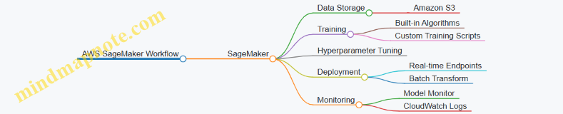
Example 2: Using Google Cloud Vertex AI for AutoML
Step 1: Upload Dataset to Google Cloud Storage
gsutil cp train.csv gs://my-bucket/data/
Step 2: Create AutoML Tabular Dataset and Train Model (via Console or Python SDK)
from google.cloud import aiplatform
aiplatform.init(project='my-project', location='us-central1')
dataset = aiplatform.TabularDataset.create(
display_name='my-dataset',
gcs_source=['gs://my-bucket/data/train.csv']
)
model = dataset.auto_train(
target_column='label',
training_fraction_split=0.8,
validation_fraction_split=0.1,
test_fraction_split=0.1,
sync=True
)
Step 3: Deploy Model to Endpoint
endpoint = model.deploy(
machine_type='n1-standard-4'
)
Step 4: Make Predictions
response = endpoint.predict(instances=[{'feature1': 5.1, 'feature2': 3.5}])
Mind Map: Google Cloud Vertex AI Components
Best Practices When Using Cloud Services for ML
- Automate Infrastructure: Use Infrastructure as Code (IaC) tools like Terraform or CloudFormation.
- Secure Access: Use IAM roles and policies to control access to data and models.
- Cost Management: Monitor usage and optimize resource allocation.
- Version Control: Track datasets, code, and models using integrated tools.
- Logging & Monitoring: Set up alerts for model performance degradation and system failures.
Summary
Cloud services provide a powerful ecosystem for ML engineers to develop, deploy, and maintain models at scale. Understanding the core components and how to orchestrate them effectively is key to building robust ML systems. The examples and mind maps above offer a practical foundation to start leveraging cloud platforms in your ML engineering workflows.
13.5 Recommended Reading and Community Resources
To deepen your understanding and stay updated in Machine Learning Engineering, here is a curated list of books, blogs, courses, and communities. These resources are organized to help you grow from foundational knowledge to advanced practices, complemented by mind maps to visualize key concepts.
Recommended Books
-
“Hands-On Machine Learning with Scikit-Learn, Keras, and TensorFlow” by Aurélien Géron
- Practical guide covering end-to-end ML workflows with clear examples.
-
“Machine Learning Engineering” by Andriy Burkov
- Focuses on production-ready ML systems and engineering best practices.
-
“Designing Data-Intensive Applications” by Martin Kleppmann
- Essential for understanding scalable data systems that underpin ML pipelines.
-
“Building Machine Learning Powered Applications” by Emmanuel Ameisen
- Step-by-step guide on building and deploying ML applications.
-
“MLOps Engineering at Scale” by Carl Osipov
- Deep dive into MLOps, CI/CD, and production ML workflows.
Influential Blogs and Websites
- Google AI Blog (https://ai.googleblog.com/)
- Distill.pub (https://distill.pub/) — for interpretability and visualization.
- Machine Learning Mastery (https://machinelearningmastery.com/)
- MLflow Blog (https://mlflow.org/blog/)
- Towards Data Science (https://towardsdatascience.com/)
Online Courses
- Coursera: Machine Learning Engineering for Production (MLOps) Specialization by DeepLearning.AI
- Udacity: Machine Learning DevOps Engineer Nanodegree
- Fast.ai: Practical Deep Learning for Coders
- edX: Principles of Machine Learning
Community and Forums
- Kaggle (https://www.kaggle.com/) — Competitions and datasets.
- Stack Overflow — For technical Q&A.
- Reddit r/MachineLearning (https://www.reddit.com/r/MachineLearning/)
- ML Engineering Slack Groups (search for “MLOps” or “ML Engineering” communities)
- LinkedIn Groups focused on Machine Learning Engineering
Mind Maps
Mind Map 1: Core Areas of Machine Learning Engineering
Mind Map 2: End-to-End Model Lifecycle

Mind Map 3: MLOps Pipeline Components
Example: Using Mind Maps for Learning
Suppose you want to understand the deployment phase better. Using the “Core Areas of Machine Learning Engineering” mind map, you can drill down into the “Deployment” node:
This helps you organize your study and implementation plan, ensuring you cover all essential subtopics with practical examples.
Final Tips
- Regularly revisit these resources to stay current.
- Engage actively in communities to solve real-world problems.
- Use mind maps as living documents to track your learning journey.
By leveraging these recommended readings and community resources, you will build a solid foundation and keep pace with the rapidly evolving field of Machine Learning Engineering.
14. Conclusion and Next Steps
14.1 Recap of Key Best Practices
In this section, we revisit the essential best practices that underpin successful machine learning engineering projects. These practices ensure robustness, scalability, maintainability, and ethical responsibility throughout the end-to-end ML lifecycle.
Mind Map: Key Best Practices in ML Engineering
Practical Examples Highlighting Best Practices
Clear Problem Definition & Success Metrics
Example: For a customer churn prediction model, defining the business goal as “reduce churn by 10% within 6 months” helps focus efforts. Success metrics like ROC-AUC and recall on the churn class guide model evaluation.
Data Quality Handling
Example: During EDA, discovering 15% missing values in key features prompts imputation using median values and flagging missingness as a feature, improving model robustness.
Feature Engineering Automation
Example: Using Featuretools to automatically generate features from transactional data reduces manual errors and accelerates pipeline development.
Reproducible Training Pipelines
Example: Using MLflow to track experiments, parameters, and artifacts ensures that training runs can be reproduced exactly, facilitating collaboration and debugging.
Hyperparameter Tuning with Cross-Validation
Example: Applying GridSearchCV with stratified k-fold cross-validation balances bias and variance, leading to a more generalized model.
Containerized Deployment
Example: Packaging a TensorFlow model with Docker ensures the production environment matches development, avoiding “works on my machine” issues.
CI/CD Pipeline Integration
Example: Automating model retraining and deployment with Jenkins triggers on new data arrival, ensuring the model stays up-to-date without manual intervention.
Monitoring Data and Model Drift
Example: Implementing statistical tests like Population Stability Index (PSI) on incoming data distributions detects drift early, prompting retraining.
Privacy-Preserving Training
Example: Incorporating differential privacy techniques during training protects sensitive user data while maintaining model utility.
Summary Table of Best Practices with Examples
| Stage | Best Practice | Example Tool/Technique |
|---|---|---|
| Problem Definition | Define clear objectives & metrics | Business KPIs, ROC-AUC, Recall |
| Data Preparation | Handle missing data & automate FE | Median imputation, Featuretools |
| Model Training | Reproducible pipelines & tuning | MLflow, GridSearchCV |
| Validation & Testing | Robust validation & fairness checks | Stratified k-fold, fairness metrics |
| Packaging & Deployment | Containerize & version models | Docker, model versioning |
| CI/CD | Automate retraining & deployment | Jenkins, MLflow pipelines |
| Monitoring & Maintenance | Detect drift & alert | PSI, Prometheus alerts |
| Security & Privacy | Privacy-preserving ML | Differential Privacy libraries |
By consistently applying these best practices, ML engineers and data scientists can build reliable, scalable, and ethical machine learning systems that deliver real business value.
14.2 Building Your Own End-to-End ML Pipeline
Building an end-to-end machine learning (ML) pipeline is a foundational skill for any ML engineer or data scientist. It involves orchestrating all the stages from data ingestion to model deployment and monitoring in a seamless, automated, and reproducible manner. In this section, we’ll walk through the key components of an ML pipeline, best practices, and provide practical examples and mind maps to help you visualize and implement your own pipeline.
What is an End-to-End ML Pipeline?
An end-to-end ML pipeline is a structured workflow that automates the entire ML lifecycle:
- Data collection and ingestion
- Data preprocessing and feature engineering
- Model training and hyperparameter tuning
- Model evaluation and validation
- Model packaging and deployment
- Monitoring and maintenance
The goal is to reduce manual intervention, improve reproducibility, and enable continuous integration and deployment of ML models.
Mind Map: Overview of an End-to-End ML Pipeline
Step 1: Data Ingestion and Validation
Best Practice: Automate data ingestion with validation checks to ensure data quality before processing.
Example: Using Python and pandas to load CSV data and validate schema.
import pandas as pd
from pandera import DataFrameSchema, Column, String, Check
# Define schema
schema = DataFrameSchema({
"user_id": Column(int, Check.greater_than(0)),
"age": Column(int, Check.in_range(0, 120)),
"income": Column(float, nullable=True),
"country": Column(String, Check.isin(["US", "UK", "CA"]))
})
# Load data
df = pd.read_csv("data/users.csv")
# Validate data
validated_df = schema.validate(df)
This ensures that only data conforming to expected formats and ranges enters the pipeline.
Step 2: Data Preprocessing and Feature Engineering
Best Practice: Modularize preprocessing steps and use pipelines to ensure reproducibility.
Example: Using scikit-learn’s Pipeline for preprocessing.
from sklearn.pipeline import Pipeline
from sklearn.impute import SimpleImputer
from sklearn.preprocessing import StandardScaler, OneHotEncoder
from sklearn.compose import ColumnTransformer
numeric_features = ["age", "income"]
categorical_features = ["country"]
numeric_transformer = Pipeline(steps=[
('imputer', SimpleImputer(strategy='median')),
('scaler', StandardScaler())
])
categorical_transformer = Pipeline(steps=[
('imputer', SimpleImputer(strategy='constant', fill_value='missing')),
('onehot', OneHotEncoder(handle_unknown='ignore'))
])
preprocessor = ColumnTransformer(
transformers=[
('num', numeric_transformer, numeric_features),
('cat', categorical_transformer, categorical_features)
])
# Example usage
X_processed = preprocessor.fit_transform(validated_df)
Step 3: Model Training and Hyperparameter Tuning
Best Practice: Use automated hyperparameter tuning and cross-validation to find the best model.
Example: Using GridSearchCV with a Random Forest classifier.
from sklearn.ensemble import RandomForestClassifier
from sklearn.model_selection import GridSearchCV
param_grid = {
'n_estimators': [50, 100],
'max_depth': [5, 10, None]
}
clf = RandomForestClassifier(random_state=42)
grid_search = GridSearchCV(clf, param_grid, cv=5, scoring='accuracy')
grid_search.fit(X_processed, y)
print(f"Best parameters: {grid_search.best_params_}")
print(f"Best cross-validation accuracy: {grid_search.best_score_:.2f}")
Step 4: Model Evaluation and Validation
Best Practice: Evaluate on a hold-out test set and check for bias or fairness issues.
Example: Calculating classification metrics and confusion matrix.
from sklearn.metrics import classification_report, confusion_matrix
# Predict on test data
predictions = grid_search.predict(X_test_processed)
# Metrics
print(classification_report(y_test, predictions))
# Confusion matrix
cm = confusion_matrix(y_test, predictions)
print(cm)
Step 5: Model Packaging and Deployment
Best Practice: Serialize models with versioning and deploy using containerized REST APIs.
Example: Saving a model with joblib and creating a simple Flask API.
import joblib
from flask import Flask, request, jsonify
# Save model
joblib.dump(grid_search.best_estimator_, 'model_v1.joblib')
# Flask app
app = Flask(__name__)
model = joblib.load('model_v1.joblib')
@app.route('/predict', methods=['POST'])
def predict():
data = request.json
features = [data[feature] for feature in numeric_features + categorical_features]
# Preprocess and predict
# (Assuming preprocessing pipeline is saved and loaded similarly)
processed = preprocessor.transform([features])
pred = model.predict(processed)
return jsonify({'prediction': int(pred[0])})
if __name__ == '__main__':
app.run(debug=True)
Step 6: Monitoring and Maintenance
Best Practice: Continuously monitor model performance and data drift to trigger retraining.
Example Mind Map: Monitoring and Retraining Workflow
Putting It All Together: Sample Pipeline Mind Map
Summary
Building your own end-to-end ML pipeline requires careful planning and modular design. By automating each stage, ensuring reproducibility, and incorporating monitoring, you can create robust ML systems that scale and adapt to changing data and business needs. The examples provided here offer a practical foundation to start building pipelines tailored to your projects.
Further Reading & Tools
- scikit-learn Pipelines
- MLflow for Experiment Tracking and Deployment
- Tfx (TensorFlow Extended) for Production Pipelines
- Kubeflow Pipelines
Feel free to experiment with these building blocks and customize your pipeline based on your project requirements!
14.3 Continuing Education and Skill Development
Machine Learning Engineering is a rapidly evolving field that demands continuous learning and skill enhancement. Staying current with new algorithms, tools, deployment strategies, and best practices is essential to remain effective and competitive.
Why Continuing Education Matters
- Rapid Technological Advancements: New frameworks, libraries, and methodologies emerge frequently.
- Evolving Best Practices: MLOps, model interpretability, and ethical AI are areas with fast-changing standards.
- Cross-disciplinary Skills: Combining software engineering, data science, and domain knowledge requires ongoing refinement.
Key Areas for Skill Development
Practical Examples & Resources
-
Online Courses & Specializations
- Example: Coursera’s “Machine Learning Engineering for Production (MLOps) Specialization” by DeepLearning.AI covers model deployment and monitoring with hands-on labs.
- Best Practice: Follow courses with project-based learning to apply concepts immediately.
-
Books & Research Papers
- Example: “Designing Data-Intensive Applications” by Martin Kleppmann for understanding scalable data systems.
- Best Practice: Regularly read recent conference papers (NeurIPS, ICML) to stay updated on cutting-edge research.
-
Hands-on Projects
- Example: Build a CI/CD pipeline for a model using Jenkins and Docker.
- Best Practice: Open-source your projects on GitHub to get feedback and showcase skills.
-
Community Engagement
- Example: Participate in Kaggle competitions to sharpen problem-solving skills.
- Best Practice: Join ML engineering forums, Slack groups, or local meetups for networking and knowledge exchange.
-
Certifications
- Example: Google Cloud Professional Machine Learning Engineer certification validates cloud deployment skills.
- Best Practice: Choose certifications aligned with your career goals and practical experience.
Learning Roadmap Mind Map
Example: Creating a Personal Learning Plan
- Assess Current Skills: Identify gaps in ML algorithms, deployment, or monitoring.
- Set Goals: E.g., “Deploy a model with automated monitoring in 3 months.”
- Select Resources: Choose courses, books, and projects aligned with goals.
- Schedule Learning: Dedicate weekly time slots for study and practice.
- Apply & Reflect: Build projects, seek feedback, and adjust plan as needed.
Summary
Continuous education is a cornerstone of success in machine learning engineering. By leveraging structured learning paths, engaging with the community, and applying knowledge through projects, you can build a resilient and future-proof career.
14.4 Joining the ML Engineering Community
Becoming an active member of the Machine Learning (ML) Engineering community is a powerful way to accelerate your learning, stay updated with the latest trends, and build meaningful professional connections. This section will guide you through practical ways to join and contribute to the community, complete with examples and mind maps to help you visualize the process.
Why Join the ML Engineering Community?
- Continuous Learning: Access to cutting-edge research, tutorials, and discussions.
- Networking: Connect with peers, mentors, and industry leaders.
- Collaboration: Participate in open-source projects and hackathons.
- Career Growth: Discover job opportunities and gain visibility.
Ways to Join the ML Engineering Community
Online Platforms
Forums and Q&A Sites
- Stack Overflow: Ask and answer ML engineering questions.
- Reddit: Subreddits like r/MachineLearning and r/MLQuestions are great for discussions.
Example: Posting a question about deploying TensorFlow models on Kubernetes can get you detailed community insights.
Social Media
- Twitter: Follow ML engineers, researchers, and organizations.
- LinkedIn: Join ML groups and participate in discussions.
Example: Engaging with tweets from ML influencers like Andrew Ng or Francois Chollet can expose you to new ideas and resources.
Learning Platforms
- Kaggle: Participate in competitions and join discussion forums.
- Coursera & edX: Join courses with active discussion boards.
Example: Kaggle kernels and forums provide hands-on examples and peer feedback.
Local Meetups and Groups
- Search for ML or AI meetups on Meetup.com.
- Join university or community clubs related to AI and ML.
Example: Attending a local ML meetup where engineers share deployment strategies using Docker and Kubernetes.
Conferences and Workshops
- Attend major conferences like NeurIPS, ICML, or domain-specific workshops.
- Many conferences offer virtual attendance options.
Example: Participating in workshops on MLOps to learn best practices directly from experts.
Open Source Contributions
- Contribute to popular ML repositories on GitHub (e.g., TensorFlow, PyTorch).
- Join Kaggle competitions to collaborate and learn.
Example: Submitting a pull request to improve documentation or add a new feature to an open-source model serving tool.
Blogs, Podcasts, and Newsletters
- Follow blogs like Towards Data Science or Distill.pub.
- Subscribe to newsletters such as The Batch by deeplearning.ai or ML Weekly.
- Listen to podcasts like Data Skeptic or TWIML AI.
Example: Implementing a new technique learned from a blog post and sharing your experience in a community forum.
Example Mind Map: How to Engage Effectively
Practical Tips for Community Engagement
- Start Small: Begin by lurking, then gradually participate by asking questions or commenting.
- Be Respectful: Maintain professionalism and respect diverse opinions.
- Share Your Work: Publish blog posts, GitHub repos, or tutorials.
- Help Others: Answer questions and provide constructive feedback.
- Stay Consistent: Regular engagement builds recognition and trust.
Real-World Example: From Learner to Contributor
- Step 1: Join Kaggle and complete beginner competitions.
- Step 2: Participate in Kaggle forums, asking and answering questions.
- Step 3: Attend local ML meetups and present your Kaggle solutions.
- Step 4: Contribute to an open-source ML project by fixing bugs or improving docs.
- Step 5: Write a blog post about your journey and share it on LinkedIn and Twitter.
Summary
Joining the ML Engineering community is a multifaceted journey involving learning, sharing, collaborating, and networking. By actively engaging through various channels and contributing your knowledge, you not only grow your skills but also help advance the field as a whole.
14.5 Final Thoughts and Encouragement
As we conclude this comprehensive journey through practical machine learning engineering, it’s important to reflect on the key takeaways and encourage continuous growth. ML engineering is a dynamic and evolving field that blends creativity, technical skill, and collaboration. Remember, mastery comes with practice, experimentation, and learning from both successes and failures.
Embrace the End-to-End Mindset
Machine learning engineering is not just about building models but about delivering reliable, maintainable, and scalable solutions that solve real-world problems. Keep the entire lifecycle in mind—from data collection and preprocessing to deployment and monitoring.
Cultivate a Growth Mindset
Mistakes and challenges are inevitable. Instead of fearing failure, treat it as an opportunity to learn and improve. For example, if a deployed model underperforms, investigate data drift or revisit feature engineering rather than abandoning the project.
Practical Example: Learning from a Deployment Failure
Imagine you deployed a customer churn prediction model that suddenly shows degraded accuracy. Instead of panic, follow these steps:
- Check Data Drift: Compare recent input data distributions with training data.
- Review Monitoring Logs: Look for anomalies or errors in the serving environment.
- Retrain Model: Incorporate new data and retrain to adapt to changes.
- Communicate: Inform stakeholders about the issue and your remediation plan.
This approach exemplifies best practices in monitoring and maintenance.
Keep Collaboration and Communication at the Forefront
ML engineering is rarely a solo endeavor. Collaborate closely with data scientists, software engineers, product managers, and domain experts. Clear documentation and shared understanding reduce friction and accelerate progress.
Final Encouragement
- Start Small, Iterate Fast: Build minimal viable models and improve incrementally.
- Automate Wisely: Use automation for repetitive tasks but maintain human oversight.
- Stay Curious: Follow new research, tools, and community discussions.
- Share Knowledge: Teach others, write blogs, or contribute to open source.
Remember, every expert was once a beginner. Your journey in machine learning engineering is a continuous adventure filled with opportunities to innovate and impact the world.
Thank you for investing your time in mastering practical ML engineering. Keep building, keep learning, and most importantly, keep experimenting!